financial risk measurement & management - idc · » quiz3will take place during the 1st class...

Risk Management Jacob Boudoukh

RM 1Risk Management - Prof. Boudoukh

financial risk

measurement & management

Prof. Jacob BoudoukhIDC-Arison

Email: [email protected]

© Please do not duplicate without permission


Course outline� Introduction to VaR Mar14

» Statistical framework. Risk and diversification: some examples.

Visual interpretation. Possible applications.

� The Stochastic Behavior of Asset Returns Mar14,Mar21» Time variations in volatility. VaR: approaches and comparison. The Hybrid Approach to

VaR.

» Quiz1

� Beyond Volatility Forecasting Mar21,Apr4» The VaR of derivatives and interest rate VaR. Structured Monte Carlo. Extreme events and

correlation breakdown. Stress testing and scenario analysis. Worst case scenario

» Guest lecture: TBA

» The Crisis

» Quiz2

…

» Quiz3 will take place during the 1st class of Multinational Financial Management on Apr11



Readings

Textbook: (ABS) Understanding Market, Credit, and Operational Risk: The Value

at Risk Approach; Linda Allen, Jacob Boudoukh and Anthony Saunders, Blackwell

Course material: copies of slides will be handed out and appear on my website.

Grading

•Final grade: 90% best 2 of 3 quiz, 10% class participation.

•There will be no makeup quiz exams. If you miss one exam for a “permissible”

reason (sickness or reserve duty with appropriate paperwork) the grade will be

ignored. If you miss an exam without a permissible reason the grade on this exam

will be zero.

•To be clear, missing an exam for work-related reason does not qualify as a

“permissible reason” even if you let me know in advance.

•Sample questions can be found at the back of this course packet.

Administration


OUTLINE

� Introduction to VaRIntroduction to VaRIntroduction to VaRIntroduction to VaR» Statistical framework. Risk and diversification: some examples.


� The Stochastic Behavior of Asset Returns» Time variations in volatility. VaR: approaches and comparison. The Hybrid

Approach to VaR.

� Beyond Volatility Forecasting» The VaR of derivatives and interest rate VaR. Structured Monte Carlo. Extreme

events and correlation breakdown. Stress testing and scenario analysis. Worst case

scenario

� VaR as a Risk Management Tool» Why do firms hedge? Optimal VaR control using derivatives.



� Market risk

» interest rate, currency, equity, commodity, spread, volatility,…

» example: Price of bond declines as interest rates rise

� Credit risk

» default, downgrade

» example: P(bond)=recovery upon default

� Other

» Operational risk, liquidity risk, regulatory risk , political risk, model risk…

� We focus primarily on Market Risk, and to a lesser extent on credit risk


Risk Measurement

�Address the question:

“ HOW MUCH CAN WE LOSE

ON OUR TRADING PORTFOLIO

BY TOMORROW’S CLOSE? ”

� Risk MEASUREMENT <=?=> Risk MANAGEMENT



VaR: Example

Consider a spot equity position worth $1,000,000

� Suppose the daily standard deviation of the S&P500 is 100 basis

points per day

� How do we make an informative statement about risk?

We can only make a probabilistic statement:

Assume ∆∆∆∆St,t+1 is distributed normally ( 0 , 100bp2 )


“Value at Risk” (VaR):(First Look)

� From the normal dist’n tables:

» -1STD to +1STD 68.3%

» -2STD to +2STD 95.4%

» What is the “value” of one standard deviation?

» What are the amounts on the X-axis?

68%

-1sd +1sd=-$10,000 =$10,000



“Value at Risk” (VaR):(First Look)

� From the normal dist’n tables:

Prob(Z< -1.65)=5%, Prob(Z< -2.33)=1%

“With probability 95% we will not see a loss greater than

?_______? on our position”

-1.65-2.33


OUTLINE

� Introduction to VaR

»Statistical frameworkStatistical frameworkStatistical frameworkStatistical framework. Risk and diversification: some examples.



Approach to VaR.



scenario

� VaR as a Risk Management Tool» Why do firms hedge? Optimal VaR control using derivatives



Quantifying the Exposure:Calculating the standard deviation

� Three ways to define the change in the spot rate

» Absolute change ∆St,t+1 = St+1 - St

» Simple rate of return ∆St,t+1 = St+1/ St

» Cont’ comp’ change ∆St,t+1 = ln( St+1/St )

� Which definition of “∆St,t+1” is most appropriate?

� To answer this we must recognize that we are going to make a

strong assumption:

the past is representative / predictive of the future

� The question is :

which prism should we use to look back into the past?


Stationarity

� We are going to assume “stationarity”

� Consider the following statements

» a 80pt change in the Dow is as likely at 6,000 as it is at 12,000

» a 2% change in the Dow is as likely at 6,000 as it is at 12,000

...which one is more likely to hold ?

� Recall: three ways to define the change in the spot rate

» Absolute change ∆St,t+1 = St+1 - St

» Percentage change (rate of return) ∆St,t+1 = St+1 / St

» C.C. change ∆St,t+1 = ln( St+1/St )



Time - consistency

� Consider the continuously compounded two-day return

∆St,t+2 = ln( St+2/St )

= ln{ (St+2/St+1 ) * (St+1/St ) }

= ln(St+2/St+1 ) + ln(St+1/St )

= ∆St,t+1 + ∆St+1,t+2

� Suppose ∆St+i,t+i+1 is distributed N(0, σ2)

� The sum ∆St,t+J is also normal: N(0, J*σ2) (under certain assumption, to be discussed later)

� Easy to extrapolate VaR:

J day VaR = SQRT(J) * (1 day VaR)

� With any other definition of returns normality is not preserved

(i.e., the product of normals is non-normal)


Non-negativity

� Consider the cont’ comp’ J-day return

∆St,t+J= ln( St+J/St )

Since ∆St,t+J is distributed N(0, J σ2), the value of any possible

St+i is guaranteed to be non-negative:

St+i = St exp{∆St,t+J }

� This is the standard log-normal diffusion process (such as in

Black/Scholes): log(returns) are normal

� With other definitions of returns positivity of asset prices is not

guaranteed



Interest rates and spreads

� The exceptions to the rule are interest rates and spreads

(e.g., zero rates, swap spreads, Brady strip spreads,…)

� For these assets the “change” is ∆it,t+J= it+J-it , usually measured

in basis points

� This is an added complication in terms of calculating risk

» for stocks, commodities, currencies etc, there is a 1-for-1 relation

between the risk index and the portfolio value

» with interest rates there is a 1-for-D relation, where D is the duration:

a 1bp move in rates ==> D bp move in bond value


Quantifying the Exposure:Calculating Standard deviation (cont’d)

� The STD of change can be calculated easily

» “Volatility” (vol)

STD(∆St,t+1 ) =SQRT[ VAR(∆St,t+1) ]

» ...where VAR(∆St,t+1) is the “Mean squared deviation”

VAR(∆St,t+1) = AVG [ (∆S-avg(∆S))2 ]



OUTLINE


» Statistical framework. Risk and diversification: some Risk and diversification: some Risk and diversification: some Risk and diversification: some

examples.examples.examples.examples.Visual interpretation. Possible applications.


Approach to VaR.



scenario



A two asset example

� Consider the following FX position(where vol($/Euro)=75bp ==> VaR=75*1.65=123,

vol($/GBP)=71bp ==> VaR=71*1.65=117 )

Position * 95% move = VaR(FX in $MM) (in percent) (in $MM)

Euro 100 1.23% $1.23

GBP -100 1.17% -$1.17

Undiversified risk $2.40

(absolute sum of exposures, ignoring the effect of diversification)



Portfolio variance: a quick review

� X, Y are random variables c, d are parameters

VAR(X+Y) =VAR(X)+VAR(Y)+2COV(X,Y)

VAR(c*X) =c2 VAR(X)

==>

VAR(cX+dY) =c2 VAR(X)+d2 VAR(Y)+2 c d COV(X,Y)

...applied to portfolio theory:

� A portfolio of two assets: Rp= w Ra + (1-w) Rb

and the vol of a portfolio, VAR( Rp ) , can now be calculated


Correlation and covariance

� Correlation: the tendency of two variables to co-move

COV(Ra, Rb) = ρRa,Rb * σRa * σRb

� The volatility of a portfolio in percent:

%STD=sqrt[wa2σRa

2 +wb2 σRb

2 +2wawb ρRa,Rb σRa σRb ]

� The volatility of a portfolio in $ terms:

$STD=sqrt[$σRa2 +$σRb

2 + 2 ρRa,Rb $σRa $σRb ]



From vol to VaR

How do we move from vol to VaR?

� Consider the $ volatility

{ $STD=sqrt[$σRa2 +$σRb

2 + 2 ρRa,Rb $σRa $σRb ] }*1.65

� and we get

$VaR=sqrt{$VaRRa2 + $VaRRb

2 + 2ρRa,Rb $VaRRa $VaRRb}

� ...or we could calculate the %vol and

VaR= %STD * value * 1.65

� The two approaches are EQUIVALENT


Portfolio VaR

� Suppose ρ$/Euro,$/GBP = 0.80

� For simplicity forget cont’ comp’ returns for the moment

� $VaR=sqrt{$VaRRa2 + $VaRRb

2 +2ρρρρRa,Rb $VaRRa$VaRRb}

=sqrt{1.232 + (-1.17)2 + 2*0.80*(-1.17)(1.23) }

=sqrt{1.5129 + 1.3689 - 2.3025 }

= $0.76Mil



The portfolio effect

� Compare: Undiversified VaR $2.40MM

Diversified VaR $0.76MM

==> Portfolio effect $1.64MM

� Risk reduction due to diversification depends on the correlation

of assets in the portfolio

� As the number of assets increases, portfolio variance becomes

more dependent on covariances and less dependent on variances

� The “marginal” risk of an asset when held in a small portion in a

large portfolio, depends on its return covariance with other

securities in the portfolio

� Exercise:

» Take an equally weighted portfolio with N uncorrelated asset.

» Assume all assets have equal volatility.

» What is the portfolio’s volatility?

» Take N to infinity. What happens to volatility?


Diversification example: hedge funds

� Consider a fund manager examining 9 positions taken by hedge

funds he invests in

� For simplicity assume that:

» the positions are valued at $100MM each, with a an annual

VaR 16.5% (i.e., vol = 10% per annum)

» the strategies are uncorrelated

(e.g., high yield FX, special situation, fixed income arb,

Japanese warrants arb, spread trading,...)

� The undiversified VaR is 9*$16.5MM = $148.5MM, on a

$900MM investment



The funds’ VaR

� The VaR of N uncorrelated assets:

VaR port = sqrt{ 9* VaR strat2 + zero covariance}

= sqrt{9} VaR strat

= 3 * $16.5MM =$49.5MM

==> the risk reduction due to diversification is 66%

� Now suppose each strategy had an annualized Sharpe ratio of

E[R]/STD[R]=2 ==> E[R]=20%, or $180MM.

� The portfolio’s Sharpe ratio would be 180/30 = 6

� What would the Sharpe Ratio and VaR be if we invested the

entire $900MM in only one strategy?


Bond portfolio VaR

� The VaR of a portfolio of $100 of face of a 1yr bond and a10yr

bond can now be calculated as usual (how?)

� What is the VaR of a 10% s.a. coupon bond w/ 10yr to maturity?

� Note that the coupon bond VaR involves

» 20 volatilities

» 190 correlations

==> MATURITY BUCKETS

(cash flow mapping)



Spread VaR

Y

t

Spread

10yr AA

10yr treasury

%VaR=2.5bp/day


The (approx) VaR of a 10yr AA bond

� VaR(treasury)=11.5bp

� VaR(spread)=2.5bp

� CORR(∆spread, ∆treasury)=0

==>VaR(AA Bond)=sqrt{11.52 + 2.52 } = 11.77bp/day

Note:

VaR(AA Bond) / VaR(treasury) = 11.77/11.5 = 1.023,

only 2.3% higher VaR!



OUTLINE


» Statistical framework. Risk and diversification: some examples. Visual Visual Visual Visual

interpretation ,interpretation ,interpretation ,interpretation , Possible applications..


Approach to VaR.



scenario



Visual interpretation

Negative Correlation

Positive Correlation

Ra

RbRp

Rp

Rb

Ra



Visual interpretation - corp’ bond example

treasury

spread

AAbond

treasury

AAbond

Think, similarly, on the total risk of an FX equity investment


Visual interpretation - FX example

Long EURLong GBP

Short GBPPosition

VaR



OUTLINE

� Introduction to VaR» Statistical framework. Risk and diversification: some examples. Visual

interpretation. Possible applicationsPossible applicationsPossible applicationsPossible applications


Approach to VaR.



scenario



Uses and applications

� Corporates

� Financial Institutions

Internal uses External uses .

- Trading limits - Reporting

- Capital Allocation - Capital requirements

- Self regulation

� Self regulation and market disclosure

» An alternative to the BIS's and the Fed's proposals, which may result in

capital inefficiency and mixed incentives



Trading Limits

� VaR for management information and resource allocation

» A unified measure of exposure at the trader, desk, group,... level

» An input for capital allocation and reserve decisions

ISSUES

� Full system may include VaR limits, notional limits, types of

securities, types of exposures,…

� Implementation isn’t simple


VaR and Performance Evaluation

� Idea:

» Desk1: corr(P&L, IntRates) close to one

» Desk2: corr(P&L, IntRates) close to zero

» VaR1=VaR2

Performance/Compensation is a function of

P&L - C * VaR

where “C” is the price of risk parameter

BUT marginal VaR contribution of Desk1 >> than Desk2

==> P&L - C * MarginalVaR

… and what if P&L=0 and MarginalVaR<0???

� In reality future P&L is a function of realized P&L and VaR or

realized risk



VaR for Reporting:

example: UBS’s VaR

� Time series of daily estimated VaR (defined as 2*STD) out of UBS’s

annual report

Source: 1996 annual report


UBS’s realized P&L

� Realized VaR=2*STD(P&L)=CHF13.6MM

<< ExAnte VaR=CHF23.4MM

� “...thereby underscoring the effectiveness of continuous risk

management” AVG(P&L)=CHF9.2MM,

STD(P&L)=CHF6.8MM

Source: 1996 annual report



Risk-type Allocation


Business Group Risk Allocation


RM 41

UBS 2010: most risk from investment bank

Risk Management - Prof. Boudoukh

RM 42

UBS 2010: risk spread across asset classes



RM 43

UBS 2010: 99%VaR rarely violated


RM 44

UBS 2010: under investigation





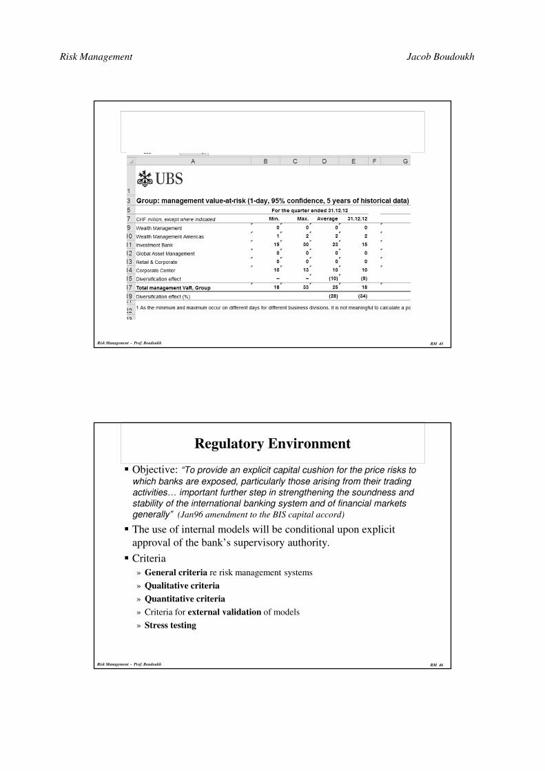
Regulatory Environment

� Objective: “To provide an explicit capital cushion for the price risks to

which banks are exposed, particularly those arising from their trading

activities… important further step in strengthening the soundness and

stability of the international banking system and of financial markets

generally” (Jan96 amendment to the BIS capital accord)

� The use of internal models will be conditional upon explicit

approval of the bank’s supervisory authority.

� Criteria

» General criteria re risk management systems

» Qualitative criteria

» Quantitative criteria

» Criteria for external validation of models

» Stress testing



Quant Standards

� No particular type of model required

(e.g., VarCov, HistSim, SMC…)

� VaR on a daily basis

» 99th %ile

» 10 day horizon

» Lookback at least 1yr

� Discretion to recognize empirical corr within broad risk

categories.

� VaR across these categories is to be aggregated (simple sum…)


Capital Requirements

CapRequ= MAX[VaR t-1, (Mult+AddOn)*AVG(VaRt,t-60)]

� Mult=3.

� AddOn related to past performance

» Green zone 4/250 exceptions 1%VaR OK

» Yellow zone up to 9/250 AddOn =0.3 To 1

» Red zone 10plus/250 Investigation starts

� Model must capture risk associated with options

� Must specify risk factors and a price-factor mapping process a

priori


RM 49

Ubs_ar_2011 methodology (pp136)





OUTLINE

� Introduction to VaR» Statistical framework. Risk and diversification: some examples. Possible

applications. Visual interpretation.

� The Stochastic Behavior of Asset ReturnsThe Stochastic Behavior of Asset ReturnsThe Stochastic Behavior of Asset ReturnsThe Stochastic Behavior of Asset Returns» Time variations in volatility. VaR: approaches and comparison. The Hybrid

Approach to VaR.



scenario



The Stochastic Behavior of Asset Returns

�The problem of f-a-t t-a-i-l-shttp://www.bloomberg.com/video/67293058/

�Time variations in volatility

�VaR: approaches and comparison

�The Hybrid Approach to VaR

�Long horizon VaR

�Benchmarking and backtesting VaR



How can we obtain the 5% tail move?

� So far the answer was: VaR(5%)= 1.65 * σσσσ

� Asset returns are assumed to be

Stable ...but vol varies through time

and

Normal ...but they are not

How do we make this determination?


3 months T-bill rate



Interest rate changes: are they normal?

N( 0, 7.3bp 2 )


The Tails of the Distribution

� There ate, say 2500 ∆ι’s

� Order them in ascending order

� The 1%-ile is, under normality

7.3*2.33=17bp

� Where should you find this “17”?

� What do you actually find there?

1

2

3

2499

2500



Fat tails

� If IR changes were normal: Prob( IR change >17bp ) = 1%

� ... but in reality Prob( IR change >21bp ) = 1%

===> “F F F F -------- A A A A -------- TTTT Tails”

� This is especially true for

return series such as oil,

Bradys, some currencies...

� The Effect subsides

gradually by aggregation

» through time

» cross sectionally


Why are tails so fat?

In trying to explain the fat tails, it could be the case that returns are

simply fat tailed relative to the normal distribution or that returns

are conditionally normal, but:

1. expectations vary through time

(well, maybe, but not enough to explain the tails)

2. volatility varies through time

(and we know it does, but is it enough to explain the tails?)

PLAN: we follow 2 . . . but go back to 1



The Effect of Cyclical Vol.

� We measure vol as 7.3bp/day

� Suppose now that in fact

� If in a given day ∆ι=22bp, then do we interpret is as

22/7.3=3sd, or 22/15=1.5sd ?

� This is the key goal of dynamic VaR engines

15

7.3

5

t

σ


The Difficulty in Estimating Cyclical Vol.

� Need few days of data to realize change in volatility

� Key question: how adaptable do you want to be

� Tradeoff exists, and we shall elaborate on it next

� But in general, measuring volatility dynamically is the key goal

of VaR engines

� … and it’s very difficult

15

7.3

5

t

σ



OUTLINE



� The Stochastic Behavior of Asset Returns

»Time variations in volatilityTime variations in volatilityTime variations in volatilityTime variations in volatility. VaR: approaches and

comparison. The Hybrid Approach to VaR.



scenario



Modeling time-variations in VaR

� PARAMETRIC approaches

estimate the parameters of a given distribution

» STD - simple historical vol + Conditional normality

» Declining weights + Conditional normality (RiskMetrics)

» Mixture of normals, t-distribution, GARCH...

� NONPARAMETRIC approaches

let the data talk

» Historical simulation

� The Hybrid Approach

� Finance-based forecasts (e.g., implied vol)



Volatility is cyclical

Long Run Mean

volatility

t

Mandelbrot (1963)

“...large changes tend to be followed by large

chages -- of either sign -- and small chages by

small changes’’


Historical STD

� Simple historical STDDEV is estimated by calculating the

average of squared changes

σt2=(1/K)(εt

2+εt-12 + εt-2

2 +...+εt-k+12 )

note that the weights sum up to one (why?)

» Note1: it is common to use 1/(K-1)

» Note2: the “suqared change” εt-i2 is in fact the de-meaned

squared returns (∆S-avg(∆S))2

� The choice of K involves a tradeoff between

» acuuracy

» adaptability

Weight

on

∆∆∆∆St,t+1 2

today

1/k

k



Time-varying vol

Three window sizes K=30, 60, 150 days,

are used to estimate STD


OUTLINE




» Time variations in volatility. VaR: approaches and VaR: approaches and VaR: approaches and VaR: approaches and

comparisoncomparisoncomparisoncomparison. The Hybrid Approach to VaR.



scenario




Exponential smoothing: the idea

� Examples: RiskMetrics, GARCH

� Idea: recent observations convey more

current information

==> use declining weights

� Pros:

» More weight on recent observations

» Uses all the data

� Cons:

» Strong assumptions

» Many parameters

to estimate

Weight

on ∆∆∆∆St,t+1 2

todayk

1/k


Exponential smoothing: RiskMetricsTM

� Simple historical STDDEV is estimated by calculating the

average of squared changes

� In RM volatility is a weighted average (with exp declining

weights) of past changes squared:

σt2=(1- λ )(εt

2+λεt-12 + λ2εt-2

2 + λ3εt-32 +... )

note that the weights sum up to one (why?)

� σt2 can be also presented as

σt2 = (1- λ) εt

2 + λ σt-12

this is an “updating scheme” given last period’s estimate of vol

and the news from last period till now

� “Optimal” λ is “estimated”



Picking the “Best” Smoothing Parameter

� For each day we have σt and ∆St-1,t .

� The “error” is σt2 - ∆St-1,t

2

� Mean Squared Error = Average[ (σt2-∆St-1,t

2 ) 2]

» note RiskMetrics “alternative”

� We look for lambda such that is minimizes the MSE

λ∗ = MINλ{ MSE( λ ) }

� Would λ∗ for oil be the same as λ∗ for interest rates?

� How do we reconcile the λ∗s for correlation

� Solution: pick λ∗ to fit all assets


RiskMetrics example

σt2=(1- λ )(εt

2+λεt-12 + λ2εt-2

2 + λ3εt-32 +... )

� Let λ=0.94» weight1 (1-λ) =(1-.94) = 6.00%

» weight2 (1-λ)λ =(1-.94)*.94 = 5.64%

» weight3 (1-λ)λ2 =(1-.94)*.942 = 5.30%

» weight4 (1-λ)λ3 =(1-.94)*.943 = 4.98%

» ...

» weight100 (1-λ)λ99 =(1-.94)*.9499 = 0.012%

» ...



RiskMetrics vol

Two smoothing params: 0.96 and 0.90


ARCH/GARCH(Engle 82, Engle Bollerslev 88)

� Generalized AutoRegressive Conditional Heteroskedasticity

� GARCH(1,1)

σt2 = a+b εt

2 +c σt-12

�Note the close relation to riskMetrics(let a=0, b=1-λ , c=λ )

� Parameters are estimated via maximum likelihood

�GARCH, by definition, is better in sample

� ...but out of sample???



GARCH in and out of sample


Nonparametric approaches

� Examples: neural nets, density estimations,…

� Pros: very flexible structure

� Cons: data intensive ==> possibly large estimation error with

limited data

� Example: estimate the changes in interest rates, CONDITIONAL

on the level, the spread and vol

� ...to the extent that level and spread have information on the

future path of rates, we “learn” from the past on the conditional

distribution of interest rate changes



Weights on past εt-i2


Historical Simulation

IN REALITY:

� Returns could be fat-tailed and skewed

� Correlations at the extremes may be misestimated

It is extremely difficult to model and estimate these effects

�� LET THE DATA “TELL” US

METHODOLOGY:

� Recalculate the value of your CURRENT portfolio during the

last 100 (or 250) periods

� The 5% VaR is

» The 5th lowest observations of the recent 100, or

» The 12th-13th lowest observation of the recent 250, or ...



Historical Simulation

� Pros:

» (almost) assumption-free:

we make no distributional assumptions

» (almost) no parameters:

no more vol, no more corr

HS works in the presence of skewness, fat tails,...

� Cons:

» Very little data is used (e.g, the bi-weekly 1%VaR)

» Stale information lingers (long flat VaRs are typical)

» Extrapolation from 1-day-VaR to J-day-VaR impossible


OUTLINE




» Time variations in volatility. VaR: approaches and comparison. The The The The

Hybrid Approach to Hybrid Approach to Hybrid Approach to Hybrid Approach to VaRVaRVaRVaR.



scenario




The Hybrid Approach

(the best of both worlds)

� Estimates VaR by applying exponentially declining weights to

the past return series

� ... and build a nonparametric time-weighted distribution

Intuition:

» If the lowest 5 returns occurred recently (e.g., between

t-1 and t-10), VaR should be higher than if they occurred long

ago (e.g., t-70 and t-100)

» If the latter is true, give these lowest returns less weight --

keep on aggregating up


The hybrid approach

� As in Historical Simulation:

» (+) almost assumption-free

» (+) OK with fat tails, skewness...

� as in EXP:

» (+) recent observations weigh more

» (+) OK for cyclical volatility

» (--) little data is used for low % VaRs

» (--) difficult to obtain j-period VaRs



The hybrid approach: implementation

� Step 1:

» denote by R(t) the realized return from t-1 to t

» To the most recent K returns: R(t), R(t-1),...,R(t-K+1), assign a

probability weight C*1, C*λ, ..., C*λΚ−1

» ( C=[(1-λ)/(1-λΚ)] ensures that the weights sum to 1 )

� Step 2:

» Order the returns in ascending order

� Step 3:

» To obtain the x% VaR of the portfolio, start from the lowest

return and accumulate weights until x% is reached » Linear interpolation is used between adjacent points to achieve exactly x% of the

distribution


Example

(λ=0.98, Κ=100 )

Hybrid: initial 5% VaR ==> 2.73%

25d later 5% VaR ==> 2.34%

HS (k=100d): 5% VaR ==> 2.35%

Hybrid H. S.



Results: BOVESPA


VaR and aggregation

1

T

w1 wn Portfolio returns

Aggregation ==>

“simulated returns”

VAR-COV

Estimation

Weights+

Parameters+

NormalityVaR

VAR only

Estimation+

Normality

Ordered

“simulated”

returns

VaR =

x% observationΣΣΣΣ



Implied vol as a vol predictor

� Pros:

» Uses all relevant information

» Completely structural

� Cons:

» Not available for all assets, and model is asset-specific

» (almost) no correlations

» Model (Black-Scholes, HJM, HW) may not apply

� Is the model biased?

» Often σimplied > σrealized

» There is no one “implied”

» Option prices compensate for crash premium, stochastic vol risk,...

» What do we make of σimplied as a predictor of σ ?


Implied vol: the GBP crash of 1992

DM/L


RM 87

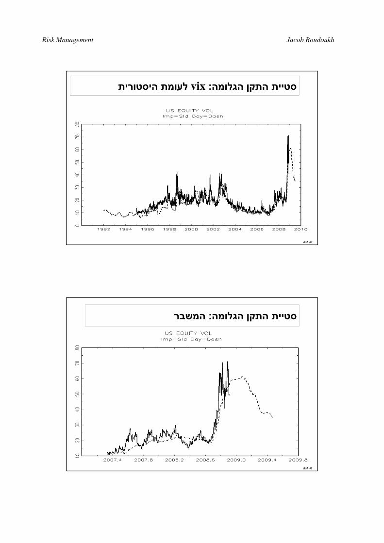
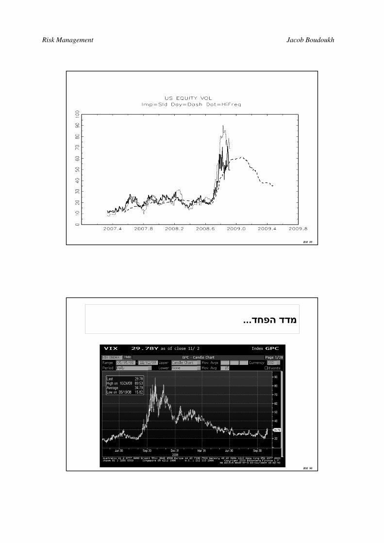
לעומת היסטורית vix: סטיית התקן הגלומה

RM 88

המשבר: סטיית התקן הגלומה


RM 89

RM 90

...מדד הפחד


RM 91

יומיות בשיא המשבר-תנודות תוך–מדד הפחד

� Note not only the level, but also the intra-daily variation� Vol-of-vol peaking� What do we make of that?

RM 92

?הידבקות–מדד הפחד

� Note the recent intra-daily move� � Must analyze scenariossss� What do we make of that?



Normalization

� Take each IR change and divide it by its pre-estimated vol

� ∆it,t+1 / σ t should be distributed N(0,1)


Long horizon vol

� What is the J-period CONDITIONAL variance of ∆St,t+J ?

� Recall: ∆St,t+2=∆St,t+1 +∆St+1,t+2

(using cont’ comp’ returns)

Under what assumptions do we obtain the SQRT-J

rule?

J-day VaR = SQRT(J) *(1day VaR)

Recall:

VAR(∆St,t+1+∆St+1,t+2) = VAR(∆St,t+1) + VAR(∆St+1,t+2)

+2 COV(∆St,t+1,∆St+1,t+2 )



Long horizon vol: assumptions

VAR(∆St,t+1+∆St+1,t+2)=VAR(∆St,t+1)+VAR(∆St+1,t+2)+2COV(∆St,t+1,∆St+1,t+2 )

To obtain the “SQRT-J rule” we need to assume

» A1: COV(∆St,t+1 ,∆St+1,t+2 )=0

» A2: VAR(∆St,t+1)=VAR(∆St+1,t+2)

� With these assumptions:

VAR(∆St,t+1+∆St+1,t+2)=2VAR(∆St,t+1)=2 σt2

==> STD(∆St,t+2)=SQRT(2) σt

...and so on for J-day returns


The empirical record of the “SQRT(J) rule”

The reliability of the “SQRT(J) rule” depends on the

reliability of the assumptions

A1: COV(∆St,t+1 ,∆St+1,t+2 )=0

“no predictability”, or “no mean-reversion”

A2: VAR(∆St,t+1)=VAR(∆St+1,t+2)

“constant volatility” or “no mean-reversion in volatility”

We need to determine:

� When would you expect A1 or A2 not to work?

� Is there a predictable bias?



No predictability assumption

A1: COV( ∆St,t+1 , ∆St+1,t+2 )=0

� Holds true for most financial series (e.g., stock prices, FX)

� However, interest rates DO exhibit mean reversion

COV( ∆St,t+1 , ∆St+1,t+2 ) <?> 0

�� 4-quarter VaR <?> SQRT(J) *(1qtr VaR)

Long Run Mean

i

t


Constant vol assumption

A2: VAR(∆St,t+1)=VAR(∆St+1,t+2)

� Most financial assets exhibit mean-reverting volatility

VAR(∆St,t+1)<?>VAR(∆St+1,t+2)

�� 4-quarter VaR <?> SQRT(J) *(1qtr VaR)

Long Run Mean

volatility

t



RM 100

Vix term structure – Feb19, 2013




Mean reversion: example

� Xt+1=a+bXt+et+1

STDt(∆Xt,t+1)= STDt(a+bXt+et+1 - Xt)= σt

� SPSE b=0.9, σt=10%

==> STDt(∆Xt,t+1)=10%

� ∆Xt,t+2= ... (write Xt+2 in terms of Xt+1, then in terms of Xt)

VAR t(∆Xt,t+2)=(1+b2) σt2 =(1+0.81)*(10%)2

==> STDt(∆Xt,t+2)=1.34*(10%)

� Lower than the SQRT-J rule volatility:

1.41* (10%)

� Especially relevant with short term arbitrage strategies


Benchmarking & backtesting VaR:

Methodology

By definition, at any given period the following must hold:

Prob[R(t+1)<-VaR(t)]=x%

Benchmarking and backtesting is done by observing

the properties of the frequency and size of VaR violations

Define: I(t)=1 if the VaR(t) is exceeded, 0 otherwise

Attributes:

� Unbiasedness:

» Unconditional: avg[I(t)]=x%

» Conditional: low Mean Absolute Error

� Proper Updating: I(t) should be i.i.d..

==> Autocorr[ I(t) ] = 0



OUTLINE




Approach to VaR.

�Beyond Volatility ForecastingBeyond Volatility ForecastingBeyond Volatility ForecastingBeyond Volatility Forecasting

»The The The The VaRVaRVaRVaR of derivativesof derivativesof derivativesof derivatives and interest rate VaR. Structured Monte

Carlo. Extreme events and correlation breakdown. Stress testing and scenario

analysis. Worst case scenario



The VaR of derivatives: introduction

� A derivative is priced off of an underlying asset

� Changes in the value of a derivatives are derived from

changes in the underlying (and the “factor(s)” moving the

underlying)

� Linear derivatives: ∆derivative is linear in ∆factor(s)

» P(f)= α + Delta ∗ f � ∆ P = Delta *∆f

» forwards, futures, swaps

� NON-linear derivatives: ∆P is Nonlinear in ∆factor(s)

» P(f)= α + Delta(Xt) ∗ f � ∆ P = Delta(Xt) ∆f ,

where X t is a state dependent variable

(e.g., the level of interest rates, the “moneyness” of the option)

» options, MBSs, Bradys, caps/floors



How to calculate the VaR of derivatives?

� If linear: straightforward

P= α + Delta ∗ f

� ∆ P = Delta *∆f

� VaRP = Delta * VaRF

� Every asset is LOCALLY linear

� …but for large moves (long horizon VaRs, stress scenarios,...)

nonlinearity matters

� Two methods/approaches to address nonlinearity:

» Full re-valuation

(usually in conjunction with structured Monte Carlo)

» Approximation to the nonlinearity effect

(“the Greeks” using Taylor expansion)


Linear derivatives:

the VaR of FX forwards

� FX forward contract: exchange $F for DM1 in at t+T

� Forwards are priced via covered parity: Ft,T = St (It,T/I*t,T)

� It is derived by arbitrage, using the fact that the following are

equivalent:

» purchase DM forward

» short $bond at It,T, convert into DM, long DMbond at I*t,

� In log terms ∆F = ∆S + ∆I - ∆I*

» in words: the change in the value of a forward contract is equivalent to (by

arbitrage) the change in the spot rate, plus the change in the $ bond, less

the change in the DM bond

==> The VaR of the forward depends linearly on the vol and corr

across the three variables: [∆St , ∆$bond , ∆DMbond ]



The VaR of an FX forward: example

� Recall: ∆F = ∆St + ∆I - ∆I*

� Hence: σ2∆F= σ2

∆S + σ2∆I

+ σ2∆I*

+2cov(∆S,∆I)-2cov(∆S,∆I*)-2cov(∆I, ∆I*)

� Example:

» S=$0.555/z, I=5%, I*=3%, T=1yr ==> F=$.566/z

» Notional amount z1.8MM=$1MM

» Suppose σ∆S=70bp/day, σ 2∆I=σ2∆I* =7bp/day, CORR=0

» VaR∆∆∆∆S= $7000*1.65=11,550,

» VaR∆I=VaR∆I*= 700*1.65=1,155

» VaR∆∆∆∆F = sqrt(11,550 2 + 1,155 2 + 1,155 2) =$11,664

» Why is VaR∆F so close to VaR∆S ?


Nonlinear derivatives

� Recall linear derivatives: ∆P = Delta ∆F

� In the case of nonlinear derivatives, the DELTA is state dependent:

∆P = Delta(Xt) * ∆F

� Examples (by increasing complexity):

» Bond are nonlinear in interest rates

» Options are nonlinear in the underlying

» Convertibles are nonlinear in the underlying

» Callable & convertible bonds are nonlinear in the underlying and in

interest rates

» Defaultable (e.g., Brady) bonds are nonlinear in the default probabilities

» MBSs are nonlinear in interest rates



The problem with duration

P

YY0 Y’

P0


Duration + convexity

P

YY0 Y’

P0

Duration +

convexityFull valuation / true price

Duration



The VaR of options: small moves

xst+T

for small changes in the underlying,

the option is nearly linear, and delta approx.

to the VaR is enough


The VaR of options: large moves

xst+T

for small changes in the underlying,

the option is nearly linear, and delta approx.

to the VaR is enough



The VaR of options: convexity correction

xst+T

for large changes in the underlying,

the option is nonlinear in the underlying,

==> use delta+gamma approximation,

or full revaluation


Empirical interest rate sensitivity of MBSs

Source: “Pricing of Mortgage-Backed Securities in a Multifactor Interest Rate Environment: A Multivariate Density

Estimation Approach”, Boudoukh, Richardson, Stanton and Whitelaw, Review of Financial Studies 1996



Theoretical interest rate sensitivity of Bradys

Source: “Hedging the Interest Rate Risk of Brady Bonds” , Ahn, Boudoukh, Richardson and Whitelaw


The VaR of options: a straddle

xst+T

What is the VaR of a long straddle?

If we go to the +/- 1.65*SD,

we won’t see it!



The VaR of a portfolio of derivatives

� As the previous example shows, the problem is not only

nonlinearities, but also nonmonotonicities (17 letters)

� The problem with full the revaluation approach is its

computational cost/time

» we need to cover the entire range of the distribution ==> simulation

» with N state variables (interest rates, exchange rates, default spreads, etc),

we need to revalue the portfolio thousands of times.

e.g., revalue MBSs, caps, swaptions etc for 10,000 scenarios

» solution: reduce the number of states

e.g., the level and spread (= 2 factors) may suffice to describe the entire term

structure


OUTLINE




Approach to VaR.

� Beyond Volatility Forecasting

» The VaR of derivatives and interest rate VaR. Structured Monte Structured Monte Structured Monte Structured Monte

Carlo.Carlo.Carlo.Carlo. Extreme events and correlation breakdown. Stress testing and

scenario analysis. Worst case scenario




Structured Monte Carlo: basic intuition

� Generating scenarios for one variable which is N( µ , σ2 )

» Generate 10,000 simulations of N(0,1). Denote: Z1 , ... Z10,000

» Calculate 10,000scenarios: St+1,i = St *exp { µ + σ∗Zi}

» Revalue the derivative for each St+1,i

� Generating scenarios for K variables which are N(M,ΣΣΣΣ)

(where M is a vector of length K, and ΣΣΣΣ is a K by K covariance matrix)

» Generate 10,000 K-vector draws, all N(0,1)’s: Z1 , ... Z10,000

» calculate scenarios St+1,i = St *exp {M + A’ Zi }

» A is the “square root matrix” (analogous to σ ) of Σ , namely A’A= ΣΣΣΣ

» Revalue the derivatives for each St+1,i set of values


Structured Monte Carlo: discussion

� The main advantage: correlated scenariosCompare to independent scenario analysis

» a 200bp shift in interest rates, a 25% decline in equities, a 500bp increase

in the sovereign spread,...

» what do we make of such isolated scenarios? do they make economic

sense?

� The main disadvantage: correlation breakdown» what happens to global yield correlation during an oil crisis?

» what happens to strip spreads during an EM currency crisis?

» what happens to the corporate-equity correlation during an equity crisis?



OUTLINE




Approach to VaR.

� Beyond Volatility Forecasting» The VaR of derivatives and interest rate VaR. Structured Monte Carlo.

Extreme events and correlation breakdownExtreme events and correlation breakdownExtreme events and correlation breakdownExtreme events and correlation breakdown.

Stress testing and scenario analysis. Worst case scenario



Generating scenarios:

what is “reasonable stress”?

Odds in 100,000



Correlation breakdown


OUTLINE




Approach to VaR.


events and correlation breakdown. Stress testing and Stress testing and Stress testing and Stress testing and

scenario analysis.scenario analysis.scenario analysis.scenario analysis. Worst case scenario




Stress testing and scenario analysis

� Subjective scenarios taken out of “thin air” + full

revaluation�yield curve shifts and twists, crashes, …

� Pros�cover rare or never-seen-before events

�Cons�no economic guidance

�no sense of probabilities

�questionable for multiple factors


Structured Monte Carlo

� Simulated scenarios using current var-cov matrix

� Full revaluation each time

� Pros�role to probabilities

�Cons�var-cov matrix unstable

�computationally time-consuming



Generating stress scenarios in practice

� Common practice: examine historical events

Instead:

� Links to the historical simulation methodology:

» use HS to generate the empirical distribution for the current portfolio

» use HS to examine the “N worst weeks” given the current portfolio, when

did they occur, and what were the circumstances

� Remember: there is no way to apply common statistical

techniques, with so few (and economically different) data points

� However: extreme value theory is now commonly applied to the

problem

� Its usefulness is very questionable


Stress Testing at XYZ

� Regular + ad hoc stress tests

� Regular tests

» Everything falls in value

yields go up, IR spreads widen, currencies fall vs USD, Vols rise

» Everything rises in value

yields go down, spreads narrow, currencies rise, Vols rise

» “SUB-Scenarios”

- EM Crisis:

all equities down, EM yields up, Spread widen, industrialized yields down + (1)

currency pegs stable, (2) currency pegs collapse:

- General Recovery/G7 Bond Crash:

all equities up, EM yields down, Spread narrow, industrialized yields up + (1)

currency pegs stable, (2) currency pegs collapse:



Issue: correlation

Structural economic models for Correlation

� Consider the following structural model for bond yields

DOM yield: Yt= Dt+Wt , FOR yield: Yt*= Dt

*+Wt

� With orthogonal factors,

corr(∆Y, ∆Y*)= σ2∆W / sqrt{(σ2

∆D+σ2∆W)*(σ2

∆D*+σ2∆W)}

� what happens to corr when:

» DOM factor volatility explodes?

» WORLD factor volatility explodes?


Issue: derivatives

Structural models for derivatives

� S&P500: S10/87=330, S11/87=250

� Vol: σ10/87=.125, σ11/87=.25

� Other data: Rf=.075, T=1yr, X=330

» C(S=330, X=330, σσσσ=.125) = 30

» C(S=250, X=330, σ=.125) = 0.76

» C(S=250, X=330, σ=.25) = 8.12

==> In extreme market conditions it is crucial

to account for changes in Vol

This could be achieved by correlating vol and prices



Issue: Asset & credit concentration

� Another critical aspect is diversification

» Consider, for example, a portfolio of MBSs, Bradys & junk

» We can quantify the systematic ($ Interest rate) and total risk

» These depend on modeling assumptions

� Some asset classes have key variables which are not well

understood

» CMOs -- prepayment -- 1994

» Bradys -- comovements -- 1994, 1997

» Junk -- correlations -- 1987

�� Asset concentration is an issue due to model risk or liquidity

risk, outside the common set of VaR models


Asset & credit concentration: solutions

� The treatment of asset-class concentration is by

» monitoring large exposures

» conducting stress tests

» (similar to credit risk monitoring)

� The assumption is that model/liquidity risk is diversifiable

� Do we leave systematic risk out (e.g., MBSs) ?



OUTLINE




Approach to VaR.


events and correlation breakdown. Stress testing and scenario analysis.

Worst case Worst case Worst case Worst case scenarioscenarioscenarioscenario



http://www.faculty.idc.ac.il/kobi/wcsrisk.pdf

The Distribution of the Worst Case

A major critique of VaR: it simply asks the wrong question.

� VaR(5%) happens on average 5 in 100 periods

� … but perhaps more, perhaps less,

� …and when it does, how bad does it look ?



VaR and the worst case scenario

� Over the next 100 bi-weekly periods, what is the worst that will

happen to the value of the firm's trading portfolio (or the

collateral value of a DPC or SPV)?

� Assume: trading portfolios are adjusted to maintain the same

fraction of capital invested (bet more when you make money)

� VaR tells us that losses greater than µ-2.33σ, the 1%tile of the

portfolio's value, will occur, on average, once over the next 100

trading periods

� Unanswered questions:

» what is the size of these losses?

» how often may they occur


The worst will happen

� WCS analyzes the distribution of losses during the worst trading

period

� Key conceptual point: a worst period will occur with

probability one! The only question is how bad will it be?

!!!



Analysis

� Generate 10,000 vectors of size H of random N(0,1)'s

(interpreted as the normalized trading returns)

� Analyze the distribution the worst observation Zi of each vector

...

z1 z2 z3,..., z10,000

1

H


Results

� H=100 (other results in the paper)

� The expected number of Zs < -2.33 is 1.00 (1% VaR)

� The distribution of the worst case:

AVG(Z)=-2.51

50% 10% 5% 1%

-2.47 -3.08 -3.28 -3.72

� In words: Over the next 100 trading periods a return worse than -2.33σ is

expected to occur once, when it does, it is expected to be of size -2.51σ, but

with probability 1% it might be -3.72σ or worse (i.e., we focus on the 1%tile

of the Z's).

� Note: WCS=VaR*1.6

� Results on bonds and bond options: see enclosed paper



Applications

� Relevant for “prudence multipliers”, applied by the regulator:

(2week VaR) * 3 = Capital requirement

» The * 3 multiplier is pulled out of thin air...

� Need to account for time varying vol, fat tails, corr breakdown,...

� Can provide

» a better understanding of the riskiness of financial institutions

» a control over desired levels of “prudence” and systemic risk

» a safer and more capital efficient financial institutions

RM 140

Coherent Risk Measures

� Monotonicic:

» if PortA>PortB for all realixations, then Risk(PortA)<Risk(PortB)

� Sub-Additive

» Risk(PortA+PortB)<=Risk(PortA)+risk(PortB)

� Homogeneous

» Risk(k*PortA)=kRisk(PortA)

� Translation-Invariant� Risk(k+PortA)=Risk(PortA)-k

� Convex

� Risk(w*PortA+(1-w)*PortB)<=w*Risk(PortA)+(1-w)*Risk(PortB)



RM 141

Is VaR coherent?

� Not generally.

� Under the elliptical distribution assumption (MVN) it is – recall

it maps to stdev etc (and portfolio is linear)

� Counter example: tail risk.

» Consider 5%VaR of 2 bonds with 4% prob of 70% loss (iid events).

» Risk(BondA)= Risk(BondB)=0

» Risk(BondA+BondB)=35%

�0 losses wp .962,

�1 loss wp 2*0.96*0.04=0.0768, loss is 35%

�2 losses wp 0.042=.0016, loss is 70%

�5%VaR is loss of 35%

�VaR may discourage diversification


RM 142

Expected shortfall

� More sensitive to the loss size at scenarios

� Measures expected (average) loss given a “VaR event”

� It is a coherent risk measure

� In the previous example

» ES(BondA)=ES(BondB)=70%

» ES(BondA+BondB)=[0.0016(-70%)+(0.05-0.0016)*(-35%)]/0.05=36.12%




OUTLINE




Approach to VaR.



scenario

�VaRVaRVaRVaR as a Risk Management Toolas a Risk Management Toolas a Risk Management Toolas a Risk Management Tool

»Why do firms hedge?Why do firms hedge?Why do firms hedge?Why do firms hedge?» Optimal VaR control using derivatives.


Why should firms NOT hedge

� Modern finance theory (e.g., the Modigliani-Miller model)

suggests that shareholders can/should diversify risks on their

own. Thus, the need to hedge either the systematic or

unsystematic risk of cash flows / firm value is limited

� The model is derived under certain assumptions (which?)

� IN REALITY, the use of derivatives for interest rate, foreign

exchange and commodity risk management (RM) is widespread

� These institutions' concept of risk is quite different from the

standard measures implied by multifactor pricing models



When does hedging matter?

� Convexity in the tax schedule

» Progressive taxation

» Tax preference items (e.g., tax loss carryforwards)

� Costs of financial distress

» Direct

» Indirect costs

�Lost credibility (sales, expenses, etc.)

�Conflicts of interest between debt and equity

� Agency costs

» Conflicts of interest between managers and other

stakeholders

� Informational asymmetries


Convexity of the Tax Schedule

� Taxes are convex in profits:

» 0% tax for loss, and a progressive tax schedule

� The NOL carryback/carryforward system is intended to remedy

the situation

� However, there are limitations and no indexation

==> the tax authority has a perpetual call option on profits

What can we do to minimize the expected value of his call?

How should it affect share prices?



Costs of financial distress and hedging

� Hedging can smooth cash flows

� reduce the probability of distress

� increase expected cash flows by reducing

the EXPECTED costs of financial distress

� reduce the required return of debt

� reduce the cost of capital to the firm

� Equity holders may or may not benefit from risk hedging

depending on whether the increase in firm value is more

or less than the value transfer to debt from the reduction

in risk.


Hedging and agency costs

� The problem: conflicts of interest between managers and other

stakeholders

� Informational asymmetries are inherent

� Monitoring and information extraction are costly activities

� Earnings are noisy



Noisy earnings and information extraction

• AVG(CompA)=70, AVG(compB)=50

Without hedging

• distinguishing between them is difficult

• monitoring the effort and project selection of the managers

is also difficult


What do firms/FIs care about?

� The above motivations for risk management are not driven

by firms' market risk, but instead by total risk:

� It is the probability and magnitude of potential losses that

determine the desire (or lack thereof) to hedge

� As a result of this different criteria for risk, the VaR concept has

become the standard tool in the exploding area of risk

measurement and management (mainly for FIs)

� While a growing number of approaches exist to risk

measurement using VaR, academics and practitioners alike

have been silent on the question of how to formally address the

question of risk management this risk



OUTLINE




Approach to VaR.



scenario

� VaR as a Risk Management Tool» Why do firms hedge?

»Optimal Optimal Optimal Optimal VaRVaRVaRVaR control using derivatives.control using derivatives.control using derivatives.control using derivatives.


“OPTIMAL RISK MANAGEMENT”

� GOAL: Provide an analytical approach to optimal risk

management in a stripped-down framework in which an

institution wishes to minimize its VaR using options

� Key assumptions

» The RM criteria is VaR

» The RM hedging tool is options

» the standard B/S setting holds

� We identify the optimal put option position that minimizes

the VaR of a given exposure given hedging cost

� We deliver a “COST / VaR optimal frontier”



Why focus on options?

� Implementing and analyzing a forward/futures hedge is easy

(basis risk, credit risk and measurement issues aside)

� Recent surveys suggest that the use of options in hedging

programs is commonplace (almost as forwards)

� Why options?

» Institution are willing, sometimes even desire, to take the underlying

exposure, leading to partial hedges (due to managerial incentives?)

» An options-based hedging program is consistent with at least some of the

above motives for RM ( taxes, securing a level of available inside

financing, reduction of distress probability...)

» Institutional constraints, such as GAAP for hedge accounting and the tax

treatment of derivatives, lead to forward hedges not being a viable

alternative for long term hedges


How to implement an options hedge?

� There is a tradeoff between an options' ability to reduce VaR and

its cost

� At high strike prices, the puts provide substantial protection but

at a high cost per option and v.v.

� For a given cost, there exists a menu of implementable pairs of

[strike price, hedge ratio]



A three option example

VaR


A preview of the results

� Given the exposure's parameters the optimal choice of options

always has the same strike price, independent of the level of

expenditure

� The benefits of choosing the options optimally are economically

significant:

» using typical equity indexes parameters

» the hedged-VaR using ATM options can exceed the optimally

hedged VaR by over 15%

» Alternatively, when trying to achieve a given VaR, using

ATM options costs 65% more than optimal strike options



The optimization problem

Min h, X { VaRt+τ τ τ τ }

s.t. C = h * P(St,X,r,σ,τ σ,τ σ,τ σ,τ )

where VaRt+τ = St - [ (1-h)St exp(qα) + h X ]

IN WORDS:

» The optimization problem identifies the h, X pair which gives the most

“bang for the buck” in terms of payoff at the VaR point

» the payoff of the hedged position consists of a fraction h of the hedged

value X, (1-h) of the “1.65 standard deviations” tail value of the

underlying

» The tail is, more generally, qα =(µ-1/2σ2)τ + cασ sqrt(τ )


The optimal exercise price

X* is the solution that satisfies:

St exp(qα) = St exp(rτ) (Φ(d2)/Φ(d

1) )

= EQ[ St+τ | St+τ < X* ]

� Intuition

» “Preferences” specified for payoff of a given percentile

» There is no aversion to any other moments

» The payoff maximizing scheme is achieved at X*, the optimal exercise

price for the chosen percentile




The benefits of optimal hedging

Two related questions:

1. Given a certain cost allocation, how does the optimal VaR

compare to VaR’s w/ other exercise prices (e.g., ATM)?

2. For a given targeted VaR level, how does the cost of

implementation differ across different choices of exercise prices?



VaR across exercise prices

Myopic

ATM hedgeOptimal

hedge

{Improve-

ment


Several natural extensions

� Non-normality, mean reversion

� Multiple asset exposure: optimal menu of options

� (or - basket options)



Thanks

RM 164

Sample Problems

The annual standard deviation of the Japanese stock market (in Yen) is 20%, and that of the Yen/$

exchange rate is 10% per annum. You believe that the expected return on the Japanese market (in

Yen) is 10% per annum, and the expected rate of appreciation of the Yen over the coming year is

5%.

Assumptions:

VaR is the 5th percentile (1.65 standard deviations),

The correlation of the Yen/$ rate with the Japanese market is zero

Questions:

a. Suppose you invest $1,000,000 in the Japanese market (currency unhedged). What is your

annualized 5% Value at Risk (in $ terms)?

b. How would you implement a currency hedge on this equity investment? Is this a perfect hedge?

How could you improve the hedge?

c. What is the effect of fully hedging the currency exposure (i.e., by how much would you reduce

your $ exposure)?

d. Suppose the $ risk free rate is 4%. What is the Sharpe Ratio of a currency-hedged and currency-

unhedged investment in the Japanese market?

e. Based on your calculations, which investment strategy should you prefer? Explain why the results

are economically counterintuitive, and how do they result from the assumptions?



RM 165

SOLUTION

$VaR=1,000,000*1.65*sqrt(.2^2+.1^2)=$368,951

some may have calculate around the expected return of x%, which is OK ($426,138)

Via Nikkei futures, traded/readjusted monthly for example, hedging the underlying position 1:1.

This is not a perfect hedge due to the residual amount during the month, hence increasing the

frequency of readjustment of hedge will improve it. Also, a statistical regression can provide a

hedge ratio more precise than the 1:1 myopic hedge.

(c) YenVaR=1,000,000*1.65*.20=$330,000.

Hence 368,951-330,000=$38,951

(d) E [ excess unhedged return ] = (1.10*1.05-1.04)*100 = 11.5%

E [ excess hedged return ] = (1.10-1.04)*100 = 6%

and SD[ excess unhedged return ] = sqrt(.2^2+.1^2)*100 = 22.36%

SD[ excess hedged return ] = sqrt(.2^2 )*100 = 20%

==> Sharpe[ unhedged ] = 11.5/22.36 = 0.51

Sharpe[ hedged ] = 6/20 = 0.30

(e) You should prefer to remain currency unhedged, particularly due to your belief that the

Yen is going to appreciate. This assumption is economically implausible, since the inflation

differential is small.


RM 166

True/False, multiple choice etc., with a brief explanation

(a) In comparing the volatility forecasts from a simple standard deviation model with a lookback

period of 100 periods (STD(100)) to that of 50 periods (STD(50)), you would expect

(1) The STD(50) to be more biased on average than the STD(100) relative to the true volatility

(2) The STD(50) to be more volatile forecast series than the STD(100)

(3) Both (1) and (2)

(4) None of the above

(b) (True/False) If the volatility of an asset moves around very slowly, you would expect an

exponential smoothing parameter closer to one (e.g., 0.97) to be a better vol forecasting

parameter than a lower smoothing parameter (e.g., 0.94)

(c) If asset returns are more "fat-tailed" than what conditional normality indicates, the VaR is

understated

(d) If current volatility is above its long run mean, then the square root rule for long horizon

volatility will understate the true long horizon volatility.



RM 167

(a) Solution: (2), due to sampling variation or true vol variation. There is no question of bias,

though.

(b) Solution: True. A higher smoothing parameter will reduce the sampling variation, and

will miss little in the way of current information, relative to the low smoothing parameter.

(c) Solution: True. The x% tail of returns will be larger than the theoretical one.

(d) Solution: False. The exact opposite is true, namely, since volatility is expected to decline,

the square root rule will overstate long horizon volatility.



The Risk of Derivatives -Summary

Approaches

� The “Delta-Normal” approach

» The “Greeks”

� Full revaluation

» Historical simulation

» Stress testing and scenario analysis

» Structured Monte Carlo



The “Delta-Normal” approach

� Assumes all returns are normal

� Pros

» relatively easy and computationally efficient

� Cons

» Delta-approx’ driven -- needs some fixing

» Inaccurate when no closed form

» Highly model dependent

�no event risk

�no fat tails

�non-factor changes not accounted for


Full Revaluation

� May be computationally intensive for large portfolios and many

factors ( => need to simulate the “full distribution”)

� Historical simulation�apply current portfolio weights to past values of factor changes

� fully revalue

�get the empirical tail

�…this is the basis for the Basel standard

» Pros

� realistic tails, accounting for “true dist’n, correlation breakdowns, nonlinearities

�computationally not as bad as SMC

» Cons

�Weighting (hybrid is a solution

� long horizons very problematic

financial risk measurement & management - idc · » quiz3will take place during the 1st class...

Documents