financial liberalization and banking crisis: a spatial ... 2_3_5.pdf · we look at one of the most...
TRANSCRIPT

Journal of Applied Finance & Banking, vol.2, no.3, 2012, 81-122 ISSN: 1792-6580 (print version), 1792-6599 (online) International Scientific Press, 2012
Financial Liberalization and Banking Crisis:
A Spatial Panel Model
Mohamed Bilel Triki1 and Samir Maktouf2
Abstract
This paper investigates the determinants of banking system fragility by
underlining the impact of bank liberalization on banking stability during the
process of financial liberalization in emerging and developed countries. To this
effect, we adopted a panel model with spatial dependency from a transmission
channel points towards trade interactions to estimate the parameters of the model
on a panel of 40 emerging and developed countries during 1989-2010. The
empirical results suggest that financial liberalization has the tendency to stimulate
the banking instability in economies. Financial liberalization played a significant
role in the transmission of the 1996 to 2002 crisis to emerging market economies
and also to American and European countries in 2007 crisis. However, credit
growth, a negative GDP growth and a high real interest rate are on average the
1 Faculty of Economics and Management, University of Tunis El Manar, Tunisia, e-mail: [email protected] 2 Faculty of Economics and Management, University of Tunis El Manar. Tunisia, e-mail: [email protected]
Article Info: Received : March 22, 2012. Revised : April 26, 2012 Published online : June 15, 2012

82 Financial Liberalization and Banking Crisis: A Spatial Panel Model
most important causes of a banking crisis. Besides we find that the impact of the
determinants differ between whole, advanced economies and emerging
economies.
JEL classification numbers: G01, G21, G28, C21, C23, E44
Keywords: Banking crisis, Spatial econometrics, Financial liberalization
1 Introduction
Many countries around the world have liberalized their financial sectors,
particularly during the 1980s and the (1990s), with the aims of improving
financial development and economic growth (Tornell et al, 2004; Bekaert et al,
2005). However, financial liberalizations are often followed by reckless lending
and severe banking crises. The identification of the causes of banks’ behavior is
often difficult because financial liberalizations entail several contemporaneous
changes.
The empirical research into the causes and consequences of banking crises
in emerging countries has only started to draw professional concentration in the
last several years. We look at one of the most central policy questions in front of
this empirical study, the responsibility of financial liberalization, in its complete
effort to present policy makers with recommendation on preventing crises,
determining their beginning earlier, and mitigating their adverse effects.
Dıaz-Alejandro (1985), in an early working titled ‘‘Goodbye Financial Repression,
Hello Financial Crash,’’ explained the relationship between financial liberalization
and financial crises founded on his clarification of the Latin American
experience—we empirically look at this hypothesized relationship in this
document.
All empirical workers that build early warning systems or think the
M.B. Triki and S. Maktouf 83
determinants of crises categorize a narrow set of macro-economic and financial
variables that envisage banking crises. One of the most robust outcomes
surrounded by this literature is that recent liberalization’s domestic financial sector
will increase the probability of a banking crisis (the literature is investigated in
Arteta and Eichengreen, 2002) and its shock affect on institutional settings, so the
economy will be destabilizing (Demirgüç-Kunt and Detragiache, 1999; and
Kaminsky and Reinhart, 1999).3
However, there is no accessible confirmation on the precise role that
financial liberalization plays in the appearance of problems in the banking sector;
it is not clear how much the augmented risk to the banking sector is conditional on
the form or cadence in which liberalization take place, and, more significantly,
what is certainly the sequence of events that leads from liberalization to crises.
Whereas there is little formal theoretical effort to elucidate the role of financial
liberalization in the emergence of systemic problems in the banking sector, two
maintaining (but not mutually exclusive) explanations emerge: henceforth, the ‘lax
supervision’ and ‘monopoly power’ hypotheses.
In review, liberalization has a tendency to generate advanced growth
nevertheless higher volatility in that reason a trade-off probably inherent (Tornell
and Westermann, 2005). Indeed, financial liberalization is often followed by a
global reorganization process in the banking system that caused an important
debate on the impact that consolidation has on financial stability.
In spite of the great number of theoretical and empirical contributions to this
area of study, the evaluation of the impact of the increase in stability, which is
effected by the global reorganization process of the financial systems and
incentives and government programs, on the risks taken by the banks and on the
banks’ stability which continues to be of great importance.
3 Caprio and Klingebiel (1996), Niimi (2000), and Gruben et al. (2003) deduce that banks are much more possible to fail in a liberalized regime than under financial repression.
84 Financial Liberalization and Banking Crisis: A Spatial Panel Model
The main contribution of this paper to the banking crisis literature is that it
presents a methodology to test the stability–liberalization relationship for some
countries. Empirical methodology of this nature is not furthermore present in the
literature. Our empirical contribution is based on spatial panel models, i.e., panel
models which explicitly take into account ‘spatial’ interactions among observed
countries with trade channels as primordial transmission mechanisms.
Spatial panel seems particularly well-suited to study the determinants of
banking crisis, which by definition can only occur if there are interactions among
subjects. Alike if banking crises is due to a transmission, transmission itself can
only happen if there are interactions between countries. Interactions can happen at
the foreign trade level, where feebleness by one member may have strong
consequences for the residual members. A crisis in one country can cause a
reduction in income and a corresponding reduction in demand for imports, thereby
affecting exports, the trade balance and related economic fundamentals.4 The
interdependence can be the resultant effect of financial linkages. In a region where
integration is high, a crisis in one country can have direct financing effects on
other countries through trade credit reductions, foreign direct investment and other
capital flows.5
Our results confirm some previous findings in the literature: spatial panel
estimates lend support in favor of the determinants of a banking crisis which
explicitly take into account ‘spatial’ interactions among observed countries with
trade channels as primordial transmission mechanisms. We find evidence that
macroeconomic factors were significant explanatory variables. Of all
macroeconomic variables, the credit growth experienced by several countries
seemed to have played the most significant role.
4 For a detailed discussion of trade linkages, see Gerlach and Smets (1995), Eichengreen et al. (1996), and Corsetti et al. (2000). 5 For a detailed discussion on financial linkages see Goldfajn and Valde´s (1997) and Van Rijckeghem and Weder (2001).

M.B. Triki and S. Maktouf 85
This paper is organized as follows. In the next section, we present a brief
review of the literature. Section 3 we summarize the spatial panel model and
discuss specification methods. Section 4 presents the methodology and data.
Section 5 reports the empirical results based on the banking crisis records across
40 countries from 1989 to 2010. Section 6 summarizes the results with concluding
remarks.
2 Literature review
Motivated by public policy debates and theoretical predictions, such as Betty
and Bailey Jones (2007), the theoretical arguments and country comparisons on
the relation between financial liberalization and stability of the banking system are
ambiguous. There exist at least two opposing visions, liberalization-stability and
liberalization-instability.
In the first point of view, there is a great guidelines literature founded on the
traditional view that there are strong arguments and some evidence to argue that
financial liberalization is beneficial in the long-term (Ranciere et al., 2003;
Tirtiroglu et al., 2005).
In the second point of view, there is a large policy literature based on the
conventional view that there is a trade-off between concentration and fragility.
This link was noted as early as 1985 in a paper by Diaz-Alejandro (1985). More
recently, this episodic evidence has been recently supported by more systematic
work that looks into the relation between financial liberalization and financial
instability (Fischer and Chenard, 1997).6 To widen a basic sense for this kind of
study, let us illustrate the essential part of what Demirguc_Kunt et Al. (1998) to
6 Also Goldstein and Turner (1996), in a survey of banking crises in emerging economies, include inadequate preparation for financial liberalization, among the key factors that lead to banking crises.

86 Financial Liberalization and Banking Crisis: A Spatial Panel Model
do. They envisaged the empirical liaison among banking crises and financial
liberalization in a panel of 53 states for the period 1980 to 1995 in a
multivariate-logit model.
In addition to a set of variables which are accepted as standard predictors
of banking crises (economic growth, terms of trade changes, real interest rates,
inflation, M2 as percent of international reserves, private sector credit to GDP,
ratio of bank liquid reserves to GDP, rate of growth of private sector credit, real
GDP per capita). They find that banking crises are more possible to happen in
liberalized financial systems, yet if institutional factors reduce the likelihood of
banking crises.7
Both the banking crisis variable and the financial liberalization variable are
constructed as dummy variables through them experiment with the exact
specification of dummies over time. They do not use the real interest rate as an
indicator on the grounds that real interest rates especially when measured ex-post
are likely to be affected by a variety of factors that have little to do with the
regulatory framework of financial markets and can be misleading. For instance,
although they argue, a positive correlation among real interest rates and the
probability of a banking crisis may simply reflect the fact that both variables tend
to be high through economic downturns, whereas financial liberalization shows no
responsibility. Some of their key outcomes are reviewed in Tables 2 and 4 in the
paper (see Demirguc-Kunt and Detragiache (1998)).
Furthermore, Demirgu¸c-Kunt and Detragiache (2001) finds that, after
controlling for a myriad of macroeconomic controls, ‘financial liberalization
exerts an independent negative effect on the stability of the banking sector, and the
magnitude of the effect is not trivial’ (p. 98). Apart from the limitations related
with such from one side to the other of a nation regressions (Rodrik, 2005), it
7 In line with most other research, Barth et al. (1998) find that restrictions on operations of the financial sector increase the long-run likelihood of a banking crisis.
M.B. Triki and S. Maktouf 87
requests to be noted that the financial liberalization variable in their cadre is
captured through a ‘catchall’ dummy variable.
Arteta and Eichengreen (2002) present an extensive review of empirical
macroeconomic research on banking crises. They identify a list of
macro-economic and financial variables that are establish to be significant in the
determination of banking crises.8 We make use of their list in defining the control
variables in our own model. In the last part of their article, they center on financial
liberalization as a determinant of crises and find that ‘‘[domestic financial
liberalization] enters with a strong positive coefficient which differs from zero at
the 99% confidence level, confirming [others’] finding that domestic financial
liberalization heightens crisis risk, presumably by facilitating risk taking by
intermediaries’’ (p. 21).9 Here, we specifically study whether the mechanism that
leads from liberalization to crises is indeed through facilitation of increased ‘risk
taking by intermediaries’—a question that has not been empirically resolved (or
even examined).
More recently, IlanNoy (2004) examine what is identified as one of the
principal reasons in the occurrence of banking crises: financial liberalization. As it
is typically disputed, if liberalization is accompanied by insufficient prudential
supervision of the banking sector, it will result in excessive risk taking by
financial intermediaries and a subsequent crisis. Having evaluated the empirical
validity of this hypothesis, they argue that such a development is, at worse, only a
medium run threat to the health of the banking sector. They find that a more
immediate danger is the loss of monopoly power that liberalization typically
entails. They base their conclusions on an empirical investigation of a panel-probit
model of the occurrence of banking crises using macro-economic, institutional and
8 Earlier papers that found the same correlation between liberalization and banking crises are Demirguc-Kunt and Detragiache (1998), and Glick and Hutchison (2001). 9 In a footnote they state, ‘‘these conclusions are robust to alternative estimation methods.’’
88 Financial Liberalization and Banking Crisis: A Spatial Panel Model
political data.
Demirguc-Kunt and Detragiache (2005) have extended their sample until
2002 and with integration of other countries compared with their article in 1998.
The number of crisis studied is increased from 31 to 77, this big number of crises
ameliorates the robustness of conclusion. In this paper, they presented two
fundamental methodologies to find out the determinant of banking fragility: signal
approach and multivariate probability model. As a result, they have a better
understanding of how systemic bank fragility is influenced by a host of factors,
including macroeconomic shocks, the structure of the banking market, broad
institutions, institutions specific to credit markets, and political economy
variables.
Ranciere et al (2006) envisage the relationship among financial
liberalization and crises using one proxy for equity market liberalization and
another for relaxation of capital account restrictions. Both financial liberalization
variables are associated with higher probabilities of banking and currency crises
(twin crises).
Betty and John Bailey (2007) in their paper they extend a dynamic
explanation, by forming the evolution of newly-liberalized bank's opportunities
and incentives to take on risk over time. The model proves that financial
liberalization, in and of itself, contributes to banking crises and that between an
initial period of rapid, low-risk growth and a long-run outcome of a safe banking
system, banking systems of emerging markets will experience a transitional period
with an increased risk of banking crisis.
Finally, Apanard et al. (2010) use a recently updated dataset for financial
reforms in 48 countries between 1973 and 2005. They focus on banking crises and
argue that they are most likely to occur after some degree, but not full,
liberalization. Their empirical results indicate that the relationship between
liberalization and banking crises be supported by strongly on the strength of
capital regulation and supervision. A rule repercussion is that positive

M.B. Triki and S. Maktouf 89
growth-effects of liberalization can be achieved without increasing the risk of a
banking crisis if appropriate institutions are developed.
Overall, this brief survey of the empirical literature suggests that there is no
consensus what the relation between financial liberalization and financial stability.
To the best of our knowledge, the only paper that tests this relationship is Betty
and Bailey Jones (2007). We propose a test for this relationship by using a spatial
panel data approach to evaluate the financial liberalization and financial stability.
We focus on an emerging market, which is the most important in Latin America,
and East Asiatic and developed countries for detecting the last crisis. We discuss
the methodology and the data more in depth in the empirical section.
3 Spatial Panel Approach
In this section, we describe spatial panel models, briefly surveying
estimation procedures. Our objective is twofold. First, to familiarize the reader
with the econometric techniques, most of which have only recently been
developed. Secondly, to lay the foundations necessary to motivate the use of
spatial panel models in the analysis of banking crises.
As pointed out by Anselin et al. (2008), when specifying spatial dependence
among the observations, a spatial panel data model may contain a spatially lagged
dependent variable, or the model may incorporate a spatially autoregressive
process in the error term. The first model is known as the spatial lag model and the
second as the spatial error model. A third model, advocated by Le Sage and Pace
(2009), is the spatial Durbin model that contains a spatially lagged dependent
variable and spatially lagged independent variables.
Formally, the spatial lag model is formulated as
1
N
it ij it it i i itj
y w y x optional optional
(1)

90 Financial Liberalization and Banking Crisis: A Spatial Panel Model
where yit is the dependent variable for cross-sectional unit i at time t (i=1, ..., N;
t=1, ..., T). The variable Σwjiyit denotes the interaction effect of the dependent
variable yit with the dependent variables yjt in neighboring units, where wij is the i,
j-th element of a prespecified nonnegative N×N spatial weights matrix W
describing the arrangement of the spatial units in the sample. α is the constant term
parameter. xit a 1×K vector of exogenous variables, and β a matching K×1 vector
of fixed but unknown parameters. εit is an independently and identically
distributed error term for i and t with zero mean and variance σ2, while μi denotes
a spatial specific effect and λt a time-period specific effect.
In the spatial error model, the error term of unit i, φit, is taken to depend on
the error terms of neighboring units j according to the spatial weights matrix W
and an idiosyncratic component εit, or formally
1
it it it
N
it ij it itj
y x
w
(2)
where ρ is called the spatial autocorrelation coefficient.
The first step in this methodology is to know if the spatial lag model or the
spatial error model is more suitable to explain the data than a model without any
spatial interaction effects, one may use Lagrange Multiplier (LM) tests for a
spatially lagged dependent variable and for spatial error autocorrelation, as well as
the robust LM-tests which test for the existence of one type of spatial dependence
conditional on the other.10 These tests are founded on the residuals of the
non-spatial model with spatial fixed effects and follow a chi-squared distribution
with one degree of freedom. If a non-spatial model is estimated without any fixed
effects or a non-spatial model with both spatial and time-period fixed effects, the
residuals of these models can be used instead (Elhorst, 2010). Since the outcomes
10 A mathematical derivation of these tests for a spatial panel data model with spatial fixed effects can be found in Debarsy and Ertur (2010).

M.B. Triki and S. Maktouf 91
of these tests depend on which effects are included, it is recommended to carry out
these LM tests for different panel data specifications.
If we accept spatial lag model or the spatial error model against, evidently,
the reject of non-spatial model when adopting these LM tests, one should be
careful to support one of these two models. LeSage and Pace (2009, Ch. 6)
recommend to think also about the spatial Durbin model. This model extends the
spatial lag model with spatially lagged independent variables
1 1
N N
it ij jt it ij ijt itj j
y w y x w x
(3)
where θ, just as β, is a K×1 vector of parameters. This model can then be used to
test the hypotheses H0: θ=0 and H0: θ+δβ=0. The first hypothesis examines
whether the spatial Durbin can be simplified to the spatial lag model and the
second hypothesis whether it can be simplified to the spatial error model (Burridge,
1981). Both tests follow a chi-squared distribution with K degrees of freedom. If
the spatial lag and the spatial error model are estimated too, these tests can take
the form of a Likelihood Ratio (LR) test. If these models are not estimated, these
tests can only take the form of a Wald test. LR tests have the disadvantage that
they require more models to be estimated, while Wald tests are more sensitive to
the parameterization of nonlinear constraints (Hayashi, 2000, p.122).
If both hypotheses H0: θ=0 and H0: θ+δβ=0 are rejected, then the spatial
Durbin best describes the data. Conversely, if the first hypothesis cannot be
rejected, then the spatial lag model best describes the data, provided that the
(robust) LM tests also pointed to the spatial lag model. Similarly, if the second
hypothesis cannot be rejected, then the spatial error model best describes the data,
provided that the (robust) LM tests also pointed to the spatial error model. If one
of these conditions is not satisfied, i.e. if the (robust) LM tests point to another
model than the Wald/LR tests, then the spatial Durbin model should be adopted.
This is because this model generalizes both the spatial lag and the spatial error
model.

92 Financial Liberalization and Banking Crisis: A Spatial Panel Model
Lee and Yu (2010) classify that the direct approach will generate, for
probably, biased estimates of (some of) the parameters. Starting with a combined
spatial lag/spatial error model, also known as the SAC model (LeSage and Pace,
2009, p.32), and using rigorous asymptotic theory, they analytically derive the size
of these biases. In this article we adopt the procedure of Lee and Yu (2010) that
recommend finding consistent results which is a bias correction procedure of the
parameters estimates when adopting the direct approach based on maximizing the
likelihood function with the purpose of adopting the transformation approach. In
this paper we adopt the bias correction procedure and translate the biases Lee and
Yu (2010a) derived for SAC model to successively the appropriate model the
spatial lag model, the spatial error model, or the spatial Durbin model.
4 Methodology and data
Our sampling covers the period 1989-2010. The choice of this period
depends of two principals’ reasons: first represent a period of financial
liberalization and second a period which knows the gravest banking crisis.
Concerning the construction of our panel, we are limited to 40 emerging and
developed countries (Table A2, see Appendix) those affected by banking crisis.
The typical manner of describing banking crisis is based on the dating,
which is the binary data, but we adopt none performing Loans as endogenous
variable. One cause of the variable use of non-performing loans is the divergence
of the empirical work on the causes of banking crises. This is caused by the use of
different dates for both the trigger and the resolution of the same crisis. So the
quantitative measurement of banking crisis remains problematic for several
reasons and this dichotomous data is inappropriate for our approach. An
alternative approach, suggested by Caprio and Klingebiel (1996) and
Demirgu¸c-Kunt and Detragianche (1997), is to adopt the bank nonperforming

M.B. Triki and S. Maktouf 93
loan (NPL) to proxy for banking crisis. While we follow this suggestion to use
NPL as the proxy of banking crisis, we also recognize that the use of the NPL is
not without shortcomings.
A list of the variables with their descriptions and their sources is provided in
the Table A1. Table A3 presents descriptive statistics for the whole sample. (see
Table A1-3, in Appendix).
The list of candidate explanatory variables was inspired by the existing
empirical and theoretical literature on baking crisis, concentration on those that are
widely available on a timely basis. These variables can be split into two groups.
The first group based on the findings of Demirguc-Kunt and Detragiache (2005),
Kaminsky and Reinhart (1999) that systemic banking crisis tend to erupt in a weak
macroeconomic environment, we construct the variables of the macroeconomic
determinants of baking crisis with the definitions and data sources presented in
table A1. The second group based on the finding of Demirguc-Kunt and
Detragiache (1998), Komulainen and Lukarila (2003), Chang et al. (2008) that
affect the health of the banking sector, or which may indicate the advent of such a
shock. We experiment with an alternative measure of institutional quality: GDP
per capita.
To test whether macroeconomic environment and financial liberalization
affect banking system fragility, we use a spatial panel model. We estimate the
probability model that a systemic crisis will occur at a particular time in a
particular country, while the sign of the estimated coefficient for each explanatory
variable indicates whether an increase of that explanatory variable increases or
decreases the probability of a crisis.
5 Spatial empirical evidence
This section utilizes the spatial econometrics tools described earlier to
analyze the period 1989 to 2010. In its most general form, the selected regression

94 Financial Liberalization and Banking Crisis: A Spatial Panel Model
model is given by:
1
,
0,1
N
it i it ij jt itj
it
z x w z
N
Where z is a nonperforming loans variable taking value for any of the 40 countries,
x is the controlled variables defined earlier. ijw is exogenously specified n x n
lag weights matrices. As suggested earlier, to test for sources of co-movement, we
can specify weights matrices based on different concepts of ‘neighborhood’. In
this article, we utilize an exogenously specifying matrices based on international
trade data. Three matrices are created:
(i) Exports-based, XW . We register at each ij−entry the 1997 exports of to i j .
As a convention in the literature, we also normalize each row to sum to 1.
Therefore, crises or tranquil episodes elsewhere are weighted by the relative
importance of country j’s market to country i.
(ii) Imports-based, MW . To overcome one of Glick and Rose (1998)
shortcomings, we create a matrix of the form described in (i), registering
instead imports of i from j at each ij−entry.
(iii) Total international trade-based, TW . This matrix adds up exports and
imports to form the weights.11
Table C.1, 2 and 3 reports the estimation results for the different weights
matrices, Exports-based, XW,
imports-based, MW and total international
trade-based, TW respectively. While the estimation results for the subsamples
of emerging markets, East Asian and Latin America.
11 All three matrices are clearly non-symmetrical, reflecting, for example, in case of the United States and Portugal, the fact that Portugal represents a small fraction of the United States total foreign trade, while the United States represents a large fraction of Portugal total foreign trade ( )ij jiW W .
M.B. Triki and S. Maktouf 95
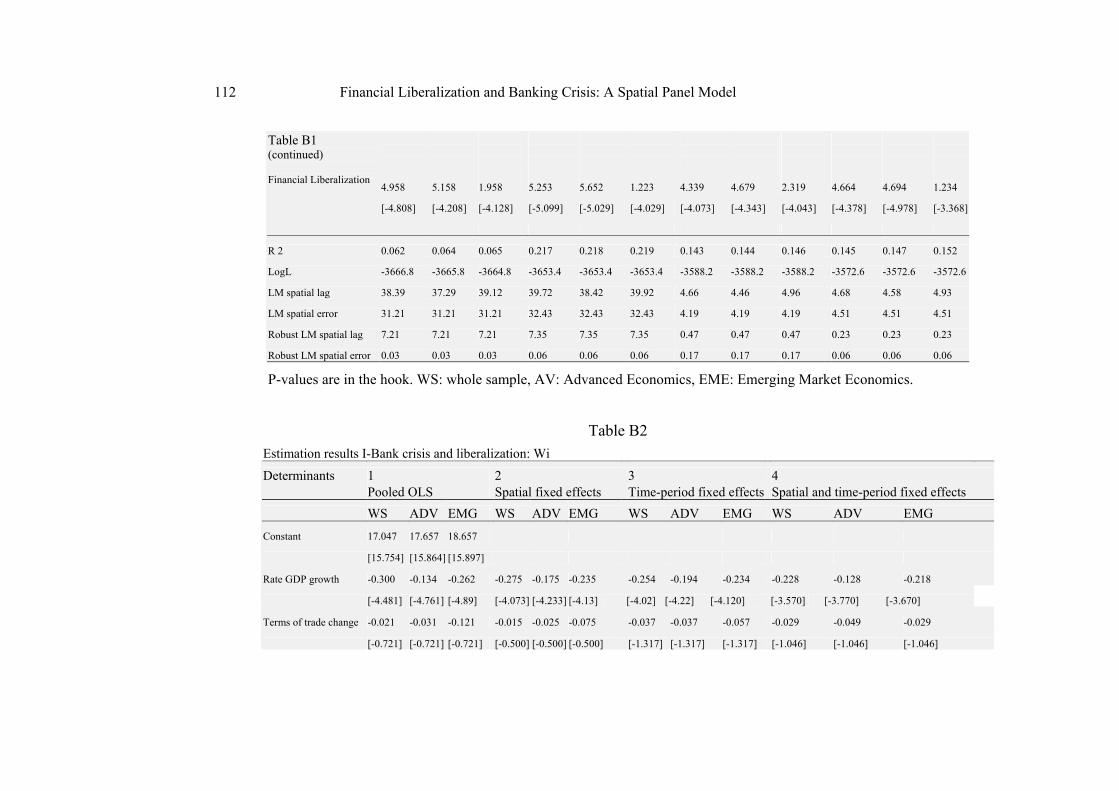
Table B reports the estimation results when adopting a non-spatial panel
data model and test results to determine whether the spatial lag model or the
spatial error model is more appropriate. When using the classic LM tests, both the
hypothesis of no spatially lagged dependent variable and the hypothesis of no
spatially auto correlated error term must be rejected at 5% as well as 1%
significance, irrespective of the inclusion of spatial and/or time-period fixed
effects. When using the robust tests, the hypothesis of no spatially auto correlated
error term must still be rejected at 5% as well as 1% significance. However, the
hypothesis of no spatially lagged dependent variable can no longer be rejected at
5% as well as 1% significance, provided that time-period or spatial and
time-period fixed effects are included.12 Apparently, the decision to control for
spatial and/or time-period fixed effects represents an important issue. (see Table
B1-3 in Appendix)
We estimate the following panel model specification:
0 1 ,¨ ,
2 , 3 ,
4 , 5 , 6 ,
7 , 8 ,
9
Rate GDP growth
Terms of trade change Real interest rate
Inflation rates M 2 / reserves Depreciation
Credit growth GDP / CAP
Financ
j tcountry j Time t
j t j t
j t j t j t
j t j t
NonPerflon
, ,ial Liberalisation j t j tTo investigate the (null) hypothesis that the spatial fixed effects are jointly
insignificant, one may perform a likelihood ratio (LR) test.13 The results (231.182,
with 40 degrees of freedom [df], p < 0.01) indicate that this hypothesis must be
12 Note that the test results satisfy the condition that LM spatial lag + robust LM spatial error = LM spatial error + robust LM spatial lag (Anselin et al., 1996). 13 These tests are based on the log-likelihood function values of the different models. Table 1 shows that these values are positive, even though the log-likelihood functions only contain terms with a minus sign. However, since σ2<1, we have –log(σ2)>0. Furthermore, since this positive term dominates the negative terms in the log-likelihood function, we eventually have LogL>0.

96 Financial Liberalization and Banking Crisis: A Spatial Panel Model
rejected. Similarly, the hypothesis that the time-period fixed effects are jointly
insignificant must be rejected (161.607, 22df, p < 0.01). These test results justify
the extension of the model with spatial and time-period fixed effects, which is also
known as the two-way fixed effects model (Baltagi, 2005). The same results are
for model when we introduce We and We+Wi and also for whole sample,
advanced economies’ and emerging economies' sub-sample.
Up to this point, the test results point to the spatial error specification of the
two-way fixed effects model. In view of our testing procedure spelled out in
Section 2, we now consider the spatial Durbin specification of the determinant of
banking fragility. Its results are reported in columns (1) and (2) of Table C. The
first column gives the results when this model is estimated using the direct
approach and the second column when the coefficients are bias corrected
according to (8). The results in columns (1) and (2) show that the difference
between the coefficients estimates of the direct approach and of the bias corrected
approach are small for the independent variables (X) and σ2. By contrast, the
coefficients of the spatially lagged dependent variable (WY) and of the
independent variables (WX) appear to be quite sensitive to the bias correction
procedure. (see Table C1-3 in Appendix)
We estimate the following panel spatial model specification:
0 1 ,¨ ,
2 , 3 ,
4 , 5 ,
6 , 7 ,
8
Rate GDP growth
Terms of trade change Real interest rate
Inflation rates M 2 / reserves
Depreciation Credit growth
GDP /
ij j tcountry j Time t
j t j t
j t j t
j t j t
NonPerflon W NonPerflon
, 9 ,
,
CAP Financial Liberalisation
j t j t
j tWX
To test the hypothesis whether the spatial Durbin model can be simplified to
the spatial error model, H0: θ+δβ=0, one may perform a Wald or LR test. The
results reported in the second column using the LR test (217.127, 9 df, p=0.000)
indicate that this hypothesis must be rejected. Similarly, the hypothesis that the

M.B. Triki and S. Maktouf 97
spatial Durbin model can be simplified to the spatial lag model, H0: θ=0, must be
rejected (LR test: 138.534, 9 df, p=0.000). This implies that both the spatial error
model and the spatial lag model must be rejected in favor of the spatial Durbin
model. The same results’ tests are for whole sample, advanced economies’ and
emerging economies' sub-sample.
In Table C, the third column reports the parameter estimates if we treat μi as
a random variable rather than a set of fixed effects. Hausman's specification test
can be used to test the random effects model against the fixed effects model (see
Lee and Yu, 2010 for mathematical details).14 The results (-31.272, 19 df, p<0.01)
indicate that the random effects model must be rejected. The same results for
model when we introduce We and We+Wi. Another way to test the random effects
model against the fixed effects model is to estimate the parameter "phi" ( φ2 in
Baltagi, 2005), which measures the weight attached to the cross-sectional
component of the data and which can take values on the interval [0,1]. If this
parameter equals 0, the random effects model converges to its fixed effects
counterpart; if it goes to 1, it converges to a model without any controls for spatial
specific effects. We find phi=0.997, with t-value of 0.00, which just as Hausman's
specification test indicates that the fixed and random effects models are
significantly different from each other.
The results of spatial and time period fixed effects, spatial and time period
fixed bias-corrected and random spatial effects, fixed time period effects are
presented in table C1-3 for the whole sample, advanced economies’ and emerging
economies’ sub-sample. Results are mostly consistent across these three different
samples. For the emerging markets samples, the effect of the interest rate and
M2/reserves appears to be significantly weaker than for developed economies and
whole sample. For the advanced economies is the effect of inflation rate appears to
14 Mutl and Pfaffermayr (2010) derive the Hausman test when the fixed and random effects models are estimated by 2SLS instead of ML.

98 Financial Liberalization and Banking Crisis: A Spatial Panel Model
be significantly weaker than for emerging economies and whole sample. This
meaning that these variables are robust to sample selection. This result is in line
with Jeroen Klamp (2010).
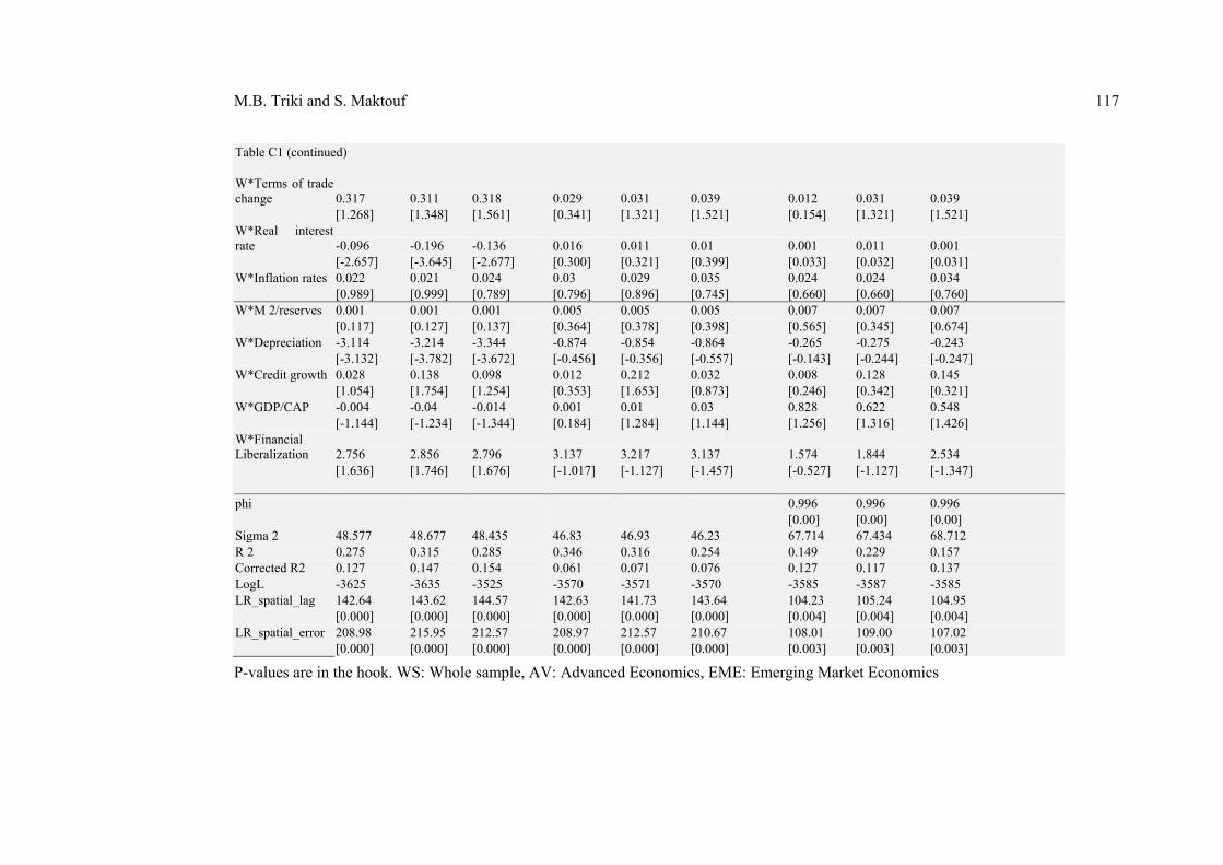
The coefficient for financial liberalization is negative in opposition to
Apanard (2010) and strongly significant in the regression for all countries,
advanced countries as well as emerging market countries. The maximum
probability occurs at an intermediate level of liberalization for both country
groups and for all countries. For the emerging countries the maximum probability
is much higher than for at a much level liberalization.
An increase of the rate GDP growth, an increase in the credit growth, an
increase in the GDP/CAP and an increase of financial liberalization are all found
to contribute to the likelihood of a banking crisis and highly significant in all
regressions and sub-sample. The results are mostly consistent with the existing
literature.
The leading coefficients of explanatory variables of the model space are
statistically significant and values are provided with superiority over classic work
of authors who have used classical models. This result is not surprising in the light
standard panel so that estimates are inconsistent and ineffective in the presence of
spatial dependence. It also implies that banking crises are not exclusively
explained by contagion, but the domestic macroeconomic fundamentals played a
role in the onset of banking crises. For spatial Durbin model specification with
spatial and time-period specific effects, also called "two-way fixed effects" (last
column of first table), we note that the financial liberalization variable is
significant even for the first two models and has a negative effect on the
dependent variable explaining banking fragility. Financial liberalization reduces
the probability of banking crises in different countries. This result corresponds to
what has been developed in the literature with the work of Kalemli-Ozcan et al
(2001) showing that macroeconomic risks can focus on certain players or sectors.
According to Samuelson (1994), by increasing microeconomic efficiency

M.B. Triki and S. Maktouf 99
financial liberalization paradoxically increases macroeconomic risks, and this is
the paradox of liquidity mentioned by A.Orléan (1999). This result also confirms
that obtained by Kaminsky & Schmukler (2003) on a panel of industrialized and
emerging countries, which states that financial liberalization has a negative
short-term, this effect disappears in the long term once the financial reforms are
familiar with the new global finance. And that country achieves sustainable
growth and its financial system will become stable. Other empirical studies such
as Ranciere et al (2006), Eichengreen & Arteta (2000) and Arricia et al (2005)
have shown that financial liberalization is the common cause of banking crises
observed over the past two decades.
In addition, the economic growth variable has a negative effect on banking
crises. An increase in economic growth reduces the likelihood of banking crises;
this corresponds to what has been developed in the literature. Our results
corroborate those of Kim & Kenny (2006) and Mah (2006) who found that a high
growth rate is a good sign for the whole economy. However, they contradict those
obtained by Borio & Lowe (2002) which showed that economic growth could be a
source of a banking crisis.
The growth of domestic credit is significant. Consequently, the growth of
domestic credit positively affects the bank failure as already confirmed by the
economic theory that a credit boom can foster an appreciation of bank fragility.
The credits were equally important channels of contagion among others of the
financial crisis in the U.S.A economy and other developed and emerging countries
if we integrate the last banking crisis.
In a period of euphoria, banks tend to loosen the conditions for granting
credits to increase the funding of projects. This was the case of easy credit to
households in the subprime mortgage finance and for company, following the
opening of many credit lines while stock markets were optimistic. This is
confirmed by Berrak thing. Neven T. Valev in their article in 2010, they show that
private credit expansion is an important predictor of future banking crises. They

100 Financial Liberalization and Banking Crisis: A Spatial Panel Model
prove this result with a new set of data from developed and emerging private
credit which is broken down in the meadows of credit to households and credit of
the company. They argue that credit growth increases household debt levels which
have a big effect on long-term income. A rapid expansion of household credit
generates vulnerabilities that can precipitate a banking crisis. Expansions Credit
Company can have the same effect, but it is tempered by the associated increase in
income. Its estimates show that the expansion of household credit was statistically
significant and economically a predictor of banking crises. The corporate credit
expansions are also associated with banking crises, but their effect is weaker and
less durable.
The reversal has occurred as soon as the asset value at the base of bank
credit has begun to crumble. Some private institutions that have been for so long
considered as too big to fail, such as Fannie Mae and Freddie Mac, have been
recipients of beneficial economic and financial support from the government,
while on September 17, 2008, the U.S. authorities decided to rescue the AIG!
Banks as important as the HSBC UK or Swiss UBS announced losses of almost
two billion dollars each. On September 18, 2008, the announcement of the
nationalization of Northern Rock, after a brief tutelage few months by the English
Central Bank, spent the magnitude of the contagion of the financial crisis in
Europe. Some authors argue that Europe does not react quickly and in a very
cooperative way and each member of Europe seeks its own interest. This was the
case of the United States in the 1929 crisis when it tried to get out of the crisis
with a very lax regime and to increase the investor confidence because the
financial market was incomplete and could not be saved. As such, the public
authority appeared as it is usually believed that market mechanisms represent the
right systems for allocating capital on the international scale. However this is not
true and this reinforces the idea of O. Orléon 2011 that the transfer of real market
rules (the general theory of Keynes) to the financial market (theoretical efficiency)
is not effective.

M.B. Triki and S. Maktouf 101
It was only towards the end of 2008 that the economic crisis spread to
emerging countries, with the backdrop of a fairly noticeable slowdown in growth.
The problem was not really the collapse of their financial systems but it was rather
the impacts on their domestic production and international trade.
However, the coefficients of the spatial model seems better than the
non-spatial model, although this comparison is invalid because the non-spatial
model coefficients represent elasticity that is not the case for the spatial model.
Besides, the coefficient in the spatial model is not the marginal effect like the
effect of financial liberalization on banking fragility, but this is not the case of the
spatial model.
The last coefficient in the case of the depreciation variable [W * depreciation] is,
at the same time, negative and significant, and it is also a positive and significant
variable for financial liberalization [W * Lib].
The information provided by the Spatial Durbin model suggests that bank
failures are contagious with the effects of interactions of commercial banks in the
network of banks that also governed the interactions for aggregate activity. So the
system becomes both more complex and focused in the form of nodes, the
network formis described by Alin Kirman (2011) as a network of ants, and the fact
that the economy operates in a network leads to problems of contagion so it is
interesting to restore confidence to economic agents. It was justified by comparing
the SARS epidemic and panic that followed the collapse of Lehman Bras. Thus,
the role of weight matrices, exports, imports and trade, provided a significant
interaction coefficient and correlated across nations implying that bank failures
seem to have special motifs that contain the exchange interactions.
6 Conclusion
We demonstrated that spatial panel models constitute a natural framework to

102 Financial Liberalization and Banking Crisis: A Spatial Panel Model
analyze the determinants of banking crises. Furthermore, if there is spatial
dependence, which is expected in the present setting, econometric issues such as
inconsistency and inefficiency are dealt with by estimating spatial panel models.
Therefore, the estimation of spatial panel models allowed us to overcome several
of the shortcomings present in the previous banking crises empirical literature.
Our empirical results seem to lend support to the determinants of banking
crises. We use spatial panel data models, among which the spatial lag model, the
spatial error model, and the spatial Durbin model extended to include spatial
and/or time-period fixed effects or extended to include spatial random effects. Not
only is there direct evidence from spatial lag + error and lag models, which
formalize the definition of contagion, but also indirect evidence provided by
spatial error models. The choice of a predominant transmission channel points
towards trade interactions. Contrasting with previous findings, we find evidence
that macroeconomic fundamental variables also contributed, either positively or
negatively, towards the observed crisis outcomes, with poor growth playing a
particularly significant role.
References
[1] A Orléan, Le pouvoir de la finance, Paris, Odile Jacob, 1999.
[2] AlinKirmanet all., The Financial Crisis and the Systemic Failure of
Academic Economics, Kiel Working Papers, 1489, Kiel Institute for the
World Economy, (2009).
[3] L. Anselin, Thirty years of spatial econometrics, Papers in Regional Science,
89, (2010), 3-25.
[4] L. Anselin, A.K. Bera, R. Florax, and M.J. Yoon., Simple diagnostic tests for
spatial dependence, Regional Science and Urban Economics, 26, (1996),
77-104.

M.B. Triki and S. Maktouf 103
[5] L. Anselin, J. Le Gallo and H. Jayet., Spatial panel econometrics, in The
econometrics of panel data, fundamentals and recent developments in theory
and practice, third edition, eds. L. Matyas and P. Sevestre, 627-662.
Dordrecht, the Netherlands: Kluwer, 2008.
[6] Arricia et al, Credit booms and lending standards: Evidence from the
subprime mortgage market, Working paper, IMF, (2008).
[7] Arteta and Eichengreen, Banking crises in emerging markets: presumptions
and evidence, in: Blejer, M., Skreb, M. (Eds.), Financial Policies in
Emerging Markets, MIT Press, Cambridge, MA, 2002.
[8] Bekaert and Harvey, Foreign speculators and Emerging Equity Markets and
Economic Growth, Journal of Devopment Economics, 66, (2000), 465-504.
[9] G. Bekaert, C.R. Harvey and C. Lundblad, Does financial liberalization spur
growth?, Journal of Financial Economics, 77, (2005), 1-56.
[10] Betty and John Bailey, Financial liberalization and banking crises in
emerging economies, Journal of International Economics, Elsevier, 72(1),
(May, 2007), 202-221.
[11] P. Burridge, Testing for a common factor in a spatial autoregression model,
Environment and Planning A, 13, (1981), 795-400.
[12] Debarsy and Ertur, Testing for spatial autocorrelation in a fixed effects panel
data model, Regional Science and Urban Economics, 40, (2010), 453-470.
[13] Demirgu¸ C-Kunt and Detragiache, Financial Liberalization and Financial
Fragility, in G. Caprio, P. Honohan and J. E. Stiglitz (eds), Financial
Liberalization: How Far, How Fast?, Cambridge University Press, 2001.
[14] Demirguc-Kunt and Detragianche, The determinants of banking crises in
developing and developed countries, IMF Staff Papers, 45, Washington,
DC, (1997).
[15] Demirguc-Kunt and Detragiache, Deposit insurance around the World: A
comprehensive database, World Bank Policy Research Working Paper, 3628,
the World Bank: Washington, DC, (2005).
104 Financial Liberalization and Banking Crisis: A Spatial Panel Model
[16] Demirguc-Kunt and Detragiache, Financial Liberalization and Financial
Fragility, World Bank Working Paper, (1998).
[17] Demirgüç-Kunt and Detragiache, Financial Liberalization and Financial
Fragility, in Annual World Bank Conference on Development Economics,
World Bank, DC, pp. 303-31, 1999.
[18] Eichengreen and Arteta, Banking crises in emerging markets: Presumptions
and evidence, University of California, Berkeley, 2000.
[19] Eichengreen et al., Contagious Currency Crises, National Bureau of
Economic Research, 5681, (1996), 1-48.
[20] Elhorst, Spatial panel data models.In Handbook of applied spatial analysis,
eds. M.M. Fischer and A. Getis, Berlin, Springer, pp. 377-407, 2010.
[21] Fischer and Chenard, Financial Liberalization Causes Banking System
Fragility, Finance 9706004, EconWPA, (1995).
[22] Gerlach and Smets, Contagious Speculative Attacks, European Journal of
Political Economy, 11, (1997), 5-63.
[23] Glick and Hutchison, Banking and currency crises: how common are twins?
in R. Glick, R. Moreno, and M. Spigel, eds. Finanial crises in emerging
markets, Cambridge, UK, Cambridge University Press, chapter 2, 2001.
[24] Goldfajn and Valde´s, Capital flows and the twin crises: The role of liquidity,
IMF Working Paper, 97/87, Washington, D.C., (1997).
[25] Goldstein and Turner, Banking Crises in Emerging Economies: Origins And
Policy Options, BIS Economic Paper, 46, (1996).
[26] Hayashi, Econometrics. Princeton: Princeton University Press, p.122, 2000.
[27] IlanNoy, Do IMF Bailouts Result in Moral Hazard? An Events-Study
Approach, Working Papers, 200402, University of Hawaii at Manoa,
Department of Economics, (2004).
[28] Kaminsky and Schmukler, Short-run pain, long-run gain: the effects of
financial liberalization, IMF Working Paper, WP/03/34, (2003).
M.B. Triki and S. Maktouf 105
[29] Kaminsky and Reinhart, The twin crises: The causes of banking and
balance-of-payment problems, American Economic Review, 89(3), (1999),
473-500.
[30] Kaminsky et al., On Crises, Contagion and Confusion, Journal of
International Economics, 51(1), (2001), 145-168.
[31] B. Kim and W.L. Kenny, Explaining when developing countries liberalize
their financial equity markets, Journal of International Financial Markets,
Institutions and Money, (Fevrier, 2006), 1-16.
[32] Kiyotaki and Moore, Credit cycles, Journal of Political Economy, 105(2),
(1997), 211-247.
[33] Komulainen and Lukarila, What drives financial crises in emerging markets?,
Emerging Market Review, 4(3), (2003), 248-272.
[34] Lee and Yu, Estimation of spatial autoregressive panel data models with
fixed effects, Journal of Econometrics, 154, (2010), 165-185.
[35] LeSage and Pace, Introduction to spatial econometrics, Boca Raton, US,
CRC Press Taylor & Francis Group, chapter 6, 2009.
[36] E. Mendoza, V. Quadrini and J.V. Rı´os-Rull, Financial integration, financial
development, and global imbalances, Journal of Political Economy, 117(3),
(2009), 371-416.
[37] Mutl and Pfaffermayr, The Hausman test in a Cliff and Ord panel model,
Econometrics Journal, 14, (2010), 48-76.
[38] R. Ranciere, A. Tornell and F. Westermann, Decomposing the effects of
financial liberalization : crises vs growth, Journal of Banking and Finance,
(Aout, 2006), 3331-3348.
[39] Ranciere et al., Crises and growth: A re-evaluation, NBER Working Paper,
10073, (2003).
[40] Rodrik Dani, Why We Learn Nothing from Regressing Economic Growth on
Policies, 2005.

106 Financial Liberalization and Banking Crisis: A Spatial Panel Model
[41] Samuelson, Where Ricardo and Mill Rebut and Confirm Arguments of
Mainstream Economists Supporting Globalization, Journal of Economic
Perspectives, American Economic Association, 18(3), (1994), 135-146.
[42] Schinasi and Smith, Portfolio Diversification, Leverage, and Financial
Contagion, in S. Claessens and K. Forbes (eds), International Financial
Contagion, Boston, MA, Kluwer Academic Publishers, pp. 187-223, 2001.
[43] Tirtiroglu et al., Deregulation, Intensity of Competition, Industry Evolution
and the Productivity Growth of US Commercial Banks, Journal of Money,
Credit and Banking, 37(2), (2005), 339-360.
[44] Tornell and Westermann, Boom-Bust Cycles and Financial Liberalization,
the MIT Press, 2005.
[45] Van Rijckeghem and Weder, Sources of Contagion: Is It Finance or Trade?,
Journal of International Economics, 54(2), (2001), 293-308.

M.B. Triki and S. Maktouf 107
Appendix
Table A1
Descriptions and sources of the variables
Variable Description and source Dependent variable:
Nonperforming loans (BNONPERLOAN)
*Bank nonperforming loans to total gross loans are the value of nonperforming loans divided
by the total value of the loan portfolio (including nonperforming loans before the deduction of
specific loan-loss provisions) FMI.
(A) Macroeconomic determinants of banking crises
Rate of growth of real GDP (GROWTH)
*GROWTH is measured as the log difference of GDP time series. The annual GDP time series
are complementally from International Financial Statistics (IFS).
Total change (TOTCH) *Change in terms of trade (and service). Source is WEO.
Real interest rate (REALINT)
*Nominal interest rate minus the contemporaneous rate of inflation. IFS.Where available,
nominal rate on short-term government securities. Otherwise, a rate charged by the central bank
to domestic banks such as the discount rate; otherwise, the commercial bank deposit interest
rate.
Inflation rates (INFLATION)
*Rate of change of the GDP deflator. INFLATION is measured as the rate of change in
consumer price indices (CPI), the data are obtained from IFS (line 64). The CPI for Taiwan is
derived from Datasream International.
GDP/CAP *Real GDP per capita (WDI)

108 Financial Liberalization and Banking Crisis: A Spatial Panel Model
(B) Financial variables
M 2/reserves (M2RESERVE)
*Ratio of M2 to foreign exchange reserves of the central bank. M2 is money plus quasi-money
(lines 34+35 from the IFS) converted into US$. Reserves are line 1dd of the IFS.
Credit growth (CREDITGROWTH)
*Rate of growth of real domestic credit to private sector. IFS line 32d divided by the GDP
deflator (WDI) (all in local currency).
Depreciation (DEPRE) *Rate of depreciation, IFS: Dollar/local currency exchange rate (line ae).
Financial Liberalisation (Official Liberalization)(LIBFULL)
*Official Liberalization dates, presented in Table 2, are based on Bekaert and Harvey (2002) A
Chronology of Important For the liberalizing countries, the associated Official Liberalization
indicator takes a value of one when the equity market is officially liberalized and thereafter,
and zero otherwise. For the remaining countries, fully segmented countries are assumed to have
an indicator value of zero, andfully liberalized countries are assumed to have anindicator value
of one.Financial, Economic and Political Events in Emerging Markets,
http://www.duke.edu/_charvey/chronology.htm.

M.B. Triki and S. Maktouf 109
Table A2
Countries included
1 Argentine 11 Finland 21 Korea, Rep. 31 South Africa
2 Australia 12 France 22 Malaysia 32 Spain
3 Austria 13 Germany 23 Mexico 33 Sweden
4 Belgium 14 Greece 24 Netherlands 34 Switzerland
5 Brazil 15 India 25 New Zealand 35 Thailand
6 Canada 16 Indonesia 26 Norway 36 Turkey
7 Chile 17 Ireland 27 Peru 37 United Kingdom
8 Colombia 18 Israel 28 Philippines 38 United States
9 Denmark 19 Italy 29 Portugal 39 Uruguay
10 Egypt, Arab Rep. 20 Japan 30 Singapore 40 Venezuela

110 Financial Liberalization and Banking Crisis: A Spatial Panel Model
Table A3
Summary statistics
Variables NPL RGDPGR TTCH RINT INFL M2RES DEPRECN CREDLAG2 GDPPC LIB
Mean 7.532 3.221 0.269 5.124 8.679 12.546 0.119 7.24 14775.94 0.943
Median 4.5 3.265 -0.086 4.126 4.087 5.216 0.05 5.839 5930 1
Maximum 77 18.3 63.244 151.2104 137.964 1116.94 4.255184 115.422 93600 1
Minimum 0.2 -14.3 -29.9568 -70.53 -23.478 0.349 -0.17917 -43.039 245.7656 0
Std. Dev. 8.192 3.477 7.519 15.82 14.775 38.146 0.337 15.045 15925.02 0.22
Skewness 2.289 -0.4352 2.029 3.54 3.752 23.332 7.84 1.367 1.148 -4.03
Kurtosis 11.041 5.674 17.864 36.881 21.209 659.34 84.446 10.7 3.93 17.3
Jarque-Bera 3846.24 355.352 10663.97 53821.24 17423.16 19429202.3 308990 2999.524 276.51 12120.6
Probability 0 0 0 0 0 0 0 0 0 0
Sum 8119.5 3473.14 290.354 5523.94 9356.464 13512.46 128.823 7804.93 15928471.5 1022
Sum Sq. Dev. 72283 13025.7 60899.78 269784.3 235124.39 1565782.35 122.692 243805.37 271342410 53.09
Observations 880 880 880 880 880 880 880 880 880 880

M.B. Triki and S. Maktouf 111
Table B1 Estimation results I-Bank crisis and liberalization: We
Determinants 1 2 3 4
Pooled OLS Spatial fixed effects Time-period fixed effects Spatial and time-period fixed effects
WS ADV EMG WS ADV EMG WS ADV EMG WS ADV EMG
Constant 17.047 17.657 18.657
[15.754] [15.864] [15.897]
Rate GDP growth -0.300 -0.134 -0.262 -0.275 -0.175 -0.235 -0.254 -0.194 -0.234 -0.228 -0.128 -0.218
[-4.481] [-4.761] [-4.89] [-4.073] [-4.233] [-4.13] [-4.020] [-4.220] [-4.120] [-3.570] [-3.770] [-3.670]
Terms of trade change -0.021 -0.031 -0.121 -0.015 -0.025 -0.075 -0.037 -0.037 -0.057 -0.029 -0.049 -0.029
[-0.721] [-0.721] [-0.721] [-0.500] [-0.500] [-0.500] [-1.317] [-1.317] [-1.317] [-1.046] [-1.046] [-1.046]
Real interest rate -0.014 -1.014 0.014 -0.012 -1.012 -0.013 0.006 0.002 0.004 0.01 0.01 0.02
[-1.041] [-1.01] [-1.321] [-0.890] [-1.190] [-0.990] [0.413] [0.313] [0.402] [0.715] [0.709] [0.725]
Inflation rates 0.000 -3.040 -2.070 0.003 -2.103 -1.03 0.007 0.004 0.005 0.011 0.009 0.01
[-0.022] [-0.722] [-1.122] [0.19] [0.59] [0.42] [0.425] [0.525] [0.425] [0.693] [0.793] [0.693]
M 2/reserves 0.001 0.001 0.11 0.002 0.002 0.12 0.004 0.004 0.014 0.005 0.005 0.015
[0.23] [0.23] [0.33] [0.343] [0.343] [0.443] [0.806] [0.806] [0.706] [0.893] [0.893] [0.793]
Depreciation -0.985 -0.965 -0.975 -0.863 -0.853 -0.887 -0.238 -0.228 -0.218 -0.045 -0.065 -0.035
[-1.383] [-0.283] [-1.353] [-1.205] [-1.125] [-1.305] [-0.334] [-0.234] [-0.374] [-0.063] [-0.073] [-0.068]
Credit growth -0.048 0.481 -0.048 -0.051 -0.051 -0.051 -0.043 -0.043 -0.043 -0.046 -0.046 -0.046
[-3.207] [-3.96] [-3.07] [-3.404] [-3.404] [-3.404] [-3.027] [-3.027] [-3.027] [-3.234] [-3.234] [-3.234]
GDP/CAP -2E-04 -2E-04 -0.001 -2E-04 -2E-04 -0.002 -1E-04 -1E-04 -1E-04 -1E-04 -1E-04 -1E-04
[-14.161] [-1.11] [-1.261] [-14.134] [-14.454] [-13.734] [-10.513] [-10.653] [-9.433] [-10.374] [-10.684] [-10.24]
112 Financial Liberalization and Banking Crisis: A Spatial Panel Model
Table B1 (continued) Financial Liberalization
4.958
5.158
1.958
5.253
5.652
1.223
4.339
4.679
2.319
4.664
4.694
1.234
[-4.808] [-4.208] [-4.128] [-5.099] [-5.029] [-4.029] [-4.073] [-4.343] [-4.043] [-4.378] [-4.978] [-3.368]
R 2 0.062 0.064 0.065 0.217 0.218 0.219 0.143 0.144 0.146 0.145 0.147 0.152
LogL -3666.8 -3665.8 -3664.8 -3653.4 -3653.4 -3653.4 -3588.2 -3588.2 -3588.2 -3572.6 -3572.6 -3572.6
LM spatial lag 38.39 37.29 39.12 39.72 38.42 39.92 4.66 4.46 4.96 4.68 4.58 4.93
LM spatial error 31.21 31.21 31.21 32.43 32.43 32.43 4.19 4.19 4.19 4.51 4.51 4.51
Robust LM spatial lag 7.21 7.21 7.21 7.35 7.35 7.35 0.47 0.47 0.47 0.23 0.23 0.23
Robust LM spatial error 0.03 0.03 0.03 0.06 0.06 0.06 0.17 0.17 0.17 0.06 0.06 0.06
P-values are in the hook. WS: whole sample, AV: Advanced Economics, EME: Emerging Market Economics.
Table B2 Estimation results I-Bank crisis and liberalization: Wi
Determinants 1 2 3 4 Pooled OLS Spatial fixed effects Time-period fixed effects Spatial and time-period fixed effects
WS ADV EMG WS ADV EMG WS ADV EMG WS ADV EMG
Constant 17.047 17.657 18.657
[15.754] [15.864] [15.897]
Rate GDP growth -0.300 -0.134 -0.262 -0.275 -0.175 -0.235 -0.254 -0.194 -0.234 -0.228 -0.128 -0.218
[-4.481] [-4.761] [-4.89] [-4.073] [-4.233] [-4.13] [-4.02] [-4.22] [-4.120] [-3.570] [-3.770] [-3.670]
Terms of trade change -0.021 -0.031 -0.121 -0.015 -0.025 -0.075 -0.037 -0.037 -0.057 -0.029 -0.049 -0.029
[-0.721] [-0.721] [-0.721] [-0.500] [-0.500] [-0.500] [-1.317] [-1.317] [-1.317] [-1.046] [-1.046] [-1.046]

M.B. Triki and S. Maktouf 113
Table B2 (continued) Real interest rate -0.014 -1.014 0.014 -0.012 -1.012 -0.013 0.006 0.002 0.004 0.01 0.01 0.02
[-1.041] [-1.01] [-1.321] [-0.890] [-1.190] [-0.990] [0.413] [0.313] [0.402] [0.715] [0.709] [0.725]
Inflation rates 0.000 -3.040 -2.070 0.003 -2.103 -1.03 0.007 0.004 0.005 0.011 0.009 0.01
[-0.022] [-0.722] [-1.122] [0.19] [0.59] [0.42] [0.425] [0.525] [0.425] [0.693] [0.793] [0.693]
M 2/reserves 0.001 0.001 0.11 0.002 0.002 0.12 0.004 0.004 0.014 0.005 0.005 0.015
[0.23] [0.23] [0.33] [0.343] [0.343] [0.443] [0.806] [0.806] [0.706] [0.893] [0.893] [0.793]
Depreciation -0.985 -0.965 -0.975 -0.863 -0.853 -0.887 -0.238 -0.228 -0.218 -0.045 -0.065 -0.035
[-1.383] [-0.283] [-1.353] [-1.205] [-1.125] [-1.305] [-0.334] [-0.234] [-0.374] [-0.063] [-0.073] [-0.068]
Credit growth -0.048 0.481 -0.048 -0.051 -0.051 -0.051 -0.043 -0.043 -0.043 -0.046 -0.046 -0.046
[-3.207] [-3.96] [-3.07] [-3.404] [-3.404] [-3.404] [-3.027] [-3.027] [-3.027] [-3.234] [-3.234] [-3.234]
GDP/CAP -2E-04 -2E-04 -0.001 -2E-04 -2E-04 -0.002 -1E-04 -1E-04 -1E-04 -1E-04 -1E-04 -0.0001
[-14.16] [-1.11] [-1.26] [-14.13] [-14.45] [-13.73] [-10.51] [-10.65] [-9.433] [-10.37] [-10.68] [-10.21]
Financial Liberalization 4.958 5.158 1.958 5.253 5.652 1.223 4.339 4.679 2.319 4.664 4.694 1.234
[-4.808] [-4.208] [-4.128] [-5.099] [-5.029] [-4.029] [-4.073] [-4.343] [-4.043] [-4.378] [-4.978] [-3.368]
R 2 0.062 0.064 0.065 0.217 0.218 0.219 0.143 0.144 0.146 0.145 0.147 0.152
LogL -3666.8 -3665.8 -3664.8 -3653.4 -3653.4 -3653.4 -3588.2 -3588.2 -3588.2 -3572.6 -3572.6 -3572.6
LM spatial lag 55.92 37.29 39.12 56.9 38.42 39.92 3.24 4.46 4.96 3.53 4.58 4.93
LM spatial error 47.2 41.21 41.25 49.64 42.43 45.43 3.57 4.19 3.19 3.85 3.51 3.91
Robust LM spatial lag 9.27 9.21 9.11 8.32 8.15 8.25 0.001 0.07 0.07 0.006 0.023 0.13
Robust LM spatial error 0.56 0.53 0.63 1.06 1.16 1.21 0.33 0.17 0.17 0.32 0.26 0.29
P-values are in the hook. WS: whole sample, AV: Advanced Economics, EME: Emerging Market Economics.

114 Financial Liberalization and Banking Crisis: A Spatial Panel Model
Table B3
Estimation results I-Bank crisis and liberalization: WT
Determinants 1 2 3 4 Pooled OLS Spatial fixed effects Time-period fixed effects Spatial and time-period fixed effects
WS ADV EMG WS ADV EMG WS ADV EMG WS ADV EMG
Constant 17.047 17.657 18.657
[15.754] [15.864] [15.897]
Rate GDP growth -0.300 -0.134 -0.262 -0.275 -0.175 -0.235 -0.254 -0.194 -0.234 -0.228 -0.128 -0.218
[-4.481] [-4.761] [-4.89] [-4.073] [-4.233] [-4.13] [-4.020] [-4.220] [-4.120] [-3.570] [-3.770] [-3.670]
Terms of trade change -0.021 -0.031 -0.121 -0.015 -0.025 -0.075 -0.037 -0.037 -0.057 -0.029 -0.049 -0.029
[-0.721] [-0.721] [-0.721] [-0.500] [-0.500] [-0.500] [-1.317] [-1.317] [-1.317] [-1.046] [-1.046] [-1.046]
Real interest rate -0.014 -1.014 0.014 -0.012 -1.012 -0.013 0.006 0.002 0.004 0.01 0.01 0.02
[-1.041] [-1.01] [-1.321] [-0.890] [-1.190] [-0.990] [0.413] [0.313] [0.402] [0.715] [0.709] [0.725]
Inflation rates 0.000 -3.040 -2.070 0.003 -2.103 -1.03 0.007 0.004 0.005 0.011 0.009 0.01
[-0.022] [-0.722] [-1.122] [0.19] [0.59] [0.42] [0.425] [0.525] [0.425] [0.693] [0.793] [0.693]
M 2/reserves 0.001 0.001 0.11 0.002 0.002 0.12 0.004 0.004 0.014 0.005 0.005 0.015
[0.23] [0.23] [0.33] [0.343] [0.343] [0.443] [0.806] [0.806] [0.706] [0.893] [0.893] [0.793]
Depreciation -0.985 -0.965 -0.975 -0.863 -0.853 -0.887 -0.238 -0.228 -0.218 -0.045 -0.065 -0.035
[-1.383] [-0.283] [-1.353] [-1.205] [-1.125] [-1.305] [-0.334] [-0.234] [-0.374] [-0.063] [-0.073] [-0.068]
Credit growth -0.048 481 -0.048 -0.051 -0.051 -0.051 -0.043 -0.043 -0.043 -0.046 -0.046 -0.046
[-3.207] [-3.96] [-3.07] [-3.404] [-3.404] [-3.404] [-3.027] [-3.027] [-3.027] [-3.234] [-3.234] [-3.234]
GDP/CAP -2E-04 -2E-04 -0.001 -2E-04 -2E-04 -0.002 -1E-04 -1E-04 -1E-04 -1E-04 -1E-04 -0.0001
[-14.161] [-1.11] [-1.261] [-14.134] [-14.454] [-13.734] [-10.513] [-10.653] [-9.433] [-10.374] [-10.684] [-10.214]

M.B. Triki and S. Maktouf 115
Table B3 (continued) Financial Liberalization 4.958 5.158 1.958 5.253 5.652 1.223 4.339 4.679 2.319 4.664 4.694 1.234
[-4.808] [-4.208] [-4.128] [-5.099] [-5.029] [-4.029] [-4.073] [-4.343] [-4.043] [-4.378] [-4.978] [-3.368]
R 2 0.062 0.064 0.065 0.217 0.218 0.219 0.143 0.144 0.146 0.145 0.147 0.152
LogL -3666.8 -3665.8 -3664.8 -3653.4 -3653.4 -3653.4 -3588.2 -3588.2 -3588.2 -3572.6 -3572.6 -3572.6
LM spatial lag 63.83 67.29 69.12 65.26 68.42 69.42 1.76 1.46 2.56 1.8 1.58 1.63
LM spatial error 51.97 51.21 51.05 54.7 52.13 55.23 2.12 2.09 2.49 2.26 2.51 3.11
Robust LM spatial lag 12.1 12.21 12.01 11.15 11.05 11.05 0.03 0.07 0.07 0.03 0.023 0.13
Robust LM spatial error 0.23 0.33 0.43 0.59 0.46 0.341 0.39 0.27 0.25 0.43 0.36 0.31
P-values are in the hook. WS: whole sample, AV: Advanced Economics, EME: Emerging Market Economics.

116 Financial Liberalization and Banking Crisis: A Spatial Panel Model
Table C1 Estimation results II-Bank crisis and liberalization: We Determinants 1 2 3
Spatial and time period effects Spatial and time-period fixed effects bias-corrected Random spatial effects, fixed time-period effects
WS ADV EMG WS ADV EMG WS ADV EMG W*Npl 0.272 1.332 0.232 -0.166 -0.096 -0.236 -0.136 -0.076 -0.064 [5.254] [5.634] [5.154] [-2.643] [-2.833] [-2.142] [-2.195] [-2.125] [-2.545] Rate GDP growth -0.245 -0.655 -1.245 -0.23 -0.43 -1.12 -0.038 -0.128 -0.238 [-3.737] [-4.137] [-3.217] [-3.493] [-4.193] [-3.213] [-3.493] [-4.113] [-3.313] Terms of trade change -0.02 -0.016 -0.032 -0.032 -0.027 -0.042 0.005 0.004 0.007 [-0.695] [-0.765] [-0.745] [-1.117] [-1.237] [-1.137] [0.382] [0.452] [0.342] Real interest rate 0.004 0.094 0.003 0.010 0.090 0.020 0.010 0.080 0.030 [0.297] [1.97] [0.137] [0.677] [1.677] [0.577] [0.581] [1.881] [0.761] Inflation rates 0.005 -2.435 -1.250 0.016 -1.236 -1.012 0.004 -1.042 -1.012 [0.349] [0.569] [2.332] [0.889] [0.799] [0.856] [0.880] [1.320] [1.780] M 2/reserves 0.003 0.01 0.14 0.005 0.04 0.15 0.004 0.04 0.11 [0.579] [0.869] [1.769] [0.904] [1.104] [1.814] [0.661] [1.631] [1.751] Depreciation -0.537 0.167 0.456 -0.094 -0.004 -0.014 -0.258 0.158 1.238 [-0.751] [-1.675] [-0.871] [-0.125] [-1.125] [-1.435] [-0.356] [-1.326] [-1.656] Credit growth -0.054 -6.034 -2.054 -0.044 -4.034 -2.056 -0.041 -4.041 -3.021 [-3.693] [-4.563] [-3.953] [-2.995] [-4.935] [-3.691] [-2.932] [-4.432] [-3.912] GDP/CAP -1E-04 -0.0001 -0.0001 0.001 0.001 0.001 -1E-04 -1E-04 -1E-04 [-11.57] [-10.67] [-12.54] [-9.847] [-9.237] [-10.457] [-10.347] [-11.327] [-10.07] Financial Liberalization 5.358 6.438 4.368 4.669 6.629 4.039 4.344 6.214 4.604 [-5.194] [-7.54] [-6.234] [-4.188] [-7.708] [-6.128] [-4.022] [-7.122] [-6.032] W*Rate GDP growth -0.126 -0.216 -0.132 0.063 0.042 0.085 0.076 0.042 0.085 [-0.715] [-0.615] [-0.825] [0.254] [0.764] [0.874] [0.317] [0.764] [0.874]
M.B. Triki and S. Maktouf 117
Table C1 (continued) W*Terms of trade change 0.317 0.311 0.318 0.029 0.031 0.039 0.012 0.031 0.039 [1.268] [1.348] [1.561] [0.341] [1.321] [1.521] [0.154] [1.321] [1.521] W*Real interest rate -0.096 -0.196 -0.136 0.016 0.011 0.01 0.001 0.011 0.001 [-2.657] [-3.645] [-2.677] [0.300] [0.321] [0.399] [0.033] [0.032] [0.031] W*Inflation rates 0.022 0.021 0.024 0.03 0.029 0.035 0.024 0.024 0.034 [0.989] [0.999] [0.789] [0.796] [0.896] [0.745] [0.660] [0.660] [0.760] W*M 2/reserves 0.001 0.001 0.001 0.005 0.005 0.005 0.007 0.007 0.007 [0.117] [0.127] [0.137] [0.364] [0.378] [0.398] [0.565] [0.345] [0.674] W*Depreciation -3.114 -3.214 -3.344 -0.874 -0.854 -0.864 -0.265 -0.275 -0.243 [-3.132] [-3.782] [-3.672] [-0.456] [-0.356] [-0.557] [-0.143] [-0.244] [-0.247] W*Credit growth 0.028 0.138 0.098 0.012 0.212 0.032 0.008 0.128 0.145 [1.054] [1.754] [1.254] [0.353] [1.653] [0.873] [0.246] [0.342] [0.321] W*GDP/CAP -0.004 -0.04 -0.014 0.001 0.01 0.03 0.828 0.622 0.548 [-1.144] [-1.234] [-1.344] [0.184] [1.284] [1.144] [1.256] [1.316] [1.426] W*Financial Liberalization 2.756 2.856 2.796 3.137 3.217 3.137 1.574 1.844 2.534 [1.636] [1.746] [1.676] [-1.017] [-1.127] [-1.457] [-0.527] [-1.127] [-1.347] phi 0.996 0.996 0.996 [0.00] [0.00] [0.00] Sigma 2 48.577 48.677 48.435 46.83 46.93 46.23 67.714 67.434 68.712 R 2 0.275 0.315 0.285 0.346 0.316 0.254 0.149 0.229 0.157 Corrected R2 0.127 0.147 0.154 0.061 0.071 0.076 0.127 0.117 0.137 LogL -3625 -3635 -3525 -3570 -3571 -3570 -3585 -3587 -3585 LR_spatial_lag 142.64 143.62 144.57 142.63 141.73 143.64 104.23 105.24 104.95 [0.000] [0.000] [0.000] [0.000] [0.000] [0.000] [0.004] [0.004] [0.004] LR_spatial_error 208.98 215.95 212.57 208.97 212.57 210.67 108.01 109.00 107.02 [0.000] [0.000] [0.000] [0.000] [0.000] [0.000] [0.003] [0.003] [0.003]
P-values are in the hook. WS: Whole sample, AV: Advanced Economics, EME: Emerging Market Economics

118 Financial Liberalization and Banking Crisis: A Spatial Panel Model
Table C2
Estimation results II-Bank crisis and liberalization: Wi
Determinants 1 2 3
Spatial and time period effects
Spatial and time-period fixed effects bias-corrected
Random spatial effects, fixed time-period effects
WS ADV EMG WS ADV EMG WS ADV EMG
W*Npl 0.295 1.412 0.312 0.439 0.396 0.136 -0.261 -0.056 -0.124
[5.339] [5.534] [5.254] [9.535] [4.833] [3.132] [-3.187] [-2.115] [-2.523]
Rate GDP growth -0.241 -0.625 -1.145 -0.227 -0.42 -1.131 -0.246 -0.122 -0.254
[-3.689] [-4.247] [-3.547] [-3.492] [-4.153] [-3.234] [-3.879] [-4.123] [-3.311]
Terms of trade change -0.017 -0.016 -0.032 -0.019 -0.027 -0.042 -0.064 0.004 0.003
[-0.601] [-0.765] [-0.745] [-0.669] [-1.237] [-1.137] [-1.147] [0.452] [0.431]
Real interest rate 0.002 0.094 0.003 -0.001 -0.060 -0.030 -0.014 -0.060 0.021
[0.164] [1.97] [0.137] [-0.103] [1.667] [0.585] [-1.20] [1.881] [0.732]
Inflation rates 0.008 -1.425 -1.310 0.013 -1.242 -1.041 -0.018 -1.041 -1.013
[0.492] [0.569] [2.332] [0.798] [0.799] [0.826] [-1.528] [1.320] [1.7420]
M 2/reserves 0.003 0.01 0.14 0.004 0.09 0.16 0.006 0.03 0.13
[0.639] [0.869] [1.769] [0.773] [1.104] [1.814] [0.872] [1.631] [1.641]
Depreciation -0.381 0.167 0.216 -0.608 -0.004 -0.324 -0.138 0.158 1.428
[-0.521] [-1.675] [-0.871] [-0.829] [-1.125] [-1.435] [2.548] [-1.326] [-1.526]
Credit growth -0.053 -5.024 -3.014 -0.045 -4.014 -2.226 -0.026 -4.121 -3.142
[-3.617] [-4.213] [-3.313] [-3.100] [-4.335] [-3.631] [-2.954] [-4.132] [-3.422]
GDP/CAP -0.001 -0.0020 -0.0030 -0.0001 0.001 0.001 -0.001 -0.0001 -1E-04
[-11.115] [-11.57] [-12.14] [-10.764] [-9.127] [-10.47] [-10.43] [-11.37] [-11.27]
Financial Liberalization 5.514 6.218 4.318 4.157 6.549 4.012 4.042 6.414 4.653
[-5.339] [-7.54] [-6.234] [-4.103] [-7.708] [-6.145] [-3.775] [-7.122] [-6.212]

M.B. Triki and S. Maktouf 119
Table C2 (continued)
W*Rate GDP growth -0.179 -0.306 -0.172 0.287 0.082 0.097 0.488 0.212 0.081
[-0.938] [-0.615] [-0.825] [1.230] [0.765] [0.871] [2.554] [0.762] [0.971]
W*Terms of trade change 1.432 0.354 0.418 0.315 0.061 0.049 0.071 0.035 0.038
[-0.513] [1.348] [1.561] [2.012] [1.621] [1.522] [0.226] [1.331] [1.211]
W*Real interest rate -0.084 -0.136 -0.126 -0.093 0.021 0.02 -0.112 0.014 0.003
[-2.124] [-3.645] [-2.677] [-0.729] [0.541] [0.519] [-0.920] [0.042] [0.032]
W*Inflation rates -0.112 -0.031 -0.027 -0.096 0.029 0.035 -0.100 0.024 0.033
[-1.616] [0.989] [0.749] [-1.00] [0.896] [0.745] [-1.090] [0.660] [0.742]
W*M 2/reserves 0.017 0.005 0.005 0.008 0.007 0.007 0.017 0.008 0.009
[1.548] [0.378] [0.398] [0.595] [0.345] [0.674] [1.548] [0.349] [0.694]
W*Depreciation -3.07 -3.231 -3.354 -2.544 -2.154 -2.894 20.897 15.275 10.246
[1.583] [-3.782] [-3.672] [-2.803] [-0.826] [-0.547] [2.305] [-0.948] [-0.947]
W*Credit growth -0.06 -0.128 -0.148 0.041 0.312 0.052 0.075 0.118 0.142
[-1.066] [1.754] [1.254] [0.502] [1.253] [0.871] [0.960] [0.343] [0.311]
W*GDP/CAP -1.066 -1.14 -1.024 0.579 0.65 0.73 0.163 0.212 0.318
[1.128] [-1.234] [-1.344] [0.711] [1.294] [1.142] [0.206] [1.116] [1.431]
W*Financial Liberalization 4.059 4.926 4.896 11.020 12.237 11.132 5.025 5.814 5.532
[2.204] [1.746] [1.676] [8.186] [-1.127] [-1.457] [0.531] [-1.542] [-1.247]
phi 0.996 0.996 0.996
[9.657] [9.657] [9.657]
Sigma 2 48.166 48.677 48.435 50.43 46.93 46.23 68.003 67.434 68.712
R 2 0.315 0.325 0.296 0.316 0.317 0.252 0.229 0.231 0.155
Corrected R2 0.128 0.147 0.154 0.07 0.071 0.076 0.128 0.117 0.137
LogL -3623 -3635 -3527 -3652 -3581.1 -3580 -1555 -3587 -3595
LR_spatial_lag 146.365 142.624 143.53 146.365 142.83 143.63 110.62 112.23 104.21
[0.000] [0.000] [0.000] [0.000] [0.000] [0.000] [0.007] [0.004] [0.004]
LR_spatial_error 218.535 215.846 212.58 218.535 211.57 210.67 114.03 109.00 108.03
[0.000] [0.000] [0.000] [0.000] [0.000] [0.000] [0.004] [0.003] [0.003]
P-values are in the hook. WS: whole sample, AV: Advanced Economics, EME: Emerging Market Economics.

120 Financial Liberalization and Banking Crisis: A Spatial Panel Model
Table C3
Estimation results II-Bank crisis and liberalization: WT
Determinants 1 2 3
Spatial and time period effects
Spatial and time-period fixed effects bias-corrected
Random spatial effects, fixed time-period effects
WS ADV EMG WS ADV EMG WS ADV EMG
W*Npl 0.102 1.112 0.211 -0.532 -0.596 -0.146 0.102 0.096 0.123
[1.037] [1.234] [2.254] [-4.435] [-4.823] [-3.432] [1.037] [1.115] [1.323]
Rate GDP growth -0.234 -0.315 -0.315 -0.249 -0.321 -0.221 -0.215 -0.128 -0.274
[-3.612] [-4.217] [-3.521] [-3.226] [-4.052] [-3.438] [-3.740] [-4.145] [-3.421]
Terms of trade change -0.044 -0.036 -0.052 -0.046 -0.037 -0.032 -0.044 -0.004 -0.003
[-0.767] [-0.765] [-0.845] [-0.800] [-1.237] [-1.21] [-0.767] [0.482] [0.731]
Real interest rate -0.027 -0.194 0.003 -0.029 -0.16 -0.03 -0.027 -0.19 0.021
[-2.226] [1.98] [0.137] [-2.327] [1.767] [0.785] [-2.226] [1.871] [0.782]
Inflation rates -0.031 -1.498 -1.11 -0.032 -1.542 -1.031 -0.031 -1.011 -1.003
[-2.548] [1.769] [2.332] [-2.547] [1.994] [1.826] [-2.548] [1.420] [1.640]
M 2/reserves 0.008 0.01 0.17 0.003 0.04 0.12 0.008 0.03 0.13
[1.077] [0.962] [1.859] [0.432] [1.102] [1.912] [1.077] [1.631] [1.641]
Depreciation 8.18 1.167 0.916 7.097 0.004 0.324 8.18 0.158 1.428
[2.969] [1.675] [0.871] [2.528] [1.725] [1.455] [2.969] [1.856] [1.936]
Credit growth -1.053 -3.024 -1.014 -1.043 -4.014 -2.226 -1.036 -4.121 -3.142
[-3.63] [-4.213] [-3.313] [-2.995] [-4.335] [-3.631] [-2.991] [-4.132] [-3.422]
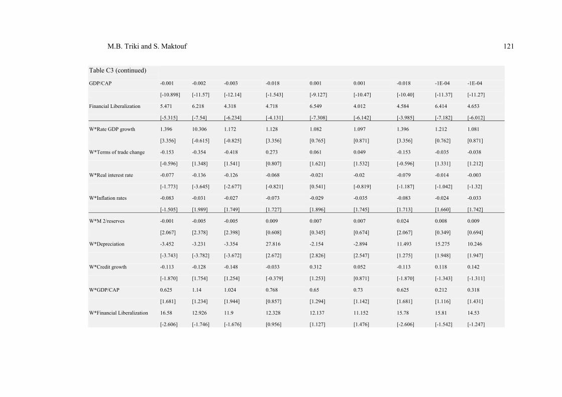
M.B. Triki and S. Maktouf 121
Table C3 (continued) GDP/CAP -0.001 -0.002 -0.003 -0.018 0.001 0.001 -0.018 -1E-04 -1E-04
[-10.898] [-11.57] [-12.14] [-1.543] [-9.127] [-10.47] [-10.40] [-11.37] [-11.27]
Financial Liberalization 5.471 6.218 4.318 4.718 6.549 4.012 4.584 6.414 4.653
[-5.315] [-7.54] [-6.234] [-4.131] [-7.308] [-6.142] [-3.985] [-7.182] [-6.012]
W*Rate GDP growth 1.396 10.306 1.172 1.128 1.082 1.097 1.396 1.212 1.081
[3.356] [-0.615] [-0.825] [3.356] [0.765] [0.871] [3.356] [0.762] [0.871]
W*Terms of trade change -0.153 -0.354 -0.418 0.273 0.061 0.049 -0.153 -0.035 -0.038
[-0.596] [1.348] [1.541] [0.807] [1.621] [1.532] [-0.596] [1.331] [1.212]
W*Real interest rate -0.077 -0.136 -0.126 -0.068 -0.021 -0.02 -0.079 -0.014 -0.003
[-1.773] [-3.645] [-2.677] [-0.821] [0.541] [-0.819] [-1.187] [-1.042] [-1.32]
W*Inflation rates -0.083 -0.031 -0.027 -0.073 -0.029 -0.035 -0.083 -0.024 -0.033
[-1.505] [1.989] [1.749] [1.727] [1.896] [1.745] [1.713] [1.660] [1.742]
W*M 2/reserves -0.001 -0.005 -0.005 0.009 0.007 0.007 0.024 0.008 0.009
[2.067] [2.378] [2.398] [0.608] [0.345] [0.674] [2.067] [0.349] [0.694]
W*Depreciation -3.452 -3.231 -3.354 27.816 -2.154 -2.894 11.493 15.275 10.246
[-3.743] [-3.782] [-3.672] [2.672] [2.826] [2.547] [1.275] [1.948] [1.947]
W*Credit growth -0.113 -0.128 -0.148 -0.033 0.312 0.052 -0.113 0.118 0.142
[-1.870] [1.754] [1.254] [-0.379] [1.253] [0.871] [-1.870] [-1.343] [-1.311]
W*GDP/CAP 0.625 1.14 1.024 0.768 0.65 0.73 0.625 0.212 0.318
[1.681] [1.234] [1.944] [0.857] [1.294] [1.142] [1.681] [1.116] [1.431]
W*Financial Liberalization 16.58 12.926 11.9 12.328 12.137 11.152 15.78 15.81 14.53
[-2.606] [-1.746] [-1.676] [0.956] [1.127] [1.476] [-2.606] [-1.542] [-1.247]

122 Financial Liberalization and Banking Crisis: A Spatial Panel Model
Table C3 (continued)
phi 0.996 0.996 0.996
[9.657] [9.657] [9.657]
Sigma 2 47.573 48.677 48.425 66.751 46.43 46.22 66.563 67.434 65.711
R 2 0.26 0.325 0.296 0.354 0.317 0.252 0.15 0.231 0.155
Corrected R2 0.144 0.146 0.144 0.067 0.071 0.076 0.144 0.117 0.137
LogL -1552 -1534.7 -1227 -1530 -1421 -1354 -1552 -14827 -1385
LR_spatial_lag 138.53 142.62 143.53 138.53 142.83 143.63 88.82 112.23 104.21
[0.000] [0.000] [0.000] [0.000] [0.000] [0.000] [0.002] [0.004] [0.004]
LR_spatial_error 217.12 216.84 213.57 217.12 211.52 210.62 94.43 119.00 110.05
[0.000] [0.000] [0.000] [0.000] [0.000] [0.000] [0.002] [0.003] [0.003]
P-values are in the hook. WS: whole sample, AV: Advanced Economics, EME: Emerging Market Economics.