Financial Inclusion, Entrepreneurship andEmployment Creation:

Theory and a Quantitative Assessment∗

Timothy BesleyLSE and CIFAR

Konrad BurchardiIIES, Stockholm

Maitreesh GhatakLSE

September 2017

Abstract

This paper develops a general equilibrium model with credit market frictions whereagents differ in entrepreneurial ability and wealth to study the benefits of financial inclu-sion. As well as modeling the impact of credit market frictions, we allow for an increasein financial market access. We calibrate the model using the US size distribution of firmsto create a benchmark. We show that it is access to finance which is quantitatively moreimportant than factors which affect credit market frictions such as use of collateral or com-petition in credit markets. The main mechanism is through selection of the highest qualityentrepreneurs, and the main beneficiaries of credit market access are wage laborers dueto an expansion in labor demand and creation of large firms. Indeed, the size distribu-tion of firms comes to resemble that in a more developed economy as credit market accessexpands.

JEL Classification: E44, G28, O16Keywords: Financial Inclusion, Entrepreneurship. Employment Creation

∗We are grateful to the ESRC-DFID growth research program for financial support (Grant referenceES/L012103 /1). We have received valuable research assistance from Kanishak Goyal, Pallavi Jindal, KoshaModi, Tanmay Sahni, and Saurav Sinha.

1

1 Introduction

Increasing financial inclusion is now regarded as one of the principal development challenges(see, for example, World Bank, 2014). Although estimates vary, it appears that around half theworld’s population does not have access to formal banking services. Not surprisingly, financialexclusion is concentrated among the poorest people in the poorest countries. There is a widevariety of ways in which lack of access to financial services results in economic costs to thoseconcerned. Lacking the capacity to save in reliable ways can damage the ability to build upassets, smooth against shocks as well as make provisions for old-age. And entrepreneurs wholack access to finance may not be able to start or scale up the operation of a business.

This paper models the gains from extending the reach of financial markets with a focus onexpanding access to capital for entrepreneurs. We develop a general equilibrium model withfour key features: (i) only a sub-group of the population are able to access financial markets,the remainder being in financial autarky (ii) all individuals in the economy, who may differin their entrepreneurial productivity and their initial wealth, make an occupational choice,between being an entrepreneur and a wage labourer (iii) those who access financial markets,negotiate optimal contracts with lenders respecting the possibility of moral hazard (iii) wagesare determined in general equilibrium.

The model highlights an important channel by which increasing financial inclusion affectsthe economy, namely the employment channel. As access to financial markets increases,labour demand is increased which pushes up equilibrium wages. Since the vast majorityof workers are wage labourers, this extends the benefits of financial inclusion across the econ-omy. As wages rise, there is stronger selection of entrepreneurs from the pool of those whoare more productive which, in turn, leads the size distribution of firms to shift towards largeremployers as capital is deepened in the economy. Hence the substantial gains from financialinclusion are through its impact on employment creation.

A key innovation in this paper is in the detailed modelling of credit market frictions in ageneral equilibrium setting. To date, much of the literature has used a reduced form modelwhere credit access is limited by repayment technologies. While instructive, it creates a some-what mechanical friction in capital markets as opposed to deriving it from optimal contracts.This makes it difficult to assess whether it is access to credit or the implications of second-bestcontracting frictions that matter quantitatively when assessing the importance of credit marketfrictions. One benefit of our approach is that we are able to separate these things out. Oneof our main findings is that embedding such frictions in a market equilibrium settings with anendogenously determined outside option actually leads to smaller losses in productivity andwelfare, compared to limited market access. Being able to show this is a benefit from havinga more detailed model of agency problems which derives optimal contracts.

The model offers a specific window on entrepreneurship and the development process.One of the striking features of low income economies is the large population of self-employedsmall-scale entrepreneurs. This can be viewed as being concomitant with a low wage economyand poor access to finance by large swathes of the population. As financial inclusion expands,large firms constitute a higher fraction of firms as the more productive firms are the ones thatstay in business with the higher wages that now ensue. As the financial market access extendsfurther, we get only a small fraction of the population running their own firms with the vastmajority relying on selling their labour power, but this is good for wage labour as wages arehigher. Indeed, it is developments in the labor market which explain many of the quantitative

2

effects that the model finds.To get a sense of the quantitative magnitude of these effects, we calibrate the model. As

well as exploring the theoretical mechanism in detail and quantifying the aggregate gains fromfinancial inclusion, we can also look at distributional effects across the population with two di-mensions of heterogeneity: wealth and entrepreneurial talent. As financial inclusion increases,inequality is influenced more by who has entrepreneurial talent and less by who owns wealth.This approach also allows us to explore how two features of the contracting environment af-fect the outcomes, namely improving property rights which enhances access to capital andincreasing competition between lenders.

The paper shows that there are indeed large aggregate benefits from extending financialmarket access. Moving from autarky to full inclusion in our calibrated economy increaseswages from 40% of the US wage to 90%. However, these are driven almost exclusively throughan employment-cum occupational choice channel which emerges from an aggregate generalequilibrium perspective. When financial inclusion is first introduced into an “unbanked econ-omy”, the most dramatic effect that we can observe is on the proportion of self-employedentrepreneurs in the economy. The big beneficiaries of financial inclusion are wage labourersdue to the employment creation that occurs and we show how the size distribution of firmsincreases with small firms being squeezed as marginal entrepreneurs exit. We also show thatfinancial inclusion breaks the link between wealth and occupational choice.

Increasing competition does mean that entrepreneurs who access capital markets get alarger share of surplus. Otherwise, the benefits of inclusion will tend to accrue to lenders. Weshow that this is mainly a distributional issue between firms and lenders while wage labourersalways gain with raising wages. Property rights also matter and increase efficiency. However,the efficiency effects of property rights expansion and increased competition are quantitivelysmall relative to the effects of expanding the domain of financial markets.

This paper explores micro-economic factors which determine differences in the level of in-come per capita. The development accounting literature, such as Caselli (2005), has shownthat it is differences in total factor productivity across economies that are key. Our paper is inthe spirit of Hsieh and Klenow [2010] who tied this explicitly to factor misallocation. This linksto older and long-standing debates in the development economics literature on how contract-ing frictions and imperfect markets matter for under-development. For example, authors suchas Bardhan (1984) and Stiglitiz (1988) have highlighted a range of such frictions but withoutproviding an approach to assess their implications quantitatively.

The idea that development of the financial sector has important implications for the econ-omy has a long history with pioneering contributions by Gerschenkron (1962) and Goldsmith(1969). Both put the development banking system at the heart of understanding differences inthe trajectories taken by economies. A large body of work has established a strong correlationbetween measures of financial market development and economic performance at the aggre-gate level (see, for example, Levine, 2005, Cihak et al, 2013). In parallel, there has also been atheoretical literature on the importance of financial frictions in affecting growth and develop-ment including Banerjee and Newman (1993) and Galor and Zeira (1993).1 This literature doesnot typically focus on heterogeneous managerial ability (Lloyd-Ellis and Bernhardt, 2000 beingan exception) and as a result, better functioning credit markets increase rather than decreasethe fraction of entrepreneurs in the economy. In our model, improved financial market access

1Reviews of the literature can be found in Banerjee and Duflo (2005) and Matsuyama (2007).

3

enables more able individuals to become entrepreneurs and hire more workers.There is also an extensive theoretical and empirical literature on how financial arrange-

ments affect households and businesses, particularly how market frictions due to transac-tions costs and informational constraints may lead to borrowing constraints, and possibly,to poverty traps (see, for example, Banerjee and Duflo 2010, Karlan and Zinman, 2009 andTownsend and Ueda, 2008). This literature looks much at the ground up and focuses on het-erogeneity and distributional implications of credit market activity.

A number of papers relate financial frictions to aggregate economic performance in waysthat combine theory, data and calibration methods. In Jeong and Townsend (2007), there is amodern and subsistence economy with agents differing in wealth and talent. There is a fixedcost of setting up a firm and some agents, as in this paper, lack access to credit markets. Theycalibrate the model to Thai data showing that credit access is an important factor in explainingTFP dynamics. Buera et al (2011) also study the aggregate implications of credit market accessemphasizing that there may be differences between manufacturing and services. They alsointroduce a non-convexity due to an entry cost. They model the financial friction as imperfectenforcement which limits the use of capital that an entrepreneur can use. After calibratingthe model to U.S. data, they find that the variation in financial frictions which they explorecan bring down output per worker to less than half of the perfect-credit benchmark. Moll(2014) builds on these approaches and explores the implications of productivity shocks whichlead to inefficient capital allocation which can persist in the long-run. This provides a link toresearch which has looked at the macroeconomic effects of micro-economic distortions such asBartelsman, Haltiwanger, and Scarpetta (2013), Hsieh and Klenow (2009) and Restuccia andRogerson (2008). In general, these models therefore do not generate any equilibrium defaultseven though they induce capital misallocation.

Our paper builds on these contributions by providing a more complete model of creditmarket distortions which has the possibility of default in equilibrium due to the presence ofshocks, a realistic feature of credit markets. Moreover, the default rate is determined endoge-nously for each type of borrower in an optimally designed credit contract with outside optionsdetermined in general equilibrium. We show that the default rate is a sufficient statistic forcredit misallocation for each type of borrower. We then explore the impact of extending thereach of credit markets exploring their impact on the size distribution of firms and equilibriumwages.

The recent concern about financial inclusion builds on these observations and tries to findmetrics to study access to different kinds of financial markets. This has highlighted howhaving large populations of unbanked populations is a key issue in many countries aroundthe world. The Global Financial Inclusion 2014 (“Global Findex”) database based on a surveyof 150,000 individuals in 148 countries shows sharp differences across countries showing lessuse of financial products in poor countries and generally among low income individuals. Forexample, in developing countries, the top quintile of earners is more than twice as likely tohave a bank account than the bottom quintile and the cost of having an account or distancefrom the nearest branch are frequently cited as the reason (Demirguc-Kunt and Klapper, 2013).A number of papers have explored the consequences of rolling out banking services. Burgessand Pande (2005) exploit a natural experiment due to bank-branching rules in India and find asignificant impact on agricultural wages. Dupas et al (2017) looked at experimental variationin access to banking services in three countries: Uganda, Malawi and Chile. They suggest that

4

there is a puzzlingly low take-up rate of banking services further underlining the challenge ofexpanding the outreach of financial services. Our approach provides a way of looking at thepotential gains from expanded financial access if it can lead to greater borrowing.

The remainder of the paper is organized as follows. In the next section, we lay out thetheoretical framework that we use. Section three moves from the model to the data and showshow it can be calibrated. Section four develops the results, first on the structure of creditcontracts in general equilibrium and second on the effects of extending financial inclusion.Section five concludes.

2 Theory

The model developed here constitutes a significant development of the framework put for-ward in Besley et al (2012) to allow for endogenous occupational choice and wages. A groupof agents who are heterogeneous in two dimensions: productivity and wealth can choose oneof two possible occupations: becoming an entrepreneur or working as a wage labourer. If theychoose to be entrepreneurs, then they have to decide how much capital and labour to employ.Capital can come from their own resources, i.e. their wealth, but can be augmented by borrow-ing if they have access to financial markets. However, lending is risky and some entrepreneursend up defaulting on their loans. Labor is then hired by the successful entrepreneurs.

When entrepreneurs can access credit markets, these are subject to frictions. Credit marketfrictions are created by a lack of wealth which limits collateral and hence creates a moral hazardproblem with respect to the effort put into project success. Wealth can be limited either becausethe borrowers are intrinsically poor or because of imperfect property rights which limit theuse of wealth as collateral. Lenders can design contracts which optimize the terms of accessto credit to maximize their profits, given that wealth is limited and effort is unobserved. Ifborrowers have some wealth that can be used as collateral, this will diminish the problem ofmoral hazard.

The first part of the theory considers optimal credit contracts to reflect heterogeneity in bor-rowers. In this part of the paper, the outside option of the borrower will be fixed exogenously.Hence, we think of this as a partial equilibrium setting. We show precisely how frictions inthe credit market lead to misallocation of capital since lenders have to charge a risk premiumto compensate for the probability of default. A high equilibrium default probability leads toless capital being allocated to an entrepreneur all else equal. This section, also illustrates theimportance of competition in the credit market. This is modelled very simply as the fractionof the surplus in a lending relationship which goes to the borrower versus the lender. Themore competitive is the credit market, the better the borrower does.

Before proceeding to general equilibrium, we introduce a financial inclusion parameterwhich, following Jeong and Townsend (2007), denotes the fraction of individuals with accessto financial markets. As in Townsend, (1978), we think of this as reflecting a prohibitively hightransaction cost which some agents face, for example due to their geographical location or levelof knowledge. The next step is to consider who becomes an entrepreneur as a function of talentand wealth. In general, this will be the most wealthy and productive individuals. Finally, weconsider the aggregate implications of the model for the level of output and equilibrium wages.To that end we will make specific functional form assumptions. In particular, we suppose thatthe production process is a standard decreasing-returns Lucas “span of control” model. This

5

will allow us to characterize the factor allocation. We will jointly determined the equilibriumwage and the fraction of agents who become entrepreneurs. This endogenously determinesthe outside option of agents who borrow to be entrepreneurs.

2.1 Entrepreneurs, Lenders and Credit Contracts

The economy is populated by a continuum of agents all of who are endowed with a unit oflabour power. Each agent is characterized by an ability level if she becomes an entrepreneur,denoted by θ and a level of wealth, denoted by a. Heterogeneous productivity can be inter-preted either as “ability” or being endowed with a particular production technology.

Workers Workers are risk neutral, and all workers can earn pl in expectation in a competitivelabour market. In equilibrium, there are two classes of workers: managers and wage labourers.All agents are assumed to be equally productive in both labour market roles. The wage of awage labourer is pl and of a manager is pe. As we detail below, managers also need to becompensated for risk since some may be contracted to work for firms which turn out to beunsuccessful. In equilibrium, managers and wage labourers earn the same expected wage.

Entrepreneurs Any agent can set up a firm and work as an entrepreneur. All firms have ac-cess to a production technology which allows them to earn a profit by using labour and capital.However, their idiosyncratic productivity level θ affects their productivity as entrepreneurs.The output price is py.

Let f (k, l; θ) denote the production function where k is the value of capital employed andl is wage labour employed; we spell out its properties in Assumption 1 below. Entrepreneurswill be residual claimants on the firm’s profit stream and therefore form a capitalist class inthis model.

Managerial Labor Firm success is stochastic and depends on managerial input. Specifically,the probability of being able to produce successfully is denoted by g (e) where e ∈ [0, 1] denotesthe level of “managerial labour”: The more managerial labour is hired, the higher is the successprobability of the firm. In our model managers only affect the success probability of firms, nottheir output in case of success. By choosing e the entrepreneur trades of higher profits in caseof success with a higher success probability. An alternative interpretation of e is therefore tounderstand it as a measure of entrepreneurial risk taking. This formulation allows for theexistence of a managerial labour market as well as owner-managers.

Henceforth, let p =(

py, pl, pe)

denote the price vector. Without loss of generality, and fornotational compactness, we allow all of the functions that depend on any price to be functionsof the entire price vector even if only some prices are relevant for some specific decisions. Wedenote the cost of managerial labour by d(e; θ, p) which is assumed to be increasing in e, pe andθ.2 Since θ will affect firm size positively, this formulation assumes that larger firms need to

2A priori, we expect this only to depend on pe and the most natural case would be where

d(e; θ, p) = peD (e; θ)

which is the case when we calibrate the model below.

6

hire more managers. Further properties of g (e) and d(e; θ, p) are introduced in Assumptions 1and 2 below.

We make the following regularity assumption throughout:

Assumption 1 The following conditions hold for the functions g(e), d(e; θ, p) and f (k, l; θ):

(i) g(e) is strictly increasing, twice-continuously differentiable, strictly concave for all e ∈ [0, 1],p(0) = 0 and p(1) ∈ [0, 1].

(ii) f (k, l; θ) is twice-continuously differentiable and strictly increasing in k ∈ R+ and l ∈ R+,strictly concave in l and is increasing in θ with fθk > 0 and fθl > 0. Further f (k, l; θ) ≥ 0 forall (k, l) ∈ R+ ×R+.

(iii) d(e; θ, p) is strictly increasing, twice-continuously differentiable and convex in e; it is increasingin θ and pe.

(iv) ε(e; θ, p) ≡ dee(e;θ,p)ge(e)

− de(e;θ,p)gee(e){ge(e)}2 is continuous and increasing for e ∈ [0, 1].

Wealth and Collateral Each entrepreneur has a level of wealth a measured in units of labourendowment. In addition to their own wealth, entrepreneurs can approach lenders to borrowmoney. Hence total capital available to an entrepreneur is k = x + a where x is the amountthat she borrows.

Collateral is from individual wealth. As in Besley et al (2012), we suppose that only afraction τa of wealth can be used as collateral where τ < 1 if property rights are imperfectlyestablished.

Lenders Credit contracts are described by a vector (x, r, c) comprising (i) an amount bor-rowed, x, (ii) an amount to be repaid if the firm is successful, r, (iii) an amount of financialcollateral c. For notational simplicity we will use t = (x, r, c) to denote a credit contract.

Lenders can all access funds at the same opportunity cost γ > 1, which is the gross interestrate (principal plus the net interest rate). A lender’s expected profit when agreeing to lend toa producer with collateral τa is therefore:

Π(t;e) = g (e) r + (1− g (e)) τa− γx. (1)

This reflects the fact that, with probability g (e), the lender is repaid and with probability(1− g (e)) there is default in which case the lender seizes the producer’s collateral.

There is a finite set of lenders with whom entrepreneurs can contract. To model compe-tition between lenders, we suppose that there is a Bertrand-style price setting game. Imaginethat there are two lenders with identical access to the capital market, γ and the same enforce-ment technologies. In principle this should lead to borrowers capturing all of the surplus aslenders compete for borrowers until ex ante payoffs are zero. However, there are good reasonsto doubt that this is a reasonable model and there are likely to be costs of switching betweenlenders. Rather than being specific about the friction, we capture imperfectly competitivecredit markets by supposing that an alternative lender provides an outside option worth ashare φ of the total surplus created by their lending contract. If φ = 1, then all of the surplusover and above the entrepreneur’s outside option accrues to the entrepreneur rather than thelender. This is the competitive benchmark. On the other hand, if φ is small, then the lender hasa lot of market power.

7

Timing The timing of production for a type (a, θ) is as follows.

1. Workers choose whether to become an entrepreneur or worker.

2a. If she chooses to become a worker, she supplies one unit of labour to the labour market.

2b. If she is an entrepreneur, then each lender offers her a contract (x, r, c) . After decidingwhether to accept this contract, she chooses managerial labour, e.

3a. With probability g (e), she is a successful entrepreneur and has a viable project. Then shechooses how much labour to hire, l. Output is realized, wages are paid to managerialand wage labourers, and the loan repayment, r, is made.

3b. With probability 1− g (e), an entrepreneur produces nothing and forfeits collateral, c.

We now work backwards through these decisions to determine the optimal contract. Here,we suppose that prices p are fixed. We then explore the general equilibrium where these aredetermined.

Labor Hiring With probability g (e), the firm produces in which case it decides how manywage labourers to hire to maximize profits, i.e.

l∗(k; θ, p) = arg maxl

{py f (k, l; θ)− pl l

}(2)

and define π (k; θ, p) ≡ py f (k, l∗(k; θ, p); θ) − pl l∗(k; θ, p) as the conditional profit functiongiven an allocation of capital k. Throughout we make the following assumption, that ensureswell-defined interior solutions.

Assumption 2 The following conditions hold for g (e) and π(k; θ, p):

(i) π(k; θ, p) is strictly concave for all k ∈ R+.

(ii) g(e)π(k; θ, p) is strictly concave for all (e, k) ∈ [0, 1]×R+.

(iii) lime→0 ge(e)π(k; θ, p)− [de(e; θ, p) + g(e)ε(e; θ, p)] > 0 for all k > 0;limk→0 g(e)πk(k; θ, p) > γ for all e > 0.

Choice of Managerial Labor We allow lenders to offer credit to entrepreneurs which are tai-lored to an entrepreneur’s characteristics, (a, θ). The timing of the managerial hiring decisioncaptures the possibility of moral hazard in the credit market which is a source of credit marketfrictions, i.e. since managerial labour is costly and unobserved to the lender, there is a risk thata firm will shirk.

The expected payoff of an entrepreneur who borrows under contract t is given by:

V(e; t,a, θ, p) = g (e) [π (x + a; θ, p)− r + c]− c− d(e; θ, p). (3)

Observe that this is decreasing in the amount of collateral, all else equal.The first order condition for managerial labour is :

ge (e) [π (x + a; θ, p)− r + c] = de(e; θ, p). (4)

8

Managerial “effort” – the amount of managerial labour hired – is increasing in collateral c andthe amount borrowed, x. However, it is decreasing in r all else equal, i.e. asking for a higherloan repayment blunts incentives and increases the default rate. Equation (4) is an incentivecompatibility constraint on credit contracts.

Managers face a risk when they work for a firm since it may turn out not to be success-ful. Since labour is equally productive in either role, persuading agents to work as managerstherefore requires that they be compensated for risk. This implies that the managerial wagerate is pe = pl/g (e). This will vary by firm if e varies and hence riskier firms will have to paymanagers more.

Acceptable Credit Contracts As well as being incentive compatible, entrepreneurs must en-ter into contracts voluntarily at stage 2. Hence all credit contracts offered to an entrepreneur oftype (a, θ) must generate a payoff which exceeds what is available elsewhere which we denoteby u. The participation constraint is therefore:

V(e, t; a, θ, p) ≥ u. (5)

In equilibrium, u is determined endogenously and depends on θ, a and p. It can be thought ofas a price which endogenously clears the credit market given outside opportunities availableto an entrepreneur. In other words, it determines the expected returns from entrepreneur-ship striking a balance between the demand and supply for different occupations in the econ-omy, which in turn depends on economic fundamentals, such as the distribution of talent andwealth and prices. Below we will determine pe and pl endogenously but all individuals takeprices as given when making their decisions.

2.2 Credit Contracts in Partial Equilibrium

In this section, we explore access to credit holding fixed who decides to become an entrepreneurand the price vector p. We begin with three key observations on the properties of such con-tracts.

First, as long as first-best effort cannot be implemented, the lender will choose c = τa, i.e.collateral is at it’s highest possible value. As long as c < τa surplus can always be extractedmore efficiently by reducing r and increasing c, thereby relaxing the incentive compatibilityconstraint and leaving the borrower’s participation constraint unchanged.

Second, when the participation constraint (5) is binding, combining (3), (4) and (5) yieldsthat the borrower’s optimal effort level is ξ (v; θ, p) defined by

de(ξ (v; θ, p) ; θ, p)g (ξ (v; θ, p))ge (ξ (v; θ, p))

− d(ξ (v; θ, p) ; θ, p) = v,

where v = u + τa. Under Assumption 1, second-best effort ξ (v; θ, p) is increasing in v, andtherefore in the outside option of the borrower and his collateralizable wealth. It also dependson prices as we are allowing the cost of managerial effort to depend on the wage (an elementof p). When the participation constraint is non-binding, we can combine (3) and (4) andmaximize lender profit over e and x. In this case optimal effort and capital, denoted e0(θ, p)and k0(θ, p), are independent of v.

The value of v also determines whether the outside option is binding and/or whether thefirst-best level of surplus is attained, as summarized in our next result:

9

Proposition 1 There exists [v (θ, p) , v (θ, p)] such that optimal lending contracts implement effort eas follows:

e(v; θ, p) =

e0 (θ, p) for v ≤ v (θ, p)ξ (v; θ, p) for v (θ, p) < v < v (θ, p)e∗ (θ, p) for v ≥ v (θ, p)

where e0 (θ, p) is a constant, e∗ (θ, p) is a constant equal to first best effort, limv→v(a,θ,p) ξ (v; θ, p) =e0 (θ, p) and limv→v(a,θ,p) ξ (v; θ, p) = e∗ (θ, p).

When v is high then effort is first best, defined by

ge (e∗ (θ, p)) [π (x(v (θ, p) + a; θ, p); θ, p)] = de (e∗ (θ, p) ; θ, p) ,

i.e. sets the marginal benefit equal to the marginal cost when the agent is a full residualclaimant. At the other extreme, for low v, the effort level is set so that the outside optiondoes not bind and the agent obtains an “efficiency” utility. This is characterized by

ge (e0 (θ, p))π (x(v (θ, p) + a; θ, p); θ, p) = ε(e0 (θ, p) ; θ, p) + de(e0 (θ, p) ; θ, p).

In this case, it is “as if” the cost of effort is increased by the term ε(e0 (θ, p) ; θ, p) which rep-resents the marginal “agency cost” due to moral hazard. At intermediate levels of v the effortdistortion is decreasing in v.

Our third observation concerns the optimal allocation of credit which is determined bymaximizing (1) with respect to x, subject to the constraints. We can show the following result:

Proposition 2 Firm capital, k(v; θ, p), and therefore x(v; θ, p) = k(v; θ, p)− a, is defined by3

πk

(k(v; θ, p); θ, p

)=

γ

g (e (v; θ, p)). (6)

This is the core equation for capital allocation. It says that capital will be allocated on a risk-adjusted basis to reflect the equilibrium default probability. So the marginal return to capital isnot equalized across firms to the extent that there are different probabilities of default. Capitalis only misallocated to the extent that capital market frictions lead to distortions in e.

The repayment r is determined, conditional on e(v; θ, p) and k(v; θ, p), from (4) as:

r(v; a, θ, p) = π(

k(v; θ, p); θ, p)+ τa− de(e(v; θ, p); θ, p)

ge (e(v; θ, p)).

Total surplus in a lending relationship is:

S (v; θ, p) = g (e (v; θ, p)) [π (x(v; θ, p) + a; θ, p)]− d (e (v; θ, p) ; θ, p)− γ · x(v; θ, p).

The result in Proposition 1 therefore provides a convenient way of summarizing optimal con-tracts since v is a sufficient statistic for the efficiency of the lending arrangement, determiningthe level of effort and hence capital.

The following result gives a characterization of the ranges in which v can fall in terms of thesurplus function, where Sv denotes the partial derivative of the surplus function with respectto v.

3Where x(v; θ, p) < 0 the entrepreneur has sufficient wealth to self-finance at first best and will not borrow.

10

Corollary 1 The surplus function, S (v; θ, p), is increasing in v whenever Sv (v; θ, p) ∈ [0, 1]. Forv ≥ v(θ, p) we have Sv (v(θ, p); θ, p) = 0. For v < v(θ, p) the participation constraint of theentrepreneur does not bind, and at v(θ, p) we have Sv (v(θ, p); θ, p) = 1.

Credit contracts will implement first best effort as long as entrepreneurs can provide suf-ficient collateral, i.e. has high a, or have a high outside option. In the intermediate v range,greater collateral allows for more efficient lending since it relaxes (4). The lender then offers ahigher x, which amplifies the effect of collateral on the incentive compatibility constraint. Sim-ilarly, a higher outside option increases lending efficiency. The lender has to transfer a greatershare of surplus to the entrepreneur, and this is optimally implemented by reducing r andincreasing x, which in turn increase effort. However, for v ≤ v(θ, p) the lender will alwaysimplement e0 (θ, p). In this range – due to the concavity of g(e) – a reduction in r increasessurplus by more than it transfers surplus to the entrepreneur. Therefore it is in the interest ofthe lender to offer a contract which leaves the entrepreneur with an expected income greaterthan the outside option. It is optimal to transfer surplus by decreasing r. In this region, thelender reacts to an increased c by increasing r by the same amount, and leaving both e and xunchanged. Surplus stays unchanged, but is transferred from the borrower to the lender.

The Lender’s Participation Constraint Whether a lender wishes to lend to an entrepreneurof type (a, θ) depends upon whether they can make a profit by doing so. Hence for an en-trepreneur of type (a, θ) to be offered any credit requires that

Π(v; a, θ, p) ≥ 0.

Determining the Entrepreneur’s Outside Option The final part of the partial equilibriumanalysis is to determine the entrepreneur’s outside option endogenously. This will be themaximum of three things: (i) what she can obtain by borrowing from another lender, (ii) self-financing the project with the (limited) wealth owned and (iii) working for a wage. We nowexplore this in detail.

Let u(φ; a, θ, p) be defined by:

φ · S(u(φ; a, θ, p) + τa; θ, p) = u(φ; a, θ, p).

This implicitly defines the equilibrium payoff of an entrepreneur if the only outside option isto receives a share φ of the surplus in a lending relationship. Note that this is not the payofffrom borrowing since the efficiency utility in Proposition 1 bounds the borrower’s payoff frombelow when φ and/or τa are low.4

Now consider the payoff where the agent chooses to self-finance, i.e. use only his ownwealth. This is given by

Vsel f (a, θ, p) = max(e,k){g (e)π (k; θ, p)− d(e; θ, p)− γk : k ≤ a} . (7)

Let{

esel f (a, θ, p) , ksel f (a, θ, p)}

denote the solutions to the maximization problem (7). Lastlythe entrepreneur could choose to become a wage labourer. The entrepreneurs outside optionwill therefore be given by

u (a, θ, p) = max{Vsel f (a, θ, p) , u(a, θ, p), pl}.4Note that even with φ = 0, the lender does not necessarily receive u since, as we observed Proposition 1, the

entrepreneur’s participation constraint might not be binding.

11

Comparative Statics We now have the following result for entrepreneur payoffs:

Proposition 3 For v > v (a, θ, p), the entrepreneur’s expected profit increases with more competition(φ) and greater wealth (a). In the absence of further assumptions, the effect of productivity (θ) on theoutcome is indeterminate.

Thus entrepreneurs benefit from increased competition since they get a larger share of thesurplus in the credit market. They also do better when they have more collateral to post.Equally, more productive entrepreneurs are better off.

2.3 General Equilibrium

So far, we have taken the price vector p and the occupational structure as given. Our generalequilibrium analysis determines these endogenously.

Financial Market Access A fraction z (a, θ) ∈ [0, 1] of agents of type (a, θ) has access to fi-nancial markets. Denote with χ ∈ {0, 1} whether any given individual has access to creditmarkets. Let h (a, θ) denote the joint density associated with the distribution of (a, θ). Totalfinancial inclusion in the economy is defined by

χ ≡∫ ∫

z (a, θ) h (a, θ) dadθ,

i.e. as the proportion of agents who have market access. If they have access then they canaccess credit markets as described in the previous section.

Occupational Choice Let σ ∈ {0, 1} denote whether an individual becomes an entrepreneurwhere σ = 1 is entrepreneurship. They will choose this when their expected payoff from beingan entrepreneur exceeds that from being a wage labourer. Formally,

σ (a, θ, χ, p) =

1 if χ = 1 and Π(u (a, θ, p) + τa; a, θ, p) ≥ 01 if Vsel f (a, θ, p) ≥ pl0 otherwise.

The borrower will always choose to become an entrepreneur if the autarchy payoff is biggerthan the wage. If she has access to credit markets, she will also become an entrepreneur ifthe lender can offer a profitable credit contract (satisfying the borrower’s outside option andincentive constraint). Clearly this depends on the individuals type (a, θ). Moreover, since thepayoff from entrepreneurship is increasing in a and θ, if a type (a, θ) becomes an entrepreneurthen so do all individuals with higher wealth and productivity. Hence, there will be criticalvalues of wealth and productivity that define the entrepreneurial class. How dense this isdepends on the joint distribution of wealth and productivity.

Equilibrium Wages To determine equilibrium wages, we need to solve for aggregate laboursupply and demand in the economy. This means aggregating over the distribution of wealthand productivity. Aggregate labour supply is determined by the fraction of individuals whochoose not to become entrepreneurs, i.e.

LS (p) =∫ ∫

z(a, θ) [1− σ (θ, a, 1, p)] + (1− z(a, θ)) [1− σ (θ, a, 0, p)] h (a, θ) dadθ. (8)

12

Denote the managerial labour demand, conditional on becoming entrepreneur, by

e(a, θ, χ, p) = χ(e(u (a, θ, p) + τa; a, θ, p) + (1− χ)esel f (a, θ, p) ,

and firm capital, conditional on becoming entrepreneur, by

k(a, θ, χ, p) = χ(k(u (a, θ, p) + τa; a, θ, p) + (1− χ)ksel f (a, θ, p) .

To solve for aggregate labour demand we need to take into account the fraction of firmsthat are operational given the equilibrium default probability which we denote by

g (a, θ, χ, p) = g(e(a, θ, χ, p)).

Note that this also depends on p through its affects on profits and the cost of manageriallabour. Labor demand also depends on the amount of labour hired by each firm, conditionalon producing. We will denote this by

l (a, θ, χ, p) = l∗(k(a, θ, χ, p); θ, p)

using (2). Aggregate labour demand is then given by

LD (p) =∫ ∫

z(a, θ)[σ (a, θ, 1, p) ·

(l (a, θ, 1, p) · g (a, θ, 1, p) + e(a, θ, 1, p)

)]h (a, θ) dadθ

+∫ ∫

(1− z(a, θ))[σ (a, θ, 0, p) ·

(l (a, θ, 0, p) · g (a, θ, 0, p) + e(a, θ, 0, p)

)]h (a, θ) dadθ (9)

This is the sum over the labour demand functions of individuals, characterized by (a, θ, χ),who choose to become entrepreneurs at prevailing prices p.

The equilibrium wage now equates supply and demand, i.e. solves

LS (p) = LD (p)

where p is the equilibrium price vector. This depends implicitly on all dimensions of choice:occupational choice, credit contracts which determines use of capital and labour demand.It also depends on the extent of financial access since this will affect who becomes an en-trepreneur and the amount of labour demand among those who do, depending on whetherthey can access financial markets.

2.4 Two Benchmarks

Before proceeding to study the calibration of the model, it is worth considering two specialcases that will serve as useful benchmarks in what follows: autarky and the first best.

Autarky We define autarky purely in terms of credit markets, i.e. to describe a situationwhere there is only trade in labour and goods markets, but not in capital. Formally, this isa case where z (a, θ) = 0 for all (a, θ). In this cases, the only way in which individuals canaccess credit is via their own wealth. The choice of managerial labour and capital are givenby (7). In autarky there can be wide dispersion in the marginal product of capital across en-trepreneurs: an entrepreneurs’ firm’s capital is constrained by his personal wealth. Associatedwith autarky will be a price vector paut which clears the labour market given the occupationalchoice decisions.

By misallocating capital, autarky also results in lower labour demand. This in turn de-presses wages. This means that wages will tend to be lower so autarky can actually encouragepeople to become entrepreneurs compared to a situation where capital markets are functioningwell.

13

The First-Best We now consider what would happen with perfect capital markets. This hastwo dimensions. First, there is complete access to financial markets, z (a, θ) = 1 for all (a, θ),and there is no moral hazard problem. In effect, the latter implies that a lender can specify alevel of managerial input as part of the lending contract.

This would result in effort and capital solving

V∗ (θ, p) = maxe,k{g (e)π (k; θ, p)− d(e; θ, p)− γk}

and capital allocation follows

π (k∗ (θ, p) ; θ, p) = γ/g(e∗(θ, p))

Note that the first best does have a level of default associated with it. However, these decisionsand payoffs are independent of a, i.e. the entrepreneur’s level of wealth is irrelevant.

Occupational choice is given by

σ∗ (θ, p) =

{1 if V∗ (θ, p) > pl0 otherwise

which is also independent of a. Associated with first-best will be a price vector p∗ whichclears the labour market given the occupational choice, capital allocation and labour demanddecisions. The wage rate will be endogenous and set to clear the labour market.

3 From Theory to Data

The model allows us to think about two main things. First, we can think about the effect ofcredit market frictions on optimal credit contracts. We can explore the effect of two specificfrictions as represented by φ and τ. Second, we can look at impact of changing market accessas represented by χ.

Changing market frictions affects labour demand for a given wage in (9) through threechannels. First, it increases access to capital and this increases labour demand since capitaland labour are complements. Second, it reduces the default probability by increasing effort.Third, it lowers the threshold productivity and wealth levels at which agents choose to becomeentrepreneurs. Increasing χ has a direct effect on labor demand since some entrepreneurs nowget access to more capital.

General equilibrium effects are largely driven by shifts in labour demand and occupationchoice which affect the wage which, in turn, feeds back on to the participation constraint ofentrepreneurs and hence to the terms of credit contracts. Wages also affect the amount ofmanagerial labour applied by changing profitability and the amount of capital used.

The model is able to give a clear sense of the different “moving parts” that affect creditmarket frictions in a general equilibrium model with endogenous occupational choice. Ournext step is to put the model to work to explore different aspects of what the model predictsquantitatively. For this, we will need to give a specific parametrization and simulate themodel’s predictions which will give insights in three main areas.

Next, we describe how we apply the model by introducing the specific functional forms.We then discuss how various key parameters are calibrated.

14

3.1 Parametrization

The production function, f (k, l; θ) is Cobb-Douglass with diminishing returns:

f (k, l; θ) = θ1−η−α(

l1−βkβ)η

, (10)

where θ is the firm specific productivity parameter and α, β, η ∈ (0, 1) are parameters govern-ing the shape of the production function. Thus the model is essentially a classic Lucas-style“span of control” model η representing the extent of diminishing returns and pure profits canbe thought of as payment to an untraded factor such as technology or ability.

Using this, a firm’s labour demand, conditional on k, is given by:

l∗(k; θ, p) =[

η (1− β)py

plθ1−η−αkηβ

] 11−η(1−β)

(11)

and the conditional profit function is

π (k; θ, p) = (1− η (1− β))

[(η (1− β)

pl

)η(1−β)

pyθ1−η−αkηβ

] 11−η(1−β)

. (12)

The marginal product of capital is therefore given by:

πk (k; θ, p) = ηβ

[(η (1− β)

pl

)η(1−β)

pyθ1−η−αkη−1

] 11−η(1−β)

(13)

In addition to the productivity level θ the producer’s credit market access is dependent onv (= u + τa), which also affects collateralizable wealth as we saw (6) above. In particular, anentrepreneur faces a cost of capital equal to γ/g(e(v; a, θ, p)) where v is determined in a creditmarket equilibrium and will therefore depend on p.

For the managerial labour technology, we also use a constant-elasticity functional formwhere:

g(e) = λeα

and

d(e; θ, p) = pe θδ e, with δ ≥ 0.

We can think of θδe as the amount of managerial labour required to set up the project given thatis going to be successful with probability e. Each agent who works as a laborer is indifferentbetween standard labour (providing input l) and managerial labour; they are paid at rate pl, or- alternatively - at a risk-adjusted wage rate pe (= pl/g(e)) in case of success. The parameterδ governs the dependence of the effort cost of θ, in effect the link to firm size. If δ = 0,then the cost of securing a given level of default does not depend on firm size whereas δ > 0means that achieving the same default in a large firm requires more managerial input. Theparameter α in the technology above governs the elasticity of the success probability withrespect to managerial effort.5 Together with the assumption in (10) this functional form implies

5The parameter α will be chosen such that first best default probabilities g (e∗ (θ, p)) match their empiricalcounter-part, including at the highest level of θ. Both for lower levels of θ and in second-best default probabilities,i.e. success probabilities will be lower. Therefore no additional assumption is required to guarantee that g(e) ∈[0, 1].

15

that output has constant returns to scale in managerial labour (e), capital (k), labour (l) andmanagerial talent (θ). Finally, the parameter λ captures the general productivity of manageriallabour at achieving project success. In the next section, we will show how to use data on thefirm size distribution and heterogeneous default probabilities by firm size to calibrate (δ, α, λ).

3.2 Calibration

Without loss of generality, we can impose values for the price vector p =(

py, pl, pe). We

will take the output price to be the same across countries and choose the unit of measurementsuch that py = 1. Since we will think of the price of capital goods (but not necessarily therental rate) to be equal across countries, we measure capital, k in value terms. Further we willassume pe/g (e) = pl. Any wage or income level in the distorted model will then be measuredrelative to the US wage.

Model Parameters We calibrate a subset of the model parameters using evidence from exist-ing studies. First, we assume that β, which in first best measures the share of output paid tocapital relative to labour6, is 1/3 in line with standard calibrations used in the macro-economicliterature. Secondly, we take the marginal cost of capital γ to be 1.1, which roughly correspondsto long run real interest rates in the US since the 1980’s (Yi and Zhang, 2016) with an allowancefor capital depreciation. Thirdly, we set η to 3/4, following the assumption of Bloom (2009) ina related context.

The remaining parameters are chosen by calibrating the model to US data, assuming thatthis is an example of perfectly functioning credit markets. While this assumption is somewhatextreme, it may still serve as a reasonable approximation of the difference between US creditmarkets and developing countries’ credit markets which is our main focus of attention. Whatmakes this assumption convenient is that all of the model’s predictions are independent ofthe asset distribution. This, in turn, allows us to calibrate the unknown parameters withoutknowledge of the asset distribution. We can then specify any asset distribution when wesimulate second best outcomes.

Managerial Labour and the Distribution of Productivity Once we suppose that the U.S. isfirst best, we can calibrate the distribution of θ jointly with α and δ. We first show how α

and δ determine the pattern of corporate default rates across firm sizes, conditional on thedistribution of θ. The distribution of θ can be backed out from data on the distribution of firmsize, conditional on α and δ. Jointly, these allow to back out the parameters affecting defaultrisk and the cost of effort (α, δ) and the distribution of θ from the US firm size distributionand the pattern of corporate default rates across firm sizes. We normalize, without loss ofgenerality, the US wage to be one. Further we assume λ = 1.05 for the calibration while inthe simulations we will set λ = 1.0. This assumes that managerial labour productivity is 5%higher in the US than in the simulated economy.

From the first order conditions we solve for the first best level of managerial labour andcapital (e∗, k∗) in closed form:

6Note that this only holds when defining the labour income share as payments to l, not e.

16

e∗ (θ, p) =

θ1−η−α

(η (1− β)

pl

)η(1−β) (ηβ

γ

)ηβ(

λα (1− η (1− β))

plθδ

)1−η 1

(1−α)(1−η)−αηβ

(14)

k∗ (θ, p) =

θ1−η−α

(η (1− β)

pl

)η(1−β) (ηβ

γ

)(1−α)(1−η(1−β))(

λα (1− η (1− β))

plθδ

)α(1−η(1−β)) 1

(1−α)(1−η)−αηβ

(15)

Note that for (δ, α) = (1−α−η1−η , α) the first best effort level, and therefore the default probability,

is independent of the scale of the firm θ. Other levels of (δ, α) imply that first best default prob-abilities increase or decrease with first best firm size. Given a distribution of productivities, α

and δ can then be chosen such that the implied pattern of default probabilities across firm sizesmatches the empirical pattern. In particular, we calibrate α and δ such that the smallest firmoperating in equilibrium has a default probability of 0.10 and the largest firm has a defaultprobability of 0.01. Note that in our model any default implies full “charge-off”. Hence wesuppose that default rate is best approximated by the charge-off rates of corporate loans whichare approximately 0.8 percentage points over the last 30 years, see Board of Governors of theFederal Reserve (2016).7

Next we show how the marginal distribution of θ can be calibrated from data on the distri-bution of firms sizes, conditional on α and δ. Plugging (15) into (11) we can write equilibriumlabour demand, l∗, as a function of θ up to a constant of proportionality. Inverting this rela-tionship, we have that:

θ = (l∗)ψ ·Ψ (16)

where Ψ and ψ are known constants. Equation (16) shows that the distribution of θ conditionalon entrepreneurship can be backed out from data on the distribution of the firm level labourforce, l∗. Empirically the distribution of firm sizes measured in terms of the size of the labourforce l∗ is well approximated by a Pareto distribution, with shape parameters σl = 1.059 (Ax-tell, 2001). Given the functional form in (16), θ also follows also a Pareto distribution withknown shape parameter.8 We take both the firm size and θ distributions to follow upper-truncated Pareto distribution, where the point of truncation is defined by the largest firm ob-served in the Axtell (2001) dataset. Note that this does not pin down the scale parameter of theθ distribution, θ, since l∗ is only observed for firms with σ (a, θ, p) = 1. We choose θ to clearthe labour market, i.e. solve LS (p) = LD (p) at pl = 1, i.e. we assume that US labour marketsare in equilibrium and find the distribution of θ such that the equilibrium wage predicted bythe model matches the observed US wage.

In what we describe above, the calibration of (δ, α) is conditional on the distribution θ, andvice versa. We find the values of δ, α and the distribution of θ to simultaneously to match thespecified pattern of default probabilities, the observed firm size distribution, and imply thatlabour markets clear at wage equal to 1.

7Delinquency rates are higher, mechanically.8A Pareto distribution with scale parameter l and shape parameter σl has a c.d.f. P(L ≤ l) = 1−

(ll

)σl. We

find the c.d.f. of θ as P(t ≤ θ) = 1−(

(θ/Ψ)1ψ

(θ/Ψ)1ψ

)σl

= 1−(

θθ

) σlψ . This is again a Pareto distribution, with shape

parameter σl/ψ and lowest value as θ = lψΨ.

17

The Distribution of Wealth We can specify the marginal asset distribution to follow anyobserved or hypothetical wealth distribution. For our baseline simulations we choose themarginal distribution of assets to approximate the wealth distribution in India. We obtaineddata on the Indian wealth distribution from the Global Wealth Report 2015 (Credit Suisse,2015). This provides information on the Gini coefficient of the Indian wealth distribution,mean wealth, median wealth and the fraction of the population in four wealth classes: 0-10k,10k-100k, 100k-1m and over 10m USD. The median wealth in India is 1.75% of median wealthin the US, and the mean wealth is 1.24% of mean wealth in the US. We assume the Indianwealth distribution to be of the Pareto family, which has been shown to be a reasonable ap-proximation in a number of countries. This reduces the calibration to choosing a shape andscale parameter of that distribution. Moreover, given the Pareto assumption, the shape param-eter has a known monotonic relation to the Gini coefficient. We use this relation together withthe aforementioned data on the empirical Gini coefficient to back out the shape parameter.Specifically, the scale parameter is chosen to minimize the sum of squared differences betweenthe empirical probability mass and the probability mass of the calibrated Pareto distributionin each of the four wealth categories, where the summation is across wealth categories.

Lastly, we need to specify the joint distribution h (a, θ) of assets and productivities. This isdifficult to back out non-parametrically from data. In a world with first best credit contracts,knowledge of individual wealth levels, occupational status, and the size of the labour forceof firms held by entrepreneurs, would be sufficient to back out the joint distribution of a andθ for the subset of individuals with a θ high enough to become entrepreneurs. However, forall individuals with a value of θ that does not lead to them becoming entrepreneurs, θ is fun-damentally unobserved. In our simulations we therefore work with several hypothetical jointdistributions.

To this end, we can specify a pattern of dependency between a and θ using the statisticalconcept of copulas.9 According to Sklar’s theorem (Sklar, 1959), the multivariate density func-tion h (a, θ) can be rewritten as h (a, θ) = ha(a) · c(Ha(a), Hθ(θ)) · hθ(θ), where Ha(·) and Hθ(·)are the cumulative density functions of the marginal distribution of a and θ, respectively, ha(·)and hθ(·) are the corresponding probability density functions, and c : [0, 1]2 → R+ is the den-sity function of the copula. We assume that the dependency between a and θ is characterizedby a Normal copula. This implies that the only free parameters that have to be specified is thecovariance which we choose such that the induced correlation between a and θ matches oneof a range of “target values” of the correlation: ρ ∈ {0.0, 0.05, 0.1, 0.2, 0.3}. As we increase ρ

we are postulating a stronger and stronger link between productivity and wealth. Using thisapproach, we can simulate our model given each value of ρ to trace out the implications ofdifferent degrees of correlation between a and θ for credit market outcomes.

3.3 Computation

In order to compute the model, we approximate the continuous distribution of a and θ bya distribution with 1000 and 10000 discrete values, respectively, both in the calibration andthe subsequent simulations. These discrete values approximately represent equally spacedcentiles of the continuous distribution.

When calibrating the model we solve jointly for the distribution of productivities, α, δ using

9See Nelson (1999) and Trivedi and Zimmer (2007) for accessible introductions.

18

an iterative process as follows. We start from an initial trial value of the parameters affectingdefault risk and the cost of effort, (δ, α), and then find the distribution of productivity, θ, tomatch the empirical firm size distribution and ensure that the labour markets clear at a wage(pl) of one as described above. Conditional on this distribution of θ we then update the value of(δ, α) to generate default probabilities of 0.1 and 0.01 for the smallest and largest firms whichare active in the equilibrium. We then iterate this process until the values of both α and δ

converge in the sense that their values change each by less than 0.1 percentage points relativeto the previous iterations.

The core problem of the simulations is to find the equilibrium wage at each level of ρ, τ

and φ. We implement this computationally using the bisection method. A wage is acceptedas a solution once labour demand relative to labour supply deviates by less than 0.001 from1. Given any ρ, τ and φ and wage, the simulations involve computing the credit contracts foreach of the 1000× 10000 tuples for (a, θ). In order to speed up the computation, we make useof the result that if a potential entrepreneur decides to become a worker at (a, θ), all individualswith the same productivity and lower wealth will also choose to become workers.

4 Results

For the results that follow, we will consider an economy where the productivity distribution isbased on the US and the wealth distribution on India as detailed in the previous section. Thebenchmark that we study has no correlation between wealth and productivity (ρ = 0). Forthe core results presented here, we set λ = 1 so that our US benchmark is 5% more productivethan the economy that we are studying translating managerial effort into repayment success.We then set τ = 1 so that property rights to wealth are perfect, i.e. all wealth can be used ascollateral. All of these assumptions will be maintained in what follows unless we explicitlystate otherwise. Capital can be acquired by lenders at borrowing rate of 10% so that γ = 1.1.In the first best, the marginal product of capital will be equal to this.

4.1 Credit Contracts

Baseline We begin by looking at credit contracts and capital allocation and how these varywith an entrepreneur’s position in the wealth distribution. In all cases, we take a highly pro-ductive entrepreneur (at the 99th percent of the productivity distribution). Since around 5%of the population are entrepreneurs when there is full access to credit markets, this constitutesthe top 20% in the distribution of entrepreneurial productivity and corresponds to a firm sizeof around 9 employees. This may still seem quite small. However, the firm-size distribu-tion implied by the calibrated values is highly skewed. Such individuals are always active asentrepreneurs in our calibration even if they have little wealth and hence we do not need toworry about their occupational choice as we vary parameter values. In all cases, Figure 1 il-lustrates the outcome for different values of the parameter φ. Recall that φ = 0 is the lowestlevel of competition and φ = 1 is the highest. We also give the contracts for a middle level ofcompetition: φ = 1/2, half the surplus goes to the entrepreneur and half to the borrower.

When interpreting the figures that follow, it should be borne in mind that there are two ef-fects of changing the level of competition. The first is a direct effect whereby the entrepreneur’sshare of the surplus varies. This affects the total amount of surplus to the extent that incentives

19

FIGURE 1: EQUILIBRIUM CREDIT CONTRACTS

0 20 40 60 80 1000.82

0.84

0.86

0.88Success Probability, p(e)

0 20 40 60 80 1003.8

4

4.2

4.4Firm Capital, k

0 20 40 60 80 1000

5

10Repayment, r

0 20 40 60 80 1000

1

2

3

4Loan Size, x

Assets (a) Centile0 20 40 60 80 100

0

50

100

150 φ=0.0

φ=0.5

φ=1.0

Net Interest Rate (%)

(A) BASELINE

0 20 40 60 80 1000.845

0.85

0.855

0.86

0.865

0.87Success Probability, p(e)

0 20 40 60 80 1001.05

1.1

1.15

1.2Firm Capital, k

0 20 40 60 80 1000

0.5

1

1.5

2Repayment, r

0 20 40 60 80 1000

0.5

1

1.5Loan Size, x

Assets (a) Centile0 20 40 60 80 100

0

20

40

60

80

φ=0.0φ=0.5

φ=1.0

Net Interest Rate (%)

(B) θ = 96TH PERCENTILE

0 20 40 60 80 1000.82

0.84

0.86

0.88Success Probability, p(e)

0 20 40 60 80 1003.6

3.8

4

4.2Firm Capital, k

0 20 40 60 80 1000

5

10Repayment, r

0 20 40 60 80 1000

1

2

3

4Loan Size, x

Assets (a) Centile0 20 40 60 80 100

0

50

100

150 φ=0.0

φ=0.5

φ=1.0

Net Interest Rate (%)

(C) ρ = 0.3

0 20 40 60 80 1000.82

0.84

0.86

0.88Success Probability, p(e)

0 20 40 60 80 1003.6

3.8

4

4.2

4.4Firm Capital, k

0 20 40 60 80 1000

5

10Repayment, r

0 20 40 60 80 1000

1

2

3

4Loan Size, x

Assets (a) Centile0 20 40 60 80 100

0

50

100

150 φ=0.0

φ=0.5

φ=1.0

Net Interest Rate (%)

(D) τ = 0.50

Notes: The figures describe characteristics of the equilibrium credit contracts for individuals across all centiles of the asset distribution,holding constant θ. Subfigure (A) presents the baseline scenario where we impose perfect collateralisability of wealth (τ = 1), assumethat the distribution of asset holdings and productivities are independent (ρ = 0) and presents results for the 99th centile of the pro-ductivity distribution. Subfigures (B), (C) and (D) preserve the baseline scenario with one exception each: In subfigure (B) we presentsresults for the 96th centile of the productivity distribution, in subfigure (C) we assume that the distribution of asset holdings and pro-ductivities are correlated (ρ = 0.3) and in subfigure (D) we impose imperfect collateralisability of wealth (τ = 0.5). Firm outcomes areshown for three distinct levels of competitiveness of credit markets: full competition (φ = 1.0), monopolistic competition (φ = 0.0), andan intermediate level (φ = 0.5). Credit contracts are characterised by the gross interest payment r and the loan size x. Both are measuredin absolute terms and in units of the annual income of a US wage labourer (taken to be 43k US$). The net interest rate is calculatedas (r/x − 1)× 100. Together with the entrepreneurs own capital x determines the firm capital k. The level of r and x also determinethrough the effort level the projects success probability g(e).

for managerial effort vary. The second is a general equilibrium effect of competition. Chang-ing competition affects aggregate labour demand, LD and hence wages thus also changingentrepreneurial profits.

In the top panel of Figure 1, the default probability which depends on managerial labourhired by the entrepreneur is illustrated for different wealth levels and competition. Two thingsare immediate. First, the default rates implied by the model are around 15% across the wealthdistribution. This reflects the fact that, in general equilibrium, even low wealth entrepreneursface good outside options (even when competition is low). This is because, for marginal en-trepreneurs, this is the option of being a wage labourer and for higher wealth individuals thisis the possibility of self-finance. The default rate is flat across most of the wealth distributionbut then decreases for very high wealth individuals who are closer to first-best self-financing.Competition does have real effects since default is lower when there is more competition. Thisis because the payoffs to entrepreneurs from being successful are higher when there is greatercompetition.

The second panel gives the use of capital as a function of the position in the wealth dis-

20

tribution. We know from equation (6) that this is the flip-side of the repayment probabilityas illustrated in the top panel. A higher repayment rate naturally means more capital as themarginal product of capital will be lower.

Firm capital (k) is lower for lower levels of assets. However, for most wealth levels, theeffect of competition on firm capital is non-monotonic. Moving competition for φ = 0 toφ = 1/2, decreases firm capital for individuals at most percentiles of the wealth distribution.However, capital usage typically increases for the move from φ = 1/2 to φ = 1. At the highestcentiles of the wealth distribution increased credit market competition leads monotonically toa decrease in capital usage. For these entrepreneurs the increased capital market competitiondoes not lead to substantially improved credit access, and the positive effect of credit marketcompetition on wages depresses capital usage. Thus the model predicts a heterogeneous, non-linear and often non-monotonic effect of competition on capital allocation which could only beseen by disaggregating by wealth level. That said, the magnitude of these effects is relativelymodest, i.e. around a 5% decrease in the amount borrowed for high wealth individuals whencompetition moves from φ = 0 to φ = 0.5.

The third panel gives the amount repaid by the entrepreneur for the loan that she takesout and the fourth panel gives the loan size. The latter shows that the amount borrowed isalmost unaffected by competition. Moreover, the amount borrowed does not depend muchon wealth except at very high wealth levels where self-financing substitutes for credit. Thispattern reflects the fact the marginal product of capital does not move much with assets in ourcalibrations.

The repayment level by contrast does vary quite a bit with competition and is highestwhen competition is low. This reflects the division of surplus between the lenders and en-trepreneurs. In highly uncompetitive environments a good amount of the profits that en-trepreneurs make are captured by investors. The only limit on this process when φ = 0 isthe outside option available and/or the possibility that an entrepreneur receives his efficiencyutility. The ability to capture entrepreneurial surplus is diminished for high wealth investorssince they have a very good autarky outside option.

In popular discussion, the interest rate is frequently used as a barometer of credit con-ditions. In general our model shows that this is a poor sufficient statistic for matters whichshould be gauged from capital allocation and surplus sharing. The reason why the interest rate,(r/x − 1)× 100, is a very poor indicator of capital allocation is that both numerator and de-nominator are functions of the default rate and the underlying source of heterogeneity (a, θ).

However, it is still interesting to see what the model predicts and how well it relates to effi-ciency and distribution in the credit market. And we know from many studies of developingcountry credit markets that interest rates charged by monopolistic borrowers can be very high.With very low competition (φ = 0), the model predicts an interest rate of between 40% and150% for almost all wealth classes. Only for very high wealth individuals is the rate less thanthis and it falls quite rapidly for the top of the distribution even with low competition whichis due to the fact that outside options for such borrowers are very good (if they need credit atall). The interest rate profile for middle levels of competition is also comparatively flat butagain turns down for very high wealth levels, though it should be noted that the horizontalscale is in terms of asset centiles, not absolute values. For the highest level of competition, theinterest rate is consistently quite low. So competition does seem to have a significant bearingon the interest rate offered to borrowers.

21

Lower Productivity Benchmark We now consider what happens when we look at a moremarginal group of entrepreneurs by focusing on the 96th percentile in the productivity dis-tribution. Such entrepreneurs typically employ around two workers so are a quarter of thesize of the firms in the baseline case. We will look at how changing this focus affects creditcontracts and credit allocation. These results are depicted in Subfigure (B) of Figure 1.

Note first the relationship between competition and default probabilities is much less forthese marginal entrepreneurs. However, we still see that at high levels of wealth (above the80th percentile of the distribution), the repayment probability rises quite steeply. Capitalallocation is now much lower (due to productivity being lower) but, in common with thebaseline, it is very flat during low levels of the wealth distribution. At the highest levels of theasset distribution both the success probability and the firm capital are independent of assets.Here the first best allocation is achieved. Although repayment and loan size are lower, thesame broad relationship with wealth and competition is observed as in the higher productivitycase. Interest rates are lower for these less productive borrowers, which is driven by theoutside option of both wage labour and self-financing being more attractive in relative termsfor these borrowers.

Overall, we find a common pattern that, with optimal second best credit contracts, wealthdoes not have a strong quantitative effect on the allocation of resources over a wide range ofwealth levels. This is because, in a general equilibrium setting, the outside option of wagelabour and/or the possibility of receiving an efficiency utility level, does most of the work.This is a general lesson from our model and would only be found by taking a general equilib-rium perspective which solves explicitly for the outside options that entrepreneurs face.

Higher Correlation Between Productivity and Wealth In subfigure (C) of Figure 1, we lookat what happens when we allow for a stronger correlation between wealth and productivity,which increases the density of high wealth/high productivity individuals. The optimal con-tracts for each (a, θ) are essentially preserved compared to the baseline. The only exception isa change in the allocation of capital. We now find a monotonic positive effect of credit mar-ket competition on firm capital for a wide range of low asset individuals. This is driven bya general equilibrium effect of high productivity individuals having likely also high wealth.This decreases the dependence of high productivity individuals on credit access, and increaseswages. Improvements in credit market competition have less of an effect on wages. This inturn means that, for most wealth levels, the positive effect of increased competition on creditaccess dominates the weak general equilibrium effect on wages throughout all levels of com-petition.

Imperfect Property Rights We now consider what happens when τ = 0.5 so that only 50%of wealth can be used as collateral. In effect, collateralizable wealth in the economy is halved.This constitutes the de Soto effect in this model. We already have a hint from the first panel thatthis will not matter much for the lower wealth part of the distribution as we observed that overthe range 0 to 80%, most variables – including the repayment rate and capital do not vary withwealth. Given this, we would not expect a strong equilibrium effect in the economy. Subfigure(D) of Figure 1 confirms that this is not the case and there is virtually no effect of changingproperty rights affecting the use of collateral in this setting. This, perhaps surprising, findingcan be put down to the general equilibrium setting where the (endogenous) wage rate plays

22

a key role in determining the outside option of borrowers. Hence, even when competitionis low, borrowers have relatively little capacity to exploit their market power. Moreover, thepossibility of an efficiency utility also limits the impact of the outside option on contracts atlower wealth levels. At higher wealth levels the possibility of self-financing provides a relevantoutside option.

The Distribution of Interest Rates and Default Probabilities Figure 2 also looks at interestrates but this time, the distribution of such rates across types of borrowers with different levelsof competition. As we would expect from Figure 1, when competition is very high then thereis no variation in interest rates at all. A feature of the high competition case is the emergenceof a modal interest rate; almost every borrower is being offered the same interest rate. Thespread of interest rates on offer starts to increase as competition is reduced. However, withφ = 0.5, there is still quite a bit of bunching.

FIGURE 2: DISTRIBUTION OF INTEREST RATES

(A) BASELINE (B) ρ = 0.3 (C) τ = 0.5

Notes: All graphs depict the distribution of interest rates ((r/x − 1)× 100) paid by individuals who borrow in equilibrium. Subfigure(A) presents the baseline scenario where we impose perfect collateralisability of wealth (τ = 1), assume that the distribution of assetholdings and productivities are independent (ρ = 0). Subfigures (B) and (C) preserve the baseline scenario with one exception each:in subfigure (B) we assume that the distribution of asset holdings and productivities are correlated (ρ = 0.3) and in subfigure (C) weimpose imperfect collateralisability of wealth (τ = 0.5). For each scenario we show the distribution of interest rates for three distinctlevels of competitiveness of credit markets: full competition (φ = 1.0, top figure), monopolistic competition (φ = 0.0, bottom figure),and an intermediate level (φ = 0.5, middle figure).

When φ = 0, i.e. no competition, then there is the widest range of interest rates whichare essential chosen to extract all of the surplus from a lending relationship between an en-trepreneur and lender. Variation in the interest rate are caused by a subset of entrepreneurshaving attractive outside options, either as wage labourers or by self-financing.

Figure 2 also allows these distributions to vary across three cases: higher productivity-wealth correlation and worse property rights. The latter, as above, leaves things almost un-changed. However, the effect of increase ρ, which tends to increase the wage, is more visiblewith a greater spread in interest rates. This partly reflects that a larger number of entrepreneurshas attractive outside options, given our assumption on the correlation of θ and a.

In Figure 3, we look at the distribution of the credit market distortion across borrower types.A sufficient statistic for this is the default probability 1− g (e). We present figures showing thisfor different levels of competition. When competition is highest (in the top panel), then thereis a modal outcome with only a few borrowers having lower default probabilities (those withhigher wealth). As competition is reduced across the second and third panels, this mode shiftsto the right (higher default) but the same broad pattern occurs. The distribution visibly widens

23

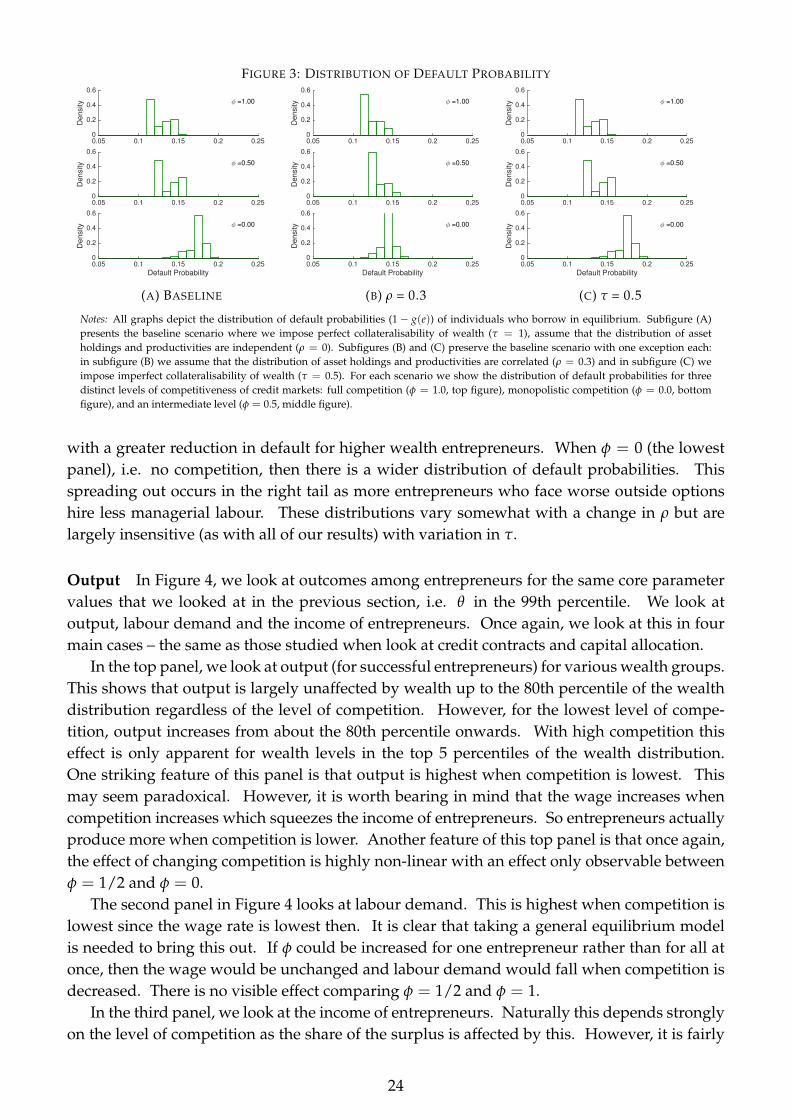
FIGURE 3: DISTRIBUTION OF DEFAULT PROBABILITY

0.05 0.1 0.15 0.2 0.25

De

nsity

0

0.2

0.4

0.6

φ =1.00

0.05 0.1 0.15 0.2 0.25

De

nsity

0

0.2

0.4

0.6

φ =0.50

Default Probability0.05 0.1 0.15 0.2 0.25

De

nsity

0

0.2

0.4

0.6

φ =0.00

(A) BASELINE

0.05 0.1 0.15 0.2 0.25

De

nsity

0

0.2

0.4

0.6

φ =1.00

0.05 0.1 0.15 0.2 0.25

De

nsity

0

0.2

0.4

0.6

φ =0.50

Default Probability0.05 0.1 0.15 0.2 0.25

De

nsity

0

0.2

0.4

0.6

φ =0.00

(B) ρ = 0.3

0.05 0.1 0.15 0.2 0.25

De

nsity

0

0.2

0.4

0.6

φ =1.00

0.05 0.1 0.15 0.2 0.25

De

nsity

0

0.2

0.4

0.6

φ =0.50

Default Probability0.05 0.1 0.15 0.2 0.25

De

nsity

0

0.2

0.4

0.6

φ =0.00

(C) τ = 0.5

Notes: All graphs depict the distribution of default probabilities (1− g(e)) of individuals who borrow in equilibrium. Subfigure (A)presents the baseline scenario where we impose perfect collateralisability of wealth (τ = 1), assume that the distribution of assetholdings and productivities are independent (ρ = 0). Subfigures (B) and (C) preserve the baseline scenario with one exception each:in subfigure (B) we assume that the distribution of asset holdings and productivities are correlated (ρ = 0.3) and in subfigure (C) weimpose imperfect collateralisability of wealth (τ = 0.5). For each scenario we show the distribution of default probabilities for threedistinct levels of competitiveness of credit markets: full competition (φ = 1.0, top figure), monopolistic competition (φ = 0.0, bottomfigure), and an intermediate level (φ = 0.5, middle figure).

with a greater reduction in default for higher wealth entrepreneurs. When φ = 0 (the lowestpanel), i.e. no competition, then there is a wider distribution of default probabilities. Thisspreading out occurs in the right tail as more entrepreneurs who face worse outside optionshire less managerial labour. These distributions vary somewhat with a change in ρ but arelargely insensitive (as with all of our results) with variation in τ.

Output In Figure 4, we look at outcomes among entrepreneurs for the same core parametervalues that we looked at in the previous section, i.e. θ in the 99th percentile. We look atoutput, labour demand and the income of entrepreneurs. Once again, we look at this in fourmain cases – the same as those studied when look at credit contracts and capital allocation.

In the top panel, we look at output (for successful entrepreneurs) for various wealth groups.This shows that output is largely unaffected by wealth up to the 80th percentile of the wealthdistribution regardless of the level of competition. However, for the lowest level of compe-tition, output increases from about the 80th percentile onwards. With high competition thiseffect is only apparent for wealth levels in the top 5 percentiles of the wealth distribution.One striking feature of this panel is that output is highest when competition is lowest. Thismay seem paradoxical. However, it is worth bearing in mind that the wage increases whencompetition increases which squeezes the income of entrepreneurs. So entrepreneurs actuallyproduce more when competition is lower. Another feature of this top panel is that once again,the effect of changing competition is highly non-linear with an effect only observable betweenφ = 1/2 and φ = 0.

The second panel in Figure 4 looks at labour demand. This is highest when competition islowest since the wage rate is lowest then. It is clear that taking a general equilibrium modelis needed to bring this out. If φ could be increased for one entrepreneur rather than for all atonce, then the wage would be unchanged and labour demand would fall when competition isdecreased. There is no visible effect comparing φ = 1/2 and φ = 1.

In the third panel, we look at the income of entrepreneurs. Naturally this depends stronglyon the level of competition as the share of the surplus is affected by this. However, it is fairly

24

FIGURE 4: EQUILIBRIUM ENTREPRENEURS

0 20 40 60 80 10017

17.5

18

18.5

19

19.5Output

0 20 40 60 80 1009

9.5

10

10.5

11Labour Demand

Assets (a) Centile0 20 40 60 80 100

0

1

2

3

4

5

φ=0.0

φ=0.5

φ=1.0

Borrower Income

(A) BASELINE

0 20 40 60 80 1004.6

4.8

5

5.2

5.4Output

0 20 40 60 80 1002.4

2.5

2.6

2.7

2.8

2.9Labour Demand

Assets (a) Centile0 20 40 60 80 100

0.9

1

1.1

1.2

1.3

φ=0.0φ=0.5

φ=1.0

Borrower Income

(B) θ = 96TH PERCENTILE

0 20 40 60 80 10016.5

17

17.5

18

18.5Output

0 20 40 60 80 1008.5

9

9.5

10Labour Demand

Assets (a) Centile0 20 40 60 80 100

0

1

2

3

4

5

φ=0.0

φ=0.5

φ=1.0

Borrower Income

(C) ρ = 0.3

0 20 40 60 80 10017

17.5

18

18.5

19

19.5Output

0 20 40 60 80 1009

9.5

10

10.5

11Labour Demand

Assets (a) Centile0 20 40 60 80 100

0

1

2

3

4

5

φ=0.0

φ=0.5

φ=1.0

Borrower Income

(D) τ = 0.5

Notes: The figures describe characteristics of the equilibrium firm level outcomes for entrepreneurs across all centiles of the asset distribution,holding constant θ. Subfigure (A) presents the baseline scenario where we impose perfect collateralisability of wealth (τ = 1), assume thatthe distribution of asset holdings and productivities are independent (ρ = 0) and presents results for the 99th centile of the productivitydistribution. Subfigures (B), (C) and (D) preserve the baseline scenario with one exception each: In subfigure (B) we presents results forthe 96th centile of the productivity distribution, in subfigure (C) we assume that the distribution of asset holdings and productivities arecorrelated (ρ = 0.3) and in subfigure (D) we impose imperfect collateralisability of wealth (τ = 0.5). Firm outcomes are shown for threedistinct levels of competitiveness of credit markets: full competition (φ = 1.0), monopolistic competition (φ = 0.0), and an intermediate level(φ = 0.5). Expected output is eαθ1−η−α(l1−β kβ)η , measured in units of average annual wage income. Total expected firm level labour demandis eα l + θδ e, measured in units of one persons annual labour supply. Expected borrower income is eα(Π(k; θ)− r)− (1− eα)c− θδ ew− γκa,measured in units of average annual wage income. Both are measured in absolute terms and in units of the annual income of a wage labourerin the US.

flat with respect to the level of wealth except when there is very low competition when it turnsupwards at the highest wealth levels.

The remaining panels look at the same variants as in Figure 1. As we might expect, Subfig-ure (B) shows that having smaller entrepreneurs scales down the size of incomes and labourdemand. Competition increases labour demand and income. Increasing the correlation be-tween wealth and productivity implies that competition has a negative effect on labour de-mand for most wealth levels. This is driven by the same general equilibrium effect that alsodrives the pattern of firm capital in Figure 2. When competition is low, now labour demandshifts down more noticeably with the level of competition. Finally, in subfigure (D), we con-tinue to see little evidence of a general equilibrium de Soto effect.

4.2 Expanding Market Access

In this section, we look at aggregate implications of extending financial inclusion. We considerdifferent values of χ (a, θ) assuming that this is independent of (a, θ) but we allow credit to beextended to a wider and wider set of individuals.

Wages and Self-Employment Figure 5 gives the core aggregate outcomes. The first is thewage as a fraction of the US wage moving form Autarky through to full credit market access.The second gives the fraction of the population that become entrepreneurs. We illustrate thisfor two cases. The first, the blue lines in Figure 5 sets φ = 1 (full competition) and τ = 1

25

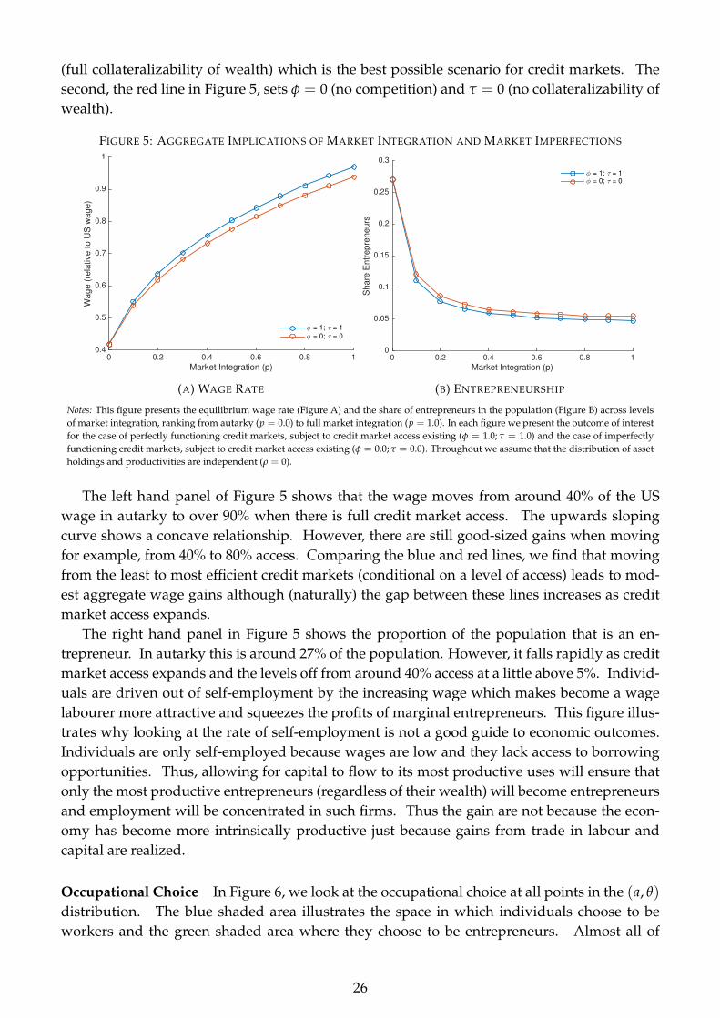
(full collateralizability of wealth) which is the best possible scenario for credit markets. Thesecond, the red line in Figure 5, sets φ = 0 (no competition) and τ = 0 (no collateralizability ofwealth).

FIGURE 5: AGGREGATE IMPLICATIONS OF MARKET INTEGRATION AND MARKET IMPERFECTIONS

Market Integration (p)0 0.2 0.4 0.6 0.8 1

Wa

ge

(re

lative

to

US

wa

ge

)

0.4

0.5

0.6

0.7

0.8

0.9

1

φ = 1; τ = 1

φ = 0; τ = 0

(A) WAGE RATE

Market Integration (p)0 0.2 0.4 0.6 0.8 1

Share

Entr

epre

neurs

0

0.05

0.1

0.15

0.2

0.25

0.3

φ = 1; τ = 1φ = 0; τ = 0

(B) ENTREPRENEURSHIP

Notes: This figure presents the equilibrium wage rate (Figure A) and the share of entrepreneurs in the population (Figure B) across levelsof market integration, ranking from autarky (p = 0.0) to full market integration (p = 1.0). In each figure we present the outcome of interestfor the case of perfectly functioning credit markets, subject to credit market access existing (φ = 1.0; τ = 1.0) and the case of imperfectlyfunctioning credit markets, subject to credit market access existing (φ = 0.0; τ = 0.0). Throughout we assume that the distribution of assetholdings and productivities are independent (ρ = 0).

The left hand panel of Figure 5 shows that the wage moves from around 40% of the USwage in autarky to over 90% when there is full credit market access. The upwards slopingcurve shows a concave relationship. However, there are still good-sized gains when movingfor example, from 40% to 80% access. Comparing the blue and red lines, we find that movingfrom the least to most efficient credit markets (conditional on a level of access) leads to mod-est aggregate wage gains although (naturally) the gap between these lines increases as creditmarket access expands.

The right hand panel in Figure 5 shows the proportion of the population that is an en-trepreneur. In autarky this is around 27% of the population. However, it falls rapidly as creditmarket access expands and the levels off from around 40% access at a little above 5%. Individ-uals are driven out of self-employment by the increasing wage which makes become a wagelabourer more attractive and squeezes the profits of marginal entrepreneurs. This figure illus-trates why looking at the rate of self-employment is not a good guide to economic outcomes.Individuals are only self-employed because wages are low and they lack access to borrowingopportunities. Thus, allowing for capital to flow to its most productive uses will ensure thatonly the most productive entrepreneurs (regardless of their wealth) will become entrepreneursand employment will be concentrated in such firms. Thus the gain are not because the econ-omy has become more intrinsically productive just because gains from trade in labour andcapital are realized.

Occupational Choice In Figure 6, we look at the occupational choice at all points in the (a, θ)

distribution. The blue shaded area illustrates the space in which individuals choose to beworkers and the green shaded area where they choose to be entrepreneurs. Almost all of

26

these entrepreneurs choose to borrow. However, those with very high wealth choose to self-finance.

On the extreme left and right hand panels, we illustrate autarky and the first best. Theleft hand panel shows, not surprisingly, that the low wealth and low productivity individualsare all workers. However, of the 27% or so who choose to become entrepreneurs, this goesquite far down the productivity distribution for people with high wealth. In the first best, onlyaround the top 4% of the productivity distribution becoming entrepreneurs. Moreover, initialwealth does not matter now since capital allocation in a firm is not dependent on this, only onthe productivity of an enterprise.

FIGURE 6: OCCUPATIONAL CHOICE

Worker

Entrepreneur (Self-Financed)

Productivity (θ) Centile10 20 30 40 50 60 70 80 90 100

Asset (a

) C

entile

10

20

30

40

50

60

70

80

90

100

(A) AUTARKY

Productivity (θ) Centile10 20 30 40 50 60 70 80 90 100

Asset (a

) C

entile

10

20

30

40

50

60

70

80

90

100

(B) p = 0.10

Productivity (θ) Centile10 20 30 40 50 60 70 80 90 100

Asset (a

) C

entile

10

20

30

40

50

60

70

80

90

100

(C) p = 0.25

Worker

En

tre

pre

ne

ur

(1B

)

Productivity (θ) Centile10 20 30 40 50 60 70 80 90 100

Asset (a

) C

entile

10

20

30

40

50

60

70

80

90

100

(D) FIRST BEST

Notes: These figure depicts the occupational choice and lending decision in the a - θ space. Throughout we assume ρ = 0. In Figure 6awe present the occupational choice in autarky; in Figure 6b we assume p = 0.1 and (φ = 1.0; τ = 1.0; κ = 1.0); in Figure 6c we assumep = 0.25 and (φ = 1.0; τ = 1.0; κ = 1.0); and in Figure 6d we present results in first best. Blue areas indicate individuals who becomeworkers when they have no credit market access. Green areas indicate individuals who become entrepreneurs when they have no creditmarket access. The while line indicates the occupational choice of individuals with credit market access: individuals to the lower-left ofit become workers, individuals to the upper-right of it become entrepreneurs.

In the middle two panels, we illustrate the occupational choice for two intermediate valuesof credit market access where credit contracts are second-best optimal. We choose χ = 0.10,i.e. 10% of the population has access to credit markets and χ = 0.25 where it is 25%. Theyshow how as credit market access expands, there are fewer entrepreneurs. Even with verylimited access, there is switch away from low-productivity high wealth individuals choosingto become entrepreneurs. Hence, the selection effect is quite powerful. The line betweenthe blue and green areas is close to vertical. It then shifts to the right as credit market accessexpands.

Competition and Distribution We now look at the division of income between labourers,lenders and entrepreneurs. We will consider this as we vary credit market access, χ, and thelevel of competition, φ. The size of the columns in Figure 7 illustrate the level of income as afraction of US income.

On the extreme left is autarky. Here, a little less than half of national income is in the formentrepreneurial profits. The next three bars are for the case where 50% of the population haveaccess to credit markets but for three levels of competition. Note, however, that with φ = 0,then most of the gains from credit markets are appropriated by lenders and entrepreneurialprofits are squeezed relative to autarky. The main effect of increasing competition is to redis-tribute surplus between lenders and entrepreneurs. There is a modest increase in the wage,due to competition with most of the gain (as we would expect from Figure 5) coming fromincreasing market access. A similar pattern of surplus redistribution is found for the case of

27

full credit market access.

FIGURE 7: DISTRIBUTION OF SURPLUS ACROSS LEVELS OF COMPETITIVENESS

Surp

lus (

Fra

ction o

f F

irst B

est)

0

0.1

0.2

0.3

0.4

0.5

0.6

0.7

0.8

0.9

1

Lenders

Entrepr.

Labour

First Bestφ = 0.0 φ = 0.5 φ = 1.0 φ = 0.0 φ = 0.5 φ = 1.0

p = 1.00p = 0.50p = 0.00

Notes: This figure depicts the size and distribution of total surplus in the economy, in units offirst best surplus. It depicts these across levels of market integration, ranking from autarky(p = 0.0) to full market integration (p = 1.0), and for distinct levels of competitiveness ofcredit markets, ranging from monopolistic competition (φ = 0.0) to full competition (φ =

1.0). Throughout we impose perfect collateralisability of wealth (τ = 1) and assume that thedistribution of asset holdings and productivities are independent (ρ = 0).

The Distribution of Firm Size In Figure 8, we look at the distribution of firm size. In eachcase, we look at variation in market access for four values varying from autarky to full access.Throughout Figure 6, the solid bars gives the distribution in the first best and the colors (greenand orange) show deviations in second best from the first best. The left hand panel gives thefull range of firms in the economy whereas the right hand panel gives the distribution of largestfirms – the upper tail of the distribution. In each panel, we give the first best distribution offirms so that we can compare this to the distribution implied by the second-best.

In the top panel left panel we compare autarky to the first best. Here, we find a very clearshift in the distribution towards small firms. This made even more apparent in the top right-hand panel which shows that there are virtually no large firms in the economy. This lack oflabour demand is what keeps the wage low. This broad pattern is found in all of the panels.However, as credit market access varies, the deviation from the “first best” distribution offirm size diminishes. By the time of full credit market access, the first best is very similar todistribution generated by second-best credit markets.

The gains from credit market access Figure 9 gives an insight into how the gains from par-ticipation in credit markets is distributed across the population. It contains two panels basedon the level of competition. Comparing the two panels, it is clear that the gains and losses ofcredit markets, relative to autarky, are highly heterogeneous.

Those who are wage labourers in autarky are all better off with the possibility of trading incredit markets. However, among those who were entrepreneurs in autarky, a large fraction alsolose from the introduction of credit markets due to rising wages. These losses are concentratedamongst entrepreneurs with higher level of wealth, holding θ constant. These entrepreneurshad good access to capital even in autarky, and benefited from low wage levels. This effectis particularly pronounced in the right hand panel of Figure 10, where we compare payoffswith credit markets (with φ = 1) to autarky. Here, high productivity entrepreneurs with low

28

FIGURE 8: DISTRIBUTION OF FIRM SIZES

1 10 100 1000

De

nsity

0.0

0.1

0.2

p =0.00

Second B. First B.

1 10 100 1000

De

nsity

0.0

0.1

0.2

p =0.25

1 10 100 1000

De

nsity

0.0

0.1

0.2

p =0.50

Firm Size1 10 100 1000

De

nsity

0.0

0.1

0.2

p =1.00

(A) FULL DISTRIBUTION

10 100 1000

De

nsity

0.0

0.005

0.01

p =0.00

Second B. First B.

10 100 1000

De

nsity

0.0

0.005

0.01

p =0.25

10 100 1000

De

nsity

0.0

0.005

0.01

p =0.50

Firm Size10 100 1000

De

nsity

0.0

0.005

0.01

p =1.00

(B) UPPER TAIL OF DISTRIBUTION

Notes: All graphs depict the distribution of firm sizes in labour units in equilibrium (grey filled bars) We show the distribution of firmsizes for four distinct levels of credit market access: autarky (p = 0.0, top figure), low credit market access (p = 0.25, second from topfigure), half the population has credit market access (p = 5.0, second from top figure), and full access (p = 1.0, top figure). Throughoutwe impose perfect collateralisability of wealth (τ = 1), perfect credit market competition (φ = 1.0) assume that the distribution of assetholdings and productivities are independent (ρ = 0). Subfigure (A) presents the full distribution of firm sizes with log10 scale on thex-axis; subfigure (B) presents a zoomed-in version of the right tail of the firm size distribution. In all figures the distribution of firm sizesin first best is also shown as benchmark (black outlined bars).

FIGURE 9: RELATIVE INCOME GAINS: CREDIT MARKETS VS. AUTARKY

Productivity (θ) Centile100 200 300 400 500 600 700 800 900 1000

Asse

t (a

) C

en

tile

10

20

30

40

50

60

70

80

90

100

0

0.5

1

1.5

2

2.5

(A) NO COMPETITION, φ = 0

Productivity (θ) Centile100 200 300 400 500 600 700 800 900 1000

Asse

t (a

) C

en

tile

10

20

30

40

50

60

70

80

90

100

0

0.5

1

1.5

2

2.5

(B) FULL COMPETITION, φ = 1 (WINZORISED)

Notes: We calculate for each level of assets a and productivity θ the ratio of income when credit markets exists over income in autarky.Both figures present contour maps of these ratios over the (a, θ) space. Figure (A) assumes fully uncompetitive credit markets (φ = 0)and Figure (B) assumes fully competitive credit markets (φ = 1). Note that in Figure (B) the income ratio is winzorised at 2.5 for visualclarity. This affects the top 2% of the θ distribution, and increasingly at lower levels of assets. The highest relative income gain witha ratio of 28.04 is observed for the highest level of θ and lowest level of a. Throughout we assume no correlation between assets andproductivity (ρ = 0) and perfect collateralisability of wealth (τ = 1).

29

levels of assets benefit form the increased access to credit, despite the fact that this comes withsizeable wage increases. However, entrepreneurs with similarly high productivity and highlevels of assets do still loose out relative to autarchy. For them the increased credit access is lessimportant, since they can to a large extent, just self-finance their investment. In the absenceof competition, all of the most productive entrepreneurs lose relative to autarchy, since theincrease in wages is not compensated by better credit access.

5 Concluding Comments

This paper has provided a quantitative exploration of the aggregate implications of credit mar-ket frictions where agents, who differ in wealth and productivity, make an occupational choicebetween being a worker and an entrepreneur. The paper has explored optimal credit contractsin a general equilibrium setting. It has then explored the impact of extending access to financeto a wider and wider group of the population.

The main aim of the paper has been to explore how lack of market access and credit marketfrictions affect the level of income per capita and wages for a fixed technology. Having speci-fied a model, a key finding is that the wage moves from around 40% of the US wage in autarkyto over 90% when there is full credit market access. Moreover, it is access to credit marketsrather than frictions due to moral hazard which are quantitatively most important.

The paper focuses on an important general equilibrium channel by which credit marketaccess affects development due to better selection of entrepreneurs, based on their talent andan increase in labour demand which increases the wage. Thus, credit market access spilloversbenefit the population at large. Hence, looking for the impact of credit market distortionspurely by focusing on capital markets and local effects where factor prices are fixed will oftenmiss the big picture that expansion of the market to the unbanked is where the big gains inpoverty reduction lie given that most of the poor in developing countries are dependent onwage labour.

The paper also highlights the importance of diminishing the extent of small-scale self-employment as development progresses with such individuals mainly switching to wage la-bor. This is consistent with anecdotal observation and evidence on the structural transforma-tion which takes place alongside extending credit market access. Hence while entrepreneur-ship is important to development, it is the capacity of the market system to get capital to thoseentrepreneurs with high productivity which matters most. When market access is limited,many of them have to rely on their own wealth and resources which implies that they cannotoperate at optimum scale.

The model has assumed a specific technology for providing credit where limits on conven-tional collateral create a friction, conditional on access. In future, we plan to explore furtherthe gains to be made by expanding collateral to non-pecuniary punishments, so-called socialcollateral. This would allow us to link the paper to discussions about the role of micro-creditin development.

The paper has focused on differences in the level of income. A natural next step in theresearch program is to look at dynamic implications. Once there are new technologies andshocks to individual firm productivity due to this then the economy has to continuously re-allocate capital. Limited market access plays a role in limiting this too if those who currentlyenjoy market access can get credit and those with new technologies are excluded. This will

30

affect the ability of the economy to benefit from growth opportunities. More generally, itwould be interesting to develop a dynamic version of the model with wealth accumulation.

31

References

[1] Axtell, R. L. [2001] “Zipf Distribution of U.S. Firm Sizes” Science, 293(5536), 1818–1820.

[2] Banerjee, Abhijit, and Andrew F. Newman, [1993] “Occupational Choice and the Processof Development.” Journal of Political Economy, 101 (2): 274–98.

[3] Banerjee, Abhijit V. and Esther Duflo [2005]: ”Growth Theory through the Lens of Devel-opment Economics”, Chapter 7 in Philippe Aghion and Steven N. Durlauf (ed.s) Handbookof Economic Growth, Volume 1, Part A, 473-552.

[4] Banerjee, Abhijit, and Esther Duflo [2010], “Giving Credit Where it is Due,” Journal ofEconomic Perspectives, 24(3), 61-79.

[5] Bardhan, Pranab, [1984], Land, Labor and Rural Poverty, Columbia University Press, NewYork and Oxford University Press, New Delhi.

[6] Bartelsman, Eric, John Haltiwanger, and Stefano Scarpetta, [2013],“Cross-Country Differ-ences in Productivity: The Role of Allocation and Selection.” American Economic Review,103 (1): 305–34.

[7] Besley, Timothy, Konrad Burchardi, and Maitreesh Ghatak [2012], “Incentives and the DeSoto Effect,”, The Quarterly Journal of Economics, 127(1), 237-282.

[8] Bloom, Nicholas, [2009], “The Impact of Uncertainty Shocks” Econometrica, 77(3), 623-685.

[9] Board of Governors of the Federal Reserve [2016] “Charge-Off and Delinquency Rates onLoans and Leases at Commercial Banks,” [Online; accessed 18-November-2016]

[10] Buera, Francisco, Joseph Kaboski, and Yongseok Shin, [2011], “Finance and Development:A Tale of Two Sectors.” American Economic Review, 101 (5): 1964–2002.

[11] Burgess, Robin and Rohini Pande, [2005], “Do Rural Banks Matter? Evidence from theIndian Social Banking Experiment,” American Economic Review, 95(3), 780-795.

[12] Caselli, Francesco, [2005], “Accounting for Cross-Country Income Differences,” Chapter 9in Philippe Aghion and Steven N. Durlauf (eds), Handbook of Economic Growth, Volume1, Part A, 679-741.

[13] Cihak, Martin, Asli Demirguc -Kunt, Eric Feyen, and Ross Levine, [2013], “Financial De-velopment in 205 Economies, 1960 to 2010,” Working paper 18946, National Bureau ofEconomic Research.

[14] Credit Suisse [2015], “Global Wealth Report,” Credit Suisse Research Institute.

[15] Demirguc-Kunt, Asli and Leora Klapper, [2013], “Measuring Financial Inclusion: Explain-ing Variation in Use of Financial Services across and within Countries,” Brookings Paperson Economic Activity (Spring), 279-327.

[16] Dupas, Pascaline, Dean Karlan, Jonathan Robinson and Diego Ubfal, [2017], “Banking theUnbanked? Evidence from three countries,” unpublished typescript.

32

[17] Galor, Oded, and Joseph Zeira, [1993] “Income Distribution and Macroeconomics.” Re-view of Economic Studies 60 (1): 35–52.

[18] Gerschenkron, Alexander [1962], Economic Backwardness in Historical Perspective – ABook of Essays, Harvard University Press, Cambridge, MA.

[19] Goldsmith, Raymond W. [1969], Financial Structure and Development. Yale UniversityPress, New Haven, CT.

[20] Jeong, Hyeok, and Robert M. Townsend, [2007] “Sources of TFP Growth: OccupationalChoice and Financial Deepening.” Economic Theory 32 (1): 179–221.

[21] Hsieh, Chang-Tai, and Peter J. Klenow, [2009], “Misallocation and Manufacturing TFP inChina and India.” Quarterly Journal of Economics 124 (4): 1403–48.

[22] Hsieh, Chang-Tai, and Peter J. Klenow, [2010], “Development Accounting,” AmericanEconomic Journal: Macroeconomics, 2(1), 207-23.

[23] Karlan, Dean and Jonathan Zinman, [2009], “Observing Unobservables: Identifying In-formation Asymmetries With a Consumer Credit Field Experiment,” Econometrica, 77(6),1993-2008.

[24] Levine, Ross, [2005] “Finance and Growth: Theory and Evidence.” In Handbook of Eco-nomic Growth. Vol. 1, Part A, edited by Philippe Aghion and Steven Durlauf, 865–934.Amsterdam: Elsevier B.V.

[25] Lloyd-Ellis, Huw, and Dan Bernhardt.[2000]: “Enterprise, Inequality and Economic De-velopment.” The Review of Economic Studies, 67(1), 147–168.

[26] Matsuyama, Kiminori, [2007], “Aggregate Implications of Credit Market Imperfections.”In NBER Macroeconomics Annual 2007, Vol. 22, edited by Daron Acemoglu, KennethRogoff, and Michael Woodford, 1–60.

[27] Moll, Benjamin [2014], “Productivity Losses from Financial Frictions: Can Self-FinancingUndo Capital Misallocation?,” American Economic Review 104 (10), 3186-3221.

[28] Nelsen, Roger B. [1999], An Introduction to Copulas, Springer.

[29] Restuccia, Diego, and Richard Rogerson, [2008] “Policy Distortions and Aggregate Pro-ductivity with Heterogeneous Plants.” Review of Economic Dynamics 11 (4): 707–20.

[30] Sklar, Abe, [1959], “Fonctions de repartition a n dimensions et leurs marges”, Publicationsde l’Institut de Statistique de l’Universite de Paris, 8, 229–231.

[31] Stiglitz, Joseph, [1988], “Economic organization, information, and development,” Chapter5 in Hollis B. Chenery and T.N. Srinivasan (eds), Handbook of Development EconomicsVolume 1, 93-160.

[32] Townsend, Robert, [1978], “Intermediation with Costly Bilateral Exchange,” Review ofEconomic Studies, 45(3), 417-25.

33

[33] Townsend, Robert and Kenichi Ueda, [2006], “Financial Deepening, Inequality, andGrowth: A Model-Based Quantitative Evaluation,” Review of Economic Studies, 73(1),251-93.

[34] Trivedi, Pravin K. and David M. Zimmer [2007], “Copula Modeling: An Introduction forPractitioners,” Foundations and Trends in Econometrics, 1(1), 1-111.

[35] World Bank, [2014], Global Financial Development Report 2014: Financial Inclusion,Washington DC, World Bank.

[36] Yi, K. , and J. Zhang, [2016], “Real Interest Rates Over the Long Run,” Economic PolicyPaper, 16(10), Federal Reserve Bank of Minneapolis.

34

A Proofs of Propositions

Proof of Proposition 1: The proof is a generalisation of the proof of Proposition 2 in Besleyet al (2012) in two ways: first, π(k; θ, p) and d(e; θ, p) are allowed to depend on θ and p; sec-ond, d(e; θ, p) is not necessarily linear in e. The first generalisation is trivial, since lender andborrower take θ and p as given in a given contracting problem. These are therefore additionalconstant, multiplicative factors, immaterial to the proof. The second generalisation is straight-forward and affects the proof in two ways.

First, when the participation constraint is non-binding (Step 3 of the Proof of Proposition 2in Besley et al (2012)), the optimal contracting problem can be written as

max(e,k)

g(e)[

π(k; θ, p)− de(e; θ, p)ge(e)

]+ τa− γk.

We have that q(e)π(k; θ, p) is strictly concave by Assumption 2 (ii) and −q(e)[

de(e;θ,p)ge(e)

]is

strictly concave by Assumption 1 (i), (iii), and (iv). Therefore the maximisation is well-behaved,and by standard arguments, a unique global maximum (e0, k0) exists. The first-order necessaryconditions for an interior optimum are:

ge(e0)π(k0; θ, p) = de(e0; θ, p) + g(e0)ε(e0; θ, p) (17)

g(e0)πk(k0; θ, p) = γ. (18)

We have that ε(e; θ, p) = dee(e;θ,p)ge(e)

− de(e;θ,p)gee(e)[ge(e)]2

> 0 since g(e) is strictly concave, g(e) andd(e; θ, p) are strictly increasing and d(e; θ, p) is weakly convex. By Assumption 2 (iii) theunique global maximum (e0, k0) is then an interior solution.

Secondly, if the participation constraint is binding (Step 4 of the Proof of Proposition 2 inBesley et al (2012)), we can use the binding participation constraint, incentive compatibilityconstraint and limited liability constraint to find optimal effort ξ defined by

g(ξ(v; θ, p))[

de(ξ(v; θ, p); θ, p)ge(ξ(v; θ, p))

]− d(ξ(v; θ, p); θ, p) = v. (19)

We have ξv(v; θ, p) = ge(ξ)[

de(ξ;θ,p)ge(ξ)

]+ g(ξ)

[dee(ξ;θ,p)

ge(ξ)− de(ξ;θ,p)gee(ξ)

[ge(ξ)]2

]> 0 by Assumption 1

(iv), and the fact that g(e) and d(e; θ, p) are increasing.

Proof of Proposition 2: When the participation constraint is non-binding, capital is definedby (18). When the participation constraint is binding, effort is pinned down by (19). Using theincentive compatibility constraint and the lender’s objective function, the optimal contractingproblem becomes

maxk

g(ξ(v; θ, p))[

π(k; θ, p)− de(ξ(v; θ, p); θ, p)ge(ξ(v; θ, p))

]+ τa− γk.

The first order condition with respect to k again takes the form:

g(ξ(v; θ, p))πk(k; θ, p) = γ.

Proof of Corollary 1: The proof is directly analogous to the proof of Lemma 1 in Besley et al(2012).

35

Proof of Proposition 3: We use the fact that

φ · S(u(φ; a, θ, p) + τa; θ, p) = u(φ; a, θ, p).

Now differentiate u(φ; a, θ, p) with respect to the various parameters to yield

∂u(φ; a, θ, p)∂θ

=Sθ(u(φ; a, θ, p) + τa; θ, p)

1− φSv(u(φ; a, θ, p) + τa; θ, p)∂u(φ; a, θ, p)

∂a=

Sv(u(φ; a, θ, p) + τa; θ, p)τ1− φSv(u(φ; a, θ, p) + τa; θ, p)

> 0

∂u(φ; a, θ, p)∂φ

=S(u(φ; a, θ, p) + τa; θ, p)

1− φSv(u(φ; a, θ, p) + τa; θ, p)> 0.

The inequalities follow noting that 1−φSv(u(φ; a, θ, p)+ τa; θ, p) > 0 for all v ∈ (v (θ, p) , v (θ, p))and 0 ≤ Sv(u(φ; a, θ, p) + τa; θ, p) ≤ 1. Further we can derive

Sθ = [ge(e)π(k; θ, p)− de(e; θ, p)]eθ + g(e)πθ(k; θ, p)− dθ(e; θ, p),

where we use the first order condition with respect to k. We have ge(e)π(k; θ, p)− de(e; θ, p) >0 as long as the first best effort is not implemented; g(e)πθ(k; θ, p) > 0 by Assumption 1 (i)and (ii); −dθ(e; θ, p) < 0 by Assumption 1 (iii). From (19) it is straight-forward to show thatthe sign of eθ is indeterminate and depends on deθ(e; θ, p), dθ(e; θ, p), and the shape of g(e).Examples can be constructed where Sθ > 0 and Sθ < 0.

36