FINANCIAL INCENTIVES AND COGNITIVE ABILITIES:

EVIDENCE FROM A FORECASTING TASK WITH VARYING COGNITIVE LOAD†

Ondrej Rydval§

April 2007

Abstract

I examine how financial incentives interact with intrinsic motivation and especially

cognitive abilities in explaining heterogeneity in performance. Using a forecasting task

with varying cognitive load, I show that the effectiveness of high-powered financial

incentives as a stimulator of economic performance can be moderated by cognitive abilities

in a causal fashion. Identifying the causality of cognitive abilities is a prerequisite for

studying their interaction with financial and intrinsic incentives in a unifying framework,

with implications for the design of efficient incentive schemes.

Keywords: Financial incentives, Cognitive ability, Heterogeneity, Performance, Experiment

JEL classification: C81, C91, D83

† This research was supported by the Grant Agency of the Czech Republic (grant 402/05/1023) and by travel funds from the Hlavka Foundation and CERGE-EI. I am grateful to Randall Engle and Richard Heitz of the Attention and Working Memory Lab at the Georgia Institute of Technology for providing me with their “automated working memory span” tests, and to Brian MacWhinney of the Department of Psychology, Carnegie Mellon University, for providing me with his “audio digit span” test. I am greatly indebted to Andreas Ortmann and Nat Wilcox for providing me with invaluable advice throughout the project. I further thank Colin Camerer, Jan Hanousek, Glenn Harrison, Stepan Jurajda and Jan Kmenta for helpful comments. All remaining errors are my own. § Center for Economic Research and Graduate Education, Charles University, and Economics Institute, Academy of Sciences of the Czech Republic, Address: Politickych veznu 7, 111 21 Prague, Czech Republic, Tel: +420-224-005-290, E-mail address: Ondrej.Rydval@cerge-ei.cz.

1

1. Introduction

Economists widely believe that, absent strategic considerations such as agency problems,

financial incentives represent the dominant and effective stimulator of human productive

activities (e.g., Gibbons, 1998; Prendergast, 1999). In production settings that are

cognitively demanding, however, the effectiveness of financial incentives may be

moderated by individual cognitive abilities and motivational characteristics. As a useful

metaphor for the moderating channels, Camerer and Hogarth (1999) propose an informal

capital-labor-production (KLP) framework, describing how financial incentives may

interact in non-trivial ways with intrinsic motivation in stimulating cognitive effort (labor),

and how the productivity of cognitive effort may in turn vary across individuals due to

their different cognitive abilities (capital). Even if financial incentives induce high effort,

both financial and cognitive resources may be wasted for individuals whose cognitive

constraints inhibit performance improvements. This prediction, if warranted, calls for

attention to individual cognitive abilities in designing efficient incentive schemes in firms,

experimental settings and elsewhere.1

This paper provides an initial empirical test of the KLP framework. I identify the key

theoretical building block of the KLP framework, namely the causal effect of cognitive

capital on performance. Establishing the causality of cognitive capital is a prerequisite for

credibly addressing fundamental economic interactions underlying the KLP framework,

such as how people perform under different incentive levels and schemes conditional on

their cognitive capital;2 how they self-select on their cognitive capital into incentive

1 See Awasthi and Pratt (1990), Libby and Lipe (1992), and Libby and Luft (1993), among others, for earlier accounts of the KLP framework. Throughout the paper, I refer to cognitive abilities and cognitive capital interchangeably. One can think of individual cognitive capital, combined with the cognitive load of a particular cognitive task, as determining the extent to which individuals face cognitive constraints when executing the task. 2 Economists, psychologists and researchers in other fields have paid considerable theoretical and empirical attention to the effect of financial incentives on (cognitive) performance, especially to their interaction with intrinsic motivation (see Bonner and Sprinkle, 2002, McDaniel and Rutström, 2001, and Rydval, 2003, for reviews). By contrast, we have much less evidence on the interaction of financial incentives with cognitive capital. In Awasthi and Pratt (1990) and Palacios-Huerta (2003), introducing and/or raising performance-contingent financial incentives yields a larger increase in judgmental performance for individuals with higher cognitive capital, as proxied by a perceptual differentiation test and schooling outcomes, respectively. Rydval and Ortmann (2004) illustrate that cognitive abilities appear at least as important for performance in an IQ test as does a sizeable variation in piece-rate incentives. Contrasting the explanatory power of cognitive capital and personality characteristics under various incentive schemes – such as piece-rate, quota and tournament schemes – is likely a fruitful area of future research (e.g., Bonner et al., 2000).

2

schemes varying in expected return to cognitive capital (and effort);3 whether people are

willing to purchase “external” cognitive capital that would relax their cognitive

constraints;4 and how cognitive capital affects the way people interact in strategic

environments.5

The notion of cognitive capital is of course not new to economists (e.g., Conlisk, 1980;

Wilcox, 1993). Ballinger et al. (2005) provide a broad but pertinent theoretical perspective

on cognitive capital, describing it as a vector of various (possibly interacting and time-

variant) limits on cognition that can at any instance be “(perhaps imperfectly) measured by

various tests of cognitive abilities.” (p.3). Recent experimental evidence suggests that

individual heterogeneity in cognitive capital can partly explain departures from rational

saving behavior (Ballinger et al., 2005), deviations from normative game-theoretic

solutions (Devetag and Warglien, 2003; Ortmann et al., 2006) and biases in risk and time

preferences (Benjamin et al., 2006). Going a step further, I ask whether the effect of

cognitive capital on economic behavior and performance is causal, and in turn whether the

effectiveness of even strong financial incentives can be moderated by cognitive capital in

a causal fashion.6

3 See Harrison et al. (2005), Lazear et al. (2006), and Vandegrift and Brown (2003) for examples of self-selection in experiments, and Bonner and Sprinkle (2002) for discussion and early evidence of self-selection on cognitive abilities into incentive schemes. 4 In a follow-up part of this project, I will interact financial incentives with the measures of cognitive capital identified here, by offering subjects to purchase a reduction of the cognitive load they face. See the Discussion section for more details. 5 While I focus on the predictive power of cognitive capital in individual decision making, the methodological approach should be of interest in interactive decision making too. Economic strategic interactions vary in their cognitive load – for instance, differentially complex signaling games (e.g., Camerer, 2003, ch.8) – and hence are likely to activate different forms of cognitive capital relying to a varying extent on automated and controlled information processing (e.g., Stanovich and West, 2000; Feldman-Barrett et al., 2004). Detecting which forms of cognitive capital matter in particular strategic environments would help us understand the cognitive nature of the environments and to more accurately interpret the observed (variance in) behavior. 6 The causal effect of cognitive abilities has been extensively addressed in the field, for example in examining human capital determinants of schooling and labor market outcomes (e.g., Cawley et al., 2001; Heckman and Vytlacil, 2001; Heckman et al., 2006; Plug and Vijverberg, 2003). However, labor economists have generally been unable to pay attention to specific forms of cognitive capital, i.e., to the underlying cognitive capital constructs. Furthermore, studying the interaction between cognitive abilities and financial incentives is inherently difficult in the field since cognitive abilities tend to be a priori unobserved in field situations where their interaction with financial incentives is most relevant, for example in within-firm compensation settings (e.g., Prendergast, 1999). I demonstrate that identifying the causal effect of specific cognitive capital constructs and studying their interaction with financial incentives and other personality characteristics proves more transparent in experimental settings.

3

To impose basic theoretical structure on the KLP framework, one can broadly think of

cognitive capital as a vector composed of general and task-specific cognitive capital.

Drawing on contemporary cognitive psychology, I choose general cognitive capital to be

represented by working memory – the ability to maintain relevant information accessible in

memory when facing information interference and to allocate attention among competing

uses while executing cognitively complex tasks. Working memory tests are strong and

robust predictors of general “fluid intelligence” and performance in a broad range of

cognitive tasks requiring controlled (as opposed to automated) information processing

(e.g., Feldman-Barrett et al., 2004; Kane et al., 2004). Further, compared to alternative

measures of general cognitive capital such as general fluid intelligence, working memory

is more firmly established theoretically, neurobiologically and psychometrically (e.g.,

Engle and Kane, 2004).

Despite the wide-ranging predictive power of working memory in cognitive tasks studied

by psychologists, working memory researchers themselves note almost complete lack of

studies on the role of working memory in everyday information processing, especially in

real-world problem-solving (“insight”) tasks requiring their solution to be gradually

discovered (Hambrick and Engle, 2003).7 Since many cognitively demanding, individual

decision making tasks in economics are “insight” tasks by their nature, I situate my test of

the KLP framework in such a setting.

As a tool for identifying the causal effect of working memory, I design a time-series

forecasting task that requires maintaining forecast-relevant information accessible in

memory while simultaneously processing it. The task therefore “activates” precisely the

type of cognitive capital that working memory theoretically represents and facilitates an

accurate identification of the causal effect of working memory on forecasting

performance.8 The causality test relies on manipulating the task’s working memory load:

7 As an exception, Welsh et al. (1999) report that working memory shares substantial variance with performance in the Tower of London puzzle, a variant of the Tower of Hanoi puzzle (e.g., McDaniel and Rutström, 2001). Hambrick and Engle (2003) further note that although working memory strongly predicts general fluid intelligence, we do not yet know through which channels. 8 The channels behind the causal relationship might be numerous, both direct and indirect. For example, working memory might influence forecasting performance not only directly through affecting subjects’ ability to effectively combine forecast-relevant information, but also indirectly through affecting their ability to develop efficient forecasting algorithms or strategies (e.g., Barrick and Spilker, 2003; Libby and Luft, 1993). Psychologists have further argued that not only the objective cognitive capital predispositions but also their self-perception and confidence in them (self-efficacy) may separately influence performance (e.g., Bandura and Locke, 2003). I discuss the alternative channels throughout the paper but do not explicitly address their relative importance.

4

two screens with forecast-relevant information are presented either concurrently or

sequentially. Since the sequential (concurrent) presentation treatment features higher

(lower) working memory load, working memory should be a stronger (weaker)

determinant of forecasting performance, after controlling for other potentially relevant

cognitive, personality (especially motivational) and demographic determinants of

forecasting performance. This causality hypothesis is confirmed for individual differences

in asymptotic forecasting performance.

To control for the effect of task-specific cognitive capital, I measure short-term memory

which cognitive psychologists often regard as a task-specific cognitive capital counterpart

of working memory (e.g., Engle et al., 1999). I find that both working memory and short-

term memory have a causal effect on forecasting performance. Basic arithmetic abilities,

another task-specific form of cognitive capital, predict forecasting performance but only in

the less memory-intensive concurrent presentation treatment. Since other forms of task-

specific cognitive capital such as prior forecasting expertise could be vital for performance

but are hard to measure, I intentionally minimize their potential relevance by

implementation features detailed later. I further obtain a proxy for prior forecasting

expertise but controlling for it leaves other results intact.

The KLP framework further warrants attention to motivational determinants of forecasting

performance. I find that even under high-powered financial incentives, intrinsic motivation

to some extent fosters forecasting performance. Also, individuals who win a large windfall

financial bonus immediately prior to the forecasting task are able to forecast considerably

better, everything else held constant. Exploring the predictive power of other personality

characteristics, forecasting performance seems positively influenced by risk aversion and

negatively by math anxiety. In sum, controlling for the alternative determinants of

performance heterogeneity provides a clearer interpretation of the causality of working

memory by confirming its robustness across alternative model specifications.

The next two sections introduce the forecasting task and experimental design and review

the measured cognitive, personality and demographic covariates. The final two sections

present the results and discuss their potential caveats, extensions and applications.

5

2. The forecasting task and experimental design

2.1 The forecasting task

The tool used for identifying the causal effect of working memory on economic

performance is a time-series forecasting task. Subjects repeatedly forecast a deterministic

seasonal process, Ωt, of the following form:

Ωt = Bt + Σs=1,2,3 γsDst + ηt = Bt + γ1D1t + γ2D2t + γ3D3t + ηt

D1t=1 if t=1,4,7,…100; 0 otherwise

D2t=1 if t=2,5,8,…98; 0 otherwise

D3t=1 if t=3,6,9,…99; 0 otherwise

γ1 = 46, γ2 = 34, γ3 = 18

Bt ∼ i.i.d. uniform 10, 20, 30, 40

ηt ∼ i.i.d. uniform -8, -4, 0, 4, 8

Ωt contains a state variable, Bt, a three-period seasonal pattern, Σs=1,2,3 γsDst, and an additive

error term, ηt. In each period t, subjects forecast the value of Ωt+1 based on observing

eight-period “history windows”, (Bt,…,Bt-7) and (Ωt,…,Ωt-7), on their screen. Subjects also

observe Bt+1 to be able to forecast Ωt+1. However, neither the length nor the parameters of

the seasonal pattern are revealed to subjects. Hence discovering the seasonal pattern and

combining it with the observed values of Bt+1 is the key to accurately forecasting Ωt+1.

After each forecast, Ft+1, subjects receive feedback in terms of their current forecast error,

Ωt+1-Ft+1.9

9 In fact, subjects are simply told by how much their forecast, Ft+1, is above or below Ωt+1. Subjects are repeatedly reminded in the instructions that ηt+1 is unpredictable, and they are guided through the implications of the presence of ηt+1 for their interpretation of the observed “noisy” forecast errors, Ωt+1-Ft+1 (as opposed to the “true” forecast errors, Ωt+1-Ft+1-ηt+1, the absolute value of which is used to measure forecasting performance). Judging from responses in a debriefing questionnaire (see Appendix 2), the instructions were successful in achieving subjects’ understanding of the role and implications of ηt, something that people apparently have trouble comprehending in forecasting experiments where the implications of randomness are (often purposefully) not clarified (e.g., Dwyer et al., 1993; Hey, 1994; Maines and Hand, 1996; Stevens and Williams, 2004). Providing only current-period forecast errors rather than a sequence of past forecast errors is meant to limit the possibility that subjects apply a simplifying feedback-tracking (exponential smoothing) forecasting heuristic often reported in the forecasting literature (e.g., Hey, 1994). I nevertheless note the potential caveat that due to subjects’ varying desire to know more about their forecasting performance progress, not providing more extensive visual feedback might lead to subjects

6

The seasonal pattern, Σs=1,2,3 γsDst, and the Bt process both account for approximately

equal shares of the total variance of Ωt (namely 49% and 41%, respectively, with the

remaining 10% attributable to the variance of ηt). As a consequence, the variability of Bt

“masks” the seasonal pattern which cannot be inferred from past values of Ωt alone.

Subjects must instead attend to the differences between past values of Ωt and Bt in order to

infer the seasonal pattern.10 Of course, the presence of ηt means that subjects can only

extract past values of Ωt-Bt = γs+ηt. Hence discovering the exact seasonal parameters, γs, is

a gradual, memory-intensive signal extraction task.11 The memory load does not cease

entirely even after discovering the seasonal pattern since subjects continuously need to

keep track of the revolving seasonal pattern and to combine it with Bt+1 in order to form

their forecasts of Ωt+1.

allocating differential amounts of their scarce memory resources to keeping track of how well they are doing, which might in turn dilute the power of the measured memory proxies in explaining forecasting performance per se. Arguably, however, providing current-period feedback is still better than providing none (e.g., Hey, 1994). Throughout the task, subjects are not provided with earnings feedback (beyond what they can infer from their forecast errors) in order to limit the potential impact of wealth accumulation on forecasting performance (e.g., Ham et al., 2005). 10 In the paper instructions preceding the computerized forecasting experiment (see Appendix 1 for the English version of the instructions), subjects observe examples of seasonal patterns of various lengths and are advised to attend to the observed past values of Ωt-Bt = γs+ηt to be able to gradually extract the seasonal parameters, γs. Furthermore, before proceeding to the forecasting task, subjects are required to complete a computerized training screen that tests their understanding of how Ωt is collectively determined by its three components (see Appendix 3). However, subjects are told neither how many nor which past values of Ωt-Bt to attend to. The seemingly most efficient forecasting strategy would first focus on detecting the length of the seasonal pattern, perhaps by experimenting with various lengths, and then on accumulating season-specific information for each of the γs+ηt distributions, conditional on γs, to be able to extract the means of the distributions, γs. Nevertheless, a debriefing questionnaire (see Appendix 2) suggests that most subjects relied on less efficient (and likely more memory-intensive) forecasting strategies, attending to successive Ωt-Bt values in an attempt to create a long enough “virtual” sequence of γs+ηt values that would allow them to gradually recognize the seasonal pattern. The debriefing questionnaire also offers suggestive evidence that subjects with higher working memory used more efficient forecasting strategies resembling the efficient strategy described above. This raises the possibility of an indirect “capital-strategy-performance” channel mentioned earlier but this paper does not address the relative importance of the channel. 11 A sequence of pilots have indicated three key aspects of the cognitive complexity associated with extracting γs from γs+ηt: the number of values in the support of ηt; the degree of “overlap” of the γs+ηt distributions, conditional on γs (i.e., their degree of non-monotonicity and non-uniqueness relative to each other; see also the discussion of “type complexity” in Archibald and Wilcox, 2006); and the size of the “history window.” Given the forecasting abilities in the student subject pool at hand, the present parameterization of γs and ηt has the convenient properties of bounding forecasting performance of a majority of subjects away from perfection throughout the task (and hence preserving financial incentives for learning) and generating sufficient potentially predictable between-subject variance in forecasting performance to be explained by individual cognitive, personality and demographic characteristics.

7

The character of the forecasting task reflects a consensus among psychologists on the cue-

discovery nature of human learning in probabilistic environments. Even in the presence of

random error, people seem proficient at discovering which cues in their probabilistic

environment are important (e.g., Dawes, 1979; Klayman 1984 and 1988), as opposed to

learning the exact weights attached to a given set of cues, especially correlated ones (e.g.,

Hammond et al., 1980; Brehmer, 1980). These findings have been largely confirmed by the

time-series forecasting and expectation formation experimental literatures: subjects are

generally not very good intuitive forecasters when it comes to determining parameter

values of stochastic time series with even simple autoregressive or moving-average

components (e.g., Hey, 1994; Maines and Hand, 1996); by contrast, subjects are good at

detecting recognizable patterns in even relatively complex real-world time series (e.g.,

Lawrence and O’Connor, 2005). Therefore, my subjects should generally be capable of

discovering the deterministic seasonal pattern even in the presence of randomness, ηt, but

I challenge them further by introducing the state variable, Bt, that raises the memory load.

The time-series forecasting literature further documents that when the nature of the

forecasted process permits so – for example, when the time series contains correlated past

values or a trending component or both – subjects tend to employ various “natural”

simplifying heuristics of the Kahneman and Tversky (1984) kind. They almost invariably

anchor their forecasts on the most recent past value of the forecasted process and adjust it

either for a previous trend (extrapolation heuristic), or for a long-term average (averaging

heuristic), or for their previous forecast error(s) (exponential smoothing heuristic). These

simplifying heuristics make forecasting strategies appear boundedly rational and ultimately

reduce the overall memory load of forecasting tasks (e.g., Harvey et al., 1994; Hey, 1994).

To minimize the possibility that such simplifying heuristics (and their heterogeneity across

subjects) dilute the memory load of my forecasting task, I choose a forecasting process that

intentionally curbs the effectiveness of the heuristics and creates substantial opportunity

cost to their use.12

12 The ineffectiveness of the heuristics follows from the deterministic nature of the seasonal pattern, combined with the relatively high variance of Bt discussed earlier. Also contributing to the ineffectiveness of simplifying heuristics is the absence of a trending component in Ωt. The relatively high opportunity cost of using a particular averaging heuristic which I call a mechanical forecasting algorithm is illustrated below in relation to the payoff function. The detailed task-property feedback in the instructions (see Appendix 1 and 3) is meant to further suppress the activation of simplifying heuristics and to instead encourage the use of memory-intensive, financially rewarding forecasting strategies described earlier.

8

2.2 The causality identification approach

To identify the impact of working memory on forecasting performance, the experimental

design consists of two between-subject treatments that vary in their working memory load

(and likely also in their short-term memory load).13 The working memory load

manipulation is achieved through temporal separation of the forecast-relevant information

that subjects observe. In the treatment with higher working memory load, the two screens

with the values of (Bt+1,…,Bt-7) and (Ωt,…,Ωt-7), respectively, are in each period displayed

sequentially – call this treatment Tseq. By contrast, in the treatment with lower working

memory load, the two screens are displayed concurrently – call this treatment Tcon.

To see the difference in the working (and short-term) memory load between Tseq and Tcon,

recall that in order to extract the seasonal pattern, subjects need to attend to the differences

between past values of Ωt and Bt. Ceteris paribus, doing so is unambiguously more

memory-intensive in the sequential presentation treatment, Tseq, where subjects repeatedly

need to memorize past Bt values of their choice from the (Bt+1,…,Bt-7) screen and then

recall them and subtract them from the appropriate Ωt values once the (Ωt,…,Ωt-7) screen

appears. By contrast, subjects in the concurrent presentation treatment, Tcon, observe the

(Bt+1,…,Bt-7) and (Ωt,…,Ωt-7) screens parallel to each other and so can combine past Bt and

Ωt values visually. Hence Tcon supplies “external memory” for the calculation of past

values of Ωt-Bt which relaxes the memory load of the calculation and leaves more memory

resources for the actual extraction of the seasonal pattern. On the other hand, no such

“external memory” is available in Tseq where past values of Ωt-Bt must be calculated

virtually, leaving less scarce memory resources for extracting the seasonal pattern.14

13 The identification approach based on cognitive load manipulation has long been used by psychologists and especially working memory researchers in various modifications to study the causal effect of working memory on lower-order and higher-order cognitive processes (e.g., Baddeley and Hitch, 1974; Engle et al., 1999). Hambrick et al. (2005) provide an overview of the identification approach, referred to as “microanalytic”, as opposed to the “macroanalytic” approach that addresses the relationship between working memory and other cognitive constructs through latent variable modeling (e.g., Kane et al., 2004). 14 In Tcon, subject observe the two parallel (Bt+1,…,Bt-7) and (Ωt,…,Ωt-7) screens for 15 seconds. In Tseq, subject observe the (Bt+1,…,Bt-7) screen for 10 seconds and subsequently the (Ωt,…,Ωt-7) screen for 15 seconds. While this arrangement does not offer the same total time across treatments for observing the forecast-relevant information, it does offer the same “processing” time of 15 seconds for combining the forecast-relevant information, be it visually in Tcon or virtually in Tseq. As regards the remaining screens, the feedback screen appears for 5 seconds in either treatment, and the two screens where subjects place their forecasts and bets (see below) are not time-constrained, allowing subjects to go along the forecasting task at their own pace. The working memory literature illustrates that sensible time constraints (and, more generally, individual

9

I therefore tailor the design so that, as hypothesized, working memory a priori constitutes

the central form of cognitive capital required to solve the forecasting task, especially in the

more memory-intensive Tseq treatment. In fact, the cognitive load imposed in Tseq closely

matches the aspects of cognition theoretically underlying the working memory construct,

namely maintenance of relevant information in active memory, resolution of conflicting

information and controlled allocation of attention (Engle and Kane, 2004). Put differently,

forecasting in Tseq predominantly requires the use of System 2 (controlled processing) type

of cognitive capital, of which working memory is a fundamental component. On the other

hand, forecasting in Tcon is likely to pose a much more reflexive, pattern-recognition

exercise requiring mostly the use of System 1 (automated processing) type of cognitive

capital (e.g., Feldman-Barrett et al., 2004; Stanovich and West, 2000).

The treatment variation in the working memory load permits identifying the causal effect

of working memory on forecasting performance by testing the following hypothesis:

Hypothesis: Ceteris paribus, since Tseq features higher working memory load

compared to Tcon, working memory has a stronger impact on forecasting

performance in Tseq compared to Tcon.

Ceteris paribus refers not only to the fact that, except for manipulating the working

memory load, other features of the forecasting task remain intact.15 It also means allowing

for the possibility that, besides working memory, the forecasting task activates other forms

of cognitive capital and that these also have a causal effect on performance. As detailed in

the next section, I measure two additional forms of cognitive capital that are more task-

specific in their nature compared to working memory, namely short-term memory and

basic arithmetic skills. I also control for individual heterogeneity in personality (especially

motivational) and demographic characteristics that may be relevant for forecasting

performance and further might be correlated with cognitive characteristics.

The fact that subjects know the distribution of the components of Ωt, combined with the

detailed, example-oriented nature of the task instructions, make the forecasting task differences in effort duration and intensity) are inconsequential for the relationship between working memory and cognitive performance. If anything, especially individuals with high working memory seem to take advantage of extra processing, coding or rehearsal time when time constraints are relaxed (Engle and Kane, 2004; Heitz et al., 2006). 15 The manipulation of the memory load appears inconsequential as regards the surface features of the forecasting task, though it might alter the nature and effectiveness of forecasting strategies. Circumstantial evidence from a debriefing questionnaire (see Appendix 2) suggests that forecasting strategies were on average less efficient in the sequential presentation treatment.

10

a logical rather than a statistical forward induction problem. This is meant to a priori

minimize the influence of task-specific cognitive capital that accrues from prior forecasting

expertise.16 Another sense in which the impact of prior expertise is minimized is that

forecasting performance is measured “asymptotically”, i.e., after learning in the forecasting

task has ceased.17 Prior expertise (or domain knowledge) effects, usually investigated as

average treatment effects, have been frequently documented in the laboratory and the

field.18 Yet individual differences in prior expertise are hard to measure, and thus

suppressing their potential importance seems desirable given my primary focus on the

causal effect of general cognitive capital, namely working memory. It is nevertheless still

possible that my measured cognitive, personality and demographic characteristics do not

capture some aspects of prior expertise relevant for the forecasting task at hand, such as

pattern recognition skills in the presence of randomness. I address this issue in the Results

section and obtain a useful proxy for prior forecasting expertise.

2.3 The properties of forecasting sequences and the payoff function

Both Tseq and Tcon feature the same set of Ωt forecasting sequences. The sequences are

“standardized” in terms of several theoretically relevant aspects of their forecasting

complexity, henceforth “Ωt-complexity,” in order to retain basic control over how

Ωt-complexity varies across subjects.19 Nevertheless, it is unlikely that the standardization

16 The detailed, example-oriented instructions are further meant to reduce the likelihood that subjects impute their own, possibly erroneous, forecasting context based on their past experience with solving “similar” forecasting problems (in the sense of Harrison and List, 2004). The Discussion section outlines a simple robustness check for this possibility, as part of a broader discussion of expertise effects. 17 See later sections for details on measuring “asymptotic” forecasting performance. Evidence from cognitive psychology suggests that experience gained through on-task learning tends to be the most productive component of task-specific cognitive capital that often overrides the influence of prior expertise (e.g., Ericcson and Smith, 1991; Anderson, 2000). 18 See, for example, Camerer and Hogarth (1999) and Libby and Luft (1993) for reviews. Rydval (2005) offers suggestive evidence on the interaction of prior expertise (accounting knowledge) and financial incentives in a memory recall task. Prior expertise is also likely to play a role in real-world forecasting settings. However, the experimental literature on forecasting company earnings provides inconclusive evidence on differences in forecasting performance of experienced and inexperienced forecasters, both in the lab and the field (e.g., Hunton and McEwen, 1997). See also Libby, Bloomfield, and Nelson (2002) for an overview of the company earnings forecasting literature, and the Discussion section for a further elaboration on expertise effects. 19 As part of the standardization, only the ηt streams vary across subjects; the remaining components of Ωt are identical across all subjects. Hence Bt is in fact not drawn entirely at random and is identical across subjects, consisting of a sequence of permutations on the support of Bt, 10,20,30,40, that are selected and adjoined in such a way as to avoid repeating values and easily memorable sequences. Further, each Bt value is paired with each value of the seasonal pattern approximately equally often.

11

would capture all empirically relevant aspects of Ωt-complexity, and hence one should

take into account the impact of the between-subject variance in Ωt-complexity on

forecasting performance, parametrically or otherwise.20 In the multivariate analysis below,

I adopt one possible solution to this issue based on removing the impact of Ωt-complexity

altogether. Specifically, provided that the effect of Ωt-complexity on forecasting

performance does not interact with the effect of cognitive, personality and other individual

characteristics (including heterogeneity in forecasting strategies), the effect of Ωt-

complexity can be removed by comparing forecasting performance of the pairs of subjects

facing identical Ωt forecasting sequences across the two treatments.

As detailed below, I measure forecasting performance in terms of the “true” absolute

forecast errors, abs(Ωt+1-Ft+1-ηt+1). I focus on performance in a couple of distinct twelve-

period segments of the 100-period forecasting task, namely in the EARLY segment

(periods 21-32) and in the LATE segment (periods 84-95). For each subject, the EARLY

and LATE segments of Ωt (as well as the eight periods directly preceding them) are exactly

matched in terms of all the Ωt components, on a period-by-period basis. Each subject thus

forecasts the same segment of his/her Ωt sequence twice, first the EARLY segment and

The ηt streams vary across subjects and their first 75 periods are generated randomly (after period 75, the ηt streams repeat a previous segment for reasons explained later). The 75-period ηt streams are to some extent standardized in terms of the complexity of extracting the seasonal parameters from past γs+ηt realizations. The theoretically most important complexity characteristic is the frequency of events with which subjects encounter the full range of the γs+ηt distributions, conditional on γs, for only after observing the range can a given seasonal parameter, γs, be determined with certainty. The arguably most salient aspect of this complexity characteristic is the frequency of events with which the range of a given γs+ηt distribution, conditional on γs, can be visually inferred from successive seasonal realizations of Ωt and Bt. To operationalize this complexity characteristic, all the 75-period ηt streams contain six such events (summed across seasons), six being approximately the sample mean of the frequency of the events for randomly generated 75-period ηt streams. Another complexity characteristic common to all of the 75-period ηt streams is that their sample mean is approximately zero (i.e., the sample mean never significantly differs from zero based on a t-statistic at the 1% significance level). Also, the sampling variance of the 75-period ηt streams, measured in period 45, varies between 27 and 37, approximately the 10th and 90th percentiles, respectively, of the appropriate sampling variance distribution for randomly generated 75-period ηt

streams. This condition is to ensure that the ηt streams are not too improbable in the early stages of the task where most learning occurs. I am greatly indebted to Nat Wilcox for guiding me through the design process of generating ηt streams with the desirable complexity characteristics. 20 In a panel estimation not reported in this paper, I parameterize a broad set of Ωt-complexity characteristics – variants of those listed in the previous footnote – that vary broadly between and within subjects throughout the forecasting task. I find that several of these characteristics weakly influence forecasting performance in early, learning stages of the forecasting task (for example, season-specific biases of the ηt streams seem to negatively affect performance) but much less so in later, asymptotic stages of the task.

12

after a while the LATE segment, based on observing the same forecast-relevant

information.21 One advantage of this design feature is that a comparison of each subject’s

performance in the EARLY and LATE segments yields an unambiguous within-subject

measure of learning in the forecasting task. As discussed below, another advantage is that

the correlation between forecasting performance in the EARLY and LATE segments

provides a useful indicator of the internal reliability of the chosen forecasting performance

measures.

The payoff function in the forecasting task has the form of a betting scheme. At the very

beginning of each period, i.e., prior to observing the screens with forecast-relevant

information, subjects are asked to bet an amount xt on their forecast, Ft+1. They can bet up

to M=100 ECU but at least xmin=50 ECU so that they always have sufficient financial

incentives to forecast accurately. The payoff (in ECU) in period t, πt, then depends on the

“noisy” absolute forecast error, abs(Ωt+1-Ft+1), as well as on the amount bet, xt:

πt = xtθgt + (1-θ)(M-xt), where xmin ≤ xt ≤ M and gt = maxc - abs(Ωt+1-Ft+1),0,

M=100 ECU

xmin=50 ECU

c=20

θ=0.1

The return to betting, θgt, is a negative linear function of the “noisy” absolute forecast

error (as long as the forecast error does not exceed c whereby the return to betting becomes

zero). On the other hand, every ECU not bet earns a riskless return of (1−θ). Clearly,

betting xt>xmin is profitable only if gt>(1-θ)/θ, i.e., only if abs(Ωt+1-Ft+1)<11. The net gain

from betting xt>xmin hence becomes positive only if subjects manage to reduce their

21 Reflecting findings from pilots, the EARLY segment is positioned sufficiently “late” in the Ωt sequence to ensure task salience before measuring the EARLY segment’s performance. The LATE segment is positioned just before the end of the 100-period forecasting task in order to avoid lapses of concentration in the last forecasting periods affecting the LATE segment’s performance. See more detailed discussion in the Results section.

13

“noisy” absolute forecast errors below 11 on average. As the (sample) mean of ηt is zero,

the same simple rule also applies to the “true” absolute forecast error.22

The parameterization of the payoff function is conveniently linked with the

parameterization of the Ωt process. To see this, consider forecasting performance of

a mechanical forecasting algorithm that, instead of focusing on extracting the seasonal

pattern, forms its point forecast simply by adding Bt+1 to the average of the three most

recent past values of Ωt-Bt. When the mechanical forecasting algorithm is applied to the set

of Ωt forecasting sequences used in the experiment, its mean “noisy” absolute forecast

error is approximately 11.3 on average (varying slightly across Ωt sequences due to the

variability of ηt streams described earlier), i.e., just outside the region of absolute forecast

errors where betting xt>xmin is profitable. Hence to find betting xt>xmin profitable, subjects

must perform better than the mechanical forecasting algorithm: they must attempt to

discover the seasonal pattern. In turn, being able to reap the gains from betting should be

a highly motivating factor for extracting the seasonal parameters, γs, as accurately as

possible.23

22 To make the betting scheme conceptually transparent, the paper instructions explain in detail that not only forecasting accuracy pays, but also that the more accurately subjects forecast on average the more profitable betting xt>xmin becomes on average. Recall that subjects are also guided through the implication of the presence of ηt+1 for the interpretation of their “noisy” forecast errors, Ft+1-Ωt+1. One of the computerized training screens preceding the forecasting task tests subjects’ understanding of the payoff function (see Appendix 3). A full payoff table is provided to subjects but they are reminded that it is far more important to understand the simple logic of how to bet profitably. The instructions also provide subjects with basic context for why they are required to bet on their forecasts in order to make it less likely that subjects provide their own, possibly misleading betting context (e.g., Harrison and List, 2004). 23 One reason I make subjects bet on their forecasts is to keep the relatively lengthy forecasting task intellectually stimulating throughout. Another reason is to extract a decision-relevant, incentive-compatible measure of confidence in forecasting abilities, and to analyze how the confidence evolves over time in relation to the evolution of forecasting performance. As mentioned earlier, psychologists have argued that confidence in one’s cognitive capital or decision making abilities (self-efficacy) may have an indirect positive effect on performance beyond the direct effect of cognitive capital itself (e.g., Bandura and Locke, 2003). After removing the effect of personality characteristics (such as risk aversion) from the betting behavior, it will be possible to examine whether the “residual” measure of confidence in forecasting abilities indeed fosters forecasting performance beyond the direct effect of forecasting abilities themselves. Betting behavior is not analyzed in this paper since doing full justice to the analysis requires collecting more observations. See the Discussion section for more details.

14

3. The measured covariates and other implementation details

3.1 Working memory and other cognitive characteristics

In order to test the causal effect of working memory on forecasting performance,

I measure working memory by a “working memory span” test, specifically by an

automated (computerized) version of the “operation span” test (Turner and Engle, 1989).

In a typical working memory span test, subjects are presented with sequences of to-be-

remembered items interspersed with an “attention interference” task. Specifically, the

automated operation span test requires subjects to remember sequences of briefly presented

letters interspersed with solving simple mathematic equations.24 At the end of each

sequence, subjects are asked to recall as many letters as possible in the correct positions in

the sequence. The operation span test score is based on the total number of correctly

remembered letters, summed across numerous letter sequences of various lengths.25

As mentioned earlier, working memory constitutes theoretically and neurobiologically

a well-defined general cognitive capital construct, and working memory span tests have

strong internal reliability (e.g., Conway et al., 2005). Both theoretically and

psychometrically, working memory appears superior to alternative, potentially broader

tests of general cognitive abilities such as the “Beta III” test or the “Raven” test.26 This is

important given my focus on accurately identifying the causal effect of general cognitive

capital. Put differently, in trying to understand the effect of general cognitive capital on

economic performance, it seems more effective to start with exploring rather reductionistic

general cognitive capital constructs such as working memory, preferring clarity of

interpretation over breadth of measurement (e.g., Kane et al., 2004).

The above reasoning applies also to the second potentially relevant form of cognitive

capital, namely short-term memory. I measure short-term memory by an automated

(computerized) auditory “digit span” test, closely resembling the individually-administered

24 Subjects in fact determine, in a true-false manner, whether the equations presented on the screen are solved correctly (e.g., “(9/3)-2=2?”). The computer initially measures subjects’ individual speed of solving the equations and subsequently requires subjects to maintain the speed throughout the operation span test while also maintaining solution accuracy. 25 Alternative scoring procedures are described in Conway et al. (2005). 26 The Beta III test is a set of “matrix reasoning”, “coding speed” and other nonverbal tasks (Kellogg and Morten, 1999); the Raven test and its variants are also “matrix reasoning” tests (Raven et al., 1998). These and similar nonverbal cognitive ability tests are thought to capture general “fluid intelligence” (e.g., Ackerman et al., 2002). In Ballinger et al. (2005), a sum of two analytical components of the Beta III test significantly predicts performance in their precautionary saving task, similar in predictive power to the operation span test.

15

Wechsler digit span test (e.g., Devetag and Warglien, 2003). Short-term memory span

tests of the digit span variety require subjects to remember sequences of items of various

lengths.27 They are thought to reflect information storage capacity as well as information

coding and rehearsal skills that make the stored information better memorable (e.g., Engle

et al., 1999). In the digit span test, for example, coding and rehearsing digits in short sub-

sequences rather than memorizing them individually (i.e., “chunking” digits together)

permits memorizing longer digit sequences overall. Such coding and rehearsal strategies

are assumed to be eliminated from working memory span tests through the presence of an

attention interference task, which in turn is the only differentiating design feature ensuring

that the working and short-term memory span tests measure separate cognitive

constructs.28

Being able to store, code and rehearse (“chunk”) forecast-relevant information might

influence forecasting performance, for instance by affecting the number of past Bt values

that subjects in the more memory-intensive Tseq treatment are able to memorize before the

screen with past Ωt values appears. Hence it seems well justified to pay attention to short-

term memory, besides working memory, as a potentially relevant cognitive capital measure

that might also have a causal effect on forecasting performance.29 Nevertheless, short-term

memory should not be regarded as a general cognitive capital measure. It is a more task-

specific cognitive capital measure, specific to the memory-intensive nature of the

forecasting task. The working memory literature extensively documents that short-term

memory is not as strongly related to general fluid intelligence and to performance in tasks

27 The auditory digit span test requires subjects to recall pseudo-random (not easily memorable) sequences of digits of various lengths immediately after hearing each sequence in the earphones. The test starts with a set of five three-digit sequences. If at least two of the five sequences are recalled entirely correctly, the sequence length increases to four digits (otherwise the sequence length decreases to two digits) and another set of five sequences follows. The same sequence-length rule applies throughout the whole test (except that the sequence length never decreases below one). Subjects complete eight sets of five sequences in total, thus being able to reach a maximum sequence length of ten digits, but most subjects reach much less than that. From several alternative digit span test scores, I use the one that is most directly comparable to my operation span test score described earlier, namely the total number of correctly remembered digits in the correct serial position summed across all sequences. 28 In the working memory literature, short-term memory span tests are often referred to as “simple span” tests, precisely because the attention interference task is absent from them. Simple span tests usually have reasonable internal reliability (e.g., Kane et al., 2004). 29 While cognitive psychology offers alternative short-term memory tests that do not allow “chunking,” such as the visual short-term memory test (e.g., Covan, 2001), I use the digit span test precisely because “chunking” skills might influence forecasting performance and are not captured by my working memory span test.

16

requiring controlled information processing as is working memory.30 In fact, the literature

usually views working memory and short-term memory as comprising a functional

working memory system, with working memory being the central component representing

the ability to control attention and short-term memory being the supporting storage, coding

and rehearsal component (e.g., Kane et al., 2004; Heitz et al., 2005).31 As detailed below,

I follow the practice common in the working memory literature and extract the “controlled

attention” component from the working memory and short-term memory span test scores.

This in turn allows me to provide a more accurate causality test for working memory (i.e.,

controlled attention) and to contrast it with the effect of short-term memory, further

enhancing clarity of interpretation.32

As a last potentially relevant cognitive capital form,33 even more task-specific in its nature,

I measure basic math abilities under time pressure. I administer an “addition and

subtraction” test in two parts, with 60 items and a two-minute time limit in each of them.

The test sheets have alternating rows of 2-digit additions and subtractions, such as

“25+29=__” or “96–24=__”.34 The addition and subtraction test belongs to the class of

basic arithmetic skill tests provided by the “ETS Kit of Referenced Tests for Cognitive

Factors” (Ekstrom et al., 1976). The tests are assumed to measure the ability to perform

basic arithmetic operations with speed and accuracy but are not meant to capture

mathematical reasoning or higher mathematical skills. The addition and subtraction test

closely matches the basic arithmetic skills required in the forecasting task and hence can be

30 This is particularly true if short-term memory is measured by verbal or numerical tests, such as the digit span, as opposed to spatial short-term memory span tests that seem to have more general predictive power (e.g., Kane et al., 2004). 31 One could perhaps view short-term memory as a clinically valid component of the system (i.e., a memory capacity benchmark in an idealized setting without attention interference), and working memory as an ecologically valid component (i.e., the ability to maintain and effectively allocate attention). 32 As Conway et al. (2005) point out, this clarity is not achieved when using alternative “dynamic” short-term memory tests, such as the “n-back” task (e.g., Kirchner, 1958) that by their nature fall somewhere between the short-term and working memory span tests used here. 33 One might argue for additionally including a measure of perceptual speed abilities as these apparently matter for basic encoding and comparison of items (such as numbers) under time pressure (e.g., Ackerman et al., 2002). Nevertheless, the working memory literature points out that complex perceptual speed tasks and working memory span tests share substantial variance and that the causality appears to run from working memory to perceptual abilities rather than vice versa (e.g., Heitz et al., 2005). 34 Subjects are asked to calculate as many correct answers as possible but are also told that due to the strict time limit they are unlikely to be able to calculate all of them. The test and retest sheets are separated by a couple of unrelated tasks with a 15-20 minute gap between them. The math score is constructed as the total count of correct answers on both test parts. The test-retest reliability of the math score as measured by the Pearson correlation coefficient is 0.852.

17

regarded as a task-specific cognitive capital measure. While I have no strong priors as

regards the relative impact of basic math skills on forecasting performance across

treatments, the impact is likely to be overridden by the working and short-term memory

constraints activated in the sequential presentation treatment.

3.2 Personality and demographic characteristics

Turning now to personality characteristics, my primary interest from the perspective of the

KLP framework is clearly in individual heterogeneity in intrinsic motivation. Economists

and especially psychologists have accumulated considerable theoretical and empirical

work on the relationship between extrinsic motivation (ranging from performance-

independent in-kind transfers to high-powered, performance-contingent financial

incentives) and intrinsic motivation to perform well in a task (cognitive or physical, easy or

demanding, interesting or mundane). The literature discusses a multitude of non-trivial

channels through which intrinsic and extrinsic motivators might interact but provides

inconclusive evidence for or against them. In certain task domains, high-powered financial

incentives may “crowd-out” intrinsic motivation to exert effort and perform well (e.g.,

Deci et al., 1999).35 Apparently, even non-salient financial incentives may have

detrimental impact on intrinsic motivation and performance if people get discouraged by

very low levels of performance-contingent pay (Gneezy and Rustichini, 2000; see also

Rydval and Ortmann, 2004).

Not directly addressing any of the complex interactions, my goal here is much more basic.

I include intrinsic motivation in the empirical model of forecasting performance in

a reduced-form manner to account for the possibility that heterogeneity in subjects’

intrinsic motivation to engage in the forecasting task affects their performance, especially

in the more cognitively demanding Tseq treatment. I anticipate that, given the high-powered

piece-rate financial incentives implemented in the forecasting task (see below), a direct

effect of intrinsic motivation on forecasting performance is unlikely. However, intrinsic

motivation might correlate with subjects’ cognitive capital and thus not including it might

confound the effect of cognitive and motivational characteristics on forecasting

35 See Eisenberger and Cameron (1996) for alternative interpretation of the (inconclusive) evidence behind the crowding-out hypothesis. McDaniel and Rutström (2001) and Ariely et al. (2005) find some empirical support for an alternative hypothesis referred to as the “distraction” hypothesis, embodied in the “Yerkes-Dodson law of optimal arousal” (Yerkes and Dodson, 1908), suggesting that high-powered incentives make people overly excited and lead to expending unwarrantedly high effort (i.e., not lower effort as predicted by the crowding out hypothesis) that subsequently turns out unproductive.

18

performance. Another reason for caution is that individual heterogeneity in intrinsic

motivation might influence the measured cognitive characteristics.36

I measure intrinsic motivation by an item-response scale called “need for cognition,”

a well-established measure of the intrinsic motivation to engage in effortful, cognitively

demanding tasks (e.g., Cacioppo et al., 1996). As with all other item-response personality

scales discussed below, the need for cognition scale consists of a collection of statements.

Subjects indicate their agreement or disagreement with each of the statements as follows:

1 = “entirely true,” 2 = “mostly true,” 3 = “mostly false” and 4 = “entirely false.” Subjects

are told that there are “neither good nor bad choices” and are asked to make choices most

closely reflecting their attitudes and behavior. Since both positively and negatively worded

statements are included, the choices are numerically recoded and each subject’s score is the

average of his/her recoded choices.37

As in the case of the need for cognition scale, the remaining personality scales are included

in the empirical model of forecasting performance in a reduced-form fashion, as potential

determinants of forecasting performance and potential correlates of the cognitive capital

measures. Below I briefly introduce the personality scales and return to them when

discussing the estimation results.

In particular, I use three of the four personality scales claimed by Whiteside and Lynam

(2001) to capture various aspects of impulsive behavior: “premeditation” scale,

“sensation-seeking” scale and “perseverance” scale (the fourth one being “urgency”

scale).38 Sensation-seeking attitudes have been found positively correlated with risk-taking

behavior (e.g., Eckel and Wilson, 2004) and such attitudes might arguably be important for

subjects’ willingness to experiment with alternative forecasting strategies, for instance with

36 Since subjects perform the cognitive tests for a flat fee rather than under performance-contingent financial incentives, intrinsic motivation might influence the cognitive test performance. I return to this issue in the Results section. 37 Following Ballinger et al. (2005), I use a short version of the need for cognition scale of Cacioppo et al. (1984). The resulting shorter scale is more focused on eliciting intrinsic motivation attitudes and permits independently examining the predictive power of other personality scales described later. Subjects mark their choice for twelve statements such as “I would prefer complex to simple problems” or “I feel relief rather than satisfaction after completing a task that required a lot of mental effort” or “I really enjoy a task that involves coming up with new solutions to problems.” The responses are recoded in such a way that a high overall score corresponds to high need for cognition. Ballinger et al. (2005) find virtually no impact of need for cognition on performance in their precautionary saving task. 38 The personality scales are discussed in more detail in Ballinger et al. (2005) where neither of them explains performance in their precautionary saving task.

19

alterative approaches to discovering the seasonal pattern and its length.39 At the same

time, sensation-seeking tends to be positively correlated with need for cognition (e.g.,

Crowley and Hoyer, 1989), so one ought to measure both to disentangle their impact.

Premeditation attitudes might also be relevant for forming successful forecasting strategies,

possibly complementing sensation-seeking.40 Last, perseverance attitudes might matter

because forecasting accurately throughout the lengthy forecasting task may require

considerable mental determination, and especially because the key, “asymptotic” measure

of forecasting performance is situated towards the end of the task.41

As a last scale in the item-response survey,42 I use a “math anxiety” scale (e.g., Pajares

and Urdan, 1996). Not only basic math skills but also anxiety to deal with numbers (under

time pressure) could affect forecasting performance. Furthermore, similarly to intrinsic

motivation, math anxiety may be a source of variance in the measured cognitive

characteristics since the cognitive tests are number-intensive. The math anxiety scale is

regarded as a measure of anxiety or feelings of tension that interfere with the manipulation

of numbers and the solving of math problems.43 The math anxiety measure has been found

correlated with mathematics achievement, aptitude and schooling grades (e.g., Pajares and

Miller, 1994; Schwarzer et al., 1989), it has strong internal reliability (e.g., Betz, 1978),

and it is closely related to other math-related psychological constructs such as math self-

efficacy and math self-concept (e.g., Cooper and Robinson, 1991; Pajares and Miller,

1994).

39 Subjects mark their choice for twelve statements such as “I sometimes like doing things that are a bit frightening” or “I generally seek new and exciting experiences and sensations” or “I'll try anything once.” The responses are recoded in such a way that a high overall score corresponds to high sensation-seeking. 40 Subjects mark their choice for eleven statements such as “My thinking is usually careful and purposeful” or “Before making up my mind, I consider all the advantages and disadvantages” or “I don't like to start a project until I know exactly how to proceed.” The responses are recoded in such a way that a high overall score corresponds to high premeditation. 41 Subjects mark their choice for ten statements such as “I finish what I start” or “Unfinished tasks really bother me” or “I am a productive person who always gets the job done.” The responses are recoded in such a way that a high overall score corresponds to high perseverance. 42 The five personality item-response scales are included in a single item-response survey and subjects encounter the various statements in a randomized order (identical across subjects). The item-response survey in fact includes an additional “judgmental confidence” scale to shed light on individual differences in betting behavior. I do not discuss the scale since the analysis of betting behavior is a focus of a separate study. 43 Subjects mark their choice for ten statements such as “When I am taking math tests, I usually feel nervous and uneasy” or “My mind goes blank and I am unable to think clearly when doing mathematics” or “Mathematics makes me feel uneasy and confused.” Note that the responses are recoded in such a way that a high overall score corresponds to low math anxiety.

20

In addition to the above personality scales, I also measure risk attitudes using a risk

elicitation task in the multiple-price-list format (e.g., Holt and Laury, 2002).44 Especially if

sensation-seeking (and perhaps premeditation) attitudes turn out important for forecasting

behavior, one may also want to have a direct measure of risk attitudes as usually measured

by economists. While it is not immediately obvious how risk aversion could influence

forecasting decisions per se (i.e., forecasts are not risky decisions in economic sense), risk

attitudes could still play a role in the formation of forecasting strategies, as hypothesized

above for sensation-seeking and premeditation attitudes.

Besides the cognitive and personality covariates, a questionnaire administered before the

forecasting task was used to collect a set of demographic characteristics such as age,

gender and university field of study. The questionnaire also collected proxies for family

socioeconomic status that are later referred to as “Carowner” (a binary indicator for

personal car ownership)45 and “Carshare” (the number of functional cars per household

member).46

Lastly, right after completing the collection of covariates (but before the forecasting task),

subjects had a chance to win a substantial windfall financial bonus that could be regarded

as a potentially interesting wealth proxy.47 The substantial financial bonus, later referred to

as “Windfall,” affected nine (out of 86) participants, eight earning 750CZK and one

earning 1500CZK (approximately PPP$117). The multivariate analysis explores whether

the bonus, though awarded completely exogenously with respect to the forecasting task,

44 I administer a risk elicitation battery with two identical booklets of six tables. Each table consists of an ordered list of risky choice pairs and subjects draw a horizontal line to indicate their willingness to switch from a fixed sure payoff to an increasingly attractive gamble. The average sure payoff across the six tables is 450 CZK (approximately PPP$35) but all choices are purely hypothetical. The test and retest booklets are separated by a couple of unrelated tasks with a 15-20 minute gap between them. The measure of risk attitudes is constructed as the summation of line locations in both test booklets. The test-retest reliability of the risk measure as indicated by the Pearson correlation coefficient is 0.936. 45 The questionnaire in fact also asked for a car price estimate but this information was not reported or was reported as a wide price range. 46 Specifically, Carshare is the reported number of functional cars the household owned in the subject’s last year of high school divided by the reported number of household members in that year. Carshare varies across subjects in both its numerator and denominator and turns out only modestly correlated with Carowner (see Table 2a and Table 2b), so I use both of the wealth proxies in the multivariate analysis. 47 In each experimental session, I conducted a short guessing game experiment from which 2-3 randomly selected subjects could earn as much as 1500CZK (approximately PPP$117), depending on their choice in the guessing game and the number of winners who split the amount. The chance of wining the bonus was pre-announced in the initial instructions. See Ortmann et al. (2006) for how subjects’ choices in the guessing game experiment are related to the cognitive, personality and demographic covariates discussed here.

21

affects forecasting performance. However, I have no priors as to whether the bonus ought

to foster or discourage ex ante intrinsic motivation to forecast well, and how the bonus

interacts with the high-powered financial incentives implemented in the forecasting task

itself.

3.3 Other implementation details

The experiment was conducted in seven experimental sessions, six in November 2005 and

one in January 2006.48 The subjects were full-time native Czech students (with a couple of

exceptions permitted based on proficiency in Czech) from Prague universities and colleges,

namely the University of Economics, the Czech Technical University, the Charles

University, and the Anglo-American College, with a majority of subjects recruited from

the first two universities in approximately equal shares.49

Experimental sessions lasted approximately 4 hours on average (but no longer than 4.5

hours). The collection of covariates in the first part of each session usually lasted 1.5-2

hours and for logistic reasons was paced by the experimenter according to the slowest

subject in a given session. For the completion, subjects earned a participation fee of 150

CZK (approximately PPP$12) and had a chance of earning the substantial financial bonus

of 1500CZK (approximately PPP$117) discussed earlier. The order of covariate collection

was the same across sessions, with the cognitive tests generally preceding the personality

scales. The operation and digit span tests were conducted using E-prime (Schneider et al.,

2002) while the remaining covariate collection was administered in a paper-and-pencil

format.

After a 15-20 minute break, the forecasting task programmed and conducted in z-Tree

(Fischbacher, 1999) lasted about two hours and was completed at each subject’s individual

48 Due to concerns that subjects in successive experimental sessions might share information relevant for performing well in the forecasting task as well as in some of the cognitive tests, every attempt was made to ensure that successive sessions were overlapping or that subjects in non-overlapping sessions were recruited from different universities or university campuses. In retrospect, subjects’ behavior in the experiment – especially the lack of “perfect” performance in early stages of the forecasting task – suggests little or no degree of social learning. 49 The Czech Technical University is a relatively non-selective Prague university admitting technically-oriented students with heterogeneous educational background, while the Prague School of Economics is a relatively selective university admitting students with predominantly business-oriented background. However, the faculties within the two universities are rather heterogeneous in their admission requirements and curriculum content. Not reported in the Results section, I do not detect any differences in forecasting performance that might be related to subjects’ university or faculty background, though the sample sizes entertained in the analysis are too small to draw any firm conclusions.

22

pace. In the 92 forecasting periods (i.e., 100 periods less the first eight periods displaying

the initial values of Ωt and Bt), subjects could earn over 900CZK (approximately PPP$70).

The average realized earnings across both treatments were 646CZK (approximately

PPP$50). After finishing the forecasting task and completing the debriefing questionnaire

(see Appendix 2), subjects were paid off privately in cash. All parts of the experiment were

conducted anonymously (subjects were assigned a unique ID that they kept throughout the

experiment).

A total of 95 subjects completed the whole experiment, five of whom did not meet an

accuracy requirement of the working memory span test (their performance on the equation-

solving part of the test fell below a 85% speed/accuracy threshold normally required by

working memory researchers), and four of whom did not follow the experimental

instructions.50 Excluding these nine subjects yields the final sample of 86 subjects, 43 in

each treatment.

4. Results

4.1 Forecasting performance

As mentioned earlier, subject i’s forecasting performance in period t is measured in terms

of his/her “true” absolute forecast error, abs(Ωi,t+1-Fi,t+1-ηi,t+1), henceforth simply “forecast

error” unless otherwise noted. More specifically, let Mi,t denote subject i’s twelve-period

moving average of forecast errors up to period t. Mcon,t and Mseq,t then denote the period-t

averages of Mi,t across subjects in the Tcon and Tseq treatments, respectively.

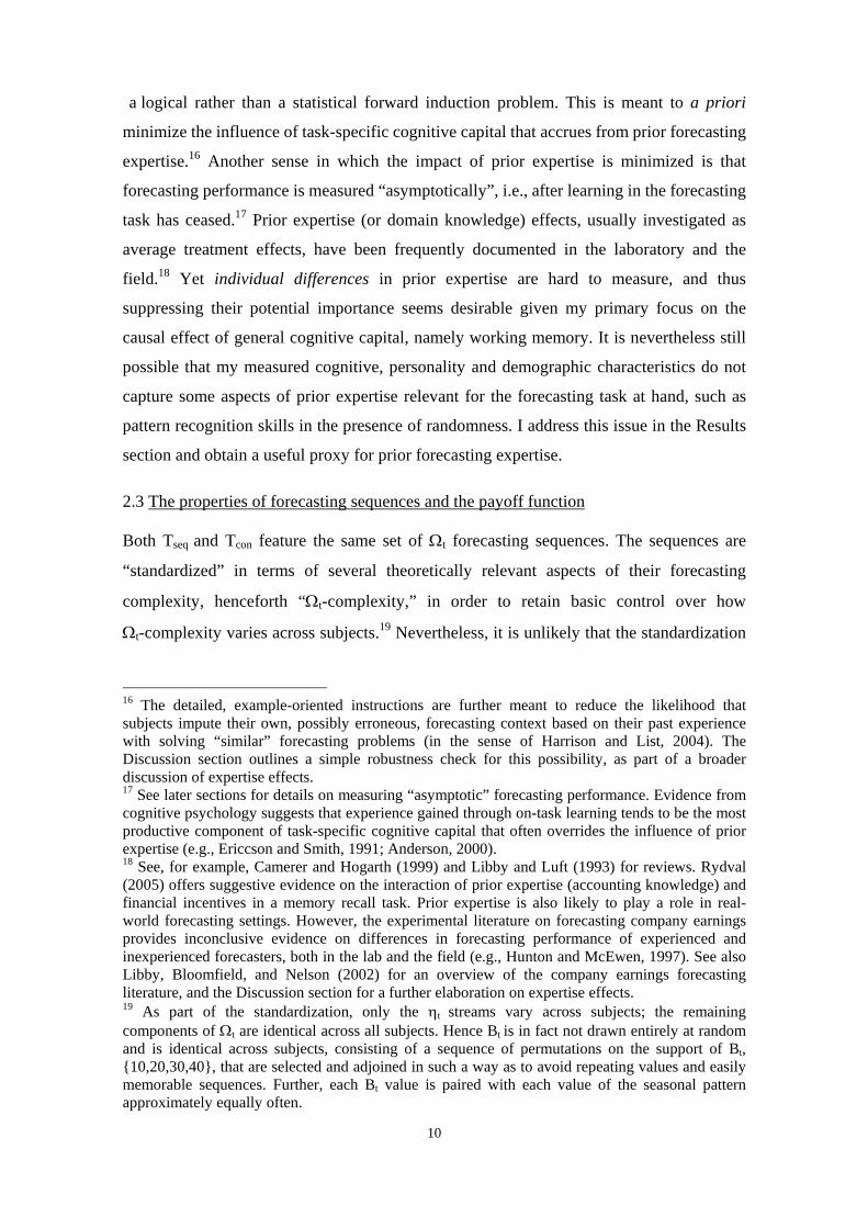
Figure 1 displays the evolution of Mcon,t and Mseq,t over time, illustrating that average

forecasting performance is clearly better in the less memory-intensive Tcon treatment

throughout the whole task. At the same time, there is a considerable extent of learning on

average in both treatments, especially in initial forecasting stages where the Mcon,t and

Mseq,t profiles are steeper compared to later stages. The evolution of average forecast errors

can be judged relative to the performance benchmark provided by the above mentioned

mechanical forecasting algorithm with the mean “true” forecast error of approximately

10.3 on average. Both Mcon,t and Mseq,t gradually fall below that benchmark performance

level, though especially Mseq,t starts well above it. Put differently, the average subject in the

50 For reasons related to the nature of the forecasting task, subjects were repeatedly reminded not to make any notes during the forecasting task itself. The four subjects who did not follow these instructions are excluded from the analysis below.

23

more memory-intensive Tseq treatment takes around 40 forecasting periods to reach the

Mseq,t=10.3 benchmark (i.e., in period 49) while the average subject in the less memory-

intensive Tcon treatment reaches the Mcon,t=10.3 benchmark more than twice as fast (i.e., in

period 24).51 This in turn suggests that subjects in Tcon on average discover the seasonal

pattern much earlier than subjects in Tseq.

Since the forthcoming analysis focuses on performance heterogeneity and what explains it,

it is worth noting that both treatments generate plenty of potentially predictable between-

subject variance in performance throughout the task. Figure 1 illustrates the substantial

performance heterogeneity by displaying the 10th and 90th percentiles of Mi,t for both

treatments. The 90th percentiles, 90Mcon,t and 90Mseq,t, suggest that the worst-performing

subjects perform more or less similarly in both treatments. On the other hand, the parallel

nature of the 10Mcon,t and 10Mseq,t profiles suggests that the best forecasters generally

perform slightly better in the less memory-intensive Tcon treatment throughout the task.

Note that despite the substantial performance heterogeneity, even the worst forecasters in

either treatment show some learning progress on average, and even the best forecasters

always have financial incentive to (and do) improve their forecasting performance. As an

exception, the best forecasters in the less memory-intensive Tcon treatment reach the

performance ceiling towards the end of the task, which potentially reduces the extent of

predictable between-subject variance in performance. This issue is addressed in the

multivariate analysis below and turns out to be of minor importance.52

To look closer at the across-treatment differentials in forecasting performance as well as

the extent of learning, I focus on performance in the perfectly matched twelve-period

forecasting segments called EARLY (periods 21-32) and LATE (periods 84-95). Denote

subject i’s performance in the EARLY and LATE segments as Mi,31≡Mi,EARLY and

Mi,94≡Mi,LATE, respectively. The summary statistics for Mi,EARLY and Mi,LATE for each

51 Recall that subjects make their first forecast, F9, in period 8 since the first eight periods of the task are reserved for displaying the initial values of Bt and Ωt. 52 An additional source of performance heterogeneity not apparent from Figure 1 is the seasonal nature of the forecasting task. In general, performance varies across the three forecasting seasons, with the “sandwich” seasonal parameter, γ2 = 34, being associated with markedly lower and less variable forecast errors. Intuitively, the forecasting seasons represent within-subject treatments featuring various degrees of “overlap” of the γs+ηt distributions, conditional on γs, which seems to matter for the relative ease of discovering the seasonal parameters, γs. While a more detailed seasonal performance analysis is possible (and available upon request), a potential caveat is that unobserved heterogeneity in subjects’ forecasting strategies may imply different seasonal performance tradeoffs, in turn limiting interpretability of the results. In this paper, I adopt a more conservative approach by aggregating forecasting performance across seasons.

24

treatment are available in the first two rows of Table 1. The treatment averages for the

EARLY segment, Mcon,EARLY=8.81 and Mseq,EARLY=13.73, are significantly different from

each other by a signed ranks test based on comparing subjects facing identical Ωt

forecasting sequences in Tcon and Tseq (p=0.0002). For the LATE segment, the treatment

averages, Mcon,LATE=5.13 and Mseq,LATE=6.56, do not differ from each other by an

analogous signed ranks test (p=0.2203). The extent of learning, unambiguously assessed

by comparing Mi,EARLY and Mi,LATE by a signed ranks test, is highly significant in both Tcon

(p=0.0000) and Tseq (p=0.0000). Finally, I compare the extent of learning, Mi,EARLY-

Mi,LATE, across treatments (see the summary statistics in the third row of Table 1). A signed

ranks test of the learning measure, Mi,EARLY-Mi,LATE, for subjects with identical Ωt

forecasting sequences in Tcon and Tseq suggests that learning is significantly stronger in the

more memory-intensive Tseq treatment (p=0.0057). Based on the above observations, this

result is mainly due to the much slower learning progress in Tseq compared Tcon in the early

stages of the forecasting task.

In the analysis that follows, I mostly focus on forecasting performance as measured by

Mi,LATE. One can think of Mi,LATE as measuring subject i’s “asymptotic” forecasting

performance since, in a statistical sense, learning has ceased by the LATE segment in

either treatment.53 I further consider an alternative measure of forecasting performance that

attempts to account for the fact that Mi,LATE might be undesirably influenced by outliers,

i.e., random “slip-ups” in forecasting performance arising from momentary distraction and

other unwanted effects. In particular, I consider Mi,MEDLATE, the average of seasonal

medians of forecast errors in the LATE segment, as an arguably more robust alternative to

Mi,LATE. 54 Analogously Mi,MEDEARLY is considered as a robust alternative to Mi,EARLY.

53 I test the “asymptoticity” by comparing Mi,LATE with the performance in the immediately preceding twelve-period segment, Mi,82. While both treatments do show a small improvement in average forecast errors – namely from Mcon,82=5.58 to Mcon,LATE=5.13 and from Mseq,82=6.89 to Mseq,LATE=6.56, respectively, a signed-ranks test cannot reject equality of Mi,LATE and Mi,82 in either Tcon (p=0.1522) or Tseq (p=0.5139). On the other hand, a signed-ranks test rejects equality of Mi,82 and Mi,70 in both Tcon (p=0.0182) and Tseq (p=0.0066), indicating significant learning between the two earlier twelve-period segments. These asymptoticity tests are not as efficient as the above learning tests based on comparing the perfectly matched EARLY and LATE segments. 54 Specifically, I use the four forecast errors per season to calculate season-specific median forecast errors separately for each season and then take an average of the medians to obtain Mi,MEDLATE. Analogous procedure is used for calculating Mi,MEDEARLY, for which eliminating random slip-ups might be more important if their occurrence is more likely in the early forecasting stages. Admittedly, one might not want to partial out slipups from the performance measure if they are related to individual differences in working memory. However, Mi,MEDLATE and Mi,MEDEARLY might conveniently avoid the influence of “exogenous” distraction that possibly arises in the experimental

25

4.2 Bivariate relationships

Tables 2a and 2b display Spearman correlations between forecasting performance and the

measured covariates for Tcon and Tseq, respectively.55 Since lower forecast errors mean

better forecasting performance, one generally expects negative correlations between the

performance measures and cognitive covariates. First of all, note that the correlation

between asymptotic forecasting performance, MLATE, and Working memory is relatively

strong at -0.345 (p=0.023) in the more memory-intensive Tseq treatment, especially

compared to the negligible correlation of -0.022 (p=0.891) in the less memory-intensive

Tcon treatment. Hence in line with the causality hypothesis, working memory is associated

with asymptotic forecasting performance much stronger when the working memory load is

higher. The multivariate analysis below examines whether this conclusion is confirmed

when other potential predictors of MLATE are taken into account.

To that end, notice that MLATE in Tseq is also relatively strongly correlated with Short-term

memory at -0.269 (p=0.081). Furthermore, Short-term memory is in both treatments

positively correlated with Working memory which in turn is positively correlated with

Math. This shared variance is not surprising given that working and short-term memory are

theoretically related cognitive constructs, and that the tests of Working memory, Short-

term memory and Math share common surface features (they all involve dealing with

numbers). To investigate the separate predictive power of working memory, psychologists

often extract the underlying working memory ability (the ability to control attention) as the

residual working memory variance that remains after removing its shared variance with

short-term memory and other cognitive constructs (e.g., Engle et al., 1999). Following this

practice, I extract WMresidual by partialling out Short-term memory, Math, Perseverance

and Math anxiety from Working memory.56 The correlation between MLATE and

lab and is entirely beyond subjects’ control. The summary statistics for Mi,MEDLATE and Mi,MEDEARLY can be inspected in the fourth and firth rows of Table 1, respectively. The statistical tests presented so far for Mi,LATE and Mi,EARLY yield qualitatively comparable results when applied to Mi,MEDLATE and Mi,MEDEARLY. For example, learning between Mi,MEDEARLY and Mi,MEDLATE as judged by a signed ranks test is statistically stronger in Tseq compared to Tcon (p=0.0124). 55 The summary statistics for the covariates are presented in Table 1. None of the covariates has a significantly different sample mean across treatments, based on a t-test at the 10% significance level. The variances of the covariate distributions differ significantly across treatments in the case of Short-term memory, Carshare and Windfall, based on an F-test at the 5% significance level. 56 I regress Working memory on Short-term memory, Math, Perseverance and Math anxiety by OLS in the pooled sample (Tcon and Tseq) and extract WMresidual as the regression residuals. There are theoretical reasons pertaining to the structure of the Working memory test for including Math, Math anxiety and Perseverance as covariates, and both Math and Perseverance indeed significantly explain some of the variance in Working memory, in addition to the explanatory power of Short-

26

WMresidual in Tseq is -0.353 (p=0.020), virtually identical to the correlation between

MLATE and Working memory. Hence the ability to control attention, as captured by

WMresidual, has considerable predictive power for forecasting performance in Tseq,

independent of the potential additional predictive power of Short-term memory, Math and

other covariates.

Turning now to the correlations of MLATE with personality and demographic covariates,

less sensation-seeking and more premeditation attitudes seem partly beneficial for

asymptotic performance in Tcon, while, as expected, the two impulsiveness proxies also

correlate with each other. In Tseq, MLATE is not correlated with any of the personality

covariates, but subjects who receive the Windfall financial bonus seem to perform better.

Similar bivariate relationships hold for the alternative asymptotic performance measure,

MMEDLATE. This is not surprising given that MMEDLATE almost perfectly correlates with

MLATE in either treatment. In fact, since the multivariate results are also closely similar for

MLATE and MMEDLATE in all important respects, I below report only the results for MLATE.

Before doing so, I briefly look at the determinants of early forecasting performance and

learning. In both Tcon and Tseq, lack of sensation-seeking attitudes seems beneficial for

early performance as measured by MEARLY or MMEDEARLY. In Tcon, male forecasters seem to

perform better than females. In Tseq, MEARLY and MMEDEARLY correlate negatively with Age

and positively with Carhsare, the latter correlation suggesting a negative effect of family

wealth on early performance. Clearly, however, all these demographic effects vanish when

considering asymptotic performance.

term memory. While it seems theoretically warranted to include Need for cognition as an additional covariate – given that Working memory is measured without performance-contingent financial incentives, Need for cognition turns out completely unrelated to Working memory, regardless of including Math anxiety and Perseverance which are both correlated with Need for cognition. Estimation details related to the extraction of WMresidual are available upon request. The working memory literature offers several alternative approaches to extracting “controlled attention,” the choice depending on the research goal. For instance, controlled attention variance can be extracted as the shared (as opposed to the residual) variance between working memory and short-term memory (e.g., Kane et al, 2004). Most approaches use latent-variable modeling to first extract the working memory and short-term memory variance from a battery of working and short-term memory tests, respectively, to remove the influence of test idiosyncrasies (i.e., surface features of the various tests). While I cannot use this approach due to the automated nature of the Working memory test (since conducting several automated working memory span tests in a sequence would alter their strategic nature), the WMresidual should be free of the surface features shared with the partialled out covariates, such as memorizing simple patterns (Short-term memory) and performing simple arithmetic operations (Math). Similar surface features in fact underlie the forecasting task itself and thus might influence the predictive power of Short-term memory and Math, but arguably not the predictive power of WMresidual.

27

The extent of learning, MEARLY-MLATE, seems partly positively related to Working

memory and to being a female in Tcon, and to Short-term memory and Windfall in Tseq.57

However, it is especially noteworthy that, despite the considerable distance between their

measurement, MEARLY and MLATE are strongly correlated with each other at 0.750 in Tcon

(p=0.000) and at 0.337 in Tseq (p=0.027). Especially the former correlation suggests strong

internal reliability of the two performance measures, with implications for my causality

test of the explanatory power of working memory: If, as hypothesized, working memory

turns out to be a stronger predictor of MLATE in Tseq compared to Tcon, this is unlikely

caused by lack of internal reliability of the MLATE performance measure in Tcon compared

to Tseq. It is much more likely due to the causal effect of working memory on asymptotic

forecasting performance.

4.3 Multivariate analysis

Now I turn to multivariate analysis appropriate for testing the causality of working

memory. The causality hypothesis proposed that, holding short-term memory, basic math

skills and other potentially relevant personality and demographic determinants of

forecasting performance constant, working memory should be a stronger determinant of

performance in the more memory-intensive Tseq treatment, compared to the less memory-

intensive Tcon treatment. I therefore estimate the impact of working memory (WMresidual)

and other personality and demographic covariates on asymptotic forecasting performance,

MLATE, and test for the presence of an across-treatment differential in the impact of

WMresidual.

Tables 3 and 4 present a sequence of empirical models, gradually expanding the set of

covariates that are assumed relevant for asymptotic forecasting performance. Due to the

different cognitive and possibly also personality (motivational) requirements of Tcon and

Tseq, each model a priori permits that not only working memory but also other included

covariates might differ in their impact across treatments (to gain efficiency though,

estimates are pooled across Tcon and Tseq wherever justified by a two-tail t-test at the 10%

57 However, the interpretability of the correlations is likely limited, for MEARLY-MLATE is likely to be appropriate as a within-subject indicator of learning (i.e., whether Mi,EARLY>Mi,LATE) but less so as an indicator of between-subject variance in the extent of learning (i.e., how much subjects learn compared to each other). Intuitively, both Mi,EARLY and Mi,LATE vary greatly across subjects, and learning progress at different initial levels of forecast errors may be differentially difficult and might involve non-linearities related to the nature of discovering the seasonal pattern. To deal with these potential caveats, I examined various alternative learning measures based, for example, on proportional learning metrics or learning speed (duration) metrics, but none of the alternative measures seems related to the measured covariates in an economically meaningful way.

28

significance level). As explained earlier, to eliminate the influence of Ωt-complexity on

MLATE, I estimate the impact of working memory and other covariates on the differences in

MLATE calculated for the pairs of subject facing identical Ωt forecasting sequences in Tcon

and Tseq. Furthermore, I take into account that MLATE is top-bounded for a small minority

of subjects and use an appropriate censored-type estimator.58

Model 1 in Table 3 presents the most bare-bone test of the causality hypothesis. It contains

only the most theoretically relevant cognitive covariates, WMresidual and Short-term

memory, implicitly assuming that Math and all the personality and demographic covariates

are irrelevant for asymptotic forecasting performance. Confirming the previous correlation

results, Model 1 shows that working memory only affects performance in the more

memory-intensive Tseq treatment while the effect is negligible in Tcon and even has a wrong

sign (recall that “helpful” covariates should have negatively signed coefficient estimates).

A t-test presented beneath the WMresidual estimates indicates that the impact of

WMresidual differs between Tseq and Tcon at the 10% significance level, in line with the

causality hypothesis. There is an even stronger across-treatment differential in the impact

of short-term memory. Both working memory and short-term memory therefore

independently contribute to explaining the variance in forecasting performance, yet only in

the more memory-intensive Tseq treatment. On average, forecasting performance is better

in Tcon than in Tseq, as indicated by the significance of the intercept.

58 The estimated model is seqMLATE – conMLATE = α + Χseqβseq – Χconβcon + (εseq – εcon), where, assuming that variables are paired across treatments according to the identical Ωt forecasting sequences, seqMLATE and conMLATE are the Nx1vectors of MLATE in Tseq and Tcon, respectively (N=43 is the number of subjects and unique forecasting sequences in each treatment), Χseq and Χcon

are the respective NxK matrices of covariates (the number of covariates, K, depending on the estimated model), βseq and βcon are the respective Kx1 parameter vectors (assuming for simplicity of exposition that none of the parameters is pooled across treatments), εseq and εcon

are the respective regression disturbances, and α is the intercept (the α estimate does not reflect the size of the average across-treatment differential in MLATE since variables are not normalized). As mentioned earlier, the estimation model implicitly assumes that the effect of Ωt-complexity on MLATE interacts neither with the effect of the included cognitive and personality covariates nor with the heterogeneity in forecasting strategies. I estimate Model 1 through Model 6 using a censored normal regression estimator that permits top-bounded performance to arise in either Tcon or Tseq. In reality, there are five perfectly top-bounded subjects (with MLATE=0) in Tcon and two such subjects in Tseq, i.e., slightly below 10% of the total number of subjects in both treatments. Most of the seven subjects already have their performance almost perfectly or perfectly top-bounded for quite a while before the LATE segment, which justifies treating their performance as censored. In one case, both subjects in a given pair are top-bounded; I treat this as a “no censoring” case with no consequences for any of the reported results. The censored normal regression is a Tobit-type, asymptotic estimator that relies on the assumption of i.i.d. normal disturbances. While this assumption generally seems to be met, I compare the censored normal estimates to OLS estimates that, while potentially biased due to the minor censoring of MLATE,might be viewed as a useful robustness check (see Model 7 in Table 4).

29

Model 2 includes two additional, theoretically relevant covariates: Math and Need for

cognition. Math, a proxy for basic arithmetic abilities, turns out to influence forecasting

performance only in the less memory-intensive Tcon treatment. By contrast, both working

memory and short-term memory again have predictive power only in the more memory-

intensive Tseq treatment. As hypothesized, therefore, the higher memory load in Tseq

activates subjects’ working and short-term memory constraints and identifies their

causality. Relaxing the memory load in Tcon makes these constraints irrelevant for

forecasting performance and shifts explanatory power to Math, suggesting that Tcon poses

a number-intensive rather than a memory-intensive forecasting exercise. As for the other

covariate added in Model 2, Need for cognition has the expected sign but is statistically

insignificant. Nevertheless, including a measure of intrinsic motivation in the empirical

model of forecasting performance seems theoretically justified, if not as a direct

determinant of forecasting performance then as a potential co-determinant of the measured

cognitive covariates.59

In Model 3, I initially attend to all the remaining personality and demographic covariates

contained in Tables 2a and 2b but eventually include only those related to forecasting

performance, namely Risk and Windfall.60 Model 3 confirms the strong explanatory power

of working memory and short-term memory in Tseq, and conversely the impact of Math in

Tcon. Need for cognition now becomes (weakly) significant across treatments, suggesting

that in addition to the high-powered financial incentives, subjects’ intrinsic motivation

fosters performance as well. In fact, the Windfall bonus appears to represent further

extrinsic incentives, despite the bonus award scheme being entirely exogenous to the

forecasting task.61 Lastly, risk aversion attitudes seem beneficial for performance in both

59 Recall that cognitive and other covariates were collected without using performance-contingent financial incentives, so individual differences in intrinsic motivation might be a source of variance in the measured values of the covariates. As discussed previously, however, I do not detect any influence of Need for cognition on Working memory (unlike Ballinger et al., 2005). This seems in line with evidence from the working memory literature suggesting that cognitive effort does not vary across the working memory distribution during working memory span tests (e.g., Heitz et al., 2006). 60 The remaining personality and demographic covariates not listed in Model 3 are individually as well as jointly highly insignificant at conventional significance levels. Including insignificant covariates in Model 3 and other models considerably reduces the precision of the reported estimates, reflecting the relatively small sample size. 61 It is possible that subjects who won the windfall bonus have higher cognitive abilities, as indicated by the positive correlation between Windfall and Math in either treatment. Nevertheless, in the models where Windfall is included (i.e., Model 3, 6 and 7), Windfall does not seem to interact with any of the cognitive, personality and demographic covariates.

30

treatments.62 In sum, Model 3 uncovers the influence of extrinsic and intrinsic incentives

and risk attitudes on performance in either treatment but taking them into account does not

harm the separate explanatory power of working memory and short-term memory in Tseq.

Next, I extend the empirical model by controlling for the influence of prior forecasting

expertise not captured by the measured covariates. Tables 2a and 2b reveal that especially

in Tcon, MEARLY and MLATE correlate noticeably stronger with each other than either of them

separately correlates with the measured covariates. Besides the implications for the internal

reliability of MLATE discussed above, this also suggests that both MEARLY and MLATE might

be influenced by “unobserved forecasting ability” such as pattern recognition skills in the

face of randomness. If such unobserved forecasting ability substantially contributes to

explaining the variance in MLATE, not including it among explanatory factors might bias

the conclusions regarding the impact of the measured covariates. As a precaution against

such a possibility, I create a proxy for unobserved forecasting ability and include it in the

empirical model of MLATE. Specifically, exploiting the design feature that MEARLY and

MLATE are based on identical segments of the Ωt forecasting sequence for each subject,

I create a proxy, MEARLYresidual, by extracting the residual variance in MEARLY that

remains after removing the influence of theoretically and statistically relevant measured

covariates.63 In this way, the impact of MEARLYresidual on MLATE will not reflect the impact

of those measured covariates, so they should retain their independent influence on MLATE if

there exists any.

62 This seems in line with the earlier reported bivariate results suggestive of a negative association between sensation-seeking and performance, especially in Tcon. When Risk and Sensation-seeking are both included in Model 3, Sensation-seeking is less relevant compared to Risk, and only in Tcon, while Risk is relevant in both treatments. Also note that Risk is strongly negatively correlated with Sensation-seeking at -0.277 (p=0.0099) and Sensation-seeking with Premeditation at -0.208 (p= 0.054) in the pooled sample (Risk is not as strongly correlated with Premeditation, only to some extent in Tseq). Hence when interpreting the positive impact of Risk on forecasting performance, one should bear in mind that a combination of risk aversion, sensation-seeking and premeditation attitudes might matter for performance, perhaps through influencing the development of successful forecasting strategies. 63 I create MEARLYresidual by regressing MEARLY on Working memory, Short-term memory, Math, Need for cognition and Premeditation. The first four covariates are included because they are theoretically relevant for forecasting performance and also statistically explain MLATE in the models presented in Table 3. Only Working memory in fact turns out statistically relevant for MEARLY, and Premeditation is the only other statistically relevant covariate. The estimation for MEARLY is analogous to that for MLATE except that the absence of top-bounded performance permits using OLS instead of censored normal regression. Furthermore, in order to retain the richest possible model of MEARLY, I use Working memory instead of WMresidual and do not allow parameters to be pooled across treatments. MEARLYresidual is extracted as the regression residuals. The estimation results are available upon request.

31

Apart from including MEARLYresidual, Model 4 and Model 5 in Table 4 are analogous to

Model 1 and Model 2, respectively. In fact, also the results in the two pairs of models are

remarkably similar. The only novel insight from Model 4 and Model 5 is that

MEARLYresidual is a strongly significant positive predictor of forecasting performance. The

predictive power of working and short-term memory in Tseq, and basic arithmetic skills in

Tcon, remains essentially unchanged compared to the models without MEARLYresidual. It is

noteworthy that the working memory across-treatment differential, and hence the support

for its causality, now becomes slightly stronger in Model 5 (p=0.0553) and reaches the 5%

significance level in Model 6 (p=0.0456).

The richest Model 6 differs from its counterpart Model 3 not only in the inclusion of

MEARLYresidual but also in that lower math anxiety appears to improve performance in

Tcon. Lower math anxiety might help subjects deal with the arithmetic nature of the

forecasting task – related to the positive impact of Math in Tcon, but it might also be helpful

for developing successful forecasting strategies – related to the positive impact of risk

aversion in both treatments. As for the influence of extrinsic and intrinsic incentives on

MLATE, both Windfall and Need for cognition again exhibit a strong positive influence. I do

not pool the impact of need for cognition across treatments, though warranted by the t-test

(p=0.128), to illustrate that in this richest model, need for cognition seems more relevant

for performance in the more memory-intensive Tseq treatment.

Finally, Model 7 is exactly analogous to Model 6 except that it is estimated by OLS. Since

the degree of censoring of MLATE is relatively minor, the OLS estimates might be viewed

as a robustness check for the censored normal estimates. As expected, most of the OLS

estimates in Model 7 seem slightly biased towards zero compared to the censored normal

estimates in Model 6. However, the precision of the estimates and hence the conclusions

drawn from the two alternative estimations are essentially identical. The OLS results

confirm the strong, independent contributions of working memory and short-term memory

to explaining asymptotic forecasting performance in Tseq, and also confirm the presence of

the across-treatment differential in the impact of working memory (p=0.064). The causality

of WMresidual is not as statistically powerful as one might like but is considerably robust

across the estimated models regardless of which classes of covariates are included.

32

5. Discussion and conclusion

This paper provides an initial test of the capital-labor-production (KLP) framework. I show

that the effectiveness of high-powered financial incentives as a stimulator of economic

performance can be moderated by cognitive capital in a causal fashion. Using a memory

intensive time-series forecasting task, I identify the causal effect of both working and

short-term memory on asymptotic forecasting performance. The effects are entirely

independent of each other since my working memory measure shares no cognitive or

surface features with short-term memory. The causal effect of working memory thus likely

reflects individual heterogeneity in the ability to control attention, a strong predictor of

performance in a wide range of tasks requiring controlled information processing (Engle

and Kane, 2004). The present paper indicates that the ability to control attention may also

affect decision quality in cognitively complex economic settings.

Exploring the role of motivational factors, I find that besides the strong financial incentives

employed in the forecasting task, subjects’ intrinsic motivation and a sizeable windfall

financial bonus won prior to the forecasting task both positively foster forecasting

performance. Given my auxiliary treatment of motivational factors (while focusing on the

causality of cognitive capital), documenting their separate impact constitutes only an initial

step in examining their interaction with cognitive capital, with implications for the design

of efficient incentive schemes. Indeed, establishing the causality of particular cognitive

capital measures is a prerequisite for examining their role in the multitude of structural

relationships that the KLP framework potentially entails, such as the substitutability among

various forms of cognitive capital and in turn their substitutability with cognitive effort.

Below I discuss some of the relationships and how one could start addressing them in the

present forecasting setting.

On of the most economically relevant interactions in the KLP framework is the degree of

substitutability between cognitive capital forms varying in task specificity.64 I examined

the predictive power of both general and specific forms of cognitive capital – working

memory, short-term memory and basic math abilities – but I intentionally minimized the

influence of task-specific cognitive capital in the form of prior expertise (or domain

knowledge). Prior expertise is clearly vital for performance in many field cognitive tasks,

64 In the following discussion, I abstract from “nature/nurture” issues related to the evolution of cognitive capital over time, such as whether various general and specific forms of cognitive capital are inherited or acquired and what determines their acquisition (e.g., Heckman et al., 2006; LeDoux, 2002; Plug and Vijverberg, 2003).

33

and is central to the KLP framework of Camerer and Hogarth (1999), cognitive science

literature (e.g., Anderson, 2000) and the “expertise paradigm” in behavioral decision

research (e.g., Libby and Luft, 1993).65 However, we still know relatively little about the

interplay between prior expertise and more general forms of cognitive capital in

economically relevant settings (e.g., Hambrick and Engle, 2003). As an initial step in that

direction, Wittmann and Suess (1999) study performance determinants in a cognitively

complex, simulated physical production task, finding that both prior expertise (domain

knowledge) and working memory contribute to explaining variance in performance.

Similarly, Ghosh and Whitecotton (1997) study performance determinants in a company

earnings prediction task, finding that general cognitive capital, measured by a perceptual

ability test, has a strong explanatory power that is overcome neither by prior expertise of

professional financial analysts nor by provision of a forecast-relevant decision aid.

Arguably, however, only after establishing the causal effect of the relatively more general

forms of cognitive capital can one credibly assess their substitutability with prior expertise.

The forecasting task lends itself to examining that substitutability as it naturally extends to

real-world settings. Imagine, for instance, a financially framed version of the forecasting

task where Ωt is a financial variable such as a commodity price that follows my (simplistic)

deterministic seasonal process and Bt is an economically relevant, perfectly predictable

state variable linearly related to Ωt. At a basic level, one could then use the above

forecasting design (again with the sequential and concurrent presentation treatments) and

challenge inexperienced forecasters (e.g., students) and experienced forecasters (e.g.,

commodity traders) with the framed and unframed versions of the task. The resulting

2x2x2 factorial design would shed further light on the above established causality of

working and short-term memory and would permit gauging their substitutability with prior

expertise.

Another key substitutability question pertains to the interaction between the various

a priori acquired (or inherited) forms of cognitive capital discussed above and arguably the

most task-specific form of cognitive capital, namely experience acquired endogenously

through on-task learning. As mentioned earlier, evidence from cognitive psychology

suggests that experience gained gradually through learning by doing (rather than learning

65 As noted by Camerer and Hogarth (1999) and others, however, prior expertise seems only imperfectly transferable across even slightly different cognitive production settings. See also Kagel and Levin (1986) and the ensuing discussion on the relative productivity of prior expertise and experience acquired through on-task learning.

34

by thinking) tends to be the most productive component of task-specific cognitive capital,

overriding the productivity of prior expertise (e.g., Anderson, 2000; Ericcson and Smith,

1991; Reber, 1989). We nevertheless have limited evidence on the interaction between

experience and general cognitive capital. Engle and Kane (2004) discuss suggestive

evidence that various forms of on-task learning are inconsequential for the causal effect of

working memory on performance in tasks requiring controlled attention. By measuring

forecasting performance at its asymptotic stage in both treatments, I supply further

evidence that the causal effect of working memory (and short-term memory) persists even

after on-task learning has entirely ceased.

Since many economic tasks are much more cognitively complex than my forecasting task

and learning in them is a continuous process, one may further want to examine the

interaction between a priori acquired (or inherited) cognitive capital and the on-task

learning process itself.66 To illustrate, one could examine the extent to which further

learning has been inhibited in the forecasting task by the artificially imposed memory load

(combined with the corresponding individual cognitive constraints) by further relaxing the

memory load. To do that, one can extend the current forecasting design (call it Stage 1) for

a number of forecasting periods with Bt=0 where the screen with (Bt+1,…, Bt-7) values

effectively disappears (call this Stage 2). Stage 2 then resembles an inductive reasoning

task (with a random component) featuring only a minimum memory (and arithmetic) load

in either treatment. We should therefore expect considerable degree of additional learning

going on in Stage 2, provided that the major source of sub-optimal performance in Stage 1

was indeed the memory (and arithmetic) load, as opposed to other sources of sub-optimal

performance such as poor pattern recognition skills and inability to deal with the random

component.

Allowing enough periods in Stage 2 for additional learning to have ceased again, one can

then decompose the effect of the cognitive load relaxation on the total between-subject

variance of asymptotic performance into three separate components. The first component is

the change in the total between-subject variance due to the additional learning

opportunities between Stages 1 and 2. This “learning drift” component can be partialled

66 As a possible approach mentioned earlier, a panel estimation not reported here reveals that several exogenously varied aspects of Ωt-complexity weakly explain learning progress in early stages of the forecasting task. After enlarging the sample sizes in both treatments, the ultimate goal of this project is to exploit the exogenous variation in the Ωt sequences – affecting not only Ωt-complexity but also the clarity of forecasting feedback and hence confidence – to analyze the relationship between cognitive capital, learning progress, and betting behavior.

35

out from the change in the total between-subject variance as the variance of the within-

subject differences in asymptotic performance between Stages 1 and 2. The second

component is the (likely) decrease in the total between-subject variance due to greater

“cognitive control” and hence smaller within-subject forecast error variance (e.g.,

Hammond and Summers, 1972). This “cognitive control” component can be partialled out

by allowing for a number of extra periods in both Stage 1 and 2 after asymptotic

performance has been reached and treating each of the extra periods as performance re-

tests. Finally, having partialled out the “learning drift” and “cognitive control”

components, the remaining component of the (likely) decrease in the total between-subject

variance is the change in the predictable between-subject variance in mean forecasting

performance, conditional on what has been learned, attributable directly to the reduced

predictive power of working and short-term memory and basic arithmetic abilities between

Stages 1 and 2.67 Hence the decomposition sheds light on the relative importance of the

three components of performance heterogeneity in Stage 1 compared to Stage 2, and also

permits comparing the components between the concurrent and the sequential presentation

treatments.

Leaving the confines of cognitive capital and getting to the heart of the KLP framework,

one naturally turns to the issue of capital-effort substitutability in cognitive production. To

that end, identifying the causality of cognitive capital is useful only to the extent that

cognitive effort is observable. As with physical effort, one can think of cognitive effort as

having two dimensions, duration and intensity, with especially effort intensity being

difficult to define, let alone measure.68 Evidence from the working memory literature is

suggestive of a limited degree of capital-effort substitutability. In tasks where working

memory is a strong predictor of performance, effort latencies (measured by response times,

pupil dilation, fMRI “scans”, etc.) do not vary across the working memory distribution in

the sample, while effort latencies tend to increase relatively uniformly with higher

financial incentives and higher task complexity (e.g., Heitz et al., 2006). Awasthi and Pratt

(1990) provide further circumstantial evidence of limited capital-effort substitutability for

cognitively constrained individuals. In their between-subject design, piece-rate (as

compared to flat-rate) financial incentives yield an improvement in judgmental 67 As a potential caveat of the variance decomposition, the asymptotic performance of a minority of subjects is already top-bounded in Stage 1 and the cognitive load reduction in Stage 2 would be likely the bring a further reduction of the total between-subject variance. For that reason, one would ideally want to increase the overall cognitive load of the forecasting task by raising the cognitive complexity of the forecasting task as discussed earlier. 68 See Camerer and Hogarth (1999) for a discussion of various measures of cognitive effort.

36

performance only for individuals with higher perceptual differentiation ability while effort

duration increases uniformly regardless of the ability. As noted by Awasthi and Pratt

(1990), Camerer and Hogarth (1999) and many others, such observations raise questions as

to why cognitively constrained individuals might be inclined to exert sub-optimally high

levels of unproductive effort. Among potential reasons, cognitively constrained decision

makers might only partly observe their cognitive capital and/or cognitive effort costs.69

These and other structural issues pertaining to the underlying cognitive “decision-making

process” have recently received attention in neurobiology (e.g., Gold and Shadlen, 2001)

and neuroeconomics (e.g., Camerer et al., 2005) but otherwise have remained empirically

unexplored. The sparse empirical accounts of the KLP framework have instead focused on

the reduced-form interaction between cognitive capital and financial incentive levels.

Awasthi and Pratt (1990) and Palacios-Huerta (2003) both conclude that raising

performance contingency of financial incentives yields a larger average improvement in

judgmental performance for individuals with higher cognitive capital. While this positive

interaction between financial incentives and cognitive capital appears economically

interesting, for example from the point of view of within-firm wage structures, it is likely

empirically tenuous. To the extent that cognitive effort is bounded from above and

diminishing returns to cognitive capital eventually set in, the interaction relies on specific

combinations of incentive variation, cognitive capital distribution in the sample and the

shape of the cognitive production function.70 This is not to question the validity of the

above results per se, but rather to offer more applicable ways of investigating the

69 My future analysis of the co-evolution of betting behavior and forecasting performance will address whether people with objectively lower forecasting abilities (as measured, for example, by working memory) demonstrate a higher degree of over-confidence in their forecasting abilities (as measured by the aggressiveness of their bets, after removing the effect of risk aversion and general judgmental confidence). The working memory literature suggests that people with lower working memory relying predominantly on automated processing might possess noisier estimates of their forecasting abilities compared to people with higher working memory relying mostly on controlled processing (e.g., Feldman-Barrett et al., 2004). 70 A potentially more fruitful approach to interacting financial incentive levels and cognitive capital involves comparing the predictive power of cognitive and personality determinants of performance under performance-contingent as compared to flat-rate financial incentives (or under low- and high-powered performance-contingent incentives). In the forecasting task, one could for instance contrast the performance-contingent version of the sequential presentation treatment with its flat-rate counterpart (with the betting scheme removed from both versions). One could then compare whether intrinsic motivation is a stronger predictor of performance in the flat-rate version, and also whether the predictive power of working and short-term memory differs across the two versions (with the predictive power perhaps a priori favored in the flat-rate version because of the cognitive tests being performed under flat-rate incentives).

37

interaction between cognitive capital and financial incentives that might ultimately be of

interest to designers of efficient incentive schemes.

In what follows, I again use the forecasting task as an illustration and the established

causality of working memory as a prerequisite. One may, for instance, view the sequential

presentation treatment as a cognitively demanding work setting and explore the welfare

implications of implementing it under various incentive schemes – say, the presently used

piece-rate scheme, a quota scheme, a tournament scheme and a flat-wage scheme. Due to

their varying returns to cognitive capital and degree of competitiveness, the incentive

schemes are likely to differ in how cognitive and personality characteristics moderate the

effectiveness of financial incentives (e.g., Bonner et al., 2000; Bonner and Sprinkle, 2002).

A steep piece-rate scheme or a tournament scheme is likely to be more suitable for less

cognitively constrained (and less risk averse) employees, whereas more cognitively

constrained but intrinsically motivated employees might perform better on average in

a flat-wage scheme. Hence, given the low capital-effort substitutability discussed above,

the utilization of both employers’ financial and the employees’ cognitive resources may be

improved by ex ante assigning employees to incentives schemes that best correspond to

their (observed) cognitive and personality characteristics. One may further like to explore

how employees self-select on their (observed) cognitive and personality characteristics into

the various incentive schemes and the extent to which such endogenous sorting is efficient

compared to the exogenous assignment.71

Finally, perhaps the most natural way of exploring the interaction between cognitive

capital and financial incentives is to investigate people’s willingness to pay for the

relaxation of their cognitive constraints. In the forecasting setting, this can be achieved by

implementing an additional treatment where subjects start forecasting in the more memory-

intensive sequential presentation treatment but have the opportunity to pay for switching to

the less memory-intensive concurrent presentation treatment. In any period, subjects can

therefore choose to purchase “external” memory and combine the forecast-relevant

information visually. Figure 1 illustrates that switching to the concurrent presentation

treatment does not guarantee perfect performance but it does improve performance and

learning progress on average. Of course, subjects do not know this and their switching

71 See Bonner and Sprinkle (2002) for a review of suggestive evidence. While the above discussion abstracts from the complexities of agency problems in real-world incentive scheme settings (e.g., Benabou and Tirole, 2003), observing individual cognitive and personality characteristics might still prove useful in designing more efficient incentive schemes.

38

decisions will presumably reflect their expectation that the net (long-run) return to

switching is positive. As with bets, switching behavior thus yields a decision-relevant and

incentive-compatible indicator of subjects’ estimates of their forecasting abilities, which

can in turn be linked to their observed cognitive and personality characteristics, betting

behavior and forecasting performance. One may further want to examine the effect of

varying the price (or cost) of switching.

To conclude, the effect of financial incentives on human behavior has received widespread

attention in the literature on the provision of incentives in organizations (e.g., Benabou and

Tirole, 2003), experimental economics (e.g., Hertwig and Ortmann, 2001; Ariely et al.,

2005) and neurobiology (e.g., Gold and Shadlen, 2001), as well as in newly emerging

fields such as neuroeconomics (e.g., Camerer et al., 2005). Recent meta-studies and

empirical surveys based on evidence from experimental economics and psychology have

indicated that incentive effects depend in a complicated fashion on the nature of cognitive

tasks.72 Camerer and Hogarth (1999) argue that a complete explanation of incentive effects

requires attending not only to how people balance financial incentives and cognitive effort

costs (e.g., Conlisk, 1988; Smith and Walker, 1993; Wilcox, 1993) but also to how they

combine cognitive effort with cognitive capital. I present initial evidence that the

effectiveness of even strong financial incentives can be moderate by cognitive capital in a

causal fashion. The evidence illustrates the need to attend to cognitive constraints, besides

personality (preference-based) factors, when interpreting observed (variance of) behavior

in cognitively demanding lab and field economic environments (Ballinger et al., 2005).

72 E.g., Bonner et al. (2000); Camerer and Hogarth (1999); Hertwig and Ortmann (2001, 2003); Jenkins et al. (1998); Prendergast (1999).

39

References

Ackerman, P. L., Beier, M. E., and M. O. Boyle (2002), “Individual differences in working memory within a nomological network of cognitive and perceptual speed abilities,” Journal of Experimental Psychology: General 131, 567-589.

Anderson, J. R. (2000), Cognitive Psychology and its Implications, New York: Worth. Archibald, G., and N. Wilcox (2006), “Contingent processing in strategic reasoning: An

experimental illustration,” University of Houston manuscript. Ariely, D., Gneezy, U., Loewenstein G., and N. Mazar (2005), “Large stakes and big

mistakes,” FRB of Boston Working Paper No. 05-11. Awasthi, V., and J. Pratt (1990), “The effects of monetary incentives on effort and decision

performance: the role of cognitive characteristics,” Accounting Review 65, 797-811. Baddeley, A. D., and G. Hitch (1974), “Working memory,” in G. Bower (Ed.), Recent

Advances in Learning and Motivation, Academic Press, New York. Ballinger, P., Hudson, E., Karkoviata, L., and N. Wilcox (2005), “Saving performance and

cognitive abilities,” University of Houston manuscript. Bandura, A., and E. E. Locke (2003), “Negative self-efficacy and goal effects revisited,”

Journal of Applied Psychology 88, 87-99. Barrick, J. A., and B. C. Spilker (2003), “The relations between knowledge, search

strategy, and performance in unaided and aided information search,” Organizational Behavior and Human Decision Processes 90, 1-18.

Benabou, R., and J. Tirole (2003), “Intrinsic and extrinsic motivation,” Review of Economic Studies 70, 489-520.

Benjamin, D. J., Brown, S. A., and J. M. Shapiro (2006), “Who is ‘behavioral’? Cognitive ability and anomalous preferences,” Dartmouth College manuscript.

Betz, N. E. (1978), “Prevalence, distribution, and correlates of math anxiety in college students,” Journal of Counseling Psychology 25, 441-448.

Bonner, S. E., Hastie, R., Sprinkle, G. B., and S. M. Young (2000), “A Review of the effects of financial incentives on performance in laboratory tasks: Implications for management accounting,” Journal of Management Accounting Research 12, 19-64.

Bonner, S. E., and G. B. Sprinkle (2002), “The effects of monetary incentives on effort and task performance: Theories, evidence, and a framework for research,” Accounting, Organizations & Society 27, 303-345.

Brehmer, B. (1980), “In one word: Not from experience,” Acta Psychologica 45, 223-241. Cacioppo, J. T., Petty, R. E., and C. F. Kao (1984), “The efficient assessment of need for

cognition,” Journal of Personality Assessment 48, 306-307. Cacioppo, J. T., Petty, R. E., Feinstein, J. A., and W. B. G. Jarvis (1996), “Dispositional

differences in cognitive motivation: The life and times of individuals varying in need for cognition,” Psychological Bulletin 119, 197-253.

Camerer, C. F., and R. Hogarth (1999), “The effects of financial incentives in experiments: A review and capital-labor-production framework,” Journal of Risk and Uncertainty 19, 7-42.

Camerer, C. F. (2003), Behavioral Game Theory: Experiments in Strategic Interaction, Princeton University Press.

Camerer, C. F., Loewenstein, G., and D. Prelec (2005), “Neuroeconomics: How neuroscience can inform economics,” Journal of Economic Literature 34, 9-64.

40

Cawley, J., Heckman, J. J., and E. J. Vytlacil (2001), “Three observations on wages and measured cognitive ability,” Labour Economics 8, 419-442.

Conlisk, J. (1980), “Costly optimization versus cheap imitators,” Journal of Economic Behavior and Organization 1, 275-293.

Conlisk, J. (1988), “Optimization Cost,” Journal of Economic Behavior and Organization 9, 213-228.

Conway, A. R. A., Kane, M. J., Bunting, M. F., Hambrick, D. Z., Wilhelm, O., and R. W. Engle (2005), “Working memory span tasks: A methodological review and user’s guide,” Psychonomic Bulletin and Review 12, 769-786.

Cooper, S., and D. Robinson (1991), “The relationship of mathematics self-efficacy beliefs to mathematics anxiety and performance,” Measurement and Evaluation in Counseling and Development 24, 4.

Cowan, N. (2001), “The magical number 4 in short-term memory: A reconsideration of mental storage capacity,” Behavioral and Brain Sciences 24, 87-185.

Crowley, A. E., and W. D. Hoyer (1989), “The relationship between need for cognition and other individual difference variables: A two-dimensional framework,” Advances in Consumer Research 16, 37-43.

Dawes, R. M. (1979), “The robust beauty of improper linear models in decision making,” American Psychologist 34, 371-582.

Deci, E., Koestner, R., and R. Ryan (1999), “A meta-analytic review of experiments examining the effects of extrinsic rewards on intrinsic motivation,” Psychological Bulletin 125, 627–668.

Devetag, G., and M. Warglien (2003), “Games and phone numbers: Do short term memory bounds affect strategic behavior?” Journal of Economic Psychology 24, 189-202.

Dwyer, G., Williams, A., Battalio, R., and T. Mason (1993), “Tests of rational expectations in a stark setting,” The Economic Journal 103, 586-601.

Eckel, C., and R. Wilson (2004), “Is trust a risky decision?” Journal of Economic Behavior and Organization 55, 447-465.

Eisenberger, R., and J. Cameron (1996), “Detrimental effects of reward: Reality or myth?” American Psychologist 51, 1153-1166.

Ekstrom, R. B., French, J. W., Harman, H., and D. Derman (1976), Kit of factor-referenced cognitive tests (rev. ed.), Princeton, NJ: Educational Testing Service.

Engle, R. W., and M. J. Kane (2004), “Executive attention, working memory capacity, and a two-factor theory of cognitive control,” in B. Ross (Ed.), The psychology of learning and motivation, Vol. 44, NY: Elsevier.

Engle, R. W., Tuholski, S. W., Laughlin, J. E., and A. R. A. Conway (1999), “Working memory, short-term memory, and general fluid intelligence: A latent variable approach,” Journal of Experimental Psychology: General 128, 309–331.

Ericsson, K. A., and J. Smith (Eds.) (1991), Toward a general theory of expertise: Prospects and Limits, Cambridge UK: Cambridge University Press.

Feldman-Barrett, L., Tugade, M. M., and R. W. Engle (2004), “Individual differences in working memory capacity and dual-process theories of the mind,” Psychological Bulletin 130, 553-573.

Fischbacher, U. (1999), “z-Tree: Zurich toolbox for readymade economic experiments – experimenter’s manual,” Working Paper No. 21, Institute for Empirical Research in Economics, University of Zurich.

41

Ghosh, D., and S. M. Whitecotton (1997), “Some determinants of analysts’ forecast accuracy,” Behavioral Research in Accounting 9 (Supplement), 50–68.

Gibbons, R. (1998), “Incentives in organizations,” Journal of Economic Perspectives 12, 115-132.

Gneezy, U., and A. Rustichini (2000), “Pay enough or don’t pay at all,” Quarterly Journal of Economics 115, 791-811.

Gold, J. I., and M. N. Shadlen (2001), “Neural computations that underlie decisions about sensory stimuli,” Trends in Cognitive Sciences 5, 10-16.

Ham, J. C., Kagel, J. H., and S. F. Lehrer (2005), “Randomization, endogeneity and laboratory experiments: The role of cash balances in private value auctions,” Journal of Econometrics 125, 175-205.

Hambrick, D. Z., and R. W. Engle (2003), “The role of working memory in problem solving,” in J. E. Davidson and R. J. Sternberg (Eds.), The psychology of Problem Solving, London: Cambridge Press.

Hambrick, D. Z., Kane, M. J., and R. W. Engle (2005), “The role of working memory in higher-level cognition: Domain-specific versus domain-general perspectives,” in R. J. Sternberg and J. E. Pretz (Eds.), Cognition and Intelligence: Identifying the Mechanisms of the Mind, New York: Cambridge University Press.

Hammond, K. R., and D. A. Summers (1972), “Cognitive control,” Psychological Review 79, 58-67.

Hammond, K. R., McClelland, G. H., and J. Mumpower (1980), Human Judgment and Decision Making: Theories, Methods, and Procedures, New York: Praeger.

Harrison, G. W., and J. A. List (2004), “Field experiments,” Journal of Economic Literature 42, 1009-1055.

Harrison, G. W., Lau, M. I., and E. E. Rutström (2005), “Risk attitudes, randomization to treatment, and self-selection into experiments,” UCF Economics Working Paper No. 05-01.

Harvey, N., Bolger, F., and A. McClelland (1994), “On the nature of expectations,” British Journal of Psychology 85, 203-229.

Heckman, J. J., and E. Vytlacil (2001), “Identifying the role of cognitive ability in explaining the level of and change in the return to schooling,” Review of Economics and Statistics 83, 1-12.

Heckmam, J. J., Stixrud, J., and S. Urzua (2006), “The effects of cognitive and noncognitive abilities on labor market outcomes and social behavior,” NBER Working Paper No. W12006.

Heitz, R. P., Schrock, J. C., Payne, T. W., and R.W. Engle (2006), “The eyes have it: Individual differences in working memory capacity and mental effort,” Georgia Institute of Technology manuscript.

Heitz, R. P., Unsworth, N., and R.W. Engle (2005), “Working memory capacity, attentional control, and fluid intelligence,” in O. Wilhelm and R.W. Engle (Eds.), Handbook of Understanding and Measuring Intelligence, London: Sage Publications.

Hertwig, R., and A. Ortmann (2003), “Economists’ and psychologists’ experimental practices: How they differ, why they differ, and how they could converge,” in I. Brocas and J. Carrillo (Eds.), Economics and Psychology, New York: OUP.

Hertwig, R., and A. Ortmann (2001), “Experimental practices in economics: A methodological challenge for psychologists?” Behavioral and Brain Sciences 24, 383-451.

42

Hey, J. D. (1994), “Expectations formation: Rational or adaptive or ...?” Journal of Economic Behavior and Organization 25, 329-349.

Holt, C. A., and S. K. Laury (2002), “Risk aversion and incentive effects,” American Economic Review 92, 1644–55.

Hunton, J. E., and R. A. McEwen (1997), “An assessment of the relation between analysts’ earnings forecast accuracy, motivational incentives and cognitive information search strategy,” The Accounting Review 72, 497-515.

Jenkins, D., Jr., Mitra, A., Gupta, N., and J. Shaw (1998), “Are financial incentives related to performance? A meta-analytic review of empirical research,” Journal of Applied Psychology 83, 777-787.

Kagel, J. H., and D. Levin (1986), “The winner's curse and public information in common value auctions,” American Economic Review 76, 894-920.

Kahneman, D., and A. Tversky (1984), “Choices, values, and frames,” American Psychologist 39, 341-350.

Kane, M. J., Hambrick, D. Z., Tuholski, S. W., Wilhelm, O., Payne, T. W., and R. W. Engle (2004), “The generality of working memory capacity: A latent variable approach to verbal and visuospatial memory span and reasoning,” Journal of Experimental Psychology: General 133, 189-217.

Kellogg, C. E., and N. W. Morten (1999), Beta III Manual, San Antonio, TX: The Psychological Corporation.

Kirchner, W. K. (1958), “Age differences in short-term retention and rapidly changing information,” Journal of Experimental Psychology 55, 352-358.

Klayman, J. (1984), “Learning from feedback in probabilistic environments,” Acta Psychologica 56, 81-92.

Klayman, J. (1988), “Cue discovery in probabilistic environments: Uncertainty and experimentation,” Learning, Memory, and Cognition 14, 317-330.

Lawrence, M., and M. O’Connor (2005), “Judgmental forecasting in the presence of loss functions,” International Journal of Forecasting 21, 3– 14.

Lazear, E. P., Malmendier, U., and R.A. Weber (2006), “Sorting in experiments with application to social preferences,” NBER Working Paper No. W12041.

LeDoux, Joseph E. (2002), Synaptic Self, New York: Viking. Libby, R., Bloomfield, R., and Nelson, M. (2002), “Experimental research in financial

accounting,” Accounting, Organizations & Society 27, 775-810. Libby, R., and M. G. Lipe. (1992), “Incentives, effort, and the cognitive processes

involved in accounting-related judgments,” Journal of Accounting Research 30, 249-273.

Libby, R., and J. Luft (1993), “Determinants of judgment performance in accounting settings: Ability, knowledge, motivation, and environment,” Accounting, Organizations & Society 18, 425-450.

Maines, L., and J. Hand (1996), “Individuals’ perceptions and misperceptions of time series properties of quarterly earnings,” Accounting Review 71, 317-336.

McDaniel, T, M., and E. E. Rutström (2001), “Decision making costs and problem solving performance,” Experimental Economics 4, 145-161.

Ortmann, A., Ostatnicky, M., and O. Rydval (2006), “Three very simple games (and what it takes to solve them),” CERGE-EI manuscript.

43

Pajares, F., and T. Urdan (1996), “An exploratory factor analysis of the mathematics anxiety scale,” Measurement and Evaluation in Counseling and Development 29, 35-47.

Pajares, F., and M. D. Miller (1994), “The role of self-efficacy and self-concept beliefs in mathematical problem-solving: A path analysis,” Journal of Educational Psychology 86, 193- 203.

Palacios-Huerta, I. (2003), “Learning to open Monty Hall’s doors,” Experimental Economics 6, 235-251.

Plug, E., and W. Vijverberg (2003), “Schooling, family background, and adoption: Is it nature or is it nurture?” Journal of Political Economy 111, 611-641.

Prendergast, C. (1999), “The provision of incentives in firms,” Journal of Economic Literature 37, 7-63.

Raven, J., Raven, J. C., and J. H. Court (1998), Manual for Raven's Progressive Matrices and Vocabulary Scales, San Antonio, TX: The Psychological Corporation.

Reber, A. S. (1989), “Implicit learning and tacit knowledge,” Journal of Experimental Psychology: General 118, 219-235.

Rydval, O. (2003), “The impact of financial incentives on task performance: The role of cognitive abilities and intrinsic motivation,” CERGE-EI Discussion Paper No. 112.

Rydval, O. (2005), “Capital and labor effects in a recall task: More evidence in support of Camerer and Hogarth (1999),” CERGE-EI Working Paper No. 264.

Rydval, O., and A. Ortmann (2004), “How financial incentives and cognitive abilities affect task performance in laboratory settings: An illustration,” Economics Letters 85, 315-320.

Schneider, W., Eschman, A., and A. Zuccolotto (2002), E-prime user’s guide, Pittsburgh: Psychology Software Tools.

Schwarzer, R., Seipp, B., and C. Schwarzer (1989), “Mathematics performance and anxiety: A meta-analysis,” in R. Schwarzer, H. M. Van Der Ploeg and C. D. Spielberger (Eds.), Advances in Test Anxiety Research, Vol. 6, 105-119, Berwyn, PA: Swets North America.

Smith, V. L., and J. Walker (1993), “Monetary rewards and decision cost in experimental economics,” Economic Inquiry 31, 245-261.

Stanovich, K. E., and R. F. West (2000), “Individual differences in reasoning: Implications for the rationality debate?” Behavioral and Brain Sciences 23, 645-665.

Stevens, D., and A. Williams (2004), “Inefficiency in earnings forecasts: Experimental evidence of reactions to positive vs. negative information,” Experimental Economics 7, 75-92.

Turner, M. L., and R. W. Engle (1989), “Is working memory capacity task-dependent?” Journal of Memory and Language 28, 127-154.

Vandegrift, D., and P. Brown (2003), “Task difficulty, incentive effects, and the selection of high-variance strategies: An experimental examination of tournament behavior,” Labour Economics 10, 481-497.

Welsh, M.C., Satterlee-Cartmell, T., and M. Stine (1999), “Towers of Hanoi and London: Contribution of working memory and inhibition to performance,” Brain and Cognition 41, 231-242.

44

Whiteside, S. P. and D. R. Lynam (2001), “The five factor model and impulsivity: Using a structural model of personality to understand impulsivity,” Personality and Individual Differences 30, 669-689.

Wilcox, N. (1993), “Lottery choice: incentives, complexity, and decision time,” The Economic Journal 103, 1397-1417.

Wittmann, W. W., and H. M. Süß (1999), “Investigating the paths between working memory, intelligence, knowledge, and complex problem solving performances via Brunswik-symmetry,” in P. L. Ackerman, P C. Kyllonen, and R. D. Roberts (Eds.), Learning and Individual Differences. Process, Trait, and Content Determinants, Washington, D.C.: APA-Books.

Yerkes, R. M., and J. D. Dodson (1908), “The relationship of strength stimulus to rapidity of habit-formation,” Journal of Comparative Neurology and Psychology 18, 459-482.

45

FIGURE 1: Forecasting performance (12-period moving average) for the average and the 10th and 90th percentile subjects in both treatments.

0

5

10

15

20

25

20 30 40 50 60 70 80 90 100

Period

Fore

cast

err

or

46

TABLE 1: Summary statistics for performance measures and covariates in both treatments.

Concurrent presentation treatment Sequential presentation treatmentTcon (subjects=43) Tseq (subjects=43)

Variable Mean St.Dev. Min Max Mean St.Dev. Min MaxMLATE 5.13 4.85 0.00 14.67 6.56 5.21 0.00 19.67MEARLY 8.81 5.53 2.00 20.75 13.73 5.12 1.50 26.58MEARLY-MLATE 3.68 4.03 -7.50 13.17 7.17 6.11 -6.17 23.92MMEDLATE 4.52 4.83 0.00 15.67 6.02 5.14 0.00 18.50MMEDEARLY 8.21 5.60 0.67 20.50 12.98 5.42 1.33 29.33Working memory 64.09 9.64 30.00 74.00 63.47 10.38 20.00 75.00Short-term memory 205.37 33.10 43.00 254.00 206.60 19.30 162.00 249.00Math 61.23 16.88 34.00 99.00 55.81 17.85 21.00 110.00Need for cognition 2.91 0.49 1.83 3.67 2.81 0.54 1.83 3.92Perseverance 2.87 0.40 1.80 3.60 2.77 0.41 1.70 3.50Risk 55.84 15.78 12.00 98.00 57.74 14.08 30.00 87.00Sensation-seeking 2.82 0.65 1.25 3.83 2.91 0.74 1.33 4.00Premeditation 2.92 0.48 1.55 3.82 2.88 0.37 1.91 3.64Math anxiety 3.08 0.64 1.20 4.00 3.14 0.61 1.50 4.00Age 22.93 2.76 19.00 35.00 22.16 2.10 19.00 27.00Male 0.56 0.50 0.00 1.00 0.58 0.50 0.00 1.00Carshare 0.32 0.23 0.00 1.00 0.40 0.45 0.00 3.00Carowner 0.12 0.32 0.00 1.00 0.12 0.32 0.00 1.00Windfall 0.09 0.29 0.00 1.00 0.14 0.41 0.00 2.00

47

TABLE 2a: Correlations between performance measures and covariates in the concurrent presentation treatment (Tcon). (Correlations are displayed in bold font with p-values underneath them.)

MLA

TE

ME

AR

LY

ME

ARLY

-MLA

TE

MM

ED

LAT

E

MM

ED

EAR

LY

Wor

king

mem

ory

Wm

resi

dual

Sho

rt-te

rm m

emor

y

Mat

h

Nee

d fo

r cog

nitio

n

Per

seve

ranc

e

Ris

k

Sen

satio

n-se

ekin

g

Pre

med

itatio

n

Mat

h an

xiet

y

Age

Mal

e

Car

shar

e

Car

owne

r

MEARLY 0.7500.000

MEARLY-MLATE -0.078 0.5490.618 0.000

MMEDLATE 0.960 0.711 -0.1160.000 0.000 0.459

MMEDEARLY 0.760 0.986 0.516 0.7240.000 0.000 0.000 0.000

Working memory -0.022 0.071 0.263 -0.001 0.0840.891 0.650 0.088 0.997 0.592

WMresidual 0.179 0.206 0.134 0.174 0.128 0.7490.444 0.250 0.186 0.391 0.265 0.000

Short-term memory -0.005 -0.131 -0.208 0.036 -0.110 0.372 -0.0430.974 0.403 0.182 0.821 0.483 0.014 0.786

Math -0.119 -0.091 0.022 -0.111 -0.113 0.207 -0.140 0.1990.447 0.562 0.889 0.478 0.472 0.182 0.372 0.200

Need for cognition 0.037 0.148 0.211 0.036 0.145 -0.027 -0.157 0.010 0.1420.812 0.343 0.174 0.817 0.354 0.862 0.315 0.947 0.364

Perseverance -0.121 -0.067 0.117 -0.072 -0.016 0.179 -0.077 -0.086 -0.006 0.3180.439 0.670 0.454 0.645 0.918 0.250 0.624 0.582 0.971 0.038

Risk -0.045 -0.166 -0.224 -0.067 -0.155 -0.207 -0.136 0.025 0.028 -0.472 -0.3020.776 0.287 0.149 0.671 0.322 0.184 0.386 0.875 0.857 0.001 0.049

Sensation-seeking 0.286 0.279 0.027 0.217 0.298 0.154 0.066 0.126 0.031 0.201 -0.008 -0.4370.063 0.070 0.864 0.163 0.052 0.324 0.673 0.419 0.843 0.195 0.961 0.003

Premeditation -0.302 -0.132 0.134 -0.251 -0.101 0.064 0.123 -0.282 0.094 0.107 0.206 0.102 -0.4450.049 0.400 0.393 0.104 0.521 0.683 0.431 0.067 0.547 0.496 0.186 0.515 0.003

Math anxiety -0.130 -0.109 0.079 -0.116 -0.092 0.057 -0.034 0.167 0.312 0.510 0.196 -0.194 -0.008 0.0700.405 0.486 0.614 0.458 0.558 0.717 0.829 0.284 0.042 0.001 0.208 0.214 0.961 0.654

Age -0.011 0.042 0.130 -0.044 0.060 -0.036 -0.028 -0.224 -0.296 0.168 0.059 0.005 -0.194 0.241 0.0830.942 0.790 0.408 0.779 0.702 0.819 0.858 0.148 0.054 0.281 0.709 0.976 0.212 0.119 0.597

Male -0.147 -0.332 -0.287 -0.142 -0.308 0.006 -0.045 0.176 0.074 -0.053 0.051 -0.047 0.130 -0.076 0.019 0.0210.346 0.030 0.062 0.364 0.045 0.971 0.773 0.260 0.639 0.736 0.744 0.764 0.405 0.629 0.904 0.894

Carshare -0.099 -0.158 -0.101 -0.089 -0.124 -0.002 -0.022 0.058 -0.048 -0.182 0.028 -0.155 -0.020 0.087 -0.215 -0.157 -0.0500.526 0.311 0.521 0.569 0.428 0.988 0.889 0.711 0.759 0.243 0.859 0.322 0.901 0.580 0.167 0.316 0.750

Carowner -0.056 -0.225 -0.158 -0.053 -0.196 -0.117 -0.158 0.105 -0.161 -0.120 -0.097 0.237 -0.275 -0.288 0.196 0.083 0.031 -0.0840.723 0.147 0.312 0.737 0.208 0.454 0.312 0.501 0.303 0.443 0.536 0.126 0.074 0.061 0.207 0.598 0.846 0.595

Windfall -0.029 0.013 -0.016 0.007 0.016 -0.068 -0.148 0.158 0.329 0.042 -0.084 0.016 -0.007 0.049 0.074 -0.085 0.285 -0.105 -0.1160.853 0.935 0.918 0.967 0.918 0.665 0.342 0.311 0.031 0.789 0.591 0.918 0.967 0.757 0.636 0.589 0.064 0.502 0.458

48

TABLE 2b: Correlations between performance measures and covariates in the sequential presentation treatment (Tseq). (Correlations are displayed in bold font with p-values underneath them.)

MLA

TE

ME

AR

LY

ME

ARLY

-MLA

TE

MM

ED

LAT

E

MM

ED

EAR

LY

Wor

king

mem

ory

Wm

resi

dual

Sho

rt-te

rm m

emor

y

Mat

h

Nee

d fo

r cog

nitio

n

Per

seve

ranc

e

Ris

k

Sen

satio

n-se

ekin

g

Pre

med

itatio

n

Mat

h an

xiet

y

Age

Mal

e

Car

shar

e

Car

owne

r

MEARLY 0.3370.027

MEARLY-MLATE -0.473 0.5880.001 0.000

MMEDLATE 0.966 0.373 -0.4160.000 0.014 0.006

MMEDEARLY 0.294 0.935 0.591 0.3230.055 0.000 0.000 0.034

Working memory -0.345 -0.039 0.253 -0.303 0.0210.023 0.807 0.102 0.048 0.894

WMresidual -0.353 -0.211 0.155 -0.359 -0.123 0.7340.020 0.174 0.322 0.018 0.434 0.000

Short-term memory -0.269 0.079 0.314 -0.250 0.059 0.294 -0.0640.081 0.616 0.040 0.105 0.706 0.056 0.685

Math -0.177 -0.109 0.011 -0.110 -0.126 0.350 0.066 -0.0270.256 0.488 0.944 0.482 0.421 0.022 0.672 0.864

Need for cognition 0.032 0.204 0.093 0.019 0.154 0.035 0.092 0.104 0.0920.841 0.190 0.555 0.905 0.326 0.823 0.558 0.507 0.556

Perseverance 0.054 0.144 -0.006 0.089 0.163 0.234 -0.149 0.045 0.068 0.0590.729 0.358 0.968 0.571 0.297 0.131 0.340 0.773 0.665 0.705

Risk -0.141 0.031 0.126 -0.193 0.064 -0.291 -0.253 0.099 -0.201 -0.119 -0.1870.366 0.845 0.419 0.216 0.682 0.058 0.101 0.528 0.196 0.448 0.229

Sensation-seeking 0.085 0.247 0.161 0.082 0.279 0.153 0.148 0.031 -0.280 0.169 0.399 -0.1580.588 0.110 0.302 0.600 0.070 0.327 0.345 0.844 0.069 0.280 0.008 0.311

Premeditation -0.102 -0.171 -0.083 0.021 -0.072 0.068 0.039 0.002 0.062 0.024 0.297 -0.287 0.0180.516 0.272 0.597 0.892 0.645 0.664 0.802 0.990 0.692 0.878 0.054 0.062 0.909

Math anxiety 0.018 0.009 0.015 0.029 0.032 0.016 0.113 0.048 0.330 0.485 0.071 -0.211 0.045 0.2500.910 0.954 0.924 0.853 0.840 0.920 0.472 0.762 0.031 0.001 0.649 0.176 0.774 0.106

Age -0.002 -0.257 -0.240 -0.048 -0.354 -0.089 0.125 -0.063 -0.170 0.184 -0.200 0.076 -0.200 -0.178 0.0730.992 0.096 0.121 0.759 0.020 0.570 0.423 0.687 0.277 0.238 0.199 0.628 0.199 0.253 0.644

Male -0.201 -0.105 0.004 -0.255 -0.082 0.128 0.160 -0.023 0.065 0.196 0.288 -0.044 0.204 0.015 -0.038 0.1520.195 0.505 0.981 0.099 0.603 0.415 0.307 0.885 0.681 0.208 0.061 0.781 0.190 0.923 0.809 0.331

Carshare -0.002 0.401 0.265 0.051 0.309 0.186 0.063 0.139 0.070 0.258 0.285 -0.126 0.488 0.037 0.161 -0.137 -0.0560.988 0.008 0.086 0.746 0.044 0.232 0.689 0.376 0.656 0.095 0.064 0.420 0.001 0.816 0.304 0.382 0.720

Carowner 0.120 0.035 -0.064 0.214 -0.023 -0.003 0.053 -0.094 0.023 0.182 -0.053 -0.234 0.091 0.293 0.003 0.130 0.014 0.2270.444 0.823 0.682 0.169 0.882 0.985 0.738 0.551 0.882 0.244 0.736 0.131 0.562 0.056 0.985 0.405 0.931 0.143

Windfall -0.352 0.186 0.401 -0.350 0.175 0.223 0.181 -0.037 0.330 -0.158 -0.273 0.060 -0.151 -0.159 0.028 -0.028 0.021 0.063 -0.1310.021 0.231 0.008 0.021 0.263 0.151 0.246 0.812 0.031 0.313 0.077 0.701 0.335 0.308 0.859 0.860 0.896 0.691 0.401

49

TABLE 3: Censored normal regression estimates of asymptotic forecasting performance (MLATE) on cognitive, personality and demographic covariates for Model 1 – Model 3.

Est. Tcon Est. Tseq Est. Tcon Est. Tseq Est. Tcon Est. Tseq

(std. err.) (std. err.) (std. err.) (std. err.) (std. err.) (std. err.)

0.023 -0.316** -0.0063 -0.352*** -0.060 -0.337***(0.131) (0.122) (0.126) (0.118) (0.106) (0.098)

-0.030 -0.174*** -0.0080 -0.166*** -0.011 -0.182***(0.033) (0.056) (0.034) (0.054) (0.028) (0.045)

-0.131* 0.037 -0.130** 0.041(0.066) (0.059) (0.055) (0.055)

(**)

31.734**(13.233)

(*)

24.253*(13.414)

(*)

(**)

(*)-0.455(1.533)

-133.039 -131.068 -123.048

27.186**(11.156)

(***)

(**)-2.726*(1.371)

Model 1 Model 2 Model 3

-5.846***(1.997)

(*)

-0.138***(0.045)

intercept

Math

Need for cognition

Risk

WMresidual

Short-term memory

Windfall

Log likelihood

REGRESSOR

⎯

⎯

⎯

⎯

⎯

⎯

NOTES: Subjects=86, 43 in Tcon and 43 in Tseq.

*,**, and *** indicate significance of estimates at the 10%, 5%, and 1% significance level, respectively. Analogously, (*),(**), and (***) indicate the significance of across-treatment differentials. In all models, the included regressors are jointly highly significant.

50

TABLE 4: Censored normal regression estimates of asymptotic forecasting performance (MLATE) on cognitive, personality and demographic covariates and MEARLYresidual for Model 4 – Model 6. OLS estimates in Model 7.

Est. Tcon Est. Tseq Est. Tcon Est. Tseq Est. Tcon Est. Tseq Est. Tcon Est. Tseq(std. err.) (std. err.) (std. err.) (std. err.) (std. err.) (std. err.) (std. err.) (std. err.)

0.018 -0.291** -0.011 -0.326*** -0.044 -0.290*** -0.060 -0.275***(0.117) (0.108) (0.111) (0.104) (0.083) (0.075) (0.069) (0.078)

-0.030 -0.175*** -0.009 -0.167*** -0.0065 -0.186*** -0.011 -0.178***(0.305) (0.050) (0.030) (0.048) (0.023) (0.035) (0.029) (0.031)

-0.130** 0.034 -0.113** 0.020 -0.113*** 0.025(0.058) (0.052) (0.044) (0.042) (0.040) (0.075)

-0.746 -4.408** -1.102 -4.188**(1.622) (1.637) (1.467) (1.593)

-4.031*** 1.565 -3.817** 1.667(1.220) (1.415) (1.791) (1.658)

Log likelihood

(11.778) (11.815) (9.731)

Model 4 Model 5 Model 6

31.800** 24.441** 24.208**

(**)-0.449

(*) (*) (**)

(**) (***) (***)

-0.135***

(1.350)

-5.168***(1.590)

(0.036)

0.542*** 0.533*** 0.557***

-127.945 -125.523 -111.758

(***)

(0.162) (0.152) (0.115)

WMresidual

Short-term memory

Windfall

MEARLYresidual

Math anxiety

REGRESSOR

Math

Need for cognition

Risk

intercept

R2=0.745

(*)

(***)

(*)

(0.039)

(**)-4.854***(1.624)

-0.112***

0.500***(0.137)

Model 7

19.542**(8.954)

⎯

(*)

⎯

⎯

⎯

⎯

⎯

⎯

⎯

NOTES: Subjects=86, 43 in Tcon and 43 in Tseq. *,**, and *** indicate significance of estimates at the 10%, 5%, and 1% significance level, respectively. Analogously, (*),(**), and (***) indicate the significance of across-treatment differentials. In all models, the included regressors are jointly highly significant. Heteroskedasticity-robust standard errors are computed for OLS estimates in Model 7.

51

APPENDIX 1: INSTRUCTIONS (SEQUENTIAL PRESENTATION TREATMENT)

The purpose of the experiment is to investigate how people make predictions. Hence we

will ask you to make a number of predictions in the prediction task described below. Your

payoff will depend on the accuracy of your predictions.

OVERVIEW OF THE PREDICTION TASK

In the prediction task you will repeatedly predict a number series that we call Omega.

You will predict the next-period value of Omega based on information displayed on

your screen. After each prediction, you will be informed on your screen how accurately you

predicted the actual next-period value of Omega.

Your predictions will have no effect on Omega because Omega was generated before this

experiment. In each period, Omega is the sum of three independent components:

• The Basic component will in each period have one of the following values drawn at random:

10, 20, 30, or 40.

• The Cyclical component is a repeating sequence of several different numbers. You will try

to discover the Cyclical component during the prediction task.

• The Error will in each period have one of the following values drawn at random (with equal

chance of being drawn): -8, -4, 0, 4, 8.

You will predict the next-period value of Omega based on the following information

displayed on your screen:

• In each period you will observe the values of Omega for the past 8 periods.

• In each period you will observe the values of the Basic component for the past 8 periods.

You will also observe the next-period value of the Basic component, so that you can

predict the next-period value of Omega.

• You will not observe the Cyclical component on your screen. However, we explain

below how you can discover the Cyclical component by paying attention to the

differences between the values of Omega and the Basic component.

• You will not observe the Error on your screen. Because the value of the Error in any

period is unpredictable, you will usually not be able to predict Omega completely

accurately. Nevertheless, the Error will affect Omega, and hence the accuracy of your

prediction, by at most -8 or +8.

Omega = Basic component + Cyclical component + Error

52

The following HELPBOX 1 and HELPBOX 2 explain the components of Omega in

detail. After that we will explain how the prediction task runs.

HELPBOX 1: What is a Cyclical component? A Cyclical component is a fixed sequence of several different numbers repeating over periods.There will be only one Cyclical component throughout the whole prediction task. The Cyclicalcomponent may consist of two or more numbers. Here are three examples of a Cyclical component consisting of two numbers:

27, 44, 27, 44, 27, 44,...etc.

62, 40, 62, 40, 62, 40,...etc.

39, 75, 39, 75, 39, 75,...etc.

Here are three examples of a Cyclical component consisting of three numbers:

27, 44, 59, 27, 44, 59, 27, 44, 59,...etc.

62, 40, 17, 62, 40, 17, 62, 40, 17,...etc.

39, 75, 53, 39, 75, 53, 39, 75, 53,...etc. Here are three examples of a Cyclical component consisting of four numbers:

27, 44, 59, 69, 27, 44, 59, 69, 27, 44, 59, 69,...etc.

62, 40, 17, 45, 62, 40, 17, 45, 62, 40, 17, 45,...etc.

39, 75, 53, 68, 39, 75, 53, 68, 39, 75, 53, 68,...etc. Here are three examples of a Cyclical component consisting of five numbers:

27, 44, 59, 69, 30, 27, 44, 59, 69, 30, 27, 44, 59, 69, 30,...etc.

62, 40, 17, 45, 71, 62, 40, 17, 45, 71, 62, 40, 17, 45, 71,...etc.

39, 75, 53, 68, 25, 39, 75, 53, 68, 25, 39, 75, 53, 68, 25,...etc. The Cyclical component in the prediction task will be similar to the examples above, but we will nottell you how many numbers and which numbers it contains. We only tell you that there will be onlyone Cyclical component throughout the whole prediction task. Discovering and correctly using the Cyclical component (see HELPBOX 2), together with observingand correctly using the Basic component, will enable you to predict Omega more accurately.

53

HELPBOX 2: How to discover the Cyclical component? The four tables below illustrate the importance of discovering the correct Cyclical component for predicting Omega. Each of the four tables contains a different Cyclical component: we chose four different Cyclical components from HELPBOX 1. By contrast, all four tables contain the same values of the Basic component and the Error.

Per

iod

Bas

ic

com

pone

nt

Cyc

lical

co

mpo

nent

Err

or

Om

ega

Bas

ic

com

pone

nt

Cyc

lical

co

mpo

nent

Err

or

Om

ega

Bas

ic

com

pone

nt

Cyc

lical

co

mpo

nent

Err

or

Om

ega

Bas

ic

com

pone

nt

Cyc

lical

co

mpo

nent

Err

or

Om

ega

1 40 27 4 71 40 62 4 106 40 39 4 83 40 27 4 71 2 20 44 -8 56 20 40 -8 52 20 75 -8 87 20 44 -8 56 3 30 27 8 65 30 17 8 55 30 53 8 91 30 59 8 97 4 10 44 0 54 10 62 0 72 10 68 0 78 10 69 0 79 5 20 27 4 51 20 40 4 64 20 39 4 63 20 30 4 54 6 40 44 0 84 40 17 0 57 40 75 0 115 40 27 0 67 7 30 27 -4 53 30 62 -4 88 30 53 -4 79 30 44 -4 70 8 10 44 8 62 10 40 8 58 10 68 8 86 10 59 8 77 9 20 27 8 55 20 17 8 45 20 39 8 67 20 69 8 97 10 10 44 0 54 10 62 0 72 10 75 0 85 10 30 0 40 11 40 27 -4 63 40 40 -4 76 40 53 -4 89 40 27 -4 63 12 10 44 -8 46 10 17 -8 19 10 68 -8 70 10 44 -8 46 13 30 27 -8 49 30 62 -8 84 30 39 -8 61 30 59 -8 81 14 20 44 4 68 20 40 4 64 20 75 4 99 20 69 4 93 15 10 27 -4 33 10 17 -4 23 10 53 -4 59 10 30 -4 36 16 30 44 -8 66 30 62 -8 84 30 68 -8 90 30 27 -8 49 17 20 27 4 51 20 40 4 64 20 39 4 63 20 44 4 68 18 30 44 8 82 30 17 8 55 30 75 8 113 30 59 8 97 19 10 27 0 37 10 62 0 72 10 53 0 63 10 69 0 79 20 40 44 -4 80 40 40 -4 76 40 68 -4 104 40 30 -4 66

You can observe in the tables that in each period, Omega is indeed the sum of the three independent components: Omega = Basic component + Cyclical component + Error. You can further see that although the four tables contain exactly the same values of the Basic component and the Error, the different Cyclical components lead to considerably different values of Omega across the four tables. That is why discovering the correct Cyclical component is important for predicting Omega. You can discover the Cyclical component by paying attention to the differences between the values of Omega and the Basic component. You will in each period observe the values of Omega and the Basic component for the past 8 periods, so you will be able to calculate the differences “Omega – Basic component”. These differences will not usually tell you the exact values of the Cyclical component since Omega – Basic component = Cyclical component + Error. Nevertheless, paying attention to the differences Omega – Basic component will enable you to gradually discover how many numbers and which numbers the Cyclical component contains. Discovering and correctly using the Cyclical component, together with observing and correctly using the Basic component, will enable you to predict Omega more accurately.

54

HOW THE PREDICTION TASK RUNS IN EACH PERIOD

The following example will show you how the prediction task runs in each period. The example uses values from the first table in HELPBOX 2. Looking back at the table, imagine you are currently in period 15 and hence you are predicting the value of Omega for the next period 16. The prediction task has the following five steps in each period: 1. On the first screen, you will be asked to bet on your prediction of Omega. Betting is

explained in the next section below. 2. After entering your bet, you will observe for 10 seconds a screen with the values of the

Basic component for the past 8 periods, and you will also observe the value of the Basic component for the next period:

Current period 15 of 100 Time remaining 10 Basic component period 8 10 period 9 20 period 10 10 period 11 40 period 12 10 period 13 30 period 14 20 Current period 15 10 Next period 16 30

3. Then you will observe for 15 seconds a screen with the values of Omega for the past 8 periods:

Current period 15 of 100 Time remaining 15 Omega period 8 62 period 9 55 period 10 54 period 11 63 period 12 46 period 13 49 period 14 68 Current period 15 33 Next period 16 ?

4. On the next screen, you will be asked “What is your prediction of Omega for the next

period?” 5. After entering your prediction, the last screen will show you the difference between your

prediction of Omega and the actual next-period value of Omega.

55

The forecasting task will in each period have the five steps described above. In each

period, the values of the Basic component and Omega displayed in steps 2 and 3 will be

updated. Hence in the example above, the updated screen with the values of Omega would

in period 16 look as follows:

Current period 16 of 100 Time remaining 15 Omega period 9 55 period 10 54 period 11 63 period 12 46 period 13 49 period 14 68 period 15 33 Current period 16 66 Next period 17 ?

The prediction task will have 92 periods: you will make the first prediction of Omega in

period 8 and the last one in period 99. The screens in the forecasting task are displayed only

until the time remaining for a given screen has elapsed. An exception are the screens on

which you will be entering your bets and your predictions of Omega – these two screens are

not time constrained and the timer on them is only informative.

Note: As you already know, the Error – one of the components of Omega – is

unpredictable and can take any of the values -8, -4, 0, 4, or 8. In the above example, the value

of the Error in period 16 is -8, which leads to the value of Omega of 66. However, the value

of the Error in period 16 could equally likely be -4, 0, 4, or 8, which would have led to the

value of Omega of 70, 74, 78, or 82, respectively. Since the next-period value of the Error

is unpredictable, you will usually not be able to predict Omega completely accurately.

Nevertheless, you do know that the Error will affect Omega, and hence the accuracy of your

prediction, by at most -8 or +8.

56

YOUR PAYOFF IN THE PREDICTION TASK

Your payoff in the prediction task will be denominated in ECU (Experimental Currency

Unit) and will be converted to CZK at the end of the experiment (see below). Your payoff

will depend on the accuracy of your prediction. The accuracy of your prediction will be

measured in terms of your prediction error, which is the difference between your prediction

of Omega and the actual next-period value of Omega. The lower your prediction error, the

higher your payoff in ECU. You will observe your prediction error on the last screen in

each period (in step 5).

Your payoff will also depend on how many ECU you bet on your prediction.

Specifically, on the first screen in each period, you will be asked “Would you like to bet

more than 50 ECU on your prediction in the current period? Please enter a bet between

50 and 100 ECU.” It will generally be profitable for you to bet more ECU the lower your

prediction error is. The following HELPBOX 3 explains why.

57

HELPBOX 3: How to bet on your prediction? On the first screen in each period, we will ask you to bet an amount between 50 and 100 ECU on your prediction in the current period. Your payoff will depend on the number of ECU you bet and the number of remaining ECU you do not bet according to the following formula:

• Every ECU you bet earns you [20 – your prediction error] ECU. (If your prediction error is 20 or more, however, every ECU you bet earns you nothing.)

• Every remaining ECU you do not bet always earns you 9 ECU. Suppose, for example, that you bet 70 ECU and your prediction error is 10.

The 70 ECU you bet earns you 70 x [20 – 10] = 700 ECU. The remaining (100 – 70) ECU you do not bet earns you (100 – 70) x 9 = 270 ECU. Thus your total payoff in this example is 700 + 270 = 970 ECU.

You can see from the above formula that if your prediction error is 11, every ECU you bet earns you [20 – 11] = 9 ECU, which is what every ECU you do not bet earns you as well. Therefore, betting more than 50 ECU is profitable only if your prediction error is on average below 11. The following payoff table closer illustrates this basic betting rule:

Your prediction error

14 11 10 5

50 750 900 950 1200

70 690 900 970 1320

Your

bet

in E

CU

100 600 900 1000 1500

The payoff table shows what your payoff would be if you bet 50, 70 or 100 ECU and your prediction error were on average 14, 11, 10 or 5. The above example, where we assumed your bet is 70 ECU and your prediction error is 10, is included in the payoff table (the resulting payoff of 970 ECU is in bold). The remaining payoffs in the payoff table are calculated in identical manner. Looking at table column by column, you can see that betting more than 50 ECU is indeed profitable only if your average prediction error is below 11, as in the last two columns. By contrast, if your average prediction error is above 11, as in the first column, it is most profitable to bet the lowest possible amount of 50 ECU. You can further see that as your average prediction error improves from 10 to 5, betting more than 50 ECU becomes even more profitable: when your prediction error is 10, you can earn 950 to 1000 ECU, whereas when your prediction error is 5, you can earn 1200 to 1500 ECU. Hence it is profitable for you to bet more ECU the lower your prediction error is. Especially in the initial periods of the prediction task, it may be hard for you to judge whether your average prediction error is above or below 11. During the prediction task, however, you should learn how to better judge your average prediction error and that will help you to make profitable betting decisions.

58

The reason we are asking you to bet is so that we can see how your ability to correctly

judge your average prediction error develops during the prediction task. If you wonder

why we are “forcing” you to bet at least 50 ECU, this is because we always want you to

benefit from improving your prediction accuracy. Of course, the more ECU you bet, the

more you can potentially benefit from improving your prediction accuracy. For your betting, it is most important that you understand the basic betting rule: you

can earn more money not only by predicting accurately, but also by making

profitable betting decisions – that is, by betting more than 50 ECU only if your

prediction error is on average below 11. Nevertheless, if you wish to have a detailed

payoff table to look at, we have provided a complete payoff table for you at the end of

these Instructions. You can read the complete payoff table in exactly the same way as the

simpler (less detailed) payoff table in HELPBOX 3.

In the prediction task, you will make 92 bets and 92 predictions. Your total payoff in

ECU will be the sum of your payoffs in the 92 periods. This means that you can earn over

180 000 ECU. Your total payoff will be converted to CZK at the rate of 200 ECU = 1 CZK,

which means that you can earn over 900 CZK. You will be paid off in cash immediately after

the experiment.

59

FINAL COMMENTS ON THE PREDICTION TASK

As you go along the prediction task, please bear in mind that predicting Omega is

not easy. Discovering and correctly using the Cyclical component, together with

observing and correctly using the Basic component, will enable you to predict Omega

more accurately. You should be able to gradually learn how to make better predictions.

Bear in mind, however, that since the next-period value of the Error is unpredictable, you

will usually not be able to predict Omega completely accurately.

If you wish to ask any questions, please raise your hand. The experimenter will come

to you and answer your question privately.

If you are ready to start the prediction task, please raise your hand holding the paper

instructions. The experimenter will come to you and launch the prediction task.

Once the prediction task is running, you will first go through a couple of training

screens which give you an opportunity to check that you have correctly understood

the instructions.

Please do not make notes of any kind during the prediction task.

60

THE COMPLETE PAYOFF TABLE

The following complete payoff table shows how your payoff in ECU depends on

“Your bet in ECU” and on “Your prediction error”. You can read this complete payoff table

in exactly the same way as the simpler (less detailed) payoff table in HELPBOX 3.

>19 19 18 17 16 15 14 13 12 11 10 9 8 7 6 5 4 3 2 1 050 450 500 550 600 650 700 750 800 850 900 950 1000 1050 1100 1150 1200 1250 1300 1350 1400 145051 441 492 543 594 645 696 747 798 849 900 951 1002 1053 1104 1155 1206 1257 1308 1359 1410 146152 432 484 536 588 640 692 744 796 848 900 952 1004 1056 1108 1160 1212 1264 1316 1368 1420 147253 423 476 529 582 635 688 741 794 847 900 953 1006 1059 1112 1165 1218 1271 1324 1377 1430 148354 414 468 522 576 630 684 738 792 846 900 954 1008 1062 1116 1170 1224 1278 1332 1386 1440 149455 405 460 515 570 625 680 735 790 845 900 955 1010 1065 1120 1175 1230 1285 1340 1395 1450 150556 396 452 508 564 620 676 732 788 844 900 956 1012 1068 1124 1180 1236 1292 1348 1404 1460 151657 387 444 501 558 615 672 729 786 843 900 957 1014 1071 1128 1185 1242 1299 1356 1413 1470 152758 378 436 494 552 610 668 726 784 842 900 958 1016 1074 1132 1190 1248 1306 1364 1422 1480 153859 369 428 487 546 605 664 723 782 841 900 959 1018 1077 1136 1195 1254 1313 1372 1431 1490 154960 360 420 480 540 600 660 720 780 840 900 960 1020 1080 1140 1200 1260 1320 1380 1440 1500 156061 351 412 473 534 595 656 717 778 839 900 961 1022 1083 1144 1205 1266 1327 1388 1449 1510 157162 342 404 466 528 590 652 714 776 838 900 962 1024 1086 1148 1210 1272 1334 1396 1458 1520 158263 333 396 459 522 585 648 711 774 837 900 963 1026 1089 1152 1215 1278 1341 1404 1467 1530 159364 324 388 452 516 580 644 708 772 836 900 964 1028 1092 1156 1220 1284 1348 1412 1476 1540 160465 315 380 445 510 575 640 705 770 835 900 965 1030 1095 1160 1225 1290 1355 1420 1485 1550 161566 306 372 438 504 570 636 702 768 834 900 966 1032 1098 1164 1230 1296 1362 1428 1494 1560 162667 297 364 431 498 565 632 699 766 833 900 967 1034 1101 1168 1235 1302 1369 1436 1503 1570 163768 288 356 424 492 560 628 696 764 832 900 968 1036 1104 1172 1240 1308 1376 1444 1512 1580 164869 279 348 417 486 555 624 693 762 831 900 969 1038 1107 1176 1245 1314 1383 1452 1521 1590 165970 270 340 410 480 550 620 690 760 830 900 970 1040 1110 1180 1250 1320 1390 1460 1530 1600 167071 261 332 403 474 545 616 687 758 829 900 971 1042 1113 1184 1255 1326 1397 1468 1539 1610 168172 252 324 396 468 540 612 684 756 828 900 972 1044 1116 1188 1260 1332 1404 1476 1548 1620 169273 243 316 389 462 535 608 681 754 827 900 973 1046 1119 1192 1265 1338 1411 1484 1557 1630 170374 234 308 382 456 530 604 678 752 826 900 974 1048 1122 1196 1270 1344 1418 1492 1566 1640 171475 225 300 375 450 525 600 675 750 825 900 975 1050 1125 1200 1275 1350 1425 1500 1575 1650 172576 216 292 368 444 520 596 672 748 824 900 976 1052 1128 1204 1280 1356 1432 1508 1584 1660 173677 207 284 361 438 515 592 669 746 823 900 977 1054 1131 1208 1285 1362 1439 1516 1593 1670 174778 198 276 354 432 510 588 666 744 822 900 978 1056 1134 1212 1290 1368 1446 1524 1602 1680 175879 189 268 347 426 505 584 663 742 821 900 979 1058 1137 1216 1295 1374 1453 1532 1611 1690 176980 180 260 340 420 500 580 660 740 820 900 980 1060 1140 1220 1300 1380 1460 1540 1620 1700 178081 171 252 333 414 495 576 657 738 819 900 981 1062 1143 1224 1305 1386 1467 1548 1629 1710 179182 162 244 326 408 490 572 654 736 818 900 982 1064 1146 1228 1310 1392 1474 1556 1638 1720 180283 153 236 319 402 485 568 651 734 817 900 983 1066 1149 1232 1315 1398 1481 1564 1647 1730 181384 144 228 312 396 480 564 648 732 816 900 984 1068 1152 1236 1320 1404 1488 1572 1656 1740 182485 135 220 305 390 475 560 645 730 815 900 985 1070 1155 1240 1325 1410 1495 1580 1665 1750 183586 126 212 298 384 470 556 642 728 814 900 986 1072 1158 1244 1330 1416 1502 1588 1674 1760 184687 117 204 291 378 465 552 639 726 813 900 987 1074 1161 1248 1335 1422 1509 1596 1683 1770 185788 108 196 284 372 460 548 636 724 812 900 988 1076 1164 1252 1340 1428 1516 1604 1692 1780 186889 99 188 277 366 455 544 633 722 811 900 989 1078 1167 1256 1345 1434 1523 1612 1701 1790 187990 90 180 270 360 450 540 630 720 810 900 990 1080 1170 1260 1350 1440 1530 1620 1710 1800 189091 81 172 263 354 445 536 627 718 809 900 991 1082 1173 1264 1355 1446 1537 1628 1719 1810 190192 72 164 256 348 440 532 624 716 808 900 992 1084 1176 1268 1360 1452 1544 1636 1728 1820 191293 63 156 249 342 435 528 621 714 807 900 993 1086 1179 1272 1365 1458 1551 1644 1737 1830 192394 54 148 242 336 430 524 618 712 806 900 994 1088 1182 1276 1370 1464 1558 1652 1746 1840 193495 45 140 235 330 425 520 615 710 805 900 995 1090 1185 1280 1375 1470 1565 1660 1755 1850 194596 36 132 228 324 420 516 612 708 804 900 996 1092 1188 1284 1380 1476 1572 1668 1764 1860 195697 27 124 221 318 415 512 609 706 803 900 997 1094 1191 1288 1385 1482 1579 1676 1773 1870 196798 18 116 214 312 410 508 606 704 802 900 998 1096 1194 1292 1390 1488 1586 1684 1782 1880 197899 9 108 207 306 405 504 603 702 801 900 999 1098 1197 1296 1395 1494 1593 1692 1791 1890 1989100 0 100 200 300 400 500 600 700 800 900 1000 1100 1200 1300 1400 1500 1600 1700 1800 1900 2000

Your prediction error

Your

bet

in E

CU

61

APPENDIX 2: EXCERPT FROM THE DEBRIEFING QUESTIONNAIRE

1. Please write down how many and which numbers the Cyclical component consisted of.

If you did not discover the exact values, please write down approximate values or

possible alternatives:

2. Imagine that you were asked to help future participants in the prediction task. What

would be your most important piece of advice? What should the future participants

concentrate on when solving the prediction task? Imagine that the future participants will

face a different Cyclical component, so it would not help them if you told them the values

of the Cyclical component. Instead, try to describe them a few key steps necessary to

accurately forecast Omega.

Please select answers which best describe your behavior in the forecasting experiment.

3. Which values of the Basic component and Omega did you pay attention to during the

experiment? Please select 1 answer best describing your behavior.

(A) I paid attention to all displayed values of the Basic component and Omega.

(B) I paid attention only to the most recent displayed values of the Basic component

and Omega in the last period.

(C) I paid attention only to the most recent displayed values of the Basic component

and Omega for the past several periods.

(D) I paid attention to different values of the Basic component and Omega.

If your chose (D), please specify which values you paid attention to:

62

4. Which of the following statements best describes your way of discovering the Cyclical

component? Please select 1 answer best describing your behavior.

(A) I paid attention to differences “Omega – Basic component” in several consecutive

periods, so that I could discover how many and which numbers the Cyclical component

consists of.

(B) I paid attention to differences “Omega – Basic component” several periods apart

(i.e. in non-consecutive periods), so that I could discover how many and which numbers

the Cyclical component consists of.

(C) I used a different way of discovering the Cyclical component.

(D) I did not pay attention to discovering the Cyclical component.

If you chose (C) or (D), please specify your answer:

5. How did the presence of the Error influence the way you were predicting Omega?

Please select 2 answers best describing how you dealt with the presence of the Error.

(A) Because the Error was affecting Omega and hence the accuracy of my predictions, I

tried to predict the value of the Error in the next period.

(B) Especially the large values of the Error (+8 and -8) allowed me to discover more

precisely the values of the Cyclical component.

(C) Even though the Error was affecting Omega and hence the accuracy of my

predictions, I tried to predict Omega as if the value of the error in the next period were

zero.

(D) Especially the smaller values of the Error (+4, 0, and -4) allowed me to discover

more precisely the values of the Cyclical component.

63

APPENDIX 3: TRAINING SCREENS COMPLETED BY SUBJECTS BEFORE THE FORECASTING TASK

64