financial growth and economic growth in europe: is the
TRANSCRIPT

HAL Id: hal-00859252https://hal-audencia.archives-ouvertes.fr/hal-00859252
Submitted on 1 Jun 2016
HAL is a multi-disciplinary open accessarchive for the deposit and dissemination of sci-entific research documents, whether they are pub-lished or not. The documents may come fromteaching and research institutions in France orabroad, or from public or private research centers.
L’archive ouverte pluridisciplinaire HAL, estdestinée au dépôt et à la diffusion de documentsscientifiques de niveau recherche, publiés ou non,émanant des établissements d’enseignement et derecherche français ou étrangers, des laboratoirespublics ou privés.
Distributed under a Creative Commons Attribution - NonCommercial - NoDerivatives| 4.0International License
Financial growth and Economic Growth in Europe : Isthe Euro Beneficial for All Countries?
Iordanis Kalaitzoglou, Beatrice Durgheu
To cite this version:Iordanis Kalaitzoglou, Beatrice Durgheu. Financial growth and Economic Growth in Europe : Is theEuro Beneficial for All Countries?. Journal of Economic Integration, Center for Economic Integration,Sejong Institution, Sejong University, 2016, 31 (2), pp.414-471. �10.11130/jei.2016.31.2.414�. �hal-00859252�

1
Financial Growth and Economic
Growth in Europe
Is Euro Beneficial for all Countries?
Iordanis Kalaitzoglou *
Audencia PRES-LUNAM, School of Management,
Centre for Financial and Risk Management
Beatrice Durgheu†
Department of Economics, Finance and Accounting
Abstract
We revisit the financial-economic growth nexus, accounting for differential effects of
large scale legislative frameworks, such as political and financial integration, in
Europe. Debt is introduced as an integral component, and potential trifold endogeneity
is investigated. Empirical findings show that neither political, nor financial integration,
appear to have a direct impact on economic growth. In contrast, only monetary
integration has a “dual” “indirect” impact on economic growth. First, the euro allows
for improved access to financing, which enhances economic growth. This increases
market values, which further accelerate economic growth. This is only evident within
Eurozone, highlighting a “euro effect”, whereas political integration seems to be
insufficient in engaging the countries in a synergetic endogeneity. Second, the
improved access to financing induced by the euro introduces an additional
macroeconomic risk of “over-borrowing”. This reverses the abovementioned spiral
link by decreasing market values and therefore, lead the economies to spiral
contraction. Consequently, the suitability of adopting euro should depend on the ability
of each country to balance its dual role, under sustainable financing.
JEL codes: F43, O11, N14
Keywords: Financial Integration, Euro, Economic Growth, Government Borrowing,
Generalized Method of Moments (GMM)
* Corresponding Author. 8 Route de la Jonelière-BP 31222, 44312, Nantes Cedex 3, France. Email:
[email protected], Tel: 0033 (240) 37 8102 † Coventry Business School, Birmingham. Email: [email protected]

2
I. Introduction
This study investigates the aptness of differential levels of integration in Europe, i.e., political and
monetary, by focusing on its impact on the relationship between financial growth and economic
growth, as well as public borrowing levels. Early literature (Schumpeter, 1911) recognizes that
“open market” economies seem to be associated with higher economic growth, raising the question
of whether and how financial growth is associated with economic growth. Several studies (e.g.,
Diaz-Alejandro, 1985; Fry, 1978) suggest that a deeper financial system is a pre-condition for
economic growth because it reduces transactions costs and accelerates trading, while others (e.g.,
Robinson, 1952, 1979; Miller, 1998) purport that economic growth requires more intense trading
and thus, a deeper financial system. Another branch of literature (e.g., Levine, 1996, 1997)
recognize that financial growth and economic growth might interact and thus, potential
endogeneity issues might render it difficult to establish direct causal relationships (Collins, 2007),
thus they implicitly highlight the empirical nature of the relationship.
The underlying theoretical argument that links financial with economic growth is that markets
influence the allocation of resources and information cross-sectionally and over time (Merton and
Bodie, 1995). They can achieve that by improving information dissemination (Bagehot, 1873;
Boyd and Prescott, 1986), mobilization of capital and resources (e.g., Sirri and Tufano, 1995),
corporate governance (Myers and Majluf, 1984) and thus, reducing risk (e.g., Gurley and Shaw,
1955; Patrick, 1966). A necessary condition for markets to achieve this is some form of integration
that allows an uninterrupted flow of capital, resources and information. Kose et al. (2009) argue
that liberalization and financial integration appear to have an positive, but indirect effect on
economic growth, especially for countries with low level of financial integration and financial
deepening, while co-existence of financial integration and liberalization amplify their (Alfaro et
al, 2004; Durham, 2004) impact.
However, not all studies come to a consensus with regards to the positive impact of financial
growth on economic growth. According to several economists (e.g., Bhagwati, 1998; Stiglitz,
2002) an increasing capital account liberalization and unfettered capital flows pose a direct
“instability” thread to economies, due to their exposure to macroeconomic shocks; a risk that they
believe overcomes the benefits of liberalization. Relevant literature recognizes three major sources
of induced risk. The first refers to “over-reliance” on market efficiency, which might lead to
“excessive optimism” and thus, to the creation of asset bubbles (e.g., Gibson et al. 2013). The
3
second. The second refers to market openness (e.g., Alessi and Detken, 2011, Popov, 2011), which
might create the conditions for premature growth and thus over exposure to macroeconomic
shocks. Along the same lines, the third source of risk is identified into the funding sources of
economic growth, where a better access to capital markets might lead to excessive borrowing.
Kose et al. (2009) purport that liberalization and financial integration appear to have a positive but
indirect effect on economic growth, in spite of the potential induction of instability due to
unfettered capital flows and thus, further integration does not always create growth. A minimum
level of financial deepening is required beforehand. This implicitly recognizes that the optimal
level and timing of integration depends on the existing relationship between financial growth and
economic growth and that higher integration does not unconditionally accelerate growth. This is
the primary objective of this study, which aims at investigating the impact of various levels of
integration by focusing on the financial-economic growth nexus.
This is particularly relevant to Europe which has promoted financial, alongside political integration
as the defining pillars of the, so called, “development model” (e.g., Friedrich et al., 2012). This
approach has been mostly unquestionable (e.g., Edwards, 1998) until the sovereign bond crisis in
2009, when several countries experienced double digit slow down. This has been attributed to prior
excessive optimism (Friedrich et al., 2012), excessive borrowing levels (De Grauwe and Ji, 2013)
and intense contagion effects and spillovers (e.g., Beetsma et al., 2013). Friedrich et al., (2012)
highlight the importance of political integration in accelerating growth, but fail to address how it
affects the financial-economic growth nexus.
This paper seeks to investigate the aptness of differential levels of integration in Europe by
focusing on how they affect financial growth and economic growth. First, we differentiate between
financial and political integration in an aggregated level and examine their direct and indirect
impact on financial growth and economic growth. We recognize that financial growth and
economic growth might evolve endogenously and thus, we model explicitly structural
endogeneity. Finally, in order to account for over-capitalization of expectations due to differential
levels of integration (Friedrich et al., 2012) we introduce public borrowing levels as an integral
part of relationship between financial growth and economic growth.
Our empirical analysis, on a sample of 27 European countries over a period from 1998 to 2012,
highlights a dual effect of euro. First, it is found to have a direct positive impact only on financial

4
growth. Markets appear to capitalize stability expectations into enhanced market values and this
has a significant spiral boosting effect on economic growth, even when debt is high. This link is
not fully observed upon political integration alone and it is absent in non-member states. Second,
the euro allows for increased borrowing, which under specific circumstances can enhance
economic growth. However, the increased financing has a negative impact on market values and
thus, it reverses the previous spiral link, suppressing growth. This is more evident during bull
market periods. Consequently, the suitability of adopting the euro depends on the borrowing
capacity of each country and its ability to benefit from financial growth in the long term.
II. Literature Review
A. Financial Growth and Economic Growth
Early literature (Schumpeter, 1911) reports positive correlation between financial growth and
economic growth. “Open market” economies aim at reducing intermediary costs, in order to assist
economic development, while centralized economies appear to experience slower growth.1 Four
major hypotheses have been developed to describe the link between the two figures (Kose et al.,
2009). The supply-leading hypothesis (e.g. Diaz-Alejandro, 1985; Fry, 1978; McKinnon, 1973;
Moore, 1986; Shaw, 1973) purports that a sustainably deepening financial system can lead to
increased economic growth. In contrast, the demand-following hypothesis (e.g. Darrat, 1999;
Demetriades and Hussein, 1996; Ireland, 1994; Patrick, 1966) suggests that increased demand
requires more intensive trading and a deeper financial system; financial growth should follow
economic growth spikes. More comprehensive approaches (e.g. Berthelemy and Varoudakis,
1996; Blackburn and Hung, 1998; Demetriades and Hussein, 1996; Greenwood and Jovanovic,
1990; Greenwood and Smith, 1997; Harrison et al. 1999; Saint-Paul, 1992) suggest a bi-directional
relationship, arguing that economic growth requires financial deepening, which in turn further
enhances economic growth. Finally, several studies (e.g. Lucas, 1988; Stern, 1989) argue that
financial deepening only occasionally has a short-term impact on economic growth.2
1 Watchel (2003) highlights that the absence of financial growth, especially before 1990 has had significant negative
impact on economic growth, especially for economies that experience state intervention. 2 Recent empirical literature (e.g. Manning, 2003; Rousseau and Wachtel, 2011) confirms that the impact of financial
growth on economic development has weakened considerably after 1990.

5
The theoretical base for discussing the impact of financial on economic growth focuses on
ameliorating market frictions (Merton and Bodie, 1995). An important function of markets towards
this direction is the dissemination of information and a more efficient allocation of resources.
Deeper and more liquid markets should make it easier, compared to individual investors, to collect
information (Begehot, 1873), either through intermediary institutions (e.g., Ramakrishnan and
Thakor, 1984; Allen, 1990; Bhattacharya and Pleiderer, 1985) or because firms would have the
incentive to do so in order to limit exploitable private information (e.g., Grossman and Stiglitz,
1980; Kyle, 1984; Holmstrom and Tirole, 1993). This undeniably could improve resource
allocation (Boyd and Prescott, 1986). Furthermore, since an enhanced capital flow would improve
firms’ access to capital, the equity capital structure is also expected to change, along with the way
information about managerial decisions is disseminated (Berle and Means, 1932). Larger
shareholders exhibit better means in acquiring this information (Grossman and Hart, 1980, 1986;
Stulz, 1988) and an improved corporate governance can better engage with innovation and growth
activities. In parallel, an improved access to the market can contribute to reducing individual firms’
cost of capital by enhancing cross-sectional (e.g., Gurley and Shaw, 1955; Patrick, 1966;
Greenwood and Jovanovic, 1990; Devereux and Smith, 1994) and time (e.g., Allen and Gale,
1997) diversification, as well as by reducing liquidity induced costs (e.g., Hicks, 1969; Diamond
and Dybvig, 1983; Levine, 1991). Finally, another function which allows financial deepening to
have an impact on economic growth is the improvement of savings’ mobilization (e.g., Boyd and
Smith, 1992; Lamoreaux, 1994) and facilitation of exchange (e.g., Williamson and Wright, 1994),
which are a costly processes for individuals
These factors are usually latent and there are several empirical proxies in the literature to measure
one or multiple dimensions of financial deepening, such as the size of financial intermediaries
(Goldsmith, 1969), the size of the private institutions with respect to GDP and credit allocation
(King and Levine, 1993), as well as the level of government ownership in the banking system (La
Porta et al., 2002). The use of various proxies results in conflicting results and highlights that the
link between financial growth and economic growth is empirical in nature and that, among other
things, the link depends on how individual variables are measured. Furthermore, empirical findings
are also affected by the models employed to account for the dynamic character of the relationship
between financial growth and economic growth. The first studies (e.g., Goldsmith, 1969; King and
Levine, 1993) employ cross-sectional samples, which although they address various dimensions
of the relationship, they generally ignore causality and temporal dependence (Shan et al, 2001).

6
Therefore, several studies employ panel data samples and dynamic panel data techniques (e.g.,
Levine 1991, 1997) in order to extract any endogenous component and focus only on the direct
impact. However, reverse causality and potential endogeneity are not explicitly accounted for.
Towards this direction, some studies employ Vector Error Correction Models (VECM) in order to
account for the temporal dependence (e.g., Ang and McKibbin, 2007), but they also ignore any
structural causality.
B. Financial Growth and Macroeconomic Risk
However, not all studies support that financial growth is beneficial. A significant part of the
literature reports a rather negative impact of financial growth on stability. Stiglitz (2000),
challenging the idea of business-cycle volatility (Lucas, 1987), argues that excessive optimism,
enhanced by more advanced financial systems, dramatically increases the probability of “asset
bubble” creation and, consequently, the frequency of macroeconomic shocks (Gibson et al., 2013).
More specifically, a deeper financial system can indeed improve mobilization of resources,
information dissemination, corporate governance and reduce risk, but all these under the
assumption that the markets operate efficiently. In contrast, a deeper inter connected structure that
is not efficient could potentially create the unfounded expectations, due to the fact that participants
expect them to be efficient, which could contribute to irrational capitalization of expectations
(Friedrich et al., 2012). In case the countries are connected, contagion effects might become very
significant (Beetsma et al., 2013). Unless efficient regulatory practices are in place (Popov and
Smets, 2011), countries are exposed to a magnified impact on economic growth. Kaminsky and
Reinhart (1999) provide empirical evidence of greater exposure to financial crises after a period
of high growth, especially for countries that exhibit a parallel growth in their financial systems.
Literature recognizes two sources of risk. First, market openness (e.g. Alessi and Detken, 2011;
Popov, 2011; Popov and Smets, 2011) is identified as one of the main sources of the trade-off
between the contribution of financial to economic growth, and macroeconomic risk. Financial
growth is seen as a funding and supporting mechanism for economic growth. However, this comes
at the price of making the economy more susceptible to immaturely generated growth and to
external shocks, both resulting from a greater contribution of individual bank risk to systemic risk.
Kindleberger (1978), Minsky (1986) and Popov and Smets (2011) distinguish between “good” and
“bad” growth. Second, another source of increased macroeconomic risk is the accumulation of
7
public debt in periods of growth, probably due to irrational optimism (Heinemann et al., 2013).
Early literature recognises this negative impact in the form of reduced income or slower
investment flows(e.g. Buchanan, 1958; Meade, 1958; Modigliani, 1961) or in the form of tighter
fiscal and tax policies applied during a post-borrowing period in an effort to improve credibility
(e.g. Adam and Bevan, 2005; Aizenman et al., 2007; Diamond, 1965; Saint-Paul, 1992). A non-
linear relationship between public debt and economic growth has also been reported (e.g.
Aschauer, 2000; Checherita and Rother, 2010; Clements et al., 2003; Krugman, 1988).3
C. Political and Monetary Integration
Heinemann et al. (2013) suggest that political and financial integrations might explain the dual
effect of financial growth on economic growth and its non-linearity with debt. They argue that
political and especially monetary integration can enhance not only the benefits of financial growth
(e.g. Edwards, 1998), but also the contaminating effects of external macroeconomic shocks (e.g.
Berglof et al., 2009), as well as that external financing might be beneficial to industries that depend
on external funding. In contrast, empirical literature appears to be inconclusive reporting a rather
moderate (Gourinchas and Jeanne, 2006, 2007; Kose et al., 2009) or long term (Kaminsky and
Schmukler, 2008) positive impact of integration, or a slower growth for countries that depend on
borrowing rather than on savings (Prasad et al., 2007).
Elaborating on this, Kose et al., (2009) argue that financial integration plays an important role on
how the relationship between financial growth and economic growth is shaped. The fundamental
principle for financial deepening is that it ameliorates resource allocation by limiting market
frictions. A necessary condition to achieve this, is the unrestricted flow of these resources, which
requires some form of integration. A more liberal market should allow capital to move, with less
restrictions, to investments in developing economies, which are expected to yield higher returns.
In parallel, a deeper and more mature financial system should also reduce relevant risks involved
and therefore should easier attract capital. Consequently, Kose et al. (2009) observe that both
financial deepening and financial integration should have a positive effect on economic growth
3 These studies argue that public debt increases consumption power and up to a level (e.g. below 40%, Pattillo et al.,
2002) may boost economic growth. However, beyond certain thresholds (e.g. beyond 90%, Clements et al. 2003;
Kumar and Woo, 2010) the impact on credibility is disproportional, and thus a negative relationship is observed.

8
(e.g., Frankel and Romer, 1999; Dollar and Kraay, 2003; Berg and Krueger, 2003), but the impact
of integration should be expected to be rather indirect.
Contrary to this, indirect, positive effect, many studies (e.g., Rodrik, 1998; Bhagwati, 1998;
Stiglitz, 2002) suggest that the current account opening and the unfettered flows of capital expose
countries to marcroeconomic shocks and external spillover effects. Sudden loss of confidence
could result in sudden stops of capital flows, with profoundly negative effects on economic growth.
The various currency crises in the 1980’s and 1990’s have shown that countries with more liberal
approaches have been more susceptible to sudden stops (e.g, Kaminsky and Reinhart, 1999;
Edwards, 20005), especially when these are combined with low financial deepening and high
public levels of debt. Indeed, the accumulation of public debt has been identified as a major source
of exposure to external shocks. Eichengreen et al. (2006) argue that the only meaningful form of
international capital flows is in the form of debt, which does not share the positive attributes of
equity-like flows and thus, they might induce inefficient capital allocation (Wei, 2006) and
increase financial instability (Berg et al. 2004). Introducing capital controls, would not reduce risk
exposure because it would decrease liquidity in the banking system (Diamond and Rajan, 2001)
and deprive the country from the necessary conditions for longer term macroeconomic growth
(Jeanne, 2003).
Kose et al. (2009) argue that the development of financial integration could, in principle, benefit
countries with lower levels of integration, but the cost-benefit analysis for more advanced
economies is not straightforward, because it depends on potential endogeneity and threshold
effects. They particularly stress out that due to the impact of potentially strong endogeneity,
financial integration might not be the key to economic growth. This argument is supported by
unique country studies, such as India and China (Prasad et al., 2003), which report that financial
integration is neither a necessary nor a sufficient condition for economic growth (Ariyoshi et al.,
2000; Bakker and Chapple, 2002). Kose et al. (2009) conclude that a more relevant question to
pose is the suitability of the magnitude and timing of integration, since its impact on economic
growth is not unconditional.
Recent studies support this view and provide evidence that financial integration could indeed under
some conditions contribute to economic growth. In more detail, financial sector development
appears to amplify the benefits of financial integration (Alfaro et al, 2004; Durham, 2004) and that
a minimum level of financial deepening is a prerequisite (Hermes and Lensik, 2003). These

9
benefits might include greater diversification and thus, might lead to greater macroeconomic
stability (Easterly et al., 2001; Denizer et al., 2002; Larrain, 2004; Beck et al., 2006), as well as a
mitigation of the adverse growth effects of financial crises by shortening the expansion and
contraction cycles (Calvo and Talvi, 2005; Kose et al., 2004). However, in order for these benefits
to be realised, a greater level of integration than financial only (Eichengreen 2001) is required.
This empirical evidence highlight the importance of the causality due to potential endogeneity.
This is particularly relevant in the context of European monetary integration and current financial
instability. European policies have promoted the open market approach, pursuing higher levels of
political, financial and trade integration, aspiring to improve government access to borrowing and
thus, to higher economic growth. Indeed, during the mid-1990’s period externally financed
economic growth was realised, but this credit boom is believed to have made the region more
vulnerable to external macroeconomic shocks (Berglof et al., 2009). Thereafter, both market
openness and excessive borrowing have been criticised in the literature as risk inducing factors.
More specifically, Heinemann et al. (2014) argue that optimism has increased confidence in the
sovereign bond market, which decreased borrowing costs, especially for economies in transition.
In contrast, De Grauwe (2011, 2012) and De Grauwe and Ji (2013) provide evidence that this
confidence has elevated fragility, due to increased borrowing levels and contagion, to the extent
that a sovereign debt crisis was inevitable, since governments have no power on money supply.
Beirne and Fratzscher (2012) report that increased contagion and herding contagion during the
financial crisis has caused a sharp “re”-focus of financial markets on fundamentals, which
dissolved the earlier beneficial impact of optimism. In parallel, several studies (Mink and De Haan,
2012; Missio and Watzka, 2011) show that EU countries experience increased contagion effects,
especially when “tangible bad” news hit the market, even if a country’s fundamentals do not
change dramatically (Gibson et al., 2013). Consequently, these studies recognize that integration
intensifies the market reaction in both tails of the distribution, but they do not distinguish between
the marginal impact of political versus financial integration.
III. Methodology
A. Model
In order to study the relationship between economic growth and the other two, potentially
endogenous growth determinants, namely financial growth and government borrowing, the

10
starting point of the empirical approach suggested here is the neo-classical growth model (e.g.,
Mankiw, 1992, 1995). Growth; of country 𝑖 at year 𝑡, is defined as the % difference of the logged
GDP, i.e. 𝐺𝑖,𝑡 = (𝛥[𝐺𝐷𝑃𝑖,𝑡]
𝐺𝐷𝑃𝑖,𝑡−1⁄ ), which implies that given a convergence parameter, 𝜆 >
0, 𝐺𝑖,𝑡 = −𝜆(𝐺𝐷𝑃𝑖,𝑡 − 𝐺𝐷𝑃𝑠𝑡𝑒𝑎𝑑𝑦 𝑠𝑡𝑎𝑡𝑒). Assuming that countries are not likely to be at their
steady states, transitional dynamics should have a significant impact on growth. Literature (e.g.,
Christopoulos and Tsionas, 2004) approximates the long-run steady state of GDP with a linear
function of structural parameters, i.e., 𝑓(∙), which produces a testable equation of the following
form
𝐺𝑖,𝑡 = 𝑎0 + 𝒂′𝑓(𝑋𝐸𝑛𝑑𝑜𝑔𝑒𝑛𝑜𝑢𝑠, 𝑋𝐸𝑥𝑜𝑔𝑒𝑛𝑜𝑢𝑠) + 𝑣𝑖,𝑡 → 𝑣𝑖,𝑡 = 𝜂𝑖 + 𝜆𝑡 + 𝜀𝑖,𝑡 (1)
where, 𝒂′ is a vector of linear parameters, to be estimated, 𝜂𝑖 is an unobservable country effect,
capturing also the initial GDP state, 𝜆𝑡 is a time dymmy that captures time unobservable effects
and 𝜀𝑖,𝑡 is a pure idiosyncratic error term. Literature (Arellano and Bond, 1991; Arellano and
Bover, 1995; Blundell and Bond, 1998) suggests estimating the linear parameters of equation 1
using a dynamic panel difference (Arellano and Bond, 1991) or system (Arellano and Bover, 1995;
Alonso-Borego and Arellano, 1996; Blundell and Bond, 1998) GMM technique. The objective of
this approach is to extract the endogenous component of the regressors and, thus investigate their
“pure” impact on economic growth, while the dynamic characteristics of the data are taken into
consideration in the moment conditions, imposing that the error term (in the levels and in the first
difference) is not autocorrelated and not correlated with the regressors. However, their approach
does not address causality among the endogenous regressors, which might introduce
multicollinearity issues (Mankiw et a., 1995; Leon-Gonzalez and Montolio; 2015).
This is a primary objective of the current study, which aims at investigating the differential impact
of political and monetary integration, by addressing the structural causality among two endogenous
regressors, namely financial, i.e., 𝐹𝐺 = (𝛥[𝑀𝐶𝐴𝑃𝑡]
𝑀𝐶𝐴𝑃𝑡−1⁄ ), measured as the % change in
market capitalization , and debt, i.e., 𝐷𝐸𝐵 = (𝛥[𝐷𝑒𝑏𝑡𝑡]
𝐷𝑒𝑏𝑡𝑡−1⁄ ), measured by the % change in
the level of public debt, growth. In line with Christopoulos and Tsionas (2004), the structural
causality is modelled by introducing two additional equations that define the long-run, equilibrium
relations of 𝐹𝐺 = 𝛽0 + 𝜷′𝑔(𝑋𝐸𝑛𝑑𝑜𝑔𝑒𝑛𝑜𝑢𝑠, 𝑋𝐸𝑥𝑜𝑔𝑒𝑛𝑜𝑢𝑠) + 𝜂𝐹𝐺;𝑖 + 𝜆𝐹𝐺;𝑡 + 𝜀𝐹𝐺;𝑖,𝑡 and 𝐷𝐸𝐵 = 𝛾0 +
𝜸′𝑧(𝑋𝐸𝑛𝑑𝑜𝑔𝑒𝑛𝑜𝑢𝑠, 𝑋𝐸𝑥𝑜𝑔𝑒𝑛𝑜𝑢𝑠) + 𝜂𝐷𝐸𝐵,𝑖 + 𝜆𝐷𝐸𝐵,𝑡 + 𝜀𝐷𝐸𝐵,𝑖,𝑡 , explicitly as stochastic endogenous
variables, where 𝑔(∙) and 𝑧(∙) are linear approximations of the conditional mean of financial and

11
debt growth. Economic growth is explicitly allowed to affect the level of both. This creates a
system of testable equations which can be summarized below:
𝐺𝑖,𝑡 = (𝑎0 + ∑ 𝑎0,𝑞𝐷𝑞,𝑖,𝑡
𝑞
) + (𝑎1 + ∑ 𝑎1,𝑞𝐷𝑞,𝑖,𝑡
2
𝑞=1
)𝐹𝐺𝑖,𝑡 + (𝑎2 + ∑ 𝑎2,𝑞𝐷𝑞,𝑖,𝑡
3
𝑞=1
)𝐷𝐸𝐵𝑖,𝑡
+ ∑ 𝑎𝑗𝐶𝑉𝑗,𝑖,𝑡
9
𝑗=3
+ 𝜀1,𝑖,𝑡
(2. a)
𝐹𝐺𝑖,𝑡 = (𝛽0 + ∑ 𝛽0,𝑞𝐷𝑞,𝑖,𝑡
𝑞
) + (𝛽1 + ∑ 𝛽1,𝑞𝐷𝑞,𝑖,𝑡
2
𝑞=1
)𝐺𝑖,𝑡 + (𝛽2 + ∑ 𝛽2,𝑞𝐷𝑞,𝑖,𝑡
3
𝑞=1
)𝐷𝐸𝐵𝑖,𝑡
+ ∑ 𝛽𝑗𝐶𝑉𝑗,𝑖,𝑡
9
𝑗=3
+ 𝜀2,𝑖,𝑡
(2. b)
𝐷𝐸𝐵𝑖,𝑡 = (𝛾0 + ∑ 𝛾0,𝑞𝐷𝑞,𝑖,𝑡
𝑞
) + (𝛾1 + ∑ 𝛾1,𝑞𝐷𝑞,𝑖,𝑡
2
𝑞=1
)𝐹𝐺𝑖,𝑡 + (𝛾2 + ∑ 𝛾1,𝑞𝐷𝑞,𝑖,𝑡
2
𝑞=1
)𝐺𝑖,𝑡
+ ∑ 𝛾𝑗𝐶𝑉𝑗,𝑖,𝑡
9
𝑗=3
+ 𝜀3,𝑖,𝑡
(2. c)
where, D is a vector of dummy variables with 𝑞 = (𝐸, 𝐸𝑈, 𝐻𝐷, 𝑇, 𝐶), which is employed in order
to capture, in a piecewise fashion, potential non-linearities (Henderson et al., 2013). E is a dummy
variable, that takes the value 1 when country i uses the euro as its currency and the value 0 when
the country i uses its own national currency. Equivalently, EU is a dummy variable indicating
whether country i has joined the European Union (not necessarily the euro) and HD is a dummy
variable distinguishing the countries that have public debt exceeding the 90% level. 𝑇𝑡𝑖𝑚𝑒 , 𝑡𝑖𝑚𝑒 =
(2000, … , 2012)′ is a vector of dummy variables that take the value of 1 to indicate a specific year
and 0 elsewhere. This accounts for extraordinary macroeconomic effects, such as the beginning of
the financial crisis in 2008-2009. Equivalently, 𝐶𝑐𝑜𝑢𝑛𝑡𝑟𝑦 , 𝑐𝑜𝑢𝑛𝑡𝑟𝑦 = (𝐵𝑒𝑙𝑔𝑖𝑢𝑚, … , 𝑈𝐾)′ is a
dummy variable that takes the value of 1 to indicate a specific country and 0 elsewhere. This
accounts for country specific fixed effects. The combination of the two captures significant
structural breaks in specific countries/time, due to regulatory changes, such as the 2003 labour
market reforms in Germany. In addition, a conditioning set of exogenous variables, i.e., CV, is
uniquely introduced in each equation in the model to account for known determinants of the
endogenous variables and thus, reducing heteroskedasticity.
12
Eq (2.a) investigates the impact of financial growth on economic development. Recent literature
provides empirical evidence that the link has dramatically weakened after the 1990s (e.g. Rousseau
and Wachtel, 2011), especially for countries afflicted by financial crises. Under this scenario,
coefficient 𝛼1would be statistically insignificant. If there is any differential effect resulting from
the political, coefficient α2,EU , or monetary integration, coefficient α1,E
, would have a statistically
significant impact on GDP. Further, coefficients 𝑎2,𝐸𝑈 , 𝑎2,𝐸
and 𝑎2,𝐻𝐷 investigate the potentially
differential effect of excessive borrowing discussed in earlier literature (e.g. Prasad et al., 2007;
Reinhart and Rogoff, 2010), within the European Union.
Following relevant literature (e.g. King and Levine, 1993, Levine, 1997), potential endogeneity
between financial growth and economic growth is also examined in equation (2.b). Coefficient β1
measures the impact of GDP on financial growth. If both 𝑎1 and 𝛽1 are statistically significant, a
bidirectional relationship may better describe the interaction within Europe. If only one is
significant, the supply-leading, 𝑎1, or the demand-following, 𝛽1, hypothesis would be confirmed.
Potentially differential effects for the EU or the euro are captured by 𝑎1,𝐸 , 𝑎1,𝐸𝑈
and 𝛽1,𝐸 , 𝛽1,𝐸𝑈
.
Furthermore, Equation (2.c) explores how the aforementioned variables affect public borrowing
levels. Coefficients 𝛾1 and 𝛾2 capture this effect, while any differential within the Eurozone,
would be captured by coefficients γ1,𝐸𝑈 and γ2,𝐸
. The inclusion of DEBT as an endogenous
variable in this system of equations also examines the role of public borrowing on development.
Accelerated DEBT, i.e., for direct investments in fiscal policies, could have a direct impact on
GDP and at least one of the coefficients α2 would be significant. In contrast, insignificant α2s,
with 𝛽2 being significant, would mean that an investment for financial growth that further
increases GDP would be a more appropriate strategy. If coefficients 𝛾1 and 𝛾2 are found to be
significant too, this would indicate that either strategy may be a long-term engaging strategy rather
than a short-term approach.
B. Estimation
This system of simultaneous equations is estimated with iterative GMM, with lags of dependent
variables employed as instrumental variables in order to account for recursive effects. This method
is preferred because it requires less strict distributional assumptions, while it accounts for
heteroskedasticity and autocorrelation of unknown form. Economic growth and Financial growth
might follow a lead lag relationship, but since potential structural endogeneity is primarily

13
investigated, a contemporaneous, simultaneous model is preferred over a VAR/VECM counterpart
(Christopoulos and Tsional, 2005; Ang and McKibbin, 2007). This raises the importance of
exploiting the dynamic features of the data in the instruments, rather than in the structural forms.
We account for dynamic effects by using lags as instruments. This, according to previous literature
(Arellano and Bond, 1991; Arellano and Bover, 1995; Alonso-Borego and Arellano, 1996;
Blundell and Bond, 1998), contributes to estimation in multiple ways: (i) the parameters are
estimated under the assumption that they are not correlated with the error terms of subsequent
periods; (ii) the structural parameters are estimated taking into consideration the dynamic structure
of the data (iii) the endogenous component of the conditioning set, i.e., CV, which, contrary to FG
and DEB, are assumed to be strictly exogenous, is extracted and thus, the parameters 𝛼𝑗 , 𝛽𝑗 , 𝛾𝑗
capture their pure direct and indirect impact on growth. Estimation follows the steps below.
𝛽 = (𝛼𝑚,𝑞 𝛽𝑚,𝑞
𝛾𝑚,𝑞 )
′, 𝑚 = 0, … ,10 and 𝑞 = (∅, 𝐸, 𝐸𝑈, 𝐻𝐷, 𝑇𝑡𝑖𝑚𝑒 , 𝐶𝑐𝑜𝑢𝑛𝑡𝑟𝑦)′ is a vector of the
parameters to be estimated, 𝜐 = (𝐺𝐷𝑃, 𝐹𝐺, 𝐷𝐸𝐵)′ a vector of all endogenous variables and 𝑧𝑟 =
𝐶𝑉𝑟, a vector of all control variables of each equation r = 1, 2, 3. 𝑒1,𝑡 = 𝐺𝐷𝑃𝑖,𝑡 − 𝐸[𝐺𝐷𝑃𝑖,𝑡|𝐻𝑖,𝑡]
is the error term in (2.a), given the information set 𝐻𝑖,𝑡 of countries i up to time t, e2,t = FGi,t −
E[FGi,t|Hi,t] is the error term in (2.b) and e3,t = DEBi,t − E[DEBi,t|Hi,t] is the error term in (2.c).
We employ the following moment conditions. In order to derive consistent and efficient parameter
estimates the idiosyncratic error terms are estimated assuming normality. The forecasting error,
er,t, is assumed to have a zero mean (E[fr,ti (β, υi,t)] = E[er,t] = 0). Forecasting errors are assumed
to be independent from each other (E[fr,tk (β, υi,t)] = E[ex,i,tey,i,t] = 0, for (x ≠ y) ∈ r) and with
homoscedastic, constant, variance (E[fr,tvar(β, υi,t)] = E [(er,t)
2] = 𝜎er
2 ). In order to investigate
the dynamic structure of the data (Levine, 2005), the errors should be serially uncorrelated
(E[fr,tl (β, υi,t)] = E[er,i,ter,i,t−j] = 0), and the regressors weakly exogenous. Therefore, previous
lags of the exogenous regressors (levels) are assumed to be uncorrelated with er,t (E[fr,tz (β, υr,t)] =
E[er,t ∗ zr,t−j ] = 0. In addition, in order to avoid the inclusion of weak instruments cross-sectional
moment conditions are introduced alongside the endogenous variables E[fr,tυ (β, υr,t)] =
E[er,t ⊗ υr,t−j ⊗ Qr,t−j
] = 0 , for j = 0,1, … , T , here 𝑗 = 0,1 . The model is estimated with
14
iterative GMM and validity of the moment conditions is tested using the J-statistic (Nansen,
1982).4
C. Data
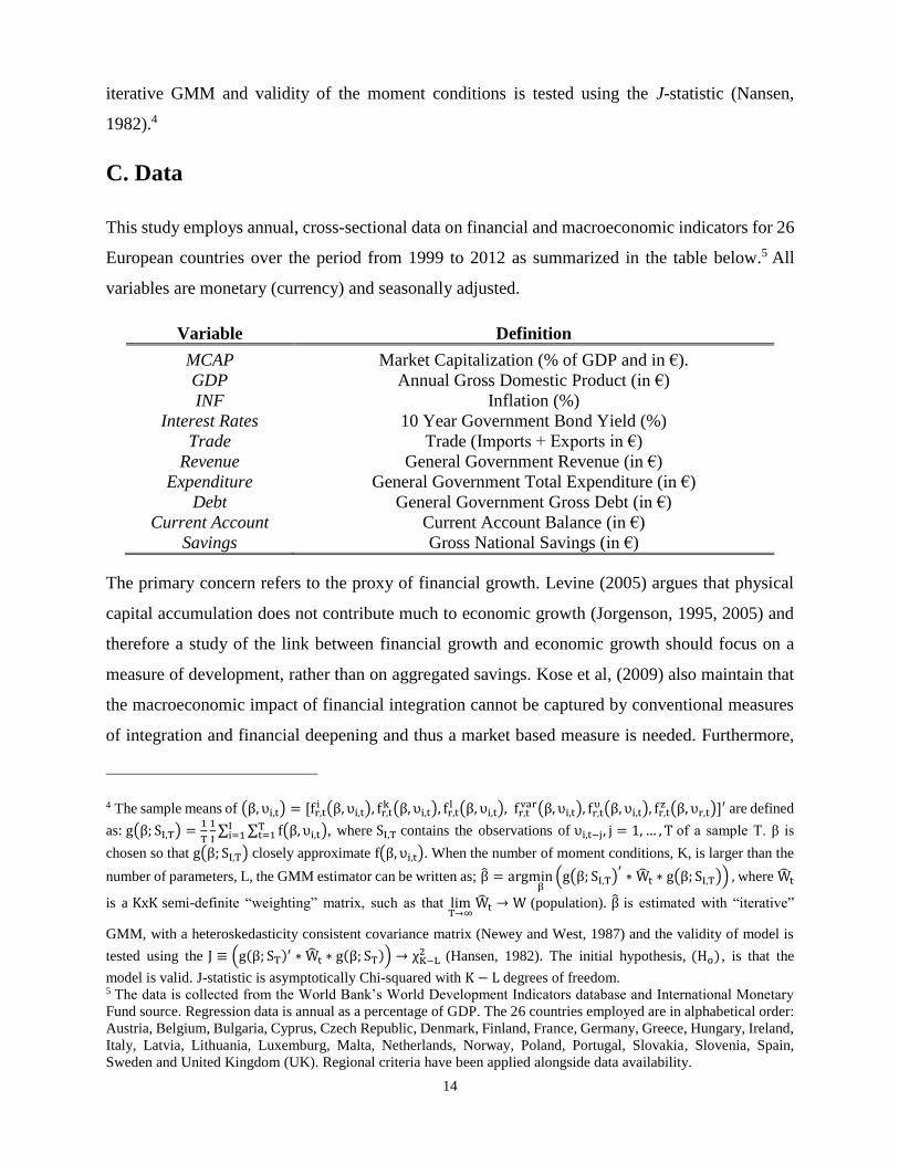
This study employs annual, cross-sectional data on financial and macroeconomic indicators for 26
European countries over the period from 1999 to 2012 as summarized in the table below.5 All
variables are monetary (currency) and seasonally adjusted.
Variable Definition
MCAP Market Capitalization (% of GDP and in €).
GDP Annual Gross Domestic Product (in €)
INF Inflation (%)
Interest Rates 10 Year Government Bond Yield (%)
Trade Trade (Imports + Exports in €)
Revenue General Government Revenue (in €)
Expenditure General Government Total Expenditure (in €)
Debt General Government Gross Debt (in €)
Current Account Current Account Balance (in €)
Savings Gross National Savings (in €)
The primary concern refers to the proxy of financial growth. Levine (2005) argues that physical
capital accumulation does not contribute much to economic growth (Jorgenson, 1995, 2005) and
therefore a study of the link between financial growth and economic growth should focus on a
measure of development, rather than on aggregated savings. Kose et al, (2009) also maintain that
the macroeconomic impact of financial integration cannot be captured by conventional measures
of integration and financial deepening and thus a market based measure is needed. Furthermore,
4 The sample means of (β, υi,t) = [fr,ti (β, υi,t), fr,t
k (β, υi,t), fr,tl (β, υi,t), fr,t
var(β, υi,t), fr,tυ (β, υi,t), fr,t
z (β, υr,t)]′ are defined
as: g(β; SI,T) =1
T
1
I∑ ∑ f(β, υi,t)T
t=1Ii=1 , where SI,T contains the observations of υi,t−j, j = 1, … , T of a sample T. β is
chosen so that g(β; SI,T) closely approximate f(β, υi,t). When the number of moment conditions, K, is larger than the
number of parameters, L, the GMM estimator can be written as; β = argminβ
(g(β; SI,T)′
∗ Wt ∗ g(β; SI,T)) , where Wt
is a KxK semi-definite “weighting” matrix, such as that limT→∞
Wt → W (population). β is estimated with “iterative”
GMM, with a heteroskedasticity consistent covariance matrix (Newey and West, 1987) and the validity of model is
tested using the J ≡ (g(β; ST)′ ∗ Wt ∗ g(β; ST)) → χK−L2 (Hansen, 1982). The initial hypothesis, (Ho) , is that the
model is valid. J-statistic is asymptotically Chi-squared with K − L degrees of freedom. 5 The data is collected from the World Bank’s World Development Indicators database and International Monetary
Fund source. Regression data is annual as a percentage of GDP. The 26 countries employed are in alphabetical order:
Austria, Belgium, Bulgaria, Cyprus, Czech Republic, Denmark, Finland, France, Germany, Greece, Hungary, Ireland,
Italy, Latvia, Lithuania, Luxemburg, Malta, Netherlands, Norway, Poland, Portugal, Slovakia, Slovenia, Spain,
Sweden and United Kingdom (UK). Regional criteria have been applied alongside data availability.

15
Friedrich et al, (2012) suggest that excessive optimism set the base for irrationally capitalized
expectations of stability and thus it led to excessive levels of borrowing, at a cost that was not fully
reflecting fundamentals. We introduce public borrowing levels in our analysis as an integral part
of the financial-economic growth nexus and thus, we postulate that any measure that does not
capture market expectations could not reveal the, potentially endogenous, inter-relations between
debt and the other two variables. Following Beck et al. (2000, 2008), MCAP, more precisely the
% change of MCAP, is employed as a proxy for financial growth. This measure has been chosen
on the grounds that it accounts not only for the quality and depth of the financial sector, but also
for two other things. First, it is a collective measure of intra-country economic entities. Recent
literature (Abiad et al., 2009; Heinemann et al., 2013; Imbs, 2006, 2007) emphasizes the
importance of micro-level data. However, because our study focuses on governmental policies
rather than on firm level analysis, the macro-level approach is more appropriate. Market
capitalization, measures - albeit rigidly - financial growth as the sum of all individual entities
within the economy. Thus it is a measure of financial activity that does not ignore firm specific
effects. Second, it accounts for investor opinions concerning risk, both unsystematic (each
individual firm) and systematic (the economy as a whole).
Then the other fundamental variables in our modelling include economic growth and debt. With
respect to economic growth, following Levine (1997), we use the % growth of GDP. We consider
public borrowing levels, because in Europe they have been the major burden in the peripheral
economies that amplified the impact of restrained capital flows. The level of debt in the sample
period has been steadily increasing and therefore this variable is not stationary. Therefore, we
employ the first % difference. We purport that this accounts also for the dynamic character of the
panel data set we have employed and that it should be expected to be more correlated with
changing expectations and thus, our measure of financial growth. In Europe, financial and political
integration have been very significant aspects of economic growth and that the foundation of this
relationship lies on capitalization of expectations. Optimism was reflected on market valuations
and thus, on capital flows, which in turn allowed a better mobilization of resources and
consequently growth. However, this growth was externally financed and at some point, public
borrowing was restricting rather than financing growth. We postulate that the impact of
expectations should be better reflected on the rate that financial growth and economic growth
accelerate with respect to the rate the borrowing grows.
16
Another important element in our study is the distinction between differential degrees of
integration. Kose et al., (2009) make an explicit distinction between de jure, i.e., explicit measures,
such as capital controls, and de facto, i.e., implicit measures that reflect legal restrictions, of
financial integration, suggesting that a combination of the two should better reflect the openness
of an economy.6 In order to account for de jure measures we employ a combination of dummy
variables that account for country specific and larger scale legislation effects. The country specific
effects, C, capture implicitly the intensity of explicit measures among other unobservable effects.
In addition, the dummy variables EU and E, capture the effects of two different levels of explicit
legislation. The first is the political integration within the European Union and the second is the
financial integration within the monetary union, namely the euro. Both are measures of differential
degrees of integration, which are explicitly regulated on an integrated level. EU and E are expected
to affect market expectations, thus, financial an depth growth and therefore, indirectly economic
growth. However, in practice their impact on market openness of individual countries, i.e.,
captured by the combination of C, EU and E, might not be reflected on the de facto measures of
financial integration. Therefore, we use the variable 𝑇𝑟𝑑𝑡 = 𝛥(𝑇𝑟𝑎𝑑𝑒𝑡), which captures changes
in trade openness, measured as the sum of the monetary value of imports and exports. Trade
openness is a conventional measure of de facto financial integration (Kose et al., 2009)
Furthermore, other variables are also introduced in the model to account for known GDP
determinants, thus reducing heteroskedasticity. CV = (EXP, REV, SAV, INF, IR, Trd, CAB) . 7
Following early literature (Arrow and Kurz, 1970; Diamond, 1989), EXP = 𝛥log(𝐸𝑥𝑝𝑒𝑛𝑑𝑖𝑡𝑢𝑟𝑒𝑡)
is used to capture changes in fiscal policies and in particular the impact of government spending
on economic growth. Similarly, 𝑅𝐸𝑉 = 𝛥𝑙𝑜𝑔(𝑅𝑒𝑣𝑒𝑛𝑢𝑒𝑡) captures the other side of fiscal
policies; changes in general government revenue. 𝐶𝐴𝐵 = 𝐶𝑢𝑟𝑟𝑒𝑛𝑡 𝐴𝑐𝑐𝑜𝑢𝑛𝑡𝐺𝐷𝑃⁄ measures the
current account balance as a proportion of GDP. Finally, in order to account for the convergence
6 Kose et al. (2009) argue that in practice there are explicit measures that limit capital flows, which are necessarily
strictly imposed. On the contrary, other countries that might follow liberal practices might experience low capital
flows. Consequently, in order to better capture nominal, i.e., de jure, and effective, i.e., de facto, integration, a
combination of the two is needed. 7 The suggested model tries, by no means, to investigate the determinants of economic or financial growth, or public
debt. The focus lies on potential endogeneity, accounting for some control variables. Please note that in (2.a), CAB is
employed instead of Trade openness because the balance of imports/exports is expected to determine long-term
growth. In contrast, in (2.b), Trade openness is preferred because it is a better indicator of total trading activity. In
(2.c), inflation is excluded because it is expected to have a simultaneously increasing (higher monetary value) and
decreasing (lower value of existing liabilities) impact on debt levels, and thus a non-significant impact.

17
in interest rates within the Eurozone, the 10 year government bond yields are employed. 𝐼𝑅 =
𝛥(𝐼𝑛𝑡𝑒𝑟𝑒𝑠𝑡 𝑅𝑎𝑡𝑒𝑠𝑡) is the change in prevailing yields and reflect changes in the fundamentals.
This is closely linked to our measure of financial growth, which also captures investors’
expectations.
IV. Empirical Findings
A. Non-Parametric Analysis
1. Initial Observations
The average economic growth in figure 1 is positive, 5.29%, and overdispersed (std is 6.48%),
which is somewhat expected due to the inclusion of both developing and developed economies, as
well as a structural break in October 2008. The negative skewness (-0.0442) and the high kurtosis
(5.6059) show that high dispersion is mainly due to the post-2008 contraction that many countries
experienced. Furthermore, market capitalization accounts for around 65% of GDP, which shows
that the financial sector plays a significant role in these economies. It is also highly dispersed, with
a significantly long right tail (kurtosis is 11.5734 and skewness is 2.0959). In several cases the
market value of listed companies exceeds GDP, by a maximum factor of 4.62, which indicates
significant exuberance mainly recorded prior to 2008 (Shiller, 2005). The contribution of the
political and financial integration to this confidence and its link with economic growth is the main
focus of this study.
DEBT accounts for approximately 61% of GDP. It has a longer right tail (skewness is 3.6013 and
kurtosis is 20.8301). This shows that several countries sustain considerably higher debt levels, in
some cases exceeding 100%. This should be more pronounced after 2008 where GDP declines
without a proportional decrease in public debt. A negative median, -€0.728b, for CAB shows that
imports exceed exports in most cases. Consistently with Trade, CAB is significantly overdispersed
with some extreme observations at both ends of the distributions. This highlights how
inhomogeneous the structure of the countries that constitute the union is. Literature recognizes the
combination of negative CAB and high debt as a major determinant of increased exposure to
macroeconomic shocks, especially under reduced flexibility induced by a monetary integration.
2. Financial Growth and Economic Growth

18
Figure 2 presents graphically the link between economic growth, financial growth (Panels A-C)
and MCAP (Panels D-F). Panels A shows that financial growth and economic growth tend to be
positively correlated with countries exhibiting simultaneous financial growth and economic
growth. According to panel B, this seems to be more intense in the countries that have joined the
euro, since the dots seem to be more aligned to a positive correlation, unlike the countries that have
kept their national currencies, which exhibit more observations closer to the XX’ axis. Panel D
shows an overall declining link between MCAP and economic growth. However there are several
large observations close to the YY’ axis, showing that there are countries that achieve high market
value without necessarily experiencing high economic growth (or small increases in economic
activity can spark high market values). The distinction becomes clearer in panels E and F. In the
Eurozone the link between market values and economic growth seems to be exponentially
increasing. In contrast, in the countries that have kept their national currencies two subgroups are
observed. In the first group higher economic growth is not associated with high market values,
while in the second, some very high figures are observed for MCAP in countries with low
economic growth. The overall link tends to be rather negative, but with no clear trend.
Figure 3 presents the relationship between economic, financial growth and debt. It reveals that
indeed economic growth and financial growth appear to be linked and this link seems to strengthen
over time, in particular after 2008. In the period prior to 2008, panels B and C reveal that the link
is relatively weaker in non-Eurozone countries. However, after 2008, the volatility of both
financial growth and economic growth is higher for this sub-sample, indicating that the euro might
cushion the impact of a macroeconomic shock on participating countries. Several studies (e.g.
Manning, 2003; Rousseau and Wachtel, 2011) report that the link between economic growth and
financial growth has weakened significantly, especially after 1990. However, in the period
following 2008 their link appears to strengthen again, following a lead-lag pattern. This shows that
this link might either be cyclical, i.e. depending on macroeconomic cycles, or that it is a natural
consequence of a macroeconomic shock.8
8 In this study we investigate the latter, without necessarily ignoring the first. We focus on the link between financial
growth and economic growth and the impact of monetary integration. MCAP as a measure of financial growth reflects
market expectations and thus is expected to better capture potential “euro” effects. If there are cyclical patterns, they
should be reflected on market prices, assuming rationality. Relaxing the rationality or investigating the link between
business cycles and macroeconomic shocks would deviate from the current focus, which is potential “euro” effects.

19
3. Bear vs Bull Market and Debt
Another observation refers to the nature of the link. Panels A-E show that economic growth
changes are mostly observed after financial growth sparks. This shows that changes in GDP
influence market expectations, which seem to precede any changes in economic growth. There is
a notable “bull” market period starting at around 2000, being followed by a strong “bear” market
period after 2008. The link between financial growth and economic growth seems to strengthen
significantly around 2008 and MCAP notably captures subsequent GDP changes, especially in the
Eurozone. This shows that the markets discount timely information about economic growth.
Consequently, the dynamic structure chosen to investigate the direction of the relationship in
equations (2.a), (2.b) and (2.c) seems to be justified.
Panels D and E focus on countries with public debt levels beyond 90% of GDP. During “bull”
markets, economic growth is more moderate, about 5-6% p.a., than in countries with lower debt,
about 6-10% p.a., while it decreases significantly during “bear” markets. Panels F-H distinguish
between Eurozone and non-Eurozone countries. Panel F shows that, overall, higher borrowing is
associated with exponentially lower economic growth. According to Panel H, this is consistent in
non-Eurozone countries. In contrast, countries that have joined the euro appear to still be able to
achieve higher economic growth. The euro seems to improve access to financing, which can further
assist growth. Investigating this further figure 4 presents the relationship between the endogenous
variables before and after the outburst of the financial crisis in 2008. The first column confirms
previous findings. However, panels F and J, show that after 2008, countries that have not joined
the Eurozone exhibit significantly lower growth across greater financial activity. Also, panels E
and H show that the link between financial growth and economic growth is significantly stronger
in a bearish market, though it does not disappear after a macroeconomic shock.
B. Parametric Analysis
1. Financial Growth and Economic Growth
Table 1 presents the estimation results of the model presented in equations (2.a), (2.b) and (2.c.)
Focusing on the full sample, no significant link is observed between financial growth and
economic growth in non-Eurozone countries. The highest absolute value of t-statistic is 1.67,
showing that the two figures are rather independent. However, financial growth appears to have a

20
significant increasing effect on economic growth in countries that have adopted the euro (FG*E is
0.0311 and t-statistic is 2.53). In parallel, looking at the determinants of financial growth, a
significant (2.04) coefficient of 0.8012 for the EU dummy shows that G has an increasing impact
on financial growth for countries that have joined the European Union. This effect is found to be
stronger for countries that have additionally joined the euro (coefficient is 0.3015 and t-statistic is
3.13). Consequently, the link between the two figures is present in Europe, and they are found to
be endogenous in the Eurozone, but not necessarily within the European Union.
In addition, political integration does not appear to have any significant direct impact on either of
the figures, since the coefficient of the EU dummy remains rather insignificant. In contrast, a
significant (3.01) coefficient of 0.7433 of the E dummy shows that monetary integration seems to
accelerate financial growth only, without any significant effect on economic growth.
A possible explanation for this finding could depend on the existence of the European Union,
particularly of the Eurozone. The EU is significantly larger than any single country and it is
therefore to be more resistant to market pressure than a single entity. Consequently, increased
endogeneity between market condition and fundamentals should be expected. Monetary
integration appears to have an increasing direct and indirect impact on financial growth, which in
turn further enhances economic growth, engaging into a spiral relationship. The absence of this
link in the non-EU countries leads to the conclusion that the contribution of EU is significant.
Given that MCAP captures expectations, this contribution may be linked to increased confidence
and thus, improved access to financing. Consequently, for a given change in GDP, market reacts
more positively in Eurozone member states, probably because investors anticipate lower exposure
to macroeconomic risk. This allows an investment flow that can further increase GDP.
However, this spiral effect does not seem to be consistent outside the Eurozone, not even in other
(non-euro) member states. EU membership would assist countries with positive GDP changes to
further increase the total market value, but this increased market value has no further impact on
GDP, unless the country has joined the euro. From a market perspective, this seems to be
distinctively different from EU membership. Market participants seem to capitalize their
expectations for future political stability and thus for lower macroeconomic risk on current prices
when a country joins the EU. This might be derived from expectations about political of financial
stability. However, this seems not to be a sufficient condition to further increase their GDP and
can only occur if they also adopt the common currency. When they do, they abandon their

21
monetary tools and, thus, they need to have discipline, aiming at increasing their competitive
advantages. This, in combination with a higher level of political and monetary integration, seems
to lead to higher stability expectations, which attract further economic development. This is a first
sign that the euro is suitable for countries which anticipate that they can gain on the long term from
the spiral link between financial growth and economic growth.
Moreover, this spiral link seems to be strongly present prior to 2008 only within the Eurozone.
GDP has an increasing impact on financial growth (e.g. G*E is 0.3589 and t-statistic is 2.01),
which in turn further increases G (e.g. FG*E is 0.0513 and t-statistic is 2.83). This shows that the
euro could accelerate economic growth in countries that can benefit from this spiral link. Again,
only financial growth is found to be directly affected by monetary integration, while political
integration is not found to have any significant direct impact on both figures.
Furthermore, the euro appears to play a smoothing role too during the period following the outburst
of the financial crisis. GDP improvements still increase market values only within the Eurozone
(e.g. G*E is 0.2758 and t-statistic is 2.21), but now the Eurozone countries seem to be less exposed
to market fluctuations. In more detail, an estimate of 0.1901 (2.60) shows that in non-Eurozone
countries changes in GDP follow changes in market value. The mostly negative financial growth
experienced during the post 2008 period appears to have a strong negative impact on the economic
growth of these economies. In contrast, a negative estimate for the Eurozone countries of -0.1548
(-2.09) indicates that this effect is milder for countries that have adopted the euro. Negative
financial growth still negatively affects economic growth, but the impact is considerably smaller
in Eurozone member states. This indicates that non-Eurozone countries appear to be more exposed
to market volatility after a macroeconomic shock than countries that belong to a monetary union.
This highlights an additional beneficial impact of the euro, which seems to bate the impact of
macroeconomic shocks.
2. Financial Growth, Economic Growth and Debt
The previous section highlights the contribution of the euro in accelerating both financial growth
and economic growth, as well as their spiral link. This might be observed due to improved access
to financing, which could be a major determinant of the spiral link. Equation (2.c) focuses on the
impact of economic growth and financial growth on public debt growth, as well as on endogeneity
issues.

22
The last section of table 1 shows that monetary integration appears to have a significant impact on
public borrowing levels. Eurozone member states exhibit significantly higher (e.g. 0.0248 and t-
statistic is 2.11) debt growth, both before (e.g. 0.1893 and t-statistic is 2.10) and after (e.g. 0.0199
and t-statistic is 1.99) 2008, while political integration does not exhibit any significant marginal
impact. This is a sign of improved access to financing, probably due to additional confidence
induced by monetary integration. This is further complemented when a member state experiences
economic growth, but not necessarily upon financial growth. In more detail, there is a statistically
significant difference in borrowing levels between member and non-member states. The impact of
G is insignificant for countries that have not joined the EU (e.g. coefficient is -0.1842 and t-statistic
is -0.36), but it has a rather increasing impact for member states (e.g. 0.1814 and t-statistic is 1.94),
especially when the euro is the currency adopted (e.g. 0.2321 and t-statistic is 5.06). In contrast,
no significant link appears to exist between financial growth and DEB. This shows that a country’s
fundamentals are more important than its financial profile in improving its borrowing position.
Further, the mostly insignificant coefficients of E and EU in the last column indicate that any euro
effect on borrowing becomes significantly less important during a “bear” market wherever
financial commitments seem to be prioritised over economic development.
Naturally, the focus shifts on how the improved borrowing position (higher growth of debt
accumulation) affects the spiral link between financial growth and economic growth. The first
observation is derived from the third panel of the first section of Table 1. DEB seems to be
endogenous to GDP growth with differing impact for member and non-member states. Higher debt
growth seems to have a limiting impact on economic growth in countries that have not joined the
euro (e.g. coefficient is -0.5076 and t-statistics is -2.08). In contrast, the higher borrowing capacity
of euro member states seems to have an overall marginally positive impact on economic growth
(e.g., 0.0075 (1.95) for DEB*E and 0.4863 (2.01) for DEB*EU). Consequently, the euro appears
to have another indirect positive impact on economic growth. The Eurozone countries seem to
have higher credibility that can be used to draw more funds, which can lead to further development.
However, there is a lack of consistency before and after 2008. During the booming period prior to
2008, higher debt growth has a positive impact (e.g., 0.0190 (2.27)) on economic growth, even
when debt exceeds 90% of GDP (e.g., 0.0380 (2.57)). In contrast, in the years following the
sovereign bond crisis, increases in debt seem to significantly limit growth opportunities (e.g., -
0.0267 (-2.77)) in the Eurozone, especially for countries with high borrowing levels (e.g., -0.0413

23
(-2.37)). This, along with the notable absence of “euro effects” on debt, raises some concerns about
the suitability, or the overall impact, of improved access to financing due to monetary integration.
In the previous section, the euro has been found to protect countries from erratic market
movements, by smoothening the negative impact of negative financial growth, but the limited
monetary flexibility appears to significantly slow down economic growth during a bear market.
Improved access to financing might endogenously accelerate economic growth, but during bear
market periods financial obligations are prioritized and thus, the increased financing might be
considered as “over-borrowing”. In this case it seems to reverse the spiral link between financial
growth and economic growth and thus, lead to recession.
Consequently, the benefits from the endogenous relationship between debt increases and economic
growth are not unconditional. The euro might assist member states to achieve higher economic
growth, but it might also lead them to unmanageable borrowing levels. This concern seems to be
reflected on the impact of debt growth on financial growth, too. The third panel of the second
section of Table 1 shows that higher DEB consistently lead to lower marker values. This slows
down the spiral effect of the endogenous economic growth and financial growth. However, this
happens only in the Eurozone countries (e.g., -0.5756 (-4.73)) and not in member states that have
not joined the euro (e.g., 0.2582 (2.57)).
These findings lead to the conclusion that markets perceive the euro to have a dual role. First, it is
found to have a beneficial impact by leading to an endogenous spiral link between financial growth
and economic growth. However, this spiral link is bounded by borrowing levels. Positive debt
growth might lead to higher growth during bull market conditions, but it reverses this spiral link
during bear market conditions. This second role of euro, has a rather limiting impact on economic
growth, especially when the increase in financing is not accompanied by improvement in the
country fundamentals. The increased financing might improve GDP when the macroeconomic
conditions allow for it, but it might also lead to unsustainable financing. This might constitute the
foundations of what is reported in the literature as “bad” growth. Countries can improve their
access to financing by joining the monetary union, but unless resources are utilized efficiently in
order to improve fundamentals, economic growth might be fragile and susceptible to volatile
macroeconomic conditions.
Consequently, the suitability of adopting the euro should depend on the ability of each country to
benefit from the increased financing by engaging on the spiral endogenous link between financial

24
growth and economic growth, which could eventually improve fundamentals. Excessive
borrowing without engaging on this link could lead to obviation of market confidence, which
introduces an additional macroeconomic risk.
3. Robustness
The robustness of the empirical findings presented above is tested by considering a potential long
term equilibrium among the endogenous variables, by considering a different estimation method,
as well as by testing the strength of the instrumental variables. Table 2 presents the estimation
results for the model presented in equations (2.a), (2.b) and (2.c). Parameters have been estimated
considering an error correction specification, as well as using the Seemingly Unrelated Regression
(SUR) method, which recognizes potential cross-correlations assuming that the innovations of the
system are i.i.d.
In more detail, the bottom panel of Table 1 reports that all variables employed in the model are
stationary, while the bottom part of the Table 3 reports that the residuals of the full sample
estimation (Total in Table 1) are also stationary and non-heteroskedastic (cross-sectionally or over
time). This indicates that the three endogenous variables might be cointegrated, exhibiting a long-
term, equilibrium relationship. The first three columns of Table 2, present the estimates of the
parameters of the model in equations (2.a), (2.b) and (2.c) with an error correction term. The error
correction term is the lagged residual of the GDP regressed on a constant, MCAP and Debt (all
values are logged). The cointegration term is a significant determinant of economic growth and
financial growth, but not of debt growth. This indicates that MCAP and GDP are strongly linked
to each other, following a long term equilibrium, while Debt only indirectly affects their growth.
The presence of the cointegration term, as well as the different estimation method produces
consistent estimates with the GMM estimation (Table 1)
Furthermore, Table 3 presents the correlations between the regressors and the instrumental
variables, which are the first lag of regressors. The instruments appear to be highly correlated with
the corresponding regressors and uncorrelated with the GMM residuals. Finally, the cross
correlation between the GMM residuals appears to be rather small.
V. Concluding Remarks

25
In this study, we investigate the suitability of adopting the euro, by revisiting the interaction
between financial growth and economic growth in Europe. We introduce the growth of public
financing as an integral component and investigate endogeneity among all three. We also
investigate for potentially differential between the impact of political (European Union) and
financial (Eurozone) integration.
The empirical findings indicate that neither political nor monetary integration exhibit any direct
impact on economic growth. Their impact is rather indirect through financial and debt growth. In
more detail, monetary integration appears to allow countries to borrow more and accelerates
financial growth, both directly and indirectly through improvements in country fundamentals.
Increased market values and improved financing further accelerate economic growth, indicating a
spiral endogenous link between the three. However, this link is only observed within Eurozone
member states, highlighting the existence of a “euro effect”. This effect seems to be strong,
especially during bear market conditions prior to 2008, when even countries with high debt
balances can benefit from the spiral link and experience higher economic growth. In contrast,
during the bearish market conditions in the post 2008 period, a sharp correction of market values
and economic growth is observed, especially for countries with high levels of debt. This reverses
the afore-mentioned spiral link and leads into recession.
Consequently, the euro is found to play a dual role. First, it has a positive indirect impact on
economic growth, by allowing the countries to engage into a spiral endogenous link between
financial growth and economic growth, as well as debt. Improved access to financing allows for
more investments, which increase GDP. This increases market values, which have a further
boosting impact on economic growth. EU members that have not joined the euro can still draw
marginally more funds upon higher economic growth, but the lack of the common currency does
not create the necessary confidence to enhance a synergetic endogeneity. However, this
exuberance might lead countries to borrow more introducing a “moral hazard” of “over-
borrowing”. This second role of the euro introduces a macroeconomic risk, where countries might
pursue economic growth through an improved credit profile due to the monetary integration, rather
than through an improvement in country fundamentals. This might set the foundation for “bad”
growth, which reverses the afore-mentioned spiral endogenous link after macroeconomic shocks,
leading to recession. Therefore, the interaction between the dual role of the euro, which is unique
for each country, should be a major determinant of the suitability of adopting the common

26
currency. On a larger scale, European policies should focus either on distinguishing between
“good” and “bad” borrowing and thus between “good” and “bad” growth or on structural changes
that will allow countries to benefit from the financial-economic growth momentum.

27
References
1. Abiad, Abdul, Leigh, Daniel, and Mody, Ashoka (2009) Financial integration, capital
mobility, and income convergence. Economic Policy, 24 (58), 241-305.
2. Adam, Christopher S and Bevan, David L (2005) Fiscal deficits and growth in developing
countries. Journal of Public Economics, 89 (4), 571-97.
3. Aizenman, Joshua, Lee, Yeonho, and Rhee, Youngseop (2007) International reserves
management and capital mobility in a volatile world: Policy considerations and a case study
of Korea. Journal of the Japanese and International Economies, 21 (1), 1-15.
4. Alessi, Lucia and Detken, Carsten (2011) Quasi real time early warning indicators for costly
asset price boom/bust cycles: A role for global liquidity. European Journal of Political
Economy, 27 (3), 520-33.
5. Alfaro, Laura, Chanda, Areendam, Kalemli-Ozcan Sebnem and Sayek Selin (2004) FDI and
economic growth: The role of local financial markets. Journal of International Economics, 64
(1), 89-112.
6. Allen, Franklin (1990) The market for information and the origin of financial intermediation.
Journal of financial intermediation, 1(1), 3-30.
7. --- and Gale, Douglas (1997) Financial markets, intermediaries and intertemporal smoothing.
Journal of political Economy, 105 (3), 523-546.
8. Alonso-Borrego, Cesar and Arellano, Manuel (1996) Symmetrically normalized instrumental-
variable estimation using panel data. Journal of Business and Economic Statistics, 17, 36-49.
9. Ang, James B. and McKibbin, Warwick J. (2007) Financial liberalization, financial sector
development and growth: evidence from Malaysia. Journal of development economics 84.(1),
215-233.
10. Arellano, Manuel and Bond, Stephen (1991) Some tests of specification for panel data. Monte
Carlo evidence and an application to employment equations. Review of Economic Studies, 58
(2), 227-297.
11. --- and Bover, Olympia (1995) Another look at the instrumental variable estimation of error-
components models. Journal of Econometrics, 68 (1), 29-51.
12. Ariyoshi, Akira, Habermeier, Friedrich, Ki, Andrei, Kriljenko, Jorge I. C. and Otker, Inci
(2000) Capital controls: Country experiences with their use and liberalization. IMF
Occasional Paper 190, International Monetary Fund, Washington.
13. Aschauer, David Alan (2000) Public capital and economic growth: issues of quantity, finance,
and efficiency. Economic Development and Cultural Change, 48 (2), 391-406.
14. Bakker, Age and Chapple, Bryan (2002) Advanced country experiences with capital account
liberalization. IMF Occasional paper 214, International Monetary Fund, Washington.
15. Bagehot, Walter (1983) Lombard Street: A description of the money market. Kegan, Paul &
Trench.
16. Beck, Thorsten, Lundberg, Mattias and Majnoni, Giovanni (2006) Financial intermediary
development and growth volatility: Do intermediaries dampen or magnify shocks? Journal of
International Money and Finance, 25 (7), 1146-1167.
17. Beck, Thorsten, Levine, Ross, and Loayza, Norman (2000) Finance and the Sources of
Growth. Journal of financial economics, 58 (1), 261-300.
18. Beck, Thorsten, Demirgüç-Kunt, Asli, and Maksimovic, Vojislav (2008) Financing patterns
around the world: Are small firms different?. Journal of Financial Economics, 89 (3), 467-
87.
19. Beetsma, Roel, Giuliodori, Massimo, De Jong, Frank, and Widijanto, Daniel (2013). Spread

28
the news: The impact of news on the European sovereign bond markets during the crisis.
Journal of International Money and Finance, 34, 83-101.
20. Beirne, John and Fratzscher, Marcel (2012) The pricing of sovereign risk and contagion during
the European sovereign debt crisis. Journal of International Money and Finance.
21. Berg, Andrew and Krueger, Anne (2003) Trade, growth, and poverty: A selective survey. IMF
Papers 3-30. International Monetary Fund, Washington.
22. Berg, Andrew, Borensztein, Eduardo and Pattillo Catherine (2004) Assessing early warning
systems. How have they worked in practice? IMF Working Paper 04/52, International
Monetary Fund, Washington.
23. Berglöf, Erik, et al. (2009) Understanding the crisis in emerging Europe. European Bank for
Reconstruction and Development Working Paper, (109).
24. Berle, Adolf and Means, Gardiner (1932) The modern corporate and private property.
McMillian, New York, NY.
25. Berthelemy, Jean-Claude and Varoudakis, Aristomene (1996) Economic growth, convergence
clubs, and the role of financial development. Oxford Economic Papers, 48 (2), 300-28.
26. Bhagwati, Jagdish (1998) The capital myth. The difference between trade in widgets and
dollars. Foreign Affairs, 7 (3) 7-12.
27. Bhattacharya, Sudipto and Pfleiderer, Paul (1985) Delegated portfolio management. Journal
of Economic Theory, 36 (1), 1-25.
28. Blackburn, Keith and Hung, Victor TY (1998) A theory of growth, financial development and
trade. Economica, 65 (257), 107-24.
29. Blundell, Richard and Bond, Stephen (1998) Initial conditions and moment restrictions in
dynamic panel data models. Journal of Econometrics, 87 (1), 115-143.
30. Boyd, John H. and Smith, Bruce D. (1992) Intermediation and the equilibrium allocation of
investment capital: Implications for economic development. Journal of Monetary Economics,
30 (3), 409-432.
31. Brown, Morton B and Forsythe, Alan B (1974) Robust tests for the equality of variances.
Journal of the American Statistical Association, 69 (346), 364-67.
32. Buchanan, James M and Buchanan, James M (1958) Public principles of public debt: a
defense and restatement. RD Irwin Homewood, IL.
33. Calvo, Guillermo and Talvi Ernesto (2005) Sudden stop, financial factors and economic
collapse in Latin America: Learning from Argentina and Chile. NBER Working Paper no
11153, National Bureau of Economic Research, Cambridge, MA.
34. Checherita, Cristina and Rother, Philipp (2010) The impact of high and growing government
debt on economic growth, An empirical investigation for the Euro Area. Frankfurt: European
Central Bank Working Paper Series, (1237).
35. Christopoulos, Dimitris K. and Tsionas Efthymios G. (2004) Financial development and
economic growth: evidence from panel unit root and cointegration tests. Journal of
Development Economics, 73 (1) 55-74
36. Clements, Benedict J, Bhattacharya, Rina, and Nguyen, Toan Quoc (2003) External debt,
public investment, and growth in low-income countries. International Monetary Fund.
37. Collins, S. M. (2007) Comments on “Financial globalization, growth, and volatility in
developing countries” by Eswar Prasad, Kenneth Rogoff, Shang-Jin Wei, and M. Ayhan
Kose.” In: Harrison, A. (Ed.), Globalization and Poverty, National Bureau of Economic
Research Conference Report. University of Chicago Press, Chicago.
38. Darrat, Alif F (1999) Are financial deepening and economic growth causally related? Another
look at the evidence. International Economic Journal, 13 (3), 19-35.

29
39. De Grauwe, Paul (2011), 'The governance of a fragile Eurozone', Revista de Economía
Institucional, 13 (25), 33-41.
40. --- (2012) Economics of monetary union. Oxford University Press.
41. De Grauwe, Paul and Ji, Yuemei (2013) Panic-driven austerity in the Eurozone and its
implications. VoxEU. org, 21.
42. Demetriades, Panicos O and Hussein, Khaled A (1996) Does financial development cause
economic growth? Time-series evidence from 16 countries. Journal of development
Economics, 51 (2), 387-411.
43. Denizer, Cevdet, Iyigun, Murat F. and Owen, Ann L. (2002) Finance and macroeconomic
volatility. Contributions to Macroeconomics, 2 (1).
44. Devereux, Michael B. and Smith, Gregor W. (1994) International risk sharing and economic
growth. International Economic Review, 535-550.
45. Diamond, Peter A (1965) National debt in a neoclassical growth model. The American
Economic Review, 55 (5), 1126-50.
46. Diamond, Douglas W. and Dybvig, Philip H. (1983) Bank runs, deposit insurance, and
liquidity. The journal of political economy, 401-419.
47. Diamond, Douglas W. and Rajan, Raghuram G. (2001) Banks and liquidity. The American
Economic Review, 91 (2), 422-425.
48. Diaz-Alejandro, Carlos (1985) Good-bye financial repression, hello financial crash. Journal
of development Economics, 19 (1), 1-24.
49. Dollar, David and Kraay, Aart (2003) Institutions, trade, and growth. Journal of monetary
economics, 50 (1), 133-162.
50. Durham, Benson J. (2004) Absorptive capacity and the effects of foreign direct investment
and equity foreign portfolio investment on economic growth. European economic review, 48
(2), 285-306.
51. Easterly, William, Islam, Roumeen and Stiglitz, Joseph E. (2001) Shaken and stirred:
Explaining growth volatility. Advances in Macroeconomic Theory, 352-372.
52. Edwards, Sebastian (1998) Openness, productivity and growth: what do we really know? The
Economic Journal, 108 (447), 383-98.
53. Eichengreen, Barry J. (2001) Capital Account Liberalization: What do cross-countrystudies
tell us? World Bannk Economic Review, 15, 341-365
54. Eichengreen, Barry J., Hausmann Richardo and Panizza Ugo (2006) The pain of original sin.
In Other People’s Money, ed. By Barry Eichengreen and Ricardo Hausmann, University of
Chicago Press, Chicago.
55. Friedrich, Christian, Schnabel, Isabel and Zettelmeyer Jeromin (2012) Financial integration
and growth. Why is Emerging Europe different? Journal of International Economics, 89 (2),
522-538.
56. Fry, Maxwell J (1978) The permanent income hypothesis in underdeveloped economies::
Additional evidence. Journal of Development Economics, 5 (4), 399-402.
57. Frankel, Jeffrey A. and Romer, David (1999) Does trade cause growth?. American economic
review, 379-399.
58.
59. Gibson, Heather D, Hall, Stephen G, and Tavlas, George S (2013) Fundamentally wrong:
Market pricing of sovereigns and the Greek financial crisis. Journal of Macroeconomics.
60. Goldsmith R. W. (1969) Financial Structure and development. Yale University Press, New
Haven, CT.
61. Gourinchas, Pierre-Olivier and Jeanne, Olivier (2006) The elusive gains from international

30
financial integration. The Review of Economic Studies, 73 (3), 715-41.
62. --- (2007).Capital flows to developing countries: The allocation puzzle. (National Bureau of
Economic Research).
63. Greenwood, Jeremy and Jovanovic, Boyan (1990) Financial Development Growth, and the
Distribution of Income. Journal of Political Economy, 98.
64. Greenwood, Jeremy and Smith, Bruce D (1997) Financial markets in development, and the
development of financial markets. Journal of Economic Dynamics and Control, 21 (1), 145-
81.
65. Grossman, Sanford J. and Hart, Oliver D. (1980) Disclosure laws and takeover bids. The
Journal of Finance, 35 (2) 323-334.
66. --- and Stiglitz. Joseph E. (1980) On the impossibility of informationally efficient markets.
The American economic review, 70(3), 393-408.
67. --- (1986) The costs and benefits of ownership: A theory of vertical and lateral integration.
The Journal of Political Economy, 691-719.
68. Gurley, John G. and Shaw, Edward S. (1995) Financial aspects of economic development.
The American Economic Review, 45 (4), 515-538.
69. Hansen, Lars Peter (1982) Large sample properties of generalized method of moments
estimators. Econometrica: Journal of the Econometric Society, 1029-54.
70. Harrison, Paul, Sussman, Oren, and Zeira, Joseph (1999) Finance and growth: Theory and
new evidence'.
71. Heinemann, Friedrich, Osterloh, Steffen, and Kalb, Alexander (2014) Sovereign risk premia:
The link between fiscal rules and stability culture. Journal of International Money and
Finance, 21, 110-127.
72. Hermes, Niels and Lensink, Robert (2003) Foreign direct investment, financial development
and economic growth. Journal of Development Studies, 40 (1), 142-63.
73. Hicks, John (1969) A theory of economic history. Vol. 163. Oxford University Press, Oxford.
74. Im, Kyung So, Pesaran, M Hashem, and Shin, Yongcheol (2003) Testing for unit roots in
heterogeneous panels. Journal of econometrics, 115 (1), 53-74.
75. Imbs, Jean (2006) The real effects of financial integration. Journal of International
Economics, 68 (2), 296-324.
76. --- (2007) Growth and volatility. Journal of Monetary Economics, 54 (7), 1848-62.
77. Ireland, Patrick Richard (1994) The policy challenge of ethnic diversity: immigrant politics in
France and Switzerland. Cambridge, MA. Harvard University Press.
78. Jeanne, Olivier M. (2003) Why do emerging economies borrow in foreign currency?
International Monetary Fund, 3-177.
79. Jorgenson, Dale W. (1995) Productivity: International comparisons of economic growth Vol.
2, Mit Press.
80. --- (2005) Accounting for growth in the information age. Handbook of economic growth 1,
743-815.
81. Kaminsky, Graciela L and Reinhart, Carmen M (1999) The twin crises: the causes of banking
and balance-of-payments problems. American economic review, 473-500.
82. Kaminsky, Graciela Laura and Schmukler, Sergio L (2008) Short-Run Pain, Long-Run Gain:
Financial Liberalization and Stock Market Cycles. Review of Finance, 12 (2), 253-92.
83. Kindleberger, Charles Poor and Kindleberger, Charles P (1978) Government and international
trade. International Finance Section, Department of Economics, Princeton University.
84. King, Robert G and Levine, Ross (1993) Finance and growth: Schumpeter might be right. The
quarterly journal of economics, 108 (3), 717-37.

31
85. Kose, Ayhan M. (2004) Volatility and comovement in an integrated world economy: An
exploration. In Horst Siebert ed., Mocroeconomic Policies in the World Economy, 89-122.
86. Kose, Ayhan, et al. (2009) Financial globalization and economic policies. Centre for
Economic Policy Research.
87. Krugman, Paul (1988) Financing vs. forgiving a debt overhang. Journal of development
Economics, 29 (3), 253-68.
88. Kumar, Manmohan and Woo, Jaejoon (2010) Public debt and growth. IMF Working Papers,
1-47.
89. Lamoreaux, Naomi R. (1994) Insider lending. Cambridge Books.
90. La Porta, R., Lopez-de-Silanes, F. Shleifer, A. and Vishny, R. (2002) Investor protection and
corporate valuation.Journal of finance, 1147-1170.
91. Larrain, Borja (2004) Financial development, financial constraints and the volatility of
industrial output. Public Policy Discussion Paper, 4 (6), Federal Reserve Bank, Boston.
92. Leon-Gonzalez, Roberto and Montolio, Daniel (2015) Endogeneity and panel data in growth
regressions: A Bayesian model averaging approach, Journal of Macroeconomics, 46, 23-39.
93. Levine, Ross (1997) Financial development and economic growth: views and agenda. Journal
of economic literature, 35 (2), 688-726.
94. --- (2005) Handbook of Economic Growth, Volume 1A, Elsevier.
95. Lucas, Robert E (1987) Models of business cycles. Basil Blackwell Oxford, 26.
96. Lucas Jr, Robert E (1988) On the mechanics of economic development. Journal of monetary
economics, 22 (1), 3-42.
97. Mankiw, Gregory N. (1992). Macroeconomics. Harward University, NY.
98. --- (1995) The growth of nations. Brooking Papers on Economics Activities, 275-310.
99. Manning, Alan (2003) The real thin theory: monopsony in modern labour markets. Labour
Economics, 10 (2), 105-31.
100. Myers, Stewart C., and Majluf, Nicholas S. (1984) Corporate financing and investment
decisions when firms have information that investors do not have. Journal of financial
economics, 13 (2), 187-221.
101. McKinnon, Ronald I (1973) Money and capital in economic development. Brookings
Institution Press.
102. Meade, James E (1958) Is the national debt a burden? Oxford Economic Papers, 10 (2), 163-
83.
103. Merton, Robert C. Bodie, Zvi (1995) A conceptual framework for analysing the financial
environment. In: Crane D.G., et al. (Eds.), The Global Financial System: A functional
Perspective. Havrard Business School Press, Boston, MA, 3-31.
104. Miller, Merton H (1998). Financial markets and economic growth. Journal of Applied
Corporate Finance, 11(3), 8-15.
105. Mink, Mark and De Haan, Jakob (2012) Contagion during the Greek sovereign debt crisis.
Journal of International Money and Finance.
106. Minsky, Hyman P (1986) The evolution of financial institutions and the performance of the
economy. Journal of Economic Issues, 20 (2), 345-53.
107. Missio, Sebastian and Watzka, Sebastian (2011) Financial contagion and the European debt
crisis. CESifo working paper: Monetary Policy and International Finance.
108. Modigliani, Franco (1961) Long-run implications of alternative fiscal policies and the burden
of the national debt. The Economic Journal, 71 (284), 730-55.
109. Moore, Michael C (1986) Elevated testosterone levels during nonbreeding-season
territoriality in a fall-breeding lizard, Sceloporus jarrovi. Journal of Comparative Physiology
32
A, 158 (2), 159-63.
110. Newey, Whitney K and West, Kenneth D (1987) Hypothesis testing with efficient method of
moments estimation. International Economic Review, 777-87.
111. Patrick, Hugh T (1966) Financial development and economic growth in underdeveloped
countries. Economic development and Cultural change, 14 (2), 174-89.
112. Pattillo, Catherine A, Poirson, Helene, and Ricci, Luca Antonio (2002) External Debt and
Growth. International Monetary Fund.
113. Popov, Alexander (2011) Financial liberalization, growth, and risk. Growth, and Risk
(January 15, 2011).
114. Popov, Alexander and Smets, Frank (2011) On the tradeoff between growth and stability: The
role of financial markets. VoxEU. org, 3.
115. Prasad, Eswar S, Rogoff, Kenneth, Wei, Shang-Jin and Kose, AAyhan (2003) Effects of
financial globalization on developing countries: Some empirical evidence. IMF Occasional
Paper 220, International Monetary Fund, Washington.
116. --- Rajan, Raghuram G, and Subramanian, Arvind (2007) Foreign capital and economic
growth. National Bureau of Economic Research.
117. Rajan, Raghuram G and Zingales, Luigi (1996) Financial dependence and growth. National
Bureau of Economic Research.
118. Ramakrishnan, Ram TS, and Thakor, Anjan V. (1984) Information reliability and a theory of
financial intermediation. The Review of Economic Studies, 51 (3), 415-432.
119. Reinhart, Carmen M and Rogoff, Kenneth S (2010) Growth in a Time of Debt. National
Bureau of Economic Research.
120. Robinson, Joan (1952) The rate of interest and other essays. McMillan, London.
121. --- (1979) The generalisation of the general theory. The Generalisation of the General Theory
and Other Essays. Palgrave Macmillan UK. 1-76.
122. Rodrik, Dani. (1998) Who needs capital-account convertibility? Essays in international
finance, 55-65.
123. Rousseau, Peter L and Wachtel, Paul (2011) What is happening to the impact of financial
deepening on economic growth? Economic Inquiry, 49 (1), 276-88.
124. Saint-Paul, Gilles (1992) Fiscal policy in an endogenous growth model. The Quarterly
Journal of Economics, 107 (4), 1243-59.
125. Schumpeter, Joseph A (1911) 1934 The theory of economic development.
126. Shaw, Edward S (1973) Financial deepening in economic development. Oxford University
Press New York, 39.
127. Sirri, Erik R., & Tufano, Peter (1995). The economics of pooling. The global financial system:
A functional perspective, 81-128.
128. Shan, J. Z., Morris, A. G. and Sun, F. (2001) Financial development and economic growth.
An egg and chicken problem? Review of International Economics, 9, 443-454.
129. Stern, Nicholas (1989) The economics of development: a survey. The Economic Journal, 99
(397), 597-685.
130. Stiglitz, Joseph E. (2002) Information and the Change in the Paradigm in Economics. The
American Economic Review, 92 (3), 460-501.
131. --- (2000) Capital market liberalization, economic growth, and instability. World development,
28 (6) 1075-1086.
132. Stulz, René M. (1988) Managerial control of voting rights: Financing policies and the market
for corporate control. Journal of financial Economics (20), 25-54.

33
133. Wachtel, Paul (2003) How much do we really know about growth and finance? Economic
review, (Q1), 33-47.
134. Wei, Shang-Ji (2006) Connecting two views on financial globalization. Can we make further
progress? Journal of the Japanese and International Economies, 20 (4), 459-481.
135. Williamson, Steve and Wright, Randall (1994) Barter and monetary exchange under private
information. The American Economic Review, 104-123.

34
Figure 1. Distribution and Descriptive Statistics
GDP
(% change) Fin Growth
(%ΔMCAP) MCAP
(% GDP) Debt
(% GDP) Debt
(% change) Interest
Rates Revenue Savings Trade CAB Inflation Expenditure
Mean 0.0529 0.1235 0.6490 0.6119 0.0854 0.0514 1.97E+11 5.49E+09 3.25E+11 1.48E+09 0.0292 2.08E+11
Median 0.0482 0.1081 0.5275 0.5146 0.0618 0.0461 7.07E+10 1.26E+09 1.56E+11 -7.28E+08 0.0250 7.45E+10
Maximum 0.3123 1.6545 4.6200 3.8778 1.3540 0.2250 1.22E+12 8.00E+10 2.36E+12 1.99E+11 0.1530 1.22E+12
Minimum -0.2289 -0.7302 0.0315 0.0633 -0.8386 0.0140 1.35E+09 -1.01E+11 5.63E+09 -1.05E+11 -0.0170 1.60E+09
Std. Dev. 0.0648 0.3880 0.5451 0.4869 0.1557 0.0232 2.92E+11 2.01E+10 4.15E+11 3.21E+10 0.0218 3.13E+11
Skewness -0.0442 0.6552 2.0959 3.6013 2.4298 2.8621 1.8474 -0.1219 2.1470 2.5195 1.9693 1.8409
Kurtosis 5.6059 4.5790 11.5734 20.8301 23.8638 15.8147 5.2145 10.6485 8.1683 16.6138 8.8387 5.0984
Unit Root-Level -3.71 (0.00)
-6.19 (0.00)
-1.59 (0.06)
2.06 (0.98)
-3.58 (0.00)
0.57 (0.72)
3.63 (0.99)
-3.64 (0.00)
4.24 (1.00)
-1.89 (0.02)
-6.13 (0.00)
5.01 (1.00)
Unit Root-1st Dif -1.91 (0.03)
-3.49 (0.00)
-5.83 (0.00)
-7.74 (0.00)
-3.71 (0.00)
Figure 1 presents the histogram of the variables employed. The bars present the frequencies while the lines are the normalized empirical distributions. The table on the bottom
of this figure presents the descriptive statistics of the variables employed, as well as the results of the Im et al. (1997) unit root test. The null hypothesis is that there is a unit
root, either on the level or the first difference of the variables employed.
-.2 -.1 .0 .1 .2 .3
GDP
(% change)
-0.5 0.0 0.5 1.0 1.5
Fin Growth
(% change)
0 1 2 3 4
MCAP
(% GDP)
0 1 2 3
Debt
(% GDP)
-0.5 0.0 0.5 1.0 1.5
Debt
(% change)
0 200,000 600,000 1,000,000
Expenditure
(€m)
0 200,000 600,000 1,000,000
Revenue
(€m)
-100,000 -50,000 0 50,000
Savings
(€m)
0 1,000,000 2,000,000
Trade
(€m)
-100,000 0 100,000 200,000
CAB
(€m)
.00 .04 .08 .12 .16
Inflation
(%)
.05 .10 .15 .20
Interest Rate
(%)

35
Figure 2. Economic Growth and Market Capitalization. Eurozone and National Currencies
A D
B E
C F
Figure 1 presents economic growth, defined as % change of GDP, over market capitalization, defined as MCAP
as % of GDP, and financial growth, defined as % change of MCAP, across all countries, as well as across
countries that have joined euro and countries that have kept their national currency. The last column presents the
Granger causality test for GDP and MCAP.

36
Figure 3. Financial, Economic Growth and Debt
A. Total F
B. Eurozone D. Debt<90% G
C. National Currencies E. Debt>90% H
The first two columns of figure 2 present the average financial growth and economic growth, as well as the average level of depth over the sample period, dissected into two
sub-samples; countries that have joined the euro and countries that have not, as well countries with debt levels higher than 90% and countries with less than 90%. The last
column links economic growth and debt levels across sample, under national currencies and in the Eurozone.
-0,1
-0,05
0
0,05
0,1
0,15
-1
-0,5
0
0,5
1
19
99
20
00
20
01
20
02
20
03
20
04
20
05
20
06
20
07
20
08
20
09
20
10
20
11
20
12
Eco
no
ic G
row
th
Fin
anci
al G
row
th &
De
bt
Financial Growth Debt (% GDP) Economic Growth
-0,04
-0,02
0
0,02
0,04
0,06
0,08
0,1
-1
-0,5
0
0,5
1
199
9
200
0
200
1
200
2
200
3
200
4
200
5
200
6
200
7
200
8
200
9
201
0
201
1
201
2
Eco
no
ic G
row
th
Fin
anci
al G
row
th &
De
bt
Financial Growth Debt (% GDP) Economic Growth
-0,1
-0,05
0
0,05
0,1
0,15
-1
-0,5
0
0,5
1
Eco
no
ic G
row
th
Fin
anci
al G
row
th &
De
bt
Financial Growth Debt (% GDP) Economic Growth
-0,15
-0,1
-0,05
0
0,05
0,1
0,15
-1
-0,5
0
0,5
1
Fin
anci
al G
row
th &
Deb
t
Eco
no
ic G
row
th
Financial Growth Debt (% GDP) Economic Growth
-0,1
-0,05
0
0,05
0,1
-1
-0,5
0
0,5
1
1,5
2
Eco
no
ic G
row
th
Fin
an
cia
l G
row
th &
De
bt
Financial Growth Debt (% GDP) Economic Growth
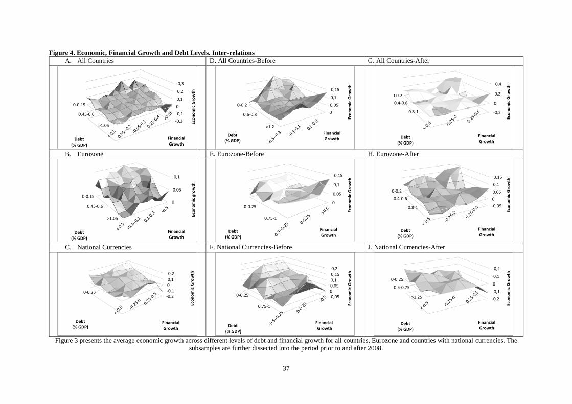
37
Figure 4. Economic, Financial Growth and Debt Levels. Inter-relations
A. All Countries D. All Countries-Before G. All Countries-After
B. Eurozone E. Eurozone-Before H. Eurozone-After
C. National Currencies F. National Currencies-Before J. National Currencies-After
Figure 3 presents the average economic growth across different levels of debt and financial growth for all countries, Eurozone and countries with national currencies. The
subsamples are further dissected into the period prior to and after 2008.
0-0.15
0.45-0.6
>1.05-0,2
-0,1
0
0,1
0,2
0,3
Debt (% GDP)
Eco
no
mic
Gro
wth
Financial Growth
0
0,05
0,1
0,15
0-0.2
0.6-0.8
>1.2
Financial Growth
Eco
no
mic
Gro
wth
Debt (% GDP)
-0,2
0
0,2
0,4
0-0.2
0.4-0.6
0.8-1
Financial Growth
Eco
no
mic
Gro
wth
Debt (% GDP)
0
0,05
0,1
0-0.15
0.45-0.6
>1.05
Debt (% GDP)
Eco
no
mic
gro
wth
FinancialGrowth
0
0,05
0,1
0,15
0-0.25
0.75-1
Financial Growth
Eco
no
mic
Gro
wth
Debt (% GDP)
-0,05
0
0,05
0,1
0,15
0-0.2
0.4-0.6
0.8-1
Financial Growth
Eco
no
mic
Gro
wth
Debt (% GDP)
-0,2-0,100,10,2
0-0.25
Financial Growth
Eco
no
mic
Gro
wth
Debt (% GDP)
-0,0500,050,10,150,2
0-0.25
0.75-1
FinancialGrowth
Eco
no
mic
Gro
wth
Debt(% GDP)
-0,2
-0,1
0
0,1
0,2
0-0.25
0.5-0.75
>1.25
Financial Growth
Eco
no
mic
Gro
wth
Debt (% GDP)

38
Table 1. Estimation Results Growth Financial Growth Debt Growth Total Before After Total Before After Total Before After
Interc 0.1725 0.1792 0.1802 0.1852 0.1548 -0.5993 -0.4198 -0.6750 -0.6244 -0.4124 0.2060 0.2342 0.2408 0.2387 0.2175 (4.76) (4.74) (4.29) (4.09) (3.17) (-2.32) (-1.56) (-2.09) (-1.82) (0.31) (1.49) (1.64) (2.44) (2.1) (1.61) E -0.0159 -0.0201 -0.0158 -0.0223 -0.01784 0.7433 0.8204 0.7952 0.8517 0.7763 0.0248 0.0197 0.1893 0.0221 0.0199 (-1.24) (-1.33) (-1.20) (-1.35) (-1.29) (3.01) (3.14) (3.09) (3.21) (3.11) (2.11) (2.17) (2.10) (2.37) (1,97) EU -0.0052 -0.0064 0.1849 0.1634 0.0147 0.0148 (-0.93) (-1.01) (1.94) (1.89) (1.88) (1.89) FG -1.1301 0.0057 -0.7675 -0.0195 0.1901 -0.5576 0.1033 -0.2874 0.0769 0.1134 (-1.67) (0.34) (-1.56) (-1.51) (2.6) (-0.74) (1.71) (-0.37) (1.17) (0.45) FG*E 0.0311 0.0313 0.0551 0.0513 -0.1548 -0.1450 -0.1325 -0.0280 -0.0531 -0.1838 (2.53) (2.46) (3.33) (2.83) (-2.09) (-1.88) (-1.67) (-0.29) (-0.54) (-0.75) FG*EU 0.1544 0.1484 0.6883 0.3971 (1.71) (1.52) (0.91) (0.51) G -0.7069 0.7946 -0.8482 0.7171 0.9850 -0.1842 -0.0348 -0.3240 -0.4537 0.5095 (-0.84) (1.52) (-0.94) (0.79) (1.37) (-0.36) (-0.12) (-0.64) (-0.92) (0.96) G*E 0.3015 3.4359 0.2750 3.3589 0.2758 0.2321 0.2349 0.2587 0.2577 0. 0877 (3.13) (3.39) (2.75) (2.01) (2.21) (5.06) (4.96) (4.21) (4.15) (1.21) G*EU 0.801 0.9378 0.1814 0.2488 (2.04) (2.03) (1.94) (2.05) DEB -0.5076 -0.0251 -0.4615 -0.0709 0.0464 0.5008 0.6366 0.6839 0.9190 0.2404 (-2.08) (-1.76) (-2.61) (-2.32) (0.69) (1.06) (2.96) (1.29) (3.09) (0.77) DEB*E 0.0075 0.0070 0.0190 0.0116 -0.0267 -0.5756 -0.5875 -0.4435 -0.4553 -0.4978 (1.95) (1.94) (2.27) (2.72) (-2.77) (-4.73) (-4.69) (-2.22) (-2.18) (-3.33) DEB*EU 0.4863 0.3844 0.2582 0.4242 (2.01) (2.18) (2.57) (2.89) DEB*HD 0.0221 0.0203 0.0380 0.0378 -0.0413 0.0268 0.0617 -0.2092 -0.1903 0.1920 (1.34) (1.17) (2.57) (2.33) (-2.37) (0.24) (0.53) (-1.35) (-1.17) (1.22) Exp -0.4183 -0.3956 0.2029 0.1915 -0.9926 0.4895 0.4379 0.186 0.5034 0.2062 -0.1832 -0.1846 -0.1870 -0.1478 -0.2757 (-1.51) (-1.37) (0.69) (0.59) (-2.1) (2.63) (2.26) (1.77) (1.61) (0.94) (-1.83) (-1.79) (-0.5) (-0.39) (-1.44) Rev 0.0839 0.0475 -0.3812 -0.4064 0.4025 -0.4599 -0.4241 -0.5361 -0.4835 -0.3220 0.3516 0.3146 0.1272 0.1549 0.4626 (0.31) (0.17) (-1.36) (-1.32) (0.81) (-2.59) (-2.3) (-1.91) (-1.67) (-1.33) (3.43) (3.28) (1.07) (1.04) (3.47) Sav 0.3908 0.3262 0.3989 0.3884 0.1937 0.3804 0.3633 0.5319 0.4665 -0.1794 -0.6771 -0.6556 -0.5671 -0.5793 -0.6765 (1.26) (1.01) (1.32) (1.18) (0.34) (1.82) (1.69) (1.81) (1.49) (-0.52) (-6.98) (-6.67) (-3.73) (-3.66) (-4.46) Trade 0.1946 0.1432 0.3977 0.3209 0.2193 -0.2560 -0.2554 -0.2640 -0.2555 -0.2855 (1.93) (1.38) (2.63) (2.05) (1.54) (-4.92) (-4.81) (-3.75) (-3.54) (-3.1) CAB 0.0178 0.0124 0.0251 0.0160 0.0120 (1.21) (0.81) (1.73) (1.03) (0.39) IR -0.0047 -0.0049 -0.0038 -0.0040 -0.0056 -0.0012 -0.0017 -0.0008 -0.0010 -0.0017 -0.0055 -0.0059 -0.0032 -0.0041 -0.0071 (-2.97) (-3.01) (-2.14) (-2.17) (-3.21) (-0.91) (-1.01) (-0.86) (-0.90) (-1.03) (-4.85) (-5.93) (-3.98) (-4.02) (-5.78) Inf 0.5111 0.4794 0.7033 0.6902 0.3609 -0.2522 -0.2091 -0.2169 -0.2075 -0.1589 (6.51) (5.82) (9.21) (8.24) (2.29) (-4.46) (-3.56) (-2.25) (-2.06) (-2.42) J 3.08 5.76 7.14 6.07 4.55 p (0.80) (0.45) (0.31) (0.41) (0.60)
Table 1 presents the estimation results for the model in equations (2.a), (2.b) and (2.c). Total refers to the full sample, while before and after include the estimation results for
the periods prior to and after 2008. An additional column is added in the “Total” and “Before” sections, where the same models are estimated, excluding the EU dummy
variable. All countries in the sample have joined the Eurozone by 2012, independently of their decision to join the euro. In order to avoid estimation problems, EU was excluded.
J-statistics is reported in pairs for the total, before and after period. All estimations include dummy variables to account for time and country fixed effects.
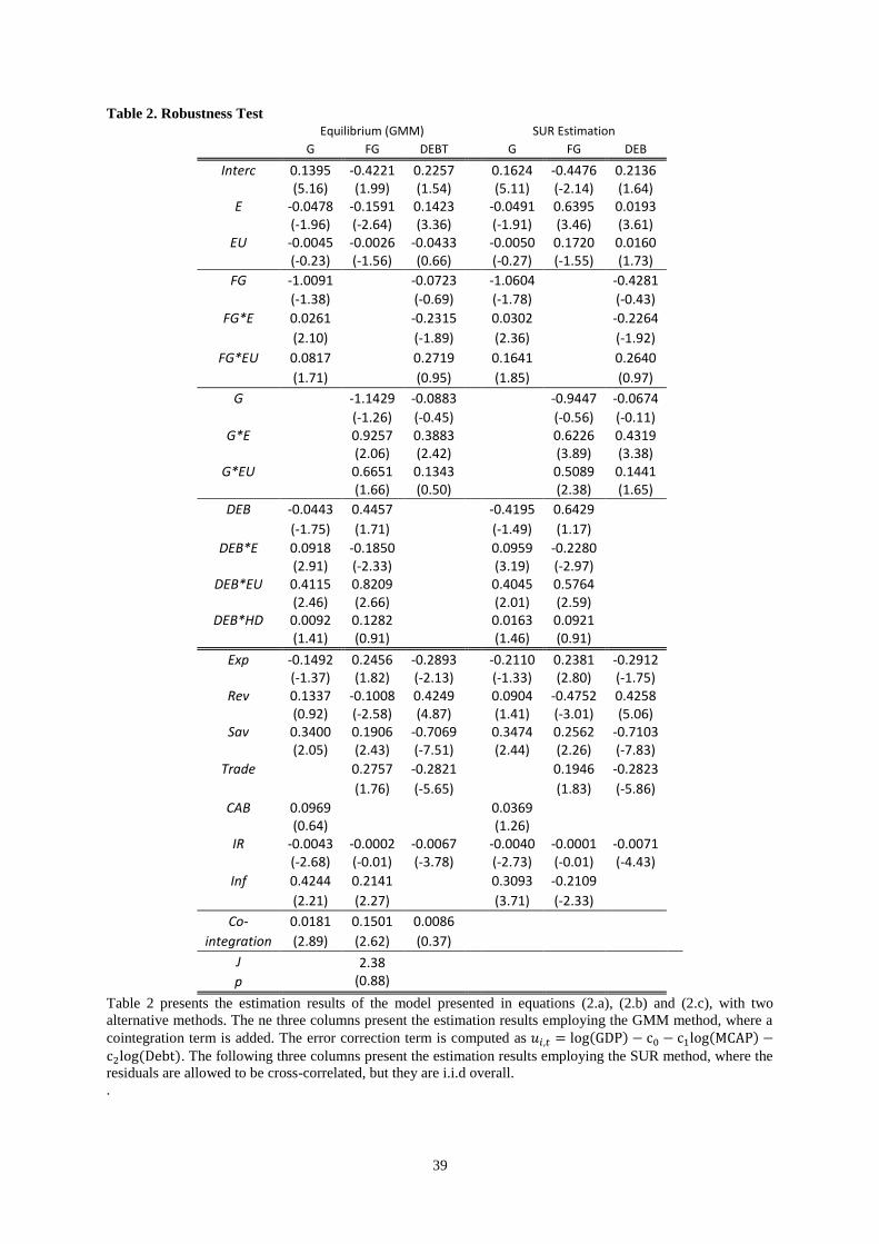
39
Table 2. Robustness Test
Equilibrium (GMM) SUR Estimation
G FG DEBT G FG DEB
Interc 0.1395 -0.4221 0.2257 0.1624 -0.4476 0.2136
(5.16) (1.99) (1.54) (5.11) (-2.14) (1.64)
E -0.0478 -0.1591 0.1423 -0.0491 0.6395 0.0193
(-1.96) (-2.64) (3.36) (-1.91) (3.46) (3.61)
EU -0.0045 -0.0026 -0.0433 -0.0050 0.1720 0.0160
(-0.23) (-1.56) (0.66) (-0.27) (-1.55) (1.73)
FG -1.0091 -0.0723 -1.0604 -0.4281 (-1.38) (-0.69) (-1.78) (-0.43)
FG*E 0.0261 -0.2315 0.0302 -0.2264 (2.10) (-1.89) (2.36) (-1.92)
FG*EU 0.0817 0.2719 0.1641 0.2640 (1.71) (0.95) (1.85) (0.97)
G -1.1429 -0.0883 -0.9447 -0.0674 (-1.26) (-0.45) (-0.56) (-0.11)
G*E 0.9257 0.3883 0.6226 0.4319
(2.06) (2.42) (3.89) (3.38)
G*EU 0.6651 0.1343 0.5089 0.1441
(1.66) (0.50) (2.38) (1.65)
DEB -0.0443 0.4457 -0.4195 0.6429 (-1.75) (1.71) (-1.49) (1.17)
DEB*E 0.0918 -0.1850 0.0959 -0.2280
(2.91) (-2.33) (3.19) (-2.97)
DEB*EU 0.4115 0.8209 0.4045 0.5764
(2.46) (2.66) (2.01) (2.59)
DEB*HD 0.0092 0.1282 0.0163 0.0921
(1.41) (0.91) (1.46) (0.91)
Exp -0.1492 0.2456 -0.2893 -0.2110 0.2381 -0.2912
(-1.37) (1.82) (-2.13) (-1.33) (2.80) (-1.75)
Rev 0.1337 -0.1008 0.4249 0.0904 -0.4752 0.4258
(0.92) (-2.58) (4.87) (1.41) (-3.01) (5.06)
Sav 0.3400 0.1906 -0.7069 0.3474 0.2562 -0.7103
(2.05) (2.43) (-7.51) (2.44) (2.26) (-7.83)
Trade 0.2757 -0.2821 0.1946 -0.2823
(1.76) (-5.65) (1.83) (-5.86)
CAB 0.0969 0.0369
(0.64) (1.26)
IR -0.0043 -0.0002 -0.0067 -0.0040 -0.0001 -0.0071
(-2.68) (-0.01) (-3.78) (-2.73) (-0.01) (-4.43)
Inf 0.4244 0.2141 0.3093 -0.2109 (2.21) (2.27) (3.71) (-2.33)
Co- 0.0181 0.1501 0.0086 integration (2.89) (2.62) (0.37)
J 2.38 (0.88)
p
Table 2 presents the estimation results of the model presented in equations (2.a), (2.b) and (2.c), with two
alternative methods. The ne three columns present the estimation results employing the GMM method, where a
cointegration term is added. The error correction term is computed as 𝑢𝑖,𝑡 = log(GDP) − c0 − c1log(MCAP) −c2log(Debt). The following three columns present the estimation results employing the SUR method, where the
residuals are allowed to be cross-correlated, but they are i.i.d overall.
.

40
Table 3. Correlation Matrix T
T-1
E1 E2 E3 E EU HD G E* G
EU* G
FG E* FG
EU* FG
DEB E* DEB
EU* DEB
HD* DEB
EXP REV SAV TRADE CAB INF
E 0.00 -0.03 0.05 0.96 0.40 0.36 -0.27 0.48 -0.08 -0.15 -0.10 -0.18 0.38 0.79 0.48 0.36 0.36 0.28 -0.11 -0.08 0.10 -0.16 EU 0.00 -0.04 0.08 0.50 0.84 0.19 -0.31 0.28 0.10 -0.12 -0.06 -0.15 0.31 0.41 0.57 0.19 0.24 0.13 -0.23 -0.10 -0.01 -0.21 HD -0.01 0.06 0.04 0.38 0.16 1.00 -0.07 0.25 0.00 -0.08 -0.07 -0.09 0.71 0.72 0.67 1.00 0.25 0.07 -0.31 -0.24 -0.16 0.00 G -0.05 -0.07 -0.09 -0.24 -0.37 -0.07 0.75 0.00 0.15 -0.06 0.03 -0.04 -0.34 -0.24 -0.39 -0.07 -0.33 -0.16 0.31 0.19 -0.07 0.36
E*G 0.02 -0.06 -0.01 0.58 0.24 0.29 -0.04 0.75 0.08 -0.12 -0.09 -0.13 0.15 0.42 0.22 0.27 0.04 0.11 0.11 0.04 -0.06 0.10 EU*G 0.03 -0.14 -0.06 0.09 0.29 0.06 0.12 0.21 0.75 -0.11 -0.01 -0.13 -0.10 0.02 0.02 0.05 -0.16 -0.03 0.18 0.12 -0.07 0.23
FG 0.04 0.02 -0.03 -0.08 0.00 -0.09 0.35 0.17 0.33 0.72 0.13 0.22 -0.16 -0.13 -0.10 -0.10 -0.21 0.00 0.29 0.17 -0.03 0.26 E*FG -0.01 0.06 0.00 -0.01 0.00 -0.07 0.16 0.29 0.17 0.15 0.72 0.16 -0.11 -0.08 -0.09 -0.08 -0.11 0.02 0.20 0.11 -0.02 0.14
EU*FG 0.03 -0.04 0.00 -0.06 0.04 -0.09 0.31 0.21 0.36 0.22 0.15 0.73 -0.10 -0.12 -0.07 -0.10 -0.14 0.01 0.23 0.17 -0.03 0.21 DEB 0.00 0.04 0.29 0.39 0.27 0.72 -0.25 0.20 -0.11 -0.08 -0.07 -0.06 0.99 0.76 0.90 0.72 0.53 0.25 -0.52 -0.47 0.03 -0.09
E*DEB 0.01 0.02 0.12 0.79 0.33 0.70 -0.23 0.39 -0.07 -0.12 -0.07 -0.13 0.74 0.97 0.76 0.71 0.45 0.26 -0.32 -0.38 0.08 -0.14 EU*DEB 0.00 0.02 0.20 0.53 0.55 0.68 -0.30 0.27 -0.03 -0.08 -0.08 -0.10 0.87 0.80 0.96 0.68 0.48 0.24 -0.47 -0.42 0.02 -0.18 HD*DEB -0.01 0.06 0.14 0.37 0.16 1.00 -0.08 0.24 0.00 -0.09 -0.08 -0.09 0.71 0.73 0.68 1.00 0.26 0.07 -0.31 -0.25 -0.16 0.00
EXP 0.03 0.00 0.03 0.33 0.19 0.25 -0.27 0.11 -0.17 0.03 0.02 0.01 0.57 0.44 0.52 0.25 0.94 0.75 -0.34 -0.24 0.09 0.03 REV 0.01 -0.01 0.03 0.31 0.06 0.08 -0.19 0.15 -0.15 -0.03 -0.03 -0.09 0.22 0.26 0.20 0.07 0.74 0.97 0.27 -0.18 0.19 -0.02 SAV -0.02 -0.03 -0.02 -0.04 -0.22 -0.29 0.16 0.05 0.05 -0.07 -0.05 -0.11 -0.59 -0.32 -0.57 -0.31 -0.32 0.25 0.90 0.18 0.08 0.00
TRADE -0.05 -0.04 -0.04 -0.06 -0.06 -0.24 0.20 0.04 0.14 0.05 0.06 0.08 -0.48 -0.37 -0.43 -0.25 -0.25 -0.16 0.22 0.98 0.02 0.27 CAB 0.02 0.00 0.02 0.09 -0.04 -0.13 0.02 0.04 0.01 0.02 0.03 0.01 0.03 0.08 0.01 -0.14 0.03 0.21 0.18 0.05 0.96 -0.17 INF -0.05 0.03 -0.04 -0.19 -0.29 -0.01 0.10 -0.13 -0.12 -0.05 0.01 -0.03 -0.10 -0.17 -0.20 -0.01 0.15 0.03 -0.09 0.21 -0.17 0.75 E1 1.00 -0.04 -0.14 E2 -0.04 1.00 0.09 E3 -0.14 0.09 1.00
RESIDUALS B-F-STAT COUNTRY 1.43
(0.09) 1.17
(0.26) 1.29
(0.16)
B-F-STAT PERIOD 1.27 (0.34)
1.64 (0.08)
1.61 (0.09)
UNIT ROOT-LEVEL -4.01 (0.00)
-6.85 (0.00)
-3.32 (0.00)
Table 3 presents the correlation matrix between the instrumental variables, the regressors and the GMM residuals, as well as the cross correlations of the GMM residuals. The
variables in the columns are the regressors, while the variables in the rows are the instruments, i.e. the first lag of the regressors. The values for the residuals are the cross-
correlations. In the bottom panel, residual diagnostics, from the full sample (Total) estimation results presented in Table 1, consist of the Brown-Forsythe (1974) test for cross-
sectional and period heteroskedasticity and the Im et al. (1997) unit root test. The null hypotheses are variance equality and the existence of a unit root, respectively.