financial globalization and the implications for … · financial globalization and the...
TRANSCRIPT
Financial globalization and the
implications for monetary and
exchange rate policy
Inaugural-Dissertationzur Erlangung des Grades
Doctor oeconomiae publicae (Dr. oec. publ.)an der Ludwig-Maximilians-Universität München
2008
vorgelegt vonJulia Bersch
Referent: Prof. Dr. Gerhard IllingKorreferentin: Prof. Graciela L. Kaminsky, PhDPromotionsabschlussberatung: 4. Februar 2009

Acknowledgements
The development and completion of this thesis would not have been possible withoutthe help and encouragement of numerous people. I would like to thank my supervisorGerhard Illing for his ongoing support. Also, I thank Graciela Kaminsky for giving methe opportunity to spend a year at the George Washington University and spuring myexcitement about international finance and applied economic work. I benefited verymuch from the joint work on financial globalization at the turn of the 20th century ofwhich chapter 4 is a part. I would also like to thank Dalia Marin who agreed to act asmy third examiner and who has supported me in many ways as my mentor within theLMU Mentoring Program.
I especially thank Uli Klüh for the inspiring and challenging discussions on all ar-eas of economics. Chapter 2 is the result of our mutual enthusiasm for contradictionsbetween observed monetary and exchange rate policies and economic theory and wasmainly developed during my stay in Washington, DC. Furthermore, I would like tothank my other present and former colleagues at the Ludwig-Maximilians-Universitätin Munich who have motivated me at different stages of my dissertation: Desislava An-dreeva, Josef Forster, Moritz Hahn, Frank Heinemann, Hannah Hörisch, Florian Kajuth,Katri Mikkonen, Nadine Riedel, Stephan Sauer, and Sebastian Watzka.
I would not be where I am without the outstanding experience and the contact withvarious people at the George Washington University. I thank the Economics departmentfor the hospitality and I am particularly indebted to Graciela Kaminsky, Yasya Babych,Marco Cipriani, Ana Fostel, Juan Ángel Jiménez Martín, Roberto Samaniego, TaraSinclair, and Pablo Vega-Garcia. Financial support by the German Academic ExchangeService (DAAD) and Stiftung Geld und Währung for my research stay at the GeorgeWashington University during the academic year 2006-2007 is highly appreciated.
Furthermore, I would like to thank the participants at various seminars and confer-ences for their helpful comments. I am also indebted to Agnès Bierprigl for excellentadministrative support and to Dirk Rösing for reliable IT assistance. Furthermore, Ithank the student research assistants at the Seminar for Macroeconomics, especiallyJohannes Kümmel for help with the data work for chapter 4.
My deepest thanks go to my family for all their support and love. Without them, thisthesis would not have been possible.
Munich, September 2008

Contents
1 Introduction 1
2 When countries do not do what they say: Systematic discrepancies be-tween exchange rate regime announcements and de facto policies 72.1 Introduction . . . . . . . . . . . . . . . . . . . . . . . . . . . . . . . . . . 72.2 Data . . . . . . . . . . . . . . . . . . . . . . . . . . . . . . . . . . . . . . 11
2.2.1 Exchange rate regimes and discrepancies . . . . . . . . . . . . . . 122.2.2 Explanatory variables . . . . . . . . . . . . . . . . . . . . . . . . . 15
2.3 Time trends and joint factors . . . . . . . . . . . . . . . . . . . . . . . . 172.4 Descriptive statistical analysis . . . . . . . . . . . . . . . . . . . . . . . . 18
2.4.1 Consistent regime combinations . . . . . . . . . . . . . . . . . . . 182.4.2 Intervening less than announced (ILA) . . . . . . . . . . . . . . . 192.4.3 Intervening more than announced (IMA) . . . . . . . . . . . . . . 22
2.5 Econometric analysis . . . . . . . . . . . . . . . . . . . . . . . . . . . . . 242.5.1 Methodological considerations . . . . . . . . . . . . . . . . . . . . 242.5.2 Baseline results . . . . . . . . . . . . . . . . . . . . . . . . . . . . 272.5.3 Robustness checks - sensitivity analysis . . . . . . . . . . . . . . . 282.5.4 Interpretation of the empirical evidence . . . . . . . . . . . . . . . 29
2.6 Conclusions and outlook . . . . . . . . . . . . . . . . . . . . . . . . . . . 342.A Appendix . . . . . . . . . . . . . . . . . . . . . . . . . . . . . . . . . . . 35
2.A.1 Data issues . . . . . . . . . . . . . . . . . . . . . . . . . . . . . . 352.A.2 Graphs and tables . . . . . . . . . . . . . . . . . . . . . . . . . . 37
3 Inflation targeting in small open economies 513.1 Introduction . . . . . . . . . . . . . . . . . . . . . . . . . . . . . . . . . . 513.2 Literature review and stylized facts . . . . . . . . . . . . . . . . . . . . . 533.3 Theoretical model . . . . . . . . . . . . . . . . . . . . . . . . . . . . . . . 57
ii

Contents
3.4 Implementing flexible inflation targeting . . . . . . . . . . . . . . . . . . 613.4.1 Basic model . . . . . . . . . . . . . . . . . . . . . . . . . . . . . . 613.4.2 Relaxing purchasing power parity . . . . . . . . . . . . . . . . . . 633.4.3 Relaxing purchasing power parity and uncovered interest rate parity 65
3.5 Comparison of the results . . . . . . . . . . . . . . . . . . . . . . . . . . 663.6 Conclusion . . . . . . . . . . . . . . . . . . . . . . . . . . . . . . . . . . . 693.A Derivation of the interest rate reaction function . . . . . . . . . . . . . . 71
4 Financial globalization in the 19th century: Germany as a financial center 744.1 Introduction . . . . . . . . . . . . . . . . . . . . . . . . . . . . . . . . . . 744.2 Capital markets, main players, and regulations in stock exchanges . . . . 77
4.2.1 Development of the German stock exchanges . . . . . . . . . . . . 774.2.2 Main players . . . . . . . . . . . . . . . . . . . . . . . . . . . . . . 794.2.3 Regulation of the stock exchanges . . . . . . . . . . . . . . . . . . 814.2.4 The process of issuance . . . . . . . . . . . . . . . . . . . . . . . . 83
4.3 International issuances . . . . . . . . . . . . . . . . . . . . . . . . . . . . 844.3.1 Data sources . . . . . . . . . . . . . . . . . . . . . . . . . . . . . . 854.3.2 Aggregate issuances . . . . . . . . . . . . . . . . . . . . . . . . . . 864.3.3 Individual foreign securities . . . . . . . . . . . . . . . . . . . . . 88
4.4 The role of external shocks . . . . . . . . . . . . . . . . . . . . . . . . . . 914.4.1 The model . . . . . . . . . . . . . . . . . . . . . . . . . . . . . . . 914.4.2 Estimation . . . . . . . . . . . . . . . . . . . . . . . . . . . . . . . 934.4.3 Robustness checks . . . . . . . . . . . . . . . . . . . . . . . . . . 95
4.5 Conclusion . . . . . . . . . . . . . . . . . . . . . . . . . . . . . . . . . . . 964.A Appendix: Figures and tables . . . . . . . . . . . . . . . . . . . . . . . . 97
Bibliography 114
iii

List of Figures
2.1 Taxonomy of de jure and de facto exchange rate regime combinations. . . 142.2 Exchange rate regimes and discrepancies over time - all countries. . . . . 382.3 Exchange rate regime discrepancies, financial openness, and world inflation. 39
4.1 Foreign issuances floated in the main financial centers. . . . . . . . . . . 974.2 Aggregate issuances floated in Germany. . . . . . . . . . . . . . . . . . . 994.3 Domestic and foreign issuances floated in Germany. . . . . . . . . . . . . 994.4 Foreign issues floated in Germany by sector. . . . . . . . . . . . . . . . . 1004.5 Domestic issues floated in Germany by sector. . . . . . . . . . . . . . . . 1004.6 Foreign and domestic issuances: bonds and equity by sectors. . . . . . . . 1014.7 Foreign securities by regions. . . . . . . . . . . . . . . . . . . . . . . . . . 1034.8 International lending: country composition, 1883-1897. . . . . . . . . . . 1044.9 Evolution of lending, 1883-1897. . . . . . . . . . . . . . . . . . . . . . . . 1054.10 Size of issues (in million British pounds). . . . . . . . . . . . . . . . . . . 1064.11 Principal components of the risk indicators. . . . . . . . . . . . . . . . . 1074.12 Interest rate differentials and private discount rate. . . . . . . . . . . . . 1084.13 Economic activity in Germany and the UK. . . . . . . . . . . . . . . . . 1094.14 Actual, fitted, and residual series, OLS (1). . . . . . . . . . . . . . . . . . 111
iv

List of Tables
2.1 Exchange rate regimes. . . . . . . . . . . . . . . . . . . . . . . . . . . . . 372.2 Country coverage. . . . . . . . . . . . . . . . . . . . . . . . . . . . . . . . 402.3 Data sources. . . . . . . . . . . . . . . . . . . . . . . . . . . . . . . . . . 412.4 Distribution of regime discrepancies by regions and country groups - ILA. 422.5 Distribution of regime discrepancies by regions and country groups - IMA. 432.6 ILA - tests for equality of means, medians, and distributions. . . . . . . . 442.7 IMA - tests for equality of means, medians, and distributions. . . . . . . 452.8 Pooled probit estimations for whole sample. . . . . . . . . . . . . . . . . 462.9 Pooled probit estimations for low income countries. . . . . . . . . . . . . 472.10 Pooled probit estimations for lower middle income countries. . . . . . . . 482.11 Pooled probit estimations for upper middle income countries. . . . . . . . 492.12 Pooled probit estimations for high income countries. . . . . . . . . . . . . 50
3.1 Interest rate reaction functions. . . . . . . . . . . . . . . . . . . . . . . . 67
4.1 Regional specialization in lending by the German stock exchanges, 1882-1892. . . . . . . . . . . . . . . . . . . . . . . . . . . . . . . . . . . . . . . 98
4.2 Pattern of foreign investment, 1883-1897. . . . . . . . . . . . . . . . . . . 1024.3 Data sources. . . . . . . . . . . . . . . . . . . . . . . . . . . . . . . . . . 1074.4 OLS regressions. . . . . . . . . . . . . . . . . . . . . . . . . . . . . . . . 1104.5 Robustness check: Tobit regressions. . . . . . . . . . . . . . . . . . . . . 1124.6 Further robustness checks. . . . . . . . . . . . . . . . . . . . . . . . . . . 113
v

Chapter 1
Introduction
The last three decades saw an extraordinary increase in cross-border capital flows and theelimination of barriers to free capital mobility. From a historical perspective, however,financial globalization is not a new phenomenon. A first wave of globalization started inthe middle of the 19th century and came to an abrupt end with World War I. This erawas characterized by a high level of integration reached again only in the 1990s. Obst-feld and Taylor (2004) characterize the development stages of global financial markets,connecting financial globalization in the 19th century with the present, by the exchangerate regimes and their consequences for capital flows. During the period from 1870 until1914, most countries successively adopted the classical gold standard and both capitaland labor markets were highly integrated. Policymakers followed a laissez-faire policyand few restrictions were imposed on financial markets. The following period, between1914 to 1945, was shaped by the two World Wars and the Great Depression leading toa rise in nationalism. During this time, policymakers increasingly focused on domesticgoals and pursued protectionist policies. Capital controls were put in place to pursuemonetary policy under more flexible exchange rates. As a consequence, private capi-tal flows ceased and national financial markets decoupled. The Bretton Woods systemcharacterized the period between 1945 and 1971 when currencies were linked througha system of fixed but adjustable exchange rates to the US-Dollar. However, significantcapital controls were in place and allowed countries some policy autonomy. Financialmarkets started to reintegrate; the process, however, was slow and mainly driven byinternational trade flows. After the breakdown of the Bretton Woods system in 1971,the developed countries moved towards more flexible exchange rates, capital accountrestrictions were successively lifted and capital increasingly flowed across borders. How-ever, Obstfeld and Taylor (2004) and others estimate that only in the 1990s did capitalmobility regain the degree achieved in 1914.
The development phases of global financial markets are strongly influenced by the
1

Chapter 1. Introduction
macroeconomic policy trilemma between free capital mobility, fixed exchange rates, andindependent monetary policy (Obstfeld and Taylor, 1998). High capital mobility is onlyreconcilable with fixed exchange rates when monetary policy is subordinated to thesegoals and with the pursuit of domestic goals only when the exchange rate is allowed toadjust to market conditions. The simultaneous achievement of domestic policy goals andexchange rate stability is only feasible when capital controls are in place. This trilemmahelps in understanding the ups and downs in financial integration.
After the breakdown of Bretton Woods and the financial liberalization in the 1970s,countries did not only experience increased real and nominal exchange rate volatilitybut also a variety of crises. Hence, financial integration poses significant challenges forpolicymaking. This thesis consists of three self-contained chapters studying financialglobalization and the implications for monetary and exchange rate policy. Chapter 2analyzes the empirical patterns underlying exchange rate regime announcements anddeviations in de facto policies and highlights the role of financial integration. Chapter 3focuses on the consequences of financial openness for monetary policy, more specifically,for inflation targeting. Financial globalization in the 19th century is the focus of chapter4 which examines the role of Germany as a financial center.
The increasing capital mobility and the emerging market crises in the 1990s led to thebipolar view and the observation of fear of floating which are the starting points for theanalysis in chapter 2. In accordance with the policy trilemma, the bipolar view statesthat countries should move towards the extreme corners of exchange rate flexibility byeither joining a monetary union, unilaterally adopting the currency of another country, oroperating a currency board, thereby, surrendering monetary independence, or by havinga freely floating exchange rate (Fischer, 2001). Intermediate exchange rate regimes,more precisely soft pegs, are not considered viable as long as capital is internationallymobile. Figure 2.2 illustrates that for the two reference years of Fischer, 1991 and 1999,there was indeed a shift from announced (de jure) intermediate exchange rate regimes tofixed and flexible ones. A more continuous appraisal of regime choices, however, is muchless clear-cut and the high share of de facto intermediate regimes throughout the 1990sfurther challenges the bipolar view. Furthermore, there is widespread agreement thatit is not uncommon for countries to declare a different exchange rate regime than theyactually follow (Calvo and Reinhart, 2002). However, the observation of fear of floatingraises the question: If countries indeed have good reasons to manage their exchange rateactively, why would they not announce a regime consistent with optimal policies?
2

Chapter 1. Introduction
Starting from this observation, chapter 2 studies the apparent disconnect betweenwhat countries announce to be their exchange rate regime and what they de facto imple-ment.1 Discrepancies between announcements and de facto policies are a quantitativelyimportant phenomenon describing policies in roughly 40 per cent of all countries. Nev-ertheless, there is still a lack of understanding of actual patterns and underlying reasons.The aim of chapter 2 is to fill some of the gaps present in existing studies. Starting fromthe hypothesis that observed regime discrepancies are systematic, i.e., not the result ofrandom policy errors, it provides evidence for the existence of systematic elements inobserved regime discrepancies by linking them to specific country characteristics. Themain empirical finding is that countries tend to communicate exchange rate regimes atthe corners of the flexibility spectrum, i.e., either fixed or flexible regimes, but to op-erate intermediate regimes. Whether countries announce a fixed or flexible exchangerate depends on country characteristics, in particular related to trade structure, finan-cial development, and financial openness. Also, countries at different stages of economicand financial development differ in the nature of regime discrepancies. Finally, thedecreasing frequency of countries managing their exchange rate less than announcedand the increasing occurrence of countries intervening more than announced align withbroader economic trends and developments worldwide related to financial globalizationand changes in monetary policy design.
The separation of communication and implementation of exchange rate policy mayprovide policymakers with an additional tool to tackle challenges from financial global-ization. In an era of high financial integration and capital mobility, countries may not berestrained to choose between pursuing an independent monetary policy and stable ex-change rates while refraining from capital controls. For numerous countries the optimalpolicy may be neither of the two extremes but a combination. However, as intermedi-ate exchange rate regimes are difficult to communicate, see, e.g., Frankel, Fajnzylber,Schmukler and Serven (2001), countries may find it optimal to use exchange rate regimeannouncements and a diverging implementation as a second best policy.
The empirical patterns point at the role of monetary policy within the macroeconomicpolicy trilemma. Especially emerging market economies that adopted inflation targetingand, hence, announce flexible exchange rates, manage their exchange rate more thanannounced. This is not surprising as the exchange rate is one, if not the most importantprice in an open economy. As small open economies steadily move away from fixed
1Chapter 2 is based on joint work with Uli Klüh.
3

Chapter 1. Introduction
exchange rates towards a more independent monetary policy, open economy aspectsbecome increasingly important in analyzing monetary policy. The literature frequentlyresorts to two simple concepts in international economics, purchasing power parity anduncovered interest rate parity, to describe the relation between prices, interest rates, andexchange rates between countries. Although the empirical relevance of these two conceptsis subject to an ongoing debate, they are frequently used in theoretical models. Chapter3 examines the implications of these concepts on the implementation of monetary policy.Monetary policy is analyzed in an open economy version of the standard New Keynesianframework described by Clarida, Galí and Gertler (1999). More specifically, flexibleinflation targeting as characterized by Svensson (2007) is the monetary policy underscrutiny. A central bank operating under flexible inflation targeting is not only concernedabout stabilizing the inflation rate around the target but additionally about stabilizingthe real economy.
Purchasing power parity is based on the idea that international goods arbitrage keepsthe relative purchasing power of two currencies constant over time. Uncovered interestrate parity is derived from arbitrage in international financial markets according to whichthe nominal exchange rate adjusts to interest rate differentials. Chapter 3 contributesto the literature by analyzing in a unified framework how these two concepts and pos-sible alternatives used in the literature affect monetary policy. More specifically, theimplications for the interest rate reaction function describing monetary policy responsesto shocks under flexible inflation targeting are examined. Thereby, useful insights intothe consequences of using the simple concepts of purchasing power parity and uncoveredinterest rate parity in monetary policy analysis are provided.
The main insight is that the interest rate reaction function is affected when purchasingpower parity and uncovered interest rate parity are relaxed. As long as purchasing powerparity holds, monetary policy reacts only to cost-push shocks and excess-demand shocks.If, however, purchasing power parity does not hold, monetary policy also fully offsets theeffects of foreign shocks. Furthermore, not the direction but the strength of the interestrate response to cost-push shocks and excess-demand shocks is affected. Whether therelation between interest rates and exchange rates is described by uncovered interestrate parity or in the more generic way proposed by Ball (1999) does affect both to whichtype of shocks monetary policy responds and how strong the response is.
Then, chapter 4 turns to the earlier period of financial globalization. Here, financialglobalization in the late 19th century is analyzed from the perspective of Germany
4

Chapter 1. Introduction
as a financial center.2 Feis (1930) describes Europe as the world’s banker during the19th century, lending capital to countries around the world. The main capital exporterwas Great Britain, followed by France and Germany, and their capital cities were themain financial centers intermediating credit through their stock exchanges and bankers.London emerged as an important financial center following the Napoleonic Wars andbecame the undisputed international financial center in the 1870s. Paris was anotherimportant financial center in the 19th century, second only to London, and contributedsignificantly to the financing of foreign governments and railroads since the 1820s. At thebeginning of the 19th century, Frankfurt was the financial center of Germany and also ofimportance on an international level. Following the political and economic restructuringsduring the mid 1860s, Berlin developed as Germany’s financial center. The constructionof the railroads and the development of heavy industries in the 19th century posed newchallenges to the financial sector until then dominated by private bankers. The immensedemand for capital of these newly developing sectors required the use of a broader capitalbase and the introduction of tradable securities allowed private investors to put theirsavings into productive use. The stock exchanges and the newly created joint-stockbanks contributed significantly in expanding financial intermediation.
The capital exports of a country are one way to quantify its importance as an inter-national financial center. While the characteristics of British capital flows have beenstudied extensively, France and Germany as smaller capital exporters have been inves-tigated to a lesser degree and to our knowledge no extensive data sets are available.Chapter 4 contributes to the literature by providing new insights into the role of Ger-many as a financial center. The development and functioning of the German capitalmarkets in the late 19th and early 20th century are described with a special focus on theintermediation of foreign securities provided by the stock exchanges. Then, the capitalintermediated by German stock exchanges in the thirty years prior to World War I andits composition, especially of foreign investment, is analyzed. The main findings are thatneighboring countries were the main recipients of German capital and that the perceivedriskiness of a country was an important determinant in investment decisions. Borrow-ers frequently floated their securities simultaneously in the main financial centers. Togive a first idea of the integration between financial centers at that time, we examineif foreign issuances in Germany reacted to shocks in the other financial centers. Themain finding is that the conditions in financial markets in Germany and relative to other
2This chapter is based on joint work with Graciela Kaminsky.
5

Chapter 1. Introduction
financial centers mattered for the amount of foreign securities floated in Germany. Morespecifically, France and Germany seem to be substitute financial centers for borrowingcountries while the relation between Germany and the UK is unclear.
The present thesis provides insights into financial globalization and the challenges itposes. Increasing capital mobility calls policymakers to choose between the pursuit ofexchange rate objectives and domestic goals. However, optimal choices are likely to beneither of the two extremes and chapter 2 provides evidence of actual policy choices aim-ing at intermediate solutions. Chapter 3 studies how the implementation of monetarypolicy is affected by the financial and economic openness of an economy. By analyzingfinancial globalization in a historical perspective, the last chapter spurs our understand-ing of fundamental patterns in financial markets and integration. All three chaptersare part of a broader research agenda that aims at improving our understanding of thepieces jointly forming the macroeconomic policy trilemma, how they relate theoreticallyand empirically. This broader research agenda can hopefully be pursued in the future.
6

Chapter 2
When countries do not do what they say:Systematic discrepancies between exchangerate regime announcements and de factopolicies1
2.1 Introduction
A look at the exchange rate regime choices of 133 countries over the period 1973-2004reveals a striking phenomenon: nearly one half of all observations show inconsistenciesbetween what countries officially declare to be their chosen regime, and what countriesactually do with respect to exchange rate management. Moreover, the exact nature ofdeviations seems to follow secular trends. In the early 1970s, countries that managedtheir exchange rate less than what could be expected given their announcement domi-nated the picture, but their share has decreased over time. The frequency of observinga country intervening more than announced, however, has been increasing, in particularin the 1990s and 2000s, a trend that has recently attracted substantial attention frompolicymakers and academics (see, for example, Barajas, Erickson and Steiner (2008)).Only the proportion of consistent regimes has remained roughly constant.
The finding that countries often do not follow their exchange rate regime announce-ment has important implications for research and policy. Most importantly, studies onthe relationship between exchange rate policies and economic development (Aghion, Bac-chetta, Ranciere and Rogoff, 2006)2, financial stability (Bubula and Ötker-Robe, 2003),or the emergence of inflation targeting as a preferred monetary policy regime for emerging
1This chapter is based on joint work with Uli Klüh.2Genberg and Swoboda (2005) show that both announcement and actual exchange rate policy matter
for the economic performance of a country.
7

Chapter 2. When countries do not do what they say: Systematic discrepancies betweenexchange rate regime announcements and de facto policies
markets (Goldstein, 2002) will remain incomplete without an understanding of regimediscrepancies. It is therefore not surprising that recent years saw the emergence of awhole body of literature reviewing the proper definition, nature and implication of dejure and de facto exchange rate regime choices, including the seminal contributions byReinhart and Rogoff (2004) and Levy-Yeyati and Sturzenegger (2003a; 2003b; 2005).
We know that discrepancies between announced and de facto exchange rate policiesare common, but we have a poor understanding of the underlying reasons. Most im-portantly, and contrary to some statements in related contributions, the literature onthe fear of floating phenomenon initiated by Calvo and Reinhart (2002) does not pro-vide an answer to the question: If countries indeed have good reasons to manage theirexchange rate actively, why would they not announce a regime consistent with optimalpolicies? Put differently, while the literature offers several theoretical explanations whycountries dislike exchange rate fluctuations3 and why countries may be forced to abandonfixed exchange rate regimes4, we know little about systematic and potentially voluntarydeviations between announced and actual exchange rate policies.
Related literature
To the best of our knowledge, there are only four contributions that address this ques-tion more or less directly. Carmignani, Colombo and Tirelli (2006) study the role ofpolitical factors in explaining regime choices more broadly, also touching upon the issueof “broken promises”. The authors argue that, in general, countries attempt to choosede facto and de jure regimes consistently, except for those cases in which political in-centives lead to some form of cheating or dynamic inconsistency. While the authors donot attempt to provide an “immediate theoretical interpretation” for their findings, animplicit assumption of the study seems to be that the stronger the incentive to peg orfloat the stronger the incentive to do so consistently, and that deviations from this policyeither mirror politically motivated or wrong decision-making.
Von Hagen and Zhou (2006) view regime gaps as part of an error-correction mechanismthat allows governments to adjust their actual policies in case the de jure regime hasbeen chosen sub-optimally. Such a view, however, does not explain why de jure regimesare chosen sub-optimally in the first place. This is particularly troublesome since manyof the significant explanatory variables used in their regression analysis do not change
3See, in particular, the literature on fear of floating started by the seminal contribution of Calvo andReinhart (2002).
4See the literature on currency crises, e.g. Krugman (1979) and Obstfeld (1996).
8

Chapter 2. When countries do not do what they say: Systematic discrepancies betweenexchange rate regime announcements and de facto policies
much over time, implying that they could have been taken into account by policymakersex ante. Similarly, a dynamic error-correction mechanism should allow for the possibilityof adapting the de jure regime to changing circumstances or policy misjudgments. Such amechanism, however, cannot be identified in the data, since regime discrepancies displaysubstantial persistence.
Alesina and Wagner (2006) analyze the relationship between regime discrepanciesand the quality of institutions. They find that countries with low institutional qualitytend to announce pegs, but are unable to sustain them. At the same time, countrieswith high institutional quality tend to either consistently float or to actively manage theexchange rate without announcing it. Alesina and Wagner (2006) interpret this behavioras indication of a signaling game, in which countries with relatively good institutions tryto distinguish themselves from countries with low institutional quality. While signalingmight indeed play an important role in explaining regime discrepancies, the evidenceprovided to support this view suffers from two major shortcomings. First, proxies forinstitutional quality display very little variation over time. Consequently, the qualityof institutions cannot explain trends in the data. Second, Alesina and Wagner do notexplain why countries with low-quality institutions announce a peg in this signalingsetting. This, in turn, also calls into question the validity of the signaling strategymore generally, since policymakers confronted with low-quality institutions have a clearincentive to imitate their counterparts, given that the expected reputation gain of anannounced but not consistently implemented peg is likely to be small. Consequently,a crucial question becomes how markets and the public actually react to attempts of“signaling by inconsistency”.
Starting from this last observation, Barajas, Erickson and Steiner (2008) study thereaction of emerging market bond spreads to de jure and de facto exchange rate regimechoices. They test the hypothesis that countries classified towards a flexible exchangerate regime are rewarded with lower spreads. As to the potential reasons for fearingto declare a more interventionist regime, the authors argue that markets might have asubjective bias against officially fixed exchange rate regimes. This bias could be eitherdue to the fact that fixed exchange rates have received much of the blame for the emergingmarket crises in the 1990s, or be the result of the perceived advantage of operating aninflation targeting regime. Their main finding is that contrary to the working hypothesisboth the announcement of a more heavily managed regime and the actual intensityof intervention lower spreads significantly. This leaves the puzzle why countries are
9
Chapter 2. When countries do not do what they say: Systematic discrepancies betweenexchange rate regime announcements and de facto policies
reluctant to declare that they are intervening given that international capital marketsdo not reward either de facto or de jure floaters.
Aim and outline of the study
While none of the mentioned contributions offers a clear-cut theoretical explanationfor the observed discrepancies, they all start from certain implicit presumptions aboutthe underlying phenomenon. Implicit in the analysis is either the view that deviationsbetween announced and implemented policies are the result of sub-optimal policies, orthe reflection of some underlying political or institutional reality, or a subjective biasin market perceptions. Apart from Alesina and Wagner (2006), existing contributionsusually assume that inconsistencies to one side or the other can be analyzed separately.Also, issues of policy communication are treated very lightly, in spite of the fact thatinflation targeting (a communication framework) is sometimes suspected to underpinmore recent trends in the data. Finally, trends over time are usually not studied buttaken for granted, in that the fear of floating phenomenon represents the motivation forthe inquiry.
The aim of this study is to fill some of the gaps present in existing studies. Firstand foremost, we believe that the existing knowledge of time-series and cross-sectionalpatterns of regime discrepancies is highly incomplete. Before testing specific hypothesesabout the reasons for and the consequences of different arrangements, it is thereforeessential to first identify empirical regularities that could form the basis of establishing aset of robust stylized facts. To this end, we extend the existing de jure regime classifica-tion for the years 2000 until 2004 and pay particular attention to regional patterns andclustering, methodological issues in defining regimes, as well as country characteristics.
While our main interest lies in establishing a series of patterns without starting fromrestrictive presumptions, it is obviously impossible to operate in a theory vacuum: Asindicated in the title, our working hypothesis is that observed regime discrepancies aresystematic, i.e. not the result of random policy errors. In fact, one of our main objectivesis to provide evidence for the existence of systematic elements in observed regime dis-crepancies, by linking them to specific country characteristics. Put differently, we showthat there indeed are country characteristics that systematically lead decision-makersto favor one type of deviation from consistency. For the case of regime discrepancies,this either means that there are actual or perceived benefits from not declaring that acertain intervention strategy is being followed, or from declaring a policy that will not
10

Chapter 2. When countries do not do what they say: Systematic discrepancies betweenexchange rate regime announcements and de facto policies
be always followed.In providing evidence for systematic discrepancies between declaration and imple-
mentation, we highlight the importance of regime announcements as elements of a morecomprehensive communication framework for monetary and exchange rate policies. Atfirst glance, the idea that inconsistencies between announcements and policies couldserve a purpose seems difficult to maintain, as markets and the public would either an-ticipate ex ante or punish ex post deviations from announcements. This, however, isnot necessarily the case if one takes into account the potentially constructive role ofambiguity. As pointed out in Best (2005), a work closely related to ours, ambiguity canserve a purpose by keeping policy regimes flexible enough to adapt to changing economicand political circumstances as well as to re-equilibrate conflicting interests.
Our main empirical finding is that countries tend to communicate exchange rateregimes at the corners of the flexibility spectrum, i.e. either fixed or flexible regimes, butto operate intermediate regimes. Whether countries announce a fixed or a freely floatingexchange rate regime depends on country characteristics, in particular related to tradestructure, financial development, and financial openness. Countries at different stages ofeconomic and financial development differ in the nature of regime discrepancies. Finally,the decreasing frequency of countries managing their exchange rate less than announcedand the increasing occurrence of countries intervening more than announced align withbroader economic trends and developments worldwide.
The rest of the chapter is organized as follows. Section 2.2 describes the data; section2.3 analyzes time trends and joint factors of regime discrepancies. In section 2.4 adescriptive statistical analysis of deviations of de facto from announced exchange rateregimes is presented. Section 2.5 contains the econometric analysis and an interpretationof the findings. The last section concludes and gives an outlook on future research.
2.2 Data
Our sample covers 133 countries from 1973 to 2004. The countries are classified ashigh, upper middle, lower middle, or low income countries according to the classificationprovided by the World Bank for 2004. Table 2.2 in the appendix lists the countriesincluded in the sample.
11

Chapter 2. When countries do not do what they say: Systematic discrepancies betweenexchange rate regime announcements and de facto policies
2.2.1 Exchange rate regimes and discrepancies
Our analysis focuses on the announcement and actual implementation of exchange ratepolicy. Until 1999, the announcement strategy is measured by the de jure exchange rateregimes as categorized by Ghosh, Gulde and Wolf (2002) based on the IMF’s AnnualReport on Exchange Arrangements and Exchange Restrictions (AREAER) data. TheAREAER contains the intended exchange rate policies that member countries reportedto the IMF on an annual basis5. To cover more recent trends, we extend the de jureregime classification for the years 2000-2004, allowing us to employ a new and uniquedataset. To update regime announcements, we start with information from AREAER,which since 1998 does not report de jure classifications anymore, but contains additionalverbal information that often allows identification of a country’s stated regime choice. Wecombine this information with other sources, such as IMF staff reports and central banksreports, to complete and cross-check our data. Due to data limitations and consistencyconcerns, we only distinguish between fixed, intermediate, and flexible exchange rateregimes, consolidating the more detailed classification of Ghosh et al. (2002) into thesethree groups.6
We capture the actual intervention strategy through the de facto exchange rate regimeclassification (“natural” classification) developed by Reinhart and Rogoff (2004). Oneof the key characteristics of this classification method is the use of data on paralleland dual exchange rate markets. These market-determined exchange rates are oftena better measure of actual and expected future monetary policy. In addition, theyusually capture the economic impact of exchange rate changes more directly than officialexchange rates, and do thus display a closer relationship to other variables of interest. Toidentify exchange rate regimes, Reinhart and Rogoff separate observations with unifiedexchange markets from those with parallel or dual markets. The de facto classificationof the former is then obtained by statistical verification of regime announcements or,in cases without announcement, by direct statistical interference, which is also usedfor country-year observations with dual or parallel markets. The statistical evaluation
5In most of the years covered by our sample, countries were required to assign themselves to oneof four categories (fixed, limited flexibility, managed floating, and independently floating). For anexposition of the IMF classification and changes over time, see e.g. Reinhart and Rogoff (2002).Ghosh et al. (2002) extended these groups to fifteen buckets, see table 2.1.
6The exact mapping is shown in table 2.1. Our coarse classification corresponds to the one usedby Ghosh et al. (2002) with the exception of the secret basket pegs which we include into theintermediate category instead of the fixed one. We explain the reasons in section 2.A.1 in theappendix.
12

Chapter 2. When countries do not do what they say: Systematic discrepancies betweenexchange rate regime announcements and de facto policies
measures de facto exchange rate behavior via the mean absolute monthly change inthe market-determined (official or parallel) nominal exchange rate, based on a five-yearmoving window.
Reinhart and Rogoff (2004) use fourteen buckets for their regime classification. How-ever, as the categorizations of de jure and de facto exchange rate regimes are not con-gruent, we regroup them into three broad categories: fixed, intermediate, and floatingregimes; the precise mapping is presented in table 2.1.7 The Reinhart and Rogoff datasetcovers 153 countries for the period 1946-2001. For the years 2002-2004 we use the up-date of the “natural” classification provided by Eichengreen and Razo-Garcia (2006).8
Compared to other de facto classifications, e.g., the widely used dataset by Levy-Yeyatiand Sturzenegger (2005), the IMF de facto classification used in Bubula and Ötker-Robe (2002), or the recent compilation by Klein and Shambaugh (2006), the Reinhartand Rogoff dataset has the advantage of offering the most extensive country and timecoverage9. Moreover, we see at least two methodological reasons to prefer the Reinhartand Rogoff classification. First, the use of market-determined exchange rates seems toprovide a much better picture of the underlying economic policies than official rates doand all other de facto classifications rely on official exchange rates. Reinhart and Rogoffpoint out that parallel markets are frequently used as back-door floating, in most caseswith simultaneous exchange controls. In these situations, the use of official rates wouldstrongly bias the results towards observing consistency between de jure and de factofixed regimes. Second, Reinhart and Rogoff take the perspective of larger and morecontinuous regimes by using a five-year moving window, making it less likely to wronglyidentify a one-time devaluation or shock as a regime change.
A drawback of the Reinhart and Rogoff approach is that only the unconditional volatil-ity of the nominal exchange rate is used, so measures of intervention intensity such asinternational reserve and interest rate changes are not taken into account. Thus, noclear distinction can be made between exchange rate stability arising from active poli-
7Our three groups correspond to the coarse classification provided by Reinhart and Rogoff (2004) whencategories 2 and 3 are subsumed as intermediate and 4 and 5 as floating regimes.
8This data covers the years 1990-2004. If observations not classified by Reinhart and Rogoff (2004)during that period were classified by Eichengreen and Razo-Garcia (2006) we use the improved data.
9The IMF de facto classification is available only since 1990. The Levy-Yeyati and Sturzenegger (2005)classification suffers from a substantial number of unclassified observations due to a lack of data,especially on international reserves. Klein and Shambaugh’s (2006) classification distinguishes onlybetween fixed and floating exchange rates which we consider insufficient as intermediate regimes arequantitatively important and different in nature from fixed and floating regimes as discussed lateron. Frankel and Wei (2008) propose a novel synthesis of techniques to determine de facto exchangerate regimes.
13

Chapter 2. When countries do not do what they say: Systematic discrepancies betweenexchange rate regime announcements and de facto policies
cies or from the absence of shocks, leading to a potential overestimation of de facto fixedexchange rate regimes. Although Reinhart and Rogoff provide evidence that potentialbiases are limited, the possibility should be kept in mind. Nonetheless, we consider theReinhart and Rogoff classification the one most suitable to the questions we post. Tocheck robustness, we test the sensitivity of our results against Levy-Yeyati and Sturzeneg-ger’s (2005) classification, which includes the volatility of international reserves, but doesnot take into account interest rate policy.
Figure 2.1: Taxonomy of de jure and de facto exchange rate regime combinations.
Communication Framework
Intervention strategy
de jure fixed
de jure intermediate
de jure flexible
de facto
fixed C IMA IMA
de facto
intermediate ILA C IMA
de facto
flexible ILA ILA C
With respect to the concrete alternatives policymakers are facing, it is useful to startwith a taxonomy of de jure and de facto regime combinations (figure 2.1). Our aim is tofind empirical regularities related to a country’s choice to locate either to the northeast(with a strategy combination in which policymakers intervene more than announced, orIMA) or to the southwest (with a strategy combination in which policymakers interveneless than announced, or ILA) of the main diagonal (consistency between de jure and defacto, or C).10 Obviously, conscious choice will never explain fully the observed combi-
10We consider the labels fear of floating and fear of pegging used by other authors inappropriate inthe present context. Consider fear of floating as introduced by Calvo and Reinhart (2002): itdescribes the desire of a country to limit exchange rate fluctuations but it does not embrace why
14
Chapter 2. When countries do not do what they say: Systematic discrepancies betweenexchange rate regime announcements and de facto policies
nation of the jure and de facto regimes, since policymakers will usually not take intoaccount all the possible future states of the world. In fact, the de jure exchange rateregime is an ex ante stated policy intention while the de facto regime resembles the expost policy decisions. However, we show that there indeed are country characteristicsthat systematically lead decision-makers to favor one type of deviation from consistency.
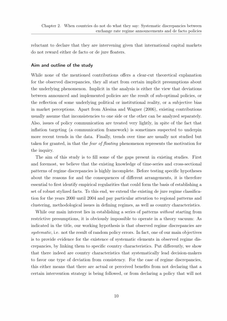
2.2.2 Explanatory variables
We use a wide set of macroeconomic, structural, institutional, and financial indicators toidentify those characteristics that are associated with regime discrepancies of a specifickind. The complete dataset is described in table 2.3. Our choice of variables is mainlyguided by previous studies on the determinants of exchange rate regimes, as we expectthat many of the variables relevant for the choice of de jure and de facto regimes sep-arately can also explain part of the variation in regime discrepancies. Underlying thisexpectation is our view that regime discrepancies are a reflection of conflicting views andagendas on exchange rate policies that give ambiguity a potentially constructive role.
Starting with trade-related variables, we measure the degree of openness as the sum ofexports and imports relative to GDP. The importance of primary commodity exports isproxied by the sum of agricultural raw materials, ores, metals, and fuel exports as a shareof all merchandise exports while trade concentration is measured as the share of totalexports to the three largest trading partners. Furthermore, we include the three yearcentered standard deviation of the terms of trade growth rate to measure the volatilityof an economy’s external environment.
The degree of financial market development seems to influence the choice of exchangerate policies (Husain, Mody and Rogoff, 2005). Stages of development are capturedby two different types of country classifications: the World Bank concept of incomegroups and the Morgan Stanley Capital International Index (MSCI) concept of emergingmarkets and developed economies. We consider the income categories of the World Bank(low, lower middle, upper middle, and high income) based on GNI per capita the mostsuitable indicator of economic development. The low and middle income countries are
countries do not announce their actual intervention strategy. Fear of pegging has been used byAlesina and Wagner (2006) and by von Hagen and Zhou (2006) to describe a situation where thede jure exchange rate regime is more rigid than the de facto one (what we label ILA). However,Levy-Yeyati and Sturzenegger (2005) have used the term to describe situations in which a countryhaving a de facto fixed exchange rate regime is unwilling to explicitly announce it (fear of floatingin a narrow sense).
15

Chapter 2. When countries do not do what they say: Systematic discrepancies betweenexchange rate regime announcements and de facto policies
often referred to as developing countries. The MSCI distinguishes between developing,emerging market, and developed economies. The separating feature of emerging marketeconomies (EMEs) from other developing countries is the level of market capitalization.The MSCI differentiates between EMEs and advanced economies using a combination ofmacroeconomic and financial indicators, such as GDP per capita, the extent and qualityof financial regulation and restrictions, and perceived investment and/or country risk.Thus, starting from a threshold level of financial market development, the separatingline between the country groups is drawn based on financial sector and institutionalstrength. We mainly use the World Bank groups for our analysis while controllingfor the robustness of our findings with respect to the alternative MSCI categorization.Additionally, we use a time-varying MSCI dummy as explanatory variable, which is equalto 1 from the year of inclusion of a country in the MSCI onwards and 0 otherwise.
Two alternative measures of financial openness are used to account for the distinctionbetween de facto and de jure policies.11 The degree of financial openness and the actualintegration into international financial markets are very likely to affect a country’s choiceof an exchange rate regime and of how to communicate this choice. When capitalmarkets are open and financial integration is high, the potential for market disciplineincreases. If capital controls are in place or the capital account is open but no capitalactually flows across borders, these possibilities are limited or absent and policymakershave additional leverage on domestic monetary policy. As de jure measure, we use theindicator of financial openness constructed by Chinn and Ito (2006) which is based onthe intensity of official restrictions on capital account transactions as reported in theAREAER. To capture the degree of actual financial integration, we follow Kose et al.(2006) and construct an additional measure based on the sum of external assets andliabilities over GDP, using the data provided by Lane and Milesi-Ferretti (2007).
In addition to variables related to trade and financial structure and openness, we assessthe role of country size (measured by population or GDP) and the level of economicdevelopment (GDP per capita). In some of the regressions in section 2.5 year dummiesare included. We also look at regional dummies to account for the geographic clusteringfound in the statistical analysis.
11For a discussion of how to measure financial openness and financial integration, see, e.g., Kose, Prasad,Rogoff and Wei (2006).
16

Chapter 2. When countries do not do what they say: Systematic discrepancies betweenexchange rate regime announcements and de facto policies
2.3 Time trends and joint factors
As already pointed out by Reinhart and Rogoff (2004) and Rogoff, Husain, Mody, Brooksand Oomes (2003) the type of discrepancy between announced and de facto policy hasbeen subject to an important shift over time, from “labeling something as a peg whenit is not, to labeling something as floating when the degree of exchange rate flexibilityhas in fact been very limited” (Reinhart and Rogoff, 2004, p.37). However, neither ofthe two publications has pursued this aspect further, so it is worthwhile to lay out someimportant patterns we find in the data. Over the whole sample period (1973-2004) only60 per cent of the total observations12 involve consistent regimes while 22 per cent areassociated with ILA and 18 per cent with IMA. However, as illustrated in figure 2.2c,the occurrence of ILA has been decreasing over time, from 28 per cent in the 1970s to 10per cent in the 2000s, while the frequency of observing IMA has been increasing, from 10per cent in the 1970s to 27 per cent in the 2000s. The proportion of consistent regimeshas remained roughly constant.
It is instructive to look at the de facto and de jure exchange rate regimes accompanyingobserved discrepancies. Not surprisingly, the higher the proportion of de jure fixed orfloating regimes, the higher is the potential for ILA and IMA, respectively. For the wholesample, 47 per cent of the total observations are de jure fixed, 33 per cent intermediate,and 20 per cent floating exchange rate regimes. However, the distribution of de factoregimes differs substantially: only 36 per cent of all observations are associated withfixed exchange rate regimes (11 percentage points less than de jure), 49 per cent withintermediate (16 percentage points more), and 15 per cent with floating regimes, whichcan be separated into 10 per cent of freely falling and, thus, only 5 per cent truly freelyfloating regimes. Note that it is important to separate out the freely falling category,characterized by (very) high inflation rates which lead to important distortions (Reinhartand Rogoff, 2004).13
As figure 2.2a illustrates, de jure regimes exhibited a clear trend from fixed towardsflexible regimes: fixed regimes declined from 66 per cent in the 1970s to 42 per cent inthe 2000s, while floating regimes increased from 7 per cent in the 1970s to 33 per centin 2000s. In contrast, the distribution of de facto regimes remained more stable (figure
12With observation we mean a country-year data point.13The freely falling category encompasses observations when the twelve-month inflation rate is equal
to or exceeds 40 per cent per annum and, additionally, includes the first six months following anexchange rate crisis if it marked a transition from a peg or quasi-peg to a managed or independentfloat. (Reinhart and Rogoff, 2004, p.3-4)
17

Chapter 2. When countries do not do what they say: Systematic discrepancies betweenexchange rate regime announcements and de facto policies
2.2b). Fixed regimes decreased from 44 per cent in the 1970s to 31 per cent in the 1980sand increased to 40 per cent in the 2000s. The floating regimes increased from 8 percent in the 1970s to 13 per cent in the 2000s while intermediate exchange rate regimesremained at 40 to 50 per cent of all observations.14
Another interesting feature is that discrepancies between announced and de factoexchange rate policies are highly persistent over time, as documented by von Hagen andZhou (2006). Discrepancies are not single observations that occur from time to time butthey seem to follow systematic patterns. Some countries display ILA or IMA over nearlythe whole sample period, while others moved from ILA to IMA following the overalltrend, sometimes transitioning through consistent combinations. Most of the countriessticking to one type of discrepancies have changed their de facto and/or de jure policiesquite frequently. The transition from announcing more rigid regimes than de factofollowed towards announcing more flexible regimes has been accompanied by increasedfinancial liberalization and financial integration (see figure 2.3a and 2.3b). While theyears around the transition from ILA towards IMA were characterized by particularlyhigh world inflation rates, they decreased to extraordinary low levels afterwards (seefigure 2.3c).
2.4 Descriptive statistical analysis
2.4.1 Consistent regime combinations
Before analyzing discrepancies between announced and de facto exchange rate regimes itis useful to point out some stylized facts and country characteristics which may inducepolicymakers to explicitly choose consistent regime combinations. A first observationis that the overwhelming part of consistent regimes are fixed (50 per cent), closelyfollowed by intermediate exchange rate regimes (39 per cent) while only 11 per cent ofthe observations are related to floating regimes.
One reason for this observation is that extreme forms of fixed regimes (monetaryunions, dollarization, and currency boards) are chosen to signal the impossibility ofdeviation from the announced regime. Failures to follow the announcements are imme-
14Additionally, we observe important differences in regime choices between country groups, specificallybetween high, upper middle, lower middle, and low income countries. For a graphical analysis ofde facto and de jure exchange rates regimes as well as resulting discrepancies, see Bersch and Klüh(2007).
18

Chapter 2. When countries do not do what they say: Systematic discrepancies betweenexchange rate regime announcements and de facto policies
diately visible and the cost of exit is extremely high.15 Indeed, these regimes represent asignificant share of consistent observations.16 Extreme forms of fixed regimes are mostlychosen by very small and open economies, such as the members of the CFA French franczone and the Eastern Caribbean Dollar zone, or by countries with a long history of highinflation and crises such as Argentina and Ecuador, but also by advanced economies inthe EMU.
Among the consistent free floaters one can distinguish two main country groups. Thefirst group consists of countries that have experienced crises and high inflation ratesover the majority of years in the sample. These countries usually are characterized asfreely falling within the de facto classification, sometimes showing short and infrequentevents to stabilize expectations through exchange-rate based stabilization programs. Thesecond group consists of highly developed countries like Australia, Japan, and the UnitedStates.
2.4.2 Intervening less than announced (ILA)
Over the whole sample the number of ILA observations is surprisingly high. Althoughthe occurrence of ILA clearly declined over time, still 14 per cent of all observationsare related to ILA in the 1990s and 2000s. How can this widespread phenomenon beexplained? The announcement of a rigid exchange rate regime is a means to importcredibility for tough monetary policy from the anchor country. Then, pursuing a moreflexible exchange rate policy, e.g., through frequent parity adjustments, should result ina loss of credibility. As a consequence, any new attempt to build up credibility via arigid exchange rate regime will most likely prove even harder. Consequently, the existingliterature would not consider ILA to be the result of actual policy choices. Instead, itwould be considered a crisis phenomenon resulting from the actual inability of a countryto pursue the rigid policy (inability to peg).17
Before taking a closer look at the economic characteristics of the countries that havea history of ILA, it is useful to point out two aspects of the data that in our view havenot received enough attention in related contributions. When studying the countriesidentified as those operating under ILA, we were surprised about the sensitivity of the
15The exit of Argentina from its currency board arrangement in 2001/2002 started a new discussionabout the transparency and disciplining capacity of this exchange rate arrangement.
16The share is 29 per cent of the consistent regime combinations until 1999; afterwards we do not havedetailed information.
17This is also the perspective taken in Alesina and Wagner (2006).
19

Chapter 2. When countries do not do what they say: Systematic discrepancies betweenexchange rate regime announcements and de facto policies
results with respect to (i.) the classification of some of the more rare or exotic exchangerate regimes, specifically secret basket pegs, and (ii.) the choice of reference currenciesfor cooperative systems. Not accounting for this sensitivity leads to potentially severemeasurement errors and implies an often counter-intuitive classification with respect tothe regime discrepancy.18
Turning to the characterization of countries that are mainly associated with ILA,exploring our data allowed us to identify a number of interesting empirical regularities.Most importantly, it is apparent from our data that ILA is not just a crisis phenomenonor a mere inability to peg. While the de jure exchange rate regimes predominatelyrelated to ILA are fixed regimes (77 per cent), the dominating intervention strategiesare de facto intermediate exchange rate regimes with 64 per cent of all ILA observations.Only 33 per cent of all ILA observations were characterized as de facto freely falling.Since the latter can be interpreted as a proxy for crises episodes and, more generally, forthe inability to implement restrictive monetary policies, crises and high inflation episodesaccount for an important, but limited proportion of ILA observations.19 The view thatILA represents an inability to stick to the announced rigid exchange rate regime is thusonly partially supported. In this respect, it is worth mentioning that such “failures”only result in ILA if policymakers do not change their announced exchange rate regimeduring the crisis. One reason for such a behavior may be some form of announcementinertia, e.g., due to the time-consuming political process necessary to change the legalframework.20
An important corollary to this observation is that de facto intermediate regimes areover-represented in the ILA group, as intermediate exchange rate regimes constitute“only” half of the de facto regime observations. Although intermediate exchange rateregimes account for a significant proportion of intervention strategy choices, there seems
18Secret basket pegs are exchange rate regimes where the national currency is pegged to a basket ofat least two currencies based on country-specific criteria with the weights of the currencies and/orthe composition of the basket being secret and possibly variable (Ghosh et al., 2002). A detaileddiscussion of the distinguishing features of intermediate regimes is provided in the appendix 2.A.1.
19Of all ILA observations 28 per cent are indeed preceded or accompanied by a currency crisis andthis proportion is higher than for IMA and consistent observations, 21 and 17 per cent, respectively.These figures refer only to 1975-1997 due to data availability.
20As the de jure regime is reported only once a year (ex ante) to the IMF, it is sufficient that policy-makers are unable to follow their announced policy to generate a single ILA observation. Also, anannounced change in the exchange rate regime may not be reflected in the official de jure classifica-tion when it occurs over the year. However, if at least two consecutive years of ILA are observed,other forces have to be in place, e.g., some form of announcement inertia. Note that only 22 ILAobservations out of 812 are neither preceded nor followed by an ILA or missing observation.
20

Chapter 2. When countries do not do what they say: Systematic discrepancies betweenexchange rate regime announcements and de facto policies
to be a preference of not communicating such choice, and rather operate against thebenchmark of an announced peg, or announced float, as argued below. Only half of allde facto intermediate exchange rate regime observations are actually announced, andcountries choose instead a strategy of more intervention (a fixed exchange rate regime)in 28 per cent of the cases, resulting in ILA, or of no intervention (a floating regime),resulting in IMA.21
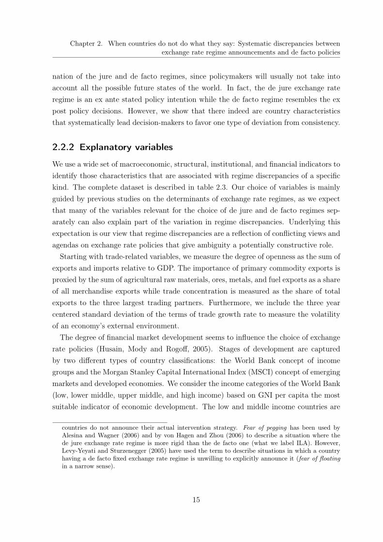
A closer look at the countries predominately characterized by ILA reveals some furtherinteresting patterns. First, with respect to geographic distribution, low and middle in-come countries in the Middle East and North Africa show a particularly strong tendencyof following less rigid exchange rate policies than announced, see table 2.4. The high pro-portion of observations involving ILA in this country group is mirrored in the dominanceof ILA in OPEC countries. Controlling for the higher prevalence of de jure fixed regimesdoes not qualitatively alter these results. The high incidence of ILA among Middle East-ern and North African as well as OPEC countries raises the question of whether therecould be a potential link between the share of primary exports, in particular fuel export,and the occurrence of ILA. While we do not want to jump to a conclusion prematurely, itis interesting to note that primary exports belong to the group of variables for which thedata shows a significant difference in group means, medians, and distribution consideringall observations, see table 2.6. However, fuel exports show significantly different means,medians, and distribution only for ILA observations related to de jure fixed regimes (seetable 2.6, lower panel). Moreover, countries with a large share of mineral exports seemto follow ILA policies in most world regions. For example, a significant share of the ILAobservations in Sub-Saharan Africa, approximately 25 per cent, is related to the casesof Botswana with its dominant diamond industry and Zambia, long dominated by cop-per. Similarly, most large mineral exporters in South America, excluding Chile, have atleast one substantial data spell characterized by ILA. Finally, Norway is among the fewEuropean countries that show a substantial ILA spell, together with its Scandinavianneighbors.
We performed parametric and non-parametric tests for the equality of means, medi-ans, and distributions for several economic characteristics of countries that have ILAobservations against consistent and IMA observations. As the assumption of a normaldistribution of economic variables seems strong, the comparison of medians and dis-
21However, if an intermediate exchange rate regime is announced, the likelihood of actually observing itis relatively high: 70 per cent of the announced intermediate regimes are consistent and, therewith,it is the exchange rate category with the highest proportion of consistent regimes.
21

Chapter 2. When countries do not do what they say: Systematic discrepancies betweenexchange rate regime announcements and de facto policies
tributions may provide a more meaningful picture of average performance in the twogroups than the comparison of means. For robustness, we provide all three. The results,reported in table 2.6, suggest that variables related to inflation, trade openness, andfinancial openness as well as to institutional quality do differ between the groups oper-ating under ILA and non-ILA regime combinations, in addition to the export structuredescribed above. The inflation rates for ILA observations are significantly higher whiletrade openness and the import share are significantly lower. Financial openness, both dejure and de facto, and institutional quality (across different measures) are significantlyhigher for non-ILA observations. Measures of economic development (GDP per capita,in USD and PPP corrected) and economic size (GDP and population), however, showonly a weak relationship with ILA observations.
2.4.3 Intervening more than announced (IMA)
Over the whole sample period from 1973 until 2004 we observe IMA in only 18 percent of all observations. However, while ILA has been decreasing, the frequency ofobserving IMA has been increasing over time. The literature on fear of floating startedby the seminal work of Calvo and Reinhart (2002) provides numerous explanations forthe reluctance of countries to tolerate substantial fluctuations in the exchange rate. Themost prominent reasons are significant balance-sheet effects, mostly due to high liabilitydollarization, and high pass-through from exchange rates to prices.22 Nevertheless, thisliterature does not offer a comprehensive justification for countries’ choices to announcea more flexible exchange rate regime. If there are no credibility gains through theannouncement of a rigid exchange rate regime, policymaker may refrain from exchangerate commitments altogether and, thus, retain full flexibility.23
Analyzing under which circumstances countries predominantly exhibit IMA revealssome interesting patterns. Remarkably, the relative frequency of observing IMA differsbetween country groups at different stages of economic and financial development, andthere has been an important shift over time. Over the whole sample period, advancedeconomies have the highest frequency of IMA (34 per cent of the observations in thecountry group) followed by EMEs with 21 per cent, see table 2.5. Developing countriesonly choose IMA in 11 per cent of all cases. However, while until the beginning of22Rationales for fear of floating are provided by Hausmann, Panizza and Stein (2001), Lahiri and Végh
(2001), Caballero and Krishnamurthy (2001), and others.23Rogoff et al. (2003) find that only countries at a low level of financial development are able to gain
low inflation credibility through the announcement of rigid exchange rate regimes.
22

Chapter 2. When countries do not do what they say: Systematic discrepancies betweenexchange rate regime announcements and de facto policies
the 1990s IMA is nearly an exclusive phenomenon of advanced economies, it is rapidlygaining importance in EMEs.24 Especially lower middle income countries display a highand increasing share of IMA observations. Additionally, IMA observations are clearlydominated by de facto intermediate exchange rate regimes, which account for 66 per centof the total IMA observations, with little time variation.25 Thus, de facto intermediateregimes are over-represented in the IMA observations as they are in the ILA ones. Withrespect to announcement choices, floating regimes dominate accordingly (72 per cent).
These figures suggest that IMA is in important ways related to the choice of intermedi-ate intervention strategies. Furthermore, the level of economic and financial developmentto which the difference between country groups can ultimately be pinned down seems tomatter. It is interesting to note, however, that IMA is more widespread amongst lowermiddle than upper middle income countries. Among the countries showing considerableIMA spells we can additionally identify the following two groups. (i) EMU membersprior to the adoption of the euro in 1999, and (ii) advanced economies which have welldeveloped financial markets and are very open, economically and financially: Switzer-land, Canada, and New Zealand. The considerable increase of IMA as regime choicein recent years, in particular for EMEs, suggests that worldwide economic trends suchas capital account liberalizations, increasing capital flows, and declining inflations ratemay be of importance for its explanation as discussed in section 2.3.
For a better understanding of the key macroeconomic variables related to IMA, welook again at differences in means, medians, and distributions of central economic andfinancial variables between the countries operating under IMA and those with consistentor ILA regimes. The results are reported in table 2.7. For IMA observations, inflationrates are significantly lower, institutional quality and financial openness significantlyhigher.26 The differences in other variables are not significant across specifications.Furthermore, conditional on having announced a flexible exchange rate regime, countrieswith IMA have a significantly higher degree of trade openness and of trade concentration.24This change comes along with the adoption of inflation targeting frameworks in EMEs which involve
the announcement of a free float. Due to the particular economic and financial situation in manyEMEs, however, they are reluctant to tolerate excessive exchange rate volatility, thus exhibiting fearof floating and mostly also IMA. This is the subject of ongoing research. The apparently revertingtrend in 1999 is entirely due to the EU member countries adopting the euro which through a verystrict implementation of the rule-based de jure regime to fulfill the Maastricht criteria have exhibitedIMA.
25Among the de facto intermediate exchange rate regimes, crawling bands dominate with 30 per centof all IMA observations closely followed by managed floats (26 per cent).
26The large difference of average inflation rates conditional on having announced a flexible regime isdue to the freely falling observations in the non-IMA groups.
23

Chapter 2. When countries do not do what they say: Systematic discrepancies betweenexchange rate regime announcements and de facto policies
For the whole sample, the degree of trade concentration and imports to GDP ratios arelower for IMA observations. Overall, countries operating under IMA have lower primaryexports, are richer, and economically more developed while conditioning on de jureflexible regimes does not deliver significant differences.
2.5 Econometric analysis
To give a more accurate picture of the potential links between country characteristicsand regime discrepancies, we regress indicators of regime discrepancies on a broad setof variables using a pooled probit approach. After briefly discussing methodology andexplanatory variables, we outline the main results of our empirical exercise. We thendiscuss the robustness of our results and provide an interpretation of the results.
2.5.1 Methodological considerations
Our main interest lies in explaining the choice variable y∗, defined as the desired combi-nation of communication and intervention strategy. y∗ is a latent variable that dependson a vector of explanatory variables x
y∗ = G(xβ) + u
where u is an error term independent of x with mean zero. Instead of the unobservedy∗, we have data on the combination y of de jure and de facto exchange rate regimes.If the announced exchange rate regime is more rigid than the de facto regime, y equals-1 (ILA), if the two regimes are of the same degree of flexibility, y equals 0 (consistent),and if the announced regime is more flexible than the de facto one, y equals 1 (IMA).
Given this characterization, one way to proceed would be to use a multinomial re-sponse model. Instead we opt for a binary approach, merging consistent and IMA (ILA)observations as control group when analyzing ILA (IMA), and then using pooled probitestimation techniques. One reason not to use a multinomial approach is that this wouldrequire assuming independence of irrelevant alternatives, a condition that is unlikely tohold in the present case. Similarly, there is no natural ordering for the three alterna-tives, precluding the use of an ordered discrete choice model. Finally, by using a binaryspecification, we make our results comparable to the related contribution of Alesina andWagner (2006), who also compare ILA and IMA separately against the remaining obser-
24

Chapter 2. When countries do not do what they say: Systematic discrepancies betweenexchange rate regime announcements and de facto policies
vations.27 We do not use fixed effects estimations since many of our variables display noor very little variation over time. Also the use of a random effects estimator appears in-appropriate because we have a very large country sample which cannot be considered asrandomly drawn from the underlying population. Finally, we prefer to follow an explicitbinary choice model and then test our results against a linear probability model.
In addition to using the complete dataset, we create sub-samples, assessing the prob-ability that a country chooses a certain regime combination conditional on observingcertain de facto or de jure regimes. For both IMA and ILA, we first code the endoge-nous variable as 1 if we observe a specific discrepancy, and 0 otherwise. However, withthis approach we cannot disentangle the general incentives to announce a more fixed ormore flexible exchange rate regime. Therefore, in a second set of regressions, we willrestrict our sample to those observations involving de jure fixed (in the case of ILA) orflexible (in the case of IMA) regimes, and then look at characteristics of countries stickingto their announcement against those that do not. As noted above, both types of discrep-ancies are dominated by intermediate de facto policies combined with the announcementof corner solutions, i.e., fixed or floating exchange rate regimes. Thus, in a last set ofregressions we confine our sample to those observations involving de facto intermediateregimes and analyze what distinguishes countries with a de jure fixed (floating) regimefrom others.
As our aim is to identify a set of stylized facts, we use a broad set of potentialexplanatory variables and report best regression results, both in terms of robustnessand significance. Starting from the observations in section 2.4, we focus on the degreeof trade openness, the importance of primary commodity exports, as well as measuresof price stability, financial openness, and economic and financial development.
With respect to price stability, it is worth pointing out that the inflation rate is notonly a likely determinant of exchange rate regime choices and possible deviations of defacto from announced policies but is itself determined by the exchange rate regime.28
However, the exchange rate policy is likely to have only a lagged effect on the inflationrate. Thus, by using the lagged yearly CPI inflation rate, the scope for endogeneity isreduced. Furthermore, the effect of the inflation rate on exchange rate regime choicesis most likely not linear. Very high inflation rates have a different effect than moderate27In contrast to our approach, Alesina and Wagner differentiate between degrees of distance between de
facto and de jure policies, i.e., conditional on de jure flexible regimes, de facto intermediate regimesare treated differently than de facto fixed, and apply an ordered logit approach.
28Ghosh et al. (2002) and Kuttner and Posen (2001) study the macroeconomic effects of differentexchange rate regimes.
25

Chapter 2. When countries do not do what they say: Systematic discrepancies betweenexchange rate regime announcements and de facto policies
rates of price increases.29 Therefore, we also include a (lagged) high inflation dummyfor observations involving inflation rates of 40 per cent or more on an annual basis.Additionally, we include the ratio of imports to GDP to proxy the extent to whichdomestic prices are exogenously determined.
In our baseline specifications, we do not include measures of institutional quality,mainly because of the effect on sample size: Including standard measures of institu-tional quality reduces the sample substantially and systematically since data is onlyavailable for a sub-set of countries and only starting in 1984. However, to account forthe importance of institutional quality and the evidence provided by Alesina and Wagner(2006), we run robustness checks, the results of which are reported below.
As pointed out above, we use two measures of financial openness: a de jure and ade facto measure. As with inflation, regime choices may affect financial integration andthe incentives to change official restrictions on capital account transactions. On the onehand, if a country has a floating exchange rate regime, capital restrictions should notplay a role. On the other hand, goods and capital markets dislike substantial uncer-tainties with respect to exchange rate fluctuations. While financial openness affects acountry’s exchange rate policy choice, exchange rate policy is likely to affect actual finan-cial integration only with some delay. Still, to mitigate potential endogeneity problemswhen using measures of financial openness as explanatory variables, we lag them by oneperiod.
To account for important differences in the relation between regime choices and coun-try characteristics at different stages of economic and financial development, we performseparate regressions for each country group. It is likely that economic and financialstructure matter in different ways for countries at different stages of financial and/oreconomic development. For example, the stability implications of financial and tradeopenness change as domestic financial markets develop, additional liquidity, insurance,hedging, and risk diversification services are provided, and credit constraints are relaxed.The development of financial markets and institutions thus influences an economy’s abil-ity to deal with and profit from international capital flows, and vice versa. A minimumlevel of financial development seems to be required to attract capital flows but countrieswithout deep financial markets may be restricted in their capacity to absorb large capitalinflows. Furthermore, if a country has important external financial positions, it is moresensitive to exchange rate volatility but it may suffer additional volatility if the positions29High inflation is defined as inflation rates of 40 per cent or more per year following the definition of
the World Bank, and Reinhart and Rogoff (2004) for the freely falling category.
26

Chapter 2. When countries do not do what they say: Systematic discrepancies betweenexchange rate regime announcements and de facto policies
are frequently changed due to high capital flows.
2.5.2 Baseline results
The results of the pooled probit estimations for ILA and IMA for the whole sample andseparated by income groups are reported in tables 2.8 and 2.9 - 2.12, respectively.30 Afirst important insight is that the separate treatment of countries at different stages ofeconomic and financial development is important. For example, higher terms of tradevolatility increases the probability of ILA when a de jure regime is announced but has nosignificant effect otherwise when considering all countries jointly. When analyzing coun-tries at different stages of economic development separately, either through sub-samplesor interaction terms, higher terms of trade volatility is associated with a significantlyhigher probability for ILA and a lower probability for IMA for lower middle incomecountries. For high income countries it reduces the likelihood of both IMA and ILA,thus making consistent combinations more likely.
With respect to other trade-related variables, a higher degree of trade openness reducesthe probability of IMA, except for high income countries, and increases the probabilityof ILA for low and lower middle income countries while reducing it for upper middleincome countries. More interestingly, higher exports of primary commodities increasethe probability of consistent regime combinations (reduces it for both IMA and ILA)for low income countries. For lower middle income countries, however, the effect tendstowards the opposite: higher primary commodity exports increase the probability ofILA. Conditional on a de facto intermediate exchange rate regime, upper middle incomecountries tend also significantly towards ILA.
In general, high inflation makes ILA more and IMA less likely, supporting the viewthat crises and inability to peg are part of the explanation. However, lower middle incomecountries having de facto intermediate regimes and having experienced high inflation inthe previous year tend to be more cautious and to announce a flexible exchange rateregime.
Turning to financial openness, a de jure more open capital account significantly reducesthe probability of ILA. Furthermore, it tends to increase the probability of IMA for allcountry groups except low income countries. The evidence for de facto financial opennessis mixed, with the exception of high income countries for which a higher de facto financial
30We use the same regressors for all sets of estimations whenever possible to avoid additional selectionproblems due to data availability.
27

Chapter 2. When countries do not do what they say: Systematic discrepancies betweenexchange rate regime announcements and de facto policies
openness makes IMA significantly more and ILA less likely.A listing in the MSCI index, a proxy for the crossing of a critical level of financial
market development, increases the likelihood of experiencing inconsistent regime com-binations, both ILA and IMA, for lower middle income countries while reducing it forupper middle income countries. Conditional on de facto intermediate regimes, all coun-tries have a higher probability of announcing a more flexible exchange rate regime whenincluded in the MSCI. More specifically, the inclusion in the MSCI increases the prob-ability of IMA for upper middle income countries while increasing the probability ofdeviations from consistent regimes for lower middle income countries.
Furthermore, we get the following insights from the regressions conditional on spe-cific exchange rate regime announcements. On the one hand, conditional on de jurefixed regimes, higher terms of trade volatility, lower trade openness, and higher de factofinancial openness reduce the likelihood of ILA for high income countries. However,lower middle income countries are more likely to have ILA when included in the MSCIindex, when they have higher primary commodity exports, and higher terms of tradevolatility. The probability of ILA is higher for low income countries when they havelower primary commodity exports and high inflation in the previous year. On the otherhand, conditional on the announcement of a flexible exchange rate regime, higher tradeopenness, lower terms of trade volatility, and higher financial openness (both de factoand de jure) make it more likely for high income countries to operate under IMA. Uppermiddle income countries are more likely to have IMA when they are not included in theMSCI, are less open to trade, have low inflation, and higher de jure financial openness.For lower middle income countries, higher primary commodity exports, lower terms oftrade volatility, and low inflation are positively related with IMA. Lower trade opennessand de jure financial openness makes IMA more likely for low income countries.
2.5.3 Robustness checks - sensitivity analysis
As to methodological robustness, we checked all our results with a linear probabilitymodel and used interaction terms instead of sub-samples and the signs of the coefficientsremained unchanged. Furthermore, regressions for narrower samples, excluding smallcountries with a population of less than one million and considering only a number ofeconomically important countries, confirmed our key results. Neither did the exclusionof the observations since 2000 for which we construed the de jure exchange rate regimesqualitatively alter the results. As previously discussed, freely falling observations may
28

Chapter 2. When countries do not do what they say: Systematic discrepancies betweenexchange rate regime announcements and de facto policies
distort our results. However, regressions excluding these observations did not changethe main results.
Alesina and Wagner’s (2006) results suggest that institutional quality is pivotal forexplaining discrepancies between exchange rate regime announcements and de facto poli-cies. As institutional quality data is only available for a sub-set of countries and since1984, the sample is substantially and systematically changed. Nevertheless, we ran ro-bustness checks including indicators of country risk (composite risk rating), bureaucraticquality, and democratic accountability. The main insight is that better institutional qual-ity significantly increases the likelihood of IMA while institutional quality has no effecton the probability of ILA across different specifications. Furthermore, the signs of thecoefficients of variables related to IMA are mostly unchanged while primary commodityexports (related to ILA) are not significantly related to regime discrepancies anymore.This, however, is not surprising since ILA is predominantly observed during the 1970sand 1980s for which institutional quality data is not available and which are thus notincluded.
The results, however, are not very robust to the use of the de facto exchange rateregime classification of Levy-Yeyati and Sturzenegger (2005). The main reason is thatthe classification differs fundamentally from Reinhart and Rogoff’s (2004), the correla-tion is only 0.5. Therefore, we consider only observations for which the two classifica-tions coincide. This reduces the number of observations involving deviations betweenannouncements and de facto policies significantly.31 However, using only observationsfor which Reinhart and Rogoff and Levy-Yeyati and Sturzenegger agree in their de factoclassifications, we can broadly confirm our results. As discussed in section 2.2, we nev-ertheless consider the Reinhart and Rogoff de facto classification the more appropriatefor our questions.
2.5.4 Interpretation of the empirical evidence
To interpret these findings, it is essential to first go back to the two fundamental in-sights of the descriptive analysis above. First, there is a clear tendency for countries toannounce either a fixed or floating exchange rate regime. This move to the corners ofthe exchange rate flexibility spectrum, however, is not mirrored in actual interventionstrategies. Countries with a higher degree of de jure financial openness and countries
31 The overall frequency of ILA and IMA is reduced from 22 to 7 per cent and from 18 to 13 per cent,respectively.
29

Chapter 2. When countries do not do what they say: Systematic discrepancies betweenexchange rate regime announcements and de facto policies
that cross a critical level of financial market development tend to intervene more thanannounced. At the same time, higher inflation and a higher share of primary commodi-ties make it more likely that countries allow their exchange rate to float more thanannounced.
Second, the tendency towards announcing extreme exchange rate regimes goes handin hand with a tendency towards de facto intermediate regimes. Countries for whichan intermediate exchange rate regime is the optimal choice face the following problem.Intermediate exchange rate regimes have the reputation of being highly vulnerable tocrises.32 Partly as a consequence, communicating intermediate regimes is complicated:In principle, policymakers could announce the parameters that will guide day-to-daypolicy decisions, for example, through publication of the threshold levels of shocks thatwill trigger intervention. This, however, involves substantial communication risks sincethe states of the world that would have to be specified ex ante would be too large tobe effectively displayed in a transparent manner. In addition, communicating the inter-mediate nature of the regime would reduce its benefits substantially, since the desiredflexibility would be reduced by any attempt to formalize the intervention strategy. Fur-thermore, there will be always situations in which the expectations created by a certainregime announcement will be frustrated. A policymaker aware of this might want tochoose a communication framework that does not aim at preventing the impossible, butat providing a suitable framework for explaining deviations. It may therefore be a viablealternative to announce a floating or fixed exchange rate regime as benchmark to explainpolicy deviations against a clear arrangement. Put differently, since ambiguity cannotbe avoided, the policymaker’s task is to manage it appropriately. Financial marketsand the public might not even be averse to such an approach: For markets, ambiguitiesmight actually represent opportunities worth exploring (Best, 2005).
The announcement of a more flexible exchange rate regime than de facto implementedis more likely the more financially open and developed countries are. As countriesdevelop economically and financially, they increasingly benefit from flexible exchangerate regimes (Rogoff et al., 2003). Advanced countries often exhibit important nominalrigidities and rely on the nominal exchange rate as an adjustment mechanism. At thesame time, they generally do not have severe currency mismatch problems as financial
32Bubula and Ötker-Robe (2003) find that for developed and emerging market economies more inte-grated with international capital markets, pegged exchange rate regimes are more prone to currencycrises than floating regimes (they use the IMF de facto regimes). However, intermediate exchangerate regimes are the most crisis prones independent of the degree of financial integration.
30

Chapter 2. When countries do not do what they say: Systematic discrepancies betweenexchange rate regime announcements and de facto policies
instruments in their own currencies and adequate hedging instruments are available.Nevertheless, these countries may opt to choose IMA. The announcement of a free floatmay be central for signaling an advanced stage of development, while the high opennessmay require intervention on a regular basis to smooth exchange rate variations.
Countries at an intermediate level of financial development often face important cur-rency mismatches33 and are confronted with large and volatile capital inflows, makinga more active exchange rate intervention strategy more likely. At the same time, thesecountries usually prefer a communication strategy that exposes the financial system’sability to manage exchange rate risks on its own. Doing so conveys the economy’s abil-ity to partly absorb external shocks without policy intervention, and may thus signal acertain degree of financial market development and a relatively resilient macroeconomicenvironment. Closely related, IMA provides a tool for learning to float34 as policymak-ers signal to financial markets the need to develop skills and instruments and, at thesame time, intervene sufficiently to support weak and not fully developed markets. Inthis context, IMA may open a channel for reputation building by allowing the public tolearn about policymakers’ abilities to stabilize the exchange rate in an otherwise market-determined system, either directly or through the stabilization of fundamentals that spillover to the exchange rate. It may in fact be easier to stabilize the exchange rate whenthe commitment to stabilization is not excessive due to the existence of escape clauses.Drazen and Masson (1994) show that announcing an overly tough policy stance towardsexchange rate changes may force policymakers to maneuver the economy into a situationin which subsequent exchange rate changes become more difficult to avoid. If carryingout an announced tough policy has lasting effects on the underlying policy trade-off,the signaling benefits of such a strategy may be outweighed by the now larger cost ofcontinuing to be tough.
Furthermore, middle income countries have been particularly prone to banking andtwin crises, especially with rigid exchange rate regimes, and may thus be very cautiousin providing any kind of explicit target.35 Clear exchange rate targets may not only
33Currency mismatches in the economy are a prominent explanation for countries exhibiting fear offloating and, thus, a reluctance to let their exchange rate float freely.
34Countries have to fulfil certain criteria to be able to take fully advantage of a flexible exchange rateregime and usually it takes time and effort to achieve critical levels. Duttagupta, Fernandez andKaracadag (2004), Asici and Wyplosz (2003), and Hakura (2005) discuss recommendable prerequi-sites.
35Twin crises have almost exclusively been an emerging market phenomenon (Rogoff et al., 2003).Kaminsky and Reinhart (1999) show that twin crises typically occur in the aftermath of financialliberalization and that the coincidence of banking and currency crises is particularly costly.
31

Chapter 2. When countries do not do what they say: Systematic discrepancies betweenexchange rate regime announcements and de facto policies
trigger speculative attacks but also distort investment and borrowing decisions. Highcapital flows combined with financial and institutional weaknesses may exacerbate thesedistortions. If the perceived risk level is high, frequent and sudden reversals of capi-tals are not unusual and may be triggered by minor events.36 However, exchange ratefluctuations may be perceived as increasing the overall risk of a country calling for anactive exchange rate management. Thus, middle income countries may find themselvesfacing a difficult policy dilemma to which IMA may provide a possible solution. Throughthe announcement of a flexible exchange rate regime, countries do not provide explicitguidance and thus no direct target for expectations. However, through active exchangerate management they limit the detrimental effects of large exchange rate fluctuations.
An interpretation of the relation between primary commodity exports and ILA can befound in discussions on exchange rate policies in countries characterized by a predomi-nant export staple. On the one hand, these countries are vulnerable to large changes inthe terms of trade, which, in theory, would require the exchange rate to depreciate (appre-ciate) after large negative (positive) shocks. On the other hand, the respective economiesface difficult trade-offs when choosing a nominal anchor other than the exchange rate.The tension between these two policy concerns has led some observers to propose non-standard exchange rate anchors, such as pegging the export price (Frankel, 2005).
But trading off the need for flexibility and the viability of a nominal anchor is not theonly challenge for these countries. The respective economies are also vulnerable to dutchdisease-type phenomena (Corden and Neary, 1982; van Wijnbergen, 1984)37: In order todiversify over the medium term, policymakers may want to keep the real exchange rateat a competitive and stable level. However, if the country is experiencing high foreigncapital inflows, e.g., due to booming primary commodity exports or large-scale remit-tances, this may lead to a steady real appreciation which threatens the competitivenessof other export sectors.38 A policymaker concerned about competitiveness may thus
36Calvo, Izquierdo and Mejía (2004) present empirical evidence on sudden stops.37The basic mechanism of dutch disease can be described as follows. Consider the discovery of natural
resources that leads to an export boom where foreign capital inflows increase, putting pressure onthe nominal exchange rate. Also real income rises and part of it is spend on non-traded goods. Ifthe exchange rate is fixed, this leads to an increase in domestic prices and, thus, to a real exchangerate appreciation (world prices are given). In case the country has a flexible exchange rate thecapital inflows will appreciate the nominal exchange rate and, thus, the real exchange rate. Thereal appreciation deteriorates the external competitiveness of the other traded good sectors in theeconomy. In the extreme case, other export sectors may be crowded out completely, increasing thecountry’s vulnerability to external shocks (especially to primary commodity prices).
38High domestic inflation may have the same effect.
32

Chapter 2. When countries do not do what they say: Systematic discrepancies betweenexchange rate regime announcements and de facto policies
want to limit real appreciations by adjusting the nominal exchange rate accordingly.This policy, however, results in an increase in foreign reserves that, if not sterilized,increases domestic money supply and inflation.39
In many countries, the monetary challenges of such a policy are reinforced by twofactors. First, money markets in the respective countries are often underdeveloped,limiting the effectiveness of standard approaches to monetary management. Second,many of the large primary exporters are also heavily dependent on imports and are thuscharacterized by a high pass-through from exchange rates to prices. Both factors tendto increase the role of the exchange rate in stabilizing prices and require authoritiesto provide clear signals with respect to the future level and volatility of the exchangerate, which are also important for emerging export sectors. It may thus be necessaryto give clear guidance as to future exchange rate movements, especially in the shortterm, while preserving the flexibility to restore competitiveness in the medium term.Put differently, the exchange rate is used to communicate with two different audiences.In specific circumstances, ILA may provide a way out of the policy dilemma. Throughthe announcement of a fixed exchange rate regime the policymaker can emphasize awillingness to maintain price stability, while using frequent parity realignments to avoidexcessive real appreciations (or depreciations).40
As an example, consider Botswana, a country that is considered by many as havingsuccessfully avoided dutch disease in the presence of large resource exports and for whichwe observe ILA since 1980.41 Botswana’s main stated policy goals are to maintain theinflation rate at reasonable levels, to promote external competitiveness, and to success-fully deal with external shocks (International Monetary Fund, 2004). It is interestingto note that the first goal can, in principle, be supported by nominal exchange ratestability while the second and third may require occasional exchange rate adjustments,which may partly explain Botswana’s relative diversification successes.
39The monetary expansion may be limited by partial sterilization. However, the viability of sterilizationis questionable and may induce an increase in domestic interest rates, triggering further capitalinflows. A possible way out of the dilemma may be to impose temporary capital controls.
40Given that these adjustments take place frequently, maybe in small steps, e.g., to smooth variationsin the nominal exchange rate as well, the de facto exchange rate regime may be considered a rela-tively flexible one, resulting in ILA. In this specific context, the expression ILA may be misleadingas policymakers are actually intervening more than announced although not to keep the nominalexchange rate stable but the real one.
41According to the chronologies accompanying the Reinhart and Rogoff (2004) classification, there wasalso a parallel market 1986-1996.
33

Chapter 2. When countries do not do what they say: Systematic discrepancies betweenexchange rate regime announcements and de facto policies
2.6 Conclusions and outlook
Our empirical analysis of discrepancies between announced and de facto exchange rateregimes suggests that discrepancies are systematic and we identify a number of stylizedfacts. Most importantly, both types of discrepancies are clearly dominated by interme-diate de facto policies. Since countries at the same time tend to communicate exchangerate regimes at the corners of the flexibility spectrum, inconsistencies emerge.
Whether ILA or IMA is observed depends on country characteristics. For example,intervening less than announced is related to high shares of primary commodity exportsand low financial openness. A potential explanation is that ILA offers a way to simul-taneously achieve short term nominal exchange rate stability while preserving mediumterm flexibility. Additionally, crises situations and high inflation periods are associ-ated with ILA. Intervening more than announced, in turn, is a widespread phenomenonamongst countries with medium to high levels of economic and financial development andhigh financial openness. IMA may provide an instrument to signal and foster financialmarket development while insulating the economy from extreme financial and economicdisruptions due to high exchange rate fluctuations. Finally, we observe a significantsecular trend from ILA towards IMA which matches the movement towards financialliberalization, the rapid development of financial markets, increasing capital mobility,and financial integration, as well as of worldwide reductions in inflation rates.42 Thesedevelopments coincide in many aspects with the individual country characteristics re-lated with ILA and IMA. A detailed analysis of the time trends in exchange rate regimediscrepancies is planned for future research.
Our study provides novel insights into the empirical regularities related to discrepan-cies between de jure and de facto exchange rate regimes. Still, there is significant workto be done to improve our understanding of the implementation and communication ofexchange rate policies.43 A theoretical analysis of our findings is left for future research.Recently, countries have emphasized the benefits of bounded de facto flexibility combinedwith a well-defined communication strategy and have been successful in following thisapproach as inflation rates and the occurrence of crises have declined. One important
42Kose et al. (2006) and Kaminsky and Schmukler (2008) study recent developments in financial mar-kets.
43Recently, Reinhart and Rogoff released an update of their de facto classification for the years2002 until 2007 and an IMF de jure classification spanning the period from 1970 until 2007, seehttp://www.wam.umd.edu/~creinhar/Papers.html. An update of our analysis is planned for thefuture.
34

Chapter 2. When countries do not do what they say: Systematic discrepancies betweenexchange rate regime announcements and de facto policies
manifestation is that the communication of explicit exchange rate targets is increasinglybeing substituted by the communication of explicit inflation targets. Inflation targetingas preferred monetary policy framework in small open economies is analyzed in the nextchapter.
2.A Appendix
2.A.1 Data issues
The first example of a potentially misleading classification is related to the choice ofreference currencies. To understand the potential measurement errors resulting froman inadequate approach, consider as an example Germany. Its de jure exchange rateregime is classified as cooperative system, EMS or predecessor, during 1973-1998 and,thus, as intermediate regime. However, the de facto regime is classified as freely floatingby Reinhart and Rogoff (2004) as they use the US-Dollar, instead of a basket of theother European currencies relative to which the announcement is made, as referencecurrency. Also Levy-Yeyati and Sturzenegger (2003a) use the USD as reference currencyfor Germany and come to the same conclusion: the exchange rate regime was a floatingone until 1998. Thus, between 1973 and 1998 Germany displays ILA, even though therewas neither unwillingness nor inability to stick to the announced policy. In fact, with25 years of ILA Germany belongs to the small country group in which ILA has beenobserved nearly throughout the sample period. To account for this problem, we dropGermany from our sample.
A second interesting finding along these lines is that the results are very sensitiveto the classification of de jure secret basket pegs. Secret basket pegs are exchange rateregimes where the national currency is pegged to a basket of at least two currencies basedon country-specific criteria with the weights of the currencies and/or the composition ofthe basket being secret and possibly variable (Ghosh et al., 2002). When secret basketpegs are included in the fixed exchange rate regimes as it is standard in the literature,e.g., Ghosh et al. (2002), Alesina and Wagner (2006), and von Hagen and Zhou (2006),the occurrence of ILA increases substantially.44 Indeed, nearly all secret basket pegobservations, i.e., 87 per cent between 1973 and 1999, are associated with intermediate
44The detailed de jure classification is only available until 1999. The share of ILA until 1999 is 24 percent when secret basket pegs are included in the intermediate category and 33 per cent when theyare included in the fixed regimes.
35

Chapter 2. When countries do not do what they say: Systematic discrepancies betweenexchange rate regime announcements and de facto policies
de facto regimes. Secret basket pegs are special in the sense that, depending on policyimplementation, they can be either considered fixed or intermediate regimes. If we regardeasy verifiability of the exchange rate regime as a distinguishing feature of fixed regimesas put forward by Frankel et al. (2001), then secret basket pegs are closer in natureto intermediate than to fixed regimes. A basket peg may have significant variationsin the composition and relative weights of the included currencies. If, in addition, thecomposition or the relative weights are not public information, as in the case of secretbasket pegs, the exchange rate regime may be very difficult or even impossible to verifyin a reasonable amount of time. Specifically, the exchange rate regime may be perceivedas intermediate without implying a diverging announcement and intervention policy.As an interesting illustration, consider Malta, which announced a basket peg with asecret composition until 1997 and published thereafter. During the same time, thecountry followed a de facto narrow moving band (Reinhart and Rogoff, 2004).45 If thecomposition and the relative weight of currencies in the basket change frequently withoutthis being public information, the exchange rate may indeed be fixed to a difficult-to-infercentral parity and appear as floating in a narrow band around some reference currency(in the case of Malta, first the UK pound, then the DM, and finally the Euro). If wecategorize secret basket pegs as fixed, we would classify all the observations as ILA, ifwe consider them as pertaining to the intermediate category, we would have consistentregime combinations until 1997. Thus, by including the secret basket pegs into thede jure intermediate regime category we get a more accurate picture of exchange rateregime choices while being more conservative in favor of consistent regime combinations.All statements in this study refer to the sample when Germany is excluded and secretbasket pegs are included in the intermediate exchange rate category.
45Malta has not been classified by Levy-Yeyati and Sturzenegger (2005).
36

Chapter 2. When countries do not do what they say: Systematic discrepancies betweenexchange rate regime announcements and de facto policies
2.A.2 Graphs and tables
Table 2.1: Exchange rate regimes.
De jure exchange rate regimes, De facto exchange rate regimes,Ghosh, Gulde and Wolf (2002) Reinhart and Rogoff (2004)
Dollarized No separate legal tenderCurrency board Pre announced peg or currency
board arrangementFixed Monetary union to outside (CFA) or
inside (EMU) set of countriesPre announced horizontal band thatis narrower than or equal to +/−2%
Single currency peg De facto pegPublished basket peg (SDR or non-SDR)
Secret basket peg Pre announced crawling pegCooperative system (EMS or prede-cessor)
Pre announced crawling band that isnarrower than or equal to +/− 2%
Crawling peg De facto crawling pegTarget zone De facto crawling band that is nar-
rower than or equal to +/− 2%Intermediate Unclassified rule-based intervention Pre announced crawling band that
is wider than or equal to +/− 2%Managed float with heavy interven-tion
De facto crawling band that is nar-rower than or equal to +/− 5%
Unclassified managed float Moving band that is narrower thanor equal to +/− 2% (i.e., allows forboth appreciation and depreciationover time)
Other floats Managed floating
Float with light intervention Freely floatingFloating
Float with no intervention Freely falling
37

Chapter 2. When countries do not do what they say: Systematic discrepancies betweenexchange rate regime announcements and de facto policies
Figure 2.2: Exchange rate regimes and discrepancies over time - all countries.
(a) De jure exchange rate regimes, 1973-2004.
0%10%20%30%40%50%60%70%80%90%
100%
1973
1975
1977
1979
1981
1983
1985
1987
1989
1991
1993
1995
1997
1999
2001
2003
fixed intermediate flexible
(b) De facto exchange rate regimes, 1973-2004.
0%10%20%30%40%50%60%70%80%90%
100%
1973
1975
1977
1979
1981
1983
1985
1987
1989
1991
1993
1995
1997
1999
2001
2003
fixed intermediate flexible
(c) Exchange rate regime discrepancies, 1973-2004.
0%10%20%30%40%50%60%70%80%90%
100%
1973
1975
1977
1979
1981
1983
1985
1987
1989
1991
1993
1995
1997
1999
2001
2003
C ILA IMA
38

Chapter 2. When countries do not do what they say: Systematic discrepancies betweenexchange rate regime announcements and de facto policies
Figure 2.3: Exchange rate regime discrepancies, financial openness, and world inflation.
(a) De jure financial openness.
0.00
0.05
0.10
0.15
0.20
0.25
0.30
0.35
1973
1975
1977
1979
1981
1983
1985
1987
1989
1991
1993
1995
1997
1999
2001
2003
-0.6
-0.4
-0.2
0
0.2
0.4
0.6
0.8
ILA (left axis) IMA (left axis) de jure financial openness (right axis)
(b) De facto financial openness (financial integration).
0.000.050.100.150.200.250.300.35
1973
1975
1977
1979
1981
1983
1985
1987
1989
1991
1993
1995
1997
1999
2001
2003
00.511.522.533.544.5
ILA (left axis)IMA (left axis)de facto financial openness (right axis)
(c) World inflation rates (per cent p.a.).
0.00
0.05
0.10
0.15
0.20
0.25
0.30
0.35
1973
1975
1977
1979
1981
1983
1985
1987
1989
1991
1993
1995
1997
1999
2001
2003
0
5
10
15
20
25
30
35
ILA (left axis) IMA (left axis) inflation (right axis)
39

Chapter 2. When countries do not do what they say: Systematic discrepancies betweenexchange rate regime announcements and de facto policies
Table 2.2: Country coverage.
High income Upper middle income Lower middle income Low income
Australia Antigua & Barbuda Albania BeninAustria Argentina* Algeria Burkina FasoBelgium Botswana Armenia BurundiCanada Chile* Azerbaijan CameroonCyprus Costa Rica Belarus Central African Rep.Denmark Czech Republic* Bolivia ChadFinland Dominica Brazil* Cote D’IvoireFrance Equatorial Guinea Bulgaria GambiaGreece Estonia China, P.R.* GhanaHong Kong Gabon Colombia* GuineaIceland Grenada Dominican Republic Guinea-BissauIreland Hungary* Ecuador HaitiIsrael* Latvia Egypt* India*Italy Lebanon El Salvador KenyaJapan Libya Georgia Kyrgyz RepublicKorea* Lithuania Guatemala Lao P.D.R.Kuwait Malaysia* Guyana LesothoLuxemburg Mauritius Honduras LiberiaMalta Mexico* Indonesia* MadagascarNetherlands Panama Iran, I.R. of MalawiNew Zealand Poland* Iraq MaliNorway Russia* Jamaica MauritaniaPortugal Slovak Republic Jordan* MoldovaSingapore South Africa* Kazakhstan MyanmarSlovenia St.Kitts & Nevis Morocco* NepalSpain St.Lucia Paraguay NicaraguaSweden St.Vincent & Grenadines Peru* NigerSwitzerland Turkey* Philippines* NigeriaUnited Kingdom Uruguay Rumania Pakistan*United States Venezuela* Sri Lanka* Senegal
Suriname TajikistanSwaziland TanzaniaSyrian Arab Republic TogoThailand* UgandaTunisia ZambiaTurkmenistan ZimbabweUkraine
The distinction between income groups follows the World Bank methodology which is based on GNI per capita inUSD. Countries are categorized as of their status in 2004. Low income countries are those with a GNI per capita< 825 USD, lower middle income with 826− 3, 255 USD, upper middle income with 3, 256− 10, 065 USD and highincome countries > 10, 065 USD. Countries with a star (*) are emerging market economies as defined by the MorganStanley Capital International (MSCI) index.
40

Chapter 2. When countries do not do what they say: Systematic discrepancies betweenexchange rate regime announcements and de facto policies
Table 2.3: Data sources.
Variable Source
Exchange rate regimes:de jure Ghosh, Gulde and Wolf (2002), AREAER (various is-
sues), information of national authorities and interna-tional institutions
de facto Reinhart and Rogoff (2004), Eichengreen and Razo-Garcia (2006), Levy-Yeyati and Sturzenegger (2005)
Financial openness:de jure Chinn and Ito (2006)de facto Lane and Milesi-Ferretti (2006), and authors’ calcula-
tions: (external assets + external liabilities)/GDP
Macroeconomic indicators:CPI inflation rate International Financial StatisticsGDP per capita (in PPP) World Economic OutlookPopulation International Financial StatisticsPrimary commodity exports World Development Indicators and authors’ calculationTerms of trade volatility World Economic Outlook and authors’ calculations:
terms of trade growth, 3 year centered standard deviationTrade concentration Ghosh, Gulde and Wolf (2002); Direction of Trade Sta-
tisticsTrade openness World Economic Outlook and authors’ calculations:
(exports + imports)/GDP
Currency crises Glick and Hutchison (2001)Institutional quality The PRS Group, Inc., 1979-2006, East Syracuse, NY
13057 USA.Regional dummies World Bank
41
Chapter 2. When countries do not do what they say: Systematic discrepancies betweenexchange rate regime announcements and de facto policies
Table 2.4: Distribution of regime discrepancies by regions and country groups - ILA.
ILA Overall Share P(ILA|de jure= fixed)
East Asia & Pacific* 70 221 31.7% 74.7%Europe & Central Asia* 69 281 24.6% 35.5%Latin America & Caribbean* 224 884 25.3% 30.1%Middle East & North Africa* 133 314 42.4% 78.3%South Asia* 29 118 24.6% 58.0%Sub-Saharan Africa* 171 975 17.5% 20.4%OECD 122 860 14.2% 47.0%OPEC 103 248 41.5% 80.5%Transition countries 85 323 26.3% 50.6%
Developing countries 533 2,119 25.2% 31.9%Emerging market economies 183 738 24.8% 57.6%Advanced countries 96 877 10.9% 40.7%
Time-varying:Developing countries+ 667 2,530 26.4% 35.2%Emerging market economies+ 50 363 13.8% 42.9%Advanced countries+ 95 841 11.3% 40.4%
Low income countries 233 1,040 22.4% 27.9%Lower middle income countries 287 952 30.1% 58.8%Upper middle income countries 176 801 22.0% 24.4%High income countries 116 941 12.3% 44.6%
Time-varying:Low income countries+ 228 1,034 22.1% 30.4%Lower middle income countries+ 305 1,222 25.0% 37.2%Upper middle income countries+ 168 651 25.8% 38.0%High income countries+ 111 827 13.4% 44.7%
All observations 812 3,734 21.7% 36.0%
* Only low and middle income countries are included. + The composition of these country groupschanges over time. We use the historical country classification of the World Bank since 1987 and changesin lending categories for the preceding years to account for changes in income levels of countries overtime (available at http://siteresources.worldbank.org/DATASTATISTICS/Resources/OGHIST.xls).
42

Chapter 2. When countries do not do what they say: Systematic discrepancies betweenexchange rate regime announcements and de facto policies
Table 2.5: Distribution of regime discrepancies by regions and country groups - IMA.
IMA Overall Share P(IMA|de jure= floating)
East Asia & Pacific* 61 221 27.6% 75.5%Europe & Central Asia* 54 281 19.2% 52.0%Latin America & Caribbean* 109 884 12.3% 70.5%Middle East & North Africa* 39 314 12.4% 72.7%South Asia* 21 118 17.8% 100.0%Sub-Saharan Africa* 95 975 9.7% 58.4%OECD 305 860 35.5% 68.6%OPEC 10 248 4.0% 36.4%Transition countries 62 323 19.2% 56.4%
Developing countries 230 2,119 10.9% 63.5%Emerging market economies 152 738 20.6% 62.6%Advanced countries 294 877 33.5% 71.0%
Time-varying:Developing countries+ 272 2,530 10.8% 62.3%Emerging market economies+ 126 363 34.7% 66.4%Advanced countries+ 278 841 33.1% 70.8%
Low income countries 113 1,040 10.9% 58.7%Lower middle income countries 188 952 19.7% 70.7%Upper middle income countries 78 801 9.7% 61.9%High income countries 297 941 31.6% 67.7%
Time-varying:Low income countries+ 139 1,034 13.4% 58.2%Lower middle income countries+ 190 1,222 15.5% 69.2%Upper middle income countries+ 58 651 8.9% 67.2%High income countries+ 289 827 34.9% 68.3%
All observations 676 3,734 18.1% 65.7%
* Only low and middle income countries are included. + The composition of these country groupschanges over time. We use the historical country classification of the World Bank since 1987 and changesin lending categories for the preceding years to account for changes in income levels of countries overtime (available at http://siteresources.worldbank.org/DATASTATISTICS/Resources/OGHIST.xls).
43

Chapter 2. When countries do not do what they say: Systematic discrepancies betweenexchange rate regime announcements and de facto policies
Table 2.6: ILA - tests for equality of means, medians, and distributions.
all observations Mean t-test(1) Median Mann-WhitneyILA = 1 ILA = 0 test(2) test(3)
MacroGDP per capita (PPP) 4271.1 6830.9 0.000 0.000 0.000Population 35.7 36.6 0.852 0.074 0.000CPI inflation 107.5 23.0 0.002 0.000 0.000
Trade regimeOpenness 0.6 0.9 0.000 0.000 0.000Trade concentration 52.1 52.9 0.275 0.289 0.193Imports to GDP 0.3 0.5 0.000 0.000 0.000Primary exports 34.7 25.6 0.000 0.000 0.000Fuel exports 20.3 11.9 0.000 1.000 0.033
InstitutionsBureaucratic quality 1.8 2.4 0.000 0.000 0.000Accountability 3.3 4.0 0.000 0.000 0.000Country risk 58.1 67.7 0.000 0.000 0.000
Financial opennessDe jure -0.9 0.3 0.000 0.000 0.000De facto 1.0 2.0 0.000 0.000 0.000
conditional on de jure Mean t-test(1) Median Mann-Whitneyfixed regime ILA = 1 ILA = 0 test(2) test(3)
MacroGDP per capita (PPP) 4374.4 4859.3 0.122 0.000 0.197Population 36.7 14.5 0.000 0.000 0.000CPI inflation 102.8 12.1 0.010 0.000 0.000
Trade regimeOpenness 0.6 1.0 0.000 0.000 0.000Trade concentration 53.6 59.2 0.000 0.000 0.000Imports to GDP 0.3 0.6 0.000 0.000 0.000Primary exports 37.6 27.8 0.000 0.372 0.000Fuel exports 22.7 9.7 0.000 0.000 0.000
InstitutionsBureaucratic quality 1.8 2.1 0.001 0.000 0.000Accountability 3.2 3.6 0.002 0.003 0.002Country risk 59.0 66.2 0.000 0.048 0.000
Financial opennessDe jure -0.9 0.1 0.000 0.000 0.000De facto 1.1 3.0 0.000 0.000 0.000
Notes: (1) The p-values are reported for the two means being different. The groups are not assumedto have equal variance. (2) The p-values are reported for the nonparametric test on the equality ofmedians testing the null hypothesis of the two samples being drawn from populations with the samemedian. The test chi-squared statistic is continuity corrected. (3) Nonparametric test on the equalityof distributions testing the null hypothesis of the two samples being drawn from populations with equaldistribution. The p-values are reported for two-tailed tests and corrected for ties.
44

Chapter 2. When countries do not do what they say: Systematic discrepancies betweenexchange rate regime announcements and de facto policies
Table 2.7: IMA - tests for equality of means, medians, and distributions.
all observations Mean t-test(1) Median Mann-WhitneyIMA = 1 IMA = 0 test(2) test(3)
MacroGDP per capita (PPP) 9883.5 5478.5 0.000 0.000 0.000Population 56.5 31.9 0.001 0.000 0.000CPI inflation 9.5 47.5 0.000 0.000 0.000
Trade regimeOpenness 0.71 0.83 0.000 0.149 0.040Trade concentration 50.8 53.1 0.007 0.001 0.001Imports to GDP 0.37 0.45 0.000 0.004 0.003Primary exports 20.0 29.3 0.000 0.000 0.000Fuel exports 7.8 15.1 0.000 0.577 0.153
InstitutionsBureaucratic quality 2.7 2.1 0.000 0.000 0.000Accountability 4.5 3.7 0.000 0.000 0.000Country risk 71.4 64.0 0.000 0.000 0.000
Financial opennessDe jure 0.94 -0.18 0.000 0.000 0.000De facto 1.76 1.73 0.884 0.000 0.000
conditional on de jure Mean t-test(1) Median Mann-Whitneyflexible regime IMA = 1 IMA = 0 test(2) test(3)
MacroGDP per capita (PPP) 8538.1 8681.6 0.830 0.585 0.430Population 52.3 60.9 0.328 0.163 0.001CPI inflation 9.4 143.0 0.003 0.000 0.000
Trade regimeOpenness 0.71 0.62 0.006 0.073 0.000Trade concentration 52.1 47.4 0.001 0.000 0.012Imports to GDP 0.38 0.34 0.022 0.483 0.001Primary exports 20.6 25.1 0.028 0.234 0.145Fuel exports 6.9 8.2 0.276 0.122 0.015
InstitutionsBureaucratic quality 2.5 2.2 0.007 0.031 0.006Accountability 4.4 4.1 0.055 0.054 0.071Country risk 69.2 64.3 0.000 0.001 0.000
Financial opennessDe jure 0.93 0.68 0.063 0.031 0.039De facto 1.72 1.28 0.000 0.076 0.000
Notes: (1) The p-values are reported for the two means being different. The groups are not assumedto have equal variance. (2) The p-values are reported for the nonparametric test on the equality ofmedians testing the null hypothesis of the two samples being drawn from populations with the samemedian. The test chi-squared statistic is continuity corrected. (3) Nonparametric test on the equalityof distributions testing the null hypothesis of the two samples being drawn from populations with equaldistribution. The p-values are reported for two-tailed tests and corrected for ties.
45
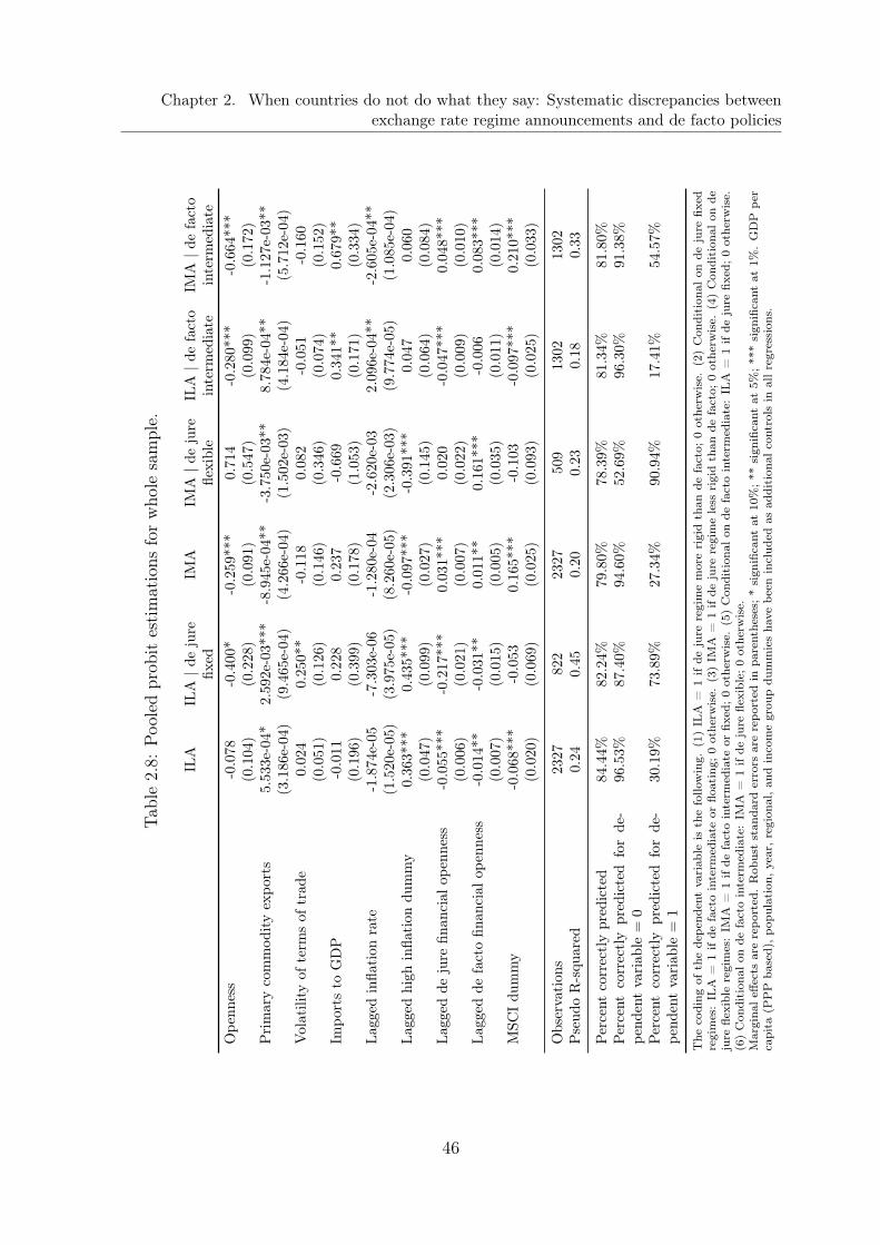
Chapter 2. When countries do not do what they say: Systematic discrepancies betweenexchange rate regime announcements and de facto policies
Tabl
e2.
8:Poo
led
prob
ites
tim
atio
nsfo
rw
hole
sam
ple.
ILA
ILA
|de
jure
IMA
IMA
|de
jure
ILA
|de
fact
oIM
A|d
efa
cto
fixed
flexi
ble
inte
rmed
iate
inte
rmed
iate
Ope
nnes
s-0
.078
-0.4
00*
-0.2
59**
*0.
714
-0.2
80**
*-0
.664
***
(0.1
04)
(0.2
28)
(0.0
91)
(0.5
47)
(0.0
99)
(0.1
72)
Pri
mar
yco
mm
odity
expo
rts
5.53
3e-0
4*2.
592e
-03*
**-8
.945
e-04
**-3
.750
e-03
**8.
784e
-04*
*-1
.127
e-03
**(3
.186
e-04
)(9
.465
e-04
)(4
.266
e-04
)(1
.502
e-03
)(4
.184
e-04
)(5
.712
e-04
)V
olat
ility
ofte
rms
oftr
ade
0.02
40.
250*
*-0
.118
0.08
2-0
.051
-0.1
60(0
.051
)(0
.126
)(0
.146
)(0
.346
)(0
.074
)(0
.152
)Im
port
sto
GD
P-0
.011
0.22
80.
237
-0.6
690.
341*
*0.
679*
*(0
.196
)(0
.399
)(0
.178
)(1
.053
)(0
.171
)(0
.334
)La
gged
infla
tion
rate
-1.8
74e-
05-7
.303
e-06
-1.2
80e-
04-2
.620
e-03
2.09
6e-0
4**
-2.6
05e-
04**
(1.5
20e-
05)
(3.9
75e-
05)
(8.2
60e-
05)
(2.3
06e-
03)
(9.7
74e-
05)
(1.0
85e-
04)
Lagg
edhi
ghin
flati
ondu
mm
y0.
363*
**0.
435*
**-0
.097
***
-0.3
91**
*0.
047
0.06
0(0
.047
)(0
.099
)(0
.027
)(0
.145
)(0
.064
)(0
.084
)La
gged
deju
refin
anci
alop
enne
ss-0
.055
***
-0.2
17**
*0.
031*
**0.
020
-0.0
47**
*0.
048*
**(0
.006
)(0
.021
)(0
.007
)(0
.022
)(0
.009
)(0
.010
)La
gged
defa
cto
finan
cial
open
ness
-0.0
14**
-0.0
31**
0.01
1**
0.16
1***
-0.0
060.
083*
**(0
.007
)(0
.015
)(0
.005
)(0
.035
)(0
.011
)(0
.014
)M
SCI
dum
my
-0.0
68**
*-0
.053
0.16
5***
-0.1
03-0
.097
***
0.21
0***
(0.0
20)
(0.0
69)
(0.0
25)
(0.0
93)
(0.0
25)
(0.0
33)
Obs
erva
tion
s23
2782
223
2750
913
0213
02P
seud
oR
-squ
ared
0.24
0.45
0.20
0.23
0.18
0.33
Per
cent
corr
ectl
ypr
edic
ted
84.4
4%82
.24%
79.8
0%78
.39%
81.3
4%81
.80%
Per
cent
corr
ectl
ypr
edic
ted
for
de-
pend
ent
vari
able
=0
96.5
3%87
.40%
94.6
0%52
.69%
96.3
0%91
.38%
Per
cent
corr
ectl
ypr
edic
ted
for
de-
pend
ent
vari
able
=1
30.1
9%73
.89%
27.3
4%90
.94%
17.4
1%54
.57%
The
codi
ngof
the
depe
nden
tva
riab
leis
the
follo
win
g.(1
)IL
A=
1if
deju
rere
gim
em
ore
rigi
dth
ande
fact
o;0
othe
rwis
e.(2
)C
ondi
tion
alon
deju
refix
edre
gim
es:
ILA
=1
ifde
fact
oin
term
edia
teor
float
ing;
0ot
herw
ise.
(3)
IMA
=1
ifde
jure
regi
me
less
rigi
dth
ande
fact
o;0
othe
rwis
e.(4
)C
ondi
tion
alon
deju
refle
xibl
ere
gim
es:
IMA
=1
ifde
fact
oin
term
edia
teor
fixed
;0
othe
rwis
e.(5
)C
ondi
tion
alon
defa
cto
inte
rmed
iate
:IL
A=
1if
deju
refix
ed;0
othe
rwis
e.(6
)C
ondi
tion
alon
defa
cto
inte
rmed
iate
:IM
A=
1if
deju
refle
xibl
e;0
othe
rwis
e.M
argi
naleff
ects
are
repo
rted
.R
obus
tst
anda
rder
rors
are
repo
rted
inpa
rent
hese
s;*
sign
ifica
ntat
10%
;**
sign
ifica
ntat
5%;**
*si
gnifi
cant
at1%
.G
DP
per
capi
ta(P
PP
base
d),po
pula
tion
,ye
ar,re
gion
al,an
din
com
egr
oup
dum
mie
sha
vebe
enin
clud
edas
addi
tion
alco
ntro
lsin
allre
gres
sion
s.
46

Chapter 2. When countries do not do what they say: Systematic discrepancies betweenexchange rate regime announcements and de facto policies
Tabl
e2.
9:Poo
led
prob
ites
tim
atio
nsfo
rlo
win
com
eco
untr
ies.
ILA
ILA
|de
jure
IMA
IMA
|de
jure
ILA
|de
fact
oIM
A|d
efa
cto
fixed
flexi
ble
inte
rmed
iate
inte
rmed
iate
Ope
nnes
s0.
311*
*0.
130
-0.3
51*
-3.5
55*
-0.7
29-1
.166
(0.1
47)
(0.2
71)
(0.1
97)
(2.0
63)
(0.6
06)
(0.9
84)
Pri
mar
yco
mm
odity
expo
rts
-0.0
02**
*-0
.003
**-0
.002
**-0
.002
0.00
0-0
.002
(0.0
01)
(0.0
02)
(0.0
01)
(0.0
03)
(0.0
02)
(0.0
03)
Vol
atili
tyof
term
sof
trad
e0.
063
0.18
10.
088
-0.9
550.
249*
0.08
0(0
.047
)(0
.110
)(0
.082
)(0
.610
)(0
.150
)(0
.247
)Im
port
sto
GD
P-0
.590
**-0
.344
0.53
75.
445
0.80
22.
794*
(0.2
87)
(0.4
53)
(0.3
73)
(3.5
75)
(1.0
43)
(1.6
44)
Lagg
edin
flati
onra
te-2
.773
e-06
-1.0
09e-
052.
878e
-06
-0.0
030.
007*
*-0
.007
(1.5
36e-
05)
(1.9
63e-
05)
(2.3
47e-
05)
(0.0
04)
(0.0
03)
(0.0
06)
Lagg
edhi
ghin
flati
ondu
mm
y0.
412*
*0.
414*
*-0
.011
-0.0
790.
451
(0.1
71)
(0.2
07)
(0.0
20)
(0.0
67)
(0.2
92)
Lagg
edde
jure
finan
cial
open
ness
-0.0
90**
*-0
.272
***
-0.0
07-0
.106
**-0
.090
**-0
.051
(0.0
23)
(0.0
51)
(0.0
08)
(0.0
52)
(0.0
38)
(0.0
45)
Lagg
edde
fact
ofin
anci
alop
enne
ss-0
.013
-0.0
08-0
.022
-0.2
03-0
.020
-0.1
21**
(0.0
14)
(0.0
10)
(0.0
26)
(0.1
81)
(0.0
37)
(0.0
58)
Obs
erva
tion
s41
022
941
082
147
147
Pse
udo
R-s
quar
ed0.
470.
410.
470.
340.
190.
09
Per
cent
corr
ectl
ypr
edic
ted
89.0
2%86
.03%
90.9
8%78
.05%
86.3
9%72
.11%
Per
cent
corr
ectl
ypr
edic
ted
for
de-
pend
ent
vari
able
=0
96.7
8%96
.11%
97.7
2%55
.17%
99.1
7%96
.00%
Per
cent
corr
ectl
ypr
edic
ted
for
de-
pend
ent
vari
able
=1
50.0
0%48
.98%
50.8
5%90
.57%
26.9
2%21
.28%
For
the
codi
ngof
the
depe
nden
tva
riab
lese
eta
ble
2.8.
Mar
gina
leffe
cts
are
repo
rted
.R
obus
tst
anda
rder
rors
are
repo
rted
inpa
rent
hese
s;*
sign
ifica
ntat
10%
;**
sign
ifica
ntat
5%;**
*si
gnifi
cant
at1%
.G
DP
per
capi
ta(P
PP
base
d)an
dpo
pula
tion
have
been
incl
uded
asad
dition
alco
ntro
lsin
allre
gres
sion
san
dye
aran
dre
gion
aldu
mm
ies
in(1
)an
d(3
).
47

Chapter 2. When countries do not do what they say: Systematic discrepancies betweenexchange rate regime announcements and de facto policies
Tabl
e2.
10:
Poo
led
prob
ites
tim
atio
nsfo
rlo
wer
mid
dle
inco
me
coun
trie
s.
ILA
ILA
|de
jure
IMA
IMA
|de
jure
ILA
|de
fact
oIM
A|d
efa
cto
fixed
flexi
ble
inte
rmed
iate
inte
rmed
iate
Ope
nnes
s0.
533*
**0.
813
-0.4
58**
-0.5
200.
213
-0.2
29(0
.145
)(1
.334
)(0
.215
)(0
.661
)(0
.287
)(0
.321
)P
rim
ary
com
mod
ity
expo
rts
0.00
2***
0.01
4***
0.00
10.
010*
*0.
002*
**-0
.001
*(0
.001
)(0
.005
)(0
.001
)(0
.005
)(0
.001
)(0
.001
)V
olat
ility
ofte
rms
oftr
ade
0.21
7*1.
672*
**-0
.467
**-2
.718
**0.
365*
*-0
.253
(0.1
22)
(0.5
83)
(0.1
85)
(1.1
88)
(0.1
43)
(0.1
63)
Impo
rts
toG
DP
-0.9
62**
*-2
.550
0.67
3*1.
379
-0.6
840.
400
(0.2
99)
(2.0
92)
(0.3
96)
(1.4
10)
(0.4
92)
(0.5
62)
Lagg
edin
flati
onra
te-6
.395
e-05
***
-1.2
01e-
04-3
.905
e-04
-7.3
42e-
042.
339e
-04*
*-1
.717
e-04
(1.7
74e-
05)
(2.5
86e-
04)
(2.4
77e-
04)
(9.8
16e-
04)
(1.0
43e-
04)
(1.2
82e-
04)
Lagg
edhi
ghin
flati
ondu
mm
y0.
568*
**0.
170
-0.0
73**
-0.4
41**
0.13
10.
257*
(0.1
00)
(0.1
76)
(0.0
33)
(0.1
74)
(0.1
49)
(0.1
47)
Lagg
edde
jure
finan
cial
open
ness
-0.1
17**
*-0
.524
***
-0.0
20*
0.00
2-0
.129
***
0.09
1***
(0.0
16)
(0.1
35)
(0.0
12)
(0.0
34)
(0.0
17)
(0.0
15)
Lagg
edde
fact
ofin
anci
alop
enne
ss-0
.142
***
-0.1
480.
016
0.05
20.
020
-0.0
14(0
.036
)(0
.243
)(0
.011
)(0
.121
)(0
.041
)(0
.050
)M
SCI
dum
my
0.18
1**
0.78
8***
0.15
8***
0.10
50.
212*
*0.
265*
**(0
.073
)(0
.091
)(0
.057
)(0
.111
)(0
.092
)(0
.075
)
Obs
erva
tion
s68
224
568
216
043
743
7P
seud
oR
-squ
ared
0.41
0.70
0.34
0.48
0.30
0.21
Per
cent
corr
ectl
ypr
edic
ted
84.7
5%93
.47%
82.2
6%88
.75%
80.3
2%79
.18%
Per
cent
corr
ectl
ypr
edic
ted
for
de-
pend
ent
vari
able
=0
91.8
3%91
.67%
93.4
7%63
.64%
91.4
1%90
.71%
Per
cent
corr
ectl
ypr
edic
ted
for
de-
pend
ent
vari
able
=1
63.1
0%94
.89%
45.9
6%95
.28%
47.7
5%46
.49%
For
the
codi
ngof
the
depe
nden
tva
riab
lese
eta
ble
2.8.
Mar
gina
leff
ects
are
repo
rted
.R
obus
tst
anda
rder
rors
are
repo
rted
inpa
rent
hese
s;*
sign
ifica
ntat
10%
;**
sign
ifica
ntat
5%;**
*si
gnifi
cant
at1%
.G
DP
per
capi
ta(P
PP
base
d)an
dpo
pula
tion
have
been
incl
uded
asad
dition
alco
ntro
lsin
allre
gres
sion
s.Yea
rdu
mm
ies
are
incl
uded
in(1
),(2
),an
d(3
)an
dre
gion
aldu
mm
ies
in(1
)to
(4).
48

Chapter 2. When countries do not do what they say: Systematic discrepancies betweenexchange rate regime announcements and de facto policies
Tabl
e2.
11:
Poo
led
prob
ites
tim
atio
nsfo
rup
per
mid
dle
inco
me
coun
trie
s.
ILA
ILA
|de
jure
IMA
IMA
|de
jure
ILA
|de
fact
oIM
A|d
efa
cto
fixed
flexi
ble
inte
rmed
iate
inte
rmed
iate
Ope
nnes
s-0
.181
-0.6
40**
*-0
.302
**-7
.462
***
-0.2
85**
-0.1
00(0
.171
)(0
.224
)(0
.128
)(2
.673
)(0
.136
)(0
.417
)P
rim
ary
com
mod
ity
expo
rts
-1.1
38e-
04-6
.728
e-05
-4.4
01e-
040.
010
0.00
1*-0
.005
***
(5.3
06e-
04)
(1.0
72e-
03)
(4.3
02e-
04)
(0.0
06)
(0.0
00)
(0.0
01)
Vol
atili
tyof
term
sof
trad
e-0
.220
**-0
.459
0.08
30.
673
-0.0
340.
091
(0.1
08)
(0.3
29)
(0.0
68)
(0.5
16)
(0.0
42)
(0.1
49)
Impo
rts
toG
DP
0.15
40.
902*
**0.
484*
*14
.610
***
0.42
9*-0
.593
(0.3
08)
(0.3
05)
(0.2
31)
(5.0
46)
(0.2
35)
(0.8
09)
Lagg
edin
flati
onra
te3.
273e
-05
-2.6
78e-
04**
-3.8
93e-
060.
018*
-0.0
03*
-0.0
05*
(4.5
06e-
05)
(1.2
45e-
04)
(4.0
86e-
05)
(0.0
09)
(0.0
02)
(0.0
03)
Lagg
edhi
ghin
flati
ondu
mm
y0.
379*
**0.
282
-0.0
50**
-0.6
99**
*0.
089
0.25
1(0
.083
)(0
.271
)(0
.020
)(0
.211
)(0
.187
)(0
.315
)La
gged
deju
refin
anci
alop
enne
ss-0
.017
-0.1
53**
*0.
002
0.14
4**
-0.0
13*
0.03
8**
(0.0
11)
(0.0
38)
(0.0
08)
(0.0
72)
(0.0
07)
(0.0
18)
Lagg
edde
fact
ofin
anci
alop
enne
ss-0
.061
***
-0.0
07-0
.042
***
0.15
6-0
.047
0.10
3**
(0.0
23)
(0.0
13)
(0.0
14)
(0.1
73)
(0.0
35)
(0.0
50)
MSC
Idu
mm
y0.
041
-0.1
55**
-0.0
59**
-0.6
55**
*-0
.089
**0.
115*
(0.0
48)
(0.0
63)
(0.0
29)
(0.1
56)
(0.0
40)
(0.0
59)
Obs
erva
tion
s40
314
240
364
191
191
Pse
udo
R-s
quar
ed0.
470.
610.
290.
470.
350.
19
Per
cent
corr
ectl
ypr
edic
ted
86.1
0%90
.85%
87.3
4%82
.81%
92.6
7%83
.77%
Per
cent
corr
ectl
ypr
edic
ted
for
de-
pend
ent
vari
able
=0
92.6
0%92
.38%
97.1
4%70
.83%
97.6
3%97
.35%
Per
cent
corr
ectl
ypr
edic
ted
for
de-
pend
ent
vari
able
=1
64.1
3%86
.49%
22.6
4%90
.00%
54.5
5%32
.50%
For
the
codi
ngof
the
depe
nden
tva
riab
lese
eta
ble
2.8.
Mar
gina
leff
ects
are
repo
rted
.R
obus
tst
anda
rder
rors
are
repo
rted
inpa
rent
hese
s;*
sign
ifica
ntat
10%
;**
sign
ifica
ntat
5%;**
*si
gnifi
cant
at1%
.G
DP
per
capi
ta(P
PP
base
d)an
dpo
pula
tion
have
been
incl
uded
asad
dition
alco
ntro
lsin
allre
gres
sion
s,ye
aran
dre
gion
aldu
mm
ies
in(1
)an
d(3
).
49

Chapter 2. When countries do not do what they say: Systematic discrepancies betweenexchange rate regime announcements and de facto policies
Tabl
e2.
12:
Poo
led
prob
ites
tim
atio
nsfo
rhi
ghin
com
eco
untr
ies.
ILA
ILA
|de
jure
IMA
IMA
|de
jure
ILA
|de
fact
oIM
A|d
efa
cto
fixed
flexi
ble
inte
rmed
iate
inte
rmed
iate
Ope
nnes
s-0
.113
1.72
8**
-0.2
504.
475*
**-0
.174
**-0
.880
***
(0.0
72)
(0.8
50)
(0.3
19)
(1.2
74)
(0.0
77)
(0.1
59)
Pri
mar
yco
mm
odity
expo
rts
1.56
8e-0
40.
029
0.00
1-0
.003
2.51
8e-0
40.
002*
*(5
.023
e-04
)(0
.018
)(0
.001
)(0
.002
)(3
.579
e-04
)(0
.001
)V
olat
ility
ofte
rms
oftr
ade
-0.0
96-3
.276
**-2
.023
***
-2.7
23**
-0.0
83-1
.430
***
(0.0
95)
(1.3
90)
(0.5
24)
(1.3
39)
(0.0
86)
(0.3
34)
Impo
rts
toG
DP
0.12
3-1
.781
-0.0
24-7
.083
***
0.21
0*1.
134*
**(0
.133
)(1
.666
)(0
.645
)(2
.674
)(0
.119
)(0
.252
)La
gged
infla
tion
rate
0.00
10.
023*
*-0
.004
0.01
2-0
.001
0.00
2(0
.000
)(0
.012
)(0
.004
)(0
.012
)(0
.001
)(0
.003
)La
gged
high
infla
tion
dum
my
-0.0
51**
(0.0
23)
Lagg
edde
jure
finan
cial
open
ness
-0.0
14*
-0.1
67*
0.06
2***
0.08
0**
-0.0
15*
0.06
2***
(0.0
08)
(0.0
89)
(0.0
17)
(0.0
37)
(0.0
09)
(0.0
18)
Lagg
edde
fact
ofin
anci
alop
enne
ss-0
.014
**-0
.253
***
0.03
0***
0.18
0***
-0.0
060.
086*
**(0
.007
)(0
.060
)(0
.009
)(0
.039
)(0
.006
)(0
.020
)M
SCI
dum
my
-0.0
60*
0.02
30.
185*
**0.
389
0.01
00.
084*
*(0
.033
)(0
.104
)(0
.037
)(0
.274
)(0
.016
)(0
.035
)
Obs
erva
tion
s83
220
482
321
552
552
5P
seud
oR
-squ
ared
0.18
0.62
0.22
0.47
0.22
0.54
Per
cent
corr
ectl
ypr
edic
ted
87.9
8%91
.67%
79.3
4%86
.98%
83.2
4%89
.14%
Per
cent
corr
ectl
ypr
edic
ted
for
de-
pend
ent
vari
able
=0
99.1
8%89
.57%
91.4
4%81
.33%
99.5
4%95
.09%
Per
cent
corr
ectl
ypr
edic
ted
for
de-
pend
ent
vari
able
=1
2.08
%94
.38%
49.7
9%90
.00%
0.00
%72
.46%
For
the
codi
ngof
the
depe
nden
tva
riab
lese
eta
ble
2.8.
Mar
gina
leff
ects
are
repo
rted
.R
obus
tst
anda
rder
rors
are
repo
rted
inpa
rent
hese
s;*
sign
ifica
ntat
10%
;**
sign
ifica
ntat
5%;**
*si
gnifi
cant
at1%
.G
DP
per
capi
ta(P
PP
base
d)an
dpo
pula
tion
have
been
incl
uded
asad
dition
alco
ntro
lsin
allre
gres
sion
s,ye
ardu
mm
ies
in(1
),(3
),an
d(4
).
50

Chapter 3
Inflation targeting in small open economies
3.1 Introduction
Many emerging and developing countries have moved away from fixed exchange ratestowards a more independent monetary policy in recent years, mostly towards inflationtargeting. Thus, open economy aspects have become increasingly important in analyzingmonetary policy. The literature frequently resorts to two simple concepts in internationaleconomics, purchasing power parity and uncovered interest rate parity, to describe therelation between prices, interest rates, and exchange rates between countries. Althoughthe empirical relevance of these two concepts is subject to an ongoing debate, they arefrequently used in theoretical models. The present study examines the implications ofthese concepts on the implementation of monetary policy.
Monetary policy is analyzed in an open economy version of the standard New Key-nesian framework described by Clarida, Galí and Gertler (1999). More specifically,flexible inflation targeting as characterized by Svensson (2007) is the monetary policyunder scrutiny. A central bank operating under flexible inflation targeting is not onlyconcerned about stabilizing the inflation rate around the target but additionally aboutstabilizing the real economy. According to Svensson (2007) “all real world inflation tar-geting is flexible”. Most theoretical work building on the New Keynesian model resorts topurchasing power parity and/or uncovered interest rate parity to describe internationalgoods and capital markets, respectively. Purchasing power parity is based on the ideathat international goods arbitrage keeps the relative purchasing power of two currenciesconstant over time. However, purchasing power parity frequently fails empirically, es-pecially in the short-run; an overview of the evidence and explanations is provided byTaylor and Taylor (2004). Uncovered interest rate parity is derived from arbitrage ininternational financial markets according to which the nominal exchange rate adjusts tointerest rate differentials. As the underlying assumption of risk neutral investors may
51
Chapter 3. Inflation targeting in small open economies
be too restrictive, in general, a time-varying risk premium is included. Still, uncoveredinterest rate parity is frequently rejected in empirical studies, for an overview see Frootand Thaler (1990) and McCallum (1994).
Notwithstanding their empirical weakness, purchasing power parity and/ or uncoveredinterest rate parity are frequently used as concepts in monetary policy analysis in openeconomies. The present study contributes to the literature by analyzing in a unifiedframework how these two concepts and possible alternatives used in the literature affectmonetary policy. More specifically, the implications for the interest rate reaction func-tion describing monetary policy responses to shocks under flexible inflation targetingare examined. Thereby, useful insights into the consequences of using the simple butempirically problematic concepts of purchasing power parity and uncovered interest rateparity in monetary policy analysis are provided.
The main insight is that the interest rate reaction function is affected when purchasingpower parity and uncovered interest rate parity are relaxed. As long as purchasing powerparity holds, monetary policy reacts only to cost-push shocks and excess-demand shocks.If, however, purchasing power parity does not hold, monetary policy also fully offsets theeffects of foreign shocks. Furthermore, not the direction but the strength of the interestrate response to cost-push shocks and excess-demand shocks is affected. Whether therelation between interest rates and exchange rates is described by uncovered interestrate parity or in the more generic way proposed by Ball (1999) does affect both to whichtype of shocks monetary policy responds and how strong the response is.
The remainder of this chapter is organized as follows. Section 3.2 provides an overviewof the related literature and stylized facts. In section 3.3 the theoretical model is devel-oped. Then, in section 3.4 the interest rate reaction functions are analyzed for the basicmodel and for hybrid models allowing deviations from purchasing power parity and un-covered interest rate parity. First, in 3.4.1 the optimality condition for monetary policyand the interest rate reaction function are derived for the basic model which assumesthat both purchasing power parity and uncovered interest rate parity hold. Then, in3.4.2 purchasing power parity is relaxed while 3.4.3 studies the implications of addition-ally relaxing uncovered interest rate parity. The case that purchasing power parity holdswhile uncovered interest rate parity does not, is briefly discussed within the basic model.Section 3.5 discusses the main results and section 3.6 concludes.
52

Chapter 3. Inflation targeting in small open economies
3.2 Literature review and stylized facts
Most central banks declare price stability as the primary or one of the main policygoals; additional goals being to minimize the volatility of other economic variables suchas output and exchange rates, to smooth interest rate changes, to act as Lender ofLast Resort, and recently also to perform a supervisory role. In recent years, inflationtargeting has attracted considerable attention as a framework to pursue price stabilityobjectives and has been adopted also in many emerging and developing countries.1 How-ever, no unanimity has been achieved about what inflation targeting exactly is. Widelyaccepted characteristics of an inflation targeting framework are (i.) the announcementof a numerical inflation target or target range as primary monetary policy objective,with increasingly explicit concerns beyond the stability of inflation, mostly about thestability of the real economy, and (ii.) a high degree of transparency and accountabilityof the central bank, generally through the regular publication of inflation reports, policydecisions, etc., see, e.g., Svensson (2007), Bernanke and Mishkin (1997), and McCallum(2003).
The standard welfare analytic framework for monetary policy is due to Kydland andPrescott (1977) and Barro and Gordon (1983) and is also used to study inflation target-ing. The policymaker minimizes the losses from inflation and output variability aroundtarget rates in an intertemporal setting in which output can be increased through un-expected inflation. When the policymaker aims at an output above the natural level,incentives to create surprise inflation are present. However, private agents are aware ofthe time-inconsistency in policymaking and internalize it in setting wages, leading tohigher inflation without output gains, the so-called inflation bias. Several suggestionshave been made on how to improve upon this discretionary outcome: reputation build-ing, delegation, timeless perspective, escape clauses, etc. Inflation targeting seems tobe another possibility even though the literature disagrees on what inflation targeting isexactly in this framework.
Svensson (2007) distinguishes strict and flexible inflation targeting. A central bankoperating under strict inflation targeting is only concerned about stabilizing the inflation
1The following developing and emerging market economies have adopted inflation targeting; the yearof adoption is reported in parenthesis: Brazil (1999), Chile (1991), Colombia (1999), Czech Republic(1998), Ghana (2007), Hungary (2001), Indonesia (2005), Israel (1992), Korea (1998), Mexico (1999),Peru (1994), Philippines (2002), Poland (1998), Rumania (2005), South Africa (2000), Thailand(2000), and Turkey (2006). (Mishkin and Schmidt-Hebbel (2001); Fraga, Goldfajn and Minella(2003); Roger and Stone (2005); web-pages of the International Monetary Fund and Central Banks)
53

Chapter 3. Inflation targeting in small open economies
rate around the target while a central bank operating under flexible inflation targetingis additionally concerned about stabilizing the real economy. Strict inflation targetingis considered a theoretical benchmark while central banks practically implement flexibleinflation targeting. Additionally, Svensson (1999) argues that the recognition that mon-etary policy cannot systematically affect capacity output, the natural-rate hypothesis,can be considered one of the foundations of inflation targeting. Therewith, Svenssonjustifies the assumption that a central bank operating under flexible inflation targetinghas an implicit output target equal to the natural output level. As a consequence, noinflation bias arises. Furthermore, the high degree of transparency and accountabilitypeculiar to inflation targeting creates appropriate incentives for the central bank notto deviate from the assigned objective function. Consequently, Svensson (2007) modelsflexible inflation targeting through the standard loss function over inflation and outputgap variability with a zero output gap target. Whether a central bank then implementsthe commitment solution or the discretionary solution, depends on the ability and thewillingness of a central bank to commit to future policies. Even a central bank not aim-ing at an output level above the natural rate, can gain from committing to a monetarypolicy rule, eliminating the so-called stabilization bias as shown by, e.g., Clarida et al.(1999). The stabilization bias arises when a central bank unable to precommit to a pol-icy rule cannot respond gradually to shocks by influencing private sector expectations,see, e.g., Dennis and Söderström (2006). The present study follows Svensson’s (2007)approach and assumes that the central bank optimizes under discretion although theadequateness of this approach may be questioned. Alternative perspectives on inflationtargeting are exposed by, e.g., Bernanke and Mishkin (1997), McCallum (2000), andKing (1997); Kuttner and Posen (1999) provide additional interpretations.
The present study takes flexible inflation targeting as given and does not discussits optimality as a monetary policy framework for small open economies. Instead, theimplementation through an interest rate reaction function is analyzed. Interest ratereaction functions relate the monetary policy instrument, in general a short-term interestrate, to predetermined variables and exogenous shocks. They are a valuable tool totheoretically analyze monetary policy responses although their practical value may belimited as shocks are difficult to identify. For practical purposes, interest rate reactionfunctions are in general transformed into Taylor-type rules relating the policy interestrate to observables such as output and inflation; a discussion of Taylor-type rules isprovided by Kozicki (1999). The interest of the present study centers around the role of
54

Chapter 3. Inflation targeting in small open economies
the concepts of purchasing power parity and uncovered interest rate parity for the interestrate reaction function describing the implementation of flexible inflation targeting insmall open economies.
Purchasing power parity and uncovered interest rate parity relate to two of the sixmajor puzzles in international macroeconomics, the purchasing power parity puzzle andthe exchange rate disconnect puzzle of which the forward premium puzzle is a manifes-tation (Obstfeld and Rogoff, 2000). Purchasing power parity states that the percentagechange of the nominal exchange rate between two currencies should just offset the infla-tion differential between these countries, thus keeping the relative purchasing power ofthe two currencies constant. The basic idea is that international goods arbitrage leadsto the equalization of the prices of tradable goods. Empirically, it seems to be relevantonly as a long-run concept, for an overview see, e.g., Taylor and Taylor (2004). Thepurchasing power parity puzzle in this context refers to the surprisingly weak empiricalconnection between exchange rates and national price levels (Rogoff, 1996). Reasons forthe empirical failure of purchasing power parity holding in the short-run are, for exam-ple, sticky prices combined with highly volatile nominal exchange rates as in Dornbusch’s(1976) overshooting model and differences in productivity growth between countries ascaptured in the Balassa-Samuelson effect.
Uncovered interest rate parity is derived from arbitrage in international financial mar-kets and states that the expected percentage change in the nominal exchange rate shouldequal the interest rate differential. As the underlying assumptions of risk neutral in-vestors and no country specific risk may be too restrictive, in general, a time-varyingrisk premium is included. Despite this, uncovered interest rate parity is frequently re-jected in empirical studies; an overview is provided by Froot and Thaler (1990) andMcCallum (1994). In this context, the exchange rate disconnect puzzle describes themore general, weak relation between the exchange rate and virtually any macroeconomicvariable. The related forward premium puzzle states that the forward premium incor-rectly predicts the direction of future changes in the exchange rate, implying a rejectionof uncovered interest rate parity, see Obstfeld and Rogoff (2000) and McCallum (1994).Abstracting from rational expectations or assuming that the time-varying risk premiumis negatively correlated with an expected depreciation may explain the empirical facts,see Froot and Thaler (1990). McCallum (1994) explains the apparent empirical failureof uncovered interest rate parity with the hypothesis that central banks systematicallymanage interest rate differentials to avoid frequent changes in the exchange rate.
55

Chapter 3. Inflation targeting in small open economies
Even though their empirical validity may be questioned, purchasing power parity anduncovered interest rate parity are such neat concepts that they are frequently used formonetary policy analysis. The aim of the present study is to theoretically analyze howthe implementation of flexible inflation targeting in small open economies is affected bythe assumption of purchasing power parity and uncovered interest rate parity holdingor not. The implementation of monetary policy is described by interest rate reactionfunctions that relate the monetary policy instrument, the nominal interest rate, to pre-determined variables and shocks.
The theoretical model exposed in the following section combines the standard NewKeynesian monetary policy framework by Clarida, Galí and Gertler (1999), which isaugmented to include open economy aspects, with the inflation targeting frameworkproposed by Svensson (2007). The description of aggregate demand and the price ad-justment mechanism follows Clarida et al. (1999). To take into account open economyaspects, an exchange rate channel is introduced. Real exchange rate depreciations raiseaggregate demand as the relative price between domestic and foreign goods changesand, hence, the domestic and foreign demand for domestic goods. This is included inthe standard fashion of the Mundell-Fleming model by adding an exchange rate term inaggregate demand. Another special aspect of small open economies is that they are fre-quently hit by external shocks which have considerable effects on the domestic economy.Therefore, shocks to foreign output and inflation as well as foreign monetary policy re-sponses are explicitly taken into account following Svensson (2000). By allowing externalshocks to affect the domestic economy and, thus, to induce monetary policy responses,the present study goes a step further than most of the simple monetary policy models.
The resulting theoretical framework is simple enough to analyze the implication ofpurchasing power parity and uncovered interest rate parity on the interest rate reactionfunction with closed form solutions and rich enough to include essential features of smallopen economies. This approach has the advantage that the implications of deviatingfrom the relatively standard assumptions of purchasing power parity and uncoveredinterest rate parity can be analyzed in a unified open economy framework. Previouswork does not lend itself to that end as the models differs also in other aspects. Clarida,Galí and Gertler (2001), for example, analyze monetary policy in an open economyversion of Clarida et al. (1999) while assuming that both purchasing power parity anduncovered interest rate parity hold. In contrast, the open economy version of Claridaet al. (1999) used by Detken and Gaspar (2003) relaxes purchasing power parity in the
56

Chapter 3. Inflation targeting in small open economies
standard fashion by including an exchange rate term in the aggregate demand relationwhile uncovered interest rate parity describes international financial markets. Ball (1999)analyzes monetary policy rules while allowing for deviations from both purchasing powerparity and uncovered interest rate parity. International financial markets are insteaddescribed by a simple proportional relation between the real interest rate and the realexchange rate with all other effects aggregated in a random term. Ball’s (1999) approachis used as alternative condition to uncovered interest rate parity. The model developedby Svensson (2000) to analyze different forms of inflation targeting in a small openeconomy model is too complex to obtain closed form solutions. Compared to Svensson(2000), the present analysis simplifies on the dynamic structure by abstracting from lagsin the transmission mechanism of monetary policy and setting aside direct effects ofexchange rate changes on inflation in order to obtain simple analytical solutions.
3.3 Theoretical model
To analyze the interest rate reaction functions arising under flexible inflation targetingin small open economies, the standard monetary policy model of Clarida et al. (1999) isaugmented to include open economy aspects. Furthermore, inflation targeting is charac-terized following Svensson (2007) and foreign monetary policy following Svensson (2000).The resulting model is simple enough to analyze the implications of purchasing powerparity and uncovered interest rate parity on the interest rate reaction function with closedform solutions and rich enough to include essential features of small open economies.
Monetary policy objective
The central bank operates under flexible inflation targeting which is characterized fol-lowing Svensson (2007), i.e., the central bank minimizes deviations of the inflation rate π
from its target (normalized to zero) and deviations of output y from its natural rate yn,thus targeting a zero output gap. When flexible inflation targeting is implemented, thecentral bank is not only concerned about stabilizing inflation around the target as wouldbe the case for strict inflation targeting, but is additionally concerned about stabilizingreal economic fluctuations as captured by the output gap. No average inflation biasarises because the implicit output target is the natural output level. Svensson (1999)argues that the natural-rate hypothesis, the perception that monetary policy cannot sys-tematically affect capacity output, can be considered one of the foundations of inflation
57

Chapter 3. Inflation targeting in small open economies
targeting and, thus, justifies the assumption of a zero output gap target. Furthermore,the high degree of transparency and accountability peculiar to inflation targeting cre-ates appropriate incentives for the central bank not to deviate. The resulting standardintertemporal loss function is
L = Et
{∞∑
n=0
βn[π2
t+n + αx2t+n
]}(3.1)
β is the discount factor, πt the inflation rate, and xt the output gap, xt ≡ yt − yn, α isthe relative weight on the output stabilization objective. In the model all variables areexpressed as deviations from a deterministic long-run trend and, with the exception ofthe interest rates, as natural logarithms and all parameters are defined as being positive.Et is the expectations operator conditional on information available at time t.
Aggregate demand
Aggregate demand expressed in terms of the output gap is characterized by equation (3.2)and depends negatively on the real interest rate, it −Etπt+1, positively on the expectedfuture output gap and log-deviations of the real exchange rate from its equilibrium level,qt.
xt = −ϕ[it − Etπt+1] + Etxt+1 + νqt + gt (3.2)
gt is an excess-demand shock described by
gt = µgt−1 + gt (3.3)
where 0 ≤ µ ≤ 1 and gt is an i.i.d. random variable with zero mean and variance σ2g .
The basic aggregate demand equation for a closed economy (with ν = 0) can be obtainedby log-linearization of the consumption Euler equation from household’s intertemporaloptimization, see Clarida et al. (1999). The expected future output gap raises thepresent output gap as a consequence of the consumption smoothing objective whilethe negative effect of the real interest rate arises due to the intertemporal substitutionof consumption. The excess-demand shock captures expected changes in governmentspending and in potential output.
A special aspect of open economies is that changes in the real exchange rate affectaggregate demand. Real exchange rate depreciations raise aggregate demand as therelative price between domestic and foreign goods changes and, hence, the domestic and
58

Chapter 3. Inflation targeting in small open economies
foreign demand for domestic goods. This is included in the standard fashion of theMundell-Fleming model. Exchange rate depreciations are assumed to be expansionary.However, that is not necessarily the case as illustrated by the J-curve effect and discussedby, e.g., Sánchez (2005). If purchasing power parity holds, however, the log-deviationof the real exchange rate from the steady-state is zero. Hence, the aggregate demandequation for an open economy simplifies to:
xt = −ϕ[it − Etπt+1] + Etxt+1 + gt (3.2’)
The real exchange rate qt is defined as
qt ≡ et + p∗t − pt (3.4)
where et is the nominal exchange rate defined as domestic price of foreign currency andp∗t the log of foreign prices. An increase in qt corresponds to a real depreciation.
Price adjustment mechanism
The price adjustment mechanism in the economy is described by an expectations aug-mented Phillips-curve:
πt = λxt + βEtπt+1 + ut (3.5)
Inflation depends on the current output gap, expected future inflation, and the cost-pushshock ut described by
ut = γut−1 + ut (3.6)
with 0 ≤ γ ≤ 1 and ut being an i.i.d. random term with mean zero and variance σ2u.
This Phillips-curve specification can be derived from staggered price setting as developedby Calvo (1983) and used by Clarida et al. (1999). Forward iteration of (3.5) revealsthat present inflation depends on current and expected future economic conditions ascaptured by output gaps and cost-push shocks. Price setting decisions of firms are basedon expected changes in marginal costs. Those related to variations in excess demandare captured through the expected future output gaps (xt+n) while the cost-push shocks(ut+n) capture everything else affecting marginal costs, see Clarida et al. (1999). Thecost-push shock introduces a short-run trade-off between inflation and output.
59

Chapter 3. Inflation targeting in small open economies
International goods and financial markets
Purchasing power parity describes the adjustment of the nominal exchange rate to theinflation differential such as to keep the relative purchasing power of the currenciesconstant:
et − et−1 = πt − π∗t (3.7)
International financial markets are described by uncovered interest rate parity includ-ing a time-varying risk premium ρt:
it = i∗t + Etet+1 − et + ρt (3.8)
where it is the domestic nominal interest rate, i∗t the foreign nominal interest rate, and,following Svensson (2000), the risk premium is characterized by
ρt = ηρt−1 + ρt (3.9)
with 0 ≤ η < 1 and ρt being an i.i.d. random term with mean zero and variance σ2ρ.
Expectations are a crucial element in forward-looking models and the process drivingtheir formation may affect the results, see, e.g., the discussion by Taylor (2002). Follow-ing most of the literature, expectations are assumed to be formed rationally.
Foreign shocks
Small open economies are frequently hit by external shocks and their effect on the do-mestic economies is considerable. Therefore, shocks to foreign output and inflation aswell as foreign monetary policy responses are explicitly taken into account. By allowingexternal shocks to affect the domestic economy and, thus, to induce monetary policyresponses, the present study goes a step further than most of the related literature.
Following Svensson (2000) the foreign inflation rate and foreign output are assumedto follow stationary univariate AR (1) processes,
π∗t = ρ∗ππ∗t−1 + η∗t (3.10)
y∗t = ρ∗yy∗t−1 + ξ∗t (3.11)
where 0 ≤ ρ∗π, ρ∗y < 1 and η∗t and ξ∗t are i.i.d. random shocks with zero mean and
60

Chapter 3. Inflation targeting in small open economies
variances σ2π∗ and σ2
y∗ , respectively. Furthermore, the foreign interest rate is assumed tofollow a Taylor-type rule as described by Svensson (2000):
i∗t = f ∗ππ∗t + f ∗y y∗t + ε∗t (3.12)
with f ∗π , f∗y being positive and ε∗t an i.i.d. shock with zero mean and variance σ2ε∗ .
These relations describe the economy in a sufficiently simple way to analyze the im-plementation of monetary policy and the implications of purchasing power parity anduncovered interest rate parity with closed form solutions. By abstracting from lags in thetransmission mechanism of monetary policy and a direct effect of exchange rate changeson inflation included by Svensson (2000), a tractable model is obtained.
3.4 Implementing flexible inflation targeting
Based on the model exposed in the preceding section, the implementation of flexibleinflation targeting as described by an interest rate reaction function is studied. First, insection 3.4.1 the optimality condition for monetary policy and the interest rate reactionfunction are derived in a basic model assuming that both purchasing power parity anduncovered interest rate parity hold. As purchasing power parity and uncovered inter-est rate parity may not hold empirically, the consequences of allowing for deviationsfrom these conditions are then studied in the following sections. In section 3.4.2 theimplications of relaxing purchasing power parity are analyzed. Then, uncovered interestrate parity is additionally relaxed in section 3.4.3. The case of purchasing power parityholding while uncovered interest rate parity does not, affects the basic model only withrespect to the determination of the nominal exchange rate. Therefore, it is not analyzedexplicitly but only briefly discussed within the basic model. The interest rate reactionfunctions derived under these alternatives are then compared in section 3.5.
3.4.1 Basic model
In the basic model purchasing power parity and uncovered interest rate parity are as-sumed to hold both.
61

Chapter 3. Inflation targeting in small open economies
Optimality condition for monetary policy
The monetary policy framework under consideration is flexible inflation targeting whichis described following Svensson (2007). By operating under flexible inflation targeting,the central bank is assigned the loss function (3.1) which implies the absence of an in-flation bias because of a zero output gap target. The central bank is assumed to beunable to commit to a state-contingent rule and, thus, central bank’s behavior is charac-terized as optimization under discretion without being able to systematically influenceexpectations.2 Hence, the central bank minimizes the loss function (3.1) subject tothe Phillips-curve (3.5) for given, rational expectations. Thus, following Clarida et al.(1999), possible reputational (sunspot) equilibria are ignored and attention is restrictedto Markov perfect equilibria, thereby circumventing the possible indeterminacy problem.The resulting optimization problem is identical to the optimal monetary policy underdiscretion in Clarida et al. (1999) for a closed economy and is solved accordingly. Asthere are no endogenous state variables, the minimization problem simplifies to a se-quence of static optimization problems. The central bank chooses inflation and outputeach period such as to minimize
π2t + αx2
t + Ft
subject toπt = λxt + Ht
where Ft ≡ Et
{∑∞n=1 βn
[π2
t+n + αx2t+n
]}and Ht ≡ βEtπt+1 + ut are taken as given.
This implies both that the central bank cannot manipulate expectations and that futureoutput and inflation are independent of present policy actions. The resulting optimalitycondition is:
xt = −λ
απt (3.13)
To represent inflation and output as functions of the state variable ut, iterate (3.5)forward using the first order condition (3.13) and the assumption of rational expectationsfor private agents, see Clarida et al. (1999):
πt =α
α(1− βγ) + λ2ut (3.14)
2For developing and emerging market economies who have just adopted inflation targeting and lackboth the experience of independent monetary policy and the credibility for low inflation policy, adiscretionary solution does not seem unreasonable. For a discussion see also Svensson (2007).
62

Chapter 3. Inflation targeting in small open economies
xt = − λ
α(1− βγ) + λ2ut (3.15)
Interest rate reaction function
The interest rate reaction function to implement the monetary policy is derived insertingthe optimality condition (3.13) into aggregate demand (3.2’) and solving for the nominalinterest rate:
it =αγϕ + λ(1− γ)
ϕ{α(1− βγ) + λ2}ut +
1
ϕgt (3.16)
Flexible inflation targeting implies that excess-demand shocks are perfectly offset bymonetary policy while cost-push shocks affect both inflation and output. Excess-demandshocks increase output and thus inflation, and an increase in the nominal interest ratecan reverse both effects completely. However, the increase in inflation following a cost-push shock can only be counteracted when output is reduced below its natural level,thus forcing a trade-off between inflation and output. To minimize the loss function,an increase in inflation and a reduction in output are optimal such that the loss from amarginal increase in inflation equals the loss from a marginal decrease in output. Thestrength of the trade-off depends on the direct effect of output on inflation, λ, and therelative importance of the stabilization objective, α.
The assumption of uncovered interest rate parity is not necessary to derive the interestrate reaction function as long as purchasing power parity holds and is only relevant forthe determination of the nominal exchange rate. Hence, allowing for deviations fromuncovered interest rate parity while purchasing power parity holds does not affect theinterest rate reaction function and is therefore not analyzed explicitly.
The optimality condition (3.13) is independent of the assumptions of purchasing powerparity and uncovered interest rate parity as they do not affect the loss function (3.1) orthe Phillips-curve (3.5). Therefore, only the implications on the interest rate reactionfunctions resulting from these assumptions are analyzed in the next sections.
3.4.2 Relaxing purchasing power parity
The basic model is very stylized and not qualitatively different from a closed economymodel due to the strong assumption of purchasing power parity. However, purchasingpower parity has been shown to hold empirically only in the long-run, e.g. Obstfeld andRogoff (2000). As the Phillips-curve is a predominantly short-term concept, purchasing
63

Chapter 3. Inflation targeting in small open economies
power parity is unlikely to hold simultaneously. Therefore, the implications of relaxingpurchasing power parity are analyzed by deriving the modified interest rate reactionfunction.
When purchasing power parity does not hold, changes in the real exchange rate affectaggregate demand. Therefore, the interest rate reaction function, obtained by insertingthe reduced form representations of inflation (3.14) and output (3.15) derived from theoptimality condition (3.13) into the aggregate demand equation (3.2), now depends onthe nominal exchange rate:
it =(1− γ)λ + αγϕ− να
ϕ[α(1− βγ) + λ2]ut +
ν
ϕ(et + p∗t − pt−1) +
1
ϕgt (3.17)
The interest rate and exchange rate are simultaneously determined and the interest ratereaction function (3.17) and uncovered interest rate parity (3.8) describe their relation.The simultaneous equation system is solved using the Minimal State Variable criterionproposed by McCallum (1983) based on the method of undetermined coefficients. Ac-cordingly, the solutions for the interest rate and the exchange rate are guessed to be linearfunctions of the state variables (ut, gt, ρt, p
∗t , p
∗t−1, ε
∗t , y
∗t , pt−1). The guessed solutions are
inserted into the interest rate reaction function (3.17) and into uncovered interest rateparity (3.8) taking into account the foreign monetary policy rule (3.12). By matchingthe coefficients of all state variables, the unknown coefficients can be solved for. Whenthe obtained coefficients are plugged into the guessed solutions, the following interestrate reaction function is obtained (for a detailed analysis see appendix 3.A):
it =αγ[ν + ϕ(1− γ)] + (1− γ)2λ
[ν + ϕ(1− γ)][α(1− βγ) + λ2]ut +
1− µ
ν + (1− µ)ϕgt (3.18)
+ν
ν + (1− η)ϕρt +
νf ∗yν + ϕ(1− ρ∗y)
y∗t +ν(f ∗π − ρ∗π)
ν + ϕ(1− ρ∗π)π∗t +
ν
ν + ϕε∗t
Thus, optimal monetary policy reacts not only to domestic but also to foreign shocks.More specifically, shocks to the risk premium ρ, foreign output y∗, foreign inflation π∗,and shocks to the foreign monetary policy rule ε∗ are perfectly offset.
64
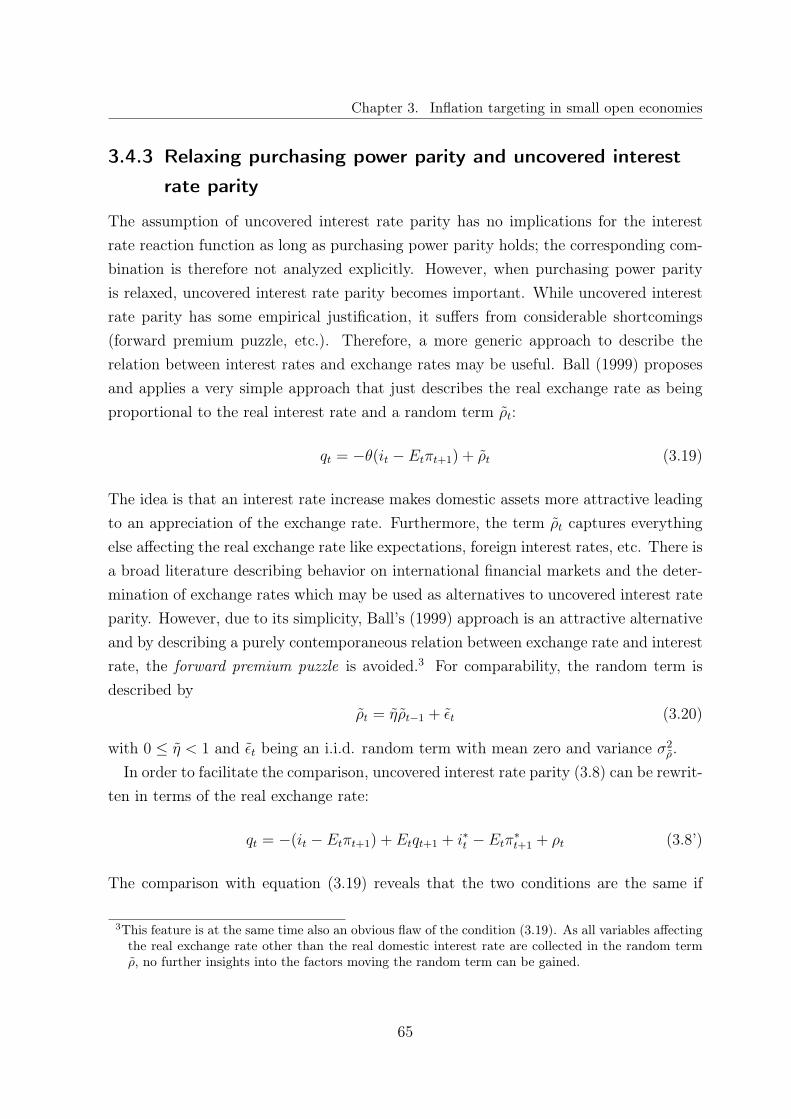
Chapter 3. Inflation targeting in small open economies
3.4.3 Relaxing purchasing power parity and uncovered interest
rate parity
The assumption of uncovered interest rate parity has no implications for the interestrate reaction function as long as purchasing power parity holds; the corresponding com-bination is therefore not analyzed explicitly. However, when purchasing power parityis relaxed, uncovered interest rate parity becomes important. While uncovered interestrate parity has some empirical justification, it suffers from considerable shortcomings(forward premium puzzle, etc.). Therefore, a more generic approach to describe therelation between interest rates and exchange rates may be useful. Ball (1999) proposesand applies a very simple approach that just describes the real exchange rate as beingproportional to the real interest rate and a random term ρt:
qt = −θ(it − Etπt+1) + ρt (3.19)
The idea is that an interest rate increase makes domestic assets more attractive leadingto an appreciation of the exchange rate. Furthermore, the term ρt captures everythingelse affecting the real exchange rate like expectations, foreign interest rates, etc. There isa broad literature describing behavior on international financial markets and the deter-mination of exchange rates which may be used as alternatives to uncovered interest rateparity. However, due to its simplicity, Ball’s (1999) approach is an attractive alternativeand by describing a purely contemporaneous relation between exchange rate and interestrate, the forward premium puzzle is avoided.3 For comparability, the random term isdescribed by
ρt = ηρt−1 + εt (3.20)
with 0 ≤ η < 1 and εt being an i.i.d. random term with mean zero and variance σ2ρ.
In order to facilitate the comparison, uncovered interest rate parity (3.8) can be rewrit-ten in terms of the real exchange rate:
qt = −(it − Etπt+1) + Etqt+1 + i∗t − Etπ∗t+1 + ρt (3.8’)
The comparison with equation (3.19) reveals that the two conditions are the same if
3This feature is at the same time also an obvious flaw of the condition (3.19). As all variables affectingthe real exchange rate other than the real domestic interest rate are collected in the random termρ, no further insights into the factors moving the random term can be gained.
65

Chapter 3. Inflation targeting in small open economies
θ = 1 and ρt = Etqt+1 + i∗t − Etπ∗t+1 + ρt.
The interest rate reaction function is obtained by inserting the optimality condition(3.13) into the aggregate demand equation (3.2) and again depends on the nominalexchange rate, see equation (3.17). Now, the interest rate and exchange rate are simul-taneously determined by (3.17) and (3.19). However, due to the absence of the expectedfuture exchange rate in the interest rate condition of Ball (3.19), the interest rate reac-tion function can be derived easily by plugging equation (3.19) into equation (3.2) takinginto account (3.13) and solving for the nominal interest rate:
it =(1− γ)λ + αγ(ϕ + νθ)
[α(1− βγ) + λ2][ϕ + νθ]ut +
1
ϕ + νθgt +
ν
ϕ + νθρt (3.21)
In combination with the reduced form equations for inflation and output, (3.14) and(3.15), this interest rate reaction function shows that monetary policy fully offsets excess-demand shocks and the shocks captured in ρ while cost-push shocks are only partiallyoffset and affect both inflation and output.
3.5 Comparison of the results
The main insight is that the interest rate reaction function is affected when purchasingpower parity and uncovered interest rate parity are relaxed. As long as purchasing powerparity holds, optimal monetary policy reacts only to cost-push shocks and excess-demandshocks. If, however, purchasing power parity does not hold, optimal monetary policyalso fully offsets the effects of foreign shocks. Furthermore, not the direction but thestrength of the interest rate response to cost-push shocks and excess-demand shocks isaffected. Table 3.1 summarizes the alternative interest rate reaction functions.
Cost-push shocks
As emphasized in the literature, e.g., Clarida et al. (1999), cost-push shocks (ut) cre-ate a trade-off between inflation and output variability. A cost-push shock increasesinflation, and inflation can only be decreased at the expense of a reduction in outputbelow potential. The optimal policy reaction is to increase the interest rate such as tobalance the effect on output and inflation with the adjustment costs shared accordingto the optimality condition (3.13). Whether purchasing power parity and/or uncovered
66
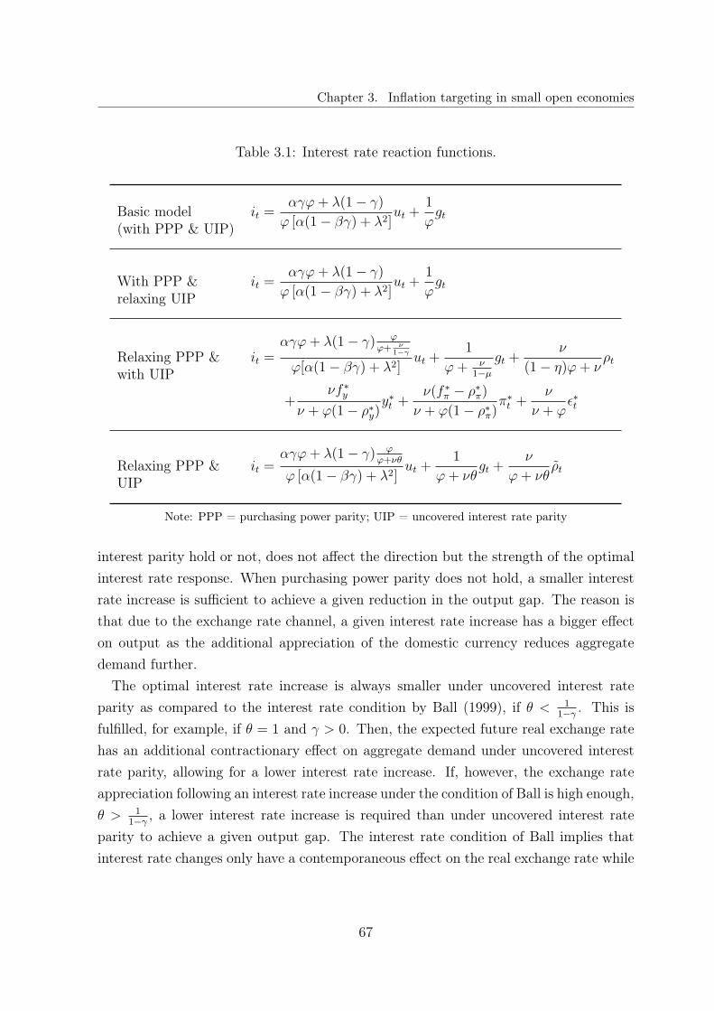
Chapter 3. Inflation targeting in small open economies
Table 3.1: Interest rate reaction functions.
Basic model(with PPP & UIP)
it =αγϕ + λ(1− γ)
ϕ [α(1− βγ) + λ2]ut +
1
ϕgt
With PPP &relaxing UIP
it =αγϕ + λ(1− γ)
ϕ [α(1− βγ) + λ2]ut +
1
ϕgt
Relaxing PPP &with UIP
it =αγϕ + λ(1− γ) ϕ
ϕ+ ν1−γ
ϕ[α(1− βγ) + λ2]ut +
1
ϕ + ν1−µ
gt +ν
(1− η)ϕ + νρt
+νf ∗y
ν + ϕ(1− ρ∗y)y∗t +
ν(f ∗π − ρ∗π)
ν + ϕ(1− ρ∗π)π∗t +
ν
ν + ϕε∗t
Relaxing PPP &UIP
it =αγϕ + λ(1− γ) ϕ
ϕ+νθ
ϕ [α(1− βγ) + λ2]ut +
1
ϕ + νθgt +
ν
ϕ + νθρt
Note: PPP = purchasing power parity; UIP = uncovered interest rate parity
interest parity hold or not, does not affect the direction but the strength of the optimalinterest rate response. When purchasing power parity does not hold, a smaller interestrate increase is sufficient to achieve a given reduction in the output gap. The reason isthat due to the exchange rate channel, a given interest rate increase has a bigger effecton output as the additional appreciation of the domestic currency reduces aggregatedemand further.
The optimal interest rate increase is always smaller under uncovered interest rateparity as compared to the interest rate condition by Ball (1999), if θ < 1
1−γ. This is
fulfilled, for example, if θ = 1 and γ > 0. Then, the expected future real exchange ratehas an additional contractionary effect on aggregate demand under uncovered interestrate parity, allowing for a lower interest rate increase. If, however, the exchange rateappreciation following an interest rate increase under the condition of Ball is high enough,θ > 1
1−γ, a lower interest rate increase is required than under uncovered interest rate
parity to achieve a given output gap. The interest rate condition of Ball implies thatinterest rate changes only have a contemporaneous effect on the real exchange rate while
67
Chapter 3. Inflation targeting in small open economies
under uncovered interest rate parity also expected future exchange rates are affected.
Excess-demand shocks
The optimal policy response to an excess-demand shock, gt > 0, is to fully offset it byraising the interest rate. The required increase in the interest rate is lower when anexchange rate channel is added, i.e., purchasing power parity does not hold. As theinduced appreciation of the domestic currency has an additional contractionary effect,a lower increase in the nominal interest rate is sufficient to perfectly offset the demandshock.
The required interest rate increase is smaller under uncovered interest rate parity thanunder the interest rate condition of Ball (1999), if θ < 1
1−γ. The basic intuition is the
same as for the cost-push shock.
Foreign shocks
When monetary policy is implemented optimally according to (3.13), inflation and out-put depend only on cost-push shocks. The interest rate is set to partially offset cost-pushshocks and to perfectly offset all other shocks.
When purchasing power parity holds, the interest rate is set independently of foreignshocks to which only the nominal exchange rate reacts. If deviations from purchasingpower parity are allowed for while uncovered interest rate parity holds, the interestrate is optimally increased following risk premium shocks, positive deviations of foreigninterest rates from the Taylor-type rule (ε∗t > 0), and increases in foreign output. Theseshocks would otherwise lead to a depreciation of the exchange rate, increasing outputabove potential and, thus, increasing inflation above target. An increase in foreigninflation is offset by an increase in the domestic interest rate if the induced increase inthe foreign interest rate, according to the Taylor-type monetary policy rule, is higherthan the persistence in foreign inflation, i.e., f ∗π > ρ∗π. If deviations from both purchasingpower parity and uncovered interest rate parity are allowed for, monetary policy perfectlyoffsets the shock ρt which captures a variety of shocks, changes in expectations, etc.
The result that monetary policy reacts only to foreign shocks when purchasing powerparity does not hold is due to the underlying assumption of foreign shocks affectingonly world interest rates. A possible extension is to include foreign output in aggregatedemand: when foreign output increases, exports to the rest of the world increase and,thus, aggregate demand.
68

Chapter 3. Inflation targeting in small open economies
Further aspects
When cost-push shocks are not persistent, i.e., γ = 0, the interest rate increase followinga given shock is lower than for γ > 0 if the condition ϕα > λ is fulfilled (sufficientbut not necessary condition). Hence, the stronger the present output reacts to the realinterest rate, i.e., the higher ϕ, the more important the stabilization objective relativeto the inflation objectives, i.e., the higher α, and the lower the direct effect of outputon inflation, i.e., the lower λ, the more likely it is, that interest rate increases are higherwhen cost-push shocks are persistent.
The interest rate response to excess-demand shocks is lower if the shock is persistent,i.e., µ > 0, while it is higher for all other shocks if they are persistent as opposed tobeing white noise. The interest rate increase following an increase in foreign inflation ishigher under persistence of the shock, i.e., ρ∗π > 0, if the foreign interest rate response isstrong enough, i.e., f ∗π > 1 + ν
ϕ.
If a country implements strict inflation targeting, i.e., α = 0, the interest rate is setto keep inflation at the target rate while increasing output volatility. As to the interestrate reaction functions, only the reaction to cost-push shocks creating a trade-off betweeninflation and output is adjusted.
3.6 Conclusion
Two central concepts in international macroeconomics, purchasing power parity and un-covered interest rate parity, are frequently used to describe open economy aspects inmonetary policy models even though their empirical relevance is controversial. As devel-oping and emerging market economies increasingly pursue independent monetary policy,in particular flexible inflation targeting, open economy aspects become increasingly im-portant for monetary policy analysis. Therefore, it is important to know if the relativelystandard and simple assumptions of purchasing power parity and uncovered interest rateparity yield different policy recommendations than alternative conditions describing therelation between prices, interest rates, and exchange rates.
The present analysis finds that the interest rate reaction function to implement flex-ible inflation targeting is affected when deviations from purchasing power parity anduncovered interest rate parity are allowed for. As long as purchasing power parity holds,monetary policy reacts only to cost-push shocks and excess-demand shocks. If, however,purchasing power parity does not hold, monetary policy also fully offsets the effects of
69

Chapter 3. Inflation targeting in small open economies
foreign shocks. Furthermore, not the direction but the strength of the interest rate re-sponse to cost-push shocks and excess-demand shocks is affected. Whether the relationbetween interest rates and exchange rates is described by uncovered interest rate parityor in the more generic way proposed by Ball (1999) does affect both to which type ofshocks monetary policy responds and how strong the response is.
However, the effects are mostly quantitative and the empirical relevance of the al-ternatives used for purchasing power parity and uncovered interest rate parity is alsonot warranted. To find alternative concepts that describe the relation between prices,interest rates, and exchange rates in an empirically relevant way while being simple, maybe the subject for future research.
The present model abstracts from a number of other important issues for small openeconomies. Foreign shocks, for example, do not only affect world interest rates but alsomore directly domestic output through the demand for exports. Additionally, foreignshocks affect inflation rates in small open economies through both imported intermedi-ate and final goods and, thus, affect both aggregate demand and potentially aggregatesupply. An extension of the present analysis to include further features of small openeconomies is planned for future research.
70

Chapter 3. Inflation targeting in small open economies
3.A Derivation of the interest rate reaction function
To derive the interest rate reaction function when the assumption of purchasing powerparity is relaxed, the reduced form representations of inflation (3.14) and output (3.15)derived from the optimality condition (3.13) are inserted into the aggregate demandequation (3.2). The resulting interest rate function depends on the nominal exchangerate:
it =(1− γ)λ + αγϕ− να
ϕ[α(1− βγ) + λ2]ut +
ν
ϕ(et + p∗t − pt−1) +
1
ϕgt (3.17)
Simultaneously, the interest rate and the exchange rate are determined by uncoveredinterest rate parity (3.8) with i∗t determined by (3.12):
it = f ∗ππ∗t + f ∗y y∗t + ε∗t + Etet+1 − et + ρt (3.8’)
The solutions for the interest and exchange rate are guessed to be linear functions ofthe state variables (ut, gt, ρt, p
∗t , p
∗t−1, ε
∗t , y
∗t , pt−1):
et = φ1ut + φ2gt + φ3ρt + φ4p∗t + φ5p
∗t−1 + φ6ε
∗t + φ7y
∗t + φ8pt−1 (3.22)
it = γ1ut + γ2gt + γ3ρt + γ4p∗t + γ5p
∗t−1 + γ6ε
∗t + γ7y
∗t + γ8pt−1 (3.23)
The guessed solutions are then inserted into the interest rate reaction function (3.17):
γ1ut + γ2gt + γ3ρt + γ4p∗t + γ5p
∗t−1 + γ6ε
∗t + γ7y
∗t + γ8pt−1
=ν
ϕ[φ1ut + φ2gt + φ3ρt + φ4p
∗t + φ5p
∗t−1 + φ6ε
∗t + φ7y
∗t + φ8pt−1]
+(1− γ)λ + αγϕ− να
ϕ[α(1− βγ) + λ2]ut +
ν
ϕ(p∗t − pt−1) +
1
ϕgt (3.24)
and into uncovered interest rate parity (3.8’):
γ1ut + γ2gt + γ3ρt + γ4p∗t + γ5p
∗t−1 + γ6ε
∗t + γ7y
∗t + γ8pt−1
= f ∗π(p∗t − p∗t−1) + f ∗y y∗t + ε∗t + φ1γut + φ2µgt + φ3ηρt
+φ4[(1 + ρ∗π)p∗t − ρ∗πp∗t−1] + φ5p∗t + φ7ρ
∗yy∗t
+φ8[α
α(1− βγ) + λ2ut + pt−1]− φ1ut − φ2gt − φ3ρt − φ4p
∗t
−φ5p∗t−1 − φ6ε
∗t − φ7y
∗t − φ8pt−1 + ρt (3.25)
71

Chapter 3. Inflation targeting in small open economies
These two equations have to hold for all values of the state variables. Matching thecoefficients of all state variables yields:
From equation (3.24): From equation (3.25):
γ1 =(1− γ)λ + αϕγ − αν
ϕ[α(1− βγ) + λ2]+
ν
ϕφ1 γ1 = φ1γ + φ8
α
α(1− βγ) + λ2− φ1
γ2 = φ2ν
ϕ+
1ϕ
γ2 = φ2µ− φ2
γ3 = φ3ν
ϕγ3 = φ3η − φ3 + 1
γ4 =ν
ϕ(φ4 + 1) γ4 = f∗π + φ4(1 + ρ∗π) + φ5 − φ4
γ5 =ν
ϕφ5 γ5 = −f∗π − φ4ρ
∗π − φ5
γ6 =ν
ϕφ6 γ6 = 1− φ6
γ7 =ν
ϕφ7 γ7 = f∗y + φ7ρ
∗y − φ7
γ8 =ν
ϕ(φ8 − 1) γ8 = φ8 − φ8
Then, the unknown coefficients can be solved for:
γ1 =αγ[ν + ϕ(1− γ)] + (1− γ)2λ[ν + ϕ(1− γ)][α(1− βγ) + λ2]
φ1 = − (1− γ)(λ− αϕ)− να
[ϕ(1− γ) + ν][α(1− βγ) + λ2]
γ2 =1− µ
ν + (1− µ)ϕφ2 = − 1
(1− µ)ϕ + ν
γ3 =ν
ν + (1− η)ϕφ3 =
ϕ
(1− η)ϕ + ν
γ4 =ν(f∗π − ρ∗π)
ν + ϕ(1− ρ∗π)φ4 = −ϕ(1− f∗π) + ν
ν + ϕ(1− ρ∗π)
γ5 = − ν(f∗π − ρ∗π)ν + ϕ(1− ρ∗π)
φ5 =ϕ(ρ∗π − f∗π)
ν + ϕ(1− ρ∗π)
γ6 =ν
ν + ϕφ6 =
ϕ
ν + ϕ
γ7 =νf∗y
ν + ϕ(1− ρ∗y)φ7 =
ϕf∗yν + ϕ(1− ρ∗y)
γ8 = 0 φ8 = 1
72

Chapter 3. Inflation targeting in small open economies
By plugging these solutions for the unknown coefficients into the guessed solution forthe interest rate (3.23), the interest rate reaction function (3.18) is obtained:
it =αγ[ν + ϕ(1− γ)] + (1− γ)2λ
[ν + ϕ(1− γ)][α(1− βγ) + λ2]ut +
1− µ
ν + (1− µ)ϕgt
+ν
ν + (1− η)ϕρt +
νf ∗yν + ϕ(1− ρ∗y)
y∗t +ν(f ∗π − ρ∗π)
ν + ϕ(1− ρ∗π)π∗t +
ν
ν + ϕε∗t
73

Chapter 4
Financial globalization in the 19th century:Germany as a financial center1
4.1 Introduction
Financial globalization is not a new phenomenon of the late 20th century. An importantera of financial globalization and integration took already place in the 19th century. Inthe 19th century, Europe was the world’s banker, lending capital to countries aroundthe world (Feis, 1930). The main capital exporter was Great Britain, followed by Franceand Germany, and their capital cities were the main financial centers intermediatingcredit through their stock exchanges and bankers. London emerged as an importantfinancial center following the Napoleonic Wars and became the undisputed internationalfinancial center in the 1870s. Another important financial center in the 19th century wasParis, second only to London, and contributed significantly to the financing of foreigngovernments and railroads since the 1820s.2 At the beginning of the 19th century,Frankfurt was the financial center of Germany and also of importance on an internationallevel. Following the political and economic restructurings in Germany during the mid1860s, Berlin developed as Germany’s financial center.3 In the early 20th century, NewYork emerged as another important financial center challenging London’s primacy (Burk,1992).
The capital exports of a country are one way to quantify its importance as an inter-national financial center. However, the collection of data on historical capital flows area challenging and time-consuming task. For Great Britain, Stone (1999) compiled an
1This chapter is based on joint work with Graciela Kaminsky.2Detailed descriptions of the developments of London and Paris as financial centers are provided, e.g.,
in Cassis and Bussière (2005).3Kindleberger (1974) describes the characteristics of financial centers and the development processes
leading to the formation of national and international financial centers.
74

Chapter 4. Financial globalization in the 19th century: Germany as a financial center
extensive data set building on previous work. The characteristics of British capital flowshave been studied extensively but surely not conclusively. The characteristics of Franceand Germany as smaller capital exporters have been investigated to a lesser degree andto our knowledge no extensive data sets are available. However, figure 4.1 provides aglance at the relative importance of the three financial centers in terms of capital exports.
Germany established as an important financial center after the Deutsche Reich wasfounded in 1871 following the German-French war. The territory then defined persisteduntil 1914. In addition to the political unification of Germany, most areas of economiclife were harmonized afterwards. In 1873 the gold standard was introduced and in 1875a central bank, the Reichsbank, was created. The era from 1870 until 1914 was char-acterized by a great expansion of economic activity in nearly all sectors, a further shiftfrom an agricultural to an industrial economy and a concentration of powers, enterprises,and capital. The rapid economic expansion was primarily the consequence but also thecause of a fast growing population and with the transition to an industrial economy ur-banization rates increased. While Germany experienced net migration outflows until themid 1890s, it turned into inflows until 1908. During most of the years, Germany had anegative balance in the trade of goods but a positive current account balance. The mainimports were raw materials, intermediate goods, and food while exports were dominatedby industrial products, especially chemicals and textiles. National income and savingswere steadily growing and made Germany a net creditor. (Hoffmann, 1965; Riesser, 1912)
Before World War I, Germany was an important capital exporter; however, the amountof foreign securities issued in German capital markets did not growth but varied signifi-cantly over time. Between 1883 and 1913, Germany invested roughly 680 million Britishpounds in foreign securities (630 million capital called) corresponding to an average of22 million pounds per year.4 The capital was predominantly invested into Europeancountries but also other regions obtained considerable amounts of capital. In the firsthalf of the 19th century, private banks were the main financial intermediaries for foreignsecurities, but they were increasingly displaced by the joint-stock banks.
The goal of the present study is to analyze the role of Germany as a financial center bycharacterizing aggregate issuances and in particular foreign issuances in German stockexchanges. The floatation of domestic securities clearly dominated aggregate issuances,quantitatively and qualitatively, and was closely linked to German economic activity.Foreign issuances were less clearly related to German economic growth than to external
4The amounts originally reported in mark are converted at the exchange rate of 20.4 marks per Britishpound.
75

Chapter 4. Financial globalization in the 19th century: Germany as a financial center
conditions. The large majority of foreign securities were bonds and the main issuers weregovernments and railroad companies. The main beneficiaries of the foreign investmentwere Germany’s neighboring countries. Furthermore, more developed and less distantcountries were more likely to additionally float equity in Germany. Thus, informationalfrictions and the pecking order relevant for trade in financial assets in the late 20thcentury seem to have been important already in the late 19th century. As most of thelarge international bonds were issued simultaneously in the main financial centers, theconditions in German capital markets relative to Great Britain and France were likelyimportant determinants of foreign issuances in Germany. Therefore, we provide insightsinto the degree of financial integration between the three main financial centers. Wefind that shocks affecting the interest rate differential between Germany and France hada significant impact on foreign issuances in Germany. Furthermore, the low interestrate differentials between the three financial centers suggest a high degree of financialintegration.
Previous work on German capital exports focuses mainly on the seeming contradic-tion between the capital exports and the apparent capital shortage in German capitalmarkets. This discussion embraces also the determinants of German capital flows, inparticular, whether political or economic considerations were the main drivers of foreigninvestment in the 19th century, see, e.g., Lenz (1922), Feis (1930), and Esteves (2008).Several studies have significantly contributed to the literature by qualifying and quan-tifying the nature of German capital exports further, e.g., Pohl (1977), Schaefer (1993),and Esteves (2008). However, these studies focus either on the determinants of Germancapital exports from the perspective of the issuing countries and, thereby, on the pulleffects on capital flows, e.g., Esteves (2008), or on the conditions in German capital mar-kets as determinants for the investment in foreign securities, e.g., Tilly (1992). We addanother aspect to the analysis and study the characteristics of Germany as a financialcenter.
The remainder of this study is organized as follows. Section 4.2 describes the devel-opment of German capital markets, the main players involved in foreign issuances, stockexchange regulations, and the process of issuance. Section 4.3 presents our data sourcesand characterizes both aggregate domestic and foreign securities issued in Germany;then, it analyzes the structure of German capital exports through the individual foreignsecurities sold in Germany. The role of external shocks on foreign issuances in Germanyand the role of Germany as a financial center are studied in section 4.4. Section 4.5
76

Chapter 4. Financial globalization in the 19th century: Germany as a financial center
concludes and provides an outlook to future research.
4.2 Capital markets, main players, and regulations in
stock exchanges
Germany was the third most important capital exporter during the 19th century lend-ing to countries around the world. At the beginning, when government credit was theprimary application, capital was mainly intermediated by private banks. Starting inthe 1830s, the financing of the railroad construction and of the advancing industriesexceeded the funding capacity of private banks and, therefore, financial intermediationshifted towards the stock exchanges and to the newly created joint-stock banks. Untilthe 1860s, Frankfurt was the financial center of Germany but lost its status to Berlinfollowing the political and economic reorganization of Germany.5 Next, the develop-ments of the German stock exchanges and the main intermediaries of foreign credit areexamined. Afterwards, the regulation of the stock exchanges and the process of issuanceare described.
4.2.1 Development of the German stock exchanges
The onset of modern trading at the stock exchange in Frankfurt a.M. is placed aroundthe turn of the 19th century. The rise of Frankfurt a.M. as a financial center wasparalleled by the decline of Amsterdam which was the most important market for gov-ernment bonds until the end of the 18th century. From the beginning, Frankfurt was animportant financial center on an international level and intermediated credits to foreigngovernments. At that time, the banking house Gebr. Bethmann was one of the mostimportant private banking houses and intermediated the majority of German govern-ment credit and made bond financing an important area of business from the middle ofthe 18th century onwards. Frankfurt’s importance as financial center rested also on thepresence of the M.A. Rothschild & Söhne whose German headquarters were located inFrankfurt. The Rothschilds increasingly displaced the Gebr. Bethmann and dominatedthe intermediation of international credits. The Frankfurt stock exchange was the mostimportant one in Germany until the 1860s when Germany was politically reorganized
5Kindleberger (1974) describes the transition from Frankfurt as the financial center to Berlin and backto Frankfurt after World War II.
77

Chapter 4. Financial globalization in the 19th century: Germany as a financial center
and Berlin became the capital of the newly founded Deutsche Reich. As a consequence,the Frankfurt stock exchange lost importance relative to Berlin although in absoluteterms it was still growing.6
The foundation of the stock exchange in Berlin was based on a decree from 1796and it had its first formal regulation in 1825. The railroad construction period in themiddle of the 19th century and the induced trading in railroad equity are consideredthe cornerstone for Berlin’s importance as a financial center.7 Frankfurt was mainlya stock exchange for bonds, in particular government bonds, and the private bankersin Frankfurt refused to introduce equity for a long time. In contrast, the Berlin stockexchange was open to equity and introduced numerous railroad shares. This contributedto a substantial shift in financial intermediation from Frankfurt to Berlin and, thereby,to the relocation of the financial center. The stock exchange in Hamburg was the third inimportance in Germany after Berlin and Frankfurt. When Amsterdam lost its position aspremier financial center, Hamburg was a major beneficiary of the reallocation of foreigntrade and, thus, of trade financing. At the onset of World War I, Hamburg had achieveda comparable position as Frankfurt as financial center (Gömmel, 1992).
In addition to their specialization in market segments, the lending of the three mainGerman stock exchanges was regionally specialized as illustrated in table 4.1. Accordingto the tax statistics reported by the Börsen-Enquete-Kommission (1893), the majority offoreign securities, 81 per cent, was taxed at the stock exchange in Berlin. Although thelocation where the taxes were paid did not necessarily coincide with the place of issuance,it gives an idea of the relative importance of the three stock exchanges. The countriesoutside Europe drew nearly exclusively on the Berlin stock exchange while North &Central Europe relied mostly on the Hamburg stock exchange. The Frankfurt stockexchange was an important alternative to Berlin for South and East European borrowers.The stock exchanges were important market places for investors and intermediatingbanks. However, international loans and investments were also made outside the stockexchanges, mainly by the banks.
6Wormser (1919) describes the developments of the stock exchange in Frankfurt in detail.7The development of the Berlin stock exchange is analyzed at length by Spangenthal (1903) and
Gebhard (1928).
78

Chapter 4. Financial globalization in the 19th century: Germany as a financial center
4.2.2 Main players
The investment in international securities and the intermediation of international loanswere made both by private banks and joint-stock banks. However, while financial in-termediation was dominated by private banks until the middle of the 19th century, theincrease in loan volumes to finance the construction of railroads and the heavy indus-try led to the formation of joint-stock banks. Following the concentration process inthe banking sector in the late 19th century, the so-called Great Banks dominated thefinancial intermediation.8 The universal banks, pursuing all kinds of banking activities,were characteristic of the German banking system in contrast to the specialized Britishbanks. The German banks engaged in the underwriting, formation, and reorganizationof companies while they refrained from creating pure deposit banks. During all times,they were also involved in the intermediation and underwriting of foreign securities.(Riesser, 1912)
Until the middle of the 19th century, foreign loans in Germany were mainly intermedi-ated by private banks who lent their own capital. However, as the demand for financingincreased beyond what banks could handle by themselves, the banking house Bethmann,founded 1748 in Frankfurt, and other private banks created the Partialobligation and,thereby, started the intermediation of securities. Through the Partialobligation banksacquired external funds while explicitly acknowledging the actual borrower and, thus,excluding any liability.9 The trading of these securities was then a next step. In Frank-furt, the Bethmanns and the banking house B. Metzler seel. Sohn & Co. (founded1674) were the main bankers around 1800. Later on, the Rothschilds became the mainprivate bankers in Frankfurt were Meyer Amschel Rothschild founded M. A. Rothschild& Söhne with his sons in 1810. The presence of the Rothschild brothers in all impor-tant financial centers was pivotal for their outstanding international financial role sinceprivate contacts and relations as well as local knowledge were crucial in overcoming in-formation asymmetries.10 Other important private banks in Frankfurt were Jacob S.
8Riesser (1912) provides a detailed account of the German banking system, its activities, and theconcentration process.
9With the Partialobligation, the private banks created a new financial instrument to acquire externalfunds which could then be lend. The novelty was that the banking house borrowed funds fromnumerous private persons, bundled them, and lent the amount as one loan. The bankers wrotepartial certificates of debt to the lenders but were not anymore liable in case of bankruptcy of theborrower. It thereby represented a new form of financial intermediation between small investors andbig borrowers without the private bankers being personally liable. (Wormser, 1919)
10The Rothschild office in London was established in 1804 and in Paris in 1812/15. The agencies inVienna and Naples, established in 1816 and 1820, respectively, were branches of the Rothschild office
79

Chapter 4. Financial globalization in the 19th century: Germany as a financial center
H. Stern (1805), Lazard Speyer-Ellissen (1846), and Erlanger & Söhne (1859). Frank-furt was the most important banking center until around 1860, followed by Cologne.The most important private banks in Cologne were Sal. Oppenheim & Cie. (1789)11
and A. Schaaffhausen (1790). Until the financing of the railroad construction and theheavy industry started in the 1830s, the main banking business was government loans.With the railroad construction, Berlin gained importance and with it the main privatebanks Gebr. Schickler (1796), S. Bleichröder (1803), Mendelssohn & Co. (1805), and R.Warschauer & Co. (1849). Hamburg played a special role in foreign trade financing andthe most important private banks were L. Behrens & Söhne (1780) and M. M. Warburg& Co. (1798). (Wormser, 1919; Gebhard, 1928; Born, 1977)
As the financial needs and transaction volumes of both industries and issuance busi-ness increased further, it became more and more difficult for private banks to managethese by themselves even with external funds. Especially the financing of the railroadconstruction posed a big challenge to private bankers. As a consequence, private bankscooperated both informally through syndicates and formally through the foundationof new banks. As a matter of fact, most joint-stock banks were created by privatebankers or were the result of reorganizing an existing private bank. In the first foun-dation wave between 1848 and 1870, four of the Great Banks were established. TheA. Schaaffhausen’scher Bankverein was founded 1848 in Cologne through the recon-struction of the bank house A. Schaaffhausen. In 1851 the Disconto-Gesellschaft wasfounded in Berlin and became an actual joint-stock bank in 1856 through a change inlegal status. Also the Bank für Handel und Industrie, founded 1853 in Darmstadt bythe private bankers Gustav Mevissen and Abraham Oppenheim, was a major player inthe intermediation of international loans. Due to its location in Darmstadt, the bank isgenerally known as Darmstädter Bank. (Riesser, 1912) The Berliner Handelsgesellschaftwas founded in 1856 under the participation of Mendelssohn & Co., S. Bleichröder,Robert Warschauer & Co., and Gebr. Schickler. In the second wave of joint-stock bankfoundations starting in 1870, the Deutsche Bank and Dresdner Bank were established.In 1870 Gebr. Schickler, A. Schaaffhausen’scher Bankverein, Gebr. Sulzbach, and othersfounded the Deutsche Bank in Berlin. The Dresdner Bank was built in 1872 on the basisof the private bank house Michael Kaskel in Dresden in cooperation with the BerlinerHandelsgesellschaft and relocated to Berlin in 1881. (Gebhard, 1928) From the late 19th
in Frankfurt until 1844, when they become independent offices. Born (1977) discusses the role ofpersonal networks in overcoming information asymmetries further.
11Salomon Oppenheim was founded 1789 in Bonn and relocated to Cologne in 1801. (Born, 1977)
80

Chapter 4. Financial globalization in the 19th century: Germany as a financial center
century onwards, a strong concentration process took place in the banking sector anduntil the beginning of the 20th century, most private banks were taken over by the GreatBanks. For example, the business of the Rothschilds in Frankfurt was taken over by theDisconto-Gesellschaft in 1901 and the Frankfurt bank house Erlanger & Söhne by theDresdner Bank in 1904. (Born, 1977)
While most private banks in Germany had their origins in the trade and shippingbusiness or were the private financiers of German sovereigns, in the last quarter of the19th century the German joint-stock banks emerged as universal banks, involved in alltypes of banking activities. They engaged in the financing of industries, trade, and gov-ernments through underwriting, foundation, and reorganization activities and throughthe foundation of appropriate institutions, both domestically and internationally. TheGreat Banks improved and extended their international business first by creating affil-iates abroad, later by founding new banks overseas and delegated part of the interna-tional issuance business.12 However, the private banks and the Great Banks continuedto carry out the biggest international transactions by themselves. The underwriting andissuance of foreign securities was in general directed by syndicates, mostly internationalones, formed for a limited number of transactions or even individual deals. Only veryfew syndicates or banking groups dominated the business with a specific country overprolonged time periods. (Born, 1977) When syndicates issued securities, the underwrit-ing syndicate was often different from the introducing syndicate and it was commonthat the underwriters themselves gave sub-participations to other banks to reduce theireconomic responsibilities. In general, the leader of the syndicate then actually sold thesecurities at the stock exchanges or entrusted another company or bank to do so. Mostly,the securities were issued piecewise trying to influence the price. (Lotz, 1890)
4.2.3 Regulation of the stock exchanges
In the first half of the 19th century, the German stock exchanges were subject only toself-determined regulations and not to government regulation, except for the ban onforward trading in Berlin. Due to widespread speculation first in Spanish, then in otherforeign securities, and finally in railroad equity, consecutive regulations were establishedthat prohibited forward trading in these securities between 1836 and 1844 in Berlinand were abolished only in 1860. (Spangenthal, 1903) The Stock Exchange Act of 1896
12Otto (1910) and Steinmetz (1913) elaborate on the activities of the Great Banks overseas includingtheir foundation activities.
81

Chapter 4. Financial globalization in the 19th century: Germany as a financial center
was the first one to regulate the stock exchanges on a national level. The regulationfollowed closely the recommendations of the Börsen-Enquete-Kommission (Committeeof the Stock Exchange Inquiry) who conducted a detailed analysis of the stock exchangesin Germany. The new regulation restricted forward trading in securities significantly,required the publication of a prospectus for securities applying for admission to trade,and made the underwriting banks accountable for the content of these prospectuses.13 Asthe individual stock exchanges had their own rules governing the admission of securitiesfor trade already prior to the Stock Exchange Act, the consequences of the regulationfor capital markets and the intermediaries are not trivial. The restrictions in forwardtrading are often mentioned as having contributed to the concentration in the bankingsystem, e.g., Fohlin (2002). The induced increase in spot transactions severely reducedthe flexibility of capital markets and favored bigger banks over private banks. Theprospectus requirements are unlikely to have significantly affected foreign issuances asalso the UK and France had similar requirements for the floatation of foreign securities.Wetzel (1996) does not find any statistically significant impact of the Stock ExchangeAct on domestic and foreign issuances and Fohlin (2002) finds only a small effect on theconcentration in the banking system.
Furthermore, starting in 1881, the government imposed two types of taxes on tradingin securities, an issuance tax (Effektenstempel) and a turnover tax (Umsatzstempel). Theissuance tax was levied on all securities sold at an initial public offering in Germany withthe exception of German government bonds; the turnover tax was levied on all securitytransactions. For both taxes, different rates applied to different types of securities and todomestic and foreign borrowers. The tax rates were successively increased in 1885, 1894,1900, and 1909. Starting in 1894, the issuance tax was also due on foreign assets boughtoutside of Germany if the investor resided in Germany and the securities were not heldin an account abroad.14 The tax increases on foreign securities significantly reducedthe attractiveness of the German stock exchanges for both foreign issuers and domesticinvestors. The displacement of German capital to foreign stock exchanges might havebeen significant. According to Fritzsche (1913), German investors increasingly boughtforeign securities outside the German capital markets; the amount of foreign securitiesheld in deposits outside the country, and, thus, not subject to the taxes, increased nearlythreefold between 1893 and 1902, from 7.5 million pounds to 22 million pounds.
13Wetzel (1996) discusses the Stock Exchange Act and its implications in detail.14Details on the tax regulation and the successive amendments are described, e.g., in Meyer (1902),
Kleiner (1914), the Frankfurter Zeitung, and the Deutsche Oekonomist.
82

Chapter 4. Financial globalization in the 19th century: Germany as a financial center
While German central government bonds were automatically admitted for trade atthe stock exchanges, all other securities had to apply for admission which had to beformally filed for by a German bank. The admission of foreign securities was requiredfor the whole amount issued and not only the share offered for subscription in Germany,thereby facilitating the international trade in these securities. (Kleiner, 1914) Eventhough the admission to official trading had the advantage of facilitating the issuanceand placement of a security, numerous securities were sold exclusively on the free market.A very rough estimate of the relative importance of the free market, i.e., the tradingoutside the stock exchanges, is provided by the Börsen-Enquete-Kommission (1893) forthe stock exchange in Hamburg. While only 129 foreign securities with a face value of17 million pounds were officially introduced to the Hamburg stock exchange between1880 and 1892, 678 securities with a nominal amount of 27 million pounds were taxed.15
This leaves 10 million pounds to 549 not officially admitted securities, corresponding to37 per cent of the value of the foreign securities bought by German investors. However,it also points at the fact that the big international issuances were traded through thestock exchanges while it were mainly smaller securities bypassing the stock exchanges.16
4.2.4 The process of issuance
Zickert (1911) describes the most common ways foreign securities were sold in Germany.The main ways of introducing new foreign securities to the investing public were theadvertisement through newspapers and circulars and the recommendation by banks andbankers to their clients. Foreign securities were sold either through the introduction ata German stock exchange or directly by the banks to their customers. Through theirdeposit banks and affiliates the Great Banks had direct access to private investors andcould sell foreign securities without requiring the admission to a stock exchange to makethe information available. Especially foreign securities underwritten by syndicates wereoften not placed on stock exchanges but directly sold to the banks’ customers. Thequantity of foreign securities publicly offered for subscription while bypassing the stockexchange administration office was also non-negligible. Zickert (1911) estimates thatin 1909 and 1910 approximately 11 per cent of all foreign securities were offered forsubscription without being admitted to a stock exchange. To introduce a foreign secu-15The tax applied to all foreign securities bought by German investors, independent on whether they
were bought through a stock exchange or not.16The average amount of the officially admitted securities was 132 thousand pounds, while the not
admitted securities only amounted to 18 thousand pounds on average.
83

Chapter 4. Financial globalization in the 19th century: Germany as a financial center
rity to the stock exchange, the underwriters had to apply for admission; afterwards, ingeneral, an invitation for subscription followed. However, it had become common prac-tice among underwriting banks at the turn of the century to carry out the subscriptionprior to the successful admission to a stock exchange as pointed out by the DeutscheOekonomist (August 5, 1899; July 9, 1904). The banks justified this procedure with thetime-consuming admission process in Germany which left them with a disadvantage overtheir fellow underwriters in international syndicates and would require them to refrainfrom such activities. (Zickert, 1911)
Marx (1913) distinguishes two ways in which new securities were distributed to thepublic: direct and indirect issuance. In case of a direct issuance, the person or companyraising capital offered its securities directly to the public though public subscriptionor over the counter. Direct issuance was only common practice for German govern-ment bonds until the middle of the 19th century, afterwards they were mediated mainlythrough the Prussia-Syndicate. The more common form was the indirect issuance wherea banker or bank syndicate intermediated between the public and the capital searcher. Ingeneral, the banks underwrote the whole security, i.e., they bought it for a fixed transferprice and distributed it at their own expenses to the public. For foreign issuances onlythe indirect method was relevant. The security was then sold to the public either by pub-lic issuance, i.e., through subscription invitations or introduction to a stock exchange,or by sale over the counter, advertised through letters to customers and non-customers.Securities issued and sold over the counter were very hard to capture statistically as theprocess took place off the public without announcements, prospectuses or suchlike in thepublic press or in other public form. Usually, more than one issuance method was usedat a time.17
4.3 International issuances
The time period under scrutiny starts in 1883, the year in which the Deutsche Oekono-mist started publishing data on securities issued on the German stock exchanges andwhen the turbulences following the Gründerkrise (Founding Crisis) of 1873 most likelyalready faded. As the capital markets basically shut down when World War I started,our sample period ends in 1913. The data sources are described next. Then, the aggre-gate amounts of capital floated on the German stock exchanges between 1883 and 1913
17Lotz (1890) provides a very detailed description of the issuance process in Germany.
84

Chapter 4. Financial globalization in the 19th century: Germany as a financial center
are analyzed and the similarities and differences between domestic and foreign issuancesare studied. Finally, we look at foreign investments made between 1883 and 1897 byusing disaggregated data of foreign securities issued on the German stock exchanges.
4.3.1 Data sources
To quantify the amount of domestic and foreign securities issued on the German stockexchanges, the most widely used and valued statistics are provided by the DeutscheOekonomist located in Berlin and the Frankfurter Zeitung located in Frankfurt. Thepurpose of the issuance statistic of the Deutsche Oekonomist was to provide “the mostprecise possible answer to the question to which extent the capital and money marketshave been drawn on by issuances of securities during a specific time period” (January 14,1911). Thus, only officially admitted securities, based on prospectuses were included. Ingeneral, the overall amount admitted based on the subscription price or the introductoryrate was reported even though only a fraction may have been introduced during the ad-mission year or allocated following the subscription. It was especially common for realestate and agricultural mortgage bonds that the issuance was extended over prolongedtime periods.18 Conversions, restructurings, and mergers were excluded; only increasesin capital were included. (Deutsche Oekonomist, January 14, 1911) A peculiarity offoreign securities was that the application to German stock exchanges had to be madefor the whole amount issued and not only the share offered for subscription or sold inGermany. As has been pointed out also elsewhere in the literature, e.g., Bankenquete(1910) and Marx (1913), it is extremely hard if not impossible to accurately know theshares of foreign securities actually placed in Germany. The Deutsche Oekonomist statesthat “the issuing house only knows the exact amount actually placed in Germany dur-ing the here considered limited time period after the issuance; but it will reveal thisamount only possibly if it was sold out, an information not identical to the informationthat there was an over-subscription” (September 11, 1909). Nevertheless, the DeutscheOekonomist reported tentative estimates of the amount of international securities sold inGermany based on information of the issuing houses if available. However, this detailedinformation is only available until 1897 as the Deutsche Oekonomist stopped publishingdetailed lists with the securities sold in Germany. The reason provided by the DeutscheOekonomist was that the number of securities had increased too much to report them
18The Deutsche Oekonomist reported rounded estimates of the German mortgage bonds for the currentyear and revised them when the bank statistics were made. (July 13, 1895)
85

Chapter 4. Financial globalization in the 19th century: Germany as a financial center
individually (January 14, 1899). However, at the same time the Kaiserliche StatistischeAmt (Government Statistical Office) started publishing the amounts of securities ad-mitted for trade. As the amounts of foreign securities admitted for trade exceeded theamounts sold in Germany by wide margins, this information is only of limited use forthe analysis of capital exports intermediated by the stock exchanges.
The issuance statistic of the Deutsche Oekonomist is available starting in 1883, whilethe statistic of the Frankfurter Zeitung is available only for a much smaller time period,starting in 1896. We therefore follow Esteves (2008) and other related literature in usingthe data provided by the Deutsche Oekonomist. The amounts originally stated in marksare converted into British pounds at the exchange rate of 20.4 marks per pound.
4.3.2 Aggregate issuances
The aggregate amount of securities issued in the German stock exchanges during aspecific year is a measure of new capital investments, both in domestic and foreign ap-plications. The aggregate issuances in Germany increased over the sample period andfluctuated with four local peaks broadly corresponding to peaks in the German busi-ness cycle19: in 1888 (98 million pounds), 1899 (110 million pounds), 1905 (148 millionpounds), and 1908 (164 million pounds), see figure 4.2. Capital was invested both in Ger-man and foreign securities. While the amount invested in domestic securities increasedover time, foreign securities fluctuated without trend, see figure 4.3. The fluctuations inaggregate issuances were mainly driven by domestic issuances exhibiting a very similartime pattern20, with the exception of the peak in 1905 due to an outstanding amountof 60 million pounds in foreign securities. Foreign securities quantitatively dominatedtotal issuances only until 1886; afterwards their share declined with the exception of twopeaks around 1897 and 1905.
The variations in foreign issuances were dominated by the floatation of governmentand railroad bonds, see figure 4.4. The exceptional amount of foreign issues in 1905is related to the Russian-Japanese war. The war led to the floatation of a Russiangovernment bond of 12 million pounds and three Japanese government bonds summingup to 16 million pounds, thereby accounting for half of all foreign securities floatedthat year. Government bonds were also an important determinant of fluctuations in
19These peaks correspond both to periods of high economic growth and to peaks in the detrendedGerman GDP series using the Hodrick-Prescott filter.
20The correlation between the two series is 0.94.
86
Chapter 4. Financial globalization in the 19th century: Germany as a financial center
domestic securities, see figure 4.5. Furthermore, investments in mortgage and industrialsecurities were quantitatively significant while railroad securities played nearly no roleamong domestic securities. The railroad boom in Germany took place earlier in the19th century and most railroad companies were nationalized starting in the late 1870s.(Riesser, 1912; Tilly, 1992) Hence, railroads were mainly financed through governmentsecurities afterwards. While government bonds exhibited a similar pattern as overalleconomic activity, industrial securities increasingly displaced mortgage securities.
In the aggregate, 82 per cent of capital was invested in bonds and only 18 per cent inequity. The preference for bonds was even stronger for foreign securities: only 8 per centof the foreign securities floated in Germany were equity. However, the relative impor-tance of bond versus equity financing varied significantly over time, both for domesticand foreign securities and across sectors, see figure 4.6. Bonds were mainly issued by do-mestic and foreign governments, followed by domestic mortgage institutions and foreignrailroad companies. The industrial sector in Germany was the main receiver of equityfinancing. Furthermore, German banks issued substantial equity. Investment in foreignequity, however, was mostly directed towards railroad financing and, at the beginningof the 20th century, increasingly towards the banking sector. As bondholders are seniorlenders relative to equity holders, investing into bonds involves a lower risk than intoequity. Accordingly, the issuance of equity was particularly volatile. Furthermore, infor-mation asymmetries between lenders and borrowers may be exacerbated by geographicaldistance and, thus, be higher for foreign than domestic investments.21
Different types of financial instruments involve diverging degrees of risk and so do dif-ferent types of borrowers. Even though governments can, and sometimes do, default ontheir debt, government bonds may be considered safer investments than bonds of otherissuers. Due to their taxing power, insolvency is a lesser concern for governments than forprivate enterprises. Furthermore, less information is needed to evaluate a government’sfinancial situation than a private company’s one.22 In the 19th century, most railroadcompanies enjoyed some form of government guarantees, either explicitly or implicitly,and, therefore, the investment risk was reduced as compared to industrial companies.Private industrial companies may be considered the riskiest borrowers as the available
21German investors’ knowledge of foreign countries was probably very limited and, therefore, the risksinvolved when investing in these countries substantial. By lending through bonds the risk couldbe reduced. The role of informational frictions for trade in financial assets is discussed in the nextsection.
22In the 19th century, information asymmetries were most likely substantial as the transmission ofinformation was costly, see, e.g., Flores (2007).
87

Chapter 4. Financial globalization in the 19th century: Germany as a financial center
information relative to the necessary one was probably the least and the solvency risksubstantially higher than for governments and government guaranteed railroad compa-nies.
Germany invested in securities of countries around the world and countries were dif-ferent and involved diverging degrees of actual and perceived risk. The disaggregationof foreign securities to the country or at least regional level helps in identifying patternsin the foreign investment and is pursued in the next section.
4.3.3 Individual foreign securities
German capital was financing governments, railroads, and industrial companies aroundthe world. Using disaggregated data on the foreign securities floated in Germany revealsthe countries and regions that were the main beneficiaries of the capital flows and con-tributes to our understanding of foreign investment decisions. However, the DeutscheOekonomist provided disaggregated data only until 1897. The collection of the disaggre-gated data for the remaining period until 1913 is the subject of ongoing research. Still,the reduced sample from 1883 until 1897 offers interesting insights into the characteristicsof German capital exports and is therefore analyzed in detail.
Table 4.2 illustrates the main regional pattern in foreign investment made through theGerman stock exchanges between 1883 and 1897.23 The majority of foreign securities,i.e., 80 per cent, was issued by European countries, more specifically Austria-Hungaryand Russia who received 21 and 22 per cent, respectively, followed by South Europe,i.e., mainly Italy, with 16 per cent. The second most important continent were theAmericas whose securities floated in Germany accounted for 16 per cent of all interna-tional issuances, with only a slightly higher share in North America than Latin America.However, the relative importance of the regions varied over time, see figure 4.7. Duringthe late 1880s, the Americas gained considerable weight in international issuances, es-pecially through increased floatations of Latin American securities. However, between1891 and 1894, no Latin American securities were floated in Germany, probably as areaction to the Baring crisis in 1890.24 The composition of the European securities alsovaried substantially. The South European countries increased the floatation of securitiesin the late 1880s and early 1890s when Austria-Hungaria had a low participation and23We focus on the country of location of a railroad, bank, or company, and, thereby, concentrate on
the characteristics and risks of the country where the business was carried out as compared to thenationality of the owner.
24For a discussion of the Baring crisis, see, e.g., Flores (2007).
88

Chapter 4. Financial globalization in the 19th century: Germany as a financial center
Russia did not contribute at all to the foreign issuances in German stock exchanges.Figure 4.8 provides a more detailed picture of the countries floating securities on
the German stock exchanges between 1883 and 1897. Austria-Hungary was the mainissuing country with 89 securities floated, followed with a considerable gap by the UnitedStates (43 issues), Italy (42 issues), and Russia (35 issues). However, the size of issuesvaried considerably across countries. The average size of securities floated was highestfor Russia and Mexico, both with 2.2 million pounds, followed by Argentina with 1.8million pounds. Accordingly, the relative importance of countries in terms of fundsobtained from German capital markets is a different one. Russia and Austria-Hungaryclearly dominated with 78 and 76 million pounds, respectively, followed by Italy (46million pounds), and the United States (30 million pounds).
The types of investment between regions also differed substantially, see table 4.2.Investment in Africa, North America, and South Europe was mainly related to railroadfinancing, securities issued by Latin American and South-East European countries weremostly government bonds while Asian, i.e., Chinese, securities were exclusively issuedby the government. Investment directed towards the banking, industrial, and mortgagesectors played a non-neglegible role only in Austria-Hungary, North and Central Europe.As previously pointed out, bonds were the dominant type of securities sold on Germanstock exchanges. However, equity financing played also a role for applications in NorthAmerica, North & Central Europe, South Europe, and Africa, especially for railroadprojects. Industrial equity was highest in Austria-Hungary and North & Central Europewith roughly 2 million pounds each and bank equity in Austria-Hungary with 2 millionpounds. These findings are consistent with some stylized facts in the literature ontrade in financial assets. Germany invested predominantly in neighboring countriesconfirming a common pattern. Portes and Rey (2005) find that a gravity model performsvery well in explaining international trade in financial assets. They explain the strongnegative correlation between geographical distance and asset trade by informationalfrictions proxied by distance. The knowledge of neighboring countries is generally higher.However, Portes, Rey and Oh (2001) do not find that equity investments react strongerto informational frictions than bond investments.
In our sample period North America issued equity in Germany while Latin Americadid not. Likewise, North and Central Europe as well as South Europe issued equity butit played nearly no role for South-East Europe. Thus, we find a tendency that closeand more developed countries received more equity investment. This may be due to
89

Chapter 4. Financial globalization in the 19th century: Germany as a financial center
informational asymmetries being lower for neighboring countries and more developedcountries being perceived as less risky. The equity investment into African railroadswas nearly exclusively into the Dutch-South African railroad company. The companywas founded in the Netherlands but was actually a German company. (Baltzer, 1916)Due to the railroad’s location in South Africa it is considered foreign investment inAfrica, even though the nationality risk was European. Thus, the investment may havebeen perceived as less risky thereby strengthening our findings. Daude and Fratzscher(2008) find an actual pecking order in foreign investment determined by informationalfrictions and institutional quality in the host country. Portfolio investment is much moresensitive to both determinants than direct investments or bank loans. Therefore, FDI andloans dominate investment in less developed countries while portfolio investment is moreprevalent in developed countries. However, in our dataset we currently cannot distinguishbetween portfolio investment and FDI and, therefore, we cannot draw inference in thisregard.25
The decision to invest into a foreign security depends also on the asset’s riskiness.One risk measure is market liquidity: if assets can be easily sold, the risk is lower. Theissuance frequency of a borrower in German stock exchanges is a possible proxy formarket liquidity. The more often a borrower issues securities in Germany, the higherthe circulation of the borrower’s securities and, thus, the more likely significant trade istaking place. Furthermore, investors may have better information on borrowers alreadypresent in German financial markets. We next look at the frequency in which coun-tries issued securities in Germany. Thereby, we learn which countries had permanent oronly temporary access to German capital markets and get some insights about investors’knowledge of specific countries. Figure 4.9 accordingly depicts borrowing behavior onGerman stock exchanges on a yearly basis. The incidence of new issuances varied signifi-cantly across countries. While some of the main recipient countries like Austria-Hungary,Italy, and the United States floated securities nearly every year, Russia as one of themain borrowers did not float securities between 1889 and 1893. This, however, was dueto political considerations. Between November 1887 and October 1894, the Reichsbankwas not allowed to accept Russian bonds as collateral for loans, thereby, Russia was
25The distinction between portfolio investment and foreign direct investment is not clear-cut. Therelated literature characterizes the securities intermediated through the stock exchanges as portfolioinvestment. In contrast, Lane and Milesi-Ferretti (2007) define an equity participation above 10 percent as FDI. However, this information is not available for our sample. In any case, equity that maybe considered FDI or portfolio investment accounts only for 8 per cent of the foreign securities inour sample and the remainder is portfolio investment.
90

Chapter 4. Financial globalization in the 19th century: Germany as a financial center
indirectly denied access to the German capital market.26 Countries like Switzerland andSweden floated securities nearly every year even though in absolute terms they werenot among the main recipient countries, while other countries like Argentina, China,and Mexico floated securities only during a couple of years but received noteworthyamounts of capital. Yet other countries only floated securities in Germany only once likeAlgeria, Canada, and Cuba. As we do not have information on denied issuances andamounts issued through other financial centers, we do not know the underlying reasons,i.e., whether a country issued only seldom securities in Germany because of denied accessor because no access was requested. Not surprisingly, the majority of securities issuedin Germany were rather small in size, both bonds and equity, see figure 4.10. The largeinternational bonds were in general issued by international syndicates and placed notonly in Germany but also in London, Paris and smaller financial centers.
4.4 The role of external shocks
The foreign securities floated in Germany were mostly issued simultaneously in othercountries, especially in the two main financial centers, London and Paris. Hence, thequantity of foreign securities floated in Germany was not only determined by the con-ditions in the borrowing countries and on German capital markets but also by the con-ditions in other financial centers, most importantly London and Paris. In this section,we examine if shocks to these other financial centers affected the floatation of foreignsecurities in Germany.
4.4.1 The model
Consider a simple partial equilibrium model of the German capital market. There aren countries including Germany, the UK, and France. All countries need funds that aresupplied only by the UK, France, and Germany as financial centers. Hence, all the othercountries are just borrowers. The German capital market is in equilibrium when thefunds demanded equal the funds supplied.
n−1∑i=1
Di(RG, RG−RUK , RG−RFr, Y i)+DG(RG, RG−RUK , RG−RFr, Y G) = SG(RG, rG, rpG)
26A more detailed description of the Lombardverbot and its implications for financial transactions isprovided by, e.g., Feis (1930) and Born (1977).
91

Chapter 4. Financial globalization in the 19th century: Germany as a financial center
The demand for German funds, Di, depends on the interest rate RG at which countriescan borrow from Germany and on the interest rate differential between Germany andthe UK, RG − RUK , and between Germany and France, RG − RFr, as countries canalternatively borrow from the UK or France. When the interest rate in Germany ishigher than in the UK, for example, the demand shifts towards the British capitalmarket. Therefore, the demand for German funds depends negatively both on the levelof the German interest rate and the differentials against the other financial centers.Furthermore, the demand increases with economic activity in the borrower country, Y i.
Investors in Germany have the alternative between lending to risky domestic or foreigncountries/firms at an interest rate RG and investing at the risk free rate rG. Hence,the supply of funds in Germany, SG, depends positively on the risky interest rate andnegatively on the risk free interest rate. The risk aversion of German investors and theoverall risk of investments are captured in the term rpG that determines the degree ofsubstitutability of the risky and the safe asset. We take RUK and RFr as exogenous.Aggregating the demand for funds of non-German countries, DF , we obtain the supplyof funds to non-German borrowers as follows:
DF (RG, RG −RUK , RG −RFr, Y F ) = SG(RG, rG, rpG)−DG(RG, RG −RUK , RG −RFr, Y G)
Then, solving for RG, we obtain a reduced form equation for foreign issuances in Ger-many:
IG(rG, rpG, RG −RUK , RG −RFr, Y G, Y F ) (4.1)
Hence, foreign issuances depend negatively on the risk free interest rate and the risk termrpG. When the opportunity cost of the risky investment, the riskiness of the investmentsthemselves, or the risk adversion of German investors increase, foreign issuances arelower. The effect of a change in the interest rate differentials on foreign issuances isambiguous. An increase in the differential reduces the demand for German funds butincreases the supply of funds to non-German borrowers. The relative interest elasticitiesof demand and supply determine whether the overall effect is positive or negative. Anincrease in economic activity in the borrower countries increases the demand and, hence,has a positive effect on foreign issuances. An increase in German economic activity,however, reduces the supply of funds to non-German borrowers.
92

Chapter 4. Financial globalization in the 19th century: Germany as a financial center
4.4.2 Estimation
The reduced form equation for foreign issuances in Germany (4.1) is estimated by re-gressing the log of the nominal amount of foreign securities issued in Germany each yearon the following explanatory variables. We use the private discount rate in Germany asthe risk free interest rate.27 The term rpG capturing both the risk aversion of Germaninvestors and the riskiness of investments can be proxied using a variety of indicators.The share of countries defaulting on sovereign debt in a given year measures the aggre-gate default risk, a higher share implying higher risk. The differential between a long-and a short-term interest rate provides a measure of the term premium, assuming thatan increase in the term differential reflects higher risk. The term premium is measuredas the difference between the long-term government bond yield and the private discountrate in Germany. A third indicator is the amount of foreign securities issued in GreatBritain, the premier financial center, as a proxy of liquidity in financial markets: higherissuances are a sign of higher liquidity and, thus, lower risk. We transform foreign is-suances in Great Britain by using the negative value. Then, an increase in each of thethree indicators reflects an increase in risk. All indicators have their relative merits andcaveats and are correlated. Therefore, instead of choosing one indicator, we derive theprincipal components of the three risk indicators and use the first principal componentas explanatory variable. The first principal component explains 69 per cent of the totalvariability of the risk indicators and the second principal component an additional 23 percent. The first principal component is a roughly equal linear combination of the threerisk indicators and can be interpreted as overall investment risk. The first two principalcomponents are illustrated in figure 4.11. The interest rate differentials between thefinancial centers are measured with long-term real interest rates obtained by substract-ing the inflation rate from the long-term nominal government bond yields. Economicactivity in Germany is measured by the GDP growth rate while economic activity inthe rest of the world is proxied by the GDP growth rate in the UK. The reason is thatthe UK was the premier financial center and we assume that when the UK entered arecession, so did the rest of the world. An alternative measure is the growth rate ofworld exports and is used as a robustness check. The data sources are described in table4.3. Figure 4.12 illustrates the fluctuations in the real interest rate differentials and the
27The private discount rates were the interest rates negotiated in the transactions between credit in-stitutes (Deutsche Bundesbank, 1976). The original interest rates are in nominal terms and areconverted into real interest rates by substracting the inflation rate.
93

Chapter 4. Financial globalization in the 19th century: Germany as a financial center
private discount rate in Germany, while figure 4.13a depicts the GDP growth rates inGermany and the UK.
Equation (4.1) is estimated using Ordinary Least Square (OLS) techniques. Foreignissuances are truncated at zero, however, the log of foreign issuances is not. The advan-tage of OLS is that the estimated coefficients can be directly interpreted as comparedto Tobit estimations. As a robustness check we perform our estimations also for foreignissuances in levels using Tobit techniques. The results of the estimations are reported intable 4.4 and figure 4.14 shows the actual series of the log of foreign issuances as well asthe fitted values and residuals for specification (1). While column (1) in table 4.4 is thebaseline regression including all the above described variables, the regression in column(2) excludes economic activity in Germany and the UK.
The main insight is that the conditions in financial markets both in Germany andrelative to the other financial centers as well as aggregate risk mattered for the amountof foreign securities floated in German stock exchanges. As expected, higher privatediscount rates in Germany and higher risk discouraged foreign lending in Germany.While an increase in the long-term interest rate in Germany relative to France affectedforeign issuances in Germany negatively, the differential between Germany and the UKdoes not have a statistically significant effect. This can be interpreted as follows. Theinterest rate semi-elasticity of the demand for funds of non-German borrowers is higherthan the interest rate semi-elasticity of supply. Hence, Germany and France seem tobe substitutes as financial centers for borrowers. The effect is quite substantial: a onepercentage point increase in the interest rate differential decreased foreign issuances byroughly 80 per cent. As the interest differential between Germany and France rangedbetween -0.2 and 0.8 per cent, the changes in the differential were commonly muchsmaller than one percentage point, see figure 4.12. The semi-elasticity of foreign issuanceswith respect to changes in the interest rate differentials is higher than with respectto changes in the domestic short-term interest rate. This may suggest that foreignshocks mattered more for international issuances than domestic shocks. However, anincrease in the differential may be due to both an increase in German long-term interestrates and a reduction in long-term interest rates in the respective other financial center.Therefore, these estimations do not provide clear guidance in this respect. Furthermore,the small interest rate differentials and their low volatility in figure 4.12 suggest thatthe financial centers were highly integrated. Economic activity in Germany and worldeconomic activity, however, are not statistically significant in explaining foreign issuances
94

Chapter 4. Financial globalization in the 19th century: Germany as a financial center
in Germany.Thus, only financial conditions seem to matter for the amount of foreign securities
floated in Germany and not economic activity, neither in Germany nor in the rest of theworld. Together, they explain roughly 45 per cent of the variation in foreign issuances.
4.4.3 Robustness checks
To check the robustness of our findings, we repeat the estimations for the level of foreignissuances in Germany as dependent variable and use Tobit estimation techniques. Theresults are reported in table 4.5. Additionally, instead of using the log of nominal foreignissuances in Germany, we state foreign issuances in real terms and in terms of capitalcalled, respectively. Thereby, we can check if forces related to the overall price level inGermany or to the discount on foreign securities are driving our results. As bonds andequity are fundamentally different types of foreign investment, e.g., with respect to theseniority of lenders and, thus, their riskiness, we run separate regressions for the twotypes. The estimation results are reported in table 4.6. Furthermore, we alternativelyuse the Hodrick-Prescott (HP) filtered deviations from GDP trend to measure economicactivity in Germany and proxy world economic activity accordingly by the HP filtereddeviations from GDP trend in the UK. Graph 4.13b illustrates the fluctuations of thesevariables over the sample period. The detrended data series are smoother than thegrowth rates; the estimation results, however, are not affected. Another proxy for worldeconomic activity is the growth rate of world exports. The regression results are reportedin column (3) in table 4.4.
In all cases, our results are not affected substantially. Only the estimation for foreignequity performs badly and the variables are neither individually nor jointly significant.This suggests that for the investment in equity other forces than the here mentionedones are in place. The literature on trade in financial assets finds that distance as aproxy for informational frictions can explain cross-border flows in equity. The inclusionof variables related to distance in the estimations is planned for future research. Fur-thermore, we are working on including an index describing the taxation of issuances ascontrol variable. As discussed previously, taxes on foreign issuances seem to have beenimportant determinants for the amount of foreign securities floated in Germany and havedisplaced part of foreign investment to other financial centers.
95

Chapter 4. Financial globalization in the 19th century: Germany as a financial center
4.5 Conclusion
After the political unification in 1871 Germany was an important financial center and thethird largest capital exporter at the turn of the 20th century. German foreign lendingwas predominantly directed towards European countries, however, also other regionsreceived substantial funds. While private banks dominated the intermediation of foreigncredit in the first half of the 19th century, they were successively displaced by the joint-stock banks. The broad picture emerging from the present analysis of German foreigninvestment in the late 19th century is the following. German lending was mainly bondfinancing and directed towards its neighboring countries. Furthermore, more advancedeconomies (either perceived or actual) and less distant countries were more likely toadditionally float equity in Germany. Thus, informational frictions and the peckingorder relevant for trade in financial assets in the late 20th century, seem to have beenimportant already in the 19th century.
Furthermore, we stress the role of Germany as one financial center besides GreatBritain and France. Borrowers could choose in which financial center to float theirsecurities and often they issued securities simultaneously in the main financial centers.In the econometric analysis we find that German foreign investment did not only reactto conditions in German capital markets but also to interest rate differentials relativeto France. When interest rates in Germany increased relative to France, less foreignsecurities were issued in Germany. Aggregate risk was also an important determinantof foreign investment. However, the present analysis abstracts from investors’ choicebetween financial markets to invest their funds. This may be the subject for futureresearch.
To further spur our understanding of financial globalization at the turn of the 20thcentury, we are working on extending the present analysis. This includes the extensionof the disaggregated data series on foreign securities to span a longer time period andto include a broader set of financial assets. This data will then allow us a more in-depth analysis of the drivers of German foreign investment and the relative importanceof Germany as a financial center.
96

Chapter 4. Financial globalization in the 19th century: Germany as a financial center
4.A Appendix: Figures and tables
Figure 4.1: Foreign issuances floated in the main financial centers.
0
40
80
120
160
200
240
1880 1885 1890 1895 1900 1905 1910
Foreign issuances in the UKForeign issuances in FranceForeign issuances in Germany
in m
illio
n po
unds
Note: Issuance data for France is only available starting in 1892.Sources: Stone (1999), Saul (2005), and Deutsche Oekonomist.
97

Chapter 4. Financial globalization in the 19th century: Germany as a financial center
Table 4.1: Regional specialization in lending by the German stock exchanges, 1882-1892.
Berlin Frankfurt Hamburgmillion share million share million sharepounds pounds pounds
Africa 7.64 95.6% 0.35 4.4% 0.00 0.0%
Asia & Pacific 0.25 100.0% 0.00 0.0% 0.00 0.0%
The Americas 34.62 90.82% 2.55 6.7% 0.98 2.6%North America 16.71 93.4% 1.12 6.3% 0.06 0.3%Latin America 17.91 88.4% 1.43 7.0% 0.92 4.6%
Europe 171.45 79.2% 28.93 13.4% 16.15 7.5%Austria-Hungary 26.20 80.9% 5.58 17.2% 0.60 1.9%North & Central Europe 10.21 39.5% 3.25 12.6% 12.40 47.9%Russia 47.35 96.2% 1.41 2.9% 0.44 0.9%South Europe 53.23 77.7% 12.55 18.3% 2.70 3.9%South-East Europe 34.47 84.9% 6.13 15.1% 0.00 0.0%
Total 213.96 81.4% 31.82 12.1% 17.13 6.5%
Source: Börsen-Enquete-Kommission (1893) and authors’ calculations.These amounts were taxed at the respective stock exchanges and most likely were also issuedthere. The shares are relative to the overall amount of securities of a specific region taxed inGermany, i.e. either in Berlin, Frankfurt, or Hamburg. The regions are defined as follows.Africa: Egypt and South Africa; Asia & Pacific: China; North America: Canada and USA;Latin America: Argentina, Brazil, Chile, Dominican Republic, and Mexico; North & CentralEurope: Denmark, Finland, Luxemburg, Netherlands, Norway, Sweden, Switzerland, UnitedKingdom; South Europe: Italy, Portugal, and Spain; South-East Europe: Greece, Rumania,Serbia, and Turkey. The choice of the regional groupings is based on purely geographicalconsiderations.
98

Chapter 4. Financial globalization in the 19th century: Germany as a financial center
Figure 4.2: Aggregate issuances floated in Germany.
0
20
40
60
80
100
120
140
160
180
1883
1885
1887
1889
1891
1893
1895
1897
1899
1901
1903
1905
1907
1909
1911
1913
in m
illion
pou
nds
0%
10%
20%
30%
40%
50%
60%
70%
Aggregate issuance (left scale) Share of foreign securities (right scale)
Figure 4.3: Domestic and foreign issuances floated in Germany.
0
20
40
60
80
100
120
140
160
1883
1885
1887
1889
1891
1893
1895
1897
1899
1901
1903
1905
1907
1909
1911
1913
in m
illio
n po
unds
Domestic issues Foreign issues
99

Chapter 4. Financial globalization in the 19th century: Germany as a financial center
Figure 4.4: Foreign issues floated in Germany by sector.
0
10
20
30
40
50
60
7018
83
1885
1887
1889
1891
1893
1895
1897
1899
1901
1903
1905
1907
1909
1911
1913
in m
illion
pou
nds
government railroad bank, industrial & mortgage
Figure 4.5: Domestic issues floated in Germany by sector.
0
20
40
60
80
100
120
140
160
1883
1885
1887
1889
1891
1893
1895
1897
1899
1901
1903
1905
1907
1909
1911
1913
in m
illion
pou
nds
government railroad bank, mortgage & insurance industrial
100

Chapter 4. Financial globalization in the 19th century: Germany as a financial center
Fig
ure
4.6:
Fore
ign
and
dom
esti
cis
suan
ces:
bond
san
deq
uity
byse
ctor
s.
Fore
ign
bond
s
01020304050601883
1885
1887
1889
1891
1893
1895
1897
1899
1901
1903
1905
1907
1909
1911
1913
in million pounds
gove
rnm
ent
mor
tgag
era
ilroa
din
dust
rial
Fore
ign
equi
ty
012345678
1883
1885
1887
1889
1891
1893
1895
1897
1899
1901
1903
1905
1907
1909
1911
1913
in million pounds
railr
oad
bank
indu
stria
l
Dom
estic
bon
ds
020406080100
120
140
160
1883
1885
1887
1889
1891
1893
1895
1897
1899
1901
1903
1905
1907
1909
1911
1913
in million pounds
gove
rnm
ent
mor
tgag
era
ilroa
din
dust
rial
Dom
estic
equ
ity
0510152025303540
1883
1885
1887
1889
1891
1893
1895
1897
1899
1901
1903
1905
1907
1909
1911
1913
in million pounds
railr
oad
bank
insu
ranc
ein
dust
rial
101
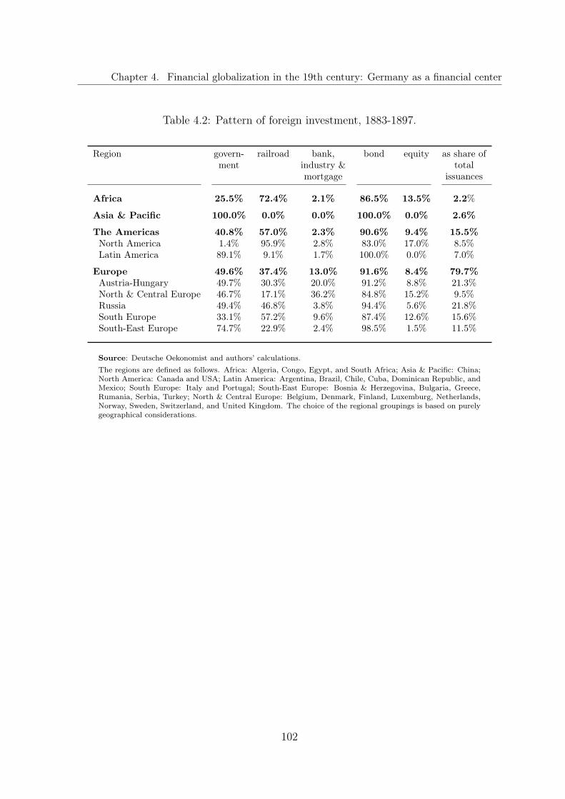
Chapter 4. Financial globalization in the 19th century: Germany as a financial center
Table 4.2: Pattern of foreign investment, 1883-1897.
Region govern- railroad bank, bond equity as share ofment industry & total
mortgage issuances
Africa 25.5% 72.4% 2.1% 86.5% 13.5% 2.2%
Asia & Pacific 100.0% 0.0% 0.0% 100.0% 0.0% 2.6%
The Americas 40.8% 57.0% 2.3% 90.6% 9.4% 15.5%North America 1.4% 95.9% 2.8% 83.0% 17.0% 8.5%Latin America 89.1% 9.1% 1.7% 100.0% 0.0% 7.0%
Europe 49.6% 37.4% 13.0% 91.6% 8.4% 79.7%Austria-Hungary 49.7% 30.3% 20.0% 91.2% 8.8% 21.3%North & Central Europe 46.7% 17.1% 36.2% 84.8% 15.2% 9.5%Russia 49.4% 46.8% 3.8% 94.4% 5.6% 21.8%South Europe 33.1% 57.2% 9.6% 87.4% 12.6% 15.6%South-East Europe 74.7% 22.9% 2.4% 98.5% 1.5% 11.5%
Source: Deutsche Oekonomist and authors’ calculations.The regions are defined as follows. Africa: Algeria, Congo, Egypt, and South Africa; Asia & Pacific: China;North America: Canada and USA; Latin America: Argentina, Brazil, Chile, Cuba, Dominican Republic, andMexico; South Europe: Italy and Portugal; South-East Europe: Bosnia & Herzegovina, Bulgaria, Greece,Rumania, Serbia, Turkey; North & Central Europe: Belgium, Denmark, Finland, Luxemburg, Netherlands,Norway, Sweden, Switzerland, and United Kingdom. The choice of the regional groupings is based on purelygeographical considerations.
102
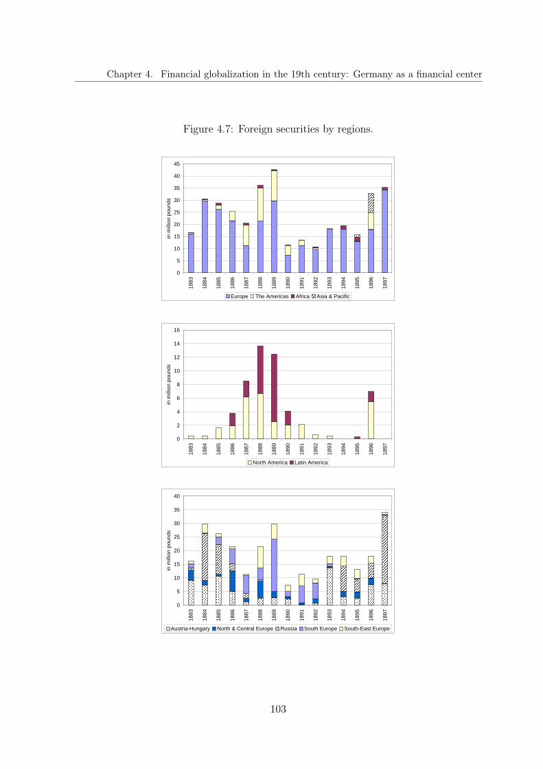
Chapter 4. Financial globalization in the 19th century: Germany as a financial center
Figure 4.7: Foreign securities by regions.
0
5
10
15
20
25
30
35
40
45
1883
1884
1885
1886
1887
1888
1889
1890
1891
1892
1893
1894
1895
1896
1897
in m
illion
pou
nds
Europe The Americas Africa Asia & Pacific
0
2
4
6
8
10
12
14
16
1883
1884
1885
1886
1887
1888
1889
1890
1891
1892
1893
1894
1895
1896
1897
in m
illion
pou
nds
North America Latin America
0
5
10
15
20
25
30
35
40
1883
1884
1885
1886
1887
1888
1889
1890
1891
1892
1893
1894
1895
1896
1897
in m
illion
pou
nds
Austria-Hungary North & Central Europe Russia South Europe South-East Europe
103

Chapter 4. Financial globalization in the 19th century: Germany as a financial center
Figure 4.8: International lending: country composition, 1883-1897.
0 10 20 30 40 50 60 70 80 90
Algeria
Argentina
Austria - Hungary
Belgium
Bosnia & Herzegovina
Brazil
Bulgaria
Canada
Chile
China
Congo
Cuba
Denmark
Dominican Republic
Egypt
Finland
Great Britain
Greece
Italy
Luxemburg
Mexico
Netherlands
Norway
Portugal
Rumania
Russia
Serbia
South Africa
Sweden
Switzerland
Turkey
USA
amounts in million pounds number of issues
104
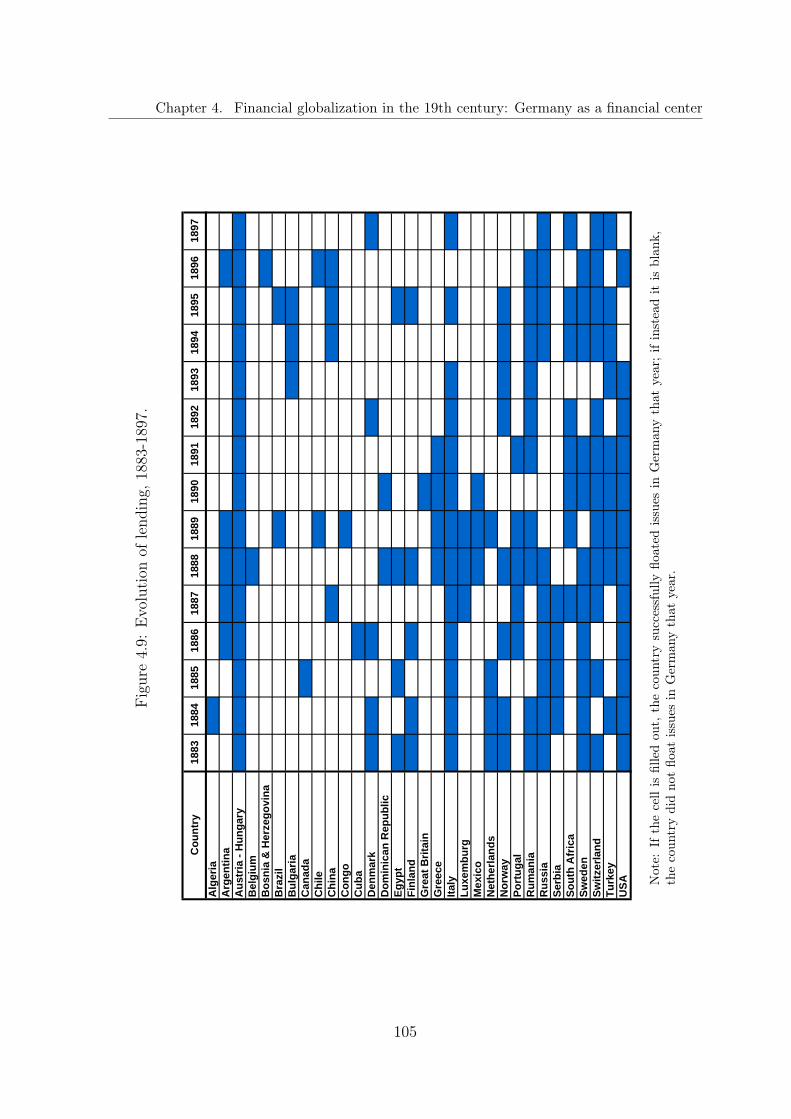
Chapter 4. Financial globalization in the 19th century: Germany as a financial center
Fig
ure
4.9:
Evo
lution
ofle
ndin
g,18
83-1
897.
Cou
ntry
1883
1884
1885
1886
1887
1888
1889
1890
1891
1892
1893
1894
1895
1896
1897
Alg
eria
Arg
entin
aA
ustr
ia -
Hun
gary
Bel
gium
Bos
nia
& H
erze
govi
naB
razi
lB
ulga
riaC
anad
aC
hile
Chi
naC
ongo
Cub
aD
enm
ark
Dom
inic
an R
epub
licEg
ypt
Finl
and
Gre
at B
ritai
nG
reec
eIta
l yLu
xem
burg
Mex
ico
Net
herla
nds
Nor
way
Port
ugal
Rum
ania
Rus
sia
Serb
iaSo
uth
Afr
ica
Swed
enSw
itzer
land
Tu
rkey
USA N
ote:
Ifth
ece
llis
fille
dou
t,th
eco
untr
ysu
cces
sful
lyflo
ated
issu
esin
Ger
man
yth
atye
ar;if
inst
ead
itis
blan
k,th
eco
untr
ydi
dno
tflo
atis
sues
inG
erm
any
that
year
.
105

Chapter 4. Financial globalization in the 19th century: Germany as a financial center
Figure 4.10: Size of issues (in million British pounds).
Size of bond issues
0.00.10.20.30.40.50.60.70.80.9
1.47
2.95
4.43
5.91
7.39
8.87
10.3
5
11.8
3
13.3
2
and
high
er
category
frequ
ency
Size of equity issues
0.00.10.20.30.40.50.60.70.80.9
0.49
0.99
1.49
1.99
2.49
2.99
3.49
3.99
4.49
and
high
er
category
frequ
ency
106

Chapter 4. Financial globalization in the 19th century: Germany as a financial center
Table 4.3: Data sources.
Variable Source
Foreign issuances in Germany Deutsche Oekonomist, various issuesGDP Spliced series, Jones and Obstfeld (2001)World exports Global Financial Data and authors’ calculationsLong-term nominal interest rates Yield on government gold bonds, Flandreau and
Zumer (2004)Private discount rates Deutsche Bundesbank (1976)Inflation rates General prices, Flandreau and Zumer (2004),
and authors’ calculationsForeign issuances in the UK Stone (1999)Default risk Standard & Poor’s (1999), and authors’ calcu-
lations
Figure 4.11: Principal components of the risk indicators.
-4
-3
-2
-1
0
1
2
3
1880 1885 1890 1895 1900 1905 1910
First principal componentSecond principal component
107

Chapter 4. Financial globalization in the 19th century: Germany as a financial center
Figure 4.12: Interest rate differentials and private discount rate.
-1
0
1
2
3
4
5
6
1880 1885 1890 1895 1900 1905 1910
Real long-term interest rate differential Germany - UKReal long-term interest rate differential Germany - FranceReal private discount rate in Germany
108

Chapter 4. Financial globalization in the 19th century: Germany as a financial center
Figure 4.13: Economic activity in Germany and the UK.
(a) GDP growth rates
-.06
-.04
-.02
.00
.02
.04
.06
.08
.10
1880 1885 1890 1895 1900 1905 1910
GDP growth rate in the UKGDP growth rate in Germany
(b) HP filtered deviations of GDP from trend
-120
-80
-40
0
40
80
120
1880 1885 1890 1895 1900 1905 1910
Detrended GDP in the UKDetrended GDP in Germany
109

Chapter 4. Financial globalization in the 19th century: Germany as a financial center
Table 4.4: OLS regressions.
Dependent variable: log of (1) (2) (3)foreign issuances in Germany
Constant 3.5728*** 3.7778*** 3.7135***(0.6508) (0.6106) (0.5997)
Growth rate GDP in the UK 0.4053(2.9896)
Growth rate GDP in Germany 2.1372 3.3366(2.8659) (3.3896)
Growth rate of world exports -1.7847(2.1284)
Real long term interest rate 1.0480 0.9716 0.9224differential between Germany (0.6375) (0.6173) (0.6105)and the UK
Real long term interest rate -0.8092** -0.9008*** -0.8199**differential between Germany (0.3797) (0.2876) (0.3888)and France
Real private discount rate in -0.4065*** -0.4097*** -0.4055**Germany (0.1361) (0.1240) (0.1491)
First principal component of -0.2845*** -0.2991*** -0.3031***risk indicators (0.0879) (0.0829) (0.1055)
R-squared 0.447 0.431 0.456Adjusted R-squared 0.309 0.343 0.315Observations 31 31 31F-statistic 3.2388 4.9210 3.2197(p-value) (0.0178) (0.0043) (0.0191)
Durbin-Watson statistic 1.915 1.856 1.793
Note: White robust standard errors reported in parentheses; * significant at 10%;** significant at 5%; *** significant at 1%.
110

Chapter 4. Financial globalization in the 19th century: Germany as a financial center
Figure 4.14: Actual, fitted, and residual series, OLS (1).
-0.8
-0.4
0.0
0.4
0.8
1.2
1.5
2.0
2.5
3.0
3.5
4.0
4.5
1885 1890 1895 1900 1905 1910
Residual Actual Fitted
111
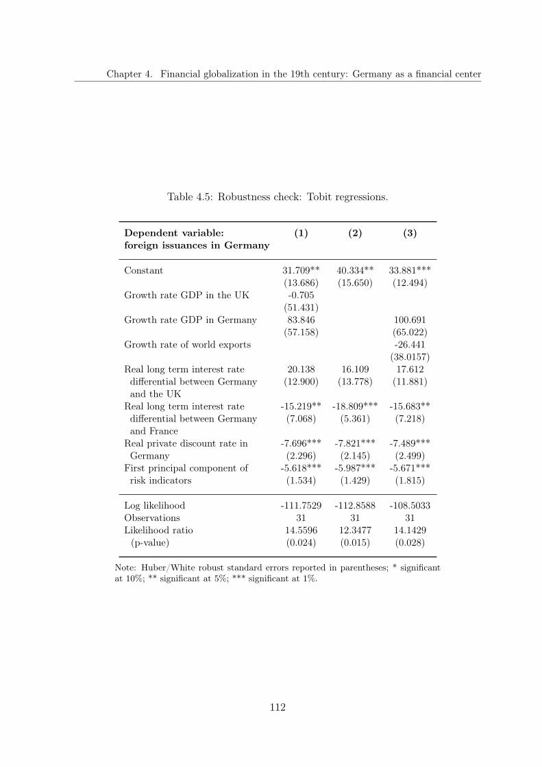
Chapter 4. Financial globalization in the 19th century: Germany as a financial center
Table 4.5: Robustness check: Tobit regressions.
Dependent variable: (1) (2) (3)foreign issuances in Germany
Constant 31.709** 40.334** 33.881***(13.686) (15.650) (12.494)
Growth rate GDP in the UK -0.705(51.431)
Growth rate GDP in Germany 83.846 100.691(57.158) (65.022)
Growth rate of world exports -26.441(38.0157)
Real long term interest rate 20.138 16.109 17.612differential between Germany (12.900) (13.778) (11.881)and the UK
Real long term interest rate -15.219** -18.809*** -15.683**differential between Germany (7.068) (5.361) (7.218)and France
Real private discount rate in -7.696*** -7.821*** -7.489***Germany (2.296) (2.145) (2.499)
First principal component of -5.618*** -5.987*** -5.671***risk indicators (1.534) (1.429) (1.815)
Log likelihood -111.7529 -112.8588 -108.5033Observations 31 31 31Likelihood ratio 14.5596 12.3477 14.1429
(p-value) (0.024) (0.015) (0.028)
Note: Huber/White robust standard errors reported in parentheses; * significantat 10%; ** significant at 5%; *** significant at 1%.
112

Chapter 4. Financial globalization in the 19th century: Germany as a financial center
Table 4.6: Further robustness checks.
Dependent variable: log of in real capital only onlyforeign issuances in Germany terms called bonds equity
Constant 3.777*** 3.552*** 3.566*** 0.636(0.659) (0.648) (0.669) (1.526)
Growth rate GDP in the UK 0.699 1.165 -0.037 1.002(2.992) (2.945) (3.105) (6.537)
Growth rate GDP in Germany 2.282 1.976 1.689 4.294(3.045) (2.983) (2.982) (5.597)
Real long term interest rate 1.221* 0.733 1.292* -1.075differential between Germany (0.655) (0.631) (0.711) (1.191)and the UK
Real long term interest rate -0.891** -0.724* -0.800** -1.143differential between Germany (0.397) (0.399) (0.376) (0.930)and France
Real private discount rate in -0.453*** -0.344** -0.499*** 0.311Germany (0.140) (0.135) (0.144) (0.257)
First principal component of -0.262*** -0.250*** -0.338*** 0.073risk indicators (0.091) (0.083) (0.102) (0.127)
Adjusted R-squared 0.375 0.239 0.334 0.033Observations 31 31 31 31F-statistic 4.0003 2.5686 3.5121 1.1657
(p-value) (0.0065) (0.0458) (0.0123) (0.3582)Durbin-Watson statistic 1.870 1.915 1.945 2.243
Note: Huber/White robust standard errors reported in parentheses; * significantat 10%; ** significant at 5%; *** significant at 1%.
113

Bibliography
Aghion, P., Bacchetta, P., Ranciere, R. and Rogoff, K. (2006). Exchange rate volatilityand productivity growth: The role of financial development, NBER Working Paper12117.
Alesina, A. and Wagner, A. F. (2006). Choosing (and reneging on) exchange rate regimes,Journal of the European Economic Association 4(4): 770–799.
Asici, A. and Wyplosz, C. (2003). The art of gracefully exiting a peg, The Economicand Social Review 34(3): 211–228.
Ball, L. (1999). Policy rules for open economies, in J. Taylor (ed.), Monetary PolicyRules, University of Chicago Press, pp. 127–144.
Baltzer, F. (1916). Die Kolonialbahnen mit besonderer Berücksichtigung Afrikas, G. J.Göschen’sche Verlagshandlung, Berlin.
Bankenquete (1910). Stenographische Berichte - Die Verhandlungen der Gesamtkom-mission zu Punkt VI des Fragebogens (Depositenwesen), Reichsdruckerei, Berlin.
Barajas, A., Erickson, L. and Steiner, R. (2008). Fear of declaring: Do markets care whatcountries say about their exchange rate policies?, IMF Staff Papers 55(3): 445–480.
Barro, R. J. and Gordon, D. B. (1983). A positive theory of monetary policy in a naturalrate model, Journal of Political Economy 91(4): 589–610.
Bernanke, B. S. and Mishkin, F. S. (1997). Inflation targeting: a new framework formonetary policy?, Journal of Economic Perspectives 11(2): 97–116.
Bersch, J. and Klüh, U. (2007). When countries do not do what they say: Systematic dis-crepancies between exchange rate regime announcements and de facto policies, Dis-cussion Paper in Economics 2007-38, Ludwig-Maximilians-Universität München.
114

Bibliography
Best, J. (2005). The Limits of Transparency - Ambiguity and the History of InternationalFinance, Cornell Studies in Money, Cornell University Press.
Born, K. E. (1977). Geld und Banken im 19. und 20. Jahrhundert, A. Kröner, Stuttgart.
Börsen-Enquete-Kommission (1893). Statistische Anlagen, Reichsdruckerei, Berlin.
Bubula, A. and Ötker-Robe, I. (2002). The evolution of exchange rate regimes since1990: Evidence from de facto policies, IMF Working Paper 02/155.
Bubula, A. and Ötker-Robe, I. (2003). Are pegged and intermediate exchange rateregimes more crisis prone?, IMF Working Paper 03/223.
Burk, K. (1992). Money and power: the shift from Great Britain to the United States, inY. Cassis (ed.), Finance and financiers in European history: 1880-1960, CambridgeUniversity Press, pp. 359–369.
Caballero, R. J. and Krishnamurthy, A. (2001). A ’vertical’ analysis of crises and inter-vention: Fear of floating and ex-ante problems, NBER Working Paper 8428.
Calvo, G. A. (1983). Staggered prices in a utility-maximizing framework, Journal ofMonetary Economics 12(3): 383–398.
Calvo, G. A., Izquierdo, A. and Mejía, L.-F. (2004). On the empirics of sudden stops:the relevance of balance-sheet effects, NBER Working Paper 10520.
Calvo, G. A. and Reinhart, C. M. (2002). Fear of floating, The Quarterly Journal ofEconomics 117(2): 379–408.
Carmignani, F., Colombo, E. and Tirelli, P. (2006). Exploring different views of exchangerate regime choice. Mimeo, Università degli Studi di Milano-Bicocca.
Cassis, Y. and Bussière, E. (eds) (2005). London and Paris as International FinancialCentres in the Twentieth Century, Oxford University Press.
Chinn, M. D. and Ito, H. (2006). What matters for financial development? Capital con-trols, institutions, and interactions, Journal of Development Economics 81(1): 163–192.
Clarida, R., Galí, J. and Gertler, M. (1999). The Science of Monetary Policy: A NewKeynesian Perspective, Journal of Economic Literature 37: 1661–1707.
115

Bibliography
Clarida, R., Galí, J. and Gertler, M. (2001). Optimal monetary policy in open versusclosed economies: An integrated approach, The American Economic Review Papersand Proceedings 91(2): 248–252.
Corden, W. M. and Neary, J. P. (1982). Booming sector and de-industrialisation in asmall open economy, The Economic Journal 92(368): 825–848.
Daude, C. and Fratzscher, M. (2008). The pecking order of cross-border investment,Journal of International Economics 74(1): 94–119.
Dennis, R. and Söderström, U. (2006). How important is precommitment for monetarypolicy?, Journal of Money, Credit and Banking 38(4): 847–872.
Detken, C. and Gaspar, V. (2003). Maintaining price stability under free-floating: afearless way out of the corner?, ECB Working Paper 241.
Deutsche Bundesbank (1976). Deutsches Geld- und Bankwesen in Zahlen 1876-1975,Frankfurt a. M.
Dornbusch, R. (1976). Expectations and exchange rate dynamics, Journal of PoliticalEconomy 84(6): 1161–1176.
Drazen, A. and Masson, P. R. (1994). Credibility of policies versus credibility of policy-makers, The Quarterly Journal of Economics 109(3): 735–754.
Duttagupta, R., Fernandez, G. and Karacadag, C. (2004). From fixed to float: Op-erational aspects of moving toward exchange rate flexibility, IMF Working Paper04/126.
Eichengreen, B. J. and Razo-Garcia, R. (2006). The international monetary system inthe last and next 20 years, Economic Policy 21(47): 393–442.
Esteves, R. P. (2008). Between imperialism and capitalism. European capital exportsbefore 1914. Mimeo, University of Oxford.
Feis, H. (1930). Europe the world’s banker 1870-1914 - An account of European foreigninvestment and the connection of world finance with diplomacy before the war, pub-lished for the Council of Foreign Relations, 1964 edn, Reprint of Economic Classics,New York.
116

Bibliography
Fischer, S. (2001). Exchange rate regimes: Is the bipolar view correct? Distinguishedlecture on economics in government, Journal of Economic Perspectives 15(2): 3–24.
Flandreau, M. and Zumer, F. (2004). The Making of Global Finance, 1880-1913, OECD.
Flores, J.-H. (2007). Information asymmetries and financial intermediation during theBaring crisis: 1880-1890, Working Paper in Economic History 07-16, UniversidadCarlos III de Madrid.
Fohlin, C. (2002). Regulation, taxation and the development of the German universalbanking system, 1884-1913, European Review of Economic History 6: 221–254.
Fraga, A., Goldfajn, I. and Minella, A. (2003). Inflation targeting in emerging marketeconomies, NBER Working Paper 10019.
Frankel, J. A. (2005). Peg the export price index: A proposed monetary regime for smallcountries, Journal of Policy Modeling 27(4): 495–508.
Frankel, J., Fajnzylber, E., Schmukler, S. and Serven, L. (2001). Verifying exchange rateregimes, Journal of Development Economics 66: 351–386.
Frankel, J. and Wei, S.-J. (2008). Estimation of de facto exchange rate regimes: Syn-thesis of the techniques for inferring flexibility and basket weights, IMF Staff Paper55(3): 384–416.
Fritzsche, H. (1913). Ausländische Anleihen auf dem deutschen Geldmarkte, PhD thesis,Universität Heidelberg, Leipzig.
Froot, K. A. and Thaler, R. H. (1990). Foreign exchange, The Journal of EconomicPerspectives 4(3): 179–192.
Gebhard, H. (1928). Die Berliner Börse von den Anfängen bis zum Jahre 1896, R. L.Prager, Berlin.
Genberg, H. and Swoboda, A. K. (2005). Exchange rate regimes: does what countriessay matter?, IMF Staff Paper, Special Issue 52.
Ghosh, A. R., Gulde, A.-M. and Wolf, H. C. (2002). Exchange Rate Regimes - Choices& Consequences, MIT Press.
117

Bibliography
Glick, R. and Hutchison, M. (2001). Banking and currency crises: How common aretwins?, in R. Glick, R. Moreno and M. Spiegel (eds), Financial Crises in EmergingMarkets, Cambridge University Press, pp. 35–69.
Goldstein, M. (2002). Managed Floating Plus, Institute for International Economics.
Gömmel, R. (1992). Entstehung und Entwicklung der Effektenbörsen im 19. Jahrhun-dert bis 1914, in H. Pohl (ed.), Deutsche Börsengeschichte, Fritz Knapp Verlag,Frankfurt a. M., pp. 133–207.
Hakura, D. S. (2005). Are emerging market countries learning to float?, IMF WorkingPaper 05/98.
Hausmann, R., Panizza, U. and Stein, E. (2001). Why do countries float the way theyfloat?, Journal of Development Economics 66(2): 387–414.
Hoffmann, W. G. (1965). Das Wachstum der deutschen Wirtschaft seit der Mitte des19.Jahrhunderts, Springer Verlag, Berlin.
Husain, A. M., Mody, A. and Rogoff, K. S. (2005). Exchange rate regime durabilityand performance in developing versus advanced economies, Journal of MonetaryEconomics 52(35-64).
International Monetary Fund (2004). Botswana: Selected issues and statistical appendix,IMF Country Report No. 04/212.
Jones, M. T. and Obstfeld, M. (2001). Saving, investment, and gold: A reassessmentof historical current account data, in G. A. Calvo, R. Dornbusch and M. Obstfeld(eds), Money, Capital Mobility, and Trade: Essays in Honor of Robert Mundell,MIT Press, Cambridge, MA, pp. 303–363.
Kaminsky, G. L. and Reinhart, C. M. (1999). The twin crises: The causes of bankingand balance-of-payments problems, American Economic Review 89(3): 473–500.
Kaminsky, G. L. and Schmukler, S. L. (2008). Short-run pain, long-run gain: Financialliberalization and stock market cycles, Review of Finance 12: 253–292.
Kindleberger, C. P. (1974). The formation of financial centers: a study in comparativeeconomic history, Princeton Studies in International Finance No. 36.
118

Bibliography
King, M. (1997). Changes in UK monetary policy: rules and discretion in practice,Journal of Monetary Economics 39: 81–97.
Klein, M. W. and Shambaugh, J. C. (2006). The nature of exchange rate regimes, NBERWorking Paper 12729.
Kleiner, H. (1914). Emissions-Statistik in Deutschland, PhD thesis, Ludwig-Maximi-lians-Universität München.
Kose, M. A., Prasad, E., Rogoff, K. and Wei, S.-J. (2006). Financial globalization: Areappraisal, IMF Working Paper 06/189.
Kozicki, S. (1999). How useful are Taylor rules for monetary policy?, Economic Review,Federal Reserve Bank of Kansas City (Q II): 5–33.
Krugman, P. (1979). A model of balance-of-payments crises, Journal of Money, Credit,and Banking 11(3): 311–325.
Kuttner, K. N. and Posen, A. S. (1999). Does talk matter after all? Inflation target-ing and central bank behavior, Working Paper 99-10, Institute for InternationalEconomics.
Kuttner, K. N. and Posen, A. S. (2001). Beyond bipolar: A three-dimensional assess-ment of monetary frameworks, International Journal of Finance and Economics6(4): 369–387.
Kydland, F. E. and Prescott, E. C. (1977). Rules rather than discretion: the inconsis-tency of optimal plans, The Journal of Political Economy 85(3): 473–492.
Lahiri, A. and Végh, C. A. (2001). Living with the fear of floating: An optimal policyperspective, NBER Working Paper 8391.
Lane, P. R. and Milesi-Ferretti, G. M. (2006). The external wealth of nations mark II:Revised and extended estimates of foreign assets and liabilities, 1970-2004, IMFWorking Paper 06/69.
Lane, P. R. and Milesi-Ferretti, G. M. (2007). The external wealth of nations mark II:Revised and extended estimates of foreign assets and liabilities, 1970-2004, Journalof International Economics 73(2): 223–250.
119

Bibliography
Lenz, F. (1922). Wesen und Struktur des deutschen Kapitalexports vor 1914,Weltwirtschaftliches Archiv 18(1): 42–54.
Levy-Yeyati, E. and Sturzenegger, F. (2003a). A de facto classification of exchangerate regimes: A methodological note, American Economic Review 93(4). Posted athttp://www.aeaweb.org/aer/contents/.
Levy-Yeyati, E. and Sturzenegger, F. (2003b). To float or to fix: Evidence on the impactof exchange rate regimes on growth, American Economic Review 93(4): 1173–1193.
Levy-Yeyati, E. and Sturzenegger, F. (2005). Classifying exchange rate regimes: Deedsvs. words, European Economic Review 49(6): 1603–1635.
Lotz, W. (1890). Die Technik des deutschen Emissionsgeschäfts - Anleihen, Konversionenund Gründungen, Jahrbuch für Gesetzgebung, Verwaltung und Volkswirtschaft imDeutschen Reich 14: 57–124 (393–460).
Marx, M. (1913). Die Emissionsstatistik in Deutschland und einigen ausländis-chen Staaten, Schmollers Jahrbuch für Gesetzgebung, Verwaltung, und Wirtschaft37(4): 1703–1763.
McCallum, B. T. (1983). On non-uniqueness in rational expectations models: An at-tempt at perspective, Journal of Monetary Economics 11: 139–168.
McCallum, B. T. (1994). A reconsideration of the uncovered interest parity relationship,Journal of Monetary Economics 33: 105–132.
McCallum, B. T. (2000). The present and future of monetary policy rules, NBERWorking Paper 7916.
McCallum, B. T. (2003). Inflation Targeting for the United States, Report to the ShadowOpen Market Committee on May 19.
Meyer, A. (1902). Die deutschen Börsensteuern 1881-1900, ihre Geschichte und ihrEinfluss auf das Bankgeschäft, Union Deutsche Verlagsgesellschaft, Stuttgart.
Mishkin, F. S. and Schmidt-Hebbel, K. (2001). One decade of inflation targeting in theworld: What do we know and what do we need to know?, NBER Working Paper8397.
120

Bibliography
Obstfeld, M. (1996). Models of currency crises with self-fulfilling features, EuropeanEconomic Review 40: 1037–1047.
Obstfeld, M. and Rogoff, K. (2000). The six major puzzles in international macroeco-nomics: Is there a common cause?, NBER Macroeconomics Annual 15: 339–390.
Obstfeld, M. and Taylor, A. M. (1998). The Great Depression as a watershed: Interna-tional capital mobility in the long run, in M. D. Bordo, C. Goldin and E. N. White(eds), The Defining Moment: The Great Depression and the American Economy inthe Twentieth Century, University of Chicago Press, Chicago, pp. 353–402.
Obstfeld, M. and Taylor, A. M. (2004). Global capital markets: Integration, crisis, andgrowth, Cambridge University Press.
Otto, W. (1910). Anleiheübernahme-, Gründungs- und Beteiligungsgeschäfte derdeutschen Grossbanken in Übersee, Borussia Druck- und Verlagsanstalt, Berlin.
Pohl, M. (1977). Deutscher Kapitalexport im 19. Jahrhundert - Emissionen, Banken,Anleger bis 1914, Erinnerungsgabe zum 25jährigen Bestehen der Börsen-Zeitung,Verlag Börsen-Zeitung.
Portes, R. and Rey, H. (2005). The determinants of cross-border equity flows, Journalof International Economics 65: 269–296.
Portes, R., Rey, H. and Oh, Y. (2001). Information and capital flows: The determinantsof transactions in financial assets, European Economic Review 45: 783–796.
Reinhart, C. M. and Rogoff, K. S. (2002). The modern history of exchange rate arrange-ments: A reinterpretation, NBER Working Paper 8963.
Reinhart, C. M. and Rogoff, K. S. (2004). The modern history of exchange rate arrange-ments: A reinterpretation, The Quarterly Journal of Economics 119(1): 1–48.
Riesser, D. (1912). Die deutschen Grossbanken und ihre Konzentration im Zusammen-hang mit der Entwicklung der Gesamtwirtschaft in Deutschland, 4th edn, Verlagvon Gustav Fischer, Jena.
Roger, S. and Stone, M. (2005). On target? The international experience with achievinginflation targets, IMF Working Paper 05/163.
121

Bibliography
Rogoff, K. (1996). The purchasing power parity puzzle, Journal of Economic Literature34(2): 647–668.
Rogoff, K. S., Husain, A. M., Mody, A., Brooks, R. and Oomes, N. (2003). Evolutionand performance of exchange rate regimes, IMF Working Paper 03/243.
Sánchez, M. (2005). The link between interest rates and exchange rates: Do contrac-tionary depreciations make a difference?, ECB Working Paper 548.
Saul, S. (2005). Banking alliances and international issues on the Paris capital market,1890-1914, in Y. Cassis and E. Bussière (eds), London and Paris as InternationalFinancial Centres in the Twentieth Century, Oxford University Press, pp. 119–150.
Schaefer, K. C. (1993). Deutsche Portfolioinvestitionen im Ausland 1870-1914 - Banken,Kapitalmärkte und Wertpapierhandel im Zeitalter des Imperialismus, LIT Verlag,Münster.
Spangenthal, S. (1903). Die Geschichte der Berliner Börse, Spangenthal’s Verlag, Berlin.
Standard & Poor’s (1999). CreditWeek, December 22.
Steinmetz, W. (1913). Die deutschen Großbanken im Dienste des Kapitalexports, Druck-erei der St. Paulus-Gesellschaft, Luxemburg.
Stone, I. (1999). The global export of capital from Great Britain, 1865-1914 - A statisticalsurvey, Macmillan Press Ltd, London.
Svensson, L. E. O. (1999). Inflation targeting as a monetary policy rule, Journal ofMonetary Economics 43: 607–654.
Svensson, L. E. O. (2000). Open-economy inflation targeting, Journal of InternationalEconomics 50: 155–183.
Svensson, L. E. O. (2007). Optimal inflation targeting: Further developments of inflationtargeting, in F. Mishkin and K. Schmidt-Hebbel (eds), Monetary Policy underInflation Targeting, Banco Central de Chile, Santiago, Chile, pp. 187–225.
Taylor, A. M. and Taylor, M. P. (2004). The purchasing power parity debate, Journalof Economic Perspectives 18(4): 135–158.
122

Bibliography
Taylor, J. B. (2002). The monetary transmission mechanism and the evaluation of mone-tary policy rules, in N. Loayza and K. Schmidt-Hebbel (eds), Monetary policy: rulesand transmission mechanisms, Banco Central de Chile, Santiago, Chile, pp. 21–46.
Tilly, R. (1992). Der deutsche Kapitalmarkt und die Auslandsinvestitionen von 1870 bis1913, IFO Studien 38: 199–225.
van Wijnbergen, S. (1984). The ‘dutch disease’: A disease after all?, The EconomicJournal 94(373): 41–55.
von Hagen, J. and Zhou, J. (2006). Fear of floating and fear of pegging: an empiricalanalysis of de facto exchange rate regimes in developing countries, CEPR DiscussionPaper 5530.
Wetzel, C. (1996). Die Auswirkungen des Reichsbörsengesetzes von 1896 auf die Ef-fektenbörsen im Deutschen Reich, insbesondere auf die Berliner Fondsbörse, LITVerlag, Münster.
Wormser, O. (1919). Die Frankfurter Börse, ihre Besonderheiten und ihre Bedeutung:Ein Beitrag zur Frage der Börsenkonzentration, Archiv für Sozialwissenschaft undSozialpolitik, Verlag von J. C. B. Mohr (Paul Siebeck), Tübingen.
Zickert, H. (1911). Die Kapitalsanlage in ausländischen Wertpapieren, Puttkammer &Mühlbrecht, Berlin.
123

Curriculum Vitae
February 2009 Ph.D. in economics (Dr. oec. publ.)
2004 - 2009 Ph.D. program in economicsMunich Graduate School of EconomicsLudwig-Maximilians-Universität Munich
2006 - 2007 Visiting scholarGeorge Washington UniversityDepartment of Economics
1999 - 2004 Diploma in economics (Diplom-Volkswirtin)Otto-Friedrich-Universität Bamberg
2001 - 2002 Exchange studentUniversidad Anáhuc del Sur, Mexico City
1999 AbiturClara-Schumann-Gymnasium Bonn
September 3, 1979 Born in Engelskirchen, Germany