Financial Crises and Exchange Rate Policy

Luca Fornaro∗

This draft: February 2013

First draft: February 2011

Abstract

This paper develops a dynamic small open economy model highlighting a trade-

off between financial and price stability. The key element of the analysis is a

pecuniary externality arising from frictions in the international credit markets. The

goal is to study the performance of alternative exchange rate policies in sudden stop-

prone economies. The main result is that the presence of pecuniary externalities in

the credit markets makes a narrow focus on price stability sub-optimal.

Keywords: Financial crises, Monetary Policy, Sudden Stops, Exchange

Rate Regime, Nominal Wage Rigidities, Pecuniary Externalities.

JEL Classification Numbers: G01, E44, E52, F32, F34, F41.

∗Department of Economics, London School of Economics, Houghton Street, WC2A 2AE London. E-mail: l.fornaro@lse.ac.uk. I am extremely grateful to Gianluca Benigno, Ethan Ilzetzki, Albert Marcet,Juan Pablo Nicolini, Michele Piffer, Christopher Pissarides, Romain Ranciere, Kevin Sheedy and SilvanaTenreyro for useful comments. I also thank seminar participants at the LSE, the PSE, the Universityof Surrey and the Paul Woolley Centre, and participants at the 13th ZEW Summer Workshop forYoung Economists, the XVI Workshop on Dynamic Macroeconomics and the XXXVI Simposio de laAsociacion Espanola de Economıa. Financial support from the French Ministere de l’EnseignementSuperieur et de la Recherche, the ESRC, the Royal Economic Society and the Paul Woolley Centre isgratefully acknowledged. This paper previously circulated under the title “Financial Crises in SmallOpen Economies: The Role of Monetary Policy”.

1

1 Introduction

Since the financial liberalization wave of the 1980s, several countries have experienced

financial crises characterized by sudden arrests of international capital inflows and sharp

drops in output, consumption and asset prices.1 These episodes, known as sudden stops,

have sparked great interest in the design of monetary and exchange rate policies in finan-

cially fragile economies. Should these economies let their exchange rate float or rather

anchor it to a foreign currency? Should monetary policy be concerned only with its tradi-

tional objective of granting price stability or should it also care about financial stability?

In this paper, I address these questions focusing on a pecuniary externality originating

from frictions on the international credit markets. I present a theoretical framework that

shows how the combination of financial frictions and nominal rigidities gives rise to a

trade-off between financial and price stability. My main result is that a narrow focus on

price stability can lead to a sub-optimal monetary policy in sudden stop-prone economies.

I study a small open economy with imperfect access to the international financial

markets. Domestic agents borrow from foreign investors against collateral. Collateral

consists in a physical asset used in production, land, valued at market price. When

the collateral constraint binds a financial accelerator mechanism akin to Fisher’s debt

deflation arises: aggregate demand for land falls, the price of land drops and collateral

declines. Since domestic agents are atomistic, they do not take into account the general

equilibrium effect of their actions on the price of land and on the value of their collateral.

This is the pecuniary externality that creates scope for policy interventions in the financial

markets.

Wages are nominally rigid.2 During a financial crisis nominal wages fail to adjust

1Diaz-Alejandro (1985) is the classic reference on the link between financial liberalization and financialcrises in emerging economies. Calvo et al. (2004) provide an overview of the facts characterizing suddenstop events.

2A growing body of evidence emphasizes how nominal wage rigidities represent a key transmissionchannel through which monetary policy affects the real economy. For instance, this conclusion is reachedby Christiano et al. (2005) using an estimated medium-scale DSGE model of the US economy. Moreover,Olivei and Tenreyro (2007) show that monetary policy shocks in the US have a bigger impact on outputif they occur during the first or second quarter of the year. They argue that this finding can be explainedwith the fact that most US firms adjust wages during the fourth quarter, and hence wages tend to bemore rigid during the first half of the year. There is also evidence describing the role of nominal wagerigidities in exacerbating the downturn during financial crises, especially if coupled with fixed exchangerates. This point is made by Eichengreen and Sachs (1985) and Bernanke and Carey (1996) in thecontext of the Great Depression, while Schmitt-Grohe and Uribe (2011) document the importance ofwage rigidities for the 2001 Argentine crisis and for the 2008-2009 recession in the Eurozone periphery.Micro-level evidence on the importance of nominal wage rigidities is provided by Fehr and Goette (2005),

1

downward, potentially worsening the impact of financial turmoil on the real economy.

The central bank can mitigate the downturn associated with a financial crisis by engi-

neering an exchange rate depreciation that increases the competitiveness of the economy.

Importantly, the stimulus provided by an exchange rate depreciation has a positive effect

on the aggregate demand for land and on the value of collateral. Through this channel,

exchange rate policy affects domestic agents’ access to the international credit markets

during crisis events.

Many narratives of financial crisis episodes have given a central role to the interaction

between capital flows, asset prices and wage rigidities. Consider the recent events in

the Eurozone periphery. Prior to 2008, several European countries underwent a period

characterized by fast build-up of foreign debt. Rising real estate prices likely contributed

to the credit boom, since housing represents an important source of collateral. Conversely,

the crisis that followed has been characterized by a vicious cycle of falling capital inflows

and plummeting asset prices.3 In addition, many commentators have argued that the

combination of rigidities in wage setting and fixed exchange rates has exacerbated the

severity of the crisis.4 This is the kind of episodes that the model is meant to capture.

I use the model to compare the performance of three alternative monetary rules: a

fixed exchange rate rule and two types of floating exchange rate regimes. The first type

of float considered is a policy of strict wage inflation targeting. This rule eliminates all

the distortions arising from nominal wage stickiness and corresponds to the price stability

rule of closed-economy sticky price models. The second type of float is a policy of flexible

exchange rate targeting in which the central bank intervenes to smooth out deviations of

the exchange rate from a target. This rule parallels flexible price level targeting rules in

closed-economy models and represents a simple alternative to wage inflation targeting. In

addition, this rule is interesting because it implies a more expansionary monetary policy

stance during crisis events compared to the strict wage inflation targeting rule.

The main result of the paper concerns the role of financial frictions in determining

the welfare ranking between strict wage inflation targeting and the flexible exchange rate

targeting rule. I show that in a version of the model in which the collateral constraint is

Gottschalk (2005), Barattieri et al. (2010) and Fabiani et al. (2010).3McKinsey (2010) and Merler and Pisani-Ferry (2012) describe the accumulation of debt, especially

foreign debt, in countries at the Eurozone periphery during the run up to the 2008 financial crisis andthe subsequent sudden stop in capital inflows, giving rise to deleveraging by the private sector.

4This point is forcefully made by Feldstein (2010) and Krugman (2010).

2

replaced by a fixed borrowing limit, and hence in which Fisher’s debt deflation channel

is shut down and financial crises are not present, the strict wage inflation targeting rule

delivers higher welfare gains than the flexible exchange rate targeting rule for any initial

state of the world. This finding is in line with the well known result that, in models

in which the only distortions come from monopolistic competition and from nominal

rigidities, a policy that corrects for nominal rigidities approximates well the optimal

policy.5

I then show that the pecuniary externality implied by the Fisherian deflation mecha-

nism has the potential to change the welfare ranking among the policy rules considered.

In fact, once the Fisherian deflation mechanism is introduced the initial stock of foreign

assets owned by domestic households becomes a key determinant of the welfare ranking.

For high levels of net foreign assets the probability of a future crisis is small and a policy

of targeting wage inflation is preferred, due to its good performance in managing normal

business cycle fluctuations. For low levels of net foreign assets the risk of a crisis is high

and flexible exchange rate targeting becomes the preferred regime, since it does a better

job in mitigating the fall in the price of land and in capital inflows during crisis events

compared to the wage inflation targeting rule. In contrast, the peg is always welfare

dominated by the other two rules. This happens because during tranquil times the peg

does not remove the distortions due to wage stickiness, while during crisis times pegging

the exchange rate amplifies the fall in the price of land and in capital inflows compared

to the other two regimes.

A second set of results concerns the impact of the monetary regime on precautionary

savings and crisis probability. The currency peg is the regime that stimulates more the

accumulation of precautionary savings, followed by the policy of targeting wage inflation

and by the flexible exchange rate targeting rule. The intuition is simple: the more crises

disrupt economic activity, the more agents accumulate precautionary savings to reduce

the risk of experiencing a sudden stop. Since the peg is the regime under which crises have

the strongest impact on output and consumption, the peg is also the regime under which

the accumulation of precautionary savings is stronger. Moreover, since crises are milder

when the central bank adopts a flexible exchange rate targeting rule, agents accumulate

5Kollmann (2002) and Schmitt-Grohe and Uribe (2007) derive this result using models with monop-olistic competition in the product market and nominal price rigidities. However, a similar logic shouldapply to models with monopolistic competition in the labor market and in which the presence of stickywages is the only source of nominal rigidities.

3

less precautionary savings under flexible exchange rate targeting than under a policy

of strict wage inflation targeting. The outcome is that the currency peg is the regime

featuring the lowest crisis probability, while the probability of experiencing a sudden stop

is highest under a policy of flexible exchange rate targeting.

This paper is related to two strands of the literature. The first one focuses on the

design of monetary policy in financially fragile small open economies. Cespedes et al.

(2004), Moron and Winkelried (2005) and Devereux et al. (2006) compare the perfor-

mance of different monetary regimes in small open economies featuring financial market

imperfections. Contrary to this paper, their models focus on business cycle fluctuations

and are not suited to study economies occasionally subject to financial crises. Christiano

et al. (2004), Cook (2004), Gertler et al. (2007), Braggion et al. (2007) and Curdia (2007)

all use quantitative models to analyze the impact of monetary policy interventions during

crisis times. In their frameworks crises are unexpected one-shot events, while this paper

presents a model in which crises alternate with tranquil times and crisis probabilities

are rationally anticipated by agents. This allows the analysis of the impact of monetary

policy on the probability of entering a crisis, an issue on which the existing literature is

silent. Moreover, this literature typically finds that the presence of financial frictions does

not alter the welfare ranking among monetary policy rules, while the key insight of this

paper is that financial frictions are a key determinant of which policy rule delivers higher

welfare. Aghion et al. (2004), Caballero and Krishnamurthy (2003), Bordo and Jeanne

(2002) and Benigno et al. (2011b) consider monetary economies featuring both tranquil

periods and crises. However their focus is on static models, while the dynamics of debt

accumulation play a key role in the model presented in this paper.6 Finally, this paper

shares with Schmitt-Grohe and Uribe (2011) the focus on the performance of different

exchange rate regimes in economies subject to the risk of experiencing a deep recession.

However, in their model recessions are exogenous events and there is no financial ampli-

fication, while in this model the probability of entering a crisis is endogenous and the

interaction between the exchange rate regime and Fisher’s debt deflation is key.

The second strand of related literature employs dynamic real business cycle models

featuring occasionally binding credit constraints and financial accelerator mechanisms to

describe economies prone to sudden stops and to draw implications about policy conduct

6I refer to these frameworks as static because they consider economies that last two or three periods,in which the stock of external debt at the onset of a crisis is essentially taken as an exogenous variable.

4

in small open economies. Examples are Mendoza (2010), Bianchi (2011), Benigno et al.

(2011a), Jeanne and Korinek (2010) and Bianchi and Mendoza (2010). The novelty of

this paper with respect to this literature resides in the focus on monetary policy and on

the interplay between Fisher’s debt deflation and nominal wage rigidities.

The rest of the paper is structured as follows. Section 2 describes the analytical frame-

work. Section 3 presents the results using numerical simulations. Section 4 concludes.

2 Model

Consider an infinite-horizon small open economy. Time is discrete and indexed by t. The

economy is populated by a continuum of mass 1 of households that consume a single

tradable good and engage in financial transactions with foreign investors. There is also

a large number of competitive firms that produce the consumption good using factors of

production supplied by the households and a central bank that uses the interest rate on

domestic bonds as its policy instrument.

2.1 Firms and production

Firms are owned by the households. They are competitive, take all prices as given and

produce the tradable consumption good according to the production function

Yt = ztF (Lt,Mt, Kt), (1)

where Yt denotes output, F (·) is a decreasing-returns-to-scale production function and zt

is a total factor productivity (TFP) shock.7 The productivity shock follows a finite-state,

stationary Markov process and represents the only source of uncertainty in the model.

Firms produce using labor Lt, an intermediate input Mt and land Kt. All the factors of

production are purchased or rented from domestic households.

As in Obstfeld and Rogoff (2000), each household supplies a differentiated labor input.

Lt is a CES aggregate of the differentiated labor services

Lt =

[∫ 1

0

Liσ−1σ

t di

] σσ−1

,

7Decreasing returns to scale in production can derive from the assumption that production alsorequires the input of managerial capital, of which each firm has a fixed supply normalized to 1.

5

where Lit denotes the labor input purchased from household i and σ > 1.

Purchasing power parity holds so Pt = StP∗t . Pt and P ∗t are respectively the domestic

and foreign currency price of the consumption good. St denotes the nominal exchange

rate, defined as the units of domestic currency needed to buy one unit of the foreign

currency. For simplicity, I assume that P ∗t is constant and normalize it to 1. Hence, the

domestic currency price of the consumption good is equal to the nominal exchange rate

Pt = St.

In every period, the representative firm maximizes profits

Πt = StYt −∫ 1

0

W itL

itdi−RM

t Mt −RKt Kt, (2)

where W it is the wage rate of household i, RM

t is the price of the intermediate input and

RKt is the rental rate of land, all expressed in units of the domestic currency.

The minimum cost of a unit of aggregate labor Lt is given by

Wt =

[∫ 1

0

W i1−σt di

] 11−σ

,

which can be taken as the aggregate wage. Using this definition, profit maximization

implies equality between factor prices and marginal productivities:

Wt = StztFL(Lt,Mt, Kt) (3)

RMt = StztFM(Lt,Mt, Kt) (4)

RKt = StztFK(Lt,Mt, Kt), (5)

where FL, FM and FK are the derivatives of the production function respectively in Lt,

Mt and Kt. Finally, cost minimization gives the demand for household’s i labor

Lit =

(Wt

W it

)σLt. (6)

2.2 Households

Households are the main actors in the economy. Each household derives utility from

consumption Cit and experiences disutility from labor effort Lit. The lifetime utility of a

6

generic household i is given by

E0

[∞∑t=0

βtU(Cit , L

it

)]. (7)

In this expression, Et[·] is the expectation operator conditional on information available at

time t and β is the subjective discount factor. The period utility function U(·) is assumed

to be increasing in the first argument, decreasing in the second argument, strictly concave

and twice continuously differentiable.

Each household can trade in one period, non-state contingent foreign and domestic

bonds. The foreign bond is traded with foreign investors, it is denominated in units of

the foreign currency and pays a fixed gross interest rate R∗, determined exogenously in

the world market. The domestic bond is denominated in units of the domestic currency,

pays the gross interest rate Rt and is traded only among domestic agents.8 Moreover,

households can purchase and sell units of land.

The budget constraint of household i in terms of the domestic currency can be written

as

StCit + StB

∗it+1 +Bi

t+1 +Qt(Kit+1 −Ki

t) =W itL

it +RK

t Kit + StR

∗B∗it +Rt−1Bit+

Πt +(RMt − StPM

)M i

t .(8)

The left-hand side of this expression represents the household’s expenditure. This is

given by the sum of consumption expenditure StCit , investment in foreign bonds StB

∗it+1,

investment in domestic bonds Bit+1 and net purchases of land Qt(K

it+1 −Ki

t). Qt is the

price of land at time t in units of the domestic currency, while Kit denotes the household’s

holdings of land at the beginning of period t.

The right-hand side captures the household’s income. W itL

it is the household’s labor

income, RKt K

it is the income derived from renting land to firms, while StR

∗B∗it and Rt−1Bit

denote respectively the gross return on investment in foreign and domestic bonds made

at time t− 1. Πt are the profits received from firms. Finally, the household imports from

foreigners the intermediate input M it and sells it to domestic firms. The world price of

the intermediate input expressed in the foreign currency is constant and denoted by PM .

8This assumption is meant to capture the fact that in small open economies loans from foreigninvestors are most often denominated in a foreign currency.

7

Hence, RMt − StPM is the return in units of the domestic currency that the household

receives from purchasing one unit of the imported input from foreign producers and selling

it to domestic firms.

A fraction φ of the intermediate input has to be paid at the start of the period and

requires working capital financing. To finance the purchase of the imported input the

household obtains a working capital loan from foreign investors at the start of the period

and repays it at the end of the same period. I assume that the interest rate on these

intra-period loans is zero.9

Foreign investors restrict loans so that total foreign debt, including both inter-temporal

debt in one-period bonds and intra-period loans, does not exceed a fraction κ of the for-

eign currency value of the household’s end of period land holdings

φPMM it −B∗it+1 ≤ κ

Qt

StKit+1. (9)

This constraint ensures that the loan-to-value ratio of domestic households does not

exceed the limit κ.10 This international collateral constraint is meant to capture in

reduced form an environment in which informational and institutional frictions affect

the credit relationship between domestic and foreign agents. A constraint of this form

arises if land can be used as collateral to mitigate the frictions on the international credit

markets. Domestic bonds are not subject to the collateral constraint since they are not

traded by foreign investors.11

I introduce nominal rigidities by assuming that each household has to set its nominal

wage W it at the very start of the period, before the realization of the productivity shock

zt is known.12 Each household acts as a monopolistic supplier of its labor input and sets

its wage to maximize the expected present discounted value of utility (7), subject to the

9One could assume that intra-period loans pay an interest rate equal to R∗. This alternative formu-lation would not change in any way the key results of the paper.

10Similar collateral constraints are widely used in the literature on sudden stops. Mendoza (2010)shows that models featuring this form of financing constraints can reproduce quantitatively well bothbusiness cycles and sudden stop episodes in emerging economies.

11The implications of segmented international and domestic financial markets is also explored, forexample, in Caballero and Krishnamurthy (2001). For simplicity, here I abstract from frictions in thedomestic credit market.

12The assumption that wages are set at the start of the period, rather than one period in advance,reduces significantly the computational costs involved by the global solution method used to solve themodel numerically.

8

budget constraint (8) and firms’ demand for its labor (6). The optimal wage satisfies

−Et−1[UL(Ci

t , Lit)L

it

]=σ − 1

σW itEt−1

[UC(Ci

t , Lit)

StLit

], (10)

where UC(·) and UL(·) denote the derivative of the period utility function with respect

to consumption and labor. At the margin, the expected disutility from an increase in

labor effort, the left-hand side, is equal to the expected utility from higher revenue, the

right-hand side.

Once wages are set, households are willing to satisfy firms’ labor demand as long as

the real wage, that is the wage expressed in units of the foreign currency, does not fall

below the marginal rate of substitution between consumption and leisure

W it

St≥ −UL(Ci

t , Lit)

UC(Cit , L

it). (11)

Given the pre-set wage and the realization of the productivity shock, each period

the household chooses Cit , B

∗it+1, B

it+1, K

it+1 and M i

t to maximize the expected present

discounted value of utility (7), subject to the budget constraint (8) and the collateral

constraint (9).

The optimality condition for Bit+1 can be written as

UC(Cit , L

it)

St= βRtEt

[UC(Ci

t+1, Lit+1)

St+1

]. (12)

The optimal investment in domestic bonds is such that the marginal utility from spending

one unit of domestic currency in period t consumption is equal to the expected marginal

utility from investing one unit of domestic currency in domestic bonds and consuming

the return in period t+ 1.

The optimal choice for B∗it+1 is given by

UC(Cit , L

it) = βR∗Et

[UC(Ci

t+1, Lit+1)]

+ µit, (13)

where µit is the Lagrange multiplier on the collateral constraint, and by the complementary

slackness condition

µit

(κQt

StKit+1 − φPMM i

t +B∗it+1

)= 0. (14)

9

The left-hand side of expression (13) is the marginal utility from spending one unit

of foreign currency in period t consumption. If the collateral constraint does not bind

(µit = 0) this is equated to the expected utility from investing one unit of foreign currency

in foreign bonds and consuming the return in period t+1. When the collateral constraint

binds (µit > 0), B∗it+1 is determined by the collateral that the household can offer to

foreign investors, as stated by condition (14). In this case, the household is not free

to borrow as much as it would like from foreign investors and the marginal utility of

period t consumption is bigger than the expected marginal utility cost of borrowing on

the international credit market.

Combining equations (12) and (13) gives

βRtEt

[UC(Ci

t+1, Lit+1)

StSt+1

]= βR∗Et

[UC(Ci

t+1, Lit+1)]

+ µit. (15)

When the collateral constraint is not binding this equation is just the usual uncovered

interest parity condition, which rules out arbitrage opportunities between domestic and

foreign bonds. However, when µit > 0 the uncovered interest parity condition breaks down

and the expected return in terms of utility from investing in domestic bonds is greater than

the expected utility from investing in foreign bonds. The presence of a spread between

the cost of borrowing on the domestic market and the world interest rate in states in

which the collateral constraint binds is due to the assumption that only foreign loans

enter the collateral constraint.13 Whether the spread materializes through an increase in

the domestic interest rate, a movement of the exchange rate or a combination of both

depends on the actions of the monetary authority.

The optimality condition for land Kit+1 is

Qt

StUC(Ci

t , Lit) = βEt

[UC(Ci

t+1, Lit+1)

RKt+1 +Qt+1

St+1

]+Qt

Stκµit. (16)

The left-hand side is the marginal cost in terms of utility of an extra unit of land invest-

ment. The right-hand side captures the marginal benefit from increasing the household’s

land holdings. The first term is the marginal return in terms of utility of renting a unit

of land to firms in period t + 1 and selling it at the end of the period. The second term

13Intuitively, when the collateral constraint binds the household cannot borrow as much as it wouldlike on the international credit market. This induces the household to stand ready to pay a higher rateon domestic loans, because they are not subject to the collateral constraint.

10

is the value that the household gets from relaxing the collateral constraint by increasing

its stock of land.

The last first order condition gives the optimal choice of M it :

RMt = StP

M

(1 +

µitUC (Ci

t , Lit)

). (17)

When the collateral constraint does not bind the price at which the intermediate input

is sold to domestic firms is equated to its world price expressed in units of the domestic

currency. If the collateral constraint binds the amount of intermediate input that the

household can import is limited by the value of its collateral. This shows up in the first

order condition as an increase in the price of the imported input.14

2.3 Equilibrium

The solution is symmetric across households and in equilibrium individual and aggregate

per capita variables are identical. For example aggregate consumption per capita Ct is

given by

Ct =

∫ 1

0

Citdi = Ci

t , (18)

where the last equality comes from the fact that each household makes the same choices

in equilibrium. Similarly, in equilibrium the aggregate net foreign asset position of the

economy B∗t is such that

B∗t = B∗it , (19)

and the individual and aggregate wage coincide

Wt = W it . (20)

To derive the resource constraint of the economy, notice that since the domestic bond

is traded only among domestic households its net supply must be equal to zero, i.e.

equilibrium on the domestic bond market requires Bit = 0 for every t. The aggregate

stock of land is assumed constant and equal to K, so that in equilibrium the households’

net purchases of land must be zero. Using these equilibrium conditions, the expression for

14Through this channel an episode of binding collateral constraint is associated with disruptions intrade credit and inefficient use of imported inputs.

11

firms’ profits (2) and the household’s budget constraint (8) gives the aggregate resource

constraint of the economy

Ct +B∗t+1 = Yt − PMMt +R∗B∗t . (21)

This expression says that the aggregate expenditure of the economy, the sum of consump-

tion plus investment in foreign bonds, must be equal to aggregate income, which is given

by the sum of the gross domestic product (Yt − PMMt) plus the gross return on foreign

bonds purchased during the previous period.

Finally, market clearing for the factors of production requires:

Lt = Lit (22)

Mt = M it (23)

Kt = Kit = K. (24)

We are now ready to define a rational expectations equilibrium as a set of stochastic

processes{Cit , Ct, B

∗it+1, B

∗t+1, L

it, Lt,M

it ,Mt, K

it+1, Kt+1, Yt,W

it ,Wt, R

Mt , R

Kt , Qt, µ

it, St

}∞t=0

satisfying (1), (3)-(5), (10)-(14) and (16)-(24), given the exogenous process {zt}∞t=0, the

central bank’s policy {Rt}∞t=0 and initial conditions B∗0 and z−1.15

2.4 Central bank and exchange rate policy

The central bank uses the interest rate on domestic loans as the monetary policy instru-

ment. I focus the analysis on the case in which the central bank credibly commits to a

policy rule at the start of period 0, before period 0 wages are set, and then sticks to that

policy forever. The general form of the interest rate rule can be written as

Rt = R∗(

Wt

Wt−1

)ξW (StS

)ξS. (25)

The parameter ξW allows the central bank to control the wage inflation rate. The pa-

rameter ξS controls the response of the interest rate to movements of the exchange rate

15z−1 has to be included among the initial conditions because at the beginning of each period thouseholds use the value of productivity in t− 1 to form expectations in the wage setting equation (10).

12

around a target level S.

I consider three policy rules. First, I consider a policy of strict wage inflation targeting

in which ξW →∞. Under this rule the central bank credibly commits to a policy of zero

nominal wage inflation. To achieve this goal the central bank acts so as to replicate the

flexible wage equilibrium in any date and state. In this way, households lack an incentive

to change the nominal wage and keep their wages constant in every period. This rule

offsets all the distortions coming from nominal rigidities and captures the traditional

price stability objective of central banks.

Second, I consider a policy of flexible exchange rate targeting in which ξS > 0 and

ξW = 0. By implementing this policy the central bank provides a nominal anchor to the

economy, while allowing some flexibility in the exchange rate. This rule corresponds to a

policy of flexible price level targeting in closed-economy models and it represents a simple

alternative to targeting wage inflation.16

The third regime considered is a perfectly credible currency peg in which ξS → ∞.

This policy is interesting because it captures the case of dollarized countries or of countries

belonging to a monetary union. Moreover it will be used to calibrate the model using

data from Eurozone peripheral countries.

2.5 The Fisherian deflation mechanism

Before proceeding to the numerical results, it is useful to build some intuition about the

financial amplification mechanism at the heart of the model. To this end, in this section

I present a brief partial equilibrium analysis that provides insights about the ability of

the model to generate crisis events.

Let’s start by combining equations (16) and (13) to write the equilibrium real price

of land as

Qt

St=

βEt

[UC(Ct+1, Lt+1)

RKt+1+Qt+1

St+1

](1− κ)UC(Ct, Lt) + κβR∗Et [UC(Ct+1, Lt+1)]

.

Since UC(Ct, Lt) is decreasing in Ct, this equation gives a positive relationship between

the real price of land and current consumption. This is due to the households’ desire to

smooth consumption over time, which implies that the rate at which future returns from

land holdings are discounted is decreasing in current consumption. I will refer to this

16The results would be similar if I assumed that the central bank was targeting a depreciation rate,rather than a level for the exchange rate.

13

Figure 1: Equilibrium with Fisherian Deflation

relationship as the QQ curve.

In states in which the collateral constraint binds another positive relationship between

Qt/St and Ct arises in equilibrium. To see this combine the resource constraint (21) and

the binding collateral constraint (9) to obtain

Ct = ztF (Lt,Mt, Kt)− (1 + φ)PMMt +R∗Bt + κQt

StK.

To gain intuition about this equation, consider that an increase in the price of land

corresponds to an increase in the value of collateral that domestic households can offer

to foreign investors. If households are borrowing constrained they will respond to the

increase in the value of their collateral by borrowing more to finance current consumption.

Hence the positive relationship between Qt/St and Ct. I will call this relationship the

RR curve.

Figure 1 shows how these two relationships give rise to a financial amplification mech-

anism based on Fisher’s debt deflation. The figure depicts the effects of a negative TFP

shock, that is a fall in zt, in states in which the collateral constraint binds. The initial

equilibrium is at point A. The negative TFP shock makes the RR curve shift left to RR′.

In absence of financial amplification households would be forced to reduce their consump-

tion, but this would not affect the value of their collateral and the new equilibrium would

correspond to point B.

However, the reduction in consumption generates a fall in the demand for land and in

its price which tightens the collateral constraint. Households are then forced to decrease

14

their foreign borrowing and further cut their consumption. This gives rise to a vicious

cycle of falls in consumption, land price and capital inflows that amplifies the impact of

the initial shock. The result is that the Fisherian deflation mechanism moves the economy

to the equilibrium depicted by point C, featuring depressed values of consumption and

land price.

This simple partial equilibrium analysis shows how the presence of the collateral

constraint can be a powerful source of nonlinearity in the response of the economy to

exogenous shocks. The numerical results presented in the next section illustrate how the

occasionally binding collateral constraint allows the model to reproduce salient features

of crisis events in open economies and how it affects the outcome of monetary policy

decisions.

3 Parameterization and results

The model cannot be solved analytically and I analyze its properties using numerical

simulations. A period in the model corresponds to one year, in accordance with the

empirical evidence suggesting that wage contracts are set on average once a year.17 The

values of the parameters are chosen using annual data from five small open economies

belonging to the Eurozone periphery: Greece, Ireland, Italy, Portugal and Spain. For

each country the period considered starts with the year of adoption of the Euro and ends

in 2010.18 I focus on this sample because it features a homogeneous exchange rate policy

and because these countries are currently experiencing a period of financial turmoil. The

calibration strategy consists in choosing values for the parameters so that the model

with monetary policy characterized by a currency peg matches some key aspects of the

countries in the sample.

17See Olivei and Tenreyro (2010).18For Ireland, Italy, Portugal and Spain the period considered is 1999-2010, while for Greece it is

2001-2010. Unless otherwise stated, the data come from Eurostat and from the World DevelopmentIndicators.

15

3.1 Functional forms and parameterization

The functional forms for preferences and technology are:

U (C,L) =

(C − Lω

ω

)1−γ − 1

1− γ,

F (L,M,K) = LαLMαMKαK ,

with ω ≥ 1, γ ≥ 1, αL ≥ 0, αM ≥ 0, αK ≥ 0 and αL + αM + αK < 1. The pe-

riod utility function takes the form introduced by Greenwood et al. (1988). This type

of preferences eliminates the wealth effect on labor supply and are widely used in the

quantitative literature on small open economies as they are able to reproduce small open

economies’ business cycles better than separable preferences.19 The production function

is the standard Cobb-Douglas aggregator.

The risk aversion parameter is set at γ = 2, a standard value in the real business

cycle literature. The Frisch elasticity of labor supply 1/(ω − 1) is set equal to 1, in line

with evidence by Kimball and Shapiro (2008). The parameter σ is set to 3 as in Smets

and Wouters (2003). The world real interest rate is set to R∗ = 1.03, a reasonable value

for the interest rate charged to small open economies during tranquil times. The stock of

land K and the price of the intermediate input PM are both normalized to one without

loss of generality.

The measure of gross output (Y ) in the data consistent with the one in the model is

the sum of GDP plus imported inputs. The average share of imported inputs in gross

output in the sample considered is 0.127, hence αM = 0.127. I assume a labor share in

GDP of 0.64 and so αL = 0.64(1− αM) = 0.558. I set αK = 0.044 following Bianchi and

Mendoza (2010). The discount factor β is set to 0.958 to match an average net foreign

assets-to-GDP ratio in the model with a currency peg of −0.41.20 This is the average net

foreign assets-to-GDP ratio across the five sample countries during the period since Euro

adoption up to 2007, computed using data from Lane and Milesi-Ferretti (2007).

The productivity shock zt follows a log-normal AR(1) process log(zt) = ρlog(zt−1)+ηt.

This process is approximated with the quadrature procedure of Tauchen and Hussey

19Mendoza (1991) is an early example of a small open economy model using GHH preferences. Correiaet al. (1995) compare different utility functions in a small open economy model and show that GHHpreferences provide the best fit with the data.

20In the model the net foreign assets-to-GDP ratio is B∗t+1/(Yt − PMMt).

16

Table 1: Parameters

Value Source/Target

Risk aversion γ = 2 Standard DSGE valueFrisch elasticity of labor supply 1/(ω − 1) = 1 Kimball and Shapiro (2008)Elasticity of demand for labor σ = 3 Smets and Wouters (2003)World interest rate R∗ = 1.03 Standard DSGE valueStock of land K = 1 NormalizationWorld price of imported input PM = 1 NormalizationImported input share in output αM = 0.127 Sample averageLabor share in output αL = 0.558 Labor share in GDP = 64%Land share in output αK = 0.044 Bianchi and Mendoza (2010)Discount factor β = 0.958 NFA/GDP = −41%TFP process σz = 0.0155, ρ = 0.9 Std. dev. and autoc. of GDPCredit coefficient κ = 0.38 Frequency of crises = 5.5%Working capital coefficient φ = 0.42 Working capital/GDP = 6%Coefficient on interest rate rule ξS = 1.5 Standard valueExchange rate target S = 1 Normalization

(1991) using 5 nodes. The first order autocorrelation ρ and the standard deviation of

the productivity shock σz are set so that the model economy under a peg reproduces the

average across the five sample countries of the corresponding moments for the cyclical

component of GDP per capita (which are respectively 3.1 percent and 0.65).21 This

procedure yields ρ = 0.9 and σz = 0.0155.

The parameter κ is set so that the unconditional probability of experiencing a crisis

in the currency peg version of the model economy is 5.5 percent, in line with the observed

frequency of sudden stops in the cross-country data set of Eichengreen et al. (2006). To

be consistent with their definition, a crisis in the model occurs when the credit constraint

binds and this leads to an improvement in the current account that exceeds one standard

deviation. This calibration results in a value of κ equal to 0.38. The fraction of imported

inputs that has to be paid in advance φ is set to 0.42 to match an average working capital-

to-GDP ratio of 6 percent. This is the same target as in Mendoza and Yue (2011).

The exponent on the exchange rate in the flexible exchange rate targeting rule ξS is

set to 1.5, a value commonly used in closed-economy sticky price models to capture the

response of policy rates to inflation or to deviations of the price level from its target. I

21More precisely, for the five countries in the sample I computed the logarithm of per capita GDP dur-ing the period 1960-2010 and removed a smooth trend using the Hodrick-Prescott filter with a smoothingparameter of 100. I then computed for each country the standard deviation and the first order autocor-relation of the detrended series, restricting the sample to the years since the adoption of the Euro. Theaverage standard deviation across the countries in the sample is 3.1 percent, while the average first orderautocorrelation is 0.65.

17

-0.16 -0.14 -0.12 -0.1 -0.08 -0.06 -0.04

-0.16

-0.14

-0.12

-0.1

-0.08

-0.06

-0.04

Current Foreign Bond Holdings

Nex

t Per

iod

Fore

ign

Bon

d H

oldi

ngs

Average TFPLow TFP

B*t = B*

t+1 line

B

A

Figure 2: Foreign Debt Dynamics

later show how the main results of the paper hold true for a variety of values for this

coefficient. Finally, the exchange rate target S is normalized to 1.

3.2 Debt dynamics

The solution is approximated numerically by applying the time iteration method proposed

by Coleman (1990) over a discretized state space. This global solution method preserves

the nonlinearities induced by the occasionally binding collateral constraint. The state of

the economy in period t ≥ 0 is given by the triplet {B∗t , zt, zt−1}. The previous period

productivity shock zt−1 must be included among the state variables because it is used by

households at the start of the period to form the expectations needed to set their wages.

The endogenous state B∗t is discretized using 700 equally spaced points.

To understand how the model is able to generate both tranquil and crisis times, it is

instructive to look at the households’ foreign borrowing decision rules. Figure 2 shows

the optimal choice of next period foreign bonds as a function of the current holdings of

foreign bonds for two different realizations of the TFP shock.22

The Fisherian deflation mechanism generates non-monotonic policy functions. The

22The decision rule depicted by the solid line is conditional on zt−1 being equal to the mean value ofTFP and zt being two standard deviations below mean, while the decision rule represented by the dashedline is conditional on zt−1 and zt being both equal to the mean. Both decision rules refer to agents livingunder a currency peg. The decision rules for the other two regimes exhibit similar shapes.

18

point at which the bond decision rules switch slope corresponds to the value of current

foreign bond holdings for which the collateral constraint is satisfied with equality but

does not bind. To the right of this point the collateral constraint is not binding and the

policy function is upward sloped. When the collateral constraint is not binding domestic

agents’ investment in foreign bonds is increasing in the value of their wealth at the start

of the period, as it is standard in models in which the current account is used to smooth

consumption over time. To the left of the kink the collateral constraint binds and the

policy function becomes downward sloped. This happens because, for a given choice of

next period foreign bonds, both consumption and the price of land are increasing in the

stock of foreign bonds held by the households at the start of the period. Hence, a decrease

in the start-of-period holdings of foreign bonds is associated with a fall in the value of

collateral and, if agents are borrowing constrained, with a decline in foreign debt. This

gives rise to a negative relationship between current and future bond holdings in states

in which the collateral constraint is binding.

Figure 2 also illustrates the process through which the economy enters a crisis. Point

A corresponds to a steady state in which the TFP shock is equal to its mean value. At

this point, the stock of foreign debt accumulated by domestic agents is big enough to

expose the economy to the risk of a sudden stop in the event of a negative TFP shock.

Facing a negative TFP shock households try to smooth the impact on consumption by

increasing their foreign borrowing. This makes the collateral constraint bind and triggers

the Fisherian deflation mechanism which generates a drop in the price of land and in the

value of collateral pledgeable to foreign investors. Domestic agents are then forced to

cut their foreign borrowing and the economy experiences a sudden stop, that is a drastic

decrease in capital inflows. For instance, a negative two-standard-deviations TFP shock

causes a fall in foreign borrowing which moves the economy to the equilibrium depicted

by point B. After the crisis, domestic agents resume their process of debt accumulation

until the economy becomes again vulnerable to the risk of a sudden stop.

Another important feature of the model that can be inferred from the figure is that

whether a negative shock makes the collateral constraint bind depends on the stock of

foreign assets owned by domestic households at the start of the period. The figure shows

that for sufficiently high levels of foreign assets, corresponding to the region to the right

of the kink in the ‘low TFP’ line, a negative two-standard-deviations TFP shock does

19

not make the collateral constraint bind. Conversely, for sufficiently low levels of foreign

assets, the region to the left of the kink in the ‘low TFP’ line, a negative two-standard-

deviations TFP shock causes the collateral constraint to bind and triggers the financial

amplification mechanism.

3.3 Crisis event analysis

This section describes how the exchange rate regime affects the behavior of the economy

during crises. To compare the response of economies with different exchange rate regimes

to a typical crisis event I use the following procedure. I simulate the model economy

under a currency peg for 100000 periods, drop the first 1000 periods and then collect all

the crisis events, that is periods in which the collateral constraint binds and the current

account-to-GDP ratio exceeds one standard deviation. Then I construct five year windows

centered around each crisis episode and calculate the median productivity shock across

all of these event windows in each year t−2 to t+2, the median holdings of foreign bonds

at t−2 and the median productivity shock at t−3. Finally, I feed this sequence of shocks

and initial values for the state variables to the decision rules of each model economy and

compute the corresponding endogenous variables.

The results are shown in figure 3. All the variables are in percentage deviations from

their ergodic mean except for the current account-to-GDP ratio, the exchange rate and

the policy rate. The policy rate corresponds to the interest rate on domestic bonds,

deflated by the expected exchange rate depreciation.

Let us start by describing the crisis dynamics under a currency peg, which correspond

to the solid lines in figure 3. Initially the economy is on a steady state in which the

productivity shock is equal to its mean value, the collateral constraint is not binding, the

policy rate is equal to the world interest rate and the net foreign assets are constant. In

period t the economy is hit by a negative TFP shock, the collateral constraint becomes

binding and the economy enters a crisis.

During the crisis GDP drops by more than 5 percentage points below its ergodic

mean. This happens because of three effects. First, the negative TFP shock induces

a fall in output for a given amount of factors of production employed. Second, there

is an inefficient fall in the imports of the intermediate input because households’ access

to working capital loans is limited by the collateral constraint. Third, the combination

20

of nominal wage rigidities and fixed exchange rate prevents real wages from adjusting

downward to accommodate the fall in firms’ labor demand caused by the two previous

effects. Because of this, employment falls by nearly 6 percentage points below its ergodic

mean.

Consumption falls by more than GDP to almost 8 percentage points below trend. This

is due to the fact that the binding collateral constraint prevents households from using

the current account to smooth the impact on consumption of the fall in GDP. Indeed,

the economy experiences a decrease in capital inflows which translates into a sharp rise

in the current account-to-GDP ratio. Moreover, the central bank is forced to raise the

policy rate above the world interest rate in order to defend the peg. Finally, the Fisherian

deflation mechanism generates a fall in the foreign currency price of land of more than 8

percentage points.

During the fourth period productivity remains below trend, but output and con-

sumption recover because of two effects. First the sudden stop causes a sharp decrease

in foreign debt, which relaxes the collateral constraint so that it is no longer binding.

This allows households to increase their imports of the intermediate input and of the

consumption good, thus having a positive effect on output and aggregate consumption.

Second, since the TFP shock is persistent after the first period of productivity below

trend households revise downward their expectations of future labor demand and lower

their wages accordingly. The drop in wages helps the recovery with his positive impact

on employment and GDP.

The dashed lines in figure 3 illustrate the behavior of the economy when the central

bank implements a policy of strict wage inflation targeting. The economy with wage

inflation targeting and the currency peg exhibit similar dynamics in the two years before

the crisis. However, when in period t the crisis hits the behavior of the two economies

diverges.

Under wage inflation targeting the central bank lets the exchange rate depreciate

during the sudden stop, in order to reduce real wages in response to the fall in firms’

demand for labor. This affects the economy through several channels. First, the decrease

in the cost of labor pushes firms to increase employment and this has a positive impact

on output. Moreover, the increase in output allows households to consume more. This

in turn sustains the demand for land and its price and relaxes households’ collateral

21

t-2 t-1 t t+1 t+2-1.5

-1

-0.5

0

0.5

TFP

t-2 t-1 t t+1 t+2

-8

-6

-4

-2

0

2

GDP

t-2 t-1 t t+1 t+2

-8

-6

-4

-2

0

2

Consumption

t-2 t-1 t t+1 t+2

-1

0

1

2

3

Current Account/GDP

t-2 t-1 t t+1 t+2-10

-5

0

Land price

t-2 t-1 t t+1 t+2

-10

-5

0

Imported input

t-2 t-1 t t+1 t+2

-6

-4

-2

0

2

Employment

t-2 t-1 t t+1 t+2-3

-2

-1

0

1

Real wage

t-2 t-1 t t+1 t+2

0

2

4

Exchange rate

t-2 t-1 t t+1 t+2

0

10

20

Policy rate

Peg Wage inflation targeting Flexible exchange rate targeting

Figure 3: Crisis event analysis

22

constraints. Finally, due to the assumption of liability dollarization the depreciation

reduces the value for foreign investors of a unit of domestic currency and this tightens

domestic agents’ borrowing limit. In equilibrium the positive impact on the price of land

prevails and the depreciation increases the value of the collateral pledgeable to foreign

investors. Indeed, the depreciation interacts with the financial amplification mechanism

and produces a virtuous cycle of increases in consumption, land price and capital inflows.

The outcome is that under wage inflation targeting the impact of the sudden stop on

output, consumption and land price is milder than under the currency peg. GDP falls

by only 2 percent below its ergodic mean, consumption falls by 5 percent below its mean

and the price of land falls by 7 percentage points below its mean. The policy rate spikes

up during the crisis, but the increase is smaller than in the case of the currency peg.

The dotted lines show the behavior of the economy when the monetary authority

follows a policy of flexible exchange rate targeting. Under this regime the exchange rate

depreciates during the sudden stop by more than under wage inflation targeting, while

the policy rate increases by less.23

The reduction in the cost of labor is sufficiently big so that employment rises above

trend during the crisis and output barely falls below its ergodic mean. Also, flexible

exchange rate targeting exhibits the smallest drops in consumption, which falls by just

2 percent below trend, and land price, which falls by nearly 5 percent below its ergodic

mean, compared to the other two regimes.

The event analysis suggests that the flexible exchange rate targeting rule fares better

than the other two rules in stabilizing output, consumption and the price of land during

sudden stops. Figure 4 further illustrates this point by showing the ergodic cumulative

probability distribution of the response of consumption and land price to sudden stops

23To understand why the exchange rate depreciates under a policy of flexible inflation targeting it isuseful to write equation (15) as

βEt

[UC(Ct+1, Lt+1)

(Rt

St

St+1−R∗

)]= µi

t.

Now suppose that a shock makes the collateral constraint bind and so µit > 0. Also suppose that the

shock does not influence the ‘long-run’ value of the exchange rate, St+1, or the future marginal utilityfrom consumption. Then a binding collateral constraint translates either in an increase in the domesticnominal interest rate Rt or in an increase in St, that is a nominal exchange rate depreciation. Under apolicy of flexible exchange rate targeting the adjustment passes through both margins and so an episodeof binding collateral constraint is associated with a nominal depreciation and a rise in the domesticinterest rate. Moreover, a weaker response of monetary policy to deviations of the exchange rate fromits target, that is a lower value of ξs, leads to a larger depreciation.

23

-40 -35 -30 -25 -20 -15 -10 -5 0

0.2

0.4

0.6

0.8

1

Percentage change in consumption

Peg

Wage inflation targeting

Flex. exchange rate targeting

-60 -50 -40 -30 -20 -10 0

0.2

0.4

0.6

0.8

1

Percentage change in land price

Figure 4: Cumulative distribution of impact effect of criseson consumption (left panel) and land price (right panel)

under the three exchange rate policies, expressed as percentage deviations from their

ergodic means.24 The figure shows that both the economy with wage inflation targeting

and the currency peg assign non-trivial probabilities, respectively 20 percent and 90

percent, to consumption drops of more than 6 percent, the maximum fall in consumption

experienced by the economy with flexible exchange rate targeting. Similarly, the economy

with flexible exchange rate targeting assigns a negligible probability to falls in land price

below 10 percent, while this happens with almost a 20 percent probability under wage

inflation targeting and with more than a 30 percent probability under a peg.

3.4 Debt accumulation and precautionary savings

The exchange rate regime not only affects the economy during sudden stops, but it also

has an impact on debt accumulation during tranquil times and on the probability that

the economy slides into a crisis.

Figure 5 displays the ergodic cumulative probability distribution of foreign bond hold-

ings for the three policy rules considered. Both the economy with wage inflation targeting

and the one with flexible exchange rate targeting tend to reach higher levels of foreign

debt than the peg. For instance, the probability of experiencing levels of foreign debt

24To construct this figure I performed for each model economy a 100000-period long simulation,dropped the first 1000 periods and collected all the crisis events. The figure plots for each economythe cumulative probability distribution function of the percentage deviations of consumption and landprice from their ergodic means conditional on the economy being in a crisis.

24

-0.16 -0.15 -0.14 -0.13 -0.12 -0.11 -0.1 -0.09 -0.08 -0.07 -0.06

0.2

0.4

0.6

0.8

1

Foreign Bond Holdings

Prob

abili

ty

PegWage inflation targetingFlex. exchange rate targeting

Figure 5: Ergodic cumulative probability distribution of foreign bond holdings

higher than the maximum attained by the currency peg is around 30 percent both for

the economy with wage inflation targeting and for the one with flexible exchange rate

targeting.

The reluctance of agents living under a currency peg to reach high levels of foreign

debt can be explained with the fact that a higher level of foreign debt increases the

chances that a negative shock makes the collateral constraint bind. Since episodes of

binding collateral constraint are more disruptive under a currency peg than under the

two other monetary regimes, households living under a peg take smaller levels of foreign

debt to reduce the risk of entering a crisis. Consistent with this, the economy with flexible

exchange rate targeting, which is the regime under which crises have the mildest effects,

reaches very high levels of foreign debt more often than the economy with wage inflation

targeting.

This can also be seen by looking at precautionary savings, defined as the difference

between the borrowing limit and foreign debt.25 Table 2 shows that the peg has the

highest average precautionary savings-to-GDP ratio (1.4 percent), followed by the econ-

omy with wage inflation targeting (0.7 percent) and by the economy with the flexible

exchange rate targeting rule (0.5 percent). This indicates the existence of a positive re-

lationship between the severity of crises and the amount of precautionary savings that

25Formally, precautionary savings at time t are defined as κKQt/St +B∗t+1 − φPMMt.

25

Table 2: Precautionary savings and crisis probability

Wage inflation Flexible exchange Currencytargeting rate targeting peg

Precautionary savings/GDP 0.7 0.5 1.4Crisis probability 8.3 9.3 5.5

Note: Precautionary savings are defined as the difference between the collateral value of landand total foreign debt, κKQt/St + B∗

t+1 − φPMMt. A crisis event is defined as a periodin which the collateral constraint binds and the current account-to-GDP ratio exceeds onestandard deviation.

agents accumulate.

By accumulating precautionary savings households influence the probability that the

economy enters a crisis. Table 2 shows that the unconditional probability of entering a

crisis is 5.5 percent for the economy with a fixed exchange rate, while the crisis probability

is 8.3 percent for the economy with wage inflation targeting and 9.3 for the economy with

flexible exchange rate targeting.

3.5 Long run moments

This section documents how the monetary policy regime affects the business cycle mo-

ments of the economy. Table 3 displays the long-run business cycle moments for the three

policies considered, computed using each economy’s ergodic distribution. The economy

with the currency peg exhibits the highest business cycle variability in GDP, labor and

consumption, signaling the role of shock absorber that flexible exchange rates perform

in the model.26 The economy with wage inflation targeting is characterized by lower

volatility in GDP and labor than the economy with flexible exchange rate targeting, but

by higher volatility in consumption. This can be explained with the fact that the flexible

exchange rate targeting rule does a better job in insulating consumption from the effect

of crises.

The model produces a higher variability in GDP than in consumption, a typical feature

of emerging markets subject to the risk of financial crises highlighted by Neumeyer and

Perri (2005). This is due to the fact that the Fisherian deflation mechanism interferes

with households’ desire to smooth consumption over time. This can be seen by looking

at the cyclicality of the trade balance-to-GDP ratio. In absence of frictions in the credit

market the trade balance would be procyclical, because households would smooth the

26For empirical evidence on the shock-absorbing role of flexible exchange rates see Broda (2004).

26

Table 3: Long Run Moments

Standard Correlation Autocorrelationdeviation with GDP

WIT FERT PEG WIT FERT PEG WIT FERT PEG

GDP 2.47 2.51 3.14 1.00 1.00 1.00 0.89 0.85 0.65Consumption 2.80 2.60 3.60 0.94 0.95 0.96 0.64 0.79 0.48Trade balance/GDP 0.78 0.60 0.89 −0.15 0.04 −0.30 −0.22 −0.27 −0.19Employment 1.28 1.61 2.62 1.00 0.89 0.94 0.86 0.52 0.32Leverage 1.48 1.32 2.29 −0.37 −0.56 −0.59 0.30 0.43 0.43Land price 3.62 3.29 4.11 0.91 0.87 0.94 0.56 0.69 0.51Exchange rate 1.28 0.96 0.00 −1.00 −0.36 − 0.86 −0.05 −Policy rate 3.94 2.54 5.36 −0.37 −0.22 −0.49 −0.09 −0.16 −0.04

Note: WIT stands for the economy with strict wage inflation targeting, FERT stands for the flexibleexchange rate targeting rule and PEG stands for the currency peg. Autocorrelation refers to the first-orderautocorrelation. Leverage is defined as (−B∗t+1 + φPMMt)St/KQt. The policy rate is the domestic nominalinterest rate Rt, deflated by the expected exchange rate depreciation.

impact of productivity shocks on consumption by decreasing net exports during periods

of low productivity. Instead, the binding collateral constraint forces agents to reduce

their foreign borrowing, and hence to increase their net exports, when productivity is low

generating a countercyclical trade balance-to-GDP ratio. By looking at the cyclicality of

the trade balance we can see that consumption smoothing works worst under the peg,

which has the highest negative cyclicality of the trade-balance-to-GDP ratio, while the

flexible exchange rate targeting rule is the regime that guarantees better consumption

smoothing, since its trade balance-to-GDP ratio is mildly procyclical.

The Fisherian deflation mechanism also affects the business cycle moments of land

price and leverage.27 Land price is much more volatile than GDP and strongly procyclical

under the three regimes. The flexible exchange rate targeting is the regime with the

lowest land price volatility, while the peg exhibits the highest volatility in land price.

Also leverage is most volatile under the peg, while the lowest volatility is attained under

the flexible exchange rate targeting rule. Leverage is countercyclical under the three

policy regimes, due to the fact that when the collateral constraint binds, and thus when

leverage has reached its maximum κ, GDP tends to fall.

The exchange rate is more volatile under the wage inflation targeting regime, com-

pared to the economy with flexible exchange rate targeting. Both regimes exhibit small

volatilities in the exchange rate compared to data from small open economies, in accor-

dance with the well known difficulty of DSGE models in accounting for the volatility of

27The leverage ratio is given by (−B∗t+1 + φPMMt)St/KQt.

27

nominal exchange rates (see for example Kollmann (2002) and Gertler et al. (2007)). In

both regimes the exchange rate is countercyclical due to the fact that it tends to de-

preciate following bad productivity shocks. While the first-order autocorrelation of the

exchange rate is strongly positive under a policy of wage inflation targeting, it becomes

mildly negative when the central bank follows a policy of flexible exchange rate targeting.

The policy rate tends to be more volatile than GDP, and the highest policy rate volatil-

ity is attained under the peg. Interestingly, the model generates countercyclical policy

rates, because crises are associated with spikes in the domestic interest rate. The flexible

exchange rate targeting rule is the regime that guarantees the lowest countercyclicality

of the policy rate.

3.6 Welfare

This section compares the welfare performance of the three monetary regimes considered.

I compute the welfare gains of moving from the policy regime r to regime s as the

proportional increase in consumption for all possible future histories that households

living under regime r must receive in order to be indifferent between remaining in regime

r and switching to regime s. Formally, the welfare gain η at a state (B0, z−1) is defined

as

E0

[∞∑t=0

βtU (Crt (1 + η(B0, z−1)) , L

rt )

]= E0

[∞∑t=0

βtU (Cst , L

st)

],

where the superscripts r and s denote allocations in the economy with the corresponding

policy regime. Since the central bank commits to a regime at the start of period 0, before

wages are set and the TFP shock is known, I compute the welfare compensation η contin-

gent on the initial stock of foreign bonds B0 and on the past TFP shock z−1. Importantly,

this welfare measure takes into account the impact on welfare of the transition to the

steady state implied by the new policy.

I start by showing how the presence of the Fisherian deflation mechanism affects the

welfare ranking between the strict wage inflation targeting and the flexible exchange rate

targeting rule. To this end, I compute the welfare gains of moving from a policy of wage

inflation targeting to the flexible exchange rate targeting rule both for the benchmark

model, in which the Fisherian deflation channel is present, and for a version of the model

28

-0.16 -0.14 -0.12 -0.1 -0.08 -0.06 -0.04 -0.02 0-0.01

0

0.01

0.02

0.03

0.04

0.05

Foreign Bond Holdings

Benchmark

Fixed borrowing limit

Figure 6: Welfare gains of switching from wage inflation targetingto flexible exchange rate targeting

in which the collateral constraint (9) is replaced by

φPMM it −B∗it+1 ≤ κQKi

t+1,

where Q is a constant.28 In this case households are subject to a fixed borrowing limit,

there is no financial amplification and the economy never experiences a financial crisis.

Figure 6 plots the welfare gains of moving from wage inflation targeting to the flex-

ible exchange rate targeting rule as a function of B∗0 , conditional on z−1 being equal to

E(z).29 The dashed line refers to the economy with a fixed borrowing limit. Absent the

Fisherian deflation channel, a policy of wage inflation targeting delivers higher welfare

than targeting the exchange rate for any initial state of the world. This happens because

with a fixed borrowing limit there are only two sources of inefficiency. First, on average

production is inefficiently low due to the presence of monopolistic competition in the

labor market. Second, the assumption of nominal wage stickiness may lead to inefficient

wedges between the wage rate and the marginal rate of substitution between consumption

28In the numerical simulations Q is set equal to the average price of land in the benchmark model witha currency peg.

29The welfare gains for other values of z−1 have similar shapes.

29

and leisure. These two sources of inefficiency are standard in monetary economics and

we know that a policy that corrects for nominal rigidities and replicates the equilibrium

with flexible wages is close to the optimal policy in this setting.

The Fisherian deflation mechanism introduces another source of inefficiency, based

on a pecuniary externality. Atomistic households do not internalize the effect of their

actions on the price of land and thus on the value of their collateral. A benevolent social

planner that internalizes the impact of its decisions on prices has an incentive to sustain

the price of land in states in which the collateral constraint binds, in order to increase the

value of the collateral pledgeable to foreign investors. This creates an incentive for the

central bank to deviate from its traditional objective of pursuing price stability and to

adopt policies that sustain households’ access to the international credit markets during

crisis times, by mitigating the fall in the price of land in states in which the collateral

constraint binds.

The relevance of this source of inefficiency is highlighted by the solid line in figure 6,

which displays the welfare gains of moving from wage inflation targeting to the flexible

exchange rate targeting rule for the benchmark economy. The figure shows that once the

Fisherian deflation mechanism is introduced the welfare ranking between a policy of wage

inflation targeting and a policy of flexible exchange rate targeting crucially depends on

the initial stock of foreign assets owned by domestic households. For high levels of initial

foreign assets, corresponding to low initial foreign debt, the wage inflation targeting rule

delivers higher welfare gains. This happens because a policy of targeting wage inflation

does a good job at managing normal business cycle fluctuations. If the economy starts

with a high stock of net foreign assets the probability of a future crisis is small and so

welfare is mostly affected by business cycle fluctuations.

As the initial stock of net foreign assets decreases the welfare gains of sticking to the

wage inflation targeting rule diminish until adopting the flexible exchange rate targeting

rule becomes the preferred option. This happens because a policy of flexible exchange

rate targeting does a better job at mitigating the fall in the price of land and at granting

access to international credit during crisis events, compared to a policy of targeting wage

inflation. Lower foreign assets are associated with higher probability of entering a crisis

in the future and so households living in an economy with a low stock of net foreign assets

attach more value to the good crisis management properties of the flexible exchange rate

30

-0.16 -0.14 -0.12 -0.1 -0.08 -0.06 -0.04 -0.02 0-0.1

-0.08

-0.06

-0.04

-0.02

0

Foreign Bond Holdings

Benchmark

Fixed borrowing limit

Figure 7: Welfare gains of switching from wageinflation targeting to currency peg

targeting rule. The gains from adopting the flexible exchange rate targeting rule become

significantly higher for very low levels of initial net foreign assets, because these are the

states of the world in which a negative TFP shock triggers a financial crisis.

In the stochastic steady state, the average welfare gains of moving from a policy of

strict wage inflation targeting to the flexible exchange rate targeting rule are positive but

small, about 0.007 percentage points of permanent consumption. On the one hand, this

can be explained with the fact that the gains of adopting a policy of flexible exchange rate

targeting are concentrated in states of the world in which the collateral constraint binds.

Due to the accumulation of precautionary savings this happens with a small probability

in steady state. On the other hand, this finding is in line with Lucas’ result on the small

welfare costs of business cycle fluctuations in models with CRRA utility, trend-stationary

income and no idiosyncratic uncertainty.30

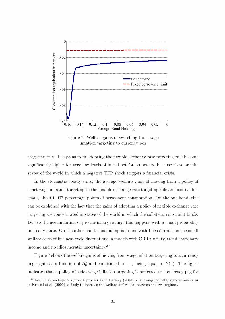
Figure 7 shows the welfare gains of moving from wage inflation targeting to a currency

peg, again as a function of B∗0 and conditional on z−1 being equal to E(z). The figure

indicates that a policy of strict wage inflation targeting is preferred to a currency peg for

30Adding an endogenous growth process as in Barlevy (2004) or allowing for heterogenous agents asin Krusell et al. (2009) is likely to increase the welfare differences between the two regimes.

31

both versions of the model and for any value of initial net foreign assets. This suggests

that the peg does a poor job in managing both normal business cycle fluctuations and

crisis events. In the benchmark version of the model, lower initial net foreign assets are

associated with higher welfare costs from pegging the exchange rate. This is due to the

fact that the currency peg amplifies the fall in the price of land and worsens households

access to international credit during crises.31

Considering the stochastic steady state, the average welfare losses from moving from

a policy of strict wage inflation targeting to a peg are small, around 0.041 percentage

points of permanent consumption. However, compared to the welfare gains of moving to

a policy of flexible exchange rate targeting the welfare costs of adopting a currency peg

are significantly larger.

3.7 Robustness checks

This section examines the robustness of the main results of the paper to changes in some

key parameters. I start by investigating whether the result that the flexible exchange

rate targeting rule welfare dominates the wage inflation targeting rule in the benchmark

version of the model is robust to changes in ξS, the parameter that governs the response

of the central bank to deviations of the exchange rate from its target. To this end, I

computed the average welfare gains that agents living in the stochastic steady state of

the economy with the wage inflation targeting regime would experience from switching to

a flexible exchange rate targeting rule for a variety of values of ξS. The results, displayed

by figure 8, indicate that the flexible exchange rate targeting rule is preferred to a policy

of targeting wage inflation over a whole range of values for ξS. Among the values of

ξS considered, setting ξS equal to 1 guarantees the highest average welfare gains from

adopting a flexible exchange rate targeting rule.

Table 4 presents the sensitivity of the main results of the paper with respect to

several parameters. The qualitative results seems not to be affected by changes in the

key parameters of the model. In particular, strict wage inflation targeting is always

welfare dominated by the flexible exchange rate targeting rule, and the currency peg is

31For very high levels of debt the welfare losses of moving from wage inflation targeting to a pegbecome decreasing in the initial stock of debt. Presumably this happens because very high initial levelsof debt are associated with a high probability of a severe crisis generating a sharp deleveraging thatreduces significantly the probability of entering a crisis again in the future.

32

0.5 1 1.5 2 2.5 30

0.002

0.004

0.006

0.008

0.01

�s

Figure 8: Average welfare gains of switching from wage inflation targetingto flexible exchange rate targeting

always the regime characterized by the worst performance in terms of welfare. Moreover,

the flexible exchange rate targeting rule is always the regime under which crises have the

mildest impact on the economy, while the currency peg always features the lowest crisis

probability.

However, some parameters have a significant effect on the quantitative results. Indeed,

the differences in the welfare performance of the three regimes increase significantly if

the coefficient of relative risk aversion rises or if the fraction of land holdings that can be

offered as collateral increases. This suggests that different calibrations of the model may

yield higher welfare gains from adopting an appropriate monetary policy regime.

33

Table

4:

Robust

ness

Check

s

Wel

fare

gain

sfr

omW

ITto

Cri

sis

pro

bab

ilit

yM

ean

imp

act

effec

tof

fin

anci

alcr

ises

GD

PC

onsu

mp

tion

Lan

dp

rice

FE

RT

PE

GW

ITF

ER

TP

EG

WIT

FE

RT

PE

GW

ITF

ER

TP

EG

WIT

FE

RT

PE

G

ben

chm

ark

0.00

7−

0.04

18.

39.

35.

5−

2.0

0.2

−5.

9−

4.8−

2.3

−9.

5−

3.0−

2.2−

4.7

γ=

1.8

0.00

3−

0.03

110.1

10.1

7.4

−1.

5−

0.2−

5.0

−3.

7−

2.1

−7.

9−

2.1−

1.7−

3.5

γ=

2.2

0.01

5−

0.09

07.

59.

04.

5−

2.2

0.2

−6.

6−

5.2−

2.0−

10.7

−3.

6−

2.4−

5.7

1/(ω−

1)=

0.9

0.00

5−

0.04

28.

59.

25.

4−

1.9−

0.2−

6.0

−4.

5−

2.2

−9.

6−

3.0−

2.2−

4.9

1/(ω−

1)=

1.1

0.00

9−

0.04

28.

39.

05.

3−

2.1

0.7

−6.

1−

4.9−

2.1

−9.

8−

3.0−

2.0−

4.7

σz

=0.

013

0.00

7−

0.03

49.

310.9

5.4

−1.

30.

8−

5.1

−3.

7−

1.6

−8.

7−

2.4−

1.6−

4.4

σz

=0.

018

0.00

6−

0.04

97.

98.

74.

9−

2.4−

0.3−

7.1

−5.

3−

2.7−

11.1

−3.

4−

2.4−

5.4

κ=

0.36

0.00

5−

0.03

68.

69.

15.

7−

1.9−

0.2−

5.9

−4.

5−

2.2

−9.

3−

2.9−

2.1−

4.7

κ=

0.4

0.01

0−

0.06

07.

99.

04.

9−

2.4−

0.8−

6.3

−5.

1−

2.1−

10.4

−4.

2−

2.1−

5.1

φ=

0.32

0.01

0−

0.03

88.

09.

05.

3−

2.0

0.1

−5.

7−

5.0−

2.0

−9.

6−

3.2−

2.1−

4.8

φ=

0.52

0.00

5−

0.04

38.

69.

05.

7−

2.0−

0.3−

6.2

−4.

5−

2.3

−9.

5−

2.8−

2.1−

4.6

Not

e:W

ITst

and

sfo

rth

eec

onom

yw

ith

stri

ctw

age

infl

atio

nta

rget

ing,

FE

RT

stan

ds

for

the

flex

ible

exch

ange

rate

targ

etin

gru

leand

PE

Gst

ands

for

the

curr

ency

peg

.

34

4 Conclusion

This paper has examined the performance of alternative monetary policy rules in a small

open economy model with an occasionally binding collateral constraint that limits access

to foreign credit and with nominal wage rigidities. The main finding is that the presence

of pecuniary externalities in the credit markets introduces a trade-off between price and

financial stability. For low levels of external debt the probability of a future crisis is small

and a policy that eliminates the distortions coming from nominal rigidities by targeting

wage inflation is the best rule. For high levels of external debt the probability of a

future crisis is high and targeting wage inflation is dominated by a flexible exchange

rate targeting rule, because the latter policy is better at mitigating the fall in output,

consumption and capital inflows during crisis events. In contrast, pegging the exchange

rate is always welfare dominated by the wage inflation targeting rule. A second key finding

is that the exchange rate regime affects both the behavior of the economy during crisis

events and the probability that the economy enters a crisis, through its impact on debt

accumulation during tranquil times. The more the monetary policy regime mitigates the

impact of crises on output and consumption, the more private agents engage in foreign

debt accumulation during tranquil times and the higher is the probability of experiencing

a crisis.

The paper represents a first step in the analysis of monetary policy in dynamic general

equilibrium models featuring tranquil and crisis times. The model is kept voluntarily

simple to reduce the computational complexities involved by the derivation of a global

numerical solution. An interesting area for future research would be to extend the model

in order to make it more suitable to deliver quantitative results. Two possible extensions

are the inclusion of endogenous capital accumulation and of a dynamic wage-setting

process.

35

References

Aghion, P., P. Bacchetta, and A. Banerjee (2004) “A corporate balance-sheet approach

to currency crises,” Journal of Economic theory, Vol. 119, No. 1, pp. 6–30.

Barattieri, A., S. Basu, and P. Gottschalk (2010) “Some evidence on the importance of

sticky wages,” NBER Working Paper No. 16130.

Barlevy, G. (2004) “The Cost of Business Cycles Under Endogenous Growth,” The Amer-

ican economic review, Vol. 94, No. 4, pp. 964–990.

Benigno, G., H. Chen, C. Otrok, A. Rebucci, and E.R. Young (2011a) “Financial Crisis

and Macro-Prudential Policies,” CEPR Discussion Paper No. 8175.

(2011b) “Monetary and Macro-Prudential Policies: An Integrated Analysis,”

Mimeo, London School of Economics.

Bernanke, B.S. and K. Carey (1996) “Nominal wage stickiness and aggregate supply

in the Great Depression,” The Quarterly Journal of Economics, Vol. 111, No. 3, pp.

853–883.

Bianchi, J. (2011) “Overborrowing and Systemic Externalities in the Business Cycle,”

American Economic Review, Vol. 101, No. 7, pp. 3400–3426.

Bianchi, J. and E.G. Mendoza (2010) “Overborrowing, Financial Crises and Macro-

prudential Taxes,” NBER Working Paper No. 16091.

Bordo, M.D. and O. Jeanne (2002) “Monetary policy and asset prices: does benign

neglectmake sense?” International Finance, Vol. 5, No. 2, pp. 139–164.

Braggion, F., L.J. Christiano, and J. Roldos (2007) “Optimal monetary policy in a sudden

stop,” Journal of Monetary Economics, Vol. 56, No. 4, pp. 582–595.

Broda, C. (2004) “Terms of trade and exchange rate regimes in developing countries,”

Journal of International Economics, Vol. 63, No. 1, pp. 31–58.

Caballero, Ricardo J and Arvind Krishnamurthy (2001) “International and domestic

collateral constraints in a model of emerging market crises,” Journal of monetary Eco-

nomics, Vol. 48, No. 3, pp. 513–548.

36

Caballero, R.J. and A. Krishnamurthy (2003) “Inflation targeting and sudden stops,”

NBER Working Paper No. 9599.

Calvo, Guillermo A, Alejandro Izquierdo, and Luis-Fernando Mejia (2004) “On the empir-

ics of sudden stops: the relevance of balance-sheet effects,”Technical report, National

Bureau of Economic Research.

Cespedes, L.F., R. Chang, and A. Velasco (2004) “Balance Sheets and Exchange Rate

Policy,” The American Economic Review, Vol. 94, No. 4, pp. 1183–1193.

Christiano, L.J., M. Eichenbaum, and C.L. Evans (2005) “Nominal rigidities and the

dynamic effects of a shock to monetary policy,” Journal of political Economy, Vol. 113,

No. 1, pp. 1–45.

Christiano, LJ, C. Gust, and J. Roldos (2004) “Monetary Policy in a Financial Crisis,”

Journal of Economic Theory, Vol. 119, No. 1, pp. 64–103.

Coleman, W. J. (1990) “Solving the stochastic growth model by policy-function itera-

tion,” Journal of Business Economic Statistics, Vol. 8, No. 1, pp. 27–29.

Cook, D. (2004) “Monetary policy in emerging markets: Can liability dollarization explain

contractionary devaluations?” Journal of Monetary Economics, Vol. 51, No. 6, pp.

1155–1181.

Correia, I., J.C. Neves, and S. Rebelo (1995) “Business cycles in a small open economy,”

European Economic Review, Vol. 39, No. 6, pp. 1089–1113.

Curdia, V. (2007) “Monetary Policy under Sudden Stops,” FRB of New York Staff Report

No. 278.

Devereux, M.B., P.R. Lane, and J. Xu (2006) “Exchange Rates and Monetary Policy in

Emerging Market Economies,” The Economic Journal, Vol. 116, No. 511, pp. 478–506.

Diaz-Alejandro, Carlos (1985) “Good-bye financial repression, hello financial crash,”

Journal of development Economics, Vol. 19, No. 1, pp. 1–24.

Eichengreen, B., P. Gupta, and A. Mody (2006) “Sudden stops and IMF-supported pro-

grams,” NBER Working Paper No. 12235.

37

Eichengreen, B. and J. Sachs (1985) “Exchange Rates and Economic Recovery in the

1930s,” The Journal of Economic History, Vol. 45, No. 4, pp. 925–946.

Fabiani, S., C. Kwapil, T. Room, K. Galuscak, and A. Lamo (2010) “Wage rigidities and

labor market adjustment in Europe,” Journal of the European Economic Association,

Vol. 8, No. 2-3, pp. 497–505.

Fehr, E. and L. Goette (2005) “Robustness and real consequences of nominal wage rigid-

ity,” Journal of Monetary Economics, Vol. 52, No. 4, pp. 779–804.

Feldstein, M. (2010) “Let Greece take a Holiday from the Euro Zone,” Financial Times.

Gertler, M., S. Gilchrist, and F.M. Natalucci (2007) “External constraints on monetary

policy and the financial accelerator,” Journal of Money, Credit and Banking, Vol. 39,

No. 2-3, pp. 295–330.

Gottschalk, P. (2005) “Downward nominal-wage flexibility: real or measurement error?”

Review of Economics and Statistics, Vol. 87, No. 3, pp. 556–568.

Greenwood, J., Z. Hercowitz, and G.W. Huffman (1988) “Investment, capacity utilization,

and the real business cycle,” The American Economic Review, Vol. 78, No. 3, pp. 402–

417.

Jeanne, O. and A. Korinek (2010) “Managing credit booms and busts: A Pigouvian

taxation approach,” NBER Working Paper No. 16377.

Kimball, M.S. and M.D. Shapiro (2008) “Labor Supply: Are the Income and Substitution

Effects Both Large or Both Small?,” NBER Working Paper No. 14208.

Kollmann, R. (2002) “Monetary policy rules in the open economy: effects on welfare and

business cycles,” Journal of Monetary Economics, Vol. 49, No. 5, pp. 989–1015.

Krugman, P. (2010) “The Making of a Euromess,” New York Times Op-Ed.

Krusell, P., T. Mukoyama, A. Sahin, and A.A. Smith Jr (2009) “Revisiting the welfare

effects of eliminating business cycles,” Review of Economic Dynamics, Vol. 12, No. 3,

pp. 393–404.

38

Lane, P.R. and G.M. Milesi-Ferretti (2007) “The external wealth of nations mark II:

Revised and extended estimates of foreign assets and liabilities, 1970-2004,” Journal

of International Economics, Vol. 73, No. 2, pp. 223–250.

McKinsey, Global Institute (2010) “Debt and deleveraging: The global credit bubble and

its economic consequences.”

Mendoza, E.G. (1991) “Real business cycles in a small open economy,” The American

Economic Review, Vol. 81, No. 4, pp. 797–818.

(2010) “Sudden stops, financial crises, and leverage,” The American Economic

Review, Vol. 100, No. 5, pp. 1941–1966.

Mendoza, E.G. and V.Z. Yue (2011) “A General Equilibrium Model of Sovereign Default

and Business Cycles,” NBER Working Paper No. 17151.

Merler, Silvia and Jean Pisani-Ferry (2012) “Sudden stops in the euro area,” Bruegel

Policy Contribution.

Moron, E. and D. Winkelried (2005) “Monetary policy rules for financially vulnerable

economies,” Journal of Development Economics, Vol. 76, No. 1, pp. 23–51.

Neumeyer, P.A. and F. Perri (2005) “Business cycles in emerging economies: the role of

interest rates,” Journal of Monetary Economics, Vol. 52, No. 2, pp. 345–380.

Obstfeld, M. and K. Rogoff (2000) “New directions for stochastic open economy models,”

Journal of international economics, Vol. 50, No. 1, pp. 117–153.

Olivei, G. and S. Tenreyro (2007) “The timing of monetary policy shocks,” The American

Economic Review, pp. 636–663.

(2010) “Wage-setting patterns and monetary policy: International evidence,”

Journal of monetary economics, Vol. 57, No. 7, pp. 785–802.

Schmitt-Grohe, S. and M. Uribe (2007) “Optimal simple and implementable monetary

and fiscal rules,” Journal of Monetary Economics, Vol. 54, pp. 1702–1725.

(2011) “Pegs and Pain,” NBER Working Paper No. 16847.

39

Smets, F. and R. Wouters (2003) “An estimated dynamic stochastic general equilibrium

model of the euro area,” Journal of the European Economic Association, Vol. 1, No. 5,

pp. 1123–1175.

Tauchen, G. and R. Hussey (1991) “Quadrature-based methods for obtaining approximate

solutions to nonlinear asset pricing models,” Econometrica, Vol. 59, No. 2, pp. 371–396.

40