1

Final  Design  Report

EK  301  C1,  Professor  Morgan

April  25th,  2014

                   David  Miller  U14269071

Emily  Ubik  U77408914

Arthur  Cooper  U54902433

2

Table  of  Contents      

Abstract                                                                                                                                                                                                                                            3

Introduction                                                                                                                                                                                                                                  4

Procedure                                                                                                                                                                                                                                      6

Analysis                                                                                                                                                                                                                                                 10

Data                                                                                                                                                                                                                                                 11

Results                                                                                                                                                                                                                                              13

Discussion                                                                                                                                                                                                                                   14

Conclusion                                                                                                                                                                                                                                       19

Appendix                                                                                                                                                                                                                                             20

3

Abstract The purpose of this report is to describe the redesign process of a final truss for

the EK301 straw truss project. The MATLAB code (found in the Appendix) created for the preliminary report is improved upon and utilized to analyze different types of trusses. Several preliminary truss designs are provided from various stages of the engineering design process. From these, an optimal design is chosen that meets the given specifications in the Truss Design Project Description manual. The final design is evaluated, and the resulting calculations are shown. Ultimately, the chosen design is a variation of the Pratt truss with a theoretical maximum load of 11.456 (+/-) 0.455 N. The final design cost is $337.20 and the load to cost ratio is 0.033975 (N/$).

   

4

Introduction  The design of a truss revolves around three fundamental aspects: the number of joints

and the connections between them (topology), the locations of the joints (geometry), and the cross-sectional area of the members (size). The material and size of the members of the truss are constrained by the fact that plastic drinking straws are used for the members. A laboratory experiment was performed to determine the buckling strength of the straws at different lengths. The data from this lab was used to obtain a functional relationship between straw length and buckling force by modeling the straws as Euler columns. Because the straws are much weaker in compression than in tension, the only failure mode for the truss is the buckling of one of the members. A computational truss analysis program calculates the internal forces in all members of the truss under a given loading scenario, and utilizes the functional relationship between straw length and buckling strength to predict which member will fail first and the maximum load the truss can withstand.

The design portion of the project began by writing the MATLAB script to find the internal forces in the members of the truss, as well as the cost and theoretical maximum load data of the truss. Once the code for the computational analysis was written, designs could be tested quickly and an iterative design process was instigated. Drawings and notes on each truss design were made so that they could be referenced later and so that comparisons could be made. These first designs were documented in our preliminary design report.

For the design of the final truss, there was an emphasis on raising the theoretical maximum load, while still having a nominal cost and load-to-cost ratio. To do this, an optimization algorithm was created in MATLAB. This supplemented the code that was created for the last stage of this project. The optimization code provided a general idea of what worked and what did not work in terms of straw size and geometry. However, different truss ideas were ultimately tested manually using the original program and the knowledge gained from the optimization code. Both contributed to the final truss design. Overall, the motivation of the final design is to improve upon the preliminary trusses in order to achieve the greatest maximum load, a lower cost, and a higher load to cost ratio.

Throughout the course of this project, the team members intended to learn about the engineering design process, standard truss designs, computational static analysis, optimization algorithms and techniques, and working effectively on a team. The engineering design process is critical to any engineering project; it enables a team to generate and improve designs methodologically through an iterative process. Going into the project, the team members were unfamiliar with standard simple, planar truss designs, so research was done to acquire information on some of these truss types. Two of these truss types, the Gambrel and the Pratt truss, were documented in our team’s preliminary design report. The computational analysis required by the MATLAB code to analyze the truss was new to the team members. Once the computational analysis was functioning, the question arose of how to optimize the truss designs we already had. Finally, effective communication of tasks and deadlines between members was needed to ensure that all of our goals were met on time. All of these skills are useful, and some critical for an engineer in professional industry. The ability to generate designs, evaluate them using computational methods, revise and optimize them, and communicate with other engineers

5

and clients is fundamentally important. Through this project, many of these fundamental skills will be learned and exercised.

6

Procedure Our design procedure for the final truss design incorporated several new methods

developed after the preliminary designs. Our preliminary designs were achieved primarily through trial and error; there was no numerical basis for the changes we made through design iterations. For our final truss design, we utilized computer optimizations to finesse our preliminary truss designs and to guide us to our final truss design. As mentioned previously there are three design aspects to consider for any truss optimization:

1) Topology - The number of joints and their connections to each other. 2) Geometry - The locations of the joints. 3) Member Size - The cross-sectional area (‘thickness’) of the members.

The cross-sectional area of the members is already constrained by our straws, so there is no need to account for that aspect in the optimization. Our preliminary designs already established the number of joints and their connections. Thus, the only unconstrained design aspect is the specific geometry of the truss. With the optimization limited to only one design aspect, the algorithm is greatly simplified. Then the choice must be made whether to use a continuous optimization or a discrete optimization. For simplicity, a discrete combinatorial optimization algorithm was used. Our truss optimization combines a discrete combinatorial method for iterating through all possible solutions, and an exhaustive search method for determining the best solution. In the optimization, selected joints are permitted to move to discrete points, or Virtual Joint Locations (VJLs) within a Virtual Joint Region (VJR). For this report, the term ‘virtual’ is attributed to a truss or aspect of the truss that is a variable within the optimization. The VJR is identical for every joint to be optimized. The size and density of the VJR are defined by the user at the beginning of the optimization.

Fig. 1: VJR for a 1 joint optimization.

The number of virtual trusses to analyze is given by the permutation 𝑛 j, where 𝑛 is the number of virtual joints in each VJR and 𝑗 is the number of joints in the optimization. The number of joints used in the optimization can be constrained by two facts: 1) The first and last joints where the supports are located cannot not be moved; as they define the length of the truss.

7

2) The time required to perform the optimization increases exponentially with the number of joints used in the optimization. Based on 1), the maximum number of joints to be used (j) must be the total number of joints (J) minus the first and last joints (j ≤ J − 2). From 2), it can be determined that as the number of joints for the optimization increases, the amount of time it takes to perform the optimization will reach an impractical length. If a limiting threshold time is set, the maximum number of joints to be optimized for in that time can be determined. Additionally, the number of joints the user wishes to optimize for can be set, and the approximate time required will be displayed.

Once the VJR is defined and the joints have been selected, the algorithm must then loop through every permutation of VJLs for each joint in the optimization and analyze the resulting virtual truss. The results from these analyses and the joint coordinates from each virtual truss are saved for sorting and analysis later. An exhaustive search method was used to sort through the virtual truss data and select the truss with the best TML, cost, and LCR.

8

This section of the code was very difficult to verify. Because of the repetitive nature of the process, many optimization runs resulted in virtual trusses with identical Theoretical Maximum Loads (TMLs), costs, or Load-Cost Ratios (LCRs). For example, for a certain optimization run there may be several hundred virtual trusses with the same lowest cost, highest TML, or highest LCR. In addition, virtual trusses were not properly sorted to eliminate trusses that violated fundamental design constraints, such as member lengths and joints existing below the axis formed by the first and last joints. For more information on how the optimization was used and the problems we encountered, see the Discussion on page 14. Due to the difficulties sorting the results of the optimization and a lack of proper verification of the optimization’s accuracy, our team decided to employ a more manual approach to optimizing the truss design. As in the Preliminary Report, our team used the “trusspgm.m” code to analyze the internal forces in each truss design. In addition due to the internal forces on each member, the code outputs the identity of the critical members in each design. Shortening these critical members causes their buckling strength to increase, as well as the overall weight-bearing strength of the truss. In the case of our final design, another pair of critical members appeared after this initial shortening. In response, the next truss design shortened those new critical members, thereby increasing the theoretical maximum load yet again. At this point the truss came very near its maximum optimization, with respect to the limitations of this project, and therefore we chose this as our final design. Regarding the plans for construction of the final truss design, our team will utilize the Pinning Jigs at the Study Center Room at 110 Cummington Mall. Using the jigs and the provided gusset plates, we will connect the straws according to the design outlined below. The construction process will require:

9

● Scissors ● A metric ruler ● A clean, flat surface ● Pins ● At least two pinning jigs ● Gusset plates (joints) ● Straws (members) ● Scale drawing of final truss design, dimensioned

Construction will take place at 2 PM on Friday, April 25, 2014.

10

Analysis Initially, the analysis would make use of an optimization feature, which could analyze

tens of thousands of virtual trusses with different joint locations until it found the most optimal design. However, due to the optimization program outputting a large number of viable trusses (which were not necessarily constrained by the rules of this project) and the amount of time required to gain results from such a complex code, our team decided to find the optimal truss with a more manual method.

For the actual analysis of the prototypes and final truss design, the MATLAB script trusspgm.m was used. The program uses the coordinates of the truss joints and a connection matrix defining their topology to calculate the internal forces on each member of the truss, the theoretical maximum load, the load-to-cost ratio, the cost of the truss, along with the critical members and the length of each member. By shortening the critical members, our team improved upon each truss design, and compared the theoretical maximum load and the load-to-cost ratio of each successive installment. Using this method, our team analyzed several variations of the Pratt Truss design, including a shorter truss, taller truss, raised or arched truss, and variations of the original truss. With each successive design, shortening the critical members and comparing each successive TML and LCR allowed for the creation of the optimal truss for our final design.

11

Data Final  Design:  Output  Data  from  Matlab  Code  for  the  Optimal  Truss,  Load  in  Each  Member

Member  Number

Joint-­‐to-­‐joint  Length  (cm)

Actual  Length  (cm)

Tension  (T)  or  Compression  (C)

Buckling  Strength  and  Uncertainty  (N)

Magnitude  of  the  force  (N)

1 10.0 9.5 T - 2.741 2 12.7 12.2 C 8.590 +/- 0.26 3.678 3 8.5 8.0 0 - 0 4 9.0 8.5 T - 2.741 5 12.7 12.2 T - 2.970 6 10.5 10.0 C 12.547 +/- 0.61 4.977 7 9.6 9.1 C 15.298 +/- 0.82 1.992 8 9.5 9.0 T - 5.163 9 12.7 12.2 T - 3.291

10 8.5 8.0 C 19.320 +/- 0.97 7.357 11 9.5 9.0 0 - 0 12 12.7 12.2 T - 3.291 13 9.5 9.0 T - 5.163 14 8.5 8.0 C 19.320 +/- 0.97 7.357 15 9.6 9.1 C 15.298 +/- 0.82 1.992 16 12.7 12.2 T - 2.970 17 9.5 9.0 T - 2.741 18 10.5 10.0 C 12.547 +/- 0.61 4.977 19 8.5 8.0 0 - 0 20 9.5 9.0 T - 2.741 21 12.7 12.2 C 8.590 +/- 0.26 3.678

12

Fig. 5: Final Design of Optimal Truss, with Critical Member Highlighted.

13

Results

Final  Design  Results:  Output  Data  from  Matlab  Code  for  the  Optimal  Truss  

Design Optimal  Truss

Critical  Member  2

Length  of  Critical  Member (cm)

12.7 (actual-­‐  12.2)  

Buckling  Strength  and  Uncertainty  (N)

 12.547   (+/-­‐)0.345  

Theoretical  Maximum  Load  and  Uncertainty  (N)

 11.456   (+/-­‐)0.455  

Theoretical  Truss  Cost  ($) 337.20

Theoretical  Load-­‐to-­‐Cost  Ratio  (N/$)

 0.033973

Actual  Maximum  Load  and  Uncertainty  (N)

12.431   (+/-­‐)  0.494  

Actual  Truss  Cost  ($) 325.48   Actual  Load-­‐to-­‐Cost  Ratio  (N/$) 0.039301   Adjusted  Maximum  Load  (N)  11.001

14

Discussion

In the preliminary report, it was decided that the final truss would be based on the design of the Pratt Truss, rather than the Gambrel. From this point, our team searched for two ways to optimize the truss design: (1) the optimization algorithm, and (2) the manual method of critical member-shortening. As mentioned before, the team ultimately employed the method of critical member-shortening to produce the optimal truss design.

The first design to be analyzed was the original Pratt Truss, which supported a theoretical maximum load of 10.311 +/- 0.550 N and had a load-to-cost ratio of 0.030053. Next, our team analyzed a shorter version of the same Pratt Truss design (lowering the overall height to 8.5cm), as well as a taller version of the Pratt Truss design (at a height of 11cm), both of which had lower theoretical maximum loads and load-to-cost ratios. In addition to the shorter and taller trusses, our team also analyzed a “raised” truss design, which differed considerably from the standard Pratt Truss.

Fig. 6: Design of Raised Truss, with Crit. Members Highlighted.

However, this design also produced a lower TML and a lower LCR than that of the

original Pratt Truss. Therefore, our team decided that it was time to begin improving upon the original design, rather than finding radically new configurations for the joints. In order to improve the weight-bearing capacity of the original Pratt Truss, we shortened the critical members of this original design (Members 10 and 14), thereby increasing their buckling strength. With these members made stronger, the truss itself would sustain more force before any of its members buckled (specifically, a TML of 10.937 +/- 0.412 N and a LCR of 0.031994). In this improved design, the critical members became members 2 and 21, which were then also shortened to improve their buckling strength. This new design produced a TML of 11.456 +/- 0.455 and a LCR ratio of 0.033975. The final alteration made to the design was the slight offsetting of Joint 2, making Member 1 longer and ensuring that there would only be one critical member (Member

15

2). After this final change, the critical member remained to be Member 2, but it could not be shortened without violating the project specifications. Therefore, our team had obtained the optimal truss design for this project.

Regarding the building process for the final design, our team will meet on Friday, April

25, 2014 at the Study Center Room at 110 Cummington Mall to construct the truss. The materials required will consist of:

● Scissors ● A metric ruler ● A clean, flat surface ● Pins ● At least two pinning jigs ● Gusset plates (joints) ● Straws (members) ● Scale drawing of final truss design, dimensioned

Using the Pinning Jigs provided according to our team’s time slot, we will pin the straws to the Gusset plates, which will be outlined with marked lines to assist with accuracy. The center of each plate will be given a 0.25cm radius (i.e., r=0.25 cm), around which the straws will be attached.

Fig. 7: Attachment Diagram for Gusset Plates and Straws.

Finally, the adjusted maximum load estimate is 11.001 N, which accounts for the value of the theoretical maximum load and its uncertainty (both of which are less than the value of the actual maximum load). Therefore, 11.001 N is the minimum of the maximum possible loads to be supported by the optimal truss. In the event of real life application of this truss design, additional adjustments should be made to produce a considerably higher safety factor, but because the goal of this project is to accurately predict the point at which the truss will fail, no such safety factor is necessary.

16

Preliminary Design 1: Original Pratt Truss

Fig. 8: Design for Original Pratt Truss, with Crit. Members Highlighted

. Preliminary  Design  Results Original  Pratt  Truss

Failure  Data     Critical  Members 10  and  14

Theoretical  Maximum  Load 10.311  (+/-­‐)  0.550  N      

Cost  Data   Total  Cost $343.11

Theoretical  Maximum   Load-­‐to-­‐Cost  Ratio

0.030053  (N/$)

17

Preliminary Design 2: Gambrel Truss

Fig. 9: Design for the Gambrel Truss, with Crit. Members Highlighted.

Preliminary  Design  Results Gambrel  Truss

Failure  Data   Critical  Members 1  and  20

Theoretical  Maximum  Load 8.833  (+/-­‐)  0.322  N  

Cost  Data Total  Cost $341.64

 Theoretical  Maximum Load-­‐to-­‐Cost  Ratio

0.025856  (N/$)

18

Preliminary Design 3: Short Pratt Truss

Fig. 10: Design for the Short Pratt Truss, with Crit. Members Highlighted

Preliminary  Design  Results Short  Pratt  Truss

Failure  Data Critical  Members 18

Theoretical  Maximum  Load  (N) 11.328  (+/-­‐)0.547  

Cost  Data Total  Cost  ($) 332.65

Theoretical  Maximum   Load-­‐to-­‐Cost  Ratio  (N/$)

0.034055

     

19

Conclusion

In conclusion, our team successfully optimized a preliminary simple truss design. The final truss design raised the theoretical maximum load to 11.456 N, while still maintaining a reasonable cost and load to cost ratio. Through this semester-long project we learned extensively about the engineering design process. A discussion of the Hartford Roof Collapse provided real world consequences of what happens when the engineering design process and design implementation are not followed completely and with the safety of others in mind. This project also required us to hone our team working and organizational abilities, in addition to our communication skills. The results from this report will be tested on Saturday, April 26th at 10:30am at the Photonics Center. Testing will show whether the computational analyses performed in this report were accurate and whether our truss design implementation was acceptable.

   

20

Appendix Hartford Roof Collapse Meeting: April 23rd, 2014 10:30pm Ingalls Engineering Resource Center Participants: David Miller Arthur Cooper (Recorder) Emily Ubik (Chair) Agenda - What is the role of the computer program in the analysis and design of the Hartford truss? - Pros? - Cons? - What are some technical, procedural and ethical concerns? - What is an appropriate safety factor to be used on our truss if it was to be built in real life? - What maximum load would we claim? - How does variability in materials play a role? - How does the variability in construction play a role? How does the level of execution affect the design? - Conclusions from this discussion? Minutes from the Meeting Arthur: What’s on the agenda, Emily? Emily: First I think we should talk about the role of the computer program in the design of the roof and the truss. D: I think they relied too much on the computer program for their design. E: Yeah, and using a PC program can lead to inaccurate results. A: Especially if you don’t check/verify your work. D: Using a computer analysis can also lead to a false sense of security. E: What are the technical concerns? D: They broke a lot of laws/codes; they didn’t build it to spec. E: They didn’t even have a structural engineer on site during the construction! A: The roof was clearly not built as it was designed (as seen on the 4th page diagram). They made a lot of changes during construction that did not reflect the design at all. D: Also, the division of responsibilities was unclear, lead to people shirking off responsibility. E: There were too many subcontractors, and an apathetic atmosphere. A: Some ethical concerns were, that even in the face of many people, the engineers refused to account for unforeseen complications. D: Yeah, the engineers consistently ignored the advice of others in regard to the safety of the roof.

21

E: OK, so what about an appropriate safety factor for our truss (in real life)? A: What is the actual max load we should express [advertise]? Like 50 percent of what the actual theoretical max load is? Even though that wouldn’t save money (which was clearly a major concern in the hartford case). D: So for our safety factor, if it’s a non-critical component that fails then the safety factor required is pretty low. But because a [our] bridge is transporting people and has a large impact on society as a major component of infrastructure, a bridge should be considered a critical component. So it needs to have a much higher safety factor, which would depend on our uncertainty calculation. For this theoretical bridge we would want a safety factor of 6 to 10. A: So we say that the [our] bridge can hold about 10% of what it can actually hold? Which is about 11N in our model. E: How does variability in materials affect the final product and the design process? D: Materials need to be quality controlled, ordered, and inspected, then accounted for in the uncertainty calculations. For example, with airplanes, the safety factor can’t be too high, or else they would end up weighing too much. Instead, they compensate with great quality control (frequent checkups and inspection of materials before building). As opposed to buildings, which would have a high safety factor, but maybe not the best quality control (infrequent inspections) E: How does the variability in the construction process play a role? And how does the level of execution affect the design? A: Again, looking at the diagram, it is clear that there was an error in the construction process which most likely led to the collapse of the roof. The builders clearly didn’t build the roof to true to the original design. E: And that brings up an ethical question too. A: Yeah, if the engineers were notified of unforeseen complications in their product, they needed to take such advice seriously and change their design to maintain a safe environment. E: What can we conclude? D: That as engineers we have a duty to put the safety of the public above all else. E: Is a follow up meeting necessary? D and A: No.

22

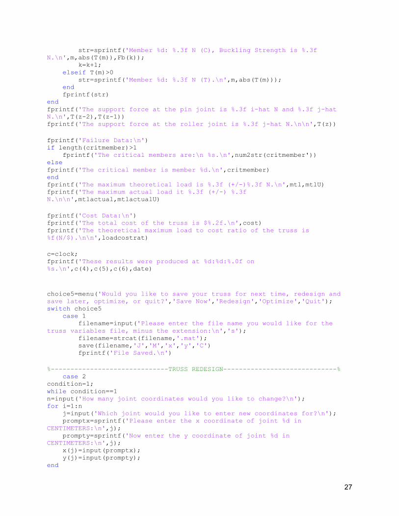
MATLAB Code: Main Script, “trusspgm.m” %EK301 C1 3/29/14 %GROUP MEMBERS: %DAVID MILLER U14269071 %EMILY UBIK U77408914 %ARTHUR COOPER U54902433 %%%%%%%%%%%%%%%%%% TRUSS DESIGN AND ANALYSIS PROGRAM %%%%%%%%%%%%%%%%%% % Program Description % The purpose of this program is to aid in the design and analysis of %simple, planar, trusses. Our program differs slightly from the input %format described in Sec.4.2.3 of the packet. This program description is to %clarify any deviations from the requirements. % The first step in the program is to define the truss parameters. %There are 3 ways to do this: % % 1: Manually define all truss dimensions. % % 2: Choose a standardized type of truss and define required % dimensions. % % 3: Open a previous truss for redesign and analysis. % The second step is creating the support matrices Sx and Sy, as well %as the the load vector L. There is an option to se the load required by %the project or to place the load at another joint and define its strength. % The third step is to construct the equilibrium equations. This is %accomplished by looping through each member and calculating its length %(x,y, and magnitude) and unit vector. Then the values of the unit vector %components are assigned to their respective locations in the coefficient %matrix. Then the equations are solved. % The fourth step analyzes the solution and determines some useful %things, like the buckling strengths of the members in compression, the %maximum theoretical load, the cost and load-cost ratio, etc. % The fifth and final step prints the results on screen and provides the user %with the option to save the truss [MATLAB variables] so that the laborious manual %entering of dimensions and connections need not occur again. %%%%%%%%%%%%%%%%%%%%%%%%%%%%%%%%%%%%%%%%%%%%%%%%%%%%%%%%%%%%%%%%%%%%%%%%%%% clear

23

clc %--------------------------DEFINE TRUSS GEOMETRY--------------------------% choice1=menu('Welcome to David, Emily, and Arthur''s Truss Program. Would you like to enter in truss dimensions manually, select a truss type and define its dimensions, or load a previous truss?'... ,'Enter Dimensions Manually','Select Truss Type','Load Previous Truss'); switch choice1 case 1 %Number of joins and members J=input('Please enter the number of joints:\n'); M=(2*J)-3; %Joint-member relationship for a simple, planar truss. C=zeros(J,M); %Preallocates the connection matrix x=zeros(J,1); %Preallocates the joint position vectors y=zeros(J,1); %Prompts user for coordinates for joint positions through a loop for j=1:J promptx=sprintf('Please enter the x coordinate of joint %d in CENTIMETERS:\n',j); x(j)=input(promptx); prompty=sprintf('Now enter the y coordinate of joint %d in CENTIMETERS:\n',j); y(j)=input(prompty); end %Builds the connection matrix from a loop of queries asking the %user which members are connected to each joint. cnct{1,J}=[]; %Each cell in 'cnct' contains the indices of the corresponding row in connection matric 'C' that are to be assigned the value of 1. for j=1:J str=sprintf('How many members are connected to joint %d?\n',j); choice2=menu(str,'1','2','3','4','5','6'); cnct{j}=zeros(choice2,1); for i=1:choice2 rem=choice2-(i-1); str2=sprintf('Which members? (%d members remaining for joint %d.)\n',rem,j); cnct{j}(i)=input(str2); end C(j,cnct{j})=1; end case 2 %Select truss geometry (i.e. warren truss, pratt truss, parker truss, etc.) type=input('Please type the name of the truss in single quotes:\n'); J=input('Please enter the number of joints:\n'); M=(2*J)-3; C=zeros(J,M); %Preallocates the connection matrix %Warren Truss if type=='warren' a=input('Please enter the base dimension (cm):\n'); b=a*sin(pi/3); %height of the truss

24

bottom=(J/2)+.5; %number of joints on top and bottom top=(J/2)-.5; v=[1 1 0 1 1]; m=2; for j=3:(J-2) C(j,m:(m+4))=v; m=m+2; end C(1,1:2)=[1 1]; C(2,1:4)=[1 0 1 1]; C((J-1),(M-3):M)=[1 1 0 1]; C(J,(M-1):M)=[1 1]; end %Creates x and y location vectors for the joints of the Warren %Truss x=zeros(1,J); y=zeros(1,J); n=0; for j=1:2:J x(j)=a*n; n=n+1; end n=0; for j=2:2:J-1 x(j)=(a/2)+a*n; y(j)=b; n=n+1; end case 3 filename=input('Please type the name of the file you would like to load without its extension:\n','s'); filename=strcat(filename,'.mat'); load(filename) end %--------------------DEFINE SUPPORT AND LOAD MATRICES---------------------% tstart=tic; %Creates support force connection matrix Sx=zeros(J,3); Sy=zeros(J,3); Sx(1,1)=1; Sy(1,2)=1; Sy(J,3)=1; %Creates a load vector describing the location and strength of the %load on the truss L=zeros(2*J,1); choice3=menu('Would you like to use the default truss loading or set a load at a joint?','Default Loading','Set a Load'); switch choice3 case 1 F=(500*9.81)/1000; Lj=input('What number joint will the load be placed at?\n'); L(J+Lj)=F;

25

case 2 Lj=input('What number joint will the load be placed at?\n'); F=input('Please enter the value of the load in Newtons: \n'); L(J+Lj)=F; end %---------------------CONSTRUCT EQUILIBRIUM EQUATIONS---------------------% %Preallocation deltax=zeros(M,1); deltay=zeros(M,1); ux=zeros(M,1); uy=zeros(M,1); Ax=zeros(J,M); Ay=zeros(J,M); %Calculates coefficients for matrix A. for m=1:M vec=find(C(:,m)); deltax(m)=abs(x(vec(2))-x(vec(1))); deltay(m)=abs(y(vec(2))-y(vec(1))); r(m)=magnitude(deltax(m),deltay(m)); ux(m)=deltax(m)/r(m); uy(m)=deltay(m)/r(m); if x(vec(1))<x(vec(2)) Ax(vec(1),m)=ux(m); Ax(vec(2),m)=-ux(m); else Ax(vec(1),m)=-ux(m); Ax(vec(2),m)=ux(m); end if y(vec(1))<y(vec(2)) Ay(vec(1),m)=uy(m); Ay(vec(2),m)=-uy(m); else Ay(vec(1),m)=-uy(m); Ay(vec(2),m)=uy(m); end end A=[Ax Sx;Ay Sy]; %Creates matrix A T=A\L; %Solves equilibrium equations %--------------------------ANALYSIS OF RESULTS----------------------------% %Shows which members are in tension/compression Tm=T(1:length(T)-3); tension=find(Tm>0); compression=find(Tm<0); zeroforce=find(Tm==0); [Fb,U]=buckle(r(compression)); %Calculates buckling strengths & uncertainties of all members in compression comprat=T(compression)./Fb'; %Compression ratios for all members in compression

26

maxcomprat=abs(min(comprat)); %T's are negative, so uses min function, not max. Absolute value will be used later n=find(min(comprat)==comprat); %finds indices of critical member(s) for those in compression critmember=compression(n); %finds indices of critical member(s) for all members mtl=(Fb(n(1))'./abs(T(critmember(1)))).*F; %maximum theoretical load (MTL) = (critical member buckling force/critical member test force)*current load percerr=(U(n(1))/Fb(n(1))); %buckling force percent error (percent uncertainty) mtlU=mtl*percerr; %MTL uncertainty mtlactual=(r(critmember(1))/(r(critmember(1))-.5))*mtl; %Actual MTL, corrected for actual straw length. Actual straw length is approximated as being as the joint to joint length minus the diameter of the straw, which is approximately 1cm. mtlactualU=mtlactual*percerr; %Actual MTL uncertainty cost=(10*J)+sum(r); loadcostrat=mtl/cost; telapsed=toc(tstart); %Finds shortest and longest members shortest=min(r); longest=max(r); shortestm=find(r==min(r)); longestm=find(r==max(r)); %Graph the truss f=plottruss(x,y,C,critmember,Lj); set(f,'Visible','on','Name','NameTest') %---------------------------PRINT/SAVE RESULTS----------------------------% clc fprintf('\n\n\t\t RESULTS\n\n') fprintf('Truss Dimensions:\n') fprintf('The length of the truss is %.1f cm.\n',x(J)) fprintf('The height of the truss is %.1f cm.\n',max(y)) fprintf('Member Number\tJoint-Joint Length (cm)\n') for m=1:M fprintf('%d\t\t%.1f\n',m,r(m)) end fprintf('Shortest Members:\nMembers %s are each %.1f cm.\n',num2str(shortestm),shortest) fprintf('Longest Members:\nMembers %s are each %.1f cm.\n\n',num2str(longestm),longest) fprintf('Member & Support Forces:\n') z=length(T); k=1; for m=1:M if abs(T(m))<=(10^-5) str=sprintf('Member %d is a zero force member.\n',m); elseif T(m)<0

27

str=sprintf('Member %d: %.3f N (C), Buckling Strength is %.3f N.\n',m,abs(T(m)),Fb(k)); k=k+1; elseif T(m)>0 str=sprintf('Member %d: %.3f N (T).\n',m,abs(T(m))); end fprintf(str) end fprintf('The support force at the pin joint is %.3f i-hat N and %.3f j-hat N.\n',T(z-2),T(z-1)) fprintf('The support force at the roller joint is %.3f j-hat N.\n\n',T(z)) fprintf('Failure Data:\n') if length(critmember)>1 fprintf('The critical members are:\n %s.\n',num2str(critmember')) else fprintf('The critical member is member %d.\n',critmember) end fprintf('The maximum theoretical load is %.3f (+/-)%.3f N.\n',mtl,mtlU) fprintf('The maximum actual load it %.3f (+/-) %.3f N.\n\n',mtlactual,mtlactualU) fprintf('Cost Data:\n') fprintf('The total cost of the truss is $%.2f.\n',cost) fprintf('The theoretical maximum load to cost ratio of the truss is %f(N/$).\n\n',loadcostrat) c=clock; fprintf('These results were produced at %d:%d:%.0f on %s.\n',c(4),c(5),c(6),date) choice5=menu('Would you like to save your truss for next time, redesign and save later, optimize, or quit?','Save Now','Redesign','Optimize','Quit'); switch choice5 case 1 filename=input('Please enter the file name you would like for the truss variables file, minus the extension:\n','s'); filename=strcat(filename,'.mat'); save(filename,'J','M','x','y','C') fprintf('File Saved.\n') %------------------------------TRUSS REDESIGN-----------------------------% case 2 condition=1; while condition==1 n=input('How many joint coordinates would you like to change?\n'); for i=1:n j=input('Which joint would you like to enter new coordinates for?\n'); promptx=sprintf('Please enter the x coordinate of joint %d in CENTIMETERS:\n',j); prompty=sprintf('Now enter the y coordinate of joint %d in CENTIMETERS:\n',j); x(j)=input(promptx); y(j)=input(prompty); end

28

plottruss(x,y,C) condition=menu('How does this look? Do you want to make more changes?','Yes','No'); end filename=input('Please enter the file name you would like for the truss, minus the extension:\n','s'); filename=strcat(filename,'.mat'); save(filename,'J','M','x','y','C') fprintf('File Saved.\n') fprintf('Your changes will be reflected when you reopen this truss next time.\nThank you for using David, Emily, and Arthur''s truss program!\n') %--------------------------------OPTIMIZATION-----------------------------% case 3 close all [indarray,datarray]=optitruss(J,M,x,y,C,Sx,Sy,L,r,F); %close all l=length(datarray); counter=1; for i=1:l r=zeros(1,M); for m=1:M vec=find(C(:,m)); deltax(m)=abs(x(vec(2))-x(vec(1))); deltay(m)=abs(y(vec(2))-y(vec(1))); r(m)=magnitude(deltax(m),deltay(m)); end if datarray(i,2)>345 disp('cost exceeded') datarray(i)=[]; indarray{i}=[]; elseif any(indarray{i}(:,2)<0) disp('truss extends below x-axis') datarray(i)=[]; indarray{i}=[]; elseif any(r>15)||any(r<8.5) disp('truss members eithr too long or too short') datarray(i)=[]; indarray{i}=[]; else mtls(counter)=datarray(i,1); costs(counter)=datarray(i,2); loadcostrats(counter)=datarray(i,3); counter=counter+1; end end [g1,i1]=sort(loadcostrats,'descend'); [g2,i2]=sort(costs,'ascend'); [g3,i3]=sort(mtls,'descend'); x1=indarray{i1(1)}(:,1); %Best load-cost ratio y1=indarray{i1(1)}(:,2); x2=indarray{i2(2)}(:,1); %Lowest cost y2=indarray{i2(2)}(:,2); x3=indarray{i3(3)}(:,1); %Highest maximum theoretical load y3=indarray{i3(3)}(:,2);

29

g1(1) g2(1) g3(1) case 4 end %%%%%%%%%%%%%%%%%%%%%%%%%%%%%%%%%%%%%%%%%%%%%%%%%%%%%%%%%%%%%%%%%%%%%%%%%%%

30

Functions function [F U] = buckle(l) %BUCKLE calculates the buckling strength (in N) of a length of straw. % Models the straw as an Euler column, uses data from the class testing labs. % Also returns the error of the buckling strength (in N). Accepts inputs in % vector form. F=1395.9./(l.^2); U=707.08./(l.^3); end function h=circle(x,y,r) %x and y are the coordinates of the center of the circle %r is the radius of the circle %0.01 is the angle step, bigger values will draw the circle faster but %you might notice imperfections (not very smooth) ang=0:0.005:2*pi; xp=r*cos(ang); yp=r*sin(ang); h=plot(x+xp,y+yp,'k-'); end function r = magnitude(x,y) %This function finds the magnitude of a vector based on its x and y %components. % Detailed explanation goes here r=((abs(x).^2)+(abs(y).^2)).^(1/2); end

31

function [T] = eqeqns(J,M,x,y,C,Sx,Sy,L) % EQEQNS constructs the equilibrium equations and solves them to find T, % a vector containing the forces in all the members and the support forces. %Preallocation deltax=zeros(M,1); deltay=zeros(M,1); ux=zeros(M,1); uy=zeros(M,1); Ax=zeros(J,M); Ay=zeros(J,M); %Calculates coefficients for matrix A. for m=1:M vec=find(C(:,m)); deltax(m)=abs(x(vec(2))-x(vec(1))); deltay(m)=abs(y(vec(2))-y(vec(1))); r(m)=magnitude(deltax(m),deltay(m)); ux(m)=deltax(m)/r(m); uy(m)=deltay(m)/r(m); if x(vec(1))<x(vec(2)) Ax(vec(1),m)=ux(m); Ax(vec(2),m)=-ux(m); else Ax(vec(1),m)=-ux(m); Ax(vec(2),m)=ux(m); end if y(vec(1))<y(vec(2)) Ay(vec(1),m)=uy(m); Ay(vec(2),m)=-uy(m); else Ay(vec(1),m)=-uy(m); Ay(vec(2),m)=uy(m); end end A=[Ax Sx;Ay Sy]; %Creates matrix A T=A\L; %Solves equilibrium equations end

32

function quickplottruss(h,x,y,C) %UNTITLED Summary of this function goes here % Detailed explanation goes here [J, M]=size(C); x0{1,M}=[]; y0{1,M}=[]; hold on for m=1:M x0{m}=x(find(C(:,m))); y0{m}=y(find(C(:,m))); sym='b-'; plot(h,x0{m},y0{m},sym,'LineWidth',1.5); end hold off axis equal end

33

function f = plottruss(x,y,C,varargin) %PLOTTRUSS plots a truss given the coordinates of the joints and a %connection matrix. % It will also plot the critical member in a different % color if a fourth argument is passed, and a vertical arrow downwards % originating from the joint where the load is placed. As a 'bonus % feature', the function also plots symbols representing the pin and % roller supports, as well as the ground the supports are % fixed to/are resting on. f=figure('Visible','off'); switch nargin case 3 [J, M]=size(C); x0{1,M}=[]; y0{1,M}=[]; hold on for m=1:M x0{m}=x(find(C(:,m))); y0{m}=y(find(C(:,m))); sym='b-'; plot(x0{m},y0{m},sym,'LineWidth',1.5); end case 4 critmember=varargin{1}; [J, M]=size(C); x0{1,M}=[]; y0{1,M}=[]; hold on for m=1:M x0{m}=x(find(C(:,m))); y0{m}=y(find(C(:,m))); if m==critmember sym='r-'; else sym='b-'; end plot(x0{m},y0{m},sym,'LineWidth',1.5); end case 5 critmember=varargin{1}; Lj=varargin{2}; arx=[x(Lj) x(Lj)]; ary=[y(Lj) y(Lj)-5]; plot(arx,ary,'k-','LineWidth',1.2); patch([(x(Lj)-.5) x(Lj) (x(Lj)+.5)],[(y(Lj)-5) (y(Lj)-5-sin(pi/2)) (y(Lj)-5)],'k'); [J, M]=size(C); x0{1,M}=[]; y0{1,M}=[]; hold on for m=1:M x0{m}=x(find(C(:,m))); y0{m}=y(find(C(:,m))); if m==critmember(m==critmember) sym='r-'; else

34

sym='b-'; end plot(x0{m},y0{m},sym,'LineWidth',1.5); end end %Plots supports using patches and a user defined circle drawing function. r=.3; plot(x,y,'k.','MarkerSize',20); a=[-1 0 1]; a1=a; floorhgt=-2; b1=[floorhgt 1-sin(pi/2) floorhgt]; a2=a+x(J); b2=[floorhgt+2*r 1-sin(pi/2) floorhgt+2*r]; patch(a1,b1,'g') patch(a2,b2,'g') hc1=circle(a2(1)+r,b2(1)-r,r); hc2=circle(a2(3)-r,b2(1)-r,r); set(hc1,'LineWidth',1.02) set(hc2,'LineWidth',1.02) %Draws the floor and the slashes or hatch-marks denoting a fixed surface. floorx1=(a1(1)-2):(a1(3)+2); floorx2=(a2(1)-2):(a2(3)+2); floory=floorhgt*ones(1,length(floorx1)); plot(floorx1,floory,'LineWidth',1.1,'Color','k') plot(floorx2,floory,'LineWidth',1.1,'Color','k') for i=1:length([floorx1 floorx2]) floorx=[floorx1 floorx2]; floory=[floory floory]; if i~=length(floorx)&&i~=length(floorx1) line(floorx(i:(i+1)),[floorhgt floorhgt-1],'LineWidth',1.1,'Color','k') end end str=sprintf('%d Joints, %d Members',J,M); title(str); xlabel('Truss Length (cm)') ylabel('Truss Height (cm)') axis('equal') hold off

35

function [Fb,U,critmember,comprat,mtl,mtlactual,cost,loadcostrat] = trussresults(T,r,F,J) %TRUSSRESULTS Summary of this function goes here % Detailed explanation goes here %Shows which members are in tension/compression Tm=T(1:length(T)-3); tension=find(Tm>0); compression=find(Tm<0); zeroforce=find(Tm==0); [Fb,U]=buckle(r(compression)); %Calculates buckling strengths & uncertainties of all members in compression comprat=T(compression)./Fb'; %Compression ratios for all members in compression maxcomprat=abs(min(comprat)); %T's are negative, so uses min function, not max. Absolute value will be used later n=find(min(comprat)==comprat); %finds indices of critical member(s) for those in compression critmember=compression(n); %finds indices of critical member(s) for all members mtl=(Fb(n(1))'./abs(T(critmember(1)))).*F; %maximum theoretical load (MTL) = (critical member buckling force/critical member test force)*current load percerr=(U(n(1))/Fb(n(1))); %buckling force percent error (percent uncertainty) mtlU=mtl*percerr; %MTL uncertainty cost=(10*J)+sum(r); mtlactual=(r(critmember(1))/(r(critmember(1))-.5))*mtl; %Actual MTL, corrected for straw length mtlactualU=mtlactual*percerr; %Actual MTL uncertainty loadcostrat=mtl/cost; end

36

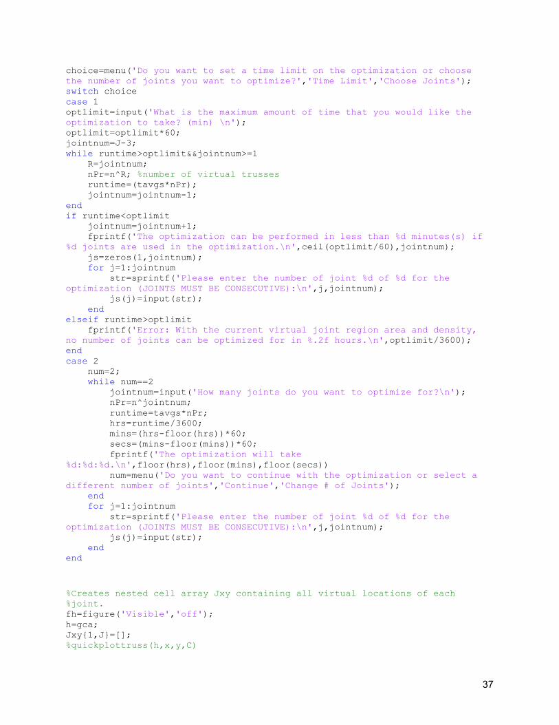
function [Y,datarray] = optitruss(J,M,x,y,C,Sx,Sy,L,r,F) %OPTITRUSS This function will optimize the truss by moving dem joints %around.Outputs: [T,Fb,U,critmember,comprat,mtl,cost,loadcostrat] Inputs: (J,M,x,y,C) % This function optimizes the joint locations of a simple planar truss. % The optimization method operates by defining an area around each joint % filled with possible joint locations. The function then iterates % through and analyzes the truss for all permutations of each joint % location, and then compares all the results. The user is able to define % the area of region around the joint where virtual joints may be placed, % as well as the density of virtual joint distribution. Optimizations may % be performed several times on the same truss with varying virtual joint % region sizes and densities, and there may be different results. %Prompts user to define virtual joint region and virtual joint density in %that region. dist=input('Enter the maximum distance from the original joint location that the joint \ncan be moved:\n'); step=input('Enter the step size to iterate through (e.g. .1cm):\n'); %Calculates permutations of virtual trusses and approximate run time of %optimization based on previous run times of single trusses. v=length(0:step:(dist*2)); n=v^2; R=J-2; nPr=n^R; %number of virtual trusses thechoice=menu('Do you want to graph see each truss permutation?','Yes','No'); switch thechoice case 1 pause on %Hit 'enter' (or any other key) once you are done viewing the truss, and the next permutation will be displayed. tavgs=0.1219; case 2 pause off tavg(1)=0.000835; tavg(2)=0.008884; tavg(3)=0.000927 ; tavg(4)=0.000823; tavg(5)=0.001020; tavg(6)=0.000879; tavg(7)=0.001053; tavg(8)=0.001314; tavg(9)=0.000629; tavg(10)=0.000812; tavgs=mean(tavg); end runtime=tavgs*nPr; fprintf('There are %d virtual trusses to analyze.\nAccording to my calculations, it will take %d hours \nto analyze all %d trusses.\n',nPr,ceil(runtime/36000),nPr) %Asks user to reduce the number of joints in the optimization until the %estimated time to complete the optimization is less than an hour, or %whatever the user defines as the time limit.

37

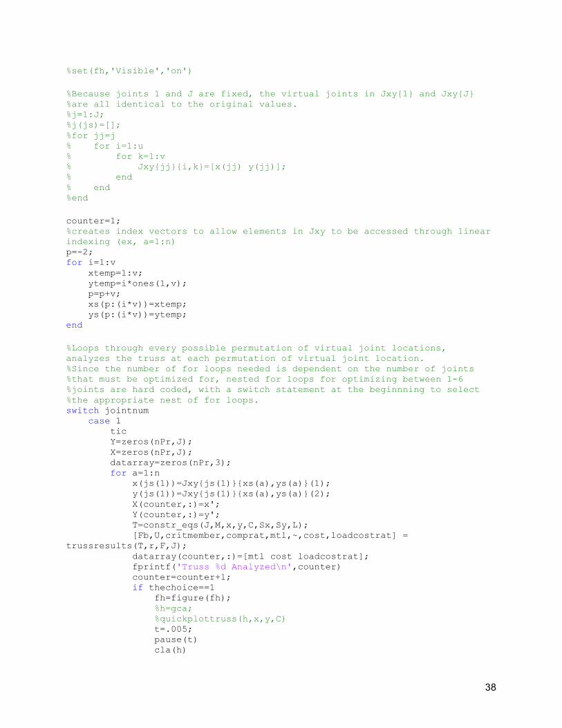
choice=menu('Do you want to set a time limit on the optimization or choose the number of joints you want to optimize?','Time Limit','Choose Joints'); switch choice case 1 optlimit=input('What is the maximum amount of time that you would like the optimization to take? (min) \n'); optlimit=optlimit*60; jointnum=J-3; while runtime>optlimit&&jointnum>=1 R=jointnum; nPr=n^R; %number of virtual trusses runtime=(tavgs*nPr); jointnum=jointnum-1; end if runtime<optlimit jointnum=jointnum+1; fprintf('The optimization can be performed in less than %d minutes(s) if %d joints are used in the optimization.\n',ceil(optlimit/60),jointnum); js=zeros(1,jointnum); for j=1:jointnum str=sprintf('Please enter the number of joint %d of %d for the optimization (JOINTS MUST BE CONSECUTIVE):\n',j,jointnum); js(j)=input(str); end elseif runtime>optlimit fprintf('Error: With the current virtual joint region area and density, no number of joints can be optimized for in %.2f hours.\n',optlimit/3600); end case 2 num=2; while num==2 jointnum=input('How many joints do you want to optimize for?\n'); nPr=n^jointnum; runtime=tavgs*nPr; hrs=runtime/3600; mins=(hrs-floor(hrs))*60; secs=(mins-floor(mins))*60; fprintf('The optimization will take %d:%d:%d.\n',floor(hrs),floor(mins),floor(secs)) num=menu('Do you want to continue with the optimization or select a different number of joints','Continue','Change # of Joints'); end for j=1:jointnum str=sprintf('Please enter the number of joint %d of %d for the optimization (JOINTS MUST BE CONSECUTIVE):\n',j,jointnum); js(j)=input(str); end end %Creates nested cell array Jxy containing all virtual locations of each %joint. fh=figure('Visible','off'); h=gca; Jxy{1,J}=[]; %quickplottruss(h,x,y,C)

38

%set(fh,'Visible','on') %Because joints 1 and J are fixed, the virtual joints in Jxy{1} and Jxy{J} %are all identical to the original values. %j=1:J; %j(js)=[]; %for jj=j % for i=1:u % for k=1:v % Jxy{jj}{i,k}=[x(jj) y(jj)]; % end % end %end counter=1; %creates index vectors to allow elements in Jxy to be accessed through linear indexing (ex, a=1:n) p=-2; for i=1:v xtemp=1:v; ytemp=i*ones(1,v); p=p+v; xs(p:(i*v))=xtemp; ys(p:(i*v))=ytemp; end %Loops through every possible permutation of virtual joint locations, analyzes the truss at each permutation of virtual joint location. %Since the number of for loops needed is dependent on the number of joints %that must be optimized for, nested for loops for optimizing between 1-6 %joints are hard coded, with a switch statement at the beginnning to select %the appropriate nest of for loops. switch jointnum case 1 tic Y=zeros(nPr,J); X=zeros(nPr,J); datarray=zeros(nPr,3); for a=1:n x(js(1))=Jxy{js(1)}{xs(a),ys(a)}(1); y(js(1))=Jxy{js(1)}{xs(a),ys(a)}(2); X(counter,:)=x'; Y(counter,:)=y'; T=constr_eqs(J,M,x,y,C,Sx,Sy,L); [Fb,U,critmember,comprat,mtl,~,cost,loadcostrat] = trussresults(T,r,F,J); datarray(counter,:)=[mtl cost loadcostrat]; fprintf('Truss %d Analyzed\n',counter) counter=counter+1; if thechoice==1 fh=figure(fh); %h=gca; %quickplottruss(h,x,y,C) t=.005; pause(t) cla(h)

39

end end toc case 2 tic Y=zeros(nPr,J); X=zeros(nPr,J); datarray=zeros(nPr,3); for a=1:n x(js(1))=Jxy{js(1)}{xs(a),ys(a)}(1); y(js(1))=Jxy{js(1)}{xs(a),ys(a)}(2); for b=1:n x(js(2))=Jxy{js(2)}{xs(b),ys(b)}(1); y(js(2))=Jxy{js(2)}{xs(b),ys(b)}(2); X(counter,:)=x'; Y(counter,:)=y'; T=constr_eqs(J,M,x,y,C,Sx,Sy,L); [Fb,U,critmember,comprat,mtl,~,cost,loadcostrat] = trussresults(T,r,F,J); datarray(counter,:)=[mtl cost loadcostrat]; fprintf('Truss %d Analyzed\n',counter) counter=counter+1; if thechoice==1 %fh=figure(fh); %h=gca; quickplottruss(h,x,y,C) t=.005; pause(t) cla(h) end end end toc case 3 tic Y=zeros(nPr,J); X=zeros(nPr,J); datarray=zeros(nPr,3); for a=1:n x(js(1))=Jxy{js(1)}{xs(a),ys(a)}(1); y(js(1))=Jxy{js(1)}{xs(a),ys(a)}(2); for b=1:n x(js(2))=Jxy{js(2)}{xs(b),ys(b)}(1); y(js(2))=Jxy{js(2)}{xs(b),ys(b)}(2); for c=1:n x(js(3))=Jxy{js(3)}{xs(c),ys(c)}(1); y(js(3))=Jxy{js(3)}{xs(c),ys(c)}(2); X(counter,:)=x'; Y(counter,:)=y'; T=constr_eqs(J,M,x,y,C,Sx,Sy,L); [Fb,U,critmember,comprat,mtl,~,cost,loadcostrat] = trussresults(T,r,F,J); datarray(counter,:)=[mtl cost loadcostrat]; fprintf('Truss %d Analyzed\n',counter) counter=counter+1; if thechoice==1 fh=figure(fh);

40

h=gca; quickplottruss(h,x,y,C) t=.005; pause(t) cla(h) end end end end toc case 4 tic Y=zeros(nPr,J); X=zeros(nPr,J); datarray=zeros(nPr,3); for a=1:n x(js(1))=Jxy{js(1)}{xs(a),ys(a)}(1); y(js(1))=Jxy{js(1)}{xs(a),ys(a)}(2); for b=1:n x(js(2))=Jxy{js(2)}{xs(b),ys(b)}(1); y(js(2))=Jxy{js(2)}{xs(b),ys(b)}(2); for c=1:n x(js(3))=Jxy{js(3)}{xs(c),ys(c)}(1); y(js(3))=Jxy{js(3)}{xs(c),ys(c)}(2); for d=1:n x(js(4))=Jxy{js(4)}{xs(d),ys(d)}(1); y(js(4))=Jxy{js(4)}{xs(d),ys(d)}(2); X(counter,:)=x'; Y(counter,:)=y'; T=constr_eqs(J,M,x,y,C,Sx,Sy,L); [Fb,U,critmember,comprat,mtl,~,cost,loadcostrat] = trussresults(T,r,F,J); datarray(counter,:)=[mtl cost loadcostrat]; fprintf('Truss %d Analyzed\n',counter) counter=counter+1; if thechoice==1 %fh=figure(fh); %h=gca; quickplottruss(h,x,y,C) t=.005; pause(t) cla(h) end end end end end toc case 5 tic Y=zeros(nPr,J); X=zeros(nPr,J); datarray=zeros(nPr,3); for a=1:n x(js(1))=Jxy{js(1)}{xs(a),ys(a)}(1); y(js(1))=Jxy{js(1)}{xs(a),ys(a)}(2); for b=1:n

41

x(js(2))=Jxy{js(2)}{xs(b),ys(b)}(1); y(js(2))=Jxy{js(2)}{xs(b),ys(b)}(2); for c=1:n x(js(3))=Jxy{js(3)}{xs(c),ys(c)}(1); y(js(3))=Jxy{js(3)}{xs(c),ys(c)}(2); for d=1:n x(js(4))=Jxy{js(4)}{xs(d),ys(d)}(1); y(js(4))=Jxy{js(4)}{xs(d),ys(d)}(2); for e=1:n x(js(5))=Jxy{js(5)}{xs(e),ys(e)}(1); y(js(5))=Jxy{js(5)}{xs(e),ys(e)}(2); X(counter,:)=x'; Y(counter,:)=y'; T=constr_eqs(J,M,x,y,C,Sx,Sy,L); [Fb,U,critmember,comprat,mtl,~,cost,loadcostrat] = trussresults(T,r,F,J); datarray(counter,:)=[mtl cost loadcostrat]; fprintf('Truss %d Analyzed\n',counter) counter=counter+1; if thechoice==1 %fh=figure(fh); %h=gca; quickplottruss(h,x,y,C) t=.005; pause(t) cla(h) end end end end end end toc case 6 tic Y=zeros(nPr,J); X=zeros(nPr,J); datarray=zeros(nPr,3); for a=1:n x(js(1))=Jxy{js(1)}{xs(a),ys(a)}(1); y(js(1))=Jxy{js(1)}{xs(a),ys(a)}(2); for b=1:n x(js(2))=Jxy{js(2)}{xs(b),ys(b)}(1); y(js(2))=Jxy{js(2)}{xs(b),ys(b)}(2); for c=1:n x(js(3))=Jxy{js(3)}{xs(c),ys(c)}(1); y(js(3))=Jxy{js(3)}{xs(c),ys(c)}(2); for d=1:n x(js(4))=Jxy{js(4)}{xs(d),ys(d)}(1); y(js(4))=Jxy{js(4)}{xs(d),ys(d)}(2); for e=1:n x(js(5))=Jxy{js(5)}{xs(e),ys(e)}(1); y(js(5))=Jxy{js(5)}{xs(e),ys(e)}(2); for f=1:n x(js(6))=Jxy{js(6)}{xs(f),ys(f)}(1); y(js(6))=Jxy{js(6)}{xs(f),ys(f)}(2); X(counter,:)=x';

42

Y(counter,:)=y'; T=constr_eqs(J,M,x,y,C,Sx,Sy,L); [Fb,U,critmember,comprat,mtl,~,cost,loadcostrat] = trussresults(T,r,F,J); datarray(counter,:)=[mtl cost loadcostrat]; fprintf('Truss %d Analyzed\n',counter) counter=counter+1; if thechoice==1 %fh=figure(fh); %h=gca; quickplottruss(h,x,y,C) t=.005; pause(t) cla(h) end end end end end end end toc end set(fh,'Visible','on') tavg=toc/counter; fprintf('The average analysis time per truss was %f seconds.\n',tavg); fid2=fopen('avgtimes.txt','a'); fprintf(fid2,'%f\n',tavg); closeresult=fclose('all'); if closeresult==0 fprintf('File Closed\n') else fprintf('Error: Filen Not Closed\n') end end

43