Quantification and Analysis of Development Densities in Whatcom County

using ArcGIS and U.S. Census Data

ALEX MACHIN-MAYES ADVANCED GIS PROJECT

SPRING 2012

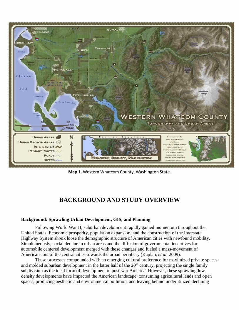
Map 1. Western Whatcom County, Washington State.

BACKGROUND AND STUDY OVERVIEW

Background: Sprawling Urban Development, GIS, and Planning

Following World War II, suburban development rapidly gained momentum throughout the

United States. Economic prosperity, population expansion, and the construction of the Interstate

Highway System shook loose the demographic structure of American cities with newfound mobility.

Simultaneously, social decline in urban areas and the diffusion of governmental incentives for

automobile centered development merged with these changes and fueled a mass-movement of

Americans out of the central cities towards the urban periphery (Kaplan, et al. 2009).

These processes compounded with an emerging cultural preference for maximized private spaces

and molded suburban development in the latter half of the 20th century; projecting the single family

subdivision as the ideal form of development in post-war America. However, these sprawling low-

density developments have impacted the American landscape; consuming agricultural lands and open

spaces, producing aesthetic and environmental pollution, and leaving behind underutilized declining

areas within the urban environment. These issues necessitate a reevaluation of traditional development

principles and the formulation of carefully considered strategies for future planning (Platt, 2004).

In 1972 the Supreme Court case Golden vs. Planning was waged over concerns of sprawl in the

town of Ramapo, NY. This case gave growth management constitutional precedent and unleashed the

growth management movement into a pro-sprawl system. Ramapo employed regulatory measures to

synchronize growth with the availability of public facilities and infrastructure. These strategies for

preventing sprawl became known as “Smart Growth” in the 1990’s (Robert Freilich & Neil Popowitz,

2010).

In 1983 the World Commission on Environment and Development, assembled by the UN, led to

the publication of the Brundtland Report. This report officially acknowledged the diminishment of

natural resources and the deterioration of human environments. It also emphasized the crit ical

importance of sustainable planning and development and disseminated these concerns to a global

audience. By the end of the 20th century, new planning and development ideals had gained momentum

with movements like New Urbanism in the United States and the Urban Village Movement in Europe.

These philosophies advocated early and pre-automobile urban forms and the rethinking of conventional

city layouts. In 1993 these ideas fused with concerns of sustainability in the formation of the Charter of

the New Urbanism (newurbanism.org, 2011).

Ultimately, New Urbanism’s goal has been to improve the quality of urban life by creating

landscapes that provide long term solutions to the economic, cultural, and environmental needs of

communities (newurbanism.org). While philosophies such as Smart Growth and New Urbanization have

emerged and developed separately, differing in their views of government involvement, social justice,

and scale, they have blended together in contemporary design and planning theory (Grant, 2009).

Unchecked growth has been allowed and even encouraged under the conventional view that the

ideal system maximizes the production of capital. As Mayo and Ellis state, “Capitalist reasoning in its

purest form argues that the best-designed city is one that generates the most profits” (Mayo & Ellis,

2009). The experience of conventional suburban development has been embedded into the American

psyche as the ordinary template for growth. However, sprawling urban development has exposed the

drawbacks of short term economic thinking. Social, environmental and aesthetic consequences along

with projections for continued growth have emphasized the importance of long-term strategic

sustainable development planning.

The minimization of sprawl in contemporary development has become a central issue to policy

makers, ecologists and citizens on local, regional, and national scales. While many assessments of

sprawl have focused on growth within metropolitan centers, it is also necessary to look at the changes

occurring outside of these areas that are often in close proximity to natural areas and protected lands. Dr.

David M. Theobald has published work describing and quantifying national patterns of change with data

based on historical, current, and future projections of housing density (Theobald, Landscape Patterns of

Urban Growth, 2005). These studies can be used to inform land use decisions by illustrating the trends

of land use change and identifying possible ecological impacts.

Sustainable planning aims to improve the quality of human life by addressing the social,

economic and environmental dimensions of human development. In their article GIS-Based Urban

Sustainability Assessment: The Case of Dammam City, Habib Alshuwaikhat and Yusuf Aina write that,

“The concept [of sustainable planning] arose from the recognition that the conventional economic

imperative to maximize economic production must be accountable to an ecological imperative to protect

the ecosphere, and a social equity imperative to minimize human suffering.” According to research

conducted by Dr. Theobald, there is general agreement that exurban land use threatens biodiversity

(Theobald, 2005). GIS has powerful spatial analysis capabilities that can monitor and evaluate the

environmental, social, and economic sustainability of area-specific change and help to inform critical

decisions involving development planning.

Study Overview: Measuring Development and Quantifying Change

The objective of this study was to quantify changes in development densities from 1990 to 2010

within the western region of Whatcom County, Washington State (Map 1) and to create a foundational

framework for analyzing urban sprawl. Understanding a region’s historical and current development

patterns is critical to making informed decisions about issues such as land use planning, public service

expansion, environmental conservation, and commercial development. Analyzing growth trends can

help planners and decision makers logically prepare for long term population changes rather than dictate

their reaction to the effects.

While the aesthetic character of sprawl is easy to identify, it is difficult to establish an exact

criterion to facilitate repeatable and comparable quantification. A common definition of urban sprawl is

a decline in population density over time, where spatial development is greater than the rate of

population growth (Theobald, 2003). The spatial extent of development exceeds the rate of population

growth and results in scattered, low density development. Constructing a framework for studying sprawl

necessitates the establishment of parameters for qualifying and measuring varying levels of

development. This study divided human development within Whatcom County, Washington into four

density types: urban, suburban, exurban, and rural using demographic data from the 1990, 2000, and

2010 U.S. Census. To begin these classifications the study first looked at definitions provided by the

U.S. Census Bureau.

The Census Bureau classifies all territory, population, and housing units within an urban cluster

(UC) or urbanized area (UA) as urban. The UA and UC boundaries are delineated to cover areas of

dense settlement, specifically, core census blocks with population densities of 1000 people per square

mile with surrounding census blocks of 500 people per square mile. Less densely settled areas may

sometimes also be included as part of a UA or UC. The Census Bureau classifies "rural" as all territory,

population, and housing units located outside of UAs and UCs. Census tracts, counties, metropolitan

areas, and lands outside of metropolitan areas are often split between urban and rural classifications, the

people and housing units they contain are then classified as partly urban and partly rural (U.S. Census

Bureau).

The term suburb describes residential communities within commuting distance of larger urban

areas with lower population densities than inner-city areas. These areas are often characterized by

detached, single-family homes. Rural refers to non-urbanized lands with low population densities. Large

portions of these areas are typically used for agricultural production. Although rural sprawl can be

identified by low-density scattered development, it is also difficult to quantify because it occurs as low

density and has weak connections to census population data (Theobald 2003). The term “exurban” is a

portmanteau that comes from “extra-urban.” It is used to describe prosperous communities beyond the

suburbs that function as commuter towns for urban areas. Although these definitions are informative,

they fail to provide quantifiable characteristics specific enough for repeatable block level analysis.

Theobald notes that, “Although population is often used as an indicator of growth and sprawl,

changes in housing units are a more robust metric. Population numbers can often belie the magnitude of

landscape change due to low-density housing,” (Theobald, 2003). He explains that housing density is a

more consistent method for analyzing the extent and patterns of development than population density

because census data is based on primary place of residence and underestimates landscape change where

vacation homes and second residences are involved.

In his article Defining and Mapping Rural Sprawl: Examples from the Northwest U.S. (2003),

Dr. David Theobald defines urban, suburban, exurban, and rural development types using measures of

housing unit density. He categorizes urban density as < 0.6 acres per housing unit (acres/HU); suburban

density as 0.6-1.7 acres/HU; exurban density as 1.7-20 acres/HU; and rural density as >20 acres/HU.

This study employed Theobald’s parameters for each of the four density types and utilized block-level

census data in tandem with ArcGIS processing tools to construct a change matrix for quantifying

specific types of change within the study area.

The four principal questions to be addressed were:

1. How much change occurred in Whatcom County between 1990 and 2010?

2. What proportion of this growth can be qualified as urban, suburban, exurban, and rural?

3. What have been the patterns of change inside and outside of the UGA?

4. What kinds of development transitions are currently taking place Whatcom County?

METHODS

The study area was delineated based on census tracts west of tract 010100 (which envelops the

eastern portion Whatcom County) using 2010 U.S. Census tract data. These western tracts contain all

areas of the county roughly west of the Cascade foothills and all of the county’s population centers.

They also include Point Roberts which is the farthest northwestern land area in the county, though

because it is not connected to the U.S. mainland and is influenced by its unique geographical location, it

was eliminated from this study. The final study area follows a southern boundary line with Skagit

County, WA from the Cascade foothills west to Samish Bay. It then follows the coastline from this

southern boundary to its northern border with British Columbia. From here it follows the border with

Canada back to the northern foothills.

ArcGIS 10 software was the central processing component in this study. ArcMap was used for

data display and cartographic production; Model Builder for organizing and recording workflow;

ArcToolbox for geoprocessing; and ArcCatalog for geodatabase management. Within ArcToolbox,

Analysis, Conversion, Data Management, and Spatial Analyst toolboxes were the most heavily utilized.

The primary datasets used in this study contained block-level housing unit counts compiled by the U.S

Census Bureau and accessed via the American Fact Finder (AFF) website (factfinder2.census.gov).

To begin processing, the 2000 and 2010 TIGER (Topologically Integrated Geographic Encoding

and Referencing System) files provided by the Census Bureau containing 2000 and 2010 census tracts,

block groups, and blocks polygons were downloaded. The TIGER files were imported into ArcMap and

displayed as feature classes. Geographic entity codes representing census block codes (i.e. BLKIDFP00

for the 2000 census and GEOID10 for the 2010 census) field were used to connect the TIGER files to

reformatted Excel tables* containing housing unit data using ArcMap’s Join function (it should be noted

that in order to display fields from the new file some of the fields’ formats may need to be changed to

numeric).

The 1990 data was obtained from the Spatial Analysis Laboratory, Huxley College, Western

Washington University and was pre-joined to a file containing census block polygons. After processing

and mapping the file, several accuracy issues were identified. The housing density calculated from the

file was larger than that of the 2010 data. It was found that the total area was larger than the area

represented by the files’ shape and the total housing units in the data were unrealistically large (over

twice as many units as the 2010 data). The file’s attribute table also contained multiple entries for each

block ID and each of those entries contained different attribute data. The shapes they represented were

spatially disconnected from shapes with identical block IDs.

However, using an unabbreviated block ID field within the attribute table, it was found that the

housing unit data was repeated for each of a specific block’s entries. Using a Dissolve function on the

unabbreviated block ID, the multiple entries were combined, though the housing unit data was not

carried over. A Join was used to reconnect the dissolved file with the data from the original file and an

association between each dissolved block ID and one housing unit entry was specified. This created a

table with single, accurate housing unit values for each block ID and the functional 1990 census data file

used for processing and analysis in this study.

After preparing the census files, areas unlikely to have been developed were identified within the

study extent and data representing these areas was collected. These consisted of polygon data files

including: public lands, federal lands, water features, Department of Natural Resources (DNR) lands,

Native American tribal lands, and zoning data. These files were collected, converted to geodatabase

(GDB) feature classes and projected. The files were all projected into the UTM NAD 1983 Zone 10

North coordinate system. Most of them had different or no associated projections, so instead of using a

Batch Project the single feature class Project tool was used for each individual feature class and

appropriate geographic transformations were used to precisely georeference the files for processing and

analysis. From ArcToolbox the conversion tool Feature Class to Feature Class was used to populate a

Working GDB (for relevant data to be analyzed and mapped) and a ‘Scratch’ GDB (for the processing

files generated by the study’s workflow) with the new feature files as well as the census files.

Next, the 2010 census file was used with the ArcGIS Select tool to choose only those census

tracts located in Whatcom County. This was done using the Structured Query Language (SQL)

expression [COUNTYFP10 = ‘073’] (073 was the 2010 census code for Whatcom County). Using

another Select and SQL expression [NOT TRACT = 010100] (010100 was the 2010 census tract

covering eastern Whatcom County) the western portion of Whatcom County was extracted.

With the extent of the study area defined, the Select tool was used with SQL expressions and the

Erase tool to extract and delete portions of the 2010 census file that were identified as unlikely to have

been developed (Model 1). Because houses are not allowed on public or protected lands, portions

overlapping blocks were removed from the analysis. Areas eliminated included: commercial and rural

forest land, lakes and small water features, rivers, federal land, Lummi tribal land, state board trust land,

granted trust lands, DNR natural areas. Public lands were also erased including state, county,

city/municipal lands, parks, as well as wildlife preserves/refuges, conservation areas, and national

forests. After erasing these areas from the census block data, several fields were added and calculated

(Model 2). Acres were calculated using the Calculate Geometry function and divided by the Housing

Units field to calculate housing density for the census block vector polygons.

As a final refinement to the study area, these newly calculated attributes were studied to identify

outlying and nonsensical data. The Erase process created many small remnants where portions of

polygons had been removed, these remnants were however, still associated with the original polygons’

data. In order to minimize any statistical influence of these remnants from the analysis, a minimum

value of 0.2 acres per census block was established. It was found that most remnants had areas less than

0.2 acres and nearly no blocks/remnants less than 0.2 acres had populations or housing units. All census

blocks less than 0.2 acres per block were also erased from the study area.

The next step was to conduct a point density raster analysis on the census vector data. From the

Features toolset in the ArcGIS Data Management toolbox, the Feature to Point tool was used to convert

the census block polygons and their attributes to point data. The Feature to Point tool created points

generated from the representative locations of the census blocks. Because the census blocks were single

part polygons, the representative locations were the calculated centers of each block.

Model 1. Erase Model 2. Add and Calculate Field

This new point layer was then processed using Spatial Analyst’s Point Density tool (Model 3).

The Point Density tool was set up to create a magnitude per acre value from the Feature to Point layer

using a floating neighborhood window around each cell. A specified circular neighborhood with a

1,135m radius and 50m resolution was specified to be calculated around each raster cell. For any point

within the neighborhood, the value of that point was weighted, divided by the area of the neighborhood,

and converted to give an output raster of housing units per acre.

Model 3. Point Density The Reclassify tool was used to create customized categories

for the densities contained in the Point Density data. The data was

classified into four categories representing the four density

classifications of this study: urban, suburban, exurban, and rural. In

order to convert the Housing Units per Acre (HU/acre) contained in the

Density raster to the desired acres/HU used in Theobald’s study, the

inverse of his density designations were calculated and the pixels of

each raster assigned accordingly. Theobald categorized the four

densities as: 0-0.6 acres/HU (urban); 0.6-1.7 acres/HU (suburban); 1.7-

20 acres/HU (exurban); and 20+ acres/HU (rural). The density intervals

calculated from the inverse of Theobald’s specifications were classified

as follows: 1.6+ HU/acre (urban) = 1; 0.59-1.6 HU/Acre (suburban) =

2; 0.05-0.59 HU/acre (exurban) = 3; and 0-0.05 HU/acre (rural) = 4.

Using these reclassifications, total areas of each density type were

calculated. The reclassified rasters were clipped to the extent of the vector

study area created using the extracted and refined 2010 census

polygons. This was accomplished using the Clip tool in Data

Management’s Raster Processing toolset (these clipping processes can

take up to an hour per raster). Having clipped the rasters to the study

area and classified their data, Raster Calculator was used to calculate

change between the three census datasets. The raster data values were

reclassified using 1, 2, 3, and 4 (representing rural, exurban, suburban,

and urban respectively) while the 2000 data was similarly classified using 100, 200, 300, and 400, and

the 1990 data classified as 10000, 20000, 30000, and 40000.

Using Raster Calculator (Model 4), each processed and reclassified census raster was added to

the one preceding it (i.e. 2010 + 2000, and 2000 + 1990).

Model 4. Raster Reclassification

Areas of specific change-types were identified and calculated for the total study area as well as the UGA

and Non-UGA regions. The change-types of interest were: Rural to Exurban, Rural to Suburban,

Exurban to Rural, Exurban to Suburban, Exurban to Urban, Suburban to Exurban, Suburban to Urban,

Urban to Suburban. The reclassified rasters allowed change to be easily detected using a matrix of the

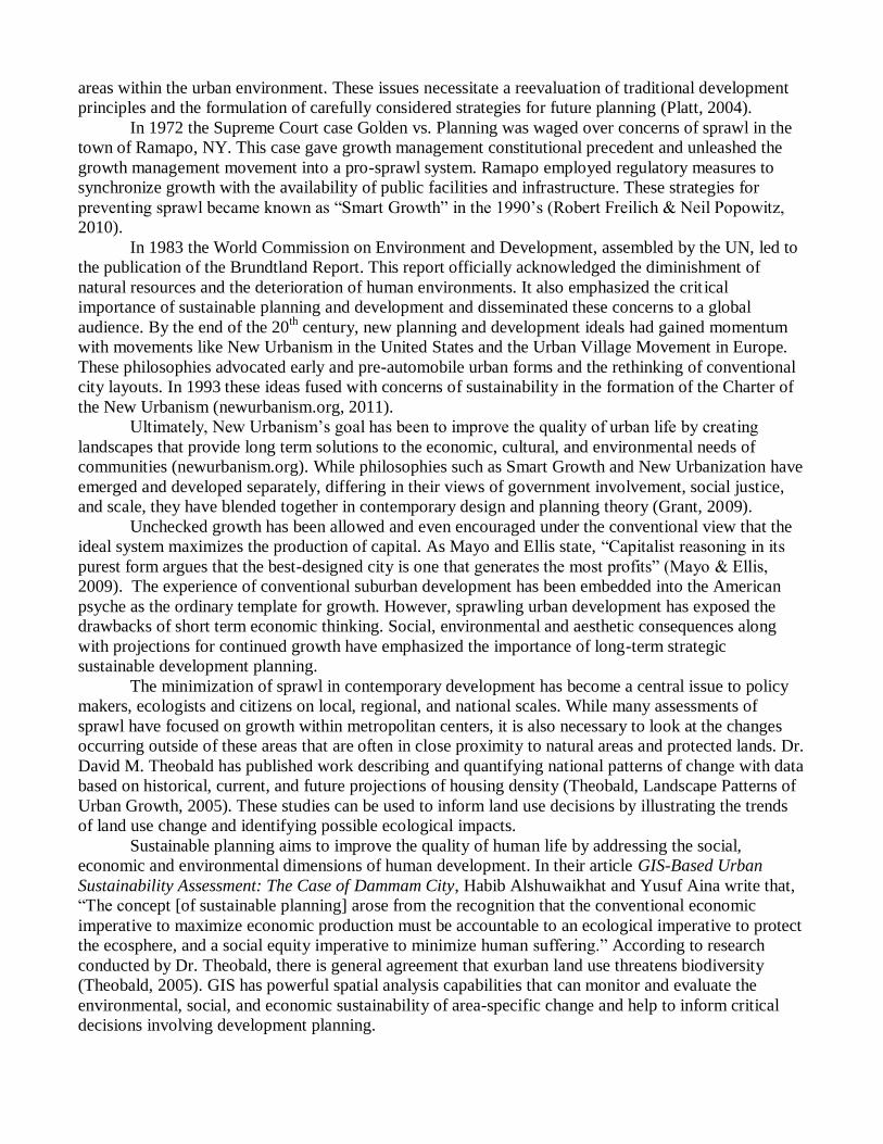
classified values (Figure 1.) and a table of possible outcome values (Figure 2.).

Methodically adding every 2000 value

to every 2010 value from Figure 1 creates a

table with all the possible combinations of

values (Figure 2). Each raster cell value is

added to exactly one corresponding cell from

the other raster. This creates a single possible

value for each cell in the change raster and all those values are contained in

Table 2. If for example, the change raster attribute table shows a count of

5,000 cells with a value of 304, this would indicate that 5000 cells of that

raster changed from Suburban to Urban density. Using a conversion from

the area of a single cell, 2500 square meters in this study (50m x 50m), to a

desired unit of area gives the area of change detected by the change raster.

This is the method with which change was calculated for each temporal

interval in this study. Finally a UGA feature class was used to clip the study

area change rasters to regions inside and outside of UGAs (Model 5).

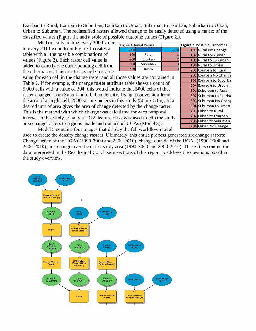
Model 5 contains four images that display the full workflow model

used to create the density change rasters. Ultimately, this entire process generated six change rasters:

Change inside of the UGAs (1990-2000 and 2000-2010), change outside of the UGAs (1990-2000 and

2000-2010), and change over the entire study area (1990-2000 and 2000-2010). These files contain the

data interpreted in the Results and Conclusion sections of this report to address the questions posed in

the study overview.

Figure 1. Initial Values

2000 2010

100 Rural 1

200 Exurban 2

300 Suburban 3

400 Urban 4

Figure 2. Possible Outcomes

101 Rural No Change

102 Rural toExurban

103 Rural to Suburban

104 Rural to Urban

201 Exurban to Rural

202 Exurban No Change

203 Exurban to Suburban

204 Exurban to Urban

301 Suburban to Rural

302 Suburban to Exurban

303 Suburban No Change

304 Suburban to Urban

401 Urban to Rural

402 Urban to Exurban

403 Urban to Suburban

404 Urban No Change

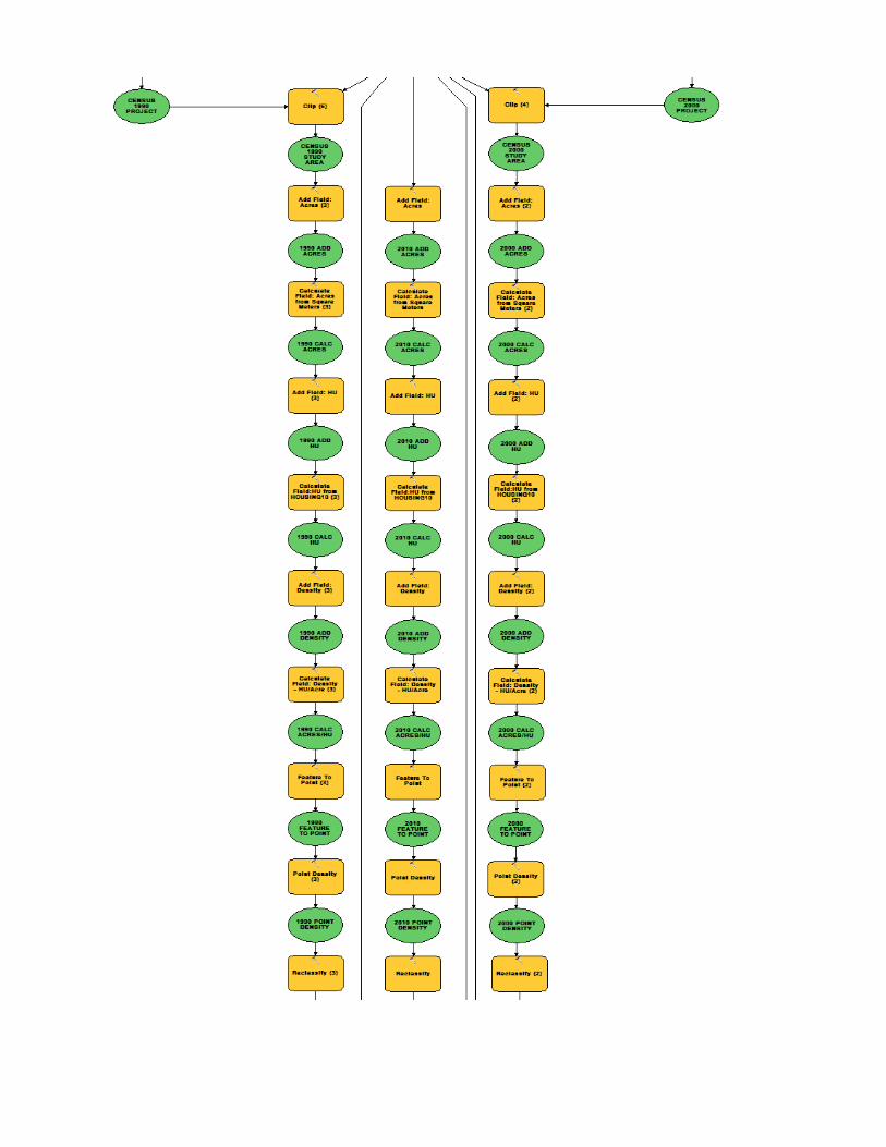
Model 5. Workflow Model

* See the Specialization section of this report for details on working with census data and

reformatting census tables.

RESULTS

The first step in this study was to establish parameters for describing the four density types to be

analyzed: urban, suburban, exurban, and rural. After defining these densities, U.S. Census data was

processed with additional data files using various ArcGIS processes. These processes generated new

rasters with large amounts of change data that were used for analysis. This section organizes,

summarizes, and discusses those results using a series of tables and maps.

The initial phase of analysis involved studying the data contained in the census vector files to

provide a general pattern of development in Whatcom County. These files were also used to compare

the three datasets (U.S. Census data: 1990, 2000, and 2010) for reasonable accuracy. Map 2 shows the

distribution of acres per housing unit densities for each of the datasets’ census blocks. However, there

were changes in the delineation of census blocks in each of the ten year census studies. A general trend

of increased density per block per time period is illustrated in Map 2 but the varying shapes, sizes, and

numbers of census blocks during each period rendered their unprocessed use unsuitable for more

advanced density analysis.

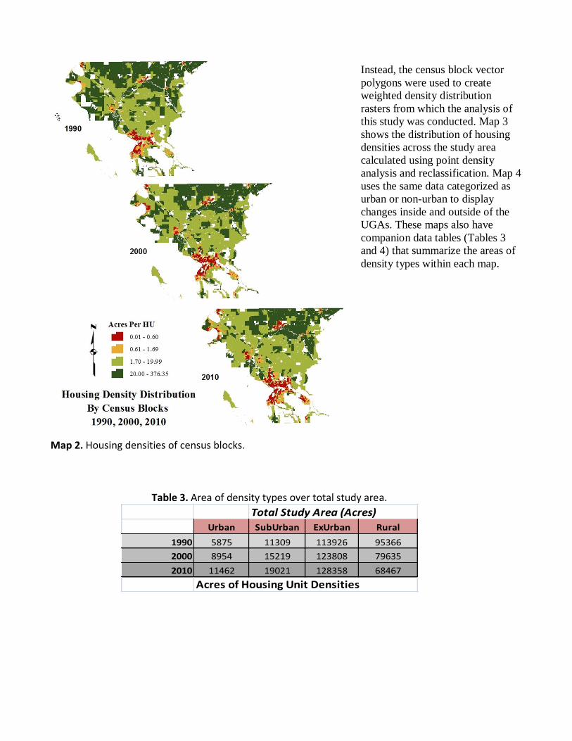
Instead, the census block vector

polygons were used to create

weighted density distribution

rasters from which the analysis of

this study was conducted. Map 3

shows the distribution of housing

densities across the study area

calculated using point density

analysis and reclassification. Map 4

uses the same data categorized as

urban or non-urban to display

changes inside and outside of the

UGAs. These maps also have

companion data tables (Tables 3

and 4) that summarize the areas of

density types within each map.

Map 2. Housing densities of census blocks.

Table 3. Area of density types over total study area.

Total Study Area (Acres)

Urban SubUrban ExUrban Rural

1990 5875 11309 113926 95366

2000 8954 15219 123808 79635

2010 11462 19021 128358 68467

Acres of Housing Unit Densities

Map 3. Housing densities calculated from point density analysis.

Table 4. Area of density types inside and outside of UGAs.

Table 4 shows the number of acres of each density type for the three census periods inside and

outside of the UGAs. The data calculated in this study indicates that there was no urban density outside

of the UGA in 1990 while in 2010 there were 96 acres of urban density. In 2010, suburban density was

4.87 times that of the 1990 area (4896 acres from 1005 acres) outside of the UGA, while there was a

28% decrease in rural density over the same period (91859 acres to 66291 acres). Inside of the UGA

there was nearly twice the area of urban density in 2010 as in 1990 (5875 acres to 11366 acres) while

exurban and rural densities fell by 35% and 50% respectively (Table 4). Tables 5, 6, and 7 summarize

the total areas of incline and decline during three intervals: 1990-2000, 2000-2010, and 1990-2010.

(Positive numbers indicate acres of increase while negative numbers show acres of decline).

Area Inside UGA (Acres)

Urban SubUrban ExUrban Rural

1990 5875 10304 21421 3507

2000 8922 12858 17107 2266

2010 11366 14112 14035 1747

Acres of Housing Unit Densities

Area Outside UGA (Acres)

Urban SubUrban ExUrban Rural

1990 0 1005 92506 91859

2000 32 2362 106483 76890

2010 96 4896 114061 66291

Acres of Housing Unit Densities

Map 4. Housing densities inside and outside of the UGA.

Table 5. Change in acres of density type over the total study area. Total Study Area

Housing Densities: Urban SubUrban ExUrban Rural

Gained 1990-2000 3078 3910 9882 -15731

Gained 2000-2010 2509 3802 4550 -11168

Total Gained 1990-2010 5587 7712 14432 -26899

Increases and Declines in Acres of Housing Densities

Table 6. Change in acres of density type outside of the UGA. Outside UGA

Housing Densities: Urban SubUrban ExUrban Rural

Gained 1990-2000 32 1357 13978 -14970

Gained 2000-2010 64 2534 7578 -10598

Total Gained 1990-2010 96 3891 21555 -25568

Increases and Declines in Acres of Housing Densities

Table 7. Change in acres of density type inside the UGA. Inside UGA

Housing Densities: Urban SubUrban ExUrban Rural

Gained 1990-2000 3046 2554 -4314 -1242

Gained 2000-2010 2445 1254 -3072 -518

Gained 1990-2010 5491 3808 -7386 -1760

Increases and Declines in Acres of Housing Densities

All three tables show declines in areas of rural density. There were increases in areas of exurban

density outside of the UGA (Table 6) and declines in exurban density within the UGA (Table 7). There

were also increases in urban and suburban density areas in all three periods. The greatest increases in

suburban density outside of the UGA occurred between 2000 and 2010 (Table 6), while there was a

greater suburban increase inside the UGA during the 2000-2010 period (Table 7).

Having determined the areas of each housing density type during the two census periods,

locations and quantities of change were calculated using the ArcGIS Raster Calculator and a

change matrix. Areas of specific change-types were identified and calculated for the total study

area as well as the UGA and non-UGA regions. These change-types included: Rural to Exurban,

Rural to Suburban, Exurban to Rural, Exurban to Suburban, Exurban to Urban, Suburban to

Exurban, Suburban to Urban, Urban to Suburban. Map 5 displays the spatial distribution of these

change-types inside and outside of the UGA and across the study area for 2000-2010 and 1990-

2000.

Map 5. Distribution of change types.

Concentric density increases were seen in the UGA from suburban to urban and exurban to

suburban around the perimeter of Bellingham, Ferndale, and Birch Bay during both the

1990-2000 and 2000-2010 periods (Map 5). The non-UGA areas show large increases in rural to

exurban density as well as unexpected changes from exurban to rural density (Map 5).

Maps 6, 7, and 8 illustrate the results of further density analysis and quantify the areas for

specific change-types during the 1990-2000 and 2000-2010 periods.

Map 6. Quantified change-types inside UGAs (1990-2000 and 2000-2010).

Map 7. Quantified change outside of UGAs.

Exurban areas transitioning to suburban was the largest change pattern inside the UGA

from 1990-2000, (5,320 acres of change) followed by suburban to urban change (2,916 acres of

change). This trend was repeated in the 2000-2010 period with exurban to suburban changes

totaling 3,728 acres and suburban to urban transitions totaling 2,913 acres. This is a gross

increase of 9,048 acres of exurban to suburban density transition and 5,829 acres of suburban to

urban transition within the UGA during the 30 year period (Map 6).

Outside of the UGA, the trend was rural to exurban density transitions. In the 1990-2000

period 22,253 acres of rural land changed to rural densities and in the 2000-2010 period, 15,315

acres made the same transition. The backwards transitions calculated for exurban to rural density

changes are significant but likely inaccurate and will be discussed in the next section of this

report. Large exurban to suburban changes also occurred in both periods inside and outside of the

UGA (Map 7).

Map 8. Quantified change over total study area.

Map 8 shows change over the entire study area. Rural to exurban density is the largest spatial

transition in both periods while the data also indicates large backward transitions from exurban

to rural densities. There were large changes in exurban to suburban densities and from suburban

to urban densities, especially around the perimeters of urban areas. These trends will be

discussed in the next section of this report.

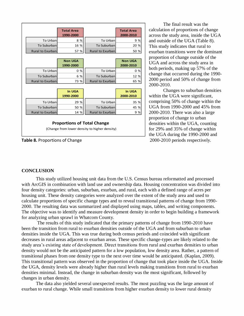
The final result was the

calculation of proportions of change

across the study area, inside the UGA

and outside of the UGA (Table 8).

This study indicates that rural to

exurban transitions were the dominant

proportion of change outside of the

UGA and across the study area in

both periods, making up 57% of the

change that occurred during the 1990-

2000 period and 50% of change from

2000-2010.

Changes to suburban densities

within the UGA were significant,

comprising 50% of change within the

UGA from 1990-2000 and 45% from

2000-2010. There was also a large

proportion of change to urban

densities within the UGA, counting

for 29% and 35% of change within

the UGA during the 1990-2000 and

Table 8. Proportions of Change 2000-2010 periods respectively.

CONCLUSION

This study utilized housing unit data from the U.S. Census bureau reformatted and processed

with ArcGIS in combination with land use and ownership data. Housing concentration was divided into

four density categories: urban, suburban, exurban, and rural, each with a defined range of acres per

housing unit. These density categories were analyzed over the extent of the study area and used to

calculate proportions of specific change types and to reveal transitional patterns of change from 1990-

2000. The resulting data was summarized and displayed using maps, tables, and writing components.

The objective was to identify and measure development density in order to begin building a framework

for analyzing urban sprawl in Whatcom County.

The results of this study indicated that the primary patterns of change from 1990-2010 have

been the transition from rural to exurban densities outside of the UGA and from suburban to urban

densities inside the UGA. This was true during both census periods and coincided with significant

decreases in rural areas adjacent to exurban areas. These specific change-types are likely related to the

study area’s existing state of development. Direct transitions from rural and exurban densities to urban

density would not be the anticipated pattern for a low population, low density area. Rather, a pattern of

transitional phases from one density type to the next over time would be anticipated. (Kaplan, 2009).

This transitional pattern was observed in the proportion of change that took place inside the UGA. Inside

the UGA, density levels were already higher than rural levels making transitions from rural to exurban

densities minimal. Instead, the change in suburban density was the most significant, followed by

changes in urban density.

The data also yielded several unexpected results. The most puzzling was the large amount of

exurban to rural change. While small transitions from higher exurban density to lower rural density

Total Area

1990-2000

Total Area

2000-2010

To Urban 8 % To Urban 9 %

To Suburban 16 % To Suburban 20 %

Rural to Exurban 57 % Rural to Exurban 50 %

Non UGA

1990-2000

Non UGA

2000-2010

To Urban 0 % To Urban 0 %

To Suburban 6 % To Suburban 12 %

Rural to Exurban 73 % Rural to Exurban 65 %

In UGA

1990-2000

In UGA

2000-2010

To Urban 29 % To Urban 35 %

To Suburban 50 % To Suburban 45 %

Rural to Exurban 14 % Rural to Exurban 9 %

Proportions of Total Change (Change from lower density to higher density)

could be explained by factors such as decreased agricultural activity and an associated slow decrease in

housing density, the quantity and spatial distribution of this change-type indicates there was likely an

error in the study parameters, and/or data processing. This change-type was primarily observed outside

of the urban growth areas and there are several possibilities as to why this occurred.

One factor may be the size of the window used to generate the point density analysis. The

parameters for this study were taken from Dr. Theobald’s study Defining and Mapping Rural Sprawl:

Examples from the Northwest US. His analysis however, was conducted over a much larger area. The

parameters of this study were not refined to fit Whatcom County’s unique characteristics. Instead, the

specifications from Dr. Theobald’s model were used as the template for developing the study.

Theobald’s work covers a larger area at a smaller map scale. Given the smaller geographical focus of the

analysis presented here, a smaller point density window with area-specific parameters may have

facilitated a more accurate analysis.

Another reason may be that the areas within the UGA contain more data points to absorb the

statistical influence of block delineation changes between census studies. Outside of the UGA census

blocks become progressively less concentrated. If the Point Density tool that was used to create a

weighted density distribution had fewer points to enter into the calculation outside of the UGA, this

coarser resolution could have generated an incomplete picture and have led to erroneous indications of

change.

However, the most likely explanation is a product of data inconsistencies between census

periods. Census block delineations change with each census period. This means that block-level data

from census years are not aligned with one another, making direct comparisons of housing data

problematic. Also, changes in census block delineations occur between census periods while population

and housing units also increase. If blocks are subdivided as population growth occurs this could obscure

patterns of change. These factors make comparisons between census studies much more complex than

the methodology employed here was designed to account for.

Further research needs to take these factors into consideration and construct a procedure that

normalizes the change in census blocks, addresses the low resolution data outside of urban areas, defines

more appropriate point density parameters, and develops assessments to gauge the statistical accuracy of

results. Continued analysis could also benefit from incorporating population change into the framework.

Conducting a similar methodology with population data to analyze change patterns and combining or

cross tabulating the results of both studies could produce a more robust foundation for measuring growth

and development.

A subtle but significant result of this study is shown in Table 8. The proportions of change that

dominated throughout the study period show declines from 2000 to 2010. As developing areas become

more concentrated, previously large transitions from one type slow while the next increases. Outside of

the UGA, proportions of change that were exurban slowed from 73% to 65% of the change area, while

at the same time the next highest density level (suburban) increased from 6% to 12% of the change area.

This pattern was also seen inside the UGA with a decrease in the proportion of change to suburban (50%

to 45%) and an increase in the proportion of change to urban (29% to 35%) between census periods.

This could indicate that a broader transition is taking place where suburban density increases begin to

dominate non-urban areas and urban densities fill in the UGA.

The changes within urban areas shown in this study were aligned with historical patterns of

urban growth in the United States. Suburban to urban density changes were the most dominant during

both time periods followed by changes from exurban to suburban development. The broad pattern

detected through this study was a tendency for declines in lower density areas to coincide with increases

in the next density level. For example, outside the UGA, decreases in rural areas corresponded with

increases in exurban densities. Areas inside the UGA (already having surpassed rural density) showed

decreases in exurban densities corresponding with increases in suburban densities. This change adjacent

to urban areas may indicate that suburban areas are becoming more urban. Likewise, rural densities

decreasing adjacent to exurban areas may be indicative of those areas transitioning to exurban. This

concentric pattern of development is consistent with growth patterns surrounding urban population

centers. As densities increase, populations and development spill out of urban centers causing exurban

and rural areas to experience growth. This has been the spatiotemporal pattern of modern urbanization in

the United States.

REFERENCES

Alshuwaikhat, Habib M., Aina, Yusuf A. (2006). GIS-Based Urban Sustainability Assessment:

The Case of Dammam City, Saudi Arabia. Local Environment, 11(2), pp.141-161.

Abbaspour, M., Gharagozlou, A. (2005). Urban Planning Using Environmental Modeling and

GIS/RS: A Case Study from Tehran. Wiley Periodicals, Inc. Environmental Quality

Management, pp.63-71

Mayo, J. M., Ellis, C. (2009) Capitalist dynamics and New Urbanist principals: junctures and

disjunctures in project development. Journal of Urbanism. Vol. 2, No. 3, p237-257

Grant, J.L. (2009) Theory and Practice in Planning the Suburbs: Challenges to Implementing

New Urbanism, Smart Growth, and Sustainability Principals, Planning Theory and

Practice. Vol. 10, No. 1, p11-33

Kaplan, D., Wheeler, J., Holloway, S. (2009) Urban Geography. Hoboken, New Jersey: John Wiley &

Sons. Second Edition

Knox, Paul L., Marston, Sallie A. (2007) Human Geography: Places and Regions in Global Context.

Upper Saddle River New Jersey: Pearson Prentice Hall. Fourth Edition

Platt, Rutherford H. (2004) Land Use and Society: Geography, Law, and Public Policy. Washington,

DC: Island Press. Revised Edition

Newurbanism.org, (2011) Principals of New Urbanism, Alexandria, VA. www.newurbanism.org

Freilich, Robert H., Popowitz, Neil M. (2010) The Umbrella of Sustainability: Smart Growth, New

Urbanism, Renewable Energy and Green Development in the 21st Century, Urban

Lawyer. Vol. 42, Issue 1, p1-39

Theobald, David, M. (2003) Defining and Mapping Rural Sprawl: Examples from the Northwest U.S.

Colorado State University, Natural Resource Ecology Lab and Department of Recreation and

Tourism.

Theobald, David M. (2005) Landscape Patterns of Exurban Growth in the USA from 1980 to 2020,

Ecology and Society. Colorado State University, 10(1):32

U.S. Census Bureau. (1990, 2000, 2010). American FactFinder: Washington, DC. Retrieved March-June

2012, from: http://factfinder2.census.gov/faces/nav/jsf/pages/index.xhtml

SPECIALIZATION: MAPPING AND ANALYSIS OF DEMOGRAPHIC DATA

Acquiring U.S. Census Data Using American FactFinder

Having conducted development density analysis in Whatcom County, Washington, I have

accumulated extensive exposure to the acquisition and manipulation of U.S. Census data files. This

experience has allowed me to develop a technical specialization in the mapping and analysis of

spatiotemporal demographic data. Here I discuss the skills and insights I have acquired throughout this

process as well as steps that can be followed to begin analyzing demographic data.

The primary datasets I used in my study contained block-level housing unit data compiled by the

U.S Census Bureau and can be accessed via the American FactFinder (AFF) website

(factfinder2.census.gov). I will discuss the processes I developed to utilize this data, however, these

techniques are by no means limited to housing unit data. The U.S. Census website (www.census.gov)

and AFF provide vast amounts of compiled demographic, geographic, and economic data that these

techniques can also be applied to.

After identifying the data of interest, the first step is to access TIGER files (Topologically

Integrated Geographic Encoding and Referencing System) provided by the Census Bureau

(www.census.gov/geo/www/tiger/). Figure 1 shows the TIGER shapefile main page. This page functions

Figure 1. TIGER Main Page

a starting point for downloading shapefiles, acquiring technical documentation, and viewing helpful

PDF instructions for joining shapefiles to census tables, understanding differences between datasets

from varying census periods, and defining census codes. From here, files that contain georeferenced

shapefiles for various features of interest, such as roads, boundaries, census blocks, address data, water

features, and urban growth areas can be accessed and downloaded (Figure 2).

After downloading the shapefiles of interest and reviewing the provided documentation the next

step is to find the data to be used in the study. Under the Data tab at the top of the TIGER page there are

links to several sites that archive demographic data including: American Community Survey, Economic

Census, Population Finder, and American FactFinder. For

my studies, AFF was the most utilized. AFF provides user

friendly search filters to sort through the archive and

identify data of interest.

The user can search for data by topics and types

such as People, Housing, Business, Product Type, and

Year. Contained under these main search preferences are

more specific filters. For example, if Housing is specified

the search can be further refined to basic housing counts or

occupancy characteristics (Figure 3). Likewise, topics such

as ethnic groups, industry, or geographical locations can be

searched and further refined by subtopics.

In addition, these filters can be used

interchangeably between topics. For example, a search can

be specified to data pertaining to Native American housing

characteristics in King County by census blocks from the

2000 census. However, the more specific the search the

few results one is likely to find, and searches often yield no

results. The 2010 census data seems to still be in the

Figure 2. TIGER Shapefiles process of being categorized.

There are currently more

complete data searches

available for the 2000 census.

After specifying the data of

interest, a list of general results

will be shown which the user

can choose from (for example,

if census block geography is

chosen, a list of “All Blocks”

for counties within a state of

interest may be presented

(Figure 4). From this list the

user can choose the data

pertinent to their study, for

Figure 3. Subtopics example, ‘All counties within

King County, WA’. When the

box for a dataset is checked it can be added to Your Selections in the upper left corner of the page

using the Add tab at the top of the results list (Figure 4).

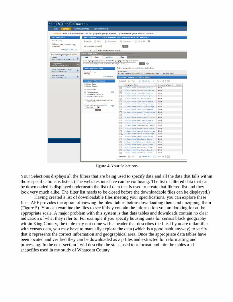
Figure 4. Your Selections

Your Selections displays all the filters that are being used to specify data and all the data that falls within

those specifications is listed. (The websites interface can be confusing. The list of filtered data that can

be downloaded is displayed underneath the list of data that is used to create that filtered list and they

look very much alike. The filter list needs to be closed before the downloadable files can be displayed.)

Having created a list of downloadable files meeting your specifications, you can explore these

files. AFF provides the option of viewing the files’ tables before downloading them and unzipping them

(Figure 5). You can examine the files to see if they contain the information you are looking for at the

appropriate scale. A major problem with this system is that data tables and downloads contain no clear

indication of what they refer to. For example if you specify housing units for census block geography

within King County, the table may not come with a header that describes the file. If you are unfamiliar

with census data, you may have to manually explore the data (which is a good habit anyway) to verify

that it represents the correct information and geographical area. Once the appropriate data tables have

been located and verified they can be downloaded as zip files and extracted for reformatting and

processing. In the next section I will describe the steps used to reformat and join the tables and

shapefiles used in my study of Whatcom County.

Figure 5. Previewing Tables

Reformatting and Joining U.S. Census Tables for ArcGIS Processing

To begin processing the files for my study of housing unit density in Whatcom County, I

downloaded 2000 and 2010 TIGER files containing 2000 and 2010 census tracts, block groups, and

blocks polygons. I also downloaded SF1 summary files containing basic hosing unit counts per census

block. The data was downloaded in zip files, extracted, and the housing unit tables opened in Excel. The

tables were then changed to a .csv comma delimited files and reformatted to be used in ArcMap. First,

the excess header rows with descriptive elements were removed so that only the field names remained.

Next the GEO.id2 field was deleted and replaced with blank fields (named BLKIDFP00 for the 2000

data and GEOID10 for the 2010 data) to be joined with the TIGER files. The GEO.id field (adjacent to

the GEOID10 field) was highlighted and Text to Columns used to populate the GEOID10 field. The

Delimited option was chosen for Original Data Type; under Delimiters, Other was checked and S

entered; Text was chosen under Column Data Format (this assured that the numbers would stay in

place); finally, the “replace all values in the column” prompt was accepted and the table saved.

These reformatted tables were imported into ArcMap as tables along with the TIGER files which

were displayed as feature classes. The geographic entity codes representing census block codes (i.e.

BLKIDFP00 and GEOID10 fields) were used to connect the TIGER files to the reformatted Excel tables

using ArcMap’s Join function. I then verified the joins by displaying the new files in ArcMap and

opening their attribute tables. At this point the TIGER shapefiles had acquired the housing unit data in

new fields within the attribute table and were ready for processing. (It should be noted that in order to

symbolize and display fields from the joined files, some of the fields’ formats may need to be changed

to numeric.)

A significant obstacle I encountered during my study involved census data acquired outside of

the AFF and U.S. Census archives. The 1990 data I used was obtained from the Spatial Analysis

Laboratory, Western Washington University and was pre-joined to a file containing census block

polygons. After fully processing and mapping the file, several accuracy issues were identified. The total

number of housing units and housing density calculated from the file was larger than that of the 2010

data. This was immediately identified as faulty data and the original table was carefully examined. I

found that the total area represented by the files’ shapes was much larger than the actual area it

represented on the maps and the total number of housing units was over twice that of the 2010. The

file’s attribute table was found to contain multiple entries for each block ID and each of those entries

contained different associated attribute data. The shapes the block IDs represented were also spatially

disconnected from other blocks with identical block IDs.

However, using an unabbreviated block ID field within the attribute table, it was noticed that

housing unit and population data was repeated for each of a block ID’s entries. Using a Dissolve

function on the unabbreviated block ID, the multiple entries were combined, however, the housing unit

data was not carried over. I used a Join function in ArcMap to reconnect the dissolved file with the data

from the original file and create an association between each dissolved block ID with only one of the

repeated housing unit counts. This created a table with one single housing unit count for each individual

block ID and facilitated the processing and analysis of the 1990 dataset conducted in my study.