Atmos. Meas. Tech., 6, 1095–1109, 2013www.atmos-meas-tech.net/6/1095/2013/doi:10.5194/amt-6-1095-2013© Author(s) 2013. CC Attribution 3.0 License.

EGU Journal Logos (RGB)

Advances in Geosciences

Open A

ccess

Natural Hazards and Earth System

Sciences

Open A

ccess

Annales Geophysicae

Open A

ccess

Nonlinear Processes in Geophysics

Open A

ccess

Atmospheric Chemistry

and Physics

Open A

ccess

Atmospheric Chemistry

and Physics

Open A

ccess

Discussions

Atmospheric Measurement

TechniquesO

pen Access

Atmospheric Measurement

Techniques

Open A

ccess

Discussions

Biogeosciences

Open A

ccess

Open A

ccess

BiogeosciencesDiscussions

Climate of the Past

Open A

ccess

Open A

ccess

Climate of the Past

Discussions

Earth System Dynamics

Open A

ccess

Open A

ccess

Earth System Dynamics

Discussions

GeoscientificInstrumentation

Methods andData Systems

Open A

ccess

GeoscientificInstrumentation

Methods andData Systems

Open A

ccess

Discussions

GeoscientificModel Development

Open A

ccess

Open A

ccess

GeoscientificModel Development

Discussions

Hydrology and Earth System

Sciences

Open A

ccess

Hydrology and Earth System

Sciences

Open A

ccess

Discussions

Ocean Science

Open A

ccess

Open A

ccess

Ocean ScienceDiscussions

Solid Earth

Open A

ccess

Open A

ccess

Solid EarthDiscussions

The Cryosphere

Open A

ccess

Open A

ccess

The CryosphereDiscussions

Natural Hazards and Earth System

Sciences

Open A

ccess

Discussions

Development of a cavity-enhanced absorption spectrometerfor airborne measurements of CH4 and CO2

S. J. O’Shea1, S. J.-B. Bauguitte2, M. W. Gallagher1, D. Lowry3, and C. J. Percival1

1School of Earth, Atmospheric and Environmental Sciences, University of Manchester, Oxford Road,Manchester, M13 9PL, UK2Facility for Airborne Atmospheric Measurements (FAAM), Building 125, Cranfield University, Cranfield,Bedford, MK43 0AL, UK3Department of Earth Sciences, Royal Holloway, University of London, Egham, UK

Correspondence to:S. J. O’Shea (sebastian.oshea@postgrad.manchester.ac.uk) and S. J.-B. Bauguitte (sbau@nerc.ac.uk)

Received: 26 November 2012 – Published in Atmos. Meas. Tech. Discuss.: 2 January 2013Revised: 27 March 2013 – Accepted: 9 April 2013 – Published: 2 May 2013

Abstract. High-resolution CH4 and CO2 measurementswere made on board the FAAM BAe-146 UK (Facility forAirborne Atmospheric Measurements, British Aerospace-146) atmospheric research aircraft during a number of fieldcampaigns. The system was based on an infrared spectrome-ter using the cavity-enhanced absorption spectroscopy tech-nique. Correction functions to convert the mole fractions re-trieved from the spectroscopy to dry-air mole fractions werederived using laboratory experiments and over a 3 month pe-riod showed good stability. Long-term performance of thesystem was monitored using WMO (World Meteorologi-cal Office) traceable calibration gases. During the first yearof operation (29 flights) analysis of the system’s in-flightcalibrations suggest that its measurements are accurate to1.28 ppb (1σ repeatability at 1 Hz = 2.48 ppb) for CH4 and0.17 ppm (1σ repeatability at 1 Hz = 0.66 ppm) for CO2. Thesystem was found to be robust, no major motion or alti-tude dependency could be detected in the measurements. Aninter-comparison between whole-air samples that were anal-ysed post-flight for CH4 and CO2 by cavity ring-down spec-troscopy showed a mean difference between the two tech-niques of−2.4 ppb (1σ = 2.3 ppb) for CH4 and−0.22 ppm(1σ = 0.45 ppm) for CO2. In September 2012, the system wasused to sample biomass-burning plumes in Brazil as part ofthe SAMBBA project (South AMerican Biomass BurningAnalysis). From these and simultaneous CO measurements,emission factors for savannah fires were calculated. Thesewere found to be 2.2± 0.2 g (kg dry matter)−1 for CH4 and1710± 171 g (kg dry matter)−1 for CO2, which are in excel-lent agreement with previous estimates in the literature.

1 Introduction

CO2 and CH4 are the 1st and 2nd most significant long livedgreenhouse gases, respectively (Forster and Ramaswamy,2007). Globally averaged CH4 increased almost continu-ously from a pre-industrial level of∼ 700 to ∼ 1800 ppbnear the end of the 20th century (Etheridge et al., 1998). Inmore recent times the growth rate has been more change-able. Between 1990 and 2006 there was a general decline inthe growth rate, but with increased year to year variationsranging from as high as 16.5± 0.9 ppb yr−1 in 1991 to aslow as−3.8± 1.2 ppb yr−1 in 2004 (Simpson et al., 2006).Based on these previous observations it was suggested thata steady state had been reached, but the latest observationssuggest that since 2007 the trend has increased once again(Rigby et al., 2008; Dlugokencky et al., 2009). A number ofpossible explanations for both the long-term and year to yearvariations have been suggested including: changes in globalOH concentration, the major atmospheric sink for CH4 (Den-tener et al., 2003; Wang et al., 2004; Fiore et al., 2006); andchanges in emissions from sources including rice agriculture,wetlands, biomass burning and the use of fossil fuels (Dlugo-kencky et al., 2001; Langenfelds et al., 2002; Simpson et al.,2006, 2012; Bousquet et al., 2011; Kai et al., 2011; Aydin etal., 2011; Levin et al., 2012). However, these changes are notyet fully understood nor unequivocally linked to the globaltrend in CH4.

CO2 mole fractions have also risen dramatically since pre-industrial times and are currently close to 400 ppm. Thisgrowth is widely attributed to anthropogenic activity (Forster

Published by Copernicus Publications on behalf of the European Geosciences Union.

1096 S. J. O’Shea et al.: Development of a cavity-enhanced absorption spectrometer for airborne measurements

and Ramaswamy, 2007). Direct measurements of CO2 havebeen made at the Manua Loa Observatory for nearly 50 years.From this remote background site along with the generalgrowth a clear seasonal cycle can be identified, which is as-sociated with varying fluxes from the Northern Hemisphere’sbiosphere. However, away from remote stations CO2 levelsreflect a myriad of competing source and sink processes (Linet al., 2006).

The current network of ground-based greenhouse gasmonitoring stations have proved sufficient to identifychanges in the hemispheric and globally averaged mole frac-tions but have not been able to attribute changes to individ-ual sources at regional scales. Such information is neededto confirm potential future feedbacks and for the mitigationof further growth (Marquis and Tans, 2008; Dlugokencky etal., 2011). Airborne measurements have been shown to bean increasingly powerful tool in assessing greenhouse gasbudgets due to their ability to sample large spatial areas athigh resolution (Pickett-Heaps et al., 2011; Patra et al., 2011;Wofsy et al., 2011; Baker et al., 2012); sample locations thatcannot be easily accessed routinely by other methods (Kortet al., 2012); provide vertical concentration profiles, whichare crucial for deriving accurate fluxes through inverse mod-elling (Stephens et al., 2007; Kort et al., 2011); and are ameans to validate column-integrated measurements from re-mote sensing techniques (Washenfelder et al., 2006; Wunchet al., 2010; Deutscher et al., 2010; Wecht et al., 2012).

The World Meteorological Office (WMO) recommendsan inter-laboratory comparability of±2 ppb for CH4 and±0.1 ppm for CO2 (WMO, 2007). Advancements in instru-ment technology to allow routine and rapid measurementof greenhouse gases to the necessary WMO specificationshave been made for ground-based networks. However, oper-ating such instruments on airborne platforms usually requiressignificant modification and understanding of environmen-tal impacts on instrument performance and more frequentcalibrations to meet these same specifications. For this rea-son, initially airborne measurements were generally made bycollecting flask samples and analysing them on the ground(Keeling et al., 1968). Recently, spectroscopic techniqueshave become more robust and have started to be routinelydeployed on airborne platforms due to their faster time re-sponse. These techniques include non-dispersive infrared ab-sorption (NDIR), for the detection of CO2 (Vay et al., 1999;Daube et al., 2002); and both direct laser absorption spec-troscopy (Wofsy et al., 2011) and cavity ring-down spec-troscopy (CRDS, Chen et al., 2010) for the detection of CO2,CH4 and other trace species.

This paper describes the development of a system forCO2 and CH4 measurements on board the FAAM BAe-146 UK (Facility for Airborne Atmospheric Measurements,British Aerospace-146) atmospheric research aircraft us-ing the cavity-enhanced absorption spectroscopy technique(CEAS). This system has been used during a number ofrecent airborne field projects. These include: the BOR-

TAS campaign (quantifying the impact of BOReal forestfires on Tropospheric oxidants over the Atlantic using Air-craft and Satellites; Palmer et al., 2013), where the sys-tem was used to sample both fresh and aged plumes fromCanadian boreal-biomass burning; the MAMM campaign(Methane and other greenhouse gases in the Arctic – Mea-surements, process studies and Modelling,http://www.arctic.ac.uk/mamm/), which is examining CH4 sources at highnorthern latitudes; the SAMBBA campaign (South AMeri-can Biomass Burning Analysis,http://www.cas.manchester.ac.uk/resprojects/sambba/) ; and finally the system has beenused to determine the natural gas leak rate from the TotalElgin gas platform in the North Sea (DECC, 2012). Firstly(Sect. 2), we describe the measurement set-up, optimisation,laboratory testing, in-flight calibration methodologies, dataprocessing and quality control. In Sect. 3 the performance ofthe system is assessed through analysis of the in-flight cal-ibrations and also by comparing to flask samples that wereanalysed for CO2 and CH4. Section 4 presents some of thefirst results from the system, where we calculate emissionfactors for Brazilian-biomass burning. A brief summary ofthe work is given in Sect. 5.

2 Experimental set-up

2.1 The CO2, CH4 and H2O sensor

The infrared spectral region is widely used for spectroscopicdetection of common atmospheric trace gases as many havestrong absorption features within this region. One of themain challenges with direct laser absorption spectroscopyis to accurately measure small changes in laser intensitydue to molecular absorption against a large, unabsorbed,background signal. Improvements in sensitivity can be madeby increasing the path length through the sample so that alarger proportion of light is absorbed, e.g. by using multi-pass cells (McManus et al., 1995, 2010). In this study, CO2,CH4 and H2O mole fraction measurements were made us-ing a Fast Greenhouse Gas Analyser (FGGA, Model RMT-200), a commercially available instrument, from Los GatosResearch Ltd., USA, which we have subsequently modi-fied to improve its performance for operation on board theUK FAAM BAe-146 research aircraft. This instrument uses atechnique known either as cavity-enhanced absorption spec-troscopy (CEAS) or off axis-integrated cavity output spec-troscopy (OA-ICOS). This involves using an optical cavity toachieve an effective path length of several kilometres (Baeret al., 2002), which is many times longer than similar sizedmulti-pass cells (e.g. Herriot cells). The technique has beendescribed in detail by Paul et al. (2001) and Baer et al. (2002).Briefly, a laser beam is aligned so that it enters an optical cav-ity at an angle to the cell optical axis. A steady state will bereached where the light intensity entering the cavity throughone mirror is equal to the total of that either absorbed by

Atmos. Meas. Tech., 6, 1095–1109, 2013 www.atmos-meas-tech.net/6/1095/2013/

S. J. O’Shea et al.: Development of a cavity-enhanced absorption spectrometer for airborne measurements 1097

a molecular species or transmitted through the mirrors. Thechange in cavity output (1I ) observed through one mirrordue to a molecular species can then be related to the unab-sorbed light intensity (I0) by

1I

I0=

GA

1 + GA(1)

where,G =R/(1− R), R is the mirror reflectivity, andA isthe absorption due to a single pass of the cavity.A is givenby A = 1− exp(−α(v, P, T )LC), whereL is the distancebetween the mirrors,C is the concentration of the absorbingspecies andα(v, P, T ) is its absorption cross section, whichis a function of the frequency of the light, and the pressureand temperature of the cavity.

The FGGA uses two near infrared distributed feedbackdiode lasers, one to probe a CO2 absorption line near1.603 µm and the other to probe CH4 and H2O absorptionlines near 1.651 µm. The laser frequency is rapidly scannedacross the absorption features of interest by varying the laserinjection current. Sample air is continuously pumped throughthe instrument detector cell, which comprises a 0.4 L opticalcavity consisting of two high-reflectivity mirrors (reflectiv-ity, R > 0.9999). Their reflectivity is continuously monitoredby setting the laser to a non-absorbing wavelength at the endof each frequency sweep, then turning the laser off and mea-suring the cavity ring-down time,τ . τ is related to the mir-ror’s reflectivity according toR = [1− L/(cτ)], wherec isthe speed of light. A Voigt profile is subsequently fitted byleast-squares regression to the transmitted spectrum and, us-ing previously determined line strengths and positions fromthe HITRAN (high-resolution transmission) database (Roth-man et al., 2009), together with the measured cavity temper-ature and pressure, the mole fraction of the absorbing speciescan be determined. The acquisition rate can be up to 10 Hz,but for this work the system was optimised for operationat 1 Hz.

This instrument and its predecessor model, the FastMethane Analyser (FMA), previously have been success-fully used for ground-based mole fraction and eddy covari-ance flux measurements (Hendriks et al., 2008; Tuzson et al.,2010). However, great care must be taken if the instrument isto be used on an aircraft due to the range and rapidly vary-ing conditions that it will be subjected to, which can signifi-cantly alter its precision and stability. The object of this workwas to develop a system capable of delivering precision andstability as close to laboratory operation as possible, whichinevitably required more thorough and frequent calibration,optimisation of flow systems, sample lag times and attentionto vibration and stability issues than ground based operationusually requires.

2.2 Flow-system assessment and improvements

To successfully install this and similar sensors on an air-craft, it is important to maintain the sample cavity pressure

at a constant value over the range of inlet pressures that willbe experienced during flight (in this case from∼ 1000 to∼ 250 mb). This is made more challenging due to the vary-ing pressure fluctuations and vibrations that are encounteredin-flight and potentially transmitted to the cavity. At highercavity pressures, absorption increases resulting in a highersignal to noise ratio. However, it becomes harder to distin-guish between individual line features due to pressure broad-ening from a reduced molecular mean free path. A set-pointcavity pressure of 50 Torr was chosen, as a compromise be-tween increased absorption and line-feature selectivity.

Figure 1 shows a schematic of both the instrument’ssample-flow system and the calibration-gas system used. Insitu measurements showed that the external diaphragm vac-uum pump (N920APDCB, KNF Neuberger, UK) and elec-tronic pressure controller (VSO-EP pressure control mod-ule, Parker Hannifin Corp, USA) used were able to maintainthe instrument’s cavity pressure at 50 Torr and a mass flowrate of∼ 0.75 SLPM (standard liters per minute) over an alti-tude range of 0 to 9150 m with the throttle valve closed. Themeasured standard deviation of the cavity pressure acrossall flights was found to be only 0.07 Torr. However, above9150 m the throttle valve had to be manually opened to main-tain the cell pressure and the precision of the pressure controlwas slightly reduced.

Another major consideration when designing the aircraft’ssystem inlet was to optimise the sample lines and flowcomponents so as to achieve the shortest possible responsetime to external-gas mole fraction changes. High-spatial-resolution measurements are needed for many airborne ap-plications where sharp, near source plumes have to be iden-tified. This is particularly important as the system’s real-time measurements may also be used to trigger the collectionof whole-air samples while penetrating plumes of limitedspatial extent.

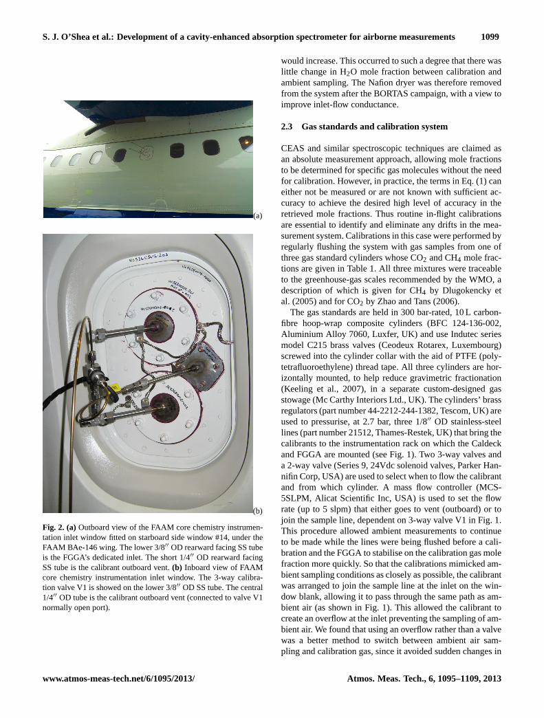
The FGGA’s aircraft inlet is mounted on a customisedFAAM BAe-146 window blank (Avalon Aero Ltd, UK). Out-board and inboard views of the FAAM core chemistry instru-mentation inlet window are shown in Fig. 2. The upper rear-ward facing 3/8′′ (9.53 mm) OD (outer diameter) stainless-steel tube inlet (lined with 1/4′′ (6.35 mm) OD PFA (perfluo-roalkoxy) Teflon tube) is used for sampling CO and O3. Thelower rearward facing 3/8′′ OD stainless-steel tube inlet isthe dedicated FGGA inlet. While, the short 1/4′′ OD rear-ward facing stainless-steel tube (in centre) is the calibrantoutboard vent.

The inlet window is located adjacent to the core chem-istry instrumentation rack, in place of starboard side win-dow #14, to optimise the FGGA’s sample-flow conductanceand reduced lag times. Window #14 is located∼ 14 m aft ofthe nose of the aircraft. At this distance, the 99 % thicknesscurve of the aircraft boundary layer, derived from computa-tional fluid dynamics and the Engineering Sciences Data Unit(ESDU) item 79020 (BAe Systems, 2003) is∼ 17 cm. Theinlet tube was designed with an extra safety margin, so that

www.atmos-meas-tech.net/6/1095/2013/ Atmos. Meas. Tech., 6, 1095–1109, 2013

1098 S. J. O’Shea et al.: Development of a cavity-enhanced absorption spectrometer for airborne measurements

Fig. 1.A diagram of the sample and calibration air flow through the CO2 and CH4 system.

its tip protrudes∼ 20 cm from the aircraft’s skin, to guaranteefree-flow sampling. This is an important factor consideringthe very high CO2 concentrations present in the aircraft’spressurised cabin (> 700 ppm), which may leak into the ex-ternal skin boundary layer, for instance via door seals, andthereby contaminate ambient air CO2 measurements. Varioustest flights of this inlet configuration confirm that the inlet tipis standing in the free flow, with no discernible CO2 contam-ination reported during roll, pitch and yaw-test manoeuvres.

The FGGA’s instrument inlet is connected to the aircraftinlet using non-porous 1/4′′ OD Eaton Synflex 1300 tubing,a material commonly used for sampling greenhouse gases.The total response time of the system is a combination of thetime taken to travel through transfer lines from the aircraftinlet to the sample cavity plus the time taken for the instru-ment to respond fully to the change in mole fraction. Eachof these were measured and assessed. First the inlet’s lagtime was determined by overflowing the inlet with N2 andmeasuring the time taken to detect a change in mole frac-tion. The e-fold response time of the instrument cavity wasdetermined by overflowing N2 directly at the inlet bulkheadof the FGGA then computing an exponential fit to the ob-served signal decay. To simulate high-altitude sampling thetests were repeated at reduced inlet pressure by connecting a

needle valve and a pressure sensor to the inlet. At 1007 mbinlet pressure the inlet lag time was 4.0± 1.0 s and the cav-ity’s e-folding time was 1.4± 0.1 s. The response time wasfound to improve marginally with altitude, e.g. at 287 mbinlet pressure the inlet lag time was 2.0± 1.0 s and the e-folding time was 1.5± 0.1 s. This compares to the theoreticalinlet lag times calculated using flow rates and pipe lengths(assuming plug-flow) of approximately∼ 4.6 s at 1007 mband∼ 1.3 s at 287 mb.

During the system’s first measurement campaign (BOR-TAS) a Nafion dryer was used to dry the sample before deliv-ery to the instrument for analysis. This consisted of a multi-stranded exchange membrane (PD-50T-24MPS, Perma PureInc, USA) and a counter flowing dry gas stream created us-ing a molecular sieve (81005, Alltech Associates AppliedScience Ltd, UK) and a pump (G24/045, Gardner DenverAlton Ltd, UK). The reason for using this was to reducethe influence of rapidly changing H2O on the retrieved molefractions, which are described in Sect. 2.4. We found thatthe Nafion dryer was able to reduce the H2O content of thesampled air to a small extent. However, during periods ofsustained high-ambient humidity (e.g. when sampling in themarine boundary layer) H2O exchange would occur in theopposite direction to that intended and the sample humidity

Atmos. Meas. Tech., 6, 1095–1109, 2013 www.atmos-meas-tech.net/6/1095/2013/

S. J. O’Shea et al.: Development of a cavity-enhanced absorption spectrometer for airborne measurements 1099

(a)

(b)

Fig. 2. (a)Outboard view of the FAAM core chemistry instrumen-tation inlet window fitted on starboard side window #14, under theFAAM BAe-146 wing. The lower 3/8′′ OD rearward facing SS tubeis the FGGA’s dedicated inlet. The short 1/4′′ OD rearward facingSS tube is the calibrant outboard vent.(b) Inboard view of FAAMcore chemistry instrumentation inlet window. The 3-way calibra-tion valve V1 is showed on the lower 3/8′′ OD SS tube. The central1/4′′ OD tube is the calibrant outboard vent (connected to valve V1normally open port).

would increase. This occurred to such a degree that there waslittle change in H2O mole fraction between calibration andambient sampling. The Nafion dryer was therefore removedfrom the system after the BORTAS campaign, with a view toimprove inlet-flow conductance.

2.3 Gas standards and calibration system

CEAS and similar spectroscopic techniques are claimed asan absolute measurement approach, allowing mole fractionsto be determined for specific gas molecules without the needfor calibration. However, in practice, the terms in Eq. (1) caneither not be measured or are not known with sufficient ac-curacy to achieve the desired high level of accuracy in theretrieved mole fractions. Thus routine in-flight calibrationsare essential to identify and eliminate any drifts in the mea-surement system. Calibrations in this case were performed byregularly flushing the system with gas samples from one ofthree gas standard cylinders whose CO2 and CH4 mole frac-tions are given in Table 1. All three mixtures were traceableto the greenhouse-gas scales recommended by the WMO, adescription of which is given for CH4 by Dlugokencky etal. (2005) and for CO2 by Zhao and Tans (2006).

The gas standards are held in 300 bar-rated, 10 L carbon-fibre hoop-wrap composite cylinders (BFC 124-136-002,Aluminium Alloy 7060, Luxfer, UK) and use Indutec seriesmodel C215 brass valves (Ceodeux Rotarex, Luxembourg)screwed into the cylinder collar with the aid of PTFE (poly-tetrafluoroethylene) thread tape. All three cylinders are hor-izontally mounted, to help reduce gravimetric fractionation(Keeling et al., 2007), in a separate custom-designed gasstowage (Mc Carthy Interiors Ltd., UK). The cylinders’ brassregulators (part number 44-2212-244-1382, Tescom, UK) areused to pressurise, at 2.7 bar, three 1/8′′ OD stainless-steellines (part number 21512, Thames-Restek, UK) that bring thecalibrants to the instrumentation rack on which the Caldeckand FGGA are mounted (see Fig. 1). Two 3-way valves anda 2-way valve (Series 9, 24Vdc solenoid valves, Parker Han-nifin Corp, USA) are used to select when to flow the calibrantand from which cylinder. A mass flow controller (MCS-5SLPM, Alicat Scientific Inc, USA) is used to set the flowrate (up to 5 slpm) that either goes to vent (outboard) or tojoin the sample line, dependent on 3-way valve V1 in Fig. 1.This procedure allowed ambient measurements to continueto be made while the lines were being flushed before a cali-bration and the FGGA to stabilise on the calibration gas molefraction more quickly. So that the calibrations mimicked am-bient sampling conditions as closely as possible, the calibrantwas arranged to join the sample line at the inlet on the win-dow blank, allowing it to pass through the same path as am-bient air (as shown in Fig. 1). This allowed the calibrant tocreate an overflow at the inlet preventing the sampling of am-bient air. We found that using an overflow rather than a valvewas a better method to switch between ambient air sam-pling and calibration gas, since it avoided sudden changes in

www.atmos-meas-tech.net/6/1095/2013/ Atmos. Meas. Tech., 6, 1095–1109, 2013

1100 S. J. O’Shea et al.: Development of a cavity-enhanced absorption spectrometer for airborne measurements

Table 1.The in-flight gas standards certified mole fractions used during the BORTAS and MAMM projects. The Max-Planck Institute for Bio-geochemistry (Jena) carried out the calibration through the Infrastructure for Measurements of the European Carbon Cycle (EU 13 IMECC)project. A 6 month-mixture stability check showed the standards were stable over this period. Theδ13C isotopic ratios, determined usingcontinuous-flow gas chromatography/isotope-ratio mass spectrometry (Fisher et al., 2006), are close enough to the ambient isotopic ratio soas not to cause a significant error in the measured mole fractions.

CO2 (ppm) CO2 (ppm) δ13C− CO2(0/00) CH4 CH4 (ppb) δ13C− CH4±1σ ±1σ ±1σ (count) (ppb)± ±1σ (0/00) ±1σ

EU 13 6 month 1σ 6 month (count)IMECC stability EU 13 stability

check IMECC check

High 489.27± 0.1 489.11± 0.04 −13.85± 0.03 (4) 2347.0± 1 2347.9± 0.2 −45.99± 0.03 (3)Low 348.93± 0.04 349.10± 0.03 −9.89± 0.03 (3) 1891.1± 0.3 1891.2± 0.2 −47.12± 0.04 (3)Target 388.38± 0.06 388.42± 0.03 −9.47± 0.03 (4) 1892.1± 0.8 1892.3± 0.2 −47.20± 0.06 (4)

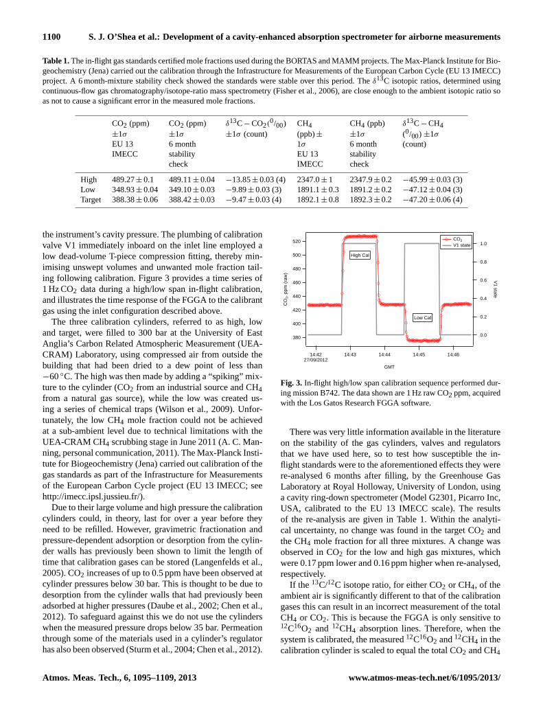
the instrument’s cavity pressure. The plumbing of calibrationvalve V1 immediately inboard on the inlet line employed alow dead-volume T-piece compression fitting, thereby min-imising unswept volumes and unwanted mole fraction tail-ing following calibration. Figure 3 provides a time series of1 Hz CO2 data during a high/low span in-flight calibration,and illustrates the time response of the FGGA to the calibrantgas using the inlet configuration described above.

The three calibration cylinders, referred to as high, lowand target, were filled to 300 bar at the University of EastAnglia’s Carbon Related Atmospheric Measurement (UEA-CRAM) Laboratory, using compressed air from outside thebuilding that had been dried to a dew point of less than−60◦C. The high was then made by adding a “spiking” mix-ture to the cylinder (CO2 from an industrial source and CH4from a natural gas source), while the low was created us-ing a series of chemical traps (Wilson et al., 2009). Unfor-tunately, the low CH4 mole fraction could not be achievedat a sub-ambient level due to technical limitations with theUEA-CRAM CH4 scrubbing stage in June 2011 (A. C. Man-ning, personal communication, 2011). The Max-Planck Insti-tute for Biogeochemistry (Jena) carried out calibration of thegas standards as part of the Infrastructure for Measurementsof the European Carbon Cycle project (EU 13 IMECC; seehttp://imecc.ipsl.jussieu.fr/).

Due to their large volume and high pressure the calibrationcylinders could, in theory, last for over a year before theyneed to be refilled. However, gravimetric fractionation andpressure-dependent adsorption or desorption from the cylin-der walls has previously been shown to limit the length oftime that calibration gases can be stored (Langenfelds et al.,2005). CO2 increases of up to 0.5 ppm have been observed atcylinder pressures below 30 bar. This is thought to be due todesorption from the cylinder walls that had previously beenadsorbed at higher pressures (Daube et al., 2002; Chen et al.,2012). To safeguard against this we do not use the cylinderswhen the measured pressure drops below 35 bar. Permeationthrough some of the materials used in a cylinder’s regulatorhas also been observed (Sturm et al., 2004; Chen et al., 2012).

520

500

480

460

440

420

400

380

CO

2, p

pm (

raw

)

14:4227/09/2012

14:43 14:44 14:45 14:46

GMT

1.0

0.8

0.6

0.4

0.2

0.0

V1 state

High Cal

Low Cal

CO2

V1 state

Fig. 3. In-flight high/low span calibration sequence performed dur-ing mission B742. The data shown are 1 Hz raw CO2 ppm, acquiredwith the Los Gatos Research FGGA software.

There was very little information available in the literatureon the stability of the gas cylinders, valves and regulatorsthat we have used here, so to test how susceptible the in-flight standards were to the aforementioned effects they werere-analysed 6 months after filling, by the Greenhouse GasLaboratory at Royal Holloway, University of London, usinga cavity ring-down spectrometer (Model G2301, Picarro Inc,USA, calibrated to the EU 13 IMECC scale). The resultsof the re-analysis are given in Table 1. Within the analyti-cal uncertainty, no change was found in the target CO2 andthe CH4 mole fraction for all three mixtures. A change wasobserved in CO2 for the low and high gas mixtures, whichwere 0.17 ppm lower and 0.16 ppm higher when re-analysed,respectively.

If the 13C/12C isotope ratio, for either CO2 or CH4, of theambient air is significantly different to that of the calibrationgases this can result in an incorrect measurement of the totalCH4 or CO2. This is because the FGGA is only sensitive to12C16O2 and 12CH4 absorption lines. Therefore, when thesystem is calibrated, the measured12C16O2 and12CH4 in thecalibration cylinder is scaled to equal the total CO2 and CH4

Atmos. Meas. Tech., 6, 1095–1109, 2013 www.atmos-meas-tech.net/6/1095/2013/

S. J. O’Shea et al.: Development of a cavity-enhanced absorption spectrometer for airborne measurements 1101

from when the mixture was certified. The same scaling factoris applied to the ambient measurement to give the total CO2and CH4 mole fraction. Since the calibration gases are nota completely natural mixture, they may have a significantlydifferent isotopic composition to the sampled ambient air, thescaling factor used to determine the total CO2 and CH4 mayno longer be valid.

For this reason, the ratio of the13C and12C isotopes ofCO2 and CH4 in the calibration cylinders were determined,by Royal Holloway University’s Greenhouse Gas Labora-tory, using gas chromatography-continuous flow-isotope ra-tio mass spectrometry (GC-CF-IRMS) (Fisher et al., 2006).The results are also given in Table 1 and are expressed us-ing δ notation on the VPDB scale (Vienna Pee Dee Belem-nite). This isotopic effect has been estimated using 2 suitesof NOAA standards at RHUL (Royal Holloway, Universityof London), one set of 3 with typical ambient-air isotopicsignatures, and one set of 3 with synthetic air, with both CO2and CH4 derived from natural gas.

Backgroundδ13C-CO2 is currently close to−8 ‰ (Alli-son and Francey, 2007) but is depleted by emissions of CO2from fossil fuel and combustion sources. Whileδ13C-CH4 istypically −47.3 ‰ (Levin et al., 2012). For both species thehigh-span’sδ13C is furthest from these values and thereforewill be responsible for the largest error. This could have beenexpected since the high-span gas mixture has been createdwith the largest proportion of the “spiking” mixture that wasunlikely to have typical background isotopic ratios. If a sam-ple is measured with typical backgroundδ13C and the samemole fraction as the high span the FGGA will overestimateits mole fraction by 0.03 ppm for CO2 and 0.03 ppb for CH4.For all the calibration mixtures theδ13C values are similarenough to typical background values that the error from onlymeasuring12C isotopologues, using the CEAS technique,is within the noise of the instrument. However, if plumesare measured that are significantly enriched in13C such asfrom biomass burning this will result in an underestimationof the total mole fraction (0.5 ppb atδ13C− CH4 =−27 ‰).Other CO2 and CH4 isotopologues are less abundant and arethought to have a smaller effect (Tohjima et al., 2009; Chenet al., 2010).

2.4 Influence of water vapour

The variability of water vapour in the atmosphere, whichcovers several orders of magnitude and can be many percentin the troposphere, is large enough to cause significant de-viations to the mole fractions retrieved using spectroscopy.This is due to three distinct mechanisms. Firstly, H2O willcause a variable dilution of the CO2 and CH4 mole fraction.H2O is the only species whose variability is large enoughto cause changes to the CO2 and CH4 mole fraction of overabout 0.1 %, purely due to a variable dilution throughout thetroposphere. Secondly, H2O has strong absorption lines inthe infrared. Spectral interference due to H2O either over-

lapping or near to the CO2 or CH4 absorption features ofinterest would likely alter the retrieved mole fractions. Fi-nally, pressure broadening between the H2O molecules andthe analyte will alter the absorption-line shape. This is trueof all molecules but the degree at which it occurs is de-pendent on the molecules involved and also the particularabsorption line.

For these reasons, dry-air mole fractions, the number ofmoles of CO2/CH4 per the number of moles of dry air, needto be used if comparisons are to be made between differenttechniques, locations and with chemical transport models.These could be determined by drying the air sample beforeit is analysed. Previously, this approach has been employedsuccessfully for airborne measurements of CO2 and CH4 us-ing a combination of a Nafion dryers and dry-ice traps (Vayet al., 1999; Daube et al., 2002; Peischl et al., 2010). How-ever, we have found that even when using the Nafion dryer,measured water vapour levels in the air sample were not suf-ficiently low to remove the aforementioned effects. Addingmore dryers to the system would likely add complexity andweight, as well as further impact the instrument’s time re-sponse, and at the same time increase the level of systemmaintenance needed. Therefore, we have opted to use theFGGA’s simultaneous H2O measurement to convert wet- todry-air mole fractions.

Previously, the FGGA’s on-board control computer soft-ware automatically removed the effects of dilution on theCO2 or CH4 mole fractions derived from the spectral fits,[X]Wet, using Eq. (2):

[X]Dilution =[X]Wet

1 − 0.01[H2O], (2)

where [H2O], % (cmol (mol)−1), is the simultaneous mea-surement of H2O in the instrument cavity. For this to worksuccessfully, absolute accuracy of H2O measurements are re-quired. Based on this approach, in order to obtain the WMOrecommended specification for CH4 and CO2 measurements,the corresponding H2O measurement must have an absoluteaccuracy of 0.1 %.

To derive a theoretical correction for the effects of pres-sure broadening and spectral interference due to H2O on theCO2 and CH4 measurements is more difficult, since the HI-TRAN database typically only contains information on thepressure-broadened line width within dry air (Brown et al.,2003). Here we use laboratory experiments to determine a re-lationship between the CO2 and CH4 wet-air mole fractionsretrieved from the spectral fits and the corresponding dry-air mole fraction, incorporating all three effects into a singlerelationship. This approach is similar to previous work us-ing other infrared absorption techniques (Neftel et al., 2010;Chen et al., 2010; Tuzson et al., 2010).

A schematic of the experimental set-up used is shownin Fig. 4. Air from a cylinder (12-N compressed air, BOC,UK), with nominal CO2 and CH4 mole fractions of 400 ppmand 2000 ppb, respectively, was passed through a dew-point

www.atmos-meas-tech.net/6/1095/2013/ Atmos. Meas. Tech., 6, 1095–1109, 2013

1102 S. J. O’Shea et al.: Development of a cavity-enhanced absorption spectrometer for airborne measurements

Fig. 4.A schematic of the experimental set-up used to determine how water vapour influences CO2 and CH4 measurements. The humidifierused was a Li-610 dew-point generator (Li-610, Li-Cor Inc., USA).

generator (Li-610, Li-Cor Inc., USA) creating a gas mixturethat had a constant dry-air mole fraction of CO2 and CH4 butwith a variable humidity controlled by the dew-point gen-erator. Depending on the position of two 3-way valves, thegas mixture can be sent either directly to the FGGA or firstthrough a stainless-steel coil that was within a dewar of dryice. This lowers the dew point of the sample to less than−60◦C (0.002 %), which we approximate to be a measure-ment of the dry-air mole fraction of the cylinder.

The dew point was varied in 5◦C increments from 0 to25◦C and back to 0◦C, which corresponds to the mole frac-tions 0.6 and 3.2 %, respectively. Between each change inthe dew point, the two 3-way valves were switched to allowthe FGGA to measure the air that had passed through thedry-ice trap. Once the system had stabilised, the signals fromeach period measuring dry air were averaged, interpolatedand used to remove any drift in the CO2 and CH4 measure-ments. Throughout the experiment, the FGGA’s water vapourmeasurement was consistently below that reported by thedew-point generator. A linear fit to the mole fraction fromthe dew-point generator versus the FGGA’s measurementyielded anR2 of 0.996, a regression slope of 1.526± 0.001and an intercept of−0.65± 0.01 %. Since the dew-point gen-erator had not been calibrated directly before these exper-iments, we do not consider it to be an absolute measure-ment, only a means to deliver variable humidity levels tothe FGGA. Also, though the experiments were conducted ina temperature-controlled laboratory (temperature maintainedat 28◦C), it is still possible that H2O could condense on thewalls of the tubing or the inlet filter. As a result, it is possi-ble that the H2O content that leaves the generator may not be

identical to that which arrives at the sample cavity (LI-COR,2004). When sampling the dry-gas stream the FGGA recordsa mean H2O content of 0.013 % (1σ = 0.008 %).

This experiment was repeated three times over a three-month period, to test the repeatability of the system’s re-sponse to varying humidity. The results are shown in Fig. 5and suggest that using Eq. (2) alone to determine the dry-air mole fraction accurately is not sufficient. There was aclear relationship between the humidity and the simultane-ous measurement of CO2 and CH4 even after Eq. (2) hadbeen applied (Fig. 5, dashed lines). Instead we approximatethe relationship between[X]Wet and the corresponding dry-air mole fraction,[X]Dry, using a quadratic function of theform:

[X]Dry =[X]Wet

a + b [H2O] + c [H2O]2(3)

wherea, b andc are the coefficients of the quadratic fit to[X]Wet/[X]Dry versus [H2O], shown in Fig. 5. The deter-mined fit coefficients are given in Table 2. To convert thefit residuals to mole fractions they have been multiplied bythe nominal values 2000 ppb and 400 ppm. On the major-ity of occasions, the CH4 residuals were typically less than1 ppb, but there are two outliers at 2.9 and−2.11 ppb. ForCO2 they are generally less than 0.2 ppm. The standard devi-ations of all the residuals are 1.0 ppb and 0.15 ppm for CH4and CO2, respectively. For this function to work successfully,absolute accuracy of H2O measurements is not needed sinceany offset or non-unity response to varying H2O should beaccounted for ina, b andc. However, if the function is to beused over an extended period of time it is important that theH2O measurement remains stable. There does not appear to

Atmos. Meas. Tech., 6, 1095–1109, 2013 www.atmos-meas-tech.net/6/1095/2013/

S. J. O’Shea et al.: Development of a cavity-enhanced absorption spectrometer for airborne measurements 1103

1.00

0.99

0.98

0.97

0.96

CH

4 W

et/ C

H4

Dry

2.01.51.00.50.0

H2O, %

-2

0

2

Res

idua

l,x2

000

ppb

02/07/2012 16/10/2012 17/10/2012 Quadratic fit No dilution

1.00

0.99

0.98

0.97

0.96

CO

2 W

et/ C

O2

Dry

2.01.51.00.50.0

H2O, %

-0.4

-0.2

0.0

0.2

0.4

Res

idua

l,x4

00 p

pm

02/07/2012 16/10/2012 17/10/2012 Quadratic fit No dilution

a)

b)

Fig. 5. The FGGA’s response to varying humidity was determinedby humidifying air from a cylinder. The dry measurements were de-termined by passing the humidified air through a dry-ice trap beforeit was analysed. This test was repeated three times over a three-month period to test the repeatability of the system. A relationshipbetween the dry-air mole fraction and the measured wet-air molefraction was determined using a quadratic fit to(a) CH4 wet/CH4dry versus H2O and(b) CO2 wet/CO2 dry versus H2O. The dashedlines have been determined by applying Eq. (2) to CH4 wet andCO2 wet, this suggests that only correcting for the dilution effectdue to H2O is not sufficient to determine dry-air mole fractions.

be any distinction between when the tests were performed.Nevertheless, we do not yet feel that these experiments havebeen repeated over a long-enough timescale. So to further en-sure the stability of the functions, these tests should and willbe repeated before and after each future flying campaign.

2.5 Data processing and quality control

The high- and low-calibration mole fractions were chosento span the range that would normally be encountered dur-

Table 2. a, b and c are the coefficients of the quadratic fit to[X]Wet/[X]Dry versus [H2O]. These values can then be used to de-termine dry-air mole fractions using Eq. (3).

a b c Standard(%−1) (%−2) deviation

of the fitresiduals

CH4 1.0006 −0.016697 −0.000533 1.0 ppbCO2 1.0001 −0.016889 −0.000444 0.15 ppm

ing flight. Measurements of these mixtures were used torescale the dry-air mole fractions determined using Eq. (3) tothe WMO scale. In-flight span calibrations were performedhourly. During a span calibration, gas from the high cylinderwould first be flushed for 45 s through the system and thenflowed through the FGGA’s sample cavity for an additional1 min. This procedure would be repeated for gas from the lowcylinder, as shown in Fig. 3. The first 20 s of measurementswere discarded to ensure the system had stabilised and theremaining 40 s of readings were averaged for both the highand low. A linear fit of the cylinder-calibration mole frac-tion versus the FGGA’s measurement for sequential high andlow calibrations was used to determine the FGGA’s responseslope and intercept values. These were linearly interpolatedacross the whole flight and applied to all ambient measure-ments placing the measurements on the WMO recommendedscale.

Measurements of the target mixture were used to checkthe effectiveness of the rescaling and the instrument perfor-mance, the analysis of which is described in Sect. 3.1. Targetcalibrations were carried out several times between span cal-ibrations under a variety of different flying conditions andaltitudes.

As mentioned previously, it is important that the FGGA’scavity pressure is maintained at a constant value, chosen tobe 50 Torr. Laboratory experiments running the system onair from a gas tank at different cavity pressures showed thatdeviations from this value caused a reduction in the instru-ment’s precision (M. Gupta, personal communication, 2011).For this reason, if the recorded cavity pressure was±5 %outside this set point, all the associated measurements werediscarded.

3 Instrument characterisation

3.1 Accuracy and precision

To assess the short-term precision of the system we use theAllan variance technique (Werle et al., 1993). Whilst sam-pling a compressed-air cylinder in the laboratory, 1 Hz (1σ )precisions of 1.88 ppb for CH4 and 0.41 ppm for CO2 aretypically obtained. The commercially available version of the

www.atmos-meas-tech.net/6/1095/2013/ Atmos. Meas. Tech., 6, 1095–1109, 2013

1104 S. J. O’Shea et al.: Development of a cavity-enhanced absorption spectrometer for airborne measurements

FGGA normally operates at 140 Torr cavity pressure, ratherthan the 50 Torr used in this work. However, as long as thefitting routines are updated for the specific cavity pressure(M. Gupta, personal communication, 2011), 1 Hz precisionsare found to be broadly comparable between 50 and 140Torr operation. This degree of precision can be replicatedin-flight, for example 1 Hz precisions are found to be typi-cally 1.61 ppb for CH4 and 0.40 ppm for CO2 . This suggeststhat as long as the instrument’s cavity pressure is maintainedwith sufficient precision, the CEAS technique employed bythe FGGA is well suited for airborne measurements.

The in-flight measurements of the target gas mixture areused to assess long-term repeatability and accuracy of thesystem’s airborne measurements. Figure 6 shows the in-flighttarget measurements, once the data had been rescaled to theWMO scale, for all flights when the system was operatedbetween 11 July 2011 and 3 May 2012. The data set com-prised a total of 29 flights. There is only a small offset in theFGGA measurement compared to the target certification, themean difference between the measurements and the certified-target mole fraction was−0.07 ppb for CH4 and−0.06 ppmfor CO2. The frequency distribution of the target measure-ments for CO2 was approximately Gaussian. However, theCH4 measurements appeared to have a small drift in the sys-tem that was not captured by the span calibrations so thedistribution of target calibrations do not show quite as goodagreement with the assumed Gaussian fit as it does for CO2.At 1 Hz the standard deviation of the frequency distributionis 2.48 ppb and 0.66 ppm for CH4 and CO2, respectively. Ifthe measurements are averaged to 10 s this drops to 2.00 ppband 0.45 ppm. Through the addition of all known uncertain-ties we estimate a total accuracy of±1.28 ppb for CH4 (H2Ocorrection 1σ fit residual±1 ppb, target standard calibration±0.8 ppb and in-flight target measurement±0.07 ppb) and±0.17 for CO2 (H2O correction 1σ fit residual±0.15 ppm,target standard calibration±0.06 ppm and in-flight targetmeasurement±0.06 ppm).

As mentioned previously, during the BORTAS flights thesystem was operated with a Nafion dryer. The performanceof the system was found to be no worse when the dryer wasused (11 July 2011–23 July 2011) compared to those flightswhen it was not (24 November 2011–3 May 2012). The lackof deviation between the measured target mixture and its cal-ibration suggests that permeation of CO2 and CH4 throughthe membrane is small, which is in agreement with work byother groups (Vay et al., 1999).

3.2 Comparison between in situ and whole-air samplemeasurements

During two flights when the FGGA was operated(flight number B682 on 14 March 2012 and B685 on18 March 2012), 26 whole-air samples were also collectedin stainless-steel sample flasks. A description of the sam-ple flasks can be found in Lewis et al. (2013). These

4

3

2

1

0

-1

-2

-3CO

2 M

easu

red-

CO

2 C

alib

ratio

n, p

pm

21/0

7/20

11

10/0

8/20

11

30/0

8/20

11

19/0

9/20

11

GMT

2500Counts

11/0

3/20

12

21/0

3/20

12

31/0

3/20

12

10/0

4/20

12

20/0

4/20

12

30/0

4/20

12

1s equilibrated target valuesMean= -0.06 ppmStandard deviation= 0.66 ppm

Gaussian fitMean= -0.04 ppmStandard deviation= 0.55 ppm

-10ppbv

-5

0

5

10

CH

4 M

easu

red-

CH

4 C

alib

ratio

n, p

pb

4002000

Counts

1s equilibrated target values Mean= -0.07 ppbStandard deviation= 2.48 ppb

Gaussian fitMean= 0.12 ppbStandard deviation= 1.52 ppb

a)

b)

Fig. 6. An estimate of the system’s accuracy can be made by ex-amining the difference between the calibration mole fraction andthe scaled FGGA measurement of the target gas mixture. At 1 Hzthe mean±1 standard deviation difference between the two is−0.07± 2.48 ppb for CH4 and−0.06± 0.66 ppb for CO2.

flasks were analysed post-flight for CO2 and CH4, by RoyalHolloway University’s Greenhouse Gas Laboratory, usingCRDS, (Model G2301, Picarro Inc, USA, calibrated to theEU 13 IMECC scale), with a reported accuracy of 0.5 ppband 0.1 ppm for CH4 and CO2, respectively. This provided asecond method to validate the in-flight FGGA measurements.For a direct comparison the 1 Hz in situ data were averagedover the recorded filling times of the flasks, this was typi-cally between 20 and 60 s. Figure 7 shows the scatter plotof the mole fraction derived from both techniques. The aver-age deviation between the two methods (the FGGA measure-ment minus the flask measurement averaged for all 26 sam-ples) was−2.4 ppb (1σ = 2.3 ppb) for CH4 and−0.22 ppm(1σ = 0.45 ppm) for CO2. For both species this is slightlylarger than the estimate of the FGGA’s accuracy from thein-flight calibrations.

Both the in situ and flask sample measurements were madeusing instruments calibrated to the same WMO scales. Sincethe only difference between calibration and ambient sam-pling should be that the calibration gases do not containH2O, the extra deviation could be attributed to one or both ofthe analysers not correctly computing dry-air mole fractions.

Atmos. Meas. Tech., 6, 1095–1109, 2013 www.atmos-meas-tech.net/6/1095/2013/

S. J. O’Shea et al.: Development of a cavity-enhanced absorption spectrometer for airborne measurements 1105

402

400

398

396

394

392

FG

GA

CO

2, p

pm

402400398396394392

Flask CO2, ppm

-1.5

-1.0

-0.5

0.0

0.5

1.0

FG

GA

CO

2 -

Fla

sk C

O2,

ppm

1940

1920

1900

1880

1860

1840

FG

GA

CH

4, p

pb

194019201900188018601840

Flask CH4, ppb

-8

-6

-4

-2

0

2

FG

GA

CH

4 -

Fla

sk C

H4,

pp

ba)

b)

Fig. 7. Scatter plots of FGGA versus whole-air sample measure-ments of(a) CH4 and(b) CO2. Whole-air samples were collected inflasks and analysed post flight using CRDS (Model G2301, PicarroInc, USA). The FGGA’s original 1 Hz measurements were averagedover the filling period of each flask. Error bars are the standard de-viation of the FGGA measurements during each filling period, indi-cating the uncertainty in the averaging of the in situ measurements.The dotted line is the one-to-one relationship.

However, a direct comparison between the two techniques iscomplicated as it is assumed that the flasks are filled at a con-stant rate and this is not thought to be the case, particularly atdifferent altitudes. Therefore, a constant averaging windowmay not be appropriate. However, with this caveat, the stan-dard deviation of the 1 Hz measurements has been includedin Fig. 7, as error bars, to show the variability in CO2 andCH4 during the filling period and as a measure of the uncer-tainty during the sample period. Previous work has shownthat agreement between in situ and whole-air sample mea-surements can improve if a weighting function is used; how-ever, in order to derive this function, the pressure in the flaskduring the flushing and filling process needs to be known

(Chen et al., 2012). Unfortunately, this information is notcurrently available on our aircraft and the comparison musttherefore be subject to this caveat.

It is also conceivable that the content of the flask has beenaltered in the two-week period between filling and analysis,due to similar mechanisms to those described in Sect. 2.4.However, no variations of this magnitude have previouslybeen detected.

4 Airborne measurements in biomass-burning plumes

The system’s measurements, made as part of the BORTASand MAMM projects, as well those assessing the Total Elgingas-platform leak rate will be presented in separate papers.To highlight the instrument capability based on the abovework we show example data, when the system was used tosample biomass-burning plumes, as part of the SAMBBAcampaign. During this experiment, measurement-flight num-ber B742 was carried out on 27 September 2012. This con-sisted of flying in the boundary layer over an active fire re-gion near Palmas, Brazil (∼ 11.1◦ S, ∼ 47.3◦ W), a regioncontaining a mixture of grassland and forests. During thisflight a number of biomass-burning plumes were interceptedwith both CO2 and CH4 mole fractions significantly en-hanced above their local background levels. Sampling thesenear source plumes are some of the most challenging mea-surements that the system will be used for due to the limitedtime spent within the plumes and the large and rapid changesin mole fractions.

Figure 8 shows that the enhancements in CO2 and CH4correspond well with coincident measurements of CO madeon board the FAAM BAe-146. The CO measurementswere determined using a VUV (vacuum ultraviolet) fast-fluorescence analyser, accurate to 2 % (AL5002, AerolaserGmbH, Germany; Gerbig et al., 1999). The CO measure-ments were used to determine an emission ratio, a com-monly used measure of emissions from biomass burning,representing the proportion of a species emitted by thefires relative to a tracer species. The emission ratio canbe calculated as the regression slope of the in-plume mea-surements of the species of interest relative to a tracerspecies for biomass burning. Due to the excellent corre-lation with CO we do not distinguish between individualplumes. Instead we calculate emission ratios, relative toCO, for the whole of the low level portion of flight B742,we find these to be 14.77± 0.03 mol CO2 (mol CO)−1 and0.0532± 0.0001 mol CH4 (mol CO)−1. This means that theemission ratios we calculate are the combination of severalfires in a small region. By assuming a carbon content ofthe soils these emission ratios can be converted to emissionfactors, an estimate of the mass of the species emitted perunit mass of biomass burnt. We use the methodology de-tailed by Yokelson et al. (1999) to determine emission factorsof 1710± 171 g (kg dry matter)−1 for CO2 and 2.2± 0.2 g

www.atmos-meas-tech.net/6/1095/2013/ Atmos. Meas. Tech., 6, 1095–1109, 2013

1106 S. J. O’Shea et al.: Development of a cavity-enhanced absorption spectrometer for airborne measurements

3000

2800

2600

2400

2200

2000

1800

CH

4, p

pb

15x1031050

CO, ppb

R2= 0.92

y=1806+0.053x

700

650

600

550

500

450

400

CO

2, p

pm

15x1031050

CO, ppb

R2=0.88

y=397+0.015x

2400

2200

2000CH

4, p

pb

15:2627/09/2012

15:28 15:30 15:32

GMT

12x103

8

4CO

, ppb

650600550500450400

CO

2 , ppm

800750700650600550

Altitude, m

a)

b) c)

Fig. 8. (a) Shows a time series whilst flying in the bound-ary layer during flight B742 where a number of biomass-burning plumes were intercepted near Palmas, Brazil. Scat-ter plots for (b) CH4 and (c) CO2 both show strong corre-lation with CO and allow emission ratios to be determined,which were found to be 14.77± 0.03 mol CO2 (mol CO)−1 and0.0532± 0.0001 mol CH4 (mol CO)−1.

(kg dry matter)−1 for CH4. These are in excellent agreementwith values in the literature for savannah and grassland fires.Andreae and Merlet (2001) report average literature valuesof 1613± 95 g (kg dry matter)−1 and 2.3± 0.9 g (kg drymatter)−1 for CO2 and CH4, respectively for savannah andgrassland fires.

5 Conclusions

A system for continuous airborne measurements of CO2and CH4 has been developed for operation on board theFAAM BAe-146 UK research aircraft. The system is shownto be capable of sampling both boundary-layer plumes andthe upper troposphere/lower stratosphere (UTLS), over an al-titude range of 0 to 9153 m. Data from 29 sampling flightswere used to assess the operational accuracy of the sys-tem. Analysis of the in-flight calibrations suggests that thelong-term 1 Hz measurements from the system are accurateto 1.28 ppb (1σ repeatability at 1 Hz = 2.48 ppb) for CH4

and 0.17 ppm (1σ repeatability at 1 Hz = 0.66 ppm) for CO2compared with WMO traceable standards. No motion or al-titude dependant behaviour was detected in these calibra-tions. When the system was compared to whole-air sam-ples there was a mean difference between the two tech-niques of−2.4 ppb (1σ = 2.3 ppb) for CH4 and−0.22 ppm(1σ = 0.45 ppm) for CO2.

The system did not incorporate a drying stage to removeH2O in the sample to< 0.1 %. Therefore, it was necessary touse the simultaneous H2O measurement to remove the effectsof H2O on the spectroscopic retrieval of CO2 and CH4. Pre-viously, the FGGA only accounted for the dilution effect ofH2O to determine the dry-air mole fraction of a species. Lab-oratory experiments measuring air from a cylinder at differ-ent humidities suggest that this is not sufficient. From theseexperiments, new correction functions have been determined.These experiments were repeated three times over a three-month period and the errors with the correction functionswere found to be 1.0 ppb and 0.15 ppm for CH4 and CO2, re-spectively. However, since this is only based on three exper-iments further repeats are planned for before and after everyflying campaign in which the system is used. These correc-tions will be routinely provided for the future FAAM FGGAdata sets.

The ability of the system to sample near source plumesof limited spatial extent was highlighted when it was usedto calculate emission factors for biomass-burning plumes,in the savannah regions near Palmas, Brazil, as part of theSAMBBA experiment. The determined emission factors of1710± 171 g (kg dry matter)−1 for CO2 and 2.2± 0.2 g(kg dry matter)−1 for CH4 are in excellent agreement withprevious studies.

Future work on the system will involve improving the in-strument’s response time to allow airborne eddy covarianceflux measurements. This will require the installation of ahigh-flow-displacement external pump (e.g. Edwards Vac-uum XDS35i or nXDS20).

Acknowledgements.The authors wish to thank in particularT. Ryerson (NOAA), J. Peischl (NOAA), B. Stephens (NCAR),A. Manning (UEA, Norwich, UK), P. Wilson (UEA, Norwich,UK), J. Muller (Uni. Manchester, UK) and M. Gupta (Los GatosResearch, Ltd), for useful discussions about greenhouse gasmeasurements and calibration. We are grateful to S. Tooley andJ. Smith (Avalon Aero Ltd, UK) for their help with the design andcertification of the aircraft instrument rack. We would like to thankFAAM staff and all those involved with the SAMBBA project.S. J. O’Shea is in receipt of a NERC PhD studentship. Part of thiswork was supported by the NERC project, Methane and OtherGreenhouse Gases in the Arctic – Measurements, Process Studiesand Modelling (MAMM), grant #NE/I029161/1.

Edited by: M. von Hobe

Atmos. Meas. Tech., 6, 1095–1109, 2013 www.atmos-meas-tech.net/6/1095/2013/

S. J. O’Shea et al.: Development of a cavity-enhanced absorption spectrometer for airborne measurements 1107

References

Allison, C. E. and Francey, R. J.: Verifying Southern Hemispheretrends in atmospheric carbon dioxide stable isotopes, J. Geophys.Res.-Atmos., 112, D21304,doi:10.1029/2006jd007345, 2007.

Andreae, M. O. and Merlet, P.: Emission of trace gases and aerosolsfrom biomass burning, Global Biogeochem. Cy., 15, 955–966,doi:10.1029/2000gb001382, 2001.

Aydin, M., Verhulst, K. R., Saltzman, E. S., Battle, M. O., Montzka,S. A., Blake, D. R., Tang, Q., and Prather, M. J.: Recent decreasesin fossil-fuel emissions of ethane and methane derived from firnair, Nature, 476, 198–201,doi:10.1038/nature10352, 2011.

BAe Systems 146 Atmospheric Research Aircraft: Location ofInlets and Sensors In Relation to the Boundary Layer, docu-ment number ADE-46D-R-463-000792, BAE SYSTEMS, UK,3 November 2003.

Baer, D. S., Paul, J. B., Gupta, J. B., and O’Keefe, A.: Sensitive ab-sorption measurements in the near-infrared region using off-axisintegrated-cavity-output spectroscopy, Appl. Phys. B, 75, 261–265,doi:10.1007/s00340-002-0971-z, 2002.

Baker, A. K., Schuck, T. J., Brenninkmeijer, C. A. M., Rauthe-Schoech, A., Slemr, F., van Velthoven, P. F. J., and Lelieveld,J.: Estimating the contribution of monsoon-related biogenicproduction to methane emissions from South Asia usingCARIBIC observations, Geophys. Res. Lett., 39, L10813,doi:10.1029/2012gl051756, 2012.

Bousquet, P., Ringeval, B., Pison, I., Dlugokencky, E. J., Brunke, E.-G., Carouge, C., Chevallier, F., Fortems-Cheiney, A., Franken-berg, C., Hauglustaine, D. A., Krummel, P. B., Langenfelds, R.L., Ramonet, M., Schmidt, M., Steele, L. P., Szopa, S., Yver,C., Viovy, N., and Ciais, P.: Source attribution of the changes inatmospheric methane for 2006–2008, Atmos. Chem. Phys., 11,3689–3700,doi:10.5194/acp-11-3689-2011, 2011.

Brown, L. R., Chris Benner, D., Champion, J. P., Devi, V. M., Fe-jard, L., Gamache, R. R., Gabard, T., Hilico, J. C., Lavorel, B.,Loete, M., Mellau, G. C., Nikitin, A., Pine, A. S., Predoi-Cross,A., Rinsland, C. P., Robert, O., Sams, R. L., Smith, M. A. H.,Tashkun, S. A., and Tyuterev, V. G.: Methane line parameters inHITRAN, J. Quant. Spectrosc. Ra., 82, 219–238, 2003.

Chen, H., Winderlich, J., Gerbig, C., Hoefer, A., Rella, C. W.,Crosson, E. R., Van Pelt, A. D., Steinbach, J., Kolle, O., Beck,V., Daube, B. C., Gottlieb, E. W., Chow, V. Y., Santoni, G. W.,and Wofsy, S. C.: High-accuracy continuous airborne measure-ments of greenhouse gases (CO2 and CH4) using the cavity ring-down spectroscopy (CRDS) technique, Atmos. Meas. Tech., 3,375–386,doi:10.5194/amt-3-375-2010, 2010.

Chen, H., Winderlich, J., Gerbig, C., Katrynski, K., Jordan, A., andHeimann, M.: Validation of routine continuous airborne CO2 ob-servations near the Bialystok Tall Tower, Atmos. Meas. Tech., 5,873–889,doi:10.5194/amt-5-873-2012, 2012.

Daube, B. C., Boering, K. A., Andrews, A. E., and Wofsy, S. C.:A high-precision fast-response airborne CO2 analyzer for in situsampling from the surface to the middle stratosphere, J. Atmos.Ocean. Tech., 19, 1532–1543, 2002.

DECC (UK Department for Energy and Climate Change): ElginGas Release, Government Interest Group update of environ-mental aspects relating to the incident,http://og.decc.gov.uk/media/viewfile.ashx?filetype=4&filepath=og/environment/5283-elgin-gas-release-gig-update1.doc&minwidth=true(lastaccess: 22 November 2012), 11 April 2012.

Dentener, F., Peters, W., Krol, M., van Weele, M., Bergamaschi, P.,and Lelieveld, J.: Interannual variability and trend of CH4 life-time as a measure for OH changes in the 1979-1993 time period,J. Geophys. Res.-Atmos., 108, 4442,doi:10.1029/2002jd002916,2003.

Deutscher, N. M., Griffith, D. W. T., Bryant, G. W., Wennberg, P.O., Toon, G. C., Washenfelder, R. A., Keppel-Aleks, G., Wunch,D., Yavin, Y., Allen, N. T., Blavier, J.-F., Jimenez, R., Daube,B. C., Bright, A. V., Matross, D. M., Wofsy, S. C., and Park, S.:Total column CO2 measurements at Darwin, Australia – site de-scription and calibration against in situ aircraft profiles, Atmos.Meas. Tech., 3, 947–958,doi:10.5194/amt-3-947-2010, 2010.

Dlugokencky, E. J., Walter, B. P., Masarie, K. A., Lang, P. M.,and Kasischke, E. S.: Measurements of an anomalous globalmethane increase during 1998, Geophys. Res. Lett., 28, 499–502,doi:10.1029/2000gl012119, 2001.

Dlugokencky, E. J., Myers, R. C., Lang, P. M., Masarie, K.A., Crotwell, A. M., Thoning, K. W., Hall, B. D., Elkins,J. W., and Steele, L. P.: Conversion of NOAA atmo-spheric dry air CH4 mole fractions to a gravimetrically pre-pared standard scale, J. Geophys. Res.-Atmos., 110, D18306,doi:10.1029/2005jd006035, 2005.

Dlugokencky, E. J., Bruhwiler, L., White, J. W. C., Emmons, L.K., Novelli, P. C., Montzka, S. A., Masarie, K. A., Lang, P. M.,Crotwell, A. M., Miller, J. B., and Gatti, L. V.: Observational con-straints on recent increases in the atmospheric CH4 burden, Geo-phys. Res. Lett., 36, L18803,doi:10.1029/2009gl039780, 2009.

Dlugokencky, E. J., Nisbet, E. G., Fisher, R., and Lowry, D.: Globalatmospheric methane: budget, changes and dangers, Philos. T.Roy. Soc. A, 369, 2058–2072,doi:10.1098/rsta.2010.0341, 2011.

Etheridge, D. M., Steele, L. P., Francey, R. J., and Lan-genfelds, R. L.: Atmospheric methane between 1000 ADand present: Evidence of anthropogenic emissions and cli-matic variability, J. Geophys. Res.-Atmos., 103, 15979–15993,doi:10.1029/98jd00923, 1998.

Fiore, A. M., Horowitz, L. W., Dlugokencky, E. J., andWest, J. J.: Impact of meteorology and emissions onmethane trends, 1990–2004, Geophys. Res. Lett., 33, L12809,doi:10.1029/2006gl026199, 2006.

Fisher, R., Lowry, D., Wilkin, O., Sriskantharajah, S., and Nisbet,E. G.: High-precision, automated stable isotope analysis of at-mospheric methane and carbon dioxide using continuous-flowisotope-ratio mass spectrometry, Rapid Commun. Mass Spec-trom., 20, 200–208,doi:10.1002/rcm.2300, 2006.

Forster, P. and Ramaswamy, V.: Changes in Atmospheric Con-stituents and in Radiative Forcing, Climate Change 2007: thePhysical Science Basis, Cambridge Univ. Press, Cambridge, UK,129–234, 2007.

Gerbig, C., Schmitgen, S., Kley, D., Volz-Thomas, A., Dewey, K.,and Haaks, D.: An improved fast-response vacuum-UV reso-nance fluorescence CO instrument, J. Geophys. Res.-Atmos.,104, 1699–1704,doi:10.1029/1998jd100031, 1999.

Hendriks, D. M. D., Dolman, A. J., van der Molen, M. K.,and van Huissteden, J.: A compact and stable eddy covari-ance set-up for methane measurements using off-axis integratedcavity output spectroscopy, Atmos. Chem. Phys., 8, 431–443,doi:10.5194/acp-8-431-2008, 2008.

Kai, F. M., Tyler, S. C., Randerson, J. T., and Blake, D.R.: Reduced methane growth rate explained by decreased

www.atmos-meas-tech.net/6/1095/2013/ Atmos. Meas. Tech., 6, 1095–1109, 2013

1108 S. J. O’Shea et al.: Development of a cavity-enhanced absorption spectrometer for airborne measurements

Northern Hemisphere microbial sources, Nature, 476, 194–197,doi:10.1038/nature10259, 2011.

Keeling, C. D., Harris, T. B., and Wilkins, E. M.: Concentration ofAtmospheric Carbon Dioxide at 500 and 700 Millibars, J. Geo-phys. Res., 73, 4511–4528, 1968.

Keeling, R. F., Manning, A. C., Paplawsky, W. J., and Cox, A.C.: On the long-term stability of reference gases for atmo-spheric O2/N2 and CO2 measurements, Tellus B, 59, 3–14,doi:10.1111/j.1600-0889.2006.00228.x, 2007.

Kort, E. A., Patra, P. K., Ishijima, K., Daube, B. C., Jimenez, R.,Elkins, J., Hurst, D., Moore, F. L., Sweeney, C., and Wofsy, S.C.: Tropospheric distribution and variability of N2O: Evidencefor strong tropical emissions, Geophys. Res. Lett., 38, L15806,doi:10.1029/2011gl047612, 2011.

Kort, E. A., Wofsy, S. C., Daube, B. C., Diao, M., Elkins, J. W.,Gao, R. S., Hintsa, E. J., Hurst, D. F., Jimenez, R., Moore, F. L.,Spackman, J. R., and Zondlo, M. A.: Atmospheric observationsof Arctic Ocean methane emissions up to 82 degrees north, Nat.Geosci., 5, 318–321,doi:10.1038/ngeo1452, 2012.

Langenfelds, R. L., Francey, R. J., Pak, B. C., Steele, L. P., Lloyd,J., Trudinger, C. M., and Allison, C. E.: Interannual growth ratevariations of atmospheric CO2 and itsδ13C, H2, CH4, and CObetween 1992 and 1999 linked to biomass burning, Global Bio-geochem. Cy., 16, 1048,doi:10.1029/2001gb001466, 2002.

Langenfelds, R. L., van der Schoot, M. V., Francey, R. J., Steele,L. P., Schmidt, M., and Mukai, H.: Modification of air stan-dard composition by diffusive and surface processes, J. Geophys.Res.-Atmos., 110, D13307,doi:10.1029/2004jd005482, 2005.

Levin, I., Veidt, C., Vaughn, B. H., Brailsford, G., Bromley, T.,Heinz, R., Lowe, D., Miller, J. B., Poss, C., and White, J. W.C.: No inter-hemisphericδ13CH4 trend observed, Nature, 486,194–197,doi:10.1038/nature11175, 2012.

Lewis, A. C., Evans, M. J., Hopkins, J. R., Punjabi, S., Read, K.A., Purvis, R. M., Andrews, S. J., Moller, S. J., Carpenter, L.J., Lee, J. D., Rickard, A. R., Palmer, P. I., and Parrington, M.:The influence of biomass burning on the global distribution ofselected non-methane organic compounds, Atmos. Chem. Phys.,13, 851–867,doi:10.5194/acp-13-851-2013, 2013.

LI-COR: LI-610 Portable Dew Point Generator Instruction Man-ual v11, LI-COR, Inc, USA, 2004.

Lin, J. C., Gerbig, C., Wofsy, S. C., Daube, B. C., Matross, D. M.,Chow, V. Y., Gottlieb, E., Andrews, A. E., Pathmathevan, M.,and Munger, J. W.: What have we learned from intensive atmo-spheric sampling field programmes of CO2?, Tellus B, 58, 331–343,doi:10.1111/j.1600-0889.2006.00202.x, 2006.

Marquis, M. and Tans, P.: Climate change – Carbon crucible, Sci-ence, 320,doi:10.1126/science.1156451, 2008.

McManus, J. B., Kebabian, P. L., and Zahniser, W. S.: Astig-matic mirror multi-pass absorption cell for long-path-lengthspectroscopy, Appl. Optics, 34, 3336–3348, 1995.

McManus, J. B., Zahniser, M. S., Nelson Jr., D. D., Shorter, J. H.,Herndon, S., Wood, E., and Wehr, R.: Application of quantumcascade lasers to high-precision atmospheric trace gas measure-ments, Opt. Engin., 49, 111124,doi:10.1117/1.3498782, 2010.

Neftel, A., Ammann, C., Fischer, C., Spirig, C., Conen, F.,Emmenegger, L., Tuzson, B., and Wahlen, S.: N2O ex-change over managed grassland: Application of a quan-tum cascade laser spectrometer for micrometeorologicalflux measurements, Agr. Forest Meteorol., 150, 775–785,

doi:10.1016/j.agrformet.2009.07.013, 2010.Palmer, P. I., Parrington, M., Lee, J. D., Lewis, A. C., Rickard, A.

R., Bernath, P. F., Duck, T. J., Waugh, D. L., Tarasick, D. W., An-drews, S., Aruffo, E., Bailey, L. J., Barrett, E., Bauguitte, S. J.-B., Curry, K. R., Di Carlo, P., Chisholm, L., Dan, L., Forster, G.,Franklin, J. E., Gibson, M. D., Griffin, D., Helmig, D., Hopkins,J. R., Hopper, J. T., Jenkin, M. E., Kindred, D., Kliever, J., LeBreton, M., Matthiesen, S., Maurice, M., Moller, S., Moore, D.P., Oram, D. E., O’Shea, S. J., Christopher Owen, R., Pagniello,C. M. L. S., Pawson, S., Percival, C. J., Pierce, J. R., Punjabi,S., Purvis, R. M., Remedios, J. J., Rotermund, K. M., Sakamoto,K. M., da Silva, A. M., Strawbridge, K. B., Strong, K., Taylor,J., Trigwell, R., Tereszchuk, K. A., Walker, K. A., Weaver, D.,Whaley, C., and Young, J. C.: Quantifying the impact of BORealforest fires on Tropospheric oxidants over the Atlantic using Air-craft and Satellites (BORTAS) experiment: design, execution andscience overview, Atmos. Chem. Phys. Discuss., 13, 4127–4181,doi:10.5194/acpd-13-4127-2013, 2013.

Patra, P. K., Niwa, Y., Schuck, T. J., Brenninkmeijer, C. A. M.,Machida, T., Matsueda, H., and Sawa, Y.: Carbon balance ofSouth Asia constrained by passenger aircraft CO2 measure-ments, Atmos. Chem. Phys., 11, 4163–4175,doi:10.5194/acp-11-4163-2011, 2011.

Paul, J. B., Lapson, L., and Anderson, J. G.: Ultrasensi-tive absorption spectroscopy with a high-finesse optical cav-ity and off-axis alignment, Appl. Optics, 40, 4904–4910,doi:10.1364/ao.40.004904, 2001.

Peischl, J., Ryerson, T. B., Holloway, J. S., Parrish, D. D.,Trainer, M., Frost, G. J., Aikin, K. C., Brown, S. S., Dube,W. P., Stark, H., and Fehsenfeld, F. C.: A top-down analy-sis of emissions from selected Texas power plants during Tex-AQS 2000 and 2006, J. Geophys. Res.-Atmos., 115, D16303,doi:10.1029/2009jd013527, 2010.

Pickett-Heaps, C. A., Jacob, D. J., Wecht, K. J., Kort, E. A., Wofsy,S. C., Diskin, G. S., Worthy, D. E. J., Kaplan, J. O., Bey, I., andDrevet, J.: Magnitude and seasonality of wetland methane emis-sions from the Hudson Bay Lowlands (Canada), Atmos. Chem.Phys., 11, 3773–3779,doi:10.5194/acp-11-3773-2011, 2011.

Rigby, M., Prinn, R. G., Fraser, P. J., Simmonds, P. G., Lan-genfelds, R. L., Huang, J., Cunnold, D. M., Steele, L. P.,Krummel, P. B., Weiss, R. F., O’Doherty, S., Salameh, P. K.,Wang, H. J., Harth, C. M., Muehle, J., and Porter, L. W.: Re-newed growth of atmospheric methane, Geophys. Res. Lett., 35,L22805,doi:10.1029/2008gl036037, 2008.

Rothman, L. S., Gordon, I. E., Barbe, A., Benner, D. C., Bernath,P. E., Birk, M., Boudon, V., Brown, L. R., Campargue, A.,Champion, J. P., Chance, K., Coudert, L. H., Dana, V., Devi,V. M., Fally, S., Flaud, J. M., Gamache, R. R., Goldman,A., Jacquemart, D., Kleiner, I., Lacome, N., Lafferty, W. J.,Mandin, J. Y., Massie, S. T., Mikhailenko, S. N., Miller, C.E., Moazzen-Ahmadi, N., Naumenko, O. V., Nikitin, A. V., Or-phal, J., Perevalov, V. I., Perrin, A., Predoi-Cross, A., Rinsland,C. P., Rotger, M., Simeckova, M., Smith, M. A. H., Sung, K.,Tashkun, S. A., Tennyson, J., Toth, R. A., Vandaele, A. C.,and Vander Auwera, J.: The HITRAN 2008 molecular spec-troscopic database, J. Quant. Spectrosc. Ra., 110, 533–572,doi:10.1016/j.jqsrt.2009.02.013, 2009.

Simpson, I. J., Rowland, F. S., Meinardi, S., and Blake, D. R.: In-fluence of biomass burning during recent fluctuations in the slow

Atmos. Meas. Tech., 6, 1095–1109, 2013 www.atmos-meas-tech.net/6/1095/2013/

S. J. O’Shea et al.: Development of a cavity-enhanced absorption spectrometer for airborne measurements 1109

growth of global tropospheric methane, Geophys. Res. Lett., 33,L22808,doi:10.1029/2006gl027330, 2006.

Simpson, I. J., Sulbaek Andersen, M. P., Meinardi, S., Bruhwiler,L., Blake, N. J., Helmig, D., Rowland, F. S., and Blake, D.R.: Long-term decline of global atmospheric ethane concen-trations and implications for methane, Nature, 488, 490–494,doi:10.1038/nature11342, 2012.

Stephens, B. B., Gurney, K. R., Tans, P. P., Sweeney, C., Pe-ters, W., Bruhwiler, L., Ciais, P., Ramonet, M., Bousquet, P.,Nakazawa, T., Aoki, S., Machida, T., Inoue, G., Vinnichenko,N., Lloyd, J., Jordan, A., Heimann, M., Shibistova, O., Lan-genfelds, R. L., Steele, L. P., Francey, R. J., and Denning, A.S.: Weak northern and strong tropical land carbon uptake fromvertical profiles of atmospheric CO2, Science, 316, 1732–1735,doi:10.1126/science.1137004, 2007.

Sturm, P., Leuenberger, M., Sirignano, C., Neubert, R. E. M., Mei-jer, H. A. J., Langenfelds, R., Brand, W. A., and Tohjima, Y.: Per-meation of atmospheric gases through polymer O-rings used inflasks for air sampling, J. Geophys. Res.-Atmos., 109, D04309,doi:10.1029/2003jd004073, 2004.

Tohjima, Y., Katsumata, K., Morino, I., Mukai, H., Machida, T.,Akama, I., Amari, T., and Tsunogai, U.: Theoretical and exper-imental evaluation of the isotope effect of NDIR analyzer onatmospheric CO2 measurement, J. Geophys. Res.-Atmos., 114,D13302,doi:10.1029/2009jd011734, 2009.

Tuzson, B., Hiller, R. V., Zeyer, K., Eugster, W., Neftel, A., Am-mann, C., and Emmenegger, L.: Field intercomparison of two op-tical analyzers for CH4 eddy covariance flux measurements, At-mos. Meas. Tech., 3, 1519–1531,doi:10.5194/amt-3-1519-2010,2010.

Vay, S. A., Anderson, B. E., Conway, T. J., Sachse, G. W., Collins,J. E., Blake, D. R., and Westberg, D. J.: Airborne observations ofthe tropospheric CO2 distribution and its controlling factors overthe South Pacific Basin, J. Geophys. Res.-Atmos., 104, 5663–5676,doi:10.1029/98jd01420, 1999.

Wang, J. S., Logan, J. A., McElroy, M. B., Duncan, B. N., Megret-skaia, I. A., and Yantosca, R. M.: A 3-D model analysis ofthe slowdown and interannual variability in the methane growthrate from 1988 to 1997, Global Biogeochem. Cy., 18, Gb3011,doi:10.1029/2003gb002180, 2004.

Washenfelder, R. A., Toon, G. C., Blavier, J. F., Yang, Z., Allen,N. T., Wennberg, P. O., Vay, S. A., Matross, D. M., andDaube, B. C.: Carbon dioxide column abundances at the Wis-consin Tall Tower site, J. Geophys. Res.-Atmos., 111, D22305,doi:10.1029/2006jd007154, 2006.

Wecht, K. J., Jacob, D. J., Wofsy, S. C., Kort, E. A., Worden, J. R.,Kulawik, S. S., Henze, D. K., Kopacz, M., and Payne, V. H.: Val-idation of TES methane with HIPPO aircraft observations: impli-cations for inverse modeling of methane sources, Atmos. Chem.Phys., 12, 1823–1832,doi:10.5194/acp-12-1823-2012, 2012.

Werle, P., Mucke, R., and Slemr, F.: The limits of signal averag-ing in atmospheric trace-gas monitoring by tunable diode-laserabsorption spectroscopy (TDLAS), Appl. Phys. B, 57, 131–139,doi:10.1007/BF00425997, 1993.

Wilson, P. A., Manning, A. C., Macdonald, A. J., Etchells, A.J., and Kozlova, E. A.: Greenhouse gas measurement capabil-ity at the Carbon Related Atmospheric Measurement (CRAM)Laboratory at the University of East Anglia, United Kingdom,15th WMO/IAEA Meeting of Experts on Carbon Dioxide, OtherGreenhouse Gases and Related Tracers Measurement Tech-niques, Jena, Germany, 2009.

WMO: 14th WMO/IAEA Meeting of Experts on Carbon Diox-ide Concentration and Related Tracers Measurement Techniques,Helsinki, Finland, 2007.

Wofsy, S. C. and The HIPPO Science Team and Cooperating Mod-ellers and Satellite Teams: HIAPER Pole-to-Pole Observations(HIPPO): fine-grained, global-scale measurements of climati-cally important atmospheric gases and aerosols, Philos. T. Roy.Soc. A, 369, 2073–2086,doi:10.1098/rsta.2010.0313, 2011.

Wunch, D., Toon, G. C., Wennberg, P. O., Wofsy, S. C., Stephens,B. B., Fischer, M. L., Uchino, O., Abshire, J. B., Bernath, P., Bi-raud, S. C., Blavier, J.-F. L., Boone, C., Bowman, K. P., Browell,E. V., Campos, T., Connor, B. J., Daube, B. C., Deutscher, N.M., Diao, M., Elkins, J. W., Gerbig, C., Gottlieb, E., Griffith, D.W. T., Hurst, D. F., Jimenez, R., Keppel-Aleks, G., Kort, E. A.,Macatangay, R., Machida, T., Matsueda, H., Moore, F., Morino,I., Park, S., Robinson, J., Roehl, C. M., Sawa, Y., Sherlock, V.,Sweeney, C., Tanaka, T., and Zondlo, M. A.: Calibration of theTotal Carbon Column Observing Network using aircraft pro-file data, Atmos. Meas. Tech., 3, 1351–1362,doi:10.5194/amt-3-1351-2010, 2010.

Yokelson, R. J., Goode, J. G., Ward, D. E., Susott, R. A., Babbitt,R. E., Wade, D. D., Bertschi, I., Griffith, D. W. T., and Hao, W.M.: Emissions of formaldehyde, acetic acid, methanol, and othertrace gases from biomass fires in North Carolina measured by air-borne Fourier transform infrared spectroscopy, J. Geophys. Res.-Atmos., 104, 30109–30125,doi:10.1029/1999jd900817, 1999.

Zhao, C. L. and Tans, P. P.: Estimating uncertainty of the WMOmole fraction scale for carbon dioxide in air, J. Geophys. Res.-Atmos., 111, D08s09,doi:10.1029/2005jd006003, 2006.

www.atmos-meas-tech.net/6/1095/2013/ Atmos. Meas. Tech., 6, 1095–1109, 2013