final research report - caltrans - state of california
TRANSCRIPT

Final Report #UCI-280 December 2011
iii
STATE OF CALIFORNIA DEPARTMENT OF TRANSPORTATION TECHNICAL REPORT DOCUMENTATION PAGE TR0003 (REV. 10/98)
1. REPORT NUMBER
CA12-1215 2. GOVERNMENT ASSOCIATION NUMBER
3. RECIPIENT’S CATALOG NUMBER 5. REPORT DATE
12/31/2011 4. TITLE AND SUBTITLE
Deployment of a Tool for Measuring Freeway Safety Performance 6. PERFORMING ORGANIZATION CODE
7. AUTHOR(S)
Dr. James Marca and Dr. Will Recker 8. PERFORMING ORGANIZATION REPORT NO.
UCI-280 10. WORK UNIT NUMBER
65-3763 9. PERFORMING ORGANIZATION NAME AND ADDRESS
Institute of Transportation Studies University of California, Irvine AIRB Suite 4000; Irvine, CA 92697-3600
11. CONTRACT OR GRANT NUMBER
65A0280
13. TYPE OF REPORT AND PERIOD COVERED
Final Report 6/1/2008-12/31/2011
12. SPONSORING AGENCY AND ADDRESS
California Department of Transportation Division of Research and Innovation, MS-83 1227 O Street; Sacramento CA 95814 14. SPONSORING AGENCY CODE
15. SUPPLEMENTAL NOTES 16. ABSTRACT
This project updated and deployed a freeway safety performance measurement tool. Freeway safety performance is measured by estimating the cumulative risk of different accident characteristics. The project built upon a previous research project that developed the core methodology. The tool evalu-ates the cumulative risk over time of an accident or a particular kind of accident. The probability is es-timated using a model that takes as input only variables that are derived from common inductive loop detectors. The estimated models predict increased risk of any accident occurring, as well as a number of characteristics of those accidents. The work done in this project included re-estimating the original models using 2007 accident and loop detector data; expanding the input period to use a full year of data; storing raw, intermediate, and final model output in a scalable, web-accessible database; and programming a web-accessible interface to the data. By using this safety performance measurement tool, Caltrans will be able to evaluate the safety im-pacts of roadway changes over time. Specifically, it is anticipated that new deployments of intelligent transportation systems elements can be evaluated for their safety impacts by comparing the net risk of different kinds of accidents before and after deployment. This tool could also be used in near real time, but only to offer insight into current traffic trends; the probability of an accident at any given time and place is too miniscule to be actionable. The models indicate when accident propensity inches up or down, and why. The model predictions are best used to evaluate the cumulative probability of accidents and accident characteristics over longer time horizons and extended stretches of road-way. 17. KEY WORDS
Traffic safety, accident analysis, VDS loop detec-tors, traffic flow models, non-relational databases.
18. DISTRIBUTION STATEMENT No restrictions. This document is available to the public through the National Technical Information Service, Springfield, VA 22161.
19. SECURITY CLASSIFICATION (of this report)
Unclassified 20. NUMBER OF PAGES
7

Deployment of a Tool for MeasuringFreeway Safety Performance
Federal Report Number CA12-1215
Final Report
State of California Department of Transportation
Division of Research and Innovation
December 2011

State of California Department of Transportation
Division of Research and Innovation
Deployment of a Tool for MeasuringFreeway Safety Performance
Final Report #UCI-280
Prepared by:Dr. James Marca, Dr. Will ReckerInstitute of Transportation Studies,
University of California, Irvine
December 2011

Final Report #UCI-280 December 2011
viii
Disclaimer Statement
This document is disseminated in the interest of information exchange. The contents of this report reflectthe views of the authors who are responsible for the facts and accuracy of the data presented herein. Thecontents do not necessarily reflect the official views or policies of the State of California or the FederalHighway Administration. This publication does not constitute a standard, specification or regulation. Thisreport does not constitute an endorsement by the Department of any product described herein.
For individuals with sensory disabilities, this document is available in Braille, large print, audiocassette,or compact disk. To obtain a copy of this document in one of these alternate formats, please contact: TheDivision of Research and Innovation, MS-83, California Department of Transportation, P.O. Box 942873,Sacramento, CA 94273-0001.

Final Report #UCI-280 December 2011
iv
Table of ContentsList of Figures . . . . . . . . . . . . . . . . . . . . . . . . . . . . . . . . . . . . . . . . . . . . . . . . . . . . . . . . . . . . . . . . . . . . . . vList of Tables . . . . . . . . . . . . . . . . . . . . . . . . . . . . . . . . . . . . . . . . . . . . . . . . . . . . . . . . . . . . . . . . . . . . . . viiDisclaimer Statement . . . . . . . . . . . . . . . . . . . . . . . . . . . . . . . . . . . . . . . . . . . . . . . . . . . . . . . . . . . . . . viiiAcknowledgments . . . . . . . . . . . . . . . . . . . . . . . . . . . . . . . . . . . . . . . . . . . . . . . . . . . . . . . . . . . . . . . . . . ixExecutive Summary . . . . . . . . . . . . . . . . . . . . . . . . . . . . . . . . . . . . . . . . . . . . . . . . . . . . . . . . . . . . . . . . . 1Section 1: Introduction . . . . . . . . . . . . . . . . . . . . . . . . . . . . . . . . . . . . . . . . . . . . . . . . . . . . . . . . . . . . . 2Section 2: Background . . . . . . . . . . . . . . . . . . . . . . . . . . . . . . . . . . . . . . . . . . . . . . . . . . . . . . . . . . . . . . 5Section 3: Storing loop detector data in a usable form . . . . . . . . . . . . . . . . . . . . . . . . . . . . . . . . . . . . . 8
3.1: CouchDB . . . . . . . . . . . . . . . . . . . . . . . . . . . . . . . . . . . . . . . . . . . . . . . . . . . . . . . . . . . . . . . . 9Section 4: Generating 27 variables for all of the available VDS data . . . . . . . . . . . . . . . . . . . . . . . . . 12Section 5: Accident data . . . . . . . . . . . . . . . . . . . . . . . . . . . . . . . . . . . . . . . . . . . . . . . . . . . . . . . . . . . 14Section 6: Sampling from the non-accident data . . . . . . . . . . . . . . . . . . . . . . . . . . . . . . . . . . . . . . . . . 15
6.1: Formulate a weighted set of detectors . . . . . . . . . . . . . . . . . . . . . . . . . . . . . . . . . . . . . . . . . 156.2: Draw one observation per selected detector . . . . . . . . . . . . . . . . . . . . . . . . . . . . . . . . . . . . 15
Section 7: Modeling accident probability as function of traffic flow . . . . . . . . . . . . . . . . . . . . . . . . . 177.1: Likelihood of any accident . . . . . . . . . . . . . . . . . . . . . . . . . . . . . . . . . . . . . . . . . . . . . . . . . 187.2: The severity of an accident . . . . . . . . . . . . . . . . . . . . . . . . . . . . . . . . . . . . . . . . . . . . . . . . . 237.3: The numbers of vehicle involved . . . . . . . . . . . . . . . . . . . . . . . . . . . . . . . . . . . . . . . . . . . . . 307.4: The location of the accident . . . . . . . . . . . . . . . . . . . . . . . . . . . . . . . . . . . . . . . . . . . . . . . . 37
Section 8: Model validation . . . . . . . . . . . . . . . . . . . . . . . . . . . . . . . . . . . . . . . . . . . . . . . . . . . . . . . . . 458.1: The location model . . . . . . . . . . . . . . . . . . . . . . . . . . . . . . . . . . . . . . . . . . . . . . . . . . . . . . . 458.2: The model of numbers of vehicles involved . . . . . . . . . . . . . . . . . . . . . . . . . . . . . . . . . . . . 478.3: The accident severity model . . . . . . . . . . . . . . . . . . . . . . . . . . . . . . . . . . . . . . . . . . . . . . . . 48
Section 9: The accident risk website . . . . . . . . . . . . . . . . . . . . . . . . . . . . . . . . . . . . . . . . . . . . . . . . . . 509.1: The web server . . . . . . . . . . . . . . . . . . . . . . . . . . . . . . . . . . . . . . . . . . . . . . . . . . . . . . . . . . . 519.2: Node server modules . . . . . . . . . . . . . . . . . . . . . . . . . . . . . . . . . . . . . . . . . . . . . . . . . . . . . . 529.3: Implementing the risk models in CouchDB . . . . . . . . . . . . . . . . . . . . . . . . . . . . . . . . . . . . 529.4: The detector information URL scheme . . . . . . . . . . . . . . . . . . . . . . . . . . . . . . . . . . . . . . . . 53
Section 10: Conclusion, recommendations and deployment . . . . . . . . . . . . . . . . . . . . . . . . . . . . . . . . . 5810.1: Short term recommendations . . . . . . . . . . . . . . . . . . . . . . . . . . . . . . . . . . . . . . . . . . . . . . . 5810.2: Deployment to other Caltrans Districts . . . . . . . . . . . . . . . . . . . . . . . . . . . . . . . . . . . . . . . . 58
Section 11: References . . . . . . . . . . . . . . . . . . . . . . . . . . . . . . . . . . . . . . . . . . . . . . . . . . . . . . . . . . . . . 60
Appendix A: HSIS accident data database schema . . . . . . . . . . . . . . . . . . . . . . . . . . . . . . . . . . . . . . . . . 61

Final Report #UCI-280 December 2011
v
List of Figures
Figure 1 The influence of mean volumes on the probability of any accident occurring. . . . . . . . . . 20Figure 2 The influence of the standard deviation of volumes on the probability of any
accident occurring. . . . . . . . . . . . . . . . . . . . . . . . . . . . . . . . . . . . . . . . . . . . . . . . . . . . . . . . 20Figure 3 The influence of the coefficient of variation of occupancy on the probability of
any accident occurring. . . . . . . . . . . . . . . . . . . . . . . . . . . . . . . . . . . . . . . . . . . . . . . . . . . . 21Figure 4 The influence of the coefficient of variation of volume/occupancy (proportional
to speed) on the probability of any accident occurring. . . . . . . . . . . . . . . . . . . . . . . . . . . . 21Figure 6 The influence of the autocorrelation of volume and occupancy within a lane on
the probability of any accident occurring. . . . . . . . . . . . . . . . . . . . . . . . . . . . . . . . . . . . . . 22Figure 5 The influence of the correlation of volume/occupancy (proportional to speed) on
the probability of any accident occurring. . . . . . . . . . . . . . . . . . . . . . . . . . . . . . . . . . . . . . 22Figure 7 The influence of the autocorrelation of occupancy on the probability of the
severity of an accident. . . . . . . . . . . . . . . . . . . . . . . . . . . . . . . . . . . . . . . . . . . . . . . . . . . . . 25Figure 8 The influence of the autocorrelation of volume on the probability of the severity
of an accident. . . . . . . . . . . . . . . . . . . . . . . . . . . . . . . . . . . . . . . . . . . . . . . . . . . . . . . . . . . 25Figure 9 The influence of the correlation of volume between lane pairs on the probability
of the severity of an accident. . . . . . . . . . . . . . . . . . . . . . . . . . . . . . . . . . . . . . . . . . . . . . . . 26Figure 10 The influence of the correlation occupancy between the left vs. middle lanes, and
the correlation of volume/occupancy between the left vs. middle, and middle vs.right on the probability of the severity of an accident. . . . . . . . . . . . . . . . . . . . . . . . . . . . . 27
Figure 11 The influence of mean volume on the probability of the severity of an accident. . . . . . . . 28Figure 12 The influence of standard deviation of volume on the probability of the severity
of an accident. . . . . . . . . . . . . . . . . . . . . . . . . . . . . . . . . . . . . . . . . . . . . . . . . . . . . . . . . . . 29Figure 13 The influence of coefficient of variation of occupancy on the probability of the
severity of an accident. . . . . . . . . . . . . . . . . . . . . . . . . . . . . . . . . . . . . . . . . . . . . . . . . . . . . 29Figure 14 The influence of coefficient of variation of volume/occupancy on the probability
of the severity of an accident. . . . . . . . . . . . . . . . . . . . . . . . . . . . . . . . . . . . . . . . . . . . . . . . 30Figure 15 The influence of the autocorrelation of occupancy on the number of vehicles
involved in an accident. . . . . . . . . . . . . . . . . . . . . . . . . . . . . . . . . . . . . . . . . . . . . . . . . . . . 32Figure 16 The influence of the autocorrelation of volume on the number of vehicles
involved in an accident. . . . . . . . . . . . . . . . . . . . . . . . . . . . . . . . . . . . . . . . . . . . . . . . . . . . 33Figure 17 The influence of the correlation of occupancy between lanes on the number of
vehicles involved in an accident. . . . . . . . . . . . . . . . . . . . . . . . . . . . . . . . . . . . . . . . . . . . . 33Figure 18 The influence of the correlation of volume between lanes on the number of
vehicles involved in an accident. . . . . . . . . . . . . . . . . . . . . . . . . . . . . . . . . . . . . . . . . . . . . 34Figure 19 The influence of the correlation of volume/occupancy between the left and
middle lanes on the number of vehicles involved in an accident. . . . . . . . . . . . . . . . . . . . 34Figure 20 The influence of the mean volume on the number of vehicles involved in an accident. . . 35Figure 21 The influence of the standard deviation of volume on the number of vehicles
involved in an accident. . . . . . . . . . . . . . . . . . . . . . . . . . . . . . . . . . . . . . . . . . . . . . . . . . . . 35Figure 22 The influence of the coefficient of variation of occupancy on the number of
vehicles involved in an accident. . . . . . . . . . . . . . . . . . . . . . . . . . . . . . . . . . . . . . . . . . . . . 36Figure 23 The influence of the coefficient of variation of volume/occupancy on the number
of vehicles involved in an accident. . . . . . . . . . . . . . . . . . . . . . . . . . . . . . . . . . . . . . . . . . . 36

Final Report #UCI-280 December 2011
vi
Figure 24 The influence of the autocorrelation of occupancy in the three lane groups on thelocation of an accident. . . . . . . . . . . . . . . . . . . . . . . . . . . . . . . . . . . . . . . . . . . . . . . . . . . . 39
Figure 25 The influence of the autocorrelation of volume on the location of an accident. . . . . . . . . 40Figure 26 The influence of the correlation of occupancy between lanes on the location of an
accident. . . . . . . . . . . . . . . . . . . . . . . . . . . . . . . . . . . . . . . . . . . . . . . . . . . . . . . . . . . . . . . . 40Figure 27 The influence of the correlation of volume between lanes on the location of an accident. 41Figure 28 The influence of the correlation of volume/occupancy between lanes on the
location of an accident. . . . . . . . . . . . . . . . . . . . . . . . . . . . . . . . . . . . . . . . . . . . . . . . . . . . 41Figure 29 The influence of the mean volume on the location of an accident. . . . . . . . . . . . . . . . . . . 42Figure 30 The influence of the standard deviation of volume on the location of an accident. . . . . . . 43Figure 31 The influence of the coefficient of variation of occupancy on the location of an accident. 43Figure 32 The influence of the coefficient of variation of volume/occupancy on the location
of an accident. . . . . . . . . . . . . . . . . . . . . . . . . . . . . . . . . . . . . . . . . . . . . . . . . . . . . . . . . . . 44

Final Report #UCI-280 December 2011
vii
List of Tables
Table 1 The twenty-seven traffic flow variables derived from raw loop detector observations . . . . 6Table 2 Binomial logit model of accident occurrence as a function of traffic flow variables
(reference category = no accident) . . . . . . . . . . . . . . . . . . . . . . . . . . . . . . . . . . . . . . . . . . . 19Table 3 Multinomial logit model of accident severity as a function of traffic flow variables
(reference category = no accident) . . . . . . . . . . . . . . . . . . . . . . . . . . . . . . . . . . . . . . . . . . . 24Table 4 Multinomial logit model of number of vehicles involved in an accident as a
function of traffic flow variables (reference category = no accident) . . . . . . . . . . . . . . . . 31Table 5 Multinomial logit model of location of an accident as a function of traffic flow
variables (reference category = no accident) . . . . . . . . . . . . . . . . . . . . . . . . . . . . . . . . . . . 38Table 6 Predicted versus observed shares of accident location outcomes in 2008. The
model performs poorly with toll road traffic . . . . . . . . . . . . . . . . . . . . . . . . . . . . . . . . . . . 46Table 7 Predicted versus observed shares of numbers of vehicles involved outcomes in
2008. The model performs poorly with toll road traffic . . . . . . . . . . . . . . . . . . . . . . . . . . . 47Table 8 Predicted versus observed shares of accident severity outcomes in 2008. The
model performs poorly with toll road traffic . . . . . . . . . . . . . . . . . . . . . . . . . . . . . . . . . . . 49

Final Report #UCI-280 December 2011
ix
Acknowledgments
This work was supported by California Department of Transportation contract number RTA-65A0280. Theauthors gratefully acknowledge the support of the State of California Department of Transportation and theUnited States Department of Transportation, Federal Highway Administration. The authors would also liketo acknowledge the use of Caltrans’ Performance Measurement System (PeMS) to obtain the raw 30-seconddata from 2006 through 2011. The authors would also like to acknowledge the support of Highway Safety In-formation System (HSIS) staff in providing this project with the accident information we requested. Withoutthe data from HSIS and PeMS, this project would not have been possible.
The researchers would also like to thank employees of Caltrans District 12 and the Caltrans Division ofResearch and Innovation for providing helpful feedback on the early development of the tool.

Final Report #UCI-280 December 2011
1
Executive Summary
The purpose of this project was to update and deploy a tool for analyzing accident risk. This project wasa continuation of a project that developed the core elements of the tool. Updating the tool meant usingmore recent data to re-estimate the models of how traffic flow variables influenced the safety of the highway.Deploying the tool meant setting up a database backend to store the raw and computed variables; a dataprocessing system to process new data; and a web site and related web services that expose the intermediateresults and safety probability predictions to authenticated and authorized users.
The tool was estimated and deployed only for Caltrans District 12, but the techniques can be applied toother Caltrans Districts..
The biggest obstacle overcome was handling the large volume of data. One of the innovations of theprior research was the development of 27 variables that capture the temporal and spatial dynamics of trafficflow, using only the raw 30-second volume and occupancy values for each lane. For each time step at each ofCaltrans’ vehicle detection system (VDS) stations, the prior twenty minutes of raw data (forty sets of 30-sec-ond observations) are used to compute measures of central tendency, statistical dispersion, autocorrelation,and correlation across lanes.
As a point of reference, Caltrans’ Performance Measurement System (PeMS) limits raw loop data to the“bulk download” section of its website. This project deliberately adds 27 more data points to each raw obser-vation, and then allows that data to be queried directly. The working (but flawed) solution from the previousproject was to store the computed values in a relational database, and then periodically purge the resultstables when they became too large. The new solution uses a combination of flat files and CouchDB data-bases to store and expose all project data and results. CouchDB’s map-reduce functionality was leveragedto evaluate the different safety models in an efficient, distributed manner.
The models were estimated using 2007 accident data, coupled with a large random sample of non-ac-cident data. The newer accident and loop detector data, improved data processing techniques, and a moreuniformly distributed sampling approach resulted in estimated models that were different from the previousproject’s models. In particular, fewer variables were found to be significant on their own, but more two-wayinteraction terms were significant.
The primary application area for the freeway accident risk analysis tool should be to evaluate safetyimpacts of roadway changes over time. As noted in the discussion of the modeling effort in Section 7 ofthis report, the models should not be expected to predict whether or not an accident will occur in the nearfuture. The true root causes of accidents—for example a sudden tire blow out—are random and unobservableusing loop detectors. The safety prediction models are only modeling the impact of traffic flow dynamicson accident risk. They should be interpreted as predicting when random incidents (a flat tire, etc) are morelikely to cause an accident and what kind of accident might occur, given the current traffic flow dynamics.
By using this tool, Caltrans will be able to evaluate the safety impacts of roadway changes over time bylooking at the aggregate risk of accidents before and after some new system is deployed. The tool allows thecumulative accident probabilities to be estimated with real conditions over any given time period.
The project’s deliverables include all source code and databases. The freeway accident risk analysistool is currently live as part of the California Traffic Management Labs website at UC Irvine (http://www.ctmlabs.net). A key value-added component of the website is that it exposes the data and model outputsdirectly via standard URL addresses. Any modern device or program that understands how to access webdata using HTTP can access the output of this project and incorporate the information into new projects anddata “mashups”.

Final Report #UCI-280 December 2011
2
Section 1: Introduction
The purpose of this project was to update and deploy a freeway accident risk analysis tool. This project was acontinuation of an earlier project that developed the core elements of the tool, with the intended applicationbeing measuring the impacts of intelligent transportation systems (ITS) on the safety of California’s free-ways. Updating the prior project’s results meant using newer, more recent data to re-estimate the differentmodels of how traffic flow variables influenced the safety of the highway. Deploying the tool meant set-ting up a database backend to store the raw and computed variables; setting up a data processing system toprocess new data; and setting up a web site and related web services that expose the intermediate results aswell as the final safety probability predictions to the public.
The previous project laid the groundwork for this one by researching methods to model how observabletraffic characteristics influence observable measures of safety. The most common tool used to measure trafficflow is the inductive loop detector (ILD) stations in Caltrans’ vehicle detection system (VDS). The bestmeasure of safety is to look at accidents that have been stored in Caltrans’ traffic accident database, which ismade available to the public via the Federal Highway Safety Information System (HSIS) multistate database(Council and Mohamedshah, 2007). The previous project devised a modeling system using binomial andmultinomial logit to relate the VDS data with the accident characteristics.
There were two technical issues that limited the applicability of the previous work. First, the accident dataused was older, and the loop detector data was limited by missing periods and by the need to avoid detectorerrors. Second, only six months of data were used for the earlier study. This project used accident data fromall of 2007, and estimated models based on 30 second loop data downloaded from Caltrans’ PerformanceMeasurement System (PeMS) (Varaiya, 2001). This was done so as to facilitate transferring this work toother Caltrans Districts.
The biggest obstacle that had to be overcome by this project was handling the large volume of data, bothraw and processed. The previous solution was to store the computed probabilities in a database, and thenperiodically purge the results tables when they became too large to serve requests. The ultimate solution,described in detail in Section 3, was to use a combination of flat files and CouchDB databases to store andexpose the raw data and the intermediate results. The flat files were generated in a preliminary step to getthe files downloaded from PeMS ready to use (see Section 4). The raw data for each mainline detector wasprocessed into 27 variables, and these plus the corresponding raw observation were stored in a CouchDBdatabase, using one database per detector per year. This system provided a data store that could be drawnupon to match up loop data with accident events, and to sample non-accident data. Once the safety mod-els were estimated, they were applied to the intermediate data (the computed 27 variables) by leveragingCouchDB’s map-reduce functionality.
The models were re-estimated using 2007 accident data along with an entire year of loop detector data.The accident data is described in Section 5. Binomial and multinomial logit models were applied to estimatehow observed traffic flow conditions influence the likelihood of whether or not an accident would occur (thebinomial case), and the different types of accidents that might occur (the multinomial cases). Once the datastorage and retrieval issues were solved, it was a simple matter to program a sampling scheme (as discussedin Section 6) that generated a representative sample of arbitrary size consisting of the 27 computed variables,and then apply the estimated models to new data by creating a map-reduce view in CouchDB.
The modeling output is discussed in Section 7. Whether it was the newer accident and loop detector data,improved data processing techniques, a more uniformly distributed sampling approach, or a much largersample of non-accident data, the newly estimated models were different from the previous project’s models.

Final Report #UCI-280 December 2011
3
In particular, fewer variables were found to be significant on their own, but more variables were found to besignificant when they interacted with other variables. Section 7 contains subsections that present each modelalong with detailed plots that show the impact of each significant variable on the predicted probabilities.
The data storage and retrieval system forms the core elements of the final implementation of the freewayaccident risk analysis tool. As described in Section 9, a web server was programmed to fetch data in responseto well-formed requests, following the Representational State Transfer (REST) (Fielding, 2000) approach. Inaddition to the server development, a client website was programmed with a map-based interface to the datathat shows the raw and processed data upon request using on a time-series plot. The website also providesan example of how to query and use the data for other applications to follow.
The primary application area for this tool should be to evaluate safety impacts of roadway changes overtime. As noted in the discussion of the modeling effort in Section 7 of this report, the models should notbe expected to predict whether or not an accident will occur in the next 5 minutes. The root causes ofaccidents—for example a sudden tire blow out—are random and unobservable using loop detectors. Insteadthe models should be understood to predict when random incidents (such as a flat tire) are more likely tocause an accident (and what kind of accident might occur) due to the current traffic flow dynamics in effectat that time.
Using this tool, Caltrans will be able to evaluate the safety impacts of roadway changes over time bylooking at the aggregate risk of accidents before and after some new system is deployed. Specifically, it isanticipated that new deployments of intelligent transportation systems elements can be evaluated for theirsafety impacts by comparing the cumulative risk of different kinds of accidents before and after deployment.This tool could also be used in near real time, for example as a driver alert tool. One idea is to use the cur-rent predictions of accident probability to choose from a set of messages to broadcast to travelers that willencourage behavior to counteract the current risky conditions. For example, excessive fluctuation in speedsmight be countered by a message to drivers that recommends limiting lane-changing to emergency situa-tions only. In fact, no message needs to be sent; a modern smartphone could query the safety performancemeasurement tool directly to provide the driver with risk reduction advice.
The tool is not well suited to identifying impending accidents. The probabilities predicted by the modelsare very small, as would be expected by the low risk of an accident at any given time and place. Discussionswith Caltrans District 12 employees about the possibility of deploying the safety performance tool as atraffic control device indicated that unless the system was very good at predicting accidents, too many “falsepositives” would cause Caltrans staff to ignore the tool’s information and devote their time and attentionto other data inputs. Thus our recommendation is for Caltrans to expose the tool’s outputs to anyone whomight be interested, and to use the output of the tool internally to evaluate the cumulative probabilities of anaccident over time before and after some change to the freeway is implemented.
After a short background section, the remainder of this report documents the steps taken to update thesafety models and to operationalize and deploy the freeway safety performance measurement tool in CaltransDistrict 12. In addition to this final report, the project’s deliverables include the source code, the databases,and the live website. The website is currently operating as part of the California Traffic Management Labo-ratories (CTMLabs) at UC Irvine, and is available to all CTMLabs users who have logged in properly. Theserver exposes the results of this project to any modern device or program that understands how to accessweb data using HTTP—websites, web browsers, statistical programs and spreadsheets, smart phones, andso on. The hope is that other researchers may use the data produced by this project in new applications anddata “mashups” that haven’t been thought of yet.
The next section presents some background on the approach used, with a description of the 27 variablesthat form the basis of the analytical work discussed throughout this report. Then Section 3 documents how

Final Report #UCI-280 December 2011
4
the raw data is handled, providing details on how we solved storing this very large data set in such a way thatit could be used in a flexible manner both by analysis tools and by website queries. Section 4 describes theprocess of generating and storing the 27 variables, and Section 5 describes the accident data. Then Section 6presents the approached used to draw uniform samples of non-accident data from the loop detector sites.Section 7 makes up the bulk of this report, containing a short discussion of the modeling approach, and thendetailed discussion of the four models that were estimated. The model validation results are presented inSection 8. Then the web server and the website are discussed in Section 9. The body of the reports concludeswith final thoughts on the implementation and some recommendations for future work.

Final Report #UCI-280 December 2011
5
Section 2: Background
This project work built upon previous work by the investigators. The bulk of the earlier research waspart of Partners for Advanced Transit and Highways (PATH) project 5307 (Golob et al., 2007). Otheraspects of the project are documented in related papers (Golob and Recker, 2003,2004 and Golob et al.,2002,2004a,2004b,2008). The premise of the research is that it is possible to design a set of statistical vari-ables that capture as many aspects of traffic flow as possible using only 30-second loop detector data. Theinductive loop detector stations in Caltrans’ vehicle detection system (VDS) detect inductance changes in aloop of wire embedded in the roadway surface. A current is passed through the loop, generating a magneticfield above the loop. When a vehicle passes over the loop, the magnetic field is disturbed and the voltagelevels in the loop fluctuate. Every 30 seconds, each mainline detector site counts the number of cars ineach lane (volume) and records the fraction of that 30 seconds during which the detector was occupied by avehicle (occupancy) by monitoring the voltage fluctuations induced by the passing vehicles.
The traditional approach to using VDS data is to aggregate the raw, lane-by-lane 30-second data into5-minute, section-wide counts and occupancies. For example, Abdel-Aty and Pande, 2005 and Abdel-Atyet al., 2005 use aggregated 5 minute data for safety research, and Caltrans’ PeMS (Caltrans and BTS, 2012,Varaiya, 2001,2005 and Choe et al., 2002) uses 5 minute imputed aggregates to evaluate freeway perfor-mance.
There are some problems with using 30-second data directly. First of all, the data can be erratic andtherefore somewhat difficult to handle. For example, an influx of vehicles from an on-ramp could spike theoccupancy values for a particular 30 second period in the right lane. A platoon of vehicles might drive up thevolume and occupancy values for a period across all lanes. These fluctuations can be misleading, especiallyif one is merely interested in hourly flow rates or prevailing speed estimates. The second problem with rawdata is that data can be missing with no explanation whatsoever. PeMS solves this problem by imputing themissing data. If, say, four time periods in a 5-minute period are missing, the remaining 6 observations, pluspast history of the detector, and so on, could be used to impute the missing observations. By aggregating theraw plus imputed values to 5 minute periods, any errors introduced by the imputations can be smoothed oversomewhat. A third problem with using raw data directly is that there is a lot of it. Ordinary relational databaseusage is difficult with really large tables when the table index is larger than can fit into the process-specificmemory limits. Under those circumstances, simple queries take longer than expected because the databaseprocess must swap data in and out of memory. A study of the PeMS approach is instructive. From usingPeMS and extensive reading of their published documentation, it appears that the raw data is loaded into anOracle database, accessed once to generate imputations, and then dumped to a daily, district-wide flat filefor long term storage. While PeMS may internally access the raw data for research work, they do not directlyaccess the raw data in any of the final products available on the PeMS website.
In contrast to the usual way of doing things, this project focuses on the 30-second raw data preciselybecause it comes closest to capturing the real-time variability of traffic. The 27 variables that were developedare designed to characterize variation over time, as well as variations between lanes. In addition to theobserved volume (vehicle counts) and occupancy, the ratio of volume to occupancy is also used, as that ratiois proportional to the prevailing time-mean speed of traffic for that period. Note that if occupancy is zero,then the volume should also be zero, and the ratio is undefined (coded NA). If occupancy is zero and volumeis not, then the observation is discarded.
The 27 variables used are presented in Table 1, reproduced from Golob et al., 2007, and each kind ofvariable will be discussed below.

Final Report #UCI-280 December 2011
6
Table 1 The twenty-seven traffic flow variables derived from raw loop detector observations
Variable type Measurement Lanes Variable Abbreviation
CentralTendencies Volume
left (1) mean volume lane 1 mean.vol.1middle (M) mean volume lane M mean.vol.mright (R) mean volume lane R mean.vol.r
StandardDeviations Volume
1 standard deviation volume lane 1 sd.vol.1M standard deviation volume lane M sd.vol.mR standard deviation volume lane R sd.vol.r
Coefficientsof Variation
Occupancy1 coef. of var. occupancy lane 1 cv.occ.1M coef. of var. occupancy lane M cv.occ.mR coef. of var. occupancy lane R cv.occ.r
Volume /Occupancy
1 coef. of var. vol./occ. lane 1 cv.volocc.1M coef. of var. vol./occ. lane M cv.volocc.mR coef. of var. vol./occ. lane R cv.volocc.r
CorrelationsAcross Lanes
Volume1 vs M correlation volume lane 1 vs M cor.vol.1.m1 vs R correlation volume lane 1 vs R cor.vol.1.rM vs R correlation volume lane M vs R cor.vol.m.r
Occupancy1 vs M correlation occupancy lane 1 vs M cor.occ.1.m1 vs R correlation occupancy lane 1 vs R cor.occ.1.rM vs R correlation occupancy lane M vs R cor.occ.m.r
Volume /Occupancy
1 vs M correlation vol./occ. lane 1 vs M cor.volocc.1.m1 vs R correlation vol./occ. lane 1 vs R cor.volocc.1.rM vs R correlation vol./occ. lane M vs R cor.volocc.m.r
Autocorrelation
Volume1 autocorrelation volume lane 1 autocor.vol.1M autocorrelation volume lane M autocor.vol.mR autocorrelation volume lane R autocor.vol.r
Occupancy1 autocorrelation occupancy lane 1 autocor.occ.1M autocorrelation occupancy lane M autocor.occ.mR autocorrelation occupancy lane R autocor.occ.r
To establish the temporal variation over time, a 20 minute window of observations is used, giving 40observations total. Out of that window, the computations allow at most 10 missing observations total, or 15minutes or more of good observations. If there are less than 30 data points, then no result is computed, thetime period is not used, and the computation program advances the 20 minute window one time step andcontinues processing. A minimum volume rule was also applied to the data, with a requirement that themean volume over a 20 minute period should be at least 0.5, or 20 vehicles in 20 minutes. This eliminatedmost of the early morning periods in which very few vehicles are on the roads.
Lanes are identified by lane groups. Every site has a number 1 lane, the left-lane in the direction of travel.The right-most lane was then labeled as lane R, and one of the middle lanes was chosen as lane M. In theprevious project, the choice of the middle lane also took into consideration which of the middle lanes hadthe most data available. For this project, using PeMS-supplied raw data, there were no cases in which justsome of the lanes had no data. Therefore, the rule was simplified to choose the middle-most lane, breakingties by choosing the lane closest to the right. For example, at a four-lane location, lane 3 would be chosen

Final Report #UCI-280 December 2011
7
as lane M. The prior project established that the characteristics of all middle lanes are highly correlated, andso the most important concern for this study was to make a consistent choice.
The first three rows in Table 1 are central tendency variables. The only one of the three traffic flowparameters for which we have a true scale is volume, and so this is the only variable for which mean values arecomputed over each 20 minute period of observation. Statistical dispersion is captured for lane volumes bythe standard deviation computation over the 20 minute period. Dispersion is also captured by the calculationof the coefficient of variation for the scale-free values of occupancy, and the ratio of volume to occupancy.
Cross-lane correlations of traffic conditions measure the synchronization (or lack thereof) of trafficbetween lanes. Cross lane correlations were computed for volumes, occupancies, and the ratio of the twofor each of the three pairings of the lanes (1 vs. M, 1 vs. R, and M vs. R). And finally autocorrelations ofvolume and occupancy are computed for each lane. Rather than being a true autocorrelation over the entire20 minute period, we instead computed a simple lagged difference, comparing how each variable changedrelative to its value in the preceding 30-second period. Tests during the course of the earlier research projectshowed that the autocorrelation value for the ratio of volume to occupancy was unstable, not illuminating,and not helpful to the modeling process.

Final Report #UCI-280 December 2011
8
Section 3: Storing loop detector data in a usable form
The bulk of the data used for this project are the raw, 30 second observations from mainline loop detectors. In2007, Caltrans District 12 collected data from 587 mainline inductive loop detectors. If all 587 detectors wereactive for the entire year, this would amount to over half a billion records of 30s volume and occupancy countsfor each lane at each detector. This total doesn’t even include the on- and off-ramps, freeway-to-freewayconnectors, high-occupancy vehicle (HOV) lanes, and other locations where Caltrans collects data.
Until very recently, this volume of information was far greater than computers and disk drives couldhandle comfortably. As an example, the PeMS system processes the raw data once, aggregating up to 5minute periods, and then puts the data into storage. Modern computers can handle the load, but the sheersize of the data set will still present problems and requires special care. This project requires that the rawdata be available for processing. The modeling step requires the ability to sample a single observation atrandom from the entire data set, while the web interface requires the ability to pull all of the data to applythe estimated models.
In the preliminary phase of this project, a few test cases of detectors were loaded into PostgreSQL tables.For up to a hundred or so detectors for a single year, the performance of queries was reasonably fast. Butas we added more detectors and more years (we attempted to load all District 12 detector data from 2007through 2009) simple queries became unacceptably slow. The problem was that the table index generated bythe database was too big to fit into the amount of computer memory allocated to the database session, andso processing the query required swapping the index back and forth from memory to disk. Most people arefamiliar with this phenomenon with their desktop computers when processing a really large spreadsheet ora document with lots of large images, and it is exactly the same situation on the server. While we could haveincreased the memory allocated to each database session, this would have reduced the number of concurrentdatabase sessions to just one or two at a time. This situation won’t work for a database backing a web server.
Note that so far the issues reported only related to the raw data. One of the unique features of this projectis that, by design, 27 more variables are added to each 30s observation. For the most common case, where aroadway has 4 or 5 lanes and is reporting 8 to 10 variables each 30s (volume and occupancy for each lane)this project will triple the storage space required.
One approach recommended by relational database documentation is to partition very large tables alongnatural boundaries, so that individual queries only have to work on part of the data to get their answer. Forexample, the data might be partitioned into months or by detector, which in turn would allow the queryplanner to look at just a part of the complete table to answer queries. However, after only an admittedlymodest amount of effort, our attempts to partition the data were unsuccessful.
There were other problems with PostgreSQL (indeed with all relational databases). Our early attemptwith PostgreSQL showed us a single query could use up all of the memory, but only use a single processorcore. Tying up one eight-core server machine to process a single query is very inefficient, especially when awebserver is likely blocking its thread waiting for the database to answer the query. The idea of partitioningthe data also spawned the idea of splitting the data up among multiple servers (either real or virtual machines).This sort of multi-machine partitioning isn’t easy to do with PostgreSQL.
At the same time we were confronting these issues, several non-relational database technologies werebecoming popular, following in the footsteps of Google’s proprietary map-reduce database and file system(Dean and Ghemawat, 2008). Most of these were variations of a simple key–value store. We tested out afew of these with sample data as well as flat file storage. Our tests were not scientifically rigorous, but ratherwere oriented towards results. The three fundamental questions were whether we could get the database
Final Report #UCI-280 December 2011
9
running, whether we could load the raw data into the database, and then whether we could use the databaseto process queries faster than in our standard relational database, PostgreSQL.
The databases we tried included Tokyo Tyrant, Redis, MongoDB, Cassandra, Hadoop, and CouchDB.We also added flat files as a “NoDB” option. Of these, we could not easily get Hadoop set up and running,and MongoDB was a bit immature at the time. Redis worked really well for small data sets that fit in memory,but is unsuitable for the data we were processing. More extensive tests were performed with Tokyo Tyrant,Cassandra, and CouchDB. At the time of our tests, only CouchDB performed well enough to be used, andbetter than PostgreSQL. To be fair, all of the database technologies, especially MongoDB and Hadoop, haveimproved dramatically since the time we first considered them. For example, Hadoop is used in productionby Yahoo, and has spawned multiple projects and companies devoted to deploying and supporting it forsmaller companies.
3.1 CouchDB
CouchDB was chosen as the primary data storage technology for this project. Because it is a new technologyand probably unfamiliar to Caltrans, we have added a special subsection describing it use and key features.
CouchDB was easy to set up, and it was indeed easy to replicate data between machines. One couldeasily partition the data over several servers, with collating servers replicating from all of the partitionedservers. Another inherent advantage of CouchDB is that it was written in Erlang, which was designed forhighly concurrent environments like telecommunications. Having just run into problems with a databasethat wanted to stop everything to process one query, we were attracted to the idea of concurrency out of thebox.
3.1.1 CouchDB deployment and use
The barrier to installing CouchDB is getting Erlang compiled and installed. After that, CouchDB installsfairly easily in most modern Linux distributions. While the CouchDB server is written in Erlang, one ofits primary selling points is that it understands HTTP natively, contains a built-in HTTP server, and itsinternal query language is actually server-side JavaScript running on Mozilla’s SpiderMonkey engine. Mostweb developers are familiar with JavaScript from writing website interfaces, and JavaScript is easy for aprogrammer to learn (unlike SQL). It is easy to write very complicated queries right away. Loading datawas easy as well, consisting of simple POST or PUT operations over HTTP. A short Perl script was writtenfor this purpose and used to start testing storing the raw VDS data.
While the start was quick and easy, the problem once again was the fact that the database was really big.Loading the data into a single database proved to be unworkable, as the database file grew too large. Westored all of the data for District 12 from 2007 in a single database, but found that computing a simple viewover the data took several days. Any change or correction to the view would take another several days torecompute.
On further reading and from consulting the CouchDB user mailing list, it became apparent that onemonolithic database isn’t the best approach to using CouchDB. CouchDB works just as well with thousandsof little databases as with one giant one. The databases are organized in a logical way, similar to howone might organize files in a tree of directories. Each database holds the raw and processed data from

Final Report #UCI-280 December 2011
10
one detector for one year (see Section 4 for details). This produces hundreds of databases per year, andwill produce thousands of databases if we expand this project to other districts. While this is a differentapproach than traditional relational databases, CouchDB performs better with many databases than withjust one. Computing views over the databases uses available memory and computer processing power quiteefficiently, as the CouchDB server assigns resources to jobs so as to maximize the computer processor usage.
3.1.2 CouchDB views
CouchDB has a distinct version of Map-Reduce that it calls “views”. The Map-Reduce concept is as follows.Given a heap of data, a map function iterates over the data and produces an output set, consisting of a keyand a value, both of which can be arbitrary JavaScript objects or arrays. Very importantly, the map operationshould be idempotent. No matter the order of the operations, the result should always be the same, and ifany document “A” should change, the result of running the map over any other document “B” should alwaysbe the same. Coming from the SQL world this is a difficult concept to master. SQL encourages pulling lotsof records from lots of tables into a single query. CouchDB’s map function requires that only one documentbe used at a time.
After the map function is run on the heap of data, the output is collected in a B-Tree. A query on theview is really a request to collect a range or specific values from that view, based on the keys output from themap function. If requested, the query can be run through the second part of the view, the “reduce” function.
As with the map function, the reduce function must also produce the same output given the same input.That said, the reduce function offers a little more flexibility as its purpose is to apply some cumulativefunction to big list of key value pairs produced by the view. For example, the simplest reduce function isjust to count up the numbers of input data. For this project, a common reduce function is to compute theminimum, maximum, mean, and count of some variable of interest like volume.
CouchDB views are an analog to a SQL query, with one important difference. Relational databaseslike PostgreSQL allow the analyst to write exploratory queries, and each of these queries tries to leveragewhatever indices exist for the tables involved in the query.
CouchDB’s views offer a similar notion of being able to prepare ad hoc queries using JavaScript asthe query language. However, a production instance of a view should be stored as a permanent view. TheCouchDB engine will then compute a full B-Tree index over the keys in the view for all of the data in thedatabase. Once this is done, querying the view over arbitrary ranges of the view’s keys is very fast—on theorder of fractions of a second compared to minutes for SQL queries. The view is both a query and a customindex. In contrast, a relational database is slightly more “general purpose”, and always recomputes eachquery to the best of its abilities with each new session.
When a view is queried the first time, CouchDB processes the entire database through the view, and thenwrites out a checkpoint for the data processed so far. If new record is added to a database, only that newrecord needs to be run through the view. When a query is sent to the view, CouchDB assembles the resultfrom the B-Tree containing the individual output of each document. For example, if the view outputs a keycontaining the year, month, and day, and a value containing the total volume and average occupancy acrossall lanes, then the view process will create a B-Tree containing these keys. If a query requests all data in aparticular month of a particular year, then the result is computed by combining just that part of the B-Tree.
The wrinkle is that the views need to be set up properly to serve the intended queries. If a database isserving lots of interesting use-cases, the database will need an equal number of views, which will in turn

Final Report #UCI-280 December 2011
11
increase the storage space requirements of the database. For this project, the primary use case is to store andserve data by time and by detector, and to apply the estimated models to the stored data. These simple viewsare handled fairly easily. A small program was written to copy the view into each of the databases, and thentrigger each view in turn to build each view’s B-Tree in advance.
We started evaluating CouchDB at version 0.4. Currently CouchDB stable is in the 1.1.x generation,and the development version is 1.2.x. We are finding 1.2 to be a significant improvement over the earlierversions, and are using it in production. The biggest improvements of version 1.2 for this project are a muchmore compact data and view storage, and a more robust server-to-server replication engine. The storagerequirements for District 12 data dropped by a factor of 7 between the initial and the current versions.
The early versions of CouchDB provided usable, workable data storage technology, whereas the otherdatabases—when tested—were not well suited to our needs or required too much effort. Over time otherprojects have matured significantly. If the same examination of data storage technologies were to be doneagain, the leading contenders should be CouchDB, MongoDB, Cassandra, and Hadoop, and another Er-lang-based database called Riak. Relational databases would not be tried at all, given how much better thenon-relational databases are able to perform this task.

Final Report #UCI-280 December 2011
12
Section 4: Generating 27 variables for all of the availableVDS data
The process of generating the 27 variables requires plenty of memory and a fast computer processor, but isnicely parallelizable. A full year of data is processed per detector, and only that year of data is required toprocess a detector. So multiple machines can process all of the data, as long as each processor avoids thedetectors that other machines are processing or have processed.
This approach is important for this project because one of the project goals is to produce a web-baseduser interface to display the safety predictions. It isn’t enough to just process some of the data for the modelestimation step. Rather all of the data for Caltrans District 12 needs to be processed and stored in advance.
The solution we developed uses the R statistical computing language(R Development Core Team, 2011)to process the data to generate the 27 variables, and relies on CouchDB’s automatic master-master databasereplication to keep all of the working machines in sync. Before processing a detector, the R process firstsaves the fact that it is going to process that detector to the CouchDB tracking database. This database is setup to replicate between all of the machines being used, so as soon as the detector’s document is saved, theother processes will know to avoid it.
Generating the 27 variables is straight forward, requiring only the application of standard functions. Wetook steps to make sure the R code runs as fast as possible, and we also set up the R script such that the amountof memory required to process a year of data can be reduced by processing less data in each iteration (halfor quarter year, rather than a full year, for example). This allows the processes to run on different machineswith different amounts of memory available.
The results for each detector are stored in a separate CouchDB database. Producing multiple databases(one per detector per year) rather than one big database allows us to more easily split the data storage betweendifferent machines. In order to easily “discover” where the data is, the databases are stored in a standard way,similar to how one might store files in a directory tree. At the very top of the tree is the identifier vdsdata.This top level identifier is used to separate this project’s databases from other CouchDB databases. Thentree of databases is split on the Caltrans District, the year, and the detector id. For example, the 2007 datafor VDS detector 1201100 would be found in the database called /vdsdata/d12/2007/1201100. Forthis project, we only stored the raw and processed data for Caltrans District 12. If the project is extended toother Caltrans Districts they will fit into the scheme in a logical way.
The database naming scheme is more than just a logical name. It is also mirrored by the filesystemthat CouchDB uses. In the previous example for detector 1201100, there will be a file holding all of thedetector’s data stored in the CouchDB disk files on the path /vdsdata/d12/2007/1201100.couch.If more districts or more years are processed, then the data could be split across multiple machines by usingCouchDB’s server-to-server replication features, or by simply moving some or all of the databases directlybetween servers.
Because the data are processed on multiple machines, the generated 27 variables are stored first insideof a CouchDB database on the local machine doing the processing. Then a one-time replication job is set upso that the database is replicated to the central database server (lysithia). We found that writing the datalocally and then letting CouchDB mirror the database to the central server was the most efficient approach,allowing CouchDB to decide when and how to pull data from the remote machines. This approach alsoallowed a safety valve of sorts. If the produced databases become too large to fit entirely on lysithia’s

Final Report #UCI-280 December 2011
13
disk drive, the 27 variable generation jobs won’t fail. The remote machines will continue to run and savedata locally. In practice we haven’t yet run into this problem.
Using the latest 1.2.x version of CouchDB, generating 27 variables and storing the raw (30 second)data as well for the years 2007, 2008, and 2009 for District 12 require just under 300 GB of disk space, sothat is roughly 100 GB per year. CouchDB has a built in compression algorithm (using Google’s “snappy”library) that automatically compresses each document. In practice we found that the bigger the individualdocuments stored in the database, the better the compression achieved. In order to get the data storagedown to the roughly 100 GB per year that we eventually achieved, we settled on storing one day of data perdocument (from midnight to midnight). This means that queries for just a single time stamp must pull theentire day of data and then extract the desired time stamp out of the day. The choice of one day of data perdocument also influences how we sample the data for the modeling step, as will be explained in Section 6.
It was mentioned in the previous section that CouchDB’s queries rely upon pre-computed views. Whilestoring the 27 variables for three years requires 300 GB, after the views were computed on the productiondatabases, and including the tracking database that stores extra figures and plots for each detector, the totalspace required for source data plus model output is around 800 GB. While this is a lot of space, it is still areasonable quantity with modern disk drive technology.

Final Report #UCI-280 December 2011
14
Section 5: Accident data
The accident data used in this project is taken from the Highway Safety Information System (HSIS). HSIScollects highway safety information from each state, and makes it available to researchers in a standardformat (Council and Mohamedshah, 2007). A data request was prepared, and the HSIS staff emailed severalcompressed files and very helpfully answered our questions regarding the data. The data were loaded into aPostgreSQL database. The table definitions (the database schema) are described in Appendix A.
Each accident is identified along a highway at a particular postmile. This information along with thedirection of travel were used to locate the nearest VDS detectors within a mile of each accident location.We limited the selection to detectors that are upstream of an accident, so as to capture conditions of vehiclesapproaching an incident, rather than those resulting from vehicles leaving the incident area.
Next the accidents had to be associated with the measured data. A simple histogram of accident timesshows that they are clearly rounded off to the nearest 5 minute period, with larger frequencies at each quarterhour. Therefore we kept the prior project’s approach of cutting off the detector data 2.5 minutes prior to thereported accident time, so as not to sample post-accident conditions. An R script was written to retrieve the27 variable estimate from the associated upstream detector. The ideal time would be 2.5 minutes earlier thanthe accident, but to account for the possibility that the 27 variables couldn’t be computed for that exact timestamp, we chose the closest existing observation between 2.5 and 5 minutes prior to the posted time of theaccident.
The HSIS accident data contained 10,937 accidents in District 12 that could be associated with VDSdetectors. Of these, 7,849 could be associated with an upstream detector with valid data between 2.5 and 5minutes prior to the accident. However, some of these valid detectors were within 1 mile of the accident, butwere not the closest detector. Keeping only those that can be associated with the closest upstream detector leftjust 5,647 accidents out of the original 10,937 accidents, or about 51%. This is higher than the 39% (1,712usable accidents) achieved by the earlier project, a fact that is most likely attributable to the better quality ofthe raw loop data compared to the data from 2001.

Final Report #UCI-280 December 2011
15
Section 6: Sampling from the non-accident data
The original approach to sampling the data for this project was to draw a random set of 10,000 or so locationsand times within the study area and period. Then each of those would be processed to compute the 27variables for the chosen time. If there wasn’t enough data to perform the calculation, then the location wasdropped. This was continued until we had about 5,000 observations to use as non-accident cases.
As the data storage issues were resolved, we were able to take a different approach. First, all of the yearsand sites in the project were processed to compute 27 variables wherever possible. The results were thenstored in the appropriate CouchDB database, as discussed in Section 4. At the same time, as an outcomefrom another California Traffic Management Labs (CTMLabs) project, the average annual segment lengthassociated with each loop detector became available. Therefore it became possible to directly sample knowngood data using a two step process that will be described below. For presentation purposes, we will draw5,000 random variables, but this number can be set much higher or much lower, as needed by the application.
6.1 Formulate a weighted set of detectors
The first step is to collect the total count of usable observations from each detector, which in practice meansto count up the times that we were able to compute the 27 variables. Then the length of each detector’ssegment is queried from the database, and the counts and the lengths are multiplied to develop a proportionalweighting of each detector. The idea behind this weighting scheme is to draw random non-accident eventsequally from all of the freeways in the study area. By multiplying the count of usable observations by thelength of the detector segment, each of the freeway segments are evenly distributed in the choice pool. Thelengths are multiplied by the valid count so as to select detectors in proportion to their activity. If a detectoris only “on” for one month out of the year but happens to have a really long segment associated with it, thecount of observations for only the one month will downscale the higher weighting from the longer length.
Once the relative weights are set, the standard R command sample is used to draw 5,000 detectors withreplacement. This list of detectors is then passed along to the next step.
6.2 Draw one observation per selected detector
The list of 5,000 detectors only contains the detector id. The next step is to pull a random valid observationfor each of the 5,000 detector draws. To do this, the first step is to draw a random day, again weighted by thenumbers of usable observations for each day in the year. There are usually multiple repeats of each detector,so these are grouped and one draw is done for each.
Again the R sample command is used, with replacement, to draw a number of days equal to the desirednumber of samples for each detector. As with the detector draw, each day is weighted properly. In this case,each day is weighted according to how many usable observations it contains. As was described in Section 4,each document stored in the CouchDB database holding the precomputed 27 variables consists of one day’sdata. One cannot directly extract a single 30 second period. Instead, the proper approach is to download asingle document from the database that contains the desired day, and then extract a single random timestampfrom that document.

Final Report #UCI-280 December 2011
16
The sampling routine can be repeated as often as desired to build one or multiple sets of non-accidentcases. The final step, performed during modeling, is to make sure none of the non-accident cases are thesame time and place as an accident case. This is a rare occurrence, but it does happen and so those duplicatecases must be removed from the non-accident sample.

Final Report #UCI-280 December 2011
17
Section 7: Modeling accident probability as function of trafficflow
This section documents the four kinds of models that were estimated as part of this project. The purposeof these models is to quantify how traffic flow influences the probability of an accident, as well as some ofthe more important characteristics of accidents. The primary techniques used are binomial and multinomiallogistic regression, also known as logit modeling.
In a binomial logistic regression, the outcome is binary. For this project, the binary outcome is whetheran accident is observed (y = 1), or not observed (y = 0) in a certain 30 second period. In this approachto modeling, the natural log of the odds of the outcome being 1 is modeled as a linear combination of themodel variables.
ln(Odds) = xβ
ln(Odds) = ln(
Pr(y = 1|x)1 − Pr(y = 1|x))
Pr(y = 1|x) = exp(xβ)1 + exp(xβ)
A multinomial regression starts with a similar idea of modeling the log odds of the outcome as a linearcombination of the variables, but instead of a binary outcome, there are multiple nominal response variables.The denominator of the odds expression will now contain the sum of the probability of all of the outcomes.For example, consider the severity of an accident as a three way event with outcome y = 0 representingno accident, y = 1 representing a property damage only event, and y = 2 representing an injury accident.Then the probability of the three cases would be:
No accident: Pr(y = 0|x) = exp(β0x)
∑2j=0 exp(βjx)
Property damage only: Pr(y = 1|x) = exp(β1x)
∑2j=0 exp(βjx)
Injury: Pr(y = 2|x) = exp(β2x)
∑2j=0 exp(βjx)
The above system of equations is unidentified, so to make the system identifiable, one category is chosen asthe reference category, and its model coefficients are set to zero. To simplify the discussion of the modeloutput, we choose as the reference case the no accident case (y = 0). Since exp(0x) = 1, the above systemsimplifies to:
No accident: Pr(y = 0|x) = 11 +∑
2j=1 exp(βjx)
Property damage only: Pr(y = 1|x) = exp(β1x)1 +∑
2j=1 exp(βjx)
Injury: Pr(y = 2|x) = exp(β2x)1 +∑
2j=1 exp(βjx)

Final Report #UCI-280 December 2011
18
Then the probabilities of each of the accident outcomes can be written as ratios relative to the referencegroup as follows:
Property damage only:Pr(y = 1|x)Pr(y = 0|x) = exp(β1x)
Injury:Pr(y = 2|x)Pr(y = 0|x) = exp(β2x)
The two coefficients, β1 and β2 represent the log odds of being in either group 1 (property damage only) orgroup 2 (injury accident), respectively, relative to the reference group no accident.
In practice, the β’s and the x’s are vectors of parameters and variables. For this project, the modelingprocess involves replacing the x’s by the 27 variables we’ve developed, as well as possible interaction termsbetween those variables, and then using binomial logit and multinomial logit regression to estimate the bestfit values for the vector of β’s. The next four subsections go over each of the models that were estimated indetail.
7.1 Likelihood of any accident
The first model explored is the likelihood of any accident, with the output shown in Table 2. All of theexplanatory variables shown are statistically significant. The model as a whole is significantly different thana pure intercept model. That said, the likelihood of the model is not very different from the likelihood ofthe null model, and while the model predicts elevated probabilities for an accident for some of the observedaccidents, the predicted probabilities are still very far from one. In short, the model is not a very goodpredictor of whether or not an accident is about to occur.
But this conclusion that the model isn’t very good is okay, given that the model is trying to explainfreeway accidents, which occur only 11,000 times per year, or less than 0.002% of the time. The true causeof most accidents most likely can never be observed—for example texting while driving or a sudden tireblow out. What this project’s models do is to use what we can observe—the traffic dynamics variables—toindicate periods when the traffic flow conditions are more likely to turn that unexpected and unobservedevent into an accident rather than a near miss.
The final model estimated contains 10 significant traffic flow variables, and an additional 14 interactionterms, indicated by the colon between the variable names. The first column in the table gives the estimatedcoefficient, and the second column gives the odds ratio. The odds ratio gives the increase in the odds ofan accident (relative to the odds of no accident) given a one unit increase in the variable. This columnis simply the exponential of the coefficient given in the first column. Although the odds ratio is easier tointerpret than the coefficient, it is missing the corresponding sign indicating the directionality of the changein odds. Further, we found that it is difficult to interpret a notion of “one unit increase” in variables such asthe coefficient of variation of occupancy. For this reason, the any accident model as well as all of the othermodels estimated are followed by a series of sensitivity plots that show the impact of some of the variablesover an observed range of values.
The third column provides the Wald z-statistic (analogous to the t-statistic) and the fourth column showsthe probability that the variable has no effect whatsoever and the coefficient is no different than zero. Lowp values indicate that coefficient is unlikely to be zero. For this model, all of the coefficients are significantat the 95% level or better, meaning there is a less than 5% chance that any of the coefficients estimated areactually zero.

Final Report #UCI-280 December 2011
19
Table 2 Binomial logit model of accident occurrence as a functionof traffic flow variables (reference category = no accident)
Explanatory variable Coefficient Odds ratio z value Pr(>z)
mean.vol.r 0.088 1.092 6.7 1.7e-11sd.vol.1 -0.057 0.945 -4.4 1.1e-05sd.vol.m -0.173 0.841 -5.6 1.8e-08cv.occ.m 0.456 1.578 4.0 5.3e-05cv.occ.r 0.256 1.292 3.8 1.4e-04cor.volocc.1.m -0.377 0.686 -3.6 3.1e-04cor.volocc.m.r 0.405 1.499 3.7 2.3e-04autocor.vol.m 1.339 3.814 3.9 8.4e-05autocor.vol.r -0.468 0.626 -3.2 1.5e-03autocor.occ.m -1.000 0.368 -2.8 4.4e-03mean.vol.r : sd.vol.r -0.013 0.987 -4.5 8.4e-06autocor.vol.m : mean.vol.m -0.090 0.914 -3.6 3.2e-04autocor.occ.m : mean.vol.m 0.073 1.076 3.1 1.7e-03mean.vol.r : cv.volocc.r -0.098 0.906 -3.5 4.1e-04sd.vol.m : cv.volocc.r 0.460 1.585 6.6 5.4e-11autocor.occ.m : cv.occ.1 0.450 1.569 2.1 3.3e-02cv.occ.m : cv.volocc.r -1.418 0.242 -6.1 1.3e-09cv.occ.m : cor.volocc.1.m 0.654 1.922 3.6 2.8e-04cv.volocc.r : cv.volocc.1 0.719 2.053 3.0 3.0e-03cor.volocc.m.r : cv.volocc.m -2.437 0.087 -6.3 4.0e-10autocor.vol.r : cv.volocc.m 1.915 6.787 3.4 7.6e-04autocor.vol.m : cv.volocc.r -2.829 0.059 -4.7 2.7e-06autocor.occ.m : cv.volocc.r 1.526 4.598 3.0 2.9e-03autocor.vol.m : autocor.occ.m 1.136 3.113 4.2 2.2e-05(Intercept) -11.035 1.6e-05 -111.4 < 2e-16
Interpretation of the model is explained below. Plots are used to illustrate the effect of each variable onthe probability of an accident in a 30 second period when all other variables are held at their mean values.As expected, the probability of an accident is very low for any given 30 second period.
In Figure 1, as the average volume in the right lane increases, the likelihood of an accident increases.This effect is the strongest of all variables. On the same plot, the effect of the mean volume in the middlelanes is shown to have a small but increasing effect. This variable is only used in crossed terms in the model.
As shown in Figure 2, accident likelihood decreases as the standard deviation of the volume in either theleft or middle lanes from one period to the next increases. A similarly scaled effect holds for the standarddeviation of the volume in the right lane, although the effect is produced by the various interaction terms inthe model.
Figure 3 shows the effect of the coefficient of variation of occupancy (a measure of statistical dispersion).As this value tends upward in the right or middle lanes, the risk of accidents also increases. The effect ofthe left lane (green in the figure) is very small over its likely range.
In Figure 4, the effect of increasing the coefficient of variation of volume/occupancy is both positive andnegative. As the coefficient increases in the left lanes, the probability of an accident increases, but as thecoefficient increases in the middle lanes, the accident probability decreases. The effect of a rise in the rightlanes generates a slight rise in accident risk. The coefficient of variation is a measure of statistical dispersion,and the ratio of volume to occupancy is proportional to speed, so an increase in this variable correspondsto an increase in the spread of speeds. Thus the model implies that as speeds get more varied in the left

Final Report #UCI-280 December 2011
20
Figure 1 The influence of mean volumes on the probability of any accident occurring.
Figure 2 The influence of the standard deviationof volumes on the probability of any accident occurring.
lanes accident risk rises, but as speeds get more varied in the middle lanes conditions become safer. Mostlikely this is capturing the fact that the left lane is the “fast” lane, and so the rise in speed variation probablycoincides with higher speeds and more aggressive driving.
A slight decrease in accident risk is observed as the correlation of speeds between left and middle, andmiddle and right lanes increases, as shown in Figure 5. The risk of an accident is highest when speeds areperfectly uncorrelated (value of -1), while they are lowest when speeds are correlated. The implication isthat start stop traffic flow increases the likelihood of an accident, as expected.

Final Report #UCI-280 December 2011
21
Figure 3 The influence of the coefficient of variationof occupancy on the probability of any accident occurring.
Figure 4 The influence of the coefficient of variation of volume/occupancy(proportional to speed) on the probability of any accident occurring.

Final Report #UCI-280 December 2011
22
Figure 6 The influence of the autocorrelation of volume andoccupancy within a lane on the probability of any accident occurring.
Figure 5 The influence of the correlation of volume/occupancy(proportional to speed) on the probability of any accident occurring.
A similar trend is shown in Figure 6 for the autocorrelation of volumes in the right and middle lanes overtime. As the autocorrelation moves from negative one (perfectly negatively correlated) to one (perfectly cor-related from one period to the next) the risk of an accident decreases, with the effect being more pronouncedfor the middle lanes than for the right lane. Thus as traffic from one 30 second period to the next oscillatesstrongly, the risk of an accident rises, whereas if one period has the same volume as the next, the risk of anaccident is lower.
The final variable that has a significant influence on the probability of any accident is the autocorrelationof occupancy of the middle lanes, also included in Figure 6. This effect is the reverse of that for volume.

Final Report #UCI-280 December 2011
23
As the autocorrelation increases, the risk of an accident also increases. Since occupancy is analogous todensity, this effect means that if the freeway is equally dense from one period to the next, conditions are lesssafe. Looking at the terms in the model, this variable is significant by itself, but also shows up in severalof the interaction terms. Thus the net effect is probably capturing the increased risk due to churning trafficduring periods of flow breakdown. Even if the occupancy is the same from one period to the next, whenflow is unstable the volume and speeds can be quite different. In periods of smooth flow (no congestion),the occupancy can change much more easily from one period to the next, but the overall conditions areuncongested.
7.2 The severity of an accident
We define severity as whether people were injured, or whether the accident only caused property damage.Our set of accident cases included 1,433 (about 25%) injury accidents, and 4,202 property damage only(PDO) accidents. The term “injury” here is quite broad, and includes the HSIS categories “Fatal”, “SevereInjury”, “Other Visible Injury”, and “Complaint of Pain”. These accident cases were again paired with alarge sampled set of non-accident cases. Rather than using a binomial logit model, the three outcomes—noaccident, PDO, or injury—call for a multinomial logit model. The results of the regression are shown inTable 3. The table is partitioned into two parts, the first showing the parameters for the PDO case, and thesecond showing the results for the Injury case, with the no accident case set as the reference category. Totry to reduce the size of the tables, only the coefficient and the probability that the coefficient is zero. TheMcFadden pseudo-R2 value for the model is 0.986, which indicates that the model is much better than simplyusing the intercept values with no coefficients.
The model includes many more crossed variables than the model of the risk of any accident. The modelis easiest to interpret by examining plots of how the probabilities of property damage only and injury ac-cidents vary as each variable moves through its observed range. As before, the following plots are set upwith all of the variables held fixed at their mean values, with only the variable being examined allowed tochange. In most cases, the probability of PDO type accidents is higher than injury accidents, as expected bythe relative frequencies. The range of each of the changing variables is from the observed minimum to theobserved maximum. This gives a good idea of how the variables influence the outcome, but do not capturethe fact that all of the variables tend to move together. For example, low volumes can correspond to eitherhigh occupancies (traffic jam conditions) or low occupancies (very light traffic), but rarely to moderate occu-pancies. Nevertheless, this is probably the best way to discuss the impact of the variables, as the interactionterms shown in the coefficients above are hard to understand.
Figure 7 shows the effect of the autocorrelation of occupancy in the left and middle lanes. While con-ditions get safer as the autocorrelation of occupancy goes up in the fast lane, the opposite effect is observedfor the middle lanes.
Figure 8 shows the effect of the autocorrelation of volumes in the left, middle, and right lanes. Theeffect of increasing autocorrelation of volume in the left lanes increases the risk of both PDO and injuryaccidents, while an increase in the middle lanes decreases the probability of both kinds of accident. Theeffect of increasing autocorrelation of volume in the right lane is pretty flat for PDO accidents, and leads toslightly less chance of an injury accident.

Final Report #UCI-280 December 2011
24
Table 3 Multinomial logit model of accident severity as a functionof traffic flow variables (reference category = no accident)
Property damage only Injury or fatality
Explanatory variable Coefficient Pr(>z) Coefficient Pr(>z)
autocor.occ.m -1.61309 0.000 -1.11005 0.190autocor.vol.m 3.17264 0.000 1.11154 0.268cv.occ.m 0.59596 0.000 0.53653 0.011mean.vol.r 0.08026 0.000 0.05103 0.034sd.vol.m -0.13007 0.000 -0.13789 0.024cv.occ.m : autocor.occ.1 -1.71321 0.000 -0.81710 0.269autocor.occ.1 : cv.volocc.m 2.44851 0.000 1.12477 0.334autocor.occ.m : autocor.vol.m 1.51724 0.000 1.26017 0.024autocor.occ.m : cv.occ.r 1.53757 0.000 1.69764 0.022autocor.occ.m : mean.vol.m 0.12850 0.000 0.05784 0.294autocor.vol.m : cor.vol.1.r -1.30151 0.003 -0.62510 0.394autocor.vol.m : cv.occ.r -1.98940 0.000 -0.22719 0.798autocor.vol.m : mean.vol.m -0.18553 0.000 -0.05161 0.422cor.occ.1.m : cv.occ.1 -0.46705 0.007 -0.61177 0.045cor.occ.1.m : mean.vol.1 -0.02166 0.007 -0.02665 0.064cor.vol.1.m : cor.vol.m.r -0.33368 0.183 0.93131 0.023cv.occ.m : autocor.vol.1 1.78180 0.000 0.56791 0.495cv.occ.m : cor.vol.m.r -1.18296 0.000 -1.24420 0.018cv.occ.m : cor.volocc.1.m 1.26187 0.000 0.03389 0.929cv.occ.m : cv.volocc.r -1.06144 0.000 -1.06836 0.008cv.occ.r : autocor.vol.r -0.69261 0.003 -1.25499 0.003sd.vol.m : cv.occ.r 0.14053 0.000 0.08746 0.203cv.volocc.m : autocor.vol.1 -2.28386 0.002 -0.93958 0.466cv.volocc.m : autocor.vol.r 1.73825 0.004 2.61786 0.013cv.volocc.m : cor.vol.m.r 2.18311 0.000 2.31632 0.017cv.volocc.m : cor.volocc.1.m -2.92011 0.000 0.53843 0.533cv.volocc.m : cor.volocc.m.r -1.98689 0.000 -4.05921 0.000cv.volocc.m : sd.vol.1 -0.43042 0.000 -0.68156 0.000cv.volocc.m : sd.vol.r 0.22139 0.022 0.40473 0.016autocor.vol.m : cv.volocc.r -2.07227 0.000 -2.26348 0.025cor.occ.1.m : cv.volocc.r 1.54393 0.000 1.26206 0.044cv.volocc.r : cor.volocc.m.r 1.30563 0.001 1.86823 0.008cv.volocc.r : cv.volocc.1 0.91641 0.001 0.04272 0.934mean.vol.1 : sd.vol.1 0.00199 0.001 0.00172 0.201mean.vol.r : sd.vol.r -0.01791 0.000 -0.01168 0.047(Intercept) -12.01746 0.000 -12.84033 0.000

Final Report #UCI-280 December 2011
25
Figure 7 The influence of the autocorrelation ofoccupancy on the probability of the severity of an accident.
Figure 8 The influence of the autocorrelation of volume on the probability of the severity of an accident.
The next two plots show the effects of inter-lane correlations. Figure 9 shows that increasing correlationof volume between left and middle, and middle and right lanes corresponds with a rise in the risk of aninjury accident, and a decline in the risk of a PDO accident. Increasing correlation between the left andright lane volumes results in almost no effect on the probability of an injury accident, and a slight increasein the probability of a PDO type accident.

Final Report #UCI-280 December 2011
26
Figure 9 The influence of the correlation of volume betweenlane pairs on the probability of the severity of an accident.
Figure 10 combines the correlation of occupancy between the left and middle lanes, with the plots ofcorrelations of volume divided by occupancy. As the occupancy gets more correlated between the left andmiddle lanes, the probabilities of both types of accidents decrease. Correlations of speeds between lanes alsohas a significant effect on the severity of the accident. Figure 10 shows that increasing correlation of vol-ume/occupancy (which is proportional to speed) between the left and middle lanes decreases the probabilityof a PDO accident and increases the risk of an injury accident. Increasing correlation of speeds between themiddle and right lanes will decrease the probability of both kinds of accidents.

Final Report #UCI-280 December 2011
27
Figure 10 The influence of the correlation occupancy between the leftvs. middle lanes, and the correlation of volume/occupancy between the left vs.middle, and middle vs. right on the probability of the severity of an accident.
Figure 11 presents the effect of mean volumes on the severity of the accident. Mean volume in the leftlane in has almost no noticeable effect on the probability of either an injury accident or a PDO accident,and is significant only when it interacts with other variables. Increasing mean volumes in the middle laneshas a slight increasing effect on injury accidents, and a stronger positive effect on the probability of a PDOaccident. Finally, the mean volume in the right lane has a strong and increasing impact on the probability ofa PDO type accident.

Final Report #UCI-280 December 2011
28
Figure 11 The influence of mean volume on the probability of the severity of an accident.
The final three figures show the impact of the statistical dispersion measures. The effect of increasingstandard deviation of volume is shown in Figure 12. When the standard deviation of volume in any laneis low, meaning the 30 second volumes in the 20 minute period are all quite close to the mean, the risk ofboth PDO and injury accidents is the highest. As the dispersion increases, the probability of both kindsof accident decreases. The only exception to this trend is that the risk of an injury accident shows a slightincrease as the standard deviation of volume in the right lane rises.
Next is the impact of the rise in the dispersion of the occupancy in each of the lanes shown in Figure 13.The coefficient of variation of occupancy for the left lane shows the highest risk of accidents at low values.In contrast, increasing dispersion of occupancy for the middle lanes produces an increase in the probabilityof PDO type accidents. An increase in the dispersion of occupancy in the right lanes leads to an increase inthe probability of both PDO and injury accidents.
The effect of dispersion of speeds in each lane is shown in Figure 14. The effect of increasing speeddispersion in the left lane is to increase PDO probability. Increasing speed variation in the middle lanes willdecrease the likelihood of both kinds of accident. Finally, a rise in the coefficient of variation of volume/oc-cupancy for the right lane will significantly increase the risk of both types of accident, with the risk of aPDO-type accident climbing sharply.

Final Report #UCI-280 December 2011
29
Figure 12 The influence of standard deviation ofvolume on the probability of the severity of an accident.
Figure 13 The influence of coefficient of variation ofoccupancy on the probability of the severity of an accident.

Final Report #UCI-280 December 2011
30
Figure 14 The influence of coefficient of variation ofvolume/occupancy on the probability of the severity of an accident.
7.3 The numbers of vehicle involved
This section presents the results of a multinomial model to predict the numbers of vehicles that are involvedin an accident. The raw data show that the majority of accidents involve two vehicles. Some accidentsinvolve just one vehicle, for example when a vehicle runs off the road or collides with an obstacle in theroadway. And there are multi-vehicle crashes, which according to the data can involve up to 9 vehicles.Because most of these higher numbers of vehicles are quite infrequent, the categories have been recodedto 0 vehicles (the reference no accident case), 1 vehicle accidents (about 12% of the accidents), 2 vehicles(about 63% of the accidents), and 3+ vehicles (about 25% of the accidents). As before the accident caseswere paired with a large sample of non-accident cases that were all coded with 0 vehicles involved.
The McFadden pseudo-R2 value for the vehicles involved model is 0.986. As before, the pseudo-R2value indicates that the model is much better than simply using the intercept values with no coefficients. Theestimated model parameters are shown in Table 4. As with the model of severity, only the coefficient andthe probability that the coefficient is equal to zero are shown for each of the three model outcomes. If theprobability value is 0.05 or below, that is the commonly accepted measure that a coefficient is significantlydifferent than zero—as with the severity model, several of the coefficients are not significant factors inexplaining one or more of the outcomes, but all of the variables included in the model have at least onesignificant coefficient for one of the three possible outcomes. The following series of plots help to explain themeaning of the model by plotting the impact of each variable on the probability of a one-vehicle, two-vehicle,or three-plus-vehicle accident occuring.
In most of the plots that follow, the most probable accident case is the two-vehicle accident, as wouldbe expected from the fact that over 60% of accidents involve two vehicles. What is interesting about the

Final Report #UCI-280 December 2011
31
Table 4 Multinomial logit model of number of vehicles involved in anaccident as a function of traffic flow variables (reference category = no accident)
1 vehicle 2 vehicles 3+ vehicles
Explanatory variable Coef Pr(>z) Coef Pr(>z) Coef Pr(>z)
autocor.occ.m -1.7237 0.144 -1.2334 0.019 -2.1161 0.008autocor.vol.m 3.6234 0.010 2.1606 0.000 3.4778 0.000cv.occ.m -0.2139 0.567 0.6332 0.000 0.6545 0.001mean.vol.r 0.0090 0.791 0.0774 0.000 0.0916 0.000sd.vol.m 0.0047 0.957 -0.1263 0.001 -0.2247 0.000autocor.occ.1 : cor.occ.m.r 1.8066 0.018 0.3002 0.355 -0.4665 0.353cv.occ.m : autocor.occ.1 -1.3912 0.102 -1.7329 0.001 -0.7245 0.246autocor.occ.1 : cv.volocc.m 2.1862 0.066 2.0341 0.024 4.0164 0.002autocor.occ.1 : cv.volocc.r -0.8856 0.433 -0.3157 0.568 -2.3992 0.006autocor.occ.m : autocor.vol.m 2.5949 0.001 0.9894 0.009 1.9793 0.000autocor.occ.m : cv.occ.r 2.8498 0.005 1.3452 0.004 1.6124 0.014autocor.occ.m : mean.vol.m 0.0699 0.386 0.1053 0.002 0.1500 0.006autocor.occ.m : autocor.occ.r -1.5778 0.071 0.1356 0.729 -1.1138 0.066cor.occ.m.r : autocor.occ.r -0.2022 0.810 -0.2081 0.569 1.8122 0.001autocor.vol.m : cor.vol.1.r -3.4243 0.002 -1.1668 0.018 -0.0805 0.912autocor.vol.m : cv.occ.r -2.7150 0.031 -1.2918 0.019 -2.2194 0.005autocor.vol.m : mean.vol.m -0.1732 0.059 -0.1204 0.002 -0.2304 0.000cor.occ.1.m : cv.occ.1 -1.1085 0.051 -0.2956 0.195 -1.3281 0.000cor.occ.1.m : mean.vol.1 -0.0609 0.006 -0.0116 0.250 -0.0468 0.003cor.occ.m.r : autocor.vol.r 1.7172 0.100 -0.1069 0.807 -1.8495 0.006cor.vol.1.m : cor.vol.m.r -0.4141 0.526 -0.3445 0.205 1.3682 0.002cv.occ.m : autocor.vol.1 0.4935 0.541 1.8788 0.000 1.2869 0.060cv.occ.m : cor.vol.m.r 0.6530 0.424 -1.3746 0.000 -1.1363 0.030cv.occ.m : cor.volocc.1.m 1.2629 0.049 0.8178 0.001 1.5386 0.000cv.occ.m : cv.volocc.r -1.0641 0.096 -0.9825 0.000 -1.2225 0.002cv.occ.r : autocor.vol.r -1.1286 0.080 -0.9201 0.001 -0.6172 0.111sd.vol.m : cv.occ.r -0.0334 0.750 0.1238 0.003 0.2037 0.001cv.volocc.m : autocor.vol.1 -1.0683 0.356 -2.5401 0.002 -1.1762 0.304cv.volocc.m : autocor.vol.r 1.6403 0.349 1.9926 0.005 2.7864 0.009cv.volocc.m : cor.occ.1.m 1.1308 0.486 -0.4322 0.545 3.1076 0.004cv.volocc.m : cor.vol.m.r -1.0652 0.497 2.9955 0.000 0.2231 0.830cv.volocc.m : cor.volocc.1.m -2.3664 0.090 -1.7014 0.003 -3.7645 0.000cv.volocc.m : cor.volocc.m.r -2.5621 0.053 -2.9413 0.000 -2.1293 0.020cv.volocc.m : sd.vol.1 -0.3614 0.058 -0.4833 0.000 -0.6246 0.000cv.volocc.m : sd.vol.r 0.1135 0.645 0.2541 0.020 0.3375 0.037autocor.vol.m : cv.volocc.r -2.8959 0.038 -1.9238 0.004 -0.6093 0.554cv.volocc.r : cor.occ.1.m 2.2373 0.010 1.1382 0.010 1.6385 0.016cv.volocc.r : cor.volocc.m.r 2.3417 0.016 1.7829 0.000 0.8677 0.223cv.volocc.r : cv.volocc.1 0.6895 0.346 0.6733 0.043 1.3491 0.007cv.occ.1 : mean.vol.1 0.0775 0.013 -0.0136 0.389 0.0066 0.771mean.vol.1 : sd.vol.1 0.0020 0.134 0.0014 0.110 0.0032 0.002mean.vol.m : cv.occ.1 -0.0780 0.039 0.0113 0.436 0.0225 0.315mean.vol.r : sd.vol.r -0.0059 0.457 -0.0168 0.000 -0.0203 0.002(Intercept) -13.3291 0.000 -12.1556 0.000 -13.1338 0.000
figures, however, are how the probabilities of the numbers of vehicles involved change relative to one another.Figure 15 shows the effect of increasing autocorrelation of occupancy in the left, middle, and right lanes. Asthe autocorrelation tends towards 1, the occupancy from one 30 second period to the next tends toward thesame value. A value of exactly 1 means that for every 30 second period in the 20 minutes used to generatethe 27 variables, the occupancy is exactly the same. A value of zero means that the occupancy values areuncorrelated over time. As the autocorrelation of occupancy in the left lane increases, the risk of two vehicle

Final Report #UCI-280 December 2011
32
Figure 15 The influence of the autocorrelation ofoccupancy on the number of vehicles involved in an accident.
accidents declines. The opposite effect occurs for autocorrelation of occupancy in the middle lanes. As theautocorrelation of occupancy in the right lane increases, the probability of a multi-vehicle accident increasesrelative to the 1 and 2 vehicle cases.
The autocorrelation of volume is presented in Figure 16. The probabilities of two and three+ accidentsrise as the autocorrelation of volume in the left lane increases. The figure also shows that the probability oftwo vehicle crashes declines with increased autocorrelation of volume in the middle lanes and the right lane,but the single vehicle and multi-vehicle cases go in opposite directions. Increasing autocorrelation of volumein the middle lanes corresponds to increasing probability of a multi-vehicle accident and decreased risk ofsingle vehicle accidents, while increasing autocorrelation of volume in the right lane leads to decreased riskof multi-vehicle accidents but increased risk of single vehicle accidents.
The next series of figures examine the impact of the correlation of variables between lanes. For themost part, the probabilities of all three kinds of accidents have the same trends for each of the variables,and those trends show only minor difference in probability across the range of the variables. The exceptionis the correlation of volume bewtween the left and middle lanes, shown in Figure 18. As the correlationincreases, which means that the volumes in the left and middle lanes become more syncronized, the risk ofmulti-vehicle accidents increase, while the risk of one and two vehicle accidents decrease. It is also worthnoting that the probabilities of all three kinds of accidents show a pronounced decline as the ratio of volumeto occupancy between the middle and right lanes increases. So as the speeds in the middle and right lanesbecome synchronized, conditions become safer, all else being equal.
Figure 20 shows the effect of mean volumes in each of the lanes. As the mean volume in the left laneincreases, the probability of a single vehicle accident increases sharply, the probability of a two vehicleaccident declines, and the probability of multi-vehicle accidents is largely unaffected. The mean volumein the middle lanes has almost the opposite effect. As the mean volume increases, the probability of twovehicle and multi-vehicle accidents increase, while the probability of a single vehicle accident drops. Finally,increasing mean volume in the right lane has an almost exponential impact on increasing the probability oftwo vehicle and multi-vehicle accidents.

Final Report #UCI-280 December 2011
33
Figure 16 The influence of the autocorrelation ofvolume on the number of vehicles involved in an accident.
Figure 17 The influence of the correlation of occupancybetween lanes on the number of vehicles involved in an accident.
The last set of figures examine the impact of the measures of statistical dispersion. First, Figure 21 showsthat as the standard deviaiton of volume increases, regardless of the lane, the probabilities of all kinds ofaccidents decrease. The effect of an increasing standard deviation of volume has the strongest effect on therisk of two vehicle accidents, and the least impact on single vehicle accidents..
The coefficient of variation of occupancy shown in Figure 22 has some interesting effects. As this vari-able increases in the left lane, the probabilities of all types of outcomes decline. So more dispersion in left

Final Report #UCI-280 December 2011
34
Figure 18 The influence of the correlation of volume betweenlanes on the number of vehicles involved in an accident.
Figure 19 The influence of the correlation of volume/occupancy between theleft and middle lanes on the number of vehicles involved in an accident.
lane occupancy over a 20 minute period corresponds to safer conditions across the board. However, increas-ing dispersion of occupancy in the middle lanes will increase the probability of two vehicle and multi-vehicleaccidents, and increasing dispersion of occupancy in the right lane has an exponential impact on increasingthe probability of two or more vehicle accidents. These probabilities are on the same scale as the impact ofmean right lane volume shown in Figure 20.
The statistical dispersion of the ratio of volume to occupancy is proportional to the dispersion of speed.Whereas the dispersion of occupancy in the left lane was different than the others, the middle lanes stand out

Final Report #UCI-280 December 2011
35
Figure 20 The influence of the mean volume on the number of vehicles involved in an accident.
Figure 21 The influence of the standard deviation ofvolume on the number of vehicles involved in an accident.
for the dispersion of the speeds. Figure 23 shows an increase in the probability of all three kinds of accidentoutcomes with increasing dispersion of speeds in the left lane. In contrast, increasing dispersion of speedsin the middle lane leads to a decline in all accident probabilities. The other interesting feature is that the riskof a single vehicle accident shows a very sharp rise with increasing speed dispersion in the right lane.
The plots of the three kinds of statistical dispersion are interesting because of how the probabilities movein different directions for different lanes. For example, for the dispersion of occupancy, the left lane behavesthe opposite of the middle and right lanes, while for the dispersion of speeds the middle lane probabilitiesmove in the opposite direction of the left and right lanes. The explanation probably relates to the nature

Final Report #UCI-280 December 2011
36
Figure 22 The influence of the coefficient of variation ofoccupancy on the number of vehicles involved in an accident.
Figure 23 The influence of the coefficient of variation ofvolume/occupancy on the number of vehicles involved in an accident.
of traffic on a freeway. The left lane typically is used by the fastest and most aggressive drivers. A widedispersion of occupancies probably corresponds to free flow traffic conditions with cars freely able to get inand out of the fast lane on an as-needed basis. In contrast, the middle and especially the right lane are usedby all kinds of traffic. Furthermore, the right lane must always be used by trucks and by any vehicle enteringor exiting the freeway, whereas the left lane cannot be used by trucks and almost never has on or off rampmixing. Increased variation in occupancies in the right lane imply different conditions, for example a blockof trucks interspersed with a block of passenger cars, which in turn has different consequences for trafficsafety.

Final Report #UCI-280 December 2011
37
7.4 The location of the accident
The final model estimated was a multinomial logit model of the location of an accident. The HSIS coding ofthe data identifies where each vehicle is at the time of the accident. We used this information to define fourcategories of accident location: in the left lane, in the interior lanes, in the right lane, or off the road, whichby definition is all the other locations of accidents that do not occur in the lanes but still are considered tooccur on the highway. One further complication is that the HSIS coding identifies a location for each vehicleinvolved in the accident, and those locations might be different from each other. When there was a conflictbetween possible locations, the approach taken was to choose the location of the first vehicle identified inthe records and use that value as the location of the accident.
From the existing accidents in 2007, there were approximately 29% that occurred in the left lane, 36% ininterior lanes, 16% in the right lane, and 19% of the accidents occured at off road locations. The referencecategory once again is the no accident case. The relatively even distribution of accidents among the 4different outcomes makes for a very interesting model.
The estimated multinomial logit model is shown in Table 5. Once again the coefficient is shown first foreach of the model outcomes, followed by the probability that the coefficient is zero (has no impact on theoutcome). As with the other multinomial models, some of the coefficients have high probabilities for someof the model outcomes (which means the coefficient is not significant for that outcome), but are included inthe overall model because they are significant explanatory variables for one or more of the other outcomes.The McFadden pseudo-R2 value for the model is 0.986. The high pseudo-R2 value indicates that the modelis much better than simply using the intercept values with no coefficients to predict accident location.
The first set of variables to be examined are the autocorrelation of occupancy in each of the left, middle,and right lanes in Figure 24. As a reminder, an autocorrelation value of 1 means that each of the 30 secondperiods in the 20 minute period used to compute an interval’s autocorrelation value has exactly the sameoccupancy. That occupancy isn’t necessarily high or low, it is just the same from period to period. Anautocorrelation of zero means there is no correlation from timestep to timestep, and a negative correlationvalue implies that the occupancies for each 30 second period are perfectly out of sync with the previousperiod.
The outcomes being modeled have long-run probabilities that are very close to each other. While acci-dents in the middle lanes dominate, the other locations still have large shares overall. This fact is obviousfrom viewing the probability plots, compared with the earlier models. Instead of just the occasional changingof positions of the most probable accident outcome, many of the plots show crossings of probability curves.
Figure 24 shows the effect of the autocorrelation of occupancy for each lane. As occupancy autocor-relation in the left lane increases, the probability of interior lane and off road accidents increases, but theprobability of a left lane accident falls. For low, negatively correlated values, left lane accidents are mostlikely, and right lane accidents are more likely than off road accidents. For the middle lanes, as the autocor-relation of occupancy rises, so does the probability of an interior lanes accident. The other probabilities riseas well, but the interior lanes rises fastest. Then as the autocorrelation of occupancy in the right lane rises,the risk of both interior lanes and right lane accidents rises, but the probabilities of off-road and left laneaccidents fall.
The effect of rising autocorrelation of volume in all of the lanes, shown in Figure 25, is almost exactlythe opposite of rising autocorrelation of occupancy. As the autocorrelation of the left lane volume movestowards one, the risk of a left lane accident increases and becomes the most likely accident location, and theprobability of a right lane accident is higher than that of on off-road accident. The most likely explanation

Final Report #UCI-280 December 2011
38
Table 5 Multinomial logit model of location of an accident asa function of traffic flow variables (reference category = no accident)
off road left lane interior lanes right lane
Explanatory variable Coef Pr(>z) Coef Pr(>z) Coef Pr(>z) Coef Pr(>z)
mean.vol.r 0.0247 0.469 0.1120 0.000 0.0698 0.003 0.1464 0.000cv.occ.r 0.6593 0.008 -0.0012 0.995 0.5434 0.001 0.2882 0.282cv.volocc.1 0.2847 0.728 -0.2149 0.738 0.0779 0.901 2.6082 0.003cv.volocc.m 0.6582 0.344 1.4952 0.006 1.1295 0.005 1.9811 0.004cor.vol.1.m 0.3515 0.490 -1.6926 0.000 -0.9545 0.009 -0.9031 0.077cor.occ.1.m 0.6700 0.331 2.4676 0.000 1.7144 0.001 1.0795 0.112cor.volocc.1.m -1.0746 0.041 -1.2173 0.001 -1.1655 0.000 -1.0087 0.061mean.vol.1 : sd.vol.m 0.0042 0.264 0.0050 0.147 -0.0019 0.535 -0.0148 0.003mean.vol.r : sd.vol.m 0.0121 0.091 -0.0240 0.005 -0.0050 0.436 -0.0059 0.591cv.occ.r : sd.vol.m -0.2481 0.037 0.1136 0.145 -0.0395 0.615 -0.1191 0.367cv.volocc.1 : sd.vol.m 0.1399 0.546 0.0407 0.839 -0.2322 0.274 -0.6683 0.026sd.vol.m : cv.volocc.r 0.3889 0.003 0.2196 0.055 0.1383 0.197 0.2168 0.185mean.vol.r : sd.vol.r -0.0166 0.038 -0.0135 0.023 -0.0107 0.022 -0.0215 0.013cv.volocc.r : cv.occ.m -1.4897 0.008 0.3216 0.391 -1.3626 0.000 -0.3082 0.534cv.volocc.1 : cv.volocc.m -0.9824 0.596 1.1476 0.359 0.6366 0.600 -5.0720 0.009cv.volocc.m : cv.volocc.r -0.1468 0.904 -1.9857 0.058 0.0632 0.902 -0.4233 0.759cor.vol.1.m : mean.vol.1 -0.0322 0.395 0.1280 0.000 0.0678 0.018 0.0530 0.214cv.volocc.r : cor.vol.m.r 0.5899 0.474 1.3708 0.029 -0.4092 0.485 0.7673 0.337cor.occ.1.m : mean.vol.1 -0.0403 0.342 -0.1475 0.000 -0.1022 0.002 -0.0410 0.382cor.occ.1.m : cv.occ.1 -0.8120 0.142 -1.1083 0.016 -1.3982 0.000 -0.1954 0.689cv.occ.m : cor.occ.1.r -0.1411 0.771 0.0442 0.907 0.6848 0.048 0.9789 0.030cv.volocc.1 : cor.occ.1.r -0.9027 0.327 0.9584 0.218 -0.9223 0.264 -2.9946 0.002cv.volocc.1 : cor.occ.m.r 0.5155 0.565 -0.4364 0.585 1.6788 0.021 2.1958 0.021cv.volocc.m : cor.occ.m.r -0.9289 0.363 1.1369 0.146 -2.4663 0.000 -2.6767 0.001cor.volocc.1.m : cv.occ.m 1.2118 0.028 1.0405 0.005 1.2243 0.000 0.8783 0.078cv.volocc.m : cor.volocc.m.r 0.0553 0.930 -1.7797 0.000 -0.2639 0.527 -0.3605 0.552mean.vol.m : autocor.vol.m 0.0400 0.573 -0.2364 0.000 -0.2570 0.000 -0.0271 0.769mean.vol.r : autocor.vol.m -0.0331 0.658 0.1278 0.031 0.2500 0.000 0.0085 0.921cv.volocc.r : autocor.vol.m -3.3487 0.000 0.4640 0.485 -0.6177 0.361 -1.5951 0.081cv.occ.r : autocor.vol.r -0.6177 0.218 -0.4075 0.302 -1.0057 0.002 -2.0628 0.000cv.volocc.m : autocor.vol.r 3.4562 0.010 0.8930 0.360 1.8359 0.027 3.7747 0.003cv.occ.m : autocor.occ.1 -0.5311 0.216 -0.8385 0.013 0.2043 0.449 -0.5403 0.205mean.vol.m : autocor.occ.m -0.1390 0.010 0.1045 0.008 0.1290 0.000 0.0672 0.223cv.occ.r : autocor.occ.m 0.7755 0.084 0.0476 0.900 0.8432 0.006 0.4859 0.296cv.volocc.1 : autocor.occ.m -0.4926 0.594 0.7042 0.356 -1.5619 0.041 1.5809 0.121cv.volocc.r : autocor.occ.r -0.9464 0.075 -0.0919 0.822 0.7539 0.042 0.4474 0.382cor.vol.m.r : sd.vol.1 0.3655 0.000 0.0592 0.551 -0.0622 0.478 -0.1649 0.206autocor.vol.m : sd.vol.1 0.0994 0.388 0.3630 0.001 0.1672 0.054 0.1378 0.419sd.vol.m : cor.vol.m.r -0.5188 0.000 -0.0896 0.505 0.1315 0.240 0.2288 0.166cor.volocc.1.m : sd.vol.r 0.2476 0.111 0.3102 0.005 0.2677 0.002 0.2439 0.143sd.vol.r : autocor.occ.m 0.2445 0.289 -0.3767 0.033 -0.3781 0.010 -0.1708 0.484cv.volocc.m : sd.vol.1 -0.5513 0.001 -0.5639 0.000 -0.3137 0.007 -0.1538 0.378cor.vol.m.r : cor.vol.1.r -0.1371 0.829 -0.6277 0.212 -1.1618 0.011 -0.0780 0.905cor.vol.m.r : autocor.vol.1 0.4575 0.546 1.8340 0.003 -0.2881 0.590 0.4965 0.529cor.occ.1.m : autocor.occ.m 1.2628 0.133 0.0162 0.980 -0.5300 0.344 -2.5369 0.002cor.occ.1.r : autocor.vol.1 -2.9459 0.002 -1.0933 0.141 -0.5847 0.426 0.6094 0.571cor.occ.1.r : autocor.occ.1 1.8710 0.026 0.8183 0.221 -0.1646 0.807 -0.7231 0.460cor.occ.1.r : autocor.occ.m 1.1853 0.199 -0.1940 0.789 0.2188 0.730 2.3648 0.011autocor.vol.m : autocor.vol.r -0.3827 0.688 -1.5516 0.039 2.0767 0.002 -1.9614 0.065(Intercept) -12.7241 0.000 -12.6281 0.000 -12.1897 0.000 -13.3491 0.000
is that the consistent volumes in the left lane will make it more likely for an errant vehicle to hit anothervehicle in the same lane than to swerve into the middle lanes or run off the road. A similar tale can be

Final Report #UCI-280 December 2011
39
Figure 24 The influence of the autocorrelation of occupancyin the three lane groups on the location of an accident.
told for the autocorrelation of volume in the middle lanes. As the volumes in the middle lanes becomesconsistent between each 30 second period, it makes sense than a vehicle will first collide with another middlelane vehicle before moving to the left or right lanes, or running off the road. However the right lane has adifferent outcome. As the autocorrelation of volume in the right lanes moves towards one, the risk of aright lane accident declines, as does the risk of an interior lanes accident, while the probability of a left laneaccident is unaffected. In contrast, the probability of an off-road accident location rises dramatically relativeto the other locations. Perhaps this captures an inclination for drivers to swerve to the perceived safety of theright shoulder when right lane volumes are consistent, rather than swerving to the left and into the interiorlanes.
The next plot examines between-lane relationships. As the occupancy between the left and middle lanesbecomes synchronized (correlation of 1), Figure 26 shows that the probability of left lane and right laneaccidents increase sharply, with a modest increase in interior lane accidents and a decrease in off-road ac-cidents. When the occupancy between the left and right lanes are synchronized, the probability of left andinterior lane accidents rises with a corresponding drop in right lane and off-road accidents. Finally, whenthe occupancies in the right and middle lanes range are exactly out of sync (a correlation of almost -1), thereis a high probability of an interior lanes accident. As the correlation moves through zero (uncorrelated) tobeing perfectly synchronized, the most probable accident location shifts to being the left lane.
Figure 27 shows the effect of the correlation of volume between lane pairs. First, as the left and middlelane volumes become negatively correlated, the risk of left and interior lanes accidents is higher than whenthe volumes are positively correlated. A similar pattern holds for the correlation of volumes between theleft and right lanes, except the off-road and right lane accident probabilties are largely unaffected by thecorrelation of left and right lane volumes. For the last lane group, middle versus right lane volumes, the shiftfrom being negatively correlated to being perfectly synchronized corresponds to a shift in outcomes frominterior lanes to right lane and left lane accidents.

Final Report #UCI-280 December 2011
40
Figure 25 The influence of the autocorrelation of volume on the location of an accident.
Figure 26 The influence of the correlation of occupancy between lanes on the location of an accident.
The impact of the lane to lane correlation of the ratio of volume to occupancy (which is proportional tospeed) is shown in Figure 28. The probabilities of all of the accident locations decline gradually as the leftand middle lane speeds move from being perfectly out of sync to being perfectly synchronized. The effectis almost negligible on the probability of an off-road accident, due to the fact that there are two significant

Final Report #UCI-280 December 2011
41
Figure 27 The influence of the correlation of volume between lanes on the location of an accident.
Figure 28 The influence of the correlation ofvolume/occupancy between lanes on the location of an accident.
terms in the off-road model involving the correlation of volume/occupancy between the left and middle lanesthat have different signs and therefore almost cancel each other out.
A much stronger effect is observed with the correlation of speeds between the middle and right lanesshown in Figure 28. The probability of an interior lanes accident is highest when the middle and right lanespeeds are out of sync, and then drops to almost half of its highest value when speeds are synchronized.

Final Report #UCI-280 December 2011
42
Figure 29 The influence of the mean volume on the location of an accident.
Figure 29 shows the effect of mean volume in each of the lane groups on accident location. The risk ofa left lane accident goes up with increasing left lane volumes, as would be expected. The probabilities forinterior lanes and right lane accidents decline at about the same rate as the mean left lane volume increases,all else being equal. The risk of an off-road accident declines too, but at a slower rate.
Rising mean volumes in the middle lanes have a positive effect on both the left lane and interior laneprobabilities. The net change of off road and right lane accidents is close to zero, with the former decliningslightly and the latter rising. Finally, as the mean volume in the right lane rises, the probability of a rightlane accident rises almost exponentially. The model predicts that when the mean volume in the right laneincreases above about 50 vehicles in 30 seconds, there is a 1 in 10,000 chance of an accident in the right lane.While anything more than 30 vehicles in a lane in a 30 second period should be considered an unusuallyhigh flow rate, even at 30 vehicles in 30 seconds the probability of a right lane accident is still about 1 in50,000, which is very high.
The next figure of this section examines the standard deviation of volume. Figure 30 shows that theprobability of all accidents declines as the left lane volumes vary further and further from the mean, andthat the likelihood of left lane and interior lanes accidents declines the fastest. As volumes become verydispersed, off-road accidents become the most probable type of accident.
A slightly different outcome is observed for a rise in the standard deviation of volume in the middlelanes. While all of the probabilities decline, this time the likelihood of a right lane accident declines thesharpest, falling almost exponentially. And finally, an increasing standard deviation of volume in the rightlane uniformly decreases the probabilities of all locations of accidents at almost identical rates.
The effect of the coefficient of variation of occupancy in the lane groups is shown in Figure 31. Asleft lane occupancies get more spread out, conditions become safer, with all accident location probabilitiesdeclining. A different story is told for the other lanes, however. When the occupancy in the middle lanesbecomes more dispersed, the risk of right lane and left lane accidents increases. The risk of middle andout of lanes accidents declines, but not enough to compensate for the increased risk of other accidents.

Final Report #UCI-280 December 2011
43
Figure 30 The influence of the standard deviation of volume on the location of an accident.
Figure 31 The influence of the coefficient of variation of occupancy on the location of an accident.
Then when the right lane occupancies become highly dispersed, the probability of an interior lanes accidentskyrockets, and the risk of a left lane accident increases as well. The conclusion from these three plots is thatif occupancies are dispersed uniformly across the freeway, the accident risk will probably hold steady. Butif either the middle lanes or the right lane gets a more dispersed occupancy while the other lanes see moreuniform occupancy from one period to the next, the risk of accidents in the undispersed lanes will increase.

Final Report #UCI-280 December 2011
44
Figure 32 The influence of the coefficient of variationof volume/occupancy on the location of an accident.
The last figure describing the location model, Figure 32, explains the effect of speed dispersion in thedifferent lanes. It shows that an increased spread of speeds in the left lanes from one period to the next willlead to a sharp rise in the probability of an off-road accident, as well as a moderate increase in left laneaccidents that is offset by a corresponding decline in middle lanes accident probability. Because the left laneis the fast lane, the intuition behind this result is that when mean speeds begin to be more dispersed fromone period to the next, most likely the dispersion is driven by very fast drivers mixed in with the usual “fastlane” drivers. These drivers also have the room to maneuver that will allow them to run off the road, ratherthan hit another vehicle in lanes.
Increased dispersion of speeds in the middle lanes goes the other way. In this case, off-road accidentdecline very sharply, accompanied by slower but significant drops in the probability of left, middle, andright lane accidents. High speed variation in the middle lanes is therefore a very safe condition.
Increased variance of speeds in the right lane echoes the story of the left lane, except in this case only theprobability of a middle lane accident declines. Left lane accident probability increases almost exponentially,which is a surprising result. Off road and right lane accident probabilities rise in lock step. High speedvariation in the right lanes is definitely bad for safety. It may be that high variation in speeds in the rightlane is only possible with an excessive amount of weaving, say from aggressive drivers. If those driverseventually end up cutting into the left lane at some time, then the spike in left lane accident probabilitymakes some sense.

Final Report #UCI-280 December 2011
45
Section 8: Model validation
The models described were estimated using 2007 accident and traffic data. A validation exercise was con-ducted using 2008 accidents and traffic data. As before, each mainline highway accident in 2008 was associ-ated with the closest detector site, so as to pair up the appropriate raw data. Then the accident observationswere compared to the accident predictions.
One disappointing outcome of the validation study was that the model does not capture variations overtime. This is expected, of course, as time does not enter into any of the models. That said, it was hoped thatthe dynamics of traffic would serve as a strong proxy for time of day and day of week, since variables such asvolume and occupancy are known to have strong temporal patterns. As an example of the poor performance,the models missed the spike in the frequency of property damage only accidents that were observed late atnight. One explanation is that the methodology requires a minimum volume of traffic, and late night andearly morning periods often do not have sufficient volume.
In general, the more time and lane miles covered by a model prediction, the better the comparison to realdata. This is because accidents are very rare events. A short stretch of freeway or a short period of time isunlikely to produce an accident, on average, but if one is observed in reality, the model predictions will bewrong. To see that this is the case, consider a single 30 second period over a one mile stretch of freeway.None of the models would ever predict that the probability of an accident would be 1 for that 30 secondperiod, and yet when an accident does happen, the observed count is incremented by one. However, overseveral days or weeks, the cumulative predicted probabilities of the different outcomes of the models beginto look more like the observed accident characteristics. Similarly, as more and more distance is added tothe predicted area, the cumulative probabilities add up to totals that are similar to the cumulative accidentcharacteristics.
This aspect of the models is especially noticeable for the small section (about two miles) of Interstate605 that is in District 12. There are only two detectors in the each direction, and two of the detectors onlygenerated predictions for part of 2008. Therefore the predicted values and proportions are much worse thanthe actual when compared to other freeways.
The tables in the following sections try to demonstrate some of these patterns. Each model is validatedagainst the observed outcomes for the different freeways in Caltrans District 12.
8.1 The location model
The location model is adequate for all non-tolled facilities, as shown in Table 6 The I-605 freeway resultsare poor, but this is most likely due to the fact that there is only a short segment of this facility in CaltransDistrict 12. As mentioned in the introduction to this section, the validation study showed that the modelsrequire distance and time to counteract the skewing effects of just a few accidents on the total fractions. Thesecond column in Table 6 displays the summed miles of freeway (computed from the length attribute withineach detector’s metadata) for which at least some part of 2008 could be processed to produce accident riskestimates, and the third column counts up the detectors within this length. The length measurement isn’texactly the same as the physical length of the roadway, since no attempt has been made to adjust for theamount of time that a detector is on and producing good values. For example, if Caltrans decided to replaceevery detector on a freeway with a new detector, then the simple summation of lengths done below wouldproduce a length that is twice as long as the actual length of roadway. But since only a few detectors are

Final Report #UCI-280 December 2011
46
Table 6 Predicted versus observed shares of accident locationoutcomes in 2008. The model performs poorly with toll road traffic
Fwy Length (mi) detectors Obs/Pred Off Road Left Lane Interior Lanes Right Lane
5 85.05 193obs 0.184 0.2466 0.409 0.1597
pred 0.188 0.2995 0.348 0.1649
22 16.67 48obs 0.134 0.2367 0.456 0.1735
pred 0.188 0.2783 0.368 0.1657
55 28.93 60obs 0.190 0.2683 0.361 0.1810
pred 0.190 0.2808 0.361 0.1684
57 23.02 57obs 0.179 0.2933 0.351 0.1768
pred 0.185 0.2882 0.359 0.1685
73 (T) 33.91 100obs 0.438 0.0883 0.189 0.2853
pred 0.310 0.2400 0.303 0.1475
91 43.45 86obs 0.198 0.2824 0.363 0.1561
pred 0.173 0.3476 0.326 0.1536
133 (T) 13.88 27obs 0.542 0.0508 0.254 0.1525
pred 0.179 0.2732 0.347 0.2005
241 (T) 36.50 84obs 0.535 0.0539 0.249 0.1616
pred 0.190 0.2661 0.366 0.1781
261 (T) 10.48 32obs 0.294 0.2353 0.382 0.0882
pred 0.143 0.4008 0.346 0.1110
405 44.33 102obs 0.189 0.2997 0.355 0.1565
pred 0.193 0.3064 0.345 0.1557
605 2.31 4obs 0.311 0.2295 0.287 0.1721
pred 0.191 0.2845 0.356 0.1688
retired or replaced each year, and since most detectors that produce good data will do so for months or yearsat a time, these columns give a good indication of the size of the input data for each predicted and observedcase.
The tolled facilities tend to under predict the off-road accident locations and over predict left lane ac-cidents. This effect might be due to the more rural character of these roads. Because there is open spacesurrounding the roadway, drivers in the left lane have an “escape route” to the left, rather than oncomingtraffic.

Final Report #UCI-280 December 2011
47
Table 7 Predicted versus observed shares of numbers of vehicles involvedoutcomes in 2008. The model performs poorly with toll road traffic
FwyObs/Pred
1 2 3+
5obs 0.1543 0.600 0.2456
pred 0.1337 0.548 0.3181
22obs 0.1097 0.599 0.2910
pred 0.1181 0.547 0.3346
55obs 0.1179 0.643 0.2393
pred 0.0979 0.424 0.4780
57obs 0.1278 0.596 0.2762
pred 0.1136 0.573 0.3138
73 (T)obs 0.4158 0.508 0.0761
pred 0.1191 0.626 0.2546
91obs 0.1486 0.639 0.2121
pred 0.1160 0.421 0.4630
133 (T)obs 0.4831 0.441 0.0763
pred 0.1039 0.654 0.2420
241 (T)obs 0.5556 0.391 0.0539
pred 0.1069 0.651 0.2418
261 (T)obs 0.3824 0.618 0.0000
pred 0.0613 0.611 0.3275
405obs 0.1196 0.623 0.2575
pred 0.1864 0.414 0.3996
605obs 0.2869 0.566 0.1475
pred 0.1215 0.639 0.2394
8.2 The model of numbers of vehicles involved
The vehicles involved model output is shown in Table 7. The model is adequate for all non-tolled facilities,with the I-605 freeway again being the exception to this. Whereas the location model for I-605 under pre-dicted off-road accidents and over predicted interior lanes accidents, this model under predicts single vehicleaccidents and over predicts multi-car accidents.
The tolled facilities follow the same pattern as I-605, but the deviations are far more extreme. For two ofthe facilities, around half of the observed accidents are single vehicle incidents, while the model predicts that

Final Report #UCI-280 December 2011
48
only around 10% should be solo incidents. Again this effect might be due to the more rural character of theseroads, but it could also be related to the lack of heavy truck traffic allowing cars more room to maneuver.
8.3 The accident severity model
The accident severity model validations are shown in Table 8. The model consistently under predicts injuryaccidents compared with 2008 observations, but the differences for most non-tolled freeways are just a fewpercent off. Again the I-605 results are poor (at about 10% deviation), and this time the SR-55 results are alsopoor, showing a 7% deviation from predicted. The fact that injury accidents are consistently underestimatedimplies that this model should be used with caution in any future work. The under prediction effect is evenmore pronounced for the toll roads, with injury accidents higher than predicted by between 10% to 20%.One explanation for higher rates of injury accidents on toll facilities is the higher prevailing speeds on thesefacilities.

Final Report #UCI-280 December 2011
49
Table 8 Predicted versus observed shares of accident severityoutcomes in 2008. The model performs poorly with toll road traffic
FwyObs/Pred
Property Only Injury
5obs 0.736 0.265
pred 0.756 0.244
22obs 0.728 0.272
pred 0.740 0.260
55obs 0.721 0.279
pred 0.800 0.200
57obs 0.743 0.257
pred 0.716 0.284
73 (T)obs 0.628 0.372
pred 0.735 0.265
91obs 0.741 0.259
pred 0.742 0.258
133 (T)obs 0.593 0.407
pred 0.736 0.264
241 (T)obs 0.630 0.370
pred 0.735 0.265
261 (T)obs 0.706 0.294
pred 0.784 0.216
405obs 0.765 0.235
pred 0.807 0.193
605obs 0.639 0.361
pred 0.737 0.263

Final Report #UCI-280 December 2011
50
Section 9: The accident risk website
A major deliverable of this project is to revise the web-based user interface for the safety model predictions.The location of this website is http://ara.ctmlabs.net. The original project (PATH 5307) also developed awebsite that displayed the safety data, but after using the site for a while major design flaws became apparent.First of all, as previously noted, the database did not perform well after more than a few months of datawere stored. Second, the website was built using Java and was tightly integrated into an obsolete serverframework, and was difficult to access outside of that environment. One of the design goals of the redesignand reimplementation is to open up the data and results of the freeway accident risk analysis tool to otherresearchers so as to allow interesting mashups of data to occur.
The basic design of the website is as follows. The user interface is map-centric, and has a simple an-imation that shows the relative probabilities for any accident to occur on the highway links. Because theprobabilities are always very small, they are scaled relative to each other on a logarithmic scale from green(safest) to red (least safe). Because 30 second and even hourly predictions are mostly uninteresting whenviewed in this way, the website accesses the daily maximum probabilities for display. A simple dialog allowsthe day of the prediction to be chosen, as well as start and stop the animation over days.
In addition to the large area animation, the user interface listens for click actions on each link. When alink is clicked, the current day (as shown in the dialog) is downloaded so that the user can view the completeset of predictions for that detector for that day, on a simple time-series plot. There is also an option to selectan annual view of daily data, rather than a daily view of 30-second data. Multiple detectors can be selectedand plotted via this interface.
There is also a plotting interface in development that allows the user to select one or more of the under-lying 27 variables to view for the selected set of detectors. These plots are rendered simultaneously witheach other in what is known as a scatter plot matrix.
The communication between the website and the server uses simple Asynchronous JavaScript and XML(AJAX) calls, in which a small query sent to the server (for example map coordinates or a detector id)will produce a JavaScript Object Notation (JSON) response that gets rendered by the web browser us-ing JavaScript. Because the design goal of the project is to expose data in an organized, human-read-able way, requests for data follow the Representational State Transfer (REST) (Fielding, 2000) approachof accessing a specific piece of content with a well-defined address. For example, the data for detector1212345 on January 16, 2007 is addressable using the URL vdsdata/1212345/2007/01/16.json.A user can intuit from the address that the equivalent data for detector 1254321 in 2012 should be found atvdsdata/1254321/2012/01/16.json. Additionally, the data are all available as comma separatedvalue (CSV) files, which are loadable into spreadsheet programs, but using csv as the file type in the addressrather than json.
The server’s primary job is to accept requests and respond with data. The client’s primary job is torender or use that data. By design, the server does nothing to render output or generate graphs, leaving thosejobs to the client requesting the data. In this way, if someone else has a new idea about how to use the data,all she or he has to do is send a well-formed URL to the server, get the data, and then deploy her or his greatidea.

Final Report #UCI-280 December 2011
51
9.1 The web server
One aspect of the website was completed by solving the data storage problems for computing the 27 variables.CouchDB natively offers a REST-based interface that encourages direct access to the underlying documents.While the decision was made to hide CouchDB behind a webserver (there are thousands of databases, afterall), the general idea makes it very easy to pipe incoming requests from clients directly to the appropriateCouchDB database.
The question then became which server technology to use to serve up the safety data to the web client.The following technologies were considered:
1. A Java Spring, Perl, Ruby, or Python-based server
2. A plug-in for the Java-based Sakai collaborative learning environment
3. A pure CouchDB based application (CouchApp)
4. A node.js based server
We ended up choosing node.js. We rejected the other options for the following reasons. First, whileSpring appears to be the de facto standard for deploying enterprise-grade Java servers, Java and Springrequire an incredible amount of work just to wrap a simple data store. This is less true of Perl and Catalyst,Ruby on Rails, and Python, but most of these still seemed more focused on serving up web sites than simplydispatching data. Another stumbling block was the large number of databases we had created to store the data.Ideally the server would be able to connect to all of the databases at once and then collate the response forthe client. In practice, each server thread will usually try to connect to each database sequentially. AlthoughJava and Perl have more robust threading and non-blocking event based mechanisms, using them wouldrequire more work that seemed warranted for the task of piping data.
We considered Sakai because we are already using it for an on-line learning environment, and there wasa big development push at the time this project was starting to deploy a generic key-value type store forSakai3. In practice it was difficult to map safety data onto the new Sakai data storage model. In addition,the Sakai3 effort fell behind its intended road map, ironically with the data storage component accountingfor much of the development difficulties.
CouchDB itself can be used as a webserver, but this isn’t practical with multiple CouchDB databases.The problem is that the map-based view would require connecting to multiple databases, one for each detectorshown on the screen, plus another connection to get the geometry information in the first place. This wouldin turn require circumventing the web browser’s “same origin” security policy within the browser code.Furthermore, each client access would then have to know which database on which physical machine heldwhich detector’s data. This would violate our original intent to keep the location of the data hidden fromand irrelevant to the connecting client.
Despite all of the drawbacks mentioned for the other web server candidates, the real reason node.js waschosen was that it was almost perfect for this application. Node is a new JavaScript-based server technologythat runs on top of Google’s V8 JavaScript engine. Node.js is ideal for this project because it is a sin-gle-threaded, non-blocking web server designed to do its job quickly and then get out of the way. When arequest comes in for some resource (for example, safety model output for a particular time range), the serverdoes not block other requests while serving that request. Instead, the server sets up the required databasecalls, and assigns a callback function to execute when those database calls are complete. A more traditionalweb server does not use this callback approach. A server like Apache or Ruby on Rails will stop all other

Final Report #UCI-280 December 2011
52
requests and wait for the results of the database call. In order to serve multiple requests at once, these kindsof webservers require multiple processes. Because this application can conceivably serve up very largeamounts of data in response to a request, node.js is a perfect web server technology to use.
9.2 Node server modules
Node.js has two major web frameworks, Connect and Express. Express is in fact built on top of Connect.Because the server only needs to do very simple things, we are using the Connect framework. User au-thentication is handled using a custom Central Authentication System (CAS) plug-in for Connect that wedeveloped. Other tasks like sessions and cookies are handled using standard Connect modules.
Serving risk model output and the raw 27-variable data is handled via a collection of node.js modulesthat are wrapped into a single package called detector_information. This module can either con-nect an incoming request to the output of any of the safety models that has been developed so far (and thathas been programmed as a view in the CouchDB databases), or it can serve requests for the underlying rawdata and the derived 27 variables. The source code is available on GitHub at http://www.github.com/jmarca/detector_information. Alternately, the latest version is always available to users of the CTMLabs website,under the “Detector Information” project.
9.3 Implementing the risk models in CouchDB
Because the 27 variables required to “run” the estimated safety models are stored and available in CouchDBdatabases, we used CouchDB Views to store the output of applying these models to the data. A more detaileddiscussion of views was given in Section 3.1.2. Here views are discussed in the context of how they are usedto apply the estimated models.
A view is a combination of a map step and a reduce step. The map step usually applies some functionto the raw input data. In our case, each document is a day’s worth of raw data. The map runs that rawdata through one of the estimated models to obtain the relative risk of a particular kind of incident for eachtimestamp with valid estimates of the 27 variables.
The reduce step typically works through the output of the map step to derive one quantity, for example acount or a sum. In our case, the reduce step computes the min, max, and mean value for the model output.The reduce is only run over the input range selected. If you request a day of data to be reduced, you get themin, max and mean for that day. If you request an entire year of data, you get those quantities for the wholeyear.
A small program was set up to copy the views for each model to each of the CouchDB databases. Afterthe initial processing is complete, each subsequent query takes almost no time at all to get an answer. Wethen reduced the output of each of these models by copying the view output to a single database and creatinga new view on that database.
The website then has the following ways it can connect with the CouchDB data. To get the results ofapplying one of the estimated models, it can directly query the central database that collects the output ofthe views. This collecting database also produces the min max and mean risk model estimates for all of thedetectors in the district by applying its own version of the map and reduce model. But if the raw data for a

Final Report #UCI-280 December 2011
53
detector are required, then the server chooses the appropriate database to contact based on the district, year,and detector id in the request.
9.4 The detector information URL scheme
Throughout the above discussion, references have been made to REST-based URLs. As part of the Safetyweb server, there is a simple data retrieval interface available, directly accessible via these well-formedURLs. The interface provides access to raw vehicle detector system (VDS) data, as well as to the 27 dynamicvariables that were computed by the safety project.
The safety performance tool data server is available to anything that understands how the internet works.These days this includes purpose built web clients (JavaScript programs running in browser or on a smartphone) as well as more generic programs such as R or Excel in which a user can hand-type an internet ad-dress and download data directly. The idea behind using a REST-based URL scheme rather than a querybased one is that each detector’s data should be addressable from a known URL format. An example is theeasiest way to explain it. A URL to fetch data from VDS detector 1209289 from 3 AM on January 16, 2007to 4 AM would look like the following: http://ara.ctmlabs.net/vdsdata/1209289/2007-01-16%2003:00/2007-01-16%2004:00.json (Note that there are spaces in the URL that have been URL-escaped as “%20”.) Forany detector between any two times, the URL pattern is:
/vdsdata/detector/start-timestamp/end-timestamp.json
Other services, such as the “any accident risk” service, have different starts to the URL than “vdsdata”.The vdsdata service described here will retrieve the stored raw data plus the computed 27 variables. Otherservices correspond to the different accident models estimated by this project. These are
risk for the probability of any accident;
severity for the probability of a PDO or injury accident;
involved for the probable numbers of vehicles involved in an accident; and
location for the probable location of an accident.
The detector portion of the URL is the Caltrans VDS ID. At the moment only District 12 detectorsare officially available, starting with 2007 and working up through 2009, with 2010 through the present inthe processing stages. There are also a few other sites in Caltrans Districts 7 and 10 that have raw data andthe 27 variables stored, but no safety prediction models have yet been estimated for these Districts.
The time stamp is in a pattern that can be easily parsed by a computer and that also has the feature thatis sorts both alphabetically and temporally. The standard format is as follows, again noting that spaces areURL-escaped as “%20”:
year-month-day%20hour:minute%20timezone
Seconds are not used, but if they are accidentally added with a third colon they will be ignored. If you donot enter the timezone, the local timezone (Pacific Time) will be implied. The data is stored in the database

Final Report #UCI-280 December 2011
54
in Coordinated Universal Time (UTC), so as to avoid all ambiguities surrounding daylight savings time, andthe data server makes that conversion transparently.
The start and end timestamps do not need to have the time appended. That is, they can be simply dates,and the time of 00:00 will be appended, as will the local timezone.
The server can’t yet retrieve anything other than continuous time ranges. You cannot ask for just thenoon hour on a number of days. To do that you would have to string together multiple requests, for example,the following five requests would get the data from 11 AM to 1 PM for the first 5 days in June:
/vdsdata/1200100/2007-06-01%2011:00/2007-06-01%2013:00/vdsdata/1200100/2007-06-02%2011:00/2007-06-02%2013:00/vdsdata/1200100/2007-06-03%2011:00/2007-06-03%2013:00/vdsdata/1200100/2007-06-04%2011:00/2007-06-04%2013:00/vdsdata/1200100/2007-06-05%2011:00/2007-06-05%2013:00
The client would then be responsible for stitching together the 5 responses as needed. While this soundstedious, a computer program in a simple loop would do this job almost instantaneously.
9.4.1 Data formats
The question of stitching together the responses from multiple requests brings up the subject of the dataformat. The data are returned as JavaScript Object Notation (JSON) files. JSON has the distinct advantageover XML in that it is easy to parse in JavaScript because it is valid JavaScript. It is also readily parsedby any other programming language one might care to use. A sample of JSON data follows, with arraystruncated for legibility:
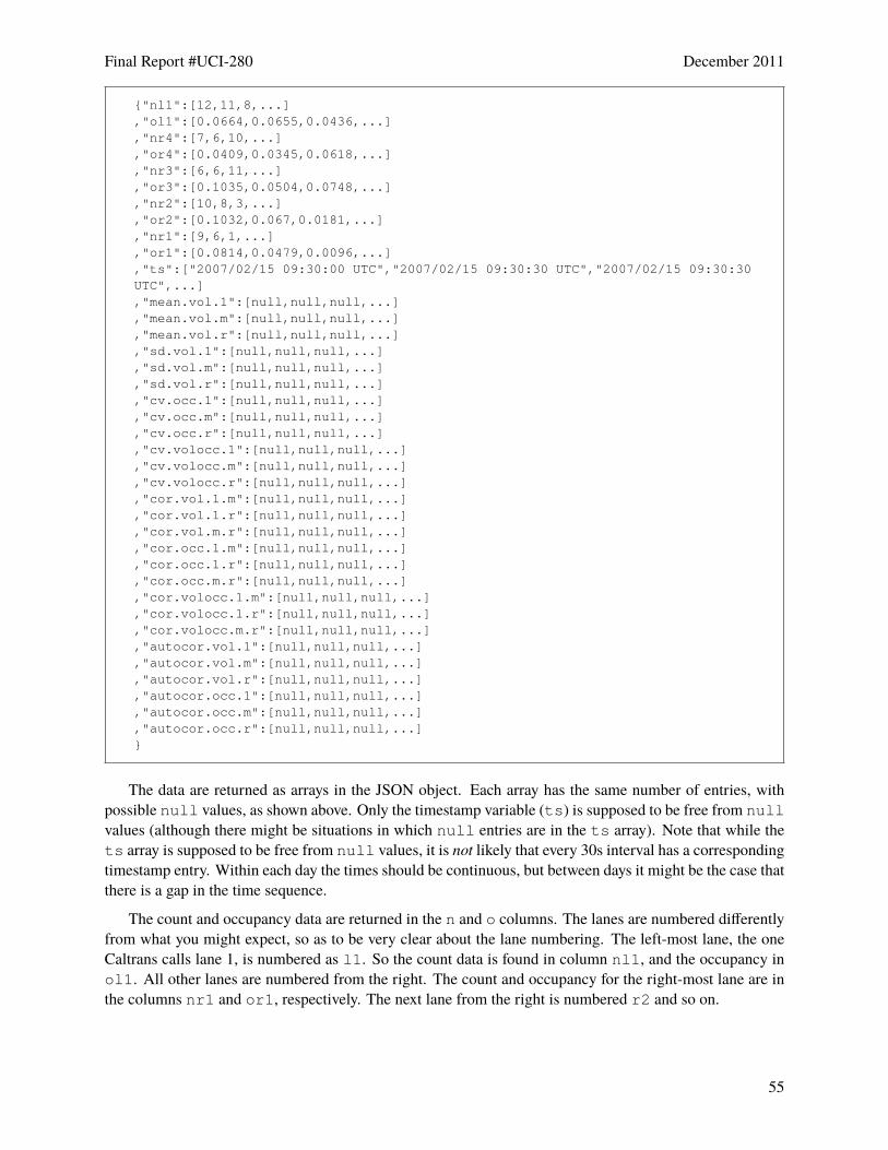
Final Report #UCI-280 December 2011
55
{"nl1":[12,11,8,...],"ol1":[0.0664,0.0655,0.0436,...],"nr4":[7,6,10,...],"or4":[0.0409,0.0345,0.0618,...],"nr3":[6,6,11,...],"or3":[0.1035,0.0504,0.0748,...],"nr2":[10,8,3,...],"or2":[0.1032,0.067,0.0181,...],"nr1":[9,6,1,...],"or1":[0.0814,0.0479,0.0096,...],"ts":["2007/02/15 09:30:00 UTC","2007/02/15 09:30:30 UTC","2007/02/15 09:30:30UTC",...],"mean.vol.1":[null,null,null,...],"mean.vol.m":[null,null,null,...],"mean.vol.r":[null,null,null,...],"sd.vol.1":[null,null,null,...],"sd.vol.m":[null,null,null,...],"sd.vol.r":[null,null,null,...],"cv.occ.1":[null,null,null,...],"cv.occ.m":[null,null,null,...],"cv.occ.r":[null,null,null,...],"cv.volocc.1":[null,null,null,...],"cv.volocc.m":[null,null,null,...],"cv.volocc.r":[null,null,null,...],"cor.vol.1.m":[null,null,null,...],"cor.vol.1.r":[null,null,null,...],"cor.vol.m.r":[null,null,null,...],"cor.occ.1.m":[null,null,null,...],"cor.occ.1.r":[null,null,null,...],"cor.occ.m.r":[null,null,null,...],"cor.volocc.1.m":[null,null,null,...],"cor.volocc.1.r":[null,null,null,...],"cor.volocc.m.r":[null,null,null,...],"autocor.vol.1":[null,null,null,...],"autocor.vol.m":[null,null,null,...],"autocor.vol.r":[null,null,null,...],"autocor.occ.1":[null,null,null,...],"autocor.occ.m":[null,null,null,...],"autocor.occ.r":[null,null,null,...]}
The data are returned as arrays in the JSON object. Each array has the same number of entries, withpossible null values, as shown above. Only the timestamp variable (ts) is supposed to be free from nullvalues (although there might be situations in which null entries are in the ts array). Note that while thets array is supposed to be free from null values, it is not likely that every 30s interval has a correspondingtimestamp entry. Within each day the times should be continuous, but between days it might be the case thatthere is a gap in the time sequence.
The count and occupancy data are returned in the n and o columns. The lanes are numbered differentlyfrom what you might expect, so as to be very clear about the lane numbering. The left-most lane, the oneCaltrans calls lane 1, is numbered as l1. So the count data is found in column nl1, and the occupancy inol1. All other lanes are numbered from the right. The count and occupancy for the right-most lane are inthe columns nr1 and or1, respectively. The next lane from the right is numbered r2 and so on.

Final Report #UCI-280 December 2011
56
Aside from being clear about which lane is which, this approach also allows comparing data from differ-ent sites with different numbers of lanes. Left lane data is always in lane l1, and right lane data is in r1.The other lane that trucks are allowed to use is always numbered r2, and so on.
Next come the so-called 27 variables that attempt to capture the temporal and spatial dynamics of thedata. These variables are the same as those described in Table 1, but they are described again below forcompleteness. These are computed using the preceding 20 minutes of data. If there is insufficient data tocompute a valid quantity, then these arrays will contain null. The other thing to notice is that there are onlythree lanes used to compute these values. Earlier research indicated that when there are 4 or more lanes at asite, the interior lanes are highly correlated with each other. It is sufficient to choose one of them. Our ruleis to pick the one with the most data, breaking ties by using the middle most lane, but cheating to the right.So on a 4 lane facility, if the number 2 and 3 lane both had equally good data, we would choose lane 3 as the“middle” lane.
mean.vol.1, mean.vol.m and mean.vol.r These three variables represent the mean vol-ume over the preceding 20 minutes.
sd.vol.1, sd.vol.m, sd.vol.r These three variables represent the standard deviation of thevolume for each lane over the preceding 20 minutes.
cv.occ.1, cv.occ.m, cv.occ.r These three variables represent the coefficient of variationof occupancy for each lane. This is a measure of central tendency that is used because the mean ofoccupancy (a ratio) isn’t meaningful.
cv.volocc.1, cv.volocc.m, cv.volocc.r These three variables represent the coefficientof variation of the ratio of volume to occupancy. Volume over occupancy is proportional to speed, butfor a calibration constant. Thus this measure captures the same characteristic of traffic as if one wereto measure the mean speed over the 20 minute period for each lane.
cor.vol.1.m, cor.vol.1.r, cor.vol.m.r These three variables represent the correlationof volume between lanes. The first value measure the correlation between lane 1 and the middle lane;the second the correlation between lane 1 and the right lane; and the third the correlation betweenvolumes in the middle and right lanes.
cor.occ.1.m, cor.occ.1.r, cor.occ.m.r These three variables represent the correlationof occupancy between lanes over the 20 minute period.
cor.volocc.1.m, cor.volocc.1.r, cor.volocc.m.r These three variables represent thecorrelation of the ratio of volume to occupancy between lanes for the preceding 20 minutes. For ex-ample, a negative value for cor.volocc.1.r would indicate that the speed in the fast lane (lane 1) isnegatively correlated with the speed in the slow lane (lane r). This might happen for example if aramp is slowing up the right lane, and cars are using the left lanes to speed around the congestion.
autocor.vol.1, autocor.vol.m, autocor.vol.r These three variables represent the au-tocorrelation of volume within each lane. These measures capture the trend over time for the volumewithin a lane. This isn’t a true measure of autocorrelation, but rather is computed using only theone-time-step lag value. Other ways to compute autocorrelation can use multiple lags between times,but we found just using the one-time-step lag to be sufficient as well as easier to compute.

Final Report #UCI-280 December 2011
57
autocor.occ.1, autocor.occ.m, autocor.occ.r These three variables represent the au-tocorrelation of occupancy within each lane. These capture the trend over time for the occupancy ofa lane.
9.4.2 Safety probability predictions format
For ease of use, there are three kinds of probability downloads available. The first is to get every 30-secondprediction for a single day. For example, the link:
http://ara.ctmlabs.net/risk/1209289/2007/01/02/30s.json
will return a JSON object containing a list of probabilities for any accident for January 2, 2009. Theoverall format follows CouchDB’s conventions for returning data from a view, with the “rows” element ofthe object containing the rows of data. Each row’s “value” element contains the timestamp and the accidentprobability predicted for that timestamp. For the three models that have multiple outcomes, the responserows will be arrays instead of a single number, with each object containing the predicted probability for eachoutcome. The order of each outcome is always the same, but in case one forgets or in case a new model iscreated, a special query can be made to the URL pattern /severity/header.json which will returnthe array [PDO,Injury]. Multiple days can be selected one at a time, or by requesting an entire monthat once by not specifying the day.
The second URL scheme for getting accident probabilities is to request daily cumulative sum values fora year. This URL format has the pattern:
http://ara.ctmlabs.net/risk/1209289/2007/dailysum.json
As the end of the URL implies, this request will return the minimum, maximum, and mean accidentprobabilities for each day in the chosen year. This request would be used to see at a glance how one detectorcompares to others over the course of a year.
The final URL query pattern that has been implemented is to get all of the daily summed values for allmodeled detectors (in practice, all of District 12 mainline detectors). This URL pattern takes the form:
http://ara.ctmlabs.net/risk/all/2008/10/04/sum.json
The URL is different than the prior ones in that the detector number has been replaced with the word“all”. As before, the “minmaxmean” part of the URL is a reminder that the data will be returned as rowscontaining the minimum, maximum, and mean accident probabilities for each detector. In this case, an extrafield will be returned in the result rows indicating the detector number. As an added bonus, an entire monthof data or even an entire year of minimum, maximum, and mean values can be downloaded all at once byskipping the day and month parts of the URL. This is a lot of data, however, and is useful only for an off-lineanalysis. This kind of query would slow down something like a web application.
In all cases, in order to select a different accident probability model than any accident, the word “risk”in the URL should be replaced with the desired model. For example, “severity” will return the minimum,maximum, and mean values for the severity predictions. Because severity has two outcomes (PDO andInjury) and the other models also have more than one outcome, the result rows of the non-“risk” URLs arearrays of triplets, with each triplet giving the minimum, maximum, and mean prediction for each outcomein the order defined by the call to the “header.json” query mentioned above. In this case, first will be the“PDO” triplet, and then the “Injury” triplet giving the minimum, maximum, and mean predictions for eachmodel outcome for the day.

Final Report #UCI-280 December 2011
58
Section 10: Conclusion, recommendations and deployment
This project has updated and deployed a tool for analyzing the risk of accidents on freeways. The tool canbe used to measure the impacts of any large scale change to the freeway (for example, a new intelligenttransportation systems (ITS) deployment) on the aggregate safety of the roadway. The safety models wereestimated on 2007 data, validated against 2008 accident observations, and have been deployed in a systemthat can process new data on request. Both a website and scriptable web services have been deployed. Thewebsite provides a map-based interface to the safety models and data, and a freeway-specific view intothe model output. The JavaScript files included in the website also provide a working model of how newapplications can access the tool’s web services. The web services allow other projects and tools to accesseverything from raw data, to intermediate results, to the final safety predictions so as to incorporate theinformation into new projects.
The validation study verified that the aggregate predictions of the models are roughly in line with theobserved accident rates and proportions. The models do not do well in predicting time of day effects onaccident risk, which was disappointing but expected. One interesting result of the validation study is thatthe 4 toll roads in District 12 do not have the same characteristics as regular, non-tolled facilities. This isperhaps due to the different mix of traffic (heavy duty trucks do not use toll roads as a rule), as well as themore rural character of these particular tolled facilities. In the future separate models should be estimatedfor toll roads and regular facilities.
10.1 Short term recommendations
The tool’s elements (the website and the data services) are currently available only to properly authenticatedusers. This policy was established for all CTMLabs projects, as befits early stage deployments and researchtools. The special concern with this project is that the output may be misunderstood by the public at large.
But there is no special reason why the data should not eventually be made broadly available. As theaccident probabilities change over time, the changes reflect the behavior of the drivers on the freeway. Thepurpose of providing the safety information to drivers isn’t to predict when and where an accident willoccur. The probability of an accident at any given time is minuscule, as shown in the many figures generatedin Section 7 of this report. Instead, providing the safety performance information to drivers is a way ofcompleting the loop. Drivers react to traffic as conditions get safer or riskier. If drivers are aware of thepossible impacts of their aggregate behavior, they might choose to drive more safely.
The second recommendation is for Caltrans staff to attempt to use the tool in a small before and afterstudy. The tool has already been integrated into the offerings of the California Traffic Management Labs(CTMLabs) at UC Irvine, and is available to anyone with a valid account, which would include anyone atCaltrans wishing to create an account. CTMLabs staff will willingly support any work by Caltrans to evaluatethe tool’s suitability in adding a safety dimension to the evaluation of the impacts of freeway projects.
10.2 Deployment to other Caltrans Districts
The tool and models can be deployed to other Caltrans Districts without too much difficulty. The data storageframework can be adopted as is, and will scale roughly linearly with the numbers of detectors in the new

Final Report #UCI-280 December 2011
59
District. After processing 3 years of data, District 12 requires approximately 800 GB of disk storage. District7 would be larger, but most other Districts would probably require no more than 500 GB of storage spaceper year. Because each detector is assigned its own CouchDB database to store the 30 second data (rawvalues and computed 27 variables), these databases can easily be migrated to multiple machines if the spacerequirements or computational load on a single server becomes too great. Virtual services offered by variousCloud computing companies can also be used to store data, as long as the company offered CouchDB storagefacilities.
As part of the request to the HSIS data repository, we received accident data for all of California from2007 and 2008. Therefore the only new data for each new District would be the raw detector data. Once theraw data is downloaded from the PeMS data repository for 2007, new models can be estimated that capturethe driving habits of each District’s drivers. We recommend that new models be estimated because we donot have any evidence to suggest that the models can be transferred directly to other regions. Because themethodology attempts to capture the behavior of drivers in relation to other drivers, any possible regionaldifferences in driving styles must be taken into account. Finally, noting the poor validation results for tollroads, separate models should be estimated for any unique facilities in a district, such as toll roads or longbridges.
The website and associated tools are largely agnostic to the District. The current tool presents datafor just District 12, but that is only because there are only model outputs for detectors within District 12.CTMLabs has meta data for all detectors in California, and so the exact same website can be used to browsethe predictions from other Districts once they are stored in the aggregate CouchDB database.

Final Report #UCI-280 December 2011
60
Section 11: References
Council, F. M. and Mohamedshah, Y. M. (2007). Highway Safety Information System: Guidebook for theCalifornia State Data Files. .Federal Highway Administration, U.S. Department of TransportationAccessed January, 2012 at http://www.hsisinfo.org/pdf/guidebook_CA.pdf.
Varaiya, P. (2001). Freeway performance measurement system, PeMS V3, phase 1: Final report. Tech-nical Report California PATH Program, Institute of Transportation Studies, University of CaliforniaBerkeley.
Fielding, R. T. (2000). Architectural Styles and the Design of Network-based Software Architectures. PhDthesis, University of California, Irvine.
Golob, T., Marca, J. and Recker, W. (2007). Implementation of a tool for measuring ITS impacts on freewaysafety performance. Technical Report Irvine, CA: Institute of Transportation Studies, University ofCalifornia. Final Report prepared for California Partners for Advanced Transit and Highways (PATH)Task Order 5307.
Golob, T. and Recker, W. (2003). Relationships among urban freeway accidents, traffic flow, weather andlighting conditions. ASCE Journal of Transportation Engineering, 129, 342–353.
Golob, T. and Recker, W. (2004). A method for relating type of crash to traffic flow characteristics on urbanfreeways. Transportation Research, Part A, 38, 53–80.
Golob, T., Recker, W. and Alvarez, V. (2002). Freeway safety as a function of traffic flow: The FITS tool forevaluating ATMS operations. Technical Report Irvine, CA: Institute of Transportation Studies, Uni-versity of California. Final Report prepared for California Partners for Advanced Transit and Highways(PATH).
Golob, T., Recker, W. and Alvarez, V. (2004a). A tool to evaluate the safety effects of changes in freewaytraffic flow. ASCE Journal of Transportation Engineering, 130, 222–230.
Golob, T., Recker, W. and Alvarez, V. (2004b). Freeway safety as a function of traffic flow. Accident Analysisand Prevention, 36, 933–946.
Golob, T., Recker, W. and Pavlis, I. (2008). Probabilistic models of freeway safety performance using trafficflow data as predictors. Safety Science, 46(9), 1306–1333.
Abdel-Aty, M. and Pande, A. (2005). Identifying crash propensity using specific traffic speed conditions.Journal of Safety Research, 36(1), 97–108.
Abdel-Aty, M., Uddin, N. and Pande, A. (2005). Split models for predicting multi-vehicle crashes duringhigh-speed and low-speed operating conditions on freeways. Journal of the Transportation ResearchBoard, 1908, 51–58.
Caltrans and BTS (2012). Freeway performance measurement system. . http://pems.dot.ca.gov/, accessedJanuary, 2012.
Choe, T., Skabardonis, A. and Varaiya, P. (2002). Freeway performance measurement system (PeMS):An operational analysis tool. In Presented at Annual Meeting of the Transportation Research Board,January 13-17, Washington, DC .
Varaiya, P. (2005). What we have learned about highway congestion.. Technical Report Institute of Trans-portation Studies, University of California Berkeley. accessed May 12, 2005.
Dean, J. and Ghemawat, S. (2008). MapReduce: Simplified data processing on large clusters. Communica-tions of the ACM, 51(1), 107–113.
R Development Core Team (2011). R: A Language and Environment for Statistical Computing. Vienna,Austria.: R Foundation for Statistical Computing ISBN 3-900051-07-0.

Final Report #UCI-280 December 2011
61
Appendix A: HSIS accident data database schema
The HSIS accident data is all loaded into the hsis schema in the PostgreSQL database. Each table is definedbelow, but note that the PostgreSQL loading script issues the command SET search_path = hsis,pg_catalog; prior to running the CREATE TABLE commands. This means that even though it isn’texplicitly written, each table should be understood to have the schema identifier hsis. prepended to thetable name.
The primary table for all HSIS data is the cases table. This stores the primary key for accidents, andallows one to piece together all of the information pertaining to a single accident.
create table hsis.cases (
caseno varchar(36) not null primary key);
Accident data itself is stored in the acc table.
CREATE TABLE hsis.acc (
id serial primary key,
cntyrte varchar(20),
milepost numeric,
rodwycls varchar(20) references hsis.rodwycls(id) on delete restrict,
caseno varchar(36) references hsis.cases on delete restrict,
psmilprf varchar(20) references hsis.psmilprf(id) on delete restrict,
psmilsuf varchar(20) references hsis.psmilsuf(id) on delete restrict,
acctype varchar(20) references hsis.acctype(id) on delete restrict,
acc_ts timestamp with time zone,
hour_known boolean,
weather1 varchar(20) references hsis.weather(id) on delete restrict,
weather2 varchar(20) references hsis.weather(id) on delete restrict,
loc_typ varchar(20) references hsis.loctyp(id) on delete restrict,
sde_hwy varchar(20) references hsis.sdehwy(id) on delete restrict,
towaway boolean,
severity varchar(20) references hsis.severity(id) on delete restrict,
rdsurf varchar(20) references hsis.rdsurf(id) on delete restrict,
light varchar(20) references hsis.light(id) on delete restrict,
trk_inv boolean,
mtcy_inv boolean,
distance integer,
numvehs integer);
The vehicle information, incluing the direction of travel of each vehicle involved in the accident, is storedin the hsis.veh table. The direction of travel is coded up in the hsis.dirtrvl table. Because morethan 4 vehicles might be involved in an accident, a join on caseno might pull in more than one record fromthe vehicle table.
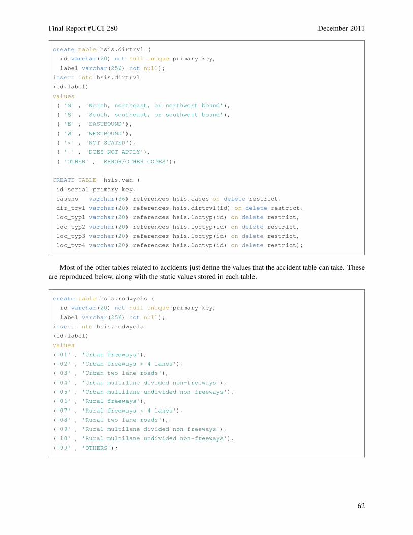
Final Report #UCI-280 December 2011
62
create table hsis.dirtrvl (
id varchar(20) not null unique primary key,
label varchar(256) not null);
insert into hsis.dirtrvl
(id,label)
values
( 'N' , 'North, northeast, or northwest bound'),
( 'S' , 'South, southeast, or southwest bound'),
( 'E' , 'EASTBOUND'),
( 'W' , 'WESTBOUND'),
( '<' , 'NOT STATED'),
( '-' , 'DOES NOT APPLY'),
( 'OTHER' , 'ERROR/OTHER CODES');
CREATE TABLE hsis.veh (
id serial primary key,
caseno varchar(36) references hsis.cases on delete restrict,
dir_trvl varchar(20) references hsis.dirtrvl(id) on delete restrict,
loc_typ1 varchar(20) references hsis.loctyp(id) on delete restrict,
loc_typ2 varchar(20) references hsis.loctyp(id) on delete restrict,
loc_typ3 varchar(20) references hsis.loctyp(id) on delete restrict,
loc_typ4 varchar(20) references hsis.loctyp(id) on delete restrict);
Most of the other tables related to accidents just define the values that the accident table can take. Theseare reproduced below, along with the static values stored in each table.
create table hsis.rodwycls (
id varchar(20) not null unique primary key,
label varchar(256) not null);
insert into hsis.rodwycls
(id,label)
values
('01' , 'Urban freeways'),
('02' , 'Urban freeways < 4 lanes'),
('03' , 'Urban two lane roads'),
('04' , 'Urban multilane divided non-freeways'),
('05' , 'Urban multilane undivided non-freeways'),
('06' , 'Rural freeways'),
('07' , 'Rural freeways < 4 lanes'),
('08' , 'Rural two lane roads'),
('09' , 'Rural multilane divided non-freeways'),
('10' , 'Rural multilane undivided non-freeways'),
('99' , 'OTHERS');

Final Report #UCI-280 December 2011
63
create table hsis.psmilprf (
id varchar(20) unique not null primary key,
label varchar (256) not null);
insert into hsis.psmilprf
(id,label)
values
(' ' , 'NO PREFIX'),
('A' , 'REPOSTED'),
('B' , 'BUS LANE'),
('C' , 'COMMERCIAL'),
('D' , 'Duplicate (meandering)'),
('F' , 'Reposted - Commercial (C)'),
('G' , 'Reposted - Duplicate (D)'),
('H' , 'Realigned - Duplicate (D)'),
('J' , 'Reposted, realigned - Duplicate'),
('K' , 'Reposted - Overlap (L)'),
('L' , 'Overlapping Postmiles'),
('M' , 'Realigned realignment (R)'),
('N' , 'Reposted, realighned realignment (M)'),
('P' , 'Reposted realignment (R)'),
('Q' , 'Reposted - Spur (S)'),
('R' , 'REALIGNMENT' ),
('S' , 'SPUR'),
('T' , 'Temporary Connection'),
('U' , 'Reposted - Temporary connection (T)'),
('-' , 'INVALID DATA'),
('+' , 'NO DATA'),
('OTHER' , 'ERROR/OTHER CODES');
create table hsis.psmilsuf (
id varchar(20) unique not null primary key,
label varchar (256) not null);
insert into hsis.psmilsuf
(id,label)
values
( ' ' , 'NO SUFFIX'),
( 'E' , 'EQUATION'),
( '-' , 'INVALID DATA'),
( '+' , 'NO DATA'),
( 'OTHER' , 'ERROR/OTHER CODES'),
('L' , 'Overlapping Postmiles'),
('R' , 'REALIGNMENT' );

Final Report #UCI-280 December 2011
64
create table hsis.acctype (
id varchar(20) unique not null primary key,
label varchar (256) not null);
insert into hsis.acctype
(id,label)
values
( 'A' , 'HEAD-ON'),
( 'B' , 'SIDESWIPE'),
( 'C' , 'REAR END'),
( 'D' , 'BROADSIDE'),
( 'E' , 'HIT OBJECT'),
( 'F' , 'OVERTURNED'),
( 'G' , 'AUTO-PEDESTRIAN'),
( 'H' , 'OTHER'),
( '-' , 'NOT STATED'),
( 'OTHER' , 'ERROR/OTHER CODES');
create table hsis.weather (
id varchar(20) unique not null primary key,
label varchar (256) not null);
insert into hsis.weather
(id,label)
values
( 'A' , 'CLEAR'),
( 'B' , 'CLOUDY'),
( 'C' , 'RAINING'),
( 'D' , 'SNOWING'),
( 'E' , 'FOG'),
( 'F' , 'OTHER'),
( 'G' , 'WIND'),
( '-' , 'NOT STATED'),
( 'OTHER' , 'ERROR/OTHER CODES');

Final Report #UCI-280 December 2011
65
create table hsis.loctyp (
id varchar(20) unique not null primary key,
label varchar (256) not null);
insert into hsis.loctyp
(id,label)
values
( 'A' , $$Beyond median or barrier stripe - driver's left$$),
( 'B' , $$Beyond shoulder - driver's left$$),
( 'C' , 'Left shoulder area'),
( 'D' , 'Left lane'),
( 'E' , 'Interior lanes'),
( 'F' , 'Right lane'),
( 'G' , 'Right shoulder area'),
( 'H' , $$Beyond shoulder - driver's right$$),
( 'I' , 'Gore area'),
( 'J' , 'Other'),
( '<' , 'Not stated'),
( 'V' , 'undefined by hsis' ),
( 'W' , 'undefined by hsis' ),
( '---' 'undefined by hsis' ),
( '-' , 'Does not apply'),
( 'OTHER' , 'ERROR/OTHER CODES');
create table hsis.sdehwy (
id varchar(20) unique not null primary key,
label varchar (256) not null);
insert into hsis.sdehwy
(id,label)
values
( 'N' , 'NORTHBOUND'),
( 'S' , 'SOUTHBOUND'),
( 'E' , 'EASTBOUND'),
( 'W' , 'WESTBOUND'),
( 'OTHER' , 'ERROR/OTHER CODES');

Final Report #UCI-280 December 2011
66
create table hsis.severity (
id varchar(20) unique not null primary key,
label varchar (256) not null);
insert into hsis.severity
(id,label)
values
( '1' , 'FATAL'),
( '2' , 'SEVERE INJURY'),
( '3' , 'Other visible injury'),
( '4' , 'Complaint of pain'),
( '0' , 'PDO - Property damage only'),
( 'OTHER' , 'ERROR/OTHER CODES');
create table hsis.rdsurf (
id varchar(20) unique not null primary key,
label varchar (256) not null);
insert into hsis.rdsurf
(id,label)
values
( 'A' , 'DRY'),
( 'B' , 'WET'),
( 'C' , 'SNOWY, ICY'),
( 'D' , 'SLIPPERY/MUDDY'),
( '-' , 'NOT STATED'),
( 'OTHER' , 'ERROR/OTHER CODES');
create table hsis.light (
id varchar(20) unique not null primary key,
label varchar (256) not null);
insert into hsis.light
(id,label)
values
( 'A' , 'Daylight'),
( 'B' , 'Dusk - dawn'),
( 'C' , 'Dark - street lights'),
( 'D' , 'Dark - no street lights'),
( 'E' , 'Dark - street lights not functioning'),
( 'F' , 'Dark - not stated'),
( '-' , 'Not stated'),
( 'OTHER' , 'ERROR/OTHER CODES');
HSIS also categorizes and saves the network information related to each accident it stores. The followingtables relate to the road network data.

Final Report #UCI-280 December 2011
67
create table hsis.access (
id varchar(20) not null unique primary key,
label varchar(256) not null);
insert into hsis.access
(id,label)
values
( 'C' , 'Conventional - No access control'),
( 'E' , 'Expressway - Partial access control'),
( 'F' , 'Freeway - Full access control'),
( 'S' , 'One-way city street - no access control'),
( '-' , 'INVALID DATA'),
( '+' , 'NO DATA'),
( 'OTHER' , 'ERROR/OTHER CODES');
create table hsis.rte_suf (
id varchar(20) not null unique primary key,
label varchar(256) not null);
insert into hsis.rte_suf
(id,label)
values
( 'P' , 'ALIGNMENT PRIOR'),
( 'S' , 'Supplemental alignment, partial opened for use before alignment is
complete'),
( 'U' , 'Unrelinquished, superseded by realignment, but not yet accepted for
non-State-highway maintenance'),
( 'Z' , 'Budgeted or under construction'),
( ' ' , 'NO SUFFIX'),
( 'OTHER' , 'ERROR/OTHER CODES');

Final Report #UCI-280 December 2011
68
create table hsis.county (
id varchar(20) not null unique primary key,
label varchar(256) not null);
insert into hsis.county
(id,label)
values
( '01' , 'ALAMEDA'), ( '02' , 'ALPINE'), ( '03' , 'AMADOR'),
( '04' , 'BUTTE'), ( '05' , 'CALAVERAS'), ( '06' , 'COLUSA'),
( '07' , 'CONTRA COSTA'), ( '08' , 'DEL NORTE'),
( '09' , 'EL DORADO'), ( '10' , 'FRESNO'), ( '11' , 'GLENN'),
( '12' , 'HUMBOLDT'), ( '13' , 'IMPERIAL'), ( '14' , 'INYO'),
( '15' , 'KERN'), ( '16' , 'KINGS'), ( '17' , 'LAKE'),
( '18' , 'LASSEN'), ( '19' , 'LOS ANGELES'), ( '20' , 'MADERA'),
( '21' , 'MARIN'), ( '22' , 'MARIPOSA'), ( '23' , 'MENDOCINO'),
( '24' , 'MERCED'), ( '25' , 'MODOC'), ( '26' , 'MONO'),
( '27' , 'MONTEREY'), ( '28' , 'NAPA'), ( '29' , 'NEVADA'),
( '30' , 'ORANGE'), ( '31' , 'PLACER'), ( '32' , 'PLUMAS'),
( '33' , 'RIVERSIDE'), ( '34' , 'SACRAMENTO'),
( '35' , 'SAN BENITO'), ( '36' , 'SAN BERNARDINO'),
( '37' , 'SAN DIEGO'), ( '38' , 'SAN FRANCISCO'),
( '39' , 'SAN JOAQUIN'), ( '40' , 'SAN LUIS OBISPO'),
( '41' , 'SAN MATEO'), ( '42' , 'SANTA BARBARA'),
( '43' , 'SANTA CLARA'), ( '44' , 'SANTA CRUZ'),
( '45' , 'SHASTA'), ( '46' , 'SIERRA'), ( '47' , 'SISKIYHOU'),
( '48' , 'SOLANO'), ( '49' , 'SONOMA'), ( '50' , 'STANISLAUS'),
( '51' , 'SUTTER'), ( '52' , 'TEHAMA'), ( '53' , 'TRINITY'),
( '54' , 'TULARE'), ( '55' , 'TUOLUME'), ( '56' , 'VENTURA'),
( '57' , 'YOLO'), ( '58' , 'YUBA');
create table hsis.hwygrp (
id varchar(20) not null unique primary key,
label varchar(256) not null);
insert into hsis.hwygrp
(id,label)
values
( 'R' , 'Right independent alignment'),
( 'L' , 'Left independent alignment'),
( 'D' , 'DIVIDED HIGHWAY'),
( 'U' , 'UNIDIVIDED HIGHWY'),
( 'X' , 'UNCONSTRUCTED' ),
( 'Z' , 'OTHER'),
( '-' , 'INVALID DATA'),
( '+' , 'NO DATA'),
( 'OTHER' , 'ERROR/OTHER CODES');

Final Report #UCI-280 December 2011
69
create table hsis.dspd (
spd integer not null unique primary key,
label varchar(256) not null);
insert into hsis.dspd
(spd,label)
values
( 25 , '< 30 MPH'),
( 30 , '30 MPH'),
( 35 , '35 MPH'),
( 40 , '40 MPH'),
( 45 , '45 MPH'),
( 50 , '50 MPH'),
( 55 , '55 MPH'),
( 60 , '60 MPH'),
( 65 , '65 MPH'),
( 70 , '> 70 MPH');
create table hsis.numlanes (
id integer not null unique primary key,
label varchar(256) not null);
insert into hsis.numlanes
(id,label)
values
( 1 , 'ONE LANE'),
( 2 , 'TWO LANES'),
( 3 , 'THREE LANES'),
( 4 , '4 TO 6 LANES'),
( 7 , '7 TO 8 LANES'),
( 9 , '> 8 LANES'),
( -1 , 'NOT STATED');

Final Report #UCI-280 December 2011
70
create table hsis.road (
id serial primary key,
yr integer,
access varchar(20) references hsis.access(id) on delete restrict,
begmp numeric,
endmp numeric,
city varchar(20),
cntyrte varchar(20) not null,
district integer,
rte_nbr integer,
rte_suf varchar(20) references hsis.rte_suf(id) on delete restrict,
county varchar(2) references hsis.county(id) on delete restrict,
psmilprf varchar(20) references hsis.psmilprf(id) on delete restrict,
hwy_grp varchar(20) references hsis.hwygrp(id) on delete restrict,
dspd integer references hsis.dspd(spd) on delete restrict,
divided boolean,
num_lane1 integer,
num_lane2 integer,
num_lanes integer,
rd_desc varchar(64),
ro_seq numeric,
rodwycls varchar(20) references hsis.rodwycls(id) on delete restrict);
Finally, there are join tables linking HSIS data with other tables. The caseno_vds table stores thelinking of VDS loop detectors with each accident case number, based on the postmile and highway of theaccident and the detector.
CREATE TABLE caseno_vds (
caseno character varying(36),
vds_id integer,
diff numeric,
keep boolean DEFAULT false);