final report on the petrology of the sonju lake intrusionmille066/teaching/2312/sonju report/sonju...

Final Report on the Petrology of the Sonju Lake Intrusion GEOL 2312 Spring 16

Page | 1

Geol 2312 - Petrology DUE DATE - TUESDAY MAY 3

Final Report on the Petrology of the Sonju Lake intrusion

Introduction Throughout the course of the lab, we have focussed much of our attention on rocks from the Sonju Lake Intrusion (SLI). You should by now be familiar with the basic petrographic characteristics (mineralogy and textures) of these rocks. You should also have developed an appreciation of how the Fe/Mg ratio of olivine and pyroxene increase up through the SLI from the SEM work. You were also shown how to use Excel and IGPET programs to create various plots of geochemical data. And, you were introduced to ways of using mass balance to calculate bulk compositions and liquid lines of descent of differentiated magma systems. With this skill set, you should now be ready to pull together your observational and quantitative data into a somewhat rigorous petrologic summary and interpretation of this unique mafic layered intrusion. While I will guide you through most of the steps that will create the elements of this report, you will be creating a scaled-down version of the type of petrologic report that you might produce for a thesis dissertation or even a professional publication.

Background The magmatic processes that create mafic layered intrusions are believed to be responsible for creating much of the compositional diversity of igneous rocks. By the basic process of fractional crystallization of a mafic magma, a broad range of differentiated magma compositions can be produced that may result ultimately in a highly siliceous felsic liquid. However, the differentiation path of magmas over the course of fractional crystallization, its liquid line of descent, will be distinctive in a given intrusion and depend on factors such as parental magma composition, depth of emplacement (pressure), ambient temperature of the country rock, size and shape of the intrusion, its openness to magma recharge and volcanic venting, and the potential for contamination by the country rock. These factors will control what cumulus mineral phases crystallize, in what order, and with what efficiency of separation (fractionation), which in turn control the path of magma differentiation.

The Sonju Lake intrusion is part of the Beaver Bay Complex — a hypabyssal, multiple-intrusive igneous complex that was emplaced into comagmatic volcanics during the development of the 1.1 billion-year old Midcontinent Rift in northeastern Minnesota. The SLI is an approximately 1 km-thick mafic layered intrusion that occurs as a southward-dipping, sheet-like body between granitic rocks (Finland Granophyre) above and older gabbroic and basaltic rocks below (see Fig. 1 and the 1:24,000 Finland-Doyle Lake map provided). The SLI displays a unidirectional progression of cumulate rock types upsection (north to south) that are consistent with fractional crystallization of a mafic magma from the floor upward under nearly closed conditions (i.e., negligible magmatic recharge, assimilation, or venting). Because of the sheet-like shape, complete exposure, and unidirectional differentiation of the SLI, we are able to make reasonably accurate estimates of its parent magma composition and determine its liquid line of descent. This liquid line of descent will be compared with the compositions of genetically-related volcanic rocks of the Midcontinent Rift to determine if the differentiation similar to that observed in the SLI might have given rise to some of the compositional diversity of the rift lavas. In addition, we have the opportunity to evaluate whether the Finland granite overlying the mafic cumulates is related to the SLI, representing a late stage differentiated magma composition. The amount of felsic magma that can be generated by the differentiation of a mafic magma has long been a point of contention among petrologists studying mafic layered intrusions. In fact, this question has recently sparked a heated debate about the differentiation history of one of the most intensely studied mafic intrusion on earth - the Skaergaard of East Greenland. However, evaluating the genetic relationship of the SLI and the Finland granite is best approached with isotopic data, so we will forego that evaluation here. (Do I hear a collective sigh of relief?)


Page | 2

Components of the Final Report

By the due date (May 3rd), you will be required to turn in two principal components that will comprise your final report:

1) A completed Excel spreadsheet containing six worksheets that summarize and manipulate stratigraphic, petrographic, mineral chemical and whole rock geochemical data from the SLI.

2) A final report composed in Word that contains all the background information, descriptions, figures, interpretations, and appendices requested. There is no set number of pages that this final report must be. Rather, I am looking for completeness of descriptions and figures and reasonableness of interpretation. If you can do this with an economy of words and good grammar, that is ideal.

Be sure to read the instructions below carefully. It will make the writing of your report go much easier when you know what is being requested. If you have any questions about any aspect of constructing this report DO NOT HESITATE TO ASK ME. There will be lots of opportunities during the last two weeks of April to work on the report in lab and to ask me questions.

PART I : COMPILATION, PROCESSING, AND PLOTTING OF STRATIGRAPHIC, PETROGRAPHIC AND GEOCHEMICAL DATA

In this part, you will compile, process, and plot data within the Excel file (SLI worksheet.xls) that will form the bases of your descriptions and petrologic interpretations of the Sonju Lake Intrusion. It will make the most sense to proceed with the following exercises in the order that they are presented below. A. Determining the Stratigraphic Height of Samples

Objective: In order to portray the variation in mineralogic, textural, mineral chemical and geochemical attributes stratigraphically upwards through the intrusion, we need to determine the stratigraphic heights of samples and unit contacts.

Need: Worksheet Strat Ht, 2 Geologic Maps w/ sample locations – Northern Traverse Area.pdf, Southern Traverse Area.pdf, and a ruler.

Procedure: On the two geologic maps are plotted the locations of all samples that collectively profile the entire SLI and are used in various parts of this study. Rather than determining the height above the basal contact, we hang our stratigraphic column on a datum horizon within the intrusion. We will choose the horizon where augite becomes a cumulus phase (i.e., where it changes from ophitic to granular in habit; i.e., the slt-slg contact). Samples above this datum will have positive values; samples below will be negative.

Because samples from the northern and southern parts of the intrusion were not collected along a co-linear profile, we will determine the stratigraphic height of samples projected to two different profile lines, both of which cross the slt-slg contact. For each profile, you should project the sample points toward the profile line parallel to the local strike of the internal layering and foliation (if it is locally variable, figure an average strike; if the sample lies close to a geologic contact, use the trend (strike) of the contact as a guide – NEVER CROSS A GEOLOGIC CONTACT WITH YOUR PROJECTION LINE). Draw this projection line on the map to where it intersects your profile line. Do this for all samples on both profiles.

Next, measure the distance in meters (see scale on maps) from where the slt-slg contact crosses the profile line to where each sample projection line and each contact intersects the profile line. Enter these distances in column C of the “Strat Ht” worksheet. Remember that for the northern profile, enter NEGATIVE values.


Page | 3

Next, determine the average dip angle of layering and foliation in the vicinity of the north and the south profile lines. Enter the average dip for the northern profile into column D cells 5 to 22. Enter the average dip for the southern profile into column D cells 23-43.

When the distance and dip angle values are entered, you should see that the stratigraphic height above cumulus augite arrival (MAAA –meters above augite arrival) should be given in column E. Note that the formula in column E multiplies the distance (D) by the sin of the dip angle (θ) to determine the stratigraphic height (SH) as shown in the diagram below (Fig. 1) showing the profile line in cross section .

Profile Line (in profile)

SH = D * Sin θ Figure 1. Cross sectional view along a sample profile line showing the relationship of the ground

distance (D) between samples (dots), the dip angle (θ), and the stratigraphic height between the samples (SH).

B. Determining the Bulk Composition of the SLI

Objective: Because the SLI is a tabular-shaped intrusion of much greater width and breadth than height, we can assume that a columnar profile through the intrusion would show the same stratigraphy of units everywhere. Therefore, if we can determine the composition of any such column, this should be close to the bulk composition of the entire intrusion. Furthermore, if we assume that the intrusion crystallized as a closed system (nothing more was added, nothing left), then we can interpret this bulk composition as being a reasonable estimate of the parent magma.

Need: Worksheets Strat Ht and PM Calc. Procedure: On the Strat Ht worksheet, samples for which there are whole rock analyses are

highlighted in yellow. We will use the sample to serve as representative compositions of intervals in the stratigraphic column. To do this we, must determine the upper and lower boundaries of these intervals within the stratigraphic column (Fig. 2). We can use several things to guide us in selecting these boundaries. One is that if a sample is close to a unit contact, that will be one of the boundaries (CTC in Fig. 2). For a sample within a map unit, we can take the midpoint between the stratigraphic heights of adjacent samples (SAM in Fig. 2). But really, the exact location of the interval boundaries between samples is not critical.

SH SH SH θ θ θ

D D D

CTC

CTC

SAM

SAM

A

B

C

A -upper

A – lower / B – upper B – lower / C – upper C - lower

Figure 2. Schematic diagram showing strategies for defining the upper and lower boundaries of sample intervals


Page | 4

Estimate the upper and lower boundaries of the stratigraphic intervals that each of the 19 whole rocks-analyzed sample represents. Enter these heights in columns F and G. Again, the samples from the northern profile should have negative stratigraphic heights and the lower boundary of one sample should correspond to the upper boundary of the sample below it.

Once you have these values estimated, determine the stratigraphic thickness of each sample interval (column G – column F) in column H (formula already in cell H28). Note that the total thickness of the intrusion is calculated in Cell H52 by summing the thicknesses of the individual sample intervals.

In column I, determine the percentage that each sample interval represents relative to the entire intrusion. As shown in cell I28, this corresponds to the interval thickness divided the total intrusion thickness ($H$52) and then formatted as a percentage. Insert this formula into all the yellow cells in column I. If you did the calculations in column I correctly, the total percentage of the individual sample intervals should total to 100% in cell I52.

Open worksheet PM calc by clicking on its tab in the lower left of the worksheet. This worksheet list all the samples for which there are whole rock chemical analyses. Major and minor oxides (in wt.%) are listed at in the upper part of the worksheet and trace element abundances (in parts per million – ppm) are listed in the lower half of the worksheet. Note that the mg# (= MgO/(MgO+FeOt), mole%) is calculated for each analysis for the typical range of Fe+2/Fe+3 found in most mafic magmas (Row 20 assumes 85% of the iron is as Fe+2 and Row 21 assumes 90% of the iron is ferrous). You should see that all the values for the stratigraphic height, the thickness of each sample interval, and the percentage that each interval represents of the total intrusion (all values that you calculated in the Strat Ht worksheet) have been transferred to rows 5, 6, and 7, respectively (you might want to verify that the number match their equivalents in the Strat Ht worksheet).

Now it’s time to calculate the bulk composition of the intrusion column by mass balance. For each elemental oxide and trace element component, you can calculate the total abundance of that component by adding the proportional compositions of each of the 19 sample intervals. For example, the total intrusion abundance of MnO is:

MnO total = MnO1*%1+MnO2+%2+MnO3*%3+… MnO19*%19.

Build similar mass balance formulas for each compositional cell in column U to calculate the bulk composition of the SLI. As a test of the plausibility of your calculations, the total cell (U19) should add up to within a few percent of 100% (note that the mg#s are also calculated). As another check, not that column V shows a bulk SLI composition reported by Miller and Ripley (1997). Your bulk composition should be somewhat close to this composition. If some elemental components are very different and/or you totals are not close to 100%, you might want to recheck your math.

C. Determining the Liquid Line of Descent of the SLI

Objective: Because the SLI is a tabular-shaped intrusion and because it evidently crystallized as a closed system from the floor up, we can estimate the composition of the differentiated magma at any level in the intrusion by calculating the composition of the column of rock above that level. In other words, we will again use the same mass balance that we used to calculate the whole intrusion column, only this time to calculate the composition of successively shorter parts of the column.

Need: Worksheet LLD Calc.

Procedure: Note that on the LLD calc worksheet, the A-U columns from the PM calc worksheet are replicated. These analyses are now available to calculate the progressively shrinking rock column


Page | 5

(from the bottom up) in columns X through AO. In this part of the spreadsheet, Row 5 lists the crystallization steps and Row 6 shows what sample intervals are being compositionally summed. Row 7 calculates the percentage of liquid remaining (F). Note that column W replicates the bulk intrusion composition, which we will now interpret to represent the SLI parental magma composition at F=100%.

Once again, construct mass balance formulas to calculate the composition of the liquid at each crystallization step (tied to the 19 sample intervals) . Note that because the column rock we are summing is progressively shrinking, we need to normalize the mass balance calculation by the percentage of the column relative to the total (i.e., the fraction of liquid remaining (F)-row 7). For example, for the composition of MnO in crystallization step 15 (column AL) would be:

MnO15 = (MnO16*%16+MnO17*%17+MnO18*%18+MnO19*%19) /%F15

Rather than construct formulas for each cell, take advantage of the fill right (ctrl+R) and the fill down (ctrl+D) functions and locking cells where appropriate using $ before the row or column character. I would suggest completing a string of formulas along the row of SiO2, and then filling the formulas down (again locking the appropriate cells).

As a check of the validity of your calculations, again the total oxide wt% (row 19) should be a few percent within 100%.

D. Summarizing the Fo and En Contents of Olivine and Pyroxene

Objective: Most layered intrusions not only show a phase layering with progressive fractional crystallization driven differentiation, but they also show a cryptic layering in solid solution phases such as olivine, plagioclase, and pyroxene. With differentiation, the Fe/Mg ratio of olivine and pyroxene and the Na/Ca ratio of plagioclase increases systematically. We reduced the analyses of olivine and pyroxene from samples that we acquired using the EDS detector on the SEM earlier in the semester. This data as well as analyses from the 2009 class are listed in worksheet Min Chem

For olivine analyses, its average Fo content (Mg/(Mg+Fe), cation %) is listed as is the standard deviation of multiple analyses. For pyroxene analyses the average En-Fs-Wo component compositions are reported as is the average En’ content (Mg/(Mg+Fe), cation %) and standard deviation.

Also note that the stratigraphic height values you calculated for each SEM analyzed sample in the Strat Ht worksheet is transferred to column C.

E. Calculating the An content of Plagioclase from CIPW norms

Objective: As mentioned in section D, plagioclase also show a cryptic layering in layered intrusions of decreasing An content (= Ca/(Ca+Na)) with progressive differentiation. However, as we have discussed several times in class, plagioclase crystals are commonly zoned so that to get a true average An content in a given sample would require many analyses to get a statistically valid average. One alternative way to estimate the average An content of a sample is to calculate the CIPW norm from a whole rock analysis and estimate the average An content of plagioclase from the proportion of An/An+Ab components from the norm calculation.

Need: Worksheets LLD calc & CIPW-An, IGPET CIPW norm calculation

Procedure: Print out the 19 whole rock analyses from the LLD calc worksheet (only need the major oxides, not the trace elements). Open the CIPW program within IGPET and calculate the CIPW


Page | 6

norms (cation%) for the major and minor element compositions for each analyses. Also calculate the CIPW norms for the three analyses of Finland granite (columns AR, AS, & AT). Record the An and Ab components from the norm calculation and enter into the CIPW-An worksheet. Note that the Strat Height of the19 analyses have been transferred from the LLD calc worksheet. For the Finland granite samples, we’ll arbitrarily assign them stratigraphic heights that are 50, 100, and 150 m above the uppermost SLI sample. Insert a formula that calculates the normative An content for each SLI sample and the three Finland granite samples.

F. Compilation of Modal and Plagioclase Grain Size Measurements from Class Averages

Objective: Phase layering of essential minerals is also a major feature of mafic layered intrusions as the progressive cooling and differentiation of the magma brings new phases into stability. In the fifth worksheet (Petrog), average modal abundances of minerals in the 40 samples investigated by the class. Also compiled are the average grain widths of plagioclase determined by the class. These data will be plotted to show stratigraphic variations in mode and texture through the SLI.

Need: Worksheet Petrog

Procedure: Sum the mode totals of the mineral combinations shown in columns Q through V for each sample. If this is done correctly, then the sums in column V should total to 100. Note that the strat. heights are automatically transferred.

G. Plotting Data and Constructing Figures in Excel, Igpet, Illustrator, and/or by hand.

Objective: Now that your basic database has been compiled and processed, you should work on plotting your data and constructing figures that you will incorporate into your final report. In this section, we will focus on plots that you can make in Excel or Igpet and export to Illustrator to finalize as an annotated figure. If do not feel comfortable enough with these programs, you do have the option of creating you figures by hand on the graphs provided below. You will embed these figures throughout your final report.

Need: Excel spreadsheet (SLI worksheets.xls), Illustrator, Igpet.

Procedure: You make the following plots in Excel using a minimum of labeling and annotation; for that we will export the plots into Illustrator. Most of the plots will be generated as X-Y (or scatter diagrams. Because many of these plots take data from different parts of the spreadsheet, you may find it helpful to copy the data (values only) that you want to plot to a different part of your worksheet.

NOTE: If you are not comfortable with making plots in Excel, IgPet or Illustrator, Matt, Ross and I will be available in the computer lab during normal lab times on April 21, 26, and 28 to assist you. Also, seek out your fellow students who do have familiarity with using these programs for help.

PLOTS/FIGURES

Note – JPEGs of all the figures shown below (and more) are downloadable from the class website

Cumulative Mode vs. Stratigraphic Height Within the Petrog worksheet, create an X-Y graph with a line connecting the points, that plot the Pl cumulative mode column (column Q) vs. strat. height. Set the scales of the plot such that mode ranges from 0-100 and the stratigraphic height stretches over the entire height of the intrusion that you calculated. Also, be sure that the strat. ht. axis is about 4 times longer than the mode axis. Copy and paste this plot into a layer in Illustrator labeled for the cumulative mode (in this case – Pl), then save. Back in Excel, do not make a new plot, rather open


Page | 7

the data series for the plot you made and change the cumulative mode series to the next cumulative mode column (Pl+Ol). By just changing the data series, you retain the dimensions of the plot. Cut and paste this plot into a new layer in Illustrator (labeled Pl+Ol). Do this for the other cumulative mode abundances. Within Illustrator, complete a figure by colorizing and labeling the fields that correspond to the modal minerals as in Figure 3 below. Note that it makes no real difference if the cumulative mode increases to the right or to the left. Also, as in the figure below, make an adjacent stratigraphic column that shows the main map units through the SLI. When you have the diagram the way you like it, export it as a jpeg (~200dpi).

Figure 3. Cumulative modal variation through the Sonju Lake Intrusion (modified from Figure XX, Miller and Ripley (1996)).


Page | 8

Grain Size vs. Strat. Height - Again within your Petrog worksheet, plot an X-Y graph of plagioclase grain size data vs. stratigraphic height. Copy and paste the graph into Illustrator and save as a jpeg. Again you should have a strat column showing the SLI units. In fact, you may choose to plot this as a column adjacent to the cumulative mode v. strat. ht. diagram. Your call.

Modal Rock Types - From the modal data for in the Petrog worksheet, plot the modal abundances of Ol, Pl and Pyx + Feox (Aug+InvPig+Opx+Ox) on the modal classification diagram below (Figure 4). First, you should make a sub-table in the worksheet that renormalizes the mineral components to 100 (like we did with the M&M lab). Make sure to distinguish each model composition point by color coding it to its map unit. Make a legend with the diagram that keys the color to the map unit. This will allow you to determine the main modal rock types of a given unit at a glance.

There are a couple of way to make these plots. An easier, though less precise and possibly more time consuming way is to place the jpeg of the figure 4 (available on the website) into Illustrator, then plot the color-coded modal data point on the layer “by hand”. The other way is to make a tri-plot in IgPet of the re-normalized modal data and then export these (via the clipboard function) to Illustrator or to WORD as we did with the SEM pyroxene data. This will involve creating a text file out of Excel, which is described below for creating an AFM diagram.

Figure 4. Modal classification scheme for mafic rocks (from Miller, Green, and Severson, 2002)


Page | 9

Fo and En vs. Strat Height – Use the average Fo and En’ data tabulated in the Min Chem worksheet to plot the variation in these parameters vs. stratigraphic height. First, make an X-Y graph (with or without lines) of average Fo contents of olivine vs. stratigraphic height. Scale the axes for the full stratigraphic height of the SLI (the samples with olivine were mostly from just the lower part of the intrusion). For the Fo axis, set the range from 0-100. Cut and paste this plot into Illustrator or Word. Back to your Excel worksheet, do the same thing for the average En’ content of your pyroxenes. Cut and paste the En vs/ St.Ht. plot into its own layer in Illustrator. Adding a strat column again, construct a figure similar to Figure 5 below. This diagram shows the cryptic layering in Fe/Mg ratio in olivine and pyroxene through the SLI.

An alternative to plotting your own graph is to use this diagram and hand plot the Fo and En contents of your samples at the approximate stratigraphic heights. Recognize that your calculations for the Strat Ht of the SLI may not exactly match the heights and unit thickness indicated on this diagram. Make your best estimate based on its approximate position within a particular unit. Make sure to label you sample points.

Normative An vs. Strat. Ht. – Make a plot similar to the Fo/En’ v. St.Ht. plot above using the normative An content determined from the CIPW normative calculations you made in the CIPW-AN worksheet. Again, if you want to, you can add this plot as a third panel adjacent to the Fo and En’ plots. If you make a stand alone figure, be sure to construct strat column of the SLI and FG units. (Note that you are needing a strat column in many of these figures. Rather than making a new column each time, the easiest thing to do is cut and paste the strat columns into your new illustrator file. You can use the scale tool to expand or contract the width or height of the column as needed).

Figure 5. Cryptic variation of Fo (=Mg/Mg+Fe) in olivine and En’ (same proportion) in clinopyroxene through the Sonju Lake Intrusion (modified from Miller and Ripley (1996)).


Page | 10

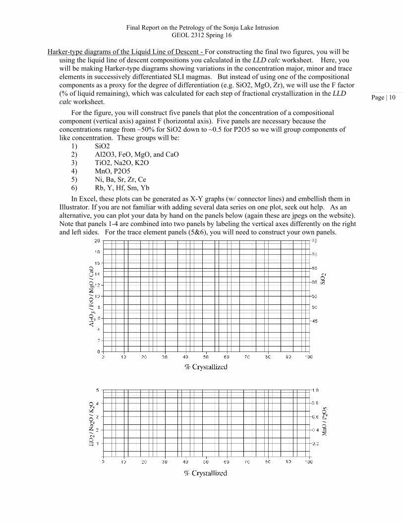
Harker-type diagrams of the Liquid Line of Descent - For constructing the final two figures, you will be using the liquid line of descent compositions you calculated in the LLD calc worksheet. Here, you will be making Harker-type diagrams showing variations in the concentration major, minor and trace elements in successively differentiated SLI magmas. But instead of using one of the compositional components as a proxy for the degree of differentiation (e.g. SiO2, MgO, Zr), we will use the F factor (% of liquid remaining), which was calculated for each step of fractional crystallization in the LLD calc worksheet.

For the figure, you will construct five panels that plot the concentration of a compositional component (vertical axis) against F (horizontal axis). Five panels are necessary because the concentrations range from ~50% for SiO2 down to ~0.5 for P2O5 so we will group components of like concentration. These groups will be:

1) SiO2 2) Al2O3, FeO, MgO, and CaO 3) TiO2, Na2O, K2O 4) MnO, P2O5 5) Ni, Ba, Sr, Zr, Ce 6) Rb, Y, Hf, Sm, Yb

In Excel, these plots can be generated as X-Y graphs (w/ connector lines) and embellish them in Illustrator. If you are not familiar with adding several data series on one plot, seek out help. As an alternative, you can plot your data by hand on the panels below (again these are jpegs on the website). Note that panels 1-4 are combined into two panels by labeling the vertical axes differently on the right and left sides. For the trace element panels (5&6), you will need to construct your own panels.


Page | 11

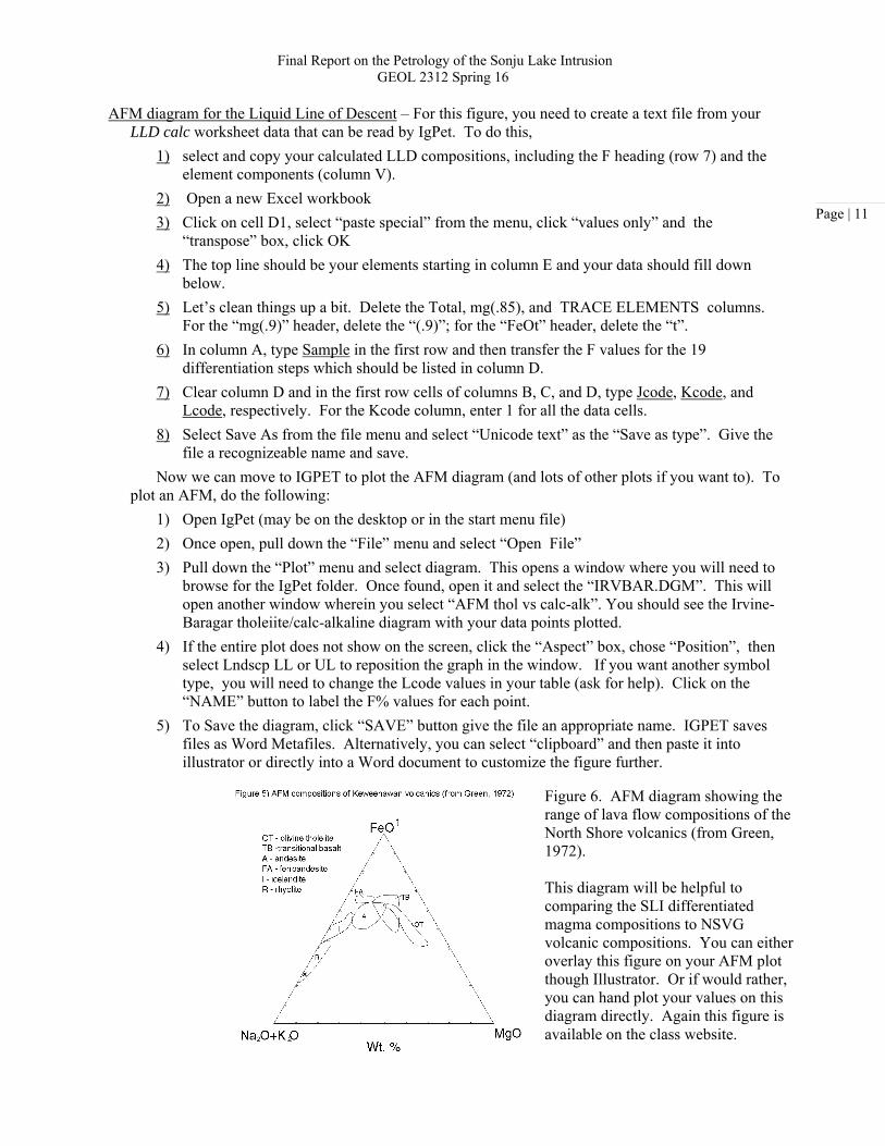
AFM diagram for the Liquid Line of Descent – For this figure, you need to create a text file from your LLD calc worksheet data that can be read by IgPet. To do this,

1) select and copy your calculated LLD compositions, including the F heading (row 7) and the element components (column V).

2) Open a new Excel workbook

3) Click on cell D1, select “paste special” from the menu, click “values only” and the “transpose” box, click OK

4) The top line should be your elements starting in column E and your data should fill down below.

5) Let’s clean things up a bit. Delete the Total, mg(.85), and TRACE ELEMENTS columns. For the “mg(.9)” header, delete the “(.9)”; for the “FeOt” header, delete the “t”.

6) In column A, type Sample in the first row and then transfer the F values for the 19 differentiation steps which should be listed in column D.

7) Clear column D and in the first row cells of columns B, C, and D, type Jcode, Kcode, and Lcode, respectively. For the Kcode column, enter 1 for all the data cells.

8) Select Save As from the file menu and select “Unicode text” as the “Save as type”. Give the file a recognizeable name and save.

Now we can move to IGPET to plot the AFM diagram (and lots of other plots if you want to). To plot an AFM, do the following:

1) Open IgPet (may be on the desktop or in the start menu file)

2) Once open, pull down the “File” menu and select “Open File”

3) Pull down the “Plot” menu and select diagram. This opens a window where you will need to browse for the IgPet folder. Once found, open it and select the “IRVBAR.DGM”. This will open another window wherein you select “AFM thol vs calc-alk”. You should see the Irvine-Baragar tholeiite/calc-alkaline diagram with your data points plotted.

4) If the entire plot does not show on the screen, click the “Aspect” box, chose “Position”, then select Lndscp LL or UL to reposition the graph in the window. If you want another symbol type, you will need to change the Lcode values in your table (ask for help). Click on the “NAME” button to label the F% values for each point.

5) To Save the diagram, click “SAVE” button give the file an appropriate name. IGPET saves files as Word Metafiles. Alternatively, you can select “clipboard” and then paste it into illustrator or directly into a Word document to customize the figure further.

Figure 6. AFM diagram showing the range of lava flow compositions of the North Shore volcanics (from Green, 1972). This diagram will be helpful to comparing the SLI differentiated magma compositions to NSVG volcanic compositions. You can either overlay this figure on your AFM plot though Illustrator. Or if would rather, you can hand plot your values on this diagram directly. Again this figure is available on the class website.


Page | 12

PART II : WRITTEN REPORT ON THE PETROLOGY OF THE SONJU LAKE INTRUSION

Given here is an annotated outline of the topical components that you should include in your report. You should embed figures and figure captions where appropriate. Remember a picture is worth a thousand words. Figures should include not only the figures you constructed above but may also be taken from other reports (many of which will be posted on the website). For each section below, I will suggest some figures that you may want to consider including.

To describe many of the elements of this report, you will need to read some articles that describe and discuss the geology and petrology of the SLI. The website has several of these manuscripts as pdfs. Note that in most articles, the SLI is a small part of the report. The main exception is Miller (1999) yet most of that report is devoted to the PGE mineralization. You will also find a cache of jpeg figures on the website that are from these articles or are figures that I have made for Powerpoint presentations and area are unpublished. The descriptions on the Finland-Doyle Lake geologic map posted in the back of the room may also come in handy.

Be sure to cite any paper that you are directly taking information from (either a text or a figure) and give the reference in the bibliography at the end of the report. A typical citation gives the authors’ last names and the publication date (e.g., Paces and Miller, 1993). No need to cite unpublished figures.

Report outline:

Table of Contents

1. Introduction

A. Briefly introduce the SLI - what is it?

B. Regional setting - Midcontinent Rift, Beaver Bay Complex

C. Purpose of report (because I made you do it doesn’t count!)

Suggested figure: Geologic map of NE Minnesota, showing the location of the SLI

2. Geology of the SLI

A. General geologic attributes of the SLI - intrusion shape, thickness, tilt, strike length, extent and quality of exposure,…

B. Related Rocks – briefly describe the geologic relationship between the SLI and the Footwall rocks, the Finland Granite, the Beaver River Diabase, and the hybrid dikes.

C. Igneous Stratigraphy of the SLI - Describe the stratigraphic sequence of SLI units from bottom to top; describe the basis by which the units are distinguished (cumulus mineralogy); describe the general lithologic (modal rock types) attributes of each unit (the Finland-Doyle Lake geologic map unit descriptions may come in handy here))

Suggested figure: Geologic map of the SLI; Modal rock type diagram

3. Petrography of the SLI

A. Modal Mineralogy - describe the changes in mineralogy upward through the SLI

B. Bulk Rock Textures – describe changes in textural attributes through the SLI; features to especially note include grain size, bulk rock texture (defined by clinopyroxene habit), and development of foliation.

C. Cumulate Interpretations – discuss the textural and modal basis for interpreting what phases are cumulus vs. intercumulus in each unit.

D. Alteration – describe the type and intensity of alteration and what primary phases are most affected

Suggested figures: Cumulative modal vs. strat ht. diagram; Plagioclase grain size vs. strat ht. diagram, You may also want to include photomicrographs in this section to illustrate certain textures, though this is optional. See me about how to take photos with the instructor microscope.


Page | 13

4. Geochemistry of SLI

A. SEM analyses – briefly describe the method used for determining mineral compositions with the SEM

B. Cryptic Variation of Fo in Olivine – Describe how the Fo content of olivine varies up section through the SLI citing the class data and the variation shown by Miller and Ripley (1997) – Figure 5 above

C. Cryptic Variation in En in Augite – Same as above

D. Cryptic Variation of An in Plagioclase – Describe the strategy for determining the average An content of plagioclase from whole rock geochemical data and discuss the results.

Suggested figures: Fo, En, and An vs. Stratigraphic Height

5. Petrology of the SLI

A. Parent magma composition -report on the basis for your calculation and its closeness to the Miller and Ripley calculation, include a table that compares the two compositions.

B. Liquid Line of Descent

i. describe the strategy for calculating the LLD compositions and how they can be interpreted to have been generated by the progressive fractional crystallization of the SLI parent magma

ii. show and discuss data displayed in Harker diagrams

iii. present the AFM figure and discuss how the SLI magmas compare to the typical suite of North Shore volcanics.

C. Comparison to the Skaergaard intrusion – generally describe the similarities and differences between the Skaergaard and the SLI. The Miller (1999) article makes some of these comparisons. You can also find a more complete description about Skaergaard by A. McBirney in the Layered Intrusion book in the lab “library”. You may find it helpful to use the figure below to plot the main SLI units in the figure below so as to compare the two systems.

Suggested figures: Harker diagrams, AFM diagram w/ NSVG compositions fields, Skaergaard figure above.


Page | 14

6. Summary and Conclusions - briefly summarize the data presented in this report that provides evidence for your interpretation of how the SLI magma crystallized and how this resulted in its differentiated nature.

7. References Cited – list any referenced cited in this report here; use the format found in most of the articles.

8. Appendix

A. Attach the Northern and Southern Traverse Area maps which show how you determined the stratigraphic heights of your samples by projections to the profile lines.

B. Attach the petrographic description sheets that you completed in lab for 16 SLI samples

TO BE EMAILED TO ME BY MAY 3rd, 2016

- An electronic copy of the final report with embedded figures as a Word or pdf document

- Completed Excel document (SLI worksheets). You can email this to me.

final report on the petrology of the sonju lake intrusionmille066/teaching/2312/sonju report/sonju...

Documents