final report- engineering-economic analysis of syngas … library/research/energy analysis... · an...

An Engineering-Economic Analysis of Syngas Storage

DOE/NETL-2008/1331

Final Report

July 31, 2008

Disclaimer

This report was prepared as an account of work sponsored by an agency of the United States Government. Neither the United States Government nor any agency thereof, nor any of their employees, makes any warranty, express or implied, or assumes any legal liability or responsibility for the accuracy, completeness, or usefulness of any information, apparatus, product, or process disclosed, or represents that its use would not infringe privately owned rights. Reference therein to any specific commercial product, process, or service by trade name, trademark, manufacturer, or otherwise does not necessarily constitute or imply its endorsement, recommendation, or favoring by the United States Government or any agency thereof. The views and opinions of authors expressed therein do not necessarily state or reflect those of the United States Government or any agency thereof.

An Engineering-Economic Analysis of Syngas Storage

DOE/NETL-2008/1331

Draft Final Report July 31, 2008

Jay Apt

Adam Newcomer Lester B. Lave

Carnegie Mellon University

Stratford Douglas Leslie Morris Dunn

West Virginia University

Contract DE-AC26-04NT 41817.404.01.02

NETL Contact: Michael Reed

Technical Monitor Office of Systems, Analyses, and Planning

National Energy Technology Laboratory

www.netl.doe.gov

This page intentionally left blank

1

Table of Contents List of Figures ................................................................................................................................. 4

List of Tables .................................................................................................................................. 7

Acknowledgements....................................................................................................................... 10

Foreword ....................................................................................................................................... 11

Executive Summary ...................................................................................................................... 15

Part 1. Technical and Economic Data (CMU Team)................................................................... 18

Overview................................................................................................................................... 18

Storage Options......................................................................................................................... 21

Syngas and SNG Storage ...................................................................................................... 24

Cryogenic Liquid Storage ..................................................................................................... 24

Compressed Gas Storage ...................................................................................................... 25

Compressors.......................................................................................................................... 26

Above Ground Compressed Gas Storage ............................................................................. 29

Gasometer Storage ................................................................................................................ 29

Pipeline Storage .................................................................................................................... 30

Underground Compressed Gas Storage ................................................................................ 30

Technical Issues ........................................................................................................................ 32

Hydrogen Embrittlement ...................................................................................................... 32

Syngas Leakage .................................................................................................................... 33

Biological Fouling ................................................................................................................ 34

Technical Note on Constructing Cost Distributions from Cost Data ................................... 34

Methanation: A Closer Examination ....................................................................................... 36

Industrial Experience ............................................................................................................ 36

SNG Production Process....................................................................................................... 37

Methanation Process ............................................................................................................. 38

Methanation Catalyst ............................................................................................................ 39

Syngas Cleanup and Special Considerations ........................................................................ 40

Commercial Methanation Processes ..................................................................................... 41

Methanation Costs ................................................................................................................ 41

2

Part 2. Modeling and Results: Analysis of Syngas Storage in the Context of Flexible IGCC Operations (CMU Team) .............................................................................................................. 45

Compression and Storage Details ......................................................................................... 47

Detailed Economic Analyses of IGCC Operations Using Syngas Storage .......................... 49

Results................................................................................................................................... 51

Results with Carbon Dioxide Capture .................................................................................. 53

SNG Results.......................................................................................................................... 54

Additional Considerations for Application in a Real World Scenario ................................. 55

Part 3. Economic Analysis of Syngas Storage Options and Markets (WVU Team)................... 59

Summary ................................................................................................................................... 59

Approach................................................................................................................................... 61

Scenario Analysis Algorithm Overview ................................................................................... 63

Risk and Return Metrics ........................................................................................................... 63

Net Present Value (NPV)...................................................................................................... 63

Return on Invested Capital (ROIC) ...................................................................................... 64

I. Methodological Issues and Implementation ......................................................................... 65

Plant Cost Model................................................................................................................... 65

Plant Availability Model....................................................................................................... 67

Year Two Study Enhancement (Task 7): Understanding the Lifetime Availability Profile of IGCC Plants .......................................................................................................................... 68

Operational Implementation of the Availability Model........................................................ 70

Year Two Study Enhancement (Task 7): Understanding Unplanned Outages.................... 73

Fuel and Power Price Scenarios............................................................................................ 73

Year Two Study Enhancement: Specification of Electricity Price Duration Curves (Task 6)............................................................................................................................................... 77

II. Alternative Plant Configurations Used in the Simulations ................................................. 80

Year 2 Enhancement: Incorporating Fuel-Switching Capability into the Simulated IGCC Plant (Task 7)........................................................................................................................ 82

Improving Plant Availability by Using Natural Gas as a Backup Fuel ................................ 83

Using Natural Gas to Increase Cycling Flexibility in the CMU 12 Hour Plant ................... 86

Year Two Study Enhancement: Underground Storage (Task 7) .............................................. 93

Year Two Study Enhancement: Comparing a Coal Boiler Plant to Simulated IGCC Plants (Task 7) ..................................................................................................................................... 94

III. Simulation Results and Analysis ....................................................................................... 95

3

1. All plant configurations that we tested, except the CMU 12 hour storage and the CMU 12 hour storage with fuel switching capabilities, are unattractive investments under base case energy prices. ................................................................................................................ 95

2. IGCC Plants perform better in high-energy-price environments.................................. 99

3. High peak power prices improve IGCC plants’ economic performance while high baseload prices improve IGCC performance only slightly................................................. 102

4. High variance in gas prices does not significantly affect the viability of an IGCC.... 105

5. The use of a backup fuel such as natural gas dominates all other configurations used for availability enhancement............................................................................................... 106

6. Under all price scenarios the most profitable plant configuration is the CMU 12 hour plant with fuel switching capabilities and backup fuel. ...................................................... 109

IV. Task 8: IGCC Optimal Control Problem........................................................................ 111

Motivation........................................................................................................................... 111

Assumptions and simplifications for our model: ................................................................ 111

Setting up the Problem:....................................................................................................... 111

Analysis............................................................................................................................... 113

Assessing the Optimality of the Capital Structure.............................................................. 116

Appendix A: Statistical Tables for All Plant Configurations .................................................... 119

Appendix B: Historical Accuracy of Energy Information Administration (EIA) Price Forecasts..................................................................................................................................................... 124

Appendix C: 1+0+CCS Scenario Operating and Financial Parameters .................................... 127

References................................................................................................................................... 133

4

List of Figures

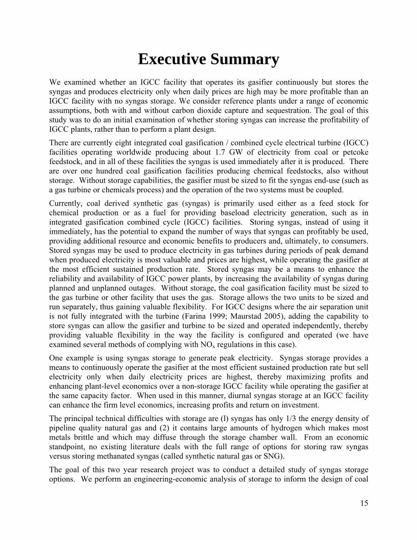
Figure 1. Methanation Capital Costs Versus SNG Production Output (Mozaffarian and Zwart 2003; Gray, Salerno et al. 2004; Gray, Salerno et al. 2004; Walker 2006) .................................. 20

Figure 2. Compressor Capital Costs Versus Size (Taylor, Alderson et al. 1986; Amos 1998; IEA GHG 2002).................................................................................................................................... 22

Figure 3. Above Ground Compressed Gas Storage Capital Cost Versus Size (Taylor, Alderson et al. 1986; Amos 1998; Padró and Putsche 1999) ....................................................................... 23

Figure 4. Capital Cost of Liquid Hydrogen Facilities (Taylor, Alderson et al. 1986)................. 25

Figure 5. Work to Compress an Ideal Gas From P1 to P2 ............................................................ 27

Figure 6. Volumetric Density Versus Pressure for Three Different Gas Mixtures Using Three Different Equations of State.......................................................................................................... 28

Figure 7. Regression Analysis Illustration with Underlying Data Points, Mean Regression Line, and Upper and Lower Prediction Intervals Plotted. The Mean and Prediction Interval for the Value of Y at Point X0 is Shown. ................................................................................................. 35

Figure 8. Cumulative Distribution Function of the Value of Y at Point x0 ................................. 35

Figure 9. SNG Production by Direct Synthesis ........................................................................... 37

Figure 10. SNG Production by Indirect Synthesis....................................................................... 37

Figure 11. Methanation Process Flow Diagram .......................................................................... 40

Figure 12. Typical Syngas to SNG Process Diagram. Reproduced from (Gray, Salerno et al. 2004) ............................................................................................................................................. 42

Figure 13. Baseline Facility (Top), Syngas Storage Scenario (Middle), SNG Storage Scenario (Bottom). Gas Turbines are GE 7FA CCGTs.............................................................................. 46

Figure 14. Conceptual Design of Syngas Storage Process Block Used in the Analysis. Gas Turbines are GE 7FA CCGTs....................................................................................................... 47

Figure 15. Conceptual Illustration of Storage Pressures, Draw Down Rates and Recompression Requirements for Syngas Storage Process Block Used in the Analysis....................................... 48

Figure 16. Storage Scheme for 8 Hours of Syngas Storage to Produce Peak Electricity. At Times of Low Price, the Gasifier Output Fills Storage. During High Price Periods, Both the Gasifier and Stored Syngas Supply Turbines. At Intermediate Prices, the Gasifier Output is Fed to One Turbine and the Storage Volume is Unchanged. .............................................................. 50

Figure 17. Change in ROI for Syngas Storage Scenario Using A 1+0 IGCC Facility With 80% Availability, Cinergy Node, 100% Debt Financing at 8% Interest Rate, Economic, and Plant Life of 30 Years (Amortization Factor 0.0888), 2007 EIA AEO Coal Price Forecast with Accuracy Factor, 63 Bar Storage Pressure.................................................................................................... 52

Figure 18. Increase in NPV from Adding a Diurnal Syngas Storage Scheme. Parameters as in Figure 17. ...................................................................................................................................... 53

5

Figure 19. Change in ROI for Syngas Storage Scenario Using a 1+0+CCS IGCC Facility with Carbon Capture, Transport, and Storage, 80% Availability, Cinergy Node, 100% Debt Financing at 8% Interest Rate, Economic and Plant Life of 30 Years (Amortization Factor 0.0888), 2007 EIA AEO Coal Price Forecast with Accuracy Factor, 63 Bar Storage Pressure. ......................... 54

Figure 20. Change in ROI for SNG Storage Scenario Using a 1+0 Gasification Plus Methanation Facility with 80% Availability, Cinergy Node, 100% Debt Financing at 8% Interest Rate, Economic and Plant Life of 30 Years (Amortization Factor 0.0888), 2007 EIA AEO Coal Price Forecast with Accuracy Factor, 63 Bar Storage Pressure............................................................. 55

Figure 21. 1+0 with 2 Trains of Air Separation Unit for NOx Control ....................................... 57

Figure 22. 1+0 with the Purchase of NOx Allowances for the Peaking Turbine ........................ 58

Figure 23. IECM vs. WVU Cost Model Comparison: Without Spare Gasifier .......................... 66

Figure 24. IECM vs. WVU Cost Model Comparison: Capacity Factors (coal price is $1.269/MMBtu, Figures in millions of 2005 dollars per year)..................................................... 67

Figure 25. Historical IGCC Plant Availability Statistics ............................................................. 68

Figure 26. Changes in Simulated IGCC Plant Availability Profiles Year 1 and Year 2 of this Study ............................................................................................................................................. 69

Figure 27. Distribution of Consecutive Online Days, Polk Power Station 1997-2001 ............... 71

Figure 28. Length of Distribution of Outages Caused by Air Separation Unit Failure ............... 72

Figure 29. Length Distribution of Outages Caused by Gasifier Failure ...................................... 72

Figure 30. Length Distribution of Outages Caused by Power Block Failure .............................. 72

Figure 31. 2006 PJM Unconditional Electricity Price Duration Curve and Piecewise Linear Fitted Value................................................................................................................................... 75

Figure 32. EPDCs Conditional on Highest-Price and Lowest-Priced 12 Hours of Each Day, Compared to Upper and Lower 50th Percentiles of the Unconditional EPD PJM 2006.............. 79

Figure 33. NPV Effects of Different Availability Enhancements (Scenario 2a, High Fuel Prices)....................................................................................................................................................... 86

Figure 34. ROIC of Various Plant Configurations, AEO Base Prices......................................... 97

Figure 35. Base Plant (0): Base Price Scenarios and AEO High Fuel Prices, Distribution of Net Present Value ................................................................................................................................ 98

Figure 36. MISO and PJM Base Prices: Economies of Scale (Plant 2) and CMU 12-hour (Plant 3) ................................................................................................................................................... 99

Figure 37. ROIC of CMU 12-Hour Plant, Different Price Levels............................................. 102

Figure 38. Net Present Value: Base Plant 0 (No Storage or Spare) Four Electricity Price Duration Curve Scenarios ........................................................................................................... 104

Figure 39. NPV Effects of Different Availability Enhancements (Scenario 2a, High Fuel Prices)..................................................................................................................................................... 108

6

Figure 40. Effect of Fuel-Switching Capability on NPV of Plant Base Prices Scenario, Natural Gas as Alternate Fuel .................................................................................................................. 110

Figure B- 1. CDF of 2007 EIA AEO Coal Price Forecasts With and Without the Historical Accuracy Factor .......................................................................................................................... 125

Figure B- 2. Coal Price Distributions. CDF of Historical and Future FOB Coal Prices. ......... 126

7

List of Tables

Table 1. Overview of Project Tasks............................................................................................. 11

Table 2. Reported Syngas Compositions ..................................................................................... 19

Table 3. Methanation Operating and Maintenance Costs (Eliason 2006) ................................... 21

Table 4. Storage Vessel Capital Cost Estimates .......................................................................... 23

Table 5. Small Compressor Capital Costs (Taylor, Alderson et al. 1986; Amos 1998)............. 26

Table 6. Compressor Capital Cost Estimates for Large (MW) Pipeline Compressors ($MM)... 27

Table 7. Above Ground High Pressure Vessel Capital Costs (Taylor, Alderson et al. 1986; Amos 1998; Padró and Putsche 1999) .......................................................................................... 29

Table 8. Above Ground Low Pressure Vessel (Gasometer) Capital Costs.................................. 30

Table 9. Underground Storage Capital Cost Estimates (Carpetis 1982; Taylor, Alderson et al. 1986; Amos 1998)......................................................................................................................... 32

Table 10. SNG Production by Syngas Methanation Cases Analyzed (Gray, Salerno et al. 2004; Gray, Salerno et al. 2004) ............................................................................................................. 42

Table 11. Example SNG Production from a Single GE/Texaco Gasifier with Methanation (Gray, Salerno et al. 2004)............................................................................................................ 43

Table 12. Summary of Capital Costs for Producing SNG from Syngas...................................... 44

Table 13. Baseline 270 MWe Net Facility Configuration and Parameters (Carnegie Mellon University, Center for Energy and Environmental Studies 2006) ................................................ 45

Table 14: IECM vs. WVU IGCC Cost Model Comparison ........................................................ 66

Table 15: ROIC Effects of Changes in Base Plant Availability Profiles Return on Invested Capital (ROIC).............................................................................................................................. 70

Table 16: Summary of Price Scenarios........................................................................................ 74

Table 17: Experimental Means and Standard Errors of Energy Prices ....................................... 77

Table 18: Summary of Plant Configurations ............................................................................... 80

Table 19: Operating Statistics: Averages Across All Experiments (Millions of 2005 Dollars) .. 82

Table 20: Comparing Availability Improvements from Syngas Storage, Spare Gasifier and Natural Gas Backup ...................................................................................................................... 84

Table 21: Hours per Year of Downtime By Cause, Base Plant 0 ................................................ 84

Table 22: ROIC Effects of Various Availability Enhancements ................................................. 85

Table 23: Hypothetical Returns from Fuel Switching, CMU 12-Hour Plant 8 ........................... 87

Table 24: Hours per Day Simulated CMU Fuel-Switching Plant Could Profitably Burn Natural Gas (After Operating on Syngas for 12 Hours) ............................................................................ 88

8

Table 25: Comparing Results Calculated from Conditional and Unconditional EPDCs: Average Prices and Returns on Invested Capital (ROIC), PJM 2006......................................................... 89

Table 26: Return on Invested Capital (ROIC): CMU 12-Hour Plant With and Without Fuel-Switching Capabilities .................................................................................................................. 90

Table 27: CMU 12-Hour Plant NPV (Millions of 2005 Dollars): Diversity in Daily Electricity Price Duration Curves................................................................................................................... 91

Table 28: Return on Invested Capital (ROIC), CMU 12-Hour Plant with Different Costs of Fuel- Switching (Switching for Cycling but not Backup)...................................................................... 92

Table 29: Hours per Year of Natural Gas Operation of CMU 12-Hour Plant for Different Levels of Switching Costs (Assuming Availability of 83.7%) ................................................................ 92

Table 30: Comparing Above Ground and Underground Storage for Availability Improvements 200,000 m3 Working Gas, Return on Invested Capital (ROIC)................................................... 94

Table 31: Pulverized Coal Boiler Plant ROIC Comparisons Return on Invested Capital (ROIC):....................................................................................................................................................... 95

Table 32: Mean ROIC and 95% Value at Risk, Base Prices ....................................................... 96

Table 33: 95% Value at Risk, High vs. Low Fuel Prices .......................................................... 100

Table 34: Mean ROIC, High vs. Low Fuel Prices..................................................................... 101

Table 35: Mean ROIC, Electricity Price Duration Curve Changes ........................................... 103

Table 36: Electricity Price Duration Curve Changes 5th Percentile ROIC ................................ 105

Table 37: Effect of Gas Price Variance on ROIC...................................................................... 106

Table 38: ROIC Effects of Various Availability Enhancements ............................................... 108

Table 39: Return on Invested Capital (ROIC): CMU 12-Hour Plant and Economies of Scale Plant With and Without Fuel-Switching Capabilities................................................................. 109

Table A- 1. Performance of Base Plant (0) Across All Scenarios ............................................. 119

Table A- 2. Performance of Base Plant with Spare (1) Across All Scenarios........................... 119

Table A- 3. Performance of 3 Gasifier System with Spare and No Storage (2) Across All Scenarios ..................................................................................................................................... 120

Table A- 4. Performance of Plant Storing for 12 hours (3) Across All Scenarios .................... 120

Table A- 5. Performance of Plant Storing for 12 hours with Availability Improvements (5) Across All Scenarios................................................................................................................... 121

Table A- 6. Base Plant with 200,000 m3 Storage and 10% Inflow (6) Across All Scenarios ... 121

Table A- 7. Base Plant with Natural Gas Backup (7) Across All Scenarios ............................. 122

Table A- 8. CMU 12 Hour with NG Fuel Switching for Cycling but Not Backup (8) All Scenarios ..................................................................................................................................... 122

Table A- 9. CMU 12 Hour with NG Fuel Switching for Cycling and Backup (9) All Scenarios..................................................................................................................................................... 123

9

Table A- 10. Base Plant with 400,000 m3 Storage and 10% Inflow (10) Across All Scenarios .......................................................................................................................................................... 123

10

Acknowledgements

This work was funded by the U.S. Department of Energy's National Energy Technology Laboratory (U.S. DOE-NETL). The NETL sponsor for this project was John Wimer, Technology Manager for the Office of Systems, Analyses, and Planning (OSAP). Michael Reed of OSAP was the NETL Technical Monitor for this work. This NETL management team provided guidance and technical oversight for this study. The authors acknowledge the significant role played by U.S. DOE/NETL in providing the programmatic guidance and review of this report.

The authors thank James Ammer, Mike Berkenpas, Seth Blumsack, Chao Chen, Mike Griffin, Robert Heard, Mark Hornick, Robert Jones, Warren Katzenstein, Ed Martin, Sean McCoy, Michael Reed, William Rosenberg, Ed Rubin, John Stolz, and Michael Walker for helpful discussions. Jay Apt acknowledges additional funding by the U.S. National Science Foundation under grant SES-0345798 to Carnegie Mellon University.

11

Foreword This is the Joint Final Report of the teams of investigators from Carnegie Mellon University (CMU) and West Virginia University (WVU), in fulfillment of the requirement in Task 9.0 of the July 27, 2007 revision of the statement of work for this project, An Engineering-Economic Analysis of Syngas Storage (Subtask no. 404.01.02 Mod A). This work has been funded under the Collaborative Initiative among the National Energy Technology Laboratory (NETL) and Carnegie Mellon University, University of Pittsburgh, and West Virginia University.

This is the product of significant collaboration between the two University teams, and between the teams and their partners at NETL. The project was completed over the course of two years. At the end of the first year, a peer review panel reviewed the work, made suggestions for improvement, and enthusiastically recommended the project continue for a second year. An overview of the tasks completed in each project year is shown in Table 1.

Table 1. Overview of Project Tasks

Year 1 Tasks (August 18, 2006 – July 31, 2007)

Task 1.0: Technical and Economic Data Gathering Subtask 1.1 – Data Gathering on Eskom’s UCG Process and Sasol’s Lurgi Process – The research will begin by gathering existing data on composition, heat content, temperature and production rate for syngas generated from Eskom’s air-oxidized UCG process and Sasol’s oxygen-oxidized Lurgi process

Subtask 1.2 – Data Gathering on Syngas Methanation – Also, during the data gathering phase, capital and operating costs for methanation of syngas to produce synthetic natural gas will be compiled. One of the potential systems under consideration is methanation of syngas and storing the methane (not the syngas) for future use.

Subtask 1.3 – Data Gathering on syngas production Subtask 1.3.1 – Data Gathering on IGCC and alternative syngas production systems – In parallel with sub-activities 1.1 and 1.2, capital and operating costs of IGCC systems and other syngas production systems will be researched.

Subtask 1.3.2 – Data Gathering on market size and penetration of product streams other than electricity – Electric power is not the only potential product. Syngas can be used as a feedstock for the production of chemicals including alcohols and methane. Also, some solid waste products can be processed into usable construction materials. This subtask will gather data on potential market size and penetration of these additional product streams.

Task 2.0: Economic Analysis of Syngas Storage Options and Markets Subtask 2.1 – Define Base Case – The research will develop an economic model that will assess the ability of syngas storage to increase the value of IGCC systems.

Subtask 2.2 – Define Scenarios and Perform Analysis – The main questions of the analysis are as follows:

1. How can syngas storage enhance the economic of IGCC facilities? 2. What is the value of increasing flexibility of IGCC through syngas storage?

12

3. Under what circumstances is investment in syngas storage economically viable?The scenario variable include the following three categories

1. Base Prices a. Coal Price (absolute price and variability in time) b. Natural Gas Price (absolute price and variability in time) c. Electricity Price (absolute price and variability in time)

2. Technical Issues a. Technological progress of IGCC and syngas storage systems b. Revenue generated from by-products and latent heat

3. Policy Concerns a. Emissions regulations: CO2, Hg, others b. Renewable power generation c. Price-responsive load management d. Availability and price of LNG e. Baseload vs. peaking installations of new generation

Subtask 2.3 – Prepare Results for Internal and External Comment and Publication

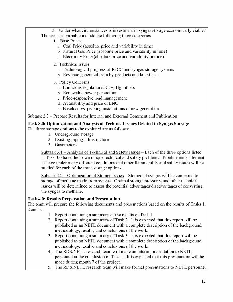
Task 3.0: Optimization and Analysis of Technical Issues Related to Syngas Storage The three storage options to be explored are as follows:

1. Underground storage 2. Existing piping infrastructure 3. Gasometers

Subtask 3.1 – Analysis of Technical and Safety Issues – Each of the three options listed in Task 3.0 have their own unique technical and safety problems. Pipeline embrittlement, leakage under many different conditions and other flammability and safety issues will be studied for each of the three storage options.

Subtask 3.2 – Optimization of Storage Issues – Storage of syngas will be compared to storage of methane made from syngas. Optimal storage pressures and other technical issues will be determined to assess the potential advantages/disadvantages of converting the syngas to methane.

Task 4.0: Results Preparation and Presentation The team will prepare the following documents and presentations based on the results of Tasks 1,2 and 3.

1. Report containing a summary of the results of Task 1 2. Report containing a summary of Task 2. It is expected that this report will be

published as an NETL document with a complete description of the background, methodology, results, and conclusions of the work.

3. Report containing a summary of Task 3. It is expected that this report will be published as an NETL document with a complete description of the background, methodology, results, and conclusions of the work.

4. The RDS/NETL research team will make an interim presentation to NETL personnel at the conclusion of Task 1. It is expected that this presentation will be made during month 7 of the project.

5. The RDS/NETL research team will make formal presentations to NETL personnel

13

at the conclusion of Activities 2 and 3. It is expected that this presentation will be made during month 13 of the project.

Year 2 Tasks (July 31, 2007 – August 31, 2008)

Task 5.0: Technical and Economic Analysis of Syngas Storage in the Context of Flexible IGCC Operations

Subtask 5.1 Detailed Technical Analyses of IGCC Operations Using Syngas Storage – The project will use the results of Year 1 activities as a starting point for detailed technical analysis of IGCC operations using syngas storage. The project will study the technical feasibility of the following operations:

1. Using stored syngas to fuel a gas turbine for the production of peaking (high value) power in the context of an IGCC system

2. Using stored methanated syngas to fuel a gas turbine for the production of peaking (high value) power

Subtask 5.2 Detailed Economic Analyses of IGCC Operations Using Syngas Storage The project will use the results of Year 1 activities as a starting point for detailed economic analysis of IGCC operations using syngas storage. The project will study the economic feasibility of the operations listed under Subtask 5.1

Task 6.0: Improvement of Electricity Price Duration Curve (EPDC) Representation 1. Review the recent literature on EPDC, determine its relevance to improvement of

simulations of power plant operation in a market environment. 2. Determine data requirements (power market supply, transmission, and demand

characteristics) for improvements to the current representation of the EPDC in the simulation model.

3. Implement improvements to the simulation model as appropriate.

Task 7.0: Miscellaneous Enhancements to WVU Model 1. Seek better industry data on the rate of technological and operational

improvement in IGCC plants. Improve understanding of the interrelationships among unplanned outages in different parts of an IGCC plant, and technological and operational improvements in an IGCC plant over its lifetime.

2. Improve understanding of underground storage options and their relationship to economic viability.

3. Implement improvements to the simulation model as appropriate. Based on industry data gathered so far (part 1 above), we are incorporating natural gas into the simulated IGCC plant as a backup fuel both for availability improvements and additional flexibility in the CMU 12 hour plant.

Task 8.0: Optimization of Syngas Storage for Maximum Economic Benefit 1. Explore modeling techniques for optimizing the use of syngas storage for cycling

flexibility. 2. Determine optimal algorithm for operating the power generation and gasification

blocks. 3. Determine the optimal size of the storage facility as a function of the cost of the

storage facility and its value under the optimal operation algorithm. 4. Implement improvements to the simulation model as appropriate.

14

Task 9.0 – Results Preparation and Presentation 1. Joint Interim report and presentation of status and results of Task 5 - 8. This

interim report and presentation will be delivered no later than February 28, 2008. 2. A Joint Draft final report and formal presentation of results of Task 5-8. It is

expected that this presentation will be made no later than June 30, 2008. 3. A joint final report will be created based on the joint draft final report and

comments from NETL. It is expected that RDS will receive comments from NETL within two weeks of receipt of the draft final report.

15

Executive Summary We examined whether an IGCC facility that operates its gasifier continuously but stores the syngas and produces electricity only when daily prices are high may be more profitable than an IGCC facility with no syngas storage. We consider reference plants under a range of economic assumptions, both with and without carbon dioxide capture and sequestration. The goal of this study was to do an initial examination of whether storing syngas can increase the profitability of IGCC plants, rather than to perform a plant design.

There are currently eight integrated coal gasification / combined cycle electrical turbine (IGCC) facilities operating worldwide producing about 1.7 GW of electricity from coal or petcoke feedstock, and in all of these facilities the syngas is used immediately after it is produced. There are over one hundred coal gasification facilities producing chemical feedstocks, also without storage. Without storage capabilities, the gasifier must be sized to fit the syngas end-use (such as a gas turbine or chemicals process) and the operation of the two systems must be coupled.

Currently, coal derived synthetic gas (syngas) is primarily used either as a feed stock for chemical production or as a fuel for providing baseload electricity generation, such as in integrated gasification combined cycle (IGCC) facilities. Storing syngas, instead of using it immediately, has the potential to expand the number of ways that syngas can profitably be used, providing additional resource and economic benefits to producers and, ultimately, to consumers. Stored syngas may be used to produce electricity in gas turbines during periods of peak demand when produced electricity is most valuable and prices are highest, while operating the gasifier at the most efficient sustained production rate. Stored syngas may be a means to enhance the reliability and availability of IGCC power plants, by increasing the availability of syngas during planned and unplanned outages. Without storage, the coal gasification facility must be sized to the gas turbine or other facility that uses the gas. Storage allows the two units to be sized and run separately, thus gaining valuable flexibility. For IGCC designs where the air separation unit is not fully integrated with the turbine (Farina 1999; Maurstad 2005), adding the capability to store syngas can allow the gasifier and turbine to be sized and operated independently, thereby providing valuable flexibility in the way the facility is configured and operated (we have examined several methods of complying with NOx regulations in this case).

One example is using syngas storage to generate peak electricity. Syngas storage provides a means to continuously operate the gasifier at the most efficient sustained production rate but sell electricity only when daily electricity prices are highest, thereby maximizing profits and enhancing plant-level economics over a non-storage IGCC facility while operating the gasifier at the same capacity factor. When used in this manner, diurnal syngas storage at an IGCC facility can enhance the firm level economics, increasing profits and return on investment.

The principal technical difficulties with storage are (l) syngas has only 1/3 the energy density of pipeline quality natural gas and (2) it contains large amounts of hydrogen which makes most metals brittle and which may diffuse through the storage chamber wall. From an economic standpoint, no existing literature deals with the full range of options for storing raw syngas versus storing methanated syngas (called synthetic natural gas or SNG).

The goal of this two year research project was to conduct a detailed study of syngas storage options. We perform an engineering-economic analysis of storage to inform the design of coal

16

gasification facilities as well as energy policy. The project collected the relevant syngas data from gasification processes; explored the technical issues of storage such as hydrogen embrittlement, leakage and energy loss from syngas storage; and performed an engineering-economic analysis of storage options. In a parallel and complementary approach, we analyzed the benefits and costs of syngas storage options under a variety of scenarios, sampling the uncertainties in commodity prices, technical options, and regulatory policies.

Adding the capability to store syngas at an IGCC facility provides valuable flexibility in the way the facility is configured and operated. One example is using syngas storage to generate peak electricity. Syngas storage provides a means to continuously operate the gasifier at the most efficient sustained production rate, but to sell electricity only when daily electricity prices are highest, thereby maximizing profits and enhancing plant-level economics over a non-storage IGCC facility while operating the gasifier at the same capacity factor. We examined whether, when used in this manner, diurnal syngas storage at an IGCC facility can increase profits and return on investment and lower the carbon price at which IGCC enters the U.S. generation mix.

The practicality of syngas storage depends upon a number of factors, both technical and economic. Technical considerations include the physical properties of the syngas (such as the composition, energy density, temperature and pressure); the possibility of syngas methanation to shift the hydrogen in the syngas to methane prior to storage; leakage, flammability and safety concerns; and the location, type, size, working pressures and other parameters of the storage vessels. Economic considerations include the relative prices of syngas and natural gas, the variability of daily electricity prices, the difference between daily high and low electricity prices, and capital and operating costs of the storage equipment including auxiliary combustion turbines.

The conditions under which syngas storage is feasible and economically attractive have not appeared in the literature. Engineering economic models are needed to enable developers and companies interested in coal gasification to make informed decisions about whether to build gasification units with syngas storage.

This research was conducted under the Collaborative Initiative among the National Energy Technology Laboratory (NETL) and Carnegie Mellon University, University of Pittsburgh, and West Virginia University. This is the product of significant collaboration between the two University teams, and between the teams and their partners at NETL. The two university teams have taken complementary approaches to conducting an engineering-economic analysis of syngas storage. The CMU team has investigated the concept that storing syngas can significantly enhance the profitability of IGCC plants in markets where the price electricity varies by time of day. CMU defined the engineering aspects of the project, and provided guidance to the WVU team in matters of engineering design. Both teams took a probabilistic approach to modeling the economic viability of syngas storage. CMU and WVU took very different approaches to modeling both the availability of the plant and the economic environment in which it will operate. The two teams use different assumptions about fuel and electricity prices over the 30-year life of the plant, and they emphasize different aspects of the analysis. The WVU team analyzed performance of the plant under different scenarios for prices of electricity and fuels and included dual-fuel turbine firing, while CMU modeled the economic impacts of plant design using actual prices for electricity in the Midwest ISO. Consistent with the different approaches to economic modeling, the statistics and modes of reporting differ slightly as well, although some aspects, notably the discount rates and the use of the IECM as a prime source for cost data, are consistent between the two teams.

17

We view the complementarities in our methods as a virtue, because they add credence to the remarkable consistency between the preliminary results of the two lines of research. We find strong evidence that syngas storage can add significant value to current IGCC plant designs, and can contribute to the adaptability of IGCC plants across different economic environments. In particular, the 12-hour storage design developed by the CMU team appears to hold considerable promise for increasing the attractiveness of investment in IGCC facilities.

The study's results supporting the economic benefits of storage do not depend on the absolute levels of capital costs. A change in capital costs would affect the basic results of this study only if storage and turbine power plant capital costs rise much faster than gasification and air separator unit capital costs (i.e., if relative capital costs change greatly), or detailed engineering design studies uncover integration issues that cannot be solved technically without incurring a very substantial cost increase relative to the costs of a non-storage plant.

Under these conditions, this study provides strong support for the proposition that syngas storage can significantly improve the economic viability of coal-fired IGCC power plants. Using a probabilistic analysis, we have calculated the plant-level return on investment (ROI) and the value of syngas storage for IGCC facilities located in the U.S. Midwest ISO using a range of storage configurations. Adding a second turbine to use the stored syngas to generate electricity at peak hours and implementing 12 hours of above ground high pressure syngas storage significantly increases the ROI (~13 percentage points over the nonstorage IGCC facility, for facilities both with and without carbon capture and sequestration) and net present value. Our simulation and analytical results both strongly support the 12-hour diurnal storage plant design (referred to here as the “CMU 12-hour plant”) as the most likely of the IGCC plants considered to be commercially viable in all scenarios, particularly scenarios with high fuel prices. Even without fuel-switching capabilities, the return on invested capital for the CMU 12-hour IGCC plant is higher than a supercritical coal-fired steam plant in our simulations, and much higher than an IGCC plant without storage. The addition of natural gas fuel-switching capabilities enhances the profitability of the CMU 12-hour plant design by roughly 20% under all scenarios studied.

18

Part 1. Technical and Economic Data (CMU Team)

Overview We have collected the relevant technical and economic data necessary to construct an engineering and economic model and to examine the economic performance of a syngas storage system in operation. An engineering and economic model was developed for syngas and methanated syngas storage in underground storage caverns, existing piping infrastructure, gasometers and in above ground high pressure storage vessels. We examined the technical and safety issues that may affect syngas storage operations, such as flammability, hydrogen embrittlement of metal, biological fouling and leakage. Additionally, the optimization of storage issues was addressed and the tradeoffs, advantages, and disadvantages (such as optimal working pressures and other parameters of the storage vessels) of storing syngas to storing methane made from syngas were explored. We concluded on the basis of these data and models that diurnal syngas storage in above ground high pressure vessels was the most cost effective widely available storage method for increasing the profitability of IGCC operations, but that methanated syngas (SNG) storage was not profitable.

Syngas The technical feasibility and economic attractiveness of syngas storage can depend on the specific properties of the syngas produced from the gasification process. These properties, such as the composition, energy density, temperature, and pressure, depend on the type and rank of coal and on the specific gasification process used to produce the syngas. Table 2 shows the composition and properties of syngas from a number of gasification processes and feedstocks. As the table shows, syngas is primarily composed of carbon monoxide and hydrogen and is characterized by a low energy density, typically ranging from 150-280 Btu/scf. The low energy density of syngas, ranging from roughly one-sixth to one-third that of natural gas, means that larger amounts of syngas are required to produce an equivalent amount of electricity in an IGCC facility. The implications for storage are that storage vessels must be designed to handle large volumes of gaseous syngas either through large physical sizes, high working pressures, or some combination. Methanation Methanation is a process used to upgrade low energy density syngas to higher pipeline quality synthetic natural gas or SNG. In the methanation process, the calorific value and other parameters of the gas are adjusted to meet natural gas pipeline specifications (Hagen, Polman, Myken, Jensen, Jönsson and Dahl 2001; Mozaffarian, Zwart, Boerrigter and Deurwaarder 2004). Common methanation reactions are (Twigg 1989):

2H3 CO + → OH CH 24 + 217H R −=Δ kJ/mol (1)

2H2 2CO + → 24 CO CH + (2)

22 H4CO + → OH2 CH 24 + 178HR −=Δ kJ/mol (3)

19

Table 2. Reported Syngas Compositions

Facility

Wabash (Lynch 1998)

Wabash (Lynch 1998)

Dow Plasquemine (Hannemann,

Koestlin, Zimmermann

and Haupt 2005)

Elcogas Puetrollano

(Hannemann, Koestlin et al.

2005)

Nuon Power (Hannemann,

Koestlin et al. 2005)

Polk (Todd and

Battista undated)

El Dorado (Todd and

Battista undated)

Schwarze Pumpe (Todd and Battista

undated)

Exxon Singapore (Todd and

Battista undated)

Eskom (Walker,

Blinderman and Brun

2001; Blinderman

and Anderson 2003)

Feedstock Coal Petcoke Coal Coal/ Petcoke

Coal/ Biomass Coal Petcoke

Lignite/ Waste Fuel Oil Coal

Gasifier E-Gas E-Gas Dow Shell Shell GE/Texaco GE/Texaco BG/Lurgi GE/Texaco ErgoExergy Composition (% vol)

Carbon Monoxide 45.3 48.6 38.5 29.2 24.8 46.6 45.0 26.2 35.4 8.3

Hydrogen 34.4 33.2 41.4 10.7 12.3 37.2 35.4 61.9 44.5 6.7 Carbon

Dioxide 15.8 15.4 18.5 1.9 0.8 13.3 17.1 2.8 17.9 9.5

Methane 1.9 0.5 0.1 0.01 -- 0.1 0.0 6.9 0.5 1.0 Argon 0.6 0.6 -- 0.6 0.6 Nitrogen 1.9 1.9 1.5 53.1 42.0 2.5 2.1 1.8 1.4 n/r

Sulfur, ppmv 68 69 n/r n/r n/r n/r n/r n/r n/r n/r Water 4.2 19.1 0.3 0.4 -- 0.44 17.0 HHV, Btu/scf 277 268 LHV, Btu/scf

n/r n/r

n/r 253 242 317 241 150

n/r, not reported

20

Because syngas is converted to methane during the methanation reaction, the problems associated with low energy density syngas and hydrogen rich gases can generally be avoided through a syngas methanation process. The main advantage of SNG is that its composition is nearly identical to natural gas and can therefore be used in the same manner and injected directly into natural gas pipelines (Collot 2004). The techniques and costs for natural gas handling and use are well known and can be directly applied to SNG. Additional details on industrial experience, the methanation and SNG production processes are provided below.

Capital costs for syngas methanation were collected from data reported in the literature and from facility developers (Mozaffarian and Zwart 2003; Gray, Salerno and Tomlinson 2004; Gray, Salerno, Tomlinson and Marano 2004; Walker 2006). The reported capital costs include all of the components required for the methanation process block, such as the methanators, compressors, and water gas shift process (see below for cost data and additional details). From these reported cost data, a distribution of predicted capital costs give for a given size of methanation system was constructed from the prediction interval. We give below additional details on how the cost distributions were constructed from the underlying cost data. Figure 1 illustrates the capital cost for methanation facilities plotted against SNG output capacity. The 95 percent prediction interval, indicating the range of the cost for a given methanation size, is plotted along with the mean regression value.

0

20

40

60

80

100

120

140

0 10 20 30 40 50 60 70 80 90 100

Capital Cost ($ million)

+95% PI-95% PI1.08x + 10.9Capital Cost

SNG Production(MMscf/day)

Coefficients Standard

Error t Stat P-value Intercept 10.9 5.87 1.9 0.14 SNG output (MMscf/d) 1.08 0.14 7.9 0.00

Figure 1. Methanation Capital Costs Versus SNG Production Output (Mozaffarian and Zwart 2003; Gray, Salerno et al. 2004; Gray, Salerno et al. 2004; Walker 2006)

21

A linear equation fits the capital cost versus SNG production capacity data well and shows that the methanation capital costs have a base cost (y-intercept) of about $10.9 million plus approximately $1.08 million per MMscf/day SNG production capacity (slope). As the size of the methanation system moves away from the mean of the underlying data, the uncertainty in the cost parameter increases resulting in an increased spread in the cost distribution. It is this capital cost distribution for a given methanation system size, reflecting the range of uncertainty in the parameter, that is used as the input to the economic cost model used in the analysis. From this regression analysis, a facility producing 50 MMscf/day of SNG from syngas would have estimated capital costs of about $65 ± 20 million (approximately ± 30 percent). This analysis suggests that methanation costs are fairly well known, consistent among data sources, and scale linearly with the SNG production rate.

Table 3 shows typical operating and maintenance costs for the methanation process, including maintenance of the reactors, compressors, exchangers and cost of the methanation catalyst.

Table 3. Methanation Operating and Maintenance Costs (Eliason 2006)

Description Cost (cents/Mscf) Maintenance (reactors, compressors, etc) 0.78 Nickel Catalyst 1.6 - 3.1 Total 2.38 - 3.88

As the table shows, estimates for overall operating and maintenance costs for methanation range from 2.38 to 3.88 cents per Mscf. Storage Options Storage options considered in the analysis are restricted to compressed gas technology since it is the most relevant large-scale stationary storage method for syngas production facilities, it can be readily used for syngas and SNG, and it less expensive that other alternatives such as liquefaction. A complete discussion of storage options and costs is included below. Compressed gas storage is the simplest storage solution as the only required equipment is a compressor and a pressure vessel (Amos 1998). The main disadvantage of compressed gas storage is the low storage density, which can be increased with the storage pressure. Operating parameters, capital and operating costs were examined for compressors and different storage vessels including high pressure cylindrical ‘bullets’ common for LPG and CNG storage, low pressure gasometers, underground in salt caverns and in excavated rock caverns.

Capital costs for compressors, which are required for all storage options, were compiled from studies in the literature (Taylor, Alderson, Kalyanam, Lyle and Phillips 1986; Amos 1998; IEA GHG 2002), and cost distributions were constructed from these data. Figure 2 shows the capital cost of the compressor plotted against the size of the compressor along with the mean regression line and the 95 percent prediction interval.

22

0.E+00

1.E+06

2.E+06

3.E+06

4.E+06

5.E+06

0 1,000 2,000 3,000 4,000 5,000 6,000 7,000

Capital Cost ($)

+95%-95%492x + 153,726Capital CostSeries5

Size (hp)

Coefficients StandardError t Stat P-value

Intercept 153,726 110,399 1.39 0.20 Size (hp) 492 28.7 17.16 0.00

Figure 2. Compressor Capital Costs Versus Size (Taylor, Alderson et al. 1986; Amos 1998; IEA GHG 2002)

As the figure illustrates, compressor capital costs scale linearly with the size of the compressor. The regression equations show a one horsepower increase in compressor size corresponds to a $492 increase in capital costs. The distribution in the capital cost for a given size compressor, reflecting the range of uncertainty in the cost parameter, is used as an input to the engineering economic models when compression is required.

Capital costs for storage vessels were compiled from studies in the literature and from professionals in industry. We give physical details, capital costs and cost distribution calculations for storage vessels later in this report. Figure 3 shows the capital cost for above ground high pressure vessel plotted against their size in cubic meters. From the regression analysis and prediction interval, a cost distribution was constructed and used as an input in the model.

23

-200,000

0

200,000

400,000

600,000

800,000

1,000,000

1,200,000

1,400,000

1,600,000

0 2,000 4,000 6,000 8,000 10,000 12,000 14,000 16,000

Capital Cost ($)

+95%-95%62.3x + 66,223Capital Cost

Size (m3)

Coefficients StandardError t Stat P-value

Intercept 66,223 70,991 0.93 0.40 Size (m3) 62.31 8.98 6.94 0.00

Figure 3. Above Ground Compressed Gas Storage Capital Cost Versus Size (Taylor, Alderson et al. 1986; Amos 1998; Padró and Putsche 1999)

As the figure illustrates, the capital costs scale linearly with the vessel size. A linear fit of the data shows a capital costs increase of approximately $62 per cubic meter increase in vessel size and a prediction interval is calculated for a given storage volume indicating the uncertainty in the cost estimate.

From data reported in the literature, capital cost distributions were constructed for salt caverns, excavated rock caverns, and low pressure gasometers. When a range of costs was reported in the literature, a triangular distribution was assumed. Table 4 shows a summary of the capital costs and cost distributions for storage vessels used in the analysis.

Table 4. Storage Vessel Capital Cost Estimates

Storage Vessel Cost Range Distribution (min, mode, max)

Salt cavern (Carpetis 1982; Taylor, Alderson et al. 1986; Amos 1998)

$19-$23/m3 Triangular (19, 21, 23)

Excavated rock caverns (Amos 1998) $34-$84/m3 Triangular (34, 60, 84)

Low pressure gasometers (Bennet 2006) $306-$374/m3 Triangular (306, 340, 374)

High pressure cylindrical bullets (Taylor, Alderson et al. 1986; Amos 1998; Padró and Putsche 1999)

approx $48-$77/m3

Prediction interval (see text)

24

Because it is the lowest cost, a salt cavern is preferred if it is available. However, because salt and rock caverns are geographically limited, this analysis considers the general case where neither is available. See below for a complete discussion of storage options and costs.

Syngas and SNG Storage Storage options for syngas and SNG are not well reported in the literature; however, both technical and economic aspects of hydrogen and natural gas storage are addressed. From these related studies, costs for syngas and SNG storage1 can be reasonably estimated, based on the composition and properties (pressure, temperature, etc) of the gas to be stored. Costs for syngas storage in above ground and underground ground vessels are estimated based on existing estimates for natural gas and hydrogen storage options.

Above ground options include storage in existing piping infrastructure, in gasometers or in cylindrical “bullets” common for LPG, LNG and CNG storage. Underground storage options include salt caverns and excavated rock caverns. The choice of storage vessel depends on both technical and economic considerations including the composition and quantity of the gas to be stored, the charge and discharge rates, as well as capital, operating and maintenance costs.

Options for the large scale, bulk storage of gasses include compressed gas, cryogenic liquid, solids such as metal hydrides and liquid carriers such as methanol and ammonia. Metal hydride storage is an emerging technology used for storing pure gases such as hydrogen. Liquid carriers such as methanol and ammonia are also useful for a pure gas. As syngas and SNG are gas mixtures of varying compositions, depending on the gasification process, solid and liquid carrier storage options are unlikely to be feasible and are not further considered in this paper.

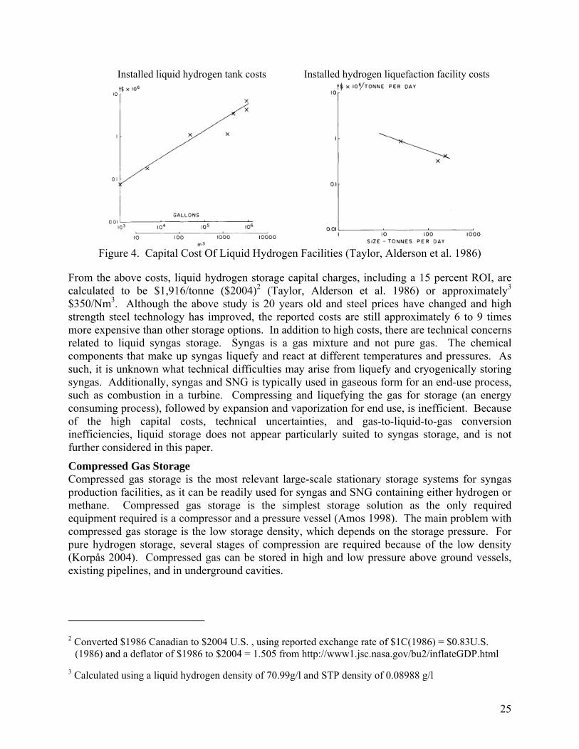
Cryogenic Liquid Storage Cryogenic liquid storage has been used for large scale hydrogen storage, with the technology largely driven by the needs of space programs. Storing liquid hydrogen presents numerous engineering challenges due to its low heat of vaporization and resultant very high loss index (Taylor, Alderson et al. 1986). Because the boil-off would be too high, liquid hydrogen cannot be stored in cylindrical tanks of the type used for LNG (Amos 1998). Spherical tanks are used for large-scale applications because this shape has the lowest surface area for heat transfer per unit volume. The National Aeronautics and Space Administration (NASA) uses liquid hydrogen tanks up to 3.8 x 103 cubic meters (106 U.S. gallons) which are about 22 meters in diameter (Taylor, Alderson et al. 1986). Liquid hydrogen storage is expensive; costs include both the spherical storage tanks as well as the facility required for cooling and liquefaction. Capital costs for liquid hydrogen storage and liquefaction facilities from a 1986 study are illustrated in Figure 4 below.

1 As used here, a storage system includes both the storage reservoir as well as the mechanism for

providing mass flow during the charging or discharging, such as a compressor.

25

Installed liquid hydrogen tank costs Installed hydrogen liquefaction facility costs

Figure 4. Capital Cost Of Liquid Hydrogen Facilities (Taylor, Alderson et al. 1986)

From the above costs, liquid hydrogen storage capital charges, including a 15 percent ROI, are calculated to be $1,916/tonne ($2004)2 (Taylor, Alderson et al. 1986) or approximately3 $350/Nm3. Although the above study is 20 years old and steel prices have changed and high strength steel technology has improved, the reported costs are still approximately 6 to 9 times more expensive than other storage options. In addition to high costs, there are technical concerns related to liquid syngas storage. Syngas is a gas mixture and not pure gas. The chemical components that make up syngas liquefy and react at different temperatures and pressures. As such, it is unknown what technical difficulties may arise from liquefy and cryogenically storing syngas. Additionally, syngas and SNG is typically used in gaseous form for an end-use process, such as combustion in a turbine. Compressing and liquefying the gas for storage (an energy consuming process), followed by expansion and vaporization for end use, is inefficient. Because of the high capital costs, technical uncertainties, and gas-to-liquid-to-gas conversion inefficiencies, liquid storage does not appear particularly suited to syngas storage, and is not further considered in this paper.

Compressed Gas Storage Compressed gas storage is the most relevant large-scale stationary storage systems for syngas production facilities, as it can be readily used for syngas and SNG containing either hydrogen or methane. Compressed gas storage is the simplest storage solution as the only required equipment required is a compressor and a pressure vessel (Amos 1998). The main problem with compressed gas storage is the low storage density, which depends on the storage pressure. For pure hydrogen storage, several stages of compression are required because of the low density (Korpås 2004). Compressed gas can be stored in high and low pressure above ground vessels, existing pipelines, and in underground cavities.

2 Converted $1986 Canadian to $2004 U.S. , using reported exchange rate of $1C(1986) = $0.83U.S.

(1986) and a deflator of $1986 to $2004 = 1.505 from http://www1.jsc.nasa.gov/bu2/inflateGDP.html 3 Calculated using a liquid hydrogen density of 70.99g/l and STP density of 0.08988 g/l

26

Compressors Compressed gas storage requires a compressor to provide the necessary mass flow of gas into the storage vessel. No literature discusses syngas compression or compressor requirements for syngas service, however reasonable estimates can be drawn from literature discussing compressors for natural gas and hydrogen service. The density and molecular weight of the gas to be compressed is an important consideration for compressor choice. Centrifugal compressors, which are widely used for natural gas, are not generally suitable for pure hydrogen compression as the pressure rise per stage is very small due to the low density and low molecular weight (Amos 1998; Leighty, Hirara, O'Hashi, Asahi, Benoit and Keith 2003). Positive displacement, reciprocating compressors may be the best choice for large-scale hydrogen compression (Leighty, Hirara et al. 2003), and hydrogen can be compressed using standard axial, radial or reciprocating piston-type compressors with slight modifications of the seals to take into account the higher diffusivity of the hydrogen molecules (Amos 1998).

The capital costs of compression depend on the properties of the gas to be compressed. Compressing pure hydrogen requires about three times the compressor power as natural gas and specific capital costs for large hydrogen compressors are expected to be 20 to 30 percent higher than for natural gas (Ogden 1999). Compressor costs are based on the amount of work done by the compressor, which depends on the inlet pressure, outlet pressure, and flow rate (Amos 1998). Capital costs of compressors reported in the literature range from $479-$4,900/hp ($650-$6,600/kW) and are shown in Table 5.

Table 5. Small Compressor Capital Costs (Taylor, Alderson et al. 1986; Amos 1998)

Size (hp) Capital cost ($) Cost/hp ($/hp) Source 13 63,700 4,900 Amos 100 180,000 1,800 Amos 100 187,373 1,874 Taylor4 335 164,150-246,225 n/a Amos

3,600 2,330,000 647 Amos 3,600 2,248,470 625 Amos 5,000 2,440,000 488 Amos 6,000 3,160,000 527 Amos 6,000 2,873,045 479 Taylor 38,000 20,000,000 526 Amos

Costs for large-scale, megawatt sized compression facilities for pipeline transport were developed by the International Energy Agency, IEA (IEA GHG 2002) and are shown in Table 6.

4 Taylor figures converted from $1986 Canadian to $2004U.S. Using $1C(1986) = $0.83U.S. (1986) and

a deflator of $1986 to $2004 = 1.505 from http://www1.jsc.nasa.gov/bu2/inflateGDP.html

27

Table 6. Compressor Capital Cost Estimates for Large (MW) Pipeline Compressors ($MM)

Type Initial Pressure Facility Booster Station Electrical Power Generation Plant CO2 export pipeline 5.590 + 0.509P - 0.006 P2 6.388 + 0.581P - 0.008 P2

Fuel Synthesis Plant Hydrogen product pipeline 24.902 + 0.549P - 0.005 P2 28.460 + 0.628P - 0.005 P2

CO2 Storage Facilities 5.590 + 0.509P - 0.006 P2 6.388 + 0.581P - 0.008 P2 Pipeline Branch CO2 6.388 + 0.581P - 0.008 P2 6.388 + 0.581P - 0.008 P2 Natural Gas and Hydrogen 28.460 + 0.628P - 0.005 P2 28.460 + 0.628P - 0.005 P2

where P is the compressor power in MW

The costs developed by the IEA are significantly higher than the costs reported in Table 5. For example, the IEA estimate for the 38,000hp (28 MW) compressor listed in Table 5 is about $36 million, or 1.8 times higher than the cost reported by Amos. Because of this difference, care should be taken to choose the appropriate cost estimated based on the size of the compressor when estimating compressor capital costs.

The largest operating cost for compressors is the energy required to compress the gas (Amos 1998). The exact energy requirements for compression depend on the desired final pressure. The theoretical work for isothermal compression of ideal gas from pressure p1 to p2 is given by:

⎟⎟⎠

⎞⎜⎜⎝

⎛=

1

2112,1 ln

pp

VpW (4)

where V1 is the volume of the gas at pressure p1. Figure 5 illustrates the work required to compress a gas from an initial pressure, p1, to a higher pressure, p2.

Gas Pressure

Wor

k to

com

pres

s a

gas

from

p1 t

o p 2

Total Work Requiredfor Compression

p1 p2

Figure 5. Work to Compress an Ideal Gas From P1 to P2

Because of the logarithmic relationship, the work and electricity consumption of the compressor is highest in the low-pressure range, and a high final storage pressure requires minimal power compared to the initial compression of the gas.

28

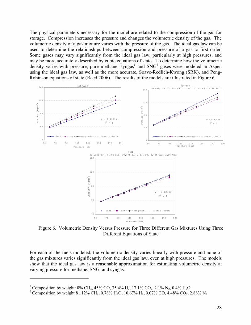
The physical parameters necessary for the model are related to the compression of the gas for storage. Compression increases the pressure and changes the volumetric density of the gas. The volumetric density of a gas mixture varies with the pressure of the gas. The ideal gas law can be used to determine the relationships between compression and pressure of a gas to first order. Some gases may vary significantly from the ideal gas law, particularly at high pressures, and may be more accurately described by cubic equations of state. To determine how the volumetric density varies with pressure, pure methane, syngas5 and SNG6 gases were modeled in Aspen using the ideal gas law, as well as the more accurate, Soave-Redlich-Kwong (SRK), and Peng-Robinson equations of state (Reed 2006). The results of the models are illustrated in Figure 6.

y = 0.6161x

R2 = 1

0

40

80

120

160

50 70 90 110 130 150 170 190

Pressure (bar)

Density (kg/m3)

Ideal SRK Peng-Rob Linear (Ideal)

Methane

y = 0.8264x

R2 = 1

0

40

80

120

160

50 70 90 110 130 150 170 190Pressure (bar)

Density (kg/m3 )


Syngas(0% CH4, 45% CO, 35.4% H2, 17.1% CO2, 2.1% N2, 0.4% H2O)

y = 0.6233x

R2 = 1

0

40

80

120

160

50 70 90 110 130 150 170 190

Pressure (bar)

Dens

ity

(kg/

m3)


(81.12% CH4, 0.78% H20, 10.67% H2, 0.07% CO, 4.48% CO2, 2.88 %N2)SNG

Figure 6. Volumetric Density Versus Pressure for Three Different Gas Mixtures Using Three

Different Equations of State

For each of the fuels modeled, the volumetric density varies linearly with pressure and none of the gas mixtures varies significantly from the ideal gas law, even at high pressures. The models show that the ideal gas law is a reasonable approximation for estimating volumetric density at varying pressure for methane, SNG, and syngas.

5 Composition by weight: 0% CH4, 45% CO, 35.4% H2, 17.1% CO2, 2.1% N2, 0.4% H2O 6 Composition by weight 81.12% CH4, 0.78% H2O, 10.67% H2, 0.07% CO, 4.48% CO2, 2.88% N2

29

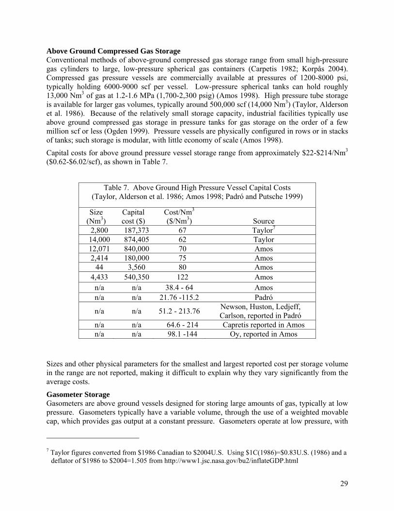
Above Ground Compressed Gas Storage Conventional methods of above-ground compressed gas storage range from small high-pressure gas cylinders to large, low-pressure spherical gas containers (Carpetis 1982; Korpås 2004). Compressed gas pressure vessels are commercially available at pressures of 1200-8000 psi, typically holding 6000-9000 scf per vessel. Low-pressure spherical tanks can hold roughly 13,000 Nm3 of gas at 1.2-1.6 MPa (1,700-2,300 psig) (Amos 1998). High pressure tube storage is available for larger gas volumes, typically around 500,000 scf (14,000 Nm3) (Taylor, Alderson et al. 1986). Because of the relatively small storage capacity, industrial facilities typically use above ground compressed gas storage in pressure tanks for gas storage on the order of a few million scf or less (Ogden 1999). Pressure vessels are physically configured in rows or in stacks of tanks; such storage is modular, with little economy of scale (Amos 1998).

Capital costs for above ground pressure vessel storage range from approximately $22-$214/Nm3 ($0.62-$6.02/scf), as shown in Table 7.

Table 7. Above Ground High Pressure Vessel Capital Costs (Taylor, Alderson et al. 1986; Amos 1998; Padró and Putsche 1999)

Size (Nm3)

Capital cost ($)

Cost/Nm3

($/Nm3) Source 2,800 187,373 67 Taylor7 14,000 874,405 62 Taylor 12,071 840,000 70 Amos 2,414 180,000 75 Amos

44 3,560 80 Amos 4,433 540,350 122 Amos

n/a n/a 38.4 - 64 Amos n/a n/a 21.76 -115.2 Padró

n/a n/a 51.2 - 213.76 Newson, Huston, Ledjeff, Carlson, reported in Padró

n/a n/a 64.6 - 214 Capretis reported in Amos n/a n/a 98.1 -144 Oy, reported in Amos

Sizes and other physical parameters for the smallest and largest reported cost per storage volume in the range are not reported, making it difficult to explain why they vary significantly from the average costs.

Gasometer Storage Gasometers are above ground vessels designed for storing large amounts of gas, typically at low pressure. Gasometers typically have a variable volume, through the use of a weighted movable cap, which provides gas output at a constant pressure. Gasometers operate at low pressure, with

7 Taylor figures converted from $1986 Canadian to $2004U.S. Using $1C(1986)=$0.83U.S. (1986) and a

deflator of $1986 to $2004=1.505 from http://www1.jsc.nasa.gov/bu2/inflateGDP.html

30

typical pressures in the range of 200-300mm water (0.28-0.43psig); maximum operating pressures are 1000mm water (1.4psig) (Bennet 2006). Typical volumes for large gasometers are about 50,000-70,000m³, with approximately 60 m diameter structures; although the largest gasholder installed by one manufacturer was 340,000m3 (Bennet 2006). Gasometers have long operating lifetimes; the structure itself can operate for over 100 years (Bennet 2006), while the diaphragm that seals the gasometer has a lifetime of 200,000 strokes or approximately 10 years (ContiTech 2006).

Table 8. Above Ground Low Pressure Vessel (Gasometer) Capital Costs

Size (Nm3) Capital cost ($) Cost/Nm3

($/Nm3) Source

65,000 22,080,0008 340 Clayton Walker (Bennet 2006)

Pipeline Storage Syngas can also be stored, or packed, in piping systems. Pipelines are usually several miles long, and in some cases may be hundreds of miles long. Because of the large volume of piping systems, a slight change in the operating pressure of a pipeline system can result in a large change in the amount of gas contained within the piping network. By making small changes in operating pressure, the pipeline can effectively used as a storage vessel (Amos 1998). Storing gas in an existing pipeline system by increasing the operating pressure requires no additional capital expense as long as the pressure rating of the pipe and the capacity of the compressors are not exceeded (Amos 1998). Existing hydrogen pipelines are generally constructed of 0.25-0.30 m (10-12 in) commercial steel and operate at 1-3 MPa (145-435 psig); natural gas mains for comparison are constructed of pipe as large as 2.5 m (5 ft) in diameter and have working pressures of 7.5 MPa (1,100 psig) (Hart 1997). A 30 km, 3 inch diameter hydrogen distribution pipeline could carry a flow of 5 MMscf of hydrogen per day. Assuming that the pipeline operated at 1000 psi, the storage volume available in the pipeline would be 340,000 scf, or about 7 percent of the total daily flow rate (Ogden 1999).

Underground Compressed Gas Storage Underground storage is a special case of compressed gas storage where the vessel is located underground and generally has a lower cost (Amos 1998). Because of their large capacities and low cost, underground compressed gas systems are generally most suitable for large quantities and/or long storage times (Padró and Putsche 1999). There are four underground formations in which gas can be stored under pressure: (a) depleted oil or gas field; (b) aquifers; (c) excavated rock caverns; and (d) salt caverns (Taylor, Alderson et al. 1986).

There is significant industrial experience in underground gas storage: natural gas has been stored underground since 1916 (Taylor, Alderson et al. 1986); the city of Kiel, Germany has been

8 Converted from reported cost of £12 million (UK 2006) using £1(UK) = $1.84U.S. Single lift, Wiggins,

dry seal gasometer.

31

storing town gas (60-65 percent hydrogen) in a gas cavern since 1971 (Taylor, Alderson et al. 1986); Gaz de France has stored town gas containing 50 percent hydrogen in a 330 million cubic meter aquifer structure near Beynes, France; Imperial Chemical Industries stores hydrogen at 50 atm (5x106 Pa) pressure in three brine compensated salt caverns at 1200 ft (366 m) near Teeside, UK; and in Texas, helium is stored in rock strata beneath an aquifer whereby water seals the rock fissures above the helium reservoir, sealing in the helium atoms (Leighty, Hirara et al. 2003).

Underground storage volumes in depleted oil and gas fields can be extremely large; volumes of gas stored exceed 109 m3 and pressures can be up to 40 atm. Salt caverns, large underground voids that are formed by solution mining of salt as brine, tend to be smaller, typically around 106-107 m3. Although smaller, salt caverns offer faster discharge rates and tend to be tighter than other underground formations, reducing leakage. Hydrogen, a small molecule with high leakage rates, has been stored in salt caverns (Morrow, Corrao, Hylkema and PRAXAIR 2005). Rock caverns are usually smaller cavities, typically on the order of 1 million to10 million m3.

Underground gas storage requires the use of a cushion gas that occupies the underground storage volume at the end of the discharge cycle. Cushion gas is non-recoverable base gas necessary to pressurize the storage reservoir. Cushion gas can be as much as 50 percent of the working volume, or several hundred thousand kilograms of gas (Amos 1998) and the cost of the cushion gas is a significant part of the capital costs for large storage reservoirs (Taylor, Alderson et al. 1986).

Capital costs for underground storage are reported in the literature. Underground storage is reported to be the most inexpensive means of storage for large quantities of gas, up to two orders of magnitude less expensive than other methods (Carpetis 1982; Amos 1998). The only case where underground storage would not be the least cost option is with small quantities of gas in large caverns where the amount of working capital invested in the cushion gas is large compared to the amount of gas stored (Amos 1998). Capital costs vary depending on whether there is a suitable natural cavern or rock formation, or whether a cavern must be mined. An abandoned natural gas well was reported to be the least expensive, however the likelihood of a gasification facility being near such a formation (and choosing to use it to store syngas rather than to sequester CO2), seems small, so it is not further considered in this paper. Solution mining, excavating a salt formation with a brine solution, capital costs were estimated at $19-$23/m3 ($0.54$0.66/ft3) (Carpetis 1982); hard rock mining costs were estimated at $34-$84/m3 ($1.00-$2.50/ft3) depending on the depth (Amos 1998). Additionally, construction times for underground storage facilities can be long and may contribute to their costs. One estimate for solution mining a salt formation to create a 160 million cubic foot cavern was 2.5 years (Ridge Energy Storage & Grid Services L.P. and Texas State Energy Conservation Office 2005). Table 9 shows reported ranges of underground storage capital costs for salt and excavated rock caverns.

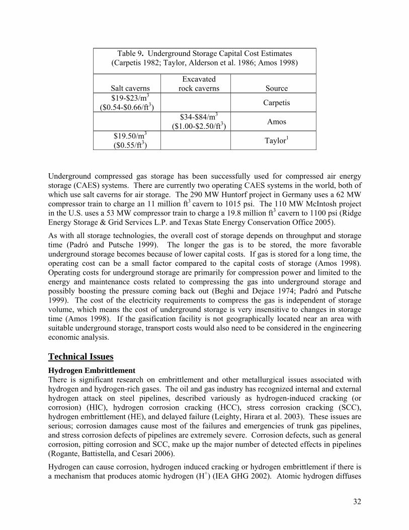
32

Table 9. Underground Storage Capital Cost Estimates (Carpetis 1982; Taylor, Alderson et al. 1986; Amos 1998)

Salt caverns Excavated

rock caverns Source $19-$23/m3

($0.54-$0.66/ft3) Carpetis

$34-$84/m3 ($1.00-$2.50/ft3) Amos

$19.50/m3 ($0.55/ft3) Taylor1

Underground compressed gas storage has been successfully used for compressed air energy storage (CAES) systems. There are currently two operating CAES systems in the world, both of which use salt caverns for air storage. The 290 MW Huntorf project in Germany uses a 62 MW compressor train to charge an 11 million ft3 cavern to 1015 psi. The 110 MW McIntosh project in the U.S. uses a 53 MW compressor train to charge a 19.8 million ft3 cavern to 1100 psi (Ridge Energy Storage & Grid Services L.P. and Texas State Energy Conservation Office 2005).

As with all storage technologies, the overall cost of storage depends on throughput and storage time (Padró and Putsche 1999). The longer the gas is to be stored, the more favorable underground storage becomes because of lower capital costs. If gas is stored for a long time, the operating cost can be a small factor compared to the capital costs of storage (Amos 1998). Operating costs for underground storage are primarily for compression power and limited to the energy and maintenance costs related to compressing the gas into underground storage and possibly boosting the pressure coming back out (Beghi and Dejace 1974; Padró and Putsche 1999). The cost of the electricity requirements to compress the gas is independent of storage volume, which means the cost of underground storage is very insensitive to changes in storage time (Amos 1998). If the gasification facility is not geographically located near an area with suitable underground storage, transport costs would also need to be considered in the engineering economic analysis. Technical Issues Hydrogen Embrittlement There is significant research on embrittlement and other metallurgical issues associated with hydrogen and hydrogen-rich gases. The oil and gas industry has recognized internal and external hydrogen attack on steel pipelines, described variously as hydrogen-induced cracking (or corrosion) (HIC), hydrogen corrosion cracking (HCC), stress corrosion cracking (SCC), hydrogen embrittlement (HE), and delayed failure (Leighty, Hirara et al. 2003). These issues are serious; corrosion damages cause most of the failures and emergencies of trunk gas pipelines, and stress corrosion defects of pipelines are extremely severe. Corrosion defects, such as general corrosion, pitting corrosion and SCC, make up the major number of detected effects in pipelines (Rogante, Battistella, and Cesari 2006).

Hydrogen can cause corrosion, hydrogen induced cracking or hydrogen embrittlement if there is a mechanism that produces atomic hydrogen (H+) (IEA GHG 2002). Atomic hydrogen diffuses

33

into a metal and reforms as microscopic pockets of molecular hydrogen gas, causing cracking, embrittlement, and corrosion which can ultimately lead to failure. The hardness of a metal correlates to the degree of embrittlement; if a material has a Vickers Hardness Number (VHN) greater than 300, the tendency for the material to fail due to plastic straining when there is significant absorption of atomic hydrogen is greater than with a softer material (Rogante, Battistella et al. 2006).

Molecular hydrogen (H2) alone does not cause embrittlement of steel; however problems can arise if there is a mechanism that produces atomic hydrogen. The two primary mechanisms leading to hydrogen induced cracking are HIC due to wet conditions and HIC due to elevated temperatures (Rogante, Battistella et al. 2006). Temperatures greater than 220°C can cause dissociation of molecular hydrogen into atomic hydrogen. Studies show that molecular hydrogen should be water dry, or below 60 percent relative humidity, to provide a sufficient margin for avoidance of moisture and water dropout (IEA GHG 2002). Molecular hydrogen, then, may be handled without problems with standard low-alloy carbon steel irrespective of the gas pressure, provided that the conditions are dry (to prevent HIC due to wet conditions) and under 220°C (to prevent HIC due to elevated temperatures) (IEA GHG 2002).

Because of the metallurgical issues associated with hydrogen, care must be taken when choosing metals for hydrogen pipelines and storage. Surveys of existing hydrogen pipelines show that a variety of steels, but primarily mild steel, is in use (Pottier 1995; Mohitpour, Golshan and Murray 2000). Options for steel pipe for 100 percent hydrogen service include Al-Fe (aluminum-iron) alloy; and variable-hardness pipe, with the harder material in the interior and softer material toward the exterior, so that any hydrogen which diffuses into the interior steel diffuses rapidly outward and escapes (Leighty, Hirara et al. 2003).

Existing natural gas pipelines can be used for less than 15 to 20 percent hydrogen, by volume, without danger of hydrogen attack on the line pipe steel, however further hydrogen enrichment will risk hydrogen embrittlement (Leighty, Hirara et al. 2003). Existing pipelines originally designed for sour service can provide additional protection against HIC and hydrogen embrittlement due to their specific metallurgy (IEA GHG 2002). If hydrogen embrittlement is found to be a potential problem for an unusual situation, costs for any materials will be relatively low. Steel used for hydrogen transport and storage are low carbon steel and low in alloy content. These steels may have a restriction of some alloy elements (those that attract and stabilize H and a structure called austenite); however the cost should not be affect by these restrictions (Heard 2006). For large diameter pipelines and vessels, options include low carbon steel plate, such as type X52, which is easy to make, readily available, easy to weld, and easy to fabricate. Smaller pipes can be constructed from either seamless or welded pipe. The main failure of the material is by hydrogen embrittlement in the zone near the weld. This area is affected by the heating and cooling during welding and has more internal stress. Because of the care required for welding, the most costly component is likely welding by certified welders (Heard 2006).

Syngas Leakage An additional potential problem resulting from the hydrogen content of syngas is that atomic hydrogen is a small molecule and can diffuse through most metals (IEA GHG 2002). However industrial experience with syngas and analogies with other industrial practices suggests that excessive diffusion and leakage of syngas through a storage chamber wall is not an issue for diurnal and relatively short-term storage (Rubin 2006).

34

Biological Fouling The subsurface storage of gas raises the issues of microbial factors and the risks of biological fouling. That is, conditions may exist underground where microbes can rapidly grow causing a number of potential problems such as contamination of the gas, plugging of the storage vessel, degrading its capacity, and biocorrosion. We have discussed these issues with a number of experts and professionals with significant industrial experience and conclude that biological fouling is likely not an issues for diurnal gas storage (Colwell 2006; Griffin 2006; Heard 2006; Stolz 2006). The rapid turnover and short residence time of gas in an underground vessel is not likely to produce conditions conducive to rapid microbial growth (Stolz 2006). Furthermore, should fouling occur, ‘work-overs’ are common and expected in industrial practice (Griffin 2006).

Technical Note on Constructing Cost Distributions from Cost Data Distributions of costs were used in the analysis to capture the uncertainty in the cost parameter. Cost distributions were constructed directly from the cost data. The cost data were plotted on the y-axis against the relevant parameter (size, output, etc) on the x-axis and a mean regression line was calculated using an ordinary least squares method shown in equation 5. mean regression line: 010ˆ xy ββ += (5)

where β0 and β1 are calculated using the usual method of ordinary least squares. At any point x0, the prediction interval for the value of y is given by

prediction interval: )ˆ(ˆ 02/1 ysety ⋅± −α (6)

= ⎟

⎟⎠

⎞⎜⎜⎝

⎛

−−

++⋅⋅±∑− 2

202

2/1 )()(11ˆxx

xxn

tyi

σα

(7)

where t1-α/2 is the student’s t distribution evaluated at the α significance level, se is the standard error, x is the average and σ2 is the mean square error. Figure 7 illustrates the prediction interval for the value of y at any given x value, in relation to the underlying data.

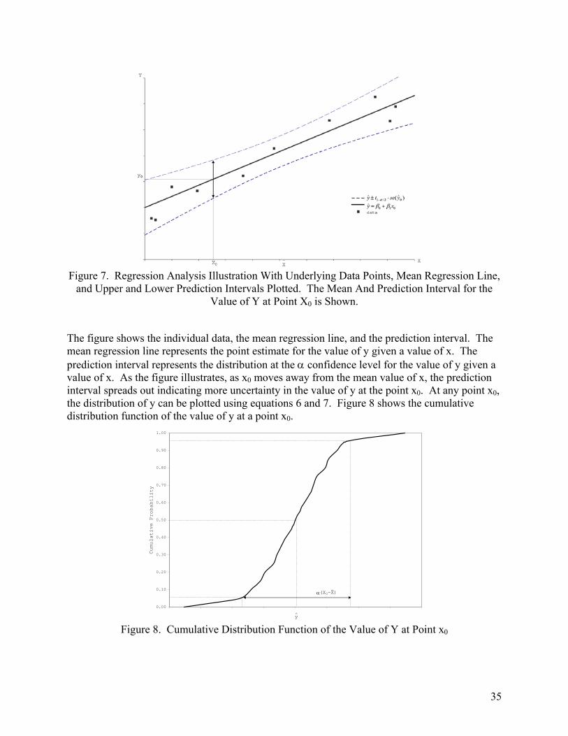
35

Figure 7. Regression Analysis Illustration With Underlying Data Points, Mean Regression Line,

and Upper and Lower Prediction Intervals Plotted. The Mean And Prediction Interval for the Value of Y at Point X0 is Shown.

The figure shows the individual data, the mean regression line, and the prediction interval. The mean regression line represents the point estimate for the value of y given a value of x. The prediction interval represents the distribution at the α confidence level for the value of y given a value of x. As the figure illustrates, as x0 moves away from the mean value of x, the prediction interval spreads out indicating more uncertainty in the value of y at the point x0. At any point x0, the distribution of y can be plotted using equations 6 and 7. Figure 8 shows the cumulative distribution function of the value of y at a point x0.

0.00

0.10

0.20

0.30

0.40

0.50

0.60

0.70

0.80

0.90

1.00

Cumulative Probability

y

α(X0-X)-

Figure 8. Cumulative Distribution Function of the Value of Y at Point x0

36

As the figure shows, the standard error of y increases as x0 moves away from x , resulting in a wider cumulative distribution function.

Methanation: A Closer Examination Methanation is a process used to upgrade low energy density syngas to higher pipeline quality synthetic natural gas or SNG. In the methanation process, the calorific value, Wobbe-index9 and other parameters of a gas are adjusted in order to meet pipeline specifications (Hagen, Polman et al. 2001; Mozaffarian, Zwart et al. 2004). The problems associated with low energy density syngas and hydrogen rich gases can be avoided through a methanation process. The main advantage of SNG is that its composition is nearly identical to that of natural gas and can therefore be used in the same manner (Collot 2004) and injected into the natural gas pipeline system. The techniques and costs for natural gas handling and use and well known, and can be directly applied to SNG.

Industrial Experience The methanation of synthesis gas from was first developed in 1902 and has been investigated intensely in the 1970s and 1980s (Deurwaarder, Boerrigter, Mozaffarian, Rabou, and van der Drift 2005). There is significant industrial experience methanating both biomass and coal-derived syngas.

The Great Plains Coal Gasification Plant in North Dakota has been operating since 1984 with nominal output of 125 million standard cubic feet per day (MMscf/d) of pipeline quality gas (DOE Coal Gasification Research Needs (COGARN) Working Group 1987). Using the Lurgi gasification process, the facility gasifies approximately 18,500 tons/d of lignite to produce gases and liquids. The plant has maximum total capacity of 170 MMscf/d of SNG. Including planned and unplanned outages and rate reductions, the average annual plant loading factor is typically about 90 to 92 percent. The product SNG is piped into the Northern Border pipeline, which runs to Ventura, Iowa for distribution in the Midwestern and Eastern United States (Perry and Eliason 2004).

Switzerland has a facility producing SNG from wood whose quality matches that of natural gas, thus allowing its direct injection in the high pressure Swiss natural gas network (Duret, Friedli. and Marechal 2005). A facility in the Netherlands uses a methanation process to upgrade biogas-derived syngas to bring the Wobbe index of the gas within the Dutch natural gas specification (between 1166.43 and 1191.93 BTU/scf (Mozaffarian, Zwart et al. 2004). In Sasolburg, South Africa, Lurgi and Sasol operated a small scale, semi-commercial methanation pilot plant from 1974 to 1976. The pilot plant methanated coal-derived, CO-rich synthesis gas to yield

9 Wobbe-index is defined as the ratio of the gross calorific value to the square root of the relative density

of a gas: airg

HHVWρρ /

=

where HHV is the high heating value, and ρg and ρair are the gas and air density). The Wobbe-index is a measure of the amount of energy delivered to a burner via an injector. Two gases of differing composition but having the same Wobbe-index will deliver the same amount of energy for any given injector under the same injector pressure.

37

specification grade SNG with a calorific value of 970 ± 2 BTU/scf or higher during over 1.5 years of continuous operation (Moeller, Roberts and Britz 1974).

SNG Production Process SNG can be produced from coal through either direct or indirect synthesis (Collot 2004). Direct synthesis is based on the hydrogasification of coal (Figure 9).

Figure 9. SNG Production by Direct Synthesis

The gas produced by hydrogasification has very high methane (CH4) concentration and a low carbon monoxide (CO) concentration, compared to the gas produced by other gasification processes. The basic chemistry of coal hydrogasification is shown in the equation (British Columbia Hydro and Power Authority and Energy Mines and Resources Canada 1975)

242 CO 4.0CH 0.6 OH coal +→+ (8)

From equation (8), it can be seen that 60% of the carbon in the coal is converted directly into CH4 while 40 percent is rejected as CO2. The aim of a hydrogasification processes is to produce as much methane as possible directly, up to this 60% theoretical limit (British Columbia Hydro and Power Authority and Energy Mines and Resources Canada 1975). With direct synthesis, no methanation or only a relatively small methanation step is required to upgrade the produced gas to SNG (Mozaffarian and Zwart 2000). The conversion of H2 and CO to CH4 via a methanation step is a highly exothermic process. Therefore, a high initial yield of CH4 through hydrogasification is attractive since methanation involves approximately 20% efficiency loss through heat production (van der Drift, van der Meijden and Boerrigter 2005). There are presently no commercial facilities based on the direct SNG synthesis from coal. However, a process based on this method, the ARCH process, was developed in Japan with the aim of reducing its dependence on natural gas imports (Maruyama and Nomura 2002). Because of its current limited use and lack of commercially available data, direct SNG synthesis is not further considered in this paper.

Indirect synthesis of SNG is based on the partial gasification of coal followed by a methanation reaction (Figure 10).

Figure 10. SNG Production by Indirect Synthesis

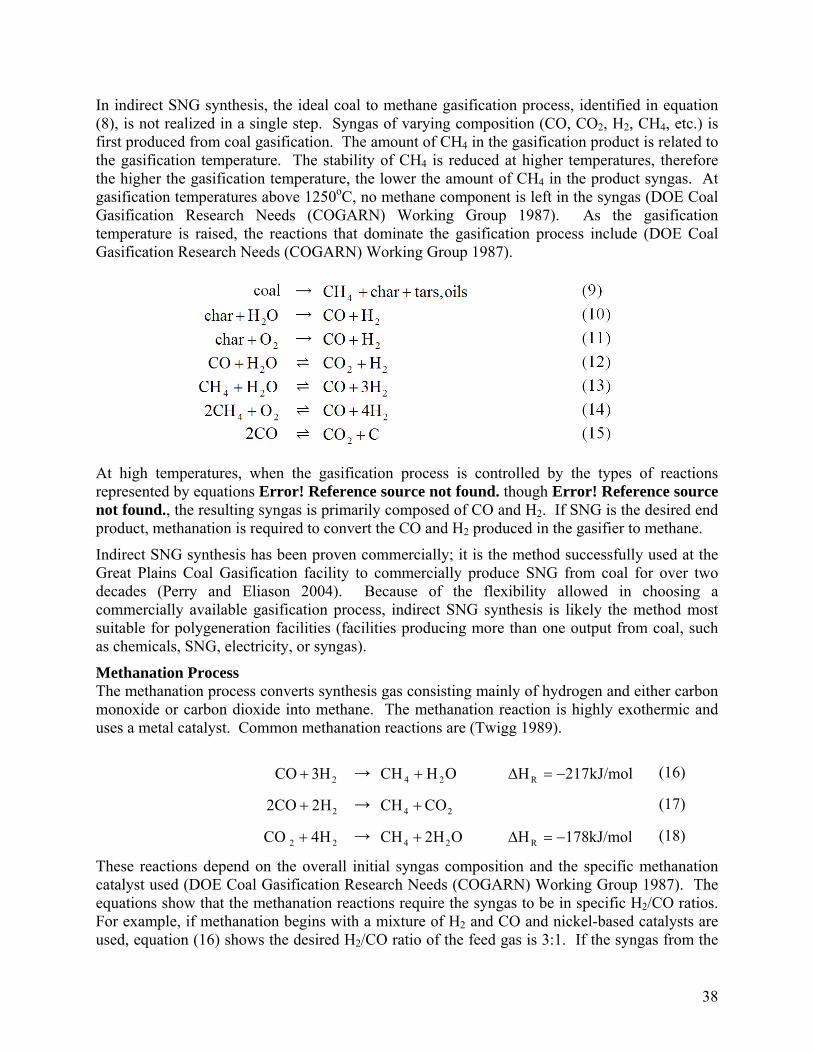
38

In indirect SNG synthesis, the ideal coal to methane gasification process, identified in equation (8), is not realized in a single step. Syngas of varying composition (CO, CO2, H2, CH4, etc.) is first produced from coal gasification. The amount of CH4 in the gasification product is related to the gasification temperature. The stability of CH4 is reduced at higher temperatures, therefore the higher the gasification temperature, the lower the amount of CH4 in the product syngas. At gasification temperatures above 1250oC, no methane component is left in the syngas (DOE Coal Gasification Research Needs (COGARN) Working Group 1987). As the gasification temperature is raised, the reactions that dominate the gasification process include (DOE Coal Gasification Research Needs (COGARN) Working Group 1987).

At high temperatures, when the gasification process is controlled by the types of reactions represented by equations Error! Reference source not found. though Error! Reference source not found., the resulting syngas is primarily composed of CO and H2. If SNG is the desired end product, methanation is required to convert the CO and H2 produced in the gasifier to methane.

Indirect SNG synthesis has been proven commercially; it is the method successfully used at the Great Plains Coal Gasification facility to commercially produce SNG from coal for over two decades (Perry and Eliason 2004). Because of the flexibility allowed in choosing a commercially available gasification process, indirect SNG synthesis is likely the method most suitable for polygeneration facilities (facilities producing more than one output from coal, such as chemicals, SNG, electricity, or syngas).

Methanation Process The methanation process converts synthesis gas consisting mainly of hydrogen and either carbon monoxide or carbon dioxide into methane. The methanation reaction is highly exothermic and uses a metal catalyst. Common methanation reactions are (Twigg 1989).

2H3 CO + → OH CH 24 + kJ/mol217HR −=Δ (16)

2H2 2CO + → 24 CO CH + (17)

22 H4CO + → OH2 CH 24 + kJ/mol178HR −=Δ (18)

These reactions depend on the overall initial syngas composition and the specific methanation catalyst used (DOE Coal Gasification Research Needs (COGARN) Working Group 1987). The equations show that the methanation reactions require the syngas to be in specific H2/CO ratios. For example, if methanation begins with a mixture of H2 and CO and nickel-based catalysts are used, equation (16) shows the desired H2/CO ratio of the feed gas is 3:1. If the syngas from the

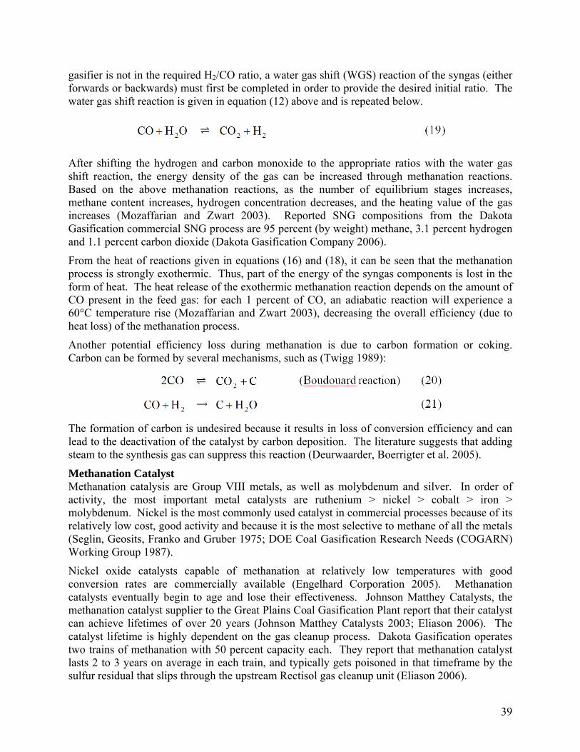
39

gasifier is not in the required H2/CO ratio, a water gas shift (WGS) reaction of the syngas (either forwards or backwards) must first be completed in order to provide the desired initial ratio. The water gas shift reaction is given in equation (12) above and is repeated below.

After shifting the hydrogen and carbon monoxide to the appropriate ratios with the water gas shift reaction, the energy density of the gas can be increased through methanation reactions. Based on the above methanation reactions, as the number of equilibrium stages increases, methane content increases, hydrogen concentration decreases, and the heating value of the gas increases (Mozaffarian and Zwart 2003). Reported SNG compositions from the Dakota Gasification commercial SNG process are 95 percent (by weight) methane, 3.1 percent hydrogen and 1.1 percent carbon dioxide (Dakota Gasification Company 2006).

From the heat of reactions given in equations (16) and (18), it can be seen that the methanation process is strongly exothermic. Thus, part of the energy of the syngas components is lost in the form of heat. The heat release of the exothermic methanation reaction depends on the amount of CO present in the feed gas: for each 1 percent of CO, an adiabatic reaction will experience a 60°C temperature rise (Mozaffarian and Zwart 2003), decreasing the overall efficiency (due to heat loss) of the methanation process.

Another potential efficiency loss during methanation is due to carbon formation or coking. Carbon can be formed by several mechanisms, such as (Twigg 1989):

The formation of carbon is undesired because it results in loss of conversion efficiency and can lead to the deactivation of the catalyst by carbon deposition. The literature suggests that adding steam to the synthesis gas can suppress this reaction (Deurwaarder, Boerrigter et al. 2005).

Methanation Catalyst Methanation catalysis are Group VIII metals, as well as molybdenum and silver. In order of activity, the most important metal catalysts are ruthenium > nickel > cobalt > iron > molybdenum. Nickel is the most commonly used catalyst in commercial processes because of its relatively low cost, good activity and because it is the most selective to methane of all the metals (Seglin, Geosits, Franko and Gruber 1975; DOE Coal Gasification Research Needs (COGARN) Working Group 1987).

Nickel oxide catalysts capable of methanation at relatively low temperatures with good conversion rates are commercially available (Engelhard Corporation 2005). Methanation catalysts eventually begin to age and lose their effectiveness. Johnson Matthey Catalysts, the methanation catalyst supplier to the Great Plains Coal Gasification Plant report that their catalyst can achieve lifetimes of over 20 years (Johnson Matthey Catalysts 2003; Eliason 2006). The catalyst lifetime is highly dependent on the gas cleanup process. Dakota Gasification operates two trains of methanation with 50 percent capacity each. They report that methanation catalyst lasts 2 to 3 years on average in each train, and typically gets poisoned in that timeframe by the sulfur residual that slips through the upstream Rectisol gas cleanup unit (Eliason 2006).

40

Syngas Cleanup and Special Considerations A common problem with all known active methanation catalysts is that they are easily poisoned by sulfur and other elements that can be in raw syngas (Mozaffarian and Zwart 2003). Therefore thorough gas cleaning or polishing is required before methanation to avoid catalyst poisoning. Mozaffarian and Zwart (Mozaffarian and Zwart 2003) conducted an extensive literature review of the effects of contaminates in syngas on catalysts. According to their review, particles can deposit on the surface of methanation catalysts and make them inactive (Mozaffarian and Zwart 2003); the amount of particles in the synthesis gas should be limited to 0.02 mg/Nm3. Light hydrocarbons do not seem to affect catalyst activity, and they reform into methane. Higher hydrocarbons, such as ethane, ethylene, and BTX (benzene, toluene, xylenes), which are still present in the product gas after the gas clean up step, will not cause any problems to the methanation reactor; they will be converted to methane and carbon dioxide. Hydrogen chloride is a permanent irreversible poison to the methanation activity of nickel catalyst; an HCl/HF concentration of less than 25 ppb would be admissible for nickel catalysts. Sulfur compounds affect the nickel catalyst through the reaction of hydrogen sulfide with nickel, according to the reaction (Mozaffarian and Zwart 2003):

Hydrogen sulfide is typically present in the feed gas, or it can be formed by excess hydrogen. A U.S. Department of Energy report (DOE Coal Gasification Research Needs (COGARN) Working Group 1987) recommends gas polishing to reduce the concentration of sulfur species in the inlet gas to less than 0.5 ppm in order to maintain adequate catalyst activity for long periods of time. Ni-based catalysts are currently used in the fixed-bed methanators at the Great Plains Coal Gasification Plant. The feed gases are preprocessed by acid-gas removal-systems to reduce the sulfur content to less than 1 ppm before they enter the methanation units (DOE Coal Gasification Research Needs (COGARN) Working Group 1987).

To meet the requirements of the methanation catalyst, a facility using a methanation process to upgrade syngas to SNG would have a simplified process flow diagram as illustrated in Figure 11.

Figure 11. Methanation Process Flow Diagram

The process flow diagram reflects the necessary water gas shift and gas cleanup process that needed to prepare syngas for the catalytic methanation step.

41

Commercial Methanation Processes There are several commercial methanation processes that have been developed that are variants of the process flow diagram illustrated in

Figure 11. These include the Kellogg-Rust-Westinghouse, Exxon, Comflux, and HICOM processes (DOE Coal Gasification Research Needs (COGARN) Working Group 1987), as well as equilibrium-limited reactors, through wall-cooled reactors and steam-moderated reactors (Mozaffarian and Zwart 2003). The processes differ in the specific gasification and catalytic processes employed; in the specific number and type of reactors used; and in methods used to control the temperatures and pressures in the methanation reactor(s). The literature discusses these differences in detail (Moeller, Roberts et al. 1974; Twigg 1989; Mozaffarian and Zwart 2000; Mozaffarian and Zwart 2003; Perry and Eliason 2004; Duret, Friedli et al. 2005) and, as they are highly technical and site specific, they are not further discussed here.

Methanation Costs The costs of SNG production by syngas methanation are dependent on the specific processes used. The gasification process determines the amount of methanation required to upgrade the syngas to SNG; a gasification process that produces syngas with less initial CH4 will require more methanation and associated costs than a gasification process producing a CH4 rich syngas. The methanation catalyst selected determines the water gas shift requirements needed to attain the required H2/CO ratios as well as the amount of gas cleaning necessary to maintain the activity of the catalyst. The required equipment also depends on the specific methanation process used by a facility. For example, the gas recycle process used by Dakota Gasification to control reactor temperatures requires a 7,000 hp compressor for each methanation train10 (Eliason 2006). Several studies have included total basic methanation costs in overall studies of gasification facilities. From these studies, a range of methanation costs can be examined. SNG production by syngas methanation was examined using a number of case studies in the literature. The different cases represent different methanation and gasification processes. Table 10 lists the cases analyzed.

10 Dakota Gasification reports that much of the operating cost of each compressor is recovered by

generating high pressure steam from the exothermic methanation reaction. Because they can use the steam elsewhere in their facility, the net operating cost for the methanation section of their operation is almost zero.

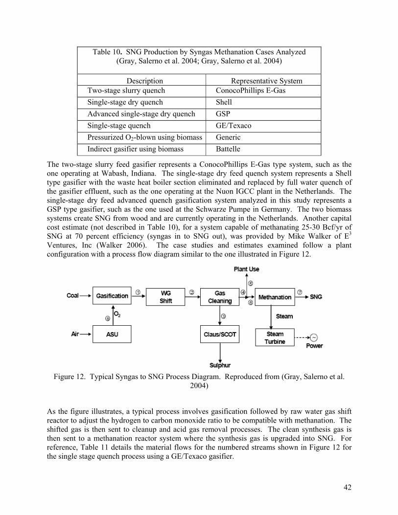
42

Table 10. SNG Production by Syngas Methanation Cases Analyzed (Gray, Salerno et al. 2004; Gray, Salerno et al. 2004)

Description Representative System Two-stage slurry quench ConocoPhillips E-Gas Single-stage dry quench Shell Advanced single-stage dry quench GSP Single-stage quench GE/Texaco Pressurized O2-blown using biomass Generic Indirect gasifier using biomass Battelle

The two-stage slurry feed gasifier represents a ConocoPhillips E-Gas type system, such as the one operating at Wabash, Indiana. The single-stage dry feed quench system represents a Shell type gasifier with the waste heat boiler section eliminated and replaced by full water quench of the gasifier effluent, such as the one operating at the Nuon IGCC plant in the Netherlands. The single-stage dry feed advanced quench gasification system analyzed in this study represents a GSP type gasifier, such as the one used at the Schwarze Pumpe in Germany. The two biomass systems create SNG from wood and are currently operating in the Netherlands. Another capital cost estimate (not described in Table 10), for a system capable of methanating 25-30 Bcf/yr of SNG at 70 percent efficiency (syngas in to SNG out), was provided by Mike Walker of E3 Ventures, Inc (Walker 2006). The case studies and estimates examined follow a plant configuration with a process flow diagram similar to the one illustrated in Figure 12.

Figure 12. Typical Syngas to SNG Process Diagram. Reproduced from (Gray, Salerno et al.

2004)

As the figure illustrates, a typical process involves gasification followed by raw water gas shift reactor to adjust the hydrogen to carbon monoxide ratio to be compatible with methanation. The shifted gas is then sent to cleanup and acid gas removal processes. The clean synthesis gas is then sent to a methanation reactor system where the synthesis gas is upgraded into SNG. For reference, Table 11 details the material flows for the numbered streams shown in Figure 12 for the single stage quench process using a GE/Texaco gasifier.

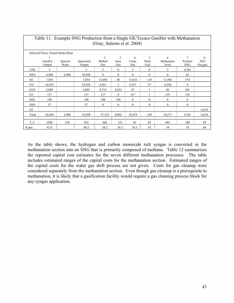
43

Table 11. Example SNG Production from a Single GE/Texaco Gasifier with Methanation (Gray, Salerno et al. 2004)

Selected Flows, Pound Moles/Hour 1 2 3 4 5 6 7 8

Gasifier Output

Quench Water

Quenched Output

Shifted Gas

Sour Gas

Clean Gas

Plant Fuel

Methanator Feed

Product SNG

ASU Oxygen

CH4 3 3 3 0 3 0 3 4,365 H2O 4,500 2,800 30,950 0 0 0 0 0 42 H2 7,854 7,854 13,684 68 13,616 110 13,506 574 CO 10,392 10,392 4,561 5 4,557 37 4,520 4 CO2 2,889 2,889 8,719 8,632 87 1 86 241 N2 157 157 157 0 157 1 155 155 H2S 198 198 198 198 0 0 0 0 NH3 57 57 0 0 0 0 0 0 O2 6,618 Total 26,048 2,800 52,498 27,322 8,902 18,419 149 18,271 5,381 6,618

T, F 2500 250 432 666 151 85 85 483 100 59 P,atm 41.8 40.2 38.2 36.3 36.3 35 34 34 44

As the table shows, the hydrogen and carbon monoxide rich syngas is converted in the methanation section into an SNG that is primarily composed of methane. Table 12 summarizes the reported capital cost estimates for the seven different methanation processes. The table includes estimated ranges of the capital costs for the methanation section. Estimated ranges of the capital costs for the water gas shift process are not given. Costs for gas cleanup were considered separately from the methanation section. Even though gas cleanup is a prerequisite to methanation, it is likely that a gasification facility would require a gas cleaning process block for any syngas application.

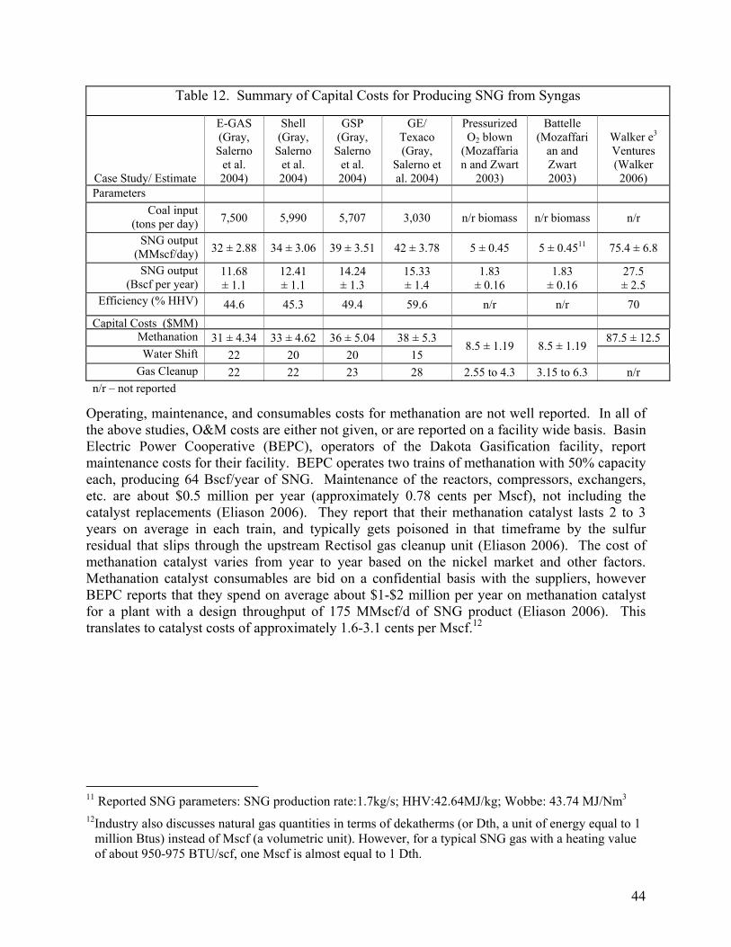
44

Table 12. Summary of Capital Costs for Producing SNG from Syngas

Case Study/ Estimate

E-GAS (Gray, Salerno

et al. 2004)

Shell

(Gray, Salerno

et al. 2004)

GSP (Gray, Salerno

et al. 2004)

GE/ Texaco (Gray,

Salerno et al. 2004)

Pressurized O2 blown

(Mozaffarian and Zwart

2003)

Battelle (Mozaffari

an and Zwart 2003)

Walker e3 Ventures (Walker 2006)

Parameters Coal input

(tons per day) 7,500 5,990 5,707 3,030 n/r biomass n/r biomass n/r

SNG output (MMscf/day) 32 ± 2.88 34 ± 3.06 39 ± 3.51 42 ± 3.78 5 ± 0.45 5 ± 0.4511 75.4 ± 6.8

SNG output (Bscf per year)

11.68 ± 1.1

12.41 ± 1.1

14.24 ± 1.3

15.33 ± 1.4

1.83 ± 0.16

1.83 ± 0.16

27.5 ± 2.5

Efficiency (% HHV) 44.6 45.3 49.4 59.6 n/r n/r 70 Capital Costs ($MM)

Methanation 31 ± 4.34 33 ± 4.62 36 ± 5.04 38 ± 5.3 87.5 ± 12.5 Water Shift 22 20 20 15

8.5 ± 1.19 8.5 ± 1.19

Gas Cleanup 22 22 23 28 2.55 to 4.3 3.15 to 6.3 n/r n/r – not reported

Operating, maintenance, and consumables costs for methanation are not well reported. In all of the above studies, O&M costs are either not given, or are reported on a facility wide basis. Basin Electric Power Cooperative (BEPC), operators of the Dakota Gasification facility, report maintenance costs for their facility. BEPC operates two trains of methanation with 50% capacity each, producing 64 Bscf/year of SNG. Maintenance of the reactors, compressors, exchangers, etc. are about $0.5 million per year (approximately 0.78 cents per Mscf), not including the catalyst replacements (Eliason 2006). They report that their methanation catalyst lasts 2 to 3 years on average in each train, and typically gets poisoned in that timeframe by the sulfur residual that slips through the upstream Rectisol gas cleanup unit (Eliason 2006). The cost of methanation catalyst varies from year to year based on the nickel market and other factors. Methanation catalyst consumables are bid on a confidential basis with the suppliers, however BEPC reports that they spend on average about $1-$2 million per year on methanation catalyst for a plant with a design throughput of 175 MMscf/d of SNG product (Eliason 2006). This translates to catalyst costs of approximately 1.6-3.1 cents per Mscf.12

11 Reported SNG parameters: SNG production rate:1.7kg/s; HHV:42.64MJ/kg; Wobbe: 43.74 MJ/Nm3 12Industry also discusses natural gas quantities in terms of dekatherms (or Dth, a unit of energy equal to 1

million Btus) instead of Mscf (a volumetric unit). However, for a typical SNG gas with a heating value of about 950-975 BTU/scf, one Mscf is almost equal to 1 Dth.

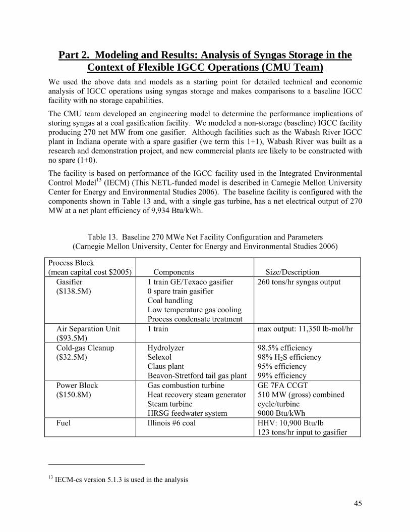
45

Part 2. Modeling and Results: Analysis of Syngas Storage in the Context of Flexible IGCC Operations (CMU Team)

We used the above data and models as a starting point for detailed technical and economic analysis of IGCC operations using syngas storage and makes comparisons to a baseline IGCC facility with no storage capabilities.

The CMU team developed an engineering model to determine the performance implications of storing syngas at a coal gasification facility. We modeled a non-storage (baseline) IGCC facility producing 270 net MW from one gasifier. Although facilities such as the Wabash River IGCC plant in Indiana operate with a spare gasifier (we term this 1+1), Wabash River was built as a research and demonstration project, and new commercial plants are likely to be constructed with no spare (1+0).

The facility is based on performance of the IGCC facility used in the Integrated Environmental Control Model13 (IECM) (This NETL-funded model is described in Carnegie Mellon University Center for Energy and Environmental Studies 2006). The baseline facility is configured with the components shown in Table 13 and, with a single gas turbine, has a net electrical output of 270 MW at a net plant efficiency of 9,934 Btu/kWh.

Table 13. Baseline 270 MWe Net Facility Configuration and Parameters (Carnegie Mellon University, Center for Energy and Environmental Studies 2006)

Process Block (mean capital cost $2005) Components Size/Description

Gasifier ($138.5M)

1 train GE/Texaco gasifier 0 spare train gasifier Coal handling Low temperature gas cooling Process condensate treatment

260 tons/hr syngas output

Air Separation Unit ($93.5M)

1 train max output: 11,350 lb-mol/hr

Cold-gas Cleanup ($32.5M)

Hydrolyzer Selexol Claus plant Beavon-Stretford tail gas plant

98.5% efficiency 98% H2S efficiency 95% efficiency 99% efficiency

Power Block ($150.8M)

Gas combustion turbine Heat recovery steam generator Steam turbine HRSG feedwater system

GE 7FA CCGT 510 MW (gross) combined cycle/turbine 9000 Btu/kWh

Fuel Illinois #6 coal HHV: 10,900 Btu/lb 123 tons/hr input to gasifier

13 IECM-cs version 5.1.3 is used in the analysis

46

Syngas and SNG storage systems were analyzed using the same gasifier size and configuration as the baseline scenario with the addition of a syngas storage process block and additional peaking turbine (Figure 13).

Figure 13. Baseline Facility (Top), Syngas Storage Scenario (Middle), SNG

Storage Scenario (Bottom). Gas Turbines are GE 7FA CCGTs.

The baseline facility is an IGCC facility with no storage or methanation capabilities, producing electricity from coal-derived syngas in a conventional manner. The syngas storage scenario is similar to the baseline facility but it adds the ability to compress and store syngas in a storage vessel. With the addition of storage, electricity can be produced from a gas turbine burning syngas directly from the gasifier as well as from a gas turbine burning syngas from the storage vessel. The final scenario looks at a facility with the capabilities to methanate syngas, store SNG and produce electricity from SNG.

The syngas produced by the gasification process is composed primarily of carbon monoxide and hydrogen and is characterized by a low energy density, typically ranging from 150-280 Btu/scf. Because of the lower energy density, larger volumes of syngas than of natural gas are required to produce electricity in a gas turbine. Syngas storage vessels thus need to be large, have high working pressures, or have these in combination. Although hydrogen is known to embrittle metals, the concentrations and partial pressures of hydrogen typically found in syngas do not

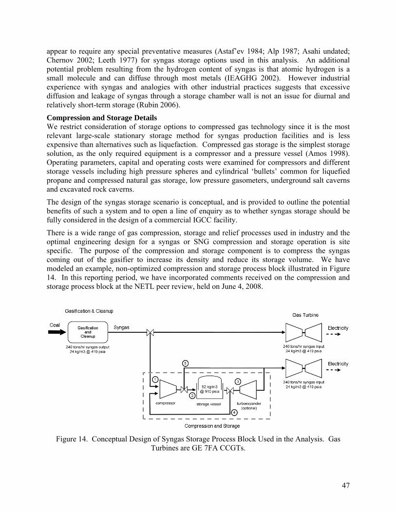
47

appear to require any special preventative measures (Astaf’ev 1984; Alp 1987; Asahi undated; Chernov 2002; Leeth 1977) for syngas storage options used in this analysis. An additional potential problem resulting from the hydrogen content of syngas is that atomic hydrogen is a small molecule and can diffuse through most metals (IEAGHG 2002). However industrial experience with syngas and analogies with other industrial practices suggests that excessive diffusion and leakage of syngas through a storage chamber wall is not an issue for diurnal and relatively short-term storage (Rubin 2006).

Compression and Storage Details We restrict consideration of storage options to compressed gas technology since it is the most relevant large-scale stationary storage method for syngas production facilities and is less expensive than alternatives such as liquefaction. Compressed gas storage is the simplest storage solution, as the only required equipment is a compressor and a pressure vessel (Amos 1998). Operating parameters, capital and operating costs were examined for compressors and different storage vessels including high pressure spheres and cylindrical ‘bullets’ common for liquefied propane and compressed natural gas storage, low pressure gasometers, underground salt caverns and excavated rock caverns.

The design of the syngas storage scenario is conceptual, and is provided to outline the potential benefits of such a system and to open a line of enquiry as to whether syngas storage should be fully considered in the design of a commercial IGCC facility.

There is a wide range of gas compression, storage and relief processes used in industry and the optimal engineering design for a syngas or SNG compression and storage operation is site specific. The purpose of the compression and storage component is to compress the syngas coming out of the gasifier to increase its density and reduce its storage volume. We have modeled an example, non-optimized compression and storage process block illustrated in Figure 14. In this reporting period, we have incorporated comments received on the compression and storage process block at the NETL peer review, held on June 4, 2008.

Figure 14. Conceptual Design of Syngas Storage Process Block Used in the Analysis. Gas

Turbines are GE 7FA CCGTs.

48

The syngas storage process for this analysis is:

1. Syngas from the gasification and cleanup block is pressurized to 910 psia

2. The high pressure syngas is stored in a vessel

3. High pressure syngas is released out of the storage vessel at a controlled rate (although not considered here, energy may be recovered through a turboexpander) and used in the second turbine (modeled as a GE 7FA CCGT)

4. As the pressure in the storage vessel is reduced, the syngas is routed through the compressor to maintain an input pressure required by the peaking turbine

5. Syngas at 419 psia is routed to the peaking turbine

An example of the storage and draw down pressures and the recompression requirements used in this process are illustrated in Figure 15.

Figure 15. Conceptual Illustration of Storage Pressures, Draw Down Rates and

Recompression Requirements for Syngas Storage Process Block Used in the Analysis

Recompression after the storage process allows the entire volume of the storage vessel to be utilized and provides a means to control the pressure and mass flow rate of syngas into the additional turbine. The particular arrangement and operating parameters will depend on site specific details such as the type of coal, gasifier and gas turbine and it is possible that there will be areas where energy losses can be reduced and efficiencies increased through smart engineering design.

For the gasifier and turbine used in the analysis, a 5.6 MW compressor is required to increase syngas pressure to approximately 910 psia (63 bar) for storage. At that pressure, a 20 meter diameter storage sphere will hold enough syngas for approximately 1 hour of turbine operation. (A larger storage vessel would require reduced storage pressure and a smaller compressor). The worst case operating scenario is that 5 MW are required to compress the syngas, and then 5 MW are required to pull syngas out of storage and into the turbine (10 MW loss). This assumes that

49

there is no turboexpander and that the compressor must be operated for the entire discharge cycle (an overestimate).

We examined storage scenarios with 4, 8, and 12 hours storage. Storage size (measured in hours) and compressor size were selected to accommodate 100 percent of the output of the gasifier for the number of hours indicated (that is also the period the peaking turbine can generate electricity from stored syngas). We fixed storage pressure at 63 bar for all storage scenarios, requiring a 5,600 kW compressor for both charging and discharging the storage vessel. This storage pressure results in a required storage vessel volume of 17,000 m3, 34,000 m3 and 51,000 m3 for 4, 8, and 12 hours of syngas storage, respectively. In the present model, the directly-fed and storage-fed gas turbines are the same size. Other arrangements may be more profitable (for example, choosing a different size peaking turbine or optimizing the storage pressures and volumes), but we wish to determine here only whether storing syngas for sale at peak times significantly increases profitability.

Detailed Economic Analyses of IGCC Operations Using Syngas Storage Engineering-economic models are developed to determine the performance implications and costs of storing syngas at a coal gasification facility. We analyze the economic feasibility of the storage operations illustrated in Figure 13.

Capital and operating cost distributions for the gasification, cleanup and power block sections in the baseline facility are based on the Integrated Environmental Control Model (IECM) version cs 5.21 (Carnegie Mellon University Center for Energy and Environmental Studies 2006). The baseline facility includes the process blocks shown in Table 13. This baseline facility represents the lowest capital cost IGCC facility that would reasonably be built and operated (Martin 2007) and has a capital cost of $415 million or $1,540/kW. Point estimates from IECM were converted into triangular distributions using assumptions of +5 percent, following capital cost estimates reported in the literature (NETL 2003; Amick 2002; Kreutz 2005). The distributions, rather than point estimates, were used as inputs into the engineering-economic models. Cost data from IECM are in 2005 constant dollars.

Capital costs for compressors, which are required for all storage options, were obtained from the literature (IEAGHG 2006; Amos 1998; Taylor 1986), and cost distributions were constructed from these data. Compressor capital costs were found to scale linearly with the size of the compressor. The distribution of the capital cost for a given size compressor, reflecting the range of cost uncertainty, was used as an input to the engineering economic models when compression was required.

Capital costs for storage vessels were compiled from studies in the literature and from industry professionals. From a regression analysis and prediction interval derived from these data, cost distributions were constructed and used as inputs in the model. The capital cost distributions suggest a salt cavern is preferred if it is available because it is the lowest cost. However, because salt and rock caverns are geographically sparse (Ammer 2006), this analysis considers the general case where neither is available.

We note that the benefits of storage are not dependent on the absolute levels of the capital costs assumed in this study, unless storage and turbine power plant capital costs rise much faster than gasification and air separator unit capital costs (which is to say that relative capital costs change), or detailed engineering design uncovers integration issues that cannon be solved technically without incurring a very substantial cost increase relative to the costs of a non-storage plant.

50

We modeled an IGCC plant located in the U.S. Midwest, using prices for Illinois number 6 coal (HHV 11,350 Btu/lb, sulfur content of 3.2 percent by weight (Energy Information Administration 2006). We used both historic coal data and price forecasts from the Energy Information Administration (EIA) to account for the variability in coal prices. We modified the EIA Annual Energy Outlook (AEO) forecasts for year 2007 coal prices with a factor to account for EIA’s historical error in forecasting price data (Energy Information Administration 2006; Energy Information Administration 2006; Rode and Fischbeck 2006). The 2005-2006 coal prices have a mean of $1.51/MMBtu and standard deviation of $0.1. The 2007 EIA forecast including the historical accuracy factor has a mean value of $1.73/MMBtu, 15 percent higher than the mean historical 2005-06 prices (see Appendix B). To estimate revenue, we obtained historical locational marginal price (LMP) data for electricity from September 1, 2005 to September 1, 2006 for nodes in the Midwest ISO region (Midwest ISO 2006).

0

20

40

60

80

100

120

140

1 3 5 7 9 11 13 15 17 19 21 23 1 3 5 7 9 11 13 15 17 19 21 23

LMP

($/M

W)

June 15, 2006

1 turbine operating

Turbines off / storage filling

2 turbines operating / storage discharging

June 16, 2006

Hour

Figure 16. Storage Scheme for 8 Hours of Syngas Storage to Produce Peak Electricity. At Times of Low Price, the Gasifier Output Fills Storage. During High Price Periods,

Both the Gasifier and Stored Syngas Supply Turbines. At Intermediate Prices, the Gasifier Output is Fed to One Turbine and the Storage Volume is Unchanged.

For each of the storage options (0, 4, 8, and 12 hours), the gasifier operates at maximum output at every hour (260 tons/hr), up to its availability. At every hour, the facility operator must decide how much electricity to produce from the IGCC turbine and from the peaking turbine. A profit maximizing operator stores syngas during hours with the lowest LMP and operates both turbines at hours with the highest LMPs. This storage scheme is illustrated for the case of 8 hours of storage, shown over two days in Figure 16. In the Midwest ISO over the year examined, the day-ahead and real-time hourly markets exhibited a correlation of 0.81, 0.77, and 0.74 for the 4,

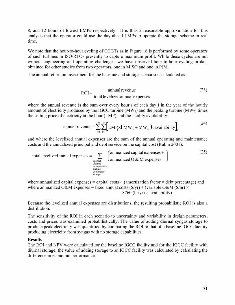
51

8, and 12 hours of lowest LMPs respectively. It is thus a reasonable approximation for this analysis that the operator could use the day ahead LMPs to operate the storage scheme in real time.

We note that the hour-to-hour cycling of CCGTs as in Figure 16 is performed by some operators of such turbines in ISO/RTOs presently to capture maximum profit. While these cycles are not without engineering and operating challenges, we have observed hour-to-hour cycling in data obtained for other studies from two operators, one in MISO and one in PJM.

The annual return on investment for the baseline and storage scenario is calculated as:

expenses annual levelized total

revenue annual ROI =

(23)

where the annual revenue is the sum over every hour i of each day j in the year of the hourly amount of electricity produced by the IGCC turbine (MW1) and the peaking turbine (MW2) times the selling price of electricity at the hour (LMP) and the facility availability:

annual revenue = ( )[ ]∑∑

= =×+×

365

1j

24

1i2i1ii tyavailabiliMWMWLMP

j

(24)

and where the levelized annual expenses are the sum of the annual operating and maintenance costs and the annualized principal and debt service on the capital cost (Rubin 2001):

∑ ⎟⎟⎠

⎞⎜⎜⎝

⎛ +=

storagecompressorturbine

separationair cleanupgasifier expenses M&O annualized

expenses capital annualized expenses annual levelized total

(25)

where annualized capital expenses = capital costs × (amortization factor × debt percentage) and where annualized O&M expenses = fixed annual costs ($/yr) + (variable O&M ($/hr) ×

8760 (hr/yr) × availability)

Because the levelized annual expenses are distributions, the resulting probabilistic ROI is also a distribution.

The sensitivity of the ROI in each scenario to uncertainty and variability in design parameters, costs and prices was examined probabilistically. The value of adding diurnal syngas storage to produce peak electricity was quantified by comparing the ROI to that of a baseline IGCC facility producing electricity from syngas with no storage capabilities.

Results The ROI and NPV were calculated for the baseline IGCC facility and for the IGCC facility with diurnal storage; the value of adding storage to an IGCC facility was calculated by calculating the difference in economic performance.

52

The cumulative probability of the ROI for the baseline 1+0 facility with no storage is shown in Figure 17. The addition of 4, 8 and 12 hours of syngas storage increases the mean ROI by 1.5, 8.8 and 12.9 percentage points, respectively.

0.0

0.1

0.2

0.3

0.4

0.5

0.6

0.7

0.8

0.9

1.0

-0.05 0.00 0.05 0.10 0.15 0.20

Cumulative

Probability

Increase in Mean Return on Investment Due to Storage

0

4

8

12

Storage Time (hours)

+1.5% +8.8% +12.9%

Baseline(no storage)

SyngasStorage

Figure 17. Change in ROI for Syngas Storage Scenario Using A 1+0 IGCC Facility With

80% Availability, Cinergy Node, 100% Debt Financing at 8% Interest Rate, Economic, And Plant Life of 30 Years (Amortization Factor 0.0888), 2007 EIA AEO Coal Price Forecast

With Accuracy Factor, 63 Bar Storage Pressure

The NPV shows similar increases with storage; with 12 hours of syngas storage, the facility realizes increased revenue from producing and selling peak power and the NPV is $90 million ($180 million more than the baseline IGCC facility with no syngas storage). Since the magnitude of the NPV increase depends on the nodal LMPs, we have modeled locating the facility at a number of nodes in the Midwest ISO. Storage increases the NPV for all nodes examined (Figure 18).

53

0

50

100

150

200

250

300

350

400

Cinergy FE Il MI ALTE.UP MOBCTG1 PRARC1 UPP

Midwest ISO node

Incr

ease

in N

PV

($ m

illio

ns)


4 hours

8 hours

12 hours

Figure 18. Increase in NPV from Adding a Diurnal Syngas Storage Scheme. Parameters as in Figure 17.

The sensitivity of the analysis to variations in the parameters was analyzed. The ROI for the 12 hour storage scenario is sensitive to the gasifier availability, structure of the financing, price of coal, and capital costs of the turbines, gasifier, air separation unit, and cleanup processes. The gasifier availability and the financing are the most important parameters over which the facility developer or operator has control. We caution that the mean prices necessary for the closed form solution do not capture the ‘peakiness’ of the price duration curves, as the gains from using syngas storage depend on the differences in electricity prices at peak and off peak hours for every hour the facility is operated.

From this analysis, there is strong evidence that producing peak electricity from diurnally stored syngas in gas turbines, while operating the gasifier at a constant output, increases firm-level profits for an IGCC facility despite the additional capital cost. Storing syngas in gas spheres at a pressure of 63 bar would add approximately 25% to the land area of the IGCC plant modeled. Other configurations, optimized storage parameters, lower fuel costs through long term contracts or more sophisticated financing arrangements may further increase profitability.

Results with Carbon Dioxide Capture The 1+0 baseline IGCC facility was modified to include a carbon capture, transport and storage (CCS) process from IECM, consisting of a water gas shift process, Selexol CO2 capture and transport process. Appropriate adjustments to the performance and the capital and operating costs were made to the engineering economic model (Appendix C provides a comprehensive list of the processes, financial and operating parameters for the 1+0+CCS scenario). Adding CCS increases capital costs, and incurs an energy penalty, increasing coal consumption and decreasing net electricity produced. The 1+0+CCS facility has a net output of 238 MW and a capital cost of $2,380/kW (compared to $1,540/kW for the 1+0 scenario). Implementing

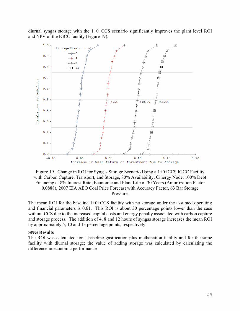
54

diurnal syngas storage with the 1+0+CCS scenario significantly improves the plant level ROI and NPV of the IGCC facility (Figure 19).

Figure 19. Change in ROI for Syngas Storage Scenario Using a 1+0+CCS IGCC Facility with Carbon Capture, Transport, and Storage, 80% Availability, Cinergy Node, 100% Debt Financing at 8% Interest Rate, Economic and Plant Life of 30 Years (Amortization Factor

0.0888), 2007 EIA AEO Coal Price Forecast with Accuracy Factor, 63 Bar Storage Pressure.

The mean ROI for the baseline 1+0+CCS facility with no storage under the assumed operating and financial parameters is 0.61. This ROI is about 30 percentage points lower than the case without CCS due to the increased capital costs and energy penalty associated with carbon capture and storage process. The addition of 4, 8 and 12 hours of syngas storage increases the mean ROI by approximately 5, 10 and 13 percentage points, respectively.

SNG Results The ROI was calculated for a baseline gasification plus methanation facility and for the same facility with diurnal storage; the value of adding storage was calculated by calculating the difference in economic performance

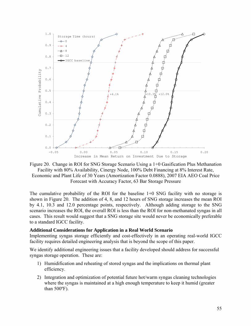
55

0.0

0.1

0.2

0.3

0.4

0.5

0.6

0.7

0.8

0.9

1.0

-0.05 0.00 0.05 0.10 0.15 0.20

Cumulative

Probability


0

4

8

12

IGCC baseline


+4.1% +10.3% +12.0%

Figure 20. Change in ROI for SNG Storage Scenario Using a 1+0 Gasification Plus Methanation

Facility with 80% Availability, Cinergy Node, 100% Debt Financing at 8% Interest Rate, Economic and Plant Life of 30 Years (Amortization Factor 0.0888), 2007 EIA AEO Coal Price

Forecast with Accuracy Factor, 63 Bar Storage Pressure

The cumulative probability of the ROI for the baseline 1+0 SNG facility with no storage is shown in Figure 20. The addition of 4, 8, and 12 hours of SNG storage increases the mean ROI by 4.1, 10.3 and 12.0 percentage points, respectively. Although adding storage to the SNG scenario increases the ROI, the overall ROI is less than the ROI for non-methanated syngas in all cases. This result would suggest that a SNG storage site would never be economically preferable to a standard IGCC facility.

Additional Considerations for Application in a Real World Scenario Implementing syngas storage efficiently and cost-effectively in an operating real-world IGCC facility requires detailed engineering analysis that is beyond the scope of this paper.

We identify additional engineering issues that a facility developed should address for successful syngas storage operation. These are:

1) Humidification and reheating of stored syngas and the implications on thermal plant efficiency.

2) Integration and optimization of potential future hot/warm syngas cleaning technologies where the syngas is maintained at a high enough temperature to keep it humid (greater than 500ºF).

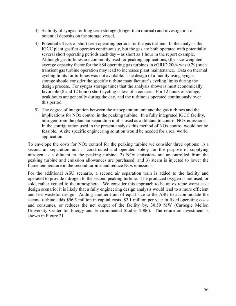
56

3) Stability of syngas for long term storage (longer than diurnal) and investigation of potential deposits on the storage vessel.

4) Potential effects of short term operating periods for the gas turbine. In the analysis the IGCC plant gasifier operates continuously, but the gas are both operated with potentially several short operating periods each day – as short as 1 hour in the report example. Although gas turbines are commonly used for peaking applications, (the size-weighted average capacity factor for the 884 operating gas turbines in eGRID 2004 was 0.29) such transient gas turbine operation may lead to increases plant maintenance. Data on thermal cycling limits for turbines was not available. The design of a facility using syngas storage should consider the specific turbine manufacturer’s cycling limits during the design process. For syngas storage times that the analysis shows is most economically favorable (8 and 12 hours) short cycling is less of a concern. For 12 hours of storage, peak hours are generally during the day, and the turbine is operated continuously over this period.

5) The degree of integration between the air separation unit and the gas turbines and the implications for NOx control in the peaking turbine. In a fully integrated IGCC facility, nitrogen from the plant air separation unit is used as a dilutant to control NOx emissions. In the configuration used in the present analysis this method of NOx control would not be feasible. A site specific engineering solution would be needed for a real world application.

To envelope the costs for NOx control for the peaking turbine we consider three options: 1) a second air separation unit is constructed and operated solely for the purpose of supplying nitrogen as a dilutant to the peaking turbine; 2) NOx emissions are uncontrolled from the peaking turbine and emission allowances are purchased; and 3) steam is injected to lower the flame temperature in the second turbine and reduce NOx emissions.

For the additional ASU scenario, a second air separation train is added to the facility and operated to provide nitrogen to the second peaking turbine. The produced oxygen is not used, or sold, rather vented to the atmosphere. We consider this approach to be an extreme worst case design scenario; it is likely that a fully engineering design analysis would lead to a more efficient and less wasteful design. Adding another train of equal size to the ASU to accommodate the second turbine adds $96.5 million in capital costs, $2.1 million per year in fixed operating costs and consumes, or reduces the net output of the facility by, 30.59 MW (Carnegie Mellon University Center for Energy and Environmental Studies 2006). The return on investment is shown in Figure 21.

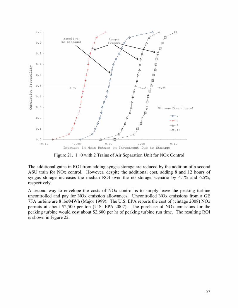
57

0.0

0.1

0.2

0.3

0.4

0.5

0.6

0.7

0.8

0.9

1.0

-0.10 -0.05 0.00 0.05 0.10

Cumulative

Probability


0

4

8

12


-3.8% +4.1% +6.5%


SyngasStorage

Figure 21. 1+0 with 2 Trains of Air Separation Unit for NOx Control

The additional gains in ROI from adding syngas storage are reduced by the addition of a second ASU train for NOx control. However, despite the additional cost, adding 8 and 12 hours of syngas storage increases the median ROI over the no storage scenario by 4.1% and 6.5%, respectively.

A second way to envelope the costs of NOx control is to simply leave the peaking turbine uncontrolled and pay for NOx emission allowances. Uncontrolled NOx emissions from a GE 7FA turbine are 8 lbs/MWh (Major 1999). The U.S. EPA reports the cost of (vintage 2008) NOx permits at about $2,500 per ton (U.S. EPA 2007). The purchase of NOx emissions for the peaking turbine would cost about $2,600 per hr of peaking turbine run time. The resulting ROI is shown in Figure 22.

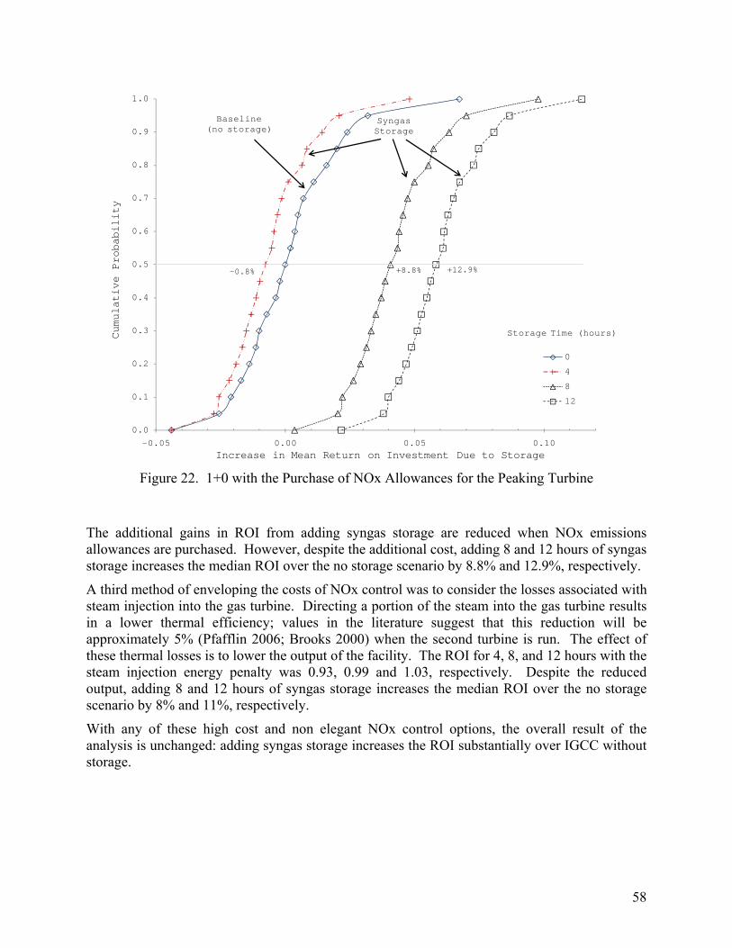
58

0.0

0.1

0.2

0.3

0.4

0.5

0.6

0.7

0.8

0.9

1.0

-0.05 0.00 0.05 0.10



0

4

8

12


-0.8% +8.8% +12.9%


SyngasStorage

Figure 22. 1+0 with the Purchase of NOx Allowances for the Peaking Turbine

The additional gains in ROI from adding syngas storage are reduced when NOx emissions allowances are purchased. However, despite the additional cost, adding 8 and 12 hours of syngas storage increases the median ROI over the no storage scenario by 8.8% and 12.9%, respectively.

A third method of enveloping the costs of NOx control was to consider the losses associated with steam injection into the gas turbine. Directing a portion of the steam into the gas turbine results in a lower thermal efficiency; values in the literature suggest that this reduction will be approximately 5% (Pfafflin 2006; Brooks 2000) when the second turbine is run. The effect of these thermal losses is to lower the output of the facility. The ROI for 4, 8, and 12 hours with the steam injection energy penalty was 0.93, 0.99 and 1.03, respectively. Despite the reduced output, adding 8 and 12 hours of syngas storage increases the median ROI over the no storage scenario by 8% and 11%, respectively.

With any of these high cost and non elegant NOx control options, the overall result of the analysis is unchanged: adding syngas storage increases the ROI substantially over IGCC without storage.

59

Part 3. Economic Analysis of Syngas Storage Options and Markets (WVU Team)

This portion of the report describes the methodology used and approach taken by the West Virginia University team in achieving the goals of Task 6, 7, and 8 of the project, and presents the results of our second year of effort. During the second year we improved the specification of our cost model of the different IGCC plants with and without storage, significantly advanced the specification of our model of the electricity pricing patterns (EPDCs) affecting the plants, improved our understanding of the economics of IGCC plants using the tools of mathematical dynamic optimization, and explored the option of adding natural gas fuel-switching capability to the CMU 12-hour design. Our simulation and analytical optimization results both strongly support the CMU 12-hour plant design as the most likely of the IGCC plants considered to be commercially viable in all scenarios, particularly scenarios with high fuel prices. Even without fuel-switching capabilities, the return on invested capital for the CMU 12-hour IGCC plant is slightly higher than a supercritical coal-fired steam plant in our simulations, and significantly better than an IGCC plant without storage. The addition of natural gas fuel-switching capabilities significantly enhances the viability of the CMU 12-hour plant design (by roughly 20%) under all scenarios studied.

The research performed by the WVU team during this project was in accordance with the outline of the tasks laid out in the Statement of Work, Table 1.

All of the WVU tasks involve changes to the simulation model. In what follows, therefore, we first review the design of the simulation model, highlighting changes implemented in Year 2. The biggest innovation from the WVU team in the second year of the project is the development and testing of plant configurations that combine syngas storage with natural gas fuel-switching capability, a feature that was prompted by discussions with an IGCC plant manager that we initiated while performing task 7.

Summary Gasification cost data, IGCC cost data, and data on costs of alternative and competitive plant technologies are widely available from websites (e.g. http://www.eia.doe.gov/), recent literature, technical reports (e.g., Tampa Electric Company, 2002), and publicly available studies (e.g. Aiken et al., 2004). The primary reference authority used to determine the costs and capabilities of IGCC technology is the Integrated Environmental Control Model (IECM), described and documented in Rubin et al (1997) and Rubin et al (2006). The IECM model was used in the current study to provide a template and calibration check for our own Matlab-based IGCC cost model, which forms the core of the simulation tool that we use to perform the analysis.

Our simulation analysis subjects ten different plant configurations to thirteen different fuel and electricity market price scenarios. Within each pricing scenario we assess different plant configurations, and each combination of pricing scenario and plant configuration is evaluated using 10,000 Monte Carlo iterations. Each iteration consists of one draw of a 30-year series of fuel prices from a specified distribution. For each year in the plant’s lifetime, the fuel prices are used to construct an electricity price duration curve (EPDC) (or, when appropriate, two conditional EPDCs) which, together with plant operational costs, determines the plant’s desired capacity factor and potential revenues. The annual plant availability model, together with the

60

operational cost, determines the plant’s actual capacity factor, revenues, and costs. We assess performance based on net present value and return on invested capital, calculated using an 8% discount rate.

The base case plant configuration is a single-train IGCC plant without storage or spare gasifier. Other plant configurations considered include a single-train plant with a spare gasifier, single-train plants with either above-ground storage, underground storage, or a backup fuel managed for availability enhancement. We also assessed a three-train plant that exhibits significant economies of scale. In addition, we looked at the CMU 12-hour plant (which has a single gasifier, two combined-cycle turbines, and storage facilities capable of storing 12 hours of gasifier output) with and without fuel switching capabilities. Finally, for comparison we assessed the performance of a pulverized coal supercritical plant under the same pricing scenarios.

Three different views of “business-as-usual” are used as base case pricing scenarios. Other pricing scenarios considered include six different fuel price scenarios, and four different electricity price scenarios. The fuel price scenarios look at relatively high and relatively low fuel prices as projected by our own model and the EIA, and relatively high and low natural gas price volatility. Electricity price scenarios are defined in terms of the shape of the EPDC. The electricity price scenarios look at relatively large and broad electricity price peaks, relatively low and narrow electricity price peak, and relatively low and relatively high baseload power prices. Generally, the high price scenarios, especially high fuel and electricity peak price scenarios, are most favorable to IGCC plants, with or without storage facilities.

We assess four different capital investments designed to improve plant availability: a spare gasifier, above-ground storage, underground storage, and a backup fuel. The primary disadvantage of using storage for backup is its limited capacity. We find that storage managed for availability, both above-ground and underground, adds slightly to an IGCC’s value, and a spare gasifier reduces the plant’s value slightly, even while increasing plant availability. Our results strongly suggest that adding fuel switching capability is the preferred backup technology for the base plant. These results are in line with the observed facts that the Wabash plant does not use its spare gasifier for backup, but the Polk plant reports success in using a supplemental fuel for backup.

The best performing plant design considered is the CMU 12-hour plant with fuel switching capability. In the CMU 12-hour configuration the gasifier runs continuously but the power block runs only twelve hours per day. On some days during some of the hours when a power plant without fuel switching capability would be shut down (i.e., hours outside the 12 highest-price hours) the price of electricity exceeds the marginal cost of producing power on natural gas. During such hours, the plant could increase its profitability by cycling its power block using natural gas. Natural gas is also used as a backup fuel when the plant experiences an unplanned outage. A plant with this configuration gives a reliably positive return on invested capital, a return that is better than that of a much larger plant, but with a much lower initial capital outlay.

There were six primary conclusions supported by the simulation results:

61

1. All plant configurations that we tested, except the CMU 12 hour storage and the CMU 12 hour storage with fuel switching capabilities, are unattractive investments under base case energy prices.

2. IGCC Plants perform better in high-energy-price environments.

3. High peak power prices improve IGCC plants’ economic performance significantly, but high baseload prices improve IGCC performance only slightly.

4. High variance in gas prices does not significantly affect the viability of an IGCC.

5. The use of a backup fuel such as natural gas dominates all other configurations used for availability enhancement.

6. Under all price scenarios the most profitable plant configuration is the CMU 12 hour plant with fuel switching capabilities used for both cycling and backup.

We analyze and solve a simple optimal control model of an IGCC plant with storage used on a daily cycle, of which the CMU 12-hour plant is a special case. We derive three propositions, stating in essence that, to maximize profits a plant able to produce g units of syngas per hour, equipped with k− = bg units of storage capacity and capable of burning x− = cg units of gas per hour, will burn gas at maximum rate cg for the highest-priced b/(c-1) hours per day. It will shut down completely for the lowest-priced b hours of the day, and will burn gas at a rate of g units per hour for the remaining hours. If electricity prices can be predicted accurately b hours in advance, the price of electricity at which the plant begins filling storage will be the same as the price at which filling is completed. Similarly, if electricity prices can be predicted accurately b/(c-1) hours in advance then the price of electricity at which the plant begins producing electricity at maximum power will equal the price at which storage is emptied.

Our optimization model also has implications for optimal capital scale. The total value of a unit increment to storage capacity is found to be the discounted sum of the electricity price increases during full-storage episodes and the absolute value of price decreases during empty-storage episodes. However, if storage is never full but is sometimes empty, then the gasifier is the constraining factor, and one should compare the discounted costs of stockouts over the plant’s lifetime to the incremental cost of a larger gasifier to determine if the gasifier is a cost-effective investment. These results provide insight into the value of storage, and help explain the excellent performance of the CMU 12-hour design.

Approach Our simulation strategy is designed to measure the size and robustness of increases in IGCC plant value and returns derived from syngas storage. Broadly, the value of syngas storage is expected to arise from two sources. First, storage capability can improve the cycling characteristics of the plant by providing a buffer between the gasification and power production blocks within the plant. Second, storage can increase IGCC plant availability without requiring backup gasification facilities. Fuel-switching capability can complement and synergize both functions of storage. Accordingly, the simulation scenarios are designed to assess and compare the performance of IGCC plants equipped with (and without) a spare gasifier, storage, and fuel-

62

switching capability managed for backup and cycling flexibility, under a wide variety of fuel and electricity price regimes.

The value of the cycling aspect of the storage capability arises from two sources. First, daily cycling capability can allow the plant to adapt to changes in the market environment (especially, to a decrease in baseload power prices relative to IGCC costs) by moving from a strictly baseload technology to a cycling technology that can compete with technologies higher up on the load curve. Secondly, daily cycling capability could allow the plant to use its gasification facilities more effectively by storing gas produced during off-peak periods and burning it when the power is most needed and the price is higher. Essentially, the storage allows the plant to double its peak period output at low capital cost. The mathematical analysis in Task 8 provides insight into the sources of increased value from storage-enabled daily plant cycling, and into the optimal sizing and management of storage facilities for cycling purposes.

Our simulation program subjects ten different plant configurations to thirteen different market price scenarios. The simulation scenario analysis seeks to assess the sensitivity of IGCC profitability to changes in market price levels and distributions while relating those changes to potential real-world policies and events. We do not, however, seek to predict exactly which outcomes will follow from which policies and events. This focus upon the effect of market conditions and price patterns on the value of storage helps distinguish this study from previous studies of IGCC viability such as Aiken et al. (2004), which used the NEMS model to project in some detail the effects of environmental policies on the viability of IGCCs. Another key distinction, of course, is that Aiken et al (2004) did not consider syngas storage as an option.

The simulation analysis builds upon a set of core “base case” market price scenarios and plant configurations. Base case price scenarios project a continuation of recent fuel and electricity market conditions, policies, and trends. Deviations from the base case price scenarios allow both fuel and electricity prices to change, positing different levels (and levels of divergence) of coal and natural gas prices, different levels (and levels of divergence) of baseload and peaking electricity prices, and different levels of volatility of natural gas and peaking electricity prices.

Within each pricing scenario we assess different plant configurations. The base case plant configuration is an IGCC plant without storage or spare gasifier. Other plant configurations depart from the base case by adding storage, adding a spare gasifier, adding an additional power generation turbine unit, changing the overall plant scale, adding natural gas as an additional fuel source, and changing the objectives of plant management with regard to cycling of storage and electrical output. (For comparison, we also briefly consider a pulverized coal fired supercritical steam plant.) We assess the outcomes in terms of plant profitability using Monte Carlo methods.

63

Scenario Analysis Algorithm Overview The algorithm for the Monte Carlo contains three nested loops:

I. Begin Scenario Loop. 1. Set scenario parameters, including distributions of fuel and electricity prices.

2. Begin Plant Configuration Loop. a) Set plant configuration. b) Begin Price Sample and Plant Operation Loop

(1) Generate stochastic annual fuel prices for each year of the plant’s life as a sample from the specified fuel price distribution.

(2) Construct the annual Electricity Price Duration Curve (EPDC) for each year using stochastic fuel prices and structural parameters.

(3) Calculate plant operational cost for each year from the IECM-based cost model and fuel prices.

(4) Calculate desired annual capacity factor from the EPDC and plant operational cost.

(5) Calculate plant availability from the plant availability model. (6) Calculate annual plant revenue from the EPDC and availability. (7) Calculate annual plant cost from the IECM-based cost model,

stochastic fuel prices, and availability. Iterate Price Sample and Plant Operation Loop 10,000 times to get a distribution of returns for the plant configuration.

Iterate Plant Configuration Loop over all 10 assessed plant configurations to assess viability of different plant capital configurations

Iterate Scenario Loop over all 13 assessed market price scenarios.

Risk and Return Metrics Our Monte Carlo experiments allow us to calculate to risk and return metrics on the different plant configurations. The statistics used to evaluate the plants are designed to show both the central tendency (expected value) and the riskiness (variance and percentiles, including value at risk) of returns under the different scenarios. Specifically, we rely on the following statistics:

Net Present Value (NPV) The present value of the annual revenues Rt that occur over a period of thirty years is calculated using the following formula:

PV(Revenues) =

30

Σt=1

Revenuet

(1+ r)t .

The present value of a plant’s cost is calculated in the same way. Notice that the present value of revenues to be collected in the distant future is much less than the value of revenues collected sooner. Also, the higher the discount rate, r, the lower the present value of the stream. We use a

64

value of 8% (r = .08) in this study to discount future values, which is similar to the rates used to discount regulated utility investments, and accords with the amortization factor of .0888 used by the CMU team.

The net present value of an investment is simply the difference between the present value of its revenue and cost streams over its lifetime:

NPV = PV(Revenues) − PV(Costs).

A plant with a positive NPV makes a profit for its owners. Because the bulk of a plant’s capital costs are incurred immediately, they are not discounted at all in our NPV calculations. Revenues and operating costs (fixed and variable) in any particular year are generally small relative to capital costs, but their discounted present value over the plant’s lifetime is of the same scale.

Return on Invested Capital (ROIC) A power plant is a large capital investment, consisting of a total capital requirement, or TCR, that must be paid for over a long lifetime. The payments for the investment come from the plant’s yearly net operating income, NOI, which is calculated as

NOIt = Rt − OMt,

where OMt is the plant’s yearly operation and maintenance costs, including fuel, labor, and materials, but not including debt service. The return on invested capital (ROIC) expresses the relationship between the present value of the NOI stream over the plant’s lifetime and the upfront capital required to generate that stream.

ROIC = PV(NOI)

TCR

Thus, if ROIC = 1, then the net present value of the inflowing cash will be just sufficient to cover the initial investment. An alternative way to think of the statistic is that, given our discount rate of 8%, if ROIC = 1, then the stream of payments from the plant will be just sufficient to service and pay off the loan that would be needed to finance the plant, if the interest rate on the note were 8%. If ROIC<1, then the owner of the plant will lose money. ROIC and ROI (the corresponding measure used by the CMU team) measure the same thing in slightly different ways. ROIC focuses on the entire lifetime of the plant, whereas ROI compares the cash flows in a given year to the levelized mortgage payment required to service and retire the debt. ROI is more convenient measure for looking at the outcome of a single year, as the CMU team often does, whereas the ROIC provides a handy summary statistic for the value of a plant over its lifetime, which is the only measure required in the WVU simulations.

65

I. Methodological Issues and Implementation The key objective of this study is to understand and estimate the value of adding storage facilities to an IGCC plant. In this section of the report, we review the plant cost model that we constructed, and explain how the cost model and economic environment were designed to measure the impact of storage-induced changes in plant availability and cycling flexibility on the plant’s profitability and value.

Plant Cost Model The cost and performance estimates for the IGCC facility used to calculate net revenues and rates of returns are based on the Integrated Environmental Control Model (IECM), version 5.2.0, described and documented in Rubin et al (1997) and Rubin et al (2006). The IECM reports capital and operating costs along with input and output values for all major components of the IGCC process which were used as the basis of the cost model developed in this research.

The process areas included in the base configuration in IECM are the air separation unit (ASU), gasifier area, cold-gas clean up area, and the power block. The gasifier section includes a GE/Texaco gasifier, coal handling, low temperature gas cooling, and process condensate treatment. The cold-gas cleanup section includes a Hydrolyzer, Selexol Sulfur System, Claus Plant, and Beavon-Stretford Plant. The power block section includes a GE 7FA gas combustion turbine, heat recovery steam generator, steam turbine, and HRSG feedwater system. The fuel being considered is Illinois #6 coal.

Although the IECM model is the template for the cost model developed here, we did not integrate the IECM program itself into our simulations. Instead, our simulations employ a Matlab program that we wrote that is designed to replicate the cost and technological relationships in the IECM model. There were several reasons that we decided to build a separate model rather than perform the analysis by interfacing directly with IECM. First, the IECM does not currently allow data to be pipelined directly into the program, as was required in the simulation iterations. The IECM does have uncertainty analysis tools available, but they are not designed to address the questions that are central to our research. Second, syngas storage is not included in the IECM. Third, our research requires the flexibility to make modifications to plant configurations that would be difficult or impossible within the IECM. Because it was created for different purposes, our cost model does not exactly replicate the IECM results, but it does track them closely. We spent considerable time and resources validating and corroborating our model against the IECM. The largest deviation between the WVU cost model and IECM calculations of the total levelized annual cost of an IGCC facility is 0.57%. Most deviations are much smaller, as is illustrated in Table 14.

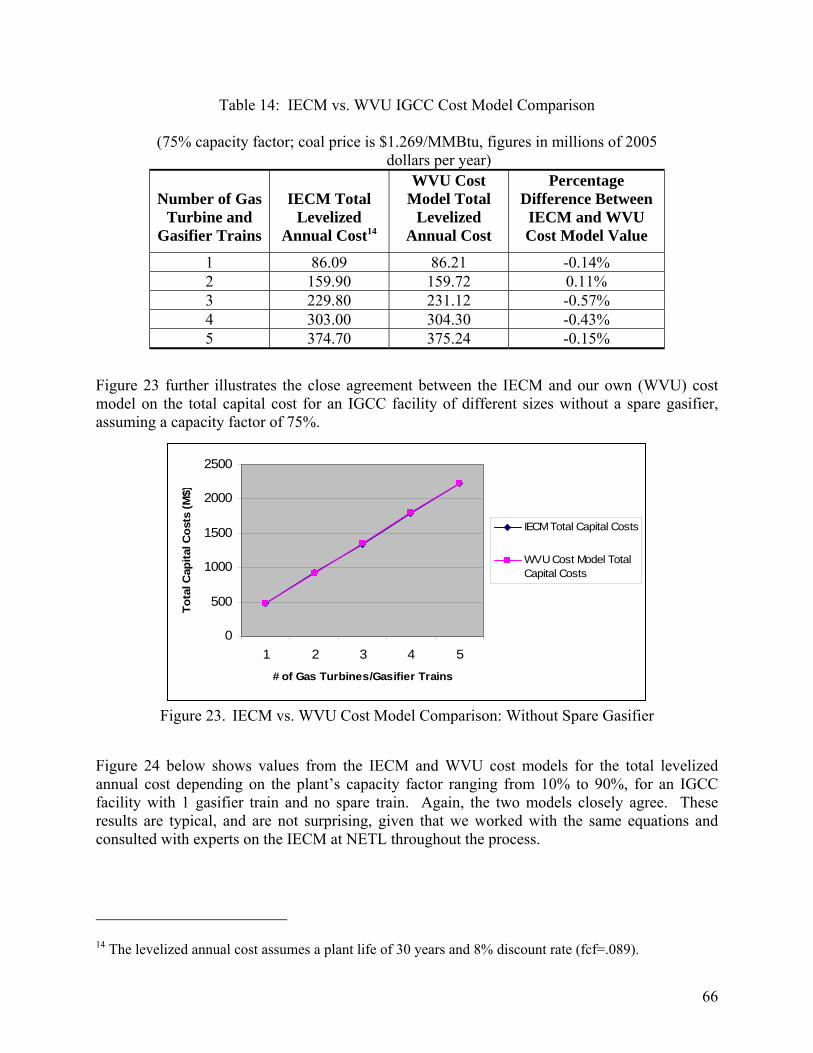
66

Table 14: IECM vs. WVU IGCC Cost Model Comparison

(75% capacity factor; coal price is $1.269/MMBtu, figures in millions of 2005 dollars per year)

Number of Gas Turbine and

Gasifier Trains

IECM Total Levelized

Annual Cost14

WVU Cost Model Total

Levelized Annual Cost

Percentage Difference Between

IECM and WVU Cost Model Value

1 86.09 86.21 -0.14% 2 159.90 159.72 0.11% 3 229.80 231.12 -0.57% 4 303.00 304.30 -0.43% 5 374.70 375.24 -0.15%

Figure 23 further illustrates the close agreement between the IECM and our own (WVU) cost model on the total capital cost for an IGCC facility of different sizes without a spare gasifier, assuming a capacity factor of 75%.

0

500

1000

1500

2000

2500

1 2 3 4 5# of Gas Turbines/Gasifier Trains

Tota

l Cap

ital C

osts

(M$)

IECM Total Capital Costs

WVU Cost Model TotalCapital Costs

Figure 23. IECM vs. WVU Cost Model Comparison: Without Spare Gasifier

Figure 24 below shows values from the IECM and WVU cost models for the total levelized annual cost depending on the plant’s capacity factor ranging from 10% to 90%, for an IGCC facility with 1 gasifier train and no spare train. Again, the two models closely agree. These results are typical, and are not surprising, given that we worked with the same equations and consulted with experts on the IECM at NETL throughout the process.

14 The levelized annual cost assumes a plant life of 30 years and 8% discount rate (fcf=.089).

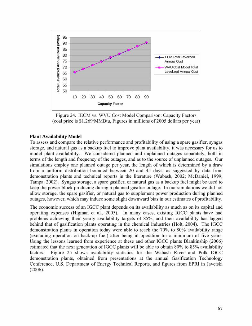
67

50556065707580859095

10 20 30 40 50 60 70 80 90Capacity Factor

Tota

l Lev

eliz

ed A

nnua

l Cos

t (M

$/yr

)IECM Total LevelizedAnnual Cost

WVU Cost Model TotalLevelized Annual Cost

Figure 24. IECM vs. WVU Cost Model Comparison: Capacity Factors

(coal price is $1.269/MMBtu, Figures in millions of 2005 dollars per year)

Plant Availability Model To assess and compare the relative performance and profitability of using a spare gasifier, syngas storage, and natural gas as a backup fuel to improve plant availability, it was necessary for us to model plant availability. We considered planned and unplanned outages separately, both in terms of the length and frequency of the outages, and as to the source of unplanned outages. Our simulations employ one planned outage per year, the length of which is determined by a draw from a uniform distribution bounded between 20 and 45 days, as suggested by data from demonstration plants and technical reports in the literature (Wabash, 2002; McDaniel, 1999; Tampa, 2002). Syngas storage, a spare gasifier, or natural gas as a backup fuel might be used to keep the power block producing during a planned gasifier outage. In our simulations we did not allow storage, the spare gasifier, or natural gas to supplement power production during planned outages, however, which may induce some slight downward bias in our estimates of profitability.

The economic success of an IGCC plant depends on its availability as much as on its capital and operating expenses (Higman et al., 2005). In many cases, existing IGCC plants have had problems achieving their yearly availability targets of 85%, and their availability has lagged behind that of gasification plants operating in the chemical industries (Holt, 2004). The IGCC demonstration plants in operation today were able to reach the 70% to 80% availability range (excluding operation on back-up fuel) after being in operation for a minimum of five years. Using the lessons learned from experience at these and other IGCC plants Blankinship (2006) estimated that the next generation of IGCC plants will be able to obtain 80% to 85% availability factors. Figure 25 shows availability statistics for the Wabash River and Polk IGCC demonstration plants, obtained from presentations at the annual Gasification Technology Conference, U.S. Department of Energy Technical Reports, and figures from EPRI in Javetski (2006).

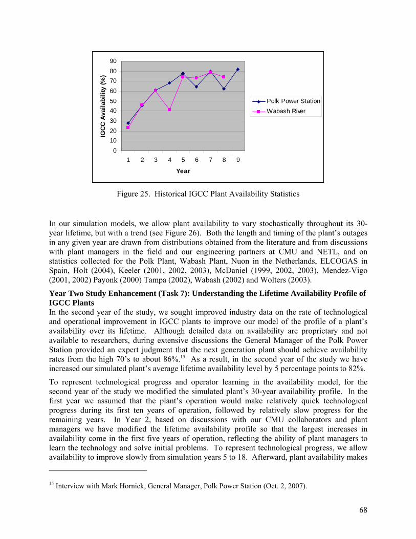
68

0102030405060708090

1 2 3 4 5 6 7 8 9

Year

IGC

C Av

aila

bilit

y (%

)Polk Power StationWabash River

Figure 25. Historical IGCC Plant Availability Statistics

In our simulation models, we allow plant availability to vary stochastically throughout its 30-year lifetime, but with a trend (see Figure 26). Both the length and timing of the plant’s outages in any given year are drawn from distributions obtained from the literature and from discussions with plant managers in the field and our engineering partners at CMU and NETL, and on statistics collected for the Polk Plant, Wabash Plant, Nuon in the Netherlands, ELCOGAS in Spain, Holt (2004), Keeler (2001, 2002, 2003), McDaniel (1999, 2002, 2003), Mendez-Vigo (2001, 2002) Payonk (2000) Tampa (2002), Wabash (2002) and Wolters (2003).

Year Two Study Enhancement (Task 7): Understanding the Lifetime Availability Profile of IGCC Plants In the second year of the study, we sought improved industry data on the rate of technological and operational improvement in IGCC plants to improve our model of the profile of a plant’s availability over its lifetime. Although detailed data on availability are proprietary and not available to researchers, during extensive discussions the General Manager of the Polk Power Station provided an expert judgment that the next generation plant should achieve availability rates from the high 70’s to about 86%.15 As a result, in the second year of the study we have increased our simulated plant’s average lifetime availability level by 5 percentage points to 82%.

To represent technological progress and operator learning in the availability model, for the second year of the study we modified the simulated plant’s 30-year availability profile. In the first year we assumed that the plant’s operation would make relatively quick technological progress during its first ten years of operation, followed by relatively slow progress for the remaining years. In Year 2, based on discussions with our CMU collaborators and plant managers we have modified the lifetime availability profile so that the largest increases in availability come in the first five years of operation, reflecting the ability of plant managers to learn the technology and solve initial problems. To represent technological progress, we allow availability to improve slowly from simulation years 5 to 18. Afterward, plant availability makes 15 Interview with Mark Hornick, General Manager, Polk Power Station (Oct. 2, 2007).

69

only slight improvements, and then begins to fall in the last five years of the plant’s lifetime as wear and tear take a toll on overall plant availability.

60

65

70

75

80

85

90

0 5 10 15 20 25 30

year

Ann

ual A

vaila

bilit

yof

the

IGC

C P

lant

year 1year 2

Figure 26. Changes in Simulated IGCC Plant Availability Profiles

Year 1 and Year 2 of this Study

Figure 26 shows the average availability over 10,000 Monte Carlo repetitions, by year, under research year one and research year two availability assumptions over the thirty years of the simulated life of the IGCC plant. Both the rate of availability improvement and the eventual level of availability are higher under the new assumptions. Note that the actual availability of a particular plant in a given year will vary stochastically from the profile in Figure 26.

The higher availability profile improves the ROIC for all plant configurations, but as one might expect, the improvement is less for plants that are configured for higher availability in the first place. Table 15 compares the base plant configuration to two configurations with availability enhancements: a plant with a spare gasifier (plant 1) and a plant with a 10% larger gasifier whose increased output is diverted into the 200,000 m3 of storage for use as backup (plant 6). The ROIC for all scenarios and plants is higher under year two assumptions. The average increase in the ROIC for the base plant from year one to year two under the different availability assumptions was 16%. On the other hand, the change in ROIC relative to the base plant is about the same in both years.

It should be noted that, besides the change in the availability profile, two factors are at work in generating the results for plant 6. First, as mentioned above, in year 2 the performance of plant 6 was depressed because its storage was not allowed to back up unplanned outages in the air separation unit. Second, we improved our model of the annual carryover of stored gas in our year 2 simulations, which enhanced the performance of plant 6. These two changes appear to approximately offset each other.

70

Table 15: ROIC Effects of Changes in Base Plant Availability Profiles Return on Invested Capital (ROIC)

Price Scenarios 0. Base Plant (Year 1)

0. Base Plant (Year 2)

1. Base Plus Spare

Gasifier (Year 1)

1. Base Plus Spare

Gasifier (Year 2)

6. Storage for

Availability (Year 1)

6. Storage for

Availability (Year 2)

AEO High Prices 0.857 0.928 0.833 0.833 0.885 0.964 AEO Low Prices 0.587 0.644 0.574 0.572 0.614 0.677 AEO Base Prices 0.714 0.778 0.697 0.696 0.742 0.813 Base Prices MISO 0.415 0.505 0.406 0.442 0.440 0.537 Base Prices PJM 0.557 0.664 0.543 0.589 0.584 0.697 2a: High Fuel Prices 0.818 0.940 0.783 0.840 0.845 0.976 2b: Low Fuel Prices 0.586 0.643 0.573 0.571 0.612 0.676 2c: High Gas Price Variance 0.557 0.662 0.542 0.588 0.583 0.696

2d: Low Gas Price Variance 0.558 0.664 0.543 0.590 0.584 0.698

3a: Peaked Electric Price Duration 0.871 1.006 0.831 0.900 0.900 1.043

3b: Flat Electric Price Duration 0.455 0.557 0.450 0.492 0.481 0.589

3c: Low Baseload Price 0.462 0.562 0.454 0.497 0.487 0.595

3d: High Baseload Price 0.653 0.766 0.632 0.682 0.680 0.800

Operational Implementation of the Availability Model The availability model achieves its overall availability rates by a “bottom-up” process, in which the various subsystems of the plant fail at rates in line with field experience to date with those subsystems. The system failures occur sequentially through time, according to a random pattern with a fixed distribution. A simulated year of plant operation always begins with the plant turned on and producing electricity and gas. The simulated plant then suffers outages at different times during the year. The number of consecutive days of each operational period is determined by a draw from a weighted mixture of uniform distributions, where the weights are based on statistics collected from published field studies and conversations with plant managers. Figure 27 shows the base weights applied to each possible operational period length. For example, the probability that a given operational period would last for 1 to 5 days was approximately 24%. The actual length of any particular 1 to 5 day operational period was drawn from a uniform distribution over the interval [1, 5]. The minimum length of a run time in the simulations is 1 day or 24 hours, and the maximum runtime is 75 consecutive days, or 1,800 hours. The weights are altered throughout the 30-year lifetime of the plant to represent technological progress, in line with the trend pictured in Figure 26.

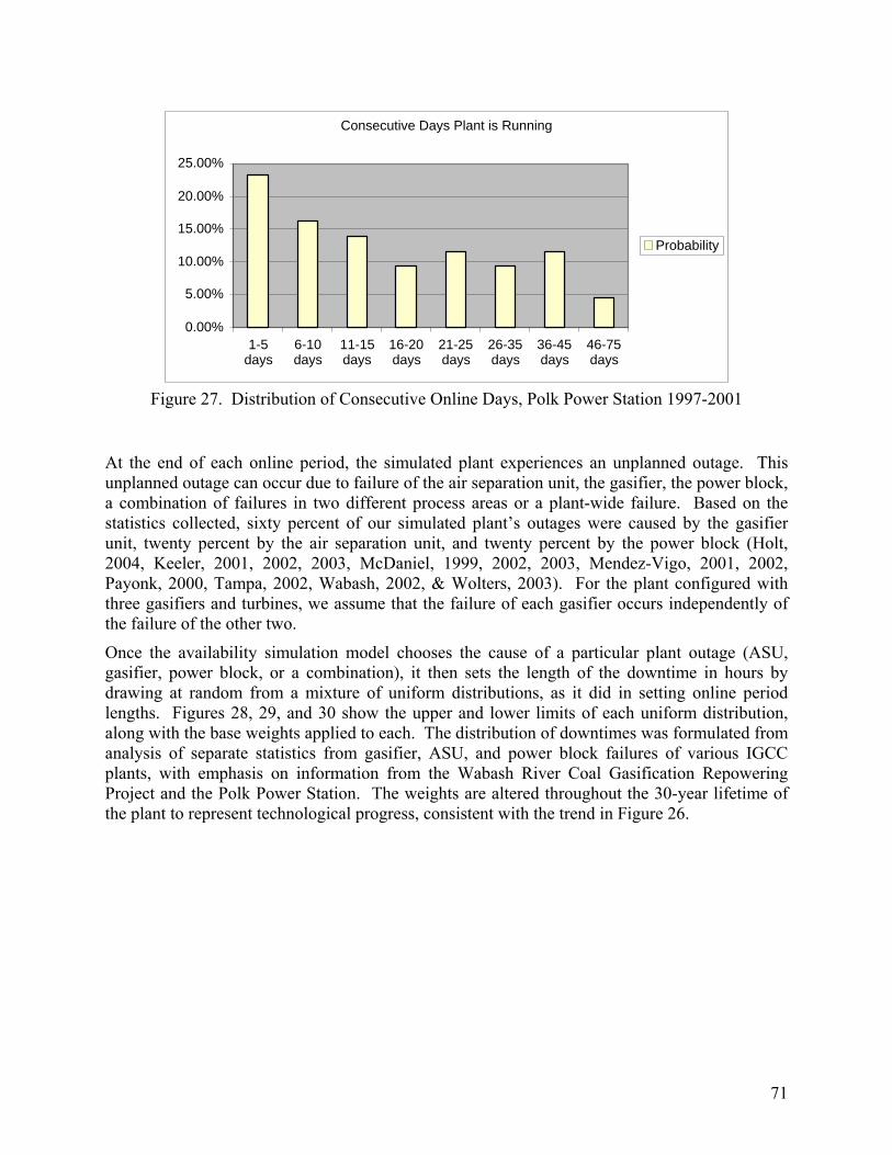
71

Consecutive Days Plant is Running

0.00%

5.00%

10.00%

15.00%

20.00%

25.00%

1-5days

6-10days

11-15days

16-20days

21-25days

26-35days

36-45days

46-75days

Probability

Figure 27. Distribution of Consecutive Online Days, Polk Power Station 1997-2001

At the end of each online period, the simulated plant experiences an unplanned outage. This unplanned outage can occur due to failure of the air separation unit, the gasifier, the power block, a combination of failures in two different process areas or a plant-wide failure. Based on the statistics collected, sixty percent of our simulated plant’s outages were caused by the gasifier unit, twenty percent by the air separation unit, and twenty percent by the power block (Holt, 2004, Keeler, 2001, 2002, 2003, McDaniel, 1999, 2002, 2003, Mendez-Vigo, 2001, 2002, Payonk, 2000, Tampa, 2002, Wabash, 2002, & Wolters, 2003). For the plant configured with three gasifiers and turbines, we assume that the failure of each gasifier occurs independently of the failure of the other two.

Once the availability simulation model chooses the cause of a particular plant outage (ASU, gasifier, power block, or a combination), it then sets the length of the downtime in hours by drawing at random from a mixture of uniform distributions, as it did in setting online period lengths. Figures 28, 29, and 30 show the upper and lower limits of each uniform distribution, along with the base weights applied to each. The distribution of downtimes was formulated from analysis of separate statistics from gasifier, ASU, and power block failures of various IGCC plants, with emphasis on information from the Wabash River Coal Gasification Repowering Project and the Polk Power Station. The weights are altered throughout the 30-year lifetime of the plant to represent technological progress, consistent with the trend in Figure 26.

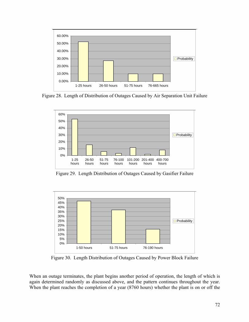
72

0.00%

10.00%

20.00%

30.00%

40.00%

50.00%

60.00%

1-25 hours 26-50 hours 51-75 hours 76-665 hours

Probability

Figure 28. Length of Distribution of Outages Caused by Air Separation Unit Failure

0%

10%

20%

30%

40%

50%

60%

1-25hours

26-50hours

51-75hours

76-100hours

101-200hours

201-400hours

400-700hours

Probability

Figure 29. Length Distribution of Outages Caused by Gasifier Failure

0%5%

10%15%20%25%30%35%40%45%50%

1-50 hours 51-75 hours 76-190 hours

Probability

Figure 30. Length Distribution of Outages Caused by Power Block Failure

When an outage terminates, the plant begins another period of operation, the length of which is again determined randomly as discussed above, and the pattern continues throughout the year. When the plant reaches the completion of a year (8760 hours) whether the plant is on or off the

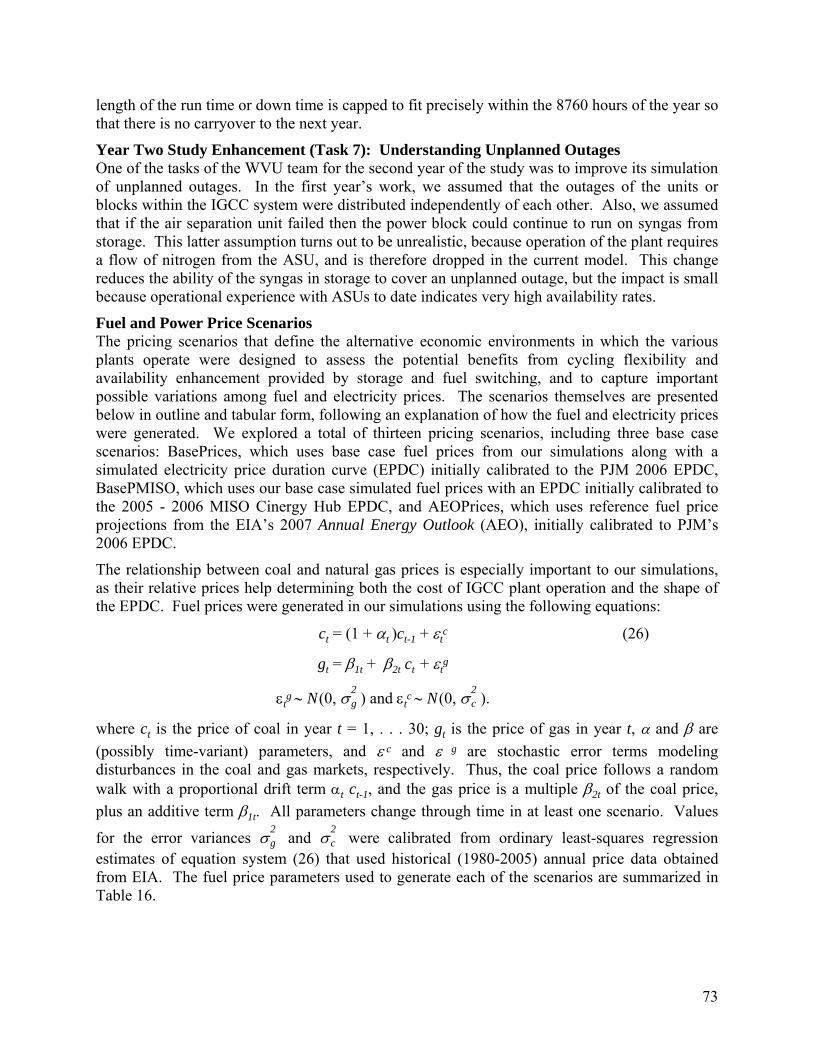
73

length of the run time or down time is capped to fit precisely within the 8760 hours of the year so that there is no carryover to the next year.

Year Two Study Enhancement (Task 7): Understanding Unplanned Outages One of the tasks of the WVU team for the second year of the study was to improve its simulation of unplanned outages. In the first year’s work, we assumed that the outages of the units or blocks within the IGCC system were distributed independently of each other. Also, we assumed that if the air separation unit failed then the power block could continue to run on syngas from storage. This latter assumption turns out to be unrealistic, because operation of the plant requires a flow of nitrogen from the ASU, and is therefore dropped in the current model. This change reduces the ability of the syngas in storage to cover an unplanned outage, but the impact is small because operational experience with ASUs to date indicates very high availability rates.

Fuel and Power Price Scenarios The pricing scenarios that define the alternative economic environments in which the various plants operate were designed to assess the potential benefits from cycling flexibility and availability enhancement provided by storage and fuel switching, and to capture important possible variations among fuel and electricity prices. The scenarios themselves are presented below in outline and tabular form, following an explanation of how the fuel and electricity prices were generated. We explored a total of thirteen pricing scenarios, including three base case scenarios: BasePrices, which uses base case fuel prices from our simulations along with a simulated electricity price duration curve (EPDC) initially calibrated to the PJM 2006 EPDC, BasePMISO, which uses our base case simulated fuel prices with an EPDC initially calibrated to the 2005 - 2006 MISO Cinergy Hub EPDC, and AEOPrices, which uses reference fuel price projections from the EIA’s 2007 Annual Energy Outlook (AEO), initially calibrated to PJM’s 2006 EPDC.

The relationship between coal and natural gas prices is especially important to our simulations, as their relative prices help determining both the cost of IGCC plant operation and the shape of the EPDC. Fuel prices were generated in our simulations using the following equations:

ct = (1 + αt )ct-1 + εt

c (26)

gt = β1t + β2t ct + εtg

εtg ∼ N (0, σ

2g ) and εt

c ∼ N (0, σ

2c ).

where ct is the price of coal in year t = 1, . . . 30; gt is the price of gas in year t, α and β are (possibly time-variant) parameters, and ε

c and ε g are stochastic error terms modeling

disturbances in the coal and gas markets, respectively. Thus, the coal price follows a random walk with a proportional drift term αt ct-1, and the gas price is a multiple β2t of the coal price, plus an additive term β1t. All parameters change through time in at least one scenario. Values

for the error variances σ

2g and σ

2c were calibrated from ordinary least-squares regression

estimates of equation system (26) that used historical (1980-2005) annual price data obtained from EIA. The fuel price parameters used to generate each of the scenarios are summarized in Table 16.

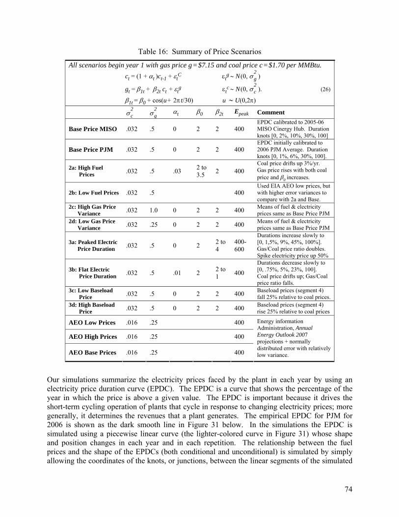
74

Table 16: Summary of Price Scenarios

All scenarios begin year 1 with gas price g = $7.15 and coal price c = $1.70 per MMBtu. ct = (1 + αt

)ct-1 + εtC εt

g ∼ N (0, σ

2g )

gt = β1t + β2t ct + εtg εt

c ∼ N (0, σ

2c ). (26)

β1t = β0 + cos(u + 2π t/30) u ∼ U(0,2π)

σ

2c σ

2g αt

β0 β2t Epeak Comment

Base Price MISO .032 .5 0 2 2 400 EPDC calibrated to 2005-06 MISO Cinergy Hub. Duration knots [0, 2%, 10%, 30%, 100]

Base Price PJM .032 .5 0 2 2 400 EPDC initially calibrated to 2006 PJM Average. Duration knots [0, 1%, 6%, 30%, 100].

2a: High Fuel Prices .032 .5 .03 2 to

3.5 2 400 Coal price drifts up 3%/yr. Gas price rises with both coal price and β0 increases.

2b: Low Fuel Prices .032 .5 400 Used EIA AEO low prices, but with higher error variances to compare with 2a and Base.

2c: High Gas Price Variance .032 1.0 0 2 2 400 Means of fuel & electricity

prices same as Base Price PJM 2d: Low Gas Price Variance .032 .25 0 2 2 400 Means of fuel & electricity

prices same as Base Price PJM

3a: Peaked Electric Price Duration .032 .5 0 2 2 to

4 400-600

Durations increase slowly to [0, 1,5%, 9%, 45%, 100%]. Gas/Coal price ratio doubles. Spike electricity price up 50%

3b: Flat Electric Price Duration .032 .5 .01 2 2 to

1 400 Durations decrease slowly to [0, .75%, 5%, 23%, 100]. Coal price drifts up; Gas/Coal price ratio falls.

3c: Low Baseload Price .032 .5 0 2 2 400 Baseload prices (segment 4)

fall 25% relative to coal prices. 3d: High Baseload Price .032 .5 0 2 2 400 Baseload prices (segment 4)

rise 25% relative to coal prices

AEO Low Prices .016 .25 400

AEO High Prices .016 .25 400

AEO Base Prices .016 .25 400

Energy information Administration, Annual Energy Outlook 2007 projections + normally distributed error with relatively low variance.

Our simulations summarize the electricity prices faced by the plant in each year by using an electricity price duration curve (EPDC). The EPDC is a curve that shows the percentage of the year in which the price is above a given value. The EPDC is important because it drives the short-term cycling operation of plants that cycle in response to changing electricity prices; more generally, it determines the revenues that a plant generates. The empirical EPDC for PJM for 2006 is shown as the dark smooth line in Figure 31 below. In the simulations the EPDC is simulated using a piecewise linear curve (the lighter-colored curve in Figure 31) whose shape and position changes in each year and in each repetition. The relationship between the fuel prices and the shape of the EPDCs (both conditional and unconditional) is simulated by simply allowing the coordinates of the knots, or junctions, between the linear segments of the simulated

75

EPDC to rise and fall with fuel prices in a structured way. Each knot in the piecewise linear curve is represented by an ordered pair of price and duration. In each case, the height and slope of the line segment begins in line with the 2006 PJM EPDC, and the changes in the locations of its knots through time is linked to changes in fuel prices through the heat rates of power plants that serve that segment. The peak price (duration of zero) was assumed to be driven by value of lost load, and is invariant to fuel prices. Prices at other knots are generated by appropriate fuel prices and mixes of generators likely to be marginal at those nodes; for example, the second node (duration .03) varied with the price of natural gas, while the last two nodes moved with the price of coal. In this way, we were able to simulate the differential effects of fuel price changes on IGCCs and the rest of the market.

-$50

$0

$50

$100

$150

$200

$250

$300

$350

$400

0 10 20 30 40 50 60 70 80 90 100

Duration: Percent of Annual Hours

Sys

tem

Ave

rage

LM

P P

rice

PriceFitted

Figure 31. 2006 PJM Unconditional Electricity Price Duration Curve

and Piecewise Linear Fitted Value

With the simulated fuel prices for each thirty year sequence in hand, we were able to generate a simulated electricity price duration curve (EPDC) for each year of a plant’s life. Calibration to actual MISO and PJM EPDCs led to the decision to use four linear segments. Four segments provide a reasonably good fit, as illustrated by the PJM 2006 EPDC and its fitted value shown in Figure 31 (weighted R2 = .987 for the fitted EPDC in Figure 31). For most scenarios, we begin the simulated plant’s life using a simulated curve calibrated to 2006 PJM EPDC, as pictured in Figure 31. All fuel and electricity price sequences begin simulation year 1 with prices at approximately 2006-7 levels, with gas at $7.15/MMBtu and coal at $1.70/MMBtu.16 In each 16 In the first quarter of 2008 the price of natural gas rose to near $10 and the spot price of coal nearly

tripled, rising above $100 per short ton (roughly $5.00 per mmBtu). Because it is difficult to gauge the

76

year of each iteration of the simulation algorithm, the segments of the EPDC move in response to changes in the fuel prices and (in some scenarios) in response to other changes in market conditions.

Table 17 shows the mean fuel and electricity prices generated by 10,000 Monte Carlo repetitions on each of the pricing scenarios. In general, the means appear to be consistent with the objectives of the scenarios, and the simulation data are not far out of line with EIA’s Annual Energy Outlook 2007. The AEO “Reference” or base case predictions project somewhat higher electricity and natural gas prices, and somewhat lower coal prices, than our base case. Our base case fuel prices are comfortably within the range of EIA’s “High” and “Low” projections. Applied to the PJM-calibrated EPDC, both sets of base case projections produce similar average wholesale electricity prices of approximately $45. The average prices in the MISO base case were about 10% lower than PJM’s. In the data sets that the EPDC construction was based on, the average electricity price for MISO August 2005 - July 2006 at 100% duration was $45.63, while PJM’s 2006 average price at 100% duration was $49.27. Thus, the scenarios here project electricity prices about 10% lower than EIA’s projections, and the estimated returns and NPVs are accordingly somewhat conservative. The high price scenarios (2a, 3a, 3d, and AEOHiPrices) may be more realistic, but no predictions of price levels 30 years into the future are likely to be accurate. The relative results among scenario outcomes are much more reliable than absolute predictions of prices and profitability.

longevity of these recent trends, however, and because electric utility fuel price data reflect spot fuel prices only with a lag (if at all), we have not adjusted the base fuel price to reflect these changes.

77

Table 17: Experimental Means and Standard Errors* of Energy Prices

Coal Price Gas Price Electricity Price (100% Duration)

Mean Std Mean Std Mean Std

AEO High Price 1.75 0.023 7.07 0.092 52.00 0.497

AEO Low Price 1.53 0.023 5.45 0.092 42.09 0.500

AEO Base Prices 1.65 0.023 6.13 0.092 46.52 0.498

Base Prices MISO 1.79 0.432 5.60 0.832 40.17 6.80

Base Prices PJM 1.81 0.417 5.65 0.806 44.10 7.33

2a: High Fuel Prices 2.72 0.726 8.03 1.367 63.19 12.61

2b: Low Fuel Prices 1.53 0.033 5.45 0.130 42.07 0.707

2c: High Gas Price Variance

1.81 0.417 5.65 0.816 44.09 7.359

2d: Low Gas Price Variance

1.81 0.417 5.65 0.801 44.11 7.316

3a: Peaked Electric Price Duration

1.81 0.417 7.39 1.308 57.33 10.62

3b: Flat Electric Price Duration

2.04 0.514 5.06 0.665 41.90 7.325

3c: Low Baseload Price

1.81 0.417 5.65 0.806 40.60 6.563

3d: High Baseload Price

1.81 0.417 5.65 0.806 47.60 8.100 *Std = Standard error of mean prices across experiments, not within experiments. See

Table 16 for standard errors of prices within experiments.

Year Two Study Enhancement: Specification of Electricity Price Duration Curves (Task 6) The specification of the electricity price duration curve (EPDC) is crucial to the validity of the simulation results because it specifies both the economic operation and the revenues generated by the plant. The construction of the EPDC for a particular simulation must take account of a plant’s operational constraints, particularly in the case of the CMU 12-hour plant. In the second year of this study, the WVU team studied the issue of EPDC specification in some depth, and made some changes to our own model of the EPDC.

An EPDC captures the distribution of electricity prices over time in a specific market (such as the PJM 2006 EPDC pictured in Figure 31) or in a specific node on the grid. Each point on the EPDC maps a specified price level against the percentage of time that the real-time electricity price exceeds that level. Electricity prices are generated by complex and instantaneous interaction among: factors that affect supply such as fuel prices, the composition of the generation stock, the topology of the transmission system, transmission and generation constraints, and emission regulations; factors that affect demand such as climate, temperatures, humidity, demand responsiveness, and the stock of electrical appliances; and factors that affect market structure and incentives, including the level of competition and the actions of regulators. The EPDC summarizes the outcome of the interaction of all of those factors and more over a

78

period of time, so predicting its location and shape in any particular year obviously involves a high degree of uncertainty.

The specification of EPDCs is an active area of current scholarship, largely because of the importance of EPDCs in assessing the value, optimal location, and optimal operation of generation and transmission facilities, and their usefulness for pricing electricity-based financial derivatives. Recent work in this area has emphasized the relationship between the predicted EPDC and a structural model of the underlying electricity market. In particular, Valenzuela and Mazumdar (2005) generate a Gram-Charlier series representation of the EPDC by using an autoregressive model of the load with Gaussian errors applied to a structural production costing model in the spirit of Bloom (1984). They also take into account a model of the offer behavior of oligopolistic generators. Valenzuela and Mazumdar (2007) further extend and refine this method by incorporating a Cournot model of the market and a stochastic model of plant availability. Michallat and Oren (2007) take a different methodological approach, describing how the EPDC can be generated using a probabilistic graphical model (PGM). Their PGM model also requires a structural model of the generators and their costs, with randomized availability and demand.

A developer considering constructing an IGCC power plant with storage in a specific location would be well-advised to adopt a detailed structural model of the EPDC (like the Valenzuela and Mazumdar model) that is based on a cost model using data on the current and projected generation stock and transmission system in the proposed location. For purposes of the current proof-of-concept simulation applied to a generic plant in a generic location, however, such a detailed and specific model was judged unnecessary. We require only a model of the EPDC that is responsive to changes in relative fuel prices, and that can be transparently manipulated to reflect different generic future market scenarios. We therefore continue to use our piecewise linear model of the EPDC, as described above.

79

0

25

50

75

100

125

150

175

200

225

250

0 10 20 30 40 50 60 70 80 90 100

Duration: Percent of 4380 Hours

Syst

em A

vera

ge L

MP

Pric

e

Conditional on Low Priced12 hours in Day

Conditional on High Priced 12 Hours in Day

Upper 50th Percentile, Unconditional

Lower 50th Percentile, Unconditional

Figure 32. EPDCs Conditional on Highest-Price and Lowest-Priced 12 Hours of Each Day, Compared to Upper and Lower 50th Percentiles of the Unconditional EPD PJM 2006

Simulation of the EPDC facing the CMU 12-hour plant poses a special problem, as the plant will produce at full power for only the 12 highest-priced hours per day, regardless of the price of electricity in the other 12 hours. (For the same reason, the CMU plant that uses fuel-switching for cycling will operate on natural gas only in the 12 lowest-priced hours of the day.) Because daily EPDCs are different on different days, the annual EPDC of prices taken only from the highest-priced twelve hours of each day will differ substantially from the upper 50th percentile of the annual EPDC. Therefore, in Year 2 of this project for simulations involving the CMU 12 hour plant we bifurcated the unconditional EPDC (Figure 31) into two conditional EPDCs, (shown as solid lines in Figure 32). The upper solid line in Figure 31 shows the empirical annual conditional EPDC for the 4380 hours that fell in the highest-priced 12 hours of days in 2006 in PJM. The dotted line just above it is the upper 50th percentile of the unconditional EPDC from Figure 31 (equivalently, the dotted line shows what the unconditional EPDC would look like if all days had identical EPDCs). It is apparent from this diagram that a simulation evaluation of the CMU 12-hour design that uses an unconditional EPDC such as the upper dotted line to calculate prices in PJM will overestimate those prices, and hence will overestimate the revenues earned by the plant. Similarly, using the lower 50th percentile of the unconditional EPDC (the

80

lower dotted line in Figure 32) will underestimate revenues for a power plant (such as the natural gas fueled phase of the fuel switching CMU 12-hour plant) that operates only in the lowest-priced 12 hours of each day.

II. Alternative Plant Configurations Used in the Simulations The plant configuration alternatives summarized in Table 18 were designed to allow the WVU team to assess the value of storage in the two identified dimensions of cycling flexibility and availability enhancement. The base plant is configuration 0, which has one gasifier train and no spare gasifier or storage. Plant 4 is the base plant included for comparison with plants 3, 5, 8 and 9, and like Plant 0 has no storage or spare. Plant 4 is included for technical reasons, to match the outage schedule for the CMU-based plants 5, 8, and 9. The differences in costs between plant 0 and 4 are small enough to ignore, so the analysis below references 4 only rarely.

Table 18: Summary of Plant Configurations

Plant Configuration

Number of Gasifiers

Number of Gas

Turbines Storage Spare

Gasifier Sized-Up Gasifier

0, 4. Base Plant 1 1 None None No 1. Base with Spare gasifier. 1 1 None 1 No

2. Economies of Scale 3 3 None 1 No

3. CMU 12 Hour 1 2 82,235 m3 None No 5. CMU 12 Hour, Storage also used for Backup

1 2 200,000 m3 None No

6. Large Storage for Backup, Above Ground 10% Inflow

1 1 200,000 m3 None 10%

7. Base Plant with Natural Gas Backup

1 1 None None No

8. CMU 12 Hour with Fuel Switching for Cycling only, not for Backup

1 2 82,235 m3 None No

9. CMU 12 Hour with Fuel Switching for Cycling and Backup

1 2 82,235 m3 None No

10. Large Storage for Backup, Underground 10% Inflow

1 1 400,000 m3 None 10%

81

Plant configuration 1 is the base plant with a spare gasifier added, which was managed in the simulation to increase plant availability. The spare gasifier is able to cover outages in the gasifier unit, however, only after it has warmed up to operating temperatures, which takes 30 hours (Wabash, 2002). Although the Wabash plant’s spare gasifier is not in practice used to increase that plant’s availability, the spare could be effective in increasing availability. As discussed below, however, our simulations indicate that this availability increase is not sufficient to provide an economic justification for the additional costs of operating the spare gasifier, which accords with the practice at the Wabash plant.

Plant configuration 2 achieves economies of scale by tripling the size of the plant. For example, although output from plant 2 is triple that of the other plants, its fixed operation and maintenance costs (as specified by the IECM model) are only 80% higher.

Plant configurations 3 and 5 use daily storage, as in the 12-hour storage plant developed by the CMU team, and described in the Task 5 report. The plants have one gasifier and two gas turbines. For 12 hours of the day the gasifier plant sends 100% of the syngas being produced to storage, and for the other 12 hours of the day the gasifier and storage combine to power two turbines. In plant 5 of our simulation, however, the storage size is much larger than in the Apt and Newcomer configuration so that the storage not only can be used to cycle the plant, but also for availability enhancement.

Plants 6 and 10 both use storage to improve plant availability. They possess storage capacity, but no spare gasifier. To send syngas to storage for use during unplanned gasifier outages the gasifier has been “sized up” by 10%. When the plant has an unplanned outage in the gasifier the syngas in storage is used to fuel the power block until the outage is over or there is no more syngas in storage. When the power block goes down the ASU and gasifier will stay online and send 100% of the syngas to storage until the storage is full or the outage is over. If the storage capacity is empty at a 10% flow rate it would take 265.3 hours to fill the 200,000 m3 of above-ground storage. Once storage is full it would be able to fuel one power block for 29.5 hours. In plant configuration 10 there is 400,000 m3 of underground storage where half of the capacity is assumed to be filled with a cushion gas which is not recoverable.

Plant 7 uses natural gas as a backup fuel to improve plant availability. This particular plant does not have syngas storage or a spare gasifier. When the plant experiences an unplanned outage in the air separation unit or the gasifier the power block switches from running on syngas to natural gas if profitable. Besides reducing capital costs, using natural gas as the backup fuel allows the plant manager to cover an unplanned outage in the air separation unit, whereas syngas storage is unable to do so because of the turbine unit’s need for nitrogen. The primary disadvantage of using natural gas to cover unplanned outages is the high level and volatility of natural gas prices.

Plant configurations 8 and 9 use syngas storage to provide cycling flexibility according to the CMU design, in the same way as plant configuration 3. These two plants, however, have the additional capability of switching the power block to natural gas fuel during its daily cycle. When its syngas storage facility is empty, plant 8 runs on natural gas if the electricity price is high enough to allow a profit. For example, if the electricity price exceeds the cost of running the plant on natural gas for 15 hours during a particular day, plant 8 would run on syngas during the highest-priced 12 hours, and then it would switch to natural gas for fuel during the remaining three hours of economical operation. Plant 8 (unlike the real-world Polk Plant) does not use its

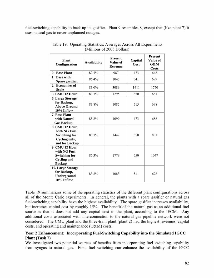
82

fuel-switching capability to back up its gasifier. Plant 9 resembles 8, except that (like plant 7) it uses natural gas to cover unplanned outages.

Table 19: Operating Statistics: Averages Across All Experiments

(Millions of 2005 Dollars)

Plant Configuration Availability

Present Value of Revenue

Capital Cost

Present Value of

O&M Costs

0. Base Plant 82.3% 987 473 648 1. Base with Spare gasifier. 86.4% 1045 541 699

2. Economies of Scale 83.0% 3089 1411 1770

3. CMU 12 Hour 83.7% 1295 650 681 6. Large Storage for Backup, Above Ground 10% Inflow

83.8% 1085 515 698


85.8% 1099 473 688

8. CMU 12 Hour with NG Fuel Switching for Cycling only, not for Backup

83.7% 1447 650 801

9. CMU 12 Hour with NG Fuel Switching for Cycling and Backup

86.3% 1779 650 1047


83.8% 1083 511 698

Table 19 summarizes some of the operating statistics of the different plant configurations across all of the Monte Carlo experiments. In general, the plants with a spare gasifier or natural gas fuel-switching capability have the highest availability. The spare gasifier increases availability, but increases capital cost by roughly 15%. The benefit of the natural gas as an additional fuel source is that it does not add any capital cost to the plant, according to the IECM. Any additional costs associated with interconnection to the natural gas pipeline network were not considered. The CMU plant and the three-train plant (plant 2) had the highest revenues, capital costs, and operating and maintenance (O&M) costs.

Year 2 Enhancement: Incorporating Fuel-Switching Capability into the Simulated IGCC Plant (Task 7) We investigated two potential sources of benefits from incorporating fuel switching capability from syngas to natural gas. First, fuel switching can enhance the availability of the IGCC

83

system, as in the case of the Polk Power Station, which uses distillate fuel as backup during unplanned outages (Tampa, 2004 p.2). Second, a supplemental fuel such as natural gas may be used to increase operational flexibility and profitability for the CMU 12 hour plant.

Incorporating fuel-switching capability into a power plant requires consideration of additional technical and financial issues. First, is the cost of switching the power block from syngas to natural gas, both in terms of time and money outlay. Industry contacts informed us that the switch takes three minutes using currently available hardware.17 Second, the use of natural gas rather than syngas reduces the power output of the plant. Based on the IECM model, gross output in our simulated plant falls by 18% when the turbine switches to natural gas. (The GE7FA turbine needs 1723.4 mmBtu of natural gas per hour to produce a net output of 253.3 MW in the IECM.) Third, as to the capital cost of fuel-switching capability, data were hard to find, so we assumed negligible additional capital cost, since in the IECM the capital cost of the power block for an NGCC plant and IGCC plant are almost identical. Finally, as to the operational (per-switch) variable costs of fuel switching, we investigated different levels for this variable, and concluded that its effect on the viability of the plant is minor.

Improving Plant Availability by Using Natural Gas as a Backup Fuel Plant availability is an important determinant of the profitability of an IGCC plant, as a plant can produce revenue only when it is available and producing power. We assessed various capital investments designed to improve plant availability: a spare gasifier, above-ground and underground storage, and natural gas as a backup fuel.

Switching to natural gas for backup has both advantages and disadvantages relative to using stored syngas for backup. Stored syngas not only allows the power plant to continue operating for a time after the gasifier (but not the ASU) goes down; it also allows the gasifier unit to continue producing gas when the power generation unit goes down, thus avoiding a costly gasifier shutdown and restart when the power unit fails briefly. In addition, a plant using stored syngas for backup is insulated from market fluctuations in the price of natural gas.

The limited capacity of storage is its primary disadvantage. If the gasifier fails, a plant using stored syngas for backup will have to shut down the power block when storage is empty, and if the power block fails the gasifier must be shut down when storage is full. In simulations, storage filled up an average of 12 times during the year, during which times it lost its ability to compensate for a failed power block. It emptied out entirely three times per year on average, and was unable to cover 416 hours of unplanned outages. Clearly, storage of the size considered can cover only a fraction of gasifier outages, as is reflected in the plant 6 availability statistics in Table 20 below.

17 Conversation with Robert Jones, Manager of Syngas Island Products, GE Energy (Dec. 17, 2007).

84

Table 20: Comparing Availability Improvements from Syngas Storage, Spare Gasifier and Natural Gas Backup

Plant Configuration Mean Availability

Availability Improvement

over Base Case 0. Base Plant (1 gasifier and 1 turbine.) 82.3% --- 1. Base Plant with Spare Gasifier. 86.4% 4.1% 6. Base Plant with 200k m3 Above-Ground Storage 83.8% 1.5% 7. Base Plant with Natural Gas Backup Fuel 84.7%-86.6% 2.4%-4.3%

There are significant advantages to using supplemental natural gas instead of stored syngas to cover unplanned outages. There is no physical limit on the length of an outage that supplemental natural gas can cover. Also, natural gas is able to cover outages in the air separation unit whereas syngas from storage is not. The primary disadvantage to the use of a purchased backup fuel such as natural gas is that the running costs of the plant vary as the price of natural gas fluctuates. When the running cost of the plant exceeds the price of electricity then the plant is shut down for economic reasons; therefore, the availability enhancement of a plant with natural gas backup (plant 7 in Table 20) covers a range from 2.4 to 4.3 percent, depending on gas and electricity prices. To achieve availability enhancement comparable to either a spare gasifier or backup fuel, storage size would have to be much larger than is being considered in this study.

Table 21: Hours per Year of Downtime By Cause, Base Plant 0

Cause Mean Standard deviation

Planned outage 769 179 Outage in ASU 105 128 Outage in gasifier 619 406 Outage in power block 138 97 Total hours offline 1549 459

Stored syngas is less effective than a spare gasifier for availability enhancement, for much the same reasons that it is inferior to a supplemental backup fuel. A spare gasifier is able to cover any length of outage in the gasifier unit, albeit after a 30 hour delay for warm-up, so the spare is operationally superior for plant outages caused by lengthy gasifier unit failures. Gasifier failures account for more than one-third of all of our simulated plant downtime, and nearly three-quarters of unplanned downtime, as shown in Table 21. In simulations, storage filled up an average of 12 times during the year, during which times it lost its ability to compensate for a failed power block. It emptied out entirely three times per year on average, and was unable to cover 416 hours of unplanned outages on average. Clearly, storage of the size considered can cover only a fraction of a typical gasifier outage.

Although a spare gasifier is operationally more effective at increasing plant availability than storage, the spare is not cost-effective. Relative to the base plant, Table 22 shows a small decline in ROIC for the base plant with a spare gasifier, a slight increase in ROIC for the plant with storage, and a much bigger gain in both ROIC by using natural gas as a backup fuel for unplanned outages. Using natural gas as an additional fuel source increases the ROIC of the

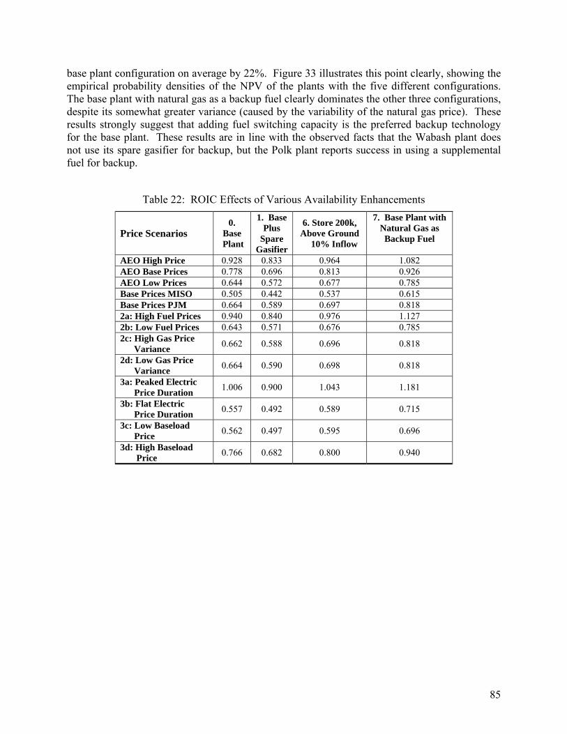
85

base plant configuration on average by 22%. Figure 33 illustrates this point clearly, showing the empirical probability densities of the NPV of the plants with the five different configurations. The base plant with natural gas as a backup fuel clearly dominates the other three configurations, despite its somewhat greater variance (caused by the variability of the natural gas price). These results strongly suggest that adding fuel switching capacity is the preferred backup technology for the base plant. These results are in line with the observed facts that the Wabash plant does not use its spare gasifier for backup, but the Polk plant reports success in using a supplemental fuel for backup.

Table 22: ROIC Effects of Various Availability Enhancements

Price Scenarios 0.

Base Plant

1. Base Plus

Spare

Gasifier

6. Store 200k, Above Ground 10% Inflow

7. Base Plant with Natural Gas as Backup Fuel

AEO High Price 0.928 0.833 0.964 1.082 AEO Base Prices 0.778 0.696 0.813 0.926 AEO Low Prices 0.644 0.572 0.677 0.785 Base Prices MISO 0.505 0.442 0.537 0.615 Base Prices PJM 0.664 0.589 0.697 0.818 2a: High Fuel Prices 0.940 0.840 0.976 1.127 2b: Low Fuel Prices 0.643 0.571 0.676 0.785 2c: High Gas Price Variance 0.662 0.588 0.696 0.818

2d: Low Gas Price Variance 0.664 0.590 0.698 0.818

3a: Peaked Electric Price Duration 1.006 0.900 1.043 1.181

3b: Flat Electric Price Duration 0.557 0.492 0.589 0.715

3c: Low Baseload Price 0.562 0.497 0.595 0.696

3d: High Baseload Price 0.766 0.682 0.800 0.940

86

Figure 33. NPV Effects of Different Availability Enhancements (Scenario 2a, High Fuel Prices)

Using Natural Gas to Increase Cycling Flexibility in the CMU 12 Hour Plant In the CMU 12 hour configuration, the gasifier runs continuously but the power plant runs on syngas only twelve hours per day, as the power plant burns gas at twice the rate that it is produced by the gasifier. As discussed above, we bifurcated the EPDC to correctly account for the revenues generated by this style of operation. A plant with fuel-switching capabilities might profitably run for some hours on certain days, as described by the lower portion of the bifurcated EPDC.

Table 23 quantifies the implications of a bifurcated EPDC for plant operation, based on actual hourly nodal electricity prices in PJM in 2006 and the MISO Cinergy node in 2005-06. For example, assuming a marginal cost of $50 for a natural-gas combined-cycle turbine (i.e., natural gas priced at $7.35 or less), there were 109 days in 2006 during which an natural-gas fired combined-cycle (NGCC) power plant could have operated profitably for more than 12 hours in PJM. Given recent and reasonably projected gas prices for fuel-switching of this kind to occur there must be diversity in the electricity price duration curve (EPDC) from one day to the next, since the annual capacity factor of an NGCC is typically well below 50%. Put another way, in roughly two days out of an average week the price of electricity exceeded $50 for more than 12 hours. On each of those 109 days the plant could have run on syngas for its usual 12 hours, and then switched to natural gas for at least an additional hour. Typically, these two days out of

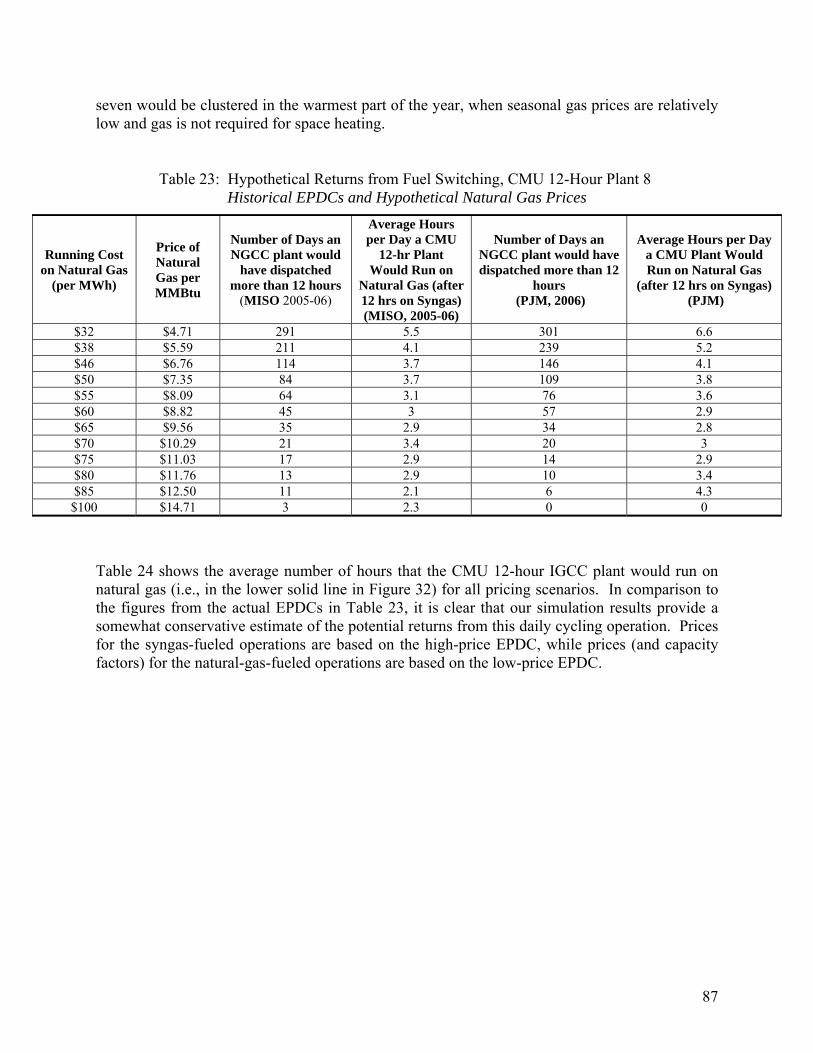
87

seven would be clustered in the warmest part of the year, when seasonal gas prices are relatively low and gas is not required for space heating.

Table 23: Hypothetical Returns from Fuel Switching, CMU 12-Hour Plant 8

Historical EPDCs and Hypothetical Natural Gas Prices

Running Cost on Natural Gas

(per MWh)

Price of Natural Gas per MMBtu

Number of Days an NGCC plant would

have dispatched more than 12 hours

(MISO 2005-06)

Average Hours per Day a CMU

12-hr Plant Would Run on

Natural Gas (after 12 hrs on Syngas) (MISO, 2005-06)

Number of Days an NGCC plant would have dispatched more than 12

hours (PJM, 2006)

Average Hours per Day a CMU Plant Would Run on Natural Gas

(after 12 hrs on Syngas) (PJM)

$32 $4.71 291 5.5 301 6.6 $38 $5.59 211 4.1 239 5.2 $46 $6.76 114 3.7 146 4.1 $50 $7.35 84 3.7 109 3.8 $55 $8.09 64 3.1 76 3.6 $60 $8.82 45 3 57 2.9 $65 $9.56 35 2.9 34 2.8 $70 $10.29 21 3.4 20 3 $75 $11.03 17 2.9 14 2.9 $80 $11.76 13 2.9 10 3.4 $85 $12.50 11 2.1 6 4.3 $100 $14.71 3 2.3 0 0

Table 24 shows the average number of hours that the CMU 12-hour IGCC plant would run on natural gas (i.e., in the lower solid line in Figure 32) for all pricing scenarios. In comparison to the figures from the actual EPDCs in Table 23, it is clear that our simulation results provide a somewhat conservative estimate of the potential returns from this daily cycling operation. Prices for the syngas-fueled operations are based on the high-price EPDC, while prices (and capacity factors) for the natural-gas-fueled operations are based on the low-price EPDC.

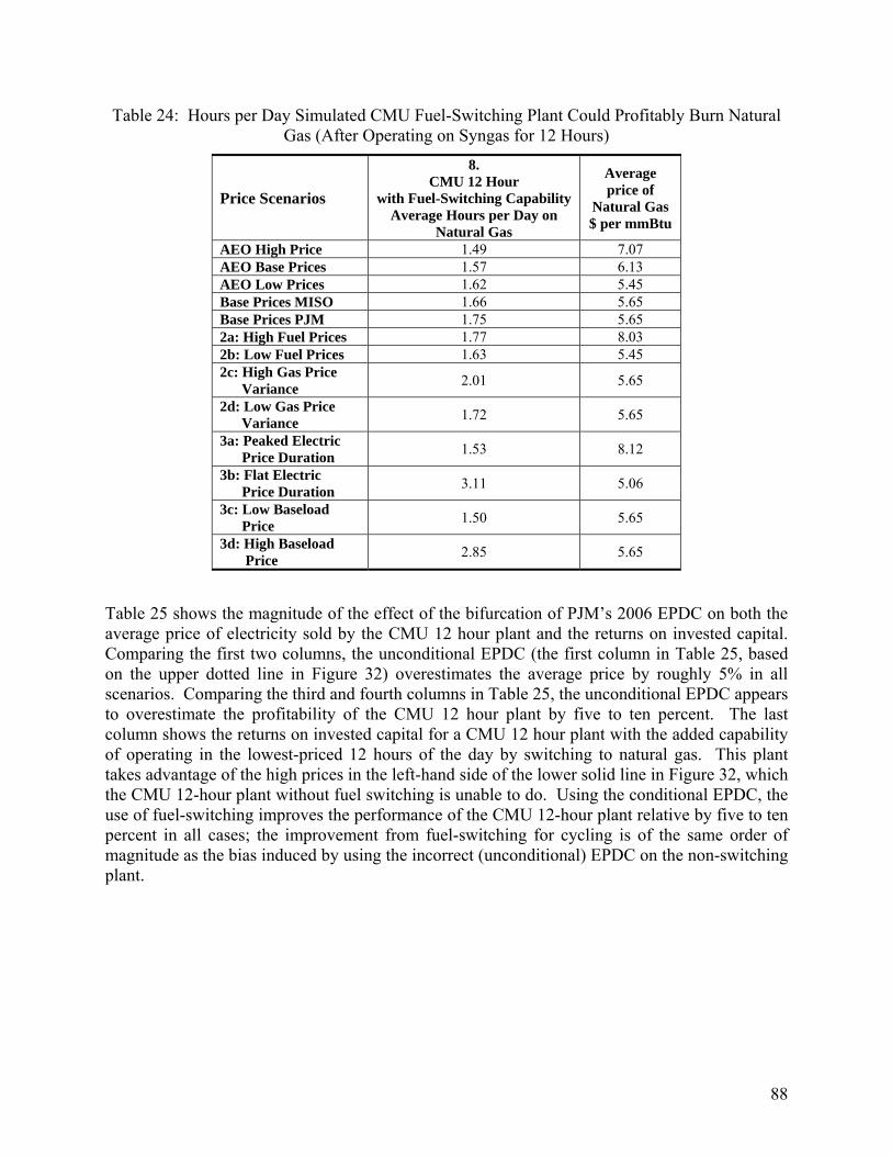
88

Table 24: Hours per Day Simulated CMU Fuel-Switching Plant Could Profitably Burn Natural Gas (After Operating on Syngas for 12 Hours)

Price Scenarios

8. CMU 12 Hour

with Fuel-Switching Capability Average Hours per Day on

Natural Gas

Average price of

Natural Gas $ per mmBtu

AEO High Price 1.49 7.07 AEO Base Prices 1.57 6.13 AEO Low Prices 1.62 5.45 Base Prices MISO 1.66 5.65 Base Prices PJM 1.75 5.65 2a: High Fuel Prices 1.77 8.03 2b: Low Fuel Prices 1.63 5.45 2c: High Gas Price Variance 2.01 5.65

2d: Low Gas Price Variance 1.72 5.65

3a: Peaked Electric Price Duration 1.53 8.12

3b: Flat Electric Price Duration 3.11 5.06

3c: Low Baseload Price 1.50 5.65

3d: High Baseload Price 2.85 5.65

Table 25 shows the magnitude of the effect of the bifurcation of PJM’s 2006 EPDC on both the average price of electricity sold by the CMU 12 hour plant and the returns on invested capital. Comparing the first two columns, the unconditional EPDC (the first column in Table 25, based on the upper dotted line in Figure 32) overestimates the average price by roughly 5% in all scenarios. Comparing the third and fourth columns in Table 25, the unconditional EPDC appears to overestimate the profitability of the CMU 12 hour plant by five to ten percent. The last column shows the returns on invested capital for a CMU 12 hour plant with the added capability of operating in the lowest-priced 12 hours of the day by switching to natural gas. This plant takes advantage of the high prices in the left-hand side of the lower solid line in Figure 32, which the CMU 12-hour plant without fuel switching is unable to do. Using the conditional EPDC, the use of fuel-switching improves the performance of the CMU 12-hour plant relative by five to ten percent in all cases; the improvement from fuel-switching for cycling is of the same order of magnitude as the bias induced by using the incorrect (unconditional) EPDC on the non-switching plant.

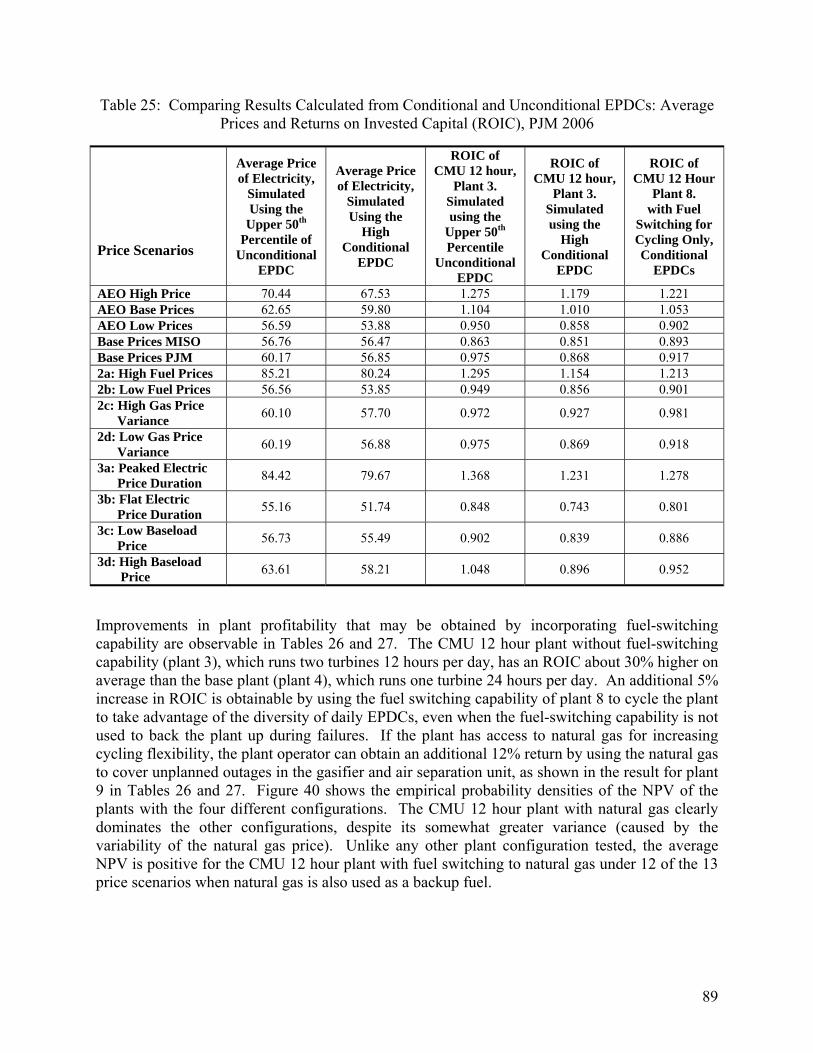
89

Table 25: Comparing Results Calculated from Conditional and Unconditional EPDCs: Average Prices and Returns on Invested Capital (ROIC), PJM 2006

Price Scenarios

Average Price of Electricity,

Simulated Using the

Upper 50th Percentile of

Unconditional EPDC

Average Price of Electricity,

Simulated Using the

High Conditional

EPDC

ROIC of CMU 12 hour,

Plant 3. Simulated using the

Upper 50th Percentile

Unconditional EPDC

ROIC of CMU 12 hour,

Plant 3. Simulated using the

High Conditional

EPDC

ROIC of CMU 12 Hour

Plant 8. with Fuel

Switching for Cycling Only,Conditional

EPDCs

AEO High Price 70.44 67.53 1.275 1.179 1.221 AEO Base Prices 62.65 59.80 1.104 1.010 1.053 AEO Low Prices 56.59 53.88 0.950 0.858 0.902 Base Prices MISO 56.76 56.47 0.863 0.851 0.893 Base Prices PJM 60.17 56.85 0.975 0.868 0.917 2a: High Fuel Prices 85.21 80.24 1.295 1.154 1.213 2b: Low Fuel Prices 56.56 53.85 0.949 0.856 0.901 2c: High Gas Price Variance 60.10 57.70 0.972 0.927 0.981

2d: Low Gas Price Variance 60.19 56.88 0.975 0.869 0.918

3a: Peaked Electric Price Duration 84.42 79.67 1.368 1.231 1.278

3b: Flat Electric Price Duration 55.16 51.74 0.848 0.743 0.801

3c: Low Baseload Price 56.73 55.49 0.902 0.839 0.886

3d: High Baseload Price 63.61 58.21 1.048 0.896 0.952

Improvements in plant profitability that may be obtained by incorporating fuel-switching capability are observable in Tables 26 and 27. The CMU 12 hour plant without fuel-switching capability (plant 3), which runs two turbines 12 hours per day, has an ROIC about 30% higher on average than the base plant (plant 4), which runs one turbine 24 hours per day. An additional 5% increase in ROIC is obtainable by using the fuel switching capability of plant 8 to cycle the plant to take advantage of the diversity of daily EPDCs, even when the fuel-switching capability is not used to back the plant up during failures. If the plant has access to natural gas for increasing cycling flexibility, the plant operator can obtain an additional 12% return by using the natural gas to cover unplanned outages in the gasifier and air separation unit, as shown in the result for plant 9 in Tables 26 and 27. Figure 40 shows the empirical probability densities of the NPV of the plants with the four different configurations. The CMU 12 hour plant with natural gas clearly dominates the other configurations, despite its somewhat greater variance (caused by the variability of the natural gas price). Unlike any other plant configuration tested, the average NPV is positive for the CMU 12 hour plant with fuel switching to natural gas under 12 of the 13 price scenarios when natural gas is also used as a backup fuel.

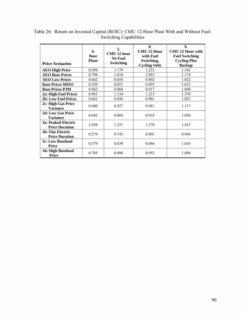
90

Table 26: Return on Invested Capital (ROIC): CMU 12-Hour Plant With and Without Fuel-Switching Capabilities

Price Scenarios

4. Base Plant

3. CMU 12 hour

No Fuel Switching

8. CMU 12 Hour

with Fuel Switching,

Cycling Only

9. CMU 12 Hour with

Fuel Switching Cycling Plus

Backup AEO High Price 0.950 1.179 1.221 1.342 AEO Base Prices 0.798 1.010 1.053 1.174 AEO Low Prices 0.662 0.858 0.902 1.022 Base Prices MISO 0.520 0.851 0.893 1.013 Base Prices PJM 0.682 0.868 0.917 1.049 2a: High Fuel Prices 0.961 1.154 1.213 1.370 2b: Low Fuel Prices 0.661 0.856 0.901 1.021 2c: High Gas Price Variance 0.680 0.927 0.981 1.117






91

Table 27: CMU 12-Hour Plant NPV (Millions of 2005 Dollars): Diversity in Daily Electricity Price Duration Curves

Price Scenarios 4. Base Plant

3. CMU 12 hour

8. CMU 12 Hour with Natural

Gas, No Backup

9. CMU 12 Hour with Natural Gas, Backup

AEO High Price -$23.73 $116.52 $143.79 $222.08 AEO Base Prices -$95.51 $6.34 $34.55 $112.97 AEO Low Prices -$160.16 -$92.64 -$63.82 $14.40 Base Prices MISO -$226.96 -$96.88 -$69.52 $8.75 Base Prices PJM -$150.50 -$85.98 -$53.85 $32.16 2a: High Fuel Prices -$18.27 $100.33 $138.39 $240.61 2b: Low Fuel Prices -$160.46 -$93.57 -$64.68 $13.77 2c: High Gas Price Variance -$151.35 -$47.29 -$12.56 $75.85

2d: Low Gas Price Variance -$150.32 -$85.35 -$53.27 $32.61

3a: Peaked Electric Price Duration $13.30 $149.98 $180.58 $269.88

3b: Flat Electric Price Duration -$201.77 -$167.16 -$129.40 -$36.17

3c: Low Baseload Price -$199.23 -$104.65 -$74.25 $6.44

3d: High Baseload Price -$101.77 -$67.31 -$30.99 $63.59

The attractiveness of switching to an alternate fuel for cycling purposes depends partly on the variable costs incurred each time there is a switch. In our simulations, a switch occurred for cycling purposes only when the expected net revenues during the expected period of operation was sufficient to cover the cost of switching. It is difficult to obtain hard data on these costs, but since our contact at GE stated that a switch takes about three minutes,18 we expect them to be small. Table 28 therefore reports the ROIC of plants over a wide range of switching costs ($0, $25, $50, and $100 per switch). As the cost associated with switching from syngas to natural gas increases the number of profitable opportunities to run the plant on natural gas decreases, and so yearly hours of operation on natural gas for cycling purposes falls, as indicated in Table 29.

18 Conversation with Robert Jones, Manager of Syngas Island Products, GE Energy (Dec. 17, 2007).

92

Table 28: Return on Invested Capital (ROIC), CMU 12-Hour Plant with Different Costs of Fuel- Switching (Switching for Cycling but not Backup)

Price Scenarios $0 Cost Per Switch

$25 Cost Per Switch

$50 Cost Per Switch

$100 Cost Per Switch

3. No Fuel Switching

AEO High Price 1.221 1.217 1.208 1.185 1.179 AEO Base Prices 1.053 1.049 1.039 1.017 1.010 AEO Low Prices 0.902 0.898 0.887 0.866 0.858 Base Prices MISO 0.893 0.885 0.876 0.859 0.851 Base Prices PJM 0.917 0.913 0.904 0.879 0.868 2a: High Fuel Prices 1.213 1.209 1.201 1.176 1.154 2b: Low Fuel Prices 0.901 0.896 0.886 0.865 0.856 2c: High Gas Price Variance 0.981 0.976 0.966 0.954 0.927






Table 29: Hours per Year of Natural Gas Operation of CMU 12-Hour Plant for

Different Levels of Switching Costs (Assuming Availability of 83.7%)

Price Scenarios $0 Cost Per Switch $25 Cost Per Switch $50 Cost Per Switch $100 Cost Per Switch AEO High Price 455 330 205 52 AEO Base Prices 480 339 202 49 AEO Low Prices 495 342 196 49 Base Prices MISO 507 241 144 55 Base Prices PJM 535 385 248 73 2a: High Fuel Prices 541 431 324 153 2b: Low Fuel Prices 498 345 202 49 2c: High Gas Price Variance 614 388 248 73

2d: Low Gas Price Variance 526 385 244 70

3a: Peaked Electric Price Duration 467 345 235 86

3b: Flat Electric Price Duration 950 522 296 89

3c: Low Baseload Price 458 342 229 70

3d: High Baseload Price 871 498 284 73

93

Year Two Study Enhancement: Underground Storage (Task 7) Underground storage has a lower cost per cubic meter than above-ground storage, and is therefore worth considering for larger storage needs. Several options for underground gas storage are currently in use in natural gas markets, but we considered salt caverns for our simulations because they have fast discharge rates than other underground formations and tend to have fewer leakage problems as well. Salt caverns are typically 1 million to 10 million m3, but the underground storage size used in our simulations is 400,000 m3, and the usable volume is only 200,000 m3, which allows comparability with our largest above-ground option. Costs for excavating a salt formation with a brine solution have been estimated at $19-$23/m3 (Newcomer, 2006). In our simulations we assumed this cost to be $21 per m3.

A cushion gas is required to pressurize an underground storage unit. The cushion gas is non-recoverable and can take up as much as 50 percent of the storage volume (Newcomer, 2006). The cost of the cushion gas depends on the coal price and the electricity price that is forgone by producing syngas that will never be available for sale. It is properly treated as a capital cost in accounting, since it only needs to be inserted once. Even though the excavation cost of an underground storage unit is less than the cost of constructing an above ground storage unit of the same usable size, the additional capital cost of the cushion gas can make the above ground storage a more cost effective option. Over the thirty year plant life it is possible that a percent of the cushion gas will leak out of the storage unit. Leakage of cushion gas can be treated the same way as depreciation of any other capital asset. Leakage rates are likely to be site-specific so a range of annual leakage rates (5%, 15%, and 30%) were explored to examine the impact of leakage on the ROIC and NPV.

Both above ground and underground storage units in our simulations are filled by a gasifier whose output is 10% larger than the power block’s requirements, which excess gas is sent to storage in preparation for an unplanned outage. With a 10% inflow it takes approximately 265 hours to fill 200,000 m3 and this storage size, if completely full, is able to cover almost 29.5 hours of an unplanned outage in the gasifier. When the storage is full the extra syngas is sent on to the power block, which is assumed to be able to burn it to produce electricity.19

Plant simulation results, shown in Table 30, indicate that underground storage on this relatively small scale affords only a slight improvement in profitability over above-ground storage. Plant configuration 6, which improves plant availability by 1.5 percent, increases the ROIC on average by 4.9 percent over the base plant. Plant 10, which uses underground storage, can increase plant availability by the same amount at slightly lower cost, resulting in an ROIC that is on average 0.28 percent higher than plant 6 when there is no leakage. A leakage rate of 5 percent reduces the ROIC on average by 0.1 percent. The ROIC is reduced on average by 0.6 percent when the leakage rate is 30 percent, which lowers the average ROIC below that of the above ground storage plant. Additional gains from underground storage that could be investigated are the larger availability enhancements from assuming a much larger storage size. This comparison was not investigated in this study because natural gas as a backup fuel clearly dominates the use of either underground or above ground storage for availability enhancement.

19 Changing this assumption reduces the ROIC of plants with storage for availability enhancement, but

qualitative comparisons with other plants (including comparison with plants that use natural gas for backup), are not affected.

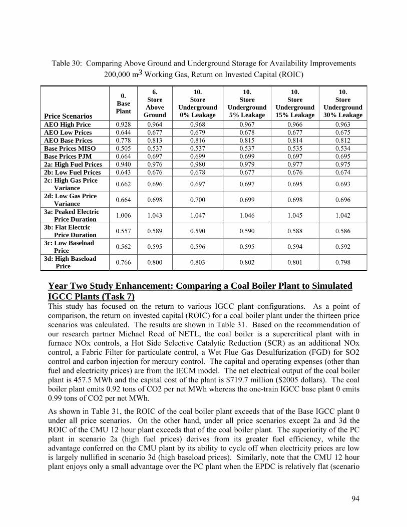
94

Table 30: Comparing Above Ground and Underground Storage for Availability Improvements

200,000 m3 Working Gas, Return on Invested Capital (ROIC)

Price Scenarios

0. Base Plant

6. Store Above

Ground

10. Store

Underground 0% Leakage

10. Store


10. Store


10. Store


AEO High Price 0.928 0.964 0.968 0.967 0.966 0.963 AEO Low Prices 0.644 0.677 0.679 0.678 0.677 0.675 AEO Base Prices 0.778 0.813 0.816 0.815 0.814 0.812 Base Prices MISO 0.505 0.537 0.537 0.537 0.535 0.534 Base Prices PJM 0.664 0.697 0.699 0.699 0.697 0.695 2a: High Fuel Prices 0.940 0.976 0.980 0.979 0.977 0.975 2b: Low Fuel Prices 0.643 0.676 0.678 0.677 0.676 0.674 2c: High Gas Price Variance 0.662 0.696 0.697 0.697 0.695 0.693

2d: Low Gas Price Variance 0.664 0.698 0.700 0.699 0.698 0.696

3a: Peaked Electric Price Duration 1.006 1.043 1.047 1.046 1.045 1.042

3b: Flat Electric Price Duration 0.557 0.589 0.590 0.590 0.588 0.586

3c: Low Baseload Price 0.562 0.595 0.596 0.595 0.594 0.592

3d: High Baseload Price 0.766 0.800 0.803 0.802 0.801 0.798

Year Two Study Enhancement: Comparing a Coal Boiler Plant to Simulated IGCC Plants (Task 7) This study has focused on the return to various IGCC plant configurations. As a point of comparison, the return on invested capital (ROIC) for a coal boiler plant under the thirteen price scenarios was calculated. The results are shown in Table 31. Based on the recommendation of our research partner Michael Reed of NETL, the coal boiler is a supercritical plant with in furnace NOx controls, a Hot Side Selective Catalytic Reduction (SCR) as an additional NOx control, a Fabric Filter for particulate control, a Wet Flue Gas Desulfurization (FGD) for SO2 control and carbon injection for mercury control. The capital and operating expenses (other than fuel and electricity prices) are from the IECM model. The net electrical output of the coal boiler plant is 457.5 MWh and the capital cost of the plant is $719.7 million ($2005 dollars). The coal boiler plant emits 0.92 tons of CO2 per net MWh whereas the one-train IGCC base plant 0 emits 0.99 tons of CO2 per net MWh.

As shown in Table 31, the ROIC of the coal boiler plant exceeds that of the Base IGCC plant 0 under all price scenarios. On the other hand, under all price scenarios except 2a and 3d the ROIC of the CMU 12 hour plant exceeds that of the coal boiler plant. The superiority of the PC plant in scenario 2a (high fuel prices) derives from its greater fuel efficiency, while the advantage conferred on the CMU plant by its ability to cycle off when electricity prices are low is largely nullified in scenario 3d (high baseload prices). Similarly, note that the CMU 12 hour plant enjoys only a small advantage over the PC plant when the EPDC is relatively flat (scenario

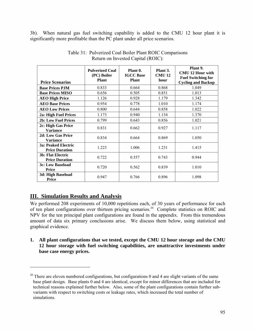
95

3b). When natural gas fuel switching capability is added to the CMU 12 hour plant it is significantly more profitable than the PC plant under all price scenarios.

Table 31: Pulverized Coal Boiler Plant ROIC Comparisons

Return on Invested Capital (ROIC):

Price Scenarios

Pulverized Coal (PC) Boiler

Plant

Plant 0. IGCC Base

Plant

Plant 3. CMU 12

hour

Plant 9. CMU 12 Hour with Fuel Switching for

Cycling and Backup Base Prices PJM 0.833 0.664 0.868 1.049 Base Prices MISO 0.656 0.505 0.851 1.013 AEO High Price 1.126 0.928 1.179 1.342 AEO Base Prices 0.954 0.778 1.010 1.174 AEO Low Prices 0.800 0.644 0.858 1.022 2a: High Fuel Prices 1.173 0.940 1.154 1.370 2b: Low Fuel Prices 0.799 0.643 0.856 1.021 2c: High Gas Price Variance 0.831 0.662 0.927 1.117






III. Simulation Results and Analysis We performed 208 experiments of 10,000 repetitions each, of 30 years of performance for each of ten plant configurations over thirteen pricing scenarios.20 Complete statistics on ROIC and NPV for the ten principal plant configurations are found in the appendix. From this tremendous amount of data six primary conclusions arise. We discuss them below, using statistical and graphical evidence.

1. All plant configurations that we tested, except the CMU 12 hour storage and the CMU 12 hour storage with fuel switching capabilities, are unattractive investments under base case energy prices.

20 There are eleven numbered configurations, but configurations 0 and 4 are slight variants of the same

base plant design. Base plants 0 and 4 are identical, except for minor differences that are included for technical reasons explained further below. Also, some of the plant configurations contain further sub-variants with respect to switching costs or leakage rates, which increased the total number of simulations.

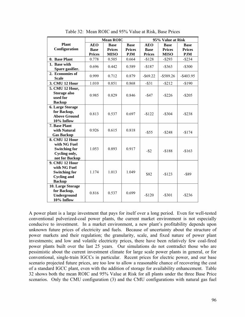
96

Table 32: Mean ROIC and 95% Value at Risk, Base Prices

Mean ROIC 95% Value at Risk Plant

Configuration AEO Base

Prices

Base Prices MISO

Base Prices PJM

AEO Base

Prices

Base Prices MISO

Base Prices PJM

0. Base Plant 0.778 0.505 0.664 -$128 -$293 -$234 1. Base with Spare gasifier. 0.696 0.442 0.589 -$187 -$363 -$300

2. Economies of Scale 0.999 0.712 0.879 -$69.22 -$589.26 -$403.95

3. CMU 12 Hour 1.010 0.851 0.868 -$31 -$212 -$190 5. CMU 12 Hour, Storage also used for Backup

0.985 0.829 0.846 -$47 -$226 -$205


0.813 0.537 0.697 -$122 -$304 -$238


0.926 0.615 0.818 -$55 -$248 -$174


1.053 0.893 0.917 -$2 -$188 -$163


1.174 1.013 1.049 $82 -$123 -$89


0.816 0.537 0.699 -$120 -$301 -$236

A power plant is a large investment that pays for itself over a long period. Even for well-tested conventional pulverized-coal power plants, the current market environment is not especially conducive to investment. In a market environment, a new plant’s profitability depends upon unknown future prices of electricity and fuels. Because of uncertainty about the structure of power markets and their regulation; the granularity, scale, and fixed nature of power plant investments; and low and volatile electricity prices, there have been relatively few coal-fired power plants built over the last 25 years. Our simulations do not contradict those who are pessimistic about the current investment climate for large scale power plants in general, or for conventional, single-train IGCCs in particular. Recent prices for electric power, and our base scenario projected future prices, are too low to allow a reasonable chance of recovering the cost of a standard IGCC plant, even with the addition of storage for availability enhancement. Table 32 shows both the mean ROIC and 95% Value at Risk for all plants under the three Base Price scenarios. Only the CMU configuration (3) and the CMU configurations with natural gas fuel

97

switching capabilities (8 and 9) are profitable on average and have positive 95% Value at Risk in any scenario, and they are attractive only in the AEO Base Price scenario.

Figure 34. ROIC of Various Plant Configurations, AEO Base Prices

Focusing on the AEO Base Price scenario, Figure 34 provides some insight into how the various plants perform under business-as-usual or base prices. The plants with no storage or spare (0) and storage (6) or spare (1) managed for availability, are similarly unprofitable, and cluster together. Because of its combination of high capital costs and long warmup time, the plant with a spare gasifier but no storage performed slightly but significantly worse than the base plant, while the plant with storage performed about the same or slightly better than the base plant. On the other hand, both the large three-train plant (plant 2) and the CMU 12-hour storage plant with natural gas (9, far right) are profitable, with the 12-hour storage plant with natural gas the most profitable. The lower Value at Risk and mean ROI for all plants under the BasePrice PJM and MISO scenarios reflects both the higher variance and lower mean levels associated with coal and electricity prices under those scenarios (see Table 17 above for a summary of fuel and electricity prices in the different scenarios).

Figure 35 sheds further light on the differences among the base price scenarios by comparing the performance of the base plant in the base price scenarios and the AEO High Price scenario. In general, the plants perform worst with the EPDC based on the low-peaked MISO Cinergy Hub, and they perform best using the AEO price projections based on the PJM EPDC. The AEO price scenarios are lower in variance, more symmetrical in distribution, and higher in mean than the

98

other base scenarios. Among the base price scenarios, PJM prices also provided the highest variance of returns for the base plant. These relationships among the base price scenarios apply to the other plant configurations as well, including the CMU 12-hour plant and the three-train plant illustrated in Figure 36.

Figure 35. Base Plant (0): Base Price Scenarios and AEO High Fuel

Prices, Distribution of Net Present Value

99

Figure 36. MISO and PJM Base Prices: Economies of Scale (Plant 2) and

CMU 12-hour (Plant 3)

2. IGCC Plants perform better in high-energy-price environments.

Increases in fuel prices have an ambiguous effect on a power plant’s profitability. Obviously, a coal-fired plant’s operating cost increases as coal prices increase, which will decrease the plant’s profitability if other factors are held constant. An increase in coal prices for one plant, however, is usually accompanied by increases in coal prices for other plants. Even in a competitive environment a general increase in coal prices will be passed along to consumers at least partially in the form of increased electricity prices. In a regulated environment, fuel price increases are relatively easily (and, in many jurisdictions automatically) passed along to customers in the form of higher regulated rates.

Thus, an increase in fuel prices will raise both costs and revenues to all plants. The increase in costs will be proportional to fuel usage, and the increase in revenues will be proportional to electricity production, so fuel price increases will tend to the advantage of more efficient plants, which by definition use less fuel per unit of electricity produced. Depending on the type of coal, the precise process used, and the authority referenced, IGCCs are 6% to 20% more efficient in terms of heat rate than the dominant subcritical pulverized coal plant technology, and roughly as efficient as the more expensive supercritical pulverized plants (Booras and Holt 2004; Wong and Whittingham, 2006). Our experimental design takes account of the efficiency advantage by specifying electricity price duration curves whose segments rise and fall through time according to fuel prices multiplied by the heat rates of plants that currently serve those segments, as described above.

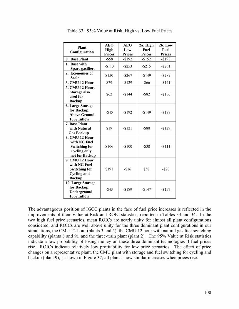
100

Table 33: 95% Value at Risk, High vs. Low Fuel Prices

Plant Configuration

AEO High Prices

AEO Low

Prices

2a: High Fuel

Prices

2b: Low Fuel

Prices 0. Base Plant -$58 -$192 -$152 -$198 1. Base with Spare gasifier. -$113 -$253 -$215 -$261

2. Economies of Scale $150 -$267 -$149 -$289

3. CMU 12 Hour $79 -$129 -$66 -$141 5. CMU 12 Hour, Storage also used for Backup

$62 -$144 -$82 -$156


-$45 -$192 -$149 -$199


$19 -$121 -$88 -$129


$106 -$100 -$38 -$111


$191 -$16 $38 -$28


-$43 -$189 -$147 -$197

The advantageous position of IGCC plants in the face of fuel price increases is reflected in the improvements of their Value at Risk and ROIC statistics, reported in Tables 33 and 34. In the two high fuel price scenarios, mean ROICs are nearly unity for almost all plant configurations considered, and ROICs are well above unity for the three dominant plant configurations in our simulations, the CMU 12-hour (plants 3 and 5), the CMU 12 hour with natural gas fuel switching capability (plants 8 and 9), and the three-train plant (plant 2). The 95% Value at Risk statistics indicate a low probability of losing money on these three dominant technologies if fuel prices rise. ROICs indicate relatively low profitability for low price scenarios. The effect of price changes on a representative plant, the CMU plant with storage and fuel switching for cycling and backup (plant 9), is shown in Figure 37; all plants show similar increases when prices rise.

101

Table 34: Mean ROIC, High vs. Low Fuel Prices

Plant Configuration AEO High Prices

AEO Low Prices

2a: High Fuel

Prices

2b: Low Fuel

Prices 0. Base Plant 0.928 0.644 0.940 0.643 1. Base with Spare gasifier. 0.833 0.572 0.840 0.571

2. Economies of Scale 1.156 0.858 1.168 0.857

3. CMU 12 Hour 1.179 0.858 1.154 0.856 5. CMU 12 Hour, Storage also used for Backup

1.151 0.836 1.126 0.834


0.964 0.677 0.976 0.676


1.082 0.785 1.127 0.785


1.221 0.902 1.213 0.901


1.342 1.022 1.370 1.021


0.968 0.679 0.980 0.678

102

Figure 37. ROIC of CMU 12-Hour Plant, Different Price Levels

3. High peak power prices improve IGCC plants’ economic performance while high baseload prices improve IGCC performance only slightly.

Electricity price increases, regardless of source, improve the economic performance of IGCC plants. In scenarios 3a through 3d we changed the shape of the electricity price duration curve in different ways, and the results are seen in Figure 38 and Tables 35 and 36. The higher and wider peak price level of scenario 3a, (which might be caused in the real world by an increase in peak period demand, or an increase in natural gas prices relative to coal prices), has the most positive effect on IGCC returns. All but one plant configuration is expected to at least break even under scenario 3a, and the dominant design generates a positive return even at the 5th percentile of outcomes. The high baseload price scenario 3d (consistent with enhanced demand responsiveness, plug-in autos, high coal prices, or low levels of baseload plant construction) provides returns similar to those of the base price scenarios, despite the 25% higher baseload period prices and unchanged peak period prices. Regardless of plant configuration, operators must look for high peak period prices in order to obtain reliably high returns on the plant.

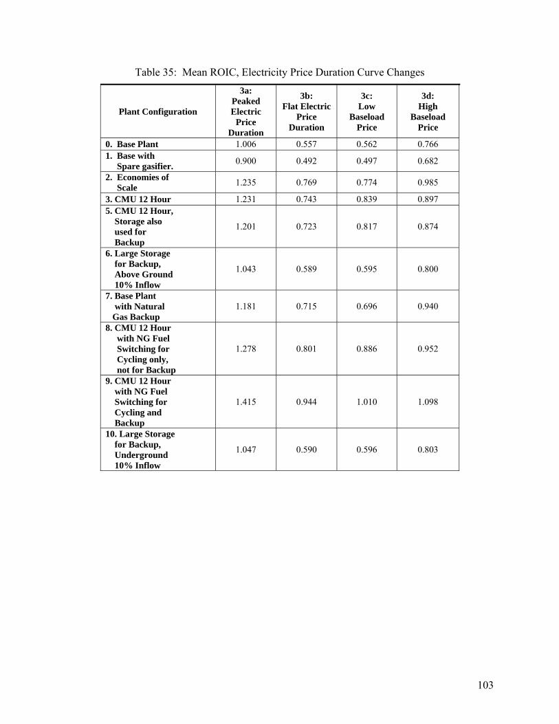
103

Table 35: Mean ROIC, Electricity Price Duration Curve Changes

Plant Configuration

3a: Peaked Electric

Price Duration

3b: Flat Electric

Price Duration

3c: Low

Baseload Price

3d: High

Baseload Price

0. Base Plant 1.006 0.557 0.562 0.766 1. Base with Spare gasifier. 0.900 0.492 0.497 0.682



1.201 0.723 0.817 0.874


1.043 0.589 0.595 0.800


1.181 0.715 0.696 0.940


1.278 0.801 0.886 0.952


1.415 0.944 1.010 1.098


1.047 0.590 0.596 0.803

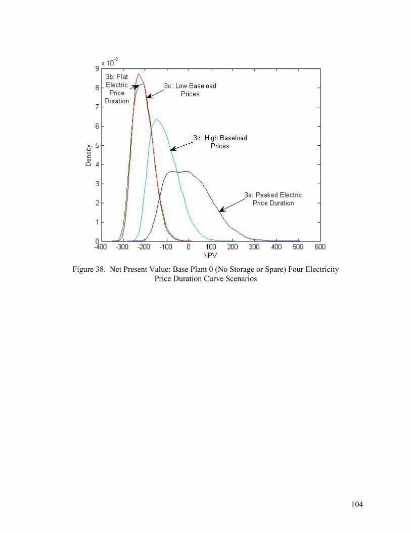
104

Figure 38. Net Present Value: Base Plant 0 (No Storage or Spare) Four Electricity Price Duration Curve Scenarios

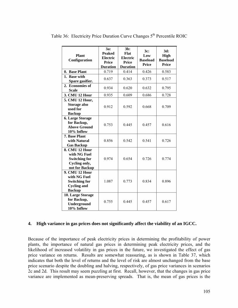
105

Table 36: Electricity Price Duration Curve Changes 5th Percentile ROIC

Plant Configuration

3a: Peaked Electric

Price Duration

3b: Flat

Electric Price

Duration

3c: Low

Baseload Price

3d: High

Baseload Price




0.912 0.592 0.668 0.709


0.753 0.445 0.457 0.616


0.856 0.542 0.541 0.726


0.974 0.654 0.726 0.774


1.087 0.773 0.834 0.896


0.755 0.445 0.457 0.617

4. High variance in gas prices does not significantly affect the viability of an IGCC.

Because of the importance of peak electricity prices in determining the profitability of power plants, the importance of natural gas prices in determining peak electricity prices, and the likelihood of increased volatility in gas prices in the future, we investigated the effect of gas price variance on returns. Results are somewhat reassuring, as is shown in Table 37, which indicates that both the level of returns and the level of risk are almost unchanged from the base price scenario despite the doubling and halving, respectively, of gas price variances in scenarios 2c and 2d. This result may seem puzzling at first. Recall, however, that the changes in gas price variance are implemented as mean-preserving spreads. That is, the mean of gas prices is the

106

same in scenarios 2a and 2b as it is in the MISO and PJM Base Price scenarios. Because the payback on a power plant is a weighted average of 30 annual revenue payments, the riskiness of returns across different experiments does not change much when the variance in gas prices increases or decreases.

Table 37: Effect of Gas Price Variance on ROIC

2c: High Gas Price Variance

2d: Low Gas Price Variance

Plant Configuration Mean 5th

Percentile Mean 5th Percentile




0.904 0.661 0.846 0.697


0.696 0.516 0.698 0.544


0.818 0.615 0.818 0.639


0.981 0.724 0.918 0.757


1.117 0.841 1.050 0.869


0.697 0.516 0.700 0.544

5. The use of a backup fuel such as natural gas dominates all other configurations used for availability enhancement.

Even though the spare gasifier is able to increase plant availability about as well as natural gas being used as a backup fuel, the capital cost associated with the spare gasifier makes it a relative unattractive option for availability enhancement in a single train plant. A spare gasifier is used

107

in the three train plant, but gains from the use of the spare are able to overcome the capital cost when considering the larger plant. The primary advantages of using supplemental natural gas is that there is no physical limit on the length of an outage that natural gas can cover and natural gas is able to cover outages in the air separation unit whereas storage and a spare gasifier are not. The primary disadvantage to the use of a purchased backup fuel such as natural gas is that the running costs of the plant vary as the price of natural gas fluctuates.

108

Table 38: ROIC Effects of Various Availability Enhancements

Price Scenarios 0. Base Plant

1. Base Plus Spare

Gasifier

6. Storage 200k, Above

Ground 10% Inflow

7. Base Plant with Natural

Gas as Backup Fuel

AEO High Price 0.928 0.833 0.964 1.082 AEO Base Prices 0.778 0.696 0.813 0.926 AEO Low Prices 0.644 0.572 0.677 0.785 Base Prices MISO 0.505 0.442 0.537 0.615 Base Prices PJM 0.664 0.589 0.697 0.818 2a: High Fuel Prices 0.940 0.840 0.976 1.127 2b: Low Fuel Prices 0.643 0.571 0.676 0.785 2c: High Gas Variance 0.662 0.588 0.696 0.818

2d: Low Gas Variance 0.664 0.590 0.698 0.818

3a: Peaked EPDC 1.006 0.900 1.043 1.181 3b: Flat EPDC 0.557 0.492 0.589 0.715 3c: Low Baseload Price 0.562 0.497 0.595 0.696


Figure 39. NPV Effects of Different Availability Enhancements (Scenario 2a, High Fuel Prices)

109

6. Under all price scenarios the most profitable plant configuration is the CMU 12 hour plant with fuel switching capabilities and backup fuel.

The most profitable plants under all price scenarios is the CMU 12 hour plant with and without fuel switching capabilities and the economies of scale plant, which are shown in Table 39. The ROIC of the economies of scale plant (plant 2) and the CMU plants without fuel switching capability (plants 3 and 5) are similar in most price scenarios. The ROIC is slightly lower for the CMU 12 hour plant where storage is also used for backup (plant 5) then the CMU 12 hour plant (plant 3) because the additional storage is only able to improve average availability by 0.40 percent which does not compensate the plant for the additional capital cost associated with the larger storage size. The CMU plant with fuel switching capabilities and backup fuel clearly dominates all other plant configurations.

Table 39: Return on Invested Capital (ROIC): CMU 12-Hour Plant and Economies of Scale

Plant With and Without Fuel-Switching Capabilities

Price Scenarios

2. Economies

of Scale

3. CMU 12

hour No Fuel

Switching

5. CMU 12 Hour,

Storage also used for

Backup

8. CMU 12 Hour

with Fuel Switching,

Cycling Only

9. CMU 12 Hour with

Fuel Switching Cycling Plus

Backup AEO High Price 1.156 1.179 1.151 1.221 1.342 AEO Base Prices 0.999 1.010 0.985 1.053 1.174 AEO Low Prices 0.858 0.858 0.836 0.902 1.022 Base Prices MISO 0.712 0.851 0.829 0.893 1.013 Base Prices PJM 0.879 0.868 0.845 0.917 1.049 2a: High Fuel Prices 1.168 1.154 1.126 1.213 1.370 2b: Low Fuel Prices 0.857 0.856 0.834 0.901 1.021 2c: High Gas Price Variance 0.878 0.927 0.904 0.981 1.117






110

Figure 40. Effect of Fuel-Switching Capability on NPV of Plant Base Prices Scenario, Natural Gas as Alternate Fuel

111

IV. Task 8: IGCC Optimal Control Problem Motivation In task 8.0 the WVU team undertook to create a mathematical model of the syngas plant with diurnal storage cycle. The purposes of this exercise are to explain the rationale for the plant’s design, to provide insights into its optimal operation, and to develop a framework within which to analyze changes to its capital composition. We begin with a general somewhat simplified model of a power plant with diurnal storage, then using tools of optimal control we analyze its operation and cost-effectiveness of its capital assets. Summaries of the optimal control dynamic optimization methods used in this section may be found in many standard works on the subject, including Chiang (1992). Dorfman (1969) provides an illuminating economic interpretation of the parameters of a typical optimal control problem.

Assumptions and simplifications for our model: • The gasifier produces g units of gas per time period. • The gasifier is must-run (i.e., shut-down and restart costs are very large). • Reliability problems are ignored, as they can be addressed using other methods. • x(t) = the amount of gas being burned currently in the powerplant.

• The powerplant can burn up to x− units of gas. • It takes 1/α units of gas to produce one unit of electricity. Thus,

electrical output = αx, and α may be interpreted as the inverse of the heat rate for the generator.

• Zero startup & commitment costs for the power block. • Zero running costs other than fuel costs. • The future time path of the price of electricity p(t) is known. • Electricity prices p(t) follow a cyclical pattern with a daily frequency and a single peak.

Setting up the Problem: • x(t) = Control Variable = Rate of burn of gas. • k(t) = State variable = the amount of gas in storage. • p(t) = price of electricity at time t.

• k⋅ = dk/dt, the rate of change of the amount of gas in storage through time. • λ(t) = costate variable, interpreted as the value of the marginal unit of gas in storage.

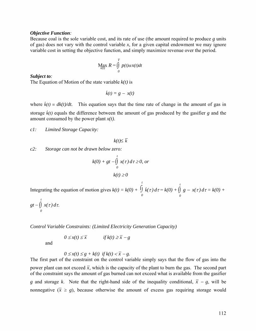
112

Objective Function: Because coal is the sole variable cost, and its rate of use (the amount required to produce g units of gas) does not vary with the control variable x, for a given capital endowment we may ignore variable cost in setting the objective function, and simply maximize revenue over the period.

Maxx(t) R = ⌡⌠0

T

p(t)α x(t)dt

Subject to: The Equation of Motion of the state variable k(t) is

k⋅(t) = g − x(t)

where k⋅(t) ≡ dk(t)/dt. This equation says that the time rate of change in the amount of gas in

storage k⋅(t) equals the difference between the amount of gas produced by the gasifier g and the amount consumed by the power plant x(t).

c1: Limited Storage Capacity:

k(t)≤ k−

c2: Storage can not be drawn below zero:

k(0) + gt − ⌡⌠0

t

x(τ ) dτ ≥ 0, or

k(t) ≥ 0

Integrating the equation of motion gives k(t) = k(0) + ⌡⌠0

t

k⋅(τ ) dτ = k(0) + ⌡⌠0

t

g − x(τ ) dτ = k(0) +

gt − ⌡⌠0

t

x(τ ) dτ.

Control Variable Constraints: (Limited Electricity Generation Capacity)

0 ≤ x(t) ≤ x− if k(t) ≥ x− − g and

0 ≤ x(t) ≤ g + k(t) if k(t) < x− − g. The first part of the constraint on the control variable simply says that the flow of gas into the power plant can not exceed x−, which is the capacity of the plant to burn the gas. The second part of the constraint says the amount of gas burned can not exceed what is available from the gasifier

g and storage k. Note that the right-hand side of the inequality conditional, x− − g, will be nonnegative (x− ≥ g), because otherwise the amount of excess gas requiring storage would

113

increase monotonically through time without limit. It is not necessary to include this constraint explicitly in the Hamiltonian, but it provides a limited range of operation for x(t).

Finally, we may constrain the optimization by specifying starting and ending values for the amount of gas in storage. Because prices and the pattern of use are cyclical on a daily pattern, we may start the planning period at any time. Without loss of generality, we may specify the initial and terminal conditions:

k(0) = k(T) = 0

so the period of interest starts and ends when storage is empty. Because x− > g and the objective is to maximize revenue, storage will be emptied (or otherwise reduced to a desirable minimum k(0)) every day. The length of the time period under consideration corresponds to the daily price cycle.

For the diurnal-cycle storage plants studied in this report, the scale of the electricity generation and storage capital investments are integer multiples of the scale of the gasifier. In particular, x−

= 2g for all of the CMU diurnal storage plants, k− = 12g for the CMU 12-hour plant, k− = 4g for the CMU 4-hour plant, and so on.

Analysis Optimal Operation To find the functional x(t) of the control variable that maximizes revenue over the period, we follow the usual procedure in solving an optimal control problem. We first set up the constrained Hamiltonian:

H = p(t)α x(t) + λ(t)(g − x(t)) + γ1(t)(k− − k(t)) + γ2(t)⎝⎜⎛

⎠⎟⎞

k(0) + gt − ⌡⌠0

t

x(τ ) dτ

and note that it is linear in the control variable x,

∂ H/∂ x(t) = p(t)α − λ(t) + γ1(t) − γ2(t), (27)

which implies that the problem has a “bang-bang” or corner solution, in which the optimal solution is that the power block should be turned all the way on or all the way off. The optimal setting for the generator x(t) depends on the sign of equation (27). If the sign of (27) is positive, then the optimal x(t)* = x− if there is sufficient gas in storage (i.e., if x− ≤ k(t) + g); otherwise x(t)*= k(t) + g. (For a CMU diurnal storage plant, if (27) is positive and then g ≤ x(t)* ≤ 2g.) If the sign of (27) is negative, then the optimal x(t)* = 0; i.e., the generator should be turned off.

In addition, the inequality constraints c1 and c2 give rise to the following Kuhn-Tucker complementary slackness conditions:

γ1(t)(k− − k(t)) = 0

which implies that either storage is full or the shadow price γ1(t) = 0, and

114

γ2(t)k(t) = 0

which implies that either storage is empty, or the shadow price γ2(t) = 0. Thus, in equation (27) if storage is neither empty nor full γ1(t) = γ2(t) = 0, and the proper control action x(t) depends on the relationship between p(t)α and λ(t). If there were an internal solution, λ(t) = p(t)α − γ2(t), which means that λ(t) = p(t)α unless storage is empty. But there is no internal solution, so generally λ(t) > p(t)α when x(t) = 0 and λ(t) < p(t)α when x(t) > 0.

The analysis of costs and electricity prices elsewhere in this report clearly indicates that, absent storage, an IGCC plant’s running costs are low enough so that it will operate as a baseload facility. Thus, an IGCC with diurnal storage cycles on and off in response to changes in p(t) only because if the power plant can burn gas more rapidly than the gasifier can produce gas (x− > g) then the proportion of the day that the power plant can operate at full power is constrained to a maximum of g / x−. Generation is therefore constrained when storage is either empty or full: when empty the plant can produce no more than αg units of power per hour; when full it can produce no less than αg.

Define the current moment as time t¸ and define s as the time when the constraint on gas storage will next bind. That is, s is the time at which storage becomes either empty or full. When the plant is operating at full power (x(t) = x−), the opportunity cost of the marginal unit of gas consumed is the loss of revenue p(s)α that will occur after storage empties out. When the power plant is not operating (x(t) = 0), increasing consumption by one unit at time t will extend the fill time of storage by the amount of time required to burn that unit of gas, and resulting in loss of

revenue p(s)α. Therefore, if 0 < k(t) < k−, the marginal cost of burning gas at time t is p(s)α, and by the same token the marginal value of increasing storage at time t is p(s)α. This observation leads directly to the following proposition.

Proposition 1) Define p(s) as the price of electricity when storage next either empties or fills. If

0 < k(t) < k−, then optimal x(t)* >0 if and only if p(t) > p(s).

Proof. It is well known (see Dorfman 1969, p.820) that the costate variable λ(t) may be interpreted as the marginal value of an increase in the state variable, which in this case is the value of increasing the amount of gas in storage by one unit. As argued above, then, λ(t) = p(s)α.

If storage is neither empty nor full (0 < k(t) < k−) then γ1 = γ2 = 0, and equation (27) becomes ∂ H/∂ x(t) = (p(t)− p(s))α, which is positive if and only if p(t) > p(s). Note that x(t)* is

indeterminate if p(t) = p(s) and x(t)*=0 if p(t) < p(s) and 0 < k(t) < k−.

Note further that proposition 1 is consistent with the basic economic tenet that production should increase when marginal revenue exceeds marginal cost. The marginal revenue obtained from burning an additional unit of gas at time t is p(t)α, while the marginal (opportunity) cost of burning that unit of gas is p(s)α. If there were an internal solution to equation (27), λ(t) = p(t)α + γ1(t) − γ2(t), implies that λ(t) = p(t)α unless storage is either empty or full. But there is no

115

internal solution, so if storage is unconstrained then λ(t) > p(t)α implies x(t) = 0 and λ(t) < p(t)α implies x(t) > 0.

To fully specify the path of the control variable x, we need similar propositions for its value when storage is full and empty. Storage can only become full when the power plant is burning less than the output of the gasifier (x* < g), and when x* < g the plant will shut down entirely, because the solution is bang-bang. Thus, the plant must have been shut down prior to storage being full if it was controlled optimally. Therefore, storage will fill up at time s only if p(t)≤ λ(t) = p(t) for t < s – that is, only if electricity prices are rising.

At the instant that storage fills, three things happen. First, the power plant must switch on, and must burn gas at a rate equal to at least g, because the gas has nowhere else to go. Second, the shadow value of increasing storage capacity γ1(t) goes from zero to a positive number, as the constraint c1 binds. Third, the marginal value of storage λ(t) (which is also the opportunity cost of burning an additional unit of gas from storage) changes:

λ(t) = min(p(t+ε)α, p(s)α) when storage is full, (28)

where ε is the amount of time required to produce a unit of gas, and s = t + k−/(x− − g) is the point in time when storage will be fully depleted at a burn rate of x−. To understand why this is so, note

that if we burn g+1 units of gas at time t then storage will no longer be full; i.e., k(t) = k− − 1. If at this point ∂ H/∂ x(t) < 0, then the burn rate will decrease momentarily at time t + ε until storage is full again, costing revenue of p(t+ε)α. If, on the other hand, ∂ H/∂ x(t) > 0 (which will occur if p(t)>p(s), as shown above in proposition 1), then the burn rate will rise to x−, and will continue as discussed in proposition 1. Allowing ε to go to zero implies proposition 2:

Proposition 2: If storage is full (k(t) = k−), then optimal x(t)* = g if p(t) < p(s) and x(t)* = x− if p(t) > p(s), where s = t + k−/(x− − g) is the time at which storage would be emptied at a

burn rate of x− units of gas per time period.

A similar line of reasoning leads to proposition 3:

Proposition 3: If storage is empty (k(t) = k−), then optimal x(t)* = g if p(t) < p(s) and x(t)* = 0 if p(t) > p(s), where s = t + k−/g is the time at which storage would be filled if no gas is burned.

These three propositions completely describe the optimal time path of the control variable x(t) through time for an IGCC plant with storage that is capable of burning all of its production during a single day’s production, operating in an environment in which electricity prices follow a daily cycle with a single peak. This approximately describes the CMU 12, 8, and 4 hour plants, in which x− = 2g, and k− = 12g, 8g, and 4g, respectively.

116

Summary of Operational Results: The prescription offered by propositions 1 – 3 offer no real surprises, but they do provide a solid framework for understanding the optimal operation of the plant. In essence, the propositions imply that a plant with low running costs, able to produce g units of syngas per hour, equipped with k− = bg units of storage capacity and capable of burning x− = cg units of gas per hour, will burn gas at maximum rate cg for the highest-priced b/(c-1) hours per day. It will shut down completely for the lowest-priced b hours of the day, and will burn gas at a rate of g units per hour for the remaining hours. If electricity prices can be predicted accurately b hours in advance, the price of electricity at which the plant begins filling storage will be the same as the price at which filling is completed. Similarly, if electricity prices can be predicted accurately b/(c-1) hours in advance then the price of electricity at which the plant begins producing electricity at maximum power will equal the price at which storage is emptied.

Assessing the Optimality of the Capital Structure The capital in place (gasifier including ASU, power plant, and storage) provides both capability and limitations to productivity of the plant. The marginal value of the capital stock can be assessed by observing the values of the costate variable λ and the Kuhn-Tucker multipliers γ1 and γ2 through time. The constraints corresponding to the multipliers γ1 and γ2 are driven by limitations of the capital assets (storage, powerplant, or gasifier), and the multipliers can therefore be interpreted as “shadow values” of relaxing their respective constraints, which is to say the value of increasing the size of the relevant capital assets. The marginal value of increasing the size of a particular capital asset can in principle be quantified by observing the anticipated time path of the relevant multiplier over the anticipated lifetime of the increment to the capital asset. The cumulative value of the multiplier over this time period can then be compared to the cost of the increment to the capital asset, and the additional investment should be made if its value exceeds its cost. In the following analysis we will take the scale of the power plant as given, and describe how to assess whether the scale of storage bg and the scale of the gasifier g are optimized relative to the chosen power plant size.

The costate variable λ(t) does not directly measure the value of capital, but instead measures the value of an incremental or decremental unit of gas in storage. Its time path is fully described in the operational section above. In general, when storage is neither full nor empty λ(t) = p(s)α is a constant (see the discussion of proposition 1 above); when x(t)=g and storage is full λ(t) ≅ p(t)α (see the discussion of equation (28) above); and by a similar argument when x(t)=g and storage is empty λ(t) ≅ p(t)α.

The shadow values γ1(t) and γ2(t) do relate to the optimal scale of capital, and they can be quantified by reference to the results for the costate variable λ(t). It is a standard result in optimal control theory that the equation of motion

− ∂H/∂k(t) = λ⋅ (t) = γ1(t) − γ2(t) (29)

117

describes the optimal evolution of λ(t) through time (see, e.g., Chiang, 1992, for a derivation of equation (29).

The time path of γ1(t) indicates at least part of the shadow value of an increase in storage

capacity (k− or bg). If storage is full, γ1(t) > 0 and equation (28) implies that the time rate of change of the value of additional gas in storage will rise with the price of electricity: dλ(t)/dt = αdp(t)/dt. In other words, if ∂ H/∂ x(t) < 0

λ⋅ (t) = αp⋅ (t) when k(t) = k−. (30)

Combining equations (30) and (29), and noting that γ2(t) = 0 when storage is full, and that full storage will remain full only if ∂ H/∂ x(t) < 0, we see that

γ1(t) = αp⋅ (t) when k(t) = k− (31)

The value of additional storage capacity increases with the length and frequency of episodes of full storage. To find the value of an incremental unit of storage capacity in avoiding losses due to full storage facilities, integrate γ1(t) over each episode of storage being full (from the t0 to t1

α⌡⌠t0

t1

p⋅ (t)dt = α(p(t1 ) − p(t0

))

which equals the change in the price of electricity through the period that storage is full, times the amount of electricity produced per unit of gas consumed. This makes sense, because the incremental unit of storage capacity allows the operator to postpone burning an incremental unit of stored syngas until after the price of electricity has risen. The total value of an incremental unit of storage capacity in avoiding revenue losses due to storage fill-up is the discounted sum of these price differences over the lifetime of the storage unit. If storage is never entirely full, then expanding storage capacity will not add value to the plant.

By a similar line of argument, and noting that prices are falling (p⋅ (t)<0) when storage is empty, the instantaneous cost of empty storage is

γ2(t) = − αp⋅ (t) when k(t) = 0, (32)

and again the value of an incremental unit of capital in avoiding revenue losses due to the storage constraint is the change in the price of electricity during the period of the stockout, times the amount of electricity α produced by a unit of gas. The total cost of the empty storage constraint is again the discounted sum of these price changes over the lifetime of the capital.

The pattern of stockouts (empty storage episodes) and fillups (full storage episodes) determines the appropriate capital changes to the plant design. Symmetric stockouts and fillups of the storage facility can be avoided by increasing gas storage capacity. The total value of a unit increment to storage capacity is the discounted sum of the electricity price increases during full-

118

storage constraint episodes and the absolute value of price decreases during empty-storage constraint episodes. However, if storage is never filled but is sometimes empty, the constraint can be relieved not by an increase in storage size but by an increase in the size of the gasifier relative to the power plant. Thus, if storage is never full but sometimes empty, then the gasifier is the constraining factor, and one should compare the discounted costs of stockouts over the plant’s lifetime to the incremental cost of a larger gasifier to determine if the gasifier is a cost-effective investment.

Storage is a relatively inexpensive factor, which is why the CMU 4-hour and 8-hour plants perform poorly relative to the CMU 12-hour plant. Figures generated by the IECM indicate that, for the CMU 12 hour plant, increasing electrical generation capacity would cost about $170 per kW. Defining a unit of syngas as the amount required to produce 1 kWh, the cost of additional gasifier capacity would cost about $500 per unit of gas, while the cost of storing the additional gas would be about $1.50 per unit. Because the CMU 12-hour plant fills storage 12 hours per day and empties it for 12 hours per day, its storage facility is never full for more than an instant. This implies that 12 hours of storage capacity is a little larger than optimal, since storage is not free. The precise level of storage capacity that equates the marginal benefits and costs of capital depends on the rate of change in the electricity price during the constrained period, which is specific to the conditions of particular electricity markets and the particular plant configuration, and should be estimated by the designer of future plants of this kind. However, because the marginal capital cost of storage is roughly two orders of magnitude lower than the marginal capital cost of generation or gasification, it is reasonable to infer that twelve hours of storage capacity is very close to optimal.

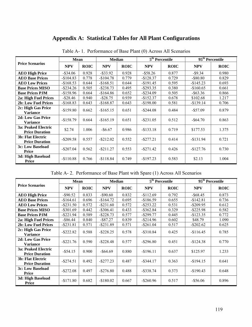
119

Appendix A: Statistical Tables for All Plant Configurations

Table A- 1. Performance of Base Plant (0) Across All Scenarios

Mean Median 5th Percentile 95th Percentile Price Scenarios

NPV ROIC NPV ROIC NPV ROIC NPV ROIC

AEO High Price -$34.06 0.928 -$33.92 0.928 -$58.26 0.877 -$9.34 0.980 AEO Base Prices -$104.83 0.778 -$104.78 0.779 -$128.37 0.729 -$80.80 0.829 AEO Low Prices -$168.53 0.644 -$168.51 0.644 -$191.45 0.595 -$145.23 0.693 Base Prices MISO -$234.26 0.505 -$238.73 0.495 -$293.35 0.380 -$160.65 0.661 Base Prices PJM -$158.96 0.664 -$164.86 0.652 -$234.09 0.505 -$63.36 0.866 2a: High Fuel Prices -$28.46 0.940 -$28.75 0.939 -$152.37 0.678 $102.68 1.217 2b: Low Fuel Prices -$168.83 0.643 -$168.87 0.643 -$198.00 0.581 -$139.14 0.706 2c: High Gas Price Variance -$159.80 0.662 -$165.15 0.651 -$244.08 0.484 -$57.09 0.879

2d: Low Gas Price Variance -$158.79 0.664 -$165.19 0.651 -$231.05 0.512 -$64.70 0.863

3a: Peaked Electric Price Duration $2.74 1.006 -$6.67 0.986 -$133.18 0.719 $177.53 1.375

3b: Flat Electric Price Duration -$209.58 0.557 -$212.02 0.552 -$277.21 0.414 -$131.94 0.721

3c: Low Baseload Price -$207.04 0.562 -$211.27 0.553 -$271.42 0.426 -$127.76 0.730

3d: High Baseload Price -$110.88 0.766 -$118.84 0.749 -$197.23 0.583 $2.13 1.004

Table A- 2. Performance of Base Plant with Spare (1) Across All Scenarios



AEO High Price -$90.52 0.833 -$90.60 0.832 -$112.69 0.792 -$68.45 0.873 AEO Base Prices -$164.61 0.696 -$164.72 0.695 -$186.59 0.655 -$142.81 0.736 AEO Low Prices -$231.50 0.572 -$231.60 0.572 -$253.22 0.531 -$209.95 0.612 Base Prices MISO -$301.69 0.442 -$306.41 0.433 -$362.84 0.329 -$225.98 0.582 Base Prices PJM -$221.94 0.589 -$228.73 0.577 -$299.77 0.445 -$123.35 0.772 2a: High Fuel Prices -$86.44 0.840 -$87.27 0.839 -$214.96 0.602 $48.79 1.090 2b: Low Fuel Prices -$231.81 0.571 -$231.89 0.571 -$261.04 0.517 -$202.62 0.625 2c: High Gas Price Variance -$222.82 0.588 -$228.25 0.578 -$310.84 0.425 -$116.45 0.785


3a: Peaked Electric Price Duration -$54.15 0.900 -$64.69 0.880 -$196.11 0.637 $125.97 1.233



3d: High Baseload Price -$171.80 0.682 -$180.02 0.667 -$260.96 0.517 -$56.06 0.896

120

Table A- 3. Performance of 3 Gasifier System with Spare and No Storage (2) Across All Scenarios Mean Median 5th Percentile 95th Percentile

Price Scenarios NPV ROIC NPV ROIC NPV ROIC NPV ROIC

AEO High Price $219.46 1.156 $219.54 1.156 $150.05 1.106 $289.71 1.205 AEO Base Prices -$1.14 0.999 -$1.02 0.999 -$69.22 0.951 $68.25 1.048 AEO Low Prices -$200.16 0.858 -$200.03 0.858 -$266.87 0.811 -$132.36 0.906 Base Prices MISO -$405.92 0.712 -$419.66 0.703 -$589.26 0.582 -$175.49 0.876 Base Prices PJM -$170.17 0.879 -$188.97 0.866 -$403.95 0.714 $128.91 1.091 2a: High Fuel Prices $236.85 1.168 $235.04 1.167 -$149.20 0.894 $648.02 1.459 2b: Low Fuel Prices -$201.07 0.857 -$201.24 0.857 -$288.73 0.795 -$111.12 0.921 2c: High Gas Price Variance -$172.78 0.878 -$189.11 0.866 -$436.03 0.691 $149.14 1.106

2d: Low Gas Price Variance -$169.63 0.880 -$188.37 0.866 -$394.16 0.721 $126.68 1.090

3a: Peaked Electric Price Duration $331.18 1.235 $300.03 1.213 -$93.54 0.934 $873.69 1.619




Table A- 4. Performance of Plant Storing for 12 hours (3) Across All Scenarios



AEO High Price $116.52 1.179 $116.50 1.179 $78.89 1.121 $154.55 1.238 AEO Base Prices $6.34 1.010 $6.20 1.010 -$30.68 0.953 $43.32 1.067 AEO Low Prices -$92.64 0.858 -$92.77 0.857 -$128.82 0.802 -$56.31 0.913 Base Prices MISO -$96.88 0.851 -$106.13 0.837 -$211.70 0.674 $50.67 1.078 Base Prices PJM -$85.98 0.868 -$93.40 0.856 -$190.29 0.707 $44.32 1.068 2a: High Fuel Prices $100.33 1.154 $100.04 1.154 -$66.09 0.898 $276.07 1.425 2b: Low Fuel Prices -$93.57 0.856 -$93.78 0.856 -$140.61 0.784 -$46.37 0.929 2c: High Gas Price Variance -$47.29 0.927 -$95.81 0.853 -$208.63 0.679 $53.50 1.082




3c: Low Baseload Price -$104.65 0.839 -$111.50 0.828 -$204.11 0.686 $19.15 1.029


121

Table A- 5. Performance of Plant Storing for 12 hours with Availability Improvements (5) Across All Scenarios



AEO High Price $98.99 1.151 $99.05 1.151 $61.70 1.094 $136.29 1.207 AEO Base Prices -$10.09 0.985 -$10.16 0.985 -$46.59 0.929 $26.45 1.040 AEO Low Prices -$108.10 0.836 -$108.18 0.835 -$143.80 0.781 -$72.32 0.890 Base Prices MISO -$112.41 0.829 -$121.64 0.815 -$225.76 0.657 $33.35 1.051 Base Prices PJM -$101.60 0.845 -$108.98 0.834 -$204.62 0.689 $27.38 1.042 2a: High Fuel Prices $82.64 1.126 $82.23 1.125 -$81.73 0.876 $256.50 1.390 2b: Low Fuel Prices -$109.03 0.834 -$109.30 0.834 -$155.52 0.764 -$62.22 0.905 2c: High Gas Price Variance -$63.21 0.904 -$111.13 0.831 -$222.78 0.661 $36.32 1.055






Table A- 6. Base Plant with 200,000 m3 Storage and 10% Inflow (6) Across All Scenarios



AEO High Price -$18.49 0.964 -$18.36 0.964 -$45.12 0.912 $8.72 1.017 AEO Base Prices -$96.29 0.813 -$96.22 0.813 -$122.17 0.763 -$69.81 0.864 AEO Low Prices -$166.33 0.677 -$166.32 0.677 -$191.51 0.628 -$140.75 0.727 Base Prices MISO -$238.61 0.537 -$243.55 0.527 -$303.53 0.410 -$157.72 0.694 Base Prices PJM -$155.83 0.697 -$162.33 0.685 -$238.33 0.537 -$50.81 0.901 2a: High Fuel Prices -$12.40 0.976 -$12.81 0.975 -$148.70 0.711 $131.63 1.256 2b: Low Fuel Prices -$166.65 0.676 -$166.72 0.676 -$198.79 0.614 -$134.01 0.740 2c: High Gas Price Variance -$156.75 0.696 -$162.63 0.684 -$249.51 0.516 -$44.02 0.915






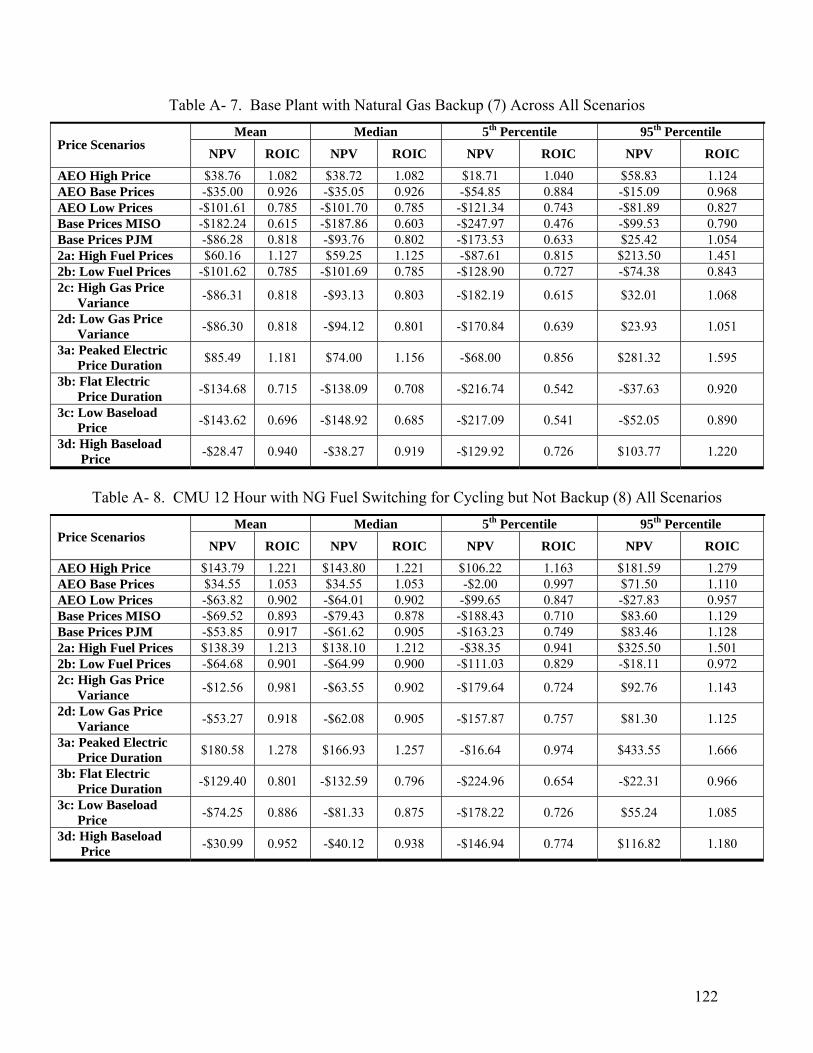
122

Table A- 7. Base Plant with Natural Gas Backup (7) Across All Scenarios Mean Median 5th Percentile 95th Percentile


AEO High Price $38.76 1.082 $38.72 1.082 $18.71 1.040 $58.83 1.124 AEO Base Prices -$35.00 0.926 -$35.05 0.926 -$54.85 0.884 -$15.09 0.968 AEO Low Prices -$101.61 0.785 -$101.70 0.785 -$121.34 0.743 -$81.89 0.827 Base Prices MISO -$182.24 0.615 -$187.86 0.603 -$247.97 0.476 -$99.53 0.790 Base Prices PJM -$86.28 0.818 -$93.76 0.802 -$173.53 0.633 $25.42 1.054 2a: High Fuel Prices $60.16 1.127 $59.25 1.125 -$87.61 0.815 $213.50 1.451 2b: Low Fuel Prices -$101.62 0.785 -$101.69 0.785 -$128.90 0.727 -$74.38 0.843 2c: High Gas Price Variance -$86.31 0.818 -$93.13 0.803 -$182.19 0.615 $32.01 1.068






Table A- 8. CMU 12 Hour with NG Fuel Switching for Cycling but Not Backup (8) All Scenarios



AEO High Price $143.79 1.221 $143.80 1.221 $106.22 1.163 $181.59 1.279 AEO Base Prices $34.55 1.053 $34.55 1.053 -$2.00 0.997 $71.50 1.110 AEO Low Prices -$63.82 0.902 -$64.01 0.902 -$99.65 0.847 -$27.83 0.957 Base Prices MISO -$69.52 0.893 -$79.43 0.878 -$188.43 0.710 $83.60 1.129 Base Prices PJM -$53.85 0.917 -$61.62 0.905 -$163.23 0.749 $83.46 1.128 2a: High Fuel Prices $138.39 1.213 $138.10 1.212 -$38.35 0.941 $325.50 1.501 2b: Low Fuel Prices -$64.68 0.901 -$64.99 0.900 -$111.03 0.829 -$18.11 0.972 2c: High Gas Price Variance -$12.56 0.981 -$63.55 0.902 -$179.64 0.724 $92.76 1.143






123

Table A- 9. CMU 12 Hour with NG Fuel Switching for Cycling and Backup (9) All Scenarios Mean Median 5th Percentile 95th Percentile


AEO High Price $222.08 1.342 $221.86 1.341 $190.78 1.293 $253.75 1.390 AEO Base Prices $112.97 1.174 $112.81 1.174 $82.18 1.126 $144.03 1.222 AEO Low Prices $14.40 1.022 $14.20 1.022 -$16.20 0.975 $45.26 1.070 Base Prices MISO $8.75 1.013 -$2.89 0.996 -$123.38 0.810 $182.03 1.280 Base Prices PJM $32.16 1.049 $21.98 1.034 -$89.41 0.862 $187.41 1.288 2a: High Fuel Prices $240.61 1.370 $239.88 1.369 $37.72 1.058 $453.22 1.697 2b: Low Fuel Prices $13.77 1.021 $13.72 1.021 -$28.25 0.957 $55.38 1.085 2c: High Gas Price Variance $75.85 1.117 $22.00 1.034 -$103.58 0.841 $195.28 1.300

2d: Low Gas Price Variance $32.61 1.050 $22.52 1.035 -$85.05 0.869 $185.83 1.286

3a: Peaked Electric Price Duration $269.88 1.415 $254.37 1.391 $56.31 1.087 $541.78 0.833

3b: Flat Electric Price Duration -$36.17 0.944 -$40.16 0.938 -$147.90 0.773 $94.61 1.146

3c: Low Baseload Price $6.44 1.010 -$2.78 0.996 -$107.89 0.834 $150.75 1.232

3d: High Baseload Price $63.59 1.098 $51.72 1.080 -$67.43 0.896 $234.45 1.361

Table A- 10. Base Plant with 400,000 m3 Storage and 10% Inflow (10) Across All Scenarios



AEO High Price -$16.31 0.968 -$16.18 0.968 -$42.94 0.916 $10.88 1.021 AEO Base Prices -$94.11 0.816 -$94.05 0.816 -$119.96 0.765 -$67.70 0.868 AEO Low Prices -$164.14 0.679 -$164.13 0.679 -$189.23 0.629 -$138.58 0.729 Base Prices MISO -$236.40 0.537 -$241.35 0.528 -$301.30 0.410 -$155.37 0.696 Base Prices PJM -$153.65 0.699 -$160.13 0.687 -$236.15 0.538 -$48.61 0.905 2a: High Fuel Prices -$10.22 0.980 -$10.56 0.979 -$146.49 0.713 $133.77 1.262 2b: Low Fuel Prices -$164.46 0.678 -$164.50 0.678 -$196.48 0.615 -$131.84 0.742 2c: High Gas Price Variance -$154.57 0.697 -$160.41 0.686 -$247.22 0.516 -$41.84 0.918






124

Appendix B: Historical Accuracy of Energy Information Administration (EIA) Price Forecasts

The economic results of the analysis depend, in part, on the price at which the facility can purchase coal. The analysis examined coal price data from different sources and timeframes in order to analyze the scenarios within an envelope of prices incorporating the recent past as well as future forecasts. The coal prices used include: historical FOB prices for Illinois #6 coal, with a higher heating value of 11,350 Btu/lb and a sulfur content of 3.2 percent by weight (Energy Information Administration Coal News and Markets 2006); Energy Information Administration Annual Energy Outlook (AEO) forecasts for year 2007 coal prices (Energy Information Administration 2006); 2007 NYMEX futures for central application coal (NYMEX 2006) and EIA forecasts for year 2007 coal prices with a factor that includes EIA’s historical error in forecasting price data (Energy Information Administration 2006) This last price distribution incorporates uncertainty in the price due to error in EIA forecasts.

EIA price forecasts do not include much data on the relative uncertainty in the estimate. We the uncertainty in EIA Annual Energy Outlook (AEO) price forecasts by examining historical deviation of actual prices from EIA forecasted prices following the methods from Rode and Fischbeck (2006).

Using recent historical AEO forecast data from 1994 to 2005, we model an EIA forecast error as a normal distribution with a mean of 2.5 percent and a standard deviation of 5.0 percent. The EIA forecast error was applied to the 2007 EIA forecast from the Annual Energy Outlook. Figure B-1 shows the 2007 EIA forecast from the Annual Energy Outlook compared to the same forecast with the EIA historical accuracy factor for the error included.

125

0.00

0.10

0.20

0.30

0.40

0.50

0.60

0.70

0.80

0.90

1.00

1.4 1.5 1.6 1.7 1.8 1.9 2

$/MMBtu


2007 EIA AEO Forecast

2007 EIA Forecast withhistorical accuracy factor

Figure B- 1. CDF of 2007 EIA AEO Coal Price Forecasts With and Without the Historical

Accuracy Factor

. As the figure shows, including a factor which incorporates the historical error in EIA forecasts significantly widens the CDF for coal prices. It is this broader price distribution, reflecting greater uncertainty in the future price for coal that is used in the analysis. Figure B-2 illustrates the cumulative distribution functions of the coal price distributions examined in the analysis including the EIA forecast with the historical accuracy factor.

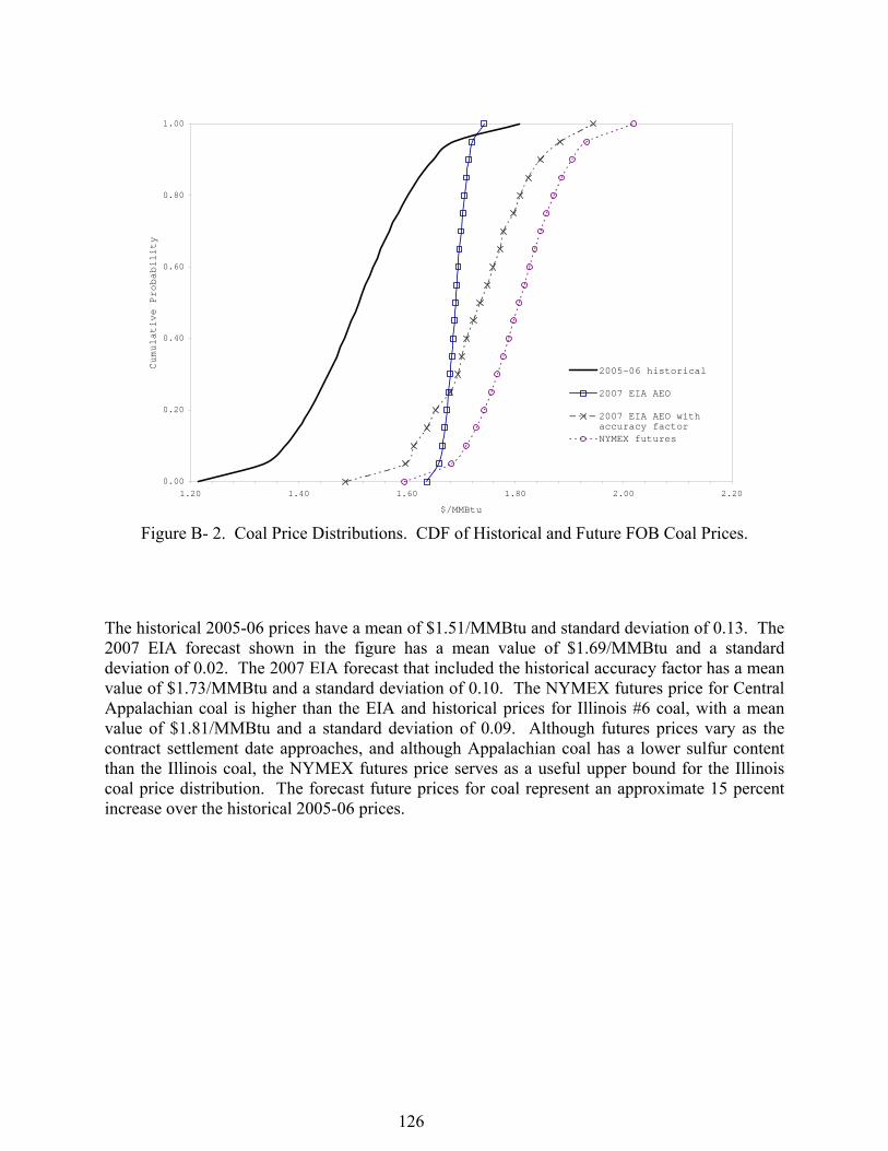
126

0.00

0.20

0.40

0.60

0.80

1.00

1.20 1.40 1.60 1.80 2.00 2.20

$/MMBtu


2005-06 historical

2007 EIA AEO

2007 EIA AEO withaccuracy factorNYMEX futures

Figure B- 2. Coal Price Distributions. CDF of Historical and Future FOB Coal Prices.

The historical 2005-06 prices have a mean of $1.51/MMBtu and standard deviation of 0.13. The 2007 EIA forecast shown in the figure has a mean value of $1.69/MMBtu and a standard deviation of 0.02. The 2007 EIA forecast that included the historical accuracy factor has a mean value of $1.73/MMBtu and a standard deviation of 0.10. The NYMEX futures price for Central Appalachian coal is higher than the EIA and historical prices for Illinois #6 coal, with a mean value of $1.81/MMBtu and a standard deviation of 0.09. Although futures prices vary as the contract settlement date approaches, and although Appalachian coal has a lower sulfur content than the Illinois coal, the NYMEX futures price serves as a useful upper bound for the Illinois coal price distribution. The forecast future prices for coal represent an approximate 15 percent increase over the historical 2005-06 prices.

127

Appendix C: 1+0+CCS Scenario Operating and Financial Parameters

IECM cs version 5.21 (February 2, 2007)

Operating parameters Financial parameters Overall Plant Base GE Quench Year Costs Reported 2005 Cold gas cleanup Constant Dollars CO2 Capture: Sour Shift + Selexol Discount Rate (Before Taxes) 8.00E-02 fraction Slag: landfill Fixed Charge Factor (FCF) 8.88E-02 fraction Sulfur: sulfur plant Inflation Rate 0 %/yr Capacity Factor 80 % Plant or Project Book Life 30 years Real Bond Interest Rate 8 % Gross Plant Size 297.7 MWg Real Preferred Stock Return 0 % Net Plant Size 238.1 MW Real Common Stock Return 0.1 % Net Electrical Output (MW) 238.1 Percent Debt 99.99 % Total Plant Energy Input (MBtu/hr) 2781 Percent Equity (Preferred Stock) 0 % Gross Plant Heat Rate, HHV (Btu/kWh) 9343 Percent Equity (Common Stock) 1.00E-02 % Net Plant Heat Rate, HHV (Btu/kWh) 11680 Federal Tax Rate 35 % Net Plant Efficiency, HHV (%) 29.17 State Tax Rate 4 % Ambient Air Temperature 77 °F Property Tax Rate 2 % Ambient Air Pressure 14.7 psia Investment Tax Credit 0 % Ambient Air Humidity 1.80E-02 lb H2O/lb dry air Construction Time 0.25 years Operating Labor Rate 24.82 $/hr

Coal Water Cost 0.8316 $/1000 gal

Illinois #6 Sulfur Byproduct Credit 68.64 $/ton Heating Value 1.09E+04 btu/lb Sulfur Disposal Cost 10 $/ton Carbon 61.2 wt% as received Selexol Solvent Cost 2.32 $/lb Hydrogen 4.2 Claus Plant Catalyst Cost 565.8 $/ton Oxygen 6.02 Beavon-Stretford Catalyst Cost 218.6 $/cu ft Chlorine 0.17 Slag Disposal Cost 13.07 $/ton Sulfur 3.25 Limestone Cost 19.64 $/ton Nitrogen 1.16 Lime Cost 72.01 $/ton Ash 11 Ammonia Cost 248.2 $/ton Moisture 13 Urea Cost 412.4 $/ton MEA Cost 1293 $/ton Plant Inputs Flow Rate (tons/hr) Activated Carbon Cost 1322 $/ton Coal 127.6 Caustic (NaOH) Cost 624.7 $/ton Oil 0.3479 High Temperature Catalyst Cost 60.1 $/cu ft Other Fuels 3.04E-02 Low Temperature Catalyst Cost 300.5 $/cu ft Other Chemicals, Solvents & Catalyst 2.39E-03 Glycol Cost 2.356 $/lb Total Chemicals 2.39E-03 Bulk Reagent Storage Time 60 days Oxidant 109.3 The following apply to all process blocks Process Water 48.63 General Facilities Capital 15 %PFC Engineering & Home Office Fees 10 %PFC Plant Outputs Flow Rate (tons/hr) Project Contingency Cost 15 %PFC Slag 16.38 Booster Pump Operating Cost 1.5 %PFC

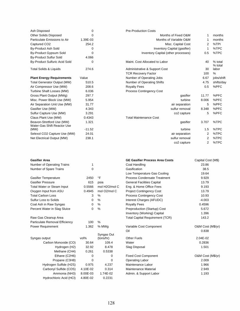
128

Ash Disposed 0 Pre-Production Costs Other Solids Disposed 0 Months of Fixed O&M 1 months Particulate Emissions to Air 1.39E-03 Months of Variable O&M 1 months Captured CO2 254.2 Misc. Capital Cost 2 %TPI By-Product Ash Sold 0 Inventory Capital (gasifier) 1 %TPC By-Product Gypsum Sold 0 Inventory Capital (other processes) 0.5 %TPC By-Product Sulfur Sold 4.066 By-Product Sulfuric Acid Sold 0 Maint. Cost Allocated to Labor 40 % total

Total Solids & Liquids 274.6 Administrative & Support Cost 30 % total labor

TCR Recovery Factor 100 % Plant Energy Requirements Value Number of Operating Jobs 6.67 jobs/shift Total Generator Output (MW) 510.5 Number of Operating Shifts 4.75 shifts/day Air Compressor Use (MW) 208.6 Royalty Fees 0.5 %PFC Turbine Shaft Losses (MW) 6.036 Process Contingency Cost Gross Plant Output (MWg) 297.7 gasifier 11.77 %PFC Misc. Power Block Use (MW) 5.954 turbine 8.006 %PFC Air Separation Unit Use (MW) 31.77 air separation 5 %PFC Gasifier Use (MW) 4.343 sulfur removal 8.348 %PFC Sulfur Capture Use (MW) 3.291 co2 capture 5 %PFC Claus Plant Use (MW) 0.4343 Total Maintenance Cost Beavon-Stretford Use (MW) 1.321 gasifier 3.707 %TPC Water-Gas Shift Reactor Use (MW) -11.52 turbine 1.5 %TPC Selexol CO2 Capture Use (MW) 24.01 air separation 2 %TPC Net Electrical Output (MW) 238.1 sulfur removal 2 %TPC co2 capture 2 %TPC Gasifier Area GE Gasifier Process Area Costs Capital Cost (M$) Number of Operating Trains 1 Coal Handling 23.86 Number of Spare Trains 0 Gasification 38.5 Low Temperature Gas Cooling 19.64 Gasifier Temperature 2450 °F Process Condensate Treatment 9.929 Gasifier Pressure 615 psia General Facilities Capital 13.79 Total Water or Steam Input 0.5566 mol H2O/mol C Eng. & Home Office Fees 9.193 Oxygen Input from ASU 0.4945 mol O2/mol C Project Contingency Cost 13.79 Total Carbon Loss 3 % Process Contingency Cost 10.93 Sulfur Loss to Solids 0 % Interest Charges (AFUDC) -4.003 Coal Ash in Raw Syngas 0 % Royalty Fees 0.4596 Percent Water in Slag Sluice 0 % Preproduction (Startup) Cost 5.672 Inventory (Working) Capital 1.396 Raw Gas Cleanup Area Total Capital Requirement (TCR) 143.2 Particulate Removal Efficiency 100 % Power Requirement 1.362 % MWg Variable Cost Component O&M Cost (M$/yr) Oil 0.838

Syngas output vol% Syngas Out (tons/hr) Other Fuels 2.04E-02

Carbon Monoxide (CO) 30.64 109.4 Water 0.2836 Hydrogen (H2) 32.92 8.478 Slag Disposal 1.501

Methane (CH4) 0.261 0.5338 Ethane (C2H6) 0 0 Fixed Cost Component O&M Cost (M$/yr)

Propane (C3H8) 0 0 Operating Labor 2.009 Hydrogen Sulfide (H2S) 0.975 4.237 Maintenance Labor 1.966 Carbonyl Sulfide (COS) 4.10E-02 0.314 Maintenance Material 2.949

Ammonia (NH3) 8.00E-03 1.74E-02 Admin. & Support Labor 1.193 Hydrochloric Acid (HCl) 4.80E-02 0.2231

129

Carbon Dioxide (CO2) 18.52 103.9 Cost Component M$/yr $/MWh Moisture (H2O) 14.86 34.13 Annual Fixed Cost 8.117 4.862

Nitrogen (N2) 0.864 3.086 Annual Variable Cost (excluding coal) 2.64 1.582 Argon (Ar) 0.872 4.442 Total Annual O&M Cost 10.76 6.44

Total 100 268.8 Annualized Capital Cost 14.86 8.898 Total Levelized Annual Cost 25.62 15.34 Gas Turbine/Generator Power Block Plant Costs Capital Cost (M$) Gas Turbine Model GE 7FA Gas Turbine 54.81 No. of Gas Turbines 1 Heat Recovery Steam Generator 17.27 Total Gas Turbine Output 202.6 MW Steam Turbine 25.86 Fuel Gas Moisture Content 33 vol % HRSG Feedwater System 3.611 Turbine Inlet Temperature 2420 °F General Facilities Capital 15.23 Turbine Back Pressure 2 psia Eng. & Home Office Fees 10.16 Adiabatic Turbine Efficiency 95 % Project Contingency Cost 15.23 Shaft/Generator Efficiency 98 % Process Contingency Cost 8.111 Air Compressor Interest Charges (AFUDC) -4.309

Pressure Ratio (outlet/inlet) 15.7 ratio Royalty Fees 0.5078 Adiabatic Compressor Efficiency 70 % Preproduction (Startup) Cost 3.307 Combustor Inventory (Working) Capital 0.7515

Combustor Inlet Pressure 294 psia Total Capital Requirement (TCR) 150.6 Combustor Pressure Drop 4 psia Excess Air For Combustor 171.1 % stoich. Fixed Cost Component O&M Cost (M$/yr)

Operating Labor 1.636 Heat Recovery Steam Generator Maintenance Labor 0.9018 HRSG Outlet Temperature 250 °F Maintenance Material 1.353 Steam Cycle Heat Rate, HHV 9000 Btu/kWh Admin. & Support Labor 0.7612 Steam Turbine Cost Component M$/yr $/MWh Total Steam Turbine Outlet 95.13 MW Annual Fixed Cost 4.651 2.79 Power Block Totals Total Annual O&M Cost 4.651 2.79 Power Requirement 2 % MWg Annualized Capital Cost 13.25 7.946 Total Levelized Annual Cost 17.9 10.74

Syngas Input

Syngas In (tons/hr) Heated Syngas In (tons/hr)

Carbon Monoxide (CO) 5.471 5.471 Hydrogen (H2) 15.97 15.97 Methane (CH4) 0.5338 0.5338 Ethane (C2H6) 0 0 Propane (C3H8) 0 0 Hydrogen Sulfide (H2S) 5.30E-03 5.30E-03 Carbonyl Sulfide (COS) 3.16E-03 3.16E-03 Ammonia (NH3) 1.74E-02 1.74E-02 Hydrochloric Acid (HCl) 2.23E-01 2.23E-01 Carbon Dioxide (CO2) 13.37 13.37 Water Vapor (H2O) 33.37 76.94 Nitrogen (N2) 3.086 3.086 Argon (Ar) 4.442 4.442 Oxygen (O2) 0 0 Total 76.5 120.1

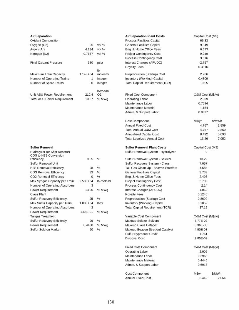
130

Air Separation Air Separation Plant Costs Capital Cost (M$) Oxidant Composition Process Facilities Capital 66.33 Oxygen (O2) 95 vol % General Facilities Capital 9.949 Argon (Ar) 4.234 vol % Eng. & Home Office Fees 6.633 Nitrogen (N2) 0.7657 vol % Project Contingency Cost 9.949 Process Contingency Cost 3.316 Final Oxidant Pressure 580 psia Interest Charges (AFUDC) -2.757 Royalty Fees 0.3316

Maximum Train Capacity 1.14E+04 lb-moles/hr Preproduction (Startup) Cost 2.266

Number of Operating Trains 1 integer Inventory (Working) Capital 0.4809 Number of Spare Trains 0 integer Total Capital Requirement (TCR) 96.5

Unit ASU Power Requirement 210.4 kWh/ton O2 Fixed Cost Component O&M Cost (M$/yr)

Total ASU Power Requirement 10.67 % MWg Operating Labor 2.009 Maintenance Labor 0.7694 Maintenance Material 1.154 Admin. & Support Labor 0.8337 Cost Component M$/yr $/MWh Annual Fixed Cost 4.767 2.859 Total Annual O&M Cost 4.767 2.859 Annualized Capital Cost 8.492 5.093 Total Levelized Annual Cost 13.26 7.952 Sulfur Removal Sulfur Removal Plant Costs Capital Cost (M$) Hydrolyzer (or Shift Reactor) Sulfur Removal System - Hydrolyzer 0 COS to H2S Conversion Efficiency 98.5 % Sulfur Removal System - Selexol 13.29 Sulfur Removal Unit Sulfur Recovery System - Claus 7.057 H2S Removal Efficiency 98 % Tail Gas Clean Up - Beavon-Stretford 4.584 COS Removal Efficiency 33 % General Facilities Capital 3.739 CO2 Removal Efficiency 0 % Eng. & Home Office Fees 2.493 Max Syngas Capacity per Train 2.50E+04 lb-mole/hr Project Contingency Cost 3.739 Number of Operating Absorbers 3 Process Contingency Cost 2.14 Power Requirement 1.106 % MWg Interest Charges (AFUDC) -1.062 Claus Plant Royalty Fees 0.1246 Sulfur Recovery Efficiency 95 % Preproduction (Startup) Cost 0.8692 Max Sulfur Capacity per Train 1.00E+04 lb/hr Inventory (Working) Capital 0.1852 Number of Operating Absorbers 3 Total Capital Requirement (TCR) 37.16 Power Requirement 1.46E-01 % MWg Tailgas Treatment Variable Cost Component O&M Cost (M$/yr) Sulfur Recovery Efficiency 99 % Makeup Selexol Solvent 7.77E-02 Power Requirement 0.4438 % MWg Makeup Claus Catalyst 3.36E-03 Sulfur Sold on Market 90 % Makeup Beavon-Stretford Catalyst 4.90E-03 Sulfur Byproduct Credit 1.761 Disposal Cost 2.85E-02 Fixed Cost Component O&M Cost (M$/yr) Operating Labor 2.009 Maintenance Labor 0.2963 Maintenance Material 0.4445 Admin. & Support Labor 0.6917 Cost Component M$/yr $/MWh Annual Fixed Cost 3.442 2.064

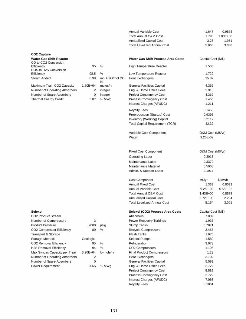
131

Annual Variable Cost -1.647 -0.9878 Total Annual O&M Cost 1.795 1.08E+00 Annualized Capital Cost 3.27 1.961 Total Levelized Annual Cost 5.065 3.038 CO2 Capture Water-Gas Shift Reactor Water Gas Shift Process Area Costs Capital Cost (M$) CO to CO2 Conversion Efficiency 95 % High Temperature Reactor 1.536 COS to H2S Conversion Efficiency 98.5 % Low Temperature Reactor 1.722 Steam Added 0.99 mol H2O/mol CO Heat Exchangers 25.87

Maximum Train CO2 Capacity 1.50E+04 lb-moles/hr General Facilities Capital 4.369

Number of Operating Absorbers 2 integer Eng. & Home Office Fees 2.913 Number of Spare Absorbers 0 integer Project Contingency Cost 4.369 Thermal Energy Credit 3.87 % MWg Process Contingency Cost 1.456 Interest Charges (AFUDC) -1.211

Royalty Fees 0.1456 Preproduction (Startup) Cost 0.9396 Inventory (Working) Capital 0.2112 Total Capital Requirement (TCR) 42.32 Variable Cost Component O&M Cost (M$/yr) Water 9.25E-02 Fixed Cost Component O&M Cost (M$/yr) Operating Labor 0.3013 Maintenance Labor 0.3379 Maintenance Material 0.5068 Admin. & Support Labor 0.1917 Cost Component M$/yr $/MWh Annual Fixed Cost 1.338 0.8023 Annual Variable Cost 9.25E-02 5.55E-02 Total Annual O&M Cost 1.43E+00 0.8578 Annualized Capital Cost 3.72E+00 2.234 Total Levelized Annual Cost 5.154 3.091 Selexol Selexol (CO2) Process Area Costs Capital Cost (M$) CO2 Product Stream Absorbers 7.809 Number of Compressors 3 Power Recovery Turbines 1.936 Product Pressure 2000 psig Slump Tanks 0.7871 CO2 Compressor Efficiency 80 % Recycle Compressors 3.467 Transport & Storage Flash Tanks 1.675 Storage Method: Geologic Selexol Pumps 1.589 CO2 Removal Efficiency 95 % Refrigeration 3.073 H2S Removal Efficiency 94 % CO2 Compressors 11.95 Max Syngas Capacity per Train 3.20E+04 lb-mole/hr Final Product Compressors 1.23 Number of Operating Absorbers 2 Heat Exchangers 3.702 Number of Spare Absorbers 0 General Facilities Capital 5.582 Power Requirement 8.065 % MWg Eng. & Home Office Fees 3.722 Project Contingency Cost 5.582 Process Contingency Cost 3.722 Interest Charges (AFUDC) 7.063 Royalty Fees 0.1861

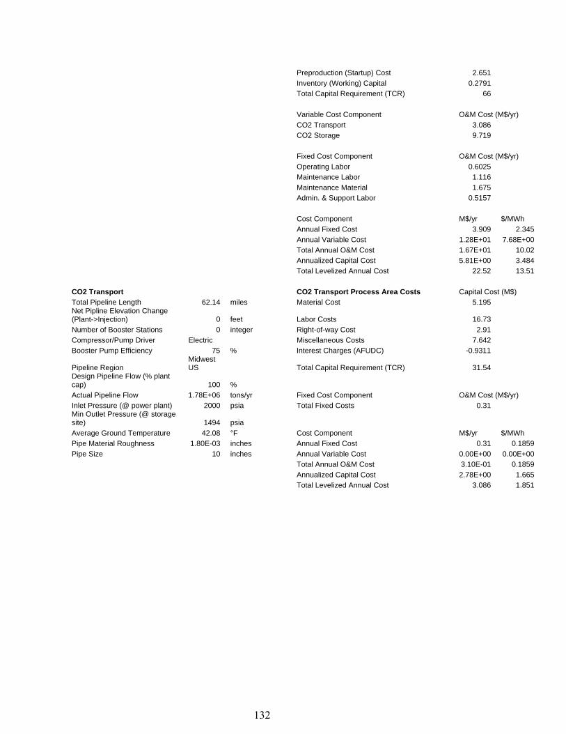
132

Preproduction (Startup) Cost 2.651 Inventory (Working) Capital 0.2791 Total Capital Requirement (TCR) 66 Variable Cost Component O&M Cost (M$/yr) CO2 Transport 3.086 CO2 Storage 9.719 Fixed Cost Component O&M Cost (M$/yr) Operating Labor 0.6025 Maintenance Labor 1.116 Maintenance Material 1.675 Admin. & Support Labor 0.5157 Cost Component M$/yr $/MWh Annual Fixed Cost 3.909 2.345 Annual Variable Cost 1.28E+01 7.68E+00 Total Annual O&M Cost 1.67E+01 10.02 Annualized Capital Cost 5.81E+00 3.484 Total Levelized Annual Cost 22.52 13.51 CO2 Transport CO2 Transport Process Area Costs Capital Cost (M$) Total Pipeline Length 62.14 miles Material Cost 5.195 Net Pipline Elevation Change (Plant->Injection) 0 feet Labor Costs 16.73 Number of Booster Stations 0 integer Right-of-way Cost 2.91 Compressor/Pump Driver Electric Miscellaneous Costs 7.642 Booster Pump Efficiency 75 % Interest Charges (AFUDC) -0.9311

Pipeline Region Midwest US Total Capital Requirement (TCR) 31.54

Design Pipeline Flow (% plant cap) 100 % Actual Pipeline Flow 1.78E+06 tons/yr Fixed Cost Component O&M Cost (M$/yr) Inlet Pressure (@ power plant) 2000 psia Total Fixed Costs 0.31 Min Outlet Pressure (@ storage site) 1494 psia Average Ground Temperature 42.08 °F Cost Component M$/yr $/MWh Pipe Material Roughness 1.80E-03 inches Annual Fixed Cost 0.31 0.1859 Pipe Size 10 inches Annual Variable Cost 0.00E+00 0.00E+00 Total Annual O&M Cost 3.10E-01 0.1859 Annualized Capital Cost 2.78E+00 1.665 Total Levelized Annual Cost 3.086 1.851

133

References

Aiken, R., K.H. Ditzel, F. Morra, D.S. Wilson (2004), “Coal-Based Integrated Gasification Combined Cycle: Market Penetration Strategies and Recommendations.” Study prepared for DOE, NETL, GTC by Booz Allen Hamilton.

Alp, T.; Dames, T. J.; Dogan, B., The effect of microstructure in the hydrogen embrittlement of a gas pipeline steel. Journal of Materials Science 1987, 22, (6), 2105-2112.

Amick, P.; Geosits, R.; Herbanek, R.; Kramer, S.; Tam, S. In A Large Coal IGCC Power Plant, Nineteenth Annual International Pittsburgh Coal Conference, Pittsburgh, PA, September 23-27, 2002; Pittsburgh, PA, 2002.

Ammer, J., Division Director, Gas Technology Management Division, NETL. Personal Communication 2006.

Amos, W. (1998). Costs of Transporting and Storing Hydrogen, NREL/TP-570-25106. National Renewable Energy Laboratory.

Asahi, H.; Hirata, M.; O’Hashi, K. Hydrogen-Related Damage in Line Pipes; Nippon Steel Corporation. Undated.

Astaf'ev, A. A., Hydrogen embrittlement of constructional steels. Metal Science and Heat Treatment 1984, 26, (2), 91-96.

Beghi, G. and J. Dejace (1974). Economics of Pipeline Transport for Hydrogen and Oxygen. Hydrogen Economy Miami Energy (THEME) Conference.

Bennet, N. (2006). MB Engineering Services, Clayton Walker Gasholder Division.

Blankinship, Steve (2006). “Gasifier Reliability and Flexibility Key to IGCC’s Future in the Power Sector” Power Engineering 110(7): pp. 4-7.

Blinderman, M. S. and B. Anderson (2003). Underground Coal Gasification for Power Generation: Efficiency and CO2-emissions. 12th International Conference on Coal Science. Cairns, Queensland, Australia.

Bloom, Jeremy A. (1984), “Generation Cost Curves Including Energy Storage,” IEEE Transactions on Power Apparatus and Systems PAS-103(7), July, pp. 1725-1731.

Booras, George, and Neville Holt (2004), “Pulverized Coal and IGCC Plant Cost and Performance Estimates,” Presentation, Gasification Technologies Conference, Washington D.C., October 3-6. http://www.gasification.org/Presentations/2004.htm.

Brooks, F. J. GE Gas Turbine Performance Characteristics; GE Power Systems: Schenectady, NY, October, 2000.

British Columbia Hydro and Power Authority and Energy Mines and Resources Canada (1975). Studies of Advanced Electric Power Generation Techniques And Coal Gasification.

Carnegie Mellon University Center for Energy and Environmental Studies. (2006). "IECM-cs Integrated Environmental Control Model Carbon Sequestration Edition." Retrieved November 21, 2006, from http://www.iecm-online.com/.

134

Carpetis, C. (1982). "Estimation of storage costs for large hydrogen storage facilities." International Journal of Hydrogen Energy 7(2): 191-203.

Chernov, V. Y.; Makarenko, V. D.; Kryzhanivs'kyi, E. I.; Shlapak, L. S., On the Causes of Corrosion Fracture of Industrial Pipelines. Materials Science 2002, 38, (6), 880-883.

Chiang, Alpha C. (1992). Elements of Dynamic Optimization. Long Grove, IL: Waveland Press.

Collot, A.-G. (2004). Clean fuels from coal, IEA Clean Coal Centre.

Colwell, R. (2006). Professor Marine Geology, Oregon State University.

ContiTech. (2006). "Diaphragms for gas holders." Retrieved August 21, 2006, from http://www.contitech.de/ct/contitech/themen/produkte/membranen/gasspeichermembranen/gasspeicher_e.html.

Dakota Gasification Company (2006). Material Safety Data Sheet: Synthetic Natural Gas.

Deurwaarder, E. P., H. Boerrigter, et al. (2005). Methanation of Milena Product Gas for the Production of Bio-SNG. 14th European Biomass Conference & Exhibition, Paris, France.

DOE Coal Gasification Research Needs (COGARN) Working Group (1987). Coal Gasification: Direct Applications and Syntheses of Chemicals and Fuels, U.S. Department of Energy, Office of Energy Research, Office of Program Analysis.

Dorfman, Robert (1969), “An Economic Interpretation of Optimal Control Theory,” The American Economic Review 59(5) December, pp. 817-831.

Duret, A., C. Friedli, et al. (2005). "Process design of Synthetic Natural Gas (SNG) production using wood gasification." Journal of Cleaner Production 13(15): 1434-1446.

Eliason, D. (2006). Basin Electric Power Cooperative. Personal communications

EIA (2007), Annual Energy Outlook 2007, with Projections to 2030. Energy Information Administration, February. http://www.eia.doe.gov/oiaf/aeo/pdf/0383(2007).pdf

Energy Information Administration. (2006). "Annual Energy Outlook 2007 (Early Release)." Retrieved December 14, 2006, from DOE/EIA-0383(2007). http://www.eia.doe.gov/oiaf/aeo/.

Energy Information Administration. (2006, December 12 , 2006 ). "Short-Term Energy Outlook." Retrieved December 14, 2006, from http://www.eia.doe.gov/emeu/steo/pub/contents.html.

Energy Information Administration Coal News and Markets. http://www.eia.doe.gov/cneaf/coal/page/coalnews/coalmar.html (November 22, 2006).

Engelhard Corporation. (2005). "Methanation catalyst. Carbon oxide conversion." Retrieved March 7, 2006, from http://www.engelhard.com/documents/MET%20datasheet%20Web%20FINAL.pdf.

Farina, G.; Bressan, L., Optimizing IGCC design: Improve performance, reduce capital cost. Foster Wheeler Review 1999, 1, (3), 16-21.

135

Gray, D., S. Salerno, et al. (2004). Potential Application of Coal-Derived Fuel Gases for the Glass Industry: A Scoping Analysis, National Energy Technology Laboratory, DOE.

Gray, D., S. Salerno, et al. (2004). Polygeneration of SNG, Hydrogen, Power, and Carbon Dioxide from Texas Lignite, National Energy Technology Laboratory, DOE.

Griffin, M. (2006). Executive Director Green Design Institute, Tepper School of Business, CMU, formerly BP. Personal communications

Hagen, M., E. Polman, et al. (2001). Adding gas from biomass to the gas grid.

Hannemann, F., B. Koestlin, et al. (2005). Hydrogen and Syngas Combustion: Pre-Condition for IGCC and ZEIGCC, Siemens AG Power Generation.

Hart, D. (1997). Hydrogen Power: The Commercial Future of 'the Ultimate Fuel'. London, UK, Financial Times Energy Publishing.

Heard, R. (2006). Carnegie Mellon University. Personal communications

Higman, C, S. DellaVilla and B. Steele (2005). “The Reliability of Integrated Gasification Combined Cycle (IGCC) Power Generation Units,” Gasification Technologies Conference, San Francisco.

Holt, Neville (2004). “Coal-based IGCC Plants – Recent Operating Experience and Lessons Learned,” Presentation, Gasification Technologies Conference, San Francisco.

Integrated Environmental Control Model (IECM), Carnegie Mellon University (CMU) Department of Engineering and Public Policy (EPP). Available online at http://www.iecm-online.com/index.html.

IEA GHG (2002). Transmission of CO2 and Energy. Cheltenham, International Energy Agency Greenhouse Gas R&D Programme. Cheltenham, 2002.

Javetski, John (2006). “Utilities split on readiness of IGCC” Power Magazine, vol. 150, issue 8.

Johnson Matthey Catalysts. (2003). "KATALCO 11-4 Methanation Catalyst." Available online at http://www.jmcatalysts.com/pct/pdfs-uploaded/Refineries%20-%20Oil%20and%20Petrochemical/11-4.pdf.

Keeler, C. (2001). “ Operating Experience at the Wabash River Repowering Project,” Conference Paper, Gasification Technologies Conference, San Francisco, October 8 – 10. Available online at http://www.gasification.org/Presentations/2001.htm.

Keeler, C.(2002). “Operating Experience at the Wabash River Repowering Project,” Conference Paper, Gasification Technologies Conference, San Francisco., October 27 – 30. Available online at http://www.gasification.org/Presentations/2002.htm.

Keeler, C.(2003). “Operating Experience at the Wabash River Repowering Project,” Conference Paper, Gasification Technologies Conference, San Francisco, October 12-15. Availabile online at http://www.gasification.org/Presentations/2003.htm.

Korpås, M. (2004). Distributed Energy Systems with Wind Power and Energy Storage. Department of Electrical Power Engineering. Trondheim, Norwegian University of Science and Technology.

136

Kreutz, T.; Williams, R.; Consonni, S.; Chiesa, P., Co-production of hydrogen, electricity and CO2 from coal with commercially ready technology. Part B: Economic analysis. International Journal of Hydrogen Energy 2005, 30, (7), 769-784.

Leeth, G. G., Transmission of gaseous hydrogen. In Hydrogen: Its technology and implications. CRC Press, Inc.: 1977; Vol. 2, pp 3-10.

Leighty, W., M. Hirara, et al. (2003). Large Renewables - Hydrogen Energy Systems: Gathering and Transmission Pipelines for Windpower and other Diffuse, Dispersed Sources. World Gas Conference 2003, Tokyo, Japan.

Lynch, T. A. (1998). “Operating Experience at the Wabash River Coal Gasification Repowering Project.” Conference Paper, Gasification Technologies Conference,San Francisco, October 4-7. Available online at http://www.gasification.org/Presentations/1998.htm.

Major, B. Cost Analysis of NOx Control Alternatives for Stationary Gas Turbines; ONSITE SYOM Energy Corporation and U.S. Department of Energy: November 5, 1999

Martin, E., Vice President R.W. Beck. Personal Communication. 2007.

Maurstad, O. An Overview of Coal based Integrated Gasification Combined Cycle (IGCC) Technology; MIT LFEE 2005-002 WP; Laboratory for Energy and the Environment, Massachusetts Institute of Technology: September, 2005.

Maruyama, H. and K. Nomura (2002). "Coal Conversion Technologies For Securing Energy In Asian Countries." Energy & Environment 13(4&5): 539-551.

McDaniel, John E.(2002). “Polk Power Station IGCC 6th Year of Commercial Operation October 2001-September 2002,” Conference Paper, Gasification Technologies Conference, San Francisco, October 27 – 30. Available online at http://www.gasification.org/Presentations/2002.htm.

McDaniel, John E.(2003). “Polk Power Station IGCC 7th Year of Commercial Operation October 2002-September 2003,” Conference Paper, Gasification Technologies Conference, San Francisco, October 12-15. Available online at http://www.gasification.org/Presentations/2003.htm.

McDaniel, John E. Charles A.Shelnut (1999). “Tampa Electric Company Polk Power Station IGCC Project Status,” Conference Paper, Gasification Technologies Conference, San Francisco, October 17 – 20. Available online at http://www.gasification.org/Presentations/1999.htm.

Mendez-Vigo, Ignacio (2001). “Gasification Technologies 2001,” Conference Paper, Gasification Technology Conference, San Francisco., October 8 – 10. Available online at http://www.gasification.org/Presentations/2001.htm.

Mendez-Vigo, Ignacio (2002). “Gasification Technologies 2002,” Conference Paper, Gasification Technologies Conference, San Francisco., October 27 – 30. Available online at http://www.gasification.org/Presentations/2002.htm.

Michaillat, Pascal, and Shmuel Oren (2007), “A Probabilistic Graphical Approach to Computing Electricity Price Duration Curves under Price and Quantity Competition.” PSERC Working paper 7-12. Proceedings of the 39th Hawaii International Conference on System Sciences HICSS40, Big Island, Hawaii, Jan. 3-6, 2007.

137

Midwest ISO Historical Real-Time LMPs. http://www.midwestmarket.org/publish/ Document/2b8a32_103ef711180_-7d220a48324a?rev=1 (July 1, 2007).

Moeller, F. W., H. Roberts, et al. (1974). "Methanation of coal gas for SNG." Hydrocarbon Processing 53(4): 69-74.

Mohitpour, M., H. Golshan, et al. (2000). Pipeline Design and Construction: A Practical Approach. New York, ASME Press.

Morrow, J. M., M. Corrao, et al. (2005). Method of storing and supplying hydrogen to a pipeline.

Mozaffarian, M. and R. W. R. Zwart (2000). Production of Substitute Natural Gas by Biomass Hydrogasification. Developments in Thermochemical Biomass Conversion, Tyrol, Austria, Energy Research Centre of the Netherlands (ECN).

Mozaffarian, M. and R. W. R. Zwart (2003). Feasibility of Biomass / Waste-Related SNG Production Technologies. Petten, The Netherlands, Energy Research Centre of the Netherlands (ECN).

Mozaffarian, M., R. W. R. Zwart, et al. (2004). “Green Gas” as SNG (Synthetic Natural Gas) A Renewable Fuel with Conventional Quality. “Science in Thermal and Chemical Biomass Conversion” Conference, Victoria, Vancouver Island, BC, Canada.

National Energy Technology Laboratory (NETL) Gasification Plant Cost and Performance Optimization; DE-AC26-99FT40342; U. S. Department of Energy: September, 2003.

New York Mercantile Exchange (NYMEX) Central Appalachian Coal Futures. http://www.nymex.com/coa_fut_termin.aspx

Ogden, J. M. (1999). "Prospects for Building a Hydrogen Energy Infrastructure." Annual Review of Energy and the Environment 24(1): 227-279.

Padró, C. and V. Putsche (1999). Survey of the Economics of Hydrogen Technologies, National Renewable Energy Laboratory.

Payonk, Richard (2000). “An Overview of the Past Year’s Activities for the Wabash River Repowering Project,” Conference Paper, Gasification Technologies Conference, San Francisco, October 8-11. Available online at http://www.gasification.org/Presentations/2000.htm.

Perry, M. and D. Eliason (2004). CO2 Recovery and Sequestration at Dakota Gasification Company. Beulah, ND, Dakota Gasification Company.

Pfafflin, J. R.; Ziegler, E. N., Nitrogen Oxides Reduction. In Encyclopedia of Environmental Science and Engineering, Gordon and Breach Science Publishers: Philadelphia 2006; Vol. 2, pp 746-768.

Polk Power Station (2006). “Welcomes Gasification Technologies Council,” Presentation, March 2. Available online at http://www.netl.doe.gov/technologies/coalpower/gasification /pubs/tampa-2006/Hornick.pdf.

Pottier, J. (1995). "Hydrogen Transmission for Future Energy Systems." Hydrogen Energy Systems: 181-193.

Rath, Larry (2007), National Energy Technology Laboratory,OSAP, private consultation, May 22.

138

Reed, Michael (2006). National Energy Technology Laboratory. Private consultation.

Ridge Energy Storage & Grid Services L.P. and Texas State Energy Conservation Office (2005). The Economic Impact of CAES on Wind in TX, OK, and NM.

Rode, D. C.; Fischbeck, P. S. The Value of Using Coal Gasification as a Long-Term Natural Gas Hedge for Ratepayers. Carnegie Mellon Electricity Industry Center Working Paper CEIC-06-12 www.cmu.edu/electricity (December 13, 2006).

Rogante, M., P. Battistella, et al. (2006). "Hydrogen interaction and stress-corrosion in hydrocarbon storage vessel and pipeline weldings." International Journal of Hydrogen Energy 31(5): 597-601.

Rubin, E. S. (2001). Introduction to Engineering and the Environment Boston McGraw-Hill.

Rubin, E. S. (2006). Personal communications

Rubin, E., M. Berkanpas, and C. Zaremsky (2006), “Technical Documentation: Integrated Gasification Combined Cycle Systems (IGCC) with Carbon Capture and Storage (CCS). Final Report of Work Performed Under Contract No. DE-AC21-92MC29094.” Available online at http://www.iecm-online.com/documentation/user.pdf.

Rubin, E.S., J.R. Kalagnanam, H.C. Frey and M.B. Berkenpas (1997). “Integrated Environmental Control Modeling of Coal-Fired Power Systems,” Journal of the Air & Waste Management Association 47, 1180-1186, (November 1997).

Seglin, L., R. Geosits, et al. (1975). Survey of methanation chemistry and processes. Methanation of synthesis gas. 146.

Stolz, J. (2006). Microbial Ecologist, Department of Biological Sciences, Duquesne University.

Stoft, Steven (2002). Power System Economics: Designing Markets for Electricity. New York: IEEE Press / Wiley-Interscience.

Tampa Electric Company (2002), Tampa Electric Polk Power Station Integrated Gasification Combine Cycle Project; Final Technical Report, August. Available online at http://www.tampaelectric.com/data/files/PolkDOEFinalTechnicalReport.pdf.

Taylor, J. B., J. E. A. Alderson, et al. (1986). "Technical and economic assessment of methods for the storage of large quantities of hydrogen." Int. J. Hydrogen Energy 11(1): 5-22.

Todd, D. M. and R. A. Battista (undated). Demonstrated Applicability of Hydrogen Fuel for Gas Turbines, GE Power Systems.

Twigg, M. V. (1989). Catalyst Handbook. London, Wolfe.

U.S. Environmental Protection Agency Clean Air Markets - Data and Maps, Vintage Year NOx Allowance Price. http://camddataandmaps.epa.gov/ (August 3, 2007).

Valenzuela, Jorge, and Mainak Mazumdar (2007), “Cournot Prices Considering Generator Availability and Demand Uncertainty,” IEEE Transactions on Power Systems 22(1), 116-125.

Valenzuela, Jorge, and Mainak Mazumdar (2005), “A Probability Model for the Electricity Price Duration Curve Under an Oligopoly Market,” IEEE Transactions on Power Systems 20(3), 1250-1256.

139

van der Drift, A., C. M. van der Meijden, et al. (2005). MILENA Gasification Technology for High Efficient SNG Production from Biomass. 14th European Biomass Conference & Exhibition, Paris, France.

Wabash River Energy Ltd. (2002). “Wabash River Coal Gasification Repowering Project: Final Technical Report” Department of Energy Technical Report.

Wolters, Carlo (2003). “Operating Experience at the Willem_Alexander Centrale” October 14, http://www.gasification.org/Docs/2003_Papers/19WOLT.pdf.

Wong, Rich and Ed Whittingham. A Comparison of Combustion Technologies for Electricity Generation, 2nd Edition. Pembina Institute, Alberta Canada, 2006.

Walker, L. K., M. S. Blinderman, et al. (2001). An IGCC Project at Chinchilla, Australia Based on Underground Coal Gasification (UCG). 2001 Gasification Technologies Conference, San Francisco.

Walker, M. (2006). e3 Ventures. Personal communications

final report- engineering-economic analysis of syngas … library/research/energy analysis... · an...

Documents