final report development of congestion performance ... · pdf filefinal report development of...
TRANSCRIPT
FINAL REPORT
DEVELOPMENT OF CONGESTION PERFORMANCE MEASURES USING ITS INFORMATION
Sarah B. Medley Graduate Research Assistant
Michael J. Demetsky, Ph.D., P.E.
Faculty Research Scientist and
Professor of Civil Engineering
Virginia Transportation Research Council (A Cooperative Organization Sponsored Jointly by the
Virginia Department of Transportation and the University of Virginia)
Charlottesville, Virginia
January 2003 VTRC 03-R1
ii
DISCLAIMER
The contents of this report reflect the views of the authors, who are responsible for the facts and the accuracy of the data presented herein. The contents do not necessarily reflect the official views or policies of the Virginia Department of Transportation, the Commonwealth Transportation Board, or the Federal Highway Administration. This report does not constitute a standard, specification, or regulation.
Copyright 2003 by the Commonwealth of Virginia.
iii
ABSTRACT
The objectives of this study were to define a performance measure(s) that could be used to show congestion levels on critical corridors throughout Virginia and to develop a method to select and calculate performance measures to quantify congestion in a transportation system. Such measures could provide benchmarks or base values of congestion to aid in measuring changes in the performance of the highway system.
A general method was developed to monitor congestion using performance measures and the intelligent transportation system information from the Virginia Smart Travel Lab. Two performance measures were selected for investigation: total delay and the buffer index. These performance measures were applied to evaluate congestion levels on the roadways in the Hampton Roads region of Virginia. Each measure shows a different dimension of congestion. In general, total delay is better suited for use by transportation professionals because it is given in units of vehicle-minutes and applies to all vehicles on a segment of roadway. The buffer index is suitable for use by the public because it addresses individual vehicle trip travel time and can be used for trip planning. The buffer index is also important to transportation professionals as a measure of variability.
This research provides information on the changing state of congestion on selected
corridors throughout Virginia. It will help the Virginia Department of Transportation determine the best ways to measure congestion and provide a way to compare congestion over periods of time to ascertain if the delay has grown worse or improved. This research can also help establish a benchmark for traveler delay on Virginia’s roadways.
FINAL REPORT
DEVELOPMENT OF CONGESTION PERFORMANCE MEASURES USING ITS INFORMATION
Sarah B. Medley
Graduate Research Assistant
Michael J. Demetsky, Ph.D., P.E. Faculty Research Scientist
and Professor of Civil Engineering
INTRODUCTION
To the traveler, congestion comprises motionless or slowly moving lines of vehicles on a freeway or city street, a lane closure because of road construction or an accident, or some sort of traffic backup. The transportation professional, on the other hand, thinks of congestion in terms of flow rates, capacities, volumes, speeds, and delay. Congestion occurs when the road capacity does not meet traffic demand at an adequate speed, traffic controls are improperly used, or there is an incident on the road such as an accident or disabled vehicle.1 Congestion can occur during any time of the day and along any type of roadway.
Congestion can take various forms, such as recurrent or nonrecurring, and can be located
across a network or at isolated points.2 Recurring congestion exists when the traffic volume on a roadway exceeds its capacity at a particular location during a predictable and repeated time of day. Nonrecurring congestion is caused by random or unpredictable events that temporarily increase, demand, or reduce capacity on a roadway. Such events include accidents, disabled vehicles, road construction, and inclement weather.
The increasing congestion on many roadways is a major concern to travelers and
transportation managers. Congestion causes longer travel times, higher fuel consumption, and increased emissions of air pollutants.3 Even though congestion is an important policy issue in most urban areas, many planning organizations have little or no quantitative information regarding levels of congestion on the roadways within their jurisdiction.4
Currently, there is no accepted set of performance measures to be used by all
transportation professionals to monitor system conditions. There is a need for reliable congestion performance measures that can be applied to specific routes in a region and be understood by the public.5 Such performance measures should define the quality of traffic flow and be useful in determining where improvements need to be made within a transportation system.
2
PURPOSE AND SCOPE
The purpose of this project was to define a performance measure(s) that reflects congestion levels on critical corridors throughout Virginia and to develop a method to select and calculate performance measures so that traffic managers can quantify congestion in a transportation system.
The traffic data used for this project were obtained from Virginia’s Smart Travel Lab at the University of Virginia. The lab has direct real-time data connections to three traffic centers in Virginia: the Hampton Roads Smart Traffic Center (HRSTC) in Norfolk, the Northern Virginia Smart Traffic Center in Arlington, and the Richmond Smart Traffic Center. These traffic centers send traffic data to the Smart Travel Lab where it is archived and stored in an Oracle database.
This research used only traffic data from the HRSTC, a freeway management system that deploys 203 stationary vehicle detectors and 38 surveillance cameras to monitor traffic in the Norfolk and Virginia Beach region.
METHOD
The following tasks were undertaken to achieve the study purpose and guide the research effort.
1. Review the literature. The literature review focused on performance measures being used in localities throughout the United States to quantify congestion levels. A TRIS search was conducted to identify measures, agencies, and research associated with defining and applying measures of congestion.
2. Develop a database. For this research, data were obtained from the Smart Travel
Lab. 3. Reduce the data. The data were reduced into a manageable form by identifying study
corridor routes and selecting time periods in which to conduct the analysis. After collecting data along each of the corridors for the specified time periods, entries with missing or unrealistic values were removed. The free flow speed was determined in the area being studied.
4. Develop performance measures. Performance measures to be used in quantifying
congestion were selected and certain performance measures were calculated for the study corridors.
3
RESULTS
Literature Review
Several congestion performance measures were described in the Texas Transportation Institute’s (TTI) Urban Mobility Study6-9 and the National Cooperative Highway Research Program’s (NCHRP) Report 398.10 Other performance measures were described in independent studies, as discussed.
Texas Transportation Institute’s Urban Mobility Study
TTI’s Urban Mobility Study was developed in the early 1980s after the Texas
Department of Transportation identified a need for “a technique to allow them to communicate with the public about the effect of increased transportation funding.”6 TTI “developed and applied a method to assess road congestion levels at a relatively broad scale—the urbanized area.”6 The study, which originally included the five largest Texas cities, expanded over the years to include 68 U.S. areas with populations above 100,000.6 The data for this study primarily came from the Federal Highway Administration’s Highway Performance Monitoring System (HPMS) database. Information was also provided by various state and local agencies. TTI publishes annual reports that detail the assessment of road congestion levels in the 68 urban areas. The results of the study have led to the development of several congestion performance measures that include:
• Roadway congestion index. This index allows for comparison across metropolitan
areas by measuring the full range of system performance by focusing on the physical capacity of the roadway in terms of vehicles.4 The index measures congestion by focusing on daily vehicle miles traveled on both freeway and arterial roads.
• Travel rate index. This index computes the “amount of additional time that is required
to make a trip because of congested conditions on the roadway.”7 It examines how fast a trip can occur during the peak period by focusing on time rather than speed. It uses both freeway and arterial road travel rates.
• Travel time index. This index compares peak period travel and free flow travel while
accounting for both recurring and incident conditions.7 It determines how long it takes to travel during a peak hour and uses both freeway and arterial travel rates.
• Travel delay. Travel delay is the extra amount of time spent traveling because of
congested conditions.7 The TTI study divided travel delay into two categories: recurring and incident.8, 9
• Buffer index. The buffer index calculates the extra percentage of travel time a
traveler should allow when making a trip in order to be on time 95 percent of the time.11 This method uses the 95th percentile travel rate and the average travel rate, rather than average travel time, to address trip concerns.
4
• Misery index. The misery index represents the worst 20 percent of trips that occur in congested conditions.11 This index examines the negative aspect of trip reliability by looking at only the travel rate of trips that exceed the average travel rate.12 This index measures how bad the congestion is on the days congestion is the worst.
National Cooperative Highways Research Program Report 398 In 1997, NCHRP published NCHRP Report 398 entitled Quantifying Congestion.10 This report is a user’s guide on how to measure congestion. Definitions and measures of congestion and the selection and application of congestion measures are outlined. The report details ways to present congestion measures so that they are both useful and understandable to the public and policy makers. The report provides both conventional and non-conventional approaches such as the speed reduction index. The suggested measures of congestion include:
• Travel rate. Travel rate, expressed in minutes per mile, is how quickly a vehicle travels over a certain segment of roadway.10 It can be used for specific segments of roadway or averaged for an entire facility. Estimates of travel rate can be compared to a target value that represents unacceptable levels of congestion.
• Delay rate. The delay rate is “the rate of time loss for vehicles operating in congested
conditions on a roadway segment or during a trip.”10 This quantity can estimate system performance and compare actual and expected performance.
• Total delay. Total delay is the sum of time lost on a segment of roadway for all
vehicles.10 This measure can show how improvements affect a transportation system, such as the effects on the entire transportation system of major improvements on one particular corridor.
• Relative delay rate. The relative delay rate can be used to compare mobility levels on
roadways or between different modes of transportation.10 This measure compares system operations to a standard or target. It can also be used to compare different parts of the transportation system and reflect differences in operation between transit and roadway modes.
• Delay ratio. The delay ratio can be used to compare mobility levels on roadways or
among different modes of transportation.10 It identifies the significance of the mobility problem in relation to actual conditions.
• Congested travel. This measure concerns the amount and extent of congestion on
roadways.10 Congested travel is a measure of the amount of travel that occurs during congestion in terms of vehicle-miles.
• Congested roadway. This measure concerns the amount and extent of congestion that
occurs on roadways.10 It describes the degree of congestion on the roadway.
5
• Accessibility. Accessibility is a measure of the time to complete travel objectives at a particular location.10 Travel objectives are defined as trips to employment, shopping, home, or other destinations of interest. This measure is the sum of objective fulfillment opportunities where travel time is less than or equal to acceptable travel time. This measure can be used with any mode of transportation but is most often used when assessing the quality of transit services.
• Speed reduction index. This measure “represents the ratio of the decline in speeds
from free flow conditions.”10 It provides a way to compare the amount of congestion on different transportation facilities by using a continuous scale to differentiate between different levels of congestion.10 The index can be applied to entire routes, entire urban areas, or individual freeway segments for off-peak and peak conditions.
Other Congestion Studies
Other congestion studies have arrived at congestion performance measures, including the following:
• Congestion severity index. This index is “a measure of freeway delay per million
miles of travel.”5 This measure estimates congestion using both freeway and arterial road delay and vehicle miles traveled.
• Lane-mile duration index. This index is a measure of recurring freeway congestion.5
This index measures congestion by summing the product of congested lane miles and congestion duration for segments of roadway.
• Level of service (LOS). LOS differs by facility type and is defined by characteristics
such as vehicle density and volume to capacity ratio.5 Congested conditions often fall into a LOS F range, where demand exceeds capacity of the roadway. Volume to capacity ratios could be compared to LOS to reach conclusions about congested conditions; however, there is no distinction between different levels of congestion once congested conditions are reached.
• Queues. Queues, or traffic back-ups, best represent the public’s view of congestion.3
Queues can be measured using aerial photography, which can often determine performance measures such as LOS and queued volume.
Database Development
As mentioned previously, the traffic data used for this project were obtained from Virginia’s Smart Travel Lab, which was created through a partnership of the University of Virginia’s Department of Civil Engineering and the Virginia Department of Transportation (VDOT). It is a state-of-the-art facility for researchers interested in transportation with an
6
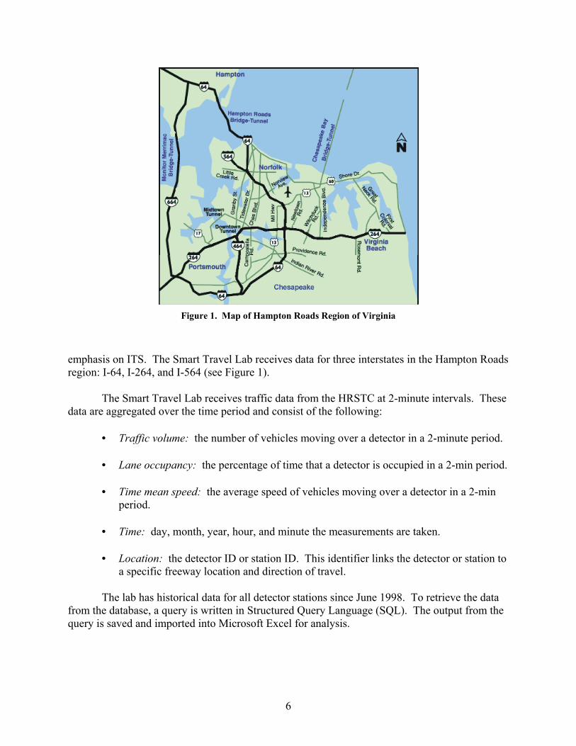
Figure 1. Map of Hampton Roads Region of Virginia
emphasis on ITS. The Smart Travel Lab receives data for three interstates in the Hampton Roads region: I-64, I-264, and I-564 (see Figure 1).
The Smart Travel Lab receives traffic data from the HRSTC at 2-minute intervals. These data are aggregated over the time period and consist of the following:
• Traffic volume: the number of vehicles moving over a detector in a 2-minute period. • Lane occupancy: the percentage of time that a detector is occupied in a 2-min period. • Time mean speed: the average speed of vehicles moving over a detector in a 2-min
period. • Time: day, month, year, hour, and minute the measurements are taken. • Location: the detector ID or station ID. This identifier links the detector or station to
a specific freeway location and direction of travel.
The lab has historical data for all detector stations since June 1998. To retrieve the data from the database, a query is written in Structured Query Language (SQL). The output from the query is saved and imported into Microsoft Excel for analysis.
7
Data Reduction Identification of Study Corridor Routes
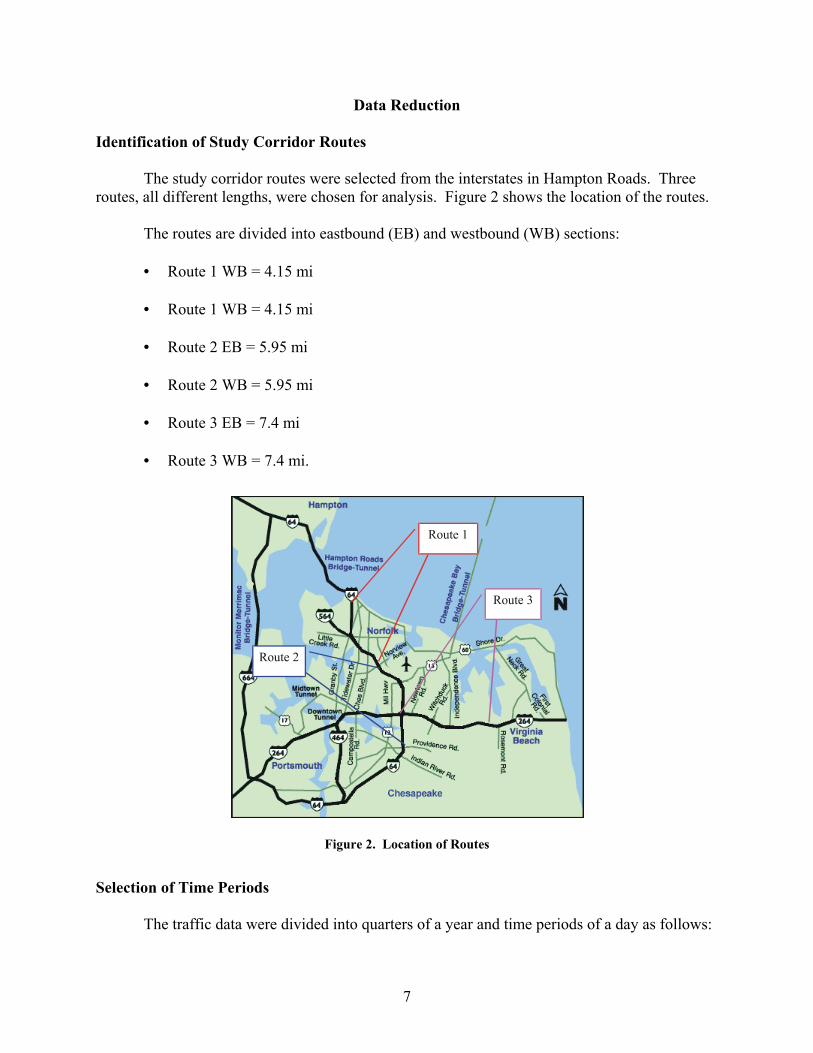
The study corridor routes were selected from the interstates in Hampton Roads. Three routes, all different lengths, were chosen for analysis. Figure 2 shows the location of the routes.
The routes are divided into eastbound (EB) and westbound (WB) sections: • Route 1 WB = 4.15 mi • Route 1 WB = 4.15 mi • Route 2 EB = 5.95 mi • Route 2 WB = 5.95 mi • Route 3 EB = 7.4 mi • Route 3 WB = 7.4 mi.
Figure 2. Location of Routes
Selection of Time Periods
The traffic data were divided into quarters of a year and time periods of a day as follows:
8
• Quarter 1: January, February, March • Quarter 2: April, May, June • Quarter 3: July, August, September • Quarter 4: October, November, December
• Early AM Off-Peak (12 AM–6 AM)
• Morning Peak (6 AM–9 AM)
• Mid-Day Peak (9 AM–4 PM)
• Evening Peak (4 PM–7 PM)
• Late PM Off-Peak (7 PM–12 AM).
The 3-month periods were chosen for two reasons: (1) the bigger picture of traveler
delay on the roadway was desired, and (2) it was assumed that traffic patterns occurred seasonally because of tourist and beach traffic during the summer.
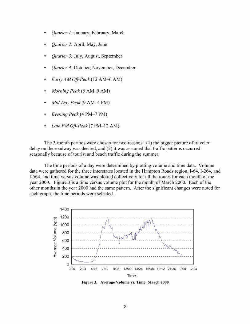
The time periods of a day were determined by plotting volume and time data. Volume data were gathered for the three interstates located in the Hampton Roads region, I-64, I-264, and I-564, and time versus volume was plotted collectively for all the routes for each month of the year 2000. Figure 3 is a time versus volume plot for the month of March 2000. Each of the other months in the year 2000 had the same pattern. After the significant changes were noted for each graph, the time periods were selected.
Figure 3. Average Volume vs. Time: March 2000
9
Data Mining and Screening
To ensure that the data were of good quality, they were screened for errors. To eliminate erroneous data, data screening tests developed by Turochy and Smith were used.13 The data screening tests included five criteria:13
1. a maximum occupancy of 95 percent 2. a collection length of at least 90 sec 3. average vehicle length between 9 and 60 ft 4. overall maximum volume of 3,100 vehicles per hour per lane 5. a maximum volume threshold for records with 0 occupancy, set as the corresponding
volume for an average vehicle length of 10 ft and 2 percent occupancy
The threshold values (i.e., the minimum and maximum values for each parameter) used for the criteria were obtained from research done with traffic data from the Smart Travel Lab.13 The research was in the area of data screening for traffic management systems. In addition to the criteria listed, the data were prescreened for negative values in speed, volume, and occupancy. Free Flow Speed
The free flow speed was needed to calculate particular performance measures. Some measures required acceptable travel time or acceptable travel rate, which is related to the free flow speed of the roadway. One free flow speed was determined for all routes. A free flow speed of 65.7 mph was determined using the method and calculations specified in the most recent Highway Capacity Manual.14
Development of Performance Measures
Selection of Performance Measures
Currently there is no standard method of measuring congestion on roadways. Many studies have been done on an area-wide basis to reflect congestion levels on the roadways, but none has been done for congestion along specific corridors. In addition, several departments of transportation across the nation have a web page displaying travel information. Often they display only speed, roadway occupancy, lane closure, or construction information and offer no indication of congestion levels.
To define a measure or measures of performance that reflect congestion levels along
specific corridors, two performance measures were selected: total delay and buffer index. The data needed to support these measures are available in VDOT’s Smart Traffic Centers and reflect
10
commonly available traffic data, therefore allowing most agencies to perform the necessary calculations to compute these measures.
These measures were selected from a set of 19 possible measures identified in the
literature review. All measures examined are listed in Table 1 along with reasons for discarding a particular measure, if applicable.
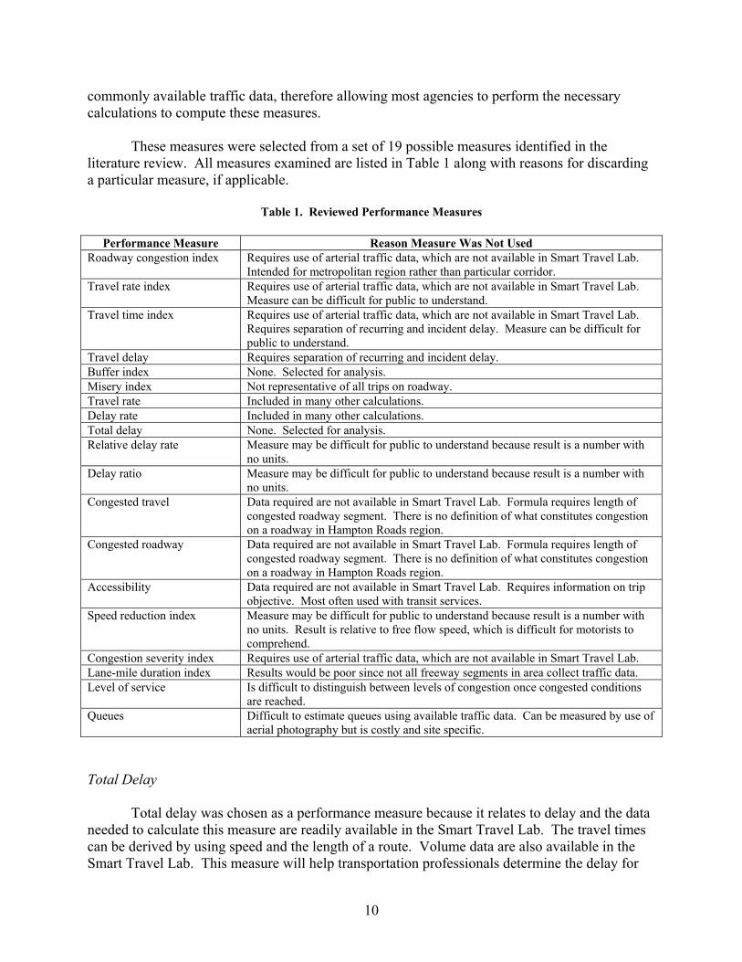
Table 1. Reviewed Performance Measures
Performance Measure Reason Measure Was Not Used Roadway congestion index Requires use of arterial traffic data, which are not available in Smart Travel Lab.
Intended for metropolitan region rather than particular corridor. Travel rate index Requires use of arterial traffic data, which are not available in Smart Travel Lab.
Measure can be difficult for public to understand. Travel time index Requires use of arterial traffic data, which are not available in Smart Travel Lab.
Requires separation of recurring and incident delay. Measure can be difficult for public to understand.
Travel delay Requires separation of recurring and incident delay. Buffer index None. Selected for analysis. Misery index Not representative of all trips on roadway. Travel rate Included in many other calculations. Delay rate Included in many other calculations. Total delay None. Selected for analysis. Relative delay rate Measure may be difficult for public to understand because result is a number with
no units. Delay ratio Measure may be difficult for public to understand because result is a number with
no units. Congested travel Data required are not available in Smart Travel Lab. Formula requires length of
congested roadway segment. There is no definition of what constitutes congestion on a roadway in Hampton Roads region.
Congested roadway Data required are not available in Smart Travel Lab. Formula requires length of congested roadway segment. There is no definition of what constitutes congestion on a roadway in Hampton Roads region.
Accessibility Data required are not available in Smart Travel Lab. Requires information on trip objective. Most often used with transit services.
Speed reduction index Measure may be difficult for public to understand because result is a number with no units. Result is relative to free flow speed, which is difficult for motorists to comprehend.
Congestion severity index Requires use of arterial traffic data, which are not available in Smart Travel Lab. Lane-mile duration index Results would be poor since not all freeway segments in area collect traffic data. Level of service Is difficult to distinguish between levels of congestion once congested conditions
are reached. Queues Difficult to estimate queues using available traffic data. Can be measured by use of
aerial photography but is costly and site specific. Total Delay
Total delay was chosen as a performance measure because it relates to delay and the data needed to calculate this measure are readily available in the Smart Travel Lab. The travel times can be derived by using speed and the length of a route. Volume data are also available in the Smart Travel Lab. This measure will help transportation professionals determine the delay for
11
all vehicles traveling over a segment of roadway during a specific time period and thus to assess the severity of the congestion. Total delay could also allow transportation professionals to estimate how improvements within a transportation system affect a particular corridor or the entire system.
Total delay may be useful to traffic managers because it represents delay for all vehicles.
Time lost for all vehicles is more important for roads that have higher volumes because higher volumes mean that more travelers are affected by the time lost, which can mean more community money is wasted. A comparison of delay among different segments of roadway is also possible when using total delay. Total delay shows the effect of congestion in terms of the amount of lost travel time. The sum of time lost on a segment of roadway due to congestion for all vehicles is represented by total delay as follows10:
Total delay (veh-min) = [Actual travel time (min) – Acceptable travel time (min)]
* Volume (veh) Buffer Index
The buffer index was chosen as a performance measure because it relates to the reliability of an individual vehicle trip, is useful to both the public and transportation professionals, and because the data needed for the calculations are available in the Smart Travel Lab. The travel rates used in this calculation can be derived from average speed readings and the length of a route. This measure will help transportation professionals determine the impact of congestion on one vehicle traveling on a segment of roadway during a specific time period. The buffer index could also be useful in alerting motorists of the anticipated changes in travel time on particular segments of roadway so trips could be planned accordingly.
The buffer index represents the reliability of travel rates associated with single vehicles.
This measure may be beneficial to the public because it tells them how congestion will affect them as individuals.
The buffer index shows the effect of congestion on the reliability of travel rates along the
roadway. The extra percentage of travel time a traveler should allow in order to be on time 95 percent of the time is represented by the buffer index as follows:11
Buffer index (%) = [(95th percentile travel rate – Average travel rate)/Average travel rate]*100%
where all rates are in minutes per mile. Calculation of Performance Measures Total Delay
Total delay calculations were performed using data from 2000 and 2001 and the first quarter of 2002. The 2000 data served as baseline data. Total delay calculations using data from
12
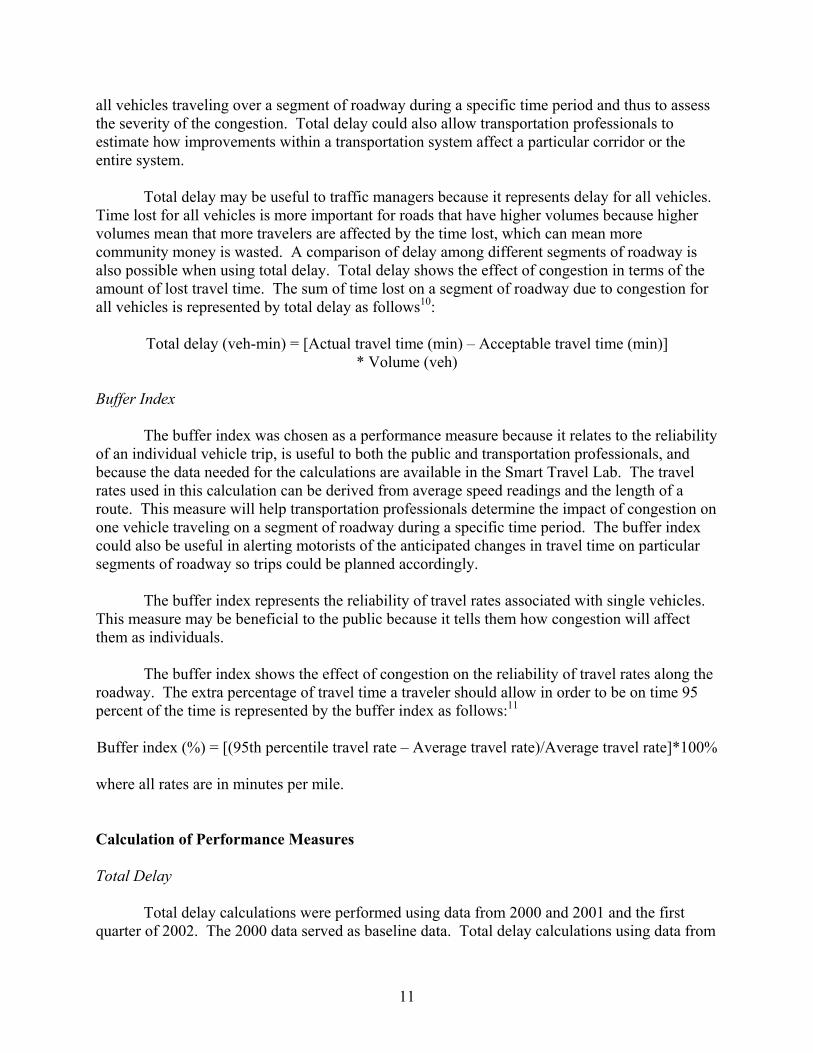
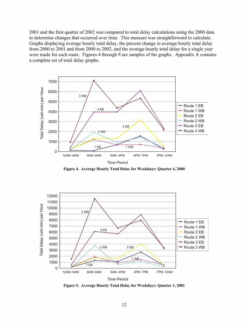
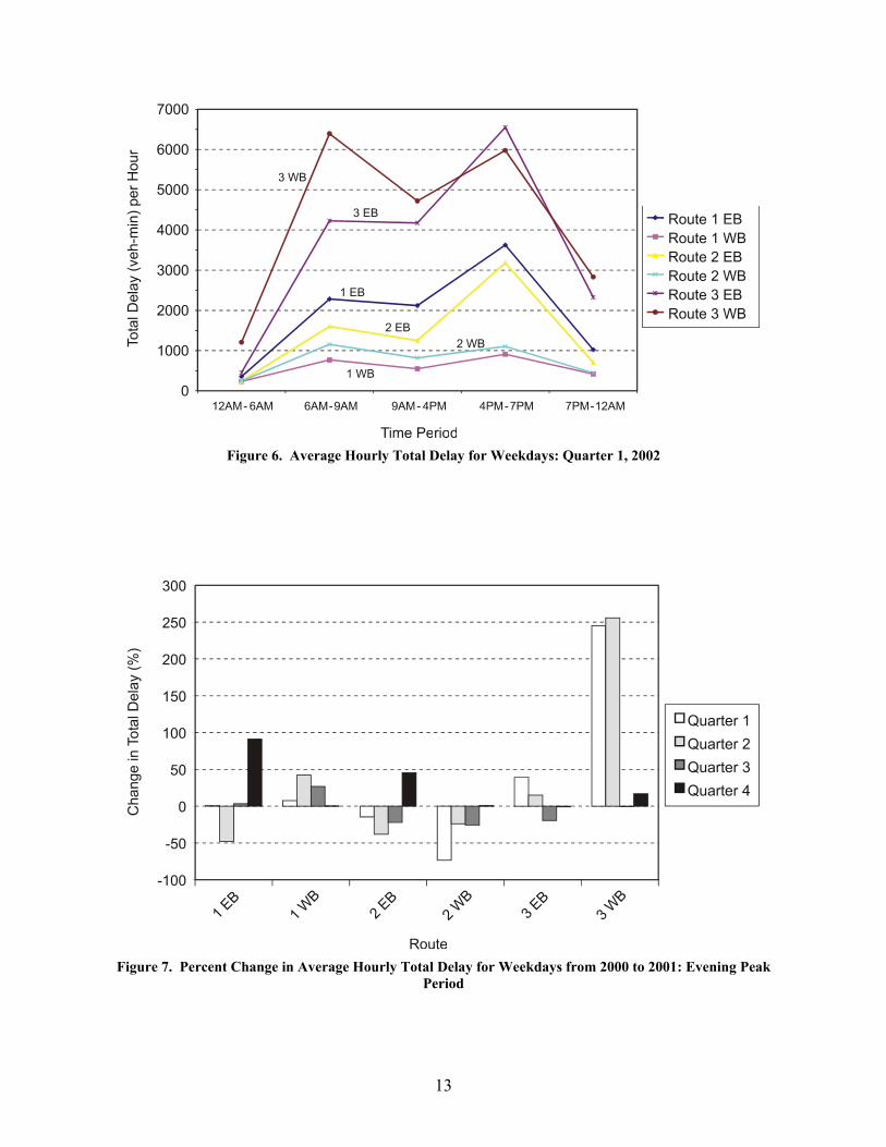
2001 and the first quarter of 2002 was compared to total delay calculations using the 2000 data to determine changes that occurred over time. This measure was straightforward to calculate. Graphs displaying average hourly total delay, the percent change in average hourly total delay from 2000 to 2001 and from 2000 to 2002, and the average hourly total delay for a single year were made for each route. Figures 4 through 9 are samples of the graphs. Appendix A contains a complete set of total delay graphs.
Figure 4. Average Hourly Total Delay for Weekdays: Quarter 4, 2000
Figure 5. Average Hourly Total Delay for Weekdays: Quarter 1, 2001
13
Figure 6. Average Hourly Total Delay for Weekdays: Quarter 1, 2002
Figure 7. Percent Change in Average Hourly Total Delay for Weekdays from 2000 to 2001: Evening Peak
Period
14
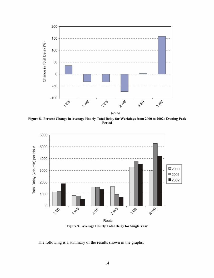
Figure 8. Percent Change in Average Hourly Total Delay for Weekdays from 2000 to 2002: Evening Peak
Period
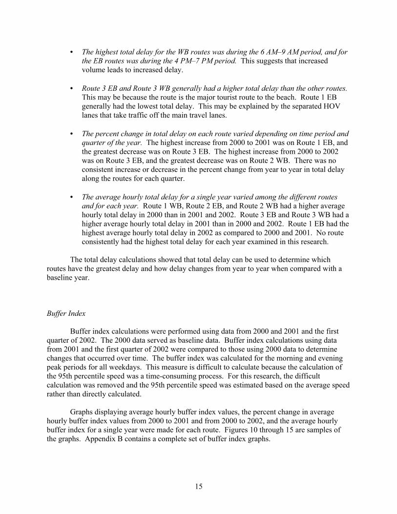
Figure 9. Average Hourly Total Delay for Single Year
The following is a summary of the results shown in the graphs:
15
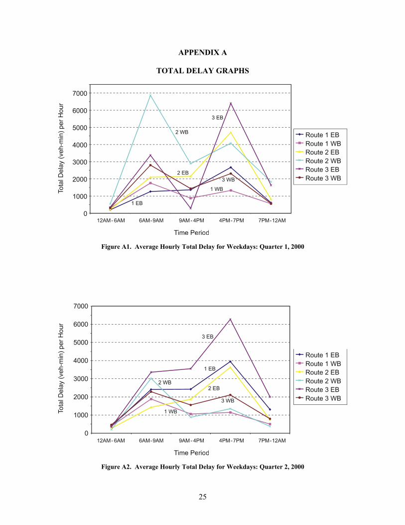
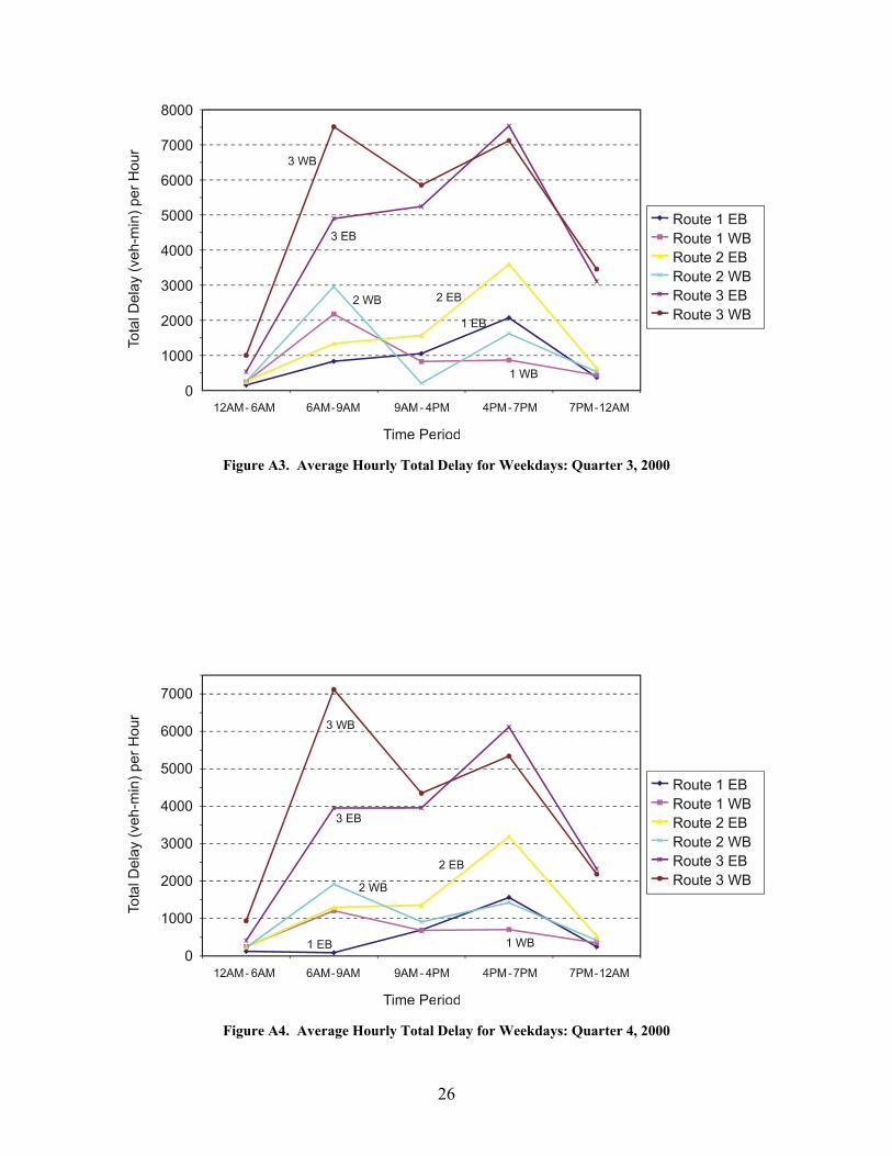
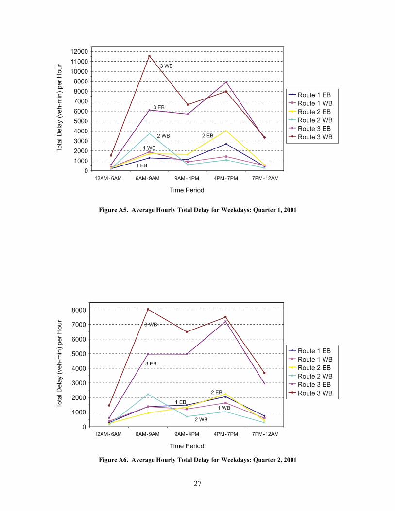
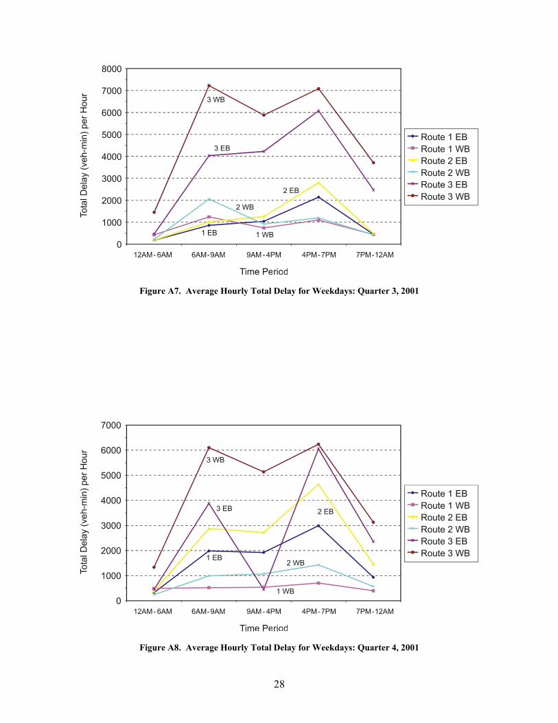
• The highest total delay for the WB routes was during the 6 AM–9 AM period, and for the EB routes was during the 4 PM–7 PM period. This suggests that increased volume leads to increased delay.
• Route 3 EB and Route 3 WB generally had a higher total delay than the other routes.
This may be because the route is the major tourist route to the beach. Route 1 EB generally had the lowest total delay. This may be explained by the separated HOV lanes that take traffic off the main travel lanes.
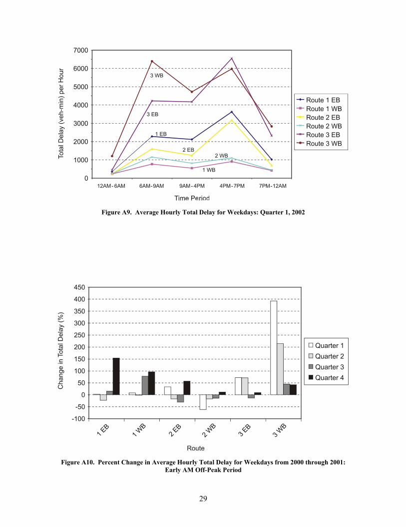
• The percent change in total delay on each route varied depending on time period and
quarter of the year. The highest increase from 2000 to 2001 was on Route 1 EB, and the greatest decrease was on Route 3 EB. The highest increase from 2000 to 2002 was on Route 3 EB, and the greatest decrease was on Route 2 WB. There was no consistent increase or decrease in the percent change from year to year in total delay along the routes for each quarter.
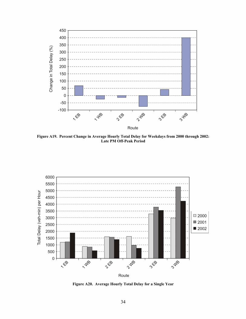
• The average hourly total delay for a single year varied among the different routes
and for each year. Route 1 WB, Route 2 EB, and Route 2 WB had a higher average hourly total delay in 2000 than in 2001 and 2002. Route 3 EB and Route 3 WB had a higher average hourly total delay in 2001 than in 2000 and 2002. Route 1 EB had the highest average hourly total delay in 2002 as compared to 2000 and 2001. No route consistently had the highest total delay for each year examined in this research.
The total delay calculations showed that total delay can be used to determine which
routes have the greatest delay and how delay changes from year to year when compared with a baseline year. Buffer Index
Buffer index calculations were performed using data from 2000 and 2001 and the first quarter of 2002. The 2000 data served as baseline data. Buffer index calculations using data from 2001 and the first quarter of 2002 were compared to those using 2000 data to determine changes that occurred over time. The buffer index was calculated for the morning and evening peak periods for all weekdays. This measure is difficult to calculate because the calculation of the 95th percentile speed was a time-consuming process. For this research, the difficult calculation was removed and the 95th percentile speed was estimated based on the average speed rather than directly calculated.
Graphs displaying average hourly buffer index values, the percent change in average hourly buffer index values from 2000 to 2001 and from 2000 to 2002, and the average hourly buffer index for a single year were made for each route. Figures 10 through 15 are samples of the graphs. Appendix B contains a complete set of buffer index graphs.
16
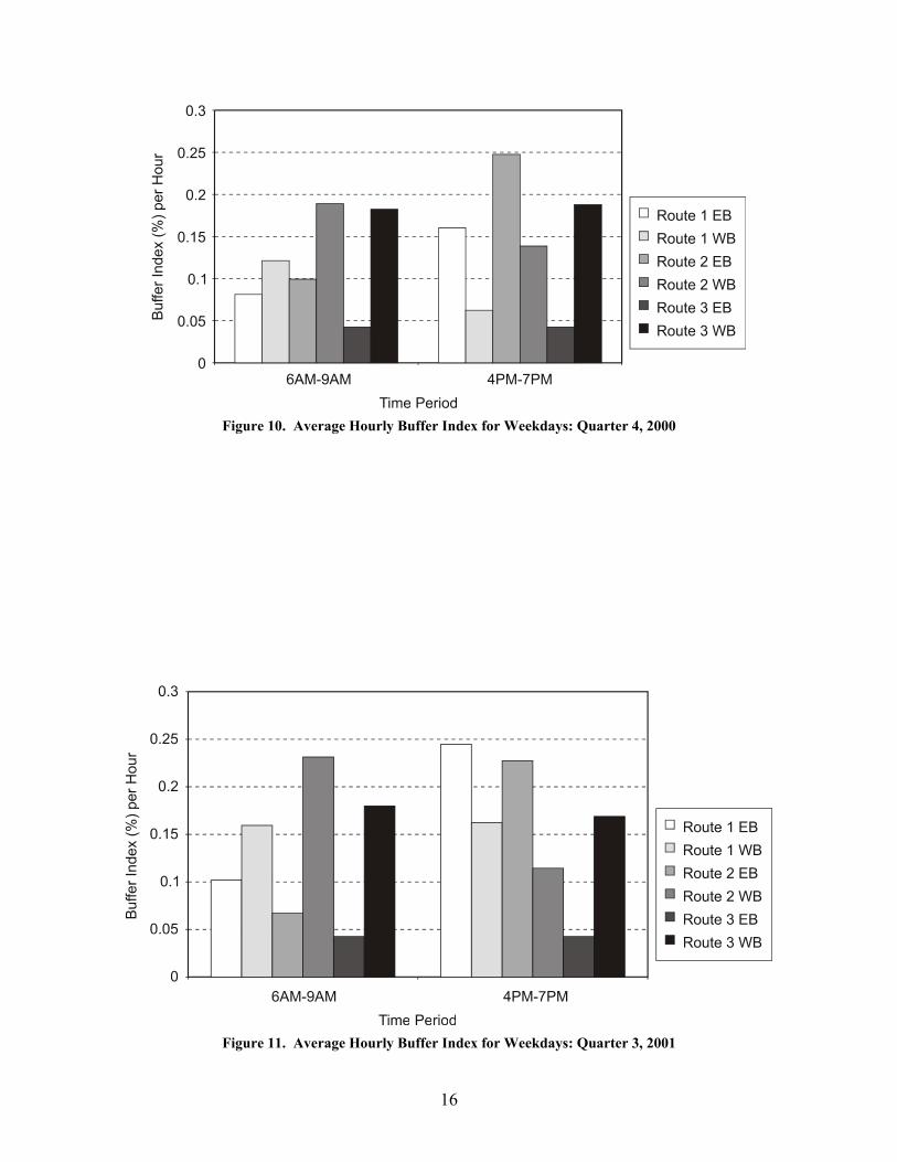
Figure 10. Average Hourly Buffer Index for Weekdays: Quarter 4, 2000
Figure 11. Average Hourly Buffer Index for Weekdays: Quarter 3, 2001
17
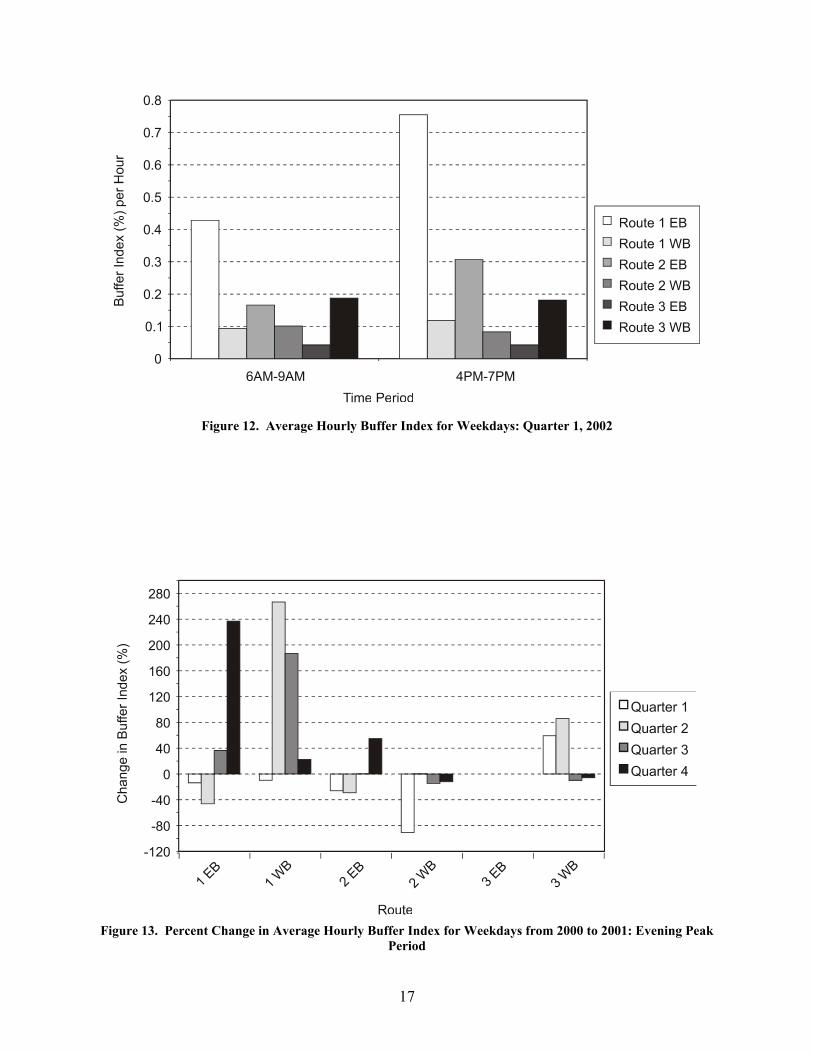
Figure 12. Average Hourly Buffer Index for Weekdays: Quarter 1, 2002
Figure 13. Percent Change in Average Hourly Buffer Index for Weekdays from 2000 to 2001: Evening Peak
Period
18
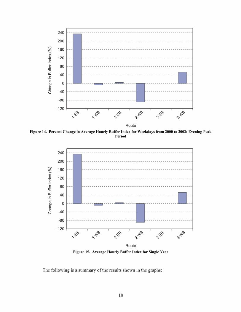
Figure 14. Percent Change in Average Hourly Buffer Index for Weekdays from 2000 to 2002: Evening Peak
Period
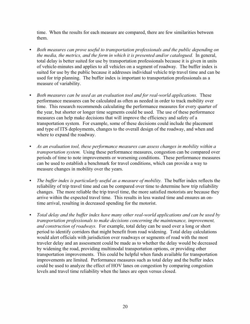
Figure 15. Average Hourly Buffer Index for Single Year
The following is a summary of the results shown in the graphs:

19
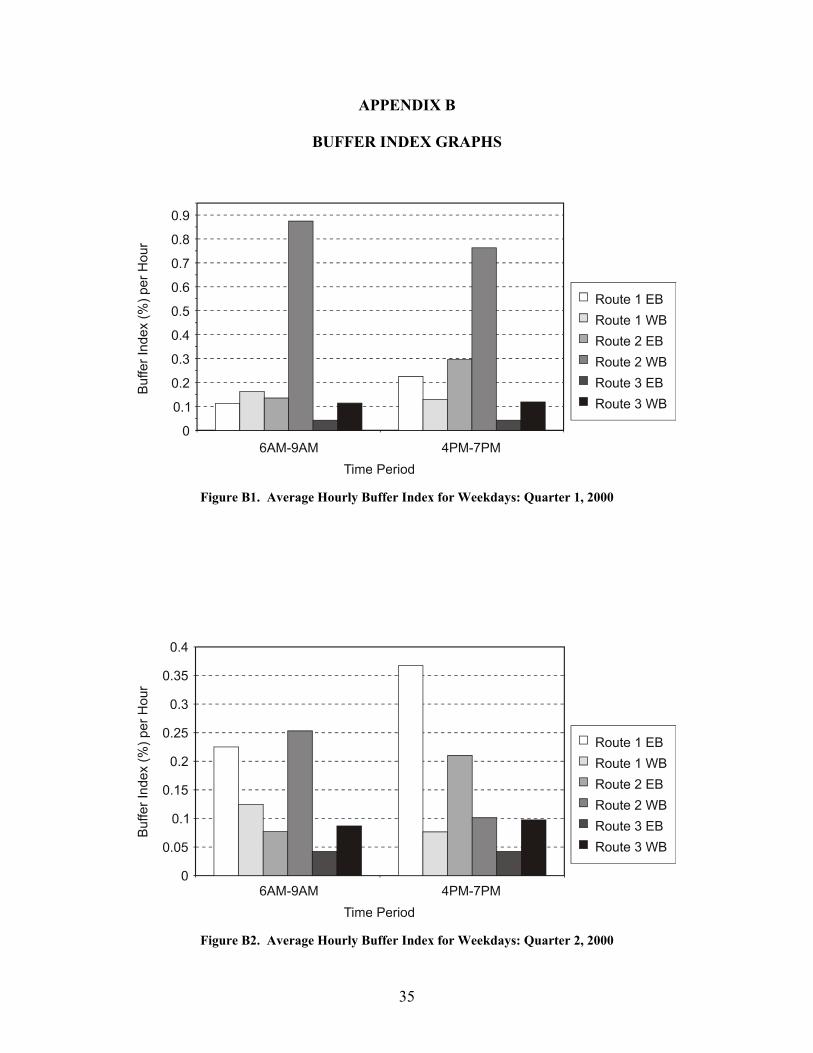
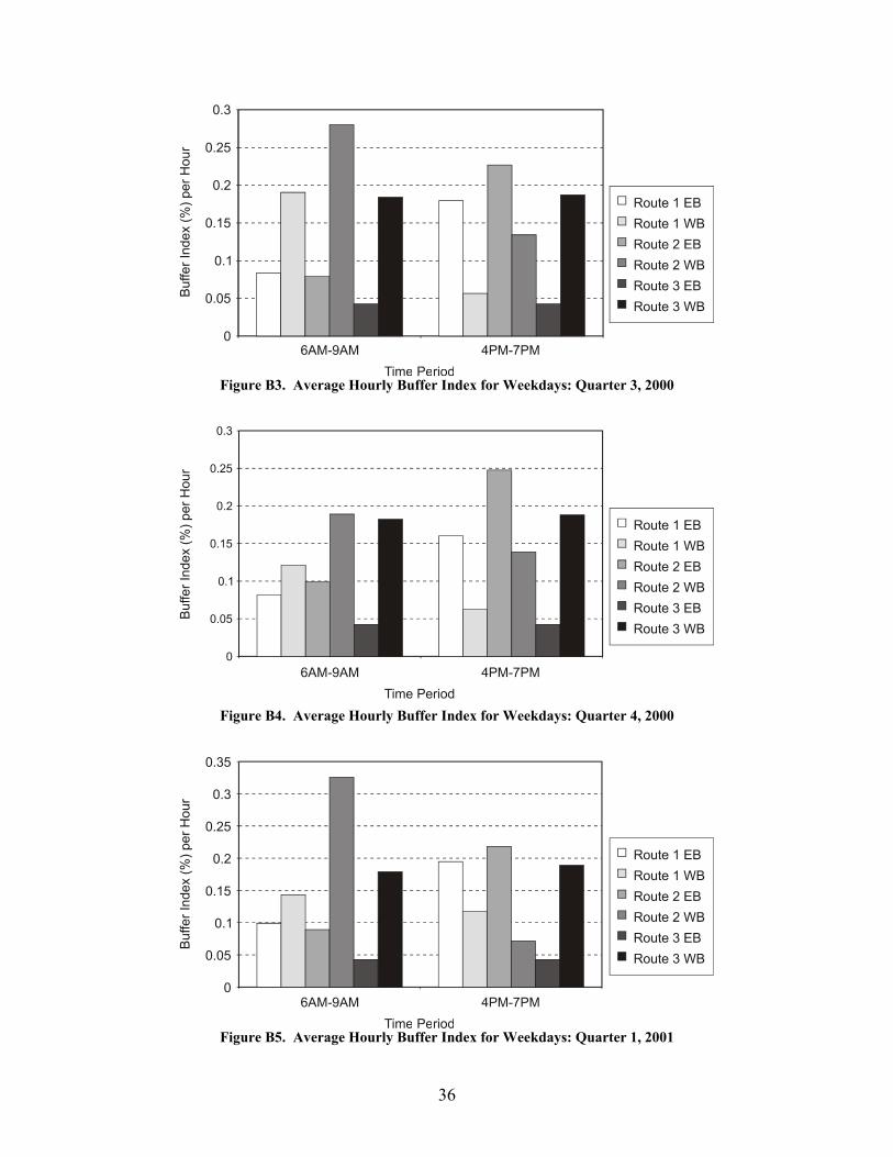
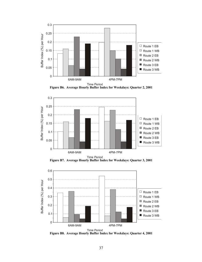
• The highest buffer index values for the WB routes were generally for the 6 AM–9 AM period, and for the EB routes were for the 4 PM–7 PM period.
• The highest buffer index values varied among the routes depending on time period
and year. Route 3 EB generally had the lowest buffer index values.
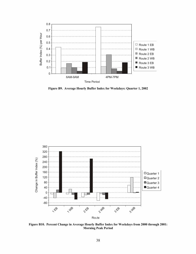
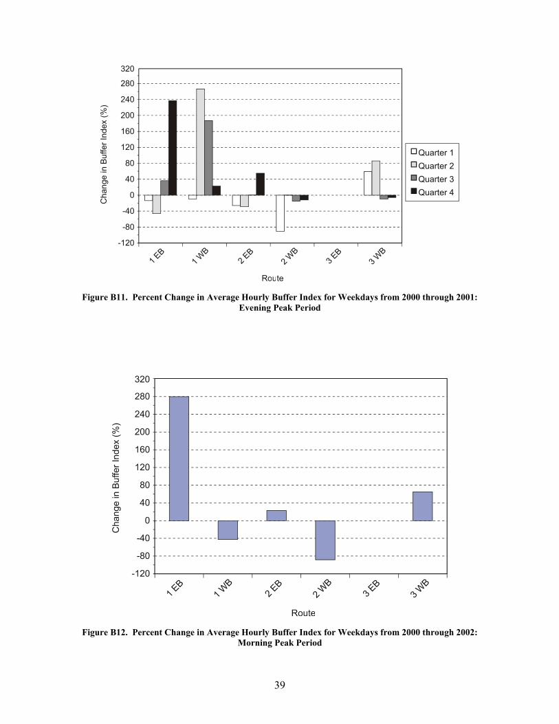
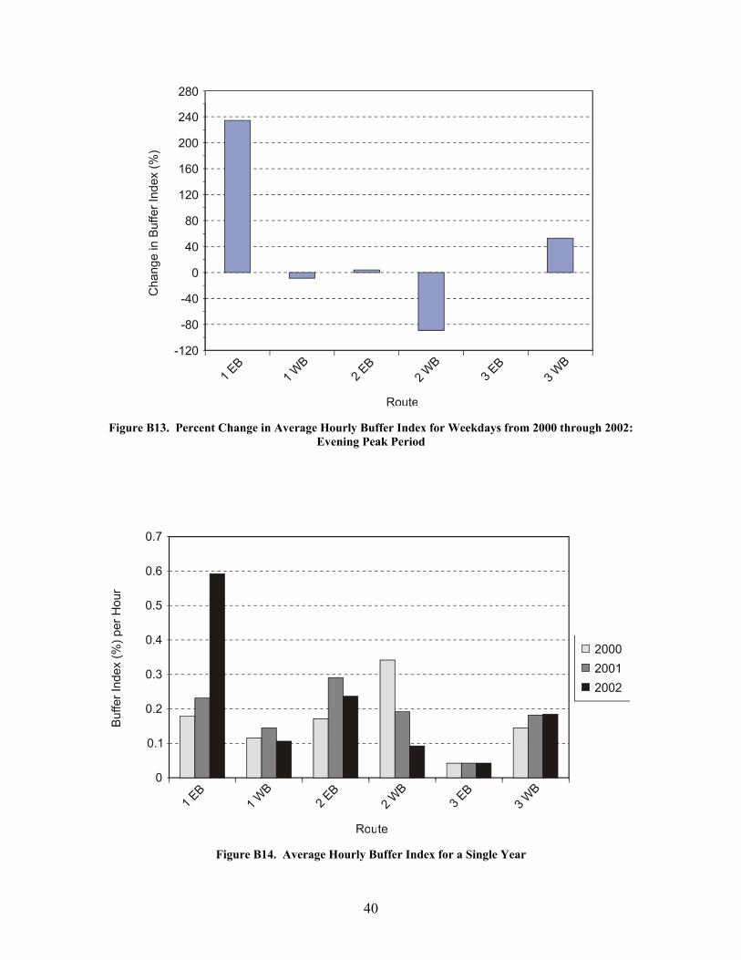
• The percent change in the buffer index values on each route varied depending on time period and quarter of the year. From 2000 to 2001, the highest percent increase was on Route 1 EB, and the greatest decrease was on Route 2 WB. From 2000 to 2002, the highest percent increase was on Route 1 EB, and the greatest decrease was on Route 2 WB. The percent change did not increase or decrease consistently from year to year along the routes for each quarter.
• The average hourly buffer index value for a single year varied among the different
routes and for each year. Route 2 WB had a higher average hourly buffer index value in 2000 than in 2001 and 2002. Route 1 WB and Route 2 EB had higher buffer index values in 2001 than in 2000 and 2002. Route 1 EB and Route 3 WB had higher buffer index values in 2002 than in 2000 and 2001. Route 3 EB had the same buffer index value in 2000, 2001, and 2002. No route consistently has the highest buffer index values for each year examined in this research.
Summary Table 2 summarizes the total delay and buffer index results and compares their similarities and differences. The results help to show that although total delay and the buffer index may be correlated, the two performance measures do not always identify the same trends in roadway congestion and performance.
Table 2. Summary of Total Delay and Buffer Index Results
Period Total Delay Buffer Index Morning Peak Period WB Routes WB Routes
Value
Evening Peak Period EB Routes EB Routes 2000-2001 Route 1 EB Route 1 EB Largest % increase 2000-2002 Route 3 EB Route 1 EB 2000-2001 Route 3 EB Route 2 WB Largest % decrease 2000-2002 Route 2 WB Route 2 WB
CONCLUSIONS
• Total delay and the buffer index may be used as performance measures to quantify the effects of congestion. Each measure shows a different dimension of congestion. Total delay indicates the total delay accumulated by all vehicles over a segment of roadway during a specific time period, and the buffer index is an estimate of the reliability of a trip arriving on
20
time. When the results for each measure are compared, there are few similarities between them.
• Both measures can prove useful to transportation professionals and the public depending on
the media, the metrics, and the form in which it is presented and/or catalogued. In general, total delay is better suited for use by transportation professionals because it is given in units of vehicle-minutes and applies to all vehicles on a segment of roadway. The buffer index is suited for use by the public because it addresses individual vehicle trip travel time and can be used for trip planning. The buffer index is important to transportation professionals as a measure of variability.
• Both measures can be used as an evaluation tool and for real-world applications. These
performance measures can be calculated as often as needed in order to track mobility over time. This research recommends calculating the performance measures for every quarter of the year, but shorter or longer time segments could be used. The use of these performance measures can help make decisions that will improve the efficiency and safety of a transportation system. For example, some of these decisions could include the placement and type of ITS deployments, changes to the overall design of the roadway, and when and where to expand the roadway.
• As an evaluation tool, these performance measures can assess changes in mobility within a
transportation system. Using these performance measures, congestion can be compared over periods of time to note improvements or worsening conditions. These performance measures can be used to establish a benchmark for travel conditions, which can provide a way to measure changes in mobility over the years.
• The buffer index is particularly useful as a measure of mobility. The buffer index reflects the
reliability of trip travel time and can be compared over time to determine how trip reliability changes. The more reliable the trip travel time, the more satisfied motorists are because they arrive within the expected travel time. This results in less wasted time and ensures an on-time arrival, resulting in decreased spending for the motorist.
• Total delay and the buffer index have many other real-world applications and can be used by
transportation professionals to make decisions concerning the maintenance, improvement, and construction of roadways. For example, total delay can be used over a long or short period to identify corridors that might benefit from road widening. Total delay calculations would alert officials with jurisdiction over roadways or segments of road with the most traveler delay and an assessment could be made as to whether the delay would be decreased by widening the road, providing multimodal transportation options, or providing other transportation improvements. This could be helpful when funds available for transportation improvements are limited. Performance measures such as total delay and the buffer index could be used to analyze the effect of HOV lanes on congestion by comparing congestion levels and travel time reliability when the lanes are open versus closed.
21
RECOMMENDATIONS
Methodology for Selecting and Calculating Performance Measures
One of the main goals of this research was to develop a methodology that VDOT traffic managers could use to select and calculate performance measures to quantify congestion in a transportation system. The following methodology is recommended:
1. Determine the area of study. Identify selected corridor routes to which performance measures will be applied.
2. Determine the source and type of data (e.g., volumes, speeds, occupancy, travel times) that are available. Data can be obtained from a database or a manual collection procedure.
3. Select time periods in which to do the analysis. Break each day into peak periods and
non-peak periods based on the available data. Also determine the time frame in which the study is to be done. Will the study be done for a whole year, several months out of a year, on a monthly basis, or on a weekly basis?
4. Collect data from the data source for the selected time periods along each corridor. 5. Remove entries from the data set that have missing or unrealistic values. 6. Determine the performance measures to be used. The performance measures should
be selected based upon the objectives and goals of the study and the type of data available.
7. Calculate the performance measures. 8. Evaluate the results from the calculation of the performance measures.
The methodology will provide a starting point for transportation managers who wish to
use performance measures to evaluate congestion on roadways within a transportation system. The results of using the methodology will allow transportation managers to track traveler delay and mobility over time and thus determine what changes need to be made to improve a transportation system.
Use of Buffer Index and Total Delay as Performance Measures 1. Use total delay to assess congestion on critical corridors in Virginia. 2. Use the buffer index to communicate travel information to commuters. 3. Apply both measures for long-term decisions based on the following needs:
22
— to measure mobility along routes and corridors — to evaluate and track mobility over time on routes and over a transportation system — to prioritize needed improvements in the transportation system — to analyze the effect of transportation improvements such as HOV lanes.
Use of Alternate Performance Measures
If the data as indicated for the additional performance measures that are not available currently in the STL were collected and archived. VDOT should consider using some of the other measures shown in Table 1. For example, the travel rate index, could not be tested in this research because arterial traffic data were not available.
The travel rate index has a relatively straightforward calculation that computes the extra
amount of time required to make a trip under congested conditions on the roadway using data from both freeways and arterials.7 Although this measure may seem similar to the buffer index, the calculations of the two are very different. The travel rate index computes the extra travel time needed to make a trip during congested conditions using average travel rates and peak period vehicle miles traveled; the buffer index computes the extra travel time needed to be on time 95 percent of the time using 95th percentile travel rates and average travel rates. The travel rate index could be useful to both the public and transportation professionals. The measure could be used to alert drivers as to how much more travel time to allow during peak travel hours. Transportation professionals could use the measure to determine the segments of roadway with the most congestion and to determine how roadway improvements affect a transportation system.
REFERENCES
1. Levin, H.S., and T.J. Lomax. A Travel Time Based Index for Evaluating Congestion. In Proceedings of the 66th Annual Meeting. Institute of Transportation Engineers, Minneapolis, September 1996.
2. Cottrell, W.D. Estimating the Probability of Freeway Congestion Recurrence. In
Transportation Research Record 1634. Transportation Research Board, Washington, D.C., 1998, pp. 19-27.
3. Levinson, H.S., and T.J. Lomax. Developing a Travel Time Congestion Index. In
Transportation Research Record 1564. Transportation Research Board, Washington, D.C., 1996, pp. 1-10.
23
4. Boarnet, M.G., E. Jae Kim, and E. Parkney. Measuring Traffic Congestion. In Transportation Research Record 1634. Transportation Research Board, Washington, D.C., 1998, pp. 93-99.
5. Turner, S.M. Examination of Indicators of Congestion Level. In Transportation Research
Record 1360. Transportation Research Board, Washington, D.C., 1992, pp. 150-157 6. Texas Transportation Institute. 2001 Urban Mobility Study Website.
http://mobility.tamu.edu/ums. Accessed September 15, 2001. 7. Schrank, D., and T. Lomax. The 2001 Urban Mobility Report. Texas Transportation
Institute, College Station, May 2001. http://mobility.tamu.edu. Accessed September 15, 2001.
8. Schrank, D., and T. Lomax. Urban Roadway Congestion 1982-1994 Annual Report.
Texas Transportation Institute, College Station, 1997. 9. Schrank, D., and T. Lomax. Urban Roadway Congestion Annual Report: 1998. Texas
Transportation Institute, College Station, 1998. 10. Lomax, T., S. Turner, G. Shunk et al. Quantifying Congestion. NCHRP Report 398.
National Cooperative Highway Research Program, Transportation Research Board, Washington, D.C., 1997.
11. Lomax, T., S. Turner, and R. Margiotta. Monitoring Urban Roadways: Using Archived
Operations Data for Reliability and Mobility Measurement. Texas Transportation Institute, College Station, 2001.
12. Pearce, V. Can I Make It to Work On Time? Traffic Technology International, Oct/Nov
2001, pp. 16-18. 13. Turochy, R., and B.L. Smith. New Procedure for Detector Data Screening in Traffic
Management Systems. In Transportation Research Record 1727. Transportation Research Board, Washington, D.C., 2000, pp. 127-131.
14. Transportation Research Board. Highway Capacity Manual. Washington, D.C., 2000.

24
25
APPENDIX A
TOTAL DELAY GRAPHS
Figure A1. Average Hourly Total Delay for Weekdays: Quarter 1, 2000
Figure A2. Average Hourly Total Delay for Weekdays: Quarter 2, 2000
26
Figure A3. Average Hourly Total Delay for Weekdays: Quarter 3, 2000
Figure A4. Average Hourly Total Delay for Weekdays: Quarter 4, 2000
27
Figure A5. Average Hourly Total Delay for Weekdays: Quarter 1, 2001
Figure A6. Average Hourly Total Delay for Weekdays: Quarter 2, 2001
28
Figure A7. Average Hourly Total Delay for Weekdays: Quarter 3, 2001
Figure A8. Average Hourly Total Delay for Weekdays: Quarter 4, 2001
29
Figure A9. Average Hourly Total Delay for Weekdays: Quarter 1, 2002
Figure A10. Percent Change in Average Hourly Total Delay for Weekdays from 2000 through 2001: Early AM Off-Peak Period
30
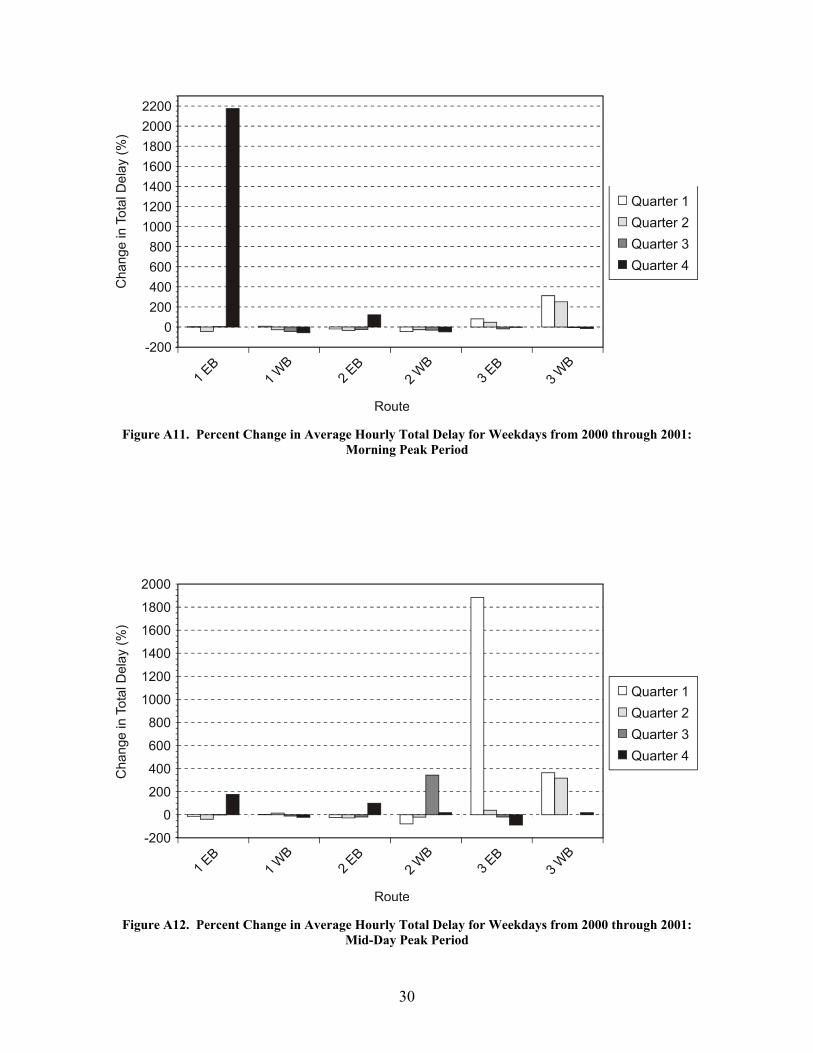
Figure A11. Percent Change in Average Hourly Total Delay for Weekdays from 2000 through 2001: Morning Peak Period
Figure A12. Percent Change in Average Hourly Total Delay for Weekdays from 2000 through 2001: Mid-Day Peak Period
31
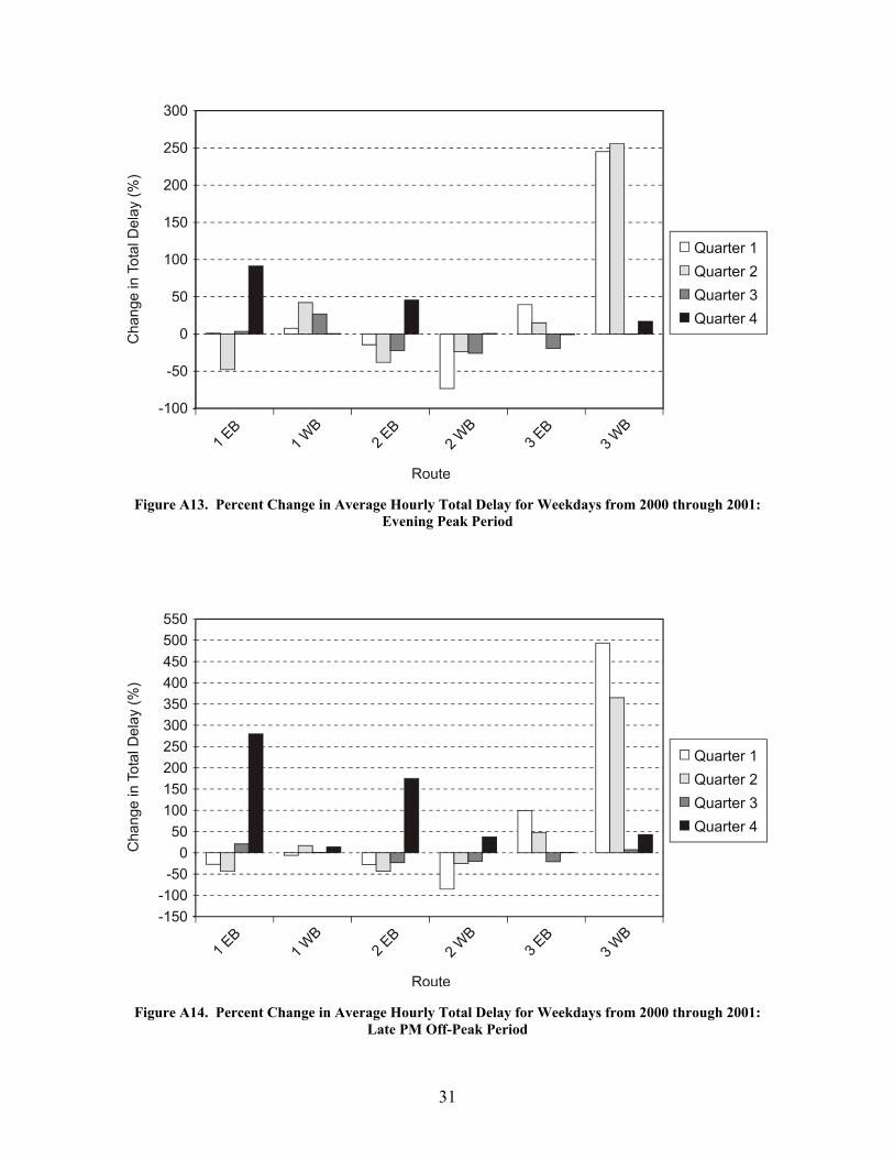
Figure A13. Percent Change in Average Hourly Total Delay for Weekdays from 2000 through 2001: Evening Peak Period
Figure A14. Percent Change in Average Hourly Total Delay for Weekdays from 2000 through 2001: Late PM Off-Peak Period
32
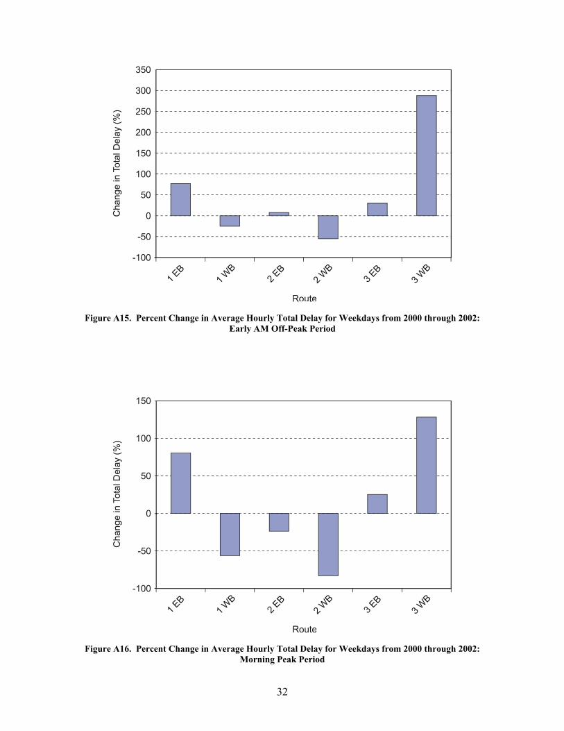
Figure A15. Percent Change in Average Hourly Total Delay for Weekdays from 2000 through 2002: Early AM Off-Peak Period
Figure A16. Percent Change in Average Hourly Total Delay for Weekdays from 2000 through 2002: Morning Peak Period
33
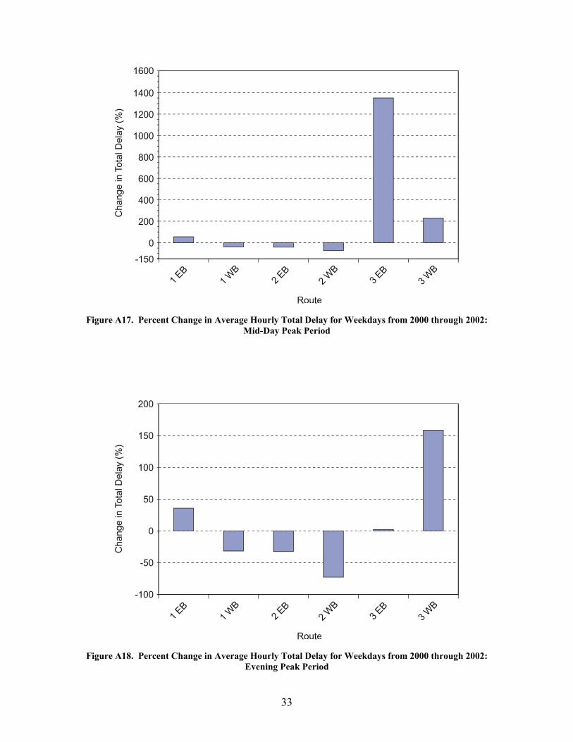
Figure A17. Percent Change in Average Hourly Total Delay for Weekdays from 2000 through 2002: Mid-Day Peak Period
Figure A18. Percent Change in Average Hourly Total Delay for Weekdays from 2000 through 2002: Evening Peak Period
34
Figure A19. Percent Change in Average Hourly Total Delay for Weekdays from 2000 through 2002: Late PM Off-Peak Period
Figure A20. Average Hourly Total Delay for a Single Year
35
APPENDIX B
BUFFER INDEX GRAPHS
Figure B1. Average Hourly Buffer Index for Weekdays: Quarter 1, 2000
Figure B2. Average Hourly Buffer Index for Weekdays: Quarter 2, 2000
36
Figure B3. Average Hourly Buffer Index for Weekdays: Quarter 3, 2000
Figure B4. Average Hourly Buffer Index for Weekdays: Quarter 4, 2000
Figure B5. Average Hourly Buffer Index for Weekdays: Quarter 1, 2001
37
Figure B6. Average Hourly Buffer Index for Weekdays: Quarter 2, 2001
Figure B7. Average Hourly Buffer Index for Weekdays: Quarter 3, 2001
Figure B8. Average Hourly Buffer Index for Weekdays: Quarter 4, 2001
38
Figure B9. Average Hourly Buffer Index for Weekdays: Quarter 1, 2002
Figure B10. Percent Change in Average Hourly Buffer Index for Weekdays from 2000 through 2001: Morning Peak Period
39
Figure B11. Percent Change in Average Hourly Buffer Index for Weekdays from 2000 through 2001: Evening Peak Period
Figure B12. Percent Change in Average Hourly Buffer Index for Weekdays from 2000 through 2002: Morning Peak Period
40
Figure B13. Percent Change in Average Hourly Buffer Index for Weekdays from 2000 through 2002: Evening Peak Period
Figure B14. Average Hourly Buffer Index for a Single Year