final report annular momentum control device …
TRANSCRIPT
VOLUME I NASA CR-144917
LABORATORY MODEL DEVELOPMENT
(NASA-CB-144917-Vol-1) ANNULAR MOMENTUM N76-19457 CONTROL DEVICE (AMCD) VOLUME 1 LABORATORY MODEL DEVELOPMENT Final Report (Ball Bros Research Corp) 108 p HC $550 CSCL 131 Unclas
GS37 20655
FINAL REPORT
ANNULAR MOMENTUM CONTROL DEVICE
(AMCD)
PREPARED FOR
NATIONAL AERONAUTICS AND SPACE ADMINISTRATION
LANGLEY RESEARCH CENTER
HAMPTON VIRGINIA
LL
Ball Brothers Research Aerospace Division
u~o BOULDER COLORADO 80302rsCorporation
F76-02
NASA CR-144917
FINAL REPORT
ANNULAR MOMENTUM CONTROL DEVICE (AMCD)
VOLUME I LABORATORY MODEL DEVELOPMENT
Prepared under Contract No NAS 1-12529 by Ball Brothers Research Corporation
Boulder Colorado 80302
for
NATIONAL AERONAUTICS AND SPACE ADMINISTRATION
m m
The MCD in Final Stages of Assembly
F76-02
SUMMARY
The annular momentum control device (ACD) is a thin hoop-like wheel
with neither shaft nor spokes (see Frontispiece) The wheel floats
in a magnetic field and can be rotated by a segmented motor
Potential advantages of such a wheel are low weight configuration
flexibility a wheel that stiffens with increased speed vibration
isolation and increased reliability
The AMCD is nearly 2 meters (6 feet) in diameter An annular
aluminum baseplate supports the entire wheel assembly Vacuum
operation is possible by enclosing the wheel in an annular housing
attached to the baseplate The rotor or rim has a diameter of
about 16 meters (63 inches) and consists principally of graphiteshy
epoxy composite material It weighs 225 kilograms (495 pounds)
and is strong enough to be spun at 3000 rpm At this speed it can
store 2200 N-m-s (3000 ft-lb-sec) of angular momentum A system of
pneumatic bearings can support the rim in the event of a magnetic
suspension failure
The magnetic suspension system supports the rim both axially and
radially at three points Combinations of permanent magnets and
electromagnets at each of the three suspension stations exert forces
on ferrite bands imbedded in the rotating rim The magnetic gaps
are about 025 cm (01 inch) above below and inside the rim The
gaps are maintained by servo loops with 50 hertz bandwidths that
The servorespond to error signals generated by inductive sensors
loops can be operated in either positioning or zero-power modes
The rim is accelerated and decelerated by a large diameter segshy
mented brushless dc motor Electromagnet stator segments are
placed at each suspension station and interact with samarium cobalt
permanent magnets placedevery 73 cm (29 inches) along the
periphery of the rim Commutation is achieved by Hall sensors that
detect the passing permanent magnets
ii
NF76-02
Volume I of this report describes the analysis design fabrication
and testing of the laboratory model of the AMCD Volume II conshy
tains a conceptual design and set of dynamic equations of a gimbaled
AMCD adapted to a Large Space Telescope (LST) Such a system
could provide maneuver capability and precision pointing by means
of one external gimbal wheel speed control and small motions of
the rim within the magnetic gap
iii1
F76-02
TABLE OF CONTENTS
Section Page
SUMMARY if
ACKNOWLEDGMENTS v
10 INTRODUCTION 1-1
20 THE AMCD CONCEPT 2-1
30 MECHANICAL SYSTEMS 3-1
31 Rim 3-1
32 Back-Up Air Bearing System 3-17
40 SUSPENSION SYSTEM 4-1
41 System Description 4-1
42 Performance 4-12
50 DRIVE SYSTEM 5-1
51 System Description 5-1
52 Magnet Selection 5-1
53 Core and Winding Design 5-2
54 Motor Commutation 523
55 Motor Control Electronics 5-3
56 Torque Calculations 5-4
APPENDICES
Appendix Page
A CURRENT DRIVER EQUATIONS AND TRANSFER FUNCTIONS A-1
B THE WAHOO CONCEPT B-I
C SOMEADDITIONAL SERVO INSIGHTS C-1
iv
P76-02
ACKNOWLEDGMENTS
The AMCD development to date has been the result of the efforts of a great many people At BBRC Frank Manders with help from Dick Mathews lead the mechanical design and fabrication effort Dick Woolley strongly influenced the magnetic design and overall configushyration Jerry Wedlake developed the drive system Glen King performed the dynamic analyses and Dave Giandinoto designed much of the intershyfacing electronics and did the final system integration
At Cambion Paul Simpson managed the magnetic suspension work with technical consulting provided by Joe Lyman and Lloyd Perper
The rim fabrication at Bristol was headed by Tom Laidlaw with analytical assistance from Keith Kedward
Analytic design of the back-up bearings at Shaker Research was conshyducted by Dr Coda Pan and Warren Waldron
The customer had a strong influence on the final system At Goddard Space Flight Center Phil Studer provided valuable suggesshytions on all magnetic aspects and the drive motor in particular
The primary influences and directions came of course from Nelson Groom and Dr Willard Anders6n of Langley Research Center who conshyceived of the AMCD and fostered its development
My thanks to all of these people
Carl Henrikson AMCD Project Manager
v
10
F76-02
INTRODUCTION
The AMCD concept was originated at the Langley Research Center of
the National Aeronautics and Space Administration (Reference 1)
Analysis design fabrication and testing of development hardware
was begun under contract to Ball Brothers Research-Corporation in
July of 1973 The contract was jointly sponsored by the Langley
Research Center and the Goddard Spaceflight Center The contract
work statement was also a joint effort with the Goddard Spaceflight
Center providing technical inputs on the magnetic bearings and
drive motor portions Hardware was delivered in February of 1975
Several key subcontractors were used by BBRC during the program
Principal among these were
1 Cambridge Thermionic Corporation (Cambion) Cambridge
Massachusetts - Development of the magnetic suspension system
2 Bristol Aerospace Limited Winnipeg Canada - Analysis
and fabrication of the rim
3 Shakei Research Corporation Ballston Lake New York -
Design of the back-up air-bearing system
These subcontractors performed well-and made major contributions
to the success of the program One subcontract did not go well
and caused a major delay in the program Failure of the subconshy
-tractor for the baseplate and vacuum enclosure to meet flatness
requirements necessitated rejection of the parts and placement
of the subcontract with another firm
This report is a description of the major hardware items and
their design considerations Details of the as-delivered hardshy
waremay be found in the Operations and Maintenance Manual that
was delivered with the hardware
I-I
A AF76-02
The report is divided into four main parts covering the concept
the mechanical systems the suspension system and the drive
system Appendices are used to cover some of the details of the
servo control loops
1-2
20
F76-02
THE AMCD CONCEPT
A purely annular wheel has many advantages Principal among
that all the rotating mass is at the greatest radius andthese is
can produce the greatest angular momentum storage Thehence
shaft and spokes of a conventional wheel add weight but very
little angular momentum storage
oneBall-bearing annular wheels have never been tried and for
obvious reason The losses associated with a large diameter ball
In order to make annular wheelsbearing-would be intolerable
practical a low-loss magnetic suspension of the (or rim)rotor
a narrow annularis necessary This then is the AMCD concept
rim supported by a magnetic suspension system
Several other advantages accrue from the AMCD concept First
of all conventional size constraints are removed The wheel
does not have to operate in an enclosure to preserve lubricants
If the diameter isincreased greatly the space is not wasted
because a spacecraft or part of a spacecraft can be placed inshy
side the wheel Furthermore motivation exists to goto larger
wheels It can be shown that for a given stress level in the
rim the mass efficiency of the rim increases as the diameter
increases The offsetting effects of increased stator weight
can be alleviated by using basic spacecraft structure to supshy
port the stator elements A further advantage of larger diashy
meter is increased moment arm for spin and precessional torquing
Another set of advantages of the AMCD concept is a result of the
arerelatively thin annular rim The stresses in such a shape
predominantly circumferential so that the structure lends itself
to filament or tape wound composite materials Furthermore as
spin rate increases the rim tends to flatten and reduce dynamic
thai structrualimbalance Also it tends to become stiffer so
2-1
F76--02
resonant frequencies increase In fact it can be shown that
the conventional crossover frequency of a spinning wheel at
which the spin frequency becomes equal to the rotor structural
frequency cannot occur for an AMCD The structural frequencies
are always greater than spin frequency no matter how limber the
rim is at zero spin rate
The use of a magnetic suspension gives rise to another set of
advantages First the suspension is relatively soft and forms
a sort of isolator between the rim and the spacecraft to which
it is attached Any-vibrations of the rim will be greatly atshy
tenuated This effect can be enhanced by proper filtering at
multiples of spin rate The suspension is also a smooth linear
force-producing system without mechanical nonlinearities such
as stiction The result is that small precision precessional
torques can be created by gimbaling the rim in the magnetic gaps
The final advantage is related to the long life and perhaps even
more important predictable long-life capability of a magnetic
suspension system vis-a-vis a ball bearing Ball bearing lifeshy
times are short dependent on number of revolutions rotational
speed and very susceptible to contamination The lifetime of a
magnetic suspension is a function of the failure rate of electronic
components an area that has been the subJect of a great deal of
study Moreover redundant suspensions are fairly simpleto
mechanize
2-2
F76-02
30 MECHANICAL SYSTEMS
The AMCD Mechanical Systems consist of 1) the rotor (or rim)
2) the back-up air bearing system and 3) the mounting base and
vacuum enclosure
The rim provides the angular momentum storage capability for
the system Embedded into the rim are ferrite rings and samarium
cobalt permanent~magnets Three ferrite rings composed of segshy
ments located on each axial surface and on the inside radial
surface react with the magnetic suspension system Seventy-two
permanent magnets located near the periphery of the rim react
with the segmented drive system
The back-up air bearing system initiated in the event of a magshy
netic suspension failure is designed to slow and support the
rim The design provides hydrostatic air pads for radial control
and hydrodynamic air pads for axial control
The mounting base and vacuum enclosure completely surround the
rim magnetic suspension and motor components and provide the
mounting points for the torque measuring fixture brackets The
annular mounting base supports the magnetic suspension and motor
lattice structure The annular vacuum enclosure U-shaped in
cross-section isbolted to the mounting base providing the capashy
bility to operate the rim in a vacuum and to add structural rigidshy
ity The vacuum environment is necessary to reduce rim air drag
31 Rim
The final rim configuration Figure 3-1 shows that all components
embedded into the rim are completely supported The distance
between the permanent magnets and ferrite bands is maximized
within the dimensional constraints of the rim
3-1
F76-02
5S1I4 A41t1s
-EAflAMW1 COWFAr nAGNC7r
Figure 3-1 Rim Conftguration
Centrifugal accelerations cause forces on the embedded comshy
ponents which are reacted directly by the base rim material
minimizing the stresses on the adhesive which bonds the components
to the rim The samarium cobalt permanent magnets are spaced
a minimum of 085 inches from the closest ferrite band to minishy
mize the coupling between the permanent magnets and the magshy
netic suspension system
The primary function of the rim is to provide maximum angular
momentum storage capacity within dimensional and weight conshy
straints The selection of the rim material graphite filament
epoxy laminate is consistent with this function The specific
momentum of a flywheel (HM) is related to material characteristics
of the rim as follows
HM c(577 (3-1)
3-2
F76-02
where a is working stress in flywheel
pis flywheel material density
Hence a high-strength low-density material is ideal for a
low-weight flywheel
-Table 3-1 shows the relationship of material ultimate tensile
strength to material density for acceptable rim materials
Table 3-1
RIM MATERIAL STRENGTH TO DENSITY RATIO
MATERIAL STRENGTHDENSITY (IN x 10 )
Graphite A-SEpoxy 36
GlassEpoxy 34
BoronEpoxy 31
Graphite M-SEpoxy 30
Graphite HM-SEpoxy 18
Beryllium 10
6A1-4V Titanium 10
7075 Aluminum 08
Not in Composite Form
Graphite AS fiber - epoxy laminate therefore will provide the
largest specific momentum for the system Graphite filamentshy
epoxy laminate also has a relatively high elastic modulus C16x
106 PSI) thus providing relatively low radial growth at high
speeds Furthermore graphite-epoxy laminate is non-magnetic
and non-conducting essential characteristics for low drag
operation of the magnetic suspension system
3-3
F76-02
311 Rim Description
The rim consists of three bands of ferrite material made up
of 180 segments each and 72 samarium cobalt permanent magnets
embedded and bonded into the AS graphite filament - DX210 epoxy
rim material Figure 3-2shows the rim dimensions
The ferrite rings and permanent magnets are bonded to the basic
rim with Fuller 7004 adhesive The rim is composed of two basic
rectangular cross-sections the first and larger contains the
bulk of the graphite-epoxy material and the ferrite bands the
second smaller section contains the remaining material and
the samarium cobalt permanent magnets
The larger section has a cross-section 53 cm (21 inches) in radial
(125 inches) deep with an inner diameter oflength by 318 cm
154 cm (608 inches) Three channels are machined into this
section 254 cm (10 inches) wide by 057 cm (0225 inches) deep
The smaller section integral withto contain the ferrite bands
the larger is axially centered 28 cm (11 inches) in radial
(0375 inches) deep with-an outer diameter oflength by 095 cm
This section contains 72 holes which contain171 cm (6725) inches
the permanent magnets
The samarium cobalt permanent magnets are 14 cm (055 inches) in
diameter by 064 cm (025 inches) long The axial and radial
ferrite segments are shown in Figures 3-3 and 3-4 respectively
The ferrite segments are machined from Ferroxcube 3C5 material
The axial segment is slightly keystone in shape to minimize gap
distances Each segment occupies 2 degrees of the band circumshy
ference
3-4
529
GEN NOTES I RAD NOT DIMENSIONED
ARE 0907 Z WNEI6t4T - 455OLISshy
3 WrUtAt MOM4ENTUM 3300^-9000 Lb-VT- S Se
2-1RAb SC
30 OOTIRAXIAL31 t5R P - pERi7VE 5E6mlENTS-2 PLACES (5S60 gEaeb)
65 i ____ _CH COPPED GR4PHITE Amb EPOY
PLACS)
1 ~TIRI Z5
_ _
(REP)
I V 4 0
1 f3 PLA IES)
00 55DIX
42B
- 425 (REF)
EikPHITE FILAMENT tipQKY coMPOSITE
SAMARIUM COBALT
4 NampE S (72tE G D) CITE7KEb IN 380310 WITHIN OO EUALLY SPACED O 33000 PADi os MAGNET cEtJTer StAALL ZE E=QUAL WITW
o20 MAGrNET OLE5 bAA5 EITWEt TULjd
Ot zlNt kITA CoPPet
---ELusIA TO oo4 scAIme h3e o
BELOW IFLUSH4 VT(P
C
Figure 3-2 Rim Dimensions
555 2 ___
985
MNT L nFE RZPO KXC BE 3C 5 MISS
CD
Figure 3-3 Axial Ferrite Segment
I
233273
5058 27
LO
-9 100
4150 C2 PLACES)
MATL - 303
I
Figure 3-4 Radial Ferrite Segment
iF76- 02
The radial segment is rectangular in cross-section and when
bonded in place produces a small wedge-shaped gap between
segments Each radial segment represents 2 degrees of the band
circumference
312 Rim Fabrication
The ASCD rim was fabricated by Bristol Aerospace Limited Winnishy
peg Canada The material AS graphite filament tape impregnated
with DX210 resin was wrapped on a special tool producing 100
percent circumferential fibers with a volume fraction of graphite
of 55 percent
The oversized cross-section rim was wound in 15 separate layers
Each layer was B stage cured with the following temperature
cycle
P
J4 7
The post cure after the fifteenth layer was identical to the
B stage cure except the temperature was increased to 1770 C
in 50 minutes and held at 177degC for 2 hours after the 1490 C exshy
-posure
3-8
3
eF76-02
Figure 3-5 shows the specially constructed tool containing
cure cyclesheaters and insulation for B stage and final
The rim was removed from the tool and machined to nearly the
final dimensions including ferrite channels and permanent magshy
net holes These operations are shown in Figures 3-6 and 3-7
The ferrite segments andmagnets were bonded in place with Fuller
7004 adhesive and cured The magnets were placed in the rim with
alternating North-South poles and the ends were covered with a
016 cm (116 inch) thickness of chopped AS graphite-DX210 resin and
After final cure the rim was machined (by grinding) tocured
final dimension The rim was coated with a 0005 cm (0002 inch)
thick layer of Fuller 7220 adhesive as a final step to minimize
Figure 3-7A shows the final rim resultsrim water absorption
313 Rim Analysis
The rim analysis conducted by Bristol Aerospace predicted the
(55434 PSI)rim maximum stress and radial growth to be 38250 Ncm
and 3 cm (0117 inches) respectively
The rim was modelled using axisymmetric finite elements using
the ANSYS system The model characterizes the heterogeneity
of the structure (including the ferrite bands and magnets) and
the orthotropic elastic properties of the graphite-epoxy comshy
posite
The results of the analysis are summarized in Table 3-2 and in
a rim speed of 366 meters per secondFigures 3-8 3-9 and 3-10 at
(1200feet per second)
3-9
N
Figure 3-5 Lay-up Tool
IIP76-02
Rim Machining OperationsFigure 3-6
3-11
MIE II
Iiue37Diln emnn antHlsi h i
3I1
DF76-02
LOCATION MAGNITUDESTRESS (PSI)COMPONENT
Radial or carbonepoxy +460 (max) -891 (min)X stress
Axial or carbonepoxy +491 (max) -433 (min)Y stress
Shear or carbonepoxy +390 (max) XY stress -176 (min)
Hoop or carbonepoxy +55434 (max) 0 (min)Z stress
Radial inner surface +01166 (max)
Displacement outer surface -01130 (min)
(inches)
Table 3-2
MAXIMUM VALUES OF STRESSDISPLACEMENT AT 1200 FTSEC RIM SPEED
3-13
5ThF-=- V- LERATfNz- 1 4U0T00
RMCO RRLYSES BRISTOL REROSPRCE LTO OCT 73
HOOPSTRESS RNSYS 5
or Hoop Stress Contour PlotFigure 3-8 Z
F76-02
- flax h st-ess= 55434-
I I-1 I Ii-- shy
60Iz-
===z_ +0 _----- --- shyi -_-O- - = -- = +----- shy+ ---= -- r E
_-------=--- --- = ---
-- ----- +- - --- -- =--- -=
=
------ shy
=T--- 7
--
-
- -_ - - - -- - -- a
a zrlt- --r-- -r - z I=tzz-z - -
- 4
o6 Zf - =4-=-t vi I_- --- zmE+s=$ Z 4-| b- =---+----- shy
+ 5-t 4 -- c Tt - 22 ~++ _------ _ __ _C - u
a zjztL- +lt+ z- I [Lt- -- Tit--
-- -+v + --F t+-- -+rr 7- h |f
0 200 -00 6800 1000 12oo
Rim SPEED (rri5Ecc~
Figure 3-9 Hoop Stress and Growth With Speed
3-15
F76-02
e 4fo
1 1 I 1 t i I I CII1I1_4I I
Itdn-branveqs sts OI - I M
---shy-- -- -- - -
t~z 2 - 1- shy
- 421 ~T2 2 -=_-- -_E---i ----
t -- EM
___ _ ZZ +-_ _-A~~ - rrrr-
TLLto LLbi i L -- k - r K -1-
irtv li V i 1 -- t 4 s-- n-L -- T4 E
000-q0o 600 800 100 A120 Rim Sp Dr (FTVEC )
Figure 3-102 Transverse Stress Components With Speed
3-16
DF7602
Figure 3-8 shows the computer-drawn plot of constant hoop tensile
stress contours the maximum being 38252 Ncm 2 (55438 PSI)
occurring at the top and bottom inside corner
Figure 3-9shows the relationship of radial growth and hoop stress
as a function of rim tip speed
Figure 3-10 shows the relationship of transverse stress components
with speed
Since the material void free is capable of withstanding 110400 2 2Ncm (160000 PSI) in tension and 8280 Ncm (12000 PSI) in shear
the safety factor is 28 minimum On a sample basis the void
fraction was determined to be less than 04 percent
32 Back-Up Air Bearing System
The design of the back-up air bearing system was completed and
analyzed by Shaker Research Corporation Ballston Lake New York
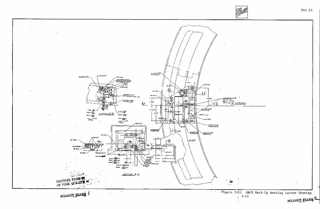
The back-up air bearing (BUB) system consists of six hydro-static
radial pads and twelve hydrodynamic axial pads These are arranged
in six BUB sets consisting of two axial (one upper and one lower)
and one radial pad and located at either end of a magnetic supshy
port station Each BUB set is approximately 60 degrees from the
adjacent set The bearings are deployed toward the rim by air
pressure when predetermined rim displacement limits are exceeded
The introduction of air through the pads as well as through a
pneumatically operated valve in the vacuum enclosure provides
the fluid for the BUB system and also introduces air drag for a
fastercoast-down Hydrostatic bearings were selected for
radial use instead of hydrodynamic types because the rather small
rim depth (115 inches) allows insufficient area to produce the
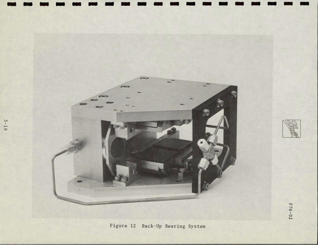
required reaction forces The back-up bearing system is shown
in Figures3-11 and 3-12
3-17
P76-02
~14
-L- 7
FiguTre 3-1 AMCD Back-Up Bearing Layout DrawingI 3-la
Figure 12 Back-Up Bearing System
7F76-02
321 Hydrostatic Radial Bearings
The movable radial pads are designed to minimize air flow and
maximize air bearing rim reaction forces The radial pads proshy
vide a centering effect on the rim to minimize dynamic and magshy
netic unbalance forces
In the normal magnetic suspension mode the radial pads are held
away from the rim-and against stops by a set of nested compression
springs (total of 22 N (50 pounds) of preload) When the radial
system Figure 3-11 is activated 207 Ncm2 (300 psig) air is introshy
duced to the pad piston cylinder which moves the pad outward
toward the rim The piston chamber is ported to the pad surface
through a 0033 cm (0012 to 0014 inch) diameter orifice A
sealed oil-filled dashpot between the piston and pad controls the
deployment velocity
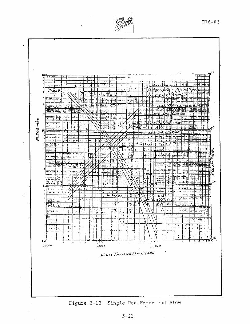
Figure 3-13 shows the relationship between- radial pad force and
gas flow versus film thickness for various orifice 4iameters
Because of limited gas available-the smaller orifice diameters
were selected
Since the rim is not at constant radius (because of radial growths)
film thickness and flow vary With rim speed Figure 3-14 shows
the relationship fo film thickness and flow versus rim speed
322 Hydrodynamic Axial Bearings
Movable- tilt type axial hydrodynamic pads were used since the
rim radial width is large and because of the limited bearing air
supply The axial pads are slightly crowned and combined with
the tilt feature are self aligning
3-20
F76-02
1 ~
It
7
I
JII ji
I L
II
---
Ft
T -
VIN I -_ Lr
TD _-
I
I+i
- 1MNV I
4~~r14 +t
Fit~Fi-~tdi I~ ~ JrV)
i ir
il-I= iH14+
i T r
F~m
shy
_ _
I L [
- i
I
_ i _
Ii
0001M -s as
Figure 3-13 Single Pad Force and Flow
3-21
A yyF76-02
WI
ii24pVshy-~~~~W
J4 i3 - Lit
I+ I~Ir~r L-- u 7t J
L 4- 1-nMLfI0__ 4~~~~- F-14--gtrF
I -- -r
4 ~ P I-
IaiH __M
1 --- t Th T1T
I- Vt prI i A
-p--t~LIV[~ VK jl77L1 1
Figure 3-14 Radial Air Pad Flow and Film Thickness With Rim Centered
3-22
F76-02
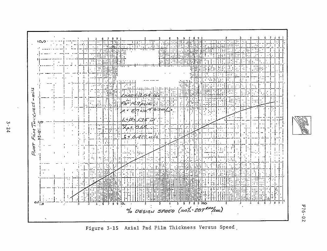
In the normal magnetic suspension mode the axial pads are held
against stops by a flexural spring The axial system is deployed
in-much the same manner as the radial system When a magnetic
suspension anomaly is detected the vacuum enclosure is flooded
with external air thus providing the film for the axial bearings
Figure 3-15 shows the relationship of film thickness with rim
speed Since the film will support the rim to about 15 radians
per second the pads are designed to accept several contacts before
replacement is necessary
323 Back-Up Bearing Pads
The primary objective in designing the pad material was to proshy
vide a material which would wear smoothly without damage to the
rim or to the pad itself Sacrificial bearing materials have
been used in gas bearings in the past which exhibit the necessary
qualitites The material used in the back-up bearings is an epoxy
resin heavily filled with aluminum powder aluminum oxide power
and molybdenum disulphide powder The mixture is poured into
silicone rubber molds degassed in a vacuum chamber then heatshy
cured The pads are then machined
When the spinning rim contacts the pads the pad will wear smoothly
and rapidly acquiring a high polish and yielding a fine dust
The rim surface should be undamaged by the contact The aluminum
filler provides high thermal conductivity to sink the heat generated
by the rim contact The aluminum oxide provides dimensional
stability so thQ pad will withstand the thermal shock generated
by the rim contact
3-23
3788I9 2 4 5 7 8 9 2
1 7 _- I
111-1 r - J
-I- --i- 1 rV1- 1 t r V
4 _ - _ _____ shy- I---7
I
r-- _- F-_- --- I ii -
I fr r l 7[-II j7shyLi +] - i I-- I
1 7 8
-- - 4 5---- 10 47 MCI 9
Figure 3-15 Axial Pad Film Thickness Versus Speed
F76-02
40 SUSPENSIONSYSTEM
41 System Description
The suspension system consists of three suspension stations
placed symmetrically about the rim At each suspension station
the rim can be pulled in either axial direction or tadially
inward by magnets A total of 12 magnets are arranged in sets
of four each to pull in these three directions (up down and
inward) The eight axial magnets are driven in concert by one
set of electronics Axial error signals are developed by a
position sensor located at the center of each station The
axial servo loops in each of the three stations are independent
of each other The four radial magnets in each station are also
driven by a set of electronics in response to a radial position
sensor located in the center of that station But the radial
station to another so asservos are interconnected from one
to prevent the servos fighting one another even in the presence
of rim radial growth
411 Magnet Description
One of the unique features of the AMCD is the support magnet
design The electromagnets are flux-biased by thin wafers of
samarium cobalt permanent magnet material placed in series in
the magnetic circuit This has the advantage of (1) providing
a high force per unit current sensitivity at zero current (2)
providing a linear relationship between force and current and -
(3) providing the static field required for zero power operation
The support magnet geometry is seen in Figure 4-1 The permanent
magnet biasing is achieved by slanted wafers of samarium cobalt
in the legs The wafers are as thin and wide as possible to
4-1
SAti 4-IUr CCBA3L~rshy
AGtJer-
AGII1
Figure 4-1 Support Magnet Geometry
RF76-02
minimize their reluctance in the magnetic-circuit The volume
of permanent magnet material is sufficient however to provide
adequate flux-biasing and static lift The reluctance of the
permanent magnets is large but does not more than double the
total reluctance since the air gap inthis system is large In
many other magnet suspension systems the gaps are small (about
01 mm) and this sort of series flux biasing would greatly inshy
crease the total reluctance in the circuit Control power would
thus be large and the systems would be impractical
The effect of flux-biasing on the force versus current characshy
teristics of the magnets is shown in Figure 4-2 With no biasing
current in either direction produces force of the same sign with
poor gain and low efficiency in the vicinity of zero current
Force is simply a function of the square of the current With
biasing the slope of force versus current is greatly increased
at zero current In the AMCD top and bottom magnets operate
together in a push-pull type of operation The coils are in
series hence both coils have zero current at the same time
The resultant force-current relationship is linear and has a
slope double that of either magnet alone
Figure 4-3 shows the U core of the magnet with the permanent
magnets in place Permanent magnet thickness is 1 mm (0040
inches) Also shown in Figure-4-3 is a fully assembled magnet
ready for potting After potting the units measure 43 cm x
167 cm x 25 cm (17 in x 42 in x 99 in) and weigh 500 grams
(11 lbs)
412 Position Sensors
The position sensors used in both the axial and radial suspension
systems are Multi-vit sensors manufactured by Kaman Sciences
4-3
7 gF76-02
-r
UPPETP HA -
C AOc~~
777
~~oeehAcn-e-r Z
Figure 4-2 Flux-Biased Magnets in Push-Pull Operation
4-4
rF76-02
I
3 i
A A
I tii A LWUv
NN
N~ i X -9
i i UI A i
IN aWIi ii i
iiiiiiiliiili
i~iiii Ii iliiiiiiiliiilii
Iilliii iiiiiliiiiiiliiiii = iiiiiiaii~iii iiiiiiiiiliiiiiiii
Uiiiii poundii=iiiii]iipoundiiiiiiiiiiiiiiiii Uigure 4-3 Support Magnet Cosri on
iliiiiur -3 ConstructiiiiIliiiiiiiiioniiiiiiiliiiSppriMge liiiiiii i iiiiliiiii3 URiliI 4-s == =
4-s
rF76-02
Corporation These are conventionally called eddy current senshy
sors although they are actually sensitive to anything that changes
the inductance of the test coil in the probe Hence either
eddy currents in a conductor or the permeability of a magnetic
material can be sensed In the AMCD the sensors look at the
ferrite bands and therefore are operating entirely ina non-eddyshy
current magnetic permeability mode Special calibration of the
sensors was required in order to operate in this mode Linear
range of the AMCD sensors is 025 cm (01 inches) and scale facshy
tor was set at 4 voltscm (10 voltsin)
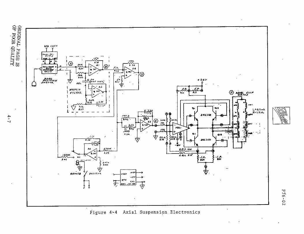
413 Control System
The axial suspension system uses three independent servo loops
to control electromagnet currents An electronic diagram of one
of these loops is shown in Figure 4-4 The heart of the elecshy
tronics is an Inland Controls MA-I DC servo amplifier which is
operated as a current driver to reduce the effects of electroshy
magnet inductance Equations of motion of this driver and an
analysis of the voltage feedback used to damp high frequency
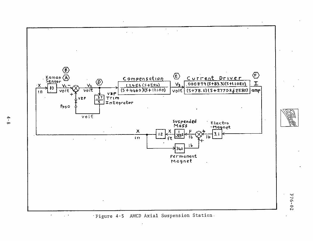
roots are given in Appendix A An analytical block diagram of
the entire servo loop is shown in Figure 4-5 Equivalent points
on the electronic and analytical diagrams are indicated by letters
within hexagons
The axial suspension system has two modes of operation a posishy
tion mode and a virtually zero power (VZP) mode In the posishy
tion mode rim position error is used to command electromagnet
current The rim has high static and dynamic stiffness about
any desired point in the gap In the VZP mode the rim position
set point is modified by positive feedback of the integral of
electromagnet current The result is that the set point is moved
until steady-state current is zero The permanent magnets are
4-6
AA
REHTUtk +26V
4-
C11 7t-Q
Fiue44Aia3upnin7lcrnc
S Cornn- EesoCo p n a cncivCrrent Driver- O deg OI 99 (5C + sm -3 (s + 1 1deg E 1 copy + F
gtosO ~
volf
iE 3 7 T r i m T ntegratadegr
Suspended
Mass
-|ectro
-ria net
16
permanent Magnet
Figure 4-5 AMCD Axial Suspension Station
R 1F76-02
then providing all of the support of the rim Dynamic stiffness
is nearly the same as in the position mode but static stiffness
is actual negative If a downward force is applied to the rim
in the VZP mode it initially moves downward but then slowly
rises to assume a new zero power position above the old equilibrium
position
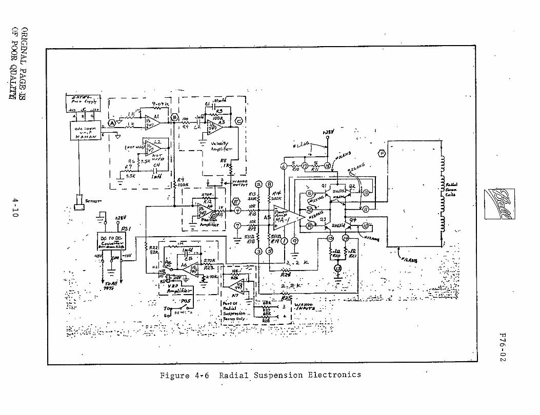
The electronic circuit diagram for a radial servo station is
shown in Figure 4-6 and the corresponding highly coupled analytishy
cal block diagram is shown in Figure 4-7 Again equivalent
points on the two diagrams are indicated by letters in hexagons
The large amount of coupling results from three servos controlshy
ling only two degrees of freedom
Two modes of operation are available a position mode and a WAHOO
mode The position mode is similar to the axial position mode
The WAHOO mode is a zero power mode that produces zero power
operation in the presence of both static loads and rim expansion
This is accomplished by adjusting the position set point at each
station as a function of the integral of the sum of the electroshy
magnet currents at the other two stations
The name WAHOOis derived from the poker game WAHOO This game
is played in a manner such that each player knows what every
other player holds but does not know what he himself holds
Inspection of the WAHOO trim loops of Figure 4-7 reveals that
for VZP trim purposes each servo only looks at what the other
two are doing This innovation was developed by BBRC to meet
the unique requirements of the AMCD
The derivation of the WAHOO concept is given in Appendix B
There it is shown that only the WAHOO concept produces zero
power operaion for both rim expansion and force disturbances
4-9
A00l 51 Ir
A-A-
F
27
ffzo xr
74 VIP KIAk
7
Ems~
n
A7-
I
A1
ter
a 2k-
-
-
-
-
-
I)
Figure 4-6 Radial Suspension Electronics
-KS
Iamp wkin47s Permanent MagnetVeloityPM VPol Aplifir PMEHM E Iectremoqnet
K5 Kmn eae t~j VOS 0bCar respond to Lettered
1vII~rb r - rr m Psitionson Cgrcwit
vol vol Im PosiMoon Pox
SlRtim rtOhkx _Q$)bsS 4lfe I
0niplPfied Cus ren Driver
Gcucv rbinn n i
+ + vt
If
in-7d FigureservoD RailSro
+i
42
F76-02
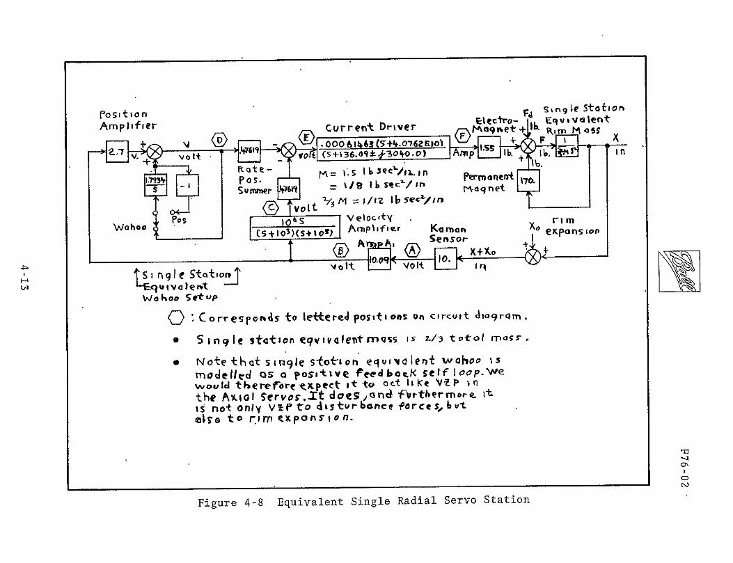
Appendix B also shows that for single station design purposes
a single station can be represented as shown in Figure 4-8 Two
points of interest are immediately evident The equivalent mass
for a single station representation is 23 the total rim mass The WAHOO concept which involves negative feedback to each station
from the sum of the other two stations resolves to a positive
feedback in the single station representation exactly like VZP
in the axial mode This representation can be used for designing
the system characteristic root locations If the characteristic
roots from the single station representation are given by A and
the WAHOO gain is Kc it is shown in Appendix B that the three
station highly coupled set of characteristic r6ots are givenby
(S + 2K )A2
Performance
421 Static Performance
At each suspension station the rim will seek an axial equilibrium
position based on the applied load and the control system mode
(position or VZP) These equilibrium positions can be preshy
sented in one plot as shown in Figure 4-9 The VZP line is a zero current line and has a slope that indicates static instability
however as shown in the next section the system can operate in a
stable manner along this line The most usual operating position
mode point is about 001 cm (025 inches) above the center of the
gap At this point the slope P of the VZP line is about 595
newtonscm (340 lbin)
In the position mode an operating line exists for each set point
of the position sensor A family of these is shown in Figure 4-9
The lines are finite in length because of the limited current drive
capability of the electronics The slopes of the lines are apshyproximately 2600 newtonscm (1500 lbin)
4-12
Stationfost ionsingle
Oecrlx- EquIva1eratArmplifir Current Driver 6 Mks$M9oqmet+ 1m
~~~~~ eroe L~r
Is + Fes I16(7+1210 r0 0 l I-
p 0 1
476 An- Per
u2 IVlt+ -Eg
o tKate - r1 1 StO Sr eq uci o lnk wahoo is
Q Correspornas toa letterd posit~ions on circuit chogr~m
Sinql~e stcton eqviclvJewtmls is 23 totil ma
~odelldas a posattve PeedbctK self IoopVe
t to o-t liKe Vf Pwould ltherefboretxpect fvrthernortn itthe Aol O Servo Xt doesonh
Figure 4-8t EqiaetSnluadapev tto
ekgeto8 rnex e o +non
A F76-02
UP
MAGNET M~A t r
lsrok os NoRMAL
kE-RITI N
P E-Nshy-OMFR
tL UPshy
- j ~
-10
h31G1NL pAGE iS
)F POOR QUML-rI
Typical Static Suspension System Performance
Figure 4-9 4-14
rF76-02
The force sensitivity F of each station is about 138 newtons
ampere (31 lbamp) Hence the force produced by a station
is given by (in English units)
F = 340X + 3lI
422 Dynamic Performance
The analytical block diagram for an axial suspension statiQn is
shown in Figure 4-5 For theposition mode the root locus and
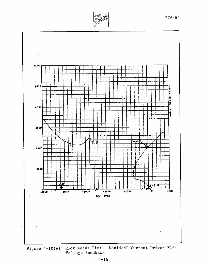
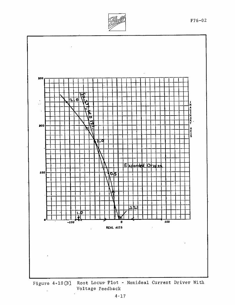
-Bode plots are shown respectively in Figures 4-l0and 4-11 The
root locus plot shows that the dominant pole pair has an undamped
natural frequency mN (which we define as bandwidth) of 171 radsec
(272 hertz) and a damping ratio of28 The Bode plot shows
that the gain crossover frequency wc (which some define as bandshy
width) is 1827 radsec (290 hertz)-and that the system phase
margin is 2320 Both plots show that the lower gain margin
is 22(-131 db) and that the upper gain margin is 201 (261 db)
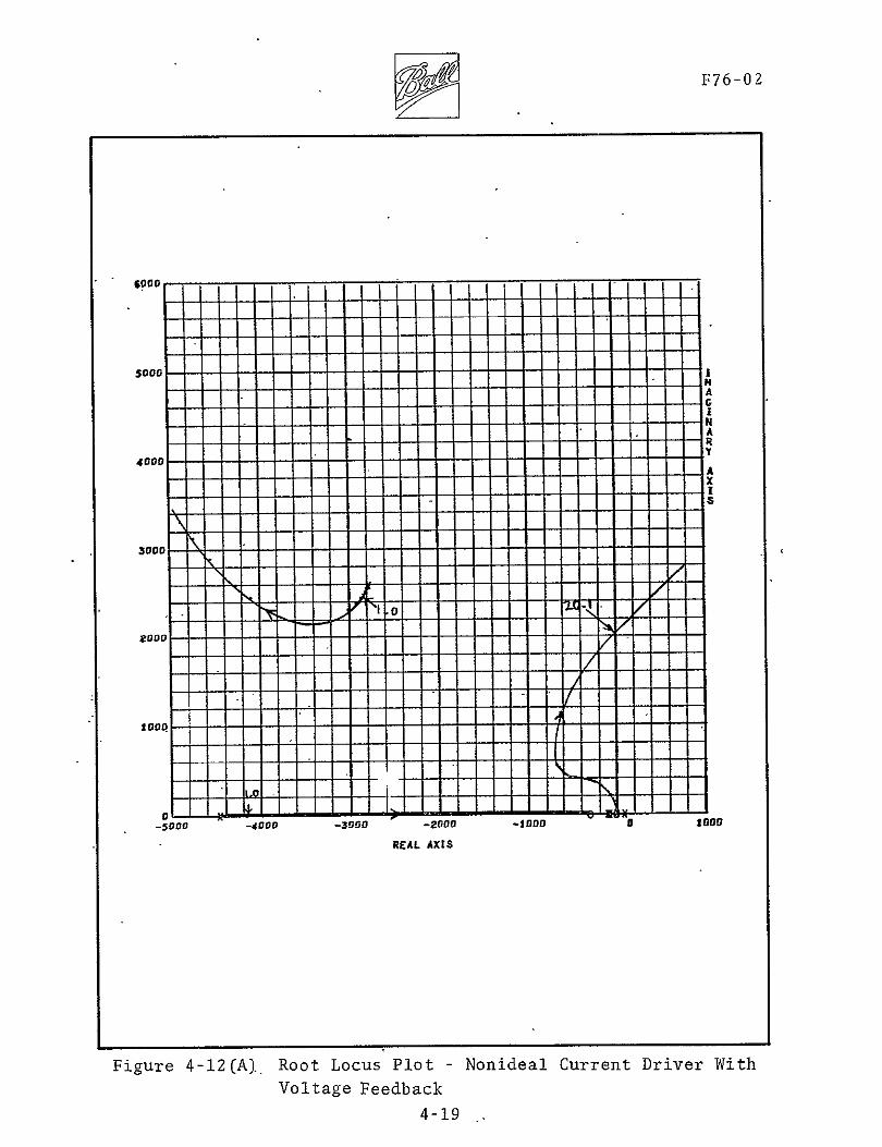
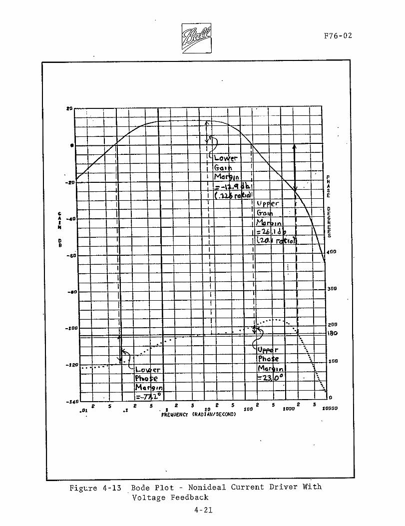
For the VZP mode the root locus and Bode plots are shown respecshy
tively in Figures 4-12 and 4-13 The root locus plot shows that
the dominant pole pair has the same undamped natural frequency
and damping ratio as the position mode that is wN = 171 radsec
= 28 The Bode plot shows that two gain crossover frequencies
at 1823 radsecexist one at0838 radsec (013 hertz) and one
(2903 hertz) The phase margin at the lower crossover frequency
is -772 and that at the upper crossover frequency is 2300
Both plots show that the lower gain margin is 226 (-129 db)
and that the upper gain margin is 2011 (261- db)
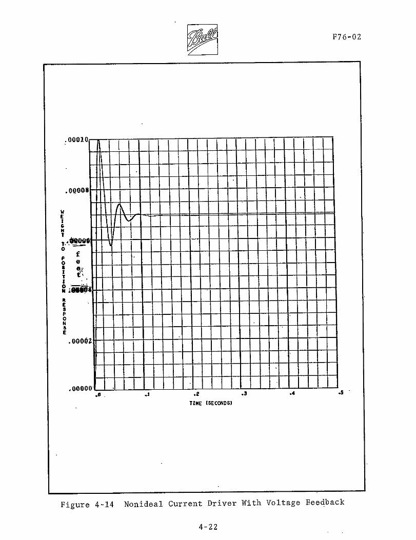
The response due to the step application of a one pound weight
is shown for the position mode in Figure 4-14 and for the VZP
4-15
OF76-02
1 -DD
-- A I 1
I I
i
3000 --------------------------------- ___tN
-5000 -400 -30U -2ODG -t I lo oD
REAL AXIS
Figure 4-10(A) Root Locus Plot - Nonideal Current Driver With
Voltage Feedback
4-16
---------------------------------
7F76-02
-I- 111 1-l Z9D
io oI 1ll t A
G
80 ----------- 0 aEu----------------shy-4--
FigueRot41001LcusPlo - Nnidal Crret DrverWit
-1---4-17
I I
F76-020
14-HLowler
)2 I__ _ p
1 N I-- A =20 41 r
I tIse0_ __ _ _ 4 6 2 4 68100
s 10 log H00 6 10009 FREQUENCY (RADIAWS$ECOND)
Figure 4-11 Bode Plot - Nonideal Current-Driver With Voltage Feedback
4-18
7F76-02
$oo I5iI000 I1
T 1 Ii
-A
S4+
N A
4000 R--- - - - - -
V A x
103 000 40 30 29
urn rvrWtFi1r -12A Roo Lou7lt-Nnda
Voltage Feedback 4-19
V gF76-02
ii
- I I I
I I I II
I lii
-I I
II I iishy
II - - -i-l
Fgr 4-2B o otocu PltrNndaCrefl rive
With Voltage Feedback
4-20
F76-02
I i E
A -4 G
E- 60I jUroI(
I
1A2zS1 me RI
3s F-1-L
IIsoM 3en
4) e r
-120---- -Marlin
fla e =2300
-140 shy
1 1 10 10g 2000 1090r FREQUENCY (RADIANSECOND)
Figure 4-13 Bode Plot - Nonideal Current Driver With
Voltage Feedback
4-21
012
F76-02
00010
00008
pound E
0
p
0 00
0zkc0
0
E
- -
4+-F
- - -
Nshy- - - - - - -
4
- -
5
-4-2
AF7602
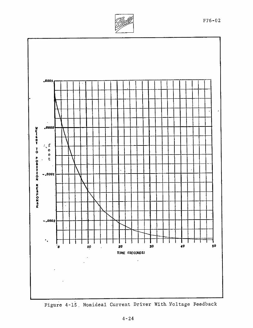
mode in Figure 4-15 The response for the position mode settles
out at 6941E-5 feet (002 cm) This yields a position mode
stiffness of Stiffness 6 1 lb
6941E_5 t X feet
1 12006 lb (21021-
N
69Th-ft Tni in cm
The response for the VZP mode settles out at -2451E-4 feet
Thisyields a VZP mode stiffness of
1 lb feet = lb NStiffness = 2451E4 ft X 12 in -3400 i (595 E-
Note that the stiffness in the VZP mode is just that of the
permanent magnet and that the movement in this mode is toward
the applied force That is if a weight is placed on the rim
in the VZP mode the rim will move up
Further insight into the system can be found by examining Ap2
pendix C When using current driirers the usual tendency is to
ignore the high frequencydynamics and simply say that the
output current is the input voltage times a constant This can
be very misleading in the case of AMCD- In Appendix C are shown
root locus plots using both an ideal current driver arid a nonshy
ideal current driver without voltage feedback It shows that
voltage feedback is necessary for the axial suspension Also
shown in Appendix C are Nyquist plots and phase-gain root locus
plots of the nominal axial systemthat is the system using curshy
rent drivers with voltage feedback The esoteric phase-gain root
locus plot shows on one plot the sensitivity of the system roots
to change in both gain and phase For example it shows what
would happen if an additional 300 of phase lag were added to the
system from some unknown source
4-23
F76-02
0001
I f
I 0 e
eshy
0a T 1-0001-shy0N
ft E F 0
E a
- 002--------------shy
0 t0 20
TINE (SECONDS]
30 40 50
Figure 4-15 Nonideal Current Driver With Voltage Feedback
4-24
F76-02
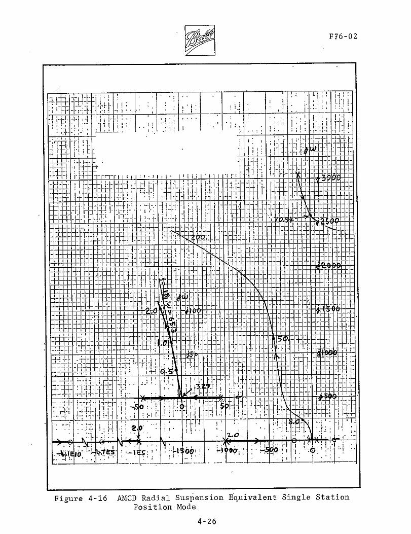
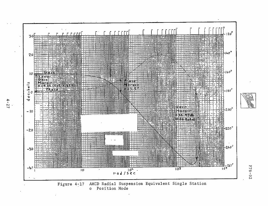
The equivalent single station radial analytic block diagram is
shown in Figure 4-8 It is very similar to an axial station
The root locus and Bode plots for the position mode are shown
respectively in Figures 4-16 and 4-17 The root locus plot shows
that the dominant pole pair has an undamped natural frequency
(bandwidth) wN of 653 radsec (104 hertz) and damping ratio C
of 18 The Bode plot shows that the gain crossover frequency
is 666 radsec (106 hertz) and that the phase margin is 1350
Both plots show that the lower gain margin is 329 (-965 db)
and that the upper gain margin is 7054 (3697 db)
The root locus and Bode plots for the WAHOO mode is shown in
Figures 4-18 and 4-19 The root locus shows that the dominant
pole pair has an undamped natural frequency of 674 radsec
(107 hertz) and damping ratio of 16 The Bode plot shows that
the upper gain crossover frequency is 691 radsec (110 hertz)
At this frequency the phase margin is 1260 Not shown is the
fact that the system also has a lower gain crossover frequency
of 594 radsec (095 hertz) At this frequency the phase marshy
gin is -715 Both plots show that the lower gain margin is
389 (-821 db) and that the upper gain margin is 6701 (365 db)
The large upper gain margins for both the position and the VZP
modes indicate that current driver voltage feedback is not needed
Considerable rim bending instabilities were encountered during
the design Early in the development the axial system was
designed to be overdamped This caused a bending mode to be
driven unstable The compensation was adjusted experimentally
until the bending became stable Unfortunately this reduced
the lead in the system resulting in the present underdamped sysshy
tem It is believed that bending will present no problem at
high spin rates because of the effective stiffening of the rim
4-25
6F76-02
_____ - _ r ____I___
141
IT___lishy
1 ii
1 F]
eir
t lj~
4-
J TT a p-
III NEA
fiIT WBKsITlK j1_11IIi I-
I
e
-Fshy
Y]-111 ji
1i1fln 4--I r
I i--I -
TFiJ-WL 1
_1(-Ii4 - I
I~ ~ ~iA_~2I ___ ii- 11 IFt-Ih
iT
h~ -iH T
+~ji+ih Iplusmn
_ _ _+ I kt ~h-II
+ LILY -
7 SO bullj
Figure 4-16 AMCD Radial Suspension Equivalent Single Station Position Mode
4-26
Elll csl- tLL[ 11--- 1_ il
V
1 MIN
2 0 H qL2~14-0IT
I M Ill 1OIHI
+-o ip Lr g
Ti I -0 1- b1 -- i
Ij _IUSi 1PIN - il
--i
41i L -I I - d jir ~J I I
00 -o
ro-d 5 c
Figure 4-17 ANCD Radial Suspension Equivalent Single Station o Position Mode
7F76-02
1LjI_----- Li -III iI - - I -shy-F ]e2 1
Is- Lr [_I
r ir -L-j 11I IALI _ _ _ ___ 2_
E11LLN1LALIF TYC -- td It 11
- KI
S1 1 1 1--shy
II
I r 11
FLL-1
U - I 4
E~~~~fL
__
f Lplusmn Xi ILIi _ _
- ii _ _ i
- H --
--------
A-1 1 F - JT-1
-- t-ti -~r -r I- t - --- IL I
IIJlri-tlrht1f tI
_+ _ l PillS 1 I
Figure 4-18 AMCD Radial Suspension Equivalent Single Station
o Wahoo Mode
4-29
rm~r 1 u i rrrrF r r r
4
130
o
I -4
7 7 1-shy iAb d
llt h
-30 Tfij4i i ~
- n0 t
Figure 4-19
01 AII-
I uji r a sec
AMCD Radial Suspension Equivalent Single Station o Wahoo Mode
AF76-02
and the averaging effect on modal pick-up caused by the bending
modes moving rapidly past each position sensor
As the rim is spun up the three axial stations become more and
more coupled by nutational effects The result of the coupling
is to reduce the dominant roots damping ratios more-and more to
the point the system could go unstable if the rim is spun fast
enough It is believed that this tendency could be greatly
reduced or possibly eliminated by the proper combination of cross
feeds from one axial suspension station to the others
4-30shy
DF76-02
50 DRIVE SYSTEM
51 System Description
The AMCD drive motor can be thought of as a large permanent magshy
net brushless dc torque motor Samarium cobalt magnets are
bonded into the rim at regular intervals The two phase armashy
ture is segmented with a winding set at each of the three susshy
pension stations Commutation is controlled by Hall effect senshy
sors mounted near the rim which sense position of the samarium
cobalt motor magnets
52 Magnet Selection
Alnico was considered along with samarium cobalt for the permanent
The large air gap and segmented winding structure meanmagnets
the magnets will become nearly air stabilized The rim was designed
with a small outer lip to hold the magnets This was done to
isolate the drive from the suspension as much as possible without
and complexity to the rim than necessary Thisadding more mass
small lip implies a short magnet Samarium cobalt has high
strength for short lengths and does not pay a penalty for air
In fact it is very difficult to demagnetize thisstabilization
material
cm (55 inches) diametertby 64 cmSamarium cobalt magnets 14
(25 inches) length were selected and bonded into the rim with
polarities alternated
The rim contains a total of 72 magnets spaced 73 cm (288 inches)
apart
5-1
53
--F76-02
Core and Winding Design
Each armature segment consists of a pair of bar-shaped winding
assemblies one above and one below the rim
Sit cos sla 0S SMa
cores in a singleThe windings-are wound toroidally around the
layer The figure above shows only the cross-section 6f conshy
ductors in the air gap as the conductors passing around the other
side of the core add nothing to torque and serve only a connectshy
ing purpose The bar-shaped cores are easy to wind and result
in a compact structure The single layer of 18 conductors adds
very littleto the overall air gap This effective electroshy
magnet design was suggested by P A Studer of Goddard Space
Flight Center
Ferrite material was chosen for the core to reduce losses Fershy
rite also is easily machined into the required irregular shapes
The windings are grouped into two phases SINE and COSINE each
of which acts upon three magnets at each motor segment In operashy
tion current in one phase is acting on the magnets while current
in the other phase is reversing in preparation for a magnet of
opposite polarity
5-2
DP76-02
54 Motor Commutation
Hall sensors act as commutation devices for the motor They sense the position of the permanent magnets in the rim and cause the drive coil currents to be switched according to magnet position
The sensors are mounted in pairs one above the rim and one below for each winding phase Outputs from each pair are summed so that the switching position is not affected if the rim moves up or down within the air gap The SIN pair controls current on the SIN windings of all three motor segments and likewise the COS pair
of Hall sensors controls all COS windings
55 Motor Control Electronics
A block diagram of the motor control electronics is shown in Figure 5-1 For each phase the Hall sensor outputs are summed and amplified to drive-threshold detectors These detectors sense magshynet position and polarity The phase control logic determines the
timing and polarity of the motor coil drivers Interconnections between the two phase control logic blqcks provide positive direcshytion and start-up information
Each of the six coil drivers controls a phase at one of the motor
segments Associated with each driver is a coil current sensor which monitors the current in that winding All six of these
current sensorsreceige a common reference from the speed control
potentiometer When current in that particular winding reaches the reference level the driver turns off until the current deshy
creases This prevents the current from reaching destructive levels at low speeds and acts as a speed control at high rim
speeds
Since the coil drivers are either full on or off a very efficient drive is achieved At low rim speeds the drivers operate as a
5-3
56
F76-02
conventional PWM (pulse width modulated) amplifier A quite faithful square wave current of controlled amplitude is fed to the coils At high speeds high acceleration (or deceleration)
is possible with the drivers full on for the period between magshynets with current rise and fall limited by the inductance of the
coils
Torque Calculations
The equation for the force betweena magnetic field and a current
carrying conductor-is
F = BLI
where
F = Force in Newtons B = Flux Density in Teslas (WebersM~ter )
L = Conductor Length in Meters
I = Current in Amps
If the magnetic field is created by a permanent magnet the force
can be considered to act on the magnet if the conductof is held
stationary which is the case with the AMCD motor
To arrive at design force each of the factors B L and I must
be evaluated
A force calculation will be made for one magnet face interacting
witha coil This can be then doubled to account for both ends of the magnet next tripled to take into account the three magnets in one motor segment and tripled again to realize the total force for the three motor segments Then using the radius of the rim
we can calculate developed torque
5-4
F76-02
Flux Density Calculation (B)
The large air gap makes it difficult to- estimate how much of the
magnet flux will couple through the winding core and how much
will be lost to leakage A measurement of coupling flux was made
using a pair ofsoft iron bars similar to the ferrite corasi
SEJSE C0115
SOFr iROh
-4 Webers with magnets of averageThe flux measured was 0375-x 10
strength
core must-be convertedThis flux that couples through the ferrite
to flux density (B) in the air gap where it interacts with the
coil windings There are two practical Choices for doing this
We can assume all the flux goes straight up from the surface of
the magnet andreacts with only those turns above the magnet or
we can assume the flux spreads out evenly over the winding area
Of course the truth liesand-reacts with all the turns equally
an adequatesomewhere in between but the second approach gives
approximation
The winding area in the air gap for one magnet coil phase is 2
19 x 36 cm or 68 cm
Flux density then is
-44m _ 0375 x10 Webers 2 0055 WebM-B_=A = 4 2A - 68 x 0-4 m
5-5
F76-02
Conductor Length Calculation (L)
are 28 turns with an effectiveIn the winding phase area there
length of 19 cm each
Total effective length is then
L = -19 x 28 = 532 cm = 0532 M
Current (I)
that the coil drivers and wiringThe elbctronics are designed so
canhandle 4 amperes Also the inductance of the coils was
examined to be sure that currents of this magnitude can be
reversed at maximum rim speed frequencies with a 60 volt power
(and torque) will then be calculated for thesupply Force
design maximum of 4 amps
Force
We can now calculate force from the equation
F = BLI
= 0055 x 0532 x 4 = 0-1-17 Newtons
Recall that this is the force for a single magnet surface inter-
For the total motor this is multiplied by 18face
Total Force = 0117 x 18 = 176 Newtons
576
0F76-02
This times the magnet radius (0838 meters) gives total torque
Total Torque = 176 x 0838 = 176 Newton-Meters
(13 lb-ft)
A small (14 diameter) test wheel was built to check the above
torque calculations Acceleration measurements were made and
from the known wheel inertia torque was determined Correlation
within 10 of the calculated torque was achieved
5-7
S in Hall Sensors
Summing
Amp
[A Threshold Sin Phase Coto-rie
DetectorsLoi
SnB1Sin
Sin C Driver
ol
Hall Sensors
~ Amp=ApDtcosLogic
etctr Control -- Die Col Ci~
Summing Threshold Phase Cos B Driver
iCosCos
Ci Co
Figure 5-1 Motor Control Electronics
C
aF76-02
60 REFERENCES
1 Anderson Willard W and Groom Nelson J The Annular
Momentum Control Device (AMCD) and Potential Applications
NASA TN D-7866 1975
6-1
F76-02
APPENDIX A
CURRENT DRIVER EQUATIONS AND TRANSFER FUNCTIONS
A-i
F76-02
Appendix A
Current Driver Equations and Transfer Functions
When using current drivers the usual tendency is to ignore the
high frequency dynamics and simply say that the output current is
just the input voltage times a constant This was very misshy
leading in the case of MCD-as shown in Appendix C The circuit
diagram of a current driver with voltage feedback and its equishy
valent diagram are shown in Figure A-i -
v A T5It
Figure A-I Current Driver and Equivalent Circuit
A-2
F76-02
The beginning equations of motion are the following
Rl11 RM -- R 10
-RM SL + R2 2 -(SL + RC) I= A(TS+I)-)V + ARI(TS+l)shy
-R 2 -(SL +R c) SL + R3 3 + S_ C I 3 0
where
R1 lt= R1 + R2 + RM
2 RM + RC22
R33-- R2 + RF + RC
Transposing I1 to the left hand side we obtain
R11 -RM -R2
-RM(TS+l) + AR 1 (TS+l) (SL+R 2 2 ) -(TS+1) (SL+Rc) 2 A S-SR22 S L+SR33+-l
What we really want is the current through the inductanceshy
1 2 T3
Adding this equation to the system we obtain
C1 C12 C1 3 0 II 1
B2 1 S+C 2 1 A 2 2S2 +B 2 2 S+C 2 2 A23s2+B 2 C 3 0 12 A V
B31S A32S2+B32S A33S2+B 3 3S+C 3 3 0 13 0
- -1 1 1 1 0
A-3
eF76-02
where by definition
-=A32 -LC R11 B22 = L+TR 22
= - C22 R22 B32 = RCCl2 RM
C13 =-R 2 A23-= -TL A33 = L
= R33B21 = -RMT B23 = -L-TRC B3 3
C = ARI-RM C = -RC C =C -I
= -R2A22= TL B31
If the voltage feedback is removed these equations reduce very
simply to
-RMIRlI+R2+RM
+ AR1 (SL+R+RM)(TS+ 1j1 2 = AKRM(TS+I) We want thewhere 12 is the current-through the inductance
transfer function 12V First divide the secondequation through by
LT to obtain
-RMR I+R2 +RM
(R C+ PM j] IAL 1 V S+L-iIARI[ RM L (SplusmnT -1)+L -lT -1A
A-4
F76-02
Then by Cramers rule
2 CR1+R2+RM)AL -1T-+RML -1(S+T- 1 )_L-1T- 1 AR1
V7 -1 r- 1 2-1 - lshy(RI+RZ+RM)(S+T +L (RC+RM) -R ML l(S+TI)+L ITIARIRM
(R2+RM)AL -T - I(S+Tshy
-(R1+R 2+RMM)(S+T 1 )(S+L-1 RC)+L -RM(R1+R 2)(S+T-I)+L T ARIRM
Further manipulation yields
S+T-1 +(R 2 +RM)ARM T12 RML -
V - 2+RM) 1 L-+RR [2 wT-ARI-L 1RM(RI+R2 -
S+T )(3+L Rc) + RR+Tl+R---
Finally the desired current driver without voltage feedback
transfer function is given by
12 RML- S+T -1 +A(I+R2 RfIj
V (RLR-+RM) - -1 LRM(RI+R2 ) (ST 1 [7AR 1 RS5 + R2 +RMR R1 L Rk 2 )
A-5
76-0 2
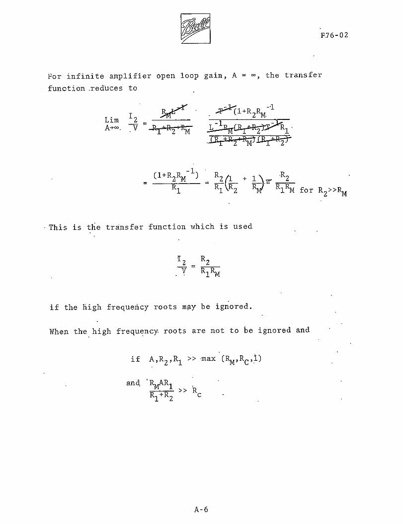
For infinite amplifier open loop gain A = the transfer
function reduces to
2R Lim 12 = R1_ 2M
(l+R2RM- R2
R - RYR RR)r112RM for R2gtgtRM
-This is the transfer function which is used
I2 R2 12 R 2V RIRM
if the high frequency roots may be ignored
When the high frequency roots are not to be ignored and
if AR2R1 gtgtmax (RMRC-i)
and RMARlRjR2gtgt
RI+R 2 c
A-6
rF76-02
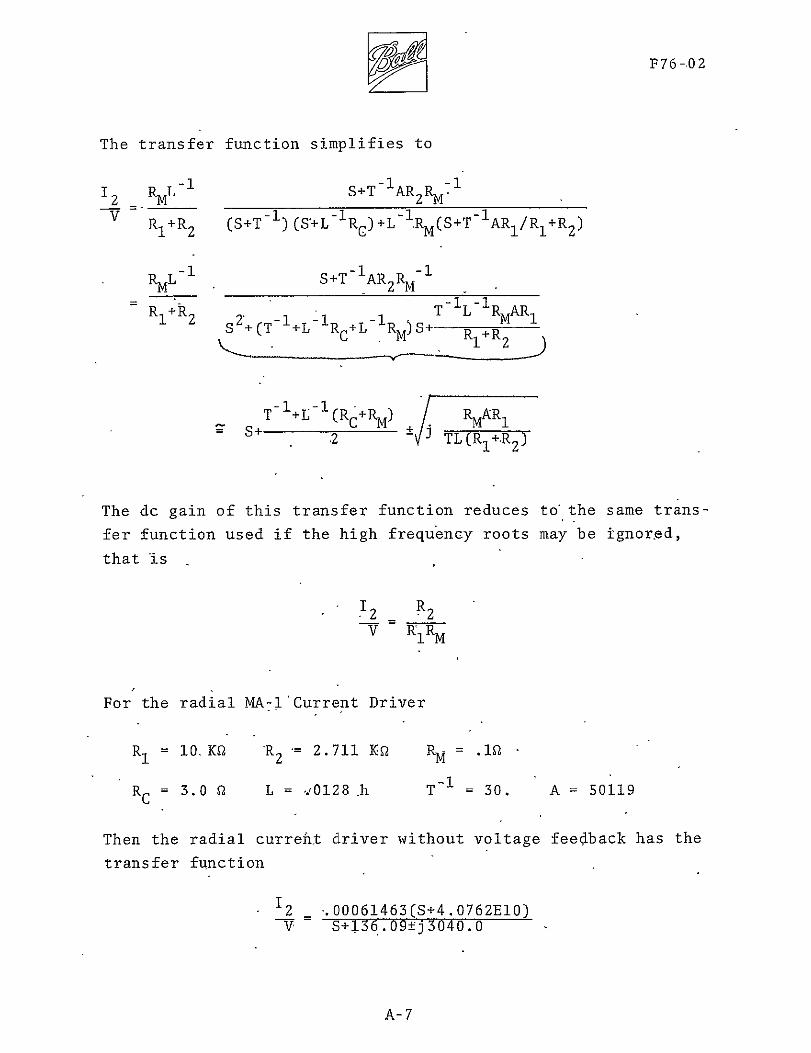
The transfer function simplifies to
S+T- AR 2RM1
12 RML-
V R1+R2 (S+T-)(S+L -Rc)+L- RM(S+T-AR1 R1 +R2)
RML-1 S+T-1AR2RM-
R1 R2 S2+ -1 -1 -1 T 1L-1RMARl - A
S +(T- +L -Rc+L RM) S+ R+R
T- +L- (RG+RM) TRLAR
2 (RI+R2)
The dc gain of this transfer function reduces to the same transshy
fer function used if the high frequency roots may be ignored
that is
2 R2 V RIRM
For the radial MA-lCurrent Driver
RI = 10K R 2 = 2711 KQ RM 10
RC = 30 Q2 L = 0128 h T - 30 A 50119
Then the radial current driver without voltage feedback has the
transfer function
12 _-00061463(S+40762E10)
V S+13609plusmnj30400 shy
A-7
F76-02
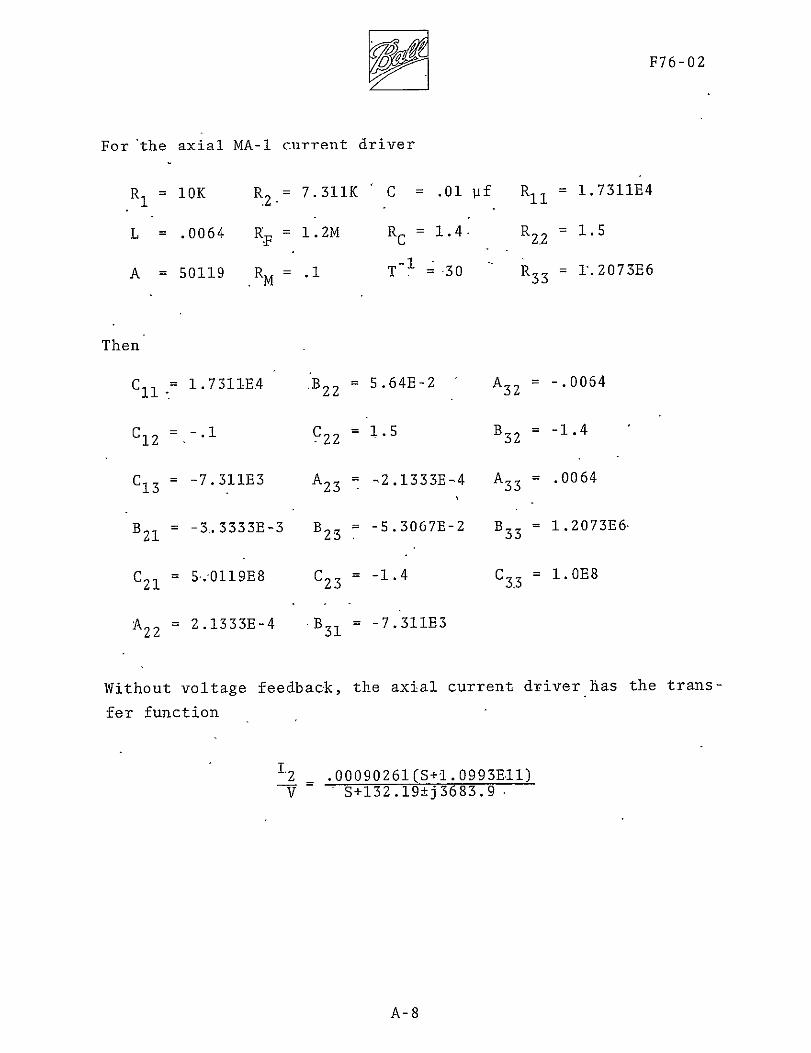
Forthe axial MA-I current driver
R=1 10K R2 = 7311K C 01 1f R11 = 17311E4
L =0064 f = 12M R = 14 R22 =15
A = 50119 RM = 1 T- = 30 R 33 I2073E6
Then
= C11 7 17311EA B2 2 = 564E-2 A 3 2 -0064
Cl2 = -- 22 = 15 B = -14
== = -7311E3 -21333E-4 A33 0064C13 A 23
B21 = -33333B-3 B2 5 -53067B-2 B 12073E6
C21 = 50119E8 C2 3 - 14 C3 = 1OE8
= A22 = 21333E-4 -B3 1 -7311E3
Without voltage feedback the axial current driver has the transshy
fer function
2 00090261(S+l0993B1)
V S+13219plusmnj36839shy
A-8
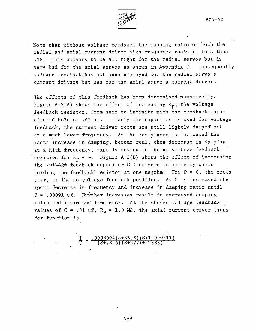
7F76-02
Note that without voltage feedback the damping ratio on both the
radial and axial current driver high frequency roots is less than
05 This appears to be all right for the radial servos but is
very bad for the axial servos as shown in Appendix C Consequently
-voltage feedback has not been employed for the radial servos
current drivers but has for the axial servos cur-rent drivers
The effects of this feedback has been determined numerically
Figure A-2(A) shows the effect of increasing RF the voltage
feedback resistor from zero to infinity with the feedback capashy
citor C held a-t 01 lif Ifonly the capacitor is used for voltage
feedback the current driver roots are still lightly damped but
at a much lower frequency As the resistance is increased the
roots increase in damping become real then decrease in damping
at a high frequency finally moving to the no voltage feedback
position for RF = Figure A-2(B) shows the effect of increasing
the voltage feedback capacitor C from zero to infinity while
holding the feedbackresistor at one megohm For C 0 the roots
start at the no voltage feedback position As C is increased the
roots decrease in frequency and-increase in damping ratio until
C = 00091 f Further increases result in decreased damping
ratio and increased frequency At the chosen voltage feedback
values of C = 01 vf RF = 10 MQ2 the axial current driver transshy
fer function is
I 0008994(S+833)(S+l099EII) V (S+786)(S+2771plusmnj2583)
A-9
~~~ L~Trrrl~I I~ I II 4
Jots_1 nr_- r177I 7F I i0K IIII __ riiTTh
17shy
tkP M T7r
Hl4plusmn ------ IIr-1-----~ -- - I -
CDl7E-~ ttbifil
LA14 -T-- 4+ -
C T -I I
H -rTH V i H
-HE I
Figure A-2 Effect of Voltage Feedback on AMCD Axial Current Drivershy
AF76-of -
APPENDIX B
THE WAHOO CONCEPT
B-I
7F76-02
Appendix B
The WAHOO Concept
Introduction
Two conditions may occur which cause the radial electromagnets
to draw more current than necessary First if the rim is tipped
This forcea gravitational force tends to pull the rim sideways
at the expense of causing the electro-shyis countered by the servos
magnets to draw more current Second as the rim spins up
centrifugal forces-cause it to expand To each radial sensor
as rim movement to be countered by thethis expansion is viewed
to try to pullservos So each electromagnet draws more current
are directed inward andthe rim inward But since the forces all
spaced 120 a-round the rim the resultant of the forces is zero
so the rim does not move The net result of the expansion then
is thatonly the current in the electromagnets increases Trim
loops are developed in this appendix which lead to VZP (Virtually
Zero Power) operation for the radial servos when either the rim
is tipped or expands or both The system employing these trim
loops is called the WAHOO system
Because the three radial servos are controlling only two degrees
of freedom the radial servo system is very highly coupled This
very high degree of coupling makes it difficult to design each
servo as a single uncoupled system Hence in this appendix we
also develop equations to show how the three-servo radial system
may be designed using a single station servo radial equivalent
Development of the WAHOO Concept
The AMCD rim is suspended radially by three servos pulling on
it from the inside much like shown in Figure B-1
B-2
F76-02
Kim
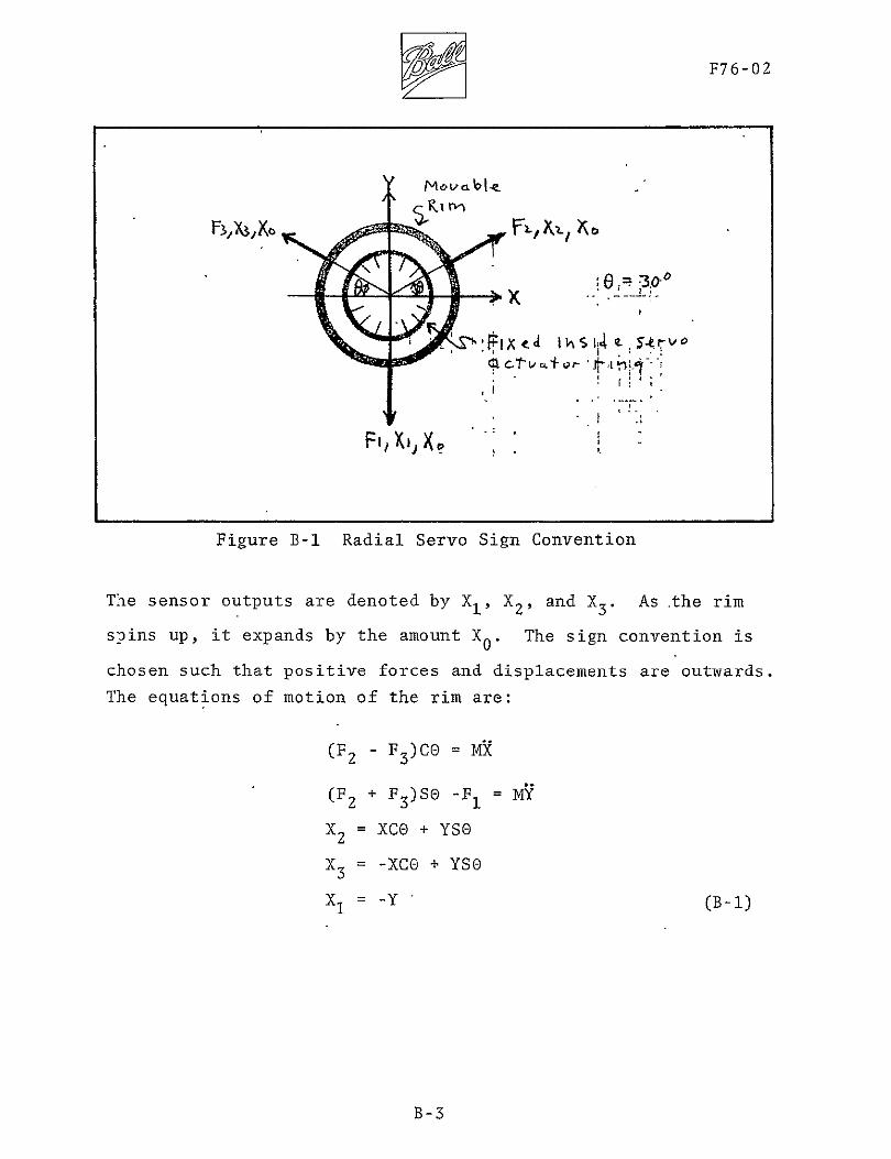
Figure B-i Radial Servo Sign Convention
The sensor outputs are denoted by X1 X2 and X3 As the rim
spins up it expands by the amount X0 The sign convention is
chosen such that positive forces and displacements are outwards
The equations of motion of the rim are
(F2 - F3 )Co = My
(F2 + F3)s8 -F1 = my
X2 = XCe + YSe
X3 = -XCe + YSO
XI = -Y (B-i)
B-3
F76102
The force acting at each station is composed of a permanent
magnet force and an electromagnet force That is
Fl = P(XI+X0) + E D1
= P(X2+X0 ) + E D2 (B-2)F2
F3 = P(X3+X0 ) + E D3
these equations are-combined with the servo equations in Figure
B-2
From the block diagram the quations of motion using five variables
are
V1 = Kp(-Y+X0 ) -S)(KsVi+KcV 2+KcV 3) EKRN_1
Y = M--p(-Y+X0)+DR (-Y+X 0)+ EV1 +pSC(YSe+XCplusmnX0 )
EKRN -fD se(YSe+XCe+Xo)- ESeV 2 + PSO(YSe-XCe+X0 )
EKRNK sOCYSe-xce-Xo)- nsev 3 + FY
-V2 = K (YSO+XCeplusmnXo)-(lSKsV2+KcVI+KcV3)
EKRN = 1=M PcO(YSe+XCe+X 0 )- D C(YS+XCc+X0)- ECOV 2
EKRN -PCO(YSe-XCO+X 0 )+ ce(YSe-XCe+X0 )+ ECOV3
)V3 = K(YSe-XCO+X0 )-(SJ(KsV 3+KcVI+KcV2 (B-3)
B-4
+ SFt
+- K + X0
+ T- SID
fRi
Figure B-2 MICfl Radial Servos With Trim Loops
7F76-02
Rearranging
(S+Ks)VI+KpSY+KcV 2+KcV 3 = KPSX0
-M-1DEv+[DS2 -DM-Ip(1+2SD)+M-EKRN(1+2S2 0)]y
+M-IDESOV2 +M-1 DESOV 3 = [M-IDP(-1+2S)+MWIEKRN(I-2SO]XO+MDFy
KcV -KpSSY+(S+Ks)V2 -KpCeSX+KcV3 = KpSX0
M- 1DECOV 2 +[DS 2DM- P(2c0 )+M-1EKRN(2C2 )]X-M-IDECOV 3 = 0
KcVI-KpSSY+KcV 2+KpCeSX+(S+Ks)V 3 KPSX0- (B-4)
Since 0 = 30
I+zs2 -1+2(5)2 = 15
-- 1+2S = -1+2(5) 0
2C = 2 )2 = 15 (B-S)
Using these simplificatfons the Laplace transformed radial
servo equations of motion in matrix form are
(S+Ks KpS 0 KC KpS 0DSL KC V1
-1IDE +lSMIEKRN SM- 1flE 0 SM- DE Y 0 M D
-1$M IDP __ __
KC 5KpS (SK S ) SrI KpS X6 V2 KK SX 0 + 0 Fy
DSz--shy
SM- 1 DE - SMDE0 0_- 54M +lSM 1 EKjN x 0I 0
-5KpS K 54 KPS (S+Ks) KpS 0KC V3
B-6 (B-6)
F76-02
The system characteristic equation is the determinant of the
coefficient matrix With much algebraic effort it can be
reduced to
A = (S+Ks+2Kc)X
FKRN-ISM- DP)+lSKpM- DES]2[(S+KsKc)(DS2 +SM-
(B-7)
Now lets simplify the expression by-removing the high frequency
roots In the Cambion hardware
KRN 107 S for low frequencies
D (S+1000)(S+10000)
With this approximation KR = D = and N = S Then
2+lM ES-lM P)+lSKpM-1ES] 2A = (S+Ks+2KC)[S+Ks-KC)(S
So the roots separate into -(Ks+2Kc) and two identical sets
within the brackets Immediately we see that Ks+2KC 2 0 for
stability Now looking within the brackets we see that S2+
1SM-ES-l5M-P represents the permanent magnet roots at
+lSM-IP moved to the left some by the rate feedback however
one remains in the right half plane Taking these roots and the
one at -C(Ks-Kc) as poles of a root locus plot and S as the zero
Figure B-3 shows that for stability KC a KS
B-7
0F76-02
Kct IKSKczk 5
Figure-B-3 Effect of Trim bull Loop Gains
Les look at three special cases
I No Trim-Loop KC = KS = 0 No VZP
A = s3 [(S2 +lSM-IES-lSM-iP)+iKIPMlE] 2 (3-8)
There are three roots at the origin from the three unconnected
integrators and two identical quadratic pairs The system is
stable
II No Cross FeedTrims KC= 0
-ISM IP )+ I S5pMIEs]2A = (S+K) [(S+Ks2) I Es(B-9)
This is unstable-for both signs of KS self trim loops alone
will not work
B-8
F76-0
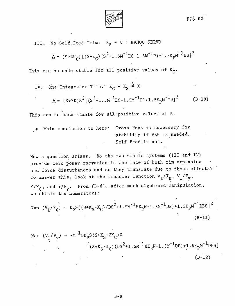
III No Self Feed Trim KS = 0 WAHOO SERVO
2
(S+2Kc) [(S-KC) (S2+lSMIES-l5M1P)+lSKpM-1ES]YA
This-can be made stable for all positive values of Kc
IV One Integrator Trim KC = KS = K
2 (B-10= (S+3K)S2[(S2+SM-1ES-lSM-Ip)+l5KpM-I[
This can be made stable for all positive values of K
Main conclusion to here Cross Feed is necessary for
stability if VZP is needed
Self Feed is not
Now a question arises Do the two stable systems (III and IV)
provide zero power operation in the face of both rim expansion
and force disturbances and do they translate due to these effects
To answer this look at the transfer function VIXp) V1 FYI
From (B-6) after much algebraic manipulationYX0 and YF
we obtain the numerators -
Num (VIX) = KpS[(S+Ks-Kc)(DS 2+lBM 1 EKRN-lSM-1DP)+lSKpM 1 DE S] 2
(B-11)
Num (V1Fy) -M-1DKpS(S+Ks+2Kc)X
[(S+Ks-KcM(DS 2 +SM -1EKRN-I MIDP)+lSK M-IDEs]
(B-12)
B-9
~F76-02
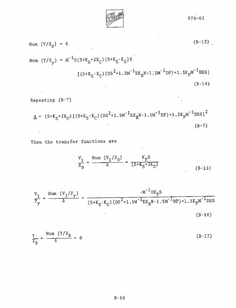
= (B-13)Num (YX 0 ) 0
Num (YFy) = M-D(S+Ks+2KC) (S+Ks-KC)X
[(S+Ks-Kc)(DS2+S5M-BKRN-1 SM- DP)+1SKPM-lDBS]
(B-14)
Repeating (B-7)
IDES] 2 A = (S+Ks+2KC) [(S+Ks-Kc)(DS2+1sM-IEKRN-15M-ID)+I5KpM-
(B-7)
Then the transfer functions are
VI Num (VIX0) KpS
X0 A(S+Ks+2K C) (B-IS)
-M-IDKpSNun (VIFy =VI
Fy A (S+KsKc)(DS2+1 SM-1EKRN-1SM 2Dp)+I5Kp-DES
(B-16)
(B-17)y Num (YX0 X0
B-10
D F76-02
Y M 1D(S+Ks-Kc) (B-18)
Fy (S+KsKc)(DS2+SMIEKRN-ISM- IDP)+lSKpM-DES
Now we can answer the question
WAHOO Servo KS = 0
Because of the S in the numerators of V1X 0 and V1Fy the steady
state power goes to zero for both rim expansion and force disturshy
bances From YX0 the rim does not translate for rim expansion
From YFy the rim does translate for disturbance forces with a
stiffness of
Y- = = -1SP (B-19)S 0
Therefore the rim translates toward the disturbance
Single Integrator Trim KC = S
From V1X0 the steady-state power goes to zero for rim expansion
With KC = KS1 the S cancels out of the numerator of VIFy thereshy
fore the system power is not zero for force disturbances From
YXo the system does not translate for rim expansion From YFy
the rim does translate for force disturbances with a stiffness
of
F = 0 = 15(KpB-P) (B-20)
B-I
~F76--02_
Therefore the rim translates away from the disturbances with
the same stiffness it has with no trim
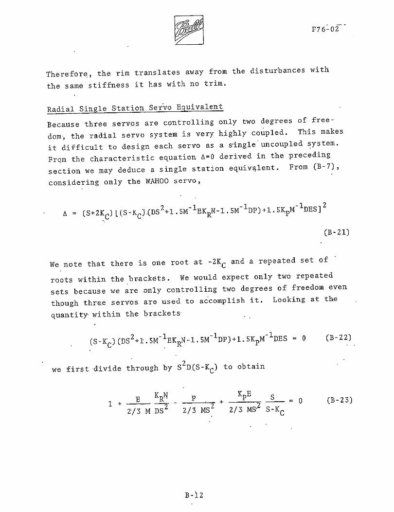
Radial Single Station Servo Equivalent
Because three servos are controlling only two degrees of freeshy
dom the radial servo system is very highly coupled This makes
as a single uncoupled systemit difficult to design each servo
From the characteristic equation A=0 derived in the preceding
section we may deduce a single station equivalent From (B-7)
considering only the WAHOO servo
A (S+2Kc)[(S-Kc)r(DS2+M-l BKRN-ISM-1 DP)+5KpM 1DES]2
(B-21)
- a repeated set ofWe note that there is one root at 2KIc and
We would expect only two repeatedroots within the brackets
sets because we are only controlling two degrees of freedom even
though three servos are used to accomplish it Looking at the
quantity within the bracketsshy
-1DES 0 (B-22)(S-Kc)(DS2+ISM-1EKRN-1SM-1DP)+lSKpM
to obtainwe first-divide through by S2D(S-Kc)
KRN KpE S 0 (B-23)1 E p
23 M DS2 23 MS2 23 MS2 S-Kc
B-i2
T WF7602
This is just the characteristicequation of the following servo
which is the single station equivalent
4I
Figure B-4 Equivalent Single Radial Servo Station
Two points of interest are immediately evident The equivalent
mass is 23 the total rim mass The WAHOO concept which involves
negative feedback to each station from the sum of the other two
stations resolves to a positive feedback in the single station
representation exactly like VZP in the axial mode Using this
single station equivalent the system may be designed just like
an uncoupled servo the final three-servo coupled system roots
being given by (B-21)
Conclusions
Only the WAHOO trim system is stable and produces zero steadyshy
statepower for both force disturbances and rim expansion
WAHOO trim consists of the sum of voltages from servos i
and j being fed back to servo K in a negative sense for each
i j and k That is for trim purposes each servo only
monitors what the other two are doing-not itself The system
stiffness is -ISP where P is the permanent magnet stiffness
at each station
B-13
OR F76-02
The highly coupled three servo radial systems may be
designed using a single station servo radial equivalent
B-14
yF76-02
APPENDIX C
SOME ADDITIONAL SERVO INSIGHTS
C-1
AyfF760__2
Appendix C
Some Additional Servo Insights
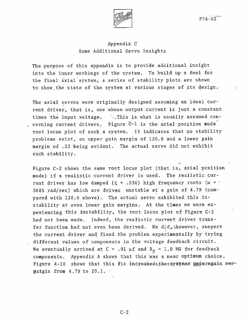
The purpose of this appendix is to provide additional insight
into the inner workings of the system To build up a feel for
the final axial system a series of stability plots are shown
to show the state of the system at various stages of its design
The axial servos were originally designed assuming an ideal curshy
rent driver that is one whose output current is just a constant
times the input-voltage This is what is usually assumed conshy
cerning current drivers Figure 0-1 is the axial position mode
root locus plot of such a system It indicates that no stability
problems exist an upper gain margin of 1206 and a lower gain
margin of 22 being evident The actual servo did not exhibit
such stability
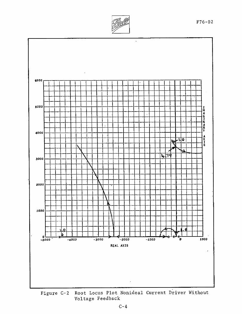
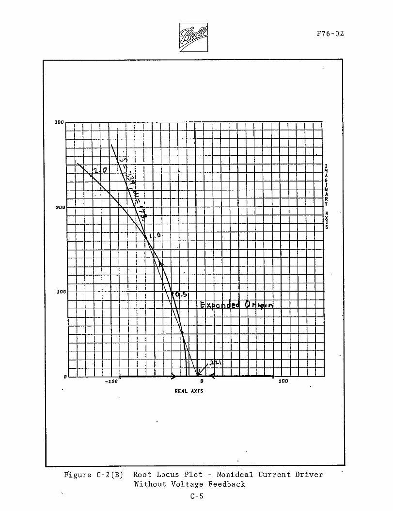
Figure C-2 shows the same root locus plot (that is axial position
mode) if a realistic -current driver is used The realistic curshy
rent driver has low damped (c = 036) high frequency roots (n =
3685 radsec) which are driven unstable at a gain of 479 (comshy
pared with 1206 above) The actual servo exhibited this inshy
stability at even lower gain margins At the times we we-re exshy
periencing this instability the root locus plot of-Figure C-2
had not been made Indeed the realistic current driver transshy
fer function had not even been derived We didhowever suspect
the current driver and fixed the problem experimentally by trying
different values of components in the voltage feedback circuit =We eventually arrived at C = 01 lif and RF 10 M for feedback
components Appendix A shows that this was a near optimum choice
Figure 4-10 shows that this fix increakedsthetaytems- gpaxmgain ma-rshy
)atgin from 479 to 201
C-2
____
i
F76-02
J- - - J F-shy I
ti eA j n wtl ifpf) L-I t- -
T I I- - -
r I I
-it t--L-1_-I-1-1- 1 H I-A -A I I-i I I r I 1 ___
~~~~~ hiit-- d31Ir~- LHtH [plusmnif 1Tf- Hshy
t I L I
L I - shy
---- l]iFli+-
HHI4KuC-1AD AaSvW Ia C
[l- 3 i iI LL41_EiI]L j7T ILl~ I i~[i tTj
-iltIIF--4l-- l II
- ~ FI I
- L I i5 YL i o ~ ~ ltI itiML
Figure C-i AMCD Axial Servo Wi~th Ideal Current Driver
C-3
ZF76-02
I I
4000 - i ii-
I 1A - I I
ooI ILJ 1000 m L
-5000 -4000 -300 -2000 -1000 0 1000
REAL AXIS
Figure C-2 Root Locus Plot Nonideal Current Driver Without Voltage Feedback
C-4
7F76-02
D
_____ I bull II
eoo1ii I I- I AI I-N
N IAt A
A I Iii T
SNM
I AIshybullI $ I~ IY
ajIe bI_Ig
-144
I I I Ishy
ai Ing REAL AXIS
Figure C-2(B) Root Locus Plot - Nonideal Current Driver
Without Voltage Feedback
C-5
F76-02
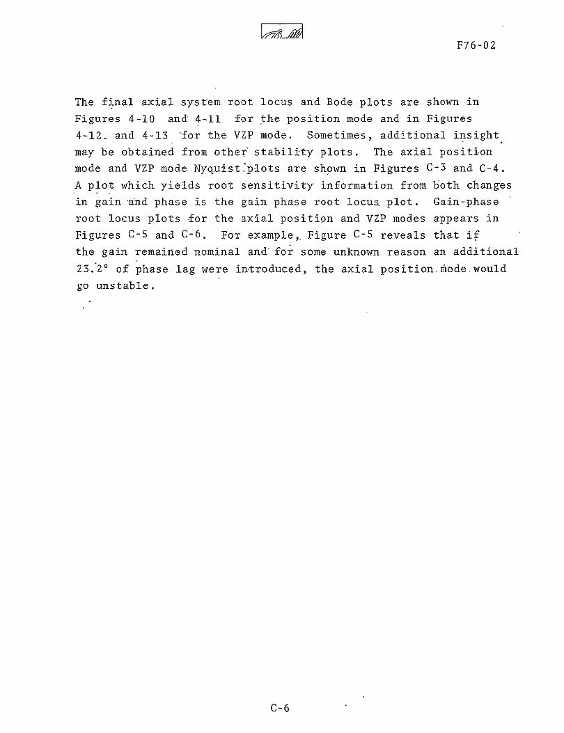
The final axial system root locus and Bode plots are shown in
Figures 4-10 and 4-11 for the position mode and in Figures
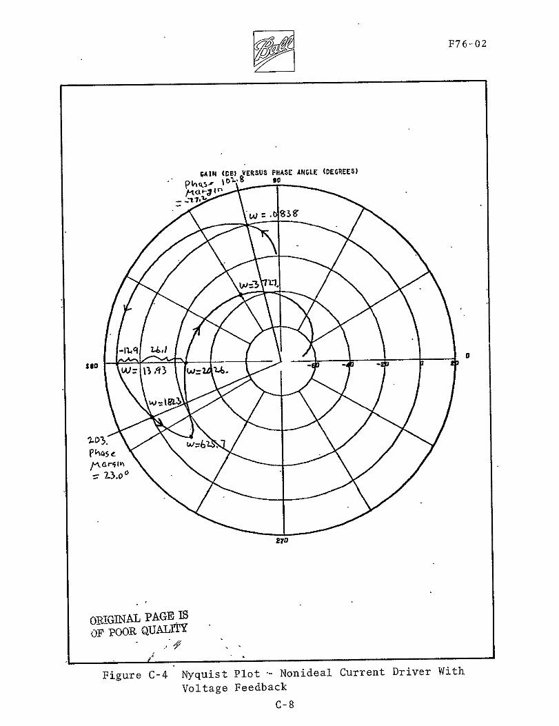
4-12- and 4-13 for the VZP mode Sometimes additional insight
may be obtained from other stability plots The axial position
mode and VZP mode Nyquistpiots are shown in Figures C-3 and C-4
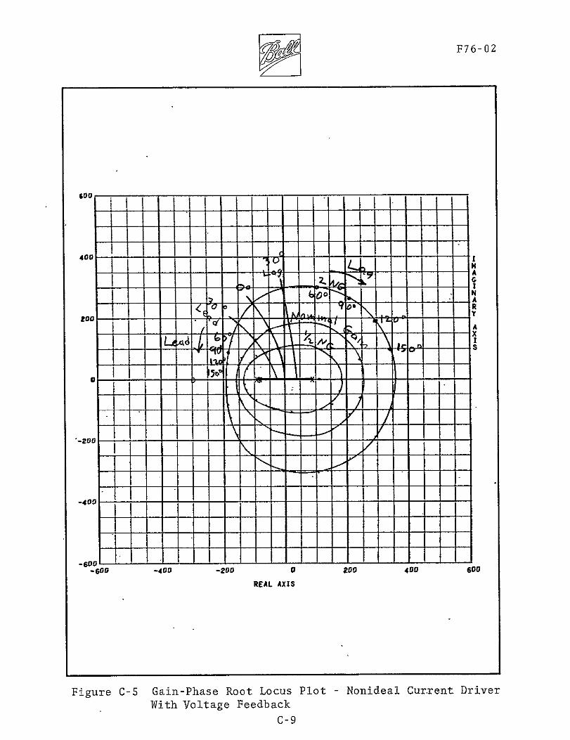
A plot which yields root sensitivity information from both changes
in gain and phase is the gain phase root locus plot Gain-phase
root locus plots for the axial position and VZP modes appears in
Figures C-5 and C-6 For example Figure C-S reveals that if
the gain remained nominal and for some unknown reason an additional
2320 of phase lag were introduced the axial positionmodewould
go unstable
C-6
F76-02
AIN IDB) VERSUS FMASE ANGLE (CEGREES)
9-a
-IINALPAGE 18
F POOR QUALITY
Figure C-3 Nyquist Plot - Nonideal Current Driver With
Voltage Feedback
C-7
DF76-02
fIN (M8) VERSUS PHASE ANGLE (DEGREES)toS PL~aos-- ItC
ID3
270
OROGTNAL PAGE IS OF POOR QUALTY
Figure C-4 Nyquist Plot - Nonideal Current Driver With
Voltage Feedback
C-8
1 gF76-02
40 I - I
I I I 0
AI 06
C2-Y 1_ I
-610 -40 _O_ -shy n n 6
-400 ~~
With VotgFebc
zloo- -400 -200 REL 0200 40D 600
-NonidealFigure C-5 Gain-Phase Root Locus Plot CurrentDriver With Voltage Feedback
C-9
-400
2F76-02
600 - E 1 II I
400
-
1
R
A
IIT
a zOO 400
REAL AXIS
-6-0O -400 -200
Figure G-6 Gain-Phase Root Locus Plot - Nonideal Current Driver With Voltage Feedback
C-go
600
F76-02
NASA CR-144917
FINAL REPORT
ANNULAR MOMENTUM CONTROL DEVICE (AMCD)
VOLUME I LABORATORY MODEL DEVELOPMENT
Prepared under Contract No NAS 1-12529 by Ball Brothers Research Corporation
Boulder Colorado 80302
for
NATIONAL AERONAUTICS AND SPACE ADMINISTRATION
m m
The MCD in Final Stages of Assembly
F76-02
SUMMARY
The annular momentum control device (ACD) is a thin hoop-like wheel
with neither shaft nor spokes (see Frontispiece) The wheel floats
in a magnetic field and can be rotated by a segmented motor
Potential advantages of such a wheel are low weight configuration
flexibility a wheel that stiffens with increased speed vibration
isolation and increased reliability
The AMCD is nearly 2 meters (6 feet) in diameter An annular
aluminum baseplate supports the entire wheel assembly Vacuum
operation is possible by enclosing the wheel in an annular housing
attached to the baseplate The rotor or rim has a diameter of
about 16 meters (63 inches) and consists principally of graphiteshy
epoxy composite material It weighs 225 kilograms (495 pounds)
and is strong enough to be spun at 3000 rpm At this speed it can
store 2200 N-m-s (3000 ft-lb-sec) of angular momentum A system of
pneumatic bearings can support the rim in the event of a magnetic
suspension failure
The magnetic suspension system supports the rim both axially and
radially at three points Combinations of permanent magnets and
electromagnets at each of the three suspension stations exert forces
on ferrite bands imbedded in the rotating rim The magnetic gaps
are about 025 cm (01 inch) above below and inside the rim The
gaps are maintained by servo loops with 50 hertz bandwidths that
The servorespond to error signals generated by inductive sensors
loops can be operated in either positioning or zero-power modes
The rim is accelerated and decelerated by a large diameter segshy
mented brushless dc motor Electromagnet stator segments are
placed at each suspension station and interact with samarium cobalt
permanent magnets placedevery 73 cm (29 inches) along the
periphery of the rim Commutation is achieved by Hall sensors that
detect the passing permanent magnets
ii
NF76-02
Volume I of this report describes the analysis design fabrication
and testing of the laboratory model of the AMCD Volume II conshy
tains a conceptual design and set of dynamic equations of a gimbaled
AMCD adapted to a Large Space Telescope (LST) Such a system
could provide maneuver capability and precision pointing by means
of one external gimbal wheel speed control and small motions of
the rim within the magnetic gap
iii1
F76-02
TABLE OF CONTENTS
Section Page
SUMMARY if
ACKNOWLEDGMENTS v
10 INTRODUCTION 1-1
20 THE AMCD CONCEPT 2-1
30 MECHANICAL SYSTEMS 3-1
31 Rim 3-1
32 Back-Up Air Bearing System 3-17
40 SUSPENSION SYSTEM 4-1
41 System Description 4-1
42 Performance 4-12
50 DRIVE SYSTEM 5-1
51 System Description 5-1
52 Magnet Selection 5-1
53 Core and Winding Design 5-2
54 Motor Commutation 523
55 Motor Control Electronics 5-3
56 Torque Calculations 5-4
APPENDICES
Appendix Page
A CURRENT DRIVER EQUATIONS AND TRANSFER FUNCTIONS A-1
B THE WAHOO CONCEPT B-I
C SOMEADDITIONAL SERVO INSIGHTS C-1
iv
P76-02
ACKNOWLEDGMENTS
The AMCD development to date has been the result of the efforts of a great many people At BBRC Frank Manders with help from Dick Mathews lead the mechanical design and fabrication effort Dick Woolley strongly influenced the magnetic design and overall configushyration Jerry Wedlake developed the drive system Glen King performed the dynamic analyses and Dave Giandinoto designed much of the intershyfacing electronics and did the final system integration
At Cambion Paul Simpson managed the magnetic suspension work with technical consulting provided by Joe Lyman and Lloyd Perper
The rim fabrication at Bristol was headed by Tom Laidlaw with analytical assistance from Keith Kedward
Analytic design of the back-up bearings at Shaker Research was conshyducted by Dr Coda Pan and Warren Waldron
The customer had a strong influence on the final system At Goddard Space Flight Center Phil Studer provided valuable suggesshytions on all magnetic aspects and the drive motor in particular
The primary influences and directions came of course from Nelson Groom and Dr Willard Anders6n of Langley Research Center who conshyceived of the AMCD and fostered its development
My thanks to all of these people
Carl Henrikson AMCD Project Manager
v
10
F76-02
INTRODUCTION
The AMCD concept was originated at the Langley Research Center of
the National Aeronautics and Space Administration (Reference 1)
Analysis design fabrication and testing of development hardware
was begun under contract to Ball Brothers Research-Corporation in
July of 1973 The contract was jointly sponsored by the Langley
Research Center and the Goddard Spaceflight Center The contract
work statement was also a joint effort with the Goddard Spaceflight
Center providing technical inputs on the magnetic bearings and
drive motor portions Hardware was delivered in February of 1975
Several key subcontractors were used by BBRC during the program
Principal among these were
1 Cambridge Thermionic Corporation (Cambion) Cambridge
Massachusetts - Development of the magnetic suspension system
2 Bristol Aerospace Limited Winnipeg Canada - Analysis
and fabrication of the rim
3 Shakei Research Corporation Ballston Lake New York -
Design of the back-up air-bearing system
These subcontractors performed well-and made major contributions
to the success of the program One subcontract did not go well
and caused a major delay in the program Failure of the subconshy
-tractor for the baseplate and vacuum enclosure to meet flatness
requirements necessitated rejection of the parts and placement
of the subcontract with another firm
This report is a description of the major hardware items and
their design considerations Details of the as-delivered hardshy
waremay be found in the Operations and Maintenance Manual that
was delivered with the hardware
I-I
A AF76-02
The report is divided into four main parts covering the concept
the mechanical systems the suspension system and the drive
system Appendices are used to cover some of the details of the
servo control loops
1-2
20
F76-02
THE AMCD CONCEPT
A purely annular wheel has many advantages Principal among
that all the rotating mass is at the greatest radius andthese is
can produce the greatest angular momentum storage Thehence
shaft and spokes of a conventional wheel add weight but very
little angular momentum storage
oneBall-bearing annular wheels have never been tried and for
obvious reason The losses associated with a large diameter ball
In order to make annular wheelsbearing-would be intolerable
practical a low-loss magnetic suspension of the (or rim)rotor
a narrow annularis necessary This then is the AMCD concept
rim supported by a magnetic suspension system
Several other advantages accrue from the AMCD concept First
of all conventional size constraints are removed The wheel
does not have to operate in an enclosure to preserve lubricants
If the diameter isincreased greatly the space is not wasted
because a spacecraft or part of a spacecraft can be placed inshy
side the wheel Furthermore motivation exists to goto larger
wheels It can be shown that for a given stress level in the
rim the mass efficiency of the rim increases as the diameter
increases The offsetting effects of increased stator weight
can be alleviated by using basic spacecraft structure to supshy
port the stator elements A further advantage of larger diashy
meter is increased moment arm for spin and precessional torquing
Another set of advantages of the AMCD concept is a result of the
arerelatively thin annular rim The stresses in such a shape
predominantly circumferential so that the structure lends itself
to filament or tape wound composite materials Furthermore as
spin rate increases the rim tends to flatten and reduce dynamic
thai structrualimbalance Also it tends to become stiffer so
2-1
F76--02
resonant frequencies increase In fact it can be shown that
the conventional crossover frequency of a spinning wheel at
which the spin frequency becomes equal to the rotor structural
frequency cannot occur for an AMCD The structural frequencies
are always greater than spin frequency no matter how limber the
rim is at zero spin rate
The use of a magnetic suspension gives rise to another set of
advantages First the suspension is relatively soft and forms
a sort of isolator between the rim and the spacecraft to which
it is attached Any-vibrations of the rim will be greatly atshy
tenuated This effect can be enhanced by proper filtering at
multiples of spin rate The suspension is also a smooth linear
force-producing system without mechanical nonlinearities such
as stiction The result is that small precision precessional
torques can be created by gimbaling the rim in the magnetic gaps
The final advantage is related to the long life and perhaps even
more important predictable long-life capability of a magnetic
suspension system vis-a-vis a ball bearing Ball bearing lifeshy
times are short dependent on number of revolutions rotational
speed and very susceptible to contamination The lifetime of a
magnetic suspension is a function of the failure rate of electronic
components an area that has been the subJect of a great deal of
study Moreover redundant suspensions are fairly simpleto
mechanize
2-2
F76-02
30 MECHANICAL SYSTEMS
The AMCD Mechanical Systems consist of 1) the rotor (or rim)
2) the back-up air bearing system and 3) the mounting base and
vacuum enclosure
The rim provides the angular momentum storage capability for
the system Embedded into the rim are ferrite rings and samarium
cobalt permanent~magnets Three ferrite rings composed of segshy
ments located on each axial surface and on the inside radial
surface react with the magnetic suspension system Seventy-two
permanent magnets located near the periphery of the rim react
with the segmented drive system
The back-up air bearing system initiated in the event of a magshy
netic suspension failure is designed to slow and support the
rim The design provides hydrostatic air pads for radial control
and hydrodynamic air pads for axial control
The mounting base and vacuum enclosure completely surround the
rim magnetic suspension and motor components and provide the
mounting points for the torque measuring fixture brackets The
annular mounting base supports the magnetic suspension and motor
lattice structure The annular vacuum enclosure U-shaped in
cross-section isbolted to the mounting base providing the capashy
bility to operate the rim in a vacuum and to add structural rigidshy
ity The vacuum environment is necessary to reduce rim air drag
31 Rim
The final rim configuration Figure 3-1 shows that all components
embedded into the rim are completely supported The distance
between the permanent magnets and ferrite bands is maximized
within the dimensional constraints of the rim
3-1
F76-02
5S1I4 A41t1s
-EAflAMW1 COWFAr nAGNC7r
Figure 3-1 Rim Conftguration
Centrifugal accelerations cause forces on the embedded comshy
ponents which are reacted directly by the base rim material
minimizing the stresses on the adhesive which bonds the components
to the rim The samarium cobalt permanent magnets are spaced
a minimum of 085 inches from the closest ferrite band to minishy
mize the coupling between the permanent magnets and the magshy
netic suspension system
The primary function of the rim is to provide maximum angular
momentum storage capacity within dimensional and weight conshy
straints The selection of the rim material graphite filament
epoxy laminate is consistent with this function The specific
momentum of a flywheel (HM) is related to material characteristics
of the rim as follows
HM c(577 (3-1)
3-2
F76-02
where a is working stress in flywheel
pis flywheel material density
Hence a high-strength low-density material is ideal for a
low-weight flywheel
-Table 3-1 shows the relationship of material ultimate tensile
strength to material density for acceptable rim materials
Table 3-1
RIM MATERIAL STRENGTH TO DENSITY RATIO
MATERIAL STRENGTHDENSITY (IN x 10 )
Graphite A-SEpoxy 36
GlassEpoxy 34
BoronEpoxy 31
Graphite M-SEpoxy 30
Graphite HM-SEpoxy 18
Beryllium 10
6A1-4V Titanium 10
7075 Aluminum 08
Not in Composite Form
Graphite AS fiber - epoxy laminate therefore will provide the
largest specific momentum for the system Graphite filamentshy
epoxy laminate also has a relatively high elastic modulus C16x
106 PSI) thus providing relatively low radial growth at high
speeds Furthermore graphite-epoxy laminate is non-magnetic
and non-conducting essential characteristics for low drag
operation of the magnetic suspension system
3-3
F76-02
311 Rim Description
The rim consists of three bands of ferrite material made up
of 180 segments each and 72 samarium cobalt permanent magnets
embedded and bonded into the AS graphite filament - DX210 epoxy
rim material Figure 3-2shows the rim dimensions
The ferrite rings and permanent magnets are bonded to the basic
rim with Fuller 7004 adhesive The rim is composed of two basic
rectangular cross-sections the first and larger contains the
bulk of the graphite-epoxy material and the ferrite bands the
second smaller section contains the remaining material and
the samarium cobalt permanent magnets
The larger section has a cross-section 53 cm (21 inches) in radial
(125 inches) deep with an inner diameter oflength by 318 cm
154 cm (608 inches) Three channels are machined into this
section 254 cm (10 inches) wide by 057 cm (0225 inches) deep
The smaller section integral withto contain the ferrite bands
the larger is axially centered 28 cm (11 inches) in radial
(0375 inches) deep with-an outer diameter oflength by 095 cm
This section contains 72 holes which contain171 cm (6725) inches
the permanent magnets
The samarium cobalt permanent magnets are 14 cm (055 inches) in
diameter by 064 cm (025 inches) long The axial and radial
ferrite segments are shown in Figures 3-3 and 3-4 respectively
The ferrite segments are machined from Ferroxcube 3C5 material
The axial segment is slightly keystone in shape to minimize gap
distances Each segment occupies 2 degrees of the band circumshy
ference
3-4
529
GEN NOTES I RAD NOT DIMENSIONED
ARE 0907 Z WNEI6t4T - 455OLISshy
3 WrUtAt MOM4ENTUM 3300^-9000 Lb-VT- S Se
2-1RAb SC
30 OOTIRAXIAL31 t5R P - pERi7VE 5E6mlENTS-2 PLACES (5S60 gEaeb)
65 i ____ _CH COPPED GR4PHITE Amb EPOY
PLACS)
1 ~TIRI Z5
_ _
(REP)
I V 4 0
1 f3 PLA IES)
00 55DIX
42B
- 425 (REF)
EikPHITE FILAMENT tipQKY coMPOSITE
SAMARIUM COBALT
4 NampE S (72tE G D) CITE7KEb IN 380310 WITHIN OO EUALLY SPACED O 33000 PADi os MAGNET cEtJTer StAALL ZE E=QUAL WITW
o20 MAGrNET OLE5 bAA5 EITWEt TULjd
Ot zlNt kITA CoPPet
---ELusIA TO oo4 scAIme h3e o
BELOW IFLUSH4 VT(P
C
Figure 3-2 Rim Dimensions
555 2 ___
985
MNT L nFE RZPO KXC BE 3C 5 MISS
CD
Figure 3-3 Axial Ferrite Segment
I
233273
5058 27
LO
-9 100
4150 C2 PLACES)
MATL - 303
I
Figure 3-4 Radial Ferrite Segment
iF76- 02
The radial segment is rectangular in cross-section and when
bonded in place produces a small wedge-shaped gap between
segments Each radial segment represents 2 degrees of the band
circumference
312 Rim Fabrication
The ASCD rim was fabricated by Bristol Aerospace Limited Winnishy
peg Canada The material AS graphite filament tape impregnated
with DX210 resin was wrapped on a special tool producing 100
percent circumferential fibers with a volume fraction of graphite
of 55 percent
The oversized cross-section rim was wound in 15 separate layers
Each layer was B stage cured with the following temperature
cycle
P
J4 7
The post cure after the fifteenth layer was identical to the
B stage cure except the temperature was increased to 1770 C
in 50 minutes and held at 177degC for 2 hours after the 1490 C exshy
-posure
3-8
3
eF76-02
Figure 3-5 shows the specially constructed tool containing
cure cyclesheaters and insulation for B stage and final
The rim was removed from the tool and machined to nearly the
final dimensions including ferrite channels and permanent magshy
net holes These operations are shown in Figures 3-6 and 3-7
The ferrite segments andmagnets were bonded in place with Fuller
7004 adhesive and cured The magnets were placed in the rim with
alternating North-South poles and the ends were covered with a
016 cm (116 inch) thickness of chopped AS graphite-DX210 resin and
After final cure the rim was machined (by grinding) tocured
final dimension The rim was coated with a 0005 cm (0002 inch)
thick layer of Fuller 7220 adhesive as a final step to minimize
Figure 3-7A shows the final rim resultsrim water absorption
313 Rim Analysis
The rim analysis conducted by Bristol Aerospace predicted the
(55434 PSI)rim maximum stress and radial growth to be 38250 Ncm
and 3 cm (0117 inches) respectively
The rim was modelled using axisymmetric finite elements using
the ANSYS system The model characterizes the heterogeneity
of the structure (including the ferrite bands and magnets) and
the orthotropic elastic properties of the graphite-epoxy comshy
posite
The results of the analysis are summarized in Table 3-2 and in
a rim speed of 366 meters per secondFigures 3-8 3-9 and 3-10 at
(1200feet per second)
3-9
N
Figure 3-5 Lay-up Tool
IIP76-02
Rim Machining OperationsFigure 3-6
3-11
MIE II
Iiue37Diln emnn antHlsi h i
3I1
DF76-02
LOCATION MAGNITUDESTRESS (PSI)COMPONENT
Radial or carbonepoxy +460 (max) -891 (min)X stress
Axial or carbonepoxy +491 (max) -433 (min)Y stress
Shear or carbonepoxy +390 (max) XY stress -176 (min)
Hoop or carbonepoxy +55434 (max) 0 (min)Z stress
Radial inner surface +01166 (max)
Displacement outer surface -01130 (min)
(inches)
Table 3-2
MAXIMUM VALUES OF STRESSDISPLACEMENT AT 1200 FTSEC RIM SPEED
3-13
5ThF-=- V- LERATfNz- 1 4U0T00
RMCO RRLYSES BRISTOL REROSPRCE LTO OCT 73
HOOPSTRESS RNSYS 5
or Hoop Stress Contour PlotFigure 3-8 Z
F76-02
- flax h st-ess= 55434-
I I-1 I Ii-- shy
60Iz-
===z_ +0 _----- --- shyi -_-O- - = -- = +----- shy+ ---= -- r E
_-------=--- --- = ---
-- ----- +- - --- -- =--- -=
=
------ shy
=T--- 7
--
-
- -_ - - - -- - -- a
a zrlt- --r-- -r - z I=tzz-z - -
- 4
o6 Zf - =4-=-t vi I_- --- zmE+s=$ Z 4-| b- =---+----- shy
+ 5-t 4 -- c Tt - 22 ~++ _------ _ __ _C - u
a zjztL- +lt+ z- I [Lt- -- Tit--
-- -+v + --F t+-- -+rr 7- h |f
0 200 -00 6800 1000 12oo
Rim SPEED (rri5Ecc~
Figure 3-9 Hoop Stress and Growth With Speed
3-15
F76-02
e 4fo
1 1 I 1 t i I I CII1I1_4I I
Itdn-branveqs sts OI - I M
---shy-- -- -- - -
t~z 2 - 1- shy
- 421 ~T2 2 -=_-- -_E---i ----
t -- EM
___ _ ZZ +-_ _-A~~ - rrrr-
TLLto LLbi i L -- k - r K -1-
irtv li V i 1 -- t 4 s-- n-L -- T4 E
000-q0o 600 800 100 A120 Rim Sp Dr (FTVEC )
Figure 3-102 Transverse Stress Components With Speed
3-16
DF7602
Figure 3-8 shows the computer-drawn plot of constant hoop tensile
stress contours the maximum being 38252 Ncm 2 (55438 PSI)
occurring at the top and bottom inside corner
Figure 3-9shows the relationship of radial growth and hoop stress
as a function of rim tip speed
Figure 3-10 shows the relationship of transverse stress components
with speed
Since the material void free is capable of withstanding 110400 2 2Ncm (160000 PSI) in tension and 8280 Ncm (12000 PSI) in shear
the safety factor is 28 minimum On a sample basis the void
fraction was determined to be less than 04 percent
32 Back-Up Air Bearing System
The design of the back-up air bearing system was completed and
analyzed by Shaker Research Corporation Ballston Lake New York
The back-up air bearing (BUB) system consists of six hydro-static
radial pads and twelve hydrodynamic axial pads These are arranged
in six BUB sets consisting of two axial (one upper and one lower)
and one radial pad and located at either end of a magnetic supshy
port station Each BUB set is approximately 60 degrees from the
adjacent set The bearings are deployed toward the rim by air
pressure when predetermined rim displacement limits are exceeded
The introduction of air through the pads as well as through a
pneumatically operated valve in the vacuum enclosure provides
the fluid for the BUB system and also introduces air drag for a
fastercoast-down Hydrostatic bearings were selected for
radial use instead of hydrodynamic types because the rather small
rim depth (115 inches) allows insufficient area to produce the
required reaction forces The back-up bearing system is shown
in Figures3-11 and 3-12
3-17
P76-02
~14
-L- 7
FiguTre 3-1 AMCD Back-Up Bearing Layout DrawingI 3-la
Figure 12 Back-Up Bearing System
7F76-02
321 Hydrostatic Radial Bearings
The movable radial pads are designed to minimize air flow and
maximize air bearing rim reaction forces The radial pads proshy
vide a centering effect on the rim to minimize dynamic and magshy
netic unbalance forces
In the normal magnetic suspension mode the radial pads are held
away from the rim-and against stops by a set of nested compression
springs (total of 22 N (50 pounds) of preload) When the radial
system Figure 3-11 is activated 207 Ncm2 (300 psig) air is introshy
duced to the pad piston cylinder which moves the pad outward
toward the rim The piston chamber is ported to the pad surface
through a 0033 cm (0012 to 0014 inch) diameter orifice A
sealed oil-filled dashpot between the piston and pad controls the
deployment velocity
Figure 3-13 shows the relationship between- radial pad force and
gas flow versus film thickness for various orifice 4iameters
Because of limited gas available-the smaller orifice diameters
were selected
Since the rim is not at constant radius (because of radial growths)
film thickness and flow vary With rim speed Figure 3-14 shows
the relationship fo film thickness and flow versus rim speed
322 Hydrodynamic Axial Bearings
Movable- tilt type axial hydrodynamic pads were used since the
rim radial width is large and because of the limited bearing air
supply The axial pads are slightly crowned and combined with
the tilt feature are self aligning
3-20
F76-02
1 ~
It
7
I
JII ji
I L
II
---
Ft
T -
VIN I -_ Lr
TD _-
I
I+i
- 1MNV I
4~~r14 +t
Fit~Fi-~tdi I~ ~ JrV)
i ir
il-I= iH14+
i T r
F~m
shy
_ _
I L [
- i
I
_ i _
Ii
0001M -s as
Figure 3-13 Single Pad Force and Flow
3-21
A yyF76-02
WI
ii24pVshy-~~~~W
J4 i3 - Lit
I+ I~Ir~r L-- u 7t J
L 4- 1-nMLfI0__ 4~~~~- F-14--gtrF
I -- -r
4 ~ P I-
IaiH __M
1 --- t Th T1T
I- Vt prI i A
-p--t~LIV[~ VK jl77L1 1
Figure 3-14 Radial Air Pad Flow and Film Thickness With Rim Centered
3-22
F76-02
In the normal magnetic suspension mode the axial pads are held
against stops by a flexural spring The axial system is deployed
in-much the same manner as the radial system When a magnetic
suspension anomaly is detected the vacuum enclosure is flooded
with external air thus providing the film for the axial bearings
Figure 3-15 shows the relationship of film thickness with rim
speed Since the film will support the rim to about 15 radians
per second the pads are designed to accept several contacts before
replacement is necessary
323 Back-Up Bearing Pads
The primary objective in designing the pad material was to proshy
vide a material which would wear smoothly without damage to the
rim or to the pad itself Sacrificial bearing materials have
been used in gas bearings in the past which exhibit the necessary
qualitites The material used in the back-up bearings is an epoxy
resin heavily filled with aluminum powder aluminum oxide power
and molybdenum disulphide powder The mixture is poured into
silicone rubber molds degassed in a vacuum chamber then heatshy
cured The pads are then machined
When the spinning rim contacts the pads the pad will wear smoothly
and rapidly acquiring a high polish and yielding a fine dust
The rim surface should be undamaged by the contact The aluminum
filler provides high thermal conductivity to sink the heat generated
by the rim contact The aluminum oxide provides dimensional
stability so thQ pad will withstand the thermal shock generated
by the rim contact
3-23
3788I9 2 4 5 7 8 9 2
1 7 _- I
111-1 r - J
-I- --i- 1 rV1- 1 t r V
4 _ - _ _____ shy- I---7
I
r-- _- F-_- --- I ii -
I fr r l 7[-II j7shyLi +] - i I-- I
1 7 8
-- - 4 5---- 10 47 MCI 9
Figure 3-15 Axial Pad Film Thickness Versus Speed
F76-02
40 SUSPENSIONSYSTEM
41 System Description
The suspension system consists of three suspension stations
placed symmetrically about the rim At each suspension station
the rim can be pulled in either axial direction or tadially
inward by magnets A total of 12 magnets are arranged in sets
of four each to pull in these three directions (up down and
inward) The eight axial magnets are driven in concert by one
set of electronics Axial error signals are developed by a
position sensor located at the center of each station The
axial servo loops in each of the three stations are independent
of each other The four radial magnets in each station are also
driven by a set of electronics in response to a radial position
sensor located in the center of that station But the radial
station to another so asservos are interconnected from one
to prevent the servos fighting one another even in the presence
of rim radial growth
411 Magnet Description
One of the unique features of the AMCD is the support magnet
design The electromagnets are flux-biased by thin wafers of
samarium cobalt permanent magnet material placed in series in
the magnetic circuit This has the advantage of (1) providing
a high force per unit current sensitivity at zero current (2)
providing a linear relationship between force and current and -
(3) providing the static field required for zero power operation
The support magnet geometry is seen in Figure 4-1 The permanent
magnet biasing is achieved by slanted wafers of samarium cobalt
in the legs The wafers are as thin and wide as possible to
4-1
SAti 4-IUr CCBA3L~rshy
AGtJer-
AGII1
Figure 4-1 Support Magnet Geometry
RF76-02
minimize their reluctance in the magnetic-circuit The volume
of permanent magnet material is sufficient however to provide
adequate flux-biasing and static lift The reluctance of the
permanent magnets is large but does not more than double the
total reluctance since the air gap inthis system is large In
many other magnet suspension systems the gaps are small (about
01 mm) and this sort of series flux biasing would greatly inshy
crease the total reluctance in the circuit Control power would
thus be large and the systems would be impractical
The effect of flux-biasing on the force versus current characshy
teristics of the magnets is shown in Figure 4-2 With no biasing
current in either direction produces force of the same sign with
poor gain and low efficiency in the vicinity of zero current
Force is simply a function of the square of the current With
biasing the slope of force versus current is greatly increased
at zero current In the AMCD top and bottom magnets operate
together in a push-pull type of operation The coils are in
series hence both coils have zero current at the same time
The resultant force-current relationship is linear and has a
slope double that of either magnet alone
Figure 4-3 shows the U core of the magnet with the permanent
magnets in place Permanent magnet thickness is 1 mm (0040
inches) Also shown in Figure-4-3 is a fully assembled magnet
ready for potting After potting the units measure 43 cm x
167 cm x 25 cm (17 in x 42 in x 99 in) and weigh 500 grams
(11 lbs)
412 Position Sensors
The position sensors used in both the axial and radial suspension
systems are Multi-vit sensors manufactured by Kaman Sciences
4-3
7 gF76-02
-r
UPPETP HA -
C AOc~~
777
~~oeehAcn-e-r Z
Figure 4-2 Flux-Biased Magnets in Push-Pull Operation
4-4
rF76-02
I
3 i
A A
I tii A LWUv
NN
N~ i X -9
i i UI A i
IN aWIi ii i
iiiiiiiliiili
i~iiii Ii iliiiiiiiliiilii
Iilliii iiiiiliiiiiiliiiii = iiiiiiaii~iii iiiiiiiiiliiiiiiii
Uiiiii poundii=iiiii]iipoundiiiiiiiiiiiiiiiii Uigure 4-3 Support Magnet Cosri on
iliiiiur -3 ConstructiiiiIliiiiiiiiioniiiiiiiliiiSppriMge liiiiiii i iiiiliiiii3 URiliI 4-s == =
4-s
rF76-02
Corporation These are conventionally called eddy current senshy
sors although they are actually sensitive to anything that changes
the inductance of the test coil in the probe Hence either
eddy currents in a conductor or the permeability of a magnetic
material can be sensed In the AMCD the sensors look at the
ferrite bands and therefore are operating entirely ina non-eddyshy
current magnetic permeability mode Special calibration of the
sensors was required in order to operate in this mode Linear
range of the AMCD sensors is 025 cm (01 inches) and scale facshy
tor was set at 4 voltscm (10 voltsin)
413 Control System
The axial suspension system uses three independent servo loops
to control electromagnet currents An electronic diagram of one
of these loops is shown in Figure 4-4 The heart of the elecshy
tronics is an Inland Controls MA-I DC servo amplifier which is
operated as a current driver to reduce the effects of electroshy
magnet inductance Equations of motion of this driver and an
analysis of the voltage feedback used to damp high frequency
roots are given in Appendix A An analytical block diagram of
the entire servo loop is shown in Figure 4-5 Equivalent points
on the electronic and analytical diagrams are indicated by letters
within hexagons
The axial suspension system has two modes of operation a posishy
tion mode and a virtually zero power (VZP) mode In the posishy
tion mode rim position error is used to command electromagnet
current The rim has high static and dynamic stiffness about
any desired point in the gap In the VZP mode the rim position
set point is modified by positive feedback of the integral of
electromagnet current The result is that the set point is moved
until steady-state current is zero The permanent magnets are
4-6
AA
REHTUtk +26V
4-
C11 7t-Q
Fiue44Aia3upnin7lcrnc
S Cornn- EesoCo p n a cncivCrrent Driver- O deg OI 99 (5C + sm -3 (s + 1 1deg E 1 copy + F
gtosO ~
volf
iE 3 7 T r i m T ntegratadegr
Suspended
Mass
-|ectro
-ria net
16
permanent Magnet
Figure 4-5 AMCD Axial Suspension Station
R 1F76-02
then providing all of the support of the rim Dynamic stiffness
is nearly the same as in the position mode but static stiffness
is actual negative If a downward force is applied to the rim
in the VZP mode it initially moves downward but then slowly
rises to assume a new zero power position above the old equilibrium
position
The electronic circuit diagram for a radial servo station is
shown in Figure 4-6 and the corresponding highly coupled analytishy
cal block diagram is shown in Figure 4-7 Again equivalent
points on the two diagrams are indicated by letters in hexagons
The large amount of coupling results from three servos controlshy
ling only two degrees of freedom
Two modes of operation are available a position mode and a WAHOO
mode The position mode is similar to the axial position mode
The WAHOO mode is a zero power mode that produces zero power
operation in the presence of both static loads and rim expansion
This is accomplished by adjusting the position set point at each
station as a function of the integral of the sum of the electroshy
magnet currents at the other two stations
The name WAHOOis derived from the poker game WAHOO This game
is played in a manner such that each player knows what every
other player holds but does not know what he himself holds
Inspection of the WAHOO trim loops of Figure 4-7 reveals that
for VZP trim purposes each servo only looks at what the other
two are doing This innovation was developed by BBRC to meet
the unique requirements of the AMCD
The derivation of the WAHOO concept is given in Appendix B
There it is shown that only the WAHOO concept produces zero
power operaion for both rim expansion and force disturbances
4-9
A00l 51 Ir
A-A-
F
27
ffzo xr
74 VIP KIAk
7
Ems~
n
A7-
I
A1
ter
a 2k-
-
-
-
-
-
I)
Figure 4-6 Radial Suspension Electronics
-KS
Iamp wkin47s Permanent MagnetVeloityPM VPol Aplifir PMEHM E Iectremoqnet
K5 Kmn eae t~j VOS 0bCar respond to Lettered
1vII~rb r - rr m Psitionson Cgrcwit
vol vol Im PosiMoon Pox
SlRtim rtOhkx _Q$)bsS 4lfe I
0niplPfied Cus ren Driver
Gcucv rbinn n i
+ + vt
If
in-7d FigureservoD RailSro
+i
42
F76-02
Appendix B also shows that for single station design purposes
a single station can be represented as shown in Figure 4-8 Two
points of interest are immediately evident The equivalent mass
for a single station representation is 23 the total rim mass The WAHOO concept which involves negative feedback to each station
from the sum of the other two stations resolves to a positive
feedback in the single station representation exactly like VZP
in the axial mode This representation can be used for designing
the system characteristic root locations If the characteristic
roots from the single station representation are given by A and
the WAHOO gain is Kc it is shown in Appendix B that the three
station highly coupled set of characteristic r6ots are givenby
(S + 2K )A2
Performance
421 Static Performance
At each suspension station the rim will seek an axial equilibrium
position based on the applied load and the control system mode
(position or VZP) These equilibrium positions can be preshy
sented in one plot as shown in Figure 4-9 The VZP line is a zero current line and has a slope that indicates static instability
however as shown in the next section the system can operate in a
stable manner along this line The most usual operating position
mode point is about 001 cm (025 inches) above the center of the
gap At this point the slope P of the VZP line is about 595
newtonscm (340 lbin)
In the position mode an operating line exists for each set point
of the position sensor A family of these is shown in Figure 4-9
The lines are finite in length because of the limited current drive
capability of the electronics The slopes of the lines are apshyproximately 2600 newtonscm (1500 lbin)
4-12
Stationfost ionsingle
Oecrlx- EquIva1eratArmplifir Current Driver 6 Mks$M9oqmet+ 1m
~~~~~ eroe L~r
Is + Fes I16(7+1210 r0 0 l I-
p 0 1
476 An- Per
u2 IVlt+ -Eg
o tKate - r1 1 StO Sr eq uci o lnk wahoo is
Q Correspornas toa letterd posit~ions on circuit chogr~m
Sinql~e stcton eqviclvJewtmls is 23 totil ma
~odelldas a posattve PeedbctK self IoopVe
t to o-t liKe Vf Pwould ltherefboretxpect fvrthernortn itthe Aol O Servo Xt doesonh
Figure 4-8t EqiaetSnluadapev tto
ekgeto8 rnex e o +non
A F76-02
UP
MAGNET M~A t r
lsrok os NoRMAL
kE-RITI N
P E-Nshy-OMFR
tL UPshy
- j ~
-10
h31G1NL pAGE iS
)F POOR QUML-rI
Typical Static Suspension System Performance
Figure 4-9 4-14
rF76-02
The force sensitivity F of each station is about 138 newtons
ampere (31 lbamp) Hence the force produced by a station
is given by (in English units)
F = 340X + 3lI
422 Dynamic Performance
The analytical block diagram for an axial suspension statiQn is
shown in Figure 4-5 For theposition mode the root locus and
-Bode plots are shown respectively in Figures 4-l0and 4-11 The
root locus plot shows that the dominant pole pair has an undamped
natural frequency mN (which we define as bandwidth) of 171 radsec
(272 hertz) and a damping ratio of28 The Bode plot shows
that the gain crossover frequency wc (which some define as bandshy
width) is 1827 radsec (290 hertz)-and that the system phase
margin is 2320 Both plots show that the lower gain margin
is 22(-131 db) and that the upper gain margin is 201 (261 db)
For the VZP mode the root locus and Bode plots are shown respecshy
tively in Figures 4-12 and 4-13 The root locus plot shows that
the dominant pole pair has the same undamped natural frequency
and damping ratio as the position mode that is wN = 171 radsec
= 28 The Bode plot shows that two gain crossover frequencies
at 1823 radsecexist one at0838 radsec (013 hertz) and one
(2903 hertz) The phase margin at the lower crossover frequency
is -772 and that at the upper crossover frequency is 2300
Both plots show that the lower gain margin is 226 (-129 db)
and that the upper gain margin is 2011 (261- db)
The response due to the step application of a one pound weight
is shown for the position mode in Figure 4-14 and for the VZP
4-15
OF76-02
1 -DD
-- A I 1
I I
i
3000 --------------------------------- ___tN
-5000 -400 -30U -2ODG -t I lo oD
REAL AXIS
Figure 4-10(A) Root Locus Plot - Nonideal Current Driver With
Voltage Feedback
4-16
---------------------------------
7F76-02
-I- 111 1-l Z9D
io oI 1ll t A
G
80 ----------- 0 aEu----------------shy-4--
FigueRot41001LcusPlo - Nnidal Crret DrverWit
-1---4-17
I I
F76-020
14-HLowler
)2 I__ _ p
1 N I-- A =20 41 r
I tIse0_ __ _ _ 4 6 2 4 68100
s 10 log H00 6 10009 FREQUENCY (RADIAWS$ECOND)
Figure 4-11 Bode Plot - Nonideal Current-Driver With Voltage Feedback
4-18
7F76-02
$oo I5iI000 I1
T 1 Ii
-A
S4+
N A
4000 R--- - - - - -
V A x
103 000 40 30 29
urn rvrWtFi1r -12A Roo Lou7lt-Nnda
Voltage Feedback 4-19
V gF76-02
ii
- I I I
I I I II
I lii
-I I
II I iishy
II - - -i-l
Fgr 4-2B o otocu PltrNndaCrefl rive
With Voltage Feedback
4-20
F76-02
I i E
A -4 G
E- 60I jUroI(
I
1A2zS1 me RI
3s F-1-L
IIsoM 3en
4) e r
-120---- -Marlin
fla e =2300
-140 shy
1 1 10 10g 2000 1090r FREQUENCY (RADIANSECOND)
Figure 4-13 Bode Plot - Nonideal Current Driver With
Voltage Feedback
4-21
012
F76-02
00010
00008
pound E
0
p
0 00
0zkc0
0
E
- -
4+-F
- - -
Nshy- - - - - - -
4
- -
5
-4-2
AF7602
mode in Figure 4-15 The response for the position mode settles
out at 6941E-5 feet (002 cm) This yields a position mode
stiffness of Stiffness 6 1 lb
6941E_5 t X feet
1 12006 lb (21021-
N
69Th-ft Tni in cm
The response for the VZP mode settles out at -2451E-4 feet
Thisyields a VZP mode stiffness of
1 lb feet = lb NStiffness = 2451E4 ft X 12 in -3400 i (595 E-
Note that the stiffness in the VZP mode is just that of the
permanent magnet and that the movement in this mode is toward
the applied force That is if a weight is placed on the rim
in the VZP mode the rim will move up
Further insight into the system can be found by examining Ap2
pendix C When using current driirers the usual tendency is to
ignore the high frequencydynamics and simply say that the
output current is the input voltage times a constant This can
be very misleading in the case of AMCD- In Appendix C are shown
root locus plots using both an ideal current driver arid a nonshy
ideal current driver without voltage feedback It shows that
voltage feedback is necessary for the axial suspension Also
shown in Appendix C are Nyquist plots and phase-gain root locus
plots of the nominal axial systemthat is the system using curshy
rent drivers with voltage feedback The esoteric phase-gain root
locus plot shows on one plot the sensitivity of the system roots
to change in both gain and phase For example it shows what
would happen if an additional 300 of phase lag were added to the
system from some unknown source
4-23
F76-02
0001
I f
I 0 e
eshy
0a T 1-0001-shy0N
ft E F 0
E a
- 002--------------shy
0 t0 20
TINE (SECONDS]
30 40 50
Figure 4-15 Nonideal Current Driver With Voltage Feedback
4-24
F76-02
The equivalent single station radial analytic block diagram is
shown in Figure 4-8 It is very similar to an axial station
The root locus and Bode plots for the position mode are shown
respectively in Figures 4-16 and 4-17 The root locus plot shows
that the dominant pole pair has an undamped natural frequency
(bandwidth) wN of 653 radsec (104 hertz) and damping ratio C
of 18 The Bode plot shows that the gain crossover frequency
is 666 radsec (106 hertz) and that the phase margin is 1350
Both plots show that the lower gain margin is 329 (-965 db)
and that the upper gain margin is 7054 (3697 db)
The root locus and Bode plots for the WAHOO mode is shown in
Figures 4-18 and 4-19 The root locus shows that the dominant
pole pair has an undamped natural frequency of 674 radsec
(107 hertz) and damping ratio of 16 The Bode plot shows that
the upper gain crossover frequency is 691 radsec (110 hertz)
At this frequency the phase margin is 1260 Not shown is the
fact that the system also has a lower gain crossover frequency
of 594 radsec (095 hertz) At this frequency the phase marshy
gin is -715 Both plots show that the lower gain margin is
389 (-821 db) and that the upper gain margin is 6701 (365 db)
The large upper gain margins for both the position and the VZP
modes indicate that current driver voltage feedback is not needed
Considerable rim bending instabilities were encountered during
the design Early in the development the axial system was
designed to be overdamped This caused a bending mode to be
driven unstable The compensation was adjusted experimentally
until the bending became stable Unfortunately this reduced
the lead in the system resulting in the present underdamped sysshy
tem It is believed that bending will present no problem at
high spin rates because of the effective stiffening of the rim
4-25
6F76-02
_____ - _ r ____I___
141
IT___lishy
1 ii
1 F]
eir
t lj~
4-
J TT a p-
III NEA
fiIT WBKsITlK j1_11IIi I-
I
e
-Fshy
Y]-111 ji
1i1fln 4--I r
I i--I -
TFiJ-WL 1
_1(-Ii4 - I
I~ ~ ~iA_~2I ___ ii- 11 IFt-Ih
iT
h~ -iH T
+~ji+ih Iplusmn
_ _ _+ I kt ~h-II
+ LILY -
7 SO bullj
Figure 4-16 AMCD Radial Suspension Equivalent Single Station Position Mode
4-26
Elll csl- tLL[ 11--- 1_ il
V
1 MIN
2 0 H qL2~14-0IT
I M Ill 1OIHI
+-o ip Lr g
Ti I -0 1- b1 -- i
Ij _IUSi 1PIN - il
--i
41i L -I I - d jir ~J I I
00 -o
ro-d 5 c
Figure 4-17 ANCD Radial Suspension Equivalent Single Station o Position Mode
7F76-02
1LjI_----- Li -III iI - - I -shy-F ]e2 1
Is- Lr [_I
r ir -L-j 11I IALI _ _ _ ___ 2_
E11LLN1LALIF TYC -- td It 11
- KI
S1 1 1 1--shy
II
I r 11
FLL-1
U - I 4
E~~~~fL
__
f Lplusmn Xi ILIi _ _
- ii _ _ i
- H --
--------
A-1 1 F - JT-1
-- t-ti -~r -r I- t - --- IL I
IIJlri-tlrht1f tI
_+ _ l PillS 1 I
Figure 4-18 AMCD Radial Suspension Equivalent Single Station
o Wahoo Mode
4-29
rm~r 1 u i rrrrF r r r
4
130
o
I -4
7 7 1-shy iAb d
llt h
-30 Tfij4i i ~
- n0 t
Figure 4-19
01 AII-
I uji r a sec
AMCD Radial Suspension Equivalent Single Station o Wahoo Mode
AF76-02
and the averaging effect on modal pick-up caused by the bending
modes moving rapidly past each position sensor
As the rim is spun up the three axial stations become more and
more coupled by nutational effects The result of the coupling
is to reduce the dominant roots damping ratios more-and more to
the point the system could go unstable if the rim is spun fast
enough It is believed that this tendency could be greatly
reduced or possibly eliminated by the proper combination of cross
feeds from one axial suspension station to the others
4-30shy
DF76-02
50 DRIVE SYSTEM
51 System Description
The AMCD drive motor can be thought of as a large permanent magshy
net brushless dc torque motor Samarium cobalt magnets are
bonded into the rim at regular intervals The two phase armashy
ture is segmented with a winding set at each of the three susshy
pension stations Commutation is controlled by Hall effect senshy
sors mounted near the rim which sense position of the samarium
cobalt motor magnets
52 Magnet Selection
Alnico was considered along with samarium cobalt for the permanent
The large air gap and segmented winding structure meanmagnets
the magnets will become nearly air stabilized The rim was designed
with a small outer lip to hold the magnets This was done to
isolate the drive from the suspension as much as possible without
and complexity to the rim than necessary Thisadding more mass
small lip implies a short magnet Samarium cobalt has high
strength for short lengths and does not pay a penalty for air
In fact it is very difficult to demagnetize thisstabilization
material
cm (55 inches) diametertby 64 cmSamarium cobalt magnets 14
(25 inches) length were selected and bonded into the rim with
polarities alternated
The rim contains a total of 72 magnets spaced 73 cm (288 inches)
apart
5-1
53
--F76-02
Core and Winding Design
Each armature segment consists of a pair of bar-shaped winding
assemblies one above and one below the rim
Sit cos sla 0S SMa
cores in a singleThe windings-are wound toroidally around the
layer The figure above shows only the cross-section 6f conshy
ductors in the air gap as the conductors passing around the other
side of the core add nothing to torque and serve only a connectshy
ing purpose The bar-shaped cores are easy to wind and result
in a compact structure The single layer of 18 conductors adds
very littleto the overall air gap This effective electroshy
magnet design was suggested by P A Studer of Goddard Space
Flight Center
Ferrite material was chosen for the core to reduce losses Fershy
rite also is easily machined into the required irregular shapes
The windings are grouped into two phases SINE and COSINE each
of which acts upon three magnets at each motor segment In operashy
tion current in one phase is acting on the magnets while current
in the other phase is reversing in preparation for a magnet of
opposite polarity
5-2
DP76-02
54 Motor Commutation
Hall sensors act as commutation devices for the motor They sense the position of the permanent magnets in the rim and cause the drive coil currents to be switched according to magnet position
The sensors are mounted in pairs one above the rim and one below for each winding phase Outputs from each pair are summed so that the switching position is not affected if the rim moves up or down within the air gap The SIN pair controls current on the SIN windings of all three motor segments and likewise the COS pair
of Hall sensors controls all COS windings
55 Motor Control Electronics
A block diagram of the motor control electronics is shown in Figure 5-1 For each phase the Hall sensor outputs are summed and amplified to drive-threshold detectors These detectors sense magshynet position and polarity The phase control logic determines the
timing and polarity of the motor coil drivers Interconnections between the two phase control logic blqcks provide positive direcshytion and start-up information
Each of the six coil drivers controls a phase at one of the motor
segments Associated with each driver is a coil current sensor which monitors the current in that winding All six of these
current sensorsreceige a common reference from the speed control
potentiometer When current in that particular winding reaches the reference level the driver turns off until the current deshy
creases This prevents the current from reaching destructive levels at low speeds and acts as a speed control at high rim
speeds
Since the coil drivers are either full on or off a very efficient drive is achieved At low rim speeds the drivers operate as a
5-3
56
F76-02
conventional PWM (pulse width modulated) amplifier A quite faithful square wave current of controlled amplitude is fed to the coils At high speeds high acceleration (or deceleration)
is possible with the drivers full on for the period between magshynets with current rise and fall limited by the inductance of the
coils
Torque Calculations
The equation for the force betweena magnetic field and a current
carrying conductor-is
F = BLI
where
F = Force in Newtons B = Flux Density in Teslas (WebersM~ter )
L = Conductor Length in Meters
I = Current in Amps
If the magnetic field is created by a permanent magnet the force
can be considered to act on the magnet if the conductof is held
stationary which is the case with the AMCD motor
To arrive at design force each of the factors B L and I must
be evaluated
A force calculation will be made for one magnet face interacting
witha coil This can be then doubled to account for both ends of the magnet next tripled to take into account the three magnets in one motor segment and tripled again to realize the total force for the three motor segments Then using the radius of the rim
we can calculate developed torque
5-4
F76-02
Flux Density Calculation (B)
The large air gap makes it difficult to- estimate how much of the
magnet flux will couple through the winding core and how much
will be lost to leakage A measurement of coupling flux was made
using a pair ofsoft iron bars similar to the ferrite corasi
SEJSE C0115
SOFr iROh
-4 Webers with magnets of averageThe flux measured was 0375-x 10
strength
core must-be convertedThis flux that couples through the ferrite
to flux density (B) in the air gap where it interacts with the
coil windings There are two practical Choices for doing this
We can assume all the flux goes straight up from the surface of
the magnet andreacts with only those turns above the magnet or
we can assume the flux spreads out evenly over the winding area
Of course the truth liesand-reacts with all the turns equally
an adequatesomewhere in between but the second approach gives
approximation
The winding area in the air gap for one magnet coil phase is 2
19 x 36 cm or 68 cm
Flux density then is
-44m _ 0375 x10 Webers 2 0055 WebM-B_=A = 4 2A - 68 x 0-4 m
5-5
F76-02
Conductor Length Calculation (L)
are 28 turns with an effectiveIn the winding phase area there
length of 19 cm each
Total effective length is then
L = -19 x 28 = 532 cm = 0532 M
Current (I)
that the coil drivers and wiringThe elbctronics are designed so
canhandle 4 amperes Also the inductance of the coils was
examined to be sure that currents of this magnitude can be
reversed at maximum rim speed frequencies with a 60 volt power
(and torque) will then be calculated for thesupply Force
design maximum of 4 amps
Force
We can now calculate force from the equation
F = BLI
= 0055 x 0532 x 4 = 0-1-17 Newtons
Recall that this is the force for a single magnet surface inter-
For the total motor this is multiplied by 18face
Total Force = 0117 x 18 = 176 Newtons
576
0F76-02
This times the magnet radius (0838 meters) gives total torque
Total Torque = 176 x 0838 = 176 Newton-Meters
(13 lb-ft)
A small (14 diameter) test wheel was built to check the above
torque calculations Acceleration measurements were made and
from the known wheel inertia torque was determined Correlation
within 10 of the calculated torque was achieved
5-7
S in Hall Sensors
Summing
Amp
[A Threshold Sin Phase Coto-rie
DetectorsLoi
SnB1Sin
Sin C Driver
ol
Hall Sensors
~ Amp=ApDtcosLogic
etctr Control -- Die Col Ci~
Summing Threshold Phase Cos B Driver
iCosCos
Ci Co
Figure 5-1 Motor Control Electronics
C
aF76-02
60 REFERENCES
1 Anderson Willard W and Groom Nelson J The Annular
Momentum Control Device (AMCD) and Potential Applications
NASA TN D-7866 1975
6-1
F76-02
APPENDIX A
CURRENT DRIVER EQUATIONS AND TRANSFER FUNCTIONS
A-i
F76-02
Appendix A
Current Driver Equations and Transfer Functions
When using current drivers the usual tendency is to ignore the
high frequency dynamics and simply say that the output current is
just the input voltage times a constant This was very misshy
leading in the case of MCD-as shown in Appendix C The circuit
diagram of a current driver with voltage feedback and its equishy
valent diagram are shown in Figure A-i -
v A T5It
Figure A-I Current Driver and Equivalent Circuit
A-2
F76-02
The beginning equations of motion are the following
Rl11 RM -- R 10
-RM SL + R2 2 -(SL + RC) I= A(TS+I)-)V + ARI(TS+l)shy
-R 2 -(SL +R c) SL + R3 3 + S_ C I 3 0
where
R1 lt= R1 + R2 + RM
2 RM + RC22
R33-- R2 + RF + RC
Transposing I1 to the left hand side we obtain
R11 -RM -R2
-RM(TS+l) + AR 1 (TS+l) (SL+R 2 2 ) -(TS+1) (SL+Rc) 2 A S-SR22 S L+SR33+-l
What we really want is the current through the inductanceshy
1 2 T3
Adding this equation to the system we obtain
C1 C12 C1 3 0 II 1
B2 1 S+C 2 1 A 2 2S2 +B 2 2 S+C 2 2 A23s2+B 2 C 3 0 12 A V
B31S A32S2+B32S A33S2+B 3 3S+C 3 3 0 13 0
- -1 1 1 1 0
A-3
eF76-02
where by definition
-=A32 -LC R11 B22 = L+TR 22
= - C22 R22 B32 = RCCl2 RM
C13 =-R 2 A23-= -TL A33 = L
= R33B21 = -RMT B23 = -L-TRC B3 3
C = ARI-RM C = -RC C =C -I
= -R2A22= TL B31
If the voltage feedback is removed these equations reduce very
simply to
-RMIRlI+R2+RM
+ AR1 (SL+R+RM)(TS+ 1j1 2 = AKRM(TS+I) We want thewhere 12 is the current-through the inductance
transfer function 12V First divide the secondequation through by
LT to obtain
-RMR I+R2 +RM
(R C+ PM j] IAL 1 V S+L-iIARI[ RM L (SplusmnT -1)+L -lT -1A
A-4
F76-02
Then by Cramers rule
2 CR1+R2+RM)AL -1T-+RML -1(S+T- 1 )_L-1T- 1 AR1
V7 -1 r- 1 2-1 - lshy(RI+RZ+RM)(S+T +L (RC+RM) -R ML l(S+TI)+L ITIARIRM
(R2+RM)AL -T - I(S+Tshy
-(R1+R 2+RMM)(S+T 1 )(S+L-1 RC)+L -RM(R1+R 2)(S+T-I)+L T ARIRM
Further manipulation yields
S+T-1 +(R 2 +RM)ARM T12 RML -
V - 2+RM) 1 L-+RR [2 wT-ARI-L 1RM(RI+R2 -
S+T )(3+L Rc) + RR+Tl+R---
Finally the desired current driver without voltage feedback
transfer function is given by
12 RML- S+T -1 +A(I+R2 RfIj
V (RLR-+RM) - -1 LRM(RI+R2 ) (ST 1 [7AR 1 RS5 + R2 +RMR R1 L Rk 2 )
A-5
76-0 2
For infinite amplifier open loop gain A = the transfer
function reduces to
2R Lim 12 = R1_ 2M
(l+R2RM- R2
R - RYR RR)r112RM for R2gtgtRM
-This is the transfer function which is used
I2 R2 12 R 2V RIRM
if the high frequency roots may be ignored
When the high frequency roots are not to be ignored and
if AR2R1 gtgtmax (RMRC-i)
and RMARlRjR2gtgt
RI+R 2 c
A-6
rF76-02
The transfer function simplifies to
S+T- AR 2RM1
12 RML-
V R1+R2 (S+T-)(S+L -Rc)+L- RM(S+T-AR1 R1 +R2)
RML-1 S+T-1AR2RM-
R1 R2 S2+ -1 -1 -1 T 1L-1RMARl - A
S +(T- +L -Rc+L RM) S+ R+R
T- +L- (RG+RM) TRLAR
2 (RI+R2)
The dc gain of this transfer function reduces to the same transshy
fer function used if the high frequency roots may be ignored
that is
2 R2 V RIRM
For the radial MA-lCurrent Driver
RI = 10K R 2 = 2711 KQ RM 10
RC = 30 Q2 L = 0128 h T - 30 A 50119
Then the radial current driver without voltage feedback has the
transfer function
12 _-00061463(S+40762E10)
V S+13609plusmnj30400 shy
A-7
F76-02
Forthe axial MA-I current driver
R=1 10K R2 = 7311K C 01 1f R11 = 17311E4
L =0064 f = 12M R = 14 R22 =15
A = 50119 RM = 1 T- = 30 R 33 I2073E6
Then
= C11 7 17311EA B2 2 = 564E-2 A 3 2 -0064
Cl2 = -- 22 = 15 B = -14
== = -7311E3 -21333E-4 A33 0064C13 A 23
B21 = -33333B-3 B2 5 -53067B-2 B 12073E6
C21 = 50119E8 C2 3 - 14 C3 = 1OE8
= A22 = 21333E-4 -B3 1 -7311E3
Without voltage feedback the axial current driver has the transshy
fer function
2 00090261(S+l0993B1)
V S+13219plusmnj36839shy
A-8
7F76-02
Note that without voltage feedback the damping ratio on both the
radial and axial current driver high frequency roots is less than
05 This appears to be all right for the radial servos but is
very bad for the axial servos as shown in Appendix C Consequently
-voltage feedback has not been employed for the radial servos
current drivers but has for the axial servos cur-rent drivers
The effects of this feedback has been determined numerically
Figure A-2(A) shows the effect of increasing RF the voltage
feedback resistor from zero to infinity with the feedback capashy
citor C held a-t 01 lif Ifonly the capacitor is used for voltage
feedback the current driver roots are still lightly damped but
at a much lower frequency As the resistance is increased the
roots increase in damping become real then decrease in damping
at a high frequency finally moving to the no voltage feedback
position for RF = Figure A-2(B) shows the effect of increasing
the voltage feedback capacitor C from zero to infinity while
holding the feedbackresistor at one megohm For C 0 the roots
start at the no voltage feedback position As C is increased the
roots decrease in frequency and-increase in damping ratio until
C = 00091 f Further increases result in decreased damping
ratio and increased frequency At the chosen voltage feedback
values of C = 01 vf RF = 10 MQ2 the axial current driver transshy
fer function is
I 0008994(S+833)(S+l099EII) V (S+786)(S+2771plusmnj2583)
A-9
~~~ L~Trrrl~I I~ I II 4
Jots_1 nr_- r177I 7F I i0K IIII __ riiTTh
17shy
tkP M T7r
Hl4plusmn ------ IIr-1-----~ -- - I -
CDl7E-~ ttbifil
LA14 -T-- 4+ -
C T -I I
H -rTH V i H
-HE I
Figure A-2 Effect of Voltage Feedback on AMCD Axial Current Drivershy
AF76-of -
APPENDIX B
THE WAHOO CONCEPT
B-I
7F76-02
Appendix B
The WAHOO Concept
Introduction
Two conditions may occur which cause the radial electromagnets
to draw more current than necessary First if the rim is tipped
This forcea gravitational force tends to pull the rim sideways
at the expense of causing the electro-shyis countered by the servos
magnets to draw more current Second as the rim spins up
centrifugal forces-cause it to expand To each radial sensor
as rim movement to be countered by thethis expansion is viewed
to try to pullservos So each electromagnet draws more current
are directed inward andthe rim inward But since the forces all
spaced 120 a-round the rim the resultant of the forces is zero
so the rim does not move The net result of the expansion then
is thatonly the current in the electromagnets increases Trim
loops are developed in this appendix which lead to VZP (Virtually
Zero Power) operation for the radial servos when either the rim
is tipped or expands or both The system employing these trim
loops is called the WAHOO system
Because the three radial servos are controlling only two degrees
of freedom the radial servo system is very highly coupled This
very high degree of coupling makes it difficult to design each
servo as a single uncoupled system Hence in this appendix we
also develop equations to show how the three-servo radial system
may be designed using a single station servo radial equivalent
Development of the WAHOO Concept
The AMCD rim is suspended radially by three servos pulling on
it from the inside much like shown in Figure B-1
B-2
F76-02
Kim
Figure B-i Radial Servo Sign Convention
The sensor outputs are denoted by X1 X2 and X3 As the rim
spins up it expands by the amount X0 The sign convention is
chosen such that positive forces and displacements are outwards
The equations of motion of the rim are
(F2 - F3 )Co = My
(F2 + F3)s8 -F1 = my
X2 = XCe + YSe
X3 = -XCe + YSO
XI = -Y (B-i)
B-3
F76102
The force acting at each station is composed of a permanent
magnet force and an electromagnet force That is
Fl = P(XI+X0) + E D1
= P(X2+X0 ) + E D2 (B-2)F2
F3 = P(X3+X0 ) + E D3
these equations are-combined with the servo equations in Figure
B-2
From the block diagram the quations of motion using five variables
are
V1 = Kp(-Y+X0 ) -S)(KsVi+KcV 2+KcV 3) EKRN_1
Y = M--p(-Y+X0)+DR (-Y+X 0)+ EV1 +pSC(YSe+XCplusmnX0 )
EKRN -fD se(YSe+XCe+Xo)- ESeV 2 + PSO(YSe-XCe+X0 )
EKRNK sOCYSe-xce-Xo)- nsev 3 + FY
-V2 = K (YSO+XCeplusmnXo)-(lSKsV2+KcVI+KcV3)
EKRN = 1=M PcO(YSe+XCe+X 0 )- D C(YS+XCc+X0)- ECOV 2
EKRN -PCO(YSe-XCO+X 0 )+ ce(YSe-XCe+X0 )+ ECOV3
)V3 = K(YSe-XCO+X0 )-(SJ(KsV 3+KcVI+KcV2 (B-3)
B-4
+ SFt
+- K + X0
+ T- SID
fRi
Figure B-2 MICfl Radial Servos With Trim Loops
7F76-02
Rearranging
(S+Ks)VI+KpSY+KcV 2+KcV 3 = KPSX0
-M-1DEv+[DS2 -DM-Ip(1+2SD)+M-EKRN(1+2S2 0)]y
+M-IDESOV2 +M-1 DESOV 3 = [M-IDP(-1+2S)+MWIEKRN(I-2SO]XO+MDFy
KcV -KpSSY+(S+Ks)V2 -KpCeSX+KcV3 = KpSX0
M- 1DECOV 2 +[DS 2DM- P(2c0 )+M-1EKRN(2C2 )]X-M-IDECOV 3 = 0
KcVI-KpSSY+KcV 2+KpCeSX+(S+Ks)V 3 KPSX0- (B-4)
Since 0 = 30
I+zs2 -1+2(5)2 = 15
-- 1+2S = -1+2(5) 0
2C = 2 )2 = 15 (B-S)
Using these simplificatfons the Laplace transformed radial
servo equations of motion in matrix form are
(S+Ks KpS 0 KC KpS 0DSL KC V1
-1IDE +lSMIEKRN SM- 1flE 0 SM- DE Y 0 M D
-1$M IDP __ __
KC 5KpS (SK S ) SrI KpS X6 V2 KK SX 0 + 0 Fy
DSz--shy
SM- 1 DE - SMDE0 0_- 54M +lSM 1 EKjN x 0I 0
-5KpS K 54 KPS (S+Ks) KpS 0KC V3
B-6 (B-6)
F76-02
The system characteristic equation is the determinant of the
coefficient matrix With much algebraic effort it can be
reduced to
A = (S+Ks+2Kc)X
FKRN-ISM- DP)+lSKpM- DES]2[(S+KsKc)(DS2 +SM-
(B-7)
Now lets simplify the expression by-removing the high frequency
roots In the Cambion hardware
KRN 107 S for low frequencies
D (S+1000)(S+10000)
With this approximation KR = D = and N = S Then
2+lM ES-lM P)+lSKpM-1ES] 2A = (S+Ks+2KC)[S+Ks-KC)(S
So the roots separate into -(Ks+2Kc) and two identical sets
within the brackets Immediately we see that Ks+2KC 2 0 for
stability Now looking within the brackets we see that S2+
1SM-ES-l5M-P represents the permanent magnet roots at
+lSM-IP moved to the left some by the rate feedback however
one remains in the right half plane Taking these roots and the
one at -C(Ks-Kc) as poles of a root locus plot and S as the zero
Figure B-3 shows that for stability KC a KS
B-7
0F76-02
Kct IKSKczk 5
Figure-B-3 Effect of Trim bull Loop Gains
Les look at three special cases
I No Trim-Loop KC = KS = 0 No VZP
A = s3 [(S2 +lSM-IES-lSM-iP)+iKIPMlE] 2 (3-8)
There are three roots at the origin from the three unconnected
integrators and two identical quadratic pairs The system is
stable
II No Cross FeedTrims KC= 0
-ISM IP )+ I S5pMIEs]2A = (S+K) [(S+Ks2) I Es(B-9)
This is unstable-for both signs of KS self trim loops alone
will not work
B-8
F76-0
III No Self Feed Trim KS = 0 WAHOO SERVO
2
(S+2Kc) [(S-KC) (S2+lSMIES-l5M1P)+lSKpM-1ES]YA
This-can be made stable for all positive values of Kc
IV One Integrator Trim KC = KS = K
2 (B-10= (S+3K)S2[(S2+SM-1ES-lSM-Ip)+l5KpM-I[
This can be made stable for all positive values of K
Main conclusion to here Cross Feed is necessary for
stability if VZP is needed
Self Feed is not
Now a question arises Do the two stable systems (III and IV)
provide zero power operation in the face of both rim expansion
and force disturbances and do they translate due to these effects
To answer this look at the transfer function VIXp) V1 FYI
From (B-6) after much algebraic manipulationYX0 and YF
we obtain the numerators -
Num (VIX) = KpS[(S+Ks-Kc)(DS 2+lBM 1 EKRN-lSM-1DP)+lSKpM 1 DE S] 2
(B-11)
Num (V1Fy) -M-1DKpS(S+Ks+2Kc)X
[(S+Ks-KcM(DS 2 +SM -1EKRN-I MIDP)+lSK M-IDEs]
(B-12)
B-9
~F76-02
= (B-13)Num (YX 0 ) 0
Num (YFy) = M-D(S+Ks+2KC) (S+Ks-KC)X
[(S+Ks-Kc)(DS2+S5M-BKRN-1 SM- DP)+1SKPM-lDBS]
(B-14)
Repeating (B-7)
IDES] 2 A = (S+Ks+2KC) [(S+Ks-Kc)(DS2+1sM-IEKRN-15M-ID)+I5KpM-
(B-7)
Then the transfer functions are
VI Num (VIX0) KpS
X0 A(S+Ks+2K C) (B-IS)
-M-IDKpSNun (VIFy =VI
Fy A (S+KsKc)(DS2+1 SM-1EKRN-1SM 2Dp)+I5Kp-DES
(B-16)
(B-17)y Num (YX0 X0
B-10
D F76-02
Y M 1D(S+Ks-Kc) (B-18)
Fy (S+KsKc)(DS2+SMIEKRN-ISM- IDP)+lSKpM-DES
Now we can answer the question
WAHOO Servo KS = 0
Because of the S in the numerators of V1X 0 and V1Fy the steady
state power goes to zero for both rim expansion and force disturshy
bances From YX0 the rim does not translate for rim expansion
From YFy the rim does translate for disturbance forces with a
stiffness of
Y- = = -1SP (B-19)S 0
Therefore the rim translates toward the disturbance
Single Integrator Trim KC = S
From V1X0 the steady-state power goes to zero for rim expansion
With KC = KS1 the S cancels out of the numerator of VIFy thereshy
fore the system power is not zero for force disturbances From
YXo the system does not translate for rim expansion From YFy
the rim does translate for force disturbances with a stiffness
of
F = 0 = 15(KpB-P) (B-20)
B-I
~F76--02_
Therefore the rim translates away from the disturbances with
the same stiffness it has with no trim
Radial Single Station Servo Equivalent
Because three servos are controlling only two degrees of freeshy
dom the radial servo system is very highly coupled This makes
as a single uncoupled systemit difficult to design each servo
From the characteristic equation A=0 derived in the preceding
section we may deduce a single station equivalent From (B-7)
considering only the WAHOO servo
A (S+2Kc)[(S-Kc)r(DS2+M-l BKRN-ISM-1 DP)+5KpM 1DES]2
(B-21)
- a repeated set ofWe note that there is one root at 2KIc and
We would expect only two repeatedroots within the brackets
sets because we are only controlling two degrees of freedom even
though three servos are used to accomplish it Looking at the
quantity within the bracketsshy
-1DES 0 (B-22)(S-Kc)(DS2+ISM-1EKRN-1SM-1DP)+lSKpM
to obtainwe first-divide through by S2D(S-Kc)
KRN KpE S 0 (B-23)1 E p
23 M DS2 23 MS2 23 MS2 S-Kc
B-i2
T WF7602
This is just the characteristicequation of the following servo
which is the single station equivalent
4I
Figure B-4 Equivalent Single Radial Servo Station
Two points of interest are immediately evident The equivalent
mass is 23 the total rim mass The WAHOO concept which involves
negative feedback to each station from the sum of the other two
stations resolves to a positive feedback in the single station
representation exactly like VZP in the axial mode Using this
single station equivalent the system may be designed just like
an uncoupled servo the final three-servo coupled system roots
being given by (B-21)
Conclusions
Only the WAHOO trim system is stable and produces zero steadyshy
statepower for both force disturbances and rim expansion
WAHOO trim consists of the sum of voltages from servos i
and j being fed back to servo K in a negative sense for each
i j and k That is for trim purposes each servo only
monitors what the other two are doing-not itself The system
stiffness is -ISP where P is the permanent magnet stiffness
at each station
B-13
OR F76-02
The highly coupled three servo radial systems may be
designed using a single station servo radial equivalent
B-14
yF76-02
APPENDIX C
SOME ADDITIONAL SERVO INSIGHTS
C-1
AyfF760__2
Appendix C
Some Additional Servo Insights
The purpose of this appendix is to provide additional insight
into the inner workings of the system To build up a feel for
the final axial system a series of stability plots are shown
to show the state of the system at various stages of its design
The axial servos were originally designed assuming an ideal curshy
rent driver that is one whose output current is just a constant
times the input-voltage This is what is usually assumed conshy
cerning current drivers Figure 0-1 is the axial position mode
root locus plot of such a system It indicates that no stability
problems exist an upper gain margin of 1206 and a lower gain
margin of 22 being evident The actual servo did not exhibit
such stability
Figure C-2 shows the same root locus plot (that is axial position
mode) if a realistic -current driver is used The realistic curshy
rent driver has low damped (c = 036) high frequency roots (n =
3685 radsec) which are driven unstable at a gain of 479 (comshy
pared with 1206 above) The actual servo exhibited this inshy
stability at even lower gain margins At the times we we-re exshy
periencing this instability the root locus plot of-Figure C-2
had not been made Indeed the realistic current driver transshy
fer function had not even been derived We didhowever suspect
the current driver and fixed the problem experimentally by trying
different values of components in the voltage feedback circuit =We eventually arrived at C = 01 lif and RF 10 M for feedback
components Appendix A shows that this was a near optimum choice
Figure 4-10 shows that this fix increakedsthetaytems- gpaxmgain ma-rshy
)atgin from 479 to 201
C-2
____
i
F76-02
J- - - J F-shy I
ti eA j n wtl ifpf) L-I t- -
T I I- - -
r I I
-it t--L-1_-I-1-1- 1 H I-A -A I I-i I I r I 1 ___
~~~~~ hiit-- d31Ir~- LHtH [plusmnif 1Tf- Hshy
t I L I
L I - shy
---- l]iFli+-
HHI4KuC-1AD AaSvW Ia C
[l- 3 i iI LL41_EiI]L j7T ILl~ I i~[i tTj
-iltIIF--4l-- l II
- ~ FI I
- L I i5 YL i o ~ ~ ltI itiML
Figure C-i AMCD Axial Servo Wi~th Ideal Current Driver
C-3
ZF76-02
I I
4000 - i ii-
I 1A - I I
ooI ILJ 1000 m L
-5000 -4000 -300 -2000 -1000 0 1000
REAL AXIS
Figure C-2 Root Locus Plot Nonideal Current Driver Without Voltage Feedback
C-4
7F76-02
D
_____ I bull II
eoo1ii I I- I AI I-N
N IAt A
A I Iii T
SNM
I AIshybullI $ I~ IY
ajIe bI_Ig
-144
I I I Ishy
ai Ing REAL AXIS
Figure C-2(B) Root Locus Plot - Nonideal Current Driver
Without Voltage Feedback
C-5
F76-02
The final axial system root locus and Bode plots are shown in
Figures 4-10 and 4-11 for the position mode and in Figures
4-12- and 4-13 for the VZP mode Sometimes additional insight
may be obtained from other stability plots The axial position
mode and VZP mode Nyquistpiots are shown in Figures C-3 and C-4
A plot which yields root sensitivity information from both changes
in gain and phase is the gain phase root locus plot Gain-phase
root locus plots for the axial position and VZP modes appears in
Figures C-5 and C-6 For example Figure C-S reveals that if
the gain remained nominal and for some unknown reason an additional
2320 of phase lag were introduced the axial positionmodewould
go unstable
C-6
F76-02
AIN IDB) VERSUS FMASE ANGLE (CEGREES)
9-a
-IINALPAGE 18
F POOR QUALITY
Figure C-3 Nyquist Plot - Nonideal Current Driver With
Voltage Feedback
C-7
DF76-02
fIN (M8) VERSUS PHASE ANGLE (DEGREES)toS PL~aos-- ItC
ID3
270
OROGTNAL PAGE IS OF POOR QUALTY
Figure C-4 Nyquist Plot - Nonideal Current Driver With
Voltage Feedback
C-8
1 gF76-02
40 I - I
I I I 0
AI 06
C2-Y 1_ I
-610 -40 _O_ -shy n n 6
-400 ~~
With VotgFebc
zloo- -400 -200 REL 0200 40D 600
-NonidealFigure C-5 Gain-Phase Root Locus Plot CurrentDriver With Voltage Feedback
C-9
-400
2F76-02
600 - E 1 II I
400
-
1
R
A
IIT
a zOO 400
REAL AXIS
-6-0O -400 -200
Figure G-6 Gain-Phase Root Locus Plot - Nonideal Current Driver With Voltage Feedback
C-go
600

F76-02
SUMMARY
The annular momentum control device (ACD) is a thin hoop-like wheel
with neither shaft nor spokes (see Frontispiece) The wheel floats
in a magnetic field and can be rotated by a segmented motor
Potential advantages of such a wheel are low weight configuration
flexibility a wheel that stiffens with increased speed vibration
isolation and increased reliability
The AMCD is nearly 2 meters (6 feet) in diameter An annular
aluminum baseplate supports the entire wheel assembly Vacuum
operation is possible by enclosing the wheel in an annular housing
attached to the baseplate The rotor or rim has a diameter of
about 16 meters (63 inches) and consists principally of graphiteshy
epoxy composite material It weighs 225 kilograms (495 pounds)
and is strong enough to be spun at 3000 rpm At this speed it can
store 2200 N-m-s (3000 ft-lb-sec) of angular momentum A system of
pneumatic bearings can support the rim in the event of a magnetic
suspension failure
The magnetic suspension system supports the rim both axially and
radially at three points Combinations of permanent magnets and
electromagnets at each of the three suspension stations exert forces
on ferrite bands imbedded in the rotating rim The magnetic gaps
are about 025 cm (01 inch) above below and inside the rim The
gaps are maintained by servo loops with 50 hertz bandwidths that
The servorespond to error signals generated by inductive sensors
loops can be operated in either positioning or zero-power modes
The rim is accelerated and decelerated by a large diameter segshy
mented brushless dc motor Electromagnet stator segments are
placed at each suspension station and interact with samarium cobalt
permanent magnets placedevery 73 cm (29 inches) along the
periphery of the rim Commutation is achieved by Hall sensors that
detect the passing permanent magnets
ii
NF76-02
Volume I of this report describes the analysis design fabrication
and testing of the laboratory model of the AMCD Volume II conshy
tains a conceptual design and set of dynamic equations of a gimbaled
AMCD adapted to a Large Space Telescope (LST) Such a system
could provide maneuver capability and precision pointing by means
of one external gimbal wheel speed control and small motions of
the rim within the magnetic gap
iii1
F76-02
TABLE OF CONTENTS
Section Page
SUMMARY if
ACKNOWLEDGMENTS v
10 INTRODUCTION 1-1
20 THE AMCD CONCEPT 2-1
30 MECHANICAL SYSTEMS 3-1
31 Rim 3-1
32 Back-Up Air Bearing System 3-17
40 SUSPENSION SYSTEM 4-1
41 System Description 4-1
42 Performance 4-12
50 DRIVE SYSTEM 5-1
51 System Description 5-1
52 Magnet Selection 5-1
53 Core and Winding Design 5-2
54 Motor Commutation 523
55 Motor Control Electronics 5-3
56 Torque Calculations 5-4
APPENDICES
Appendix Page
A CURRENT DRIVER EQUATIONS AND TRANSFER FUNCTIONS A-1
B THE WAHOO CONCEPT B-I
C SOMEADDITIONAL SERVO INSIGHTS C-1
iv
P76-02
ACKNOWLEDGMENTS
The AMCD development to date has been the result of the efforts of a great many people At BBRC Frank Manders with help from Dick Mathews lead the mechanical design and fabrication effort Dick Woolley strongly influenced the magnetic design and overall configushyration Jerry Wedlake developed the drive system Glen King performed the dynamic analyses and Dave Giandinoto designed much of the intershyfacing electronics and did the final system integration
At Cambion Paul Simpson managed the magnetic suspension work with technical consulting provided by Joe Lyman and Lloyd Perper
The rim fabrication at Bristol was headed by Tom Laidlaw with analytical assistance from Keith Kedward
Analytic design of the back-up bearings at Shaker Research was conshyducted by Dr Coda Pan and Warren Waldron
The customer had a strong influence on the final system At Goddard Space Flight Center Phil Studer provided valuable suggesshytions on all magnetic aspects and the drive motor in particular
The primary influences and directions came of course from Nelson Groom and Dr Willard Anders6n of Langley Research Center who conshyceived of the AMCD and fostered its development
My thanks to all of these people
Carl Henrikson AMCD Project Manager
v
10
F76-02
INTRODUCTION
The AMCD concept was originated at the Langley Research Center of
the National Aeronautics and Space Administration (Reference 1)
Analysis design fabrication and testing of development hardware
was begun under contract to Ball Brothers Research-Corporation in
July of 1973 The contract was jointly sponsored by the Langley
Research Center and the Goddard Spaceflight Center The contract
work statement was also a joint effort with the Goddard Spaceflight
Center providing technical inputs on the magnetic bearings and
drive motor portions Hardware was delivered in February of 1975
Several key subcontractors were used by BBRC during the program
Principal among these were
1 Cambridge Thermionic Corporation (Cambion) Cambridge
Massachusetts - Development of the magnetic suspension system
2 Bristol Aerospace Limited Winnipeg Canada - Analysis
and fabrication of the rim
3 Shakei Research Corporation Ballston Lake New York -
Design of the back-up air-bearing system
These subcontractors performed well-and made major contributions
to the success of the program One subcontract did not go well
and caused a major delay in the program Failure of the subconshy
-tractor for the baseplate and vacuum enclosure to meet flatness
requirements necessitated rejection of the parts and placement
of the subcontract with another firm
This report is a description of the major hardware items and
their design considerations Details of the as-delivered hardshy
waremay be found in the Operations and Maintenance Manual that
was delivered with the hardware
I-I
A AF76-02
The report is divided into four main parts covering the concept
the mechanical systems the suspension system and the drive
system Appendices are used to cover some of the details of the
servo control loops
1-2
20
F76-02
THE AMCD CONCEPT
A purely annular wheel has many advantages Principal among
that all the rotating mass is at the greatest radius andthese is
can produce the greatest angular momentum storage Thehence
shaft and spokes of a conventional wheel add weight but very
little angular momentum storage
oneBall-bearing annular wheels have never been tried and for
obvious reason The losses associated with a large diameter ball
In order to make annular wheelsbearing-would be intolerable
practical a low-loss magnetic suspension of the (or rim)rotor
a narrow annularis necessary This then is the AMCD concept
rim supported by a magnetic suspension system
Several other advantages accrue from the AMCD concept First
of all conventional size constraints are removed The wheel
does not have to operate in an enclosure to preserve lubricants
If the diameter isincreased greatly the space is not wasted
because a spacecraft or part of a spacecraft can be placed inshy
side the wheel Furthermore motivation exists to goto larger
wheels It can be shown that for a given stress level in the
rim the mass efficiency of the rim increases as the diameter
increases The offsetting effects of increased stator weight
can be alleviated by using basic spacecraft structure to supshy
port the stator elements A further advantage of larger diashy
meter is increased moment arm for spin and precessional torquing
Another set of advantages of the AMCD concept is a result of the
arerelatively thin annular rim The stresses in such a shape
predominantly circumferential so that the structure lends itself
to filament or tape wound composite materials Furthermore as
spin rate increases the rim tends to flatten and reduce dynamic
thai structrualimbalance Also it tends to become stiffer so
2-1
F76--02
resonant frequencies increase In fact it can be shown that
the conventional crossover frequency of a spinning wheel at
which the spin frequency becomes equal to the rotor structural
frequency cannot occur for an AMCD The structural frequencies
are always greater than spin frequency no matter how limber the
rim is at zero spin rate
The use of a magnetic suspension gives rise to another set of
advantages First the suspension is relatively soft and forms
a sort of isolator between the rim and the spacecraft to which
it is attached Any-vibrations of the rim will be greatly atshy
tenuated This effect can be enhanced by proper filtering at
multiples of spin rate The suspension is also a smooth linear
force-producing system without mechanical nonlinearities such
as stiction The result is that small precision precessional
torques can be created by gimbaling the rim in the magnetic gaps
The final advantage is related to the long life and perhaps even
more important predictable long-life capability of a magnetic
suspension system vis-a-vis a ball bearing Ball bearing lifeshy
times are short dependent on number of revolutions rotational
speed and very susceptible to contamination The lifetime of a
magnetic suspension is a function of the failure rate of electronic
components an area that has been the subJect of a great deal of
study Moreover redundant suspensions are fairly simpleto
mechanize
2-2
F76-02
30 MECHANICAL SYSTEMS
The AMCD Mechanical Systems consist of 1) the rotor (or rim)
2) the back-up air bearing system and 3) the mounting base and
vacuum enclosure
The rim provides the angular momentum storage capability for
the system Embedded into the rim are ferrite rings and samarium
cobalt permanent~magnets Three ferrite rings composed of segshy
ments located on each axial surface and on the inside radial
surface react with the magnetic suspension system Seventy-two
permanent magnets located near the periphery of the rim react
with the segmented drive system
The back-up air bearing system initiated in the event of a magshy
netic suspension failure is designed to slow and support the
rim The design provides hydrostatic air pads for radial control
and hydrodynamic air pads for axial control
The mounting base and vacuum enclosure completely surround the
rim magnetic suspension and motor components and provide the
mounting points for the torque measuring fixture brackets The
annular mounting base supports the magnetic suspension and motor
lattice structure The annular vacuum enclosure U-shaped in
cross-section isbolted to the mounting base providing the capashy
bility to operate the rim in a vacuum and to add structural rigidshy
ity The vacuum environment is necessary to reduce rim air drag
31 Rim
The final rim configuration Figure 3-1 shows that all components
embedded into the rim are completely supported The distance
between the permanent magnets and ferrite bands is maximized
within the dimensional constraints of the rim
3-1
F76-02
5S1I4 A41t1s
-EAflAMW1 COWFAr nAGNC7r
Figure 3-1 Rim Conftguration
Centrifugal accelerations cause forces on the embedded comshy
ponents which are reacted directly by the base rim material
minimizing the stresses on the adhesive which bonds the components
to the rim The samarium cobalt permanent magnets are spaced
a minimum of 085 inches from the closest ferrite band to minishy
mize the coupling between the permanent magnets and the magshy
netic suspension system
The primary function of the rim is to provide maximum angular
momentum storage capacity within dimensional and weight conshy
straints The selection of the rim material graphite filament
epoxy laminate is consistent with this function The specific
momentum of a flywheel (HM) is related to material characteristics
of the rim as follows
HM c(577 (3-1)
3-2
F76-02
where a is working stress in flywheel
pis flywheel material density
Hence a high-strength low-density material is ideal for a
low-weight flywheel
-Table 3-1 shows the relationship of material ultimate tensile
strength to material density for acceptable rim materials
Table 3-1
RIM MATERIAL STRENGTH TO DENSITY RATIO
MATERIAL STRENGTHDENSITY (IN x 10 )
Graphite A-SEpoxy 36
GlassEpoxy 34
BoronEpoxy 31
Graphite M-SEpoxy 30
Graphite HM-SEpoxy 18
Beryllium 10
6A1-4V Titanium 10
7075 Aluminum 08
Not in Composite Form
Graphite AS fiber - epoxy laminate therefore will provide the
largest specific momentum for the system Graphite filamentshy
epoxy laminate also has a relatively high elastic modulus C16x
106 PSI) thus providing relatively low radial growth at high
speeds Furthermore graphite-epoxy laminate is non-magnetic
and non-conducting essential characteristics for low drag
operation of the magnetic suspension system
3-3
F76-02
311 Rim Description
The rim consists of three bands of ferrite material made up
of 180 segments each and 72 samarium cobalt permanent magnets
embedded and bonded into the AS graphite filament - DX210 epoxy
rim material Figure 3-2shows the rim dimensions
The ferrite rings and permanent magnets are bonded to the basic
rim with Fuller 7004 adhesive The rim is composed of two basic
rectangular cross-sections the first and larger contains the
bulk of the graphite-epoxy material and the ferrite bands the
second smaller section contains the remaining material and
the samarium cobalt permanent magnets
The larger section has a cross-section 53 cm (21 inches) in radial
(125 inches) deep with an inner diameter oflength by 318 cm
154 cm (608 inches) Three channels are machined into this
section 254 cm (10 inches) wide by 057 cm (0225 inches) deep
The smaller section integral withto contain the ferrite bands
the larger is axially centered 28 cm (11 inches) in radial
(0375 inches) deep with-an outer diameter oflength by 095 cm
This section contains 72 holes which contain171 cm (6725) inches
the permanent magnets
The samarium cobalt permanent magnets are 14 cm (055 inches) in
diameter by 064 cm (025 inches) long The axial and radial
ferrite segments are shown in Figures 3-3 and 3-4 respectively
The ferrite segments are machined from Ferroxcube 3C5 material
The axial segment is slightly keystone in shape to minimize gap
distances Each segment occupies 2 degrees of the band circumshy
ference
3-4
529
GEN NOTES I RAD NOT DIMENSIONED
ARE 0907 Z WNEI6t4T - 455OLISshy
3 WrUtAt MOM4ENTUM 3300^-9000 Lb-VT- S Se
2-1RAb SC
30 OOTIRAXIAL31 t5R P - pERi7VE 5E6mlENTS-2 PLACES (5S60 gEaeb)
65 i ____ _CH COPPED GR4PHITE Amb EPOY
PLACS)
1 ~TIRI Z5
_ _
(REP)
I V 4 0
1 f3 PLA IES)
00 55DIX
42B
- 425 (REF)
EikPHITE FILAMENT tipQKY coMPOSITE
SAMARIUM COBALT
4 NampE S (72tE G D) CITE7KEb IN 380310 WITHIN OO EUALLY SPACED O 33000 PADi os MAGNET cEtJTer StAALL ZE E=QUAL WITW
o20 MAGrNET OLE5 bAA5 EITWEt TULjd
Ot zlNt kITA CoPPet
---ELusIA TO oo4 scAIme h3e o
BELOW IFLUSH4 VT(P
C
Figure 3-2 Rim Dimensions
555 2 ___
985
MNT L nFE RZPO KXC BE 3C 5 MISS
CD
Figure 3-3 Axial Ferrite Segment
I
233273
5058 27
LO
-9 100
4150 C2 PLACES)
MATL - 303
I
Figure 3-4 Radial Ferrite Segment
iF76- 02
The radial segment is rectangular in cross-section and when
bonded in place produces a small wedge-shaped gap between
segments Each radial segment represents 2 degrees of the band
circumference
312 Rim Fabrication
The ASCD rim was fabricated by Bristol Aerospace Limited Winnishy
peg Canada The material AS graphite filament tape impregnated
with DX210 resin was wrapped on a special tool producing 100
percent circumferential fibers with a volume fraction of graphite
of 55 percent
The oversized cross-section rim was wound in 15 separate layers
Each layer was B stage cured with the following temperature
cycle
P
J4 7
The post cure after the fifteenth layer was identical to the
B stage cure except the temperature was increased to 1770 C
in 50 minutes and held at 177degC for 2 hours after the 1490 C exshy
-posure
3-8
3
eF76-02
Figure 3-5 shows the specially constructed tool containing
cure cyclesheaters and insulation for B stage and final
The rim was removed from the tool and machined to nearly the
final dimensions including ferrite channels and permanent magshy
net holes These operations are shown in Figures 3-6 and 3-7
The ferrite segments andmagnets were bonded in place with Fuller
7004 adhesive and cured The magnets were placed in the rim with
alternating North-South poles and the ends were covered with a
016 cm (116 inch) thickness of chopped AS graphite-DX210 resin and
After final cure the rim was machined (by grinding) tocured
final dimension The rim was coated with a 0005 cm (0002 inch)
thick layer of Fuller 7220 adhesive as a final step to minimize
Figure 3-7A shows the final rim resultsrim water absorption
313 Rim Analysis
The rim analysis conducted by Bristol Aerospace predicted the
(55434 PSI)rim maximum stress and radial growth to be 38250 Ncm
and 3 cm (0117 inches) respectively
The rim was modelled using axisymmetric finite elements using
the ANSYS system The model characterizes the heterogeneity
of the structure (including the ferrite bands and magnets) and
the orthotropic elastic properties of the graphite-epoxy comshy
posite
The results of the analysis are summarized in Table 3-2 and in
a rim speed of 366 meters per secondFigures 3-8 3-9 and 3-10 at
(1200feet per second)
3-9
N
Figure 3-5 Lay-up Tool
IIP76-02
Rim Machining OperationsFigure 3-6
3-11
MIE II
Iiue37Diln emnn antHlsi h i
3I1
DF76-02
LOCATION MAGNITUDESTRESS (PSI)COMPONENT
Radial or carbonepoxy +460 (max) -891 (min)X stress
Axial or carbonepoxy +491 (max) -433 (min)Y stress
Shear or carbonepoxy +390 (max) XY stress -176 (min)
Hoop or carbonepoxy +55434 (max) 0 (min)Z stress
Radial inner surface +01166 (max)
Displacement outer surface -01130 (min)
(inches)
Table 3-2
MAXIMUM VALUES OF STRESSDISPLACEMENT AT 1200 FTSEC RIM SPEED
3-13
5ThF-=- V- LERATfNz- 1 4U0T00
RMCO RRLYSES BRISTOL REROSPRCE LTO OCT 73
HOOPSTRESS RNSYS 5
or Hoop Stress Contour PlotFigure 3-8 Z
F76-02
- flax h st-ess= 55434-
I I-1 I Ii-- shy
60Iz-
===z_ +0 _----- --- shyi -_-O- - = -- = +----- shy+ ---= -- r E
_-------=--- --- = ---
-- ----- +- - --- -- =--- -=
=
------ shy
=T--- 7
--
-
- -_ - - - -- - -- a
a zrlt- --r-- -r - z I=tzz-z - -
- 4
o6 Zf - =4-=-t vi I_- --- zmE+s=$ Z 4-| b- =---+----- shy
+ 5-t 4 -- c Tt - 22 ~++ _------ _ __ _C - u
a zjztL- +lt+ z- I [Lt- -- Tit--
-- -+v + --F t+-- -+rr 7- h |f
0 200 -00 6800 1000 12oo
Rim SPEED (rri5Ecc~
Figure 3-9 Hoop Stress and Growth With Speed
3-15
F76-02
e 4fo
1 1 I 1 t i I I CII1I1_4I I
Itdn-branveqs sts OI - I M
---shy-- -- -- - -
t~z 2 - 1- shy
- 421 ~T2 2 -=_-- -_E---i ----
t -- EM
___ _ ZZ +-_ _-A~~ - rrrr-
TLLto LLbi i L -- k - r K -1-
irtv li V i 1 -- t 4 s-- n-L -- T4 E
000-q0o 600 800 100 A120 Rim Sp Dr (FTVEC )
Figure 3-102 Transverse Stress Components With Speed
3-16
DF7602
Figure 3-8 shows the computer-drawn plot of constant hoop tensile
stress contours the maximum being 38252 Ncm 2 (55438 PSI)
occurring at the top and bottom inside corner
Figure 3-9shows the relationship of radial growth and hoop stress
as a function of rim tip speed
Figure 3-10 shows the relationship of transverse stress components
with speed
Since the material void free is capable of withstanding 110400 2 2Ncm (160000 PSI) in tension and 8280 Ncm (12000 PSI) in shear
the safety factor is 28 minimum On a sample basis the void
fraction was determined to be less than 04 percent
32 Back-Up Air Bearing System
The design of the back-up air bearing system was completed and
analyzed by Shaker Research Corporation Ballston Lake New York
The back-up air bearing (BUB) system consists of six hydro-static
radial pads and twelve hydrodynamic axial pads These are arranged
in six BUB sets consisting of two axial (one upper and one lower)
and one radial pad and located at either end of a magnetic supshy
port station Each BUB set is approximately 60 degrees from the
adjacent set The bearings are deployed toward the rim by air
pressure when predetermined rim displacement limits are exceeded
The introduction of air through the pads as well as through a
pneumatically operated valve in the vacuum enclosure provides
the fluid for the BUB system and also introduces air drag for a
fastercoast-down Hydrostatic bearings were selected for
radial use instead of hydrodynamic types because the rather small
rim depth (115 inches) allows insufficient area to produce the
required reaction forces The back-up bearing system is shown
in Figures3-11 and 3-12
3-17
P76-02
~14
-L- 7
FiguTre 3-1 AMCD Back-Up Bearing Layout DrawingI 3-la
Figure 12 Back-Up Bearing System
7F76-02
321 Hydrostatic Radial Bearings
The movable radial pads are designed to minimize air flow and
maximize air bearing rim reaction forces The radial pads proshy
vide a centering effect on the rim to minimize dynamic and magshy
netic unbalance forces
In the normal magnetic suspension mode the radial pads are held
away from the rim-and against stops by a set of nested compression
springs (total of 22 N (50 pounds) of preload) When the radial
system Figure 3-11 is activated 207 Ncm2 (300 psig) air is introshy
duced to the pad piston cylinder which moves the pad outward
toward the rim The piston chamber is ported to the pad surface
through a 0033 cm (0012 to 0014 inch) diameter orifice A
sealed oil-filled dashpot between the piston and pad controls the
deployment velocity
Figure 3-13 shows the relationship between- radial pad force and
gas flow versus film thickness for various orifice 4iameters
Because of limited gas available-the smaller orifice diameters
were selected
Since the rim is not at constant radius (because of radial growths)
film thickness and flow vary With rim speed Figure 3-14 shows
the relationship fo film thickness and flow versus rim speed
322 Hydrodynamic Axial Bearings
Movable- tilt type axial hydrodynamic pads were used since the
rim radial width is large and because of the limited bearing air
supply The axial pads are slightly crowned and combined with
the tilt feature are self aligning
3-20
F76-02
1 ~
It
7
I
JII ji
I L
II
---
Ft
T -
VIN I -_ Lr
TD _-
I
I+i
- 1MNV I
4~~r14 +t
Fit~Fi-~tdi I~ ~ JrV)
i ir
il-I= iH14+
i T r
F~m
shy
_ _
I L [
- i
I
_ i _
Ii
0001M -s as
Figure 3-13 Single Pad Force and Flow
3-21
A yyF76-02
WI
ii24pVshy-~~~~W
J4 i3 - Lit
I+ I~Ir~r L-- u 7t J
L 4- 1-nMLfI0__ 4~~~~- F-14--gtrF
I -- -r
4 ~ P I-
IaiH __M
1 --- t Th T1T
I- Vt prI i A
-p--t~LIV[~ VK jl77L1 1
Figure 3-14 Radial Air Pad Flow and Film Thickness With Rim Centered
3-22
F76-02
In the normal magnetic suspension mode the axial pads are held
against stops by a flexural spring The axial system is deployed
in-much the same manner as the radial system When a magnetic
suspension anomaly is detected the vacuum enclosure is flooded
with external air thus providing the film for the axial bearings
Figure 3-15 shows the relationship of film thickness with rim
speed Since the film will support the rim to about 15 radians
per second the pads are designed to accept several contacts before
replacement is necessary
323 Back-Up Bearing Pads
The primary objective in designing the pad material was to proshy
vide a material which would wear smoothly without damage to the
rim or to the pad itself Sacrificial bearing materials have
been used in gas bearings in the past which exhibit the necessary
qualitites The material used in the back-up bearings is an epoxy
resin heavily filled with aluminum powder aluminum oxide power
and molybdenum disulphide powder The mixture is poured into
silicone rubber molds degassed in a vacuum chamber then heatshy
cured The pads are then machined
When the spinning rim contacts the pads the pad will wear smoothly
and rapidly acquiring a high polish and yielding a fine dust
The rim surface should be undamaged by the contact The aluminum
filler provides high thermal conductivity to sink the heat generated
by the rim contact The aluminum oxide provides dimensional
stability so thQ pad will withstand the thermal shock generated
by the rim contact
3-23
3788I9 2 4 5 7 8 9 2
1 7 _- I
111-1 r - J
-I- --i- 1 rV1- 1 t r V
4 _ - _ _____ shy- I---7
I
r-- _- F-_- --- I ii -
I fr r l 7[-II j7shyLi +] - i I-- I
1 7 8
-- - 4 5---- 10 47 MCI 9
Figure 3-15 Axial Pad Film Thickness Versus Speed
F76-02
40 SUSPENSIONSYSTEM
41 System Description
The suspension system consists of three suspension stations
placed symmetrically about the rim At each suspension station
the rim can be pulled in either axial direction or tadially
inward by magnets A total of 12 magnets are arranged in sets
of four each to pull in these three directions (up down and
inward) The eight axial magnets are driven in concert by one
set of electronics Axial error signals are developed by a
position sensor located at the center of each station The
axial servo loops in each of the three stations are independent
of each other The four radial magnets in each station are also
driven by a set of electronics in response to a radial position
sensor located in the center of that station But the radial
station to another so asservos are interconnected from one
to prevent the servos fighting one another even in the presence
of rim radial growth
411 Magnet Description
One of the unique features of the AMCD is the support magnet
design The electromagnets are flux-biased by thin wafers of
samarium cobalt permanent magnet material placed in series in
the magnetic circuit This has the advantage of (1) providing
a high force per unit current sensitivity at zero current (2)
providing a linear relationship between force and current and -
(3) providing the static field required for zero power operation
The support magnet geometry is seen in Figure 4-1 The permanent
magnet biasing is achieved by slanted wafers of samarium cobalt
in the legs The wafers are as thin and wide as possible to
4-1
SAti 4-IUr CCBA3L~rshy
AGtJer-
AGII1
Figure 4-1 Support Magnet Geometry
RF76-02
minimize their reluctance in the magnetic-circuit The volume
of permanent magnet material is sufficient however to provide
adequate flux-biasing and static lift The reluctance of the
permanent magnets is large but does not more than double the
total reluctance since the air gap inthis system is large In
many other magnet suspension systems the gaps are small (about
01 mm) and this sort of series flux biasing would greatly inshy
crease the total reluctance in the circuit Control power would
thus be large and the systems would be impractical
The effect of flux-biasing on the force versus current characshy
teristics of the magnets is shown in Figure 4-2 With no biasing
current in either direction produces force of the same sign with
poor gain and low efficiency in the vicinity of zero current
Force is simply a function of the square of the current With
biasing the slope of force versus current is greatly increased
at zero current In the AMCD top and bottom magnets operate
together in a push-pull type of operation The coils are in
series hence both coils have zero current at the same time
The resultant force-current relationship is linear and has a
slope double that of either magnet alone
Figure 4-3 shows the U core of the magnet with the permanent
magnets in place Permanent magnet thickness is 1 mm (0040
inches) Also shown in Figure-4-3 is a fully assembled magnet
ready for potting After potting the units measure 43 cm x
167 cm x 25 cm (17 in x 42 in x 99 in) and weigh 500 grams
(11 lbs)
412 Position Sensors
The position sensors used in both the axial and radial suspension
systems are Multi-vit sensors manufactured by Kaman Sciences
4-3
7 gF76-02
-r
UPPETP HA -
C AOc~~
777
~~oeehAcn-e-r Z
Figure 4-2 Flux-Biased Magnets in Push-Pull Operation
4-4
rF76-02
I
3 i
A A
I tii A LWUv
NN
N~ i X -9
i i UI A i
IN aWIi ii i
iiiiiiiliiili
i~iiii Ii iliiiiiiiliiilii
Iilliii iiiiiliiiiiiliiiii = iiiiiiaii~iii iiiiiiiiiliiiiiiii
Uiiiii poundii=iiiii]iipoundiiiiiiiiiiiiiiiii Uigure 4-3 Support Magnet Cosri on
iliiiiur -3 ConstructiiiiIliiiiiiiiioniiiiiiiliiiSppriMge liiiiiii i iiiiliiiii3 URiliI 4-s == =
4-s
rF76-02
Corporation These are conventionally called eddy current senshy
sors although they are actually sensitive to anything that changes
the inductance of the test coil in the probe Hence either
eddy currents in a conductor or the permeability of a magnetic
material can be sensed In the AMCD the sensors look at the
ferrite bands and therefore are operating entirely ina non-eddyshy
current magnetic permeability mode Special calibration of the
sensors was required in order to operate in this mode Linear
range of the AMCD sensors is 025 cm (01 inches) and scale facshy
tor was set at 4 voltscm (10 voltsin)
413 Control System
The axial suspension system uses three independent servo loops
to control electromagnet currents An electronic diagram of one
of these loops is shown in Figure 4-4 The heart of the elecshy
tronics is an Inland Controls MA-I DC servo amplifier which is
operated as a current driver to reduce the effects of electroshy
magnet inductance Equations of motion of this driver and an
analysis of the voltage feedback used to damp high frequency
roots are given in Appendix A An analytical block diagram of
the entire servo loop is shown in Figure 4-5 Equivalent points
on the electronic and analytical diagrams are indicated by letters
within hexagons
The axial suspension system has two modes of operation a posishy
tion mode and a virtually zero power (VZP) mode In the posishy
tion mode rim position error is used to command electromagnet
current The rim has high static and dynamic stiffness about
any desired point in the gap In the VZP mode the rim position
set point is modified by positive feedback of the integral of
electromagnet current The result is that the set point is moved
until steady-state current is zero The permanent magnets are
4-6
AA
REHTUtk +26V
4-
C11 7t-Q
Fiue44Aia3upnin7lcrnc
S Cornn- EesoCo p n a cncivCrrent Driver- O deg OI 99 (5C + sm -3 (s + 1 1deg E 1 copy + F
gtosO ~
volf
iE 3 7 T r i m T ntegratadegr
Suspended
Mass
-|ectro
-ria net
16
permanent Magnet
Figure 4-5 AMCD Axial Suspension Station
R 1F76-02
then providing all of the support of the rim Dynamic stiffness
is nearly the same as in the position mode but static stiffness
is actual negative If a downward force is applied to the rim
in the VZP mode it initially moves downward but then slowly
rises to assume a new zero power position above the old equilibrium
position
The electronic circuit diagram for a radial servo station is
shown in Figure 4-6 and the corresponding highly coupled analytishy
cal block diagram is shown in Figure 4-7 Again equivalent
points on the two diagrams are indicated by letters in hexagons
The large amount of coupling results from three servos controlshy
ling only two degrees of freedom
Two modes of operation are available a position mode and a WAHOO
mode The position mode is similar to the axial position mode
The WAHOO mode is a zero power mode that produces zero power
operation in the presence of both static loads and rim expansion
This is accomplished by adjusting the position set point at each
station as a function of the integral of the sum of the electroshy
magnet currents at the other two stations
The name WAHOOis derived from the poker game WAHOO This game
is played in a manner such that each player knows what every
other player holds but does not know what he himself holds
Inspection of the WAHOO trim loops of Figure 4-7 reveals that
for VZP trim purposes each servo only looks at what the other
two are doing This innovation was developed by BBRC to meet
the unique requirements of the AMCD
The derivation of the WAHOO concept is given in Appendix B
There it is shown that only the WAHOO concept produces zero
power operaion for both rim expansion and force disturbances
4-9
A00l 51 Ir
A-A-
F
27
ffzo xr
74 VIP KIAk
7
Ems~
n
A7-
I
A1
ter
a 2k-
-
-
-
-
-
I)
Figure 4-6 Radial Suspension Electronics
-KS
Iamp wkin47s Permanent MagnetVeloityPM VPol Aplifir PMEHM E Iectremoqnet
K5 Kmn eae t~j VOS 0bCar respond to Lettered
1vII~rb r - rr m Psitionson Cgrcwit
vol vol Im PosiMoon Pox
SlRtim rtOhkx _Q$)bsS 4lfe I
0niplPfied Cus ren Driver
Gcucv rbinn n i
+ + vt
If
in-7d FigureservoD RailSro
+i
42
F76-02
Appendix B also shows that for single station design purposes
a single station can be represented as shown in Figure 4-8 Two
points of interest are immediately evident The equivalent mass
for a single station representation is 23 the total rim mass The WAHOO concept which involves negative feedback to each station
from the sum of the other two stations resolves to a positive
feedback in the single station representation exactly like VZP
in the axial mode This representation can be used for designing
the system characteristic root locations If the characteristic
roots from the single station representation are given by A and
the WAHOO gain is Kc it is shown in Appendix B that the three
station highly coupled set of characteristic r6ots are givenby
(S + 2K )A2
Performance
421 Static Performance
At each suspension station the rim will seek an axial equilibrium
position based on the applied load and the control system mode
(position or VZP) These equilibrium positions can be preshy
sented in one plot as shown in Figure 4-9 The VZP line is a zero current line and has a slope that indicates static instability
however as shown in the next section the system can operate in a
stable manner along this line The most usual operating position
mode point is about 001 cm (025 inches) above the center of the
gap At this point the slope P of the VZP line is about 595
newtonscm (340 lbin)
In the position mode an operating line exists for each set point
of the position sensor A family of these is shown in Figure 4-9
The lines are finite in length because of the limited current drive
capability of the electronics The slopes of the lines are apshyproximately 2600 newtonscm (1500 lbin)
4-12
Stationfost ionsingle
Oecrlx- EquIva1eratArmplifir Current Driver 6 Mks$M9oqmet+ 1m
~~~~~ eroe L~r
Is + Fes I16(7+1210 r0 0 l I-
p 0 1
476 An- Per
u2 IVlt+ -Eg
o tKate - r1 1 StO Sr eq uci o lnk wahoo is
Q Correspornas toa letterd posit~ions on circuit chogr~m
Sinql~e stcton eqviclvJewtmls is 23 totil ma
~odelldas a posattve PeedbctK self IoopVe
t to o-t liKe Vf Pwould ltherefboretxpect fvrthernortn itthe Aol O Servo Xt doesonh
Figure 4-8t EqiaetSnluadapev tto
ekgeto8 rnex e o +non
A F76-02
UP
MAGNET M~A t r
lsrok os NoRMAL
kE-RITI N
P E-Nshy-OMFR
tL UPshy
- j ~
-10
h31G1NL pAGE iS
)F POOR QUML-rI
Typical Static Suspension System Performance
Figure 4-9 4-14
rF76-02
The force sensitivity F of each station is about 138 newtons
ampere (31 lbamp) Hence the force produced by a station
is given by (in English units)
F = 340X + 3lI
422 Dynamic Performance
The analytical block diagram for an axial suspension statiQn is
shown in Figure 4-5 For theposition mode the root locus and
-Bode plots are shown respectively in Figures 4-l0and 4-11 The
root locus plot shows that the dominant pole pair has an undamped
natural frequency mN (which we define as bandwidth) of 171 radsec
(272 hertz) and a damping ratio of28 The Bode plot shows
that the gain crossover frequency wc (which some define as bandshy
width) is 1827 radsec (290 hertz)-and that the system phase
margin is 2320 Both plots show that the lower gain margin
is 22(-131 db) and that the upper gain margin is 201 (261 db)
For the VZP mode the root locus and Bode plots are shown respecshy
tively in Figures 4-12 and 4-13 The root locus plot shows that
the dominant pole pair has the same undamped natural frequency
and damping ratio as the position mode that is wN = 171 radsec
= 28 The Bode plot shows that two gain crossover frequencies
at 1823 radsecexist one at0838 radsec (013 hertz) and one
(2903 hertz) The phase margin at the lower crossover frequency
is -772 and that at the upper crossover frequency is 2300
Both plots show that the lower gain margin is 226 (-129 db)
and that the upper gain margin is 2011 (261- db)
The response due to the step application of a one pound weight
is shown for the position mode in Figure 4-14 and for the VZP
4-15
OF76-02
1 -DD
-- A I 1
I I
i
3000 --------------------------------- ___tN
-5000 -400 -30U -2ODG -t I lo oD
REAL AXIS
Figure 4-10(A) Root Locus Plot - Nonideal Current Driver With
Voltage Feedback
4-16
---------------------------------
7F76-02
-I- 111 1-l Z9D
io oI 1ll t A
G
80 ----------- 0 aEu----------------shy-4--
FigueRot41001LcusPlo - Nnidal Crret DrverWit
-1---4-17
I I
F76-020
14-HLowler
)2 I__ _ p
1 N I-- A =20 41 r
I tIse0_ __ _ _ 4 6 2 4 68100
s 10 log H00 6 10009 FREQUENCY (RADIAWS$ECOND)
Figure 4-11 Bode Plot - Nonideal Current-Driver With Voltage Feedback
4-18
7F76-02
$oo I5iI000 I1
T 1 Ii
-A
S4+
N A
4000 R--- - - - - -
V A x
103 000 40 30 29
urn rvrWtFi1r -12A Roo Lou7lt-Nnda
Voltage Feedback 4-19
V gF76-02
ii
- I I I
I I I II
I lii
-I I
II I iishy
II - - -i-l
Fgr 4-2B o otocu PltrNndaCrefl rive
With Voltage Feedback
4-20
F76-02
I i E
A -4 G
E- 60I jUroI(
I
1A2zS1 me RI
3s F-1-L
IIsoM 3en
4) e r
-120---- -Marlin
fla e =2300
-140 shy
1 1 10 10g 2000 1090r FREQUENCY (RADIANSECOND)
Figure 4-13 Bode Plot - Nonideal Current Driver With
Voltage Feedback
4-21
012
F76-02
00010
00008
pound E
0
p
0 00
0zkc0
0
E
- -
4+-F
- - -
Nshy- - - - - - -
4
- -
5
-4-2
AF7602
mode in Figure 4-15 The response for the position mode settles
out at 6941E-5 feet (002 cm) This yields a position mode
stiffness of Stiffness 6 1 lb
6941E_5 t X feet
1 12006 lb (21021-
N
69Th-ft Tni in cm
The response for the VZP mode settles out at -2451E-4 feet
Thisyields a VZP mode stiffness of
1 lb feet = lb NStiffness = 2451E4 ft X 12 in -3400 i (595 E-
Note that the stiffness in the VZP mode is just that of the
permanent magnet and that the movement in this mode is toward
the applied force That is if a weight is placed on the rim
in the VZP mode the rim will move up
Further insight into the system can be found by examining Ap2
pendix C When using current driirers the usual tendency is to
ignore the high frequencydynamics and simply say that the
output current is the input voltage times a constant This can
be very misleading in the case of AMCD- In Appendix C are shown
root locus plots using both an ideal current driver arid a nonshy
ideal current driver without voltage feedback It shows that
voltage feedback is necessary for the axial suspension Also
shown in Appendix C are Nyquist plots and phase-gain root locus
plots of the nominal axial systemthat is the system using curshy
rent drivers with voltage feedback The esoteric phase-gain root
locus plot shows on one plot the sensitivity of the system roots
to change in both gain and phase For example it shows what
would happen if an additional 300 of phase lag were added to the
system from some unknown source
4-23
F76-02
0001
I f
I 0 e
eshy
0a T 1-0001-shy0N
ft E F 0
E a
- 002--------------shy
0 t0 20
TINE (SECONDS]
30 40 50
Figure 4-15 Nonideal Current Driver With Voltage Feedback
4-24
F76-02
The equivalent single station radial analytic block diagram is
shown in Figure 4-8 It is very similar to an axial station
The root locus and Bode plots for the position mode are shown
respectively in Figures 4-16 and 4-17 The root locus plot shows
that the dominant pole pair has an undamped natural frequency
(bandwidth) wN of 653 radsec (104 hertz) and damping ratio C
of 18 The Bode plot shows that the gain crossover frequency
is 666 radsec (106 hertz) and that the phase margin is 1350
Both plots show that the lower gain margin is 329 (-965 db)
and that the upper gain margin is 7054 (3697 db)
The root locus and Bode plots for the WAHOO mode is shown in
Figures 4-18 and 4-19 The root locus shows that the dominant
pole pair has an undamped natural frequency of 674 radsec
(107 hertz) and damping ratio of 16 The Bode plot shows that
the upper gain crossover frequency is 691 radsec (110 hertz)
At this frequency the phase margin is 1260 Not shown is the
fact that the system also has a lower gain crossover frequency
of 594 radsec (095 hertz) At this frequency the phase marshy
gin is -715 Both plots show that the lower gain margin is
389 (-821 db) and that the upper gain margin is 6701 (365 db)
The large upper gain margins for both the position and the VZP
modes indicate that current driver voltage feedback is not needed
Considerable rim bending instabilities were encountered during
the design Early in the development the axial system was
designed to be overdamped This caused a bending mode to be
driven unstable The compensation was adjusted experimentally
until the bending became stable Unfortunately this reduced
the lead in the system resulting in the present underdamped sysshy
tem It is believed that bending will present no problem at
high spin rates because of the effective stiffening of the rim
4-25
6F76-02
_____ - _ r ____I___
141
IT___lishy
1 ii
1 F]
eir
t lj~
4-
J TT a p-
III NEA
fiIT WBKsITlK j1_11IIi I-
I
e
-Fshy
Y]-111 ji
1i1fln 4--I r
I i--I -
TFiJ-WL 1
_1(-Ii4 - I
I~ ~ ~iA_~2I ___ ii- 11 IFt-Ih
iT
h~ -iH T
+~ji+ih Iplusmn
_ _ _+ I kt ~h-II
+ LILY -
7 SO bullj
Figure 4-16 AMCD Radial Suspension Equivalent Single Station Position Mode
4-26
Elll csl- tLL[ 11--- 1_ il
V
1 MIN
2 0 H qL2~14-0IT
I M Ill 1OIHI
+-o ip Lr g
Ti I -0 1- b1 -- i
Ij _IUSi 1PIN - il
--i
41i L -I I - d jir ~J I I
00 -o
ro-d 5 c
Figure 4-17 ANCD Radial Suspension Equivalent Single Station o Position Mode
7F76-02
1LjI_----- Li -III iI - - I -shy-F ]e2 1
Is- Lr [_I
r ir -L-j 11I IALI _ _ _ ___ 2_
E11LLN1LALIF TYC -- td It 11
- KI
S1 1 1 1--shy
II
I r 11
FLL-1
U - I 4
E~~~~fL
__
f Lplusmn Xi ILIi _ _
- ii _ _ i
- H --
--------
A-1 1 F - JT-1
-- t-ti -~r -r I- t - --- IL I
IIJlri-tlrht1f tI
_+ _ l PillS 1 I
Figure 4-18 AMCD Radial Suspension Equivalent Single Station
o Wahoo Mode
4-29
rm~r 1 u i rrrrF r r r
4
130
o
I -4
7 7 1-shy iAb d
llt h
-30 Tfij4i i ~
- n0 t
Figure 4-19
01 AII-
I uji r a sec
AMCD Radial Suspension Equivalent Single Station o Wahoo Mode
AF76-02
and the averaging effect on modal pick-up caused by the bending
modes moving rapidly past each position sensor
As the rim is spun up the three axial stations become more and
more coupled by nutational effects The result of the coupling
is to reduce the dominant roots damping ratios more-and more to
the point the system could go unstable if the rim is spun fast
enough It is believed that this tendency could be greatly
reduced or possibly eliminated by the proper combination of cross
feeds from one axial suspension station to the others
4-30shy
DF76-02
50 DRIVE SYSTEM
51 System Description
The AMCD drive motor can be thought of as a large permanent magshy
net brushless dc torque motor Samarium cobalt magnets are
bonded into the rim at regular intervals The two phase armashy
ture is segmented with a winding set at each of the three susshy
pension stations Commutation is controlled by Hall effect senshy
sors mounted near the rim which sense position of the samarium
cobalt motor magnets
52 Magnet Selection
Alnico was considered along with samarium cobalt for the permanent
The large air gap and segmented winding structure meanmagnets
the magnets will become nearly air stabilized The rim was designed
with a small outer lip to hold the magnets This was done to
isolate the drive from the suspension as much as possible without
and complexity to the rim than necessary Thisadding more mass
small lip implies a short magnet Samarium cobalt has high
strength for short lengths and does not pay a penalty for air
In fact it is very difficult to demagnetize thisstabilization
material
cm (55 inches) diametertby 64 cmSamarium cobalt magnets 14
(25 inches) length were selected and bonded into the rim with
polarities alternated
The rim contains a total of 72 magnets spaced 73 cm (288 inches)
apart
5-1
53
--F76-02
Core and Winding Design
Each armature segment consists of a pair of bar-shaped winding
assemblies one above and one below the rim
Sit cos sla 0S SMa
cores in a singleThe windings-are wound toroidally around the
layer The figure above shows only the cross-section 6f conshy
ductors in the air gap as the conductors passing around the other
side of the core add nothing to torque and serve only a connectshy
ing purpose The bar-shaped cores are easy to wind and result
in a compact structure The single layer of 18 conductors adds
very littleto the overall air gap This effective electroshy
magnet design was suggested by P A Studer of Goddard Space
Flight Center
Ferrite material was chosen for the core to reduce losses Fershy
rite also is easily machined into the required irregular shapes
The windings are grouped into two phases SINE and COSINE each
of which acts upon three magnets at each motor segment In operashy
tion current in one phase is acting on the magnets while current
in the other phase is reversing in preparation for a magnet of
opposite polarity
5-2
DP76-02
54 Motor Commutation
Hall sensors act as commutation devices for the motor They sense the position of the permanent magnets in the rim and cause the drive coil currents to be switched according to magnet position
The sensors are mounted in pairs one above the rim and one below for each winding phase Outputs from each pair are summed so that the switching position is not affected if the rim moves up or down within the air gap The SIN pair controls current on the SIN windings of all three motor segments and likewise the COS pair
of Hall sensors controls all COS windings
55 Motor Control Electronics
A block diagram of the motor control electronics is shown in Figure 5-1 For each phase the Hall sensor outputs are summed and amplified to drive-threshold detectors These detectors sense magshynet position and polarity The phase control logic determines the
timing and polarity of the motor coil drivers Interconnections between the two phase control logic blqcks provide positive direcshytion and start-up information
Each of the six coil drivers controls a phase at one of the motor
segments Associated with each driver is a coil current sensor which monitors the current in that winding All six of these
current sensorsreceige a common reference from the speed control
potentiometer When current in that particular winding reaches the reference level the driver turns off until the current deshy
creases This prevents the current from reaching destructive levels at low speeds and acts as a speed control at high rim
speeds
Since the coil drivers are either full on or off a very efficient drive is achieved At low rim speeds the drivers operate as a
5-3
56
F76-02
conventional PWM (pulse width modulated) amplifier A quite faithful square wave current of controlled amplitude is fed to the coils At high speeds high acceleration (or deceleration)
is possible with the drivers full on for the period between magshynets with current rise and fall limited by the inductance of the
coils
Torque Calculations
The equation for the force betweena magnetic field and a current
carrying conductor-is
F = BLI
where
F = Force in Newtons B = Flux Density in Teslas (WebersM~ter )
L = Conductor Length in Meters
I = Current in Amps
If the magnetic field is created by a permanent magnet the force
can be considered to act on the magnet if the conductof is held
stationary which is the case with the AMCD motor
To arrive at design force each of the factors B L and I must
be evaluated
A force calculation will be made for one magnet face interacting
witha coil This can be then doubled to account for both ends of the magnet next tripled to take into account the three magnets in one motor segment and tripled again to realize the total force for the three motor segments Then using the radius of the rim
we can calculate developed torque
5-4
F76-02
Flux Density Calculation (B)
The large air gap makes it difficult to- estimate how much of the
magnet flux will couple through the winding core and how much
will be lost to leakage A measurement of coupling flux was made
using a pair ofsoft iron bars similar to the ferrite corasi
SEJSE C0115
SOFr iROh
-4 Webers with magnets of averageThe flux measured was 0375-x 10
strength
core must-be convertedThis flux that couples through the ferrite
to flux density (B) in the air gap where it interacts with the
coil windings There are two practical Choices for doing this
We can assume all the flux goes straight up from the surface of
the magnet andreacts with only those turns above the magnet or
we can assume the flux spreads out evenly over the winding area
Of course the truth liesand-reacts with all the turns equally
an adequatesomewhere in between but the second approach gives
approximation
The winding area in the air gap for one magnet coil phase is 2
19 x 36 cm or 68 cm
Flux density then is
-44m _ 0375 x10 Webers 2 0055 WebM-B_=A = 4 2A - 68 x 0-4 m
5-5
F76-02
Conductor Length Calculation (L)
are 28 turns with an effectiveIn the winding phase area there
length of 19 cm each
Total effective length is then
L = -19 x 28 = 532 cm = 0532 M
Current (I)
that the coil drivers and wiringThe elbctronics are designed so
canhandle 4 amperes Also the inductance of the coils was
examined to be sure that currents of this magnitude can be
reversed at maximum rim speed frequencies with a 60 volt power
(and torque) will then be calculated for thesupply Force
design maximum of 4 amps
Force
We can now calculate force from the equation
F = BLI
= 0055 x 0532 x 4 = 0-1-17 Newtons
Recall that this is the force for a single magnet surface inter-
For the total motor this is multiplied by 18face
Total Force = 0117 x 18 = 176 Newtons
576
0F76-02
This times the magnet radius (0838 meters) gives total torque
Total Torque = 176 x 0838 = 176 Newton-Meters
(13 lb-ft)
A small (14 diameter) test wheel was built to check the above
torque calculations Acceleration measurements were made and
from the known wheel inertia torque was determined Correlation
within 10 of the calculated torque was achieved
5-7
S in Hall Sensors
Summing
Amp
[A Threshold Sin Phase Coto-rie
DetectorsLoi
SnB1Sin
Sin C Driver
ol
Hall Sensors
~ Amp=ApDtcosLogic
etctr Control -- Die Col Ci~
Summing Threshold Phase Cos B Driver
iCosCos
Ci Co
Figure 5-1 Motor Control Electronics
C
aF76-02
60 REFERENCES
1 Anderson Willard W and Groom Nelson J The Annular
Momentum Control Device (AMCD) and Potential Applications
NASA TN D-7866 1975
6-1
F76-02
APPENDIX A
CURRENT DRIVER EQUATIONS AND TRANSFER FUNCTIONS
A-i
F76-02
Appendix A
Current Driver Equations and Transfer Functions
When using current drivers the usual tendency is to ignore the
high frequency dynamics and simply say that the output current is
just the input voltage times a constant This was very misshy
leading in the case of MCD-as shown in Appendix C The circuit
diagram of a current driver with voltage feedback and its equishy
valent diagram are shown in Figure A-i -
v A T5It
Figure A-I Current Driver and Equivalent Circuit
A-2
F76-02
The beginning equations of motion are the following
Rl11 RM -- R 10
-RM SL + R2 2 -(SL + RC) I= A(TS+I)-)V + ARI(TS+l)shy
-R 2 -(SL +R c) SL + R3 3 + S_ C I 3 0
where
R1 lt= R1 + R2 + RM
2 RM + RC22
R33-- R2 + RF + RC
Transposing I1 to the left hand side we obtain
R11 -RM -R2
-RM(TS+l) + AR 1 (TS+l) (SL+R 2 2 ) -(TS+1) (SL+Rc) 2 A S-SR22 S L+SR33+-l
What we really want is the current through the inductanceshy
1 2 T3
Adding this equation to the system we obtain
C1 C12 C1 3 0 II 1
B2 1 S+C 2 1 A 2 2S2 +B 2 2 S+C 2 2 A23s2+B 2 C 3 0 12 A V
B31S A32S2+B32S A33S2+B 3 3S+C 3 3 0 13 0
- -1 1 1 1 0
A-3
eF76-02
where by definition
-=A32 -LC R11 B22 = L+TR 22
= - C22 R22 B32 = RCCl2 RM
C13 =-R 2 A23-= -TL A33 = L
= R33B21 = -RMT B23 = -L-TRC B3 3
C = ARI-RM C = -RC C =C -I
= -R2A22= TL B31
If the voltage feedback is removed these equations reduce very
simply to
-RMIRlI+R2+RM
+ AR1 (SL+R+RM)(TS+ 1j1 2 = AKRM(TS+I) We want thewhere 12 is the current-through the inductance
transfer function 12V First divide the secondequation through by
LT to obtain
-RMR I+R2 +RM
(R C+ PM j] IAL 1 V S+L-iIARI[ RM L (SplusmnT -1)+L -lT -1A
A-4
F76-02
Then by Cramers rule
2 CR1+R2+RM)AL -1T-+RML -1(S+T- 1 )_L-1T- 1 AR1
V7 -1 r- 1 2-1 - lshy(RI+RZ+RM)(S+T +L (RC+RM) -R ML l(S+TI)+L ITIARIRM
(R2+RM)AL -T - I(S+Tshy
-(R1+R 2+RMM)(S+T 1 )(S+L-1 RC)+L -RM(R1+R 2)(S+T-I)+L T ARIRM
Further manipulation yields
S+T-1 +(R 2 +RM)ARM T12 RML -
V - 2+RM) 1 L-+RR [2 wT-ARI-L 1RM(RI+R2 -
S+T )(3+L Rc) + RR+Tl+R---
Finally the desired current driver without voltage feedback
transfer function is given by
12 RML- S+T -1 +A(I+R2 RfIj
V (RLR-+RM) - -1 LRM(RI+R2 ) (ST 1 [7AR 1 RS5 + R2 +RMR R1 L Rk 2 )
A-5
76-0 2
For infinite amplifier open loop gain A = the transfer
function reduces to
2R Lim 12 = R1_ 2M
(l+R2RM- R2
R - RYR RR)r112RM for R2gtgtRM
-This is the transfer function which is used
I2 R2 12 R 2V RIRM
if the high frequency roots may be ignored
When the high frequency roots are not to be ignored and
if AR2R1 gtgtmax (RMRC-i)
and RMARlRjR2gtgt
RI+R 2 c
A-6
rF76-02
The transfer function simplifies to
S+T- AR 2RM1
12 RML-
V R1+R2 (S+T-)(S+L -Rc)+L- RM(S+T-AR1 R1 +R2)
RML-1 S+T-1AR2RM-
R1 R2 S2+ -1 -1 -1 T 1L-1RMARl - A
S +(T- +L -Rc+L RM) S+ R+R
T- +L- (RG+RM) TRLAR
2 (RI+R2)
The dc gain of this transfer function reduces to the same transshy
fer function used if the high frequency roots may be ignored
that is
2 R2 V RIRM
For the radial MA-lCurrent Driver
RI = 10K R 2 = 2711 KQ RM 10
RC = 30 Q2 L = 0128 h T - 30 A 50119
Then the radial current driver without voltage feedback has the
transfer function
12 _-00061463(S+40762E10)
V S+13609plusmnj30400 shy
A-7
F76-02
Forthe axial MA-I current driver
R=1 10K R2 = 7311K C 01 1f R11 = 17311E4
L =0064 f = 12M R = 14 R22 =15
A = 50119 RM = 1 T- = 30 R 33 I2073E6
Then
= C11 7 17311EA B2 2 = 564E-2 A 3 2 -0064
Cl2 = -- 22 = 15 B = -14
== = -7311E3 -21333E-4 A33 0064C13 A 23
B21 = -33333B-3 B2 5 -53067B-2 B 12073E6
C21 = 50119E8 C2 3 - 14 C3 = 1OE8
= A22 = 21333E-4 -B3 1 -7311E3
Without voltage feedback the axial current driver has the transshy
fer function
2 00090261(S+l0993B1)
V S+13219plusmnj36839shy
A-8
7F76-02
Note that without voltage feedback the damping ratio on both the
radial and axial current driver high frequency roots is less than
05 This appears to be all right for the radial servos but is
very bad for the axial servos as shown in Appendix C Consequently
-voltage feedback has not been employed for the radial servos
current drivers but has for the axial servos cur-rent drivers
The effects of this feedback has been determined numerically
Figure A-2(A) shows the effect of increasing RF the voltage
feedback resistor from zero to infinity with the feedback capashy
citor C held a-t 01 lif Ifonly the capacitor is used for voltage
feedback the current driver roots are still lightly damped but
at a much lower frequency As the resistance is increased the
roots increase in damping become real then decrease in damping
at a high frequency finally moving to the no voltage feedback
position for RF = Figure A-2(B) shows the effect of increasing
the voltage feedback capacitor C from zero to infinity while
holding the feedbackresistor at one megohm For C 0 the roots
start at the no voltage feedback position As C is increased the
roots decrease in frequency and-increase in damping ratio until
C = 00091 f Further increases result in decreased damping
ratio and increased frequency At the chosen voltage feedback
values of C = 01 vf RF = 10 MQ2 the axial current driver transshy
fer function is
I 0008994(S+833)(S+l099EII) V (S+786)(S+2771plusmnj2583)
A-9
~~~ L~Trrrl~I I~ I II 4
Jots_1 nr_- r177I 7F I i0K IIII __ riiTTh
17shy
tkP M T7r
Hl4plusmn ------ IIr-1-----~ -- - I -
CDl7E-~ ttbifil
LA14 -T-- 4+ -
C T -I I
H -rTH V i H
-HE I
Figure A-2 Effect of Voltage Feedback on AMCD Axial Current Drivershy
AF76-of -
APPENDIX B
THE WAHOO CONCEPT
B-I
7F76-02
Appendix B
The WAHOO Concept
Introduction
Two conditions may occur which cause the radial electromagnets
to draw more current than necessary First if the rim is tipped
This forcea gravitational force tends to pull the rim sideways
at the expense of causing the electro-shyis countered by the servos
magnets to draw more current Second as the rim spins up
centrifugal forces-cause it to expand To each radial sensor
as rim movement to be countered by thethis expansion is viewed
to try to pullservos So each electromagnet draws more current
are directed inward andthe rim inward But since the forces all
spaced 120 a-round the rim the resultant of the forces is zero
so the rim does not move The net result of the expansion then
is thatonly the current in the electromagnets increases Trim
loops are developed in this appendix which lead to VZP (Virtually
Zero Power) operation for the radial servos when either the rim
is tipped or expands or both The system employing these trim
loops is called the WAHOO system
Because the three radial servos are controlling only two degrees
of freedom the radial servo system is very highly coupled This
very high degree of coupling makes it difficult to design each
servo as a single uncoupled system Hence in this appendix we
also develop equations to show how the three-servo radial system
may be designed using a single station servo radial equivalent
Development of the WAHOO Concept
The AMCD rim is suspended radially by three servos pulling on
it from the inside much like shown in Figure B-1
B-2
F76-02
Kim
Figure B-i Radial Servo Sign Convention
The sensor outputs are denoted by X1 X2 and X3 As the rim
spins up it expands by the amount X0 The sign convention is
chosen such that positive forces and displacements are outwards
The equations of motion of the rim are
(F2 - F3 )Co = My
(F2 + F3)s8 -F1 = my
X2 = XCe + YSe
X3 = -XCe + YSO
XI = -Y (B-i)
B-3
F76102
The force acting at each station is composed of a permanent
magnet force and an electromagnet force That is
Fl = P(XI+X0) + E D1
= P(X2+X0 ) + E D2 (B-2)F2
F3 = P(X3+X0 ) + E D3
these equations are-combined with the servo equations in Figure
B-2
From the block diagram the quations of motion using five variables
are
V1 = Kp(-Y+X0 ) -S)(KsVi+KcV 2+KcV 3) EKRN_1
Y = M--p(-Y+X0)+DR (-Y+X 0)+ EV1 +pSC(YSe+XCplusmnX0 )
EKRN -fD se(YSe+XCe+Xo)- ESeV 2 + PSO(YSe-XCe+X0 )
EKRNK sOCYSe-xce-Xo)- nsev 3 + FY
-V2 = K (YSO+XCeplusmnXo)-(lSKsV2+KcVI+KcV3)
EKRN = 1=M PcO(YSe+XCe+X 0 )- D C(YS+XCc+X0)- ECOV 2
EKRN -PCO(YSe-XCO+X 0 )+ ce(YSe-XCe+X0 )+ ECOV3
)V3 = K(YSe-XCO+X0 )-(SJ(KsV 3+KcVI+KcV2 (B-3)
B-4
+ SFt
+- K + X0
+ T- SID
fRi
Figure B-2 MICfl Radial Servos With Trim Loops
7F76-02
Rearranging
(S+Ks)VI+KpSY+KcV 2+KcV 3 = KPSX0
-M-1DEv+[DS2 -DM-Ip(1+2SD)+M-EKRN(1+2S2 0)]y
+M-IDESOV2 +M-1 DESOV 3 = [M-IDP(-1+2S)+MWIEKRN(I-2SO]XO+MDFy
KcV -KpSSY+(S+Ks)V2 -KpCeSX+KcV3 = KpSX0
M- 1DECOV 2 +[DS 2DM- P(2c0 )+M-1EKRN(2C2 )]X-M-IDECOV 3 = 0
KcVI-KpSSY+KcV 2+KpCeSX+(S+Ks)V 3 KPSX0- (B-4)
Since 0 = 30
I+zs2 -1+2(5)2 = 15
-- 1+2S = -1+2(5) 0
2C = 2 )2 = 15 (B-S)
Using these simplificatfons the Laplace transformed radial
servo equations of motion in matrix form are
(S+Ks KpS 0 KC KpS 0DSL KC V1
-1IDE +lSMIEKRN SM- 1flE 0 SM- DE Y 0 M D
-1$M IDP __ __
KC 5KpS (SK S ) SrI KpS X6 V2 KK SX 0 + 0 Fy
DSz--shy
SM- 1 DE - SMDE0 0_- 54M +lSM 1 EKjN x 0I 0
-5KpS K 54 KPS (S+Ks) KpS 0KC V3
B-6 (B-6)
F76-02
The system characteristic equation is the determinant of the
coefficient matrix With much algebraic effort it can be
reduced to
A = (S+Ks+2Kc)X
FKRN-ISM- DP)+lSKpM- DES]2[(S+KsKc)(DS2 +SM-
(B-7)
Now lets simplify the expression by-removing the high frequency
roots In the Cambion hardware
KRN 107 S for low frequencies
D (S+1000)(S+10000)
With this approximation KR = D = and N = S Then
2+lM ES-lM P)+lSKpM-1ES] 2A = (S+Ks+2KC)[S+Ks-KC)(S
So the roots separate into -(Ks+2Kc) and two identical sets
within the brackets Immediately we see that Ks+2KC 2 0 for
stability Now looking within the brackets we see that S2+
1SM-ES-l5M-P represents the permanent magnet roots at
+lSM-IP moved to the left some by the rate feedback however
one remains in the right half plane Taking these roots and the
one at -C(Ks-Kc) as poles of a root locus plot and S as the zero
Figure B-3 shows that for stability KC a KS
B-7
0F76-02
Kct IKSKczk 5
Figure-B-3 Effect of Trim bull Loop Gains
Les look at three special cases
I No Trim-Loop KC = KS = 0 No VZP
A = s3 [(S2 +lSM-IES-lSM-iP)+iKIPMlE] 2 (3-8)
There are three roots at the origin from the three unconnected
integrators and two identical quadratic pairs The system is
stable
II No Cross FeedTrims KC= 0
-ISM IP )+ I S5pMIEs]2A = (S+K) [(S+Ks2) I Es(B-9)
This is unstable-for both signs of KS self trim loops alone
will not work
B-8
F76-0
III No Self Feed Trim KS = 0 WAHOO SERVO
2
(S+2Kc) [(S-KC) (S2+lSMIES-l5M1P)+lSKpM-1ES]YA
This-can be made stable for all positive values of Kc
IV One Integrator Trim KC = KS = K
2 (B-10= (S+3K)S2[(S2+SM-1ES-lSM-Ip)+l5KpM-I[
This can be made stable for all positive values of K
Main conclusion to here Cross Feed is necessary for
stability if VZP is needed
Self Feed is not
Now a question arises Do the two stable systems (III and IV)
provide zero power operation in the face of both rim expansion
and force disturbances and do they translate due to these effects
To answer this look at the transfer function VIXp) V1 FYI
From (B-6) after much algebraic manipulationYX0 and YF
we obtain the numerators -
Num (VIX) = KpS[(S+Ks-Kc)(DS 2+lBM 1 EKRN-lSM-1DP)+lSKpM 1 DE S] 2
(B-11)
Num (V1Fy) -M-1DKpS(S+Ks+2Kc)X
[(S+Ks-KcM(DS 2 +SM -1EKRN-I MIDP)+lSK M-IDEs]
(B-12)
B-9
~F76-02
= (B-13)Num (YX 0 ) 0
Num (YFy) = M-D(S+Ks+2KC) (S+Ks-KC)X
[(S+Ks-Kc)(DS2+S5M-BKRN-1 SM- DP)+1SKPM-lDBS]
(B-14)
Repeating (B-7)
IDES] 2 A = (S+Ks+2KC) [(S+Ks-Kc)(DS2+1sM-IEKRN-15M-ID)+I5KpM-
(B-7)
Then the transfer functions are
VI Num (VIX0) KpS
X0 A(S+Ks+2K C) (B-IS)
-M-IDKpSNun (VIFy =VI
Fy A (S+KsKc)(DS2+1 SM-1EKRN-1SM 2Dp)+I5Kp-DES
(B-16)
(B-17)y Num (YX0 X0
B-10
D F76-02
Y M 1D(S+Ks-Kc) (B-18)
Fy (S+KsKc)(DS2+SMIEKRN-ISM- IDP)+lSKpM-DES
Now we can answer the question
WAHOO Servo KS = 0
Because of the S in the numerators of V1X 0 and V1Fy the steady
state power goes to zero for both rim expansion and force disturshy
bances From YX0 the rim does not translate for rim expansion
From YFy the rim does translate for disturbance forces with a
stiffness of
Y- = = -1SP (B-19)S 0
Therefore the rim translates toward the disturbance
Single Integrator Trim KC = S
From V1X0 the steady-state power goes to zero for rim expansion
With KC = KS1 the S cancels out of the numerator of VIFy thereshy
fore the system power is not zero for force disturbances From
YXo the system does not translate for rim expansion From YFy
the rim does translate for force disturbances with a stiffness
of
F = 0 = 15(KpB-P) (B-20)
B-I
~F76--02_
Therefore the rim translates away from the disturbances with
the same stiffness it has with no trim
Radial Single Station Servo Equivalent
Because three servos are controlling only two degrees of freeshy
dom the radial servo system is very highly coupled This makes
as a single uncoupled systemit difficult to design each servo
From the characteristic equation A=0 derived in the preceding
section we may deduce a single station equivalent From (B-7)
considering only the WAHOO servo
A (S+2Kc)[(S-Kc)r(DS2+M-l BKRN-ISM-1 DP)+5KpM 1DES]2
(B-21)
- a repeated set ofWe note that there is one root at 2KIc and
We would expect only two repeatedroots within the brackets
sets because we are only controlling two degrees of freedom even
though three servos are used to accomplish it Looking at the
quantity within the bracketsshy
-1DES 0 (B-22)(S-Kc)(DS2+ISM-1EKRN-1SM-1DP)+lSKpM
to obtainwe first-divide through by S2D(S-Kc)
KRN KpE S 0 (B-23)1 E p
23 M DS2 23 MS2 23 MS2 S-Kc
B-i2
T WF7602
This is just the characteristicequation of the following servo
which is the single station equivalent
4I
Figure B-4 Equivalent Single Radial Servo Station
Two points of interest are immediately evident The equivalent
mass is 23 the total rim mass The WAHOO concept which involves
negative feedback to each station from the sum of the other two
stations resolves to a positive feedback in the single station
representation exactly like VZP in the axial mode Using this
single station equivalent the system may be designed just like
an uncoupled servo the final three-servo coupled system roots
being given by (B-21)
Conclusions
Only the WAHOO trim system is stable and produces zero steadyshy
statepower for both force disturbances and rim expansion
WAHOO trim consists of the sum of voltages from servos i
and j being fed back to servo K in a negative sense for each
i j and k That is for trim purposes each servo only
monitors what the other two are doing-not itself The system
stiffness is -ISP where P is the permanent magnet stiffness
at each station
B-13
OR F76-02
The highly coupled three servo radial systems may be
designed using a single station servo radial equivalent
B-14
yF76-02
APPENDIX C
SOME ADDITIONAL SERVO INSIGHTS
C-1
AyfF760__2
Appendix C
Some Additional Servo Insights
The purpose of this appendix is to provide additional insight
into the inner workings of the system To build up a feel for
the final axial system a series of stability plots are shown
to show the state of the system at various stages of its design
The axial servos were originally designed assuming an ideal curshy
rent driver that is one whose output current is just a constant
times the input-voltage This is what is usually assumed conshy
cerning current drivers Figure 0-1 is the axial position mode
root locus plot of such a system It indicates that no stability
problems exist an upper gain margin of 1206 and a lower gain
margin of 22 being evident The actual servo did not exhibit
such stability
Figure C-2 shows the same root locus plot (that is axial position
mode) if a realistic -current driver is used The realistic curshy
rent driver has low damped (c = 036) high frequency roots (n =
3685 radsec) which are driven unstable at a gain of 479 (comshy
pared with 1206 above) The actual servo exhibited this inshy
stability at even lower gain margins At the times we we-re exshy
periencing this instability the root locus plot of-Figure C-2
had not been made Indeed the realistic current driver transshy
fer function had not even been derived We didhowever suspect
the current driver and fixed the problem experimentally by trying
different values of components in the voltage feedback circuit =We eventually arrived at C = 01 lif and RF 10 M for feedback
components Appendix A shows that this was a near optimum choice
Figure 4-10 shows that this fix increakedsthetaytems- gpaxmgain ma-rshy
)atgin from 479 to 201
C-2
____
i
F76-02
J- - - J F-shy I
ti eA j n wtl ifpf) L-I t- -
T I I- - -
r I I
-it t--L-1_-I-1-1- 1 H I-A -A I I-i I I r I 1 ___
~~~~~ hiit-- d31Ir~- LHtH [plusmnif 1Tf- Hshy
t I L I
L I - shy
---- l]iFli+-
HHI4KuC-1AD AaSvW Ia C
[l- 3 i iI LL41_EiI]L j7T ILl~ I i~[i tTj
-iltIIF--4l-- l II
- ~ FI I
- L I i5 YL i o ~ ~ ltI itiML
Figure C-i AMCD Axial Servo Wi~th Ideal Current Driver
C-3
ZF76-02
I I
4000 - i ii-
I 1A - I I
ooI ILJ 1000 m L
-5000 -4000 -300 -2000 -1000 0 1000
REAL AXIS
Figure C-2 Root Locus Plot Nonideal Current Driver Without Voltage Feedback
C-4
7F76-02
D
_____ I bull II
eoo1ii I I- I AI I-N
N IAt A
A I Iii T
SNM
I AIshybullI $ I~ IY
ajIe bI_Ig
-144
I I I Ishy
ai Ing REAL AXIS
Figure C-2(B) Root Locus Plot - Nonideal Current Driver
Without Voltage Feedback
C-5
F76-02
The final axial system root locus and Bode plots are shown in
Figures 4-10 and 4-11 for the position mode and in Figures
4-12- and 4-13 for the VZP mode Sometimes additional insight
may be obtained from other stability plots The axial position
mode and VZP mode Nyquistpiots are shown in Figures C-3 and C-4
A plot which yields root sensitivity information from both changes
in gain and phase is the gain phase root locus plot Gain-phase
root locus plots for the axial position and VZP modes appears in
Figures C-5 and C-6 For example Figure C-S reveals that if
the gain remained nominal and for some unknown reason an additional
2320 of phase lag were introduced the axial positionmodewould
go unstable
C-6
F76-02
AIN IDB) VERSUS FMASE ANGLE (CEGREES)
9-a
-IINALPAGE 18
F POOR QUALITY
Figure C-3 Nyquist Plot - Nonideal Current Driver With
Voltage Feedback
C-7
DF76-02
fIN (M8) VERSUS PHASE ANGLE (DEGREES)toS PL~aos-- ItC
ID3
270
OROGTNAL PAGE IS OF POOR QUALTY
Figure C-4 Nyquist Plot - Nonideal Current Driver With
Voltage Feedback
C-8
1 gF76-02
40 I - I
I I I 0
AI 06
C2-Y 1_ I
-610 -40 _O_ -shy n n 6
-400 ~~
With VotgFebc
zloo- -400 -200 REL 0200 40D 600
-NonidealFigure C-5 Gain-Phase Root Locus Plot CurrentDriver With Voltage Feedback
C-9
-400
2F76-02
600 - E 1 II I
400
-
1
R
A
IIT
a zOO 400
REAL AXIS
-6-0O -400 -200
Figure G-6 Gain-Phase Root Locus Plot - Nonideal Current Driver With Voltage Feedback
C-go
600

F76-02
TABLE OF CONTENTS
Section Page
SUMMARY if
ACKNOWLEDGMENTS v
10 INTRODUCTION 1-1
20 THE AMCD CONCEPT 2-1
30 MECHANICAL SYSTEMS 3-1
31 Rim 3-1
32 Back-Up Air Bearing System 3-17
40 SUSPENSION SYSTEM 4-1
41 System Description 4-1
42 Performance 4-12
50 DRIVE SYSTEM 5-1
51 System Description 5-1
52 Magnet Selection 5-1
53 Core and Winding Design 5-2
54 Motor Commutation 523
55 Motor Control Electronics 5-3
56 Torque Calculations 5-4
APPENDICES
Appendix Page
A CURRENT DRIVER EQUATIONS AND TRANSFER FUNCTIONS A-1
B THE WAHOO CONCEPT B-I
C SOMEADDITIONAL SERVO INSIGHTS C-1
iv
P76-02
ACKNOWLEDGMENTS
The AMCD development to date has been the result of the efforts of a great many people At BBRC Frank Manders with help from Dick Mathews lead the mechanical design and fabrication effort Dick Woolley strongly influenced the magnetic design and overall configushyration Jerry Wedlake developed the drive system Glen King performed the dynamic analyses and Dave Giandinoto designed much of the intershyfacing electronics and did the final system integration
At Cambion Paul Simpson managed the magnetic suspension work with technical consulting provided by Joe Lyman and Lloyd Perper
The rim fabrication at Bristol was headed by Tom Laidlaw with analytical assistance from Keith Kedward
Analytic design of the back-up bearings at Shaker Research was conshyducted by Dr Coda Pan and Warren Waldron
The customer had a strong influence on the final system At Goddard Space Flight Center Phil Studer provided valuable suggesshytions on all magnetic aspects and the drive motor in particular
The primary influences and directions came of course from Nelson Groom and Dr Willard Anders6n of Langley Research Center who conshyceived of the AMCD and fostered its development
My thanks to all of these people
Carl Henrikson AMCD Project Manager
v
10
F76-02
INTRODUCTION
The AMCD concept was originated at the Langley Research Center of
the National Aeronautics and Space Administration (Reference 1)
Analysis design fabrication and testing of development hardware
was begun under contract to Ball Brothers Research-Corporation in
July of 1973 The contract was jointly sponsored by the Langley
Research Center and the Goddard Spaceflight Center The contract
work statement was also a joint effort with the Goddard Spaceflight
Center providing technical inputs on the magnetic bearings and
drive motor portions Hardware was delivered in February of 1975
Several key subcontractors were used by BBRC during the program
Principal among these were
1 Cambridge Thermionic Corporation (Cambion) Cambridge
Massachusetts - Development of the magnetic suspension system
2 Bristol Aerospace Limited Winnipeg Canada - Analysis
and fabrication of the rim
3 Shakei Research Corporation Ballston Lake New York -
Design of the back-up air-bearing system
These subcontractors performed well-and made major contributions
to the success of the program One subcontract did not go well
and caused a major delay in the program Failure of the subconshy
-tractor for the baseplate and vacuum enclosure to meet flatness
requirements necessitated rejection of the parts and placement
of the subcontract with another firm
This report is a description of the major hardware items and
their design considerations Details of the as-delivered hardshy
waremay be found in the Operations and Maintenance Manual that
was delivered with the hardware
I-I
A AF76-02
The report is divided into four main parts covering the concept
the mechanical systems the suspension system and the drive
system Appendices are used to cover some of the details of the
servo control loops
1-2
20
F76-02
THE AMCD CONCEPT
A purely annular wheel has many advantages Principal among
that all the rotating mass is at the greatest radius andthese is
can produce the greatest angular momentum storage Thehence
shaft and spokes of a conventional wheel add weight but very
little angular momentum storage
oneBall-bearing annular wheels have never been tried and for
obvious reason The losses associated with a large diameter ball
In order to make annular wheelsbearing-would be intolerable
practical a low-loss magnetic suspension of the (or rim)rotor
a narrow annularis necessary This then is the AMCD concept
rim supported by a magnetic suspension system
Several other advantages accrue from the AMCD concept First
of all conventional size constraints are removed The wheel
does not have to operate in an enclosure to preserve lubricants
If the diameter isincreased greatly the space is not wasted
because a spacecraft or part of a spacecraft can be placed inshy
side the wheel Furthermore motivation exists to goto larger
wheels It can be shown that for a given stress level in the
rim the mass efficiency of the rim increases as the diameter
increases The offsetting effects of increased stator weight
can be alleviated by using basic spacecraft structure to supshy
port the stator elements A further advantage of larger diashy
meter is increased moment arm for spin and precessional torquing
Another set of advantages of the AMCD concept is a result of the
arerelatively thin annular rim The stresses in such a shape
predominantly circumferential so that the structure lends itself
to filament or tape wound composite materials Furthermore as
spin rate increases the rim tends to flatten and reduce dynamic
thai structrualimbalance Also it tends to become stiffer so
2-1
F76--02
resonant frequencies increase In fact it can be shown that
the conventional crossover frequency of a spinning wheel at
which the spin frequency becomes equal to the rotor structural
frequency cannot occur for an AMCD The structural frequencies
are always greater than spin frequency no matter how limber the
rim is at zero spin rate
The use of a magnetic suspension gives rise to another set of
advantages First the suspension is relatively soft and forms
a sort of isolator between the rim and the spacecraft to which
it is attached Any-vibrations of the rim will be greatly atshy
tenuated This effect can be enhanced by proper filtering at
multiples of spin rate The suspension is also a smooth linear
force-producing system without mechanical nonlinearities such
as stiction The result is that small precision precessional
torques can be created by gimbaling the rim in the magnetic gaps
The final advantage is related to the long life and perhaps even
more important predictable long-life capability of a magnetic
suspension system vis-a-vis a ball bearing Ball bearing lifeshy
times are short dependent on number of revolutions rotational
speed and very susceptible to contamination The lifetime of a
magnetic suspension is a function of the failure rate of electronic
components an area that has been the subJect of a great deal of
study Moreover redundant suspensions are fairly simpleto
mechanize
2-2
F76-02
30 MECHANICAL SYSTEMS
The AMCD Mechanical Systems consist of 1) the rotor (or rim)
2) the back-up air bearing system and 3) the mounting base and
vacuum enclosure
The rim provides the angular momentum storage capability for
the system Embedded into the rim are ferrite rings and samarium
cobalt permanent~magnets Three ferrite rings composed of segshy
ments located on each axial surface and on the inside radial
surface react with the magnetic suspension system Seventy-two
permanent magnets located near the periphery of the rim react
with the segmented drive system
The back-up air bearing system initiated in the event of a magshy
netic suspension failure is designed to slow and support the
rim The design provides hydrostatic air pads for radial control
and hydrodynamic air pads for axial control
The mounting base and vacuum enclosure completely surround the
rim magnetic suspension and motor components and provide the
mounting points for the torque measuring fixture brackets The
annular mounting base supports the magnetic suspension and motor
lattice structure The annular vacuum enclosure U-shaped in
cross-section isbolted to the mounting base providing the capashy
bility to operate the rim in a vacuum and to add structural rigidshy
ity The vacuum environment is necessary to reduce rim air drag
31 Rim
The final rim configuration Figure 3-1 shows that all components
embedded into the rim are completely supported The distance
between the permanent magnets and ferrite bands is maximized
within the dimensional constraints of the rim
3-1
F76-02
5S1I4 A41t1s
-EAflAMW1 COWFAr nAGNC7r
Figure 3-1 Rim Conftguration
Centrifugal accelerations cause forces on the embedded comshy
ponents which are reacted directly by the base rim material
minimizing the stresses on the adhesive which bonds the components
to the rim The samarium cobalt permanent magnets are spaced
a minimum of 085 inches from the closest ferrite band to minishy
mize the coupling between the permanent magnets and the magshy
netic suspension system
The primary function of the rim is to provide maximum angular
momentum storage capacity within dimensional and weight conshy
straints The selection of the rim material graphite filament
epoxy laminate is consistent with this function The specific
momentum of a flywheel (HM) is related to material characteristics
of the rim as follows
HM c(577 (3-1)
3-2
F76-02
where a is working stress in flywheel
pis flywheel material density
Hence a high-strength low-density material is ideal for a
low-weight flywheel
-Table 3-1 shows the relationship of material ultimate tensile
strength to material density for acceptable rim materials
Table 3-1
RIM MATERIAL STRENGTH TO DENSITY RATIO
MATERIAL STRENGTHDENSITY (IN x 10 )
Graphite A-SEpoxy 36
GlassEpoxy 34
BoronEpoxy 31
Graphite M-SEpoxy 30
Graphite HM-SEpoxy 18
Beryllium 10
6A1-4V Titanium 10
7075 Aluminum 08
Not in Composite Form
Graphite AS fiber - epoxy laminate therefore will provide the
largest specific momentum for the system Graphite filamentshy
epoxy laminate also has a relatively high elastic modulus C16x
106 PSI) thus providing relatively low radial growth at high
speeds Furthermore graphite-epoxy laminate is non-magnetic
and non-conducting essential characteristics for low drag
operation of the magnetic suspension system
3-3
F76-02
311 Rim Description
The rim consists of three bands of ferrite material made up
of 180 segments each and 72 samarium cobalt permanent magnets
embedded and bonded into the AS graphite filament - DX210 epoxy
rim material Figure 3-2shows the rim dimensions
The ferrite rings and permanent magnets are bonded to the basic
rim with Fuller 7004 adhesive The rim is composed of two basic
rectangular cross-sections the first and larger contains the
bulk of the graphite-epoxy material and the ferrite bands the
second smaller section contains the remaining material and
the samarium cobalt permanent magnets
The larger section has a cross-section 53 cm (21 inches) in radial
(125 inches) deep with an inner diameter oflength by 318 cm
154 cm (608 inches) Three channels are machined into this
section 254 cm (10 inches) wide by 057 cm (0225 inches) deep
The smaller section integral withto contain the ferrite bands
the larger is axially centered 28 cm (11 inches) in radial
(0375 inches) deep with-an outer diameter oflength by 095 cm
This section contains 72 holes which contain171 cm (6725) inches
the permanent magnets
The samarium cobalt permanent magnets are 14 cm (055 inches) in
diameter by 064 cm (025 inches) long The axial and radial
ferrite segments are shown in Figures 3-3 and 3-4 respectively
The ferrite segments are machined from Ferroxcube 3C5 material
The axial segment is slightly keystone in shape to minimize gap
distances Each segment occupies 2 degrees of the band circumshy
ference
3-4
529
GEN NOTES I RAD NOT DIMENSIONED
ARE 0907 Z WNEI6t4T - 455OLISshy
3 WrUtAt MOM4ENTUM 3300^-9000 Lb-VT- S Se
2-1RAb SC
30 OOTIRAXIAL31 t5R P - pERi7VE 5E6mlENTS-2 PLACES (5S60 gEaeb)
65 i ____ _CH COPPED GR4PHITE Amb EPOY
PLACS)
1 ~TIRI Z5
_ _
(REP)
I V 4 0
1 f3 PLA IES)
00 55DIX
42B
- 425 (REF)
EikPHITE FILAMENT tipQKY coMPOSITE
SAMARIUM COBALT
4 NampE S (72tE G D) CITE7KEb IN 380310 WITHIN OO EUALLY SPACED O 33000 PADi os MAGNET cEtJTer StAALL ZE E=QUAL WITW
o20 MAGrNET OLE5 bAA5 EITWEt TULjd
Ot zlNt kITA CoPPet
---ELusIA TO oo4 scAIme h3e o
BELOW IFLUSH4 VT(P
C
Figure 3-2 Rim Dimensions
555 2 ___
985
MNT L nFE RZPO KXC BE 3C 5 MISS
CD
Figure 3-3 Axial Ferrite Segment
I
233273
5058 27
LO
-9 100
4150 C2 PLACES)
MATL - 303
I
Figure 3-4 Radial Ferrite Segment
iF76- 02
The radial segment is rectangular in cross-section and when
bonded in place produces a small wedge-shaped gap between
segments Each radial segment represents 2 degrees of the band
circumference
312 Rim Fabrication
The ASCD rim was fabricated by Bristol Aerospace Limited Winnishy
peg Canada The material AS graphite filament tape impregnated
with DX210 resin was wrapped on a special tool producing 100
percent circumferential fibers with a volume fraction of graphite
of 55 percent
The oversized cross-section rim was wound in 15 separate layers
Each layer was B stage cured with the following temperature
cycle
P
J4 7
The post cure after the fifteenth layer was identical to the
B stage cure except the temperature was increased to 1770 C
in 50 minutes and held at 177degC for 2 hours after the 1490 C exshy
-posure
3-8
3
eF76-02
Figure 3-5 shows the specially constructed tool containing
cure cyclesheaters and insulation for B stage and final
The rim was removed from the tool and machined to nearly the
final dimensions including ferrite channels and permanent magshy
net holes These operations are shown in Figures 3-6 and 3-7
The ferrite segments andmagnets were bonded in place with Fuller
7004 adhesive and cured The magnets were placed in the rim with
alternating North-South poles and the ends were covered with a
016 cm (116 inch) thickness of chopped AS graphite-DX210 resin and
After final cure the rim was machined (by grinding) tocured
final dimension The rim was coated with a 0005 cm (0002 inch)
thick layer of Fuller 7220 adhesive as a final step to minimize
Figure 3-7A shows the final rim resultsrim water absorption
313 Rim Analysis
The rim analysis conducted by Bristol Aerospace predicted the
(55434 PSI)rim maximum stress and radial growth to be 38250 Ncm
and 3 cm (0117 inches) respectively
The rim was modelled using axisymmetric finite elements using
the ANSYS system The model characterizes the heterogeneity
of the structure (including the ferrite bands and magnets) and
the orthotropic elastic properties of the graphite-epoxy comshy
posite
The results of the analysis are summarized in Table 3-2 and in
a rim speed of 366 meters per secondFigures 3-8 3-9 and 3-10 at
(1200feet per second)
3-9
N
Figure 3-5 Lay-up Tool
IIP76-02
Rim Machining OperationsFigure 3-6
3-11
MIE II
Iiue37Diln emnn antHlsi h i
3I1
DF76-02
LOCATION MAGNITUDESTRESS (PSI)COMPONENT
Radial or carbonepoxy +460 (max) -891 (min)X stress
Axial or carbonepoxy +491 (max) -433 (min)Y stress
Shear or carbonepoxy +390 (max) XY stress -176 (min)
Hoop or carbonepoxy +55434 (max) 0 (min)Z stress
Radial inner surface +01166 (max)
Displacement outer surface -01130 (min)
(inches)
Table 3-2
MAXIMUM VALUES OF STRESSDISPLACEMENT AT 1200 FTSEC RIM SPEED
3-13
5ThF-=- V- LERATfNz- 1 4U0T00
RMCO RRLYSES BRISTOL REROSPRCE LTO OCT 73
HOOPSTRESS RNSYS 5
or Hoop Stress Contour PlotFigure 3-8 Z
F76-02
- flax h st-ess= 55434-
I I-1 I Ii-- shy
60Iz-
===z_ +0 _----- --- shyi -_-O- - = -- = +----- shy+ ---= -- r E
_-------=--- --- = ---
-- ----- +- - --- -- =--- -=
=
------ shy
=T--- 7
--
-
- -_ - - - -- - -- a
a zrlt- --r-- -r - z I=tzz-z - -
- 4
o6 Zf - =4-=-t vi I_- --- zmE+s=$ Z 4-| b- =---+----- shy
+ 5-t 4 -- c Tt - 22 ~++ _------ _ __ _C - u
a zjztL- +lt+ z- I [Lt- -- Tit--
-- -+v + --F t+-- -+rr 7- h |f
0 200 -00 6800 1000 12oo
Rim SPEED (rri5Ecc~
Figure 3-9 Hoop Stress and Growth With Speed
3-15
F76-02
e 4fo
1 1 I 1 t i I I CII1I1_4I I
Itdn-branveqs sts OI - I M
---shy-- -- -- - -
t~z 2 - 1- shy
- 421 ~T2 2 -=_-- -_E---i ----
t -- EM
___ _ ZZ +-_ _-A~~ - rrrr-
TLLto LLbi i L -- k - r K -1-
irtv li V i 1 -- t 4 s-- n-L -- T4 E
000-q0o 600 800 100 A120 Rim Sp Dr (FTVEC )
Figure 3-102 Transverse Stress Components With Speed
3-16
DF7602
Figure 3-8 shows the computer-drawn plot of constant hoop tensile
stress contours the maximum being 38252 Ncm 2 (55438 PSI)
occurring at the top and bottom inside corner
Figure 3-9shows the relationship of radial growth and hoop stress
as a function of rim tip speed
Figure 3-10 shows the relationship of transverse stress components
with speed
Since the material void free is capable of withstanding 110400 2 2Ncm (160000 PSI) in tension and 8280 Ncm (12000 PSI) in shear
the safety factor is 28 minimum On a sample basis the void
fraction was determined to be less than 04 percent
32 Back-Up Air Bearing System
The design of the back-up air bearing system was completed and
analyzed by Shaker Research Corporation Ballston Lake New York
The back-up air bearing (BUB) system consists of six hydro-static
radial pads and twelve hydrodynamic axial pads These are arranged
in six BUB sets consisting of two axial (one upper and one lower)
and one radial pad and located at either end of a magnetic supshy
port station Each BUB set is approximately 60 degrees from the
adjacent set The bearings are deployed toward the rim by air
pressure when predetermined rim displacement limits are exceeded
The introduction of air through the pads as well as through a
pneumatically operated valve in the vacuum enclosure provides
the fluid for the BUB system and also introduces air drag for a
fastercoast-down Hydrostatic bearings were selected for
radial use instead of hydrodynamic types because the rather small
rim depth (115 inches) allows insufficient area to produce the
required reaction forces The back-up bearing system is shown
in Figures3-11 and 3-12
3-17
P76-02
~14
-L- 7
FiguTre 3-1 AMCD Back-Up Bearing Layout DrawingI 3-la
Figure 12 Back-Up Bearing System
7F76-02
321 Hydrostatic Radial Bearings
The movable radial pads are designed to minimize air flow and
maximize air bearing rim reaction forces The radial pads proshy
vide a centering effect on the rim to minimize dynamic and magshy
netic unbalance forces
In the normal magnetic suspension mode the radial pads are held
away from the rim-and against stops by a set of nested compression
springs (total of 22 N (50 pounds) of preload) When the radial
system Figure 3-11 is activated 207 Ncm2 (300 psig) air is introshy
duced to the pad piston cylinder which moves the pad outward
toward the rim The piston chamber is ported to the pad surface
through a 0033 cm (0012 to 0014 inch) diameter orifice A
sealed oil-filled dashpot between the piston and pad controls the
deployment velocity
Figure 3-13 shows the relationship between- radial pad force and
gas flow versus film thickness for various orifice 4iameters
Because of limited gas available-the smaller orifice diameters
were selected
Since the rim is not at constant radius (because of radial growths)
film thickness and flow vary With rim speed Figure 3-14 shows
the relationship fo film thickness and flow versus rim speed
322 Hydrodynamic Axial Bearings
Movable- tilt type axial hydrodynamic pads were used since the
rim radial width is large and because of the limited bearing air
supply The axial pads are slightly crowned and combined with
the tilt feature are self aligning
3-20
F76-02
1 ~
It
7
I
JII ji
I L
II
---
Ft
T -
VIN I -_ Lr
TD _-
I
I+i
- 1MNV I
4~~r14 +t
Fit~Fi-~tdi I~ ~ JrV)
i ir
il-I= iH14+
i T r
F~m
shy
_ _
I L [
- i
I
_ i _
Ii
0001M -s as
Figure 3-13 Single Pad Force and Flow
3-21
A yyF76-02
WI
ii24pVshy-~~~~W
J4 i3 - Lit
I+ I~Ir~r L-- u 7t J
L 4- 1-nMLfI0__ 4~~~~- F-14--gtrF
I -- -r
4 ~ P I-
IaiH __M
1 --- t Th T1T
I- Vt prI i A
-p--t~LIV[~ VK jl77L1 1
Figure 3-14 Radial Air Pad Flow and Film Thickness With Rim Centered
3-22
F76-02
In the normal magnetic suspension mode the axial pads are held
against stops by a flexural spring The axial system is deployed
in-much the same manner as the radial system When a magnetic
suspension anomaly is detected the vacuum enclosure is flooded
with external air thus providing the film for the axial bearings
Figure 3-15 shows the relationship of film thickness with rim
speed Since the film will support the rim to about 15 radians
per second the pads are designed to accept several contacts before
replacement is necessary
323 Back-Up Bearing Pads
The primary objective in designing the pad material was to proshy
vide a material which would wear smoothly without damage to the
rim or to the pad itself Sacrificial bearing materials have
been used in gas bearings in the past which exhibit the necessary
qualitites The material used in the back-up bearings is an epoxy
resin heavily filled with aluminum powder aluminum oxide power
and molybdenum disulphide powder The mixture is poured into
silicone rubber molds degassed in a vacuum chamber then heatshy
cured The pads are then machined
When the spinning rim contacts the pads the pad will wear smoothly
and rapidly acquiring a high polish and yielding a fine dust
The rim surface should be undamaged by the contact The aluminum
filler provides high thermal conductivity to sink the heat generated
by the rim contact The aluminum oxide provides dimensional
stability so thQ pad will withstand the thermal shock generated
by the rim contact
3-23
3788I9 2 4 5 7 8 9 2
1 7 _- I
111-1 r - J
-I- --i- 1 rV1- 1 t r V
4 _ - _ _____ shy- I---7
I
r-- _- F-_- --- I ii -
I fr r l 7[-II j7shyLi +] - i I-- I
1 7 8
-- - 4 5---- 10 47 MCI 9
Figure 3-15 Axial Pad Film Thickness Versus Speed
F76-02
40 SUSPENSIONSYSTEM
41 System Description
The suspension system consists of three suspension stations
placed symmetrically about the rim At each suspension station
the rim can be pulled in either axial direction or tadially
inward by magnets A total of 12 magnets are arranged in sets
of four each to pull in these three directions (up down and
inward) The eight axial magnets are driven in concert by one
set of electronics Axial error signals are developed by a
position sensor located at the center of each station The
axial servo loops in each of the three stations are independent
of each other The four radial magnets in each station are also
driven by a set of electronics in response to a radial position
sensor located in the center of that station But the radial
station to another so asservos are interconnected from one
to prevent the servos fighting one another even in the presence
of rim radial growth
411 Magnet Description
One of the unique features of the AMCD is the support magnet
design The electromagnets are flux-biased by thin wafers of
samarium cobalt permanent magnet material placed in series in
the magnetic circuit This has the advantage of (1) providing
a high force per unit current sensitivity at zero current (2)
providing a linear relationship between force and current and -
(3) providing the static field required for zero power operation
The support magnet geometry is seen in Figure 4-1 The permanent
magnet biasing is achieved by slanted wafers of samarium cobalt
in the legs The wafers are as thin and wide as possible to
4-1
SAti 4-IUr CCBA3L~rshy
AGtJer-
AGII1
Figure 4-1 Support Magnet Geometry
RF76-02
minimize their reluctance in the magnetic-circuit The volume
of permanent magnet material is sufficient however to provide
adequate flux-biasing and static lift The reluctance of the
permanent magnets is large but does not more than double the
total reluctance since the air gap inthis system is large In
many other magnet suspension systems the gaps are small (about
01 mm) and this sort of series flux biasing would greatly inshy
crease the total reluctance in the circuit Control power would
thus be large and the systems would be impractical
The effect of flux-biasing on the force versus current characshy
teristics of the magnets is shown in Figure 4-2 With no biasing
current in either direction produces force of the same sign with
poor gain and low efficiency in the vicinity of zero current
Force is simply a function of the square of the current With
biasing the slope of force versus current is greatly increased
at zero current In the AMCD top and bottom magnets operate
together in a push-pull type of operation The coils are in
series hence both coils have zero current at the same time
The resultant force-current relationship is linear and has a
slope double that of either magnet alone
Figure 4-3 shows the U core of the magnet with the permanent
magnets in place Permanent magnet thickness is 1 mm (0040
inches) Also shown in Figure-4-3 is a fully assembled magnet
ready for potting After potting the units measure 43 cm x
167 cm x 25 cm (17 in x 42 in x 99 in) and weigh 500 grams
(11 lbs)
412 Position Sensors
The position sensors used in both the axial and radial suspension
systems are Multi-vit sensors manufactured by Kaman Sciences
4-3
7 gF76-02
-r
UPPETP HA -
C AOc~~
777
~~oeehAcn-e-r Z
Figure 4-2 Flux-Biased Magnets in Push-Pull Operation
4-4
rF76-02
I
3 i
A A
I tii A LWUv
NN
N~ i X -9
i i UI A i
IN aWIi ii i
iiiiiiiliiili
i~iiii Ii iliiiiiiiliiilii
Iilliii iiiiiliiiiiiliiiii = iiiiiiaii~iii iiiiiiiiiliiiiiiii
Uiiiii poundii=iiiii]iipoundiiiiiiiiiiiiiiiii Uigure 4-3 Support Magnet Cosri on
iliiiiur -3 ConstructiiiiIliiiiiiiiioniiiiiiiliiiSppriMge liiiiiii i iiiiliiiii3 URiliI 4-s == =
4-s
rF76-02
Corporation These are conventionally called eddy current senshy
sors although they are actually sensitive to anything that changes
the inductance of the test coil in the probe Hence either
eddy currents in a conductor or the permeability of a magnetic
material can be sensed In the AMCD the sensors look at the
ferrite bands and therefore are operating entirely ina non-eddyshy
current magnetic permeability mode Special calibration of the
sensors was required in order to operate in this mode Linear
range of the AMCD sensors is 025 cm (01 inches) and scale facshy
tor was set at 4 voltscm (10 voltsin)
413 Control System
The axial suspension system uses three independent servo loops
to control electromagnet currents An electronic diagram of one
of these loops is shown in Figure 4-4 The heart of the elecshy
tronics is an Inland Controls MA-I DC servo amplifier which is
operated as a current driver to reduce the effects of electroshy
magnet inductance Equations of motion of this driver and an
analysis of the voltage feedback used to damp high frequency
roots are given in Appendix A An analytical block diagram of
the entire servo loop is shown in Figure 4-5 Equivalent points
on the electronic and analytical diagrams are indicated by letters
within hexagons
The axial suspension system has two modes of operation a posishy
tion mode and a virtually zero power (VZP) mode In the posishy
tion mode rim position error is used to command electromagnet
current The rim has high static and dynamic stiffness about
any desired point in the gap In the VZP mode the rim position
set point is modified by positive feedback of the integral of
electromagnet current The result is that the set point is moved
until steady-state current is zero The permanent magnets are
4-6
AA
REHTUtk +26V
4-
C11 7t-Q
Fiue44Aia3upnin7lcrnc
S Cornn- EesoCo p n a cncivCrrent Driver- O deg OI 99 (5C + sm -3 (s + 1 1deg E 1 copy + F
gtosO ~
volf
iE 3 7 T r i m T ntegratadegr
Suspended
Mass
-|ectro
-ria net
16
permanent Magnet
Figure 4-5 AMCD Axial Suspension Station
R 1F76-02
then providing all of the support of the rim Dynamic stiffness
is nearly the same as in the position mode but static stiffness
is actual negative If a downward force is applied to the rim
in the VZP mode it initially moves downward but then slowly
rises to assume a new zero power position above the old equilibrium
position
The electronic circuit diagram for a radial servo station is
shown in Figure 4-6 and the corresponding highly coupled analytishy
cal block diagram is shown in Figure 4-7 Again equivalent
points on the two diagrams are indicated by letters in hexagons
The large amount of coupling results from three servos controlshy
ling only two degrees of freedom
Two modes of operation are available a position mode and a WAHOO
mode The position mode is similar to the axial position mode
The WAHOO mode is a zero power mode that produces zero power
operation in the presence of both static loads and rim expansion
This is accomplished by adjusting the position set point at each
station as a function of the integral of the sum of the electroshy
magnet currents at the other two stations
The name WAHOOis derived from the poker game WAHOO This game
is played in a manner such that each player knows what every
other player holds but does not know what he himself holds
Inspection of the WAHOO trim loops of Figure 4-7 reveals that
for VZP trim purposes each servo only looks at what the other
two are doing This innovation was developed by BBRC to meet
the unique requirements of the AMCD
The derivation of the WAHOO concept is given in Appendix B
There it is shown that only the WAHOO concept produces zero
power operaion for both rim expansion and force disturbances
4-9
A00l 51 Ir
A-A-
F
27
ffzo xr
74 VIP KIAk
7
Ems~
n
A7-
I
A1
ter
a 2k-
-
-
-
-
-
I)
Figure 4-6 Radial Suspension Electronics
-KS
Iamp wkin47s Permanent MagnetVeloityPM VPol Aplifir PMEHM E Iectremoqnet
K5 Kmn eae t~j VOS 0bCar respond to Lettered
1vII~rb r - rr m Psitionson Cgrcwit
vol vol Im PosiMoon Pox
SlRtim rtOhkx _Q$)bsS 4lfe I
0niplPfied Cus ren Driver
Gcucv rbinn n i
+ + vt
If
in-7d FigureservoD RailSro
+i
42
F76-02
Appendix B also shows that for single station design purposes
a single station can be represented as shown in Figure 4-8 Two
points of interest are immediately evident The equivalent mass
for a single station representation is 23 the total rim mass The WAHOO concept which involves negative feedback to each station
from the sum of the other two stations resolves to a positive
feedback in the single station representation exactly like VZP
in the axial mode This representation can be used for designing
the system characteristic root locations If the characteristic
roots from the single station representation are given by A and
the WAHOO gain is Kc it is shown in Appendix B that the three
station highly coupled set of characteristic r6ots are givenby
(S + 2K )A2
Performance
421 Static Performance
At each suspension station the rim will seek an axial equilibrium
position based on the applied load and the control system mode
(position or VZP) These equilibrium positions can be preshy
sented in one plot as shown in Figure 4-9 The VZP line is a zero current line and has a slope that indicates static instability
however as shown in the next section the system can operate in a
stable manner along this line The most usual operating position
mode point is about 001 cm (025 inches) above the center of the
gap At this point the slope P of the VZP line is about 595
newtonscm (340 lbin)
In the position mode an operating line exists for each set point
of the position sensor A family of these is shown in Figure 4-9
The lines are finite in length because of the limited current drive
capability of the electronics The slopes of the lines are apshyproximately 2600 newtonscm (1500 lbin)
4-12
Stationfost ionsingle
Oecrlx- EquIva1eratArmplifir Current Driver 6 Mks$M9oqmet+ 1m
~~~~~ eroe L~r
Is + Fes I16(7+1210 r0 0 l I-
p 0 1
476 An- Per
u2 IVlt+ -Eg
o tKate - r1 1 StO Sr eq uci o lnk wahoo is
Q Correspornas toa letterd posit~ions on circuit chogr~m
Sinql~e stcton eqviclvJewtmls is 23 totil ma
~odelldas a posattve PeedbctK self IoopVe
t to o-t liKe Vf Pwould ltherefboretxpect fvrthernortn itthe Aol O Servo Xt doesonh
Figure 4-8t EqiaetSnluadapev tto
ekgeto8 rnex e o +non
A F76-02
UP
MAGNET M~A t r
lsrok os NoRMAL
kE-RITI N
P E-Nshy-OMFR
tL UPshy
- j ~
-10
h31G1NL pAGE iS
)F POOR QUML-rI
Typical Static Suspension System Performance
Figure 4-9 4-14
rF76-02
The force sensitivity F of each station is about 138 newtons
ampere (31 lbamp) Hence the force produced by a station
is given by (in English units)
F = 340X + 3lI
422 Dynamic Performance
The analytical block diagram for an axial suspension statiQn is
shown in Figure 4-5 For theposition mode the root locus and
-Bode plots are shown respectively in Figures 4-l0and 4-11 The
root locus plot shows that the dominant pole pair has an undamped
natural frequency mN (which we define as bandwidth) of 171 radsec
(272 hertz) and a damping ratio of28 The Bode plot shows
that the gain crossover frequency wc (which some define as bandshy
width) is 1827 radsec (290 hertz)-and that the system phase
margin is 2320 Both plots show that the lower gain margin
is 22(-131 db) and that the upper gain margin is 201 (261 db)
For the VZP mode the root locus and Bode plots are shown respecshy
tively in Figures 4-12 and 4-13 The root locus plot shows that
the dominant pole pair has the same undamped natural frequency
and damping ratio as the position mode that is wN = 171 radsec
= 28 The Bode plot shows that two gain crossover frequencies
at 1823 radsecexist one at0838 radsec (013 hertz) and one
(2903 hertz) The phase margin at the lower crossover frequency
is -772 and that at the upper crossover frequency is 2300
Both plots show that the lower gain margin is 226 (-129 db)
and that the upper gain margin is 2011 (261- db)
The response due to the step application of a one pound weight
is shown for the position mode in Figure 4-14 and for the VZP
4-15
OF76-02
1 -DD
-- A I 1
I I
i
3000 --------------------------------- ___tN
-5000 -400 -30U -2ODG -t I lo oD
REAL AXIS
Figure 4-10(A) Root Locus Plot - Nonideal Current Driver With
Voltage Feedback
4-16
---------------------------------
7F76-02
-I- 111 1-l Z9D
io oI 1ll t A
G
80 ----------- 0 aEu----------------shy-4--
FigueRot41001LcusPlo - Nnidal Crret DrverWit
-1---4-17
I I
F76-020
14-HLowler
)2 I__ _ p
1 N I-- A =20 41 r
I tIse0_ __ _ _ 4 6 2 4 68100
s 10 log H00 6 10009 FREQUENCY (RADIAWS$ECOND)
Figure 4-11 Bode Plot - Nonideal Current-Driver With Voltage Feedback
4-18
7F76-02
$oo I5iI000 I1
T 1 Ii
-A
S4+
N A
4000 R--- - - - - -
V A x
103 000 40 30 29
urn rvrWtFi1r -12A Roo Lou7lt-Nnda
Voltage Feedback 4-19
V gF76-02
ii
- I I I
I I I II
I lii
-I I
II I iishy
II - - -i-l
Fgr 4-2B o otocu PltrNndaCrefl rive
With Voltage Feedback
4-20
F76-02
I i E
A -4 G
E- 60I jUroI(
I
1A2zS1 me RI
3s F-1-L
IIsoM 3en
4) e r
-120---- -Marlin
fla e =2300
-140 shy
1 1 10 10g 2000 1090r FREQUENCY (RADIANSECOND)
Figure 4-13 Bode Plot - Nonideal Current Driver With
Voltage Feedback
4-21
012
F76-02
00010
00008
pound E
0
p
0 00
0zkc0
0
E
- -
4+-F
- - -
Nshy- - - - - - -
4
- -
5
-4-2
AF7602
mode in Figure 4-15 The response for the position mode settles
out at 6941E-5 feet (002 cm) This yields a position mode
stiffness of Stiffness 6 1 lb
6941E_5 t X feet
1 12006 lb (21021-
N
69Th-ft Tni in cm
The response for the VZP mode settles out at -2451E-4 feet
Thisyields a VZP mode stiffness of
1 lb feet = lb NStiffness = 2451E4 ft X 12 in -3400 i (595 E-
Note that the stiffness in the VZP mode is just that of the
permanent magnet and that the movement in this mode is toward
the applied force That is if a weight is placed on the rim
in the VZP mode the rim will move up
Further insight into the system can be found by examining Ap2
pendix C When using current driirers the usual tendency is to
ignore the high frequencydynamics and simply say that the
output current is the input voltage times a constant This can
be very misleading in the case of AMCD- In Appendix C are shown
root locus plots using both an ideal current driver arid a nonshy
ideal current driver without voltage feedback It shows that
voltage feedback is necessary for the axial suspension Also
shown in Appendix C are Nyquist plots and phase-gain root locus
plots of the nominal axial systemthat is the system using curshy
rent drivers with voltage feedback The esoteric phase-gain root
locus plot shows on one plot the sensitivity of the system roots
to change in both gain and phase For example it shows what
would happen if an additional 300 of phase lag were added to the
system from some unknown source
4-23
F76-02
0001
I f
I 0 e
eshy
0a T 1-0001-shy0N
ft E F 0
E a
- 002--------------shy
0 t0 20
TINE (SECONDS]
30 40 50
Figure 4-15 Nonideal Current Driver With Voltage Feedback
4-24
F76-02
The equivalent single station radial analytic block diagram is
shown in Figure 4-8 It is very similar to an axial station
The root locus and Bode plots for the position mode are shown
respectively in Figures 4-16 and 4-17 The root locus plot shows
that the dominant pole pair has an undamped natural frequency
(bandwidth) wN of 653 radsec (104 hertz) and damping ratio C
of 18 The Bode plot shows that the gain crossover frequency
is 666 radsec (106 hertz) and that the phase margin is 1350
Both plots show that the lower gain margin is 329 (-965 db)
and that the upper gain margin is 7054 (3697 db)
The root locus and Bode plots for the WAHOO mode is shown in
Figures 4-18 and 4-19 The root locus shows that the dominant
pole pair has an undamped natural frequency of 674 radsec
(107 hertz) and damping ratio of 16 The Bode plot shows that
the upper gain crossover frequency is 691 radsec (110 hertz)
At this frequency the phase margin is 1260 Not shown is the
fact that the system also has a lower gain crossover frequency
of 594 radsec (095 hertz) At this frequency the phase marshy
gin is -715 Both plots show that the lower gain margin is
389 (-821 db) and that the upper gain margin is 6701 (365 db)
The large upper gain margins for both the position and the VZP
modes indicate that current driver voltage feedback is not needed
Considerable rim bending instabilities were encountered during
the design Early in the development the axial system was
designed to be overdamped This caused a bending mode to be
driven unstable The compensation was adjusted experimentally
until the bending became stable Unfortunately this reduced
the lead in the system resulting in the present underdamped sysshy
tem It is believed that bending will present no problem at
high spin rates because of the effective stiffening of the rim
4-25
6F76-02
_____ - _ r ____I___
141
IT___lishy
1 ii
1 F]
eir
t lj~
4-
J TT a p-
III NEA
fiIT WBKsITlK j1_11IIi I-
I
e
-Fshy
Y]-111 ji
1i1fln 4--I r
I i--I -
TFiJ-WL 1
_1(-Ii4 - I
I~ ~ ~iA_~2I ___ ii- 11 IFt-Ih
iT
h~ -iH T
+~ji+ih Iplusmn
_ _ _+ I kt ~h-II
+ LILY -
7 SO bullj
Figure 4-16 AMCD Radial Suspension Equivalent Single Station Position Mode
4-26
Elll csl- tLL[ 11--- 1_ il
V
1 MIN
2 0 H qL2~14-0IT
I M Ill 1OIHI
+-o ip Lr g
Ti I -0 1- b1 -- i
Ij _IUSi 1PIN - il
--i
41i L -I I - d jir ~J I I
00 -o
ro-d 5 c
Figure 4-17 ANCD Radial Suspension Equivalent Single Station o Position Mode
7F76-02
1LjI_----- Li -III iI - - I -shy-F ]e2 1
Is- Lr [_I
r ir -L-j 11I IALI _ _ _ ___ 2_
E11LLN1LALIF TYC -- td It 11
- KI
S1 1 1 1--shy
II
I r 11
FLL-1
U - I 4
E~~~~fL
__
f Lplusmn Xi ILIi _ _
- ii _ _ i
- H --
--------
A-1 1 F - JT-1
-- t-ti -~r -r I- t - --- IL I
IIJlri-tlrht1f tI
_+ _ l PillS 1 I
Figure 4-18 AMCD Radial Suspension Equivalent Single Station
o Wahoo Mode
4-29
rm~r 1 u i rrrrF r r r
4
130
o
I -4
7 7 1-shy iAb d
llt h
-30 Tfij4i i ~
- n0 t
Figure 4-19
01 AII-
I uji r a sec
AMCD Radial Suspension Equivalent Single Station o Wahoo Mode
AF76-02
and the averaging effect on modal pick-up caused by the bending
modes moving rapidly past each position sensor
As the rim is spun up the three axial stations become more and
more coupled by nutational effects The result of the coupling
is to reduce the dominant roots damping ratios more-and more to
the point the system could go unstable if the rim is spun fast
enough It is believed that this tendency could be greatly
reduced or possibly eliminated by the proper combination of cross
feeds from one axial suspension station to the others
4-30shy
DF76-02
50 DRIVE SYSTEM
51 System Description
The AMCD drive motor can be thought of as a large permanent magshy
net brushless dc torque motor Samarium cobalt magnets are
bonded into the rim at regular intervals The two phase armashy
ture is segmented with a winding set at each of the three susshy
pension stations Commutation is controlled by Hall effect senshy
sors mounted near the rim which sense position of the samarium
cobalt motor magnets
52 Magnet Selection
Alnico was considered along with samarium cobalt for the permanent
The large air gap and segmented winding structure meanmagnets
the magnets will become nearly air stabilized The rim was designed
with a small outer lip to hold the magnets This was done to
isolate the drive from the suspension as much as possible without
and complexity to the rim than necessary Thisadding more mass
small lip implies a short magnet Samarium cobalt has high
strength for short lengths and does not pay a penalty for air
In fact it is very difficult to demagnetize thisstabilization
material
cm (55 inches) diametertby 64 cmSamarium cobalt magnets 14
(25 inches) length were selected and bonded into the rim with
polarities alternated
The rim contains a total of 72 magnets spaced 73 cm (288 inches)
apart
5-1
53
--F76-02
Core and Winding Design
Each armature segment consists of a pair of bar-shaped winding
assemblies one above and one below the rim
Sit cos sla 0S SMa
cores in a singleThe windings-are wound toroidally around the
layer The figure above shows only the cross-section 6f conshy
ductors in the air gap as the conductors passing around the other
side of the core add nothing to torque and serve only a connectshy
ing purpose The bar-shaped cores are easy to wind and result
in a compact structure The single layer of 18 conductors adds
very littleto the overall air gap This effective electroshy
magnet design was suggested by P A Studer of Goddard Space
Flight Center
Ferrite material was chosen for the core to reduce losses Fershy
rite also is easily machined into the required irregular shapes
The windings are grouped into two phases SINE and COSINE each
of which acts upon three magnets at each motor segment In operashy
tion current in one phase is acting on the magnets while current
in the other phase is reversing in preparation for a magnet of
opposite polarity
5-2
DP76-02
54 Motor Commutation
Hall sensors act as commutation devices for the motor They sense the position of the permanent magnets in the rim and cause the drive coil currents to be switched according to magnet position
The sensors are mounted in pairs one above the rim and one below for each winding phase Outputs from each pair are summed so that the switching position is not affected if the rim moves up or down within the air gap The SIN pair controls current on the SIN windings of all three motor segments and likewise the COS pair
of Hall sensors controls all COS windings
55 Motor Control Electronics
A block diagram of the motor control electronics is shown in Figure 5-1 For each phase the Hall sensor outputs are summed and amplified to drive-threshold detectors These detectors sense magshynet position and polarity The phase control logic determines the
timing and polarity of the motor coil drivers Interconnections between the two phase control logic blqcks provide positive direcshytion and start-up information
Each of the six coil drivers controls a phase at one of the motor
segments Associated with each driver is a coil current sensor which monitors the current in that winding All six of these
current sensorsreceige a common reference from the speed control
potentiometer When current in that particular winding reaches the reference level the driver turns off until the current deshy
creases This prevents the current from reaching destructive levels at low speeds and acts as a speed control at high rim
speeds
Since the coil drivers are either full on or off a very efficient drive is achieved At low rim speeds the drivers operate as a
5-3
56
F76-02
conventional PWM (pulse width modulated) amplifier A quite faithful square wave current of controlled amplitude is fed to the coils At high speeds high acceleration (or deceleration)
is possible with the drivers full on for the period between magshynets with current rise and fall limited by the inductance of the
coils
Torque Calculations
The equation for the force betweena magnetic field and a current
carrying conductor-is
F = BLI
where
F = Force in Newtons B = Flux Density in Teslas (WebersM~ter )
L = Conductor Length in Meters
I = Current in Amps
If the magnetic field is created by a permanent magnet the force
can be considered to act on the magnet if the conductof is held
stationary which is the case with the AMCD motor
To arrive at design force each of the factors B L and I must
be evaluated
A force calculation will be made for one magnet face interacting
witha coil This can be then doubled to account for both ends of the magnet next tripled to take into account the three magnets in one motor segment and tripled again to realize the total force for the three motor segments Then using the radius of the rim
we can calculate developed torque
5-4
F76-02
Flux Density Calculation (B)
The large air gap makes it difficult to- estimate how much of the
magnet flux will couple through the winding core and how much
will be lost to leakage A measurement of coupling flux was made
using a pair ofsoft iron bars similar to the ferrite corasi
SEJSE C0115
SOFr iROh
-4 Webers with magnets of averageThe flux measured was 0375-x 10
strength
core must-be convertedThis flux that couples through the ferrite
to flux density (B) in the air gap where it interacts with the
coil windings There are two practical Choices for doing this
We can assume all the flux goes straight up from the surface of
the magnet andreacts with only those turns above the magnet or
we can assume the flux spreads out evenly over the winding area
Of course the truth liesand-reacts with all the turns equally
an adequatesomewhere in between but the second approach gives
approximation
The winding area in the air gap for one magnet coil phase is 2
19 x 36 cm or 68 cm
Flux density then is
-44m _ 0375 x10 Webers 2 0055 WebM-B_=A = 4 2A - 68 x 0-4 m
5-5
F76-02
Conductor Length Calculation (L)
are 28 turns with an effectiveIn the winding phase area there
length of 19 cm each
Total effective length is then
L = -19 x 28 = 532 cm = 0532 M
Current (I)
that the coil drivers and wiringThe elbctronics are designed so
canhandle 4 amperes Also the inductance of the coils was
examined to be sure that currents of this magnitude can be
reversed at maximum rim speed frequencies with a 60 volt power
(and torque) will then be calculated for thesupply Force
design maximum of 4 amps
Force
We can now calculate force from the equation
F = BLI
= 0055 x 0532 x 4 = 0-1-17 Newtons
Recall that this is the force for a single magnet surface inter-
For the total motor this is multiplied by 18face
Total Force = 0117 x 18 = 176 Newtons
576
0F76-02
This times the magnet radius (0838 meters) gives total torque
Total Torque = 176 x 0838 = 176 Newton-Meters
(13 lb-ft)
A small (14 diameter) test wheel was built to check the above
torque calculations Acceleration measurements were made and
from the known wheel inertia torque was determined Correlation
within 10 of the calculated torque was achieved
5-7
S in Hall Sensors
Summing
Amp
[A Threshold Sin Phase Coto-rie
DetectorsLoi
SnB1Sin
Sin C Driver
ol
Hall Sensors
~ Amp=ApDtcosLogic
etctr Control -- Die Col Ci~
Summing Threshold Phase Cos B Driver
iCosCos
Ci Co
Figure 5-1 Motor Control Electronics
C
aF76-02
60 REFERENCES
1 Anderson Willard W and Groom Nelson J The Annular
Momentum Control Device (AMCD) and Potential Applications
NASA TN D-7866 1975
6-1
F76-02
APPENDIX A
CURRENT DRIVER EQUATIONS AND TRANSFER FUNCTIONS
A-i
F76-02
Appendix A
Current Driver Equations and Transfer Functions
When using current drivers the usual tendency is to ignore the
high frequency dynamics and simply say that the output current is
just the input voltage times a constant This was very misshy
leading in the case of MCD-as shown in Appendix C The circuit
diagram of a current driver with voltage feedback and its equishy
valent diagram are shown in Figure A-i -
v A T5It
Figure A-I Current Driver and Equivalent Circuit
A-2
F76-02
The beginning equations of motion are the following
Rl11 RM -- R 10
-RM SL + R2 2 -(SL + RC) I= A(TS+I)-)V + ARI(TS+l)shy
-R 2 -(SL +R c) SL + R3 3 + S_ C I 3 0
where
R1 lt= R1 + R2 + RM
2 RM + RC22
R33-- R2 + RF + RC
Transposing I1 to the left hand side we obtain
R11 -RM -R2
-RM(TS+l) + AR 1 (TS+l) (SL+R 2 2 ) -(TS+1) (SL+Rc) 2 A S-SR22 S L+SR33+-l
What we really want is the current through the inductanceshy
1 2 T3
Adding this equation to the system we obtain
C1 C12 C1 3 0 II 1
B2 1 S+C 2 1 A 2 2S2 +B 2 2 S+C 2 2 A23s2+B 2 C 3 0 12 A V
B31S A32S2+B32S A33S2+B 3 3S+C 3 3 0 13 0
- -1 1 1 1 0
A-3
eF76-02
where by definition
-=A32 -LC R11 B22 = L+TR 22
= - C22 R22 B32 = RCCl2 RM
C13 =-R 2 A23-= -TL A33 = L
= R33B21 = -RMT B23 = -L-TRC B3 3
C = ARI-RM C = -RC C =C -I
= -R2A22= TL B31
If the voltage feedback is removed these equations reduce very
simply to
-RMIRlI+R2+RM
+ AR1 (SL+R+RM)(TS+ 1j1 2 = AKRM(TS+I) We want thewhere 12 is the current-through the inductance
transfer function 12V First divide the secondequation through by
LT to obtain
-RMR I+R2 +RM
(R C+ PM j] IAL 1 V S+L-iIARI[ RM L (SplusmnT -1)+L -lT -1A
A-4
F76-02
Then by Cramers rule
2 CR1+R2+RM)AL -1T-+RML -1(S+T- 1 )_L-1T- 1 AR1
V7 -1 r- 1 2-1 - lshy(RI+RZ+RM)(S+T +L (RC+RM) -R ML l(S+TI)+L ITIARIRM
(R2+RM)AL -T - I(S+Tshy
-(R1+R 2+RMM)(S+T 1 )(S+L-1 RC)+L -RM(R1+R 2)(S+T-I)+L T ARIRM
Further manipulation yields
S+T-1 +(R 2 +RM)ARM T12 RML -
V - 2+RM) 1 L-+RR [2 wT-ARI-L 1RM(RI+R2 -
S+T )(3+L Rc) + RR+Tl+R---
Finally the desired current driver without voltage feedback
transfer function is given by
12 RML- S+T -1 +A(I+R2 RfIj
V (RLR-+RM) - -1 LRM(RI+R2 ) (ST 1 [7AR 1 RS5 + R2 +RMR R1 L Rk 2 )
A-5
76-0 2
For infinite amplifier open loop gain A = the transfer
function reduces to
2R Lim 12 = R1_ 2M
(l+R2RM- R2
R - RYR RR)r112RM for R2gtgtRM
-This is the transfer function which is used
I2 R2 12 R 2V RIRM
if the high frequency roots may be ignored
When the high frequency roots are not to be ignored and
if AR2R1 gtgtmax (RMRC-i)
and RMARlRjR2gtgt
RI+R 2 c
A-6
rF76-02
The transfer function simplifies to
S+T- AR 2RM1
12 RML-
V R1+R2 (S+T-)(S+L -Rc)+L- RM(S+T-AR1 R1 +R2)
RML-1 S+T-1AR2RM-
R1 R2 S2+ -1 -1 -1 T 1L-1RMARl - A
S +(T- +L -Rc+L RM) S+ R+R
T- +L- (RG+RM) TRLAR
2 (RI+R2)
The dc gain of this transfer function reduces to the same transshy
fer function used if the high frequency roots may be ignored
that is
2 R2 V RIRM
For the radial MA-lCurrent Driver
RI = 10K R 2 = 2711 KQ RM 10
RC = 30 Q2 L = 0128 h T - 30 A 50119
Then the radial current driver without voltage feedback has the
transfer function
12 _-00061463(S+40762E10)
V S+13609plusmnj30400 shy
A-7
F76-02
Forthe axial MA-I current driver
R=1 10K R2 = 7311K C 01 1f R11 = 17311E4
L =0064 f = 12M R = 14 R22 =15
A = 50119 RM = 1 T- = 30 R 33 I2073E6
Then
= C11 7 17311EA B2 2 = 564E-2 A 3 2 -0064
Cl2 = -- 22 = 15 B = -14
== = -7311E3 -21333E-4 A33 0064C13 A 23
B21 = -33333B-3 B2 5 -53067B-2 B 12073E6
C21 = 50119E8 C2 3 - 14 C3 = 1OE8
= A22 = 21333E-4 -B3 1 -7311E3
Without voltage feedback the axial current driver has the transshy
fer function
2 00090261(S+l0993B1)
V S+13219plusmnj36839shy
A-8
7F76-02
Note that without voltage feedback the damping ratio on both the
radial and axial current driver high frequency roots is less than
05 This appears to be all right for the radial servos but is
very bad for the axial servos as shown in Appendix C Consequently
-voltage feedback has not been employed for the radial servos
current drivers but has for the axial servos cur-rent drivers
The effects of this feedback has been determined numerically
Figure A-2(A) shows the effect of increasing RF the voltage
feedback resistor from zero to infinity with the feedback capashy
citor C held a-t 01 lif Ifonly the capacitor is used for voltage
feedback the current driver roots are still lightly damped but
at a much lower frequency As the resistance is increased the
roots increase in damping become real then decrease in damping
at a high frequency finally moving to the no voltage feedback
position for RF = Figure A-2(B) shows the effect of increasing
the voltage feedback capacitor C from zero to infinity while
holding the feedbackresistor at one megohm For C 0 the roots
start at the no voltage feedback position As C is increased the
roots decrease in frequency and-increase in damping ratio until
C = 00091 f Further increases result in decreased damping
ratio and increased frequency At the chosen voltage feedback
values of C = 01 vf RF = 10 MQ2 the axial current driver transshy
fer function is
I 0008994(S+833)(S+l099EII) V (S+786)(S+2771plusmnj2583)
A-9
~~~ L~Trrrl~I I~ I II 4
Jots_1 nr_- r177I 7F I i0K IIII __ riiTTh
17shy
tkP M T7r
Hl4plusmn ------ IIr-1-----~ -- - I -
CDl7E-~ ttbifil
LA14 -T-- 4+ -
C T -I I
H -rTH V i H
-HE I
Figure A-2 Effect of Voltage Feedback on AMCD Axial Current Drivershy
AF76-of -
APPENDIX B
THE WAHOO CONCEPT
B-I
7F76-02
Appendix B
The WAHOO Concept
Introduction
Two conditions may occur which cause the radial electromagnets
to draw more current than necessary First if the rim is tipped
This forcea gravitational force tends to pull the rim sideways
at the expense of causing the electro-shyis countered by the servos
magnets to draw more current Second as the rim spins up
centrifugal forces-cause it to expand To each radial sensor
as rim movement to be countered by thethis expansion is viewed
to try to pullservos So each electromagnet draws more current
are directed inward andthe rim inward But since the forces all
spaced 120 a-round the rim the resultant of the forces is zero
so the rim does not move The net result of the expansion then
is thatonly the current in the electromagnets increases Trim
loops are developed in this appendix which lead to VZP (Virtually
Zero Power) operation for the radial servos when either the rim
is tipped or expands or both The system employing these trim
loops is called the WAHOO system
Because the three radial servos are controlling only two degrees
of freedom the radial servo system is very highly coupled This
very high degree of coupling makes it difficult to design each
servo as a single uncoupled system Hence in this appendix we
also develop equations to show how the three-servo radial system
may be designed using a single station servo radial equivalent
Development of the WAHOO Concept
The AMCD rim is suspended radially by three servos pulling on
it from the inside much like shown in Figure B-1
B-2
F76-02
Kim
Figure B-i Radial Servo Sign Convention
The sensor outputs are denoted by X1 X2 and X3 As the rim
spins up it expands by the amount X0 The sign convention is
chosen such that positive forces and displacements are outwards
The equations of motion of the rim are
(F2 - F3 )Co = My
(F2 + F3)s8 -F1 = my
X2 = XCe + YSe
X3 = -XCe + YSO
XI = -Y (B-i)
B-3
F76102
The force acting at each station is composed of a permanent
magnet force and an electromagnet force That is
Fl = P(XI+X0) + E D1
= P(X2+X0 ) + E D2 (B-2)F2
F3 = P(X3+X0 ) + E D3
these equations are-combined with the servo equations in Figure
B-2
From the block diagram the quations of motion using five variables
are
V1 = Kp(-Y+X0 ) -S)(KsVi+KcV 2+KcV 3) EKRN_1
Y = M--p(-Y+X0)+DR (-Y+X 0)+ EV1 +pSC(YSe+XCplusmnX0 )
EKRN -fD se(YSe+XCe+Xo)- ESeV 2 + PSO(YSe-XCe+X0 )
EKRNK sOCYSe-xce-Xo)- nsev 3 + FY
-V2 = K (YSO+XCeplusmnXo)-(lSKsV2+KcVI+KcV3)
EKRN = 1=M PcO(YSe+XCe+X 0 )- D C(YS+XCc+X0)- ECOV 2
EKRN -PCO(YSe-XCO+X 0 )+ ce(YSe-XCe+X0 )+ ECOV3
)V3 = K(YSe-XCO+X0 )-(SJ(KsV 3+KcVI+KcV2 (B-3)
B-4
+ SFt
+- K + X0
+ T- SID
fRi
Figure B-2 MICfl Radial Servos With Trim Loops
7F76-02
Rearranging
(S+Ks)VI+KpSY+KcV 2+KcV 3 = KPSX0
-M-1DEv+[DS2 -DM-Ip(1+2SD)+M-EKRN(1+2S2 0)]y
+M-IDESOV2 +M-1 DESOV 3 = [M-IDP(-1+2S)+MWIEKRN(I-2SO]XO+MDFy
KcV -KpSSY+(S+Ks)V2 -KpCeSX+KcV3 = KpSX0
M- 1DECOV 2 +[DS 2DM- P(2c0 )+M-1EKRN(2C2 )]X-M-IDECOV 3 = 0
KcVI-KpSSY+KcV 2+KpCeSX+(S+Ks)V 3 KPSX0- (B-4)
Since 0 = 30
I+zs2 -1+2(5)2 = 15
-- 1+2S = -1+2(5) 0
2C = 2 )2 = 15 (B-S)
Using these simplificatfons the Laplace transformed radial
servo equations of motion in matrix form are
(S+Ks KpS 0 KC KpS 0DSL KC V1
-1IDE +lSMIEKRN SM- 1flE 0 SM- DE Y 0 M D
-1$M IDP __ __
KC 5KpS (SK S ) SrI KpS X6 V2 KK SX 0 + 0 Fy
DSz--shy
SM- 1 DE - SMDE0 0_- 54M +lSM 1 EKjN x 0I 0
-5KpS K 54 KPS (S+Ks) KpS 0KC V3
B-6 (B-6)
F76-02
The system characteristic equation is the determinant of the
coefficient matrix With much algebraic effort it can be
reduced to
A = (S+Ks+2Kc)X
FKRN-ISM- DP)+lSKpM- DES]2[(S+KsKc)(DS2 +SM-
(B-7)
Now lets simplify the expression by-removing the high frequency
roots In the Cambion hardware
KRN 107 S for low frequencies
D (S+1000)(S+10000)
With this approximation KR = D = and N = S Then
2+lM ES-lM P)+lSKpM-1ES] 2A = (S+Ks+2KC)[S+Ks-KC)(S
So the roots separate into -(Ks+2Kc) and two identical sets
within the brackets Immediately we see that Ks+2KC 2 0 for
stability Now looking within the brackets we see that S2+
1SM-ES-l5M-P represents the permanent magnet roots at
+lSM-IP moved to the left some by the rate feedback however
one remains in the right half plane Taking these roots and the
one at -C(Ks-Kc) as poles of a root locus plot and S as the zero
Figure B-3 shows that for stability KC a KS
B-7
0F76-02
Kct IKSKczk 5
Figure-B-3 Effect of Trim bull Loop Gains
Les look at three special cases
I No Trim-Loop KC = KS = 0 No VZP
A = s3 [(S2 +lSM-IES-lSM-iP)+iKIPMlE] 2 (3-8)
There are three roots at the origin from the three unconnected
integrators and two identical quadratic pairs The system is
stable
II No Cross FeedTrims KC= 0
-ISM IP )+ I S5pMIEs]2A = (S+K) [(S+Ks2) I Es(B-9)
This is unstable-for both signs of KS self trim loops alone
will not work
B-8
F76-0
III No Self Feed Trim KS = 0 WAHOO SERVO
2
(S+2Kc) [(S-KC) (S2+lSMIES-l5M1P)+lSKpM-1ES]YA
This-can be made stable for all positive values of Kc
IV One Integrator Trim KC = KS = K
2 (B-10= (S+3K)S2[(S2+SM-1ES-lSM-Ip)+l5KpM-I[
This can be made stable for all positive values of K
Main conclusion to here Cross Feed is necessary for
stability if VZP is needed
Self Feed is not
Now a question arises Do the two stable systems (III and IV)
provide zero power operation in the face of both rim expansion
and force disturbances and do they translate due to these effects
To answer this look at the transfer function VIXp) V1 FYI
From (B-6) after much algebraic manipulationYX0 and YF
we obtain the numerators -
Num (VIX) = KpS[(S+Ks-Kc)(DS 2+lBM 1 EKRN-lSM-1DP)+lSKpM 1 DE S] 2
(B-11)
Num (V1Fy) -M-1DKpS(S+Ks+2Kc)X
[(S+Ks-KcM(DS 2 +SM -1EKRN-I MIDP)+lSK M-IDEs]
(B-12)
B-9
~F76-02
= (B-13)Num (YX 0 ) 0
Num (YFy) = M-D(S+Ks+2KC) (S+Ks-KC)X
[(S+Ks-Kc)(DS2+S5M-BKRN-1 SM- DP)+1SKPM-lDBS]
(B-14)
Repeating (B-7)
IDES] 2 A = (S+Ks+2KC) [(S+Ks-Kc)(DS2+1sM-IEKRN-15M-ID)+I5KpM-
(B-7)
Then the transfer functions are
VI Num (VIX0) KpS
X0 A(S+Ks+2K C) (B-IS)
-M-IDKpSNun (VIFy =VI
Fy A (S+KsKc)(DS2+1 SM-1EKRN-1SM 2Dp)+I5Kp-DES
(B-16)
(B-17)y Num (YX0 X0
B-10
D F76-02
Y M 1D(S+Ks-Kc) (B-18)
Fy (S+KsKc)(DS2+SMIEKRN-ISM- IDP)+lSKpM-DES
Now we can answer the question
WAHOO Servo KS = 0
Because of the S in the numerators of V1X 0 and V1Fy the steady
state power goes to zero for both rim expansion and force disturshy
bances From YX0 the rim does not translate for rim expansion
From YFy the rim does translate for disturbance forces with a
stiffness of
Y- = = -1SP (B-19)S 0
Therefore the rim translates toward the disturbance
Single Integrator Trim KC = S
From V1X0 the steady-state power goes to zero for rim expansion
With KC = KS1 the S cancels out of the numerator of VIFy thereshy
fore the system power is not zero for force disturbances From
YXo the system does not translate for rim expansion From YFy
the rim does translate for force disturbances with a stiffness
of
F = 0 = 15(KpB-P) (B-20)
B-I
~F76--02_
Therefore the rim translates away from the disturbances with
the same stiffness it has with no trim
Radial Single Station Servo Equivalent
Because three servos are controlling only two degrees of freeshy
dom the radial servo system is very highly coupled This makes
as a single uncoupled systemit difficult to design each servo
From the characteristic equation A=0 derived in the preceding
section we may deduce a single station equivalent From (B-7)
considering only the WAHOO servo
A (S+2Kc)[(S-Kc)r(DS2+M-l BKRN-ISM-1 DP)+5KpM 1DES]2
(B-21)
- a repeated set ofWe note that there is one root at 2KIc and
We would expect only two repeatedroots within the brackets
sets because we are only controlling two degrees of freedom even
though three servos are used to accomplish it Looking at the
quantity within the bracketsshy
-1DES 0 (B-22)(S-Kc)(DS2+ISM-1EKRN-1SM-1DP)+lSKpM
to obtainwe first-divide through by S2D(S-Kc)
KRN KpE S 0 (B-23)1 E p
23 M DS2 23 MS2 23 MS2 S-Kc
B-i2
T WF7602
This is just the characteristicequation of the following servo
which is the single station equivalent
4I
Figure B-4 Equivalent Single Radial Servo Station
Two points of interest are immediately evident The equivalent
mass is 23 the total rim mass The WAHOO concept which involves
negative feedback to each station from the sum of the other two
stations resolves to a positive feedback in the single station
representation exactly like VZP in the axial mode Using this
single station equivalent the system may be designed just like
an uncoupled servo the final three-servo coupled system roots
being given by (B-21)
Conclusions
Only the WAHOO trim system is stable and produces zero steadyshy
statepower for both force disturbances and rim expansion
WAHOO trim consists of the sum of voltages from servos i
and j being fed back to servo K in a negative sense for each
i j and k That is for trim purposes each servo only
monitors what the other two are doing-not itself The system
stiffness is -ISP where P is the permanent magnet stiffness
at each station
B-13
OR F76-02
The highly coupled three servo radial systems may be
designed using a single station servo radial equivalent
B-14
yF76-02
APPENDIX C
SOME ADDITIONAL SERVO INSIGHTS
C-1
AyfF760__2
Appendix C
Some Additional Servo Insights
The purpose of this appendix is to provide additional insight
into the inner workings of the system To build up a feel for
the final axial system a series of stability plots are shown
to show the state of the system at various stages of its design
The axial servos were originally designed assuming an ideal curshy
rent driver that is one whose output current is just a constant
times the input-voltage This is what is usually assumed conshy
cerning current drivers Figure 0-1 is the axial position mode
root locus plot of such a system It indicates that no stability
problems exist an upper gain margin of 1206 and a lower gain
margin of 22 being evident The actual servo did not exhibit
such stability
Figure C-2 shows the same root locus plot (that is axial position
mode) if a realistic -current driver is used The realistic curshy
rent driver has low damped (c = 036) high frequency roots (n =
3685 radsec) which are driven unstable at a gain of 479 (comshy
pared with 1206 above) The actual servo exhibited this inshy
stability at even lower gain margins At the times we we-re exshy
periencing this instability the root locus plot of-Figure C-2
had not been made Indeed the realistic current driver transshy
fer function had not even been derived We didhowever suspect
the current driver and fixed the problem experimentally by trying
different values of components in the voltage feedback circuit =We eventually arrived at C = 01 lif and RF 10 M for feedback
components Appendix A shows that this was a near optimum choice
Figure 4-10 shows that this fix increakedsthetaytems- gpaxmgain ma-rshy
)atgin from 479 to 201
C-2
____
i
F76-02
J- - - J F-shy I
ti eA j n wtl ifpf) L-I t- -
T I I- - -
r I I
-it t--L-1_-I-1-1- 1 H I-A -A I I-i I I r I 1 ___
~~~~~ hiit-- d31Ir~- LHtH [plusmnif 1Tf- Hshy
t I L I
L I - shy
---- l]iFli+-
HHI4KuC-1AD AaSvW Ia C
[l- 3 i iI LL41_EiI]L j7T ILl~ I i~[i tTj
-iltIIF--4l-- l II
- ~ FI I
- L I i5 YL i o ~ ~ ltI itiML
Figure C-i AMCD Axial Servo Wi~th Ideal Current Driver
C-3
ZF76-02
I I
4000 - i ii-
I 1A - I I
ooI ILJ 1000 m L
-5000 -4000 -300 -2000 -1000 0 1000
REAL AXIS
Figure C-2 Root Locus Plot Nonideal Current Driver Without Voltage Feedback
C-4
7F76-02
D
_____ I bull II
eoo1ii I I- I AI I-N
N IAt A
A I Iii T
SNM
I AIshybullI $ I~ IY
ajIe bI_Ig
-144
I I I Ishy
ai Ing REAL AXIS
Figure C-2(B) Root Locus Plot - Nonideal Current Driver
Without Voltage Feedback
C-5
F76-02
The final axial system root locus and Bode plots are shown in
Figures 4-10 and 4-11 for the position mode and in Figures
4-12- and 4-13 for the VZP mode Sometimes additional insight
may be obtained from other stability plots The axial position
mode and VZP mode Nyquistpiots are shown in Figures C-3 and C-4
A plot which yields root sensitivity information from both changes
in gain and phase is the gain phase root locus plot Gain-phase
root locus plots for the axial position and VZP modes appears in
Figures C-5 and C-6 For example Figure C-S reveals that if
the gain remained nominal and for some unknown reason an additional
2320 of phase lag were introduced the axial positionmodewould
go unstable
C-6
F76-02
AIN IDB) VERSUS FMASE ANGLE (CEGREES)
9-a
-IINALPAGE 18
F POOR QUALITY
Figure C-3 Nyquist Plot - Nonideal Current Driver With
Voltage Feedback
C-7
DF76-02
fIN (M8) VERSUS PHASE ANGLE (DEGREES)toS PL~aos-- ItC
ID3
270
OROGTNAL PAGE IS OF POOR QUALTY
Figure C-4 Nyquist Plot - Nonideal Current Driver With
Voltage Feedback
C-8
1 gF76-02
40 I - I
I I I 0
AI 06
C2-Y 1_ I
-610 -40 _O_ -shy n n 6
-400 ~~
With VotgFebc
zloo- -400 -200 REL 0200 40D 600
-NonidealFigure C-5 Gain-Phase Root Locus Plot CurrentDriver With Voltage Feedback
C-9
-400
2F76-02
600 - E 1 II I
400
-
1
R
A
IIT
a zOO 400
REAL AXIS
-6-0O -400 -200
Figure G-6 Gain-Phase Root Locus Plot - Nonideal Current Driver With Voltage Feedback
C-go
600
P76-02
ACKNOWLEDGMENTS
The AMCD development to date has been the result of the efforts of a great many people At BBRC Frank Manders with help from Dick Mathews lead the mechanical design and fabrication effort Dick Woolley strongly influenced the magnetic design and overall configushyration Jerry Wedlake developed the drive system Glen King performed the dynamic analyses and Dave Giandinoto designed much of the intershyfacing electronics and did the final system integration
At Cambion Paul Simpson managed the magnetic suspension work with technical consulting provided by Joe Lyman and Lloyd Perper
The rim fabrication at Bristol was headed by Tom Laidlaw with analytical assistance from Keith Kedward
Analytic design of the back-up bearings at Shaker Research was conshyducted by Dr Coda Pan and Warren Waldron
The customer had a strong influence on the final system At Goddard Space Flight Center Phil Studer provided valuable suggesshytions on all magnetic aspects and the drive motor in particular
The primary influences and directions came of course from Nelson Groom and Dr Willard Anders6n of Langley Research Center who conshyceived of the AMCD and fostered its development
My thanks to all of these people
Carl Henrikson AMCD Project Manager
v
10
F76-02
INTRODUCTION
The AMCD concept was originated at the Langley Research Center of
the National Aeronautics and Space Administration (Reference 1)
Analysis design fabrication and testing of development hardware
was begun under contract to Ball Brothers Research-Corporation in
July of 1973 The contract was jointly sponsored by the Langley
Research Center and the Goddard Spaceflight Center The contract
work statement was also a joint effort with the Goddard Spaceflight
Center providing technical inputs on the magnetic bearings and
drive motor portions Hardware was delivered in February of 1975
Several key subcontractors were used by BBRC during the program
Principal among these were
1 Cambridge Thermionic Corporation (Cambion) Cambridge
Massachusetts - Development of the magnetic suspension system
2 Bristol Aerospace Limited Winnipeg Canada - Analysis
and fabrication of the rim
3 Shakei Research Corporation Ballston Lake New York -
Design of the back-up air-bearing system
These subcontractors performed well-and made major contributions
to the success of the program One subcontract did not go well
and caused a major delay in the program Failure of the subconshy
-tractor for the baseplate and vacuum enclosure to meet flatness
requirements necessitated rejection of the parts and placement
of the subcontract with another firm
This report is a description of the major hardware items and
their design considerations Details of the as-delivered hardshy
waremay be found in the Operations and Maintenance Manual that
was delivered with the hardware
I-I
A AF76-02
The report is divided into four main parts covering the concept
the mechanical systems the suspension system and the drive
system Appendices are used to cover some of the details of the
servo control loops
1-2
20
F76-02
THE AMCD CONCEPT
A purely annular wheel has many advantages Principal among
that all the rotating mass is at the greatest radius andthese is
can produce the greatest angular momentum storage Thehence
shaft and spokes of a conventional wheel add weight but very
little angular momentum storage
oneBall-bearing annular wheels have never been tried and for
obvious reason The losses associated with a large diameter ball
In order to make annular wheelsbearing-would be intolerable
practical a low-loss magnetic suspension of the (or rim)rotor
a narrow annularis necessary This then is the AMCD concept
rim supported by a magnetic suspension system
Several other advantages accrue from the AMCD concept First
of all conventional size constraints are removed The wheel
does not have to operate in an enclosure to preserve lubricants
If the diameter isincreased greatly the space is not wasted
because a spacecraft or part of a spacecraft can be placed inshy
side the wheel Furthermore motivation exists to goto larger
wheels It can be shown that for a given stress level in the
rim the mass efficiency of the rim increases as the diameter
increases The offsetting effects of increased stator weight
can be alleviated by using basic spacecraft structure to supshy
port the stator elements A further advantage of larger diashy
meter is increased moment arm for spin and precessional torquing
Another set of advantages of the AMCD concept is a result of the
arerelatively thin annular rim The stresses in such a shape
predominantly circumferential so that the structure lends itself
to filament or tape wound composite materials Furthermore as
spin rate increases the rim tends to flatten and reduce dynamic
thai structrualimbalance Also it tends to become stiffer so
2-1
F76--02
resonant frequencies increase In fact it can be shown that
the conventional crossover frequency of a spinning wheel at
which the spin frequency becomes equal to the rotor structural
frequency cannot occur for an AMCD The structural frequencies
are always greater than spin frequency no matter how limber the
rim is at zero spin rate
The use of a magnetic suspension gives rise to another set of
advantages First the suspension is relatively soft and forms
a sort of isolator between the rim and the spacecraft to which
it is attached Any-vibrations of the rim will be greatly atshy
tenuated This effect can be enhanced by proper filtering at
multiples of spin rate The suspension is also a smooth linear
force-producing system without mechanical nonlinearities such
as stiction The result is that small precision precessional
torques can be created by gimbaling the rim in the magnetic gaps
The final advantage is related to the long life and perhaps even
more important predictable long-life capability of a magnetic
suspension system vis-a-vis a ball bearing Ball bearing lifeshy
times are short dependent on number of revolutions rotational
speed and very susceptible to contamination The lifetime of a
magnetic suspension is a function of the failure rate of electronic
components an area that has been the subJect of a great deal of
study Moreover redundant suspensions are fairly simpleto
mechanize
2-2
F76-02
30 MECHANICAL SYSTEMS
The AMCD Mechanical Systems consist of 1) the rotor (or rim)
2) the back-up air bearing system and 3) the mounting base and
vacuum enclosure
The rim provides the angular momentum storage capability for
the system Embedded into the rim are ferrite rings and samarium
cobalt permanent~magnets Three ferrite rings composed of segshy
ments located on each axial surface and on the inside radial
surface react with the magnetic suspension system Seventy-two
permanent magnets located near the periphery of the rim react
with the segmented drive system
The back-up air bearing system initiated in the event of a magshy
netic suspension failure is designed to slow and support the
rim The design provides hydrostatic air pads for radial control
and hydrodynamic air pads for axial control
The mounting base and vacuum enclosure completely surround the
rim magnetic suspension and motor components and provide the
mounting points for the torque measuring fixture brackets The
annular mounting base supports the magnetic suspension and motor
lattice structure The annular vacuum enclosure U-shaped in
cross-section isbolted to the mounting base providing the capashy
bility to operate the rim in a vacuum and to add structural rigidshy
ity The vacuum environment is necessary to reduce rim air drag
31 Rim
The final rim configuration Figure 3-1 shows that all components
embedded into the rim are completely supported The distance
between the permanent magnets and ferrite bands is maximized
within the dimensional constraints of the rim
3-1
F76-02
5S1I4 A41t1s
-EAflAMW1 COWFAr nAGNC7r
Figure 3-1 Rim Conftguration
Centrifugal accelerations cause forces on the embedded comshy
ponents which are reacted directly by the base rim material
minimizing the stresses on the adhesive which bonds the components
to the rim The samarium cobalt permanent magnets are spaced
a minimum of 085 inches from the closest ferrite band to minishy
mize the coupling between the permanent magnets and the magshy
netic suspension system
The primary function of the rim is to provide maximum angular
momentum storage capacity within dimensional and weight conshy
straints The selection of the rim material graphite filament
epoxy laminate is consistent with this function The specific
momentum of a flywheel (HM) is related to material characteristics
of the rim as follows
HM c(577 (3-1)
3-2
F76-02
where a is working stress in flywheel
pis flywheel material density
Hence a high-strength low-density material is ideal for a
low-weight flywheel
-Table 3-1 shows the relationship of material ultimate tensile
strength to material density for acceptable rim materials
Table 3-1
RIM MATERIAL STRENGTH TO DENSITY RATIO
MATERIAL STRENGTHDENSITY (IN x 10 )
Graphite A-SEpoxy 36
GlassEpoxy 34
BoronEpoxy 31
Graphite M-SEpoxy 30
Graphite HM-SEpoxy 18
Beryllium 10
6A1-4V Titanium 10
7075 Aluminum 08
Not in Composite Form
Graphite AS fiber - epoxy laminate therefore will provide the
largest specific momentum for the system Graphite filamentshy
epoxy laminate also has a relatively high elastic modulus C16x
106 PSI) thus providing relatively low radial growth at high
speeds Furthermore graphite-epoxy laminate is non-magnetic
and non-conducting essential characteristics for low drag
operation of the magnetic suspension system
3-3
F76-02
311 Rim Description
The rim consists of three bands of ferrite material made up
of 180 segments each and 72 samarium cobalt permanent magnets
embedded and bonded into the AS graphite filament - DX210 epoxy
rim material Figure 3-2shows the rim dimensions
The ferrite rings and permanent magnets are bonded to the basic
rim with Fuller 7004 adhesive The rim is composed of two basic
rectangular cross-sections the first and larger contains the
bulk of the graphite-epoxy material and the ferrite bands the
second smaller section contains the remaining material and
the samarium cobalt permanent magnets
The larger section has a cross-section 53 cm (21 inches) in radial
(125 inches) deep with an inner diameter oflength by 318 cm
154 cm (608 inches) Three channels are machined into this
section 254 cm (10 inches) wide by 057 cm (0225 inches) deep
The smaller section integral withto contain the ferrite bands
the larger is axially centered 28 cm (11 inches) in radial
(0375 inches) deep with-an outer diameter oflength by 095 cm
This section contains 72 holes which contain171 cm (6725) inches
the permanent magnets
The samarium cobalt permanent magnets are 14 cm (055 inches) in
diameter by 064 cm (025 inches) long The axial and radial
ferrite segments are shown in Figures 3-3 and 3-4 respectively
The ferrite segments are machined from Ferroxcube 3C5 material
The axial segment is slightly keystone in shape to minimize gap
distances Each segment occupies 2 degrees of the band circumshy
ference
3-4
529
GEN NOTES I RAD NOT DIMENSIONED
ARE 0907 Z WNEI6t4T - 455OLISshy
3 WrUtAt MOM4ENTUM 3300^-9000 Lb-VT- S Se
2-1RAb SC
30 OOTIRAXIAL31 t5R P - pERi7VE 5E6mlENTS-2 PLACES (5S60 gEaeb)
65 i ____ _CH COPPED GR4PHITE Amb EPOY
PLACS)
1 ~TIRI Z5
_ _
(REP)
I V 4 0
1 f3 PLA IES)
00 55DIX
42B
- 425 (REF)
EikPHITE FILAMENT tipQKY coMPOSITE
SAMARIUM COBALT
4 NampE S (72tE G D) CITE7KEb IN 380310 WITHIN OO EUALLY SPACED O 33000 PADi os MAGNET cEtJTer StAALL ZE E=QUAL WITW
o20 MAGrNET OLE5 bAA5 EITWEt TULjd
Ot zlNt kITA CoPPet
---ELusIA TO oo4 scAIme h3e o
BELOW IFLUSH4 VT(P
C
Figure 3-2 Rim Dimensions
555 2 ___
985
MNT L nFE RZPO KXC BE 3C 5 MISS
CD
Figure 3-3 Axial Ferrite Segment
I
233273
5058 27
LO
-9 100
4150 C2 PLACES)
MATL - 303
I
Figure 3-4 Radial Ferrite Segment
iF76- 02
The radial segment is rectangular in cross-section and when
bonded in place produces a small wedge-shaped gap between
segments Each radial segment represents 2 degrees of the band
circumference
312 Rim Fabrication
The ASCD rim was fabricated by Bristol Aerospace Limited Winnishy
peg Canada The material AS graphite filament tape impregnated
with DX210 resin was wrapped on a special tool producing 100
percent circumferential fibers with a volume fraction of graphite
of 55 percent
The oversized cross-section rim was wound in 15 separate layers
Each layer was B stage cured with the following temperature
cycle
P
J4 7
The post cure after the fifteenth layer was identical to the
B stage cure except the temperature was increased to 1770 C
in 50 minutes and held at 177degC for 2 hours after the 1490 C exshy
-posure
3-8
3
eF76-02
Figure 3-5 shows the specially constructed tool containing
cure cyclesheaters and insulation for B stage and final
The rim was removed from the tool and machined to nearly the
final dimensions including ferrite channels and permanent magshy
net holes These operations are shown in Figures 3-6 and 3-7
The ferrite segments andmagnets were bonded in place with Fuller
7004 adhesive and cured The magnets were placed in the rim with
alternating North-South poles and the ends were covered with a
016 cm (116 inch) thickness of chopped AS graphite-DX210 resin and
After final cure the rim was machined (by grinding) tocured
final dimension The rim was coated with a 0005 cm (0002 inch)
thick layer of Fuller 7220 adhesive as a final step to minimize
Figure 3-7A shows the final rim resultsrim water absorption
313 Rim Analysis
The rim analysis conducted by Bristol Aerospace predicted the
(55434 PSI)rim maximum stress and radial growth to be 38250 Ncm
and 3 cm (0117 inches) respectively
The rim was modelled using axisymmetric finite elements using
the ANSYS system The model characterizes the heterogeneity
of the structure (including the ferrite bands and magnets) and
the orthotropic elastic properties of the graphite-epoxy comshy
posite
The results of the analysis are summarized in Table 3-2 and in
a rim speed of 366 meters per secondFigures 3-8 3-9 and 3-10 at
(1200feet per second)
3-9
N
Figure 3-5 Lay-up Tool
IIP76-02
Rim Machining OperationsFigure 3-6
3-11
MIE II
Iiue37Diln emnn antHlsi h i
3I1
DF76-02
LOCATION MAGNITUDESTRESS (PSI)COMPONENT
Radial or carbonepoxy +460 (max) -891 (min)X stress
Axial or carbonepoxy +491 (max) -433 (min)Y stress
Shear or carbonepoxy +390 (max) XY stress -176 (min)
Hoop or carbonepoxy +55434 (max) 0 (min)Z stress
Radial inner surface +01166 (max)
Displacement outer surface -01130 (min)
(inches)
Table 3-2
MAXIMUM VALUES OF STRESSDISPLACEMENT AT 1200 FTSEC RIM SPEED
3-13
5ThF-=- V- LERATfNz- 1 4U0T00
RMCO RRLYSES BRISTOL REROSPRCE LTO OCT 73
HOOPSTRESS RNSYS 5
or Hoop Stress Contour PlotFigure 3-8 Z
F76-02
- flax h st-ess= 55434-
I I-1 I Ii-- shy
60Iz-
===z_ +0 _----- --- shyi -_-O- - = -- = +----- shy+ ---= -- r E
_-------=--- --- = ---
-- ----- +- - --- -- =--- -=
=
------ shy
=T--- 7
--
-
- -_ - - - -- - -- a
a zrlt- --r-- -r - z I=tzz-z - -
- 4
o6 Zf - =4-=-t vi I_- --- zmE+s=$ Z 4-| b- =---+----- shy
+ 5-t 4 -- c Tt - 22 ~++ _------ _ __ _C - u
a zjztL- +lt+ z- I [Lt- -- Tit--
-- -+v + --F t+-- -+rr 7- h |f
0 200 -00 6800 1000 12oo
Rim SPEED (rri5Ecc~
Figure 3-9 Hoop Stress and Growth With Speed
3-15
F76-02
e 4fo
1 1 I 1 t i I I CII1I1_4I I
Itdn-branveqs sts OI - I M
---shy-- -- -- - -
t~z 2 - 1- shy
- 421 ~T2 2 -=_-- -_E---i ----
t -- EM
___ _ ZZ +-_ _-A~~ - rrrr-
TLLto LLbi i L -- k - r K -1-
irtv li V i 1 -- t 4 s-- n-L -- T4 E
000-q0o 600 800 100 A120 Rim Sp Dr (FTVEC )
Figure 3-102 Transverse Stress Components With Speed
3-16
DF7602
Figure 3-8 shows the computer-drawn plot of constant hoop tensile
stress contours the maximum being 38252 Ncm 2 (55438 PSI)
occurring at the top and bottom inside corner
Figure 3-9shows the relationship of radial growth and hoop stress
as a function of rim tip speed
Figure 3-10 shows the relationship of transverse stress components
with speed
Since the material void free is capable of withstanding 110400 2 2Ncm (160000 PSI) in tension and 8280 Ncm (12000 PSI) in shear
the safety factor is 28 minimum On a sample basis the void
fraction was determined to be less than 04 percent
32 Back-Up Air Bearing System
The design of the back-up air bearing system was completed and
analyzed by Shaker Research Corporation Ballston Lake New York
The back-up air bearing (BUB) system consists of six hydro-static
radial pads and twelve hydrodynamic axial pads These are arranged
in six BUB sets consisting of two axial (one upper and one lower)
and one radial pad and located at either end of a magnetic supshy
port station Each BUB set is approximately 60 degrees from the
adjacent set The bearings are deployed toward the rim by air
pressure when predetermined rim displacement limits are exceeded
The introduction of air through the pads as well as through a
pneumatically operated valve in the vacuum enclosure provides
the fluid for the BUB system and also introduces air drag for a
fastercoast-down Hydrostatic bearings were selected for
radial use instead of hydrodynamic types because the rather small
rim depth (115 inches) allows insufficient area to produce the
required reaction forces The back-up bearing system is shown
in Figures3-11 and 3-12
3-17
P76-02
~14
-L- 7
FiguTre 3-1 AMCD Back-Up Bearing Layout DrawingI 3-la
Figure 12 Back-Up Bearing System
7F76-02
321 Hydrostatic Radial Bearings
The movable radial pads are designed to minimize air flow and
maximize air bearing rim reaction forces The radial pads proshy
vide a centering effect on the rim to minimize dynamic and magshy
netic unbalance forces
In the normal magnetic suspension mode the radial pads are held
away from the rim-and against stops by a set of nested compression
springs (total of 22 N (50 pounds) of preload) When the radial
system Figure 3-11 is activated 207 Ncm2 (300 psig) air is introshy
duced to the pad piston cylinder which moves the pad outward
toward the rim The piston chamber is ported to the pad surface
through a 0033 cm (0012 to 0014 inch) diameter orifice A
sealed oil-filled dashpot between the piston and pad controls the
deployment velocity
Figure 3-13 shows the relationship between- radial pad force and
gas flow versus film thickness for various orifice 4iameters
Because of limited gas available-the smaller orifice diameters
were selected
Since the rim is not at constant radius (because of radial growths)
film thickness and flow vary With rim speed Figure 3-14 shows
the relationship fo film thickness and flow versus rim speed
322 Hydrodynamic Axial Bearings
Movable- tilt type axial hydrodynamic pads were used since the
rim radial width is large and because of the limited bearing air
supply The axial pads are slightly crowned and combined with
the tilt feature are self aligning
3-20
F76-02
1 ~
It
7
I
JII ji
I L
II
---
Ft
T -
VIN I -_ Lr
TD _-
I
I+i
- 1MNV I
4~~r14 +t
Fit~Fi-~tdi I~ ~ JrV)
i ir
il-I= iH14+
i T r
F~m
shy
_ _
I L [
- i
I
_ i _
Ii
0001M -s as
Figure 3-13 Single Pad Force and Flow
3-21
A yyF76-02
WI
ii24pVshy-~~~~W
J4 i3 - Lit
I+ I~Ir~r L-- u 7t J
L 4- 1-nMLfI0__ 4~~~~- F-14--gtrF
I -- -r
4 ~ P I-
IaiH __M
1 --- t Th T1T
I- Vt prI i A
-p--t~LIV[~ VK jl77L1 1
Figure 3-14 Radial Air Pad Flow and Film Thickness With Rim Centered
3-22
F76-02
In the normal magnetic suspension mode the axial pads are held
against stops by a flexural spring The axial system is deployed
in-much the same manner as the radial system When a magnetic
suspension anomaly is detected the vacuum enclosure is flooded
with external air thus providing the film for the axial bearings
Figure 3-15 shows the relationship of film thickness with rim
speed Since the film will support the rim to about 15 radians
per second the pads are designed to accept several contacts before
replacement is necessary
323 Back-Up Bearing Pads
The primary objective in designing the pad material was to proshy
vide a material which would wear smoothly without damage to the
rim or to the pad itself Sacrificial bearing materials have
been used in gas bearings in the past which exhibit the necessary
qualitites The material used in the back-up bearings is an epoxy
resin heavily filled with aluminum powder aluminum oxide power
and molybdenum disulphide powder The mixture is poured into
silicone rubber molds degassed in a vacuum chamber then heatshy
cured The pads are then machined
When the spinning rim contacts the pads the pad will wear smoothly
and rapidly acquiring a high polish and yielding a fine dust
The rim surface should be undamaged by the contact The aluminum
filler provides high thermal conductivity to sink the heat generated
by the rim contact The aluminum oxide provides dimensional
stability so thQ pad will withstand the thermal shock generated
by the rim contact
3-23
3788I9 2 4 5 7 8 9 2
1 7 _- I
111-1 r - J
-I- --i- 1 rV1- 1 t r V
4 _ - _ _____ shy- I---7
I
r-- _- F-_- --- I ii -
I fr r l 7[-II j7shyLi +] - i I-- I
1 7 8
-- - 4 5---- 10 47 MCI 9
Figure 3-15 Axial Pad Film Thickness Versus Speed
F76-02
40 SUSPENSIONSYSTEM
41 System Description
The suspension system consists of three suspension stations
placed symmetrically about the rim At each suspension station
the rim can be pulled in either axial direction or tadially
inward by magnets A total of 12 magnets are arranged in sets
of four each to pull in these three directions (up down and
inward) The eight axial magnets are driven in concert by one
set of electronics Axial error signals are developed by a
position sensor located at the center of each station The
axial servo loops in each of the three stations are independent
of each other The four radial magnets in each station are also
driven by a set of electronics in response to a radial position
sensor located in the center of that station But the radial
station to another so asservos are interconnected from one
to prevent the servos fighting one another even in the presence
of rim radial growth
411 Magnet Description
One of the unique features of the AMCD is the support magnet
design The electromagnets are flux-biased by thin wafers of
samarium cobalt permanent magnet material placed in series in
the magnetic circuit This has the advantage of (1) providing
a high force per unit current sensitivity at zero current (2)
providing a linear relationship between force and current and -
(3) providing the static field required for zero power operation
The support magnet geometry is seen in Figure 4-1 The permanent
magnet biasing is achieved by slanted wafers of samarium cobalt
in the legs The wafers are as thin and wide as possible to
4-1
SAti 4-IUr CCBA3L~rshy
AGtJer-
AGII1
Figure 4-1 Support Magnet Geometry
RF76-02
minimize their reluctance in the magnetic-circuit The volume
of permanent magnet material is sufficient however to provide
adequate flux-biasing and static lift The reluctance of the
permanent magnets is large but does not more than double the
total reluctance since the air gap inthis system is large In
many other magnet suspension systems the gaps are small (about
01 mm) and this sort of series flux biasing would greatly inshy
crease the total reluctance in the circuit Control power would
thus be large and the systems would be impractical
The effect of flux-biasing on the force versus current characshy
teristics of the magnets is shown in Figure 4-2 With no biasing
current in either direction produces force of the same sign with
poor gain and low efficiency in the vicinity of zero current
Force is simply a function of the square of the current With
biasing the slope of force versus current is greatly increased
at zero current In the AMCD top and bottom magnets operate
together in a push-pull type of operation The coils are in
series hence both coils have zero current at the same time
The resultant force-current relationship is linear and has a
slope double that of either magnet alone
Figure 4-3 shows the U core of the magnet with the permanent
magnets in place Permanent magnet thickness is 1 mm (0040
inches) Also shown in Figure-4-3 is a fully assembled magnet
ready for potting After potting the units measure 43 cm x
167 cm x 25 cm (17 in x 42 in x 99 in) and weigh 500 grams
(11 lbs)
412 Position Sensors
The position sensors used in both the axial and radial suspension
systems are Multi-vit sensors manufactured by Kaman Sciences
4-3
7 gF76-02
-r
UPPETP HA -
C AOc~~
777
~~oeehAcn-e-r Z
Figure 4-2 Flux-Biased Magnets in Push-Pull Operation
4-4
rF76-02
I
3 i
A A
I tii A LWUv
NN
N~ i X -9
i i UI A i
IN aWIi ii i
iiiiiiiliiili
i~iiii Ii iliiiiiiiliiilii
Iilliii iiiiiliiiiiiliiiii = iiiiiiaii~iii iiiiiiiiiliiiiiiii
Uiiiii poundii=iiiii]iipoundiiiiiiiiiiiiiiiii Uigure 4-3 Support Magnet Cosri on
iliiiiur -3 ConstructiiiiIliiiiiiiiioniiiiiiiliiiSppriMge liiiiiii i iiiiliiiii3 URiliI 4-s == =
4-s
rF76-02
Corporation These are conventionally called eddy current senshy
sors although they are actually sensitive to anything that changes
the inductance of the test coil in the probe Hence either
eddy currents in a conductor or the permeability of a magnetic
material can be sensed In the AMCD the sensors look at the
ferrite bands and therefore are operating entirely ina non-eddyshy
current magnetic permeability mode Special calibration of the
sensors was required in order to operate in this mode Linear
range of the AMCD sensors is 025 cm (01 inches) and scale facshy
tor was set at 4 voltscm (10 voltsin)
413 Control System
The axial suspension system uses three independent servo loops
to control electromagnet currents An electronic diagram of one
of these loops is shown in Figure 4-4 The heart of the elecshy
tronics is an Inland Controls MA-I DC servo amplifier which is
operated as a current driver to reduce the effects of electroshy
magnet inductance Equations of motion of this driver and an
analysis of the voltage feedback used to damp high frequency
roots are given in Appendix A An analytical block diagram of
the entire servo loop is shown in Figure 4-5 Equivalent points
on the electronic and analytical diagrams are indicated by letters
within hexagons
The axial suspension system has two modes of operation a posishy
tion mode and a virtually zero power (VZP) mode In the posishy
tion mode rim position error is used to command electromagnet
current The rim has high static and dynamic stiffness about
any desired point in the gap In the VZP mode the rim position
set point is modified by positive feedback of the integral of
electromagnet current The result is that the set point is moved
until steady-state current is zero The permanent magnets are
4-6
AA
REHTUtk +26V
4-
C11 7t-Q
Fiue44Aia3upnin7lcrnc
S Cornn- EesoCo p n a cncivCrrent Driver- O deg OI 99 (5C + sm -3 (s + 1 1deg E 1 copy + F
gtosO ~
volf
iE 3 7 T r i m T ntegratadegr
Suspended
Mass
-|ectro
-ria net
16
permanent Magnet
Figure 4-5 AMCD Axial Suspension Station
R 1F76-02
then providing all of the support of the rim Dynamic stiffness
is nearly the same as in the position mode but static stiffness
is actual negative If a downward force is applied to the rim
in the VZP mode it initially moves downward but then slowly
rises to assume a new zero power position above the old equilibrium
position
The electronic circuit diagram for a radial servo station is
shown in Figure 4-6 and the corresponding highly coupled analytishy
cal block diagram is shown in Figure 4-7 Again equivalent
points on the two diagrams are indicated by letters in hexagons
The large amount of coupling results from three servos controlshy
ling only two degrees of freedom
Two modes of operation are available a position mode and a WAHOO
mode The position mode is similar to the axial position mode
The WAHOO mode is a zero power mode that produces zero power
operation in the presence of both static loads and rim expansion
This is accomplished by adjusting the position set point at each
station as a function of the integral of the sum of the electroshy
magnet currents at the other two stations
The name WAHOOis derived from the poker game WAHOO This game
is played in a manner such that each player knows what every
other player holds but does not know what he himself holds
Inspection of the WAHOO trim loops of Figure 4-7 reveals that
for VZP trim purposes each servo only looks at what the other
two are doing This innovation was developed by BBRC to meet
the unique requirements of the AMCD
The derivation of the WAHOO concept is given in Appendix B
There it is shown that only the WAHOO concept produces zero
power operaion for both rim expansion and force disturbances
4-9
A00l 51 Ir
A-A-
F
27
ffzo xr
74 VIP KIAk
7
Ems~
n
A7-
I
A1
ter
a 2k-
-
-
-
-
-
I)
Figure 4-6 Radial Suspension Electronics
-KS
Iamp wkin47s Permanent MagnetVeloityPM VPol Aplifir PMEHM E Iectremoqnet
K5 Kmn eae t~j VOS 0bCar respond to Lettered
1vII~rb r - rr m Psitionson Cgrcwit
vol vol Im PosiMoon Pox
SlRtim rtOhkx _Q$)bsS 4lfe I
0niplPfied Cus ren Driver
Gcucv rbinn n i
+ + vt
If
in-7d FigureservoD RailSro
+i
42
F76-02
Appendix B also shows that for single station design purposes
a single station can be represented as shown in Figure 4-8 Two
points of interest are immediately evident The equivalent mass
for a single station representation is 23 the total rim mass The WAHOO concept which involves negative feedback to each station
from the sum of the other two stations resolves to a positive
feedback in the single station representation exactly like VZP
in the axial mode This representation can be used for designing
the system characteristic root locations If the characteristic
roots from the single station representation are given by A and
the WAHOO gain is Kc it is shown in Appendix B that the three
station highly coupled set of characteristic r6ots are givenby
(S + 2K )A2
Performance
421 Static Performance
At each suspension station the rim will seek an axial equilibrium
position based on the applied load and the control system mode
(position or VZP) These equilibrium positions can be preshy
sented in one plot as shown in Figure 4-9 The VZP line is a zero current line and has a slope that indicates static instability
however as shown in the next section the system can operate in a
stable manner along this line The most usual operating position
mode point is about 001 cm (025 inches) above the center of the
gap At this point the slope P of the VZP line is about 595
newtonscm (340 lbin)
In the position mode an operating line exists for each set point
of the position sensor A family of these is shown in Figure 4-9
The lines are finite in length because of the limited current drive
capability of the electronics The slopes of the lines are apshyproximately 2600 newtonscm (1500 lbin)
4-12
Stationfost ionsingle
Oecrlx- EquIva1eratArmplifir Current Driver 6 Mks$M9oqmet+ 1m
~~~~~ eroe L~r
Is + Fes I16(7+1210 r0 0 l I-
p 0 1
476 An- Per
u2 IVlt+ -Eg
o tKate - r1 1 StO Sr eq uci o lnk wahoo is
Q Correspornas toa letterd posit~ions on circuit chogr~m
Sinql~e stcton eqviclvJewtmls is 23 totil ma
~odelldas a posattve PeedbctK self IoopVe
t to o-t liKe Vf Pwould ltherefboretxpect fvrthernortn itthe Aol O Servo Xt doesonh
Figure 4-8t EqiaetSnluadapev tto
ekgeto8 rnex e o +non
A F76-02
UP
MAGNET M~A t r
lsrok os NoRMAL
kE-RITI N
P E-Nshy-OMFR
tL UPshy
- j ~
-10
h31G1NL pAGE iS
)F POOR QUML-rI
Typical Static Suspension System Performance
Figure 4-9 4-14
rF76-02
The force sensitivity F of each station is about 138 newtons
ampere (31 lbamp) Hence the force produced by a station
is given by (in English units)
F = 340X + 3lI
422 Dynamic Performance
The analytical block diagram for an axial suspension statiQn is
shown in Figure 4-5 For theposition mode the root locus and
-Bode plots are shown respectively in Figures 4-l0and 4-11 The
root locus plot shows that the dominant pole pair has an undamped
natural frequency mN (which we define as bandwidth) of 171 radsec
(272 hertz) and a damping ratio of28 The Bode plot shows
that the gain crossover frequency wc (which some define as bandshy
width) is 1827 radsec (290 hertz)-and that the system phase
margin is 2320 Both plots show that the lower gain margin
is 22(-131 db) and that the upper gain margin is 201 (261 db)
For the VZP mode the root locus and Bode plots are shown respecshy
tively in Figures 4-12 and 4-13 The root locus plot shows that
the dominant pole pair has the same undamped natural frequency
and damping ratio as the position mode that is wN = 171 radsec
= 28 The Bode plot shows that two gain crossover frequencies
at 1823 radsecexist one at0838 radsec (013 hertz) and one
(2903 hertz) The phase margin at the lower crossover frequency
is -772 and that at the upper crossover frequency is 2300
Both plots show that the lower gain margin is 226 (-129 db)
and that the upper gain margin is 2011 (261- db)
The response due to the step application of a one pound weight
is shown for the position mode in Figure 4-14 and for the VZP
4-15
OF76-02
1 -DD
-- A I 1
I I
i
3000 --------------------------------- ___tN
-5000 -400 -30U -2ODG -t I lo oD
REAL AXIS
Figure 4-10(A) Root Locus Plot - Nonideal Current Driver With
Voltage Feedback
4-16
---------------------------------
7F76-02
-I- 111 1-l Z9D
io oI 1ll t A
G
80 ----------- 0 aEu----------------shy-4--
FigueRot41001LcusPlo - Nnidal Crret DrverWit
-1---4-17
I I
F76-020
14-HLowler
)2 I__ _ p
1 N I-- A =20 41 r
I tIse0_ __ _ _ 4 6 2 4 68100
s 10 log H00 6 10009 FREQUENCY (RADIAWS$ECOND)
Figure 4-11 Bode Plot - Nonideal Current-Driver With Voltage Feedback
4-18
7F76-02
$oo I5iI000 I1
T 1 Ii
-A
S4+
N A
4000 R--- - - - - -
V A x
103 000 40 30 29
urn rvrWtFi1r -12A Roo Lou7lt-Nnda
Voltage Feedback 4-19
V gF76-02
ii
- I I I
I I I II
I lii
-I I
II I iishy
II - - -i-l
Fgr 4-2B o otocu PltrNndaCrefl rive
With Voltage Feedback
4-20
F76-02
I i E
A -4 G
E- 60I jUroI(
I
1A2zS1 me RI
3s F-1-L
IIsoM 3en
4) e r
-120---- -Marlin
fla e =2300
-140 shy
1 1 10 10g 2000 1090r FREQUENCY (RADIANSECOND)
Figure 4-13 Bode Plot - Nonideal Current Driver With
Voltage Feedback
4-21
012
F76-02
00010
00008
pound E
0
p
0 00
0zkc0
0
E
- -
4+-F
- - -
Nshy- - - - - - -
4
- -
5
-4-2
AF7602
mode in Figure 4-15 The response for the position mode settles
out at 6941E-5 feet (002 cm) This yields a position mode
stiffness of Stiffness 6 1 lb
6941E_5 t X feet
1 12006 lb (21021-
N
69Th-ft Tni in cm
The response for the VZP mode settles out at -2451E-4 feet
Thisyields a VZP mode stiffness of
1 lb feet = lb NStiffness = 2451E4 ft X 12 in -3400 i (595 E-
Note that the stiffness in the VZP mode is just that of the
permanent magnet and that the movement in this mode is toward
the applied force That is if a weight is placed on the rim
in the VZP mode the rim will move up
Further insight into the system can be found by examining Ap2
pendix C When using current driirers the usual tendency is to
ignore the high frequencydynamics and simply say that the
output current is the input voltage times a constant This can
be very misleading in the case of AMCD- In Appendix C are shown
root locus plots using both an ideal current driver arid a nonshy
ideal current driver without voltage feedback It shows that
voltage feedback is necessary for the axial suspension Also
shown in Appendix C are Nyquist plots and phase-gain root locus
plots of the nominal axial systemthat is the system using curshy
rent drivers with voltage feedback The esoteric phase-gain root
locus plot shows on one plot the sensitivity of the system roots
to change in both gain and phase For example it shows what
would happen if an additional 300 of phase lag were added to the
system from some unknown source
4-23
F76-02
0001
I f
I 0 e
eshy
0a T 1-0001-shy0N
ft E F 0
E a
- 002--------------shy
0 t0 20
TINE (SECONDS]
30 40 50
Figure 4-15 Nonideal Current Driver With Voltage Feedback
4-24
F76-02
The equivalent single station radial analytic block diagram is
shown in Figure 4-8 It is very similar to an axial station
The root locus and Bode plots for the position mode are shown
respectively in Figures 4-16 and 4-17 The root locus plot shows
that the dominant pole pair has an undamped natural frequency
(bandwidth) wN of 653 radsec (104 hertz) and damping ratio C
of 18 The Bode plot shows that the gain crossover frequency
is 666 radsec (106 hertz) and that the phase margin is 1350
Both plots show that the lower gain margin is 329 (-965 db)
and that the upper gain margin is 7054 (3697 db)
The root locus and Bode plots for the WAHOO mode is shown in
Figures 4-18 and 4-19 The root locus shows that the dominant
pole pair has an undamped natural frequency of 674 radsec
(107 hertz) and damping ratio of 16 The Bode plot shows that
the upper gain crossover frequency is 691 radsec (110 hertz)
At this frequency the phase margin is 1260 Not shown is the
fact that the system also has a lower gain crossover frequency
of 594 radsec (095 hertz) At this frequency the phase marshy
gin is -715 Both plots show that the lower gain margin is
389 (-821 db) and that the upper gain margin is 6701 (365 db)
The large upper gain margins for both the position and the VZP
modes indicate that current driver voltage feedback is not needed
Considerable rim bending instabilities were encountered during
the design Early in the development the axial system was
designed to be overdamped This caused a bending mode to be
driven unstable The compensation was adjusted experimentally
until the bending became stable Unfortunately this reduced
the lead in the system resulting in the present underdamped sysshy
tem It is believed that bending will present no problem at
high spin rates because of the effective stiffening of the rim
4-25
6F76-02
_____ - _ r ____I___
141
IT___lishy
1 ii
1 F]
eir
t lj~
4-
J TT a p-
III NEA
fiIT WBKsITlK j1_11IIi I-
I
e
-Fshy
Y]-111 ji
1i1fln 4--I r
I i--I -
TFiJ-WL 1
_1(-Ii4 - I
I~ ~ ~iA_~2I ___ ii- 11 IFt-Ih
iT
h~ -iH T
+~ji+ih Iplusmn
_ _ _+ I kt ~h-II
+ LILY -
7 SO bullj
Figure 4-16 AMCD Radial Suspension Equivalent Single Station Position Mode
4-26
Elll csl- tLL[ 11--- 1_ il
V
1 MIN
2 0 H qL2~14-0IT
I M Ill 1OIHI
+-o ip Lr g
Ti I -0 1- b1 -- i
Ij _IUSi 1PIN - il
--i
41i L -I I - d jir ~J I I
00 -o
ro-d 5 c
Figure 4-17 ANCD Radial Suspension Equivalent Single Station o Position Mode
7F76-02
1LjI_----- Li -III iI - - I -shy-F ]e2 1
Is- Lr [_I
r ir -L-j 11I IALI _ _ _ ___ 2_
E11LLN1LALIF TYC -- td It 11
- KI
S1 1 1 1--shy
II
I r 11
FLL-1
U - I 4
E~~~~fL
__
f Lplusmn Xi ILIi _ _
- ii _ _ i
- H --
--------
A-1 1 F - JT-1
-- t-ti -~r -r I- t - --- IL I
IIJlri-tlrht1f tI
_+ _ l PillS 1 I
Figure 4-18 AMCD Radial Suspension Equivalent Single Station
o Wahoo Mode
4-29
rm~r 1 u i rrrrF r r r
4
130
o
I -4
7 7 1-shy iAb d
llt h
-30 Tfij4i i ~
- n0 t
Figure 4-19
01 AII-
I uji r a sec
AMCD Radial Suspension Equivalent Single Station o Wahoo Mode
AF76-02
and the averaging effect on modal pick-up caused by the bending
modes moving rapidly past each position sensor
As the rim is spun up the three axial stations become more and
more coupled by nutational effects The result of the coupling
is to reduce the dominant roots damping ratios more-and more to
the point the system could go unstable if the rim is spun fast
enough It is believed that this tendency could be greatly
reduced or possibly eliminated by the proper combination of cross
feeds from one axial suspension station to the others
4-30shy
DF76-02
50 DRIVE SYSTEM
51 System Description
The AMCD drive motor can be thought of as a large permanent magshy
net brushless dc torque motor Samarium cobalt magnets are
bonded into the rim at regular intervals The two phase armashy
ture is segmented with a winding set at each of the three susshy
pension stations Commutation is controlled by Hall effect senshy
sors mounted near the rim which sense position of the samarium
cobalt motor magnets
52 Magnet Selection
Alnico was considered along with samarium cobalt for the permanent
The large air gap and segmented winding structure meanmagnets
the magnets will become nearly air stabilized The rim was designed
with a small outer lip to hold the magnets This was done to
isolate the drive from the suspension as much as possible without
and complexity to the rim than necessary Thisadding more mass
small lip implies a short magnet Samarium cobalt has high
strength for short lengths and does not pay a penalty for air
In fact it is very difficult to demagnetize thisstabilization
material
cm (55 inches) diametertby 64 cmSamarium cobalt magnets 14
(25 inches) length were selected and bonded into the rim with
polarities alternated
The rim contains a total of 72 magnets spaced 73 cm (288 inches)
apart
5-1
53
--F76-02
Core and Winding Design
Each armature segment consists of a pair of bar-shaped winding
assemblies one above and one below the rim
Sit cos sla 0S SMa
cores in a singleThe windings-are wound toroidally around the
layer The figure above shows only the cross-section 6f conshy
ductors in the air gap as the conductors passing around the other
side of the core add nothing to torque and serve only a connectshy
ing purpose The bar-shaped cores are easy to wind and result
in a compact structure The single layer of 18 conductors adds
very littleto the overall air gap This effective electroshy
magnet design was suggested by P A Studer of Goddard Space
Flight Center
Ferrite material was chosen for the core to reduce losses Fershy
rite also is easily machined into the required irregular shapes
The windings are grouped into two phases SINE and COSINE each
of which acts upon three magnets at each motor segment In operashy
tion current in one phase is acting on the magnets while current
in the other phase is reversing in preparation for a magnet of
opposite polarity
5-2
DP76-02
54 Motor Commutation
Hall sensors act as commutation devices for the motor They sense the position of the permanent magnets in the rim and cause the drive coil currents to be switched according to magnet position
The sensors are mounted in pairs one above the rim and one below for each winding phase Outputs from each pair are summed so that the switching position is not affected if the rim moves up or down within the air gap The SIN pair controls current on the SIN windings of all three motor segments and likewise the COS pair
of Hall sensors controls all COS windings
55 Motor Control Electronics
A block diagram of the motor control electronics is shown in Figure 5-1 For each phase the Hall sensor outputs are summed and amplified to drive-threshold detectors These detectors sense magshynet position and polarity The phase control logic determines the
timing and polarity of the motor coil drivers Interconnections between the two phase control logic blqcks provide positive direcshytion and start-up information
Each of the six coil drivers controls a phase at one of the motor
segments Associated with each driver is a coil current sensor which monitors the current in that winding All six of these
current sensorsreceige a common reference from the speed control
potentiometer When current in that particular winding reaches the reference level the driver turns off until the current deshy
creases This prevents the current from reaching destructive levels at low speeds and acts as a speed control at high rim
speeds
Since the coil drivers are either full on or off a very efficient drive is achieved At low rim speeds the drivers operate as a
5-3
56
F76-02
conventional PWM (pulse width modulated) amplifier A quite faithful square wave current of controlled amplitude is fed to the coils At high speeds high acceleration (or deceleration)
is possible with the drivers full on for the period between magshynets with current rise and fall limited by the inductance of the
coils
Torque Calculations
The equation for the force betweena magnetic field and a current
carrying conductor-is
F = BLI
where
F = Force in Newtons B = Flux Density in Teslas (WebersM~ter )
L = Conductor Length in Meters
I = Current in Amps
If the magnetic field is created by a permanent magnet the force
can be considered to act on the magnet if the conductof is held
stationary which is the case with the AMCD motor
To arrive at design force each of the factors B L and I must
be evaluated
A force calculation will be made for one magnet face interacting
witha coil This can be then doubled to account for both ends of the magnet next tripled to take into account the three magnets in one motor segment and tripled again to realize the total force for the three motor segments Then using the radius of the rim
we can calculate developed torque
5-4
F76-02
Flux Density Calculation (B)
The large air gap makes it difficult to- estimate how much of the
magnet flux will couple through the winding core and how much
will be lost to leakage A measurement of coupling flux was made
using a pair ofsoft iron bars similar to the ferrite corasi
SEJSE C0115
SOFr iROh
-4 Webers with magnets of averageThe flux measured was 0375-x 10
strength
core must-be convertedThis flux that couples through the ferrite
to flux density (B) in the air gap where it interacts with the
coil windings There are two practical Choices for doing this
We can assume all the flux goes straight up from the surface of
the magnet andreacts with only those turns above the magnet or
we can assume the flux spreads out evenly over the winding area
Of course the truth liesand-reacts with all the turns equally
an adequatesomewhere in between but the second approach gives
approximation
The winding area in the air gap for one magnet coil phase is 2
19 x 36 cm or 68 cm
Flux density then is
-44m _ 0375 x10 Webers 2 0055 WebM-B_=A = 4 2A - 68 x 0-4 m
5-5
F76-02
Conductor Length Calculation (L)
are 28 turns with an effectiveIn the winding phase area there
length of 19 cm each
Total effective length is then
L = -19 x 28 = 532 cm = 0532 M
Current (I)
that the coil drivers and wiringThe elbctronics are designed so
canhandle 4 amperes Also the inductance of the coils was
examined to be sure that currents of this magnitude can be
reversed at maximum rim speed frequencies with a 60 volt power
(and torque) will then be calculated for thesupply Force
design maximum of 4 amps
Force
We can now calculate force from the equation
F = BLI
= 0055 x 0532 x 4 = 0-1-17 Newtons
Recall that this is the force for a single magnet surface inter-
For the total motor this is multiplied by 18face
Total Force = 0117 x 18 = 176 Newtons
576
0F76-02
This times the magnet radius (0838 meters) gives total torque
Total Torque = 176 x 0838 = 176 Newton-Meters
(13 lb-ft)
A small (14 diameter) test wheel was built to check the above
torque calculations Acceleration measurements were made and
from the known wheel inertia torque was determined Correlation
within 10 of the calculated torque was achieved
5-7
S in Hall Sensors
Summing
Amp
[A Threshold Sin Phase Coto-rie
DetectorsLoi
SnB1Sin
Sin C Driver
ol
Hall Sensors
~ Amp=ApDtcosLogic
etctr Control -- Die Col Ci~
Summing Threshold Phase Cos B Driver
iCosCos
Ci Co
Figure 5-1 Motor Control Electronics
C
aF76-02
60 REFERENCES
1 Anderson Willard W and Groom Nelson J The Annular
Momentum Control Device (AMCD) and Potential Applications
NASA TN D-7866 1975
6-1
F76-02
APPENDIX A
CURRENT DRIVER EQUATIONS AND TRANSFER FUNCTIONS
A-i
F76-02
Appendix A
Current Driver Equations and Transfer Functions
When using current drivers the usual tendency is to ignore the
high frequency dynamics and simply say that the output current is
just the input voltage times a constant This was very misshy
leading in the case of MCD-as shown in Appendix C The circuit
diagram of a current driver with voltage feedback and its equishy
valent diagram are shown in Figure A-i -
v A T5It
Figure A-I Current Driver and Equivalent Circuit
A-2
F76-02
The beginning equations of motion are the following
Rl11 RM -- R 10
-RM SL + R2 2 -(SL + RC) I= A(TS+I)-)V + ARI(TS+l)shy
-R 2 -(SL +R c) SL + R3 3 + S_ C I 3 0
where
R1 lt= R1 + R2 + RM
2 RM + RC22
R33-- R2 + RF + RC
Transposing I1 to the left hand side we obtain
R11 -RM -R2
-RM(TS+l) + AR 1 (TS+l) (SL+R 2 2 ) -(TS+1) (SL+Rc) 2 A S-SR22 S L+SR33+-l
What we really want is the current through the inductanceshy
1 2 T3
Adding this equation to the system we obtain
C1 C12 C1 3 0 II 1
B2 1 S+C 2 1 A 2 2S2 +B 2 2 S+C 2 2 A23s2+B 2 C 3 0 12 A V
B31S A32S2+B32S A33S2+B 3 3S+C 3 3 0 13 0
- -1 1 1 1 0
A-3
eF76-02
where by definition
-=A32 -LC R11 B22 = L+TR 22
= - C22 R22 B32 = RCCl2 RM
C13 =-R 2 A23-= -TL A33 = L
= R33B21 = -RMT B23 = -L-TRC B3 3
C = ARI-RM C = -RC C =C -I
= -R2A22= TL B31
If the voltage feedback is removed these equations reduce very
simply to
-RMIRlI+R2+RM
+ AR1 (SL+R+RM)(TS+ 1j1 2 = AKRM(TS+I) We want thewhere 12 is the current-through the inductance
transfer function 12V First divide the secondequation through by
LT to obtain
-RMR I+R2 +RM
(R C+ PM j] IAL 1 V S+L-iIARI[ RM L (SplusmnT -1)+L -lT -1A
A-4
F76-02
Then by Cramers rule
2 CR1+R2+RM)AL -1T-+RML -1(S+T- 1 )_L-1T- 1 AR1
V7 -1 r- 1 2-1 - lshy(RI+RZ+RM)(S+T +L (RC+RM) -R ML l(S+TI)+L ITIARIRM
(R2+RM)AL -T - I(S+Tshy
-(R1+R 2+RMM)(S+T 1 )(S+L-1 RC)+L -RM(R1+R 2)(S+T-I)+L T ARIRM
Further manipulation yields
S+T-1 +(R 2 +RM)ARM T12 RML -
V - 2+RM) 1 L-+RR [2 wT-ARI-L 1RM(RI+R2 -
S+T )(3+L Rc) + RR+Tl+R---
Finally the desired current driver without voltage feedback
transfer function is given by
12 RML- S+T -1 +A(I+R2 RfIj
V (RLR-+RM) - -1 LRM(RI+R2 ) (ST 1 [7AR 1 RS5 + R2 +RMR R1 L Rk 2 )
A-5
76-0 2
For infinite amplifier open loop gain A = the transfer
function reduces to
2R Lim 12 = R1_ 2M
(l+R2RM- R2
R - RYR RR)r112RM for R2gtgtRM
-This is the transfer function which is used
I2 R2 12 R 2V RIRM
if the high frequency roots may be ignored
When the high frequency roots are not to be ignored and
if AR2R1 gtgtmax (RMRC-i)
and RMARlRjR2gtgt
RI+R 2 c
A-6
rF76-02
The transfer function simplifies to
S+T- AR 2RM1
12 RML-
V R1+R2 (S+T-)(S+L -Rc)+L- RM(S+T-AR1 R1 +R2)
RML-1 S+T-1AR2RM-
R1 R2 S2+ -1 -1 -1 T 1L-1RMARl - A
S +(T- +L -Rc+L RM) S+ R+R
T- +L- (RG+RM) TRLAR
2 (RI+R2)
The dc gain of this transfer function reduces to the same transshy
fer function used if the high frequency roots may be ignored
that is
2 R2 V RIRM
For the radial MA-lCurrent Driver
RI = 10K R 2 = 2711 KQ RM 10
RC = 30 Q2 L = 0128 h T - 30 A 50119
Then the radial current driver without voltage feedback has the
transfer function
12 _-00061463(S+40762E10)
V S+13609plusmnj30400 shy
A-7
F76-02
Forthe axial MA-I current driver
R=1 10K R2 = 7311K C 01 1f R11 = 17311E4
L =0064 f = 12M R = 14 R22 =15
A = 50119 RM = 1 T- = 30 R 33 I2073E6
Then
= C11 7 17311EA B2 2 = 564E-2 A 3 2 -0064
Cl2 = -- 22 = 15 B = -14
== = -7311E3 -21333E-4 A33 0064C13 A 23
B21 = -33333B-3 B2 5 -53067B-2 B 12073E6
C21 = 50119E8 C2 3 - 14 C3 = 1OE8
= A22 = 21333E-4 -B3 1 -7311E3
Without voltage feedback the axial current driver has the transshy
fer function
2 00090261(S+l0993B1)
V S+13219plusmnj36839shy
A-8
7F76-02
Note that without voltage feedback the damping ratio on both the
radial and axial current driver high frequency roots is less than
05 This appears to be all right for the radial servos but is
very bad for the axial servos as shown in Appendix C Consequently
-voltage feedback has not been employed for the radial servos
current drivers but has for the axial servos cur-rent drivers
The effects of this feedback has been determined numerically
Figure A-2(A) shows the effect of increasing RF the voltage
feedback resistor from zero to infinity with the feedback capashy
citor C held a-t 01 lif Ifonly the capacitor is used for voltage
feedback the current driver roots are still lightly damped but
at a much lower frequency As the resistance is increased the
roots increase in damping become real then decrease in damping
at a high frequency finally moving to the no voltage feedback
position for RF = Figure A-2(B) shows the effect of increasing
the voltage feedback capacitor C from zero to infinity while
holding the feedbackresistor at one megohm For C 0 the roots
start at the no voltage feedback position As C is increased the
roots decrease in frequency and-increase in damping ratio until
C = 00091 f Further increases result in decreased damping
ratio and increased frequency At the chosen voltage feedback
values of C = 01 vf RF = 10 MQ2 the axial current driver transshy
fer function is
I 0008994(S+833)(S+l099EII) V (S+786)(S+2771plusmnj2583)
A-9
~~~ L~Trrrl~I I~ I II 4
Jots_1 nr_- r177I 7F I i0K IIII __ riiTTh
17shy
tkP M T7r
Hl4plusmn ------ IIr-1-----~ -- - I -
CDl7E-~ ttbifil
LA14 -T-- 4+ -
C T -I I
H -rTH V i H
-HE I
Figure A-2 Effect of Voltage Feedback on AMCD Axial Current Drivershy
AF76-of -
APPENDIX B
THE WAHOO CONCEPT
B-I
7F76-02
Appendix B
The WAHOO Concept
Introduction
Two conditions may occur which cause the radial electromagnets
to draw more current than necessary First if the rim is tipped
This forcea gravitational force tends to pull the rim sideways
at the expense of causing the electro-shyis countered by the servos
magnets to draw more current Second as the rim spins up
centrifugal forces-cause it to expand To each radial sensor
as rim movement to be countered by thethis expansion is viewed
to try to pullservos So each electromagnet draws more current
are directed inward andthe rim inward But since the forces all
spaced 120 a-round the rim the resultant of the forces is zero
so the rim does not move The net result of the expansion then
is thatonly the current in the electromagnets increases Trim
loops are developed in this appendix which lead to VZP (Virtually
Zero Power) operation for the radial servos when either the rim
is tipped or expands or both The system employing these trim
loops is called the WAHOO system
Because the three radial servos are controlling only two degrees
of freedom the radial servo system is very highly coupled This
very high degree of coupling makes it difficult to design each
servo as a single uncoupled system Hence in this appendix we
also develop equations to show how the three-servo radial system
may be designed using a single station servo radial equivalent
Development of the WAHOO Concept
The AMCD rim is suspended radially by three servos pulling on
it from the inside much like shown in Figure B-1
B-2
F76-02
Kim
Figure B-i Radial Servo Sign Convention
The sensor outputs are denoted by X1 X2 and X3 As the rim
spins up it expands by the amount X0 The sign convention is
chosen such that positive forces and displacements are outwards
The equations of motion of the rim are
(F2 - F3 )Co = My
(F2 + F3)s8 -F1 = my
X2 = XCe + YSe
X3 = -XCe + YSO
XI = -Y (B-i)
B-3
F76102
The force acting at each station is composed of a permanent
magnet force and an electromagnet force That is
Fl = P(XI+X0) + E D1
= P(X2+X0 ) + E D2 (B-2)F2
F3 = P(X3+X0 ) + E D3
these equations are-combined with the servo equations in Figure
B-2
From the block diagram the quations of motion using five variables
are
V1 = Kp(-Y+X0 ) -S)(KsVi+KcV 2+KcV 3) EKRN_1
Y = M--p(-Y+X0)+DR (-Y+X 0)+ EV1 +pSC(YSe+XCplusmnX0 )
EKRN -fD se(YSe+XCe+Xo)- ESeV 2 + PSO(YSe-XCe+X0 )
EKRNK sOCYSe-xce-Xo)- nsev 3 + FY
-V2 = K (YSO+XCeplusmnXo)-(lSKsV2+KcVI+KcV3)
EKRN = 1=M PcO(YSe+XCe+X 0 )- D C(YS+XCc+X0)- ECOV 2
EKRN -PCO(YSe-XCO+X 0 )+ ce(YSe-XCe+X0 )+ ECOV3
)V3 = K(YSe-XCO+X0 )-(SJ(KsV 3+KcVI+KcV2 (B-3)
B-4
+ SFt
+- K + X0
+ T- SID
fRi
Figure B-2 MICfl Radial Servos With Trim Loops
7F76-02
Rearranging
(S+Ks)VI+KpSY+KcV 2+KcV 3 = KPSX0
-M-1DEv+[DS2 -DM-Ip(1+2SD)+M-EKRN(1+2S2 0)]y
+M-IDESOV2 +M-1 DESOV 3 = [M-IDP(-1+2S)+MWIEKRN(I-2SO]XO+MDFy
KcV -KpSSY+(S+Ks)V2 -KpCeSX+KcV3 = KpSX0
M- 1DECOV 2 +[DS 2DM- P(2c0 )+M-1EKRN(2C2 )]X-M-IDECOV 3 = 0
KcVI-KpSSY+KcV 2+KpCeSX+(S+Ks)V 3 KPSX0- (B-4)
Since 0 = 30
I+zs2 -1+2(5)2 = 15
-- 1+2S = -1+2(5) 0
2C = 2 )2 = 15 (B-S)
Using these simplificatfons the Laplace transformed radial
servo equations of motion in matrix form are
(S+Ks KpS 0 KC KpS 0DSL KC V1
-1IDE +lSMIEKRN SM- 1flE 0 SM- DE Y 0 M D
-1$M IDP __ __
KC 5KpS (SK S ) SrI KpS X6 V2 KK SX 0 + 0 Fy
DSz--shy
SM- 1 DE - SMDE0 0_- 54M +lSM 1 EKjN x 0I 0
-5KpS K 54 KPS (S+Ks) KpS 0KC V3
B-6 (B-6)
F76-02
The system characteristic equation is the determinant of the
coefficient matrix With much algebraic effort it can be
reduced to
A = (S+Ks+2Kc)X
FKRN-ISM- DP)+lSKpM- DES]2[(S+KsKc)(DS2 +SM-
(B-7)
Now lets simplify the expression by-removing the high frequency
roots In the Cambion hardware
KRN 107 S for low frequencies
D (S+1000)(S+10000)
With this approximation KR = D = and N = S Then
2+lM ES-lM P)+lSKpM-1ES] 2A = (S+Ks+2KC)[S+Ks-KC)(S
So the roots separate into -(Ks+2Kc) and two identical sets
within the brackets Immediately we see that Ks+2KC 2 0 for
stability Now looking within the brackets we see that S2+
1SM-ES-l5M-P represents the permanent magnet roots at
+lSM-IP moved to the left some by the rate feedback however
one remains in the right half plane Taking these roots and the
one at -C(Ks-Kc) as poles of a root locus plot and S as the zero
Figure B-3 shows that for stability KC a KS
B-7
0F76-02
Kct IKSKczk 5
Figure-B-3 Effect of Trim bull Loop Gains
Les look at three special cases
I No Trim-Loop KC = KS = 0 No VZP
A = s3 [(S2 +lSM-IES-lSM-iP)+iKIPMlE] 2 (3-8)
There are three roots at the origin from the three unconnected
integrators and two identical quadratic pairs The system is
stable
II No Cross FeedTrims KC= 0
-ISM IP )+ I S5pMIEs]2A = (S+K) [(S+Ks2) I Es(B-9)
This is unstable-for both signs of KS self trim loops alone
will not work
B-8
F76-0
III No Self Feed Trim KS = 0 WAHOO SERVO
2
(S+2Kc) [(S-KC) (S2+lSMIES-l5M1P)+lSKpM-1ES]YA
This-can be made stable for all positive values of Kc
IV One Integrator Trim KC = KS = K
2 (B-10= (S+3K)S2[(S2+SM-1ES-lSM-Ip)+l5KpM-I[
This can be made stable for all positive values of K
Main conclusion to here Cross Feed is necessary for
stability if VZP is needed
Self Feed is not
Now a question arises Do the two stable systems (III and IV)
provide zero power operation in the face of both rim expansion
and force disturbances and do they translate due to these effects
To answer this look at the transfer function VIXp) V1 FYI
From (B-6) after much algebraic manipulationYX0 and YF
we obtain the numerators -
Num (VIX) = KpS[(S+Ks-Kc)(DS 2+lBM 1 EKRN-lSM-1DP)+lSKpM 1 DE S] 2
(B-11)
Num (V1Fy) -M-1DKpS(S+Ks+2Kc)X
[(S+Ks-KcM(DS 2 +SM -1EKRN-I MIDP)+lSK M-IDEs]
(B-12)
B-9
~F76-02
= (B-13)Num (YX 0 ) 0
Num (YFy) = M-D(S+Ks+2KC) (S+Ks-KC)X
[(S+Ks-Kc)(DS2+S5M-BKRN-1 SM- DP)+1SKPM-lDBS]
(B-14)
Repeating (B-7)
IDES] 2 A = (S+Ks+2KC) [(S+Ks-Kc)(DS2+1sM-IEKRN-15M-ID)+I5KpM-
(B-7)
Then the transfer functions are
VI Num (VIX0) KpS
X0 A(S+Ks+2K C) (B-IS)
-M-IDKpSNun (VIFy =VI
Fy A (S+KsKc)(DS2+1 SM-1EKRN-1SM 2Dp)+I5Kp-DES
(B-16)
(B-17)y Num (YX0 X0
B-10
D F76-02
Y M 1D(S+Ks-Kc) (B-18)
Fy (S+KsKc)(DS2+SMIEKRN-ISM- IDP)+lSKpM-DES
Now we can answer the question
WAHOO Servo KS = 0
Because of the S in the numerators of V1X 0 and V1Fy the steady
state power goes to zero for both rim expansion and force disturshy
bances From YX0 the rim does not translate for rim expansion
From YFy the rim does translate for disturbance forces with a
stiffness of
Y- = = -1SP (B-19)S 0
Therefore the rim translates toward the disturbance
Single Integrator Trim KC = S
From V1X0 the steady-state power goes to zero for rim expansion
With KC = KS1 the S cancels out of the numerator of VIFy thereshy
fore the system power is not zero for force disturbances From
YXo the system does not translate for rim expansion From YFy
the rim does translate for force disturbances with a stiffness
of
F = 0 = 15(KpB-P) (B-20)
B-I
~F76--02_
Therefore the rim translates away from the disturbances with
the same stiffness it has with no trim
Radial Single Station Servo Equivalent
Because three servos are controlling only two degrees of freeshy
dom the radial servo system is very highly coupled This makes
as a single uncoupled systemit difficult to design each servo
From the characteristic equation A=0 derived in the preceding
section we may deduce a single station equivalent From (B-7)
considering only the WAHOO servo
A (S+2Kc)[(S-Kc)r(DS2+M-l BKRN-ISM-1 DP)+5KpM 1DES]2
(B-21)
- a repeated set ofWe note that there is one root at 2KIc and
We would expect only two repeatedroots within the brackets
sets because we are only controlling two degrees of freedom even
though three servos are used to accomplish it Looking at the
quantity within the bracketsshy
-1DES 0 (B-22)(S-Kc)(DS2+ISM-1EKRN-1SM-1DP)+lSKpM
to obtainwe first-divide through by S2D(S-Kc)
KRN KpE S 0 (B-23)1 E p
23 M DS2 23 MS2 23 MS2 S-Kc
B-i2
T WF7602
This is just the characteristicequation of the following servo
which is the single station equivalent
4I
Figure B-4 Equivalent Single Radial Servo Station
Two points of interest are immediately evident The equivalent
mass is 23 the total rim mass The WAHOO concept which involves
negative feedback to each station from the sum of the other two
stations resolves to a positive feedback in the single station
representation exactly like VZP in the axial mode Using this
single station equivalent the system may be designed just like
an uncoupled servo the final three-servo coupled system roots
being given by (B-21)
Conclusions
Only the WAHOO trim system is stable and produces zero steadyshy
statepower for both force disturbances and rim expansion
WAHOO trim consists of the sum of voltages from servos i
and j being fed back to servo K in a negative sense for each
i j and k That is for trim purposes each servo only
monitors what the other two are doing-not itself The system
stiffness is -ISP where P is the permanent magnet stiffness
at each station
B-13
OR F76-02
The highly coupled three servo radial systems may be
designed using a single station servo radial equivalent
B-14
yF76-02
APPENDIX C
SOME ADDITIONAL SERVO INSIGHTS
C-1
AyfF760__2
Appendix C
Some Additional Servo Insights
The purpose of this appendix is to provide additional insight
into the inner workings of the system To build up a feel for
the final axial system a series of stability plots are shown
to show the state of the system at various stages of its design
The axial servos were originally designed assuming an ideal curshy
rent driver that is one whose output current is just a constant
times the input-voltage This is what is usually assumed conshy
cerning current drivers Figure 0-1 is the axial position mode
root locus plot of such a system It indicates that no stability
problems exist an upper gain margin of 1206 and a lower gain
margin of 22 being evident The actual servo did not exhibit
such stability
Figure C-2 shows the same root locus plot (that is axial position
mode) if a realistic -current driver is used The realistic curshy
rent driver has low damped (c = 036) high frequency roots (n =
3685 radsec) which are driven unstable at a gain of 479 (comshy
pared with 1206 above) The actual servo exhibited this inshy
stability at even lower gain margins At the times we we-re exshy
periencing this instability the root locus plot of-Figure C-2
had not been made Indeed the realistic current driver transshy
fer function had not even been derived We didhowever suspect
the current driver and fixed the problem experimentally by trying
different values of components in the voltage feedback circuit =We eventually arrived at C = 01 lif and RF 10 M for feedback
components Appendix A shows that this was a near optimum choice
Figure 4-10 shows that this fix increakedsthetaytems- gpaxmgain ma-rshy
)atgin from 479 to 201
C-2
____
i
F76-02
J- - - J F-shy I
ti eA j n wtl ifpf) L-I t- -
T I I- - -
r I I
-it t--L-1_-I-1-1- 1 H I-A -A I I-i I I r I 1 ___
~~~~~ hiit-- d31Ir~- LHtH [plusmnif 1Tf- Hshy
t I L I
L I - shy
---- l]iFli+-
HHI4KuC-1AD AaSvW Ia C
[l- 3 i iI LL41_EiI]L j7T ILl~ I i~[i tTj
-iltIIF--4l-- l II
- ~ FI I
- L I i5 YL i o ~ ~ ltI itiML
Figure C-i AMCD Axial Servo Wi~th Ideal Current Driver
C-3
ZF76-02
I I
4000 - i ii-
I 1A - I I
ooI ILJ 1000 m L
-5000 -4000 -300 -2000 -1000 0 1000
REAL AXIS
Figure C-2 Root Locus Plot Nonideal Current Driver Without Voltage Feedback
C-4
7F76-02
D
_____ I bull II
eoo1ii I I- I AI I-N
N IAt A
A I Iii T
SNM
I AIshybullI $ I~ IY
ajIe bI_Ig
-144
I I I Ishy
ai Ing REAL AXIS
Figure C-2(B) Root Locus Plot - Nonideal Current Driver
Without Voltage Feedback
C-5
F76-02
The final axial system root locus and Bode plots are shown in
Figures 4-10 and 4-11 for the position mode and in Figures
4-12- and 4-13 for the VZP mode Sometimes additional insight
may be obtained from other stability plots The axial position
mode and VZP mode Nyquistpiots are shown in Figures C-3 and C-4
A plot which yields root sensitivity information from both changes
in gain and phase is the gain phase root locus plot Gain-phase
root locus plots for the axial position and VZP modes appears in
Figures C-5 and C-6 For example Figure C-S reveals that if
the gain remained nominal and for some unknown reason an additional
2320 of phase lag were introduced the axial positionmodewould
go unstable
C-6
F76-02
AIN IDB) VERSUS FMASE ANGLE (CEGREES)
9-a
-IINALPAGE 18
F POOR QUALITY
Figure C-3 Nyquist Plot - Nonideal Current Driver With
Voltage Feedback
C-7
DF76-02
fIN (M8) VERSUS PHASE ANGLE (DEGREES)toS PL~aos-- ItC
ID3
270
OROGTNAL PAGE IS OF POOR QUALTY
Figure C-4 Nyquist Plot - Nonideal Current Driver With
Voltage Feedback
C-8
1 gF76-02
40 I - I
I I I 0
AI 06
C2-Y 1_ I
-610 -40 _O_ -shy n n 6
-400 ~~
With VotgFebc
zloo- -400 -200 REL 0200 40D 600
-NonidealFigure C-5 Gain-Phase Root Locus Plot CurrentDriver With Voltage Feedback
C-9
-400
2F76-02
600 - E 1 II I
400
-
1
R
A
IIT
a zOO 400
REAL AXIS
-6-0O -400 -200
Figure G-6 Gain-Phase Root Locus Plot - Nonideal Current Driver With Voltage Feedback
C-go
600

F76-02
5S1I4 A41t1s
-EAflAMW1 COWFAr nAGNC7r
Figure 3-1 Rim Conftguration
Centrifugal accelerations cause forces on the embedded comshy
ponents which are reacted directly by the base rim material
minimizing the stresses on the adhesive which bonds the components
to the rim The samarium cobalt permanent magnets are spaced
a minimum of 085 inches from the closest ferrite band to minishy
mize the coupling between the permanent magnets and the magshy
netic suspension system
The primary function of the rim is to provide maximum angular
momentum storage capacity within dimensional and weight conshy
straints The selection of the rim material graphite filament
epoxy laminate is consistent with this function The specific
momentum of a flywheel (HM) is related to material characteristics
of the rim as follows
HM c(577 (3-1)
3-2
F76-02
where a is working stress in flywheel
pis flywheel material density
Hence a high-strength low-density material is ideal for a
low-weight flywheel
-Table 3-1 shows the relationship of material ultimate tensile
strength to material density for acceptable rim materials
Table 3-1
RIM MATERIAL STRENGTH TO DENSITY RATIO
MATERIAL STRENGTHDENSITY (IN x 10 )
Graphite A-SEpoxy 36
GlassEpoxy 34
BoronEpoxy 31
Graphite M-SEpoxy 30
Graphite HM-SEpoxy 18
Beryllium 10
6A1-4V Titanium 10
7075 Aluminum 08
Not in Composite Form
Graphite AS fiber - epoxy laminate therefore will provide the
largest specific momentum for the system Graphite filamentshy
epoxy laminate also has a relatively high elastic modulus C16x
106 PSI) thus providing relatively low radial growth at high
speeds Furthermore graphite-epoxy laminate is non-magnetic
and non-conducting essential characteristics for low drag
operation of the magnetic suspension system
3-3
F76-02
311 Rim Description
The rim consists of three bands of ferrite material made up
of 180 segments each and 72 samarium cobalt permanent magnets
embedded and bonded into the AS graphite filament - DX210 epoxy
rim material Figure 3-2shows the rim dimensions
The ferrite rings and permanent magnets are bonded to the basic
rim with Fuller 7004 adhesive The rim is composed of two basic
rectangular cross-sections the first and larger contains the
bulk of the graphite-epoxy material and the ferrite bands the
second smaller section contains the remaining material and
the samarium cobalt permanent magnets
The larger section has a cross-section 53 cm (21 inches) in radial
(125 inches) deep with an inner diameter oflength by 318 cm
154 cm (608 inches) Three channels are machined into this
section 254 cm (10 inches) wide by 057 cm (0225 inches) deep
The smaller section integral withto contain the ferrite bands
the larger is axially centered 28 cm (11 inches) in radial
(0375 inches) deep with-an outer diameter oflength by 095 cm
This section contains 72 holes which contain171 cm (6725) inches
the permanent magnets
The samarium cobalt permanent magnets are 14 cm (055 inches) in
diameter by 064 cm (025 inches) long The axial and radial
ferrite segments are shown in Figures 3-3 and 3-4 respectively
The ferrite segments are machined from Ferroxcube 3C5 material
The axial segment is slightly keystone in shape to minimize gap
distances Each segment occupies 2 degrees of the band circumshy
ference
3-4
529
GEN NOTES I RAD NOT DIMENSIONED
ARE 0907 Z WNEI6t4T - 455OLISshy
3 WrUtAt MOM4ENTUM 3300^-9000 Lb-VT- S Se
2-1RAb SC
30 OOTIRAXIAL31 t5R P - pERi7VE 5E6mlENTS-2 PLACES (5S60 gEaeb)
65 i ____ _CH COPPED GR4PHITE Amb EPOY
PLACS)
1 ~TIRI Z5
_ _
(REP)
I V 4 0
1 f3 PLA IES)
00 55DIX
42B
- 425 (REF)
EikPHITE FILAMENT tipQKY coMPOSITE
SAMARIUM COBALT
4 NampE S (72tE G D) CITE7KEb IN 380310 WITHIN OO EUALLY SPACED O 33000 PADi os MAGNET cEtJTer StAALL ZE E=QUAL WITW
o20 MAGrNET OLE5 bAA5 EITWEt TULjd
Ot zlNt kITA CoPPet
---ELusIA TO oo4 scAIme h3e o
BELOW IFLUSH4 VT(P
C
Figure 3-2 Rim Dimensions
555 2 ___
985
MNT L nFE RZPO KXC BE 3C 5 MISS
CD
Figure 3-3 Axial Ferrite Segment
I
233273
5058 27
LO
-9 100
4150 C2 PLACES)
MATL - 303
I
Figure 3-4 Radial Ferrite Segment
iF76- 02
The radial segment is rectangular in cross-section and when
bonded in place produces a small wedge-shaped gap between
segments Each radial segment represents 2 degrees of the band
circumference
312 Rim Fabrication
The ASCD rim was fabricated by Bristol Aerospace Limited Winnishy
peg Canada The material AS graphite filament tape impregnated
with DX210 resin was wrapped on a special tool producing 100
percent circumferential fibers with a volume fraction of graphite
of 55 percent
The oversized cross-section rim was wound in 15 separate layers
Each layer was B stage cured with the following temperature
cycle
P
J4 7
The post cure after the fifteenth layer was identical to the
B stage cure except the temperature was increased to 1770 C
in 50 minutes and held at 177degC for 2 hours after the 1490 C exshy
-posure
3-8
3
eF76-02
Figure 3-5 shows the specially constructed tool containing
cure cyclesheaters and insulation for B stage and final
The rim was removed from the tool and machined to nearly the
final dimensions including ferrite channels and permanent magshy
net holes These operations are shown in Figures 3-6 and 3-7
The ferrite segments andmagnets were bonded in place with Fuller
7004 adhesive and cured The magnets were placed in the rim with
alternating North-South poles and the ends were covered with a
016 cm (116 inch) thickness of chopped AS graphite-DX210 resin and
After final cure the rim was machined (by grinding) tocured
final dimension The rim was coated with a 0005 cm (0002 inch)
thick layer of Fuller 7220 adhesive as a final step to minimize
Figure 3-7A shows the final rim resultsrim water absorption
313 Rim Analysis
The rim analysis conducted by Bristol Aerospace predicted the
(55434 PSI)rim maximum stress and radial growth to be 38250 Ncm
and 3 cm (0117 inches) respectively
The rim was modelled using axisymmetric finite elements using
the ANSYS system The model characterizes the heterogeneity
of the structure (including the ferrite bands and magnets) and
the orthotropic elastic properties of the graphite-epoxy comshy
posite
The results of the analysis are summarized in Table 3-2 and in
a rim speed of 366 meters per secondFigures 3-8 3-9 and 3-10 at
(1200feet per second)
3-9
N
Figure 3-5 Lay-up Tool
IIP76-02
Rim Machining OperationsFigure 3-6
3-11
MIE II
Iiue37Diln emnn antHlsi h i
3I1
DF76-02
LOCATION MAGNITUDESTRESS (PSI)COMPONENT
Radial or carbonepoxy +460 (max) -891 (min)X stress
Axial or carbonepoxy +491 (max) -433 (min)Y stress
Shear or carbonepoxy +390 (max) XY stress -176 (min)
Hoop or carbonepoxy +55434 (max) 0 (min)Z stress
Radial inner surface +01166 (max)
Displacement outer surface -01130 (min)
(inches)
Table 3-2
MAXIMUM VALUES OF STRESSDISPLACEMENT AT 1200 FTSEC RIM SPEED
3-13
5ThF-=- V- LERATfNz- 1 4U0T00
RMCO RRLYSES BRISTOL REROSPRCE LTO OCT 73
HOOPSTRESS RNSYS 5
or Hoop Stress Contour PlotFigure 3-8 Z
F76-02
- flax h st-ess= 55434-
I I-1 I Ii-- shy
60Iz-
===z_ +0 _----- --- shyi -_-O- - = -- = +----- shy+ ---= -- r E
_-------=--- --- = ---
-- ----- +- - --- -- =--- -=
=
------ shy
=T--- 7
--
-
- -_ - - - -- - -- a
a zrlt- --r-- -r - z I=tzz-z - -
- 4
o6 Zf - =4-=-t vi I_- --- zmE+s=$ Z 4-| b- =---+----- shy
+ 5-t 4 -- c Tt - 22 ~++ _------ _ __ _C - u
a zjztL- +lt+ z- I [Lt- -- Tit--
-- -+v + --F t+-- -+rr 7- h |f
0 200 -00 6800 1000 12oo
Rim SPEED (rri5Ecc~
Figure 3-9 Hoop Stress and Growth With Speed
3-15
F76-02
e 4fo
1 1 I 1 t i I I CII1I1_4I I
Itdn-branveqs sts OI - I M
---shy-- -- -- - -
t~z 2 - 1- shy
- 421 ~T2 2 -=_-- -_E---i ----
t -- EM
___ _ ZZ +-_ _-A~~ - rrrr-
TLLto LLbi i L -- k - r K -1-
irtv li V i 1 -- t 4 s-- n-L -- T4 E
000-q0o 600 800 100 A120 Rim Sp Dr (FTVEC )
Figure 3-102 Transverse Stress Components With Speed
3-16
DF7602
Figure 3-8 shows the computer-drawn plot of constant hoop tensile
stress contours the maximum being 38252 Ncm 2 (55438 PSI)
occurring at the top and bottom inside corner
Figure 3-9shows the relationship of radial growth and hoop stress
as a function of rim tip speed
Figure 3-10 shows the relationship of transverse stress components
with speed
Since the material void free is capable of withstanding 110400 2 2Ncm (160000 PSI) in tension and 8280 Ncm (12000 PSI) in shear
the safety factor is 28 minimum On a sample basis the void
fraction was determined to be less than 04 percent
32 Back-Up Air Bearing System
The design of the back-up air bearing system was completed and
analyzed by Shaker Research Corporation Ballston Lake New York
The back-up air bearing (BUB) system consists of six hydro-static
radial pads and twelve hydrodynamic axial pads These are arranged
in six BUB sets consisting of two axial (one upper and one lower)
and one radial pad and located at either end of a magnetic supshy
port station Each BUB set is approximately 60 degrees from the
adjacent set The bearings are deployed toward the rim by air
pressure when predetermined rim displacement limits are exceeded
The introduction of air through the pads as well as through a
pneumatically operated valve in the vacuum enclosure provides
the fluid for the BUB system and also introduces air drag for a
fastercoast-down Hydrostatic bearings were selected for
radial use instead of hydrodynamic types because the rather small
rim depth (115 inches) allows insufficient area to produce the
required reaction forces The back-up bearing system is shown
in Figures3-11 and 3-12
3-17
P76-02
~14
-L- 7
FiguTre 3-1 AMCD Back-Up Bearing Layout DrawingI 3-la
Figure 12 Back-Up Bearing System
7F76-02
321 Hydrostatic Radial Bearings
The movable radial pads are designed to minimize air flow and
maximize air bearing rim reaction forces The radial pads proshy
vide a centering effect on the rim to minimize dynamic and magshy
netic unbalance forces
In the normal magnetic suspension mode the radial pads are held
away from the rim-and against stops by a set of nested compression
springs (total of 22 N (50 pounds) of preload) When the radial
system Figure 3-11 is activated 207 Ncm2 (300 psig) air is introshy
duced to the pad piston cylinder which moves the pad outward
toward the rim The piston chamber is ported to the pad surface
through a 0033 cm (0012 to 0014 inch) diameter orifice A
sealed oil-filled dashpot between the piston and pad controls the
deployment velocity
Figure 3-13 shows the relationship between- radial pad force and
gas flow versus film thickness for various orifice 4iameters
Because of limited gas available-the smaller orifice diameters
were selected
Since the rim is not at constant radius (because of radial growths)
film thickness and flow vary With rim speed Figure 3-14 shows
the relationship fo film thickness and flow versus rim speed
322 Hydrodynamic Axial Bearings
Movable- tilt type axial hydrodynamic pads were used since the
rim radial width is large and because of the limited bearing air
supply The axial pads are slightly crowned and combined with
the tilt feature are self aligning
3-20
F76-02
1 ~
It
7
I
JII ji
I L
II
---
Ft
T -
VIN I -_ Lr
TD _-
I
I+i
- 1MNV I
4~~r14 +t
Fit~Fi-~tdi I~ ~ JrV)
i ir
il-I= iH14+
i T r
F~m
shy
_ _
I L [
- i
I
_ i _
Ii
0001M -s as
Figure 3-13 Single Pad Force and Flow
3-21
A yyF76-02
WI
ii24pVshy-~~~~W
J4 i3 - Lit
I+ I~Ir~r L-- u 7t J
L 4- 1-nMLfI0__ 4~~~~- F-14--gtrF
I -- -r
4 ~ P I-
IaiH __M
1 --- t Th T1T
I- Vt prI i A
-p--t~LIV[~ VK jl77L1 1
Figure 3-14 Radial Air Pad Flow and Film Thickness With Rim Centered
3-22
F76-02
In the normal magnetic suspension mode the axial pads are held
against stops by a flexural spring The axial system is deployed
in-much the same manner as the radial system When a magnetic
suspension anomaly is detected the vacuum enclosure is flooded
with external air thus providing the film for the axial bearings
Figure 3-15 shows the relationship of film thickness with rim
speed Since the film will support the rim to about 15 radians
per second the pads are designed to accept several contacts before
replacement is necessary
323 Back-Up Bearing Pads
The primary objective in designing the pad material was to proshy
vide a material which would wear smoothly without damage to the
rim or to the pad itself Sacrificial bearing materials have
been used in gas bearings in the past which exhibit the necessary
qualitites The material used in the back-up bearings is an epoxy
resin heavily filled with aluminum powder aluminum oxide power
and molybdenum disulphide powder The mixture is poured into
silicone rubber molds degassed in a vacuum chamber then heatshy
cured The pads are then machined
When the spinning rim contacts the pads the pad will wear smoothly
and rapidly acquiring a high polish and yielding a fine dust
The rim surface should be undamaged by the contact The aluminum
filler provides high thermal conductivity to sink the heat generated
by the rim contact The aluminum oxide provides dimensional
stability so thQ pad will withstand the thermal shock generated
by the rim contact
3-23
3788I9 2 4 5 7 8 9 2
1 7 _- I
111-1 r - J
-I- --i- 1 rV1- 1 t r V
4 _ - _ _____ shy- I---7
I
r-- _- F-_- --- I ii -
I fr r l 7[-II j7shyLi +] - i I-- I
1 7 8
-- - 4 5---- 10 47 MCI 9
Figure 3-15 Axial Pad Film Thickness Versus Speed
F76-02
40 SUSPENSIONSYSTEM
41 System Description
The suspension system consists of three suspension stations
placed symmetrically about the rim At each suspension station
the rim can be pulled in either axial direction or tadially
inward by magnets A total of 12 magnets are arranged in sets
of four each to pull in these three directions (up down and
inward) The eight axial magnets are driven in concert by one
set of electronics Axial error signals are developed by a
position sensor located at the center of each station The
axial servo loops in each of the three stations are independent
of each other The four radial magnets in each station are also
driven by a set of electronics in response to a radial position
sensor located in the center of that station But the radial
station to another so asservos are interconnected from one
to prevent the servos fighting one another even in the presence
of rim radial growth
411 Magnet Description
One of the unique features of the AMCD is the support magnet
design The electromagnets are flux-biased by thin wafers of
samarium cobalt permanent magnet material placed in series in
the magnetic circuit This has the advantage of (1) providing
a high force per unit current sensitivity at zero current (2)
providing a linear relationship between force and current and -
(3) providing the static field required for zero power operation
The support magnet geometry is seen in Figure 4-1 The permanent
magnet biasing is achieved by slanted wafers of samarium cobalt
in the legs The wafers are as thin and wide as possible to
4-1
SAti 4-IUr CCBA3L~rshy
AGtJer-
AGII1
Figure 4-1 Support Magnet Geometry
RF76-02
minimize their reluctance in the magnetic-circuit The volume
of permanent magnet material is sufficient however to provide
adequate flux-biasing and static lift The reluctance of the
permanent magnets is large but does not more than double the
total reluctance since the air gap inthis system is large In
many other magnet suspension systems the gaps are small (about
01 mm) and this sort of series flux biasing would greatly inshy
crease the total reluctance in the circuit Control power would
thus be large and the systems would be impractical
The effect of flux-biasing on the force versus current characshy
teristics of the magnets is shown in Figure 4-2 With no biasing
current in either direction produces force of the same sign with
poor gain and low efficiency in the vicinity of zero current
Force is simply a function of the square of the current With
biasing the slope of force versus current is greatly increased
at zero current In the AMCD top and bottom magnets operate
together in a push-pull type of operation The coils are in
series hence both coils have zero current at the same time
The resultant force-current relationship is linear and has a
slope double that of either magnet alone
Figure 4-3 shows the U core of the magnet with the permanent
magnets in place Permanent magnet thickness is 1 mm (0040
inches) Also shown in Figure-4-3 is a fully assembled magnet
ready for potting After potting the units measure 43 cm x
167 cm x 25 cm (17 in x 42 in x 99 in) and weigh 500 grams
(11 lbs)
412 Position Sensors
The position sensors used in both the axial and radial suspension
systems are Multi-vit sensors manufactured by Kaman Sciences
4-3
7 gF76-02
-r
UPPETP HA -
C AOc~~
777
~~oeehAcn-e-r Z
Figure 4-2 Flux-Biased Magnets in Push-Pull Operation
4-4
rF76-02
I
3 i
A A
I tii A LWUv
NN
N~ i X -9
i i UI A i
IN aWIi ii i
iiiiiiiliiili
i~iiii Ii iliiiiiiiliiilii
Iilliii iiiiiliiiiiiliiiii = iiiiiiaii~iii iiiiiiiiiliiiiiiii
Uiiiii poundii=iiiii]iipoundiiiiiiiiiiiiiiiii Uigure 4-3 Support Magnet Cosri on
iliiiiur -3 ConstructiiiiIliiiiiiiiioniiiiiiiliiiSppriMge liiiiiii i iiiiliiiii3 URiliI 4-s == =
4-s
rF76-02
Corporation These are conventionally called eddy current senshy
sors although they are actually sensitive to anything that changes
the inductance of the test coil in the probe Hence either
eddy currents in a conductor or the permeability of a magnetic
material can be sensed In the AMCD the sensors look at the
ferrite bands and therefore are operating entirely ina non-eddyshy
current magnetic permeability mode Special calibration of the
sensors was required in order to operate in this mode Linear
range of the AMCD sensors is 025 cm (01 inches) and scale facshy
tor was set at 4 voltscm (10 voltsin)
413 Control System
The axial suspension system uses three independent servo loops
to control electromagnet currents An electronic diagram of one
of these loops is shown in Figure 4-4 The heart of the elecshy
tronics is an Inland Controls MA-I DC servo amplifier which is
operated as a current driver to reduce the effects of electroshy
magnet inductance Equations of motion of this driver and an
analysis of the voltage feedback used to damp high frequency
roots are given in Appendix A An analytical block diagram of
the entire servo loop is shown in Figure 4-5 Equivalent points
on the electronic and analytical diagrams are indicated by letters
within hexagons
The axial suspension system has two modes of operation a posishy
tion mode and a virtually zero power (VZP) mode In the posishy
tion mode rim position error is used to command electromagnet
current The rim has high static and dynamic stiffness about
any desired point in the gap In the VZP mode the rim position
set point is modified by positive feedback of the integral of
electromagnet current The result is that the set point is moved
until steady-state current is zero The permanent magnets are
4-6
AA
REHTUtk +26V
4-
C11 7t-Q
Fiue44Aia3upnin7lcrnc
S Cornn- EesoCo p n a cncivCrrent Driver- O deg OI 99 (5C + sm -3 (s + 1 1deg E 1 copy + F
gtosO ~
volf
iE 3 7 T r i m T ntegratadegr
Suspended
Mass
-|ectro
-ria net
16
permanent Magnet
Figure 4-5 AMCD Axial Suspension Station
R 1F76-02
then providing all of the support of the rim Dynamic stiffness
is nearly the same as in the position mode but static stiffness
is actual negative If a downward force is applied to the rim
in the VZP mode it initially moves downward but then slowly
rises to assume a new zero power position above the old equilibrium
position
The electronic circuit diagram for a radial servo station is
shown in Figure 4-6 and the corresponding highly coupled analytishy
cal block diagram is shown in Figure 4-7 Again equivalent
points on the two diagrams are indicated by letters in hexagons
The large amount of coupling results from three servos controlshy
ling only two degrees of freedom
Two modes of operation are available a position mode and a WAHOO
mode The position mode is similar to the axial position mode
The WAHOO mode is a zero power mode that produces zero power
operation in the presence of both static loads and rim expansion
This is accomplished by adjusting the position set point at each
station as a function of the integral of the sum of the electroshy
magnet currents at the other two stations
The name WAHOOis derived from the poker game WAHOO This game
is played in a manner such that each player knows what every
other player holds but does not know what he himself holds
Inspection of the WAHOO trim loops of Figure 4-7 reveals that
for VZP trim purposes each servo only looks at what the other
two are doing This innovation was developed by BBRC to meet
the unique requirements of the AMCD
The derivation of the WAHOO concept is given in Appendix B
There it is shown that only the WAHOO concept produces zero
power operaion for both rim expansion and force disturbances
4-9
A00l 51 Ir
A-A-
F
27
ffzo xr
74 VIP KIAk
7
Ems~
n
A7-
I
A1
ter
a 2k-
-
-
-
-
-
I)
Figure 4-6 Radial Suspension Electronics
-KS
Iamp wkin47s Permanent MagnetVeloityPM VPol Aplifir PMEHM E Iectremoqnet
K5 Kmn eae t~j VOS 0bCar respond to Lettered
1vII~rb r - rr m Psitionson Cgrcwit
vol vol Im PosiMoon Pox
SlRtim rtOhkx _Q$)bsS 4lfe I
0niplPfied Cus ren Driver
Gcucv rbinn n i
+ + vt
If
in-7d FigureservoD RailSro
+i
42
F76-02
Appendix B also shows that for single station design purposes
a single station can be represented as shown in Figure 4-8 Two
points of interest are immediately evident The equivalent mass
for a single station representation is 23 the total rim mass The WAHOO concept which involves negative feedback to each station
from the sum of the other two stations resolves to a positive
feedback in the single station representation exactly like VZP
in the axial mode This representation can be used for designing
the system characteristic root locations If the characteristic
roots from the single station representation are given by A and
the WAHOO gain is Kc it is shown in Appendix B that the three
station highly coupled set of characteristic r6ots are givenby
(S + 2K )A2
Performance
421 Static Performance
At each suspension station the rim will seek an axial equilibrium
position based on the applied load and the control system mode
(position or VZP) These equilibrium positions can be preshy
sented in one plot as shown in Figure 4-9 The VZP line is a zero current line and has a slope that indicates static instability
however as shown in the next section the system can operate in a
stable manner along this line The most usual operating position
mode point is about 001 cm (025 inches) above the center of the
gap At this point the slope P of the VZP line is about 595
newtonscm (340 lbin)
In the position mode an operating line exists for each set point
of the position sensor A family of these is shown in Figure 4-9
The lines are finite in length because of the limited current drive
capability of the electronics The slopes of the lines are apshyproximately 2600 newtonscm (1500 lbin)
4-12
Stationfost ionsingle
Oecrlx- EquIva1eratArmplifir Current Driver 6 Mks$M9oqmet+ 1m
~~~~~ eroe L~r
Is + Fes I16(7+1210 r0 0 l I-
p 0 1
476 An- Per
u2 IVlt+ -Eg
o tKate - r1 1 StO Sr eq uci o lnk wahoo is
Q Correspornas toa letterd posit~ions on circuit chogr~m
Sinql~e stcton eqviclvJewtmls is 23 totil ma
~odelldas a posattve PeedbctK self IoopVe
t to o-t liKe Vf Pwould ltherefboretxpect fvrthernortn itthe Aol O Servo Xt doesonh
Figure 4-8t EqiaetSnluadapev tto
ekgeto8 rnex e o +non
A F76-02
UP
MAGNET M~A t r
lsrok os NoRMAL
kE-RITI N
P E-Nshy-OMFR
tL UPshy
- j ~
-10
h31G1NL pAGE iS
)F POOR QUML-rI
Typical Static Suspension System Performance
Figure 4-9 4-14
rF76-02
The force sensitivity F of each station is about 138 newtons
ampere (31 lbamp) Hence the force produced by a station
is given by (in English units)
F = 340X + 3lI
422 Dynamic Performance
The analytical block diagram for an axial suspension statiQn is
shown in Figure 4-5 For theposition mode the root locus and
-Bode plots are shown respectively in Figures 4-l0and 4-11 The
root locus plot shows that the dominant pole pair has an undamped
natural frequency mN (which we define as bandwidth) of 171 radsec
(272 hertz) and a damping ratio of28 The Bode plot shows
that the gain crossover frequency wc (which some define as bandshy
width) is 1827 radsec (290 hertz)-and that the system phase
margin is 2320 Both plots show that the lower gain margin
is 22(-131 db) and that the upper gain margin is 201 (261 db)
For the VZP mode the root locus and Bode plots are shown respecshy
tively in Figures 4-12 and 4-13 The root locus plot shows that
the dominant pole pair has the same undamped natural frequency
and damping ratio as the position mode that is wN = 171 radsec
= 28 The Bode plot shows that two gain crossover frequencies
at 1823 radsecexist one at0838 radsec (013 hertz) and one
(2903 hertz) The phase margin at the lower crossover frequency
is -772 and that at the upper crossover frequency is 2300
Both plots show that the lower gain margin is 226 (-129 db)
and that the upper gain margin is 2011 (261- db)
The response due to the step application of a one pound weight
is shown for the position mode in Figure 4-14 and for the VZP
4-15
OF76-02
1 -DD
-- A I 1
I I
i
3000 --------------------------------- ___tN
-5000 -400 -30U -2ODG -t I lo oD
REAL AXIS
Figure 4-10(A) Root Locus Plot - Nonideal Current Driver With
Voltage Feedback
4-16
---------------------------------
7F76-02
-I- 111 1-l Z9D
io oI 1ll t A
G
80 ----------- 0 aEu----------------shy-4--
FigueRot41001LcusPlo - Nnidal Crret DrverWit
-1---4-17
I I
F76-020
14-HLowler
)2 I__ _ p
1 N I-- A =20 41 r
I tIse0_ __ _ _ 4 6 2 4 68100
s 10 log H00 6 10009 FREQUENCY (RADIAWS$ECOND)
Figure 4-11 Bode Plot - Nonideal Current-Driver With Voltage Feedback
4-18
7F76-02
$oo I5iI000 I1
T 1 Ii
-A
S4+
N A
4000 R--- - - - - -
V A x
103 000 40 30 29
urn rvrWtFi1r -12A Roo Lou7lt-Nnda
Voltage Feedback 4-19
V gF76-02
ii
- I I I
I I I II
I lii
-I I
II I iishy
II - - -i-l
Fgr 4-2B o otocu PltrNndaCrefl rive
With Voltage Feedback
4-20
F76-02
I i E
A -4 G
E- 60I jUroI(
I
1A2zS1 me RI
3s F-1-L
IIsoM 3en
4) e r
-120---- -Marlin
fla e =2300
-140 shy
1 1 10 10g 2000 1090r FREQUENCY (RADIANSECOND)
Figure 4-13 Bode Plot - Nonideal Current Driver With
Voltage Feedback
4-21
012
F76-02
00010
00008
pound E
0
p
0 00
0zkc0
0
E
- -
4+-F
- - -
Nshy- - - - - - -
4
- -
5
-4-2
AF7602
mode in Figure 4-15 The response for the position mode settles
out at 6941E-5 feet (002 cm) This yields a position mode
stiffness of Stiffness 6 1 lb
6941E_5 t X feet
1 12006 lb (21021-
N
69Th-ft Tni in cm
The response for the VZP mode settles out at -2451E-4 feet
Thisyields a VZP mode stiffness of
1 lb feet = lb NStiffness = 2451E4 ft X 12 in -3400 i (595 E-
Note that the stiffness in the VZP mode is just that of the
permanent magnet and that the movement in this mode is toward
the applied force That is if a weight is placed on the rim
in the VZP mode the rim will move up
Further insight into the system can be found by examining Ap2
pendix C When using current driirers the usual tendency is to
ignore the high frequencydynamics and simply say that the
output current is the input voltage times a constant This can
be very misleading in the case of AMCD- In Appendix C are shown
root locus plots using both an ideal current driver arid a nonshy
ideal current driver without voltage feedback It shows that
voltage feedback is necessary for the axial suspension Also
shown in Appendix C are Nyquist plots and phase-gain root locus
plots of the nominal axial systemthat is the system using curshy
rent drivers with voltage feedback The esoteric phase-gain root
locus plot shows on one plot the sensitivity of the system roots
to change in both gain and phase For example it shows what
would happen if an additional 300 of phase lag were added to the
system from some unknown source
4-23
F76-02
0001
I f
I 0 e
eshy
0a T 1-0001-shy0N
ft E F 0
E a
- 002--------------shy
0 t0 20
TINE (SECONDS]
30 40 50
Figure 4-15 Nonideal Current Driver With Voltage Feedback
4-24
F76-02
The equivalent single station radial analytic block diagram is
shown in Figure 4-8 It is very similar to an axial station
The root locus and Bode plots for the position mode are shown
respectively in Figures 4-16 and 4-17 The root locus plot shows
that the dominant pole pair has an undamped natural frequency
(bandwidth) wN of 653 radsec (104 hertz) and damping ratio C
of 18 The Bode plot shows that the gain crossover frequency
is 666 radsec (106 hertz) and that the phase margin is 1350
Both plots show that the lower gain margin is 329 (-965 db)
and that the upper gain margin is 7054 (3697 db)
The root locus and Bode plots for the WAHOO mode is shown in
Figures 4-18 and 4-19 The root locus shows that the dominant
pole pair has an undamped natural frequency of 674 radsec
(107 hertz) and damping ratio of 16 The Bode plot shows that
the upper gain crossover frequency is 691 radsec (110 hertz)
At this frequency the phase margin is 1260 Not shown is the
fact that the system also has a lower gain crossover frequency
of 594 radsec (095 hertz) At this frequency the phase marshy
gin is -715 Both plots show that the lower gain margin is
389 (-821 db) and that the upper gain margin is 6701 (365 db)
The large upper gain margins for both the position and the VZP
modes indicate that current driver voltage feedback is not needed
Considerable rim bending instabilities were encountered during
the design Early in the development the axial system was
designed to be overdamped This caused a bending mode to be
driven unstable The compensation was adjusted experimentally
until the bending became stable Unfortunately this reduced
the lead in the system resulting in the present underdamped sysshy
tem It is believed that bending will present no problem at
high spin rates because of the effective stiffening of the rim
4-25
6F76-02
_____ - _ r ____I___
141
IT___lishy
1 ii
1 F]
eir
t lj~
4-
J TT a p-
III NEA
fiIT WBKsITlK j1_11IIi I-
I
e
-Fshy
Y]-111 ji
1i1fln 4--I r
I i--I -
TFiJ-WL 1
_1(-Ii4 - I
I~ ~ ~iA_~2I ___ ii- 11 IFt-Ih
iT
h~ -iH T
+~ji+ih Iplusmn
_ _ _+ I kt ~h-II
+ LILY -
7 SO bullj
Figure 4-16 AMCD Radial Suspension Equivalent Single Station Position Mode
4-26
Elll csl- tLL[ 11--- 1_ il
V
1 MIN
2 0 H qL2~14-0IT
I M Ill 1OIHI
+-o ip Lr g
Ti I -0 1- b1 -- i
Ij _IUSi 1PIN - il
--i
41i L -I I - d jir ~J I I
00 -o
ro-d 5 c
Figure 4-17 ANCD Radial Suspension Equivalent Single Station o Position Mode
7F76-02
1LjI_----- Li -III iI - - I -shy-F ]e2 1
Is- Lr [_I
r ir -L-j 11I IALI _ _ _ ___ 2_
E11LLN1LALIF TYC -- td It 11
- KI
S1 1 1 1--shy
II
I r 11
FLL-1
U - I 4
E~~~~fL
__
f Lplusmn Xi ILIi _ _
- ii _ _ i
- H --
--------
A-1 1 F - JT-1
-- t-ti -~r -r I- t - --- IL I
IIJlri-tlrht1f tI
_+ _ l PillS 1 I
Figure 4-18 AMCD Radial Suspension Equivalent Single Station
o Wahoo Mode
4-29
rm~r 1 u i rrrrF r r r
4
130
o
I -4
7 7 1-shy iAb d
llt h
-30 Tfij4i i ~
- n0 t
Figure 4-19
01 AII-
I uji r a sec
AMCD Radial Suspension Equivalent Single Station o Wahoo Mode
AF76-02
and the averaging effect on modal pick-up caused by the bending
modes moving rapidly past each position sensor
As the rim is spun up the three axial stations become more and
more coupled by nutational effects The result of the coupling
is to reduce the dominant roots damping ratios more-and more to
the point the system could go unstable if the rim is spun fast
enough It is believed that this tendency could be greatly
reduced or possibly eliminated by the proper combination of cross
feeds from one axial suspension station to the others
4-30shy
DF76-02
50 DRIVE SYSTEM
51 System Description
The AMCD drive motor can be thought of as a large permanent magshy
net brushless dc torque motor Samarium cobalt magnets are
bonded into the rim at regular intervals The two phase armashy
ture is segmented with a winding set at each of the three susshy
pension stations Commutation is controlled by Hall effect senshy
sors mounted near the rim which sense position of the samarium
cobalt motor magnets
52 Magnet Selection
Alnico was considered along with samarium cobalt for the permanent
The large air gap and segmented winding structure meanmagnets
the magnets will become nearly air stabilized The rim was designed
with a small outer lip to hold the magnets This was done to
isolate the drive from the suspension as much as possible without
and complexity to the rim than necessary Thisadding more mass
small lip implies a short magnet Samarium cobalt has high
strength for short lengths and does not pay a penalty for air
In fact it is very difficult to demagnetize thisstabilization
material
cm (55 inches) diametertby 64 cmSamarium cobalt magnets 14
(25 inches) length were selected and bonded into the rim with
polarities alternated
The rim contains a total of 72 magnets spaced 73 cm (288 inches)
apart
5-1
53
--F76-02
Core and Winding Design
Each armature segment consists of a pair of bar-shaped winding
assemblies one above and one below the rim
Sit cos sla 0S SMa
cores in a singleThe windings-are wound toroidally around the
layer The figure above shows only the cross-section 6f conshy
ductors in the air gap as the conductors passing around the other
side of the core add nothing to torque and serve only a connectshy
ing purpose The bar-shaped cores are easy to wind and result
in a compact structure The single layer of 18 conductors adds
very littleto the overall air gap This effective electroshy
magnet design was suggested by P A Studer of Goddard Space
Flight Center
Ferrite material was chosen for the core to reduce losses Fershy
rite also is easily machined into the required irregular shapes
The windings are grouped into two phases SINE and COSINE each
of which acts upon three magnets at each motor segment In operashy
tion current in one phase is acting on the magnets while current
in the other phase is reversing in preparation for a magnet of
opposite polarity
5-2
DP76-02
54 Motor Commutation
Hall sensors act as commutation devices for the motor They sense the position of the permanent magnets in the rim and cause the drive coil currents to be switched according to magnet position
The sensors are mounted in pairs one above the rim and one below for each winding phase Outputs from each pair are summed so that the switching position is not affected if the rim moves up or down within the air gap The SIN pair controls current on the SIN windings of all three motor segments and likewise the COS pair
of Hall sensors controls all COS windings
55 Motor Control Electronics
A block diagram of the motor control electronics is shown in Figure 5-1 For each phase the Hall sensor outputs are summed and amplified to drive-threshold detectors These detectors sense magshynet position and polarity The phase control logic determines the
timing and polarity of the motor coil drivers Interconnections between the two phase control logic blqcks provide positive direcshytion and start-up information
Each of the six coil drivers controls a phase at one of the motor
segments Associated with each driver is a coil current sensor which monitors the current in that winding All six of these
current sensorsreceige a common reference from the speed control
potentiometer When current in that particular winding reaches the reference level the driver turns off until the current deshy
creases This prevents the current from reaching destructive levels at low speeds and acts as a speed control at high rim
speeds
Since the coil drivers are either full on or off a very efficient drive is achieved At low rim speeds the drivers operate as a
5-3
56
F76-02
conventional PWM (pulse width modulated) amplifier A quite faithful square wave current of controlled amplitude is fed to the coils At high speeds high acceleration (or deceleration)
is possible with the drivers full on for the period between magshynets with current rise and fall limited by the inductance of the
coils
Torque Calculations
The equation for the force betweena magnetic field and a current
carrying conductor-is
F = BLI
where
F = Force in Newtons B = Flux Density in Teslas (WebersM~ter )
L = Conductor Length in Meters
I = Current in Amps
If the magnetic field is created by a permanent magnet the force
can be considered to act on the magnet if the conductof is held
stationary which is the case with the AMCD motor
To arrive at design force each of the factors B L and I must
be evaluated
A force calculation will be made for one magnet face interacting
witha coil This can be then doubled to account for both ends of the magnet next tripled to take into account the three magnets in one motor segment and tripled again to realize the total force for the three motor segments Then using the radius of the rim
we can calculate developed torque
5-4
F76-02
Flux Density Calculation (B)
The large air gap makes it difficult to- estimate how much of the
magnet flux will couple through the winding core and how much
will be lost to leakage A measurement of coupling flux was made
using a pair ofsoft iron bars similar to the ferrite corasi
SEJSE C0115
SOFr iROh
-4 Webers with magnets of averageThe flux measured was 0375-x 10
strength
core must-be convertedThis flux that couples through the ferrite
to flux density (B) in the air gap where it interacts with the
coil windings There are two practical Choices for doing this
We can assume all the flux goes straight up from the surface of
the magnet andreacts with only those turns above the magnet or
we can assume the flux spreads out evenly over the winding area
Of course the truth liesand-reacts with all the turns equally
an adequatesomewhere in between but the second approach gives
approximation
The winding area in the air gap for one magnet coil phase is 2
19 x 36 cm or 68 cm
Flux density then is
-44m _ 0375 x10 Webers 2 0055 WebM-B_=A = 4 2A - 68 x 0-4 m
5-5
F76-02
Conductor Length Calculation (L)
are 28 turns with an effectiveIn the winding phase area there
length of 19 cm each
Total effective length is then
L = -19 x 28 = 532 cm = 0532 M
Current (I)
that the coil drivers and wiringThe elbctronics are designed so
canhandle 4 amperes Also the inductance of the coils was
examined to be sure that currents of this magnitude can be
reversed at maximum rim speed frequencies with a 60 volt power
(and torque) will then be calculated for thesupply Force
design maximum of 4 amps
Force
We can now calculate force from the equation
F = BLI
= 0055 x 0532 x 4 = 0-1-17 Newtons
Recall that this is the force for a single magnet surface inter-
For the total motor this is multiplied by 18face
Total Force = 0117 x 18 = 176 Newtons
576
0F76-02
This times the magnet radius (0838 meters) gives total torque
Total Torque = 176 x 0838 = 176 Newton-Meters
(13 lb-ft)
A small (14 diameter) test wheel was built to check the above
torque calculations Acceleration measurements were made and
from the known wheel inertia torque was determined Correlation
within 10 of the calculated torque was achieved
5-7
S in Hall Sensors
Summing
Amp
[A Threshold Sin Phase Coto-rie
DetectorsLoi
SnB1Sin
Sin C Driver
ol
Hall Sensors
~ Amp=ApDtcosLogic
etctr Control -- Die Col Ci~
Summing Threshold Phase Cos B Driver
iCosCos
Ci Co
Figure 5-1 Motor Control Electronics
C
aF76-02
60 REFERENCES
1 Anderson Willard W and Groom Nelson J The Annular
Momentum Control Device (AMCD) and Potential Applications
NASA TN D-7866 1975
6-1
F76-02
APPENDIX A
CURRENT DRIVER EQUATIONS AND TRANSFER FUNCTIONS
A-i
F76-02
Appendix A
Current Driver Equations and Transfer Functions
When using current drivers the usual tendency is to ignore the
high frequency dynamics and simply say that the output current is
just the input voltage times a constant This was very misshy
leading in the case of MCD-as shown in Appendix C The circuit
diagram of a current driver with voltage feedback and its equishy
valent diagram are shown in Figure A-i -
v A T5It
Figure A-I Current Driver and Equivalent Circuit
A-2
F76-02
The beginning equations of motion are the following
Rl11 RM -- R 10
-RM SL + R2 2 -(SL + RC) I= A(TS+I)-)V + ARI(TS+l)shy
-R 2 -(SL +R c) SL + R3 3 + S_ C I 3 0
where
R1 lt= R1 + R2 + RM
2 RM + RC22
R33-- R2 + RF + RC
Transposing I1 to the left hand side we obtain
R11 -RM -R2
-RM(TS+l) + AR 1 (TS+l) (SL+R 2 2 ) -(TS+1) (SL+Rc) 2 A S-SR22 S L+SR33+-l
What we really want is the current through the inductanceshy
1 2 T3
Adding this equation to the system we obtain
C1 C12 C1 3 0 II 1
B2 1 S+C 2 1 A 2 2S2 +B 2 2 S+C 2 2 A23s2+B 2 C 3 0 12 A V
B31S A32S2+B32S A33S2+B 3 3S+C 3 3 0 13 0
- -1 1 1 1 0
A-3
eF76-02
where by definition
-=A32 -LC R11 B22 = L+TR 22
= - C22 R22 B32 = RCCl2 RM
C13 =-R 2 A23-= -TL A33 = L
= R33B21 = -RMT B23 = -L-TRC B3 3
C = ARI-RM C = -RC C =C -I
= -R2A22= TL B31
If the voltage feedback is removed these equations reduce very
simply to
-RMIRlI+R2+RM
+ AR1 (SL+R+RM)(TS+ 1j1 2 = AKRM(TS+I) We want thewhere 12 is the current-through the inductance
transfer function 12V First divide the secondequation through by
LT to obtain
-RMR I+R2 +RM
(R C+ PM j] IAL 1 V S+L-iIARI[ RM L (SplusmnT -1)+L -lT -1A
A-4
F76-02
Then by Cramers rule
2 CR1+R2+RM)AL -1T-+RML -1(S+T- 1 )_L-1T- 1 AR1
V7 -1 r- 1 2-1 - lshy(RI+RZ+RM)(S+T +L (RC+RM) -R ML l(S+TI)+L ITIARIRM
(R2+RM)AL -T - I(S+Tshy
-(R1+R 2+RMM)(S+T 1 )(S+L-1 RC)+L -RM(R1+R 2)(S+T-I)+L T ARIRM
Further manipulation yields
S+T-1 +(R 2 +RM)ARM T12 RML -
V - 2+RM) 1 L-+RR [2 wT-ARI-L 1RM(RI+R2 -
S+T )(3+L Rc) + RR+Tl+R---
Finally the desired current driver without voltage feedback
transfer function is given by
12 RML- S+T -1 +A(I+R2 RfIj
V (RLR-+RM) - -1 LRM(RI+R2 ) (ST 1 [7AR 1 RS5 + R2 +RMR R1 L Rk 2 )
A-5
76-0 2
For infinite amplifier open loop gain A = the transfer
function reduces to
2R Lim 12 = R1_ 2M
(l+R2RM- R2
R - RYR RR)r112RM for R2gtgtRM
-This is the transfer function which is used
I2 R2 12 R 2V RIRM
if the high frequency roots may be ignored
When the high frequency roots are not to be ignored and
if AR2R1 gtgtmax (RMRC-i)
and RMARlRjR2gtgt
RI+R 2 c
A-6
rF76-02
The transfer function simplifies to
S+T- AR 2RM1
12 RML-
V R1+R2 (S+T-)(S+L -Rc)+L- RM(S+T-AR1 R1 +R2)
RML-1 S+T-1AR2RM-
R1 R2 S2+ -1 -1 -1 T 1L-1RMARl - A
S +(T- +L -Rc+L RM) S+ R+R
T- +L- (RG+RM) TRLAR
2 (RI+R2)
The dc gain of this transfer function reduces to the same transshy
fer function used if the high frequency roots may be ignored
that is
2 R2 V RIRM
For the radial MA-lCurrent Driver
RI = 10K R 2 = 2711 KQ RM 10
RC = 30 Q2 L = 0128 h T - 30 A 50119
Then the radial current driver without voltage feedback has the
transfer function
12 _-00061463(S+40762E10)
V S+13609plusmnj30400 shy
A-7
F76-02
Forthe axial MA-I current driver
R=1 10K R2 = 7311K C 01 1f R11 = 17311E4
L =0064 f = 12M R = 14 R22 =15
A = 50119 RM = 1 T- = 30 R 33 I2073E6
Then
= C11 7 17311EA B2 2 = 564E-2 A 3 2 -0064
Cl2 = -- 22 = 15 B = -14
== = -7311E3 -21333E-4 A33 0064C13 A 23
B21 = -33333B-3 B2 5 -53067B-2 B 12073E6
C21 = 50119E8 C2 3 - 14 C3 = 1OE8
= A22 = 21333E-4 -B3 1 -7311E3
Without voltage feedback the axial current driver has the transshy
fer function
2 00090261(S+l0993B1)
V S+13219plusmnj36839shy
A-8
7F76-02
Note that without voltage feedback the damping ratio on both the
radial and axial current driver high frequency roots is less than
05 This appears to be all right for the radial servos but is
very bad for the axial servos as shown in Appendix C Consequently
-voltage feedback has not been employed for the radial servos
current drivers but has for the axial servos cur-rent drivers
The effects of this feedback has been determined numerically
Figure A-2(A) shows the effect of increasing RF the voltage
feedback resistor from zero to infinity with the feedback capashy
citor C held a-t 01 lif Ifonly the capacitor is used for voltage
feedback the current driver roots are still lightly damped but
at a much lower frequency As the resistance is increased the
roots increase in damping become real then decrease in damping
at a high frequency finally moving to the no voltage feedback
position for RF = Figure A-2(B) shows the effect of increasing
the voltage feedback capacitor C from zero to infinity while
holding the feedbackresistor at one megohm For C 0 the roots
start at the no voltage feedback position As C is increased the
roots decrease in frequency and-increase in damping ratio until
C = 00091 f Further increases result in decreased damping
ratio and increased frequency At the chosen voltage feedback
values of C = 01 vf RF = 10 MQ2 the axial current driver transshy
fer function is
I 0008994(S+833)(S+l099EII) V (S+786)(S+2771plusmnj2583)
A-9
~~~ L~Trrrl~I I~ I II 4
Jots_1 nr_- r177I 7F I i0K IIII __ riiTTh
17shy
tkP M T7r
Hl4plusmn ------ IIr-1-----~ -- - I -
CDl7E-~ ttbifil
LA14 -T-- 4+ -
C T -I I
H -rTH V i H
-HE I
Figure A-2 Effect of Voltage Feedback on AMCD Axial Current Drivershy
AF76-of -
APPENDIX B
THE WAHOO CONCEPT
B-I
7F76-02
Appendix B
The WAHOO Concept
Introduction
Two conditions may occur which cause the radial electromagnets
to draw more current than necessary First if the rim is tipped
This forcea gravitational force tends to pull the rim sideways
at the expense of causing the electro-shyis countered by the servos
magnets to draw more current Second as the rim spins up
centrifugal forces-cause it to expand To each radial sensor
as rim movement to be countered by thethis expansion is viewed
to try to pullservos So each electromagnet draws more current
are directed inward andthe rim inward But since the forces all
spaced 120 a-round the rim the resultant of the forces is zero
so the rim does not move The net result of the expansion then
is thatonly the current in the electromagnets increases Trim
loops are developed in this appendix which lead to VZP (Virtually
Zero Power) operation for the radial servos when either the rim
is tipped or expands or both The system employing these trim
loops is called the WAHOO system
Because the three radial servos are controlling only two degrees
of freedom the radial servo system is very highly coupled This
very high degree of coupling makes it difficult to design each
servo as a single uncoupled system Hence in this appendix we
also develop equations to show how the three-servo radial system
may be designed using a single station servo radial equivalent
Development of the WAHOO Concept
The AMCD rim is suspended radially by three servos pulling on
it from the inside much like shown in Figure B-1
B-2
F76-02
Kim
Figure B-i Radial Servo Sign Convention
The sensor outputs are denoted by X1 X2 and X3 As the rim
spins up it expands by the amount X0 The sign convention is
chosen such that positive forces and displacements are outwards
The equations of motion of the rim are
(F2 - F3 )Co = My
(F2 + F3)s8 -F1 = my
X2 = XCe + YSe
X3 = -XCe + YSO
XI = -Y (B-i)
B-3
F76102
The force acting at each station is composed of a permanent
magnet force and an electromagnet force That is
Fl = P(XI+X0) + E D1
= P(X2+X0 ) + E D2 (B-2)F2
F3 = P(X3+X0 ) + E D3
these equations are-combined with the servo equations in Figure
B-2
From the block diagram the quations of motion using five variables
are
V1 = Kp(-Y+X0 ) -S)(KsVi+KcV 2+KcV 3) EKRN_1
Y = M--p(-Y+X0)+DR (-Y+X 0)+ EV1 +pSC(YSe+XCplusmnX0 )
EKRN -fD se(YSe+XCe+Xo)- ESeV 2 + PSO(YSe-XCe+X0 )
EKRNK sOCYSe-xce-Xo)- nsev 3 + FY
-V2 = K (YSO+XCeplusmnXo)-(lSKsV2+KcVI+KcV3)
EKRN = 1=M PcO(YSe+XCe+X 0 )- D C(YS+XCc+X0)- ECOV 2
EKRN -PCO(YSe-XCO+X 0 )+ ce(YSe-XCe+X0 )+ ECOV3
)V3 = K(YSe-XCO+X0 )-(SJ(KsV 3+KcVI+KcV2 (B-3)
B-4
+ SFt
+- K + X0
+ T- SID
fRi
Figure B-2 MICfl Radial Servos With Trim Loops
7F76-02
Rearranging
(S+Ks)VI+KpSY+KcV 2+KcV 3 = KPSX0
-M-1DEv+[DS2 -DM-Ip(1+2SD)+M-EKRN(1+2S2 0)]y
+M-IDESOV2 +M-1 DESOV 3 = [M-IDP(-1+2S)+MWIEKRN(I-2SO]XO+MDFy
KcV -KpSSY+(S+Ks)V2 -KpCeSX+KcV3 = KpSX0
M- 1DECOV 2 +[DS 2DM- P(2c0 )+M-1EKRN(2C2 )]X-M-IDECOV 3 = 0
KcVI-KpSSY+KcV 2+KpCeSX+(S+Ks)V 3 KPSX0- (B-4)
Since 0 = 30
I+zs2 -1+2(5)2 = 15
-- 1+2S = -1+2(5) 0
2C = 2 )2 = 15 (B-S)
Using these simplificatfons the Laplace transformed radial
servo equations of motion in matrix form are
(S+Ks KpS 0 KC KpS 0DSL KC V1
-1IDE +lSMIEKRN SM- 1flE 0 SM- DE Y 0 M D
-1$M IDP __ __
KC 5KpS (SK S ) SrI KpS X6 V2 KK SX 0 + 0 Fy
DSz--shy
SM- 1 DE - SMDE0 0_- 54M +lSM 1 EKjN x 0I 0
-5KpS K 54 KPS (S+Ks) KpS 0KC V3
B-6 (B-6)
F76-02
The system characteristic equation is the determinant of the
coefficient matrix With much algebraic effort it can be
reduced to
A = (S+Ks+2Kc)X
FKRN-ISM- DP)+lSKpM- DES]2[(S+KsKc)(DS2 +SM-
(B-7)
Now lets simplify the expression by-removing the high frequency
roots In the Cambion hardware
KRN 107 S for low frequencies
D (S+1000)(S+10000)
With this approximation KR = D = and N = S Then
2+lM ES-lM P)+lSKpM-1ES] 2A = (S+Ks+2KC)[S+Ks-KC)(S
So the roots separate into -(Ks+2Kc) and two identical sets
within the brackets Immediately we see that Ks+2KC 2 0 for
stability Now looking within the brackets we see that S2+
1SM-ES-l5M-P represents the permanent magnet roots at
+lSM-IP moved to the left some by the rate feedback however
one remains in the right half plane Taking these roots and the
one at -C(Ks-Kc) as poles of a root locus plot and S as the zero
Figure B-3 shows that for stability KC a KS
B-7
0F76-02
Kct IKSKczk 5
Figure-B-3 Effect of Trim bull Loop Gains
Les look at three special cases
I No Trim-Loop KC = KS = 0 No VZP
A = s3 [(S2 +lSM-IES-lSM-iP)+iKIPMlE] 2 (3-8)
There are three roots at the origin from the three unconnected
integrators and two identical quadratic pairs The system is
stable
II No Cross FeedTrims KC= 0
-ISM IP )+ I S5pMIEs]2A = (S+K) [(S+Ks2) I Es(B-9)
This is unstable-for both signs of KS self trim loops alone
will not work
B-8
F76-0
III No Self Feed Trim KS = 0 WAHOO SERVO
2
(S+2Kc) [(S-KC) (S2+lSMIES-l5M1P)+lSKpM-1ES]YA
This-can be made stable for all positive values of Kc
IV One Integrator Trim KC = KS = K
2 (B-10= (S+3K)S2[(S2+SM-1ES-lSM-Ip)+l5KpM-I[
This can be made stable for all positive values of K
Main conclusion to here Cross Feed is necessary for
stability if VZP is needed
Self Feed is not
Now a question arises Do the two stable systems (III and IV)
provide zero power operation in the face of both rim expansion
and force disturbances and do they translate due to these effects
To answer this look at the transfer function VIXp) V1 FYI
From (B-6) after much algebraic manipulationYX0 and YF
we obtain the numerators -
Num (VIX) = KpS[(S+Ks-Kc)(DS 2+lBM 1 EKRN-lSM-1DP)+lSKpM 1 DE S] 2
(B-11)
Num (V1Fy) -M-1DKpS(S+Ks+2Kc)X
[(S+Ks-KcM(DS 2 +SM -1EKRN-I MIDP)+lSK M-IDEs]
(B-12)
B-9
~F76-02
= (B-13)Num (YX 0 ) 0
Num (YFy) = M-D(S+Ks+2KC) (S+Ks-KC)X
[(S+Ks-Kc)(DS2+S5M-BKRN-1 SM- DP)+1SKPM-lDBS]
(B-14)
Repeating (B-7)
IDES] 2 A = (S+Ks+2KC) [(S+Ks-Kc)(DS2+1sM-IEKRN-15M-ID)+I5KpM-
(B-7)
Then the transfer functions are
VI Num (VIX0) KpS
X0 A(S+Ks+2K C) (B-IS)
-M-IDKpSNun (VIFy =VI
Fy A (S+KsKc)(DS2+1 SM-1EKRN-1SM 2Dp)+I5Kp-DES
(B-16)
(B-17)y Num (YX0 X0
B-10
D F76-02
Y M 1D(S+Ks-Kc) (B-18)
Fy (S+KsKc)(DS2+SMIEKRN-ISM- IDP)+lSKpM-DES
Now we can answer the question
WAHOO Servo KS = 0
Because of the S in the numerators of V1X 0 and V1Fy the steady
state power goes to zero for both rim expansion and force disturshy
bances From YX0 the rim does not translate for rim expansion
From YFy the rim does translate for disturbance forces with a
stiffness of
Y- = = -1SP (B-19)S 0
Therefore the rim translates toward the disturbance
Single Integrator Trim KC = S
From V1X0 the steady-state power goes to zero for rim expansion
With KC = KS1 the S cancels out of the numerator of VIFy thereshy
fore the system power is not zero for force disturbances From
YXo the system does not translate for rim expansion From YFy
the rim does translate for force disturbances with a stiffness
of
F = 0 = 15(KpB-P) (B-20)
B-I
~F76--02_
Therefore the rim translates away from the disturbances with
the same stiffness it has with no trim
Radial Single Station Servo Equivalent
Because three servos are controlling only two degrees of freeshy
dom the radial servo system is very highly coupled This makes
as a single uncoupled systemit difficult to design each servo
From the characteristic equation A=0 derived in the preceding
section we may deduce a single station equivalent From (B-7)
considering only the WAHOO servo
A (S+2Kc)[(S-Kc)r(DS2+M-l BKRN-ISM-1 DP)+5KpM 1DES]2
(B-21)
- a repeated set ofWe note that there is one root at 2KIc and
We would expect only two repeatedroots within the brackets
sets because we are only controlling two degrees of freedom even
though three servos are used to accomplish it Looking at the
quantity within the bracketsshy
-1DES 0 (B-22)(S-Kc)(DS2+ISM-1EKRN-1SM-1DP)+lSKpM
to obtainwe first-divide through by S2D(S-Kc)
KRN KpE S 0 (B-23)1 E p
23 M DS2 23 MS2 23 MS2 S-Kc
B-i2
T WF7602
This is just the characteristicequation of the following servo
which is the single station equivalent
4I
Figure B-4 Equivalent Single Radial Servo Station
Two points of interest are immediately evident The equivalent
mass is 23 the total rim mass The WAHOO concept which involves
negative feedback to each station from the sum of the other two
stations resolves to a positive feedback in the single station
representation exactly like VZP in the axial mode Using this
single station equivalent the system may be designed just like
an uncoupled servo the final three-servo coupled system roots
being given by (B-21)
Conclusions
Only the WAHOO trim system is stable and produces zero steadyshy
statepower for both force disturbances and rim expansion
WAHOO trim consists of the sum of voltages from servos i
and j being fed back to servo K in a negative sense for each
i j and k That is for trim purposes each servo only
monitors what the other two are doing-not itself The system
stiffness is -ISP where P is the permanent magnet stiffness
at each station
B-13
OR F76-02
The highly coupled three servo radial systems may be
designed using a single station servo radial equivalent
B-14
yF76-02
APPENDIX C
SOME ADDITIONAL SERVO INSIGHTS
C-1
AyfF760__2
Appendix C
Some Additional Servo Insights
The purpose of this appendix is to provide additional insight
into the inner workings of the system To build up a feel for
the final axial system a series of stability plots are shown
to show the state of the system at various stages of its design
The axial servos were originally designed assuming an ideal curshy
rent driver that is one whose output current is just a constant
times the input-voltage This is what is usually assumed conshy
cerning current drivers Figure 0-1 is the axial position mode
root locus plot of such a system It indicates that no stability
problems exist an upper gain margin of 1206 and a lower gain
margin of 22 being evident The actual servo did not exhibit
such stability
Figure C-2 shows the same root locus plot (that is axial position
mode) if a realistic -current driver is used The realistic curshy
rent driver has low damped (c = 036) high frequency roots (n =
3685 radsec) which are driven unstable at a gain of 479 (comshy
pared with 1206 above) The actual servo exhibited this inshy
stability at even lower gain margins At the times we we-re exshy
periencing this instability the root locus plot of-Figure C-2
had not been made Indeed the realistic current driver transshy
fer function had not even been derived We didhowever suspect
the current driver and fixed the problem experimentally by trying
different values of components in the voltage feedback circuit =We eventually arrived at C = 01 lif and RF 10 M for feedback
components Appendix A shows that this was a near optimum choice
Figure 4-10 shows that this fix increakedsthetaytems- gpaxmgain ma-rshy
)atgin from 479 to 201
C-2
____
i
F76-02
J- - - J F-shy I
ti eA j n wtl ifpf) L-I t- -
T I I- - -
r I I
-it t--L-1_-I-1-1- 1 H I-A -A I I-i I I r I 1 ___
~~~~~ hiit-- d31Ir~- LHtH [plusmnif 1Tf- Hshy
t I L I
L I - shy
---- l]iFli+-
HHI4KuC-1AD AaSvW Ia C
[l- 3 i iI LL41_EiI]L j7T ILl~ I i~[i tTj
-iltIIF--4l-- l II
- ~ FI I
- L I i5 YL i o ~ ~ ltI itiML
Figure C-i AMCD Axial Servo Wi~th Ideal Current Driver
C-3
ZF76-02
I I
4000 - i ii-
I 1A - I I
ooI ILJ 1000 m L
-5000 -4000 -300 -2000 -1000 0 1000
REAL AXIS
Figure C-2 Root Locus Plot Nonideal Current Driver Without Voltage Feedback
C-4
7F76-02
D
_____ I bull II
eoo1ii I I- I AI I-N
N IAt A
A I Iii T
SNM
I AIshybullI $ I~ IY
ajIe bI_Ig
-144
I I I Ishy
ai Ing REAL AXIS
Figure C-2(B) Root Locus Plot - Nonideal Current Driver
Without Voltage Feedback
C-5
F76-02
The final axial system root locus and Bode plots are shown in
Figures 4-10 and 4-11 for the position mode and in Figures
4-12- and 4-13 for the VZP mode Sometimes additional insight
may be obtained from other stability plots The axial position
mode and VZP mode Nyquistpiots are shown in Figures C-3 and C-4
A plot which yields root sensitivity information from both changes
in gain and phase is the gain phase root locus plot Gain-phase
root locus plots for the axial position and VZP modes appears in
Figures C-5 and C-6 For example Figure C-S reveals that if
the gain remained nominal and for some unknown reason an additional
2320 of phase lag were introduced the axial positionmodewould
go unstable
C-6
F76-02
AIN IDB) VERSUS FMASE ANGLE (CEGREES)
9-a
-IINALPAGE 18
F POOR QUALITY
Figure C-3 Nyquist Plot - Nonideal Current Driver With
Voltage Feedback
C-7
DF76-02
fIN (M8) VERSUS PHASE ANGLE (DEGREES)toS PL~aos-- ItC
ID3
270
OROGTNAL PAGE IS OF POOR QUALTY
Figure C-4 Nyquist Plot - Nonideal Current Driver With
Voltage Feedback
C-8
1 gF76-02
40 I - I
I I I 0
AI 06
C2-Y 1_ I
-610 -40 _O_ -shy n n 6
-400 ~~
With VotgFebc
zloo- -400 -200 REL 0200 40D 600
-NonidealFigure C-5 Gain-Phase Root Locus Plot CurrentDriver With Voltage Feedback
C-9
-400
2F76-02
600 - E 1 II I
400
-
1
R
A
IIT
a zOO 400
REAL AXIS
-6-0O -400 -200
Figure G-6 Gain-Phase Root Locus Plot - Nonideal Current Driver With Voltage Feedback
C-go
600
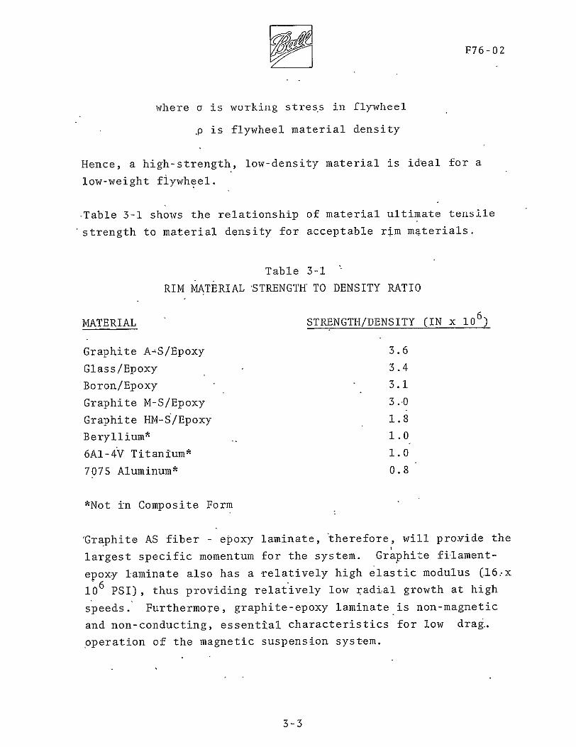
F76-02
where a is working stress in flywheel
pis flywheel material density
Hence a high-strength low-density material is ideal for a
low-weight flywheel
-Table 3-1 shows the relationship of material ultimate tensile
strength to material density for acceptable rim materials
Table 3-1
RIM MATERIAL STRENGTH TO DENSITY RATIO
MATERIAL STRENGTHDENSITY (IN x 10 )
Graphite A-SEpoxy 36
GlassEpoxy 34
BoronEpoxy 31
Graphite M-SEpoxy 30
Graphite HM-SEpoxy 18
Beryllium 10
6A1-4V Titanium 10
7075 Aluminum 08
Not in Composite Form
Graphite AS fiber - epoxy laminate therefore will provide the
largest specific momentum for the system Graphite filamentshy
epoxy laminate also has a relatively high elastic modulus C16x
106 PSI) thus providing relatively low radial growth at high
speeds Furthermore graphite-epoxy laminate is non-magnetic
and non-conducting essential characteristics for low drag
operation of the magnetic suspension system
3-3
F76-02
311 Rim Description
The rim consists of three bands of ferrite material made up
of 180 segments each and 72 samarium cobalt permanent magnets
embedded and bonded into the AS graphite filament - DX210 epoxy
rim material Figure 3-2shows the rim dimensions
The ferrite rings and permanent magnets are bonded to the basic
rim with Fuller 7004 adhesive The rim is composed of two basic
rectangular cross-sections the first and larger contains the
bulk of the graphite-epoxy material and the ferrite bands the
second smaller section contains the remaining material and
the samarium cobalt permanent magnets
The larger section has a cross-section 53 cm (21 inches) in radial
(125 inches) deep with an inner diameter oflength by 318 cm
154 cm (608 inches) Three channels are machined into this
section 254 cm (10 inches) wide by 057 cm (0225 inches) deep
The smaller section integral withto contain the ferrite bands
the larger is axially centered 28 cm (11 inches) in radial
(0375 inches) deep with-an outer diameter oflength by 095 cm
This section contains 72 holes which contain171 cm (6725) inches
the permanent magnets
The samarium cobalt permanent magnets are 14 cm (055 inches) in
diameter by 064 cm (025 inches) long The axial and radial
ferrite segments are shown in Figures 3-3 and 3-4 respectively
The ferrite segments are machined from Ferroxcube 3C5 material
The axial segment is slightly keystone in shape to minimize gap
distances Each segment occupies 2 degrees of the band circumshy
ference
3-4
529
GEN NOTES I RAD NOT DIMENSIONED
ARE 0907 Z WNEI6t4T - 455OLISshy
3 WrUtAt MOM4ENTUM 3300^-9000 Lb-VT- S Se
2-1RAb SC
30 OOTIRAXIAL31 t5R P - pERi7VE 5E6mlENTS-2 PLACES (5S60 gEaeb)
65 i ____ _CH COPPED GR4PHITE Amb EPOY
PLACS)
1 ~TIRI Z5
_ _
(REP)
I V 4 0
1 f3 PLA IES)
00 55DIX
42B
- 425 (REF)
EikPHITE FILAMENT tipQKY coMPOSITE
SAMARIUM COBALT
4 NampE S (72tE G D) CITE7KEb IN 380310 WITHIN OO EUALLY SPACED O 33000 PADi os MAGNET cEtJTer StAALL ZE E=QUAL WITW
o20 MAGrNET OLE5 bAA5 EITWEt TULjd
Ot zlNt kITA CoPPet
---ELusIA TO oo4 scAIme h3e o
BELOW IFLUSH4 VT(P
C
Figure 3-2 Rim Dimensions
555 2 ___
985
MNT L nFE RZPO KXC BE 3C 5 MISS
CD
Figure 3-3 Axial Ferrite Segment
I
233273
5058 27
LO
-9 100
4150 C2 PLACES)
MATL - 303
I
Figure 3-4 Radial Ferrite Segment
iF76- 02
The radial segment is rectangular in cross-section and when
bonded in place produces a small wedge-shaped gap between
segments Each radial segment represents 2 degrees of the band
circumference
312 Rim Fabrication
The ASCD rim was fabricated by Bristol Aerospace Limited Winnishy
peg Canada The material AS graphite filament tape impregnated
with DX210 resin was wrapped on a special tool producing 100
percent circumferential fibers with a volume fraction of graphite
of 55 percent
The oversized cross-section rim was wound in 15 separate layers
Each layer was B stage cured with the following temperature
cycle
P
J4 7
The post cure after the fifteenth layer was identical to the
B stage cure except the temperature was increased to 1770 C
in 50 minutes and held at 177degC for 2 hours after the 1490 C exshy
-posure
3-8
3
eF76-02
Figure 3-5 shows the specially constructed tool containing
cure cyclesheaters and insulation for B stage and final
The rim was removed from the tool and machined to nearly the
final dimensions including ferrite channels and permanent magshy
net holes These operations are shown in Figures 3-6 and 3-7
The ferrite segments andmagnets were bonded in place with Fuller
7004 adhesive and cured The magnets were placed in the rim with
alternating North-South poles and the ends were covered with a
016 cm (116 inch) thickness of chopped AS graphite-DX210 resin and
After final cure the rim was machined (by grinding) tocured
final dimension The rim was coated with a 0005 cm (0002 inch)
thick layer of Fuller 7220 adhesive as a final step to minimize
Figure 3-7A shows the final rim resultsrim water absorption
313 Rim Analysis
The rim analysis conducted by Bristol Aerospace predicted the
(55434 PSI)rim maximum stress and radial growth to be 38250 Ncm
and 3 cm (0117 inches) respectively
The rim was modelled using axisymmetric finite elements using
the ANSYS system The model characterizes the heterogeneity
of the structure (including the ferrite bands and magnets) and
the orthotropic elastic properties of the graphite-epoxy comshy
posite
The results of the analysis are summarized in Table 3-2 and in
a rim speed of 366 meters per secondFigures 3-8 3-9 and 3-10 at
(1200feet per second)
3-9
N
Figure 3-5 Lay-up Tool
IIP76-02
Rim Machining OperationsFigure 3-6
3-11
MIE II
Iiue37Diln emnn antHlsi h i
3I1
DF76-02
LOCATION MAGNITUDESTRESS (PSI)COMPONENT
Radial or carbonepoxy +460 (max) -891 (min)X stress
Axial or carbonepoxy +491 (max) -433 (min)Y stress
Shear or carbonepoxy +390 (max) XY stress -176 (min)
Hoop or carbonepoxy +55434 (max) 0 (min)Z stress
Radial inner surface +01166 (max)
Displacement outer surface -01130 (min)
(inches)
Table 3-2
MAXIMUM VALUES OF STRESSDISPLACEMENT AT 1200 FTSEC RIM SPEED
3-13
5ThF-=- V- LERATfNz- 1 4U0T00
RMCO RRLYSES BRISTOL REROSPRCE LTO OCT 73
HOOPSTRESS RNSYS 5
or Hoop Stress Contour PlotFigure 3-8 Z
F76-02
- flax h st-ess= 55434-
I I-1 I Ii-- shy
60Iz-
===z_ +0 _----- --- shyi -_-O- - = -- = +----- shy+ ---= -- r E
_-------=--- --- = ---
-- ----- +- - --- -- =--- -=
=
------ shy
=T--- 7
--
-
- -_ - - - -- - -- a
a zrlt- --r-- -r - z I=tzz-z - -
- 4
o6 Zf - =4-=-t vi I_- --- zmE+s=$ Z 4-| b- =---+----- shy
+ 5-t 4 -- c Tt - 22 ~++ _------ _ __ _C - u
a zjztL- +lt+ z- I [Lt- -- Tit--
-- -+v + --F t+-- -+rr 7- h |f
0 200 -00 6800 1000 12oo
Rim SPEED (rri5Ecc~
Figure 3-9 Hoop Stress and Growth With Speed
3-15
F76-02
e 4fo
1 1 I 1 t i I I CII1I1_4I I
Itdn-branveqs sts OI - I M
---shy-- -- -- - -
t~z 2 - 1- shy
- 421 ~T2 2 -=_-- -_E---i ----
t -- EM
___ _ ZZ +-_ _-A~~ - rrrr-
TLLto LLbi i L -- k - r K -1-
irtv li V i 1 -- t 4 s-- n-L -- T4 E
000-q0o 600 800 100 A120 Rim Sp Dr (FTVEC )
Figure 3-102 Transverse Stress Components With Speed
3-16
DF7602
Figure 3-8 shows the computer-drawn plot of constant hoop tensile
stress contours the maximum being 38252 Ncm 2 (55438 PSI)
occurring at the top and bottom inside corner
Figure 3-9shows the relationship of radial growth and hoop stress
as a function of rim tip speed
Figure 3-10 shows the relationship of transverse stress components
with speed
Since the material void free is capable of withstanding 110400 2 2Ncm (160000 PSI) in tension and 8280 Ncm (12000 PSI) in shear
the safety factor is 28 minimum On a sample basis the void
fraction was determined to be less than 04 percent
32 Back-Up Air Bearing System
The design of the back-up air bearing system was completed and
analyzed by Shaker Research Corporation Ballston Lake New York
The back-up air bearing (BUB) system consists of six hydro-static
radial pads and twelve hydrodynamic axial pads These are arranged
in six BUB sets consisting of two axial (one upper and one lower)
and one radial pad and located at either end of a magnetic supshy
port station Each BUB set is approximately 60 degrees from the
adjacent set The bearings are deployed toward the rim by air
pressure when predetermined rim displacement limits are exceeded
The introduction of air through the pads as well as through a
pneumatically operated valve in the vacuum enclosure provides
the fluid for the BUB system and also introduces air drag for a
fastercoast-down Hydrostatic bearings were selected for
radial use instead of hydrodynamic types because the rather small
rim depth (115 inches) allows insufficient area to produce the
required reaction forces The back-up bearing system is shown
in Figures3-11 and 3-12
3-17
P76-02
~14
-L- 7
FiguTre 3-1 AMCD Back-Up Bearing Layout DrawingI 3-la
Figure 12 Back-Up Bearing System
7F76-02
321 Hydrostatic Radial Bearings
The movable radial pads are designed to minimize air flow and
maximize air bearing rim reaction forces The radial pads proshy
vide a centering effect on the rim to minimize dynamic and magshy
netic unbalance forces
In the normal magnetic suspension mode the radial pads are held
away from the rim-and against stops by a set of nested compression
springs (total of 22 N (50 pounds) of preload) When the radial
system Figure 3-11 is activated 207 Ncm2 (300 psig) air is introshy
duced to the pad piston cylinder which moves the pad outward
toward the rim The piston chamber is ported to the pad surface
through a 0033 cm (0012 to 0014 inch) diameter orifice A
sealed oil-filled dashpot between the piston and pad controls the
deployment velocity
Figure 3-13 shows the relationship between- radial pad force and
gas flow versus film thickness for various orifice 4iameters
Because of limited gas available-the smaller orifice diameters
were selected
Since the rim is not at constant radius (because of radial growths)
film thickness and flow vary With rim speed Figure 3-14 shows
the relationship fo film thickness and flow versus rim speed
322 Hydrodynamic Axial Bearings
Movable- tilt type axial hydrodynamic pads were used since the
rim radial width is large and because of the limited bearing air
supply The axial pads are slightly crowned and combined with
the tilt feature are self aligning
3-20
F76-02
1 ~
It
7
I
JII ji
I L
II
---
Ft
T -
VIN I -_ Lr
TD _-
I
I+i
- 1MNV I
4~~r14 +t
Fit~Fi-~tdi I~ ~ JrV)
i ir
il-I= iH14+
i T r
F~m
shy
_ _
I L [
- i
I
_ i _
Ii
0001M -s as
Figure 3-13 Single Pad Force and Flow
3-21
A yyF76-02
WI
ii24pVshy-~~~~W
J4 i3 - Lit
I+ I~Ir~r L-- u 7t J
L 4- 1-nMLfI0__ 4~~~~- F-14--gtrF
I -- -r
4 ~ P I-
IaiH __M
1 --- t Th T1T
I- Vt prI i A
-p--t~LIV[~ VK jl77L1 1
Figure 3-14 Radial Air Pad Flow and Film Thickness With Rim Centered
3-22
F76-02
In the normal magnetic suspension mode the axial pads are held
against stops by a flexural spring The axial system is deployed
in-much the same manner as the radial system When a magnetic
suspension anomaly is detected the vacuum enclosure is flooded
with external air thus providing the film for the axial bearings
Figure 3-15 shows the relationship of film thickness with rim
speed Since the film will support the rim to about 15 radians
per second the pads are designed to accept several contacts before
replacement is necessary
323 Back-Up Bearing Pads
The primary objective in designing the pad material was to proshy
vide a material which would wear smoothly without damage to the
rim or to the pad itself Sacrificial bearing materials have
been used in gas bearings in the past which exhibit the necessary
qualitites The material used in the back-up bearings is an epoxy
resin heavily filled with aluminum powder aluminum oxide power
and molybdenum disulphide powder The mixture is poured into
silicone rubber molds degassed in a vacuum chamber then heatshy
cured The pads are then machined
When the spinning rim contacts the pads the pad will wear smoothly
and rapidly acquiring a high polish and yielding a fine dust
The rim surface should be undamaged by the contact The aluminum
filler provides high thermal conductivity to sink the heat generated
by the rim contact The aluminum oxide provides dimensional
stability so thQ pad will withstand the thermal shock generated
by the rim contact
3-23
3788I9 2 4 5 7 8 9 2
1 7 _- I
111-1 r - J
-I- --i- 1 rV1- 1 t r V
4 _ - _ _____ shy- I---7
I
r-- _- F-_- --- I ii -
I fr r l 7[-II j7shyLi +] - i I-- I
1 7 8
-- - 4 5---- 10 47 MCI 9
Figure 3-15 Axial Pad Film Thickness Versus Speed
F76-02
40 SUSPENSIONSYSTEM
41 System Description
The suspension system consists of three suspension stations
placed symmetrically about the rim At each suspension station
the rim can be pulled in either axial direction or tadially
inward by magnets A total of 12 magnets are arranged in sets
of four each to pull in these three directions (up down and
inward) The eight axial magnets are driven in concert by one
set of electronics Axial error signals are developed by a
position sensor located at the center of each station The
axial servo loops in each of the three stations are independent
of each other The four radial magnets in each station are also
driven by a set of electronics in response to a radial position
sensor located in the center of that station But the radial
station to another so asservos are interconnected from one
to prevent the servos fighting one another even in the presence
of rim radial growth
411 Magnet Description
One of the unique features of the AMCD is the support magnet
design The electromagnets are flux-biased by thin wafers of
samarium cobalt permanent magnet material placed in series in
the magnetic circuit This has the advantage of (1) providing
a high force per unit current sensitivity at zero current (2)
providing a linear relationship between force and current and -
(3) providing the static field required for zero power operation
The support magnet geometry is seen in Figure 4-1 The permanent
magnet biasing is achieved by slanted wafers of samarium cobalt
in the legs The wafers are as thin and wide as possible to
4-1
SAti 4-IUr CCBA3L~rshy
AGtJer-
AGII1
Figure 4-1 Support Magnet Geometry
RF76-02
minimize their reluctance in the magnetic-circuit The volume
of permanent magnet material is sufficient however to provide
adequate flux-biasing and static lift The reluctance of the
permanent magnets is large but does not more than double the
total reluctance since the air gap inthis system is large In
many other magnet suspension systems the gaps are small (about
01 mm) and this sort of series flux biasing would greatly inshy
crease the total reluctance in the circuit Control power would
thus be large and the systems would be impractical
The effect of flux-biasing on the force versus current characshy
teristics of the magnets is shown in Figure 4-2 With no biasing
current in either direction produces force of the same sign with
poor gain and low efficiency in the vicinity of zero current
Force is simply a function of the square of the current With
biasing the slope of force versus current is greatly increased
at zero current In the AMCD top and bottom magnets operate
together in a push-pull type of operation The coils are in
series hence both coils have zero current at the same time
The resultant force-current relationship is linear and has a
slope double that of either magnet alone
Figure 4-3 shows the U core of the magnet with the permanent
magnets in place Permanent magnet thickness is 1 mm (0040
inches) Also shown in Figure-4-3 is a fully assembled magnet
ready for potting After potting the units measure 43 cm x
167 cm x 25 cm (17 in x 42 in x 99 in) and weigh 500 grams
(11 lbs)
412 Position Sensors
The position sensors used in both the axial and radial suspension
systems are Multi-vit sensors manufactured by Kaman Sciences
4-3
7 gF76-02
-r
UPPETP HA -
C AOc~~
777
~~oeehAcn-e-r Z
Figure 4-2 Flux-Biased Magnets in Push-Pull Operation
4-4
rF76-02
I
3 i
A A
I tii A LWUv
NN
N~ i X -9
i i UI A i
IN aWIi ii i
iiiiiiiliiili
i~iiii Ii iliiiiiiiliiilii
Iilliii iiiiiliiiiiiliiiii = iiiiiiaii~iii iiiiiiiiiliiiiiiii
Uiiiii poundii=iiiii]iipoundiiiiiiiiiiiiiiiii Uigure 4-3 Support Magnet Cosri on
iliiiiur -3 ConstructiiiiIliiiiiiiiioniiiiiiiliiiSppriMge liiiiiii i iiiiliiiii3 URiliI 4-s == =
4-s
rF76-02
Corporation These are conventionally called eddy current senshy
sors although they are actually sensitive to anything that changes
the inductance of the test coil in the probe Hence either
eddy currents in a conductor or the permeability of a magnetic
material can be sensed In the AMCD the sensors look at the
ferrite bands and therefore are operating entirely ina non-eddyshy
current magnetic permeability mode Special calibration of the
sensors was required in order to operate in this mode Linear
range of the AMCD sensors is 025 cm (01 inches) and scale facshy
tor was set at 4 voltscm (10 voltsin)
413 Control System
The axial suspension system uses three independent servo loops
to control electromagnet currents An electronic diagram of one
of these loops is shown in Figure 4-4 The heart of the elecshy
tronics is an Inland Controls MA-I DC servo amplifier which is
operated as a current driver to reduce the effects of electroshy
magnet inductance Equations of motion of this driver and an
analysis of the voltage feedback used to damp high frequency
roots are given in Appendix A An analytical block diagram of
the entire servo loop is shown in Figure 4-5 Equivalent points
on the electronic and analytical diagrams are indicated by letters
within hexagons
The axial suspension system has two modes of operation a posishy
tion mode and a virtually zero power (VZP) mode In the posishy
tion mode rim position error is used to command electromagnet
current The rim has high static and dynamic stiffness about
any desired point in the gap In the VZP mode the rim position
set point is modified by positive feedback of the integral of
electromagnet current The result is that the set point is moved
until steady-state current is zero The permanent magnets are
4-6
AA
REHTUtk +26V
4-
C11 7t-Q
Fiue44Aia3upnin7lcrnc
S Cornn- EesoCo p n a cncivCrrent Driver- O deg OI 99 (5C + sm -3 (s + 1 1deg E 1 copy + F
gtosO ~
volf
iE 3 7 T r i m T ntegratadegr
Suspended
Mass
-|ectro
-ria net
16
permanent Magnet
Figure 4-5 AMCD Axial Suspension Station
R 1F76-02
then providing all of the support of the rim Dynamic stiffness
is nearly the same as in the position mode but static stiffness
is actual negative If a downward force is applied to the rim
in the VZP mode it initially moves downward but then slowly
rises to assume a new zero power position above the old equilibrium
position
The electronic circuit diagram for a radial servo station is
shown in Figure 4-6 and the corresponding highly coupled analytishy
cal block diagram is shown in Figure 4-7 Again equivalent
points on the two diagrams are indicated by letters in hexagons
The large amount of coupling results from three servos controlshy
ling only two degrees of freedom
Two modes of operation are available a position mode and a WAHOO
mode The position mode is similar to the axial position mode
The WAHOO mode is a zero power mode that produces zero power
operation in the presence of both static loads and rim expansion
This is accomplished by adjusting the position set point at each
station as a function of the integral of the sum of the electroshy
magnet currents at the other two stations
The name WAHOOis derived from the poker game WAHOO This game
is played in a manner such that each player knows what every
other player holds but does not know what he himself holds
Inspection of the WAHOO trim loops of Figure 4-7 reveals that
for VZP trim purposes each servo only looks at what the other
two are doing This innovation was developed by BBRC to meet
the unique requirements of the AMCD
The derivation of the WAHOO concept is given in Appendix B
There it is shown that only the WAHOO concept produces zero
power operaion for both rim expansion and force disturbances
4-9
A00l 51 Ir
A-A-
F
27
ffzo xr
74 VIP KIAk
7
Ems~
n
A7-
I
A1
ter
a 2k-
-
-
-
-
-
I)
Figure 4-6 Radial Suspension Electronics
-KS
Iamp wkin47s Permanent MagnetVeloityPM VPol Aplifir PMEHM E Iectremoqnet
K5 Kmn eae t~j VOS 0bCar respond to Lettered
1vII~rb r - rr m Psitionson Cgrcwit
vol vol Im PosiMoon Pox
SlRtim rtOhkx _Q$)bsS 4lfe I
0niplPfied Cus ren Driver
Gcucv rbinn n i
+ + vt
If
in-7d FigureservoD RailSro
+i
42
F76-02
Appendix B also shows that for single station design purposes
a single station can be represented as shown in Figure 4-8 Two
points of interest are immediately evident The equivalent mass
for a single station representation is 23 the total rim mass The WAHOO concept which involves negative feedback to each station
from the sum of the other two stations resolves to a positive
feedback in the single station representation exactly like VZP
in the axial mode This representation can be used for designing
the system characteristic root locations If the characteristic
roots from the single station representation are given by A and
the WAHOO gain is Kc it is shown in Appendix B that the three
station highly coupled set of characteristic r6ots are givenby
(S + 2K )A2
Performance
421 Static Performance
At each suspension station the rim will seek an axial equilibrium
position based on the applied load and the control system mode
(position or VZP) These equilibrium positions can be preshy
sented in one plot as shown in Figure 4-9 The VZP line is a zero current line and has a slope that indicates static instability
however as shown in the next section the system can operate in a
stable manner along this line The most usual operating position
mode point is about 001 cm (025 inches) above the center of the
gap At this point the slope P of the VZP line is about 595
newtonscm (340 lbin)
In the position mode an operating line exists for each set point
of the position sensor A family of these is shown in Figure 4-9
The lines are finite in length because of the limited current drive
capability of the electronics The slopes of the lines are apshyproximately 2600 newtonscm (1500 lbin)
4-12
Stationfost ionsingle
Oecrlx- EquIva1eratArmplifir Current Driver 6 Mks$M9oqmet+ 1m
~~~~~ eroe L~r
Is + Fes I16(7+1210 r0 0 l I-
p 0 1
476 An- Per
u2 IVlt+ -Eg
o tKate - r1 1 StO Sr eq uci o lnk wahoo is
Q Correspornas toa letterd posit~ions on circuit chogr~m
Sinql~e stcton eqviclvJewtmls is 23 totil ma
~odelldas a posattve PeedbctK self IoopVe
t to o-t liKe Vf Pwould ltherefboretxpect fvrthernortn itthe Aol O Servo Xt doesonh
Figure 4-8t EqiaetSnluadapev tto
ekgeto8 rnex e o +non
A F76-02
UP
MAGNET M~A t r
lsrok os NoRMAL
kE-RITI N
P E-Nshy-OMFR
tL UPshy
- j ~
-10
h31G1NL pAGE iS
)F POOR QUML-rI
Typical Static Suspension System Performance
Figure 4-9 4-14
rF76-02
The force sensitivity F of each station is about 138 newtons
ampere (31 lbamp) Hence the force produced by a station
is given by (in English units)
F = 340X + 3lI
422 Dynamic Performance
The analytical block diagram for an axial suspension statiQn is
shown in Figure 4-5 For theposition mode the root locus and
-Bode plots are shown respectively in Figures 4-l0and 4-11 The
root locus plot shows that the dominant pole pair has an undamped
natural frequency mN (which we define as bandwidth) of 171 radsec
(272 hertz) and a damping ratio of28 The Bode plot shows
that the gain crossover frequency wc (which some define as bandshy
width) is 1827 radsec (290 hertz)-and that the system phase
margin is 2320 Both plots show that the lower gain margin
is 22(-131 db) and that the upper gain margin is 201 (261 db)
For the VZP mode the root locus and Bode plots are shown respecshy
tively in Figures 4-12 and 4-13 The root locus plot shows that
the dominant pole pair has the same undamped natural frequency
and damping ratio as the position mode that is wN = 171 radsec
= 28 The Bode plot shows that two gain crossover frequencies
at 1823 radsecexist one at0838 radsec (013 hertz) and one
(2903 hertz) The phase margin at the lower crossover frequency
is -772 and that at the upper crossover frequency is 2300
Both plots show that the lower gain margin is 226 (-129 db)
and that the upper gain margin is 2011 (261- db)
The response due to the step application of a one pound weight
is shown for the position mode in Figure 4-14 and for the VZP
4-15
OF76-02
1 -DD
-- A I 1
I I
i
3000 --------------------------------- ___tN
-5000 -400 -30U -2ODG -t I lo oD
REAL AXIS
Figure 4-10(A) Root Locus Plot - Nonideal Current Driver With
Voltage Feedback
4-16
---------------------------------
7F76-02
-I- 111 1-l Z9D
io oI 1ll t A
G
80 ----------- 0 aEu----------------shy-4--
FigueRot41001LcusPlo - Nnidal Crret DrverWit
-1---4-17
I I
F76-020
14-HLowler
)2 I__ _ p
1 N I-- A =20 41 r
I tIse0_ __ _ _ 4 6 2 4 68100
s 10 log H00 6 10009 FREQUENCY (RADIAWS$ECOND)
Figure 4-11 Bode Plot - Nonideal Current-Driver With Voltage Feedback
4-18
7F76-02
$oo I5iI000 I1
T 1 Ii
-A
S4+
N A
4000 R--- - - - - -
V A x
103 000 40 30 29
urn rvrWtFi1r -12A Roo Lou7lt-Nnda
Voltage Feedback 4-19
V gF76-02
ii
- I I I
I I I II
I lii
-I I
II I iishy
II - - -i-l
Fgr 4-2B o otocu PltrNndaCrefl rive
With Voltage Feedback
4-20
F76-02
I i E
A -4 G
E- 60I jUroI(
I
1A2zS1 me RI
3s F-1-L
IIsoM 3en
4) e r
-120---- -Marlin
fla e =2300
-140 shy
1 1 10 10g 2000 1090r FREQUENCY (RADIANSECOND)
Figure 4-13 Bode Plot - Nonideal Current Driver With
Voltage Feedback
4-21
012
F76-02
00010
00008
pound E
0
p
0 00
0zkc0
0
E
- -
4+-F
- - -
Nshy- - - - - - -
4
- -
5
-4-2
AF7602
mode in Figure 4-15 The response for the position mode settles
out at 6941E-5 feet (002 cm) This yields a position mode
stiffness of Stiffness 6 1 lb
6941E_5 t X feet
1 12006 lb (21021-
N
69Th-ft Tni in cm
The response for the VZP mode settles out at -2451E-4 feet
Thisyields a VZP mode stiffness of
1 lb feet = lb NStiffness = 2451E4 ft X 12 in -3400 i (595 E-
Note that the stiffness in the VZP mode is just that of the
permanent magnet and that the movement in this mode is toward
the applied force That is if a weight is placed on the rim
in the VZP mode the rim will move up
Further insight into the system can be found by examining Ap2
pendix C When using current driirers the usual tendency is to
ignore the high frequencydynamics and simply say that the
output current is the input voltage times a constant This can
be very misleading in the case of AMCD- In Appendix C are shown
root locus plots using both an ideal current driver arid a nonshy
ideal current driver without voltage feedback It shows that
voltage feedback is necessary for the axial suspension Also
shown in Appendix C are Nyquist plots and phase-gain root locus
plots of the nominal axial systemthat is the system using curshy
rent drivers with voltage feedback The esoteric phase-gain root
locus plot shows on one plot the sensitivity of the system roots
to change in both gain and phase For example it shows what
would happen if an additional 300 of phase lag were added to the
system from some unknown source
4-23
F76-02
0001
I f
I 0 e
eshy
0a T 1-0001-shy0N
ft E F 0
E a
- 002--------------shy
0 t0 20
TINE (SECONDS]
30 40 50
Figure 4-15 Nonideal Current Driver With Voltage Feedback
4-24
F76-02
The equivalent single station radial analytic block diagram is
shown in Figure 4-8 It is very similar to an axial station
The root locus and Bode plots for the position mode are shown
respectively in Figures 4-16 and 4-17 The root locus plot shows
that the dominant pole pair has an undamped natural frequency
(bandwidth) wN of 653 radsec (104 hertz) and damping ratio C
of 18 The Bode plot shows that the gain crossover frequency
is 666 radsec (106 hertz) and that the phase margin is 1350
Both plots show that the lower gain margin is 329 (-965 db)
and that the upper gain margin is 7054 (3697 db)
The root locus and Bode plots for the WAHOO mode is shown in
Figures 4-18 and 4-19 The root locus shows that the dominant
pole pair has an undamped natural frequency of 674 radsec
(107 hertz) and damping ratio of 16 The Bode plot shows that
the upper gain crossover frequency is 691 radsec (110 hertz)
At this frequency the phase margin is 1260 Not shown is the
fact that the system also has a lower gain crossover frequency
of 594 radsec (095 hertz) At this frequency the phase marshy
gin is -715 Both plots show that the lower gain margin is
389 (-821 db) and that the upper gain margin is 6701 (365 db)
The large upper gain margins for both the position and the VZP
modes indicate that current driver voltage feedback is not needed
Considerable rim bending instabilities were encountered during
the design Early in the development the axial system was
designed to be overdamped This caused a bending mode to be
driven unstable The compensation was adjusted experimentally
until the bending became stable Unfortunately this reduced
the lead in the system resulting in the present underdamped sysshy
tem It is believed that bending will present no problem at
high spin rates because of the effective stiffening of the rim
4-25
6F76-02
_____ - _ r ____I___
141
IT___lishy
1 ii
1 F]
eir
t lj~
4-
J TT a p-
III NEA
fiIT WBKsITlK j1_11IIi I-
I
e
-Fshy
Y]-111 ji
1i1fln 4--I r
I i--I -
TFiJ-WL 1
_1(-Ii4 - I
I~ ~ ~iA_~2I ___ ii- 11 IFt-Ih
iT
h~ -iH T
+~ji+ih Iplusmn
_ _ _+ I kt ~h-II
+ LILY -
7 SO bullj
Figure 4-16 AMCD Radial Suspension Equivalent Single Station Position Mode
4-26
Elll csl- tLL[ 11--- 1_ il
V
1 MIN
2 0 H qL2~14-0IT
I M Ill 1OIHI
+-o ip Lr g
Ti I -0 1- b1 -- i
Ij _IUSi 1PIN - il
--i
41i L -I I - d jir ~J I I
00 -o
ro-d 5 c
Figure 4-17 ANCD Radial Suspension Equivalent Single Station o Position Mode
7F76-02
1LjI_----- Li -III iI - - I -shy-F ]e2 1
Is- Lr [_I
r ir -L-j 11I IALI _ _ _ ___ 2_
E11LLN1LALIF TYC -- td It 11
- KI
S1 1 1 1--shy
II
I r 11
FLL-1
U - I 4
E~~~~fL
__
f Lplusmn Xi ILIi _ _
- ii _ _ i
- H --
--------
A-1 1 F - JT-1
-- t-ti -~r -r I- t - --- IL I
IIJlri-tlrht1f tI
_+ _ l PillS 1 I
Figure 4-18 AMCD Radial Suspension Equivalent Single Station
o Wahoo Mode
4-29
rm~r 1 u i rrrrF r r r
4
130
o
I -4
7 7 1-shy iAb d
llt h
-30 Tfij4i i ~
- n0 t
Figure 4-19
01 AII-
I uji r a sec
AMCD Radial Suspension Equivalent Single Station o Wahoo Mode
AF76-02
and the averaging effect on modal pick-up caused by the bending
modes moving rapidly past each position sensor
As the rim is spun up the three axial stations become more and
more coupled by nutational effects The result of the coupling
is to reduce the dominant roots damping ratios more-and more to
the point the system could go unstable if the rim is spun fast
enough It is believed that this tendency could be greatly
reduced or possibly eliminated by the proper combination of cross
feeds from one axial suspension station to the others
4-30shy
DF76-02
50 DRIVE SYSTEM
51 System Description
The AMCD drive motor can be thought of as a large permanent magshy
net brushless dc torque motor Samarium cobalt magnets are
bonded into the rim at regular intervals The two phase armashy
ture is segmented with a winding set at each of the three susshy
pension stations Commutation is controlled by Hall effect senshy
sors mounted near the rim which sense position of the samarium
cobalt motor magnets
52 Magnet Selection
Alnico was considered along with samarium cobalt for the permanent
The large air gap and segmented winding structure meanmagnets
the magnets will become nearly air stabilized The rim was designed
with a small outer lip to hold the magnets This was done to
isolate the drive from the suspension as much as possible without
and complexity to the rim than necessary Thisadding more mass
small lip implies a short magnet Samarium cobalt has high
strength for short lengths and does not pay a penalty for air
In fact it is very difficult to demagnetize thisstabilization
material
cm (55 inches) diametertby 64 cmSamarium cobalt magnets 14
(25 inches) length were selected and bonded into the rim with
polarities alternated
The rim contains a total of 72 magnets spaced 73 cm (288 inches)
apart
5-1
53
--F76-02
Core and Winding Design
Each armature segment consists of a pair of bar-shaped winding
assemblies one above and one below the rim
Sit cos sla 0S SMa
cores in a singleThe windings-are wound toroidally around the
layer The figure above shows only the cross-section 6f conshy
ductors in the air gap as the conductors passing around the other
side of the core add nothing to torque and serve only a connectshy
ing purpose The bar-shaped cores are easy to wind and result
in a compact structure The single layer of 18 conductors adds
very littleto the overall air gap This effective electroshy
magnet design was suggested by P A Studer of Goddard Space
Flight Center
Ferrite material was chosen for the core to reduce losses Fershy
rite also is easily machined into the required irregular shapes
The windings are grouped into two phases SINE and COSINE each
of which acts upon three magnets at each motor segment In operashy
tion current in one phase is acting on the magnets while current
in the other phase is reversing in preparation for a magnet of
opposite polarity
5-2
DP76-02
54 Motor Commutation
Hall sensors act as commutation devices for the motor They sense the position of the permanent magnets in the rim and cause the drive coil currents to be switched according to magnet position
The sensors are mounted in pairs one above the rim and one below for each winding phase Outputs from each pair are summed so that the switching position is not affected if the rim moves up or down within the air gap The SIN pair controls current on the SIN windings of all three motor segments and likewise the COS pair
of Hall sensors controls all COS windings
55 Motor Control Electronics
A block diagram of the motor control electronics is shown in Figure 5-1 For each phase the Hall sensor outputs are summed and amplified to drive-threshold detectors These detectors sense magshynet position and polarity The phase control logic determines the
timing and polarity of the motor coil drivers Interconnections between the two phase control logic blqcks provide positive direcshytion and start-up information
Each of the six coil drivers controls a phase at one of the motor
segments Associated with each driver is a coil current sensor which monitors the current in that winding All six of these
current sensorsreceige a common reference from the speed control
potentiometer When current in that particular winding reaches the reference level the driver turns off until the current deshy
creases This prevents the current from reaching destructive levels at low speeds and acts as a speed control at high rim
speeds
Since the coil drivers are either full on or off a very efficient drive is achieved At low rim speeds the drivers operate as a
5-3
56
F76-02
conventional PWM (pulse width modulated) amplifier A quite faithful square wave current of controlled amplitude is fed to the coils At high speeds high acceleration (or deceleration)
is possible with the drivers full on for the period between magshynets with current rise and fall limited by the inductance of the
coils
Torque Calculations
The equation for the force betweena magnetic field and a current
carrying conductor-is
F = BLI
where
F = Force in Newtons B = Flux Density in Teslas (WebersM~ter )
L = Conductor Length in Meters
I = Current in Amps
If the magnetic field is created by a permanent magnet the force
can be considered to act on the magnet if the conductof is held
stationary which is the case with the AMCD motor
To arrive at design force each of the factors B L and I must
be evaluated
A force calculation will be made for one magnet face interacting
witha coil This can be then doubled to account for both ends of the magnet next tripled to take into account the three magnets in one motor segment and tripled again to realize the total force for the three motor segments Then using the radius of the rim
we can calculate developed torque
5-4
F76-02
Flux Density Calculation (B)
The large air gap makes it difficult to- estimate how much of the
magnet flux will couple through the winding core and how much
will be lost to leakage A measurement of coupling flux was made
using a pair ofsoft iron bars similar to the ferrite corasi
SEJSE C0115
SOFr iROh
-4 Webers with magnets of averageThe flux measured was 0375-x 10
strength
core must-be convertedThis flux that couples through the ferrite
to flux density (B) in the air gap where it interacts with the
coil windings There are two practical Choices for doing this
We can assume all the flux goes straight up from the surface of
the magnet andreacts with only those turns above the magnet or
we can assume the flux spreads out evenly over the winding area
Of course the truth liesand-reacts with all the turns equally
an adequatesomewhere in between but the second approach gives
approximation
The winding area in the air gap for one magnet coil phase is 2
19 x 36 cm or 68 cm
Flux density then is
-44m _ 0375 x10 Webers 2 0055 WebM-B_=A = 4 2A - 68 x 0-4 m
5-5
F76-02
Conductor Length Calculation (L)
are 28 turns with an effectiveIn the winding phase area there
length of 19 cm each
Total effective length is then
L = -19 x 28 = 532 cm = 0532 M
Current (I)
that the coil drivers and wiringThe elbctronics are designed so
canhandle 4 amperes Also the inductance of the coils was
examined to be sure that currents of this magnitude can be
reversed at maximum rim speed frequencies with a 60 volt power
(and torque) will then be calculated for thesupply Force
design maximum of 4 amps
Force
We can now calculate force from the equation
F = BLI
= 0055 x 0532 x 4 = 0-1-17 Newtons
Recall that this is the force for a single magnet surface inter-
For the total motor this is multiplied by 18face
Total Force = 0117 x 18 = 176 Newtons
576
0F76-02
This times the magnet radius (0838 meters) gives total torque
Total Torque = 176 x 0838 = 176 Newton-Meters
(13 lb-ft)
A small (14 diameter) test wheel was built to check the above
torque calculations Acceleration measurements were made and
from the known wheel inertia torque was determined Correlation
within 10 of the calculated torque was achieved
5-7
S in Hall Sensors
Summing
Amp
[A Threshold Sin Phase Coto-rie
DetectorsLoi
SnB1Sin
Sin C Driver
ol
Hall Sensors
~ Amp=ApDtcosLogic
etctr Control -- Die Col Ci~
Summing Threshold Phase Cos B Driver
iCosCos
Ci Co
Figure 5-1 Motor Control Electronics
C
aF76-02
60 REFERENCES
1 Anderson Willard W and Groom Nelson J The Annular
Momentum Control Device (AMCD) and Potential Applications
NASA TN D-7866 1975
6-1
F76-02
APPENDIX A
CURRENT DRIVER EQUATIONS AND TRANSFER FUNCTIONS
A-i
F76-02
Appendix A
Current Driver Equations and Transfer Functions
When using current drivers the usual tendency is to ignore the
high frequency dynamics and simply say that the output current is
just the input voltage times a constant This was very misshy
leading in the case of MCD-as shown in Appendix C The circuit
diagram of a current driver with voltage feedback and its equishy
valent diagram are shown in Figure A-i -
v A T5It
Figure A-I Current Driver and Equivalent Circuit
A-2
F76-02
The beginning equations of motion are the following
Rl11 RM -- R 10
-RM SL + R2 2 -(SL + RC) I= A(TS+I)-)V + ARI(TS+l)shy
-R 2 -(SL +R c) SL + R3 3 + S_ C I 3 0
where
R1 lt= R1 + R2 + RM
2 RM + RC22
R33-- R2 + RF + RC
Transposing I1 to the left hand side we obtain
R11 -RM -R2
-RM(TS+l) + AR 1 (TS+l) (SL+R 2 2 ) -(TS+1) (SL+Rc) 2 A S-SR22 S L+SR33+-l
What we really want is the current through the inductanceshy
1 2 T3
Adding this equation to the system we obtain
C1 C12 C1 3 0 II 1
B2 1 S+C 2 1 A 2 2S2 +B 2 2 S+C 2 2 A23s2+B 2 C 3 0 12 A V
B31S A32S2+B32S A33S2+B 3 3S+C 3 3 0 13 0
- -1 1 1 1 0
A-3
eF76-02
where by definition
-=A32 -LC R11 B22 = L+TR 22
= - C22 R22 B32 = RCCl2 RM
C13 =-R 2 A23-= -TL A33 = L
= R33B21 = -RMT B23 = -L-TRC B3 3
C = ARI-RM C = -RC C =C -I
= -R2A22= TL B31
If the voltage feedback is removed these equations reduce very
simply to
-RMIRlI+R2+RM
+ AR1 (SL+R+RM)(TS+ 1j1 2 = AKRM(TS+I) We want thewhere 12 is the current-through the inductance
transfer function 12V First divide the secondequation through by
LT to obtain
-RMR I+R2 +RM
(R C+ PM j] IAL 1 V S+L-iIARI[ RM L (SplusmnT -1)+L -lT -1A
A-4
F76-02
Then by Cramers rule
2 CR1+R2+RM)AL -1T-+RML -1(S+T- 1 )_L-1T- 1 AR1
V7 -1 r- 1 2-1 - lshy(RI+RZ+RM)(S+T +L (RC+RM) -R ML l(S+TI)+L ITIARIRM
(R2+RM)AL -T - I(S+Tshy
-(R1+R 2+RMM)(S+T 1 )(S+L-1 RC)+L -RM(R1+R 2)(S+T-I)+L T ARIRM
Further manipulation yields
S+T-1 +(R 2 +RM)ARM T12 RML -
V - 2+RM) 1 L-+RR [2 wT-ARI-L 1RM(RI+R2 -
S+T )(3+L Rc) + RR+Tl+R---
Finally the desired current driver without voltage feedback
transfer function is given by
12 RML- S+T -1 +A(I+R2 RfIj
V (RLR-+RM) - -1 LRM(RI+R2 ) (ST 1 [7AR 1 RS5 + R2 +RMR R1 L Rk 2 )
A-5
76-0 2
For infinite amplifier open loop gain A = the transfer
function reduces to
2R Lim 12 = R1_ 2M
(l+R2RM- R2
R - RYR RR)r112RM for R2gtgtRM
-This is the transfer function which is used
I2 R2 12 R 2V RIRM
if the high frequency roots may be ignored
When the high frequency roots are not to be ignored and
if AR2R1 gtgtmax (RMRC-i)
and RMARlRjR2gtgt
RI+R 2 c
A-6
rF76-02
The transfer function simplifies to
S+T- AR 2RM1
12 RML-
V R1+R2 (S+T-)(S+L -Rc)+L- RM(S+T-AR1 R1 +R2)
RML-1 S+T-1AR2RM-
R1 R2 S2+ -1 -1 -1 T 1L-1RMARl - A
S +(T- +L -Rc+L RM) S+ R+R
T- +L- (RG+RM) TRLAR
2 (RI+R2)
The dc gain of this transfer function reduces to the same transshy
fer function used if the high frequency roots may be ignored
that is
2 R2 V RIRM
For the radial MA-lCurrent Driver
RI = 10K R 2 = 2711 KQ RM 10
RC = 30 Q2 L = 0128 h T - 30 A 50119
Then the radial current driver without voltage feedback has the
transfer function
12 _-00061463(S+40762E10)
V S+13609plusmnj30400 shy
A-7
F76-02
Forthe axial MA-I current driver
R=1 10K R2 = 7311K C 01 1f R11 = 17311E4
L =0064 f = 12M R = 14 R22 =15
A = 50119 RM = 1 T- = 30 R 33 I2073E6
Then
= C11 7 17311EA B2 2 = 564E-2 A 3 2 -0064
Cl2 = -- 22 = 15 B = -14
== = -7311E3 -21333E-4 A33 0064C13 A 23
B21 = -33333B-3 B2 5 -53067B-2 B 12073E6
C21 = 50119E8 C2 3 - 14 C3 = 1OE8
= A22 = 21333E-4 -B3 1 -7311E3
Without voltage feedback the axial current driver has the transshy
fer function
2 00090261(S+l0993B1)
V S+13219plusmnj36839shy
A-8
7F76-02
Note that without voltage feedback the damping ratio on both the
radial and axial current driver high frequency roots is less than
05 This appears to be all right for the radial servos but is
very bad for the axial servos as shown in Appendix C Consequently
-voltage feedback has not been employed for the radial servos
current drivers but has for the axial servos cur-rent drivers
The effects of this feedback has been determined numerically
Figure A-2(A) shows the effect of increasing RF the voltage
feedback resistor from zero to infinity with the feedback capashy
citor C held a-t 01 lif Ifonly the capacitor is used for voltage
feedback the current driver roots are still lightly damped but
at a much lower frequency As the resistance is increased the
roots increase in damping become real then decrease in damping
at a high frequency finally moving to the no voltage feedback
position for RF = Figure A-2(B) shows the effect of increasing
the voltage feedback capacitor C from zero to infinity while
holding the feedbackresistor at one megohm For C 0 the roots
start at the no voltage feedback position As C is increased the
roots decrease in frequency and-increase in damping ratio until
C = 00091 f Further increases result in decreased damping
ratio and increased frequency At the chosen voltage feedback
values of C = 01 vf RF = 10 MQ2 the axial current driver transshy
fer function is
I 0008994(S+833)(S+l099EII) V (S+786)(S+2771plusmnj2583)
A-9
~~~ L~Trrrl~I I~ I II 4
Jots_1 nr_- r177I 7F I i0K IIII __ riiTTh
17shy
tkP M T7r
Hl4plusmn ------ IIr-1-----~ -- - I -
CDl7E-~ ttbifil
LA14 -T-- 4+ -
C T -I I
H -rTH V i H
-HE I
Figure A-2 Effect of Voltage Feedback on AMCD Axial Current Drivershy
AF76-of -
APPENDIX B
THE WAHOO CONCEPT
B-I
7F76-02
Appendix B
The WAHOO Concept
Introduction
Two conditions may occur which cause the radial electromagnets
to draw more current than necessary First if the rim is tipped
This forcea gravitational force tends to pull the rim sideways
at the expense of causing the electro-shyis countered by the servos
magnets to draw more current Second as the rim spins up
centrifugal forces-cause it to expand To each radial sensor
as rim movement to be countered by thethis expansion is viewed
to try to pullservos So each electromagnet draws more current
are directed inward andthe rim inward But since the forces all
spaced 120 a-round the rim the resultant of the forces is zero
so the rim does not move The net result of the expansion then
is thatonly the current in the electromagnets increases Trim
loops are developed in this appendix which lead to VZP (Virtually
Zero Power) operation for the radial servos when either the rim
is tipped or expands or both The system employing these trim
loops is called the WAHOO system
Because the three radial servos are controlling only two degrees
of freedom the radial servo system is very highly coupled This
very high degree of coupling makes it difficult to design each
servo as a single uncoupled system Hence in this appendix we
also develop equations to show how the three-servo radial system
may be designed using a single station servo radial equivalent
Development of the WAHOO Concept
The AMCD rim is suspended radially by three servos pulling on
it from the inside much like shown in Figure B-1
B-2
F76-02
Kim
Figure B-i Radial Servo Sign Convention
The sensor outputs are denoted by X1 X2 and X3 As the rim
spins up it expands by the amount X0 The sign convention is
chosen such that positive forces and displacements are outwards
The equations of motion of the rim are
(F2 - F3 )Co = My
(F2 + F3)s8 -F1 = my
X2 = XCe + YSe
X3 = -XCe + YSO
XI = -Y (B-i)
B-3
F76102
The force acting at each station is composed of a permanent
magnet force and an electromagnet force That is
Fl = P(XI+X0) + E D1
= P(X2+X0 ) + E D2 (B-2)F2
F3 = P(X3+X0 ) + E D3
these equations are-combined with the servo equations in Figure
B-2
From the block diagram the quations of motion using five variables
are
V1 = Kp(-Y+X0 ) -S)(KsVi+KcV 2+KcV 3) EKRN_1
Y = M--p(-Y+X0)+DR (-Y+X 0)+ EV1 +pSC(YSe+XCplusmnX0 )
EKRN -fD se(YSe+XCe+Xo)- ESeV 2 + PSO(YSe-XCe+X0 )
EKRNK sOCYSe-xce-Xo)- nsev 3 + FY
-V2 = K (YSO+XCeplusmnXo)-(lSKsV2+KcVI+KcV3)
EKRN = 1=M PcO(YSe+XCe+X 0 )- D C(YS+XCc+X0)- ECOV 2
EKRN -PCO(YSe-XCO+X 0 )+ ce(YSe-XCe+X0 )+ ECOV3
)V3 = K(YSe-XCO+X0 )-(SJ(KsV 3+KcVI+KcV2 (B-3)
B-4
+ SFt
+- K + X0
+ T- SID
fRi
Figure B-2 MICfl Radial Servos With Trim Loops
7F76-02
Rearranging
(S+Ks)VI+KpSY+KcV 2+KcV 3 = KPSX0
-M-1DEv+[DS2 -DM-Ip(1+2SD)+M-EKRN(1+2S2 0)]y
+M-IDESOV2 +M-1 DESOV 3 = [M-IDP(-1+2S)+MWIEKRN(I-2SO]XO+MDFy
KcV -KpSSY+(S+Ks)V2 -KpCeSX+KcV3 = KpSX0
M- 1DECOV 2 +[DS 2DM- P(2c0 )+M-1EKRN(2C2 )]X-M-IDECOV 3 = 0
KcVI-KpSSY+KcV 2+KpCeSX+(S+Ks)V 3 KPSX0- (B-4)
Since 0 = 30
I+zs2 -1+2(5)2 = 15
-- 1+2S = -1+2(5) 0
2C = 2 )2 = 15 (B-S)
Using these simplificatfons the Laplace transformed radial
servo equations of motion in matrix form are
(S+Ks KpS 0 KC KpS 0DSL KC V1
-1IDE +lSMIEKRN SM- 1flE 0 SM- DE Y 0 M D
-1$M IDP __ __
KC 5KpS (SK S ) SrI KpS X6 V2 KK SX 0 + 0 Fy
DSz--shy
SM- 1 DE - SMDE0 0_- 54M +lSM 1 EKjN x 0I 0
-5KpS K 54 KPS (S+Ks) KpS 0KC V3
B-6 (B-6)
F76-02
The system characteristic equation is the determinant of the
coefficient matrix With much algebraic effort it can be
reduced to
A = (S+Ks+2Kc)X
FKRN-ISM- DP)+lSKpM- DES]2[(S+KsKc)(DS2 +SM-
(B-7)
Now lets simplify the expression by-removing the high frequency
roots In the Cambion hardware
KRN 107 S for low frequencies
D (S+1000)(S+10000)
With this approximation KR = D = and N = S Then
2+lM ES-lM P)+lSKpM-1ES] 2A = (S+Ks+2KC)[S+Ks-KC)(S
So the roots separate into -(Ks+2Kc) and two identical sets
within the brackets Immediately we see that Ks+2KC 2 0 for
stability Now looking within the brackets we see that S2+
1SM-ES-l5M-P represents the permanent magnet roots at
+lSM-IP moved to the left some by the rate feedback however
one remains in the right half plane Taking these roots and the
one at -C(Ks-Kc) as poles of a root locus plot and S as the zero
Figure B-3 shows that for stability KC a KS
B-7
0F76-02
Kct IKSKczk 5
Figure-B-3 Effect of Trim bull Loop Gains
Les look at three special cases
I No Trim-Loop KC = KS = 0 No VZP
A = s3 [(S2 +lSM-IES-lSM-iP)+iKIPMlE] 2 (3-8)
There are three roots at the origin from the three unconnected
integrators and two identical quadratic pairs The system is
stable
II No Cross FeedTrims KC= 0
-ISM IP )+ I S5pMIEs]2A = (S+K) [(S+Ks2) I Es(B-9)
This is unstable-for both signs of KS self trim loops alone
will not work
B-8
F76-0
III No Self Feed Trim KS = 0 WAHOO SERVO
2
(S+2Kc) [(S-KC) (S2+lSMIES-l5M1P)+lSKpM-1ES]YA
This-can be made stable for all positive values of Kc
IV One Integrator Trim KC = KS = K
2 (B-10= (S+3K)S2[(S2+SM-1ES-lSM-Ip)+l5KpM-I[
This can be made stable for all positive values of K
Main conclusion to here Cross Feed is necessary for
stability if VZP is needed
Self Feed is not
Now a question arises Do the two stable systems (III and IV)
provide zero power operation in the face of both rim expansion
and force disturbances and do they translate due to these effects
To answer this look at the transfer function VIXp) V1 FYI
From (B-6) after much algebraic manipulationYX0 and YF
we obtain the numerators -
Num (VIX) = KpS[(S+Ks-Kc)(DS 2+lBM 1 EKRN-lSM-1DP)+lSKpM 1 DE S] 2
(B-11)
Num (V1Fy) -M-1DKpS(S+Ks+2Kc)X
[(S+Ks-KcM(DS 2 +SM -1EKRN-I MIDP)+lSK M-IDEs]
(B-12)
B-9
~F76-02
= (B-13)Num (YX 0 ) 0
Num (YFy) = M-D(S+Ks+2KC) (S+Ks-KC)X
[(S+Ks-Kc)(DS2+S5M-BKRN-1 SM- DP)+1SKPM-lDBS]
(B-14)
Repeating (B-7)
IDES] 2 A = (S+Ks+2KC) [(S+Ks-Kc)(DS2+1sM-IEKRN-15M-ID)+I5KpM-
(B-7)
Then the transfer functions are
VI Num (VIX0) KpS
X0 A(S+Ks+2K C) (B-IS)
-M-IDKpSNun (VIFy =VI
Fy A (S+KsKc)(DS2+1 SM-1EKRN-1SM 2Dp)+I5Kp-DES
(B-16)
(B-17)y Num (YX0 X0
B-10
D F76-02
Y M 1D(S+Ks-Kc) (B-18)
Fy (S+KsKc)(DS2+SMIEKRN-ISM- IDP)+lSKpM-DES
Now we can answer the question
WAHOO Servo KS = 0
Because of the S in the numerators of V1X 0 and V1Fy the steady
state power goes to zero for both rim expansion and force disturshy
bances From YX0 the rim does not translate for rim expansion
From YFy the rim does translate for disturbance forces with a
stiffness of
Y- = = -1SP (B-19)S 0
Therefore the rim translates toward the disturbance
Single Integrator Trim KC = S
From V1X0 the steady-state power goes to zero for rim expansion
With KC = KS1 the S cancels out of the numerator of VIFy thereshy
fore the system power is not zero for force disturbances From
YXo the system does not translate for rim expansion From YFy
the rim does translate for force disturbances with a stiffness
of
F = 0 = 15(KpB-P) (B-20)
B-I
~F76--02_
Therefore the rim translates away from the disturbances with
the same stiffness it has with no trim
Radial Single Station Servo Equivalent
Because three servos are controlling only two degrees of freeshy
dom the radial servo system is very highly coupled This makes
as a single uncoupled systemit difficult to design each servo
From the characteristic equation A=0 derived in the preceding
section we may deduce a single station equivalent From (B-7)
considering only the WAHOO servo
A (S+2Kc)[(S-Kc)r(DS2+M-l BKRN-ISM-1 DP)+5KpM 1DES]2
(B-21)
- a repeated set ofWe note that there is one root at 2KIc and
We would expect only two repeatedroots within the brackets
sets because we are only controlling two degrees of freedom even
though three servos are used to accomplish it Looking at the
quantity within the bracketsshy
-1DES 0 (B-22)(S-Kc)(DS2+ISM-1EKRN-1SM-1DP)+lSKpM
to obtainwe first-divide through by S2D(S-Kc)
KRN KpE S 0 (B-23)1 E p
23 M DS2 23 MS2 23 MS2 S-Kc
B-i2
T WF7602
This is just the characteristicequation of the following servo
which is the single station equivalent
4I
Figure B-4 Equivalent Single Radial Servo Station
Two points of interest are immediately evident The equivalent
mass is 23 the total rim mass The WAHOO concept which involves
negative feedback to each station from the sum of the other two
stations resolves to a positive feedback in the single station
representation exactly like VZP in the axial mode Using this
single station equivalent the system may be designed just like
an uncoupled servo the final three-servo coupled system roots
being given by (B-21)
Conclusions
Only the WAHOO trim system is stable and produces zero steadyshy
statepower for both force disturbances and rim expansion
WAHOO trim consists of the sum of voltages from servos i
and j being fed back to servo K in a negative sense for each
i j and k That is for trim purposes each servo only
monitors what the other two are doing-not itself The system
stiffness is -ISP where P is the permanent magnet stiffness
at each station
B-13
OR F76-02
The highly coupled three servo radial systems may be
designed using a single station servo radial equivalent
B-14
yF76-02
APPENDIX C
SOME ADDITIONAL SERVO INSIGHTS
C-1
AyfF760__2
Appendix C
Some Additional Servo Insights
The purpose of this appendix is to provide additional insight
into the inner workings of the system To build up a feel for
the final axial system a series of stability plots are shown
to show the state of the system at various stages of its design
The axial servos were originally designed assuming an ideal curshy
rent driver that is one whose output current is just a constant
times the input-voltage This is what is usually assumed conshy
cerning current drivers Figure 0-1 is the axial position mode
root locus plot of such a system It indicates that no stability
problems exist an upper gain margin of 1206 and a lower gain
margin of 22 being evident The actual servo did not exhibit
such stability
Figure C-2 shows the same root locus plot (that is axial position
mode) if a realistic -current driver is used The realistic curshy
rent driver has low damped (c = 036) high frequency roots (n =
3685 radsec) which are driven unstable at a gain of 479 (comshy
pared with 1206 above) The actual servo exhibited this inshy
stability at even lower gain margins At the times we we-re exshy
periencing this instability the root locus plot of-Figure C-2
had not been made Indeed the realistic current driver transshy
fer function had not even been derived We didhowever suspect
the current driver and fixed the problem experimentally by trying
different values of components in the voltage feedback circuit =We eventually arrived at C = 01 lif and RF 10 M for feedback
components Appendix A shows that this was a near optimum choice
Figure 4-10 shows that this fix increakedsthetaytems- gpaxmgain ma-rshy
)atgin from 479 to 201
C-2
____
i
F76-02
J- - - J F-shy I
ti eA j n wtl ifpf) L-I t- -
T I I- - -
r I I
-it t--L-1_-I-1-1- 1 H I-A -A I I-i I I r I 1 ___
~~~~~ hiit-- d31Ir~- LHtH [plusmnif 1Tf- Hshy
t I L I
L I - shy
---- l]iFli+-
HHI4KuC-1AD AaSvW Ia C
[l- 3 i iI LL41_EiI]L j7T ILl~ I i~[i tTj
-iltIIF--4l-- l II
- ~ FI I
- L I i5 YL i o ~ ~ ltI itiML
Figure C-i AMCD Axial Servo Wi~th Ideal Current Driver
C-3
ZF76-02
I I
4000 - i ii-
I 1A - I I
ooI ILJ 1000 m L
-5000 -4000 -300 -2000 -1000 0 1000
REAL AXIS
Figure C-2 Root Locus Plot Nonideal Current Driver Without Voltage Feedback
C-4
7F76-02
D
_____ I bull II
eoo1ii I I- I AI I-N
N IAt A
A I Iii T
SNM
I AIshybullI $ I~ IY
ajIe bI_Ig
-144
I I I Ishy
ai Ing REAL AXIS
Figure C-2(B) Root Locus Plot - Nonideal Current Driver
Without Voltage Feedback
C-5
F76-02
The final axial system root locus and Bode plots are shown in
Figures 4-10 and 4-11 for the position mode and in Figures
4-12- and 4-13 for the VZP mode Sometimes additional insight
may be obtained from other stability plots The axial position
mode and VZP mode Nyquistpiots are shown in Figures C-3 and C-4
A plot which yields root sensitivity information from both changes
in gain and phase is the gain phase root locus plot Gain-phase
root locus plots for the axial position and VZP modes appears in
Figures C-5 and C-6 For example Figure C-S reveals that if
the gain remained nominal and for some unknown reason an additional
2320 of phase lag were introduced the axial positionmodewould
go unstable
C-6
F76-02
AIN IDB) VERSUS FMASE ANGLE (CEGREES)
9-a
-IINALPAGE 18
F POOR QUALITY
Figure C-3 Nyquist Plot - Nonideal Current Driver With
Voltage Feedback
C-7
DF76-02
fIN (M8) VERSUS PHASE ANGLE (DEGREES)toS PL~aos-- ItC
ID3
270
OROGTNAL PAGE IS OF POOR QUALTY
Figure C-4 Nyquist Plot - Nonideal Current Driver With
Voltage Feedback
C-8
1 gF76-02
40 I - I
I I I 0
AI 06
C2-Y 1_ I
-610 -40 _O_ -shy n n 6
-400 ~~
With VotgFebc
zloo- -400 -200 REL 0200 40D 600
-NonidealFigure C-5 Gain-Phase Root Locus Plot CurrentDriver With Voltage Feedback
C-9
-400
2F76-02
600 - E 1 II I
400
-
1
R
A
IIT
a zOO 400
REAL AXIS
-6-0O -400 -200
Figure G-6 Gain-Phase Root Locus Plot - Nonideal Current Driver With Voltage Feedback
C-go
600
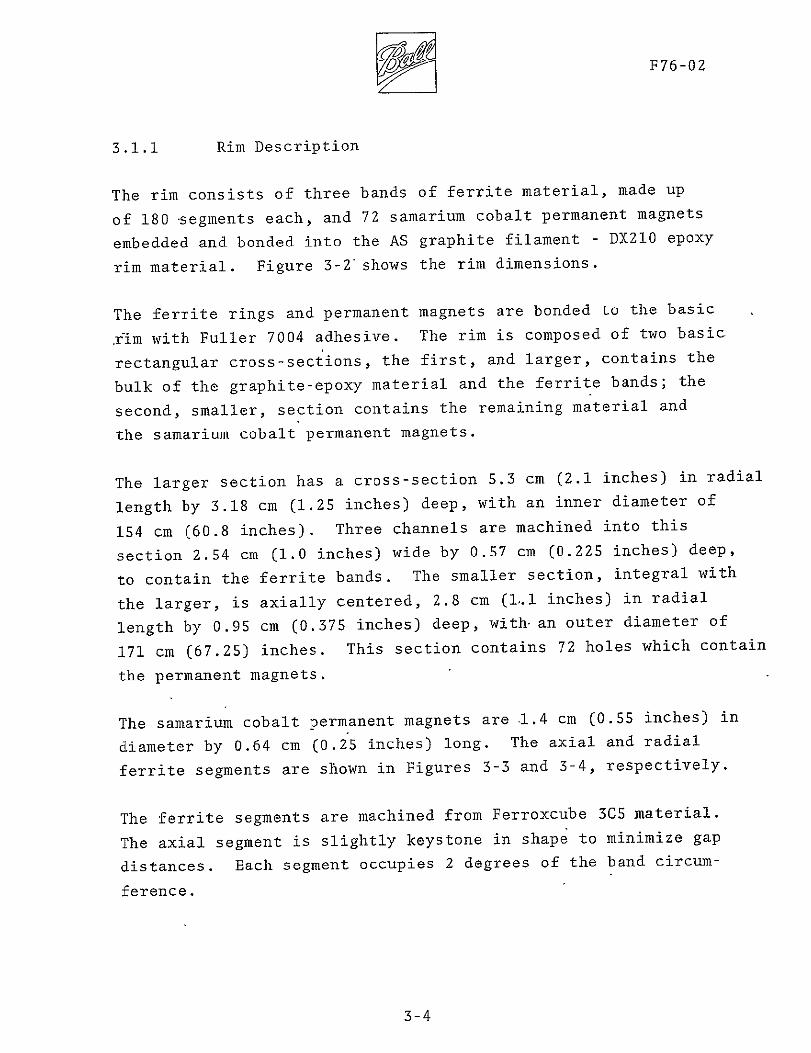
F76-02
311 Rim Description
The rim consists of three bands of ferrite material made up
of 180 segments each and 72 samarium cobalt permanent magnets
embedded and bonded into the AS graphite filament - DX210 epoxy
rim material Figure 3-2shows the rim dimensions
The ferrite rings and permanent magnets are bonded to the basic
rim with Fuller 7004 adhesive The rim is composed of two basic
rectangular cross-sections the first and larger contains the
bulk of the graphite-epoxy material and the ferrite bands the
second smaller section contains the remaining material and
the samarium cobalt permanent magnets
The larger section has a cross-section 53 cm (21 inches) in radial
(125 inches) deep with an inner diameter oflength by 318 cm
154 cm (608 inches) Three channels are machined into this
section 254 cm (10 inches) wide by 057 cm (0225 inches) deep
The smaller section integral withto contain the ferrite bands
the larger is axially centered 28 cm (11 inches) in radial
(0375 inches) deep with-an outer diameter oflength by 095 cm
This section contains 72 holes which contain171 cm (6725) inches
the permanent magnets
The samarium cobalt permanent magnets are 14 cm (055 inches) in
diameter by 064 cm (025 inches) long The axial and radial
ferrite segments are shown in Figures 3-3 and 3-4 respectively
The ferrite segments are machined from Ferroxcube 3C5 material
The axial segment is slightly keystone in shape to minimize gap
distances Each segment occupies 2 degrees of the band circumshy
ference
3-4
529
GEN NOTES I RAD NOT DIMENSIONED
ARE 0907 Z WNEI6t4T - 455OLISshy
3 WrUtAt MOM4ENTUM 3300^-9000 Lb-VT- S Se
2-1RAb SC
30 OOTIRAXIAL31 t5R P - pERi7VE 5E6mlENTS-2 PLACES (5S60 gEaeb)
65 i ____ _CH COPPED GR4PHITE Amb EPOY
PLACS)
1 ~TIRI Z5
_ _
(REP)
I V 4 0
1 f3 PLA IES)
00 55DIX
42B
- 425 (REF)
EikPHITE FILAMENT tipQKY coMPOSITE
SAMARIUM COBALT
4 NampE S (72tE G D) CITE7KEb IN 380310 WITHIN OO EUALLY SPACED O 33000 PADi os MAGNET cEtJTer StAALL ZE E=QUAL WITW
o20 MAGrNET OLE5 bAA5 EITWEt TULjd
Ot zlNt kITA CoPPet
---ELusIA TO oo4 scAIme h3e o
BELOW IFLUSH4 VT(P
C
Figure 3-2 Rim Dimensions
555 2 ___
985
MNT L nFE RZPO KXC BE 3C 5 MISS
CD
Figure 3-3 Axial Ferrite Segment
I
233273
5058 27
LO
-9 100
4150 C2 PLACES)
MATL - 303
I
Figure 3-4 Radial Ferrite Segment
iF76- 02
The radial segment is rectangular in cross-section and when
bonded in place produces a small wedge-shaped gap between
segments Each radial segment represents 2 degrees of the band
circumference
312 Rim Fabrication
The ASCD rim was fabricated by Bristol Aerospace Limited Winnishy
peg Canada The material AS graphite filament tape impregnated
with DX210 resin was wrapped on a special tool producing 100
percent circumferential fibers with a volume fraction of graphite
of 55 percent
The oversized cross-section rim was wound in 15 separate layers
Each layer was B stage cured with the following temperature
cycle
P
J4 7
The post cure after the fifteenth layer was identical to the
B stage cure except the temperature was increased to 1770 C
in 50 minutes and held at 177degC for 2 hours after the 1490 C exshy
-posure
3-8
3
eF76-02
Figure 3-5 shows the specially constructed tool containing
cure cyclesheaters and insulation for B stage and final
The rim was removed from the tool and machined to nearly the
final dimensions including ferrite channels and permanent magshy
net holes These operations are shown in Figures 3-6 and 3-7
The ferrite segments andmagnets were bonded in place with Fuller
7004 adhesive and cured The magnets were placed in the rim with
alternating North-South poles and the ends were covered with a
016 cm (116 inch) thickness of chopped AS graphite-DX210 resin and
After final cure the rim was machined (by grinding) tocured
final dimension The rim was coated with a 0005 cm (0002 inch)
thick layer of Fuller 7220 adhesive as a final step to minimize
Figure 3-7A shows the final rim resultsrim water absorption
313 Rim Analysis
The rim analysis conducted by Bristol Aerospace predicted the
(55434 PSI)rim maximum stress and radial growth to be 38250 Ncm
and 3 cm (0117 inches) respectively
The rim was modelled using axisymmetric finite elements using
the ANSYS system The model characterizes the heterogeneity
of the structure (including the ferrite bands and magnets) and
the orthotropic elastic properties of the graphite-epoxy comshy
posite
The results of the analysis are summarized in Table 3-2 and in
a rim speed of 366 meters per secondFigures 3-8 3-9 and 3-10 at
(1200feet per second)
3-9
N
Figure 3-5 Lay-up Tool
IIP76-02
Rim Machining OperationsFigure 3-6
3-11
MIE II
Iiue37Diln emnn antHlsi h i
3I1
DF76-02
LOCATION MAGNITUDESTRESS (PSI)COMPONENT
Radial or carbonepoxy +460 (max) -891 (min)X stress
Axial or carbonepoxy +491 (max) -433 (min)Y stress
Shear or carbonepoxy +390 (max) XY stress -176 (min)
Hoop or carbonepoxy +55434 (max) 0 (min)Z stress
Radial inner surface +01166 (max)
Displacement outer surface -01130 (min)
(inches)
Table 3-2
MAXIMUM VALUES OF STRESSDISPLACEMENT AT 1200 FTSEC RIM SPEED
3-13
5ThF-=- V- LERATfNz- 1 4U0T00
RMCO RRLYSES BRISTOL REROSPRCE LTO OCT 73
HOOPSTRESS RNSYS 5
or Hoop Stress Contour PlotFigure 3-8 Z
F76-02
- flax h st-ess= 55434-
I I-1 I Ii-- shy
60Iz-
===z_ +0 _----- --- shyi -_-O- - = -- = +----- shy+ ---= -- r E
_-------=--- --- = ---
-- ----- +- - --- -- =--- -=
=
------ shy
=T--- 7
--
-
- -_ - - - -- - -- a
a zrlt- --r-- -r - z I=tzz-z - -
- 4
o6 Zf - =4-=-t vi I_- --- zmE+s=$ Z 4-| b- =---+----- shy
+ 5-t 4 -- c Tt - 22 ~++ _------ _ __ _C - u
a zjztL- +lt+ z- I [Lt- -- Tit--
-- -+v + --F t+-- -+rr 7- h |f
0 200 -00 6800 1000 12oo
Rim SPEED (rri5Ecc~
Figure 3-9 Hoop Stress and Growth With Speed
3-15
F76-02
e 4fo
1 1 I 1 t i I I CII1I1_4I I
Itdn-branveqs sts OI - I M
---shy-- -- -- - -
t~z 2 - 1- shy
- 421 ~T2 2 -=_-- -_E---i ----
t -- EM
___ _ ZZ +-_ _-A~~ - rrrr-
TLLto LLbi i L -- k - r K -1-
irtv li V i 1 -- t 4 s-- n-L -- T4 E
000-q0o 600 800 100 A120 Rim Sp Dr (FTVEC )
Figure 3-102 Transverse Stress Components With Speed
3-16
DF7602
Figure 3-8 shows the computer-drawn plot of constant hoop tensile
stress contours the maximum being 38252 Ncm 2 (55438 PSI)
occurring at the top and bottom inside corner
Figure 3-9shows the relationship of radial growth and hoop stress
as a function of rim tip speed
Figure 3-10 shows the relationship of transverse stress components
with speed
Since the material void free is capable of withstanding 110400 2 2Ncm (160000 PSI) in tension and 8280 Ncm (12000 PSI) in shear
the safety factor is 28 minimum On a sample basis the void
fraction was determined to be less than 04 percent
32 Back-Up Air Bearing System
The design of the back-up air bearing system was completed and
analyzed by Shaker Research Corporation Ballston Lake New York
The back-up air bearing (BUB) system consists of six hydro-static
radial pads and twelve hydrodynamic axial pads These are arranged
in six BUB sets consisting of two axial (one upper and one lower)
and one radial pad and located at either end of a magnetic supshy
port station Each BUB set is approximately 60 degrees from the
adjacent set The bearings are deployed toward the rim by air
pressure when predetermined rim displacement limits are exceeded
The introduction of air through the pads as well as through a
pneumatically operated valve in the vacuum enclosure provides
the fluid for the BUB system and also introduces air drag for a
fastercoast-down Hydrostatic bearings were selected for
radial use instead of hydrodynamic types because the rather small
rim depth (115 inches) allows insufficient area to produce the
required reaction forces The back-up bearing system is shown
in Figures3-11 and 3-12
3-17
P76-02
~14
-L- 7
FiguTre 3-1 AMCD Back-Up Bearing Layout DrawingI 3-la
Figure 12 Back-Up Bearing System
7F76-02
321 Hydrostatic Radial Bearings
The movable radial pads are designed to minimize air flow and
maximize air bearing rim reaction forces The radial pads proshy
vide a centering effect on the rim to minimize dynamic and magshy
netic unbalance forces
In the normal magnetic suspension mode the radial pads are held
away from the rim-and against stops by a set of nested compression
springs (total of 22 N (50 pounds) of preload) When the radial
system Figure 3-11 is activated 207 Ncm2 (300 psig) air is introshy
duced to the pad piston cylinder which moves the pad outward
toward the rim The piston chamber is ported to the pad surface
through a 0033 cm (0012 to 0014 inch) diameter orifice A
sealed oil-filled dashpot between the piston and pad controls the
deployment velocity
Figure 3-13 shows the relationship between- radial pad force and
gas flow versus film thickness for various orifice 4iameters
Because of limited gas available-the smaller orifice diameters
were selected
Since the rim is not at constant radius (because of radial growths)
film thickness and flow vary With rim speed Figure 3-14 shows
the relationship fo film thickness and flow versus rim speed
322 Hydrodynamic Axial Bearings
Movable- tilt type axial hydrodynamic pads were used since the
rim radial width is large and because of the limited bearing air
supply The axial pads are slightly crowned and combined with
the tilt feature are self aligning
3-20
F76-02
1 ~
It
7
I
JII ji
I L
II
---
Ft
T -
VIN I -_ Lr
TD _-
I
I+i
- 1MNV I
4~~r14 +t
Fit~Fi-~tdi I~ ~ JrV)
i ir
il-I= iH14+
i T r
F~m
shy
_ _
I L [
- i
I
_ i _
Ii
0001M -s as
Figure 3-13 Single Pad Force and Flow
3-21
A yyF76-02
WI
ii24pVshy-~~~~W
J4 i3 - Lit
I+ I~Ir~r L-- u 7t J
L 4- 1-nMLfI0__ 4~~~~- F-14--gtrF
I -- -r
4 ~ P I-
IaiH __M
1 --- t Th T1T
I- Vt prI i A
-p--t~LIV[~ VK jl77L1 1
Figure 3-14 Radial Air Pad Flow and Film Thickness With Rim Centered
3-22
F76-02
In the normal magnetic suspension mode the axial pads are held
against stops by a flexural spring The axial system is deployed
in-much the same manner as the radial system When a magnetic
suspension anomaly is detected the vacuum enclosure is flooded
with external air thus providing the film for the axial bearings
Figure 3-15 shows the relationship of film thickness with rim
speed Since the film will support the rim to about 15 radians
per second the pads are designed to accept several contacts before
replacement is necessary
323 Back-Up Bearing Pads
The primary objective in designing the pad material was to proshy
vide a material which would wear smoothly without damage to the
rim or to the pad itself Sacrificial bearing materials have
been used in gas bearings in the past which exhibit the necessary
qualitites The material used in the back-up bearings is an epoxy
resin heavily filled with aluminum powder aluminum oxide power
and molybdenum disulphide powder The mixture is poured into
silicone rubber molds degassed in a vacuum chamber then heatshy
cured The pads are then machined
When the spinning rim contacts the pads the pad will wear smoothly
and rapidly acquiring a high polish and yielding a fine dust
The rim surface should be undamaged by the contact The aluminum
filler provides high thermal conductivity to sink the heat generated
by the rim contact The aluminum oxide provides dimensional
stability so thQ pad will withstand the thermal shock generated
by the rim contact
3-23
3788I9 2 4 5 7 8 9 2
1 7 _- I
111-1 r - J
-I- --i- 1 rV1- 1 t r V
4 _ - _ _____ shy- I---7
I
r-- _- F-_- --- I ii -
I fr r l 7[-II j7shyLi +] - i I-- I
1 7 8
-- - 4 5---- 10 47 MCI 9
Figure 3-15 Axial Pad Film Thickness Versus Speed
F76-02
40 SUSPENSIONSYSTEM
41 System Description
The suspension system consists of three suspension stations
placed symmetrically about the rim At each suspension station
the rim can be pulled in either axial direction or tadially
inward by magnets A total of 12 magnets are arranged in sets
of four each to pull in these three directions (up down and
inward) The eight axial magnets are driven in concert by one
set of electronics Axial error signals are developed by a
position sensor located at the center of each station The
axial servo loops in each of the three stations are independent
of each other The four radial magnets in each station are also
driven by a set of electronics in response to a radial position
sensor located in the center of that station But the radial
station to another so asservos are interconnected from one
to prevent the servos fighting one another even in the presence
of rim radial growth
411 Magnet Description
One of the unique features of the AMCD is the support magnet
design The electromagnets are flux-biased by thin wafers of
samarium cobalt permanent magnet material placed in series in
the magnetic circuit This has the advantage of (1) providing
a high force per unit current sensitivity at zero current (2)
providing a linear relationship between force and current and -
(3) providing the static field required for zero power operation
The support magnet geometry is seen in Figure 4-1 The permanent
magnet biasing is achieved by slanted wafers of samarium cobalt
in the legs The wafers are as thin and wide as possible to
4-1
SAti 4-IUr CCBA3L~rshy
AGtJer-
AGII1
Figure 4-1 Support Magnet Geometry
RF76-02
minimize their reluctance in the magnetic-circuit The volume
of permanent magnet material is sufficient however to provide
adequate flux-biasing and static lift The reluctance of the
permanent magnets is large but does not more than double the
total reluctance since the air gap inthis system is large In
many other magnet suspension systems the gaps are small (about
01 mm) and this sort of series flux biasing would greatly inshy
crease the total reluctance in the circuit Control power would
thus be large and the systems would be impractical
The effect of flux-biasing on the force versus current characshy
teristics of the magnets is shown in Figure 4-2 With no biasing
current in either direction produces force of the same sign with
poor gain and low efficiency in the vicinity of zero current
Force is simply a function of the square of the current With
biasing the slope of force versus current is greatly increased
at zero current In the AMCD top and bottom magnets operate
together in a push-pull type of operation The coils are in
series hence both coils have zero current at the same time
The resultant force-current relationship is linear and has a
slope double that of either magnet alone
Figure 4-3 shows the U core of the magnet with the permanent
magnets in place Permanent magnet thickness is 1 mm (0040
inches) Also shown in Figure-4-3 is a fully assembled magnet
ready for potting After potting the units measure 43 cm x
167 cm x 25 cm (17 in x 42 in x 99 in) and weigh 500 grams
(11 lbs)
412 Position Sensors
The position sensors used in both the axial and radial suspension
systems are Multi-vit sensors manufactured by Kaman Sciences
4-3
7 gF76-02
-r
UPPETP HA -
C AOc~~
777
~~oeehAcn-e-r Z
Figure 4-2 Flux-Biased Magnets in Push-Pull Operation
4-4
rF76-02
I
3 i
A A
I tii A LWUv
NN
N~ i X -9
i i UI A i
IN aWIi ii i
iiiiiiiliiili
i~iiii Ii iliiiiiiiliiilii
Iilliii iiiiiliiiiiiliiiii = iiiiiiaii~iii iiiiiiiiiliiiiiiii
Uiiiii poundii=iiiii]iipoundiiiiiiiiiiiiiiiii Uigure 4-3 Support Magnet Cosri on
iliiiiur -3 ConstructiiiiIliiiiiiiiioniiiiiiiliiiSppriMge liiiiiii i iiiiliiiii3 URiliI 4-s == =
4-s
rF76-02
Corporation These are conventionally called eddy current senshy
sors although they are actually sensitive to anything that changes
the inductance of the test coil in the probe Hence either
eddy currents in a conductor or the permeability of a magnetic
material can be sensed In the AMCD the sensors look at the
ferrite bands and therefore are operating entirely ina non-eddyshy
current magnetic permeability mode Special calibration of the
sensors was required in order to operate in this mode Linear
range of the AMCD sensors is 025 cm (01 inches) and scale facshy
tor was set at 4 voltscm (10 voltsin)
413 Control System
The axial suspension system uses three independent servo loops
to control electromagnet currents An electronic diagram of one
of these loops is shown in Figure 4-4 The heart of the elecshy
tronics is an Inland Controls MA-I DC servo amplifier which is
operated as a current driver to reduce the effects of electroshy
magnet inductance Equations of motion of this driver and an
analysis of the voltage feedback used to damp high frequency
roots are given in Appendix A An analytical block diagram of
the entire servo loop is shown in Figure 4-5 Equivalent points
on the electronic and analytical diagrams are indicated by letters
within hexagons
The axial suspension system has two modes of operation a posishy
tion mode and a virtually zero power (VZP) mode In the posishy
tion mode rim position error is used to command electromagnet
current The rim has high static and dynamic stiffness about
any desired point in the gap In the VZP mode the rim position
set point is modified by positive feedback of the integral of
electromagnet current The result is that the set point is moved
until steady-state current is zero The permanent magnets are
4-6
AA
REHTUtk +26V
4-
C11 7t-Q
Fiue44Aia3upnin7lcrnc
S Cornn- EesoCo p n a cncivCrrent Driver- O deg OI 99 (5C + sm -3 (s + 1 1deg E 1 copy + F
gtosO ~
volf
iE 3 7 T r i m T ntegratadegr
Suspended
Mass
-|ectro
-ria net
16
permanent Magnet
Figure 4-5 AMCD Axial Suspension Station
R 1F76-02
then providing all of the support of the rim Dynamic stiffness
is nearly the same as in the position mode but static stiffness
is actual negative If a downward force is applied to the rim
in the VZP mode it initially moves downward but then slowly
rises to assume a new zero power position above the old equilibrium
position
The electronic circuit diagram for a radial servo station is
shown in Figure 4-6 and the corresponding highly coupled analytishy
cal block diagram is shown in Figure 4-7 Again equivalent
points on the two diagrams are indicated by letters in hexagons
The large amount of coupling results from three servos controlshy
ling only two degrees of freedom
Two modes of operation are available a position mode and a WAHOO
mode The position mode is similar to the axial position mode
The WAHOO mode is a zero power mode that produces zero power
operation in the presence of both static loads and rim expansion
This is accomplished by adjusting the position set point at each
station as a function of the integral of the sum of the electroshy
magnet currents at the other two stations
The name WAHOOis derived from the poker game WAHOO This game
is played in a manner such that each player knows what every
other player holds but does not know what he himself holds
Inspection of the WAHOO trim loops of Figure 4-7 reveals that
for VZP trim purposes each servo only looks at what the other
two are doing This innovation was developed by BBRC to meet
the unique requirements of the AMCD
The derivation of the WAHOO concept is given in Appendix B
There it is shown that only the WAHOO concept produces zero
power operaion for both rim expansion and force disturbances
4-9
A00l 51 Ir
A-A-
F
27
ffzo xr
74 VIP KIAk
7
Ems~
n
A7-
I
A1
ter
a 2k-
-
-
-
-
-
I)
Figure 4-6 Radial Suspension Electronics
-KS
Iamp wkin47s Permanent MagnetVeloityPM VPol Aplifir PMEHM E Iectremoqnet
K5 Kmn eae t~j VOS 0bCar respond to Lettered
1vII~rb r - rr m Psitionson Cgrcwit
vol vol Im PosiMoon Pox
SlRtim rtOhkx _Q$)bsS 4lfe I
0niplPfied Cus ren Driver
Gcucv rbinn n i
+ + vt
If
in-7d FigureservoD RailSro
+i
42
F76-02
Appendix B also shows that for single station design purposes
a single station can be represented as shown in Figure 4-8 Two
points of interest are immediately evident The equivalent mass
for a single station representation is 23 the total rim mass The WAHOO concept which involves negative feedback to each station
from the sum of the other two stations resolves to a positive
feedback in the single station representation exactly like VZP
in the axial mode This representation can be used for designing
the system characteristic root locations If the characteristic
roots from the single station representation are given by A and
the WAHOO gain is Kc it is shown in Appendix B that the three
station highly coupled set of characteristic r6ots are givenby
(S + 2K )A2
Performance
421 Static Performance
At each suspension station the rim will seek an axial equilibrium
position based on the applied load and the control system mode
(position or VZP) These equilibrium positions can be preshy
sented in one plot as shown in Figure 4-9 The VZP line is a zero current line and has a slope that indicates static instability
however as shown in the next section the system can operate in a
stable manner along this line The most usual operating position
mode point is about 001 cm (025 inches) above the center of the
gap At this point the slope P of the VZP line is about 595
newtonscm (340 lbin)
In the position mode an operating line exists for each set point
of the position sensor A family of these is shown in Figure 4-9
The lines are finite in length because of the limited current drive
capability of the electronics The slopes of the lines are apshyproximately 2600 newtonscm (1500 lbin)
4-12
Stationfost ionsingle
Oecrlx- EquIva1eratArmplifir Current Driver 6 Mks$M9oqmet+ 1m
~~~~~ eroe L~r
Is + Fes I16(7+1210 r0 0 l I-
p 0 1
476 An- Per
u2 IVlt+ -Eg
o tKate - r1 1 StO Sr eq uci o lnk wahoo is
Q Correspornas toa letterd posit~ions on circuit chogr~m
Sinql~e stcton eqviclvJewtmls is 23 totil ma
~odelldas a posattve PeedbctK self IoopVe
t to o-t liKe Vf Pwould ltherefboretxpect fvrthernortn itthe Aol O Servo Xt doesonh
Figure 4-8t EqiaetSnluadapev tto
ekgeto8 rnex e o +non
A F76-02
UP
MAGNET M~A t r
lsrok os NoRMAL
kE-RITI N
P E-Nshy-OMFR
tL UPshy
- j ~
-10
h31G1NL pAGE iS
)F POOR QUML-rI
Typical Static Suspension System Performance
Figure 4-9 4-14
rF76-02
The force sensitivity F of each station is about 138 newtons
ampere (31 lbamp) Hence the force produced by a station
is given by (in English units)
F = 340X + 3lI
422 Dynamic Performance
The analytical block diagram for an axial suspension statiQn is
shown in Figure 4-5 For theposition mode the root locus and
-Bode plots are shown respectively in Figures 4-l0and 4-11 The
root locus plot shows that the dominant pole pair has an undamped
natural frequency mN (which we define as bandwidth) of 171 radsec
(272 hertz) and a damping ratio of28 The Bode plot shows
that the gain crossover frequency wc (which some define as bandshy
width) is 1827 radsec (290 hertz)-and that the system phase
margin is 2320 Both plots show that the lower gain margin
is 22(-131 db) and that the upper gain margin is 201 (261 db)
For the VZP mode the root locus and Bode plots are shown respecshy
tively in Figures 4-12 and 4-13 The root locus plot shows that
the dominant pole pair has the same undamped natural frequency
and damping ratio as the position mode that is wN = 171 radsec
= 28 The Bode plot shows that two gain crossover frequencies
at 1823 radsecexist one at0838 radsec (013 hertz) and one
(2903 hertz) The phase margin at the lower crossover frequency
is -772 and that at the upper crossover frequency is 2300
Both plots show that the lower gain margin is 226 (-129 db)
and that the upper gain margin is 2011 (261- db)
The response due to the step application of a one pound weight
is shown for the position mode in Figure 4-14 and for the VZP
4-15
OF76-02
1 -DD
-- A I 1
I I
i
3000 --------------------------------- ___tN
-5000 -400 -30U -2ODG -t I lo oD
REAL AXIS
Figure 4-10(A) Root Locus Plot - Nonideal Current Driver With
Voltage Feedback
4-16
---------------------------------
7F76-02
-I- 111 1-l Z9D
io oI 1ll t A
G
80 ----------- 0 aEu----------------shy-4--
FigueRot41001LcusPlo - Nnidal Crret DrverWit
-1---4-17
I I
F76-020
14-HLowler
)2 I__ _ p
1 N I-- A =20 41 r
I tIse0_ __ _ _ 4 6 2 4 68100
s 10 log H00 6 10009 FREQUENCY (RADIAWS$ECOND)
Figure 4-11 Bode Plot - Nonideal Current-Driver With Voltage Feedback
4-18
7F76-02
$oo I5iI000 I1
T 1 Ii
-A
S4+
N A
4000 R--- - - - - -
V A x
103 000 40 30 29
urn rvrWtFi1r -12A Roo Lou7lt-Nnda
Voltage Feedback 4-19
V gF76-02
ii
- I I I
I I I II
I lii
-I I
II I iishy
II - - -i-l
Fgr 4-2B o otocu PltrNndaCrefl rive
With Voltage Feedback
4-20
F76-02
I i E
A -4 G
E- 60I jUroI(
I
1A2zS1 me RI
3s F-1-L
IIsoM 3en
4) e r
-120---- -Marlin
fla e =2300
-140 shy
1 1 10 10g 2000 1090r FREQUENCY (RADIANSECOND)
Figure 4-13 Bode Plot - Nonideal Current Driver With
Voltage Feedback
4-21
012
F76-02
00010
00008
pound E
0
p
0 00
0zkc0
0
E
- -
4+-F
- - -
Nshy- - - - - - -
4
- -
5
-4-2
AF7602
mode in Figure 4-15 The response for the position mode settles
out at 6941E-5 feet (002 cm) This yields a position mode
stiffness of Stiffness 6 1 lb
6941E_5 t X feet
1 12006 lb (21021-
N
69Th-ft Tni in cm
The response for the VZP mode settles out at -2451E-4 feet
Thisyields a VZP mode stiffness of
1 lb feet = lb NStiffness = 2451E4 ft X 12 in -3400 i (595 E-
Note that the stiffness in the VZP mode is just that of the
permanent magnet and that the movement in this mode is toward
the applied force That is if a weight is placed on the rim
in the VZP mode the rim will move up
Further insight into the system can be found by examining Ap2
pendix C When using current driirers the usual tendency is to
ignore the high frequencydynamics and simply say that the
output current is the input voltage times a constant This can
be very misleading in the case of AMCD- In Appendix C are shown
root locus plots using both an ideal current driver arid a nonshy
ideal current driver without voltage feedback It shows that
voltage feedback is necessary for the axial suspension Also
shown in Appendix C are Nyquist plots and phase-gain root locus
plots of the nominal axial systemthat is the system using curshy
rent drivers with voltage feedback The esoteric phase-gain root
locus plot shows on one plot the sensitivity of the system roots
to change in both gain and phase For example it shows what
would happen if an additional 300 of phase lag were added to the
system from some unknown source
4-23
F76-02
0001
I f
I 0 e
eshy
0a T 1-0001-shy0N
ft E F 0
E a
- 002--------------shy
0 t0 20
TINE (SECONDS]
30 40 50
Figure 4-15 Nonideal Current Driver With Voltage Feedback
4-24
F76-02
The equivalent single station radial analytic block diagram is
shown in Figure 4-8 It is very similar to an axial station
The root locus and Bode plots for the position mode are shown
respectively in Figures 4-16 and 4-17 The root locus plot shows
that the dominant pole pair has an undamped natural frequency
(bandwidth) wN of 653 radsec (104 hertz) and damping ratio C
of 18 The Bode plot shows that the gain crossover frequency
is 666 radsec (106 hertz) and that the phase margin is 1350
Both plots show that the lower gain margin is 329 (-965 db)
and that the upper gain margin is 7054 (3697 db)
The root locus and Bode plots for the WAHOO mode is shown in
Figures 4-18 and 4-19 The root locus shows that the dominant
pole pair has an undamped natural frequency of 674 radsec
(107 hertz) and damping ratio of 16 The Bode plot shows that
the upper gain crossover frequency is 691 radsec (110 hertz)
At this frequency the phase margin is 1260 Not shown is the
fact that the system also has a lower gain crossover frequency
of 594 radsec (095 hertz) At this frequency the phase marshy
gin is -715 Both plots show that the lower gain margin is
389 (-821 db) and that the upper gain margin is 6701 (365 db)
The large upper gain margins for both the position and the VZP
modes indicate that current driver voltage feedback is not needed
Considerable rim bending instabilities were encountered during
the design Early in the development the axial system was
designed to be overdamped This caused a bending mode to be
driven unstable The compensation was adjusted experimentally
until the bending became stable Unfortunately this reduced
the lead in the system resulting in the present underdamped sysshy
tem It is believed that bending will present no problem at
high spin rates because of the effective stiffening of the rim
4-25
6F76-02
_____ - _ r ____I___
141
IT___lishy
1 ii
1 F]
eir
t lj~
4-
J TT a p-
III NEA
fiIT WBKsITlK j1_11IIi I-
I
e
-Fshy
Y]-111 ji
1i1fln 4--I r
I i--I -
TFiJ-WL 1
_1(-Ii4 - I
I~ ~ ~iA_~2I ___ ii- 11 IFt-Ih
iT
h~ -iH T
+~ji+ih Iplusmn
_ _ _+ I kt ~h-II
+ LILY -
7 SO bullj
Figure 4-16 AMCD Radial Suspension Equivalent Single Station Position Mode
4-26
Elll csl- tLL[ 11--- 1_ il
V
1 MIN
2 0 H qL2~14-0IT
I M Ill 1OIHI
+-o ip Lr g
Ti I -0 1- b1 -- i
Ij _IUSi 1PIN - il
--i
41i L -I I - d jir ~J I I
00 -o
ro-d 5 c
Figure 4-17 ANCD Radial Suspension Equivalent Single Station o Position Mode
7F76-02
1LjI_----- Li -III iI - - I -shy-F ]e2 1
Is- Lr [_I
r ir -L-j 11I IALI _ _ _ ___ 2_
E11LLN1LALIF TYC -- td It 11
- KI
S1 1 1 1--shy
II
I r 11
FLL-1
U - I 4
E~~~~fL
__
f Lplusmn Xi ILIi _ _
- ii _ _ i
- H --
--------
A-1 1 F - JT-1
-- t-ti -~r -r I- t - --- IL I
IIJlri-tlrht1f tI
_+ _ l PillS 1 I
Figure 4-18 AMCD Radial Suspension Equivalent Single Station
o Wahoo Mode
4-29
rm~r 1 u i rrrrF r r r
4
130
o
I -4
7 7 1-shy iAb d
llt h
-30 Tfij4i i ~
- n0 t
Figure 4-19
01 AII-
I uji r a sec
AMCD Radial Suspension Equivalent Single Station o Wahoo Mode
AF76-02
and the averaging effect on modal pick-up caused by the bending
modes moving rapidly past each position sensor
As the rim is spun up the three axial stations become more and
more coupled by nutational effects The result of the coupling
is to reduce the dominant roots damping ratios more-and more to
the point the system could go unstable if the rim is spun fast
enough It is believed that this tendency could be greatly
reduced or possibly eliminated by the proper combination of cross
feeds from one axial suspension station to the others
4-30shy
DF76-02
50 DRIVE SYSTEM
51 System Description
The AMCD drive motor can be thought of as a large permanent magshy
net brushless dc torque motor Samarium cobalt magnets are
bonded into the rim at regular intervals The two phase armashy
ture is segmented with a winding set at each of the three susshy
pension stations Commutation is controlled by Hall effect senshy
sors mounted near the rim which sense position of the samarium
cobalt motor magnets
52 Magnet Selection
Alnico was considered along with samarium cobalt for the permanent
The large air gap and segmented winding structure meanmagnets
the magnets will become nearly air stabilized The rim was designed
with a small outer lip to hold the magnets This was done to
isolate the drive from the suspension as much as possible without
and complexity to the rim than necessary Thisadding more mass
small lip implies a short magnet Samarium cobalt has high
strength for short lengths and does not pay a penalty for air
In fact it is very difficult to demagnetize thisstabilization
material
cm (55 inches) diametertby 64 cmSamarium cobalt magnets 14
(25 inches) length were selected and bonded into the rim with
polarities alternated
The rim contains a total of 72 magnets spaced 73 cm (288 inches)
apart
5-1
53
--F76-02
Core and Winding Design
Each armature segment consists of a pair of bar-shaped winding
assemblies one above and one below the rim
Sit cos sla 0S SMa
cores in a singleThe windings-are wound toroidally around the
layer The figure above shows only the cross-section 6f conshy
ductors in the air gap as the conductors passing around the other
side of the core add nothing to torque and serve only a connectshy
ing purpose The bar-shaped cores are easy to wind and result
in a compact structure The single layer of 18 conductors adds
very littleto the overall air gap This effective electroshy
magnet design was suggested by P A Studer of Goddard Space
Flight Center
Ferrite material was chosen for the core to reduce losses Fershy
rite also is easily machined into the required irregular shapes
The windings are grouped into two phases SINE and COSINE each
of which acts upon three magnets at each motor segment In operashy
tion current in one phase is acting on the magnets while current
in the other phase is reversing in preparation for a magnet of
opposite polarity
5-2
DP76-02
54 Motor Commutation
Hall sensors act as commutation devices for the motor They sense the position of the permanent magnets in the rim and cause the drive coil currents to be switched according to magnet position
The sensors are mounted in pairs one above the rim and one below for each winding phase Outputs from each pair are summed so that the switching position is not affected if the rim moves up or down within the air gap The SIN pair controls current on the SIN windings of all three motor segments and likewise the COS pair
of Hall sensors controls all COS windings
55 Motor Control Electronics
A block diagram of the motor control electronics is shown in Figure 5-1 For each phase the Hall sensor outputs are summed and amplified to drive-threshold detectors These detectors sense magshynet position and polarity The phase control logic determines the
timing and polarity of the motor coil drivers Interconnections between the two phase control logic blqcks provide positive direcshytion and start-up information
Each of the six coil drivers controls a phase at one of the motor
segments Associated with each driver is a coil current sensor which monitors the current in that winding All six of these
current sensorsreceige a common reference from the speed control
potentiometer When current in that particular winding reaches the reference level the driver turns off until the current deshy
creases This prevents the current from reaching destructive levels at low speeds and acts as a speed control at high rim
speeds
Since the coil drivers are either full on or off a very efficient drive is achieved At low rim speeds the drivers operate as a
5-3
56
F76-02
conventional PWM (pulse width modulated) amplifier A quite faithful square wave current of controlled amplitude is fed to the coils At high speeds high acceleration (or deceleration)
is possible with the drivers full on for the period between magshynets with current rise and fall limited by the inductance of the
coils
Torque Calculations
The equation for the force betweena magnetic field and a current
carrying conductor-is
F = BLI
where
F = Force in Newtons B = Flux Density in Teslas (WebersM~ter )
L = Conductor Length in Meters
I = Current in Amps
If the magnetic field is created by a permanent magnet the force
can be considered to act on the magnet if the conductof is held
stationary which is the case with the AMCD motor
To arrive at design force each of the factors B L and I must
be evaluated
A force calculation will be made for one magnet face interacting
witha coil This can be then doubled to account for both ends of the magnet next tripled to take into account the three magnets in one motor segment and tripled again to realize the total force for the three motor segments Then using the radius of the rim
we can calculate developed torque
5-4
F76-02
Flux Density Calculation (B)
The large air gap makes it difficult to- estimate how much of the
magnet flux will couple through the winding core and how much
will be lost to leakage A measurement of coupling flux was made
using a pair ofsoft iron bars similar to the ferrite corasi
SEJSE C0115
SOFr iROh
-4 Webers with magnets of averageThe flux measured was 0375-x 10
strength
core must-be convertedThis flux that couples through the ferrite
to flux density (B) in the air gap where it interacts with the
coil windings There are two practical Choices for doing this
We can assume all the flux goes straight up from the surface of
the magnet andreacts with only those turns above the magnet or
we can assume the flux spreads out evenly over the winding area
Of course the truth liesand-reacts with all the turns equally
an adequatesomewhere in between but the second approach gives
approximation
The winding area in the air gap for one magnet coil phase is 2
19 x 36 cm or 68 cm
Flux density then is
-44m _ 0375 x10 Webers 2 0055 WebM-B_=A = 4 2A - 68 x 0-4 m
5-5
F76-02
Conductor Length Calculation (L)
are 28 turns with an effectiveIn the winding phase area there
length of 19 cm each
Total effective length is then
L = -19 x 28 = 532 cm = 0532 M
Current (I)
that the coil drivers and wiringThe elbctronics are designed so
canhandle 4 amperes Also the inductance of the coils was
examined to be sure that currents of this magnitude can be
reversed at maximum rim speed frequencies with a 60 volt power
(and torque) will then be calculated for thesupply Force
design maximum of 4 amps
Force
We can now calculate force from the equation
F = BLI
= 0055 x 0532 x 4 = 0-1-17 Newtons
Recall that this is the force for a single magnet surface inter-
For the total motor this is multiplied by 18face
Total Force = 0117 x 18 = 176 Newtons
576
0F76-02
This times the magnet radius (0838 meters) gives total torque
Total Torque = 176 x 0838 = 176 Newton-Meters
(13 lb-ft)
A small (14 diameter) test wheel was built to check the above
torque calculations Acceleration measurements were made and
from the known wheel inertia torque was determined Correlation
within 10 of the calculated torque was achieved
5-7
S in Hall Sensors
Summing
Amp
[A Threshold Sin Phase Coto-rie
DetectorsLoi
SnB1Sin
Sin C Driver
ol
Hall Sensors
~ Amp=ApDtcosLogic
etctr Control -- Die Col Ci~
Summing Threshold Phase Cos B Driver
iCosCos
Ci Co
Figure 5-1 Motor Control Electronics
C
aF76-02
60 REFERENCES
1 Anderson Willard W and Groom Nelson J The Annular
Momentum Control Device (AMCD) and Potential Applications
NASA TN D-7866 1975
6-1
F76-02
APPENDIX A
CURRENT DRIVER EQUATIONS AND TRANSFER FUNCTIONS
A-i
F76-02
Appendix A
Current Driver Equations and Transfer Functions
When using current drivers the usual tendency is to ignore the
high frequency dynamics and simply say that the output current is
just the input voltage times a constant This was very misshy
leading in the case of MCD-as shown in Appendix C The circuit
diagram of a current driver with voltage feedback and its equishy
valent diagram are shown in Figure A-i -
v A T5It
Figure A-I Current Driver and Equivalent Circuit
A-2
F76-02
The beginning equations of motion are the following
Rl11 RM -- R 10
-RM SL + R2 2 -(SL + RC) I= A(TS+I)-)V + ARI(TS+l)shy
-R 2 -(SL +R c) SL + R3 3 + S_ C I 3 0
where
R1 lt= R1 + R2 + RM
2 RM + RC22
R33-- R2 + RF + RC
Transposing I1 to the left hand side we obtain
R11 -RM -R2
-RM(TS+l) + AR 1 (TS+l) (SL+R 2 2 ) -(TS+1) (SL+Rc) 2 A S-SR22 S L+SR33+-l
What we really want is the current through the inductanceshy
1 2 T3
Adding this equation to the system we obtain
C1 C12 C1 3 0 II 1
B2 1 S+C 2 1 A 2 2S2 +B 2 2 S+C 2 2 A23s2+B 2 C 3 0 12 A V
B31S A32S2+B32S A33S2+B 3 3S+C 3 3 0 13 0
- -1 1 1 1 0
A-3
eF76-02
where by definition
-=A32 -LC R11 B22 = L+TR 22
= - C22 R22 B32 = RCCl2 RM
C13 =-R 2 A23-= -TL A33 = L
= R33B21 = -RMT B23 = -L-TRC B3 3
C = ARI-RM C = -RC C =C -I
= -R2A22= TL B31
If the voltage feedback is removed these equations reduce very
simply to
-RMIRlI+R2+RM
+ AR1 (SL+R+RM)(TS+ 1j1 2 = AKRM(TS+I) We want thewhere 12 is the current-through the inductance
transfer function 12V First divide the secondequation through by
LT to obtain
-RMR I+R2 +RM
(R C+ PM j] IAL 1 V S+L-iIARI[ RM L (SplusmnT -1)+L -lT -1A
A-4
F76-02
Then by Cramers rule
2 CR1+R2+RM)AL -1T-+RML -1(S+T- 1 )_L-1T- 1 AR1
V7 -1 r- 1 2-1 - lshy(RI+RZ+RM)(S+T +L (RC+RM) -R ML l(S+TI)+L ITIARIRM
(R2+RM)AL -T - I(S+Tshy
-(R1+R 2+RMM)(S+T 1 )(S+L-1 RC)+L -RM(R1+R 2)(S+T-I)+L T ARIRM
Further manipulation yields
S+T-1 +(R 2 +RM)ARM T12 RML -
V - 2+RM) 1 L-+RR [2 wT-ARI-L 1RM(RI+R2 -
S+T )(3+L Rc) + RR+Tl+R---
Finally the desired current driver without voltage feedback
transfer function is given by
12 RML- S+T -1 +A(I+R2 RfIj
V (RLR-+RM) - -1 LRM(RI+R2 ) (ST 1 [7AR 1 RS5 + R2 +RMR R1 L Rk 2 )
A-5
76-0 2
For infinite amplifier open loop gain A = the transfer
function reduces to
2R Lim 12 = R1_ 2M
(l+R2RM- R2
R - RYR RR)r112RM for R2gtgtRM
-This is the transfer function which is used
I2 R2 12 R 2V RIRM
if the high frequency roots may be ignored
When the high frequency roots are not to be ignored and
if AR2R1 gtgtmax (RMRC-i)
and RMARlRjR2gtgt
RI+R 2 c
A-6
rF76-02
The transfer function simplifies to
S+T- AR 2RM1
12 RML-
V R1+R2 (S+T-)(S+L -Rc)+L- RM(S+T-AR1 R1 +R2)
RML-1 S+T-1AR2RM-
R1 R2 S2+ -1 -1 -1 T 1L-1RMARl - A
S +(T- +L -Rc+L RM) S+ R+R
T- +L- (RG+RM) TRLAR
2 (RI+R2)
The dc gain of this transfer function reduces to the same transshy
fer function used if the high frequency roots may be ignored
that is
2 R2 V RIRM
For the radial MA-lCurrent Driver
RI = 10K R 2 = 2711 KQ RM 10
RC = 30 Q2 L = 0128 h T - 30 A 50119
Then the radial current driver without voltage feedback has the
transfer function
12 _-00061463(S+40762E10)
V S+13609plusmnj30400 shy
A-7
F76-02
Forthe axial MA-I current driver
R=1 10K R2 = 7311K C 01 1f R11 = 17311E4
L =0064 f = 12M R = 14 R22 =15
A = 50119 RM = 1 T- = 30 R 33 I2073E6
Then
= C11 7 17311EA B2 2 = 564E-2 A 3 2 -0064
Cl2 = -- 22 = 15 B = -14
== = -7311E3 -21333E-4 A33 0064C13 A 23
B21 = -33333B-3 B2 5 -53067B-2 B 12073E6
C21 = 50119E8 C2 3 - 14 C3 = 1OE8
= A22 = 21333E-4 -B3 1 -7311E3
Without voltage feedback the axial current driver has the transshy
fer function
2 00090261(S+l0993B1)
V S+13219plusmnj36839shy
A-8
7F76-02
Note that without voltage feedback the damping ratio on both the
radial and axial current driver high frequency roots is less than
05 This appears to be all right for the radial servos but is
very bad for the axial servos as shown in Appendix C Consequently
-voltage feedback has not been employed for the radial servos
current drivers but has for the axial servos cur-rent drivers
The effects of this feedback has been determined numerically
Figure A-2(A) shows the effect of increasing RF the voltage
feedback resistor from zero to infinity with the feedback capashy
citor C held a-t 01 lif Ifonly the capacitor is used for voltage
feedback the current driver roots are still lightly damped but
at a much lower frequency As the resistance is increased the
roots increase in damping become real then decrease in damping
at a high frequency finally moving to the no voltage feedback
position for RF = Figure A-2(B) shows the effect of increasing
the voltage feedback capacitor C from zero to infinity while
holding the feedbackresistor at one megohm For C 0 the roots
start at the no voltage feedback position As C is increased the
roots decrease in frequency and-increase in damping ratio until
C = 00091 f Further increases result in decreased damping
ratio and increased frequency At the chosen voltage feedback
values of C = 01 vf RF = 10 MQ2 the axial current driver transshy
fer function is
I 0008994(S+833)(S+l099EII) V (S+786)(S+2771plusmnj2583)
A-9
~~~ L~Trrrl~I I~ I II 4
Jots_1 nr_- r177I 7F I i0K IIII __ riiTTh
17shy
tkP M T7r
Hl4plusmn ------ IIr-1-----~ -- - I -
CDl7E-~ ttbifil
LA14 -T-- 4+ -
C T -I I
H -rTH V i H
-HE I
Figure A-2 Effect of Voltage Feedback on AMCD Axial Current Drivershy
AF76-of -
APPENDIX B
THE WAHOO CONCEPT
B-I
7F76-02
Appendix B
The WAHOO Concept
Introduction
Two conditions may occur which cause the radial electromagnets
to draw more current than necessary First if the rim is tipped
This forcea gravitational force tends to pull the rim sideways
at the expense of causing the electro-shyis countered by the servos
magnets to draw more current Second as the rim spins up
centrifugal forces-cause it to expand To each radial sensor
as rim movement to be countered by thethis expansion is viewed
to try to pullservos So each electromagnet draws more current
are directed inward andthe rim inward But since the forces all
spaced 120 a-round the rim the resultant of the forces is zero
so the rim does not move The net result of the expansion then
is thatonly the current in the electromagnets increases Trim
loops are developed in this appendix which lead to VZP (Virtually
Zero Power) operation for the radial servos when either the rim
is tipped or expands or both The system employing these trim
loops is called the WAHOO system
Because the three radial servos are controlling only two degrees
of freedom the radial servo system is very highly coupled This
very high degree of coupling makes it difficult to design each
servo as a single uncoupled system Hence in this appendix we
also develop equations to show how the three-servo radial system
may be designed using a single station servo radial equivalent
Development of the WAHOO Concept
The AMCD rim is suspended radially by three servos pulling on
it from the inside much like shown in Figure B-1
B-2
F76-02
Kim
Figure B-i Radial Servo Sign Convention
The sensor outputs are denoted by X1 X2 and X3 As the rim
spins up it expands by the amount X0 The sign convention is
chosen such that positive forces and displacements are outwards
The equations of motion of the rim are
(F2 - F3 )Co = My
(F2 + F3)s8 -F1 = my
X2 = XCe + YSe
X3 = -XCe + YSO
XI = -Y (B-i)
B-3
F76102
The force acting at each station is composed of a permanent
magnet force and an electromagnet force That is
Fl = P(XI+X0) + E D1
= P(X2+X0 ) + E D2 (B-2)F2
F3 = P(X3+X0 ) + E D3
these equations are-combined with the servo equations in Figure
B-2
From the block diagram the quations of motion using five variables
are
V1 = Kp(-Y+X0 ) -S)(KsVi+KcV 2+KcV 3) EKRN_1
Y = M--p(-Y+X0)+DR (-Y+X 0)+ EV1 +pSC(YSe+XCplusmnX0 )
EKRN -fD se(YSe+XCe+Xo)- ESeV 2 + PSO(YSe-XCe+X0 )
EKRNK sOCYSe-xce-Xo)- nsev 3 + FY
-V2 = K (YSO+XCeplusmnXo)-(lSKsV2+KcVI+KcV3)
EKRN = 1=M PcO(YSe+XCe+X 0 )- D C(YS+XCc+X0)- ECOV 2
EKRN -PCO(YSe-XCO+X 0 )+ ce(YSe-XCe+X0 )+ ECOV3
)V3 = K(YSe-XCO+X0 )-(SJ(KsV 3+KcVI+KcV2 (B-3)
B-4
+ SFt
+- K + X0
+ T- SID
fRi
Figure B-2 MICfl Radial Servos With Trim Loops
7F76-02
Rearranging
(S+Ks)VI+KpSY+KcV 2+KcV 3 = KPSX0
-M-1DEv+[DS2 -DM-Ip(1+2SD)+M-EKRN(1+2S2 0)]y
+M-IDESOV2 +M-1 DESOV 3 = [M-IDP(-1+2S)+MWIEKRN(I-2SO]XO+MDFy
KcV -KpSSY+(S+Ks)V2 -KpCeSX+KcV3 = KpSX0
M- 1DECOV 2 +[DS 2DM- P(2c0 )+M-1EKRN(2C2 )]X-M-IDECOV 3 = 0
KcVI-KpSSY+KcV 2+KpCeSX+(S+Ks)V 3 KPSX0- (B-4)
Since 0 = 30
I+zs2 -1+2(5)2 = 15
-- 1+2S = -1+2(5) 0
2C = 2 )2 = 15 (B-S)
Using these simplificatfons the Laplace transformed radial
servo equations of motion in matrix form are
(S+Ks KpS 0 KC KpS 0DSL KC V1
-1IDE +lSMIEKRN SM- 1flE 0 SM- DE Y 0 M D
-1$M IDP __ __
KC 5KpS (SK S ) SrI KpS X6 V2 KK SX 0 + 0 Fy
DSz--shy
SM- 1 DE - SMDE0 0_- 54M +lSM 1 EKjN x 0I 0
-5KpS K 54 KPS (S+Ks) KpS 0KC V3
B-6 (B-6)
F76-02
The system characteristic equation is the determinant of the
coefficient matrix With much algebraic effort it can be
reduced to
A = (S+Ks+2Kc)X
FKRN-ISM- DP)+lSKpM- DES]2[(S+KsKc)(DS2 +SM-
(B-7)
Now lets simplify the expression by-removing the high frequency
roots In the Cambion hardware
KRN 107 S for low frequencies
D (S+1000)(S+10000)
With this approximation KR = D = and N = S Then
2+lM ES-lM P)+lSKpM-1ES] 2A = (S+Ks+2KC)[S+Ks-KC)(S
So the roots separate into -(Ks+2Kc) and two identical sets
within the brackets Immediately we see that Ks+2KC 2 0 for
stability Now looking within the brackets we see that S2+
1SM-ES-l5M-P represents the permanent magnet roots at
+lSM-IP moved to the left some by the rate feedback however
one remains in the right half plane Taking these roots and the
one at -C(Ks-Kc) as poles of a root locus plot and S as the zero
Figure B-3 shows that for stability KC a KS
B-7
0F76-02
Kct IKSKczk 5
Figure-B-3 Effect of Trim bull Loop Gains
Les look at three special cases
I No Trim-Loop KC = KS = 0 No VZP
A = s3 [(S2 +lSM-IES-lSM-iP)+iKIPMlE] 2 (3-8)
There are three roots at the origin from the three unconnected
integrators and two identical quadratic pairs The system is
stable
II No Cross FeedTrims KC= 0
-ISM IP )+ I S5pMIEs]2A = (S+K) [(S+Ks2) I Es(B-9)
This is unstable-for both signs of KS self trim loops alone
will not work
B-8
F76-0
III No Self Feed Trim KS = 0 WAHOO SERVO
2
(S+2Kc) [(S-KC) (S2+lSMIES-l5M1P)+lSKpM-1ES]YA
This-can be made stable for all positive values of Kc
IV One Integrator Trim KC = KS = K
2 (B-10= (S+3K)S2[(S2+SM-1ES-lSM-Ip)+l5KpM-I[
This can be made stable for all positive values of K
Main conclusion to here Cross Feed is necessary for
stability if VZP is needed
Self Feed is not
Now a question arises Do the two stable systems (III and IV)
provide zero power operation in the face of both rim expansion
and force disturbances and do they translate due to these effects
To answer this look at the transfer function VIXp) V1 FYI
From (B-6) after much algebraic manipulationYX0 and YF
we obtain the numerators -
Num (VIX) = KpS[(S+Ks-Kc)(DS 2+lBM 1 EKRN-lSM-1DP)+lSKpM 1 DE S] 2
(B-11)
Num (V1Fy) -M-1DKpS(S+Ks+2Kc)X
[(S+Ks-KcM(DS 2 +SM -1EKRN-I MIDP)+lSK M-IDEs]
(B-12)
B-9
~F76-02
= (B-13)Num (YX 0 ) 0
Num (YFy) = M-D(S+Ks+2KC) (S+Ks-KC)X
[(S+Ks-Kc)(DS2+S5M-BKRN-1 SM- DP)+1SKPM-lDBS]
(B-14)
Repeating (B-7)
IDES] 2 A = (S+Ks+2KC) [(S+Ks-Kc)(DS2+1sM-IEKRN-15M-ID)+I5KpM-
(B-7)
Then the transfer functions are
VI Num (VIX0) KpS
X0 A(S+Ks+2K C) (B-IS)
-M-IDKpSNun (VIFy =VI
Fy A (S+KsKc)(DS2+1 SM-1EKRN-1SM 2Dp)+I5Kp-DES
(B-16)
(B-17)y Num (YX0 X0
B-10
D F76-02
Y M 1D(S+Ks-Kc) (B-18)
Fy (S+KsKc)(DS2+SMIEKRN-ISM- IDP)+lSKpM-DES
Now we can answer the question
WAHOO Servo KS = 0
Because of the S in the numerators of V1X 0 and V1Fy the steady
state power goes to zero for both rim expansion and force disturshy
bances From YX0 the rim does not translate for rim expansion
From YFy the rim does translate for disturbance forces with a
stiffness of
Y- = = -1SP (B-19)S 0
Therefore the rim translates toward the disturbance
Single Integrator Trim KC = S
From V1X0 the steady-state power goes to zero for rim expansion
With KC = KS1 the S cancels out of the numerator of VIFy thereshy
fore the system power is not zero for force disturbances From
YXo the system does not translate for rim expansion From YFy
the rim does translate for force disturbances with a stiffness
of
F = 0 = 15(KpB-P) (B-20)
B-I
~F76--02_
Therefore the rim translates away from the disturbances with
the same stiffness it has with no trim
Radial Single Station Servo Equivalent
Because three servos are controlling only two degrees of freeshy
dom the radial servo system is very highly coupled This makes
as a single uncoupled systemit difficult to design each servo
From the characteristic equation A=0 derived in the preceding
section we may deduce a single station equivalent From (B-7)
considering only the WAHOO servo
A (S+2Kc)[(S-Kc)r(DS2+M-l BKRN-ISM-1 DP)+5KpM 1DES]2
(B-21)
- a repeated set ofWe note that there is one root at 2KIc and
We would expect only two repeatedroots within the brackets
sets because we are only controlling two degrees of freedom even
though three servos are used to accomplish it Looking at the
quantity within the bracketsshy
-1DES 0 (B-22)(S-Kc)(DS2+ISM-1EKRN-1SM-1DP)+lSKpM
to obtainwe first-divide through by S2D(S-Kc)
KRN KpE S 0 (B-23)1 E p
23 M DS2 23 MS2 23 MS2 S-Kc
B-i2
T WF7602
This is just the characteristicequation of the following servo
which is the single station equivalent
4I
Figure B-4 Equivalent Single Radial Servo Station
Two points of interest are immediately evident The equivalent
mass is 23 the total rim mass The WAHOO concept which involves
negative feedback to each station from the sum of the other two
stations resolves to a positive feedback in the single station
representation exactly like VZP in the axial mode Using this
single station equivalent the system may be designed just like
an uncoupled servo the final three-servo coupled system roots
being given by (B-21)
Conclusions
Only the WAHOO trim system is stable and produces zero steadyshy
statepower for both force disturbances and rim expansion
WAHOO trim consists of the sum of voltages from servos i
and j being fed back to servo K in a negative sense for each
i j and k That is for trim purposes each servo only
monitors what the other two are doing-not itself The system
stiffness is -ISP where P is the permanent magnet stiffness
at each station
B-13
OR F76-02
The highly coupled three servo radial systems may be
designed using a single station servo radial equivalent
B-14
yF76-02
APPENDIX C
SOME ADDITIONAL SERVO INSIGHTS
C-1
AyfF760__2
Appendix C
Some Additional Servo Insights
The purpose of this appendix is to provide additional insight
into the inner workings of the system To build up a feel for
the final axial system a series of stability plots are shown
to show the state of the system at various stages of its design
The axial servos were originally designed assuming an ideal curshy
rent driver that is one whose output current is just a constant
times the input-voltage This is what is usually assumed conshy
cerning current drivers Figure 0-1 is the axial position mode
root locus plot of such a system It indicates that no stability
problems exist an upper gain margin of 1206 and a lower gain
margin of 22 being evident The actual servo did not exhibit
such stability
Figure C-2 shows the same root locus plot (that is axial position
mode) if a realistic -current driver is used The realistic curshy
rent driver has low damped (c = 036) high frequency roots (n =
3685 radsec) which are driven unstable at a gain of 479 (comshy
pared with 1206 above) The actual servo exhibited this inshy
stability at even lower gain margins At the times we we-re exshy
periencing this instability the root locus plot of-Figure C-2
had not been made Indeed the realistic current driver transshy
fer function had not even been derived We didhowever suspect
the current driver and fixed the problem experimentally by trying
different values of components in the voltage feedback circuit =We eventually arrived at C = 01 lif and RF 10 M for feedback
components Appendix A shows that this was a near optimum choice
Figure 4-10 shows that this fix increakedsthetaytems- gpaxmgain ma-rshy
)atgin from 479 to 201
C-2
____
i
F76-02
J- - - J F-shy I
ti eA j n wtl ifpf) L-I t- -
T I I- - -
r I I
-it t--L-1_-I-1-1- 1 H I-A -A I I-i I I r I 1 ___
~~~~~ hiit-- d31Ir~- LHtH [plusmnif 1Tf- Hshy
t I L I
L I - shy
---- l]iFli+-
HHI4KuC-1AD AaSvW Ia C
[l- 3 i iI LL41_EiI]L j7T ILl~ I i~[i tTj
-iltIIF--4l-- l II
- ~ FI I
- L I i5 YL i o ~ ~ ltI itiML
Figure C-i AMCD Axial Servo Wi~th Ideal Current Driver
C-3
ZF76-02
I I
4000 - i ii-
I 1A - I I
ooI ILJ 1000 m L
-5000 -4000 -300 -2000 -1000 0 1000
REAL AXIS
Figure C-2 Root Locus Plot Nonideal Current Driver Without Voltage Feedback
C-4
7F76-02
D
_____ I bull II
eoo1ii I I- I AI I-N
N IAt A
A I Iii T
SNM
I AIshybullI $ I~ IY
ajIe bI_Ig
-144
I I I Ishy
ai Ing REAL AXIS
Figure C-2(B) Root Locus Plot - Nonideal Current Driver
Without Voltage Feedback
C-5
F76-02
The final axial system root locus and Bode plots are shown in
Figures 4-10 and 4-11 for the position mode and in Figures
4-12- and 4-13 for the VZP mode Sometimes additional insight
may be obtained from other stability plots The axial position
mode and VZP mode Nyquistpiots are shown in Figures C-3 and C-4
A plot which yields root sensitivity information from both changes
in gain and phase is the gain phase root locus plot Gain-phase
root locus plots for the axial position and VZP modes appears in
Figures C-5 and C-6 For example Figure C-S reveals that if
the gain remained nominal and for some unknown reason an additional
2320 of phase lag were introduced the axial positionmodewould
go unstable
C-6
F76-02
AIN IDB) VERSUS FMASE ANGLE (CEGREES)
9-a
-IINALPAGE 18
F POOR QUALITY
Figure C-3 Nyquist Plot - Nonideal Current Driver With
Voltage Feedback
C-7
DF76-02
fIN (M8) VERSUS PHASE ANGLE (DEGREES)toS PL~aos-- ItC
ID3
270
OROGTNAL PAGE IS OF POOR QUALTY
Figure C-4 Nyquist Plot - Nonideal Current Driver With
Voltage Feedback
C-8
1 gF76-02
40 I - I
I I I 0
AI 06
C2-Y 1_ I
-610 -40 _O_ -shy n n 6
-400 ~~
With VotgFebc
zloo- -400 -200 REL 0200 40D 600
-NonidealFigure C-5 Gain-Phase Root Locus Plot CurrentDriver With Voltage Feedback
C-9
-400
2F76-02
600 - E 1 II I
400
-
1
R
A
IIT
a zOO 400
REAL AXIS
-6-0O -400 -200
Figure G-6 Gain-Phase Root Locus Plot - Nonideal Current Driver With Voltage Feedback
C-go
600
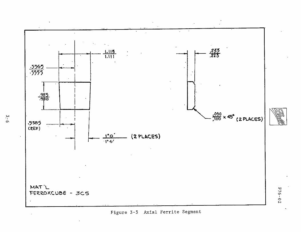
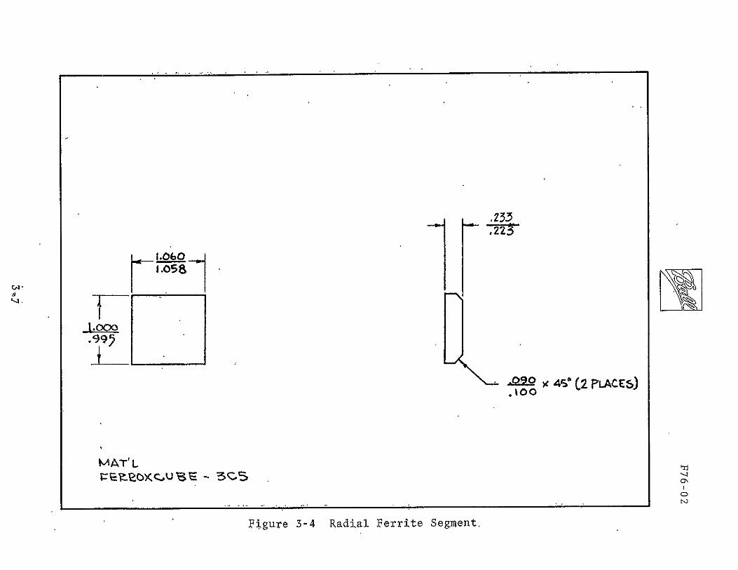
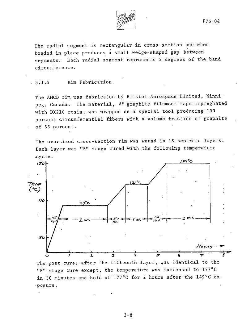

eF76-02
Figure 3-5 shows the specially constructed tool containing
cure cyclesheaters and insulation for B stage and final
The rim was removed from the tool and machined to nearly the
final dimensions including ferrite channels and permanent magshy
net holes These operations are shown in Figures 3-6 and 3-7
The ferrite segments andmagnets were bonded in place with Fuller
7004 adhesive and cured The magnets were placed in the rim with
alternating North-South poles and the ends were covered with a
016 cm (116 inch) thickness of chopped AS graphite-DX210 resin and
After final cure the rim was machined (by grinding) tocured
final dimension The rim was coated with a 0005 cm (0002 inch)
thick layer of Fuller 7220 adhesive as a final step to minimize
Figure 3-7A shows the final rim resultsrim water absorption
313 Rim Analysis
The rim analysis conducted by Bristol Aerospace predicted the
(55434 PSI)rim maximum stress and radial growth to be 38250 Ncm
and 3 cm (0117 inches) respectively
The rim was modelled using axisymmetric finite elements using
the ANSYS system The model characterizes the heterogeneity
of the structure (including the ferrite bands and magnets) and
the orthotropic elastic properties of the graphite-epoxy comshy
posite
The results of the analysis are summarized in Table 3-2 and in
a rim speed of 366 meters per secondFigures 3-8 3-9 and 3-10 at
(1200feet per second)
3-9
N
Figure 3-5 Lay-up Tool
IIP76-02
Rim Machining OperationsFigure 3-6
3-11
MIE II
Iiue37Diln emnn antHlsi h i
3I1
DF76-02
LOCATION MAGNITUDESTRESS (PSI)COMPONENT
Radial or carbonepoxy +460 (max) -891 (min)X stress
Axial or carbonepoxy +491 (max) -433 (min)Y stress
Shear or carbonepoxy +390 (max) XY stress -176 (min)
Hoop or carbonepoxy +55434 (max) 0 (min)Z stress
Radial inner surface +01166 (max)
Displacement outer surface -01130 (min)
(inches)
Table 3-2
MAXIMUM VALUES OF STRESSDISPLACEMENT AT 1200 FTSEC RIM SPEED
3-13
5ThF-=- V- LERATfNz- 1 4U0T00
RMCO RRLYSES BRISTOL REROSPRCE LTO OCT 73
HOOPSTRESS RNSYS 5
or Hoop Stress Contour PlotFigure 3-8 Z
F76-02
- flax h st-ess= 55434-
I I-1 I Ii-- shy
60Iz-
===z_ +0 _----- --- shyi -_-O- - = -- = +----- shy+ ---= -- r E
_-------=--- --- = ---
-- ----- +- - --- -- =--- -=
=
------ shy
=T--- 7
--
-
- -_ - - - -- - -- a
a zrlt- --r-- -r - z I=tzz-z - -
- 4
o6 Zf - =4-=-t vi I_- --- zmE+s=$ Z 4-| b- =---+----- shy
+ 5-t 4 -- c Tt - 22 ~++ _------ _ __ _C - u
a zjztL- +lt+ z- I [Lt- -- Tit--
-- -+v + --F t+-- -+rr 7- h |f
0 200 -00 6800 1000 12oo
Rim SPEED (rri5Ecc~
Figure 3-9 Hoop Stress and Growth With Speed
3-15
F76-02
e 4fo
1 1 I 1 t i I I CII1I1_4I I
Itdn-branveqs sts OI - I M
---shy-- -- -- - -
t~z 2 - 1- shy
- 421 ~T2 2 -=_-- -_E---i ----
t -- EM
___ _ ZZ +-_ _-A~~ - rrrr-
TLLto LLbi i L -- k - r K -1-
irtv li V i 1 -- t 4 s-- n-L -- T4 E
000-q0o 600 800 100 A120 Rim Sp Dr (FTVEC )
Figure 3-102 Transverse Stress Components With Speed
3-16
DF7602
Figure 3-8 shows the computer-drawn plot of constant hoop tensile
stress contours the maximum being 38252 Ncm 2 (55438 PSI)
occurring at the top and bottom inside corner
Figure 3-9shows the relationship of radial growth and hoop stress
as a function of rim tip speed
Figure 3-10 shows the relationship of transverse stress components
with speed
Since the material void free is capable of withstanding 110400 2 2Ncm (160000 PSI) in tension and 8280 Ncm (12000 PSI) in shear
the safety factor is 28 minimum On a sample basis the void
fraction was determined to be less than 04 percent
32 Back-Up Air Bearing System
The design of the back-up air bearing system was completed and
analyzed by Shaker Research Corporation Ballston Lake New York
The back-up air bearing (BUB) system consists of six hydro-static
radial pads and twelve hydrodynamic axial pads These are arranged
in six BUB sets consisting of two axial (one upper and one lower)
and one radial pad and located at either end of a magnetic supshy
port station Each BUB set is approximately 60 degrees from the
adjacent set The bearings are deployed toward the rim by air
pressure when predetermined rim displacement limits are exceeded
The introduction of air through the pads as well as through a
pneumatically operated valve in the vacuum enclosure provides
the fluid for the BUB system and also introduces air drag for a
fastercoast-down Hydrostatic bearings were selected for
radial use instead of hydrodynamic types because the rather small
rim depth (115 inches) allows insufficient area to produce the
required reaction forces The back-up bearing system is shown
in Figures3-11 and 3-12
3-17
P76-02
~14
-L- 7
FiguTre 3-1 AMCD Back-Up Bearing Layout DrawingI 3-la
Figure 12 Back-Up Bearing System
7F76-02
321 Hydrostatic Radial Bearings
The movable radial pads are designed to minimize air flow and
maximize air bearing rim reaction forces The radial pads proshy
vide a centering effect on the rim to minimize dynamic and magshy
netic unbalance forces
In the normal magnetic suspension mode the radial pads are held
away from the rim-and against stops by a set of nested compression
springs (total of 22 N (50 pounds) of preload) When the radial
system Figure 3-11 is activated 207 Ncm2 (300 psig) air is introshy
duced to the pad piston cylinder which moves the pad outward
toward the rim The piston chamber is ported to the pad surface
through a 0033 cm (0012 to 0014 inch) diameter orifice A
sealed oil-filled dashpot between the piston and pad controls the
deployment velocity
Figure 3-13 shows the relationship between- radial pad force and
gas flow versus film thickness for various orifice 4iameters
Because of limited gas available-the smaller orifice diameters
were selected
Since the rim is not at constant radius (because of radial growths)
film thickness and flow vary With rim speed Figure 3-14 shows
the relationship fo film thickness and flow versus rim speed
322 Hydrodynamic Axial Bearings
Movable- tilt type axial hydrodynamic pads were used since the
rim radial width is large and because of the limited bearing air
supply The axial pads are slightly crowned and combined with
the tilt feature are self aligning
3-20
F76-02
1 ~
It
7
I
JII ji
I L
II
---
Ft
T -
VIN I -_ Lr
TD _-
I
I+i
- 1MNV I
4~~r14 +t
Fit~Fi-~tdi I~ ~ JrV)
i ir
il-I= iH14+
i T r
F~m
shy
_ _
I L [
- i
I
_ i _
Ii
0001M -s as
Figure 3-13 Single Pad Force and Flow
3-21
A yyF76-02
WI
ii24pVshy-~~~~W
J4 i3 - Lit
I+ I~Ir~r L-- u 7t J
L 4- 1-nMLfI0__ 4~~~~- F-14--gtrF
I -- -r
4 ~ P I-
IaiH __M
1 --- t Th T1T
I- Vt prI i A
-p--t~LIV[~ VK jl77L1 1
Figure 3-14 Radial Air Pad Flow and Film Thickness With Rim Centered
3-22
F76-02
In the normal magnetic suspension mode the axial pads are held
against stops by a flexural spring The axial system is deployed
in-much the same manner as the radial system When a magnetic
suspension anomaly is detected the vacuum enclosure is flooded
with external air thus providing the film for the axial bearings
Figure 3-15 shows the relationship of film thickness with rim
speed Since the film will support the rim to about 15 radians
per second the pads are designed to accept several contacts before
replacement is necessary
323 Back-Up Bearing Pads
The primary objective in designing the pad material was to proshy
vide a material which would wear smoothly without damage to the
rim or to the pad itself Sacrificial bearing materials have
been used in gas bearings in the past which exhibit the necessary
qualitites The material used in the back-up bearings is an epoxy
resin heavily filled with aluminum powder aluminum oxide power
and molybdenum disulphide powder The mixture is poured into
silicone rubber molds degassed in a vacuum chamber then heatshy
cured The pads are then machined
When the spinning rim contacts the pads the pad will wear smoothly
and rapidly acquiring a high polish and yielding a fine dust
The rim surface should be undamaged by the contact The aluminum
filler provides high thermal conductivity to sink the heat generated
by the rim contact The aluminum oxide provides dimensional
stability so thQ pad will withstand the thermal shock generated
by the rim contact
3-23
3788I9 2 4 5 7 8 9 2
1 7 _- I
111-1 r - J
-I- --i- 1 rV1- 1 t r V
4 _ - _ _____ shy- I---7
I
r-- _- F-_- --- I ii -
I fr r l 7[-II j7shyLi +] - i I-- I
1 7 8
-- - 4 5---- 10 47 MCI 9
Figure 3-15 Axial Pad Film Thickness Versus Speed
F76-02
40 SUSPENSIONSYSTEM
41 System Description
The suspension system consists of three suspension stations
placed symmetrically about the rim At each suspension station
the rim can be pulled in either axial direction or tadially
inward by magnets A total of 12 magnets are arranged in sets
of four each to pull in these three directions (up down and
inward) The eight axial magnets are driven in concert by one
set of electronics Axial error signals are developed by a
position sensor located at the center of each station The
axial servo loops in each of the three stations are independent
of each other The four radial magnets in each station are also
driven by a set of electronics in response to a radial position
sensor located in the center of that station But the radial
station to another so asservos are interconnected from one
to prevent the servos fighting one another even in the presence
of rim radial growth
411 Magnet Description
One of the unique features of the AMCD is the support magnet
design The electromagnets are flux-biased by thin wafers of
samarium cobalt permanent magnet material placed in series in
the magnetic circuit This has the advantage of (1) providing
a high force per unit current sensitivity at zero current (2)
providing a linear relationship between force and current and -
(3) providing the static field required for zero power operation
The support magnet geometry is seen in Figure 4-1 The permanent
magnet biasing is achieved by slanted wafers of samarium cobalt
in the legs The wafers are as thin and wide as possible to
4-1
SAti 4-IUr CCBA3L~rshy
AGtJer-
AGII1
Figure 4-1 Support Magnet Geometry
RF76-02
minimize their reluctance in the magnetic-circuit The volume
of permanent magnet material is sufficient however to provide
adequate flux-biasing and static lift The reluctance of the
permanent magnets is large but does not more than double the
total reluctance since the air gap inthis system is large In
many other magnet suspension systems the gaps are small (about
01 mm) and this sort of series flux biasing would greatly inshy
crease the total reluctance in the circuit Control power would
thus be large and the systems would be impractical
The effect of flux-biasing on the force versus current characshy
teristics of the magnets is shown in Figure 4-2 With no biasing
current in either direction produces force of the same sign with
poor gain and low efficiency in the vicinity of zero current
Force is simply a function of the square of the current With
biasing the slope of force versus current is greatly increased
at zero current In the AMCD top and bottom magnets operate
together in a push-pull type of operation The coils are in
series hence both coils have zero current at the same time
The resultant force-current relationship is linear and has a
slope double that of either magnet alone
Figure 4-3 shows the U core of the magnet with the permanent
magnets in place Permanent magnet thickness is 1 mm (0040
inches) Also shown in Figure-4-3 is a fully assembled magnet
ready for potting After potting the units measure 43 cm x
167 cm x 25 cm (17 in x 42 in x 99 in) and weigh 500 grams
(11 lbs)
412 Position Sensors
The position sensors used in both the axial and radial suspension
systems are Multi-vit sensors manufactured by Kaman Sciences
4-3
7 gF76-02
-r
UPPETP HA -
C AOc~~
777
~~oeehAcn-e-r Z
Figure 4-2 Flux-Biased Magnets in Push-Pull Operation
4-4
rF76-02
I
3 i
A A
I tii A LWUv
NN
N~ i X -9
i i UI A i
IN aWIi ii i
iiiiiiiliiili
i~iiii Ii iliiiiiiiliiilii
Iilliii iiiiiliiiiiiliiiii = iiiiiiaii~iii iiiiiiiiiliiiiiiii
Uiiiii poundii=iiiii]iipoundiiiiiiiiiiiiiiiii Uigure 4-3 Support Magnet Cosri on
iliiiiur -3 ConstructiiiiIliiiiiiiiioniiiiiiiliiiSppriMge liiiiiii i iiiiliiiii3 URiliI 4-s == =
4-s
rF76-02
Corporation These are conventionally called eddy current senshy
sors although they are actually sensitive to anything that changes
the inductance of the test coil in the probe Hence either
eddy currents in a conductor or the permeability of a magnetic
material can be sensed In the AMCD the sensors look at the
ferrite bands and therefore are operating entirely ina non-eddyshy
current magnetic permeability mode Special calibration of the
sensors was required in order to operate in this mode Linear
range of the AMCD sensors is 025 cm (01 inches) and scale facshy
tor was set at 4 voltscm (10 voltsin)
413 Control System
The axial suspension system uses three independent servo loops
to control electromagnet currents An electronic diagram of one
of these loops is shown in Figure 4-4 The heart of the elecshy
tronics is an Inland Controls MA-I DC servo amplifier which is
operated as a current driver to reduce the effects of electroshy
magnet inductance Equations of motion of this driver and an
analysis of the voltage feedback used to damp high frequency
roots are given in Appendix A An analytical block diagram of
the entire servo loop is shown in Figure 4-5 Equivalent points
on the electronic and analytical diagrams are indicated by letters
within hexagons
The axial suspension system has two modes of operation a posishy
tion mode and a virtually zero power (VZP) mode In the posishy
tion mode rim position error is used to command electromagnet
current The rim has high static and dynamic stiffness about
any desired point in the gap In the VZP mode the rim position
set point is modified by positive feedback of the integral of
electromagnet current The result is that the set point is moved
until steady-state current is zero The permanent magnets are
4-6
AA
REHTUtk +26V
4-
C11 7t-Q
Fiue44Aia3upnin7lcrnc
S Cornn- EesoCo p n a cncivCrrent Driver- O deg OI 99 (5C + sm -3 (s + 1 1deg E 1 copy + F
gtosO ~
volf
iE 3 7 T r i m T ntegratadegr
Suspended
Mass
-|ectro
-ria net
16
permanent Magnet
Figure 4-5 AMCD Axial Suspension Station
R 1F76-02
then providing all of the support of the rim Dynamic stiffness
is nearly the same as in the position mode but static stiffness
is actual negative If a downward force is applied to the rim
in the VZP mode it initially moves downward but then slowly
rises to assume a new zero power position above the old equilibrium
position
The electronic circuit diagram for a radial servo station is
shown in Figure 4-6 and the corresponding highly coupled analytishy
cal block diagram is shown in Figure 4-7 Again equivalent
points on the two diagrams are indicated by letters in hexagons
The large amount of coupling results from three servos controlshy
ling only two degrees of freedom
Two modes of operation are available a position mode and a WAHOO
mode The position mode is similar to the axial position mode
The WAHOO mode is a zero power mode that produces zero power
operation in the presence of both static loads and rim expansion
This is accomplished by adjusting the position set point at each
station as a function of the integral of the sum of the electroshy
magnet currents at the other two stations
The name WAHOOis derived from the poker game WAHOO This game
is played in a manner such that each player knows what every
other player holds but does not know what he himself holds
Inspection of the WAHOO trim loops of Figure 4-7 reveals that
for VZP trim purposes each servo only looks at what the other
two are doing This innovation was developed by BBRC to meet
the unique requirements of the AMCD
The derivation of the WAHOO concept is given in Appendix B
There it is shown that only the WAHOO concept produces zero
power operaion for both rim expansion and force disturbances
4-9
A00l 51 Ir
A-A-
F
27
ffzo xr
74 VIP KIAk
7
Ems~
n
A7-
I
A1
ter
a 2k-
-
-
-
-
-
I)
Figure 4-6 Radial Suspension Electronics
-KS
Iamp wkin47s Permanent MagnetVeloityPM VPol Aplifir PMEHM E Iectremoqnet
K5 Kmn eae t~j VOS 0bCar respond to Lettered
1vII~rb r - rr m Psitionson Cgrcwit
vol vol Im PosiMoon Pox
SlRtim rtOhkx _Q$)bsS 4lfe I
0niplPfied Cus ren Driver
Gcucv rbinn n i
+ + vt
If
in-7d FigureservoD RailSro
+i
42
F76-02
Appendix B also shows that for single station design purposes
a single station can be represented as shown in Figure 4-8 Two
points of interest are immediately evident The equivalent mass
for a single station representation is 23 the total rim mass The WAHOO concept which involves negative feedback to each station
from the sum of the other two stations resolves to a positive
feedback in the single station representation exactly like VZP
in the axial mode This representation can be used for designing
the system characteristic root locations If the characteristic
roots from the single station representation are given by A and
the WAHOO gain is Kc it is shown in Appendix B that the three
station highly coupled set of characteristic r6ots are givenby
(S + 2K )A2
Performance
421 Static Performance
At each suspension station the rim will seek an axial equilibrium
position based on the applied load and the control system mode
(position or VZP) These equilibrium positions can be preshy
sented in one plot as shown in Figure 4-9 The VZP line is a zero current line and has a slope that indicates static instability
however as shown in the next section the system can operate in a
stable manner along this line The most usual operating position
mode point is about 001 cm (025 inches) above the center of the
gap At this point the slope P of the VZP line is about 595
newtonscm (340 lbin)
In the position mode an operating line exists for each set point
of the position sensor A family of these is shown in Figure 4-9
The lines are finite in length because of the limited current drive
capability of the electronics The slopes of the lines are apshyproximately 2600 newtonscm (1500 lbin)
4-12
Stationfost ionsingle
Oecrlx- EquIva1eratArmplifir Current Driver 6 Mks$M9oqmet+ 1m
~~~~~ eroe L~r
Is + Fes I16(7+1210 r0 0 l I-
p 0 1
476 An- Per
u2 IVlt+ -Eg
o tKate - r1 1 StO Sr eq uci o lnk wahoo is
Q Correspornas toa letterd posit~ions on circuit chogr~m
Sinql~e stcton eqviclvJewtmls is 23 totil ma
~odelldas a posattve PeedbctK self IoopVe
t to o-t liKe Vf Pwould ltherefboretxpect fvrthernortn itthe Aol O Servo Xt doesonh
Figure 4-8t EqiaetSnluadapev tto
ekgeto8 rnex e o +non
A F76-02
UP
MAGNET M~A t r
lsrok os NoRMAL
kE-RITI N
P E-Nshy-OMFR
tL UPshy
- j ~
-10
h31G1NL pAGE iS
)F POOR QUML-rI
Typical Static Suspension System Performance
Figure 4-9 4-14
rF76-02
The force sensitivity F of each station is about 138 newtons
ampere (31 lbamp) Hence the force produced by a station
is given by (in English units)
F = 340X + 3lI
422 Dynamic Performance
The analytical block diagram for an axial suspension statiQn is
shown in Figure 4-5 For theposition mode the root locus and
-Bode plots are shown respectively in Figures 4-l0and 4-11 The
root locus plot shows that the dominant pole pair has an undamped
natural frequency mN (which we define as bandwidth) of 171 radsec
(272 hertz) and a damping ratio of28 The Bode plot shows
that the gain crossover frequency wc (which some define as bandshy
width) is 1827 radsec (290 hertz)-and that the system phase
margin is 2320 Both plots show that the lower gain margin
is 22(-131 db) and that the upper gain margin is 201 (261 db)
For the VZP mode the root locus and Bode plots are shown respecshy
tively in Figures 4-12 and 4-13 The root locus plot shows that
the dominant pole pair has the same undamped natural frequency
and damping ratio as the position mode that is wN = 171 radsec
= 28 The Bode plot shows that two gain crossover frequencies
at 1823 radsecexist one at0838 radsec (013 hertz) and one
(2903 hertz) The phase margin at the lower crossover frequency
is -772 and that at the upper crossover frequency is 2300
Both plots show that the lower gain margin is 226 (-129 db)
and that the upper gain margin is 2011 (261- db)
The response due to the step application of a one pound weight
is shown for the position mode in Figure 4-14 and for the VZP
4-15
OF76-02
1 -DD
-- A I 1
I I
i
3000 --------------------------------- ___tN
-5000 -400 -30U -2ODG -t I lo oD
REAL AXIS
Figure 4-10(A) Root Locus Plot - Nonideal Current Driver With
Voltage Feedback
4-16
---------------------------------
7F76-02
-I- 111 1-l Z9D
io oI 1ll t A
G
80 ----------- 0 aEu----------------shy-4--
FigueRot41001LcusPlo - Nnidal Crret DrverWit
-1---4-17
I I
F76-020
14-HLowler
)2 I__ _ p
1 N I-- A =20 41 r
I tIse0_ __ _ _ 4 6 2 4 68100
s 10 log H00 6 10009 FREQUENCY (RADIAWS$ECOND)
Figure 4-11 Bode Plot - Nonideal Current-Driver With Voltage Feedback
4-18
7F76-02
$oo I5iI000 I1
T 1 Ii
-A
S4+
N A
4000 R--- - - - - -
V A x
103 000 40 30 29
urn rvrWtFi1r -12A Roo Lou7lt-Nnda
Voltage Feedback 4-19
V gF76-02
ii
- I I I
I I I II
I lii
-I I
II I iishy
II - - -i-l
Fgr 4-2B o otocu PltrNndaCrefl rive
With Voltage Feedback
4-20
F76-02
I i E
A -4 G
E- 60I jUroI(
I
1A2zS1 me RI
3s F-1-L
IIsoM 3en
4) e r
-120---- -Marlin
fla e =2300
-140 shy
1 1 10 10g 2000 1090r FREQUENCY (RADIANSECOND)
Figure 4-13 Bode Plot - Nonideal Current Driver With
Voltage Feedback
4-21
012
F76-02
00010
00008
pound E
0
p
0 00
0zkc0
0
E
- -
4+-F
- - -
Nshy- - - - - - -
4
- -
5
-4-2
AF7602
mode in Figure 4-15 The response for the position mode settles
out at 6941E-5 feet (002 cm) This yields a position mode
stiffness of Stiffness 6 1 lb
6941E_5 t X feet
1 12006 lb (21021-
N
69Th-ft Tni in cm
The response for the VZP mode settles out at -2451E-4 feet
Thisyields a VZP mode stiffness of
1 lb feet = lb NStiffness = 2451E4 ft X 12 in -3400 i (595 E-
Note that the stiffness in the VZP mode is just that of the
permanent magnet and that the movement in this mode is toward
the applied force That is if a weight is placed on the rim
in the VZP mode the rim will move up
Further insight into the system can be found by examining Ap2
pendix C When using current driirers the usual tendency is to
ignore the high frequencydynamics and simply say that the
output current is the input voltage times a constant This can
be very misleading in the case of AMCD- In Appendix C are shown
root locus plots using both an ideal current driver arid a nonshy
ideal current driver without voltage feedback It shows that
voltage feedback is necessary for the axial suspension Also
shown in Appendix C are Nyquist plots and phase-gain root locus
plots of the nominal axial systemthat is the system using curshy
rent drivers with voltage feedback The esoteric phase-gain root
locus plot shows on one plot the sensitivity of the system roots
to change in both gain and phase For example it shows what
would happen if an additional 300 of phase lag were added to the
system from some unknown source
4-23
F76-02
0001
I f
I 0 e
eshy
0a T 1-0001-shy0N
ft E F 0
E a
- 002--------------shy
0 t0 20
TINE (SECONDS]
30 40 50
Figure 4-15 Nonideal Current Driver With Voltage Feedback
4-24
F76-02
The equivalent single station radial analytic block diagram is
shown in Figure 4-8 It is very similar to an axial station
The root locus and Bode plots for the position mode are shown
respectively in Figures 4-16 and 4-17 The root locus plot shows
that the dominant pole pair has an undamped natural frequency
(bandwidth) wN of 653 radsec (104 hertz) and damping ratio C
of 18 The Bode plot shows that the gain crossover frequency
is 666 radsec (106 hertz) and that the phase margin is 1350
Both plots show that the lower gain margin is 329 (-965 db)
and that the upper gain margin is 7054 (3697 db)
The root locus and Bode plots for the WAHOO mode is shown in
Figures 4-18 and 4-19 The root locus shows that the dominant
pole pair has an undamped natural frequency of 674 radsec
(107 hertz) and damping ratio of 16 The Bode plot shows that
the upper gain crossover frequency is 691 radsec (110 hertz)
At this frequency the phase margin is 1260 Not shown is the
fact that the system also has a lower gain crossover frequency
of 594 radsec (095 hertz) At this frequency the phase marshy
gin is -715 Both plots show that the lower gain margin is
389 (-821 db) and that the upper gain margin is 6701 (365 db)
The large upper gain margins for both the position and the VZP
modes indicate that current driver voltage feedback is not needed
Considerable rim bending instabilities were encountered during
the design Early in the development the axial system was
designed to be overdamped This caused a bending mode to be
driven unstable The compensation was adjusted experimentally
until the bending became stable Unfortunately this reduced
the lead in the system resulting in the present underdamped sysshy
tem It is believed that bending will present no problem at
high spin rates because of the effective stiffening of the rim
4-25
6F76-02
_____ - _ r ____I___
141
IT___lishy
1 ii
1 F]
eir
t lj~
4-
J TT a p-
III NEA
fiIT WBKsITlK j1_11IIi I-
I
e
-Fshy
Y]-111 ji
1i1fln 4--I r
I i--I -
TFiJ-WL 1
_1(-Ii4 - I
I~ ~ ~iA_~2I ___ ii- 11 IFt-Ih
iT
h~ -iH T
+~ji+ih Iplusmn
_ _ _+ I kt ~h-II
+ LILY -
7 SO bullj
Figure 4-16 AMCD Radial Suspension Equivalent Single Station Position Mode
4-26
Elll csl- tLL[ 11--- 1_ il
V
1 MIN
2 0 H qL2~14-0IT
I M Ill 1OIHI
+-o ip Lr g
Ti I -0 1- b1 -- i
Ij _IUSi 1PIN - il
--i
41i L -I I - d jir ~J I I
00 -o
ro-d 5 c
Figure 4-17 ANCD Radial Suspension Equivalent Single Station o Position Mode
7F76-02
1LjI_----- Li -III iI - - I -shy-F ]e2 1
Is- Lr [_I
r ir -L-j 11I IALI _ _ _ ___ 2_
E11LLN1LALIF TYC -- td It 11
- KI
S1 1 1 1--shy
II
I r 11
FLL-1
U - I 4
E~~~~fL
__
f Lplusmn Xi ILIi _ _
- ii _ _ i
- H --
--------
A-1 1 F - JT-1
-- t-ti -~r -r I- t - --- IL I
IIJlri-tlrht1f tI
_+ _ l PillS 1 I
Figure 4-18 AMCD Radial Suspension Equivalent Single Station
o Wahoo Mode
4-29
rm~r 1 u i rrrrF r r r
4
130
o
I -4
7 7 1-shy iAb d
llt h
-30 Tfij4i i ~
- n0 t
Figure 4-19
01 AII-
I uji r a sec
AMCD Radial Suspension Equivalent Single Station o Wahoo Mode
AF76-02
and the averaging effect on modal pick-up caused by the bending
modes moving rapidly past each position sensor
As the rim is spun up the three axial stations become more and
more coupled by nutational effects The result of the coupling
is to reduce the dominant roots damping ratios more-and more to
the point the system could go unstable if the rim is spun fast
enough It is believed that this tendency could be greatly
reduced or possibly eliminated by the proper combination of cross
feeds from one axial suspension station to the others
4-30shy
DF76-02
50 DRIVE SYSTEM
51 System Description
The AMCD drive motor can be thought of as a large permanent magshy
net brushless dc torque motor Samarium cobalt magnets are
bonded into the rim at regular intervals The two phase armashy
ture is segmented with a winding set at each of the three susshy
pension stations Commutation is controlled by Hall effect senshy
sors mounted near the rim which sense position of the samarium
cobalt motor magnets
52 Magnet Selection
Alnico was considered along with samarium cobalt for the permanent
The large air gap and segmented winding structure meanmagnets
the magnets will become nearly air stabilized The rim was designed
with a small outer lip to hold the magnets This was done to
isolate the drive from the suspension as much as possible without
and complexity to the rim than necessary Thisadding more mass
small lip implies a short magnet Samarium cobalt has high
strength for short lengths and does not pay a penalty for air
In fact it is very difficult to demagnetize thisstabilization
material
cm (55 inches) diametertby 64 cmSamarium cobalt magnets 14
(25 inches) length were selected and bonded into the rim with
polarities alternated
The rim contains a total of 72 magnets spaced 73 cm (288 inches)
apart
5-1
53
--F76-02
Core and Winding Design
Each armature segment consists of a pair of bar-shaped winding
assemblies one above and one below the rim
Sit cos sla 0S SMa
cores in a singleThe windings-are wound toroidally around the
layer The figure above shows only the cross-section 6f conshy
ductors in the air gap as the conductors passing around the other
side of the core add nothing to torque and serve only a connectshy
ing purpose The bar-shaped cores are easy to wind and result
in a compact structure The single layer of 18 conductors adds
very littleto the overall air gap This effective electroshy
magnet design was suggested by P A Studer of Goddard Space
Flight Center
Ferrite material was chosen for the core to reduce losses Fershy
rite also is easily machined into the required irregular shapes
The windings are grouped into two phases SINE and COSINE each
of which acts upon three magnets at each motor segment In operashy
tion current in one phase is acting on the magnets while current
in the other phase is reversing in preparation for a magnet of
opposite polarity
5-2
DP76-02
54 Motor Commutation
Hall sensors act as commutation devices for the motor They sense the position of the permanent magnets in the rim and cause the drive coil currents to be switched according to magnet position
The sensors are mounted in pairs one above the rim and one below for each winding phase Outputs from each pair are summed so that the switching position is not affected if the rim moves up or down within the air gap The SIN pair controls current on the SIN windings of all three motor segments and likewise the COS pair
of Hall sensors controls all COS windings
55 Motor Control Electronics
A block diagram of the motor control electronics is shown in Figure 5-1 For each phase the Hall sensor outputs are summed and amplified to drive-threshold detectors These detectors sense magshynet position and polarity The phase control logic determines the
timing and polarity of the motor coil drivers Interconnections between the two phase control logic blqcks provide positive direcshytion and start-up information
Each of the six coil drivers controls a phase at one of the motor
segments Associated with each driver is a coil current sensor which monitors the current in that winding All six of these
current sensorsreceige a common reference from the speed control
potentiometer When current in that particular winding reaches the reference level the driver turns off until the current deshy
creases This prevents the current from reaching destructive levels at low speeds and acts as a speed control at high rim
speeds
Since the coil drivers are either full on or off a very efficient drive is achieved At low rim speeds the drivers operate as a
5-3
56
F76-02
conventional PWM (pulse width modulated) amplifier A quite faithful square wave current of controlled amplitude is fed to the coils At high speeds high acceleration (or deceleration)
is possible with the drivers full on for the period between magshynets with current rise and fall limited by the inductance of the
coils
Torque Calculations
The equation for the force betweena magnetic field and a current
carrying conductor-is
F = BLI
where
F = Force in Newtons B = Flux Density in Teslas (WebersM~ter )
L = Conductor Length in Meters
I = Current in Amps
If the magnetic field is created by a permanent magnet the force
can be considered to act on the magnet if the conductof is held
stationary which is the case with the AMCD motor
To arrive at design force each of the factors B L and I must
be evaluated
A force calculation will be made for one magnet face interacting
witha coil This can be then doubled to account for both ends of the magnet next tripled to take into account the three magnets in one motor segment and tripled again to realize the total force for the three motor segments Then using the radius of the rim
we can calculate developed torque
5-4
F76-02
Flux Density Calculation (B)
The large air gap makes it difficult to- estimate how much of the
magnet flux will couple through the winding core and how much
will be lost to leakage A measurement of coupling flux was made
using a pair ofsoft iron bars similar to the ferrite corasi
SEJSE C0115
SOFr iROh
-4 Webers with magnets of averageThe flux measured was 0375-x 10
strength
core must-be convertedThis flux that couples through the ferrite
to flux density (B) in the air gap where it interacts with the
coil windings There are two practical Choices for doing this
We can assume all the flux goes straight up from the surface of
the magnet andreacts with only those turns above the magnet or
we can assume the flux spreads out evenly over the winding area
Of course the truth liesand-reacts with all the turns equally
an adequatesomewhere in between but the second approach gives
approximation
The winding area in the air gap for one magnet coil phase is 2
19 x 36 cm or 68 cm
Flux density then is
-44m _ 0375 x10 Webers 2 0055 WebM-B_=A = 4 2A - 68 x 0-4 m
5-5
F76-02
Conductor Length Calculation (L)
are 28 turns with an effectiveIn the winding phase area there
length of 19 cm each
Total effective length is then
L = -19 x 28 = 532 cm = 0532 M
Current (I)
that the coil drivers and wiringThe elbctronics are designed so
canhandle 4 amperes Also the inductance of the coils was
examined to be sure that currents of this magnitude can be
reversed at maximum rim speed frequencies with a 60 volt power
(and torque) will then be calculated for thesupply Force
design maximum of 4 amps
Force
We can now calculate force from the equation
F = BLI
= 0055 x 0532 x 4 = 0-1-17 Newtons
Recall that this is the force for a single magnet surface inter-
For the total motor this is multiplied by 18face
Total Force = 0117 x 18 = 176 Newtons
576
0F76-02
This times the magnet radius (0838 meters) gives total torque
Total Torque = 176 x 0838 = 176 Newton-Meters
(13 lb-ft)
A small (14 diameter) test wheel was built to check the above
torque calculations Acceleration measurements were made and
from the known wheel inertia torque was determined Correlation
within 10 of the calculated torque was achieved
5-7
S in Hall Sensors
Summing
Amp
[A Threshold Sin Phase Coto-rie
DetectorsLoi
SnB1Sin
Sin C Driver
ol
Hall Sensors
~ Amp=ApDtcosLogic
etctr Control -- Die Col Ci~
Summing Threshold Phase Cos B Driver
iCosCos
Ci Co
Figure 5-1 Motor Control Electronics
C
aF76-02
60 REFERENCES
1 Anderson Willard W and Groom Nelson J The Annular
Momentum Control Device (AMCD) and Potential Applications
NASA TN D-7866 1975
6-1
F76-02
APPENDIX A
CURRENT DRIVER EQUATIONS AND TRANSFER FUNCTIONS
A-i
F76-02
Appendix A
Current Driver Equations and Transfer Functions
When using current drivers the usual tendency is to ignore the
high frequency dynamics and simply say that the output current is
just the input voltage times a constant This was very misshy
leading in the case of MCD-as shown in Appendix C The circuit
diagram of a current driver with voltage feedback and its equishy
valent diagram are shown in Figure A-i -
v A T5It
Figure A-I Current Driver and Equivalent Circuit
A-2
F76-02
The beginning equations of motion are the following
Rl11 RM -- R 10
-RM SL + R2 2 -(SL + RC) I= A(TS+I)-)V + ARI(TS+l)shy
-R 2 -(SL +R c) SL + R3 3 + S_ C I 3 0
where
R1 lt= R1 + R2 + RM
2 RM + RC22
R33-- R2 + RF + RC
Transposing I1 to the left hand side we obtain
R11 -RM -R2
-RM(TS+l) + AR 1 (TS+l) (SL+R 2 2 ) -(TS+1) (SL+Rc) 2 A S-SR22 S L+SR33+-l
What we really want is the current through the inductanceshy
1 2 T3
Adding this equation to the system we obtain
C1 C12 C1 3 0 II 1
B2 1 S+C 2 1 A 2 2S2 +B 2 2 S+C 2 2 A23s2+B 2 C 3 0 12 A V
B31S A32S2+B32S A33S2+B 3 3S+C 3 3 0 13 0
- -1 1 1 1 0
A-3
eF76-02
where by definition
-=A32 -LC R11 B22 = L+TR 22
= - C22 R22 B32 = RCCl2 RM
C13 =-R 2 A23-= -TL A33 = L
= R33B21 = -RMT B23 = -L-TRC B3 3
C = ARI-RM C = -RC C =C -I
= -R2A22= TL B31
If the voltage feedback is removed these equations reduce very
simply to
-RMIRlI+R2+RM
+ AR1 (SL+R+RM)(TS+ 1j1 2 = AKRM(TS+I) We want thewhere 12 is the current-through the inductance
transfer function 12V First divide the secondequation through by
LT to obtain
-RMR I+R2 +RM
(R C+ PM j] IAL 1 V S+L-iIARI[ RM L (SplusmnT -1)+L -lT -1A
A-4
F76-02
Then by Cramers rule
2 CR1+R2+RM)AL -1T-+RML -1(S+T- 1 )_L-1T- 1 AR1
V7 -1 r- 1 2-1 - lshy(RI+RZ+RM)(S+T +L (RC+RM) -R ML l(S+TI)+L ITIARIRM
(R2+RM)AL -T - I(S+Tshy
-(R1+R 2+RMM)(S+T 1 )(S+L-1 RC)+L -RM(R1+R 2)(S+T-I)+L T ARIRM
Further manipulation yields
S+T-1 +(R 2 +RM)ARM T12 RML -
V - 2+RM) 1 L-+RR [2 wT-ARI-L 1RM(RI+R2 -
S+T )(3+L Rc) + RR+Tl+R---
Finally the desired current driver without voltage feedback
transfer function is given by
12 RML- S+T -1 +A(I+R2 RfIj
V (RLR-+RM) - -1 LRM(RI+R2 ) (ST 1 [7AR 1 RS5 + R2 +RMR R1 L Rk 2 )
A-5
76-0 2
For infinite amplifier open loop gain A = the transfer
function reduces to
2R Lim 12 = R1_ 2M
(l+R2RM- R2
R - RYR RR)r112RM for R2gtgtRM
-This is the transfer function which is used
I2 R2 12 R 2V RIRM
if the high frequency roots may be ignored
When the high frequency roots are not to be ignored and
if AR2R1 gtgtmax (RMRC-i)
and RMARlRjR2gtgt
RI+R 2 c
A-6
rF76-02
The transfer function simplifies to
S+T- AR 2RM1
12 RML-
V R1+R2 (S+T-)(S+L -Rc)+L- RM(S+T-AR1 R1 +R2)
RML-1 S+T-1AR2RM-
R1 R2 S2+ -1 -1 -1 T 1L-1RMARl - A
S +(T- +L -Rc+L RM) S+ R+R
T- +L- (RG+RM) TRLAR
2 (RI+R2)
The dc gain of this transfer function reduces to the same transshy
fer function used if the high frequency roots may be ignored
that is
2 R2 V RIRM
For the radial MA-lCurrent Driver
RI = 10K R 2 = 2711 KQ RM 10
RC = 30 Q2 L = 0128 h T - 30 A 50119
Then the radial current driver without voltage feedback has the
transfer function
12 _-00061463(S+40762E10)
V S+13609plusmnj30400 shy
A-7
F76-02
Forthe axial MA-I current driver
R=1 10K R2 = 7311K C 01 1f R11 = 17311E4
L =0064 f = 12M R = 14 R22 =15
A = 50119 RM = 1 T- = 30 R 33 I2073E6
Then
= C11 7 17311EA B2 2 = 564E-2 A 3 2 -0064
Cl2 = -- 22 = 15 B = -14
== = -7311E3 -21333E-4 A33 0064C13 A 23
B21 = -33333B-3 B2 5 -53067B-2 B 12073E6
C21 = 50119E8 C2 3 - 14 C3 = 1OE8
= A22 = 21333E-4 -B3 1 -7311E3
Without voltage feedback the axial current driver has the transshy
fer function
2 00090261(S+l0993B1)
V S+13219plusmnj36839shy
A-8
7F76-02
Note that without voltage feedback the damping ratio on both the
radial and axial current driver high frequency roots is less than
05 This appears to be all right for the radial servos but is
very bad for the axial servos as shown in Appendix C Consequently
-voltage feedback has not been employed for the radial servos
current drivers but has for the axial servos cur-rent drivers
The effects of this feedback has been determined numerically
Figure A-2(A) shows the effect of increasing RF the voltage
feedback resistor from zero to infinity with the feedback capashy
citor C held a-t 01 lif Ifonly the capacitor is used for voltage
feedback the current driver roots are still lightly damped but
at a much lower frequency As the resistance is increased the
roots increase in damping become real then decrease in damping
at a high frequency finally moving to the no voltage feedback
position for RF = Figure A-2(B) shows the effect of increasing
the voltage feedback capacitor C from zero to infinity while
holding the feedbackresistor at one megohm For C 0 the roots
start at the no voltage feedback position As C is increased the
roots decrease in frequency and-increase in damping ratio until
C = 00091 f Further increases result in decreased damping
ratio and increased frequency At the chosen voltage feedback
values of C = 01 vf RF = 10 MQ2 the axial current driver transshy
fer function is
I 0008994(S+833)(S+l099EII) V (S+786)(S+2771plusmnj2583)
A-9
~~~ L~Trrrl~I I~ I II 4
Jots_1 nr_- r177I 7F I i0K IIII __ riiTTh
17shy
tkP M T7r
Hl4plusmn ------ IIr-1-----~ -- - I -
CDl7E-~ ttbifil
LA14 -T-- 4+ -
C T -I I
H -rTH V i H
-HE I
Figure A-2 Effect of Voltage Feedback on AMCD Axial Current Drivershy
AF76-of -
APPENDIX B
THE WAHOO CONCEPT
B-I
7F76-02
Appendix B
The WAHOO Concept
Introduction
Two conditions may occur which cause the radial electromagnets
to draw more current than necessary First if the rim is tipped
This forcea gravitational force tends to pull the rim sideways
at the expense of causing the electro-shyis countered by the servos
magnets to draw more current Second as the rim spins up
centrifugal forces-cause it to expand To each radial sensor
as rim movement to be countered by thethis expansion is viewed
to try to pullservos So each electromagnet draws more current
are directed inward andthe rim inward But since the forces all
spaced 120 a-round the rim the resultant of the forces is zero
so the rim does not move The net result of the expansion then
is thatonly the current in the electromagnets increases Trim
loops are developed in this appendix which lead to VZP (Virtually
Zero Power) operation for the radial servos when either the rim
is tipped or expands or both The system employing these trim
loops is called the WAHOO system
Because the three radial servos are controlling only two degrees
of freedom the radial servo system is very highly coupled This
very high degree of coupling makes it difficult to design each
servo as a single uncoupled system Hence in this appendix we
also develop equations to show how the three-servo radial system
may be designed using a single station servo radial equivalent
Development of the WAHOO Concept
The AMCD rim is suspended radially by three servos pulling on
it from the inside much like shown in Figure B-1
B-2
F76-02
Kim
Figure B-i Radial Servo Sign Convention
The sensor outputs are denoted by X1 X2 and X3 As the rim
spins up it expands by the amount X0 The sign convention is
chosen such that positive forces and displacements are outwards
The equations of motion of the rim are
(F2 - F3 )Co = My
(F2 + F3)s8 -F1 = my
X2 = XCe + YSe
X3 = -XCe + YSO
XI = -Y (B-i)
B-3
F76102
The force acting at each station is composed of a permanent
magnet force and an electromagnet force That is
Fl = P(XI+X0) + E D1
= P(X2+X0 ) + E D2 (B-2)F2
F3 = P(X3+X0 ) + E D3
these equations are-combined with the servo equations in Figure
B-2
From the block diagram the quations of motion using five variables
are
V1 = Kp(-Y+X0 ) -S)(KsVi+KcV 2+KcV 3) EKRN_1
Y = M--p(-Y+X0)+DR (-Y+X 0)+ EV1 +pSC(YSe+XCplusmnX0 )
EKRN -fD se(YSe+XCe+Xo)- ESeV 2 + PSO(YSe-XCe+X0 )
EKRNK sOCYSe-xce-Xo)- nsev 3 + FY
-V2 = K (YSO+XCeplusmnXo)-(lSKsV2+KcVI+KcV3)
EKRN = 1=M PcO(YSe+XCe+X 0 )- D C(YS+XCc+X0)- ECOV 2
EKRN -PCO(YSe-XCO+X 0 )+ ce(YSe-XCe+X0 )+ ECOV3
)V3 = K(YSe-XCO+X0 )-(SJ(KsV 3+KcVI+KcV2 (B-3)
B-4
+ SFt
+- K + X0
+ T- SID
fRi
Figure B-2 MICfl Radial Servos With Trim Loops
7F76-02
Rearranging
(S+Ks)VI+KpSY+KcV 2+KcV 3 = KPSX0
-M-1DEv+[DS2 -DM-Ip(1+2SD)+M-EKRN(1+2S2 0)]y
+M-IDESOV2 +M-1 DESOV 3 = [M-IDP(-1+2S)+MWIEKRN(I-2SO]XO+MDFy
KcV -KpSSY+(S+Ks)V2 -KpCeSX+KcV3 = KpSX0
M- 1DECOV 2 +[DS 2DM- P(2c0 )+M-1EKRN(2C2 )]X-M-IDECOV 3 = 0
KcVI-KpSSY+KcV 2+KpCeSX+(S+Ks)V 3 KPSX0- (B-4)
Since 0 = 30
I+zs2 -1+2(5)2 = 15
-- 1+2S = -1+2(5) 0
2C = 2 )2 = 15 (B-S)
Using these simplificatfons the Laplace transformed radial
servo equations of motion in matrix form are
(S+Ks KpS 0 KC KpS 0DSL KC V1
-1IDE +lSMIEKRN SM- 1flE 0 SM- DE Y 0 M D
-1$M IDP __ __
KC 5KpS (SK S ) SrI KpS X6 V2 KK SX 0 + 0 Fy
DSz--shy
SM- 1 DE - SMDE0 0_- 54M +lSM 1 EKjN x 0I 0
-5KpS K 54 KPS (S+Ks) KpS 0KC V3
B-6 (B-6)
F76-02
The system characteristic equation is the determinant of the
coefficient matrix With much algebraic effort it can be
reduced to
A = (S+Ks+2Kc)X
FKRN-ISM- DP)+lSKpM- DES]2[(S+KsKc)(DS2 +SM-
(B-7)
Now lets simplify the expression by-removing the high frequency
roots In the Cambion hardware
KRN 107 S for low frequencies
D (S+1000)(S+10000)
With this approximation KR = D = and N = S Then
2+lM ES-lM P)+lSKpM-1ES] 2A = (S+Ks+2KC)[S+Ks-KC)(S
So the roots separate into -(Ks+2Kc) and two identical sets
within the brackets Immediately we see that Ks+2KC 2 0 for
stability Now looking within the brackets we see that S2+
1SM-ES-l5M-P represents the permanent magnet roots at
+lSM-IP moved to the left some by the rate feedback however
one remains in the right half plane Taking these roots and the
one at -C(Ks-Kc) as poles of a root locus plot and S as the zero
Figure B-3 shows that for stability KC a KS
B-7
0F76-02
Kct IKSKczk 5
Figure-B-3 Effect of Trim bull Loop Gains
Les look at three special cases
I No Trim-Loop KC = KS = 0 No VZP
A = s3 [(S2 +lSM-IES-lSM-iP)+iKIPMlE] 2 (3-8)
There are three roots at the origin from the three unconnected
integrators and two identical quadratic pairs The system is
stable
II No Cross FeedTrims KC= 0
-ISM IP )+ I S5pMIEs]2A = (S+K) [(S+Ks2) I Es(B-9)
This is unstable-for both signs of KS self trim loops alone
will not work
B-8
F76-0
III No Self Feed Trim KS = 0 WAHOO SERVO
2
(S+2Kc) [(S-KC) (S2+lSMIES-l5M1P)+lSKpM-1ES]YA
This-can be made stable for all positive values of Kc
IV One Integrator Trim KC = KS = K
2 (B-10= (S+3K)S2[(S2+SM-1ES-lSM-Ip)+l5KpM-I[
This can be made stable for all positive values of K
Main conclusion to here Cross Feed is necessary for
stability if VZP is needed
Self Feed is not
Now a question arises Do the two stable systems (III and IV)
provide zero power operation in the face of both rim expansion
and force disturbances and do they translate due to these effects
To answer this look at the transfer function VIXp) V1 FYI
From (B-6) after much algebraic manipulationYX0 and YF
we obtain the numerators -
Num (VIX) = KpS[(S+Ks-Kc)(DS 2+lBM 1 EKRN-lSM-1DP)+lSKpM 1 DE S] 2
(B-11)
Num (V1Fy) -M-1DKpS(S+Ks+2Kc)X
[(S+Ks-KcM(DS 2 +SM -1EKRN-I MIDP)+lSK M-IDEs]
(B-12)
B-9
~F76-02
= (B-13)Num (YX 0 ) 0
Num (YFy) = M-D(S+Ks+2KC) (S+Ks-KC)X
[(S+Ks-Kc)(DS2+S5M-BKRN-1 SM- DP)+1SKPM-lDBS]
(B-14)
Repeating (B-7)
IDES] 2 A = (S+Ks+2KC) [(S+Ks-Kc)(DS2+1sM-IEKRN-15M-ID)+I5KpM-
(B-7)
Then the transfer functions are
VI Num (VIX0) KpS
X0 A(S+Ks+2K C) (B-IS)
-M-IDKpSNun (VIFy =VI
Fy A (S+KsKc)(DS2+1 SM-1EKRN-1SM 2Dp)+I5Kp-DES
(B-16)
(B-17)y Num (YX0 X0
B-10
D F76-02
Y M 1D(S+Ks-Kc) (B-18)
Fy (S+KsKc)(DS2+SMIEKRN-ISM- IDP)+lSKpM-DES
Now we can answer the question
WAHOO Servo KS = 0
Because of the S in the numerators of V1X 0 and V1Fy the steady
state power goes to zero for both rim expansion and force disturshy
bances From YX0 the rim does not translate for rim expansion
From YFy the rim does translate for disturbance forces with a
stiffness of
Y- = = -1SP (B-19)S 0
Therefore the rim translates toward the disturbance
Single Integrator Trim KC = S
From V1X0 the steady-state power goes to zero for rim expansion
With KC = KS1 the S cancels out of the numerator of VIFy thereshy
fore the system power is not zero for force disturbances From
YXo the system does not translate for rim expansion From YFy
the rim does translate for force disturbances with a stiffness
of
F = 0 = 15(KpB-P) (B-20)
B-I
~F76--02_
Therefore the rim translates away from the disturbances with
the same stiffness it has with no trim
Radial Single Station Servo Equivalent
Because three servos are controlling only two degrees of freeshy
dom the radial servo system is very highly coupled This makes
as a single uncoupled systemit difficult to design each servo
From the characteristic equation A=0 derived in the preceding
section we may deduce a single station equivalent From (B-7)
considering only the WAHOO servo
A (S+2Kc)[(S-Kc)r(DS2+M-l BKRN-ISM-1 DP)+5KpM 1DES]2
(B-21)
- a repeated set ofWe note that there is one root at 2KIc and
We would expect only two repeatedroots within the brackets
sets because we are only controlling two degrees of freedom even
though three servos are used to accomplish it Looking at the
quantity within the bracketsshy
-1DES 0 (B-22)(S-Kc)(DS2+ISM-1EKRN-1SM-1DP)+lSKpM
to obtainwe first-divide through by S2D(S-Kc)
KRN KpE S 0 (B-23)1 E p
23 M DS2 23 MS2 23 MS2 S-Kc
B-i2
T WF7602
This is just the characteristicequation of the following servo
which is the single station equivalent
4I
Figure B-4 Equivalent Single Radial Servo Station
Two points of interest are immediately evident The equivalent
mass is 23 the total rim mass The WAHOO concept which involves
negative feedback to each station from the sum of the other two
stations resolves to a positive feedback in the single station
representation exactly like VZP in the axial mode Using this
single station equivalent the system may be designed just like
an uncoupled servo the final three-servo coupled system roots
being given by (B-21)
Conclusions
Only the WAHOO trim system is stable and produces zero steadyshy
statepower for both force disturbances and rim expansion
WAHOO trim consists of the sum of voltages from servos i
and j being fed back to servo K in a negative sense for each
i j and k That is for trim purposes each servo only
monitors what the other two are doing-not itself The system
stiffness is -ISP where P is the permanent magnet stiffness
at each station
B-13
OR F76-02
The highly coupled three servo radial systems may be
designed using a single station servo radial equivalent
B-14
yF76-02
APPENDIX C
SOME ADDITIONAL SERVO INSIGHTS
C-1
AyfF760__2
Appendix C
Some Additional Servo Insights
The purpose of this appendix is to provide additional insight
into the inner workings of the system To build up a feel for
the final axial system a series of stability plots are shown
to show the state of the system at various stages of its design
The axial servos were originally designed assuming an ideal curshy
rent driver that is one whose output current is just a constant
times the input-voltage This is what is usually assumed conshy
cerning current drivers Figure 0-1 is the axial position mode
root locus plot of such a system It indicates that no stability
problems exist an upper gain margin of 1206 and a lower gain
margin of 22 being evident The actual servo did not exhibit
such stability
Figure C-2 shows the same root locus plot (that is axial position
mode) if a realistic -current driver is used The realistic curshy
rent driver has low damped (c = 036) high frequency roots (n =
3685 radsec) which are driven unstable at a gain of 479 (comshy
pared with 1206 above) The actual servo exhibited this inshy
stability at even lower gain margins At the times we we-re exshy
periencing this instability the root locus plot of-Figure C-2
had not been made Indeed the realistic current driver transshy
fer function had not even been derived We didhowever suspect
the current driver and fixed the problem experimentally by trying
different values of components in the voltage feedback circuit =We eventually arrived at C = 01 lif and RF 10 M for feedback
components Appendix A shows that this was a near optimum choice
Figure 4-10 shows that this fix increakedsthetaytems- gpaxmgain ma-rshy
)atgin from 479 to 201
C-2
____
i
F76-02
J- - - J F-shy I
ti eA j n wtl ifpf) L-I t- -
T I I- - -
r I I
-it t--L-1_-I-1-1- 1 H I-A -A I I-i I I r I 1 ___
~~~~~ hiit-- d31Ir~- LHtH [plusmnif 1Tf- Hshy
t I L I
L I - shy
---- l]iFli+-
HHI4KuC-1AD AaSvW Ia C
[l- 3 i iI LL41_EiI]L j7T ILl~ I i~[i tTj
-iltIIF--4l-- l II
- ~ FI I
- L I i5 YL i o ~ ~ ltI itiML
Figure C-i AMCD Axial Servo Wi~th Ideal Current Driver
C-3
ZF76-02
I I
4000 - i ii-
I 1A - I I
ooI ILJ 1000 m L
-5000 -4000 -300 -2000 -1000 0 1000
REAL AXIS
Figure C-2 Root Locus Plot Nonideal Current Driver Without Voltage Feedback
C-4
7F76-02
D
_____ I bull II
eoo1ii I I- I AI I-N
N IAt A
A I Iii T
SNM
I AIshybullI $ I~ IY
ajIe bI_Ig
-144
I I I Ishy
ai Ing REAL AXIS
Figure C-2(B) Root Locus Plot - Nonideal Current Driver
Without Voltage Feedback
C-5
F76-02
The final axial system root locus and Bode plots are shown in
Figures 4-10 and 4-11 for the position mode and in Figures
4-12- and 4-13 for the VZP mode Sometimes additional insight
may be obtained from other stability plots The axial position
mode and VZP mode Nyquistpiots are shown in Figures C-3 and C-4
A plot which yields root sensitivity information from both changes
in gain and phase is the gain phase root locus plot Gain-phase
root locus plots for the axial position and VZP modes appears in
Figures C-5 and C-6 For example Figure C-S reveals that if
the gain remained nominal and for some unknown reason an additional
2320 of phase lag were introduced the axial positionmodewould
go unstable
C-6
F76-02
AIN IDB) VERSUS FMASE ANGLE (CEGREES)
9-a
-IINALPAGE 18
F POOR QUALITY
Figure C-3 Nyquist Plot - Nonideal Current Driver With
Voltage Feedback
C-7
DF76-02
fIN (M8) VERSUS PHASE ANGLE (DEGREES)toS PL~aos-- ItC
ID3
270
OROGTNAL PAGE IS OF POOR QUALTY
Figure C-4 Nyquist Plot - Nonideal Current Driver With
Voltage Feedback
C-8
1 gF76-02
40 I - I
I I I 0
AI 06
C2-Y 1_ I
-610 -40 _O_ -shy n n 6
-400 ~~
With VotgFebc
zloo- -400 -200 REL 0200 40D 600
-NonidealFigure C-5 Gain-Phase Root Locus Plot CurrentDriver With Voltage Feedback
C-9
-400
2F76-02
600 - E 1 II I
400
-
1
R
A
IIT
a zOO 400
REAL AXIS
-6-0O -400 -200
Figure G-6 Gain-Phase Root Locus Plot - Nonideal Current Driver With Voltage Feedback
C-go
600
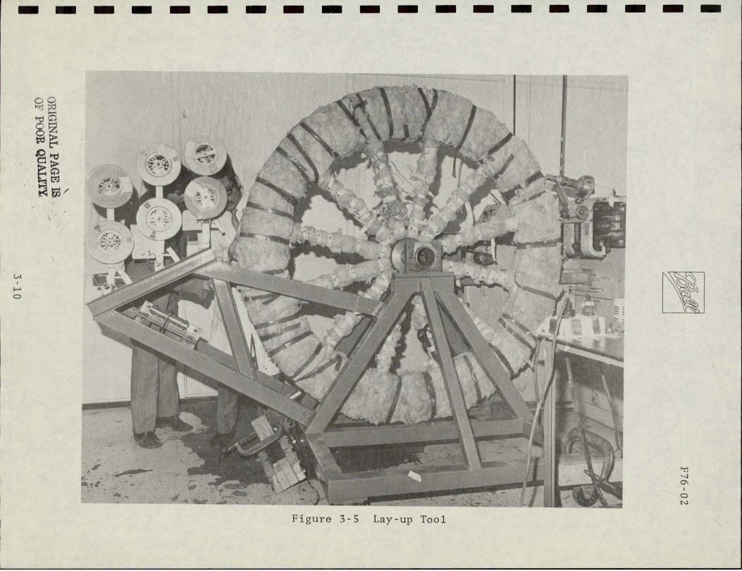
N
Figure 3-5 Lay-up Tool
IIP76-02
Rim Machining OperationsFigure 3-6
3-11
MIE II
Iiue37Diln emnn antHlsi h i
3I1
DF76-02
LOCATION MAGNITUDESTRESS (PSI)COMPONENT
Radial or carbonepoxy +460 (max) -891 (min)X stress
Axial or carbonepoxy +491 (max) -433 (min)Y stress
Shear or carbonepoxy +390 (max) XY stress -176 (min)
Hoop or carbonepoxy +55434 (max) 0 (min)Z stress
Radial inner surface +01166 (max)
Displacement outer surface -01130 (min)
(inches)
Table 3-2
MAXIMUM VALUES OF STRESSDISPLACEMENT AT 1200 FTSEC RIM SPEED
3-13
5ThF-=- V- LERATfNz- 1 4U0T00
RMCO RRLYSES BRISTOL REROSPRCE LTO OCT 73
HOOPSTRESS RNSYS 5
or Hoop Stress Contour PlotFigure 3-8 Z
F76-02
- flax h st-ess= 55434-
I I-1 I Ii-- shy
60Iz-
===z_ +0 _----- --- shyi -_-O- - = -- = +----- shy+ ---= -- r E
_-------=--- --- = ---
-- ----- +- - --- -- =--- -=
=
------ shy
=T--- 7
--
-
- -_ - - - -- - -- a
a zrlt- --r-- -r - z I=tzz-z - -
- 4
o6 Zf - =4-=-t vi I_- --- zmE+s=$ Z 4-| b- =---+----- shy
+ 5-t 4 -- c Tt - 22 ~++ _------ _ __ _C - u
a zjztL- +lt+ z- I [Lt- -- Tit--
-- -+v + --F t+-- -+rr 7- h |f
0 200 -00 6800 1000 12oo
Rim SPEED (rri5Ecc~
Figure 3-9 Hoop Stress and Growth With Speed
3-15
F76-02
e 4fo
1 1 I 1 t i I I CII1I1_4I I
Itdn-branveqs sts OI - I M
---shy-- -- -- - -
t~z 2 - 1- shy
- 421 ~T2 2 -=_-- -_E---i ----
t -- EM
___ _ ZZ +-_ _-A~~ - rrrr-
TLLto LLbi i L -- k - r K -1-
irtv li V i 1 -- t 4 s-- n-L -- T4 E
000-q0o 600 800 100 A120 Rim Sp Dr (FTVEC )
Figure 3-102 Transverse Stress Components With Speed
3-16
DF7602
Figure 3-8 shows the computer-drawn plot of constant hoop tensile
stress contours the maximum being 38252 Ncm 2 (55438 PSI)
occurring at the top and bottom inside corner
Figure 3-9shows the relationship of radial growth and hoop stress
as a function of rim tip speed
Figure 3-10 shows the relationship of transverse stress components
with speed
Since the material void free is capable of withstanding 110400 2 2Ncm (160000 PSI) in tension and 8280 Ncm (12000 PSI) in shear
the safety factor is 28 minimum On a sample basis the void
fraction was determined to be less than 04 percent
32 Back-Up Air Bearing System
The design of the back-up air bearing system was completed and
analyzed by Shaker Research Corporation Ballston Lake New York
The back-up air bearing (BUB) system consists of six hydro-static
radial pads and twelve hydrodynamic axial pads These are arranged
in six BUB sets consisting of two axial (one upper and one lower)
and one radial pad and located at either end of a magnetic supshy
port station Each BUB set is approximately 60 degrees from the
adjacent set The bearings are deployed toward the rim by air
pressure when predetermined rim displacement limits are exceeded
The introduction of air through the pads as well as through a
pneumatically operated valve in the vacuum enclosure provides
the fluid for the BUB system and also introduces air drag for a
fastercoast-down Hydrostatic bearings were selected for
radial use instead of hydrodynamic types because the rather small
rim depth (115 inches) allows insufficient area to produce the
required reaction forces The back-up bearing system is shown
in Figures3-11 and 3-12
3-17
P76-02
~14
-L- 7
FiguTre 3-1 AMCD Back-Up Bearing Layout DrawingI 3-la
Figure 12 Back-Up Bearing System
7F76-02
321 Hydrostatic Radial Bearings
The movable radial pads are designed to minimize air flow and
maximize air bearing rim reaction forces The radial pads proshy
vide a centering effect on the rim to minimize dynamic and magshy
netic unbalance forces
In the normal magnetic suspension mode the radial pads are held
away from the rim-and against stops by a set of nested compression
springs (total of 22 N (50 pounds) of preload) When the radial
system Figure 3-11 is activated 207 Ncm2 (300 psig) air is introshy
duced to the pad piston cylinder which moves the pad outward
toward the rim The piston chamber is ported to the pad surface
through a 0033 cm (0012 to 0014 inch) diameter orifice A
sealed oil-filled dashpot between the piston and pad controls the
deployment velocity
Figure 3-13 shows the relationship between- radial pad force and
gas flow versus film thickness for various orifice 4iameters
Because of limited gas available-the smaller orifice diameters
were selected
Since the rim is not at constant radius (because of radial growths)
film thickness and flow vary With rim speed Figure 3-14 shows
the relationship fo film thickness and flow versus rim speed
322 Hydrodynamic Axial Bearings
Movable- tilt type axial hydrodynamic pads were used since the
rim radial width is large and because of the limited bearing air
supply The axial pads are slightly crowned and combined with
the tilt feature are self aligning
3-20
F76-02
1 ~
It
7
I
JII ji
I L
II
---
Ft
T -
VIN I -_ Lr
TD _-
I
I+i
- 1MNV I
4~~r14 +t
Fit~Fi-~tdi I~ ~ JrV)
i ir
il-I= iH14+
i T r
F~m
shy
_ _
I L [
- i
I
_ i _
Ii
0001M -s as
Figure 3-13 Single Pad Force and Flow
3-21
A yyF76-02
WI
ii24pVshy-~~~~W
J4 i3 - Lit
I+ I~Ir~r L-- u 7t J
L 4- 1-nMLfI0__ 4~~~~- F-14--gtrF
I -- -r
4 ~ P I-
IaiH __M
1 --- t Th T1T
I- Vt prI i A
-p--t~LIV[~ VK jl77L1 1
Figure 3-14 Radial Air Pad Flow and Film Thickness With Rim Centered
3-22
F76-02
In the normal magnetic suspension mode the axial pads are held
against stops by a flexural spring The axial system is deployed
in-much the same manner as the radial system When a magnetic
suspension anomaly is detected the vacuum enclosure is flooded
with external air thus providing the film for the axial bearings
Figure 3-15 shows the relationship of film thickness with rim
speed Since the film will support the rim to about 15 radians
per second the pads are designed to accept several contacts before
replacement is necessary
323 Back-Up Bearing Pads
The primary objective in designing the pad material was to proshy
vide a material which would wear smoothly without damage to the
rim or to the pad itself Sacrificial bearing materials have
been used in gas bearings in the past which exhibit the necessary
qualitites The material used in the back-up bearings is an epoxy
resin heavily filled with aluminum powder aluminum oxide power
and molybdenum disulphide powder The mixture is poured into
silicone rubber molds degassed in a vacuum chamber then heatshy
cured The pads are then machined
When the spinning rim contacts the pads the pad will wear smoothly
and rapidly acquiring a high polish and yielding a fine dust
The rim surface should be undamaged by the contact The aluminum
filler provides high thermal conductivity to sink the heat generated
by the rim contact The aluminum oxide provides dimensional
stability so thQ pad will withstand the thermal shock generated
by the rim contact
3-23
3788I9 2 4 5 7 8 9 2
1 7 _- I
111-1 r - J
-I- --i- 1 rV1- 1 t r V
4 _ - _ _____ shy- I---7
I
r-- _- F-_- --- I ii -
I fr r l 7[-II j7shyLi +] - i I-- I
1 7 8
-- - 4 5---- 10 47 MCI 9
Figure 3-15 Axial Pad Film Thickness Versus Speed
F76-02
40 SUSPENSIONSYSTEM
41 System Description
The suspension system consists of three suspension stations
placed symmetrically about the rim At each suspension station
the rim can be pulled in either axial direction or tadially
inward by magnets A total of 12 magnets are arranged in sets
of four each to pull in these three directions (up down and
inward) The eight axial magnets are driven in concert by one
set of electronics Axial error signals are developed by a
position sensor located at the center of each station The
axial servo loops in each of the three stations are independent
of each other The four radial magnets in each station are also
driven by a set of electronics in response to a radial position
sensor located in the center of that station But the radial
station to another so asservos are interconnected from one
to prevent the servos fighting one another even in the presence
of rim radial growth
411 Magnet Description
One of the unique features of the AMCD is the support magnet
design The electromagnets are flux-biased by thin wafers of
samarium cobalt permanent magnet material placed in series in
the magnetic circuit This has the advantage of (1) providing
a high force per unit current sensitivity at zero current (2)
providing a linear relationship between force and current and -
(3) providing the static field required for zero power operation
The support magnet geometry is seen in Figure 4-1 The permanent
magnet biasing is achieved by slanted wafers of samarium cobalt
in the legs The wafers are as thin and wide as possible to
4-1
SAti 4-IUr CCBA3L~rshy
AGtJer-
AGII1
Figure 4-1 Support Magnet Geometry
RF76-02
minimize their reluctance in the magnetic-circuit The volume
of permanent magnet material is sufficient however to provide
adequate flux-biasing and static lift The reluctance of the
permanent magnets is large but does not more than double the
total reluctance since the air gap inthis system is large In
many other magnet suspension systems the gaps are small (about
01 mm) and this sort of series flux biasing would greatly inshy
crease the total reluctance in the circuit Control power would
thus be large and the systems would be impractical
The effect of flux-biasing on the force versus current characshy
teristics of the magnets is shown in Figure 4-2 With no biasing
current in either direction produces force of the same sign with
poor gain and low efficiency in the vicinity of zero current
Force is simply a function of the square of the current With
biasing the slope of force versus current is greatly increased
at zero current In the AMCD top and bottom magnets operate
together in a push-pull type of operation The coils are in
series hence both coils have zero current at the same time
The resultant force-current relationship is linear and has a
slope double that of either magnet alone
Figure 4-3 shows the U core of the magnet with the permanent
magnets in place Permanent magnet thickness is 1 mm (0040
inches) Also shown in Figure-4-3 is a fully assembled magnet
ready for potting After potting the units measure 43 cm x
167 cm x 25 cm (17 in x 42 in x 99 in) and weigh 500 grams
(11 lbs)
412 Position Sensors
The position sensors used in both the axial and radial suspension
systems are Multi-vit sensors manufactured by Kaman Sciences
4-3
7 gF76-02
-r
UPPETP HA -
C AOc~~
777
~~oeehAcn-e-r Z
Figure 4-2 Flux-Biased Magnets in Push-Pull Operation
4-4
rF76-02
I
3 i
A A
I tii A LWUv
NN
N~ i X -9
i i UI A i
IN aWIi ii i
iiiiiiiliiili
i~iiii Ii iliiiiiiiliiilii
Iilliii iiiiiliiiiiiliiiii = iiiiiiaii~iii iiiiiiiiiliiiiiiii
Uiiiii poundii=iiiii]iipoundiiiiiiiiiiiiiiiii Uigure 4-3 Support Magnet Cosri on
iliiiiur -3 ConstructiiiiIliiiiiiiiioniiiiiiiliiiSppriMge liiiiiii i iiiiliiiii3 URiliI 4-s == =
4-s
rF76-02
Corporation These are conventionally called eddy current senshy
sors although they are actually sensitive to anything that changes
the inductance of the test coil in the probe Hence either
eddy currents in a conductor or the permeability of a magnetic
material can be sensed In the AMCD the sensors look at the
ferrite bands and therefore are operating entirely ina non-eddyshy
current magnetic permeability mode Special calibration of the
sensors was required in order to operate in this mode Linear
range of the AMCD sensors is 025 cm (01 inches) and scale facshy
tor was set at 4 voltscm (10 voltsin)
413 Control System
The axial suspension system uses three independent servo loops
to control electromagnet currents An electronic diagram of one
of these loops is shown in Figure 4-4 The heart of the elecshy
tronics is an Inland Controls MA-I DC servo amplifier which is
operated as a current driver to reduce the effects of electroshy
magnet inductance Equations of motion of this driver and an
analysis of the voltage feedback used to damp high frequency
roots are given in Appendix A An analytical block diagram of
the entire servo loop is shown in Figure 4-5 Equivalent points
on the electronic and analytical diagrams are indicated by letters
within hexagons
The axial suspension system has two modes of operation a posishy
tion mode and a virtually zero power (VZP) mode In the posishy
tion mode rim position error is used to command electromagnet
current The rim has high static and dynamic stiffness about
any desired point in the gap In the VZP mode the rim position
set point is modified by positive feedback of the integral of
electromagnet current The result is that the set point is moved
until steady-state current is zero The permanent magnets are
4-6
AA
REHTUtk +26V
4-
C11 7t-Q
Fiue44Aia3upnin7lcrnc
S Cornn- EesoCo p n a cncivCrrent Driver- O deg OI 99 (5C + sm -3 (s + 1 1deg E 1 copy + F
gtosO ~
volf
iE 3 7 T r i m T ntegratadegr
Suspended
Mass
-|ectro
-ria net
16
permanent Magnet
Figure 4-5 AMCD Axial Suspension Station
R 1F76-02
then providing all of the support of the rim Dynamic stiffness
is nearly the same as in the position mode but static stiffness
is actual negative If a downward force is applied to the rim
in the VZP mode it initially moves downward but then slowly
rises to assume a new zero power position above the old equilibrium
position
The electronic circuit diagram for a radial servo station is
shown in Figure 4-6 and the corresponding highly coupled analytishy
cal block diagram is shown in Figure 4-7 Again equivalent
points on the two diagrams are indicated by letters in hexagons
The large amount of coupling results from three servos controlshy
ling only two degrees of freedom
Two modes of operation are available a position mode and a WAHOO
mode The position mode is similar to the axial position mode
The WAHOO mode is a zero power mode that produces zero power
operation in the presence of both static loads and rim expansion
This is accomplished by adjusting the position set point at each
station as a function of the integral of the sum of the electroshy
magnet currents at the other two stations
The name WAHOOis derived from the poker game WAHOO This game
is played in a manner such that each player knows what every
other player holds but does not know what he himself holds
Inspection of the WAHOO trim loops of Figure 4-7 reveals that
for VZP trim purposes each servo only looks at what the other
two are doing This innovation was developed by BBRC to meet
the unique requirements of the AMCD
The derivation of the WAHOO concept is given in Appendix B
There it is shown that only the WAHOO concept produces zero
power operaion for both rim expansion and force disturbances
4-9
A00l 51 Ir
A-A-
F
27
ffzo xr
74 VIP KIAk
7
Ems~
n
A7-
I
A1
ter
a 2k-
-
-
-
-
-
I)
Figure 4-6 Radial Suspension Electronics
-KS
Iamp wkin47s Permanent MagnetVeloityPM VPol Aplifir PMEHM E Iectremoqnet
K5 Kmn eae t~j VOS 0bCar respond to Lettered
1vII~rb r - rr m Psitionson Cgrcwit
vol vol Im PosiMoon Pox
SlRtim rtOhkx _Q$)bsS 4lfe I
0niplPfied Cus ren Driver
Gcucv rbinn n i
+ + vt
If
in-7d FigureservoD RailSro
+i
42
F76-02
Appendix B also shows that for single station design purposes
a single station can be represented as shown in Figure 4-8 Two
points of interest are immediately evident The equivalent mass
for a single station representation is 23 the total rim mass The WAHOO concept which involves negative feedback to each station
from the sum of the other two stations resolves to a positive
feedback in the single station representation exactly like VZP
in the axial mode This representation can be used for designing
the system characteristic root locations If the characteristic
roots from the single station representation are given by A and
the WAHOO gain is Kc it is shown in Appendix B that the three
station highly coupled set of characteristic r6ots are givenby
(S + 2K )A2
Performance
421 Static Performance
At each suspension station the rim will seek an axial equilibrium
position based on the applied load and the control system mode
(position or VZP) These equilibrium positions can be preshy
sented in one plot as shown in Figure 4-9 The VZP line is a zero current line and has a slope that indicates static instability
however as shown in the next section the system can operate in a
stable manner along this line The most usual operating position
mode point is about 001 cm (025 inches) above the center of the
gap At this point the slope P of the VZP line is about 595
newtonscm (340 lbin)
In the position mode an operating line exists for each set point
of the position sensor A family of these is shown in Figure 4-9
The lines are finite in length because of the limited current drive
capability of the electronics The slopes of the lines are apshyproximately 2600 newtonscm (1500 lbin)
4-12
Stationfost ionsingle
Oecrlx- EquIva1eratArmplifir Current Driver 6 Mks$M9oqmet+ 1m
~~~~~ eroe L~r
Is + Fes I16(7+1210 r0 0 l I-
p 0 1
476 An- Per
u2 IVlt+ -Eg
o tKate - r1 1 StO Sr eq uci o lnk wahoo is
Q Correspornas toa letterd posit~ions on circuit chogr~m
Sinql~e stcton eqviclvJewtmls is 23 totil ma
~odelldas a posattve PeedbctK self IoopVe
t to o-t liKe Vf Pwould ltherefboretxpect fvrthernortn itthe Aol O Servo Xt doesonh
Figure 4-8t EqiaetSnluadapev tto
ekgeto8 rnex e o +non
A F76-02
UP
MAGNET M~A t r
lsrok os NoRMAL
kE-RITI N
P E-Nshy-OMFR
tL UPshy
- j ~
-10
h31G1NL pAGE iS
)F POOR QUML-rI
Typical Static Suspension System Performance
Figure 4-9 4-14
rF76-02
The force sensitivity F of each station is about 138 newtons
ampere (31 lbamp) Hence the force produced by a station
is given by (in English units)
F = 340X + 3lI
422 Dynamic Performance
The analytical block diagram for an axial suspension statiQn is
shown in Figure 4-5 For theposition mode the root locus and
-Bode plots are shown respectively in Figures 4-l0and 4-11 The
root locus plot shows that the dominant pole pair has an undamped
natural frequency mN (which we define as bandwidth) of 171 radsec
(272 hertz) and a damping ratio of28 The Bode plot shows
that the gain crossover frequency wc (which some define as bandshy
width) is 1827 radsec (290 hertz)-and that the system phase
margin is 2320 Both plots show that the lower gain margin
is 22(-131 db) and that the upper gain margin is 201 (261 db)
For the VZP mode the root locus and Bode plots are shown respecshy
tively in Figures 4-12 and 4-13 The root locus plot shows that
the dominant pole pair has the same undamped natural frequency
and damping ratio as the position mode that is wN = 171 radsec
= 28 The Bode plot shows that two gain crossover frequencies
at 1823 radsecexist one at0838 radsec (013 hertz) and one
(2903 hertz) The phase margin at the lower crossover frequency
is -772 and that at the upper crossover frequency is 2300
Both plots show that the lower gain margin is 226 (-129 db)
and that the upper gain margin is 2011 (261- db)
The response due to the step application of a one pound weight
is shown for the position mode in Figure 4-14 and for the VZP
4-15
OF76-02
1 -DD
-- A I 1
I I
i
3000 --------------------------------- ___tN
-5000 -400 -30U -2ODG -t I lo oD
REAL AXIS
Figure 4-10(A) Root Locus Plot - Nonideal Current Driver With
Voltage Feedback
4-16
---------------------------------
7F76-02
-I- 111 1-l Z9D
io oI 1ll t A
G
80 ----------- 0 aEu----------------shy-4--
FigueRot41001LcusPlo - Nnidal Crret DrverWit
-1---4-17
I I
F76-020
14-HLowler
)2 I__ _ p
1 N I-- A =20 41 r
I tIse0_ __ _ _ 4 6 2 4 68100
s 10 log H00 6 10009 FREQUENCY (RADIAWS$ECOND)
Figure 4-11 Bode Plot - Nonideal Current-Driver With Voltage Feedback
4-18
7F76-02
$oo I5iI000 I1
T 1 Ii
-A
S4+
N A
4000 R--- - - - - -
V A x
103 000 40 30 29
urn rvrWtFi1r -12A Roo Lou7lt-Nnda
Voltage Feedback 4-19
V gF76-02
ii
- I I I
I I I II
I lii
-I I
II I iishy
II - - -i-l
Fgr 4-2B o otocu PltrNndaCrefl rive
With Voltage Feedback
4-20
F76-02
I i E
A -4 G
E- 60I jUroI(
I
1A2zS1 me RI
3s F-1-L
IIsoM 3en
4) e r
-120---- -Marlin
fla e =2300
-140 shy
1 1 10 10g 2000 1090r FREQUENCY (RADIANSECOND)
Figure 4-13 Bode Plot - Nonideal Current Driver With
Voltage Feedback
4-21
012
F76-02
00010
00008
pound E
0
p
0 00
0zkc0
0
E
- -
4+-F
- - -
Nshy- - - - - - -
4
- -
5
-4-2
AF7602
mode in Figure 4-15 The response for the position mode settles
out at 6941E-5 feet (002 cm) This yields a position mode
stiffness of Stiffness 6 1 lb
6941E_5 t X feet
1 12006 lb (21021-
N
69Th-ft Tni in cm
The response for the VZP mode settles out at -2451E-4 feet
Thisyields a VZP mode stiffness of
1 lb feet = lb NStiffness = 2451E4 ft X 12 in -3400 i (595 E-
Note that the stiffness in the VZP mode is just that of the
permanent magnet and that the movement in this mode is toward
the applied force That is if a weight is placed on the rim
in the VZP mode the rim will move up
Further insight into the system can be found by examining Ap2
pendix C When using current driirers the usual tendency is to
ignore the high frequencydynamics and simply say that the
output current is the input voltage times a constant This can
be very misleading in the case of AMCD- In Appendix C are shown
root locus plots using both an ideal current driver arid a nonshy
ideal current driver without voltage feedback It shows that
voltage feedback is necessary for the axial suspension Also
shown in Appendix C are Nyquist plots and phase-gain root locus
plots of the nominal axial systemthat is the system using curshy
rent drivers with voltage feedback The esoteric phase-gain root
locus plot shows on one plot the sensitivity of the system roots
to change in both gain and phase For example it shows what
would happen if an additional 300 of phase lag were added to the
system from some unknown source
4-23
F76-02
0001
I f
I 0 e
eshy
0a T 1-0001-shy0N
ft E F 0
E a
- 002--------------shy
0 t0 20
TINE (SECONDS]
30 40 50
Figure 4-15 Nonideal Current Driver With Voltage Feedback
4-24
F76-02
The equivalent single station radial analytic block diagram is
shown in Figure 4-8 It is very similar to an axial station
The root locus and Bode plots for the position mode are shown
respectively in Figures 4-16 and 4-17 The root locus plot shows
that the dominant pole pair has an undamped natural frequency
(bandwidth) wN of 653 radsec (104 hertz) and damping ratio C
of 18 The Bode plot shows that the gain crossover frequency
is 666 radsec (106 hertz) and that the phase margin is 1350
Both plots show that the lower gain margin is 329 (-965 db)
and that the upper gain margin is 7054 (3697 db)
The root locus and Bode plots for the WAHOO mode is shown in
Figures 4-18 and 4-19 The root locus shows that the dominant
pole pair has an undamped natural frequency of 674 radsec
(107 hertz) and damping ratio of 16 The Bode plot shows that
the upper gain crossover frequency is 691 radsec (110 hertz)
At this frequency the phase margin is 1260 Not shown is the
fact that the system also has a lower gain crossover frequency
of 594 radsec (095 hertz) At this frequency the phase marshy
gin is -715 Both plots show that the lower gain margin is
389 (-821 db) and that the upper gain margin is 6701 (365 db)
The large upper gain margins for both the position and the VZP
modes indicate that current driver voltage feedback is not needed
Considerable rim bending instabilities were encountered during
the design Early in the development the axial system was
designed to be overdamped This caused a bending mode to be
driven unstable The compensation was adjusted experimentally
until the bending became stable Unfortunately this reduced
the lead in the system resulting in the present underdamped sysshy
tem It is believed that bending will present no problem at
high spin rates because of the effective stiffening of the rim
4-25
6F76-02
_____ - _ r ____I___
141
IT___lishy
1 ii
1 F]
eir
t lj~
4-
J TT a p-
III NEA
fiIT WBKsITlK j1_11IIi I-
I
e
-Fshy
Y]-111 ji
1i1fln 4--I r
I i--I -
TFiJ-WL 1
_1(-Ii4 - I
I~ ~ ~iA_~2I ___ ii- 11 IFt-Ih
iT
h~ -iH T
+~ji+ih Iplusmn
_ _ _+ I kt ~h-II
+ LILY -
7 SO bullj
Figure 4-16 AMCD Radial Suspension Equivalent Single Station Position Mode
4-26
Elll csl- tLL[ 11--- 1_ il
V
1 MIN
2 0 H qL2~14-0IT
I M Ill 1OIHI
+-o ip Lr g
Ti I -0 1- b1 -- i
Ij _IUSi 1PIN - il
--i
41i L -I I - d jir ~J I I
00 -o
ro-d 5 c
Figure 4-17 ANCD Radial Suspension Equivalent Single Station o Position Mode
7F76-02
1LjI_----- Li -III iI - - I -shy-F ]e2 1
Is- Lr [_I
r ir -L-j 11I IALI _ _ _ ___ 2_
E11LLN1LALIF TYC -- td It 11
- KI
S1 1 1 1--shy
II
I r 11
FLL-1
U - I 4
E~~~~fL
__
f Lplusmn Xi ILIi _ _
- ii _ _ i
- H --
--------
A-1 1 F - JT-1
-- t-ti -~r -r I- t - --- IL I
IIJlri-tlrht1f tI
_+ _ l PillS 1 I
Figure 4-18 AMCD Radial Suspension Equivalent Single Station
o Wahoo Mode
4-29
rm~r 1 u i rrrrF r r r
4
130
o
I -4
7 7 1-shy iAb d
llt h
-30 Tfij4i i ~
- n0 t
Figure 4-19
01 AII-
I uji r a sec
AMCD Radial Suspension Equivalent Single Station o Wahoo Mode
AF76-02
and the averaging effect on modal pick-up caused by the bending
modes moving rapidly past each position sensor
As the rim is spun up the three axial stations become more and
more coupled by nutational effects The result of the coupling
is to reduce the dominant roots damping ratios more-and more to
the point the system could go unstable if the rim is spun fast
enough It is believed that this tendency could be greatly
reduced or possibly eliminated by the proper combination of cross
feeds from one axial suspension station to the others
4-30shy
DF76-02
50 DRIVE SYSTEM
51 System Description
The AMCD drive motor can be thought of as a large permanent magshy
net brushless dc torque motor Samarium cobalt magnets are
bonded into the rim at regular intervals The two phase armashy
ture is segmented with a winding set at each of the three susshy
pension stations Commutation is controlled by Hall effect senshy
sors mounted near the rim which sense position of the samarium
cobalt motor magnets
52 Magnet Selection
Alnico was considered along with samarium cobalt for the permanent
The large air gap and segmented winding structure meanmagnets
the magnets will become nearly air stabilized The rim was designed
with a small outer lip to hold the magnets This was done to
isolate the drive from the suspension as much as possible without
and complexity to the rim than necessary Thisadding more mass
small lip implies a short magnet Samarium cobalt has high
strength for short lengths and does not pay a penalty for air
In fact it is very difficult to demagnetize thisstabilization
material
cm (55 inches) diametertby 64 cmSamarium cobalt magnets 14
(25 inches) length were selected and bonded into the rim with
polarities alternated
The rim contains a total of 72 magnets spaced 73 cm (288 inches)
apart
5-1
53
--F76-02
Core and Winding Design
Each armature segment consists of a pair of bar-shaped winding
assemblies one above and one below the rim
Sit cos sla 0S SMa
cores in a singleThe windings-are wound toroidally around the
layer The figure above shows only the cross-section 6f conshy
ductors in the air gap as the conductors passing around the other
side of the core add nothing to torque and serve only a connectshy
ing purpose The bar-shaped cores are easy to wind and result
in a compact structure The single layer of 18 conductors adds
very littleto the overall air gap This effective electroshy
magnet design was suggested by P A Studer of Goddard Space
Flight Center
Ferrite material was chosen for the core to reduce losses Fershy
rite also is easily machined into the required irregular shapes
The windings are grouped into two phases SINE and COSINE each
of which acts upon three magnets at each motor segment In operashy
tion current in one phase is acting on the magnets while current
in the other phase is reversing in preparation for a magnet of
opposite polarity
5-2
DP76-02
54 Motor Commutation
Hall sensors act as commutation devices for the motor They sense the position of the permanent magnets in the rim and cause the drive coil currents to be switched according to magnet position
The sensors are mounted in pairs one above the rim and one below for each winding phase Outputs from each pair are summed so that the switching position is not affected if the rim moves up or down within the air gap The SIN pair controls current on the SIN windings of all three motor segments and likewise the COS pair
of Hall sensors controls all COS windings
55 Motor Control Electronics
A block diagram of the motor control electronics is shown in Figure 5-1 For each phase the Hall sensor outputs are summed and amplified to drive-threshold detectors These detectors sense magshynet position and polarity The phase control logic determines the
timing and polarity of the motor coil drivers Interconnections between the two phase control logic blqcks provide positive direcshytion and start-up information
Each of the six coil drivers controls a phase at one of the motor
segments Associated with each driver is a coil current sensor which monitors the current in that winding All six of these
current sensorsreceige a common reference from the speed control
potentiometer When current in that particular winding reaches the reference level the driver turns off until the current deshy
creases This prevents the current from reaching destructive levels at low speeds and acts as a speed control at high rim
speeds
Since the coil drivers are either full on or off a very efficient drive is achieved At low rim speeds the drivers operate as a
5-3
56
F76-02
conventional PWM (pulse width modulated) amplifier A quite faithful square wave current of controlled amplitude is fed to the coils At high speeds high acceleration (or deceleration)
is possible with the drivers full on for the period between magshynets with current rise and fall limited by the inductance of the
coils
Torque Calculations
The equation for the force betweena magnetic field and a current
carrying conductor-is
F = BLI
where
F = Force in Newtons B = Flux Density in Teslas (WebersM~ter )
L = Conductor Length in Meters
I = Current in Amps
If the magnetic field is created by a permanent magnet the force
can be considered to act on the magnet if the conductof is held
stationary which is the case with the AMCD motor
To arrive at design force each of the factors B L and I must
be evaluated
A force calculation will be made for one magnet face interacting
witha coil This can be then doubled to account for both ends of the magnet next tripled to take into account the three magnets in one motor segment and tripled again to realize the total force for the three motor segments Then using the radius of the rim
we can calculate developed torque
5-4
F76-02
Flux Density Calculation (B)
The large air gap makes it difficult to- estimate how much of the
magnet flux will couple through the winding core and how much
will be lost to leakage A measurement of coupling flux was made
using a pair ofsoft iron bars similar to the ferrite corasi
SEJSE C0115
SOFr iROh
-4 Webers with magnets of averageThe flux measured was 0375-x 10
strength
core must-be convertedThis flux that couples through the ferrite
to flux density (B) in the air gap where it interacts with the
coil windings There are two practical Choices for doing this
We can assume all the flux goes straight up from the surface of
the magnet andreacts with only those turns above the magnet or
we can assume the flux spreads out evenly over the winding area
Of course the truth liesand-reacts with all the turns equally
an adequatesomewhere in between but the second approach gives
approximation
The winding area in the air gap for one magnet coil phase is 2
19 x 36 cm or 68 cm
Flux density then is
-44m _ 0375 x10 Webers 2 0055 WebM-B_=A = 4 2A - 68 x 0-4 m
5-5
F76-02
Conductor Length Calculation (L)
are 28 turns with an effectiveIn the winding phase area there
length of 19 cm each
Total effective length is then
L = -19 x 28 = 532 cm = 0532 M
Current (I)
that the coil drivers and wiringThe elbctronics are designed so
canhandle 4 amperes Also the inductance of the coils was
examined to be sure that currents of this magnitude can be
reversed at maximum rim speed frequencies with a 60 volt power
(and torque) will then be calculated for thesupply Force
design maximum of 4 amps
Force
We can now calculate force from the equation
F = BLI
= 0055 x 0532 x 4 = 0-1-17 Newtons
Recall that this is the force for a single magnet surface inter-
For the total motor this is multiplied by 18face
Total Force = 0117 x 18 = 176 Newtons
576
0F76-02
This times the magnet radius (0838 meters) gives total torque
Total Torque = 176 x 0838 = 176 Newton-Meters
(13 lb-ft)
A small (14 diameter) test wheel was built to check the above
torque calculations Acceleration measurements were made and
from the known wheel inertia torque was determined Correlation
within 10 of the calculated torque was achieved
5-7
S in Hall Sensors
Summing
Amp
[A Threshold Sin Phase Coto-rie
DetectorsLoi
SnB1Sin
Sin C Driver
ol
Hall Sensors
~ Amp=ApDtcosLogic
etctr Control -- Die Col Ci~
Summing Threshold Phase Cos B Driver
iCosCos
Ci Co
Figure 5-1 Motor Control Electronics
C
aF76-02
60 REFERENCES
1 Anderson Willard W and Groom Nelson J The Annular
Momentum Control Device (AMCD) and Potential Applications
NASA TN D-7866 1975
6-1
F76-02
APPENDIX A
CURRENT DRIVER EQUATIONS AND TRANSFER FUNCTIONS
A-i
F76-02
Appendix A
Current Driver Equations and Transfer Functions
When using current drivers the usual tendency is to ignore the
high frequency dynamics and simply say that the output current is
just the input voltage times a constant This was very misshy
leading in the case of MCD-as shown in Appendix C The circuit
diagram of a current driver with voltage feedback and its equishy
valent diagram are shown in Figure A-i -
v A T5It
Figure A-I Current Driver and Equivalent Circuit
A-2
F76-02
The beginning equations of motion are the following
Rl11 RM -- R 10
-RM SL + R2 2 -(SL + RC) I= A(TS+I)-)V + ARI(TS+l)shy
-R 2 -(SL +R c) SL + R3 3 + S_ C I 3 0
where
R1 lt= R1 + R2 + RM
2 RM + RC22
R33-- R2 + RF + RC
Transposing I1 to the left hand side we obtain
R11 -RM -R2
-RM(TS+l) + AR 1 (TS+l) (SL+R 2 2 ) -(TS+1) (SL+Rc) 2 A S-SR22 S L+SR33+-l
What we really want is the current through the inductanceshy
1 2 T3
Adding this equation to the system we obtain
C1 C12 C1 3 0 II 1
B2 1 S+C 2 1 A 2 2S2 +B 2 2 S+C 2 2 A23s2+B 2 C 3 0 12 A V
B31S A32S2+B32S A33S2+B 3 3S+C 3 3 0 13 0
- -1 1 1 1 0
A-3
eF76-02
where by definition
-=A32 -LC R11 B22 = L+TR 22
= - C22 R22 B32 = RCCl2 RM
C13 =-R 2 A23-= -TL A33 = L
= R33B21 = -RMT B23 = -L-TRC B3 3
C = ARI-RM C = -RC C =C -I
= -R2A22= TL B31
If the voltage feedback is removed these equations reduce very
simply to
-RMIRlI+R2+RM
+ AR1 (SL+R+RM)(TS+ 1j1 2 = AKRM(TS+I) We want thewhere 12 is the current-through the inductance
transfer function 12V First divide the secondequation through by
LT to obtain
-RMR I+R2 +RM
(R C+ PM j] IAL 1 V S+L-iIARI[ RM L (SplusmnT -1)+L -lT -1A
A-4
F76-02
Then by Cramers rule
2 CR1+R2+RM)AL -1T-+RML -1(S+T- 1 )_L-1T- 1 AR1
V7 -1 r- 1 2-1 - lshy(RI+RZ+RM)(S+T +L (RC+RM) -R ML l(S+TI)+L ITIARIRM
(R2+RM)AL -T - I(S+Tshy
-(R1+R 2+RMM)(S+T 1 )(S+L-1 RC)+L -RM(R1+R 2)(S+T-I)+L T ARIRM
Further manipulation yields
S+T-1 +(R 2 +RM)ARM T12 RML -
V - 2+RM) 1 L-+RR [2 wT-ARI-L 1RM(RI+R2 -
S+T )(3+L Rc) + RR+Tl+R---
Finally the desired current driver without voltage feedback
transfer function is given by
12 RML- S+T -1 +A(I+R2 RfIj
V (RLR-+RM) - -1 LRM(RI+R2 ) (ST 1 [7AR 1 RS5 + R2 +RMR R1 L Rk 2 )
A-5
76-0 2
For infinite amplifier open loop gain A = the transfer
function reduces to
2R Lim 12 = R1_ 2M
(l+R2RM- R2
R - RYR RR)r112RM for R2gtgtRM
-This is the transfer function which is used
I2 R2 12 R 2V RIRM
if the high frequency roots may be ignored
When the high frequency roots are not to be ignored and
if AR2R1 gtgtmax (RMRC-i)
and RMARlRjR2gtgt
RI+R 2 c
A-6
rF76-02
The transfer function simplifies to
S+T- AR 2RM1
12 RML-
V R1+R2 (S+T-)(S+L -Rc)+L- RM(S+T-AR1 R1 +R2)
RML-1 S+T-1AR2RM-
R1 R2 S2+ -1 -1 -1 T 1L-1RMARl - A
S +(T- +L -Rc+L RM) S+ R+R
T- +L- (RG+RM) TRLAR
2 (RI+R2)
The dc gain of this transfer function reduces to the same transshy
fer function used if the high frequency roots may be ignored
that is
2 R2 V RIRM
For the radial MA-lCurrent Driver
RI = 10K R 2 = 2711 KQ RM 10
RC = 30 Q2 L = 0128 h T - 30 A 50119
Then the radial current driver without voltage feedback has the
transfer function
12 _-00061463(S+40762E10)
V S+13609plusmnj30400 shy
A-7
F76-02
Forthe axial MA-I current driver
R=1 10K R2 = 7311K C 01 1f R11 = 17311E4
L =0064 f = 12M R = 14 R22 =15
A = 50119 RM = 1 T- = 30 R 33 I2073E6
Then
= C11 7 17311EA B2 2 = 564E-2 A 3 2 -0064
Cl2 = -- 22 = 15 B = -14
== = -7311E3 -21333E-4 A33 0064C13 A 23
B21 = -33333B-3 B2 5 -53067B-2 B 12073E6
C21 = 50119E8 C2 3 - 14 C3 = 1OE8
= A22 = 21333E-4 -B3 1 -7311E3
Without voltage feedback the axial current driver has the transshy
fer function
2 00090261(S+l0993B1)
V S+13219plusmnj36839shy
A-8
7F76-02
Note that without voltage feedback the damping ratio on both the
radial and axial current driver high frequency roots is less than
05 This appears to be all right for the radial servos but is
very bad for the axial servos as shown in Appendix C Consequently
-voltage feedback has not been employed for the radial servos
current drivers but has for the axial servos cur-rent drivers
The effects of this feedback has been determined numerically
Figure A-2(A) shows the effect of increasing RF the voltage
feedback resistor from zero to infinity with the feedback capashy
citor C held a-t 01 lif Ifonly the capacitor is used for voltage
feedback the current driver roots are still lightly damped but
at a much lower frequency As the resistance is increased the
roots increase in damping become real then decrease in damping
at a high frequency finally moving to the no voltage feedback
position for RF = Figure A-2(B) shows the effect of increasing
the voltage feedback capacitor C from zero to infinity while
holding the feedbackresistor at one megohm For C 0 the roots
start at the no voltage feedback position As C is increased the
roots decrease in frequency and-increase in damping ratio until
C = 00091 f Further increases result in decreased damping
ratio and increased frequency At the chosen voltage feedback
values of C = 01 vf RF = 10 MQ2 the axial current driver transshy
fer function is
I 0008994(S+833)(S+l099EII) V (S+786)(S+2771plusmnj2583)
A-9
~~~ L~Trrrl~I I~ I II 4
Jots_1 nr_- r177I 7F I i0K IIII __ riiTTh
17shy
tkP M T7r
Hl4plusmn ------ IIr-1-----~ -- - I -
CDl7E-~ ttbifil
LA14 -T-- 4+ -
C T -I I
H -rTH V i H
-HE I
Figure A-2 Effect of Voltage Feedback on AMCD Axial Current Drivershy
AF76-of -
APPENDIX B
THE WAHOO CONCEPT
B-I
7F76-02
Appendix B
The WAHOO Concept
Introduction
Two conditions may occur which cause the radial electromagnets
to draw more current than necessary First if the rim is tipped
This forcea gravitational force tends to pull the rim sideways
at the expense of causing the electro-shyis countered by the servos
magnets to draw more current Second as the rim spins up
centrifugal forces-cause it to expand To each radial sensor
as rim movement to be countered by thethis expansion is viewed
to try to pullservos So each electromagnet draws more current
are directed inward andthe rim inward But since the forces all
spaced 120 a-round the rim the resultant of the forces is zero
so the rim does not move The net result of the expansion then
is thatonly the current in the electromagnets increases Trim
loops are developed in this appendix which lead to VZP (Virtually
Zero Power) operation for the radial servos when either the rim
is tipped or expands or both The system employing these trim
loops is called the WAHOO system
Because the three radial servos are controlling only two degrees
of freedom the radial servo system is very highly coupled This
very high degree of coupling makes it difficult to design each
servo as a single uncoupled system Hence in this appendix we
also develop equations to show how the three-servo radial system
may be designed using a single station servo radial equivalent
Development of the WAHOO Concept
The AMCD rim is suspended radially by three servos pulling on
it from the inside much like shown in Figure B-1
B-2
F76-02
Kim
Figure B-i Radial Servo Sign Convention
The sensor outputs are denoted by X1 X2 and X3 As the rim
spins up it expands by the amount X0 The sign convention is
chosen such that positive forces and displacements are outwards
The equations of motion of the rim are
(F2 - F3 )Co = My
(F2 + F3)s8 -F1 = my
X2 = XCe + YSe
X3 = -XCe + YSO
XI = -Y (B-i)
B-3
F76102
The force acting at each station is composed of a permanent
magnet force and an electromagnet force That is
Fl = P(XI+X0) + E D1
= P(X2+X0 ) + E D2 (B-2)F2
F3 = P(X3+X0 ) + E D3
these equations are-combined with the servo equations in Figure
B-2
From the block diagram the quations of motion using five variables
are
V1 = Kp(-Y+X0 ) -S)(KsVi+KcV 2+KcV 3) EKRN_1
Y = M--p(-Y+X0)+DR (-Y+X 0)+ EV1 +pSC(YSe+XCplusmnX0 )
EKRN -fD se(YSe+XCe+Xo)- ESeV 2 + PSO(YSe-XCe+X0 )
EKRNK sOCYSe-xce-Xo)- nsev 3 + FY
-V2 = K (YSO+XCeplusmnXo)-(lSKsV2+KcVI+KcV3)
EKRN = 1=M PcO(YSe+XCe+X 0 )- D C(YS+XCc+X0)- ECOV 2
EKRN -PCO(YSe-XCO+X 0 )+ ce(YSe-XCe+X0 )+ ECOV3
)V3 = K(YSe-XCO+X0 )-(SJ(KsV 3+KcVI+KcV2 (B-3)
B-4
+ SFt
+- K + X0
+ T- SID
fRi
Figure B-2 MICfl Radial Servos With Trim Loops
7F76-02
Rearranging
(S+Ks)VI+KpSY+KcV 2+KcV 3 = KPSX0
-M-1DEv+[DS2 -DM-Ip(1+2SD)+M-EKRN(1+2S2 0)]y
+M-IDESOV2 +M-1 DESOV 3 = [M-IDP(-1+2S)+MWIEKRN(I-2SO]XO+MDFy
KcV -KpSSY+(S+Ks)V2 -KpCeSX+KcV3 = KpSX0
M- 1DECOV 2 +[DS 2DM- P(2c0 )+M-1EKRN(2C2 )]X-M-IDECOV 3 = 0
KcVI-KpSSY+KcV 2+KpCeSX+(S+Ks)V 3 KPSX0- (B-4)
Since 0 = 30
I+zs2 -1+2(5)2 = 15
-- 1+2S = -1+2(5) 0
2C = 2 )2 = 15 (B-S)
Using these simplificatfons the Laplace transformed radial
servo equations of motion in matrix form are
(S+Ks KpS 0 KC KpS 0DSL KC V1
-1IDE +lSMIEKRN SM- 1flE 0 SM- DE Y 0 M D
-1$M IDP __ __
KC 5KpS (SK S ) SrI KpS X6 V2 KK SX 0 + 0 Fy
DSz--shy
SM- 1 DE - SMDE0 0_- 54M +lSM 1 EKjN x 0I 0
-5KpS K 54 KPS (S+Ks) KpS 0KC V3
B-6 (B-6)
F76-02
The system characteristic equation is the determinant of the
coefficient matrix With much algebraic effort it can be
reduced to
A = (S+Ks+2Kc)X
FKRN-ISM- DP)+lSKpM- DES]2[(S+KsKc)(DS2 +SM-
(B-7)
Now lets simplify the expression by-removing the high frequency
roots In the Cambion hardware
KRN 107 S for low frequencies
D (S+1000)(S+10000)
With this approximation KR = D = and N = S Then
2+lM ES-lM P)+lSKpM-1ES] 2A = (S+Ks+2KC)[S+Ks-KC)(S
So the roots separate into -(Ks+2Kc) and two identical sets
within the brackets Immediately we see that Ks+2KC 2 0 for
stability Now looking within the brackets we see that S2+
1SM-ES-l5M-P represents the permanent magnet roots at
+lSM-IP moved to the left some by the rate feedback however
one remains in the right half plane Taking these roots and the
one at -C(Ks-Kc) as poles of a root locus plot and S as the zero
Figure B-3 shows that for stability KC a KS
B-7
0F76-02
Kct IKSKczk 5
Figure-B-3 Effect of Trim bull Loop Gains
Les look at three special cases
I No Trim-Loop KC = KS = 0 No VZP
A = s3 [(S2 +lSM-IES-lSM-iP)+iKIPMlE] 2 (3-8)
There are three roots at the origin from the three unconnected
integrators and two identical quadratic pairs The system is
stable
II No Cross FeedTrims KC= 0
-ISM IP )+ I S5pMIEs]2A = (S+K) [(S+Ks2) I Es(B-9)
This is unstable-for both signs of KS self trim loops alone
will not work
B-8
F76-0
III No Self Feed Trim KS = 0 WAHOO SERVO
2
(S+2Kc) [(S-KC) (S2+lSMIES-l5M1P)+lSKpM-1ES]YA
This-can be made stable for all positive values of Kc
IV One Integrator Trim KC = KS = K
2 (B-10= (S+3K)S2[(S2+SM-1ES-lSM-Ip)+l5KpM-I[
This can be made stable for all positive values of K
Main conclusion to here Cross Feed is necessary for
stability if VZP is needed
Self Feed is not
Now a question arises Do the two stable systems (III and IV)
provide zero power operation in the face of both rim expansion
and force disturbances and do they translate due to these effects
To answer this look at the transfer function VIXp) V1 FYI
From (B-6) after much algebraic manipulationYX0 and YF
we obtain the numerators -
Num (VIX) = KpS[(S+Ks-Kc)(DS 2+lBM 1 EKRN-lSM-1DP)+lSKpM 1 DE S] 2
(B-11)
Num (V1Fy) -M-1DKpS(S+Ks+2Kc)X
[(S+Ks-KcM(DS 2 +SM -1EKRN-I MIDP)+lSK M-IDEs]
(B-12)
B-9
~F76-02
= (B-13)Num (YX 0 ) 0
Num (YFy) = M-D(S+Ks+2KC) (S+Ks-KC)X
[(S+Ks-Kc)(DS2+S5M-BKRN-1 SM- DP)+1SKPM-lDBS]
(B-14)
Repeating (B-7)
IDES] 2 A = (S+Ks+2KC) [(S+Ks-Kc)(DS2+1sM-IEKRN-15M-ID)+I5KpM-
(B-7)
Then the transfer functions are
VI Num (VIX0) KpS
X0 A(S+Ks+2K C) (B-IS)
-M-IDKpSNun (VIFy =VI
Fy A (S+KsKc)(DS2+1 SM-1EKRN-1SM 2Dp)+I5Kp-DES
(B-16)
(B-17)y Num (YX0 X0
B-10
D F76-02
Y M 1D(S+Ks-Kc) (B-18)
Fy (S+KsKc)(DS2+SMIEKRN-ISM- IDP)+lSKpM-DES
Now we can answer the question
WAHOO Servo KS = 0
Because of the S in the numerators of V1X 0 and V1Fy the steady
state power goes to zero for both rim expansion and force disturshy
bances From YX0 the rim does not translate for rim expansion
From YFy the rim does translate for disturbance forces with a
stiffness of
Y- = = -1SP (B-19)S 0
Therefore the rim translates toward the disturbance
Single Integrator Trim KC = S
From V1X0 the steady-state power goes to zero for rim expansion
With KC = KS1 the S cancels out of the numerator of VIFy thereshy
fore the system power is not zero for force disturbances From
YXo the system does not translate for rim expansion From YFy
the rim does translate for force disturbances with a stiffness
of
F = 0 = 15(KpB-P) (B-20)
B-I
~F76--02_
Therefore the rim translates away from the disturbances with
the same stiffness it has with no trim
Radial Single Station Servo Equivalent
Because three servos are controlling only two degrees of freeshy
dom the radial servo system is very highly coupled This makes
as a single uncoupled systemit difficult to design each servo
From the characteristic equation A=0 derived in the preceding
section we may deduce a single station equivalent From (B-7)
considering only the WAHOO servo
A (S+2Kc)[(S-Kc)r(DS2+M-l BKRN-ISM-1 DP)+5KpM 1DES]2
(B-21)
- a repeated set ofWe note that there is one root at 2KIc and
We would expect only two repeatedroots within the brackets
sets because we are only controlling two degrees of freedom even
though three servos are used to accomplish it Looking at the
quantity within the bracketsshy
-1DES 0 (B-22)(S-Kc)(DS2+ISM-1EKRN-1SM-1DP)+lSKpM
to obtainwe first-divide through by S2D(S-Kc)
KRN KpE S 0 (B-23)1 E p
23 M DS2 23 MS2 23 MS2 S-Kc
B-i2
T WF7602
This is just the characteristicequation of the following servo
which is the single station equivalent
4I
Figure B-4 Equivalent Single Radial Servo Station
Two points of interest are immediately evident The equivalent
mass is 23 the total rim mass The WAHOO concept which involves
negative feedback to each station from the sum of the other two
stations resolves to a positive feedback in the single station
representation exactly like VZP in the axial mode Using this
single station equivalent the system may be designed just like
an uncoupled servo the final three-servo coupled system roots
being given by (B-21)
Conclusions
Only the WAHOO trim system is stable and produces zero steadyshy
statepower for both force disturbances and rim expansion
WAHOO trim consists of the sum of voltages from servos i
and j being fed back to servo K in a negative sense for each
i j and k That is for trim purposes each servo only
monitors what the other two are doing-not itself The system
stiffness is -ISP where P is the permanent magnet stiffness
at each station
B-13
OR F76-02
The highly coupled three servo radial systems may be
designed using a single station servo radial equivalent
B-14
yF76-02
APPENDIX C
SOME ADDITIONAL SERVO INSIGHTS
C-1
AyfF760__2
Appendix C
Some Additional Servo Insights
The purpose of this appendix is to provide additional insight
into the inner workings of the system To build up a feel for
the final axial system a series of stability plots are shown
to show the state of the system at various stages of its design
The axial servos were originally designed assuming an ideal curshy
rent driver that is one whose output current is just a constant
times the input-voltage This is what is usually assumed conshy
cerning current drivers Figure 0-1 is the axial position mode
root locus plot of such a system It indicates that no stability
problems exist an upper gain margin of 1206 and a lower gain
margin of 22 being evident The actual servo did not exhibit
such stability
Figure C-2 shows the same root locus plot (that is axial position
mode) if a realistic -current driver is used The realistic curshy
rent driver has low damped (c = 036) high frequency roots (n =
3685 radsec) which are driven unstable at a gain of 479 (comshy
pared with 1206 above) The actual servo exhibited this inshy
stability at even lower gain margins At the times we we-re exshy
periencing this instability the root locus plot of-Figure C-2
had not been made Indeed the realistic current driver transshy
fer function had not even been derived We didhowever suspect
the current driver and fixed the problem experimentally by trying
different values of components in the voltage feedback circuit =We eventually arrived at C = 01 lif and RF 10 M for feedback
components Appendix A shows that this was a near optimum choice
Figure 4-10 shows that this fix increakedsthetaytems- gpaxmgain ma-rshy
)atgin from 479 to 201
C-2
____
i
F76-02
J- - - J F-shy I
ti eA j n wtl ifpf) L-I t- -
T I I- - -
r I I
-it t--L-1_-I-1-1- 1 H I-A -A I I-i I I r I 1 ___
~~~~~ hiit-- d31Ir~- LHtH [plusmnif 1Tf- Hshy
t I L I
L I - shy
---- l]iFli+-
HHI4KuC-1AD AaSvW Ia C
[l- 3 i iI LL41_EiI]L j7T ILl~ I i~[i tTj
-iltIIF--4l-- l II
- ~ FI I
- L I i5 YL i o ~ ~ ltI itiML
Figure C-i AMCD Axial Servo Wi~th Ideal Current Driver
C-3
ZF76-02
I I
4000 - i ii-
I 1A - I I
ooI ILJ 1000 m L
-5000 -4000 -300 -2000 -1000 0 1000
REAL AXIS
Figure C-2 Root Locus Plot Nonideal Current Driver Without Voltage Feedback
C-4
7F76-02
D
_____ I bull II
eoo1ii I I- I AI I-N
N IAt A
A I Iii T
SNM
I AIshybullI $ I~ IY
ajIe bI_Ig
-144
I I I Ishy
ai Ing REAL AXIS
Figure C-2(B) Root Locus Plot - Nonideal Current Driver
Without Voltage Feedback
C-5
F76-02
The final axial system root locus and Bode plots are shown in
Figures 4-10 and 4-11 for the position mode and in Figures
4-12- and 4-13 for the VZP mode Sometimes additional insight
may be obtained from other stability plots The axial position
mode and VZP mode Nyquistpiots are shown in Figures C-3 and C-4
A plot which yields root sensitivity information from both changes
in gain and phase is the gain phase root locus plot Gain-phase
root locus plots for the axial position and VZP modes appears in
Figures C-5 and C-6 For example Figure C-S reveals that if
the gain remained nominal and for some unknown reason an additional
2320 of phase lag were introduced the axial positionmodewould
go unstable
C-6
F76-02
AIN IDB) VERSUS FMASE ANGLE (CEGREES)
9-a
-IINALPAGE 18
F POOR QUALITY
Figure C-3 Nyquist Plot - Nonideal Current Driver With
Voltage Feedback
C-7
DF76-02
fIN (M8) VERSUS PHASE ANGLE (DEGREES)toS PL~aos-- ItC
ID3
270
OROGTNAL PAGE IS OF POOR QUALTY
Figure C-4 Nyquist Plot - Nonideal Current Driver With
Voltage Feedback
C-8
1 gF76-02
40 I - I
I I I 0
AI 06
C2-Y 1_ I
-610 -40 _O_ -shy n n 6
-400 ~~
With VotgFebc
zloo- -400 -200 REL 0200 40D 600
-NonidealFigure C-5 Gain-Phase Root Locus Plot CurrentDriver With Voltage Feedback
C-9
-400
2F76-02
600 - E 1 II I
400
-
1
R
A
IIT
a zOO 400
REAL AXIS
-6-0O -400 -200
Figure G-6 Gain-Phase Root Locus Plot - Nonideal Current Driver With Voltage Feedback
C-go
600
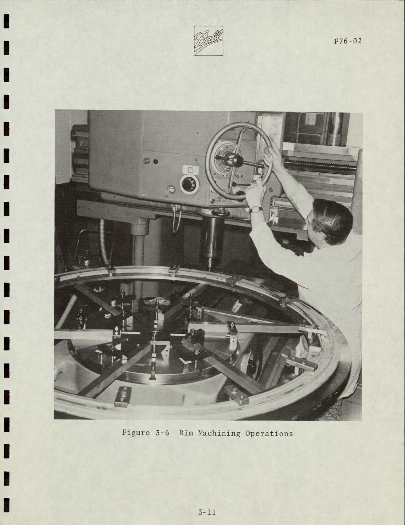

DF76-02
LOCATION MAGNITUDESTRESS (PSI)COMPONENT
Radial or carbonepoxy +460 (max) -891 (min)X stress
Axial or carbonepoxy +491 (max) -433 (min)Y stress
Shear or carbonepoxy +390 (max) XY stress -176 (min)
Hoop or carbonepoxy +55434 (max) 0 (min)Z stress
Radial inner surface +01166 (max)
Displacement outer surface -01130 (min)
(inches)
Table 3-2
MAXIMUM VALUES OF STRESSDISPLACEMENT AT 1200 FTSEC RIM SPEED
3-13
5ThF-=- V- LERATfNz- 1 4U0T00
RMCO RRLYSES BRISTOL REROSPRCE LTO OCT 73
HOOPSTRESS RNSYS 5
or Hoop Stress Contour PlotFigure 3-8 Z
F76-02
- flax h st-ess= 55434-
I I-1 I Ii-- shy
60Iz-
===z_ +0 _----- --- shyi -_-O- - = -- = +----- shy+ ---= -- r E
_-------=--- --- = ---
-- ----- +- - --- -- =--- -=
=
------ shy
=T--- 7
--
-
- -_ - - - -- - -- a
a zrlt- --r-- -r - z I=tzz-z - -
- 4
o6 Zf - =4-=-t vi I_- --- zmE+s=$ Z 4-| b- =---+----- shy
+ 5-t 4 -- c Tt - 22 ~++ _------ _ __ _C - u
a zjztL- +lt+ z- I [Lt- -- Tit--
-- -+v + --F t+-- -+rr 7- h |f
0 200 -00 6800 1000 12oo
Rim SPEED (rri5Ecc~
Figure 3-9 Hoop Stress and Growth With Speed
3-15
F76-02
e 4fo
1 1 I 1 t i I I CII1I1_4I I
Itdn-branveqs sts OI - I M
---shy-- -- -- - -
t~z 2 - 1- shy
- 421 ~T2 2 -=_-- -_E---i ----
t -- EM
___ _ ZZ +-_ _-A~~ - rrrr-
TLLto LLbi i L -- k - r K -1-
irtv li V i 1 -- t 4 s-- n-L -- T4 E
000-q0o 600 800 100 A120 Rim Sp Dr (FTVEC )
Figure 3-102 Transverse Stress Components With Speed
3-16
DF7602
Figure 3-8 shows the computer-drawn plot of constant hoop tensile
stress contours the maximum being 38252 Ncm 2 (55438 PSI)
occurring at the top and bottom inside corner
Figure 3-9shows the relationship of radial growth and hoop stress
as a function of rim tip speed
Figure 3-10 shows the relationship of transverse stress components
with speed
Since the material void free is capable of withstanding 110400 2 2Ncm (160000 PSI) in tension and 8280 Ncm (12000 PSI) in shear
the safety factor is 28 minimum On a sample basis the void
fraction was determined to be less than 04 percent
32 Back-Up Air Bearing System
The design of the back-up air bearing system was completed and
analyzed by Shaker Research Corporation Ballston Lake New York
The back-up air bearing (BUB) system consists of six hydro-static
radial pads and twelve hydrodynamic axial pads These are arranged
in six BUB sets consisting of two axial (one upper and one lower)
and one radial pad and located at either end of a magnetic supshy
port station Each BUB set is approximately 60 degrees from the
adjacent set The bearings are deployed toward the rim by air
pressure when predetermined rim displacement limits are exceeded
The introduction of air through the pads as well as through a
pneumatically operated valve in the vacuum enclosure provides
the fluid for the BUB system and also introduces air drag for a
fastercoast-down Hydrostatic bearings were selected for
radial use instead of hydrodynamic types because the rather small
rim depth (115 inches) allows insufficient area to produce the
required reaction forces The back-up bearing system is shown
in Figures3-11 and 3-12
3-17
P76-02
~14
-L- 7
FiguTre 3-1 AMCD Back-Up Bearing Layout DrawingI 3-la
Figure 12 Back-Up Bearing System
7F76-02
321 Hydrostatic Radial Bearings
The movable radial pads are designed to minimize air flow and
maximize air bearing rim reaction forces The radial pads proshy
vide a centering effect on the rim to minimize dynamic and magshy
netic unbalance forces
In the normal magnetic suspension mode the radial pads are held
away from the rim-and against stops by a set of nested compression
springs (total of 22 N (50 pounds) of preload) When the radial
system Figure 3-11 is activated 207 Ncm2 (300 psig) air is introshy
duced to the pad piston cylinder which moves the pad outward
toward the rim The piston chamber is ported to the pad surface
through a 0033 cm (0012 to 0014 inch) diameter orifice A
sealed oil-filled dashpot between the piston and pad controls the
deployment velocity
Figure 3-13 shows the relationship between- radial pad force and
gas flow versus film thickness for various orifice 4iameters
Because of limited gas available-the smaller orifice diameters
were selected
Since the rim is not at constant radius (because of radial growths)
film thickness and flow vary With rim speed Figure 3-14 shows
the relationship fo film thickness and flow versus rim speed
322 Hydrodynamic Axial Bearings
Movable- tilt type axial hydrodynamic pads were used since the
rim radial width is large and because of the limited bearing air
supply The axial pads are slightly crowned and combined with
the tilt feature are self aligning
3-20
F76-02
1 ~
It
7
I
JII ji
I L
II
---
Ft
T -
VIN I -_ Lr
TD _-
I
I+i
- 1MNV I
4~~r14 +t
Fit~Fi-~tdi I~ ~ JrV)
i ir
il-I= iH14+
i T r
F~m
shy
_ _
I L [
- i
I
_ i _
Ii
0001M -s as
Figure 3-13 Single Pad Force and Flow
3-21
A yyF76-02
WI
ii24pVshy-~~~~W
J4 i3 - Lit
I+ I~Ir~r L-- u 7t J
L 4- 1-nMLfI0__ 4~~~~- F-14--gtrF
I -- -r
4 ~ P I-
IaiH __M
1 --- t Th T1T
I- Vt prI i A
-p--t~LIV[~ VK jl77L1 1
Figure 3-14 Radial Air Pad Flow and Film Thickness With Rim Centered
3-22
F76-02
In the normal magnetic suspension mode the axial pads are held
against stops by a flexural spring The axial system is deployed
in-much the same manner as the radial system When a magnetic
suspension anomaly is detected the vacuum enclosure is flooded
with external air thus providing the film for the axial bearings
Figure 3-15 shows the relationship of film thickness with rim
speed Since the film will support the rim to about 15 radians
per second the pads are designed to accept several contacts before
replacement is necessary
323 Back-Up Bearing Pads
The primary objective in designing the pad material was to proshy
vide a material which would wear smoothly without damage to the
rim or to the pad itself Sacrificial bearing materials have
been used in gas bearings in the past which exhibit the necessary
qualitites The material used in the back-up bearings is an epoxy
resin heavily filled with aluminum powder aluminum oxide power
and molybdenum disulphide powder The mixture is poured into
silicone rubber molds degassed in a vacuum chamber then heatshy
cured The pads are then machined
When the spinning rim contacts the pads the pad will wear smoothly
and rapidly acquiring a high polish and yielding a fine dust
The rim surface should be undamaged by the contact The aluminum
filler provides high thermal conductivity to sink the heat generated
by the rim contact The aluminum oxide provides dimensional
stability so thQ pad will withstand the thermal shock generated
by the rim contact
3-23
3788I9 2 4 5 7 8 9 2
1 7 _- I
111-1 r - J
-I- --i- 1 rV1- 1 t r V
4 _ - _ _____ shy- I---7
I
r-- _- F-_- --- I ii -
I fr r l 7[-II j7shyLi +] - i I-- I
1 7 8
-- - 4 5---- 10 47 MCI 9
Figure 3-15 Axial Pad Film Thickness Versus Speed
F76-02
40 SUSPENSIONSYSTEM
41 System Description
The suspension system consists of three suspension stations
placed symmetrically about the rim At each suspension station
the rim can be pulled in either axial direction or tadially
inward by magnets A total of 12 magnets are arranged in sets
of four each to pull in these three directions (up down and
inward) The eight axial magnets are driven in concert by one
set of electronics Axial error signals are developed by a
position sensor located at the center of each station The
axial servo loops in each of the three stations are independent
of each other The four radial magnets in each station are also
driven by a set of electronics in response to a radial position
sensor located in the center of that station But the radial
station to another so asservos are interconnected from one
to prevent the servos fighting one another even in the presence
of rim radial growth
411 Magnet Description
One of the unique features of the AMCD is the support magnet
design The electromagnets are flux-biased by thin wafers of
samarium cobalt permanent magnet material placed in series in
the magnetic circuit This has the advantage of (1) providing
a high force per unit current sensitivity at zero current (2)
providing a linear relationship between force and current and -
(3) providing the static field required for zero power operation
The support magnet geometry is seen in Figure 4-1 The permanent
magnet biasing is achieved by slanted wafers of samarium cobalt
in the legs The wafers are as thin and wide as possible to
4-1
SAti 4-IUr CCBA3L~rshy
AGtJer-
AGII1
Figure 4-1 Support Magnet Geometry
RF76-02
minimize their reluctance in the magnetic-circuit The volume
of permanent magnet material is sufficient however to provide
adequate flux-biasing and static lift The reluctance of the
permanent magnets is large but does not more than double the
total reluctance since the air gap inthis system is large In
many other magnet suspension systems the gaps are small (about
01 mm) and this sort of series flux biasing would greatly inshy
crease the total reluctance in the circuit Control power would
thus be large and the systems would be impractical
The effect of flux-biasing on the force versus current characshy
teristics of the magnets is shown in Figure 4-2 With no biasing
current in either direction produces force of the same sign with
poor gain and low efficiency in the vicinity of zero current
Force is simply a function of the square of the current With
biasing the slope of force versus current is greatly increased
at zero current In the AMCD top and bottom magnets operate
together in a push-pull type of operation The coils are in
series hence both coils have zero current at the same time
The resultant force-current relationship is linear and has a
slope double that of either magnet alone
Figure 4-3 shows the U core of the magnet with the permanent
magnets in place Permanent magnet thickness is 1 mm (0040
inches) Also shown in Figure-4-3 is a fully assembled magnet
ready for potting After potting the units measure 43 cm x
167 cm x 25 cm (17 in x 42 in x 99 in) and weigh 500 grams
(11 lbs)
412 Position Sensors
The position sensors used in both the axial and radial suspension
systems are Multi-vit sensors manufactured by Kaman Sciences
4-3
7 gF76-02
-r
UPPETP HA -
C AOc~~
777
~~oeehAcn-e-r Z
Figure 4-2 Flux-Biased Magnets in Push-Pull Operation
4-4
rF76-02
I
3 i
A A
I tii A LWUv
NN
N~ i X -9
i i UI A i
IN aWIi ii i
iiiiiiiliiili
i~iiii Ii iliiiiiiiliiilii
Iilliii iiiiiliiiiiiliiiii = iiiiiiaii~iii iiiiiiiiiliiiiiiii
Uiiiii poundii=iiiii]iipoundiiiiiiiiiiiiiiiii Uigure 4-3 Support Magnet Cosri on
iliiiiur -3 ConstructiiiiIliiiiiiiiioniiiiiiiliiiSppriMge liiiiiii i iiiiliiiii3 URiliI 4-s == =
4-s
rF76-02
Corporation These are conventionally called eddy current senshy
sors although they are actually sensitive to anything that changes
the inductance of the test coil in the probe Hence either
eddy currents in a conductor or the permeability of a magnetic
material can be sensed In the AMCD the sensors look at the
ferrite bands and therefore are operating entirely ina non-eddyshy
current magnetic permeability mode Special calibration of the
sensors was required in order to operate in this mode Linear
range of the AMCD sensors is 025 cm (01 inches) and scale facshy
tor was set at 4 voltscm (10 voltsin)
413 Control System
The axial suspension system uses three independent servo loops
to control electromagnet currents An electronic diagram of one
of these loops is shown in Figure 4-4 The heart of the elecshy
tronics is an Inland Controls MA-I DC servo amplifier which is
operated as a current driver to reduce the effects of electroshy
magnet inductance Equations of motion of this driver and an
analysis of the voltage feedback used to damp high frequency
roots are given in Appendix A An analytical block diagram of
the entire servo loop is shown in Figure 4-5 Equivalent points
on the electronic and analytical diagrams are indicated by letters
within hexagons
The axial suspension system has two modes of operation a posishy
tion mode and a virtually zero power (VZP) mode In the posishy
tion mode rim position error is used to command electromagnet
current The rim has high static and dynamic stiffness about
any desired point in the gap In the VZP mode the rim position
set point is modified by positive feedback of the integral of
electromagnet current The result is that the set point is moved
until steady-state current is zero The permanent magnets are
4-6
AA
REHTUtk +26V
4-
C11 7t-Q
Fiue44Aia3upnin7lcrnc
S Cornn- EesoCo p n a cncivCrrent Driver- O deg OI 99 (5C + sm -3 (s + 1 1deg E 1 copy + F
gtosO ~
volf
iE 3 7 T r i m T ntegratadegr
Suspended
Mass
-|ectro
-ria net
16
permanent Magnet
Figure 4-5 AMCD Axial Suspension Station
R 1F76-02
then providing all of the support of the rim Dynamic stiffness
is nearly the same as in the position mode but static stiffness
is actual negative If a downward force is applied to the rim
in the VZP mode it initially moves downward but then slowly
rises to assume a new zero power position above the old equilibrium
position
The electronic circuit diagram for a radial servo station is
shown in Figure 4-6 and the corresponding highly coupled analytishy
cal block diagram is shown in Figure 4-7 Again equivalent
points on the two diagrams are indicated by letters in hexagons
The large amount of coupling results from three servos controlshy
ling only two degrees of freedom
Two modes of operation are available a position mode and a WAHOO
mode The position mode is similar to the axial position mode
The WAHOO mode is a zero power mode that produces zero power
operation in the presence of both static loads and rim expansion
This is accomplished by adjusting the position set point at each
station as a function of the integral of the sum of the electroshy
magnet currents at the other two stations
The name WAHOOis derived from the poker game WAHOO This game
is played in a manner such that each player knows what every
other player holds but does not know what he himself holds
Inspection of the WAHOO trim loops of Figure 4-7 reveals that
for VZP trim purposes each servo only looks at what the other
two are doing This innovation was developed by BBRC to meet
the unique requirements of the AMCD
The derivation of the WAHOO concept is given in Appendix B
There it is shown that only the WAHOO concept produces zero
power operaion for both rim expansion and force disturbances
4-9
A00l 51 Ir
A-A-
F
27
ffzo xr
74 VIP KIAk
7
Ems~
n
A7-
I
A1
ter
a 2k-
-
-
-
-
-
I)
Figure 4-6 Radial Suspension Electronics
-KS
Iamp wkin47s Permanent MagnetVeloityPM VPol Aplifir PMEHM E Iectremoqnet
K5 Kmn eae t~j VOS 0bCar respond to Lettered
1vII~rb r - rr m Psitionson Cgrcwit
vol vol Im PosiMoon Pox
SlRtim rtOhkx _Q$)bsS 4lfe I
0niplPfied Cus ren Driver
Gcucv rbinn n i
+ + vt
If
in-7d FigureservoD RailSro
+i
42
F76-02
Appendix B also shows that for single station design purposes
a single station can be represented as shown in Figure 4-8 Two
points of interest are immediately evident The equivalent mass
for a single station representation is 23 the total rim mass The WAHOO concept which involves negative feedback to each station
from the sum of the other two stations resolves to a positive
feedback in the single station representation exactly like VZP
in the axial mode This representation can be used for designing
the system characteristic root locations If the characteristic
roots from the single station representation are given by A and
the WAHOO gain is Kc it is shown in Appendix B that the three
station highly coupled set of characteristic r6ots are givenby
(S + 2K )A2
Performance
421 Static Performance
At each suspension station the rim will seek an axial equilibrium
position based on the applied load and the control system mode
(position or VZP) These equilibrium positions can be preshy
sented in one plot as shown in Figure 4-9 The VZP line is a zero current line and has a slope that indicates static instability
however as shown in the next section the system can operate in a
stable manner along this line The most usual operating position
mode point is about 001 cm (025 inches) above the center of the
gap At this point the slope P of the VZP line is about 595
newtonscm (340 lbin)
In the position mode an operating line exists for each set point
of the position sensor A family of these is shown in Figure 4-9
The lines are finite in length because of the limited current drive
capability of the electronics The slopes of the lines are apshyproximately 2600 newtonscm (1500 lbin)
4-12
Stationfost ionsingle
Oecrlx- EquIva1eratArmplifir Current Driver 6 Mks$M9oqmet+ 1m
~~~~~ eroe L~r
Is + Fes I16(7+1210 r0 0 l I-
p 0 1
476 An- Per
u2 IVlt+ -Eg
o tKate - r1 1 StO Sr eq uci o lnk wahoo is
Q Correspornas toa letterd posit~ions on circuit chogr~m
Sinql~e stcton eqviclvJewtmls is 23 totil ma
~odelldas a posattve PeedbctK self IoopVe
t to o-t liKe Vf Pwould ltherefboretxpect fvrthernortn itthe Aol O Servo Xt doesonh
Figure 4-8t EqiaetSnluadapev tto
ekgeto8 rnex e o +non
A F76-02
UP
MAGNET M~A t r
lsrok os NoRMAL
kE-RITI N
P E-Nshy-OMFR
tL UPshy
- j ~
-10
h31G1NL pAGE iS
)F POOR QUML-rI
Typical Static Suspension System Performance
Figure 4-9 4-14
rF76-02
The force sensitivity F of each station is about 138 newtons
ampere (31 lbamp) Hence the force produced by a station
is given by (in English units)
F = 340X + 3lI
422 Dynamic Performance
The analytical block diagram for an axial suspension statiQn is
shown in Figure 4-5 For theposition mode the root locus and
-Bode plots are shown respectively in Figures 4-l0and 4-11 The
root locus plot shows that the dominant pole pair has an undamped
natural frequency mN (which we define as bandwidth) of 171 radsec
(272 hertz) and a damping ratio of28 The Bode plot shows
that the gain crossover frequency wc (which some define as bandshy
width) is 1827 radsec (290 hertz)-and that the system phase
margin is 2320 Both plots show that the lower gain margin
is 22(-131 db) and that the upper gain margin is 201 (261 db)
For the VZP mode the root locus and Bode plots are shown respecshy
tively in Figures 4-12 and 4-13 The root locus plot shows that
the dominant pole pair has the same undamped natural frequency
and damping ratio as the position mode that is wN = 171 radsec
= 28 The Bode plot shows that two gain crossover frequencies
at 1823 radsecexist one at0838 radsec (013 hertz) and one
(2903 hertz) The phase margin at the lower crossover frequency
is -772 and that at the upper crossover frequency is 2300
Both plots show that the lower gain margin is 226 (-129 db)
and that the upper gain margin is 2011 (261- db)
The response due to the step application of a one pound weight
is shown for the position mode in Figure 4-14 and for the VZP
4-15
OF76-02
1 -DD
-- A I 1
I I
i
3000 --------------------------------- ___tN
-5000 -400 -30U -2ODG -t I lo oD
REAL AXIS
Figure 4-10(A) Root Locus Plot - Nonideal Current Driver With
Voltage Feedback
4-16
---------------------------------
7F76-02
-I- 111 1-l Z9D
io oI 1ll t A
G
80 ----------- 0 aEu----------------shy-4--
FigueRot41001LcusPlo - Nnidal Crret DrverWit
-1---4-17
I I
F76-020
14-HLowler
)2 I__ _ p
1 N I-- A =20 41 r
I tIse0_ __ _ _ 4 6 2 4 68100
s 10 log H00 6 10009 FREQUENCY (RADIAWS$ECOND)
Figure 4-11 Bode Plot - Nonideal Current-Driver With Voltage Feedback
4-18
7F76-02
$oo I5iI000 I1
T 1 Ii
-A
S4+
N A
4000 R--- - - - - -
V A x
103 000 40 30 29
urn rvrWtFi1r -12A Roo Lou7lt-Nnda
Voltage Feedback 4-19
V gF76-02
ii
- I I I
I I I II
I lii
-I I
II I iishy
II - - -i-l
Fgr 4-2B o otocu PltrNndaCrefl rive
With Voltage Feedback
4-20
F76-02
I i E
A -4 G
E- 60I jUroI(
I
1A2zS1 me RI
3s F-1-L
IIsoM 3en
4) e r
-120---- -Marlin
fla e =2300
-140 shy
1 1 10 10g 2000 1090r FREQUENCY (RADIANSECOND)
Figure 4-13 Bode Plot - Nonideal Current Driver With
Voltage Feedback
4-21
012
F76-02
00010
00008
pound E
0
p
0 00
0zkc0
0
E
- -
4+-F
- - -
Nshy- - - - - - -
4
- -
5
-4-2
AF7602
mode in Figure 4-15 The response for the position mode settles
out at 6941E-5 feet (002 cm) This yields a position mode
stiffness of Stiffness 6 1 lb
6941E_5 t X feet
1 12006 lb (21021-
N
69Th-ft Tni in cm
The response for the VZP mode settles out at -2451E-4 feet
Thisyields a VZP mode stiffness of
1 lb feet = lb NStiffness = 2451E4 ft X 12 in -3400 i (595 E-
Note that the stiffness in the VZP mode is just that of the
permanent magnet and that the movement in this mode is toward
the applied force That is if a weight is placed on the rim
in the VZP mode the rim will move up
Further insight into the system can be found by examining Ap2
pendix C When using current driirers the usual tendency is to
ignore the high frequencydynamics and simply say that the
output current is the input voltage times a constant This can
be very misleading in the case of AMCD- In Appendix C are shown
root locus plots using both an ideal current driver arid a nonshy
ideal current driver without voltage feedback It shows that
voltage feedback is necessary for the axial suspension Also
shown in Appendix C are Nyquist plots and phase-gain root locus
plots of the nominal axial systemthat is the system using curshy
rent drivers with voltage feedback The esoteric phase-gain root
locus plot shows on one plot the sensitivity of the system roots
to change in both gain and phase For example it shows what
would happen if an additional 300 of phase lag were added to the
system from some unknown source
4-23
F76-02
0001
I f
I 0 e
eshy
0a T 1-0001-shy0N
ft E F 0
E a
- 002--------------shy
0 t0 20
TINE (SECONDS]
30 40 50
Figure 4-15 Nonideal Current Driver With Voltage Feedback
4-24
F76-02
The equivalent single station radial analytic block diagram is
shown in Figure 4-8 It is very similar to an axial station
The root locus and Bode plots for the position mode are shown
respectively in Figures 4-16 and 4-17 The root locus plot shows
that the dominant pole pair has an undamped natural frequency
(bandwidth) wN of 653 radsec (104 hertz) and damping ratio C
of 18 The Bode plot shows that the gain crossover frequency
is 666 radsec (106 hertz) and that the phase margin is 1350
Both plots show that the lower gain margin is 329 (-965 db)
and that the upper gain margin is 7054 (3697 db)
The root locus and Bode plots for the WAHOO mode is shown in
Figures 4-18 and 4-19 The root locus shows that the dominant
pole pair has an undamped natural frequency of 674 radsec
(107 hertz) and damping ratio of 16 The Bode plot shows that
the upper gain crossover frequency is 691 radsec (110 hertz)
At this frequency the phase margin is 1260 Not shown is the
fact that the system also has a lower gain crossover frequency
of 594 radsec (095 hertz) At this frequency the phase marshy
gin is -715 Both plots show that the lower gain margin is
389 (-821 db) and that the upper gain margin is 6701 (365 db)
The large upper gain margins for both the position and the VZP
modes indicate that current driver voltage feedback is not needed
Considerable rim bending instabilities were encountered during
the design Early in the development the axial system was
designed to be overdamped This caused a bending mode to be
driven unstable The compensation was adjusted experimentally
until the bending became stable Unfortunately this reduced
the lead in the system resulting in the present underdamped sysshy
tem It is believed that bending will present no problem at
high spin rates because of the effective stiffening of the rim
4-25
6F76-02
_____ - _ r ____I___
141
IT___lishy
1 ii
1 F]
eir
t lj~
4-
J TT a p-
III NEA
fiIT WBKsITlK j1_11IIi I-
I
e
-Fshy
Y]-111 ji
1i1fln 4--I r
I i--I -
TFiJ-WL 1
_1(-Ii4 - I
I~ ~ ~iA_~2I ___ ii- 11 IFt-Ih
iT
h~ -iH T
+~ji+ih Iplusmn
_ _ _+ I kt ~h-II
+ LILY -
7 SO bullj
Figure 4-16 AMCD Radial Suspension Equivalent Single Station Position Mode
4-26
Elll csl- tLL[ 11--- 1_ il
V
1 MIN
2 0 H qL2~14-0IT
I M Ill 1OIHI
+-o ip Lr g
Ti I -0 1- b1 -- i
Ij _IUSi 1PIN - il
--i
41i L -I I - d jir ~J I I
00 -o
ro-d 5 c
Figure 4-17 ANCD Radial Suspension Equivalent Single Station o Position Mode
7F76-02
1LjI_----- Li -III iI - - I -shy-F ]e2 1
Is- Lr [_I
r ir -L-j 11I IALI _ _ _ ___ 2_
E11LLN1LALIF TYC -- td It 11
- KI
S1 1 1 1--shy
II
I r 11
FLL-1
U - I 4
E~~~~fL
__
f Lplusmn Xi ILIi _ _
- ii _ _ i
- H --
--------
A-1 1 F - JT-1
-- t-ti -~r -r I- t - --- IL I
IIJlri-tlrht1f tI
_+ _ l PillS 1 I
Figure 4-18 AMCD Radial Suspension Equivalent Single Station
o Wahoo Mode
4-29
rm~r 1 u i rrrrF r r r
4
130
o
I -4
7 7 1-shy iAb d
llt h
-30 Tfij4i i ~
- n0 t
Figure 4-19
01 AII-
I uji r a sec
AMCD Radial Suspension Equivalent Single Station o Wahoo Mode
AF76-02
and the averaging effect on modal pick-up caused by the bending
modes moving rapidly past each position sensor
As the rim is spun up the three axial stations become more and
more coupled by nutational effects The result of the coupling
is to reduce the dominant roots damping ratios more-and more to
the point the system could go unstable if the rim is spun fast
enough It is believed that this tendency could be greatly
reduced or possibly eliminated by the proper combination of cross
feeds from one axial suspension station to the others
4-30shy
DF76-02
50 DRIVE SYSTEM
51 System Description
The AMCD drive motor can be thought of as a large permanent magshy
net brushless dc torque motor Samarium cobalt magnets are
bonded into the rim at regular intervals The two phase armashy
ture is segmented with a winding set at each of the three susshy
pension stations Commutation is controlled by Hall effect senshy
sors mounted near the rim which sense position of the samarium
cobalt motor magnets
52 Magnet Selection
Alnico was considered along with samarium cobalt for the permanent
The large air gap and segmented winding structure meanmagnets
the magnets will become nearly air stabilized The rim was designed
with a small outer lip to hold the magnets This was done to
isolate the drive from the suspension as much as possible without
and complexity to the rim than necessary Thisadding more mass
small lip implies a short magnet Samarium cobalt has high
strength for short lengths and does not pay a penalty for air
In fact it is very difficult to demagnetize thisstabilization
material
cm (55 inches) diametertby 64 cmSamarium cobalt magnets 14
(25 inches) length were selected and bonded into the rim with
polarities alternated
The rim contains a total of 72 magnets spaced 73 cm (288 inches)
apart
5-1
53
--F76-02
Core and Winding Design
Each armature segment consists of a pair of bar-shaped winding
assemblies one above and one below the rim
Sit cos sla 0S SMa
cores in a singleThe windings-are wound toroidally around the
layer The figure above shows only the cross-section 6f conshy
ductors in the air gap as the conductors passing around the other
side of the core add nothing to torque and serve only a connectshy
ing purpose The bar-shaped cores are easy to wind and result
in a compact structure The single layer of 18 conductors adds
very littleto the overall air gap This effective electroshy
magnet design was suggested by P A Studer of Goddard Space
Flight Center
Ferrite material was chosen for the core to reduce losses Fershy
rite also is easily machined into the required irregular shapes
The windings are grouped into two phases SINE and COSINE each
of which acts upon three magnets at each motor segment In operashy
tion current in one phase is acting on the magnets while current
in the other phase is reversing in preparation for a magnet of
opposite polarity
5-2
DP76-02
54 Motor Commutation
Hall sensors act as commutation devices for the motor They sense the position of the permanent magnets in the rim and cause the drive coil currents to be switched according to magnet position
The sensors are mounted in pairs one above the rim and one below for each winding phase Outputs from each pair are summed so that the switching position is not affected if the rim moves up or down within the air gap The SIN pair controls current on the SIN windings of all three motor segments and likewise the COS pair
of Hall sensors controls all COS windings
55 Motor Control Electronics
A block diagram of the motor control electronics is shown in Figure 5-1 For each phase the Hall sensor outputs are summed and amplified to drive-threshold detectors These detectors sense magshynet position and polarity The phase control logic determines the
timing and polarity of the motor coil drivers Interconnections between the two phase control logic blqcks provide positive direcshytion and start-up information
Each of the six coil drivers controls a phase at one of the motor
segments Associated with each driver is a coil current sensor which monitors the current in that winding All six of these
current sensorsreceige a common reference from the speed control
potentiometer When current in that particular winding reaches the reference level the driver turns off until the current deshy
creases This prevents the current from reaching destructive levels at low speeds and acts as a speed control at high rim
speeds
Since the coil drivers are either full on or off a very efficient drive is achieved At low rim speeds the drivers operate as a
5-3
56
F76-02
conventional PWM (pulse width modulated) amplifier A quite faithful square wave current of controlled amplitude is fed to the coils At high speeds high acceleration (or deceleration)
is possible with the drivers full on for the period between magshynets with current rise and fall limited by the inductance of the
coils
Torque Calculations
The equation for the force betweena magnetic field and a current
carrying conductor-is
F = BLI
where
F = Force in Newtons B = Flux Density in Teslas (WebersM~ter )
L = Conductor Length in Meters
I = Current in Amps
If the magnetic field is created by a permanent magnet the force
can be considered to act on the magnet if the conductof is held
stationary which is the case with the AMCD motor
To arrive at design force each of the factors B L and I must
be evaluated
A force calculation will be made for one magnet face interacting
witha coil This can be then doubled to account for both ends of the magnet next tripled to take into account the three magnets in one motor segment and tripled again to realize the total force for the three motor segments Then using the radius of the rim
we can calculate developed torque
5-4
F76-02
Flux Density Calculation (B)
The large air gap makes it difficult to- estimate how much of the
magnet flux will couple through the winding core and how much
will be lost to leakage A measurement of coupling flux was made
using a pair ofsoft iron bars similar to the ferrite corasi
SEJSE C0115
SOFr iROh
-4 Webers with magnets of averageThe flux measured was 0375-x 10
strength
core must-be convertedThis flux that couples through the ferrite
to flux density (B) in the air gap where it interacts with the
coil windings There are two practical Choices for doing this
We can assume all the flux goes straight up from the surface of
the magnet andreacts with only those turns above the magnet or
we can assume the flux spreads out evenly over the winding area
Of course the truth liesand-reacts with all the turns equally
an adequatesomewhere in between but the second approach gives
approximation
The winding area in the air gap for one magnet coil phase is 2
19 x 36 cm or 68 cm
Flux density then is
-44m _ 0375 x10 Webers 2 0055 WebM-B_=A = 4 2A - 68 x 0-4 m
5-5
F76-02
Conductor Length Calculation (L)
are 28 turns with an effectiveIn the winding phase area there
length of 19 cm each
Total effective length is then
L = -19 x 28 = 532 cm = 0532 M
Current (I)
that the coil drivers and wiringThe elbctronics are designed so
canhandle 4 amperes Also the inductance of the coils was
examined to be sure that currents of this magnitude can be
reversed at maximum rim speed frequencies with a 60 volt power
(and torque) will then be calculated for thesupply Force
design maximum of 4 amps
Force
We can now calculate force from the equation
F = BLI
= 0055 x 0532 x 4 = 0-1-17 Newtons
Recall that this is the force for a single magnet surface inter-
For the total motor this is multiplied by 18face
Total Force = 0117 x 18 = 176 Newtons
576
0F76-02
This times the magnet radius (0838 meters) gives total torque
Total Torque = 176 x 0838 = 176 Newton-Meters
(13 lb-ft)
A small (14 diameter) test wheel was built to check the above
torque calculations Acceleration measurements were made and
from the known wheel inertia torque was determined Correlation
within 10 of the calculated torque was achieved
5-7
S in Hall Sensors
Summing
Amp
[A Threshold Sin Phase Coto-rie
DetectorsLoi
SnB1Sin
Sin C Driver
ol
Hall Sensors
~ Amp=ApDtcosLogic
etctr Control -- Die Col Ci~
Summing Threshold Phase Cos B Driver
iCosCos
Ci Co
Figure 5-1 Motor Control Electronics
C
aF76-02
60 REFERENCES
1 Anderson Willard W and Groom Nelson J The Annular
Momentum Control Device (AMCD) and Potential Applications
NASA TN D-7866 1975
6-1
F76-02
APPENDIX A
CURRENT DRIVER EQUATIONS AND TRANSFER FUNCTIONS
A-i
F76-02
Appendix A
Current Driver Equations and Transfer Functions
When using current drivers the usual tendency is to ignore the
high frequency dynamics and simply say that the output current is
just the input voltage times a constant This was very misshy
leading in the case of MCD-as shown in Appendix C The circuit
diagram of a current driver with voltage feedback and its equishy
valent diagram are shown in Figure A-i -
v A T5It
Figure A-I Current Driver and Equivalent Circuit
A-2
F76-02
The beginning equations of motion are the following
Rl11 RM -- R 10
-RM SL + R2 2 -(SL + RC) I= A(TS+I)-)V + ARI(TS+l)shy
-R 2 -(SL +R c) SL + R3 3 + S_ C I 3 0
where
R1 lt= R1 + R2 + RM
2 RM + RC22
R33-- R2 + RF + RC
Transposing I1 to the left hand side we obtain
R11 -RM -R2
-RM(TS+l) + AR 1 (TS+l) (SL+R 2 2 ) -(TS+1) (SL+Rc) 2 A S-SR22 S L+SR33+-l
What we really want is the current through the inductanceshy
1 2 T3
Adding this equation to the system we obtain
C1 C12 C1 3 0 II 1
B2 1 S+C 2 1 A 2 2S2 +B 2 2 S+C 2 2 A23s2+B 2 C 3 0 12 A V
B31S A32S2+B32S A33S2+B 3 3S+C 3 3 0 13 0
- -1 1 1 1 0
A-3
eF76-02
where by definition
-=A32 -LC R11 B22 = L+TR 22
= - C22 R22 B32 = RCCl2 RM
C13 =-R 2 A23-= -TL A33 = L
= R33B21 = -RMT B23 = -L-TRC B3 3
C = ARI-RM C = -RC C =C -I
= -R2A22= TL B31
If the voltage feedback is removed these equations reduce very
simply to
-RMIRlI+R2+RM
+ AR1 (SL+R+RM)(TS+ 1j1 2 = AKRM(TS+I) We want thewhere 12 is the current-through the inductance
transfer function 12V First divide the secondequation through by
LT to obtain
-RMR I+R2 +RM
(R C+ PM j] IAL 1 V S+L-iIARI[ RM L (SplusmnT -1)+L -lT -1A
A-4
F76-02
Then by Cramers rule
2 CR1+R2+RM)AL -1T-+RML -1(S+T- 1 )_L-1T- 1 AR1
V7 -1 r- 1 2-1 - lshy(RI+RZ+RM)(S+T +L (RC+RM) -R ML l(S+TI)+L ITIARIRM
(R2+RM)AL -T - I(S+Tshy
-(R1+R 2+RMM)(S+T 1 )(S+L-1 RC)+L -RM(R1+R 2)(S+T-I)+L T ARIRM
Further manipulation yields
S+T-1 +(R 2 +RM)ARM T12 RML -
V - 2+RM) 1 L-+RR [2 wT-ARI-L 1RM(RI+R2 -
S+T )(3+L Rc) + RR+Tl+R---
Finally the desired current driver without voltage feedback
transfer function is given by
12 RML- S+T -1 +A(I+R2 RfIj
V (RLR-+RM) - -1 LRM(RI+R2 ) (ST 1 [7AR 1 RS5 + R2 +RMR R1 L Rk 2 )
A-5
76-0 2
For infinite amplifier open loop gain A = the transfer
function reduces to
2R Lim 12 = R1_ 2M
(l+R2RM- R2
R - RYR RR)r112RM for R2gtgtRM
-This is the transfer function which is used
I2 R2 12 R 2V RIRM
if the high frequency roots may be ignored
When the high frequency roots are not to be ignored and
if AR2R1 gtgtmax (RMRC-i)
and RMARlRjR2gtgt
RI+R 2 c
A-6
rF76-02
The transfer function simplifies to
S+T- AR 2RM1
12 RML-
V R1+R2 (S+T-)(S+L -Rc)+L- RM(S+T-AR1 R1 +R2)
RML-1 S+T-1AR2RM-
R1 R2 S2+ -1 -1 -1 T 1L-1RMARl - A
S +(T- +L -Rc+L RM) S+ R+R
T- +L- (RG+RM) TRLAR
2 (RI+R2)
The dc gain of this transfer function reduces to the same transshy
fer function used if the high frequency roots may be ignored
that is
2 R2 V RIRM
For the radial MA-lCurrent Driver
RI = 10K R 2 = 2711 KQ RM 10
RC = 30 Q2 L = 0128 h T - 30 A 50119
Then the radial current driver without voltage feedback has the
transfer function
12 _-00061463(S+40762E10)
V S+13609plusmnj30400 shy
A-7
F76-02
Forthe axial MA-I current driver
R=1 10K R2 = 7311K C 01 1f R11 = 17311E4
L =0064 f = 12M R = 14 R22 =15
A = 50119 RM = 1 T- = 30 R 33 I2073E6
Then
= C11 7 17311EA B2 2 = 564E-2 A 3 2 -0064
Cl2 = -- 22 = 15 B = -14
== = -7311E3 -21333E-4 A33 0064C13 A 23
B21 = -33333B-3 B2 5 -53067B-2 B 12073E6
C21 = 50119E8 C2 3 - 14 C3 = 1OE8
= A22 = 21333E-4 -B3 1 -7311E3
Without voltage feedback the axial current driver has the transshy
fer function
2 00090261(S+l0993B1)
V S+13219plusmnj36839shy
A-8
7F76-02
Note that without voltage feedback the damping ratio on both the
radial and axial current driver high frequency roots is less than
05 This appears to be all right for the radial servos but is
very bad for the axial servos as shown in Appendix C Consequently
-voltage feedback has not been employed for the radial servos
current drivers but has for the axial servos cur-rent drivers
The effects of this feedback has been determined numerically
Figure A-2(A) shows the effect of increasing RF the voltage
feedback resistor from zero to infinity with the feedback capashy
citor C held a-t 01 lif Ifonly the capacitor is used for voltage
feedback the current driver roots are still lightly damped but
at a much lower frequency As the resistance is increased the
roots increase in damping become real then decrease in damping
at a high frequency finally moving to the no voltage feedback
position for RF = Figure A-2(B) shows the effect of increasing
the voltage feedback capacitor C from zero to infinity while
holding the feedbackresistor at one megohm For C 0 the roots
start at the no voltage feedback position As C is increased the
roots decrease in frequency and-increase in damping ratio until
C = 00091 f Further increases result in decreased damping
ratio and increased frequency At the chosen voltage feedback
values of C = 01 vf RF = 10 MQ2 the axial current driver transshy
fer function is
I 0008994(S+833)(S+l099EII) V (S+786)(S+2771plusmnj2583)
A-9
~~~ L~Trrrl~I I~ I II 4
Jots_1 nr_- r177I 7F I i0K IIII __ riiTTh
17shy
tkP M T7r
Hl4plusmn ------ IIr-1-----~ -- - I -
CDl7E-~ ttbifil
LA14 -T-- 4+ -
C T -I I
H -rTH V i H
-HE I
Figure A-2 Effect of Voltage Feedback on AMCD Axial Current Drivershy
AF76-of -
APPENDIX B
THE WAHOO CONCEPT
B-I
7F76-02
Appendix B
The WAHOO Concept
Introduction
Two conditions may occur which cause the radial electromagnets
to draw more current than necessary First if the rim is tipped
This forcea gravitational force tends to pull the rim sideways
at the expense of causing the electro-shyis countered by the servos
magnets to draw more current Second as the rim spins up
centrifugal forces-cause it to expand To each radial sensor
as rim movement to be countered by thethis expansion is viewed
to try to pullservos So each electromagnet draws more current
are directed inward andthe rim inward But since the forces all
spaced 120 a-round the rim the resultant of the forces is zero
so the rim does not move The net result of the expansion then
is thatonly the current in the electromagnets increases Trim
loops are developed in this appendix which lead to VZP (Virtually
Zero Power) operation for the radial servos when either the rim
is tipped or expands or both The system employing these trim
loops is called the WAHOO system
Because the three radial servos are controlling only two degrees
of freedom the radial servo system is very highly coupled This
very high degree of coupling makes it difficult to design each
servo as a single uncoupled system Hence in this appendix we
also develop equations to show how the three-servo radial system
may be designed using a single station servo radial equivalent
Development of the WAHOO Concept
The AMCD rim is suspended radially by three servos pulling on
it from the inside much like shown in Figure B-1
B-2
F76-02
Kim
Figure B-i Radial Servo Sign Convention
The sensor outputs are denoted by X1 X2 and X3 As the rim
spins up it expands by the amount X0 The sign convention is
chosen such that positive forces and displacements are outwards
The equations of motion of the rim are
(F2 - F3 )Co = My
(F2 + F3)s8 -F1 = my
X2 = XCe + YSe
X3 = -XCe + YSO
XI = -Y (B-i)
B-3
F76102
The force acting at each station is composed of a permanent
magnet force and an electromagnet force That is
Fl = P(XI+X0) + E D1
= P(X2+X0 ) + E D2 (B-2)F2
F3 = P(X3+X0 ) + E D3
these equations are-combined with the servo equations in Figure
B-2
From the block diagram the quations of motion using five variables
are
V1 = Kp(-Y+X0 ) -S)(KsVi+KcV 2+KcV 3) EKRN_1
Y = M--p(-Y+X0)+DR (-Y+X 0)+ EV1 +pSC(YSe+XCplusmnX0 )
EKRN -fD se(YSe+XCe+Xo)- ESeV 2 + PSO(YSe-XCe+X0 )
EKRNK sOCYSe-xce-Xo)- nsev 3 + FY
-V2 = K (YSO+XCeplusmnXo)-(lSKsV2+KcVI+KcV3)
EKRN = 1=M PcO(YSe+XCe+X 0 )- D C(YS+XCc+X0)- ECOV 2
EKRN -PCO(YSe-XCO+X 0 )+ ce(YSe-XCe+X0 )+ ECOV3
)V3 = K(YSe-XCO+X0 )-(SJ(KsV 3+KcVI+KcV2 (B-3)
B-4
+ SFt
+- K + X0
+ T- SID
fRi
Figure B-2 MICfl Radial Servos With Trim Loops
7F76-02
Rearranging
(S+Ks)VI+KpSY+KcV 2+KcV 3 = KPSX0
-M-1DEv+[DS2 -DM-Ip(1+2SD)+M-EKRN(1+2S2 0)]y
+M-IDESOV2 +M-1 DESOV 3 = [M-IDP(-1+2S)+MWIEKRN(I-2SO]XO+MDFy
KcV -KpSSY+(S+Ks)V2 -KpCeSX+KcV3 = KpSX0
M- 1DECOV 2 +[DS 2DM- P(2c0 )+M-1EKRN(2C2 )]X-M-IDECOV 3 = 0
KcVI-KpSSY+KcV 2+KpCeSX+(S+Ks)V 3 KPSX0- (B-4)
Since 0 = 30
I+zs2 -1+2(5)2 = 15
-- 1+2S = -1+2(5) 0
2C = 2 )2 = 15 (B-S)
Using these simplificatfons the Laplace transformed radial
servo equations of motion in matrix form are
(S+Ks KpS 0 KC KpS 0DSL KC V1
-1IDE +lSMIEKRN SM- 1flE 0 SM- DE Y 0 M D
-1$M IDP __ __
KC 5KpS (SK S ) SrI KpS X6 V2 KK SX 0 + 0 Fy
DSz--shy
SM- 1 DE - SMDE0 0_- 54M +lSM 1 EKjN x 0I 0
-5KpS K 54 KPS (S+Ks) KpS 0KC V3
B-6 (B-6)
F76-02
The system characteristic equation is the determinant of the
coefficient matrix With much algebraic effort it can be
reduced to
A = (S+Ks+2Kc)X
FKRN-ISM- DP)+lSKpM- DES]2[(S+KsKc)(DS2 +SM-
(B-7)
Now lets simplify the expression by-removing the high frequency
roots In the Cambion hardware
KRN 107 S for low frequencies
D (S+1000)(S+10000)
With this approximation KR = D = and N = S Then
2+lM ES-lM P)+lSKpM-1ES] 2A = (S+Ks+2KC)[S+Ks-KC)(S
So the roots separate into -(Ks+2Kc) and two identical sets
within the brackets Immediately we see that Ks+2KC 2 0 for
stability Now looking within the brackets we see that S2+
1SM-ES-l5M-P represents the permanent magnet roots at
+lSM-IP moved to the left some by the rate feedback however
one remains in the right half plane Taking these roots and the
one at -C(Ks-Kc) as poles of a root locus plot and S as the zero
Figure B-3 shows that for stability KC a KS
B-7
0F76-02
Kct IKSKczk 5
Figure-B-3 Effect of Trim bull Loop Gains
Les look at three special cases
I No Trim-Loop KC = KS = 0 No VZP
A = s3 [(S2 +lSM-IES-lSM-iP)+iKIPMlE] 2 (3-8)
There are three roots at the origin from the three unconnected
integrators and two identical quadratic pairs The system is
stable
II No Cross FeedTrims KC= 0
-ISM IP )+ I S5pMIEs]2A = (S+K) [(S+Ks2) I Es(B-9)
This is unstable-for both signs of KS self trim loops alone
will not work
B-8
F76-0
III No Self Feed Trim KS = 0 WAHOO SERVO
2
(S+2Kc) [(S-KC) (S2+lSMIES-l5M1P)+lSKpM-1ES]YA
This-can be made stable for all positive values of Kc
IV One Integrator Trim KC = KS = K
2 (B-10= (S+3K)S2[(S2+SM-1ES-lSM-Ip)+l5KpM-I[
This can be made stable for all positive values of K
Main conclusion to here Cross Feed is necessary for
stability if VZP is needed
Self Feed is not
Now a question arises Do the two stable systems (III and IV)
provide zero power operation in the face of both rim expansion
and force disturbances and do they translate due to these effects
To answer this look at the transfer function VIXp) V1 FYI
From (B-6) after much algebraic manipulationYX0 and YF
we obtain the numerators -
Num (VIX) = KpS[(S+Ks-Kc)(DS 2+lBM 1 EKRN-lSM-1DP)+lSKpM 1 DE S] 2
(B-11)
Num (V1Fy) -M-1DKpS(S+Ks+2Kc)X
[(S+Ks-KcM(DS 2 +SM -1EKRN-I MIDP)+lSK M-IDEs]
(B-12)
B-9
~F76-02
= (B-13)Num (YX 0 ) 0
Num (YFy) = M-D(S+Ks+2KC) (S+Ks-KC)X
[(S+Ks-Kc)(DS2+S5M-BKRN-1 SM- DP)+1SKPM-lDBS]
(B-14)
Repeating (B-7)
IDES] 2 A = (S+Ks+2KC) [(S+Ks-Kc)(DS2+1sM-IEKRN-15M-ID)+I5KpM-
(B-7)
Then the transfer functions are
VI Num (VIX0) KpS
X0 A(S+Ks+2K C) (B-IS)
-M-IDKpSNun (VIFy =VI
Fy A (S+KsKc)(DS2+1 SM-1EKRN-1SM 2Dp)+I5Kp-DES
(B-16)
(B-17)y Num (YX0 X0
B-10
D F76-02
Y M 1D(S+Ks-Kc) (B-18)
Fy (S+KsKc)(DS2+SMIEKRN-ISM- IDP)+lSKpM-DES
Now we can answer the question
WAHOO Servo KS = 0
Because of the S in the numerators of V1X 0 and V1Fy the steady
state power goes to zero for both rim expansion and force disturshy
bances From YX0 the rim does not translate for rim expansion
From YFy the rim does translate for disturbance forces with a
stiffness of
Y- = = -1SP (B-19)S 0
Therefore the rim translates toward the disturbance
Single Integrator Trim KC = S
From V1X0 the steady-state power goes to zero for rim expansion
With KC = KS1 the S cancels out of the numerator of VIFy thereshy
fore the system power is not zero for force disturbances From
YXo the system does not translate for rim expansion From YFy
the rim does translate for force disturbances with a stiffness
of
F = 0 = 15(KpB-P) (B-20)
B-I
~F76--02_
Therefore the rim translates away from the disturbances with
the same stiffness it has with no trim
Radial Single Station Servo Equivalent
Because three servos are controlling only two degrees of freeshy
dom the radial servo system is very highly coupled This makes
as a single uncoupled systemit difficult to design each servo
From the characteristic equation A=0 derived in the preceding
section we may deduce a single station equivalent From (B-7)
considering only the WAHOO servo
A (S+2Kc)[(S-Kc)r(DS2+M-l BKRN-ISM-1 DP)+5KpM 1DES]2
(B-21)
- a repeated set ofWe note that there is one root at 2KIc and
We would expect only two repeatedroots within the brackets
sets because we are only controlling two degrees of freedom even
though three servos are used to accomplish it Looking at the
quantity within the bracketsshy
-1DES 0 (B-22)(S-Kc)(DS2+ISM-1EKRN-1SM-1DP)+lSKpM
to obtainwe first-divide through by S2D(S-Kc)
KRN KpE S 0 (B-23)1 E p
23 M DS2 23 MS2 23 MS2 S-Kc
B-i2
T WF7602
This is just the characteristicequation of the following servo
which is the single station equivalent
4I
Figure B-4 Equivalent Single Radial Servo Station
Two points of interest are immediately evident The equivalent
mass is 23 the total rim mass The WAHOO concept which involves
negative feedback to each station from the sum of the other two
stations resolves to a positive feedback in the single station
representation exactly like VZP in the axial mode Using this
single station equivalent the system may be designed just like
an uncoupled servo the final three-servo coupled system roots
being given by (B-21)
Conclusions
Only the WAHOO trim system is stable and produces zero steadyshy
statepower for both force disturbances and rim expansion
WAHOO trim consists of the sum of voltages from servos i
and j being fed back to servo K in a negative sense for each
i j and k That is for trim purposes each servo only
monitors what the other two are doing-not itself The system
stiffness is -ISP where P is the permanent magnet stiffness
at each station
B-13
OR F76-02
The highly coupled three servo radial systems may be
designed using a single station servo radial equivalent
B-14
yF76-02
APPENDIX C
SOME ADDITIONAL SERVO INSIGHTS
C-1
AyfF760__2
Appendix C
Some Additional Servo Insights
The purpose of this appendix is to provide additional insight
into the inner workings of the system To build up a feel for
the final axial system a series of stability plots are shown
to show the state of the system at various stages of its design
The axial servos were originally designed assuming an ideal curshy
rent driver that is one whose output current is just a constant
times the input-voltage This is what is usually assumed conshy
cerning current drivers Figure 0-1 is the axial position mode
root locus plot of such a system It indicates that no stability
problems exist an upper gain margin of 1206 and a lower gain
margin of 22 being evident The actual servo did not exhibit
such stability
Figure C-2 shows the same root locus plot (that is axial position
mode) if a realistic -current driver is used The realistic curshy
rent driver has low damped (c = 036) high frequency roots (n =
3685 radsec) which are driven unstable at a gain of 479 (comshy
pared with 1206 above) The actual servo exhibited this inshy
stability at even lower gain margins At the times we we-re exshy
periencing this instability the root locus plot of-Figure C-2
had not been made Indeed the realistic current driver transshy
fer function had not even been derived We didhowever suspect
the current driver and fixed the problem experimentally by trying
different values of components in the voltage feedback circuit =We eventually arrived at C = 01 lif and RF 10 M for feedback
components Appendix A shows that this was a near optimum choice
Figure 4-10 shows that this fix increakedsthetaytems- gpaxmgain ma-rshy
)atgin from 479 to 201
C-2
____
i
F76-02
J- - - J F-shy I
ti eA j n wtl ifpf) L-I t- -
T I I- - -
r I I
-it t--L-1_-I-1-1- 1 H I-A -A I I-i I I r I 1 ___
~~~~~ hiit-- d31Ir~- LHtH [plusmnif 1Tf- Hshy
t I L I
L I - shy
---- l]iFli+-
HHI4KuC-1AD AaSvW Ia C
[l- 3 i iI LL41_EiI]L j7T ILl~ I i~[i tTj
-iltIIF--4l-- l II
- ~ FI I
- L I i5 YL i o ~ ~ ltI itiML
Figure C-i AMCD Axial Servo Wi~th Ideal Current Driver
C-3
ZF76-02
I I
4000 - i ii-
I 1A - I I
ooI ILJ 1000 m L
-5000 -4000 -300 -2000 -1000 0 1000
REAL AXIS
Figure C-2 Root Locus Plot Nonideal Current Driver Without Voltage Feedback
C-4
7F76-02
D
_____ I bull II
eoo1ii I I- I AI I-N
N IAt A
A I Iii T
SNM
I AIshybullI $ I~ IY
ajIe bI_Ig
-144
I I I Ishy
ai Ing REAL AXIS
Figure C-2(B) Root Locus Plot - Nonideal Current Driver
Without Voltage Feedback
C-5
F76-02
The final axial system root locus and Bode plots are shown in
Figures 4-10 and 4-11 for the position mode and in Figures
4-12- and 4-13 for the VZP mode Sometimes additional insight
may be obtained from other stability plots The axial position
mode and VZP mode Nyquistpiots are shown in Figures C-3 and C-4
A plot which yields root sensitivity information from both changes
in gain and phase is the gain phase root locus plot Gain-phase
root locus plots for the axial position and VZP modes appears in
Figures C-5 and C-6 For example Figure C-S reveals that if
the gain remained nominal and for some unknown reason an additional
2320 of phase lag were introduced the axial positionmodewould
go unstable
C-6
F76-02
AIN IDB) VERSUS FMASE ANGLE (CEGREES)
9-a
-IINALPAGE 18
F POOR QUALITY
Figure C-3 Nyquist Plot - Nonideal Current Driver With
Voltage Feedback
C-7
DF76-02
fIN (M8) VERSUS PHASE ANGLE (DEGREES)toS PL~aos-- ItC
ID3
270
OROGTNAL PAGE IS OF POOR QUALTY
Figure C-4 Nyquist Plot - Nonideal Current Driver With
Voltage Feedback
C-8
1 gF76-02
40 I - I
I I I 0
AI 06
C2-Y 1_ I
-610 -40 _O_ -shy n n 6
-400 ~~
With VotgFebc
zloo- -400 -200 REL 0200 40D 600
-NonidealFigure C-5 Gain-Phase Root Locus Plot CurrentDriver With Voltage Feedback
C-9
-400
2F76-02
600 - E 1 II I
400
-
1
R
A
IIT
a zOO 400
REAL AXIS
-6-0O -400 -200
Figure G-6 Gain-Phase Root Locus Plot - Nonideal Current Driver With Voltage Feedback
C-go
600

F76-02
e 4fo
1 1 I 1 t i I I CII1I1_4I I
Itdn-branveqs sts OI - I M
---shy-- -- -- - -
t~z 2 - 1- shy
- 421 ~T2 2 -=_-- -_E---i ----
t -- EM
___ _ ZZ +-_ _-A~~ - rrrr-
TLLto LLbi i L -- k - r K -1-
irtv li V i 1 -- t 4 s-- n-L -- T4 E
000-q0o 600 800 100 A120 Rim Sp Dr (FTVEC )
Figure 3-102 Transverse Stress Components With Speed
3-16
DF7602
Figure 3-8 shows the computer-drawn plot of constant hoop tensile
stress contours the maximum being 38252 Ncm 2 (55438 PSI)
occurring at the top and bottom inside corner
Figure 3-9shows the relationship of radial growth and hoop stress
as a function of rim tip speed
Figure 3-10 shows the relationship of transverse stress components
with speed
Since the material void free is capable of withstanding 110400 2 2Ncm (160000 PSI) in tension and 8280 Ncm (12000 PSI) in shear
the safety factor is 28 minimum On a sample basis the void
fraction was determined to be less than 04 percent
32 Back-Up Air Bearing System
The design of the back-up air bearing system was completed and
analyzed by Shaker Research Corporation Ballston Lake New York
The back-up air bearing (BUB) system consists of six hydro-static
radial pads and twelve hydrodynamic axial pads These are arranged
in six BUB sets consisting of two axial (one upper and one lower)
and one radial pad and located at either end of a magnetic supshy
port station Each BUB set is approximately 60 degrees from the
adjacent set The bearings are deployed toward the rim by air
pressure when predetermined rim displacement limits are exceeded
The introduction of air through the pads as well as through a
pneumatically operated valve in the vacuum enclosure provides
the fluid for the BUB system and also introduces air drag for a
fastercoast-down Hydrostatic bearings were selected for
radial use instead of hydrodynamic types because the rather small
rim depth (115 inches) allows insufficient area to produce the
required reaction forces The back-up bearing system is shown
in Figures3-11 and 3-12
3-17
P76-02
~14
-L- 7
FiguTre 3-1 AMCD Back-Up Bearing Layout DrawingI 3-la
Figure 12 Back-Up Bearing System
7F76-02
321 Hydrostatic Radial Bearings
The movable radial pads are designed to minimize air flow and
maximize air bearing rim reaction forces The radial pads proshy
vide a centering effect on the rim to minimize dynamic and magshy
netic unbalance forces
In the normal magnetic suspension mode the radial pads are held
away from the rim-and against stops by a set of nested compression
springs (total of 22 N (50 pounds) of preload) When the radial
system Figure 3-11 is activated 207 Ncm2 (300 psig) air is introshy
duced to the pad piston cylinder which moves the pad outward
toward the rim The piston chamber is ported to the pad surface
through a 0033 cm (0012 to 0014 inch) diameter orifice A
sealed oil-filled dashpot between the piston and pad controls the
deployment velocity
Figure 3-13 shows the relationship between- radial pad force and
gas flow versus film thickness for various orifice 4iameters
Because of limited gas available-the smaller orifice diameters
were selected
Since the rim is not at constant radius (because of radial growths)
film thickness and flow vary With rim speed Figure 3-14 shows
the relationship fo film thickness and flow versus rim speed
322 Hydrodynamic Axial Bearings
Movable- tilt type axial hydrodynamic pads were used since the
rim radial width is large and because of the limited bearing air
supply The axial pads are slightly crowned and combined with
the tilt feature are self aligning
3-20
F76-02
1 ~
It
7
I
JII ji
I L
II
---
Ft
T -
VIN I -_ Lr
TD _-
I
I+i
- 1MNV I
4~~r14 +t
Fit~Fi-~tdi I~ ~ JrV)
i ir
il-I= iH14+
i T r
F~m
shy
_ _
I L [
- i
I
_ i _
Ii
0001M -s as
Figure 3-13 Single Pad Force and Flow
3-21
A yyF76-02
WI
ii24pVshy-~~~~W
J4 i3 - Lit
I+ I~Ir~r L-- u 7t J
L 4- 1-nMLfI0__ 4~~~~- F-14--gtrF
I -- -r
4 ~ P I-
IaiH __M
1 --- t Th T1T
I- Vt prI i A
-p--t~LIV[~ VK jl77L1 1
Figure 3-14 Radial Air Pad Flow and Film Thickness With Rim Centered
3-22
F76-02
In the normal magnetic suspension mode the axial pads are held
against stops by a flexural spring The axial system is deployed
in-much the same manner as the radial system When a magnetic
suspension anomaly is detected the vacuum enclosure is flooded
with external air thus providing the film for the axial bearings
Figure 3-15 shows the relationship of film thickness with rim
speed Since the film will support the rim to about 15 radians
per second the pads are designed to accept several contacts before
replacement is necessary
323 Back-Up Bearing Pads
The primary objective in designing the pad material was to proshy
vide a material which would wear smoothly without damage to the
rim or to the pad itself Sacrificial bearing materials have
been used in gas bearings in the past which exhibit the necessary
qualitites The material used in the back-up bearings is an epoxy
resin heavily filled with aluminum powder aluminum oxide power
and molybdenum disulphide powder The mixture is poured into
silicone rubber molds degassed in a vacuum chamber then heatshy
cured The pads are then machined
When the spinning rim contacts the pads the pad will wear smoothly
and rapidly acquiring a high polish and yielding a fine dust
The rim surface should be undamaged by the contact The aluminum
filler provides high thermal conductivity to sink the heat generated
by the rim contact The aluminum oxide provides dimensional
stability so thQ pad will withstand the thermal shock generated
by the rim contact
3-23
3788I9 2 4 5 7 8 9 2
1 7 _- I
111-1 r - J
-I- --i- 1 rV1- 1 t r V
4 _ - _ _____ shy- I---7
I
r-- _- F-_- --- I ii -
I fr r l 7[-II j7shyLi +] - i I-- I
1 7 8
-- - 4 5---- 10 47 MCI 9
Figure 3-15 Axial Pad Film Thickness Versus Speed
F76-02
40 SUSPENSIONSYSTEM
41 System Description
The suspension system consists of three suspension stations
placed symmetrically about the rim At each suspension station
the rim can be pulled in either axial direction or tadially
inward by magnets A total of 12 magnets are arranged in sets
of four each to pull in these three directions (up down and
inward) The eight axial magnets are driven in concert by one
set of electronics Axial error signals are developed by a
position sensor located at the center of each station The
axial servo loops in each of the three stations are independent
of each other The four radial magnets in each station are also
driven by a set of electronics in response to a radial position
sensor located in the center of that station But the radial
station to another so asservos are interconnected from one
to prevent the servos fighting one another even in the presence
of rim radial growth
411 Magnet Description
One of the unique features of the AMCD is the support magnet
design The electromagnets are flux-biased by thin wafers of
samarium cobalt permanent magnet material placed in series in
the magnetic circuit This has the advantage of (1) providing
a high force per unit current sensitivity at zero current (2)
providing a linear relationship between force and current and -
(3) providing the static field required for zero power operation
The support magnet geometry is seen in Figure 4-1 The permanent
magnet biasing is achieved by slanted wafers of samarium cobalt
in the legs The wafers are as thin and wide as possible to
4-1
SAti 4-IUr CCBA3L~rshy
AGtJer-
AGII1
Figure 4-1 Support Magnet Geometry
RF76-02
minimize their reluctance in the magnetic-circuit The volume
of permanent magnet material is sufficient however to provide
adequate flux-biasing and static lift The reluctance of the
permanent magnets is large but does not more than double the
total reluctance since the air gap inthis system is large In
many other magnet suspension systems the gaps are small (about
01 mm) and this sort of series flux biasing would greatly inshy
crease the total reluctance in the circuit Control power would
thus be large and the systems would be impractical
The effect of flux-biasing on the force versus current characshy
teristics of the magnets is shown in Figure 4-2 With no biasing
current in either direction produces force of the same sign with
poor gain and low efficiency in the vicinity of zero current
Force is simply a function of the square of the current With
biasing the slope of force versus current is greatly increased
at zero current In the AMCD top and bottom magnets operate
together in a push-pull type of operation The coils are in
series hence both coils have zero current at the same time
The resultant force-current relationship is linear and has a
slope double that of either magnet alone
Figure 4-3 shows the U core of the magnet with the permanent
magnets in place Permanent magnet thickness is 1 mm (0040
inches) Also shown in Figure-4-3 is a fully assembled magnet
ready for potting After potting the units measure 43 cm x
167 cm x 25 cm (17 in x 42 in x 99 in) and weigh 500 grams
(11 lbs)
412 Position Sensors
The position sensors used in both the axial and radial suspension
systems are Multi-vit sensors manufactured by Kaman Sciences
4-3
7 gF76-02
-r
UPPETP HA -
C AOc~~
777
~~oeehAcn-e-r Z
Figure 4-2 Flux-Biased Magnets in Push-Pull Operation
4-4
rF76-02
I
3 i
A A
I tii A LWUv
NN
N~ i X -9
i i UI A i
IN aWIi ii i
iiiiiiiliiili
i~iiii Ii iliiiiiiiliiilii
Iilliii iiiiiliiiiiiliiiii = iiiiiiaii~iii iiiiiiiiiliiiiiiii
Uiiiii poundii=iiiii]iipoundiiiiiiiiiiiiiiiii Uigure 4-3 Support Magnet Cosri on
iliiiiur -3 ConstructiiiiIliiiiiiiiioniiiiiiiliiiSppriMge liiiiiii i iiiiliiiii3 URiliI 4-s == =
4-s
rF76-02
Corporation These are conventionally called eddy current senshy
sors although they are actually sensitive to anything that changes
the inductance of the test coil in the probe Hence either
eddy currents in a conductor or the permeability of a magnetic
material can be sensed In the AMCD the sensors look at the
ferrite bands and therefore are operating entirely ina non-eddyshy
current magnetic permeability mode Special calibration of the
sensors was required in order to operate in this mode Linear
range of the AMCD sensors is 025 cm (01 inches) and scale facshy
tor was set at 4 voltscm (10 voltsin)
413 Control System
The axial suspension system uses three independent servo loops
to control electromagnet currents An electronic diagram of one
of these loops is shown in Figure 4-4 The heart of the elecshy
tronics is an Inland Controls MA-I DC servo amplifier which is
operated as a current driver to reduce the effects of electroshy
magnet inductance Equations of motion of this driver and an
analysis of the voltage feedback used to damp high frequency
roots are given in Appendix A An analytical block diagram of
the entire servo loop is shown in Figure 4-5 Equivalent points
on the electronic and analytical diagrams are indicated by letters
within hexagons
The axial suspension system has two modes of operation a posishy
tion mode and a virtually zero power (VZP) mode In the posishy
tion mode rim position error is used to command electromagnet
current The rim has high static and dynamic stiffness about
any desired point in the gap In the VZP mode the rim position
set point is modified by positive feedback of the integral of
electromagnet current The result is that the set point is moved
until steady-state current is zero The permanent magnets are
4-6
AA
REHTUtk +26V
4-
C11 7t-Q
Fiue44Aia3upnin7lcrnc
S Cornn- EesoCo p n a cncivCrrent Driver- O deg OI 99 (5C + sm -3 (s + 1 1deg E 1 copy + F
gtosO ~
volf
iE 3 7 T r i m T ntegratadegr
Suspended
Mass
-|ectro
-ria net
16
permanent Magnet
Figure 4-5 AMCD Axial Suspension Station
R 1F76-02
then providing all of the support of the rim Dynamic stiffness
is nearly the same as in the position mode but static stiffness
is actual negative If a downward force is applied to the rim
in the VZP mode it initially moves downward but then slowly
rises to assume a new zero power position above the old equilibrium
position
The electronic circuit diagram for a radial servo station is
shown in Figure 4-6 and the corresponding highly coupled analytishy
cal block diagram is shown in Figure 4-7 Again equivalent
points on the two diagrams are indicated by letters in hexagons
The large amount of coupling results from three servos controlshy
ling only two degrees of freedom
Two modes of operation are available a position mode and a WAHOO
mode The position mode is similar to the axial position mode
The WAHOO mode is a zero power mode that produces zero power
operation in the presence of both static loads and rim expansion
This is accomplished by adjusting the position set point at each
station as a function of the integral of the sum of the electroshy
magnet currents at the other two stations
The name WAHOOis derived from the poker game WAHOO This game
is played in a manner such that each player knows what every
other player holds but does not know what he himself holds
Inspection of the WAHOO trim loops of Figure 4-7 reveals that
for VZP trim purposes each servo only looks at what the other
two are doing This innovation was developed by BBRC to meet
the unique requirements of the AMCD
The derivation of the WAHOO concept is given in Appendix B
There it is shown that only the WAHOO concept produces zero
power operaion for both rim expansion and force disturbances
4-9
A00l 51 Ir
A-A-
F
27
ffzo xr
74 VIP KIAk
7
Ems~
n
A7-
I
A1
ter
a 2k-
-
-
-
-
-
I)
Figure 4-6 Radial Suspension Electronics
-KS
Iamp wkin47s Permanent MagnetVeloityPM VPol Aplifir PMEHM E Iectremoqnet
K5 Kmn eae t~j VOS 0bCar respond to Lettered
1vII~rb r - rr m Psitionson Cgrcwit
vol vol Im PosiMoon Pox
SlRtim rtOhkx _Q$)bsS 4lfe I
0niplPfied Cus ren Driver
Gcucv rbinn n i
+ + vt
If
in-7d FigureservoD RailSro
+i
42
F76-02
Appendix B also shows that for single station design purposes
a single station can be represented as shown in Figure 4-8 Two
points of interest are immediately evident The equivalent mass
for a single station representation is 23 the total rim mass The WAHOO concept which involves negative feedback to each station
from the sum of the other two stations resolves to a positive
feedback in the single station representation exactly like VZP
in the axial mode This representation can be used for designing
the system characteristic root locations If the characteristic
roots from the single station representation are given by A and
the WAHOO gain is Kc it is shown in Appendix B that the three
station highly coupled set of characteristic r6ots are givenby
(S + 2K )A2
Performance
421 Static Performance
At each suspension station the rim will seek an axial equilibrium
position based on the applied load and the control system mode
(position or VZP) These equilibrium positions can be preshy
sented in one plot as shown in Figure 4-9 The VZP line is a zero current line and has a slope that indicates static instability
however as shown in the next section the system can operate in a
stable manner along this line The most usual operating position
mode point is about 001 cm (025 inches) above the center of the
gap At this point the slope P of the VZP line is about 595
newtonscm (340 lbin)
In the position mode an operating line exists for each set point
of the position sensor A family of these is shown in Figure 4-9
The lines are finite in length because of the limited current drive
capability of the electronics The slopes of the lines are apshyproximately 2600 newtonscm (1500 lbin)
4-12
Stationfost ionsingle
Oecrlx- EquIva1eratArmplifir Current Driver 6 Mks$M9oqmet+ 1m
~~~~~ eroe L~r
Is + Fes I16(7+1210 r0 0 l I-
p 0 1
476 An- Per
u2 IVlt+ -Eg
o tKate - r1 1 StO Sr eq uci o lnk wahoo is
Q Correspornas toa letterd posit~ions on circuit chogr~m
Sinql~e stcton eqviclvJewtmls is 23 totil ma
~odelldas a posattve PeedbctK self IoopVe
t to o-t liKe Vf Pwould ltherefboretxpect fvrthernortn itthe Aol O Servo Xt doesonh
Figure 4-8t EqiaetSnluadapev tto
ekgeto8 rnex e o +non
A F76-02
UP
MAGNET M~A t r
lsrok os NoRMAL
kE-RITI N
P E-Nshy-OMFR
tL UPshy
- j ~
-10
h31G1NL pAGE iS
)F POOR QUML-rI
Typical Static Suspension System Performance
Figure 4-9 4-14
rF76-02
The force sensitivity F of each station is about 138 newtons
ampere (31 lbamp) Hence the force produced by a station
is given by (in English units)
F = 340X + 3lI
422 Dynamic Performance
The analytical block diagram for an axial suspension statiQn is
shown in Figure 4-5 For theposition mode the root locus and
-Bode plots are shown respectively in Figures 4-l0and 4-11 The
root locus plot shows that the dominant pole pair has an undamped
natural frequency mN (which we define as bandwidth) of 171 radsec
(272 hertz) and a damping ratio of28 The Bode plot shows
that the gain crossover frequency wc (which some define as bandshy
width) is 1827 radsec (290 hertz)-and that the system phase
margin is 2320 Both plots show that the lower gain margin
is 22(-131 db) and that the upper gain margin is 201 (261 db)
For the VZP mode the root locus and Bode plots are shown respecshy
tively in Figures 4-12 and 4-13 The root locus plot shows that
the dominant pole pair has the same undamped natural frequency
and damping ratio as the position mode that is wN = 171 radsec
= 28 The Bode plot shows that two gain crossover frequencies
at 1823 radsecexist one at0838 radsec (013 hertz) and one
(2903 hertz) The phase margin at the lower crossover frequency
is -772 and that at the upper crossover frequency is 2300
Both plots show that the lower gain margin is 226 (-129 db)
and that the upper gain margin is 2011 (261- db)
The response due to the step application of a one pound weight
is shown for the position mode in Figure 4-14 and for the VZP
4-15
OF76-02
1 -DD
-- A I 1
I I
i
3000 --------------------------------- ___tN
-5000 -400 -30U -2ODG -t I lo oD
REAL AXIS
Figure 4-10(A) Root Locus Plot - Nonideal Current Driver With
Voltage Feedback
4-16
---------------------------------
7F76-02
-I- 111 1-l Z9D
io oI 1ll t A
G
80 ----------- 0 aEu----------------shy-4--
FigueRot41001LcusPlo - Nnidal Crret DrverWit
-1---4-17
I I
F76-020
14-HLowler
)2 I__ _ p
1 N I-- A =20 41 r
I tIse0_ __ _ _ 4 6 2 4 68100
s 10 log H00 6 10009 FREQUENCY (RADIAWS$ECOND)
Figure 4-11 Bode Plot - Nonideal Current-Driver With Voltage Feedback
4-18
7F76-02
$oo I5iI000 I1
T 1 Ii
-A
S4+
N A
4000 R--- - - - - -
V A x
103 000 40 30 29
urn rvrWtFi1r -12A Roo Lou7lt-Nnda
Voltage Feedback 4-19
V gF76-02
ii
- I I I
I I I II
I lii
-I I
II I iishy
II - - -i-l
Fgr 4-2B o otocu PltrNndaCrefl rive
With Voltage Feedback
4-20
F76-02
I i E
A -4 G
E- 60I jUroI(
I
1A2zS1 me RI
3s F-1-L
IIsoM 3en
4) e r
-120---- -Marlin
fla e =2300
-140 shy
1 1 10 10g 2000 1090r FREQUENCY (RADIANSECOND)
Figure 4-13 Bode Plot - Nonideal Current Driver With
Voltage Feedback
4-21
012
F76-02
00010
00008
pound E
0
p
0 00
0zkc0
0
E
- -
4+-F
- - -
Nshy- - - - - - -
4
- -
5
-4-2
AF7602
mode in Figure 4-15 The response for the position mode settles
out at 6941E-5 feet (002 cm) This yields a position mode
stiffness of Stiffness 6 1 lb
6941E_5 t X feet
1 12006 lb (21021-
N
69Th-ft Tni in cm
The response for the VZP mode settles out at -2451E-4 feet
Thisyields a VZP mode stiffness of
1 lb feet = lb NStiffness = 2451E4 ft X 12 in -3400 i (595 E-
Note that the stiffness in the VZP mode is just that of the
permanent magnet and that the movement in this mode is toward
the applied force That is if a weight is placed on the rim
in the VZP mode the rim will move up
Further insight into the system can be found by examining Ap2
pendix C When using current driirers the usual tendency is to
ignore the high frequencydynamics and simply say that the
output current is the input voltage times a constant This can
be very misleading in the case of AMCD- In Appendix C are shown
root locus plots using both an ideal current driver arid a nonshy
ideal current driver without voltage feedback It shows that
voltage feedback is necessary for the axial suspension Also
shown in Appendix C are Nyquist plots and phase-gain root locus
plots of the nominal axial systemthat is the system using curshy
rent drivers with voltage feedback The esoteric phase-gain root
locus plot shows on one plot the sensitivity of the system roots
to change in both gain and phase For example it shows what
would happen if an additional 300 of phase lag were added to the
system from some unknown source
4-23
F76-02
0001
I f
I 0 e
eshy
0a T 1-0001-shy0N
ft E F 0
E a
- 002--------------shy
0 t0 20
TINE (SECONDS]
30 40 50
Figure 4-15 Nonideal Current Driver With Voltage Feedback
4-24
F76-02
The equivalent single station radial analytic block diagram is
shown in Figure 4-8 It is very similar to an axial station
The root locus and Bode plots for the position mode are shown
respectively in Figures 4-16 and 4-17 The root locus plot shows
that the dominant pole pair has an undamped natural frequency
(bandwidth) wN of 653 radsec (104 hertz) and damping ratio C
of 18 The Bode plot shows that the gain crossover frequency
is 666 radsec (106 hertz) and that the phase margin is 1350
Both plots show that the lower gain margin is 329 (-965 db)
and that the upper gain margin is 7054 (3697 db)
The root locus and Bode plots for the WAHOO mode is shown in
Figures 4-18 and 4-19 The root locus shows that the dominant
pole pair has an undamped natural frequency of 674 radsec
(107 hertz) and damping ratio of 16 The Bode plot shows that
the upper gain crossover frequency is 691 radsec (110 hertz)
At this frequency the phase margin is 1260 Not shown is the
fact that the system also has a lower gain crossover frequency
of 594 radsec (095 hertz) At this frequency the phase marshy
gin is -715 Both plots show that the lower gain margin is
389 (-821 db) and that the upper gain margin is 6701 (365 db)
The large upper gain margins for both the position and the VZP
modes indicate that current driver voltage feedback is not needed
Considerable rim bending instabilities were encountered during
the design Early in the development the axial system was
designed to be overdamped This caused a bending mode to be
driven unstable The compensation was adjusted experimentally
until the bending became stable Unfortunately this reduced
the lead in the system resulting in the present underdamped sysshy
tem It is believed that bending will present no problem at
high spin rates because of the effective stiffening of the rim
4-25
6F76-02
_____ - _ r ____I___
141
IT___lishy
1 ii
1 F]
eir
t lj~
4-
J TT a p-
III NEA
fiIT WBKsITlK j1_11IIi I-
I
e
-Fshy
Y]-111 ji
1i1fln 4--I r
I i--I -
TFiJ-WL 1
_1(-Ii4 - I
I~ ~ ~iA_~2I ___ ii- 11 IFt-Ih
iT
h~ -iH T
+~ji+ih Iplusmn
_ _ _+ I kt ~h-II
+ LILY -
7 SO bullj
Figure 4-16 AMCD Radial Suspension Equivalent Single Station Position Mode
4-26
Elll csl- tLL[ 11--- 1_ il
V
1 MIN
2 0 H qL2~14-0IT
I M Ill 1OIHI
+-o ip Lr g
Ti I -0 1- b1 -- i
Ij _IUSi 1PIN - il
--i
41i L -I I - d jir ~J I I
00 -o
ro-d 5 c
Figure 4-17 ANCD Radial Suspension Equivalent Single Station o Position Mode
7F76-02
1LjI_----- Li -III iI - - I -shy-F ]e2 1
Is- Lr [_I
r ir -L-j 11I IALI _ _ _ ___ 2_
E11LLN1LALIF TYC -- td It 11
- KI
S1 1 1 1--shy
II
I r 11
FLL-1
U - I 4
E~~~~fL
__
f Lplusmn Xi ILIi _ _
- ii _ _ i
- H --
--------
A-1 1 F - JT-1
-- t-ti -~r -r I- t - --- IL I
IIJlri-tlrht1f tI
_+ _ l PillS 1 I
Figure 4-18 AMCD Radial Suspension Equivalent Single Station
o Wahoo Mode
4-29
rm~r 1 u i rrrrF r r r
4
130
o
I -4
7 7 1-shy iAb d
llt h
-30 Tfij4i i ~
- n0 t
Figure 4-19
01 AII-
I uji r a sec
AMCD Radial Suspension Equivalent Single Station o Wahoo Mode
AF76-02
and the averaging effect on modal pick-up caused by the bending
modes moving rapidly past each position sensor
As the rim is spun up the three axial stations become more and
more coupled by nutational effects The result of the coupling
is to reduce the dominant roots damping ratios more-and more to
the point the system could go unstable if the rim is spun fast
enough It is believed that this tendency could be greatly
reduced or possibly eliminated by the proper combination of cross
feeds from one axial suspension station to the others
4-30shy
DF76-02
50 DRIVE SYSTEM
51 System Description
The AMCD drive motor can be thought of as a large permanent magshy
net brushless dc torque motor Samarium cobalt magnets are
bonded into the rim at regular intervals The two phase armashy
ture is segmented with a winding set at each of the three susshy
pension stations Commutation is controlled by Hall effect senshy
sors mounted near the rim which sense position of the samarium
cobalt motor magnets
52 Magnet Selection
Alnico was considered along with samarium cobalt for the permanent
The large air gap and segmented winding structure meanmagnets
the magnets will become nearly air stabilized The rim was designed
with a small outer lip to hold the magnets This was done to
isolate the drive from the suspension as much as possible without
and complexity to the rim than necessary Thisadding more mass
small lip implies a short magnet Samarium cobalt has high
strength for short lengths and does not pay a penalty for air
In fact it is very difficult to demagnetize thisstabilization
material
cm (55 inches) diametertby 64 cmSamarium cobalt magnets 14
(25 inches) length were selected and bonded into the rim with
polarities alternated
The rim contains a total of 72 magnets spaced 73 cm (288 inches)
apart
5-1
53
--F76-02
Core and Winding Design
Each armature segment consists of a pair of bar-shaped winding
assemblies one above and one below the rim
Sit cos sla 0S SMa
cores in a singleThe windings-are wound toroidally around the
layer The figure above shows only the cross-section 6f conshy
ductors in the air gap as the conductors passing around the other
side of the core add nothing to torque and serve only a connectshy
ing purpose The bar-shaped cores are easy to wind and result
in a compact structure The single layer of 18 conductors adds
very littleto the overall air gap This effective electroshy
magnet design was suggested by P A Studer of Goddard Space
Flight Center
Ferrite material was chosen for the core to reduce losses Fershy
rite also is easily machined into the required irregular shapes
The windings are grouped into two phases SINE and COSINE each
of which acts upon three magnets at each motor segment In operashy
tion current in one phase is acting on the magnets while current
in the other phase is reversing in preparation for a magnet of
opposite polarity
5-2
DP76-02
54 Motor Commutation
Hall sensors act as commutation devices for the motor They sense the position of the permanent magnets in the rim and cause the drive coil currents to be switched according to magnet position
The sensors are mounted in pairs one above the rim and one below for each winding phase Outputs from each pair are summed so that the switching position is not affected if the rim moves up or down within the air gap The SIN pair controls current on the SIN windings of all three motor segments and likewise the COS pair
of Hall sensors controls all COS windings
55 Motor Control Electronics
A block diagram of the motor control electronics is shown in Figure 5-1 For each phase the Hall sensor outputs are summed and amplified to drive-threshold detectors These detectors sense magshynet position and polarity The phase control logic determines the
timing and polarity of the motor coil drivers Interconnections between the two phase control logic blqcks provide positive direcshytion and start-up information
Each of the six coil drivers controls a phase at one of the motor
segments Associated with each driver is a coil current sensor which monitors the current in that winding All six of these
current sensorsreceige a common reference from the speed control
potentiometer When current in that particular winding reaches the reference level the driver turns off until the current deshy
creases This prevents the current from reaching destructive levels at low speeds and acts as a speed control at high rim
speeds
Since the coil drivers are either full on or off a very efficient drive is achieved At low rim speeds the drivers operate as a
5-3
56
F76-02
conventional PWM (pulse width modulated) amplifier A quite faithful square wave current of controlled amplitude is fed to the coils At high speeds high acceleration (or deceleration)
is possible with the drivers full on for the period between magshynets with current rise and fall limited by the inductance of the
coils
Torque Calculations
The equation for the force betweena magnetic field and a current
carrying conductor-is
F = BLI
where
F = Force in Newtons B = Flux Density in Teslas (WebersM~ter )
L = Conductor Length in Meters
I = Current in Amps
If the magnetic field is created by a permanent magnet the force
can be considered to act on the magnet if the conductof is held
stationary which is the case with the AMCD motor
To arrive at design force each of the factors B L and I must
be evaluated
A force calculation will be made for one magnet face interacting
witha coil This can be then doubled to account for both ends of the magnet next tripled to take into account the three magnets in one motor segment and tripled again to realize the total force for the three motor segments Then using the radius of the rim
we can calculate developed torque
5-4
F76-02
Flux Density Calculation (B)
The large air gap makes it difficult to- estimate how much of the
magnet flux will couple through the winding core and how much
will be lost to leakage A measurement of coupling flux was made
using a pair ofsoft iron bars similar to the ferrite corasi
SEJSE C0115
SOFr iROh
-4 Webers with magnets of averageThe flux measured was 0375-x 10
strength
core must-be convertedThis flux that couples through the ferrite
to flux density (B) in the air gap where it interacts with the
coil windings There are two practical Choices for doing this
We can assume all the flux goes straight up from the surface of
the magnet andreacts with only those turns above the magnet or
we can assume the flux spreads out evenly over the winding area
Of course the truth liesand-reacts with all the turns equally
an adequatesomewhere in between but the second approach gives
approximation
The winding area in the air gap for one magnet coil phase is 2
19 x 36 cm or 68 cm
Flux density then is
-44m _ 0375 x10 Webers 2 0055 WebM-B_=A = 4 2A - 68 x 0-4 m
5-5
F76-02
Conductor Length Calculation (L)
are 28 turns with an effectiveIn the winding phase area there
length of 19 cm each
Total effective length is then
L = -19 x 28 = 532 cm = 0532 M
Current (I)
that the coil drivers and wiringThe elbctronics are designed so
canhandle 4 amperes Also the inductance of the coils was
examined to be sure that currents of this magnitude can be
reversed at maximum rim speed frequencies with a 60 volt power
(and torque) will then be calculated for thesupply Force
design maximum of 4 amps
Force
We can now calculate force from the equation
F = BLI
= 0055 x 0532 x 4 = 0-1-17 Newtons
Recall that this is the force for a single magnet surface inter-
For the total motor this is multiplied by 18face
Total Force = 0117 x 18 = 176 Newtons
576
0F76-02
This times the magnet radius (0838 meters) gives total torque
Total Torque = 176 x 0838 = 176 Newton-Meters
(13 lb-ft)
A small (14 diameter) test wheel was built to check the above
torque calculations Acceleration measurements were made and
from the known wheel inertia torque was determined Correlation
within 10 of the calculated torque was achieved
5-7
S in Hall Sensors
Summing
Amp
[A Threshold Sin Phase Coto-rie
DetectorsLoi
SnB1Sin
Sin C Driver
ol
Hall Sensors
~ Amp=ApDtcosLogic
etctr Control -- Die Col Ci~
Summing Threshold Phase Cos B Driver
iCosCos
Ci Co
Figure 5-1 Motor Control Electronics
C
aF76-02
60 REFERENCES
1 Anderson Willard W and Groom Nelson J The Annular
Momentum Control Device (AMCD) and Potential Applications
NASA TN D-7866 1975
6-1
F76-02
APPENDIX A
CURRENT DRIVER EQUATIONS AND TRANSFER FUNCTIONS
A-i
F76-02
Appendix A
Current Driver Equations and Transfer Functions
When using current drivers the usual tendency is to ignore the
high frequency dynamics and simply say that the output current is
just the input voltage times a constant This was very misshy
leading in the case of MCD-as shown in Appendix C The circuit
diagram of a current driver with voltage feedback and its equishy
valent diagram are shown in Figure A-i -
v A T5It
Figure A-I Current Driver and Equivalent Circuit
A-2
F76-02
The beginning equations of motion are the following
Rl11 RM -- R 10
-RM SL + R2 2 -(SL + RC) I= A(TS+I)-)V + ARI(TS+l)shy
-R 2 -(SL +R c) SL + R3 3 + S_ C I 3 0
where
R1 lt= R1 + R2 + RM
2 RM + RC22
R33-- R2 + RF + RC
Transposing I1 to the left hand side we obtain
R11 -RM -R2
-RM(TS+l) + AR 1 (TS+l) (SL+R 2 2 ) -(TS+1) (SL+Rc) 2 A S-SR22 S L+SR33+-l
What we really want is the current through the inductanceshy
1 2 T3
Adding this equation to the system we obtain
C1 C12 C1 3 0 II 1
B2 1 S+C 2 1 A 2 2S2 +B 2 2 S+C 2 2 A23s2+B 2 C 3 0 12 A V
B31S A32S2+B32S A33S2+B 3 3S+C 3 3 0 13 0
- -1 1 1 1 0
A-3
eF76-02
where by definition
-=A32 -LC R11 B22 = L+TR 22
= - C22 R22 B32 = RCCl2 RM
C13 =-R 2 A23-= -TL A33 = L
= R33B21 = -RMT B23 = -L-TRC B3 3
C = ARI-RM C = -RC C =C -I
= -R2A22= TL B31
If the voltage feedback is removed these equations reduce very
simply to
-RMIRlI+R2+RM
+ AR1 (SL+R+RM)(TS+ 1j1 2 = AKRM(TS+I) We want thewhere 12 is the current-through the inductance
transfer function 12V First divide the secondequation through by
LT to obtain
-RMR I+R2 +RM
(R C+ PM j] IAL 1 V S+L-iIARI[ RM L (SplusmnT -1)+L -lT -1A
A-4
F76-02
Then by Cramers rule
2 CR1+R2+RM)AL -1T-+RML -1(S+T- 1 )_L-1T- 1 AR1
V7 -1 r- 1 2-1 - lshy(RI+RZ+RM)(S+T +L (RC+RM) -R ML l(S+TI)+L ITIARIRM
(R2+RM)AL -T - I(S+Tshy
-(R1+R 2+RMM)(S+T 1 )(S+L-1 RC)+L -RM(R1+R 2)(S+T-I)+L T ARIRM
Further manipulation yields
S+T-1 +(R 2 +RM)ARM T12 RML -
V - 2+RM) 1 L-+RR [2 wT-ARI-L 1RM(RI+R2 -
S+T )(3+L Rc) + RR+Tl+R---
Finally the desired current driver without voltage feedback
transfer function is given by
12 RML- S+T -1 +A(I+R2 RfIj
V (RLR-+RM) - -1 LRM(RI+R2 ) (ST 1 [7AR 1 RS5 + R2 +RMR R1 L Rk 2 )
A-5
76-0 2
For infinite amplifier open loop gain A = the transfer
function reduces to
2R Lim 12 = R1_ 2M
(l+R2RM- R2
R - RYR RR)r112RM for R2gtgtRM
-This is the transfer function which is used
I2 R2 12 R 2V RIRM
if the high frequency roots may be ignored
When the high frequency roots are not to be ignored and
if AR2R1 gtgtmax (RMRC-i)
and RMARlRjR2gtgt
RI+R 2 c
A-6
rF76-02
The transfer function simplifies to
S+T- AR 2RM1
12 RML-
V R1+R2 (S+T-)(S+L -Rc)+L- RM(S+T-AR1 R1 +R2)
RML-1 S+T-1AR2RM-
R1 R2 S2+ -1 -1 -1 T 1L-1RMARl - A
S +(T- +L -Rc+L RM) S+ R+R
T- +L- (RG+RM) TRLAR
2 (RI+R2)
The dc gain of this transfer function reduces to the same transshy
fer function used if the high frequency roots may be ignored
that is
2 R2 V RIRM
For the radial MA-lCurrent Driver
RI = 10K R 2 = 2711 KQ RM 10
RC = 30 Q2 L = 0128 h T - 30 A 50119
Then the radial current driver without voltage feedback has the
transfer function
12 _-00061463(S+40762E10)
V S+13609plusmnj30400 shy
A-7
F76-02
Forthe axial MA-I current driver
R=1 10K R2 = 7311K C 01 1f R11 = 17311E4
L =0064 f = 12M R = 14 R22 =15
A = 50119 RM = 1 T- = 30 R 33 I2073E6
Then
= C11 7 17311EA B2 2 = 564E-2 A 3 2 -0064
Cl2 = -- 22 = 15 B = -14
== = -7311E3 -21333E-4 A33 0064C13 A 23
B21 = -33333B-3 B2 5 -53067B-2 B 12073E6
C21 = 50119E8 C2 3 - 14 C3 = 1OE8
= A22 = 21333E-4 -B3 1 -7311E3
Without voltage feedback the axial current driver has the transshy
fer function
2 00090261(S+l0993B1)
V S+13219plusmnj36839shy
A-8
7F76-02
Note that without voltage feedback the damping ratio on both the
radial and axial current driver high frequency roots is less than
05 This appears to be all right for the radial servos but is
very bad for the axial servos as shown in Appendix C Consequently
-voltage feedback has not been employed for the radial servos
current drivers but has for the axial servos cur-rent drivers
The effects of this feedback has been determined numerically
Figure A-2(A) shows the effect of increasing RF the voltage
feedback resistor from zero to infinity with the feedback capashy
citor C held a-t 01 lif Ifonly the capacitor is used for voltage
feedback the current driver roots are still lightly damped but
at a much lower frequency As the resistance is increased the
roots increase in damping become real then decrease in damping
at a high frequency finally moving to the no voltage feedback
position for RF = Figure A-2(B) shows the effect of increasing
the voltage feedback capacitor C from zero to infinity while
holding the feedbackresistor at one megohm For C 0 the roots
start at the no voltage feedback position As C is increased the
roots decrease in frequency and-increase in damping ratio until
C = 00091 f Further increases result in decreased damping
ratio and increased frequency At the chosen voltage feedback
values of C = 01 vf RF = 10 MQ2 the axial current driver transshy
fer function is
I 0008994(S+833)(S+l099EII) V (S+786)(S+2771plusmnj2583)
A-9
~~~ L~Trrrl~I I~ I II 4
Jots_1 nr_- r177I 7F I i0K IIII __ riiTTh
17shy
tkP M T7r
Hl4plusmn ------ IIr-1-----~ -- - I -
CDl7E-~ ttbifil
LA14 -T-- 4+ -
C T -I I
H -rTH V i H
-HE I
Figure A-2 Effect of Voltage Feedback on AMCD Axial Current Drivershy
AF76-of -
APPENDIX B
THE WAHOO CONCEPT
B-I
7F76-02
Appendix B
The WAHOO Concept
Introduction
Two conditions may occur which cause the radial electromagnets
to draw more current than necessary First if the rim is tipped
This forcea gravitational force tends to pull the rim sideways
at the expense of causing the electro-shyis countered by the servos
magnets to draw more current Second as the rim spins up
centrifugal forces-cause it to expand To each radial sensor
as rim movement to be countered by thethis expansion is viewed
to try to pullservos So each electromagnet draws more current
are directed inward andthe rim inward But since the forces all
spaced 120 a-round the rim the resultant of the forces is zero
so the rim does not move The net result of the expansion then
is thatonly the current in the electromagnets increases Trim
loops are developed in this appendix which lead to VZP (Virtually
Zero Power) operation for the radial servos when either the rim
is tipped or expands or both The system employing these trim
loops is called the WAHOO system
Because the three radial servos are controlling only two degrees
of freedom the radial servo system is very highly coupled This
very high degree of coupling makes it difficult to design each
servo as a single uncoupled system Hence in this appendix we
also develop equations to show how the three-servo radial system
may be designed using a single station servo radial equivalent
Development of the WAHOO Concept
The AMCD rim is suspended radially by three servos pulling on
it from the inside much like shown in Figure B-1
B-2
F76-02
Kim
Figure B-i Radial Servo Sign Convention
The sensor outputs are denoted by X1 X2 and X3 As the rim
spins up it expands by the amount X0 The sign convention is
chosen such that positive forces and displacements are outwards
The equations of motion of the rim are
(F2 - F3 )Co = My
(F2 + F3)s8 -F1 = my
X2 = XCe + YSe
X3 = -XCe + YSO
XI = -Y (B-i)
B-3
F76102
The force acting at each station is composed of a permanent
magnet force and an electromagnet force That is
Fl = P(XI+X0) + E D1
= P(X2+X0 ) + E D2 (B-2)F2
F3 = P(X3+X0 ) + E D3
these equations are-combined with the servo equations in Figure
B-2
From the block diagram the quations of motion using five variables
are
V1 = Kp(-Y+X0 ) -S)(KsVi+KcV 2+KcV 3) EKRN_1
Y = M--p(-Y+X0)+DR (-Y+X 0)+ EV1 +pSC(YSe+XCplusmnX0 )
EKRN -fD se(YSe+XCe+Xo)- ESeV 2 + PSO(YSe-XCe+X0 )
EKRNK sOCYSe-xce-Xo)- nsev 3 + FY
-V2 = K (YSO+XCeplusmnXo)-(lSKsV2+KcVI+KcV3)
EKRN = 1=M PcO(YSe+XCe+X 0 )- D C(YS+XCc+X0)- ECOV 2
EKRN -PCO(YSe-XCO+X 0 )+ ce(YSe-XCe+X0 )+ ECOV3
)V3 = K(YSe-XCO+X0 )-(SJ(KsV 3+KcVI+KcV2 (B-3)
B-4
+ SFt
+- K + X0
+ T- SID
fRi
Figure B-2 MICfl Radial Servos With Trim Loops
7F76-02
Rearranging
(S+Ks)VI+KpSY+KcV 2+KcV 3 = KPSX0
-M-1DEv+[DS2 -DM-Ip(1+2SD)+M-EKRN(1+2S2 0)]y
+M-IDESOV2 +M-1 DESOV 3 = [M-IDP(-1+2S)+MWIEKRN(I-2SO]XO+MDFy
KcV -KpSSY+(S+Ks)V2 -KpCeSX+KcV3 = KpSX0
M- 1DECOV 2 +[DS 2DM- P(2c0 )+M-1EKRN(2C2 )]X-M-IDECOV 3 = 0
KcVI-KpSSY+KcV 2+KpCeSX+(S+Ks)V 3 KPSX0- (B-4)
Since 0 = 30
I+zs2 -1+2(5)2 = 15
-- 1+2S = -1+2(5) 0
2C = 2 )2 = 15 (B-S)
Using these simplificatfons the Laplace transformed radial
servo equations of motion in matrix form are
(S+Ks KpS 0 KC KpS 0DSL KC V1
-1IDE +lSMIEKRN SM- 1flE 0 SM- DE Y 0 M D
-1$M IDP __ __
KC 5KpS (SK S ) SrI KpS X6 V2 KK SX 0 + 0 Fy
DSz--shy
SM- 1 DE - SMDE0 0_- 54M +lSM 1 EKjN x 0I 0
-5KpS K 54 KPS (S+Ks) KpS 0KC V3
B-6 (B-6)
F76-02
The system characteristic equation is the determinant of the
coefficient matrix With much algebraic effort it can be
reduced to
A = (S+Ks+2Kc)X
FKRN-ISM- DP)+lSKpM- DES]2[(S+KsKc)(DS2 +SM-
(B-7)
Now lets simplify the expression by-removing the high frequency
roots In the Cambion hardware
KRN 107 S for low frequencies
D (S+1000)(S+10000)
With this approximation KR = D = and N = S Then
2+lM ES-lM P)+lSKpM-1ES] 2A = (S+Ks+2KC)[S+Ks-KC)(S
So the roots separate into -(Ks+2Kc) and two identical sets
within the brackets Immediately we see that Ks+2KC 2 0 for
stability Now looking within the brackets we see that S2+
1SM-ES-l5M-P represents the permanent magnet roots at
+lSM-IP moved to the left some by the rate feedback however
one remains in the right half plane Taking these roots and the
one at -C(Ks-Kc) as poles of a root locus plot and S as the zero
Figure B-3 shows that for stability KC a KS
B-7
0F76-02
Kct IKSKczk 5
Figure-B-3 Effect of Trim bull Loop Gains
Les look at three special cases
I No Trim-Loop KC = KS = 0 No VZP
A = s3 [(S2 +lSM-IES-lSM-iP)+iKIPMlE] 2 (3-8)
There are three roots at the origin from the three unconnected
integrators and two identical quadratic pairs The system is
stable
II No Cross FeedTrims KC= 0
-ISM IP )+ I S5pMIEs]2A = (S+K) [(S+Ks2) I Es(B-9)
This is unstable-for both signs of KS self trim loops alone
will not work
B-8
F76-0
III No Self Feed Trim KS = 0 WAHOO SERVO
2
(S+2Kc) [(S-KC) (S2+lSMIES-l5M1P)+lSKpM-1ES]YA
This-can be made stable for all positive values of Kc
IV One Integrator Trim KC = KS = K
2 (B-10= (S+3K)S2[(S2+SM-1ES-lSM-Ip)+l5KpM-I[
This can be made stable for all positive values of K
Main conclusion to here Cross Feed is necessary for
stability if VZP is needed
Self Feed is not
Now a question arises Do the two stable systems (III and IV)
provide zero power operation in the face of both rim expansion
and force disturbances and do they translate due to these effects
To answer this look at the transfer function VIXp) V1 FYI
From (B-6) after much algebraic manipulationYX0 and YF
we obtain the numerators -
Num (VIX) = KpS[(S+Ks-Kc)(DS 2+lBM 1 EKRN-lSM-1DP)+lSKpM 1 DE S] 2
(B-11)
Num (V1Fy) -M-1DKpS(S+Ks+2Kc)X
[(S+Ks-KcM(DS 2 +SM -1EKRN-I MIDP)+lSK M-IDEs]
(B-12)
B-9
~F76-02
= (B-13)Num (YX 0 ) 0
Num (YFy) = M-D(S+Ks+2KC) (S+Ks-KC)X
[(S+Ks-Kc)(DS2+S5M-BKRN-1 SM- DP)+1SKPM-lDBS]
(B-14)
Repeating (B-7)
IDES] 2 A = (S+Ks+2KC) [(S+Ks-Kc)(DS2+1sM-IEKRN-15M-ID)+I5KpM-
(B-7)
Then the transfer functions are
VI Num (VIX0) KpS
X0 A(S+Ks+2K C) (B-IS)
-M-IDKpSNun (VIFy =VI
Fy A (S+KsKc)(DS2+1 SM-1EKRN-1SM 2Dp)+I5Kp-DES
(B-16)
(B-17)y Num (YX0 X0
B-10
D F76-02
Y M 1D(S+Ks-Kc) (B-18)
Fy (S+KsKc)(DS2+SMIEKRN-ISM- IDP)+lSKpM-DES
Now we can answer the question
WAHOO Servo KS = 0
Because of the S in the numerators of V1X 0 and V1Fy the steady
state power goes to zero for both rim expansion and force disturshy
bances From YX0 the rim does not translate for rim expansion
From YFy the rim does translate for disturbance forces with a
stiffness of
Y- = = -1SP (B-19)S 0
Therefore the rim translates toward the disturbance
Single Integrator Trim KC = S
From V1X0 the steady-state power goes to zero for rim expansion
With KC = KS1 the S cancels out of the numerator of VIFy thereshy
fore the system power is not zero for force disturbances From
YXo the system does not translate for rim expansion From YFy
the rim does translate for force disturbances with a stiffness
of
F = 0 = 15(KpB-P) (B-20)
B-I
~F76--02_
Therefore the rim translates away from the disturbances with
the same stiffness it has with no trim
Radial Single Station Servo Equivalent
Because three servos are controlling only two degrees of freeshy
dom the radial servo system is very highly coupled This makes
as a single uncoupled systemit difficult to design each servo
From the characteristic equation A=0 derived in the preceding
section we may deduce a single station equivalent From (B-7)
considering only the WAHOO servo
A (S+2Kc)[(S-Kc)r(DS2+M-l BKRN-ISM-1 DP)+5KpM 1DES]2
(B-21)
- a repeated set ofWe note that there is one root at 2KIc and
We would expect only two repeatedroots within the brackets
sets because we are only controlling two degrees of freedom even
though three servos are used to accomplish it Looking at the
quantity within the bracketsshy
-1DES 0 (B-22)(S-Kc)(DS2+ISM-1EKRN-1SM-1DP)+lSKpM
to obtainwe first-divide through by S2D(S-Kc)
KRN KpE S 0 (B-23)1 E p
23 M DS2 23 MS2 23 MS2 S-Kc
B-i2
T WF7602
This is just the characteristicequation of the following servo
which is the single station equivalent
4I
Figure B-4 Equivalent Single Radial Servo Station
Two points of interest are immediately evident The equivalent
mass is 23 the total rim mass The WAHOO concept which involves
negative feedback to each station from the sum of the other two
stations resolves to a positive feedback in the single station
representation exactly like VZP in the axial mode Using this
single station equivalent the system may be designed just like
an uncoupled servo the final three-servo coupled system roots
being given by (B-21)
Conclusions
Only the WAHOO trim system is stable and produces zero steadyshy
statepower for both force disturbances and rim expansion
WAHOO trim consists of the sum of voltages from servos i
and j being fed back to servo K in a negative sense for each
i j and k That is for trim purposes each servo only
monitors what the other two are doing-not itself The system
stiffness is -ISP where P is the permanent magnet stiffness
at each station
B-13
OR F76-02
The highly coupled three servo radial systems may be
designed using a single station servo radial equivalent
B-14
yF76-02
APPENDIX C
SOME ADDITIONAL SERVO INSIGHTS
C-1
AyfF760__2
Appendix C
Some Additional Servo Insights
The purpose of this appendix is to provide additional insight
into the inner workings of the system To build up a feel for
the final axial system a series of stability plots are shown
to show the state of the system at various stages of its design
The axial servos were originally designed assuming an ideal curshy
rent driver that is one whose output current is just a constant
times the input-voltage This is what is usually assumed conshy
cerning current drivers Figure 0-1 is the axial position mode
root locus plot of such a system It indicates that no stability
problems exist an upper gain margin of 1206 and a lower gain
margin of 22 being evident The actual servo did not exhibit
such stability
Figure C-2 shows the same root locus plot (that is axial position
mode) if a realistic -current driver is used The realistic curshy
rent driver has low damped (c = 036) high frequency roots (n =
3685 radsec) which are driven unstable at a gain of 479 (comshy
pared with 1206 above) The actual servo exhibited this inshy
stability at even lower gain margins At the times we we-re exshy
periencing this instability the root locus plot of-Figure C-2
had not been made Indeed the realistic current driver transshy
fer function had not even been derived We didhowever suspect
the current driver and fixed the problem experimentally by trying
different values of components in the voltage feedback circuit =We eventually arrived at C = 01 lif and RF 10 M for feedback
components Appendix A shows that this was a near optimum choice
Figure 4-10 shows that this fix increakedsthetaytems- gpaxmgain ma-rshy
)atgin from 479 to 201
C-2
____
i
F76-02
J- - - J F-shy I
ti eA j n wtl ifpf) L-I t- -
T I I- - -
r I I
-it t--L-1_-I-1-1- 1 H I-A -A I I-i I I r I 1 ___
~~~~~ hiit-- d31Ir~- LHtH [plusmnif 1Tf- Hshy
t I L I
L I - shy
---- l]iFli+-
HHI4KuC-1AD AaSvW Ia C
[l- 3 i iI LL41_EiI]L j7T ILl~ I i~[i tTj
-iltIIF--4l-- l II
- ~ FI I
- L I i5 YL i o ~ ~ ltI itiML
Figure C-i AMCD Axial Servo Wi~th Ideal Current Driver
C-3
ZF76-02
I I
4000 - i ii-
I 1A - I I
ooI ILJ 1000 m L
-5000 -4000 -300 -2000 -1000 0 1000
REAL AXIS
Figure C-2 Root Locus Plot Nonideal Current Driver Without Voltage Feedback
C-4
7F76-02
D
_____ I bull II
eoo1ii I I- I AI I-N
N IAt A
A I Iii T
SNM
I AIshybullI $ I~ IY
ajIe bI_Ig
-144
I I I Ishy
ai Ing REAL AXIS
Figure C-2(B) Root Locus Plot - Nonideal Current Driver
Without Voltage Feedback
C-5
F76-02
The final axial system root locus and Bode plots are shown in
Figures 4-10 and 4-11 for the position mode and in Figures
4-12- and 4-13 for the VZP mode Sometimes additional insight
may be obtained from other stability plots The axial position
mode and VZP mode Nyquistpiots are shown in Figures C-3 and C-4
A plot which yields root sensitivity information from both changes
in gain and phase is the gain phase root locus plot Gain-phase
root locus plots for the axial position and VZP modes appears in
Figures C-5 and C-6 For example Figure C-S reveals that if
the gain remained nominal and for some unknown reason an additional
2320 of phase lag were introduced the axial positionmodewould
go unstable
C-6
F76-02
AIN IDB) VERSUS FMASE ANGLE (CEGREES)
9-a
-IINALPAGE 18
F POOR QUALITY
Figure C-3 Nyquist Plot - Nonideal Current Driver With
Voltage Feedback
C-7
DF76-02
fIN (M8) VERSUS PHASE ANGLE (DEGREES)toS PL~aos-- ItC
ID3
270
OROGTNAL PAGE IS OF POOR QUALTY
Figure C-4 Nyquist Plot - Nonideal Current Driver With
Voltage Feedback
C-8
1 gF76-02
40 I - I
I I I 0
AI 06
C2-Y 1_ I
-610 -40 _O_ -shy n n 6
-400 ~~
With VotgFebc
zloo- -400 -200 REL 0200 40D 600
-NonidealFigure C-5 Gain-Phase Root Locus Plot CurrentDriver With Voltage Feedback
C-9
-400
2F76-02
600 - E 1 II I
400
-
1
R
A
IIT
a zOO 400
REAL AXIS
-6-0O -400 -200
Figure G-6 Gain-Phase Root Locus Plot - Nonideal Current Driver With Voltage Feedback
C-go
600