www.CalSolarResearch.ca.gov

Final Project Report:

BEopt-CA (Ex):

A Tool for Optimal Integration

of EE, DR and PV in Existing

California Homes

Grantee:

National Renewable Energy Laboratory

March 2014

California Solar Initiative

Research, Development, Demonstration

and Deployment Program RD&D:

PREPARED BY

National Renewable Energy Laboratory 15013 Denver West Parkway Golden, CO 80401

Principal Investigator: Craig Christensen 303-384-7510 craig.christensen@nrel.gov David Springer springer@davisenergy.com

Project Partners: Davis Energy Group Pacific Gas and Electric (PG&E) Energy and Environmental Economics (E3)

PREPARED FOR

California Public Utilities Commission California Solar Initiative: Research, Development, Demonstration, and Deployment Program

CSI RD&D PROGRAM MANAGER

Program Manager: Ann Peterson Ann.Peterson@itron.com

Project Manager: Smita Gupta Smita.Gupta@itron.com

Additional information and links to project related documents can be found at http://www.calsolarresearch.ca.gov/Funded-Projects/

DISCLAIMER

“Any opinions, findings, and conclusions or recommendations expressed in this material are those of the author(s) and do not necessarily reflect the views of the CPUC, Itron, Inc. or the CSI RD&D Program.”

Preface

The goal of the California Solar Initiative (CSI) Research, Development, Demonstration, and Deployment (RD&D) Program is to foster a sustainable and self-supporting customer-sited solar market. To achieve this, the California Legislature authorized the California Public Utilities Commission (CPUC) to allocate $50 million of the CSI budget to an RD&D program. Strategically, the RD&D program seeks to leverage cost-sharing funds from other state, federal and private research entities, and targets activities across these four stages:

Grid integration, storage, and metering: 50-65%

Production technologies: 10-25%

Business development and deployment: 10-20%

Integration of energy efficiency, demand response, and storage with photovoltaics (PV)

There are seven key principles that guide the CSI RD&D Program:

1. Improve the economics of solar technologies by reducing technology costs and increasing system performance;

2. Focus on issues that directly benefit California, and that may not be funded by others;

3. Fill knowledge gaps to enable successful, wide-scale deployment of solar distributed generation technologies;

4. Overcome significant barriers to technology adoption;

5. Take advantage of California’s wealth of data from past, current, and future installations to fulfill the above;

6. Provide bridge funding to help promising solar technologies transition from a pre-commercial state to full commercial viability; and

7. Support efforts to address the integration of distributed solar power into the grid in order to maximize its value to California ratepayers.

For more information about the CSI RD&D Program, please visit the program web site at www.calsolarresearch.ca.gov.

BEopt-CA (Ex): A Tool for Optimal Integration of EE, DR and PV in Existing California Homes

Craig Christensen, Scott Horowitz, Jeff Maguire, and Paulo Tabares Velasco National Renewable Energy Laboratory

David Springer, Peter Coates, and Christy Bell Davis Energy Group

Snuller Price, Priya Sreedharan, and Katie Pickrell Energy + Environmental Economics

Produced under direction of Itron, Inc., Project Manager for the California Solar Initiative funded by the California Public Utility Commission, by the National Renewable Energy Laboratory (NREL) under Work for Others Agreement number CRD-11-429 and Task No WRE1.6001

NREL is a national laboratory of the U.S. Department of Energy, Office of Energy Efficiency & Renewable Energy, operated by the Alliance for Sustainable Energy, LLC.

Technical Report NREL/TP-5500-61473

March 2014 Contract No. DE-AC36-08GO28308

BEopt-CA (Ex): A Tool for Optimal Integration of EE, DR and PV in Existing California Homes

Craig Christensen, Scott Horowitz, Jeff Maguire, and Paulo Tabares Velasco National Renewable Energy Laboratory

David Springer, Peter Coates and Christy Bell Davis Energy Group

Snuller Price, Priya Sreedharan, and Katie Pickrell Energy and Environmental Economics

Prepared under Task No. WRE1.6001

NREL is a national laboratory of the U.S. Department of Energy, Office of Energy Efficiency & Renewable Energy, operated by the Alliance for Sustainable Energy, LLC.

National Renewable Energy Laboratory 15013 Denver West Parkway Golden, CO 80401 303-275-3000 • www.nrel.gov

Technical Report NREL/TP-5500-61473 March 2014 Contract No. DE-AC36-08GO28308

NOTICE This manuscript has been authored by employees of the Alliance for Sustainable Energy, LLC (“Alliance”) under Contract No. DE-AC36-08GO28308 with the U.S. Department of Energy (“DOE”).

This report was prepared as an account of work sponsored by an agency of the United States government. Neither the United States government nor any agency thereof, nor any of their employees, makes any warranty, express or implied, or assumes any legal liability or responsibility for the accuracy, completeness, or usefulness of any information, apparatus, product, or process disclosed, or represents that its use would not infringe privately owned rights. Reference herein to any specific commercial product, process, or service by trade name, trademark, manufacturer, or otherwise does not necessarily constitute or imply its endorsement, recommendation, or favoring by the United States government or any agency thereof. The views and opinions of authors expressed herein do not necessarily state or reflect those of the United States government or any agency thereof.

Cover Photos: (left to right) PIX 16416, PIX 17423, PIX 16560, PIX 17613, PIX 17436, PIX 17721

Printed on paper containing at least 50% wastepaper, including 10% post consumer waste.

Nomenclature BEopt-CA (Ex) Building Energy Optimization Tool for California Existing homes

BEopt™ Building Energy Optimization (software tool)

CPP

CPUC

critical peak pricing

California Public Utilities Commission

CSE California Simulation Engine

CSI

DEG

California Solar Initiative

Davis Energy Group

DLC direct load control

DOE U.S. Department of Energy

DR

E3

demand response

Energy + Environment Economics

EE energy efficiency

EEM energy efficiency measure

FIT feed-in tariff

HVAC heating, ventilation, and air conditioning

NEM net energy metering

NPV net present value

NREL National Renewable Energy Laboratory

PAC program administrator cost test

PCT participant cost test

PG&E Pacific Gas & Electric

PV photovoltaics

RIM Ratepayer impact measurement test

RTP real-time pricing

SEER

SCE

seasonal energy efficiency ratio

Southern California Edison

SPM Standard Practice Manual

TDV time-dependent valuation

TOU time-of-use

TRC total resource cost test

ZNE zero net energy

iii

iv

Acknowledgments The National Renewable Energy Laboratory (NREL), Davis Energy Group (DEG) and Energy + Environmental Economics (E3) would like to thank: (1) the California Public Utilities Commission for the CSI-RD&D Solicitation #1 Grant that enabled this research project; (2) Itron, Inc., the CSI RD&D program manager, for guidance on this project; and (3) Pacific Gas & Electric (PG&E) for contributing match funding, energy consumption data, and utility perspective (coordinated by Peter Turnbull). We especially appreciate the insights and support of Smita Gupta (Itron) and Ann Peterson (Itron) throughout the duration of the project. Any opinions, findings, and conclusions or recommendations expressed in this material are those of the author(s) and do not necessarily reflect the views of the CPUC, Itron, Inc., or the CSI RD&D Program.

v

Executive Summary This project targeted the development of a software tool, BEopt-CA (Ex) (Building Energy Optimization Tool for California Existing Homes), that aims to facilitate balanced integration of energy efficiency (EE), demand response (DR), and photovoltaics (PV) in the residential retrofit1 market. The intent is to provide utility program managers and contractors in the EE/DR/PV marketplace with a means of balancing the integration of EE, DR, and PV.

The National Renewable Energy Laboratory’s BEopt software was enhanced by adding capabilities in the following areas:

• Existing home retrofit analysis

• Retrofit measures and cost data

• Utility tariff capabilities

• Utility cost-effectiveness tests

• Incentives for PV and whole-house efficiency

• Demand response.

These new BEopt-CA (Ex) capabilities are now available in the current version of BEopt (https://beopt.nrel.gov) and can be accessed by selecting the California-specific mode upon launching the program.

BEopt was connected to the new California Simulation Engine (CSE) to provide capability for software-to-software comparisons with EnergyPlus via the BEopt Test Suite.2 Further integration of BEopt and CSE could provide: (1) parametric (and optimization) capabilities for CSE in Title 24 development; and (2) a front end for a public CSE-based Title 24 user tool.

This report includes example analysis results to demonstrate some of the new BEopt capabilities. Utility cost test results are given for optimized building designs combining EE and PV on the path to zero net energy over a range of rate types, house types, fuel types, energy consumption levels, and climates.

1 Retrofit analysis was a major focus of the project, but many of the new BEopt capabilities are also applicable to new construction.

2 The BEopt Test Suite automates thousands runs for multiple simulation engines across a full range of building characteristics and energy efficiency measures. Statistically relevant end-use data from two existing California communities were also developed for use in validation.

vi

Table of Contents Nomenclature ............................................................................................................................................. iii Acknowledgments ..................................................................................................................................... v Executive Summary ................................................................................................................................... vi List of Figures .......................................................................................................................................... viii 1 Introduction ........................................................................................................................................... 1

1.1 Goals, Objectives ............................................................................................................................. 1 1.2 Technical Approach ......................................................................................................................... 2 1.3 Background ...................................................................................................................................... 2

2 Model Development .............................................................................................................................. 4 2.1 Residential Retrofit Analysis ........................................................................................................... 4 2.2 Retrofit Energy Efficiency Measures and Cost Data ....................................................................... 6

2.2.1 National Residential Efficiency Measures Database ........................................................ 7 2.3 Utility Tariff Capabilities ................................................................................................................. 7

2.3.1 Custom Utility Tariffs ....................................................................................................... 8 2.3.2 Utility Bill Calculations .................................................................................................... 9 2.3.3 Photovoltaics Compensation ........................................................................................... 10

2.4 Utility Cost-Effectiveness Tests .................................................................................................... 10 2.4.1 Alternative Implementations ........................................................................................... 11

2.5 Incentives: Photovoltaics and Whole-House Energy Efficiency ................................................... 13 2.6 California Metrics Project Type ..................................................................................................... 14 2.7 Demand Response .......................................................................................................................... 15

2.7.1 Large, Uncommon Miscellaneous Electric and Gas Loads ............................................ 16 2.7.2 Demand Response Schedules and Signals ...................................................................... 16

2.8 Modeling Framework (Batch Simulations) .................................................................................... 17 3 Model Validation/Calibration ............................................................................................................. 18

3.1 Energy Use Data ............................................................................................................................ 18 3.2 BEopt Test Suite for Comparing Simulation Engines Results....................................................... 20

4 California Simulation Engine ............................................................................................................. 21 4.1 Connecting BEopt to the California Simulation Engine ................................................................ 21

5 Example Analysis Results ................................................................................................................. 23 5.1 Participant Cost Test, Typical 4-Tier Utility Rate ......................................................................... 23 5.2 Participant Cost Test, Illustrative 2-Tier Utility Rate .................................................................... 24 5.3 Participant Cost Test, Illustrative Time-of-Use Utility Rate ......................................................... 25 5.4 Participant Cost Test, All Rates ..................................................................................................... 25 5.5 Total Resource Cost Test, All Rates .............................................................................................. 26 5.6 Ratepayer Impact Measurement Test, All Rates ............................................................................ 26

6 Conclusions ........................................................................................................................................ 27 6.1 Market Connection and Benefits for California Ratepayers .......................................................... 27

Appendix A: California Retrofit Energy Efficiency Measures and Cost Data Appendix B: California Utility Cost-Effectiveness Tests Appendix C: Incentives: PV and Whole-House Efficiency Appendix D: Residential Demand Response Strategies and Modeling ImplicationsAppendix E: California Investor-Owned Utility Residential Demand Response Programs Appendix F: Development of Disaggregated Energy Use Data for Model CalibrationAppendix G: BEopt Test Suite Implementation for the California Simulation EngineAppendix H: Example Analysis Results

vii

List of Figures Figure 1. BEopt inputs and outputs .......................................................................................................... 3 Figure 2. Cost-optimal building designs on the path to ZNE ................................................................. 4 Figure 3. “Existing” tab for retrofit analysis ........................................................................................... 5 Figure 4. Replacements can be today or at wear-out .............................................................................. 5 Figure 5. The reference building can include minimum future upgrades ............................................. 6 Figure 6. Example efficiency options for walls ........................................................................................ 6 Figure 7. BEopt uses cost data from the National Residential Efficiency Measures Database ......... 7 Figure 8. Detailed utility tariffs inputs ....................................................................................................... 8 Figure 9. Utility Rate Wizard: TOU example ............................................................................................. 8 Figure 10. Utility Rate Wizard: RTP example............................................................................................ 9 Figure 11. Net metering inputs ................................................................................................................ 10 Figure 12. FIT inputs ................................................................................................................................. 10 Figure 13. BEopt E3 Calculator cost test outputs ................................................................................. 12 Figure 14. BEopt output for utility cost-effectiveness test (TRC example) ........................................ 12 Figure 16. Efficiency incentives inputs ................................................................................................... 13 Figure 15. PV incentives inputs ............................................................................................................... 13 Figure 17. California Metrics project type .............................................................................................. 14 Figure 18. Climate zone utility input ....................................................................................................... 14 Figure 19. Climate zone utility/region inputs ......................................................................................... 14 Figure 20. Large uncommon loads ......................................................................................................... 16 Figure 21. Schedule Wizard: DR (bars) and non-DR (line) .................................................................... 17 Figure 22. DR event inputs ....................................................................................................................... 17 Figure 23. BEopt Test Suite visualization inputs/output ...................................................................... 20 Figure 24. BEopt-CSE automated workflow for running CSE simulations ......................................... 21 Figure 25. Gas/electric home PCT results for typical 4-tier rate .......................................................... 24 Figure 26. Gas/electric home PCT results for illustrative 2-tier rate ................................................... 25 Figure 27. Gas/electric home PCT results for illustrative TOU rate ..................................................... 25 Figure 28. Gas/electric home PCT-optimal curves for three utility rates ............................................ 26 Figure 29. Gas/electric home TRC curves for three utility rates .......................................................... 26 Figure 30. Gas/electric home RIM curves for three utility rates ........................................................... 27

viii

1 Introduction Opportunities for combining energy efficiency (EE), demand response (DR), and energy storage3 (ES) with photovoltaics (PV) are often missed, because separate organizations or individuals have the required knowledge and expertise for these technologies. Furthermore, few quantitative tools are available to optimize EE, DR and PV, especially for existing buildings. As technology costs evolve (e.g., the ongoing reduction in the cost of PV), design strategies need to be adjusted accordingly based on quantitative analysis.

This project targeted the development of a software tool, BEopt-CA (Ex) (Building Energy Optimization Tool for California Existing Homes), that aims to facilitate balanced integration of EE, DR, and PV in the residential retrofit4 market. The intent is to provide utility program managers and contractors in the EE/DR/PV marketplace with a means of balancing the integration of EE, DR, and PV.

This research was funded by the California Public Utilities Commission’s (CPUC) California Solar Initiative (CSI) Research, Development, Demonstration and Deployment Program with match funding from the Pacific Gas & Electric Company (PG&E). The National Renewable Energy Laboratory (NREL) was the overall project technical lead, the task lead for model development, software implementation, simulation engine comparison and example analysis, and collaborated with the Davis Energy Group (DEG) and Energy + Environmental Economics (E3) on other tasks. DEG served as prime contractor and led the tasks on retrofit energy efficiency measures and cost data, energy data for model validation/calibration, and DR characterization. E3 contributed utility cost analysis expertise and provided the technical basis for the utility cost-effectiveness tests and the California perspective for the incentives task.

1.1 Goals, Objectives General project goals were to:

• Fill knowledge gaps to enable wide-scale deployment of distributed solar.

• Overcome significant barriers to technology adoption.

• Support the integration of distributed generation PV into the grid, maximizing its value to California ratepayers.

3 Energy storage was part of the original project scope of work. However, electrical energy storage was not addressed, because effort was redirected to coupling BEopt to the California Simulation Engine (CSE). Thermal energy storage based on building mass, on the other hand, was addressed through the new BEopt demand response capabilities that can be used to model scheduled precooling and shifted air conditioner electrical consumption.

4 Retrofit analysis was a major focus of the project, but many of the new BEopt capabilities are also applicable to new construction.

1

Specific project objectives were to:

• Address the lack of quantitative tools available to optimize EE, DR and PV for the residential retrofit market.

• Develop a modeling tool with capabilities to facilitate identification and implementation of balanced, optimal, and cost-effective integration of EE, DR and PV.

• Integrate the California Standard Practice Manual cost-effectiveness methodologies to facilitate identification of cost-effective designs.

• Identify and target users who are in a position to impact the market, and develop tool capabilities that are appropriate for those users.

• Use a team with diverse expertise to ensure successful development of a practical, valuable product with a path to market effectiveness.

• Build on a proven analysis approach and software platform.

• Leverage previous software development: the Building Energy Optimization software (BEopt™)5 funded by the U.S Department of Energy (DOE) and BEopt-CA (T24) funded by the California Energy Commission.

• Leverage ongoing DOE-funded work on residential modeling tools.

1.2 Technical Approach The approach was to build on the existing BEopt software tool and develop a new modeling tool, BEopt-CA (Ex) [BEopt for California Existing homes], with capabilities to facilitate the identification and implementation of a balanced integration of EE, DR and PV in the California residential market.

1.3 Background BEopt provides capabilities to evaluate residential building designs and identify cost-optimal efficiency packages at various levels of whole-house energy savings along the path to zero net energy (ZNE). BEopt was developed by the National Renewable Energy Laboratory in support of the DOE Building America program goal to develop market-ready energy solutions for new and existing homes.

BEopt provides detailed simulation-based analysis based on specific house characteristics, such as size, architecture, occupancy, vintage, location, and utility rates (Figure 1). Discrete envelope and equipment options, reflecting realistic construction materials and practices, are evaluated. BEopt uses established simulation engines (currently DOE-2.2 or EnergyPlus). Simulation assumptions are based on the Building America House Simulation Protocols.

5 For more information, go to BEopt.nrel.gov.

2

Figure 1. BEopt inputs and outputs

Analysis modes include: (1) evaluation of individual building designs; (2) parametric analysis; and (3) cost-based optimizations. In optimization mode, BEopt uses a sequential search technique that:

• Finds minimum-cost building designs at different target energy savings levels.

• Identifies multiple near-optimal designs along the path, allowing for equivalent solutions based on builder or contractor preference.

• Significantly reduces the number of required simulations, and therefore runtime, compared to parametric analysis.

Figure 2 shows typical BEopt output for the path to zero net energy. The graph shows optimization search results where total annual cost (sum of annualized utility bills and annualized incremental mortgage costs; y-axis) is plotted against source energy savings (x-axis). Each iteration of the sequential search technique provides a set of points of the same color, where each point represents the simulation results for a single unique building design.

The reference building, at the left, is the point at which evaluating energy efficiency measures begins. At this point, no improvements have been made, energy savings are zero, and all the energy-related costs for the home are encompassed in the monthly utility bills. As the optimization search identifies minimum-cost points at increasing levels of energy savings, resulting in more efficient building designs, the slope initially trends downward (approximately 0-37% energy savings) reflecting utility bill savings that outweigh the increase in mortgage costs to cover those efficiency measures. Eventually higher cost efficiency options are employed, causing the slope of the cost-optimal path to trend upward (approximately 37-57% energy savings), reflecting mortgage costs that increase faster than utility bills are reduced.

3

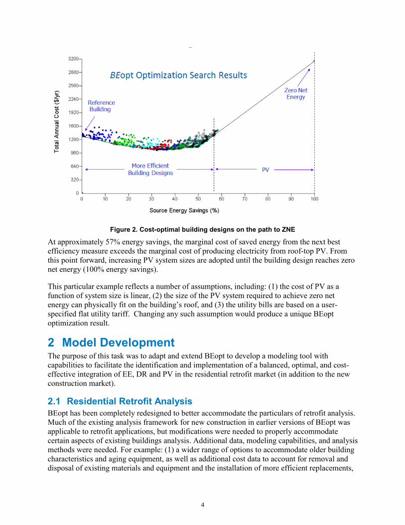
Figure 2. Cost-optimal building designs on the path to ZNE

At approximately 57% energy savings, the marginal cost of saved energy from the next best efficiency measure exceeds the marginal cost of producing electricity from roof-top PV. From this point forward, increasing PV system sizes are adopted until the building design reaches zero net energy (100% energy savings).

This particular example reflects a number of assumptions, including: (1) the cost of PV as a function of system size is linear, (2) the size of the PV system required to achieve zero net energy can physically fit on the building’s roof, and (3) the utility bills are based on a user-specified flat utility tariff. Changing any such assumption would produce a unique BEopt optimization result.

2 Model Development The purpose of this task was to adapt and extend BEopt to develop a modeling tool with capabilities to facilitate the identification and implementation of a balanced, optimal, and cost-effective integration of EE, DR and PV in the residential retrofit market (in addition to the new construction market).

2.1 Residential Retrofit Analysis BEopt has been completely redesigned to better accommodate the particulars of retrofit analysis. Much of the existing analysis framework for new construction in earlier versions of BEopt was applicable to retrofit applications, but modifications were needed to properly accommodate certain aspects of existing buildings analysis. Additional data, modeling capabilities, and analysis methods were needed. For example: (1) a wider range of options to accommodate older building characteristics and aging equipment, as well as additional cost data to account for removal and disposal of existing materials and equipment and the installation of more efficient replacements,

4

had to be provided; (2) to properly evaluate the cost effectiveness of retrofit packages involving replacement of components before the end of their useful life, changes were needed in the economic calculation methodology; and (3) the effect of reduced loads (from envelope improvements) on the performance of existing heating, ventilation, and air conditioning (HVAC) equipment needed to be evaluated, because improvements can result in oversized rather than the right-sized equipment assumed for new construction.

In previous versions of BEopt, the objective of optimization was to minimize homeowner energy-related cash flow. Cash flow was calculated as the sum of utility bill costs and increased mortgage costs to cover the payments for efficiency and PV. For energy efficiency measures (EEMs) with lifetimes shorter than the analysis period (typically 30 years), replacement costs were included by calculating present values and then annualizing them. For retrofit analysis, separate (cash or loan) financing needs to be accommodated because mortgage financing will not be applicable unless the improvements are folded into a whole-house refinance. In the BEopt-CA (Ex) model the pre-retrofit house is used as the reference (rather than the benchmark house that is used for new construction analysis). Additional potential customer metrics include life cycle cost, net present value (NPV), return on investment (ROI), etc.

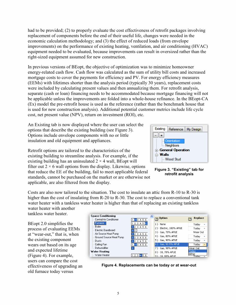
An Existing tab is now displayed where the user can select the options that describe the existing building (see Figure 3). Options include envelope components with no or little insulation and old equipment and appliances.

Retrofit options are tailored to the characteristics of the existing building to streamline analysis. For example, if the existing building has an uninsulated 2 × 4 wall, BEopt will filter out 2 × 6 wall options from the display. Likewise, options that reduce the EE of the building, fail to meet applicable federal standards, cannot be purchased on the market or are otherwise not applicable, are also filtered from the display.

Costs are also now tailored to the situation. The cost to insulate an attic from R-10 to R-30 is higher than the cost of insulating from R-20 to R-30. The cost to replace a conventional tank water heater with a tankless water heater is higher than that of replacing an existing tankless water heater with another tankless water heater.

BEopt 2.0 simplifies the process of evaluating EEMs at “wear-out,” that is, when the existing component wears out based on its age and expected lifetime (Figure 4). For example, users can compare the cost effectiveness of upgrading an old furnace today versus

Figure 3. “Existing” tab for retrofit analysis

Figure 4. Replacements can be today or at wear-out

5

upgrading the furnace when the existing one wears out. If replace at “wear-out” is selected, the option for the Existing tab is combined with the upgrade option to calculate energy and costs over the analysis period.

For calculating energy savings and cost, BEopt 2.0 introduces a new automated reference called “Existing (w/ Min Replace)” that is intended to represent the “do-nothing” baseline (Figure 5). In general, this reference matches the options of the existing building; however, in categories where the existing building’s option does not meet code or cannot be purchased on the market (e.g., a SEER 8 air conditioner), the reference includes the minimum replacement option (SEER 13) at wear out. By defining such

a reference, we ensure that energy savings for an upgraded air conditioner (e.g. SEER 15) is calculated fairly given the most typical baseline scenario for the analysis period (as opposed to using the SEER 8 air conditioner’s energy use for the entire analysis period).

2.2 Retrofit Energy Efficiency Measures and Cost Data Previous versions of BEopt included a wide range of EEMs appropriate for new residential construction. Some (but not all) of these would be applicable to the retrofit of existing homes. For example, when considering window replacement, the range of window types in BEopt could be evaluated to find the most cost-effective retrofit option based on climate. For walls, however, most of the BEopt options for new construction would not be applicable to a retrofit, and therefore new retrofit-specific EEMs (e.g., blowing insulation into wall cavities or adding exterior foam insulation) needed to be added (see Figure 6). In addition to the cost of the insulation material, other costs need to be considered such as repainting following “drill and fill” operations or replacing exterior cladding for exterior foam applications.

Additional types of retrofit-specific cost data are required for retrofit analysis. For new home analysis, BEopt included libraries of efficiency costs and lifetimes for EEMs. For retrofit analysis, however, installation costs are also needed, because cost-effectiveness calculations must include not just the incremental cost of materials (window type A versus window type B, for example), but also the cost of labor to remove and replace the windows and in some cases the cost of disposal.

Figure 6. Example efficiency options for walls

Figure 5. The reference building can include minimum

future upgrades

6

2.2.1 National Residential Efficiency Measures Database BEopt 2.0 is fully integrated with the National Residential Efficiency Measures Database (NREMDB). This public database, developed by the National Renewable Energy Laboratory (NREL), provides a centralized source of residential building measures and costs (Figure 7).

By coordinating with this database, BEopt can bring additional accuracy and standardization to its data in terms of costs, component properties, appropriate retrofit measures, etc. The database also includes disaggregated labor and material costs, which enables BEopt to adjust option costs to various retrofit situations. Results of a study completed for this project assessing detailed retrofit cost data specific to California are provided in Appendix A. These data serve to supplement the NREMDB data.

2.3 Utility Tariff Capabilities Previous versions of BEopt allowed input of flat utility rates for electricity and natural gas only, either as (1) the selection of a national or state average rate based on U.S. Energy Information Administration (EIA) data; or 2) as a user-specified input value, and in either case, a user-specified fixed monthly charge (Figure 8). BEopt has been modified to allow use of typical California utility tariffs (including tiered, time-of-use [TOU], or tiered TOU). BEopt users can now select from 5,744 (as of January 2014) residential utility tariffs (including 52 California tariffs) downloaded from the U.S. Utility Rate Database (URDB) hosted on NREL’s OpenEI.org website. Utility tariffs can be quickly searched by zip code and filtered by whether the utility is an investor-owned utility (IOU) or not.

Figure 7. BEopt uses cost data from the National Residential Efficiency Measures Database

7

2.3.1 Custom Utility Tariffs To allow users to explore custom utility tariffs (or tariffs not found in the URDB), NREL implemented a Utility Rate Wizard in BEopt (Figure 9 and Figure 10). Custom rates can be structured as tiered, TOU, tiered TOU, or hourly real-time pricing (RTP). The interface allows the user to quickly define up to 12 TOU periods or seasons and up to six tiers per period (Figure 11), or enter 8,760 hourly data (Figure 12). Fixed charges and/or minimum bill charges can also be defined. The utility rate wizard enables analysis of a variety of utility tariff structures and their effects on cost effectiveness under the various California utility cost test metrics.

Figure 9. Utility Rate Wizard: TOU example

Figure 8. Detailed utility tariffs inputs

8

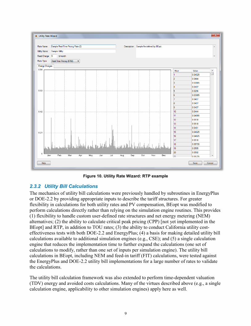
Figure 10. Utility Rate Wizard: RTP example

2.3.2 Utility Bill Calculations The mechanics of utility bill calculations were previously handled by subroutines in EnergyPlus or DOE-2.2 by providing appropriate inputs to describe the tariff structures. For greater flexibility in calculations for both utility rates and PV compensation, BEopt was modified to perform calculations directly rather than relying on the simulation engine routines. This provides (1) flexibility to handle custom user-defined rate structures and net energy metering (NEM) alternatives; (2) the ability to calculate critical peak pricing (CPP) [not yet implemented in the BEopt] and RTP, in addition to TOU rates; (3) the ability to conduct California utility cost-effectiveness tests with both DOE-2.2 and EnergyPlus; (4) a basis for making detailed utility bill calculations available to additional simulation engines (e.g., CSE); and (5) a single calculation engine that reduces the implementation time to further expand the calculations (one set of calculations to modify, rather than one set of inputs per simulation engine). The utility bill calculations in BEopt, including NEM and feed-in tariff (FIT) calculations, were tested against the EnergyPlus and DOE-2.2 utility bill implementations for a large number of rates to validate the calculations.

The utility bill calculation framework was also extended to perform time-dependent valuation (TDV) energy and avoided costs calculations. Many of the virtues described above (e.g., a single calculation engine, applicability to other simulation engines) apply here as well.

9

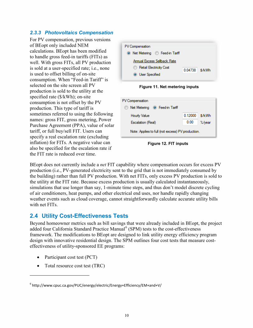
2.3.3 Photovoltaics Compensation For PV compensation, previous versions of BEopt only included NEM calculations. BEopt has been modified to handle gross feed-in tariffs (FITs) as well. With gross FITs, all PV production is sold at a user-specified rate; i.e., none is used to offset billing of on-site consumption. When “Feed-in Tariff” is selected on the site screen all PV production is sold to the utility at the specified rate ($/kWh); on-site consumption is not offset by the PV production. This type of tariff is sometimes referred to using the following names: gross FIT, gross metering, Power Purchase Agreement (PPA), value of solar tariff, or full buy/sell FIT. Users can specify a real escalation rate (excluding inflation) for FITs. A negative value can also be specified for the escalation rate if the FIT rate is reduced over time.

BEopt does not currently include a net FIT capability where compensation occurs for excess PV production (i.e., PV-generated electricity sent to the grid that is not immediately consumed by the building) rather than full PV production. With net FITs, only excess PV production is sold to the utility at the FIT rate. Because excess production is usually calculated instantaneously, simulations that use longer than say, 1-minute time steps, and thus don’t model discrete cycling of air conditioners, heat pumps, and other electrical end uses, nor handle rapidly changing weather events such as cloud coverage, cannot straightforwardly calculate accurate utility bills with net FITs.

2.4 Utility Cost-Effectiveness Tests Beyond homeowner metrics such as bill savings that were already included in BEopt, the project added four California Standard Practice Manual6 (SPM) tests to the cost-effectiveness framework. The modifications to BEopt are designed to link utility energy efficiency program design with innovative residential design. The SPM outlines four cost tests that measure cost-effectiveness of utility-sponsored EE programs:

• Participant cost test (PCT)

• Total resource cost test (TRC)

6 http://www.cpuc.ca.gov/PUC/energy/electric/Energy+Efficiency/EM+and+V/

Figure 11. Net metering inputs

Figure 12. FIT inputs

10

• Ratepayer impact measure test (RIM)

• Program administrator cost test (PAC).

The cost tests can each be calculated in three ways: (1) as a NPV of total benefits minus total costs; (2) a ratio of total benefits to total costs; or (3) as a total levelized cost. Each test reflects cost-benefit analysis of the program from a different perspective and is calculated from a different set of inputs. The inputs for all tests fall into the following categories:

• Avoided cost information

• Financial information

• Incentives to consumers

• Bill impact information

• Retrofit cost information

• Program cost information

• Energy savings and impact information. A detailed write-up of all cost test descriptions and formulas is included in Appendix B. A detailed spreadsheet quality assurance/quality control tool was developed and used to verify cost test results generated in BEopt.

2.4.1 Alternative Implementations There were two possible approaches to calculating utility cost tests: (1) performing the calculations externally based on BEopt outputs; and (2) incorporating the calculations directly into BEopt. Each approach has advantages and disadvantages. In the early stages of the project, the project team delved into the details, evaluated the pros and cons of each approach, and concluded that there was value in implementing both.

2.4.1.1 External Cost Test Calculation This external approach involved creating a special version of the E3 Calculator, the standard tool currently used to perform cost test calculations in California, to calculate cost tests directly from BEopt outputs. BEopt has been modified to create a .csv output report that contains all the variables necessary to calculate each of the four cost tests. Using those outputs and climate-zone-specific California avoided costs, the BEopt E3 Calculator calculates each of the four cost tests in each of the three formats described above: NPV, benefit-cost ratio, and levelized cost. The BEopt E3 Calculator’s output screen is shown in Figure 13. To correctly calculate the RIM, TRC, and PAC tests for a utility program, the user must additionally input the total program administration and implementation costs and the number of homes in the program. All cost tests in the BEopt E3 Calculator are performed on a per-home basis.

11

Figure 13. BEopt E3 Calculator cost test outputs

This approach provided an external means of validating that the cost test calculations were correctly implemented in BEopt (second approach, described below) for a range of scenarios (different climate zones, with and without PV, etc.).

2.4.1.2 Internal Cost Test Calculation The second approach to incorporating the SPM cost tests into BEopt involved implementing the calculations directly within the program, facilitating optimizing over the various cost test metrics. When performing an optimization in BEopt, the user can select which cost test will be used as the optimized variable; the results can be optimized for any of the four cost tests. Additionally, regardless of which cost test is selected for optimization, BEopt’s results can be displayed in terms of any of the other cost tests, as either NPVs or benefit/cost ratios. An example optimization output is shown in Figure 14.

Figure 14. BEopt output for utility cost-effectiveness test (TRC example)

To support the integration of the SPM cost tests into BEopt, California’s avoided costs were included in the software. Gas and electricity avoided costs are included for each climate zone form 2013 through 2052, allowing BEopt to calculate utility avoided costs over a 40-year analysis period.

12

2.5 Incentives: Photovoltaics and Whole-House Energy Efficiency BEopt was upgraded to allow users to input detailed information about incentives, in the form of rebates or tax credits, for EE and PV (see Appendix C for additional information). The interface can accommodate fairly elaborate incentive programs. Screenshots of BEopt’s EE and PV incentive inputs are shown in Figures 15 and 16 for PV and EE, respectively.

Whole-building7 EE rebates or tax credits for either gas or electricity savings can be entered as a flat amount, a percent of the EEM’s capital cost, a value per kilowatt-hour of energy savings, or combinations thereof. For each type of incentive, the value can be either constant or tiered.

PV rebates or tax credits can be entered as a flat amount, a percent of the PV system capital cost, a value per kilowatt-hour of electricity production, a value per Watt of PV installed, or combinations thereof. This flexibility allows BEopt to accommodate the California Solar Initiative’s (CSI) performance based rebate and upfront rebate, for example. PV incentive programs whose rebates are linked to EE savings can also be handled -- incentives can be entered as a function of one or more electricity savings levels.

7 Some EE incentive programs are defined on a measure-by-measure basis rather than a whole-house approach; future versions of BEopt may accommodate measure-by-measure EE incentives.

Figure 15. Efficiency incentives inputs

Figure 16. PV incentives inputs

13

PV and EE tax credits can be designated as either state or federal, and rebates can be designated as state, federal, utility or other. These designations are important for correctly calculating the cost tests in BEopt. Federal tax credits of 30% for PV are enabled by default.

2.6 California Metrics Project Type To use the new BEopt capabilities for utility cost-effectiveness tests and incentives, the user can choose the California Metrics project type when creating new projects, either when initially launching BEopt or from the main toolbar when BEopt is already running (Figure 17). This project type allows the calculation of individual project and program cost effectiveness for any of the standard California utility cost test metrics: the TRC, PCT, RIM, and PAC. These four tests measure the cost effectiveness of utility ratepayer-funded EE programs, per the California SPM. The project type also defaults the interface in various ways, such as defining the California Solar Initiative PV rebate, and otherwise simplifies the interface for analysis of California utility cost tests.

When the California Metrics project type is chosen, the interface is changed in the following ways:

1. Only California climate zone weather files are displayed in the EPW Location dropdown. Additional inputs on the Site input screen are then made available depending on the climate zone selected:

a. Net -to-Gross Ratio

b. Program Cost (Present Value)

c. CA Climate Zone: Utility (Figure 18)

d. CA Climate Zone: Region (Figure 19).

2. The y-axis output metric for both display and optimization defaults to Total Resource Cost Test, NPV. This can be overridden on a case-by-case basis when running BEopt, or the default can be changed under Cost/Energy Graph Settings. Specifically, the user can optimize the project for maximizing the NPV of any of the four cost tests: TRC, PCT, RIM, and PAC.

The y-axis metric can be selected to show either the NPV or the benefit-cost ratio for any cost test. However, optimizations are based on NPV (not benefit-cost ratio).

3. The x-axis output metric for both display and optimization defaults to TDV Energy Savings. This can be overridden on a case-by-case basis when running BEopt, or the

Figure 17. California Metrics project type

Figure 18. Climate zone utility input

Figure 19. Climate zone utility/region inputs

14

default can be changed under Cost/Energy Graph Settings. The full set of additional metrics that becomes available beyond source energy and site energy metrics is:

a. TDV Energy Savings

b. TDV Energy Consumption

4. The End Use graph gets an addition TDV Energy metric.

5. The marginal state income tax rate is defaulted to 9.3%.

6. The CSI PV rebate program is enabled by default. The program specifies a performance-based rebate of $0.03/kWh for 5 years or a capacity-based rebate of $0.20/WAC. The capacity-based incentive is enabled by default, but the user can easily switch to using the performance-based rebate (or disable the program rebates altogether).

7. Net-metered annual excess sellback rates (referred to as Net Surplus Compensation in California) are defaulted based on the choice of CA climate zone utility. The values, as of February 2014, are:

a. PG&E: $0.04396/kWh

b. SCE: $0.04738/kWh

c. SDG&E: $0.04680/kWh

8. The user cannot enter a value greater than 40 years for the analysis period (for which avoided cost factors are available).

2.7 Demand Response Existing and emerging mechanisms for residential DR include: direct load control (DLC), voluntary load reduction (VLR), and automated load control (ALC). DLC involves utility-controlled switches for air conditioner cycling or pool pump cycling. VLR relies on occupants changing their behavior, typically on peak event days, in response to incentivizing price signals, such as TOU rates, CPP, and critical peak rebates (CPR). ALC involves smart appliances automatically shifting load in response to the price signals mentioned above. ALC can also include smart thermostats that change set point during peak events or pre-cool homes in anticipation of peak events. A full characterization of the opportunities for residential DR in California is included in Appendices D and E.

This research effort focused on currently available DR technologies—applications that can be put in the field in the relatively near term. However, by introducing a DR module in BEopt, the project created a platform that can be used to evaluate emerging DR applications as DR and smart grid technologies mature.

The project team modified BEopt to include DR measures that shift loads away from peak times. The measures are defined by either a 24-hour schedule (weekday and/or weekend) and monthly schedule or an annual schedule of 8,760 hourly values. Each measure also allows specification of a penetration rate, which is the fraction of homes in the analysis that employ DR. The actual schedule used during DR events combines non-DR and DR schedules using the penetration rate, allowing the user to quickly perform what-if analysis with different penetration rates for each DR

15

measure. DR measures were implemented for thermostats, major appliances, and miscellaneous electric loads.

2.7.1 Large, Uncommon Miscellaneous Electric and Gas Loads In previous versions of BEopt, all electric loads not explicitly accounted for in the Space Conditioning, Water Heating, and Major Appliances (Refrigerator, Range, Dishwasher, Clothes Washer, Clothes Dryer) categories were lumped into a single variable for “Miscellaneous Electric Loads.” To make additional loads available for DR, several large, uncommon loads (i.e., pool pumps/heater, spa pumps/heaters, well pumps, second fridges, and standalone freezers) were disaggregated from the Miscellaneous Electric Loads category into separate categories (Figure 20).

Previously hardcoded schedules were also exposed in the interface for both major appliances and large, uncommon loads categories. These new interface inputs and schedules were connected to the simulation engines for energy use calculations, sensible/latent gains to the space, and scaling with number of occupants and home floor area (as appropriate).

In each of these categories, the benchmark option has a fractional number of units representing a national average for the load, where some of the homes have the load and some do not. For non-benchmark analysis, options can have zero or full loads depending on whether the equipment is present in the house being simulated.

2.7.2 Demand Response Schedules and Signals BEopt ships with example DR measures and schedules and also facilitates user-specified schedules (including schedules defining DR behavior of appliances and occupants) via the new Schedule Wizard (see Figure 21). The Schedule Wizard provides a graphical view of the schedule inputs and streamlines the process of defining custom schedules. Schedules can be defined in either a simplified format (weekday/weekend hourly profiles plus monthly variation) or in a detailed format (8,760 hourly values).

Figure 20. Large uncommon loads

16

Figure 21. Schedule Wizard: DR (bars) and non-DR (line)

DR programs that use DLC, CPP, or CPR often take the form of 10–20 event days, with the same timing and duration of the “critical peak” period on each of those days (Figure 22). Algorithms to identify event days were developed and incorporated into BEopt. The algorithms use either California TDV values (daily maximum or average) or outdoor temperatures (daily maximum or average). Users can specify the number of event days, and whether days can fall on weekdays, weekends, or both. Some utilities, for example, may only see critical peak loads when outdoor temperatures are high and on weekdays (e.g., when additional commercial loads are occurring).

If DR measures are selected for use in the analysis, BEopt will employ the DR schedules (combined with the non-DR schedules based on the penetration rate) on the identified event days.

2.8 Modeling Framework (Batch Simulations) The open-architecture modeling framework in BEopt 2.0 has been completely revamped. Simulation input files are now generated (and output files are parsed) via the open-source Python scripting language. This language provides a rich set of capabilities that can be leveraged for many purposes.

Figure 22. DR event inputs

17

Most significantly, the new BEopt modeling framework allows for batch simulation; that is, buildings can be easily defined and automatically simulated through either DOE-2.2 or EnergyPlus without using the BEopt interface. This allows power users to automate and integrate the BEopt modeling framework into their own analysis workflow. For example, one could automate the process of simulating buildings for a database of existing buildings to compare simulation results against utility bills.

The modeling framework includes capabilities for generating DOE-2.2 and EnergyPlus input files, performing HVAC sizing calculations consistent with ACCA Manual J, generating HPXML files, obtaining data from weather files, etc. For more details, see the Modeling Framework section in the BEopt Help file.

BEopt 2.0 can also automatically make use of computers with multiple processors when running EnergyPlus and DOE-2.2 simulations. BEopt defaults to using one less than the total number of processors on the machine; alternatively, users can override this default and specify the number of processors to use under the Tools > Options menu.

3 Model Validation/Calibration Previous studies8 have indicated a tendency for building energy simulation models to overpredict energy consumption for existing homes and to overpredict retrofit energy savings, resulting in retrofit savings program realization factors significantly less than 1. The purpose of this task was to provide statistically relevant data from typical California communities and software-to-software methods to validate, or as needed, calibrate, the BEopt model.

3.1 Energy Use Data Appendix F describes an effort to develop end use data obtained from older California communities for use in calibrating the BEopt-CA (Ex) model to improve confidence in use of the model for predicting energy savings for retrofit programs. Two communities, located in Stockton and Pleasanton, were selected to supply billing data for this purpose. To provide some control over the characteristics of the homes such as vintage and size, lists of addresses for each community were provided to PG&E, which supplied billing data from which account numbers, addresses, and specific billing periods (except the month) had been stripped. Separate records, but for the same homes, were provided for gas and electric energy use. The original records included 1,258 houses in Stockton and 264 houses in Pleasanton. Information from the Zillow database was used to identify the range of vintages, floor areas, and number of bedrooms for houses in the dataset.

Davis Energy Group applied previously developed methods to isolate outliers and to develop mean electric and gas energy use values.9 Outliers in four categories were filtered out. For example, homes that were likely to have swimming pools, and those that were judged to have

8http://www.calmac.org/publications/Final_Version_of_04-05_CAESNH_report.pdf 9 Project Closeout: Guidance for Final Evaluation of Building America Communities. NREL/TP-550-42448. 2008.

18

been unoccupied for more than 1 month were filtered from the main body of data. To provide more granular data for the calibration process, analysis methods similar to PRISM10 were used to separate total electric and gas energy use into end uses such as space conditioning, water heating, lighting, and appliance uses. To disaggregate the data into the various end uses it was necessary to adapt existing methods that require house characterization information and specific billing periods, and develop new methods that would improve accuracy. After filtering the data, base loads were identified and linear regression methods were used to determine heating/cooling transition months and to separate heating and cooling energy use from other end uses. A sensitivity analysis was completed to verify that variations in base load disaggregation factors have minor impact on disaggregated heating and cooling load quantities.

Electric end use categories include lighting, air conditioning, heating (furnace fan), and miscellaneous (including appliances and plug loads). Gas end use categories include space heating, water heating, and miscellaneous (including range/stove). Estimates of specific end use quantities, for example lighting loads, were obtained from the Building America House Simulation Protocols and used to separate lighting from miscellaneous end uses. Data from field monitoring studies were used to separate water heating end uses from baseline gas use.

Two disaggregation methods were tested: one that used filtered data to develop disaggregated use for each house/record and then averaged the end use results, and another that first averaged the electricity and gas uses from the filtered data for all houses/records and then applied disaggregation methods to the averaged datasets. The former method is much more time intensive but yielded a higher level of apparent accuracy for disaggregating electricity use than the simpler method. The simpler method appears to be adequate for disaggregating gas use for the two datasets and northern California communities that were evaluated.

Comparison of the results of this study to the Residential appliance Saturation Survey (RASS) data for all of PG&E’s service territory, which covers several California climate zones, suggests that differences in end use energy consumption in this area may be large enough to justify developing utility EE programs that are climate zone (or even community) specific. BEopt can be used to identify customer and utility cost parameters that can aid in the structuring of programs that are specific to communities in similar climate regions, and perhaps of particular vintages.

10 Princeton Scorekeeping Method

19

3.2 BEopt Test Suite for Comparing Simulation Engines Results The BEopt Test Suite automatically launches thousands of detailed simulations while systematically sweeping through all available building components (walls, windows, appliances, air conditioners, water heaters, etc.) one at a time in both simulation engines, allowing the impacts of individual building component changes in each engine to be compared (Figure 23). These components are evaluated in the context of typical new construction and existing buildings and a diagnostic test building with features (super-insulated envelope, zero infiltration, ideal

Figure 23. BEopt Test Suite visualization inputs/output

heating/cooling equipment) that allow the impacts of specific options to be isolated for targeted comparisons between engines. All buildings are simulated in a range of climates (weather files) to evaluate the simulation engines’ response to environmental conditions. A rich visualization tool facilitates quickly identifying discrepancies in simulation engine output, disaggregated by end uses.

NREL recently made a number of enhancements to the test suite visualization capability to facilitate identifying discrepancies between simulation engines. The new test suite viewer can now graph more than two test suite results at a time, filter graphs by end use, and dynamically graph data.

20

4 California Simulation Engine The standard version of BEopt relies on detailed calculations from an underlying building energy simulation engine, either EnergyPlus or DOE-2.2. Recently, a new residential building energy simulation engine, CSE, has been under development with CEC funding for deployment with the 2013 California Title 24 standards.

4.1 Connecting BEopt to the California Simulation Engine There would be a number of advantages to a version of BEopt that worked with CSE: (1) the ability to test CSE by comparison to EnergyPlus through the BEopt Test Suite; (2) parametric (and optimization) capabilities for CSE that could be used in Title 24 development; (3) the ability to compare CSE results with the other models that are used nationally, such as for the DOE Challenge Home program11; and (4) potentially as a front end for a CSE-based Title 24 user tool.

NREL worked to establish the connection of BEopt to CSE.12 As when connecting BEopt to any new simulation engine, this required two tasks: (1) modifying the BEopt source code to be able to call CSE executables; and (2) mapping BEopt inputs/outputs to CSE inputs/outputs. The mapping process creates equivalent building model inputs between two simulation engines by creating corresponding input parameters for each engine for a given set of BEopt inputs. NREL adapted the BEopt-EnergyPlus workflow to accommodate CSE as shown in Figure 24:

Figure 24. BEopt-CSE automated workflow for running CSE simulations

11 The California Advanced Home Program is planning to award additional incentives to Challenge Home builders. 12 With CSE under development to serve as the residential simulation engine for Title -24, the CSI project manager recommended and approved a scope of work change directing the project team to work on coupling BEopt to CSE with potential applications to: CSE testing, development of a Title -24 parametric tool, and development of BEopt as a front-end for CSE. The BEopt/CSE coupling for software testing was completed consistent the CBECC-Res 2013 version 0t Beta, which was released on April 9th, 2013. Further BEopt/CSE work may be funded by the California Energy Commission (rather than CSI RD&D).

21

In the process of running a CSE simulation, BEopt first generates a building description .xml file from a test suite building definition, which includes the building geometry, occupancy, and envelope/equipment technologies. Next, the cseInput.py python script maps the BEopt modeling inputs to a *.ribd input file for the California Building Energy Code Compliance (CBECC) software. BEopt then calls CSE via a cbecc.exe command line executable. The resulting CSE output file is parsed via a cseOutput.py script and translated into the output xml file format expected by BEopt. Finally, the results are stored in a SQLite database for easy querying. By producing a *.ribd CBECC input file (as opposed to a CSE input file), BEopt can automatically create input files that comply with CSE’s Compliance Manager and Title 24.

Much of the effort to connect BEopt to CSE involves mapping the BEopt inputs to CSE inputs for building geometry, technology options, and occupancy and operating assumptions. NREL worked with CSE development team to identify undocumented capabilities or workarounds for perceived CSE deficiencies and obtain information about CSE default values/assumptions/models.

Using the CBECC-Res 2013 version 0t Beta, which was released on April 9, 2013, NREL successfully mapped the following parameters:

• General: Weather file, building geometry, orientation, occupancy

• Envelope: Walls, ceilings, roofs , slab foundation, windows, exterior shading, exterior finish, internal thermal mass, material thermal properties

• Appliances, lighting, and miscellaneous loads: Refrigerators, clothes washers/dryers, cooking ranges, dishwashers, lighting, other electric/gas loads

• HVAC equipment and ventilation: Gas furnaces, split air conditioners, mechanical ventilation, ducts

• Water heating: Gas, propane, and electric tank and tankless water heaters, fuel oil tank water heaters, heat pump water heaters, hot water distribution (including recirculation).

NREL also modified the EnergyPlus modeling process to incorporate Title 24 occupancy and operating assumptions rather than Building America assumptions; this allows for a comparison of the different algorithms used by each simulation engine based on a consistent set of assumptions. (Note: some additional technologies in BEopt that were not available in CSE at the time of implementation have since been added to subsequent CBECC-Res releases.)

NREL also developed an artificial weather file (usable for both CSE and EnergyPlus) to compare both engines under different environmental conditions. The artificial weather file includes quasi-steady weather conditions for 2-week periods, facilitating diagnostic investigations and isolating of modeling algorithms. Initial CSE and EnergyPlus simulations for a simple “shoebox” house have been performed, but extensive use of the BEopt Test Suite has not been performed to date. Appendix G summarizes the current status of the implementation of capabilities to compare CSE to EnergyPlus to aid in the validation of CSE.

22

5 Example Analysis Results Example analysis results are shown in this section to demonstrate some of the new BEopt capabilities developed for California. The results presented here are not intended as policy analysis; in fact, they are sensitive to a number of assumptions and could change significantly over a range of plausible inputs.

As described in Appendix H, optimizations were run for three types13 of utility rates: typical 4-tier, illustrative 2-tier and illustrative time-of-use for two utilities (PG&E and SCE). The typical rates are representative of commonly used existing rates in 2013. The illustrative rates are representative of possible future rates. For the three utility rates, optimizations were run for combinations of two California climates (Sacramento and Riverside) and two energy use levels (high and low).

The results in this section are for gas/electric homes with PG&E rates and high energy use in Sacramento. TRC and RIM results, as well as PCT results, are for PCT-optimal building designs. If the building designs were instead optimized for maximum TRC, slightly different building designs (more optimal for TRC) would be found during the optimization process and TRC results would be somewhat improved, whereas the corresponding PCT results would be slightly less optimal. The PCT optimizations were performed as a function of TDV Savings (the California metric for ZNE), and the results are plotted versus TDV savings.

5.1 Participant Cost Test, Typical 4-Tier Utility Rate Figure 25 shows PCT results with the typical 4-tier utility rate (PG&E) for a gas/electric home with high energy use in Sacramento. Three distinct regions are apparent in the cost-optimal curve: (1) for TDV savings of approximately 0%–40% PCT values increase to nearly $16,000 as EE improvements are added to the house; (2) beyond approximately 40%, PCT values decrease as PV is added to the house in 1-kW increments; and (3) beyond approximately 95%, PCT values decrease more rapidly, because under net metering the homeowner is compensated for excess annual electricity production at a fraction of the lowest tier rate.

Between approximately 40% and 95%, the rate of decrease in PCT values is not perfectly constant, because two offsetting effects are in play: (1) PV costs per kilowatt in BEopt decrease as system sizes increase (economies of scale), which tends to flatten the slope of the curves; and (2) as the PV system size increases and TDV savings increase, the electricity savings occur at lower tiered rates, so the curve tends to slope more steeply downward. The more-or-less constant slope indicates that, in this case, these two effects approximately offset each other.

13 Staff Proposal for Residential Rate Reform in Compliance with R.12-0-013 and Assembly Bill 3276, California Public Utilities Commission, Energy Division, January 3, 2014

23

Figure 25. Gas/electric home PCT results for typical 4-tier rate

The slope is expected to curve downward at 100% annual electricity savings, when the PV compensation shifts to the low value of the NEM annual excess rate. The exact position of the slope-change point in the figure (at approximately 95% TDV savings), however, is the result of two offsetting effects:

• For the gas/electric house in this case, achieving 100% ZNE requires PV over-production sufficient to offset gas consumption TDV. This tends to move the slope-change point to the left.

• The x-axis shows TDV savings, not electricity savings, which are not equivalent. For all-electric houses (see Appendix H), the slope-change point occurs to the right of 100% TDV savings, implying that EE (and particularly the PV) lead to extra TDV savings relative to electricity savings. This tends to move the slope-change point to the right.

In this particular scenario, the first effect is slightly greater than the second.

5.2 Participant Cost Test, Illustrative 2-Tier Utility Rate Figure 26 shows PCT results with the illustrative 2-tier utility rate (PG&E) for a gas/electric home with high energy use in Sacramento. In this case, after EE (approximately 0%–40% TDV savings), the PCT values do not decline as in the 4-tiered utility rate case, because the energy savings are less subject to decreasing tier rates. The PV economies of scale effect can be seen in the initial decrease in PCT for the first 1 kW of PV followed by subsequent increases for additional PV increments. The fact that the slope is approximately horizontal is merely coincidental based on case parameters: PV costs, solar resource, utility rate, economic assumptions, etc.

24

Figure 26. Gas/electric home PCT results for illustrative 2-tier rate

5.3 Participant Cost Test, Illustrative Time-of-Use Utility Rate Figure 27 shows PCT results with the illustrative TOU utility rate (PG&E) for a gas/electric home with high energy use in Sacramento. In this case, after no change for the relatively high-cost first 1-kW PV increment, PCT values increase for 1–4 kW of PV. The slope change point occurs at lower TDV savings (at approximately 85%, compared to 95% for the other utility rates), because TOU rates put high values on PV production, which result in monthly credits ($) carried forward, so that so that net energy charges reach zero at lower % TDV savings.

Figure 27. Gas/electric home PCT results for illustrative TOU rate

5.4 Participant Cost Test, All Rates Figure 28 shows the PCT-optimal curves from Figures 25, 26, and 27 without the non-optimal points. As TDV savings increase, the 4-tier utility rate curve peaks with high PCT early and then declines. The illustrative TOU curve has the opposite trend, and the 2-tier curve is relatively flat. One interpretation, for this particular case, is that the 4-tier rate is more favorable for EE-based

25

designs and the TOU rate is more favorable for designs that also include PV and approach ZNE. The 2-tier rate is neutral (break-even) regarding the PCT values of PV.

Figure 28. Gas/electric home PCT-optimal curves for three utility rates

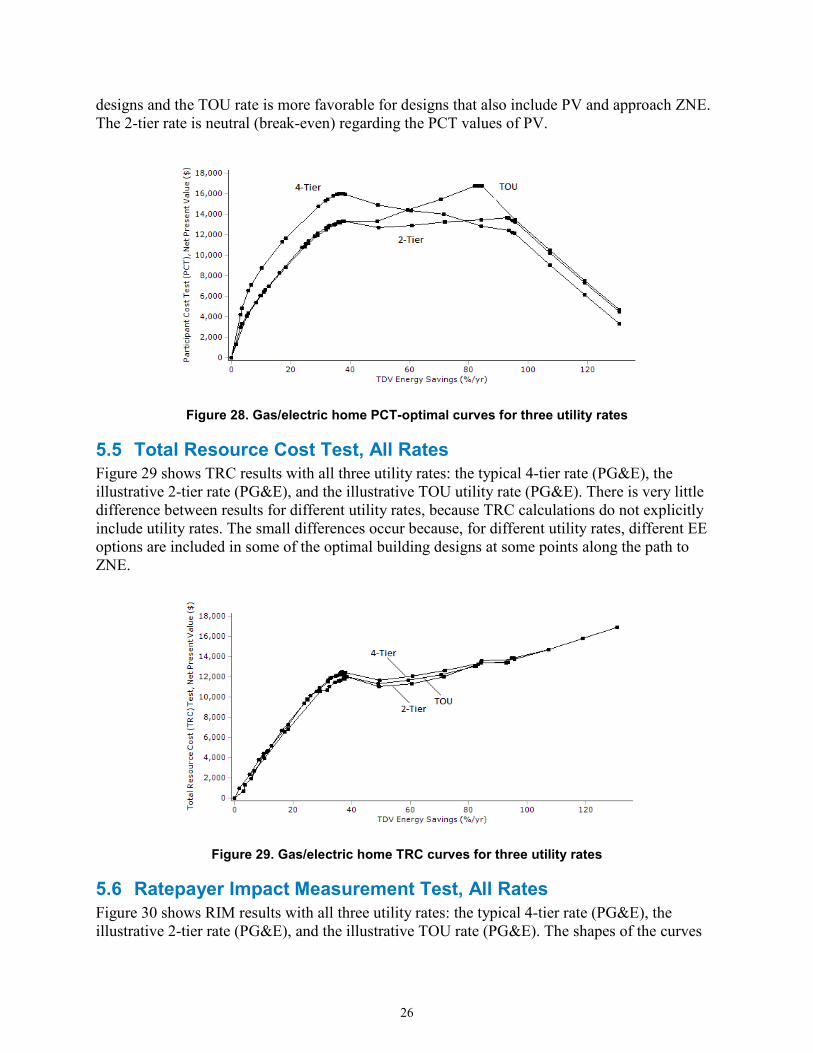
5.5 Total Resource Cost Test, All Rates Figure 29 shows TRC results with all three utility rates: the typical 4-tier rate (PG&E), the illustrative 2-tier rate (PG&E), and the illustrative TOU utility rate (PG&E). There is very little difference between results for different utility rates, because TRC calculations do not explicitly include utility rates. The small differences occur because, for different utility rates, different EE options are included in some of the optimal building designs at some points along the path to ZNE.

Figure 29. Gas/electric home TRC curves for three utility rates

5.6 Ratepayer Impact Measurement Test, All Rates Figure 30 shows RIM results with all three utility rates: the typical 4-tier rate (PG&E), the illustrative 2-tier rate (PG&E), and the illustrative TOU rate (PG&E). The shapes of the curves

26

are similar to the inverse of the PCT results in Figure 28, because high PCT values for participants translate to more negative RIM values for ratepayers in general. For example, from 0%–60% TDV savings with significant consumption in high tiers, the 4-tier rate RIM values are more negative than the other rate types.

Figure 30. Gas/electric home RIM curves for three utility rates

6 Conclusions This project targeted the development of a software tool, BEopt-CA (Ex), which aims to facilitate balanced integration of EE, DR, and PV in the residential retrofit market. The intent of the software tool is to provide utility program managers and contractors in the EE/DR/PV market place with a means of balancing the integration of EE, DR, and PV within the residential retrofit market.

NREL’s existing BEopt software was enhanced by adding capabilities in the following areas: existing home retrofit analysis, retrofit measures and cost data, utility tariff capabilities, utility cost-effectiveness tests, incentives for PV and whole-house EE, and DR. The BEopt-CA (Ex) capabilities are available in the public version of BEopt (https://beopt.nrel.gov) and can be accessed by selecting the California-specific mode upon launching the program.

As a basis for validation, parallel efforts were undertaken to: (1) develop statistically relevant end use data from two California communities; and (2) connect BEopt to the new CSE to facilitate software-to-software comparisons via the BEopt Test Suite.

6.1 Market Connection and Benefits for California Ratepayers The project addresses and aims to resolve one of the major “gaps” in the optimization of residential upgrades to increase EE. To date, homeowners, remodelers, architects, and builders have had tools to address the relative EE of some of the proposed options for upgrading a building. However, the EE of the building as well as DR potential and on-site solar have all been analyzed separately. As a result, there has been no capability to comprehensively analyze a building’s potential. More importantly, there was no ability to prioritize how much of which

27

energy enhancement should be installed. This modeling limitation has prevented consumers from having access to the most financially attractive design options.

BEopt-CA (Ex) addresses this problem by comprehensively optimizing across these resource categories. This gives the marketplace a capability it has lacked up to now: a standard approach to choosing between EEMs, DR options, and solar. Although this does not overcome all barriers to the optimum treatment of existing homes with EE, DR and PV it facilitates clear and unequivocal analytic tradeoffs of benefits and costs. Some may still choose less cost-effective approaches to reducing overall energy use, but will now do so with the knowledge of the financial tradeoffs.

Previous and current retrofit programs such as Energy Upgrade California, which are aimed at achieving large-scale activity, have not had the desired outcome. The value proposition for homeowners has apparently not reached the critical point at which energy upgrades are widely adopted. The ability to identify that level of energy savings which, combined with incentives and other drivers, will trigger movement in the existing housing sector is of key importance to policy makers. Energy compliance models are inadequate for this purpose because they cannot assess measure costs and have characteristically been very inaccurate for predicting energy use for older, poorly insulated buildings. BEopt will be an important tool for developing future programs such as time-of-sale retrofits and for establishing incentive levels that serve utility and ratepayer objectives.

Beyond retrofit applications, BEopt is a useful tool for developing optimal measure packages for new home designs on the path to ZNE (the purpose for which BEopt was originally developed). DOE-sponsored Building America teams are routinely using it to help California builders to achieve the “ZNE ready” level of performance that the DOE Challenge Home program is aiming for. The facility with which BEopt can identify optimal combinations of measures for California’s diverse climates and the power of the EnergyPlus engine make it a desirable tool for developing cost-effective designs that provide homebuyers with the best value and that can help California achieve its 2020 ZNE goal for new homes.

For energy professionals, BEopt-CA (Ex) provides an analytically sound platform, enabling them to quantify the benefits of energy performance enhancing upgrades. The new BEopt-CA (Ex) could become a “standard” for analytic tools in use to make recommendations to homeowners by architects, designers, home rating professionals, and builders.

Utility planners can use BEopt-CA (Ex) to develop preferred cost-optimal “packages” of EE/DR/PV in planning and designing demand-side programs. These can be tailored for particular climate zones and house vintages, and optimized for subsequent solar installation. The information can be utilized to educate and incentivize consumers and delivery contactors to install balanced, comprehensive measure packages.

BEopt-CA (Ex) could also become a platform for the CPUC to review its EE, DR, and PV programs from a new, comprehensive perspective. It could then move forward with additional steps to integrate and optimize the customer-side programs within its authority (within the limits of statute).

28

Appendix A: California Retrofit Energy Efficiency Measures and Cost Data

Contents Goal and General Approach .......................................................................................................................... 1 Measures for Which Costs Were Developed ................................................................................................ 1

Category: Building Enclosure ................................................................................................................... 2 Attic/Ceiling Insulation ......................................................................................................................... 2 Roof Material ........................................................................................................................................ 2 Radiant Barrier ...................................................................................................................................... 2 Floor Insulation, under­floor, crawlspace ............................................................................................. 2 Crawlspace perimeter insulation & VB ................................................................................................ 3 Insulate wall cavities ............................................................................................................................. 3 Wall sheathing (stucco) ......................................................................................................................... 3 Window film ......................................................................................................................................... 4 Window replacement ............................................................................................................................ 4 Air Sealing ­ whole house ..................................................................................................................... 4

Category: HVAC ....................................................................................................................................... 4 HVAC Tune­up ..................................................................................................................................... 4 AC replacement, split ............................................................................................................................ 5 Furnace replacement, central interior, split ........................................................................................... 5 Heat pump replacement, central interior ............................................................................................... 5 Room air conditioner ............................................................................................................................ 5 Duct Sealing .......................................................................................................................................... 5 Duct Insulation ...................................................................................................................................... 5 Duct replacement .................................................................................................................................. 6

Water Heating ........................................................................................................................................... 6 Storage replacement, standard ............................................................................................................... 6 Tankless replacement, condensing, non­condensing ............................................................................. 6 Recirculation controls ........................................................................................................................... 6 Low flow showerhead ........................................................................................................................... 7

Lighting & Appliances .............................................................................................................................. 7 High efficacy lighting upgrade, interior ................................................................................................ 7 High efficacy lighting upgrade, exterior ............................................................................................... 7 Energy Star Clothes Washer ................................................................................................................. 7 Energy Star Dishwasher ........................................................................................................................ 7 Energy Star Refrigerator ....................................................................................................................... 7 Pool Pump ............................................................................................................................................. 8 Ceiling Fan ............................................................................................................................................ 8

Renewables: .............................................................................................................................................. 8 PV System ............................................................................................................................................. 8

Davis Energy Group January 2013

Goal and General Approach During the course of the project, NREL released BEopt Version incorporating a new method for accounting for and applying costs. NREL also released the National Residential Efficiency Measure Database including retrofit cost data developed under a project completed by Navigant Consulting.

Given the parallel activities at NREL on developing cost data, the objectives of the CSI and PG&E supported effort were adjusted to complement the NREL data by zeroing in on measures that are likely to be applied in the California climate and that are appropriate for California construction practices, CSI and Navigant’s work necessarily traded a high level of scrutiny on each measure for coverage of a large spectrum of measures that apply in all climates and for all construction types. The CSI project provided the ability to develop more detailed costs for individual measures that are widely applicable in California.

Development of the CSI energy efficiency measure list was based on a review of measures that were included in BEopt Version 1, NREL’s National Retrofit Measure Database (NREMD), and input from NREL and DEG staff. Measures were ranked based on considerations of likelihood of application by California home performance contractors, estimated cost‐effectiveness, and capability of being modeled by BEopt. For example, no costs were developed for retrofitted slab edge insulation because of its low cost‐ effectiveness, and costs for retrofitted skylights were excluded because BEopt is not equipped to perform daylighting analysis. The majority of effort was expended on providing accurate costing for the highly ranked measures.

Each measure involves a certain set of circumstances that can cause the cost to vary widely. For example, there are many possible conditions a contractor may encounter in insulating walls of existing buildings. Removal of cladding may be necessary if there is existing insulation that is poorly installed or has a low u‐value. In some cases the existing cladding may have a remaining useful life, and in some cases not. The cost can include replacement with different types of cladding (e.g. fiber cement, stucco, etc.), cost of window trim, repainting, etc. Rather than attempt to address every potential scenario, measures were selected that represent the most typical or common applications. Assumptions on which costs were based were documented.

Resources used for developing or refining costs included R.S. Means (2011), contractor surveys, and wholesale costs obtained from suppliers. Where possible, DEG took advantage of bulk purchase costs obtained by its affiliate company, Advanced Energy Products. These costs are actual amounts based on negotiated volume pricing from suppliers. Retail costs (including tax and distributor markups) were used for materials, and a 20% contractor markup was added for order processing, shipping, and handling.

Labor location factors reported by Means vary from 1.03 (for San Diego) to 1.26 (for Berkeley and San Francisco). The statewide average of 1.12 from the 37 California locations listed by Means was used to develop an average labor rate of $55 per hour. This rate includes direct labor (at $24.64/hr), labor burden (20% for payroll tax & workers compensation), and an additional 86% for overhead and profit.

Measures for Which Costs Were Developed Detailed cost data was developed for the measures listed below. Detailed measure specifications and qualifications are listed in the following section.

Davis Energy Group A-1 January 2013

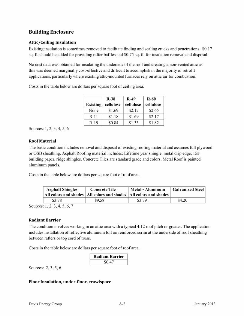
Building Enclosure

Attic/Ceiling Insulation Existing insulation is sometimes removed to facilitate finding and sealing cracks and penetrations. $0.17 sq. ft. should be added for providing rafter baffles and $0.75 sq. ft. for insulation removal and disposal. No cost data was obtained for insulating the underside of the roof and creating a non‐vented attic as this was deemed marginally cost‐effective and difficult to accomplish in the majority of retrofit applications, particularly where existing attic‐mounted furnaces rely on attic air for combustion. Costs in the table below are dollars per square foot of ceiling area.

Existing

R‐38 cellulose

R‐49 cellulose

R‐60 cellulose

None $1.69 $2.17 $2.65 R‐11 $1.18 $1.69 $2.17 R‐19 $0.84 $1.33 $1.82

Sources: 1, 2, 3, 4, 5, 6

Roof Material The basic condition includes removal and disposal of existing roofing material and assumes full plywood or OSB sheathing. Asphalt Roofing material includes: Lifetime year shingle, metal drip edge, 15# building paper, ridge shingles. Concrete Tiles are standard grade and colors. Metal Roof is painted aluminum panels. Costs in the table below are dollars per square foot of roof area.

Asphalt Shingles All colors and shades

Concrete Tile All colors and shades

Metal ‐ Aluminum All colors and shades

Galvanized Steel

$3.78 $9.58 $3.79 $4.20 Sources: 1, 2, 3, 4, 5, 6, 7

Radiant Barrier The condition involves working in an attic area with a typical 4:12 roof pitch or greater. The application includes installation of reflective aluminum foil on reinforced scrim at the underside of roof sheathing between rafters or top cord of truss. Costs in the table below are dollars per square foot of roof area.

Radiant Barrier $0.47

Sources: 2, 3, 5, 6

Floor Insulation, under­floor, crawlspace

Davis Energy Group A-2 January 2013

Condition includes application of batt insulation, wire stays, and strapping. Assumptions include: an uninsulated floor, accessible depth of crawlspace area for worker’s movement, and typical in‐floor access is assumed. Costs below are in dollars per square foot of floor area.

R‐13 R‐19 $ 1.15 $ 1.35

Sources: 1, 2, 3, 4, 5, 6, 7

Crawlspace perimeter insulation & VB The condition assumes smooth formed interior footing or wall face and a minimum 18 inch crawl space clearance. Includes rigid ESP foam installation. Add $0.80 sq. ft. for paintable moisture barrier. Costs in the table below are dollars per square foot of wall area.

R5 Interior

R10 Interior

R15 Interior

R20 Interior

$1.38 $1.90 $2.40 $2.90 Sources: 1, 2, 3, 4, 5, 6, 7

Insulate wall cavities California‐specific costs were assembled for two retrofit methods:

• Drill & fill” with cellulose or fiberglass • Removal of cladding and installation of fiberglass batt

The base condition is no insulation (or R‐7 or less) with 16” stud spacing, without masonry cladding. For drill & fill, costs assume access from interior walls. The cladding removal method includes removal and disposal of materials, caulking studs and plates, and installation of R‐13 or R‐15 insulation, moisture barrier, and fiber cement siding, and painting. An option for application of 1” exterior foam (EPS) sheathing is included. Costs below are in dollars per square foot of net wall area.

Drill & Fill R&R Exterior Cladding Cellulose Fiberglass R‐13 R‐15 R‐15 + 1" EPS

$1.06 $1.23 $6.11 $6.26 $7.02 Sources: 1, 3, 4, 5, 6,

Wall sheathing (stucco) Costs are included for removal of existing wood siding or equivalent and installation of non‐structural sheathing over existing framing. Costs do not include re‐cladding the structure. Costs below are in dollars per square foot of net wall area.

Davis Energy Group A-3 January 2013

Polyiso, 1 in, R‐6 Polyiso, 2 in, R-12) XPS, 1 in, R‐5 XPS, 2 in, R‐10

$2.10 $2.40 $2.08 $2.22 Sources: 1, 3, 4, 5, 6, 7

Window film Application includes cleaning and installation film. Costs below are in dollars per square foot of net window area.

Total Solar Energy Rejected 53%+ $11.93

Sources: 3, 5, 6

Window replacement The condition includes removal and disposal of existing windows, installation of non‐metal, Energy Star qualified window as per climate zone requirements. Typical application is double pane, insulated, Low‐E glass. The costs reflect a statewide average of per square foot of window area.

Energy Star Double pane, insulated, low‐e $38.00

Sources: 1, 2, 3, 4, 5, 6

Air Sealing ­ whole house Conditions require accessible attic area and under floor area, if applicable. Applications include, weather‐stripping doors and fenestrations as needed, caulking and foam sealing at plate lines, sealing of plumbing fixture and other envelope penetrations. Protocol includes diagnostic blower door test to identify leakage locations and verify Specific Leakage Area (SLA). Costs below are in dollars per square foot of conditioned building floor area.

Greater than 1.5 SLA Less than or Equal to 1.5 SLA $1.10 $2.00

Sources: 1, 2, 3, 4, 5, 6

HVAC

HVAC Tune­up Typical Service call Tune‐up for California contractors. Includes filter change, combustion zone safety test, adjust air to fuel ratio. Costs below are lump sum.

HVAC Tune‐up $200.00

Davis Energy Group A-4 January 2013

Sources: 4, 5, 6

AC replacement, split The condition assumes removal and installation of one (1) Mini ‐ split unit, and one (1) outside condenser unit. Costs are expressed as Lump Sum Material, Labor and markup.

2 Ton/18.9 SEER/11.5 EER PTAC 3 Ton/16 SEER Condenser $2,378.00 $2,740.00

Sources: 1, 2, 3, 4, 5, 6, 7

Furnace replacement, central interior, split Conditions include removal and disposal of existing, replacement of 100,000 Btu unit.

94% AFUE 96% AFUE $4,500.00 $4,800.00

Sources: 1, 2, 3, 4, 5, 6

Heat pump replacement, central interior Condition includes removal of existing system and installation of air to air Heat Pump system.

4 Ton Cooling/24MBH Heat $4,947.00

Sources: 1, 2, 3, 4, 5, 6

Room air conditioner The basic condition includes removal and disposal of exiting unit and installation of new window/thru the wall unit.

25,000 BTUH $1,543

Sources: 1, 3, 4, 5, 6, 7

Duct Sealing Conditions include cleaning and preparation, mastic and fasteners at all joints and boots. Includes return. Costs are per square feet of duct surface area.

Duct Sealing $1.30

Sources: 1, 2, 4, 5, 6

Duct Insulation Condition includes cleaning and preparation of duct surface, strapping (If required) as per HERS protocols, and affixing insulation to ductwork.

Davis Energy Group A-5 January 2013

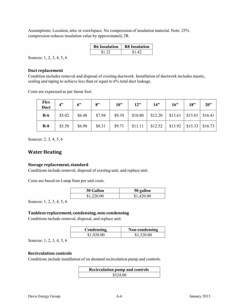
Assumptions: Location, attic or crawlspace. No compression of insulation material. Note: 25% compression reduces insulation value by approximately 2R.

R6 Insulation R8 Insulation $1.22 $1.42

Sources: 1, 2, 3, 4, 5, 6

Duct replacement Condition includes removal and disposal of existing ductwork. Installation of ductwork includes mastic, sealing and taping to achieve less than or equal to 6% total duct leakage. Costs are expressed as per linear foot.

Flex Duct 4” 6” 8” 10” 12” 14” 16” 18” 20”

R‐6 $5.02 $6.48 $7.94 $9.39 $10.80 $12.20 $13.61 $15.01 $16.41

R‐8 $5.50 $6.90 $8.31 $9.71 $11.11 $12.52 $13.92 $15.33 $16.73

Sources: 2, 3, 4, 5, 6

Water Heating

Storage replacement, standard Conditions include removal, disposal of existing unit, and replace unit. Costs are based on Lump Sum per unit costs.

30 Gallon 50 gallon $1,220.00 $1,420.00

Sources: 1, 2, 3, 4, 5, 6

Tankless replacement, condensing, non­condensing Conditions include removal, disposal, and replace unit.

Condensing, Non‐condensing $1,920.00 $1,320.00

Sources: 1, 2, 3, 4, 5, 6

Recirculation controls Conditions include installation of on demand recirculation pump and controls.

Recirculation pump and controls $524.00

Davis Energy Group A-6 January 2013

Sources: 3, 4, 5, 6

Low flow showerhead Conditions include removal of existing showerhead and installation of unit. Includes: lump sum for labor and material plus markup.

Low flow showerhead Hot water sensing showerhead, trickle flow

$60.00 $60.00 Sources: 3, 4, 5, 6, 7

Lighting & Appliances

High efficacy lighting upgrade, interior Conditions include removal, disposal of existing unit, and replace unit.

LED recessed can luminaire Drum type luminaire $96.00 152.00

Sources: 3, 4, 5, 6

High efficacy lighting upgrade, exterior Conditions include removal, disposal of existing unit, and replace unit.

LED Wall mount exterior $256.00

Sources: 3, 4, 5, 6

Energy Star Clothes Washer Conditions include removal, disposal of existing unit, and replace unit.

Top load Front load $960.00 $1260.00

Sources: 1, 2, 3, 5, 7

Energy Star Dishwasher Conditions include removal, disposal of existing unit, and replace unit. Sources: 1, 2, 3, 5, 7

Energy Star Refrigerator Conditions include removal, disposal of existing unit, and replace unit.

Standard design $1600.00

Sources: 1, 2, 3, 4, 5, 6

Davis Energy Group A-7 January 2013

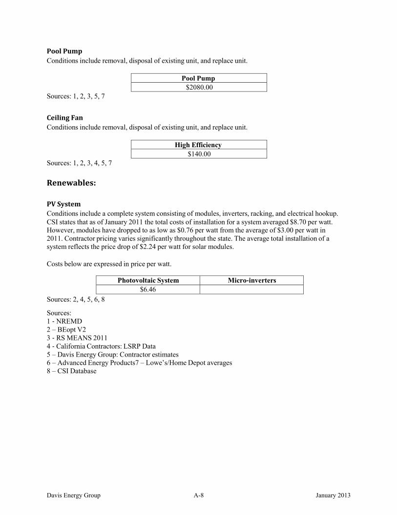
Pool Pump Conditions include removal, disposal of existing unit, and replace unit.

Pool Pump $2080.00

Sources: 1, 2, 3, 5, 7

Ceiling Fan Conditions include removal, disposal of existing unit, and replace unit.

High Efficiency $140.00

Sources: 1, 2, 3, 4, 5, 7

Renewables:

PV System Conditions include a complete system consisting of modules, inverters, racking, and electrical hookup. CSI states that as of January 2011 the total costs of installation for a system averaged $8.70 per watt. However, modules have dropped to as low as $0.76 per watt from the average of $3.00 per watt in 2011. Contractor pricing varies significantly throughout the state. The average total installation of a system reflects the price drop of $2.24 per watt for solar modules. Costs below are expressed in price per watt. Sources: 2, 4, 5, 6, 8 Sources: 1 ‐ NREMD 2 – BEopt V2 3 ‐ RS MEANS 2011 4 ‐ California Contractors: LSRP Data 5 – Davis Energy Group: Contractor estimates 6 – Advanced Energy Products7 – Lowe’s/Home Depot averages 8 – CSI Database

Photovoltaic System Micro‐inverters $6.46

Davis Energy Group A-8 January 2013

Appendix B: California Utility Cost-Effectiveness Tests

Contents California Utility Cost-Effectiveness Tests ............................................................................................... 1

Participant Cost Test .............................................................................................................................. 1 Net Present Value ............................................................................................................................ 1 Benefit-Cost Ratio ........................................................................................................................... 3 Levelized Cost ................................................................................................................................. 3

Ratepayer Impact Measure Test ............................................................................................................. 5 Net Present Value ............................................................................................................................ 6 Benefit-Cost Ratio ........................................................................................................................... 8 Lifecycle Revenue Impact ............................................................................................................... 8 Levelized Cost ................................................................................................................................. 9

Total Resource Cost Test...................................................................................................................... 11 Net Present Value .......................................................................................................................... 11 Benefit-Cost Ratio ......................................................................................................................... 12 Levelized Cost ............................................................................................................................... 12

Program Administrator Cost Test ......................................................................................................... 13 Net Present Value .......................................................................................................................... 14 Benefit-Cost Ratio ......................................................................................................................... 14 Levelized Cost ............................................................................................................................... 14

Glossary ..................................................................................................................................................... 15

Energy and Environmental Economics February 2013

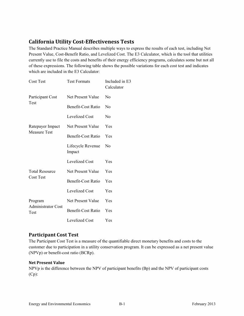
California Utility Cost-Effectiveness Tests The Standard Practice Manual describes multiple ways to express the results of each test, including Net Present Value, Cost-Benefit Ratio, and Levelized Cost. The E3 Calculator, which is the tool that utilities currently use to file the costs and benefits of their energy efficiency programs, calculates some but not all of these expressions. The following table shows the possible variations for each cost test and indicates which are included in the E3 Calculator:

Cost Test Test Formats Included in E3 Calculator

Participant Cost Test

Net Present Value No

Benefit-Cost Ratio No

Levelized Cost No

Ratepayer Impact Measure Test

Net Present Value Yes

Benefit-Cost Ratio Yes

Lifecycle Revenue Impact

No

Levelized Cost Yes

Total Resource Cost Test

Net Present Value Yes

Benefit-Cost Ratio Yes

Levelized Cost Yes

Program Administrator Cost Test

Net Present Value Yes

Benefit-Cost Ratio Yes

Levelized Cost Yes

Participant Cost Test The Participant Cost Test is a measure of the quantifiable direct monetary benefits and costs to the customer due to participation in a utility conservation program. It can be expressed as a net present value (NPVp) or benefit-cost ratio (BCRp).

Net Present Value NPVp is the difference between the NPV of participant benefits (Bp) and the NPV of participant costs (Cp):

Energy and Environmental Economics B-1 February 2013

𝑁𝑃𝑉𝑝 = 𝐵𝑝 − 𝐶𝑝

NPV of participant benefits, Bp, is calculated in BEopt using the following formula:

𝐵𝑝 = 𝑇𝐶 + 𝐼𝑁𝐶 + 𝐵𝑅

Where:

TC = Tax credits. Net present value of yearly differences in tax credits between the retrofit and reference case represented in nominal dollars. Applicable tax credits include the PV investment tax credit and tax credits available for energy efficiency. Both state and federal tax credits should be included. Because the yearly tax credit values are represented as cash flows in nominal dollars, their net present value must be calculated using the nominal discount rate. Nominal discount rate = discount rate + inflation rate.

The net present value of yearly tax credits is calculated as follows:

𝑇𝐶 = �𝑇𝐶𝑡

(1 + 𝑑𝑛)𝑡−1

𝑁

𝑡=1

Where:

N = project analysis period, in years.

t = year.

TCt = difference in tax credits between the retrofit and reference case in year t, in nominal dollars.

dn = nominal discount rate.

All NPV terms in this document can be calculated using an analogous formula, assuming that the NPV is derived from cash flows in nominal dollars.

INC = Incentives. NPV of the yearly differences in incentives between the retrofit and reference case. Incentive values should be incorporated into BEopt and included in the output file for each year in nominal dollars. See the Appendix for a description of the E3’s recommended approach for adding incentives to BEopt.

BR = Bill Reduction. Net present value of difference in utility bill between retrofit and reference case, in nominal dollars, for all years in which the retrofit case utility bill is less than that in the reference case. The difference in utility bill should be determined separately for all years. Then the total net present value of all utility bill reductions is calculated.

NPV of participant costs, Cp, is calculated as follows:

Energy and Environmental Economics B-2 February 2013

𝐶𝑝 = 𝐿𝑃 + 𝐶𝑃 + 𝑅𝐶 + 𝑂&𝑀 + 𝑅𝑉 + 𝐵𝐼

Where:

LP = Total loan payments. NPV of yearly differences in loan payments between the retrofit case and reference case, where yearly loan payments are assumed to be in nominal dollars. Values are contained in BEopt’s .csv output file, in the “Economics” section. Total loan payments include both interest and principal payments. If a homeowner uses a home equity line of credit to finance a retrofit, interest payments are tax deductible. The tax deduction should be subtracted from the annual loan payment value.

CP = Total cash payments. NPV of yearly differences in cash payments between the retrofit case and reference case, where yearly cash payments are assumed to be in nominal dollars.

RC = Replacement costs. NPV of difference in replacement costs between retrofit case and reference case in nominal dollars, also contained in .csv output file.

O&M = Operation & maintenance costs. NPV of difference in O&M costs between retrofit and reference cases in nominal dollars, in .csv file.

RV = Residual value. NPV of difference in residual value between retrofit and reference cases in nominal dollars, from .csv file.

BI = Bill Increase. This is analogous to Bill Reduction above, except that difference in utility bill between the retrofit and reference cases is included only for those years when the retrofit case has the higher utility bill. The total net present value of all utility bill increases is used.

Benefit-Cost Ratio BCRp is the ratio of NPV of participant benefits to NPV of participant costs.

𝐵𝐶𝑅𝑝 =𝐵𝑝𝐶𝑝

Where Bp and Cp are calculated as described above in NPVp.

Levelized Cost LCP presents the costs to the participant on a per kilowatt hour or per therm basis, levelized over the life of the measure. To calculate levelized costs correctly, participant costs must be separated by fuel type (electricity costs versus gas costs). E3 recommends using the ratio of electricity and gas benefits, as in the following calculations to apportion participant costs.

Gas Levelized Cost

𝐿𝐶𝑃,𝑔 =𝐶𝑃,𝑔 𝐼𝑀𝑃𝑔

Where:

Energy and Environmental Economics B-3 February 2013

CP,g = participant costs used for levelizing, adjusted to represent gas costs.

𝐶𝑃,𝑔 = [𝐿𝑃 + 𝐶𝑃 + 𝑅𝐶 + 𝑂&𝑀 + 𝑅𝑉 − 𝐼𝑁𝐶 − 𝑇𝐶] ∗𝑈𝐴𝐶𝑔

𝑈𝐴𝐶𝑒 + 𝑈𝐴𝐶𝑔

Where:

LP = NPV of loan payments, as defined above

CP = NPV of cash payments, as defined above

RC = NPV of replacement costs, as defined above

O&M = NPV of operation and maintenance costs, as defined above

RV = NPV of residual value, as defined above

TC = NPV of tax credits, defined as above

UACg = NPV of gas avoided supply costs, as defined below.

UACe = NPV of electricity avoided supply costs, as defined below.

IMPg = Total discounted gas load impacts of the program. This is a measure of the total gas load reduction of the utility program.

𝐼𝑀𝑃𝑔 =∑ ∆𝐺𝑎𝑠𝑡𝑁𝑡=1

(1 + 𝑑𝑛)𝑡−1

Where:

dn = Nominal discount rate.

ΔGast = Reduction in net gas use in year t. In BEopt, this is the total yearly difference in gas use between the retrofit case and the reference case, in therms. These values can be taken from the .csv output file’s “Energy Flow” section. All energy flows should be summed for each case for each year.

Electricity Levelized Cost

𝐿𝐶𝑃,𝑒 =𝐶𝑃,𝑒

𝐼𝑀𝑃𝑒

Where:

CP,e = total resource costs used for levelizing, adjusted to represent electricity costs.

𝐶𝑃,𝑒 = [𝐿𝑃 + 𝐶𝑃 + 𝑅𝐶 + 𝑂&𝑀 + 𝑅𝑉 − 𝐼𝑁𝐶 − 𝑇𝐶] ∗𝑈𝐴𝐶𝑒

𝑈𝐴𝐶𝑒 + 𝑈𝐴𝐶𝑔

Where:

Energy and Environmental Economics B-4 February 2013

All cost terms are defined as above in the NPV calculation.

LP = NPV of loan payments, as defined above

CP = NPV of cash payments, as defined above

RC = NPV of replacement costs, as defined above

O&M = NPV of operation and maintenance costs, as defined above

RV = NPV of residual value, as defined above

TC = NPV of tax credits, defined as above

UACg = NPV of gas avoided supply costs, as defined below.

UACe = NPV of electricity avoided supply costs, as defined below.

𝐼𝑀𝑃𝑒 = ∑ ∆𝐸𝑙𝑒𝑐𝑡𝑁𝑡=1

(1+𝑑𝑛)𝑡−1

Where:

dn = Nominal discount rate.

ΔElect = Reduction in net electricity use in year t. In BEopt, this is the total yearly difference in electricity use between the retrofit case and the reference case, in therms. These values can be taken from the .csv output file’s “Energy Flow” section. All energy flows should be summed for each case for each year.

Comment: Note, that the participant costs in the numerator of the levelized cost calculations are net of incentives and tax credit payments to the participant. This is an intentional deviation from how Participant “costs” are defined in the SPM, which assign incentives and tax credits to the benefits. However, we believe it is more useful to a user who is interested in the net impact on the participant’s pocket book. This also facilitates more direct comparison with utility rates.

To avoid potential confusion, we suggest adding a label that states the above, such as “levelized cost to participant is inclusive of tax and incentive payments”.

Ratepayer Impact Measure Test The Ratepayer Impact Measure (RIM) test measures what happens to customer bills or rates due to changes in utility revenues and operating costs caused by a conservation program. If a program causes a larger increase in utility revenues than utility costs, customer rates will decrease. If a program results in a larger increase in utility costs than revenues, customer rates will increase.

RIM can be expressed as a net present value (NPV), a benefit-cost ratio (BCR), a lifecycle revenue impact per kWh (LRI), or a levelized cost (LC).

It is also worth noting, the RIM, TRC and PA cost tests also incorporate net to gross factors, which consider only the effects that can be attributable to the program itself, taking into consideration the free-

Energy and Environmental Economics B-5 February 2013

rider effect. The formulas below take the approach of applying NTG factors towards the end of the mathematical steps.

Net Present Value NPVRIM is calculated as follows:

𝑁𝑃𝑉𝑅𝐼𝑀 = 𝐵𝑅𝐼𝑀 − 𝐶𝑅𝐼𝑀

Where BRIM and CRIM are calculated as follows:

𝐵𝑅𝐼𝑀 = 𝑁𝑇𝐺 × [𝑈𝐴𝐶 + 𝐵𝐼]

Where:

BI = Net present value of utility bill increases. Bill increases are included as a benefit in this test because they represent an increase in total utility revenue, thus reducing rates for all ratepayers.

NTG = Net-to-gross ratio

UAC = Net present value of utility avoided supply costs.

𝑈𝐴𝐶 = 𝑈𝐴𝐶𝑔 + 𝑈𝐴𝐶𝑒

Where:

UACg = Net present value of gas avoided supply costs. Since E3’s gas utility avoided supply costs are calculated on a monthly basis while gas savings are calculated in BEopt on an hourly basis, this term can be calculated two ways: 1) sum the hourly gas savings to generate monthly savings, and then take the sum product of monthly gas savings and monthly gas avoided costs, or 2) convert the monthly avoided costs into hourly avoided costs and take the sum product of hourly gas savings and hourly avoided costs. Both methods are described below.

Method 1:

𝑈𝐴𝐶𝑔 = �∑ ∆𝐺𝑎𝑠𝑖𝑡 ∙ (𝐺𝐺𝐴𝐶𝑖 + 𝐺𝑇𝐴𝐶𝑖)12𝑖=1

(1 + 𝑑𝑛)𝑡−1

𝑁

𝑡=1

Where:

GGACi = Gas generation avoided costs for month i. E3 has provided monthly utility avoided supply costs for gas generation and gas transmission & distribution (T&D). Avoided costs are in nominal dollars.

GTACi = Gas T&D avoided costs for month i, in nominal dollars.

ΔGasit = Difference in gas consumption between the retrofit and reference cases in month i in year t, in therms, for all months in which the retrofit case gas consumption is lower. This value should be calculated from hourly energy use files.

Energy and Environmental Economics B-6 February 2013

dn = Nominal discount rate. The nominal discount rate must be used because the E3 avoided costs are in nominal dollars.

N = Project analysis period.

Method 2:

𝑈𝐴𝐶𝑔 = �∑ ∆𝐺𝑎𝑠𝑖𝑡 ∙ (𝐺𝐺𝐴𝐶𝑖 + 𝐺𝑇𝐴𝐶𝑖)8760𝑖=1

(1 + 𝑑𝑛)𝑡−1

𝑁

𝑡=1

Where:

GGACi = Gas generation avoided costs for hour i. E3 has provided monthly utility avoided supply costs for gas generation and gas transmission & distribution (T&D). Avoided costs are in nominal dollars. To use this calculation method, monthly utility avoided supply costs must be converted to hourly avoided costs by replicating the cost for each hour in the month.

GTACi = Gas T&D avoided costs for hour i, in nominal dollars.

ΔGasit = Difference in gas consumption between the retrofit and reference cases in hour i in year t, in therms, for all hours in which the retrofit case gas consumption is lower.

dn = Nominal discount rate. The nominal discount rate must be used because the E3 avoided costs are in nominal dollars.

N = Project analysis period.

UACe = Net present value of electricity avoided supply costs

𝑈𝐴𝐶𝑒 = �∑ ∆𝐸𝑙𝑒𝑐𝑗𝑡 ∙ �𝐸𝐺𝐴𝐶𝑗 + 𝐸𝑇𝐴𝐶𝑗�8760𝑗=1

(1 + 𝑑𝑛)𝑡−1

𝑁

𝑡=1

Where:

EGACj = Electricity generation avoided costs for hour j. E3 has provided hourly utility avoided supply costs for electricity generation and T&D.

ETACj = Electricity T&D avoided costs for hour j.

ΔElecjt = Difference in electricity consumption between the retrofit and reference case in hour j in year t, in MWh, for all hours when retrofit electricity consumption is lower. This data comes from BEopt’s hourly energy use files.

dn = Nominal discount rate.

N = Project analysis period.

Energy and Environmental Economics B-7 February 2013

𝐶𝑅𝐼𝑀 = 𝐼𝑁𝐶 + 𝑁𝑇𝐺 × [𝑈𝐼𝐶 + 𝐵𝑅] + 𝑃𝑅

Where:

INC= Incentives, as defined above.

UIC = Net present value of utility increased costs. UIC is calculated the same way as UAC, except that only hours in which the retrofit case energy usage is higher than the reference case are included.

NTG = Net-to-gross ratio

BR = Net present value of bill reduction, as defined above.

PRC =Net present value of program administration costs on a per home basis. E3 recommends that the cost test calculation interface created in BEopt include total program administrative costs as a user input, along with the number of homes in the program. Then the NPV of total administrative cost per home can be calculated and included in cost tests.

Benefit-Cost Ratio BCRRIM is calculated using the following method:

𝐵𝐶𝑅𝑅𝐼𝑀 =𝐵𝑅𝐼𝑀𝐶𝑅𝐼𝑀

Where BRIM and CRIM are again calculated as above.

Lifecycle Revenue Impact LRI is the one-time change in rates or the bill change over the life of the program. This rate change is required in order to meet the utility’s revenue requirement. The rate increase or decrease is assumed to occur in the first year of the program. This test is not currently included in the E3 Calculator or the E3’s BEopt QA/QC spreadsheet, because the BEopt output does not delineate the bill savings by electric vs. natural gas components, however, it is outlined here because it is included in the Standard Practice Manual and we recommend including this calculation in the implementation of the cost tests in BEopt.

LRI is calculated using the following method:

𝐿𝑅𝐼𝑅𝐼𝑀 =𝐶𝑅𝐼𝑀 − 𝐵𝑅𝐼𝑀

𝐸

Where:

E = Net discounted stream of energy sales, in kWh.

𝐸 = 𝑁𝑇𝐺 × �𝐸𝑡

(1 + 𝑑𝑛)𝑡−1

𝑁

𝑡=1

Where:

Energy and Environmental Economics B-8 February 2013

Et = System sales in kWh for year t. This term represents the utility’s total energy sales, in kWh, for the year t.

dn and N are nominal discount rate and project analysis period, as defined previously.

NTG = net to gross factor

Levelized Cost LCRIM presents the total costs of the program on a per kilowatt hour or per therm basis, levelized over the life of the program. To calculate levelized costs correctly, program costs must be separated by fuel type (electricity costs versus gas costs). This is easily done for the bill reduction portion of the RIM costs, because BEopt can generate separate values for gas and electric bill savings. To apportion other types of costs, E3 recommends using the ratio of net electricity and gas avoided cost benefits, as in the following calculation. Note that the E3 QA/QC tool does not include a RIM levelized cost, because we do not have access to separate gas and electricity bill savings.

Gas Levelized Cost

𝐿𝐶𝑅𝐼𝑀,𝑔 =𝐶𝑅𝐼𝑀,𝑔

𝐼𝑀𝑃𝑔,𝑅𝐼𝑀,𝑇𝑅𝐶,𝑃𝐴

Where:

CRIM,g = total resource costs used for levelizing, adjusted to represent gas costs.

𝐶𝑅𝐼𝑀,𝑔 = (𝐼𝑁𝐶 + 𝑃𝑅𝐶) × 𝐵𝑒𝑛𝑒𝑓𝑖𝑡.𝐺𝑎𝑠. 𝑆ℎ𝑎𝑟𝑒 + 𝑁𝑇𝐺 × 𝐵𝑅𝑔 ∗𝐵𝑅𝑔

𝐵𝑅𝑔 + 𝐵𝑅𝑒

Where:

All cost terms are defined as above in the NPV calculation and

𝐵𝑒𝑛𝑒𝑓𝑖𝑡.𝐺𝑎𝑠. 𝑆ℎ𝑎𝑟𝑒 =�𝑈𝐴𝐶𝑔 − 𝑈𝐼𝐶𝑔�

�𝑈𝐴𝐶𝑒 + 𝑈𝐴𝐶𝑔 − 𝑈𝐼𝐶𝑒 − 𝑈𝐼𝐶𝑔�

UACg = NPV of gas avoided supply costs.

UACe = NPV of electricity avoided supply costs.

UICg = NPV of utility increased gas costs.

UICe = NPV of utility increased electricity costs.

BRg = NPV of gas bill reductions.

BRe = NPV of electricity bill reductions.

NTG = net to gross factor

Energy and Environmental Economics B-9 February 2013

IMPg,RIM,TRC,PA = Total discounted gas load impacts of the program. This is a measure of the gas load reduction caused by the utility program on a net basis (incorporating net to gross factors).

𝐼𝑀𝑃𝑔,𝑅𝐼𝑀,𝑇𝑅𝐶,𝑃𝐴 = 𝑁𝑇𝐺 ×∑ ∆𝐺𝑎𝑠𝑡𝑁𝑡=1

(1 + 𝑑𝑛)𝑡−1

Where:

dn = Nominal discount rate.

ΔGast = Reduction in net gas use in year t. In BEopt, this is the total yearly difference in gas use between the retrofit case and the reference case, in therms. These values can be taken from the .csv output file’s “Energy Flow” section. All energy flows should be summed for each case for each year.

NTG = net to gross factor

Electricity Levelized Cost

𝐿𝐶𝑅𝐼𝑀,𝑒 =𝐶𝑅𝐼𝑀,𝑒

𝐼𝑀𝑃𝑒,𝑅𝐼𝑀,𝑇𝑅𝐶,𝑃𝐴

Where:

CRIM,e = total resource costs used for levelizing, adjusted to represent electricity costs.

𝐶𝑅𝐼𝑀,𝑒 = (𝐼𝑁𝐶 + 𝑃𝑅𝐶) × 𝐵𝑒𝑛𝑒𝑓𝑖𝑡.𝐸𝑙𝑒𝑐. 𝑆ℎ𝑎𝑟𝑒 + 𝑁𝑇𝐺 × 𝐵𝑅 ∗𝐵𝑅𝑒

𝐵𝑅𝑔 + 𝐵𝑅𝑒

Where:

All cost terms are defined as above in the NPV calculation, and

𝐵𝑒𝑛𝑒𝑓𝑖𝑡.𝐸𝑙𝑒𝑐. 𝑆ℎ𝑎𝑟𝑒 =[𝑈𝐴𝐶𝑒 − 𝑈𝐼𝐶𝑒]

�𝑈𝐴𝐶𝑒 + 𝑈𝐴𝐶𝑔 − 𝑈𝐼𝐶𝑒 − 𝑈𝐼𝐶𝑔�

UACg = NPV of gas avoided supply costs.

UACe = NPV of electricity avoided supply costs.

UICg = NPV of utility increased gas costs.

UICe = NPV of utility increased electricity costs.

BRg = NPV of gas bill reductions.

BRe = NPV of electricity bill reductions.

NTG = net to gross factor

Energy and Environmental Economics B-10 February 2013

𝐼𝑀𝑃𝑒,𝑅𝐼𝑀,𝑅𝐼𝑀,𝑃𝐴 = 𝑁𝑇𝐺 × ∑ ∆𝐸𝑙𝑒𝑐𝑡𝑁𝑡=1

(1+𝑑𝑛)𝑡−1

Where:

dn = Nominal discount rate.

ΔElect = Reduction in net electricity use in year t. In BEopt, this is the total yearly difference in electricity use between the retrofit case and the reference case, in therms. These values can be taken from the .csv output file’s “Energy Flow” section. All energy flows should be summed for each case for each year.

Total Resource Cost Test The Total Resource Cost (TRC) Test measures the net cost of an energy conservation program, viewing the program as a utility resource option. Both utility and participant costs are included. The TRC Test reflects the impacts of a program on both participating and non-participating customers. In a sense, it is the summation of the benefit and cost terms in the Participant and RIM tests, where revenue/bill costs and incentives intuitively cancel out.

TRC can be expressed as a net present value (NPVTRC), benefit-cost ratio (BCRTRC), or levelized cost (LCTRC).

Net Present Value NPVTRC is calculated as follows:

𝑁𝑃𝑉𝑇𝑅𝐶 = 𝐵𝑇𝑅𝐶 − 𝐶𝑇𝑅𝐶

Where:

BTRC = Program benefits

𝐵𝑇𝑅𝐶 = 𝑇𝐶𝑓 + 𝑈𝐴𝐶 ∗ 𝑁𝑇𝐺

Where:

UAC = NPV of utility avoided supply costs.

NTG = Net-to-gross ratio. NTG should be incorporated into BEopt as a user input.

TCf = NPV of federal tax credits. Only federal tax credits are included in the TRC costs because state tax credits are viewed as a transfer payment. CTRC = Program costs

𝐶𝑇𝑅𝐶 = 𝑁𝑇𝐺 ∙ (𝐿𝑃 + 𝐶𝑃 + 𝑅𝐶 + 𝑂&𝑀 + 𝑅𝑉 + 𝑈𝐼𝐶) + (1 −𝑁𝑇𝐺) ∙ 𝐼𝑁𝐶 + 𝑃𝑅𝐶

Where:

NTG = Net-to-gross ratio.

LP = Total loan payments.

Energy and Environmental Economics B-11 February 2013

CP = Total cash payments.

RC = Replacement costs.

O&M = Operation and maintenance costs.

RV = Residual value.

INC = Incentives.

UIC = Utility increased costs.

PRC = Per-home program administration costs.

Benefit-Cost Ratio BCRTRC is the ratio of NPV of participant benefits to NPV of participant costs.

𝐵𝐶𝑅𝑇𝑅𝐶 =𝐵𝑇𝑅𝐶𝐶𝑇𝑅𝐶

Where BTRC and CTRC are again calculated as above in the NPV calculation.

Levelized Cost LCTRC presents the total costs of the program on a per kilowatt hour or per therm basis, levelized over the life of the program. To calculate levelized costs correctly, costs of the program should be separated by fuel type (electricity costs versus gas costs). BEopt does not distinguish between electricity and gas costs, but it is possible to calculate benefits separately for each fuel type, based on utility avoided costs and energy savings in the retrofit case. E3 recommends that program costs be divided between electricity and gas based on the ratio of electricity and gas benefits, as in the following calculation.

Gas Levelized Cost

𝐿𝐶𝑇𝑅𝐶,𝑔 =𝐶𝑇𝑅𝐶,𝑔

𝐼𝑀𝑃𝑔,𝑅𝐼𝑀,𝑇𝑅𝐶,𝑃𝐴

Where:

CTRC,g = total resource costs used for levelizing, adjusted to represent gas costs.

𝐶𝑇𝑅𝐶,𝑔 = [𝑁𝑇𝐺 ∙ (𝐿𝑃 + 𝐶𝑃 + 𝑅𝐶 + 𝑂&𝑀 + 𝑅𝑉) + (1 −𝑁𝑇𝐺) ∙ 𝐼𝑁𝐶 + 𝑃𝑅𝐶] × 𝐵𝑒𝑛𝑒𝑓𝑖𝑡.𝐺𝑎𝑠. 𝑆ℎ𝑎𝑟𝑒

Where:

All cost terms are defined as above in the NPV calculation and

𝐵𝑒𝑛𝑒𝑓𝑖𝑡.𝐺𝑎𝑠. 𝑆ℎ𝑎𝑟𝑒 =�𝑈𝐴𝐶𝑔 − 𝑈𝐼𝐶𝑔�

�𝑈𝐴𝐶𝑒 + 𝑈𝐴𝐶𝑔 − 𝑈𝐼𝐶𝑒 − 𝑈𝐼𝐶𝑔�

UACg = NPV of gas avoided supply costs.

Energy and Environmental Economics B-12 February 2013

UACe = NPV of electricity avoided supply costs.

UICg = NPV of utility increased gas costs.

UICe = NPV of utility increased electricity costs.

IMPg,RIM,TRC,PA = Total discounted gas load impacts of the program on a net basis. This term is calculated above in the RIM levelized cost section; note it considers the net to gross factor.

Electricity Levelized Cost

𝐿𝐶𝑇𝑅𝐶,𝑒 =𝐶𝑇𝑅𝐶,𝑒

𝐼𝑀𝑃𝑒,𝑅𝐼𝑀,𝑇𝑅𝐶,𝑃𝐴

Where:

CTRC,e = total resource costs used for levelizing, adjusted to represent electricity costs

𝐶𝑇𝑅𝐶,𝑒 = [𝑁𝑇𝐺 ∙ (𝐿𝑃 + 𝐶𝑃 + 𝑅𝐶 + 𝑂&𝑀 + 𝑅𝑉) + (1 −𝑁𝑇𝐺) ∙ 𝐼𝑁𝐶 + 𝑃𝑅𝐶] × 𝐵𝑒𝑛𝑒𝑓𝑖𝑡.𝐸𝑙𝑒𝑐. 𝑆ℎ𝑎𝑟𝑒

Where:

All cost terms are defined as above in the NPV calculation, and

𝐵𝑒𝑛𝑒𝑓𝑖𝑡.𝐸𝑙𝑒𝑐. 𝑆ℎ𝑎𝑟𝑒 =[𝑈𝐴𝐶𝑒 − 𝑈𝐼𝐶𝑒]

�𝑈𝐴𝐶𝑒 + 𝑈𝐴𝐶𝑔 − 𝑈𝐼𝐶𝑒 − 𝑈𝐼𝐶𝑔�

UACg = NPV of gas avoided supply costs.

UACe = NPV of electricity avoided supply costs.

UICg = NPV of utility increased gas costs.

UICe = NPV of utility increased electricity costs.

IMPe,RIM,TRC,PA = Total discounted electricity load impacts of the program. This is a measure of the total electricity load reduction caused by the utility program. This term is included in the RIM levelized cost calculation; note it considers the net to gross factor.

Program Administrator Cost Test The Program Administrator Cost Test measures the net costs of a demand-side management program as a resource option based on the costs incurred by the program administrator, including incentive costs and excluding any net costs incurred by the participant.

The Program Administrator Cost can be expressed either as a net present value (NPVpa), benefit-cost ratio (BRCpa), or levelized cost (LCpa).

As noted earlier, the PA test must consider net to gross factors, which are reflected in the formulas.

Energy and Environmental Economics B-13 February 2013

Net Present Value NPVpa is the difference between the program benefits and program costs:

𝑁𝑃𝑉𝑝𝑎 = 𝐵𝑝𝑎 − 𝐶𝑝𝑎

Where:

Bpa = Program benefits

𝐵𝑝𝑎 = 𝑁𝑇𝐺 × 𝑈𝐴𝐶

Where:

UAC = NPV of utility avoided supply costs.

NTG = net to gross factor.

Cpa = Program costs

𝐶𝑝𝑎 = 𝐼𝑁𝐶 +𝑁𝑇𝐺 × 𝑈𝐼𝐶 + 𝑃𝑅

Where:

PRC= NPV of per-home program administration program costs

INC = NPV of incentives

UIC = NPV of utility increased supply costs.

Benefit-Cost Ratio BRCpa is calculated as follows:

𝐵𝐶𝑅𝑝𝑎 =𝐵𝑝𝑎𝐶𝑝𝑎

Where Bpa and Cpa are calculated as above, in the NPVpa calculation.

Levelized Cost As in the Total Resource Cost Test, levelized cost must be calculated separately for gas and electricity.

Gas Levelized Cost

𝐿𝐶𝑝𝑎,𝑔 =𝐶𝑝𝑎,𝑔

𝐼𝑀𝑃𝑔,𝑅𝐼𝑀,𝑇𝑅𝐶,𝑃𝐴

Where:

Cpa,g = Total program administrator costs used for levelizing, adjusted to represent gas costs.

𝐶𝑝𝑎,𝑔 = [𝐼𝑁𝐶 + 𝑃𝑅𝐶] × 𝐵𝑒𝑛𝑒𝑓𝑖𝑡.𝐺𝑎𝑠. 𝑆ℎ𝑎𝑟𝑒

Energy and Environmental Economics B-14 February 2013

Where:

PRC and INC are determined as above.

𝐵𝑒𝑛𝑒𝑓𝑖𝑡.𝐺𝑎𝑠. 𝑆ℎ𝑎𝑟𝑒 =�𝑈𝐴𝐶𝑔 − 𝑈𝐼𝐶𝑔�

�𝑈𝐴𝐶𝑒 + 𝑈𝐴𝐶𝑔 − 𝑈𝐼𝐶𝑒 − 𝑈𝐼𝐶𝑔�

UACg = NPV of gas avoided supply costs.

UACe = NPV of electricity avoided supply costs.

UICg = NPV of utility increased gas costs.

UICe = NPV of utility increased electricity costs.

IMPg,RIM,TRC,PA = Total discounted gas load impacts of the program. This term is also calculated in the RIM and TRC Tests; note it includes the net to gross factor.

Electricity Levelized Cost

𝐿𝐶𝑝𝑎, 𝑒 =𝐶𝑝𝑎, 𝑒

𝐼𝑀𝑃𝑒,𝑅𝐼𝑀,𝑇𝑅𝐶,𝑃𝐴

Where:

Cpa,e = Total program administrator costs used for levelizing, adjusted to represent electricity costs.

𝐶𝑝𝑎, 𝑒 = �𝐼𝑁𝐶𝐴𝐹

+ 𝑃𝑅𝐶�× 𝐵𝑒𝑛𝑒𝑓𝑖𝑡.𝐸𝑙𝑒𝑐. 𝑆ℎ𝑎𝑟𝑒

Where:

PRC and INC are determined as above.

𝐵𝑒𝑛𝑒𝑓𝑖𝑡.𝐸𝑙𝑒𝑐. 𝑆ℎ𝑎𝑟𝑒 =[𝑈𝐴𝐶𝑒 − 𝑈𝐼𝐶𝑒]

�𝑈𝐴𝐶𝑒 + 𝑈𝐴𝐶𝑔 − 𝑈𝐼𝐶𝑒 − 𝑈𝐼𝐶𝑔�

UACg = NPV of gas avoided supply costs.

UACe = NPV of electricity avoided supply costs.

UICg = NPV of utility increased gas costs.

UICe = NPV of utility increased electricity costs.

IMPe,RIM,TRC,PA = Total discounted electricity load impacts of the program. This term is also calculated in the RIM and TRC Tests; note it includes the net to gross factor.

Glossary

Energy and Environmental Economics B-15 February 2013

BI = NPV of total bill increases

BR = NPV of total bill reductions

INC = NPV of incentives

LP = NPV of total loan payments

NTG = Net-to-gross ratio

O&M = NPV of operation and maintenance costs

PRC = NPV of per-home program administration costs

RC = NPV of replacement costs

RV = NPV of residual value

TC = NPV of tax credits

TCf = NPV of federal tax credits

UAC = NPV of total utility avoided supply costs

UIC = NPV of total utility increased supply costs

Energy and Environmental Economics B-16 February 2013

Appendix C: Incentives: PV and Whole-House Efficiency

Contents Energy Efficiency incentives ........................................................................................................................ 1

Whole system incentive ............................................................................................................................ 1 Measure by measure incentive .................................................................................................................. 2

Solar incentives ............................................................................................................................................. 2 Upfront or performance incentives ........................................................................................................... 2 Net Energy Metering (NEM) .................................................................................................................... 3

Monthly rollover credit approach ......................................................................................................... 3

Energy Efficiency incentives

Whole system incentive A whole home system incentive is awarded on the basis of total energy savings resulting from a retrofit. This type of incentive should apply to energy efficiency savings only; energy savings resulting from installation of solar PV should be tracked separately. The whole system approach could include the ability for the user to define an absolute incentive (e.g., $5000 per home) or a performance based incentive (e.g., $0.10/kWh for electricity savings and $1.0/therm of gas savings).

For the performance based incentive, NREL could incorporate default values consistent with new construction programs that offer performance based incentives, such as the Savings By Design incentive rates, which are offered by California utilities for promoting system efficiency for non-residential new construction1 or the California Advanced Home Program (CAHP), which offers performance based incentives for residential new construction.

We show the incentives for both new construction programs. For the SBD program, electricity incentives increase from $0.10/kWh to $0.30/kWh as electricity savings increase, as shown below:

Gas incentives are $1.00/therm for all levels of gas savings. In the SBD program, total incentives are capped at $4000. The kWh and therm savings are based annual savings (not life cycle).

The figure below shows the incentives for the CAHP2. The incentives are based on annual savings.

1 California’s Savings By Design program is described in detail at http://www.savingsbydesign.com/owners#Whole Building Approach

2 http://www.californiaadvancedhomes.com/about-cahp/financial-incentives

Electricity savings relative to reference case

C-1

In the CAHP program, there is no limit to the quantity of the incentive to the home owner.

Because there is no precedent of performance based incentives for deep retrofits, E3 recommends that NREL refer to the CAHP for default values of natural gas and electricity savings incentives. However, BEopt users would be able to input custom incentive programs on a per kWh and per therm basis.

Note, the incentives in the CAHP and SBD programs are based on 1st year savings, not life cycle. For new construction, the year to year savings do not change. However, in BEopt, changes can occur over the lifetime of the retrofit. We recommend that the incentives be calculated based on the 1st year savings. The savings that occur further down in time are likely to be widget based measures, such as lighting and refrigerator replacements, which already have existing programs. Secondly, the goal of ZNE program is to achieve deep savings, which are likely to come from infrastructure and HVAC based investments. By awarding an incentive for the measures that occur in year 1, we also may address the potential problem of awarding incentives for measures that have existing programs, as those measures are likely to occur beyond year 1.

Measure by measure incentive Measure by measure incentives are awarded for specific home improvements. For example, PG&E customers are eligible for a $50.00/unit incentive if they purchase a high-efficiency washing machine, or a $0.20/sq. ft. incentive for installing a cool roof. In BEopt, measure by measure incentives would be added as a user input for each type of building option. Users must choose between whole home incentives and measure by measure incentives; they cannot be used in tandem.

Solar incentives

Upfront or performance incentives Upfront incentives are paid per Watt of installed PV, while performance incentives are paid per kWh produced by the PV installation. For example, California Solar Initiative allows participants to choose

h

C-2

between an upfront incentive of $0.20/Watt or a performance incentive of $0.03/kWh. If both upfront and performance incentives are incorporated into BEopt, users should be required to choose between the two types of incentive. Users should also be able to input the level of each incentive on a per Watt or per kWh basis.

Net Energy Metering (NEM) NEM credits are awarded when a homeowner’s PV system produces more energy than the user consumes. Homeowners are eligible for NEM in addition to upfront/performance incentives. NEM can be complicated to model, but it is very important for analyzing ZNE homes because these homes may be on the brink of being net energy exporters over the year. Therefore, the way that NEM is modeled from a month to month basis is very important.

Monthly rollover credit approach NEM participants earn monthly credits by producing more energy than they consume over the course of the month, or in areas with TOU rates, by producing energy during peak periods and consuming energy during off peak periods. In most states, this credit is carried over and applied to the next month’s utility bill, as illustrated here:

If the customer has a remaining credit at the end of the year, that credit is handled differently by different states:

• Some states zero the credit out (e.g., Georgia).

• Some states, such as California, will calculate a year end payment based on the annual quantity of net exported energy, in kWh (e.g., payment is given if solar generation exceeds consumption

C-3

over the year). The per kWh payment is roughly equal to the energy portion of the avoided costs (e.g., $0.03/kWh)

• Some states carry the rollover forward infinitely

Because this project is focused on ZNE and because some of the states have Tiered rates etc., the treatment of remaining year end credit is very important. Ideally, BEopt users should be able to specify any of those three treatments.

C-4

Appendix D: Residential Demand Response Strategies and Modeling Implications

Contents Existing California IOU Demand Response Programs ................................................................................. 1

Voluntary Load Reduction Programs........................................................................................................ 1 A/C Cycling .............................................................................................................................................. 1

Emerging and Potential DR Programs .......................................................................................................... 1

Regulatory Landscape of California DR Programs .................................................................................. 1 Emerging Program Facilitators – Smart Meters, OpenADR, and SEP ..................................................... 2

Residential DR Strategies and Modeling Implications ................................................................................. 3

Energy Efficiency ..................................................................................................................................... 4 Voluntary Load Control and Air Conditioner Cycling ............................................................................. 4 Thermostat Setpoint Adjustments ............................................................................................................. 4 Pre-Cooling ............................................................................................................................................... 5 Thermal Storage ........................................................................................................................................ 5 Photovoltaics ............................................................................................................................................. 5 Battery Storage .......................................................................................................................................... 6 Other Distributed Generation Systems...................................................................................................... 6

Summary and Conclusions ........................................................................................................................... 6

Davis Energy Group January 2013

Existing California IOU Demand Response Programs Currently, all three investor-owned utilities offer similar residential demand response programs that can be categorized as voluntary programs and air conditioner cycling programs.

Voluntary Load Reduction Programs Voluntary programs allow customers to reduce their load when notified by email, text, or phone on particular summer days, typically not exceeding more than three per season. The utility monitors usage during on-peak periods and allocates incentives as a function of measured peak load. Voluntary load reduction programs include:

• PG&E “SmartRate” • SCE “Save Power Days” • SDG&E “Reduce Your Use”

Incentive levels and other program details vary. For example, the effective times differ (2-7 PM for PG&E, 2-6 PM for SCE, and 11AM-6PM for SDG&E). Since ratepayer response to these programs may vary from zero impact to complete elimination of load1, predicting program impacts using modeling is not practical. The success of these programs or modifications thereto is best determined empirically.

A/C Cycling Air conditioner cycling programs utilize a remote controlled switch installed by the utility on customers’ air conditioners. The switch cycles the air conditioner off during peak load events by simply interrupting the 24V signal from the thermostat. Incentives and program details vary by utility, for example:

• PG&E “SmartAC” cycles the air conditioner off for 15 minutes every half hour for from 2-6 hours on selected days

• SCE “Summer Discount Plan” applies a maximum off time of 30 minutes between June 1 – October

• SDG&E “Summer Saver” cycles systems off not more than 15 days in any one season and offers 50% & 30% cycling options during the months of May through October.

Emerging and Potential DR Programs

Regulatory Landscape of California DR Programs In 2010 the California Independent System Operator (CalISO) began developing a long term plan for DRparticipation in the ISO markets. A “proxy demand resource” activity involved the launch of amechanism for retail DR resources (IOU’s and aggregators) to participate in ISO markets like a generator. This market mechanism allows DR resources to offer the ISO energy in the form of load curtailments and ancillary service capacity. Also commencing in 2010, the ISO began developing

1 One DEG employee turns off their circuit breaker during the appointed times.

Davis Energy Group D-1 January 2013

standards for the participation of DR, energy storage, and other non-generation resources in ancillary service markets.

To provide a method for measuring the cost-effectiveness of demand response programs, in 2010 the CPUC developed “Demand Response Cost Effectiveness Protocols”. These protocols employ a marginal cost approach that compares the DR resource to traditional generation from a long-term resource planning perspective, and that measures the cost-effectiveness of DR programs by comparing their costs and benefits to those of a combustion turbine. The Protocol references Standard Practice Manual tests that are used to evaluate energy efficiency programs and that are now incorporated in BEopt. The Protocols document provides a framework that, with the use of BEopt, can enable the efficient determination of the cost-effectiveness of various DR strategies.

Emerging Program Facilitators – Smart Meters, OpenADR, and SEP The near total saturation of California homes by smart meters under the CPUC’s AMI program has provided communications gateways that can potentially be used for demand response.

According to aGreenTech Grid article2, SCE began offering to synch up devices from Canadian startup Rainforest Automation and home security firm ADT to the ZigBee radios inside their smart meters in 2012, and more recently SDG&E launched a program that allows customers to buy and install home area network (HAN) devices and link them to the ZigBee radios inside their smart meters.

The SCE and SDG&E programs only require a phone call or website visit to enable customers’ new devices, at which point customers can receive meter data updates as often as several times a minute. SCE offers a $50cash-back rebate for aLCD-screen energy display unit which is available through consumer electronics stores and online (see image).

PG&E recently launched its new “Home and Business Networking” program, which also promises a relatively simple validation and activation process for connecting smart meters to in-home devices. These voluntary programs appear to be overcoming obstacles the Energy Commission faced with its unsuccessful attempts to implement programmable communicating thermostat (PCT) and upgradable setback thermostat (UST) requirements in the 2005 and 2008 standards rulemakings.In October 2012 the CPUC asked the IOUs to start providing meter-to-HAN connectivity on some kind of consistent basis, as well as to make HAN-enabled devices available via third parties. All three utilities have a limited list of partner devices that they’ve certified to connect to their networks. SDG&E’s list includes Rainforest Automation’s EMU devices, as well as in-home power displays from startup Energy Aware. PG&E’s list also includes Rainforest’s EAGLE device, as well as startup Aztech’s Energy Information Display, and demand response company Comverge’s in-home display device.

Two standards for demand response signaling have been developed, OpenADR and Smart Energy Profile (SEP). Open ADR (Automated Demand Response) is a specification originally developed by Lawrence

2 http://www.greentechmedia.com/articles/read/california-expands-the-smart-meter-to-home-area-network-market

Davis Energy Group D-2 January 2013

Berkeley Laboratory’s Demand Response Research Center in 2002 to provide for utility demand response signal communications. According to LBNL, Open ADR is “a communications data model designed to facilitate sending and receiving DR signals from a utility or independent system operator to electric customers. The intention of the data model is to interact with building and industrial control systems that are pre-programmed to take action based on a DR signal, enabling a demand response event to be fully automated, with no manual intervention. The OpenADR specification is a highly flexible infrastructure design to facilitate common information exchange between a utility or Independent System Operator (ISO) and their end use participants. The concept of an open specification is intended to allow anyone to implement the signaling systems, providing the automation server or the automation clients.”

PG&E initiated research on OpenADR in 2006 and other California IOU’s followed in 2007 when IOU’s were ordered by the CPUC to adopt the specification. Development of the specification was picked up by the Organization for the Advancement of Structured Information Standards (OASIS), who has been developing OpenADR2. PG&E currently pays between $125 and $400 per kW of DR load reduction that will be controlled using OpenADR.

CE offers up to $300 per kW under a similar program.

Smart Energy Profile (SEP) is a similar specification developed by the Zigbee alliance. The forward of their draft document states “The empowerment of consumers to manage their usage and generation of energy is a critical feature of the Smart Grid and is a basis of innovation for new products and services in energy management. To enable this capability, information flow between devices such as meters, smart appliances, plug-in electric vehicles, energy management systems, and distributed energy resources (including renewable energy and storage elements) MUST occur in an open, standardized, and interoperable fashion.” Their specification is intended to fulfill those needs, and also to enable communications that are link layer agnostic and run over the Internet Protocol (specifically IPv6). SEP2.0 will include Wi-Fi and the wireline HomePlug communications standard as well, which will open a new world of connectivity once SEP 2.0 is made an official standard in 2014.

According to Albert Chiu of PG&E, OpenADR has mostly been used in commercial building applications, which are the utility’s primary focus. SEP will likely dominate residential applications because smart meters support SEP but not OpenADR. Mr. Chiu suggested that different utilities may apply different strategies. Utilities that are not subscribing to AMI would likely adopt OpenADR for residential customers. He indicated system integrators such as AT&T and Comcast may be joining other established DR aggregators, and they are more likely to gravitate toward OpenADR than SEP. Mr. Chiu also stated that there would likely be a more clear response from utilities regarding residential customer participation within the next two years.

Given the magnitude of residential demand, its influence on peak load, and the emerging communications capability that facilitates program implementation, the future for residential DR programs appears bright. BEopt can serve as an important tool for optimizing the structure of programs to the benefit of utilities as well as ratepayers.

Residential DR Strategies and Modeling Implications

Davis Energy Group D-3 January 2013

Some DR strategies such as voluntary load control programs do not require external control of residential systems. But since available technology can facilitate transmitting a DR signal to a large number of homes and can reduce program uncertainty, the key question becomes what can the signal control that would assure an uninterrupted supply of power and that will ensure that occupant comfort will be maintained. The answers will guide enhancements to BEopt that can expand its ability to evaluate DR programs. This section lists currently implemented strategies and potential DR strategies that can benefit from the application of OpenADR or SEP, addresses the ability of BEopt to be used as tool to evaluate DR, and suggests modifications that may be required.

Modeling and evaluation of any DR strategy that is applied utility-wide or to specific districts or communities should be completed so as to represent a mix of the appropriate housing types, vintage, and weather conditions. The results must then be consolidated in order to complete cost tests.

Energy Efficiency Retrofitting attic insulation, sealing ducts and enclosures, and other simple measures have a definite impact on cooling demand that can be estimated through modeling using existing BEopt functions.

Voluntary Load Control and Air Conditioner Cycling These current residential DR programs rely on the customer to agree to compromise comfort or convenience in return for utility incentives. Effectively, these programs depend on the thermal mass of

houses to absorb heat and limit the amount of temperature increase the occupant must tolerate when the cooling systems are disabled. Houses with better thermal envelopes and more internal mass would be expected to yield better program results. Since these programs allow homeowners to opt out, they introduce a significant amount of uncertainty in the load reduction value of a DR event.

It is impractical to model the voluntary programs but it may be feasible to test the impact of different program variables for AC cycling programs using models of characteristic house(s). Air conditioner cycling could be modeled by identifying likely days in the weather file that would initiate DR events and applying particular cycling schedules during the events. A time step shorter than one hour would be necessary to ensure a reasonable level of accuracy. Further, it would be necessary to use E3’s external E3 calculator to tabulate cost test results.

Thermostat Setpoint Adjustments The 2013 Title 24 45 day language included a mandatory requirement for upgradable setback thermostats (UST’s) that when upgraded with a communicating device could respond to a DR signal by raising the thermostat set point 4°F (in cooling season). Although the proposal did not survive public hearings, the conventional thinking seems to be to raise thermostat settings in lieu of cycling the compressor during peak demand events. With the availability of communicating thermostats such as Honeywell’s Prestige series (with RedLINK interface), Ecobee’s Smart Thermostat, and the NEST thermostat, the potential exists for remote adjustment of set points during demand events. Modifying set points is an alternative to cycling the compressor that may or may not yield a greater degree of load reduction.

Compared to air conditioner cycling, the modeling challenges of adjusting thermostat settings during peak weather events are relatively easy to overcome. It is not as critical to apply a shorter than one hour time step and there are fewer variables to consider.

Davis Energy Group D-4 January 2013

Pre-Cooling Cycling off the compressor or raising the thermostat set point to allow the interior temperature to drift upwards is not likely to ever achieve universal acceptance. An alternate approach that will improve, not reduce, comfort is to anticipate the peak load event and issue an advance signal to lower the thermostat set point during the off-peak hours preceding the DR event. This pre-cooling method was successfully tested by SMUD, and it was shown there was little impact on energy use and a significant reduction of peak load without compromising comfort. Through prior research Davis Energy Group has also demonstrated that nighttime ventilation is a good substitute for air conditioner pre-cooling, providing an effective EER that is 4-5 times higher that of a conventional SEER 13 air conditioner. Ventilation cooling has been shown to eliminate the need for air conditioners in the more mild climates.

Modeling pre-cooling can be accomplished as easily as raising the setpoint in response to a DR event. The model could include a routine to screen weather files and select which days would trigger DR events and apply pre-cooling on those days.

Because ventilation cooling is being incorporated in the CSE, BEopt will have the capability to model it using the parameters described in the Alternative Calculation Method (ACM) without the need for further modifications.

Thermal Storage As another approach to shifting air conditioner load without compromising comfort, thermal storage can be provided in the form of a chilled water or ice storage that is cooled during off-peak periods by a chiller. Chilled water or liquid refrigerant is delivered to fan coils to maintain comfort during the day, including during peak events. The UC Davis Western Cooling Efficiency Center completed retrofits of two residences using chilled water storage with radiant ceiling distribution. Other technologies that use water for off-peak storage may be appearing on the market.

For new homes a water chiller (or air-water heat pump) can be used to lower the temperature of a concrete slab using radiant distribution (tubing embedded in the concrete). This system type was demonstrated by Davis Energy Group under Building America projects with the result that systems can be operated fully off-peak while maintaining comfort in very hot climates.

The CSE does not have the capability to model either of these system types. Both chilled water and radiant cooling systems have been successfully modeled using TRNSYS. If there is sufficient interest generated by the substantial peak load reduction potential of these technologies, it is possible to create simulation engines to model them.

Photovoltaics PV systems, particularly those with modules oriented to the west, are capable of reducing the peak load impact on the grid. Unfortunately, even systems with west facing modules have a generation profile that does not align well with the system peak. Between 1998 and 2011 the time of occurrence of the CalISO peak ranged from 14:30 to 16:52 and on average the peak occurred at 15:44 (3:44 PM). For a central California location on a clear day, a typical west-facing PV array on a 4/12 roof peaks around 2 PM and by 4 PM has fallen to 68% of its peak output. Clean energy is a key component of California’s resource

Davis Energy Group D-5 January 2013

planning, and the CalISO and other institutions are working to find ways to balance renewable generation capacity with system loads through smart grid management.

Battery Storage The deployment of distributed stationary batteries is one way to level system loads. Whether they are charged using grid power or power generated by local PV systems, they can help avoid the need to make improvements to the grid to handle peak power demand as well as negative peaks resulting from the large scale application of PV systems as is occurring in some communities. Batteries with grid-tied inverters also can maintain basic electric service for homeowners during power outages.

Research programs are beginning to address this opportunity. Recently the California Utility Commission awarded $14.6 million to CRES research and development, including $1.8M to residential photovoltaic company SolarCity, to research the feasibility of storing electricity generated by rooftop solar arrays in batteries provided by Tesla. The study will evaluate how to integrate solar arrays and off- the-shelf Tesla lithium-ion battery backs into the grid. SolarCity plans to install systems in six homes. Other researchers are investigating the potential for using “second life” batteries removed from electric vehicles for stationary storage, and tapping plug-in EV batteries during DR events has been discussed.

Between 2010 and 2011 PNNL and the EnergyPlus development team implemented several enhancements to EnergyPlus, including electric battery model development which is now available in Version 7.0. The ability of BEopt to call the EnergyPlus engine means that no models need to be developed, but input parameters must be added in order to use BEopt to directly evaluate battery storage.

Other Distributed Generation Systems Grid-connected distributed generation systems such as conventional generators or fuel cells operated on natural gas would be capable of responding to DR signals. The initial cost of these systems probably will limit their use to outlying regions that experience frequent loss of grid power and in most cases are not of sufficient significance to justify modeling them for utility program purposes.

Summary and Conclusions California policy as driven by the CPUC and the ISO are pointing in the direction of DR as a means of solving capacity and T&D problems while integrating clean energy technologies such as PV and wind. Second generation standards for OpenADR and SEP are moving them closer to widespread adoption, and end user devices such as communicating thermostats and the prevalence of network communications and home networks are also facilitating the realization of DR as a viable and powerful tool for managing loads in residential buildings. In the three years since DR has become a priority substantial progress has been made in the regulatory environment to pave the way for DR events to trigger load reduction, and at least in the commercial sector, industry is gearing up to aggregate large numbers of customers to make the proposition attractive from a market perspective.

Opportunities to control loads go beyond current DR programs like air conditioner cycling, can reduce the uncertainty of expected capacity of DR as a proxy generating resource, and can produce much greater equivalent capacity. The most promising DR strategies include air conditioner pre-cooling, ventilation cooling (mostly for new homes in appropriate climates), and battery storage combined with PV

Davis Energy Group D-6 January 2013

generation. A pre-cooling program could have low transaction costs and would likely have far greater participation than cycling programs while yielding similar per house load reductions with little or no opting out because of comfort issues. Ventilation cooling is already implemented in the 2013 standards and will provide up to 26% TDV savings vs. prescriptive requirements making it potentially very popular with builders. Tests of PV with battery storage are underway and will yield cost and performance data to support modeling results.

Davis Energy Group D-7 January 2013

Appendix E: California IOU Residential Demand Response Programs

Contents PG&E Programs ............................................................................................................................................. 1

“SmartRate” .............................................................................................................................................. 1

General Description .............................................................................................................................. 1

Incentive/Rate Structure ....................................................................................................................... 1

“SmartAC” ................................................................................................................................................. 1

General Description .............................................................................................................................. 1

Incentives .............................................................................................................................................. 1

Time of Use Rates ................................................................................................................................. 1

Southern California Edison............................................................................................................................ 2

“Save Power Days” .................................................................................................................................... 2

General Description .............................................................................................................................. 2

Incentives .............................................................................................................................................. 2

“Summer Discount Plan” .......................................................................................................................... 2

General Description .............................................................................................................................. 2

Incentives .............................................................................................................................................. 3

Time of Use Rates ................................................................................................................................. 3

San Diego Gas & Electric ............................................................................................................................... 3

“Reduce Your Use” Rewards Program ...................................................................................................... 3

General Description .............................................................................................................................. 3

Incentives .............................................................................................................................................. 3

“Summer Saver” Program ......................................................................................................................... 4

General Description .............................................................................................................................. 4

Incentives .............................................................................................................................................. 4

Time of Use Rates ................................................................................................................................. 4

Other Statewide Programs ........................................................................................................................... 4

Aggregator Managed Portfolio ................................................................................................................. 4

Davis Energy Group January 2013

PG&E Programs

“SmartRate”

General Description SmartRate™ is a voluntary Summer Pricing Plan that provides homeowners with a way to control costs on your summer electric bills. For no more than 15 days, referred to as “SmartDays™”, they notify participating customers by phone, email, or text message to reduce their energy use between 2 p.m. and 7 p.m. A higher rate is charged between 2 p.m. and 7 p.m. on SmartDays, but at all other times during the summer season, from June through September, the normal rate is discounted. It is up to the customers to respond to the pricing signals and take appropriate action.

Incentive/Rate Structure Charges are calculated using the customer’s previous rate schedule with the following adjustments:

• Summer Pricing Plan customers will receive a credit of $0.02992/kWh for energy usage from June 1 through September 30, with the exception that the credit will not be given for energy usage that occurs from 2 p.m. to 7 p.m. on SmartDays.

• From June 1 through September 30, Summer Pricing Plan participants will receive an extra credit of $0.01/kWh for usage in tiers 3, 4 and 5.

• Summer Pricing Plan participants will be charged a $0.60/kWh surcharge in addition to the regular rate for just five hours (from 2 p.m. to 7 p.m.) on each SmartDay.

• For the first year of participation only, summer utility costs are capped at what would have been paid when the standard rate schedule is applied.

“SmartAC”

General Description A SmartAC device consisting of a switch at the air conditioner or a thermostat is installed at no cost. If a local or state energy emergency is anticipated, also referred to as “a SmartAC Event Day”, the customer’s device will be remotely activated and the air conditioner compressor will cycle on and off in short increments totaling no more than 15 minutes of every half hour. The air conditioner fan will continue to circulate air. Customers may opt out for the day at any time.

SmartAC Event Days and system tests are infrequent and last as little as two hours but never more than six.

Incentives Participants receive a one-time payment of $50.

Time of Use Rates PG&E offers a voluntary E-6 time of use rate schedule that replaced the previous E-7 schedule that was discontinued after 2007 but was retained for customers who had previously subscribed. E-6 schedule baseline rates are $0.287, $0.175, and $0.101 for on-peak, part peak, and off-peak periods respectively (rounded to the nearest tenth of a cent). More favorable off-peak and part peak rates are also provided at higher tiers of usage, but the difference between them and on-peak rates diminishes as the usage

Davis Energy Group E-1 January 2013

increases. The schedule also applies to customers supplied in part by non-utility (e.g. solar) electricity, which allows customers to apply usage credits at the higher on-peak rate.

Southern California Edison

“Save Power Days”

General Description The Save Power Day Incentive rewards participating customers for reducing energy use between 2 p.m. and 6 p.m. during Save Power Days, up to a maximum of 12 days each year. Customers are notified the day before each Save Power Day occurs by their choice of phone, text, or email. Once enrolled, participation is optional. Save Power Day Incentive Alerts are a free service.

Incentives By reducing electricity use during Save Power Days, customers can earn up to $100 annually in bill credits. Savings may vary based on actual usage reductions during Save Power Days and other factors. Earned bill credits are calculated as follows: SCE determines the average usage from 2 p.m. to 6 p.m. during the customer’s 3 highest usage weekdays of the most recent 5 (excluding any holidays and any Save Power Days that may have occurred). They then compare that average to the customer’s electricity usage during the Save Power Day. If usage on the Save Power Day is lower, a bill credit of $0.75 per kilowatt reduced is awarded.

“Summer Discount Plan”

General Description The Summer Discount Plan operates only during the summer season, which commences at 12:00 a.m. on June 1 and continues until 12:00 a.m. on October 1st of each year. A cycling device is attached to the outside of the central air conditioner and is activated by a remote radio signal, to allow SCE to periodically turn off (or "cycle") the unit when needed.

Air conditioner cycling may occur when:

1. SCE is directed by the California Independent System Operator (CAISO), the statewide electrical transmission authority, to interrupt power when electricity reserves have dropped below 7% (referred to as a Stage 1 emergency).

2. Upon determination by SCE’s grid control center of the need to implement load reductions in SCE’s service territory.

3. SCE needs to test the control device. SCE may conduct up to two tests per cycling season for a maximum of 30 minutes each. During the test, power will be interrupted to the customer's air conditioning compressor.

The SDP requires a minimum of one-year participation from the date service on the program begins, unless the program is suspended, modified, or terminated by the CPUC. Enrollment in the SDP will be continuous unless the customer requests to terminate and termination may not be done during the mandatory one-year participation period.

Davis Energy Group E-2 January 2013

Incentives Two options are offered: “Maximum Savings” and “Maximum Comfort”. The Maximum Savings”option provides up to $200 per season for up to 6 hours of “off” time, with up to $100 savings if the customer chooses to override the utility signal. The Maximum Comfort option provides up to $100 savings, and $50 savings for the override option. These savings estimates are based on a 4.5 ton air conditioner. Maximum credit amounts are subject to certain minimum usage requirements and vary by central air conditioner tonnage.

Bill credits will be calculated based on:

• The current rate schedule • The size of the central air conditioner(s) being cycled • Selection of the “override” or “standard” option • Selection of the Maximum Savings option (100% cycling) or the Maximum Comfort option

(50% cycling) • Typical household electricity usage

Credit calculations are based on the accurate actual amperage for each air conditioner unit. SEC’s tonnage calculation formula is as follows: Single Phase (Amps x Volts) / 1,400 + .09 = Tons. Daily calculated Summer Discount Plan credits are automatically applied to the customers’ monthly statements

for the periods between June 1 and Oct. 1.

Time of Use Rates SCE’s Off-Peak Savings Plan (TOU-D-T) is targeted at for households that have the flexibility to adjust electricity use during summertime weekday hours, or that are equipped with renewable energy systems. The baseline rates are affected by peak time rebates. Off-peak and on-peak rates for usage over 130% of baseline are $0.172 and $0.305 respectively (rounded to the nearest tenth of a cent).

San Diego Gas & Electric

“Reduce Your Use” Rewards Program

General Description SDG&E will reward customers with a bill credit for reducing energy use between 11 a.m. and 6 p.m. on Reduce Your UseSM days. Customers can be alerted by text message, email, or both when a Reduce Your Use day is expected. Reduce Your Use days may be called when energy use is high and usually lasts for a short time. The number of Reduce Your Use days that may be called is not limited. Days may be called any time an unusual situation requires saving energy. Participation is optional.

Incentives Rewards are calculated based on customers’ “Energy Used” and “Use Less Than” amounts. The difference between Energy Used and Use Less Than yields the amount of energy saved. The energy savedis multiplied by the type of reward the customer is eligible for; $0.75 per kWh or $1.25 per kWh if the customer has an “enabling technology”, which includes an A/C cycling device installed under the Summer Saver program.

Davis Energy Group E-3 January 2013

To determine the Use Less Than amount, SDG&E looks at the five days of electricity use before a Reduce Your Use day and averages usage from the three highest-use days. They compare weekdays with weekdays and weekend days with weekend days and look at the home’s energy use between the Reduce Your Use hours of 11 a.m. and 6 p.m. Customers can view their energy use information and reward credits by logging into their My Energy accounts.

“Summer Saver” Program

General Description Summer Saver is a no-cost, air conditioner cycling program that allows customers to manage their electricity demand more efficiently during warmer months and receive a credit on their bill. A Summer Saver device is installed on the air conditioner and when there is a power emergency or critical peak demand, the device will be activated for a conservation period of two to four hours to cycle off the air conditioner. The system fan will continue running. Summer Saver is in effect May through October. It may be used as little as one or two days, but will never be used more than 15 days. To qualify, customers can’t exceed usage of 100 kW at any point in a 12-month period.

Two cycling options are offered. With 50 percent cycling, the compressor will run half the time that it ran in the hour before the conservation period. With 30 percent cycling, the compressor will run 30 percent of the time that it ran in the hour before the conservation period.

Incentives The amount of the credit is based on the size of the central air conditioning unit and the cycling option selected by the customer. A bonus of $10 will be added to the bill credit if weekends are added to the cycling process.

Time of Use Rates SDG&E offers an “EV-TOU” rate to owners of electric vehicles only. Different rates are applied to “super off-peak” (14.4¢), “off-peak” (16.7¢), and “peak” (25.7¢) periods and there is no baseline with tiered rates in this schedule.

Other Statewide Programs

Aggregator Managed Portfolio The Aggregator Managed Portfolio program is a non-tariff program that consists of bilateral contracts with aggregators to provide PG&E with price-responsive demand response. The program can be called at PG&E’s discretion. Each aggregator is responsible for designing and implementing its own demand response program, including customer acquisition, marketing, sales, retention, support, event notification and payments. Currently, this program limits eligibility to customers on a commercial, industrial or agricultural rate schedule who have executed agreements with an aggregator.

Davis Energy Group E-4 January 2013

Appendix F: Development of Disaggregated Energy Use Data for Model Calibration

Contents Background & Objectives .......................................................................................................................... 1 General Strategies for Obtaining Calibration Data .................................................................................. 1 Data Sources and Sample Size .................................................................................................................. 2 House Characterizations ............................................................................................................................ 2 Data Filtering Methods ............................................................................................................................... 6

Overview ................................................................................................................................................ 6 Pool Outliers ........................................................................................................................................... 6 Annual Usage Outliers ........................................................................................................................... 7 Mild Outliers ........................................................................................................................................ 10 Irregular Outliers .................................................................................................................................. 11 Profile Outliers ..................................................................................................................................... 11 Final Filtered Data Populations ............................................................................................................ 14

End Use Disaggregation Methods ........................................................................................................... 16 Review of Disaggregation Methods in the Literature .......................................................................... 16 Climate Characteristics ......................................................................................................................... 16

General Disaggregation Approach .......................................................................................................... 18 Development of Base Loads ................................................................................................................. 18 Disaggregation of Electric Loads ......................................................................................................... 19

Lighting and Miscellaneous Loads ................................................................................................ 19 Cooling Energy Use ....................................................................................................................... 20

Disaggregation of Gas Loads ............................................................................................................... 22 Natural Gas Non-Space Heating Loads ......................................................................................... 22 Space Heating Gas Use .................................................................................................................. 22 Monthly Multipliers for Base load Categories ............................................................................... 22

Parameter Study of Electricity Disaggregation .................................................................................... 22 Parameter Study of Natural Gas Disaggregation .................................................................................. 24 Electricity Disaggregation Results ....................................................................................................... 25

Averages of Individually Disaggregated Electric Billing Records ................................................ 25 Disaggregation of Averaged Electric Bills .................................................................................... 29

Natural Gas Disaggregation Results ..................................................................................................... 31 Averages of Individually Disaggregated Gas Billing Records ...................................................... 31 Disaggregation of Averaged Gas Bills........................................................................................... 35

Comparisons to RASS Data ..................................................................................................................... 37 Summary and Conclusions ...................................................................................................................... 37 References ................................................................................................................................................. 38

Davis Energy Group November 2012

Background & Objectives The objective was to identify sample communities that can provide representative data for use in calibrating the BEopt model, to characterize the house types and vintages for the communities, to obtain billing data, and to develop and apply methods for cleaning and disaggregating the data for use in calibrations. The success of energy efficiency programs is dependent on the use of accurate models that can be used to identify the cost-effectiveness of energy efficiency measures and measure packages. Over-prediction of savings identified through program evaluations will ultimately raise questions about the validity of programs and jeopardize their future. Currently, there is general mistrust of energy use predictions developed using the California-certified EnergyPro compliance model, which frequently over-predicts energy use in existing homes, and therefore over predicts energy savings, highlighting the need for a calibrated model.

General Strategies for Obtaining Calibration Data There are at least two possible approaches to the development of energy use data for use in model calibration:

• Select a small sample of individual homes that are well characterized with respect to the house vintage; size; design of the enclosure; orientation; mechanical systems; thermostat settings; occupancy; and appliance, lighting, and miscellaneous energy use. Develop models that match the characteristics and calibrate them to either disaggregated utility bill data or preferably monitored end use data using actual meteorological year weather data.

• Obtain a large, statistically significant sample of utility bill data from communities of homes that that can be generally characterized with respect to vintage range, house size range, utility service (gas/electric or all electric), socioeconomic level. After removing outliers, disaggregate the utility bill data to obtain averages of heating, cooling, water heating, lighting, appliance, and miscellaneous energy use.

Miscellaneous electric use is a major and important component of whole house energy use, and it is important to identify a “typical” value for use in models. Data from a small sample of homes could fall considerably outside the mean. Similarly, the impact of typical or mean thermostat settings and other behavioral factors as they affect heating and cooling energy use as well as water heating energy use should be accounted for by models. Ideally, large samples of billing data should be used to identify these average uses for each climate and socioeconomic region and for contiguous housing types. If access to large quantities of billing data is made readily available, the development of these data can be a relatively efficient process. For the tasks described in this report, only two sets of billing data could be obtained, but similarities between the disaggregated energy use for these two target communities suggests the values can be applied

Davis Energy Group F-1 November 2012

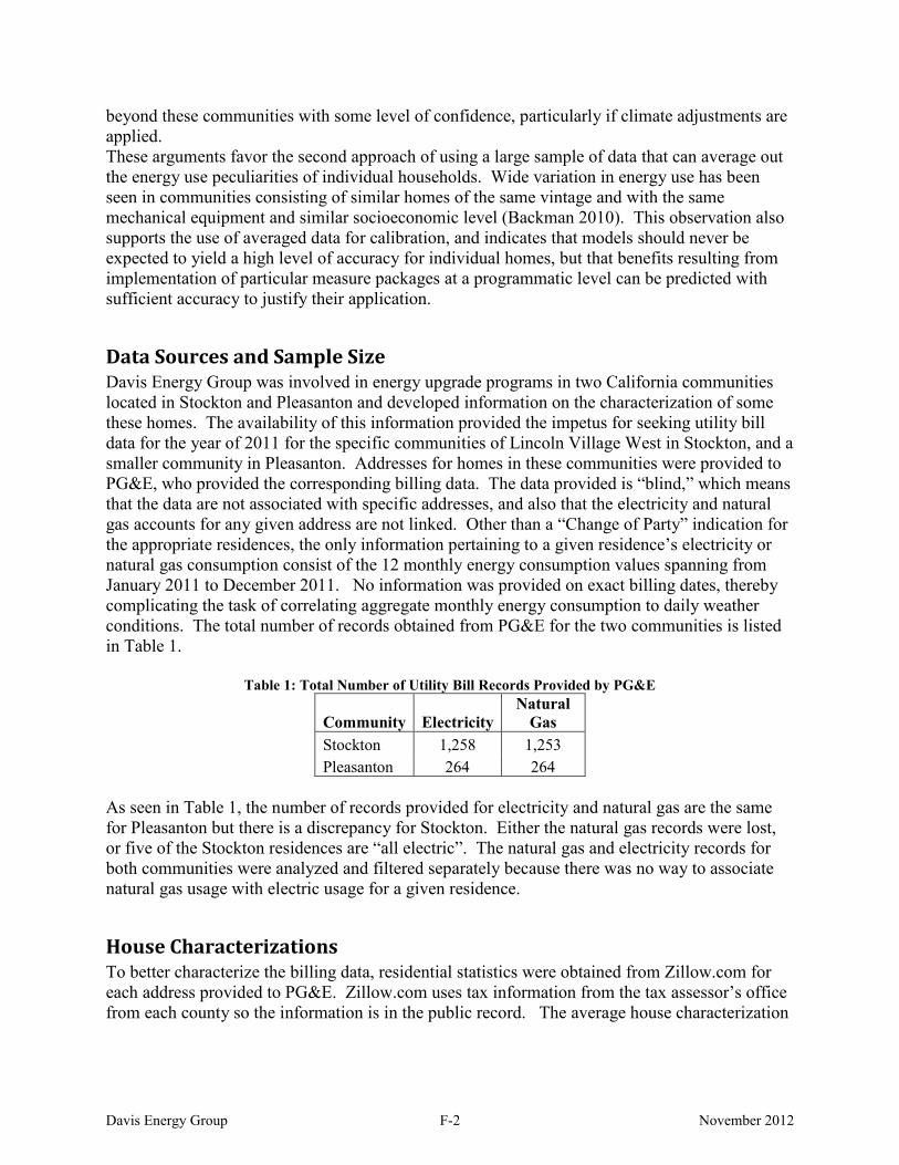
beyond these communities with some level of confidence, particularly if climate adjustments are applied. These arguments favor the second approach of using a large sample of data that can average out the energy use peculiarities of individual households. Wide variation in energy use has been seen in communities consisting of similar homes of the same vintage and with the same mechanical equipment and similar socioeconomic level (Backman 2010). This observation also supports the use of averaged data for calibration, and indicates that models should never be expected to yield a high level of accuracy for individual homes, but that benefits resulting from implementation of particular measure packages at a programmatic level can be predicted with sufficient accuracy to justify their application.

Data Sources and Sample Size Davis Energy Group was involved in energy upgrade programs in two California communities located in Stockton and Pleasanton and developed information on the characterization of some these homes. The availability of this information provided the impetus for seeking utility bill data for the year of 2011 for the specific communities of Lincoln Village West in Stockton, and a smaller community in Pleasanton. Addresses for homes in these communities were provided to PG&E, who provided the corresponding billing data. The data provided is “blind,” which means that the data are not associated with specific addresses, and also that the electricity and natural gas accounts for any given address are not linked. Other than a “Change of Party” indication for the appropriate residences, the only information pertaining to a given residence’s electricity or natural gas consumption consist of the 12 monthly energy consumption values spanning from January 2011 to December 2011. No information was provided on exact billing dates, thereby complicating the task of correlating aggregate monthly energy consumption to daily weather conditions. The total number of records obtained from PG&E for the two communities is listed in Table 1.

Table 1: Total Number of Utility Bill Records Provided by PG&E

Community Electricity Natural

Gas Stockton 1,258 1,253 Pleasanton 264 264

As seen in Table 1, the number of records provided for electricity and natural gas are the same for Pleasanton but there is a discrepancy for Stockton. Either the natural gas records were lost, or five of the Stockton residences are “all electric”. The natural gas and electricity records for both communities were analyzed and filtered separately because there was no way to associate natural gas usage with electric usage for a given residence.

House Characterizations To better characterize the billing data, residential statistics were obtained from Zillow.com for each address provided to PG&E. Zillow.com uses tax information from the tax assessor’s office from each county so the information is in the public record. The average house characterization

Davis Energy Group F-2 November 2012

data will aid calibration efforts by allowing representative plans to be developed from the data. For instance, the age of the home provides information on insulation levels and window types that were used by production builders of the particular era. Table 2 lists the range of characterization values for the two communities.

Table 2: Range of Characterization Values for Stockton and Pleasanton Data Sets

Stockton Pleasanton Minimum Maximum Minimum Maximum

Bathrooms 1 6.5 2 4 Bedrooms 2 7 2 6 Finished Floor Area 900 5,295 942 3,103 Lot Size 871 24,393 6,200 14,586 Year Built 1960 2006 1968 1989

Despite that the communities appeared to contain similar dwelling types and sizes when addresses were submitted to PG&E, the Zillow data indicated a wider variation of house size and vintage than was expected. To visualize correlations between the characteristics, three-dimensional plots were created using pairs of characteristics as shown in Figures 1-4.

Figure 1: Probability distribution of finished floor area to year built for the Stockton community.

1950 19

60 1970 19

80

0%

1%

2%

3%

4%

5%

6%

7%

8001000

12001400

16001800

20002200

24002600

28003000

6%-7%

5%-6%

4%-5%

3%-4%

2%-3%

1%-2%

0%-1%

Davis Energy Group F-3 November 2012

Figure 2: Probability distribution of finished floor area to number of bedrooms for the Stockton community.

Figure 3: Probability distribution of finished floor area to year built for the Pleasanton community.

1 2 3 4 5

0%

2%

4%

6%

8%

10%

8%-10%

6%-8%

4%-6%

2%-4%

0%-2%1950

1960

1970

1980

0%

2%

4%

6%

8%

10%

12%

10001200

14001600

18002000

2200

2400

2600

10%-12%

8%-10%

6%-8%

4%-6%

2%-4%

0%-2%

Davis Energy Group F-4 November 2012

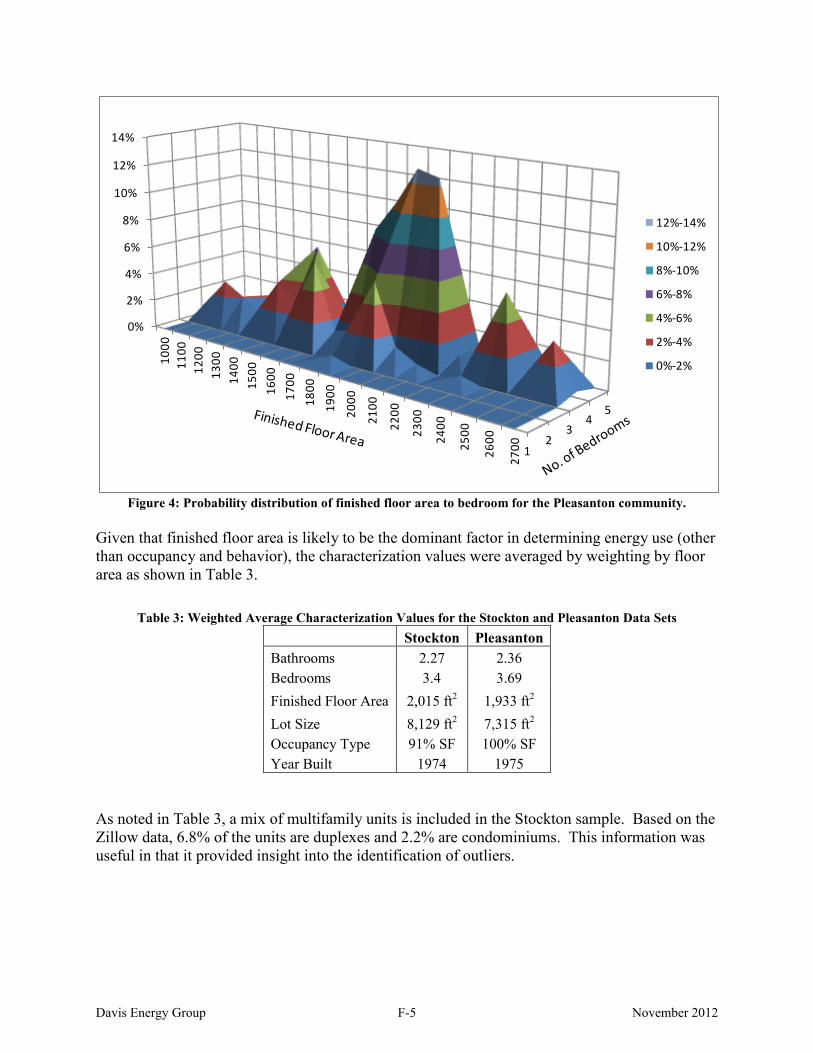
Figure 4: Probability distribution of finished floor area to bedroom for the Pleasanton community.

Given that finished floor area is likely to be the dominant factor in determining energy use (other than occupancy and behavior), the characterization values were averaged by weighting by floor area as shown in Table 3.

Table 3: Weighted Average Characterization Values for the Stockton and Pleasanton Data Sets

Stockton Pleasanton

Bathrooms 2.27 2.36 Bedrooms 3.4 3.69 Finished Floor Area 2,015 ft2 1,933 ft2 Lot Size 8,129 ft2 7,315 ft2 Occupancy Type 91% SF 100% SF Year Built 1974 1975

As noted in Table 3, a mix of multifamily units is included in the Stockton sample. Based on the Zillow data, 6.8% of the units are duplexes and 2.2% are condominiums. This information was useful in that it provided insight into the identification of outliers.

12

34

5

0%

2%

4%

6%

8%

10%

12%

14%

1000

1100

1200

1300

1400

1500

1600

1700

1800

1900

2000

2100

2200

2300

2400

2500

2600

2700

12%-14%

10%-12%

8%-10%

6%-8%

4%-6%

2%-4%

0%-2%

Davis Energy Group F-5 November 2012

Data Filtering Methods

Overview The objective of filtering the billing data was to limit the data sets to be used for calibration to complete records that are representative of typical end uses, and to eliminate records from houses that were likely to be unoccupied (abnormally low usage) and those that likely had swimming pools, spas, and other end uses that contributed to abnormally high usage. Some of the records provided by PG&E were incomplete, possibly due to vacancies or due to lost data that resulted in zero energy use for particular months. All records for which there was a change of residence indicator or that were missing at least one month of data were eliminated from the data set. This process was performed for all four data sets (gas and electric data for both communities). An example of the raw data received from PG&E is shown below.

Table 4: An example of raw electricity data received from PG&E.

For purposes of this study, electric and gas outliers were categorized as annual usage outliers, mild outliers, profile outliers, and irregular outliers (these are defined in subsequent sections). A fifth category for electric use, high spring base load, was used to identify the probable existence of swimming pools or spas.

Pool Outliers While swimming pool pumps are a valid end use, it was deemed necessary to eliminate houses that potentially include swimming pools to facilitate calibration efforts. Swimming pool pumps are among the highest household energy users, and savings resulting from their replacement are well documented and therefore do not need to be included in calibration efforts. Once the electricity data sets were purged of records that were incomplete, records that had high electric base loads that were most probably a result of swimming pools were filtered out. Comparing the list of residences with pools from Zillow data and the list of addresses in the data sets, the number of residences with pools in the Stockton and Pleasanton data sets are 203 and 24, respectively. By examining base load electrical use for the spring months including March, April, and May, houses with pools can be identified with some confidence. To eliminate the records that likely included pool pump use, electrical data sets for the two communities were separately sorted and ranked by the highest spring month energy consumption. Then, the top 203 electric users were removed from the Stockton set and the top 24 users were removed from the Pleasanton data set, corresponding to the number of pools in each community.

KWH__1 KWH__2 KWH__3 KWH__4 KWH__5 KWH__6 KWH__7 KWH__8 KWH__9 KWH__10 KWH__11 KWH__12 CHANGE OF PARTY910 657 529 573 609 615 941 622 680 552 872 931627 543 508 529 488 893 1,178 830 745 484 610 598

35 62 *

Davis Energy Group F-6 November 2012

Annual Usage Outliers While the pool outlier category focuses on the high end of the energy consumption, the annual usage outlier identifies the residences with annual energy usage that is unrealistically low. This approach establishes minimum energy consumption thresholds that the residences must meet in order to be included in the filtered data set. To qualify as an annual usage outlier, the total annual usage for either natural gas or electricity needs be less than the estimated annual base load of the smallest residence in the community, which is determined from the finished floor area (FFA) and the number of bedrooms, and from expected usage for houses of this size. If a residence falls into this category it is considered an indicator that it is not representative of the community and exhibits uncharacteristically low heating, cooling, or water heating energy use. From Zillow data the smallest reported unit sizes are as listed in Table 5.

Table 5: Lowest Unit Sizes for the Stockton and Pleasanton Data Sets

Using the values from Table 5, the annual electrical and natural gas base loads, which only include end uses that are not seasonally dependent, were estimated for the smallest residences. The base load calculations use equations from the Building America Simulation Protocols (Hendron 2010). Electric end uses and their corresponding equations for estimating annual loads are listed in Table 6. For purposes of filtering out low users, the garage area (in the garage lighting energy use calculation) was assumed to be zero.

Table 6: Estimated Annual Electric Base Load as Function of Finished Floor Area (FFA) and Number of Bedrooms (𝑵𝒃𝒓)

Category Equation (kWh/yr) Interior hard-wired lighting 0.8 × (FFA × 0.542 + 334) (1) Interior plug-in lighting 0.2 × (FFA × 0.542 + 334) (2) Garage lighting Garage Area × 0.08 + 8 (3) Exterior lighting FFA × 0.145 (4) Refrigerator 434 (5) Clothes washer (3.2 𝑓𝑡3 drum) 38.8 + 12.9 × 𝑁𝑏𝑟 (6) Clothes dryer (electric) 538.2 + 179.4 × 𝑁𝑏𝑟 (7) Clothes dryer (gas) 43 + 14.3 × 𝑁𝑏𝑟 (8) Dishwasher (8 place setting) 87.6 + 29.2 × 𝑁𝑏𝑟 (9) Range (electric) 250 + 83 × 𝑁𝑏𝑟 (10) Range (gas) 40 + 13.3 × 𝑁𝑏𝑟 (11) Miscellaneous loads (gas/electric house) 1595 + 248 ×𝑁𝑏𝑟 + 0.426 × FFA (12)

Miscellaneous loads (all-electric house) 1703 + 266 ×𝑁𝑏𝑟 + 0.454 × FFA (13)

Table 7 and Table 8 were used to calculate the minimum base loads for natural gas.

Community Finished Floor Area [Sq. Ft.] Number of BedroomsStockton, CA 900 2

Pleasanton, CA 942 2

Davis Energy Group F-7 November 2012

Table 7: Estimated Annual Natural Gas Base Load as Function of Finished Floor Area (FFA) and Number of Bedrooms (𝑵𝒃𝒓).

Category Equation (therms/yr) Clothes dryer (gas) 19.5 + 6.5 × 𝑁𝑏𝑟 (14) Range (gas) 14.3 + 4.8 × 𝑁𝑏𝑟 (15) Miscellaneous loads (gas/electric house) 3.7 + 0.6 × 𝑁𝑏𝑟 + 0.001 × FFA (16)

Table 8: Estimated Annual Domestic Hot Water Consumption

by End Use As Function of Number of Bedrooms (𝑵𝒃𝒓). Category Equation (gal/day) Clothes washer 2.35 + 0.78 × 𝑁𝑏𝑟 (hot only) (17) Dishwasher 2.26 + 0.75 × 𝑁𝑏𝑟 (hot only) (18) Shower (both standard and low-flow) 14.0 + 4.67 × 𝑁𝑏𝑟 (hot and cold) (19)

Bath 3.5 + 1.17 × 𝑁𝑏𝑟 (hot and cold) (20) Sinks 12.5 + 4.16 × 𝑁𝑏𝑟 (hot and cold) (21) When applying the equations above, especially for those appliances that can use either natural gas or electricity, it is useful to consider the saturation percentages associated with these appliances. According to the RASS (2010), the relevant saturation percentages pertaining to the four pertinent end use categories (water heating, clothes dryer, range, and miscellaneous) are listed in Table 9.

Table 9: Saturation Percentages of Natural Gas Appliances for Single Family Residences with Natural Gas Accounts

End Use Category Saturation Water Heater 95% Clothes Dryer 57% Range/Oven 76% Miscellaneous 14%

Since 95% of the single family residences and 88% of households served by PG&E have gas water heating, it was assumed that if natural gas was available at a residence, the domestic water heater would be gas-fired. The five apparent all-electric houses in Stockton community were removed during the filtering process, so it was assumed that all of the water heaters are gas-fired. Eqns. (19) through (21) estimate the total water volume used in a day for showers, baths, and sinks at a specific delivery temperature. From the Building America Simulation Protocols (Hendron 2010), for the shower, bath, and sinks categories for domestic hot water, the mixed temperature is 110°F and the temperature set point of the water heater is 130°F. The entering temperature of the cold water was approximated at 60°F. To determine the total volume of hot water used in a day for showers, baths, and sinks, mass energy conservation principles were applied using Equation 22, which for the above temperatures results in a factor of 0.714 gallons of hot water per gallon of mixed water.

Davis Energy Group F-8 November 2012

�̇�𝐻 = �̇�𝑡𝑜𝑡 �𝑇𝑡𝑜𝑡 − 𝑇𝐶𝑇𝐻 − 𝑇𝐶

� (22)

Where: �̇�𝐻 = mass flow of hot water

�̇�𝑡𝑜𝑡 = total flow of mixed water 𝑇𝑡𝑜𝑡 = temperature of the mixed water 𝑇𝐶 = temperature of the cold water For the two bedroom case, the results of applying Eqns. (17) through (22) are as listed in Table 10, and yield an estimated daily hot water usage of 43.33 gallons per day.

Table 10: Hot Water End Uses for Two Bedroom House

Use Point Total Hot Only

Clothes Washer 3.9 3.9 Dishwasher 3.76 3.76 Shower 23.34 16.66 Bath 5.8 4.14 Sinks 20.82 14.87 Total

43.33

Data from Hoeschele (2010), which included monitoring data from eighteen California water heaters, provided a relationship between daily hot water use and annual therms as shown in Figure 5. The linear regression equation was used to calculate a minimum expected annual water heating gas use of 166 therms.

Figure 5: Gallons per day vs. Therms per year measured for 18 California storage gas water heaters

0

50

100

150

200

250

300

350

0 50 100 150

Ther

ms p

er Ye

ar

Gallons per Day

Data

Linear

Y= 1.532x + 98.91R2 = 0.839

Davis Energy Group F-9 November 2012

The final values determined to be the minimum annual base loads for the two communities are listed in Table 10, as determined using Eqns. (1) through (22). The saturation percentages from RASS were used to allocate gas/electric uses for gas/electric stoves & ranges and clothes driers (included as “miscellaneous”). Consistent with the filtering methods described, the values listed in Table 10 were used as the minimum threshold for total annual energy consumption for the complete data set.

Table 10: Minimum Annual Energy Consumption Estimated Using Building America Protocol Equations.

Mild Outliers The process for filtering for mild outliers is as described in a “project closeout” document developed by NREL for the Building America program to identify energy savings for communities of new homes (NREL 2002). Mild outliers, in annual usage, were statistically identified by establishing “inner fences,” which are defined by the inner quartile range (IQR), first quartile, and third quartile for a given data-set. The first quartile, 𝑄1, includes 25% of the data points in the population, the third quartile, 𝑄3, includes 75% of the data points in the population, and the inner quartile range, 𝐼𝑄𝑅, is the difference between 𝑄3 and 𝑄1, meaning 𝐼𝑄𝑅 = 𝑄3 − 𝑄1 (23) For each energy type and community, the inner fences, which are simply statistical upper and lower limits, are quantified using Eqns. (24) and (25). 𝑈𝑝𝑝𝑒𝑟 𝐿𝑖𝑚𝑖𝑡 = 𝑄3 + 1.5 × 𝐼𝑄𝑅 (24) 𝐿𝑜𝑤𝑒𝑟 𝐿𝑖𝑚𝑖𝑡 = 𝑄1 − 1.5 × 𝐼𝑄𝑅 (25) If the annual usage of a residence is above or below the upper or lower limits, respectively, then the residence is considered a mild outlier and eliminated from the data population. Since the identification of mild outliers relies purely on statistical analysis, the importance of first eliminating the pool outliers and the annual energy usage outliers becomes apparent; if the latter two outliers were to remain in the data populations, the mild outlier statistical analysis could be significantly skewed and unrepresentative records could unintentionally persist in the data set.

End-Use by Energy Type Stockton, CA Pleasanton, CAElectricity (kWh/yr)

Lighting 960.30 989.15Miscellaneous 3,841.49 3,860.39Total 4,801.79 4,849.55

Natural Gas (therms/yr)DHW 166.46 166.46Miscellaneous 37.50 37.51Total 203.96 203.97

Davis Energy Group F-10 November 2012

Irregular Outliers Irregular outliers include two sets of outliers: data anomalies and vacancies. Data anomalies include missing data resulting from data collection or transfer issues, and physically implausible or unrealistic values for either natural gas or electricity, and are easily identified. For both natural gas and electricity data, any record that included zero or negative energy consumption was automatically eliminated from the data set. Vacancies, the second type of irregular outlier, were dealt with differently for natural gas and electricity. For electricity, records showing long term vacancies of greater than two weeks were filtered from the data set. Vacancies were identified as houses having monthly electricity usage of less than 150 kWh. This value was determined by adding end use values from RASS (2010) for typical vacant dwellings, as listed in Table 12. While occupants are out of the house it is typical to leave appliances, consumer electronics, computers, and other loads that draw standby power running, and to leave some interior lights on for security reasons. Thus, it was assumed that the exterior lighting would maintain its regular schedule, and interior lighting would be reduced to the same energy consumption as exterior lighting. These household end uses are listed in Table 11, and amount to an average load of just over 200 Watts.

Table 11: Consumption by Electric End Uses During Vacancies (from RASS 2010)

For residences with one vacancy month, the residences are still included in the analysis but there are additional steps required to properly categorize the energy consumption for the vacancy month, which will be further discussed in the disaggregation section. A similar approach was used to filter records for natural gas use. Hoeschele (2010) found that the average standby loss for gas storage water heaters was 415 Btuh, or 3.03 therms per month. Although some homeowners might shut off their water heater pilots for extended vacations, houses using less than 3 therms per month for more than one month were filtered from the samples. Houses with tankless water heaters could have a monthly usage of less than 3 therms while vacant, but the market penetration of tankless systems in existing homes is small because of the high cost of installing the larger gas lines that are required. Also, no solar water heaters were apparent from the Google Earth surveys.

Profile Outliers Certain patterns of annual energy usage are expected for natural gas and electricity. Higher gas use is expected in winter for space heating as well as water heating, and higher electric use is expected in summer for air conditioning. Billing data for Stockton, shown in Figure 6 and

Category Energy Consumed Per Year (kWh)Refrigerator 827Microwave 133Home Office Equipment 89Outdoor Lighting 388Indoor Lighting 388

Total 1825Monthly Average 152.1

Davis Energy Group F-11 November 2012

Figure 7, follow these expected patterns. Because of the more mild climate, usage in the Pleasanton houses is expected to be somewhat attenuated, as shown in Figure 8 and Figure 9.

Figure 6: Representative profiles of electricity consumption in Stockton.

Figure 7: Representative profiles of natural gas consumption in Stockton.

0

500

1000

1500

2000

2500

Ener

gy U

sage

[kW

h]

0

50

100

150

200

250

300

Ener

gy U

sage

[the

rms]

Davis Energy Group F-12 November 2012

Figure 8: The general annual profile of electricity consumption in Pleasanton.

Figure 9: The general annual profile of natural gas consumption in Pleasanton.

If a billing record displayed an annual profile that significantly deviated from either of these general trends, the record was to be considered a profile outlier and eliminated from the data set. Such deviations would include abnormally high consumption for any month, and profiles that do not display the seasonal variations representative of the norm.

0

200

400

600

800

1000

1200

1400

1600

1800En

ergy

Usa

ge [k

Wh]

0

20

40

60

80

100

120

140

160

180

200

Ener

gy U

sage

[the

rms]

Davis Energy Group F-13 November 2012

Final Filtered Data Populations Table 12 lists the surviving number of billing data records, and Table 13 lists the records that were filtered out using each criteria. “PG&E Filter” refers to records that were identified by PG&E as being incomplete due to changes in occupancy.

Table 12: Surviving Records to be Used for Disaggregation

Table 13: Number of Records Removed By Filtering Process

The complete, filtered electricity and natural gas data sets for both Stockton and Pleasanton are shown in Figure 10 and Figure 11. Electricity and natural gas consumption was slightly higher in Stockton than in Pleasanton, and this difference was higher for natural gas than for electricity.

Community Electricity Natural GasStockton, CA 679 927Pleasanton, CA 165 212

Number of Residences

Filtering Process Stockton Pleasanton Stockton PleasantonPG&E Filter 260 40 255 39Pool Outliers 203 24 0 0Annual Usage Outliers 108 33 30 4Mild Outliers 1 0 29 4Irregular Outliers 7 2 9 1Profile Outliers 0 0 3 4

Number of Residences Filtered with Each ProcessElectricity Natural Gas

Davis Energy Group F-14 November 2012

Figure 10: The filtered electricity population for Stockton and Pleasanton.

Figure 11: The filtered natural gas population for Stockton and Pleasanton.

0

1,000

2,000

3,000

4,000

5,000

6,000

7,000

8,000

9,000

10,000

11,000

12,000

13,000

14,000

15,000An

nual

Ener

gy C

onsu

mpt

ion

[kW

h]Filtered Data Set Populations - Electricity

Stockton Pleasanton

0

100

200

300

400

500

600

700

800

900

1000

1100

1200

1300

Annu

al En

ergy

Con

sum

ptio

n [th

erm

s]

Filtered Data Set Populations - Natural Gas

Stockton Pleasanton

Davis Energy Group F-15 November 2012

End Use Disaggregation Methods

Review of Disaggregation Methods in the Literature Methods for disaggregating billing data have been previously described (ASHRAE 2002, Belzer 2007, Sondregger 1998). ASHRAE Guideline 14-2002 was reviewed for applicability to the task of disaggregating the large sample of PG&E billing data. The ASHRAE Guideline describes a steady state inverse monthly model and methods to correlate annual temperature profiles to annual energy usage profiles using a linear regression approach. The ASHRAE linear regression method provides a good approach for finding the change-point temperatures, but it does not provide for seasonal variations in base load, such as increased use of lighting in winter months.

Another reference that was consulted is a report describing a statistical analysis of energy consumption data of Home Performance with Energy Star homes in Austin, Texas (Belzer 2007). The authors conducted a regression analysis using billing histories and patterns related to energy use, seasonal temperatures, kilowatt hours used, cooling reference temperatures, and other factors to estimate cooling energy savings for the program, which applied both envelope improvements and equipment upgrades. Belzer’s analytical method, while very appropriate for the Austin study, was not useful for this evaluation because the specific start and end dates of each billing period were not provided with the PG&E billing data, and very little is known about the specific characteristics of the building envelopes (insulation levels, etc.) or the level of internal gains. Without this information reference temperatures could not be identified. The Austin analysis also does not appear to vary electric base load seasonally. The California Residential Appliance Saturation Study (RASS) provides statewide and utility-specific end use data and can be used as a reference point for comparison of local data, but is not useful for disaggregating billing data from specific communities because of the diversity of building types and climates. Later in this report the RASS data is compared with the results of the disaggregated data for the Stockton and Pleasanton communities.

Climate Characteristics Monthly average maximum, minimum, and mean temperatures are shown in Figure 12 and Figure 13 for Stockton and Pleasanton for 2011, the same year for which billing data were obtained. The months of March, April, and May where the mean temperature falls between 60°F and 70°F, require little or no heating or cooling. The same is true for the month of October, although occasional “heat storms” can cause air conditioners to run in October. Figure 14 compares heating and cooling degree days for the two locations.

Davis Energy Group F-16 November 2012

Figure 12: Average maximum, minimum, and mean monthly temperatures for Stockton in 2011.

Figure 13: Average maximum, minimum, and mean monthly temperatures for Pleasanton in 2011.

30

40

50

60

70

80

90

100

1 2 3 4 5 6 7 8 9 10 11 12

Tem

pera

ture

[°F]

Month

Stockton 2011 Weather

Max T

Mean

Min T

30

40

50

60

70

80

90

100

1 2 3 4 5 6 7 8 9 10 11 12

Tem

pera

ture

[°F]

Month

Pleasanton 2011 Weather

Max T

Mean

Min T

Davis Energy Group F-17 November 2012

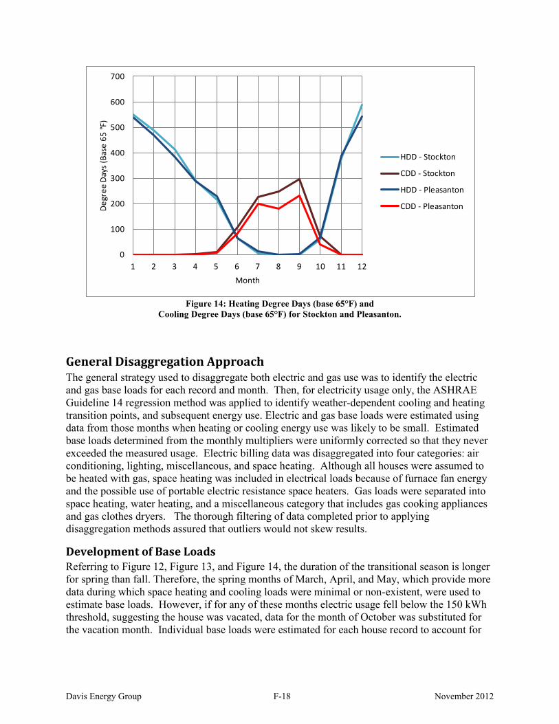
Figure 14: Heating Degree Days (base 65°F) and

Cooling Degree Days (base 65°F) for Stockton and Pleasanton.

General Disaggregation Approach The general strategy used to disaggregate both electric and gas use was to identify the electric and gas base loads for each record and month. Then, for electricity usage only, the ASHRAE Guideline 14 regression method was applied to identify weather-dependent cooling and heating transition points, and subsequent energy use. Electric and gas base loads were estimated using data from those months when heating or cooling energy use was likely to be small. Estimated base loads determined from the monthly multipliers were uniformly corrected so that they never exceeded the measured usage. Electric billing data was disaggregated into four categories: air conditioning, lighting, miscellaneous, and space heating. Although all houses were assumed to be heated with gas, space heating was included in electrical loads because of furnace fan energy and the possible use of portable electric resistance space heaters. Gas loads were separated into space heating, water heating, and a miscellaneous category that includes gas cooking appliances and gas clothes dryers. The thorough filtering of data completed prior to applying disaggregation methods assured that outliers would not skew results.

Development of Base Loads Referring to Figure 12, Figure 13, and Figure 14, the duration of the transitional season is longer for spring than fall. Therefore, the spring months of March, April, and May, which provide more data during which space heating and cooling loads were minimal or non-existent, were used to estimate base loads. However, if for any of these months electric usage fell below the 150 kWh threshold, suggesting the house was vacated, data for the month of October was substituted for the vacation month. Individual base loads were estimated for each house record to account for

0

100

200

300

400

500

600

700

1 2 3 4 5 6 7 8 9 10 11 12

Degr

ee D

ays (

Base

65

°F)

Month

HDD - Stockton

CDD - Stockton

HDD - Pleasanton

CDD - Pleasanton

Davis Energy Group F-18 November 2012

differences in house size, occupant behavior, and other factors. Additionally, due to the monthly variability in the lighting and miscellaneous energy consumption, monthly multipliers for these two categories were incorporated into the base load calculations.

Disaggregation of Electric Loads Electric end uses were separated into air conditioning, space heating, lighting, and miscellaneous loads. The following methods were used to segregate the total monthly electric use for each billing record into these four end uses:

Lighting and Miscellaneous Loads Lighting energy use was assumed to be consistent with the calculated usage from Hendron (2010), which varies monthly (see Table 14). Lighting energy use for the months of March, April, and May was calculated using Eqns. (1) and (2), factored by the monthly adjustment factors from Hendron (2010) and subtracted from the spring month billing values for each record. The result was averaged to obtain the monthly miscellaneous electric use for that record, which was assumed to also vary on a monthly basis due to seasonality. The assumption behind this method is that the spring months are relatively free of air conditioning and heating/cooling fan energy use. Lighting energy use for all other months was calculated using the same monthly adjustment factors, which would tend to make lighting energy use consistent with BEopt predictions. If for any month the sum of the calculated lighting and average non-lighting base load exceeded the actual usage, the actual values from the billing records were used, which means that the projected lighting and miscellaneous base load values had to be reduced to the actual billing values. This approach was applied to all data sets.

Table 14: Monthly Multipliers for Lighting and Miscellaneous End Uses from the Building America Simulation Protocol (Hendron 2010)

Month Lighting Misc.1 1.62 1.12 1.28 1.13 1.20 14 0.95 15 0.85 16 0.77 0.97 0.81 0.98 0.91 0.99 1.06 0.910 1.31 1.111 1.51 1.112 1.67 1.1

Monthly Multiplier

Davis Energy Group F-19 November 2012

The lighting usage multipliers from Hendron are designed to be applied to annual lighting energy use to generate monthly lighting end use profiles. These multipliers were normalized to the average of the spring months (March, April, and May) to generate the monthly multipliers. For each record, the spring lighting base load was multiplied by the corresponding multiplier for each month to develop an “unadjusted” lighting base load profile. As was done for lighting, the miscellaneous load was generated using monthly multipliers. As seen in Table 14, the multiplier for the spring months (March, April, and May) is unity. The unadjusted miscellaneous base load profile was developed using the spring miscellaneous energy base load and the corresponding monthly multiplier. The sum of the miscellaneous and the lighting base loads were adjusted by their respective percentages if the calculated load exceeded the lighting and miscellaneous electric use from the billing data. Where low monthly usage indicated a probable vacation, electrical use was attributed to lighting and miscellaneous use the same as if the house were occupied (no cooling energy use).

Cooling Energy Use Cooling energy use was estimated by first subtracting out the monthly base loads (lighting and miscellaneous) calculated as above from each record. Then the linear regression methods described in ASHRAE Guideline 14 (2002) were applied to determine the monthly change points between heating and cooling. Separate regressions were used to determine the heating-cooling and cooling-heating transitions, with the first of August being used as the center point for the two regression lines. A linear regression analysis was performed for both the spring and fall transition periods to identify the months in which the residence changed from space heating to air conditioning energy usage, or vice versa. The regression analysis generated for the disaggregation methodology captures, for the given household, the point at which the household transitions in the shoulder season and the additional energy consumption associated with the new heating or cooling load. In order to apply the regression analysis, the base load had to be removed from the annual energy profile to reduce the likelihood of incorrectly correlating energy consumption to temperature independent behavior. An automated linear regression script, using the maximum monthly temperatures for the corresponding community, was used to evaluate the temperatures at which the transition from heating to cooling and then cooling to heating occurred. The maximum monthly temperatures were used instead of the average monthly temperatures because the drastic changes in maximum temperatures are the strongest indicators of weather pattern changes. If the average temperatures were to be used, the daily temperatures would have to be averaged during the peak temperature period of the day, which occurs between noon and 8 PM, because this is the period where air conditioning is most prominently used. The average transition temperatures and periods in which they occur (by decimal month) for the two communities are listed in Table 15. As seen in Table 15, the average outdoor temperature at which the change point between heating and cooling occurred was considerably higher in fall than in spring. This phenomenon can probably be attributed to the adaptation of homeowners to lower winter temperatures in Spring, inspiring lower thermostat settings when warmer temperatures arrived, and adaptation to higher

Davis Energy Group F-20 November 2012

temperatures during summer, which caused them to be more sensitive to lower temperatures toward the end of the cooling season.

Table 15: Transition Temperatures and Months Determined by the Linear Regression Analysis Using Maximum Monthly Temperatures

The results of Table 15 are consistent with what would be expected intuitively; the spring transition temperature is lower than the fall transition temperature because people become conditioned to prevailing ambient weather conditions. To verify the validity of the linear regression analysis for the spring and fall linear regressions, the correlations of the predicted monthly energy usage, from the linear regression, and the actual monthly energy usage were evaluated and summarized in Table 16.

Table 16: Average and Standard Deviation Values for the Correlation Between Linear Regressions and Actual Electricity Consumption

It was not expected that the linear regression would have a high correlation to the actual electricity usage. Due to the unpredictable and varied nature of the actual consumption data, the superimposed linear relationship sometimes does not precisely match the actual data. Interestingly, however, examining Table 15, there is near uniformity in the fall transition occurring in November for both communities, but there is much more variation in the spring transition month. Both communities had the majority of the residences exhibit transitions from heating to cooling in April, which is shown by the average transition month being closest to 4.0. However, because the transition month is less than four, there were some residences that transitioned in March and some that transitioned in May. The variability in the spring transition is not surprising because there tend to be more sporadic temperature patterns throughout spring than in fall.

Summary of the Community Average of Independently Disaggregated Residences After the annual consumption profile for each residence was appropriately divided based on the residence’s particular transition months, the yearly data could be divided between air conditioning and space heating. If the predicted lighting and miscellaneous base loads exceeded the actual energy consumption for any given month, the lighting and miscellaneous base load values were reduced by the appropriate amount until they matches the actual value.

Community Spring Fall Spring FallStockton 61.7 65.1 3.8 11Pleasanton 62.0 71.0 3.7 10.8

Average Transition Temperature [°F] Average Transition Month

Spring Fall Spring FallStockton 0.76 0.63 0.19 0.22Pleasanton 0.43 0.48 0.27 0.22

Average R2 Standard Deviation R2

Davis Energy Group F-21 November 2012

Disaggregation of Gas Loads

Natural Gas Non-Space Heating Loads Excluding furnace gas use, natural gas end uses include water heating, and miscellaneous uses comprising cooking and clothes drying. For each record, Eqns. (14) through (18) were used to estimate miscellaneous gas use and Eqns. (19) and (22) were used to estimate hot water use. Factors to account for seasonal hot water use variations identified by Hoeschele (2011) were used to adjust the monthly water heating energy use values from those calculated using Hendron (2010). The regression equation in Figure 5 was used to convert from daily hot water use to Therms. The sum of these uses was used to estimate non-space heating gas use.

Space Heating Gas Use For each record, the space heating energy use was calculated by subtracting the projected water heating and miscellaneous base loads from the actual energy usage.

Monthly Multipliers for Base load Categories Hot water use varies seasonally primarily as a result of lower winter and higher summer water mains temperatures. To generate the annual energy consumption profiles for the miscellaneous and water heating end use categories from the summer base loads, monthly water heating end use multipliers were derived from data compiled by Hoeschele (2011). Best fits of the data yielded the following two equations, where 𝑚 is the numerical month of the year: Stockton DHW Multiplier = 0.03𝑚2 − 0.39𝑚 + 2.33 (26) Pleasanton DHW Multiplier = 0.02𝑚2 − 0.24𝑚 + 1.89 (27) The multiplier for Pleasanton has a lower slope than for Stockton due to the milder bay area climate. Because there was minimal hot water use data to work from, the equations were normalized to the lowest five non-winter consumption months. This normalization ensured that the base load usage was not abnormally low.

Parameter Study of Electricity Disaggregation To ensure that the appropriate base load percentages were chosen for the two categories, lighting and miscellaneous, a parameter study was conducted for both Stockton and Pleasanton. The desired percentages that represent the base load disaggregation are values that do not create significant variability in all of the end use categories and are representative of actual values. In the parametric study, the annual end use percentages for all four of the categories (lighting, miscellaneous, air conditioning, and space heating) were evaluated by varying the base load fractions for lighting and miscellaneous from zero to 1 and from 1 to zero, respectively. As expected and as shown in Figure 15 and Figure 16, due to the higher monthly magnitudes in the winter months, as the fraction of the lighting base load increases, the annual end use percentage for space heating decreases. Conversely, the base load ratio has very little effect on the annual end use percentages for air conditioning—for Stockton, it is nearly constant at 16%, and for Pleasanton, it is nearly constant at 10%. Based on the observed variations, the

Davis Energy Group F-22 November 2012

approximation for disaggregation of the spring base load is 20% for lighting and 80% for miscellaneous.

Figure 15: Parameter study for the Stockton electricity population with varying base load ratios.

Figure 16: Parameter study for the Pleasanton electricity population with varying base load ratios.

0%10%20%30%40%50%60%70%80%90%

100%0

/ 1

0.05

/ 0.

95

0.1

/ 0.9

0.15

/ 0.

85

0.2

/ 0.8

0.25

/ 0.

75

0.3

/ 0.7

0.35

/ 0.

65

0.4

/ 0.6

0.45

/ 0.

55

0.5

/ 0.5

0.55

/ 0.

45

0.6

/ 0.4

0.65

/ 0.

35

0.7

/ 0.3

0.75

/ 0.

25

0.8

/ 0.2

0.85

/ 0.

15

0.9

/ 0.1

0.95

/ 0.

05

1 / 0

Annu

al En

d-Us

e Pe

rcen

tage

Baseload Ratio (Lighting / Miscellaneous)

Parameter Study - Stockton Electricity

Lighting Space Heating A/C Misc.

0%10%20%30%40%50%60%70%80%90%

100%

0 / 1

0.05

/ 0.

95

0.1

/ 0.9

0.15

/ 0.

85

0.2

/ 0.8

0.25

/ 0.

75

0.3

/ 0.7

0.35

/ 0.

65

0.4

/ 0.6

0.45

/ 0.

55

0.5

/ 0.5

0.55

/ 0.

45

0.6

/ 0.4

0.65

/ 0.

35

0.7

/ 0.3

0.75

/ 0.

25

0.8

/ 0.2

0.85

/ 0.

15

0.9

/ 0.1

0.95

/ 0.

05

1 / 0

Annu

al En

d-Us

e Pe

rcen

tage

Baseload Ratio (Lighting / Miscellaneous)

Parameter Study - Pleasanton Electricity

Lighting Space Heating A/C Misc.

Davis Energy Group F-23 November 2012

Parameter Study of Natural Gas Disaggregation As was completed for the electric use data, a parameter study was done using the natural gas data to determine the most appropriate base load disaggregation ratios. In this case the annual end use percentages were evaluated by varying hot water and miscellaneous load categories, again in ratios of from zero to 1 and 1 to zero, respectively as shown in Figures 17 and 18.

Figure 17: Parameter study for the natural gas Stockton population with varying base load ratios.

Figure 18: Parameter study for the Pleasanton natural gas population with varying base load ratios.

0%10%20%30%40%50%60%70%80%90%

100%

0 / 1

0.05

/ 0.

95

0.1

/ 0.9

0.15

/ 0.

85

0.2

/ 0.8

0.25

/ 0.

75

0.3

/ 0.7

0.35

/ 0.

65

0.4

/ 0.6

0.45

/ 0.

55

0.5

/ 0.5

0.55

/ 0.

45

0.6

/ 0.4

0.65

/ 0.

35

0.7

/ 0.3

0.75

/ 0.

25

0.8

/ 0.2

0.85

/ 0.

15

0.9

/ 0.1

0.95

/ 0.

05

1 / 0

Annu

al En

d-Us

e Pe

rcen

tage

Baseload Ratio (Water Heating / Miscellaneous)

Parameter Study - Stockton Natural Gas

Water Heating Misc. Space Heating

0%10%20%30%40%50%60%70%80%90%

100%

0 / 1

0.05

/ 0.

95

0.1

/ 0.9

0.15

/ 0.

85

0.2

/ 0.8

0.25

/ 0.

75

0.3

/ 0.7

0.35

/ 0.

65

0.4

/ 0.6

0.45

/ 0.

55

0.5

/ 0.5

0.55

/ 0.

45

0.6

/ 0.4

0.65

/ 0.

35

0.7

/ 0.3

0.75

/ 0.

25

0.8

/ 0.2

0.85

/ 0.

15

0.9

/ 0.1

0.95

/ 0.

05

1 / 0

Annu

al En

d-Us

e Pe

rcen

tage

Baseload Ratio (Water Heating / Miscellaneous)

Parameter Study - Pleasanton Natural Gas

Water Heating Misc. Space Heating

Davis Energy Group F-24 November 2012

Similar to the electricity parameter study, since the water heating monthly multiplier has a much higher magnitude per month than the miscellaneous multiplier, the annual end use percentage for space heating is lower when there is more water heating usage in the base load. However, irrespective of the base load ratio combination, the space heating annual end use percentage varies only slightly around 60%. Based on the observed variations, the best base load disaggregation approximation is water heating at 67% and miscellaneous at 33% of the spring base load.

Electricity Disaggregation Results

Averages of Individually Disaggregated Electric Billing Records Using the approach of first disaggregating each electric bill record as described and then averaging the results, the end use profiles shown in Figures 19 and 20 were produced.

Figure 19: Averages of individually disaggregated electric billing records for Stockton

0

100

200

300

400

500

600

700

800

900

1000

1100

1 2 3 4 5 6 7 8 9 10 11 12

Ener

gy U

sage

[kW

h]

Month

Disaggregation of Electricity Usage for Stockton Residences

Miscellaneous Lighting Air Conditioning Space Heating

Davis Energy Group F-25 November 2012

Figure 17: Averages of individually disaggregated electric billing records for Pleasanton

Both communities showed wide variations in energy usage as indicated in Figures 10 and 11, so it is of interest to observe the means and standard deviations for each end use category and month. These variations are shown in Figures 21 through 24.

Figure 21: Mean values and standard deviation of monthly miscellaneous electric and lighting end uses for

Stockton

0

100

200

300

400

500

600

700

800

900

1000

1100

1 2 3 4 5 6 7 8 9 10 11 12

Ener

gy U

sage

[kW

h]

Month

Disaggregation of Electricity Usage for Pleasanton Residences

Miscellaneous Lighting Air Conditioning Space Heating

0

100

200

300

400

500

600

700

1 2 3 4 5 6 7 8 9 10 11 12

Ener

gy U

sage

[kW

h]

Month

Electricity Baseload - Stockton

Miscellaneous Lighting

Davis Energy Group F-26 November 2012

Figure 22: Mean values and standard deviation of monthly

space heating and air conditioning end uses for Stockton

Figure 23: Mean values and standard deviation of monthly

lighting and miscellaneous end uses for Pleasanton

-100

0

100

200

300

400

500

600

700

1 2 3 4 5 6 7 8 9 10 11 12

Ener

gy U

sage

[kW

h]

Month

Electricity Space Heating & Cooling - Stockton

Space Heating Air Conditioning

0

100

200

300

400

500

600

700

1 2 3 4 5 6 7 8 9 10 11 12

Ener

gy U

sage

[kW

h]

Month

Electricity Baseload - Pleasanton

Miscellaneous Lighting

Davis Energy Group F-27 November 2012

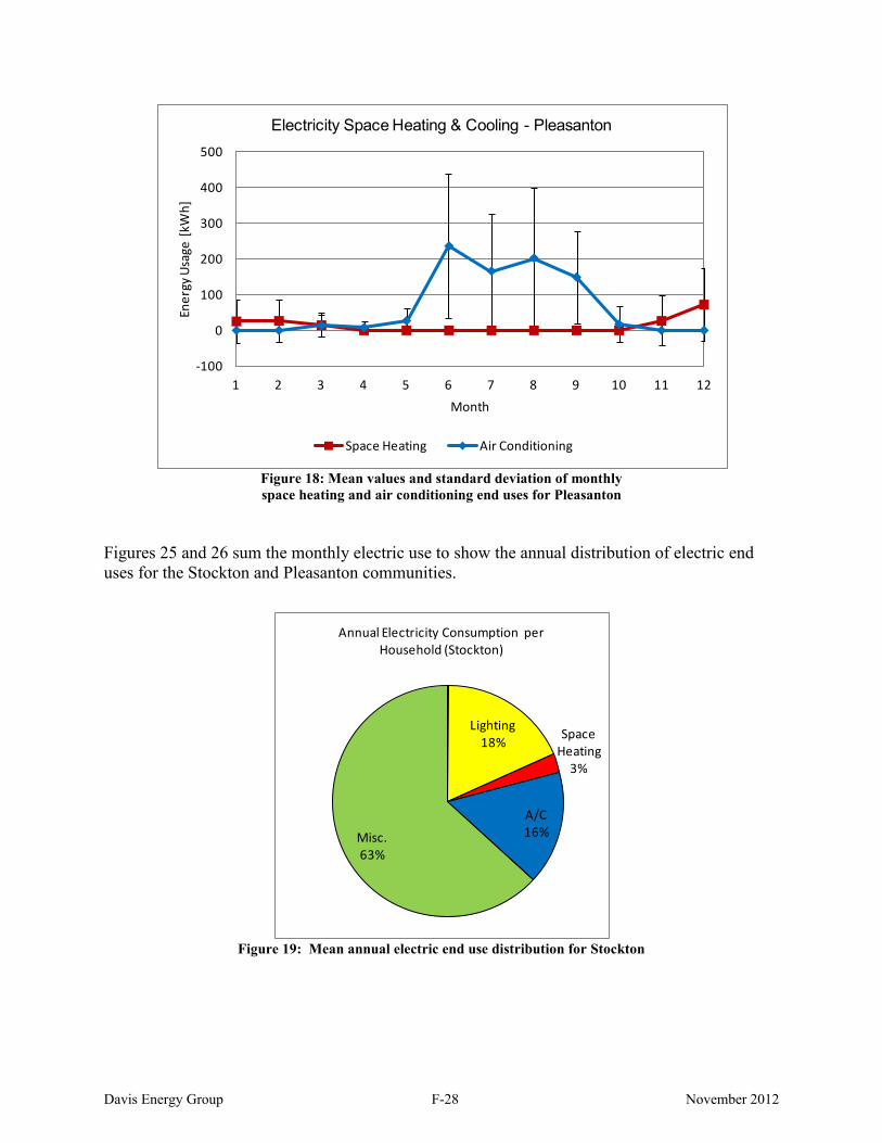
Figure 18: Mean values and standard deviation of monthly space heating and air conditioning end uses for Pleasanton

Figures 25 and 26 sum the monthly electric use to show the annual distribution of electric end uses for the Stockton and Pleasanton communities.

Figure 19: Mean annual electric end use distribution for Stockton

-100

0

100

200

300

400

500

1 2 3 4 5 6 7 8 9 10 11 12

Ener

gy U

sage

[kW

h]

Month

Electricity Space Heating & Cooling - Pleasanton

Space Heating Air Conditioning

Lighting18% Space

Heating3%

A/C16%Misc.

63%

Annual Electricity Consumption per Household (Stockton)

Davis Energy Group F-28 November 2012

Figure 20: Mean annual electric end use distribution for Pleasanton

Disaggregation of Averaged Electric Bills As a corollary to the method of disaggregating utility bill records as a first step and then averaging the results, all records were first averaged and then the averaged values were disaggregated to compare differences between the two methods. The same disaggregation methods were applied in each case. Disaggregating the averages is of course a much simpler endeavor, and if it yields reasonably similar results would save time when this effort is repeated for other communities. Comparing Figures 27 and 28 to Figures 19 and 20 shows very similar use profiles except that when averaging is applied first, space heating loads (probably mostly furnace fan energy), is absorbed into lighting and miscellaneous categories. This is also shown in Table 17, which compares breakdowns of annual usage for the two methods. When each individual household electricity record is disaggregated and then averaged with others, the end uses are more clearly defined because this method is more effective at capturing the variation in the end uses. At least for the cases presented, the second, simpler approach is an attractive way to reduce analysis time without sacrificing significant accuracy.

Table 17: Comparison of Electric End Use Disaggregation Percentages Using Different Averaging Approaches

Lighting Misc. Space

Ht. Air

Cond. Disaggregate First

Stockton 18% 63% 3% 16% Pleasanton 19% 65% 1% 15% Average First

Stockton 20% 68% 2% 10% Pleasanton 20% 71% 0% 9%

Lighting20%

Space Heating

2%

A/C10%

Misc.68%

Annual Electricity Consumption per Household (Pleasanton)

Davis Energy Group F-29 November 2012

Figure 27: Disaggregation of averaged electric billing records for Stockton

Figure 28: Disaggregation of averaged electric billing records for Pleasanton

0

100

200

300

400

500

600

700

800

900

1000

1 2 3 4 5 6 7 8 9 10 11 12

Ener

gy U

sage

[kW

h]

Month

Disaggregation of the Average Electricity Usage for Stockton Residences

Miscellaneous Lighting Air Conditioning Space Heating

0

100

200

300

400

500

600

700

800

900

1 2 3 4 5 6 7 8 9 10 11 12

Ener

gy U

sage

[kW

h]

Month

Disaggregation of the Average Electricity Usage Pleasanton Residences

Miscellaneous Lighting Air Conditioning Space Heating

Davis Energy Group F-30 November 2012

Natural Gas Disaggregation Results

Averages of Individually Disaggregated Gas Billing Records Monthly gas use for water heating, space heating, and miscellaneous gas use categories developed using the method of first disaggregating data for each record and then averaging the results is shown in Figure and Figure . Miscellaneous gas use can include gas ranges and ovens, natural gas barbecues, and gas fireplaces. However, since gas fireplace usage is limited to winter months the disaggregation method would attribute it to space heating. There is very slight dip in summer gas use that might be from reduced indoor cooking and use of outdoor propane or charcoal barbecues. Water heating displays the seasonal variation that was applied using the method described.

Figure 29: Averages of individually disaggregated gas billing records for Stockton

0

20

40

60

80

100

120

140

1 2 3 4 5 6 7 8 9 10 11 12

Ener

gy U

sage

[the

rms]

Month

Disaggregation of Natural Gas Usage For Stockton Residences

Miscellaneous Water Heating Space Heating

Davis Energy Group F-31 November 2012

Figure 30: Averages of individually disaggregated gas billings for Pleasanton

As is seen with electric use there are wide variations in gas usage amongst the billing records. Figures 31 through 34 plot the monthly mean usage and standard deviation for the two communities.

0

20

40

60

80

100

120

1 2 3 4 5 6 7 8 9 10 11 12

Ener

gy U

sage

[The

rms]

Month

Disaggregation of Natural Gas Usage For Pleasanton Residences

Miscellaneous Water Heating Space Heating

0

5

10

15

20

25

30

35

40

1 2 3 4 5 6 7 8 9 10 11 12

Ener

gy U

sage

[the

rms]

Month

Natural Gas Baseload - Stockton

Miscellaneous Water Heating

Davis Energy Group F-32 November 2012

Figure 31: Mean values and standard deviation of monthly gas base loads for Stockton

Figure 32: Mean values and standard deviation of monthly gas space heating loads for Stockton

Figure 33: Mean values and standard deviation of monthly gas base loads for Pleasanton

-20

0

20

40

60

80

100

120

140

1 2 3 4 5 6 7 8 9 10 11 12

Ener

gy U

sage

[the

rms]

Month

Natural Gas Space Heating - Stockton

Space Heating

0

5

10

15

20

25

30

1 2 3 4 5 6 7 8 9 10 11 12

Ener

gy U

sage

[the

rms]

Month

Natural Gas Baseload - Pleasanton

Miscellaneous Water Heating

Davis Energy Group F-33 November 2012

Figure 34: Mean values and standard deviation of monthly gas space heating loads for Pleasanton

Figures 35 and 36 sum the monthly gas use to show the annual distribution of natural gas end uses for the Stockton and Pleasanton communities.

Figure 35: Mean annual natural gas end use distribution for Stockton

0

20

40

60

80

100

120

1 2 3 4 5 6 7 8 9 10 11 12

Ener

gy U

sage

[the

rms]

Month

Natural Gas Space Heating - Pleasanton

Space Heating

Water Heating

29%

Misc.12%

Space Heating

59%

Annual Natural Gas Consumption per Household (Stockton)

Davis Energy Group F-34 November 2012

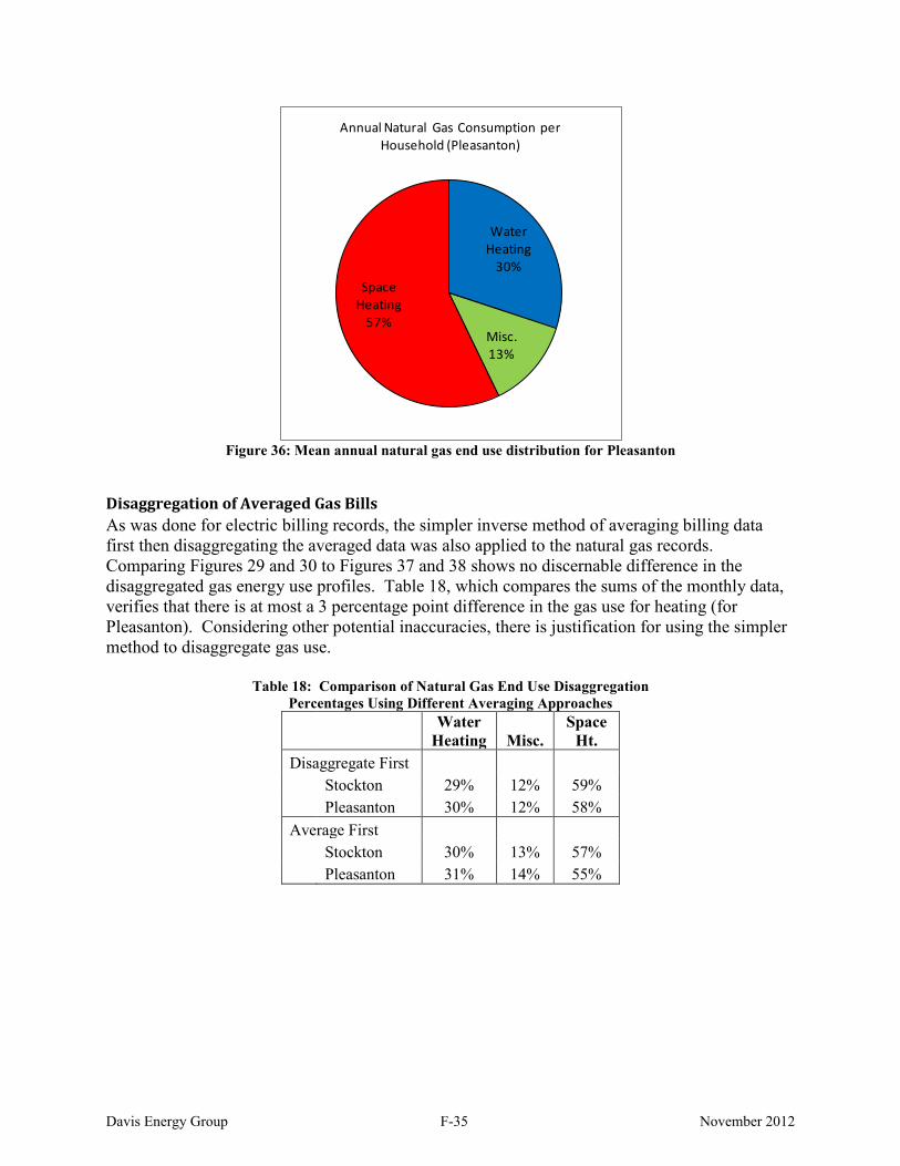
Figure 36: Mean annual natural gas end use distribution for Pleasanton

Disaggregation of Averaged Gas Bills As was done for electric billing records, the simpler inverse method of averaging billing data first then disaggregating the averaged data was also applied to the natural gas records. Comparing Figures 29 and 30 to Figures 37 and 38 shows no discernable difference in the disaggregated gas energy use profiles. Table 18, which compares the sums of the monthly data, verifies that there is at most a 3 percentage point difference in the gas use for heating (for Pleasanton). Considering other potential inaccuracies, there is justification for using the simpler method to disaggregate gas use.

Table 18: Comparison of Natural Gas End Use Disaggregation Percentages Using Different Averaging Approaches

Water

Heating Misc. Space

Ht. Disaggregate First

Stockton 29% 12% 59% Pleasanton 30% 12% 58% Average First

Stockton 30% 13% 57% Pleasanton 31% 14% 55%

Water Heating

30%

Misc.13%

Space Heating

57%

Annual Natural Gas Consumption per Household (Pleasanton)

Davis Energy Group F-35 November 2012

Figure 37: Disaggregation of averaged natural gas billing records for Stockton

Figure 38: Disaggregation of averaged natural gas billing records for Pleasanton

0

20

40

60

80

100

120

140

1 2 3 4 5 6 7 8 9 10 11 12

Ener

gy U

sage

[the

rms]

Month

Disaggregation of the Average Natural Gas Usage for Stockton Residences

Miscellaneous Water Heating Space Heating

0

20

40

60

80

100

120

1 2 3 4 5 6 7 8 9 10 11 12

Ener

gy U

sage

[The

rms]

Month

Disaggregation of the Average Natural Gas Usage for Stockton Residences

Miscellaneous Water Heating Space Heating

Davis Energy Group F-36 November 2012

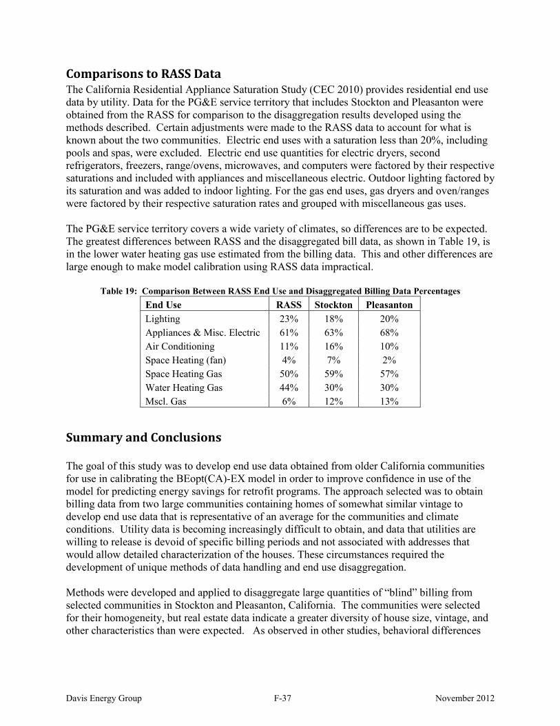
Comparisons to RASS Data The California Residential Appliance Saturation Study (CEC 2010) provides residential end use data by utility. Data for the PG&E service territory that includes Stockton and Pleasanton were obtained from the RASS for comparison to the disaggregation results developed using the methods described. Certain adjustments were made to the RASS data to account for what is known about the two communities. Electric end uses with a saturation less than 20%, including pools and spas, were excluded. Electric end use quantities for electric dryers, second refrigerators, freezers, range/ovens, microwaves, and computers were factored by their respective saturations and included with appliances and miscellaneous electric. Outdoor lighting factored by its saturation and was added to indoor lighting. For the gas end uses, gas dryers and oven/ranges were factored by their respective saturation rates and grouped with miscellaneous gas uses. The PG&E service territory covers a wide variety of climates, so differences are to be expected. The greatest differences between RASS and the disaggregated bill data, as shown in Table 19, is in the lower water heating gas use estimated from the billing data. This and other differences are large enough to make model calibration using RASS data impractical.

Table 19: Comparison Between RASS End Use and Disaggregated Billing Data Percentages End Use RASS Stockton Pleasanton Lighting 23% 18% 20% Appliances & Misc. Electric 61% 63% 68% Air Conditioning 11% 16% 10% Space Heating (fan) 4% 7% 2% Space Heating Gas 50% 59% 57% Water Heating Gas 44% 30% 30% Mscl. Gas 6% 12% 13%

Summary and Conclusions The goal of this study was to develop end use data obtained from older California communities for use in calibrating the BEopt(CA)-EX model in order to improve confidence in use of the model for predicting energy savings for retrofit programs. The approach selected was to obtain billing data from two large communities containing homes of somewhat similar vintage to develop end use data that is representative of an average for the communities and climate conditions. Utility data is becoming increasingly difficult to obtain, and data that utilities are willing to release is devoid of specific billing periods and not associated with addresses that would allow detailed characterization of the houses. These circumstances required the development of unique methods of data handling and end use disaggregation. Methods were developed and applied to disaggregate large quantities of “blind” billing from selected communities in Stockton and Pleasanton, California. The communities were selected for their homogeneity, but real estate data indicate a greater diversity of house size, vintage, and other characteristics than were expected. As observed in other studies, behavioral differences

Davis Energy Group F-37 November 2012

can produce much greater variation in energy use than differences in house characteristics, emphasizing the need to obtain averages that can be representative of both the design of the homes and the energy use habits of their owners. Two disaggregation methods were tested, one which used filtered data to develop disaggregated use for each house/record and then averaged the end use results, and another which first averaged the electric and gas uses from the filtered data for all houses/records and then applied disaggregation methods to the averaged data sets. The former method is much more time intensive but yields a higher level of apparent accuracy for disaggregating electric use than the simpler method. The simpler method appears to be adequate for disaggregating gas usage for the two data sets and Northern California communities that were evaluated. Comparison of the results of this study to RASS data for all of PG&E’s service territory suggests that differences in end use energy consumption within PG&E’s service area may be large enough to justify developing targeted programs. For example, incentive programs could be tailored to specific climate regions and/or homes that fall within a particular vintage range or socioeconomic level. The BEopt tool that is under development can be used to identify customer and utility cost parameters that can aid in the structuring of such programs. The ability to associate billing data with addresses would make it possible to improve house characterizations and would enable an analysis of the significance that building envelope characteristics, vintage, and other factors play relative to energy use behavior. This information would facilitate an uncertainty analysis that would be extremely useful to retrofit programs, particularly those that guarantee energy savings as a means of increasing participation.

References ASHRAE Guideline 14-2002: Measurement of Energy and Demand Savings. American Society of Heating, Refrigeration and Air Conditioning Engineers. Atlanta, Georgia. Backman, C., Dakin, B., Springer, D. 2010. “A Case Study in Reconciling Modeling Projections with Actual Usage”. Proceeding of the 2010 ACEEE Summer Study on Energy Efficiency in Buildings. Belzer, D., et al. 2007. “Home Performance with ENERGY STAR: Utility Bill Analysis on Homes Participating in Austin Energy’s Program.” Pacific Northwest National Laboratory. National Renewable Energy Laboratory Technical Report NREL/TP-640-41903 CEC 2010. “2009 California Residential Appliance Saturation Study – Executive Summary.” Prepared by KEMA for the California Energy Commission under Contract No. 400-07-031. Document No. CEC-200-2010-004-ES.

Davis Energy Group F-38 November 2012

Kissock, K., Haberl, J. and Claridge, D., 2002, “Development of a Toolkit for Calculating Linear, Change-point Linear and Multiple-Linear Inverse Building Energy Analysis Models”, Final Report, ASHRAE 1050-RP, November. Hendron, R., C. Engebrecht. 2010. “Building America House Simulation Protocols.” National Renewable Energy Laboratory. Golden, Colorado. Hoeschele, M. et al. 2011. “California Field Performance of Advanced Residential Gas Water Heating Technologies.” Report prepared under California Energy Commission Contract No. 500-08-060. California Energy Commission Public Interest Energy Research Program. Sacramento, California. NREL 2002. “Project Closeout: Guidance for Final Evaluation of Building America Communities” National Renewable Energy Laboratory. Golden, Colorado. Sonderegger, R. A., 1998. "Baseline Model for Utility Bill Analysis Using Both Weather and Non-Weather-Related Variables", ASHRAE Transactions, Vol. 104, No. 2, pp. 859-870.

Davis Energy Group F-39 November 2012

Appendix G: Implementing the BEopt Test Suite for the California Simulation Engine (CSE)

Table of Contents Background ................................................................................................................................................. 1 Occupancy/Operating Assumptions ......................................................................................................... 2 Input Mapping.............................................................................................................................................. 3

General Parameters................................................................................................................................. 3 Envelope ................................................................................................................................................. 3 Appliances, lighting, and miscellaneous loads ....................................................................................... 3 HVAC Equipment & Ventilation ........................................................................................................... 3 Water Heating......................................................................................................................................... 3 Mapping Status and Summary................................................................................................................ 4

Diagnostic Weather File ............................................................................................................................. 8 Preliminary Testing Results Using Diagnostic Weather Data.............................................................. 10

Known Model Differences ........................................................................................................................ 11 “Ideal” Air Conditioner Model.................................................................................................................. 12 Next steps .................................................................................................................................................. 13 References ................................................................................................................................................. 13

NREL July 2013

List of Figures Figure 1. Weather testing data for temperatures and wind speed......................................................... 9 Figure 2. Weather testing data for outdoor temperature and 7-day average........................................ 9 Figure 3. Cooling energy: BEopt (orange) and bug-fixed CSE (blue) ................................................. 10 Figure 4. Heating energy: BEopt (orange) and bug-fixed CSE (blue).................................................. 10 Figure 5. Hourly efficiency of the “Ideal” air conditioner for a home in Sacramento, California ..... 12

List of Tables Table 1. Origin of Operating Assumptions for Models ........................................................................... 2 Table 2. Summary of the Status of Implementation of Different Building Model Categories ............. 4

1 Background This document summarizes the current state of the implementation of capabilities to compare the California Simulation Engine (CSE) to EnergyPlus to aid in the validation of CSE. It captures what has been accomplished so far and documents known differences between the engines. The goal of this work is to be able to run simulations through BEopt for both CSE and EnergyPlus models of identical homes so that model results can be compared. This will allow comparative testing between CSE and EnergyPlus using BEopt’s comprehensive test suite to determine how simulation results differ and to help find possible bugs in the California Building Energy Code Compliance (CBECC) software or CSE. For this work, CSE is always called through CBECC. All work presented here was done using the CBECC-Res 2013 version 0t Beta, which was released on April 9, 2013.

The BEopt test suite automatically launches thousands of detailed simulations while systematically sweeping through all available building components (walls, windows, appliances, air conditioners, water heaters, etc.) one at a time in both simulation engines, allowing the impacts of individual building component changes in each engine to be compared. These building components are evaluated in the context of typical new construction and existing buildings. There is also a diagnostic test building with features (superinsulated envelope, zero infiltration, ideal heating/cooling equipment) that allow the impacts of specific options to be isolated for targeted comparisons between engines. All buildings are simulated in a range of climates (weather files) to evaluate the simulation engines’ responses to environment conditions. A rich visualization tool facilitates quickly identifying discrepancies in simulation engine output, disaggregated by end uses.

NREL G-1 July 2013

2 Occupancy/Operating Assumptions CSE and BEopt-EnergyPlus have different occupancy and operating assumptions (Title 24 and Building America House Simulation Protocols (Hendron & Engelbrecht, 2010), respectively) and model inputs. In this initial work, the goal was to map all inputs and assumptions between engines to allow for a comparison of the different algorithms used by each simulation engine based on a consistent set of assumptions. In general, the EnergyPlus models were modified to use the Title 24 operating assumptions, because it was not possible to modify the schedules in CBECC.

Table 1 documents which engine’s assumptions are used for all building operating parameters. For operating assumptions, there are generally two components: the magnitude (for example, the heat gain from occupants) and the schedule (for example, how many occupants are in the home at any given time). For some of the options in the table no magnitude is provided because it is a schedule that is either on or off (heating and cooling seasons, vacations). For cases where the magnitude is an input, such as refrigerator or lighting annual energy consumption, the default BEopt algorithms for determining the magnitude were used in both engines. Because the schedules in CBECC cannot be easily changed, the Title 24 assumptions of CBECC were implemented in the EnergyPlus models.

Table 1. Origin of Operating Assumptions for Models

Option/Schedule

Magnitude

Schedule Occupancy CBECC CBECC Heating Set Point CBECC CBECC Heating Season - CBECC Cooling Set Point CBECC CBECC Cooling Season - CBECC Miscellaneous Electric Loads CBECC CBECC Vacations - CBECC Mechanical Ventilation BEopt CBECC Refrigerator BEopt CBECC Cooking Range CBECC CBECC Dishwasher CBECC CBECC Clothes Washer CBECC CBECC Clothes Dryer CBECC CBECC Lighting BEopt CBECC Domestic Hot Water (DHW) Draw Profile CBECC CBECC Mains Water Temperature CBECC CBECC

NREL G-2 July 2013

3 Input Mapping The main accomplishment in this stage is the successful mapping of different model parameters between the simulation engines. Mapping is the implementation of equivalent building model inputs between the two engines by creating corresponding input parameters for each engine for a given set of BEopt options. For example, when a specific water heater is selected in BEopt, the mapped model parameters (volume, efficiency, etc.) are converted to input code specific to each simulation engine. With this mapping process, consistent models are achieved in both engines for any particular set of user input parameters. Additionally, user-created BEopt options (for example, a water heater with a different volume or efficiency) can be quickly and easily modeled in both simulation engines. The parameters mapped include:

General Parameters General parameters include the weather file, building geometry and orientation, occupancy, and availability of natural gas at the site.

Envelope Envelope related construction objects have been mapped, including:

• Slab foundation • Windows • Exterior shading • Walls, ceiling, roofs and slab properties • Material thermal properties • Exterior finish • Internal thermal mass.

Appliances, Lighting, and Miscellaneous Loads All appliances, lighting, and miscellaneous loads have been successfully mapped. In this case, the schedules in the EnergyPlus models were modified to be consistent with Title 24. Additionally, the fraction of energy use that becomes a gain to the space where the equipment is located (convective, radiant, or latent) was mapped.

HVAC Equipment and Ventilation Gas furnaces, split air conditioners, mechanical ventilation, and ducts have been mapped. Additional equipment will be mapped as the capability to model them becomes available in CBECC. Equipment sizing, consistent with ACCA Manual J, is done outside of the engines and is also mapped. Set point schedules and heating/cooling seasons were mapped and are consistent with Title 24 in both simulation engines. Mechanical ventilation is fully mapped in both engines. CBECC does not have model inputs for natural ventilation, but the ability to disable natural ventilation in both engines was implemented for comparative purposes.

Water Heating Water heating options (gas, propane, and electric tank and tankless water heaters, fuel oil tank water heaters, and heat pump water heaters [HPWHs]) as well as hot water distribution options

NREL G-3 July 2013

(including recirculation), have been successfully mapped to the California domestic hot water (DHW) engine. The EnergyPlus models were also modified to use the same mains water temperature and DHW draw profile as Title 24.

Mapping Status and Summary The following table presents a summary of the status of the mapping of options between the two engines. The “Mapped” column lists whether or not all options in that category are mapped. The “Ready for Diagnostic Test Building” column lists whether or not all options in that category can be made consistent with diagnostic test building assumptions in both engines. In cases where there are still remaining issues they are briefly described in the notes.

Table 2. Summary of the Status of Implementation of Different Building Model Categories

Building Model Category

Category Options

Mapped

Ready for Diagnostic

Test Building

Notes/Issues

Weather YES YES

Material Properties YES YES

Garage YES YES

Geometry

Wall/Floor Areas YES YES

Window/Door Location/Areas

YES

YES

Orientation YES YES

Operation

Heating Set Point YES YES Cooling Set Point YES YES Heating Season YES YES

Cooling Season YES YES

Occupancy YES YES

Natural Ventilation

YES

YES Different schedules, but can be turned off

Interior Shading

YES

YES

Schedules are different but disabled

by default

Walls Cavity Insulation R-value

YES

YES

Walls Finished Attic

Insulation Installation Quality

YES

YES

Framing Factor

YES

YES

Sheathing/ Insulation YES YES

NREL G-4 July 2013

Building Model Category

Category Options

Mapped

Ready for Diagnostic

Test Building

Notes/Issues

Exterior Finish

YES

YES Slight difference in

emissivity

Finished Attic Cavity Insulation R-Value

YES

YES

Finished Attic Unfinished Attic

Framing Factor YES YES

Sheathing/ Insulation YES YES

Cavity Insulation R-Value

YES

NO

The minimum test building uses an

adiabatic ceiling, but ceilings in CSE must

have an R-value lower than R-60. Ceilings in both

engines can be set to consistent, high R-

values.

Unfinished Attic Roof

Framing Factor YES YES

Sheathing/Insulation YES YES

Vented/Unvented YES YES

Roof Material YES YES

Roof Radiant Barrier YES YES

Foundations/Floors Slab Perimeter Insulation Depth

YES

YES

Foundations/FloorsT hermal Mass

Slab Insulation YES YES

Carpet

YES

YES

Crawlspace NO NO Not yet mapped

Basement NO NO Not yet mapped

Floor Mass YES YES

Thermal Mass Internal Thermal

Mass

Exterior Wall Mass

YES

YES

Partition Wall Mass

YES

YES

Ceiling Mass

YES

YES

Interior Walls

YES

NO

Made consistent, but cannot be zero in

CSE

NREL G-5 July 2013

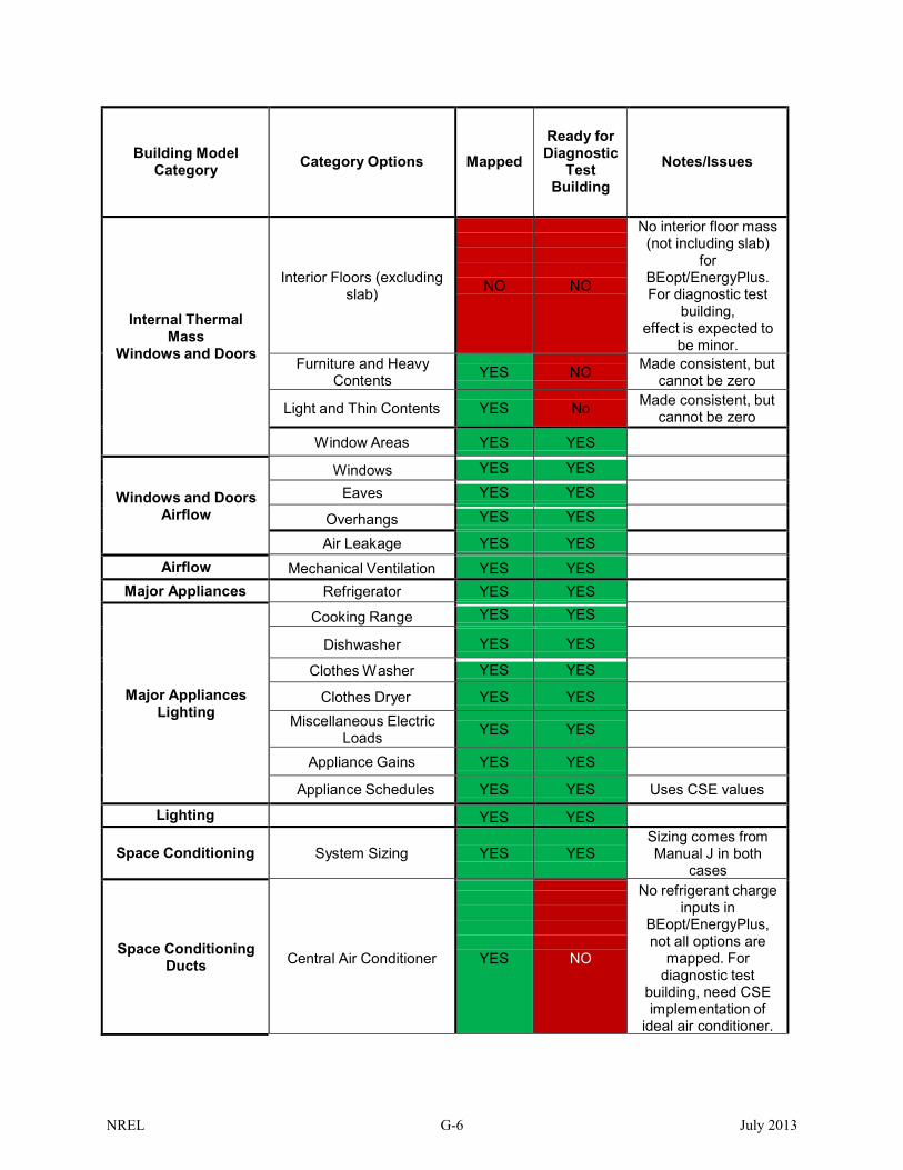
Building Model Category

Category Options

Mapped

Ready for Diagnostic

Test Building

Notes/Issues

Internal Thermal Mass

Windows and Doors

Interior Floors (excluding slab)

NO

NO

No interior floor mass (not including slab)

for BEopt/EnergyPlus. For diagnostic test

building, effect is expected to

be minor. Furniture and Heavy

Contents

YES

NO Made consistent, but cannot be zero

Light and Thin Contents

YES

No Made consistent, but cannot be zero

Window Areas YES YES

Windows and Doors Airflow

Windows YES YES

Eaves YES YES

Overhangs YES YES

Air Leakage YES YES Airflow Mechanical Ventilation YES YES

Major Appliances Refrigerator YES YES

Major Appliances Lighting

Cooking Range YES YES

Dishwasher YES YES

Clothes Washer YES YES

Clothes Dryer YES YES

Miscellaneous Electric Loads

YES

YES

Appliance Gains YES YES

Appliance Schedules YES YES Uses CSE values

Lighting YES YES

Space Conditioning

System Sizing

YES

YES Sizing comes from Manual J in both

cases

Space Conditioning Ducts

Central Air Conditioner

YES

NO

No refrigerant charge inputs in

BEopt/EnergyPlus, not all options are

mapped. For diagnostic test

building, need CSE implementation of

ideal air conditioner.

NREL G-6 July 2013

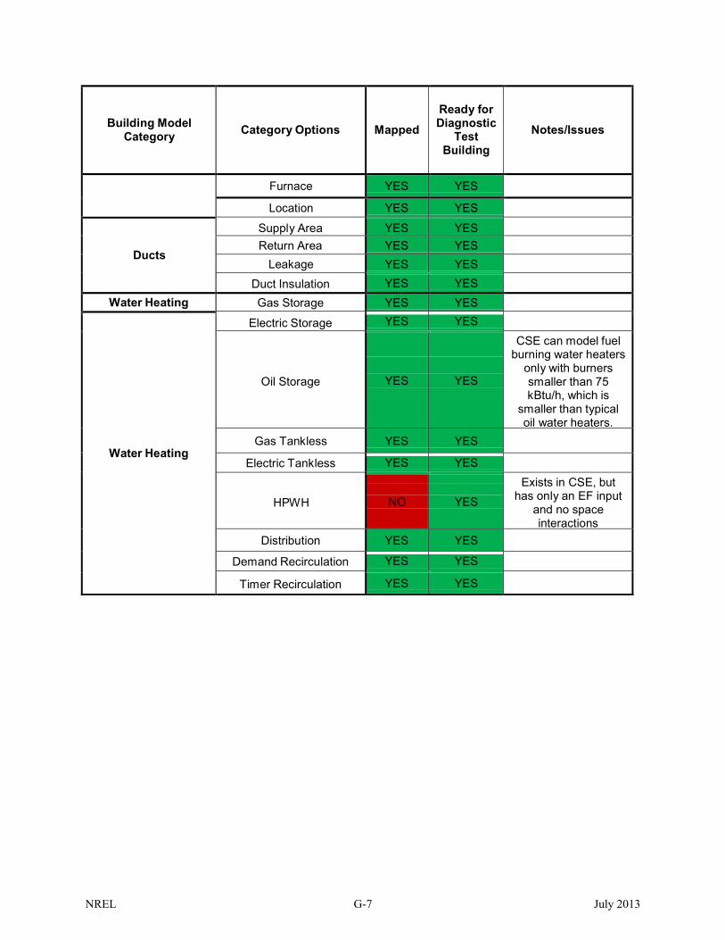
Building Model Category

Category Options

Mapped

Ready for Diagnostic

Test Building

Notes/Issues

Furnace YES YES

Location YES YES

Ducts

Supply Area YES YES Return Area YES YES

Leakage YES YES

Duct Insulation YES YES Water Heating Gas Storage YES YES

Water Heating

Electric Storage YES YES

Oil Storage

YES

YES

CSE can model fuel burning water heaters

only with burners smaller than 75 kBtu/h, which is

smaller than typical oil water heaters.

Gas Tankless YES YES

Electric Tankless YES YES

HPWH

NO

YES Exists in CSE, but

has only an EF input and no space interactions

Distribution YES YES

Demand Recirculation YES YES

Timer Recirculation YES YES

NREL G-7 July 2013

4 Diagnostic Weather File The diagnostic weather file contains environmental parameters shown in Table 3 that are kept constant for 2 consecutive weeks to allow for steady-state comparisons between programs. Variables manipulated in the testing weather file are:

1. Outdoor air temperature (Tout) 2. Solar horizontal radiation 3. Solar direct radiation 4. Solar diffuse radiation 5. Sky temperature (Tsky) 6. Wind speed 7. Ground temperature (Tground) 8. 7-,14-, and 31-day average Tout

The same file is later slightly modified to meet the specific needs of BEopt and CBECC. Table 3 summarizes the diagnostic weather data. Colors in Table 3 reflect a change in a particular variable from one period to another.

Table 3. Testing Weather Data

Month January February March April May June July August September October November December Dates

1-15

16-31

1-14

15-28

1-15

16-31

1-15

16-30

1-15

16-31

1-15

16-30

1-15

16-31

1-15

16-31

1-15

16-30

1-15

16-31

1-15

16-30

1-15

16-31

Outdoor Air Temp (F)

25

25

78

78

78

78

110

110

25

25

78

78

78

78

110

110

25

25

78

78

78

78

110

110

Solar Horizontal (W/m2)

1000

1000

1000

1000

1000

1000

1000

1000

0

0

0

0

0

0

0

0

400

400

400

400

400

400

400

400 Solar Direct (W/m2)

900

900

900

900

900

900

900

900

0

0

0

0

0

0

0

0

50

50

50

50

50

50

50

50 Solar Diffuse (W/m2)

150

150

150

150

150

150

150

150

0

0

0

0

0

0

0

0

370

370

370

370

370

370

370

370 Tsky (F) 25 25 78 78 58 200 110 110 25 25 78 78 58 200 110 110 25 25 78 78 58 200 110 110 Wind Speed (mph)

0

40

0

40

0

0

0

40

0

40

0

40

0

0

0

40

0

40

0

40

0

0

0

40 Tground (F) 60 60 60 60 60 60 60 60 60 60 60 60 60 60 60 60 60 60 60 60 60 60 60 60 Variable Setpoint

NO

NO

NO

NO

NO

NO

NO

NO

NO

NO

NO

NO

NO

NO

NO

NO

NO

NO

NO

NO

NO

NO

NO

NO

7 Day Average 90 90 25 25 25 25 25 25 90 90 25 25 25 25 25 25 90 90 25 25 25 25 25 25

The “Variable Set Point” row doesn’t control any variable but just indicates if a variable set point is being applied as a result of the 7-day average. The 7-day average Tout is manipulated to force CSE to run with constant heating and cooling set points (e.g., for cooling calculations in August, the 25°F 7-day average Tout forces CSE into “heating mode” but with a constant 78°F cooling set point while the weather file Tout hourly values are set to 110°F).

Figure 1 shows the steady-state nature of the testing weather data for all environmental temperatures and wind speeds. Figure 2 shows the Tout as well as the 7-day average temperature.

NREL G-8 July 2013

Figure 1. Weather testing data for temperatures and wind speed

Figure 2. Weather testing data for outdoor temperature and 7-day average

NREL G-9 July 2013

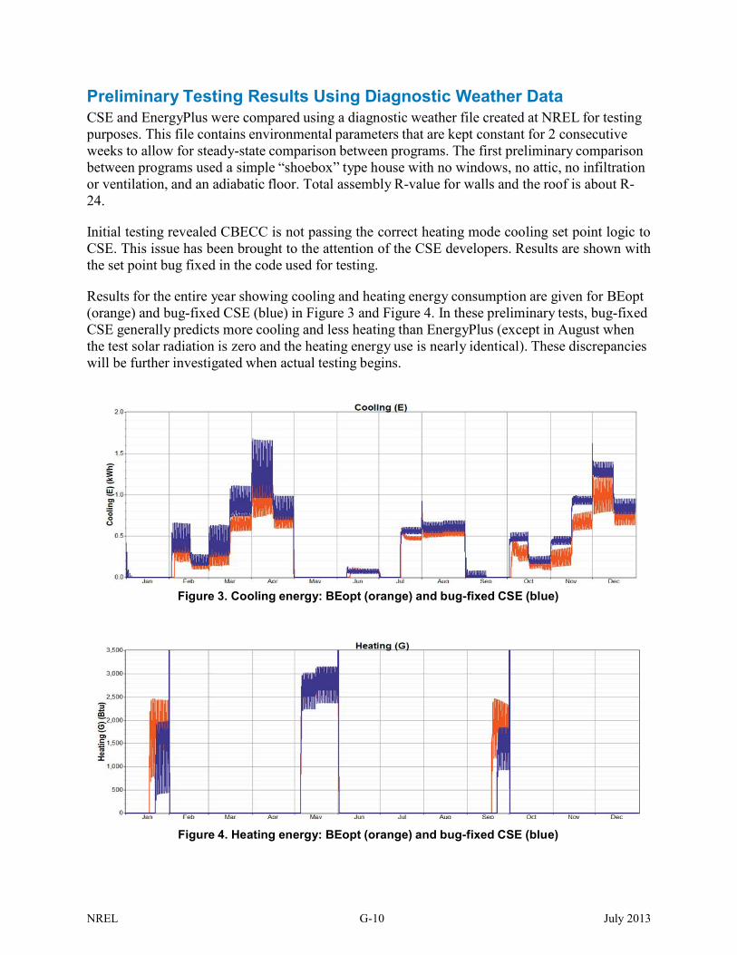
Preliminary Testing Results Using Diagnostic Weather Data CSE and EnergyPlus were compared using a diagnostic weather file created at NREL for testing purposes. This file contains environmental parameters that are kept constant for 2 consecutive weeks to allow for steady-state comparison between programs. The first preliminary comparison between programs used a simple “shoebox” type house with no windows, no attic, no infiltration or ventilation, and an adiabatic floor. Total assembly R-value for walls and the roof is about R- 24.

Initial testing revealed CBECC is not passing the correct heating mode cooling set point logic to CSE. This issue has been brought to the attention of the CSE developers. Results are shown with the set point bug fixed in the code used for testing.

Results for the entire year showing cooling and heating energy consumption are given for BEopt (orange) and bug-fixed CSE (blue) in Figure 3 and Figure 4. In these preliminary tests, bug-fixed CSE generally predicts more cooling and less heating than EnergyPlus (except in August when the test solar radiation is zero and the heating energy use is nearly identical). These discrepancies will be further investigated when actual testing begins.

Figure 3. Cooling energy: BEopt (orange) and bug-fixed CSE (blue)

Figure 4. Heating energy: BEopt (orange) and bug-fixed CSE (blue)

NREL G-10 July 2013

5 Known Model Differences The following differences are known to exist between EnergyPlus and CSE/CBECC:

Envelope

• Installed R-value for compressed insulation in cavities: There is input uncertainty related to the actual R-value used when compressing insulating batts (such as R-19 in 2×4 studs) in CSE.

• Materials conductivity temperature dependence: The thermal conductivity of many materials varies with temperature. CSE has a few materials with temperature dependence, including the R-value of empty cavities, while BEopt assumes constant values.

• CSE uses a built-in constant emissivity for walls and the value of this emissivity is unknown. In BEopt this is an input variable that depends on the exterior finish. However, typical values are around 0.82–0.96 (a relatively narrow range), so this may not have a significant impact on overall results.

• Interior floor (not slab) mass is not 100% mapped but has a minor role compared to total mass.

Appliances, Lighting, and Miscellaneous Loads

• Daylight Saving Time: During Daylight Saving Time, there is a slight discrepancy in the schedules used for lighting, appliances, and miscellaneous loads.

HVAC Equipment and Ventilation

• Air conditioner refrigerant type and charge: BEopt has no equivalent for these parameters that can be used in EnergyPlus. Currently they are set in a way to minimize the impacts of these parameters on the air conditioner energy consumption, but the impact of this has not been fully explored.

• Part load impacts: It is currently unknown how CSE handles part load impacts for HVAC equipment. This may introduce some differences between the two engines, but has not been fully explored.

• Duct diameter: CSE considers the duct diameter while calculating the actual R-value of duct insulation. Duct R-value in the EnergyPlus models is independent of diameter, although BEopt modifications to rectify this issue will be made before systems with ducts are tested.

Water Heating

• HPWH energy performance: The California DHW engine uses energy factor to characterize the performance of HPWHs, while BEopt uses a more detailed set of inputs to characterize performance for the EnergyPlus models as described in (Wilson & Christensen, 2012). For the time being, an equivalent energy factor for each HPWH in EnergyPlus is estimated.

NREL G-11 July 2013

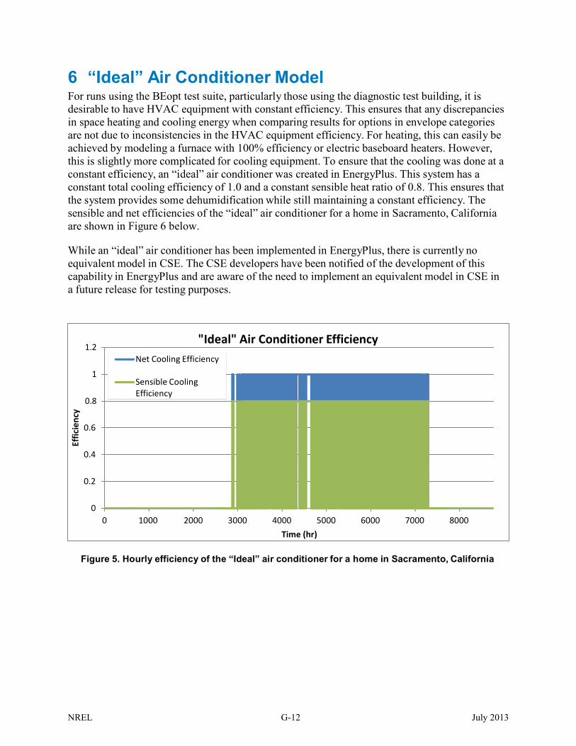
Effic

ienc

y 6 “Ideal” Air Conditioner Model For runs using the BEopt test suite, particularly those using the diagnostic test building, it is desirable to have HVAC equipment with constant efficiency. This ensures that any discrepancies in space heating and cooling energy when comparing results for options in envelope categories are not due to inconsistencies in the HVAC equipment efficiency. For heating, this can easily be achieved by modeling a furnace with 100% efficiency or electric baseboard heaters. However, this is slightly more complicated for cooling equipment. To ensure that the cooling was done at a constant efficiency, an “ideal” air conditioner was created in EnergyPlus. This system has a constant total cooling efficiency of 1.0 and a constant sensible heat ratio of 0.8. This ensures that the system provides some dehumidification while still maintaining a constant efficiency. The sensible and net efficiencies of the “ideal” air conditioner for a home in Sacramento, California are shown in Figure 6 below.

While an “ideal” air conditioner has been implemented in EnergyPlus, there is currently no equivalent model in CSE. The CSE developers have been notified of the development of this capability in EnergyPlus and are aware of the need to implement an equivalent model in CSE in a future release for testing purposes.

1.2

1

0.8

"Ideal" Air Conditioner Efficiency

Net Cooling Efficiency Sensible Cooling Efficiency

0.6

0.4

0.2

0

0 1000 2000 3000 4000 5000 6000 7000 8000 Time (hr)

Figure 5. Hourly efficiency of the “Ideal” air conditioner for a home in Sacramento, California

NREL G-12 July 2013

7 Next Steps Since this work has been performed, additional releases of CSE have occurred. Next steps would include updating the mapping as appropriate for the latest release. This would include mapping crawlspaces and basements as well as the additional space heating and cooling systems that have since been implemented.

Once the mapping has been updated to include the new features of later CSE releases, the capabilities are available to perform detailed testing and comparisons of CSE and EnergyPlus models. Testing at this level is mainly focused on comparing engine algorithms as the inputs and assumptions are consistently mapped. This testing would utilize the BEopt test suite with typical and diagnostic buildings to simulate building components one at a time and isolate the energy impacts of these options. The test suite will facilitate identifying differences between simulation engines and will help find possible bugs in CBECC or CSE. Testing will also include a test weather file, which uses diagnostic weather conditions to further isolate specific phenomena in the building models.

After this testing is complete, additional testing using each engine’s default assumptions or a sensitivity analysis of different parameters could be performed.

References Hendron, R., & Engelbrecht, C. (2010). Building America House Simulation Protocol. Golden, CO: National Renewable Energy Laboratory. Available at: http://www.nrel.gov/docs/fy11osti/49246.pdf

Polly, B., Horowitz, S., Booten, C., Kruis, N., & Christensen, C. (2012, August). Automated Comparison of Building Energy Simulation Engines. Available at: http://www.nrel.gov/docs/fy12osti/52651.pdf

Wilson, E., & Christensen, C. (2012). Heat Pump Water Heater Modeling in EnergyPlus. Retrieved from Building America Residential Energy Efficiency Stakeholder Meeting. Avaialable at: http://www.nrel.gov/docs/fy12osti/54318.pdf

NREL G-13 July 2013

Appendix H: Example Analysis Results

Contents 1 Background ........................................................................................................................................... 1 2 Analysis Inputs ..................................................................................................................................... 1

2.1 Building Characteristics ................................................................................................................... 1 2.2 Utility Rates ..................................................................................................................................... 1

3 Results ................................................................................................................................................... 2 3.1 Participant Cost Test, Gas/Electric Houses...................................................................................... 3 3.2 Participant Cost Test, All-Electric Houses ...................................................................................... 3 3.1 Total Resource Cost Test, Gas/Electric Houses ............................................................................... 6 3.2 Total Resource Cost Test, All-Electric Houses ............................................................................... 6

NREL February 2014

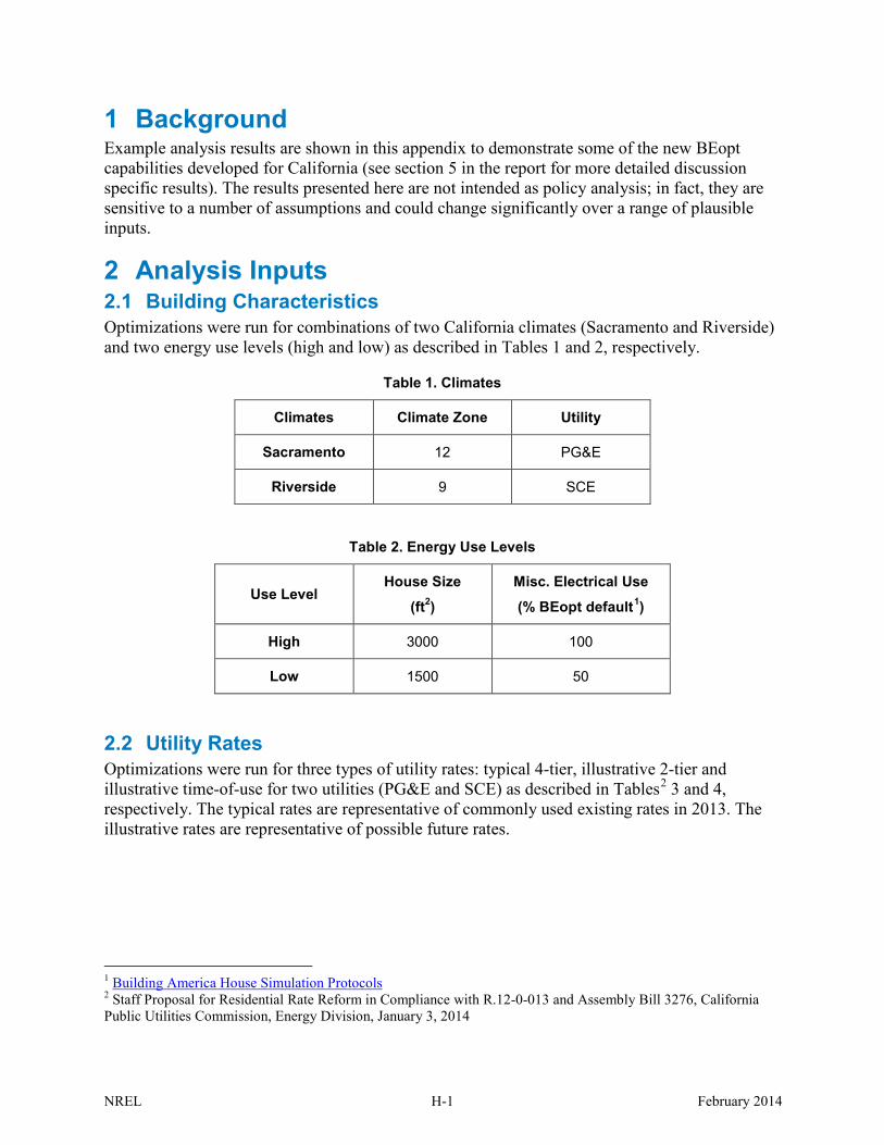
1 Background Example analysis results are shown in this appendix to demonstrate some of the new BEopt capabilities developed for California (see section 5 in the report for more detailed discussion specific results). The results presented here are not intended as policy analysis; in fact, they are sensitive to a number of assumptions and could change significantly over a range of plausible inputs.

2 Analysis Inputs 2.1 Building Characteristics Optimizations were run for combinations of two California climates (Sacramento and Riverside) and two energy use levels (high and low) as described in Tables 1 and 2, respectively.

Table 1. Climates

Climates Climate Zone Utility

Sacramento 12 PG&E

Riverside 9 SCE

Table 2. Energy Use Levels

Use Level House Size

(ft2)

Misc. Electrical Use

(% BEopt default1)

High 3000 100

Low 1500 50

2.2 Utility Rates Optimizations were run for three types of utility rates: typical 4-tier, illustrative 2-tier and illustrative time-of-use for two utilities (PG&E and SCE) as described in Tables2 3 and 4, respectively. The typical rates are representative of commonly used existing rates in 2013. The illustrative rates are representative of possible future rates.

1 Building America House Simulation Protocols 2 Staff Proposal for Residential Rate Reform in Compliance with R.12-0-013 and Assembly Bill 3276, California Public Utilities Commission, Energy Division, January 3, 2014

NREL H-1 February 2014

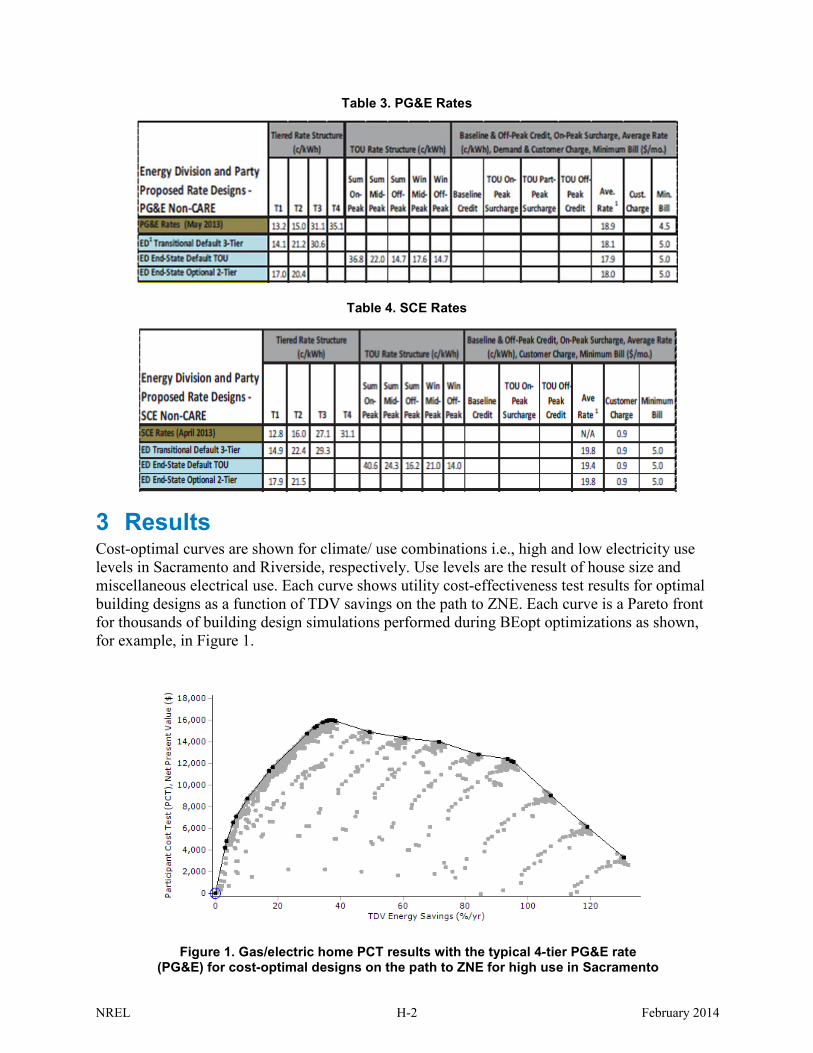
Figure 1. Gas/electric home PCT results with the typical 4-tier PG&E rate (PG&E) for cost-optimal designs on the path to ZNE for high use in Sacramento

Table 3. PG&E Rates

Table 4. SCE Rates

3 Results Cost-optimal curves are shown for climate/ use combinations i.e., high and low electricity use levels in Sacramento and Riverside, respectively. Use levels are the result of house size and miscellaneous electrical use. Each curve shows utility cost-effectiveness test results for optimal building designs as a function of TDV savings on the path to ZNE. Each curve is a Pareto front for thousands of building design simulations performed during BEopt optimizations as shown, for example, in Figure 1.

NREL H-2 February 2014

All the results in this appendix are based on PCT optimizations; TRC and RIM results, as well as PCT results, are for PCT-optimal building designs. If the building designs were instead optimized for maximum TRC, slightly different building designs (more optimal for TRC) would be found during the optimization process and TRC results would be somewhat improved, whereas the corresponding PCT results would be slightly less optimal. The PCT optimizations were performed as a function of TDV Savings (the California metric for ZNE), and the results are plotted versus TDV savings.

3.1 Participant Cost Test, Gas/Electric Houses Figures 1 shows gas/electric house PCT results for typical 4-tier, illustrative 2-tier and illustrative time-of-use utility rates, respectively. In each graph, the four curves represent (top-to-bottom) high use in Sacramento and Riverside and low use in Sacramento and Riverside, respectively. The trends are similar for the four curves in each graph, and the discussion in Section 5 in the body of the report generally applies.

3.2 Participant Cost Test, All-Electric Houses Figures 2 shows all-electric house PCT results for typical 4-tier, illustrative 2-tier and illustrative time-of-use utility rates, respectively. In each graph, the four curves represent (top-to-bottom) high use in Sacramento and Riverside and low use in Sacramento and Riverside, respectively. The trends are similar for the four curves in each graph. The results for all-electric houses (Figure 2) are generally similar to the results for gas/electric houses (Figure 1) but with some notable differences.

The slopes of the curves are more positive (or less negative) with tiered rates, because with higher total electrical loads in all-electric houses more electricity is consumed at high tier rates leading to higher PCT values with tiered rates.

PCT values are higher overall (note the different y-axis scale in Figure 2a), because savings have higher value when additional electrical loads (for space heating, water heating, clothes drying, etc.) are reduced by efficiency measures or displaced by PV production.

The slope-change points related to NEM annual excess occur at higher TDV values than in the gas/electric houses, because there is no need for PV over-production to cover gas consumption at the ZNE point.

NREL H-3 February 2014

(a)

(b)

(c)

Figure 2. Gas/electric home PCT cost-optimal curves (top-to-bottom) for high use in Sacramento and Riverside and low use in Sacramento and Riverside, respectively: (a) typical 4-tier rates, (b) illustrative 2-

tier rates, and (c) illustrative time-of-use utility rates

NREL H-4 February 2014

(a)

(b)

(c)

Figure 3. All-electric home PCT cost-optimal curves (top-to-bottom) for high use in Sacramento and Riverside and low use in Sacramento and Riverside, respectively: (a) typical 4-tier rates, (b) illustrative

2-tier rates, and (c) illustrative time-of-use utility rates

NREL H-5 February 2014

3.1 Total Resource Cost Test, Gas/Electric Houses Figure 3 shows gas/electric home TRC results with typical 4-tier, illustrative 2-tier, and illustrative time-of-use utility rates (groups of curves, respectively) for cost optimal designs on the path to ZNE: top-to-bottom, curves represent high and low use in Sacramento and high and low use in Riverside, respectively. Within each use/climate group, there is little difference between results for different utility rates, because TRC calculations do not explicitly include utility rates. The small differences occur because, for different utility rates, different EE options are included in some of the optimal building designs at some points along the path to ZNE.

3.2 Total Resource Cost Test, All-Electric Houses Figure 4 shows all-electric home TRC results with typical 4-tier, illustrative 2-tier, and illustrative time-of-use utility rates (groups of curves, respectively) for cost optimal designs on the path to ZNE: top-to-bottom, curves represent high and low use in Sacramento and high and low use in Riverside, respectively. Within each use/climate group, there is little difference between results for different utility rates, because TRC calculations do not explicitly include utility rates. The small differences occur because, for different utility rates, different EE options are included in some of the optimal building designs at some points along the path to ZNE.

NREL H-6 February 2014

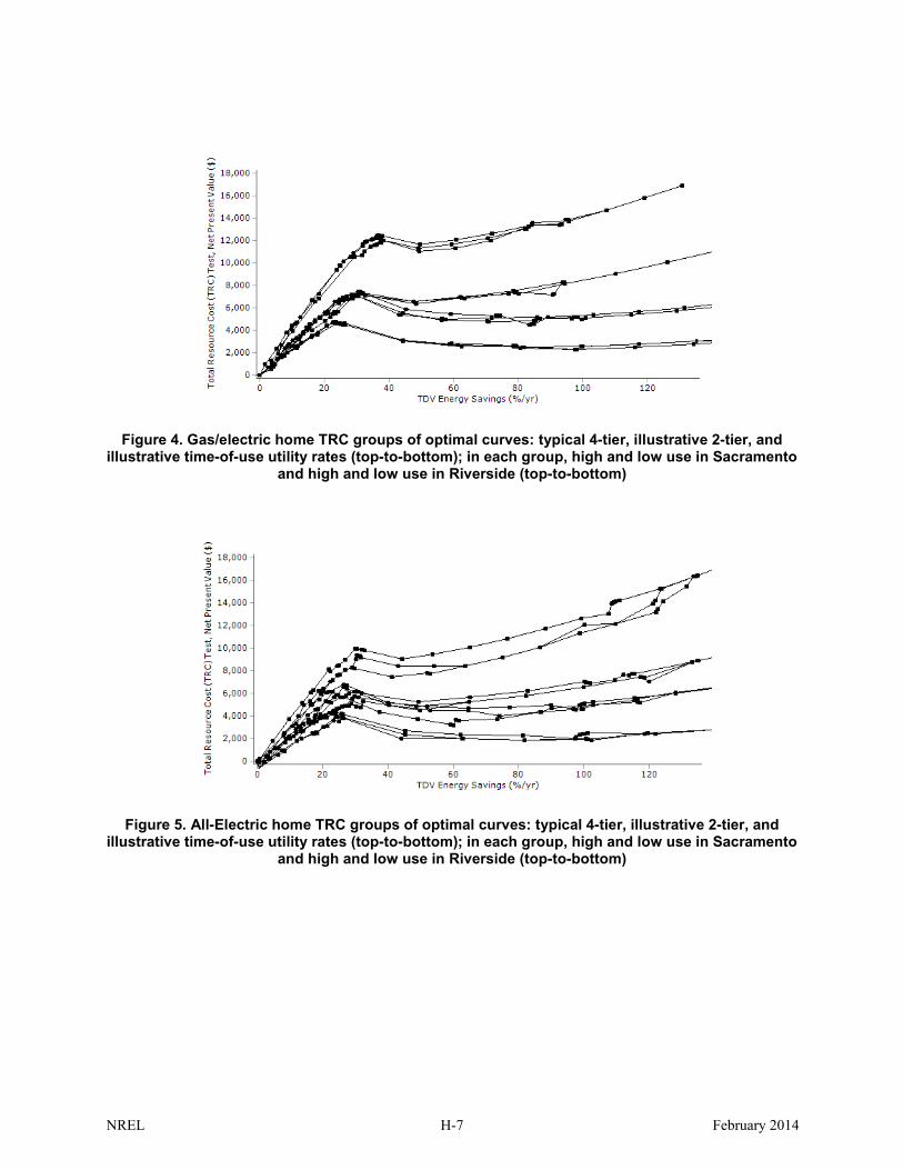
Figure 4. Gas/electric home TRC groups of optimal curves: typical 4-tier, illustrative 2-tier, and illustrative time-of-use utility rates (top-to-bottom); in each group, high and low use in Sacramento

and high and low use in Riverside (top-to-bottom)

Figure 5. All-Electric home TRC groups of optimal curves: typical 4-tier, illustrative 2-tier, and illustrative time-of-use utility rates (top-to-bottom); in each group, high and low use in Sacramento

and high and low use in Riverside (top-to-bottom)

NREL H-7 February 2014