final performance report
TRANSCRIPT

AFRL-OSR-VA-TR-2014-0093
Stochastic Quantitative Reasoning for Autonomous Mission Planning
Carlos VarelaRENSSELAER POLYTECHNIC INST TROY NY
Final Report04/09/2014
DISTRIBUTION A: Distribution approved for public release.
AF Office Of Scientific Research (AFOSR)/ RTCArlington, Virginia 22203
Air Force Research Laboratory
Air Force Materiel Command

REPORT DOCUMENTATION PAGE
Standard Form 298 (Rev. 8/98) Prescribed by ANSI Std. Z39.18
Form Approved OMB No. 0704-0188
The public reporting burden for this collection of information is estimated to average 1 hour per response, including the time for reviewing instructions, searching existing data sources, gathering and maintaining the data needed, and completing and reviewing the collection of information. Send comments regarding this burden estimate or any other aspect of this collection of information, including suggestions for reducing the burden, to Department of Defense, Washington Headquarters Services, Directorate for Information Operations and Reports (0704-0188), 1215 Jefferson Davis Highway, Suite 1204, Arlington, VA 22202-4302. Respondents should be aware that notwithstanding any other provision of law, no person shall be subject to any penalty for failing to comply with a collection of information if it does not display a currently valid OMB control number. PLEASE DO NOT RETURN YOUR FORM TO THE ABOVE ADDRESS.
1. REPORT DATE (DD-MM-YYYY) 2. REPORT TYPE 3. DATES COVERED (From - To)
4. TITLE AND SUBTITLE 5a. CONTRACT NUMBER
5b. GRANT NUMBER
5c. PROGRAM ELEMENT NUMBER
5d. PROJECT NUMBER
5e. TASK NUMBER
5f. WORK UNIT NUMBER
6. AUTHOR(S)
7. PERFORMING ORGANIZATION NAME(S) AND ADDRESS(ES) 8. PERFORMING ORGANIZATIONREPORT NUMBER
10. SPONSOR/MONITOR'S ACRONYM(S)
11. SPONSOR/MONITOR'S REPORTNUMBER(S)
9. SPONSORING/MONITORING AGENCY NAME(S) AND ADDRESS(ES)
12. DISTRIBUTION/AVAILABILITY STATEMENT
13. SUPPLEMENTARY NOTES
14. ABSTRACT
15. SUBJECT TERMS
16. SECURITY CLASSIFICATION OF:
a. REPORT b. ABSTRACT c. THIS PAGE
17. LIMITATION OFABSTRACT
18. NUMBEROFPAGES
19a. NAME OF RESPONSIBLE PERSON
19b. TELEPHONE NUMBER (Include area code)
31-03-2014 Final Performance Report 30-09-2011 TO 31-03-2014
Stochastic Quantitative Reasoning for Autonomous Mission Planning
Varela, Carlos, A, Ph.D.
Rensselaer Polytechnic Institute 110 8th Street Troy, NY 12180
USAF, AFRL DUNS 143574726 AF OFFICE OF SCIENTIFIC RESEARCH 875 N. RANDOLPH ST. ROOM 3112 ARLINGTON VA 22203
FA9550-11-1-0332
AFOSR
In research performed with funding from this grant, PI Varela has developed mathematical concepts and software to automatically detect and correct for errors in spatio-temporal data streams. Varela and his group invented and formalized the notions of error signatures and mode likelihood vectors, and developed the PILOTS programming language v0.2.3. An important application of this work was to demonstrate that the Air France flight 447 accident from June 2009 could have been avoided by using these techniques applied on air speed, ground speed, and wind speed data streams.
Spatio-temporal data streams, Error signatures, Mode likelihood vectors, PILOTS programming language, AF447 accident.
Distribution A - Approved for Public Release

FINAL&PERFORMANCE&REPORT&!Grant&Title:!!Stochastic!Quantitative!Reasoning!for!Autonomous!Mission!Planning!Grant&#:&&FA9550=11=1=0332!PI:!!Carlos!A.!Varela,!Ph.D.!Program&Manager:!!Frederica!Darema,!Ph.D.!!Reporting&Period:!September!30,!2011!to!March!31,!2014!!Executive&Summary:!In!research!performed!with!funding!from!this!grant,!PI!Varela!has!developed!mathematical!concepts!and!software!to!automatically!detect!and!correct!for!errors!in!spatio=temporal!data!streams.!Varela!and!his!group!invented!and!formalized!the!notions!of!error!signatures!and!mode!likelihood!vectors,!and!developed!the!PILOTS!programming!language!v0.2.3.!An!important!application!of!this!work!was!to!demonstrate!that!the!Air!France!flight!447!(AF447)!accident!in!June!2009!could!have!been!avoided!by!using!these!techniques!applied!on!air!speed,!ground!speed,!and!wind!speed!data!streams.!!Archival&Publications&(published)&during&reporting&period:!
1. Carlos!A.!Varela.!Programming&Distributed&Computing&Systems:&A&Foundational&Approach.!MIT!Press,!May!2013.!
2. Richard!S.!Klockowski,!Shigeru!Imai,!Colin!Rice,!and!Carlos!A.!Varela.!Autonomous&Data&Error&Detection&and&Recovery&in&Streaming&Applications.!In!Proceedings+of+the+International+Conference+on+Computational+Science+(ICCS+2013).+Dynamic+Data@Driven+Application+Systems+(DDDAS+2013)+Workshop,!pages!2036=2045,!May!2013.!
3. Matthew!Newby,!Nathan!Cole,!Heidi!Jo!Newberg,!Travis!Desell,!Malik!Magdon=Ismail,!Boleslaw!Szymanski,!Carlos!Varela,!Benjamin!Willett,!and!Brian!Yanny.!A&Spatial&Characterization&of&the&Sagittarius&Dwarf&Galaxy&Tidal&Tails.!The+Astronomical+Journal,!145(163),!May!2013.!
4. Shigeru!Imai,!Richard!Klockowski,!and!Carlos!A.!Varela.!SelfLHealing&SpatioLTemporal&Data&Streams&Using&Error&Signatures.!In!2nd+International+Conference+on+Big+Data+Science+and+Engineering+(BDSE+2013),!Sydney,!Australia,!December!2013.!
5. Shigeru!Imai,!Thomas!Chestna,!and!Carlos!A.!Varela.!Accurate&Resource&Prediction&for&Hybrid&IaaS&Clouds&Using&WorkloadLTailored&Elastic&Compute&Units.!In!6th+IEEE/ACM+International+Conference+on+Utility+and+Cloud+Computing+(UCC+2013),!Dresden,!Germany,!December!2013.!
6. David!Musser!and!Carlos!A.!Varela.!Structured&Reasoning&about&Actor&Systems.!In!Agere+Workshop+at+ACM+SPLASH+2013+Conference,!Indianapolis,!Indiana,!October!2013.!
7. Carlos!A.!Varela,!Manish!Parashar,!and!Gul!Agha,!editors.!5th&IEEE/ACM&International&Conference&on&Utility&and&Cloud&Computing,&UCC&2012,&Chicago,&IL,&USA,&November&5L8,&2012,!2012.!IEEE.!

8. Shigeru!Imai,!Thomas!Chestna,!and!Carlos!A.!Varela.!Elastic&Scalable&Cloud&Computing&Using&ApplicationLLevel&Migration.!In!5th+IEEE/ACM+International+Conference+on+Utility+and+Cloud+Computing+(UCC+2012),!Chicago,!Illinois,!USA,!November!2012.!
9. Shigeru!Imai!and!Carlos!A.!Varela.!Programming&SpatioLTemporal&Data&Streaming&Applications&with&HighLLevel&Specifications.!In!3rd+ACM+SIGSPATIAL+International+Workshop+on+Querying+and+Mining+Uncertain+Spatio@Temporal+Data+(QUeST)+2012,!Redondo!Beach,!California,!USA,!November!2012.!
10. Shigeru!Imai!and!Carlos!A.!Varela.!A&Programming&Model&for&SpatioLTemporal&Data&Streaming&Applications.!In!Dynamic+Data@Driven+Application+Systems+(DDDAS+2012),!ICCS,!Omaha,!Nebraska,!pages!1139=1148,!June!2012.!
11. David!Musser!and!Carlos!A.!Varela.!HumanLReadable&MachineLCheckable&Abstract&Reasoning&about&Actor&Systems.!Technical!report!12=01,!Rensselaer!Polytechnic!Institute!Department!of!Computer!Science,!January!2012.!
12. Shigeru!Imai.!Task&Offloading&between&Smartphones&and&Distributed&Computational&Resources.!Master's!thesis,!Rensselaer!Polytechnic!Institute,!May!2012.!
13. Marco!A.!S.!Netto,!Christian!Vecchiola,!Michael!Kirley,!Carlos!A.!Varela,!and!Rajkumar!Buyya.!Use&of&Run&Time&Predictions&for&Automatic&CoLAllocation&of&MultiLCluster&Resources&for&Iterative&Parallel&Applications.!Journal+of+Parallel+and+Distributed+Computing,!pp!43pp,!2011.!
14. Travis!Desell,!Malik!Magdon=Ismail,!Heidi!Newberg,!Lee!A.!Newberg,!Boleslaw!K.!Szymanski,!and!Carlos!A.!Varela.!A&Robust&Asynchronous&Newton&Method&for&Massive&Scale&Computing&Systems.!In!International+Conference+on+Computational+Intelligence+and+Software+Engineering+(CiSE),!Wuhan,!China,!December!2011.!
15. Shigeru!Imai!and!Carlos!A.!Varela.!LightLWeight&Adaptive&Task&Offloading&from&Smartphones&to&Nearby&Computational&Resources.!In!ACM+Research+in+Applied+Computation+Symposium+(RACS+2011),!Miami,!Florida,!November!2011.!
16. Qingling!Wang!and!Carlos!A.!Varela.!Impact&of&Cloud&Computing&Virtualization&Strategies&on&Workloads'&Performance.!In!4th+IEEE/ACM+International+Conference+on+Utility+and+Cloud+Computing(UCC+2011),!Melbourne,!Australia,!December!2011.!
17. Shigeru!Imai,!Pratik!Patel,!and!Carlos!A.!Varela.!Developing&Elastic&Software&for&the&Cloud.!Invited!book!chapter!in!Encyclopedia+on+Cloud+Computing,!editors!San!Murugesan!and!Irena!Bojanova,!submitted,!to!appear!mid=2014.!
18. Shigeru!Imai!and!Carlos!A.!Varela.!Dynamic&DataLDriven&Avionics&Systems&with&Stochastic&Error&Detection&and&Correction.!Invited!book!chapter!in!Dynamic+Data+Driven+Application+Systems+(DDDAS),!editor!Frederica!Darema,!submitted,!to!appear!mid=2014.!
!&

Students&Involved&in&this&Research:!1. Shigeru!Imai,!Ph.D.!student!2. Richard!Klockowski,!Ph.D.!student!3. Colin!Rice,!B.S.!student!4. Alessandro!Galli,!B.S.!student!
!Most&Significant&Advances&and&Conclusions:!The!key!research!results!directly!supported!by!this!grant!are!published!in!the!following!articles!(available!at!http://wcl.cs.rpi.edu/bib/Keyword/DATA=STREAMING.html!and!also!attached!to!this!report):!
1. Shigeru!Imai,!Richard!Klockowski,!and!Carlos!A.!Varela.!SelfLHealing&SpatioLTemporal&Data&Streams&Using&Error&Signatures.!In!2nd+International+Conference+on+Big+Data+Science+and+Engineering+(BDSE+2013),!Sydney,!Australia,!December!2013.!
2. Richard!S.!Klockowski,!Shigeru!Imai,!Colin!Rice,!and!Carlos!A.!Varela.!Autonomous&Data&Error&Detection&and&Recovery&in&Streaming&Applications.!In!Proceedings+of+the+International+Conference+on+Computational+Science+(ICCS+2013).+Dynamic+Data@Driven+Application+Systems+(DDDAS+2013)+Workshop,!pages!2036=2045,!May!2013.!
3. Shigeru!Imai!and!Carlos!A.!Varela.!Programming&SpatioLTemporal&Data&Streaming&Applications&with&HighLLevel&Specifications.!In!3rd+ACM+SIGSPATIAL+International+Workshop+on+Querying+and+Mining+Uncertain+Spatio@Temporal+Data+(QUeST)+2012,!Redondo!Beach,!California,!USA,!November!2012.!
4. Shigeru!Imai!and!Carlos!A.!Varela.!A&Programming&Model&for&SpatioLTemporal&Data&Streaming&Applications.!In!Dynamic+Data@Driven+Application+Systems+(DDDAS+2012),!ICCS,!Omaha,!Nebraska,!pages!1139=1148,!June!2012.!
5. Shigeru!Imai!and!Carlos!A.!Varela.!Dynamic&DataLDriven&Avionics&Systems&with&Stochastic&Error&Detection&and&Correction.!Invited!book!chapter!in!Dynamic+Data+Driven+Application+Systems+(DDDAS),!editor!Frederica!Darema,!submitted,!to!appear!mid=2014.!
!Software&and&Data:!This!report!includes!an!attachment!with!all!the!PILOTS!software!and!experimental!data!used!during!this!research!and!reported!in!the!published!articles.!!The!software!is!open=source!and!available!at!the!following!web!site:!!
http://wcl.cs.rpi.edu/pilots/!!
Self-Healing Spatio-Temporal Data StreamsUsing Error Signatures
Shigeru Imai, Richard Klockowski, Carlos A. VarelaDepartment of Computer Science, Rensselaer Polytechnic Institute
110 Eighth Street, Troy, NY 12180, USAEmail: {imais,klockr,cvarela}@cs.rpi.edu
Abstract—Spatio-temporal data streams generated from sen-sors can be erroneous and could lead to serious problems. Forexample, pitot tubes icing which occurred to Air France flight447 (AF447) in June 2009 led to faulty airspeed readings andeventually caused a fatal accident killing all 228 people onboard. As an effort to develop self-healing spatio-temporal datastream systems, we have developed a highly declarative program-ming language called PILOTS that enables error detection anddata correction based on error signatures. Error signatures aremathematical function patterns with constraints and are used tostochastically identify and categorize errors in redundant spatio-temporal data streams. In this paper, we refine the error detectionand correction methods previously reported by the authors andapply these methods to real flight data of a private Cessnaflight and the AF447 flight. The results show that the errordetection and correction methods successfully work for both setsof flight data. For the private Cessna flight, three error scenariosare simulated: pitot tube failure, GPS failure, and simultaneouspitot tube and GPS failures. The error detection accuracy isapproximately 93% and the response time to correct data is atmost 5 seconds. For the AF447 flight, 162 seconds of availableflight data including the pitot tubes failure is collected fromthe accident report and examined accordingly. The pitot tubefailure of the AF447 flight is successfully detected and correctedafter 5 seconds from the beginning of the failure. Overall errormode detection accuracy reaches 96.31%. Furthermore, oursimulations show that the system never corrects data incorrectly,i.e., all inaccurate mode detections produce either unknown orunrecoverable errors. These results suggest that the presentederror signature-based detection and correction methods can fixerroneous data readings caused by sensor failures within a fewseconds and thereby keep flight systems working properly. Suchself-healing flight systems could have prevented the tragic AF447accident from happening and saved the lives of all crew membersand passengers.
I. INTRODUCTION
Airplanes are one of the most complicated machines tooperate since pilots have to deal with a lot of informationprovided from the instruments in a cockpit. In the event ofinstrument failures, making the right decision becomes evenmore difficult because of potentially partially erroneous data.In the worst case scenario, misinterpreting the data could leadto deadly accidents such as the Air France flight 447 (AF447)tragedy of 2009 in which 228 people were fatally injured [1].
The aircraft of the AF447 flight crashed in the AtlanticOcean due to ice which temporarily formed in the pitottubes causing erroneous airspeed readings, and the subsequentinability of the auto-pilot and human pilots to recover. Theaccident could have been prevented by endowing the flight
system with the ability to understand the following datarelationship:
−→vg = −→va +−→vw. (1)
where −→vg ,−→va, and −→vw represent the ground speed, the airspeed,and the wind speed vectors. These speeds are obtained throughindependent data collection methods: the ground speed istypically computed from Global Positioning Satellite (GPS)system data, the airspeed is computed from air pressuremeasurements by pitot tubes, and the wind speed from weatherforecast computer models. Since any one of the three speedscan be calculated using the other two with Equation (1), theyare redundant to each other. Using the available redundancyin the data, we can detect and correct errors. Note that we usethis speed example throughout the paper.
We have created a highly declarative programming languagecalled PILOTS (ProgrammIng Language for spatiO-TemporalStreaming applications) [2], [3], [4] that enables data correc-tion and detection of spatio-temporal data streams based ondata redundancy. Spatio-temporal data streams refer to datastreams whose items include associated spatial and temporalcoordinates, often viewed as meta data. Examples includetemperature measurements, financial stock values, gas prices,surveillance camera imaging, and aircraft sensor readings. APILOTS program may specify 1) how to view heterogeneousdata stream sources as homogeneous spatio-temporal datastreams, 2) how to correct the data streams based on errorsignatures, and 3) how to output values of interest based onthe corrected data streams. Error signatures are mathematicalfunction patterns with constraints and are used to stochasticallyidentify and categorize errors. The PILOTS programminglanguage enables high-level development of applications tohandle spatio-temporal data streams and ultimately assist hu-mans in making better decisions.
The PILOTS project has evolved gradually to date. First,the design of the PILOTS programming language and theconcept of error signatures were proposed [2]. Next, a run-time implementation of PILOTS capable of data selectionand error signatures computation was presented [3]. Thirdly,an error detection method and a runtime implementation ofPILOTS with error detection and correction capability werepresented [4]. In this paper, we overview PILOTS version0.2.3 [5] and mathematically refine the error signature-baseddetection and data correction methods. Also, we evaluate error

detection performance with real data of a private Cessna flightand the AF447 flight.
The rest of the paper is organized as follows. Section IIdescribes technical background of the paper including methodsand software for error detection and correction. Section IIItalks about error signatures for commonly used speed data inaviation and how to express these error signatures in PILOTSprograms. Section IV shows performance metrics and resultsof error detection performance for a private Cessna flightand the AF447 flight data. Finally, we show related work inSection V and conclude the paper in Section VI with potentialfuture directions.
II. TECHNICAL BACKGROUND
A. Error Detection and Correction MethodsThe error detection and correction methods [4] are refined
and described in detail. The basic idea is that the algorithmrecognizes the shape of an error function, identifies a type oferror, and corrects associated data values if possible.
Error function An error function is an arbitrary functionthat computes a numerical value from independently measuredinput data. It is used to examine the validity of redundant data.If the value of an error function is zero, we interpret it as noerror in the given data.
A vector −→v can be defined by a tuple (v,α), where v isthe length of −→v and α is the angle between −→v and a basevector. Following this expression, −→vg ,−→va, and −→vw are definedas (vg,αg), (va,αa), and (vw,αw) respectively as shown inFigure 1. To examine the relationship in Equation (1), wecan compute −→vg by applying trigonometry to △ABC. We candefine an error function as the difference between measuredvg and computed vg as follows:
e(−→vg ,−→va,−→vw) = |−→vg − (−→va +−→vw)|= vg −
√v2a + 2vavw cos(αa − αw) + v2w.
(2)
!"#$%&''() "*($'++,+
!-#$.'/'0/'( 1,(')
Fig. 1. Trigonometry applied to the ground speed, airspeed, and wind speed.
The values of input data are assumed to be sampled period-ically from corresponding spatio-temporal data streams. Thus,an error function e changes its value as time proceeds and canalso be represented as e(t).
Error signatures An error signature is a constrained math-ematical function pattern that is used to capture the charac-teristics of an error function e(t) under a specific condition.Using a vector of constants K = ⟨k1, . . . , km⟩, a function f ,and a set of constraint predicates P = {p1(K), . . . , pm(K)},the error signature S(K, f(t), P (K)) is defined as follows:
S(K, f(t), P (K)) = {f(t)|p1(K) ∧ · · · ∧ pm(K)}. (3)
For example, an interval error signature can be defined as:
SI(K, f(t), I(K, A, B)) = {f(t)| (4)a1 ≤ k1 ≤ b1, . . .
am ≤ km ≤ bm},
where A = ⟨a1, . . . , am⟩ and B = ⟨b1, . . . , bm⟩. For example,when f(t) = t+ k, K = ⟨k⟩, A = ⟨2⟩, and B = ⟨5⟩, the errorsignature SI contains all linear functions with slope 1, andcrossing the Y-axis at values [2, 5] as shown in Figure 2. Onthe other hand, for f(t) = 0, SI only contains the constantfunction f(t) = 0.
!
!
"
!!!
"
#
!"#$%&%#%'%(
!"#$%&%#%'%)
Fig. 2. Error signature SI with a linear function f(t) = t+ k, 2 ≤ k ≤ 5.
Given an error signature S(K, f(t), P (K)), we enumerateits elements as error signature samples, i.e.,
s(t, K) = f(t) s.t. s(t, K) ∈ S(K, f(t), P (K)). (5)
An error signature sample is thus a particular function sat-isfying the constraints defined by an error signature. For theinterval error signature SI , a sample sI(t, ⟨3⟩) is f(t) = t+3.
Mode likelihood vectors Given a set of error signatures{S0, . . . , Sn}, where S0 corresponds to the normal mode sig-nature with no errors, we calculate δi(t), the distance betweenthe measured error function e(t) and each error signature Si
by:
δi(t) = minK
∫ t
t−ω|e(t)− si(t, K)|dt. (6)
where ω is the window size and si(t, K) ∈ Si. The smallerthe distance δi(t), the closer the raw data is to the theoretical

signature Si. We define the mode likelihood vector as L(t) =⟨l0(t), l1(t), . . . , ln(t)⟩ where each li(t) is defined as:
li(t) =
{1, if δi(t) = 0min{δ0(t),...,δn(t)}
δi(t), otherwise.
(7)
Observe that for each li ∈ L, 0 < li ≤ 1 where li representsthe ratio of the likelihood of signature Si being matched withrespect to the likelihood of the best signature. At each timestamp, the maximum two elements li and lj of the modelikelihood vector, where li ≥ lj , are inspected in order todetermine the error mode. Because of the way L(t) is created,the maximum entry li will always be equal to 1. Given athreshold τ ∈ (0, 1) we check for one likely candidate thatis sufficiently more likely than its successor by ensuring thatlj ≤ τ . Thus we determine the correct mode by choosing theerror signature, and error mode i, corresponding to li which isSi. If i = 0 then the system is in normal mode. If lj > τ , thenregardless of the value of j, unknown error mode is assumed.
Error correction It is problem dependent if a known errormode i is recoverable or not. If there is a mathematical rela-tionship between an erroneous value and other independentlymeasured values, the erroneous value can be replaced by anew value computed from the other independently measuredvalues. In the case of the speed example used in Equations (1)and (2), if the ground speed vg is detected as erroneous, itscorrected value vcg can be computed by the airspeed and windspeed as follows:
vcg =√v2a + 2vavw cos(αa − αw) + v2w. (8)
B. Error Detection and Correction Software
PILOTS (ProgrammIng Language for spatiO-Temporaldata Streaming applications) is a programming languagespecifically designed for analyzing data streams incorporatingspace and time. Using PILOTS, application developers caneasily program an application that handles spatio-temporaldata streams by writing a high-level (declarative) programspecification. The PILOTS code includes an inputs section tospecify the data streams and how data is to be extrapolatedfrom incomplete data, typically using declarative geometriccriteria (e.g., closest, interpolate, euclidean keywords) [3].It includes outputs and errors sections to specify the datastreams to be produced by the application, as a function ofthe input streams with a given frequency. If a detected error isrecoverable, output values are computed from corrected inputdata, otherwise original input data is used. The signatures andcorrect sections, enable PILOTS programmers to specify errorsignatures for known error conditions, as well as the functionto use to correct the data automatically if such data errors arefound.1
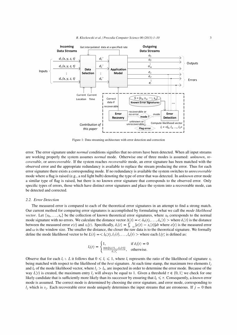
Figure 3 shows the architecture of the PILOTS runtimesystem, which implements the error detection and correctionmethods described in the previous section. It consists of
1Parameters τ and ω—for specifying threshold and time windowrespectively—can be given in command-line options.
three parts: the Data Selection, the Error Analyzer, and theApplication Model modules.
The Application Model obtains homogeneous data streams(d′1, d
′2, . . . , d
′N ) from the Data Selection module, and
then it generates outputs (o1, o2, . . . , oM ) and data errors(e1, e2, . . . , eL). The Data Selection module takes heteroge-neous incoming data streams (d1, d2, . . . , dN ) as inputs. Sincethis runtime is assumed to be working on moving objects, theData Selection module is aware of the current location andtime. Thus, it returns appropriate values to the ApplicationModel by selecting or interpolating data in time and locationdepending on the data selection method specified in thePILOTS program.
The ErrorAnalyzer collects the latest ω error values fromthe Application Model and keeps analyzing errors based onthe error signatures. If it detects a recoverable error, then itreplaces an erroneous input with the corrected one by applyinga corresponding error correction equation. The ApplicationModel computes the outputs based on the corrected inputsproduced from the Error Analyzer.
!!""#$%&$%'$%()
!#""#$%&$%'$%()
!$""#$%&$%'$%()
!!!
!"#$"#%
!""#$%&'$()
*(+,#
!"#$%&"'(
)*+*(,+-.*%/
01+'$&"'(
)*+*(,+-.*%/
*#
*!
!!!
*%
+#
+!
!!!
+&
&''('%
-&'&
.,#,%'$()
!"#$"%&''()&)')&')'%*"+,-,"('.)&"
!!,
!#,
!$,
/00(01
-,',%'$()
!""#"$%&'()*+",-
!!!
!"##$%&
'()$
!"##$%&
*+,-&(+%-%.%/-
'$%-
!$%!$%-
(0
.#/,$0
/01*$&"'2,3"2,400('5"+&0.
1%.%23'$%3
!$%444$%3
(5
12)'$,""#"
"%.%+/%0+#
/00(01
2(00,%'$()
#$,+1$#-23$0+#
/0.."+&'()&)',-'
."+05".)62"
)+4$
"%#$,+1$#-23$
%+0$##+#
2--$-(3"*456.-
!+##$,&$405-&-
Fig. 3. Data streaming architecture with error detection and correction.
III. ERROR SIGNATURES FOR SELF-HEALING SPEED DATA
In this section, we derive a set of error signatures for thespeed example used in the previous sections. Also, we presenta PILOTS program implementing the error signatures andcorresponding error correction equations.
A. Error Signatures
We consider the following four error modes: 1) normal (noerror), 2) pitot tube failure due to icing, 3) GPS failure, 4) bothpitot tube and GPS failures. Suppose the airplane is flying atairspeed va. For computing error signatures for different errorconditions, we will assume that other speeds as well as failedairspeed and ground speed can be expressed as follows.
• ground speed: vg ≈ va.• wind speed: vw ≤ ava, where a is the wind to airspeed
ratio.

• pitot tube failed airspeed: blva ≤ vfa ≤ bhva, where bland bh are the lower and higher values of pitot tubeclearance ratio and 0 ≤ bl ≤ bh ≤ 1. 0 represents afully clogged pitot tube, while 1 represents a fully clearpitot tube.
• GPS failed ground speed: vfg = 0.We assume that when a pitot tube icing occurs, it is
gradually clogged and thus the airspeed data reported fromthe pitot tube also gradually drops and eventually remains ata constant speed while iced. This resulting constant speed ischaracterized by ratio bl and bh. On the other hand, when aGPS failure occurs, the ground speed suddenly drops to zero.This is why we model the failed ground speed as vfg = 0.
In the case of pitot tube failure, let the ground speed, windspeed, and airspeed be vg = va, vw = ava, and vfa = bva. Theerror function (2) can be expressed as follows:
e = va −√v2a(b
2 + 2ab cos(αa − αw) + a2).
Since −1 ≤ cos(αa − αw) ≤ 1, the error is bounded by thefollowing:
va −√v2a(a+ b)2 ≤ e ≤ va −
√v2a(a− b)2
(1− a− b)va ≤ e ≤ (1− |a− b|)va. (9)
In the case of GPS failure, let the ground speed, wind speed,and airspeed be vfg = 0, vw = ava, and va = va. The errorfunction (2) can be expressed as follows:
e = 0−√v2a(1 + 2a cos(αa − αw) + a2).
Similarly to the pitot tube failure, we can derive the followingerror bounds:
−(a+ 1)va ≤ e ≤ −|a− 1|va. (10)
We can derive error bounds for the normal and both failurecases similarly. Applying the wind to airspeed ratio a and thepitot tube clearance ratio bl ≤ b ≤ bh to the constraints ob-tained in Inequations (9) and (10), we get the error signaturesfor each error mode as shown in Table I.
TABLE IERROR SIGNATURES FOR SPEED DATA.
Mode Error SignatureFunction Constraints
Normal e = k k ∈ [−ava, ava]Pitot tube failure e = k k ∈ [(1− a− bh)va, (1− |a− bl|)va]
GPS failure e = k k ∈ [−(a+ 1)va,−|a− 1|va]Both failures e = k k ∈ [−(a+ bh)va,−|a− bl|va]
When a = 0.1, bl = 0.2, and bh = 0.33, the error signaturesshown in Table I are visually depicted in Figure 4.
B. PILOTS programA PILOTS program called speedcheck implementing the
error signatures shown in Table I is presented in Figure 5. Thisprogram checks if the wind speed, airspeed, and ground speedare correct or not, and computes a crab angle, which is usedto adjust the direction of the aircraft to keep a desired ground
!"#$!
!
%!"#$!
!"&'$!
!"($!
%!")*$!
%!"($!
%#"#$!
"!"#$%&
'"()*+%,&-#./
0,("(*(-1.*+%,&-#.
203*+%,&-#.
Fig. 4. Error Signatures for speed data (a = 0.1, bl = 0.2, and bh = 0.33).
track. For this program to be applicable to a Cessna 182-RG,we use a cruise speed of 162 knots as va. Each section of theprogram is explained in order:
• inputs: All the speed and angle data required to computethe error and crab angle are defined here with data se-lection methods. Since heterogeneous input data streamsof air_speed, air_angle, ground_speed andground_angle are defined for 2D regions andtime, euclidean(x,y) and closest(t) select datawhich is closest to the current location in 2D eu-clidean space and then closest to the current time. Forwind_speed and wind_angle, since they are definedfor 3D regions and time, interpolate(z,2) is fi-nally used to get linearly interpolated values in the Z-axis using two data points after euclidean(x,y) andclosest(t) are applied.
• outputs: The crab angle and corrected speed data arecomputed every second.
• errors: The error function e defined in Equation (2) iscomputed. The angle signs are reversed in the formu-lae, because in mathematics, angles increase counter-clockwise (with 0◦ representing East) while in aviation,angles increase clockwise (with 0◦ representing North).
• signatures: There are four error signatures {S0, S1,S2, S3} associated with the error function e. They areall constrained by a constant k with lower and upperbounds based on the error signatures shown in Table I.
• correct: The error modes 1 and 2, which are identified byS1 and S2, can be corrected using the equations definedfor the airspeed and ground speed. If the error mode 3corresponding to S3 is detected, it is not possible tocorrect two variables at the same time, thus this erroris unrecoverable.
IV. EVALUATION
We apply the error signatures defined in Section III to twosets of real flight data. The first one is a private flight using

✬
✫
✩
✪
program speedcheck;inputs
wind_speed, wind_angle (x,y,z,t) usingeuclidean(x,y), closest(t), interpolate(z,2);
air_speed, air_angle (x,y,t) usingeuclidean(x,y), closest(t);
ground_speed, ground_angle (x,y,t) usingeuclidean(x,y), closest(t);
outputscrab_angle:
arcsin(wind_speed * sin(wind_angle - air_angle) /sqrt(air_speedˆ2 + 2 * air_speed * wind_speed *
cos(wind_angle - air_angle) + wind_speedˆ2))at every 1 sec;
air_speed_out: air_speed at every 1 sec;ground_speed_out: ground_speed at every 1 sec;wind_speed_out: wind_speed at every 1 sec;
errorse: ground_speed -
sqrt(air_speedˆ2 + wind_speedˆ2 + 2 * air_speed *wind_speed * cos(wind_angle - air_angle));
signatures/* v_a = 162 knots */S0(k): e=k, -16.2<=k, k<= 16.2 "Normal";S1(k): e=k, 91.8<=k, k<= 145.8 "Pitot tube failure";S2(k): e=k, -178.2<=k, k<=-145.8 "GPS failure";S3(k): e=k, -70.2<=k, k<= -16.2 "Both failures";
correctS1: air_speed = sqrt(ground_speedˆ2 + wind_speedˆ2
2 * ground_speed * wind_speed *cos(ground_angle - wind_angle));
S2: ground_speed = sqrt(air_speedˆ2 + wind_speedˆ22 * air_speed * wind_speed *cos(wind_angle - air_angle));
end
Fig. 5. A declarative specification of the speedcheck PILOTS program.
a Cessna 182-RG identified by N756VH [6] from Albany,NY to Fort Meade, MD on April 3rd, 2012. The other isthe Air France flight 447 using an Airbus A330-203 whichtook off from Rio de Janeiro bound for Paris on June 1st,2009. To simulate the failures mentioned in Section III, weadded corresponding errors to the N756VH Cessna flight data;however, we used the real pitot tube failure data for theAF447 flight. PILOTS programs’ error detection accuracy andresponse time to mode changes are evaluated.
A. Performance Metrics
• Accuracy: This metric is used to evaluate how accu-rately the algorithm determines the true mode. Assum-ing the true mode transition m(t) is known for t =0, 1, 2, . . . , T , let m′(t) for t = 0, 1, 2, . . . , T be the modedetermined by the error detection algorithm. We defineaccuracy(m,m′) = 1
T
∑Tt=0 p(t), where p(t) = 1 if
m(t) = m′(t) and p(t) = 0 otherwise.• Maximum/Minimum/Average Response Time: This
metric is used to evaluate how quickly the algorithmreacts to mode changes. Let a tuple (ti,mi) representa mode change point, where the mode changes to mi
at time ti. Let M = {(t1,m1), (t2,m2), . . . , (tN ,mN )}and M ′ = {(t′1,m′
1), (t′2,m
′2), . . . , (t
′N ′ ,m′
N ′)} be thesets of true mode changes and detected mode changesrespectively. For each i = 1 . . . N , we can find the
smallest t′j such that (ti ≤ t′j) ∧ (mi = m′j); if not
found, let t′j be ti+1. The response time ri for the truemode mi is given by t′j − ti. We define the maximum,minimum, and average response times by max1≤i≤N ri,min1≤i≤N ri, and 1
N
∑Ni=1 ri respectively.
B. Experiment 1: N756VH Cessna Flight1) Flight data: Flight data is collected through the follow-
ing independent sources:• ground speed: Flight track log provided by
FlightAware [6].• airspeed: Manually recorded by the pilot.• wind speed: Weather forecast information provided by
National Weather Service [7].The flight duration is 1 hour 41 minutes. The collected
speed data and error computed by Equation (2) are shownin Figure 6. Notice that the airspeed data during take off andlanding is not accurate due to the data collection mechanism.
!"##
#
"##
$##
# "### $### %### &### '### (###
!"##$%&%'(()(%*+,)-./
!"#$%&'$()
!"#$%&&'
(#)*+',$%&&'
&##)#
-"+',$%&&'
Fig. 6. Collected speeds and error for the N756VH 03-Apr-2012 KALB-KFME flight (normal).
2) Experimental Settings: Using the speedcheck PI-LOTS program shown in Figure 5, the 6060 seconds (=1 hour41 minutes) of flight departing from Albany, NY and landingat Fort Meade, MD are recreated. Three types of error aresimulated as shown below. In each case, all data streams exceptfor erroneous one(s) are actual. Defined error modes are: 0for unknown, 1 for normal, 2 for pitot tube failure, 3 for GPSfailure, and 4 for both failures.
• Pitot tube failure: 2400 seconds after the departure, theairspeed drops from 162 knots to 50 knots within 10seconds and stays at 50 knots until landing. The set oftrue mode changes is given by M = {(1, 1), (2401, 2)}.
• GPS failure: 2400 seconds after the departure, the groundspeed drops from 171 knots to 0 knots immediately andstays at 0 knots until landing. The set of true modechanges is given by M = {(1, 1), (2401, 3)}.
• Both pitot tube and GPS failures: The above twospeed changes happen simultaneously at 2400 secondsafter the departure. Both speeds remain failed untillanding. The set of true mode changes is given byM = {(1, 1), (2401, 4)}.
To find out the effect of the window size ω and thresholdvalue τ on the accuracy and response time, we measure thesemetrics for window sizes ω ∈ {1, 2, 4, 8, 16} and thresholdτ ∈ {0.2, 0.4, 0.6, 0.8}. Note that since there is only one errormode change in each true mode changes set, we can get onlyone response time result for each simulated error case.
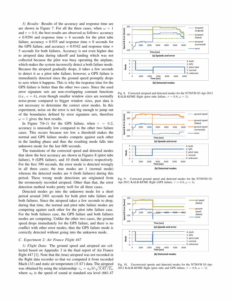
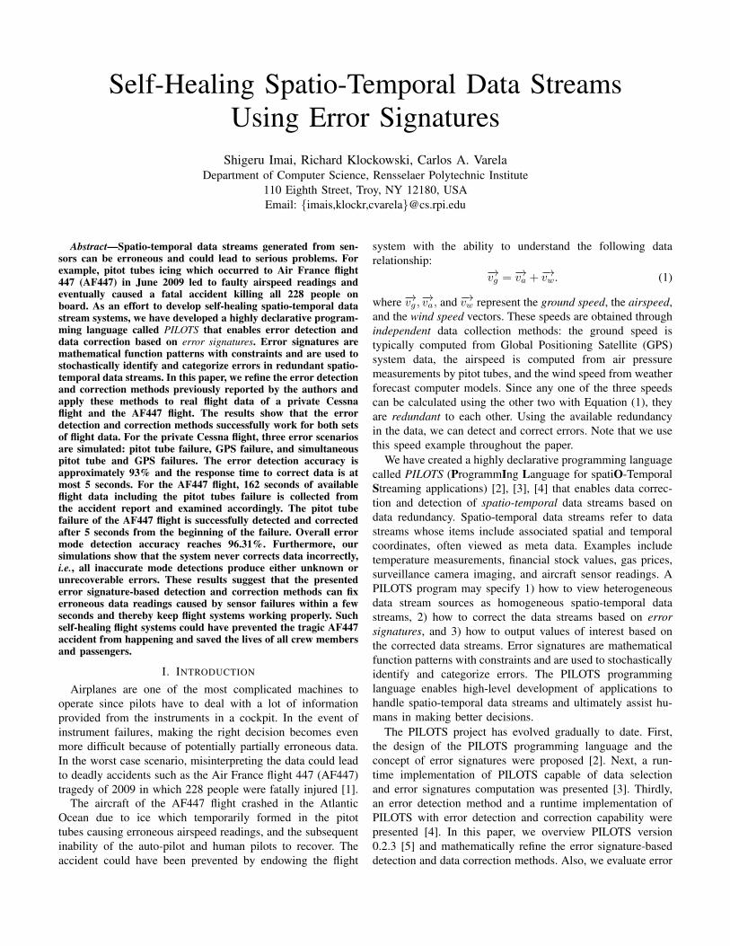
3) Results: Results of the accuracy and response time areare shown in Figure 7. For all the three cases, when ω = 1and τ = 0.8, the best results are observed as follows: accuracy= 0.9294 and response time = 4 seconds for the pitot tubefailure, accuracy = 0.935 and response time = 0 seconds forthe GPS failure, and accuracy = 0.9342 and response time =5 seconds for both failures. Accuracy is not even higher dueto airspeed data during takeoff and landing which was notcollected because the pilot was busy operating the airplane,which makes the system incorrectly detect a both failure mode.Because the airspeed gradually drops, it takes a few secondsto detect it as a pitot tube failure; however, a GPS failure isimmediately detected since the ground speed promptly dropsto zero when it happens. This is why the response time for theGPS failure is better than the other two cases. Since the usederror signature sets are non-overlapping constant functions(i.e., e = k), even though smaller window sizes are normallynoise-prone compared to bigger window sizes, past data isnot necessary to determine the correct error modes. In thisexperiment, noise on the error is not big enough to jump outof the boundaries defined by error signature sets, thereforeω = 1 gives the best results.
In Figure 7(b-1) for the GPS failure, when τ = 0.2,accuracy is unusually low compared to the other two failurecases. This occurs because too low a threshold makes thenormal and GPS failure modes compete against each otherin the landing phase and thus the resulting mode falls intounknown mode for the last 600 seconds.
The transitions of the corrected speed and detected modesthat show the best accuracy are shown in Figures 8 (pitot tubefailure), 9 (GPS failure), and 10 (both failures) respectively.For the first 390 seconds, the error mode is detected wronglyin all three cases; the true modes are 1 (normal mode)whereas the detected modes are 4 (both failures) during thisperiod. These wrong mode detections are originated fromthe erroneously recorded airspeed. Other than that, the errordetection method works pretty well for all three cases.
Detected modes go into the unknown mode for a shortperiod around 2401 seconds for both pitot tube failure andboth failures. Since the airspeed takes a few seconds to drop,during that time, the normal and pitot tube failure modes arecompeting against each other for the pitot tube failure case.For the both failures case, the GPS failure and both failuresmodes are competing. Unlike the other two cases, the groundspeed drops immediately for the GPS failure, and there is noconflict with other error modes, thus the GPS failure mode iscorrectly detected without going into the unknown mode.
C. Experiment 2: Air France Flight 4471) Flight Data: The ground speed and airspeed are col-
lected based on Appendix 3 in the final report of Air Franceflight 447 [1]. Note that the (true) airspeed was not recorded inthe flight data recorder so that we computed it from recordedMach (M ) and static air temperature (SAT ) data. The airspeedwas obtained by using the relationship: va = a0M
√SAT/T0,
where a0 is the speed of sound at standard sea level (661.47
!"##
#
"##
$##
# "### $### %### &### '### (###
!"##$%&%'(()(%*+,)-./
!"#$%&'$()
!"#$%&&'
()#"*"+!,-
!"#$%&&'
(.!",&'-
!"#$%&&'
(/)##&/0&'-
&##)#
#
"
$
%
&
# "### $### %### &### '### (###
0)$#
!"#$%&'$()
!" #$%&'
("')*+
,"'-.%$%'%/#0
1"'2$3456
7"'/282$92
!"#$%&''() "*($'++,+
!-#$.'/'0/'( 1,(')
Fig. 8. Corrected airspeed and detected modes for the N756VH 03-Apr-2012KALB-KFME flight (pitot tube failure, τ = 0.8,ω = 1).
!
"
#
$
%
! "!!! #!!! $!!! %!!! &!!! '!!!
!"#$
!"#$%&'$()
!" #$%&'
("')*+
,"'-.%$%'%/#0
1"'2$3456
7"'/282$92
(#!!
("!!
!
"!!
#!!
! "!!! #!!! $!!! %!!! &!!! '!!!
%&$$#'(')**"*'+,-"./0
!"#$%&'$()
!"#$%&'()**&
!"#$%&'()**&
+,-./*&0
!"#$%&'()**&
+1#""*12*&0
*""#"
!"#$%&''() "*($'++,+
!-#$.'/'0/'( 1,(')
Fig. 9. Corrected ground speed and detected modes for the N756VH 03-Apr-2012 KALB-KFME flight (GPS failure, τ = 0.8,ω = 1).
!"##
!$##
#
$##
"##
# $### "### %### &### '### (###
!"##$%&%'(()(%*+,)-./
!"#$%&'$()
!"#$%&''(
)*!"+'(,
-#./0(
%&''(
)*!"+'(,
'##.#
#
$
"
%
&
# $### "### %### &### '### (###
0)$#
!"#$%&'$()
!" #$%&'
("')*+
,"'-.%$%'%/#0
1"'2$3456
7"'/282$92
!"#$%&''() "*($'++,+
!-#$.'/'0/'( 1,(')
Fig. 10. Uncorrected speeds and detected modes for the N756VH 03-Apr-2012 KALB-KFME flight (pitot tube and GPS failure, τ = 0.8,ω = 1).

!"#
!"$
!"%
!"&
!"'
(
! # (! (# )!
!""#$%"&
!"#$%&'(")*'+
*+,+!")
*+,+!"-
*+,+!"$
*+,+!"&
!
#
(!
(#
)!
! # (! (# )!
!"#$%&#"'()*"'
+#",-'
!"#$%&'(")*'+
*+,+!")
*+,+!"-
*+,+!"$
*+,+!"&
!"#$%&'(()*"(+&# ,-./.&0)12 3"-4)*2
!"#5%&6278/972 0-:2&# ,-./.&0)12&3"-4)*2
!"#
!"$
!"%
!"&
!"'
(
! # (! (# )!
!""#$%"&
!"#$%&'(")*'+
*+,+!")
*+,+!"-
*+,+!"$
*+,+!"&
!
#
(!
(#
)!
! # (! (# )!
!"#$%&#"'()*"'
+#",-
!"#$%&'(")*'+
*+,+!")
*+,+!"-
*+,+!"$
*+,+!"&
!1#$%&'(()*"(+&# ;,<&3"-4)*2
!1#5%&6278/972&0-:2&# ;,<&3"-4)*2
!"#
!"$
!"%
!"&
!"'
(
! # (! (# )!
!""#$%"&
!"#$%&'(")*'+
*+,+!")
*+,+!"-
*+,+!"$
*+,+!"&
!
#
(!
(#
)!
! # (! (# )!
!"#$%&#"'()*"'
+#",-
!"#$%&'(")*'+
*+,+!")
*+,+!"-
*+,+!"$
*+,+!"&
!(#$%&'(()*"(+&# =/.> 3"-4)*27
!(#5%&6278/972&0-:2&# =/.>&3"-4)*27
Fig. 7. Accuracy and response time for the N756VH 03-Apr-2012 KALB-KFME flight
knots) and T0 is the temperature at standard sea level (288.15Kelvin). Independent wind speed information was not recordedeither. According to the description from page 47 of the finalreport: “(From the weather forecast) the wind and temperaturecharts show that the average effective wind along the routecan be estimated at approximately ten knots tail-wind.” Wefollowed this description and created the wind speed datastream as ten knots tail wind.
2) Experimental Settings: According to the final report,speed data was provided from 2:09:00 UTC on June 1st2009 and it became invalid after 2:11:42 UTC on the sameday. Thus, we examine the valid 162 seconds of speed dataincluding a period of pitot tube failure which occurred from2:10:03 to 2:10:36 UTC. We also use the speedcheckPILOTS program shown in Figure 5 except for constraintsvalues in signatures which use va = 470 knots, the cruiseairspeed of the AF447 flight. Defined error modes are thesame as Experiment 1, so the set of true mode changesis defined as M = {(1, 1), (64, 2), (98, 1)}. The accuracyand average response time are investigated for window sizesω ∈ {1, 2, 4, 8, 16} and threshold τ ∈ {0.2, 0.4, 0.6, 0.8}.
3) Results: Results of the accuracy and maximum/mini-mum/average response times are shown in Figure 11. Sameas Experiment 1, the best results, accuracy = 0.9631, maxi-mum/minimum/average response times = 5/0/2.5 seconds, areobserved when ω = 1 and τ = 0.8. Overall trends of theaccuracy and response time are same as Experiment 1 becauseof the nature of the error signature set.
The transitions of the corrected speed and detected modesthat show the best accuracy with ω = 1 and τ = 0.8 areshown in Figure 12. Looking at Figure 12(b), the pitot tubefailure is successfully detected from 69 to 97 seconds exceptfor the interval 64 to 69 seconds due to the slowly decreasingairspeed. The response time for the normal to pitot tube failuremode is 5 seconds and for the pitot tube failure to normalmode is 0 seconds (thus the average response time is 2.5seconds). From Figure 12(a), the airspeed successfully startsto get corrected at 69 seconds and seamlessly transitions tothe normal airspeed when it recovers at 98 seconds.
!"#
!"$
!"%
!"&
!"'
(
! # (! (# )!
!""#$%"&
!"#$%&'(")*'+
*+,+!")
*+,+!"-
*+,+!"$
*+,+!"&
!"#$%&&'("&)$
!
#
(!
(#
)!
! # (! (# )!
!"#$%&'()*'&$
+,-&$.'&/0
!"#$%&'(")*'+
*+,+!")
*+,+!"-
*+,+!"$
*+,+!"&
!*#$+",-.'.$/0123410 5-.0
!
#
(!
(#
)!
! # (! (# )!
!,*$%&'()*'&$
+,-&$.'&/0
!"#$%&'(")*'+
*+,+!")
*+,+!"-
*+,+!"$
*+,+!"&
!&#$+-4-.'. /0123410 5-.0
!
#
(!
(#
)!
! # (! (# )!123$%&'()*'&$+,-&$
.'&/0
!"#$%&'(")*'+
*+,+!")
*+,+!"-
*+,+!"$
*+,+!"&
!6#$%70("80$/0123410 5-.0
Fig. 11. Accuracy and response time for AF447 flight.
!"##
#
"##
$##
%##
&##
'##
(##
# $# &# (# )# "## "$# "&# "(#
!"##$%&%'(()(%*+,)-./
!"#$%&'$()
!"#$%&&'
()*##&)+&',
!"#$%&&'
(-!".&',
&##*#
#
"
$
%
&
# $# &# (# )# "## "$# "&# "(#
0)$#
!"#$%&'$()
!" #$%&'
("')*+
,"'-.%$%'%/#0
1"'2$3456
7"'/282$92
!"#$%&''() "*($'++,+
!-#$.'/'0/'( 1,(')
Fig. 12. Corrected airspeed and detected modes for AF447 flight.
V. RELATED WORK
There are several systems that combine stream processingand data base management, i.e., Data Stream ManagementSystems or DSMS, such as STREAM [8], Aurora [9], andTelegraphCQ [10]. They are designed to execute SQL-likequeries to unbounded continuous incoming data streams andoutput events of interest. Microsoft StreamInsight is a DSMS-

based system and has been extended to support spatio-temporal streams [11]. Also, the concept of the moving objectdata base (MODB) which adds support for spatio-temporaldata streaming to DSMS is discussed in [12]. These DSMS-based spatio-temporal stream management systems supportgeneral continuous queries for multiple moving objects. Ourstreaming data analytics to detect errors based on signa-tures and correct data on the fly is beyond the scope of apurely declarative SQL-based query approach. Furthermore,our domain-specific approach enables highly declarative de-scription of input-output relationships between streams, errorfunctions, error signatures, and data correction functions usingthe PILOTS programming language.
Distributed streaming systems have been studied in the con-text of cloud computing [13], [14]. Our data error correctionmethods could be useful for distributed settings as well byconnecting multiple distributed PILOTS applications.
VI. CONCLUSION AND FUTURE DIRECTIONS
We define a general error signature set for aviation speeddata and evaluate error detection performance of PILOTSprograms with real flight data. We find that the accuracy andresponse time improve as the threshold τ increases. The reasonof this behavior is that there are some cases in which thereare two competing modes whose likelihood values are closeto each other, and due to the closeness, the mode detectionalgorithm tends to regard it as an unknown error mode. Higherthreshold values are more tolerant to multiple competingmodes, thus give better results. Unsurprisingly, there is apositive correlation between the window size and responsetimes for all the threshold values. This is an intuitive resultbecause the less the error detection algorithm uses past data,the more responsive it becomes to mode changes. In addition,a faster average response time leads to a better accuracyresult since the error detection algorithm cannot predict modechanges, but only react to them. That is, a smaller windowsize implies better accuracy. This is true because our designederror signature set produces nearly orthogonal mode likelihoodvectors. Also, it is noteworthy that our error detection and datacorrection methods never correct data incorrectly.
When computing mode likelihood vectors, time to computedistances by Equation (6) can be significant due to the expo-nential growth of the search space as the size of the constantsset K increases. To use the presented error detection and cor-rection methods in larger-scale real-time systems, techniquesto bound the running time must be devised.
Future research directions include applying the errorsignature-based error detection and correction methods toother flight accidents, e.g., those fuel sensor reading errors.Also developing PILOTS flight systems that process real-timedata from external sources such as 3D terrain data, updatedweather, and information from other airplanes. More and moredata are expected to be available in cockpits in the nearfuture [15], and thus automated data analysis systems willbecome even more crucial to both manned and unmannedaerial vehicles. We envision smarter and safer flight systems
processing massive data in real-time. Such systems need toreason about spatial and temporal data and constraints andgive the pilots better information to make more accuratejudgments during critical moments. The presented techniquesand software can be used as a promising starting point todevelop these flight systems.
ACKNOWLEDGMENTS
This research is partially supported by Air Force Officeof Scientific Research Grant No. FA9550-11-1-0332 and aYamada Corporation Fellowship.
REFERENCES
[1] Bureau d’Enquetes et d’Analyses pour la Securite del’Aviation Civile, “Final Report: On the accident on 1st June2009 to the Airbus A330-203 registered F-GZCP operatedby Air France flight AF 447 Rio de Janeiro - Paris,”http://www.bea.aero/en/enquetes/flight.af.447/rapport.final.en.php,2012.
[2] S. Imai and C. A. Varela, “A programming model for spatio-temporaldata streaming applications,” in Dynamic Data-Driven Application Sys-tems (DDDAS 2012), Omaha, Nebraska, June 2012, pp. 1139–1148.
[3] ——, “Programming spatio-temporal data streaming applications withhigh-level specifications,” in 3rd ACM SIGSPATIAL InternationalWorkshop on Querying and Mining Uncertain Spatio-Temporal Data(QUeST) 2012, Redondo Beach, California, USA, November 2012.
[4] R. S. Klockowski, S. Imai, C. Rice, and C. A. Varela, “Autonomousdata error detection and recovery in streaming applications,” in DynamicData-Driven Application Systems (DDDAS 2013) Workshop, May 2013,pp. 2036–2045.
[5] Worldwide Computing Laboratory, Rensselaer Polytechnic Institute,“The PILOTS programming language,” http://wcl.cs.rpi.edu/pilots/.
[6] FlightAware, “Flight track log for N756VH on 03-Apr-2012(KALB-KFME),” http://flightaware.com/live/flight/N756VH/history/20120403/1800Z/KALB/KFME/tracklog.
[7] NOAA’s National Weather Service, “Forecast winds and temps aloft,”http://aviationweather.gov/products/nws/winds/.
[8] A. Arasu, B. Babcock, S. Babu, J. Cieslewicz, K. Ito, R. Motwani,U. Srivastava, and J. Widom, “Stream: The Stanford data streammanagement system,” in ACM SIGMOD Conference. Springer, 2004.
[9] D. J. Abadi, D. Carney, U. Cetintemel, M. Cherniack, C. Convey,S. Lee, M. Stonebraker, N. Tatbul, and S. Zdonik, “Aurora: a new modeland architecture for data stream management,” The VLDB JournalTheInternational Journal on Very Large Data Bases, vol. 12, no. 2, pp.120–139, 2003.
[10] S. Chandrasekaran, O. Cooper, A. Deshpande, M. J. Franklin, J. M.Hellerstein, W. Hong, S. Krishnamurthy, S. R. Madden, F. Reiss,and M. A. Shah, “TelegraphCQ: continuous dataflow processing,” inProceedings of the 2003 ACM SIGMOD international conference onManagement of data. ACM, 2003, pp. 668–668.
[11] M. H. Ali, B. Chandramouli, B. S. Raman, and E. Katibah, “Spatio-temporal stream processing in Microsoft StreamInsight,” IEEE DataEng. Bull., pp. 69–74, 2010.
[12] K. An and J. Kim, “Moving objects management system supportinglocation data stream,” in Proceedings of the 4th WSEAS InternationalConference on Computational Intelligence, Man-Machine Systems andCybernetics, ser. CIMMACS’05. Stevens Point, Wisconsin, USA:World Scientific and Engineering Academy and Society (WSEAS),2005, pp. 99–104.
[13] L. Neumeyer, B. Robbins, A. Nair, and A. Kesari, “S4: Distributedstream computing platform,” in Data Mining Workshops (ICDMW), 2010IEEE International Conference on. IEEE, 2010, pp. 170–177.
[14] V. Gulisano, R. Jimnez-Peris, M. Patio-Martnez, C. Soriente, and P. Val-duriez, “StreamCloud: An elastic and scalable data streaming system,”IEEE Trans. Parallel Distrib. Syst., pp. 2351–2365, 2012.
[15] U.S. Department of Transportation Federal Aviation Administra-tion, “Code of federal regulations part 91.225: Automatic de-pendent surveillance-broadcast (ADS-B) out performance require-ments to support air traffic control (ATC) service; final rule,”http://www.faa.gov/regulations policies/faa regulations/, July 2013.
Procedia Computer Science 00 (2013) 1–10
Procedia ComputerScience
International Conference on Computational Science, ICCS 2013
Autonomous Data Error Detection and Recoveryin Streaming Applications
Richard Klockowski, Shigeru Imai, Colin L Rice, Carlos A. Varela*Computer Science Department, Rensselaer Polytechnic Institute, 110 Eighth Street, Troy, NY 12180, USA
Abstract
Detecting and recovering from errors in data streams is paramount to developing successful autonomous real-timestreaming applications. In this paper, we devise a multi-modal data error detection and recovery architecture to enableautomated recovery from data errors in streaming applications based on available redundancy. We formally defineerror signatures as a way to identify classes of abnormal conditions and mode likelihood vectors as a quantitativediscriminator of data stream condition modes. Finally, we design an extension to our own declarative programminglanguage, PILOTS, to include error correction code. We define performance metrics for our approach, and evaluatethe impact of monitored data window size and mode likelihood change threshold on the accuracy and responsivenessof our data-driven multi-modal error detection and correction software. Tragic accidents—such as Air France’s flightfrom Rio de Janeiro to Paris in June 2009 killing all people on board— can be prevented by implementing auto-pilotsystems with an airspeed data stream error detection and correction algorithm following the fundamental principlesillustrated in this work.
Keywords: redundant data error correction, spatio-temporal data streams, programming languages
1. Introduction
We present a software framework for developing resilient data driven applications and systems that act upon re-dundant spatio-temporal data streams. In this work we assume a spatio-temporal data streaming application model,where input streams associated to space and time get converted into output streams and error streams according to amathematical description of the behavior of the application. Much like redundant bits in error correcting hardware,stream redundancies allow for dynamic detection and correction of known types of failures. Redundancy is a keyaspect present in many spatio-temporal data streaming applications. However, unless it is e↵ectively used by systems,autonomous recovery from error conditions is not possible. There are many complex ways in which a set of redundantinput streams may fail. We propose a system towards automatically correcting known failures that can be detected inthe source streams. We formalize error signatures, mathematical function patterns that enable autonomous systems toaccurately detect when an erroneous condition exists in an input data stream. A multi-modal architecture uses theseerror signatures to switch each stream between di↵erent modes of operation. Mode likelihood vectors are computed
Corresponding authorEmail address: [email protected] (Carlos A. Varela*)

R. Klockowski et al. / Procedia Computer Science 00 (2013) 1–10 2
in real-time by interpolating streamed data to a set of known error signatures. These vectors are used to determinethe condition that input streams are exhibiting. When in a known error condition mode, the erroneous original datastream is automatically replaced by a data stream that is computed from the redundant (correct) data streams. Thesystem dynamically adapts to errors in the data streams by switching modes, and it can resume normal behavior wheninput data is no longer categorized as being erroneous. We design an extension to PILOTS, a declarative program-ming language to not only compute error signatures from high-level specifications of spatio-temporal data streamingapplications, but also to enable these applications to recover from known errors by using available redundancy in thedata.
The Air France AF447 accident in June 2009 left 12 crew members and 216 passengers dead [1]. The reasonfor the crash was faulty sensor data that caused the automatic pilot to disengage, ultimately confusing the humanpilots who were unable to take timely corrective actions. The pitot tubes of the airplane began to freeze which causedincorrect air speed readings, switching the plane from normal law to alternate law, and eventually causing the pilots toenter an unintended fatal stall. After a technical investigation by the Bureau d’Enquetes et d’Analyses pour la Securitede l’Aviation Civile (BEA) it is clear that this error condition is detectable and can be corrected by an active redundantdata-driven flight system. We argue that disasters like this are preventable by using an automatic pilot that implementsthe framework described in this paper: a multi-modal dynamic data-driven error correction software framework usingerror signatures and mode likelihood vectors.
2. Data Error Detection and Correction Architecture
Our contribution is an autonomous error correcting architecture for data streaming applications (depicted in Fig-ure 1). The architecture was designed for applications with redundant input streams. For a set of input streamsD d1, d2, ..., dn
, the redundancy of the streams can be defined as the set of functions R r1, r2, ..., rm
whereeach r
i
is a function r
i
d1, . . . , dk
d
j
for j 1...n , k n, d1, . . . , dk
D and d
j
d1, . . . , dk
. An error function
associated to a particular input stream d
j
may take the form e
j
d
j
r
i
d1, . . . , dk
, where r
i
is the redundancy func-tion r
i
d1, . . . , dk
d
j
. We define error signatures as the shape of these error functions for previously known errorconditions. Additionally we formalize the mode likelihood vector, which is used to determine whether there is an errorand whether or not it can be corrected. Data stream error correction is provided in the case that a redundancy withinthe other working streams is available. Especially in the case of spatio-temporal streams that use inherently redundantphysical data such as those found in a flight system using sensor data, error signatures enable developing e↵ectivereal-time error warning and correction systems. We contend that our proposed software framework can be useful toprevent tragedies such as the Air France plane crash. For this purpose we are developing PILOTS: a programminglanguage for spatio-temporal data streaming applications [2]. PILOTS allows us to view heterogeneous data streamsas homogeneous by declaratively selecting data according to geometric principles. In this paper, we describe an exten-sion to the language design to include error correction code using the notion of error signatures. This software shouldprove very helpful for streaming application developers to enable them to create e↵ective error correcting software.
2.1. Error Signatures
The purpose of an error signature is to be able to reason about which data stream may contain an error. A collectionof error signatures, called an error signature set, is matched against the observed error which provides a means oferror detection. We assume the existence of an error function which is simply a function of the input streams thatcaptures the redundancy in the data streams. The measured error for an application is the value of the error functionover a window of time. Each error signature corresponds to a particular type of failure in the input streams. Thee↵ectiveness of error signatures is highly dependent on the choice of error function. When there are no problems withthe input streams, error functions typically evaluate to zero.
An error signature describes the behavior of the error function under particular operating conditions which wechoose to call modes. An important distinction is made between theoretical error signatures, which correspond toknown error modes, and measured error which is generated by looking at the raw input data. Theoretical error signa-tures are currently defined as a function of time which may contain constants k0, . . . , kn
satisfying a set of constraints.In order to identify useful error signatures for a particular application, we currently employ an empirical method ofsimply running a simulation using data that exhibits a certain type of error and observe the results in the measured
R. Klockowski et al. / Procedia Computer Science 00 (2013) 1–10 3
!!""#$%&$%'$%()
!#""#$%&$%'$%()
!$""#$%&$%'$%()
!!!
!"#$"#%
!""#$%&'$()
*(+,#
!"#$%&"'(
)*+*(,+-.*%/
01+'$&"'(
)*+*(,+-.*%/
*#
*!
!!!
*%
+#
+!
!!!
+&
&''('%
-&'&
.,#,%'$()
!"#$%&#"'()*+#",$$,+#+$+#$+$-(".%/%",$'+#"
!!,
!#,
!$,
)*$"#%
/00(01
-,',%'$()
!"#$"%&''#'%()*"+,-'./!!!
!!!
01''"&#
2%3"
01''"&#
4).+#%)&-%.%/0
'$%0
!$%!$%0
$1
0#1.%2
0)3(1#"$*%5"*%6)),$7".#)'
2%.%34'$%4
!$%555$%4
$6
34+*%.''#'
1&5&)8&$)'
/00(01
2,%(3,04
'".)7"'+9*"$)'
0)''".#
,+#+$%/$
'".)7"'+9*"
3),"
7*8(9:;<(:*8%*=%
(>:0%?@?+9
1&'".)7"'+9*"
&)$"'')'
Figure 1: Data streaming architecture with error detection and correction
error. The error signature under normal conditions signifies that no errors have been detected. When all input streamsare working properly the system assumes normal mode. Otherwise one of three modes is assumed: unknown, re-
coverable, or unrecoverable. If the system reaches recoverable mode, an error signature has been matched with theobserved error and the appropriate redundancy is available to replace the stream producing the error. Thus for eacherror signature there exists a corresponding mode. If no redundancy is available the system switches to unrecoverable
mode where a flag is raised (e.g., a red light bulb) denoting the type of error that was detected. In unknown error modea similar type of flag is raised, but there is no known error signature that corresponds to the observed error. Onlyspecific types of errors, those which have distinct error signatures and place the system into a recoverable mode, canbe detected and corrected.
2.2. Error Detection
The measured error is compared to each of the theoretical error signatures in an attempt to find a strong match.Our current method for comparing error signatures is accomplished by formulating what we call the mode likelihood
vector. Let s0, . . . , sn
be the collection of known theoretical error signatures, where s0 corresponds to the normalmode signature with no errors. We calculate the distance vector � t �0 t , . . . , �
n
t where �i
t is the distancebetween the measured error e t and s
i
t . Specifically, �i
t
t
t ! e t s
i
t dt where e t is the measured errorand ! is the window size. The smaller the distance, the closer the raw data is to the theoretical signature. We formallydefine the mode likelihood vector to be L t l0 t , l1 t , . . . , l
n
t where each l
i
t is defined as:
l
i
t
1, if �i
t 0min �0 t ,...,�
n
t
�i
t
, otherwise.
Observe that for each l
i
L it follows that 0 l
i
1, where l
i
represents the ratio of the likelihood of signature s
i
being matched with respect to the likelihood of the best signature. At each time stamp, the maximum two elements l
j
and l
k
of the mode likelihood vector, where l
j
l
k
, are inspected in order to determine the error mode. Because of theway L t is created, the maximum entry l
j
will always be equal to 1. Given a threshold ⌧ 0, 1 we check for onelikely candidate that is su�ciently more likely than its successor by ensuring that l
k
⌧. Consequently, a known errormode is assumed. The correct mode is determined by choosing the error signature, and error mode, corresponding tol
j
which is s
j
. Each recoverable error mode uniquely determines the input streams that are erroneous. If j 0 then

R. Klockowski et al. / Procedia Computer Science 00 (2013) 1–10 4
the system is in normal mode. If l
k
⌧ then, regardless of the value of j, unknown error mode is assumed and anerror flag is raised. No corrective action can be taken because the measured error cannot be recognized, and the inputdata flows through the application uncorrected. A well-behaved set of error signatures will produce nearly orthogonal
mode likelihood vectors, where one element is a one and the rest are close to zero. In sections 3 and 4 we study theimpact of the choice of theoretical error signature sets on detection and correction results.
2.3. Error Recovery
If we assume that the system is in one of the known error modes (i.e., a match has been found for the measurederror) then an attempt can be made at correcting the error. Recall that the error function is given and contains infor-mation about the redundancy between data streams. If an input stream d
j
experiences an error and a redundancy r
i
exists which can replace that stream, then the error is recoverable. After the error has been corrected, the originalinput streams will continue to be monitored to determine if the error has subsided and the system is able to reenternormal mode.
3. Twice: A Case Study
We explore how error signatures a↵ect the values of mode likelihood vectors defined in Section 2 by using a verysimple data streaming application called Twice.
3.1. A Simple Data Streaming Application
Twice is a simple data streaming application which takes two input data streams, a and b, where b is supposed tobe twice as large as a, and outputs an error defined by b 2 a. Stream data for a and b are expected to increase by onefor a and by two for b every second (i.e., a t t and b t 2 t), so the error is zero in the normal case; however,several modes of errors could happen depending on di↵erent types of failures as shown in Figure 2. Figure 2(a) showsnormal mode, where most of the time the error remains zero, but there are several spikes due to transient fluctuationof the data input timing. Figure 2(b) suggests critical failure of a’s data source. We will call this a failure mode. Ataround 50 seconds of the simulation time, the error starts growing linearly. This linear increase of the error explainsthat a remains a constant value whereas b continues increasing its value. Similarly, Figure 2(c) shows a situationwhere a correctly increases, but b fails to increase its value. Similarly, we will call this b failure mode. Figure 2(d)shows an example of an out-of-sync mode, where the error becomes consistently large at around 30 seconds of thesimulation time. This is because a’s input data stream becomes consistently one second behind b’s input data stream.
!"
!#
!$
%
$
#
"
% #% &% '% (% $%% $#%
!"#$%&!"#'
!"#$%&$'((&(
!%)*
%
%)*
$
$)*
#
#)*
% #% &% '% (% $%% $#%
$%&"'(!"#)
!*%
%
*%
$%%
$*%
% #% &% '% (% $%% $#%
$%&"'(!"#)
!$*%
!$%%
!*%
%
*%
% #% &% '% (% $%% $#%
$%&"'(!"#)
!)#$*$+",-.(' !/#$0$+",-.(' !1#$2.34&+4567/ '((&(
Figure 2: Known error patterns for twice example
3.2. Error Signatures for Twice
To correctly di↵erentiate the four di↵erent modes of errors presented in Figure 2, we define error signatures foreach mode. In the course of our case study, we evaluated three sets of error signatures as shown in Table 1. For theno error, a failure, and b failure modes, all error signatures are the same in these error signature sets. That is, e 0for no error, e 2t k for a failure, and e 2t k for b failure. Each error signature is designed to capture acharacteristic pattern of error we see in the previous section. For example, an error signature for a failure is a linearfunction with a slope of 2 and a constant k, which resembles the increasing line starting at around 50 seconds ofa failure shown in Figure 2(b). Di↵erences among error signature sets are limited to the out-of-sync failure mode.Both base and out-of-sync restricted error signature sets have e k for the out-of-sync mode, but the out-of-sync
restricted imposes a constraint on the value of k ( k ⌧oos
). The ⌧oos
threshold is intended to prevent noise and smallout-of-sync conditions from being categorized as abnormal.

R. Klockowski et al. / Procedia Computer Science 00 (2013) 1–10 5
Table 1: Error signature sets defined for twice exampleMode
Error signature set No error A failure B failure Out-of-syncBase e k, where k 0
Out-of-sync restricted e 0 e 2t k e 2t k e k, where k ⌧oos
Out-of-sync removed none
3.3. Mode Estimation Study
Using the error signatures defined in Table 1, we estimate the operating modes for a 480 seconds sequence ofmeasured error including mode change within sixty-second intervals as shown in Figure 3(a). Figure 4(a) shows theground truth: the transition of modes that is used to generate the streams. In Figure 4, modes are mapped to 0 forunknown, 1 for no error, 2 for a failure, 3 for b failure, and 4 for out-of-sync. For each set of error signatures presentedin the previous section, we first compute the likelihood of each mode, and then estimate mode likelihoods relative tothe maximum likelihood which represents the minimum signature interpolation distance.
!"#$
!"$$
!#$
$
#$
"$$
"#$
! "! #$! #%! $&! '!! '"! &$! &%!
!"#$%&"'()&&*&(
!"#$%&'$()
!"#$%&"'()&*$&))+),$&$-$.$/ 0"
!.#$%+*&$123&124++* 5+)$."'&$&))+)$'267"8()&'$'&8,$9284$:$-$;<
!=#$%+*&$123&124++* 5+)$+(8/+5/'>7=$)&'8)2=8&*$&))+)$'267"8()&$'&8,$9284$:-;<
!*#$%+*&$123&124++* 5+)$+(8/+5/'>7=$)&?+@&*$&))+)$'267"8()&$'&8,$9284$:-;<
!
!("
! "! #$! #%! $&! '!! '"! &$! &%!
!"#$%&'($)'*""#
!"#$%&'$()
*+%$,,+,
-%.-"/0,$
1%.-"/0,$
+023+.3
'4*(
5%6%789
#(!
!
!("
! "! #$! #%! $&! '!! '"! &$! &%!
!"#$%&'($)'*""#
!"#$%&'$()
*+%$,,+,
-%.-"/0,$
1%.-"/0,$
+023+.3
'4*(
5%6%789
#(!
!
!("
! "! #$! #%! $&! '!! '"! &$! &%!
!"#$%&'($)'*""#
!"#$%&'$()
*+%$,,+,
-%.-"/0,$
1%.-"/0,$
5%6%789
#(!
Figure 3: Measured error and mode likelihood results for twice example
The results of the mode likelihood and the estimated modes are shown in Figure 3(b)-(d) and 4(b)-(d) respectively.Figure 3(b) and 4(b) are results for the base error signatures, Figure 3(c) and 4(c) are results for the out-of-sync
restricted error signatures, and Figure 3(d) and 4(d) are results for the out-of-sync removed error signatures.
• Base: Looking at the result of estimated mode in Figure 4(b), most of the first and last 60 seconds are recognizedas the out-of-sync mode, where they are actually supposed to be in the normal mode. This incorrect estimation

R. Klockowski et al. / Procedia Computer Science 00 (2013) 1–10 6
occurs because the given error in Figure 3(a) contains noise so that the actual value of the error is not alwaysexactly zero. Thus, the out-of-sync error signature fits better to the measured error than no error since theconstant k in the out-of-sync error signature can be any value other than zero. This essentially illustrates anill-defined error signature set: since normal and out-of-sync conditions are di�cult to distinguish from eachother, computed mode likelihood vectors are far from orthogonal.• Out-of-sync restricted: The result of estimated mode in Figure 4(c) looks closer to the true mode in Figure 4(a)
than the result of the base error signature set. The threshold ⌧oos
(⌧oos
20 for this experiment) is a constrainton the out-of-sync error signature that prevents it from matching the first and last 60 seconds, and correctly letsthe normal signature match those periods instead.• Out-of-sync removed: The result of estimated mode in Figure 4(d) does not match the out-of-sync mode at
around 120-180 and 300-360 seconds since that mode does not exist, but it successfully goes into unknown
error mode which are valid estimations when using this signatures set. Also, it succeeds to match normal modeat around 0-60 and 420-480 seconds most of the time.
!
"
#
$
%
! &! "#! "'! #%! $!! $&! %#! %'!
!"#$%&'()*+
!"#$%&'$()
*+%,-./,0/'12(
3+%4 05"6-7$
8+%5 05"6-7$
9+%2, $77,7
:+%-2;2,<2
!"#$%&'()* +&(+,$-'&$./)/&"+/*$0+&/"1$*"+"
!2#$30+41"+/* 1'*/$-'&$2"0/$/&&'&$04.)"+(&/0$0/+5$64+,$7$8$9:;
!
"
#
$
%
! &! "#! "'! #%! $!! $&! %#! %'!
,-#./%#+*'()*+
!"#$%&'$()
*+%,-./,0/'12(
3+%4 05"6-7$
8+%5 05"6-7$
9+%2, $77,7
:+%-2;2,<2
!
"
#
$
! &! "#! "'! #%! $!! $&! %#! %'!
,-#./%#+*'()*+
!"#$%&'$()
3+%4 05"6-7$
8+%5 05"6-7$
9+%2, $77,7
:+%-2;2,<2
!<#$30+41"+/* 1'*/$-'&$'(+='-=0>)<$&/0+&4<+/*$/&&'&$04.)"+(&/0$0/+5$64+,$7$8$9:;
!*#$30+41"+/* 1'*/$-'&$'(+='-=0>)<$&/1'?/*$/&&'&$04.)"+(&/0$0/+5$64+,$7$8$9:;
!
"
#
$
%
! &! "#! "'! #%! $!! $&! %#! %'!
,-#./%#+*'()*+
!"#$%&'$()
*+%,-./,0/'12(
3+%4 05"6-7$
8+%5 05"6-7$
9+%2, $77,7
:+%-2;2,<2
Figure 4: Estimated modes for twice example
4. Performance Metrics and Experimental Results
We evaluate the performance of the proposed error detection algorithm which depends on the window size, !,representing how much historical data we consider, and the minimum likelihood threshold ⌧, representing how welldata must match a single signature in order to select a corresponding operation mode.

R. Klockowski et al. / Procedia Computer Science 00 (2013) 1–10 7
4.1. Performance Metrics
• Accuracy: This metric is used to evaluate how accurately the algorithm determines the true mode. Assumingthe true mode transition m t is known for t 0, 1, 2, ...,T , let m t for t 0, 1, 2, ...,T be the mode determinedby the error detection algorithm. We define accuracy m,m 1
T
T
t 0 p t , where p t 1 if m t m t
and p t 0 otherwise.• Average Response Time: This metric is used to evaluate how quickly the algorithm reacts to mode changes.
Let a tuple t
i
,mi
represent a mode change point, where the mode changes to m
i
at time t
i
. Let M
t1,m1 , t2,m2 , ..., t
N1 ,mN1 and M t1,m1 , t2,m2 , ..., t
N2,m
N2be the sets of true mode changes
and detected mode changes respectively. We compute the average response time as shown in Algorithm 1.
input : True mode changes M t1,m1 , t2,m2 , ..., t
N1 ,mN1 , t
N1 1 simulation end time,Detected mode changes M t1,m1 , t2,m2 , ..., t
N2,m
N2output: Average response time AvgResp
Responses 0;for i 1 to N1 do
Find the smallest t
j
such that t
i
t
j
m
i
m
j
; if not found, t
j
t
i 1;Responses Responses t
j
t
i
;endreturn AvgResp Responses N1;
Algorithm 1: Average response time computation
4.2. Experimental Results
Based on the metrics defined in the previous section, we evaluate the monitored error for the twice example inFigure 3(a) with five di↵erent random seeds for noise generation. We use each of the error signature sets for evaluation:base, out-of-sync restricted, and out-of-sync removed. For the base and out-of-sync restricted error signature sets, aset of true mode changes is given by M 1, 1 , 61, 3 , 121, 4 , 181, 2 , 301, 4 , 361, 3 , 421, 1 . However, forthe out-of-sync removed error signature, we replace the out-of-sync errors with unknown errors (respectively 4 and 0on the y-axis of Figure 4) in M. We do this for fairness because the out-of-sync removed error signatures cannot detectan out-of-sync error at all. To find out the e↵ect on the accuracy and average response time by the window size ! andthreshold value ⌧, we measure these metrics for window size ! 5, 10, 15, 20 and threshold ⌧ 0.2, 0.4, 0.6, 0.8 .
Accuracy and average response time results for the base, out-of-sync restricted, and out-of-sync removed errorsignature sets are shown in Figure 5. For all the three error signature sets, there is a trend that the accuracy andaverage response time improve as the threshold ⌧ increases. This result can be explained by the following: there aresome cases in which there are two competing modes whose likelihood values are close to each other, and due to thecloseness, the mode detection algorithm tends to regard it as an unknown error mode. Higher threshold values aremore permissive, thus give better results in this example. However if the choice of ⌧ is too large then this system maychoose to enter a known error mode when the correct choice is actually unknown error mode.
There is a positive correlation between the window size and average response time for all the threshold values.This is an intuitive result: the less the algorithm uses past data, the more responsive it becomes to mode changes.Also, a faster average response time leads to a better accuracy result since the error detection algorithm cannot predictmode changes, but only react to them. That is, a smaller window size implies better accuracy. In fact, the base andout-of-sync restricted error signature sets take the best accuracy/average response time when the window size is thesmallest ! 5 and threshold ⌧ 0.8. On the other hand, in the case of the out-of-sync removed error signature set,the accuracy and average response time are peaked when window size ! 10. Thus, the most appropriate windowsize is di↵erent depending on each error signature set.
The out-of-sync removed error signature set works best. By analyzing three di↵erent sets of error signaturesfor this simple example, we see the importance of the error signature set to get accurate mode estimation resultsquickly. Especially, as we can see in the results from the base error signatures set, error signatures should not be veryclose in terms of error patterns they match, otherwise those error signatures are vulnerable to noise. Well-behaved

R. Klockowski et al. / Procedia Computer Science 00 (2013) 1–10 8
!
!"#
!"$
!"%
!"&
!"'
!"(
!")
!"*
!"+
#
! ' #! #' $! $'
!""#$%"&
!"#$%&'(")*'+
!"#"$%&
!"#"$%'
!"#"$%(
!"#"$%)
!
'
#!
#'
$!
$'
! ' #! #' $! $'
!"#$%&#'(#)*+,)#'-./#'
0)#12
!"#$%&'(")*'+
!"#"$%&
!"#"$%'
!"#"$%(
!"#"$%)
!
!"#
!"$
!"%
!"&
!"'
!"(
!")
!"*
!"+
#
! ' #! #' $! $'
!""#$%"&
!"#$%&'(")*'+
!"#"$%&
!"#"$%'
!"#"$%(
!"#"$%)
$
*
+$
+*
&$
&*
! ' #! #' $! $'
!"#$%&#'(#)*+,)#'-./#'
0)#12
!"#$%&'(")*'+
!"#"$%&
!"#"$%'
!"#"$%(
!"#"$%)
!
!"#
!"$
!"%
!"&
!"'
!"(
!")
!"*
!"+
#
! ' #! #' $! $'
!""#$%"&
!"#$%&'(")*'+
!"#"$%&
!"#"$%'
!"#"$%(
!"#"$%)
$
*
+$
+*
&$
&*
! ' #! #' $! $'
!"#$%&#'(#)*+,)#'-./#'
0)#12
!"#$%&'(")*'+
!"#"$%&
!"#"$%'
!"#"$%(
!"#"$%)
!"#$%&'(()*"(+&# ,"-. !/#$%&'(()*"(+&# 0)1#23#-+4( *.-1*5(1.6 !(#$%&'(()*"(+&# 0)1#23#-+4( *.728.6
!"#9%&'8.*":.&;.-<24-. =57.&#
,"-.
!"#$%"&'( !"#$%"&'( !"#$%"&'(
!"#$%"&'( !"#$%"&'( !"#$%"&'(
!/#9%&'8.*":. ;.-<24-.&=57.&#
0)1#23#-+4( *.-1*5(1.6
!(#9%&'8.*":. ;.-<24-.&=57.&#
0)1#23#-+4( *.728.6
Figure 5: Results of accuracy and average response time for base, out-of-sync restricted, and out-of-sync removed error signature sets
error signatures are those that, under normal and known error conditions, produce near orthogonal mode likelihoodvectors.
5. Implementation with A Spatio-Temporal Data Streaming Programming Language
PILOTS (ProgrammIng Language for spatiO-Temporal data Streaming applications) is a programming languagespecifically designed for analyzing data streams incorporating space and time, as in applications running on movingobjects [3, 2]. Using PILOTS, application developers can easily program an application that handles spatio-temporaldata streams by writing a high-level declarative program specification. The system architecture for applications im-plemented in the PILOTS programming language is shown in Figure 1: everything outside of the dotted box. In thisarchitecture, the application gets data d1, d2, . . . , dn
from the data selection module. This takes incoming heteroge-neous spatio-temporal data streams (d1, d2, . . . , dn
) and outputs homogeneous data streams depending on the currentlocation and time, and the application generates output (o1, o2, . . . , om
) and data errors (e1, e2, . . . , el
) based on an ap-
plication model. Whereas spatio-temporal data is available with various spatial density and time frequency dependingon data sources, applications often need to process data at a constant frequency. To view such heterogeneous datastreams as homogeneous data streams, the data selection module specifically provides first-class support for data se-lection and interpolation so that applications can get data consistently regardless of the data’s original spatio-temporalheterogeneity.
We extend the PILOTS programming language to incorporate an error correction method. Two new keywords,signatures and correct, are introduced in addition to the existing PILOTS grammar defined in [3] to specifywhich data streams have an associated redundancy and how to correct the incoming data. The statements underthe signature keyword describe the application’s error signature set. Each statement has a label containing anyconstant parameters, a functional description of the error signature, and an optional list of constraints on the constantparameters separated by commas. The statements under the correct keyword declare the relationship between aparticular error signature, the corresponding erroneous stream, and the redundancy available to fix the error. Thisinformation is enough to know how to handle recoverable error modes. If a data error is detected when matching aknown error signature, we can correct an erroneous input as specified under correct. If a signature is not included inthe correct clause, then it is a known but unrecoverable error. Here we explain how error corrections can be writtenin the program specification by using the Twice example, as shown in Figure 6. The error correction support forPILOTS is realized by the error detection module, depicted in Figure 1, which takes all the error outputs e1, e2, ..., el
and tries to detect erroneous data inputs by comparing the error outputs with the known error signatures. If an error

R. Klockowski et al. / Procedia Computer Science 00 (2013) 1–10 9
on data input d
i
is detected, it will be replaced by the value specified in the correct clause by the error recovery
module. '
&
$
%
program twice;
inputs
a: (t) using closest(t);
b: (t) using closest(t);
outputs;
errors
e: (b - 2 * a) at every 1 sec;
signatures
s0: e = 0;
s1(k): e = 2*t + k;
s2(k): e = -2*t + k;
s3(k): e = k, abs(k) > 20;
correct
s1(k): a = b / 2;
s2(k): b = 2 * a;
end;
Figure 6: A simple program specification with error correction
6. Related Work
First and foremost this work builds upon the programming language PILOTS [2, 3] which targets spatio-temporaldata streaming applications such as those found in flight systems. The detailed investigation reported in [1] suggeststhat our notion of error signatures to detect data errors can be quite useful. The concept of the moving object data base(MODB) which supports spatio-temporal data streaming is discussed in [4]. This research is relevant because manyapplications of error signatures will include data corresponding to a moving object (such as a plane).
Stream processing has become very attractive in the last decade. Surveys on general data streaming applicationsand methods include [5, 6]. The concept of the rule engine is discussed in [5] which has many similarities to ourerror signatures system but does not correct the input streams. General-purpose data stream management systems[7, 8, 9] cannot a↵ord the declarative specification of data streams and data error correction that our domain-specificapproach provides. In [10] a component is added to stream processing systems to orchestrate the behavior of theapplications, including correcting domain specific errors. However this is an event driven system, the input data isnot being directly monitored. To incorporate error correction using the notion of error signatures into a distributedenvironment, the work presented in [11] for setting up a set of distributed stream processing systems may be useful.A distributed data processing framework can help with the performance and scalability of data analyses.
7. Conclusion
In this paper we devised a multi-modal data error detection and recovery architecture based on our definition oferror signatures as mathematical function patterns. We defined mode likelihood vectors as a quantifiable measureof the likelihood of the application being in a normal or a particular error mode, as defined by an error signature.Well-behaved error signatures are those that produce orthogonal mode likelihood vectors on normal and known errorconditions. Ill-defined error signatures (those producing non-orthogonal vectors) lead to more undesirable or incorrectunknown error mode conditions, rendering our error detection and correction framework less useful. Real-time anal-ysis of error streams and pattern matching against known error signatures enables streaming applications to switchfrom normal operation mode into known error modes. If the known error is recoverable, thanks to the redundancyavailable in the data, we autonomously correct the faulty data stream, so that applications continue to behave nor-mally. Furthermore, we continue monitoring the input streams, so that normal operation can be reinstated when dataare considered no longer erroneous.
Accuracy and responsiveness depend on the window size, !, of the monitored data, and on the threshold, ⌧, im-posed on the relative likelihood of a mode before accepting a change in the application’s mode of operation. Using a

R. Klockowski et al. / Procedia Computer Science 00 (2013) 1–10 10
simple streaming application we found that, the larger ! is, the less responsive (higher response time) the algorithm.However if ! is too small, the system enters unknown mode more frequently a↵ecting both accuracy and responsive-ness. When the signature set is well-behaved, ⌧ has less e↵ect on accuracy, since mode likelihood vectors will be nearorthogonal. However, for less well-behaved signature sets, smaller values of ⌧ will cause the system to enter unknown
error mode more often, while larger values of ⌧ will produce more false positives. Since, the requirements on accu-racy and responsiveness are ultimately application-dependent, application developers need to find the right balanceof these parameters to tune their applications’ error detection and correction behavior. The implementation of theextended PILOTS programming language, due to its declarative nature, will help quickly prototype new applicationsand develop better error detection and correction methodologies.
Future work includes creating well-behaved error signatures for aeronautical applications in order to correct redun-dant data such as air speed or fuel levels. We intend to extend this work to incorporate quantitative logical inferencebased on spatio-temporal knowledge and constraints to promote autonomous data stream management. A method forenforcing logical constraints within streaming applications is presented in [12]. A comprehensive look at the varia-tions of spatio-temporal logic and their computational complexity is presented in [13]: the dichotomy of qualitativeand quantitative logic is discussed with respect to space and time. Further research on spatio-temporal logic andconstraint logic programming includes [14, 15].
AcknowledgmentsThis research is partially supported by the Air Force O�ce of Scientific Research Grant No. FA9550-11-1-0332.
References
[1] B. d’Enquetes et d’Analyses pour la Securite de l’Aviation Civile, Final Report: On the accident on 1st June 2009 to the Airbus A330-203registered F-GZCP operated by Air France flight AF 447 Rio de Janeiro - Paris.URL http://e1.flightcdn.com/live/special/Air_France_447_AFR447_Final_Report-en.pdf
[2] S. Imai, C. A. Varela, Programming spatio-temporal data streaming applications with high-level specifications, in: 3rd ACM SIGSPATIALInternational Workshop on Querying and Mining Uncertain Spatio-Temporal Data (QUeST) 2012, Redondo Beach, California, USA, 2012.
[3] S. Imai, C. A. Varela, A programming model for spatio-temporal data streaming applications, in: Dynamic Data-Driven Application Systems(DDDAS 2012), Omaha, Nebraska, 2012, pp. 1139–1148.
[4] K. An, J. Kim, Moving objects management system supporting location data stream, in: Proceedings of the 4th WSEAS international confer-ence on Computational intelligence, man-machine systems and cybernetics, CIMMACS’05, World Scientific and Engineering Academy andSociety (WSEAS), Stevens Point, Wisconsin, USA, 2005, pp. 99–104.
[5] M. Stonebraker, U. Cetintemel, S. Zdonik, The 8 requirements of real-time stream processing, SIGMOD Rec. 34 (4) (2005) 42–47.[6] B. Babcock, S. Babu, M. Datar, R. Motwani, J. Widom, Models and issues in data stream systems, in: Proceedings of the twenty-first ACM
SIGMOD-SIGACT-SIGART symposium on Principles of database systems, PODS ’02, ACM, New York, NY, USA, 2002, pp. 1–16.[7] D. J. Abadi, Y. Ahmad, M. Balazinska, M. Cherniack, J. hyon Hwang, W. Lindner, A. S. Maskey, E. Rasin, E. Ryvkina, N. Tatbul, Y. Xing,
S. Zdonik, The design of the borealis stream processing engine, in: In CIDR, 2005, pp. 277–289.[8] A. Arasu, B. Babcock, S. Babu, J. Cieslewicz, K. Ito, R. Motwani, U. Srivastava, J. Widom, Stream: The stanford data stream management
system, Springer, 2004.[9] B. Gedik, H. Andrade, K.-L. Wu, P. S. Yu, M. Doo, Spade: the system s declarative stream processing engine, in: Proceedings of the 2008
ACM SIGMOD international conference on Management of data, SIGMOD ’08, ACM, New York, NY, USA, 2008, pp. 1123–1134.[10] G. Jacques-Silva, B. Gedik, R. Wagle, K.-L. Wu, V. Kumar, Building user-defined runtime adaptation routines for stream processing applica-
tions, Proc. VLDB Endow. 5 (12) (2012) 1826–1837.[11] M. Branson, F. Douglis, B. Fawcett, Z. Liu, A. Riabov, F. Ye, Clasp: collaborating, autonomous stream processing systems, in: Proceedings
of the ACM/IFIP/USENIX 2007 International Conference on Middleware, Middleware ’07, Springer-Verlag New York, Inc., New York, NY,USA, 2007, pp. 348–367.
[12] A. Lallouet, Y.-C. Law, J. H.-M. Lee, C. F. K. Siu, Constraint programming on infinite data streams., in: T. Walsh (Ed.), IJCAI, IJCAI/AAAI,2011, pp. 597–604.
[13] F. Wolter, M. Zakharyaschev, Qualitative spatio-temporal representation and reasoning: A computational perspective, in: Exploring ArtifitialIntelligence in the New Millenium, Morgan Kaufmann, 2001, pp. 175–216.
[14] R. Gennari, Temporal reasoning and constraint programming - a survey, CWI Quarterly 11 (1998) 3–163.[15] A. Ra↵aeta, T. W. Fralhwirth, Spatio-temporal annotated constraint logic programming., in: PADL’01, 2001, pp. 259–273.

Programming Spatio-Temporal Data StreamingApplications with High-Level Specifications
Shigeru ImaiDepartment of Computer ScienceRensselaer Polytechnic Institute
110 Eighth StreetTroy, NY 12180, [email protected]
Carlos A. VarelaDepartment of Computer ScienceRensselaer Polytechnic Institute
110 Eighth StreetTroy, NY 12180, USA
ABSTRACT
In this paper, we describe the design and implementationof PILOTS, a ProgrammIng Language for spatiO-Temporaldata Streaming applications. Using PILOTS, applicationdevelopers can easily program an application that handlesspatio-temporal data streams by writing a high-level declar-ative program specification.
Whereas spatio-temporal data is available with variousspatial density and time frequency depending on datasources (e.g., weather forecast data can be given hourly/-daily for a vast geographic area, while GPS data can begiven every second or at a higher frequency for a specific ge-ographic location), applications often need to process dataat a constant frequency. To view such heterogeneous datastreams as homogeneous data streams, PILOTS specificallyprovides first-class support for data selection and interpola-tion so that applications can get data consistently regardlessof the data’s original spatio-temporal heterogeneity.
To enable reasoning about errors in correlated spatio-temporal data streams, we introduce the notion of error sig-natures, patterns in output data streams that appear wheninput data is erroneous. These patterns are produced thanksto a mathematical model that explicitly specifies the redun-dancy exhibited in the input data. PILOTS applicationsreadily produce error signatures, which can be an impor-tant tool to semi-automatically detect data error conditionsand enable better decision support systems.
As a motivating application, we illustrate a PILOTS pro-gram that receives as input data: the airspeed, the groundspeed, and the wind speed for a flight. We then compute theerror signatures exhibited by failing the airspeed data streamsimulating a pitot tube icing scenario (such as the one occur-ring in Air France flight 447 in June 2009 ultimately killingall people onboard), and by failing the ground speed datastream simulating a GPS constellation shutdown.
Permission to make digital or hard copies of all or part of this work forpersonal or classroom use is granted without fee provided that copies arenot made or distributed for profit or commercial advantage and that copiesbear this notice and the full citation on the first page. To copy otherwise, torepublish, to post on servers or to redistribute to lists, requires prior specificpermission and/or a fee.ACM SIGSPATIAL QUeST’12 November 6, 2012. Redondo Beach, CA,USACopyright 2012 ACM 978-1-4503-1700-9/12/11 ...$15.00.
Categories and Subject Descriptors
D.3.3 [Programming Languages]: Language Constructsand Features—Frameworks
General Terms
Languages
Keywords
programming language, spatio-temporal, data streaming
1. MOTIVATIONOperating an aircraft is known as a complicated task since
there are a lot of complex correlations between the readingsin a cockpit’s instruments. If a failure happens during aflight, it is not easy to find the cause of the failure by look-ing at the available (potentially partially erroneous) data,and also, a misinterpretation of instrument readings couldeven lead to an accident as the tragic crash of Air Franceflight 447, killing all 216 passengers and 12 aircrew [10]. Therecords from the crash have suggested that the pilots lostcontrol of the airplane because they raised the nose of theairplane when it should not have been brought up. Manyexperts now understand that the airplane went into cloudswith thunderstorms and its iced speed sensors provided inac-curate information to the autopilot, causing it to disengage.The pilots then incorrectly reacted to the emergency by rais-ing the nose of the plane when in fact it needed to go downto avoid the stall.
An active redundant data-driven flight system may helpprevent crashes caused by malfunctioning sensors or otherdata errors. For example, by comparing the air speed datato the ground speed data, a flight system would be ableto fact check a bad air speed reading, assuming reasonableconstraints on the wind speed. If the (auto) pilot is onlyoperating by air speed data, they would have no way ofknowing that there is an error in the system and they wouldrespond to the incorrect data, upsetting the balance of theplane. The ground speed data would instead provide a factchecking mechanism because if airspeed were swiftly chang-ing, ground speed would be doing the same. If airspeed ischanging, but ground speed remains unchanged, the moreactive flight system would be able to notify the pilot of thediscrepancy, allowing for better informed decision making.
Considering the development of such an active flight sys-tem, applications running on the flight system should deal

with (1) the airplane’s constantly changing location andpotentially inaccurate and incomplete input data streamsfrom various sensors and (2) reasoning about the input datastreams to identify failures and their potential sources usingredundancy among the input data streams.
To provide a technological foundation towards the purposeof (1), we have defined a programming model for spatio-temporal data streaming applications [3], which is specif-ically designed for moving objects (e.g., airplanes, cars,trains, and so on) to take spatio-temporal data streams asinputs and output processed data streams. In this paper,we describe the design and implementation of a program-ming language following the model: PILOTS (ProgrammIngLanguage for spatiO-Temporal data Streaming applica-tions). PILOTS provides first-class support for space andtime specific operations including data selection and inter-polation when no data is available for a certain location andtime. We also show some experimental results of runningPILOTS code on actual flight data with simulated errorconditions to produce error signatures, an important steptowards the realization of (2).
The rest of the paper is organized as follows. Section 2introduces the PILOTS programming language for spatio-temporal data streaming applications. Section 3 describesthe implementation of the language in detail, and Section 4presents experimental results of running PILOTS code. Sec-tion 5 shows related work, and finally we conclude the paperin Section 6 highlighting potential future work.
2. SPATIO-TEMPORAL PROGRAMMINGLANGUAGE
2.1 System ArchitectureFigure 1 shows the system architecture for applications
implemented in the PILOTS programming language. Inthis architecture, the application gets data (d′1, d
′
2, . . . , d′
n)from the Data Selection module, which takes incoming datastreams (d1, d2, . . . , dn) as inputs, and then the applicationindefinitely generates outputs (o1, o2, . . . , om) and data er-rors (e1, e2, . . . , el) based on an Application Model. Eachinput data stream di(x, y, z, t) is a function of location andtime. The number of arguments of di varies depending ondimensions of the location information, that is, di(t) for 0-D(i.e., no location support), di(x, t) for 1-D, di(x, y, t) for 2-D,and di(x, y, z, t) for 3-D. Some data streams are coming inreal-time whereas some predicted information (e.g., weatherforecasts) is associated with future time periods.
The Data Selection module stores some amount of incom-ing data stream until it becomes out of date. The applicationacquires the selected or interpolated data (d′1, d
′
2, . . . , d′
n)from the Data Selection module at a certain rate specifiedin the Application Model and computes both outputs anddata errors. The application continues this computing pro-cess in an infinite loop unless the user explicitly specifies thetermination time.
Whereas spatio-temporal data is available with variousspatial density and time frequency depending on sources ofdata in general (e.g., weather forecast data can be givenhourly/daily for a vast geographic area, GPS data can begiven every second or at higher frequency for a specific ge-ographic location), the application often needs to processdata at a constant frequency. The Data Selection module
essentially allows an application to view a set of these het-erogeneous data streams as a homogeneous data stream, andtherefore enables a separation of concerns: application pro-grammers can focus on their application model.
Figure 1: System architecture of PILOTS programswhich handle spatio-temporal data streams
2.2 First Class Support for Data SelectionPILOTS specifically implements first-class support for
data selection and interpolation in the Data Selection mod-ule so that the application can get data consistently regard-less of its heterogeneity. Here we explain three methods fordata selection and interpolation: closest, euclidean, and in-terpolate and show an example use of these methods.
2.2.1 Data Selection/Interpolation Methods
• closestThis method takes a 1-D argument (i.e., t, x, y, or z)to find the data closest to a given location or time.Figure 2 shows examples of selecting closest data tothe current time and location respectively. In Figure2(a), when selecting the closest time to the currenttime tcurr, di(tcurr) is not defined, but di(t) is definedfor {t | t1 ≤ t ≤ t2, t3 ≤ t ≤ t4, t5 ≤ t ≤ t6}. Since t4 isclosest to tcurr, we define d′i(tcurr) ! di(t4). Similarly,we define d′i(xcurr) ! di(x3) for the example shown inFigure 2(b).
• euclideanThis method takes 2-D or 3-D arguments to find thedata closest to a given location. Figure 3 showsan example for the 2-D case, where data is not de-fined for the current location lcurr = (xcurr, ycurr),but are defined for l0, and l1. Since lcurr is clos-est to l0 = (x0, y0) in Euclidean distance, we defined′i(xcurr, ycurr) ! di(x0, y0).
• interpolateThis method takes 1-D, 2-D or 3-D arguments to lin-early interpolate the defined data. It also takes anotherargument ninterp to select the closest ninterp data froma given location to interpolate. Suppose we have a sit-uation shown in Figure 4, where data is not definedfor the current location lcurr = (xcurr, ycurr), but aredefined for l0, l1, and l2. Also, suppose that ninterp is
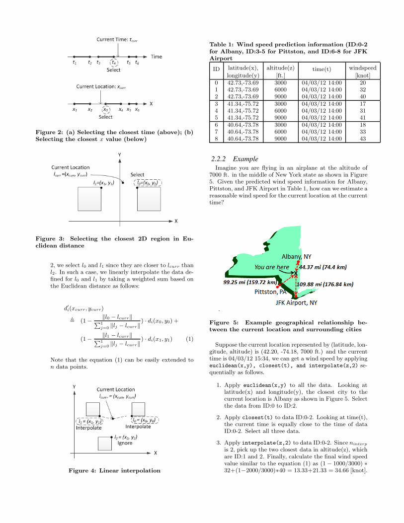
Figure 2: (a) Selecting the closest time (above); (b)Selecting the closest x value (below)
Figure 3: Selecting the closest 2D region in Eu-clidean distance
2, we select l0 and l1 since they are closer to lcurr thanl2. In such a case, we linearly interpolate the data de-fined for l0 and l1 by taking a weighted sum based onthe Euclidean distance as follows:
d′i(xcurr, ycurr)
! (1−∥l0 − lcurr∥
∑
1
j=0∥lj − lcurr∥
) · di(x0, y0) +
(1−∥l1 − lcurr∥
∑
1
j=0∥lj − lcurr∥
) · di(x1, y1) (1)
Note that the equation (1) can be easily extended ton data points.
Figure 4: Linear interpolation
Table 1: Wind speed prediction information (ID:0-2for Albany, ID:3-5 for Pittston, and ID:6-8 for JFKAirport
ID latitude(x), altitude(z) time(t) windspeedlongitude(y) [ft.] [knot]
0 42.73,-73.69 3000 04/03/12 14:00 201 42.73,-73.69 6000 04/03/12 14:00 322 42.73,-73.69 9000 04/03/12 14:00 403 41.34,-75.72 3000 04/03/12 14:00 174 41.34,-75.72 6000 04/03/12 14:00 315 41.34,-75.72 9000 04/03/12 14:00 416 40.64,-73.78 3000 04/03/12 14:00 187 40.64,-73.78 6000 04/03/12 14:00 338 40.64,-73.78 9000 04/03/12 14:00 43
2.2.2 ExampleImagine you are flying in an airplane at the altitude of
7000 ft. in the middle of New York state as shown in Figure5. Given the predicted wind speed information for Albany,Pittston, and JFK Airport in Table 1, how can we estimate areasonable wind speed for the current location at the currenttime?
Figure 5: Example geographical relationship be-tween the current location and surrounding cities
Suppose the current location represented by (latitude, lon-gitude, altitude) is (42.20, -74.18, 7000 ft.) and the currenttime is 04/03/12 15:34, we can get a wind speed by applyingeuclidean(x,y), closest(t), and interpolate(z,2) se-quentially as follows.
1. Apply euclidean(x,y) to all the data. Looking atlatitude(x) and longitude(y), the closest city to thecurrent location is Albany as shown in Figure 5. Selectthe data from ID:0 to ID:2.
2. Apply closest(t) to data ID:0-2. Looking at time(t),the current time is equally close to the time of dataID:0-2. Select all three data.
3. Apply interpolate(z,2) to data ID:0-2. Since ninterp
is 2, pick up the two closest data in altitude(z), whichare ID:1 and 2. Finally, calculate the final wind speedvalue similar to the equation (1) as (1− 1000/3000) ∗32+(1−2000/3000)∗40 = 13.33+21.33 = 34.66 [knot].

2.3 Example Program SpecificationsHere we show two example program specifications; one
is very simple and the other is slightly more complex thanthe first one. See [3] for the detailed PILOTS grammardefinition. We will see the experimental results of theseprograms later in Section 4.
2.3.1 Simple Example - TwiceFigure 6 shows one of the simplest program specifications
written in PILOTS, called twice. As the name says, it takestwo input streams, a(t) and b(t), where b is supposed to betwice as large as a, and outputs an error defined by e =(b−2∗a) every 1 second. Note that these two input streamsare not associated with any location information.
✬
✫
✩
✪
program twice ;inputs
a: (t) using closest (t);b: (t) using closest (t);
outputs ;errors
e: (b - 2 * a) at every 1 sec;end;
Figure 6: A simple declarative specification of thetwice application
2.3.2 More Complex Example - Flight PlanningThis is an example of a simplified flight planning system.
Suppose that sensors in an airplane record airspeeds va dur-ing a given flight and GPS units record the airplane’s flightpath over the ground including ground speeds vg at differ-ent locations. An aircraft’s airspeed and ground speed arerelated by the following mathematical formula (2), where vaand αa are the aircraft airspeed and angle (heading), andvw and αw are the wind speed and direction acquired fromthe weather forecast:
vg =√
v2a + 2va · vw · cos(αa − αw) + v2w (2)
Also, we can compute crosswind velocity: vx = vw ·sin(αa − αw). Therefore, given the aircraft desired courseαd, it is possible to compute the crab angle δ by using theformula (3) so that the aircraft can use αa = αd + δ asthe heading to maintain the desired direction under varyingwind conditions.
δ = arcsin(vx/vg)
= arcsin
(
vw · sin(αa − αw)√
v2a + 2va · vw · cos(αa − αw) + v2w
)
(3)
The above mentioned relationship can be brought into aprogram specification shown in Figure 7, which outputs thecrab angle δ and error e that is the difference between themonitored ground speed vg from GPS and the calculatedone with the equation (2).
In this flight planning example, there are three input datastreams in which each stream has two functions. Sinceeach of these two functions has the same source of in-formation and arguments, they are declared as a single
input data stream. In the case of the first input datastream, there are two functions, wind_speed(x,y,z,t) andwind_angle(x,y,z,t), that share the same arguments andinformation source (weather forecast). Data interpola-tion/selection methods used for these two functions are eu-clidean(x,y), closest(t), and interpolate(z,2). Justlike we explain in Section 2.2.2, these methods apply in or-der: first, the closest x and y to xcurr and ycurr in Euclideandistance are selected; second, the closest t to the currenttime tcurr is selected; and finally, the final value is linearlyinterpolated on the z-axis using up to the two closest datapoints to zcurr as specified in the argument.
✬
✫
✩
✪
program flightplan ;inputs
wind_speed , wind_angle : (x,y,z,t)using euclidean (x,y), closest (t),interpolate (z,2);
air_speed , air_angle : (x,y,t)using euclidean (x,y), closest (t);
ground_speed , ground_angle: (x,y,t)using euclidean (x,y), closest (t);
outputscrab_angle :
arcsin (wind_speed *sin(wind_angle -air_angle ) /sqrt(air_speed ^2 +
2* air_speed *wind_speed *cos(air_angle -wind_angle ) +wind_speed ^2))
at every 1 min ;
errorse: ground_speed -
sqrt( air_speed ^2 +2* air_speed *wind_speed *cos(air_angle -wind_angle ) +wind_speed ^2)
at every 1 min;end;
Figure 7: A declarative specification of the flightplanning application
3. LANGUAGE IMPLEMENTATIONWhen executing a PILOTS program, its high-level pro-
gram specification needs to be compiled into Java code bythe PILOTS compiler. The generated application programthen uses the PILOTS runtime library to run the program.
3.1 CompilerThe compiler consists of two parts: a parser and a code
generator. The parser is developed using JavaCC [4]. Thenthe code generator uses the abstract syntax tree created fromthe parser and applies visitor pattern to generate Java code.
3.2 System InteractionFigure 8 shows how a PILOTS application interacts with
the system. The interactions are based on a client-servermodel using Internet sockets in which the application worksas a server and takes inputs from the clients on a single port.

It outputs some values to the specified output ports as wellas error values to the specified error ports.
Figure 8: System interaction of a PILOTS applica-tion
When executing a compiled Java program, we specify in-put, output, and error ports as follows. In this example, theflightplan application illustrated in Section 2.3.2 takes aninput data stream on the port 10001 and sends output anderror streams to the hosts specified by 10.0.0.1:20001 and10.0.0.2:30001 respectively.
$ java pilots.tests.Flightplan -input 10001-outputs 10.0.0.1:20001 -errors 10.0.0.2:30001
3.2.1 Data FormatThe input, output, and error data streams share the same
format shown in Table 2. The first line is used to declareone or more variables (var0, var1,...) in a single datastream. The values of the declared variables start fromthe second line. The data stream can have multiple val-ues (val0, val1,...) with various spatial and temporalcombinations: ex1 is just defined for a 2-D region; ex2 isdefined for a 3-D point and a time interval; ex3 is definedfor a 1-D interval and a particular time; ex4 is defined forno location and a particular time. All lines have to end withan end-of-line marker (\n). Especially, the last line has tohave only one end-of-line marker.
Note that the data format for input is compatible withoutput and error, that is, we can connect either an output orerror port to an input port of another PILOTS application.
Table 2: The data stream format of input, output,and error
first line #var0,var1,...\nafter ex1) x0,y0∼x1,y1::val0,val1,...\nsecond line ex2) x,y,z:t0∼t1:val0,val1,...\n
ex3) x0∼x1:t:val0,val1,...\nex4) :t:val0,val1,...\n
last line \n
.
Here are some instances of spatio-temporal data forex1· · · ex4 respectively.
• ex1) 40.100,-76.300∼39.600,-76.300::166.0,215.0
• ex2) 42.749,-73.802,3000:2012-04-03 140000-0500∼2012-04-03 210000-0500:15.0,320.0
• ex3) 42.6886∼43.9258:2012-04-03 140900-0500:112.0,222.0
• ex4) :2012-04-03 141400-0500:42.5486,-74.1142,8100.0
3.2.2 Running ModeTwo modes are available for the user to run PILOTS ap-
plications as shown below.
• real-time mode: This mode is default and is intended tobe used for receiving data from sensors and processingit in real-time. If the frequency of an output is specifiedas “at every 1 min” in the program specification, theprogram actually outputs data once every 1 minute.Also, in this mode, the program finishes if one of inputdata streams sends the last line marker (\n) or certainamount of time has elapsed, which can be specified bythe user in the command line as -DtimeSpan=30min.
• simulation mode: This mode is used for simulationsand is activated if the user gives a past time spanin the command line as -DtimeSpan=t0∼t1. The PI-LOTS runtime sets its internal time as t0 and virtuallyprogress the time as the program runs, and when theinternal time reaches t1, the program finishes. Theuser can get outputs as fast as possible. This modeis intended to be used for processing recorded data inthe past.
In either mode, time stamp of input streams should matchthe internal time of the PILOTS runtime to get proper out-puts.
3.3 Runtime LibraryThe PILOTS runtime library is in charge of starting a
data receiving server, storing received data, providing dataselection/interpolation service to the application, and send-ing processed data to output/error hosts.
Primary classes included in the PILOTS runtime libraryshown in Figure 9 are explained as follows.
• PilotsRuntime class is extended by the applicationand provides all basic functions to run a PILOTS ap-plication other than application-specific processing. Itstarts DataReceiver to start receiving data, requestsstored data from DataStore, and sends calculated out-puts and errors to other hosts.
• DataReceiver class receives data from data inputclients from a port specified in the command-line argu-ments. Upon accepting data, it launches a new workerthread to receive data and the created thread requeststo add these data to DataStore.
• DataStore class accepts data from DataReceiver as astring, and then it asks SpatioTempoData to parse thestring and stores the parsed data. It also implementsgetData() method supporting closest, euclidean,interpolate for data selection. When comparing lo-cations and time for data selection/interpolation, itasks for the current time and location from Current-LocationTimeService. Stored data are accessed frommultiple threads (i.e., threads for adding data fromDataReceiver vs. threads getting data from Pilot-sRuntime), so the data have to be protected from si-multaneous data access.
• CurrentLocationTimeService class is an interfaceclass for providing the current time and location. Usershave to implement this class for the system to work

Figure 9: Class diagram of PILOTS runtime library
(e.g., SimpleTimeService and SimulationService).The implemented class can either return the actualcurrent time for the real-time mode or past time forthe simulation mode.
4. EXPERIMENTSIn this section, we report the results of two experiments.
The first experiment has been done with the twice appli-cation to illustrate how error signatures exhibit differentshapes depending on simulated input data streams. Thesecond one has been conducted with the flightplan appli-cation to apply PILOTS to data sampled in the real worldand see how PILOTS’ first-class support for data selectionand interpolation work for real data.
4.1 Simulated Data Inputs - Twice
4.1.1 Experimental SetupAs we present in Figure 6, the twice application takes two
inputs, a and b, and we prepare an independent client foreach input to test the following four different scenarios.
• Scenario A: There are random timing jitters betweenone data and another on the data input clients. Thatis, every 1 ± ϵ seconds, the variable a’s input comesas 1, 2, 3, . . ., whereas the variable b’s input comes as2, 4, 6, . . ..
• Scenario B: The variable a’s data stream becomes con-sistently one second behind the variable b’s input datastream at some point of time.
• Scenario C: The variable a’s data stream stops provid-ing data at some point of time.
• Scenario D: The variable b’s data stream stops provid-ing data at some point of time.
In all the scenarios, the application runs in the real-timemode with SimpleTimeService that returns the current timeonly. We start the twice application followed by the data in-put clients, and then record the error output for 120 secondsonce data from the clients reaches the PILOTS runtime.
4.1.2 ResultsFigure 10 shows different types of errors generated with
the four different scenarios. In Figure 10(a), most of the timethe error stays at zero, but there are several spikes due totransient fluctuation of the data input timing. It happensoccasionally since the use of closest(t) causes the DataSelection module to select data at one second earlier or onesecond later than it is supposed to select. This type of erroris unavoidable without a special synchronization mechanismbetween multiple data streams. Figure 10(b) shows a sig-nature of out-of-sync input data streams. As shown in thegraph, the error becomes consistently large at around 30 sec-onds of the simulation time. This is because the variable a’sinput data stream becomes consistently one second behindthe variable b’s input data stream. Figure 10(c) suggestsmore critical failure of the variable a’s input data source. Ataround 50 seconds of the simulation time, the error startsgrowing linearly. This linear increase of the error explainsthat the input data stream of the variable a stops comingafter 50 seconds of the simulation time, which potentiallymeans that a critical failure occurred at the source of thevariable a. Similarly, Figure 10(d) suggests that a criticalfailure occurred at the source of the variable b.
!"
!#
!$
%
$
#
"
% #% &% '% (% $%% $#%
!"#$%&'$()
!"# $%%&%'()*+",-%.'/&%'01.+"%)&'2 !3# $%%&%'()*+",-%.'/&%'01.+"%)&'4
!%)*
%
%)*
$
$)*
#
#)*
% #% &% '% (% $%% $#%
!"#$%&'$()
!*%
%
*%
$%%
$*%
% #% &% '% (% $%% $#%
!"#$%&'$()
!$*%
!$%%
!*%
%
*%
% #% &% '% (% $%% $#%
!"#$%&'$()
!1# $%%&%'()*+",-%.'/&%'01.+"%)&'5 !6# $%%&%'()*+",-%.'/&%'01.+"%)&'7
Figure 10: Error signatures generated by the twiceapplication
As we can see from the graphs, errors behave differentlydepending on the input data streams, thus those error sig-natures could tell us valuable information about potentialfailures in the data sources.
4.2 Real Data Inputs - Flight Planning
4.2.1 Experimental SetupThe second author is a general aviation private pilot
and we conducted a simulation with the flightplan pro-gram based on his actual flight from Albany, New York toTipton, Maryland (near Washington D.C.) on April 3rd,2012. air_speed and air_angle were manually collectedduring the flight, whereas ground_speed and ground_anglewere automatically collected from online data [2]. We haveto use weather forecast information for wind_speed andwind_angle from [6] since we could not record the actualwind information during the flight.
Note that air_speed and air_angle are sparsely given asshown in Figure 11 since they were manually recorded while

operating the aircraft, and also the density of wind_speedand wind_angle is not very high as we have previouslyseen in Table 1. Unlike other data, ground_speed andground_angle are given every minute.
✤
✣
✜
✢
#air_speed ,air_angle42.748 , -73.802~41.476 , -75.483::162 ,24641.476 , -75.483~41.000 , -76.000::161 ,23941.000 , -76.000~40.100 , -76.300::161 ,22140.100 , -76.300~39.600 , -76.300::166 ,21539.600 , -76.300~39.500 , -76.400::165 ,21339.500 , -76.400~39.085 , -76.759::135 ,204
Figure 11: Formatted data for airspeed and air anglefrom the April 3rd flight
Just like the previous section with the twice application,we test the following four different scenarios including threesimulated error conditions.
• Scenario A: No error is added. Use the real data only.
• Scenario B: Simulate an airspeed sensor (called pitottube) icing failure. If the airspeed sensor is iced, typ-ically the airspeed suddenly drops in a few seconds,and then it keeps reporting a constant value.
• Scenario C: Simulate a GPS failure. GPS loses satel-lites and keeps reporting 0s as the values for bothground speed and ground angle.
• Scenario D: Simulate both an airspeed sensor icing fail-ure and a GPS failure mentioned above.
For all the scenarios, we run the program in the simulationmode with SimulationService that returns the location andtime based on the actual flight path. To specify the starttime and end time of the simulation, we run the programwith the option -DtimeSpan="2012-04-03 1404∼2012-04-03 1545" for the 1 hour and 41 minutes flight.
4.2.2 ResultsFigure 12 plots the error and crab angle from the flight
planning application for Scenario A (no errors). Looking atthe graph, we notice that the error is large at the beginningof the flight (around 0∼9 minutes) and also at the end ofthe flight (around 90∼100 minutes). The reason is inaccu-racy of the airspeed, which is illustrated in Figure 13(a) inwhich we plot the airspeed, ground speed, calculated groundspeed, and error separately from the outputs of the flight-plan application to analyze the reasons of the error. In thegraph, we see that the airspeed is almost constant whereasactual ground speed changes dynamically at the time of de-parture and landing. In general, airspeed is supposed tochange a lot when departing and landing; however, sinceairspeed was manually recorded and these periods are thebusiest for flying the airplane, it is not accurate. Conse-quently, inaccuracy in airspeed makes the calculated groundspeed erroneous since it is directly related to the airspeedaccording to the equation (2). Despite the large error whendeparting and landing, the error stays relatively low around10∼90 minutes, and that fact suggests PILOTS’ data se-lection/interpolation methods work well during this period
since the relationship presented by the equation (2) holdswell.
In the case of Scenario B, Figure 13(b) shows that theerror suddenly increases at around 40 minutes caused by asudden drop of the airspeed (150 to 50 knots in two min-utes). Unlike Scenario B, Scenario C shows a different errorsignature as shown in Figure 13(c). From the graph, wecan see that the ground speed suddenly drops from 170 to0 knot at around 40 minutes and that causes the error todrop accordingly. When we have both failures, we get an er-ror signature as shown in Figure 13(d). This error signaturetells us that the errors for Scenario B and C do not cancelout, but they are emerged as a combination of the individ-ual error signatures. This result potentially means that wemay be able to tell the causes of multiple errors from onecombined error signature.
As we can see from the graphs, there is a clear distinctionbetween the error signatures. These results encourage us topursue automated reasoning about data errors and recovery.
!"#
!$%
!$&
!$'
!$"
!$#
!%
!&
!'
!"
#
!$##
!%#
!&#
!'#
!"#
#
"#
'#
&#
%#
$##
# $# "# (# '# )# &# *# %# +# $##
!"#$%&'()*%+,*("**-
.""/"%+0'/1-
!"#$%&#"'(
!"##$#
!%#&'!&()*"
Figure 12: Error and output generated by theflightplan application
5. RELATED WORKSpatio-temporal constraint logic programming has been
proposed. STACLP [7] offers first-class support for repre-senting and reasoning about spatial and temporal data. Asimilar logic language to STACLP, MuTACLP [5][1], hasbeen applied to GIS for spatio-temporal reasoning [8]. BothSTACLP and MuTACLP are implemented based on a Pro-log system. Programming languages that support proba-bilistic reasoning have also been proposed. PRISM[9] is alogic-based language that integrates logic programming andstochastic reasoning including parameter learning. PRISMis capable of parameter learning from a given set of data andestimates the probability to best explain the data. PRISM isalso built on top of a Prolog system. Our programming lan-guage is also highly declarative and generates code to helpunderstand and reason about spatio-temporal data streams.
6. CONCLUSIONSWe presented the design and implementation of PILOTS,
a programming language for spatio-temporal data streamingapplications. The language enables to specify in a declara-tive (high-level) manner the mathematical relationship be-tween data streams. We also illustrated different methodsthat can be combined to interpolate and select the data.These methods enable developers to declaratively specifyhow to convert potentially heterogeneous data streams—i.e.,streams using different scales in space and time—into homo-geneous data streams amenable to processing and analysis.

!"##
!$%#
!$##
!%#
#
%#
$##
$%#
"##
# $# "# &# '# %# (# )# *# +# $##
!"##$%&%'(()(%*+,)-.
!"#$%&#"'(
!"##
!$##
#
$##
"##
# $# "# &# '# %# (# )# *# +# $##
!"##$%&%'(()(%*+,)-.
!"#$%&#"'(
!"# $%%&%'()*+",-%.'/&%'01.+"%)&'2
!3# $%%&%'()*+",-%.'/&%'01.+"%)&'4
!1# $%%&%'()*+",-%.'/&%'01.+"%)&'5
!"##
!$##
#
$##
"##
# $# "# &# '# %# (# )# *# +# $##
!"##$%&%'(()(%*+,)-.
!"#$%&#"'(
!"##
!$##
#
$##
"##
# $# "# &# '# %# (# )# *# +# $##
!"##$%&%'(()(%*+,)-.
!"#$%&#"'(
!6# $%%&%'()*+",-%.'/&%'01.+"%)&'7
!"#$%&''(
!)$*+,(
%&''(
-".-+."/'(
)$*+,(
%&''(
!'$$*$
Figure 13: Error signatures and speed informationgenerated by the flightplan application
An important goal of this work is to enable spatio-temporal data analyses that detect errors in input datastreams with high probability. This is accomplished byexplicitly modeling redundancy in the input data streamsallowing application developers to not only specify outputdata streams but also to specify mathematically the relation-ship between redundant data as error streams. These errorstreams can be seen as signatures that characterize differentinput data error conditions with high probability.
We used PILOTS to uncover the error signatures of atrivial application (twice) illustrating clearly distinguishablepatterns on different kinds of failure (out of synchronizationand data stream loss failures). We subsequently used PI-LOTS to model the relationship between air speed, groundspeed, and wind speed of an actual general aviation flight be-tween Albany, NY and Washington, DC. We computed theerror signatures for (i) normal conditions, (ii) a simulatedpitot tube failure (affecting the airspeed data stream), (iii)a simulated GPS constellation failure (affecting the groundspeed data and ground angle stream,) and (iv) a simulta-neous failure of the pitot tube (ii) and GPS system (iii).These error signatures illustrate that patterns can be usedto discover with high likelihood the source of potential dataerrors.
Future work includes modeling more complex data rela-tionships in aviation and navigation systems, discovering er-ror signatures for common data error conditions, using er-ror signatures as a means to semi-automate error recoveryand reason about spatio-temporal data streams, and apply-ing the programming model and language to other domainsgeneralizing it as appropriate.
ACKNOWLEDGMENTS
We would like to thank Jaemyeong Eo and Yazmin Feliz fortheir help on creating test data. This research is partiallysupported by Air Force Office of Scientific Research GrantNo. FA9550-11-1-0332.
7. REFERENCES[1] P. Baldan, P. Mancarella, A. Raffaeta, and F. Turini.
MuTACLP: A language for temporal reasoning withmultiple theories. In Computational Logic: LogicProgramming and Beyond’02, pages 1–40, 2002.
[2] FlightAware. Flight track log for N756VH on03-Apr-2012 (KALB-KFME).http://flightaware.com/live/flight/N756VH/history/20120403/1800Z/KALB/KFME/tracklog.
[3] S. Imai and C. A. Varela. A programming model forspatio-temporal data streaming applications. InDynamic Data-Driven Application Systems (DDDAS2012), pages 1139–1148, Omaha, Nebraska, June 2012.
[4] JavaCC Development Group (Open Source Projectunder BSD License). Java compiler compiler (javacc) -the java parser generator. http://javacc.java.net/.
[5] P. Mancarella, G. Nerbini, A. Raffaeta, and F. Turini.MuTACLP: A language for declarative GIS analysis.In Computational Logic’00, pages 1002–1016, 2000.
[6] NOAA’s National Weather Service. Forecast windsand temps aloft.http://aviationweather.gov/products/nws/winds/.
[7] A. Raffaeta and T. W. Fruhwirth. Spatio-temporalannotated constraint logic programming. In PADL’01,pages 259–273, 2001.
[8] A. Raffaeta, F. Turini, and C. Renso. Enhancing GISsfor spatio-temporal reasoning. In Proceedings of the10th ACM international symposium on Advances ingeographic information systems, GIS ’02, pages 42–48,New York, NY, USA, 2002. ACM.
[9] T. Sato and Y. Kameya. Parameter learning of logicprograms for symbolic-statistical modeling. In Journalof Artificial Intelligence Research(JAIR), volume 15,pages 391–454, 2001.
[10] Wikipedia. Air France Flight 447. http://en.wikipedia.org/wiki/Air_France_Flight_447.

Procedia Computer Science 00 (2012) 1–10
Procedia Computer
Science
International Conference on Computational Science, ICCS 2012
A programming model forspatio-temporal data streaming applications
Shigeru Imaia,⇤, Carlos A. Varelaa
aComputer Science Department, Rensselaer Polytechnic Institute, 110 Eighth Street, Troy, NY 12180, USA
Abstract
In this paper, we describe a programming model to enable reasoning about spatio-temporal data streams. Aspatio-temporal data stream is one where each datum is related to a point in space and time. For example, sensorsin a plane record airspeeds (va) during a given flight. Similarly, GPS units record an airplane’s flight path over theground including ground speeds (vg) at di↵erent locations. An aircraft’s airspeed and ground speed are related by thefollowing mathematical formula: vg =
pv2
a + 2va · vw · cos(↵a � ↵w) + v2w, where va and ↵a are the aircraft airspeed
and heading, and vw and ↵w are the wind speed and direction. Wind speeds and directions are typically forecast in3,000-foot height intervals over discretely located fix points in 6-12 hour ranges. Modeling the relationship betweenthese spatio-temporal data streams allows us to estimate with high probability the likelihood of sensor failures andconsequent erroneous data. Tragic airplane accidents (such as Air France’s Flight 447 on June 1st, 2009 killing all 216passengers and 12 aircrew aboard) could have been avoided by giving pilots better information which can be derivedfrom inferring stochastic knowledge about spatio-temporal data streams. This work is a first step in this direction.
Keywords: programming models, spatio-temporal data, data streaming
1. Introduction
Spatio-temporal data streams, where each datum is related to a point or a range of space and time, are pervasive.We see such data streams in many occasions in our daily lives, for instance, temperatures, prices of gasoline, flightschedules of airplanes, and so on. Massive amounts of spatio-temporal data are continuously generated by sensors,IT systems, or computer programs, and consumed by humans; however, today’s most commonly used programminglanguages (e.g., C/C++, Java, PHP, JavaScript, python, etc.) do not have first-class support for space and time sincethey are designed to be general-purpose. The downside of the general-purpose approach is the complexity and size ofcode. Since these programming languages are imperative, meaning that we have to use for, if, or while to control theflow of the programs and explicitly handle state, the code can get large and complex easily.
In contrast to the general-purpose approach, if we know a specific problem domain very well and want to providefirst-class support for key domain concepts (such as space and time), we can take a domain-specific approach. The
⇤Corresponding authorEmail addresses: [email protected] (Shigeru Imai), [email protected] (Carlos A. Varela)

Shigeru Imai and Carlos A. Varela / Procedia Computer Science 00 (2012) 1–10 2
code written in the domain-specific approach is much simpler and more declarative as in logic programming lan-guages [1] and therefore simpler to write, read, and reason about, but it is generally less expressive, than code writtenin general-purpose programming languages.
Operating an aircraft is a complicated task since there are a lot of complex correlations between the instrumentsin a cockpit. If some failure happens during a flight, it is not easy to find the cause of the failure by looking at theavailable (potentially partially erroneous) data , and also, a misinterpretation of instrument readings could even lead toa tragic accident [2]. We illustrate our programming model with a flight planning system that reports potential sourcesof data problems such as mechanical failures or extreme weather conditions. An explicit mathematical model of dataco-relationships can with high probability signal data errors, potentially providing pilots with better information inemergency scenarios, allowing them to take appropriate actions in a timely manner, and ultimately reaching theirdestination safely and e�ciently.
In this paper, we present our initial e↵ort on designing a programming model for spatio-temporal data streamingapplications, aiming to apply the model to a flight planning system. The model provides first-class support for spaceand time specific operations including data selection and interpolation when no data is available for a certain locationand time.
2. Motivation
Auto-pilots cannot take the right action when the data they are receiving is out of date or incorrect. This may haveled to the tragic crash of Air France flight 447, killing all 216 passengers and 12 aircrew [2]. The records from thecrash have suggested that the pilots lost control of the airplane because they raised the nose of the airplane when itshould not have been brought up. Many experts now understand that the airplane went into clouds with thunderstormsand its iced speed sensors provided inaccurate information to the autopilot, causing it to disengage. The pilots thenincorrectly reacted to the emergency by raising the nose of the plane when in fact it needed to go down to break thestall.
An active redundant data-driven flight system may help prevent crashes caused by sensor or other data errors. Forexample, by comparing the airspeed data to the ground speed data, a flight system would be able to fact check a badairspeed reading, assuming reasonable constraints on the wind speed. If the pilot is only operating by airspeed dataalone, they would have no way of knowing that there is an error in the system and they would respond to the incorrectdata, upsetting the balance of the plane. The ground speed data would instead provide a fact checking mechanismbecause if airspeed were swiftly changing, ground speed would be doing the same. If airspeed is changing, but groundspeed remains unchanged, the more active flight system would be able to notify the pilot of the discrepancy, allowingfor better informed decision making.
Our goal is to develop a data streaming programming model that makes explicit the connections between di↵erentspatio-temporal data streams. Flight systems developed using our model would make explicit the redundancies inthe data and allow the di↵erent data streams to essentially fact check each other greatly reducing the possibility ofaccidents. The proposed spatio-temporal data streaming programming model can also be applied to other domainsgenerating space and time specific data.
3. Spatio-Temporal Data Streaming Programming Model
3.1. Programming Model
Our proposed programming model is designed for applications that handle spatio-temporal input data streams asshown in Figure 1. In this model, the application gets data (d01, d
02, . . . , d
0n) from the data selection module, which takes
incoming data streams (d1, d2, . . . , dn) as inputs, and then the application indefinitely generates outputs (o1, o2, . . . , om)and data errors (e1, e2, . . . , el) based on an application model. Each input data stream di(x, y, z, t) is a function oflocation and time. The number of arguments of di varies depending on dimensions of the location information, that is,di(t) for 0-D (i.e., no location support), di(x, t) for 1-D, di(x, y, t) for 2-D, and di(x, y, z, t) for 3-D. Some data streamsare coming in real-time whereas some predicted information (e.g., weather forecasts) is associated with future timeperiods.
Shigeru Imai and Carlos A. Varela / Procedia Computer Science 00 (2012) 1–10 3
Figure 1: Programming model handling spatio-temporal input data streams
Table 1: An example of a weather forecast input data streamLocation Altitude Time Chance of Icing
(lat1, long1) � (lat2, long2) ( f rom) � (to)(42.73, -73.69)-(42.70, -73.66) 8000 ft. 01/30/2012:10:00-12:00 (GMT) 50%(42.73, -73.69)-(42.70, -73.66) 8000 ft. 01/30/2012:12:00-14:00 (GMT) 60%(42.73, -73.69)-(42.70, -73.66) 8000 ft. 01/30/2012:14:00-16:00 (GMT) 80%
Table 1 shows an example of a weather forecast input data stream coming to the Data Selection module. Asnoted from the table, the location information is given by regions where each region is represented by two horizontallocations (latitude, longitude) and an altitude, and the time information is given by time periods where each periodis represented by two time points in GMT. Since not all the data is on the table, for example, chance of icing is notdefined when the time is 01/30/2012:09:00 (GMT); however, we can define data by selecting or interpolating theexisting data when no data is defined for a given location and time. In our programming model, the Data Selectionmodule stores some amount of incoming data stream until it becomes out of date. The application acquires the selectedor interpolated data (d01, d
02, . . . , d
0n) from the Data Interpolation module at a certain rate specified in the application
and computes both outputs and data errors. The application continues this computing process in an infinite loop untilthe user requests to stop the computation. The Data Selection module essentially allows an application to view a set ofheterogeneous data streams as a homogeneous data stream, and therefore enables a separation of concerns: applicationprogrammers can focus on their application model.
3.2. Support for Spatio-Temporal Data Selection
We define two types of data selection and one data interpolation method for the location and time as shown below.These operations are applicable to either single variables (i.e. t, x, y, or z) or multiple variables (i.e. combinations oft, x, y, and z. By using these operations, application programmers can use locally related data even in the case whenthe given data is sparse.
• closestThis method takes a 1-D argument (i.e., t, x, y, or z) to find the data closest to a given location or time. Figure2 shows examples of selecting closest data to the current time and location respectively. In Figure 2(a), whenselecting the closest time to the current time tcurr, di(tcurr) is not defined, but di(t) is defined for {t | t1 t

Shigeru Imai and Carlos A. Varela / Procedia Computer Science 00 (2012) 1–10 4
t2, t3 t t4, t5 t t6}. Since t4 is closest to tcurr, we define d0i (tcurr) , di(t4). Similarly, we defined0i (xcurr) , di(x3) for the example shown in Figure 2(b).
Figure 2: (a) Selecting the closest time; (b) Selecting the closest x value
• euclideanThis method takes 2-D or 3-D arguments to find the data closest to a given location. Figure 3 shows an examplefor the 2-D case, where data is not defined for the current location lcurr = (xcurr, ycurr), but are defined for l0, andl1. Since lcurr is closest to l0 = (x0, y0) in Euclidean distance, we define d0i (xcurr, ycurr) , di(x0, y0).
Figure 3: Selecting the closest 2D region in Euclidean distance Figure 4: Linear interpolation
• linear interpolationThis method takes 1-D, 2-D or 3-D arguments to interpolate the defined data. It also takes another argumentninterp to select closest ninterp data from a given location to interpolate. Suppose we have a situation shown inFigure 4, where data is not defined for the current location lcurr = (xcurr, ycurr), but are defined for l0, l1, and l2.Also, suppose that ninterp = 2, we select l0 and l1 since they are closer to lcurr than l2. In such a case, we linearlyinterpolate the data defined for l0 and l1 by taking a weighted sum based on the Euclidean distance as follows:
d0i (xcurr, ycurr) , (1 � kl0 � lcurrkP1i=0 kli � lcurrk
) · di(x0, y0) + (1 � kl1 � lcurrkP1i=0 kli � lcurrk
) · di(x1, y1) (1)
Note that the equation (1) can be easily extended to n data points.
Multiple methods can be specified in the application program and they apply to the input data in order. If multipledata get selected by one method (e.g., more than one closest point), a subsequent method takes that multiple data asthe input and further select data. If there still remains more than one data after applying all the methods, then weimplicitly apply linear interpolation to output the final value.
4. Spatio-Temporal Data Streaming Programming Language
In this section, we describe a spatio-temporal programming language by defining its grammar and showing twoexample programs.

Shigeru Imai and Carlos A. Varela / Procedia Computer Science 00 (2012) 1–10 5
4.1. Grammar Definition
A grammar definition for a declarative programming language following the proposed programming model isshown in Figure 5. A program (Program) consists of four parts: a program name, inputs, outputs, and errors. Theprogram name is defined by a variable name (Var). The inputs can have multiple entries of Input, which is definedby one or more input variables (Vars), a dimension of the inputs (Dim), and a data selection method described in theprevious section (Method). The outputs and errors are defined separately, but have the same output format (Output).Output is defined by one or more output variables (Vars), mathematical expressions (Exps), and a time interval tospecify the frequency of the output (Time).
'
&
$
%
Program ::= program Var;inputs Input*outputs Output*errors Output*
Input ::= Vars: Dim using Methods;Output ::= Vars: Exps at every Time;Dim ::= ’(t)’ | ’(x,t)’ | ’(x,y,t)’ | ’(x,y,z,t)’
Methods ::= Method | Method, MethodsMethod ::= (closest | euclidean | interpolate) ’(’ Exps ’)’
Time ::= Number (nsec | usec | msec | sec | min | hour | day)
Exps ::= Exp | Exp, ExpsExp ::= Func(Exps) | Exp Func Exp | ’(’ Exp ’)’ | ValueFunc = { +, -, *, /, sqrt, sin, cos, tan, abs, ...}Value ::= Number | VarNumber ::= Sign Digits | Sign Digits’.’DigitsSign ::= ’+’ | ’-’ | ’’
Digits ::= Digit | Digits DigitDigit = { 0, 1, 2, ...,9 }Vars ::= Var | Var, VarsVar = { a, b, c, ...}
Figure 5: Spatio-temporal data streaming programming language grammar
4.2. Example Programs
4.2.1. Simple ExampleHere we show one of the simplest programs implemented by the proposed programming model. It takes two input
streams, a(t) and b(t), and outputs an error defined by e = (b0 � 2a0) every 1 second as shown in Figure 6. Note thatthese two input streams are not associated to any location information.
An example specification of the above simple program is shown in Figure 7. In this example, there are two inputdata streams in which each stream is a function of time. The data selection method used in the program is specified byclosest(t), which means that the program instructs the Data selection module to select the closest t to the currenttime tcurr.
Errors behave di↵erently depending on the input data streams, thus they tell us valuable information about theinformation sources. Figure 8 shows three di↵erent types of errors generated by simulations of the simple exampleprogram specification described in Figure 7. The assumption here is that every 1 ± ✏ seconds, the variable a’s inputcomes as 1±✏, 2±✏, 3±✏, . . .whereas the variable b’s input comes as 2±✏, 4±✏, 6±✏, . . ., i.e., they hold the mathematicalrelationship: b = 2 * a. In Figure 8(a), most of the time the error stays at zero, but there are several spikes due totransient fluctuation of the data input timing. It happens occasionally since the use of closest(t) causes the DataSelection module to select data at one second earlier or one second later than it is supposed to select. This type of
Shigeru Imai and Carlos A. Varela / Procedia Computer Science 00 (2012) 1–10 6
error is unavoidable without a special synchronization mechanism between multiple data streams. Figure 8(b) showsan example of the out-of-sync error. As shown in the graph, the error becomes consistently large at around 30 secondsof the simulation time. This is because the variable a’s input data stream becomes consistently one second behindthe variable b’s input data stream. Figure 8(c) suggests more critical failure of the variable a’s input data source. Ataround 40 seconds of the simulation time, the error starts growing linearly. This linear increase of the error explainsthat the input data stream of the variable a stops coming after 40 seconds of the simulation time, which potentiallymeans that a critical failure occurred at the source of the variable a.
Figure 6: A simple application with temporal data streams
'
&
$
%
program twice;
inputs
a: (t) using closest(t);
b: (t) using closest(t);
outputs;
errors
e: (b - 2 * a)
at every 1 sec;
end;
Figure 7: A simplest program specification
Figure 8: Examples of errors generated by a simple example: (a) Timing transient error; (b) Out-of-sync error; (c) Data input failure
4.2.2. Flight PlanningThis is an example of a simplified flight planning system. Suppose that sensors in a plane record airspeeds va
during a given flight and GPS units record the airplane’s flight path over the ground including ground speeds vg
at di↵erent locations. An aircraft’s airspeed and ground speed are related by the following mathematical formula:vg =
pv2
a + 2va · vw · cos(↵a � ↵w) + v2w, where va and ↵a are the aircraft airspeed and heading, and vw and ↵w are the
wind speed and direction. Also, we can compute crosswind velocity: vx = vw · sin(↵a � ↵w). Therefore, given theaircraft desired course ↵d, it is possible to compute the crab angle � by using the formula (2) so that the aircraft canuse ↵a = ↵d + � as the heading to maintain the desired direction under varying wind conditions. The above mentionedrelationship can be modeled as an application shown in Figure 9, which outputs the crab angle � and error e that is thedi↵erence between the monitored ground speed vg from GPS and the calculated one from va, vw,↵a, and ↵w.
� = arcsin(vx/vg) = arcsin0BBBBB@
vw · sin(↵a � ↵w)p
v2a + 2va · vw · cos(↵a � ↵w) + v2
w
1CCCCCA (2)
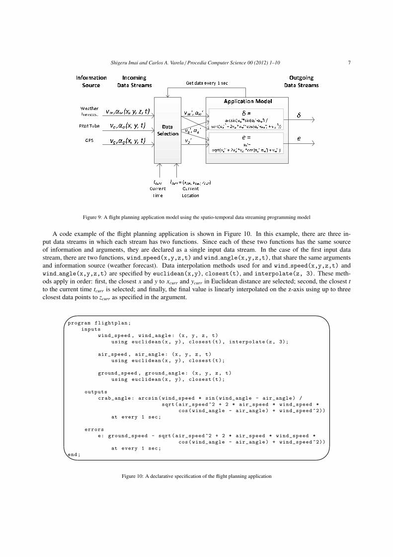
Shigeru Imai and Carlos A. Varela / Procedia Computer Science 00 (2012) 1–10 7
Figure 9: A flight planning application model using the spatio-temporal data streaming programming model
A code example of the flight planning application is shown in Figure 10. In this example, there are three in-put data streams in which each stream has two functions. Since each of these two functions has the same sourceof information and arguments, they are declared as a single input data stream. In the case of the first input datastream, there are two functions, wind speed(x,y,z,t) and wind angle(x,y,z,t), that share the same argumentsand information source (weather forecast). Data interpolation methods used for and wind speed(x,y,z,t) andwind angle(x,y,z,t) are specified by euclidean(x,y), closest(t), and interpolate(z, 3). These meth-ods apply in order: first, the closest x and y to xcurr and ycurr in Euclidean distance are selected; second, the closest tto the current time tcurr is selected; and finally, the final value is linearly interpolated on the z-axis using up to threeclosest data points to zcurr as specified in the argument.
'
&
$
%
program flightplan;
inputs
wind_speed , wind_angle: (x, y, z, t)
using euclidean(x, y), closest(t), interpolate(z, 3);
air_speed , air_angle: (x, y, z, t)
using euclidean(x, y), closest(t);
ground_speed , ground_angle: (x, y, z, t)
using euclidean(x, y), closest(t);
outputs
crab_angle: arcsin(wind_speed * sin(wind_angle - air_angle) /
sqrt(air_speed ^2 + 2 * air_speed * wind_speed *
cos(wind_angle - air_angle) + wind_speed ^2))
at every 1 sec;
errors
e: ground_speed - sqrt(air_speed ^2 + 2 * air_speed * wind_speed *
cos(wind_angle - air_angle) + wind_speed ^2))
at every 1 sec;
end;
Figure 10: A declarative specification of the flight planning application

Shigeru Imai and Carlos A. Varela / Procedia Computer Science 00 (2012) 1–10 8
Figure 11: Normal conditions signature observed from a flight planning simulation
Figure 12: Pitot tube failure error signature observed from a flight planning simulation (the monitored airspeed starts decreasing at time = 5000due to the pitot tube failure)
Example simulation results of the flight planning application generated from the program specification describedin Figure 10 are shown in Figure 11 and Figure 12. In this simulation, a simple autopilot system navigates an airplaneby using the crab angle received from the application. The airplane flies at 100 knots from Washington D.C. to Albany,which is 281 nautical miles (323 miles) away. The simulation also takes into account the e↵ect of winds. In a normalcondition, the autopilot successfully navigates the airplane to the destination with an ideal path as shown in Figure11. The error of ground speed stays zero all through the simulation and the crab angle is almost constant (it actuallyslightly increases to adapt the wind speed changes). Figure 12 shows an error signature caused by a pitot tube failure.At time = 5000, a pitot tube starts icing and that causes the monitored airspeed to decrease gradually and gets almostzero eventually, while the airplane keeps flying at 100 knots. As seen from the graph, the autopilot’s navigation doesnot work successfully this time. We can see a clear signature of the error here: the ground speed error grows quicklyas soon as the airspeed start decreasing at time = 5000 and remains around 70 knots. The crab angle also grows up asthe airspeed decreases.
As we can see from the simulation, a pilot can benefit from this application by following the crab angle to con-trol the direction of the airplane, and also monitoring the error output to see if there is a mechanical failure of theinstruments or the forecast information is wrong.
5. System Interaction
Figure 13 shows how a spatio-temporal application interacts with the system. The interactions are based on aclient-server model using Internet sockets in which the application works as a server and takes inputs from the clientson a single port. It outputs some values to the specified output ports as well as error values to the specified error ports.

Shigeru Imai and Carlos A. Varela / Procedia Computer Science 00 (2012) 1–10 9
Figure 13: System interaction of a spatio-temporal data streaming application
When executing a binary object generated from the program specification, we specify input, output, and error portsas follows. In this example, the flightplan application illustrated in Section 4.2.2 takes an input data stream on theport 10001 and sends output and error streams to the hosts specified by 10.0.0.1:20001 and 10.0.0.2:30001
respectively.
$./flightplan -input 10001 -outputs 10.0.0.1:20001 -errors 10.0.0.2:30001
The input, output, and error data streams share the same format shown in Table 2. The first line is used to declareone or more variables (var0, var1,...) in a single data stream. The values of the declared variables start from thesecond line. The data stream can have multiple values (value0, value1,...) with various spatial and temporalcombinations: ex1 is defined for a 3-D region and a time interval; ex2 is defined for a 2-D point and a time interval;ex3 is defined for a 1-D interval and a particular time; ex4 is defined for no location and a particular time. All lineshave to end with an end-of-line marker (\r\n). Especially, the last line have to have only one end-of-line marker.
Note that the data format for input is compatible with output and error, that is, we can connect either an output orerror port to an input port of another application.
Table 2: The data stream format of input, output, and errorfirst line #var0, var1,...\r\nafter second line ex1) x0,y0,z0-x1,y1,z1:t0-t1:value0,value1,...\r\n
ex2) x,y:t0-t1:value0,value1,...\r\nex3) x0-x1:t:value0,value1,...\r\nex4) :t:value0,value1,...\r\n
last line \r\n
.
6. Related Work
Spatio-temporal constraint logic programming has been proposed. STACLP [3] o↵ers first-class support for rep-resenting and reasoning about spatial and temporal data. A similar logic language to STACLP, MuTACLP [4][5], isused to analyze geographical data especially for GIS (Geographical Information Systems). Both STACLP and MuTA-CLP are implemented based on a Prolog system. Programming languages that support probabilistic reasoning havealso been proposed. PRISM[6] is a logic-based language that integrates logic programming and stochastic reasoningincluding parameter learning. PRISM is capable of parameter learning from a given set of data and estimates theprobability to best explain the data. PRISM is also built on top of a Prolog system. Our proposed programminglanguage is also highly declarative and it is to generate code that takes as inputs, spatio-temporal data streams.
There are programming languages for time-critical systems such as automatic control and monitoring systems.LUSTRE [7] [8], Giotto [9], and Esterel[10] are included in this category. These programming languages are declar-ative and designed to respond input events synchronously. Although their target systems are similar to ours, the mainfocus of these languages is real time behavior and there is no special support for spatial information nor reasoningcapabilities.
Shigeru Imai and Carlos A. Varela / Procedia Computer Science 00 (2012) 1–10 10
7. Conclusions and Future Work
We present a programming model for spatio-temporal data streaming applications. In particular, it has first-classsupport for data selection and interpolation when no data is available for a given location and time. Towards ourprimary goal of applying this programming model to flight planning applications, we have several future researchdirections: 1) development of a compiler of the proposed language and a fully-functional application using real spatio-temporal data to demonstrate the advantage of the proposed programming model; 2) learning error signatures forcommon failures in aviation system, 3) adding the probability of data accuracy as inversely proportional to the spatio-temporal distance between the current location and time and the defined data points; 4) studying stochastic reasoningtechniques and investigating the applicability of such techniques to spatio-temporal data streaming applications.
Acknowledgments
This research is partially supported by the Air Force O�ce of Scientific Research.
References
[1] J. W. Lloyd, Foundations of logic programming. Symbolic computation, Springer-Verlag, Berlin, Germany, 1984.[2] Wikipedia, Air france flight 447, http://en.wikipedia.org/wiki/Air_France_Flight_447.[3] A. Ra↵aet, T. W. Frhwirth, Spatio-temporal annotated constraint logic programming., in: PADL’01, 2001, pp. 259–273.[4] P. Mancarella, G. Nerbini, A. Ra↵aet, F. Turini, MuTACLP: A language for declarative GIS analysis., in: Computational Logic’00, 2000, pp.
1002–1016.[5] P. Baldan, P. Mancarella, A. Ra↵aet, F. Turini, MuTACLP: A language for temporal reasoning with multiple theories., in: Computational
Logic: Logic Programming and Beyond’02, 2002, pp. 1–40.[6] T. Sato, Y. Kameya, Parameter learning of logic programs for symbolic-statistical modeling, in: Journal of Artificial Intelligence Re-
search(JAIR), Vol. 15, 2001, pp. 391–454.[7] N. Halbwachs, P. Caspi, P. Raymond, D. Pilaud, The synchronous dataflow programming language LUSTRE, in: Proceedings of the IEEE,
1991, pp. 1305–1320.[8] P. Caspi, D. Pilaud, N. Halbwachs, J. Plaice, Lustre: A declarative language for programming synchronous systems., in: POPL’87, 1987, pp.
178–188.[9] T. A. Henzinger, B. Horowitz, C. M. Kirsch, Giotto: A time-triggered language for embedded programming., in: EMSOFT’01, 2001, pp.
166–184.[10] G. Berry, The foundations of Esterel., in: Proof, Language, and Interaction’00, 2000, pp. 425–454.

Dynamic Data-Driven Avionics Systems withStochastic Error Detection and Correction
Shigeru Imai and Carlos A. Varela
Abstract Dynamic Data-Driven Avionics Systems embody ideas from the DynamicData-Driven Applications Systems (DDDAS) paradigm by creating a data-drivenfeedback loop that continuously analyzes spatio-temporal data streams coming fromairplane sensors, looks for errors in the data signaling different potential failuremodes, and autonomously corrects for such erroneous data when possible. In thischapter, we define error signatures as constrained mathematical function patterns.These signatures help stochastically determine the true mode of operation of anavionics system. When a failure mode is detected, input data streams are correctedusing redundant data in order to continue normal operation of the DDDAS avion-ics system. We introduce the PILOTS programming language to enable creation ofDDDAS systems from high-level specifications of the relationships between datastreams, error signatures, and error correction functions. We illustrate the applica-bility of PILOTS by showing how the Air France AF447 accident from June 2009could have been prevented by using ground speed and wind speed to recompute airspeed upon automatic detection of the pitot tubes icing failure. Aircraft accidentsoften happen as a result of a series of small problems chained in a sequence thatcompound themselves to become unmanageable. This work intends to attack onesource of such accident chains: data errors that result from malfunctioning sensors,which can be automatically corrected thanks to the redundancy afforded by otherinstruments and physical and geometric models embedded in DDDAS systems.
1 Introduction
Operating airplanes is a difficult task; pilots have to keep making right decisionswhile dealing with a lot of information provided from the instruments in a cockpit.
Shigeru Imai and Carlos A. VarelaDepartment of Computer Science, Rensselaer Polytechnic Institute, 110 Eighth Street, Troy, NY12180, USA, e-mail: {imais, cvarela}@cs.rpi.edu
1

2 Shigeru Imai and Carlos A. Varela
Moreover, in the event of instrument failures, it becomes even more difficult becauseof potentially partially erroneous data. For example, pitot tubes icing which occurredto Air France flight 447 (AF447) in June 2009 led to faulty airspeed readings andeventually caused a fatal accident killing all 228 people on board [6]. The aircraft ofthe AF447 flight crashed in the Atlantic Ocean due to ice which temporarily formedin the pitot tubes causing erroneous airspeed readings, and the subsequent inabilityof the auto-pilot and human pilots to recover.
However, the faulty airspeed readings could have been prevented by endowingthe avionics system with the ability to understand the following data relationship:
�!vg =�!va +�!vw. (1)
where �!vg ,�!va , and �!vw represent the ground speed, the airspeed, and the wind speed
vectors. These speeds are obtained through independent data collection methods: theground speed is typically computed from Global Positioning System (GPS) data, theairspeed is computed from air pressure measurements by pitot tubes, and the windspeed from weather forecast computer models. Since any one of the three speedscan be calculated using the other two with Eq. (1), they are redundant to each other.If the auto-pilot was aware of such redundancy in the data, it could have fixed the in-correct airspeed readings quickly and thereby kept the system working properly. Tofacilitate the development of such smart avionics systems, we create the DynamicData-Driven Avionics System (see Fig. 1 for detail) based on the concept of Dy-namic Data-Driven Application Systems (DDDAS) [8]. The Dynamic Data-DrivenAvionics System is designed to dynamically correct erroneous data and interpolatesparse data.
PILOTS (ProgrammIng Language for spatiO-Temporal Streaming applications)[11, 15, 12] is a highly declarative programming language that embodies the con-cept of the Dynamic Data-Driven Avionics System. The PILOTS programming lan-guage enables high-level development of applications to handle spatio-temporaldata streams and ultimately assist humans in making better decisions. Spatio-temporal data streams refer to data streams whose items include associated spatialand temporal coordinates, often viewed as meta data. Examples include temperaturemeasurements, financial stock values, gas prices, surveillance camera imaging, andaircraft sensor readings. The PILOTS open-source project has evolved gradually todate [11, 15, 12]. In this chapter, we summarize the advancements of the project andits application to avionics systems based on PILOTS version 0.2.3 [17].
The rest of the chapter is organized as follows. Section 2 defines the requirementsto realize the proposed Dynamic Data-Driven Avionics System and describes priorart of data streaming systems. Section 3 describes the methods for error detectionand correction including the mathematical definition of error signatures. Section 4shows the detailed design of the Dynamic Data-Driven Avionics System that weimplemented as PILOTS. Section 5 shows an avionics application running on thePILOTS system and associated error signatures. Section 6 shows performance met-rics and results of error detection performance for a private Cessna flight and theAF447 flight data. Finally, we conclude the chapter in Sect. 7 with future directions.
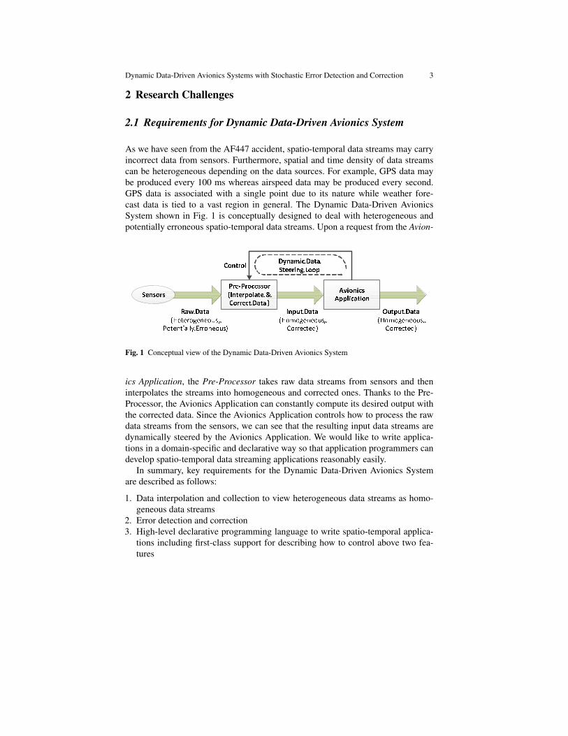
Dynamic Data-Driven Avionics Systems with Stochastic Error Detection and Correction 3
2 Research Challenges
2.1 Requirements for Dynamic Data-Driven Avionics System
As we have seen from the AF447 accident, spatio-temporal data streams may carryincorrect data from sensors. Furthermore, spatial and time density of data streamscan be heterogeneous depending on the data sources. For example, GPS data maybe produced every 100 ms whereas airspeed data may be produced every second.GPS data is associated with a single point due to its nature while weather fore-cast data is tied to a vast region in general. The Dynamic Data-Driven AvionicsSystem shown in Fig. 1 is conceptually designed to deal with heterogeneous andpotentially erroneous spatio-temporal data streams. Upon a request from the Avion-
Fig. 1 Conceptual view of the Dynamic Data-Driven Avionics System
ics Application, the Pre-Processor takes raw data streams from sensors and theninterpolates the streams into homogeneous and corrected ones. Thanks to the Pre-Processor, the Avionics Application can constantly compute its desired output withthe corrected data. Since the Avionics Application controls how to process the rawdata streams from the sensors, we can see that the resulting input data streams aredynamically steered by the Avionics Application. We would like to write applica-tions in a domain-specific and declarative way so that application programmers candevelop spatio-temporal data streaming applications reasonably easily.
In summary, key requirements for the Dynamic Data-Driven Avionics Systemare described as follows:
1. Data interpolation and collection to view heterogeneous data streams as homo-geneous data streams
2. Error detection and correction3. High-level declarative programming language to write spatio-temporal applica-
tions including first-class support for describing how to control above two fea-tures
4 Shigeru Imai and Carlos A. Varela
2.2 Prior Art
There are several systems that combine stream processing and data base manage-ment, i.e., Data Stream Management Systems or DSMS, such as STREAM [5] andAurora [1]. They are designed to execute SQL-like queries to unbounded continuousincoming data streams and output events of interest. Microsoft StreamInsight is aDSMS-based system and has been extended to support spatio-temporal streams [2].Also, the concept of the moving object data base (MODB) which adds support forspatio-temporal data streaming to DSMS is discussed in [4]. These DSMS-basedspatio-temporal stream management systems support general continuous queriesfor multiple moving objects; however, our streaming data analytics to detect er-rors based on signatures and correct data on the fly is beyond the scope of a purelydeclarative SQL-based query approach. In the context of Big Data processing, dis-tributed, scalable, and fault-tolerant data streaming systems have been popular. Suchsystems include Storm [10], Spark Streaming [18], and S4 [13]. These systems aredesigned to be flexible and general so that complex applications such as machinelearning or graph processing algorithms can run over a lot of distributed comput-ers. Unlike their general approaches, our domain-specific approach enables highlydeclarative description of spatio-temporal data streaming applications. To the bestof our knowledge, none of the existing streaming processing systems satisfies therequirements mentioned in Sec. 2.1.
3 Error Detection and Correction Methods
The error detection and correction methods are described in detail. The algorithmrecognizes the shape of an error function using error signatures, identifies the typeof error, and corrects an associated data value if possible.
3.1 Mathematical Preparations
Error function
An error function is an arbitrary function that computes a numerical value fromindependently measured input data. It is used to examine the validity of redundantdata. If the value of an error function is zero, we interpret it as no error in the givendata.
Figure 2 illustrates the relationship among the ground speed, airspeed, and windspeed when an airplane is flying. A vector �!v can be defined by a tuple (v,a), wherev is the length of �!v and a is the angle between �!v and a base vector. Following thisexpression, �!vg ,
�!va , and �!vw are defined as (vg,ag),(va,aa), and (vw,aw) respectivelyas shown in Fig. 2. To examine the relationship in Eq. (1), we can compute �!vg by

Dynamic Data-Driven Avionics Systems with Stochastic Error Detection and Correction 5
!!
!"
!!
"!"
!#
!!
!
"
#
!"
Fig. 2 Trigonometry applied to the groundspeed, airspeed, and wind speed.
!
!
"
!!!
"
#
!"#$%&%#%'%(
!"#$%&%#%'%)
Fig. 3 Error signature SI with a linear func-tion f (t) = t + k,2 k 5.
applying trigonometry to 4ABC. From measured vg and computed vg, we can definean error function as follows:
e(�!vg ,�!va ,
�!vw) = |�!vg � (�!va +�!vw)|= vg �
qv2
a +2vavw cos(aa �aw)+ v2w. (2)
The values of input data are assumed to be sampled periodically from corre-sponding spatio-temporal data streams. Thus, an error function e changes its valueas time proceeds and can also be represented as e(t).
Error signatures
An error signature is a constrained mathematical function pattern that is usedto capture the characteristics of an error function e(t). Using a vector of con-stants K = hk1, . . . ,kmi, a function f (t), and a set of constraint predicates P ={p1(K), . . . , pl(K)}, the error signature S(K, f (t), P(K)) is defined as follows:
S(K, f (t), P(K)) = { f (t)|p1(K)^ · · ·^ pl(K)}. (3)
For example, an interval error signature can be defined as:
SI(K, f (t), P(K)) = { f (t) = t + k | 2 k 5}, (4)
where f (t) = t + k, K = hki, P(K) = h2 k 5i. As shown in Fig. 3, this intervalerror signature SI contains all linear functions with slope 1, and crossing the Y-axisat values [2,5]
Given an error signature S(K, f (t), P(K)), we enumerate its elements as errorsignature samples, i.e.,
s(t, K) = f (t) s.t. s(t, K) 2 S(K, f (t), P(K)). (5)

6 Shigeru Imai and Carlos A. Varela
An error signature sample is a particular function satisfying the constraints definedby an error signature. For the interval error signature SI , a sample sI(t,h3i) is f (t) =t +3.
Mode likelihood vectors
Given a set of error signatures {S0, . . . ,Sn}, we calculate di(t), the distance betweenthe measured error function e(t) and each error signature Si by:
di(t) = minK
Z t
t�w|e(t)� si(t, K)|dt. (6)
where w is the window size and si(t, K) 2 Si. Note that our convention is to capture“normal” conditions as signature S0. The smaller the distance di(t), the closer theraw data is to the theoretical signature Si. We define the mode likelihood vector asL(t) = hl0(t), l1(t), . . . , ln(t)i where each li(t) is defined as:
li(t) =
(1, if di(t) = 0min{d0(t),...,dn(t)}
di(t), otherwise.
(7)
If di(t) = 0, it means that a measured error e and a error signature Si is perfectlymatched. Otherwise, we take the minimum of all the distances and divide it bydi(t) to normalize li. Consequently, each li 2 L,0 < li 1 represents the ratio of thelikelihood of signature Si being matched with respect to the likelihood of the bestsignature.
3.2 Error Detection and Correction
Error Detection
Using a threshold t 2 (0,1) and the previously defined likelihood vector L, an errormode is determined as follows:
• If there are more then one li > t , the error mode is unknown(-1),• Otherwise, the error mode is i, where i is the index of the greatest element of L.
Because of the way L is created, the greatest element li will always be equal to1. Given the threshold t we check for one likely candidate that is sufficiently morelikely than its successor by ensuring that l j t . Thus we determine the correct modei by choosing the error signature Si corresponding to li. If i = 0 then the system is innormal mode.

Dynamic Data-Driven Avionics Systems with Stochastic Error Detection and Correction 7
Error correction
It is problem dependent if a determined error mode i is recoverable or not. If thereis a mathematical relationship between an erroneous value and other independentlymeasured values, the erroneous value can be replaced by a new value computed fromthe other independently measured values. In the case of the speed example used inEq.s (1) and (2), if the ground speed vg is detected as erroneous, its corrected valuevc
g can be computed by the airspeed and wind speed as follows:
vcg =
qv2
a +2vavw cos(aa �aw)+ v2w. (8)
4 Dynamic Data-Driven Avionics Systems
PILOTS is a programming language and an associated runtime system specifi-cally designed for analyzing data streams incorporating space and time. Using PI-LOTS, application developers can easily program an application that handles spatio-temporal data streams by writing a high-level (declarative) program specification.Also, by defining appropriate error signatures in the program specification, the PI-LOTS runtime system automatically detects and corrects errors in the data streams.This section describes the details of the PILOTS system as a concrete implementa-tion of the Dynamic Data-Driven Avionics System.
4.1 System Overview
Figure 4 shows the architecture of the PILOTS runtime system, which implementsthe error detection and correction methods described in the previous section. It con-sists of three parts: the Data Selection, the Error Analyzer, and the ApplicationModel modules.
The Application Model obtains homogeneous data streams (d01,d
02, . . . ,d
0N) from
the Data Selection module, and then it generates outputs (o1,o2, . . . ,oM) and data er-rors (e1,e2, . . . ,eL). The Data Selection module takes heterogeneous incoming datastreams (d1,d2, . . . ,dN) as inputs. Since this runtime is assumed to be working on amoving object, the Data Selection module is aware of the current location and time.Thus, it returns appropriate values to the Application Model by selecting or interpo-lating data in time and location depending on the data selection method specified inthe PILOTS program.
The ErrorAnalyzer collects the latest w error values from the Application Modeland keeps analyzing errors based on a set of error signatures. If it detects a recover-able error, then it replaces an erroneous input with the corrected one by applying acorresponding error correction equation. The Application Model computes the out-puts based on the corrected inputs produced from the Error Analyzer.

8 Shigeru Imai and Carlos A. Varela
!!""#$%&$%'$%()
!#""#$%&$%'$%()
!$""#$%&$%'$%()
!!!
!"#$"#%
!""#$%&'$()
*(+,#
!"#$%&"'(
)*+*(,+-.*%/
01+'$&"'(
)*+*(,+-.*%/
*#
*!
!!!
*%
+#
+!
!!!
+&
&''('%
-&'&
.,#,%'$()
!"#$"%&''()&)')&')'%*"+,-,"('.)&"
!!,
!#,
!$,
/00(01
-,',%'$()
!""#"$%&'()*+",-
!!!
!"##$%&
'()$
!"##$%&
*+,-&(+%-%.%/-
'$%-
!$%!$%-
(0
.#/,$0
/01*$&"'2,3"2,400('5"+&0.
1%.%23'$%3
!$%444$%3
(5
12)'$,""#"
"%.%+/%0+#
/00(01
2(00,%'$()
#$,+1$#-23$0+#
/0.."+&'()&)',-'
."+05".)62"
)+4$
"%#$,+1$#-23$
%+0$##+#
2--$-(3"*456.-
!+##$,&$405-&-
Fig. 4 Data streaming architecture with error detection and correction.
In the PILOTS programming model, the application acquires the selected or in-terpolated data (d0
1,d02, . . . ,d
0n) from the Data Selection module at a certain rate spec-
ified in the application and computes both outputs and data errors. The applicationcontinues this computing process in an infinite loop until the user explicitly requeststo stop the computation. The Data Selection module essentially allows an applica-tion to view a set of heterogeneous data streams as a homogeneous data stream, andtherefore enables a separation of concerns: application programmers can focus ontheir application model.
4.2 Spatio-Temporal Data Selection
We define two types of data selection and one data interpolation method for thelocation and time. These operations are applicable to either single variables (i.e.t,x,y, or z) or multiple variables (i.e. combinations of t,x,y, and z).
• closestThis method takes a 1-D argument (i.e., t,x,y, or z) to find the data closest toa given location or time. Figure 5 shows examples of selecting closest data tothe current time and location respectively. In Fig. 5(a), when selecting the clos-est time to the current time tcurr, di(tcurr) is not defined, but di(t) is defined for{t | t1 t t2, t3 t t4, t5 t t6}. Since t4 is closest to tcurr, we defined0
i(tcurr) , di(t4). Similarly, we define d0i(xcurr) , di(x3) for the example shown
in Fig. 5(b).

Dynamic Data-Driven Avionics Systems with Stochastic Error Detection and Correction 9
Fig. 5 (a) Selecting the closest time; (b) Selecting the closest x value
• euclideanThis method takes 2-D or 3-D arguments to find the data closest to a given lo-cation. Figure 6 shows an example for the 2-D case, where data is not definedfor the current location lcurr = (xcurr,ycurr), but are defined for l0, and l1. Sincelcurr is closest to l0 = (x0,y0) in Euclidean distance, we define d0
i(xcurr,ycurr) ,di(x0,y0).
Fig. 6 Selecting the closest 2D region inEuclidean distance
Fig. 7 Linear interpolation
• linear interpolationThis method takes 1-D, 2-D or 3-D arguments to interpolate the defined data.It also takes another argument ninterp to select closest ninterp data from a givenlocation to interpolate. Suppose we have a situation shown in Fig. 7, where data isnot defined for the current location lcurr = (xcurr,ycurr), but are defined for l0, l1,and l2. Also, suppose that ninterp = 2, we select l0 and l1 since they are closer tolcurr than l2. In such a case, we linearly interpolate the data defined for l0 and l1by taking a weighted sum based on the Euclidean distance as follows:
d0i(xcurr,ycurr) , (1� kl0 � lcurrk
Â1i=0 kli � lcurrk
) ·di(x0,y0)+
(1� kl1 � lcurrkÂ1
i=0 kli � lcurrk) ·di(x1,y1) (9)
Note that the equation (9) can be easily extended to n data points.

10 Shigeru Imai and Carlos A. Varela
Multiple methods can be specified in the application program and they are ap-plied to the input data in order. If multiple data get selected by one method (e.g.,more than one closest point), a subsequent method takes that multiple data as theinput and further select data. If there still remains more than one data after apply-ing all the methods, then we implicitly apply linear interpolation to output the finalvalue.
4.3 Declarative Programming Language
A PILOTS program is highly declarative. It includes an inputs section to specifythe data streams and how data is to be extrapolated from incomplete data, typi-cally using declarative geometric criteria described in the previous subsection (i.e..,closest, interpolate, euclidean keywords) It also includes outputsand errors sections to specify the data streams to be produced by the applica-tion, as a function of the input streams with a given frequency. If a detected error isrecoverable, output values are computed from corrected input data, otherwise orig-inal input data is used. The signatures and correct sections enable PILOTSprogrammers to specify error signatures for known error conditions, as well as thefunction to use to correct the data automatically if such data errors are found. Anexample PILOTS program is presented in Sect. 5.2.
5 Avionics System Application Example
In this section, we derive a set of error signatures for the speed example used inthe previous sections. Also, we present a PILOTS program implementing the errorsignatures and corresponding error correction equations.
5.1 Error Signatures for Speed Data
We consider the following four operational modes: 1) normal (no error), 2) pitot tubefailure due to icing, 3) GPS failure, 4) both pitot tube and GPS failures. Supposean airplane is flying at airspeed va, we assume that other speeds as well as failedairspeed and ground speed can be expressed as follows.
• ground speed: vg ⇡ va.• wind speed: vw ava, where a is the maximum wind to airspeed ratio.• pitot tube failed airspeed: blva v f
a bhva, where bl and bh are the lower andhigher values of pitot tube clearance ratio and 0 bl bh 1. 0 represents afully clogged pitot tube, while 1 represents a fully clear pitot tube.

Dynamic Data-Driven Avionics Systems with Stochastic Error Detection and Correction 11
• GPS failed ground speed: v fg = 0.
We assume that when a pitot tube icing occurs, it is gradually clogged and thusthe airspeed data reported from the pitot tube also gradually drops and eventuallyremains at a constant speed while iced. This resulting constant speed is characterizedby ratio bl and bh. On the other hand, when a GPS failure occurs, the ground speedsuddenly drops to zero. This is why we model the failed ground speed as v f
g = 0.In the case of pitot tube failure, let the ground speed, wind speed, and airspeed be
vg = va,vw = ava, and v fa = bva. The error function (2) can be expressed as follows:
e = va �q
v2a(b2 +2abcos(aa �aw)+a2).
Since �1 cos(aa �aw) 1, the error is bounded by the following:
va �q
v2a(a+b)2 e va �
qv2
a(a�b)2
(1�a�b)va e (1� |a�b|)va. (10)
In the case of GPS failure, let the ground speed, wind speed, and airspeed be v fg =
0,vw = ava, and va = va. The error function (2) can be expressed as follows:
e = 0�q
v2a(1+2acos(aa �aw)+a2).
Similarly to the pitot tube failure, we can derive the following error bounds:
�(a+1)va e �|a�1|va. (11)
We can derive error bounds for the normal and both failure cases similarly. Applyingthe wind to airspeed ratio a and the pitot tube clearance ratio bl b bh to theconstraints obtained in Inequations (10) and (11), we get the error signatures foreach error mode as shown in Table 1.
Table 1 Error signatures for speed data.Mode Error Signature
Function ConstraintsNormal e = k k 2 [�ava,ava]
Pitot tube failure e = k k 2 [(1�a�bh)va,(1� |a�bl |)va]GPS failure e = k k 2 [�(a+1)va,�|a�1|va]Both failures e = k k 2 [�(a+bh)va,�|a�bl |va]

12 Shigeru Imai and Carlos A. Varela
5.2 Speed Checker Program
A PILOTS program called speedcheck implementing the error signatures shownin Table 1 is presented in Fig. 8. This program checks if the wind speed, airspeed,and ground speed are correct or not, and computes a crab angle, which is usedto adjust the direction of the aircraft to keep a desired ground track. The speedparameters used in this particular example are a = 0.1,bl = 0.2, and bh = 0.33,which are reasonable values from actual failure data we have observed. Also, forthis program to be applicable to a Cessna 182-RG, we use a cruise speed of 162knots as va.
6 Evaluation
We apply the error signatures defined in Sect. 5.1 to two sets of real flight data. Thefirst one is a private flight using a Cessna 182-RG identified by N756VH [9] fromAlbany, NY to Fort Meade, MD on April 3rd, 2012. The other is the Air Franceflight 447 using an Airbus A330-203 which took off from Rio de Janeiro boundfor Paris on June 1st, 2009. To simulate the failures mentioned in Sect. 5.1, weadded corresponding errors to the N756VH Cessna flight data; however, we used thereal pitot tube failure data for the AF447 flight. PILOTS programs’ error detectionaccuracy and response time to mode changes are evaluated.
6.1 Performance Metrics
• Accuracy: This metric is used to evaluate how accurately the algorithm de-termines the true mode. Assuming the true mode transition m(t) is known fort = 0,1,2, . . . ,T , let m0(t) for t = 0,1,2, . . . ,T be the mode determined bythe error detection algorithm. We define accuracy(m,m0) = 1
T ÂTt=0 p(t), where
p(t) = 1 if m(t) = m0(t) and p(t) = 0 otherwise.• Average Response Time: This metric is used to evaluate how quickly the algo-
rithm reacts to mode changes. Let a tuple (ti,mi) represent a mode change point,where the mode changes to mi at time ti. Let M = {(t1,m1),(t2,m2), . . . ,(tN ,mN)}and M0 = {(t 01,m0
1),(t02,m
02), . . . ,(t
0N0 ,m0
N0)} be the sets of true mode changes anddetected mode changes respectively. For each i = 1 . . .N, we can find the smallestt 0j such that (ti t 0j)^ (mi = m0
j); if not found, let t 0j be ti+1. The response time rifor the true mode mi is given by t 0j � ti. We define the average response time by1N ÂN
i=1 ri.

Dynamic Data-Driven Avionics Systems with Stochastic Error Detection and Correction 13'
&
$
%
program speedcheck;
inputs
wind_speed, wind_angle (x,y,z,t) using
euclidean(x,y), closest(t), interpolate(z,2);
air_speed, air_angle (x,y,t) using
euclidean(x,y), closest(t);
ground_speed, ground_angle (x,y,t) using
euclidean(x,y), closest(t);
outputs
crab_angle: arcsin(wind_speed
*
sin(wind_angle - air_angle) /
sqrt(air_speedˆ2 + 2
*
air_speed
*
wind_speed
*
cos(wind_angle - air_angle) +
wind_speedˆ2))
at every 1 sec;
errors
e: ground_speed -
sqrt(air_speedˆ2 + wind_speedˆ2 + 2
*
air_speed
*
wind_speed
*
cos(wind_angle - air_angle));
signatures
/
*
v_a = 162 knots
*
/
S0(k): e=k, -16.2<=k, k<= 16.2 "Normal";
S1(k): e=k, 91.8<=k, k<= 145.8 "Pitot tube failure";
S2(k): e=k, -178.2<=k, k<=-145.8 "GPS failure";
S3(k): e=k, -70.2<=k, k<= -16.2 "Both failures";
correct
S1: air_speed = sqrt(ground_speedˆ2 + wind_speedˆ2 +
2
*
ground_speed
*
wind_speed
*
cos(ground_angle - wind_angle));
S2: ground_speed = sqrt(air_speedˆ2 + wind_speedˆ2 +
2
*
air_speed
*
wind_speed
*
cos(wind_angle - air_angle));
end
Fig. 8 A declarative specification of the speedcheck PILOTS program.
6.2 Experiment 1: N756VH Cessna Flight
6.2.1 Flight data
Flight data is collected through the following independent sources:
• ground speed: Flight track log provided by FlightAware [9].• airspeed: Manually recorded by the pilot.• wind speed: Weather forecast information provided by National Weather Ser-
vice [14].

14 Shigeru Imai and Carlos A. Varela
The flight duration is 1 hour 41 minutes. The collected speed data and errorcomputed by Eq. (2) are shown in Fig. 9(a). Notice that the airspeed data duringtake off and landing is not accurate due to the data collection mechanism.
6.2.2 Experimental Settings
Using the speedcheck PILOTS program shown in Fig. 8, the 6060 seconds (=1hour 41 minutes) of flight departing from Albany, NY and landing at Fort Meade,MD are recreated. Three types of error are simulated as shown below. In each case,all data streams except for erroneous one(s) are actual. Defined error modes are:�1 for unknown, 0 for normal, 1 for pitot tube failure, 2 for GPS failure, and 3 forboth failures.
• Pitot tube failure: 2400 seconds after the departure, the airspeed drops from 162knots to 50 knots within 10 seconds and stays at 50 knots until landing. The setof true mode changes is given by M = {(1,0),(2401,1)}.
• GPS failure: 2400 seconds after the departure, the ground speed drops from 171knots to 0 knots immediately and stays at 0 knots until landing. The set of truemode changes is given by M = {(1,0),(2401,2)}.
• Both pitot tube and GPS failures: The above two speed changes happen simul-taneously at 2400 seconds after the departure. Both speeds remain failed untillanding. The set of true mode changes is given by M = {(1,0),(2401,3)}.
6.2.3 Results
For all the three cases, when w = 1 and t = 0.8, the best results are observed asfollows: accuracy = 0.9294 and response time = 4 seconds for the pitot tube failure,accuracy = 0.935 and response time = 0 seconds for the GPS failure, and accuracy= 0.9342 and response time = 5 seconds for both failures. The transitions of thecorrected speed and detected modes when w = 1 and t = 0.8 are shown in Fig.s 9(b)for the pitot tube failure, 9(c) for the GPS failure, and 9(d) for the both failuresrespectively. For the first 390 seconds, the error mode is detected incorrectly in allthree cases; the true modes are 0 (normal mode) whereas the detected modes are 3(both failures) during this period. These wrong mode detections are originated fromthe erroneously recorded airspeed. Other than that, the error detection method workspretty well for all three cases.
Detected modes go into the unknown mode for a short period around 2401 sec-onds for both pitot tube failure and both failures. Since the airspeed takes a fewseconds to drop, during that time, the normal and pitot tube failure modes are com-peting against each other for the pitot tube failure case. For the both failures case, theGPS failure and both failures modes are competing. Unlike the other two cases, theground speed drops immediately for the GPS failure, and there is no conflict withother error modes, thus the GPS failure mode is correctly detected without goinginto the unknown mode.

Dynamic Data-Driven Avionics Systems with Stochastic Error Detection and Correction 15
!"#$%&'(' ')"*$+,&-).*
!/#$0%1 +,&-).* !2#$3('4$5&'('$')"*$,62$0%1$+,&-).*7
!,#$8(.9,-
Fig. 9 Corrected speeds and detected modes for the N756VH 03-Apr-2012 KALB-KFME flight(t = 0.8,w = 1).
6.3 Experiment 2: Air France Flight 447
6.3.1 Flight Data
The ground speed and airspeed are collected based on Appendix 3 in the final re-port of Air France flight 447 [6]. Note that the (true) airspeed was not recorded inthe flight data recorder so that we computed it from recorded Mach (M) and staticair temperature (SAT ) data. The airspeed was obtained by using the relationship:va = a0M
pSAT/T0, where a0 is the speed of sound at standard sea level (661.47
knots) and T0 is the temperature at standard sea level (288.15 Kelvin). Independentwind speed information was not recorded either. According to the description frompage 47 of the final report: “(From the weather forecast) the wind and temperaturecharts show that the average effective wind along the route can be estimated at ap-proximately ten knots tail-wind”. We followed this description and created the windspeed data stream as ten knots tail wind.

16 Shigeru Imai and Carlos A. Varela
6.3.2 Experimental Settings
According to the final report, speed data was provided from 2:09:00 UTC on June1st 2009 and it became invalid after 2:11:42 UTC on the same day. Thus, we ex-amine the valid 162 seconds of speed data including a period of pitot tube failurewhich occurred from 2:10:03 to 2:10:36 UTC. We also use the speedcheck PI-LOTS program shown in Fig. 8 except for constraints values in signatures whichuse va = 470 knots, the cruise airspeed of the AF447 flight. Defined error modesare the same as Experiment 1, so the set of true mode changes is defined asM = {(1,0),(64,1),(98,0)}.
6.3.3 Results
Same as Experiment 1, the best results, accuracy = 0.9631 and average responsetime = 2.5 seconds, are observed when w = 1 and t = 0.8. The transitions of thecorrected speed and detected modes that show the best accuracy with w = 1 andt = 0.8 are shown in Fig. 10. Looking at the detected modes in Fig. 10, the pitot tubefailure is successfully detected from 69 to 97 seconds except for the interval 64 to69 seconds due to the slowly decreasing airspeed. The response time for the normalto pitot tube failure mode is 5 seconds and for the pitot tube failure to normal modeis 0 seconds (thus the average response time is 2.5 seconds). From the correctedairspeed in Fig. 10, the airspeed successfully starts to get corrected at 69 seconds andseamlessly transitions back to the normal airspeed when it recovers at 98 seconds.
Fig. 10 Corrected airspeed and detected modes for AF447 flight.
Dynamic Data-Driven Avionics Systems with Stochastic Error Detection and Correction 17
7 Conclusion and Future Directions
We present the concept of the Dynamic Data-Driven Avionics System and its real-ization, the PILOTS system. The PILOTS runtime system dynamically interpolatesand corrects heterogeneous data, and then provides it as homogeneous data to appli-cations. This process can be viewed as dynamic incorporation of (interpolated andcorrected) sensor data into an application. Also, since the application can controlthis process by specifying data interpolation methods and error signatures, we seethat the application dynamically steers the data pre-processing process (i.e., inter-polation and correction). Thus, there is a dynamic feedback & control loop betweenthe data pre-processing and the application, which is the core concept of DynamicData Driven Applications Systems (DDDAS).
The results for both Cessna and AF447 flight experiments illustrate the effective-ness of our approach. Since the system dynamically adapts to sparse and partiallyincorrect data, the application keeps generating valid outputs with a relatively sim-ple PILOTS program as shown in Fig. 8. The error detection accuracy is at least93% and the response time to correct data is at most 5 seconds.
When computing mode likelihood vectors, time to compute distances by Eq. (6)can be significant due to the exponential growth of the search space as the sizeof the constants set K increases. To use the presented error detection and correc-tion methods in larger-scale real-time systems, techniques to bound the runningtime must be devised. Other future research directions include applying the errorsignature-based error correction methods to other flight accidents, e.g., those dueto fuel sensor reading errors. Also, uncertainty quantification [3] is an importantfuture direction to associate confidence to data and error estimations in support ofdecision making. More and more data are expected to be available in cockpits in thenear future [16], and thus automated data analysis systems will become even morecrucial to both manned and unmanned aerial vehicles. We envision scalable smarteravionics systems processing massive data in real-time by dynamically creating andconnecting multiple PILOTS program instances. Such systems need to reason aboutspatial and temporal data and constraints and give the pilots better information tomake more accurate judgments during critical moments. The presented techniquesand software can be used as a promising starting point to develop these dynamicdata-driven avionics systems.
Acknowledgements This research is partially supported by the DDDAS program of the Air ForceOffice of Scientific Research, Grant No. FA9550-11-1-0332 and a Yamada Corporation Fellow-ship.
References
1. Abadi, D.J., Carney, D., Cetintemel, U., Cherniack, M., Convey, C., Lee, S., Stonebraker, M.,Tatbul, N., Zdonik, S.: Aurora: a new model and architecture for data stream management. The

18 Shigeru Imai and Carlos A. Varela
VLDB JournalThe International Journal on Very Large Data Bases 12(2), 120–139 (2003)2. Ali, M.H., Chandramouli, B., Raman, B.S., Katibah, E.: Spatio-temporal stream processing in
Microsoft StreamInsight. IEEE Data Eng. Bull. pp. 69–74 (2010)3. Allaire, D., Willcox, K.: Surrogate modeling for uncertainty assessment with application to
aviation environmental system models. AIAA journal 48(8), 1791–1803 (2010)4. An, K., Kim, J.: Moving objects management system supporting location data stream. In: Pro-
ceedings of the 4th WSEAS International Conference on Computational Intelligence, Man-Machine Systems and Cybernetics, CIMMACS’05, pp. 99–104. World Scientific and Engi-neering Academy and Society (WSEAS), Stevens Point, Wisconsin, USA (2005)
5. Arasu, A., Babcock, B., Babu, S., Cieslewicz, J., Ito, K., Motwani, R., Srivastava, U., Widom,J.: Stream: The Stanford data stream management system. In: ACM SIGMOD Conference.Springer (2004)
6. Bureau d’Enquetes et d’Analyses pour la Securite de l’Aviation Civile: Fi-nal Report: On the accident on 1st June 2009 to the Airbus A330-203 regis-tered F-GZCP operated by Air France flight AF 447 Rio de Janeiro - Paris.http://www.bea.aero/en/enquetes/flight.af.447/rapport.final.en.php (2012)
7. Chandrasekaran, S., Cooper, O., Deshpande, A., Franklin, M.J., Hellerstein, J.M., Hong, W.,Krishnamurthy, S., Madden, S.R., Reiss, F., Shah, M.A.: TelegraphCQ: continuous dataflowprocessing. In: Proceedings of the 2003 ACM SIGMOD international conference on Manage-ment of data, pp. 668–668. ACM (2003)
8. Darema, F.: Dynamic data driven applications systems: A new paradigm for application sim-ulations and measurements. In: Computational Science-ICCS 2004, pp. 662–669. Springer(2004)
9. FlightAware: Flight track log for N756VH on 03-Apr-2012 (KALB-KFME).http://flightaware.com/live/flight/N756VH/history/20120403/1800Z/KALB/KFME/tracklog
10. software foundation, T.A.: Storm, distributed and fault-tolerant realtime computation.http://storm.incubator.apache.org/
11. Imai, S., Varela, C.A.: A programming model for spatio-temporal data streaming applications.In: Dynamic Data-Driven Application Systems (DDDAS 2012), pp. 1139–1148. Omaha, Ne-braska (2012)
12. Klockowski, R.S., Imai, S., Rice, C., Varela, C.A.: Autonomous data error detection and re-covery in streaming applications. In: Dynamic Data-Driven Application Systems (DDDAS2013) Workshop, pp. 2036–2045 (2013)
13. Neumeyer, L., Robbins, B., Nair, A., Kesari, A.: S4: Distributed stream computing platform.In: Data Mining Workshops (ICDMW), 2010 IEEE International Conference on, pp. 170–177.IEEE (2010)
14. NOAA’s National Weather Service: Forecast winds and temps aloft.http://aviationweather.gov/products/nws/winds/
15. S. Imai and C. A. Varela: Programming spatio-temporal data streaming applications with high-level specifications. In: 3rd ACM SIGSPATIAL International Workshop on Querying andMining Uncertain Spatio-Temporal Data (QUeST) 2012. Redondo Beach, California, USA(2012)
16. U.S. Department of Transportation Federal Aviation Administration: Code of fed-eral regulations part 91.225: Automatic dependent surveillance-broadcast (ADS-B) outperformance requirements to support air traffic control (ATC) service; final rule.http://www.faa.gov/regulations policies/faa regulations/ (2013)
17. Worldwide Computing Laboratory, Rensselaer Polytechnic Institute: The PILOTS program-ming language. http://wcl.cs.rpi.edu/pilots/
18. Zaharia, M., Das, T., Li, H., Shenker, S., Stoica, I.: Discretized streams: an efficient and fault-tolerant model for stream processing on large clusters. In: Proceedings of the 4th USENIXconference on Hot Topics in Cloud Ccomputing, pp. 10–10. USENIX Association (2012)