Final Exam Schedule – Fall, 2014

11:00 Class Thursday, December 11 10:30 – 12:30

2:00 Class Thursday, December 11 1:00 – 3:00

3:30 Class Tuesday, December 9 3:30 – 5:30

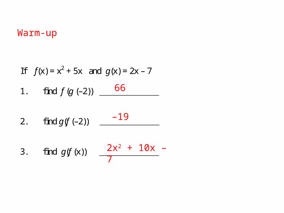
Math 1101 – Section 5.3 Exit Ticket If f(x) = x2 + 5x and g(x) = 2x – 7 1. find f (g (–2)) 2. find g(f (–2)) 3. find g(f (x)) Math 1101 – Section 5.3 Exit Ticket If f(x) = x2 + 5x and g(x) = 2x – 7 1. find f (g (–2)) 2. find g(f (–2)) 3. find g(f (x))

Name ________________________

Name ________________________

66

–19

2x2 + 10x – 7

Warm-up

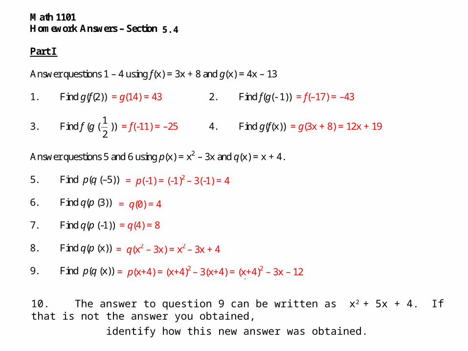
Math 1101 Homework Answers – Section 5.3 Part I Answer questions 1 – 4 using f(x) = 3x + 8 and g(x) = 4x – 13 1. Find g(f(2)) = g(14) = 43 2. Find f(g(- 1)) = f(–17) = –43

3. Find f (g (2

1)) = f(-11) = –25 4. Find g(f(x)) = g(3x + 8) = 12x + 19

Answer questions 5 and 6 using p(x) = x2 – 3x and q(x) = x + 4. 5. Find p(q (–5)) 6. Find q(p (3)) 7. Find q(p (-1)) = q(4) = 8 8. Find q(p (x)) 9. Find p(q (x)) 10. Part II 11.

The number of tons of trash produced in Indiana in any given year is related to how densely populated the state was in that year. This relationship has linear regression equation G = 1.7D – 50.4, where G = number of tons of trash and D = population density.

b. How many tons of trash were produced in Indiana in 1983? c. Form the composite function that gives the number of tons of trash produced in Indiana as a function of t.

d. Use the function found in part (c) to find the number of tons of trash produced in Indiana in 2008.

Year

D = Density (People per square

mile) 1940 37.2 1950 42.6 1970 57.5

1980 64.0 1990 71.9

= p(-1) = (-1)2 – 3(-1) = 4

= p(x+4) = (x+4)2 – 3(x+4) = (x+4)2 – 3x – 12

= q(0) = 4

= q(x2 – 3x) = x2 – 3x + 4

a. The table at the right compares population density D (in people per square mile) by year in the state of Indiana. Find the equation of the linear regression model for D as a function of t, years since 1940.

D = .70t +36.46

62.75 tons of trash were produced in Indiana 1983.

G = 1.7(.7t +36.46) – 50.4 = 1.19t + 11.582

G = 1.19 (68) + 11.582 92.5 Based on the model, there were approximately 92.5 tons of trash produced in Indiana in 2008.

(x+4)(x+4) = x2 + 4x + 4x + 16 = x2 + 8x + 16

p(q(x)) = (x+4)2 – 3x – 12 = x2 + 8x + 16 – 3x – 12 = x2 + 5x + 4

10. The answer to question 9 can be written as x2 + 5x + 4. If that is not the answer you obtained,

identify how this new answer was obtained.

5.4

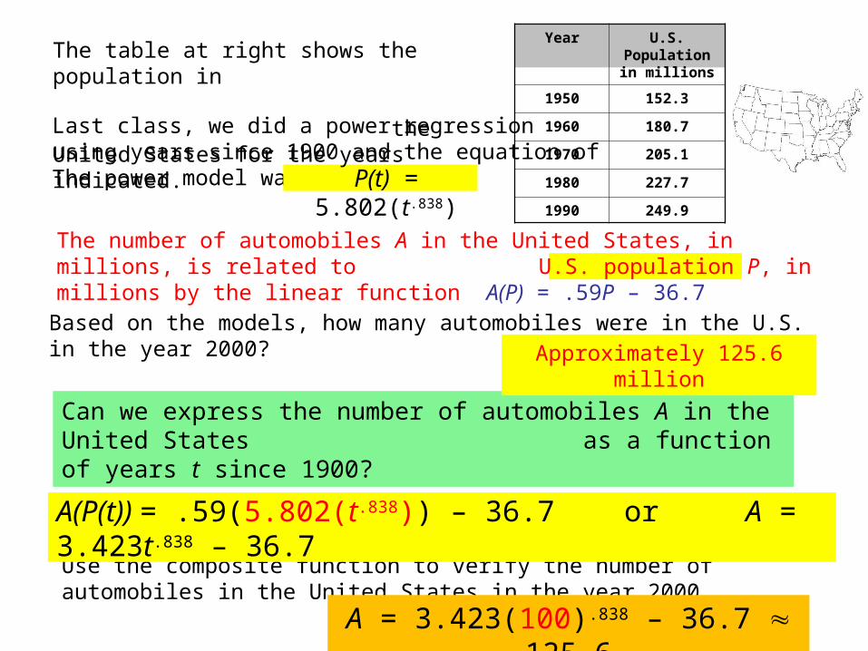
Last class, we did a power regression using years since 1900 and the equation ofThe power model was

Year U.S. Population in millions

1950 152.3

1960 180.7

1970 205.1

1980 227.7

1990 249.9

The number of automobiles A in the United States, in millions, is related to U.S. population P, in millions by the linear function A(P) = .59P – 36.7

Use the composite function to verify the number of automobiles in the United States in the year 2000.

P(t) = 5.802(t.838)

The table at right shows the population in the United States for the years indicated.

Can we express the number of automobiles A in the United States as a function of years t since 1900?

A(P(t)) = .59(5.802(t.838)) – 36.7 or A = 3.423t.838 – 36.7

Approximately 125.6 million

Based on the models, how many automobiles were in the U.S. in the year 2000?

A = 3.423(100).838 – 36.7 125.6

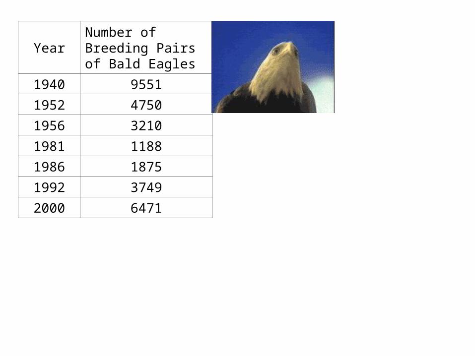
Bald Eagles were once very common throughout most of the United States. Their population numbers have been estimated at 300,000 to 500,000 birds in the early 1700s. Their population fell to threatened levels in the continental U.S. of less than 10,000 nesting pairs by the 1950s.

Bald eagles were officially declared an endangered species in 1967 in all areas of the United States. Below is a table indicating the estimated number of breeding pairs of bald eagles in the lower 48 states in various years.

YearNumber of Breeding Pairs of Bald Eagles

1940 9551

1952 4750

1956 3210

1981 1188

1986 1875

1992 3749

2000 6471

Make a scatter plot of the data using years since 1940.

YearNumber of Breeding Pairs of Bald Eagles

1940 9551

1952 4750

1956 3210

1981 1188

1986 1875

1992 3749

2000 6471

Standard Form: y = ax2 + bx + c

Quadratic Functions - Parabolas

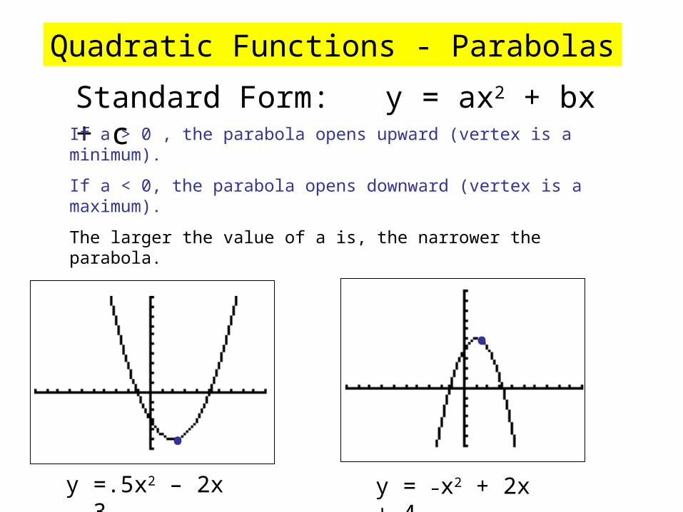
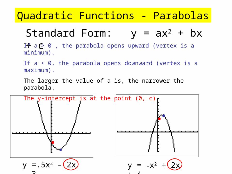
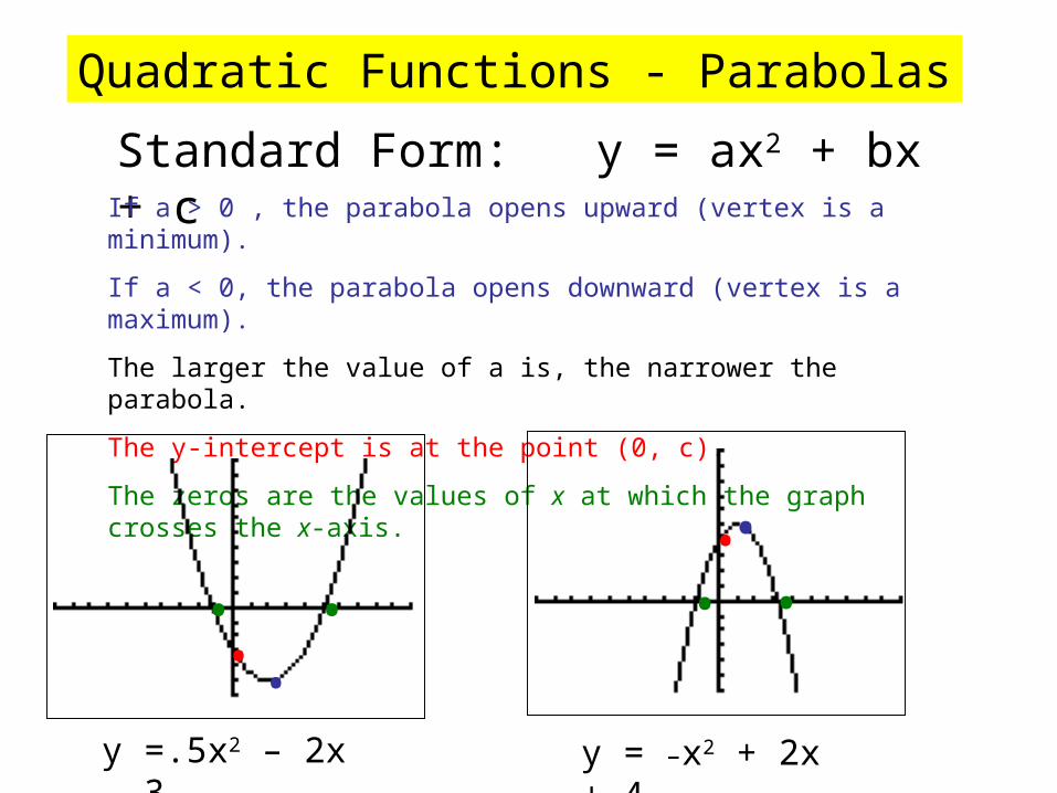
y =.5x2 – 2x – 3 y = –x2 + 2x + 4

Standard Form: y = ax2 + bx + c

Quadratic Functions - Parabolas

y =.5x2 – 2x – 3

If a > 0 , the parabola opens upward (vertex is a minimum).

If a < 0, the parabola opens downward (vertex is a maximum).

y = –x2 + 2x + 4

•

•

Standard Form: y = ax2 + bx + c

Quadratic Functions - Parabolas

y =.5x2 – 2x – 3

If a > 0 , the parabola opens upward (vertex is a minimum).

If a < 0, the parabola opens downward (vertex is a maximum).

The larger the value of a is, the narrower the parabola.

y = –x2 + 2x + 4

•

•

Standard Form: y = ax2 + bx + c

Quadratic Functions - Parabolas

y =.5x2 – 2x – 3

If a > 0 , the parabola opens upward (vertex is a minimum).

If a < 0, the parabola opens downward (vertex is a maximum).

The larger the value of a is, the narrower the parabola.

The y-intercept is at the point (0, c).

•

y = –x2 + 2x + 4

•

•

•

Standard Form: y = ax2 + bx + c

Quadratic Functions - Parabolas

y =.5x2 – 2x – 3

If a > 0 , the parabola opens upward (vertex is a minimum).

If a < 0, the parabola opens downward (vertex is a maximum).

The larger the value of a is, the narrower the parabola.

The y-intercept is at the point (0, c).

The zeros are the values of x at which the graph crosses the x-axis.

•

y = –x2 + 2x + 4

•

•

• • • •

•

YearNumber of Breeding Pairs of Bald Eagles

1940 9551

1952 4750

1956 3210

1981 1188

1986 1875

1992 3749

2000 6471

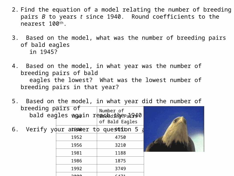
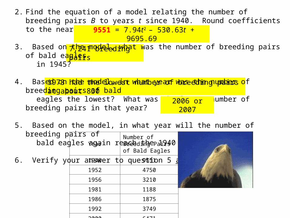
2. Find the equation of a model relating the number of breeding pairs B to years t since 1940. Round coefficients to the nearest 100th.

3. Based on the model, what was the number of breeding pairs of bald eagles in 1945?

4. Based on the model, in what year was the number of breeding pairs of bald eagles the lowest? What was the lowest number of breeding pairs in that year?

5. Based on the model, in what year did the number of breeding pairs of bald eagles again reach the 1940 level?

6. Verify your answer to question 5 algebraically.

YearNumber of Breeding Pairs of Bald Eagles

1940 9551

1952 4750

1956 3210

1981 1188

1986 1875

1992 3749

2000 6471

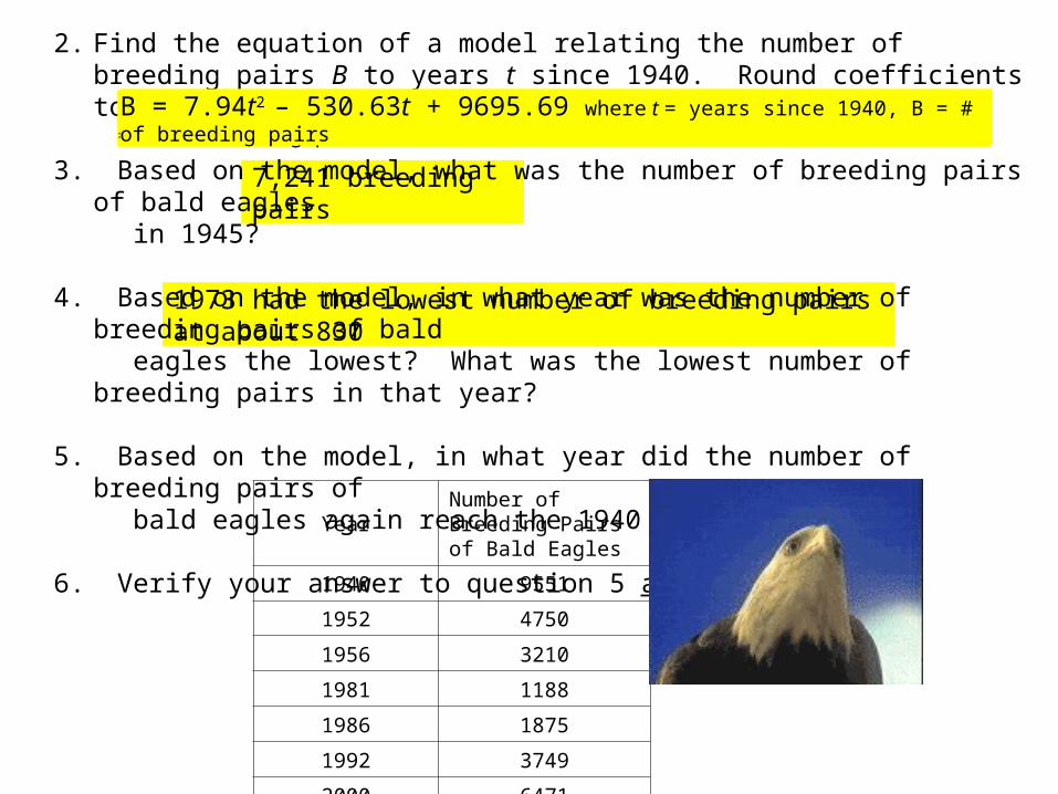
B = 7.94t2 – 530.63t + 9695.69 where t = years since 1940, B = # of breeding pairs

2. Find the equation of a model relating the number of breeding pairs B to years t since 1940. Round coefficients to the nearest 100th.

3. Based on the model, what was the number of breeding pairs of bald eagles in 1945?

4. Based on the model, in what year was the number of breeding pairs of bald eagles the lowest? What was the lowest number of breeding pairs in that year?

5. Based on the model, in what year did the number of breeding pairs of bald eagles again reach the 1940 level?

6. Verify your answer to question 5 algebraically.

YearNumber of Breeding Pairs of Bald Eagles

1940 9551

1952 4750

1956 3210

1981 1188

1986 1875

1992 3749

2000 6471

7,241 breeding pairs

2. Find the equation of a model relating the number of breeding pairs B to years t since 1940. Round coefficients to the nearest 100th.

3. Based on the model, what was the number of breeding pairs of bald eagles in 1945?

4. Based on the model, in what year was the number of breeding pairs of bald eagles the lowest? What was the lowest number of breeding pairs in that year?

5. Based on the model, in what year did the number of breeding pairs of bald eagles again reach the 1940 level?

6. Verify your answer to question 5 algebraically.

y = 794x2 – 530.63x + 9695.69 where x = years since 1940, y = # of breeding pairsB = 7.94t2 – 530.63t + 9695.69 where t = years since 1940, B = # of breeding pairs

YearNumber of Breeding Pairs of Bald Eagles

1940 9551

1952 4750

1956 3210

1981 1188

1986 1875

1992 3749

2000 6471

1973 had the lowest number of breeding pairs at about 830

7,241 breeding pairs

2. Find the equation of a model relating the number of breeding pairs B to years t since 1940. Round coefficients to the nearest 100th.

3. Based on the model, what was the number of breeding pairs of bald eagles in 1945?

4. Based on the model, in what year was the number of breeding pairs of bald eagles the lowest? What was the lowest number of breeding pairs in that year?

5. Based on the model, in what year did the number of breeding pairs of bald eagles again reach the 1940 level?

6. Verify your answer to question 5 algebraically.

y = 7.94x2 – 530.63x + 9695.69 where x = years since 1940, y = # of breeding pairsB = 7.94t2 – 530.63t + 9695.69 where t = years since 1940, B = # of breeding pairs

YearNumber of Breeding Pairs of Bald Eagles

1940 9551

1952 4750

1956 3210

1981 1188

1986 1875

1992 3749

2000 6471

1973 had the lowest number of breeding pairs at about 830

7,241 breeding pairs

2. Find the equation of a model relating the number of breeding pairs B to years t since 1940. Round coefficients to the nearest 100th.

3. Based on the model, what was the number of breeding pairs of bald eagles in 1945?

4. Based on the model, in what year was the number of breeding pairs of bald eagles the lowest? What was the lowest number of breeding pairs in that year?

5. Based on the model, in what year did the number of breeding pairs of bald eagles again reach the 1940 level?

6. Verify your answer to question 5 algebraically.

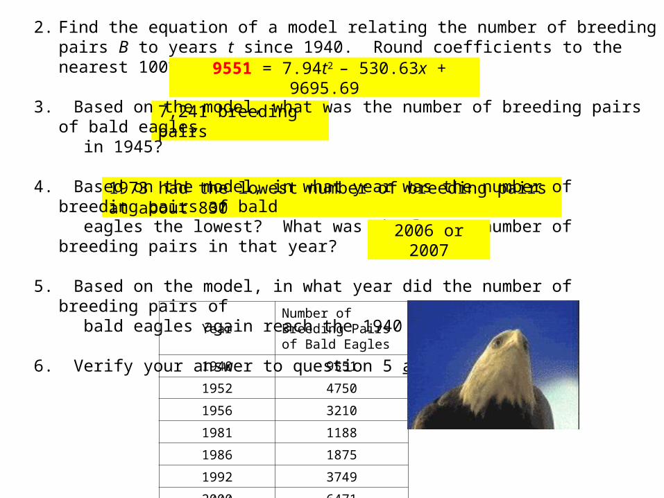
2006 or 2007

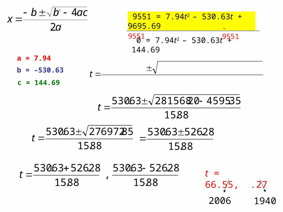
9551 = 7.94t2 – 530.63x + 9695.69

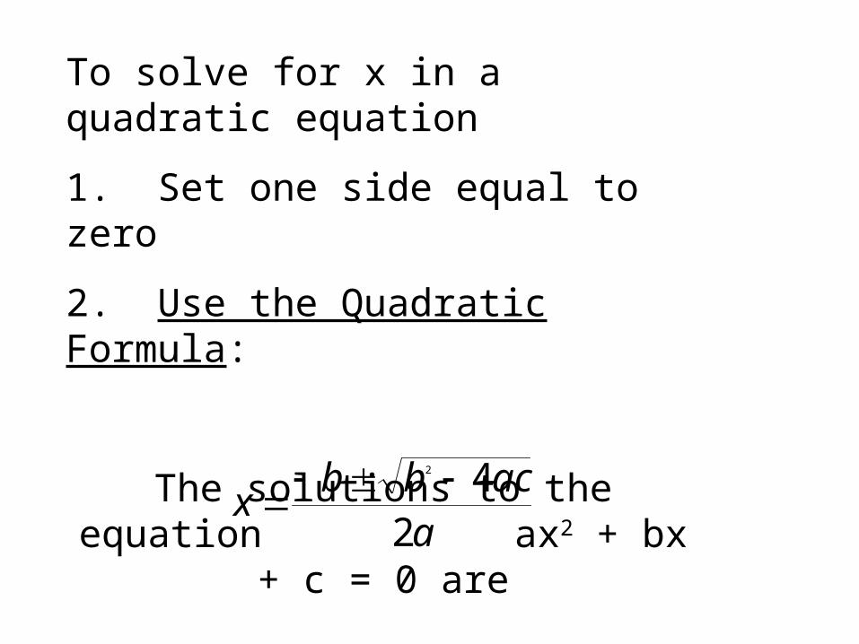
To solve for x in a quadratic equation

1. Set one side equal to zero

2. Use the Quadratic Formula:

The solutions to the equation ax2 + bx + c = 0 are

aacbb

x2

42

YearNumber of Breeding Pairs of Bald Eagles

1940 9551

1952 4750

1956 3210

1981 1188

1986 1875

1992 3749

2000 6471

1973 had the lowest number of breeding pairs at about 830

7,241 breeding pairs

2. Find the equation of a model relating the number of breeding pairs B to years t since 1940. Round coefficients to the nearest 100th.

3. Based on the model, what was the number of breeding pairs of bald eagles in 1945?

4. Based on the model, in what year was the number of breeding pairs of bald eagles the lowest? What was the lowest number of breeding pairs in that year?

5. Based on the model, in what year will the number of breeding pairs of bald eagles again reach the 1940 level?

6. Verify your answer to question 5 algebraically.

2006 or 2007

9551 = 7.94t2 – 530.63t + 9695.69

aacbb

x2

42 9551 = 7.94t2 – 530.63t + 9695.69

0 = 7.94t2 – 530.63t + 144.69

-9551 -9551

a = 7.94

)94.7(2

)69.144)(94.7(4)63.530()63.530( 2 t

88.15

35.459520.28156863.530 t

88.15

85.27697263.530 t

88.15

28.52663.530

88.15

28.52663.530,

88.15

28.52663.530 t t = 66.55, .27

2006 1940

b = –530.63

c = 144.69

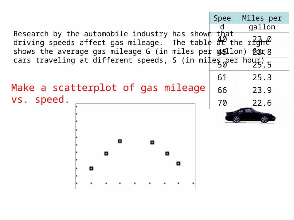
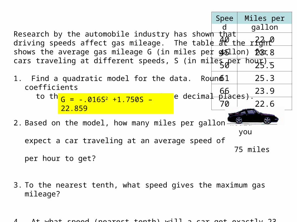
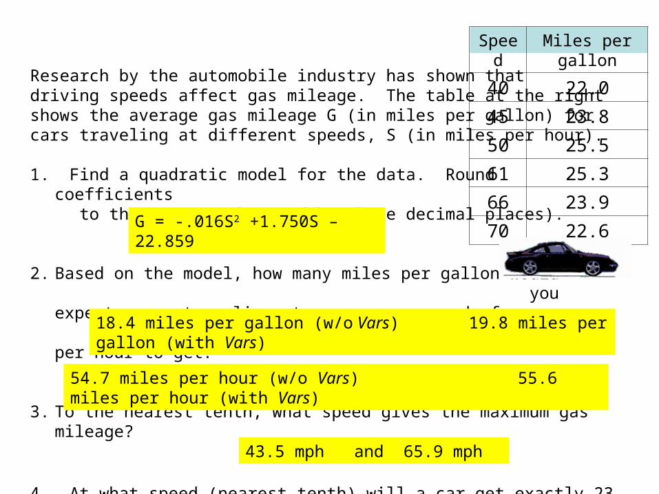
Research by the automobile industry has shown that driving speeds affect gas mileage. The table at the rightshows the average gas mileage G (in miles per gallon) for cars traveling at different speeds, S (in miles per hour).

Speed Miles per gallon

40 22.0

45 23.8

50 25.5

61 25.3

66 23.9

70 22.6Make a scatterplot of gas mileage vs. speed.

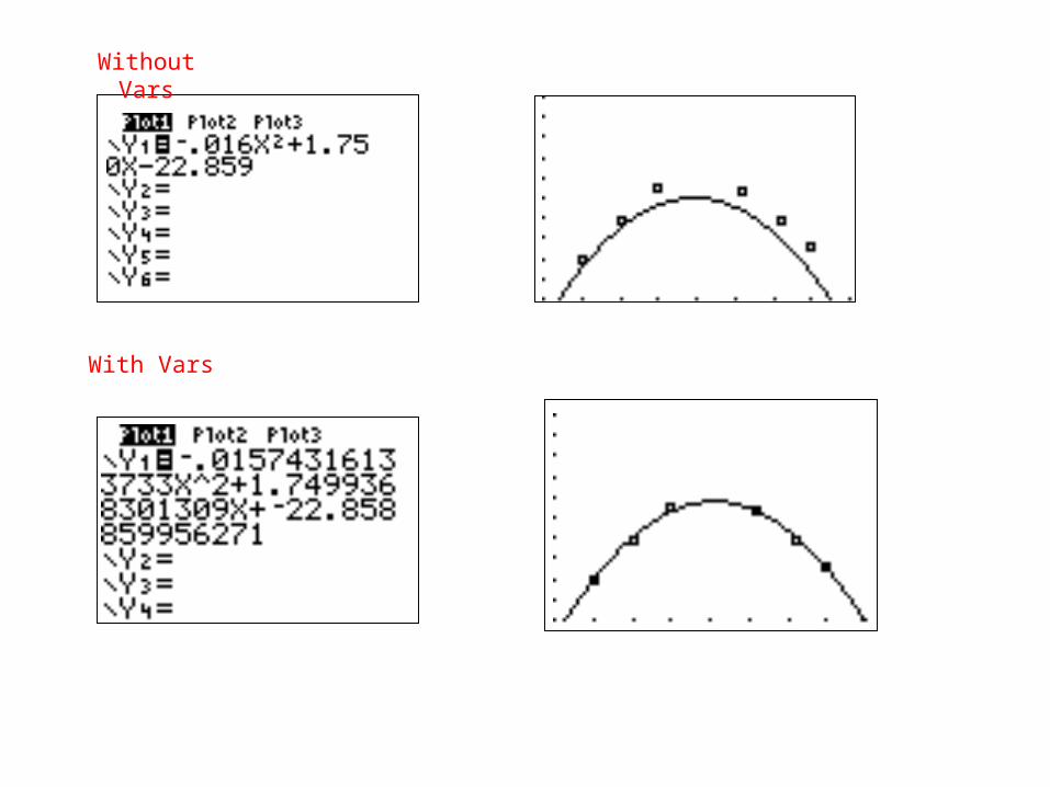
Without Vars

With Vars

Research by the automobile industry has shown that driving speeds affect gas mileage. The table at the rightshows the average gas mileage G (in miles per gallon) for cars traveling at different speeds, S (in miles per hour).

1. Find a quadratic model for the data. Round coefficients to the nearest thousandth (three decimal places).

2. Based on the model, how many miles per gallon would you expect a car traveling at an average speed of 75 miles per hour to get?

3. To the nearest tenth, what speed gives the maximum gas mileage?

4. At what speed (nearest tenth) will a car get exactly 23 miles per gallon? Give an algebraic solution.

G = -.016S2 +1.750S – 22.859

Speed Miles per gallon

40 22.0

45 23.8

50 25.5

61 25.3

66 23.9

70 22.6

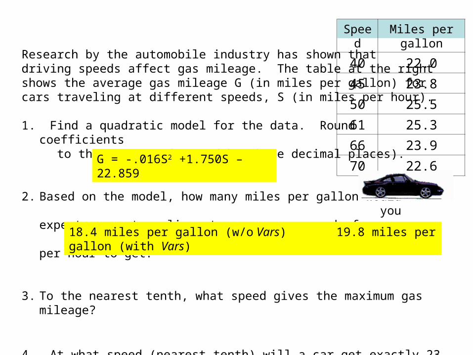
Research by the automobile industry has shown that driving speeds affect gas mileage. The table at the rightshows the average gas mileage G (in miles per gallon) for cars traveling at different speeds, S (in miles per hour).

1. Find a quadratic model for the data. Round coefficients to the nearest thousandth (three decimal places).

2. Based on the model, how many miles per gallon would you expect a car traveling at an average speed of 75 miles per hour to get?

3. To the nearest tenth, what speed gives the maximum gas mileage?

4. At what speed (nearest tenth) will a car get exactly 23 miles per gallon? Give an algebraic solution.

G = -.016S2 +1.750S – 22.859

18.4 miles per gallon (w/o Vars) 19.8 miles per gallon (with Vars)

Speed Miles per gallon

40 22.0

45 23.8

50 25.5

61 25.3

66 23.9

70 22.6

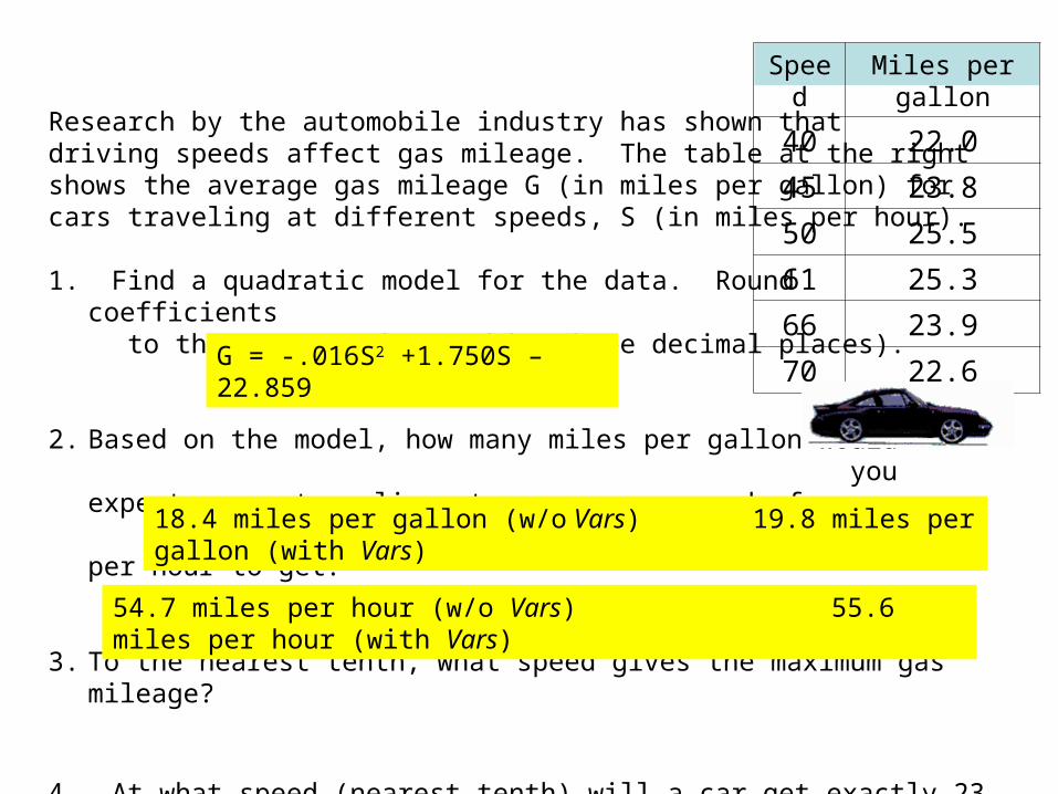
Research by the automobile industry has shown that driving speeds affect gas mileage. The table at the rightshows the average gas mileage G (in miles per gallon) for cars traveling at different speeds, S (in miles per hour).

1. Find a quadratic model for the data. Round coefficients to the nearest thousandth (three decimal places).

2. Based on the model, how many miles per gallon would you expect a car traveling at an average speed of 75 miles per hour to get?

3. To the nearest tenth, what speed gives the maximum gas mileage?

4. At what speed (nearest tenth) will a car get exactly 23 miles per gallon? Give an algebraic solution.

G = -.016S2 +1.750S – 22.859

18.4 miles per gallon (w/o Vars) 19.8 miles per gallon (with Vars)

54.7 miles per hour (w/o Vars) 55.6 miles per hour (with Vars)

Speed Miles per gallon

40 22.0

45 23.8

50 25.5

61 25.3

66 23.9

70 22.6

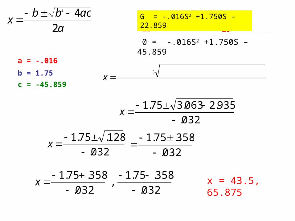
aacbb

x2

42

0 = -.016S2 +1.750S – 45.859

-23 -23

a = -.016

)016.(2

)859.45)(016.(4)75.1()75.1( 2

x

032.

935.2063.375.1

x

032.

128.75.1

x032.

358.75.1

032.

358.75.1,

032.

358.75.1

x x = 43.5, 65.875

b = 1.75

c = -45.859

23 = -.016S2 +1.750S – 22.859G

Research by the automobile industry has shown that driving speeds affect gas mileage. The table at the rightshows the average gas mileage G (in miles per gallon) for cars traveling at different speeds, S (in miles per hour).

1. Find a quadratic model for the data. Round coefficients to the nearest thousandth (three decimal places).

2. Based on the model, how many miles per gallon would you expect a car traveling at an average speed of 75 miles per hour to get?

3. To the nearest tenth, what speed gives the maximum gas mileage?

4. At what speed (nearest tenth) will a car get exactly 23 miles per gallon? Give an algebraic solution.

G = -.016S2 +1.750S – 22.859

18.4 miles per gallon (w/o Vars) 19.8 miles per gallon (with Vars)

54.7 miles per hour (w/o Vars) 55.6 miles per hour (with Vars)

Speed Miles per gallon

40 22.0

45 23.8

50 25.5

61 25.3

66 23.9

70 22.6

43.5 mph and 65.9 mph

Homework:

Complete Parts II and III Section 5.4 (Composite Functions)

AND

Section 5.5 – Quadratic Functions