final exam review cs 3610/5610n dr. jundong liu. about the final exam coverage: after midterm + heap...

Final Exam Review

CS 3610/5610NDr. Jundong Liu

About the final exam

Coverage: after midterm + heap operations

Time: Thursday, April 30, 8-10am Preparation: focus on lecture notes

& projects & homework

Structure of the exam

True/False, fill the blanks (~15%) Algorithms’ properties (~20%) Operations on certain inputs (~30%) Proof of certain claim (~10%) Code analysis (10-15%) Code writing (10-15%) Other

4

Search & Hashing: Objectives

• Learn the various search algorithms• Explore how to implement the sequential and

binary search algorithms• Discover how the sequential and binary

search algorithms perform• Become aware of the lower bound on

comparison-based search algorithms• Learn about hashing

5

Sequential Search Analysis

• Sequential search algorithm performance– Examine worst case and average case– Count number of key comparisons

• Unsuccessful search– Search item not in list– Make n comparisons

• Conducting algorithm performance analysis– Best case: make one key comparison– Worst case: algorithm makes n comparisons

6

Sequential Search Analysis (cont’d.)

• Determining the average number of comparisons (cont’d.)

7

Binary Search

• Performed only on ordered lists• Uses divide-and-conquer technique

FIGURE 9-1 List of length 12

FIGURE 9-2 Search list, list[0]...list[11]

FIGURE 9-3 Search list, list[6]...list[11]

Data Structures Using C++ 2E

Binary Search: Analysis

• Worst case complexity? • Each level in the recursion, we split

the array in half (divide by two). • Therefore maximum recursion depth

is floor(log2n) and worst case = O(log2n).

• Average case is also = O(log2n).

9

Lower Bound on Comparison-Based Search Algorithms

Worst-case complexity

10

Hashing

• Algorithm of order one (on average)• Requires data to be specially organized

– Hash table• Helps organize data• Stored in an array• Denoted by HT

– Hash function• Arithmetic function denoted by h• Applied to key X• Compute h(X): read as h of X• h(X) gives address of the item

Data Structures Using C++ 2E 11

Hashing (cont’d.)

• Synonym• Overflow: Occurs if bucket t full• Collision: Occurs if h(X1) = h(X2)• Overflow and collision occur at same time

– If r = 1 (bucket size = one)


Hashing: two issues

• Choosing a hash function– Main objectives

• Choose an easy to compute hash function• Minimize number of collisions

• Handle overflow

13

Collision Resolution

• Desirable to minimize number of collisions– Collisions unavoidable in reality

• Hash function always maps a larger domain onto a smaller range

• Collision resolution technique categories– Open addressing (closed hashing)

• Data stored within the hash table– Chaining (open hashing)

• Data organized in linked lists• Hash table: array of pointers to the linked lists

14

Linear Probing

• Starting at location t– Search array sequentially to find next available

slot• Assume circular array

– If lower portion of array full• Can continue search in top portion of array using

mod operator– Starting at t, check array locations using probe

sequence • t, (t + 1) % HTSize, (t + 2) % HTSize, . . ., (t + j)

% HTSize


Linear Probing (cont’d.)

• Improving linear probing– Skip array positions by fixed constant (c)

instead of one• Random probing• Re-hashing

16

Quadratic Probing

• Suppose– Item with key X hashed at t (h(X) = t and 0 <=

t <= HTSize – 1)– Position t already occupied

• Starting at position t– Linearly search array at locations (t + 1)%

HTSize, (t + 22 ) % HTSize = (t + 4) %HTSize, (t + 32) % HTSize = (t + 9) % HTSize, . . ., (t + i2) % HTSize

• Probe sequence: t, (t + 1) % HTSize (t + 22 ) % HTSize, (t + 32) % HTSize, . . ., (t + i2) % HTSize


Quadratic Probing (cont’d.)

• Reduces primary clustering• Does not probe all positions in the table

• But the first b/2 probes, including the initial location h(k), all end up with distinct and unique locations

• After that, probing locations may repeat• As a result: there is no guaranteed of finding an

empty cell once the table gets more than half full– Considerable number of probes

• Assume full table• Stop insertion (and search)


Quadratic Probing (cont’d.)

• Primary clustering • Secondary clustering

Linear open addressing (linear probing):

search, insert and delete


Collision Resolution: Chaining (Open Hashing)

• Hash table HT: array of pointers– For each j, where 0 <= j <= HTsize -1

• HT[j] is a pointer to a linked list

FIGURE 9-10 Linked hash table


Collision Resolutions

• Advantages of chaining in comparison with quadratic probing.

• Disadvantage of chaining– Small item size wastes space


Selection Sort: Array-Based Lists

• Selection sort operation– Find location of the smallest element in

unsorted list portion• Move it to top of unsorted portion of the list

– First time: locate smallest item in the entire list– Second time: locate smallest item in the list

starting from the second element in the list, and so on


FIGURE 10-1 List of 8 elements

FIGURE 10-2 Elements of list during the first iteration

FIGURE 10-3 Elements of list during the second iteration

24

Analysis: Selection Sort

• Search algorithms– Concerned with number of key (item)

comparisons• Sorting algorithms

– Concerned with number of key comparisons and number of data movements

• Analysis of selection sort– Function swap

• Number of item assignments: 3(n-1)– Function minLocation

• Number of key comparisons of O(n2)


Insertion Sort

• Attempts to improve high selection sort key comparisons

• Sorts list by moving each element to its proper place• Given list of length eight

FIGURE 10-4 list


Insertion Sort: Insert

• Three strategies to find proper place – Search from rear (using arrays as in the book)– Search from front (using linked lists as in the book)– Binary search

27

Insertion Sort: Array-Based Lists

• Elements list[0], list[1], list[2], list[3] in order

• Consider element list[4]– First element of unsorted list

FIGURE 10-5 list elements while moving list[4] to its proper place

28

Insertion Sort: Linked List-Based Lists

• If list stored in an array– Traverse list in either direction using index variable

• If list stored in a linked list– Traverse list in only one direction

• Starting at first node: links only in one direction

FIGURE 10-10 Linked list


Insertion Sort: Best case and worst

• Best case: sorted array– Search from rear: (n-1) comparisons and 0

data movement • Worst case: reversely sorted array

– Search from rear: (n-1) + (n-2) + (n-3) + … + 1 comparisons and movements


Shellsort

• Take advantage of the best case of insertion sort– Use global jumps to make the input quickly

close to an almost-sorted situation– Jumps are controlled by step sizes

• e.g. 30, 13, 5, 3, 1• The final step will be an insertion sort,

where the input is almost sorted.


Shellsort (cont’d.)

FIGURE 10-19 Lists during Shellsort


Quicksort: Array-Based Lists

QuickSort: implementation issues

How to choose the pivot element each time?

After the pivot is decided, how to move the elements so that the array is separated into two sub-arrays?

Time complexity: what are the determining factors to produce base and worst performance?


Quicksort: choose the Pivot

Determine the pivot: many different approaches the first element of the current sub-array the last element the middle element (textbook version) the median of first, middle, and last elements. Randomly choose an element

In this textbook, middle element is chosen as the pivot, and then swapped with the first element.

34

Quicksort: element movements in the Partition procedure

Again, many different solutions. Commonality: maintain three array

segments: The elements smaller than the pivot The elements bigger than the pivot The elements to be explored

Difference: how to maintain these three segments.

In this textbook, the areas are kept as:pivot | smaller elements | bigger | unexplored35

QuickSort The divide, conquer and combine steps

for QuickSort. What’s the complexity of the “Partition”

routine? What’re the worst-case and best-case

complexities, and when do they happen (depending on the choice of pivot)?

What’s the average-case complexity?

MergeSort (recursive version)

Complexity of MergeSort

MergeSort, Cont’d

Recursive version Using arrays Using linked list

Iterative version (basic idea)

Heap Complete binary tree + heap property Routines

Heapify O(lgn) Build-Heap O(n) Heap-Sort O(nlgn)

Implement Priority Queue Maximum O(1) Extract-Max O(lgn) Insert O(lgn) Increase-Key O(lgn)

Comparison-based sort

Decision tree model

Lower bound of comparison-based sort

44

Graph Theory: Objectives

• Learn about graphs• Become familiar with the basic terminology of

graph theory• Discover how to represent graphs in

computer memory

45

Graph Theory: Objectives (cont’d.)

• Examine and implement various graph traversal algorithms

• Learn how to implement a shortest path algorithm

• Examine and implement the minimum spanning tree algorithm


Graph Definitions and Notations

• Graph G pair– G = (V, E), where V is a finite nonempty set

• Called the set of vertices of G, and E V x V • E: set of edges of G

– G called trivial if it has only one vertex• Directed graph (digraph)

– Elements in set of edges of graph G: ordered• Undirected graph: not ordered


FIGURE 12-3 Various undirected graphs

FIGURE 12-4 Various directed graphs

Graph Definitions and Notations (cont’d.)

• Undirected graph: edges drawn using lines• Directed graph: edges drawn using arrows• u and v adjacent, if…• Definition of Loop

– Edge incident on a single vertex• e1 and e2 called parallel edge, if… • Simple graph

– No loops, no parallel edges


Graph Definitions and Notations (cont’d.)

• Undirected graph G is connected– If path from any vertex to any other vertex

exists• Component of G

– Maximal subset of connected vertices• Directed graph G is strongly connected

– If any two vertices in G are connected


Graph Representation

• Graphs represented in computer memory– Two common ways

• Adjacency matrices• Adjacency lists


Adjacency Matrices

• Let G be a graph with n vertices where n > zero• Let V(G) = {v1, v2, ..., vn}

– Adjacency matrix


Adjacency Lists (cont’d.)

FIGURE 12-6 Adjacency list ofgraph G3 of Figure 12-4

FIGURE 12-5 Adjacency listof graph G2 of Figure 12-4

53

Operations on Graphs

• Commonly performed operations– Create graph

• Store graph in computer memory using a particular graph representation

– Clear graph• Makes graph empty

– Determine if graph is empty– Traverse graph– Print graph


Graph Traversals vs. Binary tree traversals

• Two most common graph traversal algorithms– Depth first traversal in graphs pre-order traversal

in binary tree (parent, left sub-tree, right sub-tree)

– Breadth first traversal in graphs level-order traversal in binary tree (parent, children, grandchildren..)

55

Depth First Traversal

• Similar to binary tree preorder traversal

FIGURE 12-7 Directed graph G3

56

Depth First Traversal (cont’d.)

• General algorithm for depth first traversal at a given node v

– Recursive algorithm

Breadth First Traversal

• Similar to traversing binary tree level-by-level (called level-order traversal)

–Nodes at each level• Visited from left to right

–All nodes at any level i • Visited before visiting nodes at level i + one

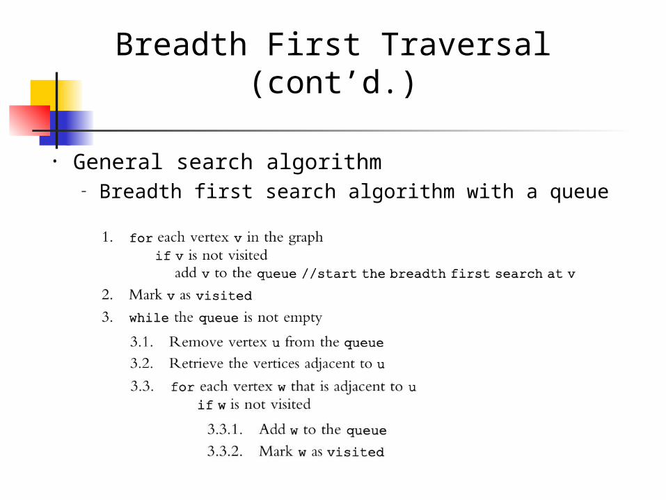
Breadth First Traversal (cont’d.)

• General search algorithm– Breadth first search algorithm with a queue

Connected components (CC) and spanning trees

(ST)

Concept of CC and ST DFT and BFT can be used to

retrieve connected components.

DFT and BFT can be used to generate spanning trees; how do the resulting STs look like?

Minimum spanning tree

Prim’s algorithm Keep the set T as a single tree; grow

it into a MST. Each step, find the shortest edge

connecting T and NON-T and include it into the set T.

Understand the procedure

Shortest path problem

Single-pair shortest path Single-source shortest paths

Dijkstra’s algorithm All-pairs shortest paths Impact of negative edges

Dijkstra’s algorithm

What is the input constraint for Dijkstra’s algorithm? Why is it necessary?

Understand the procedure Shortest distances vs. shortest

paths (project 6)

About the exam

Coverage: after midterm + heap operations

Time: Thursday, next week, 8-10am

Preparation: focus on lecture notes & & projects & homework

Any questions?

final exam review cs 3610/5610n dr. jundong liu. about the final exam coverage: after midterm + heap...

Documents

search hashing

ebinary search

htsize data structures

item data structures

technique data structures

hashing contd

array of pointers

array locations