final december 2004 - everglades restoration...
TRANSCRIPT

Final December 2004
CENTRAL AND SOUTHERN FLORIDA PROJECT COMPREHENSIVE EVERGLADES RESTORATION PLAN DEVELOPMENT OF ALTERNATIVE PLANS PART 2 - WETLAND RESTORATION
LAKE OKEECHOBEE WATERSHED PROJECT
U.S. Army Corps of Engineers South Florida Jacksonville District Water Management District Assisted By:
HDR Engineering, Inc. West Palm Beach, Florida

________________________________________________________________________
Lake Okeechobee Watershed Project Dec 2004 -i-
This document was prepared by the Lake Okeechobee Watershed Project Delivery Team, with assistance from U.S. Fish and Wildlife (Gina Paduano Ralph, Ph.D.; and Steve Schubert) and HDR Engineering, Inc. The final document will be one component of the Lake Okeechobee Project Implementation Report.
Development of Alternative Plans
Lake Okeechobee Watershed Project Dec 2004 -ii-
TABLE OF CONTENTS
1.0 INTRODUCTION 1
2.0 FORMULATION OF ALTERNATIVE PLANS FOR WETLAND RESTORATION 1 2.1.1 Wetland Restoration Objectives 1 2.1.2 Wetland Restoration Rationale 1 2.1.3 Wetland Restoration Benefits for the LOWP 7
2.1.3.1 Hydrologic Benefits 8 2.1.3.2 Fish and Wildlife Benefits 9 2.1.3.3 Commercial and Recreational Benefits 15 2.1.3.4 Water Quality Treatment Benefits 16 2.1.3.5 Programmatic and Regulatory Benefits 17 2.1.3.6 Public Support Benefits 19 2.1.3.7 Business 19
2.1.4 Potential Restoration Site Selection Process 19 2.1.5 Screening of Potential Restoration Sites 23
2.1.5.1 Siting Rules 23 2.1.5.2 Data Sources 25 2.1.5.3 Primary Screening Factors 26 2.1.5.4 Secondary Screening Factors 32
2.1.6 Prioritization of Potential Restoration Sites 39 2.1.6.1 Site Prioritization Ranking Methodology 39 2.1.6.2 Application of Site Prioritization Ranking Methodology 46 2.1.6.3 Sensitivity Analysis for Low-Ranking Potential Restoration Sites 50
2.1.7 Field Evaluation of Top-Ranked Sites 57 2.1.7.1 Determining Existing Wetland Quality 59 2.1.7.2 Wetland Evaluation Analysis Tool 65 2.1.7.3 Determination of Habitat Units and Ecological Lift Potential 75 2.1.7.4 Estimation of Planning Level Wetland Restoration Costs 140
Development of Alternative Plans
Lake Okeechobee Watershed Project Dec 2004 -iii-
TABLE OF CONTENTS List of Attachments Attachment A
Vertebrate Species Present In The Lake Okeechobee Watershed Either As Year-Round Residents Or Part-Time Migrants.
Attachment B
Secondary Screening – FLUCCS Codes and Associated Ecological Value, Contaminants and Economic Value Scores
Attachment C
Site Prioritization – Average Scores across Categories for Top-Ranked Potential Restoration Sites
Attachment D
Percentile Analysis for Potential Restoration Sites
Tab 1 – Top Potential Restoration Sites By Planning Area, Ranked By 80th, 75th And 70th Percentiles Across All Categories.
Tab 2 – Potential Restoration Sites Based Upon Percentile Ranking
Attachment E
Functioning Wetland Habitat Units For Individual Wetlands Within Top-Ranked Potential Restoration Sites.
Tab 1 – 2004 EVS and Functioning Wetland Habitat Units for Individual Wetlands within the Top-Ranked Sites
Tab 2 – 2013 EVS and Functioning Wetland Habitat Units for Individual Wetlands within the Top-Ranked Sites
Tab 3 – 2050 (Future without Project) EVS and Functioning Wetland Habitat Units for Individual Wetlands within the Top-Ranked Sites
Development of Alternative Plans
Lake Okeechobee Watershed Project Dec 2004 -iv-
TABLE OF CONTENTS List of Attachments (continued)
Tab 4 – 2050/2063 (Future with Project) EVS and Functioning Wetland Habitat Units for Individual Wetlands within the Top-Ranked Sites
Tab 5 – 2063 (Future without Project) EVS and Functioning Wetland Habitat Units for Individual Wetlands within the Top-Ranked Sites
Attachment F
Summary Reports On Individual Top-Ranked Potential Restoration Sites Attachment G
Habitat Units for Back-Up Potential Restoration Sites
Tab 1 – Existing and Projected Functioning Wetland Habitat Units for the Back-Up Sites
Tab 2 – Restorable Wetland Habitat Units for Back-Up Sites (2004, 2013, and 2050 And 2063 Future with and without Project Conditions)
Tab 3 – Functioning Upland Habitat Units for Back-Up Sites (2004, 2013, and 2050 And 2063 Future with and without Project Conditions)
Tab 4 – Restorable Upland Habitat Units for Back-Up Sites (2004, 2013, and 2050 and 2063 Future with and without Project Conditions)
Tab 5 – Total Number of Habitat Units Provided by Each Back-Up Site in 2050 under Future with and without Project Conditions
Tab 6 – Total Number of Habitat Units Provided by Each Back-Up Site in 2063 under Future with and without Project Conditions
Tab 7 – Total Number ff Habitat Units Provided by Each Back-Up Site in 2004, 2013, and 2050 under Future with and without Project Conditions
Development of Alternative Plans
Lake Okeechobee Watershed Project Dec 2004 -v-
TABLE OF CONTENTS List of Attachments (continued)
Tab 8 – Total Number of Habitat Units Provided By Each Back-Up Site in 2004, 2013, and 2063 under Future with and without Project Conditions
Tab 9 – Estimated Real Estate Costs By Planning Area For Each Of The Back-Up Sites Within The Lake Okeechobee Watershed Project
Attachment H Summary Reports On Individual Back-Up Potential Restoration Sites. Attachment I Planning Level Restoration Cost Estimates for Top-Ranked Sites
Development of Alternative Plans
Lake Okeechobee Watershed Project Dec 2004 -vi-
TABLE OF CONTENTS List of Tables 2–1 FLUCCS Codes Blocked Out From Consideration in the Siting Of Potential
Restoration Sites ............................................................................................... 2-27 2–2 FLUCCS Codes (1000 Series) Not Blocked Out From Consideration in the Siting of Potential Restoration Sites .................................................................. 2-28 2–3 Secondary Screening Factors and Suitability Attributes .................................. 2-33 2–4 Potential Restoration Site Prioritization Criteria ............................................... 2-39 2–5 Number Of Potential Restoration Sites And Acreage Based Upon Percentile
Analysis.............................................................................................................. 2-47 2–6 Potential Restoration Sites That Originally Ranked Less Than the Top 32, and the Scoring Rationale .................................................................................. 2-52 2–7 Top-Ranked Potential Restoration Sites Subjected To Field Evaluation ......... 2-57 2–8 WRAP Scores for Selected Wetlands within the Top-Ranked Sites ................. 2-63 2–9 FLUCCS Codes and Associated EVS Used By the WEAT to Assess Functioning Wetland Quality under Existing Conditions (2004) ...................... 2-68 2–10 Existing & Projected Functioning Wetland Habitat Units for the Top-Ranked Sites............................................................................................... 2-77 2–11 FLUCCS Codes and Revised EVS for 2013 and 2050 and 2063 without LOW Project ...................................................................................................... 2-81 2–12 Restorable Wetland Habitat Units for Top-Ranked Sites (Existing, 2013, 2050 Future Without and With Project Conditions) .......................................... 2-95 2–13 FLUCCS Codes and 2004 EVS Used In the Calculation of 2004 Upland
Functioning Habitat Units................................................................................ 2-101 2–14 Functioning Upland Habitat Units for Top-Ranked Sites in 2004, 2013, and 2050 without and with Implementation of the LOW Project.................... 2-107 2–15 FLUCCS Codes and Associated EVS for Calculation of 2013 and 2050 Without Low Project) Functioning Upland Habitat Units............................... 2-110 2–16 Restorable Upland Habitat Units for Top-Ranked Sites (2004, 2013, and 2050 and 2063 without and with Implementation of the LOW Project) ......... 2-123 2–17 Total Number of Habitat Units Provided By Each Top-Ranked Site in 2050 under Future without and with Project Conditions ................................. 2-132 2–18 Total Number of Habitat Units Provided By Each Top-Ranked Site in 2063 under Future without and with Project Conditions ................................. 2-134 2–19 Total Number of Habitat Units Provided By Each Top-Ranked Site in 2004, 2013 and 2050 under Future without and with Project Conditions ....... 2-136 2–20 Total Number of Habitat Units Provided By Each Top-Ranked Site in 2004, 2013 and 2063 under Future with and without Project Conditions ....... 2-138 2–21 Estimated Costs for Achieving Restoration at Site K05.................................. 2-147 2–22 Cost Analysis for Top-Ranked Sites (2063 with LOW Project)...................... 2-149

Development of Alternative Plans
Lake Okeechobee Watershed Project Dec 2004 -vii-
TABLE OF CONTENTS List of Figures 1–1 LOW Project Plan Formulation Process Summary ............................................. 1-2 1–2 LOW Project Planning Areas............................................................................... 1-3 2–1 Ecosystem Quality Expressed as a Function of Percent Anthropogenic
Degradation.......................................................................................................... 2-6 2–2 Potential Restoration Site Selection Process ..................................................... 2-22 2–3 Areas with Land Uses That Are Not Conducive To Wetland Restoration ........ 2-29 2–4 Areas with Soil Types That Are Not Conducive To Wetland Restoration........ 2-30 2–5 Areas That Are Not Conducive To Wetland Restoration Due To Land Use and Soil Type .................................................................................................... 2-31 2–6 Wetland Land Suitability Model Output............................................................ 2-36 2–7 Potential Restoration Sites Identified Through the Application of Primary and Secondary Screening Factors ...................................................................... 2-38 2–8 Top-Ranked Potential Restoration Sites ........................................................... 2-49 2–9 The Metric-Based Suitability Scoring Patterns For Potential Restoration Site T-13............................................................................................................. 2-54 2–10 The Metric-Based Suitability Scoring Patterns For Potential Restoration Site IP-07 ........................................................................................................... 2-55 2–11 Potential Restoration Site Li-24 Illustrating the Coded Aerial Map(s) Used In the Ground and Aerial Field Investigations ......................................... 2-60 2–12 Site F08 Illustrating the WEAT EVS Calculations Used In the Determination of Habitat Units ........................................................................ 2-74 2–13 Potential Restoration Site F08 Illustrating the Core Reserve Concept Employed In the Calculation of Functioning Wetland Habitat Units in 2050 And 2063 after Implementation of the LOW Project ............................... 2-89 2–14 Potential Restoration Site F08 Illustrating the Method Employed In the
Calculation of Restorable Wetland Habitat Units.............................................. 2-94 2–15 Potential Restoration Site F08 Illustrating the Method Employed In the
Calculation of Functioning Upland Habitat Units ........................................... 2-106 2–16 Site F08 Illustrating the Method Employed In the Calculation of Restorable
Upland Habitat Units ....................................................................................... 2-126 2–17 Costing Approach for Site K-05 ...................................................................... 2-145
Development of Alternative Plans
Lake Okeechobee Watershed Project Dec 2004 -viii-
ABBREVIATIONS ASR Aquifer Storage and Recovery BLOBS Basin Land Optimization Boundaries DMSTA Dynamic Model for Everglades Stormwater Treatment Areas CERP Comprehensive Everglades Restoration Plan EEE Environmental and economic equity EVM Ecological Value Model FDEP Florida Department of Environmental Protection FEC Fisheating Creek Planning Area GIS Geographical Information System HLR Hydraulic Loading Rate IWR Institute of Water Resources ISTOK Istokpoga/Indian Prairie Planning Area KISS Kissimmee River Planning Area LIW Lake Istokpoga Watershed LOPA Lake Okeechobee Protection Act LOPP Lake Okeechobee Protection Plan LOW Lake Okeechobee Watershed LOWCAP Lake Okeechobee Watershed Combinatorial Analyses Program LSM Land Suitability Model MM Management Measures Mtons Metric tonnes OMRR&R Operation, maintenance, repair, rehabilitation, and replacement P Phosphorus PA Project Alternative PAA Planning Area Alternative PPAA Preliminary Planning Area Alternative PIR Project Implementation Report RASTA Reservoir-assisted Stormwater Treatment Area SA Sensitivity Analyses SFWMD South Florida Water Management District STA Stormwater Treatment Area TCNS Taylor Creek/Nubbin Slough Planning Area TMDL Total Maximum Daily Load Allocation USACE United States Army Corps of Engineers USFWS United States Fish and Wildlife Service
Section 1.0 Development of Alternative Plans
Lake Okeechobee Watershed Project Dec 2004 1-1
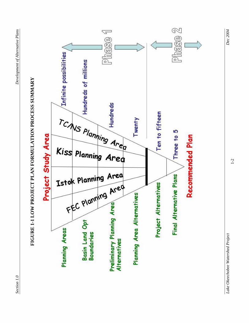
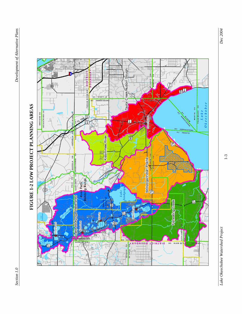
1.0 INTRODUCTION The LOW Project Plan Formulation Process was designed to identify alternative plans that would meet project goals by contributing to improving the water quality of Lake Okeechobee, provide for better management of lake water levels, reduce damaging releases to the estuaries downstream of the lake, restore isolated wetlands in the watershed, and resolve water resource problems in Lake Istokpoga that have resulted from a reduction in the range of water level fluctuations in the lake. The scope of the alternative plan formulation process started with literally an infinite number of potential alternatives that address the project objectives and a screening process that culminated in the identification of the final three to five alternatives that will be carried into more detailed evaluation which will culminate in the selection of a recommended plan (Figure 1-1). The plan formulation process addressed the questions of what to build, where to build it, and cost effectiveness. To expedite and facilitate the process, the project study area was divided into the following four planning areas based on the four major tributary systems (basins) that naturally drain the lower portion of the LOW into Lake Okeechobee (Figure1-2): 1. Fisheating Creek (FEC) 2. Lake Istokpoga/Indian Prairie/Harney Pond 3. Kissimmee River (KISS) 4. Taylor Creek/Nubbin Slough (TCNS) The Lake Istokpoga/Indian Prairie/Harney Pond planning area consists of two interconnected basins, namely the Lake Istokpoga Watershed (LIW) and the Istokpoga/Indian Prairie/Harney Pond Basin (ISTOK). Given the diverse nature of the goals and objectives that had to be addressed, two separate, but parallel and complementary, plan formulation processes were conducted, as described below: 1. Formulation of Alternative Plans for Water Quality Improvement and Storage –
This process was directed towards identifying and screening alternative plans that would address project purposes of improving the water quality of Lake Okeechobee, providing for better management of Lake Okeechobee water levels, reducing damaging releases to the estuaries, and alleviating Lake Istokpoga water resource problems. During this process alternative plans were formulated for possible siting in the Fisheating Creek (FEC), Istokpoga/Indian Prairie/Harney Pond (ISTOK), Kissimmee (KISS), and Taylor Creek/Nubbin Slough (TCNS) planning areas. Plans were developed and screened by a PDT-led planning team that consisted of planners, water resource specialists, engineers, and hydrologists.
Sect
ion
1.0
D
evel
opm
ent o
f Alte
rnat
ive
Plan
s La
ke O
keec
hobe
e W
ater
shed
Pro
ject
Dec
200
4 1-
2
FIG
UR
E 1
-1 L
OW
PR
OJE
CT
PL
AN
FO
RM
UL
AT
ION
PR
OC
ESS
SU
MM
AR
Y
Sect
ion
1.0
D
evel
opm
ent o
f Alte
rnat
ive
Plan
s La
ke O
keec
hobe
e W
ater
shed
Pro
ject
Dec
200
4 1-
3
FIG
UR
E 1
-2 L
OW
PR
OJE
CT
PL
AN
NIN
G A
RE
AS

Section 1.0 Development of Alternative Plans
Lake Okeechobee Watershed Project Dec 2004 1-4
2. Formulation of Alternative Plans for Wetland Restoration – This process was focused on identifying and screening of alternative plans for restoring wetlands in the project study area. Potential wetland restoration sites in the entire project study area (FEC, ISTOK, LIW, KISS, and TCNS) were evaluated and screened during this process. Plan formulation was conducted by the Ecological Subgroup of the LOW Project Delivery Team. This multi-agency group was led by representatives from the U.S. Fish and Wildlife Service.
This document describes the process followed for the formulation of alternative plans for wetland restoration. Results of the alternative plan formulation process along with supporting documentation are contained presented herein. Relevant back-up information is contained in a series of attachments.
Section 2.0 Development of Alternative Plans
Lake Okeechobee Watershed Project Dec 2004 2-1
2.0 FORMULATION OF ALTERNATIVE PLANS FOR WETLAND RESTORATION
The ecological subgroup of the LOW Project Delivery Team (PDT) was charged with formulating alternative plans for achieving wetland restoration in the project study area. This multi-agency group was led by representatives from the U.S. Fish and Wildlife Service (USFWS). 2.1.1 Wetland Restoration Objectives Wetland restoration in the LOW Project study area complements the following CERP objectives: • Increase the total spatial extent of natural areas; • Improve habitat and functional quality; • Improve native plant and animal species abundance and diversity; and • Enhance economic values and social well being by reducing flood damages and
providing recreational opportunities. In addition, wetland restoration directly supports several LOW Project objectives, including: • Improve habitat for fish and wildlife within the watershed; • Improve water quality in the watershed; • Enhance water supply in the watershed; and • Enhance recreational opportunities. Restoring historic wetlands in the LOW was not only recommended by the Central & South Florida Project Restudy (Restudy; USACE, 1999) but is also consistent with the recommendations of the South Florida Ecosystem Restoration Working Group’s Lake Okeechobee Issue Team and the Pollution Load Reduction Goals for Lake Okeechobee developed for the Lake Okeechobee Surface Water Improvement and Management Plan (SFWMD, 1997). Restored wetlands in the LOW are expected to contribute towards the overall water quality restoration objectives and provide significant long-term water quality benefits for Lake Okeechobee. 2.1.2 Wetland Restoration Rationale Before selecting sites to be considered for wetland restoration, it was important to determine how much wetland restoration was necessary in the project study area to achieve project benefits. To identify this target, a theoretical continuum was developed upon which watershed-wide ecological function could be predicted depending on differing degrees of anthropogenic disturbance. This approach was intended to allow for the estimation of how far the LOW ecosystem could be “bent without breaking.” It also was important to determine the functionality of existing wetlands in the project area, to
Section 2.0 Development of Alternative Plans
Lake Okeechobee Watershed Project Dec 2004 2-2
further identify the level of wetland and associated upland restoration that would be needed to truly have an ecologically functioning watershed. To determine this threshold of ecosystem functionality, one or more appropriate indicators of wetland restoration needed to be identified. Additionally, data would be needed on the: 1. Historic conditions of the selected indicator; 2. Existing condition of the selected indicator, and 3. Appearance or functional losses that would be characteristic of a “broken” wetland
ecosystem. Ultimately, the U.S. Army Corps of Engineers’ (USACE) planning process requires quantification of restoration benefits. However, simply using “acres of wetlands restored” is inadequate because it lacks a measure of quality. Both quantity and quality are important. Therefore, the use of habitat units was proposed as the indicator of wetland restoration (and associated upland restoration), as well as the overall means of assessing alternative wetland restoration plans. Habitat units represent a numerical combination of habitat quality (expressed as a score on a scale of 0.01 to 1.00) and habitat quantity (acres) within a given wetland system at a given time (existing or future conditions). The Restudy (USACE, 1999) identified the loss of the “defining characteristics of the pre-drainage ecosystem” as a major problem facing Everglades Restoration. These characteristics (spatial extent of natural areas, habitat heterogeneity, and dynamic water storage) have either been lost or substantially altered as a result of land use and water management practices during the past 100 years in south Florida. It acknowledged that “while it is true that the pre-drainage wetlands can not be fully restored, a successful restoration program will be one that recovers to the extent possible these defining characteristics of the former system. Achievement of this goal should result in the recovery of ecologically viable systems that functionally resemble the pre-drainage Everglades and its interrelated wetland systems.” Within the LOW Project study area there are many historic “defining characteristics of the watershed.” Certainly, a large spatial extent of natural areas, habitat heterogeneity, and dynamic water storage were all historically present and the vast array of wetlands once present across the landscape was the foundation for these characteristics. The historic (i.e., pre-drainage) condition of the 1.4 million-acre project area was characterized by Harshberger’s (1913) vegetative community map. He identified expansive freshwater marshes along Fisheating Creek and the area now known as Indian Prairie. The floodplain of the Kissimmee River from its confluence with the modern-day Istokpoga Canal downstream to the shoreline of Lake Okeechobee was considered to have the same wetland vegetative communities as the Everglades proper. The eastern portion of the study area was comprised of cypress forest. The Harshberger map does not quite cover the northern extent of the study area; however, the general indication is that the area north of Lake Istokpoga was drier and composed primarily of prairie vegetation and pine flatwoods.
Section 2.0 Development of Alternative Plans
Lake Okeechobee Watershed Project Dec 2004 2-3
In 1943, Davis published a more detailed vegetation map of south Florida, and although some major canals and other drainage features had been constructed, it still indicated a strong wetland signature on the LOW landscape. The planning team used the Davis map and knowledge of local experts to further clarify the features that created the “defining characteristics” of the pre-drainage LOW. The floodplains and riparian corridors of Fisheating Creek, Kissimmee River, Arbuckle Creek, Taylor Creek, and Nubbin Slough were all important wetland systems that have been lost or degraded by urban development and agricultural activities. The large freshwater marsh and downstream wet prairie dotted with hammock forest tree islands that was fed by overflows from Lake Istokpoga had the hydrological and vegetational appearance of a mini-Everglades system (Davis, 1943). Last but not least, the shoreline and interior wetlands of Lake Arbuckle, Lake Istokpoga, and Lake Okeechobee were also important native ecosystems of the pre-drainage watershed. According to the most recent National Resources Conservation Service (NRCS) soils data there were 580,653 acres of wetlands historically in the project study area. According to the most recent South Florida Water Management District (SFWMD) land use data there are only 205,433 acres of wetlands currently in the study area. This translates to a 65 percent loss in wetland spatial extent across the study area. Many more wetlands, even though they still exist, have lost at least some functionality. These combined losses are markedly larger than the 50 percent loss of the entire original Everglades ecosystem as reported in the Restudy (USACE, 1999). Therefore, if a 50 percent loss in the functionality of the Everglades has resulted in so much ecological impairment, enough to justify the CERP, then a 65 percent loss of wetlands in the LOW Project study area alone has likely resulted in even greater ecological damage in that watershed. Additionally, the conversion of dry prairie and upland forests to agricultural and urban land uses has negatively affected the overall ecological integrity of those ecosystems within the study area. While some wetlands have been irretrievably lost due to land use conversion to urban, residential, and commercial areas, or as a result of major drainage canals and the construction of the Herbert Hoover Dike, there still are opportunities within the project area where wetland restoration can occur with only a modest effort. For example, improved pasture presently occupies 52 percent of the land use in the study area. These pastures contain many remnant and partially-functioning isolated wetlands which can be restored by filling of ditches, control or eradication of exotic and invasive species, and fire management. There are also remnant riverine wetland systems that would benefit from these management strategies. These wetlands are particularly important because they are generally forested (or would be after restoration) and provide good corridors which enable wildlife to move across the landscape. This aspect of wetland restoration is likely to result in significant regional benefits to animals outside of, or isolated from, the LOW Project study area.
Section 2.0 Development of Alternative Plans
Lake Okeechobee Watershed Project Dec 2004 2-4
The physical appearance of restorable or partially-functioning wetland systems is characterized by the presence of drainage ditches or canals, lack of surface water, invasion of upland plant species into former wet areas, stressed or dying wetland vegetation, lack of vegetative buffer, lack of wetland-dependent and aquatic animals, and presence of exotic plants and animals including livestock. The degree to which a given wetland is functioning properly is dependent upon the degree of these impacts. Impaired wetlands are less effective at storing surface water, reducing flooding impacts, removing pollutants, stabilizing sediments, recharging groundwater, and providing habitat for fish and wildlife. Significant adverse impacts within the study area that can be directly or indirectly attributed to loss of wetland functions include the following: • Extreme fluctuations in high and low water levels in Lake Okeechobee that have a
major adverse impact on the lake’s littoral and pelagic zones and fish and wildlife habitats;
• Extreme fluctuations between too much and too little freshwater discharge into the Caloosahatchee and St. Lucie estuaries that have resulted in detrimental salinity conditions and physical alterations of fish and wildlife habitat;
• Increased nutrient, sediment, and other pollutant loading to Lake Istokpoga and Lake Okeechobee;
• Spread of exotic and invasive species; • Reduced recreational opportunities; and • Increased adverse impacts on native plant and animal communities including wading
and water birds, amphibians, aquatic reptiles, mammals, fish, and aquatic invertebrates.
Besides the LOW Project, several other wetland restoration initiatives are currently being implemented in the LOW. The Kissimmee River Restoration Project (KRRP), authorized in 1992, will create a more natural environment in the lower Kissimmee River Basin. Major components of the KRRP include: • Reestablishment of flows from Lake Kissimmee that will be similar to historical
discharge characteristics; • Acquisition of approximately 85,000 acres of land in the lower Kissimmee Chain of
Lakes and river valley; • Continuous backfilling of 22 miles of canal; • Removal of two water control structures; and • Recarving of nine miles of former river channel. The wetland restoration component for the LOW Project will complement the KRRP and extend benefits further downstream into Lake Okeechobee. In addition, in 2000, the Florida legislature enacted the Lake Okeechobee Protection Act (LOPA), Florida Statute 373.4595, which mandated the implementation of specific projects to restore the ecological health to the lake and reduce phosphorus loads to the
Section 2.0 Development of Alternative Plans
Lake Okeechobee Watershed Project Dec 2004 2-5
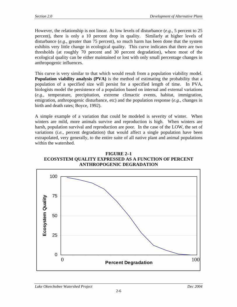
lake. To accomplish the goals of LOPA, the coordinating agencies, the SFWMD, Florida Department of Agriculture and Consumer Services (FDACS), and Florida Department of Environmental Protection (FDEP) developed a comprehensive Lake Okeechobee Protection Plan. One component of this plan involved the restoration of isolated wetlands on lands throughout the watershed. The Isolated Wetland Program was designed to reduce phosphorus discharges from agricultural and non-agricultural land parcels to tributaries that flow into Lake Okeechobee by creating or restoring wetlands. The secondary goal includes assisting landowners to cost effectively meet regulatory requirements, restoring or creating habitat for wetland dependant wildlife species, and detaining stormwater flows to Lake Okeechobee by increasing regional water storage in isolated wetlands. The SFWMD is administering this program in cooperation with a multi-agency team including, the FDACS, FDEP, United States Department of Agriculture, Natural Resources Conservation Service, USFWS, and University of Florida Institute of Food and Agricultural Science. The wetland restoration component for the LOW Project will complement the Isolated Wetland Program and provide additional benefits to Lake Okeechobee along with benefits to fish and wildlife and threatened and endangered species within the LOW Project area. The validity of a theoretical continuum, upon which one can predict watershed-wide ecological function based on the degree of anthropogenic disturbance, is supported by the Restudy (USACE, 1999), which stated that “Nearly half of the original Everglades ecosystem has been converted to agricultural and urban uses.” In south Florida, “roughly 50 percent of the pre-drainage wetland area and 90 percent of pinelands have been lost to development.” These losses have had significant negative effects on the natural system including • Altered hydrology; • Reduced water storage capacity; • Increased water pollution; • Increased spread of exotic species; • Reduced habitat options for fish and wildlife; • Reduced system-wide levels of primary and secondary production; and • Reduced spatial extent of natural areas and system resiliency. Figure 2–1 shows a theoretical example of ecosystem quality plotted against anthropogenic disturbance. “Disturbance” in this case refers to the general loss of native upland and wetland habitats through conversion to residential, commercial, and agricultural land uses typical in the LOW watershed. In this example, an ecosystem that experiences no degradation functions at maximum quality, but under complete degradation, exhibits no quality. At 50 percent degradation it functions at 50 percent quality.
Section 2.0 Development of Alternative Plans
Lake Okeechobee Watershed Project Dec 2004 2-6
However, the relationship is not linear. At low levels of disturbance (e.g., 5 percent to 25 percent), there is only a 10 percent drop in quality. Similarly at higher levels of disturbance (e.g., greater than 75 percent), so much harm has been done that the system exhibits very little change in ecological quality. This curve indicates that there are two thresholds (at roughly 70 percent and 30 percent degradation), where most of the ecological quality can be either maintained or lost with only small percentage changes in anthropogenic influences. This curve is very similar to that which would result from a population viability model. Population viability analysis (PVA) is the method of estimating the probability that a population of a specified size will persist for a specified length of time. In PVA, biologists model the persistence of a population based on internal and external variations (e.g., temperature, precipitation, extreme climactic events, habitat, immigration, emigration, anthropogenic disturbance, etc) and the population response (e.g., changes in birth and death rates; Boyce, 1992). A simple example of a variation that could be modeled is severity of winter. When winters are mild, more animals survive and reproduction is high. When winters are harsh, population survival and reproduction are poor. In the case of the LOW, the set of variations (i.e., percent degradation) that would affect a single population have been extrapolated, very generally, to the entire suite of all native plant and animal populations within the watershed.
FIGURE 2–1 ECOSYSTEM QUALITY EXPRESSED AS A FUNCTION OF PERCENT
ANTHROPOGENIC DEGRADATION
0
25
50
75
100
Percent Degradation
Ecos
yste
m Q
ualit
y
1000
Section 2.0 Development of Alternative Plans
Lake Okeechobee Watershed Project Dec 2004 2-7
On the left side of the curve, species and populations can persist because resources (e.g., food and habitat) are favorable. Furthermore, they are resilient enough recover from disturbances or changes in the environment such as droughts or floods. On the right side of the curve, past the threshold for 70 percent degradation, species and populations are so impaired due to lack of resources that change in ecological quality is limited as percent degradation increases. It is in the center of the curve, between the thresholds, that is ecologically significant. This is where disturbances such as habitat loss have their greatest effect on species and populations. Clearly there are some assumptions that position the curve centrally. It is recognized that even small disturbances in the environment could have significant changes and would skew the curve to the left, thereby reducing the threshold from 30 percent degradation to something less. For example, the manipulation of water levels just a few inches may eliminate foraging habitat for small wading birds. Or a slight increase in phosphorus concentration could have a dramatic effect on vegetative patterns in an oligotrophic system. However, we have attempted to be conservative in that we assumed that significant degradation would be needed before ecological change would be detected. To be most accurate, site specific characteristics of each ecosystem in question would need to be accounted for to verify location of these thresholds along the X axis. If the above relationship holds true, and if we accept that half of the wetlands in the Everglades are gone resulting in significant ecological damage, then it follows that the loss of 65 percent of the LOW Project wetlands would also have resulted in significant ecological damage. Using the 580,653 acres of historic LOW Project wetlands (and 205,433 acres of existing wetlands) as a starting point, the project would need to restore 84,893 acres of wetlands just to attain 50 percent of the historic wetland spatial extent. This assumes that restorable wetlands can be fully restored and that existing wetlands are also fully functioning. To achieve 70 percent of the historic wetland acreage (i.e., the 30 percent degradation threshold from Figure 2–1), 201,024 acres of wetlands would have to be restored. These targets may or may not be achievable. They would need to be evaluated in terms of project budget, public acceptance, and political will. 2.1.3 Wetland Restoration Benefits for the LOWP The Project Implementation Report (PIR) must address and quantify the project’s economic and environmental benefits. Wetland restoration provides benefits for both the immediate project area and the Greater Everglades region. These benefits are based upon the numerous functions that wetlands provide. Wetlands store, detain, and evapotranspire surface water, and recharge ground water. Wetlands also provide water quality treatment, recreation, flood protection, and habitat for fish and wildlife. During the site identification and prioritization process, the study team attempted to provide potential restoration sites with the highest percentage of hydric soils. However,
Section 2.0 Development of Alternative Plans
Lake Okeechobee Watershed Project Dec 2004 2-8
in some cases, the interspersion of upland soils within the wetland soils necessitated the inclusion of these upland soils within the restoration site. This is ecologically acceptable because wetland ecosystems need associated uplands to function optimally. The subteam identified approximately 99,700 acres of top-ranked, potential restoration sites using the methods in Section 4.3.6 (Prioritization of Potential Restoration Sites) and Section 4.3.7 (Field Evaluation of Top-Ranked Sites) in this report. Of the total 99,700 acres of top-ranked potential restoration sites, approximately 26,000 acres was historic uplands (i.e., historically xeric or mesic soils) and 74,000 acres was either historic (non-functioning) wetlands or is currently functioning wetlands (i.e., hydric soils). 2.1.3.1 Hydrologic Benefits Storage, evapotranspiration, and recharge are wetland features that are critical for the reduction of storm flow peaks that currently adversely affect the ecology and economic viability of both the LOW and downstream water bodies into the Atlantic Ocean and Gulf of Mexico. By moderating stormwater runoff, wetlands provide flood protection, reduce the direct input of pollutants to downstream water bodies, and reduce in-channel velocities that would otherwise increase scour and transport unwanted sediments downstream. These sediments can be extremely expensive to remediate once they settle out downstream. For example, the Indian River Lagoon-South (IRL-S) plan included $92 million for the dredging of 7.9 million cubic yards of ecologically damaging muck from the St. Lucie Estuary (USACE, 2004). The source of this muck was soil erosion of the largely agricultural, upstream watershed. In Lake Okeechobee, scientists estimated that 193 million cubic meters of muck (Kirby et al., 1989) covered approximately 44 percent of the lake bottom (Reddy, 1991). This muck is problematic because it eliminates ecologically valuable benthic habitat for many aquatic invertebrates and fish. These sediments also resuspend easily thereby increasing turbidity and adding nutrients to the water column which can cause harmful algal blooms. These algal blooms can make lake drinking water toxic to humans and livestock. Excess algae can also deplete the dissolved oxygen concentration within the lake and cause fish kills. The Lake Okeechobee Sediment Management Feasibility Study identified two methods to remediate the lake muck, alum treatment and hydraulic dredging (Blasland, Bouck and Lee, Inc. 2001). The investigators did not recommend alum treatment because it was only a temporary fix to the problem, would take 15 years to complete, and would cost $500 million. They did not recommend dredging because it would also take 15 years to complete and cost $3 billion plus disposal costs. Their recommendation was to use best management practices (such as wetland restoration) to control phosphorus loads and sediment entering the lake. Therefore, wetland restoration should be viewed as a vital component of the project and
Section 2.0 Development of Alternative Plans
Lake Okeechobee Watershed Project Dec 2004 2-9
comparatively a much cheaper way to remediate muck accumulation problems in both Lake Istokpoga and Lake Okeechobee. The hydrology of different wetland types can vary greatly. Sloughs, swamps, and freshwater marshes are usually wet the entire year and have depths of one to three feet, or greater. Wet prairies and hydric pine flatwoods may have up to a foot or two of visible surface water for less than six months. Dry prairies may only have a few inches of surface water for a month or two every year. Therefore, the amount of storage, detention, and evapotranspiration will vary greatly among wetland types. In the IRL-S PIR, modelers estimated that the approximate 90,000 acres of natural areas (representing about a 50:50 mix of wetlands and uplands) would store 30,000 acre-feet (ac-ft) of water each year (USACE, 2004). It is not clear how much of this storage was attributed to uplands versus wetlands. However, assuming that the LOW Project would restore a higher overall percentage of wetlands per acre (i.e., 74 percent) than the IRL-S Project’s 50 percent, it is predicted that the restoration of wetlands in the LOW would result in more water storage than the IRL-S Project. If the average restored wetland depth was 6 inches, this component would result in the storage of approximately 37,000 ac-ft/yr. Assuming that constructed reservoirs would be 10 feet deep, the additional 37,000 ac-ft of wetland storage reduces the need for the acquisition of 3,700 acres of land for reservoirs. It also eliminates the construction and pumping costs associated with that volume of water. As the planning process proceeds, this wetland storage will be more accurately estimated. Wetlands can augment the surficial aquifer and improve groundwater supply through groundwater recharge. However, specific recharge rates for the wetlands to be restored or the associated uplands are not yet available; therefore, this benefit cannot be quantified at this time. Recharged aquifers may lead to increased agricultural production due to improved water quality and a more reliable water supply for those farmers using the surficial Floridan aquifer. This benefit will be better quantified as the planning process proceeds and more data become available for the recommended plan. Evapotranspiration is another wetland benefit that can serve to lessen flooding impacts downstream and reduce the need for reservoir or lake storage. The restoration of 74,000 acres of wetlands can result in the evaporation of approximately 357,420 ac-ft/yr (based on a rate of 4.83 feet of water per year; University of Florida, 2004). The aquatic vegetation in the wetlands could transpire an additional volume of water at double that rate. Therefore, the total evapotranspiration of the restored wetlands could approximate 714,840 ac-ft/yr. This is water that would otherwise go into Lake Okeechobee or Lake Istokpoga, and potentially cause ecological problems associated with high water levels. 2.1.3.2 Fish and Wildlife Benefits 2.1.3.2.1 Quality of habitat The quality of habitat provided by reservoirs and stormwater treatment areas (STA) versus that of wetlands is still being debated. Recent observations at STA 1 West, a
Section 2.0 Development of Alternative Plans
Lake Okeechobee Watershed Project Dec 2004 2-10
component of the Everglades Nutrient Removal Project, has indicated that sunfish, mosquito fish, and some open water avian species such as coots and ducks will use utilize STA. However, the primary purposes of reservoirs and STA for storage and water treatment limit the habitat benefits that they would otherwise provide for fish and wildlife. The overall habitat of restored and functioning wetlands is much better for native fish and wildlife than that of reservoirs and STA which may be choked with exotic or nuisance vegetation, have a potentially toxic contaminant load (e.g., methylmercury), or exhibit widely fluctuating water levels that stress native fish and wildlife populations. 2.1.3.2.2 Listed species Wetlands also provide significant habitat for fish and wildlife, including some federally and state listed species. The federally listed threatened and endangered species that could benefit directly from the restoration of wetlands in the LOW project area include Everglade snail kite (Rostrhamus sociabilis), wood stork (Mycteria americana), American bald eagle (Haliaeetus leucocephalus), Audubon’s crested caracara (Polyborus plancus audubonii), eastern indigo snake (Drymarchon corais couperi), red-cockaded woodpecker (Picoides borealis), Florida panther (Puma concolor coryi), Florida grasshopper sparrow (Ammodramus savannarum floridanus), West Indian manatee (Trichechus manatus), Okeechobee gourd (Cucurbita okeechobeensis ssp. okeechobeensis) and possibly in the future, whooping crane (Grus americana). At this time, it is difficult to predict the increase in spatial extent of new wetland habitat types within the project area that will preferentially support these listed species. In the following discussion, some estimates are given. As the study team develops a smaller set of alternatives, and a recommended plan is developed, a more specific evaluation will be conducted and benefits will be better quantified. Snail kites, wood storks, and bald eagles are directly dependent on the quality of wetlands for their survival. Caracaras, indigo snakes, panthers, and to a lesser extent, red- cockaded woodpeckers and grasshopper sparrows, would use certain types of wetlands for foraging and cover. Manatees would benefit from the improved water quality conditions that upstream wetlands would provide to their aquatic habitats (i.e., the Kissimmee River (C-38), Lake Okeechobee, and downstream canals and estuaries). Conversely, there are some other federally listed upland species that occur in the project area that would probably derive little benefit from wetland restoration. They include Florida scrub-jay (Aphelocoma coerulescens), bluetail mole skink (Eumeces egregius lividus), sand skink (Neoseps reynoldsi), and 17 species of scrub plants. They may, however, benefit from the associated upland habitat that would also be restored adjacent to the wetlands. Some of these wetland-dependent species may only receive benefits locally, within the project area. Other listed species, because they are wide-ranging would receive regional, system-wide benefits in addition to more project-specific benefits. Fish and wildlife benefits of the rehydrated lands will increase in relation to the size of the aggregate of
Section 2.0 Development of Alternative Plans
Lake Okeechobee Watershed Project Dec 2004 2-11
lands in the plan due to a larger supply of resources (e.g., food and breeding areas), buffering effects, and the formation of contiguous patches or corridors that connect habitats. Birds and mammals with large home ranges require large patches of habitat and dispersal or migration corridors. For example, the Florida panther requires extensive, biotically diverse landscapes to survive. A single male panther needs between 107,520 and 160,640 acres (168 and 251 square miles) of habitat. Females need between 47,360 and 97,920 acres (74 and 153 square miles; Beier et al., 2003). Large carnivores are considered critical in maintaining ecological integrity in many large-forest systems. However, extinction processes threaten the Florida panther’s existence. Environmental factors affecting the panther include: habitat loss and fragmentation, contaminants, prey availability, human-related disturbance and mortality, disease, and genetic erosion. Panther habitat has been severely decreased by increased urbanization and agricultural expansion into its habitats. The Florida panther is ranked as G5T1 (globally imperiled) by the Florida Natural Areas Inventory (FNAI). The LOW project area is entirely within the USFWS' new Panther Expansion Area. This area was identified as potential habitat to support the core panther population which is southwest of Lake Okeechobee into Big Cypress National Preserve and Everglades National Park. Although the entire LOW project area was historically occupied by panthers, recent confirmed sitings have been limited primarily to the Fisheating Creek basin. High-quality panther habitat is needed within the Panther Expansion Area and is critical for the recovery of the species. Because this species needs large areas of habitat, the size of the wetland restoration component is critical to the recovery of panthers. The wetland restoration component would restore approximately 99,700 acres of panther habitat. At least three other federally listed animals in the LOW project area are wide-ranging species and are critically linked to that area more conventionally referred to as the “Everglades.” If implemented, this project component would support the conservation and recovery of the Everglade snail kite, wood stork, and West Indian manatee. The endangered snail kite, a medium-sized raptor, is a food specialist that feeds almost entirely on apple snails (Pomacea paludosa). Snail kites forage in long and short hydroperiod wetlands and historically occupied south Florida from the Everglades, through the LOW project area, and up into the Kissimmee Chain of Lakes and the St. Johns River area. “Each of these watersheds has experienced, and continues to experience, pervasive degradation due to urban development and agricultural activities” (USFWS, 1999). As a result of its specialized feeding requirements, the snail kite’s survival is directly dependent on the hydrology and water quality of its habitat (USFWS, 1999). The spatial extent of their foraging habitat has been greatly reduced in the LOW project area and their occurrence is limited as compared with historical conditions. Critical habitat was
Section 2.0 Development of Alternative Plans
Lake Okeechobee Watershed Project Dec 2004 2-12
designated for the snail kite in 1977 and includes, in part, the western portions of Lake Okeechobee. A complete description of the critical habitat is available in 50 CFR § 17.95 and the USFWS Multi-Species Recovery Plan (USFWS, 1999). Restoration of wetlands within the LOW project area would support recovery of the species and provide approximately 74,000 acres of high-quality snail kite habitat that will be regionally connected across the landscape to other snail kite habitat. The resulting hydrological improvements would also improve snail kite habitat within Lake Okeechobee by moderating water level fluctuations and subsequent changes in the littoral plant community. The endangered wood stork inhabits freshwater marshes, cypress swamps, and mangrove swamps. The loss or degradation of wetlands in central and south Florida is one of the principal threats to the wood stork. Nearly half of the Everglades have been drained for agriculture and urban development (Davis and Ogden, 1994). The Everglades Agricultural Area alone eliminated 1,984,000 acres of wood stork habitat (USFWS, 1999). The urban areas in Miami-Dade, Broward and Palm Beach counties have also contributed to the loss of spatial extent of wood stork habitat. Although wood storks could generally be found in any suitable habitat throughout the project area, there are no records of active breeding sites within the project area according to the most recent information in the USFWS database. Wetland restoration in the LOW project area would provide an additional 74,000 acres of high-quality wood stork foraging, and possibly, breeding habitat that would be regionally connected to other stork habitat. The endangered West Indian manatee is a frequent inhabitant of Lake Okeechobee and associated canals, and is occasionally found in the Kissimmee River (C-38). Manatees are more common along the coasts; however, individuals have traveled back and forth from the Gulf of Mexico to the Atlantic Coast through the Caloosahatchee River, Lake Okeechobee, and St. Lucie Canal (C-44). Boat-caused mortality is one of the principal threats to the manatee. Manatee mortality caused by water control structures and navigational locks is another significant threat to the species. Wetland restoration in the LOW Project could benefit manatees by improving the water quality and other hydrological conditions in the Lake Okeechobee and downstream water bodies. Federally listed species that would likely receive greater localized project area benefits than system-wide benefits include caracara, bald eagle, eastern indigo snake, red-cockaded woodpecker, Florida grasshopper sparrow, whooping crane, and Okeechobee gourd. Historically, the threatened Audubon’s crested caracara was a common resident in Florida from Brevard County south to the Everglades. Today, the region of greatest abundance for this large raptor is a five-county area north and west of Lake Okeechobee, but the exact locations of nests and foraging habitat are only moderately well documented. The typical habitat is pasture, rangeland, dry prairie, wet prairie, and freshwater marsh. Wetland restoration in the LOW project area would provide an additional 74,000 acres of caracara foraging habitat.
Section 2.0 Development of Alternative Plans
Lake Okeechobee Watershed Project Dec 2004 2-13
The threatened bald eagle is slated to be removed from the endangered species list. They are considered common and known to breed throughout the state. Nest sites are usually located near large rivers, lakes, or estuaries where they feed primarily on fish and water dependent birds. Their distribution is influenced by the availability of suitable nest and perch sites near large, open water bodies, typically with high amounts of water-to-land edge (USFWS, 1999). There are approximately 100 eagle nests within the LOW project area generally scattered around Lake Okeechobee and Lake Istokpoga. Wetland restoration could provide an additional 74,000 acres of bald eagle habitat. The threatened eastern indigo snake is present throughout the state, but its abundance is reduced to a point where it is uncommon. This species was listed as a result of dramatic population declines caused by over-collecting for the domestic and international pet trade as well as mortalities caused by rattlesnake collectors who gassed gopher tortoise burrows to collect snakes. Since its listing, habitat loss and fragmentation by residential and commercial expansion have become more significant threats to this species (USFWS, 1999). Its habitat includes a variety of uplands as well as edges of freshwater marshes and other wetland habitats. Because indigo snakes may occupy so many different types of habitat, it is difficult to quantify the increase in habitat that wetland restoration would provide; however, it is likely that it would improve the quality of indigo snake habitat even if it did not increase the spatial extent. South Florida contains significant support populations for recovery of the endangered redcockaded woodpecker in the southeastern United States. Individuals have been found in the project area in the Fisheating Creek basin and in Polk County near Lake Arbuckle. It is thought that they also occur in other remnant pine flatwoods in the study area, but private properties have been infrequently surveyed for their presence. Pine flatwoods, or pine-dominated pine/hardwood stands, with a low or sparse understory and ample old-growth pines constitute primary nesting and roosting habitat (USFWS, 1999). The restoration of hydric and mesic pine flatwoods would provide habitat for this species. The Florida grasshopper sparrow is now known to occur only from Highlands, Okeechobee, Osceola, and Polk Counties, but potential habitat is present within Glades County. The Florida grasshopper sparrow has a highly restricted range in Florida and is critically endangered. FNAI records include reports of the species from northwestern Glades County, but little is known about the possible presence of the species on private lands in the southern part of the county, closer to the Caloosahatchee River. Therefore, the USFWS believes the planning goal for this species should be to avoid effects not only on currently occupied habitat, but also on potential habitat important to recovery of the species. These habitats include wet prairie, rangeland, and pasture. As a result of the wetland restoration component of the LOW Project, wet prairie would be restored and thus provide habitat for this species. Experimental populations of the endangered whooping crane have been released from the Three Lakes Wildlife Management Area east of Lake Kissimmee. Currently, the population is widely scattered throughout the central portion of the state, including the LOW project area. One pair has nested on the Herbert Hoover Dike in Glades County.
Section 2.0 Development of Alternative Plans
Lake Okeechobee Watershed Project Dec 2004 2-14
Other individuals have nested successfully, although none of the offspring have yet survived to adulthood. Whooping cranes occupy habitats similar to that of sandhill cranes (Grus canadensis pratensis) including large fresh water marshes, pastures, wet and dry prairies, and open woods. There is a good potential for them to occupy the study project area in the future assuming the population increases and these habitats are still present. The Okeechobee gourd is a vine that was locally common in the extensive pond apple forest that once grew south of Lake Okeechobee (Small, 1922). The Okeechobee gourd is now restricted in the wild to two small disjunct populations, one along the St. Johns River which separates Volusia, Seminole, and Lake Counties in north Florida, and a second around the shoreline of Lake Okeechobee. Currently, the survival of the Okeechobee gourd in south Florida is threatened by the water-regulation practices in Lake Okeechobee, the continued expansion of exotic vegetation in the lake, aggressive weeds (especially moonflower (Ipomoea alba)), and harvesting of seeds by animals (e.g., rabbits and feral pigs). Additionally, Lake Okeechobee plants are moderately infected with at least three viruses: cucumber mosaic virus, watermelon mosaic virus 2, and squash mosaic virus. Further research is needed to evaluate the temporal changes in the prevalence of these viruses and to determine the extent to which the fitness of Okeechobee gourd populations are being negatively affected (Decker-Walters, 2002). The Okeechobee gourd could grow in any given year in any suitable shoreline areas inside the Herbert Hoover Dike or along Lake Okeechobee’s rim canal. It may also be found in freshwater marshes, cypress, or inland ponds and sloughs; therefore, wetland restoration in the LOW would benefit this species. There are 29 state listed species as well numerous non-listed species of fish and wildlife that would benefit from wetland restoration in the LOW project area. Attachment A lists the vertebrate species that are present in the watershed and Lakes Istokpoga and Okeechobee as either year-round residents or part-time migrants. Forty species of wading birds utilize wetlands in the LOW project area and are considered ecological indicators because of their wide foraging ranges, relatively narrow food requirements, and relatively specific habitat requirements. If implemented, the LOW Project wetland restoration component would support many favorable breeding colony locations for these important birds. The LOW project area is located along the Atlantic Flyway, one of the primary migratory routes for bird species that breed in temperate North America and overwinter in Florida and the tropics of the Caribbean and South American tropics. Forested wetlands and uplands within the LOW project area support 224 migratory bird species; 111 of which are wetland dependent. Residential and agricultural development has eliminated many of the traditional forested stopover areas making remaining forested areas in south Florida, and the restoration of forested wetlands in the LOW project area, more important to these species.

Section 2.0 Development of Alternative Plans
Lake Okeechobee Watershed Project Dec 2004 2-15
Regional benefits may also be realized for the wide-ranging, state listed Florida black bear (Ursus americanus floridanus) and roseate spoonbill (Ajaia ajaja). The Florida black bear uses a wide variety of forested habitats similar to the Florida panther, including cabbage palm hammocks and mixed hardwood forests, such as mesic temperate hammocks. These habitats are especially important to black bears if contiguous with large tracts of forested wetlands. Forested communities provide cover, breeding habitat, and food. Black bears are still likely present in the project area in reduced numbers around Lake Istokpoga, Arbuckle Creek, and Fisheating Creek. The Florida black bear has a large home range (2,500 acres per female; larger for a male), low population density, and a low reproductive rate. These characteristics make it particularly vulnerable to habitat loss and fragmentation. FNAI lists Florida black bear as G5T2 and S2 (both state and globally imperiled). The Florida Fish and Wildlife Conservation Commission (FWC) lists Florida black bear as threatened. Long-term conservation of this species depends on the preservation of large tracts of upland and wetland forests. The 99,700 acres of wetland restoration could support between 18 and 36 black bears (using the information in Cox et. al., 1994) to augment the existing population, and provide support to those populations north and south of the project area. The smallest stable bear population in any of Florida's five conservation areas is between 32 to 64 breeding individuals. Additional negative effects on Florida black bear populations may contribute to their listing under the Endangered Species Act. The LOW Project wetlands restoration component would also support the conservation of the state listed roseate spoonbill. The Florida population breeds primarily in Florida Bay, although additional nests have been recorded over the last decade at Merritt Island, A.R.M. Loxahatchee National Wildlife Refuge, Water Conservation Area 3, and along the Gulf Coast in Hillsborough County. Foraging habitat includes shallow marine and freshwater wetlands. After breeding, spoonbills disperse into the wetlands of the Everglades and north. Wetland restoration in the LOW project area would provide foraging habitat for spoonbills, and possibly new nesting sites. 2.1.3.3 Commercial and Recreational Benefits Many of the species listed in Attachment A are important commercially and/or recreationally. Gamefish such as largemouth bass (Micropterus salmoides), black crappie (Pomoxis nigromaculatus), redear sunfish (Lepomis microlophus), bluegill (Lepomis macrochirus), and catfish (Ameiurus spp. and Ictalurus spp.) support large commercial, recreational, and subsistence fisheries. These resources, particularly in the Lake Okeechobee vicinity, are economically important and have a large annual dollar value. Total sales for the commercial fishery was nearly $6.3 million in 1985-1986, and consisted of a trotline fishery for catfish and a haul seine fishery for catfish and bream (Lepomis spp.; Bell 1987). The total estimated economic impact for the recreational fishery, primarily largemouth bass and black crappie, was $22.1 million during this same

Section 2.0 Development of Alternative Plans
Lake Okeechobee Watershed Project Dec 2004 2-16
time period and had an estimated asset value of $100 million (Bell 1987). Approximately 1.13 million hours were fished by recreational anglers during this 12 month period. The commercial fishery supported 481 jobs, and the recreational fishery supported 495 jobs (Bell 1987). “The combined effect of the commercial and recreational fishery industries was to generate over $1.18 million in sales and gasoline taxes in 1985-1986” (Bell 1987). During the 1985 to 1986 fishing season, fishermen spent an estimated $3,723,132 fishing for largemouth bass in Lake Okeechobee alone (Bell 1987). Today, FWC permits over 500 tournaments per year, which produce annual revenue of over $5 million for local economies (Steve Gornak, FWC, personal communication, 2003). According to the 2001 National Survey of Fishing, Hunting, and Wildlife-Associated Recreation (USFWS and U.S. Department of Commerce, 2002), the public total wildlife-associated expenditure in the state of Florida was $6.2 billion, the highest of any state. This included public spending of $4.6 billion for fishing and hunting activities and $1.6 billon for wildlife viewing activities. These statistics underscore the importance of wildlife-associated recreation to the economic stability and social well-being of the citizenry. Furthermore, it emphasizes the importance of wetland habitat and other natural areas to that support these activities. Restoring large areas of wetlands will also serve to improve recreational opportunities not only within the watershed and Lake Okeechobee, but also in downstream canals and estuaries outside of the immediate project area. These activities, in addition to the fishing, hunting, and wildlife viewing benefits listed above include canoeing, kayaking, photography, environmental studies, hiking, and horseback riding. All of these activities are compatible with the goals and objectives of the CERP system-wide Master Recreation Plan. The goal of the Master Recreation Plan is to maintain and protect the C&SF Project-authorized purpose of recreation. 2.1.3.4 Water Quality Treatment Benefits Wetland restoration would also provide project benefits by reducing phosphorus and nitrogen inputs into Lake Istokpoga and Lake Okeechobee. For the IRL-S plan, modelers estimated that the 90,000 acres of natural areas would provide 19,000 kg/yr of phosphorus load reduction and 74,000 kg/yr of nitrogen load reduction. Using the estimated STA removal rates of 6.0 kg/acre/yr for phosphorus and 16.3 kg/acre/yr for nitrogen, they concluded that 3,200 acres of STA would be needed to remove an amount of phosphorus equivalent to restoration of the 90,000 acres of natural lands. Based on the nitrogen removal rates, 4,600 acres of STA would be needed to remove an equivalent amount of nitrogen. The modelers estimated further that 17 acre-feet of water pumped through 1 acre of STA would provide a phosphorus load reduction benefit equivalent to 20 acres of restored land. If these removal rates hold true for the LOW project area, then the 99,700 acres of wetlands-uplands restoration areas should provide at least this much nutrient removal, but could provide an even greater benefit since there is a higher percentage of wetland habitat
Section 2.0 Development of Alternative Plans
Lake Okeechobee Watershed Project Dec 2004 2-17
for the LOW project components (i.e., 74% in the LOW Project versus 50% for the IRL-S Project). This benefit will be more accurately quantified as the planning process proceeds. In addition to nutrient reduction, wetlands will also benefit the project by sequestering and remediating other pollutants such as total suspended solids, turbidity, and contaminants (e.g., metals and pesticides). 2.1.3.5 Programmatic and Regulatory Benefits Another benefit of LOW wetland restoration is that it fulfills two primary system-wide CERP objectives: to restore short hydroperiod wetlands, and to increase the spatial extent of natural areas. Short hydroperiod wetlands experience periodic flooding and recession, but are not continuously inundated. Proportionately, the largest loss of wetland type in south Florida has been the loss of peripheral wet prairie (Davis and Ogden, 1994). This is one type of wetland habitat which existed naturally in the LOW project area, has been most impacted by drainage, and will benefit most from the restoration elements of this plan. The LOW project area is virtually the only area within the CERP footprint where this wetland restoration objective can be reasonably met as large areas of undeveloped land remain available. Additionally, providing an increase in the spatial extent of wetland communities is instrumental in providing habitat restoration opportunities and linkages for fish and wildlife resources both within the greater Everglades ecosystem and within the Lake Istokpoga and Lake Okeechobee watersheds. Another benefit of the LOW Project wetland restoration component is that it meets the spirit of several federal regulations including the Endangered Species Act of 1973, as amended (87 Stat. 884; 16 U.S.C. 1531 et seq.), Fish and Wildlife Coordination Act of 1958, as amended (48 Stat. 401; 16 U.S.C. 661 et seq.), the USFWS’ Mitigation Policy, Migratory Bird Treaty Act, as amended (16 U.S.C. 703-712; Ch. 128; July 13, 1918; 40 Stat. 755), Federal Water Pollution Control Act, as amended (Clean Water Act; 33 U.S.C. 1251 - 1376; Chapter 758; P.L. 845, June 30, 1948; 62 Stat. 1155), Estuary Protection Act (16 USC Chapter 26 Sec. 1222), and Marine Mammal Protection Act of 1972, as amended (16 U.S.C. 1361-1407, P.L. 92-522, October 21, 1972, 86 Stat. 1027). The Endangered Species Act (ESA) states that “various species of fish, wildlife, and plants in the United States have been rendered extinct as a consequence of economic growth and development untempered by adequate concern and conservation. Other species of fish, wildlife, and plants have been so depleted in numbers that they are in danger of or threatened with extinction. These species of fish, wildlife, and plants are of aesthetic, ecological, educational, historical, recreational, and scientific value to the Nation and its people. The United States has pledged … “to conserve to the extent practicable the various species of fish or wildlife and plants facing extinction.” Section 7(a) of the ESA grants authority and imposes requirements upon Federal agencies regarding endangered and threatened species and designated critical habitat. Section 7(a) (1) directs Federal agencies, in consultation with and with the assistance of the Secretary
Section 2.0 Development of Alternative Plans
Lake Okeechobee Watershed Project Dec 2004 2-18
(Secretary of the Interior/Secretary of Commerce) to utilize their authorities to further the purposes of the ESA by carrying out conservation programs for listed species. This section of the ESA makes it clear that all Federal agencies should participate in the conservation and recovery of listed threatened and endangered species. Wetland restoration in the LOW project area will support the recovery of ten federally listed threatened or endangered species. The central objective of the Fish and Wildlife Coordination Act (FWCA) is to allow for equal consideration of wildlife conservation with other features of water resource development programs. Congress intended that the FWCA require more than a perfunctory compliance and mandated that project plans developed for water resource programs include justifiable means and measures for wildlife purposes as the USFWS finds (in cooperation with the State) and should be adopted in order to obtain the maximum overall project benefits. Wetland restoration will maximize the LOW project benefits for fish and wildlife conservation and meet the spirit of the FWCA. Wetland restoration would also fulfill the requirements of the USFWS’ mitigation policy. Mitigation follows the following sequence of steps: 1) avoiding the impact; 2) minimizing impact; 3) rectifying the impact, 4) reducing or eliminating the impact over time, and 5) compensating for the impact. The Environmental Impact Statement for the Restudy stated that the construction features will be designed to first avoid and then minimize impacts to wetlands or other aquatic sites and natural upland habitats (USACE, 1999). Restoring wetlands and associated uplands is an acceptable way to mitigate for habitat losses that are likely to occur as a result of construction of LOW Project reservoirs and STA. The Migratory Bird Treaty Act establishes a Federal prohibition for activities that do not protect migratory birds, or any part, nest, or egg of any such bird. Violation of this statute by the LOW Project is not anticipated. Rather, restoration of wetlands and associated uplands in the LOW project area would support many species of migratory birds, and therefore, meet the spirit of this Act. The intent of the Clean Water Act is to eliminate or reduce the pollution of surface and ground waters. Due regard is to be given to improvements necessary to conserve waters for public water supplies, propagation of fish and aquatic life, recreational purposes, and agricultural and industrial uses. Wetland restoration in the LOW project area would conserve waters, and therefore, achieve all of these objectives. The Estuary Protection Act states that “Congress finds and declares that many estuaries in the United States are rich in a variety of natural, commercial, and other resources, including environmental natural beauty, and are of immediate and potential value to the present and future generations of Americans.” Congress recognized that it is the responsibility of the States to protect, conserve, and restore estuaries. Wetland restoration in the LOW project area will provide water quality, water quantity, and fish and wildlife benefits towards the restoration of both the Caloosahatchee and St. Lucie Estuaries, and the Indian River Lagoon.
Section 2.0 Development of Alternative Plans
Lake Okeechobee Watershed Project Dec 2004 2-19
The Marine Mammal Protection Act establishes a Federal responsibility to conserve marine mammals. It establishes a moratorium on the taking and importation of marine mammals as well as products taken from them. The marine mammal most likely to benefit from wetland restoration in the LOW project area is the manatee. Water quality and other hydrologic benefits provided by restored wetlands will meet the spirit of this statute. 2.1.3.6 Public Support Benefits Apart from the environmental and economic merits of the LOW plan, it enjoys overwhelming local support from an impressively active and involved community that supports this project for many varied reasons. Public stakeholders include Audubon of Florida, Arthur R. Marshall Foundation, Friends of Lake Istokpoga, The Nature Conservancy, and citizens of Highlands, Okeechobee, Martin, St. Lucie, Glades, and Polk Counties. The residential community wants the environmental restoration because of the personal value system of the citizens. 2.1.3.7 Business The business community wants the restoration because the community identifies with and is built around Lake Okeechobee and Lake Istokpoga. An attractive, clean healthy environment is believed to be good for property values and attracts good business opportunities. The agricultural community recognizes the water quality and water supply enhancement potential. Not to be overlooked, many of the ranchers and growers are also avid fishermen and sportsmen who personally value a high quality environment. In this region, the urban and agricultural business interests do not compete with the environmental interests. They are mutually supportive. 2.1.4 Potential Restoration Site Selection Process This section summarizes the significant steps (Figure 3-2) that were taken during the wetland site selection process; details of each step are presented in Section 4.3.4. It should be noted that the implementation of this process coupled with the geographical characteristics of the watershed necessitated the inclusion of some uplands that are immediately adjacent to selected wetlands to be restored. Restoration of these uplands follows the same planning process as that for the wetlands. Major steps in the site selection process included the following: 1. Screening – The entire project study area encompassing approximately 1,450,000
acres, which includes approximately 580,000 acres of wetlands, was screened based on selected primary and secondary screening factors. Land use and soils were the two primary factors used in the screening. Secondary factors included ecological value, contaminants, economic value, cultural resources, and environmental and economic equity. Both, primary and secondary screening factors were based on a set of siting rules, which identified attributes to be considered during the site selection

Section 2.0 Development of Alternative Plans
Lake Okeechobee Watershed Project Dec 2004 2-20
process. The screening process resulted in the identification of 106 preliminary potential restoration sites, which covered approximately 381,450 acres.
2. Prioritization – The 106 potential restoration sites identified through the screening
process were scored and ranked based on criteria such as soil type, ecological value, contaminants, economic value, public lands connectivity, ecological connectivity, and connectivity to wading bird strategic habitat conservation areas. A scoring scale of 0 to 8 was used and all sites that received a score of three or higher, which indicated a greater suitability for siting a potential restoration project, were selected for further detailed evaluation during the planning process. Of the 106 sites that were scored and ranked, 32 sites received a score of 3 or higher. An additional 4 sites were added prior to the field evaluation process based upon best professional judgment. These 36 top-ranked potential restoration sites collectively covered approximately 99,700 acres.
3. Field Evaluation – Based on input received from the PDT and stakeholders, four
additional sites were added to the 32 top-ranked sites, and the pool of 36 top-ranked sites was subjected to field evaluation. These 36 top-ranked potential restoration sites collectively encompassed approximately 99,700 acres. During this process, ground and aerial site surveys were conducted. Field observations, which were quantified using the Wetland Rapid Assessment Procedure (WRAP), were used to develop and validate a GIS-based Wetlands Evaluation Analyses Tool (WEAT). The WEAT was used to calculate the quality (i.e., Ecological Values Scores (EVS)) of each individual wetland within the top-ranked sites.
The WEAT generated EVS was then multiplied by the acreage of the individual wetland to determine the number of habitat units (HU) provided by that particular wetland. The habitat units provided by the individual wetlands within the potential restoration site were then summed to determine the total number of habitat units provided by each of the 36 top-ranked sites under existing conditions (2004). Habitat units likely to be provided by each of the 36 sites in 2013 (end of construction/start of operations), 2050 (CERP planning horizon), and 2063 (LOWP planning horizon) without and with project conditions were also projected. For each temporal scenario (existing, 2013, 2050, and 2063) habitat units were calculated for functioning wetlands (areas that possess hydric soils and retain some degree of wetland function) and restorable wetlands (areas that possess hydric soils and but exhibit no wetland function).
In addition, habitat units provided by upland areas were also calculated for existing conditions (2004) and projected for 2013, 2050 and 2063 (under future without and with project conditions). Consistent with the approach used for wetlands, habitat units were determined for functioning uplands (areas that possess non-hydric soils and retain some degree of upland function) and restorable uplands (areas that possess non-hydric soils which are currently not in native or natural habitat) for each temporal scenario.

Section 2.0 Development of Alternative Plans
Lake Okeechobee Watershed Project Dec 2004 2-21
Wetland habitat units and upland habitat units were used to determine the total habitat units likely to be provided by each of the top-ranked sites under existing conditions (2004) and in 2013, 2050, and 2063 (under future without and with project conditions). The difference between total habitat units provided by a site under existing conditions and those likely to be provided at some point in the future was defined as the Ecological Lift Potential (ELP). By determining and comparing the ELP for each of the top-ranked sites, locations that are likely to demonstrate the greatest ecological benefit from a potential restoration project were identified. During the field evaluation step, data were also collected to determine a cost-effective approach for restoring individual wetlands within the top-ranked sites and preparing planning level cost estimates for undertaking restoration at the top-ranked sites.
4. Cost Effectiveness and Incremental Cost Analyses – Estimated planning level costs and projected ecological benefits for each of the top-ranked sites were input into the USACE’s Institute for Water Resources Decision Support Software (IWR-PLAN), which assists with the formulation and comparisons of alternative plans. The output from IWR-PLAN analyses was used to identify sites that were likely to show the greatest restoration benefit associated with the least cost.

Section 2.0 Development of Alternative Plans
Lake Okeechobee Watershed Project Dec 2004 2-22
FIGURE 2–2 POTENTIAL RESTORATION SITE SELECTION PROCESS
LOW Project Study Area
(1,450,000 acres; 580,000 acres of wetlands)
LOW Project Study Area(1,450,000 acres; 580,000 acres of
wetlands)
106 Preliminary Potential Restoration Sites
(381,450 acres)
106 Preliminary Potential Restoration Sites
(381,450 acres)
36 Top-ranked Potential Restoration Sites
(99,700 acres)
36 Top-ranked Potential Restoration Sites
(99,700 acres)
Final Alternative Plans Final Alternative Plans
Screening
Prioritization
Field Evaluation
Cost Benefit Analyses
LOW Project Study Area(1,450,000 acres; 580,000 acres of
wetlands)
LOW Project Study Area(1,450,000 acres; 580,000 acres of
wetlands)
106 Preliminary Potential Restoration Sites
(381,450 acres)
106 Preliminary Potential Restoration Sites
(381,450 acres)
36 Top-ranked Potential Restoration Sites
(99,700 acres)
36 Top-ranked Potential Restoration Sites
(99,700 acres)
Final Alternative Plans Final Alternative Plans
Screening Screening
Prioritization Prioritization
Field Evaluation Field Evaluation
Cost Benefit AnalysesCost Benefit Analyses
Section 2.0 Development of Alternative Plans
Lake Okeechobee Watershed Project Dec 2004 2-23
2.1.5 Screening of Potential Restoration Sites This section contains a detailed discussion of the methods and results of the site selection process that was outlined previously in Section 2.1.4. The basic approach was to start with the entire watershed and focus on areas that were determined to be most suitable for wetland restoration based on selected screening factors. All areas identified as being most suitable for wetland restoration were then prioritized and ranked. Top-ranked areas were flagged for further consideration in the planning process. A two-phase screening process was adopted. Phase 1 involved the use of primary screening factors, which were used as “coarse filters” to focus on areas based on desirable existing land use and soil types. A series of “fine filters” (secondary screening factors) were then applied in Phase 2 to the results of Phase 1 to further focus on areas that were deemed to be most suitable for restoration and would result in the greatest ELP. Areas determined to be suitable for wetland restoration through the application of the secondary screening factors were prioritized and ranked using eight ranking criteria. Significant steps in the potential restoration site selection process included the following: 1. Development of siting rules; 2. Identification and acquisition of relevant and appropriate data; 3. Identification and application of primary screening factors; 4. Identification of secondary screening factors, incorporation into a Land Suitability
Model (Wetland Iteration), and then application of the Wetland Land Suitability Model (LSM);
5. Site prioritization by scoring and ranking; and 6. Field Evaluation of top-ranked sites. ArcGIS 8.3®1 was the principal tool used to identify, characterize, analyze, evaluate, and rank potential restoration sites within the project study area. 2.1.5.1 Siting Rules The basic approach is outlined above; however, before this could occur, siting rules needed to be identified to guide, and set limits for, the overall process of focusing on areas that are considered to be most suitable for siting wetland restoration projects. 1. All potential sites must be located within the project study area boundary and as
such would provide benefits directly to Lake Okeechobee or its watershed including Lake Istokpoga and its drainage basins.
2. Sites with historically non-hydric soils would be avoided except in cases where
these upland areas would provide a valuable habitat mosaic associated with the restored wetlands and, as such, would measurably increase the project benefits.
1Registered trademark of Environmental Systems Research Institute, Inc., Redlands, California.
Section 2.0 Development of Alternative Plans
Lake Okeechobee Watershed Project Dec 2004 2-24
3. The overall performance of the LOW Project will be measured in terms of “ecological lift” (i.e. restoration). Ecological lift is defined as a predictable and measurable increase in wetland habitat units (i.e., acreage of wetland habitat multiplied by a quality factor). Sites that provide greater ecological lift would be preferred. In other words, restoration of impacted sites was more important than conserving or protecting existing high ecological value areas since this would result in a lower lift potential and theoretically fewer project benefits.
4. Siting wetland restoration features adjacent to public lands or areas of high
ecological value increases connectivity of habitat and is therefore desirable. Refer to Site Prioritization Ranking Methodology, Public Lands Connectivity and Ecological Connectivity sections in this report for the rationale.
5. “Add-on” wetlands which are likely to be associated with reservoirs and/or
stormwater treatment areas (i.e., not part of this effort) would be screened separately from other potential restoration sites that were intended primarily for habitat restoration benefits.
6. Although no minimum size was set for potential restoration sites, minimizing the
number of real estate transactions per site (fewer owners) was considered desirable. 7. Restored areas cannot significantly contribute to off-site flooding. 8. Adverse impacts (e.g., hydrologic alteration) on surrounding areas of high
ecological value (as could be determined by a benefits trade-off analysis) would be avoided or minimized.
9. Adverse impacts (e.g., hydrologic alteration, economic concerns, Environmental
Justice) to Sovereign, Federal, State, County, or other public lands would be avoided or minimized.
10. Restoration activities shall not adversely impact (e.g., degradation or loss of
existing habitat) the following federally listed endangered animals or their habitats: Florida panther, Florida grasshopper sparrow, and West Indian manatee.
11. Restoration activities should minimize impacts to other federally or state listed
threatened and endangered plants and animals, and their habitats. 12. Adverse impacts (e.g., hydrologic alteration) to other restoration projects (e.g.,
hydrologic alteration) in the study area including, New Palm STA, Grassy Island STA, The Nature Conservancy’s Florida Lands and Outstanding Waters (FLOW) projects, the USACE’ Bootheel Creek 206 Project, or other SFWMD projects (e.g., Dairy Best Available Technology, Isolated Wetland Critical Project, Phosphorus Source Control Grants) would be avoided or minimized.
13. Impacts to cultural resources would be avoided or minimized.
Section 2.0 Development of Alternative Plans
Lake Okeechobee Watershed Project Dec 2004 2-25
14. Achieve environmental justice by avoiding or minimizing adverse impacts to Environmental and Economic Equity populations (e.g., low income, minority, or Tribal).
2.1.5.2 Data Sources Geographic Information System (GIS) data layers used throughout the site selection process included the following: 1. Project Area Boundary – to ensure that only parcels located completely within the
project study area were considered during the selection process. 2. Current Land Use – The 2003 update of the SFWMD land use data layer was used
to identify current land use coverages and practices in the study area. Differing land uses were expressed in this layer as Florida Land Use, Cover and Forms Classification System (FLUCCS) Codes (Florida Department of Transportation, 1999).
3. Soils – NRCS soil data were obtained from the SFWMD. Layers were expressed by
the differing hydric or non-hydric characteristics. 4. Surface Water Bodies – Data layers showing boundaries of surface water bodies
such as streams, rivers, lakes, ditches, and canals were obtained from the U. S. Geological Survey (USGS) and SFWMD. Smaller features such as streams and ditches were not considered to be obstacles to the restoration process and therefore, were not avoided. However, larger features such as lakes and major canals (i.e., C-38, C-40, C-41, C-41A, etc) could possibly be an impediment to restoration and were therefore avoided. For example, in areas suitable for wetland restoration in which a major canal or lake would be encompassed within the potential restoration site, that area was divided into two potential restoration sites so that neither site encompassed the footprint of the water body feature. Lakes were judged to have an adequate hydroperiod; canals would be needed to maintain the existing level of flood protection and would lower groundwater levels which in turn would adversely affect surface water storage in adjacent wetlands.
It should be noted that data layers for ditches and canals were subsequently utilized to discern extent of anthropogenic impact, ELP, and costs of restoration associated with a particular potential restoration site. From these data and subsequent field surveys, the length and depth of ditches within the potential restoration site could be determined and costs of restoration estimated based upon their spatial extent of ditches.
5. Roads/Railroads – Smaller roads and pathways were not considered as obstacles to
potential wetland siting under the assumption that under-the-road culverts could be used to connect adjacent wetland sites. The footprints of major roads and railroads
Section 2.0 Development of Alternative Plans
Lake Okeechobee Watershed Project Dec 2004 2-26
were avoided in order to minimize construction costs, habitat fragmentation, and the higher potential for post-restoration wetland fauna road kill.
6. Gulfstream Pipeline – The footprint of this proposed natural gas pipeline was
obtained from the SFWMD. The corridor housing the pipeline and a 50-feet buffer zone on either side was generally avoided during the siting process.
7. Publicly Managed Lands – It was assumed that most or all of the potential
restoration sites would be located outside of publicly managed lands. Parcels designated as Florida Forever Project (FFP) acquisition areas however, were incorporated into the selection process because they have not yet been purchased. It should be noted that for this very reason, FFP lands are not included in the LOW Project Future without Project Conditions land use projections.
8. Digital Orthophoto Quarter Quadrangles – These infrared photographs were used
to gain a better understanding of areas which were not clearly delineated in some of the other data layers. These photographs were particularly useful in generating site-specific information based on local knowledge of the area. In addition, these photographs were used extensively throughout the Field Evaluation Process.
9. Florida Division of Historical Resources (FDHR) - This layer was used to identify
any cultural or historical resources within the LOW project area. A 300-feet buffer zone was created around areas of cultural or historical significance in order to avoid any adverse impacts on these resources. To the extent feasible, these areas were generally avoided.
2.1.5.3 Primary Screening Factors Land use patterns and soils were used as primary factors to delineate areas within the watershed that were not considered to be conducive to wetland restoration. Land Use – Since it was generally not prudent or appropriate to attempt to restore wetlands in developed residential, commercial, or urban areas, lands identified with FLUCCS codes in the 1000 (Urban, Residential & Commercial) or the 8000 (Transportation Communications & Utilities) series were blocked out from further consideration (see Table 2–1). A few exceptions to this rule included land uses such as golf courses, mobile homes, parks, and other recreational uses (see Table 2–2) which were included in the analyses based upon best professional judgment. Areas removed from consideration due to the application of the land use primary screening factor are shown in black in Figure 2–3. Soils – It was generally accepted that a wetland restoration project would be more successful when sited on hydric soils (which are indicative of historic wetlands) as compared to non-hydric soils (indicative of non-wetland habitat types). Therefore, areas with a high percentage of non-hydric soils were identified as poor candidates for potential wetland restoration. The only exceptions were areas that are poorly-drained, non-hydric
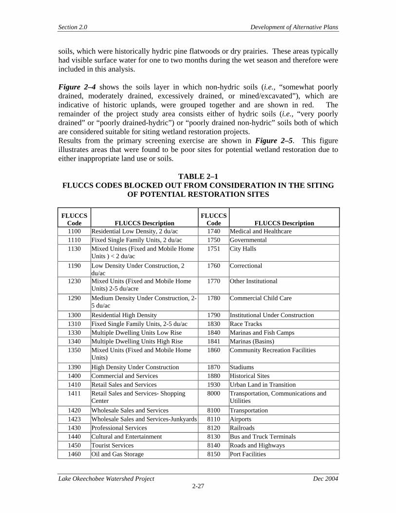
Section 2.0 Development of Alternative Plans
Lake Okeechobee Watershed Project Dec 2004 2-27
soils, which were historically hydric pine flatwoods or dry prairies. These areas typically had visible surface water for one to two months during the wet season and therefore were included in this analysis. Figure 2–4 shows the soils layer in which non-hydric soils (i.e., “somewhat poorly drained, moderately drained, excessively drained, or mined/excavated”), which are indicative of historic uplands, were grouped together and are shown in red. The remainder of the project study area consists either of hydric soils (i.e., “very poorly drained” or “poorly drained-hydric”) or “poorly drained non-hydric” soils both of which are considered suitable for siting wetland restoration projects. Results from the primary screening exercise are shown in Figure 2–5. This figure illustrates areas that were found to be poor sites for potential wetland restoration due to either inappropriate land use or soils.
TABLE 2–1 FLUCCS CODES BLOCKED OUT FROM CONSIDERATION IN THE SITING
OF POTENTIAL RESTORATION SITES FLUCCS
Code FLUCCS Description FLUCCS
Code FLUCCS Description 1100 Residential Low Density, 2 du/ac 1740 Medical and Healthcare 1110 Fixed Single Family Units, 2 du/ac 1750 Governmental 1130 Mixed Unites (Fixed and Mobile Home
Units ) < 2 du/ac 1751 City Halls
1190 Low Density Under Construction, 2 du/ac
1760 Correctional
1230 Mixed Units (Fixed and Mobile Home Units) 2-5 du/acre
1770 Other Institutional
1290 Medium Density Under Construction, 2-5 du/ac
1780 Commercial Child Care
1300 Residential High Density 1790 Institutional Under Construction 1310 Fixed Single Family Units, 2-5 du/ac 1830 Race Tracks 1330 Multiple Dwelling Units Low Rise 1840 Marinas and Fish Camps 1340 Multiple Dwelling Units High Rise 1841 Marinas (Basins) 1350 Mixed Units (Fixed and Mobile Home
Units) 1860 Community Recreation Facilities
1390 High Density Under Construction 1870 Stadiums 1400 Commercial and Services 1880 Historical Sites 1410 Retail Sales and Services 1930 Urban Land in Transition 1411 Retail Sales and Services- Shopping
Center 8000 Transportation, Communications and
Utilities 1420 Wholesale Sales and Services 8100 Transportation 1423 Wholesale Sales and Services-Junkyards 8110 Airports 1430 Professional Services 8120 Railroads 1440 Cultural and Entertainment 8130 Bus and Truck Terminals 1450 Tourist Services 8140 Roads and Highways 1460 Oil and Gas Storage 8150 Port Facilities
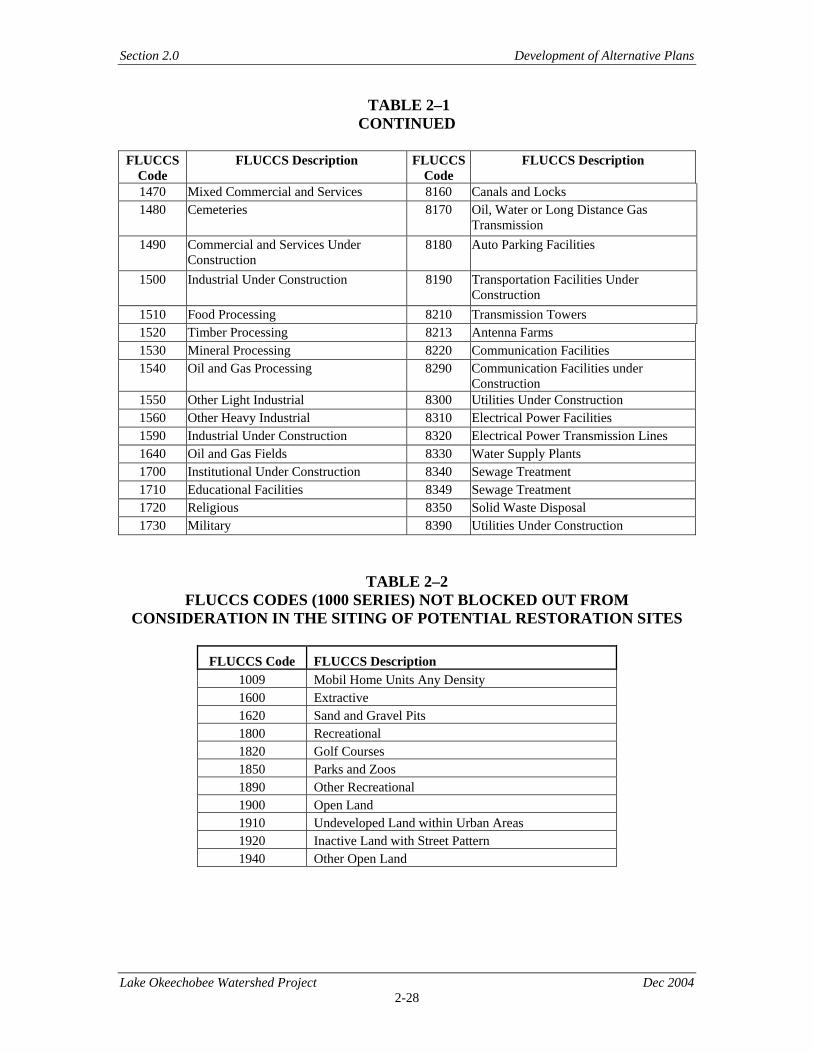
Section 2.0 Development of Alternative Plans
Lake Okeechobee Watershed Project Dec 2004 2-28
TABLE 2–1 CONTINUED
FLUCCS
Code FLUCCS Description FLUCCS
Code FLUCCS Description
1470 Mixed Commercial and Services 8160 Canals and Locks 1480 Cemeteries 8170 Oil, Water or Long Distance Gas
Transmission 1490 Commercial and Services Under
Construction 8180 Auto Parking Facilities
1500 Industrial Under Construction 8190 Transportation Facilities Under Construction
1510 Food Processing 8210 Transmission Towers 1520 Timber Processing 8213 Antenna Farms 1530 Mineral Processing 8220 Communication Facilities 1540 Oil and Gas Processing 8290 Communication Facilities under
Construction 1550 Other Light Industrial 8300 Utilities Under Construction 1560 Other Heavy Industrial 8310 Electrical Power Facilities 1590 Industrial Under Construction 8320 Electrical Power Transmission Lines 1640 Oil and Gas Fields 8330 Water Supply Plants 1700 Institutional Under Construction 8340 Sewage Treatment 1710 Educational Facilities 8349 Sewage Treatment 1720 Religious 8350 Solid Waste Disposal 1730 Military 8390 Utilities Under Construction
TABLE 2–2 FLUCCS CODES (1000 SERIES) NOT BLOCKED OUT FROM
CONSIDERATION IN THE SITING OF POTENTIAL RESTORATION SITES
FLUCCS Code FLUCCS Description 1009 Mobil Home Units Any Density 1600 Extractive 1620 Sand and Gravel Pits 1800 Recreational 1820 Golf Courses 1850 Parks and Zoos 1890 Other Recreational 1900 Open Land 1910 Undeveloped Land within Urban Areas 1920 Inactive Land with Street Pattern 1940 Other Open Land

Sect
ion
2.0
Dev
elop
men
t of A
ltern
ativ
e Pl
ans
Lake
Oke
echo
bee
Wat
ersh
ed P
roje
ct
D
ec 2
004
2-29
FIG
UR
E 2
–3
AR
EA
S W
ITH
LA
ND
USE
S T
HA
T A
RE
NO
T C
ON
DU
CIV
E T
O W
ET
LA
ND
RE
STO
RA
TIO
N
Not
es: 1.
Are
as in
bla
ck r
epre
sent
FLU
CC
S co
des
in th
e 10
00 (
Urb
an, R
esid
entia
l, &
Com
mer
cial
) an
d th
e 80
00 (
Tran
spor
tatio
n, C
omm
unic
atio
n &
Util
ities
) se
ries,
with
few
exc
eptio
ns.
2.
Bla
ck h
atch
ed a
rea
repr
esen
ts th
e B
right
on S
emin
ole
Res
erva
tion.

Sect
ion
2.0
Dev
elop
men
t of A
ltern
ativ
e Pl
ans
Lake
Oke
echo
bee
Wat
ersh
ed P
roje
ct
D
ec 2
004
2-30
FIG
UR
E 2
–4
AR
EA
S W
ITH
SO
IL T
YPE
S T
HA
T A
RE
NO
T C
ON
DU
CIV
E T
O W
ET
LA
ND
RE
STO
RA
TIO
N
N
otes
: 1.
Are
as in
red
repr
esen
t non
-hyd
ric so
ils.
2.
B
lack
hat
ched
are
a re
pres
ents
the
Brig
hton
Sem
inol
e R
eser
vatio
n.
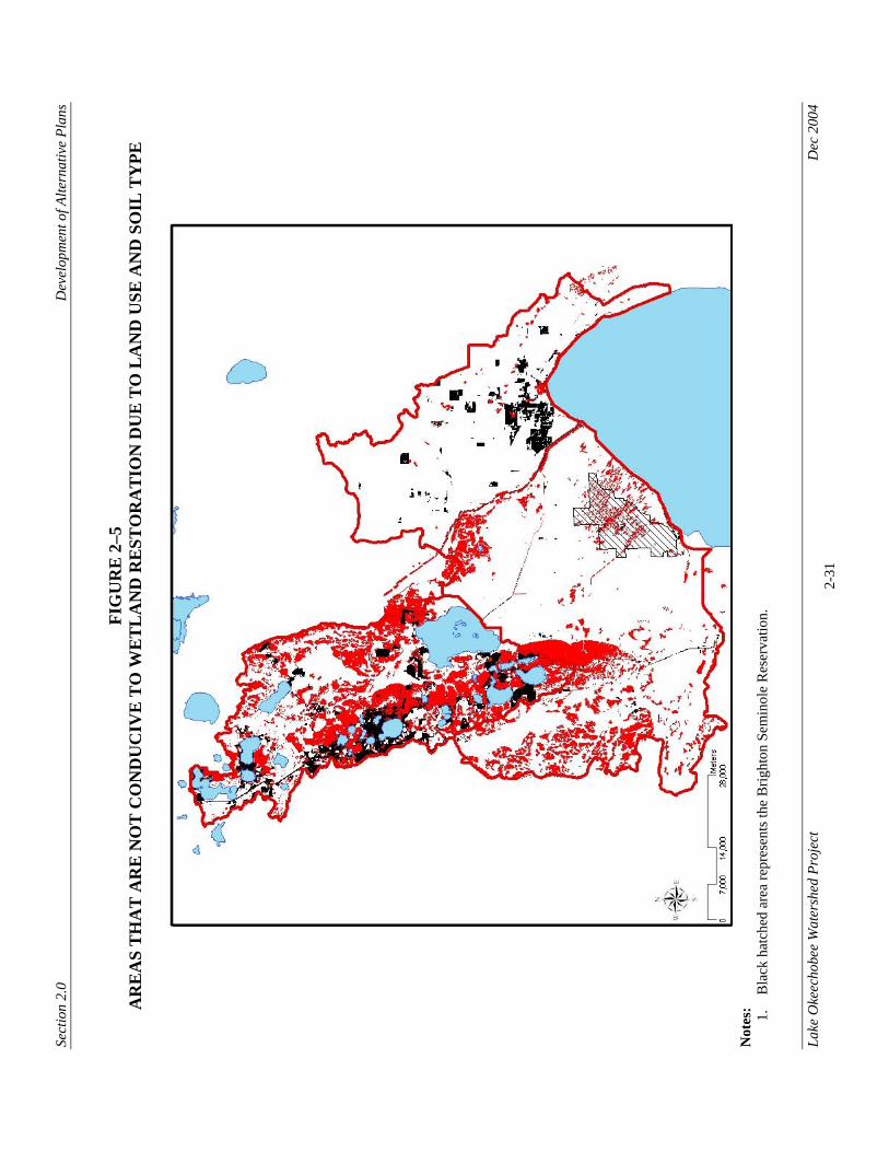
Sect
ion
2.0
Dev
elop
men
t of A
ltern
ativ
e Pl
ans
Lake
Oke
echo
bee
Wat
ersh
ed P
roje
ct
D
ec 2
004
2-31
FIG
UR
E 2
–5
AR
EA
S T
HA
T A
RE
NO
T C
ON
DU
CIV
E T
O W
ET
LA
ND
RE
STO
RA
TIO
N D
UE
TO
LA
ND
USE
AN
D S
OIL
TY
PE
N
otes
: 1.
Bla
ck h
atch
ed a
rea
repr
esen
ts th
e B
right
on S
emin
ole
Res
erva
tion.

Section 2.0 Development of Alternative Plans
Lake Okeechobee Watershed Project Dec 2004 2-32
2.1.5.4 Secondary Screening Factors The second phase in the potential restoration site selection process involved utilizing a series of secondary screening factors to further examine the results obtained from the primary screening process. The method and results from the secondary screening process are presented below. 2.1.5.4.1 Secondary Screening Methodology Five secondary screening factors were identified and for each of the five screening factors, attributes were developed for assigning high level of suitability (Level 1), moderate level of suitability (Level 2), or low level of suitability (Level 3). To facilitate the application of the screening factors and for easy interpretation of the results, suitability attributes for each factor were incorporated into a Land Suitability Model (Wetland Iteration), which was similar to the RASTA LSM described previously in Section 4.1.2.1. The Wetland LSM was then run to identify sites in the project study area with the least amount of constraints for siting wetland restoration projects. Table 2–3 lists the secondary screening factors and the suitability attributes incorporated into the Wetland LSM. Ecological Value – The rationale for selecting this screening factor was based on Siting Rule No. 8 (potential wetland restoration projects should avoid or minimize adverse impacts to high-quality ecological lands) and No.3 (potential wetland restoration projects should target degraded areas in order to maximize lift). The input data layer for this factor was based on FLUCCS Level 4 land use codes. Using best professional judgment, each cover type was given a suitability score (ranging from a low of zero to a maximum of ten) based on its ecological value to fish and wildlife. Areas with a score of zero provide few ecological benefits to fish and wildlife; whereas areas with a score of ten provide many benefits to fish and wildlife. Because the primary intention was to avoid using high-quality areas for wetland restoration, FLUCCS codes with an ecological score of 0-3 were assigned a high suitability (Level 1), 4-6 were deemed to be moderately suitable (Level 2), and 7-10 were assigned low suitability (Level 3). In general, native cover types scored high and within these, rare ecological communities scored the highest. In contrast, impacted lands such as high-intensity agricultural lands scored the lowest. Ecological value scores associated with various FLUCCS codes are summarized in Attachment B.
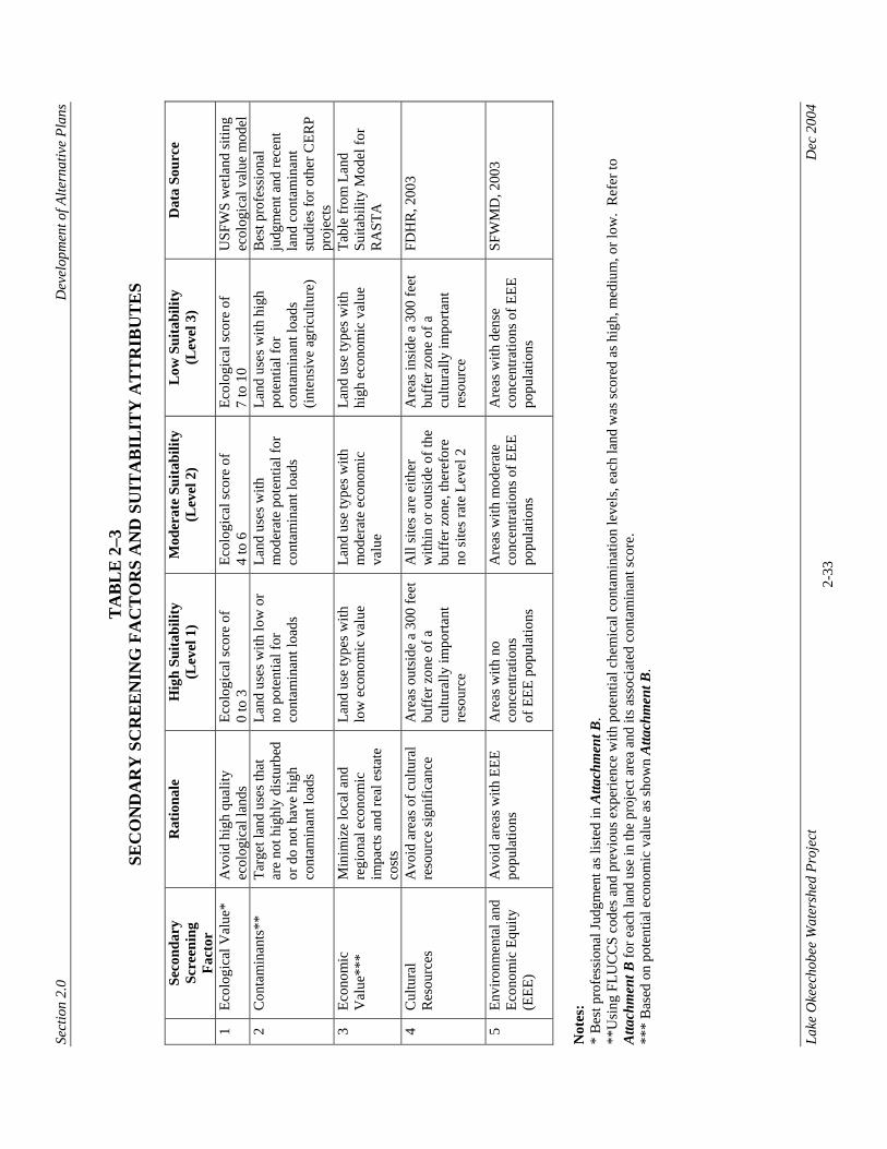
Sect
ion
2.0
Dev
elop
men
t of A
ltern
ativ
e Pl
ans
Lake
Oke
echo
bee
Wat
ersh
ed P
roje
ct
D
ec 2
004
2-33
TA
BL
E 2
–3
SEC
ON
DA
RY
SC
RE
EN
ING
FA
CT
OR
S A
ND
SU
ITA
BIL
ITY
AT
TR
IBU
TE
S
Seco
ndar
y Sc
reen
ing
Fact
or
Rat
iona
le
H
igh
Suita
bilit
y (L
evel
1)
Mod
erat
e Su
itabi
lity
(Lev
el 2
) L
ow S
uita
bilit
y (L
evel
3)
Dat
a So
urce
1 Ec
olog
ical
Val
ue*
Avo
id h
igh
qual
ity
ecol
ogic
al la
nds
Ecol
ogic
al sc
ore
of
0 to
3
Ecol
ogic
al sc
ore
of
4 to
6
Ecol
ogic
al sc
ore
of
7 to
10
USF
WS
wet
land
sitin
g ec
olog
ical
val
ue m
odel
2
Con
tam
inan
ts**
Ta
rget
land
use
s tha
t ar
e no
t hig
hly
dist
urbe
d or
do
not h
ave
high
co
ntam
inan
t loa
ds
Land
use
s with
low
or
no p
oten
tial f
or
cont
amin
ant l
oads
Land
use
s with
m
oder
ate
pote
ntia
l for
co
ntam
inan
t loa
ds
Land
use
s with
hig
h po
tent
ial f
or
cont
amin
ant l
oads
(in
tens
ive
agric
ultu
re)
Bes
t pro
fess
iona
l ju
dgm
ent a
nd re
cent
la
nd c
onta
min
ant
stud
ies f
or o
ther
CER
P pr
ojec
ts
3 Ec
onom
ic
Val
ue**
* M
inim
ize
loca
l and
re
gion
al e
cono
mic
im
pact
s and
real
est
ate
cost
s
Land
use
type
s with
lo
w e
cono
mic
val
ue
Land
use
type
s with
m
oder
ate
econ
omic
va
lue
Land
use
type
s with
hi
gh e
cono
mic
val
ue
Tabl
e fr
om L
and
Suita
bilit
y M
odel
for
RA
STA
4 C
ultu
ral
Res
ourc
es
Avo
id a
reas
of c
ultu
ral
reso
urce
sign
ifica
nce
Are
as o
utsi
de a
300
feet
bu
ffer
zon
e of
a
cultu
rally
impo
rtant
re
sour
ce
All
site
s are
eith
er
with
in o
r out
side
of t
he
buff
er z
one,
ther
efor
e no
site
s rat
e Le
vel 2
Are
as in
side
a 3
00 fe
et
buff
er z
one
of a
cu
ltura
lly im
porta
nt
reso
urce
FDH
R, 2
003
5 En
viro
nmen
tal a
nd
Econ
omic
Equ
ity
(EEE
)
Avo
id a
reas
with
EEE
po
pula
tions
A
reas
with
no
conc
entra
tions
of
EEE
pop
ulat
ions
Are
as w
ith m
oder
ate
conc
entra
tions
of E
EE
popu
latio
ns
Are
as w
ith d
ense
co
ncen
tratio
ns o
f EEE
po
pula
tions
SFW
MD
, 200
3
Not
es:
* B
est p
rofe
ssio
nal J
udgm
ent a
s lis
ted
in A
ttach
men
t B.
**U
sing
FLU
CC
S co
des a
nd p
revi
ous e
xper
ienc
e w
ith p
oten
tial c
hem
ical
con
tam
inat
ion
leve
ls, e
ach
land
was
scor
ed a
s hig
h, m
ediu
m, o
r low
. R
efer
to
Atta
chm
ent B
for e
ach
land
use
in th
e pr
ojec
t are
a an
d its
ass
ocia
ted
cont
amin
ant s
core
. **
* B
ased
on
pote
ntia
l eco
nom
ic v
alue
as s
how
n A
ttach
men
t B.
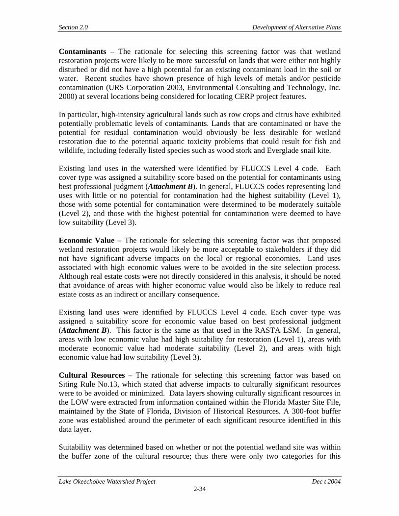
Section 2.0 Development of Alternative Plans
Lake Okeechobee Watershed Project Dec t 2004 2-34
Contaminants – The rationale for selecting this screening factor was that wetland restoration projects were likely to be more successful on lands that were either not highly disturbed or did not have a high potential for an existing contaminant load in the soil or water. Recent studies have shown presence of high levels of metals and/or pesticide contamination (URS Corporation 2003, Environmental Consulting and Technology, Inc. 2000) at several locations being considered for locating CERP project features. In particular, high-intensity agricultural lands such as row crops and citrus have exhibited potentially problematic levels of contaminants. Lands that are contaminated or have the potential for residual contamination would obviously be less desirable for wetland restoration due to the potential aquatic toxicity problems that could result for fish and wildlife, including federally listed species such as wood stork and Everglade snail kite. Existing land uses in the watershed were identified by FLUCCS Level 4 code. Each cover type was assigned a suitability score based on the potential for contaminants using best professional judgment (Attachment B). In general, FLUCCS codes representing land uses with little or no potential for contamination had the highest suitability (Level 1), those with some potential for contamination were determined to be moderately suitable (Level 2), and those with the highest potential for contamination were deemed to have low suitability (Level 3). Economic Value – The rationale for selecting this screening factor was that proposed wetland restoration projects would likely be more acceptable to stakeholders if they did not have significant adverse impacts on the local or regional economies. Land uses associated with high economic values were to be avoided in the site selection process. Although real estate costs were not directly considered in this analysis, it should be noted that avoidance of areas with higher economic value would also be likely to reduce real estate costs as an indirect or ancillary consequence. Existing land uses were identified by FLUCCS Level 4 code. Each cover type was assigned a suitability score for economic value based on best professional judgment (Attachment B). This factor is the same as that used in the RASTA LSM. In general, areas with low economic value had high suitability for restoration (Level 1), areas with moderate economic value had moderate suitability (Level 2), and areas with high economic value had low suitability (Level 3). Cultural Resources – The rationale for selecting this screening factor was based on Siting Rule No.13, which stated that adverse impacts to culturally significant resources were to be avoided or minimized. Data layers showing culturally significant resources in the LOW were extracted from information contained within the Florida Master Site File, maintained by the State of Florida, Division of Historical Resources. A 300-foot buffer zone was established around the perimeter of each significant resource identified in this data layer. Suitability was determined based on whether or not the potential wetland site was within the buffer zone of the cultural resource; thus there were only two categories for this

Section 2.0 Development of Alternative Plans
Lake Okeechobee Watershed Project Dec t 2004 2-35
factor, high or low. Areas of high suitability were outside the 300-foot buffer (Level 1); areas of low suitability (Level 3) were located within 300 feet of a culturally significant resource. Environmental and Economic Equity (EEE) – The rationale for selecting this screening factor was based on Siting Rule No.14 which stated that siting of wetland restoration projects should achieve environmental justice by avoiding or minimizing adverse impacts to EEE populations. Data layers showing locations of EEE populations in the watershed were obtained from the SFWMD. Areas with no EEE populations were considered highly suitable (Level 1) for siting wetland restoration projects, areas with moderate concentrations of EEE populations were considered to be moderately suitable (Level 2), and areas with dense concentrations of EEE populations were assigned a low suitability (Level 3). 2.1.5.4.2 Wetland Land Suitability Model (LSM) Scoring Based on the suitability attributes assigned for each of the secondary screening factors, the Wetland LSM generated a composite summary score for each 30 m x 30 m pixel within the project study area. In essence, the Wetland LSM classified different portions of the project study area from poor (very low suitability for siting wetland restoration projects) to very good (high suitability for siting wetland restoration projects). Composite Wetland LSM scores ranged from 1 to 5 based on the following scale: • Score = 1; Very good. All five secondary screening factors scored as Level 1; • Score = 2; Good. One screening factor scored as Level 2, the remainder scored as
Level 1; • Score = 3; Moderate. Two screening factors scored as Level 2, the remainder scored
as Level 1; • Score = 4; Marginal. Three or more screening factors scored as Level 2, the
remainder scored as Level 1; and • Score = 5; Poor. One or more screening factors scored as Level 3. The Wetland LSM output is shown in Figure 2–6.
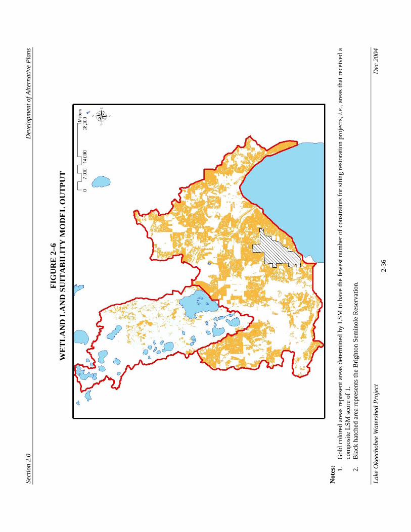
Sect
ion
2.0
Dev
elop
men
t of A
ltern
ativ
e Pl
ans
Lake
Oke
echo
bee
Wat
ersh
ed P
roje
ct
D
ec 2
004
2-36
FIG
UR
E 2
–6
WE
TL
AN
D L
AN
D S
UIT
AB
ILIT
Y M
OD
EL
OU
TPU
T
N
otes
: 1.
Gol
d co
lore
d ar
eas
repr
esen
t are
as d
eter
min
ed b
y LS
M to
hav
e th
e fe
wes
t num
ber o
f con
stra
ints
for s
iting
rest
orat
ion
proj
ects
, i.e
., ar
eas
that
rece
ived
a
com
posi
te L
SM sc
ore
of 1
. 2.
B
lack
hat
ched
are
a re
pres
ents
the
Brig
hton
Sem
inol
e R
eser
vatio
n.
Section 2.0 Development of Alternative Plans
Lake Okeechobee Watershed Project Dec 2004 2-37
2.1.5.4.3 Application of Secondary Screening Methodology Using ArcGIS software, each 30 m x 30 m pixel was color coded based on its composite Wetland LSM score with the exception of those pixels within the primary screening factor for land use (i.e., areas considered not conducive to wetland restoration, Section 4.3.4.3.). Then, by displaying the soils primary screening factor simultaneously with the composite Wetland LSM scores, potential restoration sites were drawn around areas that had a high percentage of historic or existing wetland soils, while simultaneously avoiding or minimizing impacts to marginal or poor suitability areas based on the secondary screening factors. These sites represented best options for siting potential restoration projects. In accordance with Siting Rules No.4 and No.12, public lands were generally avoided during the selection process. Polygons were drawn immediately adjacent to public areas where possible and appropriate. Areas identified as potential Florida Forever Projects however, were incorporated into the potential restoration sites, wherever appropriate, because these lands have not yet been purchased. Finally, boundaries of the potential restoration sites were modified based on local knowledge about hydrologic features and patterns such as more specific land use, flooding, elevation, real estate boundaries, and water management measures implemented, etc. One hundred and six potential restoration sites (Figure 2–7) were identified in the LOW through the application of the primary screening process and secondary screening factors.
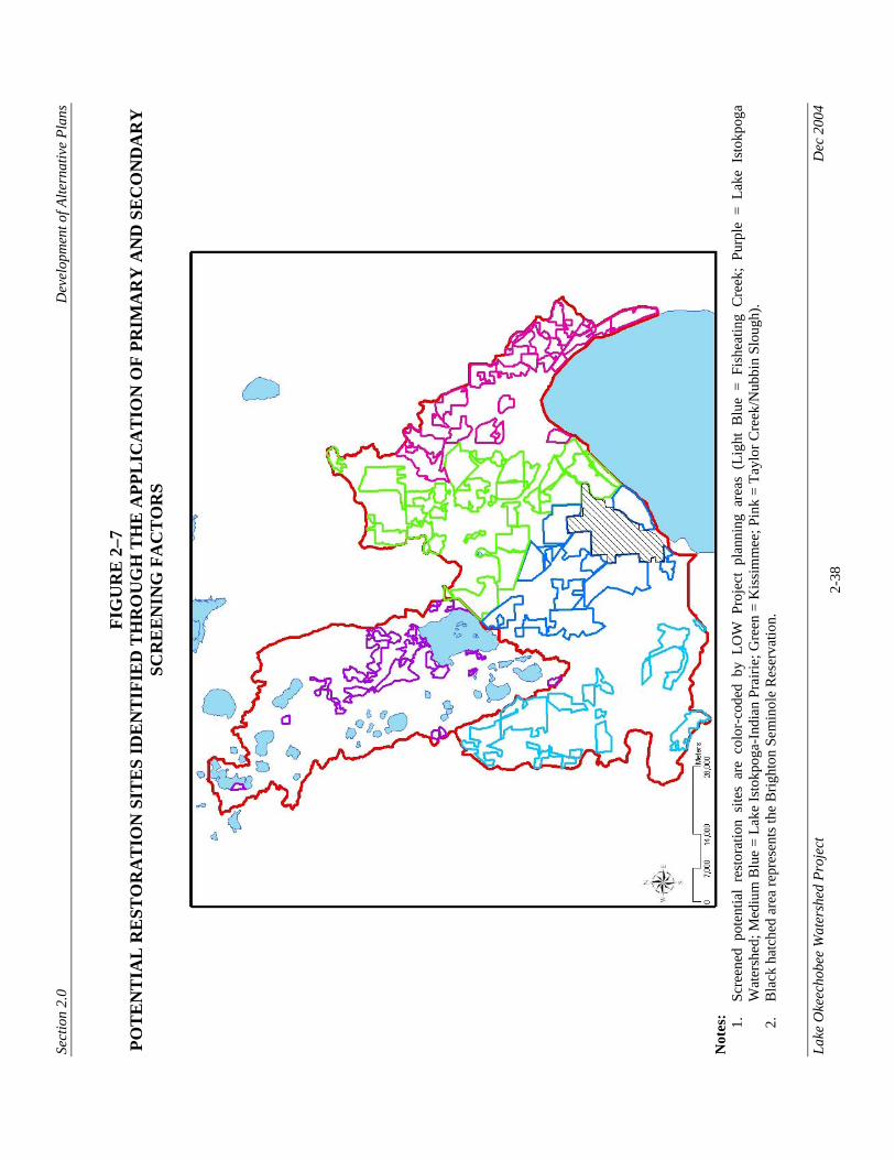
Sect
ion
2.0
Dev
elop
men
t of A
ltern
ativ
e Pl
ans
Lake
Oke
echo
bee
Wat
ersh
ed P
roje
ct
D
ec 2
004
2-38
FIG
UR
E 2
–7
POT
EN
TIA
L R
EST
OR
AT
ION
SIT
ES
IDE
NT
IFIE
D T
HR
OU
GH
TH
E A
PPL
ICA
TIO
N O
F PR
IMA
RY
AN
D S
EC
ON
DA
RY
SC
RE
EN
ING
FA
CT
OR
S
N
otes
: 1.
Scre
ened
pot
entia
l re
stor
atio
n si
tes
are
colo
r-co
ded
by L
OW
Pro
ject
pla
nnin
g ar
eas
(Lig
ht B
lue
= Fi
shea
ting
Cre
ek;
Purp
le =
Lak
e Is
tokp
oga
Wat
ersh
ed; M
ediu
m B
lue
= La
ke Is
tokp
oga-
Indi
an P
rairi
e; G
reen
= K
issi
mm
ee; P
ink
= Ta
ylor
Cre
ek/N
ubbi
n Sl
ough
). 2.
B
lack
hat
ched
are
a re
pres
ents
the
Brig
hton
Sem
inol
e R
eser
vatio
n.
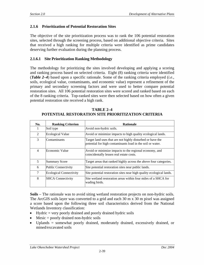
Section 2.0 Development of Alternative Plans
Lake Okeechobee Watershed Project Dec 2004 2-39
2.1.6 Prioritization of Potential Restoration Sites The objective of the site prioritization process was to rank the 106 potential restoration sites, selected through the screening process, based on additional objective criteria. Sites that received a high ranking for multiple criteria were identified as prime candidates deserving further evaluation during the planning process. 2.1.6.1 Site Prioritization Ranking Methodology The methodology for prioritizing the sites involved developing and applying a scoring and ranking process based on selected criteria. Eight (8) ranking criteria were identified (Table 2–4) based upon a specific rationale. Some of the ranking criteria employed (i.e., soils, ecological value, contaminants, and economic value) represent a refinement of the primary and secondary screening factors and were used to better compare potential restoration sites. All 106 potential restoration sites were scored and ranked based on each of the 8 ranking criteria. Top-ranked sites were then selected based on how often a given potential restoration site received a high rank.
TABLE 2–4 POTENTIAL RESTORATION SITE PRIORITIZATION CRITERIA
No. Ranking Criterion Rationale 1 Soil type Avoid non-hydric soils.
2 Ecological Value Avoid or minimize impacts to high quality ecological lands.
3 Contaminants Target land uses that are not highly disturbed or have the potential for high contaminants load in the soil or water.
4 Economic Value Avoid or minimize impacts to the regional economy, and coincidentally lessen real estate costs.
5 Summary Score Target areas that ranked highly across the above four categories.
6 Public Connectivity Site potential restoration sites near public lands.
7 Ecological Connectivity Site potential restoration sites near high quality ecological lands.
8 SHCA Connectivity Site wetland restoration areas within four miles of a SHCA for wading birds.
Soils – The rationale was to avoid siting wetland restoration projects on non-hydric soils. The ArcGIS soils layer was converted to a grid and each 30 m x 30 m pixel was assigned a score based upon the following three soil characteristics derived from the National Wetlands Inventory classification: • Hydric = very poorly drained and poorly drained hydric soils • Mesic = poorly drained non-hydric soils • Uplands = somewhat poorly drained, moderately drained, excessively drained, or
mined/excavated soils

Section 2.0 Development of Alternative Plans
Lake Okeechobee Watershed Project Dec 2004 2-40
The ArcGIS soils layer was clipped to the individual potential restoration site identified through the Wetland LSM in order to determine the number of acres of each soil category within the potential restoration site. The percentage of each soil category within the potential restoration site was then determined and the percentages were converted to a score based on the following: • Percentage of hydric soils divided by 100 times 3, • Percentage of mesic soils divided by 100 times 2, and • Percentage of uplands soils divided by 100 times 1. Values for the three soil types were averaged into a single score that was rounded to the nearest hundredth. For example, a 1,000-acre potential restoration site with 650 acres of hydric soils, 200 acres of mesic soils, and 150 acres of upland soils was scored as follows: Step 1 650/1000 x 100 = 65% Hydric 200/1000 x 100 = 20% Mesic 150/1000 x 100 = 15% Upland Step 2 Hydric: 65/100 x 3 = 1.95 Mesic: 20/100 x 2 = 0.40 Upland: 15/100 x 1 = 0.15 Average soils score for the given site = (1.95 + 0.40 + 0.15)/3 = 0.83 Average soils scores for the 106 potential restoration sites are shown in Attachment C. Ecological Value – The rationale for selecting this criterion was to avoid or minimize impacts to high quality ecological lands (Siting Rule No.8). The Ecological Suitability ArcGIS layer created for the Wetland LSM was used to determine the ecological value score for each potential restoration site. Lands with high ecological value were scored as having low suitability for potential wetland restoration (Siting Rule No.3) – i.e., more ecological lift is better. Therefore, FLUCCS codes with an ecological value score of 0-3 (low ecological value) were rated as being highly suitable for restoration, FLUCCS codes with an ecological value score of 4-6 (moderate ecological value) were rated as moderately suitable for restoration, and FLUCCS codes with a score of 7-10 (high ecological value) were rated as having low restoration suitability. This ArcGIS ecological value layer was clipped to the individual sites and the number of acres of each of the three ecological value scores (i.e., high, moderate and low) was determined. Percentages of each category within each potential restoration site were also calculated and then converted to a score as follows: • Percentage of site with high ecologic value divided by 100 times 1;
Section 2.0 Development of Alternative Plans
Lake Okeechobee Watershed Project Dec 2004 2-41
• Percentage of site with moderate ecological value divided by 100 times 2; and • Percentage of site with low ecological value divided by 100 times 3. Values for the three ecological types were averaged into a single score then rounded to the nearest hundredth. For example, a 1,000-acre potential restoration site with 150 acres rated as high ecological value, 200 acres as moderate ecological value, and 650 acres as low ecological value was scored as follows: Step 1 150/1000 x 100 = 15% High 200/1000 x 100 = 20% Moderate 650/1000 x 100 = 65% Low Step 2 High: 15/100 x 1 = 0.15 Moderate 20/100 x 2 = 0.40 Low 65/100 x 3 = 1.95 Average ecological score for the given site = (0.15 + 0.40 + 1.95)/3 = 0.83 Average ecological scores of the 106 potential restoration sites are shown in Attachment C. Contaminants – The rationale was to target land uses that are not highly disturbed or that do not have the potential for high contaminant load in the soil or water. The Contaminant Suitability ArcGIS layer created for the Wetland LSM Model was used to determine the contaminant score for each potential restoration site. This layer was clipped to the individual potential restoration sites and the number of acres of each of the three contaminant suitability attribute levels (i.e., high, moderate and low) was determined. The percentage of each category within each site was calculated and the percentages were then converted into a score as follows: • Percentage of site with high probability of contaminants divided by 100 times 1; • Percentage of site with moderate probability of contaminants divided by 100 times 2; • Percentage of site with low probability of contaminants divided by 100 times 3. The three values were averaged and rounded to the nearest hundredth to come up with a mean contaminant score for each potential restoration site. For example, a 1,000-acre potential restoration site with 150 acres rated as having high potential for contaminants, 200 acres rated as having moderate potential for contaminants, and 650 acres rated as having low potential for contaminants was scored as follows: Step 1 150/1000 x 100 = 15% High 200/1000 x 100 = 20% Moderate 650/1000 x 100 = 65% Low
Section 2.0 Development of Alternative Plans
Lake Okeechobee Watershed Project Dec 2004 2-42
Step 2 High: 15/100 x 1 = 0.15 Moderate 20/100 x 2 = 0.40 Low 65/100 x 3 = 1.95 Average contaminant score for the given site = (0.15 + 0.40 + 1.95)/3 = 0.83 Average contaminant scores for the 106 potential restoration sites are presented in Attachment C. Economic Value – The rationale was to avoid or minimize impacts to the local and regional economies, and coincidentally lessen real estate costs. The Economic Suitability ArcGIS layer created for the Wetland LSM was used to determine the ecological value score for each potential restoration site. This layer was clipped to the individual potential restoration sites and the number of acres within the site that corresponded to the three economic value attributes (i.e., high, moderate and low) was calculated. Based upon these acreage calculations, the percentage of each category within the potential restoration site was determined and the percentages were then converted into a score as follows: • Percentage of site with high economic value divided by 100 times 1; • Percentage of site with moderate economic value divided by 100 times 2; and • Percentage of site with low economic value divided by 100 times 3. The three values were averaged and rounded to the nearest hundredth to determine a mean economic value score for each potential restoration site. For example, a 1,000-acre potential restoration site with 150 acres rated as having high economic value, 200 acres rated as having moderate economic value, and 650 acres as having low economic value was scored as follows: Step 1 150/1000 x 100 = 15% High 200/1000 x 100 = 20% Moderate 650/1000 x 100 = 65% Low Step 2 High: 15/100 x 1 = 0.15 Moderate 20/100 x 2 = 0.40 Low 65/100 x 3 = 1.95 Average economic score for the given site = (0.15 + 0.40 + 1.95)/3 = 0.83 Average economic scores for the 106 potential restoration sites are shown in Attachment C.
Section 2.0 Development of Alternative Plans
Lake Okeechobee Watershed Project Dec 2004 2-43
Summary Scores – This score was included in order to weight the secondary screening factors and suitability attributes within the prioritization process. Based upon the siting rules (4.3.4.1) and best professional judgment these factors were determined to be significant contributing factors to successful wetland restoration. The summary score was developed for each of the 106 potential restoration sites by averaging the four mean site prioritization ranking criteria scores (i.e., soils, ecological value, contaminants, and economic value). Thus a potential restoration site with a soils score of 0.81, ecological value score of 0.82, contaminants score of 0.84, and an economic value score of 0.85 received a summary score of 0.83 {(0.81+0.82+0.84+0.85)/4}. Summary scores for the 106 potential restoration sites are shown in Attachment C. Public Lands Connectivity – The rationale was to site potential restoration sites, to the extent possible, contiguous with public lands since this would provide an ecological buffer for the proposed restoration project. Also, placing restored wetlands adjacent to public lands would lead to the formation of larger blocks of habitat that would serve as animal migration corridors and increase the likelihood that a diversity of habitat types would be available for species that have more complex lifecycles (e.g., terrestrial amphibians that need aquatic environments to reproduce). Corridors are thought to increase the exchange of individuals between habitat patches, promoting genetic exchange and reducing population fluctuations. In addition, corridors not only increase the exchange of animals between patches, but also facilitate two key plant-animal interactions: pollination and seed dispersal (Tewksbury et al. 2002). The beneficial effects of corridors extend beyond the area they add, and increased plant and animal movement through corridors have positive impacts on plant populations and community interactions in fragmented landscapes (Tewksbury et al. 2002). Data sources used for this analysis included those provided by FNAI (Florida Managed Lands and FFP layers), The Nature Conservancy (FLOW projects), FWC (mottled duck production area, wildlife management areas), and Natural Resources Conservation Service (Wetland Reserve Program easements). Total perimeter length of each potential restoration site and the percentage of that perimeter shared with public lands verses non-public lands was calculated and then the percentages were converted into a public connectivity score as follows: • Percentage of site adjacent to public lands divided by 100 times 1; • Percentage of site not connected to public lands divided by 100 times 0. The two values were averaged and rounded to the nearest hundredth to come up with a public connectivity score for each potential restoration site. As an example, a potential restoration site with a perimeter of 1,000 meters that borders 850 meters of public land and 150 meters of private land was scored as follows: Step 1 850/1000 x 100 = 85% Public Connectivity
Section 2.0 Development of Alternative Plans
Lake Okeechobee Watershed Project Dec 2004 2-44
150/1000 x 100 = 15% Private Connectivity Step 2 Public Connectivity: 85/100 x 1 = 0.85 Private Connectivity: 15/100 x 0 = 0.00 Average public connectivity scores for the given site = (0.85 + 0.00)/2 = 0.475 = 0.48 Average public connectivity scores for the 106 potential restoration sites are shown in Attachment C. Ecological Connectivity – The rationale was to site potential restoration areas near high quality ecological lands since this would provide substantial benefits to wildlife. Habitat patches surrounded by unfavorable land uses (i.e., urban, agricultural) behave like islands. These “island” populations are much more susceptible to problems associated with small population size. Furthermore, bird species diversity increases with size of the habitat patch in urban forests (Tilghman, 1987) and wetlands (Brown and Dinsmore, 1986). By siting potential restoration sites adjacent to high ecological value areas, the patch size effectively increases and the restored sites are more likely to be buffered from adverse ecological impacts then if they were surrounded by areas with low ecological values. Also, the formation of larger blocks of habitat provides animal migration corridors and increases the likelihood that a diversity of habitat types is available for species that have more complex lifecycles (e.g., terrestrial amphibians that spawn in water). Spatial data coverages for high ecological value areas were taken from the Wetland LSM ecological value layer. Areas with high ecological value (score of 7 to 10) were converted into a new ArcGIS layer for use in determining connectivity of potential restoration sites with high quality ecological areas. For each potential restoration site, perimeter length shared with areas of high, moderate and low ecological value was determined as a percentage of the total perimeter and the percentages were converted into an ecological connectivity score as follows: • Percentage of site adjacent to high ecological value areas divided by 100 times 3; • Percentage of site adjacent to moderate ecological value areas divided by 100 times 2; • Percentage of site adjacent to low ecological value areas divided by 100 times 1. The three values were averaged and rounded to the nearest hundredth to establish an ecological connectivity score for each potential restoration site. For example: A potential restoration site with a total perimeter of 5,000 meters, of which 3,250 meters are shared with high ecological value area, 1,000 meters are shared with moderate ecological value area, and 750 meters are shared with low ecological value area was scored as follows:
Section 2.0 Development of Alternative Plans
Lake Okeechobee Watershed Project Dec 2004 2-45
Step 1 3250/5000 x 100 = 65% High 1000/5000 x 100 = 20% Moderate 750/5000 x 100 = 15% Low Step 2 High: 65/100 x 3 = 1.95 Moderate 20/100 x 2 = 0.40 Low 15/100 x 1 = .15 Average ecological connectivity score for the given site = (1.95 + 0.40 + 0.15)/3 = 0.83 Average ecological connectivity scores for the 106 potential restoration sites are shown in Attachment C. Strategic Habitat Conservation Area (SHCA) Connectivity – The rationale was to site potential restoration areas within 4 miles of a SHCA for wading birds. One of the objectives of the CERP is to support the return of large nesting rookeries of wading birds. Wading birds (e.g., herons, egrets, ibis, and storks) are symbolic of the overall health of south Florida. Wading birds, perhaps more than any other animal, assess the quality of habitats over the entire basin of south Florida wetlands, before making “decisions” about where and when, or even whether, to nest. The recovery of the wading bird colonies will be a sure sign that the entire ecosystem has made substantial progress towards recovery (USACE 1999). ArcGIS data layer created by Cox et al. (1994) of SHCAs for wading birds was used as the input layer. This layer includes wetlands important to the breeding success of eight species of wading birds including wood stork, white ibis (Eudocimus albus), little blue heron (Egretta caerulea), tricolored heron (Egretta tricolor), snowy egret (Egretta thula), great egret (Casmerodius albus), reddish egret (Egretta rufescens), and roseate spoonbill (Ajaia ajaja). Cox et al. (1994) had generated buffers around nesting colonies based upon the maximum distances that each of the eight species would travel from the colony to a foraging area (Custer and Osborn, 1978; Frederick and Collopy, 1988; Bancroft et al., 1990). These distances varied among species; for example, the majority of the wading birds would travel a distance of approximately 15 km, while wood storks would travel up to 30 km, but reddish egrets would only travel a distance of 10 km. A four-mile buffer zone (approximately equal to the 10 km minimum distance in Cox et al. 1994) around each potential restoration site was judged to be adequate for this criterion. In order to be conservative, the buffer was based upon the smallest maximum distance that a wading bird would travel from the colony to a foraging site. GIS coverages were reviewed visually to determine whether a SHCA was either within a potential restoration site, within the 4-mile buffer, or outside the 4-mile buffer and scores were assigned to each potential restoration site as follows: • SHCA contained within the site = 3
Section 2.0 Development of Alternative Plans
Lake Okeechobee Watershed Project Dec 2004 2-46
• SHCA located within the 4-mile buffer zone = 2 • SHCA located outside the 4-mile buffer zone = 1 An “average” SHCA score was then calculated by dividing the SHCA score by 3. For example: • SHCA contained within the site – average score = 3/3 = 1 • SHCA located within the 4-mile buffer zone – average score = 2/3 = 0.67 • SHCA located outside the 4-mile buffer zone – average score = 1/3 = 0.33 Each potential restoration site was then ranked based on its average connectivity to the wading bird SHCA score. These ranking are shown in Attachment C. 2.1.6.2 Application of Site Prioritization Ranking Methodology All 106 potential restoration sites were ranked by each of the eight ranking criteria described above and the rankings were tabulated in a spreadsheet (refer to Attachment C). After examining the ranks, a potential ranking problem was noticed with the Contaminant Potential criterion. Many potential restoration sites received the maximum score of 1.0. In essence, it became difficult to separate those that scored well from those that scored less because there were too many top-ranked potential restoration sites. For example, the GIS software was able to measure extremely small differences in contaminant potential between potential restoration sites and did allow us to rank the potential restoration sites for contaminants. However, the scoring differences were so small that they were meaningless given the sensitivity of the siting process. For example the highest ranking potential restoration site received a contaminant potential score of 1.00. The 60th ranking potential restoration site received a score of 0.99517. Essentially, there is no difference between these two sites (or any others that ranked in between). Therefore, it was concluded that contaminant potential was not a good site delineator and it was removed from the prioritization analysis. However, the individual site scores for contaminant potential (see Attachment C) were maintained because they were used in calculating the summary suitability score. Furthermore, there were a few sites that scored poorly, and that information could be useful to the study team should any of those sites become available for acquisition. (Note: An earlier iteration of the ranking process had included contaminant potential as a criterion, and the subteam had selected some top-ranked potential restoration sites which underwent additional evaluation. However, when it became apparent that contaminant potential was not a good delineator, the ranking process was modified. As a result, four previously top-ranked potential restoration sites (F02, F14, T03 and T19) had their overall scores reduced to a point where they were no longer top-ranked. However, since the field data collection had already been conducted on these sites, they were carried through the next stage of the analysis and will serve as potential back-up sites for any of the higher ranked sites that may be eliminated during advanced planning stages).
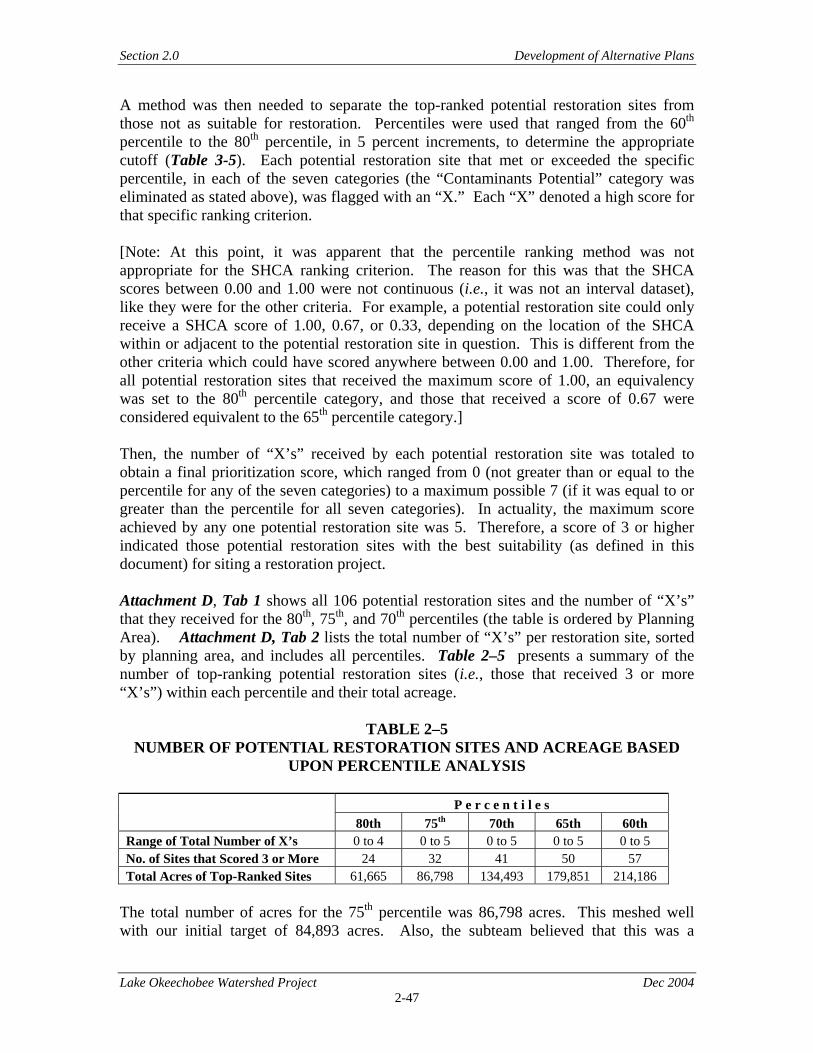
Section 2.0 Development of Alternative Plans
Lake Okeechobee Watershed Project Dec 2004 2-47
A method was then needed to separate the top-ranked potential restoration sites from those not as suitable for restoration. Percentiles were used that ranged from the 60th percentile to the 80th percentile, in 5 percent increments, to determine the appropriate cutoff (Table 3-5). Each potential restoration site that met or exceeded the specific percentile, in each of the seven categories (the “Contaminants Potential” category was eliminated as stated above), was flagged with an “X.” Each “X” denoted a high score for that specific ranking criterion. [Note: At this point, it was apparent that the percentile ranking method was not appropriate for the SHCA ranking criterion. The reason for this was that the SHCA scores between 0.00 and 1.00 were not continuous (i.e., it was not an interval dataset), like they were for the other criteria. For example, a potential restoration site could only receive a SHCA score of 1.00, 0.67, or 0.33, depending on the location of the SHCA within or adjacent to the potential restoration site in question. This is different from the other criteria which could have scored anywhere between 0.00 and 1.00. Therefore, for all potential restoration sites that received the maximum score of 1.00, an equivalency was set to the 80th percentile category, and those that received a score of 0.67 were considered equivalent to the 65th percentile category.] Then, the number of “X’s” received by each potential restoration site was totaled to obtain a final prioritization score, which ranged from 0 (not greater than or equal to the percentile for any of the seven categories) to a maximum possible 7 (if it was equal to or greater than the percentile for all seven categories). In actuality, the maximum score achieved by any one potential restoration site was 5. Therefore, a score of 3 or higher indicated those potential restoration sites with the best suitability (as defined in this document) for siting a restoration project. Attachment D, Tab 1 shows all 106 potential restoration sites and the number of “X’s” that they received for the 80th, 75th, and 70th percentiles (the table is ordered by Planning Area). Attachment D, Tab 2 lists the total number of “X’s” per restoration site, sorted by planning area, and includes all percentiles. Table 2–5 presents a summary of the number of top-ranking potential restoration sites (i.e., those that received 3 or more “X’s”) within each percentile and their total acreage.
TABLE 2–5 NUMBER OF POTENTIAL RESTORATION SITES AND ACREAGE BASED
UPON PERCENTILE ANALYSIS
P e r c e n t i l e s 80th 75th 70th 65th 60th Range of Total Number of X’s 0 to 4 0 to 5 0 to 5 0 to 5 0 to 5 No. of Sites that Scored 3 or More 24 32 41 50 57 Total Acres of Top-Ranked Sites 61,665 86,798 134,493 179,851 214,186
The total number of acres for the 75th percentile was 86,798 acres. This meshed well with our initial target of 84,893 acres. Also, the subteam believed that this was a
Section 2.0 Development of Alternative Plans
Lake Okeechobee Watershed Project Dec 2004 2-48
reasonable acreage and number of sites that could be analyzed in the time frame allotted. Therefore, the 75th percentile was used as the cutoff for identifying the top-ranked potential restoration sites. The additional nine potential restoration sites (which encompassed an additional 47,695 acres) that were top-ranked for the 70th percentile were characterized as potential back-up sites, should some of the 75th percentile sites become unavailable (refer to Attachment G). Of the 106 potential restoration sites ranked through this process, 32 received a score of 3 or higher (Figure 2–8). These top-ranked potential restoration sites were further evaluated in the planning process.
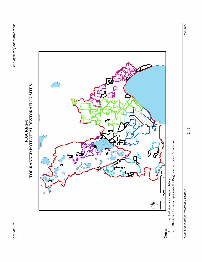
Sect
ion
2.0
Dev
elop
men
t of A
ltern
ativ
e Pl
ans
Lake
Oke
echo
bee
Wat
ersh
ed P
roje
ct
D
ec 2
004
2-49
FIG
UR
E 2
–8
TO
P-R
AN
KE
D P
OT
EN
TIA
L R
EST
OR
AT
ION
SIT
ES
N
otes
: 1.
Top
rank
ed si
tes a
re sh
own
in b
lack
. 2.
B
lack
hat
ched
are
a re
pres
ents
the
Brig
hton
Sem
inol
e R
eser
vatio
n.
Section 2.0 Development of Alternative Plans
Lake Okeechobee Watershed Project Dec 2004 2-50
2.1.6.3 Sensitivity Analysis for Low-Ranking Potential Restoration Sites Another issue raised during the review of the site prioritization methodology and results was the impact of the boundaries drawn around each potential restoration site. In other words, “What was the likelihood that any given potential restoration site would have scored higher if it was redrawn differently (and presumably could have better suitability)?” In essence, the review team wanted to know how sensitive the method was to changes at the desk-top level that could result in a potential restoration site being inappropriately excluded from the top-ranked sites. To answer this question, the planning team visually evaluated the scoring pattern of each ranking criterion within each of the 78 potential restoration sites that received a total score of 2, 1, or zero (the top-ranked sites received scores of 3 to 5). Figure 2–9 shows an example of a potential restoration site (T-13) and some of its relevant suitability metric patterns. This potential restoration site exhibited patterns of mostly moderate suitability scores (gold color in Figure 2–9) interspersed with lesser areas of good scores (yellow) for soils and economic value metrics. The ecological value metric showed mostly good scores with some interspersed poor scores (brown). This potential restoration site also exhibited a small poor suitability area for cultural resources in the southern portion; however, this was not included in the top-ranking process. The other metrics (EEE and contaminants potential) had good scores throughout. Therefore, after the evaluation of metric patterns, it was decided that it was there was no way to alter the size or shape of T-13 to improve its overall score. Most of the other potential restoration sites showed similar patterns. However, there were eight potential restoration sites that indicated a possibility for better scoring with boundary alterations (F-04, IP-05, IP-07, IP-08, K-20, LI-04, LI-20, and T-09). Table 2–6 lists the potential restoration sites that scored a 2, 1, or zero and their metrics that scored poorly. F-04 received an overall suitability score of 2. This potential restoration site scored low due to some poor ecological value scores and moderate economic value scores throughout. The patterns indicated that if the site was redrawn to eliminate the 1,500 acres of poor-scoring ecological value areas, that this potential restoration site would then be above the 75th percentile for that metric, and as such, would have received an overall score of 3. This new 7,145-acre potential restoration site will be further analyzed during the upcoming additional evaluation process. IP-05 received an overall suitability score of two. This 5,672- acre potential restoration site scored low due moderate economic value scores throughout and some poor ecological suitability scores in the southwest corner. If the poorly suited ecological areas were eliminated (approximately 1000 acres), then this potential restoration site would receive an overall suitability score of 3. As such, it will be evaluated in the additional upcoming additional evaluation process.
Section 2.0 Development of Alternative Plans
Lake Okeechobee Watershed Project Dec 2004 2-51
IP-07 received an overall suitability score of one. This potential restoration site scored low due to poor and moderate soil suitability scores, some poor ecological value scores, and moderate economic value scores (see Figure 2–10). However, this 7,277-acre potential restoration site could be redrawn as a 2,500-acre site on the eastern half around the 270-acre Wetland Restoration Program (WRP) easement parcel. If so, it would still have some poor ecologic value scores. However, the reconfigured IP-07 would likely have received a higher soils rank which should have resulted in an overall increased suitability score of 2. This would make this site an acceptable “back-up” site to those sites that scored 3 or greater. Also, this site would have the added value of connecting the WRP parcel to a large high-quality ecological natural area along the C-40 Canal to the north and a potential Florida Forever Act parcel to the south (shown in brown in Figure 2–10). IP-08 received an overall suitability score of one. This 12,230-acre potential restoration site scored low due to poor and moderate soil and ecological value scores, and moderate economic value scores. The patterns indicated that this potential restoration site could be redrawn as a 5000-acre site on the eastern portion that would avoid the mesic and upland soils thereby increasing that score and resulting in an overall suitability score of 2. This potential restoration site would then be an acceptable “back-up” site to those sites that scored 3 or greater.

Section 2.0 Development of Alternative Plans
Lake Okeechobee Watershed Project Dec 2004 2-52
TABLE 2–6 POTENTIAL RESTORATION SITES THAT ORIGINALLY RANKED LESS
THAN THE TOP 32, AND THE SCORING RATIONALE
Rationale for Overall Low Score Potential Restoration
Site Total Acres
Overall Score Soils
Ecological Value
Economic Value Contaminants
F01 1843 2 X X X F02 646 2 X X X F04 8645 2 X X F13 6183 2 X X F14 446 2 X X X IP05 5672 2 X X K10 2455 2 X X K11 455 2 X X K18 9629 2 X X K24 4197 2 X X X LI08 673 2 X X X LI09 1498 2 X X X X LI14 5705 2 X X X LI15 1270 2 X X LI16 551 2 X X X LI23 142 2 X T03 4696 2 X X T08 1871 2 X X X T09 2406 2 X X X X T11 395 2 X X T15 1702 2 X X T19 1855 2 X X F05 1979 1 X X X F07 4335 1 X X X F09 4046 1 X X X F12 6746 1 X X X IP02 10438 1 X X X IP06 3288 1 X X IP07 7277 1 X X X IP08 12230 1 X X X IP09 19879 1 X X X IP10 9906 1 X X X IP12 1945 1 X X X IP13 656 1 X X K03 2902 1 X X K06 2929 1 X X X K08 2465 1 X X X K09 2637 1 X X X K14 4621 1 X X X K16 2276 1 X X X
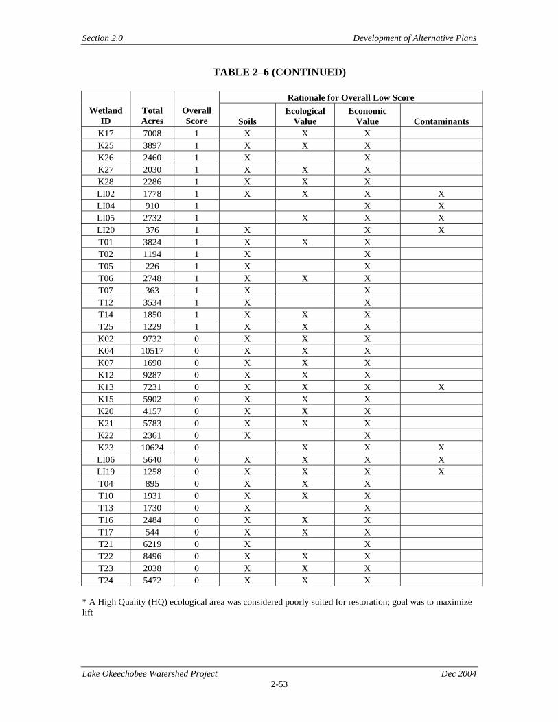
Section 2.0 Development of Alternative Plans
Lake Okeechobee Watershed Project Dec 2004 2-53
TABLE 2–6 (CONTINUED)
Rationale for Overall Low Score Wetland
ID Total Acres
Overall Score Soils
Ecological Value
Economic Value Contaminants
K17 7008 1 X X X K25 3897 1 X X X K26 2460 1 X X K27 2030 1 X X X K28 2286 1 X X X LI02 1778 1 X X X X LI04 910 1 X X LI05 2732 1 X X X LI20 376 1 X X X T01 3824 1 X X X T02 1194 1 X X T05 226 1 X X T06 2748 1 X X X T07 363 1 X X T12 3534 1 X X T14 1850 1 X X X T25 1229 1 X X X K02 9732 0 X X X K04 10517 0 X X X K07 1690 0 X X X K12 9287 0 X X X K13 7231 0 X X X X K15 5902 0 X X X K20 4157 0 X X X K21 5783 0 X X X K22 2361 0 X X K23 10624 0 X X X LI06 5640 0 X X X X LI19 1258 0 X X X X T04 895 0 X X X T10 1931 0 X X X T13 1730 0 X X T16 2484 0 X X X T17 544 0 X X X T21 6219 0 X X T22 8496 0 X X X T23 2038 0 X X X T24 5472 0 X X X
* A High Quality (HQ) ecological area was considered poorly suited for restoration; goal was to maximize lift
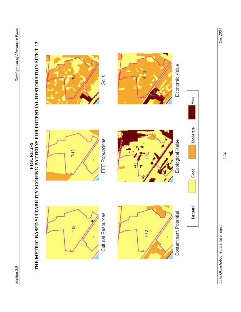
Sect
ion
2.0
Dev
elop
men
t of A
ltern
ativ
e Pl
ans
Lake
Oke
echo
bee
Wat
ersh
ed P
roje
ct
D
ec 2
004
2-54
FIG
UR
E 2
–9
TH
E M
ET
RIC
-BA
SED
SU
ITA
BIL
ITY
SC
OR
ING
PA
TT
ER
NS
FOR
PO
TE
NT
IAL
RE
STO
RA
TIO
N S
ITE
T-1
3

Sect
ion
2.0
Dev
elop
men
t of A
ltern
ativ
e Pl
ans
Lake
Oke
echo
bee
Wat
ersh
ed P
roje
ct
D
ec 2
004
2-55
FIG
UR
E 2
–10
TH
E M
ET
RIC
-BA
SED
SU
ITA
BIL
ITY
SC
OR
ING
PA
TT
ER
NS
FOR
PO
TE
NT
IAL
RE
STO
RA
TIO
N
SIT
E IP
-07

Section 2.0 Development of Alternative Plans
Lake Okeechobee Watershed Project Dec 2004 2-56
K-20 received an overall suitability score of zero. This potential restoration site scored low due to moderate soil and economic value scores and some poor ecological value scores. This site could be divided to avoid the northern areas with poor ecological value suitability scores and add approximately 1800 acres of the southern end to K-08 (which is 2465 acres and got an overall score of 2). However, the patterns indicated that this new potential restoration site would not score higher than a 2 due to moderate economic value and soil suitability scores. Also, State Highway 68 separates K-08 from K-20, so it may not be feasible to try to connect the two potential restoration sites. If K-08 is proposed as an alternative potential restoration site, it is recommended that the addition of a portion of K-20 be evaluated in more detail at that time. LI-04 received an overall suitability score of one. This potential restoration site scored low due to moderate economic value and soil scores and some poor potential contaminant scores. If the areas that were unsuitable due to contaminant potential were excluded, the site would be reduced from 910 acres to approximately 500 acres and the overall score would likely increase. If so, it should receive an overall score of 2, and be a suitable “back-up” site to those potential restoration sites that scored 3 or greater. Even though this potential restoration site is relatively small, it has some additional value of being near the shoreline of Lake Istokpoga and therefore, may be important as a migration corridor for aquatic and semi-aquatic species that utilize the lake. LI-20 received an overall suitability score of one. This potential restoration site scored low due to moderate economic value scores and some poor potential contaminant and soil scores along the western edge. If these poor suitability areas were excluded, this site should score higher and would be a suitable “back-up” site to those potential restoration sites that scored 3 or greater. The site would be reduced in size from 376 acres to approximately 280 acres. T-09 received an overall suitability score of two. This 2,460-acre potential restoration site scored low due to moderate soil, economic value, and contaminant potential scores. It also contained approximately 500 acres of poorly suited ecological value areas in the southwest and southeast corners. If these poorly suited areas were eliminated, the overall suitability score would be raised to a three. Site T-09 will be added to the additional upcoming evaluation process.
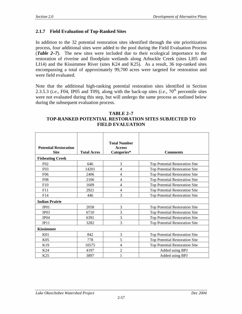
Section 2.0 Development of Alternative Plans
Lake Okeechobee Watershed Project Dec 2004 2-57
2.1.7 Field Evaluation of Top-Ranked Sites In addition to the 32 potential restoration sites identified through the site prioritization process, four additional sites were added to the pool during the Field Evaluation Process (Table 2–7). The new sites were included due to their ecological importance to the restoration of riverine and floodplain wetlands along Arbuckle Creek (sites LI05 and LI14) and the Kissimmee River (sites K24 and K25). As a result, 36 top-ranked sites encompassing a total of approximately 99,700 acres were targeted for restoration and were field evaluated. Note that the additional high-ranking potential restoration sites identified in Section 2.3.5.3 (i.e., F04, IP05 and T09), along with the back-up sites (i.e., 70th percentile sites were not evaluated during this step, but will undergo the same process as outlined below during the subsequent evaluation process.
TABLE 2–7 TOP-RANKED POTENTIAL RESTORATION SITES SUBJECTED TO
FIELD EVALUATION
Potential Restoration Site Total Acres
Total Number Across
Categories* Comments Fisheating Creek F02 646 3 Top Potential Restoration Site F03 14201 4 Top Potential Restoration Site F06 2406 4 Top Potential Restoration Site F08 2106 4 Top Potential Restoration Site F10 1609 4 Top Potential Restoration Site F11 2921 4 Top Potential Restoration Site F14 446 3 Top Potential Restoration Site Indian Prairie IP01 2058 3 Top Potential Restoration Site IP03 6710 3 Top Potential Restoration Site IP04 6391 3 Top Potential Restoration Site IP11 3282 3 Top Potential Restoration Site Kissimmee K01 842 3 Top Potential Restoration Site K05 778 5 Top Potential Restoration Site K19 10575 4 Top Potential Restoration Site K24 4197 2 Added using BPJ K25 3897 1 Added using BPJ
Section 2.0 Development of Alternative Plans
Lake Okeechobee Watershed Project Dec 2004 2-58
TABLE 2–7 (CONTINUED)
Potential Restoration Site Total Acres
Total Number Across
Categories* Comments Lake Istokpoga LI01 1086 3 Top Potential Restoration Site LI03 2589 5 Top Potential Restoration Site LI05 2732 1 Added using BPJ LI07 241 3 Top Potential Restoration Site LI10 496 4 Top Potential Restoration Site LI11 629 3 Top Potential Restoration Site LI12 554 3 Top Potential Restoration Site LI13 640 4 Top Potential Restoration Site LI14 5705 2 Added using BPJ LI17 1278 4 Top Potential Restoration Site LI18 396 5 Top Potential Restoration Site LI21 277 4 Top Potential Restoration Site LI22 275 4 Top Potential Restoration Site LI24 77 5 Top Potential Restoration Site Taylor Creek/Nubbin Slough T01 3824 1 Field Investigation Site T03 4696 3 Top Potential Restoration Site T06 2748 1 Field Investigation Site T18 1351 4 Top Potential Restoration Site T19 1855 3 Top Potential Restoration Site T20 3386 3 Top Potential Restoration Site T23 2038 1 Field Investigation Site T26 2350 3 Top Potential Restoration Site T27 5667 5 Top Potential Restoration Site
* From Step 2, Prioritization Process With the exception of LI07, which was underlain completely by hydric soils, all top-ranked potential restoration sites consisted of several individual wetland parcels. Each individual wetland located within each of the top-ranked sites was evaluated during the Field Evaluation Process. The objectives of this process were to: 1. Collect site-specific data (wetland type, quality, and spatial extent, and surrounding
land use) for individual wetlands within each of the 36 top-ranked sites; 2. Develop a GIS-based wetland evaluation analysis tool; 3. Determine an approach for achieving cost-effective restoration for individual
wetlands within each of the 36 top-ranked sites; and 4. Collect site-specific data for developing planning level costs for achieving hydrologic
restoration of individual wetlands within the top-ranked sites.
Section 2.0 Development of Alternative Plans
Lake Okeechobee Watershed Project Dec 2004 2-59
Significant steps in the Field Evaluation Process included: 1. Determining existing wetland quality within the top-ranked sites; 2. Verifying and applying a GIS-based Wetland Evaluation Analysis Tool; 3. Determining habitat units and ecological lift potential; and 4. Estimating planning level costs for achieving wetland restoration at each of the top-
ranked sites. 2.1.7.1 Determining Existing Wetland Quality Since the top-ranked sites covered a total area of approximately 99,700 acres, it was not feasible to adequately ground survey each and every individual wetland within each top-ranked site. Also, many of the sites were located on private property and landowners were generally unwilling to permit the survey team to conduct field inspections. Representative properties, including all parcels owned by the SFWMD, were therefore selected for ground field surveys. Aerial surveys were then conducted for all top-ranked sites. Data collected from the ground and aerial surveys were used to develop and calibrate a GIS-based wetland evaluation analysis tool. The tool was used to evaluate existing (i.e., 2004) and projected (i.e., 2013, 2050, and 2063) wetland quality for each individual wetland at every one of the 36 top-ranked sites. During the surveys, data were also collected on the upland habitats surrounding each individual wetland parcel. To facilitate data collection and recording in the field, a mobile-GIS-based application called the “Spatial Wetland Data Logger” was developed and utilized. This logger uses ArcPad software and runs both on a handheld unit (such as a Personal Digital Assistant) or a laptop computer. The application consisted of multiple data entry forms that were linked to relevant GIS layers. The application was linked to a Global Positioning System (GPS) unit, which allowed the user to tie data collected to a given site. The logger was used to document field data related to selecting and costing a restoration approach for each site (i.e., length of berms, canals, water control structures, exotics, etc.), and to record information related to individual wetlands within a given site (i.e., existing land use, size, vegetation characteristics, wildlife utilization, etc.) Prior to each ground and aerial field survey, GIS land use layers for the sites to be surveyed were overlaid on the 1999 infrared Digital Ortho Quarter Quadrangle (DOQQ) aerial imagery. Each individual wetland and upland within a site was assigned a unique identification number (e.g., T01-W1 or T01-U1) and its corresponding FLUCCS Level 4 Code was noted on the DOQQ(s) as shown in Figure 2–11.
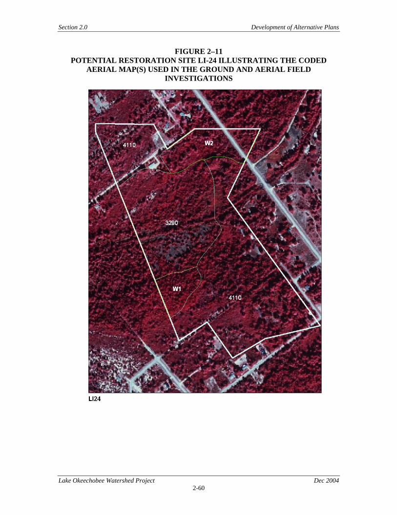
Section 2.0 Development of Alternative Plans
Lake Okeechobee Watershed Project Dec 2004 2-60
FIGURE 2–11 POTENTIAL RESTORATION SITE LI-24 ILLUSTRATING THE CODED
AERIAL MAP(S) USED IN THE GROUND AND AERIAL FIELD INVESTIGATIONS

Section 2.0 Development of Alternative Plans
Lake Okeechobee Watershed Project Dec 2004 2-61
During the ground surveys, existing wetland quality was quantified through the application of the Wetlands Rapid Assessment Procedure (WRAP) developed by the SFWMD (Miller and Gunsalus, 1997). The WRAP is a multi-metric rating index that provides an overall score, which represents the condition or quality of a particular wetland. The WRAP is commonly used to assess a wide variety of wetland systems, but the scores cannot be utilized for making comparisons between different wetland types (i.e., wet prairie to freshwater marsh). The WRAP score is based on a standardized numerical ranking of existing ecological and anthropogenic factors that include wildlife utilization, wetland overstory/shrub cover, wetland vegetative ground cover, adjacent upland support/wetland buffer, field indicators of wetland hydrology, and water quality input and treatment systems. For each WRAP variable, a score of 0 (severely impacted system) to 3 (unimpacted system) is assigned. Half-increments are also used for scoring as deemed necessary (0.5-2.5). Each applicable variable (V) is scored; these scores are totaled (∑V) and then the total is divided by the total maximum score for that variable (∑Vmax). The final rating score for the wetland is the cumulative total of all of the assessed variables and is expressed as a number between 0 and 1. Thus, WRAP score = ∑V/∑Vmax Ground Surveys – In preparation for the ground surveys, site visits were conducted to the Kissimmee Prairie State Preserve and Site T-01. The preserve encompasses relatively pristine and unimpacted wet prairie and freshwater marsh wetland ecosystems, which retain many of the pre-drainage flow and wetland community characteristics. The wetlands at the preserve would serve as “reference” sites for defining the theoretical restoration target for these wetland community types within the top-ranked sites. The trip to Site T-01 was performed to compare the reference wetlands with degraded wetlands and agree upon a standardized approach for applying the WRAP rating indices and scoring method. Subsequent ground surveys were conducted at Sites T-01, T-06, and T-23. At each site, selected individual wetlands and uplands were surveyed to collect data for: 1. Standardization of the WRAP application; 2. Authentication of existing land use with the aerial imagery; 3. Identification of a cost-effective hydrologic restoration approach; 4. Establishment of planning level restoration costs; and 5. Verification of ecological value scores for a subset of wetlands as a validation process
for the GIS-based wetland evaluation analysis tool. WRAP scores were calculated for eleven wetlands during the ground investigations. Results are summarized in Table 2–8. Field observations indicated that most of the wetlands within the sites surveyed were surrounded by, at least in part, improved pasture. This was to be expected because improved pasture is the single largest land use type

Section 2.0 Development of Alternative Plans
Lake Okeechobee Watershed Project Dec 2004 2-62
within the project area (over 50 percent), and the Wetland LSM generally scored areas with the largest proportion of improved pasture the highest. Wetland type was determined in the field based on vegetation and hydrology. The most common wetland types observed during the ground surveys were freshwater marsh and wet prairie. WRAP scores for these wetland systems located within improved pastures ranged from 0.13 to 0.25 (average 0.21) out of a possible maximum of 1.00. Some of the wetlands were surrounded by a mosaic of improved pasture and pine flatwoods. These wetlands received higher WRAP scores (averaging 0.45) due to better buffer, wildlife utilization, and land use scores. One wetland (T23-W44) was a freshwater marsh surrounded by a wet prairie, and was thus given two WRAP scores, one for each wetland type. While the wet prairie was impacted by the surrounding improved pasture (and received a WRAP score of 0.13), the freshwater marsh, because it was buffered somewhat from the impacts of the pasture by the wet prairie, received a higher WRAP score of 0.53. Two forested wetlands were also evaluated, a mixed wetland hardwood and a stream swamp (bottomland). Both of these were surrounded by improved pasture that contained sparse upland trees such as slash pine (Pinus elliottii), oaks (Quercus spp.), and cabbage palm (Sabal palmetto). These trees, along with the wetland tree species, provided for more wildlife utilization and reduced evapotranspiration thereby improving the herbaceous ground cover. As a result, these wetlands scored slightly higher than their totally herbaceous counterparts, 0.31 and 0.36, respectively. Aerial Surveys – All 36 top-ranked sites were surveyed from the air using the SFWMD helicopter. During each flight, individual wetlands were observed from an altitude of 500 to 1,000 feet and relevant data were recorded. Deviations or inconsistencies between land use categories interpreted from aerial photos and existing field conditions were noted. Inaccuracies in FLUCCS code assignments (with respect to the GIS spatial data layers) and wetland and/or upland delineations were also recorded. In addition, data were collected for selecting a cost-effective hydrological restoration approach and preparing planning level restoration costs.
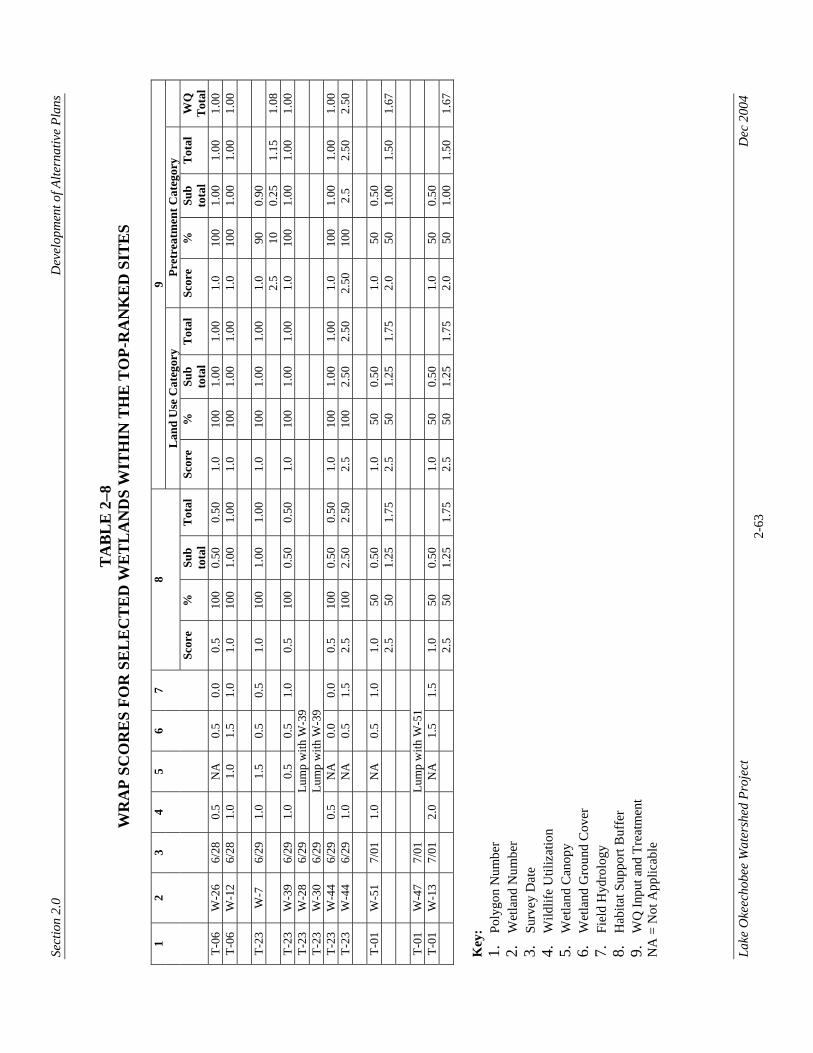
Sect
ion
2.0
Dev
elop
men
t of A
ltern
ativ
e Pl
ans
Lake
Oke
echo
bee
Wat
ersh
ed P
roje
ct
D
ec 2
004
2-63
TA
BL
E 2
–8
WR
AP
SCO
RE
S FO
R S
EL
EC
TE
D W
ET
LA
ND
S W
ITH
IN T
HE
TO
P-R
AN
KE
D S
ITE
S
9 8
Lan
d U
se C
ateg
ory
Pret
reat
men
t Cat
egor
y
1 2
3 4
5 6
7
Scor
e %
Su
b to
tal
Tot
al
Scor
e %
Su
b to
tal
Tot
al
Scor
e %
Su
b to
tal
Tot
al
WQ
T
otal
T-
06
W-2
6 6/
28
0.5
NA
0.
5 0.
0 0.
5 10
0 0.
50
0.50
1.
0 10
0 1.
00
1.00
1.
0 10
0 1.
00
1.00
1.
00
T-06
W
-12
6/28
1.
0 1.
0 1.
5 1.
0 1.
0 10
0 1.
00
1.00
1.
0 10
0 1.
00
1.00
1.
0 10
0 1.
00
1.00
1.
00
T-23
W
-7
6/29
1.
0 1.
5 0.
5 0.
5 1.
0 10
0 1.
00
1.00
1.
0 10
0 1.
00
1.00
1.
0 90
0.
90
2.
5 10
0.
25
1.15
1.
08
T-23
W
-39
6/29
1.
0 0.
5 0.
5 1.
0 0.
5 10
0 0.
50
0.50
1.
0 10
0 1.
00
1.00
1.
0 10
0 1.
00
1.00
1.
00
T-23
W
-28
6/29
Lu
mp
with
W-3
9
T-23
W
-30
6/29
Lu
mp
with
W-3
9
T-23
W
-44
6/29
0.
5 N
A
0.0
0.0
0.5
100
0.50
0.
50
1.0
100
1.00
1.
00
1.0
100
1.00
1.
00
1.00
T-
23
W-4
4 6/
29
1.0
NA
0.
5 1.
5 2.
5 10
0 2.
50
2.50
2.
5 10
0 2.
50
2.50
2.
50
100
2.5
2.50
2.
50
T-01
W
-51
7/01
1.
0 N
A
0.5
1.0
1.0
50
0.50
1.0
50
0.50
1.0
50
0.50
2.5
50
1.25
1.
75
2.5
50
1.25
1.
75
2.0
50
1.00
1.
50
1.67
T-
01
W-4
7 7/
01
Lum
p w
ith W
-51
T-
01
W-1
3 7/
01
2.0
NA
1.
5 1.
5 1.
0 50
0.
50
1.
0 50
0.
50
1.
0 50
0.
50
2.
5 50
1.
25
1.75
2.
5 50
1.
25
1.75
2.
0 50
1.
00
1.50
1.
67
Key
: 1.
Po
lygo
n N
umbe
r 2.
W
etla
nd N
umbe
r 3.
Su
rvey
Dat
e 4.
W
ildlif
e U
tiliz
atio
n 5.
W
etla
nd C
anop
y 6.
W
etla
nd G
roun
d C
over
7.
Fi
eld
Hyd
rolo
gy
8.
Hab
itat S
uppo
rt B
uffe
r 9.
W
Q In
put a
nd T
reat
men
t N
A =
Not
App
licab
le
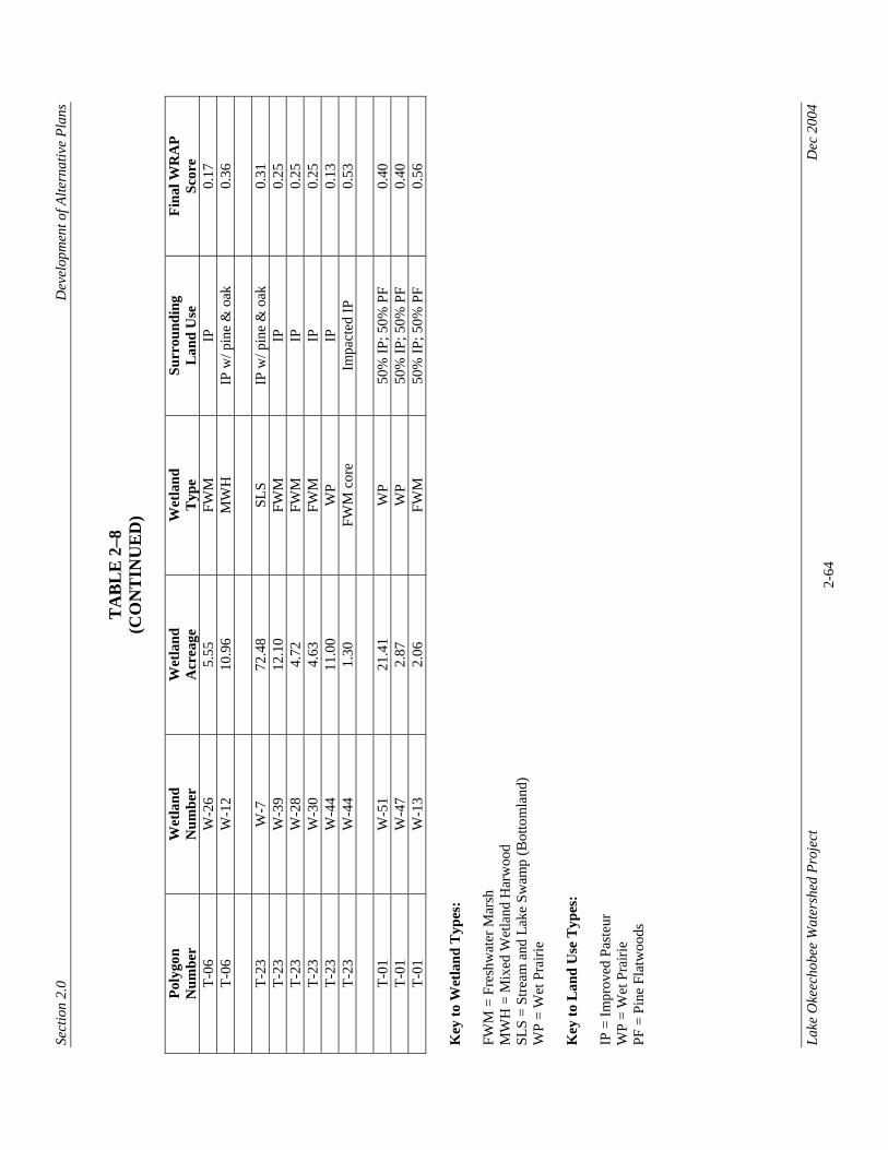
Sect
ion
2.0
Dev
elop
men
t of A
ltern
ativ
e Pl
ans
Lake
Oke
echo
bee
Wat
ersh
ed P
roje
ct
D
ec 2
004
2-64
TA
BL
E 2
–8
(CO
NT
INU
ED
)
Poly
gon
Num
ber
Wet
land
N
umbe
r W
etla
nd
Acr
eage
W
etla
nd
Typ
e Su
rrou
ndin
g
Lan
d U
se
Fina
l WR
AP
Scor
e T-
06
W-2
6 5.
55
FWM
IP
0.
17
T-06
W
-12
10.9
6 M
WH
IP
w/ p
ine
& o
ak
0.36
T-
23
W-7
72
.48
SLS
IP w
/ pin
e &
oak
0.
31
T-23
W
-39
12.1
0 FW
M
IP
0.25
T-
23
W-2
8 4.
72
FWM
IP
0.
25
T-23
W
-30
4.63
FW
M
IP
0.25
T-
23
W-4
4 11
.00
WP
IP
0.13
T-
23
W-4
4 1.
30
FWM
cor
e Im
pact
ed IP
0.
53
T-01
W
-51
21.4
1 W
P 50
% IP
; 50%
PF
0.40
T-
01
W-4
7 2.
87
WP
50%
IP; 5
0% P
F 0.
40
T-01
W
-13
2.06
FW
M
50%
IP; 5
0% P
F 0.
56
Key
to W
etla
nd T
ypes
: FW
M =
Fre
shw
ater
Mar
sh
MW
H =
Mix
ed W
etla
nd H
arw
ood
SLS
= St
ream
and
Lak
e Sw
amp
(Bot
tom
land
) W
P =
Wet
Pra
irie
Key
to L
and
Use
Typ
es:
IP =
Impr
oved
Pas
teur
W
P =
Wet
Pra
irie
PF =
Pin
e Fl
atw
oods
Section 2.0 Development of Alternative Plans
Lake Okeechobee Watershed Project Dec 2004 2-65
Restoration sites in which deviations or inconsistencies between the aerial photos, FLUCCS codes and current land uses represented greater than 10 percent of the entire potential restoration site were redigitized using Arc GIS. This information was then used to update the GIS-based wetland evaluation analysis tool to ensure greater accuracy. 2.1.7.2 Wetland Evaluation Analysis Tool Wetland quality data collected and analyzed during the ground and aerial surveys were used to develop and calibrate a GIS-based Wetland Evaluation Analysis Tool (WEAT). For each individual wetland, the WEAT predicts existing wetland quality, which is quantified as an Wetland Value Score (WVS). This score takes into account the size of the wetland, field-verified surrounding land use pattern(s), and associated Ecological Value Score (EVS) attributed to that land use (see Tables 2–9 and 2–11). It is calculated using the following input parameters: • Total acreage of the individual wetland; • Type(s) of land use categories existing within a 100-m buffer zone around the
individual wetland; and • Percent of each land use category within the buffer zone. The WEAT was used to determine wetland value scores for each individual wetland within each of the 36 top-ranked sites. Significant steps in the calculation of the EVS for an individual wetland are as follows. 1. A 100-meter (100-m) buffer zone was created around each individual wetland. The
100 meter buffer was consistent with the Adjacent Upland/Wetland Buffer Rating Index of the WRAP. Individual wetland identification numbers were assigned to each wetland and its associated 100-m buffer.
2. Using WRAP results from the field surveys and best professional judgment, a discrete
EVS was assigned to each FLUCCS Level 4 Code land use category present within the 100-m buffer and to the wetland itself. Scoring was based on the relative degree of adverse impact that a particular land use would potentially exert on the given wetland. For example, for FLUCCS Level 4 Code 2110 (improved pasture) a relatively low score of 0.20, out of a maximum possible of 1.00, was assigned based on WRAP scores generated during the ground surveys. This score is appropriate because improved pasture tends to have greater negative impacts on adjacent wetlands due to their extensive drainage patterns, altered plant communities, reduced natural buffer, and cattle impacts (vegetation loss and manure inputs). Similarly, wetlands surrounded by native or more natural communities received a higher WVS. WRAP scores generated during the ground surveys indicated that a wetland surrounded by half pine flatwoods and half improved pasture should receive an average score of 0.45 out of a possible maximum of 1.0. Therefore, if the percentage of wetland quality is equivalent to the percentage of ecologically “good
Section 2.0 Development of Alternative Plans
Lake Okeechobee Watershed Project Dec 2004 2-66
and bad” land uses surrounding a wetland, then a wetland entirely within pine flatwoods would receive a WVS of 0.70. The WVS of 0.70 was computed as follows: • WVS of wetlands surrounded entirely by improved pasture = 0.20 (field WRAP
score) • WVS of wetlands surrounded by half improved pasture and half pine flatwoods =
0.45 (field WRAP score) • If 50 percent of the buffer is improved pasture, then 0.20 x 50% = 0.10 • This means that the remaining 50% of the buffer, which is pine flatwoods, is
contributing 0.45 - 0.10 = 0.35 to the overall WRAP score • Therefore, a wetland, which is completely surrounded by pine flatwoods, would
receive an WVS of 0.35*2.0 = 0.70
Uplands in native/natural cover received an EVS of 0.70. Degraded uplands received an EVS of between 0.01 and 0.60, depending on the degree of impact. All wetlands in native/natural cover received an EVS of 1.00, with the exception of wetlands with non-native cover types [e.g., FLUCCS Level 4 Codes 6218 (cypress infested with Melaleuca species) and 6412 (freshwater marsh infested with cattails)] which were assigned an EVS of 0.70. Table 2–9 lists the FLUCCS Level 4 Codes used in the analyses and their associated ecological value scores.
For those land uses that a field WRAP of the wetlands was not conducted due to site access limitations, the assistance of one of the WRAP method co-authors, Boyd Gunsalus, was enlisted. He reviewed our entire EVS list, and based on his experience, was tasked with verifying the accuracy of the scores for each FLUCCS Code. Mr. Gunsalus indicated that the process was acceptable as an initial step at landscape level planning, but would require field verification because there can be great variability within the types of wetland systems that are described by the FLUCCS Codes. For example, wetlands located within sugar cane fields (FLUCCS Code 2156) can exhibit great variability in form and function, and therefore, receive a low, moderate, or high EVS score. Also, “Military” (FLUCCS Level 4 Codes 1731 through 1736) received an EVS of 0.30, but in the Avon Park Bombing Range (which is immediately adjacent to, but outside, the project area boundary) many of the wetlands have WRAP scores closer to 0.80 or 0.90. Adding some flexibility or more specificity to the FLUCCS codes as they are represented within the project area would make the WEAT more accurate. Additional modifications to the EVS included changing “Inactive Land with Street Pattern but without Structures” (FLUCCS Code 192) from 0.01 to 0.50; increasing both “Reservoirs Over 500 Acres” (FLUCCS Code 5310) and “Unimproved Pasture” (FLUCCS Code 2120) from 0.50 to 0.70 (Boyd Gunsalus, SFWMD, telephone communication 2004). As the spatial extents of these land uses within the LOW project area are not extensive, it is not believed that these changes would represent a significantly different outcome. However, as the siting process proceeds to a smaller set of potential restoration sites, and site access is granted, the FLUCCS codes will be reevaluated and the EVS will either be
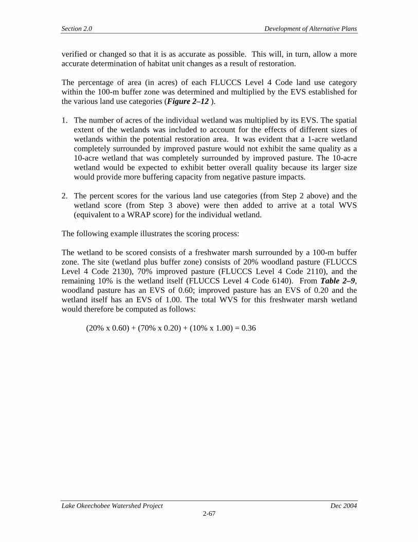
Section 2.0 Development of Alternative Plans
Lake Okeechobee Watershed Project Dec 2004 2-67
verified or changed so that it is as accurate as possible. This will, in turn, allow a more accurate determination of habitat unit changes as a result of restoration. The percentage of area (in acres) of each FLUCCS Level 4 Code land use category within the 100-m buffer zone was determined and multiplied by the EVS established for the various land use categories (Figure 2–12 ). 1. The number of acres of the individual wetland was multiplied by its EVS. The spatial
extent of the wetlands was included to account for the effects of different sizes of wetlands within the potential restoration area. It was evident that a 1-acre wetland completely surrounded by improved pasture would not exhibit the same quality as a 10-acre wetland that was completely surrounded by improved pasture. The 10-acre wetland would be expected to exhibit better overall quality because its larger size would provide more buffering capacity from negative pasture impacts.
2. The percent scores for the various land use categories (from Step 2 above) and the wetland score (from Step 3 above) were then added to arrive at a total WVS (equivalent to a WRAP score) for the individual wetland.
The following example illustrates the scoring process: The wetland to be scored consists of a freshwater marsh surrounded by a 100-m buffer zone. The site (wetland plus buffer zone) consists of 20% woodland pasture (FLUCCS Level 4 Code 2130), 70% improved pasture (FLUCCS Level 4 Code 2110), and the remaining 10% is the wetland itself (FLUCCS Level 4 Code 6140). From Table 2–9, woodland pasture has an EVS of 0.60; improved pasture has an EVS of 0.20 and the wetland itself has an EVS of 1.00. The total WVS for this freshwater marsh wetland would therefore be computed as follows:
(20% x 0.60) + (70% x 0.20) + (10% x 1.00) = 0.36
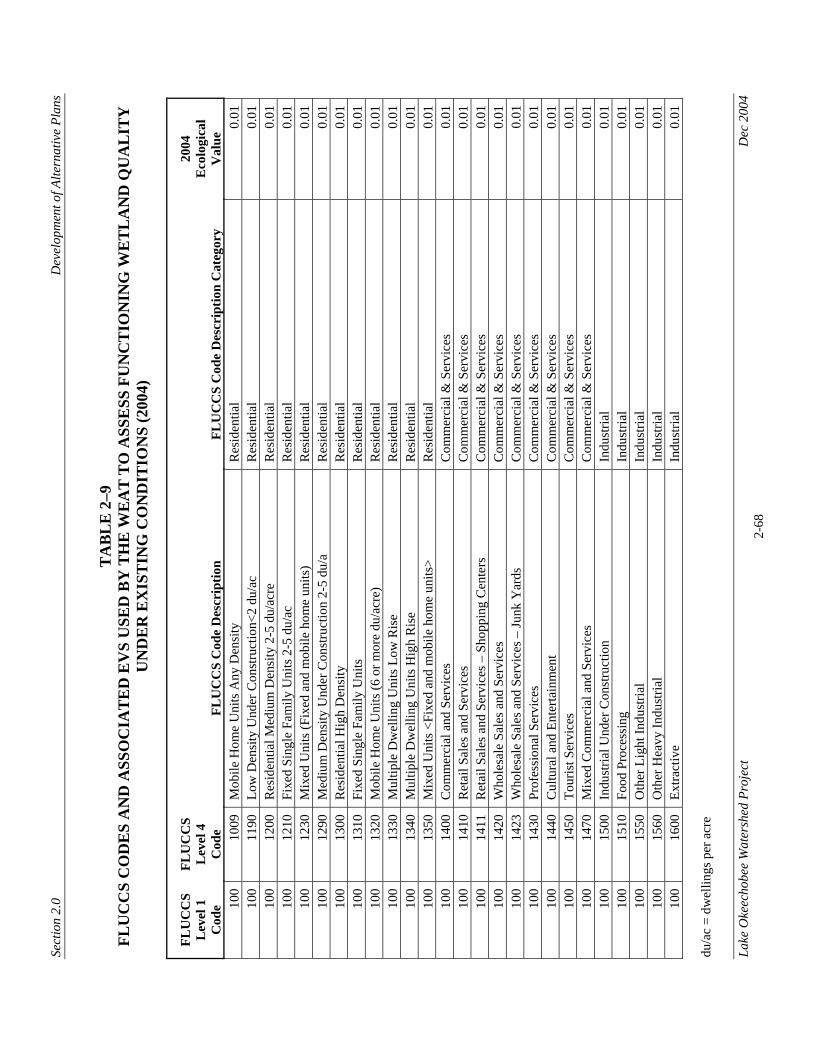
Sect
ion
2.0
Dev
elop
men
t of A
ltern
ativ
e Pl
ans
Lake
Oke
echo
bee
Wat
ersh
ed P
roje
ct
D
ec 2
004
2-68
TA
BL
E 2
–9
FLU
CC
S C
OD
ES
AN
D A
SSO
CIA
TE
D E
VS
USE
D B
Y T
HE
WE
AT
TO
ASS
ESS
FU
NC
TIO
NIN
G W
ET
LA
ND
QU
AL
ITY
U
ND
ER
EX
IST
ING
CO
ND
ITIO
NS
(200
4)
FLU
CC
S L
evel
1
Cod
e
FLU
CC
S L
evel
4
Cod
e FL
UC
CS
Cod
e D
escr
iptio
n
FLU
CC
S C
ode
Des
crip
tion
Cat
egor
y
2004
E
colo
gica
l V
alue
10
0 10
09
Mob
ile H
ome
Uni
ts A
ny D
ensi
ty
Res
iden
tial
0.01
10
0 11
90
Low
Den
sity
Und
er C
onst
ruct
ion<
2 du
/ac
Res
iden
tial
0.01
10
0 12
00
Res
iden
tial M
ediu
m D
ensi
ty 2
-5 d
u/ac
re
Res
iden
tial
0.01
10
0 12
10
Fixe
d Si
ngle
Fam
ily U
nits
2-5
du/
ac
Res
iden
tial
0.01
10
0 12
30
Mix
ed U
nits
(Fix
ed a
nd m
obile
hom
e un
its)
Res
iden
tial
0.01
10
0 12
90
Med
ium
Den
sity
Und
er C
onst
ruct
ion
2-5
du/a
R
esid
entia
l 0.
01
100
1300
R
esid
entia
l Hig
h D
ensi
ty
Res
iden
tial
0.01
10
0 13
10
Fixe
d Si
ngle
Fam
ily U
nits
R
esid
entia
l 0.
01
100
1320
M
obile
Hom
e U
nits
(6 o
r mor
e du
/acr
e)
Res
iden
tial
0.01
10
0 13
30
Mul
tiple
Dw
ellin
g U
nits
Low
Ris
e R
esid
entia
l 0.
01
100
1340
M
ultip
le D
wel
ling
Uni
ts H
igh
Ris
e R
esid
entia
l 0.
01
100
1350
M
ixed
Uni
ts <
Fixe
d an
d m
obile
hom
e un
its>
Res
iden
tial
0.01
10
0 14
00
Com
mer
cial
and
Ser
vice
s C
omm
erci
al &
Ser
vice
s 0.
01
100
1410
R
etai
l Sal
es a
nd S
ervi
ces
Com
mer
cial
& S
ervi
ces
0.01
10
0 14
11
Ret
ail S
ales
and
Ser
vice
s – S
hopp
ing
Cen
ters
C
omm
erci
al &
Ser
vice
s 0.
01
100
1420
W
hole
sale
Sal
es a
nd S
ervi
ces
Com
mer
cial
& S
ervi
ces
0.01
10
0 14
23
Who
lesa
le S
ales
and
Ser
vice
s – Ju
nk Y
ards
C
omm
erci
al &
Ser
vice
s 0.
01
100
1430
Pr
ofes
sion
al S
ervi
ces
Com
mer
cial
& S
ervi
ces
0.01
10
0 14
40
Cul
tura
l and
Ent
erta
inm
ent
Com
mer
cial
& S
ervi
ces
0.01
10
0 14
50
Tour
ist S
ervi
ces
Com
mer
cial
& S
ervi
ces
0.01
10
0 14
70
Mix
ed C
omm
erci
al a
nd S
ervi
ces
Com
mer
cial
& S
ervi
ces
0.01
10
0 15
00
Indu
stria
l Und
er C
onst
ruct
ion
Indu
stria
l 0.
01
100
1510
Fo
od P
roce
ssin
g In
dust
rial
0.01
10
0 15
50
Oth
er L
ight
Indu
stria
l In
dust
rial
0.01
10
0 15
60
Oth
er H
eavy
Indu
stria
l In
dust
rial
0.01
10
0 16
00
Extra
ctiv
e In
dust
rial
0.01
du
/ac
= dw
ellin
gs p
er a
cre

Sect
ion
2.0
Dev
elop
men
t of A
ltern
ativ
e Pl
ans
Lake
Oke
echo
bee
Wat
ersh
ed P
roje
ct
D
ec 2
004
2-69
TA
BL
E 2
–9
(CO
NT
INU
ED
)
FLU
CC
S L
evel
1
Cod
e
FLU
CC
S L
evel
4
Cod
e FL
UC
CS
Cod
e D
escr
iptio
n
FLU
CC
S C
ode
Des
crip
tion
Cat
egor
y
2004
E
colo
gica
l V
alue
10
0 16
20
Sand
and
Gra
vel P
its
Indu
stria
l 0.
01
100
1700
In
stitu
tiona
l In
stitu
tiona
l 0.
01
100
1710
Ed
ucat
iona
l Fac
ilitie
s In
stitu
tiona
l 0.
01
100
1720
R
elig
ious
In
stitu
tiona
l 0.
01
100
1740
M
edic
al a
nd H
ealth
Car
e In
stitu
tiona
l 0.
01
100
1750
G
over
nmen
tal
Inst
itutio
nal
0.01
10
0 18
30
Rac
e Tr
acks
R
ecre
atio
nal
0.01
10
0 19
20
Inac
tive
Land
with
stre
et p
atte
rn
Ope
n La
nd
0.01
20
0 21
00
Cro
plan
d an
d Pa
stur
elan
d C
ropl
and/
Past
urel
and
0.01
20
0 21
40
Row
Cro
ps
Cro
plan
d 0.
01
200
2150
Fi
eld
Cro
ps
Cro
plan
d 0.
01
200
2156
Fi
eld
Cro
ps -
Suga
r Can
e C
ropl
and
0.01
80
0 80
00
Tran
spor
tatio
n, C
omm
unic
atio
n, U
tiliti
es
Tran
spor
tatio
n, C
omm
unic
atio
n an
d U
tiliti
es
0.01
80
0 81
00
Tran
spor
tatio
n Tr
ansp
orta
tion,
Com
mun
icat
ion
and
Util
ities
0.
01
800
8110
A
irpor
ts
Tran
spor
tatio
n, C
omm
unic
atio
n an
d U
tiliti
es
0.01
80
0 81
20
Rai
lroad
s Tr
ansp
orta
tion,
Com
mun
icat
ion
and
Util
ities
0.
01
800
8140
R
oads
and
Hig
hway
s Tr
ansp
orta
tion,
Com
mun
icat
ion
and
Util
ities
0.
01
800
8213
A
nten
na F
arm
s Tr
ansp
orta
tion,
Com
mun
icat
ion
and
Util
ities
0.
01
800
8300
U
tiliti
es U
nder
Con
stru
ctio
n Tr
ansp
orta
tion,
Com
mun
icat
ion
and
Util
ities
0.
01
800
8310
El
ectri
cal P
ower
Fac
ilitie
s Tr
ansp
orta
tion,
Com
mun
icat
ion
and
Util
ities
0.
01
800
8320
El
ectri
cal P
ower
Tra
nsm
issi
on L
ines
Tr
ansp
orta
tion,
Com
mun
icat
ion
and
Util
ities
0.
01
800
8340
Se
wag
e Tr
eatm
ent
Tran
spor
tatio
n, C
omm
unic
atio
n an
d U
tiliti
es
0.01
80
0 83
49
Sew
age
Trea
tmen
t Tr
ansp
orta
tion,
Com
mun
icat
ion
and
Util
ities
0.
01
800
8350
So
lid W
aste
Dis
posa
l Tr
ansp
orta
tion,
Com
mun
icat
ion
and
Util
ities
0.
01
100
1453
Tr
avel
Tra
iler P
arks
C
omm
erci
al &
Ser
vice
s 0.
10
100
1480
C
emet
erie
s C
omm
erci
al &
Ser
vice
s 0.
10
100
1761
St
ate
Pris
ons
Inst
itutio
nal
0.10
10
0 17
63
Juve
nile
Cen
ters
In
stitu
tiona
l 0.
10
100
1860
C
omm
unity
Rec
reat
iona
l Fac
ilitie
s R
ecre
atio
nal
0.10
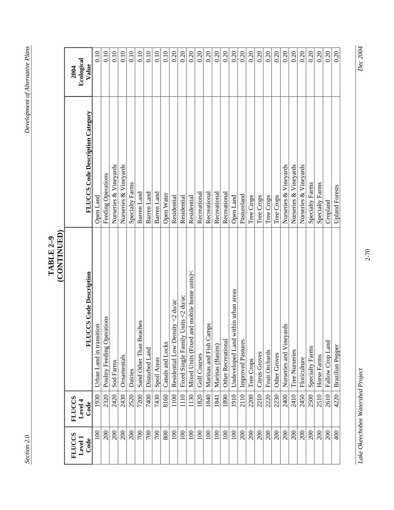
Sect
ion
2.0
Dev
elop
men
t of A
ltern
ativ
e Pl
ans
Lake
Oke
echo
bee
Wat
ersh
ed P
roje
ct
D
ec 2
004
2-70
TA
BL
E 2
–9
(CO
NT
INU
ED
)
FLU
CC
S L
evel
1
Cod
e
FLU
CC
S L
evel
4
Cod
e FL
UC
CS
Cod
e D
escr
iptio
n
FLU
CC
S C
ode
Des
crip
tion
Cat
egor
y
2004
E
colo
gica
l V
alue
10
0 19
30
Urb
an L
and
in tr
ansi
tion
Ope
n La
nd
0.10
20
0 23
20
Poul
try F
eedi
ng O
pera
tions
Fe
edin
g O
pera
tions
0.
10
200
2420
So
d Fa
rms
Nur
serie
s & V
iney
ards
0.
10
200
2430
O
rnam
enta
ls
Nur
serie
s & V
iney
ards
0.
10
200
2520
D
airie
s Sp
ecia
lty F
arm
s 0.
10
700
7200
Sa
nd O
ther
Tha
n B
each
es
Bar
ren
Land
0.
10
700
7400
D
istu
rbed
Lan
d B
arre
n La
nd
0.10
70
0 74
30
Spoi
l Are
as
Bar
ren
Land
0.
10
800
8160
C
anal
s and
Loc
ks
Ope
n W
ater
0.
10
100
1100
R
esid
entia
l Low
Den
sity
<2
du/a
c R
esid
entia
l 0.
20
100
1110
Fi
xed
Sing
le F
amily
Uni
ts <
2 du
/ac
Res
iden
tial
0.20
10
0 11
30
Mix
ed U
nits
(Fix
ed a
nd m
obile
hom
e un
its)<
R
esid
entia
l 0.
20
100
1820
G
olf C
ours
es
Rec
reat
iona
l 0.
20
100
1840
M
arin
as a
nd F
ish
Cam
ps
Rec
reat
iona
l 0.
20
100
1841
M
arin
as (B
asin
s)
Rec
reat
iona
l 0.
20
100
1890
O
ther
Rec
reat
iona
l R
ecre
atio
nal
0.20
10
0 19
10
Und
evel
oped
Lan
d w
ithin
urb
an a
reas
O
pen
Land
0.
20
200
2110
Im
prov
ed P
astu
res
Past
urel
and
0.20
20
0 22
00
Tree
Cro
ps
Tree
Cro
ps
0.20
20
0 22
10
Citr
us G
rove
s Tr
ee C
rops
0.
20
200
2220
Fr
uit O
rcha
rds
Tree
Cro
ps
0.20
20
0 22
30
Oth
er G
rove
s Tr
ee C
rops
0.
20
200
2400
N
urse
ries a
nd V
iney
ards
N
urse
ries &
Vin
eyar
ds
0.20
20
0 24
10
Tree
Nur
serie
s N
urse
ries &
Vin
eyar
ds
0.20
20
0 24
50
Flor
icul
ture
N
urse
ries &
Vin
eyar
ds
0.20
20
0 25
00
Spec
ialty
Far
ms
Spec
ialty
Far
ms
0.20
20
0 25
10
Hor
se F
arm
s Sp
ecia
lty F
arm
s 0.
20
200
2610
Fa
llow
Cro
p La
nd
Cro
plan
d 0.
20
400
4220
B
razi
lian
Pepp
er
Upl
and
Fore
sts
0.20
Sect
ion
2.0
Dev
elop
men
t of A
ltern
ativ
e Pl
ans
Lake
Oke
echo
bee
Wat
ersh
ed P
roje
ct
D
ec 2
004
2-71
TA
BL
E 2
–9
(CO
NT
INU
ED
)
FLU
CC
S L
evel
1
Cod
e
FLU
CC
S L
evel
4
Cod
e FL
UC
CS
Cod
e D
escr
iptio
n
FLU
CC
S C
ode
Des
crip
tion
Cat
egor
y
2004
E
colo
gica
l V
alue
40
0 42
40
Mel
aleu
ca
Upl
and
Fore
sts
0.20
40
0 43
70
Aus
tralia
n Pi
ne
Upl
and
Fore
sts
0.20
70
0 74
10
Rur
al la
nd in
tran
sitio
n B
arre
n La
nd
0.20
70
0 74
50
Bur
ned
Are
as
Bar
ren
Land
0.
20
100
1730
M
ilita
ry
Inst
itutio
nal
0.30
10
0 18
00
Rec
reat
iona
l R
ecre
atio
nal
0.30
10
0 18
50
Park
s and
Zoo
s R
ecre
atio
nal
0.30
20
0 25
40
Aqu
acul
ture
Sp
ecia
lty F
arm
s 0.
30
200
2549
A
quac
ultu
re
Spec
ialty
Far
ms
0.30
20
0 26
00
Oth
er O
pen
Land
s Rur
al
Ope
n La
nd
0.30
40
0 44
00
Tree
Pla
ntat
ions
Si
lvac
ultu
re
0.40
40
0 44
10
Con
ifero
us P
lant
atio
ns
Silv
acul
ture
0.
40
400
4430
Fo
rest
Reg
ener
atio
n A
reas
Si
lvac
ultu
re
0.40
10
0 19
00
Ope
n La
nd
Ope
n La
nd
0.50
10
0 19
40
Oth
er O
pen
Land
O
pen
Land
0.
50
200
2120
U
nim
prov
ed P
astu
res
Past
urel
and
0.50
40
0 41
19
Pine
Fla
twoo
ds -
Mel
aleu
ca In
fest
ed
Upl
and
Fore
sts
0.50
40
0 43
50
Dea
d Tr
ees
Upl
and
Fore
sts
0.50
50
0 53
00
Res
ervo
irs
Ope
n W
ater
0.
50
500
5310
R
eser
voirs
larg
er th
an 5
00 a
cres
O
pen
Wat
er
0.50
50
0 53
20
Res
ervo
irs la
rger
than
100
acr
es -
less
than
500
acr
es
Ope
n W
ater
0.
50
500
5330
R
eser
voirs
larg
er th
an 1
0 ac
res -
less
than
100
acr
es
Ope
n W
ater
0.
50
500
5340
R
eser
voirs
less
than
10
acre
s O
pen
Wat
er
0.50
70
0 74
20
Bor
row
Are
as
Bar
ren
Land
0.
50
200
2130
W
oodl
and
Past
ures
Pa
stur
elan
d 0.
60
300
3100
H
erba
ceou
s Ran
gela
nd
Ran
gela
nd
0.60
30
0 32
00
Shru
b an
d B
rush
land
R
ange
land
0.
60
300
3210
Pa
lmet
to P
rairi
es
Ran
gela
nd
0.60
30
0 32
90
Oth
er S
hrub
s and
Bru
sh
Ran
gela
nd
0.60
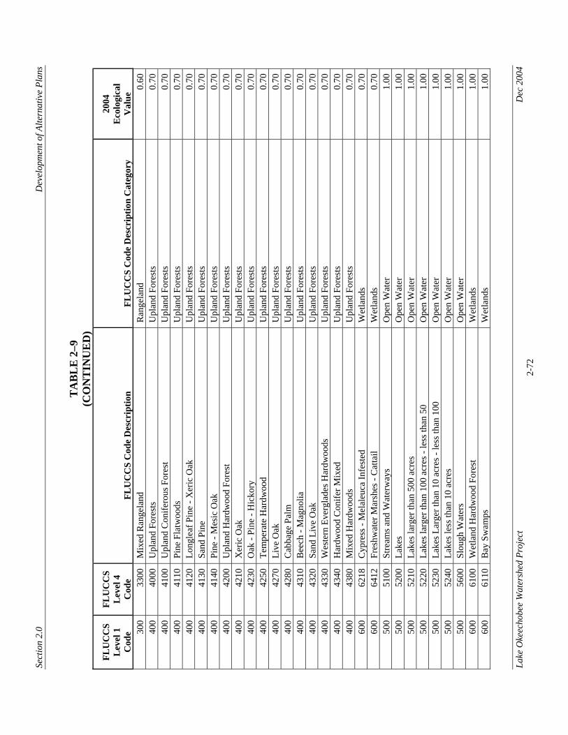
Sect
ion
2.0
Dev
elop
men
t of A
ltern
ativ
e Pl
ans
Lake
Oke
echo
bee
Wat
ersh
ed P
roje
ct
D
ec 2
004
2-72
TA
BL
E 2
–9
(CO
NT
INU
ED
)
FLU
CC
S L
evel
1
Cod
e
FLU
CC
S L
evel
4
Cod
e FL
UC
CS
Cod
e D
escr
iptio
n
FLU
CC
S C
ode
Des
crip
tion
Cat
egor
y
2004
E
colo
gica
l V
alue
30
0 33
00
Mix
ed R
ange
land
R
ange
land
0.
60
400
4000
U
plan
d Fo
rest
s U
plan
d Fo
rest
s 0.
70
400
4100
U
plan
d C
onife
rous
For
est
Upl
and
Fore
sts
0.70
40
0 41
10
Pine
Fla
twoo
ds
Upl
and
Fore
sts
0.70
40
0 41
20
Long
leaf
Pin
e - X
eric
Oak
U
plan
d Fo
rest
s 0.
70
400
4130
Sa
nd P
ine
Upl
and
Fore
sts
0.70
40
0 41
40
Pine
- M
esic
Oak
U
plan
d Fo
rest
s 0.
70
400
4200
U
plan
d H
ardw
ood
Fore
st
Upl
and
Fore
sts
0.70
40
0 42
10
Xer
ic O
ak
Upl
and
Fore
sts
0.70
40
0 42
30
Oak
- Pi
ne -
Hic
kory
U
plan
d Fo
rest
s 0.
70
400
4250
Te
mpe
rate
Har
dwoo
d U
plan
d Fo
rest
s 0.
70
400
4270
Li
ve O
ak
Upl
and
Fore
sts
0.70
40
0 42
80
Cab
bage
Pal
m
Upl
and
Fore
sts
0.70
40
0 43
10
Bee
ch -
Mag
nolia
U
plan
d Fo
rest
s 0.
70
400
4320
Sa
nd L
ive
Oak
U
plan
d Fo
rest
s 0.
70
400
4330
W
este
rn E
verg
lade
s Har
dwoo
ds
Upl
and
Fore
sts
0.70
40
0 43
40
Har
dwoo
d C
onife
r Mix
ed
Upl
and
Fore
sts
0.70
40
0 43
80
Mix
ed H
ardw
oods
U
plan
d Fo
rest
s 0.
70
600
6218
C
ypre
ss -
Mel
aleu
ca In
fest
ed
Wet
land
s 0.
70
600
6412
Fr
eshw
ater
Mar
shes
- C
atta
il W
etla
nds
0.70
50
0 51
00
Stre
ams a
nd W
ater
way
s O
pen
Wat
er
1.00
50
0 52
00
Lake
s O
pen
Wat
er
1.00
50
0 52
10
Lake
s lar
ger t
han
500
acre
s O
pen
Wat
er
1.00
50
0 52
20
Lake
s lar
ger t
han
100
acre
s - le
ss th
an 5
0 O
pen
Wat
er
1.00
50
0 52
30
Lake
s Lar
ger t
han
10 a
cres
- le
ss th
an 1
00
Ope
n W
ater
1.
00
500
5240
La
kes l
ess t
han
10 a
cres
O
pen
Wat
er
1.00
50
0 56
00
Slou
gh W
ater
s O
pen
Wat
er
1.00
60
0 61
00
Wet
land
Har
dwoo
d Fo
rest
W
etla
nds
1.00
60
0 61
10
Bay
Sw
amps
W
etla
nds
1.00
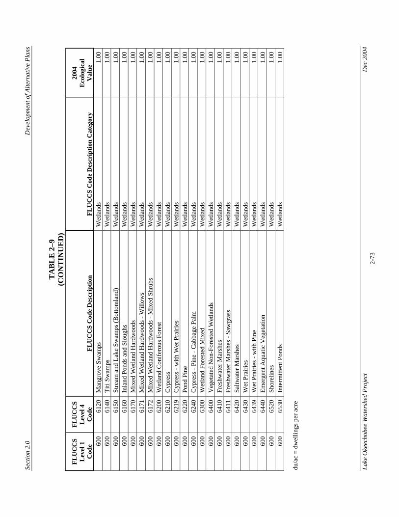
Sect
ion
2.0
Dev
elop
men
t of A
ltern
ativ
e Pl
ans
Lake
Oke
echo
bee
Wat
ersh
ed P
roje
ct
D
ec 2
004
2-73
TA
BL
E 2
–9
(CO
NT
INU
ED
)
FLU
CC
S L
evel
1
Cod
e
FLU
CC
S L
evel
4
Cod
e FL
UC
CS
Cod
e D
escr
iptio
n
FLU
CC
S C
ode
Des
crip
tion
Cat
egor
y
2004
E
colo
gica
l V
alue
60
0 61
20
Man
grov
e Sw
amps
W
etla
nds
1.00
60
0 61
40
Titi
Swam
ps
Wet
land
s 1.
00
600
6150
St
ream
and
Lak
e Sw
amps
(Bot
tom
land
) W
etla
nds
1.00
60
0 61
60
Inla
nd P
onds
and
Slo
ughs
W
etla
nds
1.00
60
0 61
70
Mix
ed W
etla
nd H
ardw
oods
W
etla
nds
1.00
60
0 61
71
Mix
ed W
etla
nd H
ardw
oods
- W
illow
s W
etla
nds
1.00
60
0 61
72
Mix
ed W
etla
nd H
ardw
oods
- M
ixed
Shr
ubs
Wet
land
s 1.
00
600
6200
W
etla
nd C
onife
rous
For
est
Wet
land
s 1.
00
600
6210
C
ypre
ss
Wet
land
s 1.
00
600
6219
C
ypre
ss -
with
Wet
Pra
iries
W
etla
nds
1.00
60
0 62
20
Pond
Pin
e W
etla
nds
1.00
60
0 62
40
Cyp
ress
- Pi
ne -
Cab
bage
Pal
m
Wet
land
s 1.
00
600
6300
W
etla
nd F
ores
ted
Mix
ed
Wet
land
s 1.
00
600
6400
V
eget
ated
Non
-For
este
d W
etla
nds
Wet
land
s 1.
00
600
6410
Fr
eshw
ater
Mar
shes
W
etla
nds
1.00
60
0 64
11
Fres
hwat
er M
arsh
es -
Saw
gras
s W
etla
nds
1.00
60
0 64
20
Saltw
ater
Mar
shes
W
etla
nds
1.00
60
0 64
30
Wet
Pra
iries
W
etla
nds
1.00
60
0 64
39
Wet
Pra
iries
- w
ith P
ine
Wet
land
s 1.
00
600
6440
Em
erge
nt A
quat
ic V
eget
atio
n W
etla
nds
1.00
60
0 65
20
Shor
elin
es
Wet
land
s 1.
00
600
6530
In
term
itten
t Pon
ds
Wet
land
s 1.
00
du/a
c =
dwel
lings
per
acr
e
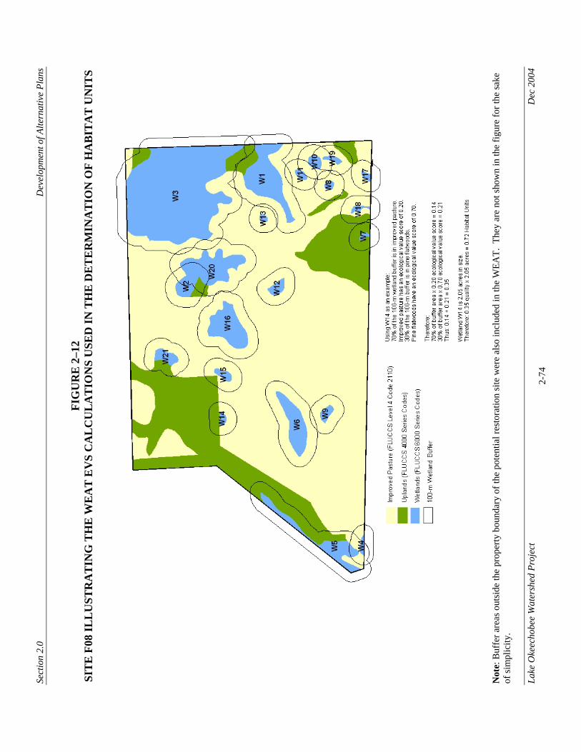
Sect
ion
2.0
Dev
elop
men
t of A
ltern
ativ
e Pl
ans
Lake
Oke
echo
bee
Wat
ersh
ed P
roje
ct
D
ec 2
004
2-74
FIG
UR
E 2
–12
SIT
E F
08 IL
LU
STR
AT
ING
TH
E W
EA
T E
VS
CA
LC
UL
AT
ION
S U
SED
IN T
HE
DE
TE
RM
INA
TIO
N O
F H
AB
ITA
T U
NIT
S
N
ote:
Buf
fer a
reas
out
side
the
prop
erty
bou
ndar
y of
the
pote
ntia
l res
tora
tion
site
wer
e al
so in
clud
ed in
the
WEA
T. T
hey
are
not s
how
n in
the
figur
e fo
r the
sake
of
sim
plic
ity.
Section 2.0 Development of Alternative Plans
Lake Okeechobee Watershed Project Dec 2004 2-75
Wetland value scores calculated for each individual wetland within each of the top-ranked sites are shown, by planning area, in Attachment E, Tab 1. 2.1.7.3 Determination of Habitat Units and Ecological Lift Potential WEAT generated wetland value scores for individual wetlands were used to determine the habitat units that the wetlands would provide. Habitat units represent a numerical combination of habitat quality (expressed as the EVS) and habitat quantity (acres) within a given wetland at a given time (existing (2004) or future). For each individual wetland within the top-ranked sites, 2004 habitat units were determined as the quality of the wetland (2004 WVS) multiplied by the number of acres of the wetland. For example, a 250-acre wetland with a 2004 WVS of 0.36 would provide 250 X 0.36 = 90 habitat units. 2004 wetland values scores and corresponding habitat units determined for each individual wetland within the top-ranked sites are shown in Attachment E, Tab1. It is reasonable to assume that if a wetland restoration project is successful then it would be marked by an increase in the habitat units for the given wetland. The difference between existing habitat units and habitat units at some point in the future following a restoration exercise is termed as the Ecological Lift Potential (ELP). By determining and comparing the ELP for each of the top-ranked sites, locations that are likely to demonstrate the greatest ecological benefit from a wetland restoration project can be identified. To determine the ELP for the top-ranked sites, habitat units were calculated for functioning wetlands, restorable (i.e., non-functioning wetlands), functioning uplands, and restorable uplands (i.e., uplands not in native or natural cover) under existing conditions (2004), at the end of construction/start of project operations (2013), at the CERP planning horizon (2050) and at the end of the LOW Project planning horizon (i.e., 50 years after completion of the project, 2063). Habitat units were also calculated for each of the four categories mentioned above for the future without project conditions in 2050 and 2063. Functioning wetlands were defined as areas that possess hydric soils and retain some degree of wetland function (FLUCCS Level 4 Code 6000 Series). Restorable wetlands were defined as areas with hydric soils and no wetland function [FLUCCS Level 4 Code 2000 (Agriculture), 3000 (Rangeland), 4000 (Upland Forest) or 7000 (Barren Land) Series]. Likewise, Functioning uplands were defined as areas that possess non-hydric soils and retain some degree of upland function [all FLUCCS Level 4 Codes except 5000 (Open Water) and 6000 (Wetlands) series]. Restorable uplands were defined as areas with non-hydric soils currently not in native or natural habitat [FLUCCS Level 4 Code 2000 (Agriculture), 3000 (Rangeland) and 7000 (Barren Land) Series, along with degraded native habitats in the 4000 Series (Level 4 codes 4119, 4220, 4240, 4350 and 4410)]. As it is not prudent or appropriate to try to restore wetlands or uplands in developed
Section 2.0 Development of Alternative Plans
Lake Okeechobee Watershed Project Dec 2004 2-76
residential, commercial or urban areas, FLUCCS Level 4 Series 1000 and 8000 Codes were eliminated from the calculation of restorable wetland and upland habitat units. The methods applied in the calculation of 2004, 2013, and 2050 and 2063 (under future without and with project conditions) habitat units were applied equally across the project area regardless of the location of the potential restoration site. In addition, for the analyses, the boundaries of the potential restoration sites were considered as fixed. In reality, depending upon real estate parcel boundaries, landowner participation, land use and various other factors, the potential restoration site boundaries may change in the future. 2.1.7.3.1 Calculation of Wetland Habitat Units Functioning Wetland Habitat Units – 2004 (Existing Conditions) Using the 2004 habitat units calculated for individual wetlands within each top-ranked site (Attachment E, Tab 1), total habitat units provided by each top-ranked site were calculated as follows: • For sites that contained a single wetland (i.e., LI07), the number of habitat units
calculated for the individual wetland was considered as the total number of habitat units for that site.
• For sites with multiple wetlands, habitat units calculated for individual wetlands were
added to determine the total number of wetland habitat units for that site. For example, a site has three individual wetlands; a 10-acre parcel with an WVS of 0.75, a 5-acre parcel with an WVS of 0.25, and a 2-acre parcel with an WVS of 0.40. The total habitat units for this site were determined as: (10 acres * 0.75) + (5 acres * 0.25) + (2 acres * 0.40) = 9.55 Habitat Units The total number of functioning wetland habitat units estimated for each top-ranked site under existing conditions (2004) is shown, by planning area, in Table 2–10.
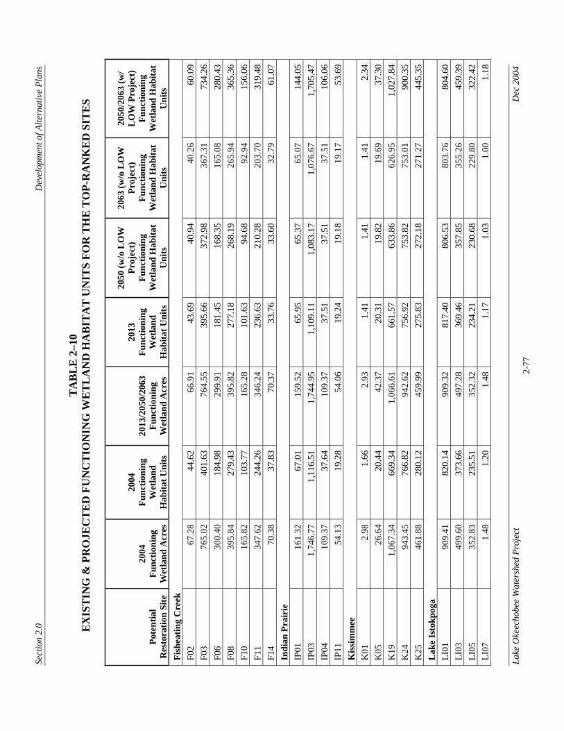
Sect
ion
2.0
Dev
elop
men
t of A
ltern
ativ
e Pl
ans
Lake
Oke
echo
bee
Wat
ersh
ed P
roje
ct
D
ec 2
004
2-77
TA
BL
E 2
–10
EX
IST
ING
& P
RO
JEC
TE
D F
UN
CT
ION
ING
WE
TL
AN
D H
AB
ITA
T U
NIT
S FO
R T
HE
TO
P-R
AN
KE
D S
ITE
S
Pote
ntia
l R
esto
ratio
n Si
te
2004
Fu
nctio
ning
W
etla
nd A
cres
2004
Fu
nctio
ning
W
etla
nd
Hab
itat U
nits
2013
/205
0/20
63
Func
tioni
ng
Wet
land
Acr
es
2013
Fu
nctio
ning
W
etla
nd
Hab
itat U
nits
2050
(w/o
LO
W
Proj
ect)
Fu
nctio
ning
W
etla
nd H
abita
t U
nits
2063
(w/o
LO
W
Proj
ect)
Fu
nctio
ning
W
etla
nd H
abita
t U
nits
2050
/206
3 (w
/ L
OW
Pro
ject
) Fu
nctio
ning
W
etla
nd H
abita
t U
nits
Fi
shea
ting
Cre
ek
F02
67.2
8 44
.62
66.9
1 43
.69
40.9
4 40
.26
60.0
9 F0
3 76
5.02
40
1.63
76
4.55
39
5.66
37
2.98
36
7.31
73
4.26
F0
6 30
0.40
18
4.98
29
9.91
18
1.45
16
8.35
16
5.08
28
0.43
F0
8 39
5.84
27
9.43
39
5.82
27
7.18
26
8.19
26
5.94
36
5.36
F1
0 16
5.82
10
3.77
16
5.28
10
1.63
94
.68
92.9
4 15
6.06
F1
1 34
7.62
24
4.26
34
6.24
23
6.63
21
0.28
20
3.70
31
9.48
F1
4 70
.38
37.8
3 70
.37
33.7
6 33
.60
32.7
9 61
.07
Indi
an P
rair
ie
IP01
16
1.32
67
.01
159.
52
65.9
5 65
.37
65.0
7 14
4.05
IP
03
1,74
6.77
1,
116.
51
1,74
4.95
1,
109.
11
1,08
3.17
1,
076.
67
1,70
5.47
IP
04
109.
37
37.6
4 10
9.37
37
.51
37.5
1 37
.51
106.
06
IP11
54
.13
19.2
8 54
.06
19.2
4 19
.18
19.1
7 53
.69
Kis
sim
mee
K
01
2.98
1.
66
2.93
1.
41
1.41
1.
41
2.34
K
05
26.6
4 20
.44
42.3
7 20
.31
19.8
2 19
.69
37.3
0 K
19
1,06
7.34
66
9.34
1,
066.
61
661.
57
633.
86
626.
95
1,02
7.84
K
24
943.
45
766.
82
942.
62
756.
92
753.
82
753.
01
900.
35
K25
46
1.88
28
0.12
45
9.99
27
5.83
27
2.18
27
1.27
44
5.35
L
ake
Isto
kpog
a LI
01
909.
41
820.
14
909.
32
817.
40
806.
53
803.
76
804.
60
LI03
49
9.60
37
3.66
49
7.28
36
9.46
35
7.85
35
5.26
45
9.39
LI
05
352.
83
235.
51
352.
32
234.
21
230.
68
229.
80
322.
42
LI07
1.
48
1.20
1.
48
1.17
1.
03
1.00
1.
18

Sect
ion
2.0
Dev
elop
men
t of A
ltern
ativ
e Pl
ans
Lake
Oke
echo
bee
Wat
ersh
ed P
roje
ct
D
ec 2
004
2-78
TA
BL
E 2
–10
(CO
NT
INU
ED
)
Pote
ntia
l R
esto
ratio
n Si
te
2004
Fu
nctio
ning
W
etla
nd A
cres
2004
Fu
nctio
ning
W
etla
nd
Hab
itat U
nits
2013
/205
0/20
63
Func
tioni
ng
Wet
land
Acr
es
2013
Fu
nctio
ning
W
etla
nd
Hab
itat U
nits
2050
(w/o
LO
W
Proj
ect)
Fu
nctio
ning
W
etla
nd H
abita
t U
nits
2063
(w/o
LO
W
Proj
ect)
Fu
nctio
ning
W
etla
nd H
abita
t U
nits
2050
/206
3 (w
/ L
OW
Pro
ject
) Fu
nctio
ning
W
etla
nd H
abita
t U
nits
L
ake
Isto
kpog
a (c
ontin
ued)
LI
10
28.3
8 11
.19
28.3
8 11
.14
10.9
5 10
.90
24.8
8 LI
11
52.0
4 31
.75
51.4
9 31
.35
31.2
9 31
.27
45.7
9 LI
12
7.51
4.
47
7.04
4.
14
3.71
3.
60
5.63
LI
13
230.
88
142.
99
230.
39
142.
39
141.
24
140.
95
217.
61
LI14
1,
030.
75
771.
19
1,02
9.04
76
4.92
74
2.80
73
7.30
98
2.52
LI
17
65.9
4 39
.29
65.3
8 39
.06
38.1
7 37
.95
57.6
1 LI
18
299.
47
274.
26
298.
82
273.
09
271.
11
270.
63
260.
93
LI21
11
5.81
99
.83
115.
36
98.1
7 97
.42
97.2
3 10
2.94
LI
22
240.
98
220.
64
240.
58
218.
96
213.
51
212.
15
207.
31
LI24
11
.32
8.53
11
.31
8.15
7.
14
6.89
9.
05
Tay
lor
Cre
ek/N
ubbi
n Sl
ough
T0
3 38
.33
13.6
9 37
.99
13.5
6 13
.41
13.3
8 36
.60
T18
112.
02
53.4
7 11
2.01
52
.69
50.8
5 50
.39
104.
32
T19
108.
10
29.9
9 10
7.83
29
.64
29.6
4 29
.64
100.
68
T20
169.
95
100.
94
168.
79
70.7
5 70
.14
69.3
7 15
6.53
T2
6 98
.56
39.6
5 97
.68
38.7
5 38
.75
38.7
5 89
.21
T27
48.5
5 18
.73
48.5
5 18
.69
18.6
9 18
.69
45.2
3
Section 2.0 Development of Alternative Plans
Lake Okeechobee Watershed Project Dec 2004 2-79
Functioning Wetland Habitat Units – 2013 Given the rapid changes in land use patterns that have occurred and continue to take place in the project study area, it was evident that 2004 habitat units for functioning wetlands would change over time. This predicted change in habitat units of functioning wetlands that is likely to occur between 2004 and 2013 was calculated using the WEAT generated WVS and incorporating a quantity and a quality factor score. Both these scores were based on best professional judgment and took into account specific assumptions. The quality factor score reflects the predicted change in ecological quality within the 100-m buffer of an individual wetland. For this analysis, it was assumed that 10 percent of uplands currently classified as unimproved pasture (FLUCCS Level 4 Codes 2120, 2130), rangeland (FLUCCS Level 4 3000 Series Codes), native/natural uplands (FLUCCS Level 4 4000 Series Codes), and rural lands in transition (FLUCCS Level 4 Code 7410) would be converted into more intensive agricultural (FLUCCS Level 4 2000 Series Codes), urban, residential, or commercial land uses (FLUCCS Level 4 1000 Series Codes) by 2013. It was hard to predict whether unimproved pasture, rangeland, native/natural uplands, or rural land in transition would be converted to either agricultural or urban development (these more intensive land uses have low existing EVS ranging from 0.01 to 0.20). Therefore, an average EVS for all intensive land uses to be used in the determination of habitat units was calculated. An EVS of 0.19 was the average of the FLUCCS Level 4 1000 and 2000 series (with the exception of FLUCCS Level 4 codes 2120 and 2130 – unimproved and woodland pastures, respectively) ecological value scores. For 2013, only 10 percent of the uplands in the 100-m wetland buffer were assessed using the average EVS of 0.19, the remaining 90 percent were assessed using their 2004 EVS. In addition, as uplands are converted into more intensive land uses, it was assumed that the EVS of associated existing high quality wetlands contained within the 100-m buffer would also be degraded. Therefore, based on best professional judgment, wetland FLUCCS Level 4 Codes in the 6000 series, with a 2004 EVS 1.00 were assessed as having a 2013 EVS of 0.80. Similarly, wetland FLUCCS Level 4 codes 6218 (Cypress–melaleuca infested) and 6412 (Freshwater marshes–cattails), with a 2004 EVS of 0.70, were assessed as having a 2013 EVS of 0.50. Table 2–11 lists the FLUCCS codes and the associated revised ecological value scores used in this analysis. The revised scores were plugged into WEAT for calculation of 2013 habitat units. The quantity factor measures the projected loss of spatial extent of wetland habitat likely to occur from 2004 to 2013. Future wetland losses across the study area were predicted based on current State and Federal regulations. For example, the SFWMD does not require an Environmental Resource Permit for wetlands <0.50 acres in size, therefore, no mitigation is required. Similarly, the USACE does not require a permit or mitigation
Section 2.0 Development of Alternative Plans
Lake Okeechobee Watershed Project Dec 2004 2-80
for wetlands <0.20 acres in size. In addition, the USACE generally does not require mitigation for isolated wetlands that are greater than 200 feet away from a "water of the U.S." and have no surface connection (either dry or wet, man-made or natural), regardless of size. Due to the lack of protection by law, and given the current rate of development in south Florida, it was therefore assumed that all isolated wetlands <0.50 acres in size would be converted to other land uses by 2013 and would no longer provide functioning wetland habitat units in 2013 or further into the future. It is, however, probable that such parcels could provide some very low habitat units as “potentially restorable wetlands.” Using both the quality and quantity factor scores described above, wetland habitat units for 2013 were calculated as shown in the example below: • Using the revised ecological value scores from Table 2–11, the WEAT indicated that
a particular site had 200 functioning wetland habitat units in 2013. Note that this value accounts for the quality factor score.
• The quantity factor score was then added into the equation. In 2004, this site
contained 20 isolated wetlands that were each 0.20 acres in size. The WEAT indicated that in 2013 the 20 isolated wetlands at the site would have had an wetland value score of 0.50. However, since it was assumed that by 2013 these isolated wetlands would have been converted to other land uses, they were subtracted from the calculation of 2013 wetland habitat units, as follows:
200 – [(20*0.20)*0.50] = 198 Habitat Units
Thus, based upon the quality and quantity factor scores, it was predicted that the given site would likely provide only 198 functioning wetland habitat units in 2013. Functioning wetland habitat units projected for each top-ranked potential restoration site for 2013 are shown, by planning area, in Table 2–10. Wetland value scores and projected 2013 wetland habitat units for each individual wetland within the top-ranked potential restoration sites are shown, by planning area, in Attachment E, Tab 2.
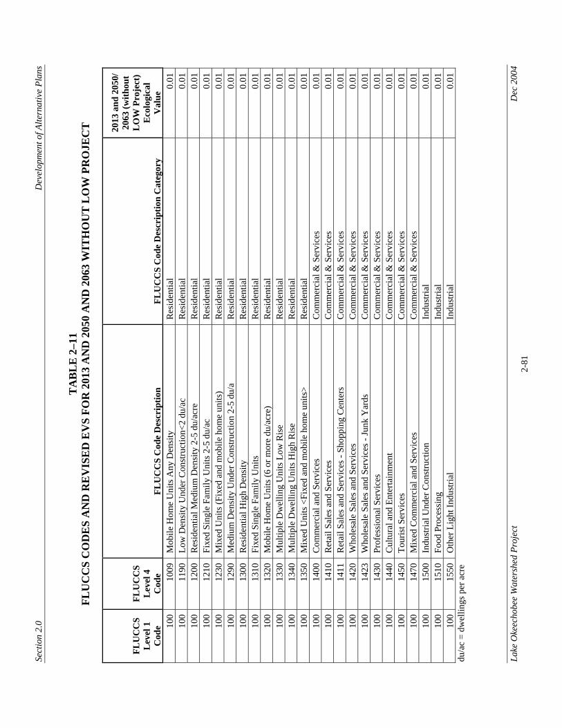
Sect
ion
2.0
Dev
elop
men
t of A
ltern
ativ
e Pl
ans
Lake
Oke
echo
bee
Wat
ersh
ed P
roje
ct
D
ec 2
004
2-81
TA
BL
E 2
–11
FLU
CC
S C
OD
ES
AN
D R
EV
ISE
D E
VS
FOR
201
3 A
ND
205
0 A
ND
206
3 W
ITH
OU
T L
OW
PR
OJE
CT
FLU
CC
S L
evel
1
Cod
e
FLU
CC
S L
evel
4
Cod
e FL
UC
CS
Cod
e D
escr
iptio
n
FLU
CC
S C
ode
Des
crip
tion
Cat
egor
y
2013
and
205
0/
2063
(with
out
LO
W P
roje
ct)
Eco
logi
cal
Val
ue
100
1009
M
obile
Hom
e U
nits
Any
Den
sity
R
esid
entia
l 0.
01
100
1190
Lo
w D
ensi
ty U
nder
Con
stru
ctio
n<2
du/a
c R
esid
entia
l 0.
01
100
1200
R
esid
entia
l Med
ium
Den
sity
2-5
du/
acre
R
esid
entia
l 0.
01
100
1210
Fi
xed
Sing
le F
amily
Uni
ts 2
-5 d
u/ac
R
esid
entia
l 0.
01
100
1230
M
ixed
Uni
ts (F
ixed
and
mob
ile h
ome
units
) R
esid
entia
l 0.
01
100
1290
M
ediu
m D
ensi
ty U
nder
Con
stru
ctio
n 2-
5 du
/a
Res
iden
tial
0.01
10
0 13
00
Res
iden
tial H
igh
Den
sity
R
esid
entia
l 0.
01
100
1310
Fi
xed
Sing
le F
amily
Uni
ts
Res
iden
tial
0.01
10
0 13
20
Mob
ile H
ome
Uni
ts (6
or m
ore
du/a
cre)
R
esid
entia
l 0.
01
100
1330
M
ultip
le D
wel
ling
Uni
ts L
ow R
ise
Res
iden
tial
0.01
10
0 13
40
Mul
tiple
Dw
ellin
g U
nits
Hig
h R
ise
Res
iden
tial
0.01
10
0 13
50
Mix
ed U
nits
<Fi
xed
and
mob
ile h
ome
units
> R
esid
entia
l 0.
01
100
1400
C
omm
erci
al a
nd S
ervi
ces
Com
mer
cial
& S
ervi
ces
0.01
10
0 14
10
Ret
ail S
ales
and
Ser
vice
s C
omm
erci
al &
Ser
vice
s 0.
01
100
1411
R
etai
l Sal
es a
nd S
ervi
ces -
Sho
ppin
g C
ente
rs
Com
mer
cial
& S
ervi
ces
0.01
10
0 14
20
Who
lesa
le S
ales
and
Ser
vice
s C
omm
erci
al &
Ser
vice
s 0.
01
100
1423
W
hole
sale
Sal
es a
nd S
ervi
ces -
Junk
Yar
ds
Com
mer
cial
& S
ervi
ces
0.01
10
0 14
30
Prof
essi
onal
Ser
vice
s C
omm
erci
al &
Ser
vice
s 0.
01
100
1440
C
ultu
ral a
nd E
nter
tain
men
t C
omm
erci
al &
Ser
vice
s 0.
01
100
1450
To
uris
t Ser
vice
s C
omm
erci
al &
Ser
vice
s 0.
01
100
1470
M
ixed
Com
mer
cial
and
Ser
vice
s C
omm
erci
al &
Ser
vice
s 0.
01
100
1500
In
dust
rial U
nder
Con
stru
ctio
n In
dust
rial
0.01
10
0 15
10
Food
Pro
cess
ing
Indu
stria
l 0.
01
100
1550
O
ther
Lig
ht In
dust
rial
Indu
stria
l 0.
01
du/a
c =
dwel
lings
per
acr
e
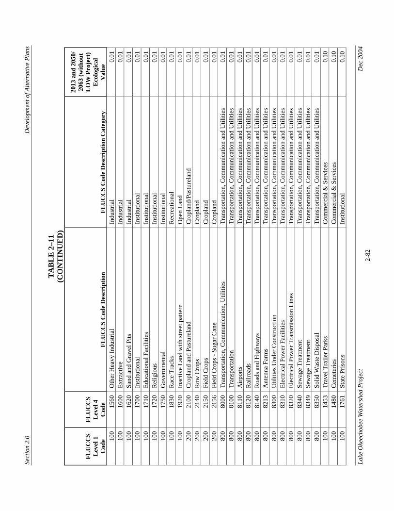
Sect
ion
2.0
Dev
elop
men
t of A
ltern
ativ
e Pl
ans
Lake
Oke
echo
bee
Wat
ersh
ed P
roje
ct
D
ec 2
004
2-82
TA
BL
E 2
–11
(CO
NT
INU
ED
)
FLU
CC
S L
evel
1
Cod
e
FLU
CC
S L
evel
4
Cod
e FL
UC
CS
Cod
e D
escr
iptio
n
FLU
CC
S C
ode
Des
crip
tion
Cat
egor
y
2013
and
205
0/
2063
(with
out
LO
W P
roje
ct)
Eco
logi
cal
Val
ue
100
1560
O
ther
Hea
vy In
dust
rial
Indu
stria
l 0.
01
100
1600
Ex
tract
ive
Indu
stria
l 0.
01
100
1620
Sa
nd a
nd G
rave
l Pits
In
dust
rial
0.01
10
0 17
00
Inst
itutio
nal
Inst
itutio
nal
0.01
10
0 17
10
Educ
atio
nal F
acili
ties
Inst
itutio
nal
0.01
10
0 17
20
Rel
igio
us
Inst
itutio
nal
0.01
10
0 17
50
Gov
ernm
enta
l In
stitu
tiona
l 0.
01
100
1830
R
ace
Trac
ks
Rec
reat
iona
l 0.
01
100
1920
In
activ
e La
nd w
ith st
reet
pat
tern
O
pen
Land
0.
01
200
2100
C
ropl
and
and
Past
urel
and
Cro
plan
d/Pa
stur
elan
d 0.
01
200
2140
R
ow C
rops
C
ropl
and
0.01
20
0 21
50
Fiel
d C
rops
C
ropl
and
0.01
20
0 21
56
Fiel
d C
rops
- Su
gar C
ane
Cro
plan
d 0.
01
800
8000
Tr
ansp
orta
tion,
Com
mun
icat
ion,
Util
ities
Tr
ansp
orta
tion,
Com
mun
icat
ion
and
Util
ities
0.
01
800
8100
Tr
ansp
orta
tion
Tran
spor
tatio
n, C
omm
unic
atio
n an
d U
tiliti
es
0.01
80
0 81
10
Airp
orts
Tr
ansp
orta
tion,
Com
mun
icat
ion
and
Util
ities
0.
01
800
8120
R
ailro
ads
Tran
spor
tatio
n, C
omm
unic
atio
n an
d U
tiliti
es
0.01
80
0 81
40
Roa
ds a
nd H
ighw
ays
Tran
spor
tatio
n, C
omm
unic
atio
n an
d U
tiliti
es
0.01
80
0 82
13
Ant
enna
Far
ms
Tran
spor
tatio
n, C
omm
unic
atio
n an
d U
tiliti
es
0.01
80
0 83
00
Util
ities
Und
er C
onst
ruct
ion
Tran
spor
tatio
n, C
omm
unic
atio
n an
d U
tiliti
es
0.01
80
0 83
10
Elec
trica
l Pow
er F
acili
ties
Tran
spor
tatio
n, C
omm
unic
atio
n an
d U
tiliti
es
0.01
80
0 83
20
Elec
trica
l Pow
er T
rans
mis
sion
Lin
es
Tran
spor
tatio
n, C
omm
unic
atio
n an
d U
tiliti
es
0.01
80
0 83
40
Sew
age
Trea
tmen
t Tr
ansp
orta
tion,
Com
mun
icat
ion
and
Util
ities
0.
01
800
8349
Se
wag
e Tr
eatm
ent
Tran
spor
tatio
n, C
omm
unic
atio
n an
d U
tiliti
es
0.01
80
0 83
50
Solid
Was
te D
ispo
sal
Tran
spor
tatio
n, C
omm
unic
atio
n an
d U
tiliti
es
0.01
10
0 14
53
Trav
el T
raile
r Par
ks
Com
mer
cial
& S
ervi
ces
0.10
10
0 14
80
Cem
eter
ies
Com
mer
cial
& S
ervi
ces
0.10
10
0 17
61
Stat
e Pr
ison
s In
stitu
tiona
l 0.
10
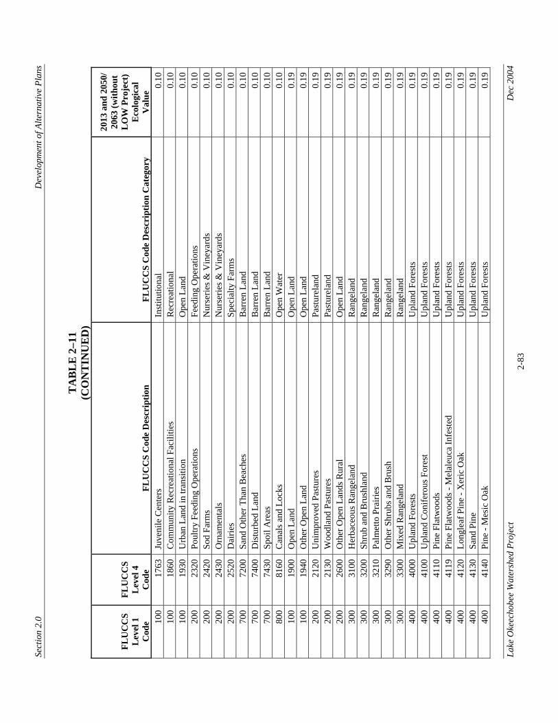
Sect
ion
2.0
Dev
elop
men
t of A
ltern
ativ
e Pl
ans
Lake
Oke
echo
bee
Wat
ersh
ed P
roje
ct
D
ec 2
004
2-83
TA
BL
E 2
–11
(CO
NT
INU
ED
)
FLU
CC
S L
evel
1
Cod
e
FLU
CC
S L
evel
4
Cod
e FL
UC
CS
Cod
e D
escr
iptio
n
FLU
CC
S C
ode
Des
crip
tion
Cat
egor
y
2013
and
205
0/
2063
(with
out
LO
W P
roje
ct)
Eco
logi
cal
Val
ue
100
1763
Ju
veni
le C
ente
rs
Inst
itutio
nal
0.10
10
0 18
60
Com
mun
ity R
ecre
atio
nal F
acili
ties
Rec
reat
iona
l 0.
10
100
1930
U
rban
Lan
d in
tran
sitio
n O
pen
Land
0.
10
200
2320
Po
ultry
Fee
ding
Ope
ratio
ns
Feed
ing
Ope
ratio
ns
0.10
20
0 24
20
Sod
Farm
s N
urse
ries &
Vin
eyar
ds
0.10
20
0 24
30
Orn
amen
tals
N
urse
ries &
Vin
eyar
ds
0.10
20
0 25
20
Dai
ries
Spec
ialty
Far
ms
0.10
70
0 72
00
Sand
Oth
er T
han
Bea
ches
B
arre
n La
nd
0.10
70
0 74
00
Dis
turb
ed L
and
Bar
ren
Land
0.
10
700
7430
Sp
oil A
reas
B
arre
n La
nd
0.10
80
0 81
60
Can
als a
nd L
ocks
O
pen
Wat
er
0.10
10
0 19
00
Ope
n La
nd
Ope
n La
nd
0.19
10
0 19
40
Oth
er O
pen
Land
O
pen
Land
0.
19
200
2120
U
nim
prov
ed P
astu
res
Past
urel
and
0.19
20
0 21
30
Woo
dlan
d Pa
stur
es
Past
urel
and
0.19
20
0 26
00
Oth
er O
pen
Land
s Rur
al
Ope
n La
nd
0.19
30
0 31
00
Her
bace
ous R
ange
land
R
ange
land
0.
19
300
3200
Sh
rub
and
Bru
shla
nd
Ran
gela
nd
0.19
30
0 32
10
Palm
etto
Pra
iries
R
ange
land
0.
19
300
3290
O
ther
Shr
ubs a
nd B
rush
R
ange
land
0.
19
300
3300
M
ixed
Ran
gela
nd
Ran
gela
nd
0.19
40
0 40
00
Upl
and
Fore
sts
Upl
and
Fore
sts
0.19
40
0 41
00
Upl
and
Con
ifero
us F
ores
t U
plan
d Fo
rest
s 0.
19
400
4110
Pi
ne F
latw
oods
U
plan
d Fo
rest
s 0.
19
400
4119
Pi
ne F
latw
oods
- M
elal
euca
Infe
sted
U
plan
d Fo
rest
s 0.
19
400
4120
Lo
ngle
af P
ine
- Xer
ic O
ak
Upl
and
Fore
sts
0.19
40
0 41
30
Sand
Pin
e U
plan
d Fo
rest
s 0.
19
400
4140
Pi
ne -
Mes
ic O
ak
Upl
and
Fore
sts
0.19

Sect
ion
2.0
Dev
elop
men
t of A
ltern
ativ
e Pl
ans
Lake
Oke
echo
bee
Wat
ersh
ed P
roje
ct
D
ec 2
004
2-84
TA
BL
E 2
–11
(CO
NT
INU
ED
)
FLU
CC
S L
evel
1
Cod
e
FLU
CC
S L
evel
4
Cod
e FL
UC
CS
Cod
e D
escr
iptio
n
FLU
CC
S C
ode
Des
crip
tion
Cat
egor
y
2013
and
205
0/
2063
(with
out
LO
W P
roje
ct)
Eco
logi
cal
Val
ue
400
4200
U
plan
d H
ardw
ood
Fore
st
Upl
and
Fore
sts
0.19
40
0 42
10
Xer
ic O
ak
Upl
and
Fore
sts
0.19
40
0 42
20
Bra
zilia
n Pe
pper
U
plan
d Fo
rest
s 0.
19
400
4230
O
ak -
Pine
- H
icko
ry
Upl
and
Fore
sts
0.19
40
0 42
40
Mel
aleu
ca
Upl
and
Fore
sts
0.19
40
0 42
50
Tem
pera
te H
ardw
ood
Upl
and
Fore
sts
0.19
40
0 42
70
Live
Oak
U
plan
d Fo
rest
s 0.
19
400
4280
C
abba
ge P
alm
U
plan
d Fo
rest
s 0.
19
400
4310
B
eech
- M
agno
lia
Upl
and
Fore
sts
0.19
40
0 43
20
Sand
Liv
e O
ak
Upl
and
Fore
sts
0.19
40
0 43
30
Wes
tern
Eve
rgla
des H
ardw
oods
U
plan
d Fo
rest
s 0.
19
400
4340
H
ardw
ood
Con
ifer M
ixed
U
plan
d Fo
rest
s 0.
19
400
4350
D
ead
Tree
s U
plan
d Fo
rest
s 0.
19
400
4370
A
ustra
lian
Pine
U
plan
d Fo
rest
s 0.
19
400
4380
M
ixed
Har
dwoo
ds
Upl
and
Fore
sts
0.19
40
0 44
00
Tree
Pla
ntat
ions
Si
lvac
ultu
re
0.19
40
0 44
10
Con
ifero
us P
lant
atio
ns
Silv
acul
ture
0.
19
400
4430
Fo
rest
Reg
ener
atio
n A
reas
Si
lvac
ultu
re
0.19
70
0 74
10
Rur
al la
nd in
tran
sitio
n B
arre
n La
nd
0.19
70
0 74
20
Bor
row
Are
as
Bar
ren
Land
0.
19
700
7450
B
urne
d A
reas
B
arre
n La
nd
0.19
10
0 11
00
Res
iden
tial L
ow D
ensi
ty <
2 du
/ac
Res
iden
tial
0.20
10
0 11
10
Fixe
d Si
ngle
Fam
ily U
nits
<2
du/a
c R
esid
entia
l 0.
20
100
1130
M
ixed
Uni
ts (F
ixed
and
mob
ile h
ome
units
)<2
du/a
c R
esid
entia
l 0.
20
100
1820
G
olf C
ours
es
Rec
reat
iona
l 0.
20
100
1840
M
arin
as a
nd F
ish
Cam
ps
Rec
reat
iona
l 0.
20
100
1841
M
arin
as (B
asin
s)
Rec
reat
iona
l 0.
20
100
1890
O
ther
Rec
reat
iona
l R
ecre
atio
nal
0.20
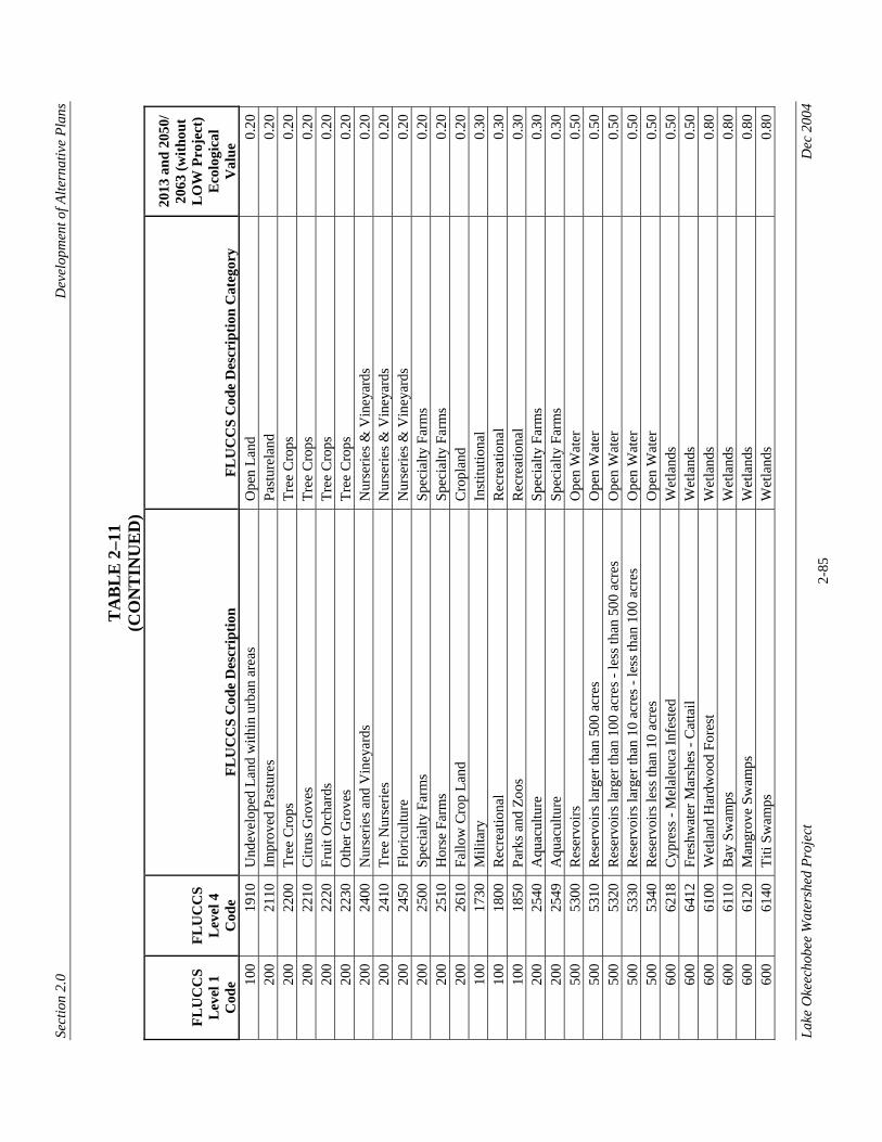
Sect
ion
2.0
Dev
elop
men
t of A
ltern
ativ
e Pl
ans
Lake
Oke
echo
bee
Wat
ersh
ed P
roje
ct
D
ec 2
004
2-85
TA
BL
E 2
–11
(CO
NT
INU
ED
)
FLU
CC
S L
evel
1
Cod
e
FLU
CC
S L
evel
4
Cod
e FL
UC
CS
Cod
e D
escr
iptio
n
FLU
CC
S C
ode
Des
crip
tion
Cat
egor
y
2013
and
205
0/
2063
(with
out
LO
W P
roje
ct)
Eco
logi
cal
Val
ue
100
1910
U
ndev
elop
ed L
and
with
in u
rban
are
as
Ope
n La
nd
0.20
20
0 21
10
Impr
oved
Pas
ture
s Pa
stur
elan
d 0.
20
200
2200
Tr
ee C
rops
Tr
ee C
rops
0.
20
200
2210
C
itrus
Gro
ves
Tree
Cro
ps
0.20
20
0 22
20
Frui
t Orc
hard
s Tr
ee C
rops
0.
20
200
2230
O
ther
Gro
ves
Tree
Cro
ps
0.20
20
0 24
00
Nur
serie
s and
Vin
eyar
ds
Nur
serie
s & V
iney
ards
0.
20
200
2410
Tr
ee N
urse
ries
Nur
serie
s & V
iney
ards
0.
20
200
2450
Fl
oric
ultu
re
Nur
serie
s & V
iney
ards
0.
20
200
2500
Sp
ecia
lty F
arm
s Sp
ecia
lty F
arm
s 0.
20
200
2510
H
orse
Far
ms
Spec
ialty
Far
ms
0.20
20
0 26
10
Fallo
w C
rop
Land
C
ropl
and
0.20
10
0 17
30
Mili
tary
In
stitu
tiona
l 0.
30
100
1800
R
ecre
atio
nal
Rec
reat
iona
l 0.
30
100
1850
Pa
rks a
nd Z
oos
Rec
reat
iona
l 0.
30
200
2540
A
quac
ultu
re
Spec
ialty
Far
ms
0.30
20
0 25
49
Aqu
acul
ture
Sp
ecia
lty F
arm
s 0.
30
500
5300
R
eser
voirs
O
pen
Wat
er
0.50
50
0 53
10
Res
ervo
irs la
rger
than
500
acr
es
Ope
n W
ater
0.
50
500
5320
R
eser
voirs
larg
er th
an 1
00 a
cres
- le
ss th
an 5
00 a
cres
O
pen
Wat
er
0.50
50
0 53
30
Res
ervo
irs la
rger
than
10
acre
s - le
ss th
an 1
00 a
cres
O
pen
Wat
er
0.50
50
0 53
40
Res
ervo
irs le
ss th
an 1
0 ac
res
Ope
n W
ater
0.
50
600
6218
C
ypre
ss -
Mel
aleu
ca In
fest
ed
Wet
land
s 0.
50
600
6412
Fr
eshw
ater
Mar
shes
- C
atta
il W
etla
nds
0.50
60
0 61
00
Wet
land
Har
dwoo
d Fo
rest
W
etla
nds
0.80
60
0 61
10
Bay
Sw
amps
W
etla
nds
0.80
60
0 61
20
Man
grov
e Sw
amps
W
etla
nds
0.80
60
0 61
40
Titi
Swam
ps
Wet
land
s 0.
80

Sect
ion
2.0
Dev
elop
men
t of A
ltern
ativ
e Pl
ans
Lake
Oke
echo
bee
Wat
ersh
ed P
roje
ct
D
ec 2
004
2-86
TA
BL
E 2
–11
(CO
NT
INU
ED
)
FLU
CC
S L
evel
1
Cod
e
FLU
CC
S L
evel
4
Cod
e FL
UC
CS
Cod
e D
escr
iptio
n
FLU
CC
S C
ode
Des
crip
tion
Cat
egor
y
2013
and
205
0/
2063
(with
out
LO
W P
roje
ct)
Eco
logi
cal
Val
ue
600
6150
St
ream
and
Lak
e Sw
amps
(Bot
tom
land
) W
etla
nds
0.80
60
0 61
60
Inla
nd P
onds
and
Slo
ughs
W
etla
nds
0.80
60
0 61
70
Mix
ed W
etla
nd H
ardw
oods
W
etla
nds
0.80
60
0 61
71
Mix
ed W
etla
nd H
ardw
oods
- W
illow
s W
etla
nds
0.80
60
0 61
72
Mix
ed W
etla
nd H
ardw
oods
- M
ixed
Shr
ubs
Wet
land
s 0.
80
600
6200
W
etla
nd C
onife
rous
For
est
Wet
land
s 0.
80
600
6210
C
ypre
ss
Wet
land
s 0.
80
600
6219
C
ypre
ss -
with
Wet
Pra
iries
W
etla
nds
0.80
60
0 62
20
Pond
Pin
e W
etla
nds
0.80
60
0 62
40
Cyp
ress
- Pi
ne -
Cab
bage
Pal
m
Wet
land
s 0.
80
600
6300
W
etla
nd F
ores
ted
Mix
ed
Wet
land
s 0.
80
600
6400
V
eget
ated
Non
-For
este
d W
etla
nds
Wet
land
s 0.
80
600
6410
Fr
eshw
ater
Mar
shes
W
etla
nds
0.80
60
0 64
11
Fres
hwat
er M
arsh
es -
Saw
gras
s W
etla
nds
0.80
60
0 64
20
Saltw
ater
Mar
shes
W
etla
nds
0.80
60
0 64
30
Wet
Pra
iries
W
etla
nds
0.80
60
0 64
39
Wet
Pra
iries
- w
ith P
ine
Wet
land
s 0.
80
600
6440
Em
erge
nt A
quat
ic V
eget
atio
n W
etla
nds
0.80
60
0 65
20
Shor
elin
es
Wet
land
s 0.
80
600
6530
In
term
itten
t Pon
ds
Wet
land
s 0.
80
500
5100
St
ream
s and
Wat
erw
ays
Ope
n W
ater
1.
00
500
5200
La
kes
Ope
n W
ater
1.
00
500
5210
La
kes l
arge
r tha
n 50
0 ac
res
Ope
n W
ater
1.
00
500
5220
La
kes l
arge
r tha
n 10
0 ac
res -
less
than
50
Ope
n W
ater
1.
00
500
5230
La
kes L
arge
r tha
n 10
acr
es -
less
than
100
O
pen
Wat
er
1.00
50
0 52
40
Lake
s les
s tha
n 10
acr
es
Ope
n W
ater
1.
00
500
5600
Sl
ough
Wat
ers
Ope
n W
ater
1.
00
du/a
c =
dwel
lings
per
acr
e
Section 2.0 Development of Alternative Plans
Lake Okeechobee Watershed Project Dec 2004 2-87
Functioning Wetland Habitat Units – 2050 (Future without Project Conditions) Functioning wetland habitat units likely to be provided in 2050 by each of the top-ranked sites under future without project conditions were calculated using the same methodology used for projecting functioning wetland habitat units for 2013. Habitat quality in the 100-m buffer of each individual wetland was expected to change as described previously. However, by 2050 without implementation of the LOW Project, it was assumed that within the 100-m wetland buffer, 50 percent of uplands currently in unimproved pasture (FLUCCS Level 4 codes 2120, 2130), rangeland (FLUCCS Level 4 3000 Series codes), native/natural uplands (FLUCCS Level 4 4000 Series codes) and rural land in transition (FLUCCS Level 4 code 7410) would be converted into more intensive agricultural (FLUCCS Level 4 2000 Series codes), urban, residential, or commercial land uses (FLUCCS Level 4 1000 Series codes). Therefore, 50 percent of the uplands in the 100-m wetland buffer were assessed with 2050 average EVS of 0.19 and the remaining 50 percent of the uplands in the 100-m buffer were assessed using their 2004 EVS. Projected wetland quality likely to exist in 2050 under future without project conditions was assessed as described in the previous section. 2050 quantity factor scores under future without project conditions were determined using the methodology used for the 2013 calculations. Table 2–11 lists the FLUCCS codes and their revised ecological value scores used in this analysis. The revised ecological value scores were plugged into the WEAT for the calculation of habitat units. Besides the loss of all isolated wetlands <0.50 acres in size by 2013, no additional wetland losses were projected through 2050. The quality and quantity factor scores were used to estimate the functioning wetland habitat units likely to be provided by the top-ranked sites in 2050 under future without project conditions, as shown in the example below: • Using the revised ecological value scores from Table 2–11, the WEAT indicated that
a given top-ranked site had 150 functioning wetland habitat units in 2050 under future without project conditions. This value accounts for the quality factor score.
• The quantity factor score was then added into the equation. In 2004, this site
contained 20 isolated wetlands that were each 0.20 acres in size. The WEAT indicated that in 2050 these 20 isolated wetlands would have had an WVS of 0.50. However, since it was assumed that by 2013 these isolated wetlands would have been converted to other land uses, they were subtracted from the calculation of 2050 wetland habitat units likely to exist under future without project conditions as follows:
150 – [(20*0.20)*0.50] = 148 Habitat Units
Thus, based upon the quality and quantity factor scores, it was predicted that the given site would likely provide only 148 functioning wetland habitat units in 2050 under future