filtering in the frequency domain - iit bombayavikb/gnr401/dip/dip_401_lecture_4.pdf · frequency...
TRANSCRIPT

FILTERING IN THE FREQUENCY DOMAINLecture 4
1GNR401 Dr. A. Bhattacharya

Spatial Vs Frequency domain
Spatial Domain (I) – “Normal” image space – Changes in pixel positions correspond to changes in the
scene – Distances in I correspond to real distances
Frequency Domain (F) – Changes in image position correspond to changes in the
spatial frequency – This is the rate at which image intensity values are
changing in the spatial domain image I
2
GNR401 Dr. A. Bhattacharya

The Fourier Series
Periodic functions can be expressed as the sum of sines and/or cosines of different frequencies each multiplied by a different coefficient
3
GNR401 Dr. A. Bhattacharya

Image processing
Spatial Domain (I) – Directly process the input image pixel array
Frequency Domain (F) – Transform the image to its frequency representation – Perform image processing – Compute inverse transform back to the spatial
domain
4
GNR401 Dr. A. Bhattacharya

Frequencies in an Image
Any spatial or temporal signal has an equivalent frequency representation
What do frequencies mean in an image ? – High frequencies correspond to pixel values that change
rapidly across the image (e.g. text, texture, leaves, etc.) – Strong low frequency components correspond to large
scale features in the image (e.g. a single, homogenous object that dominates the image)
We will investigate Fourier transformations to obtain frequency representations of an image
5
GNR401 Dr. A. Bhattacharya

Properties of a Transform
A transform maps image data into a different mathematical space via a transformation equation
Most of the discrete transforms map the image data from the spatial domain to the frequency domain, where all the pixels in the input (spatial domain) contribute to each value in the output (frequency domain)
6
GNR401 Dr. A. Bhattacharya

Spatial Frequency
Rate of change
Faster the rate of change over distance, higher the frequency
7
GNR401 Dr. A. Bhattacharya

Image Transforms
Image transforms are used as tools in many applications, including enhancement, restoration, correlation and SAR data processing
Discrete Fourier transform is the most important transform employed in image processing applications
Discrete Fourier transform is generated by sampling the basis functions of the continuous transform, i.e., the sine and cosine functions
8
GNR401 Dr. A. Bhattacharya

Concept of Fourier Transform
The Fourier transform decomposes a complex signal into a weighted sum of sinusoids, starting from zero-frequency to a high value determined by the input function
The lowest frequency is also called the fundamentalfrequency
9
GNR401 Dr. A. Bhattacharya

Frequency Decomposition
The base frequency or the fundamental frequency is the lowest frequency. All multiples of the fundamental frequency are known as harmonics.
A given signal can be constructed back from its frequency decomposition by a weighted addition of the fundamental frequency and all the harmonic frequencies
10
GNR401 Dr. A. Bhattacharya
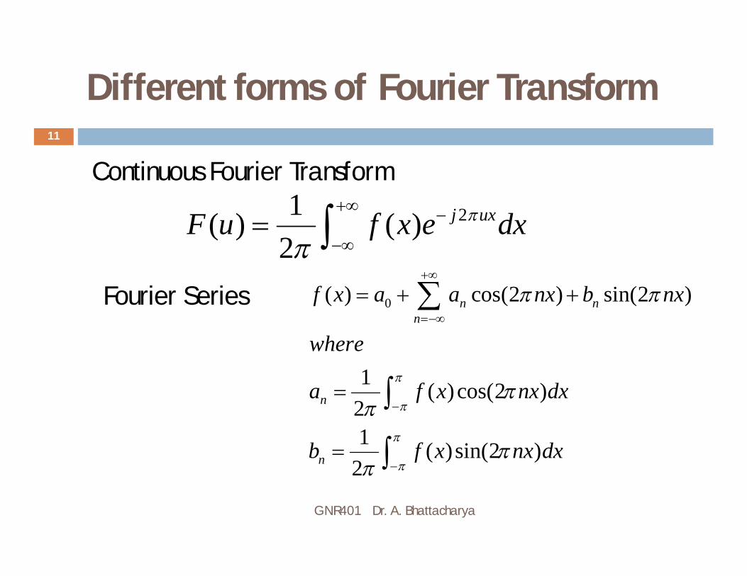
Different forms of Fourier Transform
21( ) ( )2
j uxF u f x e dx
0( ) cos(2 ) sin(2 )
1 ( )cos(2 )21 ( )sin(2 )
2
n nn
n
n
f x a a nx b nx
where
a f x nx dx
b f x nx dx
Continuous Fourier Transform
Fourier Series
11
GNR401 Dr. A. Bhattacharya

Continuous Fourier Transform
In the continuous domain, the basis functions of the Fourier transform are the complex exponentials e-j2pux
These functions extend from -∞ to + ∞
These are continuous functions, and exist everywhere
12
GNR401 Dr. A. Bhattacharya

Real and Imaginary Parts of Fourier Transform
21( ) ( )2
j uxF u f x e dx
1 1( ) ( ) cos(2 ) ( ) sin(2 )2 2
F u f x ux dx j f x ux dx
Real part Imaginary Part
13
GNR401 Dr. A. Bhattacharya

The Discrete Fourier Transform14
GNR401 Dr. A. Bhattacharya

The Discrete Fourier Transform15
GNR401 Dr. A. Bhattacharya

The 2-D Discrete Fourier Transform16
GNR401 Dr. A. Bhattacharya

The 2-D Discrete Fourier Transform17
GNR401 Dr. A. Bhattacharya
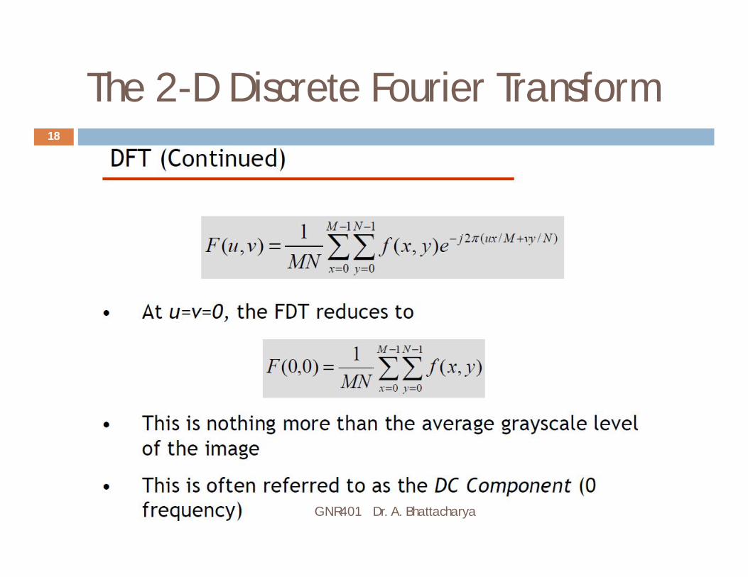
The 2-D Discrete Fourier Transform18
GNR401 Dr. A. Bhattacharya

The 2-D Discrete Fourier Transform19
GNR401 Dr. A. Bhattacharya

Properties of the Fourier Transform20
GNR401 Dr. A. Bhattacharya

Filtering ExampleSmooth an Image with a Gaussian Kernel
21
GNR401 Dr. A. Bhattacharya
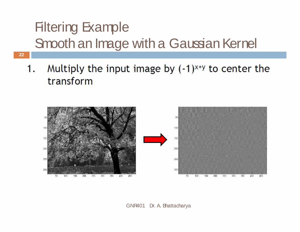
Filtering ExampleSmooth an Image with a Gaussian Kernel
22
GNR401 Dr. A. Bhattacharya

Filtering ExampleSmooth an Image with a Gaussian Kernel
23
GNR401 Dr. A. Bhattacharya

Filtering ExampleSmooth an Image with a Gaussian Kernel
24
GNR401 Dr. A. Bhattacharya

Filtering ExampleSmooth an Image with a Gaussian Kernel
25
GNR401 Dr. A. Bhattacharya

Filtering ExampleSmooth an Image with a Gaussian Kernel
26
GNR401 Dr. A. Bhattacharya

The Fourier Transform27
GNR401 Dr. A. Bhattacharya

Properties of the Fourier Transform28
GNR401 Dr. A. Bhattacharya

Some Fundamental Transform Pairs29
GNR401 Dr. A. Bhattacharya

Some Fundamental Transform Pairs30
GNR401 Dr. A. Bhattacharya

Example
Given f(n) = [3,2,2,1], corresponding to the brightness values of one row of a digital image. Find F (u) in both rectangular form, and in exponential form
31
GNR401 Dr. A. Bhattacharya

Example Contd.
2 1.1/ 4 2 2.1/ 4 2 3.1/ 4
1(0) [3 2 2 1] 241(1) [3 2 2 1. ]4
1 1 [3 2 2 ] [1 ]4 4
j j j
F
F e e e
j j j
32
GNR401 Dr. A. Bhattacharya

Example Contd.
2 3.1/ 4 2 3.2 / 4 2 3.3/ 4
1 1(2) [3 2 2 1]4 21(3) [3 2 2 1. ]4
1 1 [3 2 2 ] [1 ]4 4
j j j
F
F e e e
j j j
Therefore F(u) = [2 ¼ (1-j) ½ ¼ (1+j) ]
33
GNR401 Dr. A. Bhattacharya

Magnitude-Phase Form
F(0)= 2 = 2 + j0 Mag=sqrt(22 + 02)=2; Phase=tan-1(0/2)=0
F(1) = ¼ (1-j) = ¼ - j ¼ Mag= ¼ sqrt(12 + (-1)2)=0.35;
Phase = tan-1(-(1/4) / (1/4)) = tan-1(-1) = -p/4
F(2) = ½ = ½ + j0 Mag = sqrt(( ½ )2 + 02) = ½
Phase = tan-1( 0 / (1/2) ) = 0
F(3) = ¼ (1+j) = ¼ - j ¼ Mag= ¼ sqrt(12 + (-1)2)=0.35; Phase = tan-1((1/4) / (1/4)) = tan-1(1) = p/4
34
GNR401 Dr. A. Bhattacharya

Fourier Transform Calculation
Given f(n) = [ 3 2 2 1 ]
F(u) = [2 ¼ (1-j) ½ ¼ (1+j) ]
In phase magnitude form,
M(u) = [2 0.35 ½ 0.35 ]
F(u) = [0 p/4 0 p/4 ]
Calculate the above for f(n) = [ 0 0 4 4 4 4 0 0]
Plot f(n), F(u), M(u) and F(u) graphically
35
GNR401 Dr. A. Bhattacharya