filtering and estimation with builds
DESCRIPTION
Part of a series handouts on Upenn's Courseware on Advanced Robotics.TRANSCRIPT

Filtering and Estimation for Mobile Robots
Nathan MichaelMEAM 620Spring, 2008
University of PennsylvaniaPhiladelphia, Pennsylvania

Reference

Outline
• Kinematic Model of a Mobile Robot
• Kalman Filter
• Extended Kalman Filter
• Unscented Kalman Filter
• Particle Filter

Outline
• Kinematic Model of a Mobile Robot
• Kalman Filter
• Extended Kalman Filter
• Unscented Kalman Filter
• Particle Filter

Mobile Robot Model
t1
t0

Mobile Robot Model
t1
t0
Differential Drive
v!
(x, y)
!l
!r
!

Mobile Robot Model
t1
t0
Differential Drive
!r – Right wheel orientation!l – Left wheel orientation
v!
(x, y)
!l
!r
!

Mobile Robot Model
t1
t0
Differential Drive
! – Robot orientation(x, y) – Robot center position
!r – Right wheel orientation!l – Left wheel orientation
v!
(x, y)
!l
!r
!

Mobile Robot Model
t1
t0
Differential Drive
! – Robot orientation(x, y) – Robot center position
!r – Right wheel orientation!l – Left wheel orientation
v – Linear velocity! – Angular velocity
v!
(x, y)
!l
!r
!

Mobile Robot Model
t1
t0
Differential Drive
! – Robot orientation(x, y) – Robot center position
!r – Right wheel orientation!l – Left wheel orientation
v – Linear velocity! – Angular velocity
Pose
v!
(x, y)
!l
!r
!

Mobile Robot Model
t1
t0
Differential Drive
! – Robot orientation(x, y) – Robot center position
!r – Right wheel orientation!l – Left wheel orientation
v – Linear velocity! – Angular velocity
Pose
Kinematic Velocities
v!
(x, y)
!l
!r
!

Mobile Robot Model
t1
t0
!
(x, y)
!l
!r

Mobile Robot Model
t1
t0
!
(x, y)
!l
!r
d!
dt=
r
b
!d!r
dt! d!l
dt
"Wheel radius
Wheel base

Mobile Robot Model
t1
t0
!
(x, y)
!l
!r
d!
dt=
r
b
!d!r
dt! d!l
dt
"Wheel radius
Wheel basedx
dt=
r cos !
2
!d!l
dt+
d!r
dt
"
dy
dt=
r sin !
2
!d!l
dt+
d!r
dt
"

Mobile Robot Model
t1
t0
xt = xt!1 + !x
yt = yt!1 + !y
Discrete State Updates
!t = !t!1 + !!

Mobile Robot Model
t1
t0
xt = xt!1 + !x
yt = yt!1 + !y
Discrete State Updates
R
Treat discrete changes as motions along circles of constant radius
!t = !t!1 + !!

Mobile Robot ModelDiscrete State Updates
xc = x! v
!sin "
R
R =!!!v
!
!!!
v = R!(xc, yc)
yc = y +v
!cos "

Mobile Robot ModelDiscrete State Updates
R
(xc, yc)xt = xt!1 + !x
yt = yt!1 + !y
!t = !t!1 + !!

Mobile Robot ModelDiscrete State Updates
R
(xc, yc)xt = xt!1 + !x
yt = yt!1 + !y
!t = !t!1 + !!
?

Mobile Robot ModelDiscrete State Updates
R
(xc, yc)xt = xt!1 + !x
yt = yt!1 + !y
!t = !t!1 + !!
!
"xt
yt
!t
#
$ =
!
"xc,t!1 + v
! sin (!t!1 + "!t)yc,t!1 ! v
! cos (!t!1 + "!t)!t!1 + "!t
#
$
?

t1
t0
Velocity model
v = v + !v
! = ! + "!
yt = yt!1 +v
!cos "t!1 !
v
!cos("t!1 + !!t)
xt = xt!1 !v
!sin "t!1 +
v
!sin("t!1 + !!t)
!t = !t!1 + "!t + #!!t
Mobile Robot Model

t1
t0
Velocity model
v = v + !v
! = ! + "!
yt = yt!1 +v
!cos "t!1 !
v
!cos("t!1 + !!t)
xt = xt!1 !v
!sin "t!1 +
v
!sin("t!1 + !!t)
!t = !t!1 + "!t + #!!t
Gaussian noise
Mobile Robot Model

t1
t0
Velocity model
v = v + !v
! = ! + "!
yt = yt!1 +v
!cos "t!1 !
v
!cos("t!1 + !!t)
xt = xt!1 !v
!sin "t!1 +
v
!sin("t!1 + !!t)
!t = !t!1 + "!t + #!!t
Gaussian noise
Why?
Mobile Robot Model

Outline
• Kinematic Model of a Mobile Robot
• Kalman Filter
• Extended Kalman Filter
• Unscented Kalman Filter
• Particle Filter

Kalman Filter
• Linear system model with Gaussian noise
• Moments parameterization
• First moment - mean
• Second moment - covariance

Kalman Filter
• Linear system model with Gaussian noise
• Moments parameterization
• First moment - mean
• Second moment - covariance
What if the system isnonlinear?

Kalman Filter
• Linear system model with Gaussian noise
• Moments parameterization
• First moment - mean
• Second moment - covariance
Is this a reasonable characterization of the system?
What if the system isnonlinear?

Kalman Filter(algorithm)
!t = At!t!1ATt + Rt
µt = Atµt!1 + Btut
µt = µt + Kt(zt ! Ctµt)
!t = (I !KtCt)!t
Kt = !tCTt (Ct!tC
Tt + Qt)!1

Kalman Filter(algorithm)
!t = At!t!1ATt + Rt
µt = Atµt!1 + Btut
µt = µt + Kt(zt ! Ctµt)
!t = (I !KtCt)!t
That’s it, only five equations.
Kt = !tCTt (Ct!tC
Tt + Qt)!1

Kalman Filter(algorithm)
!t = At!t!1ATt + Rt
µt = Atµt!1 + Btut
µt = µt + Kt(zt ! Ctµt)
!t = (I !KtCt)!t
Prediction
Kt = !tCTt (Ct!tC
Tt + Qt)!1

Kalman Filter(algorithm)
!t = At!t!1ATt + Rt
µt = Atµt!1 + Btut
µt = µt + Kt(zt ! Ctµt)
!t = (I !KtCt)!t
Prediction
Where should the state be at this point?
Kt = !tCTt (Ct!tC
Tt + Qt)!1

Kalman Filter(algorithm)
!t = At!t!1ATt + Rt
µt = Atµt!1 + Btut
Linear system model

Kalman Filter(algorithm)
!t = At!t!1ATt + Rt
µt = Atµt!1 + Btut System input

Kalman Filter(algorithm)
!t = At!t!1ATt + Rt
µt = Atµt!1 + Btut System input
System covariance

Kalman Filter(algorithm)
!t = At!t!1ATt + Rt
µt = Atµt!1 + Btut
We are stating that the system process behaves based on the following assumption:
p(xt | ut, xt!1) =e!
12 (xt!Atxt!1!Btut)
T R!1t (xt!Atxt!1!Btut)
det(2!Rt)12

Kalman Filter(algorithm)
!t = At!t!1ATt + Rt
µt = Atµt!1 + BtutProcess model
We are stating that the system process behaves based on the following assumption:
p(xt | ut, xt!1) =e!
12 (xt!Atxt!1!Btut)
T R!1t (xt!Atxt!1!Btut)
det(2!Rt)12

Kalman Filter(algorithm)
!t = At!t!1ATt + Rt
µt = Atµt!1 + Btut
At this point, the filter parameters are:• First and second moments• System process model• State update• Input update• Process noise

Kalman Filter(algorithm)
!t = At!t!1ATt + Rt
µt = Atµt!1 + Btut
At this point, the filter parameters are:• First and second moments• System process model• State update• Input update• Process noise

Kalman Filter(algorithm)
!t = At!t!1ATt + Rt
µt = Atµt!1 + Btut
At this point, the filter parameters are:• First and second moments• System process model• State update• Input update• Process noise
Not always constant,consider adaptive filters for
unknown process noise.

Kalman Filter(algorithm)
!t = At!t!1ATt + Rt
µt = Atµt!1 + Btut
Example:u = [x, y]T
µt = µt!1 + [x!t, y!t]TA = I2, B = !tI2, Rt = diag(!2
1 , !22)
!t = !t!1 + diag(!21 , !2
2)

Example:u = [x, y]T
µt = µt!1 + [x!t, y!t]TA = I2, B = !tI2, Rt = diag(!2
1 , !22)
!t = !t!1 + diag(!21 , !2
2)
!1
!2x
y
Equipotentialellipse

Example:u = [x, y]T
µt = µt!1 + [x!t, y!t]TA = I2, B = !tI2, Rt = diag(!2
1 , !22)
!t = !t!1 + diag(!21 , !2
2)
!1
!2x
y
Equipotentialellipse t = 0
!0 = I2µ0 = [0, 0]T

Example:u = [x, y]T
µt = µt!1 + [x!t, y!t]TA = I2, B = !tI2, Rt = diag(!2
1 , !22)
!t = !t!1 + diag(!21 , !2
2)
!1
!2x
y
Equipotentialellipse t = 0
!0 = I2µ0 = [0, 0]T
t = 1
µ1
!1

Kalman Filter(algorithm)
!t = At!t!1ATt + Rt
µt = Atµt!1 + Btut
µt = µt + Kt(zt ! Ctµt)
!t = (I !KtCt)!t
Measurementupdate
Kt = !tCTt (Ct!tC
Tt + Qt)!1

Kalman Filter(algorithm)
!t = At!t!1ATt + Rt
µt = Atµt!1 + Btut
µt = µt + Kt(zt ! Ctµt)
!t = (I !KtCt)!t
Kalman gain
Kt = !tCTt (Ct!tC
Tt + Qt)!1

Kalman Filter(algorithm)
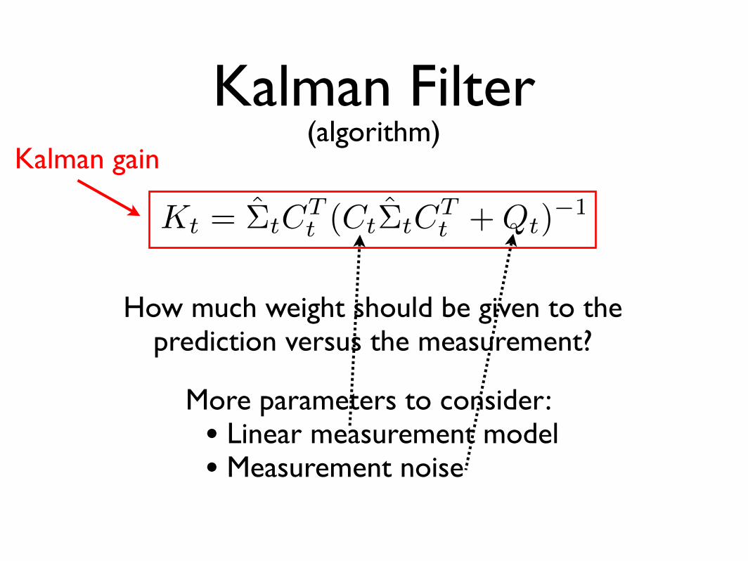
Kalman gain
Kt = !tCTt (Ct!tC
Tt + Qt)!1
How much weight should be given to the prediction versus the measurement?

Kalman Filter(algorithm)
Kalman gain
Kt = !tCTt (Ct!tC
Tt + Qt)!1
How much weight should be given to the prediction versus the measurement?
More parameters to consider:• Linear measurement model• Measurement noise
Kalman Filter(algorithm)
Kalman gain
Kt = !tCTt (Ct!tC
Tt + Qt)!1
How much weight should be given to the prediction versus the measurement?
More parameters to consider:• Linear measurement model• Measurement noise

Kalman Filter(algorithm)
Kt = !tCTt (Ct!tC
Tt + Qt)!1
The measurement of the state behaves based on the following assumption:
p(zt | xt) =e!
12 (zt!Ctxt)
T Q!1t (zt!Ctxt)
det(2!Qt)12

Kalman Filter(algorithm)
µt = µt + Kt(zt ! Ctµt)
Kt = !tCTt (Ct!tC
Tt + Qt)!1
Innovation
What is the error between the actual and predicted measurements?

Kalman Filter(algorithm)
µt = µt + Kt(zt ! Ctµt)
Kt = !tCTt (Ct!tC
Tt + Qt)!1
As a thought exercise, what if we have a perfect measurement model
and state feedback?

Kalman Filter(algorithm)
µt = µt + Kt(zt ! Ctµt)
Kt = !tCTt (Ct!tC
Tt + Qt)!1
As a thought exercise, what if we have a perfect measurement model
and state feedback?
Ct = IN , Qt = 0N ! Kt = IN , µt = zt

Kalman Filter(algorithm)
µt = µt + Kt(zt ! Ctµt)
Kt = !tCTt (Ct!tC
Tt + Qt)!1
As a thought exercise, what if we have a perfect measurement model
and state feedback?
Ct = IN , Qt = 0N ! Kt = IN , µt = zt

Kalman Filter(algorithm)
Kt = !tCTt (Ct!tC
Tt + Qt)!1
!t = (I !KtCt)!t
How does the error of the measurement model differ from the predicted error?

Kalman Filter(algorithm)
Kt = !tCTt (Ct!tC
Tt + Qt)!1
!t = (I !KtCt)!t
Consider again if we have perfect measurements.

Kalman Filter(algorithm)
Kt = !tCTt (Ct!tC
Tt + Qt)!1
!t = (I !KtCt)!t
Consider again if we have perfect measurements.
Ct = IN , Kt = IN ! !t = 0N

Kalman Filter(algorithm)
Kt = !tCTt (Ct!tC
Tt + Qt)!1
!t = (I !KtCt)!t
Consider again if we have perfect measurements.
Ct = IN , Kt = IN ! !t = 0N
Clearly perfect information means there is no error, so the error is degenerate (a point).

This is just a thought exercise!
Kalman Filter(algorithm)
Kt = !tCTt (Ct!tC
Tt + Qt)!1
!t = (I !KtCt)!t
Consider again if we have perfect measurements.
Ct = IN , Kt = IN ! !t = 0N

Kalman Filter(algorithm)
Example (cont.):
µt = µt + Kt(zt ! Ctµt)
!t = (I !KtCt)!t
Kt = !tCTt (Ct!tC
Tt + Qt)!1
Ct = I2, Qt = diag(!21, !22)

Example (cont.):
µt = µt + Kt(zt ! Ctµt)
!t = (I !KtCt)!t
Kt = !tCTt (Ct!tC
Tt + Qt)!1
Ct = I2, Qt = diag(!21, !22)
Kt = !t(!t + Qt)!1
= (!t!1 + diag(!21 , !2
2)) ·(!t!1 + diag(!2
1 + "21, !22 + "22))
!1

Kt = !t(!t + Qt)!1
= (!t!1 + diag(!21 , !2
2)) ·(!t!1 + diag(!2
1 + "21, !22 + "22))
!1
µt = (I2 !Kt)µt + Ktzt
!t = (I2 !Kt)!t
µt = µt!1 + [x!t, y!t]T
!t = !t!1 + diag(!21 , !2
2)
Example (cont.):

t = 0
!0 = I2µ0 = [0, 0]T
t = 1
µ1
!1
Prediction

t = 0
!0 = I2µ0 = [0, 0]T
t = 1
µ1
!1
Prediction
µ1
!1
zt
Qt
Measurement

t = 0
!0 = I2µ0 = [0, 0]T
t = 1
µ1
!1
!1 µ1
Prediction
µ1
!1
zt
Qt
Measurement

Kalman Filter(algorithm)
!t = At!t!1ATt + Rt
µt = Atµt!1 + Btut
µt = µt + Kt(zt ! Ctµt)
!t = (I !KtCt)!t
What about computational complexity?
Kt = !tCTt (Ct!tC
Tt + Qt)!1

Kalman Filter(algorithm)
!t = At!t!1ATt + Rt
µt = Atµt!1 + Btut
µt = µt + Kt(zt ! Ctµt)
!t = (I !KtCt)!t
What about computational complexity?
Kt = !tCTt (Ct!tC
Tt + Qt)!1 N = 2?

Kalman Filter(algorithm)
!t = At!t!1ATt + Rt
µt = Atµt!1 + Btut
µt = µt + Kt(zt ! Ctµt)
!t = (I !KtCt)!t
What about computational complexity?
Kt = !tCTt (Ct!tC
Tt + Qt)!1 N = 2?
N = 210?

Kalman Filter(algorithm)
!t = At!t!1ATt + Rt
µt = Atµt!1 + Btut
µt = µt + Kt(zt ! Ctµt)
!t = (I !KtCt)!t
What about computational complexity?
Kt = !tCTt (Ct!tC
Tt + Qt)!1 N = 2?
N = 210?
What about global
uncertainty?

Kalman Filter(algorithm)
!t = At!t!1ATt + Rt
µt = Atµt!1 + Btut
µt = µt + Kt(zt ! Ctµt)
!t = (I !KtCt)!t
What about computational complexity?
Kt = !tCTt (Ct!tC
Tt + Qt)!1
What if we redefine the parameterization?
N = 2?N = 210?
What about global
uncertainty?

Re-parameterization
! =" !1
Information matrix

Re-parameterization
! =" !1
Information matrix
! = !!1µInformation vector

Information Filter(algorithm)
!t = !t(At!!1t!1!t!1 + Btut)
!t = CTt Q!1
t Ct + !t
!t = CTt Q!1
t zt + !t
!t = (At!!1t!1A
Tt + Rt)!1

Information Filter(algorithm)
!t = !t(At!!1t!1!t!1 + Btut)
!t = CTt Q!1
t Ct + !t
!t = CTt Q!1
t zt + !t
!t = (At!!1t!1A
Tt + Rt)!1
Prediction

Information Filter(algorithm)
!t = !t(At!!1t!1!t!1 + Btut)
!t = CTt Q!1
t Ct + !t
!t = CTt Q!1
t zt + !t
!t = (At!!1t!1A
Tt + Rt)!1
Prediction
Measurement

KF/IF Comparison
!t = !t(At!!1t!1!t!1 + Btut)
!t = CTt Q!1
t Ct + !t
!t = CTt Q!1
t zt + !t
!t = (At!!1t!1A
Tt + Rt)!1
Information Filter
!t = At!t!1ATt + Rt
µt = Atµt!1 + Btut
µt = µt + Kt(zt ! Ctµt)
!t = (I !KtCt)!t
Kt = !tCTt (Ct!tC
Tt + Qt)!1
Kalman Filter
! =" !1 ! = !!1µReminder:

KF/IF Comparison
!t = !t(At!!1t!1!t!1 + Btut)
!t = CTt Q!1
t Ct + !t
!t = CTt Q!1
t zt + !t
!t = (At!!1t!1A
Tt + Rt)!1
Information Filter
!t = At!t!1ATt + Rt
µt = Atµt!1 + Btut
µt = µt + Kt(zt ! Ctµt)
!t = (I !KtCt)!t
Kt = !tCTt (Ct!tC
Tt + Qt)!1
Kalman Filter
!t = "!1t
! =" !1 ! = !!1µReminder:

KF/IF Comparison
!t = !t(At!!1t!1!t!1 + Btut)
!t = CTt Q!1
t Ct + !t
!t = CTt Q!1
t zt + !t
!t = (At!!1t!1A
Tt + Rt)!1
Information Filter
!t = At!t!1ATt + Rt
µt = Atµt!1 + Btut
µt = µt + Kt(zt ! Ctµt)
!t = (I !KtCt)!t
Kt = !tCTt (Ct!tC
Tt + Qt)!1
Kalman Filter
!t = !tµt
! =" !1 ! = !!1µReminder:

KF/IF Comparison
!t = !t(At!!1t!1!t!1 + Btut)
!t = CTt Q!1
t Ct + !t
!t = CTt Q!1
t zt + !t
!t = (At!!1t!1A
Tt + Rt)!1
Information Filter
!t = At!t!1ATt + Rt
µt = Atµt!1 + Btut
µt = µt + Kt(zt ! Ctµt)
!t = (I !KtCt)!t
Kt = !tCTt (Ct!tC
Tt + Qt)!1
Kalman Filter
! =" !1 ! = !!1µReminder:
Computational complexity?
We need the information matrix inverse to compute the mean.
µ = !!1!

KF/IF Comparison
!t = !t(At!!1t!1!t!1 + Btut)
!t = CTt Q!1
t Ct + !t
!t = CTt Q!1
t zt + !t
!t = (At!!1t!1A
Tt + Rt)!1
Information Filter
!t = At!t!1ATt + Rt
µt = Atµt!1 + Btut
µt = µt + Kt(zt ! Ctµt)
!t = (I !KtCt)!t
Kt = !tCTt (Ct!tC
Tt + Qt)!1
Kalman Filter
! =" !1 ! = !!1µReminder:
The choice of IF or KF is application dependent.

What if the process or measurement model is non-linear (or both are non-linear)?

What if the process or measurement model is non-linear (or both are non-linear)?
We could linearize the system model about the mean ...

Outline
• Kinematic Model of a Mobile Robot
• Kalman Filter
• Extended Kalman Filter
• Unscented Kalman Filter
• Particle Filter

Extending the Kalman Filter
!t = At!t!1ATt + Rt
µt = Atµt!1 + Btut
µt = µt + Kt(zt ! Ctµt)
!t = (I !KtCt)!t
Kt = !tCTt (Ct!tC
Tt + Qt)!1
(to non-linear system models)
KF algorithm

Extending the Kalman Filter
!t = At!t!1ATt + Rt
µt = Atµt!1 + Btut
µt = µt + Kt(zt ! Ctµt)
!t = (I !KtCt)!t
Kt = !tCTt (Ct!tC
Tt + Qt)!1
(to non-linear system models)
µt = g(ut, µt!1)Non-linear
process model

Extending the Kalman Filter
!t = At!t!1ATt + Rt
µt = Atµt!1 + Btut
µt = µt + Kt(zt ! Ctµt)
!t = (I !KtCt)!t
Kt = !tCTt (Ct!tC
Tt + Qt)!1
(to non-linear system models)
Linear process model
µt = g(ut, µt!1)Non-linear
process model

Extending the Kalman Filter
!t = At!t!1ATt + Rt
µt = Atµt!1 + Btut
µt = µt + Kt(zt ! Ctµt)
!t = (I !KtCt)!t
Kt = !tCTt (Ct!tC
Tt + Qt)!1
(to non-linear system models)
Linear process model
h(µt)Non-linear
measurement model
µt = g(ut, µt!1)Non-linear
process model

Extending the Kalman Filter
!t = At!t!1ATt + Rt
µt = Atµt!1 + Btut
µt = µt + Kt(zt ! Ctµt)
!t = (I !KtCt)!t
Kt = !tCTt (Ct!tC
Tt + Qt)!1
(to non-linear system models)
Linear process model
h(µt)Non-linear
measurement model
µt = g(ut, µt!1)Non-linear
process model
Linear measurement
model

Extended Kalman Filter(algorithm)
!t = Gt!t!1GTt + Rt
µt = g(ut, µt!1)
Kt = !tHTt (Ht!tH
Tt + Qt)!1
µt = µt + Kt(zt ! h(µt))
!t = (I !KtHt)!t

Extended Kalman Filter(algorithm)
!t = Gt!t!1GTt + Rt
µt = g(ut, µt!1)
Kt = !tHTt (Ht!tH
Tt + Qt)!1
µt = µt + Kt(zt ! h(µt))
!t = (I !KtHt)!t
Linearized process model

Extended Kalman Filter(algorithm)
!t = Gt!t!1GTt + Rt
µt = g(ut, µt!1)
Kt = !tHTt (Ht!tH
Tt + Qt)!1
µt = µt + Kt(zt ! h(µt))
!t = (I !KtHt)!t
Linearized process model
Linearized measurement
model

Extended Kalman Filter(algorithm)
!t = Gt!t!1GTt + Rt
µt = g(ut, µt!1)
Kt = !tHTt (Ht!tH
Tt + Qt)!1
µt = µt + Kt(zt ! h(µt))
!t = (I !KtHt)!t
Linearized process model
Linearized measurement
model
Linearization is generally a first order Taylor expansion.

Extended Kalman Filter(algorithm)
Mobile robot example:
t0

t1
Extended Kalman Filter(algorithm)
Mobile robot example:
t0

t1
Extended Kalman Filter(algorithm)
Mobile robot example:
t0(v, !)

t1
Extended Kalman Filter(algorithm)
Mobile robot example:
t0
Laser
(v, !)

t1
Extended Kalman Filter(algorithm)
Mobile robot example:
t0
Laser
(v, !)Robot has a map of the environment.

t1
Extended Kalman Filter(algorithm)
Mobile robot example:
t0
Laser
(v, !)Robot has a map of the environment.
We’ll consider the problemof localization via velocity
information and feature detection with unknown correspondence.

t1
Extended Kalman Filter(algorithm)
Mobile robot example:
t0
Velocity model
v = v + !v
! = ! + "!
yt = yt!1 +v
!cos "t!1 !
v
!cos("t!1 + !!t)
xt = xt!1 !v
!sin "t!1 +
v
!sin("t!1 + !!t)
!t = !t!1 + "!t + #!!t

t1
Extended Kalman Filter(algorithm)
Mobile robot example:
t0
Velocity model
v = v + !v
! = ! + "!
yt = yt!1 +v
!cos "t!1 !
v
!cos("t!1 + !!t)
xt = xt!1 !v
!sin "t!1 +
v
!sin("t!1 + !!t)
!t = !t!1 + "!t + #!!t
Gaussian noise

t1
Extended Kalman Filter(algorithm)
Mobile robot example:
t0
Velocity model
v = v + !v
! = ! + "!
yt = yt!1 +v
!cos "t!1 !
v
!cos("t!1 + !!t)
xt = xt!1 !v
!sin "t!1 +
v
!sin("t!1 + !!t)
!t = !t!1 + "!t + #!!t... but the EKF already accounts for noise.

t1
Extended Kalman Filter(algorithm)
Mobile robot example:
t0
Computing G:
From Taylor expansion:
g(ut, xt!1) ! g(ut, µt!1) + Gt(xt!1 " µt!1)

t1
Extended Kalman Filter(algorithm)
Mobile robot example:
t0
Computing G:
From Taylor expansion:
g(ut, xt!1) ! g(ut, µt!1) + Gt(xt!1 " µt!1)
Gt =!g(ut, µt!1)
!xt!1

t1
Extended Kalman Filter(algorithm)
Mobile robot example:
t0
dxt
dxt!1= 1,
dxt
dyt!1= 0
Computing G:
dxt
d!t!1= ! v
"cos !t!1 +
v
"cos(!t!1 + "!t)
dyt
d!t!1= ! v
"sin !t!1 +
v
"sin(!t!1 + "!t)
dyt
dxt!1= 0,
dyt
dyt!1= 1
d!t
dxt!1= 0,
d!t
dyt!1= 0,
d!t
d!t!1= 1

t1
Extended Kalman Filter(algorithm)
Mobile robot example:
t0
dxt
dxt!1= 1,
dxt
dyt!1= 0
Computing G:
dxt
d!t!1= ! v
"cos !t!1 +
v
"cos(!t!1 + "!t)
dyt
d!t!1= ! v
"sin !t!1 +
v
"sin(!t!1 + "!t)
dyt
dxt!1= 0,
dyt
dyt!1= 1
d!t
dxt!1= 0,
d!t
dyt!1= 0,
d!t
d!t!1= 1Partial derivatives

t1
Extended Kalman Filter(algorithm)
Mobile robot example:
t0
Computing G:
G =
!
"1 0 ! v
w cos !t!1 + vw cos(!t!1 + "!t)
0 1 ! vw sin !t!1 + v
w sin(!t!1 + "!t)0 0 1
#
$

t1
Extended Kalman Filter(algorithm)
Mobile robot example:
t0
Computing G:
G =
!
"1 0 ! v
w cos !t!1 + vw cos(!t!1 + "!t)
0 1 ! vw sin !t!1 + v
w sin(!t!1 + "!t)0 0 1
#
$
What about the process noise?

t1
Extended Kalman Filter(algorithm)
Mobile robot example:
t0
Computing G:
G =
!
"1 0 ! v
w cos !t!1 + vw cos(!t!1 + "!t)
0 1 ! vw sin !t!1 + v
w sin(!t!1 + "!t)0 0 1
#
$
What about the process noise?
Rt = VtMtVTt

t1
Extended Kalman Filter(algorithm)
Mobile robot example:
t0
Computing G:
G =
!
"1 0 ! v
w cos !t!1 + vw cos(!t!1 + "!t)
0 1 ! vw sin !t!1 + v
w sin(!t!1 + "!t)0 0 1
#
$
What about the process noise?
Rt = VtMtVTt
Mt =!!v 00 !!
", Vt =
"g(ut, µt!1)"ut

t1
Extended Kalman Filter(algorithm)
Mobile robot example:
t0
Computing G:
G =
!
"1 0 ! v
w cos !t!1 + vw cos(!t!1 + "!t)
0 1 ! vw sin !t!1 + v
w sin(!t!1 + "!t)0 0 1
#
$
What about the process noise?
Rt = VtMtVTt
Mt =!!v 00 !!
", Vt =
"g(ut, µt!1)"utNoise in control space

Extended Kalman Filter(algorithm)
Mobile robot example:Measurement model
Obstacles detected
!r
zit = (ri
t, !it)

Extended Kalman Filter(algorithm)
Mobile robot example:Measurement model
Obstacles detected
!r
zit = (ri
t, !it)
Obstacle
i = 1
i = 2

Extended Kalman Filter(algorithm)
Mobile robot example:Measurement model
Obstacles detected
!r
zit = (ri
t, !it)
Obstacle
i = 1
i = 2
RangeBearing

Extended Kalman Filter(algorithm)
Mobile robot example:Measurement model
Obstacles detected
!r
zit = (ri
t, !it)
We have a map, let’s use it!

Extended Kalman Filter(algorithm)
Mobile robot example:Measurement model
Obstacles detected
!r
zit = (ri
t, !it)
We have a map, let’s use it!
• We compute the predicted measurement according to the map• Correspond observed and predicted obstacles• Update the estimate parameters

Extended Kalman Filter(algorithm)
Mobile robot example:Measurement model
Obstacles detected
!r
zit = (ri
t, !it)
What if we wanted to incorporatemore information into the model, such as the shape, reflectivity, texture, etc.?

Mobile robot example (Measurement model):
For each observed obstacle:For each predicted obstacle (from the map):
imk

Mobile robot example (Measurement model):
For each observed obstacle:For each predicted obstacle (from the map):
i
What is the predicted range and bearing of each obstacle according to the map.
mk

Mobile robot example (Measurement model):
For each observed obstacle:For each predicted obstacle (from the map):
i
What is the predicted range and bearing of each obstacle according to the map.
mk
zkt =
! "(mk,x ! x)2 + (mk,y ! y)2
atan2(mk, y ! y, mk, x ! x)! !
#

Mobile robot example (Measurement model):
For each observed obstacle:For each predicted obstacle (from the map):
i
What is the predicted range and bearing of each obstacle according to the map.
Checkfor
agreement!
mk
zkt =
! "(mk,x ! x)2 + (mk,y ! y)2
atan2(mk, y ! y, mk, x ! x)! !
#

Mobile robot example (Measurement model):
For each observed obstacle:For each predicted obstacle (from the map):
i
What is the predicted range and bearing of each obstacle according to the map.
Checkfor
agreement!
mk
Linearization of the measurement model
Hkt =
!h(µt, k, m)!xt
h(xt, k, m) ! h(µt, k, m) + Hkt (xt " µt)
zkt =
! "(mk,x ! x)2 + (mk,y ! y)2
atan2(mk, y ! y, mk, x ! x)! !
#

Mobile robot example (Measurement model):
For each observed obstacle:For each predicted obstacle (from the map):
i
What is the predicted range and bearing of each obstacle according to the map.
Checkfor
agreement!
mk
What is ?h(µt, k, m)
Linearization of the measurement model
Hkt =
!h(µt, k, m)!xt
h(xt, k, m) ! h(µt, k, m) + Hkt (xt " µt)
zkt =
! "(mk,x ! x)2 + (mk,y ! y)2
atan2(mk, y ! y, mk, x ! x)! !
#

Mobile robot example (Measurement model):
For each observed obstacle:For each predicted obstacle (from the map):

Mobile robot example (Measurement model):
For each observed obstacle:For each predicted obstacle (from the map):
zkt =
! "(mk,x ! x)2 + (mk,y ! y)2
atan2(mk, y ! y, mk, x ! x)! !
#

Mobile robot example (Measurement model):
For each observed obstacle:For each predicted obstacle (from the map):
Hkt =
!
"!mk,x!x
zkt,r
!mk,y!yzk
t,r0
mk,y!y(zk
t,r)2!mk,x!x
(zkt,r)2
!1
#
$
zkt =
! "(mk,x ! x)2 + (mk,y ! y)2
atan2(mk, y ! y, mk, x ! x)! !
#

Mobile robot example (Measurement model):
For each observed obstacle:For each predicted obstacle (from the map):
Hkt =
!
"!mk,x!x
zkt,r
!mk,y!yzk
t,r0
mk,y!y(zk
t,r)2!mk,x!x
(zkt,r)2
!1
#
$
Skt = Hk
t !t(Hkt )T + Qt
Done
zkt =
! "(mk,x ! x)2 + (mk,y ! y)2
atan2(mk, y ! y, mk, x ! x)! !
#

Mobile robot example (Measurement model):
For each observed obstacle:For each predicted obstacle (from the map):
Hkt =
!
"!mk,x!x
zkt,r
!mk,y!yzk
t,r0
mk,y!y(zk
t,r)2!mk,x!x
(zkt,r)2
!1
#
$
Skt = Hk
t !t(Hkt )T + Qt
DoneError covariance of this predicted measurement
Now that we’ve gone through all of the possible obstacles, we need to figure out a correspondence.
zkt =
! "(mk,x ! x)2 + (mk,y ! y)2
atan2(mk, y ! y, mk, x ! x)! !
#

Mobile robot example (Measurement model):
For each observed obstacle:For each predicted obstacle (from the map):
DoneCompute zk
t , Hkt , Sk
t

Mobile robot example (Measurement model):
For each observed obstacle:For each predicted obstacle (from the map):
DoneCompute zk
t , Hkt , Sk
t
Compute the most likely obstacle that matches the observed obstacle using “Maximum Likelihood.”

Mobile robot example (Measurement model):
For each observed obstacle:For each predicted obstacle (from the map):
DoneCompute zk
t , Hkt , Sk
t
Compute the most likely obstacle that matches the observed obstacle using “Maximum Likelihood.”
j = arg maxk
e!12 (zi
t!zkt )T (Sk
t )!1(zit!zk
t )
det(2!Skt ) 1
2
ML gives us the predicted obstacle that corresponds with the observed obstacle
with highest probability.

Mobile robot example (Measurement model):
For each observed obstacle:For each predicted obstacle (from the map):
DoneCompute zk
t , Hkt , Sk
t
Compute jAt this point, we only need to update the estimate to
include the information from this measurement.

Mobile robot example (Measurement model):
For each observed obstacle:For each predicted obstacle (from the map):
DoneCompute zk
t , Hkt , Sk
t
Compute jAt this point, we only need to update the estimate to
include the information from this measurement.As the EKF is recursive, we can incrementally
introduce each observed obstacle.

Mobile robot example (Measurement model):
For each observed obstacle:For each predicted obstacle (from the map):
DoneCompute zk
t , Hkt , Sk
t
Compute jAt this point, we only need to update the estimate to
include the information from this measurement.As the EKF is recursive, we can incrementally
introduce each observed obstacle.Ki
t = !t(Hji )T (Sj
t )!1
!t = (I !KitH
jt )!t
µt = µt + Kit(z
it ! zj
t )
Done, µt = µt, !t = !t

Extended Kalman Filter• Handles non-linear systems via linearization• Assumes a unimodal solution

Extended Kalman Filter• Handles non-linear systems via linearization• Assumes a unimodal solution
Multi-hypothesis filters address this issue.

Extended Kalman Filter• Handles non-linear systems via linearization• Assumes a unimodal solution
Multi-hypothesis filters address this issue.
Example (multi-robot range-only sensing):

Extended Kalman Filter• Handles non-linear systems via linearization• Assumes a unimodal solution
Multi-hypothesis filters address this issue.
Example (multi-robot range-only sensing):Robot is here.

Extended Kalman Filter• Handles non-linear systems via linearization• Assumes a unimodal solution
Multi-hypothesis filters address this issue.
Example (multi-robot range-only sensing):
Measurements indicate it could
be at either location!
Robot is here.

Extended Kalman Filter• Handles non-linear systems via linearization• Assumes a unimodal solution
Multi-hypothesis filters address this issue.
Example (multi-robot range-only sensing):
Measurements indicate it could
be at either location!
Robot is here.
Consider usingmultiple hypotheses and monitor each
estimate covariance.

What about the EKF in the information form?

Extended Information Filter(algorithm)
!t = (Gt!!1t!1G
Tt + Rt)!1
!t = !t + HTt Q!1
t Ht
µt!1 = !!1t!1!t!1
!t = !t + HTt Q!1
t (zt ! h(µt)!Htµt))
µt = g(ut, µt!1)
!t = !tµt
! =" !1 ! = !!1µReminder:

Gazebo Simulation Example
Robot follows a simple trajectory:
v = 0.1 m/s! = 0.1 rad/s

Gazebo Simulation Example
Robot is equipped with a GPS sensor.

Gazebo Simulation Example

Gazebo Simulation Example
GPS

Gazebo Simulation Example
GPS
Estimate

Gazebo Simulation Example
GPS
EstimateTrue Position

Gazebo Simulation Example
Position Error Angular Error

Gazebo Simulation Example
GPS
Estimate
Position Error Angular Error

Gazebo Simulation Example
GPS
Estimate
Position Error Angular Error
Are the results reasonable given the system model and sensors?

Gazebo Simulation ExampleAre the results reasonable given the system model and sensors?

Gazebo Simulation ExampleAre the results reasonable given the system model and sensors?
To answer this question we need to examine the system characterization:
• How was the filter initialized?• How were the process and measurement noise models defined?

Gazebo Simulation ExampleAre the results reasonable given the system model and sensors?
To answer this question we need to examine the system characterization:
• How was the filter initialized?• How were the process and measurement noise models defined?
µ = [0, 0, 0]T
! = 100I3

Gazebo Simulation ExampleAre the results reasonable given the system model and sensors?
To answer this question we need to examine the system characterization:
• How was the filter initialized?• How were the process and measurement noise models defined?
µ = [0, 0, 0]T
! = 100I3
R = 0.1I3
Q =
!
"10 0 00 10 00 0 2
#
$
Why?
Filters requiretuning, guessing isnot a good idea!

Gazebo Simulation Example
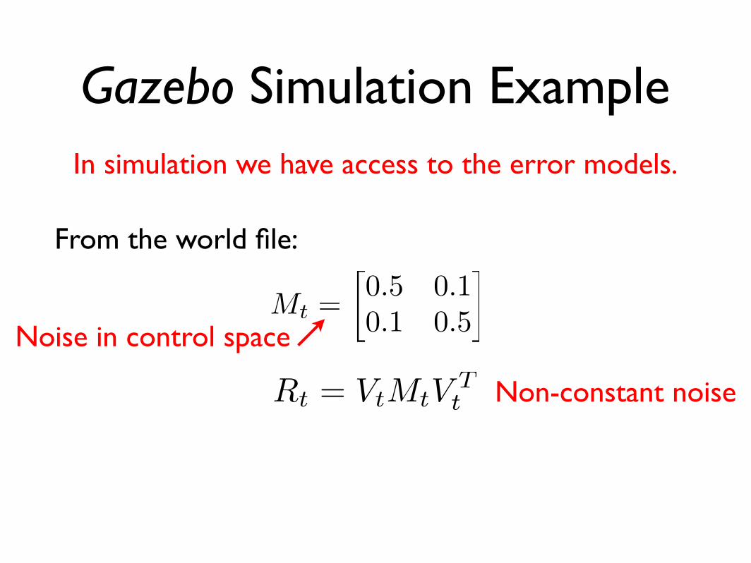
From the world file:
Mt =!0.5 0.10.1 0.5
"
In simulation we have access to the error models.

t1
Extended Kalman Filter(algorithm)
Mobile robot example:
t0
Computing G:
G =
!
"1 0 ! v
w cos !t!1 + vw cos(!t!1 + "!t)
0 1 ! vw sin !t!1 + v
w sin(!t!1 + "!t)0 0 1
#
$
What about the process noise?
Rt = VtMtVTt
Mt =!!v 00 !!
", Vt =
"g(ut, µt!1)"utNoise in control space
Recall:
Gazebo Simulation ExampleIn simulation we have access to the error models.
From the world file:
Mt =!0.5 0.10.1 0.5
"
Noise in control space
Rt = VtMtVTt Non-constant noise

Gazebo Simulation ExampleIn simulation we have access to the error models.
From the world file:
Mt =!0.5 0.10.1 0.5
"
Noise in control space
Rt = VtMtVTt
Vt =!g(ut, µt!1)
!ut=
!
"#
! sin !+sin(!+wt!t)"t
vt(sin !!sin(!+"t!t))"2
t+ vt cos(!+"t!t)!t
"tcos !!cos(!+wt!t)
"t!vt(cos !!cos(!+"t!t))
"2t
+ vt sin(!+"t!t)!t"t
0 !t
$
%&
Non-constant noise

Gazebo Simulation ExampleIn simulation we have access to the error models.
From the world file:
Q =
!
"1 0 00 1 00 0 0.4
#
$
GPS provides state information directly.

Gazebo Simulation ExampleOld Results New Results

Position Error Angular Error
Old
New

Gazebo Simulation Example
Can we improve these results?


How is it possible that these results are better?

Is there a better way to compute the noise?

Adaptive Filtering Techniques
• Generally applies to fitting or “learning” system models.
• Updates the process (measurement) model based on the disparity between the predicted and sensed state (measurements).

Gazebo Simulation using an Adaptive EKF

Gazebo Simulation using an Adaptive EKF
Position Error Angular Error

Outline
• Kinematic Model of a Mobile Robot
• Kalman Filter
• Extended Kalman Filter
• Unscented Kalman Filter
• Particle Filter

Unscented Kalman Filter
• “Derivative-free” alternative to EKF
• Higher-order approximation accuracy than EKF (2nd vs. 1st)
• Represents varying distributions via dicrete points (sigma points)

Unscented Kalman Filter
R2

Unscented Kalman Filter
Sigma point
Equipotential ellipse
R2
N = 2

Unscented Kalman Filter
g(µt!1, ut)
Sigma point
Equipotential ellipse
R2
N = 2

Unscented Kalman Filter
g(µt!1, ut)
Sigma point
Equipotential ellipse
R2
N = 2

Unscented Kalman Filter
g(µt!1, ut)
Sigma point
Sigma points are typically (but not necessarily)distributed in this manner.
Equipotential ellipse
R2
N = 2

Unscented Kalman Filter
g(µt!1, ut)
Sigma point
Sigma points are typically (but not necessarily)distributed in this manner.
Equipotential ellipse
The following derivation assumes this distribution in N.
R2
N = 2

Unscented Kalman Filter
“... it is easier to approximate a probability distributionthan it is to approximate an arbitrary nonlinear functionor transformation.”

Unscented Kalman Filter(algorithm)
At a high level:

Unscented Kalman Filter(algorithm)
At a high level:1. Initialize sigma points based on the moments parameterization.

Unscented Kalman Filter(algorithm)
At a high level:1. Initialize sigma points based on the moments parameterization.2. Transform the sigma points according to the nonlinear process model.

Unscented Kalman Filter(algorithm)
At a high level:1. Initialize sigma points based on the moments parameterization.2. Transform the sigma points according to the nonlinear process model.3. Initialize predicted sigma points based on the transformed sigma points.

Unscented Kalman Filter(algorithm)
At a high level:1. Initialize sigma points based on the moments parameterization.2. Transform the sigma points according to the nonlinear process model.3. Initialize predicted sigma points based on the transformed sigma points.4. Transform the predicted sigma points according to the nonlinear measurement model.

Unscented Kalman Filter(algorithm)
At a high level:1. Initialize sigma points based on the moments parameterization.2. Transform the sigma points according to the nonlinear process model.3. Initialize predicted sigma points based on the transformed sigma points.4. Transform the predicted sigma points according to the nonlinear measurement model.5. Update the moments parameterization based on the measurement correction.

Initialization of Sigma Points
si = {xi, Wi}
Each Sigma point is defined by a state and weight:
xi ! RN
Wi ! R

Initialization of Sigma PointsSigma points must have the following properties:
2N!
i=0
Wi = 1
µ =2N!
i=0
Wixi
! =2N!
i=0
Wi(xi ! µ)(xi ! µ)T

Initialization of Sigma PointsSigma points must have the following properties:
Consistent with first moment
2N!
i=0
Wi = 1
µ =2N!
i=0
Wixi
! =2N!
i=0
Wi(xi ! µ)(xi ! µ)T

Initialization of Sigma PointsSigma points must have the following properties:
Consistent with first moment Consistent with
second moment
2N!
i=0
Wi = 1
µ =2N!
i=0
Wixi
! =2N!
i=0
Wi(xi ! µ)(xi ! µ)T

Initialization of Sigma Points
x0 = µ

Initialization of Sigma Points
x0 = µ
xi = µ +
!"N
1!W0!
#
i

Initialization of Sigma Points
x0 = µ
xi = µ +
!"N
1!W0!
#
ii = {1, . . . , N}

Initialization of Sigma Points
x0 = µ
xi = µ +
!"N
1!W0!
#
i
rowi if B = AT A
columni if B = AAT
Matrix Square-Root
i = {1, . . . , N}

Initialization of Sigma Points
x0 = µ
xi = µ +
!"N
1!W0!
#
i
rowi if B = AT A
columni if B = AAT
Matrix Square-Root
xi+N = µ!!"
N
1!W0!
#
i
i = {1, . . . , N}

Initialization of Sigma Points
x0 x1
x2
x3
x4R2

Initialization of Sigma Points
Wi =1!W0
2N

Initialization of Sigma Points
Wi =1!W0
2Ni = {1, . . . , 2N}

Initialization of Sigma Points
Wi =1!W0
2Ni = {1, . . . , 2N}
W0 =!
N + !, ! = "2(N + #)!N

Initialization of Sigma Points
Wi =1!W0
2Ni = {1, . . . , 2N}
W0 =!
N + !, ! = "2(N + #)!N
Scaling parameters

Initialization of Sigma Points
!
! = 1, " = 0.1 : 0.1 : 1
µ = [0, 0]
! =!2 00 1
"

Initialization of Sigma PointsInitialize(µ, !, !, ") :

Initialization of Sigma PointsInitialize(µ, !, !, ") :
W0 =!
N + !, ! = "2(N + #)!N

Initialization of Sigma PointsInitialize(µ, !, !, ") :
W0 =!
N + !, ! = "2(N + #)!N
x0 = µ

Initialization of Sigma PointsInitialize(µ, !, !, ") :
W0 =!
N + !, ! = "2(N + #)!N
x0 = µ
xi = µ +
!"N
1!W0!
#
i

Initialization of Sigma PointsInitialize(µ, !, !, ") :
W0 =!
N + !, ! = "2(N + #)!N
x0 = µ
xi = µ +
!"N
1!W0!
#
i
xi+N = µ!!"
N
1!W0!
#
i

Unscented Kalman Filter(algorithm)
{x0, xi} = Initialize(µ, !, !, ")
{x0, xi} = g(x0, xi, u)
Prediction
! =2N!
i=0
Wi(xi ! µ)(xi ! µ)T + R
µ =2N!
i=0
Wixi

Unscented Kalman Filter(algorithm)
{x0, xi} = Initialize(µ, !, !, ")
{x0, xi} = g(x0, xi, u)
Prediction
! =2N!
i=0
Wi(xi ! µ)(xi ! µ)T + R
µ =2N!
i=0
Wixi

Correction of Sigma Points
{x0, xi} = Initialize(µ, !, !, ")
{z0, zi} = h(x0, xi, u)
z =2N!
i=0
Wizi
S =2N!
i=0
Wi(zi ! z)(zi ! z)T + Q
! =2N!
i=0
Wi(xi ! µ)(zi ! z)T
K = !S!1

Unscented Kalman Filter(algorithm)
{xi, µ, !} = Prediction(µ, !, u, !, ")
µ = µ + K(z ! z)
! = !!KSKT
{z, µ, !, K, S} = Sigma Correction(xi, µ, !, !, ")

Outline
• Kinematic Model of a Mobile Robot
• Kalman Filter
• Extended Kalman Filter
• Unscented Kalman Filter
• Particle Filter

Particle Filters
• Nonparametric representation of estimation
• Permits a broader space of distributions (including multimodal distributions)
• Represents estimates as discrete hypotheses (particles)
• Samples (and resamples) based on probability distribution of process and measurement models

Basic Particle Filter

Basic Particle FilterThere are many
variations!

Basic Particle FilterThere are many
variations!xm
t
Xt = {!x1t , w1
t ", . . . , !xMt , wM
t "}

Basic Particle FilterThere are many
variations!xm
t
Basic idea:
• Create a set of weighted hypotheses (particles) based on the previous set of hypotheses, system inputs, and measurements.
Xt = {!x1t , w1
t ", . . . , !xMt , wM
t "}

Basic Particle FilterThere are many
variations!xm
t
Basic idea:
• Create a set of weighted hypotheses (particles) based on the previous set of hypotheses, system inputs, and measurements.
• Create a set of hypotheses sampled from the weighted hypotheses based on the distribution of weights.
Monte Carlo method
Sample Importance Resampling
Xt = {!x1t , w1
t ", . . . , !xMt , wM
t "}

Basic Particle Filter(algorithm)
For M particles:

Basic Particle Filter(algorithm)
For M particles:sample xm
t ! p(xt | ut, xmt!1)

Basic Particle Filter(algorithm)
For M particles:sample xm
t ! p(xt | ut, xmt!1)
Sampling introduces noiseto every particle

Basic Particle Filter(algorithm)
For M particles:sample xm
t ! p(xt | ut, xmt!1)
wmt = p(zt | xm
t )
Sampling introduces noiseto every particle

Basic Particle Filter(algorithm)
For M particles:sample xm
t ! p(xt | ut, xmt!1)
wmt = p(zt | xm
t )Importance Factor
Sampling introduces noiseto every particle

Basic Particle Filter(algorithm)
For M particles:sample xm
t ! p(xt | ut, xmt!1)
wmt = p(zt | xm
t )Xt = Xt + !xm
t , wmt "
End
Importance Factor
Sampling introduces noiseto every particle

Basic Particle Filter(algorithm)
For M particles:sample xm
t ! p(xt | ut, xmt!1)
wmt = p(zt | xm
t )Xt = Xt + !xm
t , wmt "
End
Importance Factor
Xt = Importance Resampling(Xt)
Sampling introduces noiseto every particle

Importance Resampling
Take the particles and lay them side-by-side according
to each particles weight.
xmt

Importance Resampling
Take the particles and lay them side-by-side according
to each particles weight.
xmt
x1t
w1t
xmt
wmt

Importance Resampling
Take the particles and lay them side-by-side according
to each particles weight.
xmt
x1t
w1t
xmt
wmt
Normalize the weights and sample based on this distribution.

Importance Resampling
Take the particles and lay them side-by-side according
to each particles weight.
xmt
x1t
w1t
xmt
wmt
Normalize the weights and sample based on this distribution.
Particles with higher weights will be selected
with higher probability.

Common Issues
• Particle deprivation
• Random number generation
• Resampling frequency

Common Issues
• Particle deprivation
• Random number generation
• Resampling frequency
wmt =
!1 if resampling took placep(zt | xm
t ) wmt!1 otherwise