filter design - hkustpalomar/elec5470_lectures/05/slides_filter_design.… · filter design daniel...

Filter Design

Daniel P. Palomar

Hong Kong University of Science and Technology (HKUST)

ELEC5470 - Convex Optimization

Fall 2017-18, HKUST, Hong Kong

Outline of Lecture

• FIR filters

• Chebychev design

• Lowpass filter design

• Filter magnitude specification design

• Log-Chebychev magnitude specification design

• Equalizer design

• Summary

(Acknowledgement to Stephen Boyd for material for this lecture.)

Daniel P. Palomar 1

FIR Filters

• The input-output relationship for a finite-impulse response (FIR)

filter is

y (t) =

n−1∑τ=0

hτx (t− τ)

where

– x (t) is the real-valued input sequence

– y (t) is the real-valued output sequence

– hi are the real-valued filter coefficients

– n is the filter order or length.

• Observe that the output is a linear function of the input.

Daniel P. Palomar 2

• The FIR filter frequency response is

H (ω) = h0 + h1e−jω + · · ·+ hn−1e

−j(n−1)ω

=

n−1∑t=0

ht cos tω − jn−1∑t=0

ht sin tω.

• Observations:

– H (ω) is complex-valued

– H (ω) is periodic and conjugate symmetric, so only need to specify

for 0 ≤ ω ≤ π.

– H (ω) is a linear function of the filter coefficients.

• The FIR filter design problem is to design h such that it and H (ω)

satisfy/optimize some specifications.

Daniel P. Palomar 3

FIR Example

• Example of a lowpass FIR filter of order n = 21.

• The impulse response h is

from which it is difficult to infer the filtering capabilities and

properties.

Daniel P. Palomar 4

• The frequency response magnitude and phase, |H (ω)| and ∠H (ω),

are

Daniel P. Palomar 5

Chebychev Design

• The problem formulation is

minimizeh

maxω∈[0,π]

|H (ω)−Hdes (ω)|

where

– h is the optimization variable (recall that H (ω) is linear in h)

– Hdes (ω) is the desired transfer function.

• This Chebychev formulation is a semi-infinite convex problem.

(Why?)

• We can add constraints while keeping the convexity such as |hi| ≤ 1.

Daniel P. Palomar 6

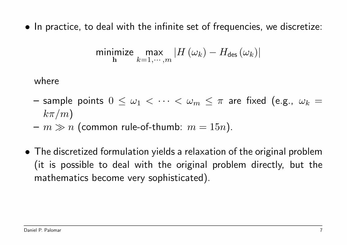
• In practice, to deal with the infinite set of frequencies, we discretize:

minimizeh

maxk=1,··· ,m

|H (ωk)−Hdes (ωk)|

where

– sample points 0 ≤ ω1 < · · · < ωm ≤ π are fixed (e.g., ωk =

kπ/m)

– m� n (common rule-of-thumb: m = 15n).

• The discretized formulation yields a relaxation of the original problem

(it is possible to deal with the original problem directly, but the

mathematics become very sophisticated).

Daniel P. Palomar 7

• Let’s now reformulate the discretized formulation in a more conve-

nient form. Can we reformulate it as an LP?

• Recall that

minimizex

maxk|fk (x)|

can be rewritten as

minimizet,x

t

subject to |fk (x)| ≤ t ∀k

and, equivalently, as the LP

minimizet,x

t

subject to −t ≤ fk (x) ≤ t ∀k .

Daniel P. Palomar 8

• Answer: No!

• The Chebychev filter design problem cannot be recast as an LP.

• The reason is that the operator |·| does not denote absolute value

but magnitude because the argument is complex-valued!

• Magnitude of a complex number:

|x| = |xR + jxI| =√x2R + x2I =

∥∥∥∥[ xRxI]∥∥∥∥ .

• The magnitude of a complex number is equivalent to the Euclidean

norm of a two-dimensional vector.

Daniel P. Palomar 9

• Therefore, the constraint

|H (ωk)−Hdes (ωk)| ≤ t

cannot be rewritten as a linear inequality but as an SOC inequality:∥∥∥∥[ ReH (ωk)− ReHdes (ωk)

ImH (ωk)− ImHdes (ωk)

]∥∥∥∥ ≤ t.

Daniel P. Palomar 10

• The discretized Chebychev filter design formulation can be finally be

written as an SOCP:

minimizet,h

t

subject to ‖Akh− bk‖ ≤ t k = 1, · · · ,m

where

h =[h0 · · · hn−1

]TAk =

[1 cosωk · · · cos (n− 1)ωk0 − sinωk · · · − sin (n− 1)ωk

]bk =

[ReHdes (ωk)

ImHdes (ωk)

] (note: Akh =

[ReH (ωk)

ImH (ωk)

]).


Lowpass Filter Specifications

• In a lowpass filter, we have the pass frequencies in passband [0, ωp]

and the block frequencies in stopband [ωs, π]:


• Specifications (specs):

– maximum passband ripple (±20 log10 δ1 in dB):

1/δ1 ≤ |H (ω)| ≤ δ1, 0 ≤ ω ≤ ωp

– minimum stopband attenuation (−20 log10 δ2 in dB):

|H (ω)| ≤ δ2, ωs ≤ ω ≤ π.

• Are these nice constraints, i.e., convex?

• Recalling that the magnitude is indeed a norm,

– the two upper-bound constraints |H (ω)| ≤ δ1 and |H (ω)| ≤ δ2are SOC constraints

– the lower-bound constraint 1/δ1 ≤ |H (ω)| is nonconvex!

• What can we do?


Interlude: Linear Phase Filters

• Linear phase filters satisfy:

1. n = 2N + 1 is odd

2. impulse response is symmetric about midpoint:

ht = hn−1−t, t = 0, · · · , n− 1.

• As a consequence, the frequency response can be written as

H (ω) = h0 + h1e−jω + · · ·+ hn−1e

−j(n−1)ω

= e−jNω (2h0 cosNω + 2h1 cos (N − 1)ω + · · ·+ hN)

, e−jNωH̃ (ω)

where we have used h0 + hn−1e−j(n−1)ω = h0

(1 + e−j2Nω

)=

e−jNωh02 cosNω.


• Observations on H (ω) = e−jNωH̃ (ω) and

H̃ (ω) = 2h0 cosNω + 2h1 cos (N − 1)ω + · · ·+ hN :

– term e−jNω represents an N -sample delay

– H̃ (ω) is real (this property is key)

– same magnitude: |H (ω)| = |H̃ (ω) |– it is called linear phase filter because the phase ∠H (ω) is linear

(except for jumps of ±π).

• How can we take advantage of these observations?

• Can we now deal with a constraint like 1/δ1 ≤ |H (ω)|?


Lowpass Filter Specs

• Using |H (ω)| = |H̃ (ω) |, we can rewrite the specs as

1/δ1 ≤ |H̃ (ω) | ≤ δ1, 0 ≤ ω ≤ ωp

and

|H̃ (ω) | ≤ δ2, ωs ≤ ω ≤ π.

• Noting that |·| now denotes absolute value instead of magnitude:

– the two upper-bound constraints |H̃ (ω) | ≤ δ1 and |H̃ (ω) | ≤ δ2are just linear constrains

– the lower-bound constraint 1/δ1 ≤ |H̃ (ω) | is still nonconvex!

• What can we do? It seems that we have not improved the problem

formulation.


• Key idea:

– the first sample at ω1, H̃ (ω1) is either be positive or negative

– we can assume w.l.o.g. that it is positive H̃ (ω1) > 1/δ1 (if it’s

negative, use −h instead)

– therefore, |H̃ (ω1) | = H̃ (ω1)

– what about the second sample at ω2?

– since H̃ (ω) is smooth in ω, H̃ (ω2) cannot possibly be negative,

so |H̃ (ω2) | = H̃ (ω2)

– same argument holds for all samples in the passband ωk ∈ [0, ωp].

• As a consequence, w.l.o.g., we can substitute the nonconvex in-

equality 1/δ1 ≤ |H̃ (ω) | by a simple linear inequality

1/δ1 ≤ H̃ (ω) .


Linear Phase Lowpass Filter Design

• Problem formulation for maximum stopband attenuation:

minimizeδ2,h

δ2

subject to 1/δ1 ≤ H̃ (ω) ≤ δ1, 0 ≤ ω ≤ ωp−δ2 ≤ H̃ (ω) ≤ δ2, ωs ≤ ω ≤ π.

• Comments:

– passband ripple δ1 is given

– the problem is an LP in variables δ2,h

– known (and used) since 1960s

– we can add other constraints, e.g., |hi| ≤ α.


• Variations and extensions:

– fix δ2; minimize δ1 (convex, but not LP)

– fix δ1 and δ2, minimize ωs (quasiconvex)

– fix δ1 and δ2, minimize order n (quasiconvex).

• Example of a linear phase filter: order n = 21, passband [0, 0.12π],

stopband [0.24π, π], max ripple δ1 = 1.012 (±0.1 dB), design for

maximum stopband attenuation.

The impulse response h is


with frequency response magnitude and phase, |H (ω)| and ∠H (ω):


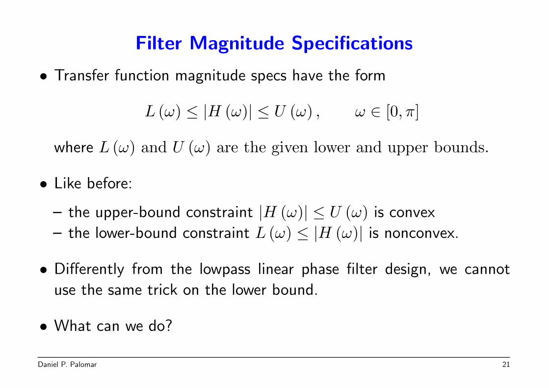
Filter Magnitude Specifications

• Transfer function magnitude specs have the form

L (ω) ≤ |H (ω)| ≤ U (ω) , ω ∈ [0, π]

where L (ω) and U (ω) are the given lower and upper bounds.

• Like before:

– the upper-bound constraint |H (ω)| ≤ U (ω) is convex

– the lower-bound constraint L (ω) ≤ |H (ω)| is nonconvex.

• Differently from the lowpass linear phase filter design, we cannot

use the same trick on the lower bound.

• What can we do?


Interlude: Autocorrelation Coefficients

• Autocorrelation coefficients are given by

rt =∑τ

hτhτ+t

(we define hk = 0 for k < 0 or k≥ n).

• Some properties:

– symmetry: rt = r−t– rt = 0 for |t| > n

– it suffices to specify r = [r0, · · · rn−1]T .


• The Fourier transform of the autocorrelation coefficients is

R (ω) =∑τ

e−jωτrτ = r0 +

n−1∑t=1

2rt cosωt = |H (ω)|2 .

• Observations:

– R (ω) ≥ 0 for all ω

– R (ω) is convex in h

– R (ω) is linear in r.

• How can we take advantage of the autocorrelation coefficients r and

its Fourier transform R (ω)?


• First of all, note that we can express the magnitude specifications

as

L (ω)2 ≤ R (ω) ≤ U (ω)

2, ω ∈ [0, π]

which are convex in r (in fact, linear).

• But, how does this help? Our optimization variable is h not r.

• We need to reformulate the optimization problem in terms of the

new optimization variable r.

• However, once we find the optimal r, how do we obtain the

corresponding optimal h?

• All these questions are answered by the spectral factorization theo-

rem.


Spectral Factorization

• Question: when is r the autocorrelation of some h?

• Answer (spectral factorization theorem): if and only if R (ω) ≥ 0

for all ω.

• The spectral factorization condition is convex in r.

• The idea is then to formulate the problem using r as a variable

(instead of h) including the constraint R (ω) ≥ 0 for all ω.

• Once the problem has been solved, we know that there exists some

h with such an autocorrelation; in fact, there are many algorithms

for spectral factorization.


Log-Chebychev Magnitude-Spec Design

• In many applications it is more meaningful to work with the magni-

tude of the frequency response in dB instead of linear scale.

• We can then reformulate the first Chebychev problem formulation

we considered

minimize maxω∈[0,π]

|H (ω)−Hdes (ω)|

but in magnitude-dB:


|20 log10 |H (ω)| − 20 log10D (ω)|

where D (ω) denotes the desired frequency response magnitude

(D (ω) > 0 for all ω).


• We can use the spectral factorization theorem to rewrite the problem

in terms of r:

minimizet,r

t

subject to∣∣10 log10R (ω)− 10 log10D

2 (ω)∣∣ ≤ t, 0 ≤ ω ≤ π

which is still nonconvex.

• Expanding the absolute value we obtain

minimizet,r

t

subject to −t ≤ log10R (ω) /D2 (ω) ≤ t, 0 ≤ ω ≤ π

which still is nonconvex.

• What can we do now?


• We can exponentiate the constraint:

minimizet,r

t

subject to 10−t ≤ R (ω) /D2 (ω) ≤ 10t, 0 ≤ ω ≤ π.

• Now, define t̃ = 10t and rewrite the problem finally in convex form

as

minimizet̃,r

t̃

subject to 1/t̃ ≤ R (ω) /D2 (ω) ≤ t̃, 0 ≤ ω ≤ π.

• Note that the spectral factorization condition is already included.


• Let’s rearrange terms now. Note that 1/t ≤ R (ω) /D2 (ω) can be

rewritten as D2 (ω) /R (ω) ≤ t.

• So we can rewrite our problem as

minimizet,r

t

subject to max{R (ω) /D2 (ω) , D2 (ω) /R (ω)

}≤ t, 0 ≤ ω ≤ π.

• More compactly, by defining the function φ (x) = max {x, 1/x}:

minimizer

maxω∈[0,π]

φ(R (ω) /D2 (ω)

).

• Does this ring any bell?


Equalizer Design

• System model: concatenation of a filter H (ω), to be designed, and

the unequalized channel response G (ω):

• Equalization problem: design the filter H (ω) (FIR equalizer) so that

the overall response is close to the desired one Gdes (ω):

H (ω)G (ω) ≈ Gdes (ω) .


• One common choice for the desired response is Gdes (ω) = e−jDω

(delay of D samples), i.e., equalization is deconvolution (up to a

delay).

• We can add constraints on the filter coefficients h and H (ω) such

as limits on |hi| or maxω |H (ω)|.

• A simple formulation is the Chebychev equalizer design:


|H (ω)G (ω)−Gdes (ω)|

which is convex and can be reformulated as an SOCP after sampling

the frequency.

• In the context of equalization, it is sometimes common to use the

time domain instead of the frequency domain.


• For example, the time-domain desired response corresponding to

Gdes (ω) = e−jDω is

gdes (t) =

{1 t = D

0 t 6= D.

• Let g̃ (t) denote the time-domain signal corresponding to the

equalized system G̃ (ω) = H (ω)G (ω).

• Time-domain equalization: Inspired by the expression of gdes (t)

above, we can then formulate the filter design problem in the time

domain as:minimize

hmaxt6=D |g̃ (t)|

subject to g̃ (D) = 1

which is an LP.


• Variations: we can use∑t6=D g̃ (t)

2 or∑t6=D |g̃ (t)| as objectives.

• Extensions:

– we can impose additional convex constraints

– we can mix the time- and frequency-domain specs

– we can equalize multiple systems, i.e., to choose

H (ω)G(k) (ω) ≈ Gdes (ω) , k = 1, · · · ,K

– we can even equalize multi-input multi-output systems where

H (ω) and G (ω) are matrices

– it extends to multidimensional systems such as image processing.


Example Filter Design

• The problem is to design a 30th order FIR equalizer with Gdes (ω) =

e−j10ω.

• Consider the unequalized system g (t) (10th order FIR):


with frequency response magnitude and phase:


• Chebychev equalizer design:


∣∣H (ω)G (ω)− e−j10ω∣∣

• The equalized system impulse response g̃ (t) is


with equalized frequency response magnitude and phase:


• Time-domain equalizer design:

minimize maxt6=10 |g̃ (t)|

• The equalized system impulse response g̃ (t) is


with equalized frequency response magnitude and phase:


Summary

• We have considered many different problem formulations of filter

design:

– Chebychev design

– lowpass filter design

– filter magnitude specification design

– log-Chebychev magnitude specification design

– equalizer design.

• Most of the formulations are initially very hard nonconvex problems.

• Using different tricks they can finally be reformulated in convex form

and solved optimally.


filter design - hkustpalomar/elec5470_lectures/05/slides_filter_design.… · filter design daniel...

Documents