USING TRACEABILITY INMODEL-TO-MODEL TRANSFORMATION TOQUANTIFY CONFIDENCE BASED ONPREVIOUS HISTORY.
by
JOHN T. SAXON
A thesis submitted toThe University of Birminghamfor the degree ofDOCTOR OF PHILOSOPHY
School of Computer ScienceCollege of Engineering and Physical SciencesThe University of BirminghamDecember 2017
brought to you by COREView metadata, citation and similar papers at core.ac.uk
provided by University of Birmingham Research Archive, E-theses Repository

University of Birmingham Research Archive
e-theses repository This unpublished thesis/dissertation is copyright of the author and/or third parties. The intellectual property rights of the author or third parties in respect of this work are as defined by The Copyright Designs and Patents Act 1988 or as modified by any successor legislation. Any use made of information contained in this thesis/dissertation must be in accordance with that legislation and must be properly acknowledged. Further distribution or reproduction in any format is prohibited without the permission of the copyright holder.
Abstract
A widely used method when generating code for the purposes of transitioning
systems, security, the automotive industry and other mission critical scenarios
is model-to-model transformation. Traceability is a mechanism for relating the
source model elements and the destination elements. It is used to identify how the
latter came from the former as well as indicating when and in what order. In these
application domains, traceability is a very useful tool for debugging, validating
and performance tuning of model transformations. Recent advances in big data
technologies have made it possible to produce a history of these executions. In this
thesis, we present a method on how we can use such historical data that quantifies
the confidence a user has on a newly proposed transformation. For a given trace of
execution, considering historical traces that are either well tested, or performed
correctly over time, we introduce a measure of confidence for the new trace. This
metric is made to compliment that of traditional verification and validation. For
example, our metric will aid in deciding whether to deploy automatically generated
code when there is not enough time or resources for thorough verification and
validation. We shall evaluate our framework by providing a transformation that
transitions a relational database into that of a NoSQL database, specifically Apache
HBase. This transformation involves changing the nature of the data that is
mapped, such that a loss in integrity occurs in the event of its failure.

ACKNOWLEDGEMENTS
Firstly I’d like to thank my supervisor and friend Behzad Bordar, whose support
and enthusiasm, to pretty much anything, has been invaluable! His guidance
throughout my PhD has helped me greatly in dealing with the many challenges I
faced to become an effective researcher. I have learnt much from him, and I know
I would have struggled without his timely help.
I’d also like to show my appreciation to those at the School of Computer Science.
I may have spent the majority of my time in coffee shops, but when I was in CS it
was always nice to have people to bounce ideas off of and then to go to the pub
afterwards!
A little cliché but I must thank my parents, as they’ve had to listen to me
for years and years talking about my work to the point where my Mum should
probably get an honorary computer science degree! Without their unwavering
support of whatever I wanted to do, I may not have got here at all.
Thanks to all of the friends that I have picked up on the way for your support.
PEER-REVIEWED PUBLICATIONS ARISINGFROM THIS WORK
Saxon, J. T., B. Bordbar, and D. H. Akehurst (2015). “Opening the Black-Box
of Model Transformation”. In: Modelling Foundations and Applications: 11th
European Conference, ECMFA 2015, Held as Part of STAF 2015, L‘Aquila,
Italy, July 20-24, 2015. Proceedings. Ed. by G. Taentzer and F. Bordeleau.
Springer International Publishing, pp. 171–186. isbn: 978-3-319-21151-0. doi:
10.1007/978-3-319-21151-0_12.
Saxon, J. T., B. Bordbar, and K. Harrison (2015a). “Efficient Retrieval of Key
Material for Inspecting Potentially Malicious Traffic in the Cloud”. In: 2015
IEEE International Conference on Cloud Engineering, pp. 155–164. doi: 10.
1109/IC2E.2015.26.
— (2015b). “Introspecting for RSA Key Material to Assist Intrusion Detection”.
In: IEEE Cloud Computing 2.5, pp. 30–38. issn: 2325-6095. doi: 10.1109/MCC.
2015.100.
Shaw, A. L., B. Bordbar, J. T. Saxon, K. Harrison, and C. I. Dalton (2014).
“Forensic Virtual Machines: Dynamic Defence in the Cloud via Introspection”.
In: 2014 IEEE International Conference on Cloud Engineering, pp. 303–310.
doi: 10.1109/IC2E.2014.59.
CONTENTS
1 Introduction 1
1.1 Objectives and Contributions of Thesis . . . . . . . . . . . . . . . . 6
2 Background 8
2.1 Model Driven Architecture . . . . . . . . . . . . . . . . . . . . . . . 8
2.2 Model Transformation . . . . . . . . . . . . . . . . . . . . . . . . . 9
2.2.1 Rule-Based Model Transformation . . . . . . . . . . . . . . . 10
2.2.2 Model-to-Model Transformation . . . . . . . . . . . . . . . . 11
2.2.3 Text-to-Model Transformation . . . . . . . . . . . . . . . . . 14
2.2.4 Model-to-Text Transformation . . . . . . . . . . . . . . . . . 15
2.3 Software Assurance . . . . . . . . . . . . . . . . . . . . . . . . . . . 16
2.3.1 Software Specific Definitions . . . . . . . . . . . . . . . . . . 17
2.3.2 Black-box Testing . . . . . . . . . . . . . . . . . . . . . . . . 19
2.3.3 Opening the Black-Box (White-box Testing) . . . . . . . . . 20
2.4 Pattern Recognition . . . . . . . . . . . . . . . . . . . . . . . . . . 26
2.4.1 Template Matching . . . . . . . . . . . . . . . . . . . . . . . 27
2.4.2 Prototype Matching . . . . . . . . . . . . . . . . . . . . . . 27
2.4.3 Feature Analysis . . . . . . . . . . . . . . . . . . . . . . . . 28
2.4.4 Recognition by Components . . . . . . . . . . . . . . . . . . 29
2.5 Chapter Summary . . . . . . . . . . . . . . . . . . . . . . . . . . . 30
3 Design of New Traceability Mechanism 32
3.1 Challenges of Tracing in Model Transformation . . . . . . . . . . . 33
3.1.1 Ordering of Rule Execution . . . . . . . . . . . . . . . . . . 35
3.1.2 Invocation and Rule Dependencies . . . . . . . . . . . . . . 39
3.1.3 Orphans Objects . . . . . . . . . . . . . . . . . . . . . . . . 42
3.2 The Simple Transformer . . . . . . . . . . . . . . . . . . . . . . . . 45
3.2.1 Capturing Rule and Transformation Dependencies . . . . . . 46
3.2.2 A Dynamic Proxy to Catch Orphans . . . . . . . . . . . . . 49
3.3 Epsilon Transformation Language . . . . . . . . . . . . . . . . . . . 54
3.3.1 Transformation Strategy . . . . . . . . . . . . . . . . . . . . 55
3.3.2 Orphans and the Execution Listener . . . . . . . . . . . . . 57
3.4 Chapter Summary . . . . . . . . . . . . . . . . . . . . . . . . . . . 59
4 Efficacy in Model-to-Model Transformation 61
4.1 Persistence of Trace Data . . . . . . . . . . . . . . . . . . . . . . . 62
4.1.1 SiTra in Python and Neo4j . . . . . . . . . . . . . . . . . . . 65
4.2 Prominence of Historical Data . . . . . . . . . . . . . . . . . . . . . 66
4.3 Complexity of Transformation Artefacts . . . . . . . . . . . . . . . 70
4.4 Complexity and Prominence Combined . . . . . . . . . . . . . . . . 75
4.5 Chapter Summary . . . . . . . . . . . . . . . . . . . . . . . . . . . 78
5 Evaluation by Case Study 80
5.1 Relational to Apache HBase . . . . . . . . . . . . . . . . . . . . . . 82
5.1.1 Meta-Models of the Source and Destination . . . . . . . . . 83
5.2 Relationship Considerations . . . . . . . . . . . . . . . . . . . . . . 87
5.2.1 One-to-Many and Many-to-One Relationships . . . . . . . . 88
5.3 Transformation Rules . . . . . . . . . . . . . . . . . . . . . . . . . . 93
5.3.1 The Database . . . . . . . . . . . . . . . . . . . . . . . . . . 95
5.3.2 Prime Tables . . . . . . . . . . . . . . . . . . . . . . . . . . 95
5.3.3 Relationships . . . . . . . . . . . . . . . . . . . . . . . . . . 97
5.4 Benchmarking Traceability for SiTra . . . . . . . . . . . . . . . . . 99
5.5 Benchmarking Traceability for ETL . . . . . . . . . . . . . . . . . . 107
5.6 Persisting the Trace for Analysis . . . . . . . . . . . . . . . . . . . . 113
5.7 Confidence within Model Transformation . . . . . . . . . . . . . . . 120
5.7.1 Applying our Metric on a Small Transformation . . . . . . . 123
5.7.2 Introducing New Features with an Increasing Knowledge Base129
5.8 Chapter Summary . . . . . . . . . . . . . . . . . . . . . . . . . . . 135
5.8.1 Testing Environment . . . . . . . . . . . . . . . . . . . . . . 137
5.8.2 Validity of Experiments . . . . . . . . . . . . . . . . . . . . 137
6 Summary, Discussion and Conclusion 140
6.1 Summary . . . . . . . . . . . . . . . . . . . . . . . . . . . . . . . . 140
6.2 Discussion . . . . . . . . . . . . . . . . . . . . . . . . . . . . . . . . 142
6.2.1 Weaknesses . . . . . . . . . . . . . . . . . . . . . . . . . . . 144
6.3 Conclusion . . . . . . . . . . . . . . . . . . . . . . . . . . . . . . . . 149
References 150
A Appendices 160

A.1 Multiple Inputs and Outputs for SiTra . . . . . . . . . . . . . . . . 160
A.1.1 Inputs . . . . . . . . . . . . . . . . . . . . . . . . . . . . . . 160
A.1.2 Outputs . . . . . . . . . . . . . . . . . . . . . . . . . . . . . 161
A.2 Multiple Inputs for ETL . . . . . . . . . . . . . . . . . . . . . . . . 165
LIST OF FIGURES
2.1 An Overview of M2M Transformation . . . . . . . . . . . . . . . . . 10
3.1 A SiTra transformation rule with a global state. . . . . . . . . . . . 35
3.2 A sample of rule dependencies. . . . . . . . . . . . . . . . . . . . . . 36
3.3 Example of ETL using the new keyword. . . . . . . . . . . . . . . . 42
3.4 Using inheritance to avoid the new keyword in ETL. . . . . . . . . . 43
3.5 Using inheritance to allow for multiple outputs in SiTra. . . . . . . 44
3.6 An example of an inter-rule dependency. . . . . . . . . . . . . . . . 46
3.7 A new meta-model for a traceable model transformation. . . . . . . 47
3.8 An example of when a dynamic proxy will not capture nested orphans
due to performing operations upon POJOs directly and not calling
for a proxy. . . . . . . . . . . . . . . . . . . . . . . . . . . . . . . . 53
3.9 An amended meta-model for a traceable model transformation in
ETL. . . . . . . . . . . . . . . . . . . . . . . . . . . . . . . . . . . . 55
3.10 The concept of an execution listener to capture orphans. . . . . . . 57
4.1 A view of two dependent rule invocations. . . . . . . . . . . . . . . 64
4.2 Trace execution graph for a simple M2M transformation. . . . . . . 68
4.3 Transformation of a class with three attributes. . . . . . . . . . . . 75
4.4 The confidence we have in a transformation of an entity with three
attributes in respect to the ratio of tests in relation to EtoT. This is
in consideration of a history of two previous transformations: one
with one attribute the other with two. . . . . . . . . . . . . . . . . 77
5.1 The meta-model of a relational database. . . . . . . . . . . . . . . . 84
5.2 The meta-model of a Apache HBase. . . . . . . . . . . . . . . . . . 86
5.3 A small UML example showing the relationship between a hospital
and its patients. . . . . . . . . . . . . . . . . . . . . . . . . . . . . . 88
5.4 A meta-model containing all types of relationships available to
relational databases, providing full coverage of the transformation. . 100
5.5 Graphical representation of Table 5.4 to show the linear impact
upon performance when capturing the nested nature of an M2M
transformation. . . . . . . . . . . . . . . . . . . . . . . . . . . . . . 102
5.6 Graphical representation of Table 5.5 to show the exponential impact
upon performance when capturing orphaned objects during an M2M
transformation. . . . . . . . . . . . . . . . . . . . . . . . . . . . . . 104
5.7 Graphical representation of ETL’s three transformation strategies
to show the linear impact upon performance when capturing the
execution graph and a transformation’s orphans. . . . . . . . . . . . 112
5.8 The execution graph of our scenario with a single row defined in
Figure 5.4 stored within Neo4j. Showing the invocations and their
relationships to each other and the rules that were used. . . . . . . 114
5.9 The invocation subgraph of Figure 5.8. . . . . . . . . . . . . . . . . 116
5.10 The rule dependency subgraph of Figure 5.8. Showing the abstract
view invocations within an M2M transformation. . . . . . . . . . . . 118
5.11 This table contains the cyclomatic complexity of the rules required to
transform the relational into Apache HBase. Each has an identifier
ri, its name (implying its use) and its McCabe value. . . . . . . . . 125
5.12 The confidence increase as we increase the knowledge base of a
database with one, two and three tables. It is weighted by McCabe’s
cyclomatic complexity as defined in Figure 5.11. . . . . . . . . . . . 126
5.13 The progression of confidence in future input models as the knowledge
base increases in size. . . . . . . . . . . . . . . . . . . . . . . . . . . 130
5.14 Further progression of confidence, given Figure 5.13 as an initial
knowledge base. . . . . . . . . . . . . . . . . . . . . . . . . . . . . . 132
5.15 Using Figure 5.14 as a knowledge base, this shows the confidence we
have in a new transformation containing two tables with a column
and a row each; however these two tables are related via a previously
unseen one-to-many relationship. . . . . . . . . . . . . . . . . . . . 134
A.1 An interim transformation to handle multiple input objects. . . . . 162
A.2 An example of how to produce multiple outputs in SiTra. . . . . . . 164
A.3 A simple transformation that generates wrappers to transform com-
binations of items using ETL. . . . . . . . . . . . . . . . . . . . . . 166

LIST OF ALGORITHMS
1 The scheduler that is provided with SiTra, which maintains the
graph structure of M2M transformations. . . . . . . . . . . . . . . . 50
LIST OF TABLES
4.1 Vertex prominence of Figure 4.2b in respect to Figure 4.2a. . . . . . 70
4.2 GAMP5 matrices to determine the Risk Priority of a task. . . . . . 74
4.3 Prominence of Figure 4.2a and Figure 4.2b in terms of Figure 4.3 to
show sudden increase of our heat value. . . . . . . . . . . . . . . . . 76
5.1 Example data related to bidirectional the one-to-many relationship
concerning hospitals and patients. . . . . . . . . . . . . . . . . . . . 90
5.2 The conceptual mapping of a many-to-one relationship in a key/value
database. . . . . . . . . . . . . . . . . . . . . . . . . . . . . . . . . 92
5.3 The conceptual mapping of a one-to-many relationship in a key/value
database. . . . . . . . . . . . . . . . . . . . . . . . . . . . . . . . . 94
5.4 Benchmark results of three of SiTra’s engines. . . . . . . . . . . . . 103
5.5 Benchmark results of orphan capture. . . . . . . . . . . . . . . . . . 104
5.6 Benchmark results of three of the ETL traceability methods. . . . . 111
CHAPTER 1
INTRODUCTION
It is common to use model-to-model (M2M) transformation to bridge the semantic
gap between a user and a developer. The skill sets between the two can vary
from equal to entirely different. In software, often the latter is closer to the truth.
Users do not always know how to implement, at least efficiently, their needs;
whereas developers are not always capable of knowing what a user wants precisely.
This difference in skill set appears in many industries including the automotive,
telecommunication, medical and other embedded industries in need of the efficient
deployment of mission critical code.
M2M transformations are black-box processes and therefore produce no ac-
countability for the resultant model. They are potentially multi-layered processes:
text-to-model (T2M, parsing), M2M and then model-to-text (M2T, code gener-
ation), this adds more complexities to what is being done to produce the result.
How do we provide confidence in what the process is doing? Traceability is a
mechanism to open this black-box and allows us to see what is going on. Unlike
most white-box approaches, which rely on static analysis, formal verification and
quality test case generation, traceability provides runtime information specific for
1
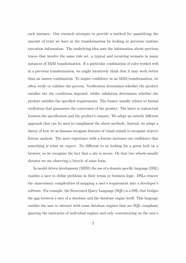
each instance. Our research attempts to provide a method for quantifying the
amount of trust we have in the transformation by looking at previous runtime
execution information. The underlying idea uses the information about previous
traces that involve the same rule set, a typical and recurring scenario in many
instances of M2M transformation. If a particular combination of rules worked well
in a previous transformation, we might intuitively think that it may work better
than an unseen combination. To inspire confidence in an M2M transformation, we
often verify or validate the process. Verification determines whether the product
satisfies the the conditions imposed, whilst validation determines whether the
product satisfies the specified requirements. The former usually relates to formal
verifcation that guarantees the correctness of the product. The latter is contractual
between the specification and the product’s outputs. We adopt an entirely different
approach that can be used to compliment the above methods. Instead, we adapt a
theory of how we as humans recognise features of visual stimuli to recognise objects:
feature analysis. The more experience with a feature increases our confidence that
something is what we expect. No different to us looking for a green lock on a
browser, so we recognise the fact that a site is secure. Or that two wheels usually
dictates we are observing a bicycle of some form.
In model driven development (MDD) the use of a domain specific language (DSL)
enables a user to define problems in their terms or business logic. DSLs remove
the unnecessary complexities of mapping a user’s requirement into a developer’s
software. For example, the Structured Query Language (SQL) is a DSL that bridges
the gap between a user of a database and the database engine itself. This language
enables the user to interact with some database engines that are SQL compliant,
ignoring the intricacies of individual engines and only concentrating on the user’s
2
view of the data. Allowing database administrators, or those that wish to query
databases, to access the data they require. Using a DSL attempts to remove the
majority of basic errors of understanding between the two parties. By their nature,
these pieces of software are modular as to allow different permutations of devices
that can work in tandem or allow for alternative devices with the same functionality
to be used or upgraded. As we have already mentioned, SQL can communicate
with multiple engines, each of those engines may optimise those queries differently
to suit their internal representations of data. We have the same source, but its
interpretation into an executable model is different.
The core motivation for our research was from a computer security perspective.
Here we described a forensic virtual machine (FVM), a small virtual machine
(VM) that uses introspection to detect symptoms of malicious behaviour in other
VMs (Harrison et al. 2012; Shaw et al. 2014). Attempting to detect malware
from outside of the OS that contains it allows us to circumvent many techniques
used by writers to hide their software, for instance disabling the anti-virus and
intercepting and modifying API calls. These symptoms may not mean anything on
their own. However, combinations of them can prove to be evidence of a piece of
malware. Introspection is used to read and interpret a raw byte stream as there is
no operating system API available to the developer. It involves generating low-level
C code from a yet unpublished declarative DSL or Cyber Observable eXpressions
(CybOX), a Mitre product (The MITRE Corporation 2017a). The latter is an
eXtended Markup Language (XML) instance to describe cyber observables that
include the types of objects we would be investigating. We, however, concentrated
our efforts on detecting key material (Saxon, Bordbar, and Harrison 2015a,b).
When completing this function, the FVM uses shared resources primarily served for
3
a VM host’s clients, for example, CPU and memory so any mistakes can be costly.
It is important to know that any automatically generated code is suitable and safe
for use in production before deployment. A typical case of our system would be the
discovery of a zero-day vulnerability; we need to produce code to monitor and find
its prevalence in an FVM’s corpus of client VMs quickly. Often there is little time
to validate or verify the FVM code in such scenarios. Unfortunately, the FVMs
we had developed had no common ground and little variability. The only variable
available to us was the RSA key length, so our attempt to gain confidence was an
equality check due to how specialised our RSA detecting FVMs were. Rather than
developing more FVMs, we chose to transform another, more general domain: a
relational database to a non-relational database.
We present a systematic framework to use the historical data, about the execu-
tion of traces, so that the experts can make informed decisions based on existing
evidence within the confines of the time available to them. Our approach stores
M2M transformation traces, extracts their execution information and compares it
to previous transactions using sub-graph isomorphism and a complexity measure
for weighing. Subgraph isomorphism is used to determine which components of the
new trace have been seen before in respect of past executions. Considerations must
be made upon the complexities of each rule, as an invocation only acknowledges
its execution. We then use McCabe’s cyclomatic complexity as a coefficient to
counter-act rule prominence on its workload. The metric is used to determine
the number of execution pathways within a function. We assume that the more
pathways that are available, there is a higher probability of traversing an incorrect
path. Therefore we must be more cautious of the function’s output. For instance,
in the event of a conditional branch, the condition may not be specific enough
4
allowing more or fewer executions of its block. Alternatively, when iterating an
array, a bounds error may occur when not handling indices properly. For the result
of a transformation to be deployed: our method uses these traits to provide a
quantifiable measure of confidence based on the previous history. In the event of
transformation fringes, i.e. segments previously unseen, we are then able to focus
validation efforts.
The process need not start with parsing or a T2M transformation. We have
transformed a live relational database into a non-relational database, specifically
Apache HBase (Saxon, Bordbar, and Akehurst 2015). Here we are transforming
the shape of the data. Rather than keeping its normalised state such that it
retains its integrity and reduces duplicate data, we denormalise the data to increase
redundancy and read speeds. The tool Kettle uses the Extract, Transform, Load
methodology to migrate data in an automated fashion (Casters, Bouman, and
Dongen 2010). Due to the lack of driver support for databases, Kettle provided a
configurable system to migrate data from one source to another, which involves
changing its structure, as well as the ability to integrate data from multiple
source types. This work sparked more frameworks and methodologies for the
transformation of relational into non-relational data (Ma, Yang, and Abraham
2016).
This thesis is structured as follows; we shall introduce our aims and some key
points related to our contribution in Section 1.1, then we provide background and
preliminary information in Chapter 2. This is then followed by three contribution
chapters: 1) the introduction of a new meta-model for traceability (Chapter 3),
2) the introduction of assurability in M2M transformation (Chapter 4), and 3) a
case study that bringing the two together (Chapter 5). Finally, we discuss our
5
findings and conclude in Chapter 6.
1.1 Objectives and Contributions of Thesis
Our objective is to design, implement and evaluate a system that can use previous
executions of M2M transformations as a basis to drive development in time critical
settings. The ability to make a risk assessment based on experience allows us to
focus efforts on lesser known artefacts to aid in the decision of mitigating those
risks or accepting them. A crucial component is the weighing mechanism that can
alter the effects of what we have seen before. This approach removes induced biases
from coverage alone as we are no longer treating each node within an execution
path as equal. As well as mapping experience onto new inputs, we can skew those
values using a configurable weighing function, providing semantic information upon
the rules invoked. Another significant capability of our work is the introduction
of a new meta-model for traceability. This new structure allows us to evade side-
effects caused in imperative or hybrid transformation languages. If transformation
languages have side-effects or any global state, then the ordering of the process is
dependent the input and that state. Our meta-model captures the order of rule
invocations to be able to recreate the state if necessary and also be able to prevent
the largest side-effect available in M2M transformation: orphans, objects created
outside of the engine.
This thesis makes the following contributions:
• A new meta-model that describes the graph-like structure of an M2M trans-
formation retaining invocation information allowing accurate debugging for
6
engines with a global state.
• A generalised algorithm to implement this within multiple transformation
engines.
• Two approaches to capturing orphaned objects created by imperative code
blocks that have no trace information; so it is impossible to know what or
why they were created.
• A quantitative evaluation of capturing this information in a well-used transfor-
mation engine, Epsilon Transformation Language (ETL) (Kolovos, Paige, and
Polack 2008), as well as our own, The Simple Transformer (SiTra) (Akehurst
et al. 2006).
• A workflow that enables users to make informed decisions to either focus
validation efforts or accept the risk of a new M2M transformation based on
experience.
• The formalisation of an execution trace and a method to persist it. This
graph and the identifying features of model elements allows for the recognition
of chains of M2M transformations.
• A tool set, in Python, that can persist, analyse and provide feedback on new
transformation traces in respect to previous executions.
7
CHAPTER 2
BACKGROUND
2.1 Model Driven Architecture
Model-driven architecture (MDA) is a methodology that puts models at the forefront
of development. At its core, it defines a Platform-Independent Model (PIM) of
an application’s business functionality and its behaviour (MDA Specifications). A
PIM defines an application’s state and how it can be interacted with or mutated. A
Platform-Specific Model (PSM) is a transformation of a PIM. The PSM is a specific
version of a PIM allowing for different underlying implementations of the same
functionality. For example, changing the volume setting on a computer changes
the output from its speakers. However, laptops come with various makes of volume
controls. Modelling the core behaviour allows us to swap devices without changing
the interaction in the main program.
The transformation of a PIM to a PSM requires a meta-model. Unlike compilers
that deal with the concrete models, transformers deal with meta-models that
describe the concrete. Meta-modelling languages define the abstract idea of a
8
component and its behaviour. In the case of a volume control, we have a current
value that defines its state, i.e. the current level. There are also four main
methods of interacting with such a device: increment, decrement and mute and
unmute. The state and the behaviour define the meta-model of the control, whilst
providing an Application Programming Interface (API) to interact with it. These
abstractions allow us to write more modular code and provide generality to our
transformation rules. MDA provides the MOF standard to define this behaviour
(Object Management Group, Inc. 2016b), others exist such as ECORE from the
Eclipse Modelling Framework (Steinberg et al. 2008) and Kermeta (Falleri, Huchard,
and Nebut 2006).
2.2 Model Transformation
The previous section described what model driven architecture is, how it is used and
how the use of meta-modelling can define it. Model transformation is a fundamental
component of MDA. It forms a general mechanism to convert a concrete model
into another using their respective abstract models. There are three variations:
1) text-to-model (T2M), 2) model-to-model (M2M) (Object Management Group,
Inc. 2016a) and 3) model-to-text (M2T) (Object Management Group, Inc. 2008).
Conceptually all of these are M2M transformations; however, the first is often linked
specifically to parsers and the latter to code generation. The fact of the matter
is that often a combination of these is used. Deserializing texts into an abstract
model, iteratively changing that model and then serialising it. These processes
can be chained to form more complex transformations. Take for example the
transformation of a domain specific language (DSL) to a general purpose language
9
transformationrules
meta-modelof source
meta-modelof destination
transformationengine
instanceof source
instanceof destination
conforms to conforms to
transforms
reads
executes
writes
refers refers
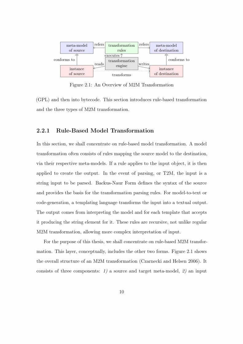
Figure 2.1: An Overview of M2M Transformation
(GPL) and then into bytecode. This section introduces rule-based transformation
and the three types of M2M transformation.
2.2.1 Rule-Based Model Transformation
In this section, we shall concentrate on rule-based model transformation. A model
transformation often consists of rules mapping the source model to the destination,
via their respective meta-models. If a rule applies to the input object, it is then
applied to create the output. In the event of parsing, or T2M, the input is a
string input to be parsed. Backus-Naur Form defines the syntax of the source
and provides the basis for the transformation parsing rules. For model-to-text or
code-generation, a templating language transforms the input into a textual output.
The output comes from interpreting the model and for each template that accepts
it producing the string element for it. These rules are recursive, not unlike regular
M2M transformation, allowing more complex interpretation of input.
For the purpose of this thesis, we shall concentrate on rule-based M2M transfor-
mation. This layer, conceptually, includes the other two forms. Figure 2.1 shows
the overall structure of an M2M transformation (Czarnecki and Helsen 2006). It
consists of three components: 1) a source and target meta-model, 2) an input
10
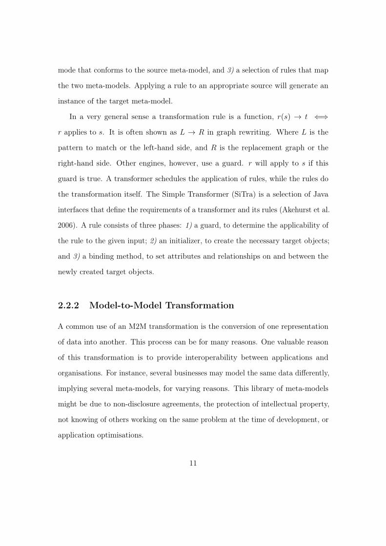
mode that conforms to the source meta-model, and 3) a selection of rules that map
the two meta-models. Applying a rule to an appropriate source will generate an
instance of the target meta-model.
In a very general sense a transformation rule is a function, r(s) → t ⇐⇒
r applies to s. It is often shown as L → R in graph rewriting. Where L is the
pattern to match or the left-hand side, and R is the replacement graph or the
right-hand side. Other engines, however, use a guard. r will apply to s if this
guard is true. A transformer schedules the application of rules, while the rules do
the transformation itself. The Simple Transformer (SiTra) is a selection of Java
interfaces that define the requirements of a transformer and its rules (Akehurst et al.
2006). A rule consists of three phases: 1) a guard, to determine the applicability of
the rule to the given input; 2) an initializer, to create the necessary target objects;
and 3) a binding method, to set attributes and relationships on and between the
newly created target objects.
2.2.2 Model-to-Model Transformation
A common use of an M2M transformation is the conversion of one representation
of data into another. This process can be for many reasons. One valuable reason
of this transformation is to provide interoperability between applications and
organisations. For instance, several businesses may model the same data differently,
implying several meta-models, for varying reasons. This library of meta-models
might be due to non-disclosure agreements, the protection of intellectual property,
not knowing of others working on the same problem at the time of development, or
application optimisations.
11
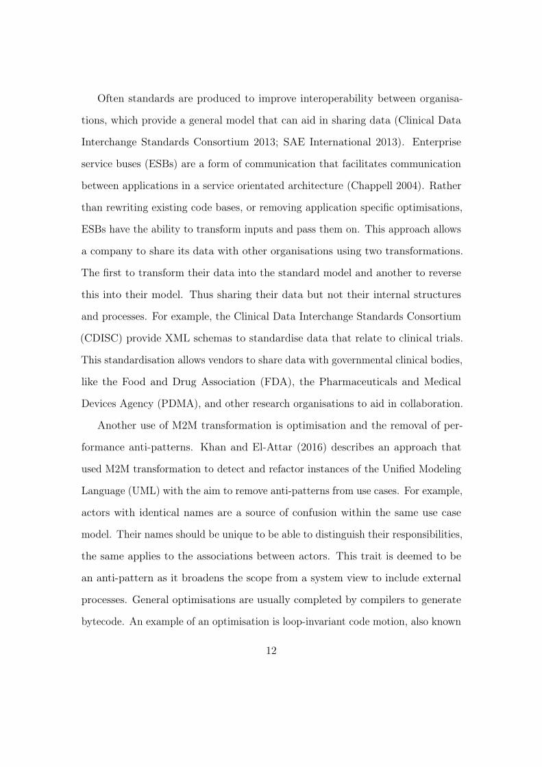
Often standards are produced to improve interoperability between organisa-
tions, which provide a general model that can aid in sharing data (Clinical Data
Interchange Standards Consortium 2013; SAE International 2013). Enterprise
service buses (ESBs) are a form of communication that facilitates communication
between applications in a service orientated architecture (Chappell 2004). Rather
than rewriting existing code bases, or removing application specific optimisations,
ESBs have the ability to transform inputs and pass them on. This approach allows
a company to share its data with other organisations using two transformations.
The first to transform their data into the standard model and another to reverse
this into their model. Thus sharing their data but not their internal structures
and processes. For example, the Clinical Data Interchange Standards Consortium
(CDISC) provide XML schemas to standardise data that relate to clinical trials.
This standardisation allows vendors to share data with governmental clinical bodies,
like the Food and Drug Association (FDA), the Pharmaceuticals and Medical
Devices Agency (PDMA), and other research organisations to aid in collaboration.
Another use of M2M transformation is optimisation and the removal of per-
formance anti-patterns. Khan and El-Attar (2016) describes an approach that
used M2M transformation to detect and refactor instances of the Unified Modeling
Language (UML) with the aim to remove anti-patterns from use cases. For example,
actors with identical names are a source of confusion within the same use case
model. Their names should be unique to be able to distinguish their responsibilities,
the same applies to the associations between actors. This trait is deemed to be
an anti-pattern as it broadens the scope from a system view to include external
processes. General optimisations are usually completed by compilers to generate
bytecode. An example of an optimisation is loop-invariant code motion, also known
12
as hoisting or scalar promotion (Srivastava 1999). Loop-invariant code motion
detects code that remains constant before and after a loop and moves it outside of
the block. Compilers apply this optimisation to increase the application’s runtime
performance by computing the detected expressions once opposed to during each
iteration.
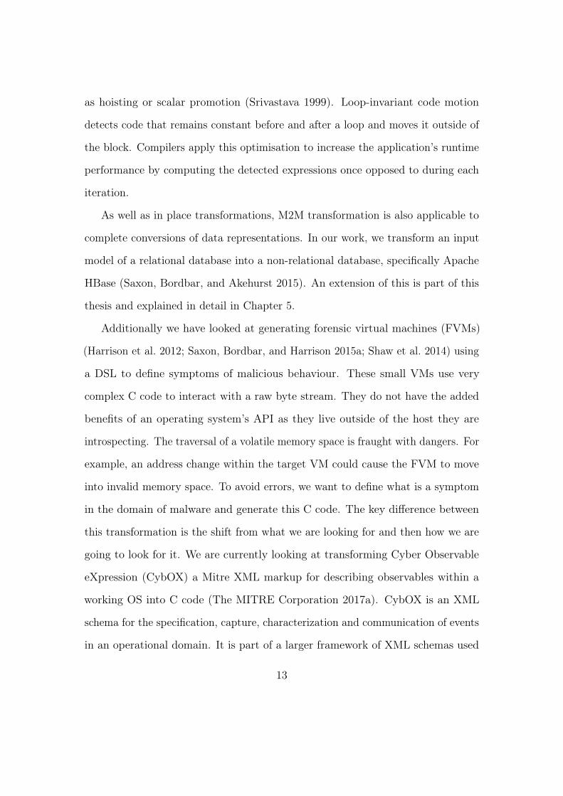
As well as in place transformations, M2M transformation is also applicable to
complete conversions of data representations. In our work, we transform an input
model of a relational database into a non-relational database, specifically Apache
HBase (Saxon, Bordbar, and Akehurst 2015). An extension of this is part of this
thesis and explained in detail in Chapter 5.
Additionally we have looked at generating forensic virtual machines (FVMs)
(Harrison et al. 2012; Saxon, Bordbar, and Harrison 2015a; Shaw et al. 2014) using
a DSL to define symptoms of malicious behaviour. These small VMs use very
complex C code to interact with a raw byte stream. They do not have the added
benefits of an operating system’s API as they live outside of the host they are
introspecting. The traversal of a volatile memory space is fraught with dangers. For
example, an address change within the target VM could cause the FVM to move
into invalid memory space. To avoid errors, we want to define what is a symptom
in the domain of malware and generate this C code. The key difference between
this transformation is the shift from what we are looking for and then how we are
going to look for it. We are currently looking at transforming Cyber Observable
eXpression (CybOX) a Mitre XML markup for describing observables within a
working OS into C code (The MITRE Corporation 2017a). CybOX is an XML
schema for the specification, capture, characterization and communication of events
in an operational domain. It is part of a larger framework of XML schemas used
13
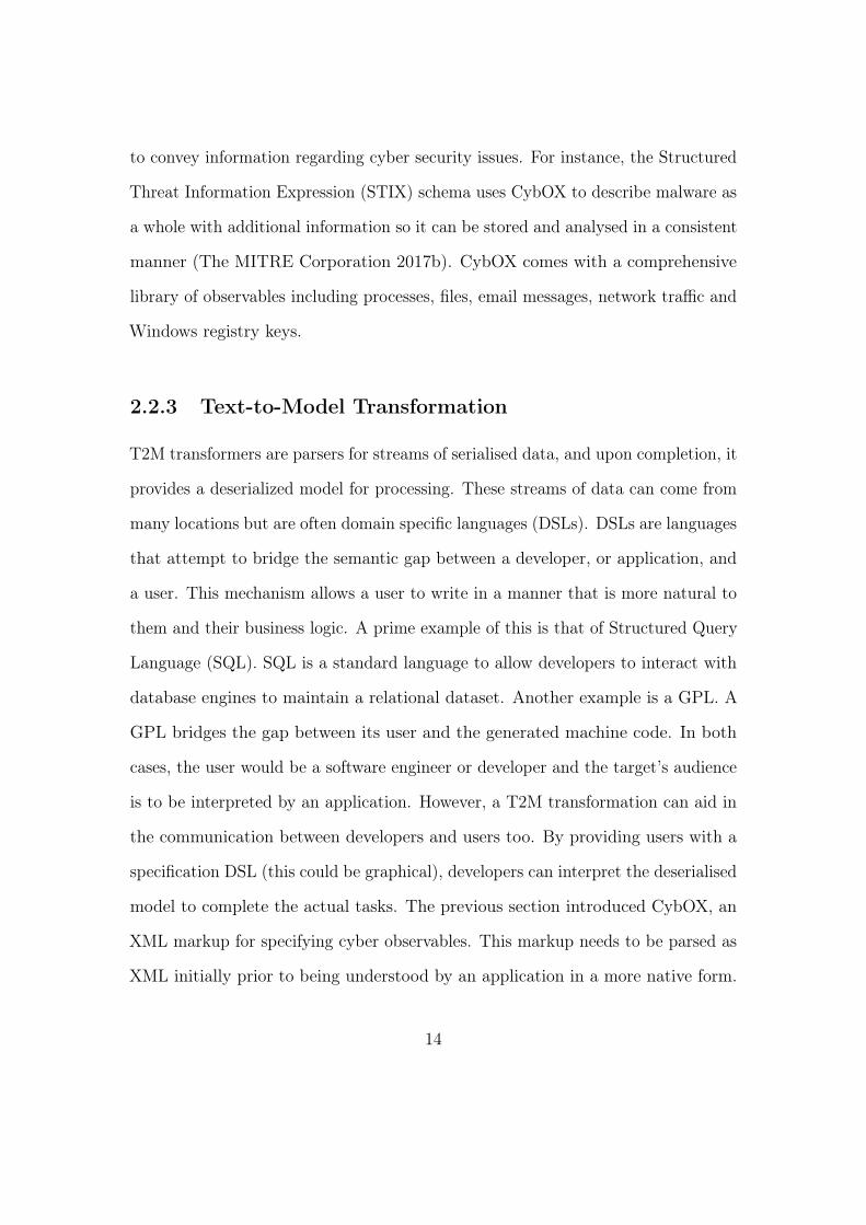
to convey information regarding cyber security issues. For instance, the Structured
Threat Information Expression (STIX) schema uses CybOX to describe malware as
a whole with additional information so it can be stored and analysed in a consistent
manner (The MITRE Corporation 2017b). CybOX comes with a comprehensive
library of observables including processes, files, email messages, network traffic and
Windows registry keys.
2.2.3 Text-to-Model Transformation
T2M transformers are parsers for streams of serialised data, and upon completion, it
provides a deserialized model for processing. These streams of data can come from
many locations but are often domain specific languages (DSLs). DSLs are languages
that attempt to bridge the semantic gap between a developer, or application, and
a user. This mechanism allows a user to write in a manner that is more natural to
them and their business logic. A prime example of this is that of Structured Query
Language (SQL). SQL is a standard language to allow developers to interact with
database engines to maintain a relational dataset. Another example is a GPL. A
GPL bridges the gap between its user and the generated machine code. In both
cases, the user would be a software engineer or developer and the target’s audience
is to be interpreted by an application. However, a T2M transformation can aid in
the communication between developers and users too. By providing users with a
specification DSL (this could be graphical), developers can interpret the deserialised
model to complete the actual tasks. The previous section introduced CybOX, an
XML markup for specifying cyber observables. This markup needs to be parsed as
XML initially prior to being understood by an application in a more native form.
14
This process makes an assumption that the user knows what they want to do
but don’t know the all of the essential details to complete the task itself. The first
part of this process involves parsing the source code, or script, into a model that
can be interpreted by a compiler. This model is often the abstract syntax tree
(AST) that represents the language in question. It is a basic model that simply
represents the expression and its location within the source. An AST allows a
compiler to further transform or interpret the input in a manner it understands
to complete its task, to generate bytecode for example. Generally speaking, all
compilers are formed of a T2M transformation, allowing them to parse source code
before mutating it and finally serialising it.
Other examples include JAXB for the serialisation and de-serialisation of JSON
and XML (Kawaguchi, Vajjhala, and Fialli 2009). XML and JSON are common
formats used throughout the Internet to communicate data. These technologies are
often used on the web to create asynchronous web applications. Asynchronous web
applications use these data formats to update their page content without sending
the raw HTML/CSS to do so. Instead, they optimise their efforts only to send raw
data or HTML snippets and allow the client to take care of presenting it. This
approach reduces the CPU utilisation on the server side, as it does not have to
prepare the full webpage, and provides an exchange that can be used by third party
vendors.
2.2.4 Model-to-Text Transformation
Model-to-text (M2T) transformation relates to the serialisation of a model into
some form of linearized text representation (Object Management Group, Inc. 2008).
15
Allowing a user to generate various text artefacts such as code, specifications,
reports and for basic data storage. These are created using a templating system
such that a f(x)→ String where x is a model element. We have already introduced
an example of M2T: JAXB (Kawaguchi, Vajjhala, and Fialli 2009). JAXB allows
its users to not only read XML and JSON but write it to files. Using Java
annotations on classes, or some XML bindings, it can generate the textual form
required for transmission. The result of which aids in the transfer of data between
systems or a format easily used for storage. JAXB comes with the application XJC.
XJC transforms an XML Schemas into Plain Old Java Objects for use within an
application. Opposed to making the developer interpret the raw XML or JSON,
they can then traverse an object orientated model based on an XML Schema.
Another example of this is an Object Relational Mapper (ORM) for example
JPA and Hibernate Goncalves 2013; Hibernate ORM . An ORM will generate
SQL from an internal representation of a query. This automatic generation allows
interaction with an SQL-compliant server without any SQL code being written,
depending on the ORM. Instead of directly interfacing with the engine, one can
instead programmatically write queries using a query builder in the native language
of the application. This API bridges the semantic gap between the developer and
the database engine itself, while simultaneously allowing the developer to interact
with a plethora of engines.
2.3 Software Assurance
In the previous section, we spoke about MDA and model transformation in all its
forms. However, once we have completed a transformation how can we use it? We
16
need to have the assurance that it works in a manner fitting for what it is meant
to do. This section describes software assurance and links it to MDA and M2M
transformation through validation.
Assurance provides the grounds for justified confidence that a claim has been
or will be achieved (“IEEE Trial-Use Standard–Adoption of ISO/IEC TR 15026-
1:2010 Systems and Software Engineering–Systems and Software Assurance–Part
1: Concepts and Vocabulary” 2011). The main use is within Quality Assurance
(QA). QA is the planned and systematic pattern of all actions necessary to provide
adequate confidence that the item or product conforms to established technical
requirements (“Systems and software engineering – Vocabulary” 2010). This trait
comes from being able to connect the requirements, design, implementation and
validation processes together within the software development life-cycle. This
assures the overall development process of a final product.
The most important aspect of the life-cycle, to stakeholders’, is that the product
functions as required. Thus the connection to requirements and tests is invaluable,
proving that they have what they needed. The level of this QA is quite high, and it
does not regard the individual components, tools and languages used in a system.
The overall process may or may not acknowledge them; they are a means to an
end. Therefore the functionality of the components are not assured themselves,
thus must be revalidated on reuse.
2.3.1 Software Specific Definitions
In the realm of software, assurability is related to the software lifecycle and how it
affects the final product. The definition provided by the National Aeronautics and
17
Space Administration (NASA) is a direct derivative of that specified by ISO-24765
(NASA 2005; “Systems and software engineering – Vocabulary” 2010). The main
alterations are to relate directly to software, processes and products, and that they
need to conform not only to requirements but standards and procedures too.
The National Information Glossary, the United States Department of Defence
(DoD) and SAFECode best practices all have a concept of confidence and assurability
within their standards (National Information Assurance (IA) Glossary ; Komaroff
and Baldwin 2005; SAFECode 2008). By showing that the final product does as
intended and that the process of creating it is free of, and does not introduce,
vulnerabilities increases this confidence. As the method of creating software can be
several layers deep, T2M → M2M → . . .→ M2T → T2M → . . . , the probability
of introducing vulnerabilities increases.
The Object Management Group, Inc. provides a very vague definition (Ob-
ject Management Group, Inc. 2005). It simply states that the process provides
justifiable trustworthiness in meeting established business and security objectives.
This statement is still comparable to the definition from the “Systems and software
engineering – Vocabulary” (2010). They mention increasing the level of justifiable
trustworthiness to meet business needs, i.e. function as intended, and security
requirements, i.e. the introduction of vulnerabilities.
Thus assurability in software processes increases the confidence in the final
product by:
1. showing that the process does as it is meant to; and
2. confirming that it does not introduce and is free of vulnerabilities.
In M2M transformation, black-box and white-box testing provide assurances that
18
the resultant model is “correct” given certain conditions. The next two sections
discuss these two types of validation.
2.3.2 Black-box Testing
M2M transformations are considered primarily to be black-box operations. Black-
boxes are processes that have no concept of what happens to an input to generate
the output. There are no execution paths between the two. More often than not, a
function is a black-box process. Since an M2M transformation is a simple function,
it is considered to be a type of black-box as there are no associations between the
source and destination model elements. Thus validation requires the comparison
between the origin and target models.
Validation within M2M Transformations
Validation in M2M transformation requires a selection of Oracle functions. These
methods provide assurances that the target model is correct concerning the source
model. Many take into account only the input and output models; these black box
methods say what the target model should look like. There are six such oracles as
defined by Mottu, Baudry, and Le Traon (2008).
1. Reference model transformation is an oracle that repeats the transformation
and compares it to an expected output model.
2. An inverse transformation attempts to get the same input model from a
target when provided an inverse function.
3. Expected model output compares the actual output with an expected model.
19
4. A generic contract is defined using constraints linking both sides of the
transformation, such that the target and the test model satisfy some rule.
5. An Object Constraint Language (OCL) assertion does not consider the input
model and instead checks to see if the output satifies a constraint.
6. Finally model snippets verify to see if the target model contains some model
fragments.
These oracles primarily concentrate on model-comparison, contracts and pattern
matching.
2.3.3 Opening the Black-Box (White-box Testing)
White-boxes consider more than the inputs and outputs; they consider the internal
processes needed to produce the result as well as model constraints. This process
involves the static analysis of a function’s dependency graph to determine related
operations. Then test models that conform to the source meta-model are deduced
using a combination of their dependency graph and other user-defined constraints
by using SAT- or CSP- based solvers. These user-defined constraints could include
UML’s association multiplicity (n..m), bounds checking, string formats and other
semantic properties for the model in question. For example, the minimum hourly
rate of an employee must be above the minimum wage for the country they are
employed.
DSLs used for M2M transformation make the creation of dependency graphs
easier as the prototype of the rule contains all of the output model elements up-
front. However, side-effects within a language can make it possible to generate
20
more model elements making the dependency graph incomplete. Take for example
a rule whereby the binding phase creates an object and binds it to the resultant
object. The program that extracts the dependency graph needs to look at more
than the prototype of the transformation. It will need to traverse the execution of
that phase to capture any new object types it may come across. Thus hybrid and
imperative languages could report incorrect dependency graphs, which could have
undesired effects. The dependency graph and user constraints may generate an
incomplete suite of tests.
Traceability
Traceability, in the general sense, is a technique to link two or more components of
the development process together such that one can trace forward, or backward, from
any given point within the process (“Systems and software engineering – Vocabulary”
2010). The primary use of this in software is requirements traceability (Winkler
and Pilgrim 2010). It allows a user, or business owner, to trace a requirement
through specification, development, validation, deployment and any iterations of
each. For example, before signing off on deploying new software, we might want to
be shown the steps in validating a particular requirement. Often using matrices,
we can trace a requirement to particular tests via the development lifecycle to see
if a reasonable amount of testing was carried out.
M2M transformation can also use this method but at a much higher level of
abstraction. Traceability, in this case, provides the associations between the source
model and the destination, and by what means the target model came to exist.
This feature allows us to see the internal execution of a transformation at runtime,
21
which in turn enables us to view what source model elements caused the existence
of particular target model elements. Although useful, it is often too fine-grained for
tracing requirements, unless it is interpreted in some manner befitting its audience.
Requirements traceability need not know how it is done, it only needs to know that
it has been. Each trace link represents the invocation of a rule upon a source or a
set of sources to generate a destination model. Given a set of rules R and a set of
sources S, an invcocation can be defined as:
(r, s)→ t where t = r(s), r ∈ R, s ⊆ S ⇐⇒ r applies to s
Engines query their trace for each input to find out if there is an existing association
to return the previously instantiated objects unless the rule is lazy and requires
new objects for each invocation (Jouault et al. 2008). Since the invocation contains
all of the information, often a cache is used to assist the process:
(r, s)→ i where i = (r, s, t), t = r(s), r ∈ R, s ⊆ S ⇐⇒ r applies to s
More often than not we want the same result back given the same input and rule.
This internal representation prevents repeated calls of the same transformation
upon the same source by using the two as a unique identifier for the invocation.
However, using this format we are unable to generate a dependency graph to
generate test cases. We have a list of invocations with no dependency information,
if they are indeed available at all.
22
Availability of Trace Data The availability of a transformation trace dif-
fers from engine to engine. Often these associations are private to the engine
and are unavailable to the developer or user for persistence or analysis. The
Atlas Transformation Language (ATL) (Jouault et al. 2008) and Operational
Query/View/Transform (QVT-O) (Object Management Group, Inc. 2016a) for
example use the transformation trace to track what it creates and is part of its
scheduler, however, does not expose these structures via an API or any other means.
These are called internal traces (Jouault 2005). The opposite, as implemented in
the SiTra (Akehurst et al. 2006) and the Epsilon Transformation Language (ETL)
(Kolovos, Paige, and Polack 2008), provide access to these internal structures for
persistence and future analysis. These are external traces. The lack of external
traces causes M2M transformations to be black-box processes, such that we do not
know what occurs within.
By High Order Transformation Jouault (2005) uses a high order transfor-
mation (HOT) to provide traceability to all engines, including those that only use
their trace internally. The HOT modifies the transformation rules themselves. This
modification adds additional output objects, which conform to a trace meta-model,
and binds them together using an imperative block. The substitution of this new
rule with the original provides an additional output model, that of a transformation
trace. This approach applies to all languages in that a transformation of the base
AST would allow the addition of these trace elements and their automatic binding.
23
Verbosity The verbosity of the trace, up to now, is usually in the form of
a linear list of invocations. These invocations contain information about what
rule transformed which source objects into what target objects. The linearity of
this list provides information regarding the order of instantiation. This trait is
only true for single-threaded transformers, which is currently standard practice.
Schedulers do not know what can and cannot be parallelized due to the lack of a
dependency graph. The ETL engine used this form of a trace, as do many others,
it is implemented by iterating all available rules and finding matching inputs. It
then instantiates the target model elements and stores it all as an invocation. The
engine iterates this list of invocations to bind all of the target objects.
Uses of Traceability
Traceability is part of the software lifecycle, not just MDA and model transformation.
It instead, in the general sense, connects each part of development together. Traces
are used to link the requirements of a product to the component that provides
it. Often they follow all phases through specification, development and validation.
The ability to show that a requirement is fulfilled by n specification points and are
validated using m tests illustrates the lifecycle of the process.
However, the result is the same: how does the final element come to exist. This
process can be applied to many fields but is prominent in M2M transformation as
it is a black box. This section describes how traceability is used in MDA to show
its prominence in the field.
Kessentini, Sahraoui, and Boukadoum (2011) uses a linear trace defined by
Falleri, Huchard, and Nebut (2006) to provide a risk assessment based on previous
24
good examples. The core of this method is the use of traceability for comparison.
Base transformation examples are encoded and compared to generate detectors
of risky transformations. These detectors are applied to new transformations for
analysis and reporting to the user to focus validation efforts. The comparison of
clean traces uses a method based on a dynamic programming algorithm used in
bioinformatics to locate similar regions between two sequences of Deoxyribonu-
cleic Acid (DNA), Ribonucleic Acid (RNA) or proteins: the Needleman-Wunsch
algorithm (Carrillo and Lipman 1988).(Carrillo and Lipman 1988).
Incremental M2M Transformation Model transformations are time con-
suming processes. The size of the input model or the complexity of the trans-
formation itself increases the time of the mapping. The naive way to consider
changes to a source model is to re-execute the process on the amended model.
However, incremental transformation is a current research field to overcome these
performance issues (Kusel et al. 2013). Incremental transformation engines concen-
trate on only reapplying rules when the source objects that concern them change.
Varró et al. (2016) discusses four patterns for this process. No incrementality, the
simple mechanism we have mentioned. Dirty incrementality, where model elements
are tagged as dirty when changed, and therefore rules that concern them are re-
executed. Incrementality by Traceability takes the trace of an initial transformation
and then when re-applied, detects untraceable elements and transforms only those
objects. Reactive incrementality closely relates to the observer pattern. They look
for changes in the source model to trigger the applicable transformation rules.
25
2.4 Pattern Recognition
At this point, we have introduced MDA and the application of traceability within
M2M transformation, a key element within MDA. Traceability comes in many
forms with differing levels of detail dependent on the requirements of the engine.
In the event of a big transformation, we will need to reduce the effects traceability
has to increase the throughput of the process itself. However, smaller input models
allow us to retain more associations with the target model. This process is, of
course, assuming that the transformation trace is available to the user at all.
The next step is to learn from previous experience. To do this, we look at
how we as humans recognise objects. For example, assuming we have no previous
knowledge, and we were provided with a stool. To begin with, we would break it
down into its components and learn its use. We might note that it has four legs
and a flat surface for sitting on. Then we would store this information. If after
this we were then provided with a chair, we would recognise the flat surface and
the four legs. However, we would have a new component the back of the chair.
We would then have to investigate what this was to learn its purpose and in turn
remember it in a knowledge base. Humans, however, do not just remember good
stimuli but the bad too. So if the chair had a spike, then they would remember
this to avoid it!
In this section, we shall look at how we as humans recognise objects to know
quality transformations based on their transformation trace.
An essential requirement of our work, once we have a transformation trace,
is the comparison of trace elements such that we “recognise” sub-components
of our new trace in respect to the older model transformations. Berry (2014)
26
describes mechanisms that we use in computer science to mimic our understanding
of recognising objects. Specifically, there are four approaches of interest: template
matching, prototype matching, feature analysis and recognition by components.
2.4.1 Template Matching
Template matching is a normalised cross-correlation between a known and a new
image to classify. These known images create a long term memory, or knowledge
base, of elements that have been seen before to represent the processes’ experience
and learning. A direct comparison between the new input and each of the templates
provides a match. This type of comparison has a drawback as they need to be
identical, preventing the recognition of variations unless those too are within the
knowledge base.
2.4.2 Prototype Matching
Prototype matching extends template matching by using a prototype that defines
the characteristics of the object in question. For instance, the concept of a vehicle
with two wheels and a chain is a prototype for a bicycle or a motorcycle. We
can extend this prototype to include an engine to represent the latter of the two.
Unlike template matching, this method allows for variations between input models
and those in the knowledge base. This method provides us with a probable match
within a hierarchy of prototypes.
27
2.4.3 Feature Analysis
This approach contains four main components: detection, pattern dissection,
comparison and recognition. In essence, sensory information is broken down and
compared with known features, partial or otherwise for a match. The process
generalises the input information and breaks it down into components. For example,
if we were received visual information that contained a dog, we might break it down
into a body, four legs, a head and a tail. We would then look into our knowledge
base looking for “things” with these traits. Naturally, using only these traits there
are a plethora of false-positives, in fact, most four legged invertebrates with tails!
This approach closely mimics the model-snippets Oracle when validating M2M
transformations, as discussed in Section 2.3.2. Model-snippets involves breaking
down the resultant model of an M2M transformation and comparing sub-models
to known models. If all sub-models are present, then the test case is deemed
successful.
Detection and Dissection To summarise, the first component looks at
receiving and dissecting relevant information from an input. We have already
mentioned how we as humans can use feature analysis to look for a dog from visual
stimuli. This process can differ between domains and look for different traits. If we
were to attempt to recognise components within a scanned image, we’d use pixel
intensities as our “visual sensory” information. Then we’d dissect the input to find
lines, arcs and other interesting vectors. Another example is in facial recognition.
We would attempt to detect dominant, or cardinal points, related to facial fiducial
points, the eyes, chin, cheeks, mouth, etc. (Wang et al. 2017).
28
Comparison and Recognition The next step is to find a match given a
set of features. This process involves comparing the input features to those of
instances that we have seen previously. Continuing our detection and dissection of
vectors, we could recognise components from various diagrams. In circuitry, if for
example, we had the knowledge that a lamp is a circle with two perpendicular lines
crossing inside, we can compare permutations of features to see if we can recognise
this configuration regarding the input. Likewise, the knowledge that two parallel
lines where one is shorter and bolder than the other can aid in distinguishing a
cell. We can use similar heuristics to find components within chemical diagrams
given the previous experience. Two parallel lines where one is shorter than the
other could denote a double bond. Characters indicate the location of atoms and
their types. The lack of a character at a junction of two bonds suggests an implicit
carbon atom.
In the case of facial recognition, we would have spatial information of the five
traits discussed above for each face in the knowledge base, as well as the original
photo. Comparing the input to each object could aid in identifying people. This
type of comparison would not be as clean cut as others.
2.4.4 Recognition by Components
Recognition-by-components specialises feature detection but rather than looking
at labelled features; we instead look at three-dimensional geometric shapes called
Geons. Thus the features are not labelled in the sense of a body; we might say
an ellipsoid instead. Geons better describe and can be more telling on what we
are viewing. A feature detector is then used to find these primitives. For example,
29
rectangles, squares and circles in two-dimensional space, but also cuboids, cubes
and spheres in three-dimensional space. A match comes from comparing the
combination and orientation of these geometric shapes with images found within a
knowledge base. Using the example of a dog, the geons of a dog’s head and that of
a cat’s head can distinguish the two animals whereas a “head” like object cannot.
The theory by Biederman (1987), suggests that there are fewer than 36 geons,
which, in combination, make up the objects seen in life. For instance, we might
decompose a cup into two cylindrical-components. The first makes up the main
body and the second for the handle. However, these two components would also
be present in many other objects. A bucket, for example, may also be composed of
the same cylindrical-components only the configuration would differ such that the
handle would be on the flat end of the body opposed to being attached to the side.
Using our dog example, geons are not labelled in the sense of a body; we might
say an ellipsoid instead. Geons better describe and can be more telling on what we
are viewing. The geons of a dog’s head and that of a cat’s head can distinguish the
two animals whereas a “head” cannot.
2.5 Chapter Summary
In this chapter, we have discussed the state-of-the-art in M2M transformation.
We then introduced software assurance: the general mechanisms that are used to
increase confidence in software processes, presenting traceability as the core effort
to provide confidence in M2M transformation. We embellish on how it is applied,
black- and white-box approaches, and its usage, incremental transformation, formal
verification and validation. After this, we then spoke about the inspiration of this
30

work, pattern recognition. Looking at some theories of how we as humans recognise
items in the real world, making comparisons to our oracles in M2M transformation
a core element that is used in our work.
31
CHAPTER 3
DESIGN OF NEW TRACEABILITYMECHANISM
To learn from a transformation’s history, we need to be able to see what is happening
within the engine to form the basis of our comparison. To do this, we must consider
the tasks that are completed to transform a source to its destination and provide
us with a representation that we can analyse. Traceability is commonly used to
open the black box of model-to-model (M2M) transformation. It is a technique for
keeping track of rule invocations (Object Management Group, Inc. 2016a). It has
been used in many applications and has been discussed at length as an essential
requirement (“Advanced Traceability for ATL”; Briand et al. 2014; Fritzsche et al.
2008; Paige et al. 2010; Vara et al. 2014; Willink and Matragkas 2014). For a survey
of traceability see “Survey of Traceability Approaches in Model-Driven Engineering”
(Galvao and Goknil 2007).
There are however two levels of traceability: a) internal; and b) external as
defined by (Jouault 2005). Internal traceability provides the transformation engine
with information regarding what it is doing and often is not available after the
completion of the process. The engine uses this trace to track what rule and
32
source combinations caused the creation of what outputs. ATLAS Transformation
Language (ATL) (Jouault et al. 2008), Xtend (Eclipse Foundation 2014) and
Eclipse’s implementation of Operational Query/View/Transform (QVT-O) follow
this mechanism. An external trace differs from an internal as it is accessible to
the user after completion. This accessibility enables its users to persist or use
the trace for further analysis. The Simple Transformer (SiTra) and the Epsilon
Transformation Language (ETL) provide a linear trace of what rules and inputs
have created what outputs.
This section concentrates on the looking into what current external traceability
provides us and considers challenges that are present in current implementations
when considering full accountability. We pay particular attention to the structure
of the trace, i.e. the standard linear trace that loses information regarding the
graph-like execution of the transformation. We also provide implementation details
for SiTra, showing how we overcame the drawbacks discovered. To demonstrate the
generality of our approach we then provide information as to how to migrate our
approach for use with ETL, this shows our efforts can provide a full transformation
trace in a plethora of engines.
3.1 Challenges of Tracing in Model Transforma-tion
M2M transformation is often a black box process. It is identified as such because the
engine does not provide associations between the source model and the destination
model. Transformation engines such as ETL (Kolovos, Paige, and Polack 2008)
and ATL (Jouault et al. 2008) require the meta-models of the source, destination
33
and a set of transformation rules as input. Then the engine, behind the scenes,
automatically executes the rules and converts an input model to generate the desti-
nation model. Even during validation, all existing research focuses on correctness
of rules, while treating the transformation engine as a black-box that is assumed
to execute correctly. One exception to this “black-box” routine is the process of
tracing (Aizenbud-Reshef et al. 2006; Ebner and Kaindl 2002; Object Management
Group, Inc. 2016a). Traceability can be supported in transformation engines and
gives access to the associations between source and destination models established
by an engine’s execution (Object Management Group, Inc. 2016a). To the best of
our knowledge the first tracing mechanism, within non-graph based transformation
engines, was implemented and used by UML2Alloy (Shah, Anastasakis, and Bord-
bar 2010) through SiTra (Akehurst et al. 2006). UML2Alloy produces Alloy models
from a Unified Modeling Language (UML) class diagram and Object Constraint
Language (OCL) statements via a transformation. The trace implemented within
SiTra was used to convert a counter example, produced by Alloy, back to UML.
To demonstrate the issues we have in current traceability: suppose we have
a set of rules, R = {r0, r1, . . . , ri} and a set of source objects S: we can define
a transformation trace as a sequence of tuples containing a set of sources and
the rule that was applied to them, as shown in Equation (3.1). This form of a
trace is one-dimensional and loses information regarding what is occurring within a
transformation. An execution of rules upon a source input model is a graph of rule
invocations, i.e. rules will require the result of other rules, while others may need
the product of a previously invoked rule. The linear trace loses these relationships.
34
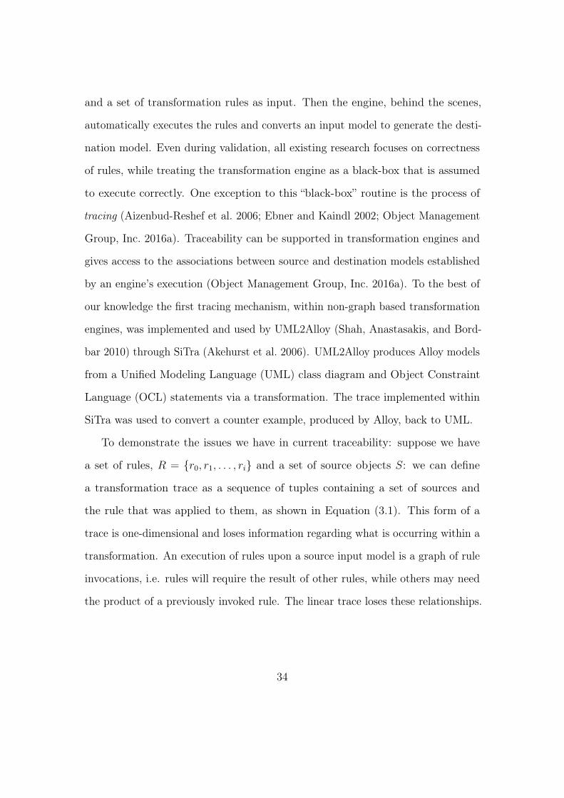
1 class AtoC extends Rule<Attribute, Column> {2 private static Integer sequence = 0;3 public void setProperties(Column target, Attribute source,4 Transformer tx) {5 target.setName(source.getName());6 target.setOrder(AtoC.sequence++);7 }8 }
Figure 3.1: A SiTra transformation rule with a global state.
T = 〈(ri, si) | si ⊆ S, ri ∈ R, i = {0, 1, . . . , |T | − 1} ⇐⇒ r applies to s〉 (3.1)
In this section, we discuss some of the shortfalls from current external trace-
ability: specifically the loss of information that comes from only having linear data.
We look at the relationships between invocations and what they imply about the
relationships between the rules themselves. Finally, we look at orphans: objects
that are not traced by the engine as the engine does not instantiate them. Instead,
the hybrid/imperative language behind it does.
3.1.1 Ordering of Rule Execution
For the maintenance and debugging of an M2M transformation, the developers
need to be able to recreate the conditions and the process itself. This ability is of
particular importance when using a language, or engine, that can cause side-effects.
Side-effects are changes in a program which occur as a by-product of the evaluation
of an expression, a rule invocation (M. et al. 2001). A global state in hybrid or
imperative languages can cause this particular side-effect. Figure 3.1 is an example
35
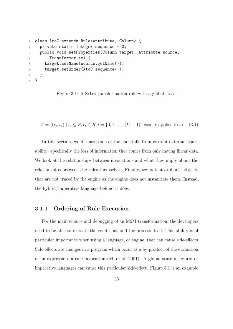
oo db
parent1
attrs0..*
parent1
cols0..*
Entity
Attribute
Table
Column
EtoT
AtoC
Figure 3.2: A sample of rule dependencies.
of side effects within a rule for SiTra. It shows a static integer that is used to
provide some form of ordering upon the columns that it creates (see line 6). Here
we can see that the value of the column’s order attribute is dependent on the order
of the rule’s invocation.
It is reasonable to assume that given a list of attributes, that their order of
application might differ. This variation could be a side-effect of the following.
1. The low-level implementation of collections used, i.e. whether it is an ordered
array or not, or the type of iterator used.
2. The input model element that was used to initiate the transformation.
3. The source model itself. If read from an eXtended Markup Language (XML)
file, for example, the process of parsing is dependent on the implementation
of the XML library. Given a schema it is possible that a complex type was
defined as a sequence, implying order, if not there may be no guarantees.
4. How the engine is scheduled.
36
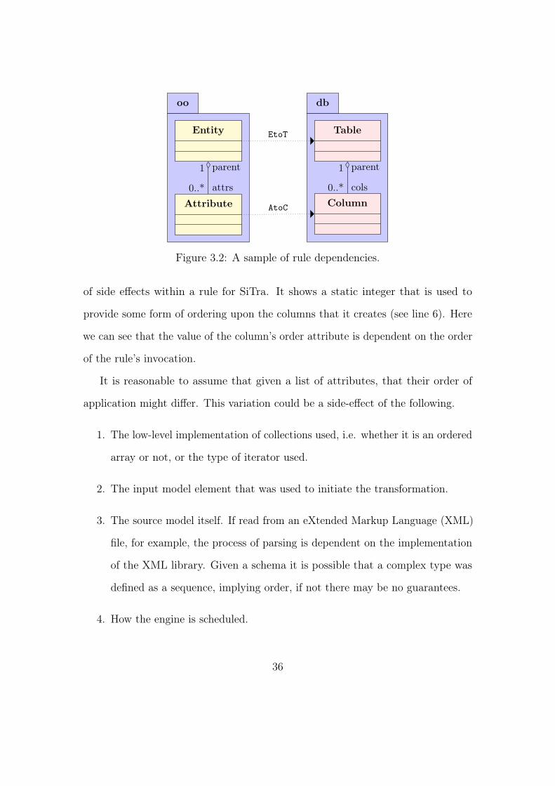
To illustrate and expand on these issues we shall introduce a simple transformation
between an Entity and Attribute to a Table and Column, as depicted in Figure 3.2.
The UML shows two meta-models, both containing a bi-directional one-to-many
relationship. This commonality creates a simple one-to-one transformation.
Collections
An Entity has an association with a collection of Attributes. The overall trans-
formation requires the rule EtoT to transform the attributes during its binding
phase to generate the columns and assign their parent to the resultant Table
object. Iterators may not return objects from a collection in the same order they
were inserted. A HashSet in Java, for example, provides no guarantees as to the
iteration order of the set. Thus a second execution may result in a different order
of elements. For example, given an ordered list one might obtain a trace that
resembles: T = 〈(EtoT, e), (AtoC, a0), (AtoC, a1), (AtoC, a2)〉. Another platform,
however, might provide T = 〈(EtoT, e), (AtoC, a2), (AtoC, a0), (AtoC, a1)〉. The
generated model may or may not be structurally correct, but is certainly not
semantically the same, as the attributes are no longer in their original order. Given
the rule in Figure 3.1: all attributes in the second transformation would have
different order values when compared to the first run, due to the evident global
state.
Starting Point
The starting point of a transformation can also change the result structurally, or
semantically if there is a global context. Take again, an entity with three attributes,
37
if we were to start the transformation with an entity our trace would look like:
T = 〈(EtoT, e), (AtoC, a0), (AtoC, a1), (AtoC, a2)〉
Whereas if we chose to start with the second attribute, a1, we would have:
T = 〈(AtoC, a1), (EtoT, e), (AtoC, a0), (AtoC, a2)〉
This effect is more apparent, given the same rule from Figure 3.1, a0 and a1 would
have different values for their order attribute.
Transformation Input
The output can also be dependent on how the source model is read, or generated,
as it could reorder collections. For instance, if an XML Schema Definition (XSD)
incorrectly defined a sequence as an all, i.e. with no order, the developer is reliant
on the parser to interpret the input deterministically. This schematic issue may
become problematic when changing parsers, or even if the current parser is updated.
Another example is when building a model from a database. If a data query does
not specify an order, the database’s natural ordering will be used, which can differ
between database engines and their versions. The effects of either of these can
produce similar results to that of the previous points.
Transformation Engine
The engine’s scheduler can have effects that may combine the all of the above. There
are four main categories within rule scheduling in use within M2M transformation:
38
a) Formed; b) Rule Selection; c) Rule Iteration; and d) Phasing (Czarnecki and
Helsen 2006). Due to the focus of the languages we have investigated, we primarily
look at explicit internal scheduling, non-deterministic Rule Selection when no
rule is specified and phasing. Explicit internal scheduling is where the developer
decides what rule should be applied when transforming an element from within
a transformation rule. If no rule is specified, then the engine determines what
it should do. This decision is often to fall back onto Rule Selection. Favouring
the first transformation rule that applies to the source. This selection may not
be deterministic as it depends on how the engine stores the available rules it can
run. Another mechanism is that of phasing, the separation of work into jobs. In
M2M transformations there are two key phases: the creation of the target elements,
instantiation; and the setting of attributes, binding. Other exist, for example, ETL
has pre- and post-phases to complete jobs before and after the transformation has
completed.
It is essential to capture the correspondence between the source and destination
elements as a part of tracing. We propose the extension of existing trace mechanisms,
such that they retain the ordering of rule invocations. This additional information
would enable developers to study the transformation to recreate the transformation
at any point for analysis.
3.1.2 Invocation and Rule Dependencies
In the previous section, we discussed four main contributing factors regarding
the relationships between the individual invocations of rules within an M2M
transformation. We paid particular attention to the ordering, which is important
39

when dealing with a global state. In this section, we look into what these invocations
suggest about the rules themselves and their execution. Consider the example
in Figure 3.2, which involves two dependent rules, EtoT and AtoC. EtoT would
call AtoC on all of the source’s attributes, and AtoC would call EtoT to set the
attribute’s parent. Here we can see the dependencies between invocations, i.e. the
invocation of EtoT upon an entity, e, will invoke AtoC upon every attribute that
e has. To demonstrate this more precisely we shall consider the scheduling of
ETL, which consists of two phases. The first involves the creation of target model
elements for all permutations of the source model when an applicable rule exists.
For instance, if we had an entity with five attributes, EtoT would instantiate a
single table once, and AtoC would instantiate a single column five times. This phase
is known as the instantiation phase. The second involves setting the relationships
between the newly generated model elements and any applicable primitive types.
This phase is known as the binding phase and is usually the main body of the rule
in question. The procedure for SiTra however differs slightly. SiTra applies rules
on demand, i.e. the initialization phase is only completed when a transformation
requires it. To maintain this information, we redefine a trace as:
T = 〈(ri, si, T ′i ) | ri ∈ R, si ⊆ S, T ′
i ⊆ T, i = {0, 1, . . . , |T |−1} ⇐⇒ ri applies to si〉
(3.2)
Where T ′i is a subset of trace elements that the current invocation call. Using
our example of one entity e, with three attributes a{0,1,2}. If the transformation
started with e, our t0 would equate to (EtoT, e, {t1, t2, t3}) such that t1, t2, t3
subsequently transforms the attributes. Thus any rule that requests the result of
another implies a dependency between the results of the transformation, i.e. the
40
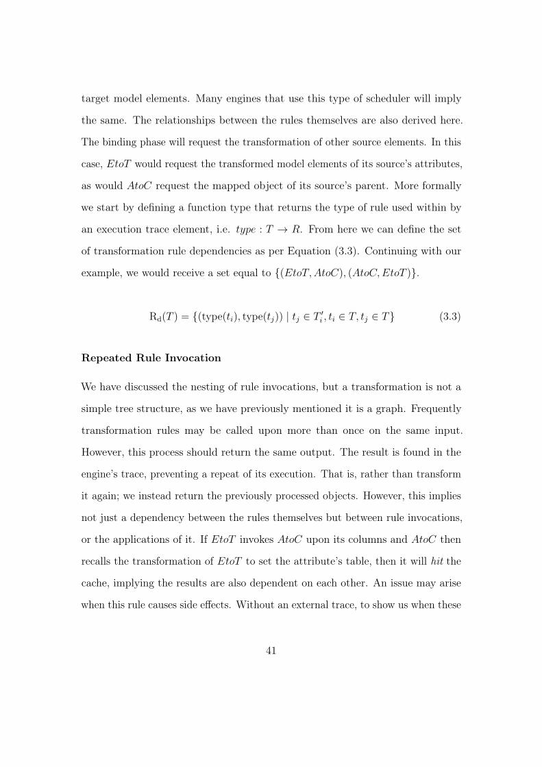
target model elements. Many engines that use this type of scheduler will imply
the same. The relationships between the rules themselves are also derived here.
The binding phase will request the transformation of other source elements. In this
case, EtoT would request the transformed model elements of its source’s attributes,
as would AtoC request the mapped object of its source’s parent. More formally
we start by defining a function type that returns the type of rule used within by
an execution trace element, i.e. type : T → R. From here we can define the set
of transformation rule dependencies as per Equation (3.3). Continuing with our
example, we would receive a set equal to {(EtoT,AtoC), (AtoC,EtoT )}.
Rd(T ) = {(type(ti), type(tj)) | tj ∈ T ′i , ti ∈ T, tj ∈ T} (3.3)
Repeated Rule Invocation
We have discussed the nesting of rule invocations, but a transformation is not a
simple tree structure, as we have previously mentioned it is a graph. Frequently
transformation rules may be called upon more than once on the same input.
However, this process should return the same output. The result is found in the
engine’s trace, preventing a repeat of its execution. That is, rather than transform
it again; we instead return the previously processed objects. However, this implies
not just a dependency between the rules themselves but between rule invocations,
or the applications of it. If EtoT invokes AtoC upon its columns and AtoC then
recalls the transformation of EtoT to set the attribute’s table, then it will hit the
cache, implying the results are also dependent on each other. An issue may arise
when this rule causes side effects. Without an external trace, to show us when these
41
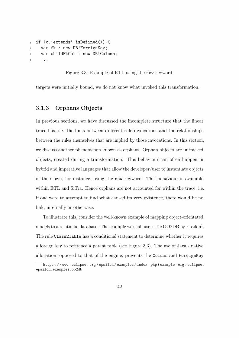
1 if (c.‘extends‘.isDefined()) {2 var fk : new DB!ForeignKey;3 var childFkCol : new DB!Column;4 ...
Figure 3.3: Example of ETL using the new keyword.
targets were initially bound, we do not know what invoked this transformation.
3.1.3 Orphans Objects
In previous sections, we have discussed the incomplete structure that the linear
trace has, i.e. the links between different rule invocations and the relationships
between the rules themselves that are implied by those invocations. In this section,
we discuss another phenomenon known as orphans. Orphan objects are untracked
objects, created during a transformation. This behaviour can often happen in
hybrid and imperative languages that allow the developer/user to instantiate objects
of their own, for instance, using the new keyword. This behaviour is available
within ETL and SiTra. Hence orphans are not accounted for within the trace, i.e.
if one were to attempt to find what caused its very existence, there would be no
link, internally or otherwise.
To illustrate this, consider the well-known example of mapping object-orientated
models to a relational database. The example we shall use is the OO2DB by Epsilon1.
The rule Class2Table has a conditional statement to determine whether it requires
a foreign key to reference a parent table (see Figure 3.3). The use of Java’s native
allocation, opposed to that of the engine, prevents the Column and ForeignKey
1https://www.eclipse.org/epsilon/examples/index.php?example=org.eclipse.epsilon.examples.oo2db
42
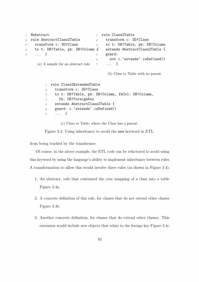
1 @abstract2 rule AbstractClass2Table3 transform c: OO!Class4 to t: DB!Table, pk: DB!Column {5 ... }
(a) A sample for an abstract rule.
1 rule Class2Table2 transform c: OO!Class3 to t: DB!Table, pk: DB!Column4 extends AbstractClass2Table {5 guard:6 not c.‘extends‘.isDefined()7 ... }
(b) Class to Table with no parent.
1 rule Class2ExtendedTable2 transform c: OO!Class3 to t: DB!Table, pk: DB!Column, fkCol: DB!Column,4 fk: DB!ForeignKey5 extends AbstractClass2Table {6 guard: c.‘extends‘.isDefined()7 ... }
(c) Class to Table, where the Class has a parent.
Figure 3.4: Using inheritance to avoid the new keyword in ETL.
from being tracked by the transformer.
Of course, in the above example, the ETL code can be refactored to avoid using
this keyword by using the language’s ability to implement inheritance between rules.
A transformation to allow this would involve three rules (as shown in Figure 3.4).
1. An abstract, rule that contained the core mapping of a class into a table
Figure 3.4a.
2. A concrete definition of this rule, for classes that do not extend other classes
Figure 3.4b.
3. Another concrete definition, for classes that do extend other classes. This
extension would include new objects that relate to the foreign key Figure 3.4c.
43
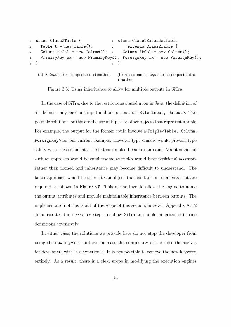
1 class Class2Table {2 Table t = new Table();3 Column pkCol = new Column();4 PrimaryKey pk = new PrimaryKey();5 }
(a) A tuple for a composite destination.
1 class Class2ExtendedTable2 extends Class2Table {3 Column fkCol = new Column();4 ForeignKey fk = new ForeignKey();5 }
(b) An extended tuple for a composite des-tination.
Figure 3.5: Using inheritance to allow for multiple outputs in SiTra.
In the case of SiTra, due to the restrictions placed upon in Java, the definition of
a rule must only have one input and one output, i.e. Rule<Input, Output>. Two
possible solutions for this are the use of tuples or other objects that represent a tuple.
For example, the output for the former could involve a Triple<Table, Column,
ForeignKey> for our current example. However type erasure would prevent type
safety with these elements, the extension also becomes an issue. Maintenance of
such an approach would be cumbersome as tuples would have positional accessors
rather than named and inheritance may become difficult to understand. The
latter approach would be to create an object that contains all elements that are
required, as shown in Figure 3.5. This method would allow the engine to name
the output attributes and provide maintainable inheritance between outputs. The
implementation of this is out of the scope of this section; however, Appendix A.1.2
demonstrates the necessary steps to allow SiTra to enable inheritance in rule
definitions extensively.
In either case, the solutions we provide here do not stop the developer from
using the new keyword and can increase the complexity of the rules themselves
for developers with less experience. It is not possible to remove the new keyword
entirely. As a result, there is a clear scope in modifying the execution engines
44
within the transformations frameworks to take good care of orphans.
This section has concentrated on the issues that arise in M2M transformations
with regards to traceability. We have focused on the loss of data when considering a
trace, post-mortem, as well as the ability to create objects out of the engine’s scope.
The next section introduces our implementation of an updated SiTra that contains
a new meta-model to hold this additional information and a dynamic proxy to
capture orphan objects. Following this, we show the generality of our approach by
adding the same functionality to another engine, ETL. This adaptation confirms
that our method can be incorporated into other engines that provide an external
trace.
3.2 The Simple Transformer
SiTra is an imperative, Java, implementation of an M2M transformation (Akehurst
et al. 2006). It provides two interfaces that can be used to create a transformation
engine and the rules for it. The bundle comes with an engine as standard. Seyyed
M. A. Shah et al. amended this to add traceability (Shah, Anastasakis, and Bordbar
2010). However this, like others, has all of the problems we have discussed in
the previous section regarding traceability. We now discuss the changes we have
made to SiTra to solve these issues. This solution comes in two parts: a) a new
meta-model for transformation’s trace; and b) a dynamic proxy. The former allows
us to store the relationships between rule invocations, while the latter provides us
with the ability to intercept setters and getters to collate objects that have not
been instantiated by the transformation engine itself.
45
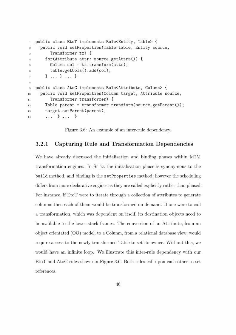
1 public class EtoT implements Rule<Entity, Table> {2 public void setProperties(Table table, Entity source,3 Transformer tx) {4 for(Attribute attr: source.getAttrs()) {5 Column col = tx.transform(attr);6 table.getCols().add(col);7 } ... } ... }8
9 public class AtoC implements Rule<Attribute, Column> {10 public void setProperties(Column target, Attribute source,11 Transformer transformer) {12 Table parent = transformer.transform(source.getParent());13 target.setParent(parent);14 ... } ... }
Figure 3.6: An example of an inter-rule dependency.
3.2.1 Capturing Rule and Transformation Dependencies
We have already discussed the initialisation and binding phases within M2M
transformation engines. In SiTra the initialisation phase is synonymous to the
build method, and binding is the setProperties method; however the scheduling
differs from more declarative engines as they are called explicitly rather than phased.
For instance, if EtoT were to iterate through a collection of attributes to generate
columns then each of them would be transformed on demand. If one were to call
a transformation, which was dependent on itself, its destination objects need to
be available to the lower stack frames. The conversion of an Attribute, from an
object orientated (OO) model, to a Column, from a relational database view, would
require access to the newly transformed Table to set its owner. Without this, we
would have an infinite loop. We illustrate this inter-rule dependency with our
EtoT and AtoC rules shown in Figure 3.6. Both rules call upon each other to set
references.
46
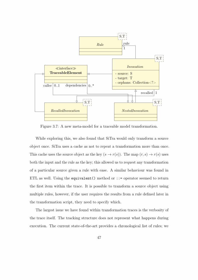
caller 0..1
recalled 1
dependencies 0..*
rule1
Rule
S,T
�interface�TraceableElement
Invocation
- source: S- target: T- orphans: Collection<?>
S,T
NestedInvocation
S,T
RecalledInvocation
S,T
Figure 3.7: A new meta-model for a traceable model transformation.
While exploring this, we also found that SiTra would only transform a source
object once. SiTra uses a cache as not to repeat a transformation more than once.
This cache uses the source object as the key (s→ r(s)). The map (r, s)→ r(s) uses
both the input and the rule as the key; this allowed us to request any transformation
of a particular source given a rule with ease. A similar behaviour was found in
ETL as well. Using the equivalent() method or ::= operator seemed to return
the first item within the trace. It is possible to transform a source object using
multiple rules, however, if the user requires the results from a rule defined later in
the transformation script, they need to specify which.
The largest issue we have found within transformation traces is the verbosity of
the trace itself. The tracking structure does not represent what happens during
execution. The current state-of-the-art provides a chronological list of rules; we
47
never get to see the dependencies between those and invocations of them. ETL
uses an equivalent structure as SiTra’s ITrace interface (Shah, Anastasakis, and
Bordbar 2010), inferred from the QVT standard (Object Management Group, Inc.
2016a). In which is contained the map as described above. This tuple does not take
into consideration the nested nature of a transformation, and only concerns the
instantiation phase on the first run. It may also be important to see what calls the
build method and which have the object returned from the cache. Figure 3.7 shows
the new transformation trace within SiTra. Here we have introduced new trace
elements to aid in retaining structural information. Invocation is the equivalent
of the previous ITrace; it contains the source, target and the rule responsible for
the transformation. This object alone can provide the current state-of-the-art in
traceability within rule-based engines. We have introduced two more types of trace-
able elements within SiTra: a) NestedInvocation; and b) RecalledInvocation.
These provide more detail to the actual internals of the transformation. The
former provides the same information as the standard, however, contains two more
elements: a) the calling transformation trace element (if applicable); and b) the
trace elements generated because of the current transformation. The latter is an
indicator that the current execution required the results of a previously transformed
set of sources. To maintain this list, and to reduce the effect on performance by
traversing it, we amended the internal cache once more: (r, s) → (r(s), t) such
that t ∈ T . Using this latest implementation, we can now see that a source
element, s, and a rule, r, returns the target object r(s) and is referenced by the
TraceableElement t. This map can be further simplified as the traceable element
includes r(s): (r, s)→ t.
Algorithm 1 demonstrates the execution of transforming an object within SiTra.
48
This process is a general algorithm allowing it to be used within a plethora of
other transformation engines to retain structural information about its internal
workings. The two phases, instantiation and binding, can be found at Line 12
and Line 20 respectively. Before either of these, we check the cache to see if the
transformation has been completed already (lines 5-9). A cache hit is indicative of a
recalled invocation. Likewise, lines 14-18 is where the first attempt of transforming
a given set of sources by a rule and therefore is where they must be instantiated and
then bound. In both cases, they depend on an execution stack to determine what
invocation is dependent on another. The stack is pushed (Line 19) and popped
(Line 21), before and after the binding phase (Line 20) as this method can induce
recursion. The recursion of transformations will increase and decrease the size of
the stack; however, the top will always be the invocation that is directly related to
the current.
Our meta-model provides solutions to retain the order of execution of transfor-
mation rules and the ability to recreate the transformation. This is provided by
the nested nature of our meta-model as it explains what rules are completed and
what invoked them. The capability to find the actual binding phase, opposed to a
recollection, is provided by the new recalled invocation type. Allowing the user
to recreate the situation at the time of creation. This recalled invocation aids in
providing a graph of rule dependencies.
3.2.2 A Dynamic Proxy to Catch Orphans
We have now described the new meta-model for traceability within M2M transfor-
mations. The amendment we have developed can include the full execution path
49

Algorithm 1 The scheduler that is provided with SiTra, which maintains thegraph structure of M2M transformations.Require: A transformation rule, r ∈ R.Require: A set of sources, s ⊆ S.Require: A first-in-last-out stack representing the execution stack of the transfor-
mation.Require: A cache of invocations defined by (r, s)→ t1: function transform(r, s)2: if r does not apply to s then return null3: end if4: if s has already been instantiated by r then5: if the execution stack is not empty then6: Record a recall of (r, s) and add it as a dependency of the top of the
execution stack.7: else8: Record a recall of (r, s).9: end if10: return the previously instantiated target objects.11: else12: Instantiate target objects, t.13: Put t into the cache with a key of (r, s).14: if the execution stack is not empty then15: Record an invocation of (r, s) and add it as a dependency of the top
of the execution stack.16: else17: Record an invocation.18: end if19: Push the invocation onto the execution stack.20: Bind t and s using r in respect to this transformation.21: Pop the execution stack.22: return t23: end if24: end function
50
that the engine completes to generate its result. In this section, we describe how we
gather orphan objects in a general way such that other engines might implement
them. Orphans are objects that are created by the rules directly rather than
delegating the work to the transformation engine. These orphans are not tracked by
the trace as they are unknown to the engine. The process of transforming an input
model involves invoking mutator methods to change the state of the destination
object. The main body of a rule takes care of setting references between objects
and their attributes. It is also the location where the new keyword is available. In
a well-formed transformation rule, these mutators would receive primitives based
on the source or objects already created by the engine. However, in the case of a
rule that is susceptible to creating orphans, mutators would receive newly allocated
objects. To catch these orphans, we need to intercept all mutators to check to see
if the additional objects are within the trace. For example, when adding a foreign
key to a child table, we need to intercept the list of constraints.
For each transformation of a source s using a rule r, we get a set of destination
objects r(s) → D. To intercept we instead return a set of proxies such that
D = {Proxy(d) | d ∈ D}. These proxies maintain the functionality of the original
destination object, however, the mutators are modified. For each mutator, we check
to see if the input argument is inside of the trace, and if not we add it the current
invocation. After this, we delegate to the actual mutator method to change the
state of the object in question. To ensure traces are added for all orphans, as well
as grandchildren of the target, instead of passing the real parameter we pass a
proxy of it. This process allows the recursion of the orphan tracking.
There are two types of call to intercept: mutator and accessors methods. We
define a mutator method as one that has no return type, one parameter and begins
51
with the string “set”. Intercepting this call allows us to catch objects that change
the state of the object in question. We define accessor methods as one that has
no parameters and begins with the string “get”. What we do here differs based
on the return type. If the accessor returns a plain old Java object (POJO), we
return a proxy of that object, if it is not already one, as to be able to capture its
mutators. In the event of a Collection, we proxy the collection and intercept their
accessors and mutators, for example, put, add and addAll. This proxy allows us
to recursively capture elements added or removed from a list, while also enabling
us to proxy its contents as well.
Our approach here is not without its drawbacks. For example, if one were to
create an orphaned list and add orphaned objects to it before adding it to the target
model. The list’s items would not be known to the engine’s trace. An orphaned
object is, in essence, a POJO. So the addition of objects to an orphaned list is
not captured. This same behaviour will occur with an orphaned object with an
orphaned state. An object’s mutator methods are not intercepted to capture its
state changes. To solve this, we can traverse the value passed into a proxied mutator.
This traversal may have a relatively significant impact on the transformation itself,
as it would require reflection. Reflection would allow the transformer to find object
accessors at runtime and traverse the new object until it finds a null value or a
previously proxied object. These terminators would prevent an infinite loop in
what could be a recursive structure. It would be beneficial to implement this for
complete coverage, however, for our experiments, it is possible to avoid this by
placing the object into the target model before modifying it.
Figure 3.8 contains a code snippet that illustrates this drawback. Here we create
a ForeignKey and a reference Column for the transformation of an Entity that
52
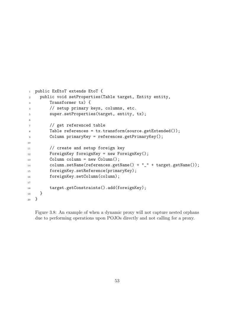
1 public ExEtoT extends EtoT {2 public void setProperties(Table target, Entity entity,3 Transformer tx) {4 // setup primary keys, columns, etc.5 super.setProperties(target, entity, tx);6
7 // get referenced table8 Table references = tx.transform(source.getExtended());9 Column primaryKey = references.getPrimaryKey();
10
11 // create and setup foreign key12 ForeignKey foreignKey = new ForeignKey();13 Column column = new Column();14 column.setName(references.getName() + "_" + target.getName());15 foreignKey.setReference(primaryKey);16 foreignKey.setColumn(column);17
18 target.getConstraints().add(foreignKey);19 }20 }
Figure 3.8: An example of when a dynamic proxy will not capture nested orphansdue to performing operations upon POJOs directly and not calling for a proxy.
53
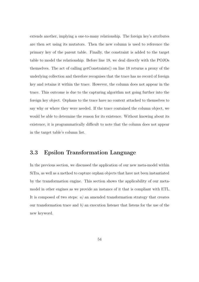
extends another, implying a one-to-many relationship. The foreign key’s attributes
are then set using its mutators. Then the new column is used to reference the
primary key of the parent table. Finally, the constraint is added to the target
table to model the relationship. Before line 18, we deal directly with the POJOs
themselves. The act of calling getConstraints() on line 18 returns a proxy of the
underlying collection and therefore recognises that the trace has no record of foreign
key and retains it within the trace. However, the column does not appear in the
trace. This outcome is due to the capturing algorithm not going further into the
foreign key object. Orphans to the trace have no context attached to themselves to
say why or where they were needed. If the trace contained the column object, we
would be able to determine the reason for its existence. Without knowing about its
existence, it is programmatically difficult to note that the column does not appear
in the target table’s column list.
3.3 Epsilon Transformation Language
In the previous section, we discussed the application of our new meta-model within
SiTra, as well as a method to capture orphan objects that have not been instantiated
by the transformation engine. This section shows the applicability of our meta-
model in other engines as we provide an instance of it that is compliant with ETL.
It is composed of two steps: a) an amended transformation strategy that creates
our transformation trace and b) an execution listener that listens for the use of the
new keyword.
54
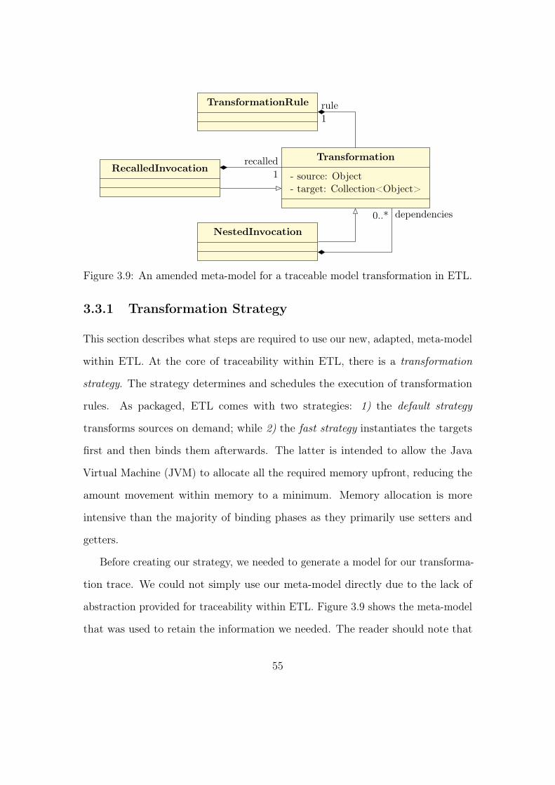
rule1
0..* dependencies
recalled1
TransformationRule
Transformation
- source: Object- target: Collection<Object>
NestedInvocation
RecalledInvocation
Figure 3.9: An amended meta-model for a traceable model transformation in ETL.
3.3.1 Transformation Strategy
This section describes what steps are required to use our new, adapted, meta-model
within ETL. At the core of traceability within ETL, there is a transformation
strategy. The strategy determines and schedules the execution of transformation
rules. As packaged, ETL comes with two strategies: 1) the default strategy
transforms sources on demand; while 2) the fast strategy instantiates the targets
first and then binds them afterwards. The latter is intended to allow the Java
Virtual Machine (JVM) to allocate all the required memory upfront, reducing the
amount movement within memory to a minimum. Memory allocation is more
intensive than the majority of binding phases as they primarily use setters and
getters.
Before creating our strategy, we needed to generate a model for our transforma-
tion trace. We could not simply use our meta-model directly due to the lack of
abstraction provided for traceability within ETL. Figure 3.9 shows the meta-model
that was used to retain the information we needed. The reader should note that
55
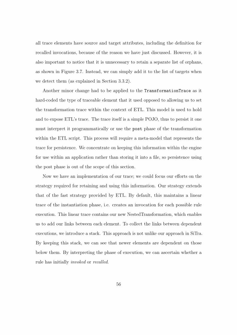
all trace elements have source and target attributes, including the definition for
recalled invocations, because of the reason we have just discussed. However, it is
also important to notice that it is unnecessary to retain a separate list of orphans,
as shown in Figure 3.7. Instead, we can simply add it to the list of targets when
we detect them (as explained in Section 3.3.2).
Another minor change had to be applied to the TransformationTrace as it
hard-coded the type of traceable element that it used opposed to allowing us to set
the transformation trace within the context of ETL. This model is used to hold
and to expose ETL’s trace. The trace itself is a simple POJO, thus to persist it one
must interpret it programmatically or use the post phase of the transformation
within the ETL script. This process will require a meta-model that represents the
trace for persistence. We concentrate on keeping this information within the engine
for use within an application rather than storing it into a file, so persistence using
the post phase is out of the scope of this section.
Now we have an implementation of our trace; we could focus our efforts on the
strategy required for retaining and using this information. Our strategy extends
that of the fast strategy provided by ETL. By default, this maintains a linear
trace of the instantiation phase, i.e. creates an invocation for each possible rule
execution. This linear trace contains our new NestedTransformation, which enables
us to add our links between each element. To collect the links between dependent
executions, we introduce a stack. This approach is not unlike our approach in SiTra.
By keeping this stack, we can see that newer elements are dependent on those
below them. By interpreting the phase of execution, we can ascertain whether a
rule has initially invoked or recalled.
56
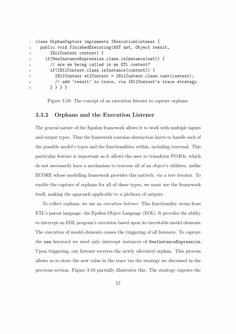
1 class OrphanCapture implements IExecutionListener {2 public void finishedExecuting(AST ast, Object result,3 IEolContext context) {4 if(NewInstanceExpression.class.isInstance(ast)) {5 // are we being called in an ETL context?6 if(IEtlContext.class.isInstance(context)) {7 IEtlContext etlContext = IEtlContext.class.cast(context);8 // add ‘result’ to trace, via IEtlContext’s trace strategy.9 } } } }
Figure 3.10: The concept of an execution listener to capture orphans.
3.3.2 Orphans and the Execution Listener
The general nature of the Epsilon framework allows it to work with multiple inputs
and output types. Thus the framework contains abstraction layers to handle each of
the possible model’s types and the functionalities within, including traversal. This
particular feature is important as it allows the user to transform POJOs, which
do not necessarily have a mechanism to traverse all of an object’s children, unlike
ECORE whose modelling framework provides this natively, via a tree iterator. To
enable the capture of orphans for all of these types, we must use the framework
itself, making the approach applicable to a plethora of outputs.
To collect orphans, we use an execution listener. This functionality stems from
ETL’s parent language: the Epsilon Object Language (EOL). It provides the ability
to intercept an EOL program’s execution based upon its executable model elements.
The execution of model elements causes the triggering of all listeners. To capture
the new keyword we need only intercept instances of NewInstanceExpression.
Upon triggering, our listener receives the newly allocated orphan. This process
allows us to store the new value in the trace via the strategy we discussed in the
previous section. Figure 3.10 partially illustrates this. The strategy exposes the
57

execution trace such that we can access the top most transformation invocation.
When triggered, the new objects belong to the rule currently being invoked.
Unlike Section 3.2.2 whereby dynamic proxies are used and therefore can lose
information if not used correctly, this approach catches all orphans created within
the binding phase. Including those that may not be present in the final target
model, this may occur when using temporary variables. Our listener enables this
behaviour by waiting on the execution of the new keyword rather than setters and
getters of POJOs. This approach has the effect of potentially gathering too much
information opposed to not enough. For example, the use of temporary variables
would incur additional orphans. These may not be relevant for the final model,
however, are nevertheless allocated outside of the engine. If this becomes an issue,
e.g. memory consumption or storage, then we can either:
1. Ensure the orphan is for an outbound model. Here we would determine
whether the orphan object belongs to an output model being generated by
the transformer.
2. Check to see if each orphan is within the output model on completion of its
binding phase. As above, but post-invocation.
3. Complete a post-mortem pruning upon the trace such that it no longer
contains objects not found in any of the output models. This process would
require the traversal of the trace to find all objects that are not part of an
output model.
58
3.4 Chapter Summary
To provide confidence, we need to gain full accountability for the transformation of
a source into its destination model. The overall process is a black-box, and this
limits this property. Traceability is used to retain the associations between source
and target; however, the current state of the art does not provide full accountability.
Current transformation traces only account for the order source elements and rules
are matched. This method does not take into consideration the transformer’s
susceptibility to side-effects. Having global state within the binding phase causes
these side-effects, moreover, tracing the order of rule invocations is more significant
than that of matching. The latter is merely a scheduling issue for the engine.
In this chapter, we have explained these challenges and discussed our solutions
for them. A vital component of this is a new meta-model that can hold these
associations. The links between invocations provide us with a trace that now
considers the binding phase opposed to the matching. This data structure affords
us with full accountability of each invocation of a rule and gives us the ability to
use the information to add context to rules that cause side-effects.
As an example of a side effect, we introduced a common practice when using
hybrid or imperative transformation languages: orphan objects, the creation of
objects outside of the instantiation phase. This trace, along with a stack trace,
allowed us to capture orphans unbeknown to the engine. To demonstrate this, we
explained a mechanism that would capture these objects via a dynamic proxy for
SiTra. The proxy would intercept setters of instantiated objects to store references
to new values unknown to the engine. It would also intercept getters as to allow
recursive checking of setters called upon objects further down the object tree. A
59
small modification to the meta-model allows us to implement our transformation
trace into ETL showing generality to our approach and that it can be incorporated
into another mature transformation engine. This alteration was required not
because the model would not work, but instead due to the lack of an interface for
a transformation trace in ETL. Additionally, a more streamlined orphan capture
method was available to us via ETL’s executable abstract syntax tree. Opposed to
intercepting calls to getters and setters, one can catch calls to the new keyword
directly. A listener would receive this object, and the transformer can then save it
as we already know it is an orphan.
60
CHAPTER 4
EFFICACY IN MODEL-TO-MODELTRANSFORMATION
In Chapter 3 we have discussed the issues that arise in the verbosity of a transfor-
mation trace, paying close attention to the loss of information. This loss includes
the actual execution of a rule and the unaccounted objects that are not in the trace
(see Section 3.1). We then solved these by implementing a meta-model that could
capture the internal execution and a set of object proxies to capture orphans for
use with the Simple Transformer (SiTra) in Section 3.2. To show the generality of
our approach amongst other engines, we implemented an adapted meta-model and
an execution listener to capture orphans for the Epsilon Transformation Language
(ETL) in Section 3.3. This process allows us to have a complete overview of what
is occurring within a transformation.
With this completed transformation trace we can retain it, when available
post-mortem, to provide a knowledge base of past executions. A newly transformed
target would produce a new trace comparable to this data set to find traits and
features that we have encountered before. We assume that if we saw some part of
the new trace before then, we are more likely to trust its result when compared
61
to that of an unknown segment. This decision process generates a heat map over
the full transformation showing areas that users are less inclined to trust. This
information can be used to focus validation resources, i.e. to resolve the cold spots,
or be used to decide what to do next: whether we accept the risks, or attempt to
mitigate it.
The following four sections discuss our approach to quantify confidence within
a model-to-model (M2M) transformation. Section 4.1 explains that to maintain a
knowledge base, we need to be able to store previous executions for comparison. To
do this, we formalise our execution graph and store it in an appropriate database.
Secondly, we look at how prominent a graph is on another, with the assumption
that if we have seen a segment before we are more confident in its use in Section 4.2.
Up to now, prominence considers all rules equally. However, this is almost never
the case as some are more complex than others. Section 4.3 then introduces a
weighing mechanism to remove prominence bias. Finally, we combine prominence
and complexity to generate a value to show the confidence that we have in a new
transformation in respect to previous executions in Section 4.4.
4.1 Persistence of Trace Data
To be able to learn from previous experience, in the case of M2M transformations,
we need to be able to store previous instances of trace data. We have discussed in
Chapter 3 a new meta-model to encompass trace data within M2M transformations.
This data, or at least part of it, requires persisting to a data store for analysis.
The trace we have modelled is an execution graph of what has occurred within the
engine after a transformation has taken place.
62
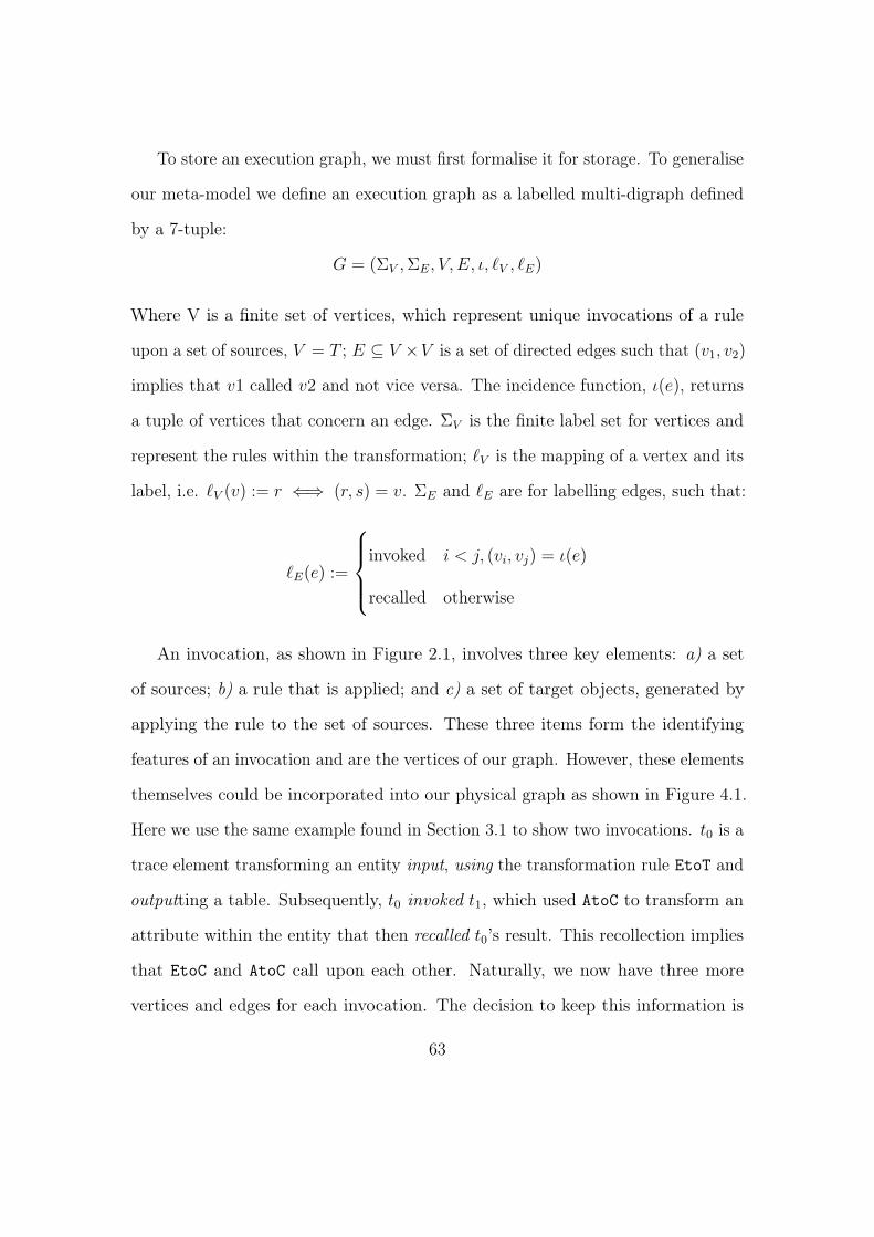
To store an execution graph, we must first formalise it for storage. To generalise
our meta-model we define an execution graph as a labelled multi-digraph defined
by a 7-tuple:
G = (ΣV ,ΣE, V, E, ι, `V , `E)
Where V is a finite set of vertices, which represent unique invocations of a rule
upon a set of sources, V = T ; E ⊆ V ×V is a set of directed edges such that (v1, v2)
implies that v1 called v2 and not vice versa. The incidence function, ι(e), returns
a tuple of vertices that concern an edge. ΣV is the finite label set for vertices and
represent the rules within the transformation; `V is the mapping of a vertex and its
label, i.e. `V (v) := r ⇐⇒ (r, s) = v. ΣE and `E are for labelling edges, such that:
`E(e) :=
invoked i < j, (vi, vj) = ι(e)
recalled otherwise
An invocation, as shown in Figure 2.1, involves three key elements: a) a set
of sources; b) a rule that is applied; and c) a set of target objects, generated by
applying the rule to the set of sources. These three items form the identifying
features of an invocation and are the vertices of our graph. However, these elements
themselves could be incorporated into our physical graph as shown in Figure 4.1.
Here we use the same example found in Section 3.1 to show two invocations. t0 is a
trace element transforming an entity input, using the transformation rule EtoT and
outputting a table. Subsequently, t0 invoked t1, which used AtoC to transform an
attribute within the entity that then recalled t0’s result. This recollection implies
that EtoC and AtoC call upon each other. Naturally, we now have three more
vertices and edges for each invocation. The decision to keep this information is
63
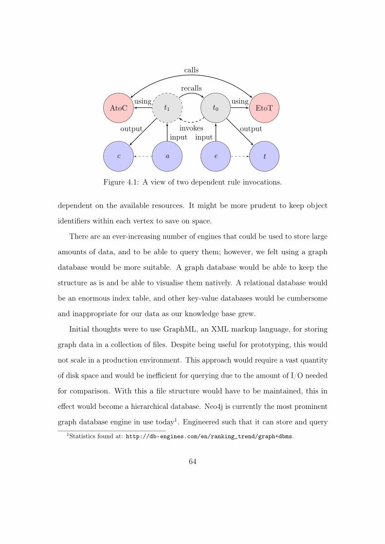
t0 EtoT
e t
using
outputinput
t1AtoC
c a
using
outputinput
invokes
recalls
calls
Figure 4.1: A view of two dependent rule invocations.
dependent on the available resources. It might be more prudent to keep object
identifiers within each vertex to save on space.
There are an ever-increasing number of engines that could be used to store large
amounts of data, and to be able to query them; however, we felt using a graph
database would be more suitable. A graph database would be able to keep the
structure as is and be able to visualise them natively. A relational database would
be an enormous index table, and other key-value databases would be cumbersome
and inappropriate for our data as our knowledge base grew.
Initial thoughts were to use GraphML, an XML markup language, for storing
graph data in a collection of files. Despite being useful for prototyping, this would
not scale in a production environment. This approach would require a vast quantity
of disk space and would be inefficient for querying due to the amount of I/O needed
for comparison. With this a file structure would have to be maintained, this in
effect would become a hierarchical database. Neo4j is currently the most prominent
graph database engine in use today1. Engineered such that it can store and query1Statistics found at: http://db-engines.com/en/ranking_trend/graph+dbms.
64
vast amounts of graph data.
4.1.1 SiTra in Python and Neo4j
To aid in prototyping for the case studies, we rewrote SiTra as a Python library1.
This change was due to its toolset for domain specific language development,
generating code, graph library support (specifically isomorphism) and its compact
form. However, due to the language’s duck typing, or lack of type safety, a
transformation rule must explicitly check the type of its input. The kind of input
is often the main criterion of a rule, for example, EtoT must have an entity passed
into it. This check is a form of guard, often implicit in type safe transformation
engines. Another fundamental difference between SiTra.py and its Java equivalent
is that of orphan capture. We can intercept Python’s “magic” methods opposed to
looking for traits that we deem look like setters and getters, i.e. does the function
start with “set” or “get”.
Upon completion of a transformation, a post-transformation method converts
the resultant trace into a graph using networkx. networkx is a Python library
used for graph creation, modification and analysis. This conversion required each
invocation to have a vertex and relationships to be generated based on their heritage,
parent and dependent invocations. A recalled invocation creates an edge between
the two vertices that represent the caller and the original invocation it is recalling.
This graph was then used to generate Cypher, the query language used in Neo4j,
for node creation within a database instance. The snippet below is an instance of
Cypher, which creates the graph shown in Figure 4.2a on Page 68 (explained in1SiTra.py is available at: http://github.com/sacko87/sitra.py.
65
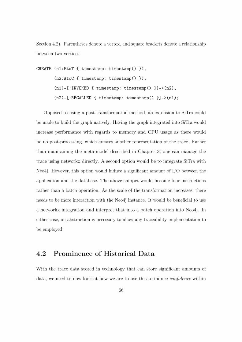
Section 4.2). Parentheses denote a vertex, and square brackets denote a relationship
between two vertices.
CREATE (n1:EtoT { timestamp: timestamp() }),
(n2:AtoC { timestamp: timestamp() }),
(n1)-[:INVOKED { timestamp: timestamp() }]->(n2),
(n2)-[:RECALLED { timestamp: timestamp() }]->(n1);
Opposed to using a post-transformation method, an extension to SiTra could
be made to build the graph natively. Having the graph integrated into SiTra would
increase performance with regards to memory and CPU usage as there would
be no post-processing, which creates another representation of the trace. Rather
than maintaining the meta-model described in Chapter 3; one can manage the
trace using networkx directly. A second option would be to integrate SiTra with
Neo4j. However, this option would induce a significant amount of I/O between the
application and the database. The above snippet would become four instructions
rather than a batch operation. As the scale of the transformation increases, there
needs to be more interaction with the Neo4j instance. It would be beneficial to use
a networkx integration and interpret that into a batch operation into Neo4j. In
either case, an abstraction is necessary to allow any traceability implementation to
be employed.
4.2 Prominence of Historical Data
With the trace data stored in technology that can store significant amounts of
data, we need to now look at how we are to use this to induce confidence within
66
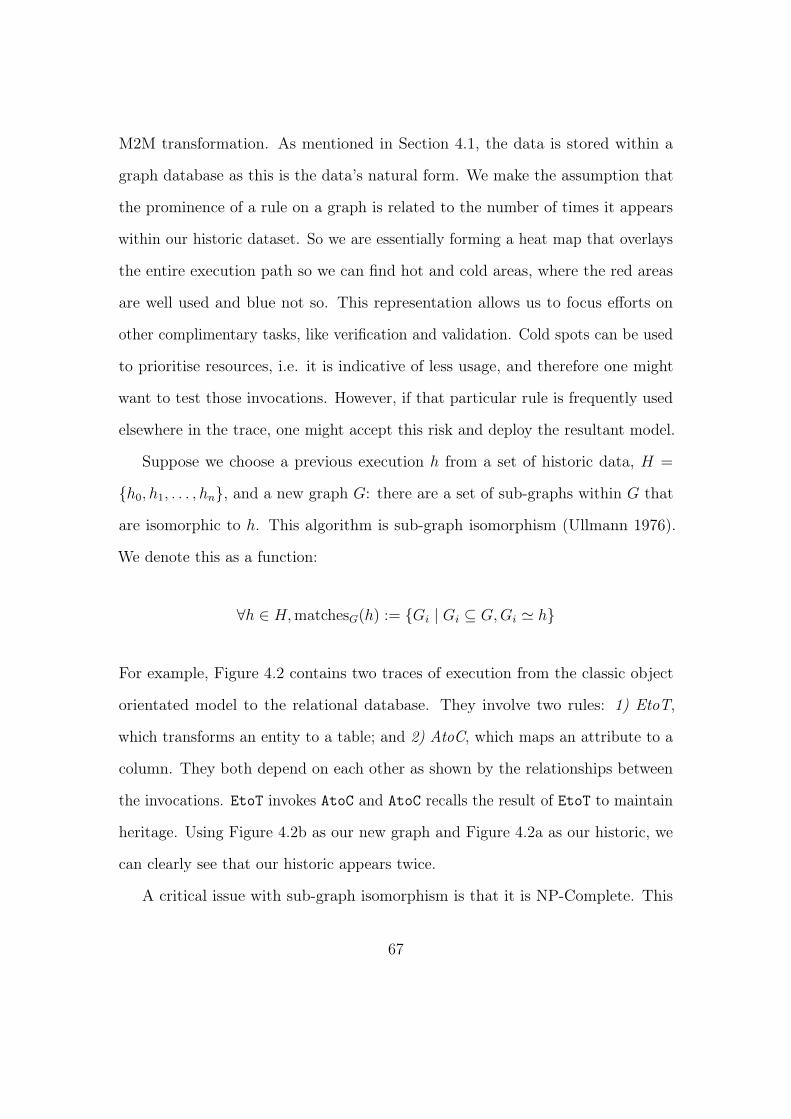
M2M transformation. As mentioned in Section 4.1, the data is stored within a
graph database as this is the data’s natural form. We make the assumption that
the prominence of a rule on a graph is related to the number of times it appears
within our historic dataset. So we are essentially forming a heat map that overlays
the entire execution path so we can find hot and cold areas, where the red areas
are well used and blue not so. This representation allows us to focus efforts on
other complimentary tasks, like verification and validation. Cold spots can be used
to prioritise resources, i.e. it is indicative of less usage, and therefore one might
want to test those invocations. However, if that particular rule is frequently used
elsewhere in the trace, one might accept this risk and deploy the resultant model.
Suppose we choose a previous execution h from a set of historic data, H =
{h0, h1, . . . , hn}, and a new graph G: there are a set of sub-graphs within G that
are isomorphic to h. This algorithm is sub-graph isomorphism (Ullmann 1976).
We denote this as a function:
∀h ∈ H,matchesG(h) := {Gi | Gi ⊆ G,Gi ' h}
For example, Figure 4.2 contains two traces of execution from the classic object
orientated model to the relational database. They involve two rules: 1) EtoT,
which transforms an entity to a table; and 2) AtoC, which maps an attribute to a
column. They both depend on each other as shown by the relationships between
the invocations. EtoT invokes AtoC and AtoC recalls the result of EtoT to maintain
heritage. Using Figure 4.2b as our new graph and Figure 4.2a as our historic, we
can clearly see that our historic appears twice.
A critical issue with sub-graph isomorphism is that it is NP-Complete. This
67
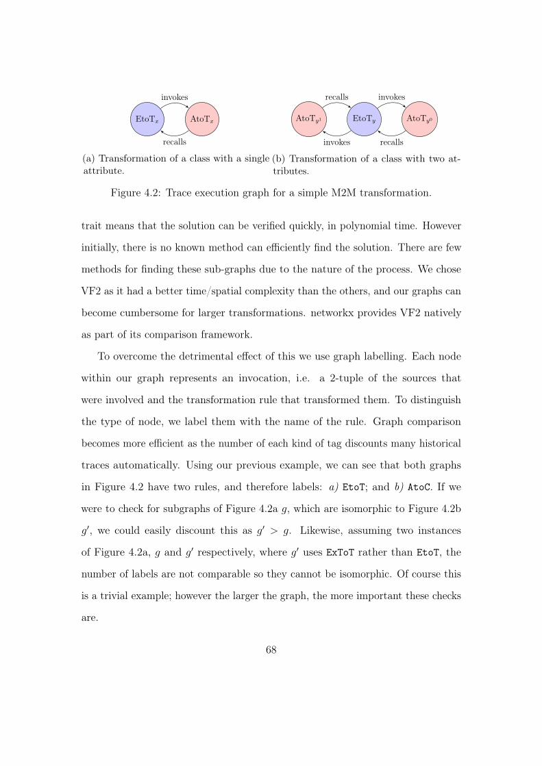
EtoTx AtoTx
invokes
recalls
(a) Transformation of a class with a singleattribute.
EtoTy AtoTy0AtoTy1
invokes
recallsinvokes
recalls
(b) Transformation of a class with two at-tributes.
Figure 4.2: Trace execution graph for a simple M2M transformation.
trait means that the solution can be verified quickly, in polynomial time. However
initially, there is no known method can efficiently find the solution. There are few
methods for finding these sub-graphs due to the nature of the process. We chose
VF2 as it had a better time/spatial complexity than the others, and our graphs can
become cumbersome for larger transformations. networkx provides VF2 natively
as part of its comparison framework.
To overcome the detrimental effect of this we use graph labelling. Each node
within our graph represents an invocation, i.e. a 2-tuple of the sources that
were involved and the transformation rule that transformed them. To distinguish
the type of node, we label them with the name of the rule. Graph comparison
becomes more efficient as the number of each kind of tag discounts many historical
traces automatically. Using our previous example, we can see that both graphs
in Figure 4.2 have two rules, and therefore labels: a) EtoT; and b) AtoC. If we
were to check for subgraphs of Figure 4.2a g, which are isomorphic to Figure 4.2b
g′, we could easily discount this as g′ > g. Likewise, assuming two instances
of Figure 4.2a, g and g′ respectively, where g′ uses ExToT rather than EtoT, the
number of labels are not comparable so they cannot be isomorphic. Of course this
is a trivial example; however the larger the graph, the more important these checks
are.
68
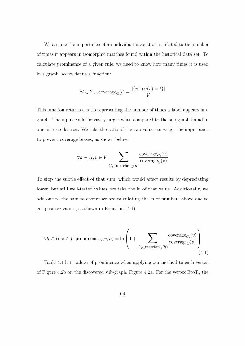
We assume the importance of an individual invocation is related to the number
of times it appears in isomorphic matches found within the historical data set. To
calculate prominence of a given rule, we need to know how many times it is used
in a graph, so we define a function:
∀l ∈ ΣV , coverageG(l) =|{v | `V (v) = l}|
|V |
This function returns a ratio representing the number of times a label appears in a
graph. The input could be vastly larger when compared to the sub-graph found in
our historic dataset. We take the ratio of the two values to weigh the importance
to prevent coverage biases, as shown below:
∀h ∈ H, v ∈ V,∑
Gi∈matchesG(h)
coverageGi(v)
coverageG(v)
To stop the subtle effect of that sum, which would affect results by depreciating
lower, but still well-tested values, we take the ln of that value. Additionally, we
add one to the sum to ensure we are calculating the ln of numbers above one to
get positive values, as shown in Equation (4.1).
∀h ∈ H, v ∈ V, prominenceG(v, h) = ln
1 +
∑Gi∈matchesG(h)
coverageGi(v)
coverageG(v)
(4.1)
Table 4.1 lists values of prominence when applying our method to each vertex
of Figure 4.2b on the discovered sub-graph, Figure 4.2a. For the vertex EtoTy the
69
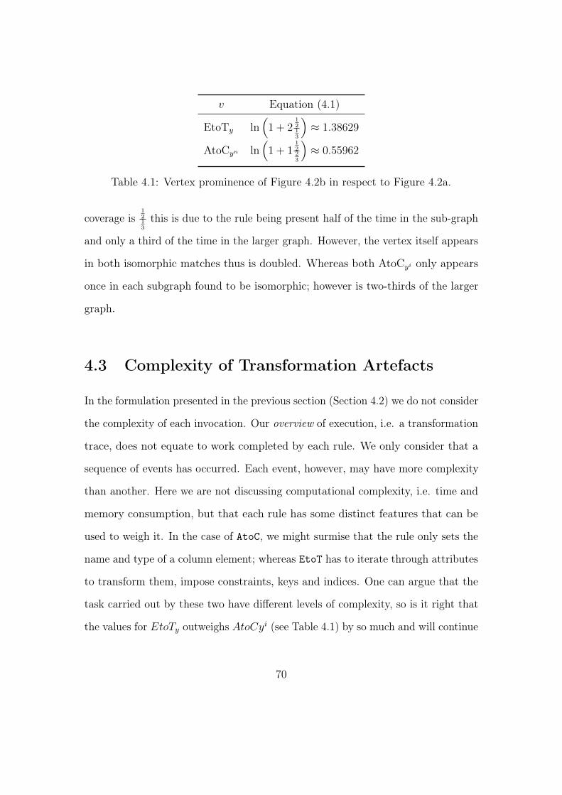
v Equation (4.1)
EtoTy ln(
1 + 21213
)≈ 1.38629
AtoCyn ln(
1 + 11223
)≈ 0.55962
Table 4.1: Vertex prominence of Figure 4.2b in respect to Figure 4.2a.
coverage is1213
this is due to the rule being present half of the time in the sub-graph
and only a third of the time in the larger graph. However, the vertex itself appears
in both isomorphic matches thus is doubled. Whereas both AtoCyi only appears
once in each subgraph found to be isomorphic; however is two-thirds of the larger
graph.
4.3 Complexity of Transformation Artefacts
In the formulation presented in the previous section (Section 4.2) we do not consider
the complexity of each invocation. Our overview of execution, i.e. a transformation
trace, does not equate to work completed by each rule. We only consider that a
sequence of events has occurred. Each event, however, may have more complexity
than another. Here we are not discussing computational complexity, i.e. time and
memory consumption, but that each rule has some distinct features that can be
used to weigh it. In the case of AtoC, we might surmise that the rule only sets the
name and type of a column element; whereas EtoT has to iterate through attributes
to transform them, impose constraints, keys and indices. One can argue that the
task carried out by these two have different levels of complexity, so is it right that
the values for EtoTy outweighs AtoCyi (see Table 4.1) by so much and will continue
70
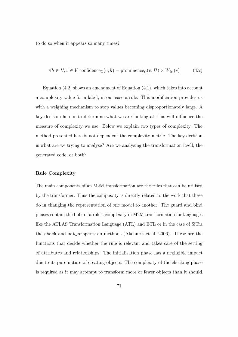
to do so when it appears so many times?
∀h ∈ H, v ∈ V, confidenceG(v, h) = prominenceG(v,H)×W`V (v) (4.2)
Equation (4.2) shows an amendment of Equation (4.1), which takes into account
a complexity value for a label, in our case a rule. This modification provides us
with a weighing mechanism to stop values becoming disproportionately large. A
key decision here is to determine what we are looking at; this will influence the
measure of complexity we use. Below we explain two types of complexity. The
method presented here is not dependent the complexity metric. The key decision
is what are we trying to analyse? Are we analysing the transformation itself, the
generated code, or both?
Rule Complexity
The main components of an M2M transformation are the rules that can be utilised
by the transformer. Thus the complexity is directly related to the work that these
do in changing the representation of one model to another. The guard and bind
phases contain the bulk of a rule’s complexity in M2M transformation for languages
like the ATLAS Transformation Language (ATL) and ETL or in the case of SiTra
the check and set_properties methods (Akehurst et al. 2006). These are the
functions that decide whether the rule is relevant and takes care of the setting
of attributes and relationships. The initialisation phase has a negligible impact
due to its pure nature of creating objects. The complexity of the checking phase
is required as it may attempt to transform more or fewer objects than it should.
71
This problem has two sides. On the one hand, it might generate an incomplete
final model as it discounts input model elements for transformation. On the other,
however, it would not only cause an increase in resources, but it may also cause
runtime errors due to incomplete value checking. These additional objects are of
particular importance when using a duck-typed language. If a rule identifies an
attribute as an entity, a TypeError would occur when looking for its constraints as
attributes do not have them. The effects are the same with regards to the binding
phase, as code becomes more complex there is a higher probability of mistakes
happening.
Complexity comes from many places when considering transformation rules.
For instance, we can attempt to calculate the complex nature of the code itself.
McCabe (1976) introduces cyclomatic complexity: an algorithm to analyse the
execution graph of a program. It is a quantitative measure of linearly independent
paths through the source code of an application. This value was an attempt to
reduce the complexity of modules. If the value was above ten, then the module
should be broken down further or a reason provided as to why it was an accepted
risk. Here we can assume the more independent paths there are, the higher the
risk of error. Particularly when we consider conditional branches, if the condition
were to be incorrect undefined behaviour could occur. With this in mind, we would
want to be more cautious of functions with higher complexity values as there is
more of a potential for error. Assume M0,M1, . . . ,Mk represents the complexity
of rules r0, r1, . . . , rk respectively. We consider the relative complexity of a ruleM`V (v)∑i∈ΣV
Mi. We use 1− M`V (v)∑
i∈ΣVMi
as a coefficient for prominence function to reduce
the confidence in more complex rules. We want for higher ratio to have smaller
confidence, as a rule, is more complex. Formally we define W`V as:
72
W`V (v) = 1− M`V (v)∑i∈ΣV
Mi
(4.3)
Another metric could be the number of test cases that have been carried out for
a given rule. It is only natural for developers to generate more test cases for larger
and more complex modules. Therefore it is reasonable to assume that the more
tests that are available to the model are indicative of the complexity of the rule.
This assumption also relates directly to the users as validation provides confidence
that a product will do as it is expected. In the case of EtoT and AtoC, if EtoT
had 200 test cases and AtoC had ten then we might accept a higher score for our
example. Unlike McCabe’s cyclomatic complexity, we want a higher ratio to have
a higher value. Here we assume that M0,M1, . . . ,Mk represent the number of tests
available to rules r0, r1, . . . , rk respectively. However this time we do not negate
the fraction as follows:
W`V (v) =M`V (v)∑i∈ΣV
Mi
Deferred Complexity
Often M2M transformations result in a model that will be used to generate code.
For example, the result of our object-orientated view to a relational might be used
to generate SQL to create the database or to create data access objects for querying.
Another, more general, example might be the generation of an imperative language
from a declarative, i.e. the translation of business logic into code that will complete
the tasks required.
Other options include annotating templates to inform what its output will
73
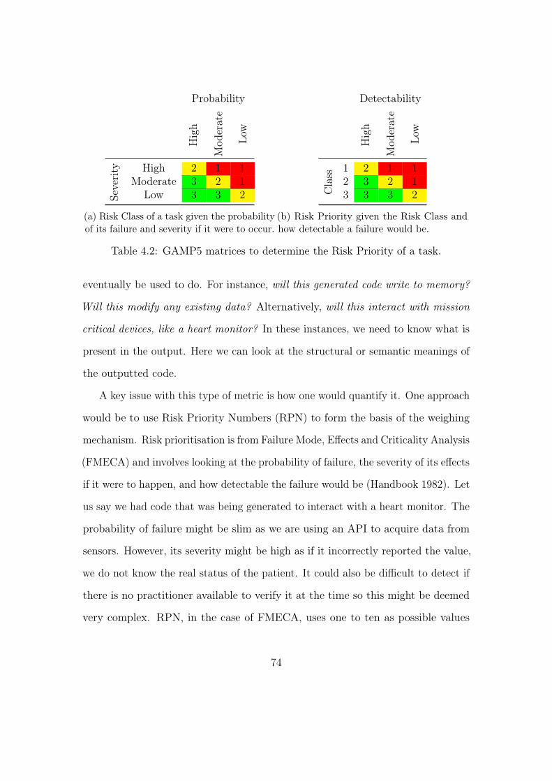
Probability
High
Mod
erate
Low
Severity High 2 1 1
Moderate 3 2 1Low 3 3 2
(a) Risk Class of a task given the probabilityof its failure and severity if it were to occur.
Detectability
High
Mod
erate
Low
Class 1 2 1 1
2 3 2 13 3 3 2
(b) Risk Priority given the Risk Class andhow detectable a failure would be.
Table 4.2: GAMP5 matrices to determine the Risk Priority of a task.
eventually be used to do. For instance, will this generated code write to memory?
Will this modify any existing data? Alternatively, will this interact with mission
critical devices, like a heart monitor? In these instances, we need to know what is
present in the output. Here we can look at the structural or semantic meanings of
the outputted code.
A key issue with this type of metric is how one would quantify it. One approach
would be to use Risk Priority Numbers (RPN) to form the basis of the weighing
mechanism. Risk prioritisation is from Failure Mode, Effects and Criticality Analysis
(FMECA) and involves looking at the probability of failure, the severity of its effects
if it were to happen, and how detectable the failure would be (Handbook 1982). Let
us say we had code that was being generated to interact with a heart monitor. The
probability of failure might be slim as we are using an API to acquire data from
sensors. However, its severity might be high as if it incorrectly reported the value,
we do not know the real status of the patient. It could also be difficult to detect if
there is no practitioner available to verify it at the time so this might be deemed
very complex. RPN, in the case of FMECA, uses one to ten as possible values
74
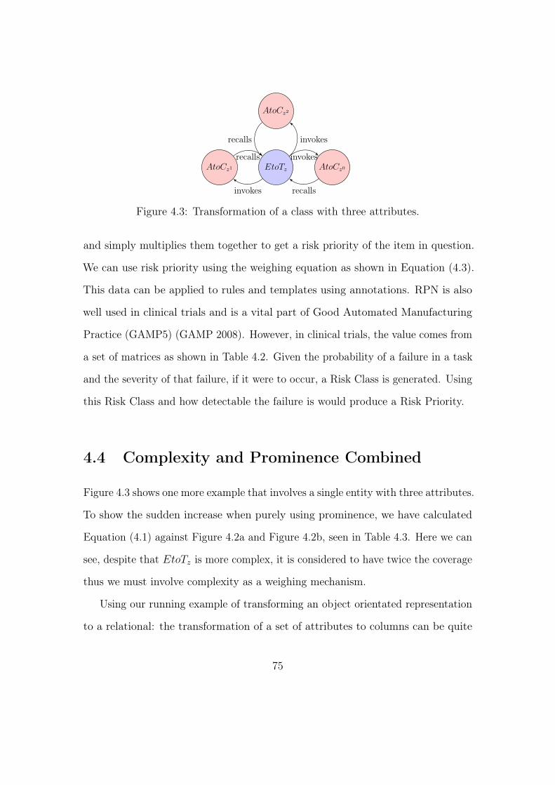
EtoTz AtoCz0AtoCz1
AtoCz2
invokes
recallsinvokes
recalls
invokesrecalls
Figure 4.3: Transformation of a class with three attributes.
and simply multiplies them together to get a risk priority of the item in question.
We can use risk priority using the weighing equation as shown in Equation (4.3).
This data can be applied to rules and templates using annotations. RPN is also
well used in clinical trials and is a vital part of Good Automated Manufacturing
Practice (GAMP5) (GAMP 2008). However, in clinical trials, the value comes from
a set of matrices as shown in Table 4.2. Given the probability of a failure in a task
and the severity of that failure, if it were to occur, a Risk Class is generated. Using
this Risk Class and how detectable the failure is would produce a Risk Priority.
4.4 Complexity and Prominence Combined
Figure 4.3 shows one more example that involves a single entity with three attributes.
To show the sudden increase when purely using prominence, we have calculated
Equation (4.1) against Figure 4.2a and Figure 4.2b, seen in Table 4.3. Here we can
see, despite that EtoTz is more complex, it is considered to have twice the coverage
thus we must involve complexity as a weighing mechanism.
Using our running example of transforming an object orientated representation
to a relational: the transformation of a set of attributes to columns can be quite
75
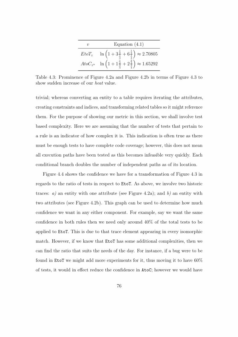
v Equation (4.1)
EtoTz ln(
1 + 31214
+ 61314
)≈ 2.70805
AtoCzn ln(
1 + 11234
+ 22334
)≈ 1.65292
Table 4.3: Prominence of Figure 4.2a and Figure 4.2b in terms of Figure 4.3 toshow sudden increase of our heat value.
trivial; whereas converting an entity to a table requires iterating the attributes,
creating constraints and indices, and transforming related tables so it might reference
them. For the purpose of showing our metric in this section, we shall involve test
based complexity. Here we are assuming that the number of tests that pertain to
a rule is an indicator of how complex it is. This indication is often true as there
must be enough tests to have complete code coverage; however, this does not mean
all execution paths have been tested as this becomes infeasible very quickly. Each
conditional branch doubles the number of independent paths as of its location.
Figure 4.4 shows the confidence we have for a transformation of Figure 4.3 in
regards to the ratio of tests in respect to EtoT. As above, we involve two historic
traces: a) an entity with one attribute (see Figure 4.2a); and b) an entity with
two attributes (see Figure 4.2b). This graph can be used to determine how much
confidence we want in any either component. For example, say we want the same
confidence in both rules then we need only around 40% of the total tests to be
applied to EtoT. This is due to that trace element appearing in every isomorphic
match. However, if we know that EtoT has some additional complexities, then we
can find the ratio that suits the needs of the day. For instance, if a bug were to be
found in EtoT we might add more experiments for it, thus moving it to have 60%
of tests, it would in effect reduce the confidence in AtoC; however we would have
76
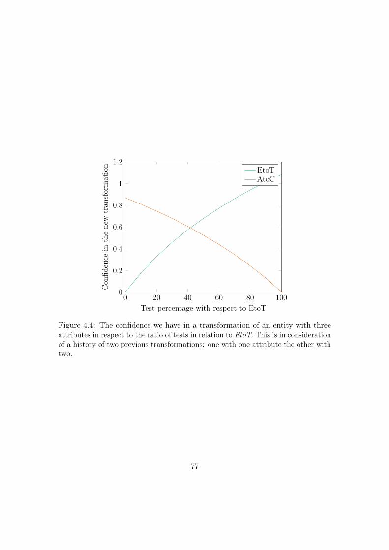
0 20 40 60 80 1000
0.2
0.4
0.6
0.8
1
1.2
Test percentage with respect to EtoT
Con
fidence
inthenew
tran
sformation EtoT
AtoC
Figure 4.4: The confidence we have in a transformation of an entity with threeattributes in respect to the ratio of tests in relation to EtoT. This is in considerationof a history of two previous transformations: one with one attribute the other withtwo.
77
accepted this when we decided to produce more test data.
4.5 Chapter Summary
In Chapter 3 we introduced a meta-model and algorithm for containing full ac-
countability within model transformation. This is a necessity for having confidence
within a transformation process. How can one be assured that we have witnessed
a sequence of events before when we do not have the full view of what has gone
on? This chapter has built upon additional trace information and turned it into a
knowledge base for learning and performance analysis.
We have formalised our trace to make it possible to store it within a graph-based
database. Retaining this representation keeps it in its natural form and presents
us with other opportunities for debugging and optimisation, as well as for our use:
providing confidence. For example, the execution graph can help developers to find
bottlenecks in their transformation to focus performance analysis to specific rules.
Parallelisation is possible where there are no recursive dependencies or loopbacks.
Further parallelisation, over different hosts, is available to connected graphs. This
information can aid in increasing the speed of M2M transformation.
For our work, however, we use it to gain assurance in a process. Acknowledging
our assumption that the more times we have seen something work before, the more
confident we are that it will work again opposed to a yet unseen operation. We
formalise a ratio of how necessary a rule is in respect to its transformation and its
use in another, more recent, one. This data provides us with the prominence of
that rule’s use in a historical trace concerning a new trace. A drawback of this
trait is that it introduces a bias into our value: it assumes that each invocation is
78

equal, which is not true. The result of that transformation can be used to generate
code that interacts with critical services or sensors. The transformation itself could
be involved when considering the code that is written to complete the task. To
avoid such biases, we include a weighing mechanism and explain a few examples.
We concentrate on cyclomatic complexity, the number if linearly accessible paths
through an execution graph. Our assumption here is that the higher the value,
there would be a higher chance of traversing the incorrect branch. Combining these
affords us a value to quantify our confidence within a process, concerning other
historical processes.
79
CHAPTER 5
EVALUATION BY CASE STUDY
Chapters 3 and 4 both introduce methods to increase our confidence in model
transformation. The former looks at what is happening in the process of transform-
ing a source into a destination model, capturing the essence of this mapping using
traceability. It finds and attempts to resolve issues with the current state of the art
to improve accountability during the generation of the target model. This property
is required to provide assurance when using imperative or hybrid transformation
engines as these can cause side-effects that may become problematic. The latter
looks at using this information to determine a value for confidence: how confident
we are that a particular invocation is going to succeed when compared to others.
Our process includes the persistence of trace data into a database and using this
as a basis for learning. We can then have more assurance of a new trace input
that can be at least somewhat composed of historical traces, than that of one that
cannot.
The key to this is our Java and Python implementations of the Simple Trans-
former (SiTra) that both enforce our meta-model to capture the links lost in the
traditional linear trace model as well as a dynamic proxy to capture objects not
80
instantiated by the engine, called orphans. We then adapted this to the Epsilon
Transformation Language (ETL) to show its generality to other engines. Persistence
into a Neo4j database allows us to retain execution graphs for analysis.
This chapter demonstrates our method with the use of a case study. It attempts
to shows that we can feasibly acquire full accountability for use in production
systems. The extra processing required to capture data regarding order and a
particularly common side-effect will have some form of impact upon the transfor-
mation itself. If it is too great, then the benefits do not outweigh the costs. To
do this, we need a non-trivial transformation that can be scaled in size to see the
lasting effects of obtaining this data.
Section 5.1 introduces a non-trivial transformation of a relational database into
that of a NoSQL database, specifically Apache HBase. This case study attempts
to transform a relational database into a view more representative of the questions
one might ask when querying the data. For example if one were to get all patients
registered to a hospital, the relational database would have to look at two tables:
a) The hospital table to find the hospital’s key; and b) The patient table to find
the patients that are assigned to it. This query would be completed using a JOIN
which can become cumbersome for large datasets. Regarding a non-relational
database, the hospital would be an entity that would contain all of its patients,
reducing the query time and the necessary computation. Likewise in the event of
the reverse, a patient would be an independent entity containing a copy of the
hospital. Data duplication implies that non-relational databases accept a loss of
integrity to increase horizontal scalability.
After showing the feasibility of live capture, we attempt to explain that it can be
persisted and used for performance analysis, specifically looking at parallelisation.
81
Focusing on what and why parts are candidates for concurrent processing. Then
using models that iteratively increase in size, explain how we can use the past to
learn using our transformation of the relational into the non-relational.
5.1 Relational to Apache HBase
A relational database is a data store that favours integrity over redundancy. This
trait is enforced by normalisation, i.e. splitting information into multiple tables
and linking them using keys. Normalisation removes the need for data duplication,
which prevents inconsistencies when reading. However, to query data in a useful
way, tables must be joined on their keys. This process can be expensive depending
on the size of the dataset. These databases can be generalised, such that a single
meta-model can be used to model the core structure of many engines in use.
Naturally these can be extended for engine specific functionalities, like Oracle and
PostgreSQL’s inheritance; however, we are concentrating on raw, tabular data, so
these are out of scope for use in our case study. The Structured Query Language
(SQL) provides us with an abstraction of what structure and the data look like
within a relational table.
The opposing approach, denormalisation, favours redundancy and fast reads
over integrity. The duplication of data means writing requires more time to
propagate throughout the database, which in turn can allow data inconsistencies
upon reporting. However, the effect allows developers to reduce the number or
queries by having relevant information in one location on a per query basis. Many
non-relational NoSQL databases apply this function. Apache HBase is such a
database engine (The Apache Foundation 2016). Apache HBase is an open source,
82
non-relational database, and is currently the second most popular of its kind and
fifteenth most popular databases engine in general1. This popularity is what drove
us to transform a general relational database into this engine.
In this section we discuss the transformation of a relational database into
Apache HBase and apply our methods within this transformation.
5.1.1 Meta-Models of the Source and Destination
As described in Figure 2.1 we need an input and target meta-model to describe
instances of the relational and Apache HBase to write rules to map them (Czarnecki
and Helsen 2006). In this section, we shall introduce both meta-models that involve
the structure and the data of each model. The transformation will allow us to
migrate a database and its data rather than just propose its structure. Adding
more complexity to the conversion, as it will need to manually traverse tables to
follow foreign keys to get related rows. Not only this, until Apache HBase has
data its form is a collection of tables and column families. There is no standard
way to transform a relational database to a non-relational, so transforming the
content would allow us to see what it might look like in an automated fashion.
The relational organises data into tables and columns in a manner that reduces
data redundancy and increases integrity (normalisation) (Sanders and Shin 2001).
Apache HBase, and indeed many other NoSQL databases do the opposite, and
they instead optimise reading data by duplicating it. These approaches vary
substantially so a transformation between the two would be complex enough to
test our approach.1http://db-engines.com/en/ranking (visited on Jan 2017)
83
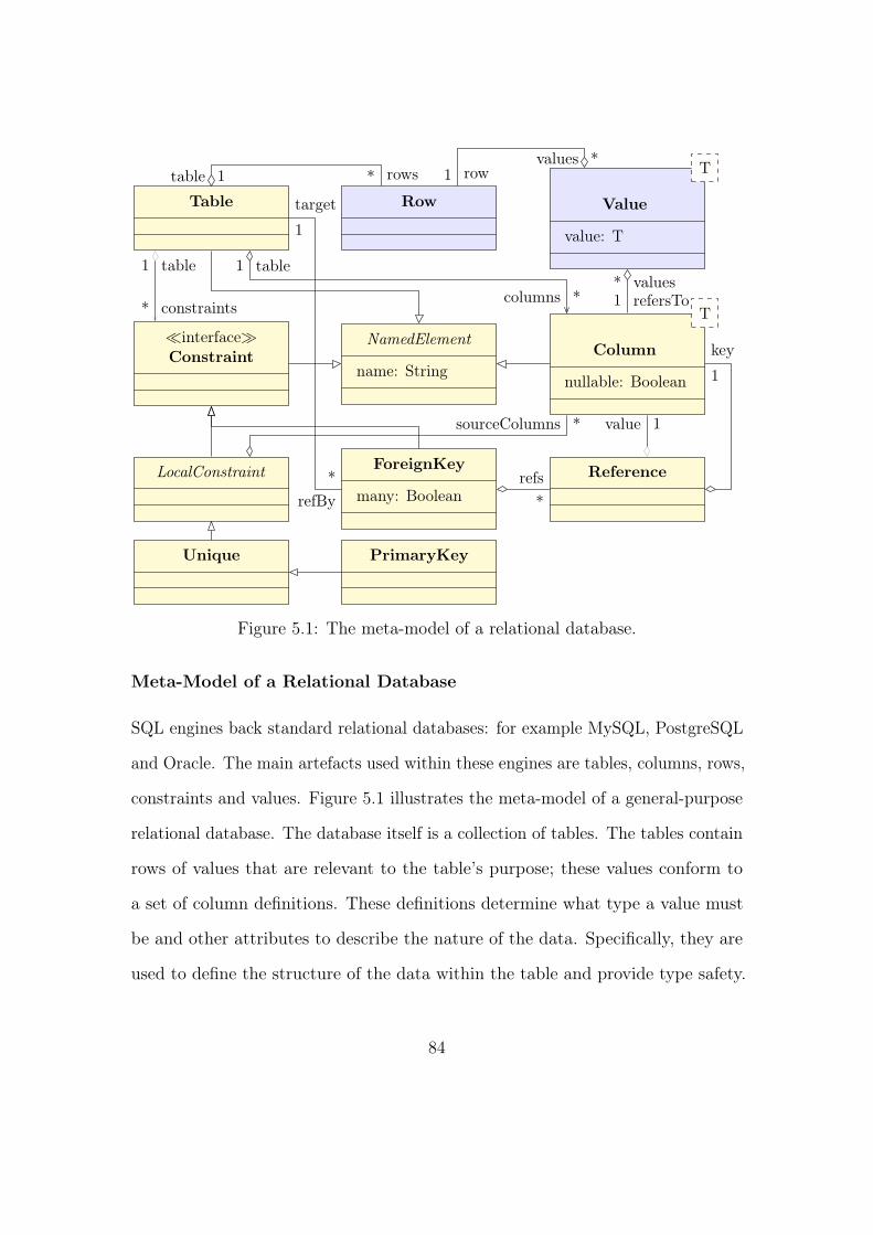
refs*
key
1
value 1sourceColumns *
table1
*columns
table1
constraints*
table 1 rows*values *
row1
values*refersTo1
*refBy
target
1
Table Row Value
value: T
T
�interface�Constraint
NamedElement
name: StringColumn
nullable: Boolean
T
LocalConstraint ForeignKey
many: BooleanReference
Unique PrimaryKey
Figure 5.1: The meta-model of a relational database.
Meta-Model of a Relational Database
SQL engines back standard relational databases: for example MySQL, PostgreSQL
and Oracle. The main artefacts used within these engines are tables, columns, rows,
constraints and values. Figure 5.1 illustrates the meta-model of a general-purpose
relational database. The database itself is a collection of tables. The tables contain
rows of values that are relevant to the table’s purpose; these values conform to
a set of column definitions. These definitions determine what type a value must
be and other attributes to describe the nature of the data. Specifically, they are
used to define the structure of the data within the table and provide type safety.
84
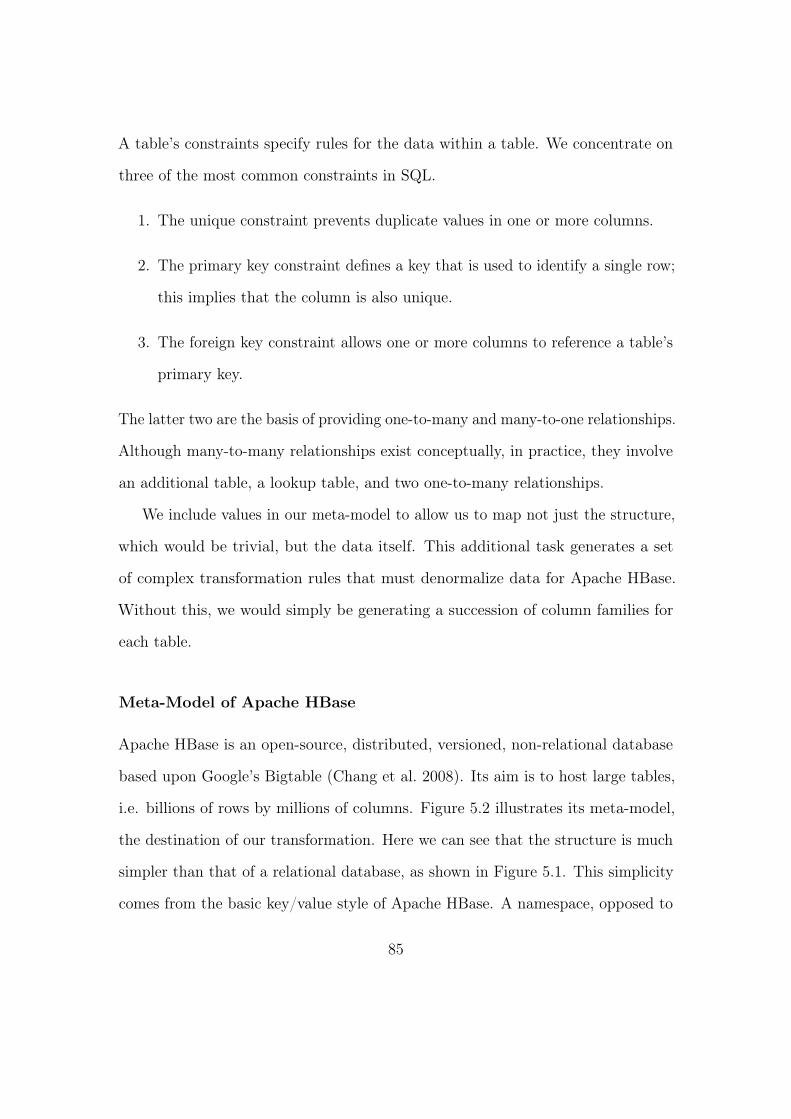
A table’s constraints specify rules for the data within a table. We concentrate on
three of the most common constraints in SQL.
1. The unique constraint prevents duplicate values in one or more columns.
2. The primary key constraint defines a key that is used to identify a single row;
this implies that the column is also unique.
3. The foreign key constraint allows one or more columns to reference a table’s
primary key.
The latter two are the basis of providing one-to-many and many-to-one relationships.
Although many-to-many relationships exist conceptually, in practice, they involve
an additional table, a lookup table, and two one-to-many relationships.
We include values in our meta-model to allow us to map not just the structure,
which would be trivial, but the data itself. This additional task generates a set
of complex transformation rules that must denormalize data for Apache HBase.
Without this, we would simply be generating a succession of column families for
each table.
Meta-Model of Apache HBase
Apache HBase is an open-source, distributed, versioned, non-relational database
based upon Google’s Bigtable (Chang et al. 2008). Its aim is to host large tables,
i.e. billions of rows by millions of columns. Figure 5.2 illustrates its meta-model,
the destination of our transformation. Here we can see that the structure is much
simpler than that of a relational database, as shown in Figure 5.1. This simplicity
comes from the basic key/value style of Apache HBase. A namespace, opposed to
85
table 1
rows *
values *row1
table1 columnFamilies *namespace1 tables *
*values
1columnFamily
NamedElement
name: String
Row
id: String
Value
key: Stringvalue: String
Namespace Table ColumnFamily
Figure 5.2: The meta-model of a Apache HBase.
a database, is a grouping of tables which each contain column families defining the
general structure of the data within. Column families are a conceptual grouping
of columns that have no definition. Users add data into the “buckets” on demand.
For example, if a column family called patients existed, one could write values
to patients:id and patients:name with no information regarding the column
qualifiers. Each table indexes a set of rows based on their ID. These IDs allow
the engine to spread the data amongst the data cluster to share resources where
needed. Finally, we include values: Apache HBase only supports textual or byte
data natively. To store other types, one must encode them or know the type upfront
to cast them within the application calling upon it. In either case, they directly
relate to a row and a column family. Our representation’s Value takes the key/value
literally and contains the value it represents and the column qualifier, or key that
identifies it.
This meta-model allows us to realise the structure and the data of Apache
HBase. Since NoSQL databases do not have schemas, we needed a meta-model
86
that includes its data. The main structures act like buckets for textual or binary
data. Therefore to properly transform a database we need to access the data within
the relational tables to create a viable destination model.
5.2 Relationship Considerations
Relational databases normalise data to reduce duplication with a goal to increase
integrity. This feature eliminates redundancy and anomalies caused by inserting,
updating or deleting data. Information is spread over tables and referenced by row
keys to provide these assurances Integrity, however, induces performance issues
as querying the databases will no doubt require joining these tables together, or
using multiple queries. Both can be expensive operations, especially since datasets
increase.
NoSQL databases take a different approach and favour data duplication to
provide faster reads; this additional redundancy makes for a more horizontally
scalable database engine. Therefore these databases have no concept of relationships,
i.e. many-to-one, one-to-one and many-to-many. This duplication can create
anomalies as data needs to be written in more locations and therefore can be
out-of-date when reported. Often this denormalisation will look at the questions
that are asked by the user. For example: What users are assigned to a project?
Or What projects is a user assigned to? This bidirectional question would imply
two tables, a projects table and a users tables. The projects table would duplicate
all of the user’s data within it, so only one read would be necessary. The reverse
would be the same; the user would have project information within its table. To
illustrate the data anomalies consider updating the user, one would first modify
87
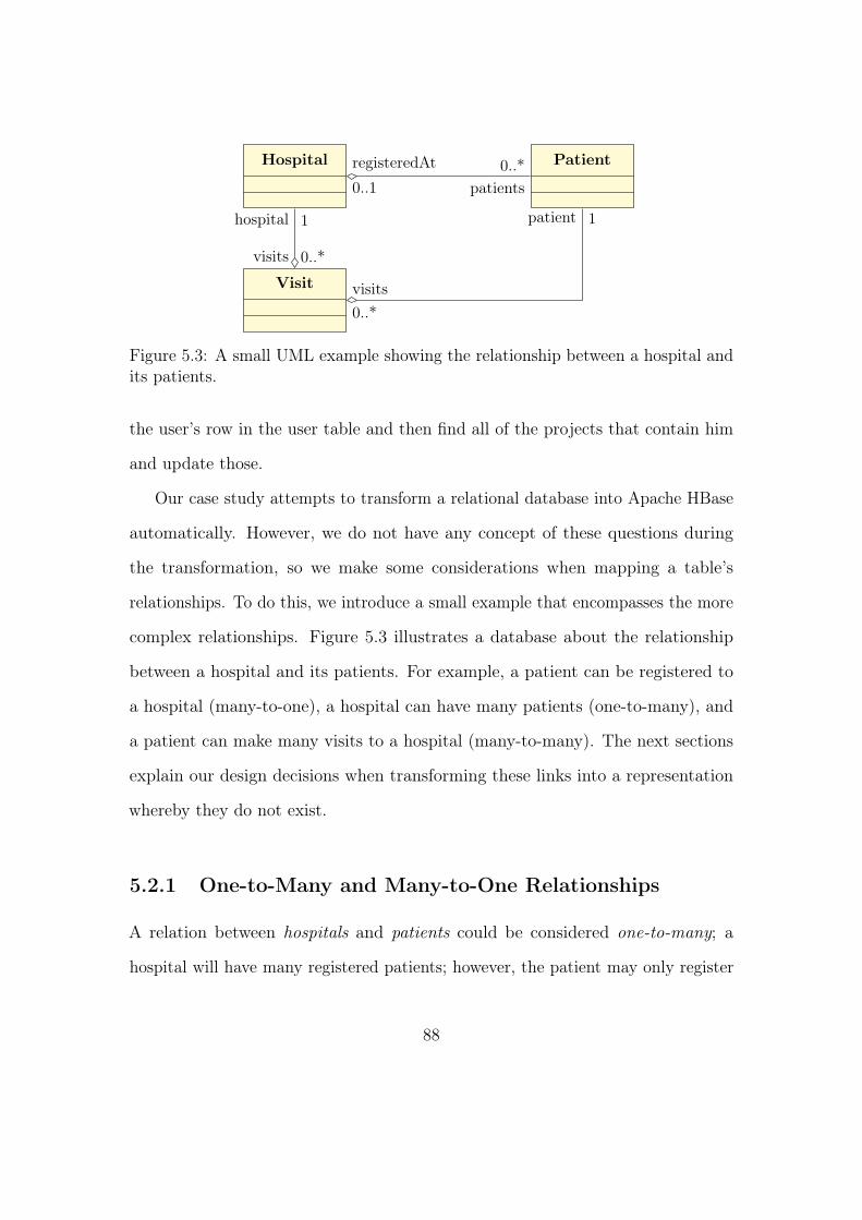
registeredAt
0..10..*
patients
visits 0..*
hospital 1
visits0..*
patient 1
Hospital Patient
Visit
Figure 5.3: A small UML example showing the relationship between a hospital andits patients.
the user’s row in the user table and then find all of the projects that contain him
and update those.
Our case study attempts to transform a relational database into Apache HBase
automatically. However, we do not have any concept of these questions during
the transformation, so we make some considerations when mapping a table’s
relationships. To do this, we introduce a small example that encompasses the more
complex relationships. Figure 5.3 illustrates a database about the relationship
between a hospital and its patients. For example, a patient can be registered to
a hospital (many-to-one), a hospital can have many patients (one-to-many), and
a patient can make many visits to a hospital (many-to-many). The next sections
explain our design decisions when transforming these links into a representation
whereby they do not exist.
5.2.1 One-to-Many and Many-to-One Relationships
A relation between hospitals and patients could be considered one-to-many; a
hospital will have many registered patients; however, the patient may only register
88
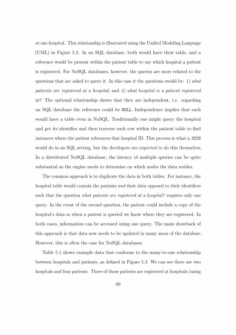
at one hospital. This relationship is illustrated using the Unified Modeling Language
(UML) in Figure 5.3. In an SQL database, both would have their table, and a
reference would be present within the patient table to say which hospital a patient
is registered. For NoSQL databases, however, the queries are more related to the
questions that are asked to query it. In this case it the questions would be: 1) what
patients are registered at a hospital; and 2) what hospital is a patient registered
at? The optional relationship shows that they are independent, i.e. regarding
an SQL database the reference could be NULL. Independence implies that each
would have a table even in NoSQL. Traditionally one might query the hospital
and get its identifier and then traverse each row within the patient table to find
instances where the patient references that hospital ID. This process is what a JOIN
would do in an SQL setting, but the developers are expected to do this themselves.
In a distributed NoSQL database, the latency of multiple queries can be quite
substantial as the engine needs to determine on which nodes the data resides.
The common approach is to duplicate the data in both tables. For instance, the
hospital table would contain the patients and their data opposed to their identifiers
such that the question what patients are registered at a hospital? requires only one
query. In the event of the second question, the patient could include a copy of the
hospital’s data so when a patient is queried we know where they are registered. In
both cases, information can be accessed using one query. The main drawback of
this approach is that data now needs to be updated in many areas of the database.
However, this is often the case for NoSQL databases.
Table 5.1 shows example data that conforms to the many-to-one relationship
between hospitals and patients, as defined in Figure 5.3. We can see there are two
hospitals and four patients. Three of those patients are registered at hospitals (using
89
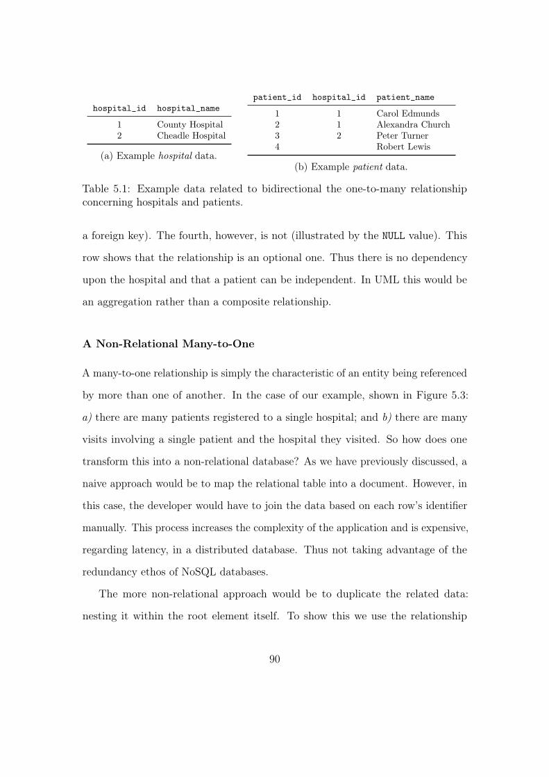
hospital_id hospital_name
1 County Hospital2 Cheadle Hospital
(a) Example hospital data.
patient_id hospital_id patient_name
1 1 Carol Edmunds2 1 Alexandra Church3 2 Peter Turner4 Robert Lewis
(b) Example patient data.
Table 5.1: Example data related to bidirectional the one-to-many relationshipconcerning hospitals and patients.
a foreign key). The fourth, however, is not (illustrated by the NULL value). This
row shows that the relationship is an optional one. Thus there is no dependency
upon the hospital and that a patient can be independent. In UML this would be
an aggregation rather than a composite relationship.
A Non-Relational Many-to-One
A many-to-one relationship is simply the characteristic of an entity being referenced
by more than one of another. In the case of our example, shown in Figure 5.3:
a) there are many patients registered to a single hospital; and b) there are many
visits involving a single patient and the hospital they visited. So how does one
transform this into a non-relational database? As we have previously discussed, a
naive approach would be to map the relational table into a document. However, in
this case, the developer would have to join the data based on each row’s identifier
manually. This process increases the complexity of the application and is expensive,
regarding latency, in a distributed database. Thus not taking advantage of the
redundancy ethos of NoSQL databases.
The more non-relational approach would be to duplicate the related data:
nesting it within the root element itself. To show this we use the relationship
90
between the patient and hospital, i.e. many patients can be registered to one
hospital. Table 5.2 illustrates how the data could be laid out in an Apache HBase
table. Each value is a tuple consisting of the row identifier, the column and a
timestamp. Thus we have null values. Physically those NULLs do not exist in HBase.
Apache HBase uses column families to denote a conceptual grouping of columns, so
our HBase table would have two column families for the patient table, per row: 1) a
column family, to hold the core attributes of the patient; and 2) a column family,
to hold the attributes of the hospital. In both cases, qualifiers are used to identify
attributes. Each hospital value would be accessible using registered_at:id and
registered_at:name, where registered_at is the column family while id and
name are qualifiers. This column family is a bucket for all of the hospital’s data via
the registered at relationahip.
A Non-Relational One-to-Many
The previous section discussed the many-to-one relationship between relational
tables and introduced the mechanism to be used to implement it within a key-value
setting. This section shall discuss a possible implementation of a one-to-many
relationship. This relationship is simply the reverse of the many-to-one. Opposed
to discussing the relationship on the patient we now look from the perspective
of the hospital. Asking for the list of patients that registered with a particular
hospital, rather than for the hospital a patient registered.
A relationship that is at the one end of a relationship can be considered fairly
trivial to maintain, i.e. a column family to place that entities data inside. However,
there is no list structure within Apache HBase to allow us to have multiple elements.
91
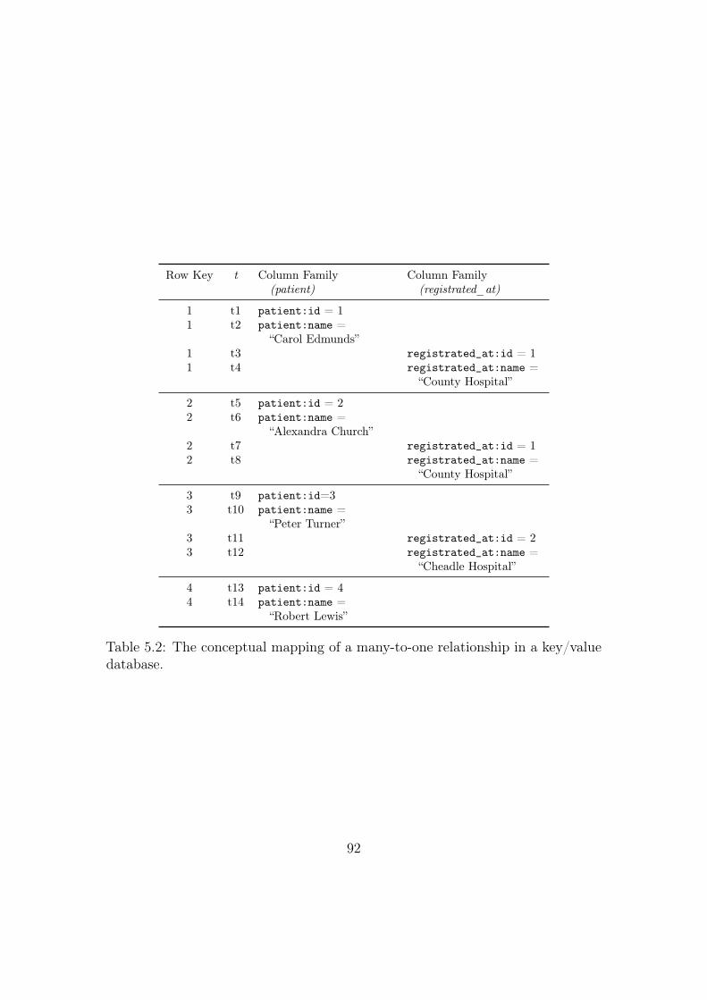
Row Key t Column Family(patient)
Column Family(registrated_at)
1 t1 patient:id = 11 t2 patient:name =
“Carol Edmunds”1 t3 registrated_at:id = 11 t4 registrated_at:name =
“County Hospital”
2 t5 patient:id = 22 t6 patient:name =
“Alexandra Church”2 t7 registrated_at:id = 12 t8 registrated_at:name =
“County Hospital”
3 t9 patient:id=33 t10 patient:name =
“Peter Turner”3 t11 registrated_at:id = 23 t12 registrated_at:name =
“Cheadle Hospital”
4 t13 patient:id = 44 t14 patient:name =
“Robert Lewis”
Table 5.2: The conceptual mapping of a many-to-one relationship in a key/valuedatabase.
92
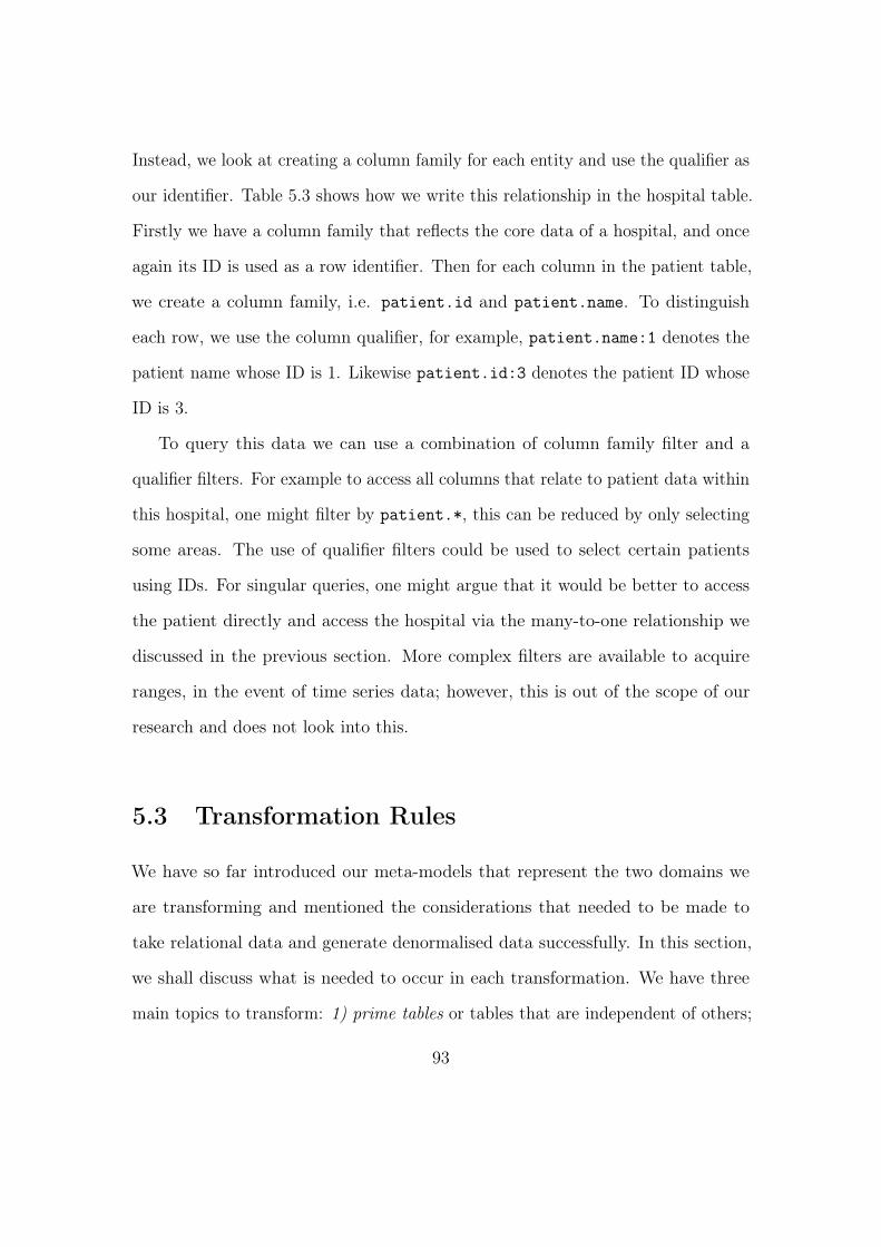
Instead, we look at creating a column family for each entity and use the qualifier as
our identifier. Table 5.3 shows how we write this relationship in the hospital table.
Firstly we have a column family that reflects the core data of a hospital, and once
again its ID is used as a row identifier. Then for each column in the patient table,
we create a column family, i.e. patient.id and patient.name. To distinguish
each row, we use the column qualifier, for example, patient.name:1 denotes the
patient name whose ID is 1. Likewise patient.id:3 denotes the patient ID whose
ID is 3.
To query this data we can use a combination of column family filter and a
qualifier filters. For example to access all columns that relate to patient data within
this hospital, one might filter by patient.*, this can be reduced by only selecting
some areas. The use of qualifier filters could be used to select certain patients
using IDs. For singular queries, one might argue that it would be better to access
the patient directly and access the hospital via the many-to-one relationship we
discussed in the previous section. More complex filters are available to acquire
ranges, in the event of time series data; however, this is out of the scope of our
research and does not look into this.
5.3 Transformation Rules
We have so far introduced our meta-models that represent the two domains we
are transforming and mentioned the considerations that needed to be made to
take relational data and generate denormalised data successfully. In this section,
we shall discuss what is needed to occur in each transformation. We have three
main topics to transform: 1) prime tables or tables that are independent of others;
93
RowKey
t Column Family(hospital)
Column Family(patients.id)
Column Family(patients.name)
1 t1 hospital:id = 11 t2 hospital:name =
“County Hospital”1 t3 patient.id:1 = 11 t4 patient.name:1 =
“Carol Edmunds”1 t5 patient.id:2 = 21 t6 patient.name:2 =
“Alexandra Church”
2 t7 hospital:id = 22 t8 hospital:name =
“Cheadle Hospital”2 t9 patient.id:3 = 32 t10 patient.name:3 =
“Peter Turner”
Table 5.3: The conceptual mapping of a one-to-many relationship in a key/valuedatabase.
2) any-to-one table relationships that end with a single item; and 3) one-to-many
table relationships that conclude with the many side of the relationship.
Our example in Figure 5.3 contains a many-to-many relationship between the
hospital and patient entities via the visit table; however, a visit is complex many-to-
many as its presence is indicative of additional attributes. Thus it is interpreted as
a prime table with two bidirectional one-to-many relationships. Our transformation
treats non-complex many-to-many relationships, i.e. simple lookup tables, and the
complex equally. An extension of our work could allow the removal of the index
table and traverse the indices to denormalise the data. Automating this is not a
trivial undertaking as we need a method to identify this data.
94
5.3.1 The Database
A relational database is simply a collection of tables; this conceptual grouping is
synonymous with the Apache HBase namespace, a collection of HBase tables. This
view is a key starting point for a transformation such that we might transform
an entire database of tables. A rule to complete this is a simple one, create a
namespace, set its name based on the input and then transform the relational
database’s contents.
5.3.2 Prime Tables
Table Transformation
For the purpose of this case study, we refer to tables with no or optional foreign
keys as prime tables. These are candidates for Apache HBase tables. If no foreign
key references the table, there is no dependency upon the entity in question. For
example the hospital references a set of patients; however a patient is independent
of the hospital, i.e. the registered status is optional. In the case of the visit table,
a visit requires a hospital, but the reverse is not true. The hospital table itself has
no dependencies it only has dependents.
For a given prime table we need an HBase table and a column family. This
family is necessary to contain the columns of a relational table. Since we are using
SiTra in Python, we can generate multiple output objects and as such will use this
approach for this rule: f(RelationalTable)→ (HBaseTable,HBaseColumnFamily).
This process, however, creates two orphans, as the trace knows about the tuple
but not its contents. We would receive no result if one were to complete a reverse
95
lookup on either the HBase table or column family. Here we depend on the proxy
we have implemented to intercept these objects when they are bound together.
However as explained in Section 3.2.2 we need to do this at the beginning of the
binding phase so we might capture subsequent orphans.
Following the transformation of the table’s basic features, we must then trans-
form its rows and foreign key constraints. These mappings would be completed
automatically given a scheduled engine. However, SiTra is explicitly scheduled and
needs to transform each as such.
Data Transformation
We now have a transformation that will generate a table and a column family for
the table’s data. Next, we concentrate on the data itself. There are two directions
for this, iterate each row or each column. The final effect of this is to transform
each value. Due to how data is indexed we chose to transform each row individually.
The rule itself returns a new Apache HBase row for each relational row it finds.
The binding phase is a simple one: 1) setup the structural elements, i.e. assign it
to the table; 2) formulate a row key, using the primary key of the relational table;
and 3) iterate each value to transform the data. The row key is the identifier for a
row within the prime table and is used to distribute the data amongst the cluster.
It involves the primary key’s value(s). For the purpose of our experiments, we do
not consider composite keys as we feel that they would need further configuration
as to determine their value. If we had a two column composite key, how should it
be used? It would be sensible to use both, however in which order. Once more we
ask the question, what are we querying? This issue makes it hard to automate, if
96
indeed necessary.
Given an Apache HBase row, we now need to iterate the values within the
relational row converting them into Apache HBase values. Since we are transforming
prime tables, the mapping of their values is a simple one. This process involves
setting up the components of an individual value and setting its attributes such
that it retains its data, a reference to the right row and a reference to the default
column family generated in Section 5.3.2. Since all data in Apache HBase can
be a string or an array of bytes: all values would be treated as strings for the
purpose of testing. In a real setting, one might attempt to serialise them correctly.
For example, an array of four bytes could be used to keep a 32-bit integer inside,
whereas when using a character array, each power of ten adds a byte to represent
its ASCII representation.
5.3.3 Relationships
We have now transformed the basic elements of a relational table; we now need to
discuss the logic on how we transform relationships. These become more complex as
we need to transform a foreign key about a table: either its target or owning table.
Since there is only one object regarding the relationship, we need a composite input,
i.e. the owning table with the foreign key and the target table with the foreign
key. Other, more declarative, languages like Operational Query/View/Transform
(QVT-O) and the ATLAS Transformation Langauge (ATL) have a scheduler that
can do such operations. SiTra, both Python and Java, is unable to do this implicitly.
To explicitly do this we need to create a composite of elements to transform and
transform that instead. In the case of Java, one might use the approach found
97
in Section 3.1.3. However, in Python, we can generate tuples on demand and
transform them without creating specific containers.
Any-to-One Relationships
Any-to-one transformations include both many-to-one and one-to-one relationships.
Specifically looking at the one side, i.e. the current element can only be referenced
by one related item. As explained in Section 5.2.1: all values within this can be
placed into a single column family, using the column name as the qualifier for the
value itself. In the case of Table 5.2, we have id and name as the qualifiers within
the column family registered_at. A column family is used to represent a bucket
for the data of each of these relationships.
To transform data however we need to map a relational row in respect of a
table and a foreign key. The table determines the direction of the transformation
and where the results should be bound. If the table is the foreign key’s target
we need to look at the referencing table, if the table is the owning table then
we need to look locally. Our transformation rule introduces many orphans as we
iterate each value within the row in question and map them manually rather than
delegating to another rule. Not unlike the foreign key and foreign key column in
the OO2DB example as explained in Section 3.1.3; however, our new objects come
from a controlled and yet variable loop. This part of our transformation was a
design decision to enable us to verify orphan capture.
98
One-to-Many Relationships
The concept of this transformation is explained in Section 5.2.1 and illustrates
that we need a column family for each column of the child table. For instance, the
hospital table would need a column family for each patient column to emulate a
nested table. The transformation would require the rule to instantiate a list of
column families for binding. This phase will initially create a list of orphans. The
engine itself knows that the transformation of a relationship produces a list, but
it does not recurse into the list to gather its contents. However, the list passed
into the binding phase is a proxy. Therefore any accessors used to retrieve column
families would automatically add them into the transformation trace.
Transforming the data is not unlike that of any-to-one relationships however the
column has its container identified by the row’s primary key. Table 5.3 has column
families for each patient column, and the patient’s ID identifies every patient “row”
as the column family’s qualifier.
5.4 Benchmarking Traceability for SiTra
In this section, we shall discuss the overhead of our latest meta-model upon a
model-to-model (M2M) transformation. We have already introduced our new
tracing mechanism and explained how we capture orphan objects in Section 3.2.
Our method was implemented primarily in Java; however, due to our usage of
Python for the efficacy of a transformation, we shall focus on our Python framework.
This piece of software consists of four engines: 1) one that has no tracking; 2) one
with a linear trace; 3) one that retains the interconnectivity of the transformation,
99
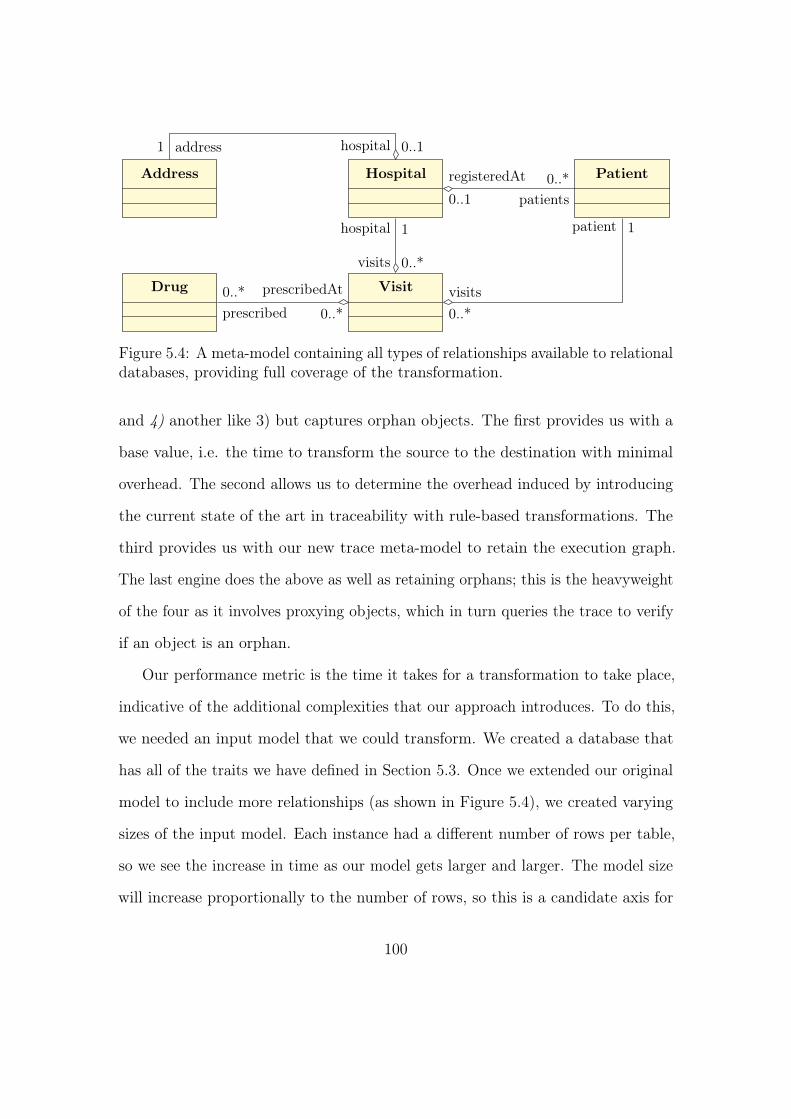
registeredAt
0..10..*
patients
visits 0..*
hospital 1
visits0..*
patient 1
hospital 0..1address1
prescribedAt
0..*0..*prescribed
Hospital PatientAddress
VisitDrug
Figure 5.4: A meta-model containing all types of relationships available to relationaldatabases, providing full coverage of the transformation.
and 4) another like 3) but captures orphan objects. The first provides us with a
base value, i.e. the time to transform the source to the destination with minimal
overhead. The second allows us to determine the overhead induced by introducing
the current state of the art in traceability with rule-based transformations. The
third provides us with our new trace meta-model to retain the execution graph.
The last engine does the above as well as retaining orphans; this is the heavyweight
of the four as it involves proxying objects, which in turn queries the trace to verify
if an object is an orphan.
Our performance metric is the time it takes for a transformation to take place,
indicative of the additional complexities that our approach introduces. To do this,
we needed an input model that we could transform. We created a database that
has all of the traits we have defined in Section 5.3. Once we extended our original
model to include more relationships (as shown in Figure 5.4), we created varying
sizes of the input model. Each instance had a different number of rows per table,
so we see the increase in time as our model gets larger and larger. The model size
will increase proportionally to the number of rows, so this is a candidate axis for
100
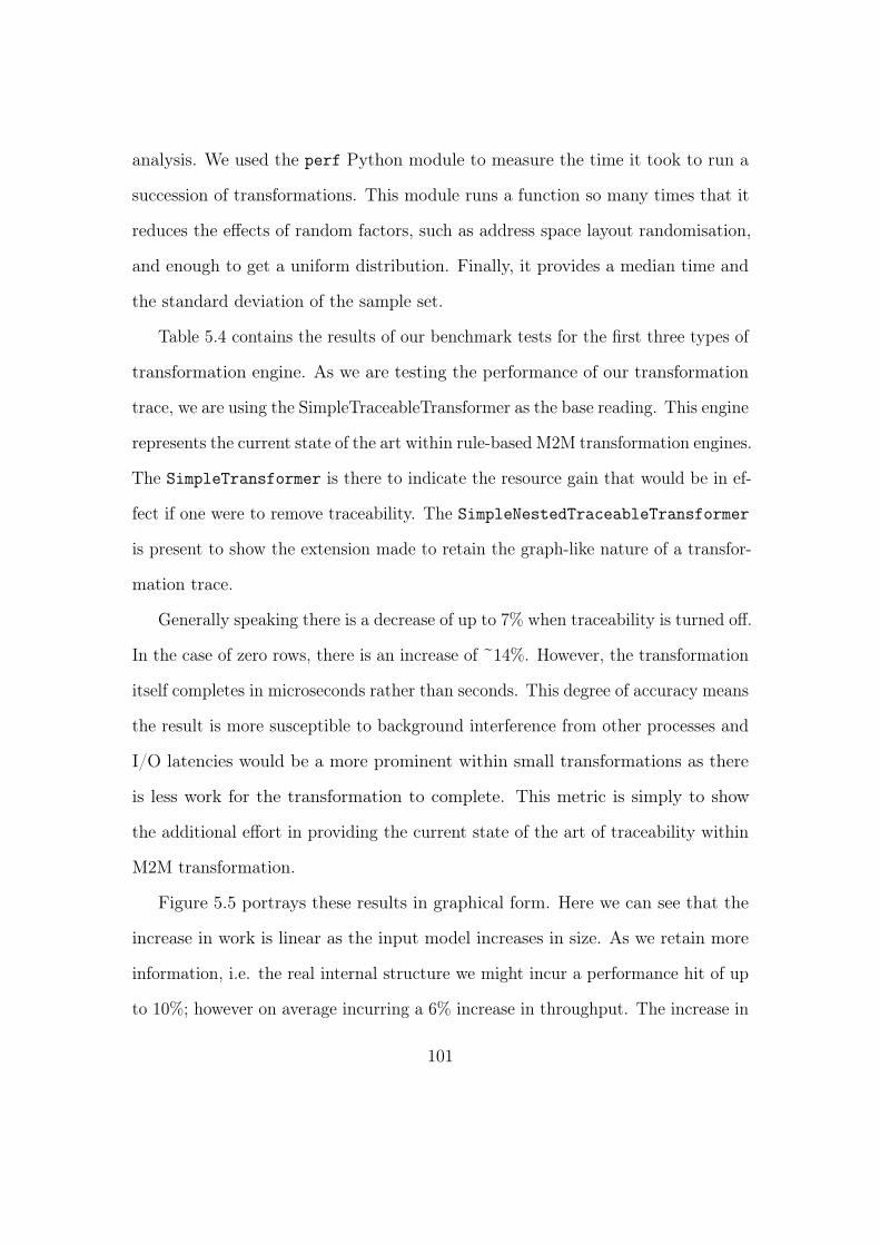
analysis. We used the perf Python module to measure the time it took to run a
succession of transformations. This module runs a function so many times that it
reduces the effects of random factors, such as address space layout randomisation,
and enough to get a uniform distribution. Finally, it provides a median time and
the standard deviation of the sample set.
Table 5.4 contains the results of our benchmark tests for the first three types of
transformation engine. As we are testing the performance of our transformation
trace, we are using the SimpleTraceableTransformer as the base reading. This engine
represents the current state of the art within rule-based M2M transformation engines.
The SimpleTransformer is there to indicate the resource gain that would be in ef-
fect if one were to remove traceability. The SimpleNestedTraceableTransformer
is present to show the extension made to retain the graph-like nature of a transfor-
mation trace.
Generally speaking there is a decrease of up to 7% when traceability is turned off.
In the case of zero rows, there is an increase of ~14%. However, the transformation
itself completes in microseconds rather than seconds. This degree of accuracy means
the result is more susceptible to background interference from other processes and
I/O latencies would be a more prominent within small transformations as there
is less work for the transformation to complete. This metric is simply to show
the additional effort in providing the current state of the art of traceability within
M2M transformation.
Figure 5.5 portrays these results in graphical form. Here we can see that the
increase in work is linear as the input model increases in size. As we retain more
information, i.e. the real internal structure we might incur a performance hit of up
to 10%; however on average incurring a 6% increase in throughput. The increase in
101
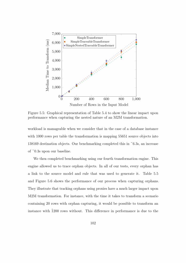
0 200 400 600 800 1,0000
1,000
2,000
3,000
4,000
5,000
6,000
7,000
Number of Rows in the Input Model
Med
ian
Tim
eto
Tran
sfor
m(m
s)
SimpleTransformerSimpleTraceableTransformer
SimpleNestedTraceableTransformer
Figure 5.5: Graphical representation of Table 5.4 to show the linear impact uponperformance when capturing the nested nature of an M2M transformation.
workload is manageable when we consider that in the case of a database instance
with 1000 rows per table the transformation is mapping 55651 source objects into
138169 destination objects. Our benchmarking completed this in ~6.3s, an increase
of ~0.3s upon our baseline.
We then completed benchmarking using our fourth transformation engine. This
engine allowed us to trace orphan objects. In all of our tests, every orphan has
a link to the source model and rule that was used to generate it. Table 5.5
and Figure 5.6 shows the performance of our process when capturing orphans.
They illustrate that tracking orphans using proxies have a much larger impact upon
M2M transformation. For instance, with the time it takes to transform a scenario
containing 20 rows with orphan capturing, it would be possible to transform an
instance with 1̃200 rows without. This difference in performance is due to the
102
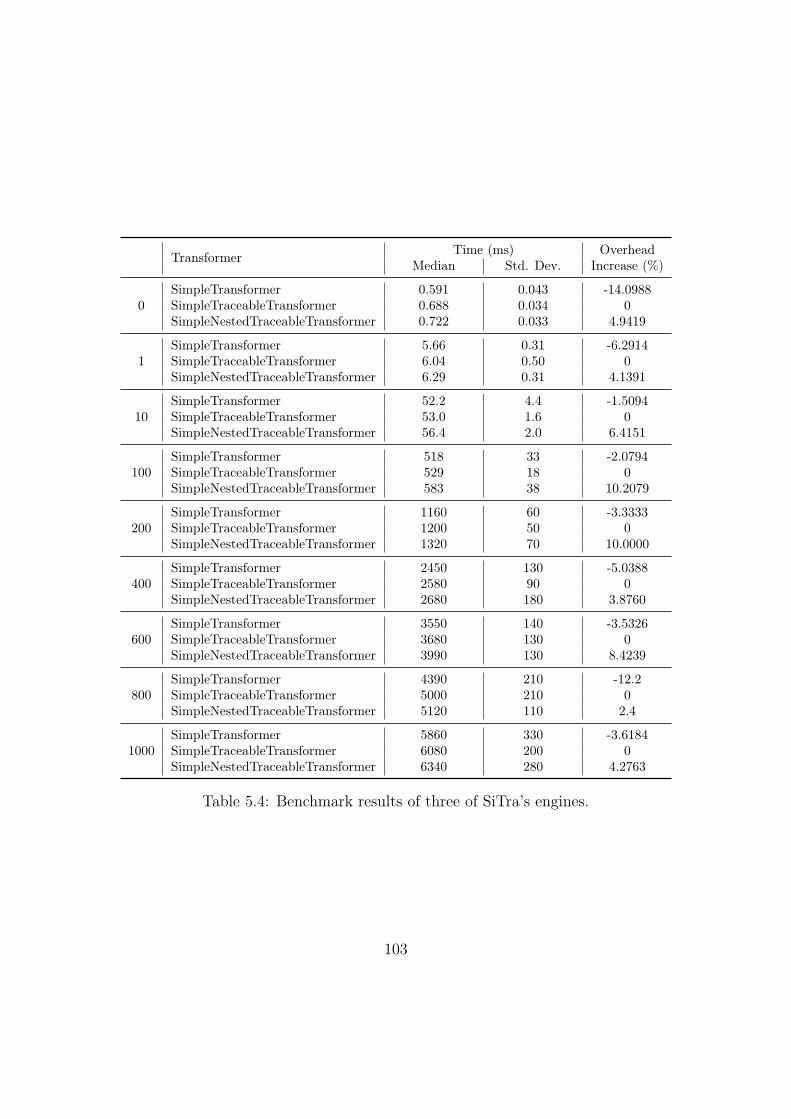
Transformer Time (ms) OverheadMedian Std. Dev. Increase (%)
0SimpleTransformer 0.591 0.043 -14.0988SimpleTraceableTransformer 0.688 0.034 0SimpleNestedTraceableTransformer 0.722 0.033 4.9419
1SimpleTransformer 5.66 0.31 -6.2914SimpleTraceableTransformer 6.04 0.50 0SimpleNestedTraceableTransformer 6.29 0.31 4.1391
10SimpleTransformer 52.2 4.4 -1.5094SimpleTraceableTransformer 53.0 1.6 0SimpleNestedTraceableTransformer 56.4 2.0 6.4151
100SimpleTransformer 518 33 -2.0794SimpleTraceableTransformer 529 18 0SimpleNestedTraceableTransformer 583 38 10.2079
200SimpleTransformer 1160 60 -3.3333SimpleTraceableTransformer 1200 50 0SimpleNestedTraceableTransformer 1320 70 10.0000
400SimpleTransformer 2450 130 -5.0388SimpleTraceableTransformer 2580 90 0SimpleNestedTraceableTransformer 2680 180 3.8760
600SimpleTransformer 3550 140 -3.5326SimpleTraceableTransformer 3680 130 0SimpleNestedTraceableTransformer 3990 130 8.4239
800SimpleTransformer 4390 210 -12.2SimpleTraceableTransformer 5000 210 0SimpleNestedTraceableTransformer 5120 110 2.4
1000SimpleTransformer 5860 330 -3.6184SimpleTraceableTransformer 6080 200 0SimpleNestedTraceableTransformer 6340 280 4.2763
Table 5.4: Benchmark results of three of SiTra’s engines.
103
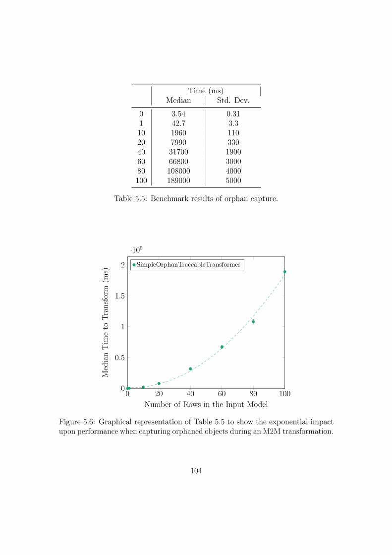
Time (ms)Median Std. Dev.
0 3.54 0.311 42.7 3.310 1960 11020 7990 33040 31700 190060 66800 300080 108000 4000100 189000 5000
Table 5.5: Benchmark results of orphan capture.
0 20 40 60 80 1000
0.5
1
1.5
2
·105
Number of Rows in the Input Model
Med
ian
Tim
eto
Tran
sfor
m(m
s)
SimpleOrphanTraceableTransformer
Figure 5.6: Graphical representation of Table 5.5 to show the exponential impactupon performance when capturing orphaned objects during an M2M transformation.
104
creation and processing overheads of object proxies to intercept accessors and
mutators. In the event of the call of a mutator method, the transformation engine
looks for the new object inside of its trace. If it is not available, the object is
an orphan and therefore kept. The object is then being proxied itself to allow
recursion. Accessors, however, return proxies for objects to allow any setters and
getters on the acquired object to be captured. A map could be used to optimise
this process. However, there are two considerations:
1. A cache is often implemented using a map, which creates a hash based on the
key object. Thus a means of determining object equality must be provided
to the destination model. hashCode is used to determine which bucket an
object will go into, while equals determine whether two objects are logically
similar. Without this implementation often the object’s memory address is
used for equality; however this value can be reused by other objects as and
when objects are swapped out and back in again. This behaviour is true for
Java and Python at the time of writing, for larger transformations this cannot
work as memory will be swapped and therefore there is a chance of reuse.
2. The cache itself can also become significant. Mapping a POJO to its proxy to
save on time creating a new one. In a worst case scenario, we need twice the
number of objects in the destination as each object needs a proxy. Potentially
inducing more memory movement and using up resources available to the
transformation itself.
The cost of using a cache to save on the instantiation time of proxies weighs against
the resources that are available. In the case of no cache, we would decrease the
transformation’s throughput, as for each item we return a new proxy, potentially
105
many proxies per destination object. However, when we introduce a cache we
would, up to a point, increase throughput but at the same time reduce the number
of resources available to the transformation itself.
This data has changed our approach to using the SimpleOrphanTraceableTrans-
former as a general purpose transformation engine and instead it is to be used
to detect orphans during development. This method will help developers to find
orphans and refactor their rules such that they do no create them. Following this
they then can fall back onto the SimpleNestedTraceableTransformer to retain the
structure of the overall transformation, knowing that all objects are accounted for.
Our case study has provided us with the concept of orphan leakage. These
come from two locations: 1) the instantiation phase, where one might return an
array of objects, and 2) the previously discussed binding phase.
Orphan leakage occurs in the binding phase of an M2M transformation. Not
unlike real memory leaks, these are potentially out of control and are unstable. For
instance if one were to allocate some memory to a pointer and forget to free it, the
leak itself has limited effects; however if one were to reuse that address, in a loop for
example, and continue to allocate memory, it could have crippling consequences for
the process. This issue applies to the accountability of destination objects within
the trace of an M2M transformation. Our case study implements this leak by
generating some value objects for each row in a loop. Apache Values are orphans
until a proxy detects them. We expected that our proxies will catch these orphans.
If one used this system to detect them during development, it would allow the
developer to refactor their rules such that they are at built during instantiation.
Thus one may fall back upon a faster engine, removing the need for proxies.
The instantiation phase produces a containment of new objects when returning
106
a collection. The engine can traverse these containments automatically as they
should be a one-dimensional array of presently unrelated objects. This collection is
iterable, and therefore the list can be traversed and its objects tracked before the
binding phase. These orphans are stable, and despite the possibility of returning a
dynamic number of elements (using generators), can all be captured before and
then passed into the set_properties method.
It is possible to rewrite the transformation of the relational to non-relational
such that it creates no orphans. These changes are minor modifications, and simply
involve the building a list of HBase values in the instantiation phase opposed to
lazily creating them. We calculate the number of values up front, and their indices
within the array can be used to identify them. Our transformation zips them with
the appropriate columns, to make related tuples of relational columns and their
Apache HBase value counterparts. The actual change adds 18 lines of code and
deletes 9.
5.5 Benchmarking Traceability for ETL
To show the applicability of our meta-model within other engines: we have imple-
mented the same transformation, as per Section 5.4 for ETL. ETL is a declarative
language used for defining M2M transformations. However, its execution uses
an executable Abstract Syntax Tree (AST). An ETL module will parse a given
script and interpret its instructions. ETL is an extension of the Epsilon Object
Language (EOL) and various other libraries that allow the framework to accept a
plethora of meta-model and model types. It also provides abstract layers to enable
different model providers the ability to use Epsilon’s toolset. We show that our
107
slight extension to ELT allows us to complete the same transformation, retain the
structure and capture orphans with relatively minor performance decreases. In all
cases, the additional workload was linear, unlike SiTra’s use of proxies which was
exponential.
The bundled version of ETL provides an external linear trace without orphan
tracking. That is a trace that does not maintain invocation or rule dependency
information. It is used by the engine to schedule the transformation. ETL’s
transformation strategy matches all sources and rules before any binding. This
phase is completed by iterating through each rule and finding all permutations of
individual input model elements. When it finds a match, it generates an invocation,
and the target objects instantiated. Once all rules are processed, and matching
sources found, the engine iterates through each of them and binds them. This
way, no rule invokes another, the scheduler itself invokes them. However, rules do
depend on other rules, i.e. they can rely on the result of other invocations. Whether
the engine scheduled it, or whether another invocation catalysed it. We build upon
this version of ETL to provide the same mechanics used in SiTra to retain the
invocation graph, by using a simple stack to track the current transformation and
the new meta-model mentioned in Figure 3.7.
ETL is also open to orphans, as shown in Section 3.1.3. EOL is what provides
the new keyword to its developers and is what causes this side effect. The nature of
ETL’s execution allows us to intercept all elements of the language’s AST. It does
this via an execution listener with pre- and post- methods. In the event of a new
object, the newly allocated instance is passed into the handler and then added to
the current invocation’s target elements. This approach bypasses checks required
by SiTra. We know that at the time of execution it is new and therefore has no
108
association to the source model. There is a possibility that this object may never
see the final model. However, it existed for a time during the transformation. At
the time of execution we cannot know whether it is a temporary variable or not, so
we err on the side of caution by retaining it.
During this investigation, we wrote a transformation rule that created many
column families and another that created many values to validate our orphan
capture. These numbers were variable, so a simple refactoring, as described in
Figure 3.4, would not suffice. Instead, we might rethink the transformation such
that one transforms the individual components, i.e. the Column or Value objects.
To keep the same type of conversion as used for SiTra, we used an EOL Sequence
and populated it within the binding phase. This method is another kind of producer
for orphans.
The conversion of our transformation we have for the Python version of SiTra
is not a simple one. The current transformation strategy of ETL only handles
individual inputs. To emulate multiple source objects, we must wrap them within
another object. For instance, the mapping of a foreign key into a NoSQL setting
is bidirectional. Thus we transform in respect to the table that owns the foreign
key its and the target table. In Python we transformed (forignKey, owner) and
(foreignKey, target). This is an interim transformation. To have the same effect,
we create an interim transformation to generate wrapper objects. This approach is
necessary for all engines that do not support multiple inputs, like ETL and the Java
implementation of SiTra. We show the transformation for ETL in Appendix A.2,
and for completeness, show an example of how to do this with SiTra in Appendix A.1,
specifically Appendix A.1.1. Once we have these wrappers, we can then run the
core transformation, which recognises them to complete the overall process.
109
The python version of SiTra does not suffer from this drawback as there is:
a) a primitive tuple type that can be used to wrap objects; and b) no automatic
scheduler, all transformations are on demand, so tuples are built ad-hoc within
the binding phase. This different strategy removes the need for an interim model
transformation that would be otherwise necessary for ETL and the Java version of
SiTra.
Naturally, as shown with SiTra, the capture of this additional information has
a cost. Retaining this information will inevitably require more resources, CPU and
memory, slowing the overall transformation. To show their effects within ETL,
we ran benchmarks upon the same transformation for 0, 1, 10, 100, 200, 400 and
600 rows of data per table using the same scenario as illustrated in Figure 5.4.
Table 5.6 show the results of this.
The original engine already has a much larger overhead than that of SiTra. An
increase of ~258% when compared with its rival SimpleTraceableTransformer upon
a model with 200 rows of data. Two factors that contribute to this are: 1) the
executable DSL, which requires parsing from a file before execution; and 2) the
overhead of abstraction within the Epsilon framework itself. The former needs I/O
and this can be a great and yet variable source of latency. The latter, however,
means the framework itself adds overhead to the transformation. Epsilon is a
library of languages and tools that share components and are built upon others
to handle many combinations of model types and meta-modelling types. These
mechanisms provide modularity to ETL where SiTra does not.
On average, retaining the full execution graph costs an extra 26.51% in processing
time, when compared to the generation of a linear trace that ETL creates by default.
This performance cost is due to retaining and managing a stack trace consisting of
110
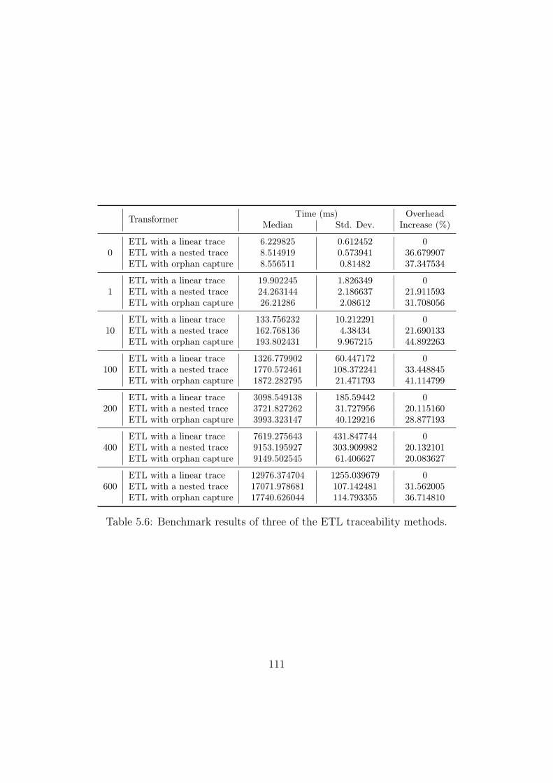
Transformer Time (ms) OverheadMedian Std. Dev. Increase (%)
0ETL with a linear trace 6.229825 0.612452 0ETL with a nested trace 8.514919 0.573941 36.679907ETL with orphan capture 8.556511 0.81482 37.347534
1ETL with a linear trace 19.902245 1.826349 0ETL with a nested trace 24.263144 2.186637 21.911593ETL with orphan capture 26.21286 2.08612 31.708056
10ETL with a linear trace 133.756232 10.212291 0ETL with a nested trace 162.768136 4.38434 21.690133ETL with orphan capture 193.802431 9.967215 44.892263
100ETL with a linear trace 1326.779902 60.447172 0ETL with a nested trace 1770.572461 108.372241 33.448845ETL with orphan capture 1872.282795 21.471793 41.114799
200ETL with a linear trace 3098.549138 185.59442 0ETL with a nested trace 3721.827262 31.727956 20.115160ETL with orphan capture 3993.323147 40.129216 28.877193
400ETL with a linear trace 7619.275643 431.847744 0ETL with a nested trace 9153.195927 303.909982 20.132101ETL with orphan capture 9149.502545 61.406627 20.083627
600ETL with a linear trace 12976.374704 1255.039679 0ETL with a nested trace 17071.978681 107.142481 31.562005ETL with orphan capture 17740.626044 114.793355 36.714810
Table 5.6: Benchmark results of three of the ETL traceability methods.
111
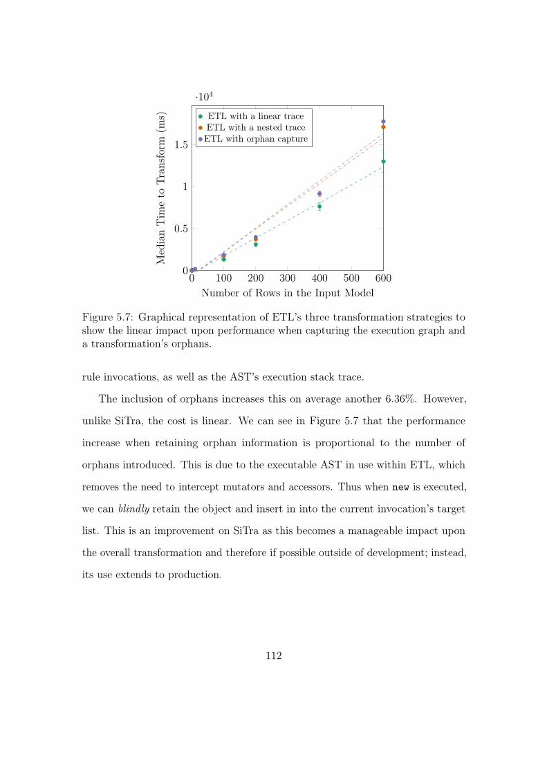
0 100 200 300 400 500 6000
0.5
1
1.5
·104
Number of Rows in the Input Model
Med
ian
Tim
eto
Tran
sfor
m(m
s) ETL with a linear traceETL with a nested traceETL with orphan capture
Figure 5.7: Graphical representation of ETL’s three transformation strategies toshow the linear impact upon performance when capturing the execution graph anda transformation’s orphans.
rule invocations, as well as the AST’s execution stack trace.
The inclusion of orphans increases this on average another 6.36%. However,
unlike SiTra, the cost is linear. We can see in Figure 5.7 that the performance
increase when retaining orphan information is proportional to the number of
orphans introduced. This is due to the executable AST in use within ETL, which
removes the need to intercept mutators and accessors. Thus when new is executed,
we can blindly retain the object and insert in into the current invocation’s target
list. This is an improvement on SiTra as this becomes a manageable impact upon
the overall transformation and therefore if possible outside of development; instead,
its use extends to production.
112
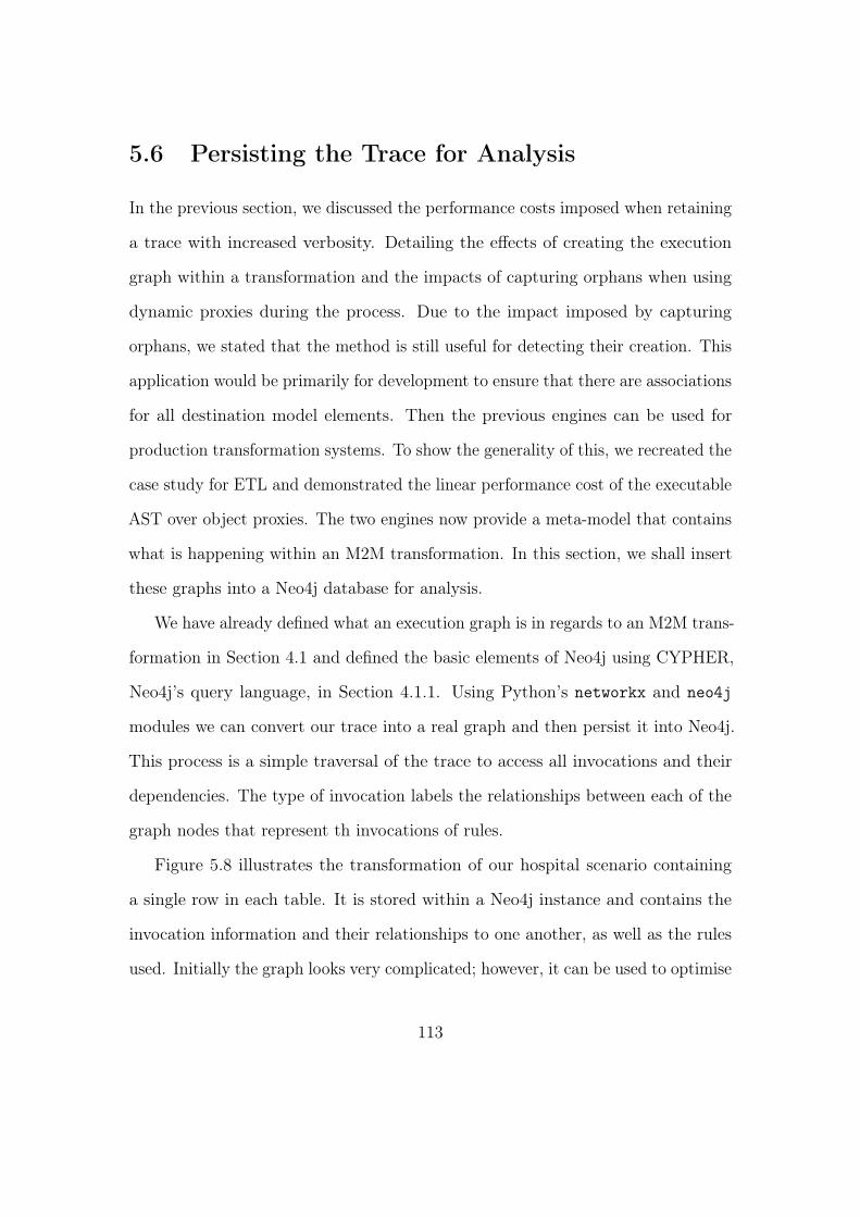
5.6 Persisting the Trace for Analysis
In the previous section, we discussed the performance costs imposed when retaining
a trace with increased verbosity. Detailing the effects of creating the execution
graph within a transformation and the impacts of capturing orphans when using
dynamic proxies during the process. Due to the impact imposed by capturing
orphans, we stated that the method is still useful for detecting their creation. This
application would be primarily for development to ensure that there are associations
for all destination model elements. Then the previous engines can be used for
production transformation systems. To show the generality of this, we recreated the
case study for ETL and demonstrated the linear performance cost of the executable
AST over object proxies. The two engines now provide a meta-model that contains
what is happening within an M2M transformation. In this section, we shall insert
these graphs into a Neo4j database for analysis.
We have already defined what an execution graph is in regards to an M2M trans-
formation in Section 4.1 and defined the basic elements of Neo4j using CYPHER,
Neo4j’s query language, in Section 4.1.1. Using Python’s networkx and neo4j
modules we can convert our trace into a real graph and then persist it into Neo4j.
This process is a simple traversal of the trace to access all invocations and their
dependencies. The type of invocation labels the relationships between each of the
graph nodes that represent th invocations of rules.
Figure 5.8 illustrates the transformation of our hospital scenario containing
a single row in each table. It is stored within a Neo4j instance and contains the
invocation information and their relationships to one another, as well as the rules
used. Initially the graph looks very complicated; however, it can be used to optimise
113
Figure 5.8: The execution graph of our scenario with a single row defined inFigure 5.4 stored within Neo4j. Showing the invocations and their relationships toeach other and the rules that were used.
the transformation itself, given a capable engine. Opposed to looking at the whole
graph we can separate it into two graphs: 1) an invocation graph; or 2) a rule
dependency graph.
Invocation Graph
With our execution graphs stored within a graph database, we can use it to see
what is happening within an M2M transformation. If for example, we see clusters of
invocations that do not depend on each other, we might look at parallelising them
onto many machines, or cores, if possible. This process is assuming that the source
model is immutable, and as a general rule, this is usually the case for common
transformations. Issues may only occur when using in-place transformations. These
occur due to the modification of associations while traversing the model. Using
114
a copy of the input model avoids this problem, and provides a stable destination
model. This problem mimics a concurrent modification exception in Java, but
rather than amending a list; we are iterating an entire object tree where references
may change. For this part, we shall only consider the use of non-in-place M2M
transformations.
To parallelize any transformation is a difficult task for two reasons: 1) parallel
code is hard to write, and 2) knowing what portions of code are eligible for
parallelisation. The former is particularly important in interpreted languages as
the most popular use a Global Interpreter Lock (GIL) (Beazley 2010). This lock
prevents interpreters from sharing code that is not thread-safe with other threads.
To complete this task, often new processes are created such that each process has
their own GIL. Compiled languages, however, do not necessarily suffer from this
trait, and allow executors to be shared and used by their threads.
Naturally adding threading code to M2M transformation rules may be considered
a cross-cutting concern, an issue for Aspect Orientated Programming (AOP). On the
one hand we want the business logic of our transformation to be obvious; however,
on the other, we wish to optimise our transformation for speed. Being able to
transform multiple tables at once reduces the overall time quite substantially. The
question as to where to implement threading is an important one. If implemented
within the rule: it is up to the developer to know the possible outcomes of what
rules depend on each other. If implemented within the engine: it must be scheduled,
but how can the engine know? In SiTra the obvious choice would be to parallelize
those transformed using the transformAll method. Its use implies that the sources
within the list are independent. Our transformation uses this method to transform
each table within the database. The denormalization of data means they do not
115
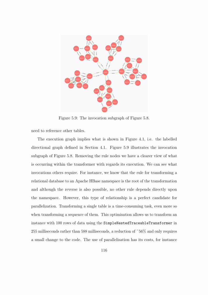
Figure 5.9: The invocation subgraph of Figure 5.8.
need to reference other tables.
The execution graph implies what is shown in Figure 4.1, i.e. the labelled
directional graph defined in Section 4.1. Figure 5.9 illustrates the invocation
subgraph of Figure 5.8. Removing the rule nodes we have a clearer view of what
is occurring within the transformer with regards its execution. We can see what
invocations others require. For instance, we know that the rule for transforming a
relational database to an Apache HBase namespace is the root of the transformation
and although the reverse is also possible, no other rule depends directly upon
the namespace. However, this type of relationship is a perfect candidate for
parallelization. Transforming a single table is a time-consuming task, even more so
when transforming a sequence of them. This optimisation allows us to transform an
instance with 100 rows of data using the SimpleNestedTraceableTransformer in
255 milliseconds rather than 588 milliseconds, a reduction of ~56% and only requires
a small change to the code. The use of parallelisation has its costs, for instance
116
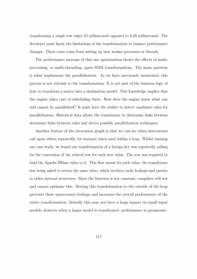
transforming a single row takes 23 milliseconds opposed to 6.29 milliseconds. The
developer must know the limitations of the transformation to balance performance
changes. These costs come from setting up new worker processes or threads.
The performance increase of this one optimisation shows the effects of multi-
processing, or multi-threading, upon M2M transformations. The main question
is what implements the parallelisation. As we have previously mentioned, this
process is not relevant to the transformation. It is not part of the business logic of
how to transform a source into a destination model. This knowledge implies that
the engine takes care of scheduling these. How does the engine know what can
and cannot be parallelised? It must have the ability to detect candidate rules for
parallelization. Historical data allows the transformer to determine links between
determine links between rules and derive possible parallelization techniques.
Another feature of the invocation graph is that we can see when invocations
call upon others repeatedly, for instance when used within a loop. Whilst running
our case study, we found our transformation of a foreign key was repeatedly calling
for the conversion of the related row for each new value. The row was required to
bind the Apache HBase value to it. This flaw meant for each value, the transformer
was being asked to return the same value, which involves cache lookups and queries
to other internal structures. Since the function is not constant, compilers will not
and cannot optimise this. Moving this transformation to the outside of the loop
prevents these unnecessary lookups and increases the overall performance of the
entire transformation. Initially this may not have a large impact on small input
models; however when a larger model is transformed: performance is paramount.
117
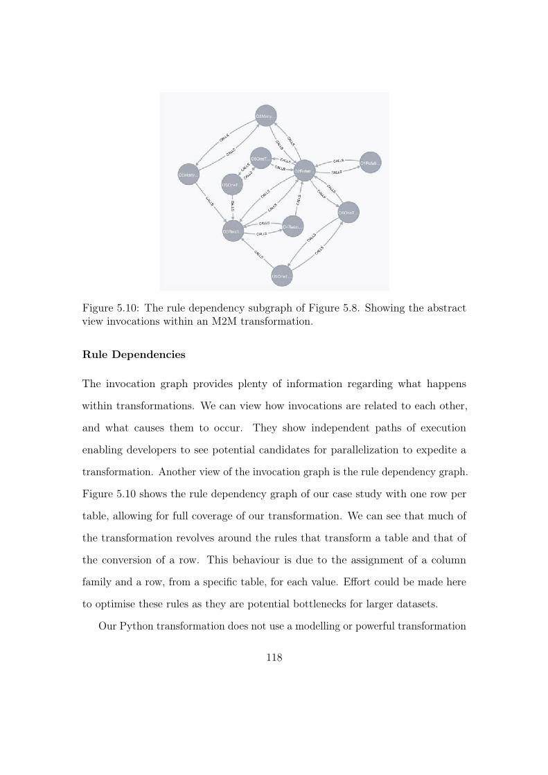
Figure 5.10: The rule dependency subgraph of Figure 5.8. Showing the abstractview invocations within an M2M transformation.
Rule Dependencies
The invocation graph provides plenty of information regarding what happens
within transformations. We can view how invocations are related to each other,
and what causes them to occur. They show independent paths of execution
enabling developers to see potential candidates for parallelization to expedite a
transformation. Another view of the invocation graph is the rule dependency graph.
Figure 5.10 shows the rule dependency graph of our case study with one row per
table, allowing for full coverage of our transformation. We can see that much of
the transformation revolves around the rules that transform a table and that of
the conversion of a row. This behaviour is due to the assignment of a column
family and a row, from a specific table, for each value. Effort could be made here
to optimise these rules as they are potential bottlenecks for larger datasets.
Our Python transformation does not use a modelling or powerful transformation
118
strategy, so it generates a heavily connected graph. To get a deterministic model,
no matter where in the model we start the conversion, we need to bind both sides
of a UML relationship. When using SiTra with plain old python objects (POPyO),
the conversion of the database must transform and add all of the tables into the
namespace’s list. The engine would not transform any tables if it were not for
this explicit call. Likewise, the transformation of a relational table into an Apache
HBase table requires the mapping of the relational table’s parent database to set
the HBase table’s namespace. Again, this explicit transformation will map the
database into a namespace if it has not already done so.
This approach applies to all transformation engines; however, it is possible to
forgo this when using a modelling framework as it will automatically modify the
attributes that represent the reverse of the relationship. Naturally, this makes the
transformation less general, and dependent on a modelling framework. OO2DB,
an example by Epsilon that we have previously looked at, applies this method.
When transforming a class into a table, it does not transform all of its columns.
Instead, it is up to the transformation of the column itself to set its parent. The
use of ECORE will automatically add it to the opposing side of the relationship.
This approach changes the dependency graph of the transformation. The mapping
of tables is dependent upon the conversion of a database; however, the reverse
is no longer true. The namespace no longer invokes, or recalls, the results of the
mapping of tables.
Another use of this graph is that it can show connected components. Connected
components in graph theory are subgraphs that are in isolation within a larger
graph. These are candidates for transformation upon different threads or even
machines due to their independence from the rest of the process.
119
5.7 Confidence within Model Transformation
In previous sections, we have benchmarked the effects of implementing our new
meta-model in two different M2M transformation engines, SiTra and the ETL. This
new meta-model allowed us to retain the full execution of a transformation, and to
capture objects instantiated within the binding phase. These mechanisms provide
full accountability as to why and how each object within the destination model
came to exist. This graph can be used to identify components for optimisation,
parallelisation and general debugging. For every transformation we make, we gain
more experience in the form of traces. These traces depicted the internal workings
of the engine and abstract from the source and result. This abstraction allows
us to discard the resultant models and focus on the events that occurred. These
invocation events can simply dictate that a type was transformed into another
type via a pathway. We persisted this information into a Neo4j instance, a graph
database, storing these traces for later analysis.
In this section, we use these previous graphs as a knowledge base to provide
some confidence in future transformations, by learning from experience. We use
a form of feature analysis to find traces that we have once seen before. Feature
analysis is a theory about how we as humans recognise certain patterns and shapes.
The theory dictates that our minds break down sensory information into features
and a comparison between that and what we have experienced previously evaluates
to whether we recognise the scene or not (see Section 2.4.3). We have explained
in Section 4.4 that there are two main components used to complete this task:
1) graph comparison: to determine how relevant previous trace executions are
concerning a new instance; and 2) a weighing mechanism based on the activities of
120
the result or the transformation to prevent prominence bias. The first represents
our recognition process of what we have seen before while the latter gives us more
information about how important individual features are.
Historic Prominence. If our knowledge base contains any applicable trace
instances, i.e. executions that are isomorphic or subgraph isomorphic to the new
input: how important are they in respect to the latest execution. Historical
prominence provides us with this information. These graphs come in varying sizes
and from different rule sets, so it stands to reason that only those that are of
equal size or less can be recognised. In the event of graph equality, the previous
transformation executed in the same manner as the latest, if that previous execution
was successful, then this is more relevant than a subgraph. However, in the event
of a smaller feature, a sub-graph, its prominence is lower. When we find subgraphs,
we are extracting features from the input. These characteristics cannot be larger
than the overall graph. If the feature is a negligible part of the transformation, then
it is of little importance for recognition. However, if we come across an execution
that closely resembles the input, then it has a higher value. If we were to have
many subgraphs that overlap, this increases the prominence of an invocation not
in the new transformation trace.
Labelling aids in reducing the workload for the NP-Complete task of sub-graph
isomorphism by reducing the possible permutations of vertices. We do not need to
look at graphs or sub-graphs that have rules that are not present in the new input,
as these cannot be isomorphic. Formally, we look for a historical entry h within
new graph G where there exists g ⊆ G such that g ' h. For g to be isomorphic to
121
h, and therefore sub-graph isomorphic to G, the label set of the candidate graph
must equal that of g and also be a subset of the whole graph. If ΣVh\ ΣVG
6= ∅
then h cannot be a subgraph of G as ΣVh' ΣVg ⊆ ΣVG
.
When found, these sub-graphs can be overlayed, creating a map of the transfor-
mation. In effect creating a heat-map of rule invocations, i.e. nodes with a higher
frequency. If this were to be inverted, then we would see cold spots concerning the
input. These areas are parts of the execution graph that we have less experience
with in respect to the rest. This experience relates to the confidence we have
with them, so we are less sure about the consequences of the result and thus less
confident in the final product. Looking at these allows us to focus efforts to mitigate
or accept the risks that are involved with these segments.
Weighing Mechanism. The prominence of previous transformation traces
only informs us that a sequence of events, invocation of transformation rules, has
occurred before. These invocations have done some work to generate the resultant
model. This task could be from: a) the transformation logic itself, or b) deferred
task. The first involves the rule specification and its logic, the rationale behind
the mapping of an object into another. This information can be measured by
the amount of validation it has had, or a complexity metric, like McCabe (1976).
The second would be similar to the first; however, it would focus on what was
next in the process specifically the use of the resultant model. For example, if the
resultant model was going to be used to generate code, i.e. there was a subsequent
model-to-text process, what does that code do? Does it interface with anything
of critical importance? Consider that the result of the transformation has some
122
interaction with a heart monitor, an infusion machine, a railway signalling system,
or the life support systems on the Hubble Space Telescope. If the generated
code were incomplete or incorrect: the use of the software could put lives at risk.
Including these risks into our metric prevents the bias of prominence, and rather
than treating all invocations as equal, we instead weigh down our level of confidence.
This approach is not too dissimilar to our interactions with technology. Take a car,
for example; we are more cautious with the response of the accelerator than the
volume control of its radio.
5.7.1 Applying our Metric on a Small Transformation
Our full case study involves the transformation of a relational database to that of
a non-relational database, specifically Apache HBase. The transformation itself
is defined in Section 5.3 and consists of several rules that map the source to the
destination including the structure and data of relational representation of data.
We have benchmarked the collation of a more verbose trace in Section 5.4 and
Section 5.5. Here we shall introduce the weighing mechanism used within our
algorithm, specifically McCabe’s cyclomatic complexity.
McCabe as a Complexity Metric
McCabe’s algorithm is used to determine the number of linearly independent
pathways within a graph, specifically within an execution graph. The core idea
behind this is to limit the complexity of modules within a code base. A higher value
is indicative of higher complexity, and therefore the module comes under scrutiny
as to why it is so complicated rather than breaking it down into smaller functions.
123
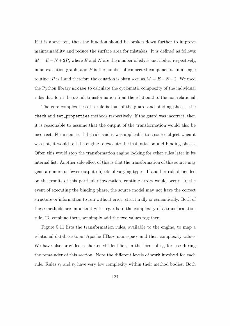
If it is above ten, then the function should be broken down further to improve
maintainability and reduce the surface area for mistakes. It is defined as follows:
M = E−N + 2P , where E and N are the number of edges and nodes, respectively,
in an execution graph, and P is the number of connected components. In a single
routine: P is 1 and therefore the equation is often seen asM = E−N +2. We used
the Python library mccabe to calculate the cyclomatic complexity of the individual
rules that form the overall transformation from the relational to the non-relational.
The core complexities of a rule is that of the guard and binding phases, the
check and set_properties methods respectively. If the guard was incorrect, then
it is reasonable to assume that the output of the transformation would also be
incorrect. For instance, if the rule said it was applicable to a source object when it
was not, it would tell the engine to execute the instantiation and binding phases.
Often this would stop the transformation engine looking for other rules later in its
internal list. Another side-effect of this is that the transformation of this source may
generate more or fewer output objects of varying types. If another rule depended
on the results of this particular invocation, runtime errors would occur. In the
event of executing the binding phase, the source model may not have the correct
structure or information to run without error, structurally or semantically. Both of
these methods are important with regards to the complexity of a transformation
rule. To combine them, we simply add the two values together.
Figure 5.11 lists the transformation rules, available to the engine, to map a
relational database to an Apache HBase namespace and their complexity values.
We have also provided a shortened identifier, in the form of ri, for use during
the remainder of this section. Note the different levels of work involved for each
rule. Rules r2 and r3 have very low complexity within their method bodies. Both
124
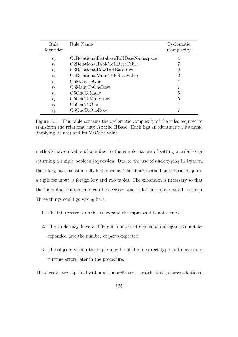
RuleIdentifier
Rule Name CyclomaticComplexity
r0 O1RelationalDatabaseToHBaseNamespace 4r1 O2RelationalTableToHBaseTable 7r2 O3RelationalRowToHBaseRow 2r3 O4RelationalValueToHBaseValue 2r4 O5ManyToOne 4r5 O5ManyToOneRow 7r6 O5OneToMany 5r7 O5OneToManyRow 5r8 O5OneToOne 4r9 O5OneToOneRow 7
Figure 5.11: This table contains the cyclomatic complexity of the rules required totransform the relational into Apache HBase. Each has an identifier ri, its name(implying its use) and its McCabe value.
.
methods have a value of one due to the simple nature of setting attributes or
returning a simple boolean expression. Due to the use of duck typing in Python,
the rule r9 has a substantially higher value. The check method for this rule requires
a tuple for input, a foreign key and two tables. The expansion is necessary so that
the individual components can be accessed and a decision made based on them.
Three things could go wrong here:
1. The interpreter is unable to expand the input as it is not a tuple.
2. The tuple may have a different number of elements and again cannot be
expanded into the number of parts expected.
3. The objects within the tuple may be of the incorrect type and may cause
runtime errors later in the procedure.
These errors are captured within an umbrella try . . . catch, which causes additional
125
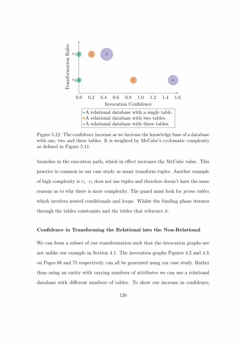
0.0 0.2 0.4 0.6 0.8 1.0 1.2 1.4 1.6
r0
r1
0
0
2
2
6
9
Invocation Confidence
Tran
sformationRules
A relational database with a single table.A relational database with two tables.A relational database with three tables.
Figure 5.12: The confidence increase as we increase the knowledge base of a databasewith one, two and three tables. It is weighted by McCabe’s cyclomatic complexityas defined in Figure 5.11.
branches in the execution path, which in effect increases the McCabe value. This
practice is common in our case study as many transform tuples. Another example
of high complexity is r1. r1 does not use tuples and therefore doesn’t have the same
reasons as to why there is more complexity. The guard must look for prime tables,
which involves nested conditionals and loops. Whilst the binding phase iterates
through the tables constraints and the tables that reference it.
Confidence in Transforming the Relational into the Non-Relational
We can form a subset of our transformation such that the invocation graphs are
not unlike our example in Section 4.1. The invocation graphs Figures 4.2 and 4.3,
on Pages 68 and 75 respectively, can all be generated using our case study. Rather
than using an entity with varying numbers of attributes we can use a relational
database with different numbers of tables. To show our increase in confidence,
126
we will initially describe our method using this, smaller, example using McCabe’s
weighing mechanism and the values in in Figure 5.11.
Figure 5.12 illustrates the progression of our metric against the rules they apply
to as the historical data set increases in size. Specifically, we use Figures 4.2a, 4.2b
and 4.3 to enhance our knowledge base incrementally and view our confidence in
their output. This bubble graph represents the distinct confidence values we have
for invocations in a new transformation concerning past transformations. The size
of each bubble is indicative of the number of instances of that value, however for
clarity, and due to the necessary limitations on the size of a bubble, the number
of instances appears within each point. The further to the right we move in the
graph the more confidence we have in that group of invocations that the bubble
represents.
No experience. Initially, we have no previous experience. There are no
models within our knowledge base and therefore no previous experience regarding
transforming the relational into the non-relational. Assume we transform a single
relational table into a single HBase table and a Column Family, which creates a
trace as per Figure 4.2a, we have nothing to compare. Thus we must complete
a form of validation on the resultant model before we deploy it to the next step.
Whether into another model transformation or possibly code generation. Our graph
illustrates this with the zero values for both rules. Assuming this is successful, we
deploy the resultant object and retain the trace within our dataset.
127
A Knowledgebase Containing a Database with a Single Table. We
now have one item within the knowledge base to use as our history. Given a
database with two tables, as per Figure 4.2b, and a knowledge base containing
Figure 4.2a, we can see two sub-graphs are isomorphic matches. r0 appears twice in
two separate graphs and r1 once for each table. Since the confidence value will be
the same for both instances of r1, we can group them. The number two within each
bubble illustrates this; there are two cases of this with a particular value. r1 has a
much lower confidence value as now the complexity of transforming columns and
constraints is taken into account. Despite having no columns or constraints, the rule
has this capability; therefore, the cyclomatic complexity still exists. Prominence
alone creates a disparity of 59.6% between the two rules; the complexity increases
this to 76.9%. Since we have only seen each of these twice we would consider more
validation and then if applicable, add this to our knowledge base.
Database with a single table and another with two tables. We now
have a knowledge base containing two traces. If we were to receive a new trans-
formation of a database with three tables: creating a trace as per Figure 4.3 on
Page 75. Six symmetric subgraphs are related to the first two: three against
Figure 4.2a and three against Figure 4.2b. When we consider symmetry in our
process, we only allow a subgraph to be considered once for a given set of vertices.
For example, assume the isomorphism between the new instance and Figure 4.2b.
Specifically the mapping of EtoTy → EtoTz, AtoCy0 → AtoCz0 , AtoCy1 → AtoCz1 .
We can see that the mappings of y0 and y1 are interchangeable. We disregard
this in a symmetric case. Once again r0 is in all instances as it is the root of all
128
transformations. Additionally, all invocations of table require the result of it to
maintain the heritage between tables and their database. r1, on the other hand,
has nine matches. Due to the underlying nature of the isomorphic graphs, all
invocations have the same value of confidence so we can group them. The weight
of r1 continues to weigh down the original value of prominence.
5.7.2 Introducing New Features with an Increasing Knowl-edge Base
The previous section discussed a small example showing the increase in confidence
as the knowledge base grew. However, the transformation traces were especially
small and unrealistic. Often an M2M transformation will consider a larger input,
in our case a few tables with varying columns and amounts of data. Using the
same incremental style, we enrol the full transformation of a relational database
into an Apache HBase namespace. Firstly we shall transform, separate tables with
different numbers of columns and rows, and then we shall include new rules that
resolve foreign key constraints.
Figure 5.13 illustrates the first phase of building confidence using separate and
unrelated tables. Here we can see the progression of trust in an M2M transformation
as the input size increases in various ways. Our knowledge base increases in size as
we continue to transform more input models and accept their result. Subsequent
models develop in structural complexity, i.e. we use more relational features, which
in turn increases the number of rule types that are utilised by the engine. Initially,
when we have one table and one column there is no experience to speak of, our
confidence is zero. We then introduce rows of data into it and increment the
129
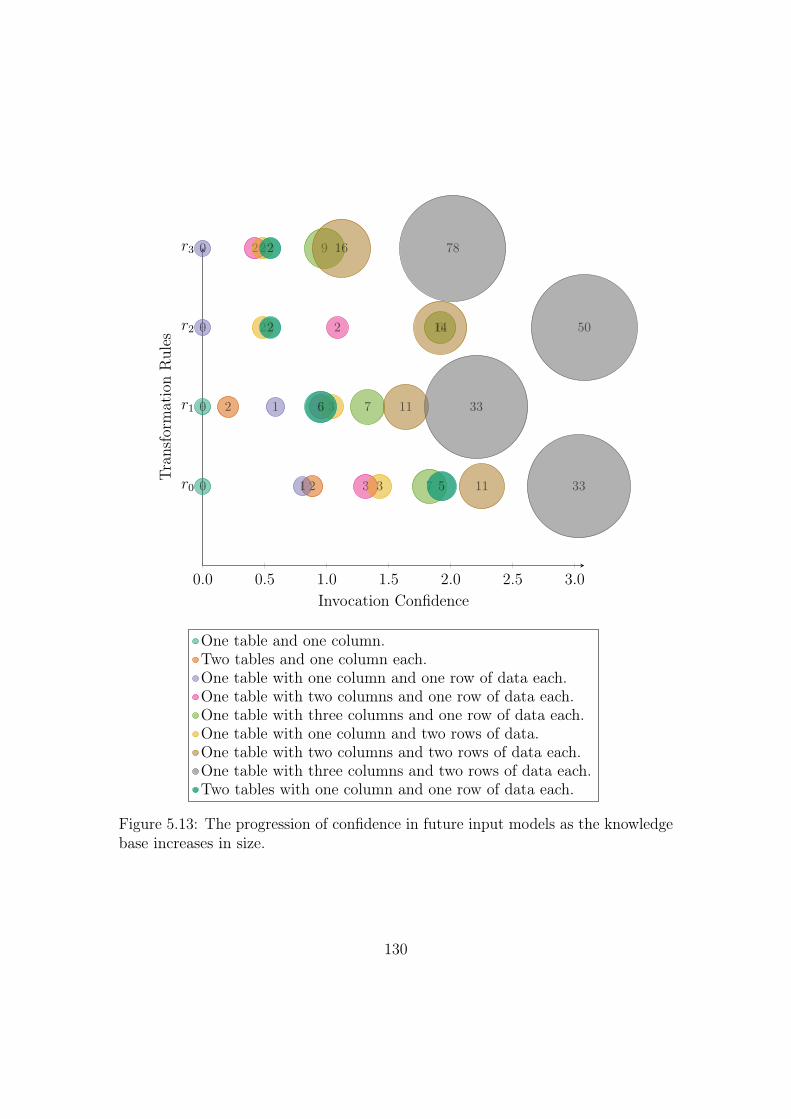
0.0 0.5 1.0 1.5 2.0 2.5 3.0
r0
r1
r2
r3
0
0
2
2
1
1
0
0
3
3
2
2
7
7
6
9
3
3
2
2
11
11
14
16
33
33
50
78
5
6
2
2
Invocation Confidence
Tran
sformationRules
One table and one column.Two tables and one column each.One table with one column and one row of data each.One table with two columns and one row of data each.One table with three columns and one row of data each.One table with one column and two rows of data.One table with two columns and two rows of data each.One table with three columns and two rows of data each.Two tables with one column and one row of data each.
Figure 5.13: The progression of confidence in future input models as the knowledgebase increases in size.
130
number of columns. The general trend of confidence is that the more times a node
appears in historical traces, the more confident we are. So we expect our trust in a
transformation to increase as we recognise more and more features of it.
Our test data was designed to increase linearly, such that our confidence would
rise as experience increases. However, this is not always the case. This graph also
shows a drop in trust when considering another dimension, the number of columns.
The test case of two tables with one column and one row of data each only matches
with the first three input models. Anything with more than one row or column
is not comparable due to the historical trace having more vertices labelled as r2
and/or r3:
{v | v ∈ V (h), l = `Vh(v) = ri} \ {v | v ∈ V (g), l = `Vg(v) = ri} 6= ∅ for i ∈ {2, 3}
Here we remark that there is a drop in confidence as we cannot reconcile much of
the graph in question.
Continuing this process, Figure 5.14 shows more transformations given the
previous data sets. In this instance, we transform models that related to more of
our knowledge base. Specifically, we introduce more inputs that contain two tables
and then create a new three table model. This incremental approach increases the
applicable historical traces that relate to the three table. We see that there is a
general increase in our confidence value as we see more and more matches in the
past set. However, there is a sudden decrease when we reach the last as there are
only five historic graphs that are relevant for analysis due to the reduction of rows
in each table.
Another key difference to note that there are more values per rule for a given
131
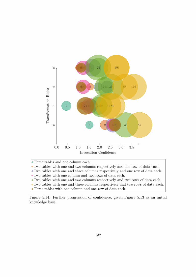
0.0 0.5 1.0 1.5 2.0 2.5 3.0 3.5
r0
r1
r2
r3
6
9
9
5 7
53
63
17
9 15
7 13
217
13
18
16
16
33
2129
24 36
2444
85
51 81
68 116
18668
13
21
9
9
Invocation Confidence
Tran
sformationRules
Three tables and one column each.Two tables with one and two columns respectively and one row of data each.Two tables with one and three columns respectively and one row of data each.Two tables with one column and two rows of data each.Two tables with one and two columns respectively and two rows of data each.Two tables with one and three columns respectively and two rows of data each.Three tables with one column and one row of data each.
Figure 5.14: Further progression of confidence, given Figure 5.13 as an initialknowledge base.
132
transformation. This trait occurs by the introduction of a variable number of
columns within tables. So far the input models have been symmetrical, and
therefore the confidence we have in invocations that use a particular rule has been
equal across the graph. We now have invocations of the same rule with multiple
confidence values. This result is due to the coverage of previous traces. For instance,
when looking at two tables with one and two columns respecively, we can only have
instances with one column apply to the first, while the opposing side can match
with those with one and two causing us to have a higher confidence in the second
table as more matches apply. Consider a knowledge base consisting of two traces
that have transformed the individual tables separately, i.e. a table with one column,
h0, and another with two, h1. Assuming that our new execution trace is composed
of them both g = h0 ∪ h1: since h0 ⊂ h1, all matches that relate to h1 will contain
matches of h0 too. Once more, since h1 is larger than h0, the reverse is not true
and results in different confidence values for those nodes.
These effects happen when we introduce brand new rules, i.e. new behaviour.
Figure 5.15 uses the same knowledge base as our previous examples; however this
time we introduce a one-to-many relationship between the two tables. We are yet
to have seen, test or investigate the results of this transformation. Thus we have
four zero points. This value is indicative of having no previous knowledge of a
subgraph that is smaller than the input graph invoking such a rule. These rules, r4,
r5, r6 and r7, all relate to the de-normalisation of either side of a one-to-many rule.
The graph then shows what happens if we see the same graph as an input, now it
has theoretically been tested and added to the database of historical traces. You’ll
notice that we now have an instance of each of those four rule types, allowing us to
determine whether we should continue or not. Since we only have one instance,
133
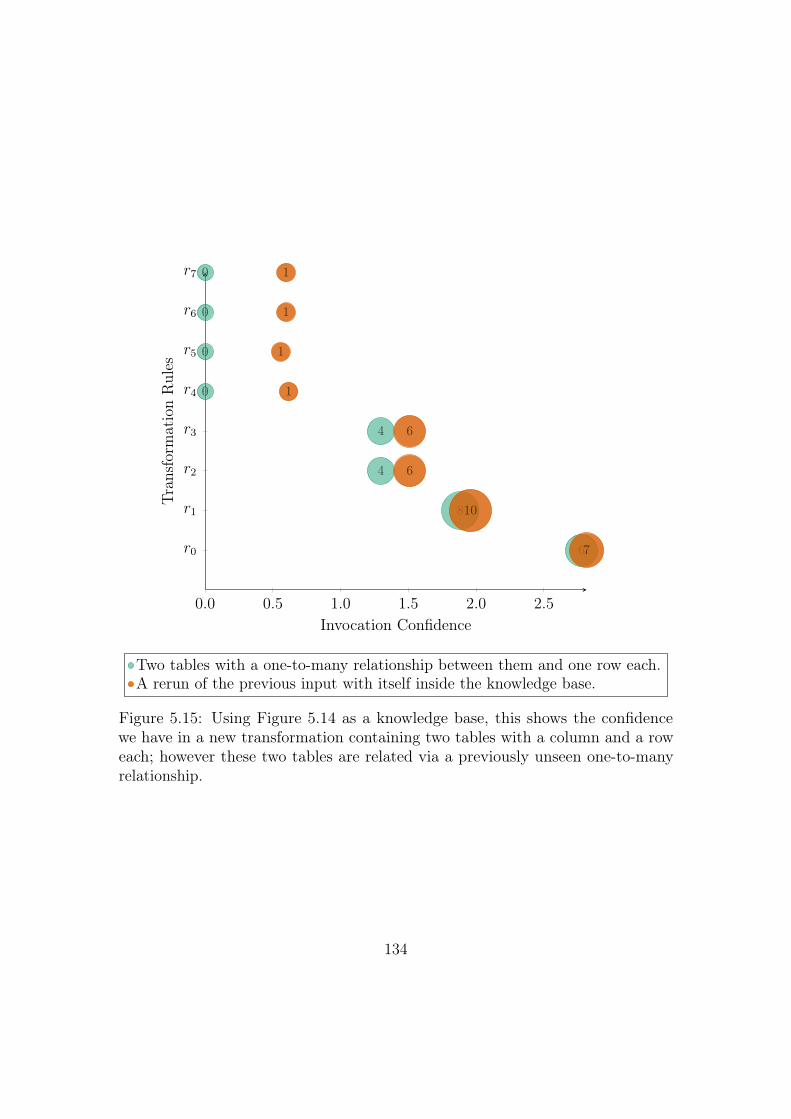
0.0 0.5 1.0 1.5 2.0 2.5
r0
r1
r2
r3
r4
r5
r6
r7
6
8
4
4
0
0
0
0
7
10
6
6
1
1
1
1
Invocation Confidence
Tran
sformationRules
Two tables with a one-to-many relationship between them and one row each.A rerun of the previous input with itself inside the knowledge base.
Figure 5.15: Using Figure 5.14 as a knowledge base, this shows the confidencewe have in a new transformation containing two tables with a column and a roweach; however these two tables are related via a previously unseen one-to-manyrelationship.
134
it would be more prudent to generate and test a succession of input models that
include this trait. In turn increasing the number of cases within the knowledge
base that become a subgraph of the input, thus improving their prominence and
confidence.
5.8 Chapter Summary
In showing benchmarks for both our meta-model and our new algorithm in SiTra
and ETL (see Sections 5.4 and 5.5), we have shown that collecting data regarding the
execution of a transformation is feasible within production environments. Therefore
the accountability of a transformation has been increased with minimal effects upon
performance. However, when capturing orphans ETL is the only engine of the two
that was able to complete this task acceptably. The effects to performance when
considering SiTra is exponential. This time increase is due to the generation of
proxies that recursively intercept new objects assigned to the target tree. Generally
speaking, processes such as this should be side-effect free. So we argue that while
this component is not of any use within a production environment, it is possible to
use it during development, to avoid the generation of orphans in the first place.
This approach would allow the user the efficiency of a simple Java-based engine
while training developers to evade making these kinds of rules.
Following this, we placed these traces into Neo4j, a graph-based database (see
Section 5.6). Here we formalised the transformation trace to define what nodes
and vertices would mean. We then show that we can use this graph for more than
confidence. The whole graph contains essential subgraphs that are vital for optimi-
sation of transformations. For instance, an invocation graph minus the rule nodes
135
can unravel a graph into subgraphs that are not backwards dependent: these are
candidates for parallelisation. Another example, it makes sense that an invocation
should only call upon another once and if this is not true there is an issue with
the calling rule. An instance of this appears in our transformation; we attempted
to transform an element within a loop. The input of this transformation did not
change, so the engine had to complete the same job (checking for applicable rules,
finding the result if it had been transformed before, transform it if not, and return
it). Moving this call outside of loop reduced the engine’s workload. Additionally,
the rule dependency graph can potentially detect connected components. The
independent graphs are indicative of independent transformations, which can be
cut down and potentially completed on other hardware.
Finally, we demonstrated the acquisition of confidence using our newly created
knowledge base (see Section 5.7). This process entailed running our case study
using our Python version of SiTra to transform instances of a relational database
that gradually increase in size and feature set, for instance, variations of singular
and multiple tables and columns, and table relationships. By phasing the process,
we were able to use smaller and less feature-rich samples to provide a knowledge
base that provides confidence in a new, more feature rich sample. We illustrated
this in a bubble graph where each bubble represents a distinct confidence value,
and its size represents the number of instances that value appears in the graph.
The larger the number of instances of a given value demonstrates the importance of
the overall graph of that particular type of invocation. If we had a low confidence
value and many of them, we would have noticeably low assurance in that group of
invocations for that transformation.
136
5.8.1 Testing Environment
A MacBook Pro 15” (Late 2013) with a 2.3GHz i7 and 16GB of RAM sequentially
executed our benchmark experiments. The machine was left alone until completion
or until it was deemed too infeasible to wait for the result. The latter was particularly
important when we consider the exponential effects of capturing orphans with
SiTra.
5.8.2 Validity of Experiments
Decision to use SiTra and ETL
We limited our evaluation to using SiTra and ETL due to the availability of the trace
in rule-based M2M transformation engines. As we have discussed in Section 2.3.3,
there are two types of trace: internal and external, and only the latter makes
the associations available to post-mortem processes. The ATLAS Transformation
Language (ATL) (Jouault et al. 2008) and Operational Query/View/Transform
(QVT-O) (Object Management Group, Inc. 2016a) both use an internal trace. It is
questionably possible to access the trace from QVT-O; however, it uses an API
that has restricted access. This access requirement informs us that it is meant
to be for internal use only, and therefore we did not want to tamper with it, as
we were unsure as to how it would affect the engine’s internals. Additionally, our
previous work heavily involved SiTra, so implementation and porting to Python
was a relatively simple task. We also had some support from the ETL community
that allowed us to know how ETL worked and how we might inject our trace
meta-model safely. Even with these two engines, we have shown some generality
137
for those wishing to implement our algorithm into their engines.
We attempted to use Xtend (Eclipse Foundation 2014), however, this was simply
a declarative Java language with inbuilt templating. Thus, Xtend has no natural
transformation engine or scheduler. The development of this is out of the scope of
our work and would have virtually recreated SiTra, as that is what we know! The
only additional feature would have been the ability to use polymorphic dispatch.
This functionality allows a specific method for each sub-class without the need of
a visitor pattern or multiple rules: a feature unavailable in Java. The benefits of
this are minute when we consider that the guard will become more complicated
as to allow for all instances where it is applicable. One would have to determine
what was better for the process: inheritance or the visitor pattern. We believed,
based on the fact we were using object orientation, inheritance was a better choice,
which in turn just recreated SiTra.
Comparion between SiTra and ETL
The biggest factor threatening the validity of our comparison between the results
of SiTra and ETL was the way in which ETL executes. Due to the executable
abstract syntax tree, we were unable to reuse the result of parsing an ETL script.
The effect of this was that for each iteration, we needed to read the ETL script and
clean up each time. This interaction with I/O can be variably affected by other
system processes that we attempted to minimise, power saving, system updates, etc.
Rules for SiTra, on the other hand, were purely written in its native programming
language: Python or Java. Thus rules were present for subsequent transformations,
and no more I/O was involved as they were already in memory. To make the
138
comparison valid, we used a new instance of the SiTra transformer as to start afresh
for each transformation. Creating the new instances would involve reinitialising the
rules used, the caches and traces. Using a specialised ClassLoader in the event of
Java, or using reload to reload the Python module containing the rules, would
induce a certain level of I/O variability to the process. At this point, we felt that
altering how the JVM or the Python interpreter loaded and unloaded class and
modules would again introduce more variability, so we chose to continue without
this.
139
CHAPTER 6
SUMMARY, DISCUSSION AND CONCLUSION
6.1 Summary
We presented an approach to quantify confidence in a model-to-model (M2M) trans-
formation based upon previous executions, specifically combining the validation
Oracle, model-snippets, and a theory of how humans recognise objects. We investi-
gated issues within the current state-of-the-art in rule based M2M transformation.
This research uncovered some problems that, for full assurance, needed to be fixed
to provide full accountability of all resultant objects. We introduced a general
algorithm to resolve these issues and demonstrated these in two transformation
engines, the Simple Transformer (SiTra) and the Epsilon Transformation Language
(ETL). From the point of full coverage, we were then able to store traces into
a database to form a knowledge base of what we have seen before. Basing our
comparison on the execution itself opposed to the resultant model allowed us to
look for features within a path and provide information based on coverage. We
generate a heat map over a new trace to view components that we have experienced
140
before, inverting this gives us information about items that we have no or less
experience. This process, however, was biased as it treated every invocation of a
rule as equal, which is not true. Our method then incorporated a mechanism to
weigh down, or even up, the value of a node based on the complexity of the rule
itself and its place in the transformation.
Our work has made the following contributions:
• An investigation into traceability within M2M transformation and the identi-
fication of elements that prevent full accountability, namely orphans and the
use of an inappropriate structure.
• The design of a general algorithm to maintain a full trace to provide account-
ability.
• A full implementation of SiTra that addresses these issues and a quantitative
analysis of its drawbacks with regards to performance.
• To demonstrate the independence of our approach, we have written an
extension of ETL that also maintains a full trace and quantitatively analysed
its performance.
• A qualitative analysis of how one might learn from previous experience
regarding M2M transformation.
• A toolset that enables a trace to be persisted into a knowledge base and
later analysed for comparison to new transformations to aid in the quick
deployment of resultant models based on previous experience.
141
6.2 Discussion
The primary contributions of this thesis are the introduction of a new meta-model
for traceability within M2M transformation (see Figure 3.7) and a general algorithm
for collecting information about the execution of a transformation (see Algorithm 1).
We introduced mechanisms to collect objects that were not created by the engine
(see Sections 3.2.2 and 3.3.2). Then with the complete transformation trace, we
were able to develop a metric to determine how much of a transformation we
recognise from previous experience (see Chapter 4).
Our algorithm and meta-model provides an implementation independent ap-
proach to be used in many M2M transformation engines that have problems with
side-effects and the lack of information within their own trace system. These come
in the form of imperative or hybrid languages that are not specific to transforma-
tion and allow global state, such as Operational Query/View/Transform (QVT-O),
SiTra and ETL (Saxon, Bordbar, and Akehurst 2015). With this meta-model, rule
dependencies can be derived, assuming full code coverage, enabling the possibilty
of incremental transformations. This dependency information allows us to see what
transformed a source and then what that transformation called, enabling the engine
to re-transform any subsequent rules. Once the rule dependency structure is known,
it is also possible to parallelise rule types depending their interactions. This time
we must assume that the source model is fixed and is not going to change during
the transformation itself.
Naturally, we can store more than just the invocation information. We can
actually store the source and target information too. This enables us to view chains
of transformations, i.e. the result of one going into another. When using ETL, the
142
context is only relevant to one transformation, which in turn is assigned to a script.
We had issues when testing the performance of our approach as we were unable to
reuse transformers so our tests included the I/O required to open and close the
the ETL scripts themselves. However, if this is true, it means a context cannot
be related to another and therefore relationships between them must be derived.
The ATLAS Transformation Language (ATL) also requires a re-initialise before
continuing with another transformation. However, our implemenation of SiTra
allows us to change the rule set and then transform again using the same context
and therefore retain the entire transformation. This ability enables us to store the
source and target models, whilst at the same time automatically connecting the
links between chained transformations.
The additonal work load in collecting this information is, for SiTra, on average
6% with a worst case of upto 10%. However, transforming 55k objects into 138k
objects took around 6.3s opposed to 6s (see Section 5.4). In the greater scheme
of transformation this performance hit is manageable for most transformations.
However, when we include the orphans it increases exponentially. We shall explain
more on this in the next section. Whereas our addition to ETL increases the overall
throughput by 26.51%. Consider that the use of this framework decreases the
performance by around 258% when compared to SiTra before retaining any more
information than a linear trace. The inclusion of ophans is an important point
though, it rises linearly and is only an extra 6.36% on average (see Section 5.5). It
is up to the developer whether, they need to be nearer the processor or whether
they can accept higher thoughputs for the convenience a framework like Epsilon
suppies.
The previous work allows us to have complete accountability within M2M
143
transformation. Without this we would not necessarily know what caused an
invocation of a rule to begin with, or how the transformer completed its task.
Additionally, the target model may contain elements that cannot be reversed back
to the source; an object with an existential crisis, with no reason to be. Now we
can see the entire transformation we can compare it to previous invocations to
learn from past experience. Our system can quantify how much of a execution
graph it has seen before by overlaying the old over the new creating a heat map
of a transformation, taking into account the differences in size of the historic to
the new (see Section 4.3). It does this by associating information to each node
within the latest execution path from each historial path. To avoid bias we have
provided a mechanism to weight up or down a rule invocation (see Section 4.4).
Validating this by using McCabe’s cyclomatic complexity, showing that not all rule
invocations are equal (see Section 5.7.1). This is a general function pointer, taking
in a rule and returning its weight and is customisable for different algorithms.
6.2.1 Weaknesses
A fundamental issue with our approach is that sub-graph isomorphism is NP-
Complete (or more specifically, it is NP-Complete when there are no labels or when
repeated labels are present). That is the solution is difficult to discover, however,
once found is easy to verify. This trait is proven by the clique problem and the
Hamiltonian cycle problem (Cook 1971; Karp 1972). This obstacle results in an
exponential amount of work finding matches, per historical trace. Our framework
currently doesn’t do anything to reduce this. Due to the way our graphs are stored,
in Neo4j, labels are indexed within the database engine. It would be more prudent
144
to narrow down the number of candidate graphs before passing them over the
network. We have already discussed in Section 5.7 that we need only involve graphs
that are less than or equal to the size of the new graph G, use a subset of the rules
that were used and have no more instances of those rules than those in G. More
formally, where we have a new trace G = 〈V,E, `V , `E, ι〉 and a historical trace
h = 〈V ′, E ′, `′V , `′E, ι
′〉, we only require it for comparison if |VG| ≥ |Vh|, `′V \ `V = ∅
and ∀l ∈ `′V , |{v | v ∈ V, `V (v) = l}| ≥ |{v | v ∈ V ′, `′V (v) = l}| for all historical
traces in the system. This reduction could substantially reduce the number of
candidates delivered from the database engine preventing unnecessary comparisons
and network traffic.
Additionally, performance increases may be achievable using other sub-graph
isomorphism techniques. Bonnici et al. (2013) introduced a method that creates a
search tree, not unlike VF2, however, reorders the search tree based on fast and
straightforward heuristics to prune options earlier in the proceedings. The process
reorders the search tree such that nodes with the most-constraints fail-first (Bonnici
and Giugno 2017). Using the fail-first principle stops the traversal earlier, opposed
to the general brute force or look-ahead methods. We were unable to test this
approach as there was no viable method to use it within our framework. To allow
this, we would need to implement this method in Java or Python to work with our
current toolset. However, performance increases in subgraph-isomorphism may be
negligible within small transformations, as shown by Carletti, Foggia, and Vento
(2013).
Another key area of weakness is that of orphan capture, as described in Sec-
tion 3.2.2. The approach for our engine, SiTra, increases exponentially as the input
increases. The effects are manageable for smaller transformations; however, the
145
more invocations that occur time will become an issue. This problem comes from
intercepting all accessor and mutator methods to proxy the inputs and outputs to
capture what we have not seen before. We are increasing the workload for simple
getter and setters quite substantially. The engine needs to know whether the input
of a setter came from any previous rule invocations as well as the orphans created
by them. By this point, the trace could be massive. A way we could get around
this is to, once we have found an orphan is to keep a mapping of it to the invocation
that created it, but where do we stop caching? The more we cache, the more
memory the engine needs. Despite ETL having longer response times, they are
at least linear when capturing orphans. The executable abstract syntax tree that
ETL uses captures the new keyword and only needs to retain the object. This is
because the object is an orphan at this point, the engine did not create it, and
therefore can blindly be preserved. A framework specific version of SiTra would
be able to use meta-modelling observer patterns. For example, if one were to use
EMF we could use the notification adapters that it implements to track setters to
find orphans. It would also enable us to traverse with ease into new objects via
their tree iterable.
Our approach also only looks at good trace elements. That is the knowledge
base contains transformation traces that are deemed to have been successful in
deployment. It does not include times where they did not work. An extension
of our framework could include the ability to use anti-trace patterns. A way of
negating the cumulative effect of the transformation trace. This consequence would
occur when a trace has not completed its task correctly. However, for this to work
rules would have to be versioned as it would be unrealistic to expect brand new
transformation rules for every bug discovered. An inclusion of a version number
146
in the graph labelling would enable the engine to distinguish the variety of rules.
An argument against this is the increase in graphs within the knowledge base,
increasing the number of candidate graphs to analyse.
Another drawback is that it does not take into account rule maintenance or the
fact that software progresses. The way we label our rules is using its name, it would
be more prudent to add a version string to it. This addition would automatically
ignore all previous traces that include older versions for comparison as the label
would differ. Therefore pruning the potential list of traces that apply to the new
transformation. A further idea may include the ability to specify a range of possible
versions for comparison. However, the matching technique would become more
complicated due to the additional pruning code required. Additionally, as software
progresses rapidly, traces may become irrelevant and numerous quite quickly. A
consideration to evade this would be to have a sliding window of traces that makes
traces obsolete after a period. How much time may depend on the frequency of
transformations and the development of the rules required and thus would be
dependent upon the domain in question.
Our work was only evaluated using one simulated domain, the transformation
of a relational database into a non-relational database, specifically Apache HBase.
However, this transformation had all of the hallmarks that we have defined in
Section 3.1 and since the move to big data is becoming prominent, we felt that
this was a good demonstration of both capturing trace data and making sure that
the data is in good shape afterwards. A continuation of this work should revisit
our assumptions about transforming relationships and possibly create a library
to enable others to migrate their data to test our framework in a real setting.
Additionally, other domains should be investigated. In our view the future of our
147
work could be extended in a few ways:
• Investigation of new matching techniques — this may include new heuristics
to reduce the number of graphs to check or other ways to compare the graphs.
• The use within other domains — initial efforts were on transforming a DSL
to describe the symptomatic behaviour of malware into C code to find them;
however, the transformation albeit not simple in regards to the binding phase,
it was regarding the invocation of the transformation. It was also very orphan
intensive, which started our research into that area.
• Investigate anti-trace patterns — currently we know what worked well, but if
something ceased to work: what should we do next?
• How to interact with this information — currently we have a bubble graph
to show the values about the rules in question. Depending on the size of the
transformation, a navigable graph might be better placed to allow us to see
exactly where the cold spots are.
• Parsing and code generation — we have the information for many levels of
M2M transformations, however in the event of text-to-model, we have no
knowledge of what part of the AST caused the source to exist. Likewise, with
model-to-text, what source becomes part of the final AST?
• Handle evolving transformation rules and software systems — our process
currently uses all historic traces and does not take into account rule versioning.
Naturally as software progresses legacy traces should be pruned, and as rules
are modified previous versions should be deprecated.
148
6.3 Conclusion
Verification and validation are common methods to make sure that something
works as intended, however, sometimes these mechanisms are time-consuming and
can be too complex to be feasible. We have looked into using traceability to provide
information to focus validation efforts or to give developers the ability to mitigate
risk based on previously deployed instances. Systems like this could be used to
expedite the development process when needed, for instance, when migrating large
amounts of data or generating low-level, mission critical code. We hope that we
have introduced work and ideas to provide a base for future development.
149
REFERENCES
“Advanced Traceability for ATL”. In:
Aizenbud-Reshef, N., B. T. Nolan, J. Rubin, and Y. Shaham-Gafni (2006). “Model
Traceability”. In: IBM Syst. J. 45.3, pp. 515–526. issn: 0018-8670. doi: 10.
1147/sj.453.0515. url: http://dx.doi.org/10.1147/sj.453.0515.
Akehurst, D. H., B. Bordbar, M. J. Evans, W. G. J. Howells, and K. D. McDonald-
Maier (2006). “SiTra: Simple Transformations in Java”. In: Proceedings of the
9th International Conference on Model Driven Engineering Languages and
Systems. MoDELS’06. Genova, Italy: Springer-Verlag, pp. 351–364. isbn: 3-
540-45772-0, 978-3-540-45772-5. doi: 10 . 1007 / 11880240 _ 25. url: http :
//dx.doi.org/10.1007/11880240_25.
Beazley, D. (2010). Understanding the python GIL. url: http://www.dabeaz.
com/python/UnderstandingGIL.pdf.
Berry, D. M. (2014). Critical theory and the digital. Critical Theory and Contem-
porary Society. Bloomsbury Publishing USA. isbn: 9781441118301.
Biederman, I. (1987). “Recognition-by-components: a theory of human image
understanding.” In: Psychological review 94.2, p. 115. doi: 10.1037/0033-
295X.94.2.115.
150
Bonnici, V. and R. Giugno (2017). “On the Variable Ordering in Subgraph Isomor-
phism Algorithms”. In: IEEE/ACM Transactions on Computational Biology
and Bioinformatics 14.1, pp. 193–203. issn: 1545-5963. doi: 10.1109/TCBB.
2016.2515595.
Bonnici, V., R. Giugno, A. Pulvirenti, D. Shasha, and A. Ferro (2013). “A subgraph
isomorphism algorithm and its application to biochemical data”. In: BMC
bioinformatics 14.7. doi: 10.1186/1471-2105-14-S7-S13.
Briand, L., D. Falessi, S. Nejati, M. Sabetzadeh, and T. Yue (2014). “Traceability and
SysML Design Slices to Support Safety Inspections: A Controlled Experiment”.
In: ACM Trans. Softw. Eng. Methodol. 23.1, 9:1–9:43. issn: 1049-331X. doi:
10.1145/2559978. url: http://doi.acm.org/10.1145/2559978.
Carletti, V., P. Foggia, and M. Vento (2013). “Performance Comparison of Five
Exact Graph Matching Algorithms on Biological Databases”. In: New Trends
in Image Analysis and Processing – Proceeedings of International Conference
on Image Analysis and Processing 2013. Ed. by A. Petrosino, L. Maddalena,
and P. Pala. Berlin, Heidelberg: Springer Berlin Heidelberg, pp. 409–417. isbn:
978-3-642-41190-8. doi: 10.1007/978- 3- 642- 41190- 8_44. url: https:
//doi.org/10.1007/978-3-642-41190-8_44.
Carrillo, H. and David Lipman (1988). “The Multiple Sequence Alignment Problem
in Biology”. In: SIAM Journal on Applied Mathematics 48.5, pp. 1073–1082.
doi: 10.1137/0148063.
Casters, M., R. Bouman, and J. van Dongen (2010). Pentaho Kettle solutions:
building open source ETL solutions with Pentaho Data Integration. John Wiley
& Sons. isbn: 978-0-470-63517-9.
151
Chang, F., J. Dean, S. Ghemawat, W. C. Hsieh, D. A. Wallach, M. Burrows, T.
Chandra, A. Fikes, and R. E. Gruber (2008). “Bigtable: A Distributed Storage
System for Structured Data”. In: ACM Trans. Comput. Syst. 26.2, 4:1–4:26.
issn: 0734-2071. doi: 10.1145/1365815.1365816. url: http://doi.acm.
org/10.1145/1365815.1365816.
Chappell, D. (2004). Enterprise service bus. O’Reilly Media, Inc. isbn: 978-
0596006754.
Clinical Data Interchange Standards Consortium (2013). Specification for the
Operational Data Model (ODM). url: https://www.cdisc.org/standards/
transport/odm (visited on 04/21/2017).
National Information Assurance (IA) Glossary. Vol. 4009. url: http://www.ncix.
gov/publications/policy/docs/CNSSI_4009.pdf (visited on 11/15/2013).
Cook, Stephen A. (1971). “The Complexity of Theorem-proving Procedures”. In:
Proceedings of the Third Annual ACM Symposium on Theory of Computing.
STOC ’71. Shaker Heights, Ohio, USA: ACM, pp. 151–158. doi: 10.1145/
800157.805047. url: http://doi.acm.org/10.1145/800157.805047.
Czarnecki, K. and S. Helsen (2006). “Feature-based Survey of Model Transformation
Approaches”. In: IBM Syst. J. 45.3, pp. 621–645. issn: 0018-8670. doi: 10.1147/
sj.453.0621. url: http://dx.doi.org/10.1147/sj.453.0621.
Ebner, G. and H. Kaindl (2002). “Tracing all around in reengineering”. In: IEEE
Software 19.3, pp. 70–77. issn: 0740-7459. doi: 10.1109/MS.2002.1003459.
Eclipse Foundation (2014). Xtend. url: http://www.eclipse.org/xtend/ (visited
on 03/04/2015).
Falleri, J., M. Huchard, and C. Nebut (2006). “Towards a Traceability Framework for
Model Transformations in Kermeta”. In: ECMDA-TW’06: ECMDA Traceability
152
Workshop. Ed. by J. Aagedal, T. Neple, and J. Oldevik. Bilbao, Spain: Sintef
ICT, Norway, pp. 31–40. url: https://hal-lirmm.ccsd.cnrs.fr/lirmm-
00102855.
Fritzsche, M., J. Johannes, S. Zschaler, A. Zherebtsov, and A. Terekhov (2008).
“Application of Tracing Techniques in Model-Driven Performance Engineering”.
In: ECMDA Traceability Workshop Proceedings, pp. 111–120. isbn: 978-82-14-
04396-9.
Galvao, I. and A. Goknil (2007). “Survey of Traceability Approaches in Model-
Driven Engineering”. In: 11th IEEE International Enterprise Distributed Object
Computing Conference (EDOC 2007), pp. 313–313. doi: 10.1109/EDOC.2007.
42.
GAMP (2008). GAMP R©5: A Risk-Based Approach to Compliant GxP Computerized
Systems. Tech. rep. International Society for Pharmaceutical Engineering.
Goncalves, A. (2013). Beginning Java EE 7. Books for professionals by professionals.
Apress. isbn: 978-1430246268.
Handbook, Electronic Reliability Design (1982). “MIL-HDBK-338B, October 1998”.
In: Robert G. Arno received his BS in Electrical Engineering from State Univer-
sity of New York at Utica/Rome in.
Harrison, K., B. Bordbar, S. T. T. Ali, C. I. Dalton, and Norman. A. (2012). “A
Framework for Detecting Malware in Cloud by Identifying Symptoms”. In: 2012
IEEE 16th International Enterprise Distributed Object Computing Conference,
pp. 164–172. doi: 10.1109/EDOC.2012.27.
Hibernate. Hibernate ORM. url: http : / / hibernate . org / orm/ (visited on
04/11/2017).
153
“IEEE Trial-Use Standard–Adoption of ISO/IEC TR 15026-1:2010 Systems and
Software Engineering–Systems and Software Assurance–Part 1: Concepts and
Vocabulary” (2011). In: IEEE Std 15026-1-2011, pp. 1–114.
Jouault, F., F. Allilaire, J. Bézivin, and I. Kurtev (2008). “ATL: A model transforma-
tion tool”. In: Science of Computer Programming 72.1. Special Issue on Second
issue of experimental software and toolkits (EST), pp. 31–39. issn: 0167-6423.
doi: 10.1016/j.scico.2007.08.002. url: http://www.sciencedirect.
com/science/article/pii/S0167642308000439.
Jouault, Frédéric (2005). “Loosely coupled traceability for ATL”. In: Proceedings of
the European Conference on Model Driven Architecture (ECMDA) Workshop
on Traceability. Nuremberg, Germany, pp. 29–37. isbn: 82-14-03813-8.
Karp, R. M. (1972). “Reducibility among Combinatorial Problems”. In: Complexity
of Computer Computations: Proceedings of a symposium on the Complexity
of Computer Computations. Ed. by R. E. Miller, J. W. Thatcher, and J. D.
Bohlinger. Boston, MA: Springer, pp. 85–103. isbn: 978-1-4684-2001-2. doi:
10.1007/978-1-4684-2001-2_9. url: https://doi.org/10.1007/978-1-
4684-2001-2_9.
Kawaguchi, K, S. Vajjhala, and J. Fialli (2009). The JavaTMArchitecture for XML
Binding (JAXB) 2.2. url: https://jcp.org/en/jsr/detail?id=222 (visited
on 04/11/2017).
Kessentini, M., H. Sahraoui, and M. Boukadoum (2011). “Example-based model-
transformation testing”. In: Automated Software Engineering 18.2, pp. 199–224.
issn: 1573-7535. doi: 10.1007/s10515-010-0079-3. url: https://doi.org/
10.1007/s10515-010-0079-3.
154
Khan, Y. A. and M. El-Attar (2016). “Using model transformation to refactor use
case models based on antipatterns”. In: Information Systems Frontiers 18.1,
pp. 171–204. doi: 10.1007/s10796-014-9528-z. url: http://dx.doi.org/
10.1007/s10796-014-9528-z.
Kolovos, Dimitrios S., Richard F. Paige, and Fiona A. C. Polack (2008). “The Epsilon
Transformation Language”. In: Theory and Practice of Model Transformations:
First International Conference, ICMT 2008, Zürich, Switzerland, July 1-2, 2008
Proceedings. Ed. by Antonio Vallecillo, Jeff Gray, and Alfonso Pierantonio. Berlin,
Heidelberg: Springer Berlin Heidelberg, pp. 46–60. isbn: 978-3-540-69927-9.
doi: 10.1007/978-3-540-69927-9_4. url: https://doi.org/10.1007/978-
3-540-69927-9_4.
Komaroff, M. and K. Baldwin (2005). DoD Software Assurance Initiative. url:
https://acc.dau.mil/adl/en-US/25749/file/3178/DoD/SW/Assurance/
Initiative.pdf (visited on 11/15/2013).
Kusel, A., J. Etzlstorfer, E. Kapsammer, P. Langer, W. Retschitzegger, J. Schoen-
boeck, W. Schwinger, and M. Wimmer (2013). “A Survey on Incremental Model
Transformation Approaches”. In: ME 2013 – Models and Evolution Workshop
Proceedings. Miami, Florida (USA), pp. 2–11.
M., Harman, M. Munro, Lin Hu, and Xingyuan Zhang (2001). “Side-effect re-
moval transformation”. In: Proceedings 9th International Workshop on Program
Comprehension. IWPC 2001, pp. 310–319. doi: 10.1109/WPC.2001.921741.
Ma, K., B. Yang, and A. Abraham (2016). “Asynchronous data translation frame-
work for converting relational tables to document stores”. In: International Jour-
nal of Computers and Applications 38.1, pp. 19–28. doi: 10.1080/1206212X.
2016.1188563. eprint: http://www.tandfonline.com/doi/pdf/10.1080/
155
1206212X.2016.1188563. url: http://www.tandfonline.com/doi/abs/10.
1080/1206212X.2016.1188563.
McCabe, T. J. (1976). “A Complexity Measure”. In: IEEE Transactions on Software
Engineering SE-2.4, pp. 308–320. issn: 0098-5589. doi: 10.1109/TSE.1976.
233837.
Mottu, J. M., B. Baudry, and Y. Le Traon (2008). “Model transformation testing:
oracle issue”. In: 2008 IEEE International Conference on Software Testing
Verification and Validation Workshop, pp. 105–112. doi: 10.1109/ICSTW.2008.
27.
NASA (2005). Software Assurance Standard, NASA-STD-8739.8 w/Change 1. Tech.
rep. National Aeronautics and Space Administration. url: http://www.hq.
nasa.gov/office/codeq/software/index.htm.
Object Management Group, Inc. MDA Specifications. url: http://www.omg.org/
mda/specs.htm (visited on 04/08/2017).
— (2005). A White Paper on Software Assurance. Tech. rep. Object Management
Group, Inc. url: http://swa.omg.org/docs/softwareassurance.v3.pdf.
— (2008). MOF Model to Text Transformation Language, v1.0. url: http://www.
omg.org/spec/MOFM2T/1.0/ (visited on 04/21/2017).
— (2016a). Meta Object Facility (MOF) 2.0 Query View Transformation Speci-
fication Version 1.3. url: http://www.omg.org/spec/QVT/1.3/ (visited on
04/10/2017).
— (2016b). Meta Object FacilityTM(MOFTM) Version 2.5.1. url: http://www.
omg.org/spec/MOF/2.5.1/ (visited on 04/10/2017).
156
Paige, R. F., G. K. Olsen, D. Kolovos, S Zschaler, and C. D. Power (2010). “Building
Model-Driven Engineering Traceability Classifications”. In: Sintef, p. 49. url:
http://eprints.whiterose.ac.uk/109242/.
SAE International (2013). Serial Control and Communications Heavy Duty Vehicle
Network - Top Level Document. url: https://saemobilus.sae.org/content/
J1939_201308 (visited on 04/21/2017).
SAFECode (2008). Software Assurance: An Overview of Current Industry Best
Practices. Tech. rep. SAFECode.
Sanders, G. L. and Seungkyoon Shin (2001). “Denormalization effects on perfor-
mance of RDBMS”. In: Proceedings of the 34th Annual Hawaii International
Conference on System Sciences, 9 pp.–. doi: 10.1109/HICSS.2001.926306.
Saxon, J. T., B. Bordbar, and D. H. Akehurst (2015). “Opening the Black-Box
of Model Transformation”. In: Modelling Foundations and Applications: 11th
European Conference, ECMFA 2015, Held as Part of STAF 2015, L‘Aquila,
Italy, July 20-24, 2015. Proceedings. Ed. by G. Taentzer and F. Bordeleau.
Springer International Publishing, pp. 171–186. isbn: 978-3-319-21151-0. doi:
10.1007/978-3-319-21151-0_12.
Saxon, J. T., B. Bordbar, and K. Harrison (2015a). “Efficient Retrieval of Key
Material for Inspecting Potentially Malicious Traffic in the Cloud”. In: 2015
IEEE International Conference on Cloud Engineering, pp. 155–164. doi: 10.
1109/IC2E.2015.26.
— (2015b). “Introspecting for RSA Key Material to Assist Intrusion Detection”.
In: IEEE Cloud Computing 2.5, pp. 30–38. issn: 2325-6095. doi: 10.1109/MCC.
2015.100.
157

Shah, S. M. A., K. Anastasakis, and B. Bordbar (2010). “From UML to Alloy and
Back Again”. In: Models in Software Engineering: Workshops and Symposia at
MODELS 2009, Denver, CO, USA, October 4-9, 2009, Reports and Revised
Selected Papers. Ed. by S. Ghosh. Berlin, Heidelberg: Springer Berlin Heidelberg,
pp. 158–171. isbn: 978-3-642-12261-3. doi: 10.1007/978-3-642-12261-3_16.
url: https://doi.org/10.1007/978-3-642-12261-3_16.
Shaw, A. L., B. Bordbar, J. T. Saxon, K. Harrison, and C. I. Dalton (2014).
“Forensic Virtual Machines: Dynamic Defence in the Cloud via Introspection”.
In: 2014 IEEE International Conference on Cloud Engineering, pp. 303–310.
doi: 10.1109/IC2E.2014.59.
Srivastava, A. (1999). Link time optimization via dead code elimination, code
motion, code partitioning, code grouping, loop analysis with code motion, loop
invariant analysis and active variable to register analysis. US Patent 5,999,737.
url: https://www.google.com/patents/US5999737.
Steinberg, D., F. Budinsky, E. Merks, and M. Paternostro (2008). EMF: Eclipse
Modeling Framework. Eclipse Series. Pearson Education. isbn: 978-0132702218.
“Systems and software engineering – Vocabulary” (2010). In: ISO/IEC/IEEE
24765:2010(E), pp. 1–418. doi: 10.1109/IEEESTD.2010.5733835.
The Apache Foundation (2016). Apache HBase. url: https://hbase.apache.org
(visited on 01/23/2017).
The MITRE Corporation (2017a). CybOX - Cyber Observable eXpression. url:
https://cyboxproject.github.io/ (visited on 06/06/2017).
— (2017b). STIX - Structured Threat Information Expression. url: http://
stixproject.github.io/ (visited on 06/06/2017).
158
Ullmann, J. R. (1976). “An Algorithm for Subgraph Isomorphism”. In: J. ACM
23.1, pp. 31–42. issn: 0004-5411. doi: 10.1145/321921.321925. url: http:
//doi.acm.org/10.1145/321921.321925.
Vara, J. M., V. A. Bollati, Á. Jiménez, and E. Marcos (2014). “Dealing with
Traceability in the MDDof Model Transformations”. In: IEEE Transactions on
Software Engineering 40.6, pp. 555–583. issn: 0098-5589. doi: 10.1109/TSE.
2014.2316132.
Varró, D., G. Bergmann, Á. Hegedüs, Á. Horváth, I. Ráth, and Z. Ujhelyi (2016).
“Road to a reactive and incremental model transformation platform: three
generations of the VIATRA framework”. In: Software & Systems Modeling
15.3, pp. 609–629. issn: 1619-1374. doi: 10.1007/s10270-016-0530-4. url:
https://doi.org/10.1007/s10270-016-0530-4.
Wang, Nannan, Xinbo Gao, Dacheng Tao, Heng Yang, and Xuelong Li (2017).
“Facial feature point detection: A comprehensive survey”. In: Neurocomputing.
issn: 0925-2312. doi: 10.1016/j.neucom.2017.05.013. url: http://www.
sciencedirect.com/science/article/pii/S0925231217308202.
Willink, E. D. and N. Matragkas (2014). QVT Traceability: What does it re-
ally mean? url: http://www.eclipse.org/mmt/qvt/docs/ICMT2014/
QVTtraceability.pdf (visited on 03/04/2015).
Winkler, S. and J. von Pilgrim (2010). “A survey of traceability in requirements
engineering and model-driven development”. In: Software & Systems Modeling
9.4, pp. 529–565. issn: 1619-1374. doi: 10.1007/s10270-009-0145-0. url:
https://doi.org/10.1007/s10270-009-0145-0.
159
APPENDIX A
APPENDICES
A.1 Multiple Inputs and Outputs for SiTra
At the core of the Simple Transformer (SiTra) is the definition of a rule. A rule is
a simple mapping of a single type to another, Rule<S, T>. The use of generics,
however, makes the transformation of composite objects difficult. Specifically, in
the type safe world of Java. Here we shall demonstrate a method to solve this issue
using a wrapper for composite sources.
A.1.1 Inputs
To have multiple inputs we need to generate wrappers for transformation. To do this,
we perform another interim mapping. Figure A.1 illustrates such a transformation.
Continuing with our case study example, the mapping of a relational database
to an Apache HBase database (see Section 5.1), we need to view foreign keys
bidirectionally. This process is necessary for the denormalization of data. Firstly
we define some wrapper classes: Relationship, FromOne, FromMany, ToOne and
160
ToMany. These objects wrap the applicable tables with the foreign key for expansion
into their Apache HBase tables. The From* variety of relationship relates to the
target table. The To* variety of relationship relate to the table that owns the
foreign key, or the table that refers to the target. A transformation of a ToOne
relationship would build a column family within the target Apache HBase table.
A conversion of a ToMany would involve creating column families for all fields of
the owning table to emulate a sub-table within the target instance. Next, we
define a transformation rule for one-to-many relationships in Figure A.1. This rule
simply creates an pair of relationships, in essence creating two stable orphans. This
method, however, allows the engine to iterate the collection before the binding
phase to detect these orphans. Alternatively, the engine will proxy the entry and
intercept its accessors.
A.1.2 Outputs
Many alternative transformation engines allow the user to return a collection of
objects. This feature is often available in transformation specific languages opposed
to general purpose languages. In the case of our Java version of SiTra we are only
able to return one object, T (defined in Rule<S, T>). To evade this drawback, we
can wrap output objects. Not unlike how we created wrappers for inputs. However,
our outputs contain constant values.
Figure A.2 illustrates the transformation of an entity to a table, comparable to
that explained in Section 3.1.3. Here we have four classes: two output wrappers
and two transformation rules that use them. The first two are wrappers containing
only the objects required for each output. We need only a table, a primary key and
161
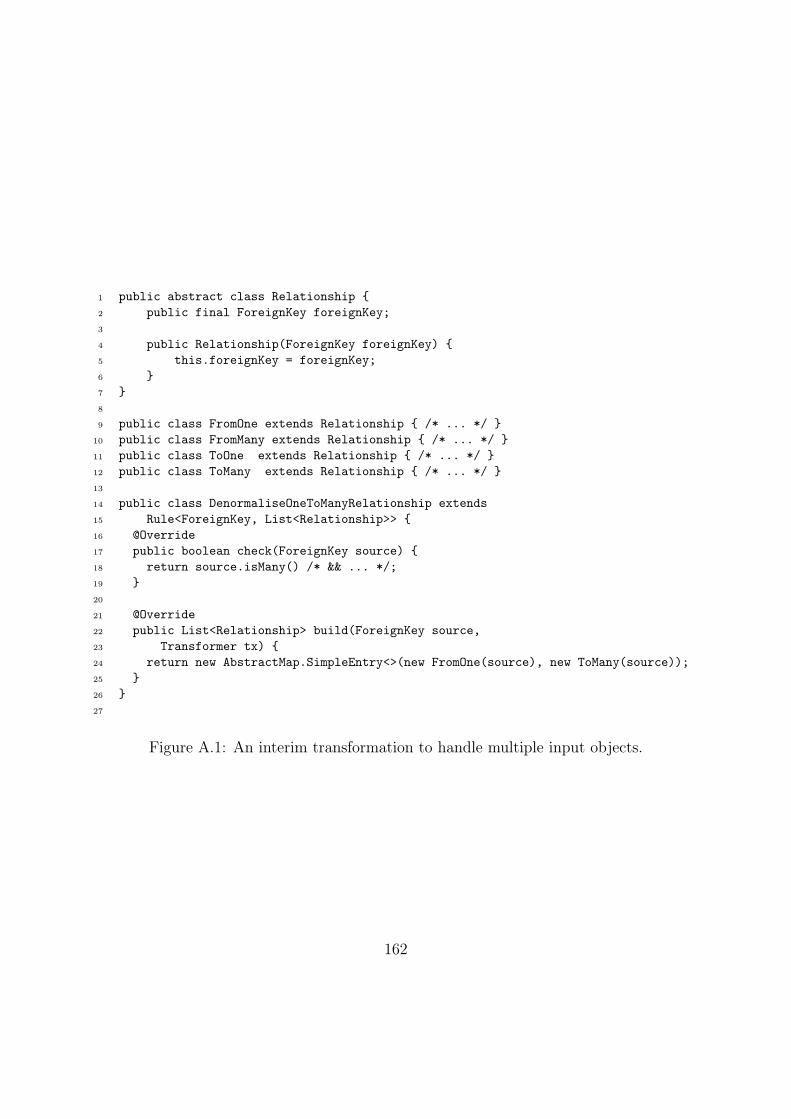
1 public abstract class Relationship {2 public final ForeignKey foreignKey;3
4 public Relationship(ForeignKey foreignKey) {5 this.foreignKey = foreignKey;6 }7 }8
9 public class FromOne extends Relationship { /* ... */ }10 public class FromMany extends Relationship { /* ... */ }11 public class ToOne extends Relationship { /* ... */ }12 public class ToMany extends Relationship { /* ... */ }13
14 public class DenormaliseOneToManyRelationship extends15 Rule<ForeignKey, List<Relationship>> {16 @Override17 public boolean check(ForeignKey source) {18 return source.isMany() /* && ... */;19 }20
21 @Override22 public List<Relationship> build(ForeignKey source,23 Transformer tx) {24 return new AbstractMap.SimpleEntry<>(new FromOne(source), new ToMany(source));25 }26 }27
Figure A.1: An interim transformation to handle multiple input objects.
162

a column for a basic transformation. However, the transformation itself changes if
the input entity extends another. If this is the case, a foreign key and a referring
column are required to create the relationship between the table and its target. We
then have two rules. This first defines the transformation of a Java Class into the
base model of our output. The latter extends the former but builds the extended
wrapper. This class calls upon the binding phase of the parent rule (on line 41)
and then continues with its specific binding.
163
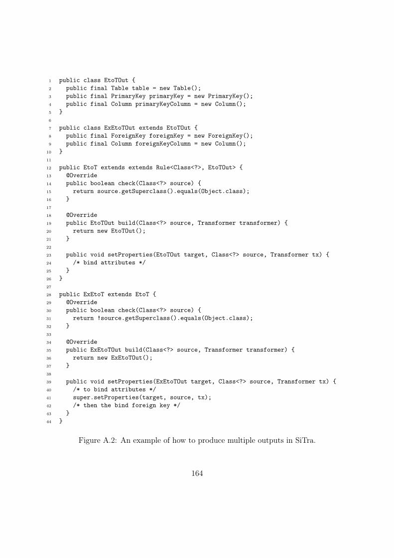
1 public class EtoTOut {2 public final Table table = new Table();3 public final PrimaryKey primaryKey = new PrimaryKey();4 public final Column primaryKeyColumn = new Column();5 }6
7 public class ExEtoTOut extends EtoTOut {8 public final ForeignKey foreignKey = new ForeignKey();9 public final Column foreignKeyColumn = new Column();
10 }11
12 public EtoT extends extends Rule<Class<?>, EtoTOut> {13 @Override14 public boolean check(Class<?> source) {15 return source.getSuperclass().equals(Object.class);16 }17
18 @Override19 public EtoTOut build(Class<?> source, Transformer transformer) {20 return new EtoTOut();21 }22
23 public void setProperties(EtoTOut target, Class<?> source, Transformer tx) {24 /* bind attributes */25 }26 }27
28 public ExEtoT extends EtoT {29 @Override30 public boolean check(Class<?> source) {31 return !source.getSuperclass().equals(Object.class);32 }33
34 @Override35 public ExEtoTOut build(Class<?> source, Transformer transformer) {36 return new ExEtoTOut();37 }38
39 public void setProperties(ExEtoTOut target, Class<?> source, Transformer tx) {40 /* to bind attributes */41 super.setProperties(target, source, tx);42 /* then the bind foreign key */43 }44 }
Figure A.2: An example of how to produce multiple outputs in SiTra.
164
A.2 Multiple Inputs for ETL
Like SiTra, the Epsilon Transformation Language (ETL) is also unable to accept
multiple inputs. The domain specific language does not account for this and
therefore is currently unable be written in such a way. The engine itself is also
unable to accept more than one object as a source object. This behaviour is due
to the underlying implementation only taking a single source object. Thus the
language and the engine would need modification to enable multiple inputs in ETL.
However, like SiTra, it is possible to resolve this using an interim transformation.
Our case study in Section Section 5.5 uses this approach. Figure A.3 shows one
of these transformations. The transformation here is a more primitive form of
Appendix A.1.1; however, it does not imply which side the transformation is on.
The To* and From* forms implicitly indicate whether it the transformation is with
the referred table or the referencing table. Instead, we explicitly define the table
in which the wrapper relates. For our purpose, we assume all relationships are
bidirectional and therefore two wrappers are created for each relationship. The
transformation of such a wrapper involves an additional guard within the rule as
to verify that the table given is the referrer or the referring table. Opposed to a
simple type check that forms the core operation of ETL’s scheduling process.
165
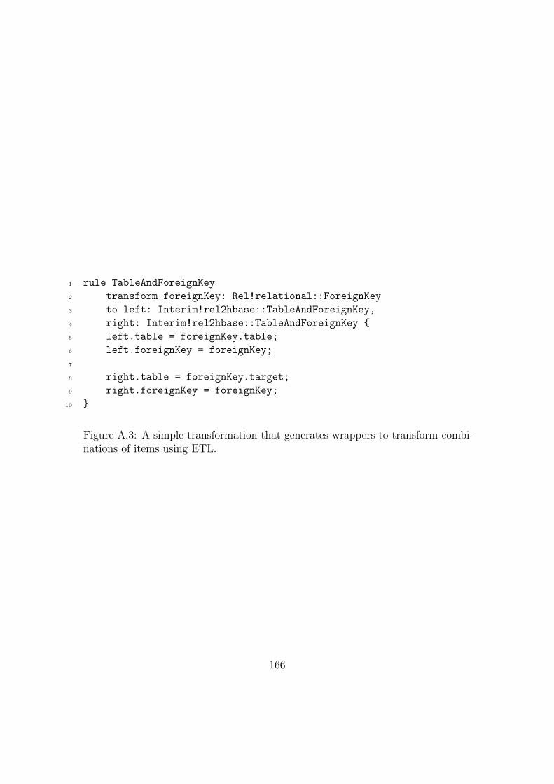
1 rule TableAndForeignKey2 transform foreignKey: Rel!relational::ForeignKey3 to left: Interim!rel2hbase::TableAndForeignKey,4 right: Interim!rel2hbase::TableAndForeignKey {5 left.table = foreignKey.table;6 left.foreignKey = foreignKey;7
8 right.table = foreignKey.target;9 right.foreignKey = foreignKey;
10 }
Figure A.3: A simple transformation that generates wrappers to transform combi-nations of items using ETL.
166


