Turbulence structures in isolated pool-
riffle units
by
Hamed Dashtpeyma
A thesis
presented to the University of Waterloo
in fulfillment of the
thesis requirement for the degree of
Doctoral philosophy
in
Civil and Environmental Engineering
Waterloo, Ontario, Canada, 2019
©Hamed Dashtpeyma 2019

ii
AUTHOR'S DECLARATION
This thesis consists of material all of which I authored or co-authored: see Statement of Contributions
included in the thesis. This is a true copy of the thesis, including any required final revisions, as accepted
by my examiners.
I understand that my thesis may be made electronically available to the public.
iii
Statement of Contributions
I would like to acknowledge the contributions made towards this thesis by my supervisor Dr. Bruce
MacVicar. All the results were generated by myself, and I prepared the final document under the
supervision of Dr. MacVicar. I have done 90% of conceptual design, writing and editing, and Dr.
MacVicar has done the rest. Chapter 3 is based on a manuscript that has been submitted to the Journal of
Geophysical Research: Earth Surface.

iv
Examining Committee Membership
The following served on the Examining Committee for this thesis. The decision of the Examining
Committee is by majority vote.
External Examiner:
Dr. Ana Maria da Silva
Professor
Supervisor:
Dr. Bruce MacVicar
Associate Professor
Internal Member:
Dr. Don Burn
Professor
Internal-external Member:
Dr. Marek Stastna
Professor
Internal-external Member:
Dr. Mike Stone
Professor
v
Abstract
The macroscale morphology of a river has significant effects on sediment transport, flow pattern, bed
stability, and ecosystem function. Pools and riffles, which are respectively the deeper and shallower parts
of the bed, are a common morphology that is formed naturally in many rivers and also used as an analog
in stream restoration. However, the formation and maintenance mechanisms of these structures remain
unclear. Most of the previous studies on pool-riffle maintenance and shaping mechanisms did not
consider the effects of riffle height, stream width variations, and constrictions on stream flow patterns and
turbulence. These studies also did not comprehensively investigate different responses of sediments to
turbulence.
The contributions of this thesis can be summarized as 1) identifying and characterizing turbulent structures
in idealized pool-riffle units based on transient turbulence modelling; 2) studying the effect of pool-riffle
geometrical parameters on turbulent structures, and 3) studying the influence of turbulent structures on
sediment transport.
Riffle pools are defined by their undulating bed, and for this reason the simplest geometry of the bedforms
we investigated were bed rises in straight channels similar to broad crested weirs. Other investigated
geometries considered the additional effects of local constrictions in width and the overall width of the
channel.
The research is a combined numerical and experimental study of turbulent structures and sediment transport
in idealized pool-riffle units. Large eddy simulation was used to capture detailed information on flow
characteristics. The numerical simulations were then validated using previously reported results and the
experimental part of this study. The Q-criterion was used to detect turbulent flow structures in simulation
vi
results. For the experiment on sediment transport, a visual qualitative scoring method was designed to assess
sediment entrainment. Velocity profiles were acquired in the lab using an acoustic Doppler profiling
velocimeter (Vectrino II) to validate the simulation results.
In the results, four types of vortical structures that largely control the flow pattern were identified, namely,
(1) ramp rollers, (2) corner eddies, (3) surface turbulent structures, and (4) axial tails. Ramp rollers are
shaped on downsloping ramps, corner eddies are formed at the corners of pool heads, surface turbulence
structures are shaped at the free-surface of pool-head, and all the generated vortices in the pool-head get
stretched and form axial tails vortices.
Pool-riffle geometry (riffle height, width size, and width constriction) and hydraulic characteristics (sub or
supercritical flow types in riffles) exert a strong control over the size and strength of vortical structures as
described below:
Higher riffles create stronger ramp rollers and corner eddies.
If the riffle height creates critical or supercritical flow in the riffle, surface undulation hydraulic
jump will create strong surface turbulent structures.
Wider channels provide more space for the shaping of corner eddies and ramp rollers.
Width constrictions amplify corner eddies and ramp rollers and create horseshoe vortices in the
upstream at convective accelerating flow zone.
Even in subcritical flow condition, strong corner eddies can be transported to the free surface and
shape boiling structures in the form of surface turbulence.
These structures are generated as a result of flow deceleration and are large structures generated away from
the boundary and so are not thought to be dependant on surface roughness. To help unite the observations
of the interaction between the main flow and turbulent structures, the ‘vortex-resistance hypothesis’ is
vii
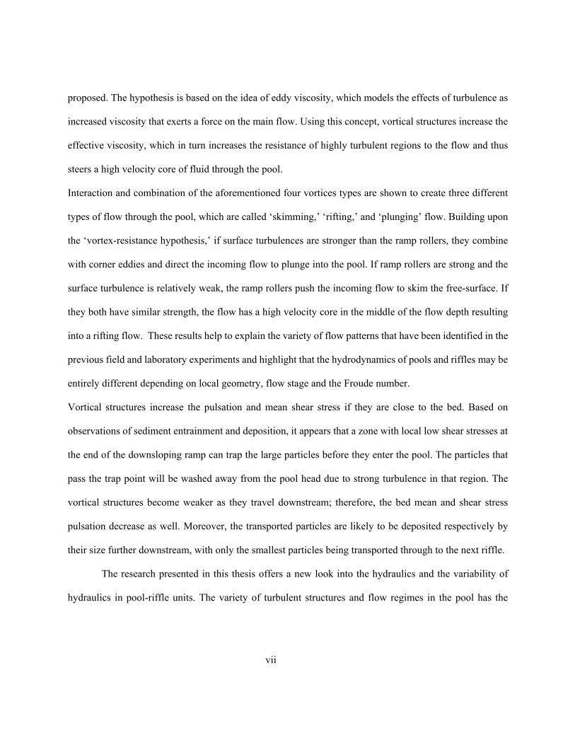
proposed. The hypothesis is based on the idea of eddy viscosity, which models the effects of turbulence as
increased viscosity that exerts a force on the main flow. Using this concept, vortical structures increase the
effective viscosity, which in turn increases the resistance of highly turbulent regions to the flow and thus
steers a high velocity core of fluid through the pool.
Interaction and combination of the aforementioned four vortices types are shown to create three different
types of flow through the pool, which are called ‘skimming,’ ‘rifting,’ and ‘plunging’ flow. Building upon
the ‘vortex-resistance hypothesis,’ if surface turbulences are stronger than the ramp rollers, they combine
with corner eddies and direct the incoming flow to plunge into the pool. If ramp rollers are strong and the
surface turbulence is relatively weak, the ramp rollers push the incoming flow to skim the free-surface. If
they both have similar strength, the flow has a high velocity core in the middle of the flow depth resulting
into a rifting flow. These results help to explain the variety of flow patterns that have been identified in the
previous field and laboratory experiments and highlight that the hydrodynamics of pools and riffles may be
entirely different depending on local geometry, flow stage and the Froude number.
Vortical structures increase the pulsation and mean shear stress if they are close to the bed. Based on
observations of sediment entrainment and deposition, it appears that a zone with local low shear stresses at
the end of the downsloping ramp can trap the large particles before they enter the pool. The particles that
pass the trap point will be washed away from the pool head due to strong turbulence in that region. The
vortical structures become weaker as they travel downstream; therefore, the bed mean and shear stress
pulsation decrease as well. Moreover, the transported particles are likely to be deposited respectively by
their size further downstream, with only the smallest particles being transported through to the next riffle.
The research presented in this thesis offers a new look into the hydraulics and the variability of
hydraulics in pool-riffle units. The variety of turbulent structures and flow regimes in the pool has the
viii
potential to unite a wide set of seemingly contradictory observations and hypotheses that have propagated
through the literature on this subject. The research also has important implications for design that should
lead to better rehabilitation and maintenance strategies for natural or restored streams. The original scope
of work should be extended to include more realistic natural shapes for the bedforms with lateral asymmetry
and meandering, but the richness of behaviours and similarities with more complex forms of these structures
necessitated a deeper examination of these relatively simple forms before extending the results to real
systems.

ix
Acknowledgements
We acknowledge that we live and work on the traditional territory of the Attawandaron (Neutral),
Anishinaabeg and Haudenosaunee peoples. The University of Waterloo is situated on the Haldimand
Tract, the land promised to the Six Nations that includes ten kilometers on each side of the Grand River.
I would like to express my sincere appreciation to my advisor Prof. Bruce MacVicar. I have been
amazingly fortunate to have an advisor who gave me the freedom to explore on my own. A distinguished
supervisor whose academic advice, encouragement, and unconditional support helped me step forward
throughout my PhD. I appreciate all his contributions of time, inspiring suggestions, and funding to make
my PhD experience productive and stimulating.
x
Table of Contents
List of Figures ......................................................................................................................................... xiv
List of Tables ........................................................................................................................................... xx
Chapter 1 : Introduction ................................................................................................................................ 1
1.1 Motivation ........................................................................................................................................... 1
1.2 Research gap ....................................................................................................................................... 2
1.3 Objectives ........................................................................................................................................... 3
Chapter 2 : Literature Review ....................................................................................................................... 5
2.1 Definition of pools and riffles ............................................................................................................. 5
2.2 The formation of pools and riffles ...................................................................................................... 6
2.2.1 Meandering development ............................................................................................................. 7
2.3 Hydrodynamics in pools and riffles .................................................................................................... 9
2.3.1 Mean flow .................................................................................................................................... 9
2.4 Turbulence ........................................................................................................................................ 12
2.5 Sediment transport in pools and riffles ............................................................................................. 15
2.5.1 Sediment entrainment ................................................................................................................ 15
2.5.2 Bedload routing .......................................................................................................................... 19
2.5.3 Effect of hydrodynamic on sediment transport .......................................................................... 19
2.6 Numerical analysis ............................................................................................................................ 20
2.7 Numerical methods ........................................................................................................................... 23
2.7.1 Numerical concepts .................................................................................................................... 23
2.7.2 Reynolds Averaged Navier-Stokes (RANS) .............................................................................. 24
xi
2.7.3 Large Eddy Simulation (LES) .................................................................................................... 25
2.8 Research gap ..................................................................................................................................... 26
Chapter 3 : Effect of riffle height on turbulent structures and flow pattern in isolated pool-riffle units .... 27
3.1 Abstract ............................................................................................................................................. 28
3.2 Introduction ....................................................................................................................................... 29
3.3 Methodology ..................................................................................................................................... 32
3.3.1 Model Geometry ........................................................................................................................ 32
3.3.2 Numerical Method ..................................................................................................................... 33
3.3.3 Boundary Conditions ................................................................................................................. 34
3.3.4 Q-criterion for detection of vortex cores .................................................................................... 35
3.3.5 Validation ................................................................................................................................... 36
3.4 Results ............................................................................................................................................... 38
3.4.1 Skimming and plunging flow over bedforms of different heights ............................................. 38
3.4.2 Vortical turbulent structures in the decelerating flow ................................................................ 41
3.4.3 Effect of riffle height on dynamics of turbulent structures and stresses on the bed................... 43
3.4.4 Bed shear stress .......................................................................................................................... 47
3.5 Discussion ......................................................................................................................................... 49
3.6 Conclusions ....................................................................................................................................... 56
Chapter 4 : Effect of width variations on turbulent structures and flow patterns in isolated pool-riffle units
.................................................................................................................................................................... 58
4.1 Introduction ....................................................................................................................................... 58
4.2 Methodology ..................................................................................................................................... 62
xii
4.2.1 Model Geometry ........................................................................................................................ 62
4.2.2 Numerical Method ..................................................................................................................... 65
4.2.3 Boundary Conditions ................................................................................................................. 66
4.2.4 Validation ................................................................................................................................... 66
4.3 Results ............................................................................................................................................... 68
4.3.1 The effects of total width variation on skimming flow in isolated pool-riffle units .................. 68
4.3.2 The effects of total width variation on plunging flow in isolated pool-riffle units .................... 79
4.3.3 The effects of width constriction on vortical structures ............................................................. 83
4.3.4 Effects of constriction on skimming flow in pool-riffle units .................................................... 90
4.3.5 The effects of constriction location on bed shear stress ............................................................. 97
4.4 Discussion ....................................................................................................................................... 100
4.4.1 Plunging flow in Black Canyon ............................................................................................... 103
4.4.2 Meandering initiations from straight channels ......................................................................... 104
4.4.3 A suggestion for designing self-maintaining pool-riffle units ................................................. 106
4.5 Conclusion ...................................................................................................................................... 107
Chapter 5 : Effect of turbulent structures on sediment entrainment in isolated pool-riffle units .............. 109
5.1 Introduction ..................................................................................................................................... 109
5.2 Methods........................................................................................................................................... 111
5.2.1 Model Geometry ...................................................................................................................... 111
5.2.2 Experimental Method ............................................................................................................... 113
5.2.3 Numerical method .................................................................................................................... 117
5.2.4 Boundary Conditions ............................................................................................................... 118
xiii
5.2.5 Validation ................................................................................................................................. 118
5.3 Results ............................................................................................................................................. 120
5.3.1 Hydrodynamics and vortical structures .................................................................................... 120
5.3.2 Sediment entrainment .............................................................................................................. 124
5.4 Discussion ....................................................................................................................................... 129
5.5 Conclusion ...................................................................................................................................... 131
Chapter 6 : Conclusions and future work .................................................................................................. 132
6.1 Summary of Thesis Contributions .................................................................................................. 132
6.1.1 Contribution 1: Proposing and validating the vortex-resistance hypothesis ............................ 133
6.1.2 Contribution 2: Study of the influence of the riffle height on the characteristics of the vorticial
structures ........................................................................................................................................... 133
6.1.3 Contribution 3: Study of the influence of the channel width variation on on the characteristics
of the vorticial structures .................................................................................................................. 134
6.1.4 Contribution 4: Study of the influence of vorticial structures on sediment entrainment ......... 135
6.2 Future research ................................................................................................................................ 136
Refrences............................................................................................................................................... 137
xiv
List of Figures
Figure 2-1- Morphological similarities between straight, meandering, and wandering channels (A.
Thompson, 1986) .......................................................................................................................................... 7
Figure 2-2- Helical flow in straight and meandering channel (Thompson, 1986) ........................................ 8
Figure 2-3- Development of meandering from the straight channel (Thompson, 1986) .............................. 9
Figure 2-4- Near bed velocity (0.05 ft above the bed) versus total discharge in a pool-riffle unit (Keller,
1971) ........................................................................................................................................................... 10
Figure 2-5 Conceptual model of flow convergence routing for pool-riffle sequence (MacWilliams et al.,
2006) ........................................................................................................................................................... 11
Figure 2-6- Schematic figure of pool-riffle unit with CAF and CDF zones (B. J. MacVicar & Obach,
2015) ........................................................................................................................................................... 13
Figure 2-7 - Velocity domains at pool section for four different flow rates using a 3D numerical model
(MacWilliams et al., 2006) ......................................................................................................................... 14
Figure 2-8 a) mean streamwise velocity b) Reynolds stress in a section crossing centerline of a pool-riffle
unit (MacVicar & Best, 2013) .................................................................................................................... 14
Figure 2-9- Force balance on a grain (Wiberg & Smith, 1987) .................................................................. 16
Figure 2-10- Schematic diagram of applied and critical shear stress (Yager & Schott, 2013) ................... 18
Figure 2-11 Bed picture and grain size distribution on a bed with a constant flow rate (Left) with pulsation
(Right) (Venditti et al., 2010)...................................................................................................................... 20
Figure 2-12- 3D visualization of strong vortices by Q-criterion, blue parts are rotating counterclockwise,
and red parts are rotating clockwise (Koken et al., 2013). .......................................................................... 22
Figure 3-1- Simplified geometry of a pool-riffle unit as used in the current study .................................... 33
xv
Figure 3-2- Validation of numerical results with available experimental data, a) water surface elevation at
centerline, b) profiles of time-average streamwise velocity (Ux) for locations shown in a) ...................... 38
Figure 3-3- a) time-average velocity magnitude (U) in the X-Y plane at channel centerline, b) total
velocity standard deviation (Ustdv) in the X-Y plane at the channel centreline. ........................................... 40
Figure 3-4- a) time-average velocity, and b) Reynolds stress profiles at the centre of the pool for the five
cases listed in Table 3-1. ............................................................................................................................. 41
Figure 3-6- Instantaneous vorticity and hydrodynamics for case R45, showing: a) Iso-surface of Q=12 s^-
2 showing flow structures, and contour of relative vertical pressure gradient at the bed, b) contour and
vector of bed shear stress magnitude, c) contour of Q in three cross-sections. .......................................... 45
Figure 3-7 Instantaneous vorticity and hydrodynamics for case R55, showing: a) iso-surface of Q=12 s^-2
showing flow structures, and contour of relative vertical pressure gradient at the bed, b) contour and
vector of bed shear stress magnitude, c) contour of Q in three cross-sections ........................................... 46
Figure 3-8- Instantaneous vorticity and hydrodynamics for case R65, showing: a) Iso-surface of Q=12 s^-
2 showing flow structures, and contour of relative vertical pressure gradient at the bed, b) contour and
vector of bed shear stress magnitude, c) contour of Q in three cross-sections ........................................... 47
Figure 3-9- Time-average (black line) and 95% confidence range (dashed line) of bed shear stress at
centreline for cases R45, R55, and R65. ..................................................................................................... 48
Figure 3-10- a) the maximum velocity magnitude in the profile at the centre of the pool, b) the elevation
of the maximum velocity point in the profile at the centre of the pool ....................................................... 52
Figure 3-11-Instantaneous a) velocity magnitude, b) ratio of eddy viscosity and dynamic viscosity ........ 54
Figure 3-12- Turbulent kinetic energy (K), turbulent dissipation rate ( ), and turbulent viscosity based on
K-epsilon concept in the pool-head of cases R45, R55, and R65. .............................................................. 55
Figure 4-1- Simplified geometry of a pool-riffle unit with in-phase constriction as used in the current
study, a) linear constriction, b) concave curve constriction ........................................................................ 64
xvi
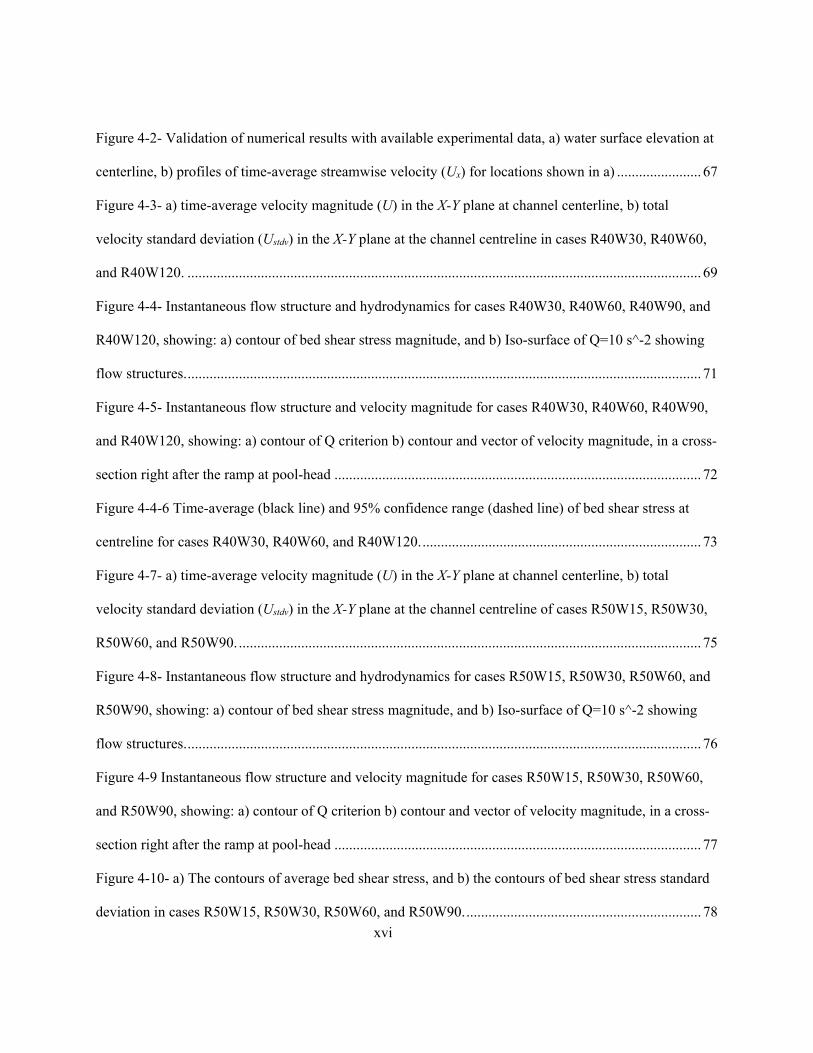
Figure 4-2- Validation of numerical results with available experimental data, a) water surface elevation at
centerline, b) profiles of time-average streamwise velocity (Ux) for locations shown in a) ....................... 67
Figure 4-3- a) time-average velocity magnitude (U) in the X-Y plane at channel centerline, b) total
velocity standard deviation (Ustdv) in the X-Y plane at the channel centreline in cases R40W30, R40W60,
and R40W120. ............................................................................................................................................ 69
Figure 4-4- Instantaneous flow structure and hydrodynamics for cases R40W30, R40W60, R40W90, and
R40W120, showing: a) contour of bed shear stress magnitude, and b) Iso-surface of Q=10 s^-2 showing
flow structures. ............................................................................................................................................ 71
Figure 4-5- Instantaneous flow structure and velocity magnitude for cases R40W30, R40W60, R40W90,
and R40W120, showing: a) contour of Q criterion b) contour and vector of velocity magnitude, in a cross-
section right after the ramp at pool-head .................................................................................................... 72
Figure 4-4-6 Time-average (black line) and 95% confidence range (dashed line) of bed shear stress at
centreline for cases R40W30, R40W60, and R40W120. ............................................................................ 73
Figure 4-7- a) time-average velocity magnitude (U) in the X-Y plane at channel centerline, b) total
velocity standard deviation (Ustdv) in the X-Y plane at the channel centreline of cases R50W15, R50W30,
R50W60, and R50W90. .............................................................................................................................. 75
Figure 4-8- Instantaneous flow structure and hydrodynamics for cases R50W15, R50W30, R50W60, and
R50W90, showing: a) contour of bed shear stress magnitude, and b) Iso-surface of Q=10 s^-2 showing
flow structures. ............................................................................................................................................ 76
Figure 4-9 Instantaneous flow structure and velocity magnitude for cases R50W15, R50W30, R50W60,
and R50W90, showing: a) contour of Q criterion b) contour and vector of velocity magnitude, in a cross-
section right after the ramp at pool-head .................................................................................................... 77
Figure 4-10- a) The contours of average bed shear stress, and b) the contours of bed shear stress standard
deviation in cases R50W15, R50W30, R50W60, and R50W90. ................................................................ 78
xvii
Figure 4-11 a) time-average velocity magnitude (U) in the X-Y plane at channel centerline, b) total
velocity standard deviation (Ustdv) in the X-Y plane at the channel centreline of cases R60W30, R60W60,
and R60W120. ............................................................................................................................................ 79
Figure 4-12 Instantaneous flow structure and hydrodynamics for cases R60W30, R60W60, and
R60W120, showing: a) Iso-surface of Q=10 s^-2 showing flow structures, and b) contour of bed shear
stress magnitude. ......................................................................................................................................... 81
Figure 4-13 Instantaneous flow structure and velocity magnitude for cases R50W15, R50W30, R50W60,
and R50W90, showing: a) contour of Q criterion b) contour and vector of velocity magnitude, in a cross-
section right after the ramp at pool-head .................................................................................................... 82
Figure 4-14 a) The contours of average bed shear stress, and b) the contours of bed shear stress standard
deviation in cases R60W30, R60W60, and R60W120. .............................................................................. 83
Figure 4-15 Instantaneous flow structure and hydrodynamics for cases C10W30, C20W30, C20W30C,
C20W30S, C25W30C, and, C25W30L showing: a) contour of bed shear stress magnitude, and b) Iso-
surface of Q=10 s^-2 showing flow structures. .......................................................................................... 86
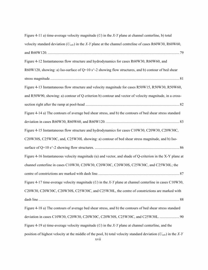
Figure 4-16 Instantaneous velocity magnitude (u) and vector, and shade of Q-criterion in the X-Y plane at
channel centerline in cases C10W30, C20W30, C20W30C, C20W30S, C25W30C, and C25W30L; the
centre of constrictions are marked with dash line. ...................................................................................... 87
Figure 4-17 time-average velocity magnitude (U) in the X-Y plane at channel centerline in cases C10W30,
C20W30, C20W30C, C20W30S, C25W30C, and C25W30L, the centre of constrictions are marked with
dash line ...................................................................................................................................................... 88
Figure 4-18 a) The contours of average bed shear stress, and b) the contours of bed shear stress standard
deviation in cases C10W30, C20W30, C20W30C, C20W30S, C25W30C, and C25W30L. ..................... 90
Figure 4-19 a) time-average velocity magnitude (U) in the X-Y plane at channel centerline, and the
position of highest velocity at the middle of the pool, b) total velocity standard deviation (Ustdv) in the X-Y
xviii
plane at the channel centreline for case R40W30C10, R40W30C20, R40W60C10, R40W60C20,
R40W60C25C, R40W120C10, and R40W120C20. ................................................................................... 92
Figure 4-20- Instantaneous flow structure and hydrodynamics for cases R40W30C10, R40W30C20,
R40W60C10, R40W60C20, R40W60C25C, R40W120C10, and R40W120C20 showing: a) contour of
bed shear stress magnitude and b) Iso-surface of Q=20 s^-2 showing flow structures. ............................. 94
Figure 4-21 a) the contours of bed shear stress standard deviation, and b) The contours of average bed
shear stress, in cases R40W30C10, R40W30C20, R40W60C10, R40W60C20, R40W60C25C,
R40W120C10, and R40W120C20. ............................................................................................................. 96
Figure 4-22 Time-average (black line) and 95% confidence range (dashed line) of bed shear stress at
centreline for cases R40W60, R40W60C10, R40W60C20 and R40W60C25C. ........................................ 97
Figure 4-23 Instantaneous flow structure for cases R40W60, R40W60C10U, R40W60C10, and
R40W60C10D showing Iso-surface of Q=5 s^-2, and the contour of bed elevation. ................................. 98
Figure 4-24 Time-average (black line) and 95% confidence range (dashed line) of bed shear stress at
centreline for cases R40W60, R40W60C10U, R40W60C10, and R40W60C10D. .................................... 99
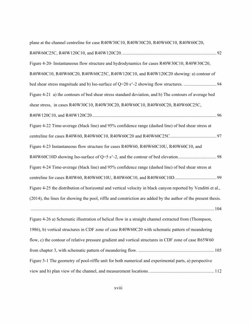
Figure 4-25 the distribution of horizontal and vertical velocity in black canyon reported by Venditti et al.,
(2014), the lines for showing the pool, riffle and constriction are added by the author of the present thesis.
.................................................................................................................................................................. 104
Figure 4-26 a) Schematic illustration of helical flow in a straight channel extracted from (Thompson,
1986), b) vortical structures in CDF zone of case R40W60C20 with schematic pattern of meandering
flow, c) the contour of relative pressure gradient and vortical structures in CDF zone of case R65W60
from chapter 3, with schematic pattern of meandering flow. ................................................................... 105
Figure 5-1 The geometry of pool-riffle unit for both numerical and experimental parts, a) perspective
view and b) plan view of the channel, and measurement locations. ......................................................... 112
xix
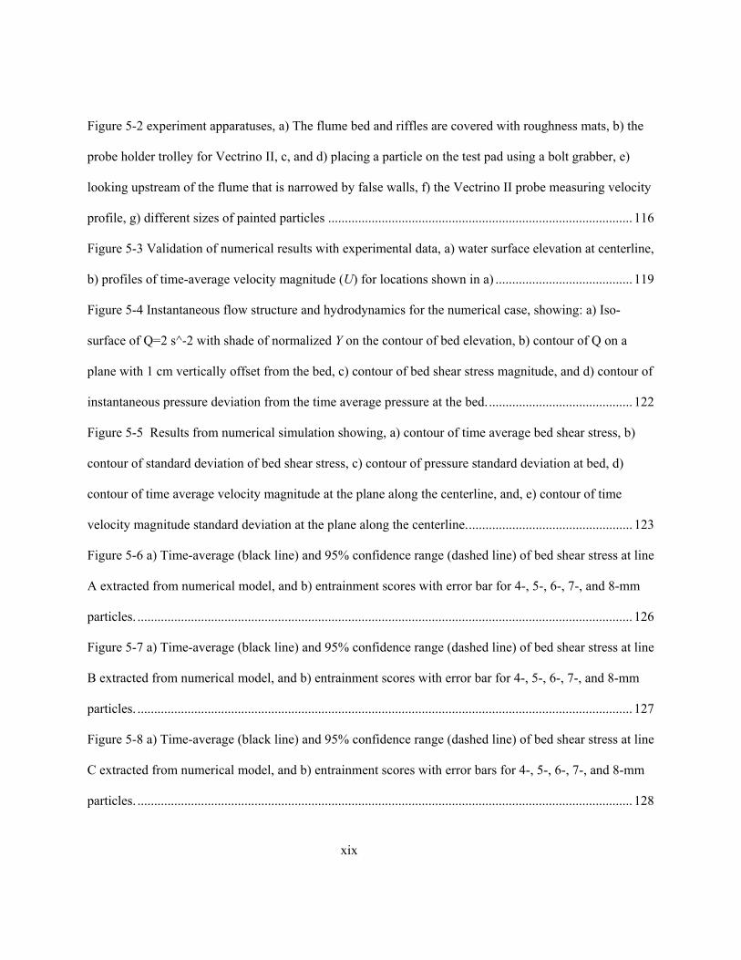
Figure 5-2 experiment apparatuses, a) The flume bed and riffles are covered with roughness mats, b) the
probe holder trolley for Vectrino II, c, and d) placing a particle on the test pad using a bolt grabber, e)
looking upstream of the flume that is narrowed by false walls, f) the Vectrino II probe measuring velocity
profile, g) different sizes of painted particles ........................................................................................... 116
Figure 5-3 Validation of numerical results with experimental data, a) water surface elevation at centerline,
b) profiles of time-average velocity magnitude (U) for locations shown in a) ......................................... 119
Figure 5-4 Instantaneous flow structure and hydrodynamics for the numerical case, showing: a) Iso-
surface of Q=2 s^-2 with shade of normalized Y on the contour of bed elevation, b) contour of Q on a
plane with 1 cm vertically offset from the bed, c) contour of bed shear stress magnitude, and d) contour of
instantaneous pressure deviation from the time average pressure at the bed. ........................................... 122
Figure 5-5 Results from numerical simulation showing, a) contour of time average bed shear stress, b)
contour of standard deviation of bed shear stress, c) contour of pressure standard deviation at bed, d)
contour of time average velocity magnitude at the plane along the centerline, and, e) contour of time
velocity magnitude standard deviation at the plane along the centerline. ................................................. 123
Figure 5-6 a) Time-average (black line) and 95% confidence range (dashed line) of bed shear stress at line
A extracted from numerical model, and b) entrainment scores with error bar for 4-, 5-, 6-, 7-, and 8-mm
particles. .................................................................................................................................................... 126
Figure 5-7 a) Time-average (black line) and 95% confidence range (dashed line) of bed shear stress at line
B extracted from numerical model, and b) entrainment scores with error bar for 4-, 5-, 6-, 7-, and 8-mm
particles. .................................................................................................................................................... 127
Figure 5-8 a) Time-average (black line) and 95% confidence range (dashed line) of bed shear stress at line
C extracted from numerical model, and b) entrainment scores with error bars for 4-, 5-, 6-, 7-, and 8-mm
particles. .................................................................................................................................................... 128

xx
List of Tables
Table 3-1- Simulation parameters ............................................................................................................... 33
Table 4-1- Simulation parameters ............................................................................................................... 64
Table 5-1 entrainment score ...................................................................................................................... 115
1
Chapter 1: Introduction
1.1 Motivation
One of the most common topographical elements of rivers are pool-riffle units. The deeper parts of
undulations in the bed are called pools, whereas the shallower parts are riffles. Pool-riffle sequences can be
shaped naturally, but are also made artificially. Pools and riffles are essential elements in river restoration
projects. As reported by Bernhardt et al. (2005) the most imperative objectives of restoration projects are
to 1) improve water quality 2) improve fish habitats and aquatic lives 3) control sediment transport rate and
stream energy. “Prior to July 2004, 37099 restoration projects were documented in National River
Restoration Science (NRRSS) “ in the United States alone, a number thought to be underestimated due to
underreporting of projects to NRRSS for various reasons. Between 1990 and 2004, they estimated that 15
billion dollars had been spent on restoration projects. Among the projects, only 10% of them were assessed
by NRRSS (Bernhardt et al., 2005). Despite these reporting problems, a high failure rate of restoration
projects is reported by researchers, which is caused by the irrational design of channel geometry; therefore,
there is a need for better understanding of river elements, river mechanics, and hydrodynamics in natural
streams (Bernhardt and Palmer 2007; Miller and Kochel 2009; Wohl et al. 2005).
2
1.2 Research gap
Many researchers have focused on the hydraulic characteristics of pool-riffle sequences using numerical
analyzes, experimental investigations, and field work studies, but many of the existing studies have
limitations. Many researchers noted that the turbulent structures are the most influential sources of shear
stress in pools (Roy et al. 2004). Moreover, bed shear stress can maintain the form of pool-riffle units by
cleaning the pools and storing large particles in the riffles. The most significant part of the pool-riffle unit
in terms of turbulence generation is the area of convective decelerating flow (CDF) in the ramp at the head
of pools (MacVicar and Rennie 2012). This turbulence is thought to be important in sediment transport
mechanism (Celik et al. 2013) and pool-riffle maintenance (Thompson 2006) but most of the researches in
this field have limitations in assessing bed shear stress and turbulent structures for the reason that most of
the experimental analysis cannot instantaneously measure velocity domain in near-wall regions. Existing
numerical studies also did not consider turbulent structures accurately because of their predominant use of
steady-state methods, which cannot model dynamic structures in pool-riffle units. Transient numerical
analysis is particularly suited to illustrate the complex mechanisms of flow such as vortex generation and
dissipation, turbulent structures, and instantaneous bed shear stress (Keylock et al. 2012). Also, a better
understanding of hydrodynamic in pool-riffle units helps to unify the controversial hypothesis in pool-riffle
formation, which are based on field observations. However, the key problem in numerical simulations is
that sediment transport and scouring cannot be modelled directly and without using empirical
approximations; therefore, there is a need to establish a linking between numerical hydrodynamics results
and experimental sediment transport studies.
1.3 Approach
This study is using advanced numerical methods to continue a series of flume experiments, which was
done by MacVicar and Obach (2015). They used a reductionist approach by representing the complex
3
geometry of pool-riffle units as a two-dimensional bedform in an open channel flume with smooth
vertical walls. In addition, they stated that this unnatural and artificial geometry was chosen to allow them
to isolate the effects of longitudinal vertical contraction and expansion from different geometrical
characteristics. Another benefit of modelling pool-riffle units as a two-dimensional bedform is that it can
contribute to the current design methods in restoration projects suggested by Newbury (2013), which is
based on fundamental hydraulic principles and constructing simple two-dimensional riffles along the
width of the channel. This thesis was designed to investigate the effects of two major geometrical factors
(riffle height and width variation) on the formation of flow pattern and turbulent structures.
This approach has some limitations; for instance, the effects of alternate bars, bed roughness, side slopes,
and meandering on flow pattern and turbulent structures in pool-riffle units are not investigated. Sediment
transport mechanisms are not completely investigated, and it is limited to entrainment of non-cohesive
particles without considering the covering factor and pocket geometry. However, the relatively simple
geometries used in this study revealed a rich variety of flow dynamics that were highly sensitive to a few
basic parameters. The complexity of the observed preliminary results suggested that a thorough
investigation of these simplified geometries was needed before the flow hydrodynamics over more
complex geometries could be unambiguously interpreted.
1.4 Objectives
The objectives of the present study are to numerically investigate the effects of fundamental
geometry factors on hydrodynamic in pool-riffle units, and experimentally assess the fundamental
mechanism of sediment transport, more specifically to: 1) identify and characterize turbulent structures in
pool-riffle units based on an advanced transient turbulence modelling; 2) study the effect of pool-riffle
geometry on generation, transport and dissipation of turbulent structures, and 3) study the influence of
turbulent structures on non-cohesive sediment entrainment. By achieving these objectives, this research can
4
help engineers and researchers to understand better the hydrodynamics and turbulence in pool-riffle units.
This study can clarify the pool-riffle hydrodynamics and maintenance hypotheses, while also helping to
guide a more rational design. The experimental part of this research can provide a better understanding of
sediment transport mechanism; moreover, by linking the transient numerical results and experimental data,
a better understanding of turbulence effects on pool-riffle maintenance can be achieved. It is hoped that
the results from the current study can be an important step in the understanding of complex hydrodynamics
in pool-riffle units and provide a base framework for further researches.

5
Chapter 2: Literature Review
2.1 Definition of pools and riffles
Many researchers have tried to propose an accurate and comprehensive definition for pools and riffles,
but their definitions remain problematic (Thompson, 2013). Pools and riffles can be considered either as a
single morphological element or as distinct subunits because of their distinct influence on the flow (Clifford
1993; Thompson 2001). Pools can form by scouring in a particular location or where the flow is slowed by
bars of deposited sediment (Clifford 1993). “Forced pools” can be formed by obstruction to flow and “free-
formed pools” can be shaped freely by flow pattern (Lisle & Hilton, 1992; Montgomery et al., 1995; D. M.
Thompson, 2013). Based on the hydraulic characteristics of the stream, riffles are those regions with steeper
water-surface slope and pools are deeper part with horizontal water-surface in low discharge conditions
(Lisle & Hilton, 1992; Lisle, 1979a). Another method for describing pools and riffles is “residual-depth
criterion” that says if the flow at the upstream is ceased, after reaching to complete stable condition, those
regions where are inundated with water are pools (Lisle, 1979b). However, this method cannot explain the
definition of riffles (Thompson, 2013). Moreover, a quantitative method is needed to distinguish pools and
riffles from common undulations in the streambed. A statistical approach based on the elevation distribution
of streambed and a limit for the ordinary variation of elevation can help to distinguish pools from small-
sized depressions.
6
Another method for defining pools and riffles in addition to previous methods is based on the bed grain
size. Because of the maintenance or formation mechanism in pools and riffles, the material of riffles is
coarser than that in pools (Leopold et al. 1960).
Most of these methods can only define pools and riffles; they cannot be extended to all morphological
components such as runs and glides (Thompson, 2013). Runs and glides are small common undulations in
the streambed that they are made because of small local scouring around boulders in streambed (Dietrich
et al. 1979). Runs and glides do not have an influential impact on the hydraulic characteristics of the flow.
They can only increase the turbulence because of their heterogeneity and roughness in the streambed.
However, they can be vital for the quality of small species aquatic habitat (Halwas & Church, 2002; Lisle,
1982; Thompson, 2013; Wyrick & Pasternack, 2014).
2.2 The formation of pools and riffles
Most researchers agree with the concept that the scouring of pools and aggrading of riffles happens in
high flow discharges (Thompson, 2013). Some researchers believe that the regular formation of spaced
pools and riffles is a fundamental feature of many streams, and it does not depend on the main streambed
material (Keller & Melhorn, 1978). Another issue is that most hypotheses for the shaping of pool-riffle
units cannot explain the formation and stability of small undulations (e.g. runs and glides) in the streambeds
(Thompson, 2013). A more clear idea about the shaping of pools and riffles is that the scouring of the
streambed, which creates pools, and formation of bars from deposited sediments, which creates riffles, are
the morphological response of streambed to the external forces from the flow (e.g. excessive shear stress)
(Dolling 1968). These principles can illustrate the variety of pool-riffle types based on the diversity of the
hydraulic characteristics of streams. Some researchers suggested that the geometric characteristics of pools,
for example, higher length, are the result of streambed response for the minimization of stream power in
the presence of a higher inlet stream power (Thompson, 2002). Some researchers showed that the geometric
7
characteristics of pools and riffles helped to maximize the resistance to the energy of flow then it limits the
increase of velocity in high stage flows (Wohl & Merritt, 2008).
At the first stage in the study of pools and riffles, most of the researchers focused on the formation of them
in meandering channels, and they tried to find a similarity between the helical flow pattern in meandering
channels and the reason of pools formation in straight ones (Thompson, 2013).
2.2.1 Meandering development
In early studies, there was an idea that the flow and bed pattern in straight channels and meandering ones
have some similarities; therefore, they started to describe the formation of pools and riffles in the straight
ones based on the concept of helical flows in meanderings (Thompson, 1986).
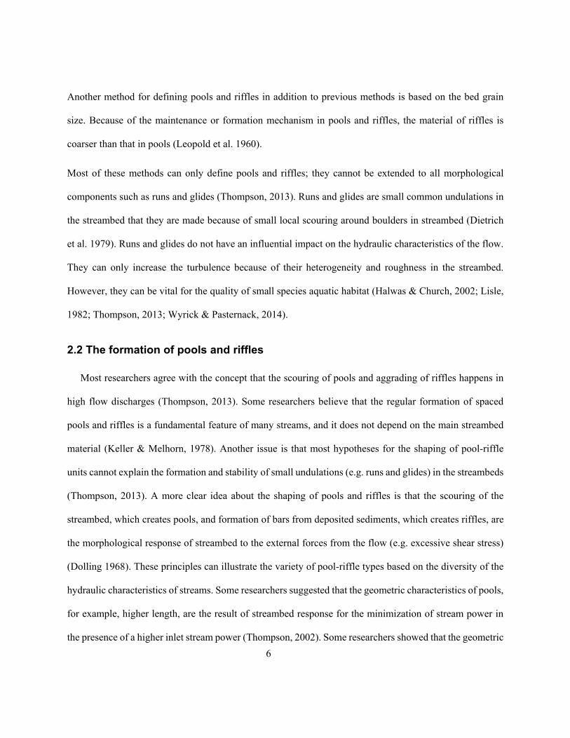
As described by Thompson (1986), the formation and geometry of bars in the natural straight streams vary
based on the flow stages and the types of channels. The form of bars in meandering channels is slightly
different but shows many similarities with those from straight channels (Figure 2-5).
Figure 2-1- Morphological similarities between straight, meandering, and wandering channels
(Thompson 1986)
For instance, the bar head in the meandering channels has a larger flat area at the top and steeper ramp at
the upstream and larger bar tail. In “wandering channels” the bar tail is faded. However, the order of
elements based on the flow pattern is the same. They suggested that an ordered sequence of scouring and
deposition of sediment were needed for the shaping of pools and riffles, and it can be the result of
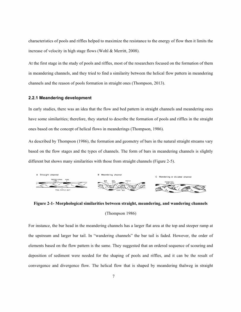
convergence and divergence flow. The helical flow that is shaped by meandering thalweg in straight
8
channels can produce those convergence and divergence flows. Those helical vortices are generated
because of turbulence and vortex shedding in near-wall regions. The shedding and length scale of those
vortices can shape the meandering thalweg (Figure 2-2). The interaction between the shaped thalweg and
flow pattern can have a secondary effect on the formation of final and stable pools and riffles (Thompson,
1986).
Figure 2-2- Helical flow in straight and meandering channel (Thompson, 1986)
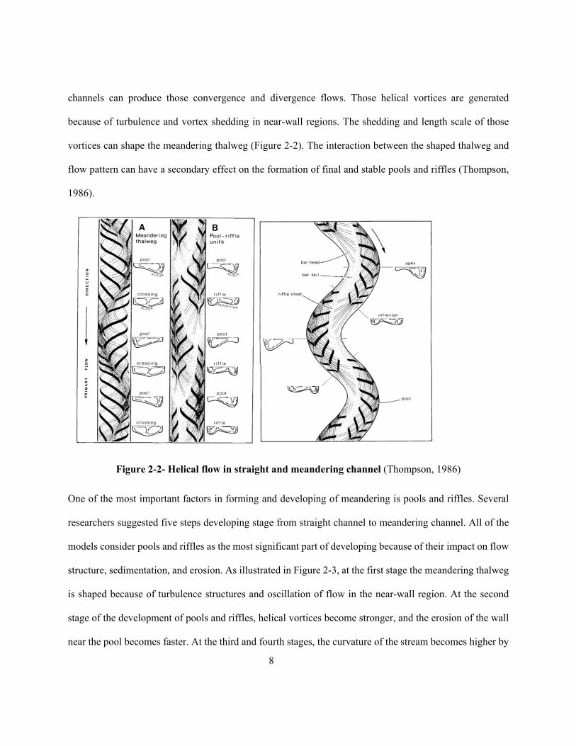
One of the most important factors in forming and developing of meandering is pools and riffles. Several
researchers suggested five steps developing stage from straight channel to meandering channel. All of the
models consider pools and riffles as the most significant part of developing because of their impact on flow
structure, sedimentation, and erosion. As illustrated in Figure 2-3, at the first stage the meandering thalweg
is shaped because of turbulence structures and oscillation of flow in the near-wall region. At the second
stage of the development of pools and riffles, helical vortices become stronger, and the erosion of the wall
near the pool becomes faster. At the third and fourth stages, the curvature of the stream becomes higher by
9
the growth of pools and the translation of riffles. At stage five, because of growth and development, the
distance between two pools becomes higher, and then the stages one to four happen again for the semi-
straight part between two bends. At the fifth stage the complex shape of meandering shapes. The stages
one to five repeatedly happen for different parts until the equilibrium state is shaped for the streambed
(Lotsari et al., 2014; Thompson, 1986).
Figure 2-3- Development of meandering from the straight channel (Thompson, 1986)
2.3 Hydrodynamics in pools and riffles
2.3.1 Mean flow
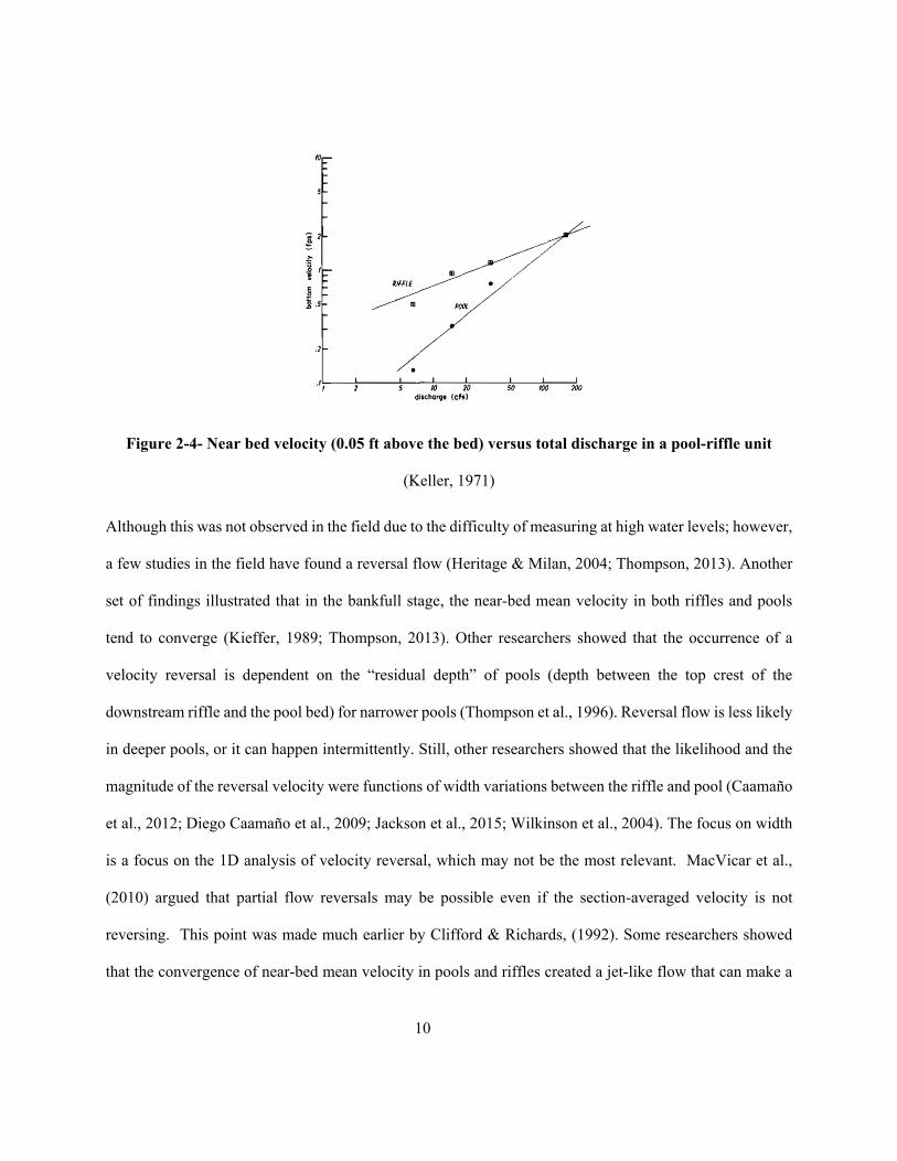
One of the most famous hypotheses in pool-riffle hydrodynamics is “velocity reversal.” It says that
by increasing the flow discharge the increasing rate of near-bed velocity in riffles is lower than the one in
pools and there is a point that the near-bed velocity in the pool is equal to the one in the riffle, in addition,
the shear stress is projected to be higher in pools in high flow rate conditions (Keller 1971) (Figure 2-4).
10
Figure 2-4- Near bed velocity (0.05 ft above the bed) versus total discharge in a pool-riffle unit
(Keller, 1971)
Although this was not observed in the field due to the difficulty of measuring at high water levels; however,
a few studies in the field have found a reversal flow (Heritage & Milan, 2004; Thompson, 2013). Another
set of findings illustrated that in the bankfull stage, the near-bed mean velocity in both riffles and pools
tend to converge (Kieffer, 1989; Thompson, 2013). Other researchers showed that the occurrence of a
velocity reversal is dependent on the “residual depth” of pools (depth between the top crest of the
downstream riffle and the pool bed) for narrower pools (Thompson et al., 1996). Reversal flow is less likely
in deeper pools, or it can happen intermittently. Still, other researchers showed that the likelihood and the
magnitude of the reversal velocity were functions of width variations between the riffle and pool (Caamaño
et al., 2012; Diego Caamaño et al., 2009; Jackson et al., 2015; Wilkinson et al., 2004). The focus on width
is a focus on the 1D analysis of velocity reversal, which may not be the most relevant. MacVicar et al.,
(2010) argued that partial flow reversals may be possible even if the section-averaged velocity is not
reversing. This point was made much earlier by Clifford & Richards, (1992). Some researchers showed
that the convergence of near-bed mean velocity in pools and riffles created a jet-like flow that can make a
11
scour hole in the pools (Kieffer, 1985). They showed that the location of convergence shifts from the riffles
to pools by increasing the flow level.
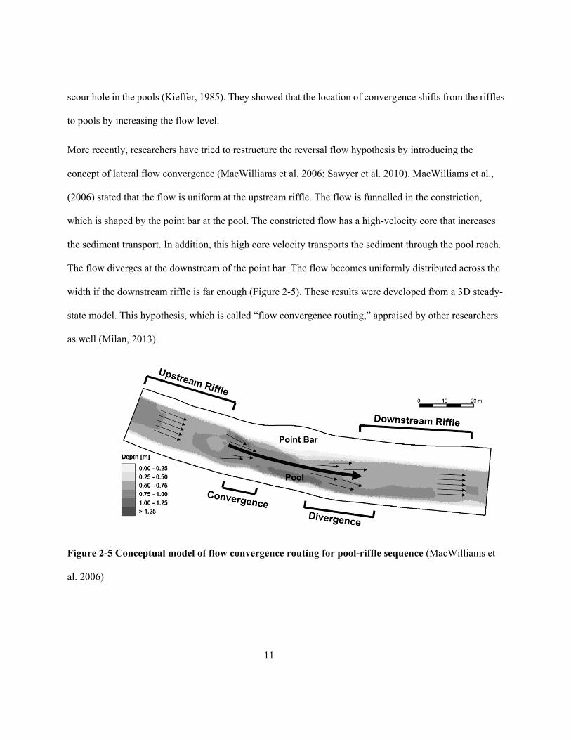
More recently, researchers have tried to restructure the reversal flow hypothesis by introducing the
concept of lateral flow convergence (MacWilliams et al. 2006; Sawyer et al. 2010). MacWilliams et al.,
(2006) stated that the flow is uniform at the upstream riffle. The flow is funnelled in the constriction,
which is shaped by the point bar at the pool. The constricted flow has a high-velocity core that increases
the sediment transport. In addition, this high core velocity transports the sediment through the pool reach.
The flow diverges at the downstream of the point bar. The flow becomes uniformly distributed across the
width if the downstream riffle is far enough (Figure 2-5). These results were developed from a 3D steady-
state model. This hypothesis, which is called “flow convergence routing,” appraised by other researchers
as well (Milan, 2013).
Figure 2-5 Conceptual model of flow convergence routing for pool-riffle sequence (MacWilliams et
al. 2006)
12
2.4 Turbulence
Some detailed studies of hydrodynamics in pools and riffles have argued that turbulence plays a
significant role in sediment transport, formation, and maintenance of pools and riffles (Clifford 1993;
Clifford and Richards 1992; MacVicar and Roy 2007b). The turbulence in most natural streams is the
result of the interaction between flow and irregularities in bed morphology (Thompson, 2013). Turbulent
flows increase the pulsation in shear stress exertion and due to the dynamic loading of grains; the
sediment transport rate will be increased (Roy et al., 1999). Pools and riffles make flow accelerate and
decelerate, and the resulting pressure gradients act as perturbations on the flow and generate significant
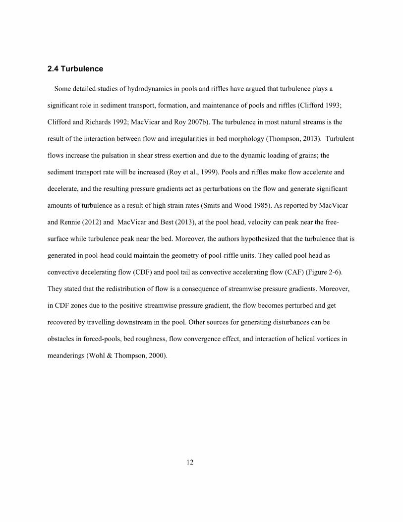
amounts of turbulence as a result of high strain rates (Smits and Wood 1985). As reported by MacVicar
and Rennie (2012) and MacVicar and Best (2013), at the pool head, velocity can peak near the free-
surface while turbulence peak near the bed. Moreover, the authors hypothesized that the turbulence that is
generated in pool-head could maintain the geometry of pool-riffle units. They called pool head as
convective decelerating flow (CDF) and pool tail as convective accelerating flow (CAF) (Figure 2-6).
They stated that the redistribution of flow is a consequence of streamwise pressure gradients. Moreover,
in CDF zones due to the positive streamwise pressure gradient, the flow becomes perturbed and get
recovered by travelling downstream in the pool. Other sources for generating disturbances can be
obstacles in forced-pools, bed roughness, flow convergence effect, and interaction of helical vortices in
meanderings (Wohl & Thompson, 2000).
13
Figure 2-6- Schematic figure of pool-riffle unit with CAF and CDF zones (MacVicar and Obach
2015)
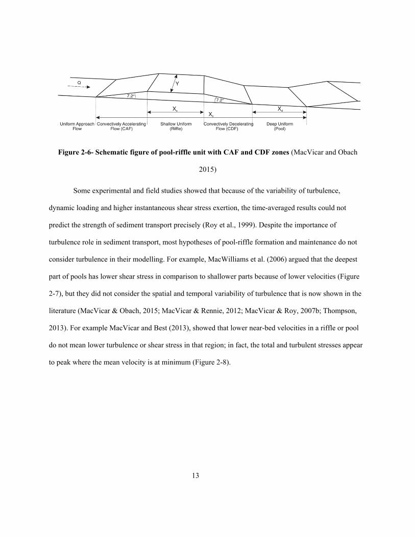
Some experimental and field studies showed that because of the variability of turbulence,
dynamic loading and higher instantaneous shear stress exertion, the time-averaged results could not
predict the strength of sediment transport precisely (Roy et al., 1999). Despite the importance of
turbulence role in sediment transport, most hypotheses of pool-riffle formation and maintenance do not
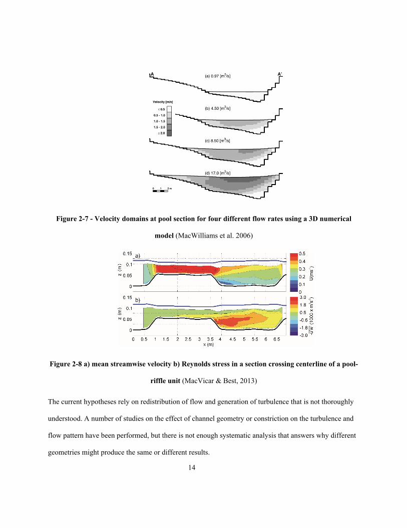
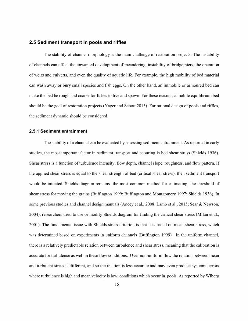
consider turbulence in their modelling. For example, MacWilliams et al. (2006) argued that the deepest
part of pools has lower shear stress in comparison to shallower parts because of lower velocities (Figure
2-7), but they did not consider the spatial and temporal variability of turbulence that is now shown in the
literature (MacVicar & Obach, 2015; MacVicar & Rennie, 2012; MacVicar & Roy, 2007b; Thompson,
2013). For example MacVicar and Best (2013), showed that lower near-bed velocities in a riffle or pool
do not mean lower turbulence or shear stress in that region; in fact, the total and turbulent stresses appear
to peak where the mean velocity is at minimum (Figure 2-8).
14
Figure 2-7 - Velocity domains at pool section for four different flow rates using a 3D numerical
model (MacWilliams et al. 2006)
Figure 2-8 a) mean streamwise velocity b) Reynolds stress in a section crossing centerline of a pool-
riffle unit (MacVicar & Best, 2013)
The current hypotheses rely on redistribution of flow and generation of turbulence that is not thoroughly
understood. A number of studies on the effect of channel geometry or constriction on the turbulence and
flow pattern have been performed, but there is not enough systematic analysis that answers why different
geometries might produce the same or different results.
15
2.5 Sediment transport in pools and riffles
The stability of channel morphology is the main challenge of restoration projects. The instability
of channels can affect the unwanted development of meandering, instability of bridge piers, the operation
of weirs and culverts, and even the quality of aquatic life. For example, the high mobility of bed material
can wash away or bury small species and fish eggs. On the other hand, an immobile or armoured bed can
make the bed be rough and coarse for fishes to live and spawn. For these reasons, a mobile equilibrium bed
should be the goal of restoration projects (Yager and Schott 2013). For rational design of pools and riffles,
the sediment dynamic should be considered.
2.5.1 Sediment entrainment
The stability of a channel can be evaluated by assessing sediment entrainment. As reported in early
studies, the most important factor in sediment transport and scouring is bed shear stress (Shields 1936).
Shear stress is a function of turbulence intensity, flow depth, channel slope, roughness, and flow pattern. If
the applied shear stress is equal to the shear strength of bed (critical shear stress), then sediment transport
would be initiated. Shields diagram remains the most common method for estimating the threshold of
shear stress for moving the grains (Buffington 1999; Buffington and Montgomery 1997; Shields 1936). In
some previous studies and channel design manuals (Ancey et al., 2008; Lamb et al., 2015; Sear & Newson,
2004); researchers tried to use or modify Shields diagram for finding the critical shear stress (Milan et al.,
2001). The fundamental issue with Shields stress criterion is that it is based on mean shear stress, which
was determined based on experiments in uniform channels (Buffington 1999). In the uniform channel,
there is a relatively predictable relation between turbulence and shear stress, meaning that the calibration is
accurate for turbulence as well in these flow conditions. Over non-uniform flow the relation between mean
and turbulent stress is different, and so the relation is less accurate and may even produce systemic errors
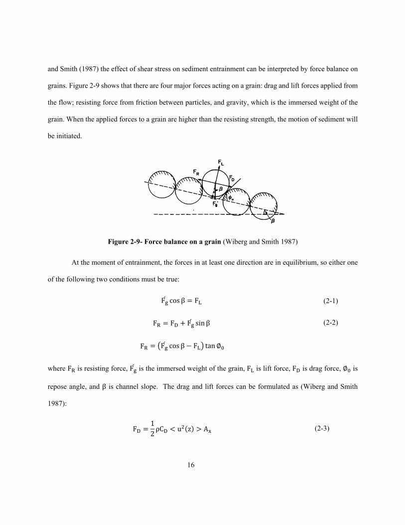
where turbulence is high and mean velocity is low, conditions which occur in pools. As reported by Wiberg
16
and Smith (1987) the effect of shear stress on sediment entrainment can be interpreted by force balance on
grains. Figure 2-9 shows that there are four major forces acting on a grain: drag and lift forces applied from
the flow; resisting force from friction between particles, and gravity, which is the immersed weight of the
grain. When the applied forces to a grain are higher than the resisting strength, the motion of sediment will
be initiated.
Figure 2-9- Force balance on a grain (Wiberg and Smith 1987)
At the moment of entrainment, the forces in at least one direction are in equilibrium, so either one
of the following two conditions must be true:
F cos β F (2-1)
F F F sin β
F F cos β F tan∅
(2-2)
where F is resisting force, F is the immersed weight of the grain, F is lift force, F is drag force, ∅ is
repose angle, and β is channel slope. The drag and lift forces can be formulated as (Wiberg and Smith
1987):
F12ρC u z A (2-3)
17
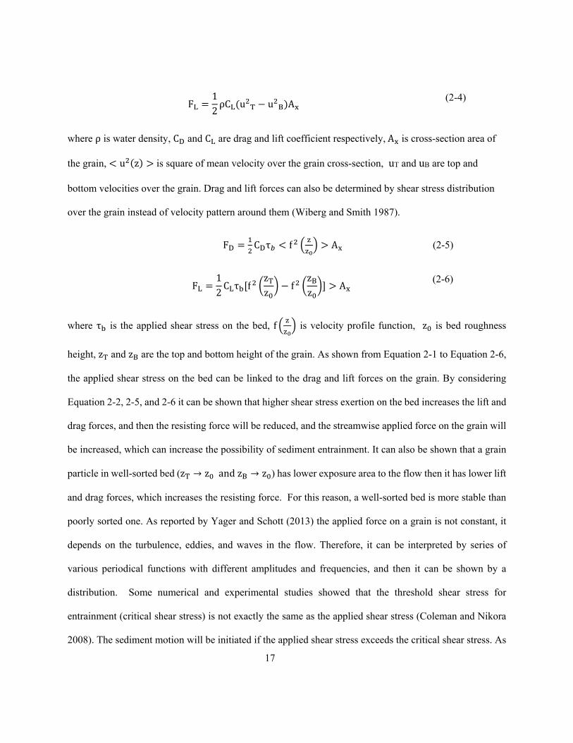
F12ρC u u A
(2-4)
where ρ is water density, C and C are drag and lift coefficient respectively,A is cross-section area of
the grain, u z is square of mean velocity over the grain cross-section, uT and uB are top and
bottom velocities over the grain. Drag and lift forces can also be determined by shear stress distribution
over the grain instead of velocity pattern around them (Wiberg and Smith 1987).
F C τ f A (2-5)
F12C τ f
zz
fzz
A (2-6)
where τ is the applied shear stress on the bed, f is velocity profile function, z is bed roughness
height, z and z are the top and bottom height of the grain. As shown from Equation 2-1 to Equation 2-6,
the applied shear stress on the bed can be linked to the drag and lift forces on the grain. By considering
Equation 2-2, 2-5, and 2-6 it can be shown that higher shear stress exertion on the bed increases the lift and
drag forces, and then the resisting force will be reduced, and the streamwise applied force on the grain will
be increased, which can increase the possibility of sediment entrainment. It can also be shown that a grain
particle in well-sorted bed (z → z andz → z ) has lower exposure area to the flow then it has lower lift
and drag forces, which increases the resisting force. For this reason, a well-sorted bed is more stable than
poorly sorted one. As reported by Yager and Schott (2013) the applied force on a grain is not constant, it
depends on the turbulence, eddies, and waves in the flow. Therefore, it can be interpreted by series of
various periodical functions with different amplitudes and frequencies, and then it can be shown by a
distribution. Some numerical and experimental studies showed that the threshold shear stress for
entrainment (critical shear stress) is not exactly the same as the applied shear stress (Coleman and Nikora
2008). The sediment motion will be initiated if the applied shear stress exceeds the critical shear stress. As
18
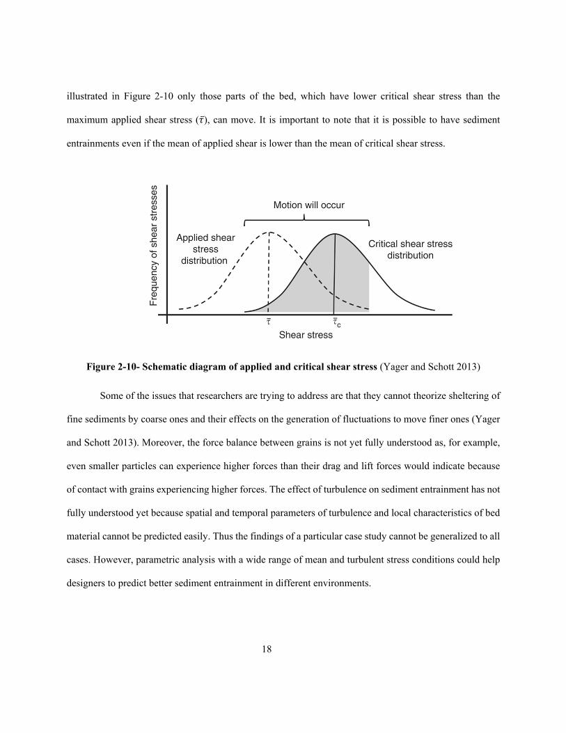
illustrated in Figure 2-10 only those parts of the bed, which have lower critical shear stress than the
maximum applied shear stress ( ), can move. It is important to note that it is possible to have sediment
entrainments even if the mean of applied shear is lower than the mean of critical shear stress.
Figure 2-10- Schematic diagram of applied and critical shear stress (Yager and Schott 2013)
Some of the issues that researchers are trying to address are that they cannot theorize sheltering of
fine sediments by coarse ones and their effects on the generation of fluctuations to move finer ones (Yager
and Schott 2013). Moreover, the force balance between grains is not yet fully understood as, for example,
even smaller particles can experience higher forces than their drag and lift forces would indicate because
of contact with grains experiencing higher forces. The effect of turbulence on sediment entrainment has not
fully understood yet because spatial and temporal parameters of turbulence and local characteristics of bed
material cannot be predicted easily. Thus the findings of a particular case study cannot be generalized to all
cases. However, parametric analysis with a wide range of mean and turbulent stress conditions could help
designers to predict better sediment entrainment in different environments.
19
2.5.2 Bedload routing
When the applied force on a moving particle drops below the force required to keep it in motion
the particle starts to deposit. The travel distance of particles depends on the flow behaviour and particle
characteristics; therefore, the same particles with the same sizes tend to deposit in the same places. This
mechanism is called sediment sorting. This is one of the most significant reasons for natural pool-riffle
formation and maintenance based on the travel distance of particles, coarser material stores in riffle and
finer in pools (Lisle 1979b). Some researchers showed that the transport of fine sediment from the center
of pools was the result of the jet flow and flow convergence (Thompson & Wohl, 2009). The reason could
be the higher turbulence condition, and dynamic loading of grain due to pulsation effect at the pools head
after the deceleration part (MacVicar & Roy, 2011). The deposition of transported sediment from the center
and head of pools at the tail of them can make the downstream riffle. And the deposition is the result of
lateral flow divergence and boiling at the tail of pools (Buffington et al. 2002).
2.5.3 Effect of hydrodynamic on sediment transport
Despite limitations and issues related to scaling of sediment transport in the lab, it remains
important due to the complexity of sediment transport and its interaction with the mean and turbulent
components of the flow. Some researchers used the mobile bed for assessing the formation of
morphological elements in rivers (e.g. pool-riffle). Lisle et al. (1991) used a poorly-sorted mixture of gravel
and sand as bed material and inlet sediment in the flume for investigating the formation mechanism of bars
in the steep channel. They saw a series of scouring and deposition in the flume that led to the formation and
development of a meandering. Many researchers used completely or partially mobile bed in the flume to
investigate sediment transport mechanism (Madej et al. 2009; Wilcock and Mcardell 1997; Wilcock and
McArdell 1993). Diplas et al. (2008) used electromagnetic force to model drag force acting on steel spheres
to investigate the effect of pulsation on motion initiation of sediment. They noted that because of turbulence
20
in the natural stream, the drag force, which is acting on the particles, has intensive fluctuations then they
model this fact by making fluctuation in electromagnetic force. They stated that the sediment entrainment
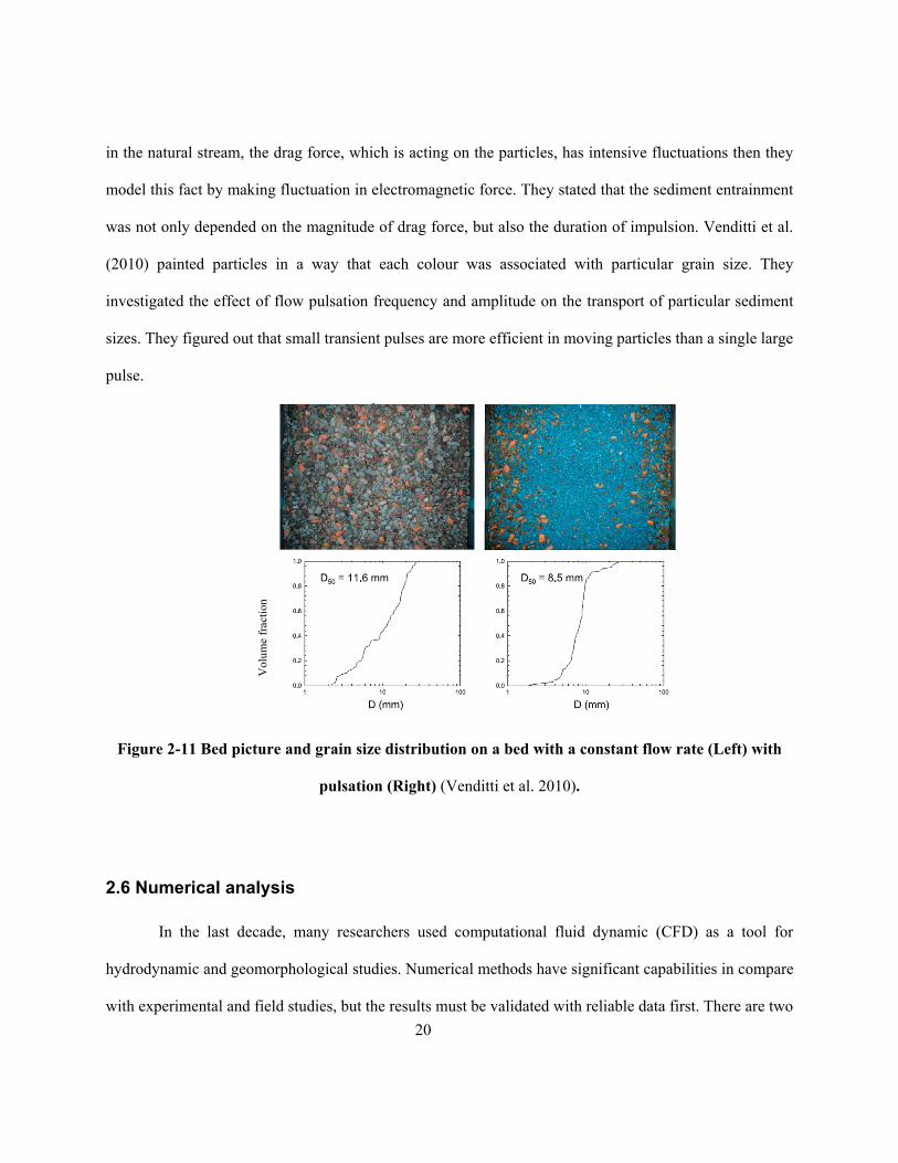
was not only depended on the magnitude of drag force, but also the duration of impulsion. Venditti et al.
(2010) painted particles in a way that each colour was associated with particular grain size. They
investigated the effect of flow pulsation frequency and amplitude on the transport of particular sediment
sizes. They figured out that small transient pulses are more efficient in moving particles than a single large
pulse.
Figure 2-11 Bed picture and grain size distribution on a bed with a constant flow rate (Left) with
pulsation (Right) (Venditti et al. 2010).
2.6 Numerical analysis
In the last decade, many researchers used computational fluid dynamic (CFD) as a tool for
hydrodynamic and geomorphological studies. Numerical methods have significant capabilities in compare
with experimental and field studies, but the results must be validated with reliable data first. There are two
Vol
ume
frac
tion
21
types of approaches in numerical analysis, steady state, and transient modelling. In steady state modelling,
the variations of variables are zero in time. This kind of modelling is suitable for laminar flows and cases
with steady, coherent structures. One of the advantageous of the numerical methods is that the velocity
domain can be acquired for all regions, but in experimental and field studies, it is not possible due to the
limitations of instruments. As stated before the most important parameters in hydrodynamic studies is shear
stress; in numerical analysis, because of the possibility to measure velocity gradient in near-wall regions,
the bed shear stress can be calculated precisely. The turbulence intensity is another important parameter for
assessing the sediment transport rate and bed shear stress; therefore, numerical analysis is the best tool for
this purpose. One of the limitations of using a steady state approach in hydrodynamic studies is that most
of the phenomenon in this field is turbulent and containing dynamic behaviours. The capability of transient
modelling enables researchers to study dynamic vortices and turbulent structures better. Another
consideration in the modelling of the turbulent condition is that turbulence cannot happen in 2D modelling,
and the case must be modelled in 3D because large-scale vortices must be stretched by all vorticity
components before breaking into smaller scales. In the absence of one dimension, two component of
vorticity is zero then large-scale eddies cannot be stretched. Viscosity cannot dissipate the energy of large-
scale eddies; therefore, when they break into a smaller scale, by energy cascading the kinematic energy of
large-scale eddies is transported to the smaller one, and then the viscosity can dissipate their energy.
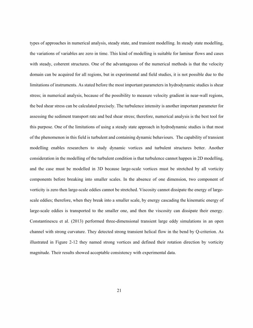
Constantinescu et al. (2013) performed three-dimensional transient large eddy simulations in an open
channel with strong curvature. They detected strong transient helical flow in the bend by Q-criterion. As
illustrated in Figure 2-12 they named strong vortices and defined their rotation direction by vorticity
magnitude. Their results showed acceptable consistency with experimental data.
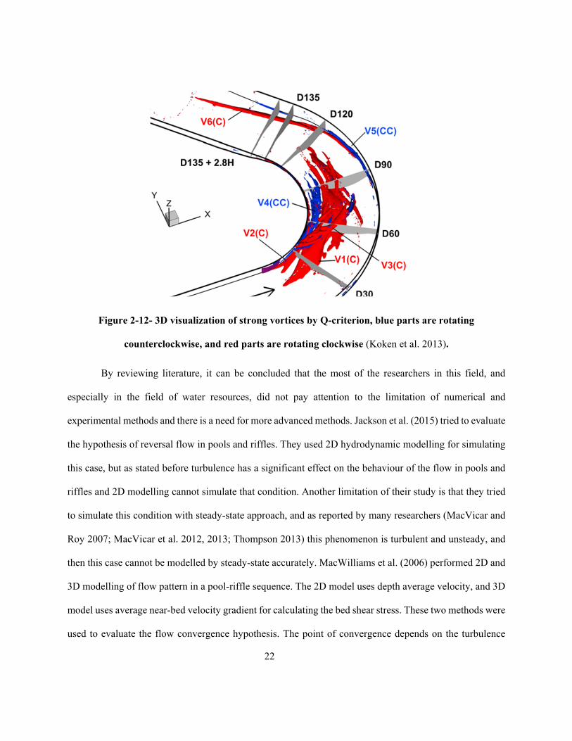
22
Figure 2-12- 3D visualization of strong vortices by Q-criterion, blue parts are rotating
counterclockwise, and red parts are rotating clockwise (Koken et al. 2013).
By reviewing literature, it can be concluded that the most of the researchers in this field, and
especially in the field of water resources, did not pay attention to the limitation of numerical and
experimental methods and there is a need for more advanced methods. Jackson et al. (2015) tried to evaluate
the hypothesis of reversal flow in pools and riffles. They used 2D hydrodynamic modelling for simulating
this case, but as stated before turbulence has a significant effect on the behaviour of the flow in pools and
riffles and 2D modelling cannot simulate that condition. Another limitation of their study is that they tried
to simulate this condition with steady-state approach, and as reported by many researchers (MacVicar and
Roy 2007; MacVicar et al. 2012, 2013; Thompson 2013) this phenomenon is turbulent and unsteady, and
then this case cannot be modelled by steady-state accurately. MacWilliams et al. (2006) performed 2D and
3D modelling of flow pattern in a pool-riffle sequence. The 2D model uses depth average velocity, and 3D
model uses average near-bed velocity gradient for calculating the bed shear stress. These two methods were
used to evaluate the flow convergence hypothesis. The point of convergence depends on the turbulence
23
condition; therefore, these two methods cannot precisely predict the flow convergence behaviour and shear
stress exertion. They have stated that the deeper part of pools has lower shear stress in comparison to the
shallower one, but they did not discuss the turbulence intensity and the effect of it on bed shear stress. They
have stated that the highest bed shear stress only occurs in riffles, but as stated in the literature, pools have
the most turbulent condition in pool-riffle units and because of turbulent condition the shear stress exertion
could be higher in pools. de Almeida and Rodríguez (2011) used 1D unsteady flow for assessing the
sediment transport rate and morphological changes. They used an empirical equation for calculating the
sediment transport rate. Their empirical method was based on the ratio of bed shear stress and the strength
of the bed. The shear stress in their model is based on the mean cross-section velocity. They did not consider
the effect of turbulence intensity on sediment transport rate and shear stress exertion on the bed. It is not
stated if they consider the secondary effect of scouring on flow pattern shaping or not.
2.7 Numerical methods
Due to the turbulent condition in most of the natural streams, it is better to use eddy-resolving
techniques for more accurate results. In this chapter, the concepts of common techniques in CFD will be
discussed briefly.
2.7.1 Numerical concepts
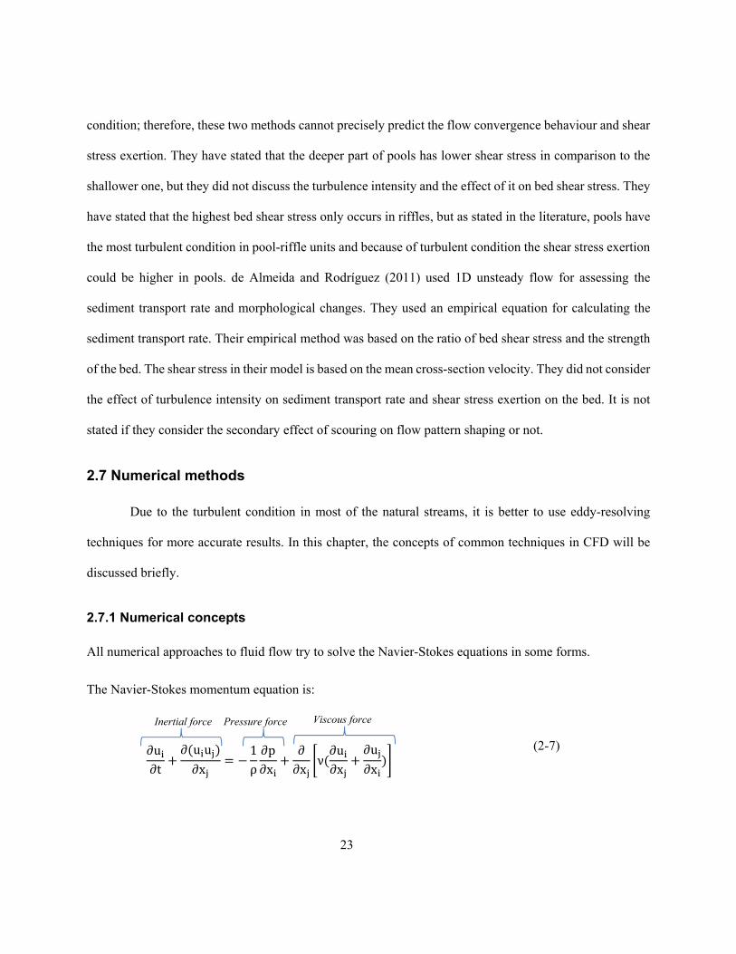
All numerical approaches to fluid flow try to solve the Navier-Stokes equations in some forms.
The Navier-Stokes momentum equation is:
∂u∂t
∂ u u
∂x1ρ∂p∂x
∂∂x
ν∂u∂x
∂u
∂x
(2-7)
Inertial force Pressure force Viscous force
24
where t is time, p is pressure and ν is kinematic viscosity. By choosing (i, j) as (1, 2), (1, 3), and (2, 3) then
we have three coupled equations for a 3D model. The continuity equation for incompressible flow is:
∂u∂x
0 (2-8)
where (u,v,w) are velocity components in x,y,z directions, u1, u2, u3 are streamwise, spanwise, and vertical
components of velocity.
In direct numerical simulations (DNS), there is no turbulence closure scheme for approximation and all of
the turbulence effects are simulated directly based on the exact behaviour of the flow. This approach
requires high-resolution grids to simulate the viscous sub-layer and Kolmogorov's eddy scales. For
example, Schlatter et al. (2014) used 4000 cores in parallel for simulating flow over a rough plate. In other
approaches such as the Reynolds-averaged Navier-Stokes (RANS) equations, large eddy simulation (LES),
and detached eddy simulation (DES) the effect of small-scale eddies are modelled separately and added to
the Navier-Stokes equations as a means of reducing the computational requirements.
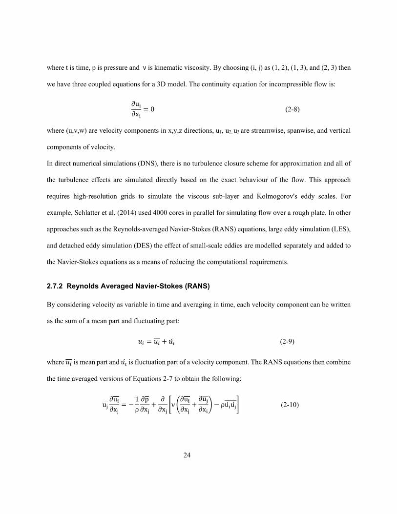
2.7.2 Reynolds Averaged Navier-Stokes (RANS)
By considering velocity as variable in time and averaging in time, each velocity component can be written
as the sum of a mean part and fluctuating part:
(2-9)
where is mean part and is fluctuation part of a velocity component. The RANS equations then combine
the time averaged versions of Equations 2-7 to obtain the following:
u∂u∂x
1ρ∂p∂x
∂∂x
ν∂u∂x
∂u
∂xρu u (2-10)
25
As can be seen in Equation 2-10, the most-right term ( ρu u ) is the combination of fluctuation in
velocity components. This term called the Reynolds stress, and it cannot be simulated in steady state
modelling; therefore, researchers tried to approximate it with different methods. One of the most common
for estimating Reynolds stress and modifying Equation 2-10 is using a turbulence closure scheme that is
called k-ε. In k-ε two additional equations will be coupled with Equation 2-10 that are related to the kinetic
turbulent energy and dissipation rate.
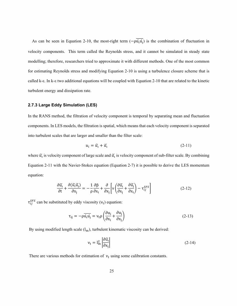
2.7.3 Large Eddy Simulation (LES)
In the RANS method, the filtration of velocity component is temporal by separating mean and fluctuation
components. In LES models, the filtration is spatial, which means that each velocity component is separated
into turbulent scales that are larger and smaller than the filter scale:
(2-11)
where is velocity component of large scale and is velocity component of sub-filter scale. By combining
Equation 2-11 with the Navier-Stokes equation (Equation 2-7) it is possible to derive the LES momentum
equation:
∂u∂t
∂ u u
∂x1ρ∂p∂x
∂∂x
ν∂u∂x
∂u
∂xτ (2-12)
τ can be substituted by eddy viscosity (ν ) equation:
τ ρu u ν ρ∂u∂x
∂u
∂x (2-13)
By using modified length scale (l ), turbulent kinematic viscosity can be derived:
ν l∂u∂x
(2-14)
There are various methods for estimation of using some calibration constants.
26
2.8 Research gap
The overall research gap is that there is no comprehensive and unanimously agreed hypothesis on pool-
riffle formation and maintenance. In addition, the effect and variation of pool-riffle geometry, which are
the most important factors in hydrodynamics of pool-riffle units, is not investigated adequately, which
makes it difficult to predict the success or failure of restoration designs. Limitations inherent in
experimental and field studies mean that the understanding of hydrodynamics in pools and riffles can be
improved with transient numerical studies. Due to the turbulent behaviour of the flow in pool-riffles, 3D
and unsteady numerical approaches with appropriate turbulence closure schemes would be particularly
insightful. Turbulence, temporal and spatial distribution of shear stress and their effects on sediment
transport, which are the main gaps in pool-riffle research, can be investigated by linking of well-designed
numerical simulations with experimental modelling. The most significant advantage of experimental and
field studies is that they enable researchers to assess and evaluate the sediment transport mechanism. This
objective cannot be addressed easily by numerical approaches; therefore, a targeted flume-experimental
study could help to improve the understanding of the role of vortices in sediment transport and the
relation between turbulence and pool-riffle maintenance.
27
Chapter 3: Effect of riffle height on
turbulent structures and flow pattern in
isolated pool-riffle units
This chapter is based on a manuscript that has been submitted to the Journal of Geophysical Research:
Earth Surface. All the results were generated by myself, and I prepared the final document under the
supervision of Dr. MacVicar.
28
Large eddy simulations of turbulent structures in plunging and skimming flow in straight pool-
riffle bedforms
H. Dashtpeyma1, and B. J. MacVicar1
1 Department of Civil and Environmental Engineering, 200 University Avenue West, Waterloo, Ontario,
Canada N2L 3G, University of Waterloo.
Corresponding author: Hamed Dashtpeyma ([email protected])
Key Points:
1-Four different types of vortical turbulent structures were detected in the zone of flow expansion in the
pool head.
2-The turbulent structures steer the main flow by increasing the turbulent Reynolds stresses and the
effective viscosity.
3-The degree of plunging or skimming of the main flow through the pool can be controlled by the height
of the riffle and the Froude number at the riffle crest.
3.1 Abstract
Pool-riffle units are common topographical elements of rivers. Many hypotheses such as flow
reversal and lateral flow convergence have been proposed for clarification of hydrodynamics in pool-
riffle units. In this study, large eddy simulation (LES) is used to capture detailed information on flow
characteristics in idealized pools and riffles. The Q-criterion is used to detect flow structures. The
idealized structure is a straight channel with sloped bed rises and drops acting as zones of convective
acceleration and deceleration. Four types of vortical structures are detected of these forms. Ramp rollers
and corner eddies are shaped on the ramp and in the corners of the upstream part of the pool (i.e. the pool
head), respectively. Surface turbulence is shaped at the free-surface of the pool-head. All the generated
29
vortices in the pool-head get stretched and form axial tail vortices. Interaction and combination of these
vortices create three different types of incoming flow to the pool. If surface turbulence is strong it can
interact with corner eddies and direct the incoming flow to plunge into the pool. If ramp rollers are strong,
they can push the incoming flow away from the bed so that it skims the free-surface. If the ramp and
surface rollers have similar strength, the incoming flow will be squeezed between the high turbulence
zones so that streamwise velocity peaks in the middle of the flow depth.
3.2 Introduction
One of the most common topographical elements of rivers are pool-riffle units. The deeper parts
of undulations in the bed are called pools, whereas the shallower parts are riffles (Figure 3-1). Pool-riffle
sequences can be shaped naturally, but are also frequently used in river restoration projects (Bernhardt
and Palmer 2007; Miller and Kochel 2009; Wohl et al. 2005). Many researchers have investigated the
formation and maintenance mechanism of pool-riffle units (Keller, 1971; Keller & Florsheim, 1993;
MacVicar & Roy, 2007; Wilkinson et al., 2008). One of the most famous hypotheses is “velocity
reversal,” which says that the near-bed velocity in pools will increase faster than the corresponding
velocity in riffles, leading to higher shear stress and scour in pools at flood stages (Keller 1971). This
hypothesis was not connected to a hydraulic analysis of flow over bedforms, however, and it has been
difficult to confirm or refute, with several researchers finding rivers with stable pool-riffle units without
velocity-reversal effects (Heritage and Milan 2004; MacVicar and Roy 2007a; Thompson 2013), and
others qualifying that the likelihood and the magnitude of the reversal velocity are functions of width
variations between the riffle and pool (Wilkinson et al., 2004). The importance of width variations has
been reinforced by field, numerical, and laboratory demonstrations (de Almeida & Rodríguez, 2012;
Nelson et al., 2015; White et al., 2010). The velocity reversal hypothesis has now largely been
restructured by introducing the concepts of lateral flow convergence and sediment routing (MacWilliams
30
et al. 2006; Milan 2013; Sawyer et al. 2010), and considering the bulk flow properties in width
restrictions (Caamaño et al., 2012, 2009). The flow convergence hypothesis does not explicitly consider
turbulence, however, which is known to be strongly influenced by pool-riffle morphology (Clifford,
1993; Clifford & Richards, 1992; MacVicar & Roy, 2007b; Thompson, 2013), and influence in turn the
scour and transport of sediment (Celik et al., 2013; Nelson et al., 1995; Sumer et al., 2003). Length scales
of turbulent dissipation have also been shown to be similar to commonly observed scaling relations
between channel width and the frequency of riffles and pools (MacVicar and Best 2013, MacVicar &
Obach 2015), which suggests an appealing link between turbulence and macroscale morphology. More
research is required to clearly understand turbulence generation and dissipation over pool-riffle bedforms
in a way that integrates existing observations and considers both mean flow and turbulence induced
stresses.
From a hydraulic perspective, the morphology of pools and riffles causes streamwise pressure gradients
that forces flow to accelerate and decelerate. In such environments, turbulence is generated as a result of
high strain rates during acceleration (Smits and Wood 1985) then spreads across the domain and
dissipates when pressure gradients are removed. In a series of laboratory experiments in straight channels
with low angle ramps (<7°) to simulate bedforms, MacVicar and Rennie (2012) and MacVicar and Best
(2013) considered the convective accelerating flow (CAF) and convective decelerating flow (CDF) zones
as flow perturbations and documented their effects on mean flow and turbulence. They found high
turbulence intensities near the bed and channel sidewalls at the head of the pool in CDF, with the
turbulent structures growing, expanding laterally from the side walls, and dissipating as they travelled
downstream (MacVicar et al. 2013). Critically for theories of pool formation, they observed that the
fastest mean flow occurs near the water surface along the centerline of the channel, i.e. that it ‘skims’
across the top of the pool rather than ‘plunging’ to the bottom of the pool where it could exert a strong
influence on particle mobility. These patterns of mean flow and turbulence matched what occurred in the
31
head of a forced pool system (MacVicar and Roy 2007a, 2007b), which supported the hypotheses that the
turbulence must be contributing to sediment mobilization and scour, particularly over the downstream
riffle face and into the head of the pool (MacVicar and Roy, 2011). Limitations inherent to field and
laboratory studies, however, mean that it is difficult or impossible to extrapolate these hypotheses to pool-
riffles at different flow levels and with differing geometries.
In the last decade, many researchers have used large eddy simulation (LES) as a tool to understand the
hydrodynamics over river morphologies (Bradbrook et al., 2000; Hardy et al., 2005; Keylock et al., 2012;
Keylock et al., 2016; Stoesser et al., 2008). This method uses a subgrid-scale model to include the effect
of small turbulent eddies on the mean and turbulent flow while allowing the larger turbulent eddies to be
simulated explicitly investigated (Smagorinsky, 1963; Stoesser, 2014). In this way, it is possible to change
parameters such as the flow or geometry that may be difficult in the field or physical models. Riffle
height, for instance, requires multiple models to be constructed in the lab and is difficult or impossible to
control in the field. Numeric simulations also have the advantage of allowing the instantaneous
visualization and analysis of the entire flow field, which can be used to clarify the genesis and evolution
of intermittent turbulent structures.
In the current study, transient turbulent flow is simulated using LES in isolated pool-riffle units with
various riffle heights. Though many aspects of pool and riffle morphology are not investigated, the study
is part of a larger effort to investigate turbulence generation and dissipation in pools and riffles that will
increase the generalizability of the results. Given the novelty of the approach, we focused for the moment
on a description of the turbulent structures and the key parameter of riffle height, which was found to
exert an important control on the hydrodynamics, with observations of both plunging and skimming flow
in pools. Specific objectives are to: 1) investigate, identify, and characterize turbulent structures in
straight pool-riffle units; 2) demonstrate the effect of riffle height on flow patterns, and 3) illustrate the
influence of turbulent structures on variation and mean bed shear stress. It is hoped that the results will
32
help to connect various observations of hydrodynamics in pools and riffles and contribute to better
designs of pool-riffle structures that are sensitive to the local flow conditions.
3.3 Methodology
3.3.1 Model Geometry
The model geometry is based on one of the flume experiments completed by MacVicar and Obach
(2015), which was in turn based on a geometric (1:10) and Froude scale (Fr ~ 0.6) matching of a field
example (MacVicar and Roy 2007). The physical and numerical models use a simplified straight
geometry of pool and riffle units in a 0.6 m wide channel (Figure 3-1). The simulated flume in the
numerical model is 6 m long with a 1 m long uniform upstream section followed by a 0.52 m long
upsloping ramp, a flat uniform shallow ‘riffle’ of 0.4 m, a 0.52 m long downsloping ramp, a flat uniform
deep ‘pool’ of 2.4 m. A final upsloping ramp and short uniform shallow section were used to define the
downstream boundary of the model. For the series of simulations in this study, the riffle height was varied
as shown in Table 1. With the fixed length of the ramped sections, the change of riffle height also
changed the ramp angles. The average inlet velocity (Uo), the flow depth in the pool (h) and the Froude
number in the pool were 0.21 m/s, 0.12 m, and 0.2 for all cases, respectively. For reference, X, Y, and Z
represent the streamwise, vertical, and spanwise directions, respectively.
The cases described in this study were designed to approach and slightly exceed the thresholds for
choking flow based on a specific energy analysis. By considering the velocity variation in only the
streamwise direction, the specific energy m is calculated as 2⁄ , where α is the energy
coefficient, U is the cross-section average flow velocity, and g is the gravitational constant (9.81 ms-2). A
critical height for a bed rise that is just sufficient to induce choking flow (ΔZc) can then be found as the
difference between the critical specific energy (Ec) and E, where 3 2⁄ ⁄ , Q is the total
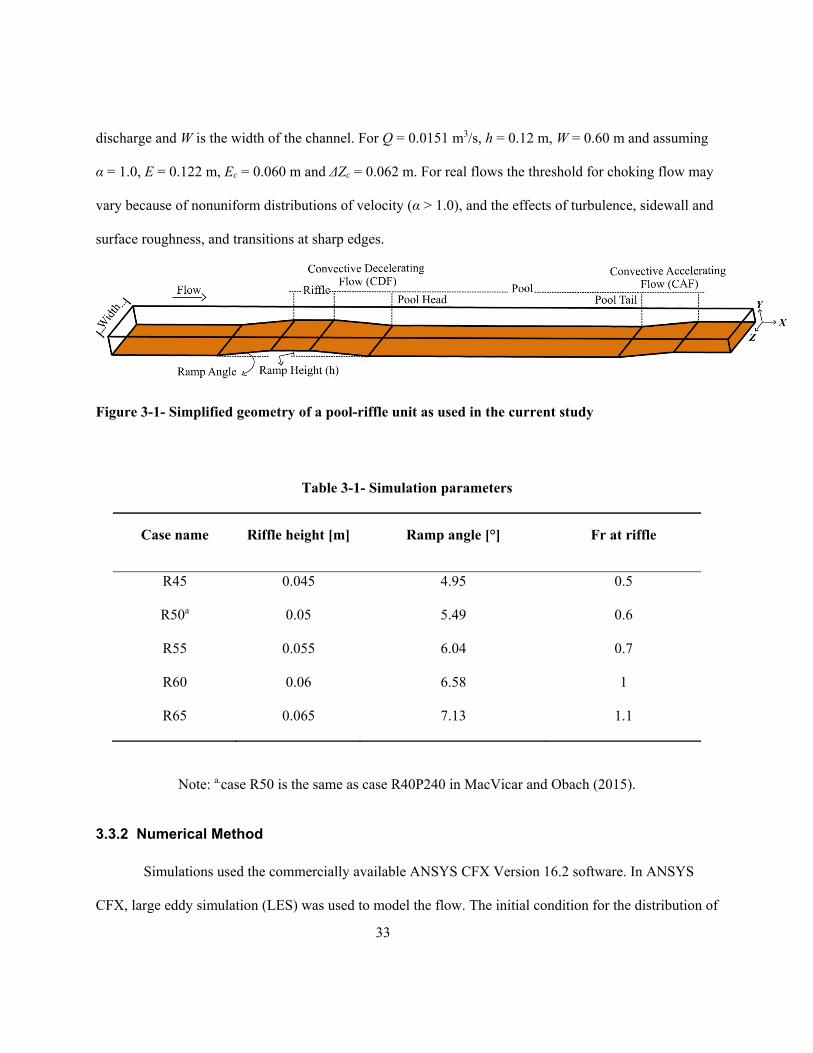
33
discharge and W is the width of the channel. For Q = 0.0151 m3/s, h = 0.12 m, W = 0.60 m and assuming
α = 1.0, E = 0.122 m, Ec = 0.060 m and ΔZc = 0.062 m. For real flows the threshold for choking flow may
vary because of nonuniform distributions of velocity (α > 1.0), and the effects of turbulence, sidewall and
surface roughness, and transitions at sharp edges.
Figure 3-1- Simplified geometry of a pool-riffle unit as used in the current study
Table 3-1- Simulation parameters
Case name Riffle height [m] Ramp angle [°] Fr at riffle
R45 0.045 4.95 0.5
R50a 0.05 5.49 0.6
R55 0.055 6.04 0.7
R60 0.06 6.58 1
R65 0.065 7.13 1.1
Note: a.case R50 is the same as case R40P240 in MacVicar and Obach (2015).
3.3.2 Numerical Method
Simulations used the commercially available ANSYS CFX Version 16.2 software. In ANSYS
CFX, large eddy simulation (LES) was used to model the flow. The initial condition for the distribution of
34
flow and turbulence intensity was determined by first modelling the system with a steady state Reynolds
average Navier-Stokes (RANS) approach and a K-epsilon model for turbulence. Because of smooth and
non-slip walls and bed, a wall-function is not required. Instead, the LES Smagorinsky (1963) method was
chosen, which has been widely used in similar geomorphic research (Keylock et al., 2005, 2012). For
more detailed information about formulations and equations of LES see Rodi et al., (2013). The
simulations were 3D, with a structured mesh generated using ICEM Version 16.2, and a total number of
elements equal to 48.5×10⁶. Minimum cell size in the near-wall region was 1×10⁻³ m, which was selected
to satisfy the criteria suggested by Keylock et al. (2012), who recommended at least six points for
resolving small eddies generated in this region, which they have the same scale as the height of the riffle.
Also following Keylock et al. (2012), cell sizes were 1/40 of the depth, which meets the recommendation
to keep the free surface cells to less than 1/20 of the flow depth. The total time for transient modelling
was 250 s, which is > 300x the largest eddy scale (~h/Uo) and easily exceeded the recommendation of 20x
the eddy time scale by Keylock et al. (2012). The first 50 s were not considered because of initial
condition effects, so only the results between 50 s and 250 s were recorded for analysis. On the machine
we used, which has dual CPUs, each with ten cores of 2.3 GHz with CPU model Intel(R) Xeon(R) 2650
V3, and 192 GB RAM, one complete simulation took approximately 240 hours. Post processing was
completed with CFD-POST Version 16.2 and MATLAB R2017b.
3.3.3 Boundary Conditions
Following (Hirt and Nichols 1981), the volume of fraction (VOF) method was used to model the
multi-phase flow and locate the free surface. In VOF, the assumption is that the fluid occupies the entire
domain with the characteristics that are a function of the fractional volume of the primary fluid (i.e. water
in this study), which its value is one at any nodes that are occupied by primary fluid and zero when they
are empty or occupied by the secondary fluid (i.e. air). Considering free surface is moving with the fluid,
35
by adding a kinematic transport equation for fractional volume to other equations, the free-surface can be
located in transient models as well. By using this method, there is no need to solve two sets of equations
for each phase. Therefore the calculation can be done with lower computational cost. For more details and
formulation see (Hirt and Nichols 1981).
Using VOF, the inlet was separated into air and water zones at the experimental flow depth (h =
0.12 m). The air zone had zero velocity inlet and the constant pressure of zero. The water zone was
defined as having a hydrostatic pressure distribution with a fully developed steady water velocity profile.
To define the inlet velocity profile, a separate simulation was done with uniform velocity inlet (U0 = 0.21
m/s) in a ten meter long uniform channel (i.e. without pools and riffles) with the same slope, width, flow
height and simulation adjustments. The time-averaged velocity profile at the end of the plain channel was
used as the inlet profile of pool-riffle simulations. The outlet was defined as having a constant hydrostatic
pressure distribution for water and constant zero pressure for air. In all locations, a distance of at least 4
cm was maintained between the water surface and the top of the simulation space, which allowed the free
surface to be shaped based on the hydraulic characteristics alone.
3.3.4 Q-criterion for detection of vortex cores
One of the most challenging problems in hydrodynamic studies of open channel flows is the
detection of dynamic vortices and turbulent structures. Moreover, in turbulence and transient modelling,
the core of dynamic vortices are not detectable in the streamlines or vectors of mean or instantaneous
velocities. In addition, even the vorticity cannot give sufficient information about them near the wall-
region due to high velocity gradient (Dubief and Delcayre 2000; Roy et al. 2004; Schlatter et al. 2014).
Dubief and Delcayre, (2000) showed that the dynamic vortices in turbulence could be detected by Q-
criterion, even in regions with high strain rates, defined as:
Q (3-1)
36
, , (3-2)
, , (3-3)
where is instantaneous velocity in direction, ∈ , , , and related to different spatial coordinate,
, is the spatial gradient of in direction. Positive values of Q occur where the rotation term of
equation (2) ( ) exceeds the strain rate ( ) and indicate the presence of rotational flow or
vortices. This method has been used recently in several hydrodynamic and geomorphological studies to
identify and describe vortices in channel confluences, around groynes, and in channel bends (Beheshti et
al., 2017; Ettema et al., 2017; Guillén Ludeña et al., 2017; Keylock et al., 2012, 2016; Zeng &
Constantinescu, 2017). Based on its success in similar studies in rivers and the utility of comparing
structures between morphologic environments, the Q-criterion was applied in the current study.
3.3.5 Validation
The experimental data for the case of R40P240 from MacVicar and Obach (2015), corresponding
with case R50 (Table 1), was used to validate the flow behaviour, water surface elevation, and the
distribution of time average streamwise flow velocity (Ux) in the numerical simulations. As a note, the
ramp angle of 7.2° reported by MacVicar and Obach (2015) referred to the design rather than the as-built
angle of the physical model, which was in fact 5.5°. Time-averaged numerical results and experimental
data are compared in Figure 3-2. Water surface level is similar in both numerical and experimental
results, with a drop at the riffle that is consistent with what is expected from a specific energy analysis for
subcritical flow (Figure 3-2a). Froude numbers from simulated models calculated at the top downstream
edge of the riffle match the analytical calculations (Table 1). Seven time-averaged streamwise velocity
profiles normalized by the inlet velocity (Ux/Uo) are shown at different points along the channel centerline
between the middle of the riffle and middle of the pool (Figure 3-2b). Numerical results are generally

37
consistent with experimental data, especially in the pool, which is a key area for assessing existing
hypotheses for pool-riffle hydrodynamics. The numerical results show higher velocity near the surface
and lower near the bed, which are similar to the experiments. The numerical and experimental profiles of
Ux diverge near the bed at the middle of the ramp (profile 3). This divergence is thought to be related to
experimental uncertainty in the measurement technique of MacVicar and Obach (2015), which used
single beam ultrasonic velocity Doppler profilers (UDVPs) and interpolated profile results measured at
different angles to estimate the orthogonal velocity components. The UDVPs were more accurate where
turbulence intensity was low, and the interpolation was more accurate where gradients in velocity and
turbulence intensity were low, conditions that were not met close to the bed within the flow expansion.
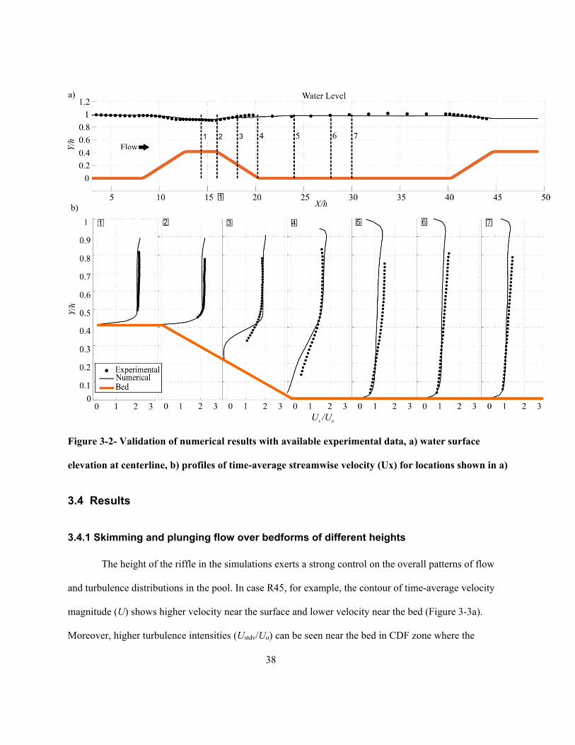
38
Figure 3-2- Validation of numerical results with available experimental data, a) water surface
elevation at centerline, b) profiles of time-average streamwise velocity (Ux) for locations shown in a)
3.4 Results
3.4.1 Skimming and plunging flow over bedforms of different heights
The height of the riffle in the simulations exerts a strong control on the overall patterns of flow
and turbulence distributions in the pool. In case R45, for example, the contour of time-average velocity
magnitude (U) shows higher velocity near the surface and lower velocity near the bed (Figure 3-3a).
Moreover, higher turbulence intensities (Ustdv/Uo) can be seen near the bed in CDF zone where the
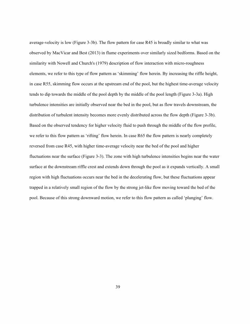
39
average-velocity is low (Figure 3-3b). The flow pattern for case R45 is broadly similar to what was
observed by MacVicar and Best (2013) in flume experiments over similarly sized bedforms. Based on the
similarity with Nowell and Church's (1979) description of flow interaction with micro-roughness
elements, we refer to this type of flow pattern as ‘skimming’ flow herein. By increasing the riffle height,
in case R55, skimming flow occurs at the upstream end of the pool, but the highest time-average velocity
tends to dip towards the middle of the pool depth by the middle of the pool length (Figure 3-3a). High
turbulence intensities are initially observed near the bed in the pool, but as flow travels downstream, the
distribution of turbulent intensity becomes more evenly distributed across the flow depth (Figure 3-3b).
Based on the observed tendency for higher velocity fluid to push through the middle of the flow profile,
we refer to this flow pattern as ‘rifting’ flow herein. In case R65 the flow pattern is nearly completely
reversed from case R45, with higher time-average velocity near the bed of the pool and higher
fluctuations near the surface (Figure 3-3). The zone with high turbulence intensities begins near the water
surface at the downstream riffle crest and extends down through the pool as it expands vertically. A small
region with high fluctuations occurs near the bed in the decelerating flow, but these fluctuations appear
trapped in a relatively small region of the flow by the strong jet-like flow moving toward the bed of the
pool. Because of this strong downward motion, we refer to this flow pattern as called ‘plunging’ flow.
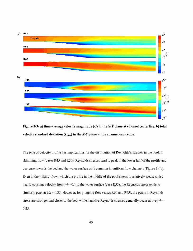
40
Figure 3-3- a) time-average velocity magnitude (U) in the X-Y plane at channel centerline, b) total
velocity standard deviation (Ustdv) in the X-Y plane at the channel centreline.
The type of velocity profile has implications for the distribution of Reynolds’s stresses in the pool. In
skimming flow (cases R45 and R50), Reynolds stresses tend to peak in the lower half of the profile and
decrease towards the bed and the water surface as is common in uniform flow channels (Figure 3-4b).
Even in the ‘rifting’ flow, which the profile in the middle of the pool shows is relatively weak, with a
nearly constant velocity from y/h =0.1 to the water surface (case R55), the Reynolds stress tends to
similarly peak at y/h ~ 0.35. However, for plunging flow (cases R60 and R65), the peaks in Reynolds
stress are stronger and closer to the bed, while negative Reynolds stresses generally occur above y/h ~
0.25.
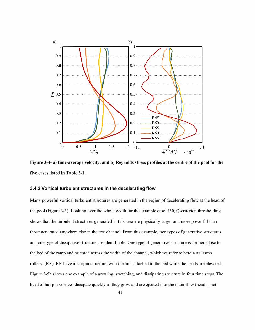
41
Figure 3-4- a) time-average velocity, and b) Reynolds stress profiles at the centre of the pool for the
five cases listed in Table 3-1.
3.4.2 Vortical turbulent structures in the decelerating flow
Many powerful vortical turbulent structures are generated in the region of decelerating flow at the head of
the pool (Figure 3-5). Looking over the whole width for the example case R50, Q-criterion thresholding
shows that the turbulent structures generated in this area are physically larger and more powerful than
those generated anywhere else in the test channel. From this example, two types of generative structures
and one type of dissipative structure are identifiable. One type of generative structure is formed close to
the bed of the ramp and oriented across the width of the channel, which we refer to herein as ‘ramp
rollers’ (RR). RR have a hairpin structure, with the tails attached to the bed while the heads are elevated.
Figure 3-5b shows one example of a growing, stretching, and dissipating structure in four time steps. The
head of hairpin vortices dissipate quickly as they grow and are ejected into the main flow (head is not
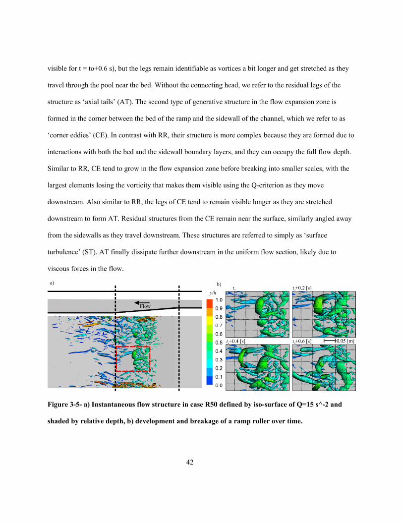
42
visible for t = to+0.6 s), but the legs remain identifiable as vortices a bit longer and get stretched as they
travel through the pool near the bed. Without the connecting head, we refer to the residual legs of the
structure as ‘axial tails’ (AT). The second type of generative structure in the flow expansion zone is
formed in the corner between the bed of the ramp and the sidewall of the channel, which we refer to as
‘corner eddies’ (CE). In contrast with RR, their structure is more complex because they are formed due to
interactions with both the bed and the sidewall boundary layers, and they can occupy the full flow depth.
Similar to RR, CE tend to grow in the flow expansion zone before breaking into smaller scales, with the
largest elements losing the vorticity that makes them visible using the Q-criterion as they move
downstream. Also similar to RR, the legs of CE tend to remain visible longer as they are stretched
downstream to form AT. Residual structures from the CE remain near the surface, similarly angled away
from the sidewalls as they travel downstream. These structures are referred to simply as ‘surface
turbulence’ (ST). AT finally dissipate further downstream in the uniform flow section, likely due to
viscous forces in the flow.
Figure 3-5- a) Instantaneous flow structure in case R50 defined by iso-surface of Q=15 s^-2 and
shaded by relative depth, b) development and breakage of a ramp roller over time.
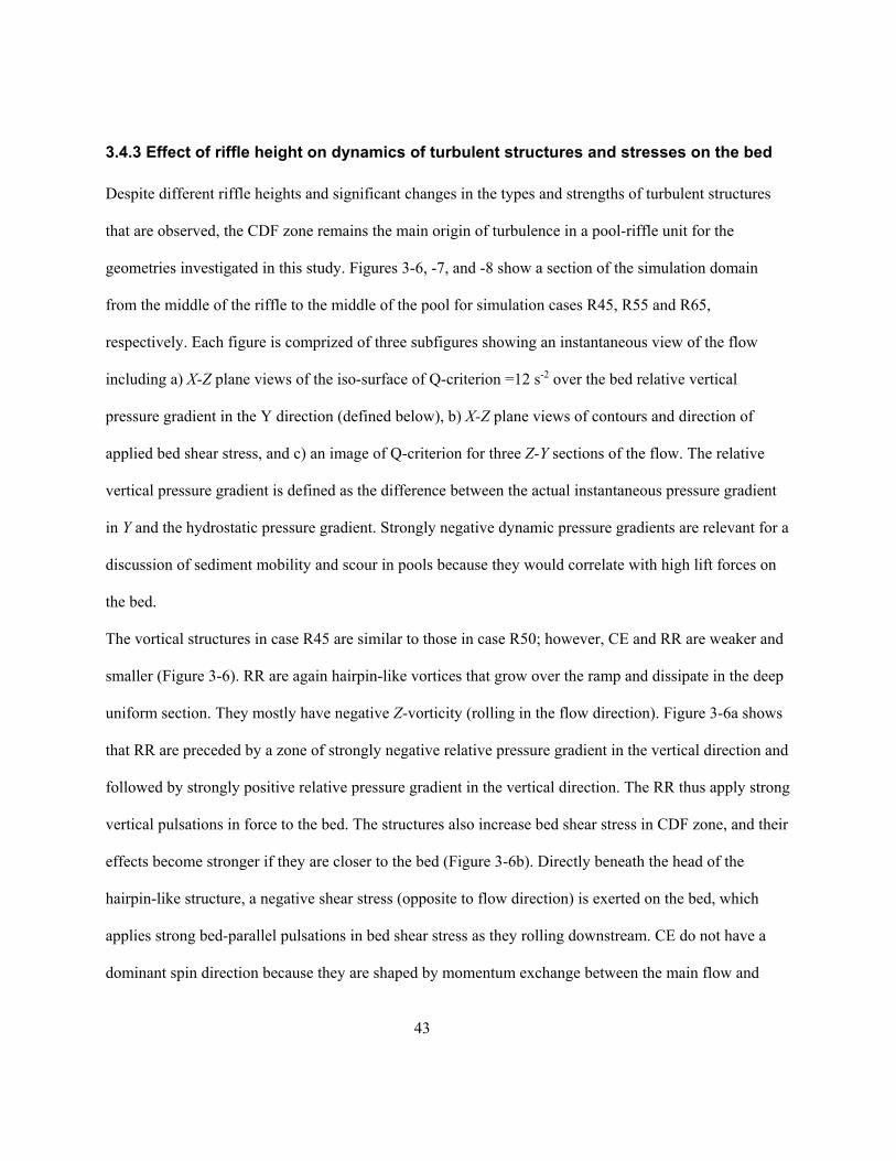
43
3.4.3 Effect of riffle height on dynamics of turbulent structures and stresses on the bed
Despite different riffle heights and significant changes in the types and strengths of turbulent structures
that are observed, the CDF zone remains the main origin of turbulence in a pool-riffle unit for the
geometries investigated in this study. Figures 3-6, -7, and -8 show a section of the simulation domain
from the middle of the riffle to the middle of the pool for simulation cases R45, R55 and R65,
respectively. Each figure is comprized of three subfigures showing an instantaneous view of the flow
including a) X-Z plane views of the iso-surface of Q-criterion =12 s-2 over the bed relative vertical
pressure gradient in the Y direction (defined below), b) X-Z plane views of contours and direction of
applied bed shear stress, and c) an image of Q-criterion for three Z-Y sections of the flow. The relative
vertical pressure gradient is defined as the difference between the actual instantaneous pressure gradient
in Y and the hydrostatic pressure gradient. Strongly negative dynamic pressure gradients are relevant for a
discussion of sediment mobility and scour in pools because they would correlate with high lift forces on
the bed.
The vortical structures in case R45 are similar to those in case R50; however, CE and RR are weaker and
smaller (Figure 3-6). RR are again hairpin-like vortices that grow over the ramp and dissipate in the deep
uniform section. They mostly have negative Z-vorticity (rolling in the flow direction). Figure 3-6a shows
that RR are preceded by a zone of strongly negative relative pressure gradient in the vertical direction and
followed by strongly positive relative pressure gradient in the vertical direction. The RR thus apply strong
vertical pulsations in force to the bed. The structures also increase bed shear stress in CDF zone, and their
effects become stronger if they are closer to the bed (Figure 3-6b). Directly beneath the head of the
hairpin-like structure, a negative shear stress (opposite to flow direction) is exerted on the bed, which
applies strong bed-parallel pulsations in bed shear stress as they rolling downstream. CE do not have a
dominant spin direction because they are shaped by momentum exchange between the main flow and
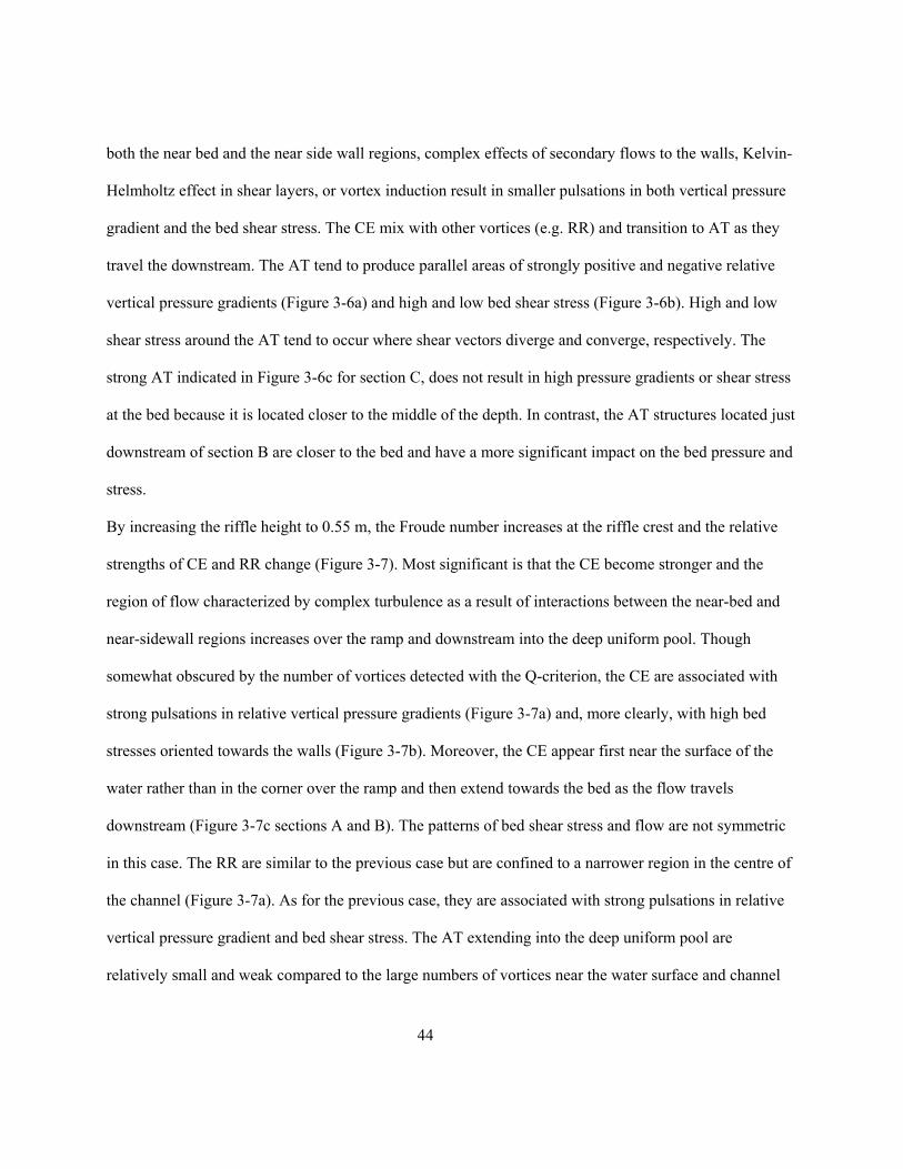
44
both the near bed and the near side wall regions, complex effects of secondary flows to the walls, Kelvin-
Helmholtz effect in shear layers, or vortex induction result in smaller pulsations in both vertical pressure
gradient and the bed shear stress. The CE mix with other vortices (e.g. RR) and transition to AT as they
travel the downstream. The AT tend to produce parallel areas of strongly positive and negative relative
vertical pressure gradients (Figure 3-6a) and high and low bed shear stress (Figure 3-6b). High and low
shear stress around the AT tend to occur where shear vectors diverge and converge, respectively. The
strong AT indicated in Figure 3-6c for section C, does not result in high pressure gradients or shear stress
at the bed because it is located closer to the middle of the depth. In contrast, the AT structures located just
downstream of section B are closer to the bed and have a more significant impact on the bed pressure and
stress.
By increasing the riffle height to 0.55 m, the Froude number increases at the riffle crest and the relative
strengths of CE and RR change (Figure 3-7). Most significant is that the CE become stronger and the
region of flow characterized by complex turbulence as a result of interactions between the near-bed and
near-sidewall regions increases over the ramp and downstream into the deep uniform pool. Though
somewhat obscured by the number of vortices detected with the Q-criterion, the CE are associated with
strong pulsations in relative vertical pressure gradients (Figure 3-7a) and, more clearly, with high bed
stresses oriented towards the walls (Figure 3-7b). Moreover, the CE appear first near the surface of the
water rather than in the corner over the ramp and then extend towards the bed as the flow travels
downstream (Figure 3-7c sections A and B). The patterns of bed shear stress and flow are not symmetric
in this case. The RR are similar to the previous case but are confined to a narrower region in the centre of
the channel (Figure 3-7a). As for the previous case, they are associated with strong pulsations in relative
vertical pressure gradient and bed shear stress. The AT extending into the deep uniform pool are
relatively small and weak compared to the large numbers of vortices near the water surface and channel
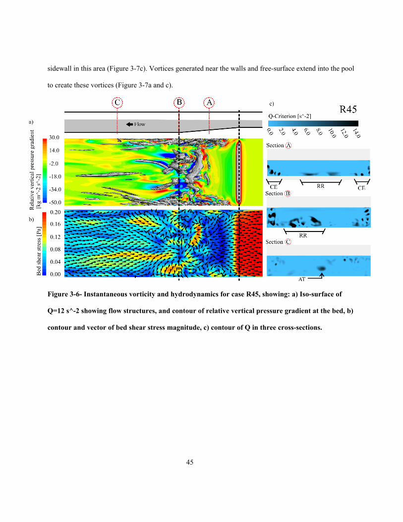
45
sidewall in this area (Figure 3-7c). Vortices generated near the walls and free-surface extend into the pool
to create these vortices (Figure 3-7a and c).
Figure 3-6- Instantaneous vorticity and hydrodynamics for case R45, showing: a) Iso-surface of
Q=12 s^-2 showing flow structures, and contour of relative vertical pressure gradient at the bed, b)
contour and vector of bed shear stress magnitude, c) contour of Q in three cross-sections.
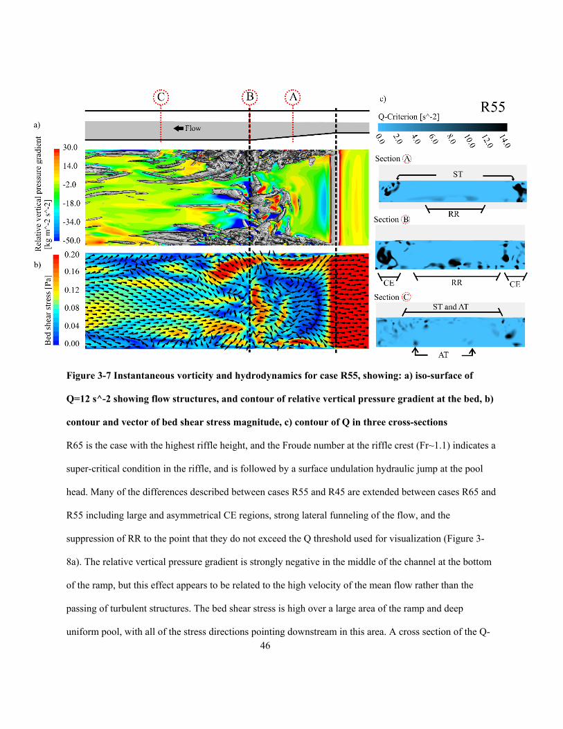
46
Figure 3-7 Instantaneous vorticity and hydrodynamics for case R55, showing: a) iso-surface of
Q=12 s^-2 showing flow structures, and contour of relative vertical pressure gradient at the bed, b)
contour and vector of bed shear stress magnitude, c) contour of Q in three cross-sections
R65 is the case with the highest riffle height, and the Froude number at the riffle crest (Fr~1.1) indicates a
super-critical condition in the riffle, and is followed by a surface undulation hydraulic jump at the pool
head. Many of the differences described between cases R55 and R45 are extended between cases R65 and
R55 including large and asymmetrical CE regions, strong lateral funneling of the flow, and the
suppression of RR to the point that they do not exceed the Q threshold used for visualization (Figure 3-
8a). The relative vertical pressure gradient is strongly negative in the middle of the channel at the bottom
of the ramp, but this effect appears to be related to the high velocity of the mean flow rather than the
passing of turbulent structures. The bed shear stress is high over a large area of the ramp and deep
uniform pool, with all of the stress directions pointing downstream in this area. A cross section of the Q-
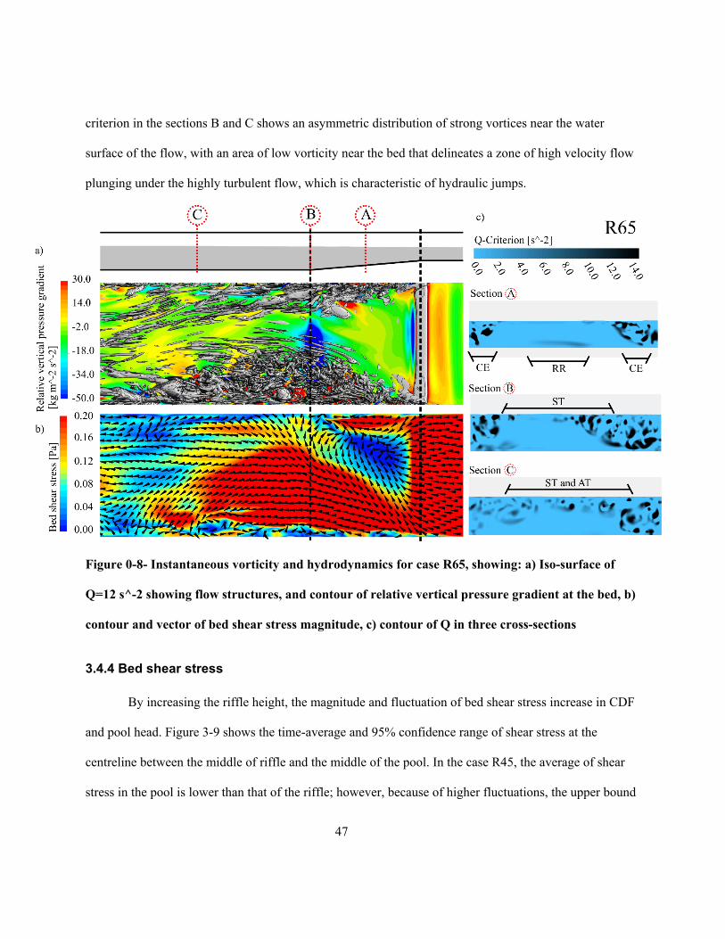
47
criterion in the sections B and C shows an asymmetric distribution of strong vortices near the water
surface of the flow, with an area of low vorticity near the bed that delineates a zone of high velocity flow
plunging under the highly turbulent flow, which is characteristic of hydraulic jumps.
Figure 0-8- Instantaneous vorticity and hydrodynamics for case R65, showing: a) Iso-surface of
Q=12 s^-2 showing flow structures, and contour of relative vertical pressure gradient at the bed, b)
contour and vector of bed shear stress magnitude, c) contour of Q in three cross-sections
3.4.4 Bed shear stress
By increasing the riffle height, the magnitude and fluctuation of bed shear stress increase in CDF
and pool head. Figure 3-9 shows the time-average and 95% confidence range of shear stress at the
centreline between the middle of riffle and the middle of the pool. In the case R45, the average of shear
stress in the pool is lower than that of the riffle; however, because of higher fluctuations, the upper bound
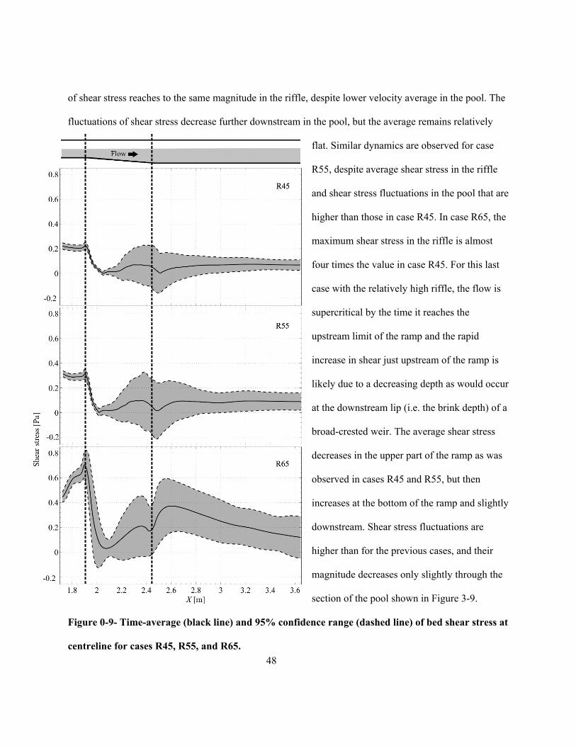
48
of shear stress reaches to the same magnitude in the riffle, despite lower velocity average in the pool. The
fluctuations of shear stress decrease further downstream in the pool, but the average remains relatively
flat. Similar dynamics are observed for case
R55, despite average shear stress in the riffle
and shear stress fluctuations in the pool that are
higher than those in case R45. In case R65, the
maximum shear stress in the riffle is almost
four times the value in case R45. For this last
case with the relatively high riffle, the flow is
supercritical by the time it reaches the
upstream limit of the ramp and the rapid
increase in shear just upstream of the ramp is
likely due to a decreasing depth as would occur
at the downstream lip (i.e. the brink depth) of a
broad-crested weir. The average shear stress
decreases in the upper part of the ramp as was
observed in cases R45 and R55, but then
increases at the bottom of the ramp and slightly
downstream. Shear stress fluctuations are
higher than for the previous cases, and their
magnitude decreases only slightly through the
section of the pool shown in Figure 3-9.
Figure 0-9- Time-average (black line) and 95% confidence range (dashed line) of bed shear stress at
centreline for cases R45, R55, and R65.
49
3.5 Discussion
The simulations described in the current study offer a detailed look at turbulence generation and
mean flow in a simplified pool-riffle morphology in open channels. The novelty of the work is the
application of an advanced turbulence scheme that uses transient, three-dimensional, and deformable free-
surface approaches to the studied morphology, which exceeds what has been applied to date with
comparable bed morphologies (Jackson et al., 2015; Keller & Florsheim, 1993; MacWilliams et al., 2006;
Stoesser et al., 2008). This modelling approach allows a unique examination of the interplay between
areas of high velocity and areas of high turbulence over time and allows the magnitude and pulsation of
shear stress and pressure gradients on the bed to be approximated. It is shown that there is a hydraulic
reason to expect fundamentally different flow dynamics in riffle-pools dependant on the discharge, flow
depth, and the relative height of the riffle. As the critical condition is approached, the mean flow can
switch from a state where the high velocity core skims across the surface of the pool to one in which it
plunges towards the bed. This bifurcation fundamentally alters the distribution of mean and fluctuating
shear and pressure forces on the bed and provides a foundation for reconciling patterns of flow and
turbulence that have been observed in pool-riffles with different geometries.
The results of the current study most directly help to explain the distributions of velocity and turbulence
that were reported in previous laboratory studies of flow in straight pools (MacVicar & Rennie, 2012;
MacVicar & Best, 2013; MacVicar & Obach, 2015). Four types of flow structures (CE, RR, ST, and AT)
are seen developing and dissipating in a pool-riffle unit, while momentum exchange near the walls can
shape CE and RR due to the development of secondary flow in vertical expansion in CDF and instabilities
in shearing flow downstream of the riffle crest. In the lab, MacVicar & Rennie (2012), found that sweeps
tended to be angled towards side-walls with ejections angled towards the middle of flow in CDF zone.
These series of sweeps and ejections in CDF near the walls are identifiable as vortical structures (CE) in
50
the current simulations. They also found that specific discharge was higher in the middle of the pool and
hypothesized that the higher turbulence near the wall was acting to steer the flow towards the middle, a
result that was reproduced here. MacVicar and Best (2013) showed how high strain rates were correlated
with high Reynolds stresses and higher bed shear stress in the expansion of flow at the head of the pool,
while further downstream an area of enlarging but weakening structures was convected away from the
boundary. The current study largely confirms their conceptual model, with both higher average and
fluctuations of shear stress in the pool-head than in the rest of the pool for cases R45 and R55 (Figure 3-
9). The patterns of turbulent fluctuations are explained by the generation of vortical structures in the areas
of high strain (CE and RR) and their weakening and dissipation in the pool where only occasional AT
remain visible (Figures 3-5 and 6). The results thus offer greater clarity than the simulations of Kara et al.
(2008), which did not include the effect of the side walls and so could not show the generation and
dissipation of the CE structures and their effect on steering the main flow. However, the current study
also shows the limit of the conceptual model presented by MacVicar and Best (2013), as the observed
hydrodynamic cs are characteristic of only one of the possible regimes in straight pools and riffles.
In total, three types of flow patterns were seen in pool-riffle units. By varying the riffle height, it was
possible to affect both the maximum velocity (Figure 3-10a) and the vertical location of the maximum
velocity (Figure 3-10b) in the pool. For the purposes of this numerical study we looked a section in the
middle of the pool and defined ‘skimming’, ‘rifting’, and ‘plunging’ flows based on whether the elevation
of maximum velocity in profile at the centre of the pool was in the top 30%, middle 40%, or bottom 30%
of the flow depth. For lower riffles, the skimming flow regime is characterized by turbulence generated
near the boundaries and high velocity main flow in the middle of the channel. The flip from skimming to
rifting and then plunging flow is based on flow specific energy, where the critical flow condition is
approached as the riffle height increases, eventually causing a choked flow condition. In a 1D analysis
(see, e.g. Sturm, 2010), the choked flow causes a local increase in potential energy upstream of the riffle
51
and higher kinetic energy in the pool. This choked flow condition also results in more downward
momentum into the pool and is known to result in a transition from sub to supercritical flow. In locations
where the depth in the pool is sufficiently high, the supercritical flow will be forced to jump back to a
subcritical condition in the pool, either as a free or submerged jump. In profile, the water surface profile
appears to be characteristic of an undular jump, which are ‘weak’ jumps that occur for Froude numbers <
1.7 (Sturm, 2010), with a zone of high turbulence on top of the high velocity flow (Figure 3-3b – R65).
Viewed in the plan form, however, the picture becomes more complex as the area of high velocity flow is
laterally restricted by zones of high turbulence that gradually cover the plunging flow (Figure 3-8).
Plunging flow is significant because it may corroborate observations of plunging flow in the field
(Carling 1991; Keller and Florsheim 1993; Thompson et al. 1996) and support the hypothesis of velocity
reversal (Keller, 1972), demonstrating that a local velocity reversal can happen as a result of the
redistribution of flow in a cross-section, as argued by MacVicar et al. (2009), and that the shear stresses
on the bed are very high for such a condition (Figure 3-8). As has been done for flows in confluences
(Guillén Ludeña et al. 2017), future work should examine the effect of more realistic pool and riffle
geometries on turbulence generation and the redistribution of flow to more fully understand the
hydrodynamics in pool formation and maintenance in natural channels.
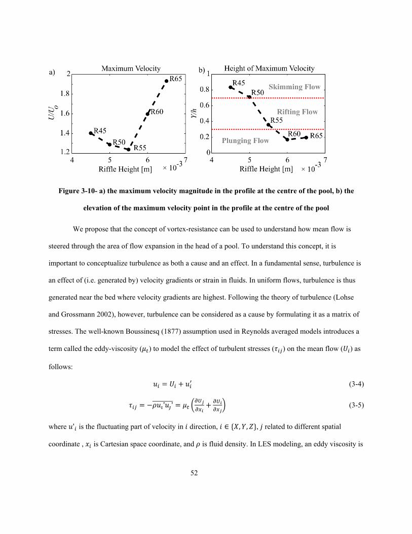
52
Figure 3-10- a) the maximum velocity magnitude in the profile at the centre of the pool, b) the
elevation of the maximum velocity point in the profile at the centre of the pool
We propose that the concept of vortex-resistance can be used to understand how mean flow is
steered through the area of flow expansion in the head of a pool. To understand this concept, it is
important to conceptualize turbulence as both a cause and an effect. In a fundamental sense, turbulence is
an effect of (i.e. generated by) velocity gradients or strain in fluids. In uniform flows, turbulence is thus
generated near the bed where velocity gradients are highest. Following the theory of turbulence (Lohse
and Grossmann 2002), however, turbulence can be considered as a cause by formulating it as a matrix of
stresses. The well-known Boussinesq (1877) assumption used in Reynolds averaged models introduces a
term called the eddy-viscosity ( ) to model the effect of turbulent stresses ( ) on the mean flow ( ) as
follows:
(3-4)
ʹ ʹ (3-5)
where ʹ is the fluctuating part of velocity in direction, ∈ , , , related to different spatial
coordinate , is Cartesian space coordinate, and is fluid density. In LES modeling, an eddy viscosity is
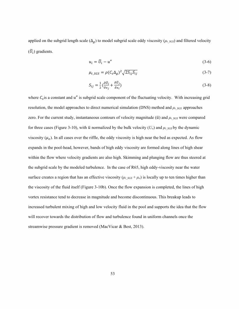
53
applied on the subgrid length scale (∆ ) to model subgrid scale eddy viscosity (μt_SGS) and filtered velocity
( ) gradients.
″ (3-6)
_ ∆ 2 (3-7)
(3-8)
where is a constant and ″ is subgrid scale component of the fluctuating velocity. With increasing grid
resolution, the model approaches to direct numerical simulation (DNS) method and μt_SGS approaches
zero. For the current study, instantaneous contours of velocity magnitude ( ) and μt_SGS were compared
for three cases (Figure 3-10), with normalized by the bulk velocity (Uo) and μt_SGS by the dynamic
viscosity ( ). In all cases over the riffle, the eddy viscosity is high near the bed as expected. As flow
expands in the pool-head, however, bands of high eddy viscosity are formed along lines of high shear
within the flow where velocity gradients are also high. Skimming and plunging flow are thus steered at
the subgrid scale by the modeled turbulence. In the case of R65, high eddy-viscosity near the water
surface creates a region that has an effective viscosity (μt_SGS + μo) is locally up to ten times higher than
the viscosity of the fluid itself (Figure 3-10b). Once the flow expansion is completed, the lines of high
vortex resistance tend to decrease in magnitude and become discontinuous. This breakup leads to
increased turbulent mixing of high and low velocity fluid in the pool and supports the idea that the flow
will recover towards the distribution of flow and turbulence found in uniform channels once the
streamwise pressure gradient is removed (MacVicar & Best, 2013).
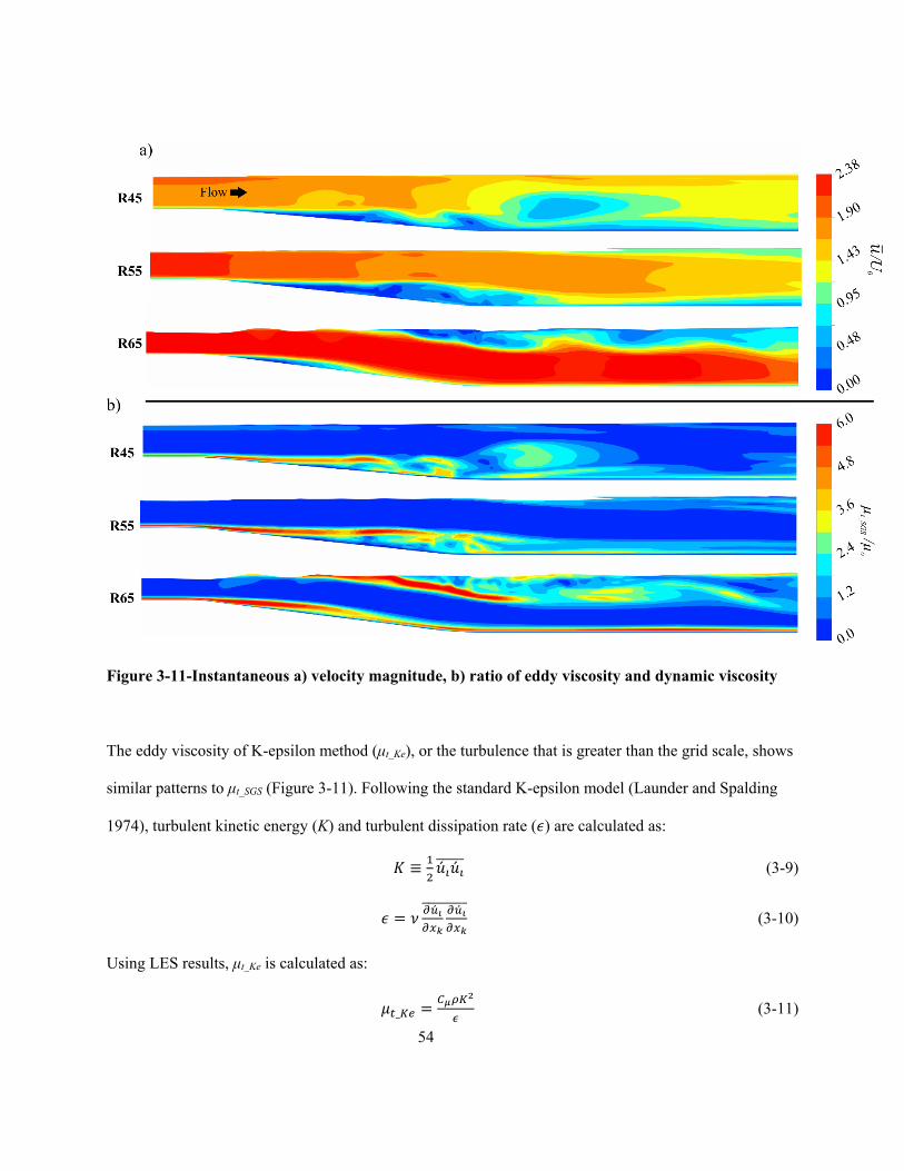
54
Figure 3-11-Instantaneous a) velocity magnitude, b) ratio of eddy viscosity and dynamic viscosity
The eddy viscosity of K-epsilon method (μt_Ke), or the turbulence that is greater than the grid scale, shows
similar patterns to μt_SGS (Figure 3-11). Following the standard K-epsilon model (Launder and Spalding
1974), turbulent kinetic energy (K) and turbulent dissipation rate ( ) are calculated as:
≡ (3-9)
(3-10)
Using LES results, μt_Ke is calculated as:
_ (3-11)
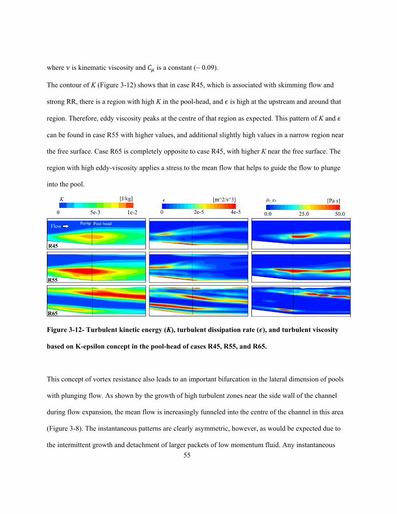
55
where is kinematic viscosity and is a constant (~ 0.09).
The contour of K (Figure 3-12) shows that in case R45, which is associated with skimming flow and
strong RR, there is a region with high K in the pool-head, and is high at the upstream and around that
region. Therefore, eddy viscosity peaks at the centre of that region as expected. This pattern of K and
can be found in case R55 with higher values, and additional slightly high values in a narrow region near
the free surface. Case R65 is completely opposite to case R45, with higher K near the free surface. The
region with high eddy-viscosity applies a stress to the mean flow that helps to guide the flow to plunge
into the pool.
Figure 3-12- Turbulent kinetic energy (K), turbulent dissipation rate ( ), and turbulent viscosity
based on K-epsilon concept in the pool-head of cases R45, R55, and R65.
This concept of vortex resistance also leads to an important bifurcation in the lateral dimension of pools
with plunging flow. As shown by the growth of high turbulent zones near the side wall of the channel
during flow expansion, the mean flow is increasingly funneled into the centre of the channel in this area
(Figure 3-8). The instantaneous patterns are clearly asymmetric, however, as would be expected due to
the intermittent growth and detachment of larger packets of low momentum fluid. Any instantaneous
56
asymmetry, however, has the potential for positive feedback by steering more flow away from the region,
which was observed to lead to an asymmetric time average state for some simulations with plunging flow
in the pool. Lateral flow bifurcations in a straight pool-riffle unit, which distribute bed shear stress
biasedly to one side of the channel, suggests a physical mechanism for the link between pools and the
initiation of meandering in a straight channel. Such a result is also significant because it indicates that a
small bias in the laterally funnelled flow, such as a minor geometrical deviation, could preferentially
expand the recirculation at one side and deflect the main flow away from this area. In field cases such as
the study by MacWilliams et al., (2006), a jet-like flow was observed in a pool-riffle unit, which led to the
“flow convergence routing” hypothesis for pool maintenance. As part of this hypothesis, however, the
authors assumed a need for an upstream constriction to induce the jet-like flow into the pool. The current
study shows that the resistance of CE and ST in CDF zone can act as a constriction and shape this jet-like
flow (i.e. ‘plunging’ flow in the current study) as well as a function of the chaotic behaviour of turbulent
flow. Investigations into the role of turbulent vortices in more realistic pool geometries are again
warranted to determine how they affect pool formation and maintenance in natural channels.
3.6 Conclusions
The transient numerical simulations of turbulent flow in isolated pool-riffle units showed that:
1) Four different types of vortices are shaped in the convective decelerating zone: surface
turbulence, ramp rollers, corner eddies, and axial tails;
2) Ramp and corner eddies are dominant near the bed and responsible for high bed shear stress in
skimming flow;
3) Based on this finding that, vortices exert resistance to the flow by increasing the mixing
effects, and changing the pressure domain, the vortex-resistance hypothesis has been suggested;
57
4) Froude number close to one at riffle can make surface undulation hydraulic jump, which steers
the flow to plunge into the pool near the bed;
5) If ramp rollers are strong enough, they push the flow to skim the free-surface and increase near
bed turbulence;
6) Axial bifurcation occurs where strong plunging flow happens, such one side of the channel
experiences higher velocities and shear stresses while the opposite side is dominated by flow
recirculations.
58
Chapter 4: Effect of width variations on
turbulent structures and flow patterns in
isolated pool-riffle units
4.1 Introduction
Macromorphological variations in natural and restored streams have significant effects on sediment
transport, flow pattern, and bed stability. Pools and riffles, which are respectively deeper and shallower
part of the bed, are known as the main reason of channel deformation and meandering developments
(Hooke 2013; Montgomery 1995; Stoesser et al. 2010). They are mostly found in gravel bed streams, but
they can shape and become stable in both alluvial and bedrock channels (MacVicar and Roy 2007b; Sear
1996; Thompson 2013). They play essential roles in the quality of aquatic habitats by providing enough
volume of water during low discharge seasons or protect them from freezing during ice developing
seasons (Gorman and Karr 1978). Pools and riffles increase the turbulence that can protect the channel
from the unwanted deposition of sediment, or causes erosion and make the channel unstable (MacVicar &
Roy, 2007b, 2007a, Thompson, 2001, 2004; Thompson et al., 1999). Another important geometry factor
in natural and restored streams is the size and variation of channel width. The spacing and frequency of
59
some of the large bedforms are thought to be a function of the channel width. For example, the frequency
of pool-riffle unit is five to seven times of the channel width ( Keller & Melhorn, 1978). Also, the
curvature and wavelength of meanderings are two to three, and ten to fourteen times of the channel width,
respectively (Hooke 2013). Local variations in the width of the channel, which are known as constrictions
and expansions, are also a primary control on pool formation (Buffington et al., 2002; Thompson et al.,
1999). Channel constrictions; by shaping jet flows, flow convergences, increasing bed shear stress, and
generation of strong turbulent structures, have influential effects on sediment transport and pool
maintenance mechanism (Buffington et al., 2002; MacVicar & Roy, 2007b, 2007a, Thompson, 2001,
2004; Thompson et al., 1999). Most of the studies on pool-riffle maintenance and shaping mechanism did
not consider the effects of width size and variation; therefore, there is a need for more hydraulic studies to
demonstrate the effects of basic geometry factors on flow patterns in pools and riffles.
The mechanisms underlying the formation and maintenance mechanism of pool-riffle units have many
uncertainties due to the variability in the field, complexity of flow interaction with the morphology and
the chaotic behaviour of turbulence. One of the first hypothesis in pool-riffle formation and maintenance
is “velocity reversal.” It says that by increasing the flow discharge, the increasing rate of near-bed
velocity in riffle is lower than the one in the pool and there is a point that the near-bed velocity in the pool
is equal to the one in the riffle (Keller & Florsheim, 1993). They suggested that high near bed velocity in
the pools exerts high shear stress to the bed and increases the sediment transport rate. They defined this
scouring process as the maintenance mechanism in pools and riffles. Another hypothesis in this field is
“flow convergence.” It says that the high near bed velocity and bed shear stress in the pools are the results
of a jet-like flow, which is induced by upstream constrictions (MacWilliams et al. 2006). These two
hypotheses are based on the spatial distribution of time-averaged velocity in the pools and riffles, without
considering the effects of turbulence. MacVicar and Rennie (2012) and MacVicar and Best (2013) treated
the convective accelerating flow (CAF) and convective decelerating flow (CDF) zones as perturbations.
60
They used the idea of recovery from perturbation to assess the impact of macro bed forms (i.e. riffles) on
flow behaviour. They defined ‘recovery length’ that is a required length for dissipating the perturbation
effects (e.g. Reynolds stresses). They found that recovery length is higher in wider channels with the
same vertical expansion geometry. They have stated that in the CDF zone, adverse pressure gradient
shapes the flow in a way that high turbulence shapes near the bed and high velocity peaks near the free-
surface.
The up-scaled geometry of pool-riffle units, with or without constriction, can be found in the field as well.
Venditti et al., (2014) found the similar geometry of pool-riffle units with a constriction in Fraser Canyon,
British Columbia, Canada. They did the first three-dimensional measurement of velocity domain in
bedrock canyons (Hunt et al. 2018). They observed a plunging flow into the pool and boiling structures
on the free-surface. They argued that the CDF zone and lateral constrictions form upwelling flows, which
are seen as boiling structures when they reach the free-surface. They stated that the upwelling flows, by
reducing the local dynamic pressure near the bed, guide the incoming flow to plunge into the pool.
Moreover, this plunging flow intensifies the upwelling flow as positive feedback. Hunt et al., (2018)
conducted a series of flume experiments in support of Venditti et al., (2014). Their flume model was a
constriction varying from 20 to 50% and a downslope ramp entering the pool. In the experiments,
however, the Froude number in the constriction (0.61< Fr <1.21) is not matched with the field value (Fr=
0.3), which means that the lab case largely considered choked flow conditions rather than matching what
occurs in a subcritical flow in the field.. Thompson & Wohl (1998) used a sharp plate as constriction
downstream of the riffle at pool-head. They argued that the constrictions make a vena contracta at the
downstream, which is necessary to the maintenance mechanism of pools, and that the characteristics of
the vena contracta were primarily controlled by pool length. The creation of vena contracta because of the
sharp plate may not replicate the actual geometry of constrictions and pool-riffle units in the field.
61
Using large eddy simulation (LES) of turbulent flow in isolated pool-riffle units with various riffle height
in the previous chapter, four types of vortices were detected. The Q criterion was used to detect vortices
cores. In the cases with Froude number lower than 1 in the riffle crest, a series of vortices were found near
the bed on the ramp, called ‘ramp rollers’ (RR), which were found to have a similar generation and
dissipation mechanisms as hairpin vortices that form at the top of the viscous sublayer in boundary flows
(Kline et al. 1967). As they travel downstream, their head elevates from the bed and dissipates quickly,
but the legs remain longer and form stretched tube-like vortices called ‘axial tails’ (AT). Near the corners
in CDF zone, ‘corner eddies’ (CE) were detected. By increasing the riffle height, RR become weaker, and
series of vortices appear near the free-surface in CDF zone, which are called ‘surface turbulences’ (ST).
ST mix with CE and occupy the top and both sides of the channels; they steer the flow to plunge into the
pool. This flow pattern with high velocity core in the bottom 30% of the flow depth, in the centre of the
pool, was called ‘plunging flow.’ In the absence of ST, RR push the flow to skim the free surface. This
flow pattern with high-velocity core in the top 30% of the flow depth was called ‘skimming flow.’ If ST
and RR have similar strength, flow velocity peaks in the middle 40% of the flow depth in the centre of the
pool. This flow pattern was called ‘rifting flow.’ The results are significant because they show that
dramatically different flow patterns can occur in pools and riffles depending on the channel geometry and
the flow regime in the riffle. More research is needed to understand how the overall width and local
constrictions affect the channel hydrodynamics.
The current chapter aims to continue the study of vortical structures in pool-riffle units with different
geometrical parameters with an advanced transient, and turbulent numerical approach. The specific
objectives are to: 1) study the effects of width variation on flow pattern and vortical structures in isolated
pool-riffle units 2) study the effects of lateral constrictions on flow pattern, 3) detect and study the
constriction-induced vortical structures, 4) investigate the interactions of constriction and pool-riffle
induced flow structures. The geometry of the models is based on the previous experiments in pool-riffle
62
units by MacVicar & Obach, (2015), which is a simplified geometry of common pool-riffle units found in
the field. Pool-riffle units are considered to be in a straight channel with a lateral constriction in the
riffles. It is hoped that this research will provide a clear visualization of hydrodynamics in pool-riffle
units and lead to a more complete understanding of the formation and maintenance mechanisms of pool-
riffle units.
4.2 Methodology
4.2.1 Model Geometry
The model geometry is based on one of the flume experiments completed by MacVicar and Obach
(2015), which was in turn based on a geometric (1:10) and Froude scale (Fr ~ 0.6) matching of a field
example (MacVicar and Roy 2007). The physical and numerical models use a simplified straight
geometry of pool and riffle units with and without constriction in a 0.6 m wide channel. The constrictions
are placed in the upstream riffles, and there are some cases that have constrictions alone. The simulated
flume in the numerical model is 6 m long with a 1 m long uniform upstream section followed by a 0.52 m
long upsloping ramp, a flat uniform shallow ‘riffle’ of 0.4 m, a 0.52 m long downsloping ramp, a flat
uniform deep ‘pool’ of 2.4 m. In the cases with constriction, the constriction and riffle are in phase. A
final upsloping ramp and short uniform shallow section were used to define the downstream boundary of
the model. For the series of simulations in this study, three riffle heights (hR= 40 mm, 50 mm and 60 mm)
was chosen to model skimming and plunging flows (Table 4-1). With the fixed length of the ramped
sections, the change of riffle height also changed the ramp angles. The average inlet velocity (Uo), the
flow depth in the pool (h) and the Froude number in the pool were 0.21 m/s, 0.12 m, and 0.2 for case R50,
respectively. For other cases, the average inlet velocity (Uo), the flow depth in the pool (h) and the Froude
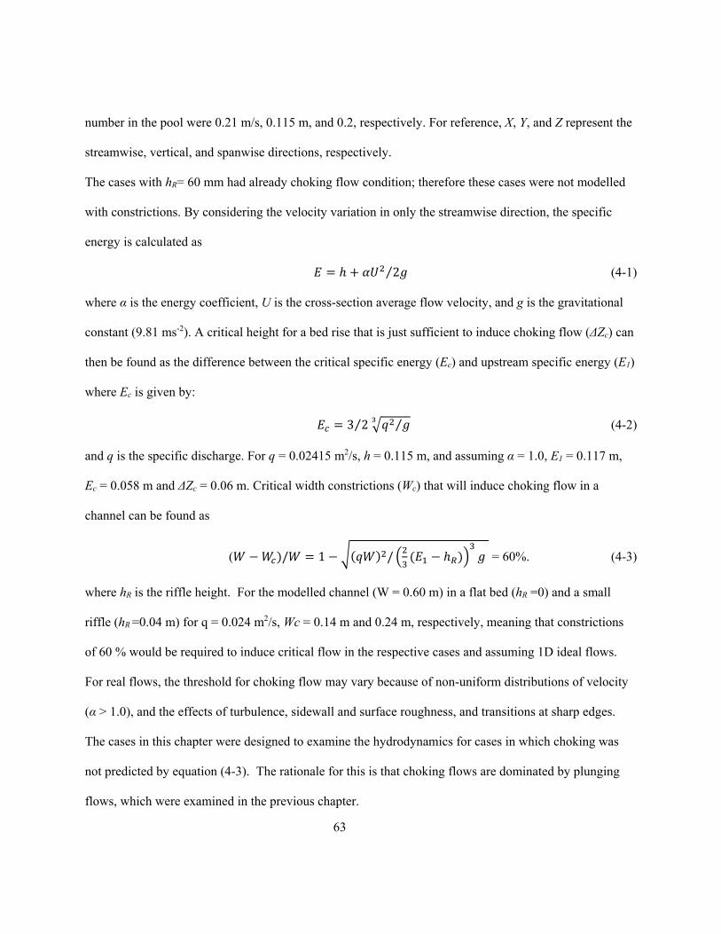
63
number in the pool were 0.21 m/s, 0.115 m, and 0.2, respectively. For reference, X, Y, and Z represent the
streamwise, vertical, and spanwise directions, respectively.
The cases with hR= 60 mm had already choking flow condition; therefore these cases were not modelled
with constrictions. By considering the velocity variation in only the streamwise direction, the specific
energy is calculated as
2⁄ (4-1)
where α is the energy coefficient, U is the cross-section average flow velocity, and g is the gravitational
constant (9.81 ms-2). A critical height for a bed rise that is just sufficient to induce choking flow (ΔZc) can
then be found as the difference between the critical specific energy (Ec) and upstream specific energy (E1)
where Ec is given by:
3 2⁄ ⁄ (4-2)
and q is the specific discharge. For q = 0.02415 m2/s, h = 0.115 m, and assuming α = 1.0, E1 = 0.117 m,
Ec = 0.058 m and ΔZc = 0.06 m. Critical width constrictions (Wc) that will induce choking flow in a
channel can be found as
( / 1 / = 60%. (4-3)
where hR is the riffle height. For the modelled channel (W = 0.60 m) in a flat bed (hR =0) and a small
riffle (hR =0.04 m) for q = 0.024 m2/s, Wc = 0.14 m and 0.24 m, respectively, meaning that constrictions
of 60 % would be required to induce critical flow in the respective cases and assuming 1D ideal flows.
For real flows, the threshold for choking flow may vary because of non-uniform distributions of velocity
(α > 1.0), and the effects of turbulence, sidewall and surface roughness, and transitions at sharp edges.
The cases in this chapter were designed to examine the hydrodynamics for cases in which choking was
not predicted by equation (4-3). The rationale for this is that choking flows are dominated by plunging
flows, which were examined in the previous chapter.
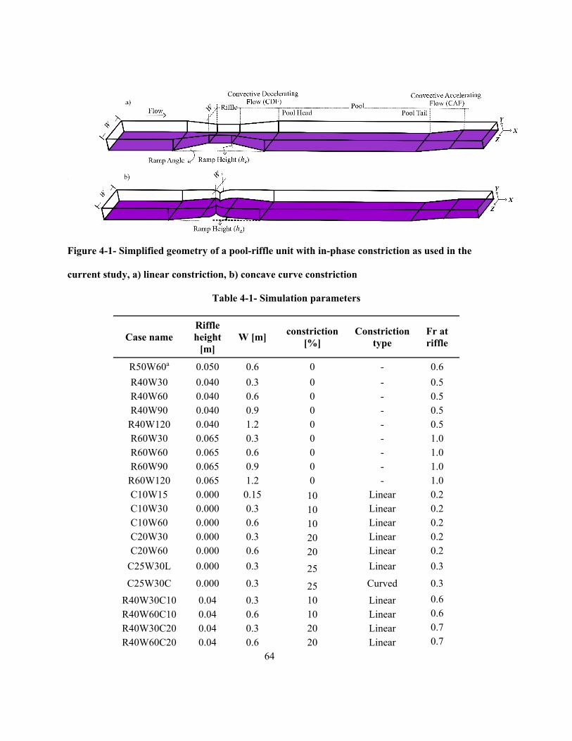
64
Figure 4-1- Simplified geometry of a pool-riffle unit with in-phase constriction as used in the
current study, a) linear constriction, b) concave curve constriction
Table 4-1- Simulation parameters
Case name Riffle height
[m] W [m]
constriction [%]
Constriction type
Fr at riffle
R50W60a 0.050 0.6 0 - 0.6
R40W30 0.040 0.3 0 - 0.5 R40W60 0.040 0.6 0 - 0.5 R40W90 0.040 0.9 0 - 0.5
R40W120 0.040 1.2 0 - 0.5 R60W30 0.065 0.3 0 - 1.0 R60W60 0.065 0.6 0 - 1.0 R60W90 0.065 0.9 0 - 1.0
R60W120 0.065 1.2 0 - 1.0 C10W15 0.000 0.15 10 Linear 0.2 C10W30 0.000 0.3 10 Linear 0.2 C10W60 0.000 0.6 10 Linear 0.2 C20W30 0.000 0.3 20 Linear 0.2 C20W60 0.000 0.6 20 Linear 0.2
C25W30L 0.000 0.3 25 Linear 0.3
C25W30C 0.000 0.3 25 Curved 0.3
R40W30C10 0.04 0.3 10 Linear 0.6
R40W60C10 0.04 0.6 10 Linear 0.6
R40W30C20 0.04 0.3 20 Linear 0.7
R40W60C20 0.04 0.6 20 Linear 0.7
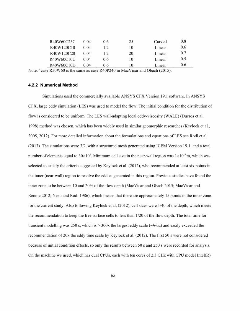
65
R40W60C25C 0.04 0.6 25 Curved 0.8
R40W120C10 0.04 1.2 10 Linear 0.6
R40W120C20 0.04 1.2 20 Linear 0.7
R40W60C10U 0.04 0.6 10 Linear 0.5
R40W60C10D 0.04 0.6 10 Linear 0.6 Note: a.case R50W60 is the same as case R40P240 in MacVicar and Obach (2015).
4.2.2 Numerical Method
Simulations used the commercially available ANSYS CFX Version 19.1 software. In ANSYS
CFX, large eddy simulation (LES) was used to model the flow. The initial condition for the distribution of
flow is considered to be uniform. The LES wall-adapting local eddy-viscosity (WALE) (Ducros et al.
1998) method was chosen, which has been widely used in similar geomorphic researches (Keylock et al.,
2005, 2012). For more detailed information about the formulations and equations of LES see Rodi et al.
(2013). The simulations were 3D, with a structured mesh generated using ICEM Version 19.1, and a total
number of elements equal to 30×106. Minimum cell size in the near-wall region was 1×10⁻³ m, which was
selected to satisfy the criteria suggested by Keylock et al. (2012), who recommended at least six points in
the inner (near-wall) region to resolve the eddies generated in this region. Previous studies have found the
inner zone to be between 10 and 20% of the flow depth (MacVicar and Obach 2015; MacVicar and
Rennie 2012; Nezu and Rodi 1986), which means that there are approximately 15 points in the inner zone
for the current study. Also following Keylock et al. (2012), cell sizes were 1/40 of the depth, which meets
the recommendation to keep the free surface cells to less than 1/20 of the flow depth. The total time for
transient modelling was 250 s, which is > 300x the largest eddy scale (~h/Uo) and easily exceeded the
recommendation of 20x the eddy time scale by Keylock et al. (2012). The first 50 s were not considered
because of initial condition effects, so only the results between 50 s and 250 s were recorded for analysis.
On the machine we used, which has dual CPUs, each with ten cores of 2.3 GHz with CPU model Intel(R)
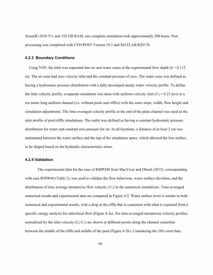
66
Xeon(R) 2650 V3, and 192 GB RAM, one complete simulation took approximately 200 hours. Post
processing was completed with CFD-POST Version 19.1 and MATLAB R2017b.
4.2.3 Boundary Conditions
Using VOF, the inlet was separated into air and water zones at the experimental flow depth (h = 0.115
m). The air zone had zero velocity inlet and the constant pressure of zero. The water zone was defined as
having a hydrostatic pressure distribution with a fully developed steady water velocity profile. To define
the inlet velocity profile, a separate simulation was done with uniform velocity inlet (U0 = 0.21 m/s) in a
ten meter long uniform channel (i.e. without pools and riffles) with the same slope, width, flow height and
simulation adjustments. The time-averaged velocity profile at the end of the plain channel was used as the
inlet profile of pool-riffle simulations. The outlet was defined as having a constant hydrostatic pressure
distribution for water and constant zero pressure for air. In all locations, a distance of at least 3 cm was
maintained between the water surface and the top of the simulation space, which allowed the free surface
to be shaped based on the hydraulic characteristics alone.
4.2.4 Validation
The experimental data for the case of R40P240 from MacVicar and Obach (2015), corresponding
with case R50W60 (Table 1), was used to validate the flow behaviour, water surface elevation, and the
distribution of time average streamwise flow velocity (Ux) in the numerical simulations. Time-averaged
numerical results and experimental data are compared in Figure 4-2. Water surface level is similar in both
numerical and experimental results, with a drop at the riffle that is consistent with what is expected from a
specific energy analysis for subcritical flow (Figure 4-2a). Six time-averaged streamwise velocity profiles
normalized by the inlet velocity (Ux/Uo) are shown at different points along the channel centerline
between the middle of the riffle and middle of the pool (Figure 4-2b). Considering the 10% error bars,
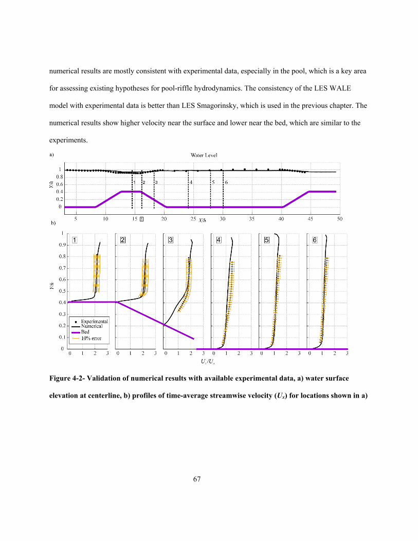
67
numerical results are mostly consistent with experimental data, especially in the pool, which is a key area
for assessing existing hypotheses for pool-riffle hydrodynamics. The consistency of the LES WALE
model with experimental data is better than LES Smagorinsky, which is used in the previous chapter. The
numerical results show higher velocity near the surface and lower near the bed, which are similar to the
experiments.
Figure 4-2- Validation of numerical results with available experimental data, a) water surface
elevation at centerline, b) profiles of time-average streamwise velocity (Ux) for locations shown in a)
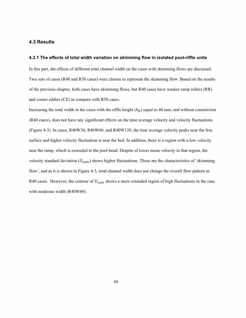
68
4.3 Results
4.3.1 The effects of total width variation on skimming flow in isolated pool-riffle units
In this part, the effects of different total channel width on the cases with skimming flows are discussed.
Two sets of cases (R40 and R50 cases) were chosen to represent the skimming flow. Based on the results
of the previous chapter, both cases have skimming flows, but R40 cases have weaker ramp rollers (RR)
and corner eddies (CE) in compare with R50 cases.
Increasing the total width in the cases with the riffle height ( ) equal to 40 mm, and without constriction
(R40 cases), does not have any significant effects on the time average velocity and velocity fluctuations
(Figure 4-3). In cases, R40W30, R40W60, and R40W120, the time average velocity peaks near the free
surface and higher velocity fluctuation is near the bed. In addition, there is a region with a low velocity
near the ramp, which is extended to the pool-head. Despite of lower mean velocity in that region, the
velocity standard deviation ( ) shows higher fluctuations. These are the characteristics of ‘skimming
flow’, and as it is shown in Figure 4-3, total channel width does not change the overall flow pattern in
R40 cases. However, the contour of shows a more extended region of high fluctuations in the case
with moderate width (R40W60).
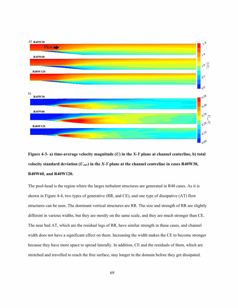
69
Figure 4-3- a) time-average velocity magnitude (U) in the X-Y plane at channel centerline, b) total
velocity standard deviation (Ustdv) in the X-Y plane at the channel centreline in cases R40W30,
R40W60, and R40W120.
The pool-head is the region where the larges turbulent structures are generated in R40 cases. As it is
shown in Figure 4-4, two types of generative (RR, and CE), and one type of dissipative (AT) flow
structures can be seen. The dominant vortical structures are RR. The size and strength of RR are slightly
different in various widths, but they are mostly on the same scale, and they are much stronger than CE.
The near bed AT, which are the residual legs of RR, have similar strength in these cases, and channel
width does not have a significant effect on them. Increasing the width makes the CE to become stronger
because they have more space to spread laterally. In addition, CE and the residuals of them, which are
stretched and travelled to reach the free surface, stay longer in the domain before they get dissipated.
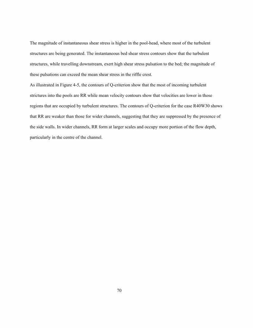
70
The magnitude of instantaneous shear stress is higher in the pool-head, where most of the turbulent
structures are being generated. The instantaneous bed shear stress contours show that the turbulent
structures, while travelling downstream, exert high shear stress pulsation to the bed; the magnitude of
these pulsations can exceed the mean shear stress in the riffle crest.
As illustrated in Figure 4-5, the contours of Q-criterion show that the most of incoming turbulent
strictures into the pools are RR while mean velocity contours show that velocities are lower in those
regions that are occupied by turbulent structures. The contours of Q-criterion for the case R40W30 shows
that RR are weaker than those for wider channels, suggesting that they are suppressed by the presence of
the side walls. In wider channels, RR form at larger scales and occupy more portion of the flow depth,
particularly in the centre of the channel.
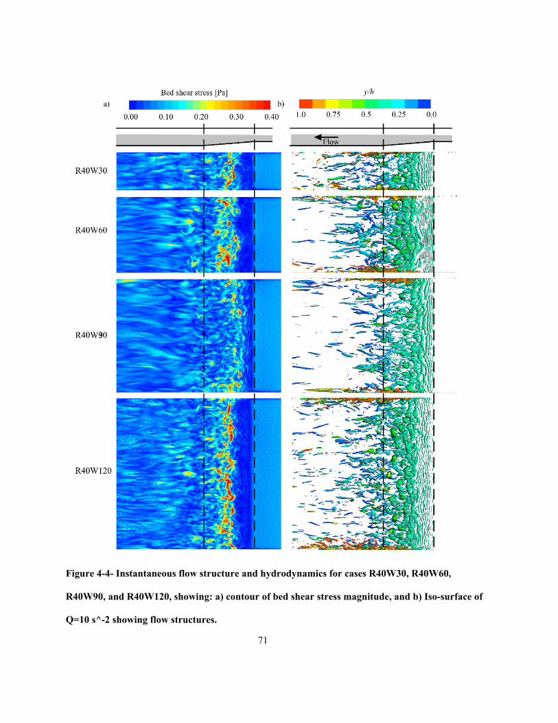
71
Figure 4-4- Instantaneous flow structure and hydrodynamics for cases R40W30, R40W60,
R40W90, and R40W120, showing: a) contour of bed shear stress magnitude, and b) Iso-surface of
Q=10 s^-2 showing flow structures.
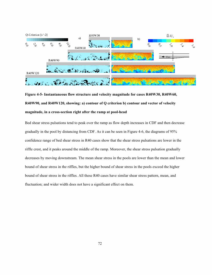
72
Figure 4-5- Instantaneous flow structure and velocity magnitude for cases R40W30, R40W60,
R40W90, and R40W120, showing: a) contour of Q criterion b) contour and vector of velocity
magnitude, in a cross-section right after the ramp at pool-head
Bed shear stress pulsations tend to peak over the ramp as flow depth increases in CDF and then decrease
gradually in the pool by distancing from CDF. As it can be seen in Figure 4-6, the diagrams of 95%
confidence range of bed shear stress in R40 cases show that the shear stress pulsations are lower in the
riffle crest, and it peaks around the middle of the ramp. Moreover, the shear stress pulsation gradually
decreases by moving downstream. The mean shear stress in the pools are lower than the mean and lower
bound of shear stress in the riffles, but the higher bound of shear stress in the pools exceed the higher
bound of shear stress in the riffles. All these R40 cases have similar shear stress pattern, mean, and
fluctuation; and wider width does not have a significant effect on them.
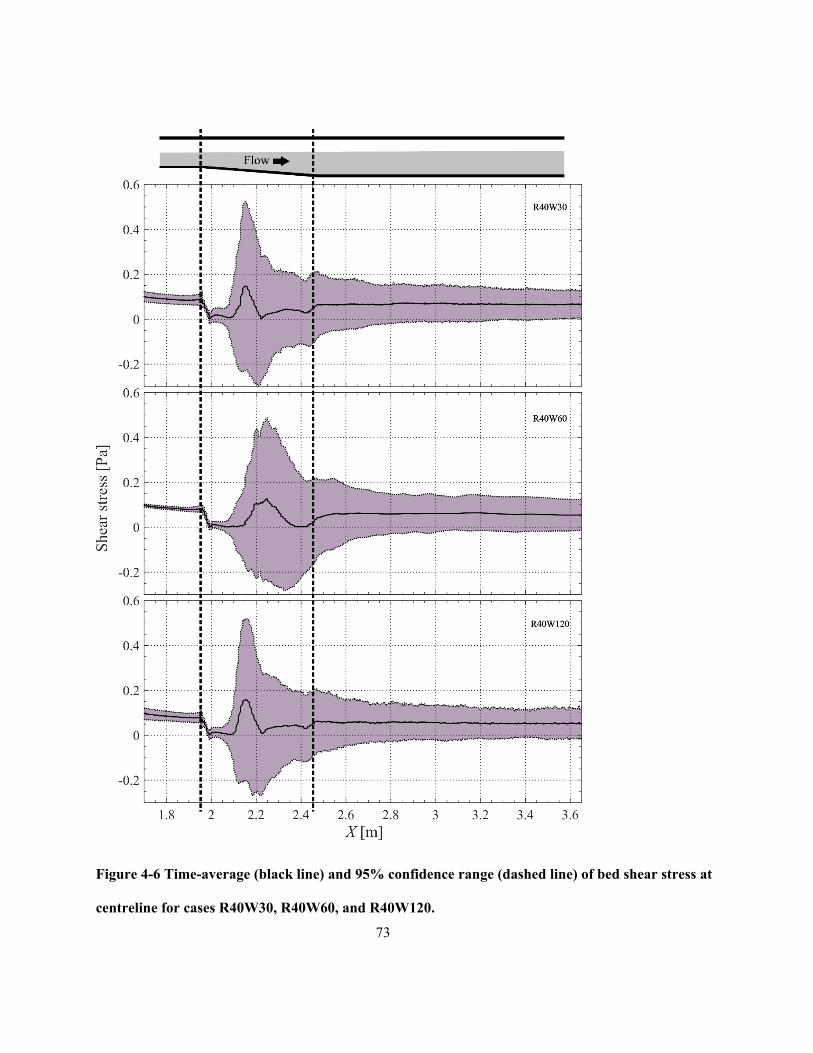
73
Figure 4-6 Time-average (black line) and 95% confidence range (dashed line) of bed shear stress at
centreline for cases R40W30, R40W60, and R40W120.
74
By increasing the riffle height (hR =50 mm) the flow pattern and distribution of turbulence are changed.
As it is illustrated in Figure 4-7, the contours of time average velocity at the centreline of the channels
show that the distribution of velocity at the middle of the pool, which is at the right end of these contours,
changes by changing the width. The narrower R50 case, which is R50W15, has high velocity near the
surface. The next case, which is R50W30, shows vertically extended core of high velocity in depth at the
middle of the pool. Case R50W60 shows a typical skimming flow pattern. The widest R40, which is
R50W90, has a region of low velocity near the free surface at the middle of the pool. While, the flow
type can still be classified as ‘skimming’ given that the highest velocity at the centre of the pool is located
at the first 30% of the depth from the free surface, but the appearance of this dip in velocity near the water
surface indicates that the flow may be close to switching to a rifting or plunging type profile.
Increasing the channel width in R50 cases increases the velocity fluctuations and turbulence. As it is
illustrated in Figure 4-7, the contours of Ustdv show that the velocity fluctuations are stronger and extended
further downstream by increasing the width from W=15 cm to 60 cm. In case R50W90 a very thin layer
of high-velocity fluctuation is shaped near the free surface, and it is extended from slightly before the
riffle crest to the middle of the pool. This region of high-velocity fluctuation made the high-velocity flow
to dip a little at the pool head, but the mean flow is recovered to the pattern of skimming flow as it
reaches to the middle of the pool. Also, this thin layer of locally high turbulence is seen in other R50
cases as well, but they are less stronger than the one in case R50W90.
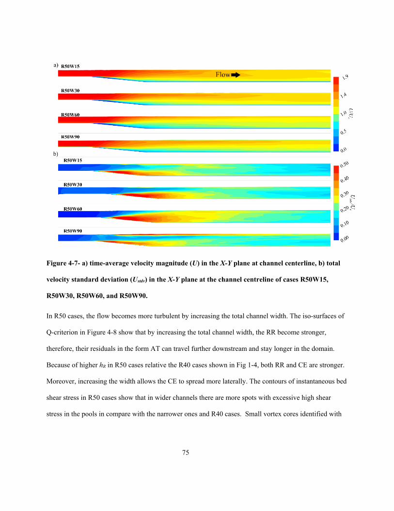
75
Figure 4-7- a) time-average velocity magnitude (U) in the X-Y plane at channel centerline, b) total
velocity standard deviation (Ustdv) in the X-Y plane at the channel centreline of cases R50W15,
R50W30, R50W60, and R50W90.
In R50 cases, the flow becomes more turbulent by increasing the total channel width. The iso-surfaces of
Q-criterion in Figure 4-8 show that by increasing the total channel width, the RR become stronger,
therefore, their residuals in the form AT can travel further downstream and stay longer in the domain.
Because of higher hR in R50 cases relative the R40 cases shown in Fig 1-4, both RR and CE are stronger.
Moreover, increasing the width allows the CE to spread more laterally. The contours of instantaneous bed
shear stress in R50 cases show that in wider channels there are more spots with excessive high shear
stress in the pools in compare with the narrower ones and R40 cases. Small vortex cores identified with
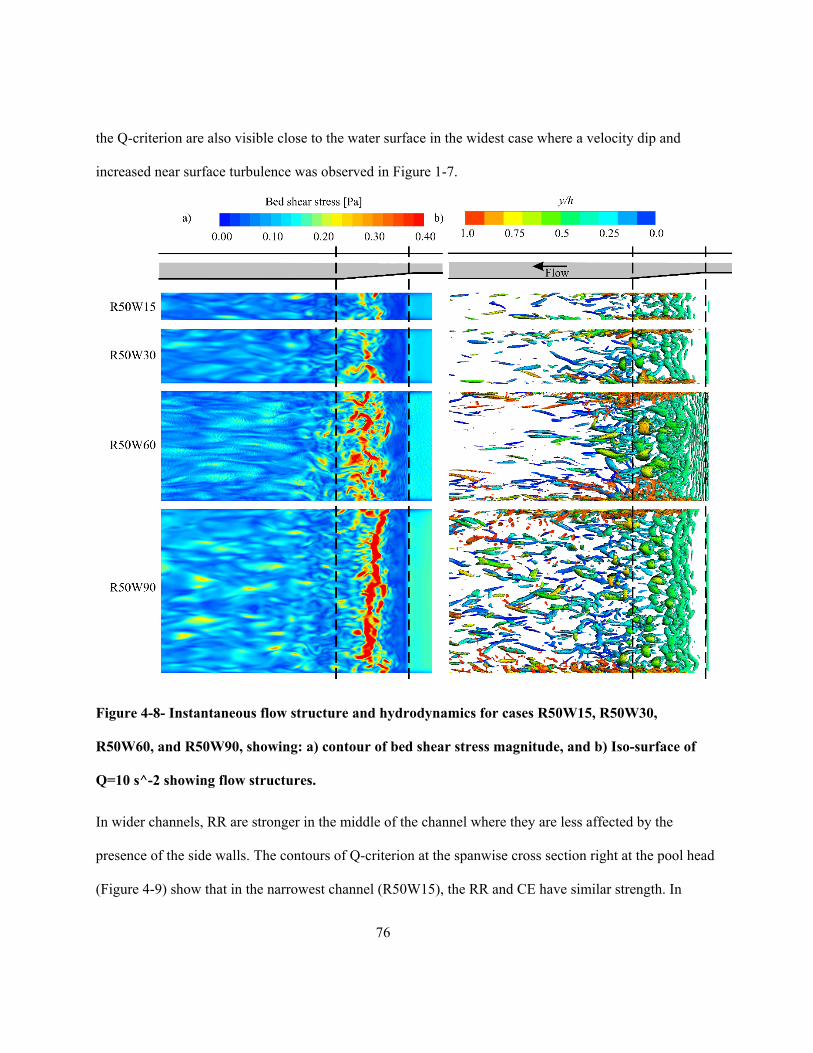
76
the Q-criterion are also visible close to the water surface in the widest case where a velocity dip and
increased near surface turbulence was observed in Figure 1-7.
Figure 4-8- Instantaneous flow structure and hydrodynamics for cases R50W15, R50W30,
R50W60, and R50W90, showing: a) contour of bed shear stress magnitude, and b) Iso-surface of
Q=10 s^-2 showing flow structures.
In wider channels, RR are stronger in the middle of the channel where they are less affected by the
presence of the side walls. The contours of Q-criterion at the spanwise cross section right at the pool head
(Figure 4-9) show that in the narrowest channel (R50W15), the RR and CE have similar strength. In
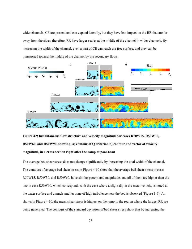
77
wider channels, CE are present and can expand laterally, but they have less impact on the RR that are far
away from the sides; therefore, RR have larger scales at the middle of the channel in wider channels. By
increasing the width of the channel, even a part of CE can reach the free surface, and they can be
transported toward the middle of the channel by the secondary flows.
Figure 4-9 Instantaneous flow structure and velocity magnitude for cases R50W15, R50W30,
R50W60, and R50W90, showing: a) contour of Q criterion b) contour and vector of velocity
magnitude, in a cross-section right after the ramp at pool-head
The average bed shear stress does not change significantly by increasing the total width of the channel.
The contours of average bed shear stress in Figure 4-10 show that the average bed shear stress in cases
R50W15, R50W30, and R50W60, have similar pattern and magnitude, and all of them are higher than the
one in case R50W90, which corresponds with the case where a slight dip in the mean velocity is noted at
the water surface and a much smaller zone of high turbulence near the bed is observed (Figure 1-7). As
shown in Figure 4-10, the mean shear stress is highest on the ramp in the region where the largest RR are
being generated. The contours of the standard deviation of bed shear stress show that by increasing the
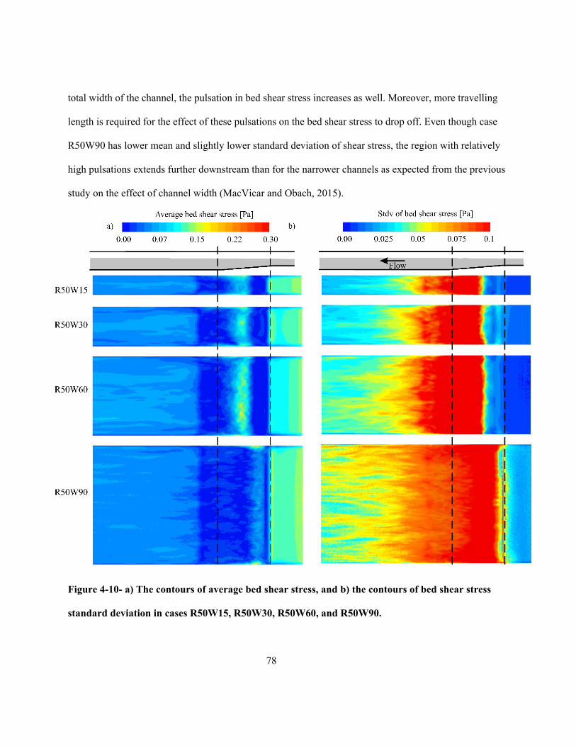
78
total width of the channel, the pulsation in bed shear stress increases as well. Moreover, more travelling
length is required for the effect of these pulsations on the bed shear stress to drop off. Even though case
R50W90 has lower mean and slightly lower standard deviation of shear stress, the region with relatively
high pulsations extends further downstream than for the narrower channels as expected from the previous
study on the effect of channel width (MacVicar and Obach, 2015).
Figure 4-10- a) The contours of average bed shear stress, and b) the contours of bed shear stress
standard deviation in cases R50W15, R50W30, R50W60, and R50W90.
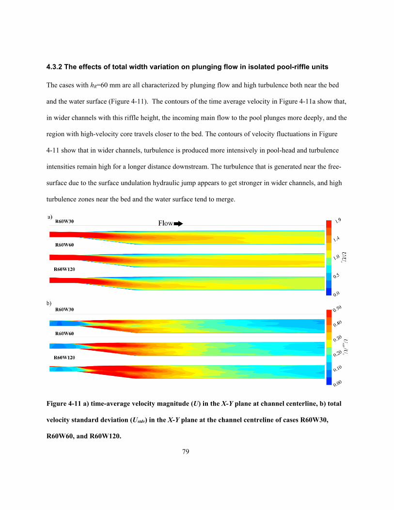
79
4.3.2 The effects of total width variation on plunging flow in isolated pool-riffle units
The cases with hR=60 mm are all characterized by plunging flow and high turbulence both near the bed
and the water surface (Figure 4-11). The contours of the time average velocity in Figure 4-11a show that,
in wider channels with this riffle height, the incoming main flow to the pool plunges more deeply, and the
region with high-velocity core travels closer to the bed. The contours of velocity fluctuations in Figure
4-11 show that in wider channels, turbulence is produced more intensively in pool-head and turbulence
intensities remain high for a longer distance downstream. The turbulence that is generated near the free-
surface due to the surface undulation hydraulic jump appears to get stronger in wider channels, and high
turbulence zones near the bed and the water surface tend to merge.
Figure 4-11 a) time-average velocity magnitude (U) in the X-Y plane at channel centerline, b) total
velocity standard deviation (Ustdv) in the X-Y plane at the channel centreline of cases R60W30,
R60W60, and R60W120.
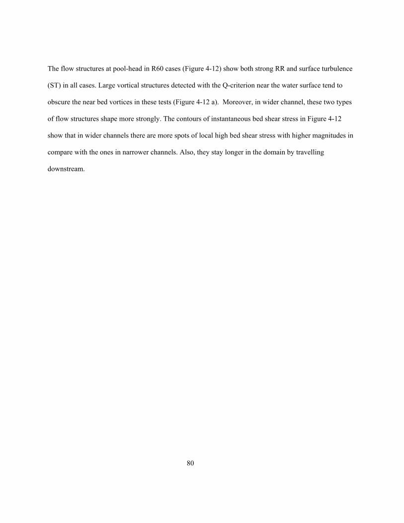
80
The flow structures at pool-head in R60 cases (Figure 4-12) show both strong RR and surface turbulence
(ST) in all cases. Large vortical structures detected with the Q-criterion near the water surface tend to
obscure the near bed vortices in these tests (Figure 4-12 a). Moreover, in wider channel, these two types
of flow structures shape more strongly. The contours of instantaneous bed shear stress in Figure 4-12
show that in wider channels there are more spots of local high bed shear stress with higher magnitudes in
compare with the ones in narrower channels. Also, they stay longer in the domain by travelling
downstream.
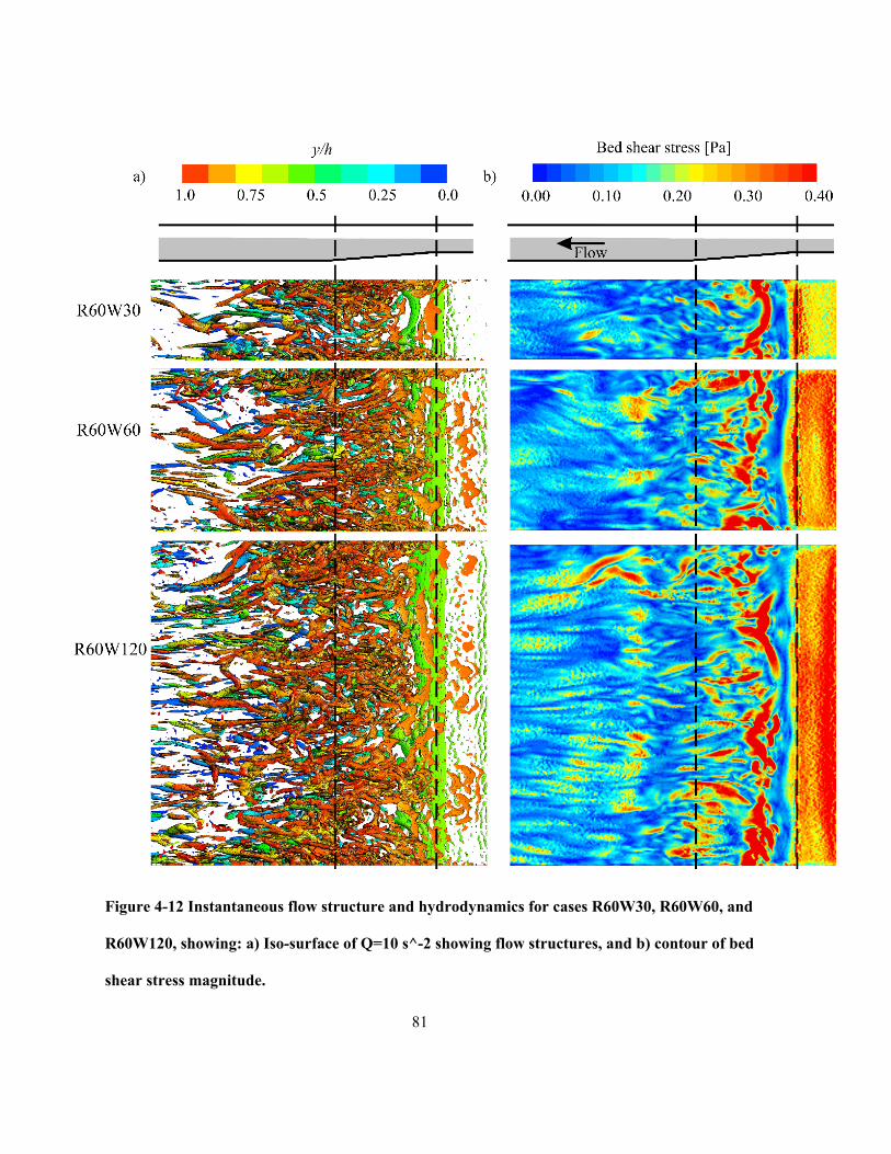
81
Figure 4-12 Instantaneous flow structure and hydrodynamics for cases R60W30, R60W60, and
R60W120, showing: a) Iso-surface of Q=10 s^-2 showing flow structures, and b) contour of bed
shear stress magnitude.
82
The contours of Q-criterion at the pool-head show that in R60 cases strong turbulent structures are present
in all areas of the flow (Figure 4-12). All the three types of flow structures (RR, CE, and ST) are visible
and strongly interacting. In all cases, ST have occupied the whole width near the free surface, and CE
have occupied the sides. In the narrowest channel (R40W30), the mean flow is concentrated mostly at the
centre of the cross-section and slightly near the corners between ST and CE. In the case with a midsize
width (R60W60), RR are stronger than the ones in R60W30. In the widest channel (R60W120), the RR
are strong enough to expand and reach the free surface, and some areas of low turbulence exist between
the sidewalls and channel centerline. by resisting the flow, they can separate the mean flow into two
substreams.
Figure 4-13 Instantaneous flow structure and velocity magnitude for cases R50W15, R50W30,
R50W60, and R50W90, showing: a) contour of Q criterion b) contour and vector of velocity
magnitude, in a cross-section right after the ramp at pool-head
Both the mean and standard deviation of bed shear stress are higher in wider channels for the cases with a
60 mm high riffle (Figure 4-12). The contour of mean bed shear stress in case R60W120 shows that the
mean and standard deviation of bed shear stress peaks at the middle of those two substreams. Moreover,
the regions with high mean and standard deviation of shear stress are extended more in the downstream.
By comparing the bed shear stresses in R60 cases to the ones in R40 and R50 cases, it can be said that the
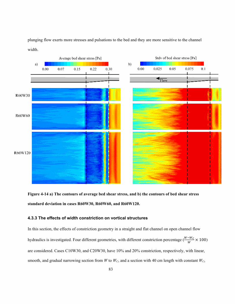
83
plunging flow exerts more stresses and pulsations to the bed and they are more sensitive to the channel
width.
Figure 4-14 a) The contours of average bed shear stress, and b) the contours of bed shear stress
standard deviation in cases R60W30, R60W60, and R60W120.
4.3.3 The effects of width constriction on vortical structures
In this section, the effects of constriction geometry in a straight and flat channel on open channel flow
hydraulics is investigated. Four different geometries, with different constriction percentage ( 100)
are considered. Cases C10W30, and C20W30, have 10% and 20% constriction, respectively, with linear,
smooth, and gradual narrowing section from W to WC, and a section with 40 cm length with constant WC,
84
and then a linear, smooth, and gradual widening to the normal width (W). Cases C20W30C and
C25W30C, have a sharp constriction with concave rather than linear sidewalls for the narrowing and
widening sections. The motivation for this particular geometry comes from a constriction in Black
Canyon, BC, Canada (Venditti et al. 2014) and the desire to more fully understand the hydrodynamics for
this site, which includes plunging despite a relatively low Froude number in the constriction. Case
C20W30S has a rectangular constriction with 20% ratio while Case C25W30L has a triangular
constriction. In all cases the Froude number at the constriction, based on a 1D analysis, is between 0.2
and 0.3 (Table 4-1).
The constrictions with sharp edges or geometries that shape stronger spanwise velocity produce more
turbulence and exert higher magnitude fluctuations in bed shear stress. The iso-surfaces of Q-criterion in
Figure 4-15 show that the constrictions produce strong vortical structures in the CDF zone (widening
section). In case C10W30 a series of vortices are shaped near the bed at the downstream of the constricted
section, which we refer to these vortices as bed rollers (BR) herein, and they are stronger in case
C20W30, which has higher constriction ratio. The case C20W30C has the same constriction ratio as
C20W30, but with concaved curves profile in the narrowing and widening sections. The vortical
structures, in this case, are stronger than previous cases. Groups of horseshoe vortices (HV) are shaped at
the upstream of in CAF zone, and they are being stretched and transported to the constricted section. HV
cause excessive bed shear stress at the upstream of the constriction. They interact with BR and make them
weaker as they pass the constriction. The ST near the walls and downstream of the constriction are
stronger and propagated more widely than previous cases. The vortical structures, in this case, stay longer
in the domain before they get entirely dissipated. The case C20W30S has a rectangular constriction
section that results in stronger HV that originate farther upstream from the constriction. These HV result
in high bed shear stresses in and upstream of the constricted section. For the case C25W30C, which has a
85
25% constriction with concave curve narrowing and widening sections, the ST, HV, and BR are stronger
than the ones in other cases. These strong vortical structures appear to exert higher shear stress on the
bed. Case C25W30L has the same constriction ratio as case C25W30L, but the vortical structures are
weaker.
BR are shaped closer to the constriction in more constricted channels, and they are weaker in cases that
have strong ST and HV. The instantaneous longitudinal contours and vectors of velocity magnitude along
the centerline of the channel (Figure 4-16) show that BR shape farther downstream of the constriction in
cases C10W30 and C20W30, and they are stretched and elevated to the middle of the flow depth as they
travel downstream. For the shorter constriction, the near-bed turbulence is stronger upstream while the
near-surface turbulence develops later and is weaker along the centerline.. They are weaker than BR, and
they do not grow and last longer. In case C20W30S the long HV are mixed with BR and start to elevate
from the bed at the middle of the constriction. The ST, in this case, are decidedly weaker than bed
turbulences, which is in contrast with case C25W30C. Bed turbulences are reduced to a thin layer near the
bed that do not grow or elevate to enter the main flow. In contrast with other cases, in case C25W30C, the
core of high velocity is located near the bed. In comparison with C25W30C, the ST in case C25W30L,
appear later at the plane along the centerline. In addition, BR are stronger than previous cases but not
strong enough to occupy the bottom half of the flow depth. In all cases, the generated turbulence are
stretched in the form of AT as they leave their genesis and travel downstream.
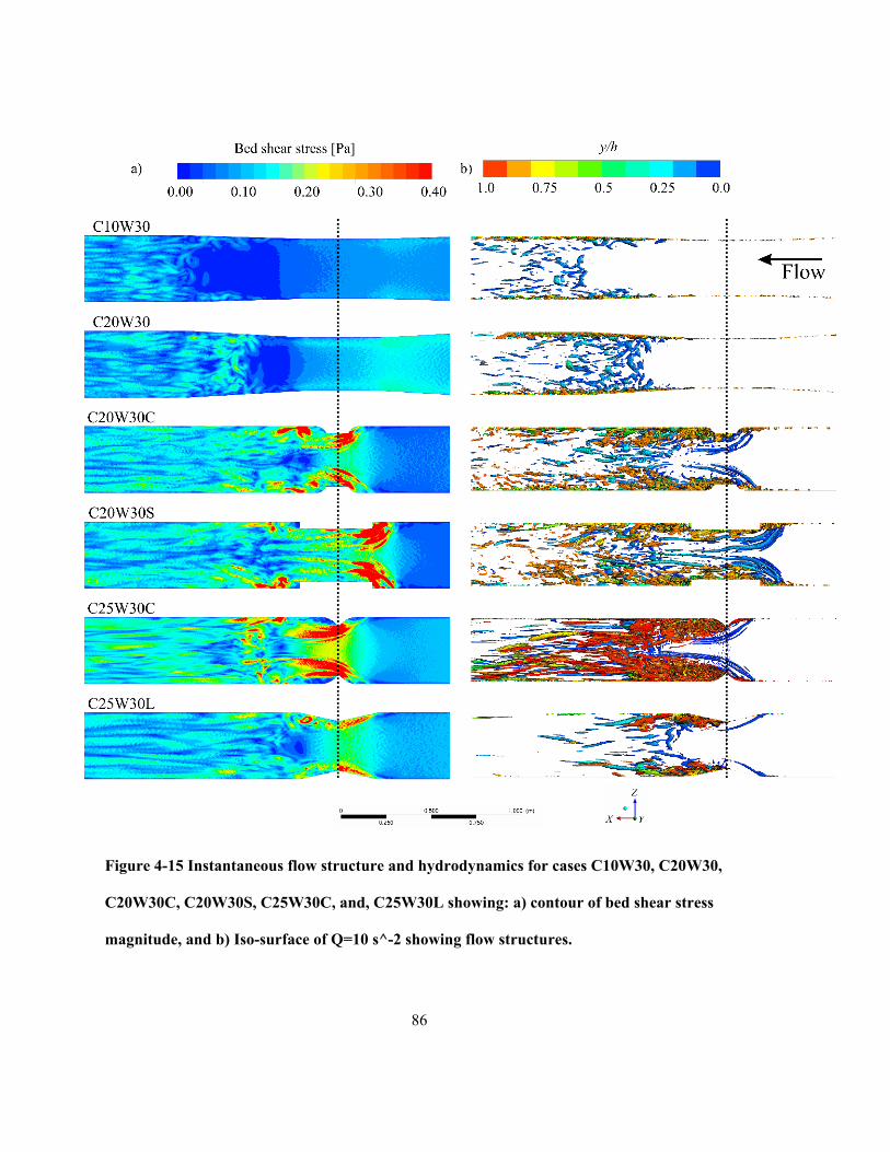
86
Figure 4-15 Instantaneous flow structure and hydrodynamics for cases C10W30, C20W30,
C20W30C, C20W30S, C25W30C, and, C25W30L showing: a) contour of bed shear stress
magnitude, and b) Iso-surface of Q=10 s^-2 showing flow structures.
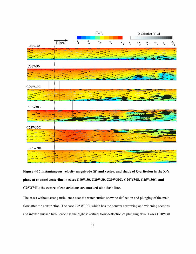
87
Figure 4-16 Instantaneous velocity magnitude ( ) and vector, and shade of Q-criterion in the X-Y
plane at channel centerline in cases C10W30, C20W30, C20W30C, C20W30S, C25W30C, and
C25W30L; the centre of constrictions are marked with dash line.
The cases without strong turbulence near the water surfact show no deflection and plunging of the main
flow after the constriction. The case C25W30C, which has the convex narrowing and widening sections
and intense surface turbulence has the highest vertical flow deflection of plunging flow. Cases C10W30
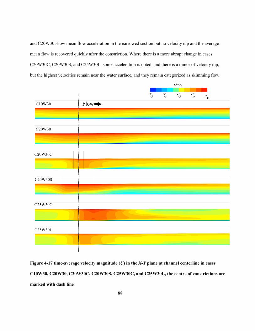
88
and C20W30 show mean flow acceleration in the narrowed section but no velocity dip and the average
mean flow is recovered quickly after the constriction. Where there is a more abrupt change in cases
C20W30C, C20W30S, and C25W30L, some acceleration is noted, and there is a minor of velocity dip,
but the highest velocities remain near the water surface, and they remain categorized as skimming flow.
Figure 4-17 time-average velocity magnitude (U) in the X-Y plane at channel centerline in cases
C10W30, C20W30, C20W30C, C20W30S, C25W30C, and C25W30L, the centre of constrictions are
marked with dash line
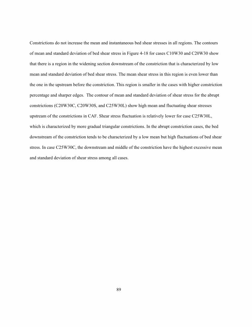
89
Constrictions do not increase the mean and instantaneous bed shear stresses in all regions. The contours
of mean and standard deviation of bed shear stress in Figure 4-18 for cases C10W30 and C20W30 show
that there is a region in the widening section downstream of the constriction that is characterized by low
mean and standard deviation of bed shear stress. The mean shear stress in this region is even lower than
the one in the upstream before the constriction. This region is smaller in the cases with higher constriction
percentage and sharper edges. The contour of mean and standard deviation of shear stress for the abrupt
constrictions (C20W30C, C20W30S, and C25W30L) show high mean and fluctuating shear stresses
upstream of the constrictions in CAF. Shear stress fluctuation is relatively lower for case C25W30L,
which is characterized by more gradual triangular constrictions. In the abrupt constriction cases, the bed
downstream of the constriction tends to be characterized by a low mean but high fluctuations of bed shear
stress. In case C25W30C, the downstream and middle of the constriction have the highest excessive mean
and standard deviation of shear stress among all cases.
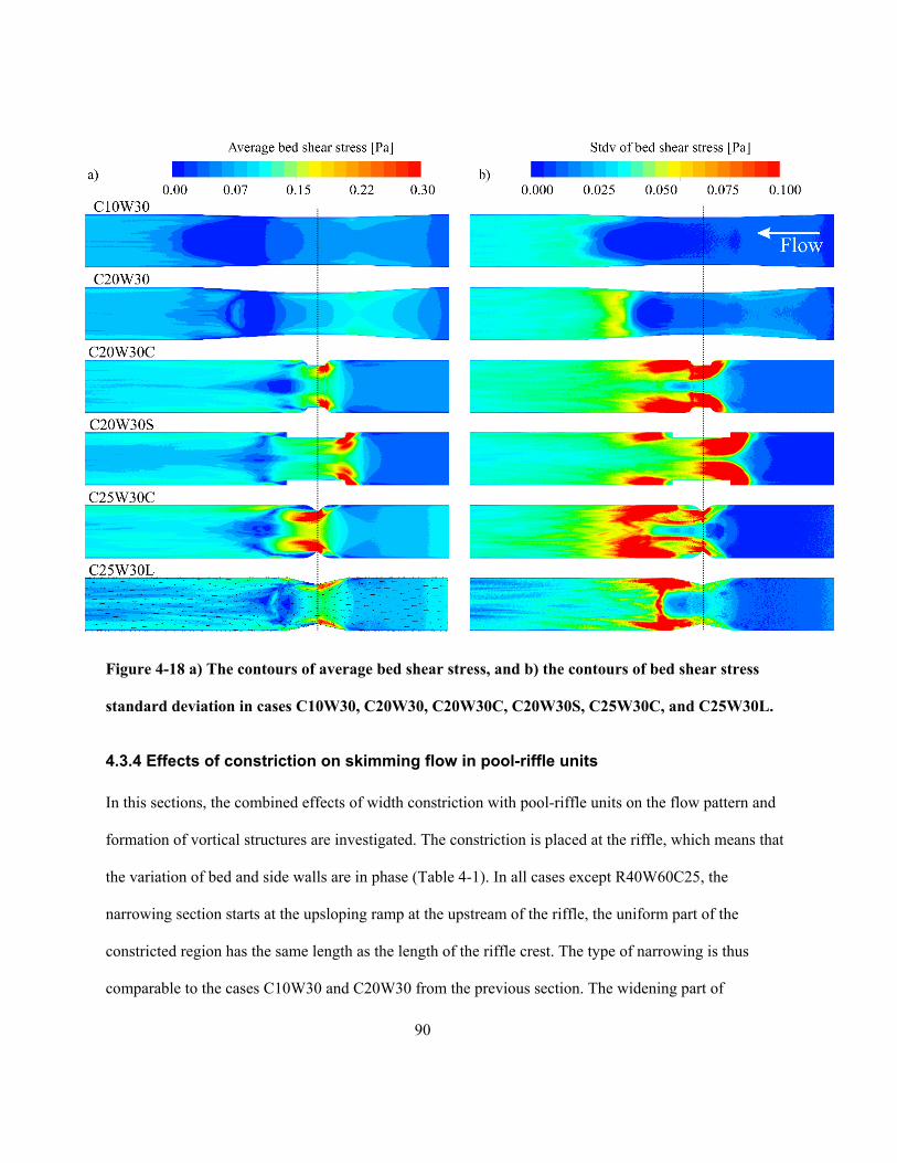
90
Figure 4-18 a) The contours of average bed shear stress, and b) the contours of bed shear stress
standard deviation in cases C10W30, C20W30, C20W30C, C20W30S, C25W30C, and C25W30L.
4.3.4 Effects of constriction on skimming flow in pool-riffle units
In this sections, the combined effects of width constriction with pool-riffle units on the flow pattern and
formation of vortical structures are investigated. The constriction is placed at the riffle, which means that
the variation of bed and side walls are in phase (Table 4-1). In all cases except R40W60C25, the
narrowing section starts at the upsloping ramp at the upstream of the riffle, the uniform part of the
constricted region has the same length as the length of the riffle crest. The type of narrowing is thus
comparable to the cases C10W30 and C20W30 from the previous section. The widening part of
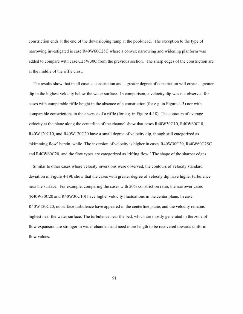
91
constriction ends at the end of the downsloping ramp at the pool-head. The exception to the type of
narrowing investigated is case R40W60C25C where a convex narrowing and widening planform was
added to compare with case C25W30C from the previous section. The sharp edges of the constriction are
at the middle of the riffle crest.
The results show that in all cases a constriction and a greater degree of constriction will create a greater
dip in the highest velocity below the water surface. In comparison, a velocity dip was not observed for
cases with comparable riffle height in the absence of a constriction (for e.g. in Figure 4-3) nor with
comparable constrictions in the absence of a riffle (for e.g. in Figure 4-18). The contours of average
velocity at the plane along the centerline of the channel show that cases R40W30C10, R40W60C10,
R40W120C10, and R40W120C20 have a small degree of velocity dip, though still categorized as
‘skimming flow’ herein, while The inversion of velocity is higher in cases R40W30C20, R40W60C25C
and R40W60C20, and the flow types are categorized as ‘rifting flow.’ The shape of the sharper edges
Similar to other cases where velocity inversions were observed, the contours of velocity standard
deviation in Figure 4-19b show that the cases with greater degree of velocity dip have higher turbulence
near the surface. For example, comparing the cases with 20% constriction ratio, the narrower cases
(R40W30C20 and R40W30C10) have higher velocity fluctuations in the center plane. In case
R40W120C20, no surface turbulence have appeared in the centerline plane, and the velocity remains
highest near the water surface. The turbulence near the bed, which are mostly generated in the zone of
flow expansion are stronger in wider channels and need more length to be recovered towards uniform
flow values.
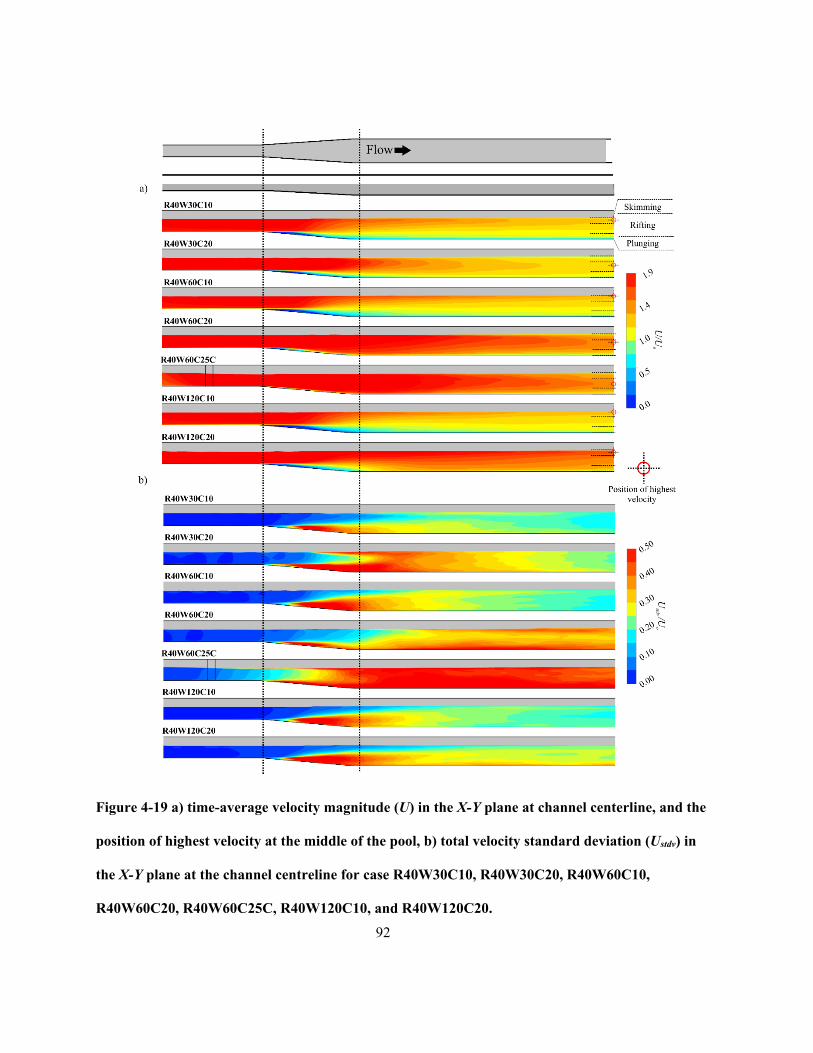
92
Figure 4-19 a) time-average velocity magnitude (U) in the X-Y plane at channel centerline, and the
position of highest velocity at the middle of the pool, b) total velocity standard deviation (Ustdv) in
the X-Y plane at the channel centreline for case R40W30C10, R40W30C20, R40W60C10,
R40W60C20, R40W60C25C, R40W120C10, and R40W120C20.
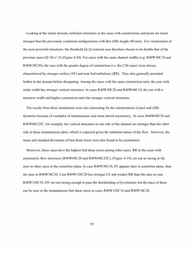
93
Looking at the whole domain, turbulent structures in the cases with constrictions and pools are much
stronger than the previously examined configurations with this riffle height (40 mm). For visualization of
the most powerful structures, the threshold for Q-criterion was therefore chosen to be double that of the
previous cases (Q=20 s^-2) (Figure 4-20). For cases with the same channel widths (e.g. R40W30C10 and
R40W30C20), the case with the greater degree of constriction (i.e. the C20 cases) were always
characterized by stronger surface (ST) and near bed turbulence (RR). They also generally persisted
farther in the domain before dissipating. Among the cases with the same constriction ratio, the case with
wider width has stronger vortical structures. In cases R40W30C20 and R40W60C10, the one with a
narrower width and higher constriction ratio has stronger vortical structures.
The results from these simulations were also interesting for the interpretation of pool and riffle
dynamics because of examples of instantaneous and mean lateral asymmetry. In cases R40W60C20 and
R40W60C25C, for example, the vortical structures in one side of the channel are stronger than the other
side in these instantaneous plots, which is expected given the turbulent nature of the flow. However, the
mean and standard deviations of bed shear stress were also found to be asymmetric.
Moreover, these cases have the highest bed shear stress among other cases. RR in the cases with
asymmetric flow structures (R40W60C20 and R40W60C25C), (Figure 4-19), are not as strong as the
ones in other cases in the centerline plane. In case R40W30C10, ST appears later in centerline plane, than
the ones in R40W30C20. Case R40W120C20 has stronger CE and weaker RR than the ones in case
R40W120C10. HV are not strong enough to pass the thresholding of Q-criterion, but the trace of them
can be seen in the instantaneous bed shear stress in cases R40W120C10 and R40W10C20.
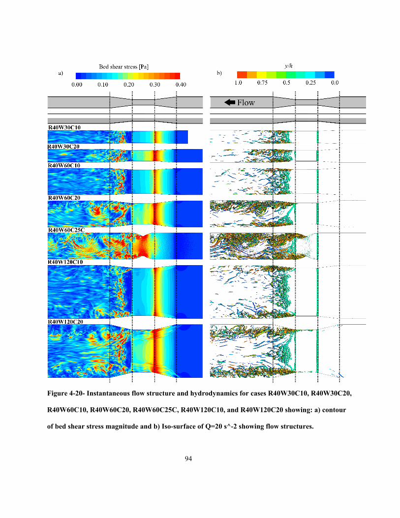
94
Figure 4-20- Instantaneous flow structure and hydrodynamics for cases R40W30C10, R40W30C20,
R40W60C10, R40W60C20, R40W60C25C, R40W120C10, and R40W120C20 showing: a) contour
of bed shear stress magnitude and b) Iso-surface of Q=20 s^-2 showing flow structures.
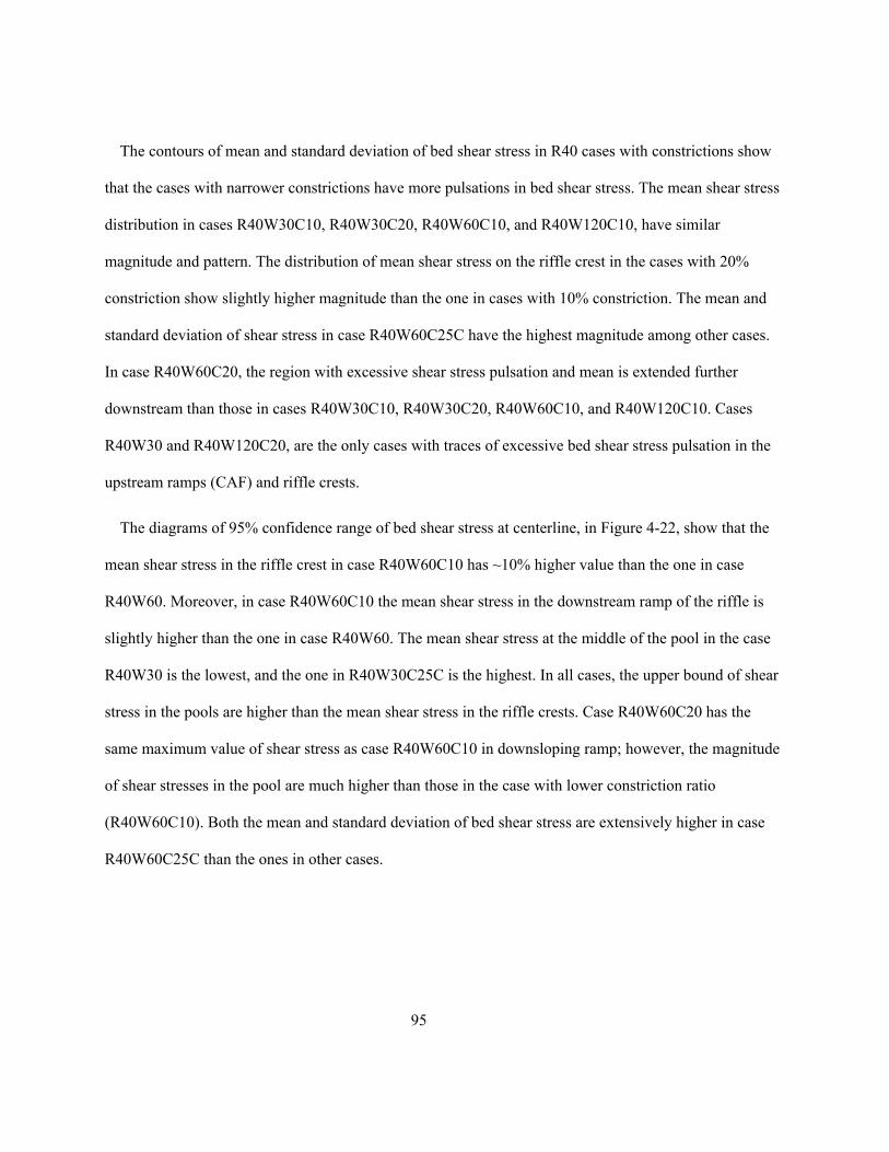
95
The contours of mean and standard deviation of bed shear stress in R40 cases with constrictions show
that the cases with narrower constrictions have more pulsations in bed shear stress. The mean shear stress
distribution in cases R40W30C10, R40W30C20, R40W60C10, and R40W120C10, have similar
magnitude and pattern. The distribution of mean shear stress on the riffle crest in the cases with 20%
constriction show slightly higher magnitude than the one in cases with 10% constriction. The mean and
standard deviation of shear stress in case R40W60C25C have the highest magnitude among other cases.
In case R40W60C20, the region with excessive shear stress pulsation and mean is extended further
downstream than those in cases R40W30C10, R40W30C20, R40W60C10, and R40W120C10. Cases
R40W30 and R40W120C20, are the only cases with traces of excessive bed shear stress pulsation in the
upstream ramps (CAF) and riffle crests.
The diagrams of 95% confidence range of bed shear stress at centerline, in Figure 4-22, show that the
mean shear stress in the riffle crest in case R40W60C10 has ~10% higher value than the one in case
R40W60. Moreover, in case R40W60C10 the mean shear stress in the downstream ramp of the riffle is
slightly higher than the one in case R40W60. The mean shear stress at the middle of the pool in the case
R40W30 is the lowest, and the one in R40W30C25C is the highest. In all cases, the upper bound of shear
stress in the pools are higher than the mean shear stress in the riffle crests. Case R40W60C20 has the
same maximum value of shear stress as case R40W60C10 in downsloping ramp; however, the magnitude
of shear stresses in the pool are much higher than those in the case with lower constriction ratio
(R40W60C10). Both the mean and standard deviation of bed shear stress are extensively higher in case
R40W60C25C than the ones in other cases.
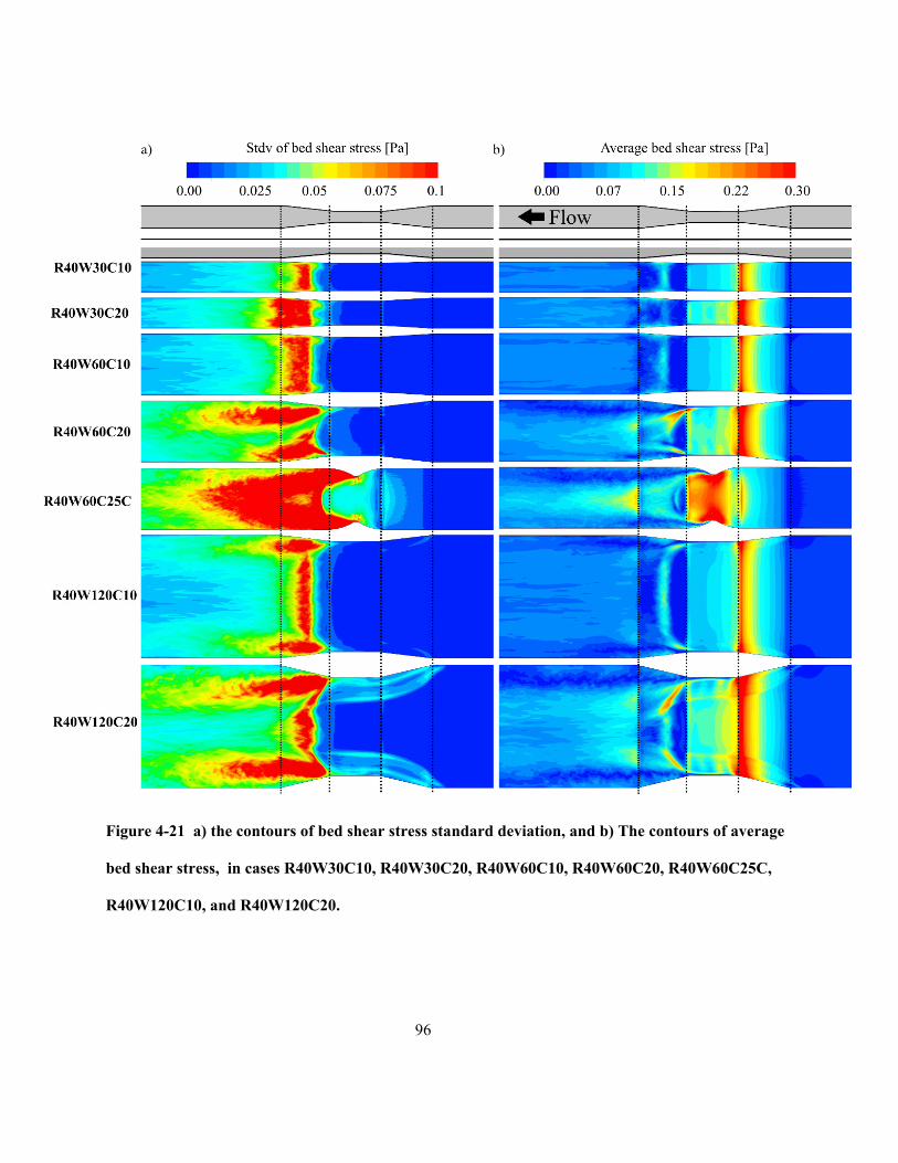
96
Figure 4-21 a) the contours of bed shear stress standard deviation, and b) The contours of average
bed shear stress, in cases R40W30C10, R40W30C20, R40W60C10, R40W60C20, R40W60C25C,
R40W120C10, and R40W120C20.
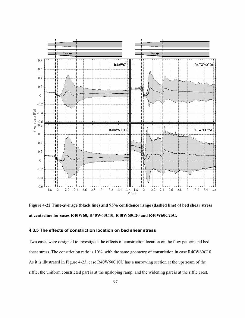
97
Figure 4-22 Time-average (black line) and 95% confidence range (dashed line) of bed shear stress
at centreline for cases R40W60, R40W60C10, R40W60C20 and R40W60C25C.
4.3.5 The effects of constriction location on bed shear stress
Two cases were designed to investigate the effects of constriction location on the flow pattern and bed
shear stress. The constriction ratio is 10%, with the same geometry of constriction in case R40W60C10.
As it is illustrated in Figure 4-23, case R40W60C10U has a narrowing section at the upstream of the
riffle, the uniform constricted part is at the upsloping ramp, and the widening part is at the riffle crest.
98
Case R40W60C10D has the narrowing part at the riffle crest, the uniform constricted part is at the
downsloping ramp, and the widening part is at the pool head. RR in case R40W60C10U is stronger than
other cases illustrated in Figure 4-23. CE are stronger in case R40W60C10 than other cases. Case
R40W60C10D has the weakest RR among other cases.
Figure 4-23 Instantaneous flow structure for cases R40W60, R40W60C10U, R40W60C10, and
R40W60C10D showing Iso-surface of Q=5 s^-2, and the contour of bed elevation.
The diagrams of 95% confidence range of bed shear stress, in Figure 4-24, show that the case with
widening part at the riffle crest has the lowest mean shear stress at the riffle crest. The case with
narrowing part at the riffle crest has the highest mean shear stress and fluctuation in the riffle crest, even
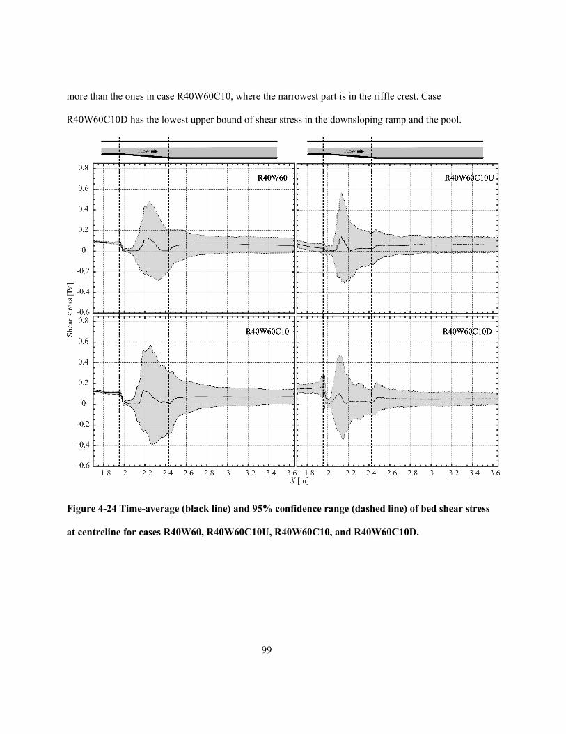
99
more than the ones in case R40W60C10, where the narrowest part is in the riffle crest. Case
R40W60C10D has the lowest upper bound of shear stress in the downsloping ramp and the pool.
Figure 4-24 Time-average (black line) and 95% confidence range (dashed line) of bed shear stress
at centreline for cases R40W60, R40W60C10U, R40W60C10, and R40W60C10D.
100
4.4 Discussion
In the previous chapter, the formation mechanism of skimming, rifting, and plunging flow; and
bifurcation in mean flow are discussed by introducing the vortex-resistance hypothesis. We showed that
the reason for scouring and high shear stress in the stable pools is not only the high velocity near the bed,
which previously named as velocity reversal (Keller, 1971). This chapter for designing new models aims
to investigate the effects of constriction on flow pattern and maintenance of pool-riffle units, which
previously described as flow convergence hypothesis (MacWilliams et al. 2006).
MacVicar & Best, (2013) used the concept of recovery from perturbation to describe the effects of
geometry induced flow behaviour. They mentioned two stages for recovery from perturbation. The first
stage that is called “spreading” refers to production, propagation, and transport of turbulence, which is
induced by morphological changes, and streamwise adverse pressure gradient (positive). After the
completion of “spreading” phase, the “relaxation” phase is initiated. “Relaxation” refers to the phase that
there are no significant irregularities in the morphology and the flow tries to recover to the normal state,
which it had before the emergence of perturbation. In the “relaxation” phase, the vortical structures get
stretched, break into smaller scales and finally dissipated by viscous forces, while they are travelling
downstream. The concept of “spreading and relaxation,” and the length that the flow should travel to
reach the normal state (recovery length), is used in this section to qualitatively describe the hydrodynamic
response of the channel to the total and local variation of the width.
The most of perturbation generations, in spreading phase, happen in CDF zone, which is located at the
widening section and downsloping ramp at the pool-head. The widening section and downsloping ramp
are in phase in the cases that are described previously in this chapter. Four generative vortical structures
(RR, BR, CE, and ST) produce perturbation in CDF.
101
In the cases without local width variation (no spanwise constriction and expansion), and with skimming
flows (R40 and R50 cases) the strength of RR and CE, which are related to their sizes, are mostly
controlled by the height of the riffle (hR). This claim is shown in the previous chapter and comparing the
hydrodynamics in R40 and R50 cases. These two major vortical structures (RR and CE) appear to
influence each other’s strength such that in narrower channels, these two types of vortices are forming
very closely to each other and do not have enough space to shape and grow fully. In wider channels, RR
in the centre of the channel, far away from CE, have more space and grow to bigger sizes. Meanwhile, CE
have more space as well and they are also stronger in wider channels. Stronger RR and CE mean that the
“spreading” phase results in larger and more powerful eddies that require a longer streamwise distance to
dissipate. The differences in turbulent eddies with respect to channel width thus help explain the longer
recovery length for wider channels. The contours of the standard deviation of shear stress in the previous
section show that longer recovery lengths extend the excessive pulsation in shear stress to farther
downstream. This pattern of hydrodynamic response to morphological irregularities can be found in the
cases with plunging flows (R60 cases) as well. The resistance of stronger RR at the middle of the width in
wider channels acts as a wall and divides the channel into two substreams; therefore, with more walls and
CE, there are more sources of turbulence in CDF.
In the cases with just a constriction (i.e. without a riffle), the perturbation generations in “spreading”
phase commence before the constriction (in CAF). The illustration of vortical structures for these cases in
the previous section shows that there are three major generative vortical structures in those cases. BR and
CE at the downstream of the constriction (CDF zone), and HV at the upstream (CAF zone). HV are
reported by various researchers that have studied the vortical structures around obstacles in shallow
streams (Beheshti et al. 2017; Celik et al. 2014; Ettema et al. 2017; Kumar et al. 2012; Zeng and
Constantinescu 2017). They reported that HV are the result of the combination of downward flow at the
upstream face of the obstacle that induces vortices at the front of the obstacle that is then stretched around
102
the base of the object by the main flow. BR have similar formation mechanism as RR in pool-riffle units
both cases are forced by an adverse pressure gradient and result in mean flow moving away from the bed
and creating a region of relatively high strain at the middle of the profile that can generate new
turbulence(Krogstad and Skåre 1995). The formation of CE are due to the irregularity in the sidewalls and
the impact of secondary flow to the walls. If the constriction has sharper edges or a geometry that shape
more powerful spanwise component of velocity, the CE become stronger. In sharp edge constrictions, CE
are stronger near the surface, because the logarithmic profile of incoming flow has higher velocity near
the surface than near the bed. Therefore, CE near the surface in the form of ST have larger sizes than the
ones near the bed. Stronger CE, BR, and HV need more recovery length in “relaxation” phase.
By adding the constriction to pool-riffle units, the constriction induced vortical structures both amplify
and suppress some vortical structures found in the straight pool-riffle units. BR combine and amplify the
RR, but they are not strong enough to cancel out the impact of CE and HV. HV, which are generated in
CAF zone at the upstream, amplify CE, confine the generation space of RR and decrease the impact of
RR on suppressing the CE. The CE, which are induced by the constriction, amplify the CE in the pool.
The strong CE, at the downstream of the riffle, can get transported to the free surface by the secondary
flow. The combination of secondary flow and transported CE can make boiling structures on the free
surface. These ST guide the mean flow to plunge into the pool. The secondary effect of plunging flow
suppress the formation of RR and amplify the secondary flow and CE; therefore, as positive feedback, the
CE become stronger until the system reaches to an equilibrium balance of forces and momentums. Due to
the resistance of CE and powerful plunging flow, bifurcation can happen to the mean flow and deflect it
to one side. The deflected mean flow amplify the vortical structures of one side; therefore, the
“relaxation” phase will be delayed, and the flow needs a more prolonged recovery length to reach the
normal state.
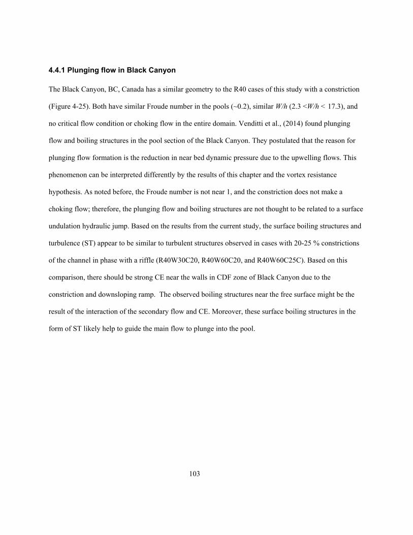
103
4.4.1 Plunging flow in Black Canyon
The Black Canyon, BC, Canada has a similar geometry to the R40 cases of this study with a constriction
(Figure 4-25). Both have similar Froude number in the pools (~0.2), similar W/h (2.3 <W/h < 17.3), and
no critical flow condition or choking flow in the entire domain. Venditti et al., (2014) found plunging
flow and boiling structures in the pool section of the Black Canyon. They postulated that the reason for
plunging flow formation is the reduction in near bed dynamic pressure due to the upwelling flows. This
phenomenon can be interpreted differently by the results of this chapter and the vortex resistance
hypothesis. As noted before, the Froude number is not near 1, and the constriction does not make a
choking flow; therefore, the plunging flow and boiling structures are not thought to be related to a surface
undulation hydraulic jump. Based on the results from the current study, the surface boiling structures and
turbulence (ST) appear to be similar to turbulent structures observed in cases with 20-25 % constrictions
of the channel in phase with a riffle (R40W30C20, R40W60C20, and R40W60C25C). Based on this
comparison, there should be strong CE near the walls in CDF zone of Black Canyon due to the
constriction and downsloping ramp. The observed boiling structures near the free surface might be the
result of the interaction of the secondary flow and CE. Moreover, these surface boiling structures in the
form of ST likely help to guide the main flow to plunge into the pool.
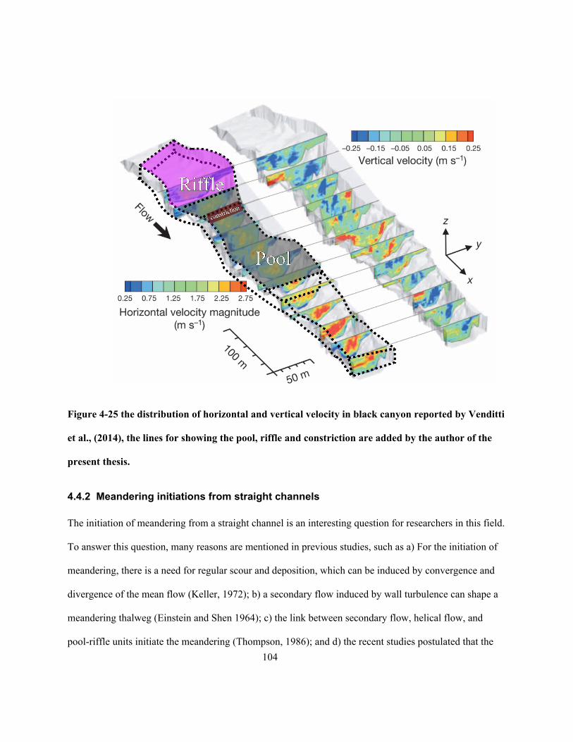
104
Figure 4-25 the distribution of horizontal and vertical velocity in black canyon reported by Venditti
et al., (2014), the lines for showing the pool, riffle and constriction are added by the author of the
present thesis.
4.4.2 Meandering initiations from straight channels
The initiation of meandering from a straight channel is an interesting question for researchers in this field.
To answer this question, many reasons are mentioned in previous studies, such as a) For the initiation of
meandering, there is a need for regular scour and deposition, which can be induced by convergence and
divergence of the mean flow (Keller, 1972); b) a secondary flow induced by wall turbulence can shape a
meandering thalweg (Einstein and Shen 1964); c) the link between secondary flow, helical flow, and
pool-riffle units initiate the meandering (Thompson, 1986); and d) the recent studies postulated that the
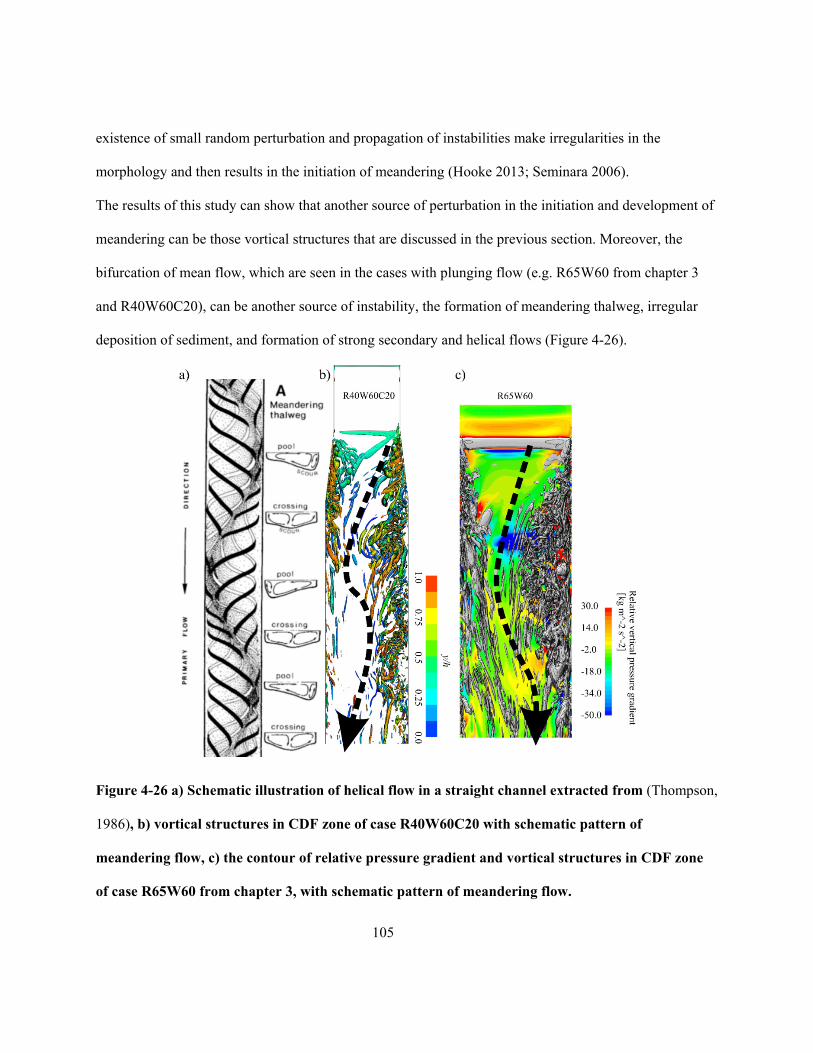
105
existence of small random perturbation and propagation of instabilities make irregularities in the
morphology and then results in the initiation of meandering (Hooke 2013; Seminara 2006).
The results of this study can show that another source of perturbation in the initiation and development of
meandering can be those vortical structures that are discussed in the previous section. Moreover, the
bifurcation of mean flow, which are seen in the cases with plunging flow (e.g. R65W60 from chapter 3
and R40W60C20), can be another source of instability, the formation of meandering thalweg, irregular
deposition of sediment, and formation of strong secondary and helical flows (Figure 4-26).
Figure 4-26 a) Schematic illustration of helical flow in a straight channel extracted from (Thompson,
1986), b) vortical structures in CDF zone of case R40W60C20 with schematic pattern of
meandering flow, c) the contour of relative pressure gradient and vortical structures in CDF zone
of case R65W60 from chapter 3, with schematic pattern of meandering flow.
106
4.4.3 A suggestion for designing self-maintaining pool-riffle units
Based on the results in the previous section, it can be seen that the constrictions provide a low shear stress
zone with low standard deviation in their widening section (Figure 4-18), and high shear stress with high
standard deviation at the downstream. One of the challenges of restoration projects is to design stable
riffles in combination with pools that are ‘self-scouring’ in that they maintain their relatively higher depth
during floods. Placing the widening part of the constriction on the riffle crest can reduce the mean and
fluctuation of shear stress in the riffles (Figure 4-24); therefore, the riffle becomes more stable. The BR at
the downstream of the constriction can amplify the RR and exert stronger shear stress pulsation to the
pool bed; therefore, excessive sediments cannot deposit in the pools. The locally low shear stress on the
riffles can act as a trap point to deposit the incoming sediments on the riffle, however, if they pass the
riffle, high shear stress pulsations in the pools can wash them away and keep the pools clean.
107
4.5 Conclusion
The results of this chapter show that:
1. As has been found in other studies, the hydrodynamics of straight pool-riffle units are dominated
by the generation and dissipation of turbulent structures generated in the region of an adverse
pressure gradient (also called convectively decelerating flow or CDF).
2. The interplay between turbulent structures generated in near the bed (called ‘ramp’ or ‘bed’ rollers
herein) with those generated near the side wall (called ‘corner eddies’ herein) help explain the
variety of hydrodynamics found in pool-riffle units.
3. Generation of turbulence near the bed is associated with higher mean velocities near the water
surface (‘skimming’), while stronger turbulence generated near the side walls of the channel at the
water surface will result in the peak velocity dipping below the surface or even plunging to the bed
of the channels through the pool. Conceptually the turbulence can be thought of as helping to
steer the main flow through the concept of vortex resistance
4. Not all of the strongest vortical structures are generated in CDF; horseshoe vortices are formed
upstream of constrictions in the region of a favourable pressure gradient (convectively accelerating
flow or CAF).
5. Wider widths provide more space for vortical structures in the CDF zone to form and grow.
6. Wider channels produce more turbulence and bed shear stress pulsation.
7. The plunging flow is not just the result of a hydraulic jump; the vortical structures that are
generated in constrictions can guide the flow to plunge as well.

108
8. In addition to the lateral bifurcation of the distribution in mean flow that can occur where a
submerged hydraulic jump is induced downstream of the riffle crest, turbulence feedback
mechanisms can induce it in subcritical flows where a constriction is present in the riffle.
109
Chapter 5: Effect of turbulent structures
on sediment entrainment in isolated pool-
riffle units
5.1 Introduction
The self-maintenance of pool-riffle units is one of the biggest challenges facing river restoration and
rehabilitation processes. There are controversial views on maintenance mechanism of the pool-riffle units.
For instance, Keller & Florsheim (1993) suggested that there is a need for scouring in the pools to prevent
them from filling. The authors assumed that scouring was caused by high velocity flows near the bed due
to a phenomenon that they referred to as ‘velocity reversal.’ MacWilliams et al. (2006) suggested a
competing hypothesis known as flow convergence. They attributed scouring and routing of incoming
sediment to upstream constriction-induced jet-like flow in the pools. Sear (1996) suggested that
sediment transport does not require shear stress nor velocity reversal, which means that neither
contributes to scouring and filling mechanisms in pool-riffle units. Instead, he suggested that the riffle bed
becomes tightly packed and interlocked during low flow stages due to high turbulence and in situ
vibrations of particles. The interlocked riffle bed remains stable during high flow stages with less
110
turbulence. This results in the pool material becoming mobile and flushed out due to rapidly rising shear
stress.
The conflict in these views is probably due to the lack of comprehensive characterization of the
interaction between sediments, hydrodynamic and turbulence in pool-riffle units, especially the influence
of turbulence on sediment entrainment. Raudkivi, (1963) showed that sediment motion is related to the
turbulence induced pulsation, as well as mean shear stress. Sumer et al., (2003) showed that a 20%
increase in the turbulence results in an increase the sediment transport by a factor of six for the same
value of the Shields parameter. Diplas et al., (2008) argued that the impulse (product of force and
duration) is the most relevant parameter for initiating the dislodgement. Their work showed that to initiate
the dislodgement; there is a need for higher forces if the application duration is shorter. The study was
based on modelling the electromagnetic lift and drag forces on a metal sphere.
The response of sediment to turbulence and hydrodynamic is dependent on various parameters and
conditions which are not easily analyzed. Experimental methods have many limitations in acquiring
instantaneous hydrodynamic and turbulence data. Without empirical equations or simplification of the
force balance (lift is notoriously difficult to parameterize(Schmeeckle 2014)), there is no efficient
numerical method available for simulating sediment transport. Due to these limitations in both numerical
and experimental methods in sediment-related studies, a combined method can help researchers better
understand this complex phenomenon.
In this chapter, a pool-riffle case with skimming flow is modelled both experimentally and numerically to
link the numerical results of hydrodynamic and turbulence to the results of experimental sediment
entrainment tests. Skimming flow is of particular interest because it results in low mean shear at the
channel bed but high turbulence with generative structures including ramp rollers and corner vortices.
Given the relatively large size and strength of these structures, the overall aim was to assess whether they
111
had any role in moving, shaking, or sorting the bed particles by size. The specific objectives are to
investigate:
1. the effect of bed roughness on vortical structures and flow pattern,
2. the sediment entrainment in different parts of pool-riffle units,
3. the entrainment of particles based on their size in different parts of pool-riffle units,
The results of this chapter can help researchers and engineers to understand the mechanisms underlying
self-maintenance of pool-riffle units better. It thus contributes towards developing a systematic design
methodology for self-maintaining pool riffle-units.
5.2 Methods
5.2.1 Model Geometry
Both experimental and numerical models utilize the same geometry. They both use a simplified straight
geometry of pool and riffle units in a 0.6 m wide channel with bed roughness of 4 mm and slope of
0.0015 m/m. As shown in Figure 5-1, the simulated and actual flumes are 18 m long with the following
sections:
● 7 m long uniform upstream
● 1.03 m long upsloping ramp
● flat uniform shallow ‘riffle’ of 0.61 m with height (hR) of 0.08 m
● 1.03 m long downsloping ramp
● flat uniform deep ‘pool’ of 4.56 m
● final upsloping ramp and short uniform shallow section used to define the downstream boundary
of the model
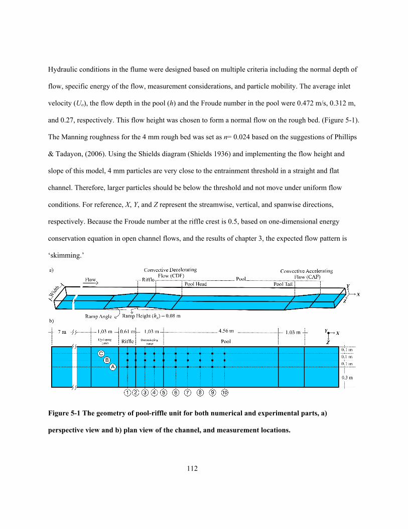
112
Hydraulic conditions in the flume were designed based on multiple criteria including the normal depth of
flow, specific energy of the flow, measurement considerations, and particle mobility. The average inlet
velocity (Uo), the flow depth in the pool (h) and the Froude number in the pool were 0.472 m/s, 0.312 m,
and 0.27, respectively. This flow height was chosen to form a normal flow on the rough bed. (Figure 5-1).
The Manning roughness for the 4 mm rough bed was set as n= 0.024 based on the suggestions of Phillips
& Tadayon, (2006). Using the Shields diagram (Shields 1936) and implementing the flow height and
slope of this model, 4 mm particles are very close to the entrainment threshold in a straight and flat
channel. Therefore, larger particles should be below the threshold and not move under uniform flow
conditions. For reference, X, Y, and Z represent the streamwise, vertical, and spanwise directions,
respectively. Because the Froude number at the riffle crest is 0.5, based on one-dimensional energy
conservation equation in open channel flows, and the results of chapter 3, the expected flow pattern is
‘skimming.’
Figure 5-1 The geometry of pool-riffle unit for both numerical and experimental parts, a)
perspective view and b) plan view of the channel, and measurement locations.
113
5.2.2 Experimental Method
The experimental part of this chapter was completed in the flume (Rocky) in the Fluid Mechanics
Laboratory at the University of Waterloo. This flume is 18 m long, 1.2 m wide, and 0.6 m deep. Rocky is
a tilting flume, with the slope adjustable by hydraulic jacks and held in place at the upstream pivot point
and 4 additional supports along the flume. Water is pumped from a sub-floor reservoir to a head tank at a
central location in the laboratory, which then gravity feeds the head tank for the flume. A butterfly valve
is used to control the discharge in the flume. The large size of the head tank, baffles, and floating
styrofoam boards help to dissipate the kinetic energy of flow, break-up the large vortices, and reduce the
surface fluctuations in the flow as it exits the head tank. A set of stacked small pipes (40 mm diameter)
placed at the outlet of the head tank further reduce fluctuations in the inlet flow. The flume outlet is
controlled by a variable height gate. A basin at the end of the flume traps any transported sediments and
guides the flow to the returning channel that routes the flow to the sub-floor reservoir.
5.2.2.1 Experiment setup
The riffles were made of ¾ inch PVC sheets and glued to the flume bed. For making the rough bed,
series of roughness mats were made by gluing 4 mm gravels to sheets of canvas fabric by extra strength
PL glue and painting with water-resistant paint for better fixing of gravels and more adhesion. The whole
bed of the flume and riffles were covered with these roughness mats (Figure 5-2a). Due to the limitations
in supplying enough discharge for the flume, the flume was narrowed down using false walls made of
stainless steel, which are fixed in place using silicone glue and bagged sands for the support. For
supporting the false walls and controlling the leakage underneath of the walls, the back of the walls was
filled with water with the same height as the main flow (Figure 5-2e). As it can be seen in Figure 5-2f, for
reducing the effect of local pocket geometry on sediment entrainment, the gap between gravels were filled
114
with silicone in a 3cm ×3cm square at the test points that are shown in Figure 5-1. 0.5-mm sand was
sprinkled on the wet silicone to keep the surface rough. These spots are referred to test pads herein.
Velocity profiles were measured with a Vectrino II profiler manufactured by Nortek Solutions (Craig et
al. 2011). The Vectrino uses a bistatic acoustic Doppler velocimetry method with one central emitter and
four receivers (Figure 5-2f) to measure velocity in streamwise, vertical and lateral velocities over a 3 cm
profile of velocity in a series of spatial bins as small as 1 mm in height at a frequency of up to 100 Hz.
The sampling bins are located from 4 cm to 7 cm below the central emitter, though bins near the limits of
this range are known to suffer from low signal to noise ratios (MacVicar et al., 2014). Vectrino II also
shows higher velocity near the upper bound and lower velocity near the lower bound of its profiling
range. For the current experiment, the Vectrino II was used at frequency of 50 Hz, and bin size of 1mm.
The acquired velocity profiles were despiked and organized by the open source MATLAB algorithms
called “multi-instrument turbulence toolbox (MITT)” developed by MacVicar et al., (2014).
5.2.2.2 Experiment procedure
A qualitative scoring method based on visual inspection was designed to evaluate particle
entrainment. Evaluations started after carefully placing a test particle in the middle of the test pad using a
bolt grabber. The bolt grabber is a long thin device with a catch and release mechanism designed for
retrieving bolts from hard to reach locations in machinery or beneath grates. In the flume it allowed us to
place the particle from a slightly downstream angle to minimize the disturbance to the flow. For each
test, particle entrainment was classified after waiting for 120 s, which ensured that the particles
experienced approximately 200 cycles of flow sweeps and bursts (~h/Uo) (Nezu and Rodi 1986). The
scores, which are listed in Table 5-1, are varied from one (no movement) to five (shooting). Five different
particle sizes (4, 5, 6, 7, and 8 mm), which are colour coded using fluorescent paints (Figure 5-2g), and at
least four different particles for each size, and three trials for each particle was done and scored. To make
115
sure that the particles were placed at the test pads on their most stable side, the particles were resting on a
flat surface before grabbing and moving to the test pads. Particles were placed at different flow attack
angles for different trials.
Table 5-1 entrainment score
Score Description
1 No movement or vibration
2 The particle vibrates or moves but stays in the test pad
3 The particle moves out of the test pad but still touches the pad border
4 The particle moves out of the test pad completely
5 The flow shoots the particle rapidly
Four profiles of velocity were measured for 120 s duration at A1, A3, A6, and A8 locations. The
velocity profile of the first 10 cm of the flow depth, from free surface, was not measurable because there
is a need for at least 6 cm water height above the centre of the probe for preventing the air bubbles to get
trapped under the probe, and Vectrino II can only measure the velocity between 4 cm and 7 cm under the
centre of the probe.
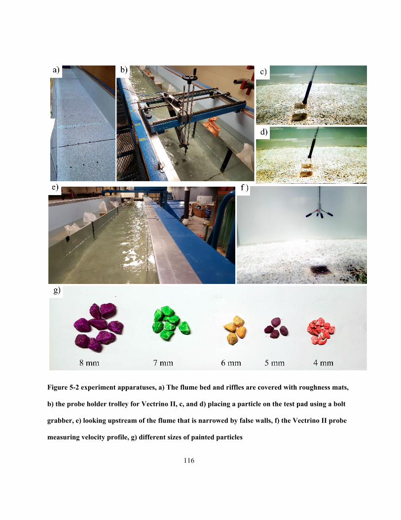
116
Figure 5-2 experiment apparatuses, a) The flume bed and riffles are covered with roughness mats,
b) the probe holder trolley for Vectrino II, c, and d) placing a particle on the test pad using a bolt
grabber, e) looking upstream of the flume that is narrowed by false walls, f) the Vectrino II probe
measuring velocity profile, g) different sizes of painted particles
117
5.2.3 Numerical method
Simulations used the commercially available ANSYS CFX Version 19.1 software. In ANSYS CFX, large
eddy simulation (LES) was used to model the flow. The initial condition for the distribution of flow is
considered to be uniform. The LES wall-adapting local eddy-viscosity (WALE) (Ducros et al. 1998)
method was chosen, which has been widely used in similar geomorphic researches (Keylock et al., 2005,
2012). For more detailed information about the formulations and equations of LES see Rodi et al. (2013).
The simulations were 3D, with a structured mesh generated using ICEM Version 19.1, and a total number
of elements equal to 45×106. A coarser mesh size was selected for the first 5 m of the uniform section at
the upstream. Minimum cell size in the near-wall region was 1.5×10⁻³ m, which was selected to satisfy the
criteria suggested by Keylock et al. (2012), who recommended at least six points in the inner (near-wall)
region to resolve the eddies generated in this region. Previous studies have found the inner zone to be
between 10 and 20% of the flow depth ( MacVicar & Obach, 2015; MacVicar & Rennie, 2012; Nezu &
Rodi, 1986), which means that there are approximately 20 points in the inner zone for the current study.
Also following Keylock et al. (2012), cell sizes were 1/50 of the depth, which meets the recommendation
to keep the free surface cells to less than 1/20 of the flow depth. The total time for transient modelling
was 250 s, which is > 400x the largest eddy scale (~h/Uo) and easily exceeded the recommendation of 20x
the eddy time scale by Keylock et al. (2012). The first 50 s were not considered because of initial
condition effects, so only the results between 50 s and 250 s were recorded for analysis. On the machine
we used, which has dual CPUs, each with ten cores of 2.3 GHz with CPU model Intel(R) Xeon(R) 2650
V3, and 192 GB RAM, the simulation took approximately 240 hours. Post processing was completed
with CFD-POST Version 19.1 and MATLAB R2017b.
118
5.2.4 Boundary Conditions
The side walls and bed are defined as no-slip smooth walls and rough wall (4 mm roughness),
respectively. Using VOF, the inlet was separated into air and water zones at the experimental flow depth
(h = 0.312 m). The air zone had zero velocity inlet and the constant pressure of zero. The water zone was
defined as having a hydrostatic pressure distribution with uniform water velocity profile (Uo= 0.472 m/s).
The outlet was defined as having a constant hydrostatic pressure distribution for water and constant zero
pressure for air. In all locations, a distance of at least 5 cm was maintained between the water surface and
the top of the simulation space, which allowed the free surface to be shaped based on the hydraulic
characteristics alone.
5.2.5 Validation
The time average, organized and despiked profile of velocity magnitude at A1, A3, A6, and A8 locations,
which are measured in the flume, was used to validate the flow behaviour, water surface elevation, and
the distribution of time average flow velocity magnitude (U) in the numerical simulations. Time-averaged
numerical results and experimental data are compared in Figure 5-3. Water surface level is similar in both
numerical and experimental results, with a drop at the riffle that is consistent with what is expected from a
specific energy analysis for subcritical flow (Figure 5-3a). Four time-averaged velocity magnitude
profiles normalized by the inlet velocity (U/Uo) are shown at different points along the channel centerline
between the middle of the riffle and middle of the pool (Figure 5-3b). Considering the 10% error bars,
numerical results are mostly consistent with experimental data, especially in the middle of the flow depth.
The near bed parts of the experimentally acquired velocity profiles are not matched with numerical
results. This divergence can have several potential sources:
● The cells near the edges of measuring range in Vectrino II have very low signal to noise ratio,
which causes uncertainty in results;
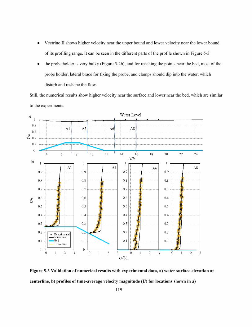
119
● Vectrino II shows higher velocity near the upper bound and lower velocity near the lower bound
of its profiling range. It can be seen in the different parts of the profile shown in Figure 5-3
● the probe holder is very bulky (Figure 5-2b), and for reaching the points near the bed, most of the
probe holder, lateral brace for fixing the probe, and clamps should dip into the water, which
disturb and reshape the flow.
Still, the numerical results show higher velocity near the surface and lower near the bed, which are similar
to the experiments.
Figure 5-3 Validation of numerical results with experimental data, a) water surface elevation at
centerline, b) profiles of time-average velocity magnitude (U) for locations shown in a)
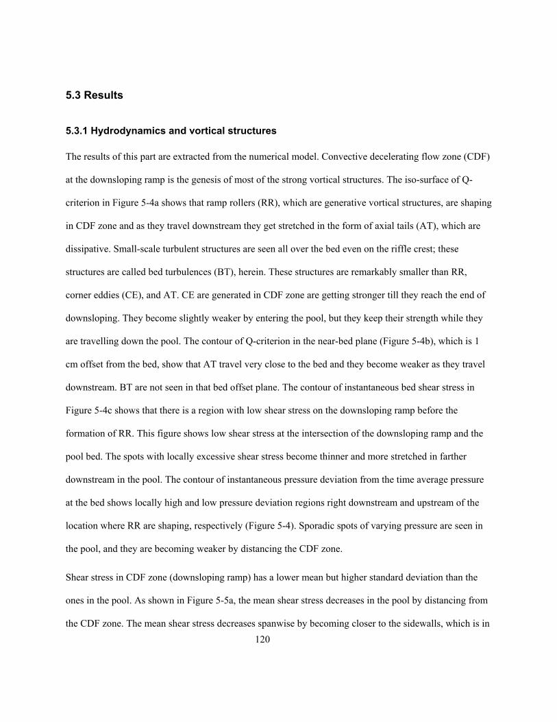
120
5.3 Results
5.3.1 Hydrodynamics and vortical structures
The results of this part are extracted from the numerical model. Convective decelerating flow zone (CDF)
at the downsloping ramp is the genesis of most of the strong vortical structures. The iso-surface of Q-
criterion in Figure 5-4a shows that ramp rollers (RR), which are generative vortical structures, are shaping
in CDF zone and as they travel downstream they get stretched in the form of axial tails (AT), which are
dissipative. Small-scale turbulent structures are seen all over the bed even on the riffle crest; these
structures are called bed turbulences (BT), herein. These structures are remarkably smaller than RR,
corner eddies (CE), and AT. CE are generated in CDF zone are getting stronger till they reach the end of
downsloping. They become slightly weaker by entering the pool, but they keep their strength while they
are travelling down the pool. The contour of Q-criterion in the near-bed plane (Figure 5-4b), which is 1
cm offset from the bed, show that AT travel very close to the bed and they become weaker as they travel
downstream. BT are not seen in that bed offset plane. The contour of instantaneous bed shear stress in
Figure 5-4c shows that there is a region with low shear stress on the downsloping ramp before the
formation of RR. This figure shows low shear stress at the intersection of the downsloping ramp and the
pool bed. The spots with locally excessive shear stress become thinner and more stretched in farther
downstream in the pool. The contour of instantaneous pressure deviation from the time average pressure
at the bed shows locally high and low pressure deviation regions right downstream and upstream of the
location where RR are shaping, respectively (Figure 5-4). Sporadic spots of varying pressure are seen in
the pool, and they are becoming weaker by distancing the CDF zone.
Shear stress in CDF zone (downsloping ramp) has a lower mean but higher standard deviation than the
ones in the pool. As shown in Figure 5-5a, the mean shear stress decreases in the pool by distancing from
the CDF zone. The mean shear stress decreases spanwise by becoming closer to the sidewalls, which is in
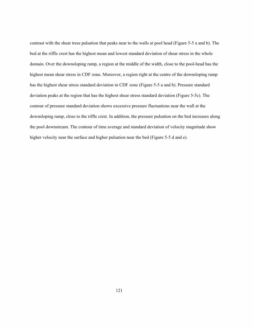
121
contrast with the shear tress pulsation that peaks near to the walls at pool head (Figure 5-5 a and b). The
bed at the riffle crest has the highest mean and lowest standard deviation of shear stress in the whole
domain. Over the downsloping ramp, a region at the middle of the width, close to the pool-head has the
highest mean shear stress in CDF zone. Moreover, a region right at the centre of the downsloping ramp
has the highest shear stress standard deviation in CDF zone (Figure 5-5 a and b). Pressure standard
deviation peaks at the region that has the highest shear stress standard deviation (Figure 5-5c). The
contour of pressure standard deviation shows excessive pressure fluctuations near the wall at the
downsloping ramp, close to the riffle crest. In addition, the pressure pulsation on the bed increases along
the pool downstream. The contour of time average and standard deviation of velocity magnitude show
higher velocity near the surface and higher pulsation near the bed (Figure 5-5 d and e).
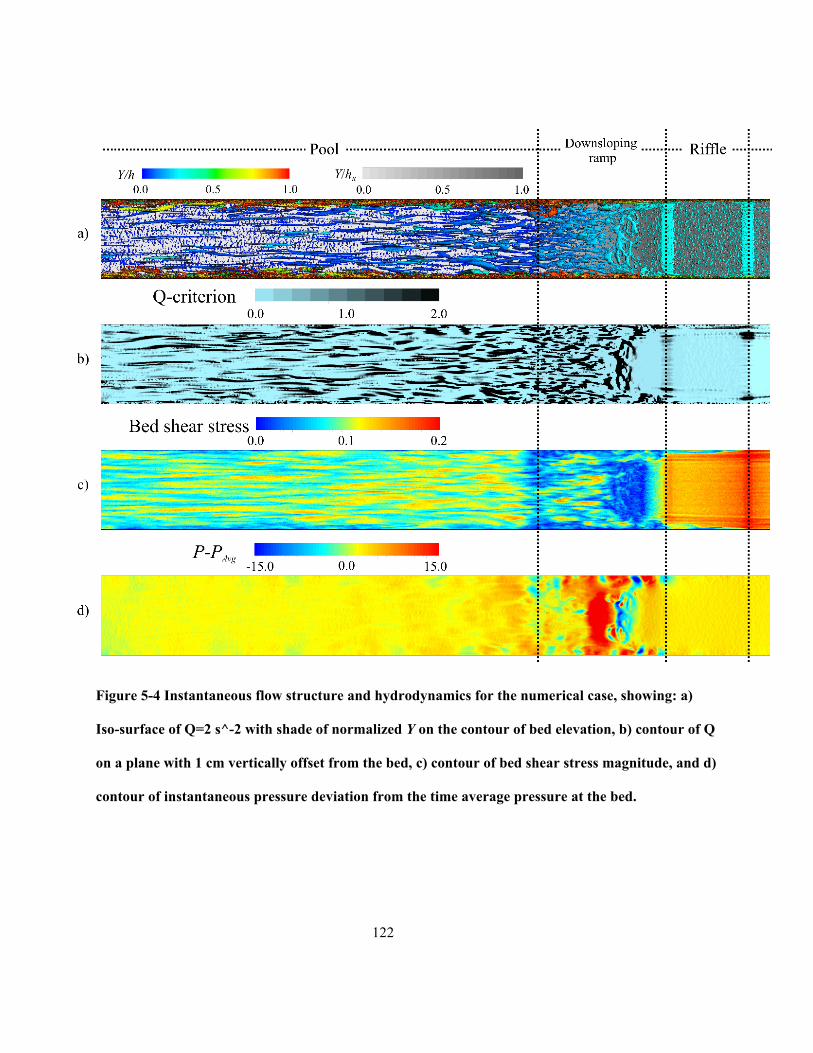
122
Figure 5-4 Instantaneous flow structure and hydrodynamics for the numerical case, showing: a)
Iso-surface of Q=2 s^-2 with shade of normalized Y on the contour of bed elevation, b) contour of Q
on a plane with 1 cm vertically offset from the bed, c) contour of bed shear stress magnitude, and d)
contour of instantaneous pressure deviation from the time average pressure at the bed.
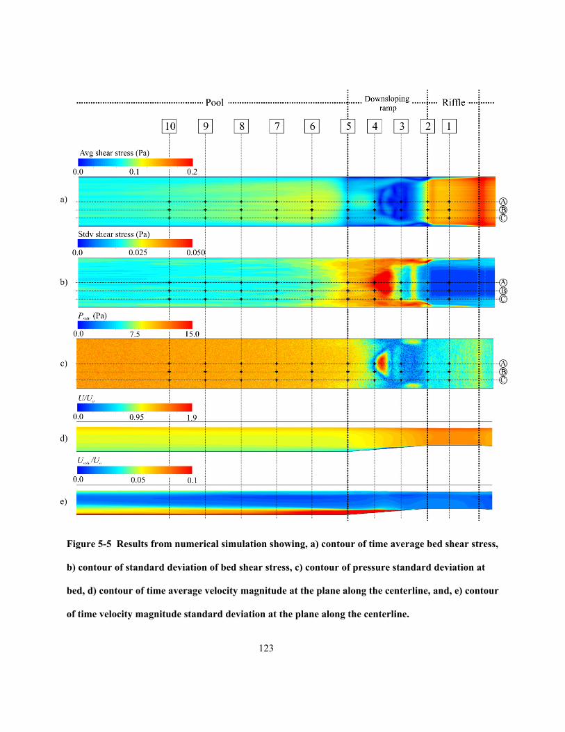
123
Figure 5-5 Results from numerical simulation showing, a) contour of time average bed shear stress,
b) contour of standard deviation of bed shear stress, c) contour of pressure standard deviation at
bed, d) contour of time average velocity magnitude at the plane along the centerline, and, e) contour
of time velocity magnitude standard deviation at the plane along the centerline.
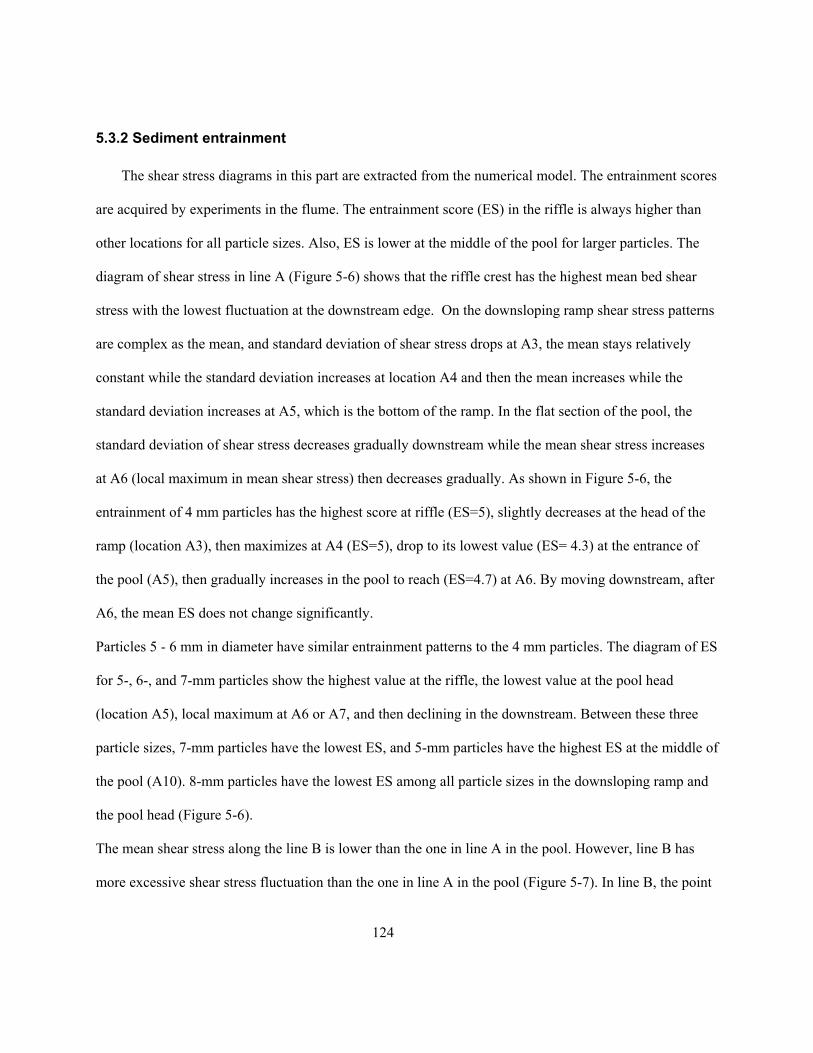
124
5.3.2 Sediment entrainment
The shear stress diagrams in this part are extracted from the numerical model. The entrainment scores
are acquired by experiments in the flume. The entrainment score (ES) in the riffle is always higher than
other locations for all particle sizes. Also, ES is lower at the middle of the pool for larger particles. The
diagram of shear stress in line A (Figure 5-6) shows that the riffle crest has the highest mean bed shear
stress with the lowest fluctuation at the downstream edge. On the downsloping ramp shear stress patterns
are complex as the mean, and standard deviation of shear stress drops at A3, the mean stays relatively
constant while the standard deviation increases at location A4 and then the mean increases while the
standard deviation increases at A5, which is the bottom of the ramp. In the flat section of the pool, the
standard deviation of shear stress decreases gradually downstream while the mean shear stress increases
at A6 (local maximum in mean shear stress) then decreases gradually. As shown in Figure 5-6, the
entrainment of 4 mm particles has the highest score at riffle (ES=5), slightly decreases at the head of the
ramp (location A3), then maximizes at A4 (ES=5), drop to its lowest value (ES= 4.3) at the entrance of
the pool (A5), then gradually increases in the pool to reach (ES=4.7) at A6. By moving downstream, after
A6, the mean ES does not change significantly.
Particles 5 - 6 mm in diameter have similar entrainment patterns to the 4 mm particles. The diagram of ES
for 5-, 6-, and 7-mm particles show the highest value at the riffle, the lowest value at the pool head
(location A5), local maximum at A6 or A7, and then declining in the downstream. Between these three
particle sizes, 7-mm particles have the lowest ES, and 5-mm particles have the highest ES at the middle of
the pool (A10). 8-mm particles have the lowest ES among all particle sizes in the downsloping ramp and
the pool head (Figure 5-6).
The mean shear stress along the line B is lower than the one in line A in the pool. However, line B has
more excessive shear stress fluctuation than the one in line A in the pool (Figure 5-7). In line B, the point
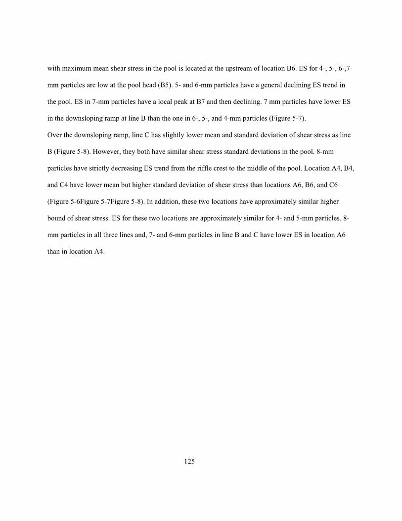
125
with maximum mean shear stress in the pool is located at the upstream of location B6. ES for 4-, 5-, 6-,7-
mm particles are low at the pool head (B5). 5- and 6-mm particles have a general declining ES trend in
the pool. ES in 7-mm particles have a local peak at B7 and then declining. 7 mm particles have lower ES
in the downsloping ramp at line B than the one in 6-, 5-, and 4-mm particles (Figure 5-7).
Over the downsloping ramp, line C has slightly lower mean and standard deviation of shear stress as line
B (Figure 5-8). However, they both have similar shear stress standard deviations in the pool. 8-mm
particles have strictly decreasing ES trend from the riffle crest to the middle of the pool. Location A4, B4,
and C4 have lower mean but higher standard deviation of shear stress than locations A6, B6, and C6
(Figure 5-6Figure 5-7Figure 5-8). In addition, these two locations have approximately similar higher
bound of shear stress. ES for these two locations are approximately similar for 4- and 5-mm particles. 8-
mm particles in all three lines and, 7- and 6-mm particles in line B and C have lower ES in location A6
than in location A4.
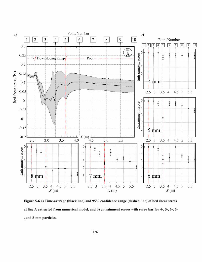
126
Figure 5-6 a) Time-average (black line) and 95% confidence range (dashed line) of bed shear stress
at line A extracted from numerical model, and b) entrainment scores with error bar for 4-, 5-, 6-, 7-
, and 8-mm particles.
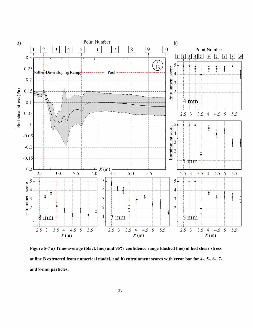
127
Figure 5-7 a) Time-average (black line) and 95% confidence range (dashed line) of bed shear stress
at line B extracted from numerical model, and b) entrainment scores with error bar for 4-, 5-, 6-, 7-,
and 8-mm particles.
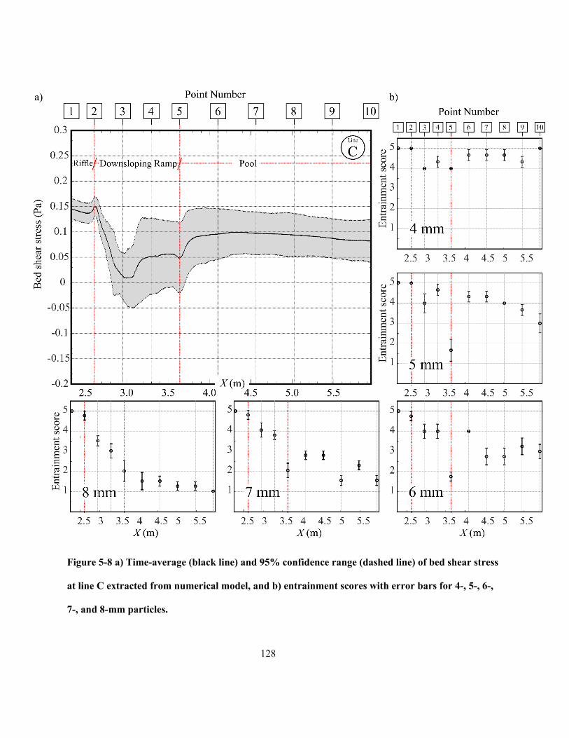
128
Figure 5-8 a) Time-average (black line) and 95% confidence range (dashed line) of bed shear stress
at line C extracted from numerical model, and b) entrainment scores with error bars for 4-, 5-, 6-,
7-, and 8-mm particles.
129
5.4 Discussion
Based on Shields thresholding for moving of sediments, in this case, 4-mm particles are very close to the
entrainment threshold, and they should barely move in the pool, and larger particles should not move at
all. The results herein showed that this thresholding does not anticipate the mobility of sediments
precisely in such cases with high pulsation and variable shear stress distribution. This finding is thus in
general agreement with recent studies on the relevance of turbulent structures for sediment transport
(Celik et al. 2013; Diplas et al. 2008; Lamb et al. 2015; Sumer et al. 2003). The particle entrainment
generally has a positive relation with shear stress, which means that in the regions with both higher mean
and standard deviation of shear stress, entrainment is higher. However, pulsation can amplify the effect of
mean shear stress. The entrance of the pool near the end of downsloping ramp mostly has the lowest
sediment entrainment score which can act as a trap point to deposit the particles in that region and prevent
them from entering the pool. The downsloping ramp, generally, have lower mean shear stress and higher
pulsation than upstream part of the pool. By comparing the results of A4, B4, and C4 locations, which are
the points right upstream of the pool entrance on downsloping ramp, with A6, B6, and C6 locations,
which are the points right downstream of the pool entrance in the pool, it can be said that smaller particles
(4-, 5-, and 6-mm particles) in the regions with lower mean shear stress can have similar entrainment if
the pulsation be higher. Pulsation, which is referred to shear standard deviation herein, has less effect on
the entrainment of larger particles.
The results can be used to develop a conceptual model of sediment sorting by size in a riffle-pool unit due
to differential entrainment and deposition. All particles are assumed to move intermittent saltation, rest,
and entrainment cycles rather than suspension. We consider the effects of pocket geometry, covering
effects, and interlocking as an increase in the threshold of entrainment score. By considering these effects,
we assume that ES< 3 means deposition with no movement afterwards. Based on our observations, the
130
bed median size articles (4 mm), travel down the ramp, enter the pool, travel down the pool, pass the
middle of the pool, and may deposit at the far end downstream of the pool. In contrast, a fraction of the
5-mm particles will pass the ramp but are likely to get trapped at the end of the ramp. If they pass that trap
point, they pass the pool head and deposit at the middle of the pool near the wall and further downstream
at the centerline as well. In a downstream direction, they will deposit before 4-mm particles. 6- and 7-mm
particles have a similar scenario as 5-mm particles, but the size gradation means that the larger particles
will deposit before the smaller sized particles deposit later. They both deposit much earlier than 5-mm
particles near the sidewalls and centerline. In contrast with the smaller particles, the 8-mm particles will
leave the riffle crest but start to deposit on the ramp, particularly near the channel walls, and there is a low
possibility for them to enter the pool. In this scenario, the larger particles form a coarse deposit on the
downstream face of the riffle and cannot reach the pool or be transported through the channel.
By looking at this assumptive scenario of incoming sediment, the downstream fining process, which is
reported previously by many researchers (Hoey & Ferguson, 1997; Milan, 2013; Seal & Paola, 1995;
Sear, 1996; Thompson, 2013), can be seen. The generated turbulence at CDF, travelling near the bed,
plays a crucial role in the downstream fining process. This process is due to the gradually decreasing of
bed mean and standard deviation shear stress because of gradually dissipation of vortical structures that
are formed in CDF. In this scenario, the riffle and downsloping part of the riffle become armoured by
large particles, which can trap more smaller particles at the riffle and prevent them from entering the pool.
Armoured riffles are reported in the field and experimental studies previously (Madej et al., 2009; Sear,
1996; Thompson, 2006; Yager & Schott, 2013). The pool head stays clean, because the small particles
that are entered the pool are washed away from the upstream part of the pool, and they respectively
deposit by their size in the downstream. This sediment routing mechanism herein describes the self-
maintaining mechanism of pool-riffle units that is induced by turbulence.
131
5.5 Conclusion
Based on the linking of numerical and experimental results, we can conclude that:
1. Turbulence plays a key role in sediment routing.
2. Pulsation in shear stress amplify the effect of mean shear stress in moving the particles.
3. The zone with local low shear stress at the end of the downsloping ramp, trap the particles before
entering the pool.
4. Large particles are trapped in the riffle, and there is a low chance for them to enter the pool.
5. The turbulence that is generated in the region with convective declarative flow keep the pool head
clean from the deposition of incoming particles that are passed the riffle.
6. Particles that pass the riffle deposit respectively in the pool by their size, in a way that larger
particles deposit earlier than smaller ones.
7. The downstream fining is due to the gradually dissipation and decay of vortical structures that are
generated in the CDF zone.
132
Chapter 6: Conclusions and future work
6.1 Summary of Thesis Contributions
A summary of the contributions of this thesis and their possible impacts are presented in this chapter. The
chapter also lists the important directions of future work. The central problem addressed in this thesis is
the characterization of the effects of macromorphological variations in natural and restored streams on
flow pattern and turbulent structures. The focus of the thesis is on pools and riffles, i.e., deeper and
shallower part of the bed. More specifically, the work presented in this thesis thoroughly studies the
effects of
(a) riffle height,
(b) riffle width,
(c) width constriction, and
(d) response of sediment to turbulence
on hydrodynamics and sediment entrainment in pools and riffles.
An approach that combines hydraulic and geomorphological techniques utilizing both experimental and
computational fluid dynamic methodologies was employed in this thesis to provide a more
comprehensive and accurate analysis of sediment routing and flow patterns in pools and riffles. The direct
implication of this analysis is to enable practical design and study practices that can be incorporated in
133
pool-riffle maintenance and shaping. Eventually, this will lead to better rehabilitation and maintenance
strategies for natural or restored streams.
The reliance on a more holistic approach in this thesis combining both numerical simulations and
experimentation helped in settling a long-standing critical debate on the reason behind the formation and
maintenance mechanisms for pool-riffle units. The results in this thesis showed that scouring can be
attributed to either higher near bed velocity (plunging flow) or turbulence near the pool bed (skimming
flow). The consolidation of both perspectives by providing the hydrodynamic conditions where both or
either can be observed in the field should help to resolve some longstanding debates in the field.
6.1.1 Contribution 1: Proposing and validating the vortex-resistance hypothesis
The thesis proposed and evaluated the ‘vortex-resistance hypotheses’. The main claim is that vortices
exert resistance to the flow by increasing the mixing effects and changing the pressure domain. The
significance of this hypothesis is that it links the role that turbulence structures play in formation of flow
patterns. Moreover, it provides a unified framework for explaining the effects of different geometrical
parameters on the flow pattern.
6.1.2 Contribution 2: Study of the influence of the riffle height on the characteristics of
the vortical structures
The effects that the riffle height have on flow turbulent structures were carefully investigated in this
thesis. This was further linked to the flow pattern relying on the vortex-resistance hypothesis, which
provided a plausible interpretation for forming plunging, rifting, and skimming flow patterns in pools.
Through numerical simulations, the following findings were identified:
Surface turbulence, ramp rollers, corner eddies, and axial tails are shaped in the convective
decelerating flow zone;
134
In skimming flow, ramp and corner eddies are dominant near the bed and responsible for high
bed shear stress;
Riffles with Froude number close to one can result into surface undulation hydraulic jump, which
steers the flow to plunge into the pool near the bed;
If ramp rollers are strong enough, they push the flow to skim the free-surface and increase near
bed turbulence;
Strong plunging flow can cause axial bifurcation, where one side of the channel experiences
higher velocities and shear stresses while the opposite side is dominated by flow recirculations.
6.1.3 Contribution 3: Study of the influence of the channel width variation on the
characteristics of the vortical structures
Relying on advanced numerical approaches that model transient and turbulent flow, the influence of
variability in channel width on the characteristics of vortical structures has been investigated in detail.
Among the most relevant findings, the analysis revealed the following:
Strong vortical structures can be generated in areas other than CDF. For instance, the horseshoe
vortices are formed upstream of constrictions in the region of a favourable pressure gradient, such
as convectively accelerating flow;
Wider channels produce more turbulence and bed shear stress pulsation;
Plunging flow cannot be only attributed to a hydraulic jump. The thesis also identified that
vortical structures generated in constrictions can lead the flow to plunge as well; and
Turbulence feedback mechanisms can induce lateral bifurcation in subcritical flows where a
constriction is present in the riffle.
135
6.1.4 Contribution 4: Study of the influence of vorticial structures on sediment
entrainment
Pool-riffle case with skimming flow is modelled both experimentally and numerically to link the
numerical results of hydrodynamic and turbulence to the results of experimental sediment entrainment
tests. Skimming flow is of interest because it results in low mean shear at the channel bed but high
turbulence with generative structures including ramp rollers and corner vortices. Given the relatively
large size and strength of these structures, the overall aim was to assess whether they had any role in
moving, shaking, or sorting the bed particles by size.
We can conclude that:
1. Pulsation in shear stress amplify the effect of mean shear stress in moving the particles;
2. The zone with local low shear stress at the end of the downsloping ramp, trap the particles before
entering the pool;
3. Large particles are trapped in the riffle, and there is a low chance for them to enter the pool;
4. The turbulence that is generated in the region with convective declarative flow keep the pool head
clean from deposition of incoming particles that are passed the riffle;
5. Particles that pass the riffle, deposit respectively in the pool by their size, in a way that larger
particles deposit earlier than smaller ones; and
6. The downstream fining is due to the gradually dissipation and decay of vortical structures that are
generated in the CDF zone.
The results of this chapter can help researchers and engineers to understand the mechanisms underlying
self-maintenance of pool-riffle units better. It thus contributes towards developing a systematic design
methodology for self-maintaining pool riffle-units.
136
6.2 Future research
1) The geometry, which is used in this study, is a simplified geometry of pool rifle units. Including more
various geometry factors can make the results more applicable in designing and developing projects.
There are various controversial views that link the formation and maintenance of pool-riffle units to
development of meandering and bends; therefore, considering the effect of channel bend and interaction
of curvature-induced vortices with pool-riffle vortical structures can more clarify the evolution
mechanism of streams.
2) Hyporheic flow, defined as the intragranular flow in the shallow subsurface below a riverbed, is
another interesting topics with direct relevance for the function and habitat utility of pool-riffles. The
effect of different types of flow that are found in this study (plunging, rifting, and skimming) should be
investigated for their interactions with hyporheic flows in riffles and beneath the pools.
3) Modelling sediment transport with more realistic conditions in pool-riffle units (e.g. fully mobile bed
and various conditions of sediment feeding) can lead to a more complete understanding of the formation
and maintenance mechanisms of pool-riffle units.
137
References
De Almeida, Gustavo Adolfo Mazza and José F. Rodríguez. (2012). “Spontaneous Formation and Degradation of Pool-Riffle Morphology and Sediment Sorting Using a Simple Fractional Transport Model.” Geophys. Res. Lett. 39(6):L06407.
De Almeida, Gustavo Adolfo Mazza, José F. Rodríguez. (2011). “Understanding Pool-Riffle Dynamics through Continuous Morphological Simulations.” Water Resour. Res. 47(1):1–15.
Ancey, C., a. C. Davison, T. Böhm, M. Jodeau, and P. Frey. (2008). “Entrainment and Motion of Coarse Particles in a Shallow Water Stream down a Steep Slope.” J. Fluid Mech. 595:83–114.
Beheshti, Ali-Asghar A. A., Behzad Ataie-Ashtiani, and Hamed Dashtpeyma. (2017). “Numerical Simulations of Turbulent Flow around Side-by-Side Circular Piles with Different Spacing Ratios.” Int. J. River Basin Manag. 15(2):227–38.
Bernhardt, E. S., M. A. Palmer, J. D. Allan, G. Alexander, K. Barnas, S. Brooks, J. Carr, S. Clayton, C. Dahm, D. Galat, S. Gloss, P. Goodwin, D. Hart, B. Hassett, R. Jenkinson, S. Katz, G. M. Kondolf, P. S. Lake, R. Lave, J. L. Meyer, T. K. O. Donnell, L. Pagano, B. Powell, and E. Sudduth. (2005). “Synthesizing U.S. River Restoration Efforts.” Science 308(5722):636–37.
Bernhardt, Emily S. and Margaret A. Palmer. (2007). “Restoring Streams in an Urbanizing World.” Freshw. Biol. 52(4):738–51.
Boussinesq, J. (1877). “Théorie de l’écoulement Tourbillant.” Mem. Présentés Par Divers Savants Acad. Sci. Inst. Fr 23(46–50):5–6.
Bradbrook, K. F., S. N. Lane, K. S. Richards, P. M. Biron, and A. G. Roy. (2000). “Large Eddy Simulation of Periodic Flow Characteristics at River Channel Confluences.” J. Hydraul. Res. 38(3):207–15.
Buffington, John M. (1999). “The Legend of A. F. Shields.” J. Hydraul. Eng. 125(4):376–87.
Buffington, John M., Thomas E. Lisle, Richard D. Woodsmith, and Sue Hilton. (2002). “Controls on the Size and Occurrence of Pools in Coarse-Grained Forest Rivers.” River Res. Appl. 18(6):507–31.
Buffington, John M. and David R. Montgomery. (1997). “A Systematic Analysis of Eight Decades of Incipient Motion Studies, with Special Reference to Gravel-Bedded Rivers.” Water Resour. Res. 33(8):1993–2029.
Caamaño, D., P. Goodwin, and J. M. Buffington. (2012). “Flow Structure through Pool-Riffle Sequences and a Conceptual Model for Their Sustainability in Gravel-Bed Rivers.” River Res. Appl. 28(3):377–89.
Caamaño, Diego, Peter Goodwin, John M. Buffington, Jim C. Liou, and Steve Daley-Laursen.
138
(2009). “Unifying Criterion for the Velocity Reversal Hypothesis in Gravel-Bed Rivers.” J. Hydraul. Eng. 135(1):66–70.
Carling, P. A. (1991). “An Appraisal of the Velocity‐reversal Hypothesis for Stable Pool‐riffle Sequences in the River Severn, England.” Earth Surf. Process. Landforms 16(1):19–31.
Celik, Ahmet O., P. Diplas, and C. L. Dancey. (2014). “Instantaneous Pressure Measurements on a Spherical Grain under Threshold Flow Conditions.” J. Fluid Mech 741:60–97.
Celik, Ahmet Ozan, Panayiotis Diplas, and Clint L. Dancey. (2013). “Instantaneous Turbulent Forces and Impulse on a Rough Bed: Implications for Initiation of Bed Material Movement.” Water Resour. Res. 49(4):2213–27.
Clifford, N. J. J. (1993). “Differential Bed Sedimentology and the Maintenance of Riffle-Pool Sequences.” Catena 20(5):447–68.
Clifford, N. J. and K. Richards. (1992). “The Reversal Hypothesis and the Maintenance of Riffle-Pool Sequences: A Review and Field Appraisal.” Lowl. Floodplain Rivers 43–70.
Clifford, Nicholas J. NJ. (1993). “Formation of Riffle—pool Sequences: Field Evidence for an Autogenetic Process.” Sediment. Geol. 85(1–4):39–51.
Coleman, S. E. and V. I. Nikora. (2008). “A Unifying Framework for Particle Entrainment.” Water Resour. Res. 44(4):1–10.
Craig, Robert G. A., Chris Loadman, Bernard Clement, Peter J. Rusello, and Eric Siegel. (2011). “Characterization and Testing of a New Bistatic Profiling Acoustic Doppler Velocimeter: The Vectrino-II.” Pp. 246–52 in 2011 IEEE/OES/CWTM 10th Working Conference on Current, Waves and Turbulence Measurement, CWTM 2011. IEEE.
Dietrich, William E., J. Dungan Smith, and Thomas Dunne. (1979). “Flow and Sediment Transport in a Sand Bedded Meander.” J. Geol. 87(3):305–15.
Diplas, Panayiotis, Clint L. Dancey, Ahmet O. Celik, Manousos Valyrakis, Krista Greer, and Tanju Akar. (2008). “The Role of Impulse on the Initiation of Particle Movement under Turbulent Flow Conditions.” Science 322(5902):717–20.
Dolling, R. K. (1968). “Occurrence of Pools and Riffles: An Element in the Quasi-Equilibrium State of River Channels.” Ontario Geogr. 2:03–Nov.
Dubief, Yves and Franck Delcayre. (2000). “On Coherent-Vortex Identification in Turbulence.” J. Turbul. 1(January):1–22.
Ducros, F., F. Nicoud, and T. Poinsot. (1998). “Wall-Adapting Local Eddy-Viscosity Models for Simulations in Complex Geometries.” Conf. Numer. Methods Fluid Dyn. 1–7.
Einstein, H. A. and H. W. Shen. (1964). “A Study on Meandering in Straight Alluvial Channels.” J. Geophys. Res. 69(24):5239–47.
Ettema, Robert, George Constantinescu, and Bruce W. Melville. (2017). “Flow-Field Complexity and Design Estimation of Pier-Scour Depth: Sixty Years since Laursen and Toch.” J. Hydraul. Eng. 143(9):03117006.
139
Gorman, O. T. and James R. Karr. (1978). “Habitat Structure and Stream Fish Communities.” Ecology 59(3):507–15.
Guillén Ludeña, S., Z. Cheng, G. Constantinescu, and M. J. Franca. (2017). “Hydrodynamics of Mountain-River Confluences and Its Relationship to Sediment Transport.” J. Geophys. Res. Earth Surf. 122(4):901–24.
Halwas, Karen L. and Michael Church. (2002). “Channel Units in Small, High Gradient Streams on Vancouver Island, British Columbia.” Geomorphology 43(3–4):243–56.
Hardy, R. J., S. N. Lane, M. R. Lawless, J. L. Best, L. Elliott, and D. B. Ingham. (2005). “Development and Testing of a Numerical Code for Treatment of Complex River Channel Topography in Three-Dimensional CFD Models with Structured Grids.” J. Hydraul. Res. 43(5):468–80.
Heritage, G. L. and D. J. Milan. (2004). “A Conceptual Model of the Role of Excess Energy in the Maintenance of a Riffle-Pool Sequence.” Catena 58(3):235–57.
Hirt, C. .. and B. .. Nichols. (1981). “Volume of Fluid (VOF) Method for the Dynamics of Free Boundaries.” J. Comput. Phys. 39(1):201–25.
Hoey, Trevor B. and Robert I. Ferguson. (1997). “Controls of Strength and Rate of Downstream Fining above a River Base Level.” Water Resour. Res. 33(11):2601–8.
Hooke, J. M. M. (2013). River Meandering. Elsevier Ltd.
Hunt, Brendan, Jeremy G. Venditti, and Eva Kwoll. (2018). “Experiments on the Morphological Controls of Velocity Inversions in Bedrock Canyons.” Earth Surf. Process. Landforms 43(3):654–68.
Jackson, J. R., G. B. Pasternack, and J. M. Wheaton. (2015). “Virtual Manipulation of Topography to Test Potential Pool–riffle Maintenance Mechanisms.” Geomorphology 228:617–27.
Keller, E. A. (1972). “Development of Alluvial Stream Channels: A Five-Stage Model.” Bull. Geol. Soc. Am. 83(5):1531–36.
Keller, E. A. (1975). “Channelization: A Search for a Better Way.” Geology 3(5):246–48.
Keller, E. A. EA and WN N. Melhorn. (1978). “Rhythmic Spacing and Origin of Pools and Riffles.” Geol. Soc. Am. … 89(80):723–30.
Keller, E. A. and J. L. Florsheim. (1993). “Velocity-Reversal Hypothesis: A Model Approach.” Earth Surf. Process. Landforms 18(8):733–40.
Keller, Edward A. EA A. (1971). “Areal Sorting of Bed-Load Material: The Hypothesis of Velocity Reversal.” Geol. Soc. Am. Bull. 82(3):753–56.
Keylock, C. J., R. J. Hardy, D. R. Parsons, R. I. Ferguson, S. N. Lane, and K. S. Richards. (2005). “The Theoretical Foundations and Potential for Large-Eddy Simulation (LES) in Fluvial Geomorphic and Sedimentological Research.” Earth-Science Rev. 71(3–4):271–304.
140
Keylock, C. J., G. Constantinescu, and R. J. Hardy. (2012). “The Application of Computational Fluid Dynamics to Natural River Channels: Eddy Resolving versus Mean Flow Approaches.” Geomorphology 179:1–20.
Keylock, Christopher J., Kyoungsik S. Chang, and George S. Constantinescu. (2016). “Large Eddy Simulation of the Velocity-Intermittency Structure for Flow over a Field of Symmetric Dunes.” J. Fluid Mech. 805:656–85.
Kieffer, S. W. (1985). “The 1983 Hydraulic Jump in Crystal Rapid: Implications for River- Running and Geomorphic Evolution in the Grand Canyon.” J. Geol. 93(4):385–406.
Kieffer, Susan Werner. (1989). “Geologic Nozzles.” Rev. Geophys. 27(1):3–38.
Kline, S. J., W. C. Reynolds, F. A. Schraub, and P. W. Runstadler. (1967). “The Structure of Turbulent Boundary Layers.” J. Fluid Mech. 30(04):741.
Koken, Mete, George Constantinescu, and Koen Blanckaert. (2013). “Hydrodynamic Processes, Sediment Erosion Mechanisms, and Reynolds-Number-Induced Scale Effects in an Open Channel Bend of Strong Curvature with Flat Bathymetry.” J. Geophys. Res. Earth Surf. 118(4):2308–24.
Krogstad, Per‐Åge and Per Egil Skåre. (1995). “Influence of a Strong Adverse Pressure Gradient on the Turbulent Structure in a Boundary Layer.” Phys. Fluids 7(8):2014–24.
Kumar, Ashish, Umesh C. Kothyari, and Kittur G. Ranga Raju. (2012). “Flow Structure and Scour around Circular Compound Bridge Piers - A Review.” J. Hydro-Environment Res. 6(4):251–65.
Lamb, Michael P., Noah J. Finnegan, Joel S. Scheingross, and Leonard S. Sklar. (2015). “New Insights into the Mechanics of Fluvial Bedrock Erosion through Flume Experiments and Theory.” Geomorphology 244:33–55.
Launder, B. E. and D. B. Spalding. (1974). “The Numerical Computation of Turbulent Flows.” Comput. Methods Appl. Mech. Eng. 3(2):269–89.
Leopold, L. B., M. G. Wolman, and G. M. Wolman. (1960). “Rivee Meanders.” Bull. Geol. Soc. Am. 71(3):769–94.
Lisle, TE and S. Hilton. (1992). “The Volume of Fine Sediment in Pools: An Index of the Supply of Mobile Sediment in Stram Channels.” Water Resour. Bull. 28(2):371–83.
Lisle, Thomas. (1979a). “A Sorting Mechanism for a Riffle-Pool Sequence.” Bull. Geol. Soc. Am. 90(7 PART II):1142–57.
Lisle, Thomas. (1979b). “Geological Society of America Bulletin A Sorting Mechanism for a Riffle-Pool Sequence A Sorting Mechanism for a Riffle-Pool Sequence.” Geol. Soc. Am. Bull. 90(7):616.
Lisle, Thomas E. (1982). “Effects of Aggredation and Degredation on Riffle-Pool Morphology in Natural Gravel Channels, Northwest California.” Water Resour. Res. 18(6):1643–51.
Lisle, Thomas E., Hiroshi Ikeda, and Fujiko Iseya. (1991). “Formation of Stationary Alternate
141
Bars in a Steep Channel with Mixed‐size Sediment: A Flume Experiment.” Earth Surf. Process. Landforms 16(5):463–69.
Lohse, Detlef and Siegfried Grossmann. (2002). Theories of Turbulence. edited by M. Oberlack and F. H. Busse. Vienna: Springer Vienna.
Lotsari, E., M. Vaaja, C. Flener, H. Kaartinen, A. Kukko, E. Kasvi, H. Hyypp??, J. Hyypp??, and P. Alho. (2014). “Annual Bank and Point Bar Morphodynamics of a Meandering River Determined by High-Accuracy Multitemporal Laser Scanning and Flow Data.” Water Resour. Res. 50(7):5532–59.
MacVicar, B. J. and J. L. Best. (2013). “A Flume Experiment on the Effect of Channel Width on the Perturbation and Recovery of Flow in Straight Pools and Riffles with Smooth Boundaries.” J. Geophys. Res. Earth Surf. 118(3):1850–63.
MacVicar, B. J. and L. Obach. (2015). “Shear Stress and Hydrodynamic Recovery over Bedforms of Different Lengths in a Straight Channel.” J. Hydraul. Eng. 141(11):04015025.
MacVicar, B. J., Lana Obach, and James L. Best. (2013). “Large-Scale Coherent Flow Structures in Alluvial Pools.” Pp. 243–59 in Coherent Flow Structures at Earth’s Surface. Chichester, UK: John Wiley & Sons, Ltd.
MacVicar, B. J. and Colin D. Rennie. (2012). “Flow and Turbulence Redistribution in a Straight Artificial Pool.” Water Resour. Res. 48(2):W02503.
MacVicar, B. J. and A. G. Roy. (2007a). “Hydrodynamics of a Forced Riffle Pool in a Gravel Bed River: 1. Mean Velocity and Turbulence Intensity.” Water Resour. Res. 43(12):W12401.
MacVicar, B. J. and A. G. Roy. (2007b). “Hydrodynamics of a Forced Riffle Pool in a Gravel Bed River: 2. Scale and Structure of Coherent Turbulent Events.” Water Resour. Res. 43(12):W12402.
MacVicar, B. J. and A. G. Roy. (2011). “Sediment Mobility in a Forced Riffle-Pool.” Geomorphology 125(3):445–56.
MacVicar, BJ, Scott Dilling, J. Lacey, and K. Hipel. (2014). “A Quality Analysis of the Vectrino II Instrument Using a New Open-Source MATLAB Toolbox and 2D ARMA Models to Detect and Replace Spikes.” Pp. 1951–59 in River Flow 2014.
MacVicar, Bruce J., Scott Dilling, and Jay Lacey. (2014). “Multi-Instrument Turbulence Toolbox (MITT): Open-Source MATLAB Algorithms for the Analysis of High-Frequency Flow Velocity Time Series Datasets.” Comput. Geosci. 73:88–98.
MacVicar, Bruce J., Colin D. Rennie, and André G. Roy. (2010). “Discussion of ‘Unifying Criterion for the Velocity Reversal Hypothesis in Gravel-Bed Rivers’ by D. Caamaño, P. Goodwin, J. M. Buffington, J. C. P. Liou, and S. Daley-Laursen.” J. Hydraul. Eng. 136(8):550–52.
MacWilliams, M. L. (2004). “Three-Dimensional Hydrodynamic Simulation of River Channels and Floodplains.” (March).
142
MacWilliams, M. L., Joseph M. Wheaton, Gregory B. Pasternack, Robert L. Street, and Peter K. Kitanidis. (2006). “Flow Convergence Routing Hypothesis for Pool-Riffle Maintenance in Alluvial Rivers.” Water Resour. Res. 42(10):1–21.
Madej, Mary Ann, Diane G. Sutherland, Thomas E. Lisle, and Bonnie Pryor. (2009). “Channel Responses to Varying Sediment Input: A Flume Experiment Modeled after Redwood Creek, California.” Geomorphology 103(4):507–19.
Milan, D. J. J., G. L. L. Heritage, A. R. G. R. G. Large, and M. E. E. Charlton. (2001). “Stage Dependent Variability in Tractive Force Distribution through a Riffle–pool Sequence.” Catena 44(2):85–109.
Milan, David J. (2013). “Sediment Routing Hypothesis for Pool-Riffle Maintenance.” Earth Surf. Process. Landforms 38(14):1623–41.
Miller, Jerry R. and R. Craig Kochel. (2009). “Assessment of Channel Dynamics, in-Stream Structures and Post-Project Channel Adjustments in North Carolina and Its Implications to Effective Stream Restoration.” Environ. Earth Sci. 59(8):1681–92.
Montgomery, D. R. (1995). “Pool spacing in forest channels” Water Resour Eng. 31(4):1097–1105.
Montgomery, David R., John M. Buffington, Richard D. Smith, Kevin M. Schmidt, and George Pess. (1995). “Pool Spacing in Forest Channels.” Water Resour. Res. 31(4):1097–1105.
Nelson, Jonathan M., Ronald L. Shreve, Stephen R. McLean, and Thomas G. Drake. (1995). “Role of Near‐Bed Turbulence Structure in Bed Load Transport and Bed Form Mechanics.” Water Resour. Res. 31(8):2071–86.
Nelson, Peter A., Andrew K. Brew, and Jacob A. Morgan. (2015). “Morphodynamic Response of a Variable-Width Channel to Changes in Sediment Supply.” Water Resour. Res. 51(7):5717–34.
Newbury, Robert W. (2013). “Designing Fish-Passable Riffles as Gradient Controls in Canadian Streams.” Can. Water Resour. J. 38(3):232–50.
Nezu, Iehisa and Wolfgang Rodi. (1986). “Open‐channel Flow Measurements with a Laser Doppler Anemometer.” J. Hydraul. Eng. 112(5):335–55.
Nowell, Arthur R. M. and Michael Church. (1979). “Turbulent Flow in a Depth-Limited Boundary Layer.” J. Geophys. Res. 84(C8):4816.
Phillips, Jeff V and Saeid Tadayon. (2006). Selection of Manning’s Roughness Coefficient for Natural and Constructed Vegetated and Non-Vegetated Channels, and Vegetation Maintenance Plan Guidelines for Vegetated Channels. Reston, Virginia: 2007: U.S. Department of the Interior- Scientic Investigations Report 2006–5108.
Raudkivi, A. J. (1963). “Study of Sediment Ripple Formation.” J. Hydraul. Div. Proc. Am. Soc. Civ. Eng. 89(HY6):15–33.
Rodi, Wolfgang, George Constantinescu, Thorsten Stoesser, George Constantinescu, and Thorsten Stoesser. (2013). Large-Eddy Simulation in Hydraulics. CRC Press.
143
Roy, André G., Pascale M. Biron, Thomas Buffin-Bélanger, and Mylène Levasseur. (1999). “Combined Visual and Quantitative Techniques in the Study of Natural Turbulent Flows.” Water Resour. Res. 35(3):871–77.
Roy, Andre G., Thomas Buffin-Blanger, Hlne Lamarre, and Alisttair D. Kirkbride. (2004). “Size, Shape and Dynamics of Large-Scale Turbulent Flow Structures in a Gravel-Bed River.” J. Fluid Mech. 500(2004):1–27.
Sawyer, April M., Gregory B. Pasternack, Hamish J. Moir, and Aaron A. Fulton. (2010). “Riffle-Pool Maintenance and Flow Convergence Routing Observed on a Large Gravel-Bed River.” Geomorphology 114(3):143–60.
Schlatter, P., Q. Li, R. Örlü, F. Hussain, and D. S. Henningson. (2014). “On the Near-Wall Vortical Structures at Moderate Reynolds Numbers.” Eur. J. Mech. B/Fluids 48:75–93.
Schmeeckle, Mark W. (2014). “Numerical Simulation of Turbulence and Sediment Transport of Medium Sand.” J. Geophys. Res. Earth Surf. 119(6):1240–62.
Seal, Rebecca and Chris Paola. (1995). “Observations of Downstream Fining on the North Fork Toutle River Near Mount St. Helens, Washington.” Water Resour. Res. 31(5):1409–19.
Sear, D. A. (1996). “Sediment Transport Processes in Pool-Riffle Sequences.” Earth Surf. Process. Landforms 21(3):241–62.
Sear, D. A. DA A. and MD D. Newson. (2004). “The Hydraulic Impact and Performance of a Lowland Rehabilitation Scheme Based on Pool-Riffle Installation: The River Waveney, Scole, Suffolk, UK.” River Res. Appl. 20(7):847–63.
Seminara, Giovanni. (2006). “Meanders.” J. Fluid Mech. 554(1):271–97.
Shields, a. (1936). “Application of Similarity Principles and Turbulence Research to Bed-Load Movement.” Mitt. Preuss. Versuchsanst. Wasserbau Schiffbau 26(5–24):47.
Smagorinsky, J. (1963). “General Circulation Experiments with the Primitive Equations: I. The Basic Experiment.” Mon. Weather Rev. 91(3):99–164.
Smits, A. J. and D. H. Wood. (1985). “The Response of Turbulent Boundary Layers to Sudden Pertubations.” Annu. Rev. Fluid Mech. 17(1):321–58.
Stoesser, T., C. Braun, M. García-Villalba, W. Rodi, M. Garcia-Villalba, W. Rodi, M. García-Villalba, and W. Rodi. (2008). “Turbulence Structures in Flow over Two-Dimensional Dunes.” J. Hydraul. Eng. 134(1):42–55.
Stoesser, Thorsten. (2014). “Large-Eddy Simulation in Hydraulics: Quo Vadis?” J. Hydraul. Res. 52(4):441–52.
Stoesser, Thorsten, Nils Ruether, and Nils Reidar Boe Olsen. (2010). “Calculation of Primary and Secondary Flow and Boundary Shear Stresses in a Meandering Channel.” Adv. Water Resour. 33(2):158–70.
Sumer, B. Mutlu, Lloyd H. C. Chua, N. S. Cheng, and Jørgen Fredsøe. (2003). “Influence of Turbulence on Bed Load Sediment Transport.” J. Hydraul. Eng. 129(8):585–96.
144
Thompson, Alan. (1986). “Secondary Flows and the Pool-Riffle Unit: A Case Study of the Processes of Meander Development.” Earth Surf. Process. Landforms 11(6):631–41.
Thompson, D. M. (2013). “Pool-Riffle.” Pp. 364–78 in Treatise on Geomorphology, vol. 9. Elsevier.
Thompson, D. M. and E. E. Wohl. (2009). “The Linkage between Velocity Patterns and Sediment Entrainment in a Forced-Pool and Riffle Unit.” Earth Surf. Process. Landforms 34(2):177–92.
Thompson, D. M., E. E. Wohl, and R. D. Jarrett. (1996). “A Revised Velocity-Reversal and Sediment-Sorting Model for a High-Gradient, Pool-Riffle Stream.” Phys. Geogr. 17(2):142–56.
Thompson, Douglas M. (2001). “Random Controls on Semi-Rhythmic Spacing of Pools and Riffles in Constriction-Dominated Rivers.” Earth Surf. Process. Landforms 26(11):1195–1212.
Thompson, Douglas M. (2004). “The Influence of Pool Length on Local Turbulence Production and Energy Slope: A Flume Experiment.” Earth Surf. Process. Landforms 29(11):1341–58.
Thompson, Douglas M. (2006). “Changes in Pool Size in Response to a Reduction in Discharge: A Flume Experiment.” River Res. Appl. 22(3):343–51.
Thompson, Douglas M. DM. (2002). “Geometric Adjustment of Pools to Changes in Slope and Discharge: A Flume Experiment.” Geomorphology 46(3–4):257–65.
Thompson, Douglas M., Jonathan M. Nelson, and Ellen E. Wohl. (1998). “Interactions between Pool Geometry and Hydraulics.” Water Resour. Res. 34(12):3673–81.
Thompson, Douglas M., Ellen E. Wohl, and Robert D. Jarrett. (1999). “Velocity Reversals and Sediment Sorting in Pools and Riffles Controlled by Channel Constrictions.” Geomorphology 27(3–4):229–41.
Venditti, J. G., W. E. Dietrich, P. A. Nelson, M. A. Wydzga, J. Fadde, and L. Sklar. (2010). “Effect of Sediment Pulse Grain Size on Sediment Transport Rates and Bed Mobility in Gravel Bed Rivers.” J. Geophys. Res. Earth Surf. 115(3):1–19.
Venditti, Jeremy G., Colin D. Rennie, James Bomhof, Ryan W. Bradley, Malcolm Little, and Michael Church. (2014). “Flow in Bedrock Canyons.” Nature 513(7519):534–37.
White, Jason Q., Gregory B. Pasternack, and Hamish J. Moir. (2010). “Valley Width Variation Influences Riffle-Pool Location and Persistence on a Rapidly Incising Gravel-Bed River.” Geomorphology 121(3–4):206–21.
Wiberg, Patricia L. and J. Dungan Smith. (1987). “Calculations of the Critical Shear Stress for Motion of Uniform and Heterogeneous Sediments.” Water Resour. Res. 23(8):1471–80.
Wilcock, Peter R. and Brian W. Mcardell. (1997). “Partial Transport of a Sand / Gravel Sediment Flume.” Water Resour. Res. 33(1):235–45.
Wilcock, Peter R. and Brian W. McArdell. (1993). “Surface Based Fractional Transport Rates:
145
Mobilization Thresholds and Partial Transport of a Sand???Gravel Sediment.” Water Resour. Res. 29(4):1297–1312.
Wilkinson, S. N., Robert J. Keller, and Ian D. Rutherfurd. (2004). “Phase-Shifts in Shear Stress as an Explanation for the Maintenance of Pool–riffle Sequences.” Earth Surf. Process. … 29(6):737–53.
Wilkinson, S. N., Ian D. Rutherfurd, and Robert J. Keller. (2008). “An Experimental Test of Whether Bar Instability Contributes to the Formation, Periodicity and Maintenance of Pool-Riffle Sequences.” Earth Surf. Process. Landforms 33(11):1742–56.
Wohl, Ellen, Paul L. Angermeier, Brian Bledsoe, G. Mathias Kondolf, Larry MacDonnell, David M. Merritt, Margaret A. Palmer, N. LeRoy Poff, and David Tarboton. (2005). “River Restoration.” Water Resour. Res. 41(10):1–12.
Wohl, Ellen E. and Douglas M. Thompson. (2000). “Velocity Characteristics along a Small Step-Pool Channel.” Earth Surf. Process. Landforms 25(4):353–67.
Wohl, Ellen and David M. Merritt. (2008). “Reach-Scale Channel Geometry of Mountain Streams.” Geomorphology 93(3–4):168–85.
Wyrick, J. R. and G. B. Pasternack. (2014). “Geospatial Organization of Fluvial Landforms in a Gravel-Cobble River: Beyond the Riffle-Pool Couplet.” Geomorphology 213:48–65.
Yager, E. M. and H. E. Schott. (2013). The Initiation of Sediment Motion and Formation of Armor Layers. Elsevier Ltd.
Zeng, Jie and George Constantinescu. (2017). “Flow and Coherent Structures around Circular Cylinders in Shallow Water.” Phys. Fluids 29(6).


