
IEEE
Proo
f
IEEE GEOSCIENCE AND REMOTE SENSING LETTERS 1
Tractor Wheel Tracks Detection, Delineation, andCharacterization in Very High Spatial
Resolution SAR Imagery
1
2
3
Christina Corbane, Nicolas Baghdadi, and Michaël Clairotte4
Abstract—Compacted tractor wheel tracks have been recog-5nized as key factors controlling runoff and erosion processes in6agricultural landscapes. In this context, the availability of an au-7tomatic tool for wheel tracks detection and characterization would8be very useful. In this letter, an original algorithm based on Radon9Transform is proposed for automatic wheel tracks detection on10Synthetic aperture radar images with a spatial resolution of 1 m.11Compared to on-screen measurements, wheel tracks orientations12and widths were accurately estimated for the images acquired with13shallow incidence angles whereas poorer results were observed for14sharp incidence angles.15
Index Terms—Detection, radon transform, Synthetic Aperture16Radar (SAR), tractor wheel tracks.17
I. INTRODUCTION18
WHEEL TRAFFIC used in certain agricultural manage-19
ment practices such as tillage, planting and harvesting20
operations may affect both soil erodibility and hydrological21
properties due to severe soil compaction [1]. Wheel tracks play22
the role of water guiding channels and may, hence, influence23
the drainage direction and intensity depending, respectively,24
on their orientation with respect to the terrain slope and on25
the spacing between wheels. Knowledge of the orientation and26
width of tractor wheel tracks, at the scale of an agriculture plot,27
can give partial evidence of the magnitude of soil compaction28
and is therefore essential for modeling runoff and erosion29
processes. Because remote sensing is considered as the favorite30
tool to provide spatial and temporal information, it can facil-31
itate the detection and monitoring of wheel tracks over large32
areas, representing a promising alternative to conventional field33
surveying methods. Typically, Very High Spatial Resolution34
(VHSR) Synthetic Aperture Radar (SAR) sensors could be used35
for monitoring wheel tracks at the scale of the agricultural36
plot thanks to their well-known sensitivity to variations of37
soil roughness and surface geometry and to their ability to38
image during all-weather conditions. The issue of tractor wheel39
tracks detection and delineation in VHSR SAR images can40
be described as follows: wheel tracks exhibit periodical linear41
patterns consisting of parallel rows with almost invariant inter-42
Manuscript received March 8, 2011; revised April 22, 2011; acceptedMay 23, 2011.
C. Corbane and M. Clairotte are with the European Commission, JointResearch Center, 21020 Ispra, Italy (e-mail: [email protected];[email protected]).
N. Baghdadi is with CEMAGREF, UMR TETIS, 34093 MontpellierCedex 5, France (e-mail: [email protected]).
Color versions of one or more of the figures in this paper are available onlineat http://ieeexplore.ieee.org.
Digital Object Identifier 10.1109/LGRS.2011.2158184
row widths but with a large range of possible orientations which 43
prevent using classical textural approaches. Due to the periodic 44
organization of wheeled plots into straight lines both frequency 45
analysis (e.g., Fourier Transform) and linear feature detection 46
approaches (e.g., Radon Transform) seem suitable for wheel 47
tracks detection and characterization. Fourier transform (FT) 48
is suited for oriented and periodic texture detection. Its ef- 49
ficiency has been demonstrated to characterize and monitor 50
natural periodic vegetation [2]. Both Delenne et al. [3] and 51
Wassenaar et al. [4] applied FT to extract information on 52
the type of vineyard planting as well as crop spacing and 53
orientation on VHSR optical data. In the current study, SAR 54
imagery known for its inherent noise-like phenomenon is ex- 55
plored, thus limiting the use of FT approaches and privileging 56
a method that relies on linear feature detection such as the 57
Radon transform (RT). The RT integrates values of the pixels 58
along every line while each integral becomes a single point in 59
the transform space; this process of averaging diminishes noise 60
perturbations and hence increases the signal-to-noise ratio of 61
features of interest. For that reason RT has been considered a 62
quite appropriate method for the enhancement and detection of 63
linear patterns on SAR imagery. Several applications in SAR 64
exploited this property like ship wake detection [5], extraction 65
of roads and railways for the update of geographic maps [6] and 66
characterization of internal waves in oceanography [7]. 67
In this letter, an original algorithm based on RT is proposed 68
for the automatic wheel tracks detection and characterization 69
of previously delimited plots on VHSR SAR images. The 70
accuracy and the robustness of the method are analyzed for both 71
wheeled and nonwheeled plots observed at different dates with 72
varying SAR acquisition parameters. 73
II. STUDY SITE AND DATA SET 74
The selected study site is located in the Orgeval watershed, 75
East of Paris (France; Lat. 48◦ 51′ N and Long. 3◦ 07′ E). The 76
soil has a loamy texture and is very flat (slope < 5%). This 77
predominantly agricultural area is composed of wheat and corn- 78
growing plots. From September 2008 to April 2009, the winter 79
wheat covered approximately 50% of the watershed total sur- 80
face. The remaining surface portion corresponded to ploughed 81
soils awaiting future cultivation. The wheat height was about 82
5 cm in January, 10 cm February, 20 cm in March, and 35 cm 83
at the end of April. Following the sowing season (September 84
to October), the tractors are usually operated starting February 85
or March for spreading agricultural fertilizers. In some cases 86
fertilizer application operations take place from March until 87
June with two to five passages of tractors. The repeated passage 88
of wheel traffic over a plot has a compacting action on the soil 89
1545-598X/$26.00 © 2011 IEEE

IEEE
Proo
f
2 IEEE GEOSCIENCE AND REMOTE SENSING LETTERS
Fig. 1. (a) Illustration of a typical wheeled plot. (b) A wheeled plot observedon a SAR scene acquired on 30 April 2008.
TABLE ITHE EXPERIMENTAL DATA SET CONSISTING OF A TOTAL OF
85 WHEELED (WP) AND NONWHEELED PLOTS (NWP)MANUALLY DELINEATED ON FOUR TERRASAR SCENES
in the wheel track that is observable in the field by the presence90
of parallel rows [Fig. 1(a)].91
For this experiment, four TerraSAR-X images (∼9.65 GHz),92
acquired at low and high incidence angles (26◦ and 50◦) in93
‘Spotlight mode’, in April 2008 and 2009, were analyzed. The94
TerraSAR images were taken with HH and VV polarized beams95
and with a ground pixel spacing of 1 m. The characteristics96
of the SAR scenes are summarized in Table I. For the vali-97
dation of the algorithm a total of 85 manually delimited plots98
were defined on the four SAR scenes. The experimental plots99
were selected in such a way they included both patterns of100
wheeled and nonwheeled plots (Table I). For each delineated101
plot, measurements of the rows’ orientation (α) and inter-102
row’s width (w) have been done by photo-interpretation as103
follows: assessment of the mean angle of all visible rows for104
row orientation and of the mean distance of all visible rows105
for inter-rows’ width [Fig. 1(b)]. The brightest radar returns in106
linear forms at the interior of some agricultural plots are caused107
by the double-bounce scattering between the compacted tractor108
wheel tracks and the wheat plants [Fig. 1(b)].109
III. METHOD110
A. Algorithm Overview111
The method to be developed to detect accurately tractor112
wheel tracks on SAR images described above under all con-113
ditions encountered, needs to fulfill a number of requirements:114
1) it should be able to detect linear structures, 2) it should allow115
the estimation of the rows directions and inter-rows’ width,116
3) it should be able to detect structures without user interaction,117
4) it should be robust to noises.118
To meet these requirements, a three step algorithm centered119
on the RT was developed (Fig. 2): In a first step, RT was120
computed for each pre-delineated agricultural plot allowing121
the detection of the bright lines corresponding to the ridges122
generated by the passage of wheel tracks; in a second step,123
wheeled plots were distinguished from nonwheeled plots and124
the orientation of the previously detected lines was computed;125
Fig. 2. Illustration of the three-step algorithm developed for the automaticdetection and characterization of tractor wheel tracks.
in a final step, inter-rows’ width was estimated though a proper 126
noise filtering, thresholding and peak detection approach. 127
B. Detection of Wheel Tracks’ Rows 128
The developed workflow is based on the assumption that 129
agriculture plots under process are previously delineated using 130
either existing digitized fields boundaries or a proven automated 131
field delineation method. A Gamma speckle filter was first 132
applied on the experimental plots manually delineated in the 133
SAR scenes. This was followed by an edge enhancement using 134
a 3 × 3 Laplacian filter. These two preprocessing operations 135
were meant to improve the visibility of the wheel tracks and 136
to facilitate their detection using the RT. At the heart of the 137
algorithm lies the RT. The RT of a 2-D function f(x, y) is the 138
set of projections along angles θ: 139
R(ρ, θ) =
∫ +∞∫−∞
f(x, y)δ(x cos θ + y sin θ − ρ)dxdy
=
+∞∫−∞
f(ρ cos θ − l sin θ, ρ sin θ + l cos θ)dl
where
[ρl
]=
[cos θ sin θ− sin θ cos θ
][xy
](coordinate rotation) (1)

IEEE
Proo
f
CORBANE et al.: TRACTOR WHEEL TRACKS DETECTION, DELINEATION, AND CHARACTERIZATION 3
Fig. 3. Scaled RT corresponding to the agricultural plot of Fig. 1(b).
where δ (x) is the Dirac function, ρ ∈ π(−∞,+∞) and θ ∈140
[0, π]. The RT performs the integration of the image along141
each possible straight line of the image with polar parameters142
(ρ, θ). The RT of an image containing a segment will therefore143
exhibit a prominent peak of coordinates (ρ0, θ0) such that ρ0 =144
x cos θ0 + y sin θ0 is the equation of the straight line along145
which the segment lies [8]. The RT, therefore, contains a peak146
corresponding to every line in the image that is brighter than147
its surroundings and a valley for every dark line. Thus, the148
problem of detecting lines is reduced to detecting the peaks149
and valleys in the transform domain. To differentiate candidate150
peaks from the surrounding clutter, it is necessary to adequately151
threshold the transformed image R(ρ, θ). Therefore, a scaling152
of RT based on the average intensity was applied allowing to153
display only those values greater than the average of R(ρ, θ).154
Fig. 3 illustrates the scaled RT corresponding to a typical155
image of a wheeled plot shown in Fig. 1(b). It reveals the156
presence of several bright spots at the abscissa θ = 0.8 radians.157
These peaks correspond to the parallel rows generated by the158
tractor’s wheels. Two other bright spots can be seen at θ = 1.85159
and one spot at θ = 2.65. They correspond to the left (for160
θ = 1.85), the upper and lower linear borders (for θ = 2.65)161
of the plot.162
C. Estimation of Rows’ Orientation163
It is often the case that for the same date, some agricultural164
plots may be subjected to wheeled traffic while others are165
not. This is reflected in the SAR scene by the presence of166
highly anisotropic wheeled plots and isotropic nonwheeled167
plots. In the presence of an anisotropic plot, the projection168
of the absolute values of ρ along the θ axis (Cumulated ρ:169
ρCum,θ) is characterized by the presence of a prominent peak170
[Fig. 4(a)]. Inversely, in the case of isotropic plots, there is171
a random variation of ρ values [Fig. 4(b)]. The distinction172
between wheeled and nonwheeled plots was implemented using173
an experimentally defined threshold as follows:174
Tanisotropic = max ρCum,θ>(XρCum,θ
+σρCum,θ×5
)(2)
where XρCum,θand σρCum,θ
are, respectively the average and175
the standard deviation values of ρCum,θ.176
For anisotropic plots, the peaks corresponding to the wheel177
tracks observed on the SAR scene have theoretically the same178
Fig. 4. Results of the projection of ρ along the θ axis (ρCum,θ) for(a) a wheeled plot and (b) a nonwheeled plot.
abscissa in the transformed image since they correspond to 179
parallel lines. This abscissa of the projected ρ along the θ axis, 180
with the largest value of ρCum,θ(argmax ρCum,θ) corresponds 181
to the angle of the orientation of the spectrum and thus gives 182
the orientation α of the wheel tracks as follows: 183
α = argmaxρCum,θ(degrees)− 90. (3)
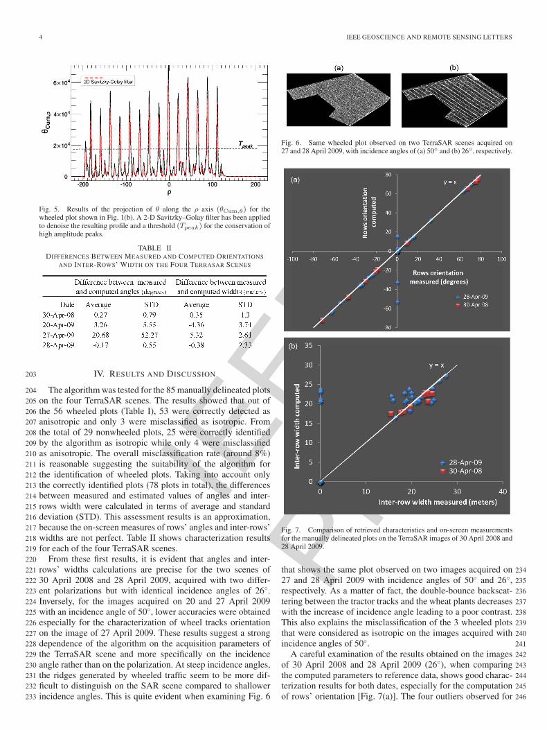
D. Estimation of Inter-Rows’ Width 184
The spectrum of the transformed image R(ρ, θ) allows also 185
the automatic estimation of the inter-rows’ width (w) which can 186
be derived through the projection of θ on the ρ axis (cumulated 187
θ: θcum,ρ). The regularly spaced rows generated by wheel 188
tracks will hence exhibit a series of periodical peaks on the θ 189
profile (Fig. 5). To reduce the effect of undesirable peaks, often 190
related to plot’s boundaries, an interval of 20 pixels centered 191
on the previously determined abscissa was defined. Only those 192
values of θ falling within this interval were hence projected 193
on the ρ axis. To further denoise the resulting θcum,ρ profile, 194
thereby achieving higher precision in the determination of w, a 195
2-D Savitzky–Golay filter [9] was used allowing the smoothing 196
of the peaks while preserving their shapes. Only high amplitude 197
peaks were conserved for the estimation of inter-rows’ width 198
using a threshold value experimentally defined as follows: 199
Tpeak =(max θCum,ρ +XθCum,ρ
)/6 (4)
where XθCum,ρis the average value of θcum,ρ. 200
The remaining peaks Pi (i: 1 → n), are finally used for 201
computing the mean inter-rows’ width 202
w =1
n− 1
n−1∑i=1
(Pi+1 − Pi). (5)
IEEE
Proo
f
4 IEEE GEOSCIENCE AND REMOTE SENSING LETTERS
Fig. 5. Results of the projection of θ along the ρ axis (θCum,θ) for thewheeled plot shown in Fig. 1(b). A 2-D Savitzky–Golay filter has been appliedto denoise the resulting profile and a threshold (Tpeak) for the conservation ofhigh amplitude peaks.
TABLE IIDIFFERENCES BETWEEN MEASURED AND COMPUTED ORIENTATIONS
AND INTER-ROWS’ WIDTH ON THE FOUR TERRASAR SCENES
IV. RESULTS AND DISCUSSION203
The algorithm was tested for the 85 manually delineated plots204
on the four TerraSAR scenes. The results showed that out of205
the 56 wheeled plots (Table I), 53 were correctly detected as206
anisotropic and only 3 were misclassified as isotropic. From207
the total of 29 nonwheeled plots, 25 were correctly identified208
by the algorithm as isotropic while only 4 were misclassified209
as anisotropic. The overall misclassification rate (around 8%)210
is reasonable suggesting the suitability of the algorithm for211
the identification of wheeled plots. Taking into account only212
the correctly identified plots (78 plots in total), the differences213
between measured and estimated values of angles and inter-214
rows width were calculated in terms of average and standard215
deviation (STD). This assessment results is an approximation,216
because the on-screen measures of rows’ angles and inter-rows’217
widths are not perfect. Table II shows characterization results218
for each of the four TerraSAR scenes.219
From these first results, it is evident that angles and inter-220
rows’ widths calculations are precise for the two scenes of221
30 April 2008 and 28 April 2009, acquired with two differ-222
ent polarizations but with identical incidence angles of 26◦.223
Inversely, for the images acquired on 20 and 27 April 2009224
with an incidence angle of 50◦, lower accuracies were obtained225
especially for the characterization of wheel tracks orientation226
on the image of 27 April 2009. These results suggest a strong227
dependence of the algorithm on the acquisition parameters of228
the TerraSAR scene and more specifically on the incidence229
angle rather than on the polarization. At steep incidence angles,230
the ridges generated by wheeled traffic seem to be more dif-231
ficult to distinguish on the SAR scene compared to shallower232
incidence angles. This is quite evident when examining Fig. 6233
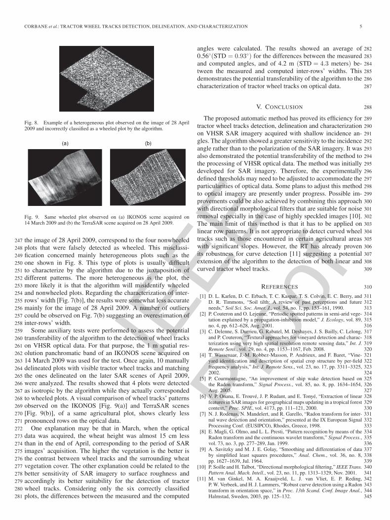
Fig. 6. Same wheeled plot observed on two TerraSAR scenes acquired on27 and 28 April 2009, with incidence angles of (a) 50◦ and (b) 26◦, respectively.
Fig. 7. Comparison of retrieved characteristics and on-screen measurementsfor the manually delineated plots on the TerraSAR images of 30 April 2008 and28 April 2009.
that shows the same plot observed on two images acquired on 234
27 and 28 April 2009 with incidence angles of 50◦ and 26◦, 235
respectively. As a matter of fact, the double-bounce backscat- 236
tering between the tractor tracks and the wheat plants decreases 237
with the increase of incidence angle leading to a poor contrast. 238
This also explains the misclassification of the 3 wheeled plots 239
that were considered as isotropic on the images acquired with 240
incidence angles of 50◦. 241
A careful examination of the results obtained on the images 242
of 30 April 2008 and 28 April 2009 (26◦), when comparing 243
the computed parameters to reference data, shows good charac- 244
terization results for both dates, especially for the computation 245
of rows’ orientation [Fig. 7(a)]. The four outliers observed for 246
IEEE
Proo
f
CORBANE et al.: TRACTOR WHEEL TRACKS DETECTION, DELINEATION, AND CHARACTERIZATION 5
Fig. 8. Example of a heterogeneous plot observed on the image of 28 April2009 and incorrectly classified as a wheeled plot by the algorithm.
Fig. 9. Same wheeled plot observed on (a) IKONOS scene acquired on14 March 2009 and (b) the TerraSAR scene acquired on 28 April 2009.
the image of 28 April 2009, correspond to the four nonwheeled247
plots that were falsely detected as wheeled. This misclassi-248
fication concerned mainly heterogeneous plots such as the249
one shown in Fig. 8. This type of plots is usually difficult250
to characterize by the algorithm due to the juxtaposition of251
different patterns. The more heterogeneous is the plot, the252
more likely it is that the algorithm will misidentify wheeled253
and nonwheeled plots. Regarding the characterization of inter-254
rows’ width [Fig. 7(b)], the results were somewhat less accurate255
mainly for the image of 28 April 2009. A number of outliers256
could be observed on Fig. 7(b) suggesting an overestimation of257
inter-rows’ width.258
Some auxiliary tests were performed to assess the potential259
transferability of the algorithm to the detection of wheel tracks260
on VHSR optical data. For that purpose, the 1 m spatial res-261
olution panchromatic band of an IKONOS scene acquired on262
14 March 2009 was used for the test. Once again, 10 manually263
delineated plots with visible tractor wheel tracks and matching264
the ones delineated on the later SAR scenes of April 2009,265
were analyzed. The results showed that 4 plots were detected266
as isotropic by the algorithm while they actually corresponded267
to wheeled plots. A visual comparison of wheel tracks’ patterns268
observed on the IKONOS [Fig. 9(a)] and TerraSAR scenes269
[Fig. 9(b)], of a same agricultural plot, shows clearly less270
pronounced rows on the optical data.271
One explanation may be that in March, when the optical272
data was acquired, the wheat height was almost 15 cm less273
than in the end of April, corresponding to the period of SAR274
images’ acquisition. The higher the vegetation is the better is275
the contrast between wheel tracks and the surrounding wheat276
vegetation cover. The other explanation could be related to the277
better sensitivity of SAR imagery to surface roughness and278
accordingly its better suitability for the detection of tractor279
wheel tracks. Considering only the six correctly classified280
plots, the differences between the measured and the computed281
angles were calculated. The results showed an average of 282
0.56◦(STD = 0.93◦) for the differences between the measured 283
and computed angles, and of 4.2 m (STD = 4.3 meters) be- 284
tween the measured and computed inter-rows’ widths. This 285
demonstrates the potential transferability of the algorithm to the 286
characterization of tractor wheel tracks on optical data. 287
V. CONCLUSION 288
The proposed automatic method has proved its efficiency for 289
tractor wheel tracks detection, delineation and characterization 290
on VHSR SAR imagery acquired with shallow incidence an- 291
gles. The algorithm showed a greater sensitivity to the incidence 292
angle rather than to the polarization of the SAR imagery. It was 293
also demonstrated the potential transferability of the method to 294
the processing of VHSR optical data. The method was initially 295
developed for SAR imagery. Therefore, the experimentally 296
defined thresholds may need to be adjusted to accommodate the 297
particularities of optical data. Some plans to adjust this method 298
to optical imagery are presently under progress. Possible im- 299
provements could be also achieved by combining this approach 300
with directional morphological filters that are suitable for noise 301
removal especially in the case of highly speckled images [10]. 302
The main limit of this method is that it has to be applied on 303
linear row patterns. It is not appropriate to detect curved wheel 304
tracks such as those encountered in certain agricultural areas 305
with significant slopes. However, the RT has already proven 306
its robustness for curve detection [11] suggesting a potential 307
extension of the algorithm to the detection of both linear and 308
curved tractor wheel tracks. 309
REFERENCES 310
[1] D. L. Karlen, D. C. Erbach, T. C. Kaspar, T. S. Colvin, E. C. Berry, and 311D. R. Timmons, “Soil tilth: A review of past perceptions and future 312needs,” Soil Sci. Soc. Amer. J., vol. 54, no. 1, pp. 153–161, 1990. 313
[2] P. Couteron and O. Lejeune, “Periodic spotted patterns in semi-arid vege- 314tation explained by a propagation-inhibition model,” J. Ecology, vol. 89, 315no. 4, pp. 612–628, Aug. 2001. 316
[3] C. Delenne, S. Durrieu, G. Rabatel, M. Deshayes, J. S. Bailly, C. Lelong, 317and P. Couteron, “Textural approaches for vineyard detection and charac- 318terization using very high spatial resolution remote sensing data,” Int. J. 319Remote Sens., vol. 29, no. 4, pp. 1153–1167, Feb. 2008. 320
[4] T. Wassenaar, J.-M. Robbez-Masson, P. Andrieux, and F. Baret, “Vine- 321yard identification and description of spatial crop structure by per-field 322frequency analysis,” Int. J. Remote Sens., vol. 23, no. 17, pp. 3311–3325, 3232002. 324
[5] P. Courmontagne, “An improvement of ship wake detection based on 325the Radon transform,” Signal Process., vol. 85, no. 8, pp. 1634–1654, 326Aug. 2005. 327
[6] V. P. Onana, E. Trouvé, J. P. Rudant, and E. Tonyé, “Extraction of linear 328features in SAR images for geographical maps updating in a tropical forest 329context,” Proc. SPIE, vol. 4173, pp. 111–121, 2000. 330
[7] N. J. Rodenas, N. Mandelert, and R. Garello, “Radon transform for inter- 331nal wave detection and orientation,” presented at the IX European Signal 332Processing Conf. (EUSIPCO), Rhodes, Greece, 1998. 333
[8] E. Magli, G. Olmo, and L. L. Presti, “Pattern recognition by means of the 334Radon transform and the continuous wavelet transform,” Signal Process., 335vol. 73, no. 3, pp. 277–289, Jan. 1999. 336
[9] A. Savitzky and M. J. E. Golay, “Smoothing and differentiation of data 337by simplified least squares procedures,” Anal. Chem., vol. 36, no. 8, 338pp. 1627–1639, Jul. 1964. 339
[10] P. Soille and H. Talbot, “Directional morphological filtering,” IEEE Trans. 340Pattern Anal. Mach. Intell., vol. 23, no. 11, pp. 1313–1329, Nov. 2001. 341
[11] M. van Ginkel, M. A. Kraaijveld, L. J. van Vliet, E. P. Reding, 342P. W. Verbeek, and H. J. Lammers, “Robust curve detection using a Radon 343transform in orientation space,” in Proc. 13th Scand. Conf. Image Anal., 344Halmstad, Sweden, 2003, pp. 125–132. 345

IEEE
Proo
f
AUTHOR QUERY
NO QUERY.

IEEE
Proo
f
IEEE GEOSCIENCE AND REMOTE SENSING LETTERS 1
Tractor Wheel Tracks Detection, Delineation, andCharacterization in Very High Spatial
Resolution SAR Imagery
1
2
3
Christina Corbane, Nicolas Baghdadi, and Michaël Clairotte4
Abstract—Compacted tractor wheel tracks have been recog-5nized as key factors controlling runoff and erosion processes in6agricultural landscapes. In this context, the availability of an au-7tomatic tool for wheel tracks detection and characterization would8be very useful. In this letter, an original algorithm based on Radon9Transform is proposed for automatic wheel tracks detection on10Synthetic aperture radar images with a spatial resolution of 1 m.11Compared to on-screen measurements, wheel tracks orientations12and widths were accurately estimated for the images acquired with13shallow incidence angles whereas poorer results were observed for14sharp incidence angles.15
Index Terms—Detection, radon transform, Synthetic Aperture16Radar (SAR), tractor wheel tracks.17
I. INTRODUCTION18
WHEEL TRAFFIC used in certain agricultural manage-19
ment practices such as tillage, planting and harvesting20
operations may affect both soil erodibility and hydrological21
properties due to severe soil compaction [1]. Wheel tracks play22
the role of water guiding channels and may, hence, influence23
the drainage direction and intensity depending, respectively,24
on their orientation with respect to the terrain slope and on25
the spacing between wheels. Knowledge of the orientation and26
width of tractor wheel tracks, at the scale of an agriculture plot,27
can give partial evidence of the magnitude of soil compaction28
and is therefore essential for modeling runoff and erosion29
processes. Because remote sensing is considered as the favorite30
tool to provide spatial and temporal information, it can facil-31
itate the detection and monitoring of wheel tracks over large32
areas, representing a promising alternative to conventional field33
surveying methods. Typically, Very High Spatial Resolution34
(VHSR) Synthetic Aperture Radar (SAR) sensors could be used35
for monitoring wheel tracks at the scale of the agricultural36
plot thanks to their well-known sensitivity to variations of37
soil roughness and surface geometry and to their ability to38
image during all-weather conditions. The issue of tractor wheel39
tracks detection and delineation in VHSR SAR images can40
be described as follows: wheel tracks exhibit periodical linear41
patterns consisting of parallel rows with almost invariant inter-42
Manuscript received March 8, 2011; revised April 22, 2011; acceptedMay 23, 2011.
C. Corbane and M. Clairotte are with the European Commission, JointResearch Center, 21020 Ispra, Italy (e-mail: [email protected];[email protected]).
N. Baghdadi is with CEMAGREF, UMR TETIS, 34093 MontpellierCedex 5, France (e-mail: [email protected]).
Color versions of one or more of the figures in this paper are available onlineat http://ieeexplore.ieee.org.
Digital Object Identifier 10.1109/LGRS.2011.2158184
row widths but with a large range of possible orientations which 43
prevent using classical textural approaches. Due to the periodic 44
organization of wheeled plots into straight lines both frequency 45
analysis (e.g., Fourier Transform) and linear feature detection 46
approaches (e.g., Radon Transform) seem suitable for wheel 47
tracks detection and characterization. Fourier transform (FT) 48
is suited for oriented and periodic texture detection. Its ef- 49
ficiency has been demonstrated to characterize and monitor 50
natural periodic vegetation [2]. Both Delenne et al. [3] and 51
Wassenaar et al. [4] applied FT to extract information on 52
the type of vineyard planting as well as crop spacing and 53
orientation on VHSR optical data. In the current study, SAR 54
imagery known for its inherent noise-like phenomenon is ex- 55
plored, thus limiting the use of FT approaches and privileging 56
a method that relies on linear feature detection such as the 57
Radon transform (RT). The RT integrates values of the pixels 58
along every line while each integral becomes a single point in 59
the transform space; this process of averaging diminishes noise 60
perturbations and hence increases the signal-to-noise ratio of 61
features of interest. For that reason RT has been considered a 62
quite appropriate method for the enhancement and detection of 63
linear patterns on SAR imagery. Several applications in SAR 64
exploited this property like ship wake detection [5], extraction 65
of roads and railways for the update of geographic maps [6] and 66
characterization of internal waves in oceanography [7]. 67
In this letter, an original algorithm based on RT is proposed 68
for the automatic wheel tracks detection and characterization 69
of previously delimited plots on VHSR SAR images. The 70
accuracy and the robustness of the method are analyzed for both 71
wheeled and nonwheeled plots observed at different dates with 72
varying SAR acquisition parameters. 73
II. STUDY SITE AND DATA SET 74
The selected study site is located in the Orgeval watershed, 75
East of Paris (France; Lat. 48◦ 51′ N and Long. 3◦ 07′ E). The 76
soil has a loamy texture and is very flat (slope < 5%). This 77
predominantly agricultural area is composed of wheat and corn- 78
growing plots. From September 2008 to April 2009, the winter 79
wheat covered approximately 50% of the watershed total sur- 80
face. The remaining surface portion corresponded to ploughed 81
soils awaiting future cultivation. The wheat height was about 82
5 cm in January, 10 cm February, 20 cm in March, and 35 cm 83
at the end of April. Following the sowing season (September 84
to October), the tractors are usually operated starting February 85
or March for spreading agricultural fertilizers. In some cases 86
fertilizer application operations take place from March until 87
June with two to five passages of tractors. The repeated passage 88
of wheel traffic over a plot has a compacting action on the soil 89
1545-598X/$26.00 © 2011 IEEE

IEEE
Proo
f
2 IEEE GEOSCIENCE AND REMOTE SENSING LETTERS
Fig. 1. (a) Illustration of a typical wheeled plot. (b) A wheeled plot observedon a SAR scene acquired on 30 April 2008.
TABLE ITHE EXPERIMENTAL DATA SET CONSISTING OF A TOTAL OF
85 WHEELED (WP) AND NONWHEELED PLOTS (NWP)MANUALLY DELINEATED ON FOUR TERRASAR SCENES
in the wheel track that is observable in the field by the presence90
of parallel rows [Fig. 1(a)].91
For this experiment, four TerraSAR-X images (∼9.65 GHz),92
acquired at low and high incidence angles (26◦ and 50◦) in93
‘Spotlight mode’, in April 2008 and 2009, were analyzed. The94
TerraSAR images were taken with HH and VV polarized beams95
and with a ground pixel spacing of 1 m. The characteristics96
of the SAR scenes are summarized in Table I. For the vali-97
dation of the algorithm a total of 85 manually delimited plots98
were defined on the four SAR scenes. The experimental plots99
were selected in such a way they included both patterns of100
wheeled and nonwheeled plots (Table I). For each delineated101
plot, measurements of the rows’ orientation (α) and inter-102
row’s width (w) have been done by photo-interpretation as103
follows: assessment of the mean angle of all visible rows for104
row orientation and of the mean distance of all visible rows105
for inter-rows’ width [Fig. 1(b)]. The brightest radar returns in106
linear forms at the interior of some agricultural plots are caused107
by the double-bounce scattering between the compacted tractor108
wheel tracks and the wheat plants [Fig. 1(b)].109
III. METHOD110
A. Algorithm Overview111
The method to be developed to detect accurately tractor112
wheel tracks on SAR images described above under all con-113
ditions encountered, needs to fulfill a number of requirements:114
1) it should be able to detect linear structures, 2) it should allow115
the estimation of the rows directions and inter-rows’ width,116
3) it should be able to detect structures without user interaction,117
4) it should be robust to noises.118
To meet these requirements, a three step algorithm centered119
on the RT was developed (Fig. 2): In a first step, RT was120
computed for each pre-delineated agricultural plot allowing121
the detection of the bright lines corresponding to the ridges122
generated by the passage of wheel tracks; in a second step,123
wheeled plots were distinguished from nonwheeled plots and124
the orientation of the previously detected lines was computed;125
Fig. 2. Illustration of the three-step algorithm developed for the automaticdetection and characterization of tractor wheel tracks.
in a final step, inter-rows’ width was estimated though a proper 126
noise filtering, thresholding and peak detection approach. 127
B. Detection of Wheel Tracks’ Rows 128
The developed workflow is based on the assumption that 129
agriculture plots under process are previously delineated using 130
either existing digitized fields boundaries or a proven automated 131
field delineation method. A Gamma speckle filter was first 132
applied on the experimental plots manually delineated in the 133
SAR scenes. This was followed by an edge enhancement using 134
a 3 × 3 Laplacian filter. These two preprocessing operations 135
were meant to improve the visibility of the wheel tracks and 136
to facilitate their detection using the RT. At the heart of the 137
algorithm lies the RT. The RT of a 2-D function f(x, y) is the 138
set of projections along angles θ: 139
R(ρ, θ) =
∫ +∞∫−∞
f(x, y)δ(x cos θ + y sin θ − ρ)dxdy
=
+∞∫−∞
f(ρ cos θ − l sin θ, ρ sin θ + l cos θ)dl
where
[ρl
]=
[cos θ sin θ− sin θ cos θ
][xy
](coordinate rotation) (1)

IEEE
Proo
f
CORBANE et al.: TRACTOR WHEEL TRACKS DETECTION, DELINEATION, AND CHARACTERIZATION 3
Fig. 3. Scaled RT corresponding to the agricultural plot of Fig. 1(b).
where δ (x) is the Dirac function, ρ ∈ π(−∞,+∞) and θ ∈140
[0, π]. The RT performs the integration of the image along141
each possible straight line of the image with polar parameters142
(ρ, θ). The RT of an image containing a segment will therefore143
exhibit a prominent peak of coordinates (ρ0, θ0) such that ρ0 =144
x cos θ0 + y sin θ0 is the equation of the straight line along145
which the segment lies [8]. The RT, therefore, contains a peak146
corresponding to every line in the image that is brighter than147
its surroundings and a valley for every dark line. Thus, the148
problem of detecting lines is reduced to detecting the peaks149
and valleys in the transform domain. To differentiate candidate150
peaks from the surrounding clutter, it is necessary to adequately151
threshold the transformed image R(ρ, θ). Therefore, a scaling152
of RT based on the average intensity was applied allowing to153
display only those values greater than the average of R(ρ, θ).154
Fig. 3 illustrates the scaled RT corresponding to a typical155
image of a wheeled plot shown in Fig. 1(b). It reveals the156
presence of several bright spots at the abscissa θ = 0.8 radians.157
These peaks correspond to the parallel rows generated by the158
tractor’s wheels. Two other bright spots can be seen at θ = 1.85159
and one spot at θ = 2.65. They correspond to the left (for160
θ = 1.85), the upper and lower linear borders (for θ = 2.65)161
of the plot.162
C. Estimation of Rows’ Orientation163
It is often the case that for the same date, some agricultural164
plots may be subjected to wheeled traffic while others are165
not. This is reflected in the SAR scene by the presence of166
highly anisotropic wheeled plots and isotropic nonwheeled167
plots. In the presence of an anisotropic plot, the projection168
of the absolute values of ρ along the θ axis (Cumulated ρ:169
ρCum,θ) is characterized by the presence of a prominent peak170
[Fig. 4(a)]. Inversely, in the case of isotropic plots, there is171
a random variation of ρ values [Fig. 4(b)]. The distinction172
between wheeled and nonwheeled plots was implemented using173
an experimentally defined threshold as follows:174
Tanisotropic = max ρCum,θ>(XρCum,θ
+σρCum,θ×5
)(2)
where XρCum,θand σρCum,θ
are, respectively the average and175
the standard deviation values of ρCum,θ.176
For anisotropic plots, the peaks corresponding to the wheel177
tracks observed on the SAR scene have theoretically the same178
Fig. 4. Results of the projection of ρ along the θ axis (ρCum,θ) for(a) a wheeled plot and (b) a nonwheeled plot.
abscissa in the transformed image since they correspond to 179
parallel lines. This abscissa of the projected ρ along the θ axis, 180
with the largest value of ρCum,θ(argmax ρCum,θ) corresponds 181
to the angle of the orientation of the spectrum and thus gives 182
the orientation α of the wheel tracks as follows: 183
α = argmaxρCum,θ(degrees)− 90. (3)
D. Estimation of Inter-Rows’ Width 184
The spectrum of the transformed image R(ρ, θ) allows also 185
the automatic estimation of the inter-rows’ width (w) which can 186
be derived through the projection of θ on the ρ axis (cumulated 187
θ: θcum,ρ). The regularly spaced rows generated by wheel 188
tracks will hence exhibit a series of periodical peaks on the θ 189
profile (Fig. 5). To reduce the effect of undesirable peaks, often 190
related to plot’s boundaries, an interval of 20 pixels centered 191
on the previously determined abscissa was defined. Only those 192
values of θ falling within this interval were hence projected 193
on the ρ axis. To further denoise the resulting θcum,ρ profile, 194
thereby achieving higher precision in the determination of w, a 195
2-D Savitzky–Golay filter [9] was used allowing the smoothing 196
of the peaks while preserving their shapes. Only high amplitude 197
peaks were conserved for the estimation of inter-rows’ width 198
using a threshold value experimentally defined as follows: 199
Tpeak =(max θCum,ρ +XθCum,ρ
)/6 (4)
where XθCum,ρis the average value of θcum,ρ. 200
The remaining peaks Pi (i: 1 → n), are finally used for 201
computing the mean inter-rows’ width 202
w =1
n− 1
n−1∑i=1
(Pi+1 − Pi). (5)

IEEE
Proo
f
4 IEEE GEOSCIENCE AND REMOTE SENSING LETTERS
Fig. 5. Results of the projection of θ along the ρ axis (θCum,θ) for thewheeled plot shown in Fig. 1(b). A 2-D Savitzky–Golay filter has been appliedto denoise the resulting profile and a threshold (Tpeak) for the conservation ofhigh amplitude peaks.
TABLE IIDIFFERENCES BETWEEN MEASURED AND COMPUTED ORIENTATIONS
AND INTER-ROWS’ WIDTH ON THE FOUR TERRASAR SCENES
IV. RESULTS AND DISCUSSION203
The algorithm was tested for the 85 manually delineated plots204
on the four TerraSAR scenes. The results showed that out of205
the 56 wheeled plots (Table I), 53 were correctly detected as206
anisotropic and only 3 were misclassified as isotropic. From207
the total of 29 nonwheeled plots, 25 were correctly identified208
by the algorithm as isotropic while only 4 were misclassified209
as anisotropic. The overall misclassification rate (around 8%)210
is reasonable suggesting the suitability of the algorithm for211
the identification of wheeled plots. Taking into account only212
the correctly identified plots (78 plots in total), the differences213
between measured and estimated values of angles and inter-214
rows width were calculated in terms of average and standard215
deviation (STD). This assessment results is an approximation,216
because the on-screen measures of rows’ angles and inter-rows’217
widths are not perfect. Table II shows characterization results218
for each of the four TerraSAR scenes.219
From these first results, it is evident that angles and inter-220
rows’ widths calculations are precise for the two scenes of221
30 April 2008 and 28 April 2009, acquired with two differ-222
ent polarizations but with identical incidence angles of 26◦.223
Inversely, for the images acquired on 20 and 27 April 2009224
with an incidence angle of 50◦, lower accuracies were obtained225
especially for the characterization of wheel tracks orientation226
on the image of 27 April 2009. These results suggest a strong227
dependence of the algorithm on the acquisition parameters of228
the TerraSAR scene and more specifically on the incidence229
angle rather than on the polarization. At steep incidence angles,230
the ridges generated by wheeled traffic seem to be more dif-231
ficult to distinguish on the SAR scene compared to shallower232
incidence angles. This is quite evident when examining Fig. 6233
Fig. 6. Same wheeled plot observed on two TerraSAR scenes acquired on27 and 28 April 2009, with incidence angles of (a) 50◦ and (b) 26◦, respectively.
Fig. 7. Comparison of retrieved characteristics and on-screen measurementsfor the manually delineated plots on the TerraSAR images of 30 April 2008 and28 April 2009.
that shows the same plot observed on two images acquired on 234
27 and 28 April 2009 with incidence angles of 50◦ and 26◦, 235
respectively. As a matter of fact, the double-bounce backscat- 236
tering between the tractor tracks and the wheat plants decreases 237
with the increase of incidence angle leading to a poor contrast. 238
This also explains the misclassification of the 3 wheeled plots 239
that were considered as isotropic on the images acquired with 240
incidence angles of 50◦. 241
A careful examination of the results obtained on the images 242
of 30 April 2008 and 28 April 2009 (26◦), when comparing 243
the computed parameters to reference data, shows good charac- 244
terization results for both dates, especially for the computation 245
of rows’ orientation [Fig. 7(a)]. The four outliers observed for 246

IEEE
Proo
f
CORBANE et al.: TRACTOR WHEEL TRACKS DETECTION, DELINEATION, AND CHARACTERIZATION 5
Fig. 8. Example of a heterogeneous plot observed on the image of 28 April2009 and incorrectly classified as a wheeled plot by the algorithm.
Fig. 9. Same wheeled plot observed on (a) IKONOS scene acquired on14 March 2009 and (b) the TerraSAR scene acquired on 28 April 2009.
the image of 28 April 2009, correspond to the four nonwheeled247
plots that were falsely detected as wheeled. This misclassi-248
fication concerned mainly heterogeneous plots such as the249
one shown in Fig. 8. This type of plots is usually difficult250
to characterize by the algorithm due to the juxtaposition of251
different patterns. The more heterogeneous is the plot, the252
more likely it is that the algorithm will misidentify wheeled253
and nonwheeled plots. Regarding the characterization of inter-254
rows’ width [Fig. 7(b)], the results were somewhat less accurate255
mainly for the image of 28 April 2009. A number of outliers256
could be observed on Fig. 7(b) suggesting an overestimation of257
inter-rows’ width.258
Some auxiliary tests were performed to assess the potential259
transferability of the algorithm to the detection of wheel tracks260
on VHSR optical data. For that purpose, the 1 m spatial res-261
olution panchromatic band of an IKONOS scene acquired on262
14 March 2009 was used for the test. Once again, 10 manually263
delineated plots with visible tractor wheel tracks and matching264
the ones delineated on the later SAR scenes of April 2009,265
were analyzed. The results showed that 4 plots were detected266
as isotropic by the algorithm while they actually corresponded267
to wheeled plots. A visual comparison of wheel tracks’ patterns268
observed on the IKONOS [Fig. 9(a)] and TerraSAR scenes269
[Fig. 9(b)], of a same agricultural plot, shows clearly less270
pronounced rows on the optical data.271
One explanation may be that in March, when the optical272
data was acquired, the wheat height was almost 15 cm less273
than in the end of April, corresponding to the period of SAR274
images’ acquisition. The higher the vegetation is the better is275
the contrast between wheel tracks and the surrounding wheat276
vegetation cover. The other explanation could be related to the277
better sensitivity of SAR imagery to surface roughness and278
accordingly its better suitability for the detection of tractor279
wheel tracks. Considering only the six correctly classified280
plots, the differences between the measured and the computed281
angles were calculated. The results showed an average of 282
0.56◦(STD = 0.93◦) for the differences between the measured 283
and computed angles, and of 4.2 m (STD = 4.3 meters) be- 284
tween the measured and computed inter-rows’ widths. This 285
demonstrates the potential transferability of the algorithm to the 286
characterization of tractor wheel tracks on optical data. 287
V. CONCLUSION 288
The proposed automatic method has proved its efficiency for 289
tractor wheel tracks detection, delineation and characterization 290
on VHSR SAR imagery acquired with shallow incidence an- 291
gles. The algorithm showed a greater sensitivity to the incidence 292
angle rather than to the polarization of the SAR imagery. It was 293
also demonstrated the potential transferability of the method to 294
the processing of VHSR optical data. The method was initially 295
developed for SAR imagery. Therefore, the experimentally 296
defined thresholds may need to be adjusted to accommodate the 297
particularities of optical data. Some plans to adjust this method 298
to optical imagery are presently under progress. Possible im- 299
provements could be also achieved by combining this approach 300
with directional morphological filters that are suitable for noise 301
removal especially in the case of highly speckled images [10]. 302
The main limit of this method is that it has to be applied on 303
linear row patterns. It is not appropriate to detect curved wheel 304
tracks such as those encountered in certain agricultural areas 305
with significant slopes. However, the RT has already proven 306
its robustness for curve detection [11] suggesting a potential 307
extension of the algorithm to the detection of both linear and 308
curved tractor wheel tracks. 309
REFERENCES 310
[1] D. L. Karlen, D. C. Erbach, T. C. Kaspar, T. S. Colvin, E. C. Berry, and 311D. R. Timmons, “Soil tilth: A review of past perceptions and future 312needs,” Soil Sci. Soc. Amer. J., vol. 54, no. 1, pp. 153–161, 1990. 313
[2] P. Couteron and O. Lejeune, “Periodic spotted patterns in semi-arid vege- 314tation explained by a propagation-inhibition model,” J. Ecology, vol. 89, 315no. 4, pp. 612–628, Aug. 2001. 316
[3] C. Delenne, S. Durrieu, G. Rabatel, M. Deshayes, J. S. Bailly, C. Lelong, 317and P. Couteron, “Textural approaches for vineyard detection and charac- 318terization using very high spatial resolution remote sensing data,” Int. J. 319Remote Sens., vol. 29, no. 4, pp. 1153–1167, Feb. 2008. 320
[4] T. Wassenaar, J.-M. Robbez-Masson, P. Andrieux, and F. Baret, “Vine- 321yard identification and description of spatial crop structure by per-field 322frequency analysis,” Int. J. Remote Sens., vol. 23, no. 17, pp. 3311–3325, 3232002. 324
[5] P. Courmontagne, “An improvement of ship wake detection based on 325the Radon transform,” Signal Process., vol. 85, no. 8, pp. 1634–1654, 326Aug. 2005. 327
[6] V. P. Onana, E. Trouvé, J. P. Rudant, and E. Tonyé, “Extraction of linear 328features in SAR images for geographical maps updating in a tropical forest 329context,” Proc. SPIE, vol. 4173, pp. 111–121, 2000. 330
[7] N. J. Rodenas, N. Mandelert, and R. Garello, “Radon transform for inter- 331nal wave detection and orientation,” presented at the IX European Signal 332Processing Conf. (EUSIPCO), Rhodes, Greece, 1998. 333
[8] E. Magli, G. Olmo, and L. L. Presti, “Pattern recognition by means of the 334Radon transform and the continuous wavelet transform,” Signal Process., 335vol. 73, no. 3, pp. 277–289, Jan. 1999. 336
[9] A. Savitzky and M. J. E. Golay, “Smoothing and differentiation of data 337by simplified least squares procedures,” Anal. Chem., vol. 36, no. 8, 338pp. 1627–1639, Jul. 1964. 339
[10] P. Soille and H. Talbot, “Directional morphological filtering,” IEEE Trans. 340Pattern Anal. Mach. Intell., vol. 23, no. 11, pp. 1313–1329, Nov. 2001. 341
[11] M. van Ginkel, M. A. Kraaijveld, L. J. van Vliet, E. P. Reding, 342P. W. Verbeek, and H. J. Lammers, “Robust curve detection using a Radon 343transform in orientation space,” in Proc. 13th Scand. Conf. Image Anal., 344Halmstad, Sweden, 2003, pp. 125–132. 345

IEEE
Proo
f
AUTHOR QUERY
NO QUERY.


