Download - The Gaia -ESO Survey: Stellar content and elemental abundances in the massive cluster NGC 6705

arX

iv:1

407.

1510

v1 [

astr

o-ph

.SR

] 6

Jul 2

014

Astronomy& Astrophysicsmanuscript no. m11_AA_accepted c©ESO 2014July 10, 2014

The Gaia-ESO Survey⋆: Stellar content and elemental abundancesin the massive cluster NGC 6705

T. Cantat-Gaudin1, 2, A. Vallenari2, S. Zaggia2, A. Bragaglia3, R. Sordo2, J. E. Drew4, J. Eisloeffel5, H. J. Farnhill4, E.Gonzalez-Solares6, R. Greimel7, M. J. Irwin6, A. Kupcu-Yoldas6, C. Jordi8, R. Blomme9, L. Sampedro10, M. T.

Costado10, E. Alfaro10, R. Smiljanic11,12, L. Magrini13, P. Donati3,14, E. D. Friel15, H. Jacobson16, U. Abbas18, D.Hatzidimitriou19, A. Spagna18, A. Vecchiato18, L. Balaguer-Nunez8, C. Lardo3, M. Tosi3, E. Pancino3, A. Klutsch20, G.Tautvaisiene17, A. Drazdauskas17, E. Puzeras17, F. Jiménez-Esteban26, E. Maiorca13, D. Geisler24, I. San Roman24, S.

Villanova24, G. Gilmore21, S. Randich13, T. Bensby22, E. Flaccomio23, A. Lanzafame20, A. Recio-Blanco25, F.Damiani23, A. Hourihane21, P. Jofré21, P. de Laverny25, T. Masseron21, L. Morbidelli13, L. Prisinzano23, G. G. Sacco13,

L. Sbordone27, 28, and C. C. Worley21

(Affiliations can be found after the references)

Received date/ Accepted date

ABSTRACT

Context. Chemically inhomogeneous populations are observed in mostglobular clusters, but not in open clusters. Cluster mass seemsto play a key role in the existence of multiple populations.Aims. Studying the chemical homogeneity of the most massive open clusters is necessary to better understand the mechanism of theirformation and determine the mass limit under which clusterscannot host multiple populations. Here we studied NGC 6705,that is ayoung and massive open cluster located towards the inner region of the Milky Way. This cluster is located inside the solarcircle. Thismakes it an important tracer of the inner disk abundance gradient.Methods. This study makes use ofBVI andri photometry and comparisons with theoretical isochrones toderive the age of NGC 6705.We study the density profile of the cluster and the mass function to infer the cluster mass. Based on abundances of the chemicalelements distributed in the first internal data release of the Gaia-ESO Survey, we study elemental ratios and the chemical homogeneityof the red clump stars. Radial velocities enable us to study the rotation and internal kinematics of the cluster.Results. The estimated ages range from 250 to 316 Myr, depending on theadopted stellar model. Luminosity profiles and massfunctions show strong signs of mass segregation. We derive the mass of the cluster from its luminosity function and from thekinematics, finding values between 3700 M⊙ and 11 000 M⊙. After selecting the cluster members from their radial velocities, we obtaina metallicity of [Fe/H]=0.10±0.06 based on 21 candidate members. Moreover, NGC 6705 showsno sign of the typical correlationsor anti-correlations between Al, Mg, Si, and Na, that are expected in multiple populations. This is consistent with our cluster massestimate, which is lower than the required mass limit proposed in literature to develop multiple populations.

Key words. stars: abundances - open clusters and associations: general - open clusters and associations: individual: NGC 6705

1. Introduction

Once thought to be the best example of simple stellar populations(coeval, mono-metallic systems), the globular clusters (GCs)have been shown to be instead complex objects. In particular, ev-idence that they host distinct populations (possibly, distinct gen-erations) of stars has been mounting. Gratton et al. (2004, 2012)present reviews based on spectroscopy, while Piotto (2009)andMilone et al. (2012) can be consulted for results based on pho-tometry.

While variations in iron content seem limited to very fewcases, the most notable beingω Cen (e.g. Lee et al. 1999;Johnson & Pilachowski 2010) and M 22 (e.g. Marino et al.2011), GC stars show large star-to-star variations in some lightelements, like C, N, O, Na, Mg, and Al. It has been knownfor a long time that there are variations in the CN and CHbands strengths, with spreads and bimodal distributions (e.g.

⋆ Based on the data obtained at ESO telescopes under programme188.B-3002 (the public Gaia-ESO spectroscopic survey, PIsGilmore &Randich) and on the archive data of the programme 083.D-0671

Kraft 1979, 1994, for reviews), and not all the variations canbe attributed to internal processes like mixing. Na and Ohave been extensively studied as summarised in the review byGratton et al. (2004) and Carretta et al. (2009a,b), which showan anti-correlation: in the same GC there are stars with “nor-mal” O and Na (normal with respect to the cluster metallic-ity) and stars showing a (strong) depletion in O and an en-hancement in Na. Most of the stars have a modified composi-tion. A similar anti-correlation can be found between Mg andAl, but not in all clusters, and with lower depletions than inO (e.g. Carretta et al. 2009b; Marino et al. 2008). Most impor-tantly, these star-to-star variations occur also in unevolved, main-sequence stars, as demonstrated first by Gratton et al. (2001) andRamírez & Cohen (2002) and later confirmed on much largersamples (e.g. Lind et al. 2009; D’Orazi et al. 2010). These lowmass stars cannot have produced these variations, since theircores do not reach the high temperatures necessary for the rel-evant proton-capture reactions and, in any case, the stars lackthe mixing mechanism needed to bring processed material to thesurface. This implies that the chemical inhomogeneities were

Article number, page 1 of 19

http://de.arxiv.org/abs/1407.1510v1

already present in the gas out of which these stars formed. Thishas led to the belief that GCs are made of at least two gen-erations of stars, with the second generation formed from gaspolluted by the material processed by the first. Exactly whichkind of first-generation stars were the polluters is debated; themost promising candidates are intermediate mass asymptotic gi-ant branch stars (Ventura et al. 2001) and fast rotating massivestars (Decressin et al. 2007), but refinements and comparisonsto robust observational constraints are required.

The multiple populations scenario for GCs requires that thecluster is massive enough to retain some of its primordial gas atthe any of any subsequent star formation; indeed, existing mod-els postulate that GCs were many times more massive at the timeof their formations than they appear today (e.g. D’Ercole etal.2008). Such models suffer from several drawkbacks. For in-stance, they do not explain the observed properties of the youngmassive clusters (Bastian & Silva-Villa 2013), or the abundancepatterns of the halo stars (see e.g. Martell et al. 2011). Re-cently, a mechanism based on accretion on circumstellar discs,not requiring multiple generation of stars has been presented byBastian et al. (2013). This model does not require that clusterswere initially extremely massive. In any case, the efficiency ofthe accretion process depends on the density and velocity disper-sion of the cluster, that both scale with the cluster mass, suggest-ing that more massive clusters should exhibit broader chemicaldishonomegeneities.

Carretta et al. (2010), combining the data on 18 GCs of theFLAMES survey (Carretta et al. 2009a) and literature studies,showed that all Galactic GCs for which Na and O abundanceswere available presented a Na-O anti correlation, i.e., multi-ple populations. The only possible exceptions were Terzan 7and Palomar 12, two young and low-mass GCs belonging tothe Sagittarius dwarf galaxy. This apparent universality of theNa-O anti correlation was suggested to be a defining propertyof GCs, separating them from the other clusters where only asingle population is present. Cluster mass seems to play a de-terminant role in this separation and, studies of low-mass GCsand massive and old open clusters (OCs) are needed to deter-mine the mass threshold under which no multiple populationscan be formed. This scenario needs however to be verifiedobservationally, which motivated further studies in this "greyzone" between the two kind of clusters. Recent additions in-clude the GCs Rup 106 (Villanova et al. 2013), which showsno Na-O anti correlation, and Terzan 8 (Carretta et al. 2013), inwhich the second generation, if present, represents a minority,and two of the most massive and oldest OCs, Berkeley 39 andNGC 6791. High-resolution spectroscopy in 30 stars of Berke-ley 39 by Bragaglia et al. (2012) showed a single, homogeneouspopulation. Geisler et al. (2012) have found signs of a bi-modalNa distribution in NGC 6791, which would make it the firstknown OC with multiple populations. This suggestion has notbeen confirmed by another study (Bragaglia et al. 2013, submit-ted) where no variations exceeding the errors were found in thesame cluster. Further studies are called for to settle the issue.

The Gaia-ESO Survey (hereafter GES, Gilmore et al. 2012;Randich & Gilmore 2013) is a large, public spectroscopic surveyusing the high-resolution multi-object spectrograph FLAMESon the Very Large Telescope (ESO, Chile). It targets more than105 stars, covering the bulge, thick and thin discs, and halo com-ponents, and a sample of about 100 open clusters (OCs) of allages, metallicities, locations, and masses. The focus of the GESis to quantify the kinematical and chemical element abundancedistributions in the different components of the Milky Way, thus

providing a complement to the limited spectroscopic capabilitiesof the astrometric Gaia mission.

Here we focus on NGC 6705 (M 11, Mel 213, Cr 391,OCl 76), a massive and concentrated OC located in the firstgalactic quadrant (Messina et al. 2010; Santos et al. 2005) at thegalactic coordinates (l = 27.3, b = −2.8). This cluster, one ofthe three intermediate-age clusters observed in the first GES in-ternal data release, contains a total of several thousands of solarmasses (McNamara & Sanders 1977; Santos et al. 2005), whichplaces it near the limit between the most massive OCs and theleast massive GCs (Bragaglia et al. 2012). Being located to-wards the central parts of the Galaxy it is projected againstadense background, but its rich main sequence and populated redclump clearly stand out in a color-magnitude diagram.

NGC 6705 is situated in a clear area and suffers from rela-tively little extinction for an object at such a low galacticlat-itude. Moreover, due to its position inside the solar circle, itis an important tracer of the inner disk gradient. In a compan-ion paper, Magrini et al. (2014) compare the abundance patternsof the three intermediate-age OCs of the first GES data release(NGC 6705, Tr 20 and NGC 4815) for Fe, Si, Mg, Ca, and Ti.They showed that each cluster has a unique pattern, with in par-ticular a high value of [Mg/Fe] in NGC 6705. Moreover, theabundances of two of these clusters are consistent with theirgalactocentric radius, whereas the abundances of NGC 6705are more compatible with a formation between 4 and 6 kpcfrom the Galactic Center despite its current galactocentric ra-dius of 6.9 kpc. The present paper focuses on the determinationof the structural parameters, age and chemical abundances ofNGC 6705, using VPHAS+, ESO 2.2.m telescope WFI photom-etry, and spectroscopic data from the Gaia-ESO Survey.

−1.0−0.5

0.00.51.0

V - V

S

⟨V - VS

⟩=-0.02

−1.0−0.5

0.00.51.0

BV -

BVS

⟨BV - BVS

⟩=0.01

V−1.0−0.5

0.00.51.0

VI -

VIS

⟨VI - VIS

⟩=0.01

−1.0−0.5

0.00.51.0

V - V

K

⟨V - VK

⟩=0.00

10 12 14 16 18 20V

−1.0−0.5

0.00.51.0

BV -

BVK

⟨BV - BVK

⟩=-0.01

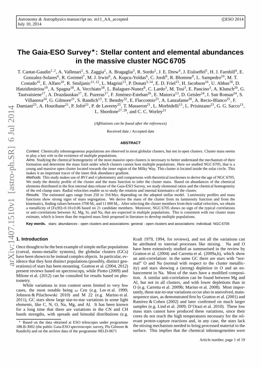
Fig. 1. Upper three panels: comparison of our photometry with thatof Sung et al. (1999).Lower two panels: comparison with Koo et al.(2007). The labels indicate the residual zero point differences.

The photometric and spectroscopic data are presented inSect. 2. The membership determination is given in Sect. 3. InSect. 4 we derive the extintion map in the region surrounding


T. Cantat-Gaudin et al.: The Gaia-ESO Survey: Stellar content and elemental abundances in the massive cluster NGC 6705

the cluster. In Sect. 5 we study the luminosity profile and masssegregation of the cluster, and provide cluster mass estimates. InSect. 6 we look at the rotation and kinematics in the cluster.InSect. 7 we make use of isochrones to determine the distance andage of the cluster. Finally, the chemical abundances of Al, Mg,Si, and Na for NGC 6705 are presented in Sect. 8.

2. The data

2.1. WFI BVI photometry

The photometry used in this paper has been extracted fromarchival images inB, V and I taken on the 13th of May 1999with the Wide Field Imager at the MPG/ESO 2.2m Telescopefor the ESO Imaging Survey (ESO programme 163.O-0741(C),PI Renzini). The sample of images comprise for each band twolong exposure time images (240 sec each for a total of 480 sec),in order to reach a photometric precision of 20% at V≃ 21 mag,and single short (20 sec) exposure carefully chosen not to satu-rate the brighter targets.

Data reduction has been performed using the ESO/Alambicsoftware (Vandame 2002) especially designed for mosaic CCDcameras and providing fully astrometrically and photometricallycalibrated images with special care to the so-called “illumi-nation correction”. The photometry was performed using theDaophot/Allstar software (Stetson 1987) wrapped in an auto-matic procedure which performed the PSF calculation and allthe steps for extracting the final magnitudes. The PSF photome-try from the short and long exposures for each single band havebeen combined in a single photometric dataset using the Dao-master program. The internal astrometric accuracy (both withinthe short/long exposures and in the different bands) resulted tobe better than 0.05 arcsec while the external comparison with the2MASS catalogue gave an rms of≃ 0.20 arcsec.

The observations consist in a single 33′ × 34′ field centeredon the cluster, covering completely the photometry of Sung et al.(1999). The geometry of the WFI imaging is shown in Fig 9.We tied our instrumental WFI photometry to their photometriccalibration, comparing the magnitudes of the common objects,calculating solutions for the zero point and color term for eachpass band. In the magnitude range V<14 the dispersion is of theorder of 0.05 magnitudes, increasing to 0.1 for stars as faint asV∼ 17 (see the upper panels of Fig. 1). Unfortunately, theB-band filter of WFI is quite far from the JohnsonB filter with alarge color term of≃-0.33 mag. After applying the calibration,the B magnitudes present a residual second-order trend in colorwhich appears as a residual offset of -0.05 mag for the extremeblue and red stars. We decided not to apply any correction forthis effect, and instead we used the photometry of Sung et al.(1999) for all objects withV < 12 and (B − V) > 1. For fainterstars, the photometries show good agreement, with a residualoffset of≃0.02 mag atV=14, increasing to 0.1 mag atV ≃17.The comparison between our photometry and that of Sung et al.(1999) is shown in the upper three panels of Fig. 1.

Our data were also compared with theBV photometric dataof Koo et al. (2007), acquired in a search for variable stars.Thecomparison (lower panels of Fig. 1) also shows good agreementwith no systematics, with a dispersion of 0.08 forV < 14, in-creasing for fainter magnitudes.

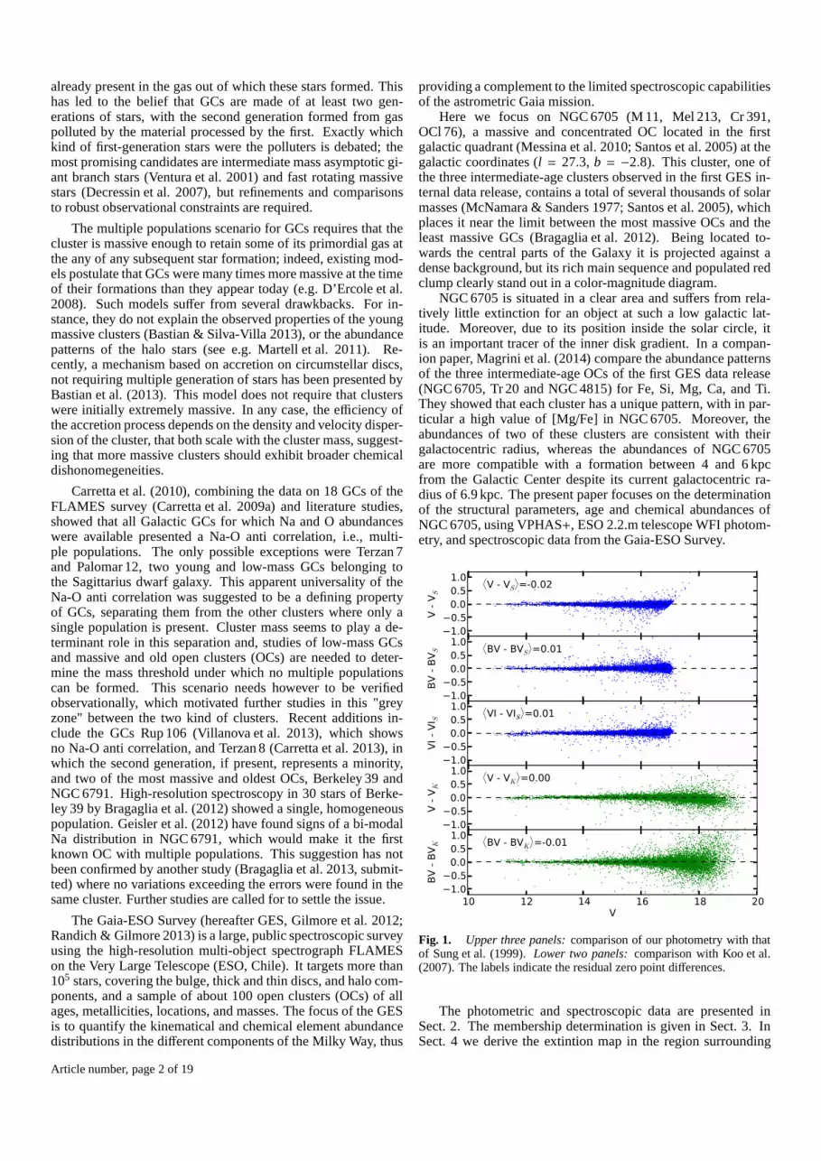
Since the cluster is very dense, our photometry suffers fromcrowding effects, especially in the central parts. The complete-ness of the photometry was estimated as usual by randomlyadding stars of magnitudeV ranging from 16 to 22 and runningthe source detection step again, then counting how many of the

added stars were recovered. This method allows to estimate thecompleteness for each magnitude bin in a given region of thecluster. The completeness is better than 50% up to magnitudeV ≃ 18 in the central regions andV ≃ 19.7 in the less crowdedoutskirts (see Fig. 2).

16 17 18 19 20 21 22V

0

20

40

60

80

100

com

ple

teness

[%

]

Completeness from crowding experiments

r < 5'

5' < r < 19'

r > 19'

Fig. 2. Completeness of our photometry obtained from crowdingexperiments for different regions of the cluster.

The data contain a total of 123 037 stars. TheBV CMDshows a very clear main sequence standing out of the back-ground as can be seen in Fig. 3. Evolved stars are also visible,with a red clump located around (B − V,V) = (1.5, 12). Thelower panels of Fig. 3 show that the main sequence can be easilyfollowed down toV=16 in the inner regions of the cluster, whilethe top-right panel shows that the signature of the cluster is notvisible outside of 18′.

2.2. VPHAS+ ri photometry

The VPHAS+ observations used here arer- andi-band data fromthree fields (numbered 212, 213, and 237) that overlap near thesky position of NGC 6705. A general description of this publicsurvey continuing to execute using the OmegaCAM instrumenton the VLT Survey Telescope is provided by Drew et al. (2014).Each pointing captures a square degree at a time, with the centerof NGC 6705 falling within a couple of arcminutes of the south-ern edge of field 212, and towards the boundary with 237. Thedata were all obtained at a time of very good seeing (0.5 to 0.6arcseconds) during the night of 7th July 2012 when the moonwas relatively bright (FLI= 0.77). Inr, the formal 10-σ mag-nitude limit falls between 20.5 and 20.8 with a likely complete-ness limit of∼19.5, while these limits are approximately 0.5–0.7magnitudes brighter in thei band. All magnitudes are specifiedin the Vega system.

The CMD of the inner 12′ is shown in Fig. 4. The data areused in Sect. 4 to derive the extinction map of the region sur-rounding the cluster. Due to the very good seeing, stars brighterthanr ∼ 12 are partially saturated in bothr andi bands, makingthe position of the main sequence turn-off point and red clumpstars quite uncertain in the CMD.

2.3. GES spectroscopic data

The GES makes use of the GIRAFFE (R∼20 000) and UVES(R∼47 000) spectrographs of the VLT UT-2. The GES con-


Fig. 3. Top-left: BV CMD of all 123 037 in our sample.Top-right: CMD of the outer 18′, which we consider as our background field.Bottom-leftandbottom-right: CMD of the inner 6′ and 3′. In the latter three panels, the grey points correspond to the wide-field CMD.

sortium is structured in several working groups (WGs). Thereduction of the GIRAFFE and UVES spectra by WG7 is de-scribed in Lewis et al. (in prep.) and Sacco et al. (2014), re-spectively. The analysis is performed independently by teamsusing different methods, but make use of the same model atmo-spheres (MARCS, Gustafsson et al. 2008) and the same line list(Heiter et al. in prep.). The results are then gathered and con-trolled to produce a homogenised set (for a comparison of theresults obtained with different spectroscopic methods, see forinstance Jofre et al. 2013). The analysis of the GIRAFFE databy WG10 is described in Recio-Blanco et al. (in prep.), and theanalysis of UVES spectra by WG11 is described in Smiljanic etal. (in prep.).

Stellar parameters and elemental abundances for the stars ob-served during the first six months of the campaign were deliveredto the members of the collaboration as an internal data release(internal data release 1, or GESviDR1Final) for the purposeofscience verification and validation.

The target selection for NGC 6705 and the exposure timesfor the various setups are described in Bragaglia et al. (in prep.).For the GIRAFFE targets, potential members were selected onthe basis of their optical and infrared photometry following thecluster main sequence, and the proper motions from the UCAC4catalog (Zacharias et al. 2012) were used in order to discardob-jects whose proper motions are more than five sigma from thecluster centroid. In total, 1028 main-sequence stars were ob-served with 8 GIRAFFE setups. All the red giants located inthe clump region in the inner 12′ were observed with the UVESsetup 580 (25 targets). The number of targets observed with each

Table 1. Summary of GES GIRAFFE observations

Setup Centralλ Spectral range R nb Stars Median S/N[nm] [nm]

HR3 412.4 403.3–420.1 24 800 166 24HR5A 447.1 434.0–458.7 18 470 166 25HR6 465.6 453.8–475.9 20 350 166 21HR9B 525.8 514.3–535.6 25 900 526 37HR10 447.1 434.0–458.7 18 470 284 50HR14A 651.5 630.8–670.1 17 740 166 44HR15N 665.0 647.0–679.0 17 000 1028 52HR21 875.7 434.0–458.7 18 470 284 55

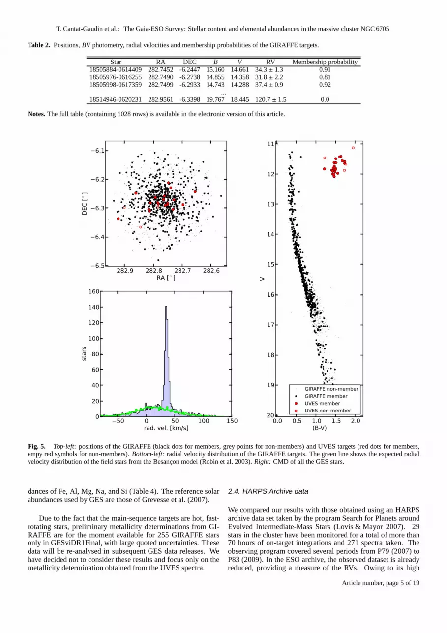
GIRAFFE setup is summarised in Table 1. The coordinates,B,V, J, H, andK magnitudes, radial velocities and membershipprobabilities (see Sect. 3) are shown in Table 2.

The spatial distribution of the targets is shown in the top-left panel of Fig. 5, and theBV photometry of the targets is theWFI photometry presented in the present paper. The bottom-leftpanel of Fig. 5 shows the radial velocity (RV) distribution of allthe GIRAFFE targets. From the GESviDR1Final data release,we have RVs for 1028 GIRAFFE targets and 25 UVES targets.

The 25 UVES stars have well-defined values of effectivetemperature, surface gravity, and microturbulence derived di-rectly from these spectra (summarised in Table 3). While el-emental abundances are available for various elements in theGESviDR1final data release, this work focused on the abun-



Table 2. Positions,BV photometry, radial velocities and membership probabilities of the GIRAFFE targets.

Star RA DEC B V RV Membership probability18505884-0614409 282.7452 -6.2447 15.160 14.661 34.3± 1.3 0.9118505976-0616255 282.7490 -6.2738 14.855 14.358 31.8± 2.2 0.8118505998-0617359 282.7499 -6.2933 14.743 14.288 37.4± 0.9 0.92

...18514946-0620231 282.9561 -6.3398 19.767 18.445 120.7± 1.5 0.0

Notes. The full table (containing 1028 rows) is available in the electronic version of this article.

0.0 0.5 1.0 1.5 2.0(B-V)

11

12

13

14

15

16

17

18

19

20

V

GIRAFFE non-memberGIRAFFE memberUVES memberUVES non-member

282.6282.7282.8282.9RA [ ◦ ]

−6.5

−6.4

−6.3

−6.2

−6.1

DEC

[◦]

−50 0 50 100 150rad. vel. [km/s]

0

20

40

60

80

100

120

140

160

star

s

Fig. 5. Top-left: positions of the GIRAFFE (black dots for members, grey points for non-members) and UVES targets (red dots for members,empy red symbols for non-members).Bottom-left: radial velocity distribution of the GIRAFFE targets. The green line shows the expected radialvelocity distribution of the field stars from the Besançon model (Robin et al. 2003).Right: CMD of all the GES stars.

dances of Fe, Al, Mg, Na, and Si (Table 4). The reference solarabundances used by GES are those of Grevesse et al. (2007).

Due to the fact that the main-sequence targets are hot, fast-rotating stars, preliminary metallicity determinations from GI-RAFFE are for the moment available for 255 GIRAFFE starsonly in GESviDR1Final, with large quoted uncertainties. Thesedata will be re-analysed in subsequent GES data releases. Wehave decided not to consider these results and focus only on themetallicity determination obtained from the UVES spectra.

2.4. HARPS Archive data

We compared our results with those obtained using an HARPSarchive data set taken by the program Search for Planets aroundEvolved Intermediate-Mass Stars (Lovis & Mayor 2007). 29stars in the cluster have been monitored for a total of more than70 hours of on-target integrations and 271 spectra taken. Theobserving program covered several periods from P79 (2007) toP83 (2009). In the ESO archive, the observed dataset is alreadyreduced, providing a measure of the RVs. Owing to its high


Table 3. Photometry and stellar parameters of the UVES stars.

Star RA DEC B V J H Ks RV Teff log g [Fe/H] vmic

[◦] [ ◦] [km s−1] [K] [km s−1]Members

18503724-0614364 282.6552 -6.2434 13.423 12.001 9.427 8.808 8.616 35.2 4820± 71 2.42± 0.21 0.03± 0.14 1.82± 0.1318504737-0617184 282.6974 -6.2884 13.381 11.652 8.527 7.808 7.523 31.8 4325± 130 1.72± 0.29 0.03± 0.15 1.56± 0.1618505494-0616182 282.7289 -6.2717 13.328 11.860 9.199 8.498 8.318 34.8 4689± 109 2.37± 0.43 0.13± 0.09 1.46± 0.1218505581-0618148 282.7325 -6.3041 13.050 11.414 8.557 7.895 7.698 35.1 4577± 139 2.23± 0.31 0.17± 0.18 1.60± 0.2418505755-0613461 282.7398 -6.2295 13.041 11.830 9.426 8.852 8.675 30.4 4873± 114 2.37± 0.32 0.03± 0.14 1.33± 0.1918505944-0612435 282.7477 -6.2121 13.270 11.872 9.330 8.722 8.523 34.6 4925± 177 2.56± 0.39 0.19± 0.18 1.50± 0.5018510023-0616594 282.7510 -6.2832 13.319 11.586 8.524 7.776 7.589 35.2 4433± 95 1.94± 0.47 0.17± 0.12 1.50± 0.1418510032-0617183 282.7513 -6.2884 13.542 12.081 9.368 8.751 8.549 35.2 4850± 100 2.38± 0.21 0.07± 0.15 1.60± 0.3318510200-0617265 282.7583 -6.2907 13.030 11.426 8.446 7.766 7.493 32.0 4415± 87 2.35± 0.45 0.18± 0.14 1.48± 0.0718510289-0615301 282.7620 -6.2584 13.467 12.014 9.389 8.758 8.543 32.8 4750± 112 2.40± 0.28 0.05± 0.07 1.45± 0.1318510341-0616202 282.7642 -6.2723 13.239 11.801 9.216 8.579 8.386 36.3 4975± 146 2.50± 0.30 0.07± 0.15 1.94± 0.2718510358-0616112 282.7649 -6.2698 13.320 11.902 9.357 8.691 8.511 34.7 4832± 79 2.31± 0.31 0.15± 0.08 1.62± 0.1918510786-0617119 282.7828 -6.2866 13.084 11.621 9.030 8.399 8.206 33.6 4768± 53 2.11± 0.19 0.03± 0.14 1.80± 0.2818510833-0616532 282.7847 -6.2814 13.202 11.736 8.911 8.311 8.227 33.3 4750± 112 2.25± 0.22 0.18± 0.10 1.60± 0.2518511013-0615486 282.7922 -6.2635 12.996 11.493 8.613 7.933 7.705 36.9 4439± 59 1.87± 0.53 0.10± 0.12 1.50± 0.1018511048-0615470 282.7937 -6.2631 13.134 11.627 8.817 8.224 7.991 33.3 4744± 122 2.12± 0.33 0.05± 0.14 1.70± 0.3018511452-0616551 282.8105 -6.2820 13.403 11.923 9.263 8.620 8.420 35.1 4800± 59 2.40± 0.25 0.11± 0.08 1.69± 0.2018511534-0618359 282.8139 -6.3100 13.527 11.974 9.163 8.507 8.303 33.7 4755± 57 2.16± 0.21 0.05± 0.22 1.79± 0.1718511571-0618146 282.8155 -6.3041 13.297 11.807 9.088 8.445 8.211 35.0 4710± 159 2.27± 0.30 0.15± 0.12 1.60± 0.1818512662-0614537 282.8609 -6.2482 13.228 11.559 8.611 7.921 7.700 33.8 4459± 91 2.10± 0.48 0.12± 0.17 1.48± 0.1918514130-0620125 282.9221 -6.3368 13.348 11.849 9.185 8.570 8.361 33.2 4671± 140 2.20± 0.28 0.07± 0.19 1.62± 0.20

Non-members18510093-0614564 282.7539 -6.2490 12.677 11.462 9.016 8.395 8.205 41.4 4755± 35 2.30± 0.24 -0.10± 0.10 1.50± 0.1518510837-0617495 282.7849 -6.2971 13.438 11.674 8.469 7.649 7.429 -72.5 4217± 83 1.62± 0.33 -0.10± 0.12 1.47± 0.1618512283-0621589 282.8451 -6.3664 13.604 11.879 8.831 8.084 7.872 3.4 4305± 95 2.08± 0.34 0.18± 0.18 1.61± 0.2118513636-0617499 282.9015 -6.2972 13.075 11.128 7.295 6.451 6.127 -1.4 4041± 225 1.57± 0.42 -0.20± 0.20 1.45± 0.03

Notes. The photometry was not corrected for extinction. The nominal uncertainty on UVES radial velocities is 0.6 km s−1.

resolving power (R∼115 000) and simultaneous wavelength cal-ibration, HARPS delivers a typical radial velocity error ofabout0.06 km s−1 for these stars. 19 of them stars were also observedby GES with the UVES instrument, allowing for a sanity checkof our UVES measurements, but none were observed with GI-RAFFE. Fig. 6 shows a comparison between the RVs derivedfrom UVES and HARPS spectra. The nominal uncertainty onthe UVES RVs is 0.6 km s−1. The measurements from UVESare systematically lower by 0.8 km s−1 on average, with a stan-dard deviation of 0.4 km s−1. We corrected for the differencesin zero-point between the GIRAFFE, UVES and HARPS radialvelocities when using them together later in this study.

3. Membership

The spectroscopic targets were photometrically selected to belikely cluster members, but this selection obviously includes asignificant number of field stars, that can be separated from thecluster stars on the basis of their RVs. In Fig. 5, a green lineshows the RV distribution of the field stars expected from theBesançon model (Robin et al. 2003). We selected from the sim-ulation the stars belonging to the bright main sequence region,with B−V < 1.2 andV < 17 (the region of the CMD covered bythe majority of the GIRAFFE targets) and scaled the distributionso that its tails (RV< 20 km s−1 and RV> 50 km s−1) contain thesame number of objects as those of the observed distribution.The Besançon model reproduces very well the observed RV dis-tribution of the background, while the signature of the cluster isclearly visible as a peak around 36 km s−1.

We performed a membership determination, for GIRAFFEand UVES stars independently.

3.1. Membership of the GIRAFFE stars

We determined the membership of the GIRAFFE stars from theHR15N radial velocities only, because of the good signal-to-noise ratio (S/N) of these spectra and because all 1028 GIRAFFEstars were observed with this setup. The analysis of the dataob-tained with the other gratings will be available in further datareleases.

We applied a classical parametric procedure where the ra-dial velocity distribution is fitted with two Gaussian compo-nents: one for the cluster members and one for the field stars.We followed the procedure described in Cabrera-Caño & Alfaro(1985), but based on the RVs only. The RVs of stars thatwere observed with different GIRAFFE gratings are the 2-sigmaclipped averages. The method computes the membership prob-abilities through an iterative method. The probability densityfunction (hereafter PDF) model is defined as:

φi(vi) = ncφi,c(vi) + n fφi, f (vi) (1)

wherenc andn f are the priors of the cluster member and fieldstars distributions respectively,φi(vi) the PDF for the whole sam-ple and,φi,c(vi) andφi, f (vi) the PDFs for the cluster members andthe field stars related to thei-th star.



Table 4. Elemental abundances for the UVES stars.

Star [Fe/H] [Al /Fe] [Mg/Fe] [Na/Fe] [Si/Fe]Members

18503724-0614364 0.03± 0.14 0.12± 0.15 0.23± 0.17 0.51± 0.17 0.09± 0.1518504737-0617184 0.03± 0.15 0.17± 0.17 0.23± 0.15 0.74± 0.21 0.03± 0.1718505494-0616182 0.13± 0.09 0.26± 0.09 0.14± 0.09 0.5± 0.11 0.07± 0.0918505581-0618148 0.17± 0.18 0.10± 0.18 0.12± 0.20 0.32± 0.21 0.05± 0.1918505755-0613461 0.03± 0.14 -0.04± 0.38 0.10± 0.15 0.52± 0.14 0.07± 0.1518505944-0612435 0.19± 0.18 0.14± 0.18 0.14± 0.22 0.49± 0.19 -0.04± 0.1918510023-0616594 0.17± 0.12 0.21± 0.12 0.20± 0.16 0.39± 0.13 0.02± 0.1818510032-0617183 0.07± 0.15 0.20± 0.15 0.21± 0.18 0.53± 0.16 0.02± 0.1618510200-0617265 0.18± 0.14 0.13± 0.15 0.16± 0.16 0.17± 0.14 0.02± 0.1518510289-0615301 0.05± 0.07 0.22± 0.07 0.13± 0.13 0.53± 0.11 0.05± 0.0918510341-0616202 0.07± 0.15 0.19± 0.15 0.30± 0.16 0.54± 0.17 -0.07± 0.1718510358-0616112 0.15± 0.08 0.18± 0.08 0.12± 0.10 0.49± 0.10 0.07± 0.1118510786-0617119 0.03± 0.14 0.25± 0.14 0.42± 0.14 0.58± 0.18 0.08± 0.1818510833-0616532 0.18± 0.10 0.18± 0.10 0.19± 0.14 0.51± 0.13 -0.06± 0.1218511013-0615486 0.10± 0.12 0.23± 0.12 0.23± 0.16 0.52± 0.15 0.07± 0.1418511048-0615470 0.05± 0.14 0.23± 0.15 0.39± 0.14 0.54± 0.21 -0.03± 0.2318511452-0616551 0.11± 0.08 0.15± 0.11 0.15± 0.29 0.55± 0.16 0.06± 0.1118511534-0618359 0.05± 0.22 0.25± 0.22 0.33± 0.24 0.49± 0.23 0.08± 0.2418511571-0618146 0.15± 0.12 0.20± 0.13 0.09± 0.17 0.45± 0.14 0.0± 0.1318512662-0614537 0.12± 0.17 0.29± 0.17 0.24± 0.22 0.59± 0.21 0.13± 0.2218514130-0620125 0.07± 0.19 0.21± 0.19 0.11± 0.21 0.45± 0.20 0.01± 0.20µ 0.10± 0.04 0.20± 0.04 0.19± 0.05 0.48± 0.05 0.04± 0.04σ 0+0.04 0+0.05 0+0.07 0+0.06 0+0.05

Non-members18510093-0614564 -0.10± 0.10 0.23± 0.11 0.11± 0.16 0.45± 0.13 0.07± 0.1218510837-0617495 -0.10± 0.12 0.20± 0.12 0.28± 0.14 0.32± 0.12 0.02± 0.1318512283-0621589 0.18± 0.18 0.27± 0.20 0.24± 0.20 0.38± 0.23 0.06± 0.2018513636-0617499 -0.20± 0.20 0.53± 0.21 0.43± 0.20 0.41± 0.23 0.06± 0.21

Suna 7.45 6.37 7.53 6.17 7.51

Notes. aThe solar reference abundances are those of Grevesse et al. (2007).µ andσ are the intrinsic mean and dispersion, respectively (cf. Sect. 8).

The membership probabilities are obtained making use ofthese PDFs and by using Bayes’ theorem as follows:

Pc(vi) =ncφi,c(vi)φi(vi)

(2)

wherePc(vi) is the probability of thei-th star to be a cluster mem-ber. According to Bayes’ minimum error rate decision rule, athreshold value of 0.5 minimises the misclassification. At theend of the analysis, 536 stars (out of 1028) have a member-ship probability larger than 0.5. The mean RV of these starsis 35.9 km s−1, with a standard deviation of 2.8 km s−1.

Note that undetected member binaries may have discrepantRVs and be classified as non-members by this procedure.Rigourously speaking, the RV distribution of the members maydeviate from a Gaussian. The measured RVs of unresolved bina-ries are the combination of the motion of the center of mass andof the orbital motion, and tend to have larger uncertaintiesthanisolated stars. The result of convolving a binary model withanormal distribution is a modification of the tails of the Gaussian,by extending and increasing them. Here some unresolved pairsmay therefore be classified as non-members.

3.2. Membership of the UVES stars

We have stellar parameters and accurate metallicities for the 25UVES targets of NGC 6705, including three stars that show avery discrepant RV and are not members of the clusters (seeFig. 7). A fourth star (18510093-0614564)has an outlying radial

velocity of 41.4 km s−1, even though its photometry is compati-ble with the other cluster members. As a possible explanation,this star could be a single-lined binary, made of a red clump starand a main-sequence star. Being much hotter, the main-sequencecompanion contributes to the spectrum with a continuum emis-sion only, making the lines shallower. This hypothesis wouldexplain why this star has a discrepant radial velocity, and is alsoan outlier in metallicity, with [Fe/H]= −0.10 ± 0.10 (see fol-lowing section). In the absence of further elements, we did notconsider it as a member in the rest of this study.

Finally, 21 stars can be considered as bona-fide members ofthe cluster. The mean RV for the UVES members is 34.1 km s−1

(with a standard deviation of 1.5 km s−1), which is lower thanthe mean value of 35.9±2.8km s−1 found for GIRAFFE stars.The lack of targets in common between both instruments do notallow for a solid comparison of the systematics between UVESand GIRAFFE, and both results are compatible within their stan-dard deviations. In the first GES data release, Sacco et al. (2014)note an average offset of 0.87 km s−1 between the UVES and GI-RAFFE HR15N radial velocities, which is consistent with theoffset we observe here.

4. Extinction maps

When looking towards the inner parts of the Galaxy, the lineof sight often meets regions of high extinction. Before dis-cussing the age and the structure of NGC 6705, we need to assesswhether the studied region is affected by differential extinction.The available VPHAS+ ri photometry covers a very wide field,


0.2 0.4 0.6 0.8 1.0 1.2 1.4 1.6(r-i)

12

14

16

18

20

r

PARSEC isochrone - 316Myr, Z=0.015, (V-MV)=11.45, E(B-V)=0.4

VPHAS photometry

Fig. 4. VPHAS+ ri CMD of the central 12′ of the cluster. The spatialdistribution of the selected stars (black points) is shown in Fig. 9. Thesolide line corresponds to the PARSEC isochrone of best parameters,shifted for distance modulus and extinction (see Sect. 7 fordetail). Starsbrigther thanr = 12 suffer from saturation and are not shown here.

31 32 33 34 35 36 37 38RVHARPS [km.s−1 ]

−2.5

−2.0

−1.5

−1.0

−0.5

0.0

0.5

1.0

RVUVES -

RVHARPS [k

m.s−1

]

∆=-0.8 km.s−1

σ=0.4 km.s−1

Fig. 6. Comparison between the radial velocity measurements fromHARPS spectra and UVES spectra for 19 red giants.

much larger than ourBVI photometry, which allows us to studythe extinction of the background around the cluster. Theri CMDof the inner 12′ of the cluster is shown in Fig. 4. The PAR-SEC isochrone (Bressan et al. 2012) shown in that figure corre-sponds to the parameters of the best fit of theBV photometry (seeSect. 7). First we make use of the GIRAFFE members to derivethe extinction law in the direction of the cluster. Fig. 8 presentsthe color-color diagrams in the passbandsBVIri. To fit the data,we need to adopt the relationsE(V− I) = 1.24(±0.05)×E(B−V)and E(r − i) = 0.68(±0.04) × E(B − V). While the ratio

−60 −40 −20 0 20 40radial velocity [km.s−1 ]

−0.4

−0.3

−0.2

−0.1

0.0

0.1

0.2

0.3

0.4

[Fe/

H]

Fig. 7. Identification of the red clump cluster members from radial ve-locities and iron abundance. The error bars for the radial velocities aresmaller than the symbols. The 21 filled circles correspond tothe mem-bers, while the 4 open circles are the stars we consider non-members.

E(V− I)/E(B−V) is consistent with the total-to-selective extinc-tion ratio RV = AV/E(B − V)=3.1 using the Fitzpatrick (1999)law, the relationE(r− i)/E(B−V) is slightly larger than the valueof E(r − i) = 0.6× E(B − V) given by Yuan et al. (2013).

Fig. 8. Color-color diagrams on NGC 6705 GIRAFFE membersmain-sequence stars, compared with the relation expected from PAR-SEC isochrones for various extinction laws.

Red clump stars in intermediate and old populations are of-ten used in literature as distance and extinction indicators. ThePARSEC isochrones indicate that ther− i color of the red clumpvaries by 0.07 for ages from 2 to 10 Gyr, and by 0.14 for Z from0.001 to 0.03. Due to the small dependence of their magnitudeand color on age and metallicity, they make good tracers of theextinction across the field.



We simulated a field corresponding to the coordinate of thecluster using the Padova Galaxy Model (Vallenari et al. 2006).The red clump stars in the model have an absoluter magnitudeof 0.55 and an intrinsic color (r − i) = 0.525. We followed thecolor excess of the red clump stars at different distances. Thefield was divided in cells of 0.25◦ × 0.25◦. In each of these cells,we computed the reddening as follows: the red giant stars fallingin the magnitude range that corresponds to the distance range wewant to probe (for instance, 11.5< r < 13 for 2 – 4 kpc) were di-vided in bins of 0.05 in the (r − i) color, and we looked for themost populated color bin. This color was then compared to thereference value of (r−i) = 0.525, to find the color excess. We ap-plied the procedure a second time, looking at a fainter magnitudeslice, to take into account the fact that one must look at faintermagnitudes to probe stars that are more reddened. We found thatgoing for more iterations did not significantly change the results.After this second step, the final color excessE(r − i) was con-verted toE(B−V) using the relationE(r− i) = 0.68× E(B−V).Our bins of 0.05 inr − i color correspond to a resolution of 0.07in E(B−V). The extinction map we obtain for the distance range2− 4 kpc is visible in Fig. 9.

The inner region of the cluster studied with the WFIBVIphotometry sits in a zone of relatively low and uniform extinc-tion, with E(B − V) = 0.40 out to 11′ from the center. Ahigher extinction is found at DEC> -6◦and RA< 283.25◦, withE(B − V) up to 0.7. A comparison with the map by Schlegel(1998) shows consistency, with the north-west quadrant beingthe most reddened. However, the maps of Schlegel (1998) givethe integrated extinction along the line of sight while we restrictour determination to the distance range 2–4 kpc. For this rea-son, our values of extinction are lower and the distributionis notdirectly comparable.

Although the cluster itself lies in a window of constant ex-tinction, the bottom-left panel of Fig. 9 shows clearly thatthe stardensity distribution of the photometrically selected VPHAS+cluster stars (Fig. 4) is correlated with the extinction, makingthe background density inhomogeneous.

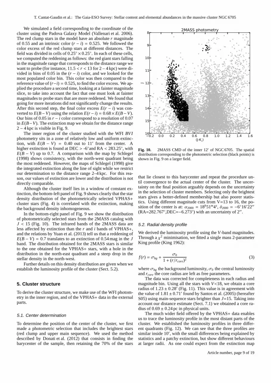
In the bottom-right panel of Fig. 9 we show the distributionof photometrically selected stars from the 2MASS catalog withJ < 15 (Fig. 10). The infrared bands of the 2MASS data areless affected by extinction than ther and i bands of VPHAS+,and the relations by Yuan et al. (2013) tell us that a reddening ofE(B − V) = 0.7 translates to an extinction of 0.54 mag in theJband. The distribution obtained for the 2MASS stars is similarto the one obtained for the VPHAS+ stars, with a hole in thedistribution in the north-east quadrant and a steep drop in thestellar density in the north-west.

Further details on this density distribution are given whenweestablish the luminosity profile of the cluster (Sect. 5.2).

5. Cluster structure

To derive the cluster structure, we make use of the WFI photom-etry in the inner region, and of the VPHAS+ data in the externalparts.

5.1. Center determination

To determine the position of the center of the cluster, we firstmade a photometric selection that includes the brightest stars(red clump and upper main sequence). We used the methoddescribed by Donati et al. (2012) that consists in finding thebarycenter of the sample, then retaining the 70% of the stars

−0.2 0.0 0.2 0.4 0.6 0.8 1.0 1.2 1.4 1.6(J-Ks)

8

9

10

11

12

13

14

15

16

J

2MASS photometry

Fig. 10. 2MASS CMD of the inner 12′ of NGC 6705. The spatialdistribution corresponding to the photometric selection (black points) isshown in Fig. 9 on a larger field.

that lie closest to this barycenter and repeat the procedureun-til convergence to the actual center of the cluster. The uncer-tainty on the final position arguably depends on the uncertaintyin the selection of cluster members. Selecting only the brighteststars gives a better-defined membership but also poorer statis-tics. Using different magnitude cuts from V=13 to 16, the po-sition of the center is at:α2000 = 18h51m4s, δ2000 = −6◦16′22′′

(RA=282.767◦,DEC=−6.273◦) with an uncertainty of 2′′.

5.2. Radial density profile

We derived the luminosity profile using theV-band magnitudes.Through aχ2 minimisation, we fitted a single mass 2-parameterKing profile (King 1962):

f (r) = σbg +σ0

1+ (r/rcore)2(3)

whereσbg the background luminosity,σ0 the central luminosityandrcore the core radius are left as free parameters.

The data was corrected for completeness in each radius andmagnitude bin. Using all the stars withV<18, we obtain a coreradius of 1.23± 0.28′ (Fig. 11). This value is in agreement withthe value of 1.81± 0.71′ found by Santos et al. (2005) (hereafterS05) using main-sequence stars brighter thanJ=15. Taking intoaccount our distance estimate (Sect. 7.1) we obtained a corera-dius of 0.69± 0.24 pc in physical units.

The much wider field offered by the VPHAS+ data enablesus to trace the luminosity profile in the most distant parts ofthecluster. We established the luminosity profiles in three differ-ent quadrants (Fig. 12). We can see that the three profiles aresimilar inside 10′, with the small differences being explained bystatistics and a patchy extinction, but show different behavioursat larger radii. As one could expect from the extinction map


Fig. 9. Top-left: extinction map obtained from VPHAS+ photometry in the distance range 2-4 kpc. The cross indicates the center of the cluster.The dashed line shows the footprint of ourBVI photometry.Bottom-left: same extinction map. The black points are cluster stars selected from the(r − i, r) VPHAS+ CMD, with r<16. The CCD gaps are visible as horizontal lines.Top-right: extinction map from Schlegel (1998) for this field.Bottom-right: same as bottom-left, but with 2MASS main-sequence stars (J<15).

of Fig. 9, the luminosity in the north-west quadrant drops tolower values than in the other two. In the north-east quadrant,a dip is visible between 25′ and 40′, corresponding to a re-gion of stronger extinction of the background (see Fig. 9). Inthe south-west quadrant, beyond 20′, the background density in-creases with radius as the extinction decreases. Since outside ofthe core the luminosity profile is mainly shaped by extinction, itis not possible to estimate the tidal radius of NGC 6705 by fit-ting a 3-parameter King profile. The value ofrtidal = 52± 27′

reported by S05 falls exactly in the distance range affected bystrong extinction. S05 also observed a deviation of the luminos-ity profile from their model between 11′ and 16′, and suggestthis excess could be due to low-mass stars moving to larger radiidue to mass segregation. Without a proper model for the back-ground density, it seems very difficult to draw conclusions on thestructure of the cluster beyond 10′.

5.3. Mass segregation from the luminosity profile

Mass segregation is an internal dynamical phenomenon thattakes place in star clusters and leads the most massive starsto be

more tightly clumped than the least massive ones (Spitzer 1969).A certain number of methods can be used to see whether or notmass segregation is occurring in a cluster, for instance applyinga Minimum Spanning Tree analysis (Allison et al. 2009), or di-rectly comparing the distance to the center for stars of differentbrightness. Here we compare the density profiles of stars in dif-ferent mass ranges (cf. Sect. 5.2) and compare the slope of themass function in different regions of the cluster (our Sect. 7.3,and S05).

Figure 13 shows the luminosity profiles established in fourdifferent magnitude ranges: 10 – 13, 13 – 15, 15 – 16, 16 – 18.For our best-fitting PARSEC isochrone, these correspond to themass ranges: M> 2.14 M⊙, 2.14 – 1.37, 1.37 – 1.14, 1.14 – 0.81.For stars withV > 16, we applied a completeness correctionbased on the distance and magnitude.

In the faintest range (16< V < 18) we discarded the datapoint corresponding to the most central bin (r < 0.5′), due to thevery low completeness for faint stars at the center of the cluster.It is clear that the core radius increases as fainter stars are consid-ered, from 1.02± 0.25′ in the range 10< V < 13 to 3.62± 1.12′

in the range 16< V < 18. This result is consistent with results



10-1 100 101 102

r [arcmin]

10-4

10-3

10-2

10-1

100

flux de

nsity

[arcmin−2

]

V<18

rcore=1.23±0.28'

σbg=0.003±0.005

including background

100 101 102

r [arcmin]

background-subtracted2-parameter King profile

Fig. 11. Observed luminosity profile (black dots) for stars withV<18,fitted with a two-parameters King profile (continuous line),includingbackground (left) and after subtracting the background (right). The fluxdensity was normalised to the central luminosity so thatσ0 = 1.

100 101 102r [arcmin]

10-3

10-2

10-1

100

flux de

nsity

[arcmin−2]

r<16

NWNESW

Fig. 12. Stellar density profiles for the north-west, north-east andsouth-west quadrants (respectively NW, NE and SW) of the VPHAS+photometry, using stars withr < 16. The profiles in the three quadrantswere normalised to the flux in the innermost bin. The background levelwas not subtracted.

by Sung et al. (1999), although they do not quantify the increasein radius for the distribution of progressively fainter stars.

6. Kinematics

6.1. Rotation

Since NGC 6705 is a massive system and radial velocities areavailable for a large number of targets, we looked for hints of therotational signature of the cluster, as is routinely done for GCs(see e.g. Cote et al. 1995; Bellazzini et al. 2012; Bianchiniet al.2013). We first corrected the GIRAFFE radial velocities for theoffset observed in Sect.2.4, then applied the procedure to thewhole sample. The method consists in dividing the cluster in

10-1 100 101 10210-3

10-2

10-1

100

101

flux

dens

ity [a

rcm

in−2

] 10<V<13

rcore=1.09±0.25'

10-1 100 101 10210-3

10-2

10-1

100

101

13<V<15

rcore=1.44±0.23'

10-1 100 101 102

r [arcmin]

10-3

10-2

10-1

100

101

flux

dens

ity [a

rcm

in−2

] 15<V<16

rcore=2.46±0.38'

10-1 100 101 102

r [arcmin]

10-3

10-2

10-1

100

101

16<V<18

rcore=3.62±1.12'

2-parameter King profiles in different magnitude bins

Fig. 13. Observed and fitted luminosity profiles obtained with stars indifferent magnitude ranges. The background was fitted and subtracted.In the bottom-right panel, the open symbol is the datapoint that wasdiscarded when fitting the luminosity profile.

two and selecting one half, according to a position angleφ mea-sured here from north to east (φ = 0◦ corresponds to the northhalf, whileφ = +90◦ andφ = −90◦ correspond to the east andwest halves, respectively). The mean radial velocity is computedin the selected region. Varying the angleφ by steps of 5◦ wetrace the mean radial velocity in different regions. For a rotatingobject, we expect the radial velocities to follow a sinusoidal de-pendance on the position angleφ, being equal to the mean radialvelocity of the cluster whenφ corresponds to the orientation ofthe rotation axis (projected on the sky), following the equation:

∆Vr = Arot sin(φ0 + φ) (4)

whereArot corresponds to the amplitude of the rotation andφ0 isthe position angle of the rotation axis. We estimated the uncer-tainty on the mean radial velocity by bootstrapping: in eachposi-tion angle bin, containing N datapoints, we created 100 setsof Ndatapoints by randomly sampling the radial velocity dataset, cal-culated the mean velocity for each one, and computed the stan-dard deviation of these results. The best-fitting sine function cor-responds to an orientation angleφ0 = 4± 45◦, and an amplitudeArot = 0.3±0.1km s−1 around the mean radial velocity (Fig. 14).Since the RV is averaged over the full range of radii covered bythe sample, the derived Arot is a lower limit to the maximumrotation amplitude, depending on the rotational gradient of thecluster. The observed pattern is however very weak, with an am-plitude much smaller than the velocity dispersion of the cluster,and we can conclude that rotation does not play a significant rolein the observed velocity dispersion in NGC 6705.

6.2. Intrinsic velocity dispersion

Due to uncertainties on the radial velocities of each invidid-ual star, the velocity dispersions we observe in our samples(2.8 km s−1 for the GIRAFFE sample, 1.5 km s−1 for the com-bined HARPS and UVES sample) are larger than the true, in-trinsic dispersion of those stars. Assuming this intrinsicdistri-bution is gaussian, and that the quoted uncertainties{ǫ1, ..., ǫN}on the observed radial velocities{v1, ..., vN} are gaussian errors,


−150 −100 −50 0 50 100 150φ [ ◦ ]

−0.6

−0.4

−0.2

0.0

0.2

0.4

∆Vr [

km.s−1

]

φ0=4 ± 45 ◦

Arot=0.3 ± 0.1 km.s−1

Fig. 14. Rotation curve obtained from the cluster members. Theshaded region show the uncertainty estimated via bootstrapping. Thebest fitting sine corresponds to a position angle of the rotation axisφ0 =

4◦ and an amplitudeArot = 0.3 km s−1.

it is possible to estimate the dispersionσ and the mean radial ve-locity µ of the true underlying distribution (see e.g. Walker et al.2006).

The probability of measuring the radial velocityvi by sam-pling a random point from a normal distribution that has meanµand dispersionσ is:

P(vi, µ, σ) =1

√

2π(

σ2 + ǫi2)

exp

(

−12

(vi − µ)2

σ2 + ǫi2

)

(5)

For a sample of N stars, the joint probability is simply theproduct of the N individual probabilities:

L = P({v1, ..., vN} , µ, σ) =N

∏

i=1

1√

2π(

σ2 + ǫi2)

exp

(

−12

(vi − µ)2

σ2 + ǫi2

)

(6)

and the best estimates ofµ andσ are those that maximiseL. Ap-plying this method to our sample of GIRAFFE RVs, we foundthe valuesµG = 36.0 ± 0.2 km s−1, σG = 2.5 ± 0.1 km s−1.For the HARPS+UVES sample the results are:µH+U = 34.8±0.4 km s−1, σH+U = 1.3+0.3

−0.2 km s−1. We do not expect such largedifference between the radial velocity dispersion of both sam-ples. The most likely source of this difference is that the quoteduncertainties on the GIRAFFE radial velocities are underesti-mated. The GIRAFFE targets are hot, fast-rotating stars forwhich RVs can be difficult to measure, and the main source ofdispersion in the GIRAFFE sample is likely to be the measure-ment errors. This hypothesis may be tested when the final anal-ysis is available for all gratings in a further GES data release.

6.3. Virial mass

A complete kinematical study of the cluster would require propermotions and radial velocities for a significant share of the stars.We do not have such a dataset, but we have accurate radial veloc-ities for 31 red clump stars of NGC 6705 (combining the HARPSand UVES datasets) that we can use to estimate a lower limit tothe total mass of the cluster.

NGC 6705 exhibits mass segregation, which is a sign of adynamically relaxed cluster, at least in its core. The mass of a

dynamically relaxed cluster is related to its average radius andvelocity dispersion through the virial theorem:

Mtot =2〈v2〉〈R〉

G(7)

whereG is the gravitational constant,〈R〉 the average radius, and〈v2〉 = v2

µ + v2σ + v2

r the 3-dimensional velocity dispersion. In thisstudy we only have access to the radial velocity dispersionvr.However, assuming that the velocity distribution is isotropic, thethree components of the velocity dispersion are equal and wecanwrite:

〈v2〉 = v2µ + v2

σ + v2r = 3v2

r (8)

With√

〈v2r 〉 = 1.34+0.32

−0.22km s−1 and an average radius〈R〉 =3.42′ (2.0±0.2pc) (with the most distan star locate at an agulardistance of 10.1′) this equation yields: Mtot = 5083± 1600 M⊙.The number is in good agreement with the virial mass obtainedby McNamara & Sanders (1977) with the same method, but us-ing proper motions (5621 M⊙). It is possible to plug in the valuesobtained from the GIRAFFE targets, that spread out to 12.6′ andshow a larger average radial distance and a considerably highervelocity dispersion (4.52′ and 2.8 km s−1, respectively). The re-sult is a mass of 21 900±2700M⊙. Since the velocity dispersionof the GIRAFFE stars is affected by the larger uncertainty on theradial velocities, this value can be considered an upper limit.

This simple method only provides a first order estimation. Amore sophisticated approach would include detailed kinematicalmodelling, for instance adopting a multi-mass model approachas is generally done for GCs (see for instance Miocchi 2006).This is however, outside the scope of the paper. The calculationpresented here only considers the positions and radial velocitiesof the massive stars in the central region, and may suffer frombiases due to the low number of selected targets. With a mass ofthe order of 5× 103 M⊙ contained in the inner part (within 2 pc),we confirm that NGC 6705 is a relatively massive OC.

7. Age determination

In this section we give an estimate of the age, distance, andmetallicity of NGC 6705 from the CMD analysis of the WFIphotometry, which corresponds to the part of the cluster that isnot affected by variable extinction. We first compared the CMDwith PARSEC (Bressan et al. 2012) and Dartmouth (Dotter et al.2008) isochrones, then proceeded to fit a synthetic luminosityfunction in the inner region of the cluster.

7.1. Comparison with theoretical isochrones

We have compared theBVI CMD of the inner 6′ of NGC 6705with PARSEC and Dartmouth isochrones. The age, distancemodulus, reddening and metallicity of the cluster can be esti-mated by matching the key features of the CMD (such as themain sequence slope and the positions of the main sequenceturn-off and the red clump) traced by the cluster members es-tablished in Sect. 3.1 to the shape of the theoretical isochrones.

The PARSEC isochrone that reproduces best the morphol-ogy of the CMD is a model of 316 Myr (logt=8.5), solar metal-licity (Z=0.0152),E(B − V) = 0.40 and (V − MV ) = 11.45(d⊙ = 1995±180pc). The left-hand side panels of Fig. 15 showsthis isochrone, along with different choices of distance modu-lus and extinction, and different ages and metallicities. Using a



PARSEC isochrone of slightly super-solar metallicity produces amarginally compatible fit. On the other hand, a sub-solar metal-licity fails to reproduce the position of both the red clump andthe main sequence turn off at the same time. We estimate theuncertainty on the extinction to be of the order of 0.03, the un-certainty on the age 50 Myr. For an age of 316 Myr, the mass ofthe main sequence turn off stars is 3.2 M⊙.

The best set of parameters for fitting a Dartmouth isochroneis an age of 250 Myr, extinctionE(B−V) = 0.37, distance modu-lus (V −MV ) = 11.6 (d⊙=2090 pc), shown in Fig. 15. Again, us-ing isochrones of super-solar metallicities produces a less satis-fying fit than a solar metallicity. The age of 250 Myr is in agree-ment with the result of S05, who used Dartmouth isochrones on2MASS photometry. This age corresponds to a turn off mass of3.47 M⊙.

The best fits for these two sets of isochrones are both shownon Fig. 16 for a direct comparison.

0.0 0.5 1.0 1.5 2.0(B-V)

11

12

13

14

15

16

17

V

PARSECDartmouth

0.0 0.5 1.0 1.5 2.0(V-I)

11

12

13

14

15

16

17

V

Fig. 16. Comparison between theoretical isochrones and our pho-tometry (PARSEC isochrone of solar metallicity, 316 Myr, shifted byE(B − V) = 0.40 and (V − MV ) = 11.45) and Dartmouth isochrone ofsolar metallicity, 250 Myr,E(B − V) = 0.37, (V − MV ) = 11.6). Thegrey points are all the stars in our photometry, while the redpoints arethe radial velocity members.

As already discussed, PARSEC and Dartmouth isochronesgive different determination of the age. This difference is due tothe fact that the red clump stars tend to be brighter in the PAR-SEC tracks than in the Dartmouth tracks, because of a differentchoice of mixing-length parameter and solar metallicity refer-ence (see Sect. 5.6 of Bressan et al. 2012). As a consequence,aPARSEC isochrone of higher age is necessary to reproduce theposition of the red clump.

In order to fit the (V−I) color in Fig. 16 we adopt the relationE(V − I)/E(B − V) = 1.24 derived in Section 4.

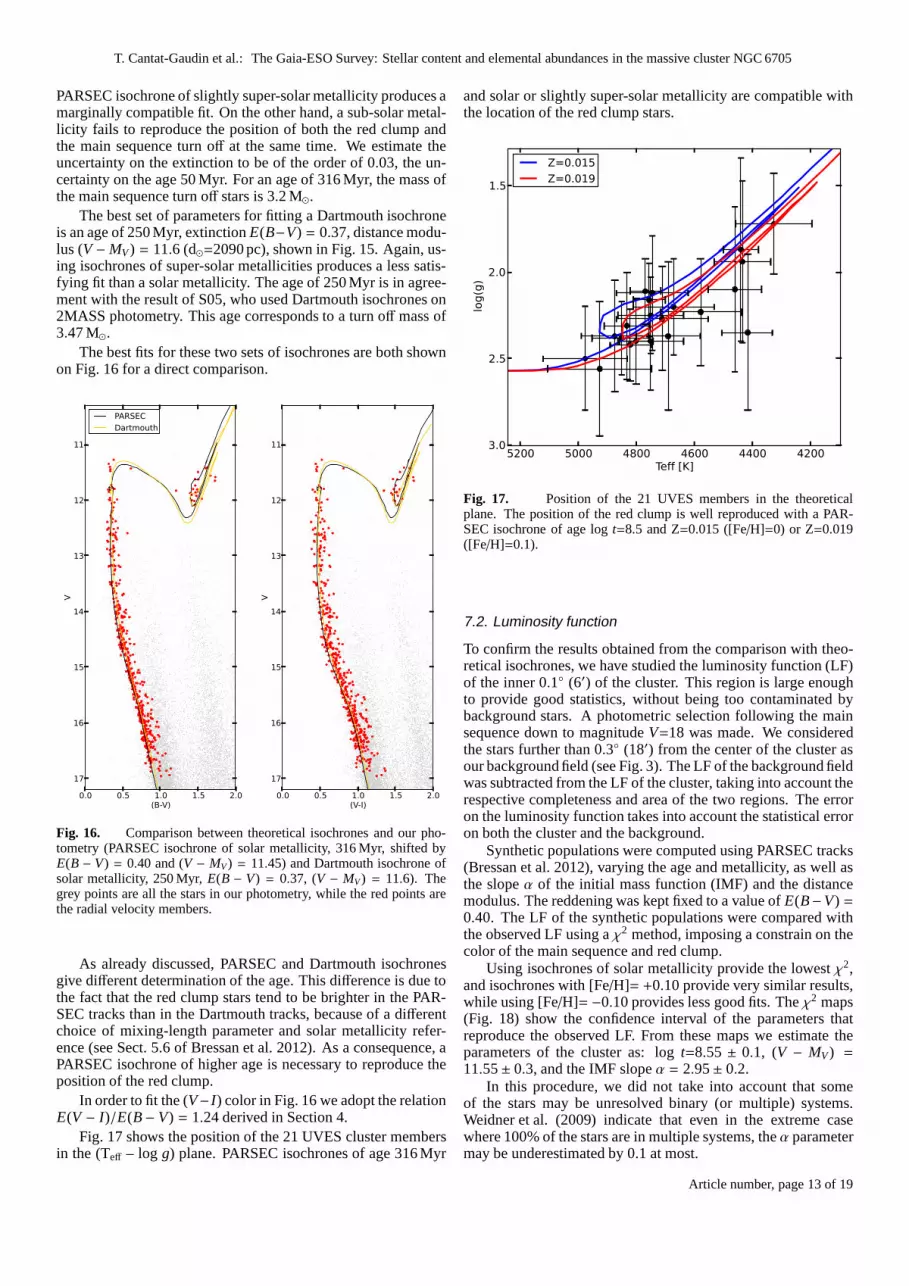
Fig. 17 shows the position of the 21 UVES cluster membersin the (Teff – log g) plane. PARSEC isochrones of age 316 Myr

and solar or slightly super-solar metallicity are compatible withthe location of the red clump stars.

420044004600480050005200Teff [K]

1.5

2.0

2.5

3.0

log(g)

Z=0.015Z=0.019

Fig. 17. Position of the 21 UVES members in the theoreticalplane. The position of the red clump is well reproduced with aPAR-SEC isochrone of age logt=8.5 and Z=0.015 ([Fe/H]=0) or Z=0.019([Fe/H]=0.1).

7.2. Luminosity function

To confirm the results obtained from the comparison with theo-retical isochrones, we have studied the luminosity function (LF)of the inner 0.1◦ (6′) of the cluster. This region is large enoughto provide good statistics, without being too contaminatedbybackground stars. A photometric selection following the mainsequence down to magnitudeV=18 was made. We consideredthe stars further than 0.3◦ (18′) from the center of the cluster asour background field (see Fig. 3). The LF of the background fieldwas subtracted from the LF of the cluster, taking into account therespective completeness and area of the two regions. The erroron the luminosity function takes into account the statistical erroron both the cluster and the background.

Synthetic populations were computed using PARSEC tracks(Bressan et al. 2012), varying the age and metallicity, as well asthe slopeα of the initial mass function (IMF) and the distancemodulus. The reddening was kept fixed to a value ofE(B−V) =0.40. The LF of the synthetic populations were compared withthe observed LF using aχ2 method, imposing a constrain on thecolor of the main sequence and red clump.

Using isochrones of solar metallicity provide the lowestχ2,and isochrones with [Fe/H]= +0.10 provide very similar results,while using [Fe/H]= −0.10 provides less good fits. Theχ2 maps(Fig. 18) show the confidence interval of the parameters thatreproduce the observed LF. From these maps we estimate theparameters of the cluster as: logt=8.55 ± 0.1, (V − MV ) =11.55± 0.3, and the IMF slopeα = 2.95± 0.2.

In this procedure, we did not take into account that someof the stars may be unresolved binary (or multiple) systems.Weidner et al. (2009) indicate that even in the extreme casewhere 100% of the stars are in multiple systems, theα parametermay be underestimated by 0.1 at most.


11.0

11.5

12.0

12.5

13.0

13.5

14.0

V

PARSEC isochrones Solid line: 316 Myr, Z=0.015, E(B-V)=0.4, (V-MV)=11.45

E(B-V)=0.44E(B-V)=0.38

(B-V)

(V-MV)=11.65(V-MV)=11.25

0.4 0.6 0.8 1.0 1.2 1.4 1.6(B-V)

11.0

11.5

12.0

12.5

13.0

13.5

14.0

V

355 Myr282 Myr

0.4 0.6 0.8 1.0 1.2 1.4 1.6(B-V)

[Fe/H]=-0.10[Fe/H]=+0.10

(B-V)

Dartmouth isochrones Solid line: 250 Myr, [Fe/H]=0, E(B-V)=0.37, (V-MV)=11.6

E(B-V)=0.40E(B-V)=0.34

(B-V)

(V-MV)=11.8(V-MV)=11.4

0.4 0.6 0.8 1.0 1.2 1.4 1.6(B-V)

300 Myr

0.4 0.6 0.8 1.0 1.2 1.4 1.6(B-V)

[Fe/H]=0.15

Fig. 15. The grey points are all the stars in our photometry, and the radial velocity members are marked in red.Left-hand side panels: Thebest-fitting PARSEC isochrone (solid blue line) corresponds to an age of 316 Myr, a solar metallicity, a reddeningE(B − V) = 0.40 and a distancemodulus (V−MV ) = 11.45. The four panels show the change in the isochrone when modifying the extinction, distance modulus, age and metallicitywith respect to the best-fitting isochrone.Right-hand side panels: same procedure with Dartmouth isochrones. The best-fittingisochrone is thesolid green line. In all cases, the data are uncorrected for extinction (the isochrones are shifted along the extinctionvector).

7.3. Mass function and total mass

In this section we derive the mass of the cluster using its LF.We produce the LF of the cluster in three annuli (correspondingto distance the ranges 0′ − 3′, 3′ − 6′, and 6′ − 9′) and converttheV magnitudes to masses using a PARSEC isochrone with theparameters determined in section 7.1. The observed magnituderange (V<18) corresponds to a mass range of 1 to 3.2 M⊙. Wehave chosen to limit ourselves to the inner 9′. At larger radii, thecluster is hardly visible against the field stars and our procedurethat consists in subtracting the LF of the background from theobserved one becomes very uncertain.

In each region, we have derived the parameterα, defined asN(M) dM ∝ M−α. The results of the fit are shown in Fig. 19.The value ofα increases with the radius, indicating that the massfunction gets steeper because of a deficit of high-mass stars. Inthe most central region,α = 1.18 indicates an excess of high-mass stars with respect to what would be expected from theSalpeter IMF (α = 2.35). Over the whole range 0 – 9′, the slopeof the mass function isα = 2.70± 0.2.

The previous studies of the evolution of the slope of the IMFwith the radius also found that the mass function was flatter inthe inner region. S05 found a slope ofα = 0.27 in the inner 1.8′,α = 2.41 in the region 1.8 – 10′, andα = 3.88 in the region 10 –21′. Sung et al. (1999) found slopes ofα = 0.5 to 1.7 inside 3′.The slope values found by those two studies are listed in Table 5along with our estimates. The distance ranges given by S05 wereconverted back from parsecs to arcminutes using their valueofthe distance.

0.0 0.1 0.2 0.3 0.4 0.5 0.6 0.7log(M/M⊙)

1.0

1.5

2.0

2.5

3.0

log(co

unts) +

cst

r < 3'α=1.18±0.11

3' < r < 6'α=3.01±0.11

6' < r < 9'α=3.79±0.10

Fig. 19. Mass functions obtained in three different regions of thecluster, showing the flattening of the IMF in the center. The y-axis wasshifted so that the observed number of stars in the lowest mass bin isthe same for all three.

In theory, if the mass function of a cluster is known for itsbrightest stars, it is possible to extrapolate the mass functionsdown to smaller masses and estimate the total stellar mass con-tained in the cluster. When dealing with mass segregated OCspossibly affected by evaporation and tidal mass loss, inferringthe mass function from the observed range to the lower masses



10.6 10.8 11.0 11.2 11.4 11.6 11.8 12.0(V-MV)

8.30

8.35

8.40

8.45

8.50

8.55

8.60

8.65

8.70

log(t)

α=2.95, E(B-V)=0.40

2.6 2.8 3.0 3.2 3.4α

8.30

8.35

8.40

8.45

8.50

8.55

8.60

8.65

8.70

log(t)

(V-MV)=11.3, E(B-V)=0.40

10.6 10.8 11.0 11.2 11.4 11.6 11.8 12.0(V-MV)

2.6

2.8

3.0

3.2

3.4

α

log(t)=8.55, E(B-V)=0.40

11 12 13 14 15 16 17 18 19 20V

100

101

102

103

counts

[Fe/H]=0log(t)=8.55±0.1(V-MV)=11.3±0.3E(B-V)=0.40±0.05α=2.95±0.2

Best-fitting luminosity function

Fig. 18. Probability contours for the fit of the luminosity function.The cyan, yellow, and red lines show the 50%, 68% and 90% confidenceregions, respectively. The white cross indicates the best-fitting solution. The bottom-right panel shows the observedLF (cleaned from thebackground) and the best-fitting theoretical one. The bins with V > 18 are shown but were not used in the fitting procedure.

Table 5. Slope of the mass function in different regions on the cluster.

Radius (′) α

This study0 - 1.8 0.50± 0.150 - 3 1.18± 0.113 - 6 3.01± 0.116 - 9 3.79± 0.100 - 9 2.70± 0.191.8 - 9 3.29± 0.07

Santos et al. (2005)0 - 1.8 0.27± 0.151.8 - 10 2.41± 0.1010 - 21 3.88± 0.200 - 21 2.49± 0.09

Notes. α is the parameter in the mass function:N(M) dM ∝ M−α.

is affected by large uncertainties. To obtain the slope of the massfunction in the non-observed range (under 1 M⊙) we have usedtwo methods. The simplest one is to assume that the slope ofthe power-law derived from the stars with M<1 M⊙ is the sameall over the mass range. The second one is to use the IMF byKroupa et al. (2001):α = 1.3 for 0.08< M⊙ < 0.5 andα = 2.3for 0.5 < M⊙ < 1. For masses over 1 M⊙ we have used the val-

ues obtained from our fit. In the inner region (r<3′) we observe anearly flat mass function, which means that using this slope overthe whole mass range produces fewer low-mass stars than usingthe Kroupa IMF. In the other two regions, the mass function issteeper and in the low-mass range it is well over the prediction ofthe Kroupa IMF. The result of integrating these mass functionsare shown in Table 6 for the different choices of mass functionin the different regions.

When integrating the mass function over the whole 0− 9′

region, we obtain values between 3683± 1063 M⊙ (using theKroupa IMF under 1 M⊙) and 6851± 1865 M⊙ (using the ex-trapolated power-law). This latter number is compatible withthe number quoted by S05, who estimate a total mass of 6500±

2100M⊙ inside 10′, and 11 000± 3800 M⊙ inside 21′ using theIMF slopes listed in Table 6, and the Kroupa IMF under 1 M⊙).Our determination does not take into account the presence ofbinary stars whose percentage is unknown. The effect of thepresence of unresolved binaries on the observedα parameter issmall, but according to Weidner et al. (2009) not accountingforthe presence of multiple systems can hide 15 to 60% of the stel-lar mass of a cluster. In addition, less massive stars could beeither lost from the cluster due to the effect of the disk tidal field,or located in a surrounding halo. For these reasons, our determi-nation is a lower limit to the cluster mass. Owing to the largeun-certainties on the determinations, the derived values of the mass


Table 6. Mass contained in different regions of the cluster.

Region α Observed Extrapolated (power-law) Extrapolated (Kroupa)[′] [M ⊙] [M ⊙] [M ⊙]

0 – 3 1.18± 0.11 242± 64 375± 56 664± 1153 – 6 3.01± 0.11 241± 46 4303± 1127 1430± 1516 – 9 3.79± 0.10 181± 43 18 888± 4702 1437± 242Total 664± 153 26 566± 5885 3531± 5080 – 9 2.70± 0.19 700± 310 6851± 1865 3683± 1063

Notes. α is the parameter in the mass function:N(M) dM ∝ M−α. The stars were observed down to 1 M⊙. The extrapolation was done down to0.08 M⊙.

of NGC 6705 are in reasonable agreement with the virial massesderived in Sect. 6.3.

8. Chemical analysis of the red clump stars

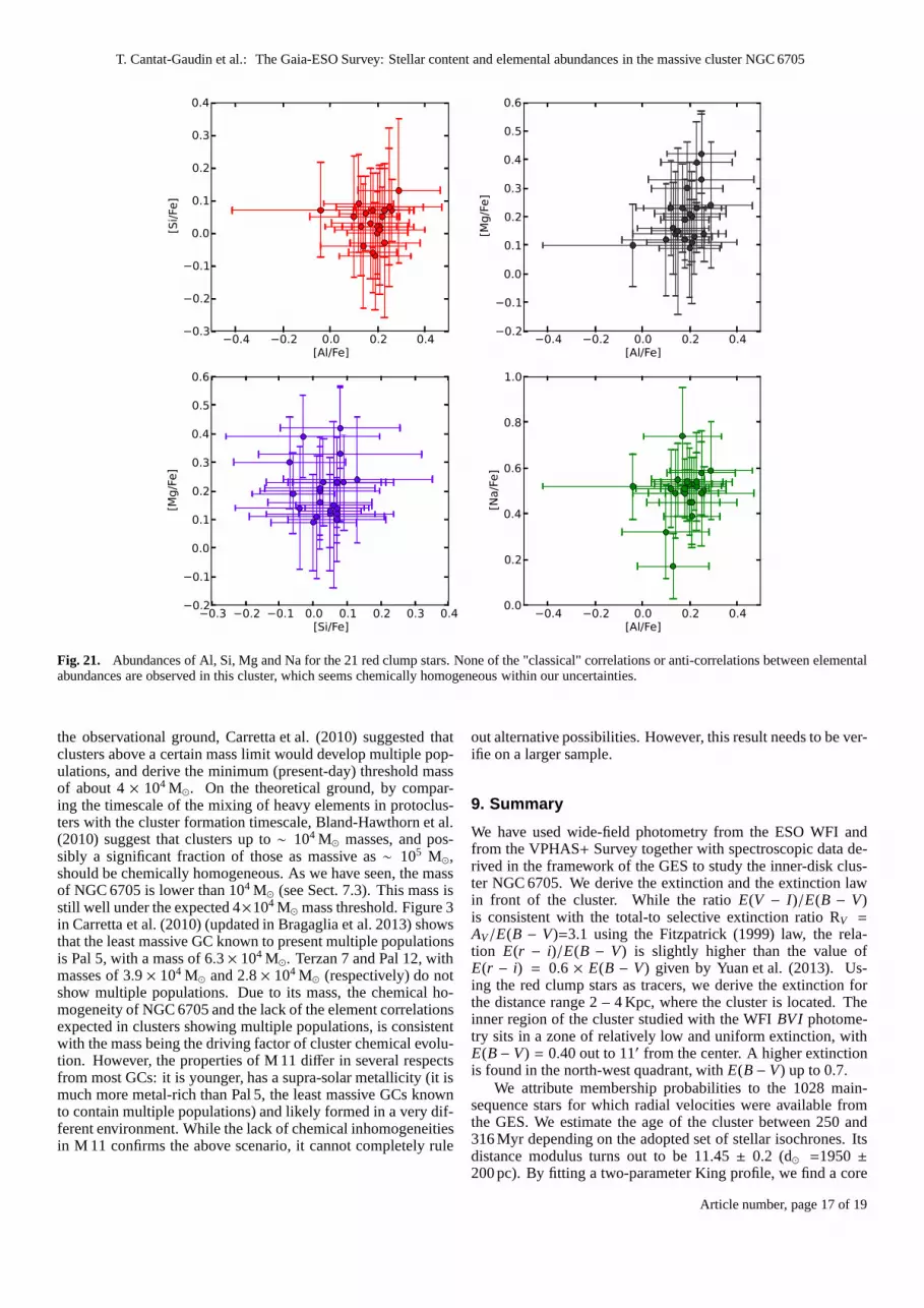
The average iron abundance of the bona-fide members fromUVES spectroscopy is [Fe/H]=0.10 with a dispersion of 0.06.This value is in agreement with Gonzalez & Wallerstein (2000)who found iron abundances between 0.07 and 0.20 from high-resolution spectroscopy of 10 K-giants of NGC 6705 and withthe values we derived from isochrone fitting. In this sectionwestudy the relations between the abundances of Al and of otherproton-capture elements Na, Mg, and Si. Al and Na abundancesare plotted against Teff and logg in Fig. 20. These abundancesdo not display any significant trend. We observe star-to-star vari-ations in the Al and Na content of the order of 0.2 dex, inside theexpected uncertainties. Similar diagnostics for Mg and Si areshown in Magrini et al. (2014).

Abundances of Al, Mg, Si and Na are plotted in Fig. 21.In case of multiple populations, correlations between the abun-dances of Al and Si, and between Al and Na, and anti-correlations between Si and Mg and between Al and Mg(Gratton et al. 2012) can be found. Models predict that Al shouldshow correlations with elements that are enhanced by the ac-tion of the Ne–Na (such as Na) and Mg–Al cycles, and is anti-correlated with elements that are depleted in H burning at hightemperature (such as O and Mg). We do not see any sign of such(anti-)correlations within our uncertainties.

One star shows a low Al abundance with a large uncertainty,with [Al /Fe]= −0.04± 0.38, probably due to the low number ofdetected lines for this element. Two outliers in Na abundancecould suggest an internal spread, but they are still compatiblewith a homogeneous cluster within the uncertainties. The starwith the highest Na abundance ([Na/Fe]=+0.74dex) has the low-est Fe abundance in the sample ([Fe/H]=+0.03dex), while thestar with the lowest Na content ([Na/Fe]=+0.17dex) has a Fecontent [Fe/H]=+0.18dex. This suggests that the apparent dis-crepant [Na/Fe] for that star can be explained by considering theuncertainties on both Na and Fe abundances.

The mean [Na/Fe] for the cluster members is 0.48 dex. Thisvalue is significantly higher than the Na abundance derived infield stars. (Soubiran & Girard 2005) show that at high metal-licities thin disk stars exhibit an average of [Na/Fe]=0.11dex,even though they notice a rise at super-solar metallicities. For allelements presented here, the abundances were calculated intheLTE approximation. Na is subject to deviations from LTE (e.g.,Lind et al. 2011). The effect of non-LTE correction in stars ofsuper-solar metallicity is expected to be small, but could lowerthe Na abundance of our sample by 0.15–0.20dex at most. On aside note, since the corrections depend on the evolutionarystage

4000 4200 4400 4600 4800 5000 5200Teff [K]

0.0

0.2

0.4

0.6

0.8

[X/Fe]

[Na/Fe][Al/Fe]

1.2 1.4 1.6 1.8 2.0 2.2 2.4 2.6 2.8 3.0log(g)

0.0

0.2

0.4

0.6

0.8

[X/Fe]

Fig. 20. Solar-scaled abundances of [Na/Fe] (blue filled dots) and[Al /Fe] (red open squares) for the 21 UVES member stars, as a functionof Teff and logg.

of the star, we expect them to affect all of the red clump stars inthe same way, and not to create an additional spread in Na.

The approach presented in Sect. 6.2 to estimate the intrinsicradial velocity dispersion of the sample can also be appliedtothe elemental abundances. Assuming an intrinsic Gaussian dis-tribution of the abundance for each element, the most probablemean abundance (µ) and intrinsic dispersion (σ) we computedare listed in Table 4. For all five elements, the observed distri-bution is compatible with the cluster being homogeneous, andthe observed spread can be entirely attributed to the individualuncertainties.

As far as we can see, NGC 6705 is clearly a homogeneousobject where the star-to-star scatter is explained by the uncer-tainties on the determination of the chemical abundances. On



−0.4 −0.2 0.0 0.2 0.4[Al/Fe]

−0.3

−0.2

−0.1

0.0

0.1

0.2

0.3

0.4

[Si/Fe]

−0.4 −0.2 0.0 0.2 0.4[Al/Fe]

−0.2

−0.1

0.0

0.1

0.2

0.3

0.4

0.5

0.6

[Mg/Fe]

−0.3 −0.2 −0.1 0.0 0.1 0.2 0.3 0.4[Si/Fe]

−0.2

−0.1

0.0

0.1

0.2

0.3

0.4

0.5

0.6

[Mg/Fe]

−0.4 −0.2 0.0 0.2 0.4[Al/Fe]

0.0

0.2

0.4

0.6

0.8

1.0

[Na/Fe]

Fig. 21. Abundances of Al, Si, Mg and Na for the 21 red clump stars. Noneof the "classical" correlations or anti-correlations between elementalabundances are observed in this cluster, which seems chemically homogeneous within our uncertainties.

the observational ground, Carretta et al. (2010) suggestedthatclusters above a certain mass limit would develop multiple pop-ulations, and derive the minimum (present-day) threshold massof about 4× 104 M⊙. On the theoretical ground, by compar-ing the timescale of the mixing of heavy elements in protoclus-ters with the cluster formation timescale, Bland-Hawthornet al.(2010) suggest that clusters up to∼ 104 M⊙ masses, and pos-sibly a significant fraction of those as massive as∼ 105 M⊙,should be chemically homogeneous. As we have seen, the massof NGC 6705 is lower than 104 M⊙ (see Sect. 7.3). This mass isstill well under the expected 4×104 M⊙ mass threshold. Figure 3in Carretta et al. (2010) (updated in Bragaglia et al. 2013) showsthat the least massive GC known to present multiple populationsis Pal 5, with a mass of 6.3× 104 M⊙. Terzan 7 and Pal 12, withmasses of 3.9× 104 M⊙ and 2.8× 104 M⊙ (respectively) do notshow multiple populations. Due to its mass, the chemical ho-mogeneity of NGC 6705 and the lack of the element correlationsexpected in clusters showing multiple populations, is consistentwith the mass being the driving factor of cluster chemical evolu-tion. However, the properties of M 11 differ in several respectsfrom most GCs: it is younger, has a supra-solar metallicity (it ismuch more metal-rich than Pal 5, the least massive GCs knownto contain multiple populations) and likely formed in a verydif-ferent environment. While the lack of chemical inhomogeneitiesin M 11 confirms the above scenario, it cannot completely rule

out alternative possibilities. However, this result needsto be ver-ifie on a larger sample.

9. Summary

We have used wide-field photometry from the ESO WFI andfrom the VPHAS+ Survey together with spectroscopic data de-rived in the framework of the GES to study the inner-disk clus-ter NGC 6705. We derive the extinction and the extinction lawin front of the cluster. While the ratioE(V − I)/E(B − V)is consistent with the total-to selective extinction ratioRV =

AV/E(B − V)=3.1 using the Fitzpatrick (1999) law, the rela-tion E(r − i)/E(B − V) is slightly higher than the value ofE(r − i) = 0.6 × E(B − V) given by Yuan et al. (2013). Us-ing the red clump stars as tracers, we derive the extinction forthe distance range 2 – 4 Kpc, where the cluster is located. Theinner region of the cluster studied with the WFIBVI photome-try sits in a zone of relatively low and uniform extinction, withE(B − V) = 0.40 out to 11′ from the center. A higher extinctionis found in the north-west quadrant, withE(B − V) up to 0.7.

We attribute membership probabilities to the 1028 main-sequence stars for which radial velocities were available fromthe GES. We estimate the age of the cluster between 250 and316 Myr depending on the adopted set of stellar isochrones. Itsdistance modulus turns out to be 11.45± 0.2 (d⊙ =1950 ±200 pc). By fitting a two-parameter King profile, we find a core


radius of 1.23± 0.28′ (0.69± 0.23 pc). The brightest stars ofthe cluster show a tighter spatial distribution, while the fainteststars are more widely distributed. Studying the mass function indifferent regions of the cluster shows that the inner parts con-tain a larger proportion of massive stars than the outer parts,confirming that NGC 6705 is undergoing mass segregation. Us-ing the velocity dispersion of the sample of members stars ob-served by the GES consortium using UVES, we derive the virialmass of Mtot = 5083± 1600 M⊙, in agreement with the virialmass of 5621 M⊙ found by McNamara & Sanders (1977) usingproper motions. The sample of stars observed by GIRAFFE overa larger radius presents considerably higher velocity dispersion(4.52′ and 2.8 km s−1, respectively). This sample leads to a virialmass of 21 900±2700M⊙. However, the uncertainties on the GI-RAFFE RVs are most likely underestimated, and this high virialmass must be considered an upper limit. We estimated a massfrom photometry, converting theV-band luminosity function to amass function. When integrating the mass function of the whole0-9′ region, we obtain values between 3683± 1063 M⊙ (usingthe Kroupa IMF under 1 M⊙) and 6851± 1865M⊙ (using theextrapolated power-law).

The GES data enables us to study the chemical compositionof the red clump stars. We find an iron abundance [Fe/H]=0.10with a dispersion of 0.06. Despite being a massive open cluster,NGC 6705 does not show any sign of an inhomogeneous stellarpopulation of the kind observed in globular clusters. This clusteris well below the mass limit of 4× 104 M⊙ proposed in literaturefor clusters hosting multiple populations. However, few massiveclusters have been observed with high-resolution spectroscopy,and more studies are needed in order to observationally confirmthis mass threshold.

The reliability of the results that can be obtained for stellarclusters greatly depends on the determination of the member-ship and chemical abundances in the inner regions and in theoutskirts, where haloes of unbound stars can be present. This es-pecially holds for open clusters, which are more affected by thetidal field of the disks and by background contamination. Thesynergy between the GES and the ground-based surveys in gen-eral and the Gaia mission will provide invaluable information onthe chemical abundances, distances and proper motions of unbi-ased samples of stars, allowing for more accurate determinationsof the cluster properties.

Acknowledgements

Based on data products from observations made with ESO Tele-scopes at the La Silla Paranal Observatory under programme ID188.B-3002. This work was partially supported by the Gaia Re-search for European Astronomy Training (GREAT-ITN) MarieCurie network, funded through the European Union SeventhFramework Programme (FP7/2007-2013)under grant agreementno. 264895, partly supported by the European Union FP7 pro-gramme through ERC grant number 320360 and by the Lev-erhulme Trust through grant RPG-2012-541. We acknowl-edge the support from INAF and Ministero dell’ Istruzione,dell’Università’ e della Ricerca (MIUR) in the form of thegrants "Premiale VLT 2012" and "The Chemical and DynamicalEvolution of the Milky Way and Local Group Galaxies" (prot.2010LY5N2T).

The results presented here benefit from discussions held dur-ing the Gaia-ESO workshops and conferences supported by theESF (European Science Foundation) through the GREAT Re-search Network Programme. This work was supported in partby the National Science Foundation under Grant No. PHYS-

1066293 and the hospitality of the Aspen Center for Physics dur-ing summer 2013.

The authors wish to thank M. Bellazzini for his suggestionsand comments that helped improve this work.

L.S. aknowledges the support of Project IC120009 "Millen-nium Institute of Astrophysics (MAS)" of Iniciativa CientíficaMilenio del Ministerio de Economía, Fomento y Turismo deChile.

T.B. was funded by grant No. 621-2009-3911 from TheSwedish Research Council. I.S.R. gratefully acknowledgesthesupport provided by the Gemini-CONICYT project 32110029.S.V. gratefully acknowledges the support provided by FONDE-CYT N. 1130721.

ReferencesAllison, R. J., Goodwin, S. P., Parker, R. J., et al. 2009, MNRAS, 395, 1449Bastian, N., Silva-Villa, E. 2013, MNRAS, 431, L122Bastian, N., Lamers, H. J. G. L. M., de Mink, S. E., et al. 2013,MNRAS, 436,

2398Bellazzini, M., Bragaglia, A., Carretta, E., Gratton, R. G., Lucatello, S., Catan-

zaro, G., Leone, F. 2012, A&A, 493, 959Bianchini, P., Varri, A. L., Bertin, G., Zocchi, A. 2013, ApJ, 772, 67Bland-Hawthorn, J., Karlsson, T., Sharma, S., Krumholz, M.and Silk, J. 2010,

ApJ, 721, 582Bragaglia, A., Gratton, R. G., Carretta, E., et al. 2012, A&A, 548, A122Bragaglia, A., Sneden, C., Gratton. R.G., Carretta, E., Lucatello, S. 2013, ApJ,

submittedBressan, A., Marigo, P., Girardi, L., et al. 2012, MNRAS, 427, 127Cabrera-Cano J., Alfaro E. J., 1985, A&A, 150, 298Carretta, E., Bragaglia, A., Gratton, R. G., et al. 2009, A&A, 505, 117Carretta, E., Bragaglia, A., Gratton, R. G., & Lucatello, S.2009, A&A, 505, 139Carretta, E., Bragaglia, A., Gratton, R. G., et al. 2010, A&A, 516, A55Carretta, E., Bragaglia, A., Gratton, R. G., et al. 2013, A&A, 561, A87Cote, P., Welch, D. L., Fischer, P., Gebhardt, K. 1995, ApJ, 454, 788Decressin, T., Meynet, G., Charbonnel, C., Prantzos, N., & Ekström, S. 2007,

A&A, 464, 1029D’Ercole, A., Vesperini, E., D’Antona, F., McMillan, S. L. W., & Recchi, S.

2008, MNRAS, 391, 825Donati, P., Bragaglia, A., Cignoni, M., Cocozza, G., Tosi, M. 2012, MNRAS,

424, 1132D’Orazi, V., Lucatello, S., Gratton, R., et al. 2010, ApJ, 713, L1Drew, J. E., Gonzalez-Solares, E., Greimel, R. et al. 2014, MNRAS, 440, 2036Dotter, A., Chaboyer, B., Jevremovic, D., et al. 2008, ApJS, 178, 89Fitzpatrick E. L., 1999, PASP, 111, 6Geisler, D., Villanova, S., Carraro, G., et al. 2012, ApJ, 756, L40Gilmore, G., Randich, S., Asplund, M., et al. 2012, The Messenger, 147, 25Gonzalez, G., Wallerstein, G. 2000, PASP, 112, 1081Gratton, R. G., Bonifacio, P., Bragaglia, A., et al. 2001, A&A, 369, 87Gratton, R., Sneden, C., & Carretta, E. 2004, ARA&A, 42, 385Gratton, R. G., Carretta, E., & Bragaglia, A. 2012, A&A Rev.,20, 50Grevesse, N., Asplund, M., Sauval, A. J. 2007, SSRv,130, 105Gustafsson, B., Edvardsson, B., Eriksson, K., et al., 2008,A&A, 486, 951Heiter, U., and the GES Line List group, in preparation.Jofre P., Heiter U., Soubiran C. et al. 2013, arXiv:1309.1099Johnson, C. I., & Pilachowski, C. A. 2010, ApJ, 722, 1373King, I. 1962, AJ, 67, 471Koo, J.-R., Kim, S.-L., Rey, S.-C., et al. 2007, PASP, 119, 1233Kraft, R. P. 1979, ARA&A, 17, 309Kraft, R. P. 1994, PASP, 106, 553Kroupa, P. 2001, MNRAS, 322, 231Lee, Y.-W., Joo, J.-M., Sohn, Y.-J., Rey, S.-C., Lee, H.-C.,Walker, A.R. 1999,

Nature 402, 55Lind, K., Primas, F., Charbonnel, C., Grundahl, F., & Asplund, M. 2009, A&A,

503, 545Lind K., Asplund M., Barklem P. S., Belyaev A. K., 2011, A&A, 528, A103Lovis, C., Mayor, M. 2007, A&A, 472, 657Magrini, L., Sestito, P., Randich, S., & Galli, D. 2009, A&A,494, 95Magrini, L., Randich, S., Zoccali, M., et al. 2010, A&A, 523,A11Magrini, L., Randich, S., Romano, D., et al. 2014, A&A, 563, 44Marino, A. F., Villanova, S., Piotto, G., et al. 2008, A&A, 490, 625Marino, A. F., Sneden, C., Kraft, R. P., et al. 2011, A&A, 532,A8Martell, S. L., Smolinski, J. P., Beers, T. C., Grebel, E. K. 2011, A&A, 534,

A136Mathieu, R. D. 1984, ApJ, 284, 643McNamara, B. J., Sanders, W. L. 1977, A&A, 54, 569


http://de.arxiv.org/abs/1309.1099


Messina, S., Parihar, P., Koo, J.-R., et al. 2010, A&A, 513, A29

Milone, A. P., Piotto, G., Bedin, L. R., et al. 2012, ApJ, 744,58

Miocchi, P. 2006, MNRAS, 366, 227

Piotto, G. 2009, IAU Symposium, 258, 233

Randich, S., Gilmore, G. 2013, The Messenger, 154, 47

Ramírez, S. V., & Cohen, J. G. 2002, AJ, 123, 3277

Robin, A. C., Reylé, C., Derrière, S., Picaud, S. 2003, A&A, 409, 523

Sacco, G. G., Morbidelli, L., Franciosini, E. et al. 2014, A&A, 565, 113

Santos, Jr., J. F. C., Bica, E., Dottori, H. 1990, PASP, 102, 454

Santos, Jr., J. F. C., Bonatto, C., Bica, E. 2005, A&A, 442, 201

Schlegel D. J., Finkbeiner D. P., Davis M., 1998, ApJ, 500, 525

Soubiran, C., Girard, P. 2005, A&A, 438, 139

Spina L. et al., submitted.

Spitzer L. Jr., 1969, ApJ, 158, L139

Stetson P. B., 1987, PASP, 99, 191

Sung, H., Bessell, M. S., Lee, H.-W., Kang, Y. H., Lee, S.-W. 1999, MNRAS,310, 982

Vallenari, A., Pasetto, S., Bertelli, G., et al. 2006, A&A, 451, 125

Vandame, B. 2002, in Society of Photo-Optical Instrumentation Engineers(SPIE) Conference Series, Vol. 4847, Society of Photo-Optical Instrumen-tation Engineers (SPIE) Conference Series, ed. J.-L. Starck & F. D. Murtagh,123–134

Ventura, P., D’Antona, F., Mazzitelli, I., & Gratton, R. 2001, ApJ, 550, L65

Villanova, S., Geisler, D., Carraro, G., Moni Bidin, C., Munoz, C. 2013, A&A,778, 186

Walker, M. G., Mateo, M., Olszewski, E. W., et al. 2006, AJ, 131, 2114

Weidner, C., Kroupa, P., Maschberger, T., 2009, MNRAS, 393,663

Yuan H. B., Liu X. W., Xiang M. S., 2013, MNRAS, 430, 2188

Zacharias, N., Finch, C. T., Girard, T. M., et al. 2012, VizieR Online Data Cata-log: I/322

1 Dipartimento di Fisica e Astronomia, Università di Padova,vicoloOsservatorio 3, 35122 Padova, Italy

2 INAF-Osservatorio Astronomico di Padova, vicolo Osservatorio 5,35122 Padova, Italy

3 INAF-Osservatorio Astronomico di Bologna, via Ranzani 1, 40127Bologna, Italy

4 School of Physics, Astronomy & Maths, University of Hertford-shire, Hatfield, Herts. AL10 9AB, UK

5 Thueringer Landessternwarte, Sternwarte 5, 07778, Tautenburg,Germany

6 CASU, Institute of Astronomy, Madingley Road, University ofCambridge, CB3 0HA, UK

7 IGAM, Institute of Physics, University of Graz, Universitätsplatz. 5,A-8010 Graz, Austria

8 Departament d’Astronomia i Meteorologia, Universitat deBarcelona, Avda. Diagonal 647, E-08028 Barcelona, Spain

9 Royal Observatory of Belgium, Ringlaan 3, 1180 Brussel, Belgium10 Instituto de Astrofísica de Andalucía, CSIC, Apdo 3004, 18080

Granada, Spain11 European Southern Observatory, Karl-Schwarzschild-Str.2, 85748

Garching bei München, Germany12 Department for Astrophysics, Nicolaus Copernicus Astronomical

Center, ul. Rabianska 8, 87-100 Torun, Poland13 INAF-Osservatorio Astrofisico di Arcetri, Largo E. Fermi, 5, 50125

Firenze, Italy14 Dipartimento di Fisica e Astronomia, Università di Bologna, via

Ranzani 1, 40127 Bologna, Italy15 Department of Astronomy, Indiana University, Bloomington, IN

47405, USA16 Massachusetts Institute of Technology and Kavli Institutefor Astro-

physics and Space Research, 77 Massachusetts Avenue, Cambridge,MA 02139, USA

17 Institute of Theoretical Physics and Astronomy, Vilnius University,Goštauto 12, LT-01108 Vilnius, Lithuania

18 INAF - Astrophysical Observatory of Torino, via Osservatorio 20,10025 Pino Torinese, Italy

19 Section of Astrophysics, Astronomy and Mechanics, Department ofPhysics, University of Athens, GR-15784 Athens, Greece

20 INAF - Osservatorio Astrofisico di Catania, via S. Sofia 78, 95123Catania, Italy

21 Institute of Astronomy, University of Cambridge, Madingley Road,Cambridge CB3 0HA, UK

22 Lund Observatory, Department of Astronomy and TheoreticalPhysics, Box 43, SE-221 00

23 INAF - Osservatorio Astronomico di Palermo, Piazza del Parla-mento 1, 90134, Palermo, Italy

24 Departamento de Astronomía, Universidad de Concepción, Casilla160-C, Concepción, Chile

25 Laboratoire Lagrange (UMR7293), Université de Nice SophiaAn-tipolis, CNRS, Observatoire de la Côte d’Azur, BP 4229, F-06304Nice cedex 4, France

26 Spanish Virtual Observatory, Centro de Astrobiología (INTA-CSIC), P.O. Box 78, 28691 Villanueva de la Cañada, Madrid, Spain

27 Millennium Institute of Astrophysics, Av. Vicuña Mackenna4860,782-0436 Macul, Santiago, Chile

28 Pontificia Universidad Católica de Chile, Av. Vicuña Mackenna4860, 782-0436 Macul, Santiago, Chile


Download - The Gaia -ESO Survey: Stellar content and elemental abundances in the massive cluster NGC 6705

Top Related