Download - Temporal motifs in time-dependent networks

Temporal motifs in time-dependent networks
Lauri Kovanen1, Marton Karsai1, Kimmo Kaski1, Janos
Kertesz1,2 and Jari Saramaki1
1 Department of Biomedical Engineering and Computational Science, Aalto
University School of Science, P.O. Box 12200, FI-00076, Finland2 Institute of Physics, BME, Budapest, Budafoki ut 8., H-1111, Hungary
E-mail: [email protected]
Abstract. Temporal networks are commonly used to represent systems where
connections between elements are active only for restricted periods of time, such as
networks of telecommunication, neural signal processing, biochemical reactions and
human social interactions. We introduce the framework of temporal motifs to study
the mesoscale topological-temporal structure of temporal networks in which the events
of nodes do not overlap in time. Temporal motifs are classes of similar event sequences,
where the similarity refers not only to topology but also to the temporal order of the
events. We provide a mapping from event sequences to colored directed graphs that
enables an efficient algorithm for identifying temporal motifs. We discuss some aspects
of temporal motifs, including causality and null models, and present basic statistics of
temporal motifs in a large mobile call network.
PACS numbers: 89.75.-k, 05.45.-Tp, 89.75.Hc
arX
iv:1
107.
5646
v2 [
phys
ics.
data
-an]
10
Oct
201
1

Temporal motifs in time-dependent networks 2
1. Introduction
The network approach, where interacting elements are represented as nodes and
interactions as edges, has become widely used in the study of complex systems [1, 2].
Although this approach unquestionably discards many details, it has turned out to
provide much insight into the function and dynamics of the systems in question. Many
large networks display similar properties on the global scale, such as broad degree
distributions, short path lengths, and abundance of triangles; on the mesoscopic level,
complex networks often display community structure [3]. There is much variation
in the mesoscale structure of different networks [4, 5], reflecting different underlying
functional and dynamical mechanisms. Such differences can also be observed in the
relative significance of motifs, sets of small topologically equivalent subgraphs [6, 7].
The concept of motifs has also been generalized to unweighted [6, 7] and weighted [8]
networks.
Static networks are often time-aggregates of systems where connections are not
continuously active but established only during limited periods of time. This temporal
aspect turns out to be crucial for processes like spreading of information and electronic
viruses in communication networks [9, 10, 11, 12, 13, 14, 15], epidemiological applications
[16, 17], and signal processing in the brain (see, e.g., [18, 19]). Sometimes temporal
aspects such as link activation frequencies are incorporated in the static network
representation as link weights, which are then assumed to affect dynamic processes
like spreading in probabilistic mean field manner. However, it has recently become clear
that temporal inhomogeneities not captured by this approach have an important effect
on many processes [12, 13, 14, 15, 16].
In this article we use the temporal networks approach (see, e.g., [20] and [21] for
a review) to study the details of link activations without projecting out the temporal
dimension. While static networks consist of nodes and edges, temporal networks consist
of nodes and events. A (directed) event ei = (ni,1, ni,2, ti, δi) connects the two nodes
ni,1 → ni,2 only during the time interval from ti to ti + δi. Our presentation uses
directed events for generality, but undirected events can be used with minimal changes.
We restrict ourselves to the case where nodes cannot participate in simultaneous events,
i.e., at any given time at most one event can be assigned to a node.
It is reasonable to expect temporal networks to have mesoscale structures both in
topology and time. These structures are likely to reflect the function of the system even
better than mesoscale structures in static networks and thus their characterization can
improve our understanding of various complex systems, from the nature of human social
interactions and information processing by groups to temporal patterns that determine
the outcomes of dynamical processes like spreading. Nicosia et al. have studied strongly
and weakly connected components in temporal networks [22]. Braha and Bar-Yam [23]
have studied motifs in static snapshot networks, aggregated over one day of email data,
and found that dense subgraphs are overrepresented. Bajardi et al. [24] have defined
dynamical motifs as sequences of connected events belonging to adjacent time windows
Temporal motifs in time-dependent networks 3
of network aggregation. In essence, these are time-respecting paths [25, 9], that is, linear
chains of events, and are thus different from the temporal motifs discussed in this paper.
Zhao et al. [26] have studied communication motifs in electronic social networks with
an approach that has some similarity to the approach we take in this paper – they, too,
consider subsets of communication events where the time between consecutive events
sharing a node is within a chosen threshold time. However, in their analysis, the time
dimension of such temporal subgraphs appears to have been projected out by projecting
the patterns into static subgraphs.
The temporal motifs we introduce here can be used to study the full mesoscale
topological-temporal structure of temporal networks. We also present an efficient
algorithm for identifying all temporal motifs in empirical data sets on temporal graphs,
that is, time-stamped sequences of events between nodes. In static networks the motifs
are—in a very general sense—defined as classes of isomorphic, connected subgraphs. We
define temporal motifs analogously, first by defining connected subgraphs in temporal
networks and then by extending the definition of isomorphism such that it also takes
into account the temporal information in these subgraphs.
As an example, in a social communication network one might detect an event
sequence where Alice calls Bob, who then calls Carol and Dave. A similar sequence
might be observed to often take place between the same people, as well as between
other sets of four individuals. All these sequences are members of the same class,
which we call a temporal motif. In genetic regulation data the event sequence would
correspond to regulatory interactions switching on and off as the intercellular system
performs its function. In addition to providing insight into the operation of the system
under study, temporal motifs allow studying similarities and differences of temporal
networks, as originally proposed for static motifs in [7]. In addition they may help in
building models of network evolution [27].
We start with a formal definition of temporal motifs in Section 2, and then cover
the main ideas of the identification algorithm. In Section 4 we discuss some useful
generalizations and show how they can also be implemented efficiently. Section 5 glances
at different methods for evaluating the significance of the observed motif counts. Finally,
in Section 6 we use the methods to identify temporal motifs in a large temporal network
constructed from mobile phone data and discuss the insights the motifs provide. A
detailed account on all algorithms is provided in the Appendix.
2. Temporal motifs
Static motifs are classes of isomorphic subgraphs. While there is variation in exactly
what kind of subgraphs are studied, it is practically always required that these subgraphs
be connected. For static graphs connectivity means that there is a path between all pairs
of nodes, or equivalently that there is a sequence of mutually adjacent edges between
all pairs of edges, where two edges are adjacent if they have one node in common.
In temporal networks the definition of adjacency should intuitively also include

Temporal motifs in time-dependent networks 4
time; two calls made by the same person a month apart are hardly close to each other.
We consider two events ∆t-adjacent if they have at least one node in common and
the time difference between the end of the first event and the beginning of the second
event is no longer than ∆t. Equivalently, two events are ∆t-connected if there exists a
sequence of events ei = ek0ek1 . . . ekn = ej such that all pairs of consecutive events are
∆t-adjacent.‡Using these definitions, a connected temporal subgraph consists of a set of events such
that all pairs of events in it are ∆t-connected. This ensures that subgraphs are connected
both topologically and temporally§. While this definition could already be used as a
basis of temporal motifs, it suffers from the same shortcoming as its static cousin: in
some simple cases the number of connected subgraphs explodes. For example an n-star
where all events take place within ∆t contains(nk
)connected temporal subgraphs with
k events, which would make the resulting motif statistics difficult to interpret in any
intuitive fashion.
With static motifs the most common restriction is to require the subgraphs to be
both connected and induced, i.e. require that they include all edges between the nodes
in the subgraph. While this choice does reduce the number of subgraphs and makes it
easier to interpret the resulting motifs, it unfortunately fails to solve the problem with
the n-star above.
With temporal networks our choices are not as restricted. One alternative is to
consider only those connected subgraphs where all ∆t-connected events of each node
are consecutive. This not only solves the problem with the n-star—we now get n−k+1
subgraphs with k events—but also offers an intuitive interpretation: each subgraph
takes into account all relevant events for each node within the time span covered for
that node, in the sense that no events can be skipped. We call connected subgraphs
that satisfy this requirement valid temporal subgraphs and denote them by E∗. Figure
1 illustrates the concept.
Temporal motifs are now defined as classes of isomorphic valid subgraphs, where
the isomorphism is taken to include also the similarity of the temporal order of events.
Accordingly, two temporal subgraphs are isomorphic if they are topologically equivalent
and the order of their events is identical. In cases where the requirement for the identity
of the full order of events is too strict, it can easily be weakened. This is discussed in
Section 4.
Some special temporal motifs are worth mentioning. The unit set E∗ = {ei} is
trivially a valid subgraph for all events, and hence the smallest temporal motif contains
only one event. For every event ei there is a unique maximal subgraph E∗max that
contains ei and in which all event pairs are still ∆t-connected. The maximal subgraph
is always also a valid subgraph. When motifs are based only on maximal subgraphs
they are called maximal motifs.
‡ Note that this sequence does not need to be a journey, i.e. the events need not be temporally ordered.§ This is different from the approach taken by Zhao et al. [26], where temporal subgraphs may be
topologically disconnected.

Temporal motifs in time-dependent networks 5
Figure 1. (a) An example event data set E with six events. Durations have been
omitted for simplicity. With ∆t = 10 there are two maximal subgraphs, shown in (b)
and (c). (d) Valid subgraphs contained in the maximal subgraph in (b). In addition
to these the maximal subgraph itself and all unit subgraphs are valid subgraphs. The
maximal subgraph in (c) does not contain other valid subgraphs than the maximal and
unit subgraphs. (e) Event sets that are contained in (b) but are not valid subgraphs:
the upper one because it is not ∆t-connected, the lower one because it does not include
all consecutive ∆t-connected events of node c.
The presented definition for temporal subgraph is meaningful only when each node
is involved in at most one event at a time. When overlapping events are allowed, the
large number of different situations that can arise in the most general case makes it
more difficult to define temporal subgraphs in such a way that the results could still be
easily interpreted. Yet the prospects of such a definition are enticing, as it would allow
for the exploration of almost any temporal network data, for example transportation
networks [28] and time-varying brain functional networks [29].
3. Algorithm for identification of temporal motifs
Because maximal subgraphs are temporally separated from all other events by at least
time ∆t, all subgraphs are fully contained in some maximal subgraph. Based on this
observation the process of identifying all temporal motifs in a given event set E can be
separated to three parts:
(i) Find all maximal connected subgraphs E∗max.

Temporal motifs in time-dependent networks 6
(ii) Find all valid subgraphs E∗ ⊆ E∗max.
(iii) Identify the motif corresponding to E∗.
To find the maximal subgraph where ei belongs to, we start from ei and iterate
forward and backward in time to find all ∆t-adjacent events; this process is then repeated
recursively with all new events encountered. Assuming the ∆t-adjacent events can be
found in constant time, the time complexity of this step is O(|E∗max|). Since the same
maximal set is discovered starting from any event in it, the total time complexity of this
part is O(|E|).For the second part, consider an undirected graph G where the vertices corresponds
to events in E∗max and there is an edge between two vertices if those events are ∆t-
adjacent and consecutive for either node. Now each valid subgraph contained in E∗max
corresponds to some connected vertex set of G (see Appendix A for proof), and the
problem of finding all valid temporal subgraphs reduces to identifying all induced
subgraphs of G and checking that the events of each node are consecutive. The algorithm
for identifying valid subgraphs is given in Appendix A.
Identifying the motif for subgraph E∗ requires solving the isomorphism problem
such that we also include information about the order of the events. We do this by
mapping all relevant information into a directed and coloured‖ graph as illustrated in
Figure 2, for which the isomorphism can be readily solved with existing algorithms.
In practice we calculate for this graph its canonical form, a labeling of vertices that
is identical for all isomorphic graphs, so that we can easily tell if two valid subgraphs
correspond to the same motif. Finding the canonical form is a non-trivial task, but many
efficient algorithms have been developed for this purpose; the one we used is called bliss
and described in [31].
As a final step, to make temporal motifs more accessible we convert the information
about the order of events back into plain integers. Figure 2e shows a concise presentation
of the motif corresponding to the original temporal subgraph in Figure 2a.
4. Flow motifs and partial order of events
Assuming that the node colours are denoted by integers—as is often the case—we could
have used the colours to mark the order of events in Figure 2c instead of putting in
additional links. The edge notation, however, has another benefit: it can be used to
denote a partial order of events. Unlike total order, partial order does not necessarily
define the order of all pairs. For example, an order where ei takes place before both ejand ek, but the mutual order of ej and ek remains undefined, is a partial order and as
such cannot be represented with integer labels.
To see why this is useful, consider mobile phone communication where information
flows both ways—both can talk regardless of who placed the call—and the two temporal
‖ In a coloured graph each vertex has an additional property called colour. We represent both actual
nodes and events as vertices and need colours to distinguish the two.

Temporal motifs in time-dependent networks 7
Figure 2. Illustration of the algorithm for identifying temporal motifs. (a) A valid
subgraph E∗ with four events. (b) A vertex is created for each event and edges are
added to connect them to the corresponding nodes. Colours are used to distinguish
between the two types of vertices; the labels of the event vertices are arbitrary. (c)
Directed edges are created between event vertices to denote their order: from the first
event (t1 = 3) to the second (t2 = 5), from the second to the third (t3 = 9) and from
the third to the fourth (t4 = 17). When durations are included we use the order of
the starting times. A canonical labeling is then calculated for this graph; all temporal
subgraphs with that are isomorphic at this stage will yield the same canonical labeling.
(d) A concise presentation for the temporal motif. The numbers next to edges denote
the order of the events. Note that the numbers are always on the side of the arrow
heads.
Figure 3. (a) Two valid subgraphs that differ only in the mutual order of events
e2 and e3. (b) If the events are mobile phone calls, the possible flow of information
(red arrows) is identical in the two subgraphs. The mutual order of e2 and e3 is
irrelevant. (c) The temporal flow motif corresponding to both event sets in (a) where
the only requirement is that e1 takes place before the other two events. (d) Compact
notation for the temporal motif in (c). As described in the text, with this notation
1 = (1, ∅) < (2, {a}) = 2a and 1 < 2b, but the order of 2a and 2b is undefined.
subgraphs in Figure 3a that differ only in the order of the last two events. If we are only
interested in the flow of information, the two subgraphs are identical because they allow
the same flows, shown in Figure 3b. In general such flows are known as time-respecting
paths or journeys [9, 25, 32]: a sequence of events e1e2 . . . en such that consecutive events
are adjacent and ti < ti+1 ∀i = 1, . . . , n− 1.
In a flow motif the order of two events is restricted if and only if it is relevant to the
flow pattern in the subgraphs, that is, only when reversing the mutual order of two events
would either create a new journey or remove an existing one. Because journeys must
progress via adjacent events it is enough to place restrictions on the order of adjacent
events; all longer journeys will be automatically included. If the flow is undirected, such
as information flow during phone calls, preserving journeys (and not making new ones)
corresponds to restricting the order of all adjacent events as shown in Figure 3c. In the
case of directed flow we would only restrict the order of events that meet head-to-tail;
no flow is possible if the events meet either head-to-head or tail-to-tail.

Temporal motifs in time-dependent networks 8
If the events have a partial order we can of course no longer use integers to denote
this order as was done in Figure 2d. Arbitrary sets could be used to represent partial
orders by defining x < y ⇔ x ⊂ y, but they would render the most common simple
motifs unnecessarily complicated. We propose a notation that uses sets when necessary
but falls back to plain integers when possible. We label events with pair (r, s) where
r ∈ N and s is a set, and define order relation as
(ri, si) < (rj, sj) ⇔ ri < rj ∧ si ⊆ sj .
By choosing si = ∅ ∀ i whenever possible the notation reduces to a comparison of integers
because in this case si ⊆ sj ∀i, j. To make the notation more compact we write (r, s) as
‘rs’ or simply ‘r’ if s = ∅. For example in Figure 3d the label ‘1’ corresponds to (1, ∅)and ‘2a’ to (2, {a}). In Appendix B we present an algorithm for finding such labels for
any partial order of events.
5. Evaluation of motif statistics
The standard interpretation of a static motif count, i.e. the number of subgraphs in
the motif, is presented in terms of a null model [6, 7]. The null model is usually a
conditionally randomized version of the empirical network, e.g. a configuration model
with the same degree sequence as the empirical network. If for some motif the count
significantly exceeds that of the null model, the hypothesis (i.e., lack of correlations
reflected in the motif) is rejected and the motifs are considered to be structurally
significant. However, as pointed out in [33], the proper choice of the null model is
non-trivial. If the null model is far from having any realistic features, then it is no
wonder that it is rejected but this plain fact does not tell anything about the nature of
the correlations. The standard z-score analysis compares the difference of the empirical
motif count and the average value from the null model to the variance of the latter.
This Gaussian assumption about the null model has no a priori justification.
This problem is even more severe for temporal motifs. Here the most obvious
randomized reference is time-shuffling [24]: given a random permutation φ of events
we count the occurrence of motifs in time-shuffled data set where event ei occurs at
time tφ(i). Unlike in the time-shuffled reference, in most complex systems temporal
distributions are far from Poissonian and contain strong temporal correlations [14, 15,
16, 24]. The situation is improved if we use parametrized null models, where in some
limit the empirical situation is restored. Then we can hope that by monitoring the
parameter dependence of the deviations from the null model we can learn about the
nature of the correlations.
Another intuitive choice is to compare the occurrence of motifs to a time-reversed
reference [24]. Since causality depends on the direction of time but correlation does not,
this comparison should highlight motifs whose occurrence at least partially results from
causality. On the other hand, if a motif is abundant only because of correlations, it
should be equally common in both the data and the time-reversed reference. Note that

Temporal motifs in time-dependent networks 9
it is not necessary to explicitly construct the time-reversed reference: the occurrence of
a motif in the time-reversed data is equal to the occurrence of a time-reversed motif in
the actual data.
Considering the problems with null models, it seems to be important to compare
parts of the data with itself. If there are different types of nodes and events, we can
study whether the occurrence of temporal motifs differs between them. Also, we can
always study the occurrence of motifs at different times. In this way we would gain
information about the relative weights of the motifs without any reference to arbitrary
null models.
When analyzing motif counts we need to take into account that they are trivially
correlated with average activity and correlations of adjacent events. To get more insight
into the occurrence patterns of temporal motifs we suggest looking at the relative
occurrence of different motifs. Suppose that we have two sequences of motif counts—
for example the counts of all 3-event temporal motifs in the empirical data and the
reference—and the relative frequencies of the ith motif are pi and qi. The symmetrized
Kullback-Leibler divergence measures the relative entropy of these two distributions and
is defined as
DKL({p}, {q}) =n∑i=1
pi logpiqi
+n∑i=1
qi logqipi
provided that pi > 0 and qi > 0 ∀i (we exclude motifs that are not present in either).
The Kullback-Leibler divergence places more weight on common motifs, and even
large relative differences in the rarest motifs do not change the value too much. Kendall‘s
τ , on the other hand, measures the similarity of the ordered sequences and places an
equal weight on all the motifs regardless of their count. Given two motif sequences of
length n, both sorted by count, Kendall‘s τ is defined as
τ =R+ −R−
12n(n− 1)
where R+ is the number of motif pairs that are in the same order in both sequences and
R− the number of motif pairs in different order. The value τ = 1 is reached when the
two sequences are identical, and τ = −1 when they are in opposite order.
6. Results
We use temporal motifs to study the short time-scale structure of mobile phone calls of
a single European mobile phone operator. The data covers a period of 120 days, but we
exclude motifs that occur entirely on the first or the last day of this period to remove
possible bias caused by the limits of the data. The remaining data contains 320 million
mobile phone calls between nearly 9 million customers. The data has been mutualized
by removing all events on unidirectional edges, i.e. we require that the communication
is reciprocated on each edge. The time window is ∆t = 10 min except in Figure 6 where
other time windows are explored. With ∆t = 10 min, 35 % of events are ∆t-adjacent

Temporal motifs in time-dependent networks 10
1,2,3
5.83e6(0.270)
3
2
1
1.19e4(0.001)
3
1,2
1.70e6(0.079)
2
3
1
2.06e4(0.001)
1
2,3
1.55e6(0.072)
2
3
1
3.02e4(0.001)
2
1,3
1.36e6(0.063)
2
3
1
3.19e4(0.001)
(a) Empirical
...
1,2,3
8.67e4(0.063)
3
2
1
1988(0.001)
3
2
1
4.76e4(0.035)
1
2
3
1996(0.001)
3
1,2
4.24e4(0.031)
2
3
1
2674(0.002)
1
2,3
4.23e4(0.031)
3
1
2
2721(0.002)
(b) Time-shuffled (unbiased)
...
1,2,3
1.58e6(0.121)
3
2
1
2.44e4(0.002)
1
2,3
8.20e5(0.063)
1
2
3
2.44e4(0.002)
3
1,2
8.20e5(0.063)
2
3
1
3.30e4(0.003)
2
1,3
8.20e5(0.063)
2
3
13.30e4(0.003)
(c) Time-shuffled (m = 32)
...
Figure 4. The four most common (on left) and least common (on right) motifs in (a)
the empirical data, (b) unbiased time-shuffled reference and (c) the biased reference
with bias strength m = 32. The values below each motif denote the total count and,
in parenthesis, the fraction out of all motifs with three events.
to at least one other event and hence non-trivial temporal motifs are not all that rare.
All results with time-shuffled references have been averaged over 5 independent runs.
Figure 4a shows the four most and least common 3-event temporal motifs (there
are 68 3-event motifs in total) in the data, and Figure 4b the same in the time-shuffled
reference. Unsurprisingly, the number of non-trivial motifs in the reference is lower—
only 8.6 % of events are ∆t-adjacent to some other event—but the two cases still appear
qualitatively similar. The most common motifs illustrate the bursty nature of the mobile
phone data, while the least common motifs are triangles even though triangles are often
considered to be the building blocks of social networks. The distribution of different
motifs is more balanced in the reference: in the empirical data the most common 3-event
motif makes up 27 % of all 3-event motifs, but only 6.3 % in the time-shuffled reference.
To make the comparison more interesting, we add a bias to the time-shuffling that
favors shorter inter-event times and therefore increases the number of motifs. The
shuffling is done using Markov chain Monte Carlo sampling, which is also necessary to
enforce the condition that each user is involved in at most one event at a time. In the
unbiased case each step consists of selecting two events uniformly at random, ei and ej,
and switching their times if this does not result in overlapping events for any of the (at
most) four nodes involved. To create a single randomized reference we make 5|E| such
switches, which equals on average 10 switches per event.
To introduce a bias, instead of picking only two events at each step we randomly
select one target event ei and m ≥ 1 candidates, (ej1 , . . . , ejm), and then make a switch
with the candidate that places ei closest to its new adjacent events. To measure this
closeness we use the geometric average of time differences to the temporally closest
Temporal motifs in time-dependent networks 11
3
1
2
A B
C
80173
1
3
2
A B
C
45352
1
3
2
A B
C
44553
3
2
1
A B
C
43543
2
3
1
A B
C
30175
2
3
1
A B
C
20558
(a)
1
2
3
31953
3
2
1
11946
(b)
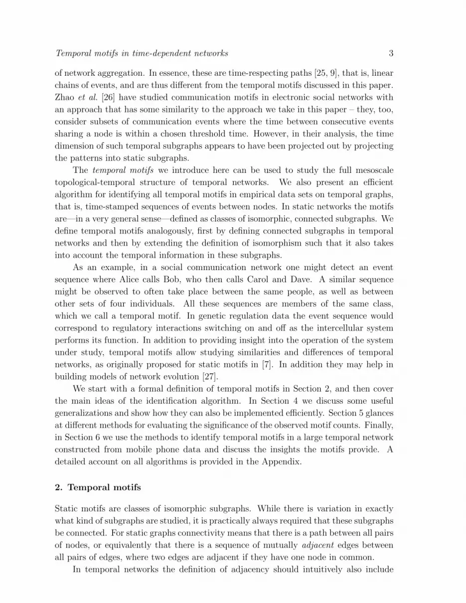
Figure 5. The two different kinds of directed triangle motifs with 3 events. Both
groups have been ordered by count in the empirical data that is also shown below the
motifs. All motifs in (a), as well as those two in (b), differ only in the order of events.
adjacent events.¶ The parameter m controls the bias strength: the more candidates
there are, the more likely it is to find one close to ei. Setting m = 1 gives the normal
unbiased randomization.
Figure 4c shows the most and least common motifs in the biased reference with
m = 32. This reference naturally has higher motif counts than the unbiased reference,
but the total number of 3-event motifs is still only 60 % of that of the empirical data.
Perhaps surprisingly, the least common motif is now twice as common as in the empirical
data. In the empirical data this motif is uncommon partly because the events take
place in a non-causal order, whereas the order has little significance in the reference.
Furthermore, because this kind of subgraph takes place primarily due to correlations,
it is likely that the nodes have other events at approximately the same time. If these
events take place between those in the triangle, the subgraph would no longer be valid
(see lower subgraph in Figure 1e). In the references the maximal subgraphs are smaller,
which makes it less likely that such interfering events would destroy the validity. The
bias makes triangles more common while keeping the maximal subgraphs small, and
therefore the triangles are more often valid.
As a further example clarifying this point, we present in Figure 5 all motifs based
on the different directed triangles with 3 events. The six motifs in Figure 5a would by
equally common in the time-shuffled reference, but in the empirical data we observe a
4-fold difference between the most and least common triangle. There are two factors
that explain this: burstiness and causality. Burstiness appears in the fact that in the
four most common motifs the two calls made by C are consecutive; in the two least
common motifs they are not. Causality is most apparent when comparing the most and
the least common motif. In the most common motif the caller of the second call (C)
knows about the first call (because he made it himself), and the caller of the third call
(B) could know about both previous calls. In the least common motif the caller of the
second call (B) cannot know about the first one, and the caller of the third call (C)
cannot know about the call made by B. The most common motif is both bursty and
causal, while the least common is neither.
Causality is an obvious explanation also for the counts in Figure 5b: the triangle
where events could cause one another is three times as common as the other one. Note
¶ As we are only interested in the order of these averages and not their exact values, comparing
geometric averages is equal to comparing the arithmetic average of logarithms of time differences. This
puts more importance to small time differences than plain arithmetic average.

Temporal motifs in time-dependent networks 12
100 101 102 103 104
# of nodes
10−310−210−1
100101102103104105106107108109
#of
maxim
al
moti
fs
4800 s2400 s1200 s600 s300 s
100 101 102 103 104
# of events
10−310−210−1
100101102103104105106107108109
#of
maxim
al
moti
fs
(a) (b)
100 101 102 103 104
# of events
10−8
10−7
10−6
10−5
10−4
10−3
10−2
10−1
100
Fra
ctio
nof
even
ts
4800 s2400 s1200 s600 s300 s
100 101 102 103 104
# of events
10−6
10−5
10−4
10−3
10−2
10−1
100
Fra
ctio
nof
even
ts(c
um
.)
(c) (d)
Figure 6. Number of maximal motifs of different size when the size is measured by
(a) the number of nodes and (b) the number of events in the motif. In both plots
the values larger than 10 have been binned with logarithmic bins using factor 1.2.
(c) Fraction of events in motifs of a given size, and (d) the corresponding cumulative
distribution. In all plots the solid lines correspond to empirical data, dotted lines to
the unbiased time-shuffled reference.
that these two motifs are time-reversals of each other, i.e. if the time were reversed,
each motif of the first kind would turn into the second, and vice versa.
Figures 6a–b show the number of maximal motifs of different size for different
values of ∆t, measured either by the number of nodes or by the number of events in
the motifs. The distributions are broad for all time windows, and those with larger
∆t are naturally broader. Figures 6c–d show the fraction of events in maximal motifs
of different size. Comparing the distributions with ∆t = 1200 and 2400 suggests that
between these values a giant temporal component is beginning to form. The distribution
with ∆t = 1200 is very close to a power-law, as both the density and cumulative
distributions are straight lines. When ∆t = 2400 the number of events contained in
very large maximal motifs is starting to grow. Increasing the time window further
beyond ∆t = 4800 would at some point give birth to a giant temporal component: a
large fraction of events would become ∆t-connected.
Finally, Figure 7a shows that if we only look at the number of motifs, the biased
references seem to approach the actual data as we increase the bias strength. Similar

Temporal motifs in time-dependent networks 13
5 10 15 20 25 30
Bias strength m
100
101
102N/〈N
ref〉
2 events3 events4 events
5 10 15 20 25 30
Bias strength m
0.0
0.2
0.4
0.6
0.8
1.0
1.2
1.4
DK
L({p},{q})
5 10 15 20 25 30
Bias strength m
0.0
0.2
0.4
0.6
0.8
1.0
Ken
dall
’sτ
(a) (b) (c)
Figure 7. (a) The ratio of total number of motifs with a given number of events in the
actual data versus the time-shuffled reference. The lines correspond to motifs with 2,
3 and 4 events, from bottom to top. (b) The symmetric Kullback-Leibler divergence
between motifs in the actual data and the time-shuffled reference. (c) Kendall’s τ
between motifs in the actual data and the time-shuffled reference. The motif counts of
the references are averages of 5 different runs for each value of the bias strength.
behaviour is seen in Figure 7b for the symmetrized KL divergence calculated between
the actual data and the reference, and also for Kendall‘s τ in Figure 7c. However, in
Figure 4 we saw that with m = 32 there are already motifs that are more common in the
reference than in the real data; it is therefore not possible that the reference becomes
identical to the data when the total number of motifs become equal. In addition, motifs
with more events are relatively more common in the empirical data regardless of the
bias. A qualitative difference between motif sequences remains even if we were able to
match the total number of motifs.
7. Conclusions
In this paper we have introduced the concept of temporal motifs, and provide a
mapping between temporal subgraphs and colored directed graphs that allows an
efficient algorithm for their identification. Using this algorithm we can locate and make
statistics about the main mesoscopic building blocks of temporal networks, which will
carry great importance for understanding their functions and underlying mechanisms.
While the focus of this article is more on technical definitions, algorithms, and
general aspects of the evaluation of motif counts, we have also presented some results
on a huge temporal network based on mobile phone call data. Some conclusions
can already be drawn. Of all temporal motifs with three events, the most common
ones involve only two nodes. This is in accord with the independent finding that
burstiness in human communication is mostly a link property [34]. Another interesting—
though not surprising—result is that the motifs which allow causal interpretations are
more common. The fat-tailed distributions of maximal motifs are in agreement with
observations about the correlations in the network [14], although our present approach
gives a more detailed insight about the mechanisms. Our initial results also show that

Temporal motifs in time-dependent networks 14
the temporal motifs are common enough to have an impact on dynamics and too complex
to be explained by simple temporal correlations. The occurrence of motifs is intuitively
sensible, as they highlight two universal properties of human communication, namely
burstiness and causality.
There are a number of directions to pursuit in the future. For example here we
have ignored the case where nodes can have simultaneously multiple events. This
generalization presents a challenge both in defining the valid subgraphs and in developing
the algorithms for their identification. Further research is also needed to develop
measures for analyzing the occurrence patterns of motifs.
The presented examples are far from being able to illustrate the full richness of
phenomena that can be explored with temporal motifs. Currently we are in the course
of investigating several temporal networks and hope that it this approach will be useful
in a broad range of studies, even more so as the presented algorithm is able to handle
large networks. As empirical temporal networks are becoming more and more common,
we expect temporal motifs and their analysis to prove useful in many different fields of
science.
Acknowledgments
The project ICTeCollective acknowledges the financial support of the Future and
Emerging Technologies (FET) programme within the Seventh Framework Programme
for Research of the European Commission, under FET-Open grant number: 238597.
We acknowledge support by the Academy of Finland, the Finnish Centre of Excellence
program 2006–2011, project no. 213470. JK is supported by the Finland Distinguished
Professor (FiDiPro) program of TEKES.
We would like to thank Renaud Lambiotte for his comments and Albert-Laszlo
Barabasi of Northeastern University for providing access to the unique mobile phone
data set.
Appendix A. Finding temporal subgraphs
The following result is used in Section 3 to find temporal subgraphs inside maximal
temporal subgraphs:
Theorem 1. Let G(E∗max) be an undirected graph that has a vertex for each event in
E∗max and every vertex is connected to the next and previous ∆t-adjacent event of both
nodes in that event (there are at most four such events). Then every valid subgraph
contained in E∗max corresponds to a connected subgraph of G(E∗
max).
Proof. Consider a valid subgraph E∗ ⊆ E∗max and the corresponding vertex set in
G. Because all event pairs in E∗ are ∆t-connected and the events of every node are
consecutive, there is at least one path between all vertex pairs in this set. Therefore
there is at least one connected subgraph of G that corresponds to E∗.

Temporal motifs in time-dependent networks 15
Figure A1. (a) An example of a maximal subgraph E∗max with ∆t = 10 and (b) the
corresponding undirected graph G(E∗max) used to identify all valid subgraphs contained
in E∗max. (c) A connected subgraph of G and (d) the corresponding temporal subgraph
that is not a valid subgraph because the events of node c are not consecutive: e2 takes
place between e1 and e3 and is ∆t-connected to them, so it should be included.
Note that the inverse is not true: there are connected subgraphs of G whose
vertex sets do not correspond to any valid subgraph; an example is given in Figure
A1. Therefore to identify all valid subgraphs E∗ ⊆ E∗max we first need to find all distinct
connected subgraphs of G and then ensure that the corresponding subgraphs are valid
by checking that for every node the events (that are in E∗max and hence ∆t-connected)
are consecutive. This check can be carried out with little extra cost while constructing
the colored graph needed to calculate the canonical form, as the construction requires
going through all events anyway.
A pseudo-code to identify all connected vertex sets of an arbitrary graph (in this
case G(E∗max)) is given in Algorithm 1. In function FindConnectedSets we first start
|V | search trees so that the tree initialized with node i will find all connected sets where
i is the smallest node. The nodes in the set V− are excluded from that search tree;
initially this set contains all nodes smaller than i. The set V+ includes nodes where the
search can progress, initially all neighbours larger than i. Because each search tree finds
only sets where i is the smallest node, the trees are necessarily distinct.
The function SubFind first adds the current set to be returned (line 10) and then
grows the sets recursively. For each node i ∈ V+, V− is updated by excluding nodes
smaller than i. Thus each subtree has a different smallest node from those in V+ and
the subtrees are again distinct. The set V+ is updated to contain nodes where the search
can progress: previously allowed nodes larger than i and those new neighbours of i that
are not yet excluded.
Because the subtrees are distinct at each step, the algorithm will return each
connected set at most once. To see that it returns all possible connected set, consider
how we could arrive at an arbitrary connected set S. The search path is rooted at
i1 = minS. Let Sk, k < |S|, be the set of elements added at depth k. Because S
is connected, there is at least one node in S\Sk that is a neighbour of some node in
Sk. The only way the construction can fail is if for some k there is a node i∗ ∈ S\Skthat has already been excluded, i.e. it is in V−. It is not possible that i∗ was excluded
in the beginning—the tree was rooted at i1 < i∗ and only nodes smaller than i1 were
excluded—so it must have happened during the search. But if i∗ was added to V−

Temporal motifs in time-dependent networks 16
Algorithm 1 Find the vertex sets of all connected subgraphs of a arbitrary graph
G. The algorithm assumes that nodes are labeled with integers from 1 to |V |. The
parameter nmax can be used to limit the size of the vertex sets returned. N(i) denotes
the neighbours of node i in graph G.
Require: G = (V, L) is an undirected graph.
1: function FindConnectedSets(G, nmax)
2: Sall ← ∅3: for i in V do
4: S ← {i}5: V− ← {j ∈ V | j ≤ i}6: V+ ← {j ∈ N(i) | j > i}7: SubFind(G, nmax, Sall, S, V−, V+)
8: return Sall
9: function SubFind(G, nmax, Sall, S, V−, V+)
10: Sall ← Sall ∪ {S}11: if |S| = nmax then return
12: for i in V+ do
13: S∗ ← S ∪ {i}14: V ∗
− ← V− ∪ {j ∈ V+ | j ≤ i}15: V ∗
+ ← {j ∈ V+ | j > i} ∪ {j ∈ N(i) | j 6∈ V ∗−}
16: SubFind(G, nmax, Sall, S∗, V ∗
−, V ∗+)
it means that it was in V+ but some larger node of S was added instead, which is a
contradiction—in the subtree leading to S we would have added i∗. Hence no node i∗
can exist and the construction can always proceed until S is obtained.
Appendix B. Event labels with partial order
Pseudo-code for finding the labels is presented in Algorithm 2. On lines 2–8 we first
initialize all labels to (1, ∅), unless there are multiple roots which get each initialized
with a unique element. The loop on lines 9–19 then iteratively pushes the labels forward
along directed paths, adding new elements when needed: first pick any node with zero
in-degree (line 10), and find its children who can not be reached through other children
(V −c ) (lines 11–13). The labels of these children are then updated by incrementing the
value of r and pushing the set si down to the child (line 14–15), adding a new unique
element to each set if there are multiple children to update (lines 16–18).
It is easy to see that this algorithm results in valid labels:
• If event ei must come before ej then there is (at least one) directed path from ei to

Temporal motifs in time-dependent networks 17
Algorithm 2 Find the labels to denote the ordering of events. The vertices in the input
graph G correspond to events, and the graph contains at least one directed path from
event ei to ej if ei must take place before ej.
Require: G = (V, L) is a directed acyclic graph.
Require: P (i) is the set of nodes from which there is a directed path to vi.
1: function FindEventLabels(G)
2: smax ← 0
3: V0 ← {ei ∈ V | kin(ei) = 0}4: for ei in V do
5: ri ← 1, si ← ∅6: if |V0| > 1 and ei ∈ V0 then
7: si ← {smax}8: smax ← smax + 1
9: while V 6= ∅ do
10: Pick any node ei with kin(ei) = 0 in G
11: Vc ← {ej ∈ V | (ei, ej) ∈ L}12: V −
c ← {ej ∈ Vc |Vc ∩ P (j) = ∅}13: for all ec in V −
c do
14: rc ← max{rc, ri + 1}15: sc ← sc ∪ si16: if |V +
c | > 1 then
17: sc ← sc ∪ {smax}18: smax ← smax + 1
19: Remove ei from G = (V, L)
ej. The set si will be pushed along this path and therefore si ⊆ sj, and the value
r will increase along this path and therefore ri < rj.
• If there is no restriction for the mutual order of ei and ej, there is no directed path
between these nodes. We can trace backwards all paths from these nodes to find
that either
(i) the paths traced from ei and from ej end up in distinct root nodes and hence
si ∩ sj = ∅ because each root was initialized with a different element,
(ii) the paths converge to a common node that hence has multiple children and
the two branches were assigned unique elements of S, and therefore si 6⊆ sjand sj 6⊆ si, or
(iii) both of the above (there can be multiple directed paths leading to these nodes),
which also means that si 6⊆ sj and sj 6⊆ si.
The labels this algorithm provides are plain integers when the input graph G contains
a total order of events.

Temporal motifs in time-dependent networks 18
Bibliography
[1] Newman M, Barabasi A L and Watts D J (2009) The Structure and Dynamics of Networks
(Princeton University Press)
[2] Newman M E J (2010) Networks: An Introduction (Oxford University Press)
[3] Fortunato S (2010) Physics Reports 486 75
[4] Lancichinetti A, Kivela M, Saramaki J and Fortunato S (2010) PLoS One 5 e11976
[5] Onnela J P, Fenn D J, Reid S, Porter M A, Mucha P J, Fricker M D and Jones N S (2010)
arXiv :1006.5731
[6] Shen-Orr S S, Milo R, Mangan S and Alon U (2002) Nature Genetics 31 64
[7] Milo R, Shen-Orr S, Itzkovitz S, Kashtan N, Chklovskii D and Alon U (2002) Science 298 824
[8] Onnela J P, Saramaki J, Kertesz J and Kaski K (2005) Phys. Rev. E 71 065103
[9] Holme P (2005) Phys. Rev. E 71 046119
[10] Kossinets G, Kleinberg J and Watts D (2008) The Structure of Information Pathways in a Social
Communication Network. arXiv :0806.3201
[11] Centola D (2010) Science 329 1194
[12] Vazquez A, Racz B, Lukacs A and Barabasi A L (2007) Phys. Rev. Lett. 98 158702
[13] Iribarren J L and Moro E (2009) Phys. Rev. Lett. 103 038702
[14] Karsai M, Kivela M, Pan R K, Kaski K, Kertesz J, Barabasi A L and Saramaki J (2011) Phys.
Rev. E 83 025102
[15] Miritello G, Moro E and Lara R (2011) Phys. Rev. E 83 045102
[16] Rocha L E C, Liljeros F and Holme P (2011) PLoS Computational Biology 7(3) e1001109
[17] Lee S, Rocha L E C, Liljeros F and Holme P (2010) arXiv :1011.3928
[18] Valencia M, Martinerie J, Dupont S and Chavez M (2008) Phys. Rev. E 77 050905
[19] Dimitriadis S I, Laskaris N A, Tsirka V, Vourkas M, Micheloyannis S and Fotopoulos S (2010)
Journal of Neuroscience Methods 193 145
[20] Cui L, Kumara S and Albert R (2010) Circuits and Systems Magazine, IEEE 10 10
[21] Holme P and Saramaki J (2011) arXiv :1108.1780
[22] Nicosia V, Tang J, Musolesi M, Russo G, Mascolo C, and Latora V (2011) arXiv :1106.2134
[23] Braha D and Bar-Yam Y (2008) Gross T and Sayama H (eds) Adaptive networks: Theory, models
and applications p 39 (Springer Verlag)
[24] Bajardi P, Barrat A, Natale F, Savini L and Colizza V (2011) arXiv :1105.3882
[25] Kempe D, Kleinberg J and Kumar A (2002) Journal of Computer and System Sciences 76 036113
[26] Zhao Q, Tian Y, He Q, Oliver N, Jin R and Lee W C (2010) In CIKM p 1645
[27] Kumpula J M, Onnela J P, Saramaki J, Kaski K and Kertesz J (2007) Phys. Rev. Lett. 99 228701
[28] Pan R K and Saramaki J (2011) Phys. Rev. E 84 016105
[29] Valencia M, Martinerie J, Dupont S, and Chavez M (2008) Phys. Rev. E 77 050905
[30] Casteigts A, Flocchini P, Quattrociocchi W and Santoro N (2011) arXiv :1012.0009
[31] Junttila T and Kaski P (2007) D Applegate, G S Brodal, D Panario and R Sedgewick (eds)
Proceedings of the Ninth Workshop on Algorithm Engineering and Experiments and the Fourth
Workshop on Analytic Algorithms and Combinatorics p 135 (SIAM)
[32] Xuan BB, Ferreira A and Jarry A (2003) International Journal of Foundations of Computer Science
14 2 p 267
[33] Artzy-Randrup Y, Fleishman S J, Ben-Tal N and Stone L (2004) Science 305 1107
[34] Karsai M et al. to be published


