)riginal

Spectral element methods for of an Euler-Bernoulli beam

P. Z. Bar-Yoseph, D. Fisher, O. Gottlieb

Computational Mechanics 19 (1996) 136-151 �9 Springer-Verlag 1996

nonlinear spatio-temporal dynamics

136 Abstract Spectral element methods are high order accu- rate methods which have been successfully utilized for solving ordinary and partial differential equations. In this paper the space-time spectral element (STSE) method is employed to solve a simply supported modified Euler- Bernoulli nonlinear beam undergoing forced lateral vi- brations. This system was chosen for analysis due to the availability of a reference solution of the form of a forced Duffing's equation. Two formulations were examined: i) a generalized Galerkin method with Hermitian polynomials as interpolants both in spatial and temporal discretization (HHSE), ii) a mixed discontinuous Galerkin formulation with Hermitian cubic polynomials as interpolants for spatial discretization and Lagrangian spectral polynomials as interpolants for temporal discretization (HLSE). The first method revealed severe stability problems while the second method exhibited unconditional stability and was selected for detailed analysis. The spatial h-convergence rate of the HLSE method is of order ~ - Ps + 1 (where Ps is the spatial polynomial order). Temporal p-convergence of the HLSE method is exponential and the h-convergence rate based on the end points (the points corresponding to the final time of each element) is of order 2px - 1 < ~ < 2pr + 1 (where PT is the temporal polynomial or- der). Due to the high accuracy of the HLSE method, good results were achieved for the cases considered using a relatively large spatial grid siz e (4 elements for first mode solutions) and a large integration time step (1/4 of the system period for first mode solutions, with PT = 3). All the first mode solution features were detected including the onset of the first period doubling bifurcation, the onset of chaos and the return to periodic motion.

Two examples of second mode excitation produced homogeneous second mode and coupled first and second mode periodic solutions.

Consequently, the STSE method is shown to be an ac- curate numerical method for simulation of nonlinear spatio-temporal dynamical systems exhibiting chaotic re- sponse.

Communicated by S. N. Atluri, 10 July 1996

P. Z. Bar-Yoseph, D. Fisher, O. Gottlieb Computational Mechanics Laboratory, Faculty of Mechanical Engineering, Technion-Israel Institute of Technology, Haifa 32000, Israel, E-mail: merbygr@cmlp.technion.ac.il

Correspondence to: P. Z. Bar-Yoseph

1 Introduction and problem formulation Nonlinear spatio-temporal dynamical systems may display a wide range of behavior consisting of periodic and aperiodic solutions in space and time. These solutions include solitons, shock waves, ultrasubharmonic, quasi- periodic and chaotic attractors.

These systems are described by partial differential equations (PDE) and can rarely be solved in closed form. Therefore, numerical methods are employed to analyze global system behavior.

The numerical solution usually involves discretization of the spatial domain with a finite spatial grid size thus ob- taining a large set of nonlinear ordinary differential equa- tions (ODE) which are then solved using a numerical integration scheme with a finite time step size. In this process, the continuous PDE is replaced by a discrete equation with two additional parameters: the spatial grid size and the time step size. The behavior of this discrete equation may be very different than that of its continuous counterpart and is sensitive to the spatial grid size, the time step size, the nonlinear terms and the numerical scheme chosen. Lorenz (1989) showed that use of an excessively large time step using Euler, Runge-Kutta and Taylor series expansions schemes may lead to computational chaos, namely a spurious chaotic solution solely due to the nu- merical solver. Yee and Sweby (1995) have demonstrated that even for small time step sizes the numerical solutions obtained by various Euler, Runge-Kutta, predictor-cor- rector and trapezoidal schemes may produce spurious so- lutions which coexist with the correct solution having their own basins of attraction. Corless et al. (1991) demonstrated that the Euler numerical scheme can even suppress existing chaos. Investigation of steady state dynamics of possible chaotic systems requires large finite time. However, chaotic solutions are by definition sensitive to initial conditions therefore requiring extremely small integration steps. This leads Belic et al. (1992) to conclude that no numerical al- gorithm can predict accurately the state of a chaotic system after a long period of time. Although the detail of the chaotic solution may be inaccurate the numerical method is required to reproduce system behavior qualitatively while using an optimal finite integration time step.

The time finite element (TFE) method is an alternative numerical scheme for solving both linear and nonlinear differential equations involving a finite element dis- cretization of the temporal domain using the method of weighted residuals (c.f. Baruch and Rift (1984), Bar-Yo- seph (1989), Bar-Yoseph and Elata (1990), Borri et al.

(1990 and 1991), Aharoni and Bar-Yoseph (1992) and Bar- Yoseph et at. (1993)). This method has been extended, in the form of the space-time finite element method (STFE), to solve linear and nonlinear initial-boundary value pro- blems in space and time where both the temporal and spatial domains are discretized (c.f. Peters and Izadpanah (1988), Bar-Yoseph (1989), Hulbert and Hughes (1990) and Johnson (1993)). Patera (1984) introduced high order spectral elements, thus exploiting the rapid convergence rates of spectral methods and achieving high numerical efficiency. The spectral element method was utilized by Zrahia and Bar-Yoseph (1994) and Bar-Yoseph et al. (1995) for solving initial-boundary value problems in the form of the space-time spectral dement method (STSE). The STSE method was successfully adapted by Ben-Tal et al. (1995 and 1996) to the optimal control of a flexible Timoshenko beam model. Furthermore, the time spectral element method (TSE) was successfully applied by Bar- Yoseph et al. (1996) for resolving temporal chaotic system dynamics.

In this paper the space-time spectral element method (STSE) is employed to solve a simply supported modified Euler-Bernoulli beam undergoing external forced lateral vibrations. The beam considered (Holmes (1979)) includes a prescribed initial compression by an applied axial load and a nonlinear contribution from membrane stretching (cf. Huang and Nachbar (1968)). Assuming first mode behavior allows the reduction of the PDE to an ODE in the form of a forced, damped Duffing equation. Holmes (1979) in his study of the ODE analytically found conditions for the existence of chaotic solutions which he then confirmed numerically. Abhyankar et al. (1993) presented a numer- ical study of the buckled beam using a finite difference method and demonstrated the similarity between ODE and PDE when the spatial behavior was dominated by the first mode. We note that mechanisms leading to chaotic beam dynamics are not limited to field excitation (Moon and Holmes (1979)) or to a specific form of boundary conditions. Tseng and Dugundi (1971) obtained evidence of chaotic dynamics of a buckled beam excited by hat- : monic motion of its supporting base. Holmes and Marsden (1981) demonstrated analytically existence of chaotic os- cillations of a forced beam and Abou-Rayan et al. (1993) obtained chaotic response of a parametrically excited buckled beam where the axial load was varied harmoni- cally. Furthermore, Szemplinsk-Stupnicka et al. (1989) demonstrated existence of chaotic response of a buckled mechanism where there was no snap-through.

Consequently, we anticipate nonlinear instabilities (e.g. period doubling) leading to chaotic dynamics for weakly damped beams undergoing large amplitude vibrations due to additional nonlinear effects (cf. Atluri (1973)) subject to harmonic field and/or boundary excitation.

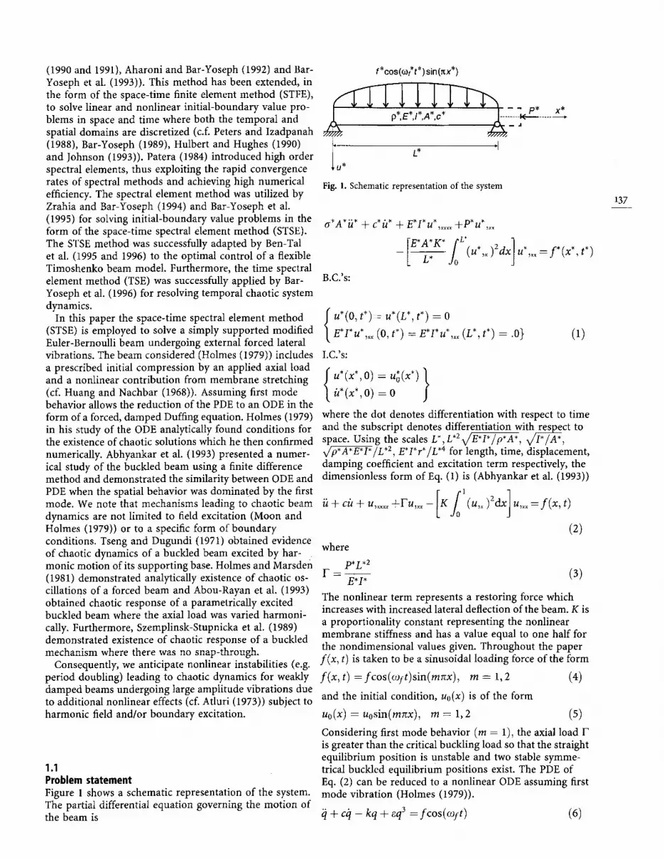
1.1 Problem statement Figure 1 shows a schematic representation of the system. The partial differential equation governing the motion of the beam is

f* cos(o~'t*)sin(nx*)

1, ,I U* L*

Fig. 1. Schematic representation of the system

a*A*fi* + c* fi* + E I u ..... +P u ,~

L--- ~ (u*,.)2dx u*,xx=f*(x*,t*)

B.C.'s:

u*(o, t*)-- u*(L*, t*) -- o

E*I*u*,.~ (0, t*) = E*I*u*,** (L*, t*) ---- .0} (1)

I.C.'s:

a*(x*, 0) = o

where the dot denotes differentiation with respect to time and the subscript denotes differentiation with re_~S ect to space. Using the scales L*, L*2v/E*I*/p*A *, x/P/a* , ~ / L .2, E*I*r*/L .4 for length, time, displacement, damping coefficient and excitation term respectively, the dimensionless form of Eq. (1) is (Abhyankar et al. (1993))

[/01 ] ~ + c i t + u , ~ + F u , ~ - K (u,~)2dx u ,xx=f (x , t )

(2)

where

p*L*a F - E'I* (3)

The nonlinear term represents a restoring force which increases with increased lateral deflection of the beam. K is a proportionality constant representing the nonlinear membrane stiffness and has a value equal to one half for the nondimensional values given. Throughout the paper f (x , t) is taken to be a sinusoidal loading force of the form

f ( x , t) =fcos(oJf t )s in(mnx) , m = 1,2 (4)

and the initial condition, u0 (x) is of the form

Uo(X) = uosin(mnx), m = 1,2 (5)

Considering first mode behavior (m = 1), the axial load F is greater than the critical buckling load so that the straight equilibrium position is unstable and two stable symme- trical buckled equilibrium positions exist. The PDE of Eq. (2) can be reduced to a nonlinear ODE assuming first mode vibration (Holmes (1979)).

+ ci t - kq + eq 3 = fcos(coft) (6)

137

138

where

k = ztZ(F - rc 2) (7)

and

g = 1/2Krc 4 (8)

Near the primary resonance the contribution of the higher modes in Eq. (2) is expected to be small compared to that of the first mode and therefore Eq. (6) serves as an ap- proximate model of the behavior of our system. Based on this model the following behavior as analyzed by Holmes (1979) is expected from the numerical simulation of the system. The equilibrium positions are identified by the displacement of the midpoint of the beam denoted by ft, there being two sinks at the locations

(~,~) = ( + X / 2 ( F - =2)/(KrS),0) (9)

and a saddle at (h, h) = (0, 0). For small load amplitudes, f , the beam oscillates about one of the sinks. As f is in- creased the solution goes through a series of period dou- bling bifurcations culminating with chaotic response. A further increase o f f results in periodic response about all three equilibrium positions.

Initially, STSE will be employed to solve several cases of Eq. (2) with m = 1. The various solutions will be in- vestigated and compared with those obtained from Eq. (5) using TSE (Bar-Yoseph et al. (1996)). Finally, STSE will be employed to solve two cases of second mode vibration (m = 2).

2 Spectral element formulation In this section the spectral element formulation of the PDE represented by Eq. (2) will be presented. Initially the spatial domain is discretized and cubic Hermitian poly- nomials are utilized as interpolants for the displacement, u. Thereafter the temporal domain is discretized and two methods are examined, the first utilizing cubic Hermitian polynomials as interpolants of u with a general Galerkin method (Bar-Yoseph (1996)) and the second utilizing La- grangian polynomials as interpolants of u with a dis- continuous Galerkin mixed formulation (Aharoni and Bar- Yoseph (1992)).

2.1 Spatial discretization Using Galerkin's method of weighted residuals, Eq. (2) becomes

u lx ll} =o/lO/ where w is the weighting function. Integration by parts of Eq. (10) yields

1 1 2

x wu,x~ -wf(x , t)[ dx + WU,xx I~ -w,~ u,~x 1~= 0 - i

(11)

Fulfilling the natural and essential boundary conditions reduces Eq. (11) to

[/01 ] (w, 2) + (w, c/,) + a(w, u) + r - K (u,x)2&

• (w, u,x~ ) = (w,f) (12)

where

~0 1 a(w, u) = W,~x U,xx dx (13)

fl (w, u) = wu dx (14)

Hermitian cubic polynomials are introduced as inter- polants for both the base and weight functions having C l continuity across the element borders. Approximation of the nonlinearity is performed using the grouping method (Fletcher (1991)), utilizing a quadratic Lagrangian poly- nomial as an interpolant through the Gauss-Lobatto in- tegration points. The value of U,x at the single internal nodal point is found by interpolation using the Hermitian polynomial. The vector, U containing the values of u 2 at

'x

the end and single internal nodal points is then defined as

= {(1~, x)2 (1,2~, x)2 (2~, x)2, (2,3~, x)2,

(3-~, x )2, ..., (Ns-l,Ns-~, x )2, (Ns-~, x )2} T (15)

the left superscript denoting the end point number (one number) or the element midpoint relating to the element's left and right end point numbers (two numbers) and Ns representing the number of spatial nodal points.

Equation (12) is then represented in matrix form as

MO + C(J + KLU + KN(U)U= Fcos(oft) (16)

/o M = ~t'~'Tdx (i7)

/o 1 c = c ~t'~'rdx (18)

/o 1 /o = v, xdx + r Ve, xdX (19)

KN~- (-g[o~olf~TdxlU} folVtrtt,T dx (20)

V ---- f [fo' WOFdx]f(X)

U = {U1, UI,x, U2, U2,x,...,UNs, UNs,x} T

(21)

(22)

X = {XI,Xi,X2,X2,...,XN~,XN~} T (23)

andf(X) of Eq. (21) is given by

{ sin(mnxt), mn cos(mzcxl), }T

f(X) = sin(mnx2), I n cos(mTcx2),

..., sin(mnxN,), mn cos(mnx,,)

m = 1, 2 (24)

and W, q3 are the Hermitian cubic and Lagrangian quad- ratic polynomials respectively.

2.2 Temporal discretization Equation (16) is a multi-degree-of-freedom nonlinear set of ODE's which is now discretized in the temporal domain.

2.2.1 Hermitian interpolants Using the generalized Galerkin method as presented by Bar-Yoseph (1996). Eq. (16) becomes

tl {w(MfI + C(J + KLU + KN(U)U

- F cos(coil)) }dr = 0 (25)

where w is the generalized weighting function of the form

w = a06U + alSLr + a280 (26)

The following cases can be identified: Standard Galerkin method: a0 = 1, as = 0, a2 = 0, Accleration weighted method: ao = 0, as = 0, a2 = 1. Substituting Eq. (26) into Eq. (25) and integrating by parts

[a2M[J~O q- a2CO~)(J-- (az(KL + KN(U)) ]

tf [ __ al c .J_ aoM) (j~O [

ft~ I + a,M(J~)(J + at(KL + KN(-U))U80 I dt

L +aoCfJ~U+ao(KL+KN(-U))U~U J

+aoM[fJgUl'S +a2(KI. + KN(~))[USfJ] tf to to

= fro 'I [(az60 + a16/.)+ao6U)Fcos(coft)Jdt (27)

The time interval I = (to, tf) is partitioned into sub- intervals I. = (t., t.+l) where tn and tn+i belong to an ordered partition of time levels to < tt < ... < tlv = tf. _ f ]T Hermitian cubic polynomials are taken as interpolants for Q = ~.ql, q2, �9 "., qN~ the base and weight functions so that

Ui ,~ tIJT qi where

�9 , T

qi = {qi(t~),qi(tn),qi(t.+'),qi(tn+a)} and

Each Hermitian temporal element has two degrees of freedom at its left hand node and two degrees of freedom at its right hand node�9 Similarly, U is temporally dis- cretized using the grouping method (Fletcher (1991)) and Lagrangian quadratic interpolants so that

gi ~,~ !~jTqi (31)

where

{i- , qi (1 U,x )2, )2 (32) = (2u,x (3v,x

the left subscript denoting the temporal element nodal point number. Eq. (27) then becomes

a2 M @/-I22 + a2C @ H12-

(azKL - alC + aoM) | H11 + aiM @ H21

+ alKL | Hol + aoKL | Hoo Q

+ aoM | Hlo + a2KL | Hol

-}- {aor--Noo q- alKNol - a2KNll + aZ~NO1 }

= F | [--a2Ull -}- alUm q- aoHoo q- azHol]f(Tn) (33)

W = ao~ + alCP q- a2@

or

A(0) O = b (34)

where

f tn+l ~i~tl 8tpT

HO = Jr. 5t i St) dt (35)

_ W v = (36) uij [ &i Ot; J to

KNij ~-K[follqdtlYtl,Tdx] @ ftntn+l { ( { { j~OI(~Tdx}

| T 0 et i etJ dt (37)

| r 0 - ~ V T (38)

tn

Q = {qa,q2,...,qNs} T (39)

TH = {tn, t~, tn+t, t~+l} r (28)

(29) f(Tu)={COS(COftn),--Cofsin(cOftn),

(40)

(41)

(30) cos(coftn+l), -COl sin(coftn+i ) } 7" (42)

139

14o

The members of A multiplying the members of Q asso- ciated with the time level t, (i.e. initial conditions) are transferred to the right hand side. The resulting nonlinear algebraic set of equations is solved for each time step, AG, thus advancing in time until t s.

2.2.2 Lagrangian interpolants In this method momentum, P is introduced and Eq. (16) is reduced to two first order equations.

= - C M - 1 p -- KLU -- KN(U) U + V cos(cost )

(43)

Eq. (43) is weighted using the discontinuous Galerkin method for each time interval, I,.

L t"+' {(~J__ M - 1 p ) S P } d t

f tn+l { + (J~ + CM-IP + KLU + KN(-U)U

J t n

- V cos(cost) )gU}dt

+ + = 0

where [[.]] denotes a jump operator defined by

[[e]] = ( e n - - P ( t n ) )

(44)

(45)

where P(t,) is the initial condition from the previous time step, and P, is the initial variable of the new time step as depicted in Fig. 2. The continuity of the variables is weakly enforced by the jump operator, thus satisfying the initial conditions in an average sense. Integrating Eq. (44) by parts yields

L t " + ' { - U S P - M IPSP}dt

f tn+l I + -- PS[J + C M - 1 p S u + KLUSU d tn

K N ( U ) U~U - F cos(~of t )SU}dt +

+ [[P]] 5U -}- PSU Itt: +1 -~- [[U]] 5P ---[- u s e [tt:+l= 0

(46) which leads to

I n tn+l {-US/5 M- 'PSP}dt

tn+l I + - P6U + C M - 1 p S u + KLU$U

J t n

+ u 6 w - v cos( st)6W}dt

+ Un+lSP(tn+l) - U(tn)SP(tn)

+ P,+,SU(G+I) - P(tn)SU(G) = 0 (47)

within each temporal element the dependent variables are expanded in terms of pth-order Lagrangian interpolants

tn+lT Un+l'mn+l

I / nth Atn time step

tn - J - U., Pn

tn I U(tn), P(tn)

tn-1 Fig. 2. Discontinuous dement

through the Legendre-Gauss-Lobatto collocation points. These polynomials are used for both the base and weight functions so that

Ui ,~ (llTif/i, Ui ~ ~[}T~i, "T

Pi ~ r Pi "~ li)Tyi, ~P ~-~ if)j:

5P ~ r i = I , . . . , N , , j = I , . . . , N T (48)

where NT is the number of temporal element nodal points. Equation (47) can be approximated in the following matrix form

I Q G1 --M -1 | G2

EL | G2 +-KN(~) CM -I | G2 + I | G1

where

{:) (49)

tn+1 G1 = (b. (1)rdt

J tn

tn+l G2 = ~ . r dt

J t n

(50)

(51)

f l = { { - - P l (tn), 0, ..., 0, --la 1 (tn+l)} T, ...,

{--PNs (t,), 0, ..., 0,--PNs (t,+l) } T } (53)

f2 = r (tn), 0, ..., 0 , - v l (tn+t)} T, ...,

-vN, (t~), O, ..., O, --VN~ (t,+l)}T } {

+ v | a2 cos(wi L ) (54) where TL is the discretized time in terms of the element local coordinate, z, ( -1 < z < 1) given by

TL = {r l , T 2 , . . . , "~NT} T (55)

Initial conditions are enforced on average and the mem- bers of the right hand side multiplying pi(rn+l) or vi(r~+~) are transferred to the left hand side. The resulting set of nonlinear algebraic equations is solved per each time step until ty.

Where applicable, the displacement error at time tn was defined (in both methods) as

ed ( t , ) = I[ Od(tn) -- U d ( t . ) II II ud(t )II (56)

where 0d is the displacement of the calculated solution, Ud, the displacement of the reference solution and [[. ]1 denotes the Euclidean norm. An error vector is then de- fined as

ed = {ed(tO), ed( t l ) , ..., ed(tn) , ..., ed( tN-1) , ed ( tN)} T

(57)

and the error estimate is therefore [1 ea II

defined as r = A t / A x . It may be observed that the accel- eration method (a0 = al = 0; az = 1) as presented by Baruch and Rift (1984) and the (a0 = -a2) weighting method displaying the highest convergence rate of all the combinations as proved by Bar-Yoseph (1996) (see Sec. 3.2.2), display greater stability than the Galerkin weighting method (a0 = 1, a l z a2 = 0). The three meth- ods, however, show a similar correlation between rcrit and Ax. The stability condition derived for the Galerkin weighting method is: A t / A x z3 < 2 �9 10 -3 and for the ac- celeration and the (a0 = -az) weighting methods: At /Ax2" l< 7 �9 10 -2. The velocity weighting method (a0 ---- 0; a l z 1; a: = 0) is not shown in Fig. 3, its stability condition being very similar to the Galerkin method. Furthermore, after analyzing the stability of other combi- nations of a0, al and a2 it may be concluded that all cases of a2 ~ 0 display similar stability conditions to that of the acceleration method. It is therefore preferable to assign a2 ~ 0, thus improving the method's stability and con- vergence properties (see Sec. 3.2.2). Note that the stability condition of the Galerkin method is very strict as it implies the use of extremely small time step sizes; for example if 4 elements are employed in the spatial discretization (Ax = 0.25), the above stability condition enforces a maximum time step size of 8 .10 -5 [sec] in comparison with 4 .10 -3 [sec] for the acceleration weighting method. It will be shown in Sec. 3.3 that due to the above stability limitations, the HHSE method is ineffective in comparison to the HLSE method.

141

3 Results This section includes a stability analysis of the Hermite (space)-Hermite (time) spectral element (HHSE) method and the Hermite (space)-Lagrange (time) spectral element (HLSE) method followed by a convergence analysis. After verifying the convergence and stability properties of the two methods a comparison of the effectiveness of the two methods is made. Thereafter, numerical solutions of the nonlinear beam are presented for both first and second : mode behavior where the first mode solutions are com- pared with the solutions of the Duffing equation (Eq. 6).

3.1 Stability analysis

3.1.1 HHSE method The stability of the methods was examined using the matrix method. The analysis was performed on a linear system for which this approach is exact. Note that al- though p-version refinement may be employed with im- proved convergence properties, the present study utilizes only the Hermitian cubic polynomial although the exten- sion of the method to use of higher order polynomials is straightforward. This method is conditionally stable and the stability criteria are shown in Fig. 3 the region below each line being stable and the region above being unstable. Each spatial grid size, Ax, dictates a certain critical time step size, Atcrit the method being unstable for any At above this critical value. Figure 3 depicts rcrit vs. Ax where r is

3.1.2 HLSE method Again, the matrix method is used and the stability analysis of the method is performed for the linear system. As mentioned in Sec. 3.1.1, a cubic Hermitian polynomial is employed for spatial discretization and spectral La-

-1 10

10 -2

1.3

10 -4 10 - I 10 0

Ax ~-

Fig. 3. Linear, 1st mode , free vibra t ing b e a m - Stability analysis of var ious fo rmu la t i ons of the HHSE m e t h o d - rcrit vs. Ax - *: Galerkin Method; o: Accelerat ion me thod ; +: (a0 = 1; al = 0; a2 = - 1 ) - ( c = F = K = f = c o y = O ; u0 = 1.0; Ps = P T = 3 )

t42

grangian elements for temporal discretization. Figure 4 1 shows the spectral radius of the amplification matrix as a function of the non dimensional time step for a Lagrangian o.9 quadratic polynomial and various Ax. A similar graph is 0.8 shown in Fig. 5 for various Lagrangian polynomial orders with a fixed Ax = 1.0. It may be concluded from both the 0.7 above Figures that in the application of the method to a linear system unconditional stability is obtained. We ob- [ 0.6 serve asymptotic annihilation, namely [ 0,5

Po~ = lim = 0 (58) AtlTcyc-~oe 0.4

(where Tcyc is the system period), thus making the method 0.3 dissipative. This trend decreases with the increase of the polynomial order. When considering the nonlinear beam, o.2 the spectral radius is time dependent, therefore the stabi- 0.1 lity analysis method described above is inapplicable. However, the stability of the solution and its convergence 0 c to the reference solution provide a measure of the meth- od's stability. Indeed, the results achieved by this method (see Secs. 3.4 and 3.5) indicate that the method remains stable when applied to the solution of the nonlinear beam, at least for all the cases considered in this research.

At/Tcyc

Fig. 5. Linear, 1st mode, free vibrating beam - Stability analysis o f the HLSE method - Spectral radius vs. A t / T c y c for various PT - (c = F = K = f = cof = O; uo = l.O; ps = 3; A x = 1 . 0 )

3.2 Convergence analysis The convergence analysis of a spatio-temporal discretiza- tion method consists of two components: i) convergence of the solution with refinement of Ax, (h-version), or with increase of Ps, (p-version) and ii) convergence of the so- lution with refinement of At, (h-version), or with increase OfpT, (p-version). Note that for all the results presented in this paper, At is maintained constant for to <_ t <_ tf. In this section spatial and temporal convergence is analyzed for the two methods studied (HHSE and HLSE).

1 . . . . ,

0.9

0.8

0.7

0.6

i 0.5

Q" 0.4

0.3

0.2 =0.5

0.1 DX =1

At/Tcy c ~ -

Fig. 4. Linear, 1st mode, free vibrating beam - Stability analysis of the HLSE method - Spectra] radius vs. At/Tcyc for various Ax - (c = F = K = f = o f = 0 ; u 0 = 1 . 0 ; p s = 3 ; P T = 2)

3.2.1 Spatial convergence Since the spatial discretization formulation is the same for both the HHSE and the HLSE methods, identical spatial convergence rates are expected for these methods. Fig. 6 shows spatial convergence of the two methods where for the HHSE method two variations are displayed: the Ga- lerkin method and the acceleration weighting method. The system tested in this analysis is a linear, undamped, first mode (m = 1), free-vibrating beam. In order to ensure stability of the HHSE method, an appropriate fixed r was chosen for each variation in accordance with the condi- tions stated in Sec. 3.1.1. All the methods shown in Fig. 6 display identical results and a spatial convergence rate of as = 4 is achieved. This convergence rate corresponds to an expected rate of as = Ps + 1 where ps is in this case cubic Hermitian (Ps = 3), and agrees with the theoretical convergence rate.

3.2.2 Temporal convergence Due to the stability limitations cited above (Sec. 3.1.1), the temporal convergence of the HHSE method cannot be analyzed as stability conditions dictate Ax >> At thus making the spatial discretization error dominant. How- ever, a study by Bar-Yoseph (1996) of the general Galerkin method utilizing Hermitian cubic polynomials applied to a single-degree-of-freedom system shows that different temporal convergence rates are obtained depending on the combination of a0, a~ and a2, the optimal combination being a0 = -a z with a convergence rate of aT = 6.

Fig. 7 shows the temporal convergence for the HLSE method applied to a linear, free vibrating beam using several temporal polynomial degrees. Since the con- vergence rates are asymptotic, the calculated rates are in- accurate as only two or three points can be measured per polynomial degree. The error minimum occurs at

101

10 0

10 -I

10 -2

10 - 1 10 10 0

A x

Fig. 6. Linear , 1 st m o d e , f ree v i b r a t i n g b e a m - Spat ia l c o n v e r g e n c e of

the va r i ous m e t h o d s - E r r o r vs. Ax - o: HHSE, G a l e r k i n (r = 0.0001);

+: HHSE, Acce le ra t ion (r = 0.002); x: HLSE (pT = 2, r = 0.1) --

( c = F = K = f = ~ o f = 0 ; u 0 = 1 . 0 ; N ~ y , = 2 0 0 ; p s = 3 )

10 -1

10 -2

1 1o .3

10 ~

10 -~ , , , . . . . . . . . i . . . . . . . .

10 -2. 10 -1 10 0

A t~ Tcyc

Fig. 8. Nonl inear beam ( ls t mode) - Tempora l convergence of the HLSE m e t h o d - E r ro r vs. At~Tore for v a r i o u s PT - O: pT = 2; + : p T = 3 ; X : p T = 4 - - ( C = 1.0; F = 9 . 5 ; K = 0 . 5 ;

f = 1.0; (o/ = 3.76; u0 = 1.0; N,,( = 40; Nss = 0; ps = 3; Ax = 0.1)

143

l[edlt ~ 3 - 10 -4 and is due to the dominance of the spatial discretization error. It is observed that a convergence rate of order 2pT -- 1 _< C~X _< 2pT + 1 is achieved for the ele- ment end points (the points corresponding to the final time of each element), pT being the Lagrangian polynomial order. Figure 8 depicts the convergence analysis of a test case, nonlinear beam for which a harmonic, first mode solution is assumed and substituted into Eq. (1) thus producing a residual representing the applied load. The convergence results are similar to the linear case and al-

10 ~

10 -1

t 10_2

10 -3

4.6

10 -4 . . . . . . . . i . . . . . . . . , . . . . . . . .

1 0 -3 10 -2 1 0 -1 1 0 0

At/-I 'cyc ~-

Fig. 7. Linear , 1st m o d e , f ree v i b r a t i n g b e a m - T e m p o r a l c o n v e r g e n c e of the HLSE m e t h o d - E r r o r vs. At/Tcyc for va r i ous pT -

o: PT = 2; X: PT = 3; + : pT = 4 -- (C = F = K = f = (of = 0; uo = 1.0; N,y~ = 200; Ps = 3; Ax = 0.05)

though a coarser spatial grid was used, the convergence rate remains 2pT -- 1 ~ ~T "( 2pT + 1. The above analysis provides information about the optimal combinations of time step size and temporal polynomial order that should be employed for this first mode test case in order to achieve visually accurate solutions (i.e. [[e[[ ~ 10-3). It can be observed that the following combinations are adequate for visual accuracy: (1) pT = 2; At/Tcyr = 1/16, (2) PT = 3; At/Tcyc = 1/8 and (3) pT ---- 4; At/Tcyc = 1/4. Extension of this rule of thumb to other solutions of the first and higher modes of the nonlinear beam should be applied cautiously (see Sees. 3.4 and 3.5).

3.2.3 Convergence of the Picard method In this section the convergence of the iterative solution of the nonlinear system of equations represented by EQ. (49) is presented. The Picard method was utilized to solve Eq. (49). Fig. 9 shows statistically the variance of the error norm with the number of iterations for pT = 3 for At/Tcyc = 1/8 and an approximate line drawn through these measurements indicates an average convergence rate. The mean error at each iteration number is measured and the result is shown in Fig. 10 for various combinations OfpT and At/Tcrc. It is clearly observed that using pT = 3 achieves a higher convergence rate of the Picard method and reduces, by up to 50%, the number of iterations re- quired for convergence to the specified tolerance. The er- ror improvement averages a decade per iteration which is a relatively high convergence rate for the Picard method. We note that as the Picard method displays an adequately high convergence rate, it was selected for the system so- lution over the more complex Newton-Raphson proce- dure.

z44

10 ~

10 -2

-4 10

I 10_6

10 -8

10 -10

i

i

-12 i i I 10 0 2 4 6 8 10

N i t e r

Fig. 9. Nonlinear beam (lst mode) - Statistical convergence of the Picard solver - Error vs. number of ~teratioas - (c = 1.0; F = 10.88; K = 0.5; f = 1.74; co[ = 3.76; uo ---- 0.0; N,~ = 50; Nss = 0; p, = 3; pT = 3; At /L , = 1/8; Ax = 0.25)

10 0

10 -1

10 -2

10 -3

i 10_4

lO .5

10 -6

10 -7

10 -8 / ( z

10-% 5 10 t 5 20

N i t e r

Fig. 10. Nonlinear beam (lst mode) - Mean convergence of the Picard solver - Mean error "vs. number of iterations - O:pT = 2, At~Text = 1/4; +: pT = 2, At/Tc, c = 1/8; X: pT = 3, At~Toy, = 1/8 - (c = 1.0; r = 10.88; K = 0.5; f = 1.74; oof = 3.76; Uo = 0.0; N~y~ = 50; Nss = 0; ps = 3; Ax = 0.25)

3,3 Effectiveness analysis

(m = D, l inear beam. Opt ima l sets of Ax and At are uti- l ized for each method , the on ly l imi ta t ion being the sta- b i l i ty cond i t ion of the HHSE method . The accelera t ion weight ing method, having the least s tabil i ty l imi ta t ions , was selected for the effectiveness analysis of the HHSE method . Fig. 11 shows the resul ts of this analysis wi th the d i sp l acemen t e r ror p lo t ted agains t CPU t ime thus for any given accuracy the magni tude o f CPU t ime may be found. The values of At and Ax respect ive ly are ind ica ted at each po in t wi th in the brackets . It is clearly observed that the HLSE m e t h o d surpasses the HHSE me thod and therefore we conclude , that the HLSE me thod is the preferable me thod for this system. In the l ight of the above, the re- suits p resen ted in the r e m a i n d e r of this paper were ob- t a ined us ing the HLSE method .

3.4 First mode phase planes, Poincar~ maps and beam configurations In this section, results of the first mode solut ion of the non l inea r beam b y the STSE me thod using the HLSE fo rmula t ion are p resen ted in the phase planes or Poincar6 maps , where applicable. The sect ion is closed with an ex- a m p l e o f the s teady s~ate b e a m configurat ion thus verify- ing the type of m o d a l behavior . Figure t2 depicts the phase plane of a per iodic solut ion where pT = 2 and At/Tcrc = 1/16 and as observed, the solut ion is accurate . In this and subsequent figures the cont inuous line re- p resen ts the TSE solut ion o f the forced Duffing equat ion , achieved using PT = 3 and At/Tcyc = 1/128, and serves as a reference solut ion as expla ined above in Sec. 1. This so lu t ion was found to ma tch that ob ta ined f rom a s t anda rd Runge-Kut ta scheme (cf. Bar-Yoseph et al. (1996)). The

'-5"

E

E

ok. r

10 3

(0.002, 0.13) a ~ 0 0 2 , 0.14)

k "04 .008, 0.25

1 0 ~ ,~0.008, 0.5

\(O. 16, 0.5) ~ . ( 0 . 0 8 , 1)

10 o . . . . . . . . i . . . . . . . . i . . . . . . . . i . . . . . . . . 10 -3 10 -2 10 -1 100 101

iledll "

In o rde r to de t e rmine which of the two me thods (HHSE Fig. 11. Linear, 1st mode, free vibrating beam - CPU time comparison of the HHSE and HLSE methods - CPU time vs. error -

and HLSE) is the mos t effective, CPU t ime is measu red for o: HHSE, Acceleration; +: HLSE, pr = 2 - bracketed nttmbers; the solut ion o f the free-vibrat ing, u n d a m p e d , first mode at, Ax - (c = F = K = f ---- col = 0; uo = 10; N., = 780; Ps = 3)

1.5

1

0.5

1~ - 0 . 5

-1

-1.~ 0:2 0'.3 014 0'.5 016 0'.7 018

Fig. 12. Nonlinear beam (lst mode) - Phase plane of a periodic solution . . . . : Duffing (pT = 3, At/T~yc = 1/128); o: PDE - (c = 1.0; Y = 10.88; K = 0.5; f = 1.70; o)f = 3.76; Uo = 0.0; Nc,, = 50; hiss = 40; ps = 3; pT = 2; At/T,,, = 1/16; Ax = 0.25)

1.5

1

0 .5

t ~

--0.

-1 o'2 o'.3 0'.4 o'.s 0'.6 0'.7 o'.8 0

Fig. 13. Nonlinear beam (lst mode) - Phase plane of a second sub- harmonic solution . . . . : Duffing (pT = 3, At/Tcyc = 1/128); O: PDE - (c = 1.0; F = 10.88; K = 0.5; f = 1.73; co I. = 3 .76; Uo = 0.0;

N,,c = 50; Nss = 40; p, = 3; pr = 3; ht/rc, c = 1/4; Ax = 0.25)

145

symbols represent the STSE method solution corre- sponding to the deflection and velocity of the b e a m mid- poin t (fl, fi) after the t ransient mot ion has died down. Nss denotes the n u m b e r of cycles for the t ransient mo t ion and Ncyc denotes the total n u m b e r of cycles in the simulation. The points displayed are the tempora l e lement end points and al though the solution is also known at the internal nodal points, the solution at these points is not depicted, it being less accurate. Ten periods are plotted and this ex- plains the slight smear ing of the symbols due to a slight phase error. Fig. 13 shows the phase plane of the second subharmonic solution immedia te ly after the per iod dou- bling bifurcat ion point . The STSE solution reproduces this subharmonic solution using only four t ime steps per per iod (At/Tcyc = 1/4) with pT = 3 and Ax = 0.25. Fig. 14 shows the second subharmonic solution after a further increase in the ampl i tude of the exci tement for several t empora l polynomial orders. While using a t ime step of At/Tcy~ = 1/4, p -convergence is observed with the accu- racy of the solution improv ing as pT is increased f rom

1.5

1

0.5

"'~ 0 5

o'.2 o:3 o14 o'.s o16 o'7 o's

Fig. 14. Nonl inear beam ( ls t mode) - Phase plane of a second sub- h a r m o n i c s o l u t i o n f o r v a r i o u s p r . . . . : D u f f i n g (pT = 3,

PT = 2 tO PT = 4. Note that the coarse spatial grid size also At/rcyc = 1/128); o: PDE, PT = 2; +: PDE, pT = 3; x: PDE, affects the accuracy of the solution. This is i l lustrated by pr = 4 - (c = 1.0; F = 10.88; K = 0.5; f = 1.74; COl = 3 .76 ;

Fig. 15 which shows the same solution for var ious spatial grid sizes, Ax, and in Fig. 16 an enlargement of the boxed area shows how the accuracy is improved when a finer spatial grid is utilized.

As stated in Sec. 1, as the forcing ampli tude is increased, the solution proceeds through a per iod doubl ing sequence, culminat ing in a chaotic solution. The reference chaotic solution of the Duffing equat ion is presented in the Poincar6 m a p of Fig. 17 utilizing pT = 3 and At/Tcyc = 1/128. A series of Poincar6 maps of a chaotic solution of the nonl inear beam (f = 3.0) is presented in Figs. 18-20 utilizing pT = 3 with At/Tcyc decreasing f rom At/Tcy~ =1/4 in Fig. 18 to At/Tcyr = 1/64 in Fig. 20. It is observed that the strange at t ractor folds and changes

u0 = 0.0; N,y, = 50; Nss = 40; Ps = 3; At/T~yc = 1 /4 ; A x = 0 .25)

shape as At/Tcyc is refined until convergence to a fixed shape, indicating the strange a t t ractor ' s sensitivity to the t ime step size. Compar i son of the strange at t ractor 's fo rm for At/Tcyc = 1/64 with that o f the s trange at t ractor of the Duffing equat ion in Fig. 17 reveals a similar topological structure. Fig. 21 shows the same chaotic solution ( f = 3.0), using a finer spatial grid (Ax = 0.125 corre- sponding to 8 elements). Compar i son of the size and shape of the s trange at t ractor in this m a p with that o f Fig. 20 shows clearly that for a finer spatial grid size and thus a larger n u m b e r of degrees of f reedom, the strange at t ractor

.46

1.5

0.5

l~ "= 0 5

-1

o'2 013 o'4 015 0'6 0'7 018

Fig. 15. Nonl inear beam ( lst mode) - Phase plane of a second sub- harmonic solution for various Ax . . . . : Duffing (PT = 3, At/Tcyc = 1/128); o: PDE, Ax = 0.25; +: PDE, Ax = 0.125 - (c = 1.0; F = 10.88; K = 0.5; f = 1.74; o~f = 3.76; u0 = 0.0; N~y~ = 50; Nss = 40; Ps = 3; pT = 2; At/T~y~ = 1/16)

2

1.5

1

I 0.5

: j -.: ".,.

~: ,,"

V

-0.5

. . / .

.1. "~ . f . . '

;,'..'

.;:'..

~;,':

" 1

. " .

~.. �9 .... y.. , . �9 ".::~.,,-..;,,..:

i

-0 .5 0 0.5 q ~

. j - - .

~,: .~ ~:.

,.~;

Fig. 17. Forced Duffing equation - Poincar6 map of a chaotic solution - (c = 1.0; k = 10.0; e = 24.4; f = 3.0; %~ = 3.76; x0 = [0.0, 0.0]; N~,, ---= 1000; Nss = 40; PT = 3; At/T,,c = 1/128)

0.4

0.3

0.2

I 0.1

o

-o.1

-0.2

0 .15

o

o12

y ~ O

0 .25

Pig. 16. Nonlinear beam (lst mode) - Phase plane of a second sub- harmonic solution for various Ax - enlargement of Fig. 14 - (c = 1.0; F = 10.88; K = 0.5; f = 1.74; o~f = 3.76; Uo = 0.0; N~r~ = 50; Nss = 40; ps = 3; pT = 2; At/T,,~ = 1/16)

occup ies an a rea a p p r o x i m a t e l y 50% sm a l l e r t h a n that o c c u p i e d by the c o a r s e r grid. F igure 22 shows this chao t ic

so lu t ion ( f = 3.0) for PT = 6 a n d At/Tcy~ = 1 /4 and it is aga in o b s e r v e d tha t the topo log ica l s t r u c t u r e o f the s t r ange a t t r ac to r is sens i t ive to the n u m e r i c a l i n t e g r a t i o n pa ra - meters .

Final ly af ter f u r t he r inc rease in the fo rc ing a m p l i t u d e the so lu t ion b e c o m e s p e r i o d i c abou t all t h ree o f its equi l i - b r i u m pos i t ions . F igure 23 shows the p h a s e p l ane o f this pe r iod ic so lu t ion for f = 5.0 wi th v a r i o u s p o l y n o m i a l or- ders (At/Tcyc = 1/4 ; Ax = 0.25) a n d it is o b s e r v e d tha t on ly jOT = 4 s u c c e e d e d in r e p r o d u c i n g the so lu t i on whi le

1.5

~

1 - !

y t~-

0 ."

-0 .5

-1 .!

"".' ='~'e . J - . .

.~,: : " ,. . [!

.,; , !! �9 . q;

,e �9 a

4 ":r k j ' " . . ' " ..

- 1 "" "~ "" r "~, ; ' " " ' " ~. �9 j ,*"

't.. / . ,~ ~" \ sj

5 . , 'a" .. ..

1 -0.5 0 0.5 0

Fig. 18. Nonlinear beam (lst mode) - Poincar6 map of a chaotic so- lution - (c ----- 1.0; F = 10.88; K = 0.5; f = 3.0; (o f = 3.76; u0 = 0.0; Ncyc = 1000; Nss = 40; ps = 3; PT = 3; At/Tcyc = 1/4; AX = 0.25)

b o t h pT = 2 and pT = 3 p r o d u c e spu r ious s u b h a r m o n i c so lu t ions . F igure 24 shows a s imi l a r pa t t e rn o f b e h a v i o r w h e n At/Tcyc is r e f ined (PT = 3; Ax = 0.25) wi th At/Tcyc = 1 /8 and At/Tcr~ = 1 /16 fa i thful ly r e p r o d u c i n g the p e r i o d i c solut ion�9

F igure 25 shows the m a x i m u m and m i n i m u m a m p l i t u d e (sol id l ine) and two i n t e r m e d i a t e (do t t ed l ine) b e a m c o n - f igura t ions for the pe r iod ic s o l u t i o n s h o w n in Fig. 12. The so l id a n d d o t t e d l ines r e p r e s e n t the s inuso ida l first m o d e so lu t i on o f the fo rced Duf f ing e q u a t i o n a n d the s y m b o l s

1.5

t O.5

-0 .5

-1

. ~ " - . , . .

:'.:~'~x '

"r "..

r *- i

..

" I - " i ~ 4" .

. ' j . �9

�9 . : , ,"

/ . �9 �9 �9 ~ t !

�9 % "~. , . ; f , . "

-s'.,r

i

%:7/

- 1 . 5 ' ' ' - -0.5 0 0.5

0 ------'~-

Fig. 19. Nonlinear beam (lst mode) - Poincar6 map of a chaotic solution (c = 1.0; F = 10.88; K = 0.5; f = 3.0; ~f = 3.76; u0 = 0.0; N,z~ = 1000; Nss = 40 ; ps = 3; P T = 3; At/T,y~ = 1 / 1 6 ; A x = 0 . 2 5 )

1.5

1

0.5

0

- 0 . 5

. - " . .

.~" .,~ ,

" 3 ' : "

] - . t

r

.* " d ,"

.". "r' �9

; : : -" ~ . ".;" ."

" ~ . ' t 7

m

�9 J �9

i

-0 .5

t '

" 7 " ' , . ! : . . . .

' ~'~'i:Y , , t '

~ i ~ d

I r

0 0.5 0 -------:~

Fig. 20. Nonlinear beam (lst mode) - Poincar6 map of a chaotic so- lution - (c = 1.0; F = 10.88; K = 0.5; f = 3.0; o3f = 3.76; u0 = 0.0; N,y~ = 1000; Nss = 40 ; Ps = 3; P T = 3; At/T,r ~ = 1 / 6 4 ; A x = 0 . 2 5 )

1.5

0.5

t

-0.

. r ~ ,*~. ".

li ' , . f

b:

,,; ,;,{: . ", . . ..;. �9

�9 .o . ' f iZ. "

�9 ."~:.;- ; . ~ . . �9

. ~ : . ~

I

�9 t" .."- ";( i',~.,':" 7 : "

,, ~ r ]

_ - i i i I i i

-0.6 -0.4 0 0.2 -( -002~ ~ 0.4

21. (1st mode) - of a chaotic Fig. Nonlinear beam Poincar6 map so- (c = 1.0; F 3.0; ~of l u t i o n - = 1 0 . 8 8 ; K = 0 .5 ; f = = 3 . 7 6 ; u0 = 0 .0 ;

N~y c = 1 0 0 0 ; Nss = 40 ; Ps = 3; pT = 3; At/T, yc = 1 / 6 4 ; A x = 0 . 1 2 5 )

0.5[- ' ; / ~ " ~M;'~;,.,

, ; :i: : ; 7:,

�9 _o.5t.: l ; / /,." , . , . f

-1 -', ./" , . " , / r .'.":" " "' z;" " '# , , t ' : . .

o

- 1 . 5 "" �9 . . : ' : " . " ' % "

-1 -0.5 0 0.5

Fig. 22. Nonlinear beam (lst mode) - Poincar~ map of a chaotic s o l u t i o n - ( c = 1 .0; F = 1 0 . 8 8 ; K = 0 . 5 ; f = 3 . 0 ; 6 o / = 3 . 7 6 ;

Uo = 0 .0 ; N , yc = 1 0 0 0 ; Nss = 4 0 ; Ps = 3; P T = 6; At/T,yr = 1 / 4 ;

A x = 0 . 2 5 )

represent the STSE solutions for two different spatial grid sizes; Ax = 0.25 and Ax = 0.125. This periodic solution is clearly observed to be entirely first mode. Furthermore, Fig. 26 shows the max imum and minimum amplitude beam configurations of the chaotic solution (see Fig. 19) and first mode behavior is again observed. It may be shown by sampling the time history at random that this chaotic solution consists entirely of first mode vibrations. This result corresponds to that of Abhyankar et al. (1993) (see their Figs. 2, 3 for F = 3.0).

3.5 Second mode phase planes and beam configurations In this section, results of second mode solutions of the nonlinear beam by the STSE method using the HLSE formulation are presented in the steady state phase planes and beam configurations which verify the type of modal behavior. In our analysis of second mode behavior, it was found that for low amplitude forcing ( f < 103) the second mode beam configuration proved unstable with respect to

147

1.5

4

3

2

1

t~ -1

-2

-3

- 4 1 -1.5

O0 ~ ~ + 40

o + o (~ +GI-

o o

+++(3 o +'~ o /

i i i i i

-1 -0 .5 0 0.5 1 ^

U ~

i i

0.2 0.4 0.6 0.8 X ~

0.9

0.8

0.7

0.6

0.5

0.4

0.3

0.2

0.1

~8

Pig. 23. N o n l i n e a r b e a m ( l s t m o d e ) - Phase p l a n e of a p e r i o d i c

s o l u t i o n for v a r i o u s pT . . . . : Duff ing (pT = 3, At/Tcyc = 1/128) ;

o: PDE, pT = 2; + : PDE, PT = 3; x: PDE, pT = 4 - (c = 1.0;

F = 10.88; K = 0.5; f = 5.0; ~f = 3.76; u0 = 0.0; Ncyc = 50;

Nss ---- 40; Ps = 3; At/Tcyc = 1/4; Ax = 0.25)

4 , ,

3

2 o

O0 O0 O

I

I oO ~ ~

" ~ ooo

O O O

O O - g

- 4 ' ' ' ' ' -1 .5 -1 -0 .5 0 0.5 1 1.5

0 --- - - - - - ,~

Fig. 24. N o n l i n e a r b e a m ( l s t m o d e ) - Phase p l a n e o f a p e r i o d i c

s o l u t i o n for v a r i o u s At/Tc~, ----: Duff ing (PT = 3, At/Tc~ = 1/128) ; o: PDE, At/T~y~ = 1/4; +: PDE, At/T~yc = I/8; x: PDE, At/Tcyc = 1/16

- (c = 1.0; F = 10.88; K = 0.5; f = 5.0; COl = 3.76; Uo = 0.0;

N~,~ = 50; Nss = 40; Ps = 3; pT = 3; AX = 0.25)

Fig. 25. N o n l i n e a r B e a m ( l s t m o d e ) - Spat ia l c o n f i g u r a t i o n of pe r i -

od ic s o l u t i o n for v a r i o u s Ax . . . . . : Duf f ing (pT = 3, At/Tcyc = 1/128) , m a x i m u m a n d m i n i m u m a m p l i t u d e ; ........ : Duf f ing (pT = 3,

At/Zyc = 1/128) , 2 i n t e r m e d i a t e i n s t an t s ; - o: PDE, Ax = 0.25;

+: PDE, Ax = 0.125; - (c = 1.0; F = 10.88; K = 0.5; f = 1.7;

(Df = 3.76; Uo : 0.0; Ncyc = 80; Nss = 40; Ps = 3; p r = 3; At/T~,~ = 1/16)

1

0.8

0.6

0.4

0.2

to -0 .2

-0 .4

-0 .6

-0 .8

- 0 0.2 0.4 0.6 0.8 X ~

Fig. 26. N o n l i n e a r B e a m ( l s t m o d e ) - Spa t ia l c o n f i g u r a t i o n o f chao t i c s o l u t i o n for v a r i o u s Ax . . . . . : Duf f ing (pT = 3, At/Tc~c = 1/128) , m a x i m u m a n d m i n i m u m a m p l i t u d e ; - o: PDE, Ax = 0.25; +: PDE,

Ax = 0.125; - ( c = 1.0; F = 10.88; K = 0 . 5 ; f = 3.0; o f = 3.76;

u0 = 0.0; N~yc = 80; Nss = 40; Ps = 3; PT = 3; At/T,,c = 1 /16 )

the first mode. Thus, although the transient displayed second mode behavior, at steady state this reverted to small second mode vibrations about the first mode beam configuration. An investigation consisting of both spatial and temporal h-convergence (At/Tcyc = 1/4 - 1/128, Ax = 0.25 - 0.0625) revealed convergence of the solution to the behavior described above. Figure 27 shows the phase plane of u(x = 1/4) for a periodic solution of the second mode ( f = 4000, e~f = 60) for several temporal polynomial orders. This jo-convergence is similar to that

obtained for first mode behavior for large amplitude vi- brations about both stable fixed points (Fig. 23). The solid line in this and the following phase plane graphs re- presents an STSE converged reference solution achieved by utilizing PT = 3, At/Tcyc = 1/128 and Ax = 0.125. While using a time step of At/Tcy~ = 1/4, jo-convergence is observed with the accuracy of the solution improving as JOT is increased from JOT = 2 to jOT = 4. The second mode beam configuration at steady state is shown in Fig. 28 at four instants: maximum and minimum amplitude (solid

250

200

150

100

50

T, o

-50

- lOO

-15o

-200

-25c s 5

u(x=l/4)

Pig. 27. Nonlinear beam - 2nd mode - Phase plane of a periodic solution for various pf . . . . : pf = 3, AtlT~ = 1/128, Ax = 0.125; O : p T = 2 ; + : p T = 3 ; X : p T = 4 - - ( C = 5 . 0 ; F=80 ; K=0.5; f = 4000; ~f = 60; Uo = 0.0; N~r~ = 50; Nss = 40; Ps = 3; At/r~,~ = 1/4; Ax = 0.125)

line) and two intermediate instants (dotted line). The solid and dotted lines represent a s inusoidal form through the first peak of the reference STSE solution (Ax = 0.0625). The symbols represent the STSE solutions for three dif- ferent spatial grid sizes: Ax = 0.25, Ax = 0.125 and Ax = 0.0625.

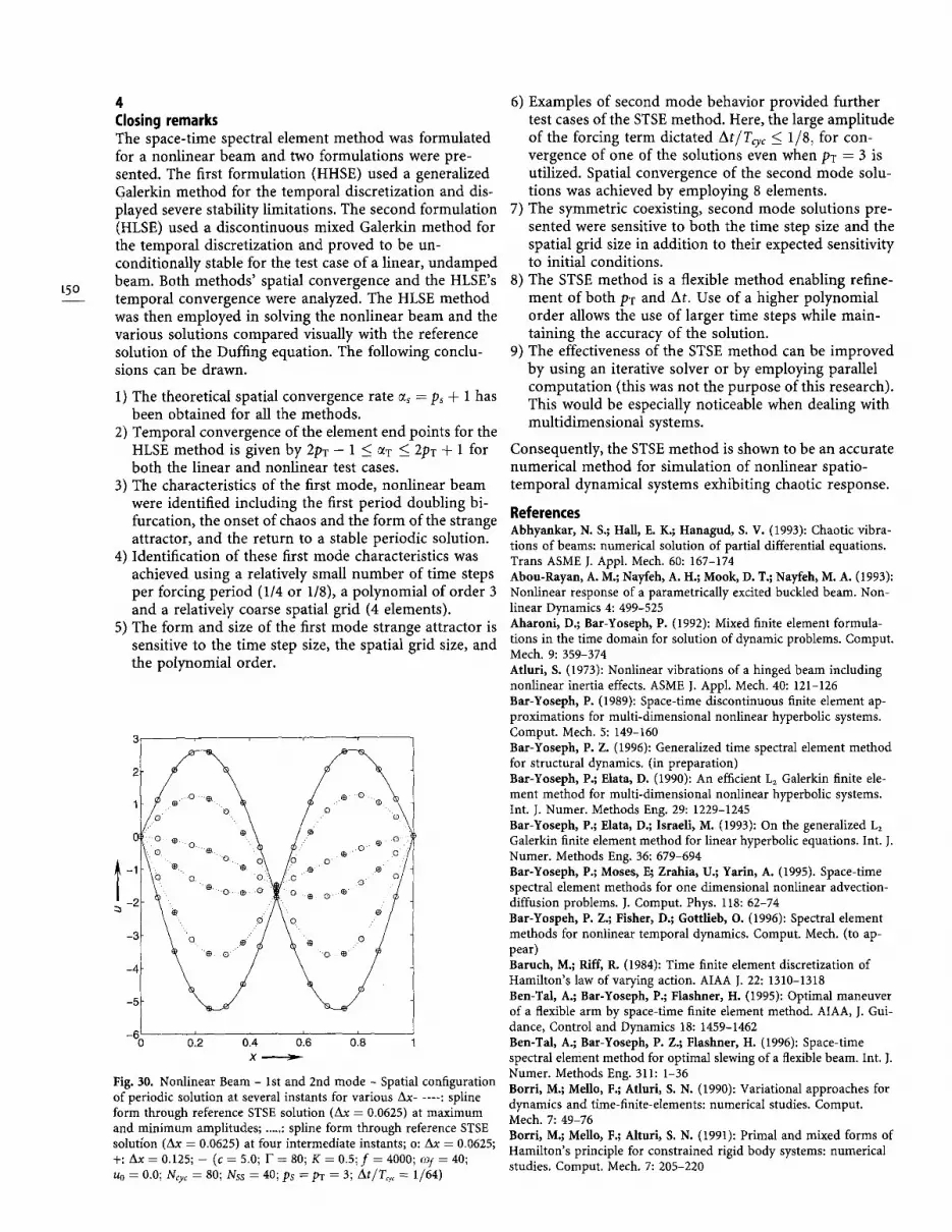
An example of combined first and second mode beha- vior ( f -- 4000, COl = 40) is shown in the phase of Fig. 29. Here h-convergence is observed with At/Tr162 decreasing from At/Tcyc = 1/4 to At/Tcyc = 1/64 while ut i l izing PT = 3 and Ax = 0.125. Note that the solut ions lie on symmetric coexisting reference solutions (At/Tcyc = 1/128) described by a con t inuous line (right) and a dotted line (left) which were achieved by varying the initial condi t ions slightly. While At/Tcyc = 1/4 and At/Tcyc = 1/64 lie on the 'left' reference solution, At/r~y~ = 1/8 and At/r~yc = 1/16 lie on the ' r ight ' re- ference solution. This indicates that this highly non l inea r system is sensitive to both the t ime step and to the initial condi t ions so that the two coexisting solut ions are pro- duced by variat ion of either the initial condi t ions or the t ime step size. The solut ion for At/Tcyc = 1/32 lies on the trajectory indicated by the cont inuous line and for reasons of clarity is not presented here. As men t ioned above in Sec. 3.4, the STSE solut ion points displayed on the graphs are temporal end points and the solut ion at the in ternal nodal points is not depicted. Therefore, al though the At/T~yc = 1/4 solution does not appear to fully describe the phase plane trajectory, inclusion of the two in ternal nodal points would produce a better defined trajectory. The beam configurat ion at steady state is shown in Fig. 30 at six instants: m a x i m u m and m i n i m u m ampl i tude (solid line) and four intermediate instants (dotted line). The lines represent spline interpolat ions through the points of the reference STSE solut ion (Ax = 0.0625). In this case the behavior is not entirely second mode as the center of the

�9 ~ �9 m.

- 0 0.2 0.4 0.6 0.8 X , - ~ - ~ m , , -

Pig. 28. Nonlinear Beam - 2rid mode - Spatial configuration of per- iodic solution at several instants for various Ax . . . . . : 2nd mode si- nusoidal form through 1st peak of Ax = 0.0625, STSE solution at maximum and minimum amplitudes; ..... : 2nd mode sinusoidal form through 1st peak of Ax = 0.0625 STSE solution at two intermediate instants; o: Ax = 0.0625; +: Ax = 0.125; x: Ax = 0.25; - (c = 5.0; F = 80; K = 0.5; f = 4000; ~of = 60; Uo = 0.0; N~ = 50; Nss = 40; ps = pT = 3; At/T~y~ = 1/64)

150

100 �9

50 :

~1 0 ~ .'~

-50

~fD .:

-100 ~ ~ "

~ ~ ~ : ~ ~ r , , ,

- 1 5 0 - 4 - 2 0 2 4 6

U(X= 1/4)

Fig. 29. Nonlinear Beam - 1st and 2nd mode - Phase plane of a periodic solution for various At/Tcyc - --: At/Tcyc = 1/128 (Uo = 0.1); .... : At/T,.y< = 1/128 (u0 = -0.1); o: At/T,,, = 1/4; .: At~T<,< = 1/8; x: At/T~y~ = 1/16; ,: At/T~z ~ = 1/64; (c = 5.0; F = 80; K = 0.5; f = 4000; (of = 40; Uo = 0.0; Ncyc = 80; Nss = 40; Ps = PT = 3; AX = 0.125)

beam is also observed to vibrate about a point which does not lie on u = 0. Note that uti l izing Ax = 0.25 with At/Tcyc = 1/64 produced the symmetr ic coexisting solu- t ion and is therefore not shown in Fig. 30. It is evident from Fig. 30 that the use of Ax = 0.125 with At/Tcyc = 1/64 provides sufficient accuracy.

149

t5o

4 Closing remarks The space-time spectral element method was formulated for a nonlinear beam and two formulations were pre- sented. The first formulat ion (HHSE) used a generalized Galerkin method for the temporal discretization and dis- played severe stability limitations. The second formulation (HLSE) used a discontinuous mixed Galerkin method for the temporal discretization and proved to be un- conditionally stable for the test case o f a linear, undamped beam. Both methods ' spatial convergence and the HLSE's temporal convergence were analyzed. The HLSE method was then employed in solving the nonl inear beam and the various solutions compared visually with the reference solution of the Duffing equation. The following conclu- sions can be drawn.

1) The theoretical spatial convergence rate ~s = ps § i has been obtained for all the methods.

2) Temporal convergence of the element end points for the HLSE method is given by 2pT -- 1 _~ aT ~_ 2pT § 1 for both the linear and nonlinear test cases.

3) The characteristics of the first mode, nonlinear beam were identified including the first period doubling bi- furcation, the onset of chaos and the form of the strange attractor, and the return to a stable periodic solution.

4) Identification of these first mode characteristics was achieved using a relatively small number of time steps per forcing period (1/4 or 1/8), a polynomial of order 3 and a relatively coarse spatial grid (4 elements).

5) The form and size of the first mode strange attractor is sensitive to the time step size, the spatial grid size, and the polynomial order.

-3

-!

-%

�9 O

.~ ~ o . o �9 . . o o

o . o 0 o

O O O 0 ~ ' . 0 . ~ 0 0 ~ . 0 ~ "

o o 'O ~'4 ~ O

o12 o14 o16 08 x ~

Fig. 30. Nonlinear Beam - 1st and 2nd mode - Spatial configuration of periodic solution at several instants for various Ax . . . . . : spline form through reference STSE solution (Ax = 0.0625) at maximum and minimum amplitudes; ..... : spline form through reference STSE solution (Ax = 0.0625) at four intermediate instants; o: Ax = 0.0625; +: Ax = 0.125; - (c = 5.0; F = 80; K = 0.5; f = 4000; o~f = 40; Uo = 0.0; Ncyc = 80; Nss = 40; Ps = pT = 3; A t / T o y c ~- 1/64)

6) Examples of second mode behavior provided further test cases of the STSE method. Here, the large ampli tude of the forcing term dictated A t /Tc y c <_ 1/8, for con- vergence of one of the solutions even when PT = 3 is utilized. Spatial convergence of the second mode solu- t ions was achieved by employing 8 elements.

7) The symmetric coexisting, second mode solutions pre- sented were sensitive to bo th the time step size and the spatial grid size in addit ion to their expected sensitivity to initial conditions.

8) The STSE method is a flexible method enabling refine- ment of both pT and At. Use of a higher polynomial order allows the use of larger time steps while main- taining the accuracy of the solution.

9) The effectiveness of the STSE method can be improved by using an iterative solver or by employing parallel computa t ion (this was not the purpose of this research). This would be especially noticeable when dealing with mult idimensional systems.

Consequently, the STSE method is shown to be an accurate numerical method for simulation of nonlinear spatio- temporal dynamical systems exhibiting chaotic response.

References Abhyankar, N. S.; Hall, E. K.; Hanagud, S. V. (1993): Chaotic vibra- tions of beams: numerical solution of partial differential equations. Trans ASME J. Appl. Mech. 60:167-174 Abou-Rayan, A. M.; Nayfeh, A. H.; Mook, D. T.; Nayfeh, M. A. (1993): Nonlinear response of a parametrically excited buckled beam. Non- linear Dynamics 4:499-525 Aharoni, D.; Bar-Yoseph, P. (1992): Mixed finite element formula- tions in the time domain for solution of dynamic problems. Comput. Mech. 9:359-374 Atluri, S. (1973): Nonlinear vibrations of a hinged beam including nonlinear inertia effects. ASME J. Appl. Mech. 40:121-126 Bar-Yoseph, P. (1989): Space-time discontinuous finite element ap- proximations for multi-dimensional nonlinear hyperbolic systems. Comput. Mech. 5:149-160 Bar-Yoseph, P. Z. (1996): Generalized time spectral element method for structural dynamics. (in preparation) Bar-Yoseph, P.; Elata, D. (1990): An efficient L2 Galerkin finite ele- ment method for multi-dimensional nonlinear hyperbolic systems. Int. ]. Numer. Methods Eng. 29:1229-1245 Bar-Yoseph, P.; Elata, D.; Israeli, M. (1993): On the generalized L2 Galerkin finite element method for linear hyperbolic equations. Int. J. Numer. Methods Eng. 36:679-694 Bar-Yoseph, P.; Moses, E; Zrahia, U.; Yarin, A. (1995). Space-time spectral element methods for one dimensional nonlinear advection- diffusion problems. ]. Comput. Phys. 118:62-74 Bar-Yospeh, P. Z.; Fisher, D.; Gottlieb, O. (1996): Spectral element methods for nonlinear temporal dynamics. Comput. Mech. (to ap- pear) Baruch, M.; Rift, R. (1984): Time finite element discretization of Hamilton's law of varying action. AIAA ]. 22:1310-1318 Ben-Tal, A.; Bar-Yoseph, P.; Flashner, H. (1995): Optimal maneuver of a flexible arm by space-time finite element method. AIAA, ]. Gui- dance, Control and Dynamics 18:1459-1462 Ben-Tal, A.; Bar-Yoseph, P. Z.; Flashner, H. (1996): Space-time spectral element method for optimal slewing of a flexible beam. Int. ]. Numer. Methods Eng. 311:1-36 Borri, M.; Mello, F.; Atluri, S. N. (1990): Variational approaches for dynamics and time-finite-elements: numerical studies. Comput. Mech. 7:49-76 Borri, M.; Mello, F.; Alturi, S. N. (1991): Primal and mixed forms of Hamilton's principle for constrained rigid body systems: numerical studies. Comput. Mech. 7:205-220

Belic, M.; Liuboje, Z.; Sauer, M.; Kaiser, F. (1992): Computational chaos in nonlinear optics. Appl. Phys. B 55:109-116 Corless, R. M.; Essex, C.; Nerenberg, M. A. H. (1991): Numerical methods can suppress chaos. Phys. Letters A 157:27-36 Fletcher, C. A. I. (1991): Computational techniques for fluid dy- namics, 2nd ed. Berlin: Springer-Verlag, Vol. I: 355-360 Holmes, P./ . (1979): A nonlinear oscillator with a strange attractor. Philosoph. Trans. Royal Soc. A292:419-448 Holmes, P. ]4 Marsden, J. (1981): A partial differential equation with infinitely many periodic orbits: chaotic oscillations of a forced beam, Arch. Rat. Mech. Anal. 76:135-166 Huang, N. C.; Nachbar, W. (1968): Dynamic snap-through of im- perfect viscoelastic shallow arches. Trans ASME J. Appl. Mech. 35: 289-297 Hulbert, G. M.; Hnghes, T. J. R. (1990): Space-time finite element methods for second-order hyperbolic equations. Comput. Methods Appl. Mech. Eng. 84:327-348 Johnson, C. (1993). Discontinuous Galerkin finite element methods for second order hyperbolic problems. Comput. Methods Appl. Mech. Eng. 107:117-129

Lorenz, E. N. (1989): Computational chaos - a prelude to computa- tional instability. Physica D 35:299-317 Moon, F. C.; Holmes, P. J. (1979): A magneto-elastic strange attractor. J. Sound and Vibrat. 65:275-296 Patera, A. T. (1984): A spectral element method for fluid dynamics; laminar flow in a channel expansion. J. Comput. Phys. 54:468-488 Szemplinska-Stupnicka, W.; Plaut, R. H.; Hsieh, J. C. (1989): Period doubling and chaos in unsymmetric structures under parametric excitation. ASME 1. AppI. Mech. 56:947-952 Tseng, W. Y.; Dugund~i, l (1971): Nonlinear vibrations of a buck/ed beam under harmonic excitation. ASME ). Appl. Mech. 38:467-476 Yee, H. C.; Sweby, (1995): Dynamical approach study of spurious steady state numerical solutions of nonlinear differential equations. II. Global asymptotic behavior of time discretizations. Comp. Fluid Dyn. 4:219-283 Zrahia, U.; Bar-Yoseph, P. (1994): Space-time spectral element method for solution of second-order hyperbolic equations. Comput. Methods Appl. Mech. Eng. 116:135-146

151