Pergamon Atmospheric Environment Vol, 30, No. 22, pp. 3837-3855, 1996 Copyright © 1996 Elsevier Science Ltd

Printed in Great Britain. All rights reserved P I I : S1352-2310(96)00085-4 1352-2310/96 $15.00 + 0.00

SOURCE APPORTIONMENT OF AIRBORNE PARTICULATE MATTER USING ORGANIC COMPOUNDS AS TRACERS

JAMES J. S C H A U E R , W O L F G A N G F. R O G G E , * L Y N N M. H I L D E M A N N , t M O N I C A A. MAZUREK:~ and G L E N R. CASS§

Environmental Engineering Science Department, California Institute of Technology, Pasadena, CA 91125, U.S.A.

and

B E R N D R. T. S I M O N E I T Petroleum and Environmental Geochemistry Group, College of Oceanic and Atmospheric Sciences,

Oregon State University, Corvallis, Oregon 97331, U.S.A.

(First received 29 June 1995 and in final form 8 February 1996)

Abstract--A chemical mass balance receptor model based on organic compounds has been developed that relates source contributions to airborne fine particle mass concentrations. Source contributions to the concentrations of specific organic compounds are revealed as well. The model is applied to four air quality monitoring sites in southern California using atmospheric organic compound concentration data and source test &~ta collected specifically for the purpose of testing this model. The contributions of up to nine primary particle source types can be separately identified in ambient samples based on this method, and approximately 85% of the organic fine aerosol is assigned to primary sources on an annual average basis. The model provides information on source contributions to fine mass concentrations, fine organic aerosol concentrations and individual organic compound concentrations. The largest primary source contributors to fine partic]Le mass concentrations in Los Angeles are found to include diesel engine exhaust, paved road dust, gasoline-powered vehicle exhaust, plus emissions from food cooking and wood smoke, with smaller contribution,; from tire dust, plant fragments, natural gas combustion aerosol, and cigarette smoke. Once these primary aerosol source contributions are added to the secondary sulfates, nitrates and organics present, virtually all of the annual average fine particle mass at Los Angeles area monitoring sites can be assigned to i~:s source. Copyright © 1996 Elsevier Science Ltd

Key word index: Receptor models, organic aerosol, fine particles, source contributions, emissions.

liNTRODUCTION

Suspected adverse ihealth effects of even low levels of airborne particulate matter have led to increased con- cern over how fine particulate concentrations might best be controlled (Dockery et al., 1993). The develop- ment of effective control strategies for fine particulate air pollution abatement in turn requires a knowledge of the relative importance of the various sources that

*Present address: Department of Civil and Environmental Engineering, Florida International University, Miami, FL 33199, U.S.A.

tPresent address: Department of Civil Engineering, Stan- ford University, Stanford, CA 94305-4020, U.S.A.

:~Present address: Institute of Marine and Coastal Sciences, Rutgers Uni versity, P.O. Box 231, New Brunswick, NJ 08903, U.S.A.

§Author to whom correspondence should be addressed.

contribute to the particulate matter concentrations at ambient air monitoring sites (Atkinson and Lewis, 1974; Harley et al., 1989).

Two approaches can be employed to evaluate source contributions from source emissions data and ambient monitoring data: source-oriented models and receptor-oriented models. Source-oriented models use emissions data and fluid mechanically explicit trans- port calculations to predict pollutant concentrations at specific receptor air monitoring locations. This type of model is validated by comparison of the predicted spatial and temporal distribution of pollutant concen- trations against measured concentrations (Bencala and Seinfeld, 1979; Liu and Seinfeld, 1975). Receptor- oriented models infer source contributions by deter- mining the best-fit linear combination of emission source chemical composition profiles needed to re- construct the measured chemical composition of am- bient samples (Watson, 1984).

3837

3838 J.J. SCHAUER et al.

Determination of source contributions from ambi- ent monitoring data by receptor modeling techniques relies on the ability to characterize and distinguish differences in the chemical composition of different source types. The elemental composition of source emissions has been used on many occasions to ident- ify separately different sources of airborne particles (Miller et al., 1972; Hopke et al., 1976; Gordon, 1980; Cooper and Watson, 1980; Cass and McRae, 1983). Unfortunately, a large number of sources that emit fine particulate matter do not produce emissions that have unique elemental compositions; instead, many sources emit principally organic compounds and el- emental carbon. Examples of such sources include diesel engine exhaust, combustion of unleaded gaso- line, the effluent from meat cooking operations, and cigarette smoke (Hildemann et al., 1991). When such important sources of primary particle emissions can- not be identified in ambient samples, then much of the true nature of a particulate air pollution problem remains obscured.

Recent advances in source testing techniques make it possible to measure the concentrations of hundreds of specific organic compounds in the fine aerosol emitted from air pollution sources (Rogge et al., 1991, 1993b-e; Rogge, 1993). By analogous methods, the organic compounds present in the fine aerosol col- lected at ambient sampling sites also can be deter- mined (Rogge et al., 1993a; Rogge, 1993). The relative distribution of single organic compounds in source emissions provides a means to fingerprint sources that cannot be uniquely identified by elemental composi- tion alone. These advances in measurement methods therefore create the practical possibility of devising receptor models for aerosol source apportionment that rely on organic compound concentration data and that potentially can identify separately the

contributions of many more source types than has been possible based on elemental data alone.

In the present paper, receptor modeling methods will be developed that use organic compound distri- butions in both source samples and in ambient sam- ples to determine source contributions to airborne particulate matter samples. Two critical aspects of this work are (1) selection of the sources to be included in such a model and (2) identification of the organic compounds for which material balances can be writ- ten. Methods developed will be tested by application to data taken in southern California.

EXPERIMENTAL

Ambient samples

Throughout 1982, airborne fine particulate matter (dp < 2/~m) samples were collected for 24 h every sixth day at 10 Los Angeles-area air quality monitoring sites and one upwind remote off-shore island (Gray et al., 1986). The present study uses samples from four of these sampling sites: West Los Angeles, Downtown Los Angeles, Pasadena, and Rubidoux (see Fig. 1).

The ambient aerosol samples used in this study were collected downstream of an AIHL cyclone separator oper- ated at 25.9 • min-1 that removed particles with aerody- namic diameters larger than 2/tin (John and Reischl, 1980). Air leaving the cyclone was divided between four parallel 47 mm diameter filter assemblies: two containing quartz fiber filters (Pallflex Tissuequartz 2500 QAO), one contain- ing a Teflon membrane filter (Membrana 0.5/tm pore size), and one containing a Nuclepore filter (0.4/an pore size). Each of the quartz fiber filters was operated at an air flow rate of 10 ~ min- 1, while the Teflon filters and the Nuclepore filters were operated at 4.9 and 1.0 ~ min - 1, respectively. The quartz fiber filters were baked at 600°C for a minimum of 2 h prior to sample collection to lower residual carbon levels associated with untreated filters.

One quartz fiber filter from each day at each sampling site was analyzed for elemental carbon (EC) and organic carbon

! "l i l ", i .: ",. i

" ~ :J i ~ , ~ ...... .' Pasadena l

_ ~ . -" West LA • • / ~ Downtown LA,,d , . , . - . ; . . . . . : . . . . . . . . . . r - . . . . . . . . . . . . . . . . .

~ , ,~ . . . . . . ... , " Rubidoux , . - ~,. ,

PACIFIC OCEAN ,/"

Fig. 1. Air quality monitoring sites in southern California used in the present study.

Airborne particulate matter 3839

(OC) by the method of Huntzicker et al. (1982) and Johnson et al. (1981). Monthly composites formed by utilizing the second quartz fiber filter from each site on each day were reserved for the identification and quantification of the indi- vidual organic compounds present by high-resolution gas chromatography (HRGC) and gas chromatography/mass spectrometry (GC/MS) (Rogge et al., 1993a; Rogge, 1993).

The particulate matter collected on the Teflon filters was used to determine total fine particulate mass concentrations by gravimetric analysis. The Teflon filters were also analyzed by X-ray fluorescence to quantify the concentrations of 34 trace elements including aluminum and silicon, which will be used in the present study. Samples collected on the Nuc- lepore filters were ana.lyzed for sulfate and nitrate by ion chromatography (Mueller et al., 1978), and for ammonium ion by the phenol-hypochlorite method (Solorzano, 1967).

Source samples

A source sampling program was undertaken in order to determine the mass emission rate and chemical composition of the fine particulate matter released from the most promin- ent sources of carbonaceous aerosol emissions in southern California. Fifteen source types were tested, as shown in Table 1, that accounted for approximately 80% of the fine carbonaceous aerosol emissions in the Los Angeles basin during the 1982 period for which ambient samples are avail- able (Gray, 1986; Hildemann et al., 1991). Detailed descrip- tions of the procedures used for fine particulate source samp- ling from each source have been presented previously (Hil- demann et al., 1991). Briefly, combustion source emissions were collected utilizirLg a dilution stack sampling system (Hildemann et al., 1989). Dilution air, which was passed through a HEPA filter and an activated carbon bed, was mixed with source emissions to simulate the condensation

process that occurs due to dilution and cooling as a plume enters the atmosphere. After sufficient residence time in the sampler, several streams of diluted emissions were drawn through AIHL cyclones at conditions designed to remove particles with aerodynamic diameters greater than 2 #m, followed by fine particle collection on appropriate filter substrates. Quartz fiber filters (Pallflex Tissuequartz 2500 QAO) were used in the same manner as described for ambi- ent sampling for both EC/OC analysis and for identification and quantification of organic compounds by HRGC and GC/MS. Samples collected on Teflon filters (Gelman Teflo, 2 pm pore size) were used for gravimetric determination, X-ray fluorescence analysis, and for ion chromatography. The emissions from catalyst-equipped autos, non-catalyst autos, diesel trucks, oil-fired boilers, natural gas home appli- ances, meat charbroiling and frying, and fireplace combus- tion of wood were measured in this manner.

The diesel trucks tested by Hildemann et al. (1991) repre- sented vehicles newer than the fleet of diesel trucks in opera- tion in the Los Angeles basin in 1982, when the ambient samples used in this study were collected. Comparison of the Hildemann et al. source test data for newer trucks to source test data on older diesel trucks summarized by Gray (1986) shows that the organic compound emission rates from both the newer and older trucks are similar, while the elemental carbon emissions from the older trucks are much higher than for the newer trucks. For this reason, the elemental carbon emissions rate used in the present study to represent diesel- powered vehicles in 1982 is taken from Gray et al. (1986), while the emissions rate and distribution of the organic compounds is taken from Hildemann et al. (1991).

Cigarette smoke and roofing tar pot emissions were sam- pled with a modified dilution sampler (Hildemann et al., 1991) that employed the same cyclone and filter collection

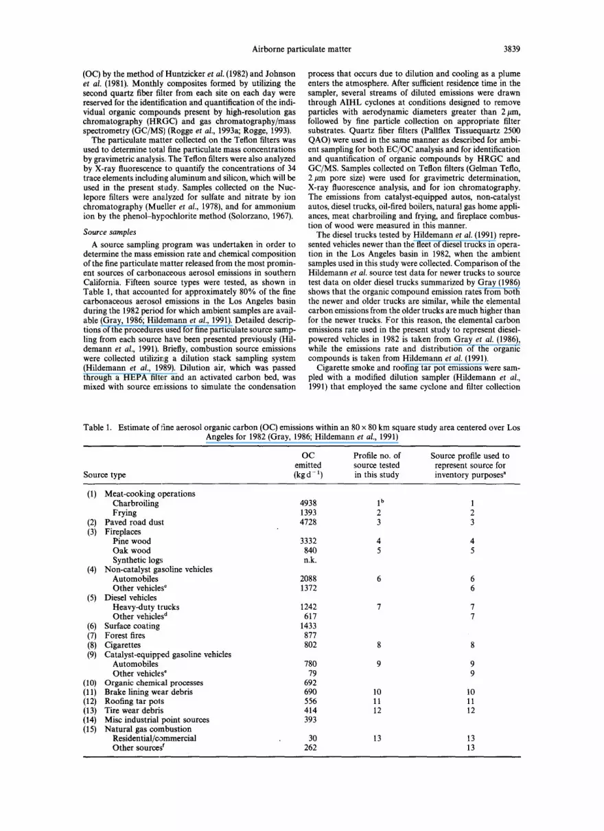
Table I. Estimate of fine aerosol organic carbon (OC) emissions within an 80 x 80 km square study area centered over Los Angeles for 1982 (Gray, 1986; Hildemann et al., 1991)

Source type

OC Profile no. of Source profile used to emitted source tested represent source for (kg d-1) in this study inventory purposes a

(1) Meat-cooking operations Charbroiling 4938 1 b 1 Frying 1393 2 2

(2) Paved road dust 4728 3 3 (3) Fireplaces

Pine wood 3332 4 4 Oak wood 840 5 5 Synthetic log,; n.k.

(4) Non-catalyst gasoline vehicles Automobiles 2088 6 6 Other vehicles c 1372 6

(5) Diesel vehicles Heavy-duty trucks 1242 7 7 Other vehicles d 617 7

(6) Surface coating 1433 (7) Forest fires 877 (8) Cigarettes 802 8 8 (9) Catalyst-equipped gasoline vehicles

Automobiles 780 9 9 Other vehicles e 79 9

(10) Organic chemical processes 692 (11) Brake lining wear debris 690 10 10 (12) Roofing tar pols 556 11 11 (13) Tire wear debris 414 12 12 (14) Misc industrial point sources 393 (15) Natural gas combustion

Residential/commercial 30 13 13 Other sources f 262 13

3840 J. J. SCHAUER et al.

Table 1. (continued)

Source type

OC emitted (kg d - 1)

Profile no. of source tested in this study

Source profile used to represent source for inventory purposes a

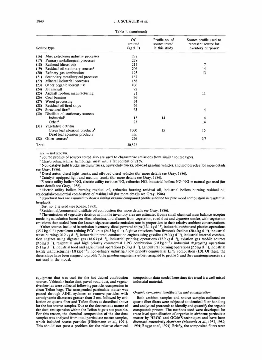
(16) Misc petroleum industry processes 278 (17) Primary metallurgical processes 228 (18) Railroad (diesel oil) 211 (19) Residual oil stationary sources g 206 (20) Refinery gas combustion 195 (21) Secondary metallurgical processes 167 (22) Mineral industrial processes 158 (23) Other organic solvent use 106 (24) Jet aircraft 92 (25) Asphalt roofing manufacturing 81 (26) Coal burning 76 (27) Wood processing 74 (28) Residual oil-fired ships 66 (29) Structural fires h 63 (30) Distillate oil stationary sources

Industrial i 13 Other j 23

(31) Vegetative detritus Green leaf abrasion products k 1000 Dead leaf abrasion products n.k.

(32) Other sources I 226

Total 30,822

14

15

7 14 13

11

4

14 14

15

6,7

n.k. = not known. a SourCe profiles of sources tested also are used to characterize emissions from similar source types. b Charbroiling regular hamburger meat with a fat content of 21%. o Non-catalyst light trucks, medium trucks, heavy-duty trucks, off-road gasoline vehicles, and motorcycles (for more details

see Gray, 1986). d Diesel autos, diesel light trucks, and off-road diesel vehicles (for more details see Gray, 1986). e Catalyst-equipped light and medium trucks (for more details see Gray, 1986). f Electric utility boilers NG, electric utility turbines NG, refineries NG, industrial boilers NG; N G = natural gas used (for

more details see Gray, 1986). g Electric utility boilers burning residual oil, refineries burning residual oil, industrial boilers burning residual oil,

residential/commercial combustion of residual oil (for more details see Gray, 1986). h Structural fires are assumed to show a similar organic compound profile as found for pine wood combustion in residential

fireplaces. iTest no. 2 is used (see Rogge, 1993). J Residential/commercial distillate oil combustion (for more details see Gray, 1986). k The emissions of vegetative detritus within the inventory area are estimated from a small chemical mass balance receptor

modeling calculation based on silica, alumina, and alkanes from vegetation, road dust and cigarette smoke, with vegetation emissions then scaled from the known cigarette smoke emission rate in proport ion to their relative ambient concentrations.

Other sources included in emission inventory: diesel powered ships (42.1 kg d - 1), industrial rubber and plastics operations (35.7 kg d - 1), petroleum refining FCC units (24.5 kg d - 1), fugitive emissions from livestock feedlots (20.4 kg d - 1), industrial waste burning (20.2 kg d - 1), industrial internal combustion engines using gasoline (19.0 kg d - 1), industrial internal combus- tion engines using digester gas (18.6 kgd-1) , industrial printing operations (12.9 kgd-~) , aviation gas mobile sources (9.6 kg d-~), residential and high priority commercial LPG combustion (7.8 kgd-1) , industrial degreasing operations (5.1 kg d - 1), industrial food and agricultural operations (5.0 kg d - 1), agricultural burning operations (2.5 kg d - 1), industrial textile manufacturing (1.8 kg d - 1), non-refinery industr ia l / low priority commercial LPG combustion (1.3). Of these, the diesel ships have been assigned to profile 7, the gasoline engines have been assigned to profile 6, and the remaining sources are not used in the model.

equipment that was used for the hot ducted combustion sources. Vehicular brake dust, paved road dust, and vegeta- tive detritus were collected following particle resuspension in clean Teflon bags. The resuspended particulate matter was passed through AIHL cyclones to remove particles with aerodynamic diameters greater than 2 #m, followed by col- lection on quartz fiber and Teflon filters as described above for the hot source samples. Due to the electrostatic nature of tire dust, resuspension within the Teflon bags is not possible. For this reason, the chemical composition of the tire dust samples was analyzed from total particulate matter samples, which included coarse particles (Hildemann et aL, 1991). This should not pose a problem for the relative chemical

composition data needed here since tire tread is a well-mixed industrial material.

Organic compound identification and quantification

Both ambient samples and source samples collected on quartz fiber filters were subjected to identical filter handling and analytical protocols to identify and quantify the organic compounds present. The methods used were developed for trace level quantification of organics in airborne particulate matter by H R G C and GC/MS techniques and have been discussed extensively elsewhere (Mazurek et al., 1987, 1989, 1991; Rogge et al., 1991). Briefly, the composited filters were

Airborne particulate matter 3841

spiked with an internal recovery standard, perdeuterated tetracosane (n-C24Dso). The samples were extracted twice with hexane, followed by three successive benzene/2-pro- panol (2 : 1) extractions. Extracts were combined and each final extract mixture was reduced to 200-500 #1 total vol- ume. An aliquot of the concentrated extract was derivatized with diazomethane to convert organic acids to their methyl ester analogues (Mazurek et al., 1987). Then the concentra- tions of the 100 individual organic compounds, listed in Table 2, were quantified in the ambient fine particulate samples by GC/MS techniques (Rogge et al., 1993a; Rogge, 1993). The same compounds plus other readily identified organics were sought in the source samples. Tracer com- pound mass concentrations in both source and ambient samples were corrected for recovery efficiency during extrac- tion (see Mazurek et al., 1987 for example) such that the total tracer content of each sample was measured. Single

compound mass emission rates from each of the 15 source types studied are reported by Rogge et al. (1991, 1993b-e, 1994) and by Rogge (1993). These references by Rogge et al. when combined with gravimetric mass concentration data and total carbon data reported by Gray et al. (1986) and Hildemann et al. (1991) yield source profiles and ambient aerosol composition data that show the fine particle mass, overall organic carbon and elemental carbon content, extractable organics content, individual organic compound content and trace element content of each sample. The source profile and ambient data used in the present study also can be obtained in consolidated form from the authors.

Confidence intervals for the organic compound quantifi- cation procedures used in this study were estimated from analysis of the variance of the historical ambient data along with more recent experiments conducted in our laboratory.

Table 2. List of compounds available for possible use in the receptor model-1982, Los Angeles

Compound name

Range of annual average ambient fine particulate Used in Reason

concentration (ng m- a) receptor model not used

n-Alkanes n-Tricosane n-Tetracosane n-Pentacosane n-Hexacosane n-Heptacosane n-Octacosane n-Nonacosane n-Triacontane n-Hentriacontane n-Dotriacontane n-Tritriacontane n-Tetratriacontane

iso- and anteiso-Alkanes anteiso-Triacontane iso-Hentriacontane anteiso-Hentriacontane iso-Dotriacontane anteiso-Dot riacontan~: iso-Tritriacontane

Hopanes and steranes 20S&R-5ct(H),I 4fl(H),il 7fl(H)-Cholestanes 20R-5ct(H), 14ct(H), 17ctlH)-Cholestane 20S&R-5ct(H), 14fl(H), :t 7fl(H)-Ergostanes 20S&R-5ct(H), 14/~(H),~l 7~(H)-Sitostanes 22,29,30-Trisnorneohopane 17e(H),21/~(H)-29-Norhopane 17ct(H),21 fl(H)-Hopan e 22S- 17e(H),21 fl(H)-30..Homohopane 22R-17e(H),21fl(H)-30-Homohopane 22S- 17e(H),2 lfl(H)-30.-Bishomohopane 22R-17e(H),21fl(H)-30-Bishomohopane

n-AIkenoic acids cis-9-n-Octadecenoic acid

Aldehydes Nonanal

n-Akanoic acids n-Nonanoic acid n-Decanoic acid n-Undecanoic acid n-Dodecanoic acid n-Tridecanoic acid

3.2-6.7 Yes 3.9-5.0 Yes 6.7-11.2 Yes 4.3-8.2 Yes 5.2-6.7 Yes 2.1-3.1 Yes 4.7-7.1 Yes 2.4-2.7 Yes 9.3-12.6 Yes 1.0-1.5 Yes 1.5-2.3 Yes 0.36-0.68 Yes

< 0.03-0.23 Yes 0.73-1.50 Yes

< 0.03-0.12 Yes < 0.03-0.13 Yes

0.89-1.31 Yes 0.30-0.33 Yes

0.34-1.18 Yes 0.34-1.23 Yes 0.51-1.75 Yes 0.52-1.67 Yes 0.32-0.93 Yes 0.66-2.42 Yes 1.32-4.02 Yes 0.52-1.42 Yes 0.36-1.06 Yes 0.33-0.84 Yes 0.20-0.58 Yes

17.3-26.0 Yes

5.7-9.5 Yes

3.3-9.9 No 1.3-3.1 No 2.8-6.0 No 3.7-7.0 No 3.3-4.9 No

3842

Compound name

n-Tetradecanoic acid n-Pentadecanoic acid n-Hexadecanoic acid n-Heptadecanoic acid n-Octadecanoic acid n-Nonadecanoic acid n-Eicosanoic acid n-Heneicosanoic acid n-Docosanoic acid n-Tricosanoic acid n-Tetracosanoic acid n-Pentacosanoic acid n-Hexacosanoic acid n-Heptacosanoic acid n-Octacosanoic acid n-Nonacosanoic acid n-Triacontanoic acid

Dicarboxylic acids Propanedioic acid 2-Butenedioic acid Butanedioic acid Methylbutanedioic acid Pentanedioic acid Methylpentanedioic acid Hydroxybutanedioic acid Hexanedioic acid Octanedioic acid Nonanedioic acid

Aromatic carboxylic acids 1,2-Benzenedicarboxylic acid 1,3-Benzenedicarboxylic acid 1,4-Benzenedicarboxylic acid 4-Methyl- 1,2-benzenedicarboxylic acid 1,2,4-Benzenet ricarboxylic acid 1,3,5-Benzenet ricarboxylic acid 1,2,4,5-Benzenetetracarboxylic acid

Wood smoke markers Dehydroabietic acid 13-Isopropyl-5ct-podocarpa-6,8,11,13-

tetraen-16-oic acid 8,15-Pimaradien- 18-oic acid Pimaric acid Isopimaric acid 7-Oxodehydroabietic acid Sandaracopimaric acid Retene

Polycyclic aromatic hydrocarbons Fluoranthene Pyrene Benz[a]anthracene Cyclopenta [cd] pyrene Benzo[ghi]fluoranthene Chrysene/triphenylene Benzo[k]fluoranthene Benzo[b]fluoranthene Benzo[e]pyrene Benzo[a]pyrene Indenol- 1,2,3-cd]pyrene Indeno[1,2,3-cd]fluoranthene Benzol-ghi]perylene Coronene

J. J. SCHAUER et al.

Table 2. (continued)

Range of annual average ambient fine particulate

concentration (ng m - 3) Used in

receptor model

14.4-22.8 4.3-6.1

118-141 3.4-5.2

41.1-59.2 0.79-1.1 3.1-6.1 1.4-2.3 5.7-9.9 1.5-2.5 9.2-16.5 1.1-1.6 5.3-9.3 0.47-0.81 2.7-4.9 0.33-0.57 1.0 2.2

28.0-51.0 0.58-1.3

51.2-84.1 11.6-20.3 28.3-38.7 15.5-23.7 7.8-22.1

14.1-24.3 2.5-4.1

22.8-44.7

53.5-60.6 2.1-3.4 0.88-2.8

15.2-28.8 0.45-0.84

11.3-22.6 0.40-0.80

10.2-23.6 0.30-1.2

0.07-1.1 0.94-4.8 0.71-2.3 1.9-4.1 0.60-2.2 0.01-0.10

0.07-0.15 0.12-0.26 0.09-0.29 0.04-0.41 0.11-0.39 0.23-0.61 0.33-1.20 0.68-1.23 0.38-0.97 0.18-0.44 0.07-0.43 0.26-1.09 1.12-4.47 2.41 °

No No No No No No No No No No No No No No No No No

No No No No No No No No No No

No No No No No No No

No No

Yes Yes Yes No No Yes

No No No No No No Yes Yes Yes No Yes Yes Yes Yes

Reason not used

Airborne particulate matter

Table 2. (continued)

3843

Compound name

Range of annual average ambient fine particulate Used in

concentration (ng m- 3) receptor model Reason not used

PAH ketones and quinones 7H-Benz[de]anthracen-7-one Benz[a]anthracene-7,12-dione Benzo [cd] pyren-6-one

Steroids Cholesterol

N-containing compounds 3-Methoxypyridine Isoquinoline 1 -Methylisoquinoline 1,2-Dimethoxy-4-nitro benzene

Inorganic elements Elemental carbon Particulate aluminum Particulate silicon

0.25-0.84 Yes 0.12-0.25 Yes 0.02-1.24 Yes

1.9-2.7 No

0.46-1.4 No 0.61-1.1 No 0.24-1.1 No 0.22-3.9 No

3030-4870 Yes 249-330 Yes 336-600 Yes

a Significant source not in model. b Species fails check for apparent conservation in the atmosphere c Some monitoring sites have missing data.

(it behaves as if it is formed or depleted).

The annual average atabient organic compound concentra- tions represent the mean of 12 monthly composites of daily samples taken at six day intervals. The uncertainties in the annual means of these atmospheric samples (+ l a) typi- cally are approximately +20%; and arise mainly from the fact that not all days of the year were sampled. The quantifi- able uncertainties in the source samples are principally ana- lytical uncertainties and also average approximately ___ 20% (+1~).

SOURCE/RECEPTOR RECONCILIATION

Chemical mass balance approach

The chemical composition of the emissions from individual sources can be used to estimate source contributions to atmospheric samples taken at recep- tor air monitoring sites (Hidy et al., 1974; Miller et al., 1972; Friedlander, 1973; Cass and McRae, 1983). One useful method for assigning ambient par- ticulate matter concentration increments to the sour- ces from which they originate is the chemical mass balance (CMB) technique. In the CMB method, a mass balance is constructed in which the concentra- tion of specific chemical constituents in a given ambi- ent sample is described as arising from a linear combi- nation of the relative chemical compositions of the contributing sources. The concentration of chemical constituent i at receptor site k, cik, can be expressed as:

c,: = ~ fijkaiisjk (1) j = l

where Sjk is the increment to total particulate mass concentration at receptor site k originating from source j, a o is the relative concentration of chemical

constituent i in the emissions from source j, andf~jk is the coefficient of fractionation that represents the modification of aij during transport from source j to receptor k. The fractionation coefficient accounts for selective loss of constituent i due to processes such as gravitational settling, chemical transformation, or evaporation; it can also be used to account for selec- tive gains in constituent i due to chemical formation or condensation. In the present study, chemical con- stituents which do not have fractionation coefficients near unity will not be used in mass balance calcu- lations. With the chemical composition of both the source samples (aij) and the ambient samples (Cik) known from experimental measurements and with J~jk near unity for each chosen chemical substance, the system of equations (1) can be solved for the unknown source contributions, Sjk, to the ambient pollutant concentrations.

If the number of chemical constituents included in the mass balance calculations exceeds the number of sources then the system of equations (1) is overdeter- mined, and exact agreement between the ambient concentrations and a unique linear combination of the source profiles is not expected due to the presence of small measurement errors. In this usual case, an ordinary least-squares solution to the system of equa- tions (1) can be employed. Alternatively, an effective variance weighted least-squares solution, which takes advantage of known uncertainties in ambient measure- ments and emissions data, can be used to solve the linear system of equations (Watson et al., 1984). In the present study, the system of equations (1) will be solved using the CMB7 source-receptor modeling computer program (Watson et al., 1990) that employs

3844 J.J. SCHAUER et al.

this effective variance weighted least-squares tech- nique.

Selection o f sources and organic compounds: an emissions inventory assisted approach

For the use of a chemical mass balance receptor model to be successful, several criteria must be met. First, if the coefficient of fractionation, f~jk, in equa- tion (1) is to be set to unity, then the chemical species for which material balance equations are written must be suffÉciently stable that they are conserved during transport from their sources to the receptor air monitor- ing sites. The species must not be significantly depleted from the fine particulate fraction by volatilization or chemical reaction, and the species concentration must not be significantly increased by atmospheric chemical formation processes. Second, all major sour- ces of each chemical species used in the mass balance must be included in the model, and the relative chem- ical compositions of the emissions from different source types that are included in the model must be different from each other in a statistical sense such that the problems of source profile collinearity are avoided. Little prior experience exists to show how a chemical mass balance receptor model based on organic tracer compounds should be constructed in order to exclude compounds that are insufficiently stable chemically, to assure that all major source types are included, and to detect and deal with source profiles from sources that are so similar to each other that collinearity problems would arise. In the follow- ing sections of the present paper, these issues are addressed within the context of example calculations in the Los Angeles area. In general, the methods used are similar to the emissions inventory-assisted chem- ical mass balance modeling procedures developed previously for data sets involving trace metals by Cass and McRae (1983).

A test for apparent chemical stability. One hun- dred organic compounds, listed in Table 2, were quan- tified both in source emissions and in fine aerosol samples collected at the four urban air monitoring sites used in this study (Rogge et al., 1993a; Rogge, 1993). An individual organic compound listed in Table 2 can be used successfully in the present CMB model only if it is conserved during transport from source to receptor (f~jk--~1). Since the atmospheric stability of many of these organic compounds has not been examined in this light previously, the first step in our analysis is to perform an initial screening to ident- ify and exclude compounds that do appear to be significantly modified during transport from source to receptor. The approach taken is to examine the ratio of the average atmospheric concentration to the area- wide emission rate for each organic compound studied. Fine elemental carbon particles have been employed previously as a nearly conserved tracer be- cause they are not depleted by chemical reaction and because, by virtue of their small size (Ouimette and Flagan, 1982; Venkataraman and Friedlander, 1994),

they are not depleted rapidly by dry deposition (Seh- mel, 1980). Those organic compounds in fine particles that likewise are conserved in the atmosphere ought to show a ratio of ambient concentration to source emission rate that is fairly similar to that for elemental carbon particles. Those compounds that are formed by atmospheric reactions will have a much higher than average ratio of atmospheric concentration to mass emissions, while those compounds that are de- pleted rapidly by evaporation or chemical reaction will show lower average ratios of their ambient con- centrations to emissions than is the case for a conser- ved species like elemental carbon.

The first step in this procedure for screening the compounds to be used is to construct a comparison of area-wide emissions and ambient concentrations for each chemical substance. Table 1 provides an emis- sions inventory for fine organic aerosol mass within an 80× 80 km area centered over the city of Los Angeles for 1982 (Hildemann et al., 1991). The sources sampled by Hildemann et al. (1991) and analyzed by Rogge et al. (1991, 1993a-d, 1994; Rogge, 1993) are indicated in Table 1. Several sources which were not tested by Hildemann et al. (1991) can be approxim- ated, for purposes of an emissions inventory, by sour- ces for which detailed emissions data are available (see Table 1). Including untested sources which can be represented by a tested source, the speciated emissions inventory data account for approximately 84% of the fine organic aerosol emissions within the 80 × 80 km inventory area. Using the atmospheric organic com- pound concentration data of Rogge et al. (1993a), along with chemical composition profiles generated by Hildemann et al. (1991) and Rogge et al. (1991, 1993b-e, 1994; Rogge, 1993) a quantitative compari- son of emissions and ambient concentrations for each compound can be constructed. Figures 2a and b show the ratio of average airborne organic aerosol compound concentrations to the area-wide emissions rate within the 80 × 80 km inventory area for each of the 100 fine aerosol organic compounds in Table 2, plus fine par- ticle silicon, fine particle aluminum, and fine particle elemental carbon. For our inert indicator species, fine elemental carbon, fine silicon, and fine aluminum, there exists reasonable consistency between estimated area-wide emission rates and the average ambient concentration at the three central basin air monitor- ing sites that are within the emission inventory area: West Los Angeles, Downtown Los Angeles and Pasadena. Organic compounds having a ratio of am- bient concentration to primary emission rate in the same range as seen for fine elemental carbon, silicon, and aluminum will pass our initial screening check that fijk ' ~ 1 over the relatively short distance from source to receptor that exists in the western and central portions of the Los Angeles basin. To formal- ize that concept, an organic compound having an atmospheric concentration to emission rate ratio fall- ing within a specific interval will be considered to be sufficiently stable that it can be used for mass balance

Airborne particulate matter 3845

,,.4

O O

c~

I.r.l ~,

O @

>10+3 -

10+2 -

10+1 -

10 0 -

10-1 -

10-2 -

10-3 -

10-4

>10+3 -

10+2 -

10+1 -

10 0 -

10-1 -

10-2 -

10-3 -

10-4

[ a ]

~ ± ~ , .

+ , +++++++++++ + + ~ - . + . + ~ ' , + + + ' ' ~ . + + +

i m I l U l l I I I U l I l l I n I I U U U l l I I I l l I l U U l I l l U l I I I I I I l l I n I l l U l

.~,.~.~.~,.~.~,.o.~.~.o.~.~,.~,.~

[b] + + + : : : I I - I ' - F - + + + t !

+ + +

-k + +

+ + + + + ~ + + + + + + + + + + + + + +

+ , + +

+ + +

-I-

I I I I I I I I I I I I I I I I I I I I I I I I I I I I I I I I I I I I I I I I I I I I I I I I I I

Fig. 2. Central basin 1982 annual average ambient compound concentrations divided by compound emissions within the 80 x 80 km emissions inventory area centered over Downtown Los Angeles (Hil- demann et al., 1991). Solid lines represent the average ___ two standard deviations of the ratio of concentra- tion to emission rate observed for the conserved reference materials: elemental carbon, fine particle aluminum, and fine particle silicon. Central basin average ambient concentrations include all data from within the e~tissions inventory area: Pasadena, West Los Angeles, and Downtown Los Angeles. Values

shown at 103 are greater than or equal to 103 .

3846 J.J. SCHAUER et al.

calculations. That interval is defined by the mean of the ambient concentration to emissions ratio seen for the inert reference species elemental carbon, fine alu- minum and fine silicon, plus and minus two standard deviations of that population of three reference spe- cies ratios. This range is shown between the horizon- tal solid lines in Figs 2a and b. Emissions inventories for elemental carbon, fine aluminum and fine silicon are taken from Gray (1986).

Figure 2 shows that on a yearly average the normal alkanes are not removed from fine aerosols any more rapidly than inert substances such as elemental car- bon, fine aluminum, or fine silicon over the time scale of transport between sources and receptors in the western and central Los Angeles basin. Similarly, regular steranes, pentacyclic triterpanes, iso-alkanes, and anteiso-alkanes show the same basic relationship between emission rates and ambient concentrations and therefore do not appear to have major selective losses or gains from the fine aerosol fraction. This empirical result is consistent with the expected decay rates of these species. All of the above-noted conser- ved organic compounds are considered to react rela- tively slowly. On a yearly average their fractionation coefficient can be taken to be close to one. Therefore, these compounds will be included in the base case CMB model.

In contrast, the polycarboxylic aromatic acids, the dicarboxylic acids, 3-methoxypyridine, 1-methyliso- quinoline, and 1,3-dimethoxy-4-nitrobenzene show very high values of the ratio of their ambient concen- tration to their emissions rate within the area-wide primary particle emissions inventory. The concentra- tions of these compounds are thought to be domin- ated by secondary formation due to atmospheric chemical reactions. Aliphatic dicarboxylic acids are known to be formed from gas-phase precursors under photochemical smog conditions (Appel et al., 1980; Cronn et al., 1977; Grosjean, 1977; Grosjean and Friedlander, 1980; Satsumabayashi and Kurita, 1989). Emissions of aromatic polycarboxylic acids are below detection limits in all of the sources tested here, and cluster analysis applied to atmospheric concentration data shows that the concentrations of these com- pounds follow the behavior of the aliphatic dicar- boxylic acids (Rogge e t al., 1993a). Thus, aromatic polycarboxylic acids are also believed to be formed by atmospheric chemical reactions. These compounds that appear to be formed by atmospheric chemical reactions will not be used within the model.

The selective loss of many of the lower molecular weight primary particle-phase polycyclic aromatic hy- drocarbons (PAH) is suggested by Figs 2a and b. All of the PAH with molecular weights less than benzo- [k]fluoranthene, with the possible exception of cyclo- penta[cd]pyrene, have normalized ambient concen- trations that are much lower than is exhibited by the conserved species. The lighter of these compounds, fluoranthene, pyrene, and benz[a]anthracene, would be expected to be lost from the fine particle phase due

to volatilization. The losses of some of these PAH also are believed to result from heterogeneous reactions in the particle phase (Kamens et al., 1988), although little data exist to quantify the rate of these reactions under ambient conditions. Kamens et al. (1988) measured the reactivity of several PAH on wood soot particles in a smog chamber and found a semi-empirical correlation for reactivity that depends on temper- ature, total solar radiation intensity, and humidity. Cyclopenta[cd]pyrene, benz[a]anthracene, and ben- zo[a]pyrene were found to have the fastest reaction rates under the conditions tested by Kamens et al. (1988) on wood soot particles. For that reason, these three compounds will be excluded as fitting species in the base case CMB model, even though the average particle composition and the atmospheric conditions of the Kamens et al. tests may be very different than the annual average particle composition and atmo- spheric conditions experienced in the Los Angeles basin. For these reasons, all of the PAH with molecu- lar weights less than 252 (i.e. those having lower molecular weights than benzo[k]fluoranthene) are also not used as mass balance species in the CMB model.

For the PAH with molecular weights of 252 or greater (except for benzo[a]pyrene), there is insuffi- cient data to allow a sharp dividing line to be drawn between individual compounds that should be in- cluded or excluded from our analysis. For this reason, two cases have been investigated. In the base case, all of the PAH with molecular weights greater than or equal to 252 (i.e. PAH having molecular weights at least as great as that of benzo[k]fluoranthene), except benzo[a]pyrene, are included as if they were stable compounds in the mass balance calculations. In an alternative case, only the four highest molecular weight PAH are included: indeno[1,2,3-cd]pyrene, in- deno[1,2,3-cd]fluoranthene, benzo[ghi]perylene, and coronene. While Fig. 2 suggests that the longer list of PAH can be used as if they were conserved species over the short distance transport within the central Los Angeles basin, a similar analysis shows that ben- zo[k]fluoranthene, benzo[b]fluoranthene, and benzo- [e]pyrene can be depleted over the longer transport distance to downwind Rubidoux.

Kamens e t al. (1988, 1989) also have examined the stability of several polycyclic aromatic ketones and quinones (oxy-PAH) and a wood smoke marker, re- tene, in smog chamber experiments. Retene was found to react at a rate comparable to benzo[a-lpyrene on wood smoke particles under conditions of high solar irradiance, humidity, and temperature, but showed much lower relative reactivity at lower solar irra- diance, humidity, and temperature. Since retene ap- pears from Fig. 2 to be conserved based on the rela- tionship of its emissions and ambient concentration, retene is used as a mass balance species in our model. Of the remaining wood smoke components, only 8,15- pimaradien-18-oic acid, pimaric acid, isopimaric acid, and sandaracopimaric acid pass the initial screening

Airborne particulate matter 3847

test. As seen in Fig. 2, sandaracopimaric acid does not cluster with the three other wood smoke components just mentioned above and therefore will not be in- cluded in the base case model application. Dehydro- abietic acid, 13-isopropyl-5ct-podocarpa-6,8,11,13-tet- raen-16-oic acid, and 7-oxodehydroabietic acid, all have ratios of ambient concentrations to emission rates that fail the initial screening test.

The several oxy-PAH tested by Kamens et al. (1989) were found to be stable both in the absence of sunlight and in the absence of appreciable ozone on wood smoke particles. The three oxy-PAH shown in Fig. 2, 7H-benz[de]anthracen-7-one, benz[a]anthra- cene-7,12-dione, and benzo[cd]pyren-6-one, appear to be conserved over short transport distances within the central Los Angeles basin, but a further analysis shows that they are not very well conserved over longer downwind transport to Rubidoux. These three oxy-PAH are emitted predominantly by natural gas home appliances anti non-catalyst gasoline-powered vehicles in Los Angeles, while the Kamens et al. re- suits apply to oxy-PAH adsorbed onto wood smoke particles. Our analysis in Fig. 2 plus the work of Kamens et al. (1989) suggest that these compounds are reasonably well conserved over short distance transport. For this reason, these compounds are in- eluded as mass balance compounds in the base case air quality model.

Oleic acid appears from Fig. 2 to be present in about the expected quantity in airborne fine particles even though oleic acid is an olefinic com- pound susceptible to ozone attack. This compound is a key tracer for aerosols from food cooking and therefore should not be excluded from the present model unless it is absolutely clear that it must be excluded. Thus, oleic acid is used as a mass balance species in this study. The sensitivity of the CMB model results to this assumption will be discussed later.

Although cholesterol is thought to be an excellent marker for the aerosol released from meat cooking (Rogge et al., 1991), quantification of trace cholesterol concentrations in ambient samples was not possible for some samples. Cholesterol is therefore not in- cluded in the base case model as a mass balance component. Alternative case models, which include cholesterol as a mass balance compound, will be pre- sented later for the apportionment of sources contri- buting to the two air monitoring sites for which cho- lesterol data are available, West Los Angeles and Pasadena. Coronene elutes very late from the chromatographic cc,lumn used here and was only quantified in the West Los Angeles samples. Coro- nene is only included in the model for that site. Sim- ilarly, the anteiso-C3o and C31 alkanes and the iso- C32 alkane were not identified in the Downtown Los Angeles and Rubidoux ambient samples and thus are also not included in the base case model at those sites. Table 2 summarize,; those compounds that are in- cluded in the base case model.

Elimination of collinearity between source profiles. Use of the chemical mass balance model requires that the source profiles be sufficiently different from each other. Therefore, several steps were taken to remove collinearities. Elemental carbon plus silicon and alu- minum measurements from the source sampling pro- gram (Hildemann et al., 1991) and the ambient samp- ling program (Gray et al., 1986) were added to the database. The aluminum and silicon data when com- bined with the organics yield a distinguishing finger- print for paved road dust. The elemental carbon data when combined with the organic compound concen- trations provides a unique fingerprint for diesel engine exhaust. There are three generic source types that each have two source profiles in our data base: gaso- line-powered vehicles, fireplace combustion of wood, and meat cooking. Within pairs, these source profiles are sufficiently similar that each pair was combined to form a single emissions-weighted average source pro- file. Catalyst-equipped gasoline-powered vehicle emissions and non-catalyst gasoline-powered vehicle emissions were combined in proportions equivalent to their contributions to the fine organic aerosol emis- sions inventory to produce a single emissions- weighted overall source profile for gasoline-powered vehicles. Similarly, source profiles for fireplace com- bustion of hardwood and softwood were combined to form an emissions-weighted average wood smoke source profile. The source profiles for meat charbroil- ing and meat frying also were combined into a single emissions-weighted average meat cooking source pro- file. Following creation of these combined source pro- files, a total of 12 separate source profiles remain for use in the CMB model.

Completeness of the Source Profile Library

More than 70 different carbon particle emissions source types can be identified in the Los Angeles area (Cass et al., 1982; Gray, 1986). As a practical matter, receptor models based on elemental composition data seldom can resolve as many as a half dozen separate source contributions within a real application. The species selected for use in a mass balance model that seeks to resolve less than the full set of sources actual- ly present must be chosen carefully so that the sources included in the model in fact do complete a mass balance on the subset of chemical species entered into the model. As a starting point, such a check for the completeness of the set of sources used can be con- structed based on emissions inventory data. Using the set of 15 source profiles available together with the knowledge that they represent more than 80% of the primary organic aerosol emissions within the Los Angeles airshed, emission inventories were construc- ted for each chemical compound listed in Table 2 that was found in the source emissions. The contributions of the individual sources to the emissions of each organic compound are shown in Figs 3a-c. Before running the CMB7 computer code, these figures were used to perform consistency checks to assure that if

3848 J .J . SCHAUER et al.

Hardwood Combustion Softwood Combustion

Fuel Oil Combustion Roofing Tar Pots Cigarette Smoke

[a] ~0o

. . ° ° ° ° ! ° - ~

Na~l G~ Combustion ~ Die~l Ve~cles Vege~tive ~ m s C~l~c G ~ I ~ Vehicles

Pav~ Road Dust Nonca~lytic Gasoline Veh. B ~ e We~ ~bds Meat F~mg

Ti~ We~ ~bfis Meat Charbroiling

i b] I !

"i 0

11 "O

] _I

Fig. 3. Distribution of particulate organic compound emissions by source type within the Los Angeles basin, 1982.

Airborne particulate matter 3849

a source profile must be deleted from the model (e.g. because it makes an insignificant contribution to the ambient aerosol), then at no time a species remained as a mass balance component when a significant known source of thal compound was missing from the model. No compounds had to be deleted from the list of mass balance species due to this screening step.

The alkanoic acids shown in Fig. 2 appear to be stable enough chemically to be used in receptor modeling calculations. However, we suspect that cooking with seed oils is a significant source of n- alkanoic acids emissions to the urban atmosphere (Eckey, 1954), and the emission rate from such activ- ities is not presently known. For that reason, we have not included the n-alkanoic acids in the base case model.

Following the application of the above consistency checks, 45 organic compounds plus data on silicon, aluminum, and elemental carbon concentrations re- main for use in the model, and 12 separate source profiles remain.

RESULTS

The chemical mass balance model constructed above was tested by application to the southern Cali- fornia database. Compounds included as mass bal- ance species in the base case model are listed in Table 2. As previously indicated, coronene and three of the iso- and antei~so-alkanes were eliminated from

the mass balance calculations on a site-by-site basis in those cases where ambient data were not available.

A comparison of the modeled and measured ambi- ent concentrations of each of the mass balance species at Downtown Los Angeles is given in Fig. 4. Generally, excellent agreement is obtained between observa- tions and model predictions across the 45 diverse organic compounds used, plus aluminum, silicon, and elemental carbon. For each group of chemically similar tracers, the mean of the ratio of measured to predicted concentrations as well as the standard error of that ratio for the population of tracers in each chemical class was computed as follows: n-alkanes (0.88+0.29), iso- and anteiso-alkanes (1.03+0.42), hopanes and steranes (0.85_0.14), alkenoic acids (1.00), aldehydes (1.09), conifer resin acids and their thermal alteration products (1.01 0.26), PAH (1.14_0.35), and oxy-PAH (0.87 _ 0.34).

Source contributions to annual average particulate organics mass and overall fine particulate mass con- centrations that are statistically different from zero with greater than 95% confidence can be determined at West Los Angeles, at Downtown Los Angeles and at Pasadena for nine separate source types: diesel engine exhaust, paved road dust, gasoline-powered vehicle exhaust, emissions from food cooking and wood smoke, natural gas combustion aerosol, ciga- rette smoke, plant fragments, and tire dust as shown in Table 3. At the Rubidoux site, contributions from

10.0 ~l-

:::L

0

1.0-

0.1

0.01

0.001

0.0001

0.00001

Measured []

Calculated -I-

Fig. 4. Comparison of model predictions to measured ambient concentrations for the mass balance compounds - - Downtown Los Angeles, 1982 annual average.

3850

Table 3. Source apportionment of primary fine

J. J. SCHAUER et al.

organic aerosol: 1982 annual average determined by chemical mass balance (avg ± std in pg m - 3)

Source Pasadena Downtown LA West Los Angeles Rubidoux

Dieselexhaust 1.24 +0.17 2.72 +0.28 1.02 +0.15 1.26 +0.12 Tire wear debris 0.13 +0.046 0.096+0.040 0.11 +0.040 a Paved road dust 0.56 ___ 0.070 0.59 + 0.075 0.49 ___ 0.063 0.89 + 0.099 Vegetative detritus 0.13 + 0.039 0.095 ___ 0.046 0.15 + 0.043 0.071 + 0.033 Natural gas combustion aerosol 0.048 + 0.020 0.041 + 0.019 0.035 + 0.016 0.029 + 0.008 Cigarette smoke 0.13 +0.018 0.19 +0.033 0.14 +0.020 0.13 +0.023 Meat charbroiling and frying 1.69 ___ 0.32 1.22 ± 0.24 1.42 ___ 0.27 1.35 ± 0.25 Catalyst andnon-catalyst 1.20 ±0.14 1.56 ±0.17 1.06 ±0.12 0.25 ±0.040

gasoline-powered vehicle exhaust Wood smoke 1.57 ±0.25 1.07 ±0.18 1.54 ±0.24 0.31 ±0.060

Sum 6.68 ±0.41 7.58 ±0.38 5.97 ±0.37 4.30 ±0.27

Measured b 8.14 ±0.52 8.72 ±0.66 7.00 ±0.61 6.24 +0.35

Not statistically different from zero with greater than 95% confidence. b Includes secondary organic aerosol; receptor model results should be less than or equal

organic concentration. to measured total fine particle

the first eight of the above sources can be identified. The emissions from industrial boilers burning distil- late fuel oil, vehicular brake lining wear, and roofing tar pot effluent could not be identified in the ambient samples. Each of these is a minor source according to the emissions inventory. The nine sources that remain in the model account for approximately 80% of the primary aerosol organic carbon emissions according to the emissions inventory. The standard errors of the source contribution estimates reported for each source type in Table 3 are smaller than the standard error of the combined source contributions estimated for any linear combinat ion of these source profiles, as judged by the absence of any similarity/uncertainty clusters within the CMB7 program results (see Wat- son et al., 1990).

In an alternative model calculation, three PAH with questionable stability were removed from the base case list of compounds: benzo[k]fluoranthene, benzo[b]fluoranthene and benzo[e]pyrene. For all four monitoring sites, this alternative model calcu- lation produced the same result as the base case within 95% confidence limits.

A second alternative case examined cholesterol as a marker for meat cooking operations. Cholesterol data are only available for two sites, West Los Angeles and Pasadena. Generally, cholesterol concentrations in the atmosphere are less than would be expected from the ambient concentrations of compounds large- ly derived from meat cooking operations, oleic acid, nonanal, and the C2a-C27 normal alkanes. If we add cholesterol data to the base case model compounds, we find that the quantity of ambient meat cooking aerosol predicted by the model is decreased. For West Los Angeles, the results of this alternative case were not statistically different from the base case, while for Pasadena the ambient aerosol mass concentration increment assigned to meat cooking was decreased by 0.78 ttg m -3 and none of the other source contribu-

tions changed significantly from the base case model results.

Computed source contributions to the annual aver- age fine organic aerosol at each monitoring site are shown in Fig. 5. The contribution from "other sour- ces," which includes secondary organic aerosol forma- tion, is obtained by subtracting the concentration increments due to identified sources from the annual average fine organic compound concentration measure- ments reported by Gray et al. (1986) (organic com- pounds --~ 1.2 x OC).

The dominant sources of fine organic aerosol were found to be diesel exhaust, gasoline-powered vehicle exhaust, meat cooking operations, and wood combustion. Paved road dust is the next largest con- tributor followed by four smaller sources: tire wear, vegetative detritus, natural gas combustion, and ciga- rette smoke. The relative and absolute contributions are very similar for West Los Angeles and Pasadena, while the Downtown Los Angeles site is noticeably different from the other two sites in the western por- tion of the air basin. The diesel exhaust contribution to the Downtown Los Angeles site is approximately twice the value seen at the other two more residential sites in the western basin. This increase is believed to be a result of the higher density of commercial truck- ing and the presence of a major railroad yard near the Downtown Los Angeles sampling site. Auto exhaust aerosol is also significantly increased near the Down- town Los Angeles sampling site.

The quanti ty of organic aerosol that cannot be attributed to the nine primary sources resolved by the model places an upper limit on the annual average secondary organic aerosol concentration that could be present due to gas-to-particle conversion processes in the atmosphere. Both qualitative consideration of transport direction and airmass aging plus quantita- tive analysis of the ambient samples used here to determine the concentrations of likely secondary

Airborne particulate matter 3851

15

14

0 11

1= lO

~ 9

g r~ N 7

• ~ 5

0 3

1

0 Pasadena Downtown LA West LA Rubidoux

* Other Sources include see,~adary formation

Fig. 5. Source apportionment of ambient fine organic aerosol mass concent ra t ion- 1982 annual average.

Table 4. Source apportionment of fine particulate mass concentration: 1982 annual average determined by chemical mass balance (avg _ std in #g m- 3)

Source Pasadena Downtown LA West Los Angeles Rubidoux

Dieselexhaust 5.27 +0.72 11.6 +1.19 4.36 +0.64 5.35 +0.51 Tire wear debris 0.29 _0.11 0.22 ___0.09 0.25 +0.09 a Paved road dust 3.46 + 0.43 3.62 + 0.46 3.00 ___ 0.39 5.50 _ 0.61 Vegetative detritus 0.33 0 . 1 0 0.24 -I-0.12 0.38 +0.11 0.18 +0.08 Natural gas combustion aerosol 0.047 + 0.02 0.040 _ 0.019 0.034 + 0.016 0.029 + 0.008 Cigarette smoke 0.18 +0.03 0.26 +0.045 0.20 +0.028 0.19 +0.032 Meat charbroiling and frying 2.41 _ 0.46 1.74 _ 0.34 2.03 _ 0.39 1.94 + 0.35 Catalyst and non-catalyst 1.63 + 0.20 2.12 _ 0.23 1.44 ___ 0.16 0.34 + 0.05

gasoline-powered velhicle exhaust Woodsmoke 2.70 +0.43 1.85 +0.31 2.65 +0.41 0.54 +0.10 Organics (other + secondary) 1.46 _ 0.66 1.16 _ 0.76 b 1.03 -I- 0.71 b 1.94 _ 0.44 Sulfate ion (secondary + background) 5.9 + 0.60 6.6 + 0.65 5.9 + 0.60 5.8 ___ 0.51 Secondary nitrate ion 2.1 + 0.27 3.0 + 0.54 1.9 _ 0.29 10.4 ___ 1.2 Secondary ammonium ion 2.6 _ 0.34 3.0 _ 0.37 2.3 + 0.23 5.1 + 0.59

Sum 28.3 _ 1.5 35.5 _ 1.9 25.3 + 1.4 37.3 + 1.8

Measured 28.2 + 1.9 32.5 _+2.8 24.5 _2.0 42.1 +3.3

a Not statistically different from zero with greater than 95% confidence, and therefore removed from CMB model. bNot statistically different from zero with greater than 95% confidence.

aerosol reaction products (e.g. dicarboxylic acids, see Rogge e t al., 1993a) suggest that the secondary aero- sol levels should be highest at the far downwind site at Rubidoux. The model results indeed show that 31% of the organic aerosol at Rubidoux cannot be at- tr ibuted to the major primary sources. This places an upper limit of 31% on the contr ibut ion of secondary organic aerosol at that site. At West Los Angeles,

Downtown Los Angeles, and Pasadena, the compara- ble upper limit on secondary organic aerosol concen- trations in 1982 is in the range of 15-18% of the fine organic aerosol. These estimates can be compared to previous work. Based on the ratio of organic carbon to elemental carbon in ambient samples and in source emissions, Gray e t al. (1986) estimated that 27-38% of the organic aerosol at Rubidoux in 1982 was

3852 J.J. SCHAUER et al.

secondary in origin. The photochemical trajectory modeling study by Pandis et al. (1992) placed second- ary organic aerosol concentrations as a fraction of total organic aerosol during a 1987 summer smog episode in the Los Angeles area at 5-8% at near- coastal sites and at about 15-22% at Claremont, CA (located approximately half-way between Pasadena and Rubidoux). Based on differences observed be- tween ambient organic aerosol concentrations vs primary source contributions to acidic organics calculated using a Lagrangian transport model, Hildemann et al. (1993) estimated as an upper limit that 18-27% of the organic aerosol was secondary in origin at the three western basin sites studied here. The upper limits on secondary organic aerosol con- centrations established by the present study are con- sistent with these prior estimates.

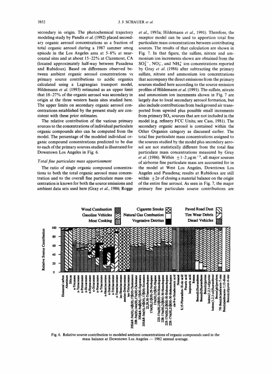
The relative contribution of the various primary sources to the concentrations of individual particulate organic compounds also can be computed from the model. The percentage of the modeled individual or- ganic compound concentrations predicted to be due to each of the primary sources studied is illustrated for Downtown Los Angeles in Fig. 6.

To ta l f ine part iculate mass appor t ionment

The ratio of single organic compound concentra- tions to both the total organic aerosol mass concen- tration and to the overall fine particulate mass con- centration is known for both the source emissions and ambient data sets used here (Gray et al., 1986; Rogge

et al., 1993a; Hildemann et al., 1991). Therefore, the receptor model can be used to apportion total fine particulate mass concentrations between contributing sources. The results of that calculation are shown in Fig. 7. In that figure, the sulfate, nitrate and am- monium ion increments shown are obtained from the SO ] - , NO3, and NH~ ion concentrations reported by Gray et al. (1986) after subtracting the primary sulfate, nitrate and ammonium ion concentrations that accompany the direct emissions from the primary sources studied here according to the source emission profiles of Hildemann et al. (1991). The sulfate, nitrate and ammonium ion increments shown in Fig. 7 are largely due to local secondary aerosol formation, but also include contributions from background air trans- ported from upwind plus possible small increments from primary SO~ sources that are not included in the model (e.g. refinery FCC Units; see Cass, 1981). The secondary organic aerosol is contained within the Other Organics category as discussed earlier. The total fine particulate mass concentrations assigned to the sources studied by the model plus secondary aero- sol are not statistically different from the total fine particulate mass concentrations measured by Gray et al. (1986). Within + 1-2/~gm -3, all major sources of airborne fine particulate mass are accounted for in the model at West Los Angeles, Downtown Los Angeles and Pasadena; results at Rubidoux are still within + 2a of closing a material balance on the origin of the entire fine aerosol. As seen in Fig. 7, the major primary fine particulate source contributions are

t ~

Gasoline Vehicles Natural Gas Combustion Tire Wear Debris

Meat Cooking Vegetative Detritus Diesel Vehicles

I00

80

60

4o

20

0

' gg,s-"g]'1 ig

- - .~g

Fig. 6. Relative source contribution to modeled ambient concentrations of organic compounds used in the mass balance at Downtown Los Angeles - - 1982 annual average.

Airborne particulate matter 3853

50

45

d 40 Q

35

¢D 30

O

20

I:~ 10

° ,,,,I ~ 5

o

Other Organics Wood Combustion Gasoline Vehicles

Meat Cooking Cigarette Smoke

Ammonium Nitrate

Sulfate

~ Nataral Gas Combustion Vegetative Detritus

Paved Road Dust Tire Wear Debris

Diesel Vehicles

Ammonium

Nitrate

Sulfate i n l l n o m u m

Ammonium

Nitrate

IIII11111111111111111111111111

W Pasadena Downtown LA West LA Rubidoux

Fig. 7. Source apportionment of fine mass concentrations - - 1982 annual average.

attributed to diesel :soot, paved road dust, gasoline- powered motor vehicles exhaust, food cooking opera- tions and wood smoke with small but quantifiable contributions from cigarette smoke, natural gas com- bustion aerosol, tire 'wear debris, and plant fragments. Secondary aerosol concentrations again are highest at the farthest downwind site at Rubidoux, as expected.

Acknowledgements--This research was supported by the Caltech Center for Air Quality Analysis. Acquisition of the source profile and a~bient organic compound data was supported by the U. S. Environmental Protection Agency under agreement R-81377-01-0, by the California Air Re- sources Board under agreement A932-127, and by the South Coast Air Quality Management District.

SUPPLENIENTAL MATERIALS

Tables containing 1982 annual average ambient concen- tration data for the air quality monitoring sites used in this study are contained in the references by Rogge et al. (1993a), Rogge (1993), and Gray (1986) and also can be obtained in consolidated form frora the authors of the present article. Source profiles showing the organic compound distributions in primary source emissions are reproduced in the references cited, and also can be obtained in consolidated form from the authors of the present article.

REFERENCES

Appel B. R., Wall S. M. and Knights R. L. (1980) Character- ization of carbonaceous materials in atmospheric aerosols by high-resolution mass spectrometric thermal analysis. In The Character and Origin of Smog Aerosols, Advances in Environmental Science and Technology (edited by Pitts J. N. Jr and Metcalf R. L.), Vol. 9, pp. 353-365. Wiley, New York.

Atkinson S. E. and Lewis D. H. (1974) A cost-effective analysis of alternative air quality control strategies. J. Envir. Econ. Management 1, 237-250.

Bencala K. E. and Seinfeld J. H. (1979) An air quality model performance assessment package. Atmospheric Environ- ment 13, 1181-1185.

Cass G. R. (1981) Sulfate air quality control strategy design. Atmospheric Environment 15, 1227-1249.

Cass G. R. and McRae G. J. (1983) Source-receptor reconcili- ation of routine air monitoring data for trace metals: an emissions inventory assisted approach. Envir. Sci. Technol. 17, 129 139.

Cass G. R., Boone P. M. and Macias E. S. (1982) Emissions and air quality relationships for atmospheric carbon par- ticles in Los Angeles. In Particulate Carbon: Atmospheric Life Cycle (edited by Wolff G. T. and Klimisch R. L.), pp. 207-243. Plenum Press, New York.

Cooper J. A. and Watson J. G. (1980) Receptor oriented methods of air particulate source apportionment. JAPCA 30, 1116-1125.

Cronn D. L., Charlson R. J. and Appel B. R. (1977) A study of the molecular nature of primary and secondary compo- nents of particles in urban air by high-resolution mass spectrometry. Atmospheric Environment 11, 929-937.

Doekery D. W., Pope C. A. III, Xu X., Spengler J. D., Ware J. H., Martha E. F., Ferris B. G. Jr and Speizer F. E. (1993) An association between air pollution and mortality in six U.S. Cities. N. Engl. J. Med. 329, 1753-1759.

Eckey E. W. (1954) Vegetable Fats and Oils, p. 25. Reinhold, New York.

Friedlander S. K. (1973) Chemical element balances and identification of air pollution sources. Envir. Sci. Technol. 7, 235-240.

Gordon, G. E. (1980) Receptor models. Envir. Sci. Technol. 14, 792 800.

Gray H. A. (1986) Control of atmospheric fine primary carbon particle concentrations. Ph.D. thesis, California Institute of Technology, Pasadena, California.

Gray H. A., Cass G. R., Huntzicker J. J., Heyerdahl E. K. and Rau J. A. (1986) Characterization of atmospheric organic and elemental carbon particle concentrations in Los Angeles. Sci. Total Envir. 20, 580-589.

3854 J.J. SCHAUER et al.

Grosjean D. (1977) Aerosols. In Ozone and Other Photo- chemical Oxidants, Chap. 3. National Academy of Sciences, Washington, District of Columbia.

Grosjean D. and Friedlander S. K. (1980) Formation of organic aerosols from cyclic olefins and diolefins. In The Character and Origin of Smog Aerosols, Advances in Environmental Science and Technology (edited by Pitts J. N. Jr and Metcalf, R. L.),Vol. 9, pp. 435-473. Wiley, New York.

Harley R. A., Hunts S. E. and Cass G. R. (1989) Strategies for the control of particulate air quality: least-cost solutions based on receptor oriented models. Envir. Sci. Technol. 23, 1007-1014.

Hidy G. M. et al. (1974) Characterization of aerosols in California (ACHEX). Rockwell International, Science Center. Prepared under California Air Resources Board Contract No. 358.

Hildemann L. M., Markowski G. R. and Cass G. R. (1989) A dilution stack sampler for collection of organic aerosol emissions: design, characterization, and field tests. Aerosol Sci. Technol. 10, 193-204.

Hildemann L. M., Markowski G. R. and Cass G. R. (1991) Chemical composition of emissions from urban sources of fine organic aerosol. Envir. Sci. Technol. 25, 744-759.

Hildemann L. M., Cass G. R., Mazurek M. A. and Simoneit B. R. T. (1993) Mathematical modeling of urban organic aerosol: properties measured by high-resolu- tion gas chromatography. Envir. Sci. Technol. 27, 2045-2055.

Hopke P. K., Gladney E. S., Gordon G. E., Zoller W. H. and Jones A. G. (1976) The use of multivariate analysis to identify sources of selected elements in Boston aerosol. Atmospheric Environment 10, 1015-1025.

Huntzicker J. J., Johnson R. L., Shah J. J. and Cary R. A. (1982) Analysis of organic and elemental carbon in ambient samples by a thermal optical method. In Particulate Carbon: Atmospheric Life Cycle (edited by Wolff G. T. and Klimisch R. L.), pp. 79-85. Plenum Press, New York.

John W. and Reischl G. (1980) A cyclone for size-selective sampling of ambient air. JAPCA 30, 872-876.

Johnson R. L., Shah J. J., Cary R. A. and Huntzicker J. J. (1981) An automated thermal-optical method for the anal- ysis of carbonaceous aerosol. In Atmospheric Aerosols: Source/Air Quality Relationship (edited by Macias E. S. and Hopke P. K.). American Chemical Society, Washing- ton, District of Columbia.

Kamens R. M., Guo Z., Fulcher J. N. and Bell D. A. (1988) Influence of humidity, sunlight, and temperature on the daytime decay rate of polyaromatic hydrocarbons on atmospheric soot particles. Envir. Sci. Technol. 22, 103 108.

Kamens R. M., Karam H., Guo J., Perry J. M. and Stockbur- ger L. (1989) Behavior of oxygenated polycylic aromatic hydrocarbons on atmospheric soot particles. Envir. Sci. Teehnol. 23, 801-806.

Liu M. K. and Seinfeld J. H. (1975) On the validity of grid and trajectory models of urban air pollution. Atmospheric Environment 9, 555-574.

Mazurek M. A., Simoneit B. R. T., Cass G. R. and Gray H. A. (1987) Quantitative high-resolution gas chromatography and high-resolution gas chromatography/mass spectro- metry analysis of carbonaceous fine aerosol particles. Int. J. Envir. Anal. Chem. 29, 119 139.

Mazurek M. A., Simoneit B. R. T. and Cass G. R. (1989) Interpretation of high-resolution gas chromatography and high-resolution gas chromatography/mass spectrometry data acquired from atmospheric aerosol samples. Aerosol Sci. Technol. 10, 408-419.

Mazurek M. A., Cass G. R. and Simoneit B. R. T. (1991) Biological input to visibility-reducing particles in the re- mote arid southwestern United States. Envir. Sci. Technol. 25, 684-694.

Mazurek M. A., Hildemann L. M., Cass G. R., Simoneit B. R. T. and Rogge W. F. (1993) Methods of analysis for com- plex organic aerosol mixtures from urban emission sour- ces of particle carbon. In Measurement of Airborne Com- pounds: Sampling, Analysis, and Data Interpretation (edited by Winegar E. D. and Keith L. H.), pp. 177 190. American Chemical Society Symposium Series, CRC Press, Boca Raton, Florida.

Miller M. S., Friedlander S. K. and Hidy G. M. (1972) A chemical element balance for the Pasadena aerosol. J. Colloid Interface Sei. 39, 165 176.

Mueller P. K., Mendoza B. V., Collins J. C. and Wilgus E. A. (1978) Application of ion chromatography to the analysis of anions extracted from airborne particulate matter. In Ion Chromatographic Analysis of Environmental Pollutants (edited by Sawicki E., Mulik J. D. and Wittgen- stein E.), pp. 77-86. Ann Arbor Science, Ann Arbor, Michigan.

Ouimette J. R. and Flagan R. C. (1982) The extinction coefficient of multicomponent aerosols. Atmospheric Envi- ronment 16, 2405-2419.

Pandis S. N., Harley R. A., Cass G. R. and Seinfeld J. H. (1992) Secondary organic aerosol formation and trans- port. Atmospheric Environment 26A, 2269-2282.

Rogge W. F. (1993) Molecular tracers for sources of atmo- spheric carbon particles: Measurements and model predic- tions. Ph.D. thesis. California Institute of Technology, Pasadena, California.

Rogge W. F., Hildemann L. M., Mazurek M. A., Cass G. R. and Simoneit B. R. T. (1991) Sources of fine organic aerosol. 1. Charbroilers and meat cooking operations. Envir. Sci. Technol. 25, 1112-1125.

Rogge W. F., Mazurek M. A., Hildemann L. M., Cass G. R. and Simoneit B. R. T. (1993a) Quantification of urban organic aerosols at a molecular level: identification, abundance and seasonal variation. Atmospheric Environ- ment 27, 1309-1330.

Rogge W. F., Hildemann L. M., Mazurek M. A., Cass G. R. and Simoneit B. R. T. (1993b) Sources of fine organic aerosol. 2. Noncatalyst and catalyst-equipped automo- biles and heavy duty diesel trucks. Envir. Sci. Technol. 27, 636-651.

Rogge W. F., Hildemann L. M., Mazurek M. A., Cass G. R. and Simoneit B. R. T. (1993c) Sources of fine organic aerosol. 3. Road dust, tire debris, and organometallic brake lining dust: Roads as sources and sinks. Envir. Sci. Technol. 27, 1892-1904.

Rogge W. F., Hildemann L. M., Mazurek M. A., Cass G. R. and Simoneit B. R. T. (1993d) Sources of fine organic aerosol. 4. Particulate abrasion products from leaf surfaces of urban plants. Envir. Sci. Technol. 27, 2700-2711.

Rogge W. F., Hildemann L. M., Mazurek M. A., Cass G. R. and Simoneit B. R. T. (1993 0 Sources of fine organic aerosol. 5. Natural gas home appliances. Envir. Sci. Tech- nol. 27, 2736-2744.

Rogge W. F., Hildemann L. M., Mazurek M. A., Cass G. R. and Simoneit B. R. T. (1994) Sources of fine organic aerosol: 6. Cigarette smoke in the urban atmosphere. En- vir. Sci. Technol. 28, 1375-1388.

Satsumabayashi H. and Kurita H. (1989) Photochemical formation of particulate dicarboxylic acids under long- range transport in central Japan. Atmospheric Environ- ment 24A, 1443-1450.

Sehmel G. A. (1980) Particle and gas dry deposition: a re- view. Atmospheric Environment 14, 983-1011.

Solorzano L. (1969) Determination of ammonia in natural waters by the phenolhypochlorite method. Limnol. Oceanogr. 14, 799-801.

Venkataraman C. and Friedlander S. K. (1994) Size distribu- tion of polycyclic aromatic hydrocarbons and elemental carbon. 2. Ambient measurements and effects of atmo- spheric processes. Envir. Sci. Technol. 28, 563-572.

Airborne particulate matter 3855

Watson J. G. (1984) Overview of receptor model principles. JAPCA 34, 619-623.

Watson J. G., Cooper I. A. and Huntzicker J. J. (1984) The effective variance weighting for least squares calculations applied to the mass balance receptor model. Atmospheric Environment 15, 1347-1355.

Watson J. G., Robinson N. F., Chow J. C., Henry R. C., Kim B. M., Pace T. G., Meyer E. I. and Nguyen Q. (1990) The USEPA/DRI chemical mass balance receptor model, CMB 7.0. Envir. Software 5, 38-49.