Real Time Tracking System and Data
Reduction
by
Nor Ababtein
A thesis
presented to the University of Waterloo
in fulfillment of the
thesis requirement for the degree of
Master of Applied Science
in
Electrical and Computer Engineering
Waterloo, Ontario, Canada, 2017
© Nor Ababtein 2017
ii
I hereby declare that I am the sole author of this thesis. This is a true copy of the thesis, including
any required final revision, as accepted by my examiners.
I understand that my thesis may be made electronically available to the public.
iii
Abstract
Today, for various purposes, vehicle tracking systems are used for determining the
geographic location of vehicles and transmitting this information to a data center. For detecting
the location, a GPS is used, and for the transmission mechanism, a satellite or cell tower is
deployed. Tracking systems are producing a massive data since they monitor moving vehicles
continuously and report vehicle status. Since the amount of collected data is large and needs a
storage unit that can handle all the transmitted data, storage becomes more challenging. The cost
of transmitting, processing, storing, and accessing the data grows as the number of vehicles
being tracked increases. The amount of data collected by the system depends on the uploading
frequency. For example, the amount of data will increase as the uploading frequency (seconds)
decreases and vice versa.
This work provides a storage management solution that reduces the size of cloud
databases, both SQL and NoSQL databases, by eliminating repeated data. One of the causes of
massive data in the tracking system is the high uploading frequency that causes a huge amount of
repetitive values. We propose two algorithms for minimizing database storage: The Reducing
Data Redundancy algorithm and the Data Lifetime algorithm. We implement these two
algorithms in the cloud, for both SQL and NoSQL databases. For evaluation, a vehicle tracking
system is developed by using Global Positioning System (GPS) and GSM/GPRS module. Our
experiments use two different approaches: Static testing for when a vehicle is not in motion
mode, and dynamic for when it is. The result of the experiments shows the effectiveness of these
two algorithms in decreasing storage size and increasing process time.
The system has four parts, which are the tracking unit, cloud database, web application,
and Android Application. The tracking unit is installed inside a vehicle to detect the vehicle’s
location, speed, and temperature then uploads this information to a cloud database. The main
functions of the system are to track a vehicle, transmit the information to the cloud, and send
notifications to the system administrator and users. The Android application is designed to
receive notifications and view the vehicle’s information such as the current location and
temperature. The administrator of the system uses the web application to set constraints for
users’ vehicles, such as the temperature range and location restriction.
iv
Acknowledgment
First of all, I would like to thank my supervisor Professor Sagar Naik for his guidance,
motivation, and help throughout my thesis.
Besides that, I would like to extend my appreciation to my family members for their support.
v
Dedication
To my beloved family; my mother, my husband, my daughter, and my son who have supported
me in completing my thesis.
vi
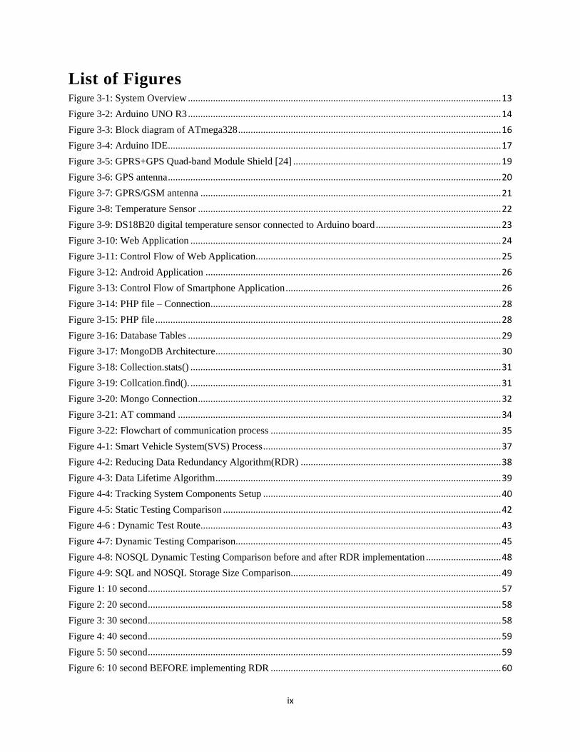
Table of Contents List of Tables ..................................................................................................................................................... viii
List of Figures ...................................................................................................................................................... ix
List of Abbreviation ............................................................................................................................................. xi
1 Introduction ................................................................................................................................................... 1
1.1 Problem Description............................................................................................................................. 3
1.2 Solution Strategy and Contribution ...................................................................................................... 4
1.3 Organization of Thesis ......................................................................................................................... 5
2 Literature Review ......................................................................................................................................... 6
2.1 Existing Tracking System Models ....................................................................................................... 6
2.2 Storage Solutions for Massive Databases in IoT .................................................................................. 8
3 Methodology ............................................................................................................................................... 12
3.1 Introduction ........................................................................................................................................ 12
3.2 System Design .................................................................................................................................... 12
3.2.1 Arduino UNO R3 (ATmega328P) Microcontroller ....................................................................... 14
3.2.1.1 Power ..................................................................................................................................... 16
3.2.1.2 Programming ......................................................................................................................... 16
3.2.2 GPRS+GPS Quad-band Module Shield (SIM908): ....................................................................... 17
3.2.2.1 The External GPS Antenna .................................................................................................... 20
3.2.2.2 The External GPRS/GSM Antenna ....................................................................................... 21
3.2.3 Temperature Sensor DS18B20 ....................................................................................................... 21
3.2.4 Web Application ............................................................................................................................ 23
3.2.5 Smartphone Application ................................................................................................................ 25
3.2.5.1 Google Maps API .................................................................................................................. 27
3.2.6 Web Server ..................................................................................................................................... 27
3.2.7 Database Design ............................................................................................................................. 27
3.2.7.1 SQL database: ........................................................................................................................ 27
3.2.7.2 NoSQL database: ................................................................................................................... 29
3.3 Communication .................................................................................................................................. 32
vii
4 Experiment and Result ................................................................................................................................ 36
4.1 Proposed Algorithms .......................................................................................................................... 36
4.1.1 Reducing Data Redundancy Algorithm (RDR) ............................................................................. 36
4.1.2 Data Lifetime Algorithm ................................................................................................................ 39
4.2 Experiment Setup ............................................................................................................................... 39
4.3 Experimental Results for SQL Database ............................................................................................ 40
4.3.1 Static Testing ................................................................................................................................. 41
4.3.2 Results ............................................................................................................................................ 42
4.3.3 Dynamic Testing ............................................................................................................................ 42
4.3.4 Results ............................................................................................................................................ 44
4.4 Experimental Results for NOSQL Database ...................................................................................... 45
4.4.1 Dynamic Testing ............................................................................................................................ 46
4.4.2 Results ............................................................................................................................................ 47
4.5 SQL Vs NOSQL ................................................................................................................................ 48
5 Conclusion .................................................................................................................................................. 50
References ........................................................................................................................................................... 52
APPENDEICE .................................................................................................................................................... 56
All Figures of The Mongodb Collection for The Following Uploading Frequencies 10, 20, 30, 40, 50
Seconds (Static Testing) Used in Chapter 4 .................................................................................................... 57
All Figures of The Mongodb Collection for The Following Uploading Frequencies 10, and 40 Seconds
(dynamic Testing) Used in Chapter 4 ............................................................................................................. 60
viii
List of Tables Table 1: Number or Records for Four-hour static ................................................................................................. 3
Table 2: Database size (30 second - one device) .................................................................................................. 4
Table 3: Static Testing – Before Implementation of RDR Algorithm ................................................................ 41
Table 4 : Static Testing – After Implementation RDR Algorithm ...................................................................... 41
Table 5 : Dynamic Testing – Before Implementing RDR Algorithm ................................................................. 44
Table 6: Dynamic Testing – After Implementing RDR Algorithm .................................................................... 44
Table 7: NOSQL 5 hours static testing ............................................................................................................... 46
Table 8: NOSQL Dynamic Testing before Implementing RDR algorithm ........................................................ 47
Table 9:NOSQL Dynamic Testing after Implementing RDR algorithm ............................................................ 47
Table 10: NOSQL and SQL Comparison ........................................................................................................... 48
ix
List of Figures Figure 3-1: System Overview ............................................................................................................................. 13
Figure 3-2: Arduino UNO R3 ............................................................................................................................. 14
Figure 3-3: Block diagram of ATmega328 ......................................................................................................... 16
Figure 3-4: Arduino IDE ..................................................................................................................................... 17
Figure 3-5: GPRS+GPS Quad-band Module Shield [24] ................................................................................... 19
Figure 3-6: GPS antenna ..................................................................................................................................... 20
Figure 3-7: GPRS/GSM antenna ........................................................................................................................ 21
Figure 3-8: Temperature Sensor ......................................................................................................................... 22
Figure 3-9: DS18B20 digital temperature sensor connected to Arduino board .................................................. 23
Figure 3-10: Web Application ............................................................................................................................ 24
Figure 3-11: Control Flow of Web Application .................................................................................................. 25
Figure 3-12: Android Application ...................................................................................................................... 26
Figure 3-13: Control Flow of Smartphone Application ...................................................................................... 26
Figure 3-14: PHP file – Connection .................................................................................................................... 28
Figure 3-15: PHP file .......................................................................................................................................... 28
Figure 3-16: Database Tables ............................................................................................................................. 29
Figure 3-17: MongoDB Architecture .................................................................................................................. 30
Figure 3-18: Collection.stats() ............................................................................................................................ 31
Figure 3-19: Collcation.find(). ............................................................................................................................ 31
Figure 3-20: Mongo Connection ......................................................................................................................... 32
Figure 3-21: AT command ................................................................................................................................. 34
Figure 3-22: Flowchart of communication process ............................................................................................ 35
Figure 4-1: Smart Vehicle System(SVS) Process ............................................................................................... 37
Figure 4-2: Reducing Data Redundancy Algorithm(RDR) ................................................................................ 38
Figure 4-3: Data Lifetime Algorithm .................................................................................................................. 39
Figure 4-4: Tracking System Components Setup ............................................................................................... 40
Figure 4-5: Static Testing Comparison ............................................................................................................... 42
Figure 4-6 : Dynamic Test Route........................................................................................................................ 43
Figure 4-7: Dynamic Testing Comparison.......................................................................................................... 45
Figure 4-8: NOSQL Dynamic Testing Comparison before and after RDR implementation .............................. 48
Figure 4-9: SQL and NOSQL Storage Size Comparison.................................................................................... 49
Figure 1: 10 second ............................................................................................................................................. 57
Figure 2: 20 second ............................................................................................................................................. 58
Figure 3: 30 second ............................................................................................................................................. 58
Figure 4: 40 second ............................................................................................................................................. 59
Figure 5: 50 second ............................................................................................................................................. 59
Figure 6: 10 second BEFORE implementing RDR ............................................................................................ 60
x
Figure 7:10 second AFTER implementing RDR ................................................................................................ 61
Figure 8: 40 second BEFORE implementing RDR ............................................................................................ 61
Figure 9: 40 second AFTER implementing RDR ............................................................................................... 62
xi
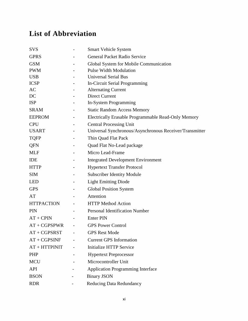
List of Abbreviation
SVS - Smart Vehicle System
GPRS - General Packet Radio Service
GSM - Global System for Mobile Communication
PWM - Pulse Width Modulation
USB - Universal Serial Bus
ICSP - In-Circuit Serial Programming
AC - Alternating Current
DC - Direct Current
ISP - In-System Programming
SRAM - Static Random Access Memory
EEPROM - Electrically Erasable Programmable Read-Only Memory
CPU - Central Processing Unit
USART - Universal Synchronous/Asynchronous Receiver/Transmitter
TQFP - Thin Quad Flat Pack
QFN - Quad Flat No-Lead package
MLF - Micro Lead-Frame
IDE - Integrated Development Environment
HTTP - Hypertext Transfer Protocol
SIM - Subscriber Identity Module
LED - Light Emitting Diode
GPS - Global Position System
AT - Attention
HTTPACTION - HTTP Method Action
PIN - Personal Identification Number
AT + CPIN - Enter PIN
AT + CGPSPWR - GPS Power Control
AT + CGPSRST - GPS Rest Mode
AT + CGPSINF - Current GPS Information
AT + HTTPINIT - Initialize HTTP Service
PHP - Hypertext Preprocessor
MCU - Microcontroller Unit
API - Application Programming Interface
BSON - Binary JSON
RDR - Reducing Data Redundancy
1
Chapter 1
1 Introduction
The Internet of Things (IoT) was introduced by Kevin Ashton in 1998 by using Radio-Frequency
Identification (RFID) since then the IoT has rapidly gained widespread attention in academia and
industry [1]. In 2008, the number of connected devices exceeded the number of connected
people. Cisco has estimated that by 2020 there will be 50 billion connected devices, which is
seven times the world population [2]. The Internet of Things (IoT) connects objects like smart
phones, Internet TVs, sensors, and actuators to the World Wide Web. All these devices are
linked together to simultaneously generate data and communicate with each other, which results
in a massive amount of data flow over the network. The major challenge in the IoT is how to
handle the large amount of data and objects efficiently.
There are three types of IoT database storage [3 ,4,5]: local, distributed, and centralized.
Local storage is a storage unit where the data collected from sensors is stored. Distributed
storage is used when data is stored on more than one node. Centralized storage is used when data
is collected by a node and then sent to a data center. Local and distributed storage are not
suitable for IoT applications due to the limited storage capacity and constrained power of the
sensors [6].
A vehicle tracking system is an example of IoT. Vehicle tracking systems were first
implemented for the shipping industry since people want to know where each vehicle is at any
given time [7]. Vehicle tracking systems are being used and developed in a variety of ways for
tracking and displaying a vehicle’s location and speed in real-time. For example, there are
vehicle position tracking systems, vehicle anti-theft tracking systems, fleet management systems,
and intelligent transportation systems (ITS) [7]. Initially, vehicle tracking systems were
developed for fleet management and used for passive tracking. In passive tracking, a hardware
device is installed in a vehicle to track and store information about that vehicle, such as its
location and speed. When the vehicle returns to a specific location, the hardware device is
removed and all the stored data are downloaded to a computer for analysis. On the other hand,
real-time tracking systems require a GSM/GPRS model for transmitting the collected
information to a database storage regularly. In short, active systems are developed to transmit
information about the vehicle’s location and other data in real time via cellular or satellite
networks to a data center [8].
In our research paper, we develop a Smart Vehicle System (SVS) using GPS/GSM/GPRS
technology, a Smartphone application, and a web application. This system will provide better
service and a more cost-effective solution for users by reducing database storage. The GPS
2
technology is used to provide the location and time information. Serval data sets can be obtained
from GPS satellites by the GPS receiver, such as the number of satellites received by the GPS,
speed, and accurate date and time based on Universal Time Coordination. The GSM and GPRS
are used for wireless data transmission. The main objective of the Smart Vehicle System (SVS)
is to track a vehicle’s location and temperature, and notify a user if the vehicle moves out of a
specific location or temperature range. The tracking system is placed inside a vehicle.
The features of the SVS system are as follows:
• Detects a vehicle's geographic coordinates using the GPS module
• Detects inside vehicle temperature using temperature sensor
• Transmits the vehicle's location and temperature information to a web server after
a specified time interval using the GSM/GPRS module
• Uses cloud database to store and manage received vehicle's location and
temperature information
A Cloud database is flexible and cost effective in providing real-time data to users at any
given time, with extensive coverage and quality. The concept of cloud computing is that all
computer resources such as memory, storage, processing capabilities are rented by third party
providers over the Internet. All the resources are accessed through a web application. The cloud
consists of the following: the hardware, network, services, storage, and interface [14]. Together,
they allow the delivery of computing as a service.
This work aims to build an affective tracking system and to apply data reduction to the
database to reduce database storage on the cloud since the system produces so much data that
needs to be transmitted, processed, and stored. Data reduction is the process of reducing the
amount of data that needs to be stored in the database [9]. It increases storage efficiency and
decreases cost. We used two different databases for our experiment: SQL and NoSQL. We
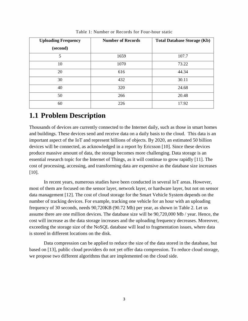
performed six hours long experiments for the following uploading frequencies 5, 10, 20, 30, 40,
50, and 60 seconds. Table 1 shows how many records for each uploading frequency are collected
and uploaded to the cloud database by one device. The need for storage space that can handle
huge amount of data is a very important aspect in developing the tracking system. The cost of
storage will increase yearly as the number of records increases and the number of devices
increases as well.
3
Table 1: Number or Records for Four-hour static
Uploading Frequency
(second)
Number of Records Total Database Storage (Kb)
5 1659 107.7
10 1070 73.22
20 616 44.34
30 432 30.11
40 320 24.68
50 266 20.48
60 226 17.92
1.1 Problem Description
Thousands of devices are currently connected to the Internet daily, such as those in smart homes
and buildings. These devices send and receive data on a daily basis to the cloud. This data is an
important aspect of the IoT and represent billions of objects. By 2020, an estimated 50 billion
devices will be connected, as acknowledged in a report by Ericsson [10]. Since these devices
produce massive amount of data, the storage becomes more challenging. Data storage is an
essential research topic for the Internet of Things, as it will continue to grow rapidly [11]. The
cost of processing, accessing, and transforming data are expensive as the database size increases
[10].
In recent years, numerous studies have been conducted in several IoT areas. However,
most of them are focused on the sensor layer, network layer, or hardware layer, but not on sensor
data management [12]. The cost of cloud storage for the Smart Vehicle System depends on the
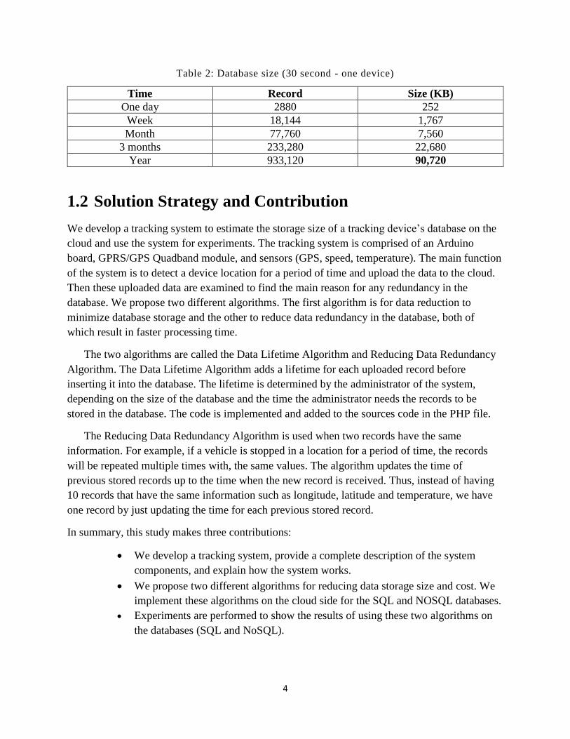
number of tracking devices. For example, tracking one vehicle for an hour with an uploading
frequency of 30 seconds, needs 90,720KB (90.72 Mb) per year, as shown in Table 2. Let us
assume there are one million devices. The database size will be 90,720,000 Mb / year. Hence, the
cost will increase as the data storage increases and the uploading frequency decreases. Moreover,
exceeding the storage size of the NoSQL database will lead to fragmentation issues, where data
is stored in different locations on the disk.
Data compression can be applied to reduce the size of the data stored in the database, but
based on [13], public cloud providers do not yet offer data compression. To reduce cloud storage,
we propose two different algorithms that are implemented on the cloud side.
4
Table 2: Database size (30 second - one device)
Time Record Size (KB)
One day 2880 252
Week 18,144 1,767
Month 77,760 7,560
3 months 233,280 22,680
Year 933,120 90,720
1.2 Solution Strategy and Contribution
We develop a tracking system to estimate the storage size of a tracking device’s database on the
cloud and use the system for experiments. The tracking system is comprised of an Arduino
board, GPRS/GPS Quadband module, and sensors (GPS, speed, temperature). The main function
of the system is to detect a device location for a period of time and upload the data to the cloud.
Then these uploaded data are examined to find the main reason for any redundancy in the
database. We propose two different algorithms. The first algorithm is for data reduction to
minimize database storage and the other to reduce data redundancy in the database, both of
which result in faster processing time.
The two algorithms are called the Data Lifetime Algorithm and Reducing Data Redundancy
Algorithm. The Data Lifetime Algorithm adds a lifetime for each uploaded record before
inserting it into the database. The lifetime is determined by the administrator of the system,
depending on the size of the database and the time the administrator needs the records to be
stored in the database. The code is implemented and added to the sources code in the PHP file.
The Reducing Data Redundancy Algorithm is used when two records have the same
information. For example, if a vehicle is stopped in a location for a period of time, the records
will be repeated multiple times with, the same values. The algorithm updates the time of
previous stored records up to the time when the new record is received. Thus, instead of having
10 records that have the same information such as longitude, latitude and temperature, we have
one record by just updating the time for each previous stored record.
In summary, this study makes three contributions:
• We develop a tracking system, provide a complete description of the system
components, and explain how the system works.
• We propose two different algorithms for reducing data storage size and cost. We
implement these algorithms on the cloud side for the SQL and NOSQL databases.
• Experiments are performed to show the results of using these two algorithms on
the databases (SQL and NoSQL).
5
1.3 Organization of Thesis
The rest of the thesis is organized as follows. In Chapter 2, we present a comprehensive literature
review of storage solutions of IoT and existing tracking system models. In Chapter 3, the Smart
Vehicle System (SVS) and its implementation details are explained. In Chapter 4, we explain the
proposed algorithms in more detail. Furthermore, experiments are performed and the results
before and after implementing the algorithms are presented in Chapter 4. Concluding remarks are
provided in Chapter 5.
6
Chapter 2
2 Literature Review
2.1 Existing Tracking System Models
Real-time tracking systems for vehicles have been a field of interest for many researchers and
much work has been done on vehicle tracking systems since 2010. Nowadays, the number of
anti-theft modules such as steering-wheel-lock equipment and mobile network tracking systems
are being developed along with client identification and real-time performance monitoring.
The paper presented by El-Medany and Al-Omary describes a real-time tracking system
that provides accurate location information of a tracked vehicle with low cost [14]. The system
is developed using a GM862 cellular quad band module. In addition, a monitoring server and a
graphical user interface on a website have been developed using Microsoft SQL Server 2003 and
ASP.net to view the exact location of a vehicle on a map. The system provides users with
information about their vehicle’s status, such as its speed and mileage. The objective of the paper
is to develop a low-cost system by using the latest technologies. The GM862 module integrates
GPS/GPRS/GSM instead of having separate devices. Google Maps is used to show the location
of vehicles on a Map. A website is developed to view the vehicle’s current location on Google
map, plus its speed and mileage.
Hu, Li, and Guang-Hui [15] developed an automobile anti-theft tracking system using a
GSM/GPS module. The system uses a high-speed single-chip C8051F120. For detecting a stolen
automobile, a vibration sensor has been used. The system has the following components: a GSM
module, GPS receiver module, a vibration sensor, wireless remote control, and Micro-Controller
Unit (MCU). The location of the automobile is obtained using a GPS module. The system keeps
the owner of the automobile updated through the GSM module. The owner can receive
information about his vehicle’s location through a mobile phone and control the alarm. In
addition, the owner of the automobile can control his vehicle by a remote-controlled alarm. All
the information collected by GPS and GSM module is processed by an MCU.
The paper presented by Fleischer and Nelson [16] shows the development and deployment
of a GPS/GSM based Vehicle Tracking and Alert System. This system allows inter-city transport
companies to track their vehicles in real-time and provides security from armed robbery and
accidents occurrences. The main functions of the system are to perform real-time tracking of a
vehicle and show the routes taken on Google map, monitor the vehicle’s speed to make sure the
driver is not speeding, monitor the fuel level and consumption rate of the vehicle, send alert
information to the police if there is a highway robbery, keep passengers informed about the next
stop the vehicle will reach, and finally, notify the owner of the system if there is an accident. The
7
system contains four main modules: the management system, robbery-alert system, onboard
location display, and accident-alert system. The system was built using the following
components:
• Microsoft SQL Server Management Studio 2008
• SMS Gateway
• Microsoft Visual Studio 2010 for development the software
• Google Map API
• Crystal Report API to allow the programmer to create reports from different data
sources
• PMB-648 GPS Module
• GSM Modem & Microcontroller
• LCD Screen Display
• AVR-JTAG-USB Programmer/Emulator.
• GSM/GPRS 3-BAND MODULE 900/1800/1900Mhz that includes build on the
ship GSM cellular antenna
ElShafee, ElMenshawi , and Saeed [17] built a tracking system that uses Twitter as a value
added service for the traditional tracking system. Each vehicle has an account that users can
easily follow. This account will have all posts about the vehicle’s location information. The
location will display in real-time on Google maps. The vehicle sends tweets regularly, with a link
to a map showing the current location of the vehicle. The system was developed using GPS for
location information, GSM/GPRS for information transmission, Google map for showing the
current location of the vehicle, an Arduino microcontroller, plus Twitter, and a web server with a
database. The system detects the current location of a vehicle, its speed, door status (open
/closed), and ignition status (on/off). Then the system sends all this information to the tracking
server through the internet.
Vigneshwaran, Sumithra, and Janani [18] implemented a tracking system for theft
prevention of two-wheelers, using a GSM/GPS module and Android technology. The GPS/GSM
module is used to track the two-wheeler and send messages to the owner. The system gives the
owner the ability to track, monitor, and stop his/her stolen two-wheelers through an android
application. The application is used to control the air solenoid, water solenoid and power cable in
the vehicle’s engine system. The Peltier unit and Thermal Electric Generator (TEG) is connected
to the exhaust of the two-wheeler to convert heat energy into power. This power will be stored in
the battery used in the vehicle. The GSM module sends and receives SMS messages to and from
the owner of the vehicle. The owner can send SMS to the GSM asking about the location, speed,
water level, movement status, engine level, and geographical limit. Moreover, the owner can turn
the engine of the vehicle off by sending over SMS. The location of the vehicle is sent to a
standalone server continuously. The system was built using the GSM Modem SIM900-D, GPS
module, microcontroller ATmega-16, Thermoelectric Generator for converting heat into
8
electricity, 16 × 2 LCD Display,12V Battery, MAX 232 IC, Solenoid control valve that is used
for controlling liquid or gas by running or stopping an electrical current through a solenoid, Flow
control valve that controls the flow or pressure of a fluid, Relay Driver Circuit is used to allow a
low-power circuit to switch on and off , and finally android application to display the location of
the vehicle on Google map.
2.2 Storage Solutions for Massive Databases in IoT
All the previous tracking systems generate massive data that need to be transmitted, stored, and
processed. The storage will increase continuously as the number of devices increases. In recent
years, only a few studies on a massive data management have effectively proposed models and
methods.
For supporting massive data management and processing it in IoT, Zhiming, Qi, and
Hong [12] proposed a Sea-Cloud-based massive heterogeneous sensor Data Management
(“SeaCloudDM”) framework. The architecture of the framework is divided into four layers: the
sensor deployment layer, the sea computing layer, the cloud data management layer, and the data
analysis application layer. The sensor deployment layer has different categories of sensors. Each
category can be divided into more detailed classes of sensors. In the framework, the sampled
data are organized based on objects instead of sensors. Objects are divided into static and moving
objects, depending on their locations change.
The sea computing layer has a set of nodes that are connected to sensors. The tasks of the
nodes are to receive, store, and process the raw sampled data from the connected sensors. After
that, the nodes send the processed sampled data to the cloud data management layer. There are
two kinds of sampled data: numerical, such as data sampled from temperature and GPS sensors,
and multimedia, such as data from video and audio devices. For each sensor, the authors have
defined a state change threshold to compare between the new raw sampling data and the last
reported key sampled data. If the difference between them is larger than the threshold, then new
sampled data will be the next key sampling data. Finally, the new key sampled data is sent to the
cloud data management layer.
The cloud data management layer does not store any data generated by the sensors; it
only manages keys sampled data that are generated from the nodes in the sea computing layer.
The cloud of the framework uses a Relational Data-Base and Key-Value store combined (RDB-
KV) model. The RDB-KV cloud contains a large number of RDB-KV databases, which support
both SQL queries and keyword searches efficiently. These databases are organized into a tree
structure in the cloud. Finally, the massive sensor sampled data that is stored in the cloud data
management layer can be used in data analysis such as statistical analysis, data mining, and
recommendation. From these analysis, the authors can get information about the objects and
physical world. This framework is for managing massive sensor data and increasing query
response times.
9
Tingli, Yang, Ye, Shuo, and Wei [11] have designed a system called IOTMDB, based on
NOSQL, to solve the storage problem of massive IoT data. The system has four nodes: the
master node, standby node, data reception node, and slave node. The main functions of the
master node are to handle all the connections from clients, keep a map between the key range
and chunks and between chunks and partitions, and estimate if a chunk has reached its maximum
capacity. The standby node is a duplicate node that stays in sync with the master node; if the
master node fails, the standby node takes over. The data reception node’s job is to receive data
from sensors and do some processing. Finally, the slave node will have all the application data.
Data from sensors are gathered and sent to the IOTMDB system. The system also provides data
sharing and collaboration. The authors also developed a public service platform called RNS
based on DNS for allowing data sharing between different IoT applications, data searching, and
data locating. When any new object is added to the IOTMDB system, the object will be
registered in the RNS.
For data storage strategy, the authors designed a preprocessing mechanism for received
data. After receiving the data from the sensors, the processing method is determined by
extracting specific information from the raw data and finding out the type of data. Then data
cleaning is performed to ensure the accuracy of the received data. Finally, to reduce repeated
data, the authors used a simple method; they set a threshold to a value to determine whether this
value should be accepted or not. If the difference between the current value and previous
accepted value is large, then the current value should be accepted; otherwise it should be
rejected.
The authors of [19] presented a universal storage architecture for IoT big data in cloud
environment using clustering analysis. It divides the nodes in cloud storage into several clusters
depending on the communication cost between different nodes. Each cluster stores data with a
special model such as a key value model or document model. Clusters that have the strongest
computing power for providing universal storage and query interface for users are selected. The
architecture can be divided into two layers: the data analysis layer and data storage layer.
Data analysis layer:
After receiving a huge amount of heterogeneous data, the data storage module examines the
characteristics of the data and decides on a suitable data model to normalize the data. To store
the data, the normalized data is transmitted to the corresponding cluster in the data storage layer.
In addition, after receiving a query from a user, the data query module evaluates the size of the
query, sends the query to the query command, and finally transforms the query command to the
right cluster for execution.
Data storage layer:
To store data, the node of the cloud storage center is divided into several clusters. Each cluster
stores data with one special model, such as spatiotemporal data model for the sensor data in the
Internet of Things (IoT). When the data center supports n numbers of data models, the cloud
10
nodes is divided into n+1 clusters. The clusters that have the strongest computing power are
selected for the data analysis layer. This layer’s groups objects based on the information found in
the data describing the objects and their relations.
The authors did their experiment using 12 distributed nodes as cloud nodes. Each node
has the following features: a 2.8GHz core, 1GB memory and 250GB hard drive. They used three
different data models: the key value model, extensible record model and structured
spatiotemporal model. The cloud nodes are divided into four clusters, and three database
managements are used. The three databases are: Redis for the key-value model, HBase for
storing the data of extensible record model, and Oracle for structured spatiotemporal model. The
authors used three different kinds of data for their experiment: the spatiotemporal data is
collected from digital home labs, and include three groups of data: temperature, humidity, and
carbon dioxide concentration; the semi-structured data, collected from huge web pages as an
example of an extensible record model, and finally the log data of a Linux system, which are
unstructured. In their experiment, they evaluated the performance of the storage architecture in
terms of data loading and query processing. Moreover, they compared CloST with Redis and
HBase. These two production systems are widely used to store big data in IoT.
For the data loading performance evaluation, the authors used two datasets, one of 10GB
and the other 20GB. Their experiment shows that the data loading speed of the storage
architecture is faster than that of the other systems, and it is more suitable for storing massive
heterogeneous data. In addition, they used spatial query to evaluate the query performance of the
storage architecture. To define the relation between the query response time and the range size, a
number of spatial ranges are selected. The results show that the query response time increases as
the time range increases.
The authors of [20] have proposed an efficient technique to store data with a row-key
system on NoSQL database, and developed a smartphone application to validate it. They
emphasized that NoSQL databases are more suitable for IoT applications because they are
adequate with disrupted systems, big data, and scalability. NoSQL databases work well with
huge amounts of data that does not have a complicated relation and structure. They claim that the
most popular NoSQL databases are MangoDB, HBase, and Cassandra, each of which has its own
strengths and weaknesses. For instance, many frameworks support MangoDB because of its
simple JSON style, while HBase performs better on consistency and partitions tolerance, and
Cassandra focuses on availability and partitions tolerance. The authors preferred to use HBase
for their system design because of its excellent consistency. Moreover, they developed a
smartphone application for three reasons: to control appliances remotely, to monitor accumulated
electricity bills, and to predict the monthly cost of electricity bills. This smartphone application
uses an efficient technique to store data in HBase database. Then, the author conducted an
experiment to evaluate the required time for a query from a smartphone or web application to be
executed. The evaluated results of this experiment were that over 95% of the clients could get
their information in 0.5 seconds, with many other applications running at the same time.
11
In summary, all the previous researches show that tracking systems are developed for
several reasons using distinctive designs. For example, in [14] and [15] the hardware, setup, and
connection differ from those of our system. In [16] and [18] the system uses SMS messages to
send and receive the vehicle location information. In addition, the systems use LCDs to give the
drivers the ability to view their vehicle’s information while driving, and the tracking unit is
powered using the vehicle’s electricity. In contrast, our system uploads information
automatically to the web server, and it operates on battery. Furthermore, in [17] the tracking
system uses Twitter for displaying the vehicle’s location information. However, our system uses
Android and web application to review the vehicle’s location information.
In [11], [12], [19], and [20] show different modules for minimizing database’s storage
using NoSQL database. However, our system uses both SQL and NoSQL as a storage solution,
and compares them. Additionally, we use real data by developing and testing a complete tracking
system that uses a cloud as a data storage solution. Most researchers focus on the tracking system
without providing storage solution for cloud databases. On the other hand, our system combined
both real-time tracking system and minimizing data storage.
12
CHAPTER 3
3 Methodology
3.1 Introduction
In this chapter, we discuss the design of the tracking system and the process that we used to
complete it. Each of the hardware devices and software components that we used in this system
is explained in more detail.
3.2 System Design
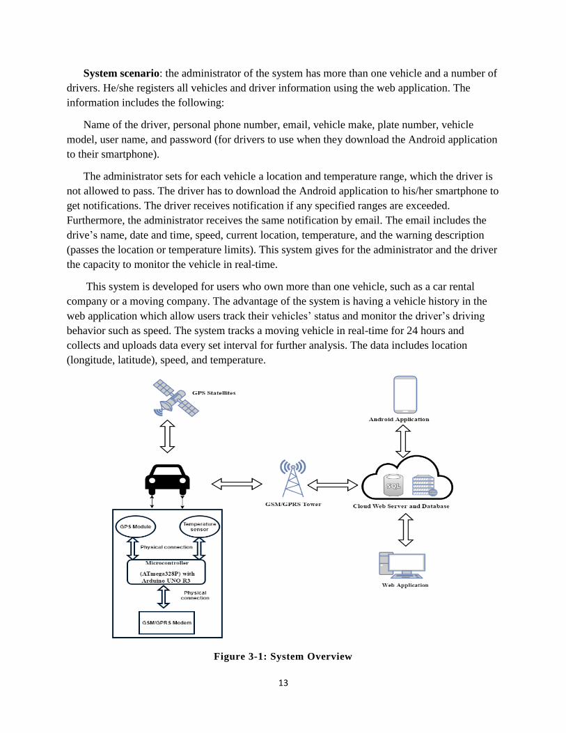
The Smart Vehicle System (SVS) has been developed to continuously track a moving vehicle
and then report the status of the vehicle to the administrator of the system. It has the following
components:
➢ Arduino UNO R3 (ATmega328P)
➢ GPRS+GPS Quad-band Module Shield (SIM908)
➢ Temperature Sensor DS18B20
➢ GPS Sensor
➢ Smartphone Application
➢ Web Application
➢ Web Server
The SVS is shown in Figure 3-1. The microcontroller ATmega328P, GPS sensor,
Temperature sensor, and GPRS+GPS Quad-band Module Shield (SIM908) are placed inside a
vehicle for real-time tracking and detecting the temperature inside the vehicle with respect to
time. After the GPS receiver receives the location (latitude/longitude) of the vehicle, speed, and
time from the satellite, the GPRS+GPS Quad-band Module Shield (SIM908) upload all the
information, including the temperature of the vehicle, to the web server for further analysis.
The system provides a report about the vehicle’s location, speed and temperature inside the
vehicle. Furthermore, it sends a notification to users through a smartphone application if their
vehicle passes the location or temperature range, pre-set though a web application by the
administrator. The location range is a zone out of which the driver should not passes, such as a
city’s limits. The temperature range defines the highest and the lowest permitted values. Vehicles
should remain within these boundaries.
13
System scenario: the administrator of the system has more than one vehicle and a number of
drivers. He/she registers all vehicles and driver information using the web application. The
information includes the following:
Name of the driver, personal phone number, email, vehicle make, plate number, vehicle
model, user name, and password (for drivers to use when they download the Android application
to their smartphone).
The administrator sets for each vehicle a location and temperature range, which the driver is
not allowed to pass. The driver has to download the Android application to his/her smartphone to
get notifications. The driver receives notification if any specified ranges are exceeded.
Furthermore, the administrator receives the same notification by email. The email includes the
drive’s name, date and time, speed, current location, temperature, and the warning description
(passes the location or temperature limits). This system gives for the administrator and the driver
the capacity to monitor the vehicle in real-time.
This system is developed for users who own more than one vehicle, such as a car rental
company or a moving company. The advantage of the system is having a vehicle history in the
web application which allow users track their vehicles’ status and monitor the driver’s driving
behavior such as speed. The system tracks a moving vehicle in real-time for 24 hours and
collects and uploads data every set interval for further analysis. The data includes location
(longitude, latitude), speed, and temperature.
Figure 3-1: System Overview
14
3.2.1 Arduino UNO R3 (ATmega328P) Microcontroller
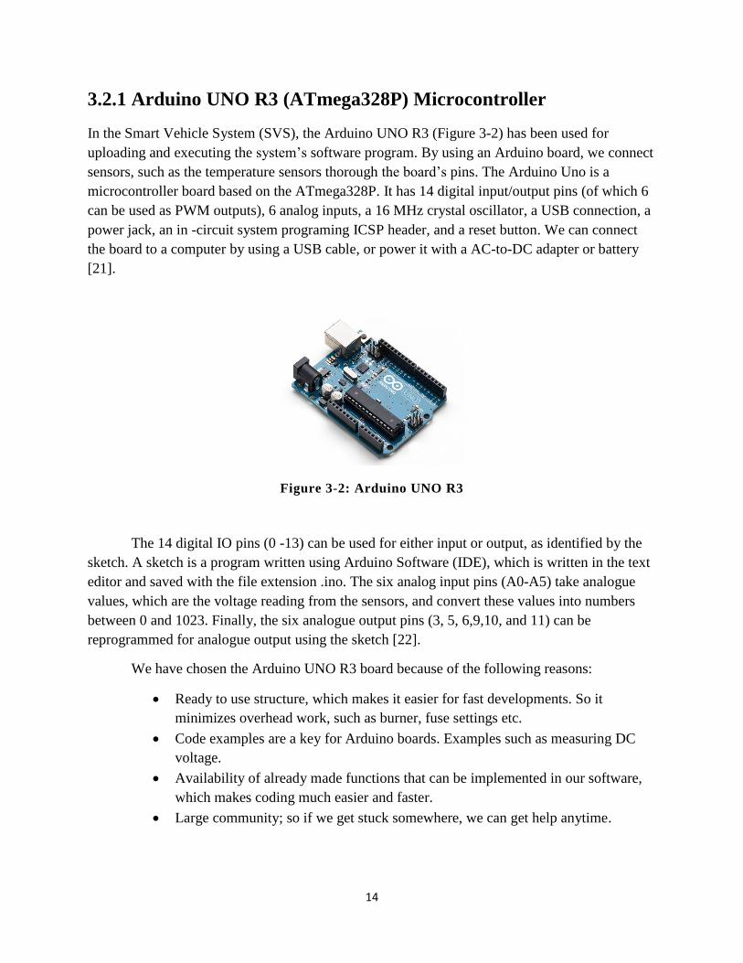
In the Smart Vehicle System (SVS), the Arduino UNO R3 (Figure 3-2) has been used for
uploading and executing the system’s software program. By using an Arduino board, we connect
sensors, such as the temperature sensors thorough the board’s pins. The Arduino Uno is a
microcontroller board based on the ATmega328P. It has 14 digital input/output pins (of which 6
can be used as PWM outputs), 6 analog inputs, a 16 MHz crystal oscillator, a USB connection, a
power jack, an in -circuit system programing ICSP header, and a reset button. We can connect
the board to a computer by using a USB cable, or power it with a AC-to-DC adapter or battery
[21].
Figure 3-2: Arduino UNO R3
The 14 digital IO pins (0 -13) can be used for either input or output, as identified by the
sketch. A sketch is a program written using Arduino Software (IDE), which is written in the text
editor and saved with the file extension .ino. The six analog input pins (A0-A5) take analogue
values, which are the voltage reading from the sensors, and convert these values into numbers
between 0 and 1023. Finally, the six analogue output pins (3, 5, 6,9,10, and 11) can be
reprogrammed for analogue output using the sketch [22].
We have chosen the Arduino UNO R3 board because of the following reasons:
• Ready to use structure, which makes it easier for fast developments. So it
minimizes overhead work, such as burner, fuse settings etc.
• Code examples are a key for Arduino boards. Examples such as measuring DC
voltage.
• Availability of already made functions that can be implemented in our software,
which makes coding much easier and faster.
• Large community; so if we get stuck somewhere, we can get help anytime.
15
Since the Arduino UNO R3 has a clock speed of 16 MHz, it can execute the task faster
than other micro-controllers, such as Arduino Fio. In addition, the Arduino UNO R3 board
supports I2C and In-System Programming (ISP) communication. The Arduino software has a
wire library for I2C and an ISP library for supporting ISP communication [21].
The Arduino UNO R3 features are as follow:
✓ Microcontroller: ATmega328
✓ Operating Voltage: 5V
✓ Input Voltage (recommended): 7-12V
✓ Input Voltage (limits): 6-20V
✓ Digital I/O Pins: 14 (of which 6 provide PWM output)
✓ Analog Input Pins: 6
✓ PWM Digital I/O Pins: 6
✓ DC Current per I/O Pin: 20 mA
✓ DC Current for 3.3V Pin: 50 mA
✓ Flash Memory: 32 KB (ATmega328P) of which 0.5 KB used by bootloader
✓ SRAM: 2 KB (ATmega328P)
✓ EEPROM: 1 KB (ATmega328P)
✓ Clock Speed: 16 MHz
The ATmega328P is a low-power CMOS 8-bit microcontroller and it is attached to the
Arduino UNO R3 board. Figure 3-3 shows the main features of the ATmega328. The CPU is the
brain of the microcontroller and controls everything that goes into the microcontroller. For
example, it fetches the program (uploaded sketches) that is stored in the flash memory and then
executes it [23].
The ATmega328P provides the following features: 32K bytes of internal flash memory, 1K
bytes EEPROM, 2K bytes SRAM, 23 general purpose I/O lines, 32 general purpose working
registers, three flexible Timer/Counters with compare modes, internal and external interrupts, a
serial programmable called Universal Synchronous/Asynchronous Receiver/Transmitte
(USART), a byte-oriented 2-wire Serial Interface, an ISP serial port, a 6-channel 10-bit ADC (8
channels in TQFP and QFN/MLF packages), a programmable Watchdog Timer with internal
Oscillator, and five software selectable power saving modes [24].

16
Figure 3-3: Block diagram of ATmega328
3.2.1.1 Power
The Arduino Uno R3 board is powered by using a USB connection or an external power supply
such as an AC-to-DC adapter or battery. The recommended input voltage for the board is from 7
to 12 volts for operation, so the external power supply is needed. If the board gets less than 7V, it
is not stable and may produce incorrect data. On the other hand, if it gets more than 12V, the
voltage regulator may overheat and damage the board [25].
In our system, we have used the battery since the system will be placed in a moving vehicle.
The battery is plugged into the board through the power jack, and the battery’s voltage is 9V.
There are four different power pins in the board:
❖ VIN: used and accessed when the external power sources is used, for example, if
supplying voltage by using the power jack.
❖ 5V: the regulated power supply used to power the microcontroller and other components
that are connected to the board. The board is powered via USB (5V), DC power jack (7 -
12V), or from the VIN pin of the board (7-12V).
❖ 3V3: A 3.3-volt supply generated by the on-board regulator. Maximum current draw is
50 mA.
❖ GND: the Ground pins.
3.2.1.2 Programming
The Arduino UNO R3 can be programmed by using Arduino software called Arduino IDE
(Integrated Development Environment). The Arduino IDE software is an open source software
that can be downloaded to a computer. It allows users to create and compile the sketches and
17
then upload the sketches to the Arduino board. Furthermore, the software has its own library,
called “Wiring”, that makes the input/output operation easier [23].
The C programming language is used for coding in developing the tracking system. The
code has two main functions, which are setup () and loop (), as shown in Figure 3-4. The setup ()
function runs only one time, when the board starts up or resets for initializing the setting. The
loop () function is used for execution of the program and is called continuously.
The code file is uploaded to the microcontroller by using a USB cable that connects the
PC to the Arduino board. After uploading the file, the USB is disconnected and the file will be
saved in the Arduino’s memory. The file runs each time the board is ON or the reset button is
pressed. The disadvantage of the board is that the board uses only one file at a time. For
example, each time we change the code, we have to disconnect all sensors from the board,
connect the USB cable from a computer to the board, and upload the file, which consumes time.
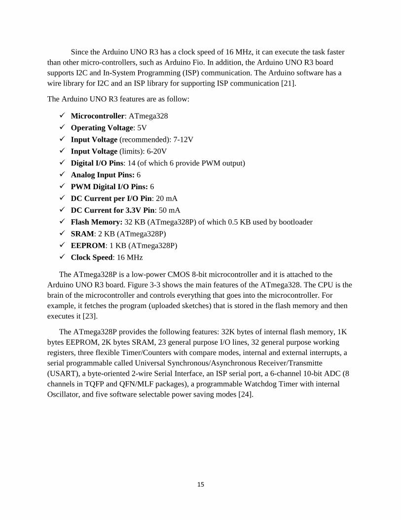
Figure 3-4: Arduino IDE
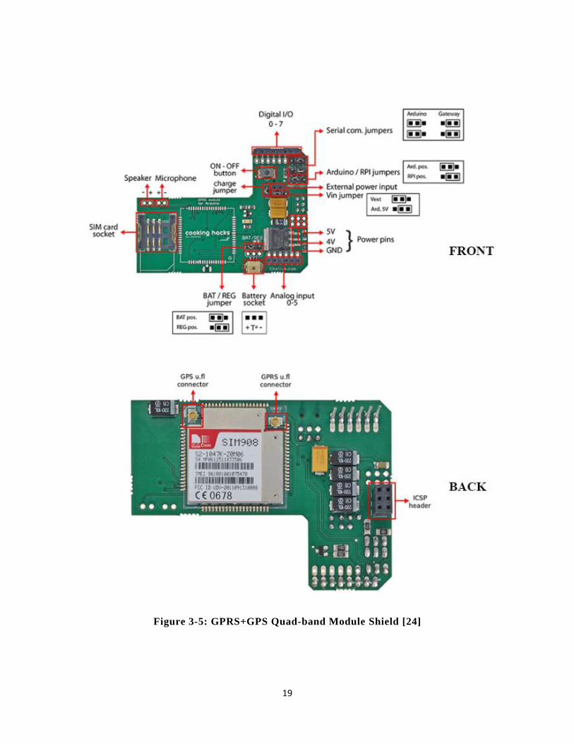
3.2.2 GPRS+GPS Quad-band Module Shield (SIM908):
The GPRS/GPS module is a shield that uses an embedded SIM908 chip as shown in Figure 3-5
and uses both GPRS and GPS technologies for real time tracking. It has a Quad-band GPRS/GPS
engine which works with the frequencies of 850 MHz, 900 MHz, 1800 MHz, and 1900 MHz.
Since this module has low power consumption, an external power supply is needed. The idea
here is to use the shield to get the GPS coordinates (Longitude and Latitude) and then send these
values via HTTP to a web server [26].
The tracking system components, which are the external GPS antenna and external
GPRS/GSM antenna, are connected to the shield, and then the shield is connected to the Arduino
board. After connecting the shield to the board, we change the serial communication jumpers and
Arduino/RPI jumper to the Arduino position to use the board as gateway for the shield. Since we
18
are using external power, that is, the battery, we set a VIN jumper to the left in the RPI position
and BAT/REG jumper to the left as well, in the REG position. The GPRS/GPS module has a
SIM card socket where the SIM card is inserted.
The general features of the GPRS/GPS Quad-band module shield (SIM908) are:
❖ Quad-band: 850/900/1800/1900 MHz
❖ GPRS multi-slot class 10 standard
❖ GPRS mobile station class B standard (class B can manage either packet data or voice at
one time)
❖ Meet the GSM phase 2/2 standard
• Class 4 (2W @ 850/900 MHz)
• Class 1 (1W @ 1800/1900 MHz)
❖ Controlled via AT commands (GSM 07.07, 07.05 and SIMCom Enhanced AT
Commands set)
❖ SIM application toolkit
❖ GPRS supply voltage range: 3.2V to 4.8V
❖ GPS supply voltage range: 3.0V to 4.5V
❖ Operating temperature: -40 to +85 °C
❖ Dual analog audio interfaces
❖ RTC backup
❖ Serial interface and debug interface for GSM/GPRS
❖ Debug interface for GPS NMEA output
❖ Two separate U.FL antenna connectors: one for GSM/GPRS and one for GPS
❖ Configurable baud rate
The SIM908 module shield specification:
❖ PCB size: 80mm X 70mm X 1.6mm
❖ Operating level: 5V/3.3V (optional)
❖ Indicator: PWR, Status, NET
❖ Communication protocol: UART
❖ Support PBCCH
❖ Uses USSD protocol
❖ Non transparent mode
❖ PPP-stack
❖ Included TCP/IP protocol stack for internet data transfer over GPRS
❖ CID up to 14.4kbps
❖ GPRS class 10 max 85.6 downlink
19
Figure 3-5: GPRS+GPS Quad-band Module Shield [24]
20
3.2.2.1 The External GPS Antenna
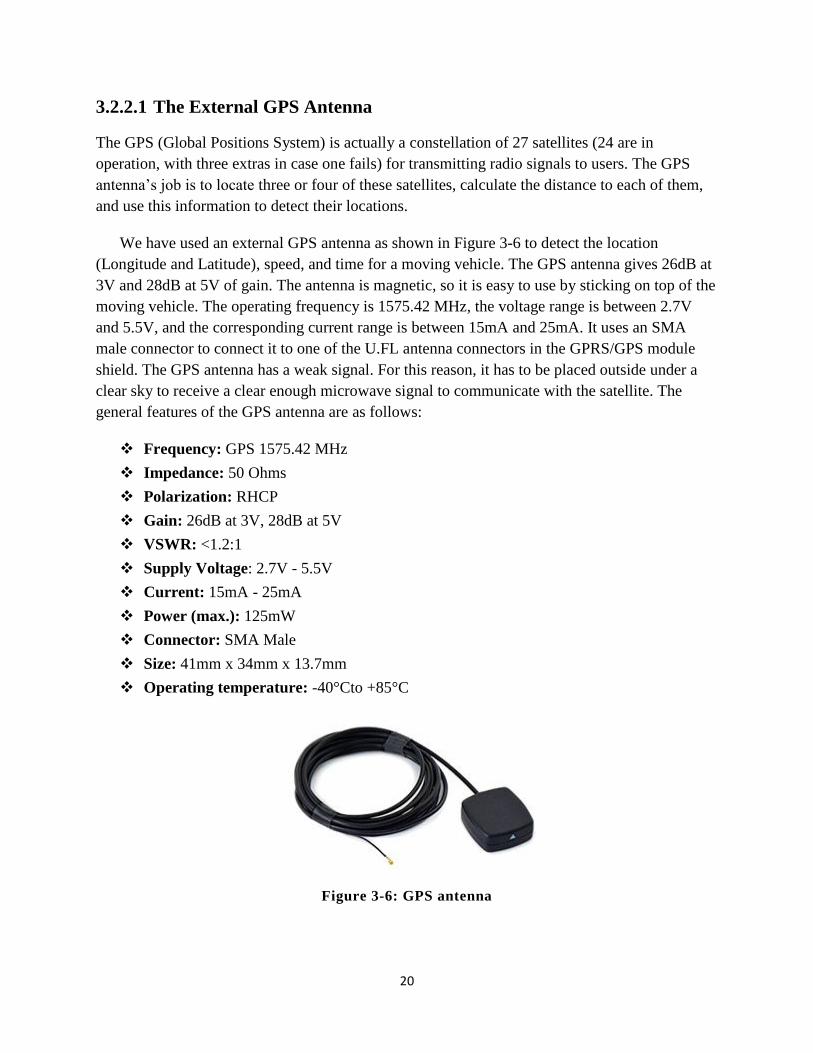
The GPS (Global Positions System) is actually a constellation of 27 satellites (24 are in
operation, with three extras in case one fails) for transmitting radio signals to users. The GPS
antenna’s job is to locate three or four of these satellites, calculate the distance to each of them,
and use this information to detect their locations.
We have used an external GPS antenna as shown in Figure 3-6 to detect the location
(Longitude and Latitude), speed, and time for a moving vehicle. The GPS antenna gives 26dB at
3V and 28dB at 5V of gain. The antenna is magnetic, so it is easy to use by sticking on top of the
moving vehicle. The operating frequency is 1575.42 MHz, the voltage range is between 2.7V
and 5.5V, and the corresponding current range is between 15mA and 25mA. It uses an SMA
male connector to connect it to one of the U.FL antenna connectors in the GPRS/GPS module
shield. The GPS antenna has a weak signal. For this reason, it has to be placed outside under a
clear sky to receive a clear enough microwave signal to communicate with the satellite. The
general features of the GPS antenna are as follows:
❖ Frequency: GPS 1575.42 MHz
❖ Impedance: 50 Ohms
❖ Polarization: RHCP
❖ Gain: 26dB at 3V, 28dB at 5V
❖ VSWR: <1.2:1
❖ Supply Voltage: 2.7V - 5.5V
❖ Current: 15mA - 25mA
❖ Power (max.): 125mW
❖ Connector: SMA Male
❖ Size: 41mm x 34mm x 13.7mm
❖ Operating temperature: -40°Cto +85°C
Figure 3-6: GPS antenna
21
3.2.2.2 The External GPRS/GSM Antenna
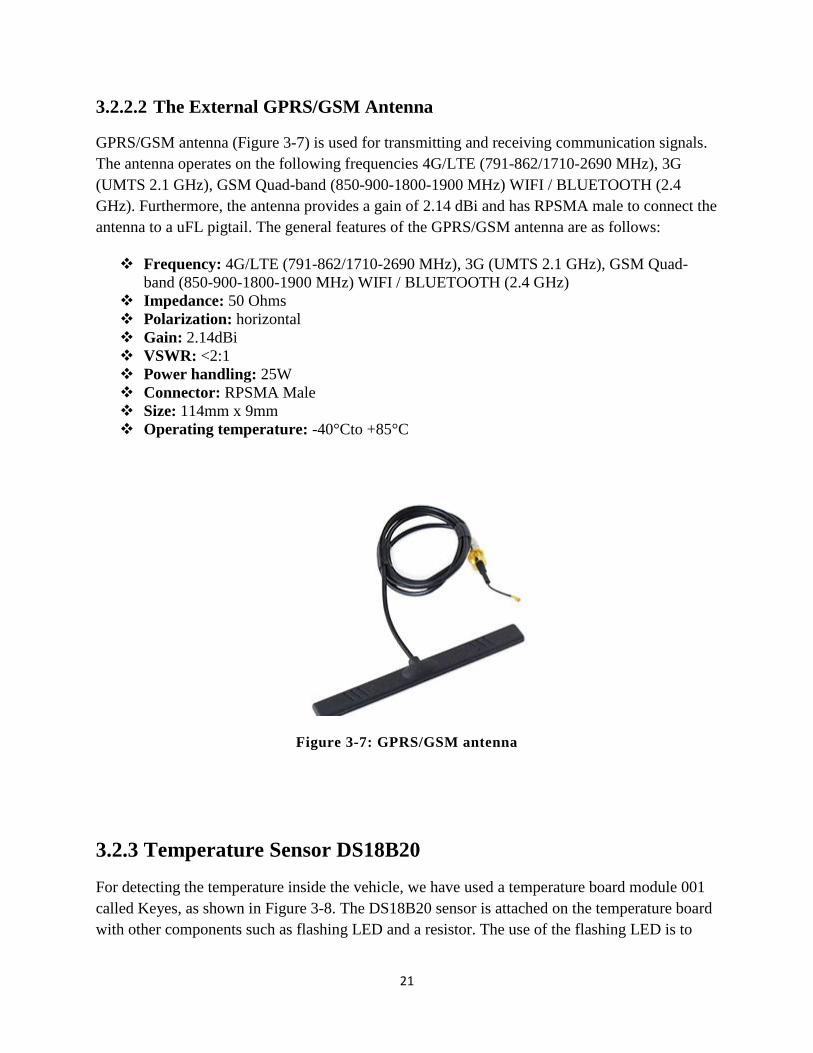
GPRS/GSM antenna (Figure 3-7) is used for transmitting and receiving communication signals.
The antenna operates on the following frequencies 4G/LTE (791-862/1710-2690 MHz), 3G
(UMTS 2.1 GHz), GSM Quad-band (850-900-1800-1900 MHz) WIFI / BLUETOOTH (2.4
GHz). Furthermore, the antenna provides a gain of 2.14 dBi and has RPSMA male to connect the
antenna to a uFL pigtail. The general features of the GPRS/GSM antenna are as follows:
❖ Frequency: 4G/LTE (791-862/1710-2690 MHz), 3G (UMTS 2.1 GHz), GSM Quad-
band (850-900-1800-1900 MHz) WIFI / BLUETOOTH (2.4 GHz)
❖ Impedance: 50 Ohms
❖ Polarization: horizontal
❖ Gain: 2.14dBi
❖ VSWR: <2:1
❖ Power handling: 25W
❖ Connector: RPSMA Male
❖ Size: 114mm x 9mm
❖ Operating temperature: -40°Cto +85°C
Figure 3-7: GPRS/GSM antenna
3.2.3 Temperature Sensor DS18B20
For detecting the temperature inside the vehicle, we have used a temperature board module 001
called Keyes, as shown in Figure 3-8. The DS18B20 sensor is attached on the temperature board
with other components such as flashing LED and a resistor. The use of the flashing LED is to
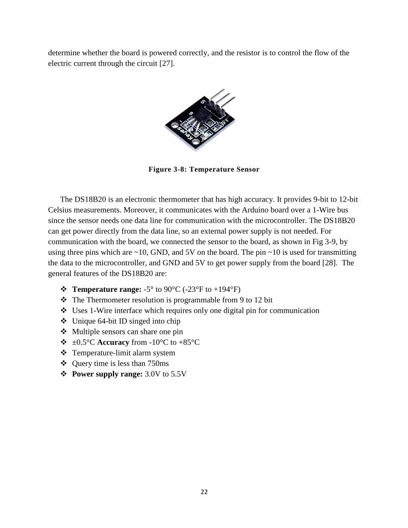
22
determine whether the board is powered correctly, and the resistor is to control the flow of the
electric current through the circuit [27].
Figure 3-8: Temperature Sensor
The DS18B20 is an electronic thermometer that has high accuracy. It provides 9-bit to 12-bit
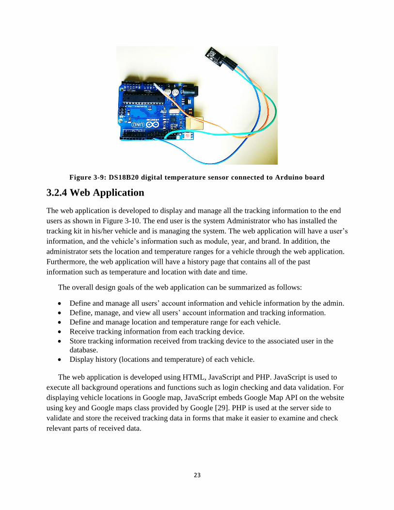
Celsius measurements. Moreover, it communicates with the Arduino board over a 1-Wire bus
since the sensor needs one data line for communication with the microcontroller. The DS18B20
can get power directly from the data line, so an external power supply is not needed. For
communication with the board, we connected the sensor to the board, as shown in Fig 3-9, by
using three pins which are ~10, GND, and 5V on the board. The pin ~10 is used for transmitting
the data to the microcontroller, and GND and 5V to get power supply from the board [28]. The
general features of the DS18B20 are:
❖ Temperature range: -5° to 90°C (-23°F to +194°F)
❖ The Thermometer resolution is programmable from 9 to 12 bit
❖ Uses 1-Wire interface which requires only one digital pin for communication
❖ Unique 64-bit ID singed into chip
❖ Multiple sensors can share one pin
❖ ±0.5°C Accuracy from -10°C to +85°C
❖ Temperature-limit alarm system
❖ Query time is less than 750ms
❖ Power supply range: 3.0V to 5.5V
23
Figure 3-9: DS18B20 digital temperature sensor connected to Arduino board
3.2.4 Web Application
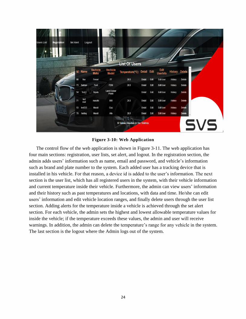
The web application is developed to display and manage all the tracking information to the end
users as shown in Figure 3-10. The end user is the system Administrator who has installed the
tracking kit in his/her vehicle and is managing the system. The web application will have a user’s
information, and the vehicle’s information such as module, year, and brand. In addition, the
administrator sets the location and temperature ranges for a vehicle through the web application.
Furthermore, the web application will have a history page that contains all of the past
information such as temperature and location with date and time.
The overall design goals of the web application can be summarized as follows:
• Define and manage all users’ account information and vehicle information by the admin.
• Define, manage, and view all users’ account information and tracking information.
• Define and manage location and temperature range for each vehicle.
• Receive tracking information from each tracking device.
• Store tracking information received from tracking device to the associated user in the
database.
• Display history (locations and temperature) of each vehicle.
The web application is developed using HTML, JavaScript and PHP. JavaScript is used to
execute all background operations and functions such as login checking and data validation. For
displaying vehicle locations in Google map, JavaScript embeds Google Map API on the website
using key and Google maps class provided by Google [29]. PHP is used at the server side to
validate and store the received tracking data in forms that make it easier to examine and check
relevant parts of received data.
24
Figure 3-10: Web Application
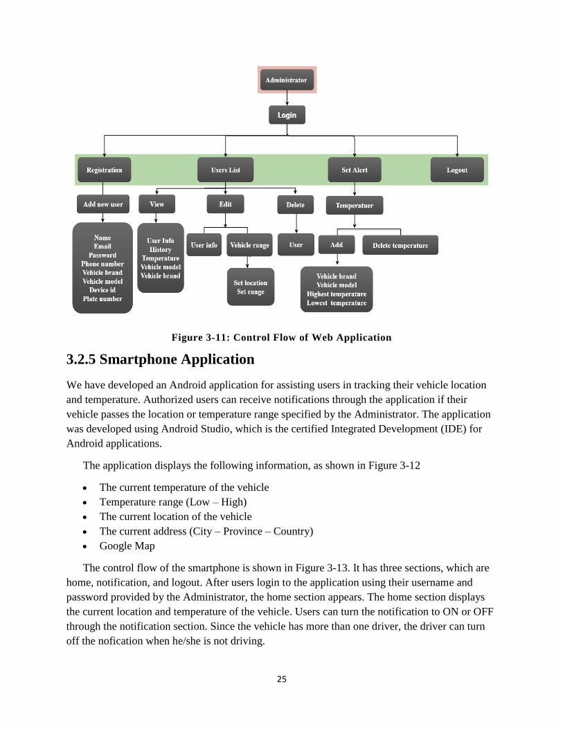
The control flow of the web application is shown in Figure 3-11. The web application has
four main sections: registration, user lists, set alert, and logout. In the registration section, the
admin adds users’ information such as name, email and password, and vehicle’s information
such as brand and plate number to the system. Each added user has a tracking device that is
installed in his vehicle. For that reason, a device id is added to the user’s information. The next
section is the user list, which has all registered users in the system, with their vehicle information
and current temperature inside their vehicle. Furthermore, the admin can view users’ information
and their history such as past temperatures and locations, with data and time. He/she can edit
users’ information and edit vehicle location ranges, and finally delete users through the user list
section. Adding alerts for the temperature inside a vehicle is achieved through the set alert
section. For each vehicle, the admin sets the highest and lowest allowable temperature values for
inside the vehicle; if the temperature exceeds these values, the admin and user will receive
warnings. In addition, the admin can delete the temperature’s range for any vehicle in the system.
The last section is the logout where the Admin logs out of the system.
25
Figure 3-11: Control Flow of Web Application
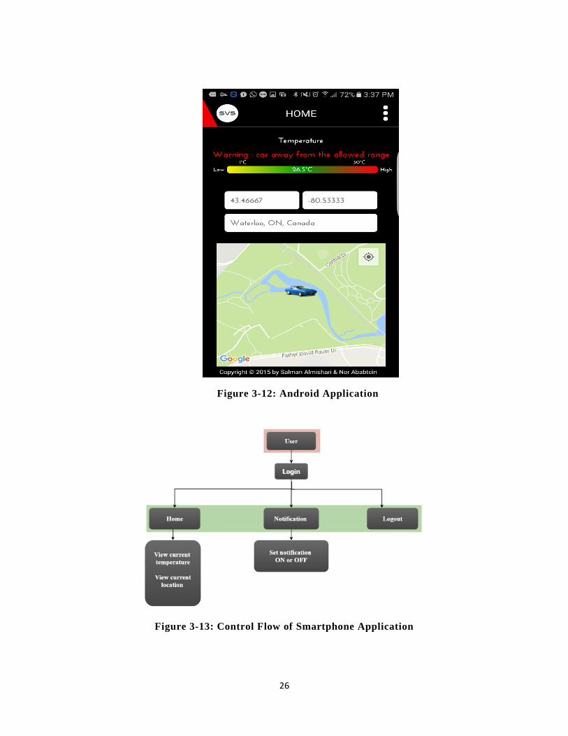
3.2.5 Smartphone Application
We have developed an Android application for assisting users in tracking their vehicle location
and temperature. Authorized users can receive notifications through the application if their
vehicle passes the location or temperature range specified by the Administrator. The application
was developed using Android Studio, which is the certified Integrated Development (IDE) for
Android applications.
The application displays the following information, as shown in Figure 3-12
• The current temperature of the vehicle
• Temperature range (Low – High)
• The current location of the vehicle
• The current address (City – Province – Country)
• Google Map
The control flow of the smartphone is shown in Figure 3-13. It has three sections, which are
home, notification, and logout. After users login to the application using their username and
password provided by the Administrator, the home section appears. The home section displays
the current location and temperature of the vehicle. Users can turn the notification to ON or OFF
through the notification section. Since the vehicle has more than one driver, the driver can turn
off the nofication when he/she is not driving.
26
Figure 3-12: Android Application
Figure 3-13: Control Flow of Smartphone Application
27
3.2.5.1 Google Maps API
We use a Google maps API (Application Programming Interface) for Android to display the
location of the vehicle on an Android application in real-time by using an HTTP request. The
main function of the Google maps API is to handle access to Google Maps servers, display maps
on the smartphone application or on the web application, and respond to user actions, such as
clicks and zooms in/out.
3.2.6 Web Server
The web server stores all information received from the tracking system installed in different
vehicles. The database is available for authorized users and accessible over the Internet.
Authorized users can track, manage, and view all previous information stored in the database for
their vehicle. Moreover, user information and vehicle information are stored in the database.
3.2.7 Database Design
The database is designed to store all system information, including admin login credentials, user
information, vehicle information, and tracking data received from the tracking system. In our
thesis, we have used two different databases - the SQL database and NoSQL database - for
storing all received data from the tracking unit. For the SQL database, MySQL is used, which is
relational database that uses tables. For the NoSQL, MongoDB is used, which is non-relational
database that is based on documents instead of tables.
3.2.7.1 SQL database:
SQL database is based on a fixed table structures. A structured query language is used for
selecting data from the tables. By using the join operation, we can select data from multiple
tables. SQL databases typically work well in a vertical manner, such as for upgrading a server
that runs a database. On the other hand, it does not work well in a horizontal manner, such as for
adding a server to a cluster [30].
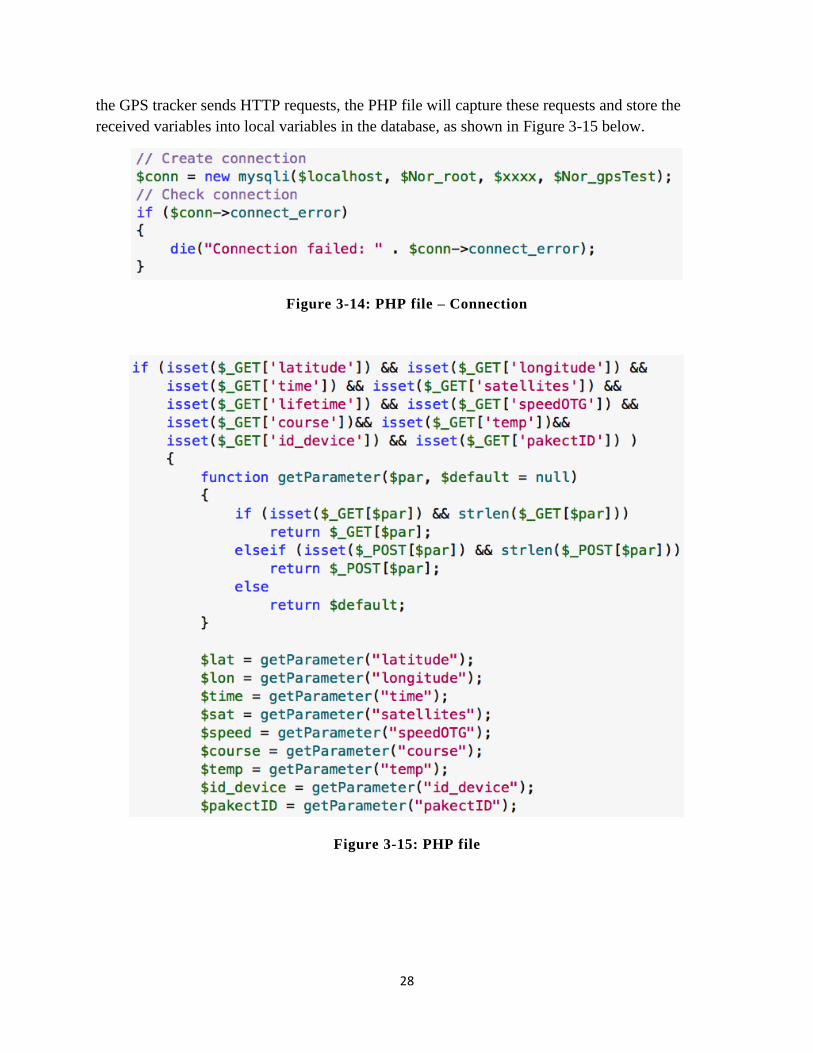
The MySQL database consists of the following tables, as shown in Figure 3-16 below:
• MyData table: it has all the location information (longitude, latitude, and speed)
received from the tracking system including time, temperature, device id, and packet id.
• tb_vehicle table: it holds vehicle information and temperature ranges for each vehicle.
• Registration table: all users’ information, account information, and current location of
the registered vehicles are stored in the registration table.
• Admin table: it has admin’s login information.
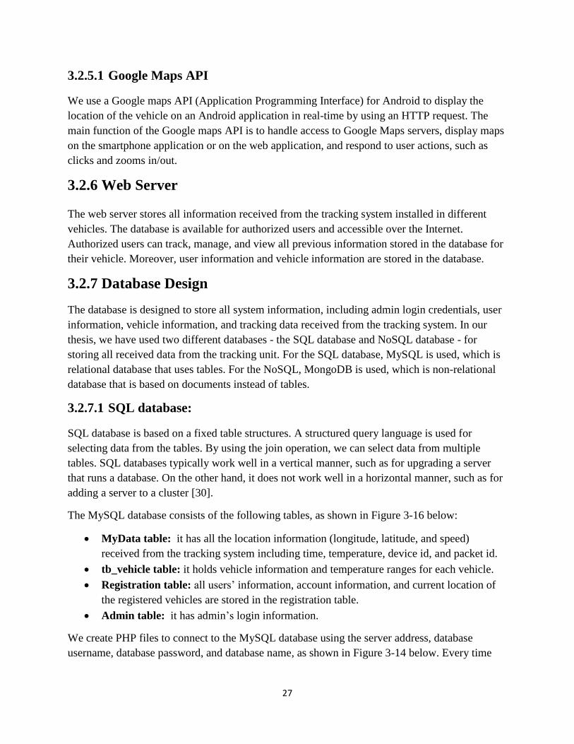
We create PHP files to connect to the MySQL database using the server address, database
username, database password, and database name, as shown in Figure 3-14 below. Every time
28
the GPS tracker sends HTTP requests, the PHP file will capture these requests and store the
received variables into local variables in the database, as shown in Figure 3-15 below.
Figure 3-14: PHP file – Connection
Figure 3-15: PHP file
29
Figure 3-16: Database Tables
3.2.7.2 NoSQL database:
The term ‘NoSQL’ collectively refers to the database technologies that use non-relational
databases. By losing some of the ACID transactional properties (atomicity, consistency, isolation
and durability) of relational databases, NoSQL databases achieve higher availability and
scalability, which are critical requirements for big data processing. In addition, NoSQL databases
do not require fixed schema with pre-defined data structures and constraints in the early stages of
database design. Furthermore, an NoSQL database allows horizontal scaling, by duplicating and
partitioning data over many nodes, thereby promoting fast read and write operations of massive
data [31].
NoSQL databases have three types of models: key-value stores, document databases, and
column-oriented databases. In the key-value stores model, data are stored and retrieved by a key.
This model can hold unstructured and structured data. The document database is based on the
key-value stores concept but has added complexity. Each document has its own data and a
unique key for retrieving the document. The column oriented database stores data tables as
columns rather than rows. This model is more effective with database that require column-
oriented calculations such as aggregation [30].
30
MongoDB is an open source NoSQL database developed by 10gen. In addition, it is a
document-oriented NoSQL database and written in C++. The MongoDB components are the
mongod, mongos, replica sets, shard, and config server. The mongod handles all the data
requests, manages data access, and performs background management operations. The mongos is
the routing service for MongoDB shard configurations. It processes all the queries from the
application layer and then determines the location of the requested data in the shared cluster. The
replica sets is a group of mongod processes that has the same dataset. In cases where the primary
mongod is unavailable, the replica sets will choose a new primary mongod. The data is stored in
the shard, and each shard is a replica set to make the data available and consistent. Finally, the
config server stores the cluster’s metadata, which contain all the mapping between the cluster’s
dataset and the shards [31].
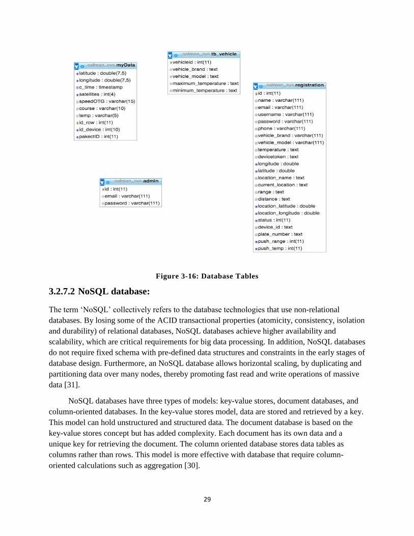
MongoDB stores data as documents in a binary representation called BSON (Binary
JSON) or BSON objects. Its drivers send and receive data in BSON as shown in Figure 3-17.
MongoDB clusters data through collections. A collection is a grouping of documents (records)
that share a similar structure. The collection acts the same as a table in an SQL database, and
documents act as records inside the table(rows), and field as columns. Each collection can have a
different structure from one another, unlike in SQL, where each table has to be restrict by a
schema. This feature will reduce the need to divide data in a document into several different
tables, as is often done in SQL implementations. [32].
Figure 3-17: MongoDB Architecture
We created two databases, svs (Smart Tracking System) and svs_dataSaving. Each
database has its own collection for storing all data received from the tracking unit. We use the
following commands:
• use name of database: To create a new database for our experiments.
• db.name of the collection.stats(): To show the information of the collection, as in Figure
3-18, such as the name of the database, the size of the collection, and the number of
documents stored in the collection, etc. .
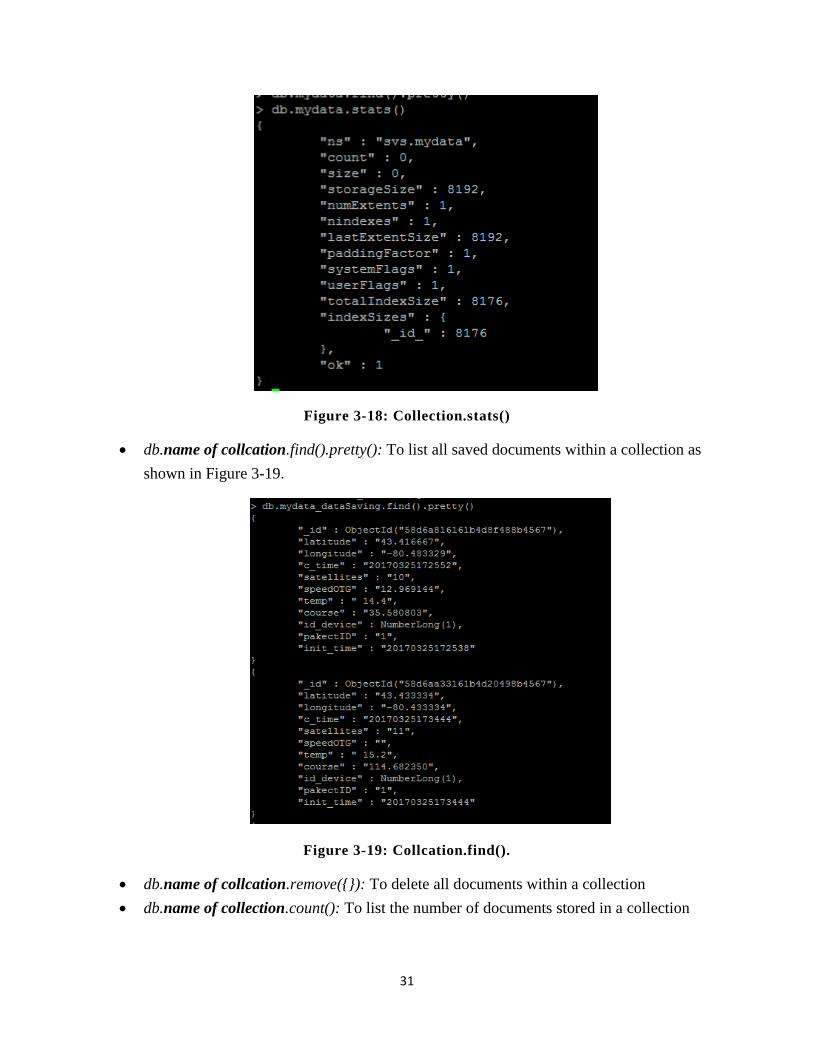
31
Figure 3-18: Collection.stats()
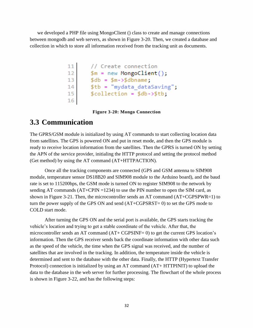
• db.name of collcation.find().pretty(): To list all saved documents within a collection as
shown in Figure 3-19.
Figure 3-19: Collcation.find().
• db.name of collcation.remove({}): To delete all documents within a collection
• db.name of collection.count(): To list the number of documents stored in a collection
32
we developed a PHP file using MongoClient () class to create and manage connections
between mongodb and web servers, as shown in Figure 3-20. Then, we created a database and
collection in which to store all information received from the tracking unit as documents.
Figure 3-20: Mongo Connection
3.3 Communication
The GPRS/GSM module is initialized by using AT commands to start collecting location data
from satellites. The GPS is powered ON and put in reset mode, and then the GPS module is
ready to receive location information from the satellites. Then the GPRS is turned ON by setting
the APN of the service provider, initialing the HTTP protocol and setting the protocol method
(Get method) by using the AT command (AT+HTTPACTION).
Once all the tracking components are connected (GPS and GSM antenna to SIM908
module, temperature sensor DS18B20 and SIM908 module to the Arduino board), and the baud
rate is set to 115200bps, the GSM mode is turned ON to register SIM908 to the network by
sending AT commands (AT+CPIN =1234) to use the PIN number to open the SIM card, as
shown in Figure 3-21. Then, the microcontroller sends an AT command (AT+CGPSPWR=1) to
turn the power supply of the GPS ON and send (AT+CGPSRST= 0) to set the GPS mode to
COLD start mode.
After turning the GPS ON and the serial port is available, the GPS starts tracking the
vehicle’s location and trying to get a stable coordinate of the vehicle. After that, the
microcontroller sends an AT command (AT+ CGPSINF= 0) to get the current GPS location’s
information. Then the GPS receiver sends back the coordinate information with other data such
as the speed of the vehicle, the time when the GPS signal was received, and the number of
satellites that are involved in the tracking. In addition, the temperature inside the vehicle is
determined and sent to the database with the other data. Finally, the HTTP (Hypertext Transfer
Protocol) connection is initialized by using an AT command (AT+ HTTPINIT) to upload the
data to the database in the web server for further processing. The flowchart of the whole process
is shown in Figure 3-22, and has the following steps:
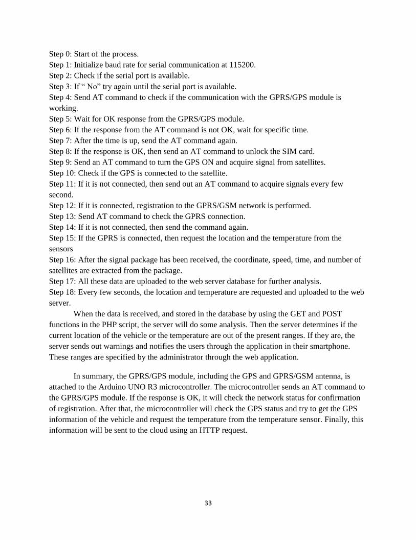
33
Step 0: Start of the process.
Step 1: Initialize baud rate for serial communication at 115200.
Step 2: Check if the serial port is available.
Step 3: If “ No” try again until the serial port is available.
Step 4: Send AT command to check if the communication with the GPRS/GPS module is
working.
Step 5: Wait for OK response from the GPRS/GPS module.
Step 6: If the response from the AT command is not OK, wait for specific time.
Step 7: After the time is up, send the AT command again.
Step 8: If the response is OK, then send an AT command to unlock the SIM card.
Step 9: Send an AT command to turn the GPS ON and acquire signal from satellites.
Step 10: Check if the GPS is connected to the satellite.
Step 11: If it is not connected, then send out an AT command to acquire signals every few
second.
Step 12: If it is connected, registration to the GPRS/GSM network is performed.
Step 13: Send AT command to check the GPRS connection.
Step 14: If it is not connected, then send the command again.
Step 15: If the GPRS is connected, then request the location and the temperature from the
sensors
Step 16: After the signal package has been received, the coordinate, speed, time, and number of
satellites are extracted from the package.
Step 17: All these data are uploaded to the web server database for further analysis.
Step 18: Every few seconds, the location and temperature are requested and uploaded to the web
server.
When the data is received, and stored in the database by using the GET and POST
functions in the PHP script, the server will do some analysis. Then the server determines if the
current location of the vehicle or the temperature are out of the present ranges. If they are, the
server sends out warnings and notifies the users through the application in their smartphone.
These ranges are specified by the administrator through the web application.
In summary, the GPRS/GPS module, including the GPS and GPRS/GSM antenna, is
attached to the Arduino UNO R3 microcontroller. The microcontroller sends an AT command to
the GPRS/GPS module. If the response is OK, it will check the network status for confirmation
of registration. After that, the microcontroller will check the GPS status and try to get the GPS
information of the vehicle and request the temperature from the temperature sensor. Finally, this
information will be sent to the cloud using an HTTP request.
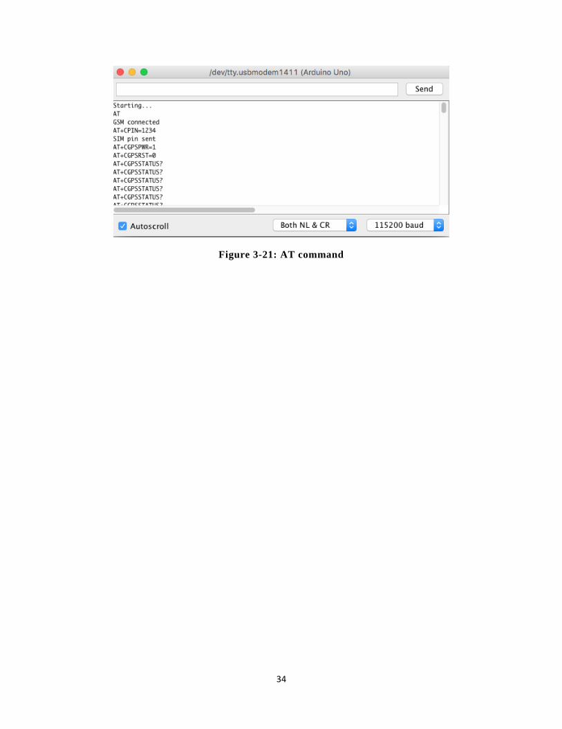
34
Figure 3-21: AT command
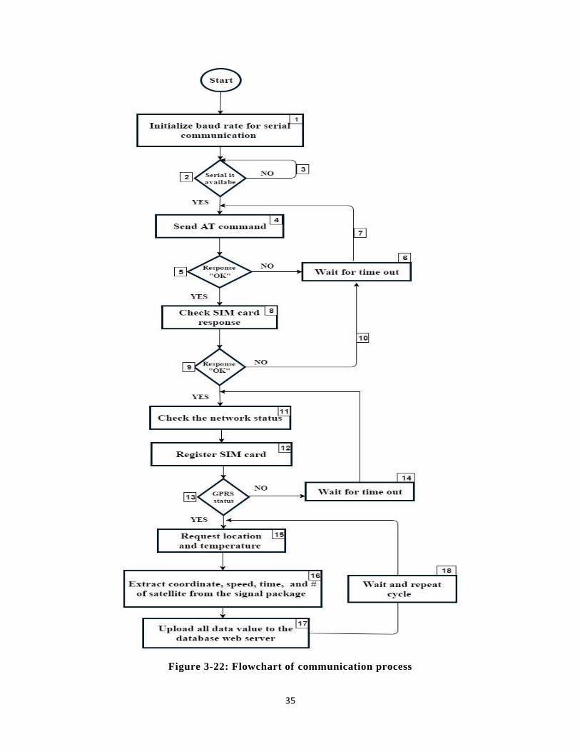
35
Figure 3-22: Flowchart of communication process
36
Chapter 4
4 Experiment and Result
In this chapter, we introduce two algorithms for minimizing database storage in the cloud and
explain their functions. Furthermore, experiments that we performed are explained and their
results are discussed. In our experiments, two different tests are completed: static and dynamic.
Static means when the vehicle is not moving for a period of time, and dynamic is the driving
mode when the vehicle moves from one location to another. These experiments are performed on
SQL and NOSQL databases.
4.1 Proposed Algorithms
To decrease database storage, we propose two different algorithms. The first is used to reduce
data redundancy, which occurs when two uploaded records have duplicate values such as for
longitude, latitude and temperature. The second algorithm is used for un-repetitive data for
which there are no duplicate values in the stored record. Before new records are uploaded, a
lifetime, specified by the administrator of the database, is added. Records will then be deleted
from the database after their specified lifetime is reached.
The second algorithm is a suggested feature of our system but was not included in our
experiment because of the variable times that an administrator might need to store the data. If the
administrator uses the second algorithm the size of the database will be steady and will not
increase. The database size will be stable since some of the stored records in the database will be
deleted after a period of time specified by the administrator. Therefore, the administrator would
have the ability to determine how much data should be stored for future processing.
4.1.1 Reducing Data Redundancy Algorithm (RDR)
After the Smart Vehicle System (SVS) collects the data from the vehicle tracking unit as shown
in Figure 4-1, the raw data is examined to determine if the data is new or already exists in the
database. Then, data cleaning is performed to ensure the accuracy of the data by filling in any
missing data and levelling the noise [33]. The data collected from sensors in the real world is
usually incomplete or invalid. We fill in the missing values using the average value of the last
values in the previous records. For example, if the speed is missing, the average speed of
previous records is calculated and the result is inserted in the open spot. However, if the data
already exists in the database, a custom process is performed.
.
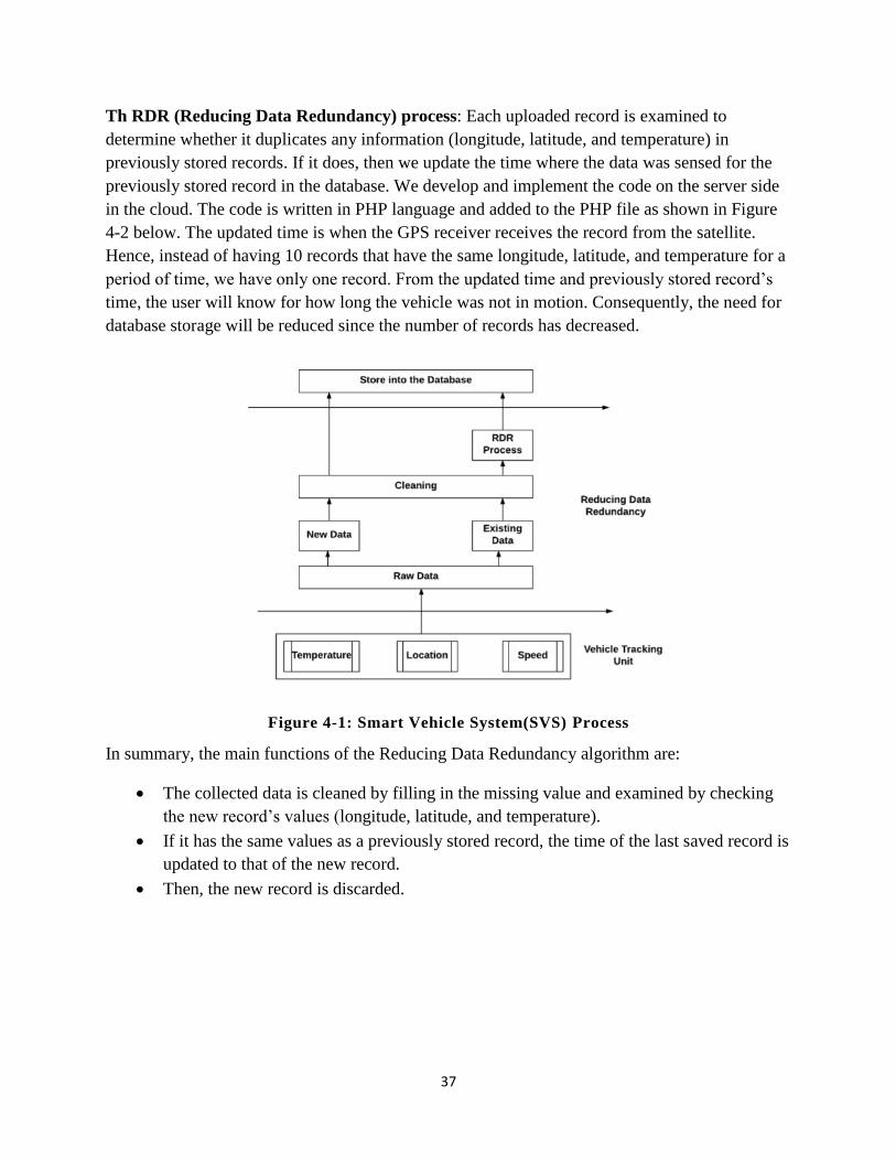
37
Th RDR (Reducing Data Redundancy) process: Each uploaded record is examined to
determine whether it duplicates any information (longitude, latitude, and temperature) in
previously stored records. If it does, then we update the time where the data was sensed for the
previously stored record in the database. We develop and implement the code on the server side
in the cloud. The code is written in PHP language and added to the PHP file as shown in Figure
4-2 below. The updated time is when the GPS receiver receives the record from the satellite.
Hence, instead of having 10 records that have the same longitude, latitude, and temperature for a
period of time, we have only one record. From the updated time and previously stored record’s
time, the user will know for how long the vehicle was not in motion. Consequently, the need for
database storage will be reduced since the number of records has decreased.
Figure 4-1: Smart Vehicle System(SVS) Process
In summary, the main functions of the Reducing Data Redundancy algorithm are:
• The collected data is cleaned by filling in the missing value and examined by checking
the new record’s values (longitude, latitude, and temperature).
• If it has the same values as a previously stored record, the time of the last saved record is
updated to that of the new record.
• Then, the new record is discarded.
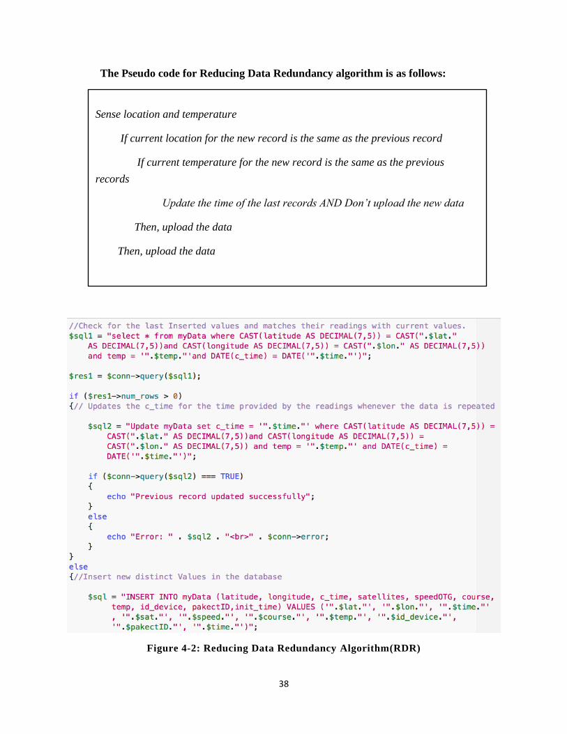
38
The Pseudo code for Reducing Data Redundancy algorithm is as follows:
Figure 4-2: Reducing Data Redundancy Algorithm(RDR)
Sense location and temperature
If current location for the new record is the same as the previous record
If current temperature for the new record is the same as the previous
records
Update the time of the last records AND Don’t upload the new data
Then, upload the data
Then, upload the data
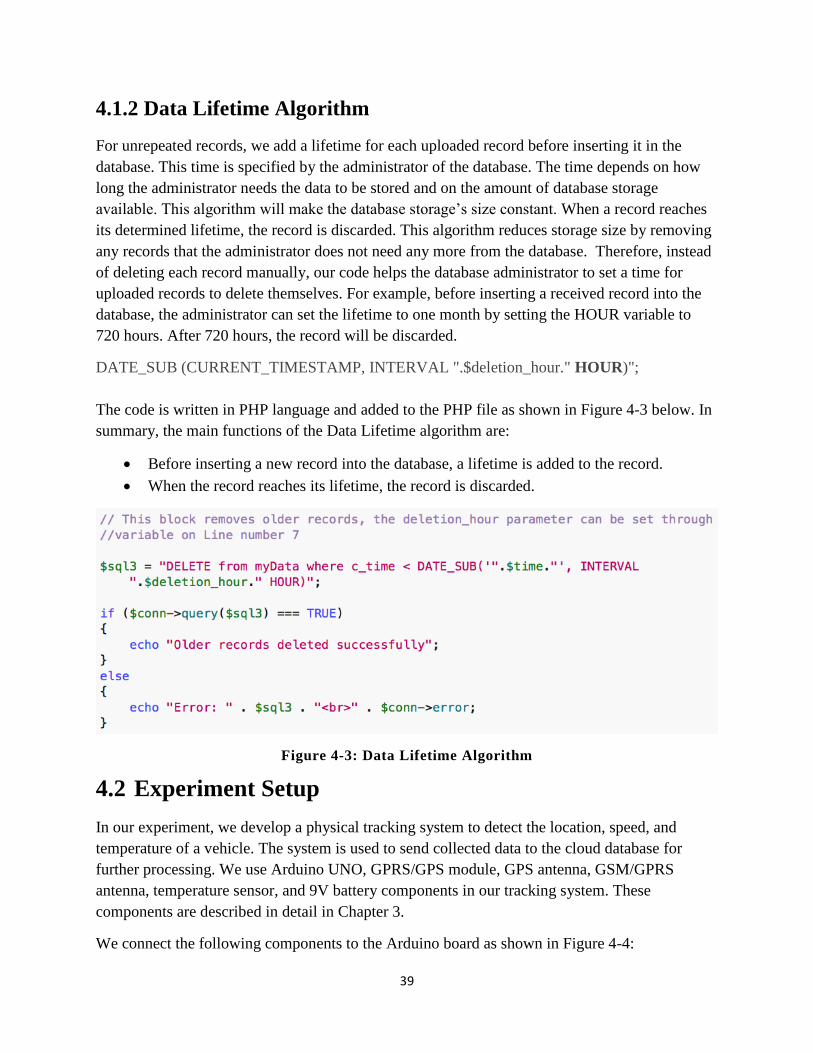
39
4.1.2 Data Lifetime Algorithm
For unrepeated records, we add a lifetime for each uploaded record before inserting it in the
database. This time is specified by the administrator of the database. The time depends on how
long the administrator needs the data to be stored and on the amount of database storage
available. This algorithm will make the database storage’s size constant. When a record reaches
its determined lifetime, the record is discarded. This algorithm reduces storage size by removing
any records that the administrator does not need any more from the database. Therefore, instead
of deleting each record manually, our code helps the database administrator to set a time for
uploaded records to delete themselves. For example, before inserting a received record into the
database, the administrator can set the lifetime to one month by setting the HOUR variable to
720 hours. After 720 hours, the record will be discarded.
DATE_SUB (CURRENT_TIMESTAMP, INTERVAL ".$deletion_hour." HOUR)";
The code is written in PHP language and added to the PHP file as shown in Figure 4-3 below. In
summary, the main functions of the Data Lifetime algorithm are:
• Before inserting a new record into the database, a lifetime is added to the record.
• When the record reaches its lifetime, the record is discarded.
Figure 4-3: Data Lifetime Algorithm
4.2 Experiment Setup
In our experiment, we develop a physical tracking system to detect the location, speed, and
temperature of a vehicle. The system is used to send collected data to the cloud database for
further processing. We use Arduino UNO, GPRS/GPS module, GPS antenna, GSM/GPRS
antenna, temperature sensor, and 9V battery components in our tracking system. These
components are described in detail in Chapter 3.
We connect the following components to the Arduino board as shown in Figure 4-4:
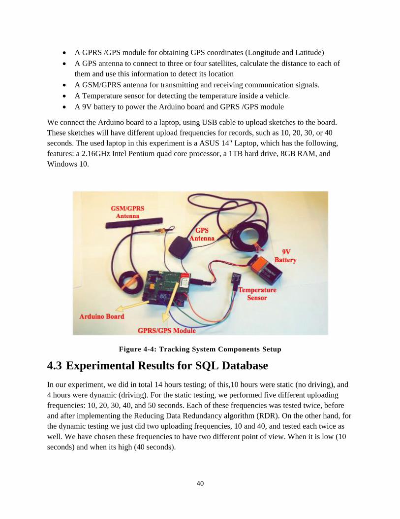
40
• A GPRS /GPS module for obtaining GPS coordinates (Longitude and Latitude)
• A GPS antenna to connect to three or four satellites, calculate the distance to each of
them and use this information to detect its location
• A GSM/GPRS antenna for transmitting and receiving communication signals.
• A Temperature sensor for detecting the temperature inside a vehicle.
• A 9V battery to power the Arduino board and GPRS /GPS module
We connect the Arduino board to a laptop, using USB cable to upload sketches to the board.
These sketches will have different upload frequencies for records, such as 10, 20, 30, or 40
seconds. The used laptop in this experiment is a ASUS 14" Laptop, which has the following,
features: a 2.16GHz Intel Pentium quad core processor, a 1TB hard drive, 8GB RAM, and
Windows 10.
Figure 4-4: Tracking System Components Setup
4.3 Experimental Results for SQL Database
In our experiment, we did in total 14 hours testing; of this,10 hours were static (no driving), and
4 hours were dynamic (driving). For the static testing, we performed five different uploading
frequencies: 10, 20, 30, 40, and 50 seconds. Each of these frequencies was tested twice, before
and after implementing the Reducing Data Redundancy algorithm (RDR). On the other hand, for
the dynamic testing we just did two uploading frequencies, 10 and 40, and tested each twice as
well. We have chosen these frequencies to have two different point of view. When it is low (10
seconds) and when its high (40 seconds).
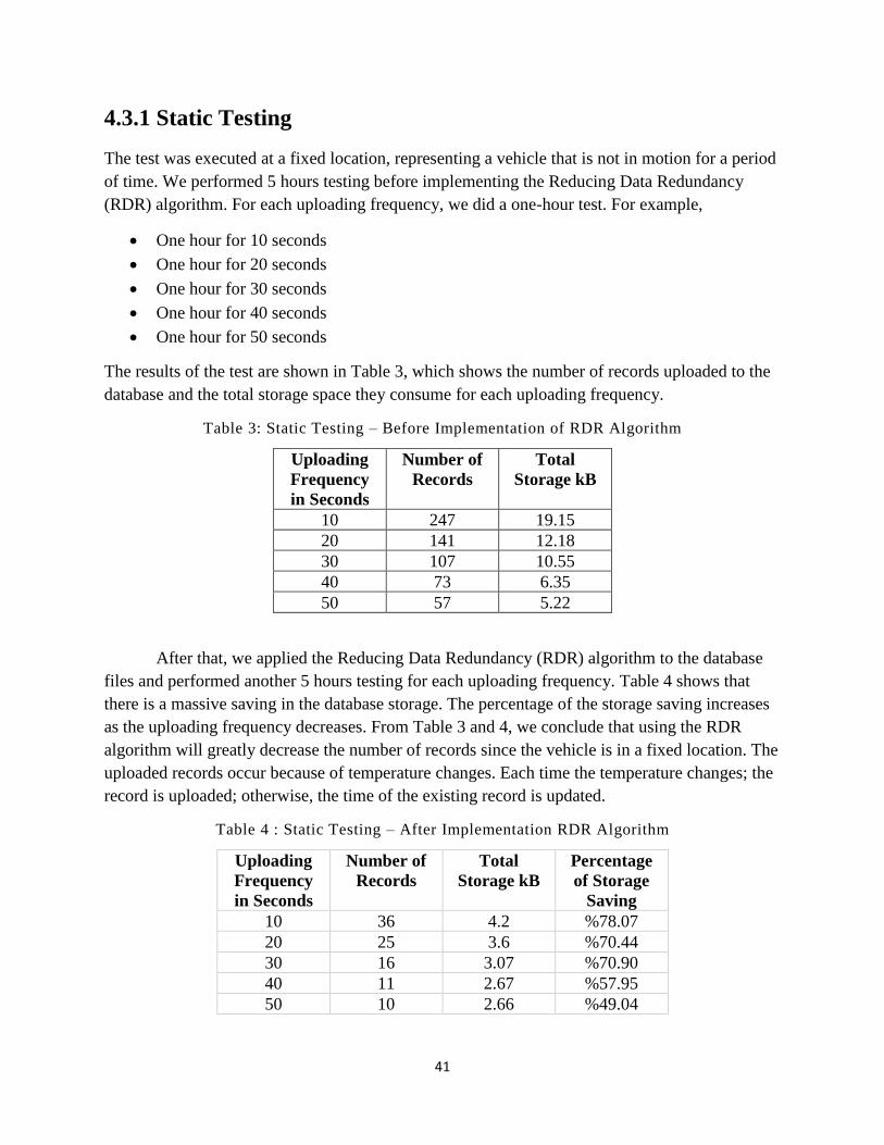
41
4.3.1 Static Testing
The test was executed at a fixed location, representing a vehicle that is not in motion for a period
of time. We performed 5 hours testing before implementing the Reducing Data Redundancy
(RDR) algorithm. For each uploading frequency, we did a one-hour test. For example,
• One hour for 10 seconds
• One hour for 20 seconds
• One hour for 30 seconds
• One hour for 40 seconds
• One hour for 50 seconds
The results of the test are shown in Table 3, which shows the number of records uploaded to the
database and the total storage space they consume for each uploading frequency.
Table 3: Static Testing – Before Implementation of RDR Algorithm
Uploading
Frequency
in Seconds
Number of
Records
Total
Storage kB
10 247 19.15
20 141 12.18
30 107 10.55
40 73 6.35
50 57 5.22
After that, we applied the Reducing Data Redundancy (RDR) algorithm to the database
files and performed another 5 hours testing for each uploading frequency. Table 4 shows that
there is a massive saving in the database storage. The percentage of the storage saving increases
as the uploading frequency decreases. From Table 3 and 4, we conclude that using the RDR
algorithm will greatly decrease the number of records since the vehicle is in a fixed location. The
uploaded records occur because of temperature changes. Each time the temperature changes; the
record is uploaded; otherwise, the time of the existing record is updated.
Table 4 : Static Testing – After Implementation RDR Algorithm
Uploading
Frequency
in Seconds
Number of
Records
Total
Storage kB
Percentage
of Storage
Saving
10 36 4.2 %78.07
20 25 3.6 %70.44
30 16 3.07 %70.90
40 11 2.67 %57.95
50 10 2.66 %49.04
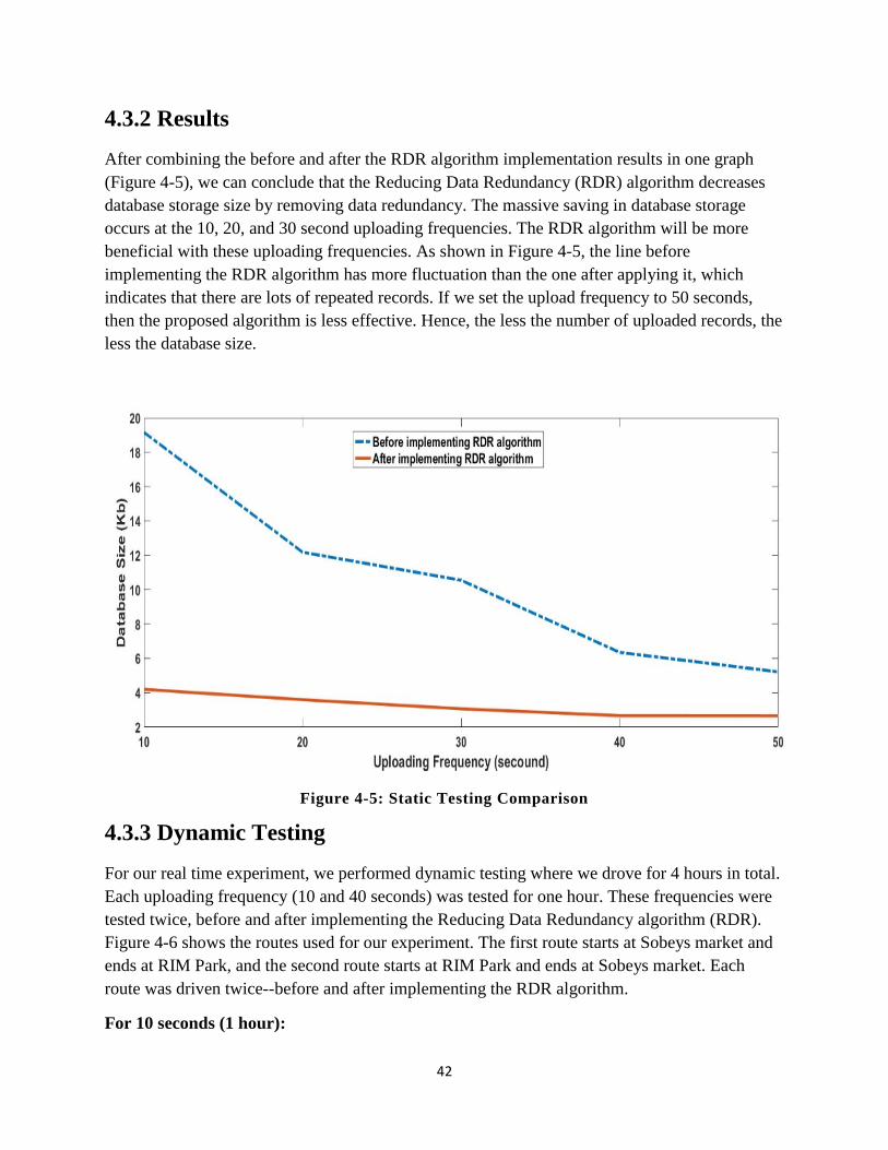
42
4.3.2 Results
After combining the before and after the RDR algorithm implementation results in one graph
(Figure 4-5), we can conclude that the Reducing Data Redundancy (RDR) algorithm decreases
database storage size by removing data redundancy. The massive saving in database storage
occurs at the 10, 20, and 30 second uploading frequencies. The RDR algorithm will be more
beneficial with these uploading frequencies. As shown in Figure 4-5, the line before
implementing the RDR algorithm has more fluctuation than the one after applying it, which
indicates that there are lots of repeated records. If we set the upload frequency to 50 seconds,
then the proposed algorithm is less effective. Hence, the less the number of uploaded records, the
less the database size.
Figure 4-5: Static Testing Comparison
4.3.3 Dynamic Testing
For our real time experiment, we performed dynamic testing where we drove for 4 hours in total.
Each uploading frequency (10 and 40 seconds) was tested for one hour. These frequencies were
tested twice, before and after implementing the Reducing Data Redundancy algorithm (RDR).
Figure 4-6 shows the routes used for our experiment. The first route starts at Sobeys market and
ends at RIM Park, and the second route starts at RIM Park and ends at Sobeys market. Each
route was driven twice--before and after implementing the RDR algorithm.
For 10 seconds (1 hour):
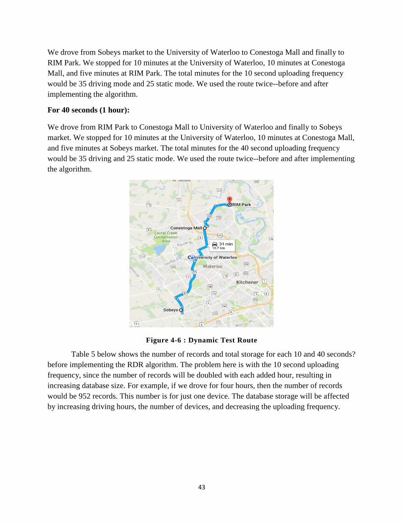
43
We drove from Sobeys market to the University of Waterloo to Conestoga Mall and finally to
RIM Park. We stopped for 10 minutes at the University of Waterloo, 10 minutes at Conestoga
Mall, and five minutes at RIM Park. The total minutes for the 10 second uploading frequency
would be 35 driving mode and 25 static mode. We used the route twice--before and after
implementing the algorithm.
For 40 seconds (1 hour):
We drove from RIM Park to Conestoga Mall to University of Waterloo and finally to Sobeys
market. We stopped for 10 minutes at the University of Waterloo, 10 minutes at Conestoga Mall,
and five minutes at Sobeys market. The total minutes for the 40 second uploading frequency
would be 35 driving and 25 static mode. We used the route twice--before and after implementing
the algorithm.
Figure 4-6 : Dynamic Test Route
Table 5 below shows the number of records and total storage for each 10 and 40 seconds?
before implementing the RDR algorithm. The problem here is with the 10 second uploading
frequency, since the number of records will be doubled with each added hour, resulting in
increasing database size. For example, if we drove for four hours, then the number of records
would be 952 records. This number is for just one device. The database storage will be affected
by increasing driving hours, the number of devices, and decreasing the uploading frequency.
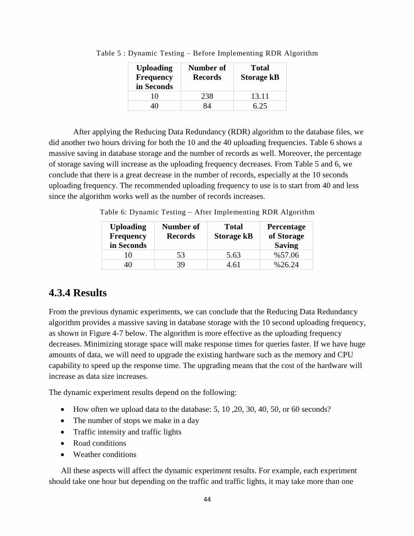
44
Table 5 : Dynamic Testing – Before Implementing RDR Algorithm
Uploading
Frequency
in Seconds
Number of
Records
Total
Storage kB
10 238 13.11
40 84 6.25
After applying the Reducing Data Redundancy (RDR) algorithm to the database files, we
did another two hours driving for both the 10 and the 40 uploading frequencies. Table 6 shows a
massive saving in database storage and the number of records as well. Moreover, the percentage
of storage saving will increase as the uploading frequency decreases. From Table 5 and 6, we
conclude that there is a great decrease in the number of records, especially at the 10 seconds
uploading frequency. The recommended uploading frequency to use is to start from 40 and less
since the algorithm works well as the number of records increases.
Table 6: Dynamic Testing – After Implementing RDR Algorithm
Uploading
Frequency
in Seconds
Number of
Records
Total
Storage kB
Percentage
of Storage
Saving
10 53 5.63 %57.06
40 39 4.61 %26.24
4.3.4 Results
From the previous dynamic experiments, we can conclude that the Reducing Data Redundancy
algorithm provides a massive saving in database storage with the 10 second uploading frequency,
as shown in Figure 4-7 below. The algorithm is more effective as the uploading frequency
decreases. Minimizing storage space will make response times for queries faster. If we have huge
amounts of data, we will need to upgrade the existing hardware such as the memory and CPU
capability to speed up the response time. The upgrading means that the cost of the hardware will
increase as data size increases.
The dynamic experiment results depend on the following:
• How often we upload data to the database: 5, 10 ,20, 30, 40, 50, or 60 seconds?
• The number of stops we make in a day
• Traffic intensity and traffic lights
• Road conditions
• Weather conditions
All these aspects will affect the dynamic experiment results. For example, each experiment
should take one hour but depending on the traffic and traffic lights, it may take more than one
45
hour. If the experiment takes less than one hour, we must wait at our final destination until the
one hour is reached. For that reason, a route that has less traffic and less traffic lights was
chosen. The experiment was performed multiple times due to road conditions such as accidents
or construction work, or weather conditions such as rain or snow. The results of the dynamic
experiment are closest to the results of real-time tracking.
Figure 4-7: Dynamic Testing Comparison
4.4 Experimental Results for NOSQL Database
To determine the size of the NOSQL database, we performed five hours of static testing in total
before implementing the RDR algorithm, one hour for each of the following frequencies: 10, 20,
30, 40, 50 seconds. As shown in Table 7, the size of the database increases as the uploading
frequency decreases. For each updating document, we have to consider the effect of the new data
on document growth. If the update operation causes the document to exceed the allocated space
on the disk, MongoDB relocates that document to a new location on the disk, which affects
system performance and leads to disk-fragmentation issues.
Mongodb has a feature called Capped Collection that allows collection sizes to be capped
at a certain size limit. The administrator of the tracking system can activate this feature by fixing
the acceptable size for a collection. Thus, when adding a new document to a collection will cause
that collection to exceed its pre-determined limits, the oldest document in the collection is
deleted so that the new document can be added. The capping feature works well for systems that
have a high rate of insertion, retrieval, and deletion. The problem with capped collections is that
old documents can be deleted at any time without the administrator’s notice. For example, if the
collection has a high rate of insertion, it may exceed its fixed size in a month, and if the
46
administrator of the system needs the documents for the last three months, some documents will
already have been deleted.
Table 7: NOSQL 5 hours static testing
Uploading
Frequency
in Seconds
Number of
Document
MongoDB
Total
Storage kB
MongoDB
10 279 66.96
20 133 31.92
30 109 26.16
40 79 18.96
50 61 14.64
4.4.1 Dynamic Testing
In real time experiment, we drove for 4 hours in total, two hours before implementing the
Reducing Data Redundancy Algorithm (RDR) and two hours after the implementation for each
of the uploading frequencies (10 and 40 seconds). We used the same route as shown in Figure 4-
6 above. The first route starts from Sobeys market and ends at RIM Park and the second route
starts from RIM Park and ends at Sobeys market. Each route was taken twice-- before and after
implementing the RDR algorithm.
For 10 seconds (1 hour):
We drove from Sobeys market to the University of Waterloo to Conestoga Mall and finally to
RIM Park. We stopped for 10 minutes at the University of Waterloo, 10 minutes at Conestoga
Mall, and five minutes at RIM Park. The total minutes for the 10 second uploading frequency
were 35 in driving mode and 25 in static mode. We used the route twice before and after
implementing the algorithm.
For 40 seconds (1 hour):
We drove from RIM Park to Conestoga Mall to the University of Waterloo and finally to Sobeys
market. We stopped for 10 minutes at University of Waterloo, 10 minutes at Conestoga Mall,
and five minutes at Sobeys market. The total minutes for the 40 seconds uploading frequency
were 35 in driving mode and 25 in static mode. We used the route twice-- before and after
implementing the algorithm.
Table 8 below shows the number of documents and total storage for each 10 and 40
seconds before implementing the RDR algorithm. The problem here is that the size of the
database will increase as the driving time and number of tracking devices increase and uploading
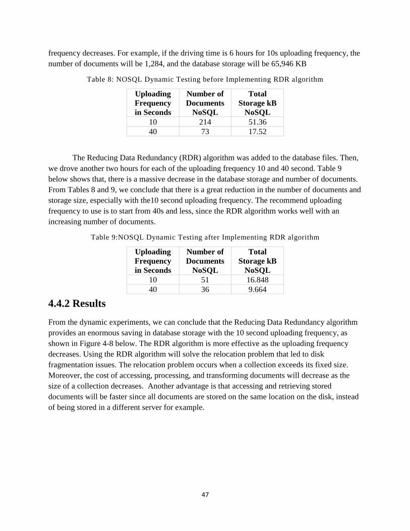
47
frequency decreases. For example, if the driving time is 6 hours for 10s uploading frequency, the
number of documents will be 1,284, and the database storage will be 65,946 KB
Table 8: NOSQL Dynamic Testing before Implementing RDR algorithm
Uploading
Frequency
in Seconds
Number of
Documents
NoSQL
Total
Storage kB
NoSQL
10 214 51.36
40 73 17.52
The Reducing Data Redundancy (RDR) algorithm was added to the database files. Then,
we drove another two hours for each of the uploading frequency 10 and 40 second. Table 9
below shows that, there is a massive decrease in the database storage and number of documents.
From Tables 8 and 9, we conclude that there is a great reduction in the number of documents and
storage size, especially with the10 second uploading frequency. The recommend uploading
frequency to use is to start from 40s and less, since the RDR algorithm works well with an
increasing number of documents.
Table 9:NOSQL Dynamic Testing after Implementing RDR algorithm
Uploading
Frequency
in Seconds
Number of
Documents
NoSQL
Total
Storage kB
NoSQL
10 51 16.848
40 36 9.664
4.4.2 Results
From the dynamic experiments, we can conclude that the Reducing Data Redundancy algorithm
provides an enormous saving in database storage with the 10 second uploading frequency, as
shown in Figure 4-8 below. The RDR algorithm is more effective as the uploading frequency
decreases. Using the RDR algorithm will solve the relocation problem that led to disk
fragmentation issues. The relocation problem occurs when a collection exceeds its fixed size.
Moreover, the cost of accessing, processing, and transforming documents will decrease as the
size of a collection decreases. Another advantage is that accessing and retrieving stored
documents will be faster since all documents are stored on the same location on the disk, instead
of being stored in a different server for example.
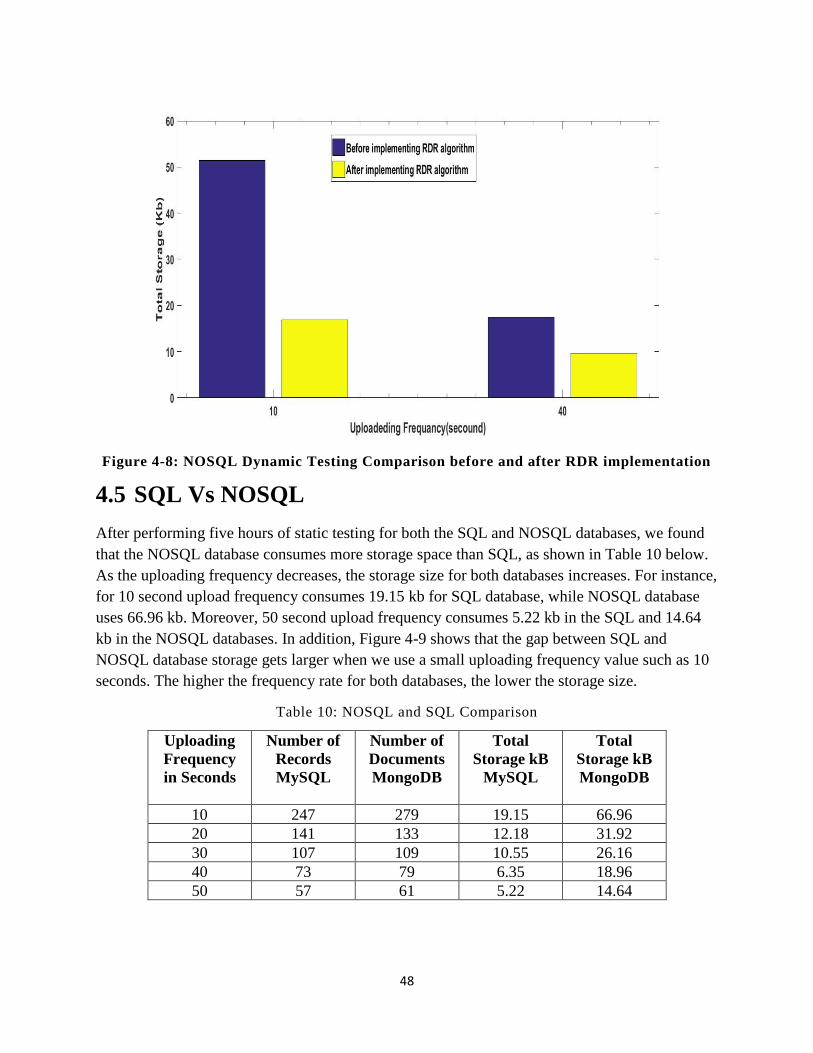
48
Figure 4-8: NOSQL Dynamic Testing Comparison before and after RDR implementation
4.5 SQL Vs NOSQL
After performing five hours of static testing for both the SQL and NOSQL databases, we found
that the NOSQL database consumes more storage space than SQL, as shown in Table 10 below.
As the uploading frequency decreases, the storage size for both databases increases. For instance,
for 10 second upload frequency consumes 19.15 kb for SQL database, while NOSQL database
uses 66.96 kb. Moreover, 50 second upload frequency consumes 5.22 kb in the SQL and 14.64
kb in the NOSQL databases. In addition, Figure 4-9 shows that the gap between SQL and
NOSQL database storage gets larger when we use a small uploading frequency value such as 10
seconds. The higher the frequency rate for both databases, the lower the storage size.
Table 10: NOSQL and SQL Comparison
Uploading
Frequency
in Seconds
Number of
Records
MySQL
Number of
Documents
MongoDB
Total
Storage kB
MySQL
Total
Storage kB
MongoDB
10 247 279 19.15 66.96
20 141 133 12.18 31.92
30 107 109 10.55 26.16
40 73 79 6.35 18.96
50 57 61 5.22 14.64
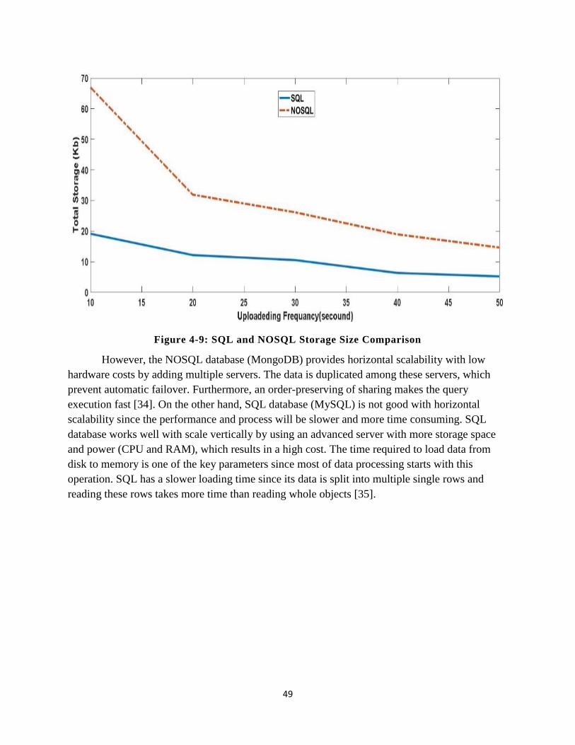
49
Figure 4-9: SQL and NOSQL Storage Size Comparison
However, the NOSQL database (MongoDB) provides horizontal scalability with low
hardware costs by adding multiple servers. The data is duplicated among these servers, which
prevent automatic failover. Furthermore, an order-preserving of sharing makes the query
execution fast [34]. On the other hand, SQL database (MySQL) is not good with horizontal
scalability since the performance and process will be slower and more time consuming. SQL
database works well with scale vertically by using an advanced server with more storage space
and power (CPU and RAM), which results in a high cost. The time required to load data from
disk to memory is one of the key parameters since most of data processing starts with this
operation. SQL has a slower loading time since its data is split into multiple single rows and
reading these rows takes more time than reading whole objects [35].
50
Chapter 5
5 Conclusion
In this thesis, we have developed a complete a vehicle tracking system that is flexible and
efficient. This system will give users the ability to track their vehicle with low cost for cloud
database storage. The SVS system provides accurate data in real time and eliminates data
redundancy in the cloud side for both SQL and NOSQL databases. In chapter 2, we provided a
literature survey of exiting tracking system model and storage solution for a massive database in
Internet of Things (IoT). We discussed various methodologies of storage efficiency
improvement. In addition, we compare our tracking system and modeling process with existing
works.
In chapter 3, we explained the system model of our Smart Vehicle System (SVS), its
components’ feature, and implementation details. The SVS system is build using Arduino board,
GPRS/GPS Quad-band module shield, temperature sensor, external GPS antenna, external
GPRS/GSM antenna, web application, and smartphone application. The system is designed to
track a vehicle’s location, speed, and temperature. Users can control their vehicle’s location and
temperature range through the web application where it is not allowed to pass. If their vehicle
passes these ranges, they will receive notification through the smartphone application. All data
collected from the system tracker such as location, speed, and temperature are uploaded and
stored into the cloud database. The database will have all the system information, admin login
identifications, users’ information, vehicles’ information, and all data received from the tracking
system.
Chapter 4 present two algorithms for data reduction that have been implemented and
validated. First algorithm is used to check each uploaded record before inserting it into the
database. If it has the same information as the previous stored record, then the time is updated for
the previous record. The second algorithm is developed to add lifetime to each record before
inserting it into the database. This lifetime will determine when the record should be discarded
from the database. The lifetime is controlled by the administrator of the database. We performed
an experiment to demonstrate the effectiveness of using these algorithms in reducing database
storage size for both SQL and NOSQL databases. Two type of experiments have been done
which are static and dynamic. For the static, we did five uploading frequency which are 10, 20,
30, 40, 50 second. Each one tested twice before and after algorithm implementation. The
dynamic experiment is done using two uploading frequencies 10 and 40 second. We drove for
51
one hour for each second twice. For example, two hours for 10 second and two hours for 40
second to test the algorithm before and after implementation. The result of the experiments
shows there is a massive decrease in database storage size. The percentage of storage saving
increase as the uploading frequency decrease.
Thus, we were able to develop a vehicle tracking system that provide users the ability to
track their vehicle’s location and temperature with lower cost for data storage. Users can
download the smartphone application for notification and use web application for controlling the
system such as setting location and temperature ranges for each vehicle and adding or deleting
vehicles and users. The system will provide users the exact location and temperature for each
tracking vehicle with increasing database storage. Minimizing database storage gives the user the
ability to add more vehicles and users to the system without any consideration about the data
growth. For example, users will not consider how many records are stored in database for each
tracking vehicle. In the future, this system may perhaps offer a variety of features for users such
as monitoring tires pressure, adding alarm motion detector, and much more.
52
References
[1] Bandyopadhyay, D., & Sen, J. (2011). Internet of things: Applications and challenges in
technology and standardization. Wireless Personal Communications, 58(1), 49-69.
[2] Piyare, R., & Lee, S. R. (2013). Towards internet of things (iots): Integration of wireless
sensor network to cloud services for data collection and sharing. arXiv preprint
arXiv:1310.2095.
[3] Tsiftes, N., & Dunkels, A. (2011, November). A database in every sensor. In Proceedings of
the 9th ACM Conference on Embedded Networked Sensor Systems (pp. 316-332). ACM.
[4] Guo, Q., & Liu, Y. (2011). A data storage method suitable for WSN. Journal of Shenyang
Ligonge University, 10, 15-19.
[5] Madden, S. R., Franklin, M. J., Hellerstein, J. M., & Hong, W. (2005). TinyDB: an
acquisitional query processing system for sensor networks. ACM Transactions on database
systems (TODS), 30(1), 122-173.
[6] Zhonglin, H., & Yuhua, H. (2011, August). Preliminary study on data management
technologies of internet of things. In Intelligence Science and Information Engineering (ISIE),
2011 International Conference on (pp. 137-140). IEEE.
[7] Lee, S., Tewolde, G., & Kwon, J. (2014, March). Design and implementation of vehicle
tracking system using GPS/GSM/GPRS technology and smartphone application. In Internet of
Things (WF-IoT), 2014 IEEE World Forum on (pp. 353-358). IEEE.
[8] Kamble, K. P. (2012). Smart Vehicle Tracking System. International Journal of Distributed
and Parallel Systems, 3(4), 91.
[9] Thaker, M. B., Nagaraj, U., & Ganjewar, P. D. (2014). Data Reduction Techniques in
Wireless Sensor Network: A Servey. International Journal of Innovative research in Computer
and Communication Engineering-2014, 2(11).
[10] Copie, A., Fortis, T. F., & Munteanu, V. I. (2013, June). Benchmarking cloud databases for
the requirements of the Internet of Things. In Information Technology Interfaces (ITI),
Proceedings of the ITI 2013 35th International Conference on (pp. 77-82). IEEE.
53
[11] Li, T., Liu, Y., Tian, Y., Shen, S., & Mao, W. (2012, November). A storage solution for
massive iot data based on nosql. In Green Computing and Communications (GreenCom), 2012
IEEE International Conference on (pp. 50-57). IEEE.
[12] Ding, Z., Yang, Q., & Wu, H. (2011, October). Massive heterogeneous sensor data
management in the Internet of Things. In Internet of Things (iThings/CPSCom), 2011
International Conference on and 4th International Conference on Cyber, Physical and Social
Computing (pp. 100-108). IEEE.
[13] Laatikainen, G., Mazhelis, O., & Tyrväinen, P. (2014). Role of acquisition intervals in
private and public cloud storage costs. Decision Support Systems, 57, 320-330.
[14] El-Medany, W., Al-Omary, A., Al-Hakim, R., Al-Irhayim, S., & Nusaif, M. (2010,
September). A cost effective real-time tracking system prototype using integrated GPS/GPRS
module. In Wireless and Mobile Communications (ICWMC), 2010 6th International Conference
on (pp. 521-525). IEEE.
[15] Hu, J. M., Li, J., & Li, G. H. (2012, November). Automobile anti-theft system based on
GSM and GPS module. In Intelligent Networks and Intelligent Systems (ICINIS), 2012 Fifth
International Conference on (pp. 199-201). IEEE.
[16] Fleischer, P. B., Nelson, A. Y., Sowah, R. A., & Bremang, A. (2012, October). Design and
development of GPS/GSM based vehicle tracking and alert system for commercial inter-city
buses. In Adaptive Science & Technology (ICAST), 2012 IEEE 4th International Conference
on (pp. 1-6). IEEE.
[17] El Shafee, A., El Menshawi, M., & Saeed, M. (2013). Integrating social network services
with vehicle tracking technologies. International Journal of Computer Applications, 72(11).
[18] Vigneshwaran, K., Sumithra, S., & Janani, R. (2015). An intelligent tracking system based
on GSM and GPS using smartphones. International Journal of Advanced Research in Electrical,
Electronics and Instrumentation Engineering, 4(5), 3487-903.
[19] Zhang, Q., Chen, Z., Lv, A., Zhao, L., Liu, F., & Zou, J. (2013, August). A universal storage
architecture for big data in cloud environment. In Green Computing and Communications
(GreenCom), 2013 IEEE and Internet of Things (iThings/CPSCom), IEEE International
Conference on and IEEE Cyber, Physical and Social Computing (pp. 476-480). IEEE.
[20] Chen, W. C., Chen, Y. H., Wu, C. L., & Fu, L. C. (2014, September). An Efficient Data
Storage Method of NoSQL Database for HEM Mobile Applications in IoT. In Internet of Things
(iThings), 2014 IEEE International Conference on, and Green Computing and Communications
54
(GreenCom), IEEE and Cyber, Physical and Social Computing (CPSCom), IEEE (pp. 336-339).
IEEE.
[21] D-c-Arduino uno. (n.d.). Retrieved September 9, 2016, from
http://digital.csic.es/bitstream/10261/127788/7/D-c-%20Arduino%20uno.pdf
[22] Banzi, M., & Shiloh, M. (2015). Getting started with Arduino. Sebastopol, CA:
MakerMedia.
[23] Monk, S. (2012). Programming Arduino: getting started with sketches. New York:
McGraw-Hill.
[24] 8-bit Microcontroller with 4/8/16/32K Bytes In-System Programmable Flash. (2010).
Retrieved October 22, 2015, from http://elecfreaks.com/store/download/mega328.pdf
[25] Arduino - ArduinoBoardUno. (n.d.). Retrieved October 22, 2015, from
https://www.arduino.cc/en/main/arduinoBoardUno
[26] SIM908 GSM/GPRS/GPS Module. (2014, March 22). Retrieved November 10, 2015, from
https://elty.pl/pl/p/file/.../DS_IM140402002.pdf
[27] Resistor Kit - 1/4W (500 total). (n.d.). Retrieved October 27, 2015, from
https://learn.sparkfun.com/tutorials/resistors
[28] Programmable Resolution 1-Wire Digital Thermometer . (2015). Retrieved February 15,
2016, from https://datasheets.maximintegrated.com/en/ds/DS18B20.pdf
[29] Salim, K. A., & Idrees, I. M. (2013). Design and Implementation of Web-Based GPS-GPRS
Vehicle Tracking System. International Journal of Science, Engineering and Computer
Technology, 3(12), 443.
[30] Van der Veen, J. S., Van der Waaij, B., & Meijer, R. J. (2012, June). Sensor data storage
performance: SQL or NoSQL, physical or virtual. In Cloud Computing (CLOUD), 2012 IEEE
5th International Conference on (pp. 431-438). IEEE.
[31] Kang, Y. S., Park, I. H., Rhee, J., & Lee, Y. H. (2016). MongoDB-based repository design
for IoT-generated RFID/sensor big data. IEEE Sensors Journal, 16(2), 485-497.
[32] Dayley, B. (2015). Sams Teach Yourself NoSQL with MongoDB in 24 hours. Portland, OR:
Sams.
[33] Han, J., Pei, J., & Kamber, M. (2011). Data mining: concepts and techniques. Elsevier
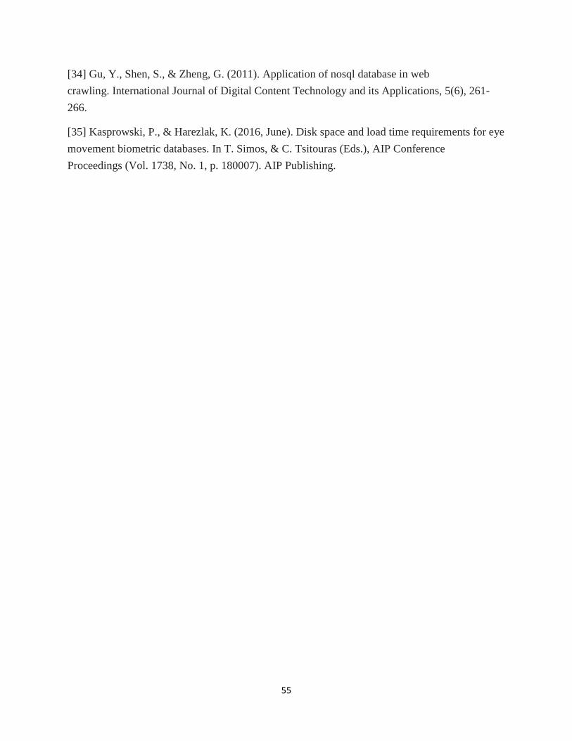
55
[34] Gu, Y., Shen, S., & Zheng, G. (2011). Application of nosql database in web
crawling. International Journal of Digital Content Technology and its Applications, 5(6), 261-
266.
[35] Kasprowski, P., & Harezlak, K. (2016, June). Disk space and load time requirements for eye
movement biometric databases. In T. Simos, & C. Tsitouras (Eds.), AIP Conference
Proceedings (Vol. 1738, No. 1, p. 180007). AIP Publishing.

56
APPENDEICE

57
All Figures of The Mongodb Collection for The
Following Uploading Frequencies 10, 20, 30, 40, 50
Seconds (Static Testing) Used in Chapter 4
Figure 1: 10 second
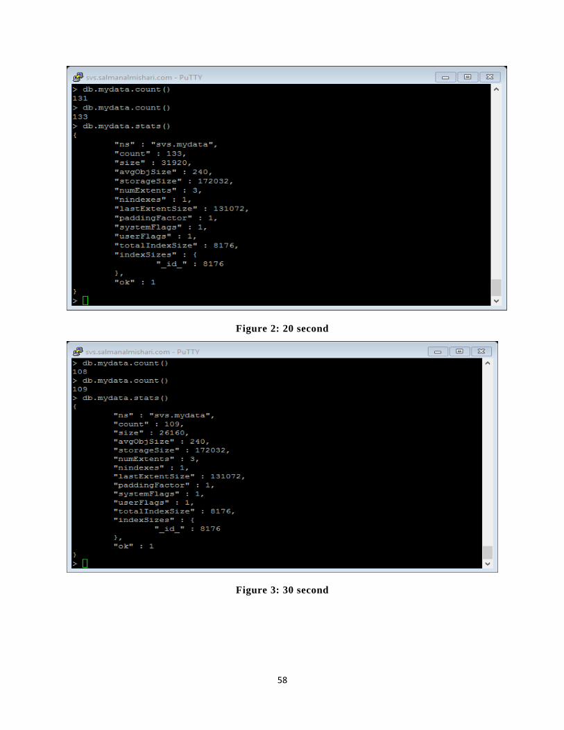
58
Figure 2: 20 second
Figure 3: 30 second
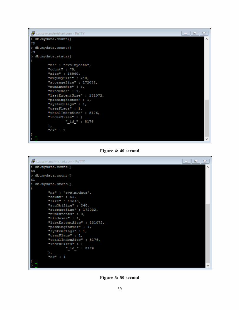
59
Figure 4: 40 second
Figure 5: 50 second
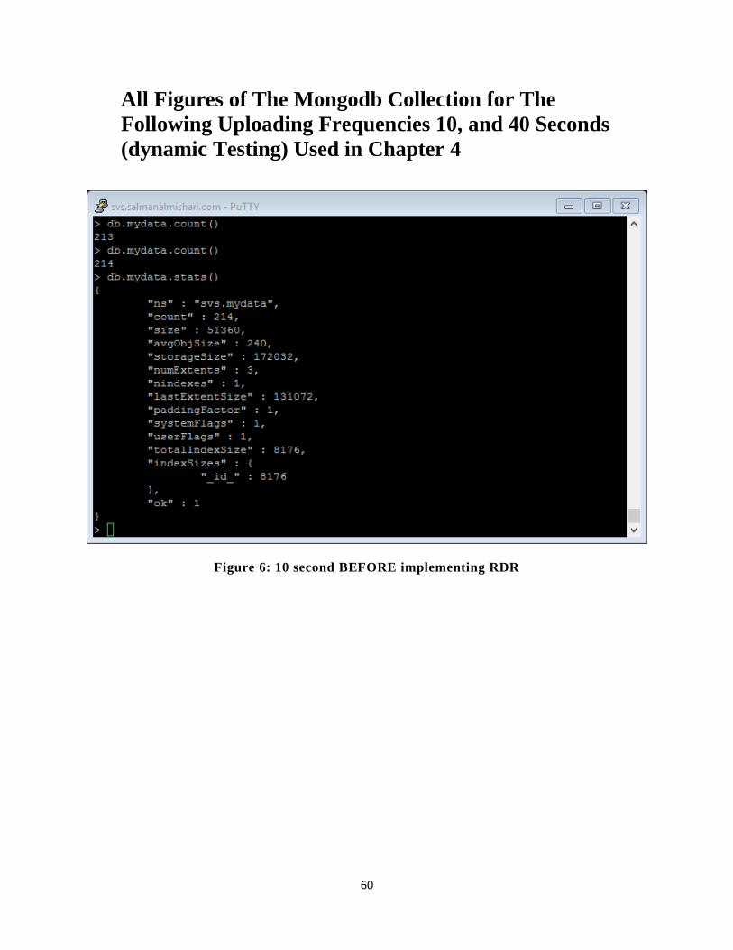
60
All Figures of The Mongodb Collection for The
Following Uploading Frequencies 10, and 40 Seconds
(dynamic Testing) Used in Chapter 4
Figure 6: 10 second BEFORE implementing RDR
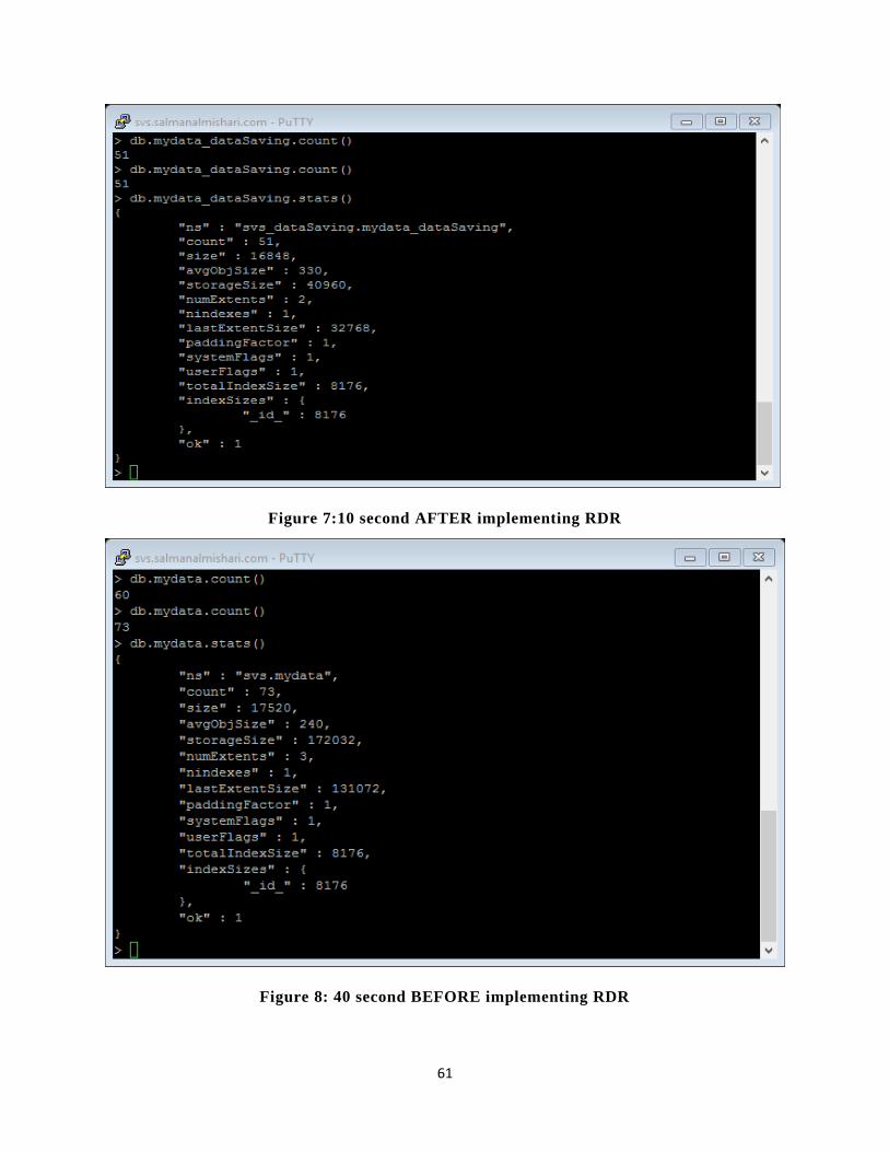
61
Figure 7:10 second AFTER implementing RDR
Figure 8: 40 second BEFORE implementing RDR
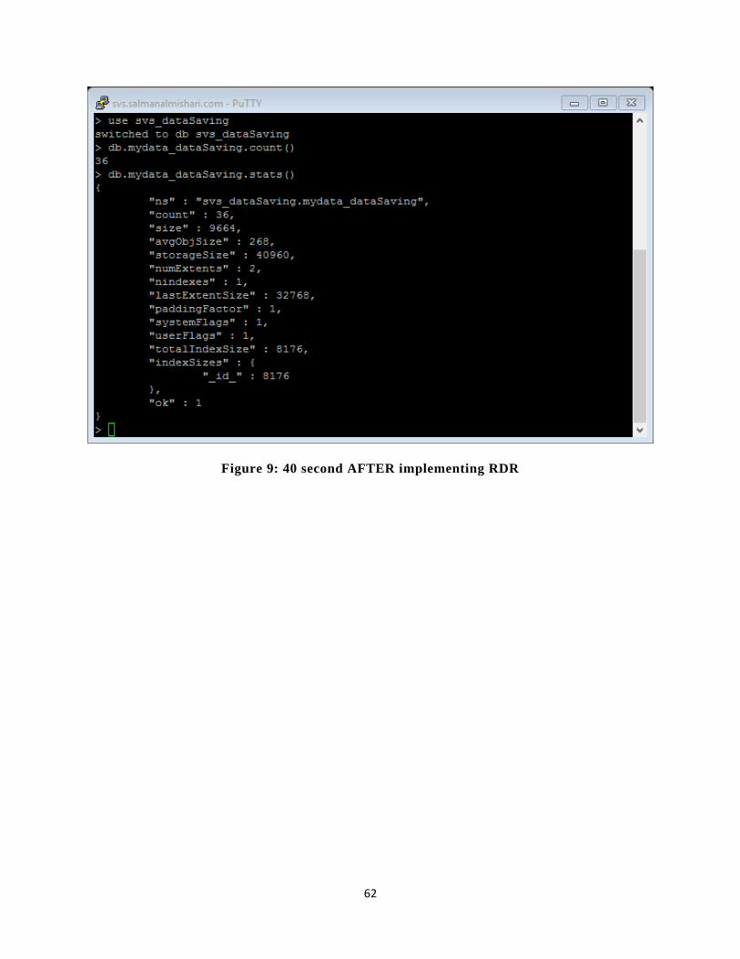
62
Figure 9: 40 second AFTER implementing RDR


