
ISSN 1937 - 1055
VOLUME 1, 2015
INTERNATIONAL JOURNAL OF
MATHEMATICAL COMBINATORICS
EDITED BY
THE MADIS OF CHINESE ACADEMY OF SCIENCES AND
ACADEMY OF MATHEMATICAL COMBINATORICS & APPLICATIONS
March, 2015

Vol.1, 2015 ISSN 1937-1055
International Journal of
Mathematical Combinatorics
Edited By
The Madis of Chinese Academy of Sciences and
Academy of Mathematical Combinatorics & Applications
March, 2015

Aims and Scope: The International J.Mathematical Combinatorics (ISSN 1937-1055)
is a fully refereed international journal, sponsored by the MADIS of Chinese Academy of Sci-
ences and published in USA quarterly comprising 100-150 pages approx. per volume, which
publishes original research papers and survey articles in all aspects of Smarandache multi-spaces,
Smarandache geometries, mathematical combinatorics, non-euclidean geometry and topology
and their applications to other sciences. Topics in detail to be covered are:
Smarandache multi-spaces with applications to other sciences, such as those of algebraic
multi-systems, multi-metric spaces,· · · , etc.. Smarandache geometries;
Topological graphs; Algebraic graphs; Random graphs; Combinatorial maps; Graph and
map enumeration; Combinatorial designs; Combinatorial enumeration;
Differential Geometry; Geometry on manifolds; Low Dimensional Topology; Differential
Topology; Topology of Manifolds; Geometrical aspects of Mathematical Physics and Relations
with Manifold Topology;
Applications of Smarandache multi-spaces to theoretical physics; Applications of Combi-
natorics to mathematics and theoretical physics; Mathematical theory on gravitational fields;
Mathematical theory on parallel universes; Other applications of Smarandache multi-space and
combinatorics.
Generally, papers on mathematics with its applications not including in above topics are
also welcome.
It is also available from the below international databases:
Serials Group/Editorial Department of EBSCO Publishing
10 Estes St. Ipswich, MA 01938-2106, USA
Tel.: (978) 356-6500, Ext. 2262 Fax: (978) 356-9371
http://www.ebsco.com/home/printsubs/priceproj.asp
and
Gale Directory of Publications and Broadcast Media, Gale, a part of Cengage Learning
27500 Drake Rd. Farmington Hills, MI 48331-3535, USA
Tel.: (248) 699-4253, ext. 1326; 1-800-347-GALE Fax: (248) 699-8075
http://www.gale.com
Indexing and Reviews: Mathematical Reviews (USA), Zentralblatt Math (Germany), Refer-
ativnyi Zhurnal (Russia), Mathematika (Russia), Directory of Open Access (DoAJ), Interna-
tional Statistical Institute (ISI), International Scientific Indexing (ISI, impact factor 1.416),
Institute for Scientific Information (PA, USA), Library of Congress Subject Headings (USA).
Subscription A subscription can be ordered by an email directly to
Linfan Mao
The Editor-in-Chief of International Journal of Mathematical Combinatorics
Chinese Academy of Mathematics and System Science
Beijing, 100190, P.R.China
Email: [email protected]
Price: US$48.00

Editorial Board (3nd)
Editor-in-Chief
Linfan MAO
Chinese Academy of Mathematics and System
Science, P.R.China
and
Academy of Mathematical Combinatorics &
Applications, USA
Email: [email protected]
Deputy Editor-in-Chief
Guohua Song
Beijing University of Civil Engineering and
Architecture, P.R.China
Email: [email protected]
Editors
S.Bhattacharya
Deakin University
Geelong Campus at Waurn Ponds
Australia
Email: [email protected]
Said Broumi
Hassan II University Mohammedia
Hay El Baraka Ben M’sik Casablanca
B.P.7951 Morocco
Junliang Cai
Beijing Normal University, P.R.China
Email: [email protected]
Yanxun Chang
Beijing Jiaotong University, P.R.China
Email: [email protected]
Jingan Cui
Beijing University of Civil Engineering and
Architecture, P.R.China
Email: [email protected]
Shaofei Du
Capital Normal University, P.R.China
Email: [email protected]
Baizhou He
Beijing University of Civil Engineering and
Architecture, P.R.China
Email: [email protected]
Xiaodong Hu
Chinese Academy of Mathematics and System
Science, P.R.China
Email: [email protected]
Yuanqiu Huang
Hunan Normal University, P.R.China
Email: [email protected]
H.Iseri
Mansfield University, USA
Email: [email protected]
Xueliang Li
Nankai University, P.R.China
Email: [email protected]
Guodong Liu
Huizhou University
Email: [email protected]
W.B.Vasantha Kandasamy
Indian Institute of Technology, India
Email: [email protected]
Ion Patrascu
Fratii Buzesti National College
Craiova Romania
Han Ren
East China Normal University, P.R.China
Email: [email protected]
Ovidiu-Ilie Sandru
Politechnica University of Bucharest
Romania

ii International Journal of Mathematical Combinatorics
Mingyao Xu
Peking University, P.R.China
Email: [email protected]
Guiying Yan
Chinese Academy of Mathematics and System
Science, P.R.China
Email: [email protected]
Y. Zhang
Department of Computer Science
Georgia State University, Atlanta, USA
Famous Words:
Nothing in life is to be feared. It is only to be understood.
By Marie Curie, a Polish and naturalized-French physicist and chemist.
International J.Math. Combin. Vol.1(2015), 1-13
N∗C∗− Smarandache Curves of Mannheim Curve Couple
According to Frenet Frame
Suleyman SENYURT and Abdussamet CALISKAN
(Faculty of Arts and Sciences, Department of Mathematics, Ordu University, 52100, Ordu/Turkey)
E-mail: [email protected]
Abstract: In this paper, when the unit Darboux vector of the partner curve of Mannheim
curve are taken as the position vectors, the curvature and the torsion of Smarandache curve
are calculated. These values are expressed depending upon the Mannheim curve. Besides,
we illustrate example of our main results.
Key Words: Mannheim curve, Mannheim partner curve, Smarandache Curves, Frenet
invariants.
AMS(2010): 53A04
§1. Introduction
A regular curve in Minkowski space-time, whose position vector is composed by Frenet frame
vectors on another regular curve, is called a Smarandache curve ([12]). Special Smarandache
curves have been studied by some authors .
Melih Turgut and Suha Yılmaz studied a special case of such curves and called it Smaran-
dache TB2 curves in the space E41 ([12]). Ahmad T.Ali studied some special Smarandache curves
in the Euclidean space. He studied Frenet-Serret invariants of a special case ([1]). Muhammed
Cetin , Yılmaz Tuncer and Kemal Karacan investigated special Smarandache curves according
to Bishop frame in Euclidean 3-Space and they gave some differential goematric properties of
Smarandache curves, also they found the centers of the osculating spheres and curvature spheres
of Smarandache curves ([5]). Senyurt and Calıskan investigated special Smarandache curves in
terms of Sabban frame of spherical indicatrix curves and they gave some characterization of
Smarandache curves ([4]). Ozcan Bektas and Salim Yuce studied some special Smarandache
curves according to Darboux Frame in E3 ([2]). Nurten Bayrak, Ozcan Bektas and Salim Yuce
studied some special Smarandache curves in E31 [3]. Kemal Tas.kopru, Murat Tosun studied
special Smarandache curves according to Sabban frame on S2 ([11]).
In this paper, special Smarandache curve belonging to α∗ Mannheim partner curve such
as N∗C∗ drawn by Frenet frame are defined and some related results are given.
1Received September 8, 2014, Accepted February 12, 2015.

2 Suleyman SENYURT and Abdussamet CALISKAN
§2. Preliminaries
The Euclidean 3-space E3 be inner product given by
〈, 〉 = x21 + x3
2 + x23
where (x1, x2, x3) ∈ E3. Let α : I → E3 be a unit speed curve denote by T, N, B the
moving Frenet frame . For an arbitrary curve α ∈ E3, with first and second curvature, κ and
τ respectively, the Frenet formulae is given by ([6], [9])
T ′ = κN
N ′ = −κT + τB
B′ = −τN.
(2.1)
For any unit speed α : I → E3, the vector W is called Darboux vector defined by
W = τ(s)T (s) + κ(s) + B(s).
If consider the normalization of the Darboux C =1
‖W‖W , we have
cosϕ =κ(s)
‖W‖ , sin ϕ =τ(s)
‖W‖ ,
C = sin ϕT (s) + cosϕB(s) (2.2)
where ∠(W, B) = ϕ. Let α : I → E3 and α∗ : I → E3 be the C2− class differentiable unit
speed two curves and let T (s), N(s), B(s) and T ∗(s), N∗(s), B∗(s) be the Frenet frames of
the curves α and α∗, respectively. If the principal normal vector N of the curve α is linearly
dependent on the binormal vector B of the curve α∗, then (α) is called a Mannheim curve and
(α∗) a Mannheim partner curve of (α). The pair (α, α∗) is said to be Mannheim pair ([7], [8]).
The relations between the Frenet frames T (s), N(s), B(s) and T ∗(s), N∗(s), B∗(s) are as
follows:
T ∗ = cos θT − sin θB
N∗ = sin θT + cos θB
B∗ = N
(2.3)
cos θ =ds∗ds
sin θ = λτ∗ ds∗ds
.(2.4)
where ∠(T, T ∗) = θ ([8]).
Theorem 2.1([7]) The distance between corresponding points of the Mannheim partner curves
in E3 is constant.

N∗C∗− Smarandache Curves of Mannheim Curve Couple According to Frenet Frame 3
Theorem 2.2 Let (α, α∗) be a Mannheim pair curves in E3. For the curvatures and the torsions
of the Mannheim curve pair (α, α∗) we have,
κ = τ∗ sin θds∗ds
τ = −τ∗ cos θds∗ds
(2.5)
and
κ∗ =dθ
ds∗ = θ′κ
λτ√
κ2 + τ2
τ∗ = (κ sin θ − τ cos θ)ds∗ds
(2.6)
Theorem 2.3 Let (α, α∗) be a Mannheim pair curves in E3. For the torsions τ∗ of the
Mannheim partner curve α∗ we have
τ∗ =κ
λτ
Theorem 2.4([10]) Let (α, α∗) be a Mannheim pair curves in E3. For the vector C∗ is the
direction of the Mannheim partner curve α∗ we have
C∗ =1√
1 +( θ′
‖W‖)2
C +
θ′
‖W‖√1 +
( θ′
‖W‖)2
N (2.7)
where the vector C is the direction of the Darboux vector W of the Mannheim curve α.
§3. N∗C∗− Smarandache Curves of Mannheim Curve Couple According to
Frenet Frame
Let (α, α∗) be a Mannheim pair curves in E3 and T ∗N∗B∗ be the Frenet frame of the
Mannheim partner curve α∗ at α∗(s). In this case, N∗C∗ - Smarandache curve can be defined
by
β1(s) =1√2(N∗ + C∗). (3.1)
Solving the above equation by substitution of N∗ and C∗ from (2.3) and (2.7), we obtain
β1(s) =
(cos θ‖W‖ + sin θ
√θ′2 + ‖W‖2
)T + θ′N +
(cos θ
√θ′2 + ‖W‖2 − sin θ‖W‖
)B
√θ′2 + ‖W‖2
.
(3.2)

4 Suleyman SENYURT and Abdussamet CALISKAN
The derivative of this equation with respect to s is as follows,
Tβ1(s) =
[(‖W‖√
θ′2+‖W‖2
)′cos θ − θ′κ cos θ
λτ‖W‖
]T +
[κλτ −
(‖W‖√
θ′2+‖W‖2
)′ ‖W‖θ′
]N
√√√√√√√
[(‖W‖√
θ′2+‖W‖2
)′√θ′2+‖W‖2
θ′
]2+ κ(θ′2+‖W‖2)
λτ‖W‖
[κ
λτ‖W‖ − 2(
‖W‖√θ′2+‖W‖2
)′1θ′
]
+
[θ′κ sin θλτ‖W‖ −
(‖W‖√
θ′2+‖W‖2
)′sin θ
]B
√√√√[(
‖W‖√θ′2+‖W‖2
)′√θ′2+‖W‖2
θ′
]2+ κ(θ′2+‖W‖2)
λτ‖W‖
[κ
λτ‖W‖ − 2(
‖W‖√θ′2+‖W‖2
)′1θ′
](3.3)
·
In order to determine the first curvature and the principal normal of the curve β1(s), we
formalize
T ′β1
(s) =
√2[(r1 cos θ + r2 sin θ)T + r3N + (−r1 sin θ + r2 cos θ)B
]
([(‖W‖√
θ′2+‖W‖2
)′√θ′2+‖W‖2
θ′
]2+ κ(θ′2+‖W‖2)
λτ‖W‖
[κ
λτ‖W‖ − 2(
‖W‖√θ′2+‖W‖2
)′1θ′
])2
where
r1 = 2( κ
λτ
)2([( ‖W‖√
θ′2 + ‖W‖2
)′√
θ′2 + ‖W‖2
θ′
]′)( θ′√θ′2 + ‖W‖2
)
−( θ′κ
λτ‖W‖)[( ‖W‖√
θ′2 + ‖W‖2
)′√
θ′2 + ‖W‖2
θ′
][( ‖W‖√θ′2 + ‖W‖2
)′√
θ′2 + ‖W‖2
θ′
]′
( θ′√θ′2 + ‖W‖2
)2
−( κ
λτ
)[( ‖W‖√θ′2 + ‖W‖2
)′√
θ′2 + ‖W‖2
θ′
]([( ‖W‖√θ′2 + ‖W‖2
)′
√θ′2 + ‖W‖2
θ′
]′)( ‖W‖√θ′2 + ‖W‖2
)( θ′√θ′2 + ‖W‖2
)−[( ‖W‖√
θ′2 + ‖W‖2
)′
√θ′2 + ‖W‖2
θ′
]4( ‖W‖√θ′2 + ‖W‖2
)−( κ
λτ
)2( θ′κ
λτ‖W‖)′
−( κ
λτ
)2[( ‖W‖√
θ′2 + ‖W‖2
)′

N∗C∗− Smarandache Curves of Mannheim Curve Couple According to Frenet Frame 5
×
√θ′2 + ‖W‖2
θ′
]2( ‖W‖√θ′2 + ‖W‖2
)+ 2( θ′κ
λτ‖W‖)[( ‖W‖√
θ′2 + ‖W‖2
)′√
θ′2 + ‖W‖2
θ′
]3
( ‖W‖√θ′2 + ‖W‖2
)( θ′√θ′2 + ‖W‖2
)+ 2( κ
λτ
)[( ‖W‖√θ′2 + ‖W‖2
)′√
θ′2 + ‖W‖2
θ′
]3
( ‖W‖√θ′2 + ‖W‖2
)2
−( θ′κ
λτ‖W‖)2[( ‖W‖√
θ′2 + ‖W‖2
)′√
θ′2 + ‖W‖2
θ′
]2( ‖W‖√θ′2 + ‖W‖2
)
−2κ∗( θ′κ
λτ‖W‖)′[( ‖W‖√
θ′2 + ‖W‖2
)′√
θ′2 + ‖W‖2
θ′
]( θ′√θ′2 + ‖W‖2
)− 2( θ′κ
λτ‖W‖)′
( κ
λτ
)[( ‖W‖√θ′2 + ‖W‖2
)′√
θ′2 + ‖W‖2
θ′
]( ‖W‖√θ′2 + ‖W‖2
)− τ∗
( κ
λτ
)′
[( ‖W‖√θ′2 + ‖W‖2
)′√
θ′2 + ‖W‖2
θ′
]( θ′√θ′2 + ‖W‖2
)+( θ′κ
λτ‖W‖)′[( ‖W‖√
θ′2 + ‖W‖2
)′
√θ′2 + ‖W‖2
θ′
]( θ′√θ′2 + ‖W‖2
)2
−( θ′κ
λτ‖W‖)′[( ‖W‖√
θ′2 + ‖W‖2
)′√
θ′2 + ‖W‖2
θ′
]2
+( κ
λτ
)′[( ‖W‖√θ′2 + ‖W‖2
)′√
θ′2 + ‖W‖2
θ′
]2( ‖W‖√θ′2 + ‖W‖2
)( θ′√θ′2 + ‖W‖2
)
( θ′κ
λτ‖W‖)[( ‖W‖√
θ′2 + ‖W‖2
)′√
θ′2 + ‖W‖2
θ′
]([( ‖W‖√θ′2 + ‖W‖2
)′√
θ′2 + ‖W‖2
θ′
]′)
+( θ′κ
λτ‖W‖)( κ
λτ
)( κ
λτ
)′−( θ′κ
λτ‖W‖)( κ
λτ
)([( ‖W‖√θ′2 + ‖W‖2
)′√
θ′2 + ‖W‖2
θ′
]′)
( ‖W‖√θ′2 + ‖W‖2
)−[( ‖W‖√
θ′2 + ‖W‖2
)′√
θ′2 + ‖W‖2
θ′
]( κ
λτ
)′( θ′κ
λτ‖W‖)( ‖W‖√
θ′2 + ‖W‖2
),
r2 =( θ′κ
λτ‖W‖)[( ‖W‖√
θ′2 + ‖W‖2
)′√
θ′2 + ‖W‖2
θ′
]3( θ′√θ′2 + ‖W‖2
)+ 3( θ′κ
λτ‖W‖)3
[( ‖W‖√θ′2 + ‖W‖2
)′√
θ′2 + ‖W‖2
θ′
]( θ′√θ′2 + ‖W‖2
)+ 3( κ
λτ
)2( θ′κ
λτ‖W‖)

6 Suleyman SENYURT and Abdussamet CALISKAN
[( ‖W‖√θ′2 + ‖W‖2
)′√
θ′2 + ‖W‖2
θ′
]( θ′√θ′2 + ‖W‖2
)− 2( θ′κ
λτ‖W‖)2
[( ‖W‖√θ′2 + ‖W‖2
)′√
θ′2 + ‖W‖2
θ′
]2( θ′√θ′2 + ‖W‖2
)2
−( θ′κ
λτ‖W‖)2
[( ‖W‖√θ′2 + ‖W‖2
)′√
θ′2 + ‖W‖2
θ′
]2−( κ
λτ
)2[( ‖W‖√
θ′2 + ‖W‖2
)′√
θ′2 + ‖W‖2
θ′
]2
+3( κ
λτ
)3[( ‖W‖√
θ′2 + ‖W‖2
)′√
θ′2 + ‖W‖2
θ′
]( ‖W‖√θ′2 + ‖W‖2
)+( κ
λτ
)
[( ‖W‖√θ′2 + ‖W‖2
)′√
θ′2 + ‖W‖2
θ′
]3( ‖W‖√θ′2 + ‖W‖2
)− 2( κ
λτ
)2[( ‖W‖√
θ′2 + ‖W‖2
)′
√θ′2 + ‖W‖2
θ′
]2( ‖W‖√θ′2 + ‖W‖2
)2
− 4( θ′κ
λτ‖W‖)( κ
λτ
)[( ‖W‖√θ′2 + ‖W‖2
)′
√θ′2 + ‖W‖2
θ′
]2( ‖W‖√θ′2 + ‖W‖2
)( θ′√θ′2 + ‖W‖2
)−( θ′κ
λτ‖W‖)4
− 2( θ′κ
λτ‖W‖)2
( κ
λτ
)2+ 3( θ′κ
λτ‖W‖)2( κ
λτ
)[( ‖W‖√θ′2 + ‖W‖2
)′√
θ′2 + ‖W‖2
θ′
]( ‖W‖√θ′2 + ‖W‖2
)
r3 = 2( κ
λτ
)′[( ‖W‖√
θ′2 + ‖W‖2
)′√
θ′2 + ‖W‖2
θ′
]2+( θ′κ
λτ‖W‖)2( κ
λτ
)′ − 2( θ′κ
λτ‖W‖)
( κ
λτ
)′[( ‖W‖√
θ′2 + ‖W‖2
)′√
θ′2 + ‖W‖2
θ′
]( θ′√θ′2 + ‖W‖2
)−( θ′κ
λτ‖W‖)2
[( ‖W‖√θ′2 + ‖W‖2
)′√
θ′2 + ‖W‖2
θ′
]′( ‖W‖√θ′2 + ‖W‖2
)+( θ′κ
λτ‖W‖)[( ‖W‖√
θ′2 + ‖W‖2
)′
√θ′2 + ‖W‖2
θ′
][( ‖W‖√θ′2 + ‖W‖2
)′√
θ′2 + ‖W‖2
θ′
]′( ‖W‖√θ′2 + ‖W‖2
)( θ′√θ′2 + ‖W‖2
)
+( κ
λτ
)[( ‖W‖√θ′2 + ‖W‖2
)′√
θ′2 + ‖W‖2
θ′
][( ‖W‖√θ′2 + ‖W‖2
)′√
θ′2 + ‖W‖2
θ′
]′

N∗C∗− Smarandache Curves of Mannheim Curve Couple According to Frenet Frame 7
×( ‖W‖√
θ′2 + ‖W‖2
)2
−[( ‖W‖√
θ′2 + ‖W‖2
)′√
θ′2 + ‖W‖2
θ′
]4( θ′√θ′2 + ‖W‖2
)
−( θ′κ
λτ‖W‖)2[( ‖W‖√
θ′2 + ‖W‖2
)′√
θ′2 + ‖W‖2
θ′
]2( θ′√θ′2 + ‖W‖2
)−( κ
λτ
)′
[( ‖W‖√θ′2 + ‖W‖2
)′√
θ′2 + ‖W‖2
θ′
]2( ‖W‖√θ′2 + ‖W‖2
)2
−( κ
λτ
)2[( ‖W‖√
θ′2 + ‖W‖2
)′
√θ′2 + ‖W‖2
θ′
]2( θ′√θ′2 + ‖W‖2
)+ 2( θ′κ
λτ‖W‖)[( ‖W‖√
θ′2 + ‖W‖2
)′√
θ′2 + ‖W‖2
θ′
]3
( θ′√θ′2 + ‖W‖2
)2
+ 2( κ
λτ
)[( ‖W‖√θ′2 + ‖W‖2
)′√
θ′2 + ‖W‖2
θ′
]3( ‖W‖√θ′2 + ‖W‖2
)
( θ′√θ′2 + ‖W‖2
)−( κ
λτ
)[( ‖W‖√θ′2 + ‖W‖2
)′√
θ′2 + ‖W‖2
θ′
][( ‖W‖√θ′2 + ‖W‖2
)′
√θ′2 + ‖W‖2
θ′
]′−( κ
λτ
)( θ′κ
λτ‖W‖)( θ′κ
λτ‖W‖)′
+( κ
λτ
)( θ′κ
λτ‖W‖)[( ‖W‖√
θ′2 + ‖W‖2
)′
√θ′2 + ‖W‖2
θ′
]′( θ′√θ′2 + ‖W‖2
)+( θ′κ
λτ‖W‖)′( κ
λτ
)[( ‖W‖√θ′2 + ‖W‖2
)′
√θ′2 + ‖W‖2
θ′
]( θ′√θ′2 + ‖W‖2
)+( θ′κ
λτ‖W‖)( θ′κ
λτ‖W‖)′[( ‖W‖√
θ′2 + ‖W‖2
)′
√θ′2 + ‖W‖2
θ′
]( ‖W‖√θ′2 + ‖W‖2
)−( θ′κ
λτ‖W‖)′[( ‖W‖√
θ′2 + ‖W‖2
)′√
θ′2 + ‖W‖2
θ′
]2
( ‖W‖√θ′2 + ‖W‖2
)( θ′√θ′2 + ‖W‖2
)·
The first curvature is
κβ1=
√2(√
r12 + r2
2 + r32)
([(‖W‖√
θ′2+‖W‖2
)′√θ′2+‖W‖2
θ′
]2+ κ(θ′2+‖W‖2)
λτ‖W‖
[κ
λτ‖W‖ − 2(
‖W‖√θ′2+‖W‖2
)′1θ′
])2 ·

8 Suleyman SENYURT and Abdussamet CALISKAN
The principal normal vector field and the binormal vector field are respectively given by
Nβ1=
(r1 cos θ + r2 sin θ)T + r3N + (−r1 sin θ + r2 cos θ)B√r1
2 + r22 + r3
2, (3.4)
Bβ1(s) =
ξ1
ξ4T +
ξ2
ξ4N +
ξ3
ξ4B, (3.5)
where
ξ1 = r2 cos θ(
‖W‖√θ′2+‖W‖2
)′ ‖W‖θ′
− r2 cos θ κλτ −
[r1
κλτ − r1
(‖W‖√
θ′2+‖W‖2
)′ ‖W‖θ′
−r3
(‖W‖√
θ′2+‖W‖2
)′+ r3
(θ′κ
λτ‖W‖
)]sin θ
ξ2 = r1
[(‖W‖√
θ′2+‖W‖2
)′− θ′κ
λτ‖W‖
]
ξ3 = r2 sin θ
[(‖W‖√
θ′2+‖W‖2
)′ ‖W‖θ′
− κλτ
]+
[r1
κλτ − r1
(‖W‖√
θ′2+‖W‖2
)′ ‖W‖θ′
−r3
(‖W‖√
θ′2+‖W‖2
)′+ r3
θ′κλτ‖W‖
]cos θ
ξ4 =
√√√√√√√√√
((r1
2 + r22 + r3
2)
[(‖W‖√
θ′2+‖W‖2
)′√θ′2+‖W‖2
θ′
]2+ (r1
2 + r22 + r3
2)κ(θ′2+‖W‖2)λτ‖W‖
[κ
λτ‖W‖ − 2(
‖W‖√θ′2+‖W‖2
)′1θ′
]).
In order to calculate the torsion of the curve β1, we differentiate
β′′1 =
1√2
([cos θ
([( ‖W‖√θ′2 + ‖W‖2
)′√
θ′2 + ‖W‖2
θ′
]′ θ′√θ′2 + ‖W‖2
−[( ‖W‖√
θ′2 + ‖W‖2
)′√
θ′2 + ‖W‖2
θ′
]2 ‖W‖√θ′2 + ‖W‖2
−( θ′κ
λτ‖W‖)′)
+
+ sin θ
(( θ′κ
λτ‖W‖)[( ‖W‖√
θ′2 + ‖W‖2
)′√
θ′2 + ‖W‖2
θ′
]θ′√
θ′2 + ‖W‖2
+( κ
λτ
)
[( ‖W‖√θ′2 + ‖W‖2
)′√
θ′2 + ‖W‖2
θ′
] ‖W‖√θ′2 + ‖W‖2
−( θ′κ
λτ‖W‖)2
−( κ
λτ
)2)]
T
+
[( κ
λτ
)−[( ‖W‖√
θ′2 + ‖W‖2
)′√
θ′2 + ‖W‖2
θ′
]′ ‖W‖√θ′2 + ‖W‖2

N∗C∗− Smarandache Curves of Mannheim Curve Couple According to Frenet Frame 9
−[( ‖W‖√
θ′2 + ‖W‖2
)′√
θ′2 + ‖W‖2
θ′
]2θ′√
θ′2 + ‖W‖2
]N
[− sin θ
([( ‖W‖√θ′2 + ‖W‖2
)′√
θ′2 + ‖W‖2
θ′
]′ θ′√θ′2 + ‖W‖2
−[( ‖W‖√
θ′2 + ‖W‖2
)′√
θ′2 + ‖W‖2
θ′
]2 ‖W‖√θ′2 + ‖W‖2
−( θ′κ
λτ‖W‖)′)
+
+ cos θ
(( θ′κ
λτ‖W‖)[( ‖W‖√
θ′2 + ‖W‖2
)′√
θ′2 + ‖W‖2
θ′
]θ′√
θ′2 + ‖W‖2
+( κ
λτ
)
[( ‖W‖√θ′2 + ‖W‖2
)′√
θ′2 + ‖W‖2
θ′
] ‖W‖√θ′2 + ‖W‖2
−( θ′κ
λτ‖W‖)2
−( κ
λτ
)2)]
B
).
and thus
β′′′1 =
(t1 cos θ + t2 sin θ + t3)T + t3N + (t2 cos θ − t1 sin θ + t3)T√2
,
where
t1 =
[( ‖W‖√θ′2 + ‖W‖2
)′√
θ′2 + ‖W‖2
θ′
]′′θ′√
θ′2 + ‖W‖2
− 3
[( ‖W‖√θ′2 + ‖W‖2
)′
√θ′2 + ‖W‖2
θ′
][( ‖W‖√θ′2 + ‖W‖2
)′√
θ′2 + ‖W‖2
θ′
]′ ‖W‖√θ′2 + ‖W‖2
−[( ‖W‖√
θ′2 + ‖W‖2
)′√
θ′2 + ‖W‖2
θ′
]3θ′√
θ′2 + ‖W‖2
−( θ′κ
λτ‖W‖)′′
−( θ′κ
λτ‖W‖)2[( ‖W‖√
θ′2 + ‖W‖2
)′√
θ′2 + ‖W‖2
θ′
]θ′√
θ′2 + ‖W‖2
−( θ′κ
λτ‖W‖)( κ
λτ
)
[( ‖W‖√θ′2 + ‖W‖2
)′√
θ′2 + ‖W‖2
θ′
] ‖W‖√θ′2 + ‖W‖2
+( θ′κ
λτ‖W‖)3
+( θ′κ
λτ‖W‖)( κ
λτ
)2
t2 = 2( θ′κ
λτ‖W‖)[( ‖W‖√
θ′2 + ‖W‖2
)′√
θ′2 + ‖W‖2
θ′
]′θ′√
θ′2 + ‖W‖2
− 2( θ′κ
λτ‖W‖)
[( ‖W‖√θ′2 + ‖W‖2
)′√
θ′2 + ‖W‖2
θ′
]2 ‖W‖√θ′2 + ‖W‖2
− 3( θ′κ
λτ‖W‖)( θ′κ
λτ‖W‖)′

10 Suleyman SENYURT and Abdussamet CALISKAN
+( θ′κ
λτ‖W‖)[( ‖W‖√
θ′2 + ‖W‖2
)′√
θ′2 + ‖W‖2
θ′
]′θ′√
θ′2 + ‖W‖2
+( κ
λτ
)′
[( ‖W‖√θ′2 + ‖W‖2
)′√
θ′2 + ‖W‖2
θ′
] ‖W‖√θ′2 + ‖W‖2
+ 2( κ
λτ
)[( ‖W‖√θ′2 + ‖W‖2
)′
√θ′2 + ‖W‖2
θ′
]′ ‖W‖√θ′2 + ‖W‖2
+ 2
[( ‖W‖√θ′2 + ‖W‖2
)′√
θ′2 + ‖W‖2
θ′
]2
θ′√θ′2 + ‖W‖2
− 3( κ
λτ
)( κ
λτ
)′
t3 =
(( θ′κ
λτ‖W‖)( κ
λτ
)[( ‖W‖√θ′2 + ‖W‖2
)′√
θ′2 + ‖W‖2
θ′
]− 3
[( ‖W‖√θ′2 + ‖W‖2
)′
√θ′2 + ‖W‖2
θ′
][( ‖W‖√θ′2 + ‖W‖2
)′√
θ′2 + ‖W‖2
θ′
]′)θ′√
θ′2 + ‖W‖2
+
(( κ
λτ
)2
[( ‖W‖√θ′2 + ‖W‖2
)′√
θ′2 + ‖W‖2
θ′
]−[( ‖W‖√
θ′2 + ‖W‖2
)′√
θ′2 + ‖W‖2
θ′
]′′
+
[( ‖W‖√θ′2 + ‖W‖2
)′√
θ′2 + ‖W‖2
θ′
]3) ‖W‖√θ′2 + ‖W‖2
−( θ′κ
λτ‖W‖)2( κ
λτ
)
−( κ
λτ
)3+( κ
λτ
)′′
The torsion is then given by
τβ1=
det(β′1, β
′′1 , β′′′
1 )
‖β′1 ∧ β′′
1 ‖2,
τβ1=
√2Ω1
Ω2
where
Ω1 = −2t1( κ
λτ
)2( ‖W‖√θ′2 + ‖W‖2
)′ ‖W‖
θ′+ t1
κ
λτ
[( ‖W‖√θ′2 + ‖W‖2
)′]2
‖W‖2
θ′2− t1
( θ′κ
λτ‖W‖
)2
( ‖W‖√θ′2 + ‖W‖2
)′ ‖W‖
θ′+( θ′κ
λτ‖W‖
)t2( κ
λτ
)+
[( ‖W‖√θ′2 + ‖W‖2
)′√θ′2 + ‖W‖2
θ′
]3θ′2
θ′2 + ‖W‖2t2

N∗C∗− Smarandache Curves of Mannheim Curve Couple According to Frenet Frame 11
+
[( ‖W‖√θ′2 + ‖W‖2
)′]2
t3
(θ′κ
λτ‖W‖
)− 2( ‖W‖√
θ′2 + ‖W‖2
)′
t3
(θ′κ
λτ‖W‖
)2
−( ‖W‖√
θ′2 + ‖W‖2
)′
t3( κ
λτ
)2
−( ‖W‖√
θ′2 + ‖W‖2
)′
t2( κ
λτ
)−(
θ′κ
λτ‖W‖
)t2
[( ‖W‖√θ′2 + ‖W‖2
)′√
θ′2 + ‖W‖2
θ′
]′‖W‖√
θ′2 + ‖W‖2−(
θ′κ
λτ‖W‖
)
t2
[( ‖W‖√θ′2 + ‖W‖2
)′√
θ′2 + ‖W‖2
θ′
]2θ′
√θ′2 + ‖W‖2
+ t2κ
λτ
[( ‖W‖√θ′2 + ‖W‖2
)′√θ′2 + ‖W‖2
θ′
]′θ′
√θ′2 + ‖W‖2
−t2κ
λτ
[( ‖W‖√θ′2 + ‖W‖2
)′√
θ′2 + ‖W‖2
θ′
]2‖W‖√
θ′2 + ‖W‖2+
[( ‖W‖√θ′2 + ‖W‖2
)′]2
t3κ
λτ
‖W‖
θ′+ t2
(θ′κ
λτ‖W‖
)′
( ‖W‖√θ′2 + ‖W‖2
)′ ‖W‖
θ′−(
θ′κ
λτ‖W‖
)t3
κ
λτ
( ‖W‖√θ′2 + ‖W‖2
)′ ‖W‖
θ′− t1
κ
λτ
(θ′κ
λτ‖W‖
)( ‖W‖√θ′2 + ‖W‖2
)′
+t1κ
λτ
[( ‖W‖√θ′2 + ‖W‖2
)′]2
+ t1
(θ′κ
λτ‖W‖
)2( κ
λτ
)+ t2
[( ‖W‖√θ′2 + ‖W‖2
)′√
θ′2 + ‖W‖2
θ′
]3‖W‖2
θ′2 + ‖W‖2
−t2
(θ′κ
λτ‖W‖
)′( κ
λτ
)+(
θ′κ
λτ‖W‖
)t3( κ
λτ
)2+ t3
(θ′κ
λτ‖W‖
)3
+ t1( κ
λτ
)3,
Ω2 =
(κ
λτ
[( ‖W‖√θ′2 + ‖W‖2
)′]2
+κ
λτ
[( ‖W‖√θ′2 + ‖W‖2
)′√
θ′2 + ‖W‖2
θ′
]2‖W‖√
θ′2 + ‖W‖2−(
θ′κ
λτ‖W‖
)2
[( ‖W‖√θ′2 + ‖W‖2
)′√θ′2 + ‖W‖2
θ′
]− 2( κ
λτ
)2( ‖W‖√θ′2 + ‖W‖2
)′ ‖W‖
θ′+(
θ′κ
λτ‖W‖
)2( κ
λτ
)+( κ
λτ
)3)2
+
(κ
λτ
[( ‖W‖√θ′2 + ‖W‖2
)′√
θ′2 + ‖W‖2
θ′
]′−( κ
λτ
)′[( ‖W‖√
θ′2 + ‖W‖2
)′√
θ′2 + ‖W‖2
θ′
][( ‖W‖√θ′2 + ‖W‖2
)′
√θ′2 + ‖W‖2
θ′
]2
−( θ′κ
λτ‖W‖
) θ′
√θ′2 + ‖W‖2
+( θ′κ
λτ‖W‖
)′[( ‖W‖√
θ′2 + ‖W‖2
)′√
θ′2 + ‖W‖2
θ′
]
−κ
λτ
[( ‖W‖√θ′2 + ‖W‖2
)′√
θ′2 + ‖W‖2
θ′
]2−( θ′κ
λτ‖W‖
)[( ‖W‖√θ′2 + ‖W‖2
)′√
θ′2 + ‖W‖2
θ′
]′‖W‖√
θ′2 + ‖W‖2
−κ
λτ
( θ′κ
λτ‖W‖
)′
+
[( ‖W‖√θ′2 + ‖W‖2
)′√
θ′2 + ‖W‖2
θ′
]3+( θ′κ
λτ‖W‖
)( κ
λτ
)′)
)2
+
([( θ′κ
λτ‖W‖
)
[( ‖W‖√θ′2 + ‖W‖2
)′√θ′2 + ‖W‖2
θ′
]2θ′
√θ′2 + ‖W‖2
+( κ
λτ
)[( ‖W‖√θ′2 + ‖W‖2
)′√
θ′2 + ‖W‖2
θ′
]2‖W‖√
θ′2 + ‖W‖2
−2( θ′κ
λτ‖W‖
)2[( ‖W‖√
θ′2 + ‖W‖2
)′√
θ′2 + ‖W‖2
θ′
]−( κ
λτ
)2[( ‖W‖√
θ′2 + ‖W‖2
)′√θ′2 + ‖W‖2
θ′
]]
θ′
√θ′2 + ‖W‖2
+( θ′κ
λτ‖W‖
)3
+( θ′κ
λτ‖W‖
)( κ
λτ
)2−( κ
λτ
) κ
λτ
( ‖W‖√θ′2 + ‖W‖2
)′)2
· 2Example 3.1 Let us consider the unit speed Mannheim curve and Mannheim partner curve:
α(s) =1√2
(− cos s,− sin s, s
), α∗(s) =
1√2(−2 cos s,−2 sin s, s)·
The Frenet invariants of the partner curve, α∗(s) are given as following
T ∗(s) =1√5
(2 sin s,−2 cos s, 1
),
12 Suleyman SENYURT and Abdussamet CALISKAN
N∗(s) =1√5
(sin s, cos s,−2
)
B∗(s) =(cos s, sin s, 0
)
C∗(s) =(25
sin s +2√5
cos s,−2
5cos s +
2√5
sin s,1
5
)
κ∗(s) =2√
2
5
τ∗(s) =
√2
5·
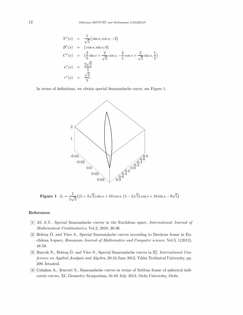
In terms of definitions, we obtain special Smarandache curve, see Figure 1.
........................................
......
......
......
......
...-0.04
0.04
0.0
-0.02
0.02
0.80.6
0.40.2
0.0-0.2
-0.4-0.6
-0.8
..
..
..
..
..
..
..
..
.2
1
Figure 1 β1 =1
5√
5
((5 + 2
√5) sin s + 10 cos s, (5 − 2
√5) cos s + 10 sin s,−9
√5)
References
[1] Ali A.T., Special Smarandache curves in the Euclidean space, International Journal of
Mathematical Combinatorics, Vol.2, 2010, 30-36.
[2] Bektas O. and Yuce S., Special Smarandache curves according to Dardoux frame in Eu-
clidean 3-space, Romanian Journal of Mathematics and Computer science, Vol.3, 1(2013),
48-59.
[3] Bayrak N., Bektas O. and Yuce S., Special Smarandache curves in E31, International Con-
ference on Applied Analysis and Algebra, 20-24 June 2012, Yıldız Techinical University, pp.
209, Istanbul.
[4] Calıskan A., Senyurt S., Smarandache curves in terms of Sabban frame of spherical indi-
catrix curves, XI, Geometry Symposium, 01-05 July 2013, Ordu University, Ordu.
N∗C∗− Smarandache Curves of Mannheim Curve Couple According to Frenet Frame 13
[5] Cetin M., Tuncer Y. and Karacan M.K.,Smarandache curves according to bishop frame in
Euclidean 3-space, arxiv:1106.3202, vl [math.DG], 2011.
[6] Hacısalihoglu H.H., Differential Geometry, Inonu University, Malatya, Mat. no.7, 1983.
[7] Liu H. and Wang F.,Mannheim partner curves in 3-space, Journal of Geometry, Vol.88, No
1-2(2008), 120-126(7).
[8] Orbay K. and Kasap E., On mannheim partner curves, International Journal of Physical
Sciences, Vol. 4 (5)(2009), 261-264.
[9] Sabuncuoglu A., Differential Geometry, Nobel Publications, Ankara, 2006.
[10] Senyurt S. Natural lifts and the geodesic sprays for the spherical indicatrices of the mannheim
partner curves in E3, International Journal of the Physical Sciences, vol.7, No.16, 2012,
2414-2421.
[11] Taskopru K. and Tosun M., Smarandache curves according to Sabban frame on S2, Boletim
da Sociedade parananse de Mathemtica, 3 srie, Vol.32, No.1(2014), 51-59 ssn-0037-8712.
[12] Turgut M., Yılmaz S., Smarandache curves in Minkowski space-time, International Journal
of Mathematical Combinatorics, Vol.3(2008), pp.51-55.
[13] Wang, F. and Liu, H., Mannheim partner curves in 3-space, Proceedings of The Eleventh
International Workshop on Diff. Geom., 2007, 25-31.

International J.Math. Combin. Vol.1(2015), 14-23
Fixed Point Theorems of Two-Step
Iterations for Generalized Z-Type Condition in CAT(0) Spaces
G.S.Saluja
(Department of Mathematics, Govt. Nagarjuna P.G. College of Science, Raipur - 492010 (C.G.), India)
E-mail: [email protected]
Abstract: In this paper, we establish some strong convergence theorems of modified two-
step iterations for generalized Z-type condition in the setting of CAT(0) spaces. Our results
extend and improve the corresponding results of [3, 6, 28] and many others from the current
existing literature.
Key Words: Strong convergence, modified two-step iteration scheme, fixed point, CAT(0)
space.
AMS(2010): 54H25, 54E40
§1. Introduction
A metric space X is a CAT(0) space if it is geodesically connected and if every geodesic triangle
in X is at least as ‘thin’ as its comparison triangle in the Euclidean plane. It is well known that
any complete, simply connected Riemannian manifold having non-positive sectional curvature
is a CAT(0) space. Fixed point theory in a CAT(0) space was first studied by Kirk (see [19,
20]). He showed that every nonexpansive (single-valued) mapping defined on a bounded closed
convex subset of a complete CAT(0) space always has a fixed point. Since, then the fixed
point theory for single-valued and multi-valued mappings in CAT(0) spaces has been rapidly
developed, and many papers have appeared (see, e.g., [2], [9], [11]-[13], [17]-[18], [21]-[22], [24]-
[26] and references therein). It is worth mentioning that the results in CAT(0) spaces can be
applied to any CAT(k) space with k ≤ 0 since any CAT(k) space is a CAT(m) space for every
m ≥ k (see [7).
Let (X, d) be a metric space. A geodesic path joining x ∈ X to y ∈ X (or, more briefly,
a geodesic from x to y) is a map c from a closed interval [0, l] ⊂ R to X such that c(0) = x,
c(l) = y and d(c(t), c(t′)) = |t − t′| for all t, t′ ∈ [0, l]. In particular, c is an isometry, and
d(x, y) = l. The image α of c is called a geodesic (or metric) segment joining x and y. We say
X is (i) a geodesic space if any two points of X are joined by a geodesic and (ii) a uniquely
geodesic if there is exactly one geodesic joining x and y for each x, y ∈ X , which we will denoted
by [x, y], called the segment joining x to y.
A geodesic triangle (x1, x2, x3) in a geodesic metric space (X, d) consists of three points
1Received July 16, 2014, Accepted February 16, 2015.

Fixed Point Theorems of Two-Step Iterations for Generalized Z-Type Condition in CAT(0) Spaces 15
in X (the vertices of ) and a geodesic segment between each pair of vertices (the edges of ).
A comparison triangle for geodesic triangle (x1, x2, x3) in (X, d) is a triangle (x1, x2, x3) :=
(x1, x2, x3) in R2 such that dR2(xi, xj) = d(xi, xj) for i, j ∈ 1, 2, 3. Such a triangle always
exists (see [7]).
1.1 CAT(0) Space
A geodesic metric space is said to be a CAT (0) space if all geodesic triangles of appropriate
size satisfy the following CAT (0) comparison axiom.
Let be a geodesic triangle in X , and let ⊂ R2 be a comparison triangle for . Then
is said to satisfy the CAT (0) inequality if for all x, y ∈ and all comparison points x, y ∈ ,
d(x, y) ≤ dR2(x, y). (1.1)
Complete CAT (0) spaces are often called Hadamard spaces (see [16]). If x, y1, y2 are points
of a CAT (0) space and y0 is the mid point of the segment [y1, y2] which we will denote by
(y1 ⊕ y2)/2, then the CAT (0) inequality implies
d2(x,
y1 ⊕ y2
2
)≤ 1
2d2(x, y1) +
1
2d2(x, y2) −
1
4d2(y1, y2). (1.2)
The inequality (1.2) is the (CN) inequality of Bruhat and Tits [8]. The above inequality was
extended in [12] as
d2(z, αx ⊕ (1 − α)y) ≤ αd2(z, x) + (1 − α)d2(z, y)
−α(1 − α)d2(x, y) (1.3)
for any α ∈ [0, 1] and x, y, z ∈ X .
Let us recall that a geodesic metric space is a CAT (0) space if and only if it satisfies the
(CN) inequality (see [7, page 163]). Moreover, if X is a CAT (0) metric space and x, y ∈ X ,
then for any α ∈ [0, 1], there exists a unique point αx ⊕ (1 − α)y ∈ [x, y] such that
d(z, αx ⊕ (1 − α)y) ≤ αd(z, x) + (1 − α)d(z, y), (1.4)
for any z ∈ X and [x, y] =αx ⊕ (1 − α)y : α ∈ [0, 1]
.
A subset C of a CAT (0) space X is convex if for any x, y ∈ C, we have [x, y] ⊂ C.
We recall the following definitions in a metric space (X, d). A mapping T : X → X is called
an a-contraction if
d(Tx, T y) ≤ a d(x, y) for all x, y ∈ X, (1.5)
where a ∈ (0, 1).
The mapping T is called Kannan mapping [15] if there exists b ∈ (0, 12 ) such that
d(Tx, T y) ≤ b [d(x, Tx) + d(y, T y)] (1.6)
for all x, y ∈ X .

16 G.S.Saluja
The mapping T is called Chatterjea mapping [10] if there exists c ∈ (0, 12 ) such that
d(Tx, T y) ≤ c [d(x, T y) + d(y, Tx)] (1.7)
for all x, y ∈ X .
In 1972, Zamfirescu [29] proved the following important result.
Theorem Z Let (X, d) be a complete metric space and T : X → X a mapping for which
there exists the real number a, b and c satisfying a ∈ (0, 1), b, c ∈ (0, 12 ) such that for any pair
x, y ∈ X, at least one of the following conditions holds:
(z1) d(Tx, T y) ≤ a d(x, y);
(z2) d(Tx, T y) ≤ b [d(x, Tx) + d(y, T y)];
(z3) d(Tx, T y) ≤ c [d(x, T y) + d(y, Tx)].
Then T has a unique fixed point p and the Picard iteration xn∞n=0 defined by
xn+1 = Txn, n = 0, 1, 2, . . .
converges to p for any arbitrary but fixed x0 ∈ X.
An operator T which satisfies at least one of the contractive conditions (z1), (z2) and (z3)
is called a Zamfirescu operator or a Z-operator.
In 2004, Berinde [5] proved the strong convergence of Ishikawa iterative process defined by:
for x0 ∈ C, the sequence xn∞n=0 given by
xn+1 = (1 − αn)xn + αnTyn,
yn = (1 − βn)xn + βnTxn, n ≥ 0, (1.8)
to approximate fixed points of Zamfirescu operator in an arbitrary Banach space E. While
proving the theorem, he made use of the condition,
‖Tx − Ty‖ ≤ δ ‖x − y‖ + 2δ ‖x − Tx‖ (1.9)
which holds for any x, y ∈ E where 0 ≤ δ < 1.
In 1953, W.R. Mann defined the Mann iteration [23] as
un+1 = (1 − an)un + anTun, (1.10)
where an is a sequence of positive numbers in [0,1].
In 1974, S.Ishikawa defined the Ishikawa iteration [14] as
sn+1 = (1 − an)sn + anT tn,
tn = (1 − bn)sn + bnTsn, (1.11)
where an and bn are sequences of positive numbers in [0,1].

Fixed Point Theorems of Two-Step Iterations for Generalized Z-Type Condition in CAT(0) Spaces 17
In 2008, S.Thianwan defined the new two step iteration [27] as
νn+1 = (1 − an)wn + anTwn,
wn = (1 − bn)νn + bnTνn, (1.12)
where an and bn are sequences of positive numbers in [0,1].
Recently, Agarwal et al. [1] introduced the S-iteration process defined as
xn+1 = (1 − an)Txn + anTyn,
yn = (1 − bn)xn + bnTxn, (1.13)
where an and bn are sequences of positive numbers in (0,1).
In this paper, inspired and motivated [5, 29], we employ a condition introduced in [6] which
is more general than condition (1.9) and establish fixed point theorems of S- iteration scheme
in the framework of CAT(0) spaces. The condition is defined as follows:
Let C be a nonempty, closed, convex subset of a CAT(0) space X and T : C → C a self
map of C. There exists a constant L ≥ 0 such that for all x, y ∈ C, we have
d(Tx, T y) ≤ eL d(x,Tx)[δ d(x, y) + 2δ d(x, Tx)
], (1.14)
where 0 ≤ δ < 1 and ex denotes the exponential function of x ∈ C. Throughout this paper, we
call this condition as generalized Z-type condition.
Remark 1.1 If L = 0, in the above condition, we obtain
d(Tx, T y) ≤ δ d(x, y) + 2δ d(x, Tx),
which is the Zamfirescu condition used by Berinde [5] where
δ = maxa,
b
1 − b,
c
1 − c
, 0 ≤ δ < 1,
while constants a, b and c are as defined in Theorem Z.
Example 1.2 Let X be the real line with the usual norm ‖.‖ and suppose C = [0, 1]. Define
T : C → C by Tx = x+12 for all x, y ∈ C. Obviously T is self-mapping with a unique fixed
point 1. Now we check that condition (1.14) is true. If x, y ∈ [0, 1], then ‖Tx − Ty‖ ≤eL ‖x−Tx‖[δ ‖x − y‖ + 2δ ‖x − Tx‖] where 0 ≤ δ < 1. In fact
‖Tx− Ty‖ =
∥∥∥∥x − y
2
∥∥∥∥
and
eL ‖x−Tx‖[δ ‖x − y‖ + 2δ ‖x − Tx‖
]= eL‖x−1
2 ‖[δ ‖x − y‖ + δ ‖x − 1‖].

18 G.S.Saluja
Clearly, if we chose x = 0 and y = 1, then contractive condition (??) is satisfied since
‖Tx − Ty‖ =
∥∥∥∥x − y
2
∥∥∥∥ =1
2,
and for L ≥ 0, we chose L = 0, then
eL ‖x−Tx‖[δ ‖x − y‖ + 2δ ‖x − Tx‖
]= eL‖x−1
2 ‖[δ ‖x − y‖ + δ ‖x − 1‖]
= e0(1/2)(2δ) = 2δ, where 0 < δ < 1.
Therefore
‖Tx − Ty‖ ≤ eL ‖x−Tx‖[δ ‖x − y‖ + 2δ ‖x − Tx‖
].
Hence T is a self mapping with unique fixed point satisfying the contractive condition
(1.14).
Example 1.3 Let X be the real line with the usual norm ‖.‖ and suppose K = 0, 1, 2, 3.Define T : K → K by
Tx = 2, if x = 0
= 3, otherwise.
Let us take x = 0, y = 1 and L = 0. Then from condition (1.14), we have
1 ≤ e0(2)[δ(1) + 2δ(2)]
≤ 1(5δ) = 5δ
which implies δ ≥ 15 . Now if we take 0 < δ < 1, then condition (1.14) is satisfied and 3 is of
course a unique fixed point of T .
1.2 Modified Two-Step Iteration Schemes in CAT(0) Space
Let C be a nonempty closed convex subset of a complete CAT(0) space X . Let T : C → C
be a contractive operator. Then for a given x1 = x0 ∈ C, compute the sequence xn by the
iterative scheme as follows:
xn+1 = (1 − an)Txn ⊕ anTyn,
yn = (1 − bn)xn ⊕ bnTxn, (1.15)
where an and bn are sequences of positive numbers in (0,1). Iteration scheme (1.15) is
called modified S-iteration scheme in CAT(0) space.
νn+1 = (1 − an)wn ⊕ anTwn,
wn = (1 − bn)νn ⊕ bnTνn, (1.16)
where an and bn are sequences of positive numbers in [0,1]. Iteration scheme (1.16) is called

Fixed Point Theorems of Two-Step Iterations for Generalized Z-Type Condition in CAT(0) Spaces 19
modified S.Thianwan iteration scheme in CAT(0) space.
sn+1 = (1 − an)sn ⊕ anT tn,
tn = (1 − bn)sn ⊕ bnTsn, (1.17)
where an and bn are sequences of positive numbers in [0,1]. Iteration scheme (1.17) is called
modified Ishikawa iteration scheme in CAT(0) space.
We need the following useful lemmas to prove our main results in this paper.
Lemma 1.4([24]) Let X be a CAT(0) space.
(i) For x, y ∈ X and t ∈ [0, 1], there exists a unique point z ∈ [x, y] such that
d(x, z) = t d(x, y) and d(y, z) = (1 − t) d(x, y). (A)
We use the notation (1 − t)x ⊕ ty for the unique point z satisfying (A).
(ii) For x, y ∈ X and t ∈ [0, 1], we have
d((1 − t)x ⊕ ty, z) ≤ (1 − t)d(x, z) + td(y, z).
Lemma 1.5([4]) Let pn∞n=0, qn∞n=0, rn∞n=0 be sequences of nonnegative numbers satisfying
the following condition:
pn+1 ≤ (1 − sn)pn + qn + rn, ∀n ≥ 0,
where sn∞n=0 ⊂ [0, 1]. If∑∞
n=0 sn = ∞, limn→∞ qn = O(sn) and∑∞
n=0 rn < ∞, then
limn→∞ pn = 0.
§2. Strong Convergence Theorems in CAT(0) Space
In this section, we establish some strong convergence theorems of modified two-step iterations
to converge to a fixed point of generalized Z-type condition in the framework of CAT(0) spaces.
Theorem 2.1 Let C be a nonempty closed convex subset of a complete CAT(0) space X and
let T : C → C be a self mapping satisfying generalized Z-type condition given by (1.14) with
F (T ) 6= ∅. For any x0 ∈ C, let xn∞n=0 be the sequence defined by (1.15). If∑∞
n=0 an = ∞and
∑∞n=0 anbn = ∞, then xn∞n=0 converges strongly to the unique fixed point of T .
Proof From the assumption F (T ) 6= ∅, it follows that T has a fixed point in C, say u.
Since T satisfies generalized Z-type condition given by (1.14), then from (1.14), taking x = u

20 G.S.Saluja
and y = xn, we have
d(Tu, Txn) ≤ eL d(u,Tu)(δ d(u, xn) + 2δ d(u, Tu)
)
= eL d(u,u)(δ d(u, xn) + 2δ d(u, u)
)
= eL (0)(δ d(u, xn) + 2δ (0)
),
which implies that
d(Txn, u) ≤ δ d(xn, u). (2.1)
Similarly by taking x = u and y = yn in (1.14), we have
d(Tyn, u) ≤ δ d(yn, u), (2.2)
Now using (1.15), (2.2) and Lemma 1.4(ii), we have
d(yn, u) = d((1 − bn)xn ⊕ bnTxn, u)
≤ (1 − bn)d(xn, u) + bn d(Txn, u)
≤ (1 − bn)d(xn, u) + bnδ d(xn, u)
= (1 − bn + bn δ)d(xn, u). (2.3)
Now using (1.15), (2.1), (2.3) and Lemma 1.4(ii), we have
d(xn+1, u) = d((1 − an)Txn ⊕ anTyn, u)
≤ (1 − an)d(Txn, u) + and(Tyn, u)
≤ (1 − an)δ d(xn, u) + anδ d(yn, u)
≤ (1 − an + an δ)d(xn, u) + anδ(1 − bn + bn δ)d(xn, u)
= [1 − (1 − δ)an]d(xn, u) + anδ[1 − (1 − δ)bn]d(xn, u)
= [1 − (1 − δ)an + anδ(1 − (1 − δ)bn)]d(xn, u)
= [1 − (1 − δ)an + δ(1 − δ)anbn]d(xn, u) = (1 − µn)d(xn, u) (2.4)
where µn = (1 − δ)an + δ(1 − δ)anbn. Since 0 ≤ δ < 1; an, bn ∈ (0, 1);∑∞
n=0 an = ∞ and∑∞n=0 anbn = ∞, it follows that
∑∞n=0 µn = ∞. Setting pn = d(xn, u), sn = µn and by applying
Lemma 1.5, it follows that limn→∞ d(xn, u) = 0. Thus xn∞n=0 converges strongly to a fixed
point of T .
To show uniqueness of the fixed point u, assume that u1, u2 ∈ F (T ) and u1 6= u2. Applying
generalized Z-type condition given by (1.14) and using the fact that 0 ≤ δ < 1, we obtain
d(u1, u2) = d(Tu1, Tu2)
≤ eL d(u1,Tu1)δ d(u1, u2) + 2δ d(u1, Tu1)
= eL d(u1,u1)δ d(u1, u2) + 2δ d(u1, u1)
Fixed Point Theorems of Two-Step Iterations for Generalized Z-Type Condition in CAT(0) Spaces 21
= eL (0)
δ d(u1, u2) + 2δ (0)
= δ d(u1, u2) < d(u1, u2),
which is a contradiction. Therefore u1 = u2. Thus xn∞n=0 converges strongly to the unique
fixed point of T . 2Theorem 2.2 Let C be a nonempty closed convex subset of a complete CAT(0) space X and
let T : C → C be a self mapping satisfying generalized Z-type condition given by (1.14) with
F (T ) 6= ∅. For any x0 ∈ C, let xn∞n=0 be the sequence defined by (1.16). If∑∞
n=0 an = ∞,
then xn∞n=0 converges strongly to the unique fixed point of T .
Proof The proof of Theorem 2.2 is similar to that of Theorem 2.1. 2Theorem 2.3 Let C be a nonempty closed convex subset of a complete CAT(0) space X and
let T : C → C be a self mapping satisfying generalized Z-type condition given by (1.14) with
F (T ) 6= ∅. For any x0 ∈ C, let xn∞n=0 be the sequence defined by (1.17). If∑∞
n=0 an = ∞and
∑∞n=0 anbn = ∞, then xn∞n=0 converges strongly to the unique fixed point of T .
Proof The proof of Theorem 2.3 is also similar to that of Theorem 2.1. 2If we take L = 0 in condition (1.14), then we obtain the following result as corollary which
extends the corresponding result of Berinde [5] to the case of modified S-iteration scheme and
from arbitrary Banach space to the setting of CAT(0) spaces.
Corollary 2.4 Let C be a nonempty closed convex subset of a complete CAT(0) space X and
let T : C → C a Zamfirescu operator. For any x0 ∈ C, let xn∞n=0 be the sequence defined by
(1.15). If∑∞
n=0 an = ∞ and∑∞
n=0 anbn = ∞, then xn converges strongly to the unique fixed
point of T .
Remark 2.5 Our results extend and improve upon, among others, the corresponding results
proved by Berinde [3], Yildirim et al. [28] and Bosede [6] to the case of generalized Z-type
condition, modified S-iteration scheme and from Banach space or normed linear space to the
setting of CAT(0) spaces.
§3. Conclusion
The generalized Z-type condition is more general than Zamfirescu operators. Thus the results
obtained in this paper are improvement and generalization of several known results in the
existing literature (see, e.g., [3, 6, 28] and some others).
References
[1] R.P.Agarwal, Donal O’Regan and D.R.Sahu, Iterative construction of fixed points of nearly
asymptotically nonexpansive mappings, Nonlinear Convex Anal. 8(1)(2007), 61-79.

22 G.S.Saluja
[2] A.Abkar and M.Eslamian, Common fixed point results in CAT(0) spaces, Nonlinear Anal.:
TMA, 74(5)(2011), 1835-1840.
[3] V.Berinde, A convergence theorem for Mann iteration in the class of Zamfirescu operators,
An. Univ. Vest Timis., Ser. Mat.-Inform., 45(1) (2007), 33-41.
[4] V.Berinde, Iterative Approximation of Fixed Points, Springer-Verlag, Berlin Heidelberg,
2007.
[5] V.Berinde, On the convergence of the Ishikawa iteration in the class of Quasi-contractive
operators, Acta Math. Univ. Comenianae, 73(1) (2004), 119-126.
[6] A.O.Bosede, Some common fixed point theorems in normed linear spaces, Acta Univ.
Palacki. Olomuc. Fac. rer. nat. Math., 49(1) (2010), 17-24.
[7] M.R.Bridson and A.Haefliger, Metric spaces of non-positive curvature, Vol.319 of Grundlehren
der Mathematischen Wissenschaften, Springer, Berlin, Germany, 1999.
[8] F.Bruhat and J.Tits, “Groups reductifs sur un corps local”, Institut des Hautes Etudes
Scientifiques, Publications Mathematiques, 41(1972), 5-251.
[9] P.Chaoha and A.Phon-on, A note on fixed point sets in CAT(0) spaces, J. Math. Anal.
Appl., 320(2) (2006), 983-987.
[10] S.K.Chatterjea, Fixed point theorems compactes, Rend. Acad. Bulgare Sci., 25(1972),
727-730.
[11] S.Dhompongsa, A.Kaewkho and B.Panyanak, Lim’s theorems for multivalued mappings in
CAT(0) spaces, J. Math. Anal. Appl., 312(2) (2005), 478-487.
[12] S.Dhompongsa and B.Panyanak, On -convergence theorem in CAT(0) spaces, Comput.
Math. Appl., 56(10)(2008), 2572-2579.
[13] R.Espinola and A.Fernandez-Leon, CAT(k)-spaces, weak convergence and fixed point, J.
Math. Anal. Appl., 353(1) (2009), 410-427.
[14] S.Ishikawa, Fixed points by a new iteration method, Proc. Amer. Math. Soc., 44 (1974),
147-150.
[15] R.Kannan, Some results on fixed point theorems, Bull. Calcutta Math. Soc., 60(1969),
71-78.
[16] M.A.Khamsi and W.A.Kirk, An Introduction to Metric Spaces and Fixed Point Theory,
Pure Appl. Math, Wiley-Interscience, New York, NY, USA, 2001.
[17] S.H.Khan and M.Abbas, Strong and -convergence of some iterative schemes in CAT(0)
spaces, Comput. Math. Appl., 61(1) (2011), 109-116.
[18] A.R.Khan, M.A.Khamsi and H.Fukhar-ud-din, Strong convergence of a general iteration
scheme in CAT(0) spaces, Nonlinear Anal.: TMA, 74(3) (2011), 783-791.
[19] W.A.Kirk, Geodesic geometry and fixed point theory, in Seminar of Mathematical Analysis
(Malaga/Seville, 2002/2003), Vol.64 of Coleccion Abierta, 195-225, University of Seville
Secretary of Publications, Seville, Spain, 2003.
[20] W.A.Kirk, Geodesic geometry and fixed point theory II, in International Conference on
Fixed Point Theory and Applications, 113-142, Yokohama Publishers, Yokohama, Japan,
2004.
[21] W.Laowang and B.Panyanak, Strong and convergence theorems for multivalued map-
pings in CAT(0) spaces, J. Inequal. Appl., Article ID 730132, 16 pages, 2009.

Fixed Point Theorems of Two-Step Iterations for Generalized Z-Type Condition in CAT(0) Spaces 23
[22] L.Leustean, A quadratic rate of asymptotic regularity for CAT(0)-spaces, J. Math. Anal.
Appl., 325(1) (2007), 386-399.
[23] W.R.Mann, Mean value methods in iteration, Proc. Amer. Math. Soc., 4 (1953), 506-510.
[24] Y.Niwongsa and B.Panyanak, Noor iterations for asymptotically nonexpansive mappings
in CAT(0) spaces, Int. J. Math. Anal., 4(13), (2010), 645-656.
[25] S.Saejung, Halpern’s iteration in CAT(0) spaces, Fixed Point Theory Appl., Article ID
471781, 13 pages, 2010.
[26] N.Shahzad, Fixed point results for multimaps in CAT(0) spaces, Topology and its Appli-
cations, 156(5) (2009), 997-1001.
[27] S.Thianwan, Common fixed points of new iterations for two asymptotically nonexpansive
nonself mappings in Banach spaces, J. Comput. Appl. Math., 224(2) (2008), 688-695.
[28] I.Yildirim, M.Ozdemir and H.Kizltung, On the convergence of a new two-step iteration in
the class of Quasi-contractive operators, Int. J. Math. Anal., 38(3) (2009), 1881-1892.
[29] T.Zamfirescu, Fixed point theorems in metric space, Arch. Math. (Basel), 23 (1972),
292-298.

International J.Math. Combin. Vol.1(2015), 24-34
Antidegree Equitable Sets in a Graph
Chandrashekar Adiga and K. N. Subba Krishna
(Department of Studies in Mathematics, University of Mysore, Manasagangotri, Mysore - 570 006, India)
E-mail: c [email protected]; [email protected]
Abstract: Let G = (V, E) be a graph. A subset S of V is called a Smarandachely antidegree
equitable k-set for any integer k, 0 ≤ k ≤ ∆(G), if |deg(u) − deg(v)| 6= k, for all u, v ∈ S.
A Smarandachely antidegree equitable 1-set is usually called an antidegree equitable set.
The antidegree equitable number ADe(G), the lower antidegree equitable number ade(G),
the independent antidegree equitablenumber ADie(G) and lower independent antidegree
equitable number adie(G) are defined as follows:
ADe(G) = max|S| : S is a maximal antidegree equitable set in G,
ade(G) = min|S| : S is a maximal antidegree equitable set in G,
ADie(G) = max|S| : S is a maximal independent and antidegree equitable set in G,
adie(G) = min|S| : S is a maximal independent and antidegree equitable set in G.
In this paper, we study these four parameters on Smarandachely antidegree equitable 1-sets.
Key Words: Smarandachely antidegree equitable k-set, antidegree equitable set, antide-
gree equitable number, lower antidegree equitable number, independent antidegree equitable
number, lower independent antidegree equitable number.
AMS(2010): 05C69
§1. Introduction
By a graph G = (V, E) we mean a finite, undirected graph with neither loops nor multiple
edges. The number of vertices in a graph G is called the order of G and number of edges in
G is called the size of G. For standard definitions and terminologies on graphs we refer to the
books [2] and [3].
In this paper we introduce four graph theoretic parameters which just depend on the basic
concept of vertex degrees. We need the following definitions and theorems, which can be found
in [2] or [3].
Definition 1.1 A graph G1 is isomorphic to a graph G2, if there exists a bijection φ from
V (G1) to V (G2) such that uv ∈ E(G1) if, and only if, φ(u)φ(v) ∈ E(G2).
If G1 is isomorphic to G2, we write G1∼= G2 or sometimes G1 = G2.
1Received June 16, 2014, Accepted February 18, 2015.

Antidegree Equitable Sets in a Graph 25
Definition 1.2 The degree of a vertex v in a graph G is the number of edges of G incident
with v and is denoted by deg(v) or degG(v).
The minimum and maximum degrees of G are denoted by δ(G) and ∆(G) respectively.
Theorem 1.3 In any graph G, the number of odd vertices is even.
Theorem 1.4 The sum of the degrees of vertices of a graph G is twice the number of edges.
Definition 1.5 The corona of two graphs G1 and G2 is defined to be the graph G = G1 G2
formed from one copy of G1 and |V (G1)| copies of G2 where the ith vertex of G1 is adjacent to
every vertex in the ith copy of G2.
Theorem 1.6 Let G be a simple graph i.e, a undirected graph without loops and multiple edges,
with n ≥ 2. Then G has atleast two vertices of the same degree.
Definition 1.7 Any connected graph G having a unique cycle is called a unicyclic graph.
Definition 1.8 A graph is called a caterpillar if the deletion of all its pendent vertices produces
a path graph.
Definition 1.9 A subset S of the vertex set V in a graph G is said to be independent if no two
vertices in S are adjacent in G.
The maximum number of vertices in an independent set of G is called the independence
number and is denoted by β0(G).
Theorem 1.10 Let G be a graph and S ⊂ V . S is an independent set of G if, and only if,
V − S is a covering of G.
Definition 1.11 A clique of a graph is a maximal complete subgraph.
Definition 1.12 A clique is said to be maximal if no super set of it is a clique.
Definition 1.13 The vertex degrees of a graph G arranged in non-increasing order is called
degree sequence of the graph G.
Definition 1.14 For any graph G, the set D(G) of all distinct degrees of the vertices of G is
called the degree set of G.
Definition 1.15 A sequence of non-negative integers is said to be graphical if it is the degree
sequence of some simple graph.
Theorem 1.16([1]) Let G be any graph. The number of edges in Gde the degree equitable graph
of G, is given by∆−1∑
i=δ
(|Si|2
)−
∆∑
i=δ+1
(|Si′|
2
),
where, Si = v|v ∈ V, deg(v) = i or i + 1 and Si′ = v|v ∈ V, deg(v) = i.

26 Chandrashekar Adiga and K. N. Subba Krishna
Theorem 1.17 The maximum number of edges in G with radius r ≥ 3 is given by
n2 − 4nr + 5n + 4r2 − 6r
2.
Definition 1.18 A vertex cover in a graph G is such a set of vertices that covers all edges of
G. The minimum number of vertices in a vertex cover of G is the vertex covering number α(G)
of G.
Recently A. Anitha, S. Arumugam and E. Sampathkumar [1] have introduced degree eq-
uitable sets in a graph and studied them. “The characterization of degree equitable graphs”
is still an open problem. In this paper we give some necessary conditions for a graph to be
degree equitable. For this purpose, we introduce another concept “Antidegree equitable sets”
in a graph and we study them.
§2. Antidegree Equitable Sets
Definition 2.1 Let G = (V, E) be a graph. A non-empty subset S of V is called an antidegree
equitable set if |deg(u) − deg(v)| 6= 1 for all u, v ∈ S.
Definition 2.2 An antidegree equitable set is called a maximal antidegree equitable set if for
every v ∈ V − S, there exists at least one element u ∈ S such that |deg(u) − deg(v)| = 1.
Definition 2.3 The antidegree equitable number ADe(G) of a graph G is defined as ADe(G) =
max|S| : S is a maximal antidegree equitable set.
Definition 2.4 The lower antidegree equitable number ade(G) of a graph G is defined as
ade(G) = min|S| : S is a maximal antidegree equitable set.
A few ADe(G) and ade(G) of some graphs are listed in the following:
(i) For the complete bipartite graph Km,n, we have
ADe(Km,n) =
m + n if |m − n| 6= 1,
maxm, n if |m − n| = 1
and
ade(Km,n) =
m + n if |m − n| 6= 1,
minm, n if |m − n| = 1.
(ii) For the wheel Wn on n-vertices, we have
ADe(Wn) =
n if n 6= 5,
4 if n = 5

Antidegree Equitable Sets in a Graph 27
and
ade(Wn) =
n if n 6= 5,
1 if n = 5.
(iii) For the complete graph Kn, we have ADe(Kn) = ade(Kn) = n − 1.
Now we study some important basic properties of antidegree equitable sets and independent
antidegree equitable sets in a graph.
Theorem 2.5 Let G be a simple graph on n-vertices. Then
(i) 1 ≤ ade(G) ≤ ADe(G) ≤ n;
(ii) ADe(G) = 1 if, and only if, G = K1;
(iii) ade(G) = ade(G), ADe(G) = ADe(G).
(iv) ade(G) = 1 if, and only if, there exists a vertex u ∈ V (G) such that |deg(u)−deg(v)| =
1 for all v ∈ V − u;(v) If G is a non-trivial connected graph and ade(G) = 1, then ADe(G) = n − 1 and n
must be odd.
Proof (i) follows from the definition.
(ii) Suppose ADe(G) = 1 and G 6= K1. Then G is a non-trivial graph and from Theorem
1.6 there exists at least two vertices of same degree and they form an antidegree equitable set
in G. So ADe(G) ≥ 2 which is a contradiction. The converse is obvious.
(iii) Since degG(u) = (n− 1)− degG(u), it follows that an antidegree equitable set in G is
also an antidegree equitable set in G.
(iv) If ade(G) = 1 and there is no such vertex u in G, then u is not a maximal antidegree
equitable set for any u ∈ V (G) and hence ade(G) ≥ 2 which is a contradiction. The converse is
obvious.
(v) Suppose G is a non-trivial connected graph with ade(G) = 1. Then there exists a vertex
u ∈ V such that |deg(u) − deg(v)| = 1, ∀ v ∈ V − u. Clearly, |deg(v) − deg(w)| = 0 or 2,
∀ v, w ∈ V − u. Hence, ADe(G) = |V − u| = n − 1. It follows from Theorem 1.4 that
(n − 1) is even and thus n is odd. 2Theorem 2.6 Let G be a non-trivial connected graph on n-vertices. Then 2 ≤ ADe(G) ≤ n
and ADe(G) = 2 if, and only if, G ∼= K2 or P2 or P3 or L(H) or L2(H) where H is the
caterpillar T5 with spine P = (v1v2).
Proof By Theorem 2.5, for a non-trivial connected graph G on n-vertices, we have 2 ≤ADe(G) ≤ n. Suppose ADe(G) = 2. Then for each antidegree equitable set S in G, we have
|S| ≤ 2. Let D(G) = d1, d2, . . . , dk, where d1 < d2 < d3 < · · · < dk. As there are at least
two vertices with same degree, we have k ≤ n − 1. Since ADe(G) = 2, more than two vertices
cannot have the same degree. Let di ∈ D(G) be such that exactly two vertices of G have degree
di. Since the cardinality of each antidegree equitable set S cannot exceed two, it follows that

28 Chandrashekar Adiga and K. N. Subba Krishna
· · · , di−3, di−2, di+2, di+3, di+4, · · · do not belong to D(G). Thus D(G) ⊂ di−1, di, di+1.
Case 1. If di − 1, di + 1 do not belong to D(G) then D(G) = di and the degree sequence
di, di is clearly graphical. Thus n = 2 and di = 1 which implies G = K2.
Case 2. If di − 1, di + 1 ∈ D(G), then the degree sequence di − 1, di, di, di + 1 is graphical.
Thus n = 4 and di = 2 which implies G ∼= L(H), where H is the caterpillar T5 with spine
P = (v1v2).
Case 3. If di−1 ∈ D(G) and di+1 does not belong to D(G), then di−1 may or may not repeat
twice in degree sequence. Thus degree sequence is given by di−1, di, di or di−1, di−1, di, di.The first sequence is not graphical but the second sequence is graphical. Thus n = 4 and di = 2
which implies G ∼= P4.
Case 4. If di − 1 does not belong to D(G) and di + 1 ∈ D(G), then the degree sequence is
given by di, di, di + 1 or di, di, di + 1, di +1. Both sequences are graphical. In the first case
n = 3, di = 1 which implies G ∼= P2, and in the second case n = 4, di = 1 or 2 which implies
G ∼= P3 or G ∼= L2(H) respectively.
The converse is obvious. 2Theorem 2.7 If a and b are positive integers with a ≤ b, then there exists a connected simple
graph G with ade(G) = a and ADe(G) = b except when a = 1 and b = 2m + 1, m ∈ N .
Proof If a = b then for any regular graph of order a, we have ade(G) = ADe(G) = a.
If b = a + 1, then for the complete bipartite graph G = ka,a+1 we have ade(G) = a and
ADe(G) = a + 1 = b. If b ≥ a + 2, a ≥ 2, and b > 4, then for the graph G consisting of the
wheel Wb−1 and the path Pa = (v1v2v3 . . . va) with an edge joining a pendant vertex of Pa to
the center of the wheel Wb−1, we have ade(G) = a, ADe(G) = b. If a = 1 and b = 2m, m ∈ N ,
then the graph consisting of two cycles Cm and Cm+1 along with edges joining ith vertex of Cm
to ith vertex of Cm+1, we have ade(G) = 1 = a and ADe(G) = 2m = b.
Figure 1

Antidegree Equitable Sets in a Graph 29
For a = 2 and b = 4 we consider graph G in Figure 1, for which ade(G) = 2 and ADe(G) =
4. Also, it follows from Theorem 2.5 that there is no graph G with ade(G) = 1 and ADe(G) =
2m + 1. 2Theorem 2.8 Let G be a non-trivial connected graph on n vertices and let S∗ be a subset of V
such that |deg(u)− deg(v)| ≥ 2 for all u, v ∈ S∗. Then 1 ≤ |S∗| ≤[∆ − δ
2
]+ 1 and also, if S∗
is a maximal subset of V such that |deg(u)−deg(v)| ≥ 2 for all u, v ∈ S∗, then S =⋃
v∈S∗
Sdeg(v)
is a maximal antidegree equitable set in G, where Sdeg(v) = u ∈ V : deg(u) = deg(v).
Proof For any two vertices u, v ∈ S∗, d(u) and d(v) cannot be two successive members of
A = δ, δ + 1, δ + 2, . . . , δ + k = ∆ and D(G) ⊂ A. Hence
|S∗| ≤[ |D(G)| + 1
2
]≤[ |A| + 1
2
]=
[∆ − δ
2
]+ 1.
If a, b ∈ S =⋃
v∈S∗ Sdeg(v), then it is clear that either |deg(a)−deg(b)| = 0 or |deg(a)−deg(b)| ≥2 and hence S is an antidegree equitable set. Suppose u ∈ V − S. Then deg(u) 6= deg(v) for
any v ∈ S∗. So, u do not belong to S∗ and hence |deg(u) − deg(v)| = 1 for all v ∈ S. This
implies that S is a maximal antidegree equitable set. 2Theorem 2.9 Given a positive integer k, there exists graphs G1 and G2 such that ade(G1) −ade(G1 − e) = k and ade(G2 − e) − ade(G2) = k.
Proof Let G1 = Kk+2. Then ade(G1) = k + 2 and ade(G1 − e) = 2, where e ∈ E(G1).
Hence ade(G1) − ade(G1 − e) = k. Let G2 be the graph obtained from Ck+1 by attaching one
leaf e at (k + 1)th vertex of Ck+1. Then ade(G2 − e) − ade(G2) = k. 2Theorem 2.10 Given two positive integers n and k with k ≤ n. Then there exists a graph G
of order n with ade(G) = k.
Proof If k < n2 , then we take G to be the graph obtained from the path Pk = (v1v2v3 . . . vk)
and the complete graph Kn−k by joining v1 and a vertex of Kn−k by an edge. Clearly, ade(G) =
k. If k ≥ n2 , then we take G to be the graph obtained from the cycle Ck by attaching exactly
one leaf at (n − k) vertices of Ck. Clearly, ade(G) = k. 2§3. Independent Antidegree Equitable Sets
In this section, we introduce the concepts of independent antidegree equitable number and lower
independent antidegree equitable number and establish important results on these parameters.
Definition 3.1 The independent antidegree equitable number ADie(G) = max|S| : S ⊂V, S is a maximal independent and antidegree equitable set in G.
Definition 3.2 The lower independent antidegree equitable number adie(G) = min|S| :

30 Chandrashekar Adiga and K. N. Subba Krishna
S is a maximal independent and antidegree equitable set in G.
A few ADie and adie of graphs are listed in the following.
(i) For the star graph K1,n we have, ADie(K1,n) = n and adie(K1,n) = 1.
(ii) For the complete bipartite graph Km,n we have ADie(Km,n) = maxm, n and
adie(Km,n) = minm, n.
(iii) For any regular graph G we have, ADie(G) = adie(G) = βo(G).
The following theorem shows that on removal of an edge in G, ADie(G) can decrease by
at most one and increase by at most 2.
Theorem 3.3 Let G be a connected graph, e = uv ∈ E(G). Then
ADie(G) − 1 ≤ ADie(G − e) ≤ ADie(G) + 2.
Proof Let S be an independent antidegree equitable set in G with |S| = ADie(G). After
removing an edge e = uv from the graph G, we shall give an upper and a lower bound for
ADie(G − e).
Case 1. If u, v does not belong to S, then S is a maximal independent antidegree equitable
set in G − e as well as in G. Hence, ADie(G − e) = ADie(G).
Case 2. If u ∈ S and v does not belong to S, then S − u is an independent antidegree
equitable set in G − e. Hence, ADie(G − e) ≥ |S − u| = ADie(G) − 1. Thus, ADie(G) − 1 ≤ADie(G − e).
Now, Let S be an independent antidegree equitable set in G − e with |S| = ADie(G − e).
Case 3. If u, v ∈ S, then S − u, v is an independent antidegree equitable set in G. Hence,
by definition ADie(G) ≥ |S − u, v| = ADie(G − e) − 2.
Case 4. If u ∈ S and v does not belong to S, then S − u is an independent antidegree
equitable set in G. Hence, by definition ADie(G) ≥ |S − u| = ADie(G − e) − 1.
Case 5. If u, v do not belong to S, then S is an independent antidegree equitable set in G.
Hence, by definition ADie(G) ≥ |S| = ADie(G−e). It follows that ADie(G) ≥ ADie(G−e)−2.
Hence,
ADie(G) − 1 ≤ ADie(G − e) ≤ ADie(G) + 2. 2Theorem 3.4 Let G be a connected graph. ADie(G) = 1 if, and only if, G ∼= Kn or for any
two non-adjacent vertices u, v ∈ V , |deg(u) − deg(v)| = 1.
Proof Suppose ADie(G) = 1.
Case 1. If G ∼= Kn, then there is nothing to prove.
Case 2. Let G 6= Kn, and u, v be any two non-adjacent vertices in G. Since ADie(G) = 1,
u, v is not an antidegree equitable set and hence |deg(u) − deg(v)| = 1. The converse is

Antidegree Equitable Sets in a Graph 31
obvious. 2Theorem 3.5 Let G be a connected graph. adie(G) = 1 if, and only if, either ∆ = n − 1 or
for any two non-adjacent vertices u, v ∈ V , |deg(u) − deg(v)| = 1.
Proof Suppose adie(G) = 1, then for any two non-adjacent vertices u and v, u, v is not
an antidegree equitable set.
Case 1. If ∆ = n − 1, then there is nothing to prove.
Case 2. Let ∆ < n − 1, and u, v be any two non-adjacent vertices in G. Then u, v is not
an antidegree equitable set and hence, |deg(u) − deg(v)| = 1.
The converse is obvious. 2Remark 3.6 Theorems 3.4 and 3.5 are equivalent.
§4. Degree Equitable and Antidegree Equitable Graphs
After studying the basic properties of antidegree equitable and independent antidegree equitable
sets in a graph, in this section we give some conditions for a graph to be degree equitable.
We recall the definition of degree equitable graph given by A. Anitha, S. Arumugam, and E.
Sampathkumar [1].
Definition 4.1 Let G = (V, E) be a graph. The degree equitable graph of G, denoted by Gde
is defined as follows:V (Gde) = V (G) and two vertices u and v are adjacent vertices in Gde if,
and only if, |deg(u) − deg(v)| ≤ 1.
Example 4.2 For any regular graph G on n vertices, we have Gde = Kn.
Definition 4.3 A graph H is called degree equitable graph if there exists a graph G such that
H ∼= Gde.
Example 4.4 Any complete graph Kn is a degree equitable graph because Kn = Gde for any
regular graph G on n-vertices.
Theorem 4.5 Let G = (V, E) be any graph on n vertices with radius r ≥ 3. Then
(i) 1 ≤ β0(Gde) ≤
√n2 − 4nr + 5n + 4r2 − 6r.
(ii) β0(Gde) ≤
[∆−δ
2
]+ 1, where ∆ = ∆(G) and δ = δ(G).
Proof (i) Let A be an independent set of Gde such that |A| = β0(Gde). Then A is an
antidegree equitable set in G and hence
∑
v∈V
degG(v) ≥∑
v∈A
degG(v) =
β0(Gde)∑
ℓ=1
2ℓ − 1 = β02(Gde).

32 Chandrashekar Adiga and K. N. Subba Krishna
By Theorem 1.17 it follows that
2
(n2 − 4nr + 5n + 4r2 − 6r
2
)≥ β0
2(Gde).
Therefore,
1 ≤ β0(Gde) ≤
√n2 − 4nr + 5n + 4r2 − 6r.
(ii) We know that every independent set A in Gde is an antidegree equitable set in G and hence
by Theorem 2.8,
|A| ≤[∆(G) − δ(G)
2
]+ 1.
Therefore,
β0(Gde) ≤
[∆(G) − δ(G)
2
]+ 1.
This completes the proof. 2Theorem 4.6 Let H be any degree equitable graph on n vertices and H = Gde for some graph
G. Then √∑
v∈A
degG(v) ≤[∆(G) − δ(G)
2
]+ 1
where A is an independent set in Gde such that |A| = β0(Gde).
Proof We know that if A is an independent set in H then it is an antidegree equitable set
in G. Hence,
∑
v∈A
degG(v) ≤β0(H)∑
ℓ=1
2ℓ − 1 = β02(H).
By Theorem 4.5∑
v∈A
degG(v) ≤([
∆(G) − δ(G)
2
]+ 1
)2
.
Therefore, √∑
v∈A
degG(v) ≤[∆(G) − δ(G)
2
]+ 1. 2
We introduce a new concept antidegree equitable graph and present some basic results.
Definition 4.7 Let G = (V, E) be a graph. The antidegree equitable graph of G, denoted by
Gade defined as follows: V (Gade) = V (G) and two vertices u and v are adjacent in Gade if, and
only if, |deg(u) − deg(v)| 6= 1.
Example 4.8 For a complete bipartite graph Km,n, we have
Gade =
Km+n if |m − n| ≥ 2,or = 0
Km ∪ Kn if |m − n| = 1.

Antidegree Equitable Sets in a Graph 33
Definition 4.9 A graph H is called an antidegree equitable graph if there exists a graph G such
that H ∼= Gade.
Example 4.10 Any complete graph Kn is an antidegree equitable graph because Kn = Gade
for any regular graph G on n-vertices.
Theorem 4.11 Let G be any graph on n vertices. Then the number of edges in Gade is given
by (n
2
)−
∆−1∑
i=δ
(|Si|2
)+
(|Sδ′|
2
)+ 2
∆∑
i=δ+1
(|Si′|
2
),
where Si = v| v ∈ V degG(v) = i or i + 1, Si′ = v| v ∈ V degG(v) = i, ∆ = ∆(G) and
δ = δ(G).
Proof By Theorem 1.16, we have the number of edges in Gade with end vertices having
the difference degree greater than two in G is
(n
2
)−
∆−1∑
i=δ
(|Si|2
)+
∆∑
i=δ+1
(|Si′|
2
).
and also, the number of edges in Gade with end vertices having the same degree is
∆∑
i=δ
(|Si′|
2
).
Hence, the total number of edges in Gade is
(n
2
)−
∆−1∑
i=δ
(|Si|2
)+
∆∑
i=δ+1
(|Si′|
2
)+
∆∑
i=δ
(|Si′|
2
)
=
(n
2
)−
∆−1∑
i=δ
(|Si|2
)+
(|Sδ′|
2
)+ 2
∆∑
i=δ+1
(|Si′|
2
). 2
Theorem 4.12 Let G be any graph on n vertices. Then
(i) α(Gade) ≤√
n(n − 1);
(ii) α(Gade) ≤[∆−δ
2
]+ 1, where ∆ = ∆(G) and δ = δ(G).
Proof Let A ⊂ V be the set of vertices that covers all edges of Gade. Then A is an
antidegree equitable set in G. Hence,
∑
v∈A
degG(v) ≥α(Gade)∑
ℓ=1
2ℓ − 1 = α2(Gade).
Therefore,
2
(n(n − 1)
2
)≥ α2(Gade),

34 Chandrashekar Adiga and K. N. Subba Krishna
α(Gade) ≤√
n(n − 1).
Since, the set A is an antidegree equitable set in G, by Theorem 2.8, we have
|A| ≤[∆ − δ
2
]+ 1.
This implies
α(Gade) ≤[∆ − δ
2
]+ 1. 2
References
[1] A. Anitha, S. Arumugam and E. Sampathkumar, Degree equitable sets in a graph, Inter-
national J. Math. Combin., 3 (2009), 32-47.
[2] G. Chartrand and P. Zhang, Introduction to Graph Theory, 8th edition, Tata McGraw-Hill,
2006.
[3] F.Harary, Graph Theory, Addison-Wesley, Reading, MA, 1969.

International J.Math. Combin. Vol.1(2015), 35-48
A New Approach to Natural Lift Curves of
The Spherical Indicatrices of Timelike Bertrand Mate of a Spacelike
Curve in Minkowski 3-Space
Mustafa Bilici
(Department of Mathematics, Educational Faculty of Ondokuz, Mayıs University, Atakum 55200, Samsun, Turkey)
Evren Ergun
(Carsamba Chamber of Commerce Vocational School of Ondokuz, Mayıs University, Carsamba 55500, Samsun, Turkey)
Mustafa Calıskan
(Department of Mathematics, Faculty of Sciences of Gazi University, Teknik Okullar 06500, Ankara, Turkey)
E-mail: [email protected], [email protected], [email protected]
Abstract: In this study, we present a new approach the natural lift curves for the spher-
ical indicatrices of the timelike Bertrand mate of a spacelike curve on the tangent bundle
T(S2
1
)or T
(H2
0
)in Minkowski 3-space and we give some new characterizations for these
curves. Additionally we illustrate an example of our main results.
Key Words: Bertrand curve, natural lift curve, geodesic spray, spherical indicatrix.
AMS(2010): 53A35, 53B30, 53C50
§1. Introduction
Bertrand curves are one of the associated curve pairs for which at the corresponding points of
the curves one of the Frenet vectors of a curve coincides with the one of the Frenet vectors
of the other curve. These special curves are very interesting and characterized as a kind of
corresponding relation between two curves such that the curves have the common principal
normal i.e., the Bertrand curve is a curve which shares the normal line with another curve. It
is proved in most texts on the subject that the characteristic property of such a curve is the
existence of a linear relation between the curvature and the torsion; the discussion appears as
an application of the Frenet-Serret formulas. So, a circular helix is a Bertrand curve. Bertrand
mates represent particular examples of offset curves [11] which are used in computer-aided
design (CAD) and computer-aided manufacturing (CAM). For classical and basic treatments
of Bertrand curves, we refer to [3], [6] and [12].
There are recent works about the Bertrand curves. Ekmekci and Ilarslan studied Nonnull
Bertrand curves in the n-dimensional Lorentzian space. Straightforward modication of classical
theory to spacelike or timelike curves in Minkowski 3-space is easily obtained, (see [1]). Izumiya
1Received August 28, 2014, Accepted February 19, 2015.

36 Mustafa Bilici, Evren Ergun and Mustafa Calıskan
and Takeuchi [16] have shown that cylindrical helices can be constructed from plane curves and
Bertrand curves can be constructed from spherical curves. Also, the representation formulae
for Bertrand curves were given by [8].
In differential geometry, especially the theory of space curves, the Darboux vector is the
areal velocity vector of the Frenet frame of a space curve. It is named after Gaston Darboux who
discovered it. In terms of the Frenet-Serret apparatus, the Darboux vector can be expressed as
w = τt + κb . In addition, the concepts of the natural lift and the geodesic sprays have first
been given by Thorpe (1979). On the other hand, Calıskan et al. [4] have studied the natural
lift curves and the geodesic sprays in Euclidean 3-space R3 . Bilici et al. [7] have proposed the
natural lift curves and the geodesic sprays for the spherical indicatrices of the involute-evolute
curve couple in R3. Recently, Bilici [9] adapted this problem for the spherical indicatrices of
the involutes of a timelike curve in Minkowski 3-space.
Kula and Yaylı [17] have studied spherical images of the tangent indicatrix and binormal
indicatrix of a slant helix and they have shown that the spherical images are spherical helices.
In [19] Suha et. all investigated tangent and trinormal spherical images of timelike curve lying
on the pseudo hyperbolic space H30 in Minkowski space-time. Iyigun [20] defined the tangent
spherical image of a unit speed timelike curve lying on the on the pseudo hyperbolic space H20
in R31.
Senyurt and Calıskan [22] obtained arc-lengths and geodesic curvatures of the spherical
indicatrices (T ∗) , (N∗) , (B∗) and the fixed pole curve (C∗) which are generated by Frenet
trihedron and the unit Darboux vector of the timelike Bertrand mate of a spacelike curve with
respect to Minkowski space R31 and Lorentzian sphere S2
1 or hyperbolic sphere H20 . Furthermore,
they give some criteria of being integral curve for the geodesic spray of the natural lift curves
of this spherical indicatrices.
In this study, the conditions of being integral curve for the geodesic spray of the the natural
lift curves of the the spherical indicatrices (T ∗) , (N∗) , (B∗) are investigated according to the
relations given by [8] on the tangent bundle T(S2
1
)or T
(H2
0
)in Minkowski 3-space. Also, we
present an example which illustrates these spherical indicatrices (Figs. 1-4). It is seen that the
principal normal indicatrix (N∗) is geodesic on S21 and its natural lift curve is an integral curve
for the geodesic spray on T(S2
1
).
§2. Preliminaries
To meet the requirements in the next sections, the basic elements of the theory of curves and
hypersurfaces in the Minkowski 3-space are briefly presented in this section. A more detailed
information can be found in [10].
The Minkowski 3-space R31 is the real vector space R3endowed with standard flat Lorentzian
metric given by
g = −dx21 + dx2
2 + dx23,
where (x1, x2, x3) is a rectangular coordinate system of R31 . A vector V = (v1, v2, v3) ∈ R3
1 is
said to be timelike if g(V, V ) < 0 , spacelike if g(V, V ) > 0 or V = 0 and null (lightlike) if

A New Approach to Natural Lift Curves of the Spherical Indicatrices of Timelike Bertrand Mate 37
g(V, V ) = 0 and V 6= 0 .Similarly, an arbitrary Γ = Γ (s) curve in R31 can locally be timelike,
spacelike or null (lightlike), if all of its velocity vectors Γ′
are respectively timelike, spacelike or
null (lightlike), for every t ∈ I ⊂ R. The pseudo-norm of an arbitrary vector V ∈ R31 is given by
‖V ‖ =√|g(V, V )|. Γ is called a unit speed curve if the velocity vector V of Γ satisfies ‖V ‖ = 1.
A timelike vector V is said to be positive (resp. negative) if and only if v1 > 0 (resp.v1 < 0 ) .
Let Γ be a unit speed spacelike curve with curvature κ and torsion τ . Denote by
t (s) , n (s) , b (s) the moving Frenet frame along the curve Γ in the space R31. Then t, n and b
are the tangent, the principal normal and the binormal vector of the curve Γ, respectively.
The angle between two vectors in Minkowski 3-space is defined by [21]
Definition 2.1 Let X and Y be spacelike vectors in R31 that span a spacelike vector subspace,
then we have |g(X, Y )| ≤ ‖X‖‖Y ‖ and hence, there is a unique positive real number ϕ such
that
|g(X, Y )| = ‖X‖‖Y ‖cosϕ.
The real numberϕ is called the Lorentzian spacelike angle between X and Y .
Definition 2.2 Let X and Y be spacelike vectors in R31 that span a timelike vector subspace,
then we have |g(X, Y )| > ‖X‖‖Y ‖ and hence, there is a unique positive real number ϕ such
that
|g(X, Y )| = ‖X‖‖Y ‖coshϕ.
The real number ϕ is called the Lorentzian timelike angle between X and Y .
Definition 2.3 Let X be a spacelike vector and Y a positive timelike vector in R31, then there
is a unique non-negative real number ϕ such that
|g(X, Y )| = ‖X‖‖Y ‖sinhϕ.
The real number ϕ is called the Lorentzian timelike angle between X and Y .
Definition 2.4 Let X and Y be positive (negative) timelike vectors in R31, then there is a
unique non-negative real number ϕ such that
g(X, Y ) = ‖X‖‖Y ‖coshϕ.
The real number ϕ is called the Lorentzian timelike angle between X and Y .
Case I. Let Γ be a unit speed spacelike curve with a spacelike binormal. For these Frenet
vectors, we can write
T × N = −B, N × B = −T, B × T = N
where ”×” is the Lorentzian cross product in space R31. Depending on the causal character of
the curve Γ, the following Frenet formulae are given in [5].
·T = κN,
·N = κT + τB,
·B = τN

38 Mustafa Bilici, Evren Ergun and Mustafa Calıskan
The Darboux vector for the spacelike curve with a spacelike binormal is defined by [11]:
w = −τT + κB
If b and w spacelike vectors that span a spacelike vector subspace then by the Definition1.
we can write
κ = ‖w‖ cosh ϕ
τ = ‖w‖ sinhϕ,
where ‖w‖2 = g (w, w) = τ2 + κ2.
Case II. Let Γ be a unit speed spacelike curve with a timelike binormal. For these Frenet
vectors, we can write
T × N = B, N × B = −T, B × T = −N
Depending on the causal character of the curve Γ , the following Frenet formulae are given
in [5].·T = κN,
·N = −κT + τB,
·B = τN
The Darboux vector for the spacelike curve with a timelike binormal is defined by [11]:
w = τT − κB
There are two cases corresponding to the causal characteristic of Darboux vector w.
(i) If |κ| < |τ | , then w is a timelike vector. In this situation, we have
κ = ‖w‖ sinhϕ
τ = ‖w‖ coshϕ,
where ‖w‖2= −g (w, w) = τ2 − κ2. So the unit vector c of direction w is
c =1
‖w‖w = sinhϕT − cosh ϕB.
(ii) If |κ| > |τ |, then w is a spacelike vector. In this situation, we can write
κ = ‖w‖ cosh ϕ
τ = ‖w‖ sinhϕ,
where ‖w‖2= g (w, w) = κ2 − τ2. So the unit vector c of direction w is
c =1
‖w‖w = sinhϕT − cosh ϕB.
Proposition 2.5([13]) Let α be a timelike (or spacelike) curve with curvatures κ and τ . The

A New Approach to Natural Lift Curves of the Spherical Indicatrices of Timelike Bertrand Mate 39
curve is a general helix if and only if τκ is constant.
Remark 2.6 We can easily see fromequations of the section Case I and Case II that: τκ = tanϕ,
τκ = tanhϕ
(or τ
κ = coth ϕ)
, if ϕ =constant then α is a general helix.
Lemma 2.7([9])The natural lift α of the curve α is an integral curve of the geodesic spray X
if and only if α is a geodesic on M.
Definition 2.8 Let α = (α (s) ; T (s) , N (s) , B (s)) and β = (β (s∗) ; T ∗ (s∗) , N∗ (s∗) , B∗ (s∗))
be two regular non-null curves in R31. α (s) and β (s∗) are called Bertrand curves if N (s) and
N∗ (s∗) are linearly dependent. In this situation,(α, β) is called a Bertrand couple in R31. (See
[1] for the more details in the n-dimensional space).
Lemma 2.9 Let α be a spacelike curve with a timelike binormal. In this situation, β is a
timelike Bertrand mate of α. The relations between the Frenet vectors of the (α, β) is as follow
T ∗
N∗
B∗
=
sinh θ 0 cosh θ
0 1 0
cosh θ 0 sinh θ
T
N
B
, g (T, T ∗) = sinh θ = constant, [8].
Definition 2.11([10]) Let S21 and H2
0 be hypersphere in R31. The Lorentzian sphere and
hyperbolic sphere of radius 1 in are given by
S21 =
V = (v1, v2, v3) ∈ R3
1 : g (V, V ) = 1
and
H20 =
V = (v1, v2, v3) ∈ R3
1 : g (V, V ) = −1
respectively.
Definition 2.12([9]) Let M be a hypersurface in R31 equipped with a metric g. Let TM be
the set ∪Tp (M) : p ∈ M of all tangent vectors to M . Then each v ∈ TM is in a unique
Tp (M), and the projection π : TM → M sends v to p. Thus π−1 (p) = Tp (M). There is a
natural way to makeTM a manifold, called the tangent bundle of M.
A vector field X ∈ χ (M) is exactly a smooth section of TM , that is, a smooth function
X : M → TM such that π X = idM .
Definition 2.13([9]) Let M be a hypersurface in R31. A curve α : I → TM is an integral
curve of X ∈ χ (M) provided α = Xα ; that is
d
ds(α (s)) = X (α (s)) for all s ∈ I, [10]. (1)
Definition 2.14 For any parametrized curve α : I → TM , the parametrized curve given by

40 Mustafa Bilici, Evren Ergun and Mustafa Calıskan
α : I → TM
s → α (s) = (α (s) , α (s)) = α (s) |α(s) (2)
is called the natural lift of α on TM . Thus, we can write
dα
ds=
d
ds
(α′ (s) |α(s)
)= Dα′(s)α (s) , (3)
where D is the standard connection on R31.
Definition 2.15([9]) For v ∈ TM , the smooth vector field X ∈ χ (TM) defined by
X (v) = εg (v, S (v)) ξ |α(s), ε = g (ξ, ξ) (4)
is called the geodesic spray on the manifold TM , where ξ is the unit normal vector field of M
and S is the shape operator of M .
§3. Natural Lift Curves for the Spherical Indicatrices of Spacelike-Timelike Bertrand
Couple in Minkowski 3-Space
In this section we investigate the natural lift curves of the spherical indicatrices of Bertrand
curves (α, β) as in Lemma 2.9. Furthermore, some interesting theorems about the original
curve were obtained depending on the assumption that the natural lift curves should be the
integral curve of the geodesic spray on the tangent bundle T(S2
1
)or T
(H2
0
).
Note that−D and
=
D are Levi-Civita connections on S21 and H2
0 , respectively. Then Gauss
equations are given by the followings
Let D,−D and
=
D be connections in R31, S2
1 and H20 respectively and ξ be a unit normal
vector field of S21 and H2
0 . Then Gauss Equations are given by the followings
DXY =−DXY + εg (S (X) , Y ) ξ, DXY =
=
DXY + εg (S (X) , Y ) ξ, ε = g (ξ, ξ)
where ξ is a unit normal vector field and S is the shape operator of S21 (or H2
0 ).
3.1 The natural lift of the spherical indicatrix of the tangent vector of β
Let (α, β) be Bertrand curves as in Lemma 2.9. We will investigate the curve α to satisfy the
condition that the natural lift curve of βT∗ is an integral curve of geodesic spray, where βT∗ is
the tangent indicatrix of β. If the natural lift curve βT∗ is an integral curve of the geodesic
spray, then by means of Lemma 2.9. we get,
=
DβT∗βT∗ = 0, (5)
where=
D is the connection on the hyperbolic unit sphere H20 and the equation of tangent
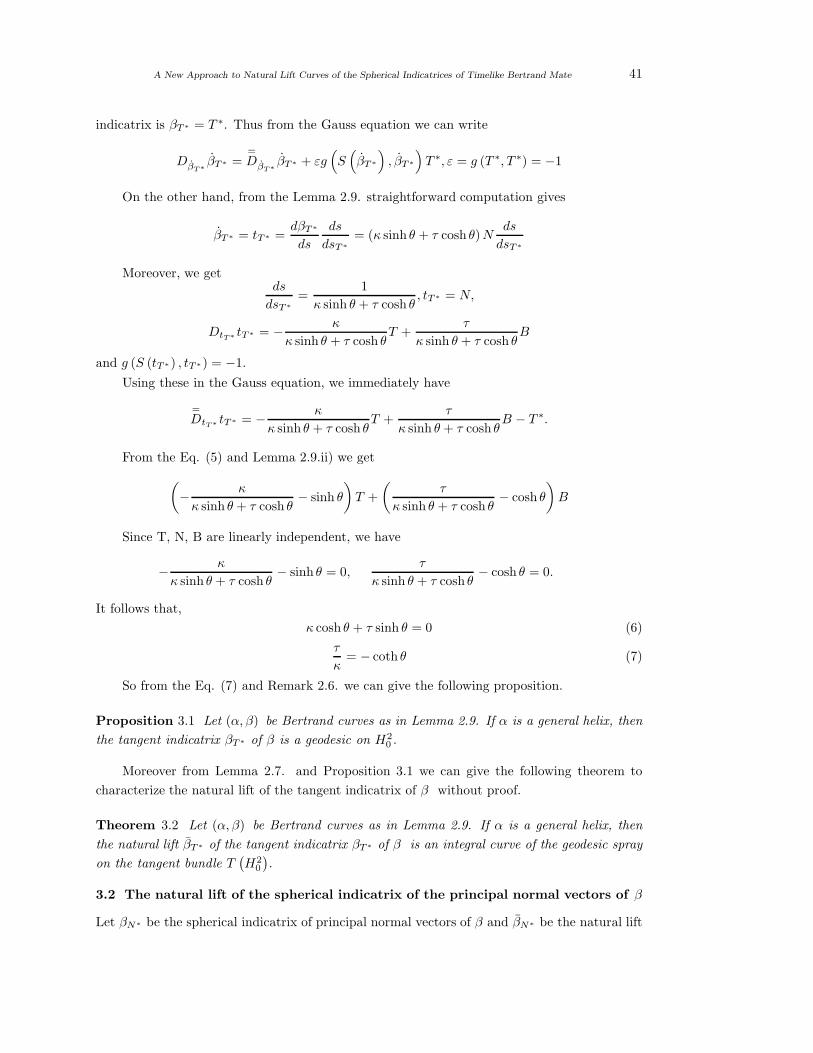
A New Approach to Natural Lift Curves of the Spherical Indicatrices of Timelike Bertrand Mate 41
indicatrix is βT∗ = T ∗. Thus from the Gauss equation we can write
DβT∗βT∗ =
=
DβT∗βT∗ + εg
(S(βT∗
), βT∗
)T ∗, ε = g (T ∗, T ∗) = −1
On the other hand, from the Lemma 2.9. straightforward computation gives
βT∗ = tT∗ =dβT∗
ds
ds
dsT∗
= (κ sinh θ + τ cosh θ)Nds
dsT∗
Moreover, we getds
dsT∗
=1
κ sinh θ + τ cosh θ, tT∗ = N,
DtT∗tT∗ = − κ
κ sinh θ + τ cosh θT +
τ
κ sinh θ + τ cosh θB
and g (S (tT∗) , tT∗) = −1.
Using these in the Gauss equation, we immediately have
=
DtT∗tT∗ = − κ
κ sinh θ + τ cosh θT +
τ
κ sinh θ + τ cosh θB − T ∗.
From the Eq. (5) and Lemma 2.9.ii) we get
(− κ
κ sinh θ + τ cosh θ− sinh θ
)T +
(τ
κ sinh θ + τ cosh θ− cosh θ
)B
Since T, N, B are linearly independent, we have
− κ
κ sinh θ + τ cosh θ− sinh θ = 0,
τ
κ sinh θ + τ cosh θ− cosh θ = 0.
It follows that,
κ cosh θ + τ sinh θ = 0 (6)
τ
κ= − coth θ (7)
So from the Eq. (7) and Remark 2.6. we can give the following proposition.
Proposition 3.1 Let (α, β) be Bertrand curves as in Lemma 2.9. If α is a general helix, then
the tangent indicatrix βT∗ of β is a geodesic on H20 .
Moreover from Lemma 2.7. and Proposition 3.1 we can give the following theorem to
characterize the natural lift of the tangent indicatrix of β without proof.
Theorem 3.2 Let (α, β) be Bertrand curves as in Lemma 2.9. If α is a general helix, then
the natural lift βT∗ of the tangent indicatrix βT∗ of β is an integral curve of the geodesic spray
on the tangent bundle T(H2
0
).
3.2 The natural lift of the spherical indicatrix of the principal normal vectors of β
Let βN∗ be the spherical indicatrix of principal normal vectors of β and βN∗ be the natural lift

42 Mustafa Bilici, Evren Ergun and Mustafa Calıskan
of the curve . If βN∗ is an integral curve of the geodesic spray, then by means of Lemma 2.7.
we get,
DtN∗tN∗ = 0, (8)
that is
DtN∗tN∗ = DtN∗
tN∗ + εg (S (tN∗) , tN∗)N∗, ε = g (N∗, N∗) = 1
On the other hand, from Lemma 2.9. and Case II. i) straightforward computation gives
βN∗ = tN∗ = − sinhϕT + coshϕB
Moreover we get
DtN∗tN∗ = − ϕ coshϕ
‖W‖ T +−κ sinhϕ + τ coshϕ
‖W‖ N +ϕ sinhϕ
‖W‖ B and g (S (tN∗) , tN∗) = 1
Using these in the Gauss equation, we immediately have
DtN∗tN∗ = − ϕ cosh ϕ
‖W‖ T +ϕ sinhϕ
‖W‖ B.
Since T, N, B are linearly independent, we have
− ϕ coshϕ
‖W‖ = 0,ϕ sinhϕ
‖W‖ = 0.
It follows that,
ϕ = 0, (9)
τ
κ= cons tan t. (10)
So from the Eq. (10) and Remark 2.6. we can give the following proposition.
Proposition 3.3 Let (α, β) be Bertrand curves as in Lemma 2.9. If α is a general helix, then
the principal normal indicatrix βN∗ of β is a geodesic on S21 .
Moreover from Lemma 2.7. and Proposition 4.3. we can give the following theorem to
characterize the natural lift of the principal normal indicatrix of β without proof.
Theorem 3.4 Let (α, β) be Bertrand curves as in Lemma 2.9. If α is a general helix, then
the natural lift βN∗ of the principal normal indicatrix of βN∗ is β an integral curve of the
geodesic spray on the tangent bundle T(S2
1
).
3.3 The natural lift of the spherical indicatrix of the binormal vectors of β
Let βB∗ be the spherical indicatrix of binormal vectors of β and βB∗ be the natural lift of the
curve βB∗ . If βB∗ is an integral curve of the geodesic spray, then by means of Lemma 2.7. we
get
DtB∗tB∗ = 0, (11)

A New Approach to Natural Lift Curves of the Spherical Indicatrices of Timelike Bertrand Mate 43
that is
DtB∗tB∗ = DtB∗
tB∗ + εg (S (tB∗) , tB∗)B∗, ε = g (B∗, B∗) = 1
On the other hand, from Lemma 2.9.ii) straightforward computation gives
tB∗ = (κ cosh θ + τ sinh θ)Nds
dsB∗
Moreover we getds
dsB∗
=1
κ cosh θ + τ sinh θ, tB∗ = N,
DtB∗tB∗ = − κ
κ cosh θ + τ sinh θT +
τ
κ cosh θ + τ sinh θB
and g (S (tB∗) , tB∗) = −1.
Using these in the Gauss equation, we immediately have
DtB∗tB∗ =
κ
κ cosh θ + τ sinh θT − τ
κ cosh θ + τ sinh θB + B∗
From the Eq. (11) and Lemma 2.9.ii) we get
(− κ
κ cosh θ + τ sinh θ+ cosh θ
)T +
(τ
κ cosh θ + τ sinh θ+ sinh θ
)B = 0.
Since T, N, B are linearly independent, we have
− κ
κ cosh θ + τ sinh θ+ cosh θ = 0
τ
κ cosh θ + τ sinh θ+ sinh θ = 0
it follows that
κ sinh θ + τ cosh θ = 0 (12)
τ
κ= − tanh θ (13)
So from the Eq. (13) and Remark 2.6. we can give the following proposition.
Proposition 3.5 Let (α, β) be Bertrand curves as in Lemma 2.9. If α is a general helix, then
the binormal indicatrix βB∗ of β is a geodesic on S21 .
Moreover from Lemma 2.7. and Proposition 4.5. we can give the following theorem to
characterize the natural lift of the binormal indicatrix of β without proof.
Theorem 3.6 Let (α, β) be Bertrand curves as in Lemma 2.9. If α is a general helix, then the
natural lift βB∗ of the binormal indicatrix βB∗ of β is an integral curve of the geodesic spray
on the tangent bundle T(S2
1
).
From the classification of all W-curves (i.e. a curves for which a curvature and a torsion
are constants) in (Walrawe, 1995), we have following proposition with relation to curve.

44 Mustafa Bilici, Evren Ergun and Mustafa Calıskan
Proposition 3.7 (1) If the curve α with κ =constant > 0 , τ = 0 then α is a part of a circle;
(2) If the curve α with κ =constant > 0 , τ =constant 6= 0 , and |τ | > κ then α is a part
of a spacelike hyperbolic helix,
α (s)=1
K
(κ sinh
(√Ks)
,√
τ2Ks, κ cosh(√
Ks))
, K = τ2 − κ2;
(3) If the curve α with κ =constant > 0, τ =constant 6= 0 and |τ | < κ, then α is a part of
a spacelike circular helix,
α (s)=1
K
(√τ2Ks, κ cos
(√Ks)
, κ sin(√
Ks)
,√
τ2Ks,)
, K = κ2 − τ2;
From Lemma 3.1 in Choi et al 2012, we can write the following proposition.
Proposition 3.8 There is no spacelike general helix of spacelike curve with a timelike binormal
in Minkowski 3-space with condition |τ | = |κ|.
Example 3.9 Let α (s)= 13
(sinh
(√3s), 2√
3s, cosh(√
3s))
be a unit speed spacelike hyperbolic
helix with
T =
√3
3
(cosh
(√3s)
, 2, sinh(√
3s))
N =(sinh
(√3s)
, 0, cosh(√
3s))
, κ = 1 and τ = 2
B =
√3
3
(2 cosh
(√3s)
, 1, 2 sinh(√
3s))
In this situation, spacelike with spacelike binormal Bertrand mate for can be given by the
equation
β (s) =
((λ +
1
3
)sinh
(√3s)
,2√
3
3s,
(λ +
1
3
)cosh
(√3s))
, λ ∈ R
For λ =√
7−13 , we have
β (s) =
(√7
3sinh
(√3s)
,2√
3
3s,
√7
3cosh
(√3s))
.
The straight forward calculations give the following spherical indicatrices and natural lift
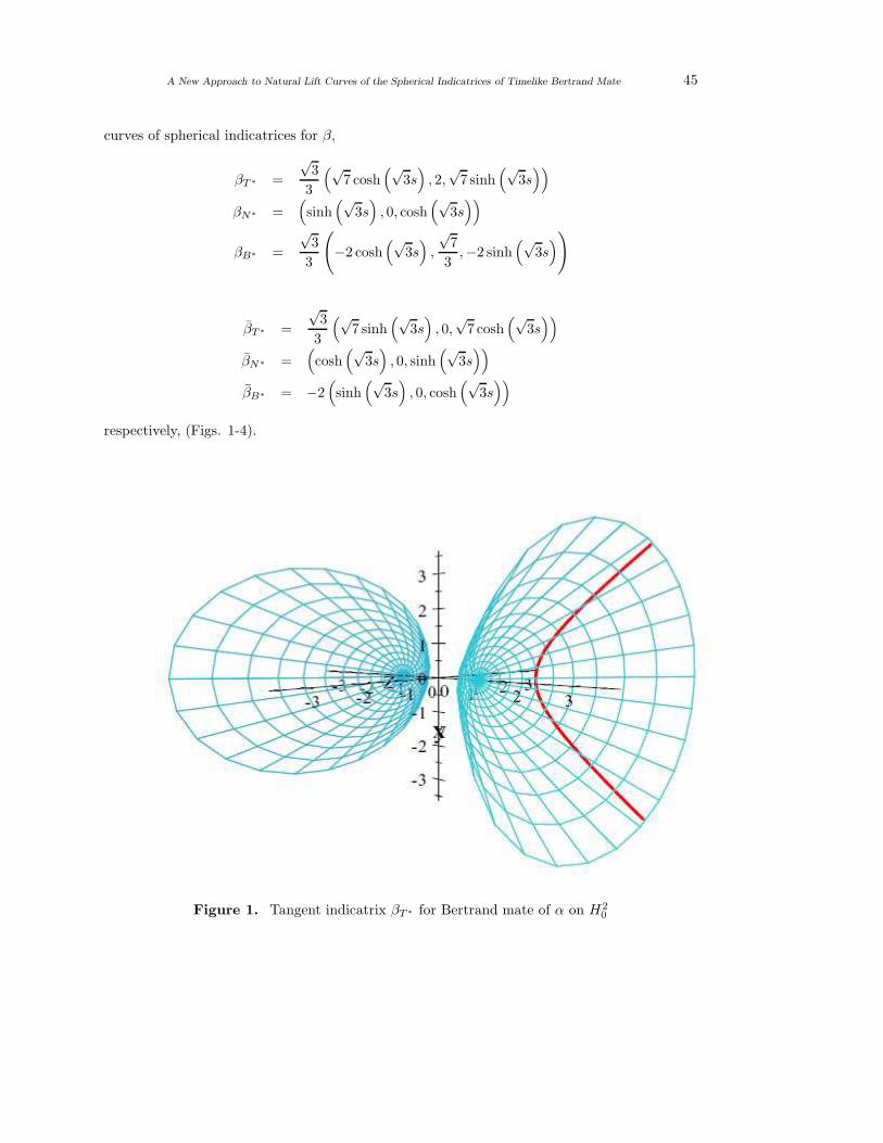
A New Approach to Natural Lift Curves of the Spherical Indicatrices of Timelike Bertrand Mate 45
curves of spherical indicatrices for β,
βT∗ =
√3
3
(√7 cosh
(√3s)
, 2,√
7 sinh(√
3s))
βN∗ =(sinh
(√3s)
, 0, cosh(√
3s))
βB∗ =
√3
3
(−2 cosh
(√3s)
,
√7
3,−2 sinh
(√3s))
βT∗ =
√3
3
(√7 sinh
(√3s)
, 0,√
7 cosh(√
3s))
βN∗ =(cosh
(√3s)
, 0, sinh(√
3s))
βB∗ = −2(sinh
(√3s)
, 0, cosh(√
3s))
respectively, (Figs. 1-4).
Figure 1. Tangent indicatrix βT∗ for Bertrand mate of α on H20

46 Mustafa Bilici, Evren Ergun and Mustafa Calıskan
Figure 2. Principal norma indicatrix βN∗ for Bertrand mate of α on S21
Figure 3. Binormal indicatrix βB∗ for Bertrand mate of α on S21

A New Approach to Natural Lift Curves of the Spherical Indicatrices of Timelike Bertrand Mate 47
Figure 4. Principal norma indicatrix βN∗ and its natural lift curve βN∗ on S21
References
[1] Ekmekci N., Ilarslan K., On Bertrand curves and their characterization, Differential Ge-
omety Dynamical Systems, 3, No.2, 17-24, 2001.
[2] Thorpe J.A., Elemantary Topics In Differantial Geometry, Springer-Verlag, New York,
Heidelberg-Berlin, 1979.
[3] M.P. Do Carmo, Differential Geometry of Curves and Surfaces, Pearson Education, 1976.
[4] Calıskan M., Sivridag A.I. & Hacısalihoglu H.H., Some characterizations for the natural
lift curves and the geodesic spray, Commun. Fac. Sci. Univ., 33: 235-242, 1984.
[5] Petrovic-Torgasev M., Sucurovic E., Some characterizations of the spacelike, the timelike
and null curves on the pseudohyperbolic space in ??, Kragujevac J. Math., 22: 71-82, 2000.
[6] W. Kuhnel, Differential Geometry: Curves-Surfaces-Manifolds, Braunschweig, Wiesbaden,
1999.
[7] Bilici M., Calıskan M. & Aydemir I., The natural lift curves and the geodesic sprays for
the spherical indicatrices of the pair of evolute-involute curves, Int. J. of Appl. Math.,
11(4): 415-420, 2003
[8] Oztekin H. B., Bektas M., Representation formulae for Bertrand curves in the Minkowski
3-space, Scientia Magna, 6(11): 89-96, 2010.
[9] Bilici M., Natural lift curves and the geodesic sprays for the spherical indicatrices of the
involutes of a timelike curve in Minkowski 3-space, International Journal of the Physical

48 Mustafa Bilici, Evren Ergun and Mustafa Calıskan
Sciences, 6(20): 4706-4711, 2011.
[10] O’Neill B., Semi Riemann Geometry, Academic Press, New York, London, 1983.
[11] Ugurlu H.H., On the geometry of time-like surfaces, Commun. Fac. Sci. Univ. Ank.,
Series A1, 46: 211-223, 1997.
[12] Struik D.J., Differential Geometry, Second ed., Addison-Wesley, Reading, Massachusetts,
1961.
[13] Choi J.H., Kim Y.H. & Ali A.T., Some associated curves of Frenet non-lightlike curves in
??, J. Math. Anal. Appl., 394: 712-723, 2012.
[14] Barros M., Ferrandez A., Lucas P. & Merono M.A., General helices in the three-dimensional
Lorentzian space forms, Rocky Mountain J. Math., 31(2): 373-388, 2001.
[15] Nutbourne A.W., Martin R. R., —it Differential Geometry Applied to the Design of Curves
and Surfaces, Ellis Horwood, Chichester, UK, 1988.
[16] Izumiya S., Takeuchi N., Generic properties of helices and Bertrand curves, J. Geom., 74:
97-109, 2002.
[17] Kula L., YaylıY., On slant helix and its spherical indicatrix, Applied Mathematics and
Computation, 169(1): 600-607, 2005.
[18] Millman R.S., Parker G.D., Elements of Differential Geometry, Prentice-Hall Inc., Engle-
wood Cliffs, New Jersey, 1977.
[19] Yılmaz S., Ozyılmaz E., YaylıY. & Turgut M., Tangent and trinormal spherical images of
a time-like curve on the pseudohyperbolic space, Proc. Est. Acad. Sci., 59(3):216–224,
2010.
[20] Iyigun E., The tangent spherical image and ccr-curve of a time-like curve in ??, 2013.
[21] Journal of Inequalities and Applicat2ions,10.1186/1029-242X-2013-55.
[22] Ratcliffe J.G., Foundations of Hyperbolic Manifolds, Springer-Verlag, New York, Inc., New
York, 1994.
[23] Senyurt S., Calıskan O.F., The natural lift curves and geodesic curvatures of the spherical
indicatrices of the spacelike-timelike Bertrand curve pair, International J. Math. Combin.,
2: 47-62, 2014.

International J.Math. Combin. Vol.1(2015), 49-56
Totally Umbilical Hemislant
Submanifolds of Lorentzian (α)-Sasakian Manifold
Barnali Laha and Arindam Bhattacharyya
(Department of Mathematics, Jadavpur University, Kolkata, India)
E-mail: [email protected], [email protected]
Abstract: This paper is summarized as follows. In the first section we have given a brief
history about slant and hemi-slant submanifold of Lorentzian (α)-Sasakian manifold. This
section is followed by some preliminaries about Lorentzian (α)-Sasakian manifold. Finally,
we have derived some interesting results on the existence of extrinsic sphere for totally
umbilical hemi-slant submanifold of Lorentzian (α)-Sasakian manifold.
Key Words: Totally Umbilical, hemi-slant submanifold, extrinsic sphere.
AMS(2010): 53C25, 53C40, 53C42, 53D15
§1. Introduction
Chen in 1990 [2] initiated the study of slant submanifold of an almost Hermitian manifold as
a natural generalization of both holomorphic and totally real submanifolds. After this many
research papers on slant submanifolds appeared. The notion of slant immersion of a Riemannian
manifold into an almost contact metric manifold was introduced by A. Lotta in 1996 [5]. He
studied the intrinsic geometry of 3-dimensional non-anti-invariant slant submanifolds of K-
contact manifold. Further investigation regarding slant submanifolds of a Sasakian manifold
[8] was done by Cabrerizo et al. in 2000. Khan et al. in 2010 defined and studied slant
submanifolds in Lorentzian almost paracontact manifolds [14].
The idea of hemislant submanifold was introduced by Carriazo as a particular class of
bislant submanifolds, and he called them antislant submanifolds in [9]. Recently, in 2009 totally
umbilical slant submanifolds of Kaehler manifold was studied by B.Sahin. Later on, in 2011
Siraj Uddin et.al. studied totally umbilical proper slant and hemislant submanifolds of an
LP-cosymplectic manifold [21].
Our present note deals with a special kind of manifold i.e. Lorentzian (α)-Sasakian man-
ifold. At first we give some introduction about the development of such manifold. An almost
contact metric structure (φ, ξ, η, g) on M is called a trans-Sasakian structure [17] if (MXR, J, G)
belongs to the class W4 [11], where J is the almost complex structure on (MXR) defined by
(J, Xd
dt) = (φX − f, η(X)
d
dt)
1Received May 23, 2014, Accepted February 20, 2015.

50 Barnali Laha and Arindam Bhattacharyya
for all vector fields X on M and smooth functions f on M × R , G is the product metric on
MXR. This may be expressed by the condition
(∇Xφ)Y = α[g(X, Y )ξ + η(Y )X ] + β[g(φX, Y ) − η(Y )φX ],
for some smooth functions α and β on M in [1], and we say that the trans-Sasakian structure
is of type (α, β). A trans-Sasakian structure of type (α, β) is α-Sasakian, if β = 0 and α a
nonzero constant [13]. If α = 1, then α-Sasakian manifold is a Sasakian manifold. Also in
2008 and 2009 many scientists have extended the study to Lorentzian (α)-Sasakian manifold in
[22], [18]. In this paper we have studied some special properties of totally umbilical hemislant
submanifolds of Lorentzian (α)-Sasakian manifold.
§2. Preliminaries
An n-dimensional Lorentzian manifold M is a smooth connected paracontact Hausdorff mani-
fold with a Lorentzian metric g, that is, M admits a smooth symmetric tensor field g of type
(0, 2) such that for each point p ∈ M , the tensor gp : TpM × TpM 7−→ R is a non-degenerate
inner product of signature (−, +, +, · · · , +), where TpM denotes the tangent vector space of
M at p and R is the real number space. A non-zero vector v ∈ TpM is said to be timelike if
it satisfies gp(v, v) < 0 [16]. Let M be an n-dimensional differentiable manifold. An almost
paracontact structure (φ, ξ, η, g), where φ is a tensor of type (1, 1), ξ is a vector field, η is a
1-form and g is Lorentzian metric, satisfying following properties :
φ2X = X + η(X)ξ, η φ = 0, φξ = 0, η(ξ) = −1, (2.1)
g(φX, φY ) = g(X, Y ) + η(X)η(Y ), g(X, ξ) = η(X). (2.2)
for all vector fields X, Y on M . On M if the following additional condition hold for any
X, Y ∈ TM ,
(∇Xφ)Y = α[g(X, Y )ξ + η(Y )X ], (2.3)
∇Xξ = αφX, (2.4)
where ∇ is the Levi-Civita connection on M , then M is said to be an Lorentzian α-Sasakian
manifold (Matsumoto, 1989 [15], [22]).
Let M be a submanifold of M with Lorentzian almost paracontact structure (φ, ξ, η, g)
with induced metric g and let ∇ is the induced connection on the tangent bundle TM and ∇⊥
is the induced connection on the normal bundle T⊥M of M .
The Gauss and Weingarten formulae are characterized by
∇XY = ∇XY + h(X, Y ), (2.5)
∇XN = −ANX + ∇⊥XN, (2.6)
for any X, Y ∈ TM , N ∈ T⊥M , h is the second fundamental form and AN is the Weingarten

Totally Umbilical Hemislant Submanifolds of Lorentzian (α)-Sasakian Manifold 51
map associated with N via
g(ANX, Y ) = g(h(X, Y ), N). (2.7)
For any X ∈ Γ(TM) we can write,
φX = TX + FX, (2.8)
where TX is the tangential component and FX is the normal component of φX . Similarly for
any N ∈ Γ(T⊥M) we can put
φV = tV + fV, (2.9)
where tV denote the tangential component and fV denote the normal component of φV . The
covariant derivatives of the tensor fields T and F are defined as
(∇Xφ)Y = ∇XφY − φ∇XY ∀ X, Y ∈ TM, (2.10)
(∇XT )Y = ∇XTY − T∇XY ∀ X, Y ∈ TM, (2.11)
(∇XF )Y = ∇⊥XFY − F∇XY, ∀ X, Y ∈ TM. (2.12)
From equation (2.3), (2.5), (2.8), (2.9), (2.11) and (2.12) we can calculate
(∇XT )Y = α[g(X, Y )ξ + η(Y )X ] + AFY X + th(X, Y ), (2.13)
(∇XF )Y = −h(X, TY ) + fh(X, Y ). (2.14)
A submanifold M is said to be invariant if F is identically zero, i.e., φX ∈ Γ(TM) for any
X ∈ Γ(TM). On the other hand, M is said to be anti-invariant if T is identically zero, i.e.,
φX ∈ Γ(T⊥M) for any X ∈ Γ(TM).
A submanifold M of M is called totally umbilical if
h(X, Y ) = g(X, Y )H, (2.15)
for any X, Y ∈ Γ(TM). The mean curvature vector H is denoted by H =∑ki=1 h(ei, ei), where k is the dimension of M and e1, e2, e3, · · · , ek is the local orthonormal
frame on M . A submanifold M is said to be totally geodesic if h(X, Y ) = 0 for each X, Y ∈Γ(TM) and is minimal if H = 0 on M .
§3. Slant Submanifolds of a Lorentzian (alpha)-Sasakian Manifold
Here, we consider M as a proper slant submanifold of a Lorentzian (α)-Sasakian manifold M .
We always consider such submanifold tangent to the structure vector field ξ.
Definition 3.1 A submanifold M of M is said to be slant submanifold if for any x ∈ M and
X ∈ TxM \ ξ, the angle between φX and TxM is constant. The constant angle θ ∈ [0, π/2] is
then called slant angle of M in M . If θ = 0 the submanifold is invariant submanifold, if θ = π/2
52 Barnali Laha and Arindam Bhattacharyya
then it is anti-invariant submanifold and if θ 6= 0, π/2 then it is proper slant submanifold.
From [20] we have
Theorem 3.1 Let M be a submanifold of an Lorentzian (α)-Sasakian manifold M such that
ξ ∈ TM . Then M is slant submanifold if and only if there exists a constant λ ∈ [0, 1] such that
T 2 = λ(I + η ⊗ ξ). (3.1)
Again, if θ is slant angle of M , then λ = cos2 θ.
From [20], for any X, Y tangent to M , we can easily draw the following results for an
Lorentzian (α)-Sasakian manifold M ,
g(TX, TY ) = cos2θg(X, Y ) + η(X)η(Y ), g(FX, FY ) = sin2θg(X, Y ) + η(X)η(Y ).
Definition 3.2 A submanifold M of M is said to be hemi-slant submanifold of a Lorentzian
(α)-Sasakian manifold M if there exists two orthogonal distribution D1 and D2 on M such that
(a) TM = D1 ⊕ D2⊕ < ξ >;
(b) The distribution D1 is anti-invariant i.e., φD1 ⊆ T⊥M ;
(c) The distribution D2 is slant with slant angle θ 6= π/2.
If µ is invariant subspace under φ of the normal bundle T⊥M , then in the case of hemi-slant
submanifold, the normal bundle T⊥M decomposes as
T⊥M =< µ > ⊕φD⊥ ⊕ FDθ.
The curvature tensor of an Lorentzian (α)-Sasakian manifold is defined as [4]
R(X, Y )Z = ∇X∇Y Z − ∇Y ∇XZ − ∇[X,Y ]Z. (3.2)
For the curvature tensor we can compute by using the equations (2.10) and (3.2) the relation
R(X, Y )φZ = φR(X, Y )Z + α2g(Y, Z)φX − α2g(X, Z)φY (3.3)
−α2g([X, Y ], Z)φX + αg(X, ∇Y Z)ξ + αη(∇Y Z)X
−αg(Y, ∇XZ)ξ − αη(∇XZ)Y − αη(Z)∇XY
+αη(Z)∇Y X − αη(Z)[X, Y ] + αg(∇XY, Z)ξ + αg(∇Y X, Z)ξ.
Definition 3.3 A submanifold of an arbitrary Lorentzian (α)-Sasakian manifold which is totally
umbilical and has a nonzero parallel mean curvature vector [10] is called an Extrinsic sphere.
§4. Main Results
This section mainly deals with a special class of hemi-slant submanifolds which are totally

Totally Umbilical Hemislant Submanifolds of Lorentzian (α)-Sasakian Manifold 53
umbilical. Throughout this section we have considered M as a totally umbilical hemi-slant
submanifold of Lorentzian (α)-Sasakian manifold. We derive the following.
Theorem 4.1 Let M be a totally umbilical hemi-slant submanifold of a Lorentzian (α)-Sasakian
manifold M such that the mean curvature vector H ∈< µ >. Then one of the following is true:
(i) M is totally geodesic;
(ii) M is semi-invariant submanifold.
Proof For V ∈ φD⊥ and X ∈ Dθ, we have from (2.3), (2.5),(2.6) and (2.10)
α[g(X, V )ξ + η(V )X ] = ∇XφV + g(X, φV )H + φAV X − φ∇⊥XV. (4.1)
Since the distributions are orthogonal and from the assumption that H ∈ µ, above equation
can be written as
g(∇⊥XV, H) = g(V,∇⊥
XH) = 0. (4.2)
This implies ∇⊥XH ∈ µ ⊕ FDθ. Now for any X ∈ Dθ, we obtain on using the Gauss and
Weingarten equations
α[g(X, H)ξ + η(H)X ] = ∇⊥XφH − AφHX + φAHX − φ∇⊥
XH. (4.3)
Now, using the assumption that , M is totally umbilical we have
αη(H)X = ∇⊥XφH − Xg(H, φH) + φXg(H, H) − φ∇⊥
XH. (4.4)
On using equation (2.8) we calculate
αη(H)X = ∇⊥XφH + TXg(H, H) + FXg(H, H)− φ∇⊥
XH. (4.5)
Taking inner product with FX ∈ FDθ,
αη(H)g(X, FX) = g(∇⊥XφH, FX) + g(FX, FX)g(H, H) − g(φ∇⊥
XH, FX). (4.6)
From Theorem 3.1 the equation becomes
αη(H)g(X, FX) − g(∇⊥XφH, FX) − sin2θ||H ||2||X ||2 + g(φ∇⊥
XH, FX) = 0. (4.7)
If either H 6= 0 then Dθ = 0, i.e. M is totally real submanifold, and if Dθ 6= 0, M is totally
geodesic submanifold or M is semi-invariant submanifold. For any Z ∈ D⊥ from (2.13) we get
∇ZTZ − T∇ZZ = α[g(Z, Z)ξ + η(Z)Z] + AFZZ + th(Z, Z). (4.8)

54 Barnali Laha and Arindam Bhattacharyya
Taking inner product with W ∈ D⊥ the above equation takes the form
g(∇ZTZ, W ) − g(T∇ZZ, W ) = α[g(Z, Z)g(ξ, W ) + η(Z)g(Z, W )] (4.9)
+g(AFZZ, W ) + g(th(Z, Z), W ).
As M is totally umbilical hemi-slant submanifold and using (2.7) we can write
g(∇ZTZ, W ) − g(T∇ZZ, Z) = αg(Z, W )g(H, FZ) + g(tH, W )||Z||2. (4.10)
The above equation has a solution if either H ∈ µ or dim D⊥ = 1. 2If however, H does not belong to µ then we give the next theorem.
Theorem 4.2 Let M be a totally umbilical hemi-slant submanifold of a Lorentzian (α)-Sasakian
manifold M such that the dimension of slant distribution Dθ ≥ 4 and F is parallel to the
submanifold, then M is either extrinsic sphere or anti-invariant submanifold.
Proof Since the dimension of slant distribution Dθ ≥ 4, therefore we can select a set of
orthogonal vectors X, Y ∈ Dθ, such that g(X, Y ) = 0. Now by replacing Z by TY in (3.4) we
have for any X, Y, Z ∈ Dθ,
R(X, Y )φTY = φR(X, Y )TY + α2g(Y, TY )φX (4.11)
−α2g(X, TY )φY − α2g([X, Y ], TY )
+αg(X, ∇Y TY )ξ + αη(∇Y TY )X
−αg(Y, ∇XTY )ξ − αη(∇XTY )Y.
Now using equation (2.3) and (3.1) we obtain on calculation
R(X, Y )FTY + cos2θR(X, Y )Y = φR(X, Y )TY + α2g(Y, TY )φX (4.12)
−α2g(X, TY )φY − α2g([X, Y ], TY )
+αg(X, ∇Y TY )ξ + αη(∇Y TY )X
−αg(Y, ∇XTY )ξ − αη(∇XTY )Y.
Again if F is parallel, then above equation can be written as
FR(X, Y )TY + cos2θR(X, Y )Y = φR(X, Y )TY + α2g(Y, TY )φX (4.13)
−α2g(X, TY )φY − α2g([X, Y ], TY )
+αg(X, ∇Y TY )ξ + αη(∇Y TY )X
−αg(Y, ∇XTY )ξ − αη(∇XTY )Y.
Taking inner product with N ∈ T⊥M , we obtain on using (3.3) and the orthogonality of
X and Y vectors,
cos2θ||Y ||2g(∇⊥XH, N) = 0
Totally Umbilical Hemislant Submanifolds of Lorentzian (α)-Sasakian Manifold 55
The above equation has a solution if either θ = π/2 i.e. M is anti-invariant or ∇⊥XH =
0 ∀ X ∈ Dθ. Similarly for any X ∈ D⊥⊕ < ξ > we can obtain ∇⊥XH = 0, therefore ∇⊥
XH =
0 ∀ X ∈ TM i.e. the mean curvature vector H is parallel to submanifold, i.e., M is extrinsic
sphere. Hence the theorem is proved. 2Now we are in a position to draw our main conclusions following.
Theorem 4.3 Let M be a totally umbilical hemi-slant submanifold of a Lorentzian (α)-Sasakian
manifold M. then M is either totally geodesic, or semi-invariant, or dim D⊥ = 1, or Extrinsic
sphere, and the case (iv) holds if F is parallel and dim M ≥ 5.
Proof The proof follows immediately from Theorems 4.1 and 4.2. 2References
[1] D.E.Blair and J.A.Oubina, Conformal and related changes of metric on the product of two
almost contact metric manifolds, Publications Matematiques, Vol. 34, 1990, pp. 99-207.
[2] B.Y.Chen, Slant immersions, Bulletin of the Australian Mathematical Society, vol. 41,
no.1, pp. 135-147, 1990.
[3] B.Y.Chen, Geometry of slant Submnaifolds, Katholieke Universiteit Leuven, Leuven, Bel-
gium, 1990.
[4] U.C.De, A.A.Shaikh, Complex Manifolds and Contact Manifolds, Narosa Publishing House
Pvt. Ltd.
[5] A.Lotta, Slant submanifolds in contact geometry, Bull.Math.Soc. Roumanie, 39(1996),
183-198.
[6] N.Papaghiuc, Semi-slant submanifolds of Kaehlerian manifold, An.Stiint.Univ.Al. I. Cuza
Iasi, Ser.Noua, mat. 40(1)(1994), 55-61.
[7] J.L.Cabrerizo, A.Carriazo, L.M.Fernandez, M.Fernandez, Semi-slant submanifolds of a
Sasakian manifold, Geom.Dedicata, 78(1999), 183-199.
[8] J.L.Cabrerizo, A.Carriazo, L.M.Fernandez, M.Fernandez, Slant submanifolds in Sasakian
manifolds, Glasg. Math. J., 42(2000).
[9] A.Carriazo, Bi-slant immersions, in Proceedings of the Integrated Car Rental and Accounts
Management System, pp 88-97, Kharagpur, West Bengal, India, 2000.
[10] S.Deshmukh and S.I.Hussain, Totally umbilical CR-submanifolds of a Kaehler manifold,
Kodai Math. J., 9(3)(1986), 425-429.
[11] A.Gray and L.M.Hervella, The sixteen classes of almost Hermitian manifolds and their
linear invariants, Annali di Matematica Pura ed Applicata, Vol. 123, No. 4, 1980, pp.
35-58. doi:10.1007/BF01796539.
[12] S.K.Hui, S.Uddin, C.Ozel, A.A.Mustafa, Warped product submanifolds of LP-Sasakian
manifold, Hindawi Publishing Corporation, Discrete Dynamics in nature and Society,
Vol.2012, Article ID 868549.
[13] D.Janssens and L.Vanhecke, Almost contact structures and curvature tensors, Kodai Math-
ematical Journal, Vol. 4, No. 1, 1981, pp.1-27. doi:10.2996/kmj/1138036310.
56 Barnali Laha and Arindam Bhattacharyya
[14] M.A.Khan, K.Singh and V.A.Khan, Slant submanifolds of LP-contact manifolds, Differ-
ential Geometry Dynamical Systems, vol.12, pp. 102-108, 2010.
[15] K.Matsumoto, On Lorentzian paracontact manifolds, Bull.Yamagata Univ. Nat. Sci., 12,
pp. 151-156.
[16] B.O’Neill, Semi Riemannian Geometry with Applications to Relativity, Academy Press,
Inc.1953.
[17] J.A.Oubina, New classes of contact metric structures, Publicationes Mathematicae Debre-
cen, Vol.32, No. 4, 1985, pp. 187-193.
[18] D.G.Prakasha, C.S.Bagewadi and N.S.Basavarajappa, On pseudosymmetric Lorentzian α-
Sasakian manifolds, IJPAM, Vol. 48, No. 1, 2008, 57-65.
[19] B.Sahin, Every totally umbilical proper slant submanifold of a Kaehler manifold is totally
geodesic, Results in Mathematics, vol.54, no.1-2, pp. 167-172, 2009.
[20] Khushwant Singh, Siraj Uddin, Cenap Ozel, M.A.Khan, A class of totally umbilical slant
submanifolds of Lorentzian para-saskian manifolds, International Journal of Physical Sci-
ence, vol. 7(10), pp. 1526-1529, 2012.
[21] S.Uddin, M.A.Khan, K.Singh, Totally Umbilical Proper slant and hemislant submanifolds
of an LP-cosymplectic manifold, Hindawi Publishing Corporation, Mathematical Problems
in Engineering, vol.2011, Article ID 516238.
[22] A.Yildiz, M.Turan and B.F.Acet, On three dimensional Lorentzian α-Sasakian manifolds,
Bulletin of mathematical Analysis and Applications, Vol. 1, Issue 3(2009), pp. 90-98.

International J.Math. Combin. Vol.1(2015), 57-64
On Translational Hull Of Completely J ∗,∼-Simple Semigroups
Yizhi Chen1, Siyan Li1 and Wei Chen2
1. Department of Mathematics, Huizhou University, Huizhou 516007, P.R.China
2. School of Mathematics and Statistics, Minnan Normal University, Zhangzhou 363000, P.R.China.
E-mail: [email protected]
Abstract: In this paper, we give a construction theorem about the translational hull
of completely J ∗,∼−simple semigroups which extends the translational hulls of completely
J ∗−simple semigroups and completely simple semigroups.
Key Words: Translational hull; completely J ∗,∼−simple semigroup; construction.
AMS(2010): 20M10
§1. Introduction
Let S be a semigroup. A mapping λ from a semigroup S to itself is a left translation of S if
λ(ab) = (λa)b for all elements a, b of S; a mapping ρ from S to itself is a right translation of S if
(ab)ρ = a(bρ) for all elements a, b of S. A left translation λ and right translation ρ are linked if
a(λb) = (aρ)b for all a, b of S, in this case, the pair (λ, ρ) is a bitranslation of S. The set Λ(S) of
all left translations of S and the set P (S) of all right translations of S are semigroups under the
composition of mappings. The translational hull of S is the subsemigroup Ω(S) of Λ(S)×P (S)
of all bitranslations of S. A left translation λ is inner if λ = λa for some a ∈ S, where λax = ax
for all x ∈ S; an inner right translation ρa is defined dually; the pair πa = (λa, ρa) is an inner
bitranslation and the set Π(S) of all inner bitranslations is the inner part of Ω(S) (actually an
ideal of Ω(S)).
The translation hull of semigroups plays an important role in the algebraic theory of
semigroups. It is an important tool in the study of ideal extensions. For more related details
of translational hulls, the reader is referred to [1], [4], [5], [7],[14],[15]..
In order to generalize regular semigroups, new Green’s relations, namely, the Green’s ∗-relations on a semigroup have been introduced as follows ([11], [12]):
L∗ = (a, b) ∈ S × S : (∀x, y ∈ S1)ax = ay ⇔ bx = by,
R∗ = (a, b) ∈ S × S : (∀x, y ∈ S1)xa = ya ⇔ xb = yb,1Supported by Grants of the NNSF of China (No. 11401246, 11426112); the NSF of Guangdong Province
(Nos.2014A030310087, 2014A030310119); the NSF of Fujian Province(2014J01019); the Outstanding YoungInnovative Talent Training Project in Guangdong Universities (No. 2013LYM0086); Science Technology Projectof Huizhou City .
2Received May 23, 2014, Accepted December 2, 2014.

58 Yizhi Chen, Siyan Li and Wei Chen
H∗ = L∗ ∩R∗,
D∗ = L∗ ∨R∗,
(a, b) ∈ J ∗ ⇔ J∗(a) = J∗(b),
where J∗(a) and J∗(b) are the principal ∗− ideals generated by a and b respectively.
In [3], Fountain investigated a class of semigroups called abundant semigroups in which
each L∗−class and each R∗−class of S contain at least an idempotent. And from which,
we know that, the class of regular semigroups are properly contained in the one of abundant
semigroups.
According to [3], a semigroup in which every idempotent is primitive is said to be a primitive
semigroup, and an abundant semigroup S is called a completely J ∗−simple semigroup if S itself
is primitive and the idempotents of S generate a regular subsemigroup of S. Clearly, completely
J ∗−simple semigroups extend completely simple semigroups studied by Clifford and Petrich in
[2].
Later on, Ren and Shum [16] investigated the structure of superabundant semigroups, and
generalized the corresponding results of completely regular semigroups in [15].
On the other hand, in order to further generalize completely regular semigroups [super-
abundant semigroups] in the class of rpp semigroups, Guo, Shum and Gong [10] introduced the
so-called (∗,∼)-Green’s relations on a semigroup S. The relations L∗,∼ and R∗,∼ are respec-
tively defined as L∗ and R. The intersection and the join of L∗,∼ and R∗,∼ are respectively
denoted by H∗,∼ and D∗,∼ . The relation J ∗,∼ is defined by the rule that aJ ∗,∼b if and only
if J∗,∼(a) = J∗,∼(b), Where, for any a, b ∈ S, aRb if and only if for all e ∈ E(S), ea = a if and
only if eb = b, and J∗,∼(a) is the smallest ideal containing a and saturated by L∗,∼ and R∗,∼.
According to [10], a semigroup S is called an r-ample semigroup if S is L∗,∼-abundant and
R∗,∼-abundant, here we call that S is σ-abundant, if every equivalence σ-class of S contains
idempotents of S. An r-ample semigroup is called a super-r-ample semigroup, if S is H∗,∼-
abundant. The class of super-r-ample semigroups forms a proper extension class of the class of
superabundant semigroups. It was shown in [10] that R∗,∼ usually is not a left congruence on
S even if S is anR∗,∼-abundant semigroup, but in a super-r-ample semigroup S, the relation
R∗,∼ is a left congruence on S.
In [9], the authors defined a class of completely J ∗,∼-simple semigroups, and give the
structure of such semigroups which extended the celebrated Rees theorem for completely simple
semigroups. According to [9], a super-r-ample semigroup S is called a completely J ∗,∼-simple
semigroup if S is J ∗,∼-simple. Clearly, a completely J ∗-simple semigroup must be completely
J ∗,∼-simple.
Note from [15] and [1] that, the translational hulls of completely simple semigroups and
completely J ∗−simple semigroups have been solved, so naturally, we will quote such a question:
what is the translational hull of completely J ∗,∼−simple semigroups, do we have some similar
results with the ones of completely J ∗,∼−simple semigroups or completely simple semigroups?
In this paper, we will set out to discuss the above question, and finally establish a construc-
tion theorem about the translational hull of completely J ∗,∼−simple semigroups which extend
the translational hulls of completely J ∗−simple semigroups and completely simple semigroups.

On Translational Hull Of Completely J ∗,∼-Simple Semigroups 59
For notations and terminologies not mentioned in this paper, the readers are referred to
[5],[9] or [10].
§2. Main Results
Definition 2.1 ([6], Definition 1) Let M[T ; I, Λ; P ] be a Rees matrix semigroup and P the
Λ × I matrix over a left cancellative monoid T . Then P is said to be normalized at 1 if there
is an element 1 ∈ I ∩ Λ such that p1i = pλ1 = e for all i ∈ I, λ ∈ Λ, where e is the identity of
the left cancellative monoid T . Furthermore, the Rees matrix semigroup M[T ; I, Λ; P ] is called
normalized if P is normalized.
Lemma 2.2 ([6], Theorem 1) Let T be a left cancellative monoid with an identity element e
and I, Λ be nonempty sets. Let P = (pλi) be a Λ × I matrix where each entry in P is a unit
of T . Suppose that P is normalized at 1 ∈ I ∩ Λ. Then the normalized Rees matrix semigroup
M = M[T ; I, Λ; P ] is completely J ∗,∼−simple semigroup.
Conversely, every completely J ∗,∼−simple semigroup is isomorphic to a normalized Rees
matrix semigroup M = M[T ; I, Λ; P ] over a left cancellative monoid T .
By Lemma 2.2, we know that if S is a completely J ∗,∼− simple semigroup, then it can be
isomorphic to a normalized Rees matrix semigroup M = M[T ; I, Λ; P ] over a left cancellative
monoid T . Hence, to discuss the translational hulls of completelyJ ∗,∼−simple semigroups, we
can also consider the cases of normalized Rees matrix semigroups M = M[T ; I, Λ; P ] over a
left cancellative monoid T for convenience.
In the following, we will establish the translational hull of a normalized Rees matrix semi-
group M = M[T ; I, Λ; P ] over a left cancellative monoid T . Before we give our main result, it
will be useful to make use of the following notation.
Notation We set M[T ; I, Λ; P ] with P normalized at 1 ∈ I × Λ and denoted by e the
identity of T . Let T (S) = (F, t, Φ) ∈T ′
(I)×T×T (Λ)| for all i ∈ I, µ ∈ Λ, pµ,Fitp1Φ,i =
pµ,F1tpµΦ,i with multiplication (F, t, Φ)(F′
, t′
, Φ′
) = (FF′
, tp1Φ,F ′1t′
, ΦΦ′
) for all i ∈ I and
λ ∈ Λ, where T ′
(I) (T (Λ)) means the semigroup of all full transformations on I (Λ) and all of
the transformations are written on the left (right).
Theorem 2.3 Let S = M[T ; I, Λ; P ] with P normalized, each entry in P is a unit of T ,and
let e be the identity of T . Define a mapping σ from Ω(S) to T (S) by
σ : (λ, ρ) → (F, t, Φ) ((λ, ρ) ∈ Ω(S))
where F, t and Φ are defined by the requirements
λ(i, e, 1) = (Fi, · · · , · · · ) ∈ S, (1)
(1, e, 1)ρ = (· · · , t, · · · ) ∈ S, (2)
60 Yizhi Chen, Siyan Li and Wei Chen
(1, e, µ)ρ = (· · · , · · · , µΦ) ∈ S. (3)
Further define a mapping τ from T (S) to Ω(S) by
τ : (F, t, Φ) → (λ, ρ) ((F, t, Φ) ∈ T (S)),
where λ and ρ are defined by the formulas
λ(i, h, µ) = (Fi, tp1Φ,ih, µ) ((i, h, µ) ∈ S), (4)
(i, h, µ)ρ = (i, hpµ,F1t, µΦ) ((i, h, µ) ∈ S). (5)
Then σ and τ are mutually inverse isomorphisms between Ω(S) and T (S).
Proof We will show the theorem by the following steps.
(i) σ is a mapping.
Let (λ, ρ) ∈ Ω(S). For any (i, h, µ) ∈ S, we have
λ(i, h, µ) = λ[(i, h, 1)(1, e, µ)] = [λ(i, h, 1)](1, e, µ),
so that λ(i, h, µ) = (j, h′
, µ) for some j ∈ I and h′ ∈ T . Similarly, we have (i, h, µ)ρ = (i, h
′′
, ν)
for some h′′ ∈ T and ν ∈ Λ. In the following, we will use the above statements repeatedly. In
particular, we may define si and rµ by
λ(i, e, 1) = (Fi, si, 1) (i ∈ I),
(1, e, µ)ρ = (1, rµ, µΦ) (λ ∈ Λ).
By the definition of t in this theorem, we have t = r1. Also, notice that
[(1, e, 1)ρ](i, e, 1) = (1, t, 1Φ)(i, e, 1) = (1, tp1Φ,i, 1),
(1, e, 1)[λ(i, e, 1)] = (1, e, 1)(Fi, si, 1) = (1, si, 1),
we have si = tp1Φ,i. Thus,
λ(i, h, µ) = λ[(i, e, 1)(1, h, µ)] = [λ(i, e, 1)](1, h, µ)
= (Fi, si, 1)(1, h, µ) = (Fi, tp1Φ,i, 1)(1, h, µ)
= (Fi, tp1Φ,ih, µ).
This proves (4). With a similar argument, we can establish (5). Hence,
(1, e, µ)[λ(i, e, 1)] = (1, e, µ)(Fi, tp1Φ,i, 1) = (1, pµ,Fitp1Φ,i, 1),
[(1, e, µ)ρ](i, e, 1) = (1, pµ,F1, µΦ)(i, e, 1) = (1, pµ,F1tpµΦ,i, 1).

On Translational Hull Of Completely J ∗,∼-Simple Semigroups 61
Since (λ, ρ) ∈ Ω(S), we have pµ,Fitp1Φ,i = pµ,F1tpµΦ,i, and then (F, t, Φ) ∈ T (S), and (i) holds.
(ii) τ is a mapping.
Let (F, t, Φ) ∈ T (S), and let λ and ρ be defined as (4) and (5) respectively. Then for
(i, h, µ), (j, k, ν) ∈ S, we have
[λ(i, h, µ)](j, k, ν) = (Fi, tp1Φ,ih, µ)(j, k, ν) = (Fi, tp1Φ,ihpµjk, ν)
= λ(i, hpµjk, ν) = λ[(i, h, µ)(j, k, ν)].
Hence, λ is a left translation. Similarly, we can show that ρ is a right translation. Further, on
the one hand,
(i, h, µ)[λ(j, k, ν)] = (i, h, µ)(Fj, tp1Φ,jk, ν) = (i, hpµ,Fjtp1Φ,jk, ν), (6)
on the other hand,
[(i, h, µ)ρ](j, k, ν) = (i, hpµ,F1t, µΦ)(j, k, ν) = (i, hpµ,F1tpµΦ,jk, ν), (7)
and notice that (F, t, Φ) ∈ T (S), we can immediately obtain that (6) and (7) are equal. And
then (λ, ρ) ∈ Ω(S). Thus, τ is a mapping from T (S) to Ω(S), and (ii) holds.
(iii) στ is an identity mapping on Ω(S).
Let (λ, ρ) ∈ Ω(S), and let (λ, ρ)στ = (F, t, Φ)τ = (λ′
, ρ′
) so that λ′
(i, h, µ) = (Fi, tp1Φ,ih, µ).
By the proof of (i), we know (4) holds for λ,thus, we have λ = λ′
. Similarly, we have ρ = ρ′
.
Hence, (iii) holds.
(iv) τσ is an identity mapping on T (S).
Let (F, t, Φ) ∈ T (S), and let (F, t, Φ)τσ = (λ, ρ)σ = (F′
, t′
, Φ′
). Then (4) and (5) are
satisfied, and thus λ(i, e, 1) = (Fi, tp1Φ,1, 1), (1, e, µ)ρ = (1, pµ,F1t, µΦ). By (1),(2) and (3), we
immediately obtain that F = F′
, t = t′
, and Φ = Φ′
. Consequently, τσ is the identity mapping
on T (S).
(v) τ is a homomorphism.
Let (F, t, Φ)τ = (λ, ρ), (F′
, t′
, Φ′
)τ = (λ′
, ρ′
), and (FF′
, tp1Φ,F ′1t′
, ΦΦ′
)τ = (ξ, η). On the
one hand, we have
λλ′
(i, h, µ) = λ(F′
i, t′
p1Φ′,ih, µ) = (FF′
i, tp1Φ,F ′ it′
p1Φ′ ,ih, µ). (8)
On the other hand ,
ξ(i, h, µ) = (FF′
i, tp1Φ,F ′1t′
p1ΦΦ′ ,ih, µ). (9)
Since (F′
, t′
, Φ′
) ∈ T (S), we have p1Φ,F ′ it′
p1Φ′ ,i = p1Φ,F ′1t′
p1ΦΦ′ ,i, and then (8) and (9) are
equal. That is, λλ′
= ξ. Similarly, we can prove that ρρ′
= η. Therefore, τ is a homomorphism.

62 Yizhi Chen, Siyan Li and Wei Chen
(vi) Analogous with the proof of (v), we can prove that σ is a homomorphism.
Summing up the six steps above, we have shown that both σ and τ are isomorphisms. 2Remark 2.4 From Theorem 2.3, we know that, under the isomorphism, the translational hull
of a normalized Rees matrix semigroup M = M[T ; I, Λ; P ] over a left cancellative monoid T can
regard as the semigroup T (S), whose elements and multiplications are defined in the Notation.
And then by Lemma 2.2, the translational hull of a completely J ∗,∼-simple semigroup can be
also regarded as this form up to isomorphism.
Further, from Remark 1 in [9], we know that if S is an abundant semigroup, then R∗,∼=R∗.
Hence S is a completely J ∗,∼ -simple semigroup if and only if S is a completely J ∗-simple
semigroup; S is a left cancellative monoid if and only if S is a cancellative monoid. If S is a
regular semigroup, then R∗,∼=R∗, L∗,∼=L∗. Hence S is a completely J ∗,∼-simple semigroup
if and only if S is a completely simple semigroup; S is a left cancellative monoid if and only if
S is a group.
Now, if we let left cancellative monoid T be a cancellative monoid in Theorem 2.3, then
we can immediately get the translational hull of a completely J ∗–simple semigroup which is
the main theorem in [1].
Corollary 2.5 Let S = M[T ; I, Λ; P ] with P normalized, each entry in P is a unit of cancella-
tive monoid T ,and let e be the identity of T . Define a mapping σ by
σ : (λ, ρ) → (F, t, Φ) ((λ, ρ) ∈ Ω(S))
where F, t and Φ are defined by the requirements
λ(i, e, 1) = (Fi, · · · , · · · ) ∈ S, (1)
(1, e, 1)ρ = (· · · , t, · · · ) ∈ S, (2)
(1, e, µ)ρ = (· · · , · · · , µΦ) ∈ S. (3)
Further define a mapping τ by
τ : (F, t, Φ) → (λ, ρ) ((F, t, Φ) ∈ T (S)),
where λ and ρ are defined by the formulas
λ(i, h, µ) = (Fi, tp1Φ,ih, µ) ((i, h, µ) ∈ S), (4)
(i, h, µ)ρ = (i, hpµ,F1t, µΦ) ((i, h, µ) ∈ S). (5)
Then σ and τ are mutually inverse isomorphisms between Ω(S) and T (S).
Also, if we let T be a group G in Theorem 2.3, then we can immediately get the translational
hull of a completely simple semigroup which is the Theorem III.7.2 in [15].

On Translational Hull Of Completely J ∗,∼-Simple Semigroups 63
Corollary 2.6 Let S = M[G; I, Λ; P ] with P normalized, and let e be the identity of group G.
Define a mapping σ by
σ : (λ, ρ) → (F, g, Φ) (λ, ρ) ∈ Ω(S))
where F, g and Φ are defined by the requirements
λ(i, e, 1) = (Fi, · · · , · · · ) (1)
(1, e, 1)ρ = (· · · , g, · · · ) (2)
(1, e, µ)ρ = (· · · , · · · , µΦ) (3)
Further define a mapping τ by
τ : (F, g, Φ) → (λ, ρ) ((F, g, Φ) ∈ T (S)),
where λ and ρ are defined by the formulas
λ(i, h, µ) = (Fi, gp1Φ,ih, µ) (i, h, µ) ∈ S), (4)
(i, h, µ)ρ = (i, hpµ,F1g, µΦ), (i, h, µ) ∈ S). (5)
Then σ and τ are mutually inverse isomorphisms between Ω(S) and T (S).
References
[1] CHEN Y.Z., LI Y.H., The translational hull of completely J ∗– simple semigroups, Journal
of South China Normal University, 2007,1:28–31.
[2] CLIFFORD A.H., PETRICH M., Some classes of completely regular semigroups, J. Alge-
bra, 1977, 46:462–480.
[3] FOUNTAIN J.B., Abundant semigroups, Proc London Math. Soc., 1982,44(3):103–129.
[4] FOUNTAIN J.B., LAWSON M V., The translational hull of an adequte semigroup, Semi-
group Forum, 1985, 32:79–86.
[5] HOWIE J.M., Fundamentals of Semigroup Theory, Oxford:Clarendon Press,1995.
[6] GONG C., ZHANG D., YUAN Y., The structure of completely J ∗,∼– simple semigroups,
Journal of Southwest Normal University(Natural Science Edition), 2011, 36(1): 21-25.
[7] GUO X.J., SHUM K.P., On translational hulls of type A semigroups, J. Algebra, 2003,
269: 240–249.
[8] GUO X.J., GUO Y.Q., The translational hull of a strongly right type A semigroup, Science
in China, Ser A, Math, 2000, 43(1): 6–12.
[9] GUO Y.Q., GONG C.M., REN X.M., A survey on the origin and developments of green’s
relations on semigroups, Journal of Shandong University(Natural Science Edition), 2010,
45(8): 1-18.
[10] GUO Y.Q., SHUM K.P., GONG C.M., On (∗,∼)-Green’s relations and ortho-lc-monoids,
Communications in Algebra, 2010, 39(1),5-31.

64 Yizhi Chen, Siyan Li and Wei Chen
[11] MCALISTER D.B., One–to–one partial right translations of a right cancellative semigroup,
J Algebra, 1976,43:231-251.
[12] PASTIJN F., A representation of a semigroup by a semigroup of matrices over a group
with zero, Semigroup Forum, 1975,10: 238–249.
[13] PETRICH M., The structure of completely regular semigroups, Trans Amer Math Soc.,
1974, 189 : 211–236.
[14] PETRICH M., The translational hull in semigroups and rings, Semigroup Forum, 1970,1:
283–360.
[15] PETRICH M., REILLY N., Completely Regular Semigroups, Wiley, 1999.
[16] REN X.M., SHUM K.P., The structure of superabundant semigroups, Science in China,
Ser A, Math, 2004. 47(5): 756–771.

International J.Math. Combin. Vol.1(2015), 65-73
Some Minimal (r, 2, k)-Regular Graphs Containing a Given
Graph and its Complement
N.R.Santhi Maheswari
(Department of Mathematics, G.Venkataswamy Naidu College, Kovilpatti, India)
C.Sekar
(Department of Mathematics, Aditanar College of Arts and Science, Tiruchendur, India)
E-mail: [email protected], [email protected]
Abstract: A graph G is called (r, 2, k)-regular graph if each vertex of G is at a distance 1
away from r vertices of G and each vertex of G is at a distance 2 away from k vertices of G [9].
This paper suggest a method to construct a ((m+2(n−1)), 2, (m−1)(2n−1)))-regular graph
H4 of smallest order 2mn containing a given graph G of order n ≥ 2, and its complement Gc
as induced subgraphs, for any m > 1. Also, in this paper we calculate the topological indices
Wiener index W , hyper Wiener index WW , degree distance DD, variance of degrees, first,
second and third Zagreb indexes of the graphs H4 which we constructed in this paper.
Key Words: Induced subgraph; clique number; independent number; (d, k)-regular
graphs; (2, k)-regular graphs;(r, 2, k)-regular graphs; semiregular.
AMS(2010): 05C12
§1. Introduction
In this paper, we consider only finite, simple, connected graphs. For basic definitions and
terminologies we refer Harary [7] and J.A.Bondy and U.S.R.Murty [4]. We denote the vertex
set and edge set of a graph G by V (G) and E(G) respectively. The degree of a vertex v is the
number of edges incident at v. A graph G is regular if all its vertices have the same degree.
For a connected graph G, the distance d(u, v) between two vertices u and v is the length of
a shortest (u, v) path. Therefore, the degree of a vertex v is the number of vertices at a distance
1 from v, and it is denoted by d(v). This observation suggests a generalization of degree. That
is, dd(v) is defined as the number of vertices at a distance d from v. Hence d1(v) = d(v) and
Nd(v) denote the set of all vertices that are at a distance d away from v in a graph G. That is,
N1(v) = N(v) and N2(v) denotes the set of all vertices that are at a distance 2 away from v in
a graph G and closed neighbourhood N [v] = N(v) ∪ v.The concept of distance d-regular graph was introduced and studied by G.S. Bloom, J.K.
Kennedy and L.V.Quintas [3]. A graph G is said to be distance d-regular if every vertex of G
has the same number of vertices at a distance d from it. A graph G is said to be (d, k)-regular
1Received August 12, 2014, Accepted February 22, 2015.
66 N.R.Santhi Maheswari and C.Sekar
graph if dd(v) = k, for all v in V (G). A graph G is (2, k) regular if d2(v) = k, for all v in V (G).
The concept of the semiregular graph was introduced and studied by Alison Northup [2]. We
observe that (2, k) - regular graph and k - semiregular graph are the same. A graph G is said
to be (r, 2, k)-regular if d(v) = r and d2(v) = k, for all v ∈ V (G).
An induced subgraph of G is a subgraph H of G such that E(H) consists of all edges of
G whose end points belong to V (H).In 1936, Konig [8] proved that if G is any graph, whose
largest degree is r, then there is an r-regular graph H containing G as an induced subgraph.
In 1963, Paul Erdos and Paul Kelly [6] determined the smallest number of new vertices which
must be added to a given graph G to obtain such a graph. We now suggest a method that may
be considered an analogue to Konig’s theorem for (r, 2, k)-regular graph.
With this motivation, already we have constructed a (m+n−2), 2, (m−1)(n−1))-regular
graph S of order mn containing a given graph G of order n ≥ 2 as an induced subgraph, for any
m > 1 [12]. In this paper, our main objective is to construct a ((m+2(n−1)), 2, (m−1)(2n−1))-
regular graph of smallest order 2mn containing the given graph G of order n ≥ 2, and its
complement Gc as induced subgraphs, for any m > 1.
§2. (r, 2, k)-Regular Graph
Definition 2.1 A graph G is called (r, 2, k)-regular if each vertex in graph G is at a distance
one from exactly r-vertices and at a distance two from exactly k vertices. That is, d(v) = r and
d2(v) = k, for all v in G.
Example 2.2 A few (r, 2, k)-regular graphs are listed following.
(1) The Peterson graph is a (3, 2, 6)-regular graph .
(2) A complete bipartite graph Kn,n is a (n, 2, (n − 1))-regular graph.
Observation 2.3 For any n ≥ 1, the smallest order of (n, 2, (n− 1))- regular graph containing
the complete bipartite graph Kn,n of order 2n is Kn,n itself.
The following facts can be verified easily.
Observation 2.4([9]) If G is (r, 2, k)-regular graph, then 0 ≤ k ≤ r(r − 1).
Observation 2.5([10]) For any r > 1, a graph G is (r, 2, r(r−1))-regular if G is r-regular with
girth at least five.
Observation 2.6([11]) For any odd r ≥ 3, there is no (r, 2, 1)-regular graph.
Observation 2.7([11]) Any (r, 2, k)-regular graph has at least k + r + 1 vertices.
Observation 2.8([11]) If r and k are odd, then (r, 2, k)-regular graph has at least k + r + 2
vertices.
Observation 2.9([12]) For any m ≥ 1, every graph G of order n ≥ 2 is an induced subgraph
of (n + m − 1, 2, (mn− 1))-regular graph H of order 2mn.
Observation 2.10([13]) For any m > 1, every graph G of order n ≥ 2 is an induced subgraph
of (n + m − 2, 2, (m− 1)(n − 1))-regular graph H of order mn.
Some Minimal (r, 2, k)-Regular Graphs Containing a Given Graph and its Complement 67
§3. Minimal (r, 2, k)-Regular Graphs Containing Given Graph and
Its Complement as an Induced Subgraph
In this section we construct a smallest (r, 2, k)-regular graphs containing given graph and its
complement as an induced subgraph.
Theorem 3.1 For a graph G of order n ≥ 2, there exists a (m + 2(n− 1), 2, (m− 1)(2n− 1))-
regular graph H4 of order 2mn such that G and Gc are the induced subgraphs of H4.
Proof Let G be a graph of order n ≥ 2, G and Gc has the same vertex set v1i : 1 ≤ i ≤ n.
Take a graph G′ which is isomorphic to Gc. The vertex set of G′ is denoted as u1i : 1 ≤
i ≤ n and u1i corresponds to v1
i (1 ≤ i ≤ n). Let G1 = G ∪ G′. Then V (G1) = v1i , u1
i :
1 ≤ i ≤ n. Let Gt(2 ≤ t ≤ m) be the (m − 1) copies of G1 with the vertex set V (Gt) =
vti , u
ti : 1 ≤ i ≤ n, for (2 ≤ t ≤ m) and vt
i , uti(2 ≤ t ≤ m) correspond to v1
i , u1i (1 ≤ i ≤
n) respectively. The desired graph H4 has the vertex set V (H4) =m⋃
t=1V (Gt), and edge set
E(H4) =m⋃
t=1
E(Gt)⋃
E1
⋃E2
⋃E3
⋃E4
⋃E5, where,
E1 =m−1⋃t=1
vtjv
t+1i , vm
j v1i : v1
j v1i /∈ E(G1)(1 ≤ j ≤ n), (j + 1 ≤ i ≤ n),
E2 =n⋃
k=1
vikvi+j
k : (1 ≤ i ≤ m − 1), (1 ≤ j ≤ m − i),
E3 =m−1⋃t=1
utju
t+1i , um
j u1i : u1
ju1i /∈ E(G1)(1 ≤ j ≤ n), (j + 1 ≤ i ≤ n),
E4 =n⋃
k=1
uikui+j
k : (1 ≤ i ≤ m − 1), (1 ≤ j ≤ m − i),
E5 =m−1⋃t=1
vtju
t+1i , vm
j u1i : (1 ≤ i, j ≤ n).
The resulting graph H4 contains G1 as an induced subgraph. More over in H4, (1 ≤ t ≤m), d(vt
i) = m + 2(n − 1), for (1 ≤ i ≤ n). Then H4 is m + 2(n − 1), regular graph with 2mn
vertices. Hence H4 contains G and Gc as induced subgraphs. In H4, d(vi) = d(v1i ) = d(ui) =
d(u1i ) = m + 2n − 2, 1 ≤ i ≤ n. To find the d2 degree of each vertex in H4, the following cases
are examined.
Case 1. t = 1. If v ∈ V (G1), then v ∈ V (G) (or) v ∈ V (G′).
Subcase 1.1 If v ∈ V (G), then v = v1j , for some j. Let v1
j ∈ V (H4) − N [v1i ]. Then v1
j and v1i
are non-adjacent vertices in H4. By our construction, v1j is adjacent to v2
i and v2i is adjacent
to v1i . Then d(v1
j , v1i ) = 2. Hence v1
j ∈ N2(v1i ). This implies that V (H4) − N [v1
i ] ⊆ N2(v1i ). If
v1j ∈ N2(v
1i ), then v1
j is non-adjacent with v1i . This implies that v1
j ∈ V (H4) − N [v1i ]. Hence
N2(v1i ) = V (H4) − N [v1
i ], (1 ≤ i ≤ n) and d2(v1i ) = (m − 1)(2n − 1), (1 ≤ i ≤ n).
Subcase 1.2 If v ∈ V (G′), then v = u1j , for some j.
Let u1j ∈ V (H4) − N [u1
i ]. Then, u1j and u1
i are non-adjacent vertices in H4. By our con-
struction, u1j is adjacent to u2
i and u2i is adjacent to u1
i . Then d(u1j , u
1i ) = 2. Hence u1
j ∈ N2(u1i ).
This implies that V (H4) − N [u1i ] ⊆ N2(u
1i ). if u1
j ∈ N2(u1i ), then u1
j is non-adjacent with u1i .
Hence u1j ∈ V (H4) − N [u1
i ]. This implies that N2(u1i ) = V (H4) − N [u1
i ], (1 ≤ i ≤ n) and
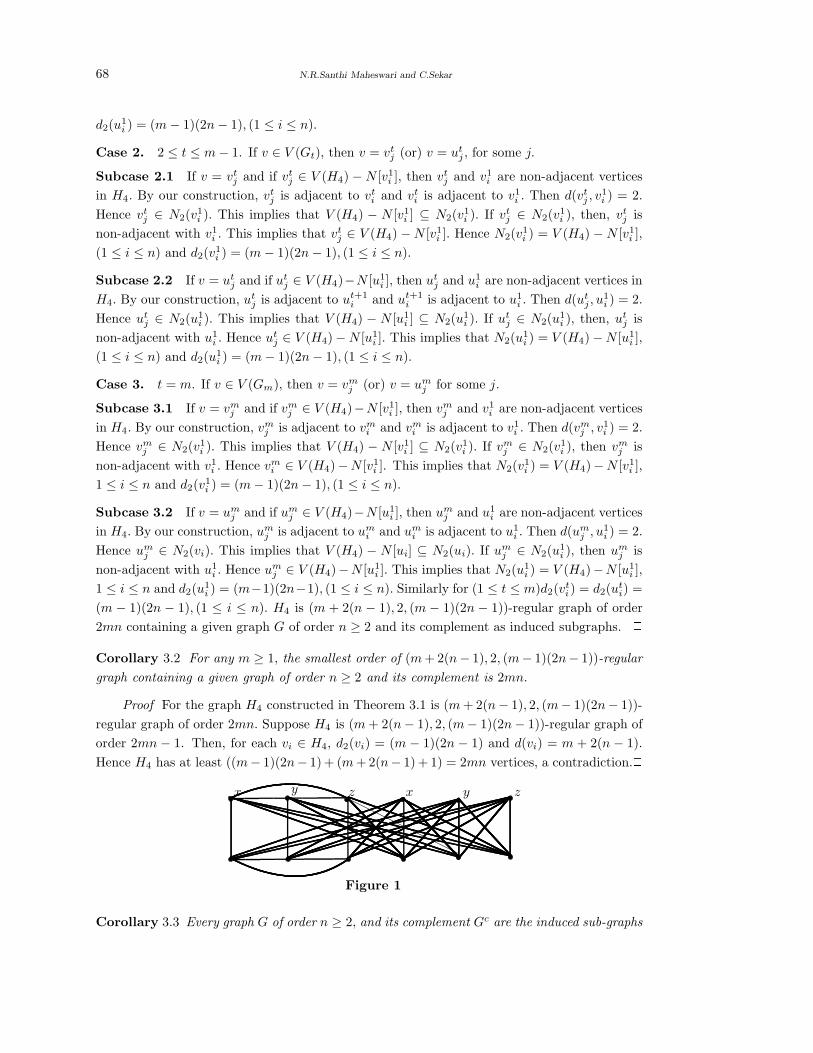
68 N.R.Santhi Maheswari and C.Sekar
d2(u1i ) = (m − 1)(2n − 1), (1 ≤ i ≤ n).
Case 2. 2 ≤ t ≤ m − 1. If v ∈ V (Gt), then v = vtj (or) v = ut
j , for some j.
Subcase 2.1 If v = vtj and if vt
j ∈ V (H4) − N [v1i ], then vt
j and v1i are non-adjacent vertices
in H4. By our construction, vtj is adjacent to vt
i and vti is adjacent to v1
i . Then d(vtj , v
1i ) = 2.
Hence vtj ∈ N2(v
1i ). This implies that V (H4) − N [v1
i ] ⊆ N2(v1i ). If vt
j ∈ N2(v1i ), then, vt
j is
non-adjacent with v1i . This implies that vt
j ∈ V (H4) − N [v1i ]. Hence N2(v
1i ) = V (H4) − N [v1
i ],
(1 ≤ i ≤ n) and d2(v1i ) = (m − 1)(2n − 1), (1 ≤ i ≤ n).
Subcase 2.2 If v = utj and if ut
j ∈ V (H4)−N [u1i ], then ut
j and u1i are non-adjacent vertices in
H4. By our construction, utj is adjacent to ut+1
i and ut+1i is adjacent to u1
i . Then d(utj , u
1i ) = 2.
Hence utj ∈ N2(u
1i ). This implies that V (H4) − N [u1
i ] ⊆ N2(u1i ). If ut
j ∈ N2(u1i ), then, ut
j is
non-adjacent with u1i . Hence ut
j ∈ V (H4) − N [u1i ]. This implies that N2(u
1i ) = V (H4) − N [u1
i ],
(1 ≤ i ≤ n) and d2(u1i ) = (m − 1)(2n − 1), (1 ≤ i ≤ n).
Case 3. t = m. If v ∈ V (Gm), then v = vmj (or) v = um
j for some j.
Subcase 3.1 If v = vmj and if vm
j ∈ V (H4)−N [v1i ], then vm
j and v1i are non-adjacent vertices
in H4. By our construction, vmj is adjacent to vm
i and vmi is adjacent to v1
i . Then d(vmj , v1
i ) = 2.
Hence vmj ∈ N2(v
1i ). This implies that V (H4) − N [v1
i ] ⊆ N2(v1i ). If vm
j ∈ N2(v1i ), then vm
j is
non-adjacent with v1i . Hence vm
i ∈ V (H4)−N [v1i ]. This implies that N2(v
1i ) = V (H4)−N [v1
i ],
1 ≤ i ≤ n and d2(v1i ) = (m − 1)(2n − 1), (1 ≤ i ≤ n).
Subcase 3.2 If v = umj and if um
j ∈ V (H4)−N [u1i ], then um
j and u1i are non-adjacent vertices
in H4. By our construction, umj is adjacent to um
i and umi is adjacent to u1
i . Then d(umj , u1
i ) = 2.
Hence umj ∈ N2(vi). This implies that V (H4) − N [ui] ⊆ N2(ui). If um
j ∈ N2(u1i ), then um
j is
non-adjacent with u1i . Hence um
j ∈ V (H4)−N [u1i ]. This implies that N2(u
1i ) = V (H4)−N [u1
i ],
1 ≤ i ≤ n and d2(u1i ) = (m−1)(2n−1), (1 ≤ i ≤ n). Similarly for (1 ≤ t ≤ m)d2(v
ti) = d2(u
ti) =
(m − 1)(2n − 1), (1 ≤ i ≤ n). H4 is (m + 2(n − 1), 2, (m − 1)(2n − 1))-regular graph of order
2mn containing a given graph G of order n ≥ 2 and its complement as induced subgraphs. 2Corollary 3.2 For any m ≥ 1, the smallest order of (m + 2(n− 1), 2, (m− 1)(2n− 1))-regular
graph containing a given graph of order n ≥ 2 and its complement is 2mn.
Proof For the graph H4 constructed in Theorem 3.1 is (m + 2(n− 1), 2, (m− 1)(2n− 1))-
regular graph of order 2mn. Suppose H4 is (m + 2(n− 1), 2, (m− 1)(2n− 1))-regular graph of
order 2mn − 1. Then, for each vi ∈ H4, d2(vi) = (m − 1)(2n − 1) and d(vi) = m + 2(n − 1).
Hence H4 has at least ((m− 1)(2n− 1) + (m + 2(n− 1) + 1) = 2mn vertices, a contradiction.2x y z x y z
Figure 1
Corollary 3.3 Every graph G of order n ≥ 2, and its complement Gc are the induced sub-graphs

Some Minimal (r, 2, k)-Regular Graphs Containing a Given Graph and its Complement 69
of (2n, 2, (2n− 1))-regular graph of smallest order 4n.
In Figure 1, Corollary 3.3 is illustrated for G = K3, in which the graph G is induced by
the vertices x, y, z.
Corollary 3.4 Every graph G of order n ≥ 2, and its complement Gc are the induced subgraphs
of (2n + 1, 2, 2(2n− 1))-regular graph of smallest order 6n.
G = K2 Gc = Kc2
G = K3 Gc = Kc3
x y x y x y z x y z
Figure 2
In Figure 2, Corollary 3.4 is illustrated for G = K2 and G = K3, in which the graph G
and Gcis induced by the vertices x, y for G = K2. In the second graph, the graph G and Gcis
induced by the vertices x, y, z for G = K3.
Corollary 3.5 Every graph G of order n ≥ 2, and its complement Gc are the induced subgraphs
of (2n + 2, 2, 3(2n− 1))-regular graph of smallest order 8n.
Corollary 3.6 Every graph G of order n ≥ 2, and its complement Gc are the induced subgraph
of (2n + 3, 2, 4(2n− 1))-regular graph of smallest order 10n.
Remark 3.7 There are at least as many (m+2(n−1), 2, (m−1)(2n−1))-regular of order 2mn
as there are graphs G of order n ≥ 2. If m = 2, 3, 4, 5, . . . , then there are (2n, 2, (2n− 1)), (2n+
1, 2, 2(2n− 1)), (2n + 2, 2, 3(2n− 1)), (2n + 3, 2, 4(2n− 1)), . . . regular graphs of smallest order
4n, 6n, 8n, 10n, 12n . . . respectively containing any graph G of order n ≥ 2 and its complement
as induced subgraphs.
§4. Topological Indices of the Graph H4
The topological indices Wiener Index W , Hyper Wiener Index WW , Degree Distance DD,
Variance of degrees, The first Zagreb index, The second Zagreb Index and the third Zagreb
Index of the graph H4, which was constructed in Theorem 3.1 are calculated in this section.
Topological index Top(G) of a graph G is a number with this property that for every graph
H isomorphic to G, Top(G) = Top(H). For historical background, computational techniques
and mathematical properties of Zagreb indices and Wiener, Hyper Wiener one can refer to
[21,22,23,24,25].
The graph H4 is (m + 2n − 2, 2, (m − 1)(2n − 1))-regular graph having 2mn vertices and
mn(m + 2n − 2)) edges with diameter 2. Also, for each v ∈ H4, d2(v) = (m − 1)(2n − 1) and

70 N.R.Santhi Maheswari and C.Sekar
d(v) = m + 2n − 2.
Computation of W , WW and DD for H4 is done by using the following theorem [14]:
Let G be a graph with n vertices, m edges and with diameter 2, then
(1) W (G) = n(n − 1) − m;
(2) WW (G) = 3/2(n(n− 1)) − 2m;
(3) DD(G) = 4(n − 1)m − M1(G).
The Wiener index W is the first and important topological index in chemistry which was
introduced by H. Wiener in 1947 to study the boiling points of parafins. This index is useful
to describe molecular structures and also crystal lattice that depends on its W value.
Definition 4.1 The Wiener index, W (G) of a finite, connected graph G is defined to be
W (G) =1
2
∑d(u, v), where d(u, v) denotes the distance between u and v in G.
Wiener Index of a graphH4 = W (H4) = 2mn(2mn− 1) − ((mn)(m + 2(n − 1))
= mn(4mn− 2 − m − 2n + 2) = (mn)(4mn − (m + 2n))
The Hyper Wiener index WW was introduced by Randic. The Hyper Wiener Index WW is
used as a structure descriptor for predicting physicochemical properties of organic compounds.
Definition 4.2 The Hyper Wiener index WW (G) of a finite, connected graph G is defined to
be WW (G) =1
2(W1(G) + W2(G)), where W1(G) = W (G) and Wλ(G) =
∑dG(k)(kλ) is called
the Wiener-type invariant of G associated to a real number.
Hyper Wiener Index of a graphH4 = WW (H4)
= (3/2)(2mn(2mn− 1) − 2mn(m + 2(n − 1)))
= (mn)(6mn − 3 − 2m − 4n + 4)
= (mn)(6mn − (2m + 4n) + 1)
The Zagreb indices were introduced by Gutman and Trinajestic [7,10,14].
Definition 4.3 The oldest and most investigated topological graph indices are defined as: First
Zagreb index M1(G) =∑
v∈V (G)(dG(v))2, second Zagreb index M2(G) =∑
uv∈E(G)(dG(u)dG(v))
and third Zagreb index M3(G) =∑ |d(u) − d(v)| , uv ∈ E(G).
Some Minimal (r, 2, k)-Regular Graphs Containing a Given Graph and its Complement 71
The Zagreb Indices of graph H4 are
1. M1(H4) =∑
d(u)d(u) =∑
d(u)2 = 2mn((m + 2n − 2)2)
2. M2(H4) =∑
d(u)d(v), uv ∈ E(H4)
= (mn)(m + 2(n − 1)(m + 2(n − 1)(m + 2(n − 1)
= (mn)((m + 2(n − 1))3)
3. M3(H4) =∑
|d(u) − d(v)|| , uv ∈ E(H4)
=∑
|(m + 2(n − 1)) − (m + 2(n − 1))| = 0.
Definition 4.4([4]) The degree distance (Schultz index) of G was introduced by Dobrynin
and Kochetova and Gutman as a weighted version of the Wiener index defined as DD(G) =∑(d(u)+ d(v))d(u, v). It is to be noted that DD(G) and W (G) are closely mutually related for
certain classes of molecular graphs.
The degree distance of graph H4 is
DD(H4) = 4(2mn− 1)(mn)(m + 2(n − 1)) − M1(H4)
= 2mn(m + 2n − 2)[2(2mn− 1) − (m + 2n − 2))
= 2mn(m + 2n − 2)[4mn− (m + 2n)]
Definition 4.5([13]) The status, or distance sum of a vertex v in a graph is defined by s(v)
=∑
d(u, v), where d(u, v) is the distance between the vertices u and v and u 6= v. The status
sequence of a graph consists of a list of the stati of all the vertices.
Since diameter of H4 is two, the status of a vertex v in H4 is
s(v) = (m + 2(n − 1) + 2(m − 1)(2n − 1)
= m + 2n − 2 + 4mn − 2m − 4n + 2 = 4mn− 2(m + n)
Definition 4.6 A graph is said to be self-median, or SM, if the stati of its vertices are all equal.
Every vertex in H4 has the same status 4mn − 2(m + n). Whence, H4 is a self-median
graph.
§5. Open Problems
For further investigation, the following open problem is suggested:
(1) Construct (r, m, k)-regular graphs containing a given graph G and its complement of
order n ≥ 2, as induced subgraph, for m ≥ 3.
(2) Construct (r, m, k)-regular graphs containing a given graph G and its complement of
order n ≥ 2, as induced subgraph, for all values of k.

72 N.R.Santhi Maheswari and C.Sekar
References
[1] Yousef Alavi, Gary Chartrand, F.R.K. Chang, Paul Erdos, H.L.Graham and O.R. Oeller-
mann, J. Graph Theory, 11(2) (1987), 235-249.
[2] Alison Northup, A Study of Semiregular Graphs, Bachelor Thesis, Stetson University
(2002).
[3] G.S. Bloom, J.K. Kennedy and L.V. Quintas, Distance degree regular graphs, The Theory
and Applications of Graphs, Wiley, New York, (1981), 95-108.
[4] J. A. Bondy and U.S.R. Murty, Graph Theory with Applications, MacMillan, London, 1979.
[5] Gary Chartrand, Paul Erdos, Ortrud R. Oellerman, How to Define an irregular graph,
College Math. Journal, 39(1998).
[6] P. Erdos and P.J. Kelly, The minimal regular graph containing a given graph, Amer. Math.
Monthly, 70(1963), 1074-1075.
[7] G.H. Fath -Tabar, Old and New Zagreb Indices of graphs, MATCH Commun. Math.Comput.
Chem.,65 (2011) 79-84.
[8] I.Gutman, Selected Properties of the Schulz molecular topological index J.Chem.Inf.Comput.
Sci., 34(1994) 1087-1089.
[9] I.Gutman,N.Trinajstic,Graph theory and molecular orbitals, Total electron energy of al-
ternant hydrocarbons, Chem. Phys. Lett, 17(1972), 535-538.
[10] I.Gutman and Kinkar Ch. Das, The First Zagreb Index 30 Years After, MATCH Commun.
Math.Comput.Chem., (50) (2004), 83-92.
[11] F. Harary, Graph Theory, Addison - Wesley, 1969.
[12] D. Konig, Theoritie der Endlichen und Unendlichen Graphen,Akademische Verlagesellschaft
m.b.h Leipizig (1936).
[13] Lior Pachter, Constructing status injective graphs, Discrete Applied Mathematics, 80(1997),
107-113.
[14] Mohamed Essalih, Mohamed El Marraki,Gabrelhagri, Calculation of Some Topological
Indices Of Graphs,Journal of Theoretical and Applied Information Technology, Vol 30,
NO.2(2011).
[15] S.Nikolic, G.Kovacevic, A.Milicevic, N.Trinajstic, The Zagreb indices 30 years after, Croat,
Chem. Acta , 76 (2003), 113-124.
[16] Orest Bucicovschi, Sebastian M.Cioaba, The minimum degree distance of graphs of given
order and size,Discrete Applied Mathematics, 156 (2008) 3518-3521.
[17] K.R. Parthasarathy, Basic Graph Theory, Tata McGraw- Hill Publishing company Limited,
New Delhi. Years?
[18] N. R. Santhi Maheswari and C. Sekar, (r, 2, r(r − 1))−regular graphsInternational journal
of Mathematics and Soft Computing, Vol 2.No.2 (2012), 25-33.
[19] N. R. Santhi Maheswari and C. Sekar, On (r, 2, (r−1)(r−1))−regular graphs, International
journal of Mathematical combinatorics, Vol 4, December (2012).
[20] N. R. Santhi Maheswari and C.Sekar, Some Minimal (r, 2, k))−regular graphs containing
given graph as an induced subgraph, Accepted by JCMCC.
[21] Yeong - Nan Yeh, Ivan Gutman, On the sum of all distances in composite graphs,Discrete
Mathematics, 135(1994) 359-365.

Some Minimal (r, 2, k)-Regular Graphs Containing a Given Graph and its Complement 73
[22] H.Wiener, Structural determination of paraffin boiling points, J. Am. Chem.Soc.69 (1947)17
-20.
[23] B.Zhou, I,Gutman, Relation between Wiener, hyper-Wiener and Zagreb indices, Chem.Phys.
Lett.394 (2004)93-95.
[24] B.Zhou, Zagreb indices, MATCH Commun.Math.Comput.chem 52 (2004) 113-118.
[25] B.Zhou, I.Gutman, Further properties of Zagreb indices, MATCH Commun.Math.Comput.
Chem., 54 (2005) 233-239.

International J.Math. Combin. Vol.1(2015), 74-79
On Signed Graphs Whose Two Path Signed
Graphs are Switching Equivalent to Their Jump Signed Graphs
P. Siva Kota Reddy1, P. N. Samanta2 and Kavita S Permi3
1. Department of Mathematics, Siddaganga Institute of Technology, B.H.Road, Tumkur-572 103, India
2. Department of Mathematics, Berhampur University, Berhampur-760 007, Orissa, India
3. Department of Mathematics, Acharya Institute of Technology, Soladevanahalli, Bangalore-560 107, India
E-mail: reddy [email protected]; [email protected]
Abstract: In this paper, we obtained a characterization of signed graphs whose jump
signed graphs are switching equivalent to their two path signed graphs.
Key Words: Smarandachely k-signed graph, t-Path graphs, jump graphs, signed graphs,
balance, switching, t-path signed graphs and jump signed graphs.
AMS(2010): 05C38, 05C22
§1. Introduction
For standard terminology and notation in graph theory we refer Harary [6] and Zaslavsky [20]
for signed graphs. Throughout the text, we consider finite, undirected graph with no loops or
multiple edges.
Given a graph Γ and a positive integer t, the t-path graph (Γ)t of Γ is formed by taking a
copy of the vertex set V (Γ) of Γ, joining two vertices u and v in the copy by a single edge e = uv
whenever there is a u− v path of length t in Γ. The notion of t-path graphs was introduced by
Escalante et al. [4]. A graph G for which
(Γ)t∼= Γ (1)
has been termed as t-path invariant graph by Esclante et al. in [4], Escalante & Montejano [5]
where the explicit solution to (1) has been determined for t = 2, 3. The structure of t-path
invariant graphs are still remains uninvestigated in literature for all t ≥ 4.
The line graph L(Γ) of a graph Γ = (V, E) is that graph whose vertices can be put in
one-to-one correspondence with the edges of Γ so that two vertices of L(Γ) are adjacent if, and
only if, the corresponding edges of Γ are adjacent.
The jump graph J(Γ) of a graph Γ = (V, E) is L(Γ), the complement of the line graph
L(Γ) of Γ (see [6]).
A Smarandachely k-signed graph is an ordered pair S = (G, σ) (S = (G, µ)) where
G = (V, E) is a graph called underlying graph of S and σ : E → (e1, e2, · · · , ek) (µ : V →1Received June 9, 2014, Accepted February 26, 2015.

On Signed Graphs Whose Two Path Signed Graphs are Switching Equivalent to Their Jump Signed Graphs 75
(e1, e2, · · · , ek)) is a function, where each ei ∈ +,−. Particularly, a Smarandachely 2-signed
graph is called abbreviated to signed graph, where Γ = (V, E) is a graph called underlying
graph of Σ and σ : E → +,− is a function. We say that a signed graph is connected if its
underlying graph is connected. A signed graph Σ = (Γ, σ) is balanced, if every cycle in Σ has
an even number of negative edges (See [7]). Equivalently, a signed graph is balanced if product
of signs of the edges on every cycle of Σ is positive.
Signed graphs Σ1 and Σ2 are isomorphic, written Σ1∼= Σ2, if there is an isomorphism
between their underlying graphs that preserves the signs of edges.
The theory of balance goes back to Heider [8] who asserted that a social system is balanced
if there is no tension and that unbalanced social structures exhibit a tension resulting in a
tendency to change in the direction of balance. Since this first work of Heider, the notion
of balance has been extensively studied by many mathematicians and psychologists. In 1956,
Cartwright and Harary [3] provided a mathematical model for balance through graphs. For
more new notions on signed graphs refer the papers (see [12-17, 20]).
A marking of Σ is a function ζ : V (Γ) → +,−. Given a signed graph Σ one can easily
define a marking ζ of Σ as follows: For any vertex v ∈ V (Σ),
ζ(v) =∏
uv∈E(Σ)
σ(uv),
the marking ζ of Σ is called canonical marking of Σ.
A switching function for Σ is a function ζ : V → +,−. The switched signature is
σζ(e) := ζ(v)σ(e)ζ(w), where e has end points v, w. The switched signed graph is Σζ := (Σ|σζ).
We say that Σ switched by ζ. Note that Σζ = Σ−ζ (see [1]).
If X ⊆ V , switching Σ by X (or simply switching X) means reversing the sign of every
edge in the cut set E(X, Xc). The switched signed graph is ΣX . This is the same as Σζ where
ζ(v) := − if and only if v ∈ X . Switching by ζ or X is the same operation with different
notation. Note that ΣX = ΣXc
.
Signed graphs Σ1 and Σ2 are switching equivalent, written Σ1 ∼ Σ2 if they have the same
underlying graph and there exists a switching function ζ such that Σζ1∼= Σ2. The equivalence
class of Σ,
[Σ] := Σ′ : Σ′ ∼ Σ,
is called the its switching class.
Similarly, Σ1 and Σ2 are switching isomorphic, written Σ1∼= Σ2, if Σ1 is isomorphic to a
switching of Σ2. The equivalence class of Σ is called its switching isomorphism class.
Two signed graphs Σ1 = (Γ1, σ1) and Σ2 = (Γ2, σ2) are said to be weakly isomorphic (see
[18]) or cycle isomorphic (see [19]) if there exists an isomorphism φ : Γ1 → Γ2 such that the
sign of every cycle Z in Σ1 equals to the sign of φ(Z) in Σ2. The following result is well known
(see [19]).
Theorem 1.(T. Zaslavsky, [19]) Two signed graphs Σ1 and Σ2 with the same underlying graph
are switching equivalent if and only if they are cycle isomorphic.
76 P. Siva Kota Reddy, P. N. Samanta and Kavita S Permi
In [11], the authors introduced the switching and cycle isomorphism for signed digraphs.
The notion of t-path graph of a given graph was extended to the class of signed graphs by
Mishra [9] as follows:
Given a signed graph Σ and a positive integer t, the t-path signed graph (Σ)t of Σ is formed
by taking a copy of the vertex set V (Σ) of Σ, joining two vertices u and v in the copy by a single
edge e = uv whenever there is a u − v path of length t in S and then by defining its sign to be
− whenever in every u − v path of length t in Σ all the edges are negative.
In [13], P. S. K. Reddy introduced a variation of the concept of t-path signed graphs studied
above. The motivation stems naturally from one’s mathematically inquisitiveness as to ask why
not define the sign of an edge e = uv in (Σ)t as the product of the signs of the vertices u and
v in Σ. The t-path signed graph (Σ)t = ((Γ)t, σ′) of a signed graph Σ = (Γ, σ) is a signed
graph whose underlying graph is (Γ)t called t-path graph and sign of any edge e = uv in (Σ)t is
µ(u)µ(v), where µ is the canonical marking of Σ. Further, a signed graph Σ = (Γ, σ) is called
t-path signed graph, if Σ ∼= (Σ′)t, for some signed graph Σ′. In this paper, we follow the notion
of t-path signed graphs defined by P. S. K. Reddy as above.
Theorem 2.(P. S. K. Reddy, [13]) For any signed graph Σ = (Γ, σ), its t-path signed graph
(Σ)t is balanced.
Corollary 3. For any signed graph Σ = (Γ, σ), its 2-path signed graph (Σ)2 is balanced.
The jump signed graph of a signed graph S = (G, σ) is a signed graph J(S) = (J(G), σ′),
where for any edge ee′ in J(S), σ′(ee′) = σ(e)σ(e′). This concept was introduced by M. Acharya
and D. Sinha [2] (See also E. Sampathkumar et al. [10]).
Theorem 4.(M. Acharya and D. Sinha, [2]) For any signed graph Σ = (Γ, σ), its jump signed
graph J(Σ) is balanced.
§2. Switching Equivalence of Two Path Signed Graphs and Jump Signed Graphs
The main aim of this paper is to prove the following signed graph equation
(Σ)2 ∼ J(Σ).
We first characterize graphs whose two path graphs are isomorphic to their jump graphs.
Theorem 5. A graph Γ = (V, E) satisfies (Γ)2 ∼= J(Γ) if, and only if, G = C4 or C5.
Proof Suppose Γ is a graph such that (Γ)2 ∼= J(Γ). Hence number of vertices and number
of edges of Γ are equal and so Γ must be unicyclic. Let C = Cm be the cycle of length m ≥ 3
in Γ.
Case 1. m = 3.
Let V (C) = u1, u2, u3. Then C is also a cycle in (Γ)2, where as in J(Γ), the vertices

On Signed Graphs Whose Two Path Signed Graphs are Switching Equivalent to Their Jump Signed Graphs 77
corresponds the edges of C are mutually non-adjacent. Since (Γ)2 ∼= J(Γ), J(Γ) must also
contain a C3 and hence Γ must contain 3K2, disjoint union of 3 copies of K2. Whence Γ must
contain either Γ1, Γ2 or Γ3 as shown in Figure 1 as induced subgraph.
Subcase 1.1 If Γ contains Γ2 or Γ3. Let v be the vertex satisfying d(v, C) = 2. Since
d(v, C) = 2 there exists a vertex u in Γ adjacent to v and a vertex in C say u1. Now, in (Γ)2,
the vertex v is not adjacent to u. Since C is also a cycle in (Γ)2 and w is adjacent to u1 in
Γ, the vertices w u2 and u3 forms a cycle C′ in (Γ)2. Further, the vertex v is not adjacent to
C′. Hence, Γ contains H = C3 ∪ K1 as a induced subgraph. But since Γ′ = K1,3 which is a
forbidden induced subgraph for line graph L(Γ) and J(Γ) = L(Γ), we must have (Γ)2 6∼= J(Γ).
Subcase 1.2 If Γ contains Γ1. Then by subcase(i), Γ = Γ1. But clearly, (Γ)2 6∼= J(Γ).
Case 2. m ≥ 4.
Suppose that m ≥ 4 and there exists vertex v in Γ which is not on the cycle C. Let
C = (v1, v2, v3, v4, ..., vm, v1). Since Γ is connected v is adjacent to a vertex say, vi in C. Then
the subgraph induced by the vertices vi−1, v, vi+1 and vi in (Γ)2 is K3 ∪ K1. Now the graph
K3oK1 is K1,3 which is a forbidden induced subgraph for L(Γ) = J(Γ). Hence Γ is not a jump
graph. Hence Γ must be a cycle. Clearly (Γ)2(C4) = 2K2 = J(C4) and J(C5) = (Γ)2(C5) = C5
it remains to show that for Γ = Cm with m ≥ 6 does not satisfy J(Cm) = (Γ)2(Cm), for m ≥ 6.
Suppose that m ≥ 6. Then clearly every vertex in J(Cm) is adjacent to at least m− 2 ≥ 4
vertices where as in (Γ)2, degree of every vertex is 2. This proves the necessary part. The
converse part is obvious. 2We now give a characterization of signed graphs whose two path signed graphs are switching
equivalent to their jump signed graphs.
Theorem 6. For any signed graph Σ = (Γ, σ), (Σ)2 ∼ J(Σ) if, and only if, the underlying
graph Γ is either C5 or C4.
Proof Suppose that (Σ)2 ∼ J(Σ). Then clearly, (Γ)2 ∼= J(Γ). Hence by Theorem 5, Γ
must be either C4 or C5.
Conversely, suppose that Σ is a signed graph on C4 or C5. Then by Theorem 5, (Γ)2 ∼= J(Γ).

78 P. Siva Kota Reddy, P. N. Samanta and Kavita S Permi
Since for any signed graph Σ, by Corollary 3 and Theorem 4, (Σ)2 and J(Σ) are balanced, the
result follows by Theorem 1. 2Remark The only possible cases for which (Σ)2 ∼= J(Σ) are shown in Figure 2.
References
[1] R. P. Abelson and M. J. Rosenberg, Symoblic psychologic:A model of attitudinal cognition,
Behav. Sci., 3 (1958), 1-13.
[2] M. Acharya and D.Sinha, A characterization of signed graphs that are switching equivalent
to other jump signed graphs, Graph Theory Notes of New York, XLIII(1) (2002), 7-8.
[3] D. Cartwright and F. Harary, Structural Balance: A Generalization of Heider s Theory,
Psychological Review, 63 (1956), 277-293.
[4] F. Escalante, L. Montejano and T. Rojno, A characterization of n-path connected graphs
and of graphs having n-th root, J. Combin. Th., Ser. B, 16(3) (1974), 282-289.
[5] F. Escalante and L. Montejano, Trees and n-path invariant graphs, Graph Theory Newslet-
ter, 3(3), 1974.
[6] F. Harary, Graph Theory, Addison-Wesley Publishing Co., 1969.
[7] F. Harary, On the notion of balance of a signed graph, Michigan Math. J., 2 (1953),
143-146.
[8] F. Heider, Attitudes and Cognitive Organisation, Journal of Psychology, 21 (1946), 107-
112.
[9] V. Mishra, Graphs associated with (0, 1) and (0, 1,−1) matrices, Ph.D. Thesis, IIT Bombay,
1974.
[10] E. Sampathkumar, P. Siva Kota Reddy, and M. S. Subramanya, Jump symmetric n-signed
graph, Proceedings of the Jangjeon Math. Soc., 11(1) (2008), 89-95.

On Signed Graphs Whose Two Path Signed Graphs are Switching Equivalent to Their Jump Signed Graphs 79
[11] E. Sampathkumar, M. S. Subramanya and P. Siva Kota Reddy, Characterization of line
sidigraphs, Southeast Asian Bull. Math., 35(2) (2011), 297-304.
[12] P. Siva Kota Reddy, S. Vijay and V. Lokesha, nth Power signed graphs, Proceedings of the
Jangjeon Math. Soc., 12(3) (2009), 307-313.
[13] P. Siva Kota Reddy, t-Path Sigraphs, Tamsui Oxford J. of Math. Sciences, 26(4) (2010),
433-441.
[14] P. Siva Kota Reddy, B. Prashanth, and T. R. Vasanth Kumar, Antipodal Signed Directed
Graphs, Advn. Stud. Contemp. Math., 21(4) (2011), 355-360.
[15] P. Siva Kota Reddy and B. Prashanth, S-Antipodal Signed Graphs, Tamsui Oxf. J. Inf.
Math. Sci., 28(2) (2012), 165-174.
[16] P. Siva Kota Reddy and U. K. Misra, The Equitable Associate Signed Graphs, Bull. Int.
Math. Virtual Inst., 3(1) (2013), 15-20.
[17] P. Siva Kota Reddy and U. K. Misra, Graphoidal Signed Graphs, Advn. Stud. Contemp.
Math., 23(3) (2013), 451-460.
[18] T. Sozansky, Enueration of weak isomorphism classes of signed graphs, J. Graph Theory,
4(2)(1980), 127-144.
[19] T. Zaslavsky, Signed graphs, Discrete Appl. Math., 4(1) (1982), 47-74.
[20] T. Zaslavsky, A mathematical bibliography of signed and gain graphs and its allied areas,
Electronic J. Combin., 8(1) (1998), Dynamic Surveys (1999), No. DS8.

International J.Math. Combin. Vol.1(2015), 80-85
A Note on Prime and Sequential Labelings of Finite Graphs
Mathew Varkey T.K
(Department of Mathematics, T.K.M. College of Engineering, Kollam-5, India)
Sunoj. B.S
(Department of Mathematics, Government Polytechnic College, Ezhukone, Kollam, Kerala, India)
E-mail: [email protected], [email protected]
Abstract: A labeling or valuation of a graph G is an assignment f of labels to the vertices
of G that induces for each edge xy a label depending on the vertex labels f(x) and f(y). In
this paper, we study some classes of graphs and their corresponding labelings.
Key Words: Labeling, sequential graph, harmonious graph, prime graph, Smarandache
common k-factor labeling.
AMS(2010): 05C78
§1. Introduction
Unless mentioned or otherwise, a graph in this paper shall mean a simple finite graph without
isolated vertices. For all terminology and notations in Graph Theory, we follow [5] and all
terminology regarding to sequential labeling, we follow [3]. Graph labelings where the vertices
are assigned values subject to certain conditions have been motivated by practical problems.
Labeled graphs serves as useful mathematical models for a broad range of applications such as
coding theory, including the design of good radar type codes, synch-set codes, missile guidance
codes and convolutional codes with optimal autoconvolutional properties. They facilitate the
optimal nonstandard encodings of integers.
Labeled graphs have also been applied in determining ambiguities in X-ray crystallographic
analysis, to design a communication network addressing system, in determining optimal circuit
layouts and radio astronomy problems etc. A systematic presentation of diverse applications of
graph labelings is presented in [1].
Let G be a (p, q)-graph. Let V (G), E(G) denote respectively the vertex set and edge set
of G. Consider an injective function g : V (G) → X , where X = 0, 1, 2, · · · , q if G is a tree
and X = 0, 1, 2, · · · , q − 1 otherwise. Define the function f∗ : E(G) → N , the set of natural
numbers such that f∗(uv) = f(u) + f(v) for all edges uv. If f∗(E(G)) is a sequence of distinct
consecutive integers, say k, k + 1, · · · , k + q − 1 for some k, then the function f is said to be
sequential labeling and the graph which admits such a labeling is called a sequential graph.
Another labeling has been suggested by Graham and S Loane [4] named as harmonious
1Received January 21, 2014, Accepted February 27, 2015.
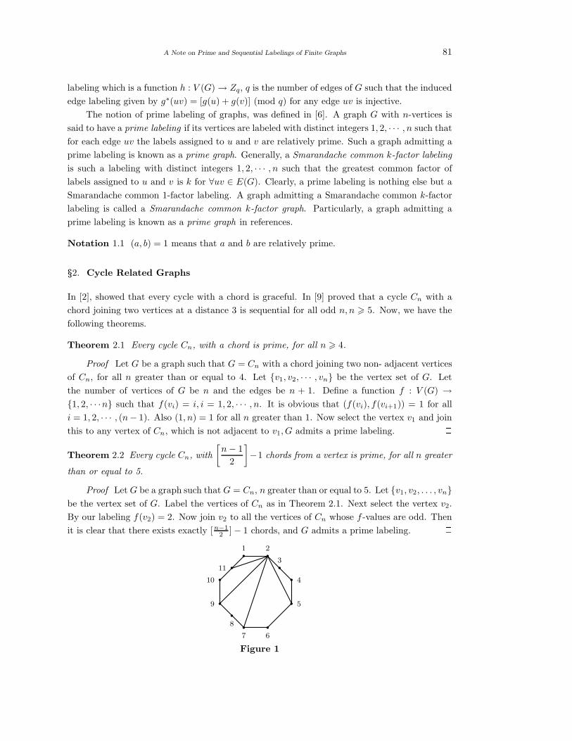
A Note on Prime and Sequential Labelings of Finite Graphs 81
labeling which is a function h : V (G) → Zq, q is the number of edges of G such that the induced
edge labeling given by g∗(uv) = [g(u) + g(v)] (mod q) for any edge uv is injective.
The notion of prime labeling of graphs, was defined in [6]. A graph G with n-vertices is
said to have a prime labeling if its vertices are labeled with distinct integers 1, 2, · · · , n such that
for each edge uv the labels assigned to u and v are relatively prime. Such a graph admitting a
prime labeling is known as a prime graph. Generally, a Smarandache common k-factor labeling
is such a labeling with distinct integers 1, 2, · · · , n such that the greatest common factor of
labels assigned to u and v is k for ∀uv ∈ E(G). Clearly, a prime labeling is nothing else but a
Smarandache common 1-factor labeling. A graph admitting a Smarandache common k-factor
labeling is called a Smarandache common k-factor graph. Particularly, a graph admitting a
prime labeling is known as a prime graph in references.
Notation 1.1 (a, b) = 1 means that a and b are relatively prime.
§2. Cycle Related Graphs
In [2], showed that every cycle with a chord is graceful. In [9] proved that a cycle Cn with a
chord joining two vertices at a distance 3 is sequential for all odd n, n > 5. Now, we have the
following theorems.
Theorem 2.1 Every cycle Cn, with a chord is prime, for all n > 4.
Proof Let G be a graph such that G = Cn with a chord joining two non- adjacent vertices
of Cn, for all n greater than or equal to 4. Let v1, v2, · · · , vn be the vertex set of G. Let
the number of vertices of G be n and the edges be n + 1. Define a function f : V (G) →1, 2, · · ·n such that f(vi) = i, i = 1, 2, · · · , n. It is obvious that (f(vi), f(vi+1)) = 1 for all
i = 1, 2, · · · , (n− 1). Also (1, n) = 1 for all n greater than 1. Now select the vertex v1 and join
this to any vertex of Cn, which is not adjacent to v1, G admits a prime labeling. 2Theorem 2.2 Every cycle Cn, with
[n − 1
2
]−1 chords from a vertex is prime, for all n greater
than or equal to 5.
Proof Let G be a graph such that G = Cn, n greater than or equal to 5. Let v1, v2, . . . , vnbe the vertex set of G. Label the vertices of Cn as in Theorem 2.1. Next select the vertex v2.
By our labeling f(v2) = 2. Now join v2 to all the vertices of Cn whose f -values are odd. Then
it is clear that there exists exactly [n−12 ] − 1 chords, and G admits a prime labeling. 2
9
10
11
1 2
3
4
5
67
8
Figure 1

82 Mathew Varkey T.K and Sunoj. B.S
Remark 2.1 From Theorem 2.1, it is clear that there is possible to get n − 3 chords and
Theorem 2.2 tells us there are [n−12 ] − 1 chords. Thus the bound n − 3 is best possible and all
other possible chords of less than these two bounds.
Example 2.1 Figure 1 gives the prime labeling of C11 with 4-chords.
Theorem 2.3 The graph Cn + K1,t is sequential for all odd n, n > 3.
Proof Let v1, v2, · · · , vn (n is odd) be the set of vertices of Cn and u, u1, u2, · · · , ut be the
t + 1 isolated vertices of K1,t. Let G = Cn + K1,t and note that, G has n + t + 1 vertices and
n(2 + t) edges.
Define a function f : V (G) → 0, 1, 2, · · · , n−12 + tn such that
f(v2i−1) = i − 1, for i = 1, 2, · · · ,n + 1
2
f(v2i) =n − 1
2+ i, for i = 1, 2, · · · ,
n − 1
2
f(u1) =3
2n − 1
and f(ui) =n − 1
2+ ni, i = 2, 3, · · · , t
We can easily observe that the above defined f is injective. Hence f becomes a sequential
labeling of Cn + K1,t. Thus Cn + K1,t is sequential for all odd n, n > 3. 2Corollary 2.4 The graph Cn + K1,t is harmonious for all odd n > 3.
Proof Any sequential is harmonius implies that Cn + K1,t is harmonius, n > 3. 2Theorem 2.5 The graph Cn + K1,1,t is sequential and harmonius for all odd n, n > 3.
Theorem 2.6 The graph Cn + K1,1,1,t is sequential and harmonius for all odd n, n > 3.
Example 2.2 Figure 2 gives the sequential labeling of the graph C5 + K1,1,1,3.
4
2
0
17
12
7
27
32
22
3
1
Figure 2

A Note on Prime and Sequential Labelings of Finite Graphs 83
Theorem 2.7 The graph Cn + K1,1,...,1,t is sequential as harmonius for odd n, n > 3.
Theorem 2.8 The graph Cn + K1,m,n is sequential and harmonius for all odd n, n > 3, m > 1.
§3. On Join of Complete Graphs
In [7], it is shown that Ln + K1 and Bn + K1 are prime and join of any two connected graphs
are not odd sequential. Now, we have the following.
Theorem 3.1 The graph K1,n + K2 is prime for n > 4.
Proof Let G = K1,n + K2. We can notice that G has (n + 3)-vertices and (3n + 2)-edges.
Let w, v1, v2, · · · , vn be the vertices of K1,n and u1, u2 be the two vertices of K2. Assign
the first two largest primes less than or equal to n + 3 to the two vertices of K2. Assign 1 to
w and remaining n values to the n vertices arbitrarily, we can obtain a prime numbering of
K1,n + K2. 2Corollary 3.1 The graph K1,n + K2 is prime for all n > 4.
§4. Product Related Graphs
Definition 4.1 Let G and H be graphs with V (G) = V1 and V (H) = V2. The cartesian product
of G and H is the graph G2H whose vertex set is V1 ×V2 such that two vertices u = (x, y) and
v = (x′, y′) are adjacent if and only if either x = x′ and y is adjacent to y′ in H or y = y′ and
x is adjacent to x′ in G. That is, u adj v in G2H whenever [x = x′ and y adj y′] or [y = y′
and x adj x′].
In [8] A.Nagarajan, A.Nellai Murugan and A.Subramanian proved that Pn2K2, Pn2Pn
are near mean graphs.
Definition 4.2 Let Pn be a path on n vertices and K4 be a complete graph on 4 vertices. The
Cartesian product Pn and K4 is denoted as Pn2K4 with 4n vertices and 10n− 4 edges.
Theorem 4.1 The graph Pn2K4 is sequential, for all n > 1.
Proof Let G = Pn2K4. Let vi,1, vi,2, vi,3, vi,4/i = 1, 2, · · · , n be the vertex set of G.

84 Mathew Varkey T.K and Sunoj. B.S
Define a function f : V (G) → 0, 1, 2, · · · , 5n − 1 such that
f(v2i−1,1) = 10i − 6 ; 1 6 i 6n
2if n is even or 1 6 i 6
n + 1
2if n is odd.
f(v2i−1,2) = 10(i − 1) ; 1 6 i 6n
2if n is even or 1 6 i 6
n + 1
2if n is odd.
f(v2i−1,3) = 10i − 9 ; 1 6 i 6n
2if n is even or 1 6 i 6
n + 1
2if n is odd.
f(v2i−1,4) = 10i − 8 ; 1 6 i 6n
2if n is even or 1 6 i 6
n + 1
2if n is odd.
f(v2i,1) = 10i − 4 ; 1 6 i 6n
2if n is even or 1 6 i 6
n − 1
2if n is odd.
f(v2i,2) = 10i − 1 ; 1 6 i 6n
2if n is even or 1 6 i 6
n − 1
2if n is odd.
f(v2i,3) = 10i − 3 ; 1 6 i 6n
2if n is even or 1 6 i 6
n − 1
2if n is odd.
and
f(v2i,4) = 10i − 5 ; 1 6 i 6n
2if n is even or 1 6 i 6
n − 1
2if n is odd.
(a) Clearly we can see that f is injective.
(b) Also, maxv∈V f(v) = maxmaxi 10i−6; maxi 10(i−1); maxi 10i−9; maxi 10i−8; maxi 10i
−4; maxi 10i−1; maxi 10i−3; maxi 10i−5 = 5n−1. Thus, f(v) = 0, 1, 2, . . . , 5n−1. Finally,
it can be easily verified that the labels of the edge values are distinct positive integers in the
interval [1, 10n− 4]. Thus, f is a sequential numbering. Hence, the graph G is sequential. 2Example 4.1 Figure 4 gives the sequential labeling of the graph P42K4.
17
11
7
1
16
14
6
4
15
12
5
2
19
10
9
0
Figure 3
Corollary 4.1 The graph Pn2K4 is harmonius, for n > 2.

A Note on Prime and Sequential Labelings of Finite Graphs 85
References
[1] G.S.Bloom and S.W.Golomb, Pro. of the IEEE, 165(4), (1977) 562-70.
[2] C.Delmore, M.Maheo. H.Thuiller, K.M.Koh and H.K.Teo, Cycles with a chord are graceful,
Jour. of Graph Theory, 4 (1980) 409-415.
[3] T.Grace, On sequential labeling of graphs, Jour. of Graph Theory, 7 (1983) 195-201.
[4] R.L.Graham and N.J.A.Sloance, On additive bases and harmonious graphs, SIAM, Jour.of.Alg,
Discrete Math. 1 (1980) 382-404.
[5] F.Harary, Graph Theory, Addison-Wesley, Reading, Massachussets, USA, 1969.
[6] Joseph A.Gallian, A dynamic survey of Graph labeling, The Electronic J. Combinatorics.
16 (2013) 1-298.
[7] T.K.Mathew Varkey, Some Graph Theoretic Operations Associated with Graph Labelings,
Ph.D Thesis, University of Kerala, 2000.
[8] A.Nagarajan, A.Nellai Murugan and A.Subramanian, Near meanness on product graphs,
Scientia Magna, Vol.6, 3(2010), 40-49.
[9] G.Suresh Singh, Graph Theory - A study of certain Labeling problems, Ph.D Thesis, Uni-
versity of Kerala, (1993).

International J.Math. Combin. Vol.1(2015), 86-95
The Forcing Vertex Monophonic Number of a Graph
P.Titus
(University College of Engineering Nagercoil, Anna University, Tirunelveli Region, Nagercoil-629004, India)
K.Iyappan
(Department of Mathematics, National College of Engineering, Maruthakulam, Tirunelveli-627151, India)
E-mail: [email protected]; iyappan [email protected]
Abstract: For any vertex x in a connected graph G of order p ≥ 2, a set Sx ⊆ V (G) is an
x-monophonic set of G if each vertex v ∈ V (G) lies on an x − y monophonic path for some
element y in Sx. The minimum cardinality of an x-monophonic set of G is the x-monophonic
number of G and is denoted by mx(G). A subset Tx of a minimum x-monophonic set Sx of
G is an x-forcing subset for Sx if Sx is the unique minimum x-monophonic set containing Tx.
An x-forcing subset for Sx of minimum cardinality is a minimum x-forcing subset of Sx. The
forcing x-monophonic number of Sx, denoted by fmx(Sx), is the cardinality of a minimum
x-forcing subset for Sx. The forcing x-monophonic number of G is fmx (G) = minfmx (Sx),
where the minimum is taken over all minimum x-monophonic sets Sx in G. We determine
bounds for it and find the forcing vertex monophonic number for some special classes of
graphs. It is shown that for any three positive integers a, b and c with 2 ≤ a ≤ b < c, there
exists a connected graph G such that fmx (G) = a, mx(G) = b and cmx(G) = c for some
vertex x in G, where cmx(G) is the connected x-monophonic number of G.
Key Words: monophonic path, vertex monophonic number, forcing vertex monophonic
number, connected vertex monophonic number, Smarandachely geodetic k-set, Smaran-
dachely hull k-set.
AMS(2010): 05C12
§1. Introduction
By a graph G = (V, E) we mean a finite undirected connected graph without loops or multiple
edges. The order and size of G are denoted by p and q respectively. For basic graph theoretic
terminology we refer to Harary [6]. For vertices x and y in a connected graph G, the distance
d(x, y) is the length of a shortest x − y path in G. An x − y path of length d(x, y) is called an
x − y geodesic. The neibourhood of a vertex v is the set N(v) consisting of all vertices u which
are adjacent with v. The closed neibourhood of a vertex v is the set N [v] = N(v)⋃ v. A
vertex v is a simplicial vertex if the subgraph induced by its neighbors is complete.
1Received April 8, 2014, Accepted February 28, 2015.

The Forcing Vertex Monophonic Number of a Graph 87
The closed interval I[x, y] consists of all vertices lying on some x − y geodesic of G, while
for S ⊆ V, I[S] =⋃
x,y∈S
I[x, y]. A set S of vertices is a geodetic set if I[S] = V , and the minimum
cardinality of a geodetic set is the geodetic number g(G). The geodetic number of a graph was
introduced in [1,8] and further studied in [2,5]. A geodetic set of cardinality g(G) is called a
g− set of G. Generally, for an integer k ≥ 0, a subset S ⊆ V is called a Smarandachely geodetic
k-set if I[S⋃
S+] = V and a Smarandachely hull k-set if Ih(S⋃
S+) = V for a subset S+ ⊂ V
with |S+| ≤ k. Let k = 0. Then a Smarandachely geodetic 0-set and Smarandachely hull 0-set
are nothing else but the geodetic set and hull set, respectively.
The concept of vertex geodomination number was introduced in [9] and further studied in
[10]. For any vertex x in a connected graph G, a set S of vertices of G is an x-geodominating
set of G if each vertex v of G lies on an x − y geodesic in G for some element y in S. The
minimum cardinality of an x-geodominating set of G is defined as the x-geodomination number
of G and is denoted by gx(G). An x-geodominating set of cardinality gx(G) is called a gx − set.
A chord of a path P is an edge joining any two non-adjacent vertices of P . A path P
is called a monophonic path if it is a chordless path. A set S of vertices of a graph G is a
monophonic set of G if each vertex v of G lies on an x − y monophonic path in G for some
x, y ∈ S. The minimum cardinality of a monophonic set of G is the monophonic number of G
and is denoted by m(G).
The concept of vertex monophonic number was introduced in [11]. For a connected graph
G of order p ≥ 2 and a vertex x of G, a set Sx ⊆ V (G) is an x-monophonic set of G if each
vertex v of G lies on an x − y monophonic path for some element y in Sx. The minimum
cardinality of an x-monophonic set of G is defined as the x-monophonic number of G, denoted
by mx(G). An x-monophonic set of cardinality mx(G) is called a mx − set of G. The concept
of upper vertex monophonic number was introduced in [13]. An x-monophonic set Sx is called
a minimal x-monophonic set if no proper subset of Sx is an x-monophonic set. The upper
x-monophonic number, denoted by m+x (G), is defined as the minimum cardinality of a minimal
x-monophonic set of G. The connected x-monophonic number was introduced and studied in
[12]. A connected x-monophonic set of G is an x-monophonic set Sx such that the subgraph
G[Sx] induced by Sx is connected. The minimum cardinality of a connected x-monophonic set
of G is the connected x-monophonic number of G and is denoted by cmx(G). A connected
x-monophonic set of cardinality cmx(G) is called a cmx − set of G.
The following theorems will be used in the sequel.
Theorem 1.1([11]) Let x be a vertex of a connected graph G.
(1) Every simplicial vertex of G other than the vertex x (whether x is simplicial vertex or
not) belongs to every mx − set;
(2) No cut vertex of G belongs to any mx − set.
Theorem 1.2([11]) (1) For any vertex x in a cycle Cp(p ≥ 4), mx(Cp) = 1;
(2) For the wheel Wp = K1 + Cp−1(p ≥ 5), mx(Wp) = p − 1 or 1 according as x is K1 or
x is in Cp−1.

88 P.Titus and K.Iyappan
Theorem 1.3([11]) For n ≥ 2, mx(Qn) = 1 for every vertex x in Qn.
Throughout this paper G denotes a connected graph with at least two vertices.
§2. Vertex Forcing Subsets in Vertex Monophonic Sets of a Graph
Let x be any vertex of a connected graph G. Although G contains a minimum x-monophonic set
there are connected graphs which may contain more than one minimum x-monophonic set. For
example, the graph G given in Figure 2.1 contains more than one minimum x-monophonic set.
For each minimum x-monophonic set Sx in a connected graph G there is always some subset
T of Sx that uniquely determines Sx as the minimum x-monophonic set containing T . Such
sets are called ”vertex forcing subsets” and we discuss these sets in this section. Also, forcing
concepts have been studied for such diverse parameters in graphs as the geodetic number [3],
the domination number [4] and the graph reconstruction number [7].
Definition 2.1 Let x be any vertex of a connected graph G and let Sx be a minimum x-
monophonic set of G. A subset T of Sx is called an x-forcing subset for Sx if Sx is the unique
minimum x-monophonic set containing T . An x-forcing subset for Sx of minimum cardinality
is a minimum x-forcing subset of Sx. The forcing x-monophonic number of Sx, denoted by
fmx(Sx), is the cardinality of a minimum x-forcing subset for Sx. The forcing x-monophonic
number of G is fmx(G) = min fmx
(Sx), where the minimum is taken over all minimum
x-monophonic sets Sx in G.
Example 2.2 For the graph G given in Figure 2.1, the minimum vertex monophonic sets,
the vertex monophonic numbers, the minimum forcing vertex monophonic sets and the forcing
vertex monophonic numbers are given in Table 2.1.
Vertex Minimum mx(G) Minimum forcing fmx(G)
x x-monophonic sets x-monophonic sets
u r, y, r, z, r, s 2 y, z, s 1
v u, r, y, u, r, z, u, r, s 3 y, z, s 1
w u, r 2 ∅ 0
y u, r 2 ∅ 0
z u, r 2 ∅ 0
s u, r 2 ∅ 0
t u, r, w, u, r, y, u, r, z 3 w, y, z 1
r u, w, u, y, u, z 2 w, y, z 1
Table 2.1

The Forcing Vertex Monophonic Number of a Graph 89
b b
b
b b
b
b b
Figure 2.1
u v
w
y z
s
t r
Theorem 2.3 For any vertex x in a connected graph G, 0 ≤ fmx(G) ≤ mx(G).
Proof Let x be any vertex of G. It is clear from the definition of fmx(G) that fmx
(G) ≥ 0.
Let Sx be a minimum x-monophonic set of G. Since fmx(Sx) ≤ mx(G) and since fmx
(G) =
min fmx(Sx) : Sx is a minimum x-monophonic set in G, it follows that fmx
(G) ≤ mx(G).
Thus 0 ≤ fmx(G) ≤ mx(G). 2
b b
b b
b
bb
Figure 2.2
u v
w y
z
st
Remark 2.4 The bounds in Theorem 2.3 are sharp. For the graph G given in Figure 2.2,
S = u, z, t is the unique minimum w-monophonic set of G and the empty set φ is the unique
minimum w-forcing subset for S. Hence fmw(G) = 0. Also, for the graph G given in Figure
2.2, S1 = y and S2 = z are the minimum u-monophonic sets of G and so mu(G) = 1. It is
clear that no minimum u-monophonic set is the unique minimum u-monophonic set containing
any of its proper subsets. It follows that fmu(G) = 1 and hence fmu
(G) = mu(G) = 1. The
inequalities in Theorem 2.3 can be strict. For the graph G given in Figure 2.1, mu(G) = 2 and
fmu(G) = 1. Thus 0 < fmu
(G) < mu(G).
In the following theorem we characterize graphs G for which the bounds in Theorem 2.3
are attained and also graphs for which fmx(G) = 1.
Theorem 2.5 Let x be any vertex of a connected graph G. Then
90 P.Titus and K.Iyappan
(1) fmx(G) = 0 if and only if G has a unique minimum x-monophonic set;
(2) fmx(G) = 1 if and only if G has at least two minimum x-monophonic sets, one of which
is a unique minimum x-monophonic set containing one of its elements, and
(3) fmx(G) = mx(G) if and only if no minimum x-monophonic set of G is the unique
minimum x-monophonic set containing any of its proper subsets.
Definition 2.6 A vertex u in a connected graph G is said to be an x-monophonic vertex if u
belongs to every minimum x-monophonic set of G.
For the graph G in Figure 2.1, S1 = u, r, y, S2 = u, r, z and S3 = u, r, s are the
minimum v-monophonic sets and so u and r are the v-monophonic vertices of G. In particular,
every simplicial vertex of G other than x is an x-monophonic vertex of G.
Next theorem follows immediately from the definitions of an x-monophonic vertex and
forcing x-monophonic subset of G.
Theorem 2.7 Let x be any vertex of a connected graph G and let Fmxbe the set of relative
complements of the minimum x-forcing subsets in their respective minimum x-monophonic sets
in G. Then⋂
F∈FmxF is the set of x-monophonic vertices of G.
Theorem 2.8 Let x be any vertex of a connected graph G and let Mx be the set of all x-
monophonic vertices of G. Then 0 ≤ fmx(G) ≤ mx(G) − |Mx|.
Proof Let Sx be any minimum x-monophonic set of G. Then mx(G) = |Sx|, Mx ⊆ Sx and
Sx is the unique minimum x-monophonic set containing Sx−Mx and so fmx(G) ≤ |Sx−Mx| =
mx(G) − |Mx|. 2Theorem 2.9 Let x be any vertex of a connected graph G and let Sx be any minimum x-
monophonic set of G. Then
(1) no cut vertex of G belongs to any minimum x-forcing subset of Sx;
(2) no x-monophonic vertex of G belongs to any minimum x-forcing subset of Sx.
Proof (1) Since any minimum x-forcing subset of Sx is a subset of Sx, the result follows
from Theorem 1.1(2).
(2) Let v be an x-monophonic vertex of G. Then v belongs to every minimum x-monophonic
set of G. Let T ⊆ Sx be any minimum x-forcing subset for any minimum x-monophonic set Sx
of G. If v ∈ T , then T ′ = T − v is a proper subset of T such that Sx is the unique minimum
x-monophonic set containing T ′ so that T ′ is an x-forcing subset for Sx with |T ′| < |T |, which
is a contradiction to T a minimum x-forcing subset for Sx. Hence v /∈ T . 2Corollary 2.10 Let x be any vertex of a connected graph G. If G contains k simplicial vertices,
then fmx(G) ≤ mx(G) − k + 1.
Proof This follows from Theorem 1.1(1) and Theorem 2.9(2). 2Remark 2.11 The bound for fmx
(G) in Corollary 2.10 is sharp. For a non-trivial tree T with

The Forcing Vertex Monophonic Number of a Graph 91
k end-vertices, fmx(T ) = 0 = mx(T ) − k + 1 for any end-vertex x in T .
Theorem 2.12 (1) If T is a non-trivial tree, then fmx(T ) = 0 for every vertex x in T ;
(2) If G is the complete graph, then fmx(G) = 0 for every vertex x in G.
Proof This follows from Theorem 2.9. 2Theorem 2.13 For every vertex x in the cycle Cp(p ≥ 3), fmx
(Cp) =
0 if p = 3, 4
1 if p ≥ 5.
Proof Let Cp : u1, u2, · · · , up, u1 be a cycle of order p ≥ 3. Let x be any vertex in Cp,
say x = u1. If p = 3 or 4, then Cp has unique minimum x-monophonic set. Then by Theorem
2.5(1), fmx(Cp) = 0. Now, assume that p ≥ 5. Let y be a non-adjacent vertex of x in Cp.
Then Sx = y is a minimum x-monophonic set of Cp. Hence Cp has more than one minimum
x-monophonic set and it follows from Theorem 2.5(1) that fmx(Cp) 6= 0. Now it follows from
Theorems 1.2(1) and 2.3 that fmx(G) = mx(G) = 1. 2
Theorem 2.14 For any vertex x in a complete bipartite graph Km,n(m, n ≥ 2), fmx(Km,n) = 0.
Proof Let (V1, V2) be the bipartition of Km,n. If x ∈ V1, then Sx = V1 − x is the
unique minimum x-monophonic set of G and so by Theorem 2.5(1), fmx(G) = 0. If x ∈ V2,
then Sx = V2 − x is the unique minimum x-monophonic set of G and so by Theorem 2.5(1),
fmx(G) = 0. 2
Theorem 2.15 (1) If G is the wheel Wp = K1 + Cp−1(p = 4, 5), then fmx(G) = 0 for any
vertex x in Wp;
(2) If G is the wheel Wp = K1 + Cp−1(p ≥ 6), then fmx(G) = 0 or 1 according as x is K1
or x is in Cp−1.
Proof Let Cp−1 : u1, u2, · · · , up−1, u1 be a cycle of order p − 1 and let u be the vertex of
K1.
(1) If p = 4 or 5, then G has unique minimum x-monophonic set for any vertex x in G
and so by Theorem 2.5(1), fmx(G) = 0.
(2) Let p ≥ 6. If x = u, then Sx = u1, u2, · · · , up−1 is the unique minimum x-
monophonic set and so by Theorem 2.5(1), fmx(G) = 0. If x ∈ V (Cp−1), say x = u1, then
Si = ui (3 ≤ i ≤ p−2) is a minimum x-monophonic set of G. Since p ≥ 6, there is more than
one minimum x-monophonic set of G. Hence it follows from Theorem 2.5(1) that fmx(G) 6= 0.
Now it follows from Theorems 1.2(2) and 2.3 that fmx(G) = mx(G) = 1. 2
Theorem 2.16 For any vertex x in the n-cube Qn (n ≥ 2), then fmx(Qn) =
0 if n = 2
1 if n ≥ 3.
Proof If n = 2, then Qn has unique minimum x-monophonic set for any vertex x in Qn
and so by Theorem 2.5(1), fmx(Qn) = 0. If n ≥ 3, then it is easily seen that there is more than
one minimum x-monophonic set for any vertex x in Qn. Hence it follows from Theorem 2.5(1)

92 P.Titus and K.Iyappan
that fmx(Qn) 6= 0. Now it follows from Theorems 1.3 and 2.3 that fmx
(Qn) = mx(Qn) = 1. 2The following theorem gives a realization result for the parameters fmx
(G), mx(G) and
m+x (G).
Theorem 2.17 For any three positive integers a, b and c with 2 ≤ a ≤ b ≤ c, there exists a
connected graph G with fmx(G) = a, mx(G) = b and m+
x (G) = c for some vertex x in G.
Proof For each integer i with 1 ≤ i ≤ a − 1, let Fi : u0,i, u1,i, u2,i, u3,i be a path of order
4. Let C6 : t, u, v, w, x, y, t be a cycle of order 6. Let H be a graph obtained from Fi and C6 by
joining the vertex x of C6 to the vertices u0,i and u3,i of Fi(1 ≤ i ≤ a− 1). Let G be the graph
obtained from H by adding c− a new vertices y1, y2, · · · , yc−b, v1, v2, · · · , vb−a and joining each
yi(1 ≤ i ≤ c − b) to both u and y, and joining each vj(1 ≤ j ≤ b − a) with x. The graph G is
shown in Figure 2.3.
b b b b b b
b
b
b
b
b
b
b
b
b b
b
b
b b b
b
b
b
b
b
b
b b b
b
b
b
Figure 2.3
x
u0,a−1 u0,2 u0,1 u3,a−1u3,2u3,1
u1,1 u2,1
u1,2 u2,2
u1,a−1 u2,a−1
w
v u
y
t y1 y2 yc−b
v1
v2
vb−a
Let S = v1, v2, · · · , vb−a be the set of all simplicial vertices of G. For 1 ≤ j ≤ a − 1,
let Sj = u1,j, u2,j. If b = c, then let Sa = u, v, t. Otherwise, let Sa = u, v. Now, we
observe that a set Sx of vertices of G is a mx-set if Sx contains S and exactly one vertex from
each set Sj(1 ≤ j ≤ a) so that mx(G) ≥ b. Since S′
x = S⋃ u, u1,1, u1,2, · · · , u1,a−1 is an
x-monophonic set of G, we have mx(G) = b.
Now, we show that fmx(G) = a. Let Sx = S
⋃ u, u1,1, u1,2, · · · , u1,a−1 be a mx-set of G
and let Tx be a minimum x-forcing subset of Sx. Since S is the set of all x-monophonic vertices
of G and by Theorem 2.8, fmx(G) ≤ mx(G) − |S| = a.

The Forcing Vertex Monophonic Number of a Graph 93
If |Tx| < a, then there exists a vertex y ∈ Sx such that y /∈ Tx. It is clear that y ∈ Sj for
some j = 1, 2, · · · , a, say y = u1,1. Let S′
x = (Sx − u1,1)⋃ u2,1. Then S
′
x 6= Sx and S′
x is
also a minimum x-monophonic set of G such that it contains Tx, which is a contradiction to Tx
a minimum x-forcing subset of Sx. Thus |Tx| = a and so fmx(G) = a.
Next, we show that m+x (G) = c. Let Ux = S
⋃ u1,1, u1,2, · · · , u1,a−1, t, y1, y2, · · · , yc−b.Clearly Ux is a minimal x-monophonic set of G and so m+
x (G) ≥ c. Also, it is clear that every
minimal x-monophonic set of G contains at most c elements and hence m+x (G) ≤ c. Therefore,
m+x (G) = c. 2
The following theorem gives a realization for the parameters fmx(G), mx(G) and cmx(G).
Theorem 2.18 For any three positive integers a, b and c with 2 ≤ a ≤ b < c, there exists a
connected graph G with fmx(G) = a, mx(G) = b and cmx(G) = c for some vertex x in G.
Proof We prove this theorem by considering three cases.
Case 1. 2 ≤ a < b < c.
For each integer i with 1 ≤ i ≤ a − 1, let Fi : y1, u1,i, u2,i, y3 be a path of order 4. Let
Pc−b+2 : y1, y2, y3, · · · , yc−b+2 be a path of order c − b + 2 and let P : v1, v2, v3 be a path of
order 3. Let H1 be a graph obtained from Fi(1 ≤ i ≤ a − 1) and Pc−b+2 by identifying the
vertices y1 and y3 of all Fi(1 ≤ i ≤ a − 1) and Pc−b+2. Let H2 be the graph obtained from
H1 and P by joining the vertex v1 of P to the vertex y2 of H1 and joining the vertex v3 of P
to the vertex y3 of H1. Let G be the graph obtained from H2 by adding b − a new vertices
z1, z2, ..., zb−a and joining each zi(1 ≤ i ≤ b− a) with the vertex yc−b+2. The graph G is shown
in Figure 2.4.
b b b b b b b
b
b
b
b
b
b
b b
b
b
b
b
b
b
b
b b b
Figure 2.4
v1
v2
v3
u1,1 u2,1
u1,2 u2,2
u1,a−1 u2,a−1
y1 x = y2 y3 y4 y5 yc−b+2
z1
z2
zb−a
Let x = y2 and let S = z1, z2, · · · , zb−a be the set of all simplicial vertices of G. For
1 ≤ j ≤ a − 1, let Sj = u1,j, u2,j and let Sa = v2, v3. Now, we observe that a set Sx of
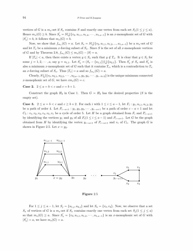
94 P.Titus and K.Iyappan
vertices of G is a mx-set if Sx contains S and exactly one vertex from each set Sj(1 ≤ j ≤ a).
Hence mx(G) ≥ b. Since S′
x = S⋃ v2, u1,1, u1,2, · · · , u1,a−1 is an x-monophonic set of G with
|S′
x| = b, it follows that mx(G) = b.
Now, we show that fmx(G) = a. Let Sx = S
⋃ v2, u1,1, u1,2, ..., u1,a−1 be a mx-set of G
and let Tx be a minimum x-forcing subset of Sx. Since S is the set of all x-monophonic vertices
of G and by Theorem 2.8, fmx(G) ≤ mx(G) − |S| = a.
If |Tx| < a, then there exists a vertex y ∈ Sx such that y /∈ Tx. It is clear that y ∈ Sj for
some j = 1, 2, · · · , a, say y = u1,1. Let S′
x = (Sx − u1,1)⋃ u2,1. Then S
′
x 6= Sx and S′
x is
also a minimum x-monophonic set of G such that it contains Tx, which is a contradiction to Tx
an x-forcing subset of Sx. Thus |Tx| = a and so fmx(G) = a.
Clearly, S⋃ v3, u2,1, u2,2, · · · , u2,a−1, y3, y4, · · · , yc−b+2 is the unique minimum connected
x-monophonic set of G, we have cmx(G) = c.
Case 2. 2 ≤ a = b < c and c = b + 1.
Construct the graph H2 in Case 1. Then G = H2 has the desired properties (S is the
empty set).
Case 3. 2 ≤ a = b < c and c ≥ b + 2. For each i with 1 ≤ i ≤ a − 1, let Fi : y1, ui,1, ui,2, y3
be a path of order 4. Let Pc−a+1 : y1, y2, y3, · · · , yc−a+1 be a path of order c − a + 1 and let
C5 : v1, v2, v3, v4, v5, v1 be a cycle of order 5. Let H be a graph obtained from Fi and Pc−a+1
by identifying the vertices y1 and y3 of all Fi(1 ≤ i ≤ a − 1) and Pc−a+1. Let G be the graph
obtained from H by identifying the vertex yc−a+1 of Pc−a+1 and v1 of C5. The graph G is
shown in Figure 2.5. Let x = y2.
b b b b b b
b
b
b
b
b
b
b b
b b
b b b
Figure 2.5
u1,1 u2,1
u1,2 u2,2
u1,a−1 u2,a−1
y1 x = y2 y3 y4 yc−a+1
v1
v2 v3
v4v5
For 1 ≤ j ≤ a − 1, let Sj = u1,j, u2,j and let Sa = v3, v4. Now, we observe that a set
Sx of vertices of G is a mx-set if Sx contains exactly one vertex from each set Sj(1 ≤ j ≤ a)
so that mx(G) ≥ a. Since S′
x = v3, u1,1, u1,2, · · · , u1,a−1 is an x-monophonic set of G with
|S′
x| = a, we have mx(G) = a.

The Forcing Vertex Monophonic Number of a Graph 95
Now, we show that fmx(G) = a. Let Sx = v3, u1,1, u1,2, · · · , u1,a−1 be a mx-set of G and
let Tx be a minimum x-forcing subset of Sx. Then by Theorem 2.3, fmx(G) ≤ mx(G) = a.
If |Tx| < a, then there exists a vertex y ∈ Sx such that y /∈ Tx. It is clear that y ∈ Sj for
some j = 1, 2, · · · , a, say y = u1,1. Let S′
x = (Sx − u1,1)⋃ u1,2. Then S
′
x 6= Sx and S′
x is
also a minimum x-monophonic set of G such that it contains Tx, which is a contradiction to Tx
an x-forcing subset of Sx. Thus |Tx| = a and so fmx(G) = a.
Let S = v2, v3, u2,1, u2,2, · · · , u2,a−1, y3, y4, · · · , yc−a+1. It is easily verified that S is a
minimum connected x-monophonic set of G and so cmx(G) = c. 2Problem 2.19 For any three positive integers a, b and c with 2 ≤ a ≤ b = c, does there exist
a connected graph G with fmx(G) = a, mx(G) = b and cmx(G) = c for some vertex x in G?
References
[1] F. Buckley and F. Harary, Distance in Graphs, Addison-Wesley, Redwood City, CA, 1990.
[2] F. Buckley and F. Harary and L.U.Quintas, Extremal results on the geodetic number of a
graph, Scientia, A2 (1988), 17-26.
[3] G. Chartrand and P. Zhang, The forcing geodetic number of a graph, Discuss. Math.
Graph Theory, 19 (1999), 45-58.
[4] G. Chartrand, H.Galvas, F. Harary and R.C. Vandell, The forcing domination number of
a graph, J. Combin. Math. Combin. Comput., 25(1997), 161-174.
[5] G. Chartrand, F. Harary and P. Zhang, On the geodetic number of a graph, Networks,
39(1)(2002), 1-6.
[6] F. Harary, Graph Theory, Addison-Wesley, 1969.
[7] F. Harary and M. Plantholt, The graph reconstruction number, J. Graph Theory, 9 (1985),
451-454.
[8] F. Harary, E.Loukakis and C. Tsouros, The geodetic number of a graph, Math. Comput.
Modeling, 17(11)(1993), 87-95.
[9] A.P. Santhakumaran and P. Titus, Vertex geodomination in graphs, Bulletin of Kerala
Mathematics Association, 2(2)(2005), 45-57.
[10] A.P. Santhakumaran and P. Titus, On the vertex geodomination number of a graphs, Ars
Combinatoria, 1011(2011),137-151.
[11] A.P. Santhakumaran and P. Titus, The vertex monophonic number of a graph, Discussiones
Mathematicae Graph Theory, 32 (2012) 191-204.
[12] P. Titus and K. Iyappan, The connected vertex monophonic number of a graph, Commu-
nicated.
[13] P. Titus and K. Iyappan, The upper vertex monophonic number of a graph, Communicated.

International J.Math. Combin. Vol.1(2015), 96-106
Skolem Difference Odd Mean Labeling of H-Graphs
P.Sugirtha, R.Vasuki and J.Venkateswari
Department of Mathematics, Dr.Sivanthi Aditanar College of Engineering
Tiruchendur-628 215, Tamil Nadu, India
E-mail: [email protected], [email protected], [email protected]
Abstract: A graph G with p vertices and q edges is said to have a skolem difference odd
mean labeling if there exists an injective function f : V (G) → 1, 2, 3, · · · , 4q − 1 such
that the induced map f∗ : E(G) → 1, 3, 5, · · · , 2q − 1 defined by f∗(uv) =⌈
|f(u)−f(v)|2
⌉
is a bijection. A graph that admits skolem difference odd mean labeling is called a skolem
difference odd mean graph. In this paper, we investigate skolem difference odd mean labeling
of some H-graphs.
Key Words: Skolem difference odd mean labeling, skolem difference odd mean graph.
AMS(2010): 05C78
§1. Introduction
Throughout this paper, by a graph we mean a finite, undirected and simple graph. Let G(V, E)
be a graph with p vertices and q edges. For notations and terminology we follow [1].
Path on n vertices is denoted by Pn. K1,m is called a star and is denoted by Sm. The
bistar Bm,n is the graph obtained from K2 by identifying the center vertices of K1,m and K1,n
at the end vertices of K2 respectively. The H-graph of a path Pn, denoted by Hn is the graph
obtained from two copies of Pn with vertices v1, v2, · · · , vn and u1, u2, · · · , un by joining the
vertices vn+1
2
and u n+1
2
if n is odd and the vertices vn2+1 and u n
2if n is even. The corona of
a graph G on p vertices v1, v2, · · · , vp is the graph obtained from G by adding p new vertices
u1, u2, . . . , up and the new edges uivi for 1 ≤ i ≤ p. The corona of G is denoted by G ⊙ K1.
The 2-corona of a graph G, denoted by G ⊙ S2 is a graph obtained from G by identifying the
center vertex of the star S2 at each vertex of G. The disjoint union of two graphs G1 and G2 is
the graph G1 ∪ G2 with V (G1 ∪ G2) = V (G1) ∪ V (G2) and E(G1 ∪ G2) = E(G1) ∪ E(G2).
The concept of mean labeling was introduced and studied by S. Somasundaram and R.
Ponraj [5]. Some new families of mean graphs are studied by S.K. Vaidya et al. [6]. Further
some more results on mean graphs are discussed in [4,7,8]. A graph G is said to be a mean
graph if there exists an injective function f from V (G) to 0, 1, 2, · · · , q such that the induced
map f∗ from E(G) to 1, 2, 3, · · · , q defined by f∗(uv) =⌈
f(u)+f(v)2
⌉is a bijection.
1Received June 4, 2014, Accepted March 2, 2015.

Skolem Difference Odd Mean Labeling of H-Graphs 97
In [2], K. Manickam and M. Marudai introduced odd mean labeling of a graph. A graph G
is said to be odd mean if there exists an injective function f from V (G) to 0, 1, 2, 3, · · · , 2q−1such that the induced map f∗ from E(G) to 1, 3, 5, · · · , 2q−1 defined by f∗(uv) =
⌈f(u)+f(v)
2
⌉
is a bijection. Some more results on odd mean graphs are discussed in [9,10].
The concept of skolem difference mean labeling was introduced and studied by K. Murugan
and A. Subramanian [3]. A graph G = (V, E) with p vertices and q edges is said to have skolem
difference mean labeling if it is possible to label the vertices x ∈ V with distinct elements f(x)
from 1, 2, 3, · · · , p + q in such a way that for each edge e = uv, let f∗(e) =⌈|f(u)−f(v)|
2
⌉and
the resulting labels of the edges are distinct and are from 1, 2, 3, · · · , q. A graph that admits a
skolem difference mean labeling is called a skolem difference mean graph.
The concept of skolem difference odd mean labeling was introduced in [11]. A graph with
p vertices and q edges is said to have a skolem difference odd mean labeling if there exists an
injective function f : V (G) → 1, 2, 3, · · · , 4q − 1 such that the induced map f∗ : E(G) →1, 3, 5, · · · , 2q − 1 defined by f∗(uv) =
⌈|f(u)−f(v)|
2
⌉is a bijection. A graph that admits a
skolem difference odd mean labeling is called a skolem difference odd mean graph.
A skolem difference odd mean labeling of B4,7 is shown in Figure 1.
1 47
3 7 11 15 5 9 13 17 21 25 29
Figure 1
In this paper, we prove that the H-graph, corona of a H-graph, 2-corona of a H-graph are
skolem difference odd mean graph. Also we prove that union of any two skolem difference odd
mean H-graphs is also a skolem difference odd mean graph.
§2. Skolem Difference Odd Mean Graphs
Theorem 2.1 The H-graph G is a skolem difference odd mean graph.
Proof Let v1, v2, · · · , vn and u1, u2, · · · , un be the vertices of the H-graph G. The graph
G has 2n vertices and 2n − 1 edges.

98 P.Sugirtha, R.Vasuki and J.Venkateswari
Define f : V (G) → 1, 2, 3, · · · , 4q − 1 = 8n − 5 as follows:
f(vi) =
2i − 1, 1 ≤ i ≤ n and i is odd
8n − 2i − 1, 1 ≤ i ≤ n and i is even
f(ui) =
6n − 2i − 1, if n is odd, 1 ≤ i ≤ n and i is odd
2n + 2i − 1, if n is odd, 1 ≤ i ≤ n and i is even
2n + 2i − 1, if n is even, 1 ≤ i ≤ n and i is odd
6n − 2i − 1, if n is even, 1 ≤ i ≤ n and i is even.
For the vertex labeling f, the induced edge labeling f∗ is given as follows:
f∗(vivi+1) = 4n − 2i − 1, 1 ≤ i ≤ n − 1
f∗(uiui+1) = 2n − 2i − 1, 1 ≤ i ≤ n − 1
f∗(vn+1
2
u n+1
2
)= 2n − 1 if n is odd and
f∗ (vn2+1u n
2
)= 2n − 1 if n is even.
Thus, f is a skolem difference odd mean labeling and hence the H-graph G is a skolem
difference odd mean graph. 2For example, a skolem difference odd mean labeling of H-graphs G1 and G2 are shown in
Figure 2.
1
35
5
31
9
27
13
23
17
19
1
27
5
23
9
19
13
15
G1 = H5 G2 = H4
Figure 2
Theorem 2.2 For a H-graph G, G ⊙ K1 is a skolem difference odd mean graph.
Proof By Theorem 2.1, there exists a skolem difference odd mean labeling f for G. Let

Skolem Difference Odd Mean Labeling of H-Graphs 99
v1, v2, · · · , vn and u1, u2, · · · , un be the vertices of G.
Let V (G ⊙ K1) = V (G) ∪ v′1, v′2, . . . , v′n ∪ u′1, u
′2, . . . , u
′n
and E(G ⊙ K1) = E(G) ∪ viv′i, uiu
′i : 1 ≤ i ≤ n.
Case 1. n is odd.
Define g : V (G ⊙ K1) → 1, 2, · · · , 16n− 5 as follows:
g(v2i−1) = f(v2i−1), 1 ≤ i ≤ n + 1
2
g(v2i) = f(v2i) + 8n, 1 ≤ i ≤ n − 1
2
g(u2i−1) = f(u2i−1) + 8n, 1 ≤ i ≤ n + 1
2
g(u2i) = f(u2i)
g(v′2i−1) = g(un) − 4n − 4(i − 1), 1 ≤ i ≤ n + 1
2
g(v′2i) = g(un−1) + 4n + 4i, 1 ≤ i ≤ n − 1
2
g(u′2i−1) = g(un) − 2n + 4(i − 1), 1 ≤ i ≤ n + 1
2
g(u′2i) = g(un−1) + 2n − 4(i − 1), 1 ≤ i ≤ n − 1
2.
For the vertex labeling g, the induced edge labeling g∗ is given as follows:
g∗(vivi+1) = f∗(vivi+1) + 4n, 1 ≤ i ≤ n − 1
g∗(uiui+1) = f∗(uiui+1) + 4n, 1 ≤ i ≤ n − 1
g∗(viv′i) = 4n + 1 − 2i, 1 ≤ i ≤ n
g∗(uiu′i) = 2n + 1 − 2i, 1 ≤ i ≤ n
g∗(vn+1
2
u n+1
2
)= 3f∗
(vn+1
2
u n+1
2
)+ 2.
Case 2. n is even.
Define g : V (G ⊙ K1) → 1, 2, 3, · · · , 16n − 5 as follows:
g(v2i−1) = f(v2i−1), 1 ≤ i ≤ n
2
g(v2i) = f(v2i) + 8n, 1 ≤ i ≤ n
2
g(u2i−1) = f(u2i−1), 1 ≤ i ≤ n
2
g(u2i) = f(u2i) + 8n, 1 ≤ i ≤ n
2
g(v′2i−1) = g(un−1) + 4n + 6 − 4i, 1 ≤ i ≤ n
2

100 P.Sugirtha, R.Vasuki and J.Venkateswari
g(v′2i) = g(un) − 4n − 2 + 4i, 1 ≤ i ≤ n
2
g(u′2i−1) = g(un−1) + 2(n + 1) − 4(i − 1), 1 ≤ i ≤ n
2
g(u′2i) = g(un) − 2(n + 1) + 4i, 1 ≤ i ≤ n
2.
For the vertex labeling g, the induced edge labeling g∗ is obtained as follows:
g∗(vivi+1) = f∗(vivi+1) + 4n
g∗(uiui+1) = f∗(uiui+1) + 4n
g∗(viv′i) = 4n + 1 − 2i
g∗(uiu′i) = 2n + 1 − 2i
g∗(vn
2+1u n
2
)= 3f∗ (vn
2+1u n
2
)+ 2.
Thus, g is a skolem difference odd mean labeling and hence G ⊙ K1 is a skolem difference
odd mean graph. 2For example, a skolem difference odd mean labeling of H-graphs G1, G2, G1 ⊙ K1 and
G2 ⊙ K1 are shown in Figure 3.
G1 = H5
1
35
5
31
9
27
13
23
17
19
43
5
39
9
35
1 13
31
17
27
21
23G2 = H6
G1 ⊙ K1
39 1
41
35
45
31
75
5
71
9
67
13
63
17
59
49
27
53
23
57G2 ⊙ K1
47
49
43
53
39
57
1
91
5
87
9
83
13
79
17
75
21
71
35
61
31
65
27
69
Figure 3

Skolem Difference Odd Mean Labeling of H-Graphs 101
Theorem 2.3 For a H-graph G, G ⊙ S2 is a skolem difference odd mean graph.
Proof By Theorem 2.1, there exists a skolem difference odd mean labeling f for G. Let
v1, v2, · · · , vn and u1, u2, · · · , un be the vertices of G. Let V (G) together with v′1, v′2, · · · , v′n, v′′1 , v′′2 ,
· · · , v′′n, u′1, u
′2, · · · , u′
n and u′′1 , u′′
2 , · · · , u′′n form the vertex set of G⊙S2 and the edge set is E(G)
together with viv′i, viv
′′i , uiu
′i, uiu
′′i : 1 ≤ i ≤ n.
Case 1. n is odd.
Define g : V (G ⊙ S2) → 1, 2, 3, · · · , 24n− 5 as follows:
g(v2i−1) = f(v2i−1), 1 ≤ i ≤ n + 1
2
g(v2i) = f(v2i) + 16n, 1 ≤ i ≤ n − 1
2
g(u2i−1) = f(u2i−1) + 16n, 1 ≤ i ≤ n + 1
2
g(u2i) = f(u2i), 1 ≤ i ≤ n − 1
2
g(v′2i−1) = g(un) − 4n − 12(i − 1), 1 ≤ i ≤ n + 1
2
g(v′2i) = g(un−1) + 4n − 4 + 12i, 1 ≤ i ≤ n − 1
2
g(v′′2i−1) = g(v′2i−1) − 4, 1 ≤ i ≤ n + 1
2
g(v′′2i) = g(v′2i) + 4, 1 ≤ i ≤ n − 1
2
g(u′2i−1) = g(un) − 6n + 12(i − 1), 1 ≤ i ≤ n + 1
2
g(u′2i) = g(un−1) + 4n + 18 − 12i, 1 ≤ i ≤ n − 1
2
g(u′′2i−1) = g(u′
2i−1) + 4, 1 ≤ i ≤ n + 1
2
g(u′′2i) = g(u′
2i) − 4, 1 ≤ i ≤ n − 1
2.
For the vertex labeling g, the induced edge labeling g∗ is given as follows:
g∗(vivi+1) = f∗(vivi+1) + 8n, 1 ≤ i ≤ n − 1
g∗(uiui+1) = f∗(uiui+1) + 8n, 1 ≤ i ≤ n − 1
g∗(viv′i) = 8n + 3 − 4i, 1 ≤ i ≤ n
g∗(viv′′i ) = 8n + 1 − 4i, 1 ≤ i ≤ n
g∗(uiu′i) = 4n + 3 − 4i, 1 ≤ i ≤ n
g∗(uiu′′i ) = 4n + 1 − 4i, 1 ≤ i ≤ n
g∗(vn+1
2
u n+1
2
)= 5f∗
(vn+1
2
u n+1
2
)+ 4.
Case 2. n is even.

102 P.Sugirtha, R.Vasuki and J.Venkateswari
Define g : V (G ⊙ S2) → 1, 2, 3, · · · , 24n− 5 as follows:
g(v2i−1) = f(v2i−1), 1 ≤ i ≤ n
2
g(v2i) = f(v2i) + 16n, 1 ≤ i ≤ n
2
g(u2i−1) = f(u2i−1), 1 ≤ i ≤ n
2
g(u2i) = f(u2i) + 16n, 1 ≤ i ≤ n
2
g(v′2i−1) = g(un−1) + 12n + 14 − 12i, 1 ≤ i ≤ n
2
g(v′2i) = g(un) − 12n− 6 + 12i, 1 ≤ i ≤ n
2
g(v′′2i−1) = g(v′2i−1) − 4, 1 ≤ i ≤ n
2
g(v′′2i) = g(v′2i) + 4, 1 ≤ i ≤ n
2
g(u′2i−1) = g(un−1) + 6n + 14 − 12i, 1 ≤ i ≤ n
2
g(u′2i) = g(un) − 6n− 6 + 12i, 1 ≤ i ≤ n
2
g(u′′2i−1) = g(u′
2i−1) − 4, 1 ≤ i ≤ n
2
g(u′′2i) = g(u′
2i) + 4, 1 ≤ i ≤ n
2.
G1 = H9
1
67
5
63
9
59
13
55
17
51
21
47
25
43
29
39
33
35G2 = H8
1
59
5
55
9
51
13
47
17
43
21
39
25
35
29
31
Figure 4
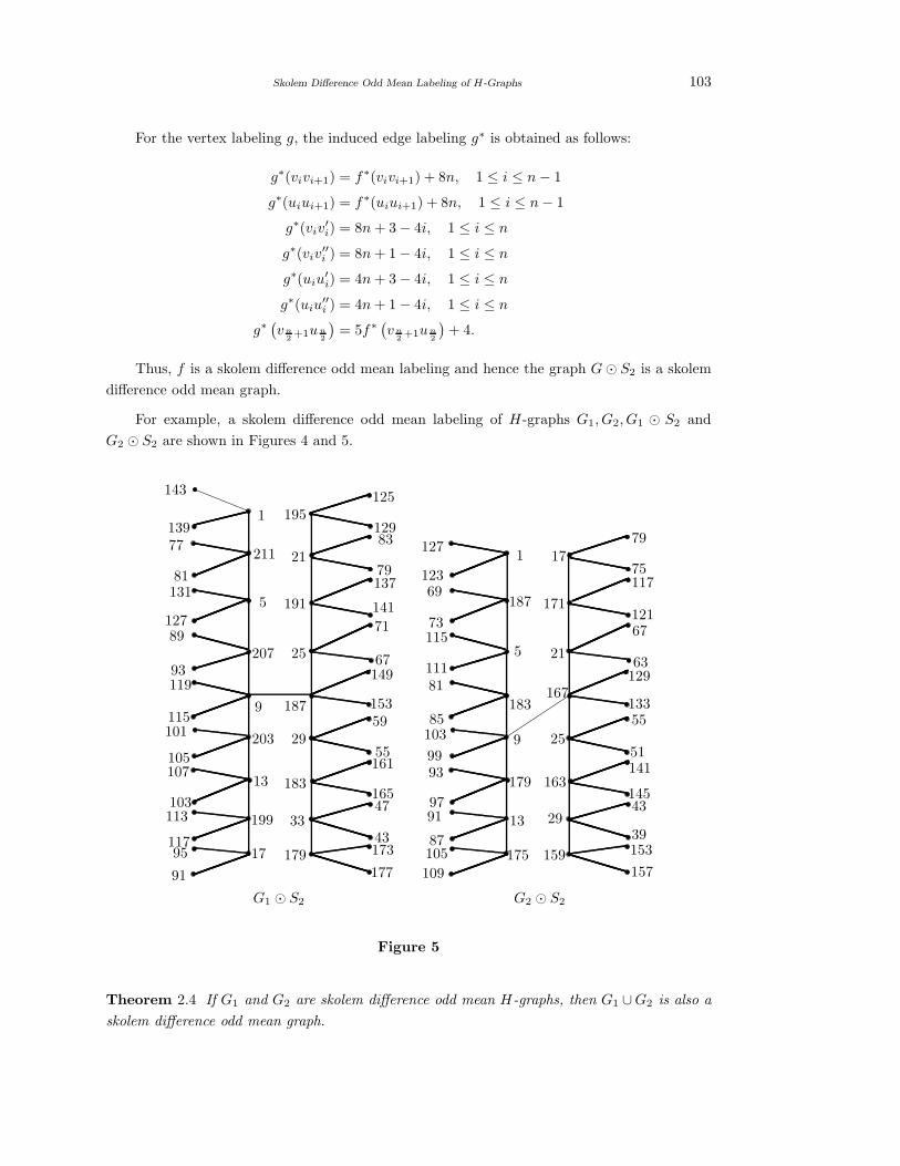
Skolem Difference Odd Mean Labeling of H-Graphs 103
For the vertex labeling g, the induced edge labeling g∗ is obtained as follows:
g∗(vivi+1) = f∗(vivi+1) + 8n, 1 ≤ i ≤ n − 1
g∗(uiui+1) = f∗(uiui+1) + 8n, 1 ≤ i ≤ n − 1
g∗(viv′i) = 8n + 3 − 4i, 1 ≤ i ≤ n
g∗(viv′′i ) = 8n + 1 − 4i, 1 ≤ i ≤ n
g∗(uiu′i) = 4n + 3 − 4i, 1 ≤ i ≤ n
g∗(uiu′′i ) = 4n + 1 − 4i, 1 ≤ i ≤ n
g∗(vn
2+1u n
2
)= 5f∗ (vn
2+1u n
2
)+ 4.
Thus, f is a skolem difference odd mean labeling and hence the graph G ⊙ S2 is a skolem
difference odd mean graph. 2For example, a skolem difference odd mean labeling of H-graphs G1, G2, G1 ⊙ S2 and
G2 ⊙ S2 are shown in Figures 4 and 5.
G1 ⊙ S2 G2 ⊙ S2
143
13977
81131
12789
93119
115101
105107
103113
11795
91
1
211
5
207
9
203
13
199
17
195
21
191
25
187
29
183
33
179
125
12983
79137
141
71
67149
15359
55161
16547
43173
177
127
12369
73115
11181
85103
9993
9791
87105
109
1
187
5
183
9
179
13
175
17
171
21
167
25
163
29
159
79
75117
12167
63129
13355
51141
14543
39153
157
Figure 5
Theorem 2.4 If G1 and G2 are skolem difference odd mean H-graphs, then G1 ∪G2 is also a
skolem difference odd mean graph.

104 P.Sugirtha, R.Vasuki and J.Venkateswari
Proof Let V (G1) = ui, vi : 1 ≤ i ≤ n and V (G2) = sj, tj : 1 ≤ j ≤ m be the vertices
of the H-graphs G1 and G2 respectively. Then the graph G1 ∪ G2 has 2(n + m) vertices and
2(n+m−1) edges. Let f : V (G1) → 1, 2, 3, · · · , 8n−5 and g : V (G2) → 1, 2, 3, · · · , 8m−5be a skolem difference odd mean labeling of G1 and G2 respectively.
Define h : V (G1 ∪ G2) → 1, 2, 3, · · · , 4q − 1 = 8(n + m) − 9 as follows:
For 1 ≤ i ≤ n and n ≥ 1,
h(ui) =
f(ui) if i is odd
f(ui) + 8m − 4 if i is even
h(vi) =
f(vi) + 8m − 4 if n is odd and i is odd
f(vi) if n is odd and i is even
f(vi) if n is even and i is odd
f(vi) + 8m − 4 if n is even and i is even.
For 1 ≤ j ≤ m and m ≥ 1,
h(sj) = g(sj) + 2
h(tj) = g(tj) + 2.
For the vertex labeling h, the induced edge labeling h∗ is given as follows:
For 1 ≤ i ≤ n − 1 and n ≥ 1,
h∗(uiui+1) = f∗(uiui+1) + 4m − 2
h∗(vivi+1) = f∗(vivi+1) + 4m − 2
h∗(u n+1
2
vn+1
2
)= f∗
(u n+1
2
vn+1
2
)+ 4m− 2 if n is odd and
h∗ (u n2+1vn
2
)= f∗ (u n
2+1vn
2
)+ 4m − 2 if n is even.
For 1 ≤ j ≤ m − 1 and m ≥ 1,
h∗(sjsj+1) = g∗(sjsj+1)
h∗(tjtj+1) = g∗(tjtj+1)
h∗(sm+1
2
tm+1
2
)= g∗
(sm+1
2
tm+1
2
)if m is odd
h∗ (sm2
+1tm2
)= g∗
(sm
2+1tm
2
)if m is even.
Thus, h is a skolem difference odd mean labeling of G1 ∪G2 and hence the graph G1 ∪G2
is a skolem difference odd mean graph. 2For example, a skolem difference odd mean labeling of G1 ∪ G2 where G1 = H3; G2 =

Skolem Difference Odd Mean Labeling of H-Graphs 105
H5, G1 = H5; G2 = H6, G1 = H4; G2 = H6 and G1 = H4; G2 = H4 are shown in Figures 6-9
following.
G2 = H5
G1 = H3
1
19
5
15
9
11
1
35
5
31
9
27
13
23
17
19
1
55
5
51
9
47
3
37
7
33
11
29
15
25
19
21G1 ∪ G2 = H3 ∪ H5
Figure 6
G1 = H5
1
35
5
31
9
27
13
23
17
19
G2 = H6
1
43
5
39
9
35
13
31
17
27
21
23
1
79
5
75
9
71
13
67
17
63
3
45
7
41
11
37
15
33
19
29
23
25G1 ∪ G2 = H5 ∪ H6
Figure 7
G1 = H4
1
27
5
23
9
13
G2 = H6
1
43
5
39
9
35
13
31
17
27
21
23
3
45
7
41
11
37
15
33
19
29
23
G1 ∪ G2 = H4 ∪ H6
19
1
71
5
67
9
63
13
59 2515
Figure 8

106 P.Sugirtha, R.Vasuki and J.Venkateswari
G1 = H4
1
27
5
23
9
13
19
15
G2 = H4 G1 ∪ G2 = H4 ∪ H4
1
27
5
23
9
19
13
15
1
55
5
51
9
47
13
43
3
29
7
25
11
21
15
17
Figure 9
References
[1] F.Harary, Graph Theory, Addison-Wesley, Reading Mass., 1972.
[2] K.Manikam and M.Marudai, Odd mean labeling of graphs, Bulletin of Pure and Applied
Sciences, 25E(1) (2006), 149–153.
[3] K.Murugan and A.Subramanian, Skolem difference mean labeling of H-graphs, Interna-
tional Journal of Mathematics and Soft Computing, 1(1) (2011), 115–129.
[4] A.Nagarajan and R.Vasuki, On the meanness of arbitrary path super subdivision of paths,
Australas. J. Combin., 51(2011), 41–48.
[5] S.Somasundaram and R. Ponraj, Mean labelings of graphs, National Academy Science
Letters, 26(2003), 210–213.
[6] S.K.Vaidya and Lekha Bijukumar, Some new familes of mean graphs, Journal of Mathe-
matics Research, 2(3) (2010), 169–176.
[7] R.Vasuki and A.Nagarajan, Meanness of the graphs Pa,b and P ba , International Journal of
Applied Mathematics, 22(4) (2009), 663–675.
[8] R.Vasuki and S.Arokiaraj, On mean graphs, International Journal of Mathematical Com-
binatorics, 3(2013), 22–34.
[9] R.Vasuki and A.Nagarajan, Odd mean labeling of the graphs Pa,b, Pba and P b
〈2a〉, Kragujevac
Journal of Mathematics, 36(1) (2012), 125–134.
[10] R.Vasuki and S.Arokiaraj, On odd mean graphs, Journal of Discrete Mathematical Sciences
and Cryptography, (To appear).
[11] R.Vasuki, J.Venkateswari and G.Pooranam, Skolem difference odd mean labeling of graphs
(Communicated).

International J.Math. Combin. Vol.1(2015), 107-112
Equitable Total Coloring of Some Graphs
Girija.G
(Department of Mathematics, Government Arts College, Coimbatore - 641 018, Tamil Nadu, India)
Veninstine Vivik.J
(Department of Mathematics, Karunya University, Coimbatore 641 114, Tamil Nadu, India)
E-mail: prof [email protected]; [email protected]
Abstract: In this paper we determine the equitable total chromatic number χet for the
double star graph K1,n,n and the fan graph Fm,n.
Key Words: Equitable total coloring, double star graph, fan graph.
AMS(2010): 05C15, 05C69
§1. Introduction
In this paper, we consider only finite simple graphs without loops or multiple edges. Let G(V, E)
be a graph with the set of vertices V and the edge set E. Total coloring χt(G) was introduced by
Vizing [7] and Behzad [1]. They both conjectured that for any graph G the following inequality
holds: ∆(G) + 1 ≤ χt(G) ≤ ∆(G) + 2. It is obvious that ∆(G) + 1 is the best possible lower
bound. This conjecture is proved so far for some specific classes of graphs. In general the
equitable total coloring problem is more difficult than the total coloring problem. In 1994, Fu
[4] gave the concepts of an equitable total coloring and the equitable total chromatic number
of a graph. For a simple graph G (V, E), let f be a proper k−total coloring of G
||Ti| − |Tj || ≤ 1, i, j = 1, 2, . . . , k.
The partition Ti = Vi ∪ Ei : 1 ≤ i ≤ k is called a k−equitable total coloring (k−ETC
of G in brief), and
χet (G) = min k|k − ETC of G
is called the equitable total chromatic number [2-6, 10] of G, where ∀x ∈ Ti = Vi ∪ Ei, f (x) =
i, i = 1, 2, · · · , k. It is obvious that χet(G) ≥ ∆ + 1. Furthermore Fu presented a conjecture
concerning the equitable total chromatic number (simply denoted by ETCC)
Conjecture 1.1([4]) For any simple graph G (V, E),
χet(G) ≤ ∆(G) + 2.
1Received September 3, 2014, Accepted March 8, 2015.

108 Girija.G and Veninstine Vivik.J
These Researchers in [2, 3, 5, 6, 8-10] have concentrated in providing the equitable total
chromatic number for specific families of graphs.
Lemma 1.2([10]) For any simple graph G (V, E),
χet (G) ≥ χt(G) ≥ ∆(G) + 1.
Lemma 1.3([4]) For complete graph Kp with order p,
χet (Kp) =
p, p ≡ 1mod 2
p + 1, p ≡ 0mod 2.
Lemma 1.4([3]) For n ≥ 13 the total equitable chromatic number of Hypo-Mycielski Graph,
χet(HM(Wn)) = n + 2.
In [9], equitable total chromatic numbers of some join graphs were given. Gong Kun et.al
[2] proved some results on the equitable total chromatic number of Wm ∨ Kn, Fm ∨ Kn and
Sm ∨ Kn. In 2012, Ma Gang and Ma Ming [6] proved some results concerning the equtiable
total chromatic number of Pm ∨ Sn, Pm ∨ Fn and Pm ∨ Wn.
In the present paper, we find the equitable total chromatic number χet for the double star
graph K1,n,n and the fan graph Fm,n.
§2. Preliminaries
Definition 2.1 A double star K1,n,n is a tree obtained from the star K1,n by adding a new pen-
dant edge of the existing n pendant vertices. It has 2n+1 vertices and 2n edges. Let V (K1,n,n) =
v ∪ v1, v2, . . . , vn ∪ u1, u2, . . . , un and E (K1,n,n) = e1, e2, . . . , en ∪ s1, s2, . . . , sn.
Definition 2.2 A Fan graph Km + Pn where Pn is path on n vertices. All the vertices of the
fan corresponding to the path Pn are labeled from m to n consecutively. The vertices in the fan
corresponding Km is labeled m + n.
§3. Equitable Total Coloring of Double Star Graphs
Theorem 3.1 For any positive integer n,
χet (K1,n,n) = n + 1.
Proof Let V (K1,n,n) = u0 ∪ ui : 1 ≤ i ≤ n ∪ vi : 1 ≤ i ≤ n and E (K1,n,n) =
ei : 1 ≤ i ≤ n∪si : 1 ≤ i ≤ n, where ei (1 ≤ i ≤ n) is the edge u0ui (1 ≤ i ≤ n) and si(1 ≤ i
≤ n) is the edge uivi (1 ≤ i ≤ n). Now we partition the edge and vertex sets in K1,n,n as follows.

Equitable Total Coloring of Some Graphs 109
T1 = e1, un, sn−1, vn−2T2 = e2, u1, sn, vn−1T3 = e3, u2, vnT4 = e4, u3, s1Tk = ek, uk−1, sk−3, vk−4 (5 ≤ k ≤ n)
Tn+1 = u0, sn−2, vn−3
Clearly T1, T2, T3, T4, Tk and Tn+1 are independent sets of K1,n,n. Also |T1| = |T2| =
|Tk| = 4 (5 ≤ k ≤ n) and |T3| = |T4| = |Tn+1| = 3, it holds the inequality ||Ti| − |Tj || ≤ 1 for
every pair (i, j). This implies χet (K1,n,n) ≤ n + 1. Since the set of edges e1, e2, . . . en and u0
receives distinct color, χet (K1,n,n) ≥ χt (K1,n,n) ≥ n+1. Hence χet (K1,n,n) ≥ n+1. Therefore
χet (K1,n,n) = n + 1. 2§4. Equitable Total Coloring of Fan Graphs
Theorem 4.1 For any positive integer n, m (n ≥ m), then
χet (Fm,n) =
∆ + 2 if n = m
∆ + 2 if n − m = 2
∆ + 1 if n − m = 1
n + 2 if n − m ≥ 3
Proof Let V (Fm,n) = ui : 1 ≤ i ≤ m∪vj : 1 ≤ j ≤ n and E (Fm,n) =m⋃
i=1
ei,j : 1 ≤ j ≤ n∪ej : 1 ≤ j ≤ n − 1, where ej (1 ≤ j ≤ n − 1) is the edge vjvj+1 (1 ≤ j ≤ n − 1) and ei,j is the
edge uivj (1 ≤ i ≤ m, 1 ≤ j ≤ n). Now we partition the edge and vertex sets of Fm,n in the
following cases.
Case 1. n = m
T1 = e1,1 ∪ e4,n, e5,n−1, e6,n−2, . . . , em,4 ∪ v3T2 = e1,2, e2,1 ∪ e5,n, e6,n−1, e7,n−2, . . . , em,5 ∪ v4T3 = e1,3, e2,2, e3,1 ∪ e6,n, e7,n−1, e8,n−2, . . . , em,6 ∪ v5
. . . . . . . . . . . . . . . . . . . . .
. . . . . . . . . . . . . . . . . . . . .
T∆−4 = e1,n−2, e2,n−3, . . . , em−2,1 ∪ vnT∆−3 = e1,n−1, e2,n−2, . . . , em−1,1

110 Girija.G and Veninstine Vivik.J
T∆−2 = e1,n, e2,n−1, . . . , em,1T∆−1 = e2,n, e3,n−1, . . . , em,2 ∪ v1
T∆ = e3,n, e4,n−1, . . . , em,3 ∪ v2
T∆+1 =
e2i : 1 ≤ i ≤
⌊n − 1
2
⌋∪
u2i−1 : 1 ≤ i ≤⌈n
2
⌉
T∆+2 =
e2i−1 : 1 ≤ i ≤
⌈n − 1
2
⌉∪
u2i : 1 ≤ i ≤⌊n
2
⌋
Clearly T1, T2, T3, . . . T∆+2 are independent sets of Fm,n. It holds the inequality ||Ti| − |Tj || ≤1 for every pair (i, j). This implies χet (Fm,n) ≤ ∆ + 2. Each edge vjvj+1 (1 ≤ j ≤ n − 1) is
adjacent with 2m + 2 edges and incident with two vertices,it forms a triangle with atleast one
vertex of ui : 1 ≤ i ≤ m. Therefore equitable total coloring needs ∆ + 2 colors.χet (Fm,n)
≥ χt (Fm,n) ≥ ∆ + 2. Hence χet (Fm,n) ≥ ∆ + 2. Therefore χet (Fm,n) = ∆ + 2.
Case 2. n − m = 2
T1 = e1,1 ∪ e2,n, e3,n−1, e4,n−2, . . . , em,4 ∪ v3T2 = e1,2, e2,1 ∪ e3,n, e4,n−1, e5,n−2, . . . , em,5 ∪ v4T3 = e1,3, e2,2, e3,1 ∪ e4,n, e5,n−1, e6,n−2, . . . , em,6 ∪ v5
. . . . . . . . . . . . . . . . . . . . .
. . . . . . . . . . . . . . . . . . . . .
T∆−2 = e1,n−2, e2,n−3, . . . , em,1 ∪ vnT∆−1 = e1,n−1, e2,n−2, . . . , em,2 ∪ v1
T∆ = e1,n, e2,n−1, . . . , em,3 ∪ v2
T∆+1 =
u2i−1 : 1 ≤ i ≤
⌊n − 1
2
⌋∪
e2i : 1 ≤ i ≤⌊
n − 1
2
⌋
T∆+2 =
u2i : 1 ≤ i ≤
⌊n − 2
2
⌋∪
e2i−1 : 1 ≤ i ≤⌈
n − 1
2
⌉
Clearly T1, T2, T3, . . . T∆+2 are independent sets of Fm,n. It holds the inequality ||Ti| − |Tj || ≤1 for every pair (i, j). This implies χet (Fm,n) ≤ ∆ + 2. Since each edge vjvj+1 (1 ≤ j ≤ n − 1)
is adjacent with 2m+2 edges and incident with two vertices,it forms a triangle with atleast one
vertex of ui : 1 ≤ i ≤ m. Therefore equitable total coloring needs ∆ + 2 colors. χet (Fm,n) ≥χt (Fm,n) ≥ ∆ + 2. Hence χet (Fm,n) ≥ ∆ + 2. Therefore χet (Fm,n) = ∆ + 2.
Case 3. n − m = 1
T1 = e1,1 ∪ e2,n, e3,n−1, e4,n−2, . . . , em,3 ∪ v2T2 = e1,2, e2,1 ∪ e3,n, e4,n−1, e5,n−2, . . . , em,4 ∪ v3T3 = e1,3, e2,2, e3,1 ∪ e4,n, e5,n−1, e6,n−2, . . . , em,5 ∪ v4
. . . . . . . . . . . . . . . . . . . . .
. . . . . . . . . . . . . . . . . . . . .
Equitable Total Coloring of Some Graphs 111
T∆−2 = e1,n−1, e2,n−2, . . . , em,1 ∪ vnT∆−1 = e1,n, e2,n−1, . . . , em,2 ∪ v1
T∆ =
e2i : 1 ≤ i ≤
⌊n − 1
2
⌋∪
u2i−1 : 1 ≤ i ≤⌈
n − 1
2
⌉
T∆+1 =
e2i−1 : 1 ≤ i ≤
⌈n − 1
2
⌉∪
u2i : 1 ≤ i ≤⌊
n − 1
2
⌋
Clearly T1, T2, T3, . . . T∆+1 are independent sets of Fm,n. It holds the inequality ||Ti| − |Tj || ≤1 for every pair (i,j). This implies χet (Fm,n) ≤ ∆ + 1. Since at each vertex vj (2 ≤ j ≤ n − 1)
there exist ∆ mutually adjacent edges and vj (2 ≤ j ≤ n − 1) needs one more color. χet (Fm,n) ≥χt (Fm,n) ≥ ∆ + 1. Hence χet (Fm,n) ≥ ∆ + 1. Therefore χet (Fm,n) = ∆ + 1.
Case 4. n − m ≥ 3
T1 = e1,1 ∪ e2,n, e3,n−1, e4,n−2, . . . , em,4 ∪ v3T2 = e1,2, e2,1 ∪ e3,n, e4,n−1, e5,n−2, . . . , em,5 ∪ v4T3 = e1,3, e2,2, e3,1 ∪ e4,n, e5,n−1, e6,n−2, . . . , em,6 ∪ v5
. . . . . . . . . . . . . . . . . . . . .
. . . . . . . . . . . . . . . . . . . . .
Tn−2 = e1,n−2, e2,n−3, . . . , em,1 ∪ vnTn−1 = e1,n−1, e2,n−2, . . . , em,2 ∪ v1
Tn = e1,n, e2,n−1, . . . , em,3 ∪ v2
Tn+1 =
u2i−1 : 1 ≤ i ≤⌈m
2
⌉∪
e2i : 1 ≤ i ≤⌊
n − 1
2
⌋
Tn+2 =
u2i : 1 ≤ i ≤⌊m
2
⌋∪
e2i−1 : 1 ≤ i ≤⌈
n − 1
2
⌉
Clearly T1, T2, T3, . . . Tn+2 are independent sets of Fm,n. It holds the inequality ||Ti| − |Tj|| ≤1 for every pair (i, j). This implies χet (Fm,n) ≤ n + 2. Since at each vertex ui (1 ≤ i ≤ m)
there exist n mutually adjacent edges and ui (1 ≤ i ≤ m) needs one more color. χet (Fm,n) ≥χt (Fm,n) ≥ n + 2. Hence χet (Fm,n) ≥ n + 2. Therefore χet (Fm,n) = n + 2. 2References
[1] Behzad.M, Graphs and Their Chromatic Numbers, Doctoral Thesis, East Lansing: Michi-
gan State University, 1965.
[2] Gong Kun, Zhang Zhongfu, Wang Jian Fang, Equitable total coloring of some join graphs,
Journal of Mathematical Research & Exposition, 28(4), (2008), 823-828. DOI:10.3770/j.issn:
1000-341X.2008.04.010
[3] Haiying Wang, Jianxin Wei, The equitable total chromatic number of the graph HM(Wn),
J. Appl. Math. & Computing, Vol. 24(1-2), (2007), 313–323.
[4] Hung-lin Fu, Some results on equalized total coloring, Congr. Numer., 102, (1994), 111-

112 Girija.G and Veninstine Vivik.J
119.
[5] Ma Gang, Ma Ming, The equitable total chromatic number of some join-graphs, Open
Journal of Applied Sciences, (2012), 96-99.
[6] Ma Gang, Zhang Zhongfu, On the equitable total coloring of multiple join-graph, Journal
of Mathematical Research and Exposition, 2007. 27(2), 351–354.
[7] Vizing.V.G, On an estimate of the chromatic class of a p-graph(in Russian), M etody
Diskret. Analiz., 3, (1964), 25-30.
[8] Wei-fan Wang, Equitable total coloring of graphs with maximum degree 3, Graphs Combin.,
18, (2002) 677-685.
[9] Zhang Zhongfu, Wang Weifan, Bau Sheng. et al. On the equitable total colorings of some
join graphs, J. Info. & Comput. Sci., 2(4), (2005), 829-834.
[10] Zhang Zhongfu, Zhang Jianxun, Wang Jianfang, The total chromatic number of some
graph, Sci. Sinica, Ser.A, 31(12), (1988) 1434-1441.
International J.Math. Combin. Vol.1(2015), 113-125
Some Characterizations for the Involute Curves in Dual Space
Suleyman SENYURT
( Department of Mathematics, Faculty of Arts and Sciences, Ordu University, 52100, Ordu/Turkey)
Mustafa BILICI
(Department of Mathematics, Faculty of Education, Ondokuz Mayis University, Turkey)
Mustafa CALISKAN
(Department of Mathematics, Faculty of Science, Gazi University, Turkey)
E-mail: [email protected], [email protected], [email protected]
Abstract: In this paper, we investigate some characterizations of involute – evolute curves
in dual space. Then the relationships between dual Frenet frame and Darboux vectors of
these curves are found.
Key Words: Dual curve, involute, evolute, dual space.
AMS(2010): 53A04, 45F10
§1. Introduction
Involute-evolute curve couple was originally defined by Christian Huygens in 1668. In the
theory of curves in Euclidean space, one of the important and interesting problems is the
characterizations of a regular curve. In particular, the involute of a given curve is a well known
concept in the classical differential geometry (for the details see [7]). For classical and basic
treatments of Involute-evolute curve couple, we refer to [1], [5], [7-9] and [13].
The relationships between the Frenet frames of the involute-evolute curve couple have been
found as depend on the angle between binormal vector B and Darboux vector W of evolute
curve, [1]. In the light of the existing literature, similar studies have been constructed on
Lorentz and Dual Lorentz space,[2-4, 10-12].
In this paper, The relationships between dual Frenet frame and Darboux vectors of these
curves have been found. Additionally, some important results concerning these curves are given.
§2. Preliminaries
Dual numbers were introduced by W.K. Clifford (1849-79) as a tool for his geometrical investi-
1Received July 2, 2014, Accepted March 10, 2015.
114 Suleyman SENYURT, Mustafa BILICI and Mustafa CALISKAN
gations. The set ID =A = a + εa∗ | a, a∗ǫIR, ε2 = 0
is called dual numbers set. On this
set product and addition operations are described as
(a + εa∗) + (b + εb∗) = (a + b) + ε (a∗ + b∗) ,
(a + εa∗) . (b + εb∗) = ab + ε (ab∗ + a∗b) ,
respectively. The elements of the set ID3 =
→A |
→A =
→a + ε
→a∗,
→a ,
→a∗ǫIR3
are called dual
vectors. On this set, addition and scalar product operations are described as
⊕ : ID3 × ID3 → ID3 ,→A ⊕
→B =
(→a +
→b
)+ ǫ
(→a∗ +
→b∗)
,
⊙ : ID × ID3 → ID3 ,∼
λ ⊙→A = λ
→a + ǫ
(λ→a∗ + λ∗→a
),
respectively. Algebraic construction(ID3,⊕, ID, +, .,⊙
)is a modul. This modul is called
ID-Modul.
The inner product and vectorel product of dual vectors→A,
→BǫID3 are defined by respec-
tively,
〈 , 〉 : ID3 × ID3 → ID ,
⟨→A,
→B
⟩=
⟨→a ,
→b
⟩+ ε
(⟨→a ,
→b∗⟩
+
⟨→a∗,
→b
⟩)
∧ : ID3 × ID3 → ID3 ,→A ∧
→B =
(→a ∧
→b
)+ ε
(→a ∧
→b∗ +
→a∗ ∧
→b
).
For→A 6= 0, the norm
∥∥∥∥→A
∥∥∥∥of→A =
→a + ε
→a∗ is defined by
∥∥∥∥→A
∥∥∥∥ =
√⟨→A,
→A
⟩=∥∥∥→a∥∥∥+ ε
⟨→a ,
→a∗⟩
∥∥∥→a∥∥∥
,∥∥∥→a∥∥∥ 6= 0.
The angle between unit dual vectors→A and
→B Φ = ϕ + εϕ∗ is called dual angle and this
angle is denoted by ([6]) ⟨→A,
→B
⟩= cosΦ = cosϕ − εϕ∗sinϕ
Let
∼
α : I ⊂ IR → ID3
s → ∼
α (s) = α (s) + εα∗ (s)
be differential unit speed dual curve in dual space ID3. Denote by T, N, B the moving dual
Frenet frame along the dual space curve∼
α (s) in the dual space ID3. Then T, N and B are the
dual tangent, the dual principal normal and the dual binormal vector fields, respectively. The
function κ (s) = k1 + εk∗1 and τ (s) = k2 + εk∗
2 are called dual curvature and dual torsion of∼
α,

Some Characterizations for the Involute Curves in Dual Space 115
respectively. Then for the dual curve∼
α the Frenet formulae are given by,
T′
(s) = κ (s)N (s)
N′
(s) = −κ (s)T (s) + τ (s)B (s) (2.1)
B′
(s) = −τ (s)N (s)
The formulae (2.1) are called the Frenet formulae of dual curve. In this palace curvature
and torsion are calculated by,
κ (s) =√〈T ′ , T ′〉 , τ (s) =
det(T, T
′
, T′′
)
〈T ′ , T ′〉 (2.2)
If α is not unit speed curve, then curvature and torsion are calculated by
κ (s) =
∥∥∥α′
(s) ∧ α′′
(s)∥∥∥
‖α′ (s)‖3 , τ (s) =det(α
′
(s) , α′′
(s) , α′′′
(s))
‖α′ (s) ∧ α′′ (s)‖2 (2.3)
By separating formulas (2.1) into real and dual part, we obtain
t′
(s) = k1n
n′
(s) = −k1t + k2b (2.4)
b′
(s) = −k2n
t∗′
(s) = k1n∗ + k∗
1n
n∗′
(s) = −k1t∗ − k∗
1t + k2b∗ + k∗
2b (2.5)
b∗′
(s) = −k2n∗ − k∗
2n
§3. Some Characterizations Involute of Dual Curves
Definition 3.1 Let α : I → ID3 and β : I → ID3 be dual unit speed curves. If the tangent
lines of the dual curve α is orthogonal to the tangent lines of the dual curve β , the dual curve
β is called involute of the dual curve α or the dual curve α is called evolute of the dual curve β
(see Fig.1). According to this definition, if the tangent of the dual curve α is denoted by T and
the tangent of the dual curve β is denoted by−T , we can write
⟨T,
−T
⟩= 0 (3.1)
Theorem 3.1 Let α and β be dual curves. If the dual curve β involute of the dual curve α, we
can write
β (s) = α (s) + [(c1 − s) + εc2] T (s) , c1, c2ǫIR.

116 Suleyman SENYURT, Mustafa BILICI and Mustafa CALISKAN
Proof Then by the definition we can assume that
β (s) = α (s) + λT (s) , λ (s) = µ (s) + εµ∗ (s) (3.2)
for some function λ (s). By taking derivative of the equation (3.2) with respect to s and applying
the Frenet formulae (2.1) we have
dβ
ds=
(1 +
dλ
ds
)T + λκN
where s and s∗ are arc parameter of the dual curves α and β, respectively. It follows that
−T
ds∗
ds=
(1 +
dλ
ds
)T + λκN (3.3)
the inner product of (3.3) with T is
ds∗
ds
⟨T,
−T
⟩=
(1 +
dλ
ds
)〈T, T 〉+ λ 〈T, N〉 (3.4)
From the definition of the involute-evolute curve couple, we can write
⟨T,
−T
⟩= 0
By substituting the last equation in (3.4) we get
1 +dλ
ds= 0 and
d
ds(µ (s) + εµ∗ (s)) = −1 (3.5)
Straightforward computation gives
µ′
(s) = −1 and µ∗′
(s) = 0
integrating last equation, we get
µ (s) = c1 − s and µ∗ (s) = c2 (3.6)
By substituting (3.6) in (3.2), we get
β (s) − α (s) = [(c1 − s) + εc2] T (s) . (3.7)
This completes the proof. 2Corollary 3.1 The distance between the dual curves β and α is |c1 − s| ∓ εc2.
Proof By taking the norm of the equation (3.7) we get
d(α (s) , β (s)
)= |c1 − s| ∓ εc2 (3.8)

Some Characterizations for the Involute Curves in Dual Space 117
This completes the proof. 2
Fig.1
Theorem 3.2 Let α, β be dual curves. If the dual curve β involute of the dual curve α, then
the relationships between the dual Frenet vectors of the dual curves α and β
−T = N−N = −cosΦT + sinΦB−B = sinΦT + cosΦB
Proof By differentiating the equation (3.2) with respect to s we obtain
β′ (s) = λκ (s)N (s) , λ = (c1 − s) + εc2 (3.9)
and ∥∥∥β′ (s)∥∥∥ = λκ (s)
Thus, the tangent vector of β is found
−T =
β′ (s)∥∥∥β′ (s)∥∥∥
=λκ (s)N (s)
λκ (s)
If we arrange the last equation we obtain
−T = N (s) (3.10)

118 Suleyman SENYURT, Mustafa BILICI and Mustafa CALISKAN
By differentiating the equation (3.9) with respect to s we obtain
β′′
= −λκ2T +(λκ
′ − κ)
N + λκτB
If the cross product β′ ∧ β′′
is calculated we have
β′ ∧ β′′
= λ2κ2τT + λ2κ3B (3.11)
The norm of vector β′ ∧ β′′
is found
∥∥∥β′ ∧ β′′
∥∥∥ = λ2κ2√
κ2 + τ2 (3.12)
For the dual binormal vector of the dual curve β we can write
−B =
β′ ∧ β′′
∥∥∥β′ ∧ β′′
∥∥∥
By substituting (3.11) and (3.12) in the last equation we get
−B =
τ√κ2 + τ2
T +κ√
κ2 + τ2B (3.13)
For the dual principal normal vector of the dual curve β we can write
−N =
−B ∧
−T
and−N = − κ√
κ2 + τ2T +
τ√κ2 + τ2
B (3.14)
Let Φ(Φ = ϕ + εϕ∗ , ε2 = 0
)be dual angle between the dual Darboux vector W of α and
dual unit binormal vector B in this situation we can write
sinΦ =τ
κ2 + τ2, cosΦ =
κ
κ2 + τ2· (3.15)
By substituting (3.15) in (3.12) and (3.13) the proof is completed. 2The real and dual parts of
−T ,
−N ,
−B are
−T = N−N = −cosΦT + sinΦB−B = sinΦT + cosΦB
is separated into the real and dual part, we can obtain
Some Characterizations for the Involute Curves in Dual Space 119
−t = n,−n = −cosϕt + sinϕb,−b = sinϕt + cosϕb
−t∗
= n∗
−n∗
= −cosϕt∗ + sinϕb∗ + ϕ∗ (sinϕt + cosϕb)
−b∗
= sinϕt∗ + cosϕb∗ + ϕ∗ (cosϕt − sinϕb)
On the way
sinΦ = sin (ϕ + εϕ∗) = sinϕ + εϕ∗cosϕ
cosΦ = cos (ϕ + εϕ∗) = cosϕ − εϕ∗sinϕ
If the equation
sinΦ =τ
κ2 + τ2
is separated into the real and dual part, we can obtain
sinϕ =k2
k21 + k2
2
cosϕ =k21 + k∗
2 − 2k1k2k∗1 − 2k2
2k∗2
ϕ (k21 + k2
2)2
If the equation
cosΦ =κ
κ2 + τ2
is separated into the real and dual part, we can obtain
cosϕ =k1
k21 + k2
2
sinϕ =2k2
1 + k∗1 + 2k1k2k
∗2 − k2
1k∗1 − k2
2k∗1
ϕ (k21 + k2
2)2
Theorem 3.3 Let α, β be dual curves. If the dual curve β involute of the dual curve α ,
curvature and torsion of the dual curve β are
−κ
2
(s) =κ2 (s) + τ2 (s)
λ2 (s)κ2 (s),
−τ (s) =
κ (s) τ′
(s) − κ′
(s) τ (s)
λ (s)κ (s) (κ2 (s) + τ2 (s))(3.16)
Proof By the definition of involute we can write
β (s) = α (s) + |λ|T (s) (3.17)
120 Suleyman SENYURT, Mustafa BILICI and Mustafa CALISKAN
By differentiating the equation (3.17) with respect to s we obtain
dβ
ds∗ds∗
ds= T (s) + |λ|
′
T (s) + |λ|κ (s)N (s) ,
dβ
ds∗ds∗
ds= T (s) − T (s) + |λ|κ (s)N (s) ,
−T (s)
ds∗
ds= |λ|κ (s)N (s) . (3.18)
Since the direction of−T (s) is coincident with N (s) we have
−T (s) = N (s) . (3.19)
Taking the inner product of (3.18) with T and necessary operation are made we get
ds∗
ds= |λ (s)|κ (s) . (3.20)
By taking derivative of (3.19) and applying the Frenet formulae ( 2.1) we have
−T (s) = N (s) ⇒
−T
′
(s)ds∗
ds= −κT + τB. (3.21)
From (3.20) and (3.21), we have
−T
′
(s) =−κT + τB
|λ (s)|κ (s)·
From the last equation we can write
−κ (s)
−N (s) =
−κT + τB
|λ (s)|κ (s)·
Taking the inner product the last equation with each other we have
⟨−κ (s)
−N (s) ,
−κ (s)
−N (s)
⟩=
⟨−κT + τB
|λ (s)|κ (s),−κT + τB
|λ (s)|κ (s)
⟩·
Thus, we find−κ
2
(s) =κ2 (s) + τ2 (s)
λ2 (s)κ2 (s)·
We know that
β′ ∧ β′′
= λ2κ2τT + λ2κ3B.
Taking the norm the last equation, we get
∥∥∥β′ ∧ β′′
∥∥∥ = κ4λ4(κ2 + τ2
).

Some Characterizations for the Involute Curves in Dual Space 121
By substituting these equations in (2.3), we get
−τ =
∣∣∣∣∣∣∣∣
0 κλ 0
−κ2λ (κλ)′
κτλ(−κ2λ
)′− κ (κλ)
′
−κ3λ + (κλ)′′
− κτ2λ (κλ)′
τ + (κτλ)′
∣∣∣∣∣∣∣∣∥∥∥β′ ∧ β′′
∥∥∥2 ,
−τ =
κτ′ − κ
′
τ
κ |λ| (κ2 + τ2)·
This completes the proof. 2If the equation (3.16) is separated into the real and dual part, we can obtain
−k1 =
√k21 + k2
2
µk1,
−k1
∗=
(µ2k2
1
)(2k1k
∗1 + 2k2k
∗2) −
(2k1k
∗1µ2) (
k21 + k2
2
)
2µ3k31
√k21 + k2
2
,
−k2 =
k1k′
2 − k2k′
1
µk1 (k21 + k2
2),
−k2
∗=
(k1k
′∗
2 + k′
2k∗1 − k
′
1k∗2 − k2k
′∗
1
)
(µk31 + k1k2
2µ)
−[2 (k1k
∗1 + k2k
∗2) k1µ +
(k21 + k2
2
)(k∗
1µ + k1µ∗)] (
k1k′
2 − k2k′
1
)
(µk31 + k1k2
2µ)2 ·
Theorem 3.4 Let α, β be dual curves and the dual curve β involute of the dual curve α . If
W and−W are Darboux vectors of the dual curves α and β we can write
−W =
1
λκ
(W + Φ
′
N)
(3.22)
Proof Since−W is Darboux vector of β (s) we can write
−W (s) =
−τ (s)
−T (s) +
−κ (s)
−B (s) (3.23)
By substituting−τ ,
−T ,
−κ,
−B in the last equation, we get
−W (s) =
κτ′ − κ
′
τ
κ |λ| (κ2 + τ2)N (s) +
√κ2 + τ2
κ |λ| (sinΦT + cosΦB) . (3.24)

122 Suleyman SENYURT, Mustafa BILICI and Mustafa CALISKAN
By substituting (3.15) in (3.24), we get
−W (s) =
κτ′ − κ
′
τ
κ |λ| (κ2 + τ2)N (s) +
√κ2 + τ2
κ |λ|
(τT + κB√
κ2 + τ2
).
The necessary operation are made, we get
−W (s) =
τT + κB
κ |λ| +κτ
′ − κ′
τ
κ |λ| (κ2 + τ2)N (s) ,
−W (s) =
1
κ |λ|
(τT + κB +
κτ′ − κ
′
τ
κ2 + τ2N
)
and
−W (s) =
1
κ |λ|
W +
(τκ
)′κ2
κ2 + τ2N
.
Furthermore, SincesinΦ
cosΦ=
τ√
κ2 + τ2
κ√
κ2 + τ2,
τ
κ= tanΦ.
By taking derivative of the last equation, we have
Φ′
sec2Φ =( τ
κ
)′
·
By a straightforward calculation, we get
Φ′
=( τ
κ
)′
κ
κ2 + τ2,
−W (s) =
1
κ |λ|(W + Φ
′
N)
,
which completes the proof. 2If the equation (3.22) is separated into the real and dual part, we can obtain
−w =
w + ϕ′
n
µk1,
−w
∗=
µk1
(w∗ + ϕ
′
n + ϕ′∗n)− (µk∗
1 + µ∗k1)(w + ϕ
′
n)
µ2k21
·
If the equation (3.24) is separated into the real and dual part, we can obtain
−w =
√k21 + k2
2
µk1(sinϕt + cosϕb) ,

Some Characterizations for the Involute Curves in Dual Space 123
−w
∗=
√k21 + k2
2
µk1(sinϕt∗ + cosϕb∗ + ϕ∗ (cosϕt − sinϕb))
+µk1 (k1k
∗1 + k2k
∗2) −
(k21 + k2
2
)(µk∗
1 + µ∗k1)√k21 + k2
2µ2k2
1
(sinϕt + cosϕb) ·
Theorem 3.5 Let α, β be dual curves and the dual curve β involute of the dual curve α . If C
and−C are unit vectors of the direction of W and
−W , respectively
−C =
Φ′
√Φ′2 + κ2 + τ2
N +
√κ2 + τ2
√Φ′2 + κ2 + τ2
C. (3.25)
Proof Since β the dual angle between−W and
−B we can write
−C (s) = sinβ
−T (s) + cosβ
−B (s) .
In here, we want to find the statements sinβ and cosβ, we know that
sinβ =
−τ∥∥∥∥−W
∥∥∥∥=
−τ√
−κ
2
+−τ
2·
By substituting−τ and
−κ in the last equation and necessary operations are made, we get
sinβ =Φ
′
√Φ′2 + κ2 + τ2
· (3.26)
Similarly,
cosβ =
√κ2 + τ2
√Φ′2 + κ2 + τ2
· (3.27)
Thus we find−C =
Φ′
√Φ′2 + κ2 + τ2
−T +
√κ2 + τ2
√Φ′2 + κ2 + τ2
C,
which completes the proof. 2If the equation (3.25) is separated into the real and dual part, we can obtain
−c =
ϕ′
n +√
k21 + k2
2c√ϕ′ + k2
1 + k22
,
−c∗
=ϕ
′
n∗ + ϕ′∗
n +√
k21 + k2
2c∗ +k1k∗
1+k2k∗
2√k21+k2
2
c −ϕ
′
n(√
k21+k2
2
)c
(ϕ
′
ϕ′∗
+k1k∗
1+k2k∗
2
)
√ϕ′+k2
1+k2
2√ϕ′ + k2
1 + k22
·

124 Suleyman SENYURT, Mustafa BILICI and Mustafa CALISKAN
If the equation (3.26) and (3.27) are separated into the real and dual part, we can obtain
sin−ϕ =
ϕ′
√ϕ′ + k2
1 + k22
,
cos−ϕ =
(Φ
′2 + κ2 + τ2)
Φ′∗ − ϕ
′
ϕ∗
+ k1k∗1 + k2k
∗2ϕ
′
−ϕ∗(Φ′2 + κ2 + τ2)
32
,
cos−ϕ =
√k21 + k2
2
ϕ′2
+ k21 + k2
2
,
sin−ϕ =
(ϕ
′
ϕ′∗
+ k1k∗1 + k2k
∗2
)√k21 + k2
2 −(ϕ
′2
+ k21 + k2
2
)(k1k
∗1 + k2k
∗2)
−ϕ∗(Φ′2 + κ2 + τ2)
32
√k21 + k2
2
·
Corollary 3.2 Let α, β be dual curves and the dual curve β involute of the dual curve α . If
evolute curve α is helix,
(1) The vectors−W and
−B of the involute curve β are linearly dependent;
(2) C=−C;
(3) β is planar.
Proof (1) If the evolute curve α is helix, then we have
τ
κ= tanΦ = cons or Φ
′
= 0
and then we have
sin−Φ = 0,
cos−Φ = 1.
Thus, we get−Φ = 0. (3.28)
(2) Substituting by the equation (3.28) into the equation (3.25), we have
C =−C.
(3) For being is a helix , then we have
τ
κ= cons,
( τ
κ
)′
= 0. (3.29)

Some Characterizations for the Involute Curves in Dual Space 125
On the other hand, from the equation (3.16), we can write
−τ−κ
=
κτ′−κ
′
τλκ(κ2+τ2)
(κ2+τ2)12
λκ
=
(τκ
)′κ2
(κ2+τ2
) 32
· (3.30)
Substituting by the equation (3.29) into the equation (3.30), then we find
−τ = 0,
which completes the proof. 2References
[1] Bilici M. and Calıskan M., Some characterizations for the pair of involute-evolute curves
in Euclidean space, Bulletin of Pure and Applied Sciences, Vol.21E, No.2, 289-294, 2002.
[2] Bilici M. and Calıskan M., On the involutes of the spacelike curve with a timelike binormal
in Minkowski 3-space, International Mathematical Forum, Vol. 4, No.31, 1497-1509, 2009.
[3] Bilici M. and Calıskan M., Some new notes on the involutes of the timelike curves in
Minkowski3-space, Int.J.Contemp.Math. Sciences, Vol.6, No.41, 2019-2030, 2011.
[4] Bukcu B and Karacan M.K., On the involute and evolute curves of the spacelike curve
with a spacelike binormal in Minkowski 3 space, Int. J. Contemp. Math. Sciences, Vol. 2,
No. 5, 221 - 232, 2007.
[5] Fenchel W., On the differential geometry of closed space curves, Bull. Amer. Math. Soc.,
Vol.57, No.1, 44-54, 1951.
[6] Hacısalihoglu H. H., Acceleration Axes in Spatial Kinematics I, Communications, Serie A:
Mathematiques, Physique et Astronomie, Tome 20 A, pp. 1-15, Annee 1971.
[7] Hacısalihoglu H.H., Differential Geometry, (Turkish) Ankara University of Faculty of Sci-
ence, 2000.
[8] Millman R.S. and Parker G.D., Elements of Differential Geometry, Prentice-Hall Inc.,
Englewood Cliffs, New Jersey, 1977.
[9] Sabuncuoglu, A., Differential Geometry (Turkish), Nobel Publishing, 2006.
[10] Senyurt S. and Gur S., On the dual spacelike-spacelike involute-evolute curve couple on
dual Lorentzian space, International Journal of Mathematical Engineering and Science,
ıssn:2277-6982, vol.1, Issue :5, 14-29, 2012.
[11] Senyurt S. and Gur S., Timelike - spacelike involute - evolute curve couple on dual
Lorentzian space, J. Math. Comput. Sci., Vol.2, No. 6, 1808-1823, 2012.
[12] Senyurt S. and Gur S., Spacelike - timelike involute- evolute curve couple on dual Lorentzian
space, J. Math. Comput. Sci., Vol.3, No.4,1054-1075, 2013.
[13] Yuce S. and Bektas O., Special involute-evolute partner D-curves in E3 , European Journal
of Pure and Applied Mathematics, Vol. 6, No. 1, 20-29, 2013.
International J.Math. Combin. Vol.1(2015), 126-135
One Modulo N Gracefulness of
Some Arbitrary Supersubdivision and Removal Graphs
V.Ramachandran
(Department of Mathematics, P.S.R Engineering College, Sivakasi, Tamil Nadu, India)
C.Sekar
(Department of Mathematics, Aditanar College of Arts and Science, Tiruchendur, Tamil Nadu, India)
E-mail: [email protected]; [email protected]
Abstract: A graph G is said to be one modulo N graceful (where N is a positive integer)
if there is a function φ from the vertex set of G to 0, 1, N, (N +1), 2N, (2N +1), · · · , N(q−
1), N(q − 1) + 1in such a way that (i) φ is 1− 1 (ii) φ induces a bijection φ∗ from the edge
set of G to 1, N +1, 2N +1, · · · , N(q−1)+1where φ∗(uv)=|φ(u)−φ(v)|. In this paper we
prove that arbitrary supersubdivision of disconnected path and cycle Pn ∪Cr is one modulo
N graceful for all positive integer N . Also we prove that the graph P+n − v
(1)k is one modulo
N graceful for every positive integer N.
Key Words: Graceful, Graceful, modulo N graceful, disconnected graphs, arbitrary su-
persubdivision graphs, Pn
⋃Cn and P+
n − v(1)k .
AMS(2010): 05C78
§1. Introduction
S. W. Golomb [3] introduced graceful labelling. Odd gracefulness was introduced by R. B.
Gnanajothi [4]. C. Sekar [11] introduced one modulo three graceful labelling. In [8,9], we
introduced the concept of one modulo N graceful where N is any positive integer. In the case
N = 2, the labelling is odd graceful and in the case N = 1 the labelling is graceful. Joseph
A. Gallian [2] surveyed numerous graph labelling methods. Recently G. Sethuraman and P.
Selvaraju [5] have introduced a new method of construction called supersubdivision of a graph.
Let G be a graph with n vertices and t edges. A graph H is said to be a supersubdivision of G
if H is obtained by replacing every edge ei of G by the complete bipartite graph K2,m for some
positive integer m in such a way that the ends of ei are merged with the two vertices part of
K2,m after removing the edge ei from G. A supersubdivision H of a graph G is said to be an
arbitrary supersubdivision of the graph G if every edge of G is replaced by an arbitrary K2,m
(m may vary for each edge arbitrarily). A graph G is said to be connected if any two vertices
of G are joined by a path. Otherwise it is called disconnected graph.
G. Sethuraman and P. Selvaraju [6] proved that every connected graph has some supersub-
1Received July 15, 2014, Accepted March 12, 2015.
One Modulo N Gracefulness of Some Arbitrary Supersubdivision and Removal Graphs 127
division that is graceful. They pose the question as to whether some supersubdivision is valid
for disconnected graphs. [10] We proved that an arbitrary supersubdivision of disconnected
paths are graceful. Barrientos and Barrientos [1] proved that any disconnected graph has a
supersubdivision that admits an α-labeling. They also proved that every supersubdivision of a
connected graph admits an α-labeling.
In this paper we prove that arbitrary supersubdivision of disconnected path and cycle
Pn ∪Cr is one modulo N graceful for all positive integer N . When N = 1 we get an affirmative
answer for their question. Also we prove that the graph P+n − v
(1)k is one modulo N graceful
for every positive integer N.
§2. Main Results
Definition 2.1 A graph G with q edges is said to be one modulo N graceful (where N is a
positive integer) if there is a function φ from the vertex set of G to 0, 1, N, (N + 1), 2N, (2N +
1), . . . , N(q − 1), N(q − 1) + 1 in such a way that (i) φ is 1 − 1 (ii) φ induces a bijection φ∗
from the edge set of G to 1, N + 1, 2N + 1, . . . , N(q − 1) + 1where φ∗(uv)=|φ(u) − φ(v)|.
Definition 2.2 In the complete bipartite graph K2,m we call the part consisting of two vertices,
the 2-vertices part of K2,m and the part consisting of m vertices the m-vertices part of K2,m.Let
G be a graph with p vertices and q edges. A graph H is said to be a supersubdivision of G if
H is obtained by replacing every edge e of G by the complete bipartite graph K2,m for some
positive integer m in such a way that the ends of e are merged with the two vertices part of
K2,m after removing the edge e from G. H is denoted by SS(G).
Definition 2.3 A supersubdivision H of a graph G is said to be an arbitrary supersubdivision
of the graph G if every edge of G is replaced by an arbitrary K2,m (m may vary for each edge
arbitrarily). H is denoted by ASS(G).
Definition 2.4 Let v1, v2, . . . , vn be the vertices of a path of length n and v(1)1 , v
(1)2 , . . . , v
(1)n be
the pendant vertices attached with v1, v2, . . . , vn respectively. The removal of a pendant vertex
v(1)k where 1 ≤ k ≤ n from P+
n yields the graph P+n − v
(1)k .
Theorem 2.5 Arbitrary supersubdivision of disconnected path and cycle Pn ∪Cr is one modulo
N graceful provided the arbitrary supersubdivision is obtained by replacing each edge of G by
K2,m with m > 2.
Proof Let Pn be a path with successive vertices v1, v2, · · · , vn and let ei (1 ≤ i ≤ n − 1)
denote the edge vivi+1 of Pn. Let Cr be a cycle with successive vertices vn+1, vn+2, · · · , vn+r
and let ei(n + 1 ≤ i ≤ n + r) denote the edge vivi+1.
Let H be an arbitrary supersubdivision of the disconnected graph Pn∪Cr where each edge
ei of Pn ∪ Cr is replaced by a complete bipartite graph K2,miwith mi > 2 for 1 ≤ i ≤ n − 1
and n + 1 ≤ i ≤ n + r. Here the edge vn+rvn+1 is replaced by k2,r−1. We observe that H has
M = 2(m1 + m2 + · · · + mn−1 + mn+1 + · · · + mn+r) edges.

128 V.Ramachandran and C.Sekar
v4
v5
v6
v1 v2 v3
v(1)56
v(2)56 = v
(m5)56v
(1)64
v(1)64 = v
(m6)64
v(2)12 = v
(m1)12
v(1)12
v(1)23
v(2)23
v(3)23 = v
(m2)23
v(1)45
v(2)45
v(3)45
v(4)45 = v
(m4)45
Figure 1 Supersubdivision of P3 ∪ C3
Define
φ(vi) = N(i − 1), i = 1, 2, 3, · · · , n,
φ(vi) = N(i), i = n + 1, n + 2, n + 3, · · · , n + r, and for k = 1, 2, 3, . . . , mi,
φ(v(k)i,i+1) =
N(M − 2k + 1) + 1 if i = 1
N(M − 2 + i) + 1 − 2N(m1 + m2 + · · · + mi−1 + k − 1) if i = 2, 3, . . . n − 1
N(M − 1 + i) + 1 − 2N(m1 + m2 + · · · + mn−1 + k − 1) if i = n + 1
N(M − 1 + i) + 1 − 2N [(m1 + m2 + · · · + mn−1)+
(mn+1 + · · · + mi−1) + k − 1] if i = n + 2, n + 3, . . . n + r − 1
and for k = 1, 2, 3, · · · , mn+r, φ(v(k)n+r,n+1) = N(n + r − k + mn+r) + 1
From the definition of φ it is clear that
φ(vi), i = 1, 2, · · · , n + r⋃
φ(v(k)i,i+1), i = 1, 2, · · · , n + r − 1 and
k = 1, 2, 3, · · · , mi⋃
φ(v(k)n+r,n+1), k = 1, 2, 3, · · · , mi
= 0, N, 2N, · · · , N(n − 1)⋃
N(n + 1), N(n + 2), · · · , N(n + r)⋃
N [M − 2k + 1] + 1, N [M − 2m1] + 1, N [M − 2m1 − 2] + 1 · · · ,
N [M − 2(m1 + m2) + 2] + 1, N [M − 2(m1 + m2) + 1] + 1,
N [M − 2(m1 + m2) − 1] + 1, . . . , N [M − 2(m1 + m2 + m3) + 3] + 1,
. . . , N [M − 3 + n − 2(m1 + m2 + · · · + mn−2)] + 1,
N [M − 5 + n − 2(m1 + m2 + · · · + mn−2)] + 1, . . . ,
N [M − 1 + n − 2(m1 + m2 + · · · + mn−1)] + 1,
N [M + n − 2(m1 + m2 + · · · + mn−1)] + 1,
N [M + n − 2(m1 + m2 + · · · + mn−1 + 1)] + 1, . . . ,
N [M + n − 2(m1 + m2 + · · · + mn−1 + mn+1 − 1)] + 1,
N [M + 1 + n − 2(m1 + m2 + · · · + mn−1 + mn+1)] + 1,
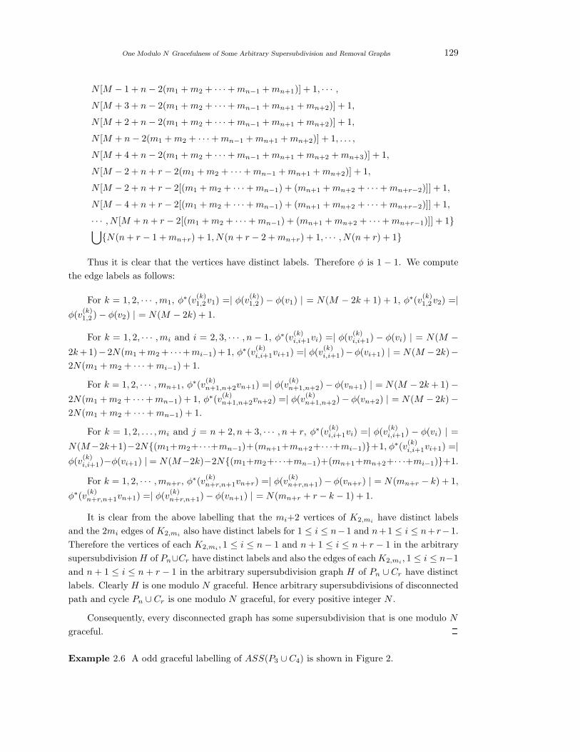
One Modulo N Gracefulness of Some Arbitrary Supersubdivision and Removal Graphs 129
N [M − 1 + n − 2(m1 + m2 + · · · + mn−1 + mn+1)] + 1, · · · ,
N [M + 3 + n − 2(m1 + m2 + · · · + mn−1 + mn+1 + mn+2)] + 1,
N [M + 2 + n − 2(m1 + m2 + · · · + mn−1 + mn+1 + mn+2)] + 1,
N [M + n − 2(m1 + m2 + · · · + mn−1 + mn+1 + mn+2)] + 1, . . . ,
N [M + 4 + n − 2(m1 + m2 + · · · + mn−1 + mn+1 + mn+2 + mn+3)] + 1,
N [M − 2 + n + r − 2(m1 + m2 + · · · + mn−1 + mn+1 + mn+2)] + 1,
N [M − 2 + n + r − 2[(m1 + m2 + · · · + mn−1) + (mn+1 + mn+2 + · · · + mn+r−2)]] + 1,
N [M − 4 + n + r − 2[(m1 + m2 + · · · + mn−1) + (mn+1 + mn+2 + · · · + mn+r−2)]] + 1,
· · · , N [M + n + r − 2[(m1 + m2 + · · · + mn−1) + (mn+1 + mn+2 + · · · + mn+r−1)]] + 1⋃
N(n + r − 1 + mn+r) + 1, N(n + r − 2 + mn+r) + 1, · · · , N(n + r) + 1
Thus it is clear that the vertices have distinct labels. Therefore φ is 1 − 1. We compute
the edge labels as follows:
For k = 1, 2, · · · , m1, φ∗(v(k)1,2v1) =| φ(v
(k)1,2 ) − φ(v1) | = N(M − 2k + 1) + 1, φ∗(v(k)
1,2v2) =|φ(v
(k)1,2 ) − φ(v2) | = N(M − 2k) + 1.
For k = 1, 2, · · · , mi and i = 2, 3, · · · , n − 1, φ∗(v(k)i,i+1vi) =| φ(v
(k)i,i+1) − φ(vi) | = N(M −
2k +1)− 2N(m1 +m2 + · · ·+mi−1)+1, φ∗(v(k)i,i+1vi+1) =| φ(v
(k)i,i+1)−φ(vi+1) | = N(M − 2k)−
2N(m1 + m2 + · · · + mi−1) + 1.
For k = 1, 2, · · · , mn+1, φ∗(v(k)n+1,n+2vn+1) =| φ(v
(k)n+1,n+2) − φ(vn+1) | = N(M − 2k + 1) −
2N(m1 + m2 + · · ·+ mn−1) + 1, φ∗(v(k)n+1,n+2vn+2) =| φ(v
(k)n+1,n+2)− φ(vn+2) | = N(M − 2k)−
2N(m1 + m2 + · · · + mn−1) + 1.
For k = 1, 2, . . . , mi and j = n + 2, n + 3, · · · , n + r, φ∗(v(k)i,i+1vi) =| φ(v
(k)i,i+1) − φ(vi) | =
N(M−2k+1)−2N(m1+m2+· · ·+mn−1)+(mn+1+mn+2+· · ·+mi−1)+1, φ∗(v(k)i,i+1vi+1) =|
φ(v(k)i,i+1)−φ(vi+1) | = N(M−2k)−2N(m1+m2+· · ·+mn−1)+(mn+1+mn+2+· · ·+mi−1)+1.
For k = 1, 2, · · · , mn+r, φ∗(v(k)n+r,n+1vn+r) =| φ(v
(k)n+r,n+1) − φ(vn+r) | = N(mn+r − k) + 1,
φ∗(v(k)n+r,n+1vn+1) =| φ(v
(k)n+r,n+1) − φ(vn+1) | = N(mn+r + r − k − 1) + 1.
It is clear from the above labelling that the mi+2 vertices of K2,mihave distinct labels
and the 2mi edges of K2,mialso have distinct labels for 1 ≤ i ≤ n−1 and n+1 ≤ i ≤ n+ r−1.
Therefore the vertices of each K2,mi, 1 ≤ i ≤ n − 1 and n + 1 ≤ i ≤ n + r − 1 in the arbitrary
supersubdivision H of Pn∪Cr have distinct labels and also the edges of each K2,mi, 1 ≤ i ≤ n−1
and n + 1 ≤ i ≤ n + r − 1 in the arbitrary supersubdivision graph H of Pn ∪ Cr have distinct
labels. Clearly H is one modulo N graceful. Hence arbitrary supersubdivisions of disconnected
path and cycle Pn ∪ Cr is one modulo N graceful, for every positive integer N .
Consequently, every disconnected graph has some supersubdivision that is one modulo N
graceful. 2Example 2.6 A odd graceful labelling of ASS(P3 ∪ C4) is shown in Figure 2.

130 V.Ramachandran and C.Sekar
8
10
12
14
27
19 1715
0 2 4
3329
55
59
53
49
45
47
43
39
35
Figure 2
Example 2.7 A graceful labelling of ASS(P3 ∪ C3) is shown in Figure 3.
4
5
6
0 1 2
13118
7
24
26
23
21
19
20
18
16
14
Figure 3
Theorem 2.8 For any pendant vertex v(1)k ∈ V (P+
n ), the graph P+n − v
(1)k is one modulo N
graceful for every positive integer N.

One Modulo N Gracefulness of Some Arbitrary Supersubdivision and Removal Graphs 131
Proof Let v1, v2, · · · , vn be the vertices of a path of length n and v(1)1 , v
(1)2 , · · · , v
(1)n the
pendant vertices attached with v1, v2, · · · , vn respectively. Consider the graph P+n −v
(1)k , where
1 ≤ k ≤ n. It has 2n − 1 vertices and 2n − 2 edges.
Case 1. n is even and k is even
Define
φ(v2i−1) =
N(2n − 3) + 1 − 2N(i − 1) for i = 1, 2, · · · , k2
N(2n − 3) + 1 − 2N(k2 − 1) − N − 2N(i − (k
2 + 1)) for i = k2 + 1, · · · , n
2
,
φ(v2i) = N(2i − 1) for i = 1, 2, · · · , n2 ,
φ(v(1)2i ) =
2N(n − 2) + 1 − 2N(i − 1) for i = 1, 2, · · · , k
2 − 1
2N(n − 2) + 1 − 2N(k2 − 2) − 3N − 2N(i − (k
2 + 1)) fori = k2 + 1, k
2 + 2, · · · , n2
,
φ(v(1)2i−1) = 2N(i − 1) for i = 1, 2, · · · , n
2 .
From the definition of φ it is clear that
φ(v2i−1), i = 1, 2, · · · ,n
2⋃
φ(v2i), i = 1, 2, · · · ,n
2
⋃φ(v
(1)2i ), i = 1, 2, · · · ,
k
2− 1,
k
2+ 1,
k
2+ 2, · · · ,
n
2
⋃φ(v
(1)2i−1), i = 1, 2, · · · ,
n
2
= N(2n− 3) + 1, N(2n− 5) + 1, · · · , N(2n− k − 1) + 1, N(2n− k − 2) + 1,
N(2n − k − 4) + 1, . . . , Nn + 1⋃
N, 3N, · · · , N(n − 1)⋃
2N(n − 2) + 1, 2N(n− 3) + 1, · · · , N(2n − k) + 1, N(2n− k − 3) + 1,
N(2n − k − 5) + 1, · · · , N(n − 1) + 1⋃
0, 2N, . . . , N(n − 2)
Thus it is clear that the vertices have distinct labels. Therefore φ is 1 − 1. We compute
the edge labels as follows.
For i = 1, 2, · · · , k2 , φ∗(v2i−1v2i)=| φ(v2i−1) − φ(v2i) |= N(2n − 4i) + 1, φ∗(v2i−1v
(1)2i−1) =
| φ(v2i−1) − φ(v(1)2i−1) |= N(2n − 4i + 1) + 1.
For i = 1, 2, · · · , k2 −1, φ∗(v2i+1v2i) =| φ(v2i+1)−φ(v2i) |= N(2n−4i−2)+1, φ∗(v
(1)2i v2i) =
| φ(v(1)2i ) − φ(v2i) |= N(2n − 4i − 1) + 1.
For i = k2 + 1, k
2 + 2, · · · , n2 , φ∗(v2i−1v2i)=| φ(v2i−1) − φ(v2i) |= N(2n − 4i + 1) + 1,
φ∗(v2i−1v(1)2i−1)=| φ(v2i−1) − φ(v
(1)2i−1) |= N(2n − 4i + 2) + 1, φ∗(v
(1)2i v2i)=| φ(v
(1)2i ) − φ(v2i) |=
N(2n − 4i) + 1.
For i = k2 + 1, k
2 + 2, · · · , n2 − 1, φ∗(v2i+1v2i)=| φ(v2i+1) − φ(v2i) | = N(2n − 4i − 1) + 1.
This show that the edges have the distinct labels 1, N + 1, 2N + 1, · · · , N(q − 1) + 1,where q = 2n− 2. Hence for every positive integer N , P+
n − v(1)k is one modulo N graceful if n
is even and k is even.

132 V.Ramachandran and C.Sekar
Example 2.9 A one modulo 10 graceful labelling of P+10 − v
(1)6 is shown in Figure 4.
171 10 151 30 131 50 121 70 101 90
91801116040141201610
Figure 4
Case 2. n is even and k is odd
Define
φ(v2i) =
N(2i − 1) for i = 1, 2, · · · , k−12
N(k − 2) + N + 2N(i − ( (k+1)2 )) for i = k+1
2 , k+32 , · · · , n
2
,
φ(v2i−1) = N(2n − 3) + 1 − 2N(i − 1) for i = 1, 2, · · · , n2 ,
φ(v(1)2i−1) =
2N(i − 1) for i = 1, 2, · · · , k−12
2N(k−12 − 1) + 3N + 2N(i − (k+3
2 )) fori = k+32 , k+5
2 , · · · , n2
,
φ(v(1)2i ) = 2N(n − 2) + 1 − 2N(i − 1) for i = 1, 2, · · · , n
2 .
The proof is similar to that of Case 1. Hence for every positive integer N , P+n − v
(1)k is one
modulo N graceful if n is even and k is odd.
Example 2.10 A one modulo 4 graceful labelling of P+12 − v
(1)9 is shown in Figure 5.
77 20 3228 4085 12 61 45534 69
24 3681 160 738 65 4957 41
Figure 5
Case 3. n is odd and k is even
Define

One Modulo N Gracefulness of Some Arbitrary Supersubdivision and Removal Graphs 133
φ(v2i−1) =
N(2n − 3) + 1 − 2N(i − 1) for i = 1, 2, · · · , k2
N(2n − 3) + 1 − 2N(k2 − 1) − N − 2N(i − (k
2 + 1)) fori = k2 + 1, · · · , n−1
2
,
φ(v2i) = N(2i − 1) for i = 1, 2, . . . , n−12 ,
φ(v(1)2i ) =
2N(n − 2) + 1 − 2N(i − 1) for i = 1, 2, . . . , k
2 − 1
2N(n − 2) + 1 − 2N(k2 − 2) − 3N − 2N(i − (k
2 + 1)) fori = k2 + 1, · · · , n−1
2
,
φ(v(1)2i−1) = 2N(i − 1) for i = 1, 2, . . . , n−1
2 .
From the definition of φ it is clear that
φ(v2i−1), i = 1, 2, · · · ,n − 1
2⋃
φ(v2i), i = 1, 2, · · · ,n − 1
2
⋃φ(v
(1)2i ), i = 1, 2, · · · ,
k
2− 1,
k
2+ 1,
k
2+ 2, · · · ,
n − 1
2⋃
φ(v(1)2i−1), i = 1, 2, · · · ,
n − 1
2
= N(2n− 3) + 1, N(2n − 5) + 1, . . . , N(2n − k − 1) + 1, N(2n − k − 2) + 1,
N(2n − k − 4) + 1, . . . , N(n − 1) + 1⋃
N, 3N, . . . , N(n − 2)⋃
2N(n − 2) + 1, 2N(n− 3) + 1, . . . , N(2n− k) + 1, N(2n− k − 3) + 1,
N(2n − k − 5) + 1, . . . , Nn + 1⋃
0, 2N, . . . , N(n − 1)
Thus it is clear that the vertices have distinct labels. Therefore φ is 1 − 1. We compute
the edge labels as follows:
For i = 1, 2, · · · , k2 , φ∗(v2i−1v2i)=| φ(v2i−1) − φ(v2i) | = N(2n − 4i) + 1, φ∗(v2i−1v
(1)2i−1) =
| φ(v2i−1) − φ(v(1)2i−1) | = N(2n − 4i + 1) + 1.
For i = 1, 2, · · · , k2 −1, φ∗(v2i+1v2i)=| φ(v2i+1)−φ(v2i) | = N(2n−4i−2)+1, φ∗(v(1)
2i v2i) =
| φ(v(1)2i ) − φ(v2i) | = N(2n − 4i − 1) + 1.
For i = k2 + 1, k
2 + 2, · · · , n−12 , φ∗(v2i−1v2i)=| φ(v2i−1) − φ(v2i) | = N(2n − 4i + 1) + 1,
φ∗(v(1)2i v2i) = | φ(v
(1)2i ) − φ(v2i) | = N(2n − 4i) + 1.
For i = k2 + 1, k
2 + 2, · · · , n−12 , φ∗(v2i+1v2i) = | φ(v2i+1) − φ(v2i) | = N(2n − 4i − 1) + 1.
For i = k2 +1, k
2 +2, · · · , n+12 , φ∗(v2i−1v
(1)2i−1) = | φ(v2i−1)−φ(v
(1)2i−1) | = N(2n−4i+2)+1.
This show that the edges have the distinct labels 1, N + 1, 2N + 1, · · · , N(q − 1) + 1,where q = 2n− 2. Hence for every positive integer N , P+
n − v(1)k is one modulo N graceful if n
is odd and k is even.
Example 2.11 A one modulo 3 graceful labelling of P+13 − v
(1)2 is shown in Figure 6.

134 V.Ramachandran and C.Sekar
67 15 2749 3721 3370 9 61 55 433
18 30120 646 58 4624 3652 40
Figure 6
Case 4. n is odd and k is odd
Define
φ(v2i) =
N(2i − 1) for i = 1, 2, · · · , k−1
2
N(k − 2) + N + 2N(i − ( (k+1)2 )) fori = k+1
2 , k+32 , · · · , n−1
2
,
φ(v2i−1) = N(2n − 3) + 1 − 2N(i − 1) for i = 1, 2, . . . , n−12 ,
φ(v(1)2i−1) =
2N(i − 1) for i = 1, 2, · · · , k−12
2N(k−12 − 1) + 3N + 2N(i − (k+3
2 )) fori = k+32 , k+5
2 , · · · , n−12
,
φ(v(1)2i ) = 2N(n − 2) + 1 − 2N(i − 1) for i = 1, 2, . . . , n−1
2 .
The proof is similar to that of Case 3. Hence for every positive integer N , P+n − v
(1)k is one
modulo N graceful if n is odd and k is odd. 2Example 2.12 A one modulo 5 graceful labelling of P+
11 − v(1)5 is shown in Figure 7.
5 86 1596 76 20 66 30 56 40 46
45513571 61810 10 2591
Figure 7

One Modulo N Gracefulness of Some Arbitrary Supersubdivision and Removal Graphs 135
§3. Conclusion
Subdivision or supersubdivision or arbitrary supersubdivision of certain graphs which are not
graceful may be graceful. The method adopted in making a graph one modulo N graceful will
provide a new approach to have graceful labelling of graphs and it will be helpful to attack
standard conjectures and unsolved open problems.
References
[1] C. Barrientos and S. Barrientos, On graceful supersubdivisions of graphs, Bull. Inst.
Combin. Appl., 70 (2014) 77-85.
[2] Joseph A. Gallian, A Dynamic Survey of Graph Labeling, The Electronic Journal of Com-
binatorics, 18 (2011), #DS6.
[3] S.W.Golomb, How to number a graph in Graph theory and computing R.C. Read, ed.,
Academic press, New York (1972)23-27.
[4] R. B. Gnanajothi, Topics in Graph Theory, Ph.D. Thesis, Madurai Kamaraj University,
1991.
[5] G. Sethuraman and P. Selvaraju, Gracefulness of arbitrary supersubdivisions of graphs,
Indian J. Pure Appl. Math., 32 (2001) 1059-1064.
[6] G. Sethuraman and P. Selvaraju, Super-subdivisions of connected graphs are graceful,
preprint.
[7] Z. Liang, On the gracefulness of the graph Cm ∪ Pn, Ars Combin., 62(2002), 273-280.
[8] V. Ramachandran, C. Sekar, One modulo N gracefullness of arbitrary supersubdivisions of
graphs, International J. Math. Combin., Vol.2 (2014) 36-46.
[9] V. Ramachandran, C. Sekar, One modulo N gracefulness of supersubdivision of ladder,
Journal of Discrete Mathematical Sciences and Cryptography (Accepted).
[10] C. Sekar and V. Ramachandren, Graceful labelling of arbitrary supersubdivision of discon-
nected graph, Ultra Scientist, 25(2)A (2013) 315-318.
[11] C. Sekar, Studies in Graph Theory, Ph.D. Thesis, Madurai Kamaraj University, 2002.

International J.Math. Combin. Vol.1(2015), 136-136
AMCA – An International Academy Has Been Established
W.Barbara
(Academy of Mathematical Combinatorics & Applications, Colorado, USA)
The Academy of Mathematical Combinatorics & Appli-
cations (AMCA), initiated by mathematicians of USA,
China and India in December of last year has been es-
tablished in USA. Its aim is promoting the progress
and upholding the development of combinatorics and
Smarandache multispaces with mathematical sciences,
i.e., mathematical combinatorics, including algebra, topology, geometry, differential equations,
theoretical physics, theoretical chemistry and mathematical theory on recycling economy or
environmental sciences, for instance, the industrial ecology, and so as to advance a sustainable
developing for global economy.
The activities of AMCA include organizing meetings of the membership, discussions on
important topics, edit and publish scientific journals, special volumes and members monographs,
awards and honours, recognizing mathematical talent, improvement of mathematics education
and taking up other issues concerning to mathematical science.
Now, AMCA is online with a website: http://www.mathcombin.com, including columns:
Organizers, Current News, Membership, Meetings & Workshops, Publications and Notions,
etc., in which, the notions are mainly recommending on Smarandache notion and combinatorial
notion on mathematical sciences by published papers, such as those of Mixed non-Euclidean
Geometries by Prof.Smarandache, Combinatorial Speculation and Combinatorial Conjecture for
Mathematics and Mathematics on non-Mathematics by Prof.Linfan Mao, and the publications
included e-books, such as those of Only Problems, Not Solutions! by Prof.F.Smarandache,
Theory of Algebraic Invariants by Prof.David Hilbert, Bislgebraic Structures and Smarandache
Bialgebraic Structures by Prof.W.B.Vasantha Kandasamy. Each column is constantly enrich in
order to meet the needs of readers, to catch up with the pace of the times.
There are 3 classes of membership in AMCA, i.e., academician, co-academician and fellow
with doctorate under different requirements, also with different right in operation of AMCA.
Each class is always open to those persons who are or who have been actively engaged in research
or teaching mathematics, such as those of combinatorics, multispaces, graph theory, algebra,
topology, geometry, differential equations, system control,· · · ,etc., theoretical physics, astro-
physics, theoretical chemistry, the mathematical theory on recycling economy or environmental
sciences. A Ph.D candidate can apply for a student member. All applicants can download
Application Form in the website.
With the times of mathematics in 21th century, the AMCA is working on serving the
whole mathematical community and working hard to become the first-class academy in scientific
research and dissemination of combinatorial knowledge.

If a man empties his purse into his head, no man can take it away from him,
an investment in knowledge always pays the best interest.
By Benjamin Franklin , an American president.

Author Information
Submission: Papers only in electronic form are considered for possible publication. Papers
prepared in formats, viz., .tex, .dvi, .pdf, or.ps may be submitted electronically to one member
of the Editorial Board for consideration in the International Journal of Mathematical
Combinatorics (ISSN 1937-1055). An effort is made to publish a paper duly recommended
by a referee within a period of 3 months. Articles received are immediately put the refer-
ees/members of the Editorial Board for their opinion who generally pass on the same in six
week’s time or less. In case of clear recommendation for publication, the paper is accommo-
dated in an issue to appear next. Each submitted paper is not returned, hence we advise the
authors to keep a copy of their submitted papers for further processing.
Abstract: Authors are requested to provide an abstract of not more than 250 words, lat-
est Mathematics Subject Classification of the American Mathematical Society, Keywords and
phrases. Statements of Lemmas, Propositions and Theorems should be set in italics and ref-
erences should be arranged in alphabetical order by the surname of the first author in the
following style:
Books
[4]Linfan Mao, Combinatorial Geometry with Applications to Field Theory, InfoQuest Press,
2009.
[12]W.S.Massey, Algebraic topology: an introduction, Springer-Verlag, New York 1977.
Research papers
[6]Linfan Mao, Mathematics on non-mathematics - A combinatorial contribution, International
J.Math. Combin., Vol.3(2014), 1-34.
[9]Kavita Srivastava, On singular H-closed extensions, Proc. Amer. Math. Soc. (to appear).
Figures: Figures should be drawn by TEXCAD in text directly, or as EPS file. In addition,
all figures and tables should be numbered and the appropriate space reserved in the text, with
the insertion point clearly indicated.
Copyright: It is assumed that the submitted manuscript has not been published and will not
be simultaneously submitted or published elsewhere. By submitting a manuscript, the authors
agree that the copyright for their articles is transferred to the publisher, if and when, the
paper is accepted for publication. The publisher cannot take the responsibility of any loss of
manuscript. Therefore, authors are requested to maintain a copy at their end.
Proofs: One set of galley proofs of a paper will be sent to the author submitting the paper,
unless requested otherwise, without the original manuscript, for corrections after the paper is
accepted for publication on the basis of the recommendation of referees. Corrections should be
restricted to typesetting errors. Authors are advised to check their proofs very carefully before
return.

March 2015
Contents
N∗C∗ Smarandache Curves of Mannheim Curve Couple According to Frenet
Frame By SULEYMAN SENYURT, ABDUSSAMET CALISKAN . . . . . . . . . . . . . . . . . . . . . . . . 01
Fixed Point Theorems of Two-Step Iterations for Generalized Z-Type
Condition in CAT(0) Spaces By G.S.SALUJA. . . . . . . . . . . . . . . . . . . . . . . . . . . . . . . . . . . . . . . . . 14
Antidegree Equitable Sets in a Graph By C.ADIGA, K.N.S.KRISHNA . . . . . . . . . . 24
A New Approach to Natural Lift Curves of the Spherical Indicatrices of Timelike
Bertrand Mate By MUSTAFA BILICI, EVREN ERGUN, MUSTAFA CALISKAN . . . . . . 35
Totally Umbilical Hemislant Submanifolds of Lorentzian (α)-Sasakian Manifold
By B.LAHA, A.BHATTACHARYYA . . . . . . . . . . . . . . . . . . . . . . . . . . . . . . . . . . . . . . . . . . . . . . . . . . . . . . . 49
On Translational Hull Of Completely J∗, -Simple Semigroups
By YIZHI CHEN, SIYAN LI, WEI CHEN . . . . . . . . . . . . . . . . . . . . . . . . . . . . . . . . . . . . . . . . . . . . . . . . . . 57
Some Minimal (r, 2, k)-Regular Graphs Containing a Given Graph and its
Complement By N.R.SANTHI MAHESWARI, C.SEKAR . . . . . . . . . . . . . . . . . . . . . . . . . . . . . . . 65
On Signed Graphs Whose Two Path Signed Graphs are Switching Equivalent to
Their Jump Signed Graphs By P.S.K.REDDY, P.N.SAMANTA, K.S.PERMI . . . . . . . . . . 74
A Note on Prime and Sequential Labelings of Finite Graphs
By MATHEW VARKEY T.K, SUNOJ B.S . . . . . . . . . . . . . . . . . . . . . . . . . . . . . . . . . . . . . . . . . . . . . . . . . 80
The Forcing Vertex Monophonic Number of a Graph By P.TITUS, K.IYAPPAN . . . . 86
Skolem Difference Odd Mean Labeling of H-Graphs
By P.SUGIRTHA, R.VASUKI, J.VENKATESWARI . . . . . . . . . . . . . . . . . . . . . . . . . . . . . . . . . . . . . . . 96
Equitable Total Coloring of Some Graphs By GIRIJA G, V.VIVIK J . . . . . . . . . . . . . . 107
Some Characterizations for the Involute Curves in Dual Space
By SULEYMAN SENYURT, MUSTAFA BILICI, MUSTAFA CALISKAN . . . . . . . . . . . . . . . . . 113
One Modulo N Gracefulness of Some Arbitrary Supersubdivision and
Removal Graphs By V.RAMACHANDRAN, C.SEKAR . . . . . . . . . . . . . . . . . . . . . . . . . . . . . . . 125
An International Academy AMCA Has Been Established W.BARBARA . . . . . . . . 136
An International Journal on Mathematical Combinatorics


![[LIPIcs,Vol.18,FSTTCS'12] 32nd International Conference on](https://cdn.vdocuments.mx/doc/165x107/63137ffb6ebca169bd0a7fc9/lipicsvol18fsttcs12-32nd-international-conference-on-.jpg)

