
This content has been downloaded from IOPscience. Please scroll down to see the full text.
Download details:
This content was downloaded by: sonumaths
IP Address: 14.139.242.18
This content was downloaded on 19/11/2013 at 11:30
Please note that terms and conditions apply.
Instability in temperature modulated rotating Rayleigh–Bénard convection
View the table of contents for this issue, or go to the journal homepage for more
2014 Fluid Dyn. Res. 46 015504
(http://iopscience.iop.org/1873-7005/46/1/015504)
Home Search Collections Journals About Contact us My IOPscience

The Japan Society of Fluid Mechanics Fluid Dynamics Research
Fluid Dyn. Res. 46 (2014) 015504 (18pp) doi:10.1088/0169-5983/46/1/015504
Instability in temperature modulatedrotating Rayleigh–Benard convection
Jitender Singh1 and S S Singh2
1 Department of Mathematics, Guru Nanak Dev University, Amritsar 143005, India2 Department of Mathematics & Computer Science, Mizoram University,Aizawl 796 004, India
E-mail: [email protected], [email protected] [email protected]
Received 28 January 2013, in final form 3 October 2013Published 18 November 2013
Communicated by E Knobloch
AbstractThe problem of instability in an infinite horizontal thin layer of a Boussinesqfluid, uniformly rotated and heated from below with time periodic oscillationsof the wall temperatures is investigated theoretically and numerically. In doingso, modest rotation rate is considered such that the Froude number does notexceed 0.05 which allows neglect of centrifugal effects. The Floquet analysisis used to obtain the critical Rayleigh number as a function of the parameterscontrolling the system. The instability is found to manifest itself in the formof a flow which oscillates either harmonically or subharmonically dependingupon the control parameters. Instability regions in an appropriate parametricspace of the dimensionless wave number of disturbance imposed over theflow and the dimensionless amplitude of modulation, at the onset of timeperiodic fluid flows are obtained numerically. The modulation amplitude, themodulation frequency and the rotation rate, are observed to affect the stabilityof the flow considerably.
(Some figures may appear in colour only in the online journal)
1. Introduction
The study of Rayleigh–Benard convection (RBC) in a horizontal fluid layer heated frombelow has been the subject of scientific interest for a long time because of its great utility inexplaining the convection phenomena occurring in astrophysics, geophysics and atmosphericsciences. The fluid motion driven by RBC occurs when a sufficiently large temperature
0169-5983/14/015504+18$33.00 © 2014 The Japan Society of Fluid Mechanics and IOP Publishing Ltd Printed in the UK 1

Fluid Dyn. Res. 46 (2014) 015504 J Singh and S S Singh
gradient is applied across the fluid layer. At this stage, the fluid layer is observed to partitionoff into polygonal patterns. Keeping in view the rich dynamics and wide range of itsapplications, RBC has become a paradigm that has kept the researchers engaged for more than100 years since Benard’s early experiments in 1900, followed by the work of Rayleigh (seeCross and Hohenberg 1993, Koschmieder 1993, Getling 1998, Bodenschatz et al 2000, etc).
The effect of imposing uniform rotation on RBC was considered by Chan-drasekhar (1966). He observed numerically that, at a given rotation rate, there is a minimumtemperature gradient required to be exceeded before the onset of the instability can occurin the fluid layer. On increasing the rotation rate, the minimum temperature gradient rises,which results in delay of the onset of RBC. This is due to the fact that the disturbances inthe fluid layer do not move up or down as easily as without rotation, because of the presenceof Coriolis force. This instability problem is commonly known as rotating Rayleigh–Benardconvection (RRBC) and has been extensively studied. For a quick review, we recommend theinterested reader to go through the work of Kuppers and Lortz (1969), Somerville (1971),Tu and Cross (1992), Clune and Knobloch (1993), Cox and Matthews (2001), Kloosterzieland Carnevale (2003), Rudiger and Knobloch (2003), Khiri (2004), Lopez et al (2006),Marques et al (2007), Scheel (2007) and Teed et al (2010).
An external time-periodic forcing induces a change in the stability of a system and theinstability induced in this way is known as parametric instability. The RBC in a horizontalfluid layer can be controlled using parametric excitation via a mechanical source, magneticfield, buoyancy, temperature-gradient, etc. The temperature modulation of the boundariesaffects the thermal convection of a fluid-layer resting between two horizontal planes, and as aresult of this the instability appears in the form of convection cells which oscillate either withthe forcing frequency (harmonically) or with half the forcing frequency (subharmonically).For a review of extensive research on temperature modulated RBC, it is worthwhile to mentionthe work by Venezian (1969), Rosenblat and Tanaka (1971), Yih and Li (1972), Davis (1976),Finucane and Kelly (1976), Roppo et al (1984), Meyer et al (1992), Rogers et al (2000) andSingh and Bajaj (2008).
The onset of RRBC in a horizontal fluid layer subject to time periodic thermal modulationof the boundary temperatures was considered by Rauscher and Kelly (1974) in the limit oflow amplitude modulation. They found that the rotation of the fluid layer delays the onset ofthe instability in the modulated system except for one case in which the Taylor number (adimensionless measure of the rotation rate of the fluid layer) of the flow is of the order of105 and the frequency of modulation is high where the onset of the instability is favored byrotation.
The combined effect of rotation and temperature modulation on RBC, has not beenstudied. Thus the investigation regarding the effect of coupling of rotation and temperaturemodulation on the onset of instability of the fluid layer needs attention. In the present study,we address this issue. A comprehensive study of the temperature modulated RRBC in aninfinite-horizontal layer of a Boussinesq fluid is carried out using the classical Floquet theory.The critical onset of instability which depends upon the control parameters is discussed indetail.
The rest of the paper is organized as follows. The problem is described in section 2.The linear instability analysis of basic conduction state is carried out in section 3. In thesame section, Floquet theory is utilized to obtain a criterion for the onset of instability. Alsoconsidered is, the eigenvalue problem using the method of Kumar and Tuckerman (1994) (seealso Kumar (1996)) from which the low amplitude modulation is discussed to get an idea ofthe behavior of modulation and rotation on the onset of instability. The numerical results arepresented in section 4 and possible conclusions from them are obtained in the last section.
2

Fluid Dyn. Res. 46 (2014) 015504 J Singh and S S Singh
2. Problem formulation
We consider an infinite horizontal, Boussinesq fluid layer of thickness d , resting betweentwo stress-free boundaries located at the planes z = 0 and d . The system is uniformly heatedfrom below at temperature T1 and cooled from the above at temperature T2 < T1. The systemis rotated uniformly with constant angular velocity Ω= (0, 0, ) about the vertical (z-axis).We assume that the rotation rate does not exceed a frequency of = 0.3 Hz such that theFroude number satisfies Fr < 0.05 (e.g. water). In this range of , the centrifugal force isnegligible as compared to the gravitational force and, therefore, we neglect it so that theeffect of rotation is restricted to the Coriolis force. The system is governed by the followingPDEs:
∂u∂t
+ u · ∇u + 2 × u = −1
ρ0∇ p +
ρ
ρ0g + ν∇
2u, (2.1)
∇ · u = 0, (2.2)
∂T
∂t+ u · ∇T = κT ∇
2 T, (2.3)
where u = (u, v, w) is the velocity, p is the pressure and T is the temperature of the fluidat any point (x, y, z) in the fluid layer at time t . The vector g = (0, 0, −g) denotes theacceleration due to gravity; ν is the kinematic viscosity of the fluid; ρ is the density of thefluid which is a function of the temperature T and defined as
ρ = ρ01 − α(T − T0), (2.4)
where ρ0 is the fluid density at a reference-temperature T0, α is the coefficient of volumeexpansion and κT is the thermal-diffusivity.
The temperatures of the horizontal boundaries of the fluid layer are modulated abouttheir mean values T1 and T2, such that the boundary conditions for the temperature field Tare
T =
T1 − ε0 cos(ω0t) at z = 0,
T2 + ε0 cos(ω0t) at z = d,(2.5)
where ω0 > 0 is the frequency of modulation and ε0 > 0 is the amplitude of modulation.The basic solution for the system (2.1)–(2.5) is the conduction state described by the
following:
ue = 0, pe = ρ0 g∫
1 − α(Te − T0) dz,
Te = T1 + (T2 − T1)z/d + ε0 real
[sinh(z/d − 1/2)λ
sinh(λ/2)expıω0t
],
(2.6)
where the subscript e denotes the equilibrium state and λ2= ıd2ω0/kT . Note that in the basic
state the temperature field oscillates time periodically within the fluid layer.
3. Instability analysis
We make the variables in the governing equations dimensionless, using the thickness d ofthe fluid layer as the distance scale, d2/kT as the time scale, and the temperature differenceT1 − T2 as the temperature scale. During this process, we obtain the following dimensionless
3

Fluid Dyn. Res. 46 (2014) 015504 J Singh and S S Singh
parameters:
Ra =(T1 − T2)αd4 g
kT ν, σ =
ν
kT, T a =
42d4
ν2,
where Ra is the Rayleigh number, σ is the Prandtl number and T a is the Taylor number.Note that for < 0.3 Hz, the Taylor number can vary in the range 06 T a 6 103. Along withthese parameters, we obtain the amplitude of modulation ε and the modulation frequency ω
given by
ε =ε0
T1 − T2, ω =
ω0d2
kT.
We consider small perturbations in (2.6) such that
u = (kT /d)(u, v, w), p = pe + (ρ0k2T /d4)p1, T = Te + (T1 − T2)θ. (3.1)
Using equation (3.1) as a solution of (2.1)–(2.5); applying the operator ∇ ×∇× throughoutequation (2.1) and considering its z-component; we obtain the following linearized system ofPDEs satisfied by the perturbations:
1
σ
∂ζ
∂t= ∇
2ζ +√
T aDw, (3.2)
1
σ∇
2 ∂w
∂t= −
√T aDζ + ∇
4w − Ra(D2
− ∇2)θ, (3.3)
∂θ
∂t= −DTew + ∇
2θ, (3.4)
where
ζ =∂v
∂x−
∂u
∂y
is the vertical component of the vorticity vector ∇ × u, D =∂∂z and z ∈ [0, 1]. Also, the
vertical temperature gradient is given by
DTe = −1 + ε real
[λ
cosh(z − 1/2)λ
sinh(λ/2)exp(iωt)
].
The boundary conditions for the stress-free planes are given by
w = D2w = θ = Dζ = 0 for z = 0, 1. (3.5)
To solve the system (3.2)–(3.4) with boundary conditions (3.5), we expand w and θ in termsof truncated Fourier series so that
(ζ, w, θ) =
N∑`=1
(ζ`(t) cos(`π z), w`(t) sin(`π z), θ`(t) sin(`π z)) expi(k1x + k2 y), (3.6)
for some positive integer N to be chosen appropriately for numerical calculations. Using theseexpansions in the system (3.2)–(3.4), multiplying (3.2) throughout by cos( jπ z) for each fixedj ∈ 1, . . . , N , and (3.3)–(3.4) throughout by sin( jπ z) and, integrating w.r.t. z over [0, 1],we obtain the following system of ODEs:
A X = BX, det A 6= 0, (3.7)
4

Fluid Dyn. Res. 46 (2014) 015504 J Singh and S S Singh
where A = (a`j )3N×3N and B = (b`j )3N×3N are the respective coefficient matrix functionsof the dimensionless parameters and each of them is a 2π/ω-periodic in t . The matrix ofunknowns is the column vector
X = (ζ1 ζ2 . . . ζN w1 w2 . . . wN θ1 θ2 . . . θN )′
.
The linear system (3.7) is a system of ODEs with periodic coefficients. So, the Floquetanalysis has been used to analyze it (Jordan and Smith 1988, Miklos Farkas 1994). Severaltechniques are available for applying the Floquet theory. However, we will describe two suchtechniques which we have used in the present study.
In the first technique the Floquet multipliers are obtained from the numerically evaluatedfundamental matrix for the system (3.7) at t = 2π/ω, which are the functions of thedimensionless parameters: ω, ε, Ra, σ , T a, and k. The marginal state of the basic modulatedsystem is determined by setting maximum of the real part taken over all the Floquet exponents,equal to zero. The basic flow is stable if the maximum real part is negative and, unstable if themaximum real part is positive. If a Floquet exponent satisfying the marginal state conditionis identically zero, then the disturbance in the marginal state oscillates periodically withthe forcing frequency ω and the instability response is harmonic. On the other hand, if theimaginary part of the Floquet exponent in the marginal state is equal to ω/r for some positiveinteger r > 1, then the disturbance in the marginal state oscillates with a frequency ω/r , andthe instability response is called subharmonic of order 1/r .
The second technique is due to Kumar and Tuckerman (1994) (see also Singhand Bajaj 2008) in which the instability regions in the (k, ε)-plane are obtained forvarious fixed parameter values. Here, we expand X as a truncated complex Fourier seriesgiven by
X =
L∑`=−L
X` exp(ιω` + s)t, L = 1, 2, . . . , (3.8)
where s is the Floquet exponent. For s = 0, the solution corresponds to harmonic responsewhile for s = ιω/2, the response is subharmonic. Using equation (3.8) in equation (3.7), thefollowing eigenvalue problem arises:
UZ = εSZ, det U 6= 0, (3.9)
where 1/ε is the eigenvalue of the matrix U−1S with eigenvector Z, the coefficient matrixfunctions U and S are banded square matrices. Equation (3.9) has been used to obtaininstability regions in the (k, ε)-space. This method can be used to obtain critical Rayleighnumber Rac as well, but for that one needs to redefine the coefficient matrices U and Sin equation (3.9) corresponding to the eigenvalue problem where the eigenvalue will beRa−1. We will not make any attempt at this and prefer to use equation (3.7) for calculatingRac.
3.1. Low amplitude modulation
To get an idea of how modulation affects the RRBC, we first consider the simplest case of‘low amplitude modulation’. To this, the simplest mode of excitation is the harmonic responsewhich corresponds to s = 0. So, we explicitly obtain the eigenvalue problem for s = 0 nearε = 0 and take N = 1, L = 1. To this end, we assume that the amplitude of modulation
5

Fluid Dyn. Res. 46 (2014) 015504 J Singh and S S Singh
satisfies 0 < ε 1. We solve the eigenvalue problem given by equation (3.9) for
U =
a−1 0 0 −π√
T a 0 0 0 0 0
0 a0 0 0 −π√
T a 0 0 0 0
0 0 a1 0 0 −π√
T a 0 0 0
−π√
T a 0 0 b−1 0 0 Rak2 0 0
0 −π√
T a 0 0 b0 0 0 Rak2 0
0 0 −π√
T a 0 0 b1 0 0 Rak2
0 0 0 1 0 0 c−1 0 0
0 0 0 0 1 0 0 c0 0
0 0 0 0 0 1 0 0 c1
,
where
a` =ιω` + s
σ+ k2 + π2, b` = −(k2 + π2)a`,
c` = −(ιω` + s + k2 + π2), ` = −1, 0, 1.
Also note that
a−` = a`, b−` = b`, c−` = c`.
The entries of the 9 × 9 matrix S are zero, except for the following elements:
S75 = S86 =8π2ε
4π2 + ω2
( ω
2ι− 2π2
), S84 = S95 = −
8π2ε
4π2 + ω2
( ω
2ι+ 2π2
).
For finite ε and Ra 6=a3
0 + π2T a
k2, the characteristic equation for the eigenvalue problem
(3.9) reduces to the following:
a30 + π2T a
k2− Ra + ε2k2 Ra2 32π4(16π4 + ω2)
(4π2 + ω2)2real
a1
k2 Raa1 + (π2T a − a1b1)c1
= 0. (3.10)
Note that equation (3.10) gives an estimate of Ra in the presence of small modulation effects
(ε 1) which deviates from the classical Rayleigh number Ra :=a3
0 + π2T a
k2by a term of
the order of ε2. A similar result was predicted by Rauscher and Kelly (1974).We now analyze equation (3.10) to extract information regarding the following limiting
cases:
Case I. For ε → 0+. When ε = 0, there is no modulation. In this case, equation (3.10) givesexpression for Ra in the classical steady state convection with a non-negative term π2T a inthe numerator as given by
limε→0+
Ra =a3
0 + π2T a
k2. (3.11)
Clearly, the effect of an imposed rotation rate is to delay the onset of the steady state RBC.
Case II. For ω → ∞. In the presence of high-frequency modulation, i.e. for ω → ∞ thecoefficient of ε2 in equation (3.10) tends to zero and again we obtain the same expression
6

Fluid Dyn. Res. 46 (2014) 015504 J Singh and S S Singh
0 200 400 600 800 10002
2.5
3
3.5
4
4.5
Ta
kc
= 0= 0
Figure 1. Variation of kc with Ta for Rac =27π4
4 in the low amplitude modulation.
for Ra as in case I, namely, the following:
limω→∞
Ra =a3
0 + π2T a
k2. (3.12)
This shows that in the presence of high forcing frequency, the modulation effects cease andthe onset of instability is essentially the same as the steady state RRBC.
Case III. For ω → 0. In the presence of low-frequency modulation, i.e. ω → 0, we observe
that a1 → a0, b1 → −a20, c1 → −a0. Consequently, equation (3.10) for 0 < ε <
1
4√
2π2
reduces to
limω→0
Ra =1
1 − 4√
2π2ε
a30 + π2T a
k2. (3.13)
Equation (3.13) shows that for 0 < ε < 14√
2π2 , Ra rises with ε in the low-frequency
modulation from the classical valuea3
0 + π2T a
k2. This predicts partially that at least for the
low-frequency modulation, an increased amplitude of modulation would result in ‘delay ofthe onset of the modulated RRBC’, by which we mean that the instability will appear at ahigher temperature gradient as compared to the one in the no modulation case. Also, in theabsence of modulation, it is clear that the critical wave number kc rises with an increase inT a. So, in the presence of modulation, we expect enhancement of this effect which can beseen from figure 1.
The limiting cases indicate that the Rayleigh number is not a continuous function of theamplitude of modulation ε, the points of discontinuity might be corresponding to a transitionbetween the harmonic and subharmonic response or otherwise! The numerical solution of the
7

Fluid Dyn. Res. 46 (2014) 015504 J Singh and S S Singh
eigenvalue problem equation (3.9) in full without assuming the low amplitude modulation, isobtained in the next section.
4. Results and discussion
To complete investigation of combined effect of the rotation and modulation on the onset ofRBC in the present study, we make numerical calculations for a wide range of ε and ω.
The fundamental matrix 8(2π/ω) is obtained by integrating (3.7) numerically, for a fixedN , using the Runge–Kutta method or the iterative method involving matrix-exponentials as inSingh and Bajaj (2008), over one time period [0, 2π/ω] with the initial condition 8(0) = Iwhere I is the identity matrix of order 3N . The eigenvalues of 8(2π/ω) are obtained usingQ Z -algorithm available as a subroutine in MATLAB. The Floquet theorem ensures existenceof a periodic solution, i.e. at least one of the eigenvalues of Φ(2π/ω) must be 1 whichdetermines the stability boundary. The Floquet exponents λ j ’s and the Floquet multipliersµ j ’s are related by
µ j = exp2πλ j/ω, 16 j 6 3N , (4.1)
where µ j ’s and hence λ j ’s, are functions of the dimensionless parameters Ra, T a, σ, ω, ε andk. The marginal state of the modulated system is determined by setting
max16 j63N
real(λ j )
= 0. (4.2)
4.1. Numerical convergence
Starting with a known solution, the numerical iterations are performed over trial values of(Ra, k) by fixing rest of the parameters, for a neighboring solution (Ra, T a, σ, ω, ε, k) tillequation (4.2) satisfies the tolerance condition
max16 j63N
real(λ j (Ra, T a, σ, ω, ε, k))
< 10−3.
To validate the numerical accuracy of the present numerical results, we have performednumerical computations in MATLAB for Rac for the case of no modulation (ε = 0) and foundthe following critical values:
kc = 2.2214, Rac = 657.511, T a = 0,
kc = 3.7104, Rac = 1676.11, T a = 1000.
These results match with the closed form expressions available for the steady state criticalvalues given by
kc =
√2π
2, Rac =
27π4
4for T a = 0
and
kc = 3.710439, Rac = 1676.118026 for T a = 1000.
A closed form expression for kc can also be found and is given by
k2c = −
π2
2+
π10/3
2(π4 + 2T a + 2
√π4T a + T a2
)1/3 +π2/3
2
(π4 + 2T a + 2
√
π4T a + T a2)1/3
.
8

Fluid Dyn. Res. 46 (2014) 015504 J Singh and S S Singh
Table 1. Dependence of the numerical convergence of the solution on N in obtainingRac corresponding to the harmonic response for fixed parameter values σ = 0.73,ω = 20 and ε = 5. ER denotes the relative error in the respective numerical evaluationof Rac with tolerance < 10−3.
N T a kc Rac ER N T a kc Rac ER
1 0 2.1628 814.504 0.001 35 1 1000 2.7940 1209.44 0.025 062 2.1628 814.504 0.001 35 2 2.7940 1209.44 0.025 063 2.1790 813.415 0.000 01 3 2.8256 1179.95 0.000 064 2.1790 813.415 0.000 01 4 2.8256 1179.95 0.000 065 2.1790 813.402 0.000 00 5 2.8257 1179.87 0.000 006 2.1790 813.402 0.000 00 6 2.8257 1179.87 0.000 007 2.1790 813.402 0.000 00 7 2.8257 1179.87 0.000 008 2.1790 813.402 0.000 00 8 2.8257 1179.87 0.000 00
We have found that the convergence of the solution to the exact value of Rac for ε = 0 isachieved at N = 1.
However, in the presence of modulation, the convergence depends upon the number N ofthe Galerkin terms. This can be seen from table 1, where Rac is obtained numerically for fixedparameter values σ = 0.73, ω = 20 and ε = 5. The symbol ER stands for the relative error innumerical calculation of Rac. Clearly, the solution converges for N > 3 in the consideredtolerance condition. So, for the present numerical calculations, we choose appropriatelyN = 4. Some of the calculations such as those related to the perturbation profiles are doneby taking N = 8.
Similarly, to obtain the instability regions in (k, ε)-plane, we have taken L = 19 and 20in order to solve (3.9) using the method of Kumar and Tuckerman (1994).
4.2. Critical curves
Figure 2 shows variation of Rac with ε, for three typical values of T a = 0, 102, 103 at the onsetof harmonic and subharmonic response. The fixed parameter values are σ = 0.73 and ω = 20.The thick (red) curves in figure 2 correspond to harmonic response while the thin (black)curves are the critical curves for the onset of subharmonic flow. In the absence of temperaturemodulation (ε = 0) and rotation (T a = 0), RBC starts at the classical value Rac = 657.51.The critical curve in the absence of Coriolis force consists of two connected components; onecomponent corresponds to the onset of RBC and the other one is for subharmonic response.Rac value for the onset of RBC rises with rise in ε. The subharmonic instability appearsfor ε > 1.2 and the critical instability response remains subharmonic. The Rac value for theonset of subharmonic response falls with rise in ε. We have observed that for ε > 2.1, Rac
values are less than the one obtained without modulation. These observations indicate thatin absence of the Coriolis force, the low amplitude modulation favors the onset of harmonicresponse, while the high amplitude modulation favors the onset of subharmonic response. Wenote that in comparison to the no modulation case, more temperature gradient is required tobe maintained across the fluid layer in order to see the convection pattern, when the systemis driven by low amplitude modulation. On the other hand, the instability can appear with acomparatively smaller temperature gradient across the fluid layer, when it is subjected to highamplitude modulation. Similar observations can be made for the critical curve correspondingto T a = 102 where the presence of Coriolis force significantly delays the onset of RBC for06 ε < 1.1. This is due to the fact that the presence of rotation is dominant when ε is small
9

Fluid Dyn. Res. 46 (2014) 015504 J Singh and S S Singh
0 2 4 6 8 100
500
1000
1500
2000
2500
Rac
SubharmonicHarmonic
Ta = 0
Ta = 102Ta = 0
Ta = 103
Ta = 102
Figure 2. The critical curves in the (ε, Rac)-plane for three typical values T a =
0, 102, 103 and the fixed parameter values σ = 0.73 and ω = 20. The thicker curvescorrespond to the harmonic response. The thinner curves and the dashed-
dotted curve, correspond to the subharmonic response.
so that the Coriolis force provides a significant hinderance toward the flow in the fluid layeralong the vertical directions (upward as well as downward directions). Whenever ε > 1.1, thecritical instability response is subharmonic for T a = 102
; here the corresponding part of thecritical curve almost coincides with the one drawn for T a = 0. This shows that for ε > 1.1,the forces arising from the modulation dominate over the Coriolis force (for T a = 102) thatresults in instability even at lowered temperature gradient across the fluid layer. To see thecombined effect of Coriolis force and modulation, a third critical curve is drawn in figure 2for T a = 103. Here Rac for the onset of RRBC for ε = 0 is 1676.1. In this case, the criticalcurve consists of three connected components corresponding to the following:
1. the onset of the harmonic flow for 06 ε < 0.6,2. the onset of the subharmonic flow for 0.6 < ε < 2.1,3. the onset of harmonic flow for ε > 2.1.
The first component of the critical curve predicts the same result of dominance of Coriolisforce over modulation as predicted previously for T a = 102 and 0 (i.e. the dominant effect ofCoriolis force for the low-amplitude modulation) with a difference that now there is a declinein Ra values for very small ε. For the third connected component which now correspondsto the harmonic response (ε > 2.1), both the modulation effect and the Coriolis force, areoperative; however, qualitatively the result is similar except that the critical mode of excitationis harmonic now. Here, the region of interest is the one that corresponds to the secondconnected component of the critical curve for 0.6 < ε < 2.1 where the effects of Coriolisforce as well as ε are important. The instability response is subharmonic and we see that Rac
first rises with rise in ε, attains a minimum at ε ≈ 1.8 and then again starts increasing with ε.We note that a significant fall in Rac can be achieved at this moderate range of ε. It is not
10

Fluid Dyn. Res. 46 (2014) 015504 J Singh and S S Singh
0 50 100 1500
1000
2000
3000
4000
5000
6000
ω
Rac
Ta = 0
Ta = 103
Sub harmonicHarmonic
Ta = 103
Ta = 0
Ta = 0
Figure 3. The critical curves in the (ω, Rac)-plane for σ = 0.73 and ε = 5. The thickercurves/points (red) correspond to the harmonic response and the thinner curves/points(black) correspond to the subharmonic response. Also for T a = 103, there are somepoints in the graph marked as which correspond to the subharmonic response whilethe other points marked • correspond to the harmonic response.
clear how the Coriolis force couples with ε to produce such a dramatic variation. Certainly,there is a role being played by ω which is kept fixed here at ω = 20.
To understand dependence of ω on the onset of instability, we have obtained figure 3which illustrates variation of Rac with ω for T a = 0, 103
; the fixed parameter values areσ = 0.73 and ε = 5. The thicker points (red) in the figure correspond to the critical onset ofharmonic response and the thinner (black) points represent the critical onset of subharmonicresponse. There are points marked in figure 3 which correspond to subharmonic responseand the three points marked • in the same figure correspond to harmonic response.
We first explain the critical curve in figure 3 corresponding to T a = 0. It consists ofalternate harmonic and subharmonic parts for 1 < ω 6 150. For 1 < ω 6 11.9 approximately,the critical mode of excitation is the usual RBC and for ω values higher than ω ≈ 70, thecritical mode of excitation is harmonic. For the rest of the ω values i.e. for 126 ω 6 69, thecritical mode of excitation is subharmonic. It is clear from figure 3 that, for ε = 5 and T a = 0,an increase in ω advances or delays the onset of RBC. Furthermore, if the critical mode ofexcitation is harmonic, then it is favored by an increase in ω. On the other hand, if the criticalmode of the onset is subharmonic, then it is delayed by increasing ω.
In the presence of rotation (T a = 103), the corresponding critical curve (figure 3) consistsof alternate harmonic and subharmonic parts. The harmonic and subharmonic parts alternatefor comparatively small intervals of ω values in the region corresponding to 16 ω 6 20.
11

Fluid Dyn. Res. 46 (2014) 015504 J Singh and S S Singh
0 2 4 6 80
2
4
6Ta = 0
0 2 4 6 80
2
4
6Ta = 100
0 2 4 6 80
2
4
6Ta = 1000
0 2 4 6 80
2
4
6Ta = 2000
0 2 4 6 80
2
4
6
k
Ta = 4000
0 2 4 6 80
2
4
6
k
Ta = 6000
Figure 4. Instability regions in (k, ε) space for Ra = 103, σ = 0.73 and ω = 20. Thethicker points (red) correspond to the harmonic response and the thinner points (black)correspond to the subharmonic response.
The critical curves for T a = 103 in the figure, lie above those which are drawn in the absenceof rotation (T a = 0) for the low and the high frequencies. In contrast to this, the marginalcurve corresponding to T a = 0 lies above the one for T a = 103 for 346 ω 6 69 wherethe two curves intersect at ω ≈ 34. These observations show that for ε = 5, the presenceof rotation (T a = 103) delays the critical onset of instability (harmonic and subharmonicresponse) for the low and high frequencies, while the effect is opposite for the frequencyrange 346 ω 6 69. We also observe that, after ω ≈ 69, there is a large difference betweenRac values for T a = 0 and 103. This indicates that, the effect of the presence of rotationcan greatly delay the critical onset of the parametric instability in the system by a sufficientincrease in ω. These observations are sufficient to conclude that the Coriolis force generatedin the fluid layer as a result of rotation acts to advance or delay the harmonic and subharmonicmodes of the parametric excitation in the temperature modulated RBC, depending upon ω.
4.3. Instability regions
The instability regions in (k, ε)-plane are obtained for various combinations of the parametervalues, using the method of Kumar and Tuckerman (1994). Each band-pattern has been foundto be composed of alternate harmonic and subharmonic resonance-bands. In each of thesubsequent figures, the thicker points (red) correspond to harmonic response and the thinnerpoints (black) correspond to subharmonic response. The basic flow is stable for those k andε values which lie outside a resonance band, and the flow is unstable for the k and ε valueswhich lie inside the resonance band. Each point lying on a resonance band corresponds toa periodic flow (harmonic/subharmonic). The band pattern shows the classification of theinstability regions in the (k, ε)-space for the onset of periodic flows with respect to theamplitude modulation, for fixed values of the rest of the parameters.
Figure 4 illustrates the instability regions in the (k, ε)-plane for supercritical Ra = 1000,σ = 0.73 and ω = 20. The presence of the fundamental region in the absence of Corilos force
12

Fluid Dyn. Res. 46 (2014) 015504 J Singh and S S Singh
0 2 4 6 80
2
4
6Ra = 600
0 2 4 6 80
2
4
6Ra = 800
0 2 4 6 80
2
4
6Ra = 1000
0 2 4 6 80
2
4
6Ra = 1200
0 2 4 6 80
2
4
6Ra = 1400
0 2 4 6 80
2
4
6Ra = 1600
0 2 4 6 80
2
4
6
k
Ra = 1800
0 2 4 6 80
2
4
6
k
Ra = 2000
Figure 5. Instability regions in (k, ε) space for T a = 103, σ = 0.73 and ω = 20. Thethicker points (red) correspond to the harmonic response and the thinner points (black)correspond to the subharmonic response.
T a = 0, shows that the critical (lowest) mode of the onset is the usual RBC. The harmonicand the subharmonic modes of excitation also appear in the presence of rotation. However,the critical higher modes of excitation occur at comparatively higher values of k and ε. AsT a is increased, the instability regions start shifting gradually toward higher values of ε andthus, they disappear one by one in the considered range of k and ε. This shows that for thesupercritical Ra values, the critical mode of excitation in the temperature modulated RRBC,can be harmonic or subharmonic, depending upon the magnitude of Coriolis force. A shiftingof the lowest mode of excitation toward higher k and ε values with increasing T a can also beobserved from figure 4. Correlating the subfigure for T a = 103 in figure 4 with figure 2, wefind that the critical onset of instability is harmonic response that occurs for ε between 2 and 4which can be extended to other smaller values of k by a proper tuning of ε. This is important,since the system prefers smaller wave number k. Furthermore, it allows us to see the result offigure 2 for T a = 103, ε ≈ 3.12 and Rac = 103, in a wider range of ε and k in figure 4. Thishelps us to understand figure 2 as well for which we may conclude that corresponding to anypoint in figure 2, the predicted critical mode of excitation can be maintained the same for awide range of ε and k. The parametric excitation may be done by selecting ε-value from theconcerned instability region, that corresponds to the lowest possible wave number.
The effect of increasing Ra on the onset of instability is shown in figure 5 for T a = 103,σ = 0.73 and ω = 20. The fundamental region disappears in the presence of sufficiently highrotation rate (T a = 103) for the supercritical Ra in the range Ra 6 1600 which, otherwise
13

Fluid Dyn. Res. 46 (2014) 015504 J Singh and S S Singh
0 2 4 6 80
2
4
6ω = 10
0 2 4 6 80
2
4
6ω = 20
0 2 4 6 80
2
4
6ω = 30
0 2 4 6 80
2
4
6ω = 40
0 2 4 6 80
2
4
6
k
ω = 50
0 2 4 6 80
2
4
6
k
ω = 60
Figure 6. Instability regions in (k, ε)-space for Ra = 103, T a = 103 and σ = 0.73. Thethicker points (red) correspond to the harmonic response and the thinner points (black)correspond to the subharmonic response.
always appears in the absence of rotation (T a = 0) for Ra > 657.51 approximately. Withincreasing Ra, the resonance bands tend to shift downwards and left in (k, ε)-plane and theirnumber also increases in the considered range of k and ε. This shows that an increase in Raunder modulation and rotation, always favors the onset of the periodic flows. The fundamentalregion appears for a sufficiently large supercritical Rayleigh number which shows that at asufficiently large supercritical Rayleigh-number, the critical mode of excitation is the usualRBC.
The dependence of the pattern of the instability regions on ω is illustrated in figure 6for Ra = 103, T a = 103 and σ = 0.73. For ω = 10, the instability regions in the figureconsist of alternate harmonic and subharmonic bands; here the critical mode of excitationis subharmonic. The critical mode of excitation is harmonic for ω = 20. For 306 ω 6 60,the critical mode of excitation is found to be subharmonic. It is clear from the figure thatincrease in ω delays the critical onset of subharmonic response, at least for moderate ω-values.Comparing the subfigures for ω = 50, 60 in figure 6 with figure 3, we observe that the criticalmode of excitation is subharmonic, as predicted by figure 3 for Rac = 103 at ε = 5, T a = 103
and ω ≈ 55.5. Here also, the parametric excitation can be done in the system by selecting theε-value from figure 6 that corresponds to the lowest possible k.
4.4. Velocity and temperature profiles
The spatial variation of profiles for the vertical velocity w and the temperature field θ areshown in figure 7 at the onset of instability under modulation, for the fixed parameter valuesσ = 0.73, ω = 20, ε = 5 and T a = 103 and different values of t over one complete timeperiod [0, 2π/ω]. The different curves correspond to different instants. Each arrow headin a particular subfigure shows the profile curves in an increasing order of time instants.The symmetry of the profiles about the plane z = 1/2 is evident where the stress attains
14

Fluid Dyn. Res. 46 (2014) 015504 J Singh and S S Singh
00.
51
0
0.2
0.4
0.6
0.81
wz
t∈[0,0.0125]
−1
−0.
50
0
0.2
0.4
0.6
0.81
θ
z−
10
10
0.2
0.4
0.6
0.81
w
t∈[0.0126,0.0251]
−1
−0.
50
0
0.2
0.4
0.6
0.81
θ
−1
−0.
50
0
0.2
0.4
0.6
0.81
w
t∈[0.0252,0.0377]
−1
01
0
0.2
0.4
0.6
0.81
θ
−1
−0.
50
0
0.2
0.4
0.6
0.81
w
t∈[0.0378,0.0879]
00.
51
0
0.2
0.4
0.6
0.81
θ
−1
01
0
0.2
0.4
0.6
0.81
w
t∈[0.0880,0.1005]
00.
51
0
0.2
0.4
0.6
0.81
θ
00.
51
0
0.2
0.4
0.6
0.81
w
t∈[0.1006,0.3141]
−1
01
0
0.2
0.4
0.6
0.81
θ
Figure 7. Time evolution of the vertical velocity profile and the temperature profile overone time period at the onset of instability (harmonic response) for parameter valuesσ = 0.73, T a = 103, ε = 5 and ω = 20. The different curves correspond to differentinstants. The arrow heads show the profile curves in increasing order of the timeinstants.
extreme values for most of the time instants. Initially, at t = 0, θ < 0 and w > 0 throughoutthe fluid layer and remains so for all t 6 0.0125. This means that initially, the perturbationstend to cool the fluid layer throughout. After the time progresses and as soon as the maximum
15
Fluid Dyn. Res. 46 (2014) 015504 J Singh and S S Singh
0 0.5 1 1.5−1
0
1
w
Ta = 0
Ta = 102
Ta = 103
0 0.5 1 1.5−1
−0.5
0
0.5
1
t
θ
Ta = 0
Ta = 102
Ta = 103
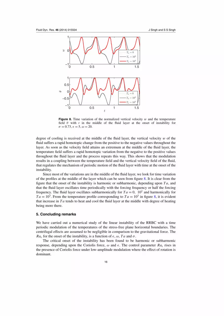
Figure 8. Time variation of the normalized vertical velocity w and the temperaturefield θ with t in the middle of the fluid layer at the onset of instability forσ = 0.73, ε = 5, ω = 20.
degree of cooling is received at the middle of the fluid layer, the vertical velocity w of thefluid suffers a rapid homotopic change from the positive to the negative values throughout thelayer. As soon as the velocity field attains an extremum at the middle of the fluid layer, thetemperature field suffers a rapid homotopic variation from the negative to the positive valuesthroughout the fluid layer and the process repeats this way. This shows that the modulationresults in a coupling between the temperature field and the vertical velocity field of the fluid,that regulates the mechanism of periodic motion of the fluid layer with time at the onset of theinstability.
Since most of the variations are in the middle of the fluid layer, we look for time variationof the profiles at the middle of the layer which can be seen from figure 8. It is clear from thefigure that the onset of the instability is harmonic or subharmonic, depending upon T a, andthat the fluid layer oscillates time periodically with the forcing frequency or half the forcingfrequency. The fluid layer oscillates subharmonically for T a = 0, 102 and harmonically forT a = 103. From the temperature profile corresponding to T a = 103 in figure 8, it is evidentthat increase in T a tends to heat and cool the fluid layer at the middle with degree of heatingbeing more there.
5. Concluding remarks
We have carried out a numerical study of the linear instability of the RRBC with a timeperiodic modulation of the temperatures of the stress-free plane horizontal boundaries. Thecentrifugal effects are assumed to be negligible in comparison to the gravitational force. TheRac for the onset of the instability, is a function of ε, ω, T a and σ .
The critical onset of the instability has been found to be harmonic or subharmonicresponse, depending upon the Coriolis force, ω and ε. The control parameter Rac rises inthe presence of Coriolis force under low-amplitude modulation where the effect of rotation isdominant.
16

Fluid Dyn. Res. 46 (2014) 015504 J Singh and S S Singh
In the absence of the Coriolis force in the fluid layer, the low-amplitude modulationand the low-frequency modulation, favor the critical onset of RBC while high-amplitudemodulation favors the critical onset of subharmonic response. Here, in comparison to theno modulation case, more temperature gradient is required to be maintained across the fluidlayer in order to see the convection pattern, when the system is driven by the low-amplitudemodulation. On the other hand, the instability can appear with a comparatively smallertemperature gradient across the fluid layer, when it is subjected to high-amplitude modulation.In the absence of the rotation in the fluid layer, the low- and high- frequency modulation favorthe critical onset of RBC.
In the presence of significant rotation rate (T a = 103) in the fluid layer, both the high-amplitude modulation and high-frequency modulation favor the critical onset of harmonicresponse. Here, the effects of Coriolis force are dominant in low-amplitude modulation, whilethe effects of modulation are dominant in the presence of high-amplitude modulation. Thevariation of Rac is dramatic when both the Coriolis force and modulation are operative. Inthis regime, a significant lowering of Rac for the critical onset of instability can be achievedwhich may facilitate the future experimental study of this important instability problem.
The patterns of the instability regions in the parametric space of k and ε have been foundto consist of alternate harmonic and subharmonic tongues which change significantly in thepresence of rotation. The presence of Coriolis force tends to suppress the appearance of thefundamental region of the instability which means that the critical instability response is likelyto be either harmonic or subharmonic and not the usual RBC. The instability regions allow usto see a particular periodic flow for the choice of lowest possible wave number just by propertuning of ε. This is important because the onset of the instability prefers smaller wave number(longer wavelengths) of the disturbance.
For a given rotation rate, the qualitative effect of Ra, σ and ω, on the critical onset ofRBC, remains similar as if without the presence of Coriolis force.
Acknowledgments
The authors are indebted to the unknown referees for their valuable comments and theconstructive criticism, to improve the manuscript.
References
Bodenschatz E, Pesch W and Ahler G 2000 Recent developments in Rayleigh–Benard convection Annu.Rev. Fluid. Mech. 32 709–78
Chandrasekhar S 1966 Hydrodynamic and Hydromagnetic Stability (Oxford: Oxford University Press)Clune T and Knobloch E 1993 Pattern selection in rotating convection with experimental boundary
conditions Phys. Rev. E 47 2536–50Cox S M and Matthews P C 2001 New instabilities in two-dimensional rotating convection and
magnetoconvection Physica D 149 210–29Cross M C and Hohenberg P C 1993 Pattern formation outside equilibrium Rev. Mod. Phys. 65 854–1086Davis S H 1976 The stability of time periodic flows Annu. Rev. Fluid Mech. 8 57–74Finucane R G and Kelly R E 1976 Onset of instability in fluid layer heated sinusoidally from below
Int. J. Heat Mass Transfer 19 71–85Getling A V 1998 Rayleigh–Benard Convection: Structures and Dynamics (Singapore: World Scientific)Jordan D W and Smith P 1988 Nonlinear Ordinary Differential Equations (Oxford: Clarendon Press)Khiri R 2004 Coriolis effect on convection for a low Prandtl number fluid Int. J. Nonlinear Mech.
39 593–604
17

Fluid Dyn. Res. 46 (2014) 015504 J Singh and S S Singh
Kloosterziel R C and Carnevale G F 2003 Closed-form linear stability conditions for rotatingRayleigh–Benard convection with rigid stress-free upper and lower boundaries J. Fluid Mech.480 25–42
Koschmieder E L 1993 Benard Cells and Taylor Vortices (Cambridge: Cambridge University Press)Kumar K 1996 Linear theory of Faraday instability in viscous liquids Proc. R. Soc. Lond. A 452 1113–26Kumar K and Tuckerman L S 1994 Parametric instability of the interface between two fluids J. Fluid
Mech. 279 49–68Kuppers G and Lortz D 1969 Transition from laminar convection to thermal turbulence in a rotating
fluid layer J. Fluid Mech. 35 609–20Lopez J M, Rubio A and Marques F 2006 Travelling circular waves in axisymmetric rotating convection
J. Fluid Mech. 569 331–48Marques F, Mercader I, Batiste O and Lopez J M 2007 Centrifugal effects in rotating convection:
axysymmetric states and three-dimensional instabilities J. Fluid Mech. 580 303–18Meyer C W, Cannell D S and Ahlers G 1992 Hexagonal rolls and roll flow patterns in temporally
modulated Rayleigh–Benard convection Phys. Rev. A 45 8583–604Miklos Farkas 1994 Periodic Motions (New York: Springer)Rauscher J W and Kelly R E 1974 Effect of modulation on the onset of thermal convection in a rotating
fluid Int. J. Heat Mass Transfer 18 1216–7Rogers J L, Schatz M F, Bougie J L and Swift J B 2000 Rayleigh–Benard convection in a vertically
oscillated fluid layer Phys. Rev. Lett. 84 87–90Roppo M N, Davis S H and Rosenblat S 1984 Benard convection with time periodic heating Phys. of
Fluids 27 796–803Rosenblat S and Tanaka G A 1971 Modulation of thermal convection instability Phys. Fluids 14 1319–22Rudiger S and Knobloch E 2003 Mode interaction in rotating Rayleigh–Benard convection Fluid Dyn.
Res. 33 477–92Scheel J D 2007 The amplitude equation for rotating Rayleigh–Benard convection Phys. Fluids
19 1041051–8Singh J and Bajaj R 2008 Thermal modulation in the Rayleigh–Benard convection ANZIAM J.
50 231–45Somerville C J 1971 Benard convection in rotating fluid Geophys. Fluid Dyn. 2 247–62Teed R J, Jones C A and Hollerbach R 2010 Rapidly rotating plane layer convection with zonal flow
Geophys. Astrophys. Fluid Dyn. 104 457–80Tu Y and Cross M C 1992 Chaotic domain structure in rotating convection Phys. Rev. Lett. 69 2515–8Venezian G 1969 Effect of modulation on the onset of thermal convection J. Fluid Mech. 35 243–54Yih C S and Li C H 1972 Instability of unsteady flows or configurations: 2. Convective instability
J. Fluid Mech. 54 143–52
18


