Gender Differences in the Labour
Market Status, Wages and Occupations
in Pakistan
Mehak Ejaz
A thesis submitted to the University of Sheffield for the degree of Doctor ofPhilosophy in the Department of Economics .
Monday 22nd February, 2016
brought to you by COREView metadata, citation and similar papers at core.ac.uk
provided by White Rose E-theses Online
Dedicated to my parents
Mr and Mrs Ejaz Ahmad Khan
ii
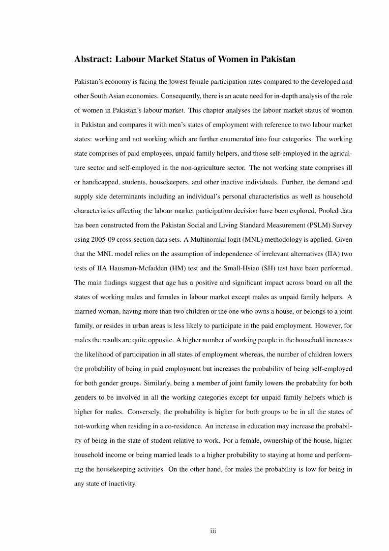
Abstract: Labour Market Status of Women in Pakistan
Pakistan’s economy is facing the lowest female participation rates compared to the developed and
other South Asian economies. Consequently, there is an acute need for in-depth analysis of the role
of women in Pakistan’s labour market. This chapter analyses the labour market status of women
in Pakistan and compares it with men’s states of employment with reference to two labour market
states: working and not working which are further enumerated into four categories. The working
state comprises of paid employees, unpaid family helpers, and those self-employed in the agricul-
ture sector and self-employed in the non-agriculture sector. The not working state comprises ill
or handicapped, students, housekeepers, and other inactive individuals. Further, the demand and
supply side determinants including an individual’s personal characteristics as well as household
characteristics affecting the labour market participation decision have been explored. Pooled data
has been constructed from the Pakistan Social and Living Standard Measurement (PSLM) Survey
using 2005-09 cross-section data sets. A Multinomial logit (MNL) methodology is applied. Given
that the MNL model relies on the assumption of independence of irrelevant alternatives (IIA) two
tests of IIA Hausman-Mcfadden (HM) test and the Small-Hsiao (SH) test have been performed.
The main findings suggest that age has a positive and significant impact across board on all the
states of working males and females in labour market except males as unpaid family helpers. A
married woman, having more than two children or the one who owns a house, or belongs to a joint
family, or resides in urban areas is less likely to participate in the paid employment. However, for
males the results are quite opposite. A higher number of working people in the household increases
the likelihood of participation in all states of employment whereas, the number of children lowers
the probability of being in paid employment but increases the probability of being self-employed
for both gender groups. Similarly, being a member of joint family lowers the probability for both
genders to be involved in all the working categories except for unpaid family helpers which is
higher for males. Conversely, the probability is higher for both groups to be in all the states of
not-working when residing in a co-residence. An increase in education may increase the probabil-
ity of being in the state of student relative to work. For a female, ownership of the house, higher
household income or being married leads to a higher probability to staying at home and perform-
ing the housekeeping activities. On the other hand, for males the probability is low for being in
any state of inactivity.
iii
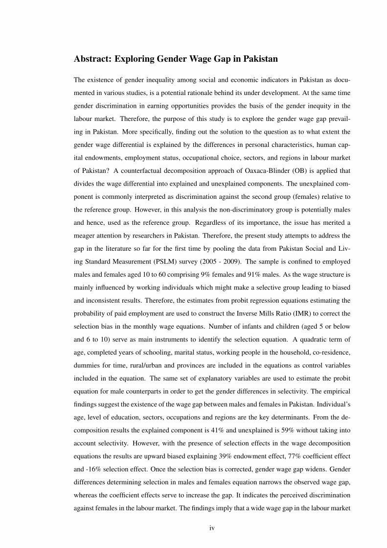
Abstract: Exploring Gender Wage Gap in Pakistan
The existence of gender inequality among social and economic indicators in Pakistan as docu-
mented in various studies, is a potential rationale behind its under development. At the same time
gender discrimination in earning opportunities provides the basis of the gender inequity in the
labour market. Therefore, the purpose of this study is to explore the gender wage gap prevail-
ing in Pakistan. More specifically, finding out the solution to the question as to what extent the
gender wage differential is explained by the differences in personal characteristics, human cap-
ital endowments, employment status, occupational choice, sectors, and regions in labour market
of Pakistan? A counterfactual decomposition approach of Oaxaca-Blinder (OB) is applied that
divides the wage differential into explained and unexplained components. The unexplained com-
ponent is commonly interpreted as discrimination against the second group (females) relative to
the reference group. However, in this analysis the non-discriminatory group is potentially males
and hence, used as the reference group. Regardless of its importance, the issue has merited a
meager attention by researchers in Pakistan. Therefore, the present study attempts to address the
gap in the literature so far for the first time by pooling the data from Pakistan Social and Liv-
ing Standard Measurement (PSLM) survey (2005 - 2009). The sample is confined to employed
males and females aged 10 to 60 comprising 9% females and 91% males. As the wage structure is
mainly influenced by working individuals which might make a selective group leading to biased
and inconsistent results. Therefore, the estimates from probit regression equations estimating the
probability of paid employment are used to construct the Inverse Mills Ratio (IMR) to correct the
selection bias in the monthly wage equations. Number of infants and children (aged 5 or below
and 6 to 10) serve as main instruments to identify the selection equation. A quadratic term of
age, completed years of schooling, marital status, working people in the household, co-residence,
dummies for time, rural/urban and provinces are included in the equations as control variables
included in the equation. The same set of explanatory variables are used to estimate the probit
equation for male counterparts in order to get the gender differences in selectivity. The empirical
findings suggest the existence of the wage gap between males and females in Pakistan. Individual’s
age, level of education, sectors, occupations and regions are the key determinants. From the de-
composition results the explained component is 41% and unexplained is 59% without taking into
account selectivity. However, with the presence of selection effects in the wage decomposition
equations the results are upward biased explaining 39% endowment effect, 77% coefficient effect
and -16% selection effect. Once the selection bias is corrected, gender wage gap widens. Gender
differences determining selection in males and females equation narrows the observed wage gap,
whereas the coefficient effects serve to increase the gap. It indicates the perceived discrimination
against females in the labour market. The findings imply that a wide wage gap in the labour market
iv
is explained by factors such as education and employments types i.e. sectors. It may be due to
the occupation differences in all the sectors of the economy that leads to discrimination and hence
widening the monthly wage gaps between genders across all the regions in Pakistan. Moreover, it
is has been observed that female remuneration in Pakistan is not based on merely discrimination
rather on a low education level which could be a potential reason to increasing the gender wage
gap in the labour market.
Abstract: Explaining Gender Differences across Gender and Regions
in Pakistan
Extensive empirical literature in Pakistan provides evidence of discrimination against women, in-
dicating the presence of occupational segregation and differences in the labour market. However,
this argument is based on stylized facts and has not been supported by the empirical analysis
so far. The main objective of the chapter is to estimate the extent of occupational differences
across gender and regions in Pakistan. In this regard, the occupational gap between males and
females within nine occupations in the labour market has been estimated. Further, for a compre-
hensive spatial analysis, the differences are calculated separately for an overall Pakistan and its
four provinces. It is expected that the study contributes to the literature by explaining the proba-
bility differentials between males and females selecting into different occupations of employment
using Oaxaca decomposition but for a binary outcomes. The study utilises pooled data constructed
from three cross-section data sets (2005, 2007 and 2009) of Pakistan Social and Living Standard
Measurement (PSLM) Survey. A non-linear decomposition technique which is an extension of
Blinder-Oaxaca decomposition method is applied. It decomposes the difference in the binary
dependent outcome variables (i.e. between males and females) into a part that is explained by dif-
ferences in observable characteristics and a part attributable to differences in the returns to these
characteristics. The empirical findings suggest the existence of a wide gap in the occupations be-
tween genders mainly due to a discriminatory behaviour against females rather than differences in
observable characteristics. In the analysis, males are considered as the non-discriminatory group
because of a high majority of the employed males compared to females. The results indicate that in
the low paid jobs (such as clerks, sales persons, skilled workers in agriculture and fishery, craft and
trade workers, plant and machinery operators and unskilled or elementary occupations) a major
part of the gender differential is attributed to differences in the coefficients indicating substantial
differences in attitudes towards males and females. However, almost 50 percent of the differences
in high earning jobs (such as professional and senior officials) are explained by different character-
istics. The findings conclude that females are not only relegated disproportionately to jobs viewed
v
as less important, requiring lower skills, and with lower earnings but are also facing higher level
of discrimination in these occupations.
JEL Classification:
J20, J21, J23, J240, J30, J31, J70, J71
Keywords:
Multinomial Logit model, employment status, IIA Test, employment Probits, wage gap, endow-
ment, discrimination, selectivity, Oaxaca-Blinder wage decomposition, occupation differences,
gender differences, binary outcome variable, non-linear extension to Oaxaca-Blinder decomposi-
tion.
vi
Acknowledgements
I wish to thank, first and foremost, Almighty Allah for providing me an opportunity to take up
this challenging task at at a time when my newly born son Mahad needed an equal engagement at
home. Managing both was not easy and yet I learnt that nothing can be attained without the will
of Allah.
I am highly grateful to my supervisor Professor Dr. Karl B Taylor for his constant aspiring
guidance, invaluable comments and honest-constructive feedback. I am highly indebted to him
for his sincere, honest and useful suggestions. He has been a tremendous mentor who has not
only enhanced my knowledge and interest in Labour Economics but also helped me grow as an
independent researcher. I would like to acknowledge the contribution of my second supervisor Dr.
Pamela Lenton for her supportive comments, suggestions and above all the moral support.
I consider it an honor to have worked with Professor Dr. Sarah Brown when I initially under-
took research. She will as ever remain my inspiration throughout my academic career. It is with
immense gratitude that I also acknowledge the support and help of Professor Dr. Steve McIntosh
specially during the process of my admission to the University, the logistic and moral support he
continued to provide till the end. I am also indebted to the PhD Director, Dr. Arne. R. Hole for his
patience and supportive attitude who steered me out of an acute depression and frustration during
research. I would like to extend thankyou to Professor Dr. Andrew Dickerson on advising me
during the phase of financial crisis in the third year.
I would especially like to thank the academic staff and the technical staff (Jane Mundy, Rachel
Watson, Linda Brabbs, Lousise Harte, Charlotte Hobson and Mike Crabtree) for providing a con-
stant and exampling logistic help throughout. Furthermore, the resources and facilities within the
department as well as the University of Sheffield remained simply exceptional. I am thankful to all
those faculty members who contributed effectively in giving me constructive comments and sug-
gestions during my upgrade meeting, especially Dr. Anita Ratcliffe, internal seminars and White
Rose Doctoral Conferences.
It gives me immense pleasure in recognising the financial support of partial scholarship from
the Department of Economics, University of Sheffield. In addition, a thank you to the State Bank of
Pakistan for granting me an interest free loan to cover the difference of the international fee for two
years. Last, but not least, thanks to Higher Education Commission (HEC) Pakistan for providing
me a ”Partial scholarship for students studying abroad” to cover my last year’s expenses.
In this regard, Uncle Nasir Shirazi also deserves special thanks for arranging a free accom-
modation for my family in Sheffield for four years. Nothing short of blessing especially for an
international female student belonging to a middle class. I am also obliged to Mr. Haider Zaidi,
a PhD student, for his timely help to pay my fee while awaiting HEC’s scholarship. Deepest
vii

gratitude however, to my father for sending me money whenever I needed it.
This thesis would not have been possible without the love, support and encouragement of
Kalim Hyder, my husband. He has shown an immense level of tolerance throughout my studies.
His substantial support has enabled me to survive through thick and thin, from child care to finan-
cial care; from thought provoking discussions to guidance at moments when there was no one to
answer my queries. Words cannot express how blessed and grateful I feel for having him beside
me.
A special thanks to my friends and colleagues (Fatima Alaali, Hanan Naser, Manzur Quader,
Zainab Jehan, Nora Abu Asab, Bo Tang and Uzma Ahmed) for sharing their experiences and
giving valuable suggestions. I will definitely miss them all as they become a part of my pleasant
memories forever.
I owe my hearty gratitude to my parents (Ejaz Ahmad Khan and Humaira Ejaz) and siblings
(Khushboo Ejaz, Muhammad Ahmad Khan , Muneeb Ahmad Khan, Maham Ejaz and Bilal Ahmad
Khan and most importantly my dear nephew, Muhammad Ahmed Kamil whom I missed every
day) for all ther sacrifices and prayers. Can‘t wait to see the sparkling pride of my parents whose
daughter’s achievemen would’nt have been possible without their support and motivation.
viii
Contents
Abstract iii
Acknowledgements vii
Table of Contents ix
List of Tables xii
List of Figures xv
Chapter 1: Introduction 1
1.1 Background and Motivation . . . . . . . . . . . . . . . . . . . . . . . . . . . . 1
1.2 Aims, Objectives and Research Questions . . . . . . . . . . . . . . . . . . . . . 5
1.3 Data . . . . . . . . . . . . . . . . . . . . . . . . . . . . . . . . . . . . . . . . . 6
1.4 Contribution to the literature . . . . . . . . . . . . . . . . . . . . . . . . . . . . 9
1.5 Structure of the thesis . . . . . . . . . . . . . . . . . . . . . . . . . . . . . . . . 11
Chapter 2: Labour Market Status of Women in Pakistan 12
2.1 Introduction . . . . . . . . . . . . . . . . . . . . . . . . . . . . . . . . . . . . . 12
2.1.1 Background . . . . . . . . . . . . . . . . . . . . . . . . . . . . . . . . . 12
2.1.2 Research Question and Objective . . . . . . . . . . . . . . . . . . . . . 16
2.2 Literature Review . . . . . . . . . . . . . . . . . . . . . . . . . . . . . . . . . . 17
2.2.1 Determinants of women’s participation in the labour market . . . . . . . 18
2.2.1.1 International Studies: . . . . . . . . . . . . . . . . . . . . . . 18
2.2.1.2 Multinomial Logit Model used in Literature: . . . . . . . . . . 22
2.2.1.3 Pakistan Studies: . . . . . . . . . . . . . . . . . . . . . . . . . 25
2.3 Data Source and Variable Description . . . . . . . . . . . . . . . . . . . . . . . 28
2.3.1 Pakistan Social and Living Standard Measurement Survey (PSLM) . . . 28
2.3.2 Dependent Variable . . . . . . . . . . . . . . . . . . . . . . . . . . . . . 29
2.3.3 Explanatory Variables . . . . . . . . . . . . . . . . . . . . . . . . . . . 31
2.4 Methodology . . . . . . . . . . . . . . . . . . . . . . . . . . . . . . . . . . . . 34
2.4.1 Unordered Multiple Choice Models . . . . . . . . . . . . . . . . . . . . 34
2.4.2 The Multinomial Logit Model . . . . . . . . . . . . . . . . . . . . . . . 35
2.4.3 Dependent Variable Outcomes . . . . . . . . . . . . . . . . . . . . . . . 37
2.4.4 Base Category . . . . . . . . . . . . . . . . . . . . . . . . . . . . . . . 37
2.4.5 Marginal Effects . . . . . . . . . . . . . . . . . . . . . . . . . . . . . . 38
ix
2.5 Results and Empirical Findings . . . . . . . . . . . . . . . . . . . . . . . . . . . 39
2.5.1 Model 1 and 3: Gender differences in Employment Outcomes . . . . . . 39
2.5.2 Model 2 and 4: Gender Differences in Inactivity . . . . . . . . . . . . . 44
2.5.3 Multinomial Logit Model Results with 8 alternatives of Working and Not-
working states as an Outcome Variable . . . . . . . . . . . . . . . . . . 47
2.5.4 Multinomial Logit Model Results for Working Males with Paid employ-
ment as base category and Not-working Males with Housekeepers as base
Category . . . . . . . . . . . . . . . . . . . . . . . . . . . . . . . . . . 50
2.5.5 Multinomial Logit Model Results for Working Females with Paid em-
ployment as base category and Not-working Males with Housekeepers as
base Category . . . . . . . . . . . . . . . . . . . . . . . . . . . . . . . . 52
2.6 Post - estimation Results . . . . . . . . . . . . . . . . . . . . . . . . . . . . . . 53
2.6.1 Independence of Irrelevant Alternatives . . . . . . . . . . . . . . . . . . 53
2.6.1.1 Hausman test of IIA . . . . . . . . . . . . . . . . . . . . . . . 55
2.6.1.2 Small-Hasiao test of IIA . . . . . . . . . . . . . . . . . . . . . 56
2.7 Conclusion . . . . . . . . . . . . . . . . . . . . . . . . . . . . . . . . . . . . . 57
Chapter 3: Exploring Gender Wage Gap in Pakistan 59
3.1 Introduction . . . . . . . . . . . . . . . . . . . . . . . . . . . . . . . . . . . . . 59
3.2 Literature Review . . . . . . . . . . . . . . . . . . . . . . . . . . . . . . . . . . 62
3.2.1 Literature Review (International Studies) . . . . . . . . . . . . . . . . . 62
3.2.2 Literature Review (Pakistan Literature) . . . . . . . . . . . . . . . . . . 70
3.3 Data Source and Variable Description . . . . . . . . . . . . . . . . . . . . . . . 72
3.3.1 Dependent Variable (monthly wages) . . . . . . . . . . . . . . . . . . . 73
3.4 Methodology . . . . . . . . . . . . . . . . . . . . . . . . . . . . . . . . . . . . 78
3.4.1 Decomposition for Linear Regression Model: Oaxaca Blinder Approach . 79
3.4.2 Correction for Selectivity bias . . . . . . . . . . . . . . . . . . . . . . . 81
3.5 Results and Findings . . . . . . . . . . . . . . . . . . . . . . . . . . . . . . . . 85
3.5.1 Probit Regressions: Selectivity Equation . . . . . . . . . . . . . . . . . . 85
3.5.2 Wage Equations . . . . . . . . . . . . . . . . . . . . . . . . . . . . . . 90
3.5.3 Gender Wage Decomposition: Blinder-Oaxaca Decomposition Method . 91
3.6 Conclusion . . . . . . . . . . . . . . . . . . . . . . . . . . . . . . . . . . . . . 99
Chapter 4: Explaining Occupational Differences across Genders and Regions in Pakistan101
4.1 Introduction . . . . . . . . . . . . . . . . . . . . . . . . . . . . . . . . . . . . . 101
4.2 Literature Review . . . . . . . . . . . . . . . . . . . . . . . . . . . . . . . . . . 104
x
4.3 Data and Variables . . . . . . . . . . . . . . . . . . . . . . . . . . . . . . . . . 107
4.4 Methodology . . . . . . . . . . . . . . . . . . . . . . . . . . . . . . . . . . . . 109
4.4.1 Oaxaca-Blinder extension to Probit Model . . . . . . . . . . . . . . . . . 110
4.5 Decomposition Results of Occupation Probits . . . . . . . . . . . . . . . . . . . 112
4.6 Conclusion . . . . . . . . . . . . . . . . . . . . . . . . . . . . . . . . . . . . . 130
Chapter 5: Conclusion 132
5.1 Summary of the thesis . . . . . . . . . . . . . . . . . . . . . . . . . . . . . . . 132
5.2 Policy Implications . . . . . . . . . . . . . . . . . . . . . . . . . . . . . . . . . 136
5.3 Limitations . . . . . . . . . . . . . . . . . . . . . . . . . . . . . . . . . . . . . 138
5.4 Future Research . . . . . . . . . . . . . . . . . . . . . . . . . . . . . . . . . . . 140
Appendix A: Multinomial Logit Results 141
Appendix B: Results of Wage Equations 150
Appendix C: Probits, Marginal effects and Classification of Occupations 153
C.1 Results of Occupation Probits with Marginal effects . . . . . . . . . . . . . . 153
C.2 ILO Classification of Occupations . . . . . . . . . . . . . . . . . . . . . . . . 193
References 199
xi
List of Tables
Table 2.1 Characteristics of PSLM . . . . . . . . . . . . . . . . . . . . . . . . . . . 28
Table 2.2 Descriptive Statistics of Explanatory variables before and after pooling . . 30
Table 2.3 Category wise Observations . . . . . . . . . . . . . . . . . . . . . . . . . 31
Table 2.4 Descriptive Statistics of Pooled Data . . . . . . . . . . . . . . . . . . . . . 32
Table 2.5 Description of Explanatory Variables . . . . . . . . . . . . . . . . . . . . 33
Table 2.6 Summary Statistics of Both Genders . . . . . . . . . . . . . . . . . . . . . 33
Table 2.7 Multinomial Logit Model 1 and Model 3 Results; Working as Dependent
Variable taking Not-working as Base category (0) . . . . . . . . . . . . . . 40
Table 2.8 Multinomial Logit Model 2 and Model 4 Results; Not working as Dependent
Variable taking Working as Base category (0) . . . . . . . . . . . . . . . . 46
Table 2.9 Hausman (HM) Test Results . . . . . . . . . . . . . . . . . . . . . . . . . 55
Table 2.10 Small Hasiao (SM) Test Results . . . . . . . . . . . . . . . . . . . . . . . 56
Table 3.1 Description of Explanatory Variables . . . . . . . . . . . . . . . . . . . . 74
Table 3.2 Summary Statistics of Explanatory Variables (Males) . . . . . . . . . . . . 75
Table 3.3 Summary Statistics of Explanatory Variables (Females) . . . . . . . . . . . 76
Table 3.4 Descriptive Stats of Dependent Variable (Ln(Wages)) . . . . . . . . . . . . 77
Table 3.5 Probit Regressions . . . . . . . . . . . . . . . . . . . . . . . . . . . . . . 87
Table 3.6 Gender Wage Decomposition with and without Selectivity . . . . . . . . . 93
Table 3.7 Decomposition of Wage Differentials by Alternative Methods . . . . . . . 98
Table 4.1 Mean of the Explanatory Variables for Different Regions . . . . . . . . . . 109
Table 4.2 Male/Female Occupation Probit Decomposition (Senior Officials) . . . . . 113
Table 4.3 Male/Female Occupation Probit Decomposition (Professionals) . . . . . . 115
Table 4.4 Male/Female Occupation Probit Decomposition (Technicians) . . . . . . . 118
Table 4.5 Male/Female Occupation Probit Decomposition (Clerks) . . . . . . . . . . 120
Table 4.6 Male/Female Occupation Probit Decomposition (Services/Shop) . . . . . . 122
Table 4.7 Male/Female Occupation Probit Decomposition (Skilled Agriculture) . . . 123
Table 4.8 Male/Female Occupation Probit Decomposition (Craft/Trade worker) . . . 125
Table 4.9 Male/Female Occupation Probit Decomposition (Machinery Operator) . . . 127
Table 4.10 Male/Female Occupation Probit Decomposition (Elementary/Unskilled) . . 129
Table A1 Multinomial Logit Model 2 and Model 4 Results; Not working as Dependent
Variable (without ill/handicapped) taking Working as Base category (0) . . 141
Table A2 Likelihood-ratio test (for Working Females) . . . . . . . . . . . . . . . . 141
Table A3 Likelihood-ratio test (for Working Males) . . . . . . . . . . . . . . . . . . 142
xii
Table A4 Likelihood-ratio test (for Not-working Females) . . . . . . . . . . . . . . 142
Table A5 Likelihood-ratio test (for Not-working Males) . . . . . . . . . . . . . . . . 143
Table A6 Wald tests for independent variables (Working Females) . . . . . . . . . . 143
Table A7 Wald tests for independent variables (Working Males) . . . . . . . . . . . 144
Table A8 Wald tests for independent variables (Not-working Females) . . . . . . . . 144
Table A9 Wald tests for independent variables (Not-working Males) . . . . . . . . . 145
Table A10 Wald tests for combining outcome categories . . . . . . . . . . . . . . . . 146
Table A11 Multinomial Logit Model (Females age (15-60)) . . . . . . . . . . . . . . 147
Table A12 Multinomial Logit Model (Males age (15-60)) . . . . . . . . . . . . . . . 147
Table A13 Multinomial Logit Model with 8 alternatives (base category is paid employ-
ment) . . . . . . . . . . . . . . . . . . . . . . . . . . . . . . . . . . . . . 148
Table A14 Multinomial Logit Model with 8 alternatives (base category is paid employ-
ment) . . . . . . . . . . . . . . . . . . . . . . . . . . . . . . . . . . . . . 148
Table A15 Multinomial Logit Model (Females (15-60)) . . . . . . . . . . . . . . . . 149
Table A16 Multinomial Logit Model (Males (15-60)) . . . . . . . . . . . . . . . . . . 149
Table B1 Wage Equation (log of monthly wages) . . . . . . . . . . . . . . . . . . . 150
Table B2 Wage Equation (log of monthly wages) . . . . . . . . . . . . . . . . . . . 151
Table B3 Gender Wage Decomposition With and Without Selectivity (Excluding Oc-
cupations) . . . . . . . . . . . . . . . . . . . . . . . . . . . . . . . . . . . 152
Table C1 Frequency Distribution of Occupations across Regions (Males) . . . . . . . 153
Table C2 Frequency Distribution of Occupations across Regions (Females) . . . . . 154
Table C3 Occupation Probits of Pakistan by Gender . . . . . . . . . . . . . . . . . . 155
Table C4 Occupation Probits of Punjab by Gender . . . . . . . . . . . . . . . . . . . 156
Table C5 Occupation Probits of Sindh by Gender . . . . . . . . . . . . . . . . . . . 157
Table C6 Occupation Probits of KPK by Gender . . . . . . . . . . . . . . . . . . . . 158
Table C7 Occupation Probits of Balochistan by Gender . . . . . . . . . . . . . . . . 159
Table C8 Male/Female Occupation Probit Decomposition (Senior officials). . . . . . 160
Table C9 Male/Female Occupation Probit Decomposition (Professionals). . . . . . . 163
Table C10 Male/Female Occupation Probit Decomposition (Technicians). . . . . . . . 167
Table C11 Male/Female Occupation Probit Decomposition (Clerks). . . . . . . . . . . 170
Table C12 Male/Female Occupation Probit Decomposition (Service/shop). . . . . . . 173
Table C13 Male/Female Occupation Probit Decomposition (Skilled/agri/fishery). . . . 177
Table C14 Male/Female Occupation Probit Decomposition (Craft/trade). . . . . . . . 181
Table C15 Male/Female Occupation Probit Decomposition (Machinery operator). . . 184
Table C16 Male/Female Occupation Probit Decomposition (Elementry/unskilled). . . 187
xiii

Table C17 Bootstrapping Results with (1000) replications . . . . . . . . . . . . . . . 191
Table C18 Ratio Analysis Male-Female Occupation Differences . . . . . . . . . . . . 192
xiv
List of Figures
Figure 2.1 Female Labour Force Participation. . . . . . . . . . . . . . . . . . . . . . . 13
Figure 2.2 Trend of Women Labour Force. . . . . . . . . . . . . . . . . . . . . . . . . 14
Figure 2.3 Employment Status. . . . . . . . . . . . . . . . . . . . . . . . . . . . . . 14
Figure 2.4 Construction of Dependent Variable. . . . . . . . . . . . . . . . . . . . . . 29
Figure 3.1 Kernel Density Plot of Wages by Gender. . . . . . . . . . . . . . . . . . . . 77
xv
Chapter 1
Introduction
1.1 Background and Motivation
The role of the labour market is crucial in the macro economy due to its significant backward and
forward linkages. Backward linkages exist when growth in the labour market leads to the growth
in the sectors that supply labour such as education and training. The strong backward linkages help
creating supply of labour and generate employment opportunities, not only for the skilled but for
unskilled individuals as well. The forward linkages occur when the growth in the labour market
leads to the growth of the sectors that utilise the labour, hence generating demand for labour. As a
consequence, the per capita income, standard of living, production and output level gets an uplift
which in turn has a significant impact on the economic development of the country.
Over the last three decades, a substantial rise in the female labour force participation (FLFP)
has been observed in the world. Subsequently, the female’s participation rate has increased from
4% to 70% in developed economies (Hotchkiss (2006)). However, in Pakistan, despite the spells
of high growth rates from 2004-07, females labour market participation is still very low compared
with developed and other Asian countries. In Pakistan, overall labour force participation remained
between 49 to 52.5 % from 1971-72 to 2007-08. These numbers are based on the total population
aged 15 years and above. This implies that 47.5% of the population is out of labour force. The
gender-wise statistics shows a decline in males labour force participation from 88.5% in 1971-72
to 83% in 2000s. However, females participation has increased from 9% in 1971-72 to 22% in
2007-08. Yet, it is still depressing that out of total female labour force 78% are economically
inactive compared to 17% inactive males.
On the basis of ILO (2014) data on key indicators of the labour market for sixteen selected
countries from 1980 to 2007, the marginal improvement in female labour force participation rate
(from 5.5% in 1980 to 16% in 2000 to 20.8 in 2007), shows Pakistan continues to take the bottom
position compared to East Asian countries like China, Thailand, Korea and Philippines where
the females labour market participation is 70.6 % , 69.3% , 49.3% and 49.8% respectively in
2007. Even among Muslim countries, Pakistan falls behind Indonesia which lies within 43 to
49 %); Malaysia between 41-44%, and Bangladesh in the range of 57-62 % showing continuous
improvement. The progress is clearly more than twice to that of Pakistan. In South Asia, India
and Sri Lanka have shown significant progress with participation rates of over 34 percent and 43
percent respectively.
1
Although the participation rate has shown a rising trend in Pakistan from the 1970’s to 2007,
two-thirds of the increase is attributed to unpaid family helpers. The stylised facts gathered from
the data set used in this thesis reveal that 86.6% of the females, as a part of the labour force, are
not working, and only 13.4% are working out of which 6.9% are unpaid family helpers. In terms
of numbers, the male to female participation ratio is 4:1. These statistics raise important issues
concerning Pakistans labour market. One, the extent to which the FLFP is increasing, is overstated
due to the inclusion of unpaid family helpers. Perhaps, the transition of FLFP from agricultural
activities to the informal sector and eventually to the formal sector in urban areas is not taking
place. Moreover, there exists a weak link between education and employment. It might be due to
the prevailing socio-cultural attitude that allows women to obtain higher education, but continues
to restrict female employment. Thus, reflecting the potential existence of gender inequality in the
given society. One of the possible explanations for gender inequity is discrimination in wage-
related earning opportunities.
Pakistan’s education system is deteriorating despite the introduction of new constitutional obli-
gation of free compulsory education for children between the ages of five and sixteen as well as
the eighteenth amendment in the constitution to devolve education to the provinces. The idea is
to address the local needs and become more efficient and responsive. Yet, Pakistan is at second
highest number out of school children in the world. 22 percent of the children are constitutionally
obliged but still deprived of proper schooling. Pakistan is far behind in meeting the MDG i.e. pro-
viding universal primary education by 2015. The main factor is lowest expenditure on education
as a percentage of GDP compared to other South Asian counties. According to Pakistan Eco-
nomic Survey (2014), Pakistan spends 2% of GDP on education while Bhutan spend 4.8%, Nepal
4.1%, India 3.1%, Sri Lanka 2.6% and Bangladesh 2.4% of GDP on education sector. The main
challenge that Pakistan confront is the low level of education and high dropout rates which gov-
ernment and policy makers can overcome if education becomes their top priority.Cconsequently,
the system has failed to equip the youth for job market.
According to the World Bank, the number of female paid workers has risen in most of the
developing countries. However, gender disparities still persist in many areas, and even in rich
countries. Income growth itself does not deliver equality. In fact, where gender gaps became
close, it is because of the combined behaviour of markets and institutions (formal and informal),
or the interaction between the two to influence household decisions especially in favour of females.
The gaps remain for poor women and these disparities become even worse when combined with
ethnicity, backwardness and disability (Wong (2012)).
Unequal access to opportunities is another dilemma. Females all over the world are more
likely than men to work as an unpaid worker or in informal sectors. As a result, males tend to earn
2
more than women. Agriculture is becoming increasingly feminized occupation. At the same time,
female participation in the manufacturing sector is falling. Meanwhile, poor women in developing
and transition economies continue to be employed in the low-wage informal sector and gender
gaps in wages and occupational hierarchies persist (Wong (2012)).
One of the significant Millennium Development Goals (MDGs) is to promote gender equality.
Gender equality is important not only as a goal in itself, but also as means to combating poverty,
hunger and disease, and empowering women. (The World Bank (2003)). As stated by (Atkinson
(1997); Atkinson and Bourguignon (2000)) inequality remains a crucial issue in complementing
welfare enhancement strategies. However, Pakistan seems too far behind to accomplish this spe-
cific goal, and consequently the related goals. According to the Global Gender Gap Index 2014,
Pakistan‘s ranking is second worse out of 142 countries around the globe. The ranking is getting
worse over time from 112 out of 115 in 2006 to 132 out of 134 in 2010 to 134 out of 135 in 2012
and 141 out of 142 in 2014. The Global Gender Gap index is calculated on the basis of economic
participation, education attainment, health & survival, and political empowerment. The deterio-
rating trend overtime is alarming and requires special attention of researchers and policy makers
to find out a viable solution to the problem in this regard (Hausmann et al. (2014)). This factual
analysis attracts the attention of the researcher to investigate the causes behind such a consistent
low rank. The worsening social indicators overtime, can possibly explain the causal factors behind
the employment gaps as well as provides a comprehensive idea on the issues concerning Pakistan’s
labour market.
A limited number of studies in Pakistan explore the subsistence of gender inequality among
the social and economic indicators. However, there exists a general consensus among researchers
that men earn higher wages than women. Wages are directly linked to the standard of living and
the extent of poverty. There is an acute need for a better understanding of the factors affecting
the offered wage and to identify the wage determinants in the developing countries in general and
in Pakistan, in particular. The awareness of this mechanism can provide a proper guidance to
policy makers to invest in those factors that can improve labour income which can further boost
the economic growth.
Furthermore, other evidence of the unfavourable conditions for females in Pakistans labour
market comes from the study by International Labour organisation (ILO) 2006, stating that fe-
males are often treated as inferior participants in the labour market. It is due to the traditional
view that the primary role of women is to fulfil reproductive and domestic functions, rather than
fully participate in education and paid work. This, in turn, limits female’s choice of employment
activities and results in the sectoral or occupational segregation. Consequently, women relegate
themselves to jobs that require low skills, less time and with lower wages. This situation again
3
raised some key points concerning the disadvantageous position of females as compared to males
has in the labour market. Therefore, an in-depth analysis of the gender differences across occupa-
tions is an essential area of this research. Further, recognition of the determining factors behind
the concentration (of either males or females) in a particular occupation may provide a clear un-
derstanding of the problem.
The topic of FLFP has attracted many researchers since the seminal contribution of Mincer
(1962). He has explored this issue by incorporating the advancements in the theory of labour sup-
ply as well as econometrics during the last three decades. Following the traditional labour supply
theory, Becker (1965) has discussed the household production model and females time allocation.
Further, Chiappori (1992) presents a collective household model, providing the theoretical foun-
dations for the analysis of female labour force participation. Empirical investigations by Gronau
(1974) and Heckman (1979) focus on the appropriate estimation method. Most of the time series
studies focus on the developed economies and investigate the rising trend in the female labour
force participation during the last three decades. However, the cross section studies have utilised
micro data in determining the probability of FLFP, whereas panel data studies investigate a U
shaped relationship between economic development and female labour force participation.
Gender differences in access to economic opportunities in the labour market participation has
been a topic of debate for academics and policy makers. However despite its great significance, the
issue of gender differences in the labour market has not received much attention from researchers
in Pakistan, except for a few studies. These exclusively focus on the decision to join or not to
join the labour market. There is an utmost need to look at the labour market issues beyond such
participation and focus on productivity and earnings for two main reasons: firstly, emphasis on
participation alone marks gender differences in the dynamics of work; secondly the reallocation
of time for other (caring & household) activities for which the opportunity cost may vary across
genders. Although there is significant progress overtime in the female labour force participation,
the gender differences in earnings and productivity persist in almost all the sectors of occupations
and jobs. The general argument for this gap is due to the gender differences in human capital
and returns to the employment characteristics. Furthermore, females are facing a higher level of
discrimination across occupations.
The gender differences in economic participation are mainly caused by the differences in car-
ing responsibilities and access to the productive inputs and differences in the occupations. This
provides the motivation of this thesis to look at the differences in the employment status, earnings
and occupations across gender. The overarching goal of the thesis is to quantify the gender dif-
ferences in labour market. Firstly, by identifying if there exists a difference in the labour market
states. Secondly, measuring the mean differences in the earnings and then exploring whether it is
4
coming from the human capital, or discrimination against females or it is due to the self-selection
by choice to stay out of labour force due to the higher opportunity cost of other household activi-
ties. Finally, explaining the occupation differences in detail.
1.2 Aims, Objectives and Research Questions
On the basis of the above stated background and significance of this study, the aims, objectives
and research questions have been set separately for each chapter.
Chapter two enlightens the analysis of the labour market status of women in Pakistan. Given
that labour market states can be divided into two main categories namely, working and not-
working, the probability of being in either states is explored. These categories are further enu-
merated into four groups, which have been discussed in detail. The labour market state of work-
ing includes paid employee, unpaid family helper, self-employed (agriculture sector) and self-
employed (non-agriculture sector), whereas, the not-working state includes ill or handicapped,
student, housekeepers, and other states of inactivity. Having defined these states, further, the de-
terminants of labour market participation have been explored. The demand side and supply side
factors include women’s own characteristics as well as household characteristics that affect her
decision to participate in the labour force. The research question is as follows: What factors
determines the employment status of women in Pakistan’s labour market?
The objective of the first chapter of this thesis is to identify the socio-economic factors that
determine the employment status across gender in Pakistan and to explore individuals own and
household level characteristics that discourage or encourage the participation in the labour market.
The empirical analysis is carried out to compute the gender wage gap in the third chapter.
The main objective is to investigate the factors that contribute towards wage determination in
Pakistan. Subsequently, it aims at identifying the impact of personal characteristics such as human
capital endowments, employment status, occupational choice, sectors, and regions in the wage
determination of males and females in Pakistans labour market. The research question is: To what
extent the gender wage differential in the labour market of Pakistan is explained by the differences
in personal characteristics, human capital endowments, employment status, occupational choice,
sectors, and regions in labour market of Pakistan?
Following the empirical findings of the third chapter, the goal of the fourth chapter is to es-
timate the occupational differences across gender and regions in Pakistan. The specific research
question is: to what extend the occupation differences across gender and regions are explained by
the observed characteristics?
5
1.3 Data
The data used in the research is obtained from Pakistan Social & Living Standard Measurement
(PSLM) Survey. Since all main chapters are inter-related and the results of one lead to the objec-
tives and motivation of the other, the same data set is used for consistent analysis. A pooled data is
constructed from the three (PSLM 2004-05, 2006-07 and 2008-09) cross-section household level
data sets.1 The total number of observations in the pooled data is 1,496,493.
The sample for the second chapter includes information on the number of working and non
working males and females aged (15-60), whereas, the analysis of third chapter is based on em-
ployed individuals comprising 268,434 observations of which 9% of the sample represents the
participation of females in the labour market and 91% shows the contribution of males. This com-
position reflects the fact that most of the females participate in the labour market as unpaid family
helpers with no monetary benefits. The sample for third and fourth chapter is confined to working
or employed males and females aged from 10 to 60. The reason for selecting this age bracket is
the actual definition of the labour force adopted in the labour force survey of Pakistan which is a
population 10 years age and above who were found employed or unemployed during the reference
period (last one week preceding the date of enumeration). In the fourth chapter, the observations
of males are 519,120 and females are 491,765 for the nine occupations for overall Pakistan, i.e.
the senior officials, professionals, technicians, clerks, sales persons, skilled workers in agriculture
and fishery, craft and trade workers, plant and machinery operators and unskilled or elementary
occupations.
Out of 1496493 observation in the pooled data. The sample for chapter 2 is males and females
aged 15-60 years . The sample for females is 379657 and males is 388151. This final sample is
arrived on the basis of age restriction, missing values in some of the explanatory variables, and
finally introducing consistency in the number of observations of all the explanatory variables used
in the estimation.
Keeping in view the consistency in the number of observations of all the explanatory variables
including personal and household characteristics such as employment, sector, occupation, region
(provinces and rural/urban) and year dummies, the final sample of males and females in chapter 3
is 244688 for males and 23746 for females. This sample is arrived at applying the age restriction
i.e. 10-60 years, deleting any observation for which the information about wages is missing or the
income is not reported. Moreover, the analysis includes only the working individuals with income
or wages so unpaid family helpers which make a large proportion of data are excluded from the
sample automatically. In chapter 4, the number of observations is high compared to the previous
1Pooling the three cross section is statistically legitimate is tested by log likelihood ratio test and wald test for thesignificance of interactive terms. The diagnostics of these results are given in Table 2.2.
6
two chapters for overall Pakistan which is due to the fact that only age restriction is applied. The
analysis is about participating and not participating in a particular occupation. So, the final sample
size is arrived on the basis of explanatory variables, restrictions of age (10-60), gender and regions.
There are two sources of data provided by the Federal Bureau of Statistics, one is the PSLM
and the other is the labour Force Survey (LFS). Since 2004, PSLM surveys have been conducted
alternatively at district and provincial level. The sample size of the district level survey is ap-
proximately 80,000 households and the provincial level is approximately 16,000. PSLM district
level survey collects information on key social indicators. It has detailed data on members of the
household, age, marital status, education, employment, health, ownership of assets and income
at the household level. On the other hand, provincial level surveys collects information on social
indicators as well as on income and consumption. Out of a total five rounds of the survey from
2005 to 2009, three data sets have been conducted at district level and two at provincial level.
So, for the analysis, PSLM 2004-05, 2006-07 and 2008-09 district level cross-sectional data sets
are preferred over provincial for three reasons. First, it is good to pool three data sets rather than
two, yielding more observations over a longer period of time. Second, it is observed that these
surveys are consistent overtime, specifically the employment module, which is the focus of this
study. Last but not least, the number of observations is much larger in terms of the number of
households covered in comparison to the provincial datasets, consequently, justified to be a better
representative of population at micro-level.
Another important reason to pool the data is to get a reasonable number of females (over the
period) for the analysis to compare with male counterparts. For instance total female participation
in the labour force is only 13% out of which 7% are unpaid family helpers. If we want to perform
econometric analysis on the remaining 6% of wage earning females, the number of observations
for any particular cross section data will reduce further. Moreover, if we further decompose the
working females in to nine occupations according to thier participation it is revealed that the
number of females in each occupation is low which may not be sufficient enough to perform
empirical estimations. For example, female senior officials are 426 in Pakistan, 246 in Punjab,
107 in Sindh, 39 in KPK and 34 in Balochistan after pooling three cross section data sets (see
Table C2 in appendix).
The PSLM survey is conducted by the Pakistan Bureau of Statistics, Government of Pakistan.
It is designed to provide the social and economic indicators at provincial and district level. The
project was started in 2004 and will continue till 2015. The data generated from these surveys is
used to assist the government to formulate the poverty reduction strategy as well as development
plans at district level. Basically it is used for the rapid assessment and monitoring of MDGs
indicators. Moreover, it provides a set of representative, population-based estimates of social
7
indicators and their progress under the Poverty Reduction Strategy Paper (PRSP) Secretariat. It
provides secretarial support to the National PRSP Implementation Committee. The Committee,
headed by the Secretary of Finance, comprises secretaries of Federal and Provincial PRSP partner
government agencies to oversee the implementation of Pakistans PRSPs. This data is also used
by the Planning Commission of Pakistan for Poverty analysis. The IMF and World Bank relay on
the information in the PRSP and the raw data for the formulation of the strategies for Pakistan.
Furthermore, the Government and international agencies make use of the PSLM Survey to find
out the distributional impact of development programs which either benefits the poor or favours
the rich through an increased government expenditures on the social sectors.
The universe of this survey consists of all urban and rural areas of the four provinces and Islam-
abad excluding military restricted areas. The sampling frame includes the urban and rural frames.
The urban frame is developed by the Bureau of Statistics. Each city or town has been divided into
enumeration blocks consisting of 200-250 households. Keeping in view the standard of living of
the people each enumeration block has been classified into low, middle and high income groups.
The list of villages is taken from the Population Census 1998 to prepare the rural frame. A two-
stage stratified sample design has been adopted (for further details of primary and secondary sam-
pling units see Pakistan Bureau of Statistics website; http://www.pbs.gov.pk/content/methodology-
1).
The response rate of the survey is more than 90% which is quite satisfactory. 2
For the quality and reliability of the data, PBS usually take special measures. A team of two
males and two females along with a specialised and trained supervisor go for field work. It is
further monitored by the team of PBS headquarters. The preliminary editing of the data is done in
the regional and field offices to ensure the data quality. Later the entire data from all the regions is
taken to the head office in Islamabad where the data entry process is carried out. There are various
in built consistency checks in the data entry programme. To determine the reliability coefficient
of variation and confidence limit of key indicators is applied.
One can argue why the PSLM is preferred to Labour Force Survey (LFS)? The rationale for
using the PSLM rather than the LFS is due to several reasons. First of all, it is unique in a sense
that it is a relatively new survey which collects information on a wide range of topics using an
integrated questionnaire at both the individual and household levels, hence covering a larger num-
ber of households than the LFS. The sample size of PSLM surveys at the district level comprises
of approximately 80,000 households per survey and is significantly larger than LFS survey, which
2Response rate or completion rate or return rate in survey refers to the number of people who answered the surveydivided by the number of people in the sample. In the thesis, the response rate is calculated by the number of HHsanswered to the questionnaire divided by the total number of Households in the sample. i.e.73423, 73953 and 75188divided by 80,000 to calculate the response rate for 2005, 2007 and 2009 respectively.
8
samples only 36,464 households. This survey is also one of the main mechanisms for moni-
toring Millennium Development Goals (MDGs) indicators in Pakistan. Moreover, it provides a
wide range of micro level information at the district level to analyse the demographic and socio-
economic characteristics of individuals along with their employment status.
Although the LFS provides hourly wages which the PSLM does not, it just reports the wages
of those who are on payroll or salaried persons. The PSLM contains detailed information on the
individual’s monthly wages, their type of employment, occupation, organization and sector they
work in. However, the LFS does not supply any information on the self-employed which is an
important category of employment. Another advantage of using the PSLM instead of the LFS is
that the latter does not include variables that can be used for the correction of sample selection bias
e.g. infants and children etc. In addition to that, there is a separate female module in the PSLM
questionnaire.
A consensus has developed overtime among researchers and demographers about the limita-
tions of LFS. There is a problem of misreporting because male enumerators usually interview the
male members of the household on behalf of all the members of the household including females.
Other problems may be the definitional issues which is criticised by (ILO (2000)) stating that the
conventional definitions and associated approches for measuring economic activity are developed
for western economies which are inappropriate for developing countries. It is due to the infor-
mal nature of work in various sectors and a large proportion of labour force which is related to
farm/agriculture activities or self-employed. Another limitation of LFS is that seasonal variation
in work is not captured. The survey is conducted in Jan-Feb which is a period of slack labour
demand whereas females in rural areas are active in sowing and harvesting time i.e. May-June and
Oct-Nov. In this way females participation is heavily reduced.
Most importantly, the PSLM data has not been used in earlier studies that are related to labour
economics as extensively as the LFS and specifically the pooled data has not been constructed
before. This study plays a pioneering role in analysing specifically this data set, and has thus
provided a significance of using PSLM data.
1.4 Contribution to the literature
The issue of female labour force participation has not received much attention among researchers
in Pakistan despite its great significance for developing economies, except for a few studies3.
To highlight the contribution of this thesis, it is essential to draw attention to the gaps identified
gaps in studies conducted so far particularly focusing on Pakistan. Such studies have relied on the
3Shah et al. (1976), Shah (1986), Chishti et al. (1989), Ibraz (1993), Naqvi et al. (2002), Hafeez and Ahmad (2002),Ahmad and Hafeez (2007), Ejaz (2007), Faridi et al. (2009) and Faridi and Basit (2011), Azid et al. (2010), Safana et al.(2011) and Ejaz (2011)
9
females participation or no participation in the labour market, rather than providing an in-depth
analysis of the nature and composition of working and non-working groups. Therefore, the second
chapter which investigate the female employment status and employment profile is a significant
contribution to the current literature in this field. More precisely, investigating the determinants
of females’ labour force participation with special focus on the status of working and not-working
women.
Pertaining to methodology , previous research so far has examined the socio-economic and de-
mographic factors affecting the probability of female participation in Pakistan using either binary
Probit or Logit models. Therefore, it is expected that this study contributes to the economic litera-
ture significantly by addressing the gap in previous studies, particularly by highlighting women’s
economic status in greater detail than previous works. This has been achieved through utilizing
a random sample of pooled data for Pakistan. To researchers knowledge, this has not been used
so far to address the labour market issues. Considering an appropriate estimation procedure, the
Multinomial Logit Model has been applied to discuss the multiple potential labour market states
of females in Pakistan rather than a simple binary; participation/ non-participation approach. To
draw a comprehensive picture of Pakistan’s labour market, a similar exercise is also performed for
males participation as well.
It is noted that the most important discussion about the women’s employment status and profile
has been neglected in Pakistans studies. As stated above, the literature relies on participating
and non-participating women in labour force and does not take into account the breakdown of
working and not-working categories. However, chapter two aims to provide a detailed analysis on
the various working (such as paid, unpaid, self-employed) and not-working (such as ill, student,
housekeeper) women in Pakistan. The chapter also highlights that the major proportion of female
labour force consists of unpaid family helpers and housekeepers.
In addition to the above discussion, it is observed that the datasets used so far in the studies are
either cross-section and confined to one district of any of the provinces of Pakistan, or collected
from some surveys which are potentially not a random sample conducted by the authors concen-
trating again on any one district or city. This study has used a random sample survey of data
covering three cross-sections of approximately 80,000 households from all over Pakistan. Hence,
it provides a true representation of Pakistan for the analysis.
Understanding the factors affecting the wages that individuals receive for their labour supply is
a fundamental goal in labour economics. A better understanding of this mechanism can guide the
public and private sectors to invest in those factors, which can boost labour income and ultimately
economic growth. Identifying wage determinants in the less developed countries is of even greater
importance as wages are directly linked to living standards of masses.
10
With an existing gender inequality and gender discrimination in earning opportunities in the
labour market, this thesis contributes towards the understanding of wage differentials in Pakistan.
Apart from standard control variables (e.g. age and education) this study also includes a combi-
nation of a wide range of personal, educational, regional and however characteristics along with
occupation, sector, and (public-private) organization choices. None of the studies conducted in
Pakistan has dealt with all these factors simultaneously in the empirical analysis. In addition, the
analysis incorporates the gender differences in the selection effects in the wage decomposition
equation for the individuals who have self selected themselves to stay out of labour market due
to caring responsibilities etc. Furthermore, the comparison of different alternative decomposition
methods of wage differentials is made with and without selectivity, and females selectivity only.
Given the evidence of discrimination against women in the Pakistan’s labour market, it is
worthwhile to determine the extent of occupational differences across gender. None of the studies
conducted in Pakistan has estimated the occupational differences among males and females in
the labour market. Therefore, using a non-linear decomposition technique for a binary outcome
variable is another significant contribution of the thesis. This research attempts to address the
above mentioned gaps in the literature by using pooled data from PSLM Surveys (2005 to 2009)
in Pakistan. As mentioned in the data section, one of the major contributions of the study is its
analysis of the gender differences in employment outcome, wage gap and occupations using PSLM
repeated cross-section data sets.
1.5 Structure of the thesis
Following prologue, the thesis is divided into three interconnected chapters where the findings
of each motivate the base for the next chapter. The second chapter identifies the labour market
status of working and not-working males and females. The third chapter explores the gender wage
gap, whereas the fourth chapter explains the occupation differences across gender and regions.
Given the interrelated aims and objectives of the thesis specifically related to Pakistan, the same
dataset has been used consistently in all the empirical estimations. The chapters are independently
structured into different sub-sections i.e. introduction, literature review, data source and variable
description, methodology, empirical findings and the conclusion. Last but not least the final chap-
ter concludes the entire thesis, followed by references.
11
Chapter 2
Labour Market Status of Women in Pakistan
2.1 Introduction
2.1.1 Background
This chapter discusses women’s labour market status in Pakistan by exploring the factors behind
their decision to work or not to work in the labour market. The labour market is important due to its
backward and forward linkages in the economy. Backward linkages exist when growth in labour
market leads to growth in the sectors that supply labour e.g. education sector, professional and
vocational training centres. Strong backward linkages help to generate employment opportunities
not only for professional and skilled labours but for unskilled as well and therefore, improve their
income levels, which enhance the standard of living and welfare of the masses. Forward linkages
exist when the growth of labour market leads to the growth of the sectors that use it. It increases
the production and output level in the economy that boost economic growth and raises per capita
income with a significant impact on the economic development of a country.
It is observed that increased role of females in the labour market is one of the main drivers
of economic development in the developed economies. The participation rate has increased from
4 percent in 1900 to more than 70 percent in 2000 (Hotchkiss (2006)). The spillovers of the im-
proved females participation rate have contributed in uplifting the socio-economic status of the
public in developed countries. Technological advancements (Greenwood et al. (2002, 2005)),
narrowing gender inequality, declining fertility4 and structural changes (Galor and Weil (1996),
Fernandez et al. (2004)) are main factors that increasingly channelise female labour force partici-
pation (FLFP) in economic activities.
Despite spells of relatively high growth rates in the history of Pakistan (during 2004 to 2007
when GDP was above 5%-7%) and structural transformation, Pakistan’s economy is still facing
the lowest female participation rates5compared with developed and other South Asian economies.6
4Fertility is endogenous, as it has a causal relationship with FLFP i.e. both decisions are taken simultaneously.Either participation in the labour market can cause a decline in fertility or a decline in fertility may cause an increase inparticipation.
5FLFP rate in Pakistan is 17.9% (2004), 19.3% (2005), 20.9%( 2006) and 21.1% (2007) World Development Indi-cators (2010). It takes percentage of females 15+
6Labour force participation rate (is a percentage of population between (15-64 years)) in US is 70.1%, Canada73.2%, Europe and Central Asia 58.0%, in High income OECD 65.3%, Korea 54.3%, Japan 60.6%, East Asian Pacific
12
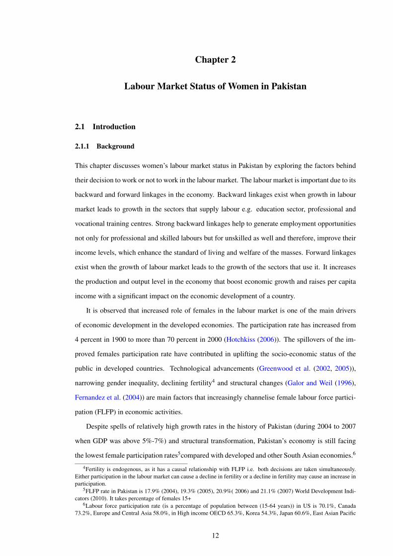
Therefore, there is a need for an in-depth analysis regarding the role of females in Pakistan’s labour
market.
Figure 2.1: Female Labour Force Participation.
Figure 2.1 highlights the fact that the female labour force participation rate, as a percentage
of the female population aged 15 and above, is only 22% which is the lowest level compared to
U.S, U.K Australia and other Asian countries. According to the Global Competitiveness Report
(2010), Pakistan ranked 137 out of 139 countries on females participation in the labour market.
Pakistan is the sixth most populated country in the world and ninth largest country in terms
of labour force. It has 180 million population with 2.05% growth rate and 54.92 million labour
force (out of which 42.44 million are males and 12.48 million are females) with a growth rate of
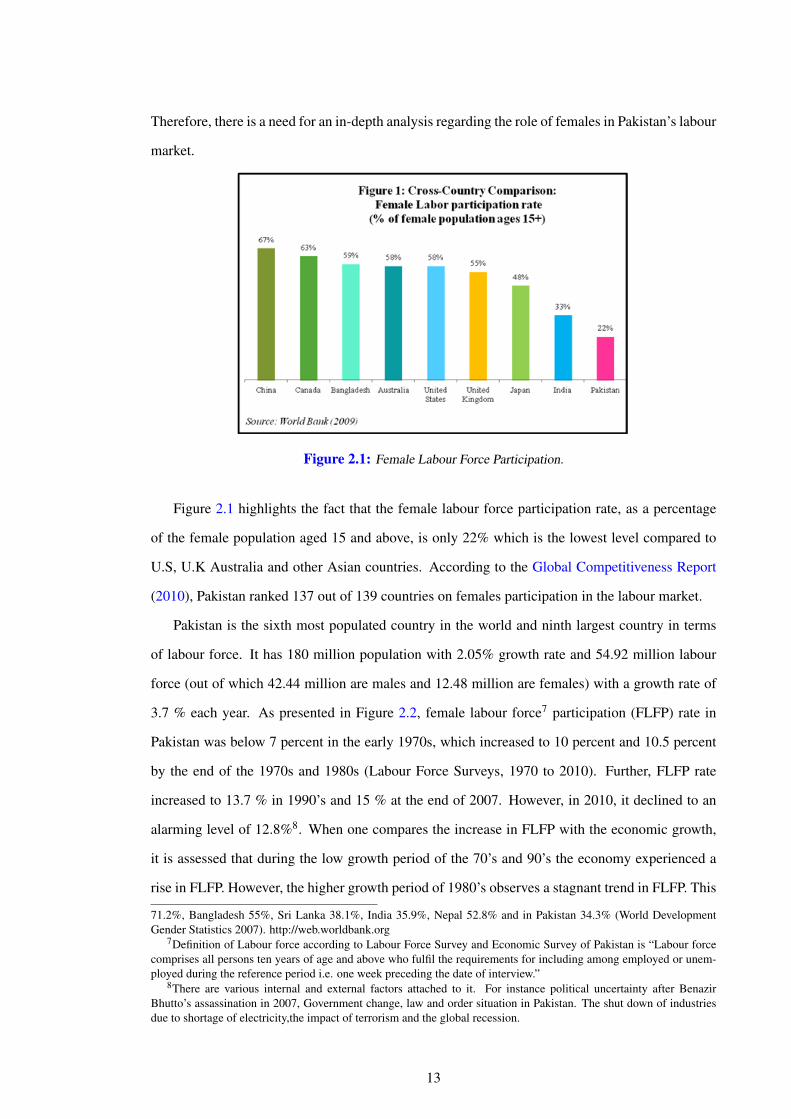
3.7 % each year. As presented in Figure 2.2, female labour force7 participation (FLFP) rate in
Pakistan was below 7 percent in the early 1970s, which increased to 10 percent and 10.5 percent
by the end of the 1970s and 1980s (Labour Force Surveys, 1970 to 2010). Further, FLFP rate
increased to 13.7 % in 1990’s and 15 % at the end of 2007. However, in 2010, it declined to an
alarming level of 12.8%8. When one compares the increase in FLFP with the economic growth,
it is assessed that during the low growth period of the 70’s and 90’s the economy experienced a
rise in FLFP. However, the higher growth period of 1980’s observes a stagnant trend in FLFP. This
71.2%, Bangladesh 55%, Sri Lanka 38.1%, India 35.9%, Nepal 52.8% and in Pakistan 34.3% (World DevelopmentGender Statistics 2007). http://web.worldbank.org
7Definition of Labour force according to Labour Force Survey and Economic Survey of Pakistan is “Labour forcecomprises all persons ten years of age and above who fulfil the requirements for including among employed or unem-ployed during the reference period i.e. one week preceding the date of interview.”
8There are various internal and external factors attached to it. For instance political uncertainty after BenazirBhutto’s assassination in 2007, Government change, law and order situation in Pakistan. The shut down of industriesdue to shortage of electricity,the impact of terrorism and the global recession.
13
can be explained by the persistent gender discrimination and a set of exacerbating factors such as
a conservative culture which typically lead to the main causes of lower FLFP in Pakistan (Ibraz
(1993)).
Figure 2.2: Trend of Women Labour Force.
Although female participation has shown a rising trend from the 1970’s to 2007, it needs to
be highlighted that two-thirds of the increase was attributed to unpaid family helpers while wage-
employment had not increased at a significant pace.
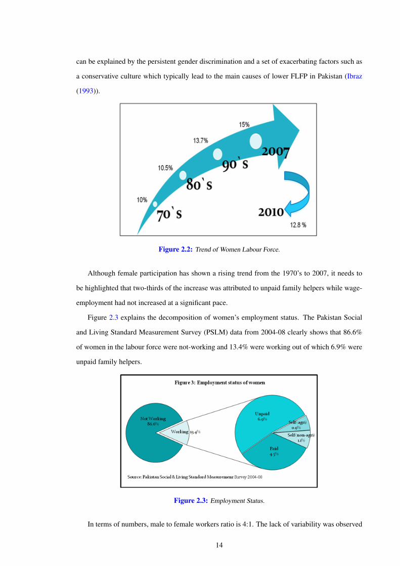
Figure 2.3 explains the decomposition of women’s employment status. The Pakistan Social
and Living Standard Measurement Survey (PSLM) data from 2004-08 clearly shows that 86.6%
of women in the labour force were not-working and 13.4% were working out of which 6.9% were
unpaid family helpers.
Figure 2.3: Employment Status.
In terms of numbers, male to female workers ratio is 4:1. The lack of variability was observed
14
in male employment, whereas large fluctuations were seen in the female employment. During
an economic era of buoyancy in the labour market, there was a rapid growth in employment of
women. However, when there was a recession, the economy observed a reduction and slow growth
in female’s employment, (SPDC (2008)).
The discussion about the female labour force is incomplete without highlighting the issues
in Pakistan’s labour market. The share of rural areas is almost double in the total employment.
Almost 74% of females are engaged in agriculture, mainly livestock. By and large, the proportion
of females in the formal sector is low and the transition from the informal sector (traditional
agricultural activities) to formal sector is not taking place. The fundamental problem is that the
connection between education and employment is not strong. Although females are entering into
higher education institutions, this does not guarantee subsequent participation in the labour market
which is a reflection of gender discrimination prevailing in the labour market. Another issue which
needs attention is, females participation is overstated by the inclusion of unpaid family helpers in
the labour force and underestimated by the exclusion of women employed in some marginalized
activities. According to the (SPDC (2008)),9 47% women are engaged in marginalized activities,
31% are unpaid family helpers and only 22% receive significant remuneration of their work.
Since the seminal paper of Mincer in 1965, female labour force participation has attracted
researchers over the last three decades. Explorative studies have taken into account the develop-
ments in the labour supply theory along with the application of econometric advancements. In
addition, Becker (1965) has incorporated a household production model along with female time
allocation, to the conventional labour supply theory. Later, Chiappori (1992) presents a collective
household model, which provided the theoretical foundations to the decision making process of
the household for females labour market participation. The empirical contributions by Gronau
(1973) and Heckman (1979) put emphasis on the appropriate estimation method. Most of the time
series studies are related to the researching developed economies and rising trend in the female
labour force participation during the last few decades. Cross sectional studies have utilized the
micro data in determining the probability of female labour force participation, whereas, panel data
studies have investigated the U-shaped relationship between FLFP and economic development.
Despite its great significance for developing economies, the issue of female labour force par-
ticipation has not received much attention from researchers in Pakistan, except for a few studies.
Therefore, there is a need to explore the determinants of female labour force participation with
9(SPDC (2008)), Annual Review Social Policy and Development Centre.
15
special focus on the status of working and not-working women. Research pertaining to Pakistan10
has only examined the socio-economic and demographic factors affecting the probability of female
participation and applied either binary “Probit” or “Logit” models using the cross section data, or
conducted their own survey concentrating on a specific city, district or province. Therefore, it is
expected that this study will contribute significantly to the economic literature by addressing the
gap in previous studies, particularly by highlighting women’s economic status. This is achieved
through utilizing a random sample of pooled data for the first time in Pakistan, and by considering
an appropriate estimation procedure, the “ Multinomial Logit Model. This data and methodol-
ogy has not been used so far in the empirical studies conducted in Pakistan, that consider the
multiple potential labour market status of females rather than a simple binary; participation/ non-
participation. Moreover, to get a comprehensive picture of labour market in Pakistan, the exercise
is also performed for males as well.
2.1.2 Research Question and Objective
What factors determine employment status of females in the labour market of Pakistan? The pre-
vious discussion leads to the following set of determinants of female labour force participation.
Females personal and the household characteristics play an important role in determining their
participation in the labour market. Female’s own characteristics include education endowment,
marital status, and age whereas, the household characteristics are indicated by house ownership,
co-residence (living with extended family), number of children, number of dependents in a house-
hold, and location (rural or urban). The financial condition of household is represented by the
number of working people in the family and the total household income, whereas, woman as head
of house signifies her position in the house.
The objective of the study is three-fold. First, to identify the socio-economic factors that de-
termine the employment status for males and females in Pakistan. Second, to explore individual’s
own and household characteristics that discourage or encourage them to participate in the labour
market and third, to compare working and not working women with men in the labour market.
Following the first section, the second section reviews the literature, highlighting the main
ideas, methods and findings of the relevant studies conducted at national and international level.
The data source and description of dependent and independent variables is provided in section
10Studies conducted in Pakistan such as Shah et al. (1976) and Shah (1986), Chishti et al. (1989), Ibraz (1993), Naqviet al. (2002), Hafeez and Ahmad (2002) and Ahmad and Hafeez (2007) Ejaz (2007) and Ejaz (2011), Faridi et al. (2009)and Faridi and Basit (2011), Azid et al. (2010) and Safana et al. (2011).
16
three. Section four describes the methodology with detailed discussion on the multinomial logit
model. Section five reports the empirical findings and results followed by conclusions.
2.2 Literature Review
The seminal contributions of Mincer (1962), Becker (1965), and Cain (1969) have introduced the
issues concerning females’ labour market participation. These pioneering works raised interest
among other researchers, who further analysed the female labour supply with different sets of
explanatory variables. The studies have applied various econometric techniques to cross section,
time series and panel data, which resulted in a vast literature on the theory of female labour supply.
Mincer (1962) interprets the static analysis of labour supply by including lifetime variables11
and proposes that number of children can have a significant effect on women’s lifetime labour
supply. Becker (1965) generalizes the role of time in employment and laid foundation for the
household production model. Since then, time has become a center of attention in decisions af-
fecting health, fertility and location. Gronau (1973) estimates the behavioural relations of market
wage and shadow wage and finds that education is an important factor to determine the market
wages. Heckman (1974) presents a seminal methodological contribution in the labour supply esti-
mation. This approach allows estimation of parameters which formulate the function determining
the probability to work for a woman, hours of working, observed wage rate and shadow wages 12.
McFadden (1974) develops the logit model which is used to analyse the discrete choice by
individuals among a limited number of alternatives.13 Theil (1969) develops the multinomial logit
model, benefited by important contributions from McFadden (1974) and Nerlove and Press (1973),
which proves to be useful for analysing occupational choice problems.
Earlier, the studies on FLFP (e.g., Mincer (1962); Heckman (1979); Hausman (1982); Moffitt
(1984)) focused on the impact of marriage. Later on, the role of childbearing and child rearing
is added in to the analysis (such as Cain (1969)) by developing a simultaneous equation model
of females labour supply, schooling, marriage, and fertility decisions (Heckman (1974); Schultz
(1994)).
11lifetime variables include consumption, leisure, house work, wages, time and budget constraints.12Marginal value placed on women’s leisure13This method utilizes not only observable facts about characteristics associated with individual and information
about each available alternative choice but also unobservable differences among individuals and alternatives which arerepresented by random error terms.
17
2.2.1 Determinants of women’s participation in the labour market
This section provides a review of the literature on global FLFP patterns with emphasis on the fac-
tors affecting women’s participation in the labour market namely, human capital, socio-economic
and demographic variables. This is then followed by the review of studies that have used Multi-
nomial logit model for the analysis of labour market status of women.
2.2.1.1 International Studies: Factors determining females employment are very complex.
Women’s decision to work is subject to the aspects such as their education level, skills, and job
availability at the individual level. On the other hand, FLFP rate is largely determined by factors
which are in one form or the other, indicative of social, economic, cultural and demographic
conditions of the society as a whole.
Cross sectional studies (Sweet (1973), Waite (1980)) show an inverted U shape relationship
between married women’s labour force participation and age (14-54 years). The effect of women’s
age on LFP behaviour appears to depend on number of the pre-school children. Smith-Lovin and
Tickamyer (1978) argue that vast majority of young married women intend to have children and
carry out these intentions during the early years of marriage consequently showing a relatively
lower rate of labour force participation. The participation rate keeps on increasing as women
complete their fertility and their children grow until it drops again at the age of about 55, therefore,
the impact of age on women work participation is likely to be curvilinear. Berndt (1996) identifies
that females’ labour force participation rate varies by age and has significantly increased across
all age groups over the last three decades. Mackellar and Bird (1997) indicate that “ageing” is
an important feature that is increasing the size of the labour force in the developing countries.
Nevertheless, the proportion remains constant for the middle aged group. In the population under-
15 age group the LFP is very low, whereas participation is substantial within 60-plus age group.
However, Sheehan and Standing (1978) show that for females age has relatively less significance
than education and other social and environmental factors, to participate in the labour market.
Lee et al. (2008) claim that marriage remains a main obstruction against young female’s em-
ployment in Korea. The findings demonstrate that an average married woman is 40- 60% less
likely to participate in the labour force compared to single woman in urban Korea. On the other
hand,Yakubu (2010) argues the point that a married woman is more likely to participate in labour
force compared to a female living with a partner, widows or those never married using quarterly
Labour Force Survey of Statistics 2008 data for South Africa. Berndt (1996) elaborates the frame-
18
work of neoclassical labour supply to encompass household in order to address the issues of the
discouraged worker hypothesis (the idea is that the employers sometimes discriminate against the
wives on the basis of the suspicion that they may quit the job when their husbands will find the
employment), and the male chauvinist model (where wives take their husbands’ income as exoge-
nous).
Education is a prime determinant of the labour market outcome according to the human capital
theories. The most popular hypothesis among human capital theory is based on the idea of oppor-
tunity cost. Since education is an investment, and given that, education and earning potential are
positively related, the opportunity cost of not-working gets higher with education. Consequently,
the incentive to seek employment, is raised (Finegan (1962). However, Sheehan and Standing
(1978) argue the mere fact that education improves women employment opportunities does not
mean that they will necessary or wish to be able to take advantage of those. There may be an
inverse relationship between women educational attainment and FLFP. Mundial (1995) posit the
view that, the decision not to participate in labour market is neither the reflection of the females
own choice, nor does it correspond to the concept of maximum utilisation of household resources.
In addition, the market wage does not take conscious knowledge of the social benefits of females
education and employment. This implies that discrimination in households and in the market car-
ries not only private costs for individuals and households, but social costs for society as well.
Addison and Demery (1993) observe that FLFP is low on average compared to males. It is due
to the fact that the opportunity cost of non-participation falls with lower offered wages. As a re-
sult, the unemployment rates are higher for females while the opportunity cost of job search is
relatively low and discrimination in hiring leads to lesser job-prospects for them.
Besides marital status and child-rearing, education is considered the most important deter-
minant of female labour supply amongst other socio-economic factors in empirical studies. The
vision behind this perspective is that education increases the opportunity cost of housework for
females by raising the potential for higher earnings and social status through labour market partic-
ipation. However, the effect cannot be generalised and it is hard to detect the impact at the aggre-
gate level (Bloom et al. (2009) ). It seems to be strong in countries with U shaped labour supply
curve. It is because of modernization that attitudes have changed, and the advancement in the
technology as well as economic developments have transformed the nature of jobs, offering new
positions that females can attain through higher education. At such levels, the educational oppor-
tunities and awareness contributes towards the reduction of fertility, which in turn has a significant
19
impact on female LFP. Spierings and Smits (2007), indicate that higher education is an important
factor in womens LFP in five Middle Eastern & North African countries (MENA-Egypt, Jordan,
Morocco, Syria and Tunisia). Tansel (2002) and Gunduz-Hocsgor and Smits (2008) conclude the
same for Turkey. Duryea et al. (2001) examine the FLFP in 18 countries of Latin America and the
Caribbean during the 1990s and demonstrate that the increase in the years of schooling accounts
for about 30 percent of the total increase in FLFP rates, whereas, the remaining 70 percent orig-
inate from other factors impacting upon an increased participation rates. The higher the level of
education, the greater is the likelihood of females to participate in the labour market.
The social norms and traditions with respect to female labour force participation can be over-
come by investing in education. Certainly, empirical studies conducted in the developing countries
strongly assert the theoretical prediction that education has a positive effect on the female labour
supply. However, the emphasis is on the main finding that higher education plays a crucial role.
Evans and Saraiva (1993), considering the socio-economic conditions to measure the impact on
women’s labour force participation in Brazil, find that labour force participation rises with the
years of schooling. However, the increase is largest at secondary level and above. Evidence from
Asian countries also intimate that higher education plays a key part in increasing females’ par-
ticipation. Cameron et al. (2001), explore a U-shaped relationship between female labour supply
and education in Indonesia, Korea, Philippine, Sri Lanka, and Thailand. Primary education has
either a negative or no influence on FLFP, whilst higher education has a positive association with
participation. Moreover, the tertiary education is positively related to the probability of women’s
employment for each of the five countries mentioned above. However, Benham (1974) does not
look at it so simply. In his view, there are multiple other factors for example, household income
besides education, which encourage women to participate in the labour market.
Demographic factors like household structure is also considered an important characteristic
that can effect the FLFP rate. Mackellar and Bird (1997) suggest that demography and labour
force participation are inter-connected and should therefore be considered jointly. Sasaki (2002)
studies the effect of family structure on FLFP in Australia and observes that co-residence with
one’s own parents or in laws has a positive and significant impact on the participation. This
suggests that sharing a residence or living with extended family allows married women to share
the household activities with other family members. Thus, providing an incentive to participate
in the labour market. However, it varies from country to country due to cultural and demographic
differences. Chun et al. (2007) refute the argument that co-residence with parents has a significant
20
positive effect on the labour supply of married females in Korea by using the Korean Labour and
Income Panel Survey (KLIPS) 2004.
Aslam et al. (2008) acknowledge that with the constraint of nuclear family14 the opportunity
cost of non participation in the labour force may be even lower for educated women with children
because an educated woman is probably better able to take care of the child in a vitally important
early education of her children than a less educated woman. He emphasizes that this is particularly
likely to be the case in the developing countries. Bradbury and Katz (2005) identify a decline in
female labour force participation during the 1990’s, specifically among the well educated married
women with children. They utilized the U.S Bureau of Labour Statistics (BLS) along with the
Current Population Survey (CPS) to analyse labour market involvement of women over the last
two decades. They found out that the unobserved and unpredictable factors are larger contributors
towards a decline in the participation of women. They further discussed that the possible explana-
tions of this outcome shift might be the shift in women’s preferences or social norms, worsening
of opportunities at workplace, or the availability of more than one source of income for a family.
Other factors “ especially the presence of children and elderly in the household, are often con-
sidered as key factors that shape individuals’ incentives and opportunities to seek employment. For
women in traditional societies, these factors are often found to act as impediments”(Esfahani and
Shajari (2012), p.3). The presence of children particularly those under six years of age constraint
married womens employment. A large body of economics research has been devoted to the issue
of childbearing and its effects on female labour force participation (see, e.g., Blau and Robins
(1988); Gronau (1977); Hotz and Miller (1993); Moffitt (1984); Nakamura and Nakamura (1981);
Schultz (1978)). Behrman and Wolfe (1984) argue that having children in the household has a
small effect on participation; schooling and experience rather have significant and large effects on
labour supply. Ettner (1995) based on 1986-1988 “Survey of Income and Program Participation”
panels, investigates the impact of care-giving to disabled elderly parents on female labour supply.
He recognises that females are more likely than males to be engaged in elder care.
For women, particularly wives and mothers, household characteristics are major considera-
tions in making decisions concerning work participation. Economic conditions are of particular
importance. Women may decide to work out of economic necessity; economic pressures, either
from low family income or from a discrepancy between life style aspirations, and available eco-
nomic resources to afford such aspirations (Oppenheimer (1982)). Numerous studies support the
14Family comprising of one couple with or without children living in household. It is a family which is not extendedor joint family.
21
income effect on labour supply behaviour. A negative impact of family income is found with
womens participation in the labour market (Cain (1969), Sweet (1973), Joseph (1983)). With the
rise in income, it becomes more affordable for families to observe conservative customs which in
turn, leads to the decline in FLFP rate. However, the trend may be reversed, if the development
in education and awareness can help change the social attitude towards gender in the long run
(Bahramitash and Esfahani (2011)).
The importance of culture in determining the female labour force participation cannot be de-
nied. In the recent literature, it has gained more attention in the empirical analysis as one strand
of a more general attempt to rigorously measure the relationship between culture and economic
phenomena (Fernandez et al. (2004)).
Dwyer and Coward (1992), examine that women are expected to perform a dual responsibility
as the head of household. One is, to provide income and other is, to make available the resources
required to meet the family needs. Some women are generally the principal caregivers at home, for
them it is extremely vulnerable to meet the demands of family and work at the same time. How-
ever, De Munoz (2007) believes that the women as heads of house are more likely to participate
in the labour market.
Finally, there are some other potential determinants mentioned in the literature as the potential
determinants of FLFP. Given the objectives, and limitations of the dataset, this study focuses
mainly on personal and household characteristics discussed in the data section in detail.
2.2.1.2 Multinomial Logit Model used in Literature: Many important aspects of household
behaviour involve choices among discrete alternatives. Therefore, it is observed that a Multinomial
logit (MNL) procedure is adopted in international literature when the dependent variable is a
choice variable with more than two options. The main advantage of this procedure is to evaluate
more than two decisions.
In the international literature, it has also been observed that the issues related to developed
economies are entirely different from that of developing countries. As depicted by studies related
to Australia and New Zealand. In those countries the problem is not that women have to choose
between working and leisure rather their choice lies among switching between the employment
states i.e. full time to part time employments. They tend to take such a decision due to the child
birth or child rearing activities. On the other hand, a woman belonging to under developed soci-
eties like Pakistan has to choose between states of employment given their cultural, demographic
22
and socio-economic constraints, specifically within the household and generally in the society.
Chzhen (2009) explores the effect of childbirth on the risks of downgrading (i.e. switching
from full-time employment to part-time) in thirteen European countries. It has been observed that
in Netherlands, Belgium, Austria and the UK, the part-time rates are relatively higher. Therefore,
women are more likely to switch to part-time jobs than to remain employed as full-time worker.
However, in case of Italy, despite lower part-time wages females are still moving to the part-
time work. Furthermore, the likelihood of moving from full-time job to unemployment becomes
higher with the increase in child birth in Ireland, Italy, the UK and Finland. Similarly, recent
childbirth increases the risk to switch to inactivity in Netherlands, France, Italy, Greece, Germany
and Austria. However, the results from Denmark and Spain contradict the point of view, if human
capital and workplace characteristics are controlled, for those full-time workers who gave birth in
year t, the probability to stay as full-time in the following year t+1 is high. Du and yuan Dong
(2010) examine the impact of labour force participation on childcare choices during the economic
transition in urban China. The Multinomial Logit model takes the options 0 mother does not work,
1 mother works but does not use non-parental care, 2 mother works and uses formal care relative to
option 3 that mother works and uses informal care suggesting that due to childcare reform, access
to informal caregivers became increasingly critical for women’s labour force participation.
The probability of being in full employment, part-time employment, unemployed or out of
labour force is observed by Du and yuan Dong (2010) and Winkelmann and Winkelmann (1997).
The factors namely age, marital status, education, unemployment rate and location are used as
explanatory variables in the MNL model. They sample of 150,000 Maori and non-Maori working-
age individuals is taken from the census of New-Zealand for the period of 1981, 1986 and 1991.
The findings support the viewpoint that the probability of full-employment increases and that of
unemployment decreases with the increase in qualifications. Moreover, the results highlight that
married men are more likely to be in full-time employment than non-married men.
De Munoz (2007) also estimates the determinants of FLFP for Venezuela using cross-section
data between 1995 and 1998. MNL regressions are performed on a sample of women 15-60 years
old and also for sub-samples of married women, single women and women heads of household
using individual, demographic, socioeconomic, and geographical characteristics to examine labour
market behaviour. There are three choices: whether to participate in the formal sector; the informal
sector or not to participate at all. The findings underlie important observations that a woman who
is a head of household is significantly more likely to participate in both the informal and formal
23
sectors. Age and marital status of women also has a significant positive impact on participating in
the employment activities. The marginal effects of education show that probability of participation
increases with greater educational attainment. By utilizing the labour force surveys of 2007 and
2010 for Swaziland on a sample of youth aged 20-29 years, the MNL model has been applied
among five groups of labour market status, (inactive, employed in an informal private sector,
formal private sector, public sector or is self-employed), where unemployment is the reference
status. The independent variables are age in years, gender, region and educational level. Brixiova
and Kangoye (2013) show that age has a positive relationship with the likelihood of being in the
private sector, public sector employment or self-employed, rather than being unemployed (base
category). Compared with men, females are more likely to be inactive than unemployed. Stephens
(2010) explores the factors affecting the labour market status of indigenous individuals in Australia
by utilising the 2002 “ National Aboriginal and Torres Strait Islander Social Survey (NATSISS)”.
The MNL regression analysis is used to model labour force status as a function of factors covering
the geographic, demographic, education, health, culture, crime and housing characteristics. Given
the significant variation across remote and non-remote areas, a particular attention is given to
the geographical areas. The study demonstrates the relevance of all the diversified factors in
determining labour force status among the Indigenous population. Also, it highlights the complex
array of key issues which are crucial in raising the employment.
The impact of education on female labour market participation is measured by Sackey (Sackey)
using Ghana living standards survey cross-section data for 1998-99, covering the sample of fe-
males aged 15 years and above. On the basis of MNL estimates, she proposes that female school-
ing matters in both rural and urban areas. Improvements in the human capital as well as productive
employment of females always impacts favourably on participation and a negatively on their fer-
tility.
A MNL approach has also been applied to investigate labour market status of female carers in
Australia. Gray and Edwards (2009) modelled the labour force states as employed, not employed
but wants to be in paid employment, and not in the labour force. They claim that major factors
associated with lower rates of employment for female carers are: low levels of education attain-
ment, poor health, caring for a child with disability and not having people outside the household
to provide support.
Neimann (2007) explores the impact of having a spouse on the labour force participation deci-
sion of older married individuals by using monthly observations from the German Socio-Economic
24
Panel (GSOEP). The analysis focuses on the relationship between the retirement decision and the
labour market status of the partner. Therefore, transition probabilities of a set of discrete labour
force states defined by the employment status of the two spouses are estimated by using multino-
mial logit models. He notices that the labour force status of the spouse effects the labour market
behaviour not only through its financial consequences but also through the possibilities to share
leisure time together.
Multinomial models of labour market exit are estimated for UK and Germany. Oswald (1999),
using panel data from the BHPS (1991 to 1997) and GSOEP data (1984 to 1997) takes the sample
of individuals in a status of work from the age of 50 to 68. The sample includes two possible
non-working states of labor force from Germany i.e. unemployed and retired, and three from
UK i.e. retired, unemployed and sick. In Germany, the development was mostly attributed to the
favourable conditions in the social security system. In UK, the increasing coverage of occupational
and private pensions seems to be responsible for the low labour force participation of older persons.
2.2.1.3 Pakistan Studies: A number of factors have been identified in the studies determining
the involvement of women in the labour market in Pakistan. Among these are traditional factors
such as age, education, marital status, etc. Shah et al. (1976) propose demographic and socio-
economic variables affecting women’s labour force participation decision in four provinces of
Pakistan. They indicate that work participation is inversely related to the child-women ratio and
nuclear family type, however, it is positively related to marital status, literacy rates and dependency
ratio. Later, Chishti et al. (1989) maintain their point of view by focusing on Karachi, the city
in Sindh province. Interestingly, based on a probit model, they observe that the presence of a
male figure in the household reduces the likelihood of female participation in the labour force.
However, the presence of other females in the house increases the probability that a woman will
work. Similarly, Hafeez and Ahmad (2002) explore socio-economic and demographic factors that
influence decision of educated married women by applying Probit and Logit model using the field
survey conducted in Mundi-Bahaudin district in the north of Punjab during 1998-99. In addition to
the standard explanatory variables, they suggest that the husband’s education, monthly household
income, financial assets and number of workers have a significant inverse relationship with female
participation in labour market.
Education has been found to affect the probability of female labour market participation pos-
itively. Apart from female’s own education and her husband’s education, Ahmad and Hafeez
25
(2007) focus on the parental education when analysing the earning functions of married women in
Mandi-Bahaudin district in Punjab in 2002. Contrarily, Faridi et al. (2009) challenge that parents‘
education turns out to be insignificant. They acknowledge a positive trend between education and
FLFP by using the data for 164 women aged (15-64) from the rural areas of district Bahawalpur in
the south of Punjab for the year 2007-08. However, using the same data set and same technique,
Faridi et al. (2009) supports that spouse education and female’s own education has a positive and
significant impact on female participation in labour market by increasing her employment oppor-
tunities. However, an argument is raised with the difference of opinion by Safana et al. (2011)
that the head of households education, primary and matric level education relates negatively with
women’s employment decision. However, women with higher level of education are more likely
to participate in economic activities. The findings are based on a logit model using Multiple In-
dicators Cluster Survey (MICS) data 2007-08 for Punjab. Ahmad and Hafeez (2007) claim that
distance from the city centre, net wealth, husband’s income and number of dependents are also the
important factors that affect women’s decision to participate.
Culture is also inextricably linked to labour force participation especially in case of Pakistan.
Shah (1986) claims that observance of veil has negative impact on women’s participation in eco-
nomic activities while interpreting changes in women’s role in labour force participation between
1951 to 1981. Kazi et al. (1988) gauge the changes overtime in the level and pattern of women’s
employment by utilizing Agricultural Census (1972 and 1980) and Labour Force Survey (1987-
88). They argue that women are in a disadvantaged position due to cultural restrictions, household
responsibilities and low levels of education and skills. That is why they have to undertake a di-
verse range of activities to meet their subsistence need and are increasingly relegated to casual,
low paid and unskilled jobs in the informal sector. Further, Ibraz (1993) contends that the women’s
role is considered unimportant in the villages. Above and beyond agriculture, women also make a
significant contribution towards caring of livestock which is important for village economy. But,
the dominant cultural notions undermine their productive role. His statistical analysis is based on
a 1989-90 survey, concentrated on Rajpur village in Rawalpindi district of Punjab province.
Another important dimension to the analysis is looking at the household related factors that
lead to female participation in economic activities. Naqvi et al. (2002) using cross-sectional data
from the Pakistan Integrated Household Survey PIHS (1998-99) confined to women aged 15-49,
point out that the employment status of head of household and presence of a male member in the
house have a positive effect. However, infants have an inverse effect on her decision to participate
26
in the labour market. Ejaz (2007) accounts for the determinants of female labour force partici-
pation in Pakistan by using a different cross-sectional data source of Pakistan Social and living
Standard Measurement survey (PSLM) 2004-05. She applies Probit and logit models utilising the
same set of control variables (such as age, education marital status, household income, infants,
family type, family size, working people in the house) with the addition of ownership of agri-
cultural land, weighted index of home appliances and access to vehicles. She finds that owning
agricultural land and having access to vehicles increases the females likelihood to participate in
economic activities, whereas availability of home appliances reduces the probability of her partic-
ipation. Besides other variables, Azid et al. (2010) remark that poverty, literacy, and number of
boys and girls (of school going age) are important household factors that influence female labour
force participation. Concentrating on women aged 16-60, he utilizes primary data from the survey
of 4000 households in the districts of Punjab in the year 2004-05.
Ejaz (2011) draws attention to the potential problem of endogeneity. Endogenous covariates
include fertility and ownership of home appliances. Moreover, to measure empowerment quan-
titatively, the variable gender wage gap is used as proxy variable for empowerment. Probit and
instrumental variable technique is used based on the PSLM 2006-07. The results suggest an in-
verse and significant relationship between female labour market participation and both fertility and
the gender-wage gap; whereas a direct and significant relationship between FLFP and ownership
of home appliances is found.
From the above mentioned literature review of studies conducted in Pakistan, it can be in-
ferred that various socio-economic, demographic and cultural factors that have profound effects
on women’s labour force participation have been taken into account in almost all the studies. The
factors important in determining the participation of women in different categories of the labour
market are identified as age, education, marital status, household headship, and income, number of
children, household type (co-residence) and location. However, the variables considered relevant
for determining FLFP in Pakistan are grouped as individual characteristics and household charac-
teristics in this study. It is felt that the most important discussion about the women’s employment
status and profile has been neglected in the previous studies. The literature relies on participating
and non participating women in labour force and does not provide an in-depth analysis about what
includes working and not-working groups. This chapter aims to provide a detailed analysis on the
various categories of work (such as paid, unpaid, self-employed) and not-work (such as ill, stu-
dent, housekeeper) for women in Pakistan. The chapter also highlights that the major proportion
27
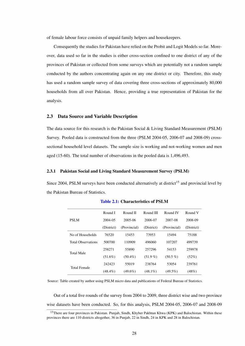
of female labour force consists of unpaid family helpers and housekeepers.
Consequently the studies for Pakistan have relied on the Probit and Logit Models so far. More-
over, data used so far in the studies is either cross-section confined to one district of any of the
provinces of Pakistan or collected from some surveys which are potentially not a random sample
conducted by the authors concentrating again on any one district or city. Therefore, this study
has used a random sample survey of data covering three cross-sections of approximately 80,000
households from all over Pakistan. Hence, providing a true representation of Pakistan for the
analysis.
2.3 Data Source and Variable Description
The data source for this research is the Pakistan Social & Living Standard Measurement (PSLM)
Survey. Pooled data is constructed from the three (PSLM 2004-05, 2006-07 and 2008-09) cross-
sectional household level datasets. The sample size is working and not-working women and men
aged (15-60). The total number of observations in the pooled data is 1,496,493.
2.3.1 Pakistan Social and Living Standard Measurement Survey (PSLM)
Since 2004, PSLM surveys have been conducted alternatively at district15 and provincial level by
the Pakistan Bureau of Statistics.
Table 2.1: Characteristics of PSLM
PSLM
Round I Round II Round III Round IV Round V
2004-05 2005-06 2006-07 2007-08 2008-09
(District) (Provincial) (District) (Provincial) (District)
No of Households 76520 15453 73953 15494 75188
Total Observations 500700 110909 496060 107207 499739
Total Male258271 55890 257296 54153 259978
(51.6%) (50.4%) (51.9 %) (50.5 %) (52%)
Total Female242423 55019 238764 53054 239761
(48.4%) (49.6%) (48.1%) (49.5%) (48%)
Source: Table created by author using PSLM micro data and publications of Federal Bureau of Statistics.
Out of a total five rounds of the survey from 2004 to 2009, three district wise and two province
wise datasets have been conducted. So, for this analysis, PSLM 2004-05, 2006-07 and 2008-09
15There are four provinces in Pakistan. Punjab, Sindh, Khyber Pakhtun Khwa (KPK) and Balochistan. Within theseprovinces there are 110 districts altogether, 36 in Punjab, 22 in Sindh, 24 in KPK and 28 in Balochistan.
28
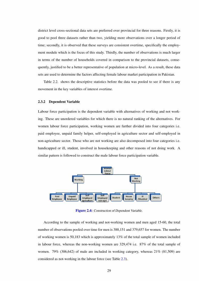
district level cross-sectional data sets are preferred over provincial for three reasons. Firstly, it is
good to pool three datasets rather than two, yielding more observations over a longer period of
time; secondly, it is observed that these surveys are consistent overtime, specifically the employ-
ment module which is the focus of this study. Thirdly, the number of observations is much larger
in terms of the number of households covered in comparison to the provincial datasets, conse-
quently, justified to be a better representative of population at micro-level. As a result, these data
sets are used to determine the factors affecting female labour market participation in Pakistan.
Table 2.2. shows the descriptive statistics before the data was pooled to see if there is any
movement in the key variables of interest overtime.
2.3.2 Dependent Variable
Labour force participation is the dependent variable with alternatives of working and not work-
ing. These are unordered variables for which there is no natural ranking of the alternatives. For
women labour force participation, working women are further divided into four categories i.e.
paid employee, unpaid family helper, self-employed in agriculture sector and self-employed in
non-agriculture sector. Those who are not working are also decomposed into four categories i.e.
handicapped or ill, student, involved in housekeeping and other reasons of not doing work. A
similar pattern is followed to construct the male labour force participation variable.
Figure 2.4: Construction of Dependent Variable.
According to the sample of working and not-working women and men aged 15-60, the total
number of observations pooled over time for men is 388,151 and 379,657 for women. The number
of working women is 50,183 which is approximately 13% of the total sample of women included
in labour force, whereas the non-working women are 329,474 i.e. 87% of the total sample of
women. 79% (306,642) of male are included in working category, whereas 21% (81,509) are
considered as not-working in the labour force (see Table 2.3).
29
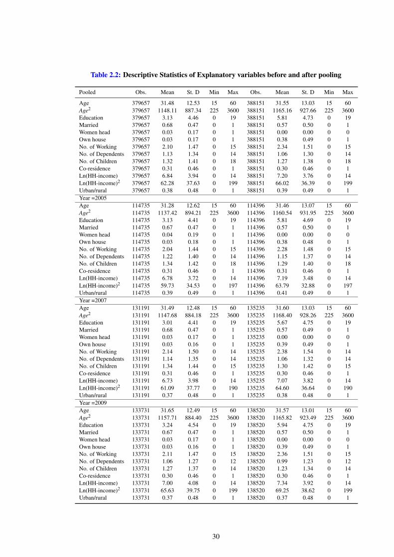
Table 2.2: Descriptive Statistics of Explanatory variables before and after pooling
Pooled Obs. Mean St. D Min Max Obs. Mean St. D Min Max
Age 379657 31.48 12.53 15 60 388151 31.55 13.03 15 60Age2 379657 1148.11 887.34 225 3600 388151 1165.16 927.66 225 3600Education 379657 3.13 4.46 0 19 388151 5.81 4.73 0 19Married 379657 0.68 0.47 0 1 388151 0.57 0.50 0 1Women head 379657 0.03 0.17 0 1 388151 0.00 0.00 0 0Own house 379657 0.03 0.17 0 1 388151 0.38 0.49 0 1No. of Working 379657 2.10 1.47 0 15 388151 2.34 1.51 0 15No. of Dependents 379657 1.13 1.34 0 14 388151 1.06 1.30 0 14No. of Children 379657 1.32 1.41 0 18 388151 1.27 1.38 0 18Co-residence 379657 0.31 0.46 0 1 388151 0.30 0.46 0 1Ln(HH-income) 379657 6.84 3.94 0 14 388151 7.20 3.76 0 14Ln(HH-income)2 379657 62.28 37.63 0 199 388151 66.02 36.39 0 199Urban/rural 379657 0.38 0.48 0 1 388151 0.39 0.49 0 1Year =2005Age 114735 31.28 12.62 15 60 114396 31.46 13.07 15 60Age2 114735 1137.42 894.21 225 3600 114396 1160.54 931.95 225 3600Education 114735 3.13 4.41 0 19 114396 5.81 4.69 0 19Married 114735 0.67 0.47 0 1 114396 0.57 0.50 0 1Women head 114735 0.04 0.19 0 1 114396 0.00 0.00 0 0Own house 114735 0.03 0.18 0 1 114396 0.38 0.48 0 1No. of Working 114735 2.04 1.44 0 15 114396 2.28 1.48 0 15No. of Dependents 114735 1.22 1.40 0 14 114396 1.15 1.37 0 14No. of Children 114735 1.34 1.42 0 18 114396 1.29 1.40 0 18Co-residence 114735 0.31 0.46 0 1 114396 0.31 0.46 0 1Ln(HH-income) 114735 6.78 3.72 0 14 114396 7.19 3.48 0 14Ln(HH-income)2 114735 59.73 34.53 0 197 114396 63.79 32.88 0 197Urban/rural 114735 0.39 0.49 0 1 114396 0.41 0.49 0 1Year =2007Age 131191 31.49 12.48 15 60 135235 31.60 13.03 15 60Age2 131191 1147.68 884.18 225 3600 135235 1168.40 928.26 225 3600Education 131191 3.01 4.41 0 19 135235 5.67 4.75 0 19Married 131191 0.68 0.47 0 1 135235 0.57 0.49 0 1Women head 131191 0.03 0.17 0 1 135235 0.00 0.00 0 0Own house 131191 0.03 0.16 0 1 135235 0.39 0.49 0 1No. of Working 131191 2.14 1.50 0 14 135235 2.38 1.54 0 14No. of Dependents 131191 1.14 1.35 0 14 135235 1.06 1.32 0 14No. of Children 131191 1.34 1.44 0 15 135235 1.30 1.42 0 15Co-residence 131191 0.31 0.46 0 1 135235 0.30 0.46 0 1Ln(HH-income) 131191 6.73 3.98 0 14 135235 7.07 3.82 0 14Ln(HH-income)2 131191 61.09 37.77 0 190 135235 64.60 36.64 0 190Urban/rural 131191 0.37 0.48 0 1 135235 0.38 0.48 0 1Year =2009Age 133731 31.65 12.49 15 60 138520 31.57 13.01 15 60Age2 133731 1157.71 884.40 225 3600 138520 1165.82 923.49 225 3600Education 133731 3.24 4.54 0 19 138520 5.94 4.75 0 19Married 133731 0.67 0.47 0 1 138520 0.57 0.50 0 1Women head 133731 0.03 0.17 0 1 138520 0.00 0.00 0 0Own house 133731 0.03 0.16 0 1 138520 0.39 0.49 0 1No. of Working 133731 2.11 1.47 0 15 138520 2.36 1.51 0 15No. of Dependents 133731 1.06 1.27 0 12 138520 0.99 1.23 0 12No. of Children 133731 1.27 1.37 0 14 138520 1.23 1.34 0 14Co-residence 133731 0.30 0.46 0 1 138520 0.30 0.46 0 1Ln(HH-income) 133731 7.00 4.08 0 14 138520 7.34 3.92 0 14Ln(HH-income)2 133731 65.63 39.75 0 199 138520 69.25 38.62 0 199Urban/rural 133731 0.37 0.48 0 1 138520 0.37 0.48 0 1
30
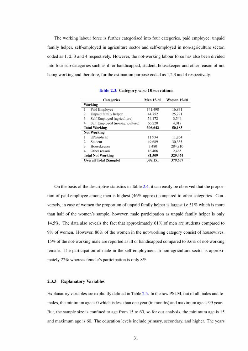
The working labour force is further categorised into four categories, paid employee, unpaid
family helper, self-employed in agriculture sector and self-employed in non-agriculture sector,
coded as 1, 2, 3 and 4 respectively. However, the not-working labour force has also been divided
into four sub-categories such as ill or handicapped, student, housekeeper and other reason of not
being working and therefore, for the estimation purpose coded as 1,2,3 and 4 respectively.
Table 2.3: Category wise Observations
Categories Men 15-60 Women 15-60Working1 Paid Employee 141,498 16,8312 Unpaid family helper 44,752 25,7913 Self Employed (agriculture) 54,172 3,5444 Self Employed (non-agriculture) 66,220 4,017Total Working 306,642 50,183Not Working1 ill/handicap 11,934 11,8642 Student 49,689 30,3353 Housekeeper 3,480 284,8104 Other reason 16,406 2,465Total Not Working 81,509 329,474Overall Total (Sample) 388,151 379,657
On the basis of the descriptive statistics in Table 2.4, it can easily be observed that the propor-
tion of paid employee among men is highest (46% approx) compared to other categories. Con-
versely, in case of women the proportion of unpaid family helper is largest i.e 51% which is more
than half of the women’s sample, however, male participation as unpaid family helper is only
14.5%. The data also reveals the fact that approximately 61% of men are students compared to
9% of women. However, 86% of the women in the not-working category consist of housewives.
15% of the not-working male are reported as ill or handicapped compared to 3.6% of not-working
female. The participation of male in the self employment in non-agriculture sector is approxi-
mately 22% whereas female’s participation is only 8%.
2.3.3 Explanatory Variables
Explanatory variables are explicitly defined in Table 2.5. In the raw PSLM, out of all males and fe-
males, the minimum age is 0 which is less than one year (in months) and maximum age is 99 years.
But, the sample size is confined to age from 15 to 60, so for our analysis, the minimum age is 15
and maximum age is 60. The education levels include primary, secondary, and higher. The years
31
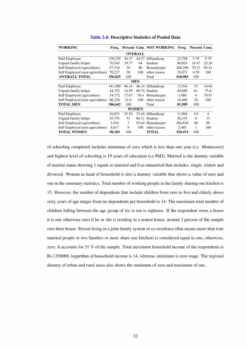
Table 2.4: Descriptive Statistics of Pooled Data
WORKING Freq. Percent Cum. NOT WORKING Freq. Percent Cum.
OVERALLPaid Employee 158,329 44.37 44.37 ill/handicap 23,798 5.79 5.79Unpaid family helper 70,543 19.77 64 Student 80,024 19.47 25.26Self Employed (agriculture) 57,716 16 80 Housekeeper 288,290 70.15 95.41Self Employed (non-agriculture) 70,237 20 100 other reason 18,871 4.59 100OVERALL TOTAL 356,825 100 Total 410,983 100
MENPaid Employee 141,498 46.14 46.14 ill/handicap 11,934 15 14.64Unpaid family helper 44,752 14.59 60.74 Student 49,689 61 75.6Self Employed (agriculture) 54,172 17.67 78.4 Housekeeper 3,480 4 79.87Self Employed (non-agriculture) 66,220 21.6 100 other reason 16,406 20 100TOTAL MEN 306,642 100 Total 81,509 100
WOMENPaid Employee 16,831 33.54 31.44 ill/handicap 11,864 3.6 4Unpaid family helper 25,791 51 86.11 Student 30,335 9 13Self Employed (agriculture) 3,544 7 92.64 Housekeeper 284,810 86 99Self Employed (non-agriculture) 4,017 8 100 other reason 2,465 1 100TOTAL WOMEN 50,183 100 TOTAL 329,474 100
of schooling completed includes minimum of zero which is less than one year (i.e. Montessori)
and highest level of schooling is 19 years of education (i.e PhD). Married is the dummy variable
of marital status showing 1 equals to married and 0 as unmarried that includes, single, widow and
divorced. Woman as head of household is also a dummy variable that shows a value of zero and
one in the summary statistics. Total number of working people in the family sharing one kitchen is
15. However, the number of dependents that include children from zero to five and elderly above
sixty years of age ranges from no dependents per household to 14. The maximum total number of
children falling between the age group of six to ten is eighteen. If the respondent owns a house
it is one otherwise zero if he or she is residing in a rented house, around 3 percent of the sample
own their house. Person living in a joint family system or co-residence (that means more than four
married people or two families or more share one kitchen) is considered equal to one, otherwise,
zero. It accounts for 31 % of the sample. Total maximum household income of the respondents is
Rs.1350000, logarithm of household income is 14, whereas, minimum is zero wage. The regional
dummy of urban and rural areas also shows the minimum of zero and maximum of one.
32
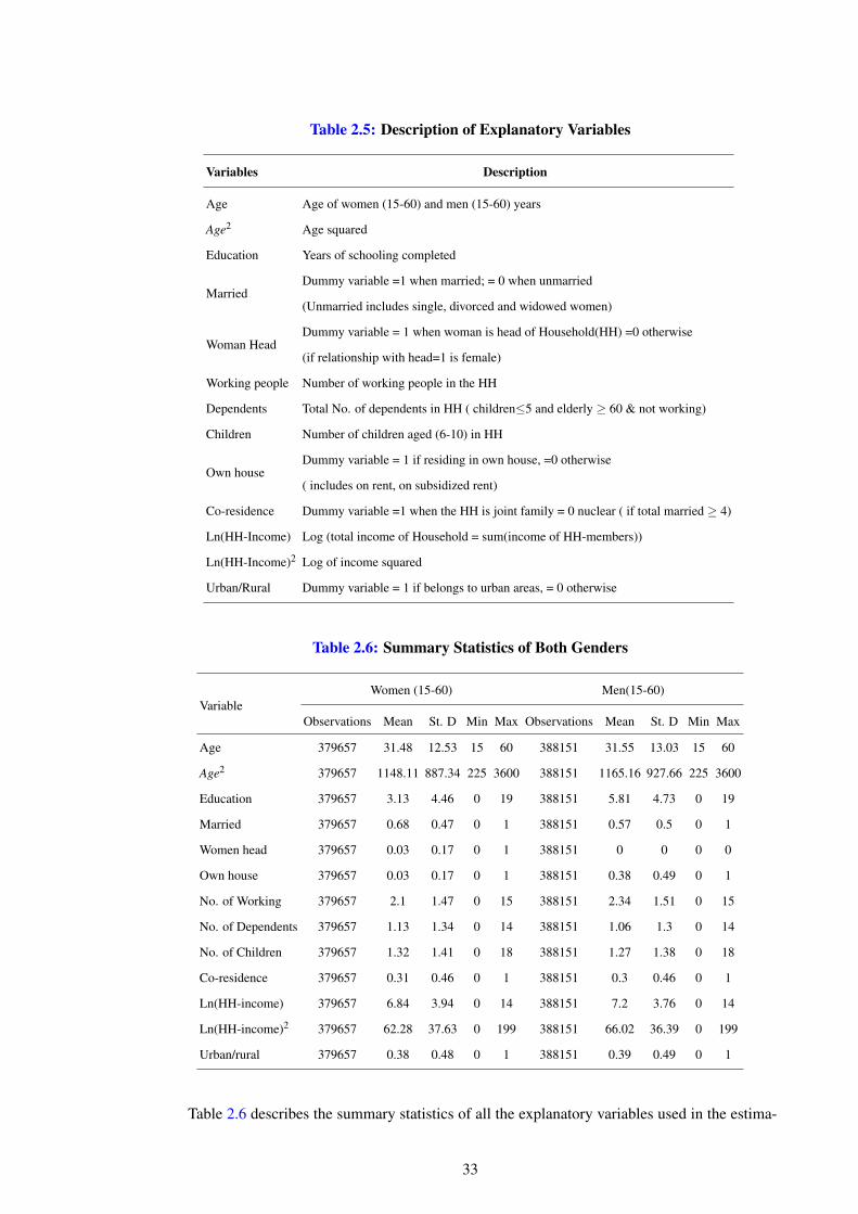
Table 2.5: Description of Explanatory Variables
Variables Description
Age Age of women (15-60) and men (15-60) years
Age2 Age squared
Education Years of schooling completed
MarriedDummy variable =1 when married; = 0 when unmarried
(Unmarried includes single, divorced and widowed women)
Woman HeadDummy variable = 1 when woman is head of Household(HH) =0 otherwise
(if relationship with head=1 is female)
Working people Number of working people in the HH
Dependents Total No. of dependents in HH ( children≤5 and elderly ≥ 60 & not working)
Children Number of children aged (6-10) in HH
Own houseDummy variable = 1 if residing in own house, =0 otherwise
( includes on rent, on subsidized rent)
Co-residence Dummy variable =1 when the HH is joint family = 0 nuclear ( if total married ≥ 4)
Ln(HH-Income) Log (total income of Household = sum(income of HH-members))
Ln(HH-Income)2 Log of income squared
Urban/Rural Dummy variable = 1 if belongs to urban areas, = 0 otherwise
Table 2.6: Summary Statistics of Both Genders
VariableWomen (15-60) Men(15-60)
Observations Mean St. D Min Max Observations Mean St. D Min Max
Age 379657 31.48 12.53 15 60 388151 31.55 13.03 15 60
Age2 379657 1148.11 887.34 225 3600 388151 1165.16 927.66 225 3600
Education 379657 3.13 4.46 0 19 388151 5.81 4.73 0 19
Married 379657 0.68 0.47 0 1 388151 0.57 0.5 0 1
Women head 379657 0.03 0.17 0 1 388151 0 0 0 0
Own house 379657 0.03 0.17 0 1 388151 0.38 0.49 0 1
No. of Working 379657 2.1 1.47 0 15 388151 2.34 1.51 0 15
No. of Dependents 379657 1.13 1.34 0 14 388151 1.06 1.3 0 14
No. of Children 379657 1.32 1.41 0 18 388151 1.27 1.38 0 18
Co-residence 379657 0.31 0.46 0 1 388151 0.3 0.46 0 1
Ln(HH-income) 379657 6.84 3.94 0 14 388151 7.2 3.76 0 14
Ln(HH-income)2 379657 62.28 37.63 0 199 388151 66.02 36.39 0 199
Urban/rural 379657 0.38 0.48 0 1 388151 0.39 0.49 0 1
Table 2.6 describes the summary statistics of all the explanatory variables used in the estima-
33
tion procedure in detail. The variables clearly reflect the stylized facts of Pakistan data. Table 2.6
compares the explanatory variables used in the estimation of both male and female equations. The
number of observations for men is 388,151 and women 379,657.
2.4 Methodology
Consider qualitative response models where the dependent variable is a discrete rather than a
continuous variable. There are two types of discrete variables ordered and unordered where the
latter is the focus of this analysis. Unordered variables are the variables for which there is no
natural ranking of the alternatives.
2.4.1 Unordered Multiple Choice Models
The extension of logit model for binary outcomes to the cases where the unordered response has
more than two outcomes. The examples of the unordered multinomial responses are occupational
choices, or choice of the modes of transportation for commuting purpose etc. Unordered choice
models can be motivated by a random utility model.
From the group of choices, each individual chooses only one alternative. In each case, an
individual chooses one alternative from the group of choices. The choices are labelled arbitrarily.
Define y as a random variable that takes the values {0,1... j} where, j a positive integer, and x is
denoted as a set of explanatory variables. For instance, if y denotes employment choice, x includes
characteristics like, age, gender, marital status, education etc. Usually, (xi,yi) is randomly drawn
from the population (Wooldridge (2010)). Imagine a group of individuals i = 1,2, ,n faced with
j = 1,2, , j choices, then utility, conditional on a set of characteristics xi j is written as:
yi j = x′i jβ + ei j (2.1)
If the individual makes choice j then one assumes that yi j is the maximum among the j options.
So one can derive a statistical model which is driven by the probability that choice j is made:
The dependent variable (labour force status) in this analysis is not continuous, so, ordinary
least squares regression is not appropriate to apply in this situation. It is necessary to use a tech-
nique suitable for a dependent variable with four possible values. Therefore, a Multinomial logit
model is preferred because of the four possible outcomes which are categorical rather than ordinal.
34
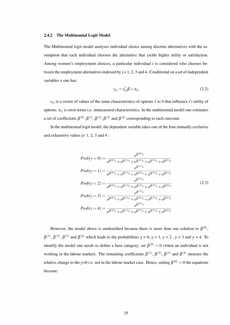
2.4.2 The Multinomial Logit Model
The Multinomial logit model analyses individual choice among discrete alternatives with the as-
sumption that each individual chooses the alternative that yields higher utility or satisfaction.
Among women’s employment choices, a particular individual i is considered who chooses be-
tween the employment alternatives indexed by j = 1, 2, 3 and 4. Conditional on a set of independent
variables x one has:
yi j = x′i jβ + εi j (2.2)
xi j is a vector of values of the same characteristics of options 1 to 4 that influence i′s utility of
options. εi j is error terms i.e. unmeasured characteristics. In the multinomial model one estimates
a set of coefficients β (0),β (1),β (2),β (3) and β (4) corresponding to each outcome.
In the multinomial logit model, the dependent variable takes one of the four mutually exclusive
and exhaustive values j= 1, 2, 3 and 4 :
Prob(y = 0) =eβ (0)′x
eβ (0)′x + eβ (1)′x + eβ (2)′x + eβ (3)′x + eβ (4)′x
Prob(y = 1) =eβ (1)′x
eβ (0)′x + eβ (1)′x + eβ (2)′x + eβ (3)′x + eβ (4)′x
Prob(y = 2) =eβ (2)′x
eβ (0)′x + eβ (1)′x + eβ (2)′x + eβ (3)′x + eβ (4)′x
Prob(y = 3) =eβ (3)′x
eβ (0)′x + eβ (1)′x + eβ (2)′x + eβ (3)′x + eβ (4)′x
Prob(y = 4) =eβ (4)′x
eβ (0)′x + eβ (1)′x + eβ (2)′x + eβ (3)′x + eβ (4)′x
(2.3)
However, the model above is unidentified because there is more than one solution to β (0),
β (1), β (2), β (3) and β (4) which leads to the probabilities y = 0, y = 1, y = 2 , y = 3 and y = 4. To
identify the model one needs to define a base category; set β (0) = 0 (when an individual is not
working in the labour market). The remaining coefficients β (1), β (2), β (3) and β (4) measure the
relative change to the y=0 i.e. not in the labour market case. Hence, setting β (0) = 0 the equations
become:
35
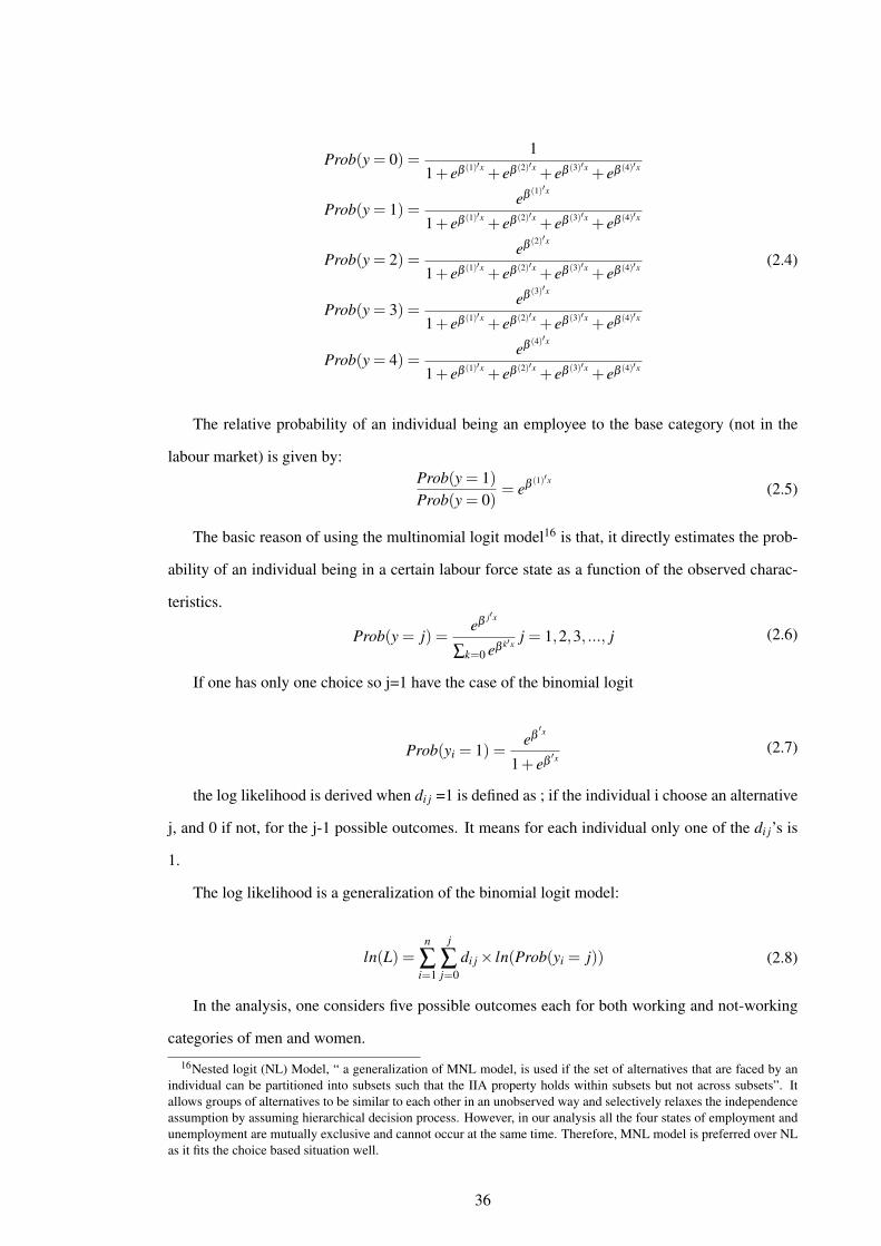
Prob(y = 0) =1
1+ eβ (1)′x+ eβ (2)′x
+ eβ (3)′x+ eβ (4)′x
Prob(y = 1) =eβ (1)′x
1+ eβ (1)′x+ eβ (2)′x
+ eβ (3)′x+ eβ (4)′x
Prob(y = 2) =eβ (2)′x
1+ eβ (1)′x+ eβ (2)′x
+ eβ (3)′x+ eβ (4)′x
Prob(y = 3) =eβ (3)′x
1+ eβ (1)′x+ eβ (2)′x
+ eβ (3)′x+ eβ (4)′x
Prob(y = 4) =eβ (4)′x
1+ eβ (1)′x+ eβ (2)′x
+ eβ (3)′x+ eβ (4)′x
(2.4)
The relative probability of an individual being an employee to the base category (not in the
labour market) is given by:Prob(y = 1)Prob(y = 0)
= eβ (1)′x(2.5)
The basic reason of using the multinomial logit model16 is that, it directly estimates the prob-
ability of an individual being in a certain labour force state as a function of the observed charac-
teristics.
Prob(y = j) =eβ j′x
∑k=0 eβ k′x j = 1,2,3, ..., j (2.6)
If one has only one choice so j=1 have the case of the binomial logit
Prob(yi = 1) =eβ′x
1+ eβ′x
(2.7)
the log likelihood is derived when di j =1 is defined as ; if the individual i choose an alternative
j, and 0 if not, for the j-1 possible outcomes. It means for each individual only one of the di j’s is
1.
The log likelihood is a generalization of the binomial logit model:
ln(L) =n
∑i=1
j
∑j=0
di j× ln(Prob(yi = j)) (2.8)
In the analysis, one considers five possible outcomes each for both working and not-working
categories of men and women.
16Nested logit (NL) Model, “ a generalization of MNL model, is used if the set of alternatives that are faced by anindividual can be partitioned into subsets such that the IIA property holds within subsets but not across subsets”. Itallows groups of alternatives to be similar to each other in an unobserved way and selectively relaxes the independenceassumption by assuming hierarchical decision process. However, in our analysis all the four states of employment andunemployment are mutually exclusive and cannot occur at the same time. Therefore, MNL model is preferred over NLas it fits the choice based situation well.
36
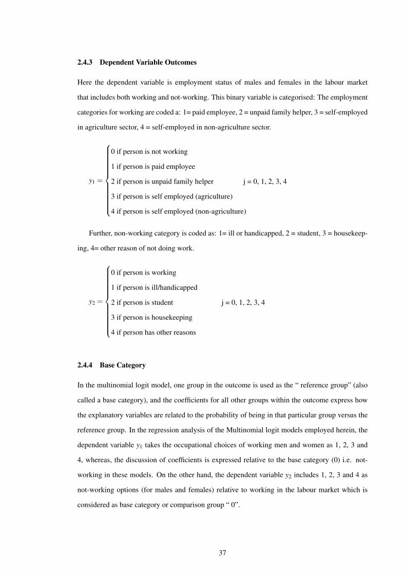
2.4.3 Dependent Variable Outcomes
Here the dependent variable is employment status of males and females in the labour market
that includes both working and not-working. This binary variable is categorised: The employment
categories for working are coded a: 1= paid employee, 2 = unpaid family helper, 3 = self-employed
in agriculture sector, 4 = self-employed in non-agriculture sector.
y1 =
0 if person is not working
1 if person is paid employee
2 if person is unpaid family helper j = 0, 1, 2, 3, 4
3 if person is self employed (agriculture)
4 if person is self employed (non-agriculture)
Further, non-working category is coded as: 1= ill or handicapped, 2 = student, 3 = housekeep-
ing, 4= other reason of not doing work.
y2 =
0 if person is working
1 if person is ill/handicapped
2 if person is student j = 0, 1, 2, 3, 4
3 if person is housekeeping
4 if person has other reasons
2.4.4 Base Category
In the multinomial logit model, one group in the outcome is used as the “ reference group” (also
called a base category), and the coefficients for all other groups within the outcome express how
the explanatory variables are related to the probability of being in that particular group versus the
reference group. In the regression analysis of the Multinomial logit models employed herein, the
dependent variable y1 takes the occupational choices of working men and women as 1, 2, 3 and
4, whereas, the discussion of coefficients is expressed relative to the base category (0) i.e. not-
working in these models. On the other hand, the dependent variable y2 includes 1, 2, 3 and 4 as
not-working options (for males and females) relative to working in the labour market which is
considered as base category or comparison group “ 0”.
37
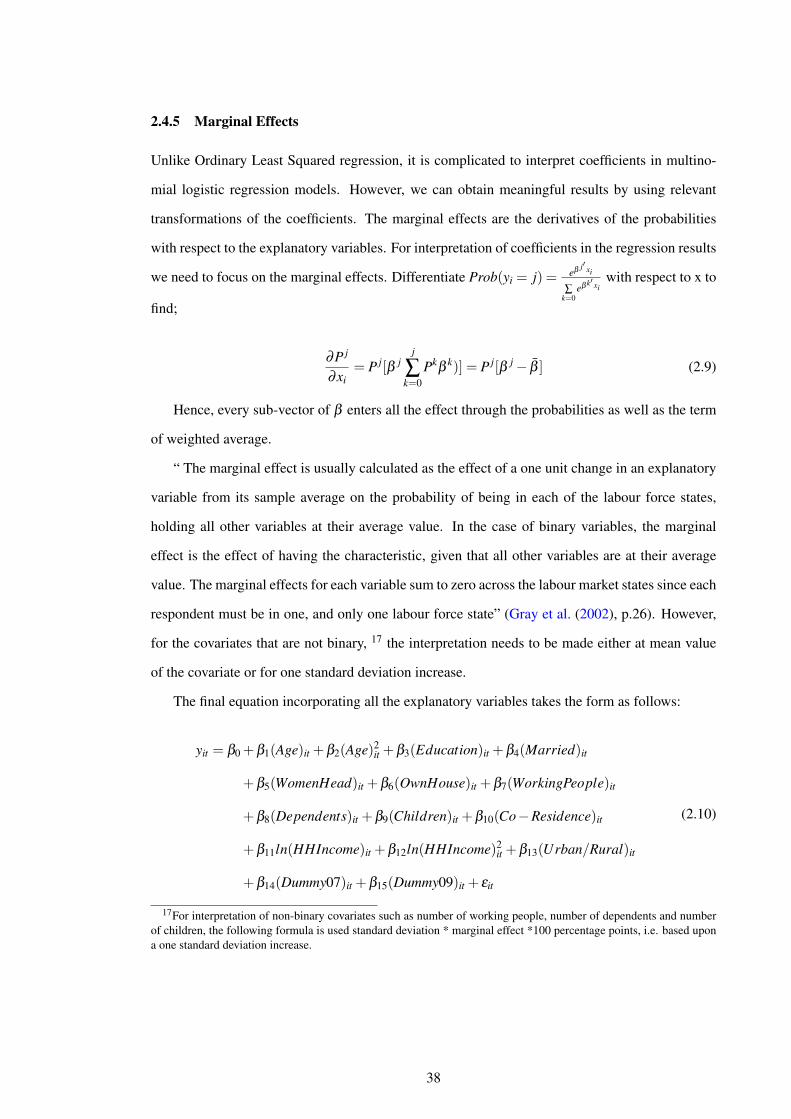
2.4.5 Marginal Effects
Unlike Ordinary Least Squared regression, it is complicated to interpret coefficients in multino-
mial logistic regression models. However, we can obtain meaningful results by using relevant
transformations of the coefficients. The marginal effects are the derivatives of the probabilities
with respect to the explanatory variables. For interpretation of coefficients in the regression results
we need to focus on the marginal effects. Differentiate Prob(yi = j) = eβ j′ xi
∑k=0
eβk′ xiwith respect to x to
find;
∂P j
∂xi= P j[β j
j
∑k=0
Pkβ
k)] = P j[β j− β ] (2.9)
Hence, every sub-vector of β enters all the effect through the probabilities as well as the term
of weighted average.
“ The marginal effect is usually calculated as the effect of a one unit change in an explanatory
variable from its sample average on the probability of being in each of the labour force states,
holding all other variables at their average value. In the case of binary variables, the marginal
effect is the effect of having the characteristic, given that all other variables are at their average
value. The marginal effects for each variable sum to zero across the labour market states since each
respondent must be in one, and only one labour force state” (Gray et al. (2002), p.26). However,
for the covariates that are not binary, 17 the interpretation needs to be made either at mean value
of the covariate or for one standard deviation increase.
The final equation incorporating all the explanatory variables takes the form as follows:
yit = β0 +β1(Age)it +β2(Age)2it +β3(Education)it +β4(Married)it
+β5(WomenHead)it +β6(OwnHouse)it +β7(WorkingPeople)it
+β8(Dependents)it +β9(Children)it +β10(Co−Residence)it
+β11ln(HHIncome)it +β12ln(HHIncome)2it +β13(Urban/Rural)it
+β14(Dummy07)it +β15(Dummy09)it + εit
(2.10)
17For interpretation of non-binary covariates such as number of working people, number of dependents and numberof children, the following formula is used standard deviation * marginal effect *100 percentage points, i.e. based upona one standard deviation increase.
38
2.5 Results and Empirical Findings
This section discusses the estimation results of the determinants of women’s labour force partici-
pation in Pakistan. Marginal effects have been computed and reported throughout.
The results showing gender differences in employment outcomes and inactivity are based on
four multinomial logit models given in Table 2.7 and Table 2.8.
Model 1: takes working women as the dependent variable and not-working as base category
Model 2: considers not-working women as the dependent variable and working as base category
Model 3: takes working men as the dependent variable and not-working as base category
Model 4: considers not-working men as the dependent variable and working as base category
There exists a consensus among researchers on the belief that the decision to participate in
the economic activities is based on a combination of individuals personal as well as household
characteristics. It is also an established concept that a number of supply side and demand side
factors contribute to the decision making process.
Following literature so far, the set of explanatory variables is grouped into two categories:
personal characteristics (quadratic term of age, education, marital status, and head of house) and
household characteristics (number of children, dependents and working people in the household,
household income and its squared term, ownership of house and co-residence). These variables
remain the same in all models except the female-headed household, an indicator which is omitted
from the male’s equations. In addition, dummies of urban-rural, year 2007 and 2009 are also in-
cluded. It is found that most of the results are consistent with the theories reported in the literature
pertaining to labour force participation.
2.5.1 Model 1 and 3: Gender differences in Employment Outcomes
For the interpretation of results, the marginal effects for participation in different categories of
working in the labour market were computed. The results are presented in Table 2.7. This sec-
tion highlights the main gender differences in all the employment outcomes. For both males and
females the mean value of age is 31.5 (see Table 2.6). The results show that an additional year
of age from its mean increases their probability to participate in all the categories of employment
with the exception of males for the category of unpaid family helpers. However, their magnitudes
are different and the probability of being in paid employment for men is highest (5.69 percentage
points (pp)) relative to not-working. The reason to include age squared is to gauge a non-linear
relationship between age and the probability of being in any particular labour force state.
39
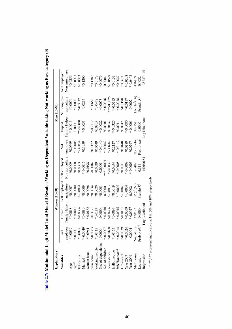
Tabl
e2.
7:M
ultin
omia
lLog
itM
odel
1an
dM
odel
3R
esul
ts;W
orki
ngas
Dep
ende
ntVa
riab
leta
king
Not
-wor
king
asB
ase
cate
gory
(0)
Exp
lana
tory
Wom
en(1
5-60
)M
en(1
5-60
)
Vari
able
sPa
idU
npai
dSe
lfem
ploy
edSe
lfem
ploy
edPa
idU
npai
dSe
lfem
ploy
edSe
lfem
ploy
edem
ploy
eeFa
mily
Hel
per
agri
cultu
reN
onag
ricu
lture
empl
oyee
Fam
ilyH
elpe
rag
ricu
lture
Non
agri
cultu
reA
ge*0
.003
9*0
.001
8*0
.000
7*0
.000
9*0
.056
9*-
0.00
13*0
.007
0*0
.025
6A
ge2
*-0.
0001
*0.0
000
*0.0
000
*0.0
000
*-0.
0008
0.00
00*0
.000
0*-
0.00
03E
duca
tion
*0.0
022
*-0.
0006
*-0.
0001
*0.0
003
*-0.
0034
**-0
.000
1*-
0.00
32*-
0.00
63M
arri
ed*-
0.00
49*0
.008
0*0
.000
9*-
0.00
16*0
.195
9*-
0.00
51*0
.021
5*0
.120
0w
omen
head
*0.0
961
*-0.
0182
*0.0
096
*0.0
198
own
hous
e*-
0.00
630.
0312
*0.0
034
-0.0
004
*0.1
122
*-0.
2112
*0.0
669
*0.1
389
wor
king
peop
le*0
.011
7*0
.018
4*0
.002
0*0
.002
9*0
.064
9*0
.020
5*0
.047
8*0
.017
3N
o.of
depe
nden
ts0.
0000
0.00
00*0
.000
10.
0000
*-0.
0149
*-0.
0022
*0.0
073
*0.0
079
No.
ofch
ildre
n*-
0.00
07*-
0.00
100.
0000
***-
0.00
01*-
0.00
47*0
.001
0*-
0.00
160.
0004
co-r
esid
ence
*-0.
0168
*-0.
0206
*-0.
0037
*-0.
0039
*-0.
1682
*0.0
196
***-
0.00
25*-
0.06
29ln
HH
inco
me
*0.0
177
*0.0
094
*0.0
019
*0.0
054
*0.2
127
*-0.
0325
*-0.
0213
*0.0
133
lnH
Hin
com
e2*-
0.00
14*-
0.00
15*-
0.00
02*-
0.00
05*-
0.01
12*0
.001
1*-
0.00
38*0
.002
7U
rban
-rur
al*-
0.00
39*-
0.01
51*-
0.00
46*0
.001
1*0
.014
8*0
.004
2*-
0.11
98*0
.067
1Y
ear2
007
*-0.
0024
*-0.
0059
*-0.
0007
*-0.
0009
*0.0
289
*-0.
0080
*-0.
0117
*-0.
0208
Yea
r200
9-0
.000
4*-
0.00
270.
0002
*-0.
0005
*0.0
297
*-0.
0001
0.00
02*-
0.04
08M
ultin
omia
lN
o.of
obs.
3796
57L
Rχ
2 (60)
1264
89N
o.of
obs.
3881
51L
Rch
i2 (56)
4761
59L
ogis
ticPr
ob>
chi2
0.00
00Ps
eudo
R2
0.31
1Pr
ob>
chi2
0.00
00Ps
eudo
R2
0.40
32R
egre
ssio
nL
ogL
ikel
ihoo
d-1
4010
6.81
Log
Lik
elih
ood
-352
374.
15
*,**
,***
repr
esen
tsig
nific
ance
at1%
,5%
and
10%
resp
ectiv
ely.
40
It was observed that with the increase in the quadratic term of age, the probability for the men
and women to be in the paid employment was lower (0.08 pp and 0.01 pp respectively) relative
to not in the labour market. Although the quadratic term of age had a significant positive impact
on determining the probabilities for men and women, the magnitudes remained very low. Results
are consistent with literature refering to by studies ((Brixiova and Kangoye (2013), Ejaz (2011),
De Munoz (2007), Naqvi et al. (2002)) wherein women’s age has a positive and significant effect
on the probability of being active in the labour market.
It is found that education has a positive effect on the probability of being a part of the labour
market (Safana et al. (2011), Hafeez and Ahmad (2002), Winkelmann and Winkelmann (1997),
Behrman and Wolfe (1984)). According to the current reseach data 63% of women and 33%
of men are illiterate in the sample that leads to lower mean value of almost 3 and 6 years of
education for women and men respectively. It was found that an additional year of education
from the mean values increased the probability for women to be in paid employment (0.22pp) and
self employment in non agriculture sector (0.03 pp). For men, an additional year of schooling
decreased the probability to be in any category of employment relative to not working.
For married women, the probability of being in the paid employment was lower than the
unmarried women at 0.49 pp as opposed to men who had a higher probability with a very high
magnitude of 19.59 pp relative to those not in the labour market. Our sample includes 68% of the
married women. Therefore, according to the results it can be stated that the majority of females are
more likely to work as unpaid family helpers (0.80 pp) or to be self employed in agriculture sector
(0.09 pp). These results are consistent with the literature (Lee et al. (2008), Becker (1965)Yakubu
(2010), Ejaz (2007), Bradbury and Katz (2005), Naqvi et al. (2002)) that shows a negative effect
of marriage on the labour force participation of females. However, married men had (0.51 pp
lower probability of being an unpaid family helper. As per the culture of Pakistan, marriage
brings greater financial responsibility for men, which is clearly depicted in the results for paid
employment.
In the sample, 75% of women had 2 or more children. The results indicate and support the
stylized fact that the majority of women join unpaid jobs and work in the agriculture sector relative
to not work (Bradbury and Katz (2005)). This study considers children between six to ten years of
age as a potentially important determinant of women’s labour force participation. A one standard
deviation increase in the number of children in the household decreased the probability of being
41
in paid employment by 0.10 pp18 and even for unpaid family helper (with children in school going
age) the probability of participation was low relative to not being in the labour market. The finding
supports the studies articulating that the number of children are inversely related to female’s labour
market participation (Bradbury and Katz (2005), Naqvi et al. (2002), Duleep and Sanders (1994).
On the other hand for men, the likelihood of being involved in unpaid family help increases by
0.05 pp but for paid employment the probability was low relative to not working.
For women, a one standard deviation increase in the number of dependents in the household,
the probability of being in all the categories of working shows a negligible effect relative to not
being in the labour market. It was observed that the magnitudes of the marginal effects of all
the categories of employment (paid, unpaid, self-employment) are statistically insignificant. The
literature suggests women are more likely to be engaged in elderly care than men (Behrman and
Wolfe (1984)) whereas Faridi et al. (2009), Faridi and Basit (2011) contradict the finding and
explain the inverse relationship. Interestingly, for men a one standard deviation increase in the
number of dependents19 in the household decreases the probability of being in paid employment
by 1.93 pp and for unpaid family helper by 0.28 pp relative to not working in the labour market.
Co-residence (living in joint family with in-laws or parents) is based on mutual understanding
of two or more families so that each family shares some responsibilities. The data indicates almost
30% of the men and women in the sample as living in joint families and the results indicate
lower probability for both the genders to be in any of the categories of employment relative to not
working. The exception was males residing in joint family had higher probability to be unpaid
family helper (1.96 pp). Living together with parents or in laws has a significant but negative
effect on the labour supply which is consistent with the results of other studies related to Pakistan
(Kazi and Raza (1990), Ejaz (2007), Naqvi et al. (2002).
Household’s monthly income is also another important factor that influences the labour market
participation decision of women. The estimated results suggest that the logarithm of household in-
come has a positive and significant correlation with female labour force participation. This simply
implies that an increase in household income (log-level) is associated with higher probability of
females’s employment. However, the increase in its quadratic term indicates the backward bending
supply curve; where the leisure becomes expensive (i.e. opportunity cost of leisure become high)
resulting in lower probability for females to participate in any state of employment. The marginal
18This number is calculated by taking product of standard deviation (SD)* marginal effect (ME) *100 percentagepoints i.e. 1.41*0.0007*100 = 0.10pp (0.0987 is rounded up to two decimal points).
19In our analysis the dependents consist of all the infants (less than 5) and elderly (60 and above) members of thehousehold.
42
effects of log of household income suggest that a 1% increase in household income increases the
likelihood for female being in each labour market state but at a decreasing rate relative to not
being in the labour market. Contrarily in case of males, as household income increases by 1%,
the likelihood that men are self-employed (agriculture) decreases to 3.25 pp and unpaid family
helpers one reduced to 2.13 pp but at increasing rate of 0.11pp and 0.38 pp respectively. However,
the probability of being in paid employment increases by a very high magnitude of 21.27 pp but at
decreasing rate of 1.12 pp relative to not working. These results are consistent with (Ejaz (2011),
Bahramitash and Esfahani (2011)) which shows that family income has positive and significant
association with womens participation in the labour market however, (Hafeez and Ahmad (2002),
Oppenheimer (1982) Cain (1969), Sweet (1973), Joseph (1983)) have displayed different results.
Women’s ownership of a house exerts 0.63 pp lower probability of being in paid employment
and 0.04 pp lower probability of being in self-employment related to non-agriculture sector, rela-
tive to not being in the labour market whereas the likelihood of being unpaid family helper remains
higher by 3.12 pp and self employed in agriculture by 0.34 pp. The reason might be that she be-
longs to agricultural household where her main responsibility is to look after the farms, crops
and cattle to help the family in income generating activities. On the other hand, if a man owns a
house there exist higher probability of being in paid and self-employment (agricultural and non-
agricultural) with higher magnitudes of marginal effects (11.22 pp, 6.69 pp 13.89 pp respectively).
However, owning a house had 21.12 pp less probability of being an unpaid family helper.
An increase in the number of working of people in the household increases the likelihood of
employment for both the genders. The results suggested that based on one standard deviation
increase in number of working people in the household, for women the probability of being in
paid employment, unpaid family help, self employment (agriculture and non-agriculture sector)
increases by 1.71, 2.70, 0.29 and 0.42 pp, respectively, relative to not being in the labour market.
Similarly, in the case of men, based on one standard deviation increase in number of working
people in the household the probability of being in all the categories of working, increases by 9.8,
3.09, 7.21 and 2.61 pp respectively, relative to not working in the labour market. By having more
working people in the household men get encouraged to work. The results support Ejaz (2007)
and Naqvi et al. (2002).
The probability of working in all the categories of employment except unpaid family helper
was higher for women as head of the house. It shows that women as head of house are unwill-
ing to work as unpaid family helper without any monetary reward. Some married women such
43
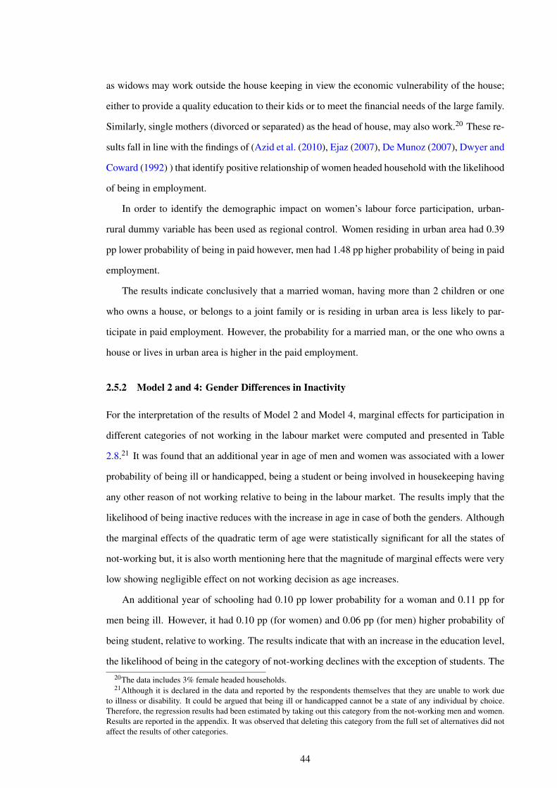
as widows may work outside the house keeping in view the economic vulnerability of the house;
either to provide a quality education to their kids or to meet the financial needs of the large family.
Similarly, single mothers (divorced or separated) as the head of house, may also work.20 These re-
sults fall in line with the findings of (Azid et al. (2010), Ejaz (2007), De Munoz (2007), Dwyer and
Coward (1992) ) that identify positive relationship of women headed household with the likelihood
of being in employment.
In order to identify the demographic impact on women’s labour force participation, urban-
rural dummy variable has been used as regional control. Women residing in urban area had 0.39
pp lower probability of being in paid however, men had 1.48 pp higher probability of being in paid
employment.
The results indicate conclusively that a married woman, having more than 2 children or one
who owns a house, or belongs to a joint family or is residing in urban area is less likely to par-
ticipate in paid employment. However, the probability for a married man, or the one who owns a
house or lives in urban area is higher in the paid employment.
2.5.2 Model 2 and 4: Gender Differences in Inactivity
For the interpretation of the results of Model 2 and Model 4, marginal effects for participation in
different categories of not working in the labour market were computed and presented in Table
2.8.21 It was found that an additional year in age of men and women was associated with a lower
probability of being ill or handicapped, being a student or being involved in housekeeping having
any other reason of not working relative to being in the labour market. The results imply that the
likelihood of being inactive reduces with the increase in age in case of both the genders. Although
the marginal effects of the quadratic term of age were statistically significant for all the states of
not-working but, it is also worth mentioning here that the magnitude of marginal effects were very
low showing negligible effect on not working decision as age increases.
An additional year of schooling had 0.10 pp lower probability for a woman and 0.11 pp for
men being ill. However, it had 0.10 pp (for women) and 0.06 pp (for men) higher probability of
being student, relative to working. The results indicate that with an increase in the education level,
the likelihood of being in the category of not-working declines with the exception of students. The20The data includes 3% female headed households.21Although it is declared in the data and reported by the respondents themselves that they are unable to work due
to illness or disability. It could be argued that being ill or handicapped cannot be a state of any individual by choice.Therefore, the regression results had been estimated by taking out this category from the not-working men and women.Results are reported in the appendix. It was observed that deleting this category from the full set of alternatives did notaffect the results of other categories.
44
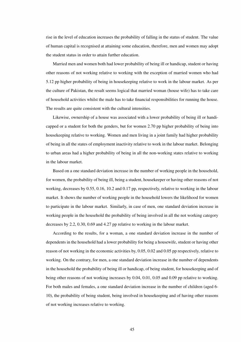
rise in the level of education increases the probability of falling in the status of student. The value
of human capital is recognised at attaining some education, therefore, men and women may adopt
the student status in order to attain further education.
Married men and women both had lower probability of being ill or handicap, student or having
other reasons of not working relative to working with the exception of married women who had
5.12 pp higher probability of being in housekeeping relative to work in the labour market. As per
the culture of Pakistan, the result seems logical that married woman (house wife) has to take care
of household activities whilst the male has to take financial responsibilities for running the house.
The results are quite consistent with the cultural intensities.
Likewise, ownership of a house was associated with a lower probability of being ill or handi-
capped or a student for both the genders, but for women 2.70 pp higher probability of being into
housekeeping relative to working. Women and men living in a joint family had higher probability
of being in all the states of employment inactivity relative to work in the labour market. Belonging
to urban areas had a higher probability of being in all the non-working states relative to working
in the labour market.
Based on a one standard deviation increase in the number of working people in the household,
for women, the probability of being ill, being a student, housekeeper or having other reasons of not
working, decreases by 0.55, 0.16, 10.2 and 0.17 pp, respectively, relative to working in the labour
market. It shows the number of working people in the household lowers the likelihood for women
to participate in the labour market. Similarly, in case of men, one standard deviation increase in
working people in the household the probability of being involved in all the not working category
decreases by 2.2, 0.30, 0.69 and 4.27 pp relative to working in the labour market.
According to the results, for a woman, a one standard deviation increase in the number of
dependents in the household had a lower probability for being a housewife, student or having other
reason of not working in the economic activities by, 0.05, 0.02 and 0.05 pp respectively, relative to
working. On the contrary, for men, a one standard deviation increase in the number of dependents
in the household the probability of being ill or handicap, of being student, for housekeeping and of
being other reasons of not working increases by 0.04, 0.01, 0.05 and 0.09 pp relative to working.
For both males and females, a one standard deviation increase in the number of children (aged 6-
10), the probability of being student, being involved in housekeeping and of having other reasons
of not working increases relative to working.
45
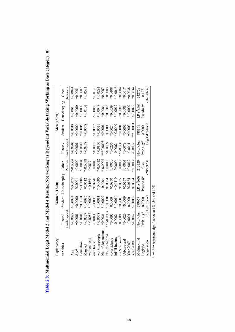
Tabl
e2.
8:M
ultin
omia
lLog
itM
odel
2an
dM
odel
4R
esul
ts;N
otw
orki
ngas
Dep
ende
ntVa
riab
leta
king
Wor
king
asB
ase
cate
gory
(0)
Exp
lana
tory
Wom
en(1
5-60
)M
en(1
5-60
)
vari
able
sIl
lnes
s/St
uden
tH
ouse
keep
ing
Oth
erIl
lnes
s/
Stud
ent
Hou
seke
epin
gO
ther
hand
icap
ped
Rea
sons
hand
icap
ped
Rea
sons
Age
*-0.
0027
*-0.
0024
*-0.
0078
*-0.
0004
*-0.
0040
*-0.
0018
*-0.
0015
*-0.
0044
Age
2*0
.000
1*0
.000
0*0
.000
1*0
.000
0*0
.000
1*0
.000
0*0
.000
0*0
.000
1E
duca
tion
*-0.
0010
*0.0
010
*-0.
0088
*0.0
004
*-0.
0011
*0.0
006
*-0.
0002
*0.0
007
Mar
ried
*-0.
0277
*-0.
0086
*0.0
512
*-0.
0098
*-0.
0358
*-0.
0058
*-0.
0102
*-0.
0531
wom
enhe
ad*-
0.00
82*-
0.00
28*-
0.16
440.
0017
own
hous
e-0
.001
4-0
.000
8*0
.027
00.
0001
*-0.
0085
*-0.
0032
*-0.
0080
*-0.
0170
wor
king
peop
le*-
0.00
38*-
0.00
11*-
0.06
96*-
0.00
12*-
0.01
50*-
0.00
21*-
0.00
47*-
0.02
91N
o.of
depe
nden
ts*0
.002
1*-
0.00
02-0
.000
4*-
0.00
04**
*0.0
003
*0.0
001
*0.0
004
*0.0
007
No.
ofch
ildre
n**
*-0.
0003
**0.
0001
*0.0
034
0.00
00*-
0.00
090.
0000
*0.0
002
*0.0
003
co-r
esid
ence
*0.0
093
0.00
00*0
.085
0*0
.002
0*0
.023
6*0
.002
4*0
.005
9*0
.040
8ln
HH
inco
me
0.00
02*-
0.00
10*-
0.04
190.
0000
0.00
02*-
0.00
09*-
0.00
17*-
0.00
46ln
HH
inco
me2
0.00
00*0
.000
1*0
.005
50.
0000
***-
0.00
01*0
.000
1*0
.000
2*0
.000
4U
rban
-rur
al*0
.002
6*0
.000
9*0
.026
7*0
.000
7*0
.007
9*0
.000
3*0
.000
8*0
.001
7Y
ear2
007
-0.0
001
0.00
00*0
.018
4*0
.001
2-0
.000
4*0
.000
3*-
0.00
09*0
.003
8Y
ear2
009
*-0.
0026
*-0.
0002
*0.0
084
**0.
0006
-0.0
007
***0
.000
1*-
0.00
28*0
.003
4M
ultin
omia
lN
oof
obs.
3796
57L
Rχ
2 (60)
2132
29N
oof
obs.
3881
51L
Rχ
2 (56)
2427
58L
ogis
ticPr
ob>
χ2
0.00
00Ps
eudo
R2
0.34
Prob>
χ2
0.00
00Ps
eudo
R2
0.42
7R
egre
ssio
nL
ogL
ikel
ihoo
d-2
0699
2.49
Log
Lik
elih
ood
-162
906.
48
*,**
,***
repr
esen
tsig
nific
ance
at1%
,5%
and
10%
46
The effect is almost negligible for a male student and a woman having an other reason of not
working. However, the probability of being ill or handicapped is lowering by 0.05 pp for women,
and 0.11 pp for men, relative to work in the labour market.
A 1% increase in household income increases the likelihood for female being ill or handi-
capped by 0.02 pp but at decreasing rate of 0.00 pp which means it does not make any difference.
On the other hand, a 1% increase in the household income, increases the probability of being ill
or handicapped by 0.02 pp for males but at decreasing rate of 0.01 pp relative to working in the
labour market. However with 1% increase in household income the likelihood of men and women
as student decreases by 0.09 pp and 0.10 pp but at increasing rate of 0.01 pp. Similarly, the prob-
ability of being in housekeeping decreases by 0.17 and 4.19 pp but at increasing rate of 0.02 and
0.55pp, relative to work in the labour market.
Women as head of house have a 0.82 pp lower probability of being ill or handicap 0.28 pp
lower probability of being student, 16.44 pp lower of being in housekeeping, and 0.17 pp higher
probability of being in other reasons of not working relative to working. These results sound
consistent with the theory that woman as a head of household will adopt paid employment and
will not fall in the category of not-working except for other reasons.
Previous studies both national and international have demonstrated a wide array of relevant
factors that determine labour force status of females in the labour market. Following them, this
study used those explanatory variables and found similar results.
2.5.3 Multinomial Logit Model Results with 8 alternatives of Working and Not-working
states as an Outcome Variable
The results for the MNL regression model including all the eight alternatives of work and not-work
in the dependent variable is presented in the Appendix A. The dependent variable is labour market
status (LMS) that takes the values 1,2....8 i.e. paid, self employed in agriculture, self employed in
non agriculture, unpaid, ill, student, housekeeper and other inactive individuals. Paid employee is
taken as a base category. Two separate regression for males and females aged 15-60 are reported
in Table A14 and Table A13. The explanatory variables include quadratic term of age, education,
marital status, women headed household (HH), ownership of the house, working people in the HH,
number of dependents and number of children in the HH, co-residence, household income along
with its squared term, urban dummy, time dummies, interaction of year 2007 and 2009 with edu-
cation and income to capture the overtime effect of education and household income on the labour
47
market participation of an individual. As the interpretation of MNL model is not straight forward
therefore, marginal effects have been computed. According to Table A13 for females, the results
for the quadratic term of age for all the states remains unchanged compared to the previous results
in Table 2.7 and Table 2.8. The results for education remain the same for all the states. With an
additional year of schooling from the mean value the probability for the females to work as unpaid
family helpers and self employed in agriculture sector relative to the paid employees. The results
for marital status remain unchanged for all the alternatives. However, the results are insignificant
for unpaid family helpers. Similarly, the output for the women headed household stays the same
for all the categories except for self employed in agriculture sector. There exists a lower proba-
bility for a woman being self employed in agriculture if she is the head of house relative to paid
employee. The ownership of house differ in the signs with the previous results for self employed
in non-agriculture sector, unpaid family helpers, housekeepers and other inactive. There exists a
lower probability for being in any state of inactivity vice versa for the employment states relative
to paid employment if the female own the house. Also the results for working people in the family
remain unchanged i.e. higher probability for being in any working state and lower for being in any
inactive state relative to paid employment. Previously, the dependents had a negligible effect on
the working states, but now it has positive association with probability of being self employed in
non-agriculture and negative associated with the self employed in agriculture and unpaid family
helpers. However, for the inactive states the results remain the same i.e. a one standard deviation
change in the number of dependents lowers probability for being a student, housekeeper or any
other reason of inactivity relative to paid employment. The more the number of children of school
going age, the higher is the probability of being in self employment non-agriculture and unpaid
work relative to paid work. The results are opposite to the regression results of working states
shown in Table 2.7 and Table 2.8 but unchanged for not-working states. Living with the parents or
in-laws or in a joint family lowers the likelihood of participating in any alternative states except for
an ill person relative to the paid employee. These results are consistent with the previous with the
exception of student which was positively associated with the co-residence. If the household in-
come increases by 1%, the probability of being in self employed in agriculture and non agriculture
sector, unpaid family helpers and ill may increase but at decreasing rate. However, the likelihood
of being a student, housekeeper or other reason of inactivity decreases at an increasing rate. These
results are also in line with the findings of the Table 2.7 and Table 2.8. Residing in an urban area
may reduce the probability of being self employed in agriculture as well as non-agriculture sector
48
whereas; the probability is higher for all the other alternatives relative to paid employment. The
results are the same compared to previous regression except for self employed in non-agriculture
and unpaid. The year dummies for 2007 and 2009 shows the reduction in the probability of being
in any working states relative to 2005 and paid employment while, the probability of being in
the states of inactivity is higher in 2007 an 2009 in comparison to 2005. The interaction terms
of education with year 2007 and 2009 indicates that the probability of participation of females in
the labour market has increased overtime with an increase in the education in almost all the states
except for housekeepers and ill relative to paid employment. The interaction terms of household
income with year 2007 and 2009 shows that after 2005, with an increase in income the probability
of participation in the working states of employment has been increasing overtime whereas, the
likelihood of participation in the inactive sates is reduced over the years.
In the case of males, the results have not changed much for the not working alternatives for
almost all the explanatory variables. An additional year in age of males is associated with lower
probability of being in all the working and not working states of employment except for unpaid
family helpers relative to the paid employment. An increase in the year of schooling is associated
with the higher probability of being in the state of self employment in agri and non-agri, student or
other inactive states. Marital status has a positive association with the probability of being in all the
alternative states except for unpaid relative to paid employment. Ownership of the house results
in lowering the probability of taking part in any state except unpaid relative to paid employment.
The working people in the household is associated with higher probability of participation in the
working states whereas lower probability of being in the not-working states. The results are similar
to the Table 2.7 and Table 2.8. A one standard deviation increase in the number of dependents
reduces the probability of for males to participate in self employment but raises the probability
of participation in all the other categories relative to paid employment. For males, a one standard
deviation increase in the number of children aged 6 to 10 raises the likelihood of taking part in
all the states except for being ill. Similarly, there exists a higher probability for males living in a
joint family to take part in all the alternative states of employment and unemployment except for
unpaid family help relative to paid work. The increase in the household income is associated with
the decrease in the probability of participation in all the states of activity and inactivity but at an
increasing rate. The results for inactive states were the same in the previous regression. Residing
in urban areas is associated with a higher probability of being in all the states of employment. The
time dummies for 2007 and 2009 show that the probability of participation all the alternative states
49
has increased over time after 2005 except for unpaid. The interaction terms of education with year
07 and 09 shows that participation of males in the labour market has increased over time with an
increase in education. However, unpaid and ill category has shown lower participation after 2005
relative to paid employment. Interaction terms of household income with time dummies indicate
that an increase in income overtime is associated with the fall in participation in all the states of
employment with the exception of unpaid relative to paid work.
2.5.4 Multinomial Logit Model Results for Working Males with Paid employment as base
category and Not-working Males with Housekeepers as base Category
The MNL results for working males by taking out the paid employment as a base category are
reported in the Table A16 (see Appendix A). The omitted category is selected on the basis of largest
category of the employment states. Out of total employed individuals, 42% are paid workers.
The marginal effects of all the states of employment have been computed for the interpretation
of the results. The probability of being engaged in the unpaid family help or self employment
in agriculture sector decreases at an increasing rate with an increase in the age relative to the
paid work. For males, there exist a lower probability of being involved in self employment with
an additional year of schooling relative to paid work. The more people working in the house,
the higher will be the probability of being involved in unpaid family help and self employment
in the agriculture sector but lower is the probability for self employed in non-agriculture sector
relative to paid employment. A one standard deviation increase in the number of working people
in the household increases the probability of participation in the unpaid family work and self
employment in agriculture relative to paid work. Also a one standard deviation increase in the
number of dependents in the household which include infants and elderly people, the probability of
being engaged in unpaid work gets low while self employment becomes high relative to paid work.
A one standard deviation increase in the number of children in the household is associated with
the higher probability of participation in all the states of working relative to paid work. Similarly,
residing with a joint family or extended family increases the likelihood for the males to be involved
in unpaid work and self employment relative to paid work. An increase in the household income is
associated with the lower probability of being participating in all the working states of employment
relative to paid employment. Living in an urban area is associated with a lower probability of being
involved in self employment in agriculture sector and higher probability of being engaged in the
self employment in non-agriculture sector and unpaid family work relative to paid work. The year
50
dummies for 2007 and 2009 suggest a higher probability of participation or males in all the states
of employment relative to paid work. The interaction terms of education with year 2007 and year
2009 shows that an additional year of schooling in the year 2007 and 2009 is associated with
a higher probability of being involved in the self employment in agriculture sector and unpaid
work but a lower probability of being self employed in non-agriculture sector relative to paid
employment. Higher household income in 2007 and 2009 is associated with lower probability of
being unpaid helper and self employed in agriculture sector relative to paid employment.
The MNL results from the not-working males with housekeepers as base category suggest that
an increase in the age has a higher probability of being ill or having other reasons of unemploy-
ment but at decreasing rate whereas, for students the probability is decreasing at an increasing rate
relative housekeeping. An increase in the year of schooling for males lowerers the probability of
being ill or being involved in any other state of inactivity. However, the probability for a student
status increases. The marginal effects have been computed and reported in the Table A16 (see
Appendix A). For a married male there is a higher probability of being ill or have any other reason
of unemployment, but a higher probability of being a student relative to being involved in house-
keeping activities. A one standard deviation increase in the number of dependents in the household
decreases the probability for males to be ill or have any other kind of inactivity relative to take part
in the housekeeping. However, this variable is statistical insignificant. A one standard deviation
increase in the number of school going children in the household is associated with lower proba-
bility of being ill or have any other reason of unemployment relative to housekeeping. Residing in
a joint family household reduces the probability of being ill or a student but raises the probability
of having any other reason of inactivity, relative to housekeeping. Contrarily, living in an urban
area has a higher probability for males of being ill or student relative to housekeeping. Higher
levels of household income is associated with lower probability of being ill but higher probability
of taking part in studies relative to housekeeping. The year dummies of 2007 and 2009 indicate
that probability of being ill or unemployed was higher in 2007 and 2009 for males. However, the
probability of being a student was higher in 2007 but falls in 2009 relative to housekeeping. The
interaction terms of education and year 2007 and 2009 suggest that with an increase in the years of
schooling, the probability of being ill and or have any other reason of inactivity gets lower while
the probability of being a student gets high relative to be involved in the housekeeping. Household
income in the years 2007 and 2009 raises the probability of being in the ill or other inactive state
of not-working relative to housekeeping.
51
2.5.5 Multinomial Logit Model Results for Working Females with Paid employment as
base category and Not-working Males with Housekeepers as base Category
The MNL results of working females by taking out the paid employment as a base category are
reported in the Table A15 (see Appendix A). The marginal effects of all the states of employment
have been computed for the interpretation of the results. The probability of being engaged in the
unpaid family help decreases at an increasing rate with an increase in age. However, the probabil-
ity of being self employed in both agriculture and non agriculture sector increases at a decreasing
rate relative to the paid work. For females, there exists a lower probability of being involved in
self employment (non-agriculture) with an additional year of schooling but also a lower probabil-
ity of being involved in unpaid work and self employed (agriculture), relative to paid work. A one
standard deviation increase in the number of working people in the household increases the prob-
ability of participation in the unpaid family work and lowers the probability of self employment
relative to paid employment. Also a one standard deviation increase in the number of dependents
in the household such as infants and elderly, the probability of being engaged in unpaid work falls
while the likelihood of self employment increases relative to paid work. A one standard devia-
tion increase in the number of children in the household is associated with the higher probability
of participation in all the states of working relative to paid work. Residing with the joint family
or living with inlaws or parents increases the likelihood for the females to be involved in unpaid
work but increases the probability of self employment relative to paid employment. An increase
in household income is associated with the lower probability of being participating in the unpaid
work but at increasing rate. However, the probability of being self employed is higher relative
to paid worker. Living in urban areas is associated with a higher probability of being involved
in self employment in non-agriculture sector and lower probability of being engaged in the self
employment in non-agriculture sector and unpaid family work relative to paid work. The year
dummies for 2007 and 2009 suggest a higher probability of participation for females in unpaid
and self employed work in the agriculture sector but lower probability for participating in self
employment(non-agriculture sector). The interaction terms of education with year 2007 and year
2009 shows that an additional year of schooling in the year 2007 and 2009 is associated with a
higher probability of being involved in self employment in the agriculture sector and unpaid work
but a lower probability of being self employed in the non-agriculture sector relative to paid em-
ployment. Higher Household income in 2007 and 2009 is associated with a lower probability of
being unpaid helper and self employed in agriculture sector relative to paid employment.
52
The MNL results of the not-working females with Housekeepers as base category are pre-
sented in Table A15 (see Appendix A). Based on the marginal effects, the findings suggest that
an increase in the age has a low probability of being in any state of inactivity but at an increasing
rate relative to housekeeping. An increase in a year of schooling for females has lower probability
of being ill and higher probability of being a student rather than involving in housekeeping. For
a married female there is a higher probability of being in any state of inactivity relative to being
involved in the housekeeping activities. For a female head of house there exists a lower prob-
ability of being ill or a student relative to take part in housekeeping. A one standard deviation
increase in the number of dependents in the household decreases the probability for females to
be a student or have any other kind of inactivity relative to being a housekeeper. A one standard
deviation increase in the number of school going children in the household is associated with a
lower probability of being ill but a higher probability to have any other reason of unemployment
or to take part in studies relative to housekeeping. Residing in a joint family household raises
the probability of being ill or having any other reason of inactivity, but lower probability of being
a student relative to housekeeping. Contrarily, living in an urban area has higher probability for
females to be involved in any state of unemployment relative to housekeeping. Higher levels of
household income is associated with a lower probability of being ill but a higher probability of
taking part in studies relative to housekeeping. The year dummies of 2007 and 2009 indicate the
higher probability of being in any state of inactivity in 2007 and 2009 for females except for lower
probability of being ill in 2009 relative to housekeeping. The interaction terms of education and
year 2007 and 2009 suggests that with an increase in the years of schooling, the probability of
being a student or having any other reason of inactivity increases while the probability of being
ill falls relative to being involved in the housekeeping. Household income in year 2007 lowers the
probability of being in any unemployment state but the likelihood is raised in 2009 to be involved
in inactive state relative to housekeeping.
2.6 Post - estimation Results
2.6.1 Independence of Irrelevant Alternatives
A multinomial logit (MNL) model is used when the outcome variable is nominal and the data
structure is choice specific. The MNL approach depends on the assumption of independence of
irrelevant alternatives (IIA). According to this assumption, if the alternative outcome is added
or deleted, it should not effect the remaining outcome categories. More specifically, the relative
53
probabilities of doing paid job or unpaid do not change if a choice of self-employment is added
as an additional possibility. Therefore, the choice of j alternatives is modelled as a set of j-1
independent binary choices, in which one alternative is chosen at one time against the other j-1
choices (Long and Freese (2006b)).
The assumption is modelled as:
Pr(y = m|x)Pr(y = n|x)
= exp[x(βm|b−βn|b)
](2.11)
Where “m” and “n” are the odds of the alternatives which do not depend on the other available
alternative categories showing that they are irrelevant. βm|b is the vector of coefficients with m
alternatives relative to the base category and βn|b is the vector of coefficients with n categories
relative to the omitted category. IIA implies that the odd should have one to one choice between
the two alternatives which means that the odds of preferring one category over another do not
depend on the presence or absence of any irrelevant alternatives.
The validity of IIA assumption for the MNL estimates is tested by computing two most com-
mon tests of IIA: Hausman-Mcfadden (HM) test (Hausman and McFadden (1984)) and the Small
Hsiao (SH) test (Small and Hsiao (1985)).
The IIA test compares the estimated coefficients from the full model with the restricted model
that excludes at least one of the alternatives. If the test statistic is significant, the assumption of IIA
is violated suggesting that MNL model is inappropriate (Long and Freese (2006a)). However, there
is a general perception among the econometricians that both HM and SH tests provide conflicting
results on whether the IIA assumptions are violated i.e. some of the tests reject the null hypothesis,
whereas others do not.
Four tests of IIA from each of the four Models (i.e. working and not-working males and
females) have been reported (see the results of HM test in Table 2.9 and SH test in Table 2.10.
For working women, none of the tests reject the H0 that IIA holds. However, the results might
differ considerably depending on the outcome considered. Further, most of the tests statistics
are negative, which is an evidence that IIA assumption is not violated (Hausman and McFadden
(1984). It is worth mentioning here that simulation studies by Fry and Harris (1998, 1996) and
Cheng and Long (2007) have shown that both the HM test and the SH test may perform poorly,
even in the large sample data set.
54
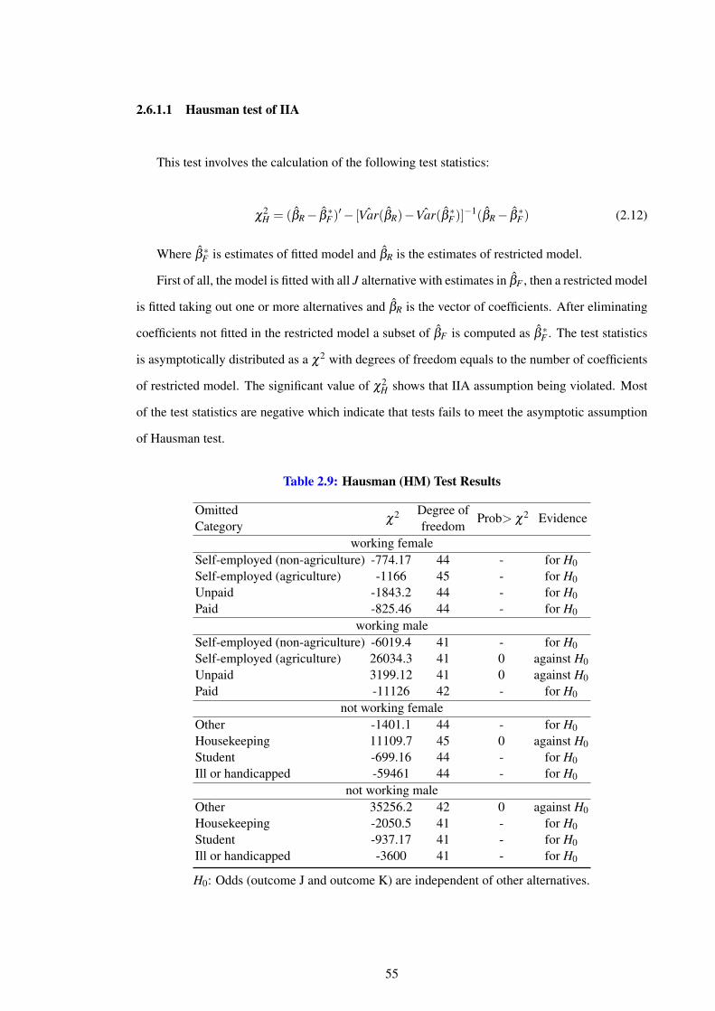
2.6.1.1 Hausman test of IIA
This test involves the calculation of the following test statistics:
χ2H = (βR− β
∗F)′− [ ˆVar(βR)− ˆVar(β ∗F)]
−1(βR− β∗F) (2.12)
Where β ∗F is estimates of fitted model and βR is the estimates of restricted model.
First of all, the model is fitted with all J alternative with estimates in βF , then a restricted model
is fitted taking out one or more alternatives and βR is the vector of coefficients. After eliminating
coefficients not fitted in the restricted model a subset of βF is computed as β ∗F . The test statistics
is asymptotically distributed as a χ2 with degrees of freedom equals to the number of coefficients
of restricted model. The significant value of χ2H shows that IIA assumption being violated. Most
of the test statistics are negative which indicate that tests fails to meet the asymptotic assumption
of Hausman test.
Table 2.9: Hausman (HM) Test Results
Omittedχ2 Degree of
Prob> χ2 EvidenceCategory freedom
working femaleSelf-employed (non-agriculture) -774.17 44 - for H0Self-employed (agriculture) -1166 45 - for H0Unpaid -1843.2 44 - for H0Paid -825.46 44 - for H0
working maleSelf-employed (non-agriculture) -6019.4 41 - for H0Self-employed (agriculture) 26034.3 41 0 against H0Unpaid 3199.12 41 0 against H0Paid -11126 42 - for H0
not working femaleOther -1401.1 44 - for H0Housekeeping 11109.7 45 0 against H0Student -699.16 44 - for H0Ill or handicapped -59461 44 - for H0
not working maleOther 35256.2 42 0 against H0Housekeeping -2050.5 41 - for H0Student -937.17 41 - for H0Ill or handicapped -3600 41 - for H0
H0: Odds (outcome J and outcome K) are independent of other alternatives.
55
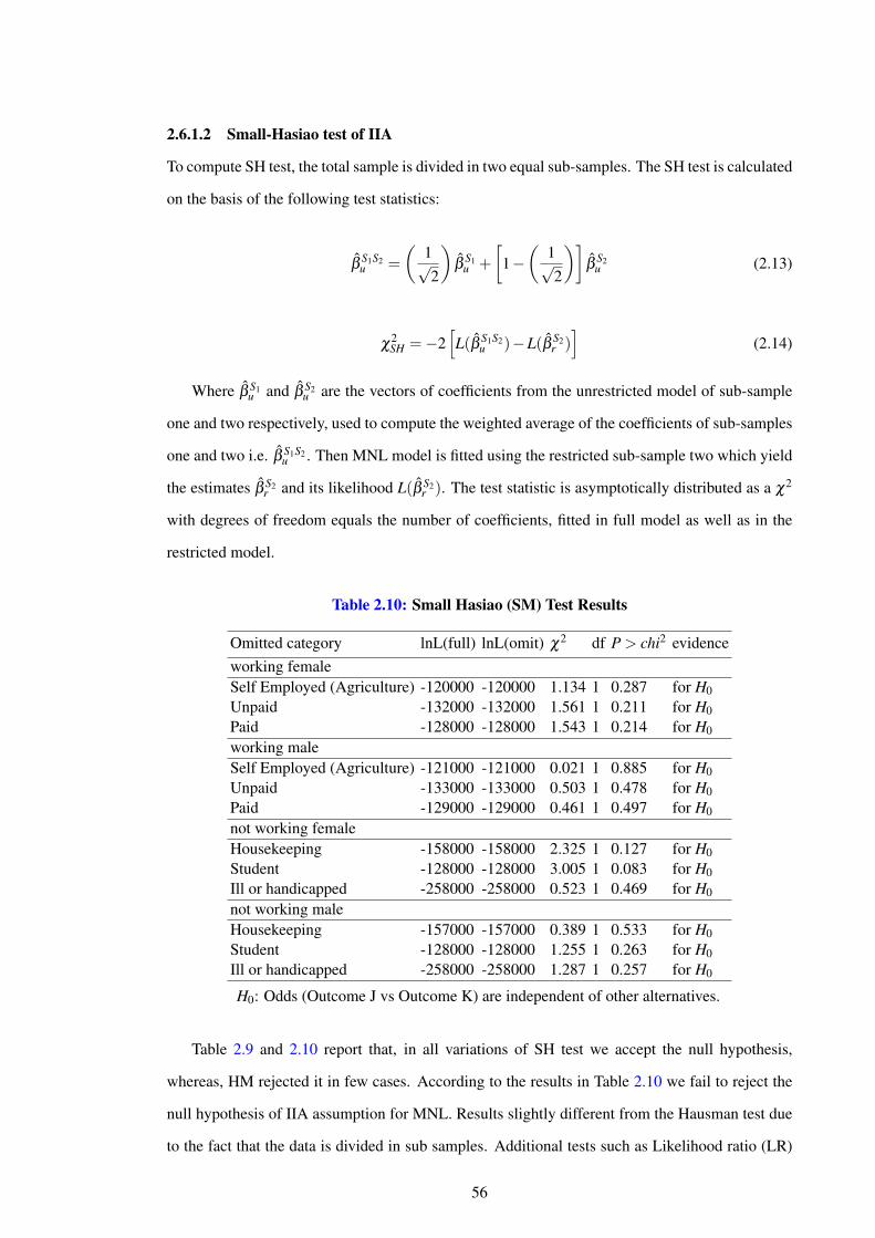
2.6.1.2 Small-Hasiao test of IIA
To compute SH test, the total sample is divided in two equal sub-samples. The SH test is calculated
on the basis of the following test statistics:
βS1S2u =
(1√2
)β
S1u +
[1−(
1√2
)]β
S2u (2.13)
χ2SH =−2
[L(β S1S2
u )−L(β S2r )]
(2.14)
Where β S1u and β S2
u are the vectors of coefficients from the unrestricted model of sub-sample
one and two respectively, used to compute the weighted average of the coefficients of sub-samples
one and two i.e. β S1S2u . Then MNL model is fitted using the restricted sub-sample two which yield
the estimates β S2r and its likelihood L(β S2
r ). The test statistic is asymptotically distributed as a χ2
with degrees of freedom equals the number of coefficients, fitted in full model as well as in the
restricted model.
Table 2.10: Small Hasiao (SM) Test Results
Omitted category lnL(full) lnL(omit) χ2 df P > chi2 evidenceworking femaleSelf Employed (Agriculture) -120000 -120000 1.134 1 0.287 for H0Unpaid -132000 -132000 1.561 1 0.211 for H0Paid -128000 -128000 1.543 1 0.214 for H0
working maleSelf Employed (Agriculture) -121000 -121000 0.021 1 0.885 for H0Unpaid -133000 -133000 0.503 1 0.478 for H0Paid -129000 -129000 0.461 1 0.497 for H0
not working femaleHousekeeping -158000 -158000 2.325 1 0.127 for H0Student -128000 -128000 3.005 1 0.083 for H0Ill or handicapped -258000 -258000 0.523 1 0.469 for H0
not working maleHousekeeping -157000 -157000 0.389 1 0.533 for H0Student -128000 -128000 1.255 1 0.263 for H0Ill or handicapped -258000 -258000 1.287 1 0.257 for H0
H0: Odds (Outcome J vs Outcome K) are independent of other alternatives.
Table 2.9 and 2.10 report that, in all variations of SH test we accept the null hypothesis,
whereas, HM rejected it in few cases. According to the results in Table 2.10 we fail to reject the
null hypothesis of IIA assumption for MNL. Results slightly different from the Hausman test due
to the fact that the data is divided in sub samples. Additional tests such as Likelihood ratio (LR)
56
test and Wald test for independent variables are reported in Tables A2 to A9 in Appendix-A.
2.7 Conclusion
The chapter enlightens the analysis of the labour market status of women in Pakistan. In this re-
gard, two labour market states working and not working have been further enumerated into four
categories each and discussed in detail. Labour market states of working include paid employee,
unpaid family helper, self-employed (agriculture sector) and self-employed (non-agriculture sec-
tor), whereas, not-working states include ill or handicapped, student, housekeepers, and others.
Having defined these states, further, the determinants of labour market participation has been
explored. The demand side and supply side factors include women’s own and household charac-
teristics that effect her decision to participate in the labour force. Therefore, the explanatory vari-
ables used in the analysis are age, age-squared, education, marital status, women headed house,
ownership of house, number of dependents, number of children, working people in the family,
co-residence, household income, household income-squared, regional dummy and year dummy.
Pooled data has been constructed from PSLM (2004-09) cross-section data sets. Multinomial
logit model has been applied by taking firstly working states of women as the dependent variable
against the explanatory variables and using not-working as base category and then, considering
not-working states as the dependent and working as base category.
To capture the complete picture of labour market in Pakistan, results have been repeated for
working men and non-working men and comparison is made. In this regard, four models have
been estimated.
The main findings shows that age has a positive and significant impact on all the states of
working males and females in labour market with the exception of men as unpaid family helper.
Married woman, having more than 2 children or those who own a house, or belong to a joint
family or reside in urban areas are less likely to participate in the paid employment. However,
married men, or those who own a house or live in urban area are more likely to participate in paid
employment. The higher the number of working people in the household, greater the likelihood
of participating in all states of employment for both males and females. However, an increase
in the number of children lowers the probability of being in paid employment, but raises the
probability of self employment for both the genders. Similarly belonging to a joint family lowers
the probability for men and women being involved in all the working categories with the exception
of unpaid family helper which is high for male. Having more dependents in the household appears
57
to have no impact on women being involved in any kind of work. On the other hand, for men
the likelihood of paid and unpaid is more and self-employment is high relative to not working. It
has been found that household income has a higher probability for women to work in any of the
working state of labour force, but as the income increases considerably the situation is conversed.
However, in the case of males, when income increases too much, it lowers the probability of being
in paid employment and self-employment (agriculture) and the likelihood of being unpaid family
helper and self-employed in non-agriculture becomes high.
In addition to that, the empirical findings considering men and women not-working as the
dependent variable show that age has lower probability of not being a part of labour market in
case of both genders. With an increase in age up to a certain level, there is a lower probability
of being in any of not-working category relative to working. More years of schooling raise the
probability of being in the status of student relative to work. Marital status of both the genders
lowers the probability of being ill, a student or having other reason of not-working, whereas,
married women have a higher probability of being in housekeeping. For women, owning a house
lowers the probability of being ill or a student, but increases the probability of housekeeping and
other reasons of not-working. On the other hand, for men the probability is lower for being in any
of the inactivity states. More working people in the household decreases the likelihood for both
the genders of being in any not-working states. As household income increases for both genders,
the likelihood of being in housekeeping or a student falls. Men who have more dependents in the
house have a higher probability of being ill, student housekeeping and other reason. However, the
situation is opposite for women with the exception of being ill. Living in a joint family or residing
in urban areas, have a higher probability for both men and women to be in all states of not-working
relative to working.
During the sample period, the labour force participation has shown declining probabilities
as indicated by negative marginal effects of dummies for 2007 and 2009. This may be due to
the adverse situation of macroeconomic fundamentals that can be presumed as the consequence
of backward linkages of labour market. In the presence of backward linkages, the spillovers of
reduced economic activity have resulted in a decrease in employment opportunities for skilled and
unskilled labourers.
58
Chapter 3
Exploring Gender Wage Gap in Pakistan
3.1 Introduction
A wide range of empirical studies, which explore the gender wage gap, utilize the counter factual
decomposition approach of Oaxaca (1973) that splits the wage differential into explained and un-
explained components. The unexplained part is commonly interpreted as discrimination (Brown
et al. (2011)). However, in Pakistan, a limited number of studies22 have attempted to identify the
extent of the differential in male-female wages. Therefore, the purpose of an empirical analysis
in this chapter is to explore the gender wage differential prevailing in the labour market of Pak-
istan. In this regard, the Oaxaca-Blinder (OB) (Oaxaca (1973) and Blinder (1973)) decomposition
method is applied on pooled data from the Pakistan Social and Living Standard Measurement
(PSLM) survey which has not been analysed in the previous studies conducted in Pakistan. 23
The importance of the PSLM survey is due to the fact that it is designed to assess the progress
of Millennium Development Goals (MDGs) in Pakistan over the period of 2004 to 2015. The
United Nations (UN) has set 18 targets for 48 indicators for its member countries to achieve by
2015. Pakistan has committed to implement 16 targets for 37 indicators out of which 6 targets of
13 indicators are being monitored through PSLM Surveys. Therefore, it would be valuable to use
such information which is different from the Labour Force surveys that have been conventionally
used in the Pakistani literature related to labour market issues.
A report by the World Bank state that females are less likely to participate in the labour market,
i.e. the likelihood to be employed or actively looking for employment is less for them in most of
the developing countries. The participation rate for females also tends to be a U-shaped curve with
respect to income in the low income countries. In those countries, most of the females are active
because they are engaged in the unpaid work related to agriculture sector. Females represent 40
% of the global labour force out of which 43 % is the agriculture labour force. Nevertheless, more
than half the worlds university students are females. It is recommended that the productivity in
22Ashraf and Ashraf (1993)), Siddiqui and Siddiqui (1998)23PSLM is designed to provide Social & Economic indicators in the alternate years at provincial and district levels.
The project was initiated in July 2004 and will continue up to June 2015. As such this survey is one of the mainmechanisms for monitoring the Millennium Development Goals MDGs indicators. The sample size of the PSLMsurveys district level is approximately 80,000 households and approximately 17,000 at Provincial level.
59
developing countries can be raised by can be raised by 25 % if the talents and skills of the females
is fully utilised and the discrimination against them in the labour market is eliminated (Wong
(2012)).
About half a billion females have joined the labour force over the last three decades around the
world. At the same time females’ participation in paid employment has also increased, as womens
participation in paid work has increased in most of the developing world. However, gender dispar-
ities still persist in many areas even in developed countries. Income growth itself does not deliver
equality. In fact, gender gaps draw closer, it is because of the combined behaviour of markets and
institutions (formal and informal) and how they have interacted to influence household decisions
especially in favour of women. The gaps remain for poor women and these disparities worsen
when combined with ethnicity, backwardness and disability (Wong (2012)).
Unequal access to opportunities is another dilemma. Females are more likely than males to
take part in the unpaid work in the informal sectors of the economy. As a result, males tend
to earn more than women do. Agriculture is becoming an increasingly feminized occupation.
On the other hand, females participation rate in the manufacturing sector appears to be falling
at the same time. Meanwhile, poorer women in developing and transition economies continue
to be employed in the informal sector where low wages are accompanied by the gender gaps
in wages and occupational hierarchies persist. One of the significant Millennium Development
Goals (MDGs) is to promote gender equality. Inequality remains a crucial issue in complementing
welfare enhancement strategies (Atkinson (1997), Atkinson and Bourguignon (2000)). Gender
equality is important not only as a goal in itself, but also as a path towards achieving the other
goals (Mundial (2002)).
In the case of Pakistan, the existence of gender inequality among its various social and eco-
nomic indicators is potentially a rationale behind its under development. One of the possible
explanations for this gender inequity is gender discrimination in earning opportunities. The evi-
dence of gender discrimination in Pakistan’s labour market has been documented in several studies
( Ashraf and Ashraf (1993), Siddiqui and Siddiqui (1998), Sabir and Aftab (2007), Nasir and Na-
zli (2000) and Siddiqui (2006)), which confirm that males earn higher wages than females after
controlling for measurable characteristics affecting productivity.
The Labour Force Survey (2011) reports disparity in nominal wages across gender, and areas
in Pakistan. Average nominal wages in rural areas is lower by one-third in the urban areas which
reflects that the higher share of urban employment is coming from non-agriculture and formal
60
sectors. The decline in real wages and wide wage gaps have marked the wage structure in Pakistan
in the recent years (IMF 2011). Although the minimum wage level has been set legally, the
authorities have been unable to enforce it across sectors due to the fact that a large part of the
working labour force is either unpaid or works in the informal sector as a part time worker i.e. less
than 35 hours a week. Pakistan’s labour force constitutes 77 % males and 23 % females. Even
though the female participation rate has increased from 9.3 % in 2000 to 15.6 % in 2011, it is less
than one-third of the participation of the male counterparts. It is even lowest in comparison to
other South Asian countries, where the average female participation rate is 44%. “ Although the
labour market access for women has improved over time, this has not gone hand in hand with the
creation of equal work opportunities for them. The share of women working in wage employment
has declined from 33 percent in 2000 to 21 percent in 2011; female employees earn around 63
percent of the average wage of males, and over 63 percent of employed women work as (unpaid)
contributing family workers. ” (Wong (2012), chapter 5).
A fundamental goal in labour economics is to understand the factors that effect the offered
wages of individuals in return for their labour supply. A better understanding of this mechanism
can guide the policy makers in the public and private sectors to invest in the areas which can aug-
ment the labour income and ultimately boost the economic growth. To identify the determinants
of wages in the developing countries is even more important as the wages are directly associated
with the standard of living and the level of poverty.
This chapter contributes towards the understanding of wage differentials in Pakistan. In this
regard, it estimates separate wage equations by gender incorporating factors related to the individ-
uals, households and labour market. Apart from standard control variables e.g. age and education,
this study also includes a combination of a wide range of personal, educational, regional and de-
mographic characteristics along with occupation, sector (public-private), and organisation choices.
None of the studies conducted in Pakistan has dealt with all these factors simultaneously in the
empirical analysis. Therefore, this research attempts to address this gap in the literature by us-
ing pooled data from PSLM Surveys (2005 to 2009) for the first time in Pakistan. Moreover, it
is important to use this data (rather than the usual Labour Force surveys) due to the fact that it
is specifically designed to focus on the MDGs which Pakistan promised to achieve by the end of
2015. Hence, the PSLM survey as an effective mechanism to monitoring the indicators of MDG. It
provides the population-based estimates of social indicators which represent the overall population
along with the progress under the MDGs.
61
The main objective of the empirical analysis is to compute the gender wage gap by using
pooled data. Further, identifying the impact of personal characteristics, human capital endow-
ments, employment status, occupational choice, sectors and regions in the wage determination
of males and females in Pakistan’s labour market. Wage determination equations are estimated
for both gender groups using the Mincerian approach and the gender wage gap is computed by
employing the Blinder-Oaxaca decomposition methodology. The specific focus of this study is
to investigate the factors contributing towards the wage determination in Pakistan. Further, the
research question looks at the extent to which the gender wage differential in the labour market
of Pakistan can be explained by the differences in personal characteristics, human capital endow-
ments, employment status, occupational choice, sectors and regions of Pakistan. In this regard
a human capital approach is implemented. Therefore, the Blinder- Oaxaca (1973) methodology
seems the most suitable according to which earning equations can be used to determine how much
of the wage differential is due to characteristic differences and how much is owing to discrimina-
tion.
Following the introduction , Section 2 reviews literature so far drawing on international and
Pakistan studies and the role of race, ethnicity and gender. Section 3 explains the data source
and variable description. Section 4 discusses the methodology. Section 5 displays results for the
selection effects and gender wage decomposition while Section 6 concludes the chapter.
3.2 Literature Review
The implication of recent trends in females employment in the developing as well as developed
countries is a contentious issue under much consideration by international forums. A remarkable
range of theoretical and empirical studies has explored the global employment trends and highlight
the changes in female’s participation in the formal and informal sectors of the economy. Such
topics are still drawing relevant attention in the economics literature.
3.2.1 Literature Review (International Studies)
Since Becker (1957) seminal paper on the economics of discrimination, studies on the magnitude
and sources of the gender wage gap have proliferated. Numerous empirical studies on the labour
markets have focused on issues such as participation, unemployment, discrimination, segregation,
wage structure and wage differentials. There is an evidence of a gender wage gap both in devel-
oped and developing countries. Mincer (1974) provides the analytical foundation to investigate
62
the determinants of wages empirically, and thus monetary returns to the factors such as age, edu-
cation, schooling quality, work experience, and occupation were estimated. The body of literature
has been developed by integrating theoretical, methodological and econometric issues to estimate
the wage gap empirically. Polachek (1975, 1976, 1979), Polachek and Kim (1994) are prominent
in using the human capital theories to explain the wage gap between males and females. Bergmann
(1974, 1986, 1997) offer another set of studies that accentuates on discrimination. Oaxaca (1973)
and Blinder (1973) disentangled the contribution of differences in the human capital and of dis-
crimination to decompose the (gender, ethnic or racial) wage gap. Since then a countless number
of studies have been conducted either to estimate the returns to the productive factors for instance,
education and experience, or to measure the extent of discrimination in a labour market due to fac-
tors like race and gender. Oaxaca (1973) puts emphasis on the gender wage gap (between males
and females), Blinder (1973) highlights the racial wage gap (between Black and White) whereas,
Reimers (1983) focused on the ethnic wage gap (Hispanic and Black). These decompositions are
now standard practice in economics, focusing on the mean and are based on simple counterfactu-
als. The methodology commonly used to study the outcomes in the labour market by gender, race
and ethnicity etc. is known as the Oaxaca-Blinder (OB) decomposition technique. It decomposes
the mean difference in the log of wages between the two groups into a part “ explained” by the
differences in the productivity characteristics and a part “ unexplained” that is the difference in the
coefficients associated with these characteristics (Jann (2008)).
Oaxaca (1973), in his seminal paper on estimating the average extent of discrimination against
working women in urban labour markets of the U.S provides a quantitative assessment of male-
female wage differentials. The estimation process is based on two assumption: one is the wage
structure for the females should be the same as males if there is no discrimination. The other
due to the in the presence of discrimination, males would have received more and females less as
compared to what they would have received in a non-discriminatory labour market. The Ordinary
least squares method has been applied on the wage equation that provides the wage structure for
each group of workers. The dependent variable, male-female wage differential has been expressed
in natural logarithms. The control variables used in the estimation are potential experience,24 age,
years of schooling (linear and quadratic terms), dummy variables for social class of workers, indus-
24It is a proxy for actual experience for males. However, it overstates the actual years of experience for femalesas they might left the labour force due their household or child bearing commitments. Therefore, the problem of lostexperience has been controlled by the number of children born to the female. The cost of children in terms of theireffect on the hourly wages have been translated into an equivalent number of years of potential experience (Oaxaca(1973)).
63
try and occupation, health problems, marital status, region, size of urban area. The estimated wage
differentials were decomposed into the effect of discrimination, and the effect of differences in the
individual characteristics. The analysis is based on the data from the 1967 Survey of Economic
Opportunity. The sample includes individuals aged sixteen years and above who have shown their
hourly wages, who live in urban areas and have reported that they are White or Negro. According
to the two sets of regressions, the findings suggest that discrimination accounts for 77.7% of the
wage differential for whites and 93.6% for blacks. For both race and gender differences in the
distribution of part time employment and marital status have contributed significantly to narrow
down the wage gap.
Blinder (1973) investigates discrimination in a structural model and compares it with the es-
timated reduced form models for the U.S. He estimates structural and reduced form equations of
wage determination for the white and black males. The structural and reduced form models are
also estimated for White males and White females as well. He uses the Michigan Survey Research
Centres Panel Study of Income Dynamics. The differential due to coefficients and unexplained
are termed as discrimination. The wage differential representing discrimination is 20.4% from
the structural model and 35.5% from the reduced form model in case of White and Black males.
White females face discrimination of 30.1% and 45.8% compared to white males respectively in
the structural and reduced form models.
As the unexplained part in the wage decomposition equation is typically interpreted as discrim-
ination, the advancement has been made in this method by Oaxaca and Ransom (1999) to examine
four alternative methods to estimate the extent of labour market discrimination in the U.S. In all
these methods the unadjusted wage differential is decomposed into productivity and discrimina-
tion. The methodology is applied on the U.S Current Population Survey data. The dependent
variable is the logarithmic wage, whereas, the control variables are years of experience, school-
ing (linear and quadratic), government employee, occupation, industry, regional, location and city
size. The results show that whites are overpaid by 1% and blacks are underpaid by 12-13%. Males
are overpaid by 32% and females are underpaid by 26%. The productivity advantage of males is
estimated to be 2%, whereas productivity advantage for whites is estimated to be 9-10%.
Afterwards, Oaxaca and Ransom (1999) highlight the identification issues in the detailed wage
decomposition. The idea is that the decomposition methodology may produce arbitrary results for
the dummy variables especially when one want to estimate the separate contributions of each of
them in the unexplained part. However, it is seen that the separate contributions of the set of
64
dummy variables in the explained part do not depend on the reference group. A similar argument
applies for continuous variables but it is not necessarily an identification issue. Using the sample
of 2,624 males and 892 females from the colleges and universities professors in the United States,
the salary wage differential was estimated. While reporting the detailed decomposition, a dummy
variable indicated the set of highest degree level. Differences in the average qualification between
males and females were calculated by using two reference groups i.e. no advanced degree and
the PhD degree. The degree of discrimination which is measured from the unexplained part dra-
matically varies by changing the choice of the reference group. Discrimination with no advanced
degree as reference group is -19.9 log points whereas, with Ph.D. as the omitted category it is
-1.1 log points. The study concludes that since the estimated wage equations contain categorical
variables; therefore, the identification problem may be inevitable in the detailed decompositions.
However, to address this issue the deviation contrast transformation technique has been introduced
by Yun (2005a). This method transforms the coefficients of dummy variables to reflect the devi-
ation from the “ grand mean” rather than deviations from the omitted category. As a result, the
decomposition is invariant to the omitted category.
There exists a general agreement in the literature that the wage structure of one of the group of
workers is dominant over the relative or comparison group. Therefore, the estimation procedure
considers the wage structure of one group as non-discriminatory. The examples of such kind of
decompositions can be seen in Neumark (1988), Oaxaca and Ransom (1988, 1994). Typically
the non-discriminatory wage structure is estimated from a pooled sample of two demographic
groups. Neumark (1988) develops an alternate procedure from a particular Beckerian discrimina-
tion model. He suggests a least squares criterion to estimate the non-discriminatory wage structure
from the pooled sample of males and females. The approach is to estimate the competitive wage
structure that would exist when there is no wage discrimination which can be used as weights in
the wage gap decomposition equation.
Many theorists suggest labour market discrimination models. Cotton (1988) proposes the
procedure to decompose the discrimination coefficient into the cost imposed upon minority and
the benefit gained by majority groups. The Public Use Samples 1980 census data covering almost
12 states of the U.S has been utilised for the analysis. The sample is restricted to Black and White
males aged 16 years and above with positive hourly earnings. In the decomposition, discrimination
is made up of two elements; one represents the amount by which white productivity characteristics
are overvalued and the other by which black productivity characteristics are undervalued.
65
Ethnic discrimination has also been a topic of investigation for the economists.25 Reimers
(1983) studies labour market discrimination against Hispanic and Black Men in U.S. The study
indicates that age, education, geographic location, immigration, language problems, and discrim-
ination could be the possible reasons behind lower wages of Hispanics. The estimation procedure
takes into account selectivity bias in the observed wage sample. The wage differentials have been
separated into portions due to differences in the average characteristics and the portion due to
differences in the unobserved factors and discrimination. Discrimination is measured using three
different weights to add up differences in the parameters; the average characteristics of minorities,
non-white Hispanics and the average of the two. The results reveal that average wages offered to
the minority are 15% lower than white non-Hispanics.
Another set of research papers investigates the econometric and specification issues. The pio-
neering work of Heckman (1976, 1979) raised the issue of sample selection bias as a specification
error if the non-random sample is used to estimate the behavioural relationship. He suggests a two-
stage estimation method to correct the bias (the procedure is formally explained in the method-
ology section). Since then, a substantial number of research papers have investigated the wage
structure by addressing the issue of selection bias.
An important development in this method is found in Neuman and Oaxaca (2004) that incor-
porates alternative selectivity methods to investigate wage structures of professional workers in
the Israeli labour market across gender and ethnicity. Within each gender, a distinction is made
between Easterners (Asian/African) and Westerners (European/American countries) using data
from the 1995 Census. Wage equations include the Inverse of Mills Ratio as a regressor to correct
for selection into the professional occupations. Wage differences have been examined and de-
composed into endowments, discrimination and selectivity. The results suggest that gender wage
differentials at the mean points are wider than ethnic wage differentials. Among both Westerners
and Easterners Jewish men earn 26% more (per hour) than Jewish women, while among both men
and women Westerners earn 19% more than Easterners. Without the selectivity correction for pro-
fessional employment, differences in the characteristics explain between 36% to 74% of the wage
differentials. The explained share is smallest (36%) in a gender comparison among Westerners and
largest (74%) in an ethnic comparison of women. The main idea behind the empirical analysis of
this chapter is based on the this paper.
Wage determination in rural and urban areas or measuring the role of sectoral interactions in
25Kaas and Manger (2012)
66
wage determination and comparison between public and private sectors has also been a topic of
interest of many in the last two decades (Peng et al. (2009) for China, Lee and Pesaran (1993) for
UK. However, the latest studies in the UK using the British Household Panel Data (BHPS) mainly
emphasize the usual Oaxaca-Blinder decomposition methodology in addressing the differential
analysis in the outcome of interest to analyse gender discrimination. Brown et al. (2011) employ
the same data and technique to compute the gender reservation wage gap for UK. The sample in-
cludes economically inactive (family carers, full time students, disables etc.) individuals between
(16-65) years of age and also the ones who have reported their reservation wages i.e. the lowest
wage acceptable to the unemployed worker. This shows their attachment to the labour market and
also recognises that unemployment and inactivity are two distinct features. The analysis is based
on an unbalanced panel of data from 1991 to 2008. It takes attributes to individuals characteris-
tics as explained or the endowment component and differences in returns to endowments as the
unexplained or discriminatory component. The finding shows the existence of a gender reserva-
tion wage gap in the UK. The explained part of the gap is determined mainly due to the presence
of pre-school age children. On the other hand, for individuals without children, the unexplained
component of the reservation wage differential is 99% compared to only 22% for those with pre-
school age children. The results have been interpreted as perceived discrimination in the labour
market which effect the reservation wages for females. Anees (2010) applies the (Oaxaca-Blinder)
OB method to gender discrimination in UK and decomposes the gender wage gap into two parts,
which are attributable to endowments and due to coefficients. Using the BHPS 1995, a significant
gap between male-female wages was found.
In the UK, the research on racial discrimination in the labour market has two dimensions, one
is descriptive: some of the prominent studies are Daniel (1968), Brown et al. (1980) and Modood
et al. (1997), and the other is quantitative that has used econometric techniques in order to measure
the labour market discrimination. Most of the latest studies are confined to racial discrimination
and some emphasise the employment discrimination in the UK such as Blackaby et al. (1994) and
Blackaby et al. (2002).
Blackaby et al. (1994) explore the black and white male earning and employment prospects in
Britain. The analysis is based on the data for the 1970’s and 1980’s. It has been observed that over-
time in the 1980’s employment prospects for blacks has worsened compared to the 1970’s. The
data on earnings, racial origin and employment status has been collected from the continuous gov-
ernment survey series of the General Household Survey (GHS). The time period is from 1973-79
67
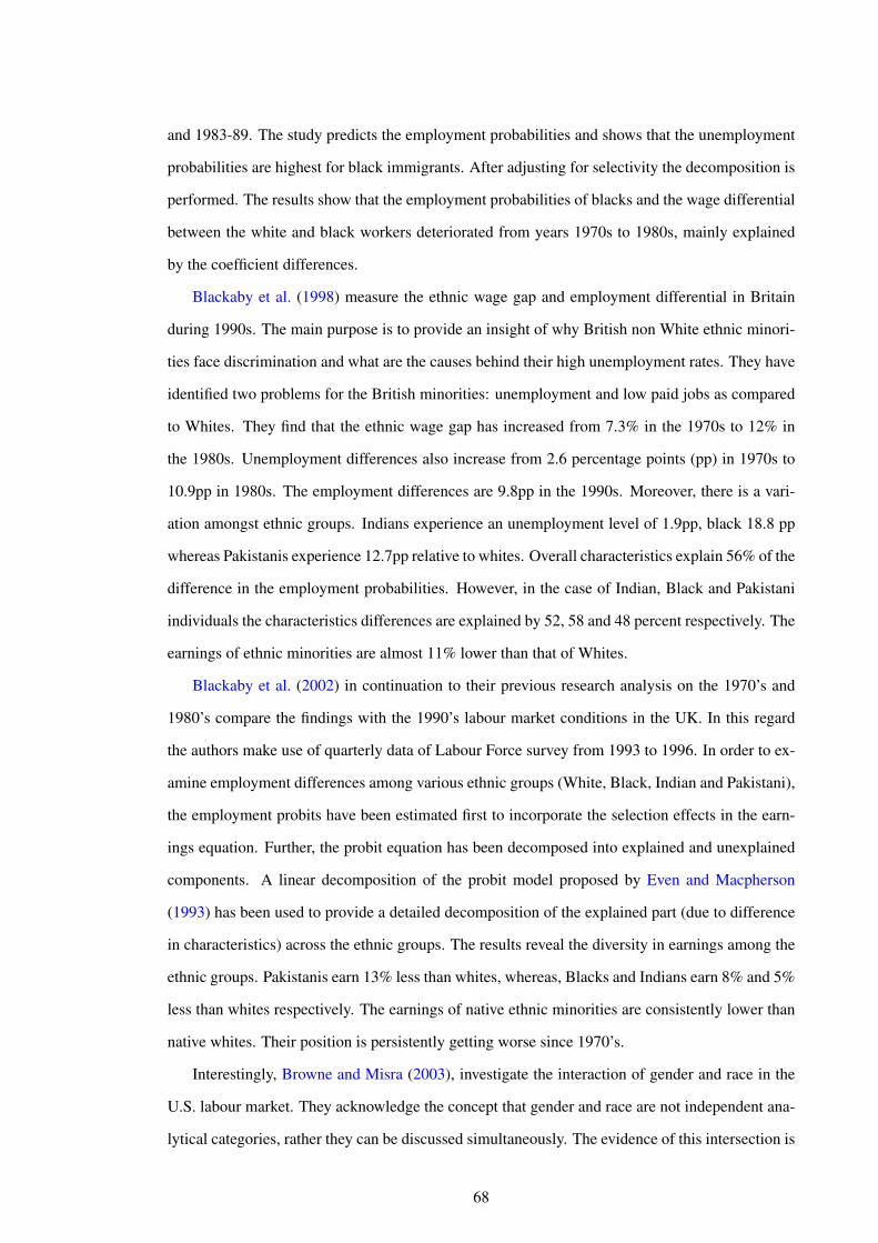
and 1983-89. The study predicts the employment probabilities and shows that the unemployment
probabilities are highest for black immigrants. After adjusting for selectivity the decomposition is
performed. The results show that the employment probabilities of blacks and the wage differential
between the white and black workers deteriorated from years 1970s to 1980s, mainly explained
by the coefficient differences.
Blackaby et al. (1998) measure the ethnic wage gap and employment differential in Britain
during 1990s. The main purpose is to provide an insight of why British non White ethnic minori-
ties face discrimination and what are the causes behind their high unemployment rates. They have
identified two problems for the British minorities: unemployment and low paid jobs as compared
to Whites. They find that the ethnic wage gap has increased from 7.3% in the 1970s to 12% in
the 1980s. Unemployment differences also increase from 2.6 percentage points (pp) in 1970s to
10.9pp in 1980s. The employment differences are 9.8pp in the 1990s. Moreover, there is a vari-
ation amongst ethnic groups. Indians experience an unemployment level of 1.9pp, black 18.8 pp
whereas Pakistanis experience 12.7pp relative to whites. Overall characteristics explain 56% of the
difference in the employment probabilities. However, in the case of Indian, Black and Pakistani
individuals the characteristics differences are explained by 52, 58 and 48 percent respectively. The
earnings of ethnic minorities are almost 11% lower than that of Whites.
Blackaby et al. (2002) in continuation to their previous research analysis on the 1970’s and
1980’s compare the findings with the 1990’s labour market conditions in the UK. In this regard
the authors make use of quarterly data of Labour Force survey from 1993 to 1996. In order to ex-
amine employment differences among various ethnic groups (White, Black, Indian and Pakistani),
the employment probits have been estimated first to incorporate the selection effects in the earn-
ings equation. Further, the probit equation has been decomposed into explained and unexplained
components. A linear decomposition of the probit model proposed by Even and Macpherson
(1993) has been used to provide a detailed decomposition of the explained part (due to difference
in characteristics) across the ethnic groups. The results reveal the diversity in earnings among the
ethnic groups. Pakistanis earn 13% less than whites, whereas, Blacks and Indians earn 8% and 5%
less than whites respectively. The earnings of native ethnic minorities are consistently lower than
native whites. Their position is persistently getting worse since 1970’s.
Interestingly, Browne and Misra (2003), investigate the interaction of gender and race in the
U.S. labour market. They acknowledge the concept that gender and race are not independent ana-
lytical categories, rather they can be discussed simultaneously. The evidence of this intersection is
68
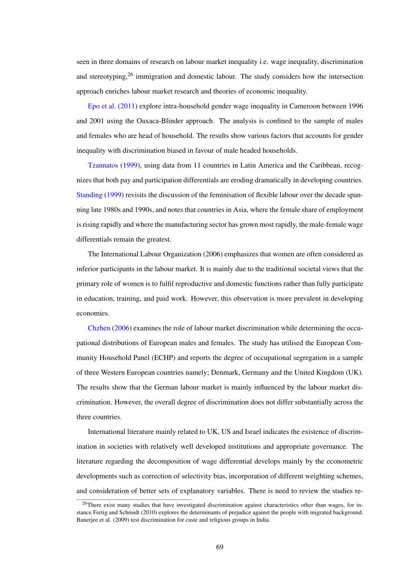
seen in three domains of research on labour market inequality i.e. wage inequality, discrimination
and stereotyping,26 immigration and domestic labour. The study considers how the intersection
approach enriches labour market research and theories of economic inequality.
Epo et al. (2011) explore intra-household gender wage inequality in Cameroon between 1996
and 2001 using the Oaxaca-Blinder approach. The analysis is confined to the sample of males
and females who are head of household. The results show various factors that accounts for gender
inequality with discrimination biased in favour of male headed households.
Tzannatos (1999), using data from 11 countries in Latin America and the Caribbean, recog-
nizes that both pay and participation differentials are eroding dramatically in developing countries.
Standing (1999) revisits the discussion of the feminisation of flexible labour over the decade span-
ning late 1980s and 1990s, and notes that countries in Asia, where the female share of employment
is rising rapidly and where the manufacturing sector has grown most rapidly, the male-female wage
differentials remain the greatest.
The International Labour Organization (2006) emphasizes that women are often considered as
inferior participants in the labour market. It is mainly due to the traditional societal views that the
primary role of women is to fulfil reproductive and domestic functions rather than fully participate
in education, training, and paid work. However, this observation is more prevalent in developing
economies.
Chzhen (2006) examines the role of labour market discrimination while determining the occu-
pational distributions of European males and females. The study has utilised the European Com-
munity Household Panel (ECHP) and reports the degree of occupational segregation in a sample
of three Western European countries namely; Denmark, Germany and the United Kingdom (UK).
The results show that the German labour market is mainly influenced by the labour market dis-
crimination. However, the overall degree of discrimination does not differ substantially across the
three countries.
International literature mainly related to UK, US and Israel indicates the existence of discrim-
ination in societies with relatively well developed institutions and appropriate governance. The
literature regarding the decomposition of wage differential develops mainly by the econometric
developments such as correction of selectivity bias, incorporation of different weighting schemes,
and consideration of better sets of explanatory variables. There is need to review the studies re-
26There exist many studies that have investigated discrimination against characteristics other than wages, for in-stance Fertig and Schmidt (2010) explores the determinants of prejudice against the people with migrated background.Banerjee et al. (2009) test discrimination for caste and religious groups in India.
69

lated to Pakistan so that the gaps in literature are properly identified and efforts are made to fill
these gaps in the light of literature reviewed for international economies.
3.2.2 Literature Review (Pakistan Literature)
The gender wage gap issue has also gained the attention of researchers in Pakistan. Ashraf and
Ashraf (1993) estimate wage discrimination against women in Rawalpindi city of Punjab by using
primary data (collected by Authors) for 1975 which reveals an earnings gap of 68.55% between
males and females. As this analysis is confined to a limited sample, Ashraf and Ashraf (1996) have
extended their analysis by utilizing a comprehensive data set of Household Integrated Economic
Surveys (HIES) 1979 and 1985-86 to measure the magnitude of the earnings gap between males
and females in overall Pakistan. The approaches of Oaxaca (1973), Cotton (1988) and Neumark
(1988) have been applied to derive the estimates. The variables used in the model are a quadratic in
age, and education along with dummies for provinces, rural urban areas and industrial groups. The
gender wage differential as per the results of the HIES 1979 data was 63.27% which has narrowed
to 33.09% according to the HIES 1985-86. Ashraf and Ashraf (1998a) find 47.90% of male-female
earnings differentials using the HIES 1984-85 by utilizing the same technique and set of variables.
Further Ashraf and Ashraf (1998b) employ the same methodology and variables, but a different
data set focusing on one city Karachi (the largest city of Sindh province) and find an earnings gap
of 14.5% between males and females. Afterwards, Ashraf et al. (2009) updated the earlier work
of Ashraf and Ashraf (1993) to Ashraf and Ashraf (1998a) by using the 2001-02 HIES data set
and reported a gender earnings gap of 15.4% for the entire sample covering 16,182 households.
Given, a considerable variation in the estimates of earnings gap in the studies spread over a period
of time i.e. more than decade, accuracy in the results can be questioned. However, the high levels
of discrimination against women is clearly obvious from the estimates of the earnings differentials.
The basic criticism of the studies is that although the need for correcting the selectivity bias has
been discussed in the methodology, the correction for sample selection, i.e. the inverse mills ratio,
has not been incorporated in the wage determination equation.
In Pakistan, cultural and demographic features have a dominating effect on employment or
wage earning activities. Sathar and Kazi (2000) investigate the factors that constitute women’s
empowerment in rural Pakistan. For the first time, the research focused on the backward areas
realizing the fact that women’s status may vary across community and region, each of which has
distinctive features. It is found that Northern Punjabi women are financially less self-sufficient
70
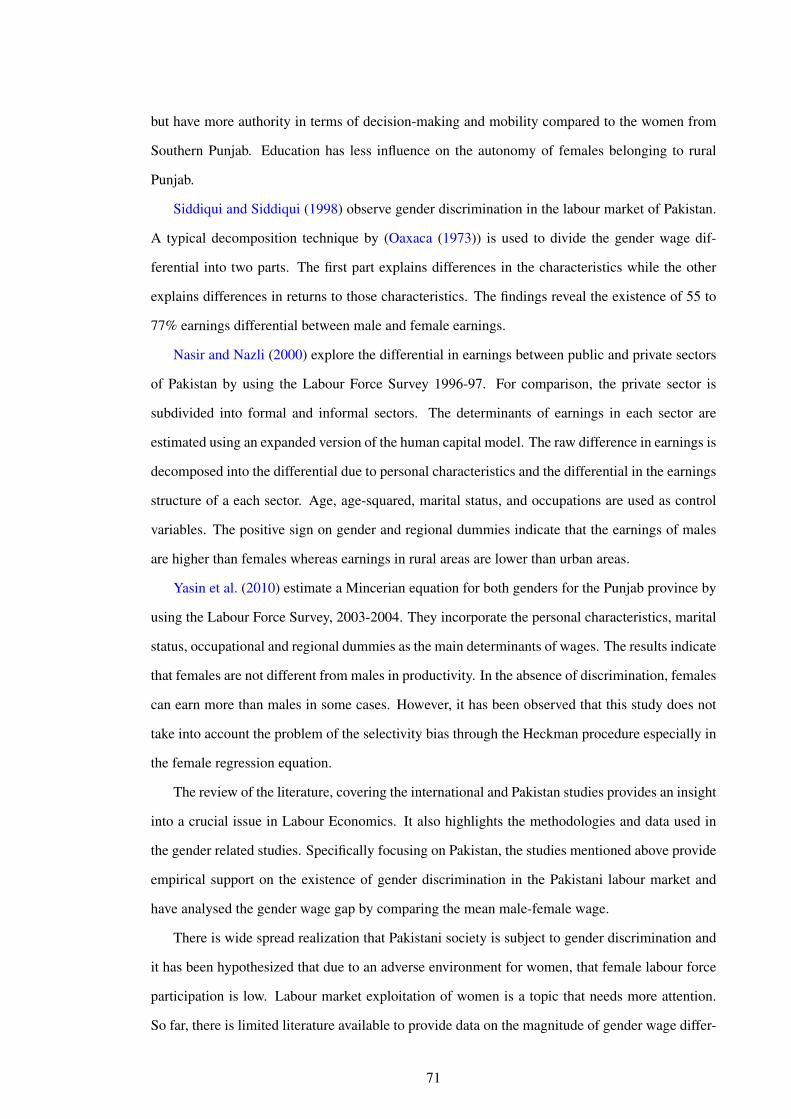
but have more authority in terms of decision-making and mobility compared to the women from
Southern Punjab. Education has less influence on the autonomy of females belonging to rural
Punjab.
Siddiqui and Siddiqui (1998) observe gender discrimination in the labour market of Pakistan.
A typical decomposition technique by (Oaxaca (1973)) is used to divide the gender wage dif-
ferential into two parts. The first part explains differences in the characteristics while the other
explains differences in returns to those characteristics. The findings reveal the existence of 55 to
77% earnings differential between male and female earnings.
Nasir and Nazli (2000) explore the differential in earnings between public and private sectors
of Pakistan by using the Labour Force Survey 1996-97. For comparison, the private sector is
subdivided into formal and informal sectors. The determinants of earnings in each sector are
estimated using an expanded version of the human capital model. The raw difference in earnings is
decomposed into the differential due to personal characteristics and the differential in the earnings
structure of a each sector. Age, age-squared, marital status, and occupations are used as control
variables. The positive sign on gender and regional dummies indicate that the earnings of males
are higher than females whereas earnings in rural areas are lower than urban areas.
Yasin et al. (2010) estimate a Mincerian equation for both genders for the Punjab province by
using the Labour Force Survey, 2003-2004. They incorporate the personal characteristics, marital
status, occupational and regional dummies as the main determinants of wages. The results indicate
that females are not different from males in productivity. In the absence of discrimination, females
can earn more than males in some cases. However, it has been observed that this study does not
take into account the problem of the selectivity bias through the Heckman procedure especially in
the female regression equation.
The review of the literature, covering the international and Pakistan studies provides an insight
into a crucial issue in Labour Economics. It also highlights the methodologies and data used in
the gender related studies. Specifically focusing on Pakistan, the studies mentioned above provide
empirical support on the existence of gender discrimination in the Pakistani labour market and
have analysed the gender wage gap by comparing the mean male-female wage.
There is wide spread realization that Pakistani society is subject to gender discrimination and
it has been hypothesized that due to an adverse environment for women, that female labour force
participation is low. Labour market exploitation of women is a topic that needs more attention.
So far, there is limited literature available to provide data on the magnitude of gender wage differ-
71
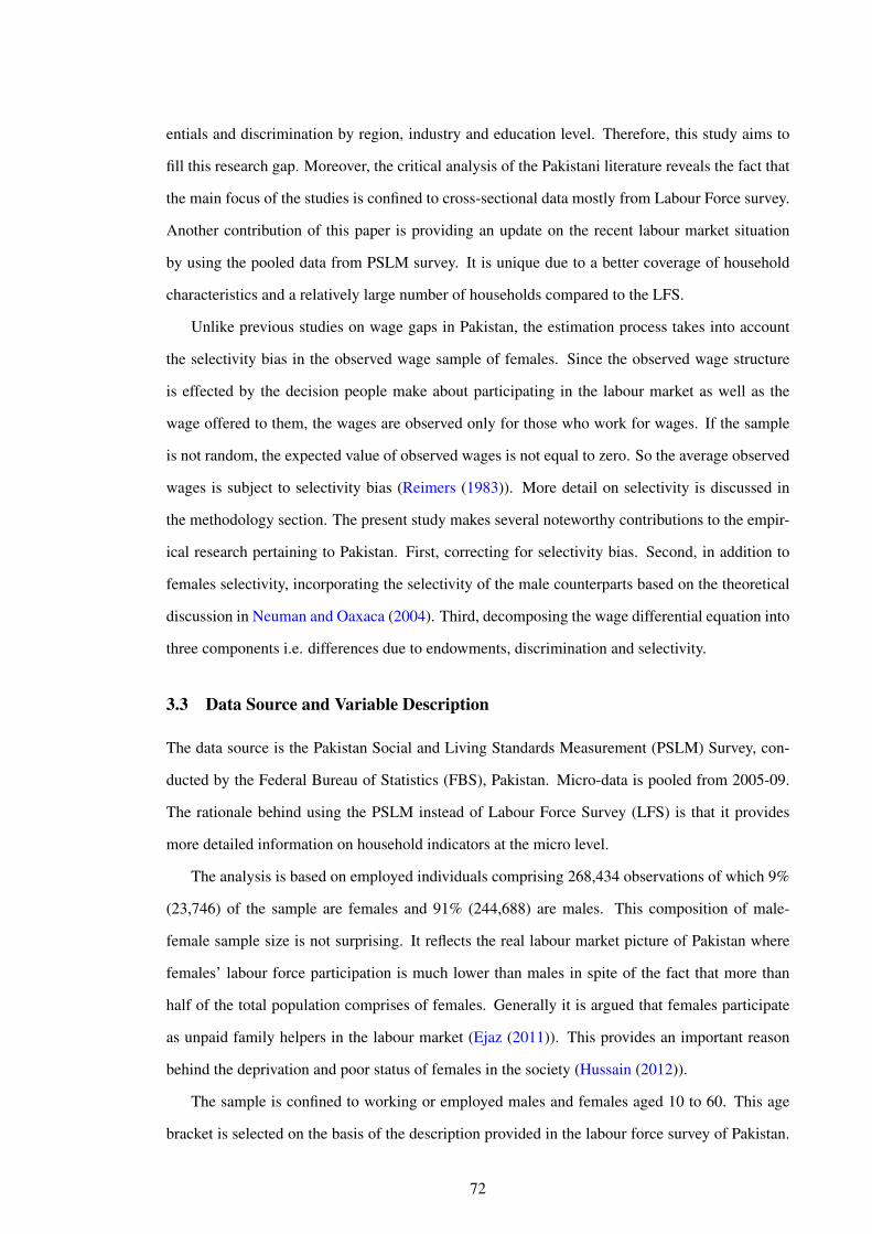
entials and discrimination by region, industry and education level. Therefore, this study aims to
fill this research gap. Moreover, the critical analysis of the Pakistani literature reveals the fact that
the main focus of the studies is confined to cross-sectional data mostly from Labour Force survey.
Another contribution of this paper is providing an update on the recent labour market situation
by using the pooled data from PSLM survey. It is unique due to a better coverage of household
characteristics and a relatively large number of households compared to the LFS.
Unlike previous studies on wage gaps in Pakistan, the estimation process takes into account
the selectivity bias in the observed wage sample of females. Since the observed wage structure
is effected by the decision people make about participating in the labour market as well as the
wage offered to them, the wages are observed only for those who work for wages. If the sample
is not random, the expected value of observed wages is not equal to zero. So the average observed
wages is subject to selectivity bias (Reimers (1983)). More detail on selectivity is discussed in
the methodology section. The present study makes several noteworthy contributions to the empir-
ical research pertaining to Pakistan. First, correcting for selectivity bias. Second, in addition to
females selectivity, incorporating the selectivity of the male counterparts based on the theoretical
discussion in Neuman and Oaxaca (2004). Third, decomposing the wage differential equation into
three components i.e. differences due to endowments, discrimination and selectivity.
3.3 Data Source and Variable Description
The data source is the Pakistan Social and Living Standards Measurement (PSLM) Survey, con-
ducted by the Federal Bureau of Statistics (FBS), Pakistan. Micro-data is pooled from 2005-09.
The rationale behind using the PSLM instead of Labour Force Survey (LFS) is that it provides
more detailed information on household indicators at the micro level.
The analysis is based on employed individuals comprising 268,434 observations of which 9%
(23,746) of the sample are females and 91% (244,688) are males. This composition of male-
female sample size is not surprising. It reflects the real labour market picture of Pakistan where
females’ labour force participation is much lower than males in spite of the fact that more than
half of the total population comprises of females. Generally it is argued that females participate
as unpaid family helpers in the labour market (Ejaz (2011)). This provides an important reason
behind the deprivation and poor status of females in the society (Hussain (2012)).
The sample is confined to working or employed males and females aged 10 to 60. This age
bracket is selected on the basis of the description provided in the labour force survey of Pakistan.
72
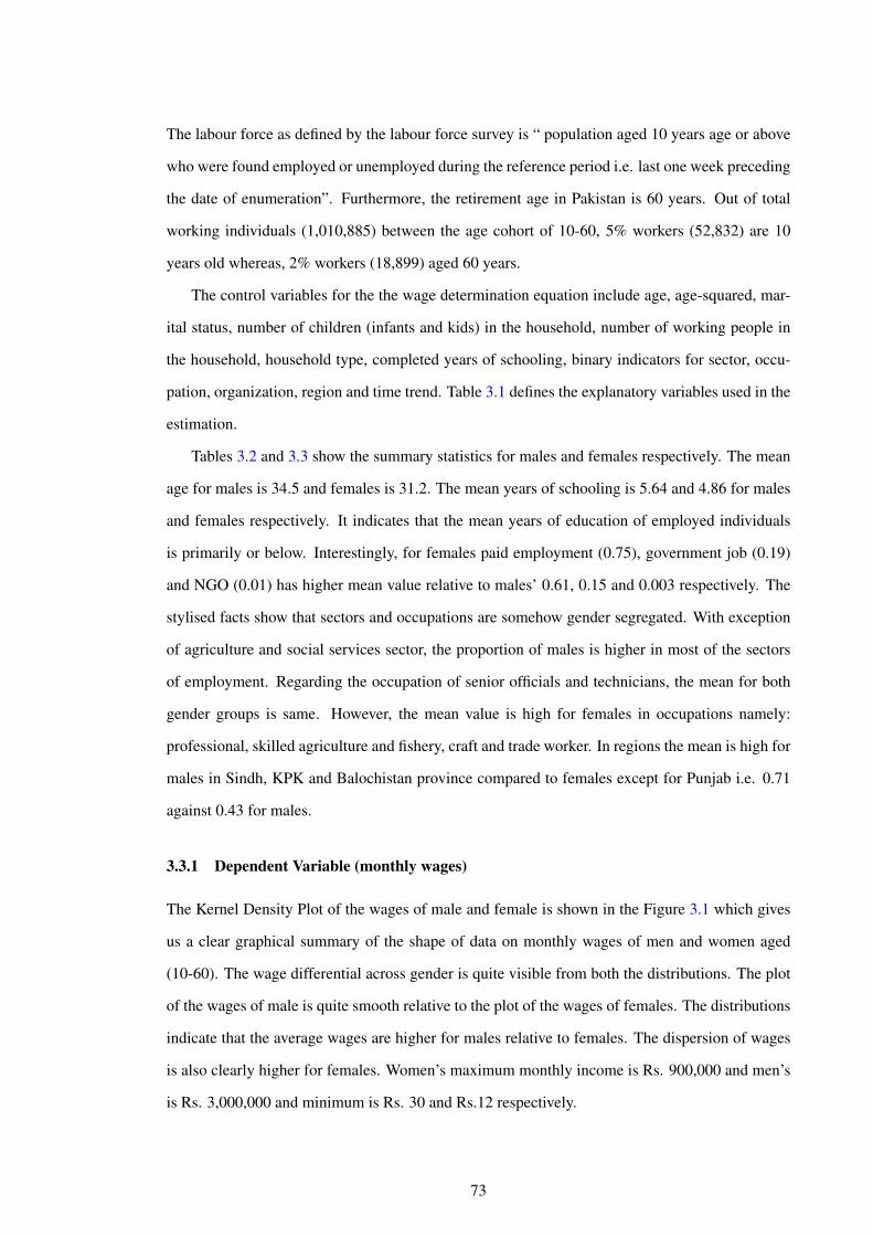
The labour force as defined by the labour force survey is “ population aged 10 years age or above
who were found employed or unemployed during the reference period i.e. last one week preceding
the date of enumeration”. Furthermore, the retirement age in Pakistan is 60 years. Out of total
working individuals (1,010,885) between the age cohort of 10-60, 5% workers (52,832) are 10
years old whereas, 2% workers (18,899) aged 60 years.
The control variables for the the wage determination equation include age, age-squared, mar-
ital status, number of children (infants and kids) in the household, number of working people in
the household, household type, completed years of schooling, binary indicators for sector, occu-
pation, organization, region and time trend. Table 3.1 defines the explanatory variables used in the
estimation.
Tables 3.2 and 3.3 show the summary statistics for males and females respectively. The mean
age for males is 34.5 and females is 31.2. The mean years of schooling is 5.64 and 4.86 for males
and females respectively. It indicates that the mean years of education of employed individuals
is primarily or below. Interestingly, for females paid employment (0.75), government job (0.19)
and NGO (0.01) has higher mean value relative to males’ 0.61, 0.15 and 0.003 respectively. The
stylised facts show that sectors and occupations are somehow gender segregated. With exception
of agriculture and social services sector, the proportion of males is higher in most of the sectors
of employment. Regarding the occupation of senior officials and technicians, the mean for both
gender groups is same. However, the mean value is high for females in occupations namely:
professional, skilled agriculture and fishery, craft and trade worker. In regions the mean is high for
males in Sindh, KPK and Balochistan province compared to females except for Punjab i.e. 0.71
against 0.43 for males.
3.3.1 Dependent Variable (monthly wages)
The Kernel Density Plot of the wages of male and female is shown in the Figure 3.1 which gives
us a clear graphical summary of the shape of data on monthly wages of men and women aged
(10-60). The wage differential across gender is quite visible from both the distributions. The plot
of the wages of male is quite smooth relative to the plot of the wages of females. The distributions
indicate that the average wages are higher for males relative to females. The dispersion of wages
is also clearly higher for females. Women’s maximum monthly income is Rs. 900,000 and men’s
is Rs. 3,000,000 and minimum is Rs. 30 and Rs.12 respectively.
73
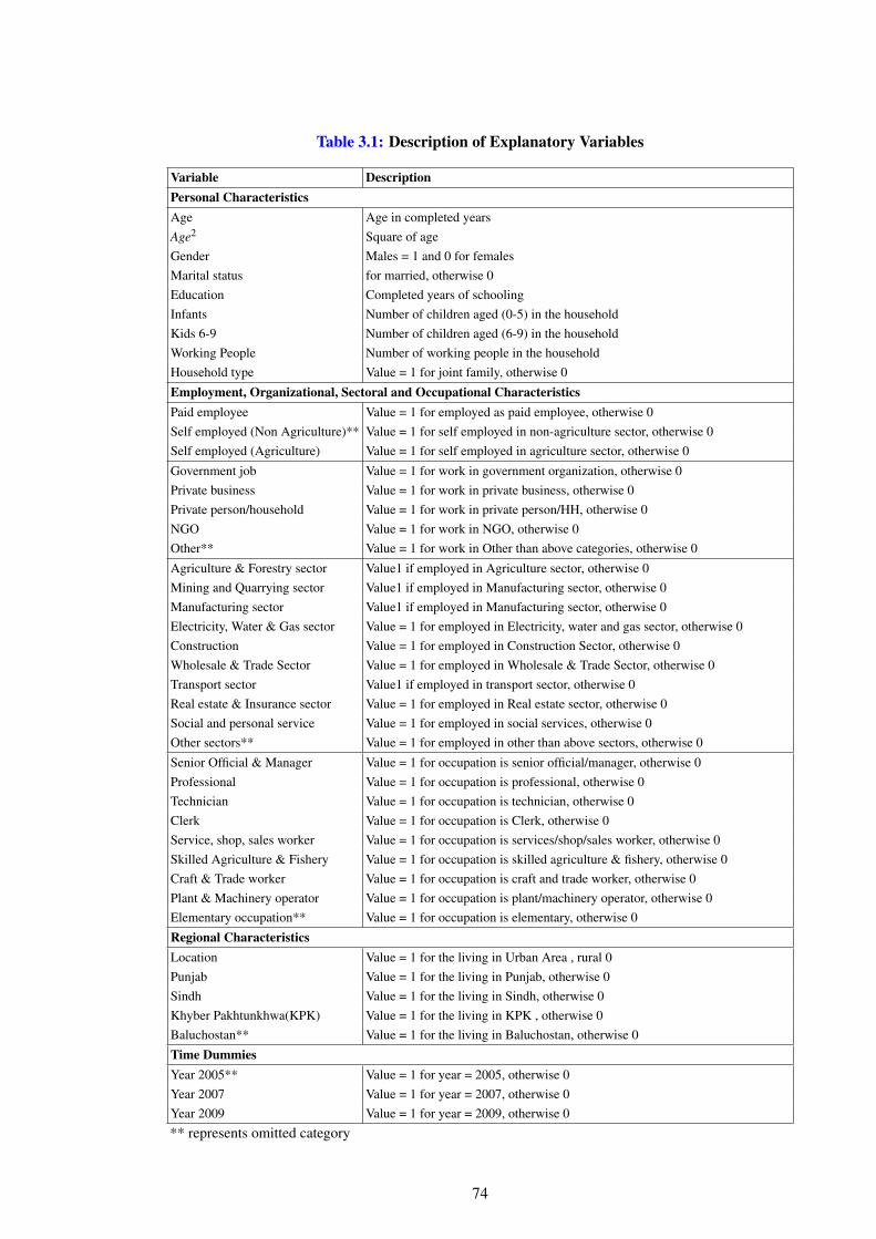
Table 3.1: Description of Explanatory Variables
Variable DescriptionPersonal CharacteristicsAge Age in completed yearsAge2 Square of ageGender Males = 1 and 0 for femalesMarital status for married, otherwise 0Education Completed years of schoolingInfants Number of children aged (0-5) in the householdKids 6-9 Number of children aged (6-9) in the householdWorking People Number of working people in the householdHousehold type Value = 1 for joint family, otherwise 0
Employment, Organizational, Sectoral and Occupational CharacteristicsPaid employee Value = 1 for employed as paid employee, otherwise 0Self employed (Non Agriculture)** Value = 1 for self employed in non-agriculture sector, otherwise 0Self employed (Agriculture) Value = 1 for self employed in agriculture sector, otherwise 0
Government job Value = 1 for work in government organization, otherwise 0Private business Value = 1 for work in private business, otherwise 0Private person/household Value = 1 for work in private person/HH, otherwise 0NGO Value = 1 for work in NGO, otherwise 0Other** Value = 1 for work in Other than above categories, otherwise 0
Agriculture & Forestry sector Value1 if employed in Agriculture sector, otherwise 0Mining and Quarrying sector Value1 if employed in Manufacturing sector, otherwise 0Manufacturing sector Value1 if employed in Manufacturing sector, otherwise 0Electricity, Water & Gas sector Value = 1 for employed in Electricity, water and gas sector, otherwise 0Construction Value = 1 for employed in Construction Sector, otherwise 0Wholesale & Trade Sector Value = 1 for employed in Wholesale & Trade Sector, otherwise 0Transport sector Value1 if employed in transport sector, otherwise 0Real estate & Insurance sector Value = 1 for employed in Real estate sector, otherwise 0Social and personal service Value = 1 for employed in social services, otherwise 0Other sectors** Value = 1 for employed in other than above sectors, otherwise 0
Senior Official & Manager Value = 1 for occupation is senior official/manager, otherwise 0Professional Value = 1 for occupation is professional, otherwise 0Technician Value = 1 for occupation is technician, otherwise 0Clerk Value = 1 for occupation is Clerk, otherwise 0Service, shop, sales worker Value = 1 for occupation is services/shop/sales worker, otherwise 0Skilled Agriculture & Fishery Value = 1 for occupation is skilled agriculture & fishery, otherwise 0Craft & Trade worker Value = 1 for occupation is craft and trade worker, otherwise 0Plant & Machinery operator Value = 1 for occupation is plant/machinery operator, otherwise 0Elementary occupation** Value = 1 for occupation is elementary, otherwise 0
Regional CharacteristicsLocation Value = 1 for the living in Urban Area , rural 0Punjab Value = 1 for the living in Punjab, otherwise 0Sindh Value = 1 for the living in Sindh, otherwise 0Khyber Pakhtunkhwa(KPK) Value = 1 for the living in KPK , otherwise 0Baluchostan** Value = 1 for the living in Baluchostan, otherwise 0
Time DummiesYear 2005** Value = 1 for year = 2005, otherwise 0Year 2007 Value = 1 for year = 2007, otherwise 0Year 2009 Value = 1 for year = 2009, otherwise 0
** represents omitted category
74
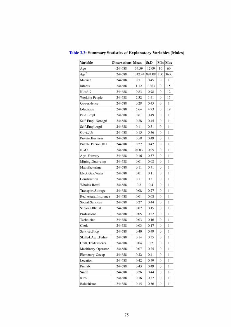
Table 3.2: Summary Statistics of Explanatory Variables (Males)
Variable Observations Mean St.D Min Max
Age 244688 34.59 12.09 10 60
Age2 244688 1342.44 884.08 100 3600
Married 244688 0.71 0.45 0 1
Infants 244688 1.12 1.363 0 15
Kids6-9 244688 0.83 0.98 0 12
Working People 244688 2.32 1.41 0 15
Co-residence 244688 0.28 0.45 0 1
Education 244688 5.64 4.93 0 19
Paid Empl 244688 0.61 0.49 0 1
Self Empl Nonagri 244688 0.28 0.45 0 1
Self Empl Agri 244688 0.11 0.31 0 1
Govt Job 244688 0.15 0.36 0 1
Private Business 244688 0.58 0.49 0 1
Private Person HH 244688 0.22 0.42 0 1
NGO 244688 0.003 0.05 0 1
Agri Forestry 244688 0.16 0.37 0 1
Mining Quarrying 244688 0.01 0.08 0 1
Manufacturing 244688 0.11 0.31 0 1
Elect Gas Water 244688 0.01 0.11 0 1
Construction 244688 0.11 0.31 0 1
Wholes Retail 244688 0.2 0.4 0 1
Transport Storage 244688 0.08 0.27 0 1
Real estate Insurance 244688 0.01 0.08 0 1
Social Services 244688 0.27 0.44 0 1
Senior Official 244688 0.02 0.15 0 1
Professional 244688 0.05 0.22 0 1
Technician 244688 0.03 0.16 0 1
Clerk 244688 0.03 0.17 0 1
Service Shop 244688 0.40 0.49 0 1
Skilled Agri Fishry 244688 0.14 0.35 0 1
Craft Tradeworker 244688 0.04 0.2 0 1
Machinery Operator 244688 0.07 0.25 0 1
Elementry Occup 244688 0.22 0.41 0 1
Location 244688 0.42 0.49 0 1
Punjab 244688 0.43 0.49 0 1
Sindh 244688 0.26 0.44 0 1
KPK 244688 0.16 0.37 0 1
Balochistan 244688 0.15 0.36 0 1
75
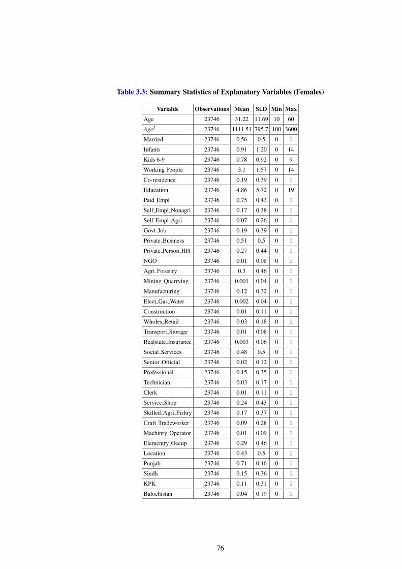
Table 3.3: Summary Statistics of Explanatory Variables (Females)
Variable Observations Mean St.D Min Max
Age 23746 31.22 11.69 10 60
Age2 23746 1111.51 795.7 100 3600
Married 23746 0.56 0.5 0 1
Infants 23746 0.91 1.20 0 14
Kids 6-9 23746 0.78 0.92 0 9
Working People 23746 3.1 1.57 0 14
Co-residence 23746 0.19 0.39 0 1
Education 23746 4.86 5.72 0 19
Paid Empl 23746 0.75 0.43 0 1
Self Empl Nonagri 23746 0.17 0.38 0 1
Self Empl Agri 23746 0.07 0.26 0 1
Govt Job 23746 0.19 0.39 0 1
Private Business 23746 0.51 0.5 0 1
Private Person HH 23746 0.27 0.44 0 1
NGO 23746 0.01 0.08 0 1
Agri Forestry 23746 0.3 0.46 0 1
Mining Quarrying 23746 0.001 0.04 0 1
Manufacturing 23746 0.12 0.32 0 1
Elect Gas Water 23746 0.002 0.04 0 1
Construction 23746 0.01 0.11 0 1
Wholes Retail 23746 0.03 0.18 0 1
Transport Storage 23746 0.01 0.08 0 1
Realstate Insurance 23746 0.003 0.06 0 1
Social Services 23746 0.48 0.5 0 1
Senior Official 23746 0.02 0.12 0 1
Professional 23746 0.15 0.35 0 1
Technician 23746 0.03 0.17 0 1
Clerk 23746 0.01 0.11 0 1
Service Shop 23746 0.24 0.43 0 1
Skilled Agri Fishry 23746 0.17 0.37 0 1
Craft Tradeworker 23746 0.09 0.28 0 1
Machinry Operator 23746 0.01 0.09 0 1
Elementry Occup 23746 0.29 0.46 0 1
Location 23746 0.43 0.5 0 1
Punjab 23746 0.71 0.46 0 1
Sindh 23746 0.15 0.36 0 1
KPK 23746 0.11 0.31 0 1
Balochistan 23746 0.04 0.19 0 1
76
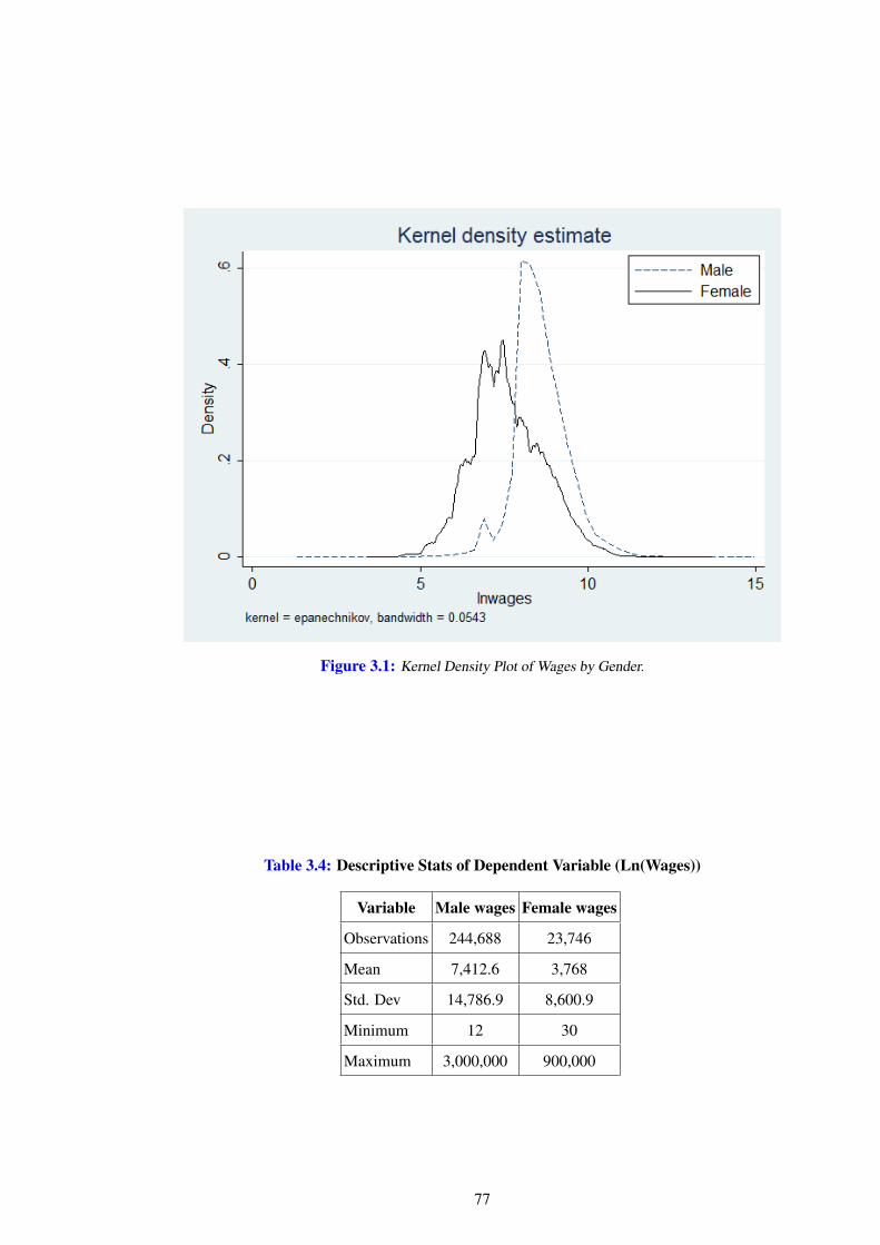
Figure 3.1: Kernel Density Plot of Wages by Gender.
Table 3.4: Descriptive Stats of Dependent Variable (Ln(Wages))
Variable Male wages Female wages
Observations 244,688 23,746
Mean 7,412.6 3,768
Std. Dev 14,786.9 8,600.9
Minimum 12 30
Maximum 3,000,000 900,000
77
3.4 Methodology
While analysing earnings in the labour market the question arises as to what factors determine the
wages and why do individuals receive different rewards for their human capital even though they
have the same ability and productivity, though a different gender. The “ Theory of Human Capital”
provides the answer to these questions as; two similar agents can differ in their wages and earnings
because of the differences in their age, level of education, experience, skills and training (Funding
(2001)) and if a wage gap remains, then it might be due to discrimination. The most frequently
used empirical approach to measure the wage differential between two groups is the Mincerian
earnings function which determines the rates of returns to the human capital and identifies their
effect on the wages (Mincer (1974)).
Another strand of recent growing literature explains the wage differential between the sub-
groups by using the distributional measures. In contrast to simple mean comparisons, the distri-
butional impact of various programs or interventions is the key area of interest in the literature
exploring the factors responsible for the differences in distributions. The main distribution tech-
niques are the plug-in procedure by Juhn et al. (1993), the re-weighting methodology by DiNardo
et al. (1996), alternative decomposition techniques stated in (Tzannatos (1999) and Donald et al.
(2000)), the quantile-based decomposition method explained by Machado and Mata (2005). The
quantile regression method by DiNardo et al. (1996) measures the effect of different factors on
the wage gap at multiple points of the wage distribution. In extension to DiNardo et al. (1996)
decomposition, Firpo et al. (2007) propose the specific contribution of single covariates to the
gender wage gap. Even though the conditional quantile regression models have been used in the
empirical literature it is worth mentioning that they have many restrictions. First, a change in
the distribution of covariates can change the interpretation of the coefficients estimates (Powell
(2011)). Second, in these regression models, the differences in conditional quantiles are not equal
to the differences in unconditional quantiles which is an important property of OB method of lin-
ear regression (Bazen (2011)). Although, several studies e.g. Juhn et al. (1993), DiNardo et al.
(1996), Machado and Mata (2000) and Melly (2005) tried to address these points they were unable
to come up to any satisfactory solution. Thus, this provides a valid reason for using OB approach
in this chapter.
The reason for not considering any of the above mentioned techniques in the analysis is that
the distributional measures provide limited information regarding the contribution of determinants.
However, in the OB approach the mean wage differentials can be decomposed into the wage struc-
78
ture effect and the composition effect. Therefore, the OB approach is preferred to the distributional
approach because it provides the composition effect of each covariate separately. In addition, the
answer to the question “ to what extent changes in education has contributed to wage inequality
can be tackled in a straightforward manner in case of the mean using OB decomposition.
The Oaxaca (1973) approach is the most commonly applied statistical technique for decom-
posing wages of two groups into a part explained by the differences in endowments and a part
which remains unexplained. The unexplained part is a measure of discrimination of the second
group in comparison with the reference group. There are several suggestions in literature for the
selection of the reference group. The reference group is assumed as the non-discriminatory group
and in choosing of the appropriate weights (Cotton (1988)). In this analysis the non-discriminatory
group is potentially males and is used as the reference group. In this chapter the regression for the
offered wage gap (linear outcome variable) between working males and females (aged 10-60) has
been estimated by Oaxaca-Blinder approach.
3.4.1 Decomposition for Linear Regression Model: Oaxaca Blinder Approach
If one considers log of wages of males (M) and females (F) as an outcome variable Y, whereas,
age, education and experience are included in the set of explanatory variables. Then the mean
difference in the outcome is written as;
R = E(YM)−E(YF) (3.1)
Where E(Y ) indicates the expected value of an outcome variable, comprise of group differences
in the set of explanatory variables.
On the basis of the linear model
Yκ = X ′κβκ + εκ , E(εκ) = 0 κ ∈ (M,F) (3.2)
where “ X” is a vector of set of explanatory variables including constant. β symbolises the slope
parameters as well as the intercept. The error term is denoted as ε . The mean difference in
the outcome variable is expressed as the difference in the linear prediction by the means of the
independent variables in each group.
R = E(YM)−E(YF) = E(XM)′βM−E(XF)′βF (3.3)
79
and
E(Yκ) = E(X ′κβκ + εκ) = E(X ′κβκ)+E(εκ) = E(Xκ)′βκ
As per assumptions E(βκ) = βκ and E(εκ) = 0. The contribution of the differences in the ex-
planatory variables to the total difference in the outcome is arranged by following (Winsborough
and Dickinson (1971), Jones and Kelley (1984) and Daymont and Andrisani (1984)): Consider
a twofold equation R = C+U . The first the part of the outcome differential is the “ endowment
effect” that is explained by males and females differences in the explanatory variables
C = {E(XM)−E(XF)}′β ∗ (3.4)
and the second part is the “ unexplained part” which captures the effect of the difference in the
unobserved variables. It is usually attributed as discrimination.
U = {E(XM)′(βM−β∗)+E(XF)
′(β ∗−βF)} (3.5)
The unexplained part is further decomposed as;
βM = β ∗+δM and βF = β ∗+δF
where δM and δF are vectors of (male and female) groups discrimination parameter. The signs
identify the positive or negative effect of these symbols. U can be written as
U = E(XM)′δM−E(XF)′δF (3.6)
In other words the unexplained part of the differential can be subdivided into UM = E(XM)′δM
(quantifies discrimination in favour of males) and UF = E(XF)′δF (gauges discrimination against
females). The interpretation is based on the assumption that there is no relevant unobserved vari-
able. UM and UF show opposite interpretation. “ A positive value for UM means positive discrimi-
nation of female group whereas, a positive value for UF points out negative discrimination of male
group” (Jann (2008)).
There is an alternative way to interpret the decomposition explained in the discrimination lit-
erature that uses a vector of non-discriminatory coefficient measure the contribution of the differ-
ences in the set of explanatory variables. Consider β ∗ as a vector of non-discriminatory coefficient
80
in the equation given below. So the outcome difference is expressed as;
R = {E(XM)−E(XF)}′β ∗+{E(XM)′(βM−β∗)+E(XF)
′(β ∗−βF)} (3.7)
The decomposition in (3.3) is put together by keeping in view the males perspective. It means
the gender differences in the explanatory variables are weighted by the coefficients of males to
measure the endowment or productivity effect known as explained part. The endowment effect
is the expected change in the mean outcome of female if the male group has the same level of
coefficients as females. Likewise, in the unexplained part considered as coefficient effect, the dif-
ferences in the associated coefficients are weighted by the females’ characteristics. The expected
change in the mean of females’ outcome if females’ group has males’ group coefficients is shown
by the unexplained component. The coefficient effect or unexplained part captures the intercept
differential as well. βM and βF are the least-squares estimates for βM and βF , obtained from male
and female samples respectively and means of the explanatory variable for both gender groups XM
and XF are estimates for E(XM) and E(XF).
It is quite complicated to determine the components from the twofold decomposition equation
in (3.3) because in that estimation procedure, the the non-discriminatory coefficients vector β ∗
needs to be estimated which is unknown. There exist many suggestions in the literature to tackle
this issue. Assuming that discrimination is always directed towards one group. Then, β ∗ = βM or
β ∗ = βF (Oaxaca (1973) ). Accordingly, if wages are discriminated against females, βM is used as
an estimate for β ∗ and can therefore;
R = (XM− XF)′βF + X ′F(βM− βF) (3.8)
On the other hand, if there is discrimination of males, and no discrimination of females, decom-
position looks like;
R = (XM− XF)′βF + X ′M(βM− βF) (3.9)
3.4.2 Correction for Selectivity bias
As the wage structure is mainly influenced by working individuals, therefore, the sample of work-
ing males and females that earn wages are used for the analysis and this might be a selective group.
However, the current analysis is concerned with correcting for selectivity bias based on the argu-
ment that the sample of females working in the labour market is not a random sample of females.
81
Womens participation decision may depend upon the number of dependents in the household but
this variable should not have any effect on the wages.
In the presence of sample selection the wage equations can yield biased and inconsistent es-
timators (Gronau (1974)). To address this issue, it is documented in labour market research to
incorporate sample selectivity corrected component in the wage equations. Therefore, a Heckman
correction, based on the procedure by Heckman (1976) and Heckman (1979) has been undertaken
to control for selectivity bias. The most straightforward technique to address the issue of selection
bias in the decomposition equations is to separate the selection effect from the the raw differen-
tial and then the standard decomposition approach is applied to the adjusted differential (Reimers
(1983)).
LFP∗i = H ′i γ + εi
Yi = X ′i β +µi
(3.10)
Where LFP∗i is a latent variable representing labour force participation, H ′i , is a vector of vari-
ables effecting the labour force participation, Yi is the market monthly wage (in logs) for those
working, X ′i includes a set of determinants of wages, γ and β are the vectors of associated param-
eters. The εi and µi are the error terms that are assumed to follow a bivariate normal distribution
(0,0,σε ,σµ ,ρ).
In the Probit models the dependent variable takes on the value of 1 if the individual participates
in the labour force and 0 if they do not participate. The estimates of the probit regressions are used
to construct the Inverse Mills Ratio (IMR) for the purpose of correcting monthly wage equations
for selection bias. The instruments used to identify the selection equation are completed years
of schooling, the number of children (aged 5 or below and 6 to 10) in the household to capture
the effect of the reservation wage if the woman is in her child bearing process and dependents to
account for her care giving responsibility. Moreover, time dummies for each year (to capture the
overtime effect), the dummy for residents of rural/urban areas and provincial dummies (Punjab,
Sindh, Khyber Pakhtun Khwa, Baluchistan) are also included in the equation to capture the poten-
tial employment discrimination against people living in backward areas of Pakistan. The same set
of explanatory variables are used to estimate the probit equation for male counterparts in order to
get the gender differences in selectivity.
Prob (LFP∗i > 0) = Prob(εi >−H ′i γ) = Φ(H ′i γ),
82
where Φ(H ′i γ) is the standard normal cumulative density function. The variance of ε is normalized
to 1. Wages are observed for the individuals having LFP∗i > 0, so that the expected wage of a
worker observed to be employed in labour force is given by
E(Yi|LFP∗i > 0) = X ′i β +θλi,+E(µi|εi > H ′i γ
Where θ = ρσµ and λi = φ(H ′i γ)/Φ(H ′i γ)
E(Yi|LFP∗i > 0) = X ′i β +θλi,
Yi|E∗i > 0 = X ′i β +θλi + ε (3.11)
Equation (3.11) is estimated by the Heckman procedure separately for males and females.
When the gender wage gap is decomposed in the presence of sample selectivity:
YM− YF = (X ′MβM + θMλM)− (X ′F βF + θF λF) (3.12)
Correcting for selectivity bias for both the genders leads to the following wage decomposition:
YM− YF = X ′M(βM− β∗)+ X ′F(β
∗− βF)︸ ︷︷ ︸Discrimination
+(X ′M− X ′F)β∗︸ ︷︷ ︸
Endowment
+(θMλM− θF λF)︸ ︷︷ ︸Selectivity
(3.13)
where β ∗ is an estimated non-discriminatory wage structure apart from selectivity effects. The
first two terms in (3.13) represents the discrimination against females, the third term shows the
endowment effect. The last term measures the contribution of selection effects to the observed
gender wage gap (Neuman and Oaxaca (2004) ).
If males are considered as the non-discriminatory group so β ∗ = βM, so (3.13) will reduced to
YM− YF = X ′F(βM− βF)︸ ︷︷ ︸Discrimination
+(XM− XF)′βM︸ ︷︷ ︸
Endowment
+(θMλM− θF λF)︸ ︷︷ ︸Selectivity
(3.14)
In case if the sample selection problem is considered in the female’s equation only.
YM− YF = X ′F(βM− βF)︸ ︷︷ ︸Discrimination
+(X ′M− X ′F)βM︸ ︷︷ ︸Endowment
+(−θF λF)︸ ︷︷ ︸Selectivity
(3.15)
Neuman and Oaxaca (2004) suggest that sample selection can complicate the interpretation
of wage decompositions, therefore, they suggest several alternative decompositions which are
83
based on different assumptions. These alternative decompositions of selectivity corrected wage
equations are incorporated in the analysis of this chapter.
The first approach to incorporate selectivity is
(YM− YF)− (θMλM− θF λF)︸ ︷︷ ︸Ad justed
= X ′F(βM− βF)︸ ︷︷ ︸Discrimination
+(X ′M− X ′F)βM︸ ︷︷ ︸Endowment
(3.16)
It has been used by Reimers (1983) and Neuman and Oaxaca (2004). Eq (3.16) simply takes out
the selection effect from the observed wage gap. However, it doest not decompose the gender
wage differential.
If the difference in the males and females Probit selection parameters is considered as discrim-
ination and the personal characteristics that determine the labour force participation represents
endowment differences, then the decomposition would be adjusted accordingly
YM− YF︸ ︷︷ ︸Raw
= X ′F(βM− βF)+ θM(λ 0F − λF)︸ ︷︷ ︸
Discrimination
+(XM− XF)′βM + θM(λM− λ
0F)︸ ︷︷ ︸
Endowments
+(θM− θF)λF︸ ︷︷ ︸Selectivity
(3.17)
where λ 0F is the mean value of Inverse Mills ratio when females selection equation is same as
males. Furthermore, another decomposition is based on the gender differences in error correlation
coefficients (ρ) and variances of the errors of wage equations (σ ). According to Neuman and
Oaxaca (2004), the differential in (ρ) and (σ ) are part of endowment and selectivity respectively.
YM− YF︸ ︷︷ ︸Raw
= X ′F(βM− βF)+ θM(λ 0F − λF)︸ ︷︷ ︸
Discrimination
+(XM− XF)′βM + θM(λM− λ
0F)+(ρM− ρF)σuF︸ ︷︷ ︸
Endowments
+(σuM− σuF)ρM︸ ︷︷ ︸Selectivity
(3.18)
If the gender differences in the characteristics and coefficient in the probit equations of males
and females are treated in the same way as endowment and discrimination in the wage equation,
then the decomposition equation becomes:
YM− YF︸ ︷︷ ︸Raw
= X ′F(βM− βF)+ θMλ0F − θF λF)︸ ︷︷ ︸
Discrimination
+(XM− XF)′βM + θM(λM− λ
0F)︸ ︷︷ ︸
Endowment
(3.19)
84
To summarise, the estimation process includes six alternative decomposition methods to ex-
plore the gender wage differentials. It starts with measuring the wage differential by the standard
Oaxaca decomposition method ignoring the issue of selectivity in the equation (3.9). Then, it con-
siders the selection bias and estimate the Probit equation for the females only in equation (3.15).
Equation (3.14) adjusts the gender wage differential by taking out the selectivity (in both the gen-
ders) from the observed wage gap. Further, in equation (3.17) the endowment and discrimination
parameters from the males and females Probit selectivity equation are adjusted in the gender wage
differential decomposition along with the coefficient differences of males and females in the se-
lectivity. Equation (3.18) provides the decomposition in which the variances of the errors of wage
equations are considered along with the error correlation coefficients of males and females. This
decomposition is subject to the issue of identification. Finally, the differential of males and fe-
males in the probit equations is considered as the endowment and coefficient effects not selectivity
in the equation (3.19).
3.5 Results and Findings
3.5.1 Probit Regressions: Selectivity Equation
The Probit regression has been estimated for females labour force participation. These estimates
are used to construct the sample selection bias variable IMR (λ ). There exists a potential sample
selection problem in the wage equation. The sample contains workers who have no information on
their wages. Therefore, estimation of the wage equation without non-workers introduces selectiv-
ity bias. This bias may be due to self-selection by individuals being studied. For example, many
married women choose not to work and thus their wages are not observed (i.e., they self-select
themselves out of the sample). Using data only on workers in the estimation is not appropriate
because the wages of those who choose to work may not necessarily give valid estimates of po-
tential wages of those who did not work. Heckman (1979) treats this censored wage equation as
a specification error in which a variable is incorrectly omitted from the wage equation. He shows
that the expected value of the error term in the wage equation is not zero and therefore the OLS es-
timates are biased. Heckmans solution to this problem involves first estimating a probit model that
relates the probability of an individual being in the labour force to a set of determinants, and then
using these probit estimates to compute the inverse Mills ratio. This variable is then included as a
covariate in the wage equation. Table 3.5 presents the results of selectivity equations for females
and males along with their marginal effects.
85
The labour force participation equations identify the factors that effect an individuals decision
to enter into the labour market. It is a well established concept in research literature that human
capital, personal, household and demographic characteristics are likely to affect the reservation
wage and labour force participation decision of the individual. The other control variables used
to model labour force participation are human capital variables that include the highest/completed
years of education (Education). The personal characteristics include the individuals marital status
(Married) and a quadratic in age. The household factors which may affect an individual’s labour
force participation are the joint family (Co-residence) and the total number of working people
in the household (Working people). The demographic factors include dummies for location (ru-
ral/urban) and provinces in Pakistan.
Brown et al. (2011) suggest that the presence of children in a household may increase the
opportunity cost of accepting work outside the home. If this effect females more than males (as
females are more likely to be responsible for the child care), it means that children could increase
the reservation wages of females relative to those of males. This implies that females with children
(mothers) face difficulties in receiving employment offers which are above the reservation wages.
As a result they are less likely to be employed. Keeping in view this argument the decomposition
equation is adjusted after correcting for selection bias.
To identify the selection equation, the following instruments have been used; number of infants
in the household (Infants) i.e. the number of children under six years of age, and number of school
going children i.e. kids aged six to nine (Kids 6-9). 27 These variables tend to influence the choice
of household activities versus the market activities which include income earning activities. As
expected, the results indicate that individuals (both males and females) with infants and kids are
27The instruments used to address the selectivity issue are based on the previous literature. Conventionally theseinstruments have been used most of the time in the studies e.g. Gronau (1973) and Brown and Taylor (2011). Gronau(1973) corrected for the selectivity bias while calculating the offered wage differential between males and femalesand between females with and without children. The idea is, for a married woman if the opportunity cost of timespent on household activities is relatively higher than the market productivity then she will prefer to stay out of labourmarket. Also, the study highlight the point that females wage is not only affected by the number but also the agecomposition. Particularly due to the presence of pre-school age children the tendency to participate in labour market isreduced. Becker (1985) suggests that females with particularly dependent children have more household commitments.Hence, the energy required for paid work is reduced compared to males and consequently ends up with lower wagesthan males. There are other studies which have used different instruments such as pre-school institution available to afemale; demand and supply of social services were also taken into account instead of household characteristics (Kanburand Svejnar (2009)) see pg. 86. However, these instruments came out to be insignificant. Considering the importantpoint that power and strength of the instrument does matter, the instrument (infants aged (0-5) and children aged (6-9))used in the regression analysis of chapter 3 is quite justified. As far as the extended family point is concerned in case ofPakistan, woman cannot decide to work entirely relaying on the caring facility of grandmothers. It could be a temporarything but not a permanent solution to child care. Another study by Angrist and Evans (1996) used instruments such aschildren with gender mix and twins at the first birth to capture the effect of additional child on parents labour supply.Given the details in the limitations section of the thesis on pg. 139 it is clear that we cannot identify the parents of thechild living in the joint family the relationship is given with respect to the head of the house.
86
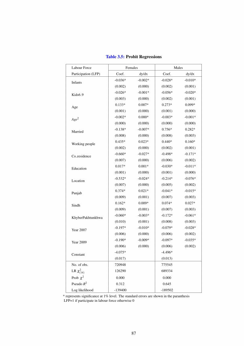
Table 3.5: Probit Regressions
Labour Force Females Males
Participation (LFP) Coef. dy/dx Coef. dy/dx
Infants-0.036* -0.002* -0.028* -0.010*
(0.002) (0.000) (0.002) (0.001)
Kids6 9-0.026* -0.001* -0.056* -0.020*
(0.003) (0.000) (0.002) (0.001)
Age0.133* 0.007* 0.273* 0.099*
(0.001) (0.000) (0.001) (0.000)
Age2 -0.002* 0.000* -0.003* -0.001*
(0.000) (0.000) (0.000) (0.000)
Married-0.138* -0.007* 0.756* 0.282*
(0.008) (0.000) (0.008) (0.003)
Working people0.435* 0.023* 0.440* 0.160*
(0.002) (0.000) (0.002) (0.001)
Co residence-0.660* -0.027* -0.498* -0.171*
(0.007) (0.000) (0.006) (0.002)
Education0.017* 0.001* -0.030* -0.011*
(0.001) (0.000) (0.001) (0.000)
Location-0.532* -0.024* -0.214* -0.076*
(0.007) (0.000) (0.005) (0.002)
Punjab0.374* 0.021* -0.041* -0.015*
(0.009) (0.001) (0.007) (0.003)
Sindh0.162* 0.009* 0.074* 0.027*
(0.009) (0.001) (0.007) (0.003)
KhyberPakhtunkhwa-0.060* -0.003* -0.172* -0.061*
(0.010) (0.001) (0.008) (0.003)
Year 2007-0.197* -0.010* -0.079* -0.028*
(0.006) (0.000) (0.006) (0.002)
Year 2009-0.190* -0.009* -0.097* -0.035*
(0.006) (0.000) (0.006) (0.002)
Constant-4.075* -4.496*
(0.017) (0.013)
No. of obs. 720948 775545
LR χ2(14) 126290 689334
Prob χ2 0.000 0.000
Pseudo R2 0.312 0.645
Log likelihood -139400 -189502
* represents significance at 1% level. The standard errors are shown in the paranthesisLFP=1 if participate in labour force otherwise 0
87
less likely to participate in the labour force.
In developing countries, it is assumed that females have to devote more time to the childcare
responsibilities compared to male counterparts. Mizala et al. (1999) observe that females labour
market participation is not only restricted by the presence of children under the age of 7 years
but also by all the children under 15 years of age. The findings of Dolton and Makepeace (1986)
also support the negative effect of having children less than 6 years on the female employment.
Regarding Pakistan, Aslam (2009) also finds that the presence of children under 7 years negatively
effects the female participation decision. Moreover, he claims that the opportunity cost of female
is higher as education increases as she might have a higher wage rate than the one who is relatively
less educated.
The results suggest that an addition of one or more infants in the HH in Pakistan decreases the
probability of female participation in the labour market by 0.2 percentage points (pp) and for males
by 1 pp. Similarly, having an additional child decreases the probability of participation in labour
market for females by 0.1 pp and males by 2.0 pp. Perhaps the reason behind higher marginal
effects for males is the specification of these two variables. Infants and kids are the total number
of infants and kids in the household because the data is limited by the lack of information on the
identifier for mother, father or parents of particular child. Therefore, this caveat needs to be noted
regarding the present study. However, the limitation is not confined to PSLM only. It is rather
very unfortunate and an arguable weakness in all the datasets or surveys available at national level
in Pakistan that preclude such information. In addition to this argument, as far as the number of
employed individuals in the labour force is concerned the females are only 9% which may have
served as a valid basis for these results.
These results are consistent with the seminal work of Gronau (1974) and Brown et al. (2011)
and Ejaz (2007). Further, Hamid and Al-Jalali (1991), Naqvi et al. (2002) and Faridi et al. (2009)
also support the argument that the presence of young children in the household negatively effects
the mother’s labour market participation. However, Glick (1999) discovers that the presence of
children under 6 increases the probability of market work for females by 1.5 hours a week. At
the same time her household work is also increased by 3.5 hours a week perhaps due to additional
financial burden. Similarly, Azid et al. (2001) find a positive effect of the presence of young
children on labour market participation in the rural areas of Pakistan where older children can take
care of household activities.
The quadratic variable of age shows that for every additional year of age the probability of
88
participation increases by 0.70pp for females and 9.9pp for males, however, with the age above
33.25 and 45.5 years the probability of labour force participation starts to fall for females and
males respectively. The results are consistent with Becker (1965), Ashraf and Ashraf (1993),
Ashraf and Ashraf (1996), Naqvi et al. (2002), and Ejaz (2011).
It has been acknowledged in the literature that marriage influences the female labour market
participation negatively. The probit results show that the likelihood for a married woman to par-
ticipate in the labour force is reduced by 0.7pp. It confirms the findings of previous literature on
Pakistan (Ejaz (2007) Ejaz (2011)). Further, it supports the findings of Naqvi et al. (2002) who
found that married women are 4.2 percent less likely to participate in the labour market compared
to unmarried. This directly points out the assertion of husbands or males in the traditional so-
cieties and socio-cultural expectations of women to stay at home (Hussain (2012)). Contrarily,
Faridi et al. (2009) demonstrates that marital status has a positive impact on the labour force par-
ticipation and they justified this argument by relating it to low family income. This argument is
valid in case of males in the probit regression as the probability of married males being involved
in the income earning activities is higher by 28.2 pp.
An additional individual working in the house increases the probability of females and males
participation in the labour force by 2.3 pp and 16 pp respectively. These findings are aligned with
Ejaz (2007) and Naqvi et al. (2002). These results can also be related to the previous studies
that emphasized on the family composition and household size while determining the probability
of female work participation. Kazi and Raza (1990) suggest that for women belonging to a poor
family the possibility of participating in the labour market increases with the increase in the family
size.
The results show that the likelihood for females living in a joint family (living with parents or
in-laws) is lower by 2.7pp to participate in the labour market . Similarly, for males the likelihood
is lower by 17.1 pp. This is consistent with Becker (1965), Kazi and Raza (1990), Naqvi et al.
(2002) and Ejaz (2007). However, in contrast according to Azid et al. (2001) and Faridi et al.
(2009) belonging to the joint family or extended family tends to have a positive influence on
female labour market participation.
It is a recognised fact that an increase in the number of years of schooling should have a
positive impact on the labour force participation. It is found that a one year increase in schooling
increases the probability for female to participate in economic activity by 0.1pp. The results are
consistent with Becker (1965), Hafeez and Ahmad (2002), Ejaz (2007), Ejaz (2011). However, a
89
one year increase in schooling lowers the probability of employment by 1.1pp for males.
Being a resident of urban area reduces the probability for female to participate by 2.4pp. Again
these findings are supported by the related literature Ejaz (2007), Ejaz (2011), Naqvi et al. (2002)
and Azid et al. (2001). Residing in Punjab and Sindh province increases the probability of female’s
labour market participation, however, being in KPK decreases the probability of being employed.
These findings are also consistent with existing studies related to Pakistan.
The year dummies indicate the falling trend in the participation for the years 2007 and 2009
relative to 2005. It is clear from the stylised facts discussed in the chapter 2 and statistical evidence
in the intoduction of chapter 1 that male participation has decreased over the years from 88% to
85% in 2007-08. It is mainly due to the law and order situation in the country. High incidents of
terrorist attacks and bomb blasts has reduced the foreign investment which in turn affect the eco-
nomic growth and unemployment rate. The nominal wages observed per annum average growth
of 20% during 2005-2009 whereas average annual inflation remains at 15% during the same pe-
riod, therefore, the real wages witnesses a positive annual growth during the peiod of pooled data.
Increase in the nominal wages from 2005 to 2007 is 30% and from 2005 to 2009 is 80% whereas
prices grew by 19% and 66% respectively. 28
3.5.2 Wage Equations
To explore the wage structure of both gender groups in Pakistan, the wage equations for males and
females are estimated by the Mincerian approach. The logarithm of individual’s monthly income
is taken as the outcome variable regressed against the explanatory variables: quadratic term of age,
education (completed years of schooling), dummies for marital status and location (rural/urban),
three dummy variables of employment, nine dummy variables for occupations, ten dummy vari-
ables for sectors an four dummy variables for provinces (a detailed list of explanatory variables is
given in Table 3.1). To capture trend effects time dummies are included in the regression equation
as well. The results are presented in Table B1 and Table B2 in the appendix. These equations are
further used to calculate the contribution of explained, unexplained and selectivity components to
explain the differential between the wages of males and females. Therefore, it is crucial to review
the wage equations of males and females to make sure it does not violate any theoretical property.
The findings are consistent with the literature. A U-shaped relationship between quadratic term of28The real GDP growth was 9.0% in 2005 which reduced to 6.8% in 2007 and further plummeted to 1.7% in 2009.
The inflation rate was 9.3% in 2005 that became 7.8% in 2007 and 17% in 2009. This is a period of declining growthbut the unprecedented increase in oil prices resulted in higher inflation in 2009. (Source: Pakistan Economic Survey(2012))
90
age and earnings is found. It is justified due to the fact that earnings improve with age but start
to decline in later life. Marriage increases the financial responsibility of the males and household
responsibilities of the females. It is verified by the negative sign of the binary variable of marital
status in females equation and positive sign in the males equation. Residing in an urban area im-
proves earnings due to the fact that earnings in rural areas are mainly driven from the subsistent
agriculture sector. The coefficients of the dummy variables of the type of employment such as paid
employed and self employed in agriculture sector are negative indicating that earnings are lower
in paid employment and self employed in agriculture sector relative to self employed in the non
agriculture sector i.e. the omitted category. However, for females it is found that wages are higher
if self employed in agriculture sector. Regarding organisation dummies, the results suggest that for
both males and females employed in the public sector and NGOs the wages are higher relative to
the private job or business. The magnitudes of the coefficients show that individuals (both gender
groups) involved in personal work at the household level, are earning the lowest. The results from
the set of sector dummy variables indicate that females working in the transport and storage sector
are earning highest. Further, sectors namely mining and quarrying, manufacturing, construction,
real estate and insurance pay higher wages to the females compared to lower wages in agriculture
and forestry, utilities, trade, and social services sectors relative to the base category of employed in
all other sectors. However, wages for males are higher in almost all the sectors except electricity,
gas and water and social services relative to the other sectors. As far as the regions are concerned,
the wages for both males and females are lower in Punjab, Sindh and KPK relative to Baluchistan
province in Pakistan. The monthly earnings for both the gender groups increase with the urban
location relative to rural areas.
3.5.3 Gender Wage Decomposition: Blinder-Oaxaca Decomposition Method
The wage decomposition regressions are performed to investigate what determines the differences
in earnings between males and females. If it is differences in the mean characteristics or differ-
ences in rewards to these characteristics. The results are presented in Table 3.6. The empirical
analysis also incorporates the differential being adjusted for the sample selection into labour mar-
ket participation. The dependent variable is monthly wage of males and females as a natural loga-
rithm (lnwages) whereas, the control variables in the decomposition equation are age, a quadratic
in age, marital status and completed years of schooling. In addition to these, the innovative aspect
of the analysis is investigating the wage differentials due to employment status, organizations,
91
sectors, occupations and location. In this regard, binary indicators and categorical variables along
with the continuous variables are used in the estimation. Given the categorical and dummy vari-
ables in the equation, the deviation contrast approach is used to address the identification issues
stated in the earlier section of the chapter.
Table 3.7 presents the comparison of the gender wage gap decomposition results with and
without selectivity in four columns. These panels are further divided into two rows each providing
the contribution of explained and unexplained parts along with the p values. The decomposition
output reports the mean predictions by groups and their difference. In the first panel, according
to the sample, the mean of ln(wage) is 8.545 for men and 7.606 for women, yielding a raw wage
differential of 0.94 log points. The first panel presents the gender wage decomposition output
without taking into account the selection effect. This panel is further divided in two parts showing
endowment and coefficient effects. The first part reflects the mean increase in women’s wages if
they had the same characteristics as men i.e. 0.38 (41%). The second part quantifies the change
in women’s wages when applying the men’s coefficients to the women’s characteristics i.e. 0.55
(59%). The findings signify that there exist a statistically significant and positive wage gap across
gender. Of the explained or endowment component the most important contributing factors are
sector (51.5%), age (32.6%) region (18%) and education (13%).
92
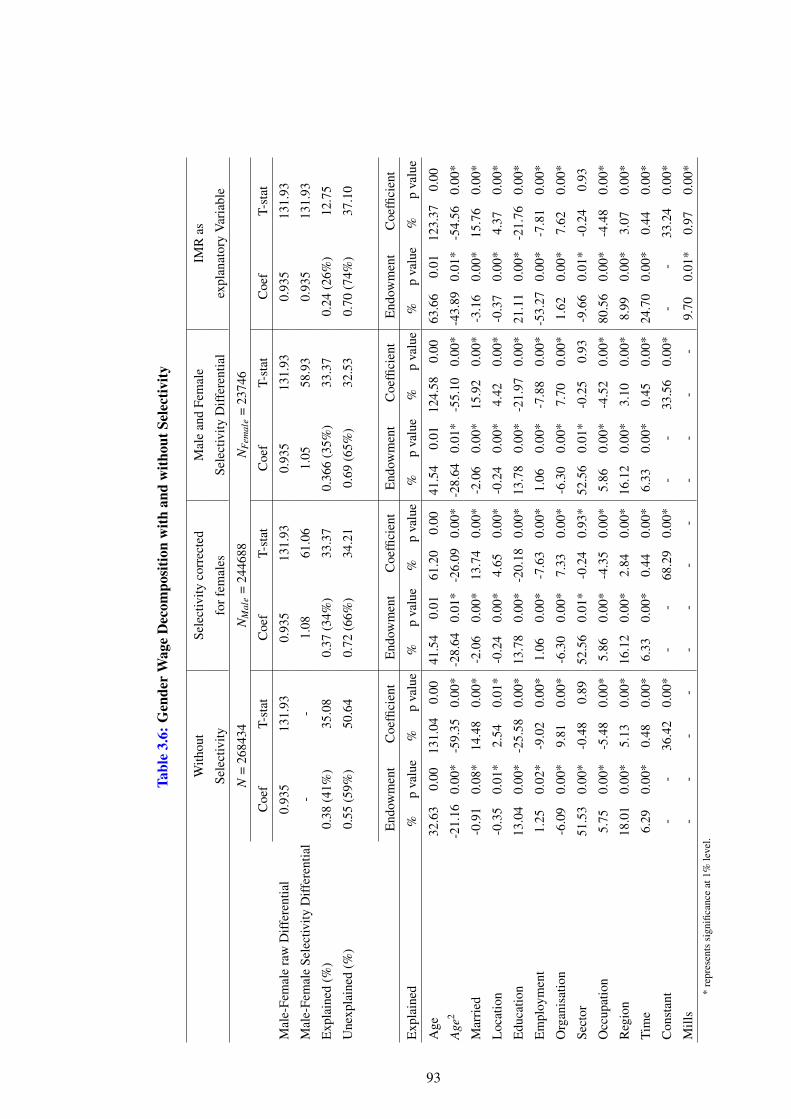
Tabl
e3.
6:G
ende
rW
age
Dec
ompo
sitio
nw
ithan
dw
ithou
tSel
ectiv
ity
With
out
Sele
ctiv
ityco
rrec
ted
Mal
ean
dFe
mal
eIM
Ras
Sele
ctiv
ityfo
rfem
ales
Sele
ctiv
ityD
iffer
entia
lex
plan
ator
yV
aria
ble
N=
2684
34N
Mal
e=
2446
88N
Fem
ale
=23
746
Coe
fT-
stat
Coe
fT-
stat
Coe
fT-
stat
Coe
fT-
stat
Mal
e-Fe
mal
era
wD
iffer
entia
l0.
935
131.
930.
935
131.
930.
935
131.
930.
935
131.
93
Mal
e-Fe
mal
eSe
lect
ivity
Diff
eren
tial
--
1.08
61.0
61.
0558
.93
0.93
513
1.93
Exp
lain
ed(%
)0.
38(4
1%)
35.0
80.
37(3
4%)
33.3
70.
366
(35%
)33
.37
0.24
(26%
)12
.75
Une
xpla
ined
(%)
0.55
(59%
)50
.64
0.72
(66%
)34
.21
0.69
(65%
)32
.53
0.70
(74%
)37
.10
End
owm
ent
Coe
ffici
ent
End
owm
ent
Coe
ffici
ent
End
owm
ent
Coe
ffici
ent
End
owm
ent
Coe
ffici
ent
Exp
lain
ed%
pva
lue
%p
valu
e%
pva
lue
%p
valu
e%
pva
lue
%p
valu
e%
pva
lue
%p
valu
e
Age
32.6
30.
0013
1.04
0.00
41.5
40.
0161
.20
0.00
41.5
40.
0112
4.58
0.00
63.6
60.
0112
3.37
0.00
Age
2-2
1.16
0.00
*-5
9.35
0.00
*-2
8.64
0.01
*-2
6.09
0.00
*-2
8.64
0.01
*-5
5.10
0.00
*-4
3.89
0.01
*-5
4.56
0.00
*
Mar
ried
-0.9
10.
08*
14.4
80.
00*
-2.0
60.
00*
13.7
40.
00*
-2.0
60.
00*
15.9
20.
00*
-3.1
60.
00*
15.7
60.
00*
Loc
atio
n-0
.35
0.01
*2.
540.
01*
-0.2
40.
00*
4.65
0.00
*-0
.24
0.00
*4.
420.
00*
-0.3
70.
00*
4.37
0.00
*
Edu
catio
n13
.04
0.00
*-2
5.58
0.00
*13
.78
0.00
*-2
0.18
0.00
*13
.78
0.00
*-2
1.97
0.00
*21
.11
0.00
*-2
1.76
0.00
*
Em
ploy
men
t1.
250.
02*
-9.0
20.
00*
1.06
0.00
*-7
.63
0.00
*1.
060.
00*
-7.8
80.
00*
-53.
270.
00*
-7.8
10.
00*
Org
anis
atio
n-6
.09
0.00
*9.
810.
00*
-6.3
00.
00*
7.33
0.00
*-6
.30
0.00
*7.
700.
00*
1.62
0.00
*7.
620.
00*
Sect
or51
.53
0.00
*-0
.48
0.89
52.5
60.
01*
-0.2
40.
93*
52.5
60.
01*
-0.2
50.
93-9
.66
0.01
*-0
.24
0.93
Occ
upat
ion
5.75
0.00
*-5
.48
0.00
*5.
860.
00*
-4.3
50.
00*
5.86
0.00
*-4
.52
0.00
*80
.56
0.00
*-4
.48
0.00
*
Reg
ion
18.0
10.
00*
5.13
0.00
*16
.12
0.00
*2.
840.
00*
16.1
20.
00*
3.10
0.00
*8.
990.
00*
3.07
0.00
*
Tim
e6.
290.
00*
0.48
0.00
*6.
330.
00*
0.44
0.00
*6.
330.
00*
0.45
0.00
*24
.70
0.00
*0.
440.
00*
Con
stan
t-
-36
.42
0.00
*-
-68
.29
0.00
*-
-33
.56
0.00
*-
-33
.24
0.00
*
Mill
s-
--
--
--
--
--
-9.
700.
01*
0.97
0.00
**
repr
esen
tssi
gnifi
canc
eat
1%le
vel.
93
If only females selectivity is taken into account, the results in the adjusted offered wage gap
are 1.08 log points with 34% explained and 66% unexplained. However, the adjusted gap nar-
rows down to 1.05 log points if selection effects of both genders were incorporated. These results
indicate that without selectivity results are downward biased. The detailed decomposition of the
female selectivity equation shows slightly different endowment effects, whereas the coefficient
effects vary a lot compared to when selection effects are not accounted for. Interestingly, it is
revealed that the characteristics effect remains unchanged; however, there is an increase in the
coefficients effects of males when the Inverse Mills ratio (IMR) is included in the males and fe-
males selectivity differential equation compared to the selectivity corrected equation for females
only. Again the major share (more than 50%) is coming from the sectors, age (40%), regions
(16%) and education (13%). The fourth panel presents the results if IMR is considered as an
explanatory variable in the gender wage decomposition equation. The adjusted male-female se-
lectivity difference is same as the raw difference of wages. However, the contribution of explained
part has dramatically gone down to 26% and of unexplained part goes up to 74%. Interestingly
the contribution of the coefficient effect remains unchanged. However, the share of endowment
characteristics gets almost reversed compared to the third panel of results. The contribution of
employment and sectors becomes negative with 53.2% and 9.6% respectively. The share of occu-
pation is the highest at 80.5%. Education contributes to 21.1% whereas, regions share is declined
to 8.9% with the inclusion of IMR as an explanatory variable in the selectivity equation. On the
basis of these one can argue that the inclusion of occupation in the earnings equation may have
accounted for the discrimination effect. To understand the pay gap fully, gender wage decompo-
sition is calculated with and without selectivity but taking out the occupation variable from the
list of explanatory variables. The results are presented in Table B3 in the Appendix. The results
without selectivity remains more or less the same. The contribution of education is increased upto
2% and employment is reduced to 0.01%. In the second panel of results of selectivity corected
equation for females, the contribution of explanatory variables in the explained part does not show
much difference compared to the results of Table 3.6. The exception is education (increase by
3%), sector ( increase by 5% and employment become negative (-0.25%). The results of contribu-
tion of explained part of the selectivity differential decomposition equation of males and females
stays the same as selectivity equation of females alone. Some differences have been observed in
the shares of unexplained part of the differential equation. The share of sectors is increased to
5% in the explained part, whereas it’s share in an unexplained part is reduced by 0.25% but still
94
shows negative contribution. The employmet share in the endowment has reduced from 1.06% to
-0.25 %. Although its share in the coefficient effect is reduced to 2% but remains negative. When
using IMR as an explanatory variable in the final panel of the Table, the biggest change is seen in
the contribution of sectors i.e. 93%. The share of education and region is increased by10% ( i.e.
26% and 25% respectively). The share of IMR is -63% compared to 9.7% when the occupation
was included in the decomposition equation. So the major differnce in both equations is due to the
contribution of the inverse Mill’s ratio.
The findings reveal that there exists a positive and statistically significant gender wage gap.
Within the explained or endowment part, the most important contributing factor is sector. The
positive coefficient of this variable clearly identifies that sectors of employment plays a key role
in widening the gap between the both gender groups in Pakistan. Referring back to the summary
statistics in Table 3.2 and 3.3, the proportion of males’ is higher in most of the sectors of em-
ployment. Another imperative contributing factor that explains endowment effect is education,
with a positive and significant share of more than 13% in widening the gender gap. However, the
coefficient difference due to education accounts for lessening the wage differential by 25.6%. As
women are less educated relative to men therefore, it can be argued that marginal return to educa-
tion is higher for females than males. With the consideration of self selection bias in case of males
and females or females only, the endowment parts are contributed by a positive effect of education
whereas the coefficients part shows negative impact of education. The mean level of education is
low for both males in females in the sample (see 3.2 and 3.3). The findings suggest that education
is crucial to narrow the wage gap. With the consideration of selection bias, more than 20% of the
share of unexplained part is coming from education in all the decomposition equations. When the
IMR is considered as explanatory variable, the contribution of education further increases relative
to other consideration. Interestingly, the contribution of occupations in the this specification is
approximately 81% in contrast to with and without correcting for selectivity equations where the
share is either 5.75% or 5.86%. The net impact of the variables of age and age square is 11.5%
in standard Oaxaca decomposition that increases to 12.9% in case of selectivity adjustment of
males and females, further, it increases to 19.8% in the specification in which the IMR is included
as explanatory variable separately. The net impact of age and age square is approximately the
same (68.8% - 71.7%) in all the considerations except in case of female selectivity in which it
decreases to 35.1 %. In response to the net impact of the variables of age and age square, the
explained as well as the unexplained differential between the males and females earnings is in-
95
creased. This indicates that discrimination increases with age. The characteristic effect of marital
status is quite low and shows reduction in a wage gap in specifications. But the coefficient effect
implies an increase in the discrimination against women between 13.7% to 15.7%. The highest
level of discrimination against earnings of females is coming from the intercept (68%) in the fe-
male’s selectivity decomposition output compared to 36% with no selection effects and 33% with
male-female differential selectivity effects.
“ A related issue that has received much attention in the literature is that the decomposition
results for categorical predictors depend on the choice of the omitted base category” (Jones and
Kelley (1984); Jones and Kelley (1984); Oaxaca and Ransom (1999); Nielsen (2000); Horrace and
Oaxaca (2001); Yun (2005a)). Usually dummy variables are included in the regression equation
to model the effect of categorical variables. Further, to avoid collinearity, one of the categories is
omitted. The decomposition results change with the chosen omitted category. However, it is not
critical for the sum of contributions of the single indicator which is the total contribution of the
categorical variable, as it is unaffected by the choice of the omitted category. On the other hand,
from the unexplained part of the decomposition, there is a trade-off between the differences in
intercepts and the attributed part (Jann (2008)). Therefore, in the context of Oaxaca decomposi-
tion, (Suits (1984); and Yun (2005a)) suggest a convenient method that is, “ to estimate the group
models by using the standard dummy coding and then transform the coefficient vectors so that
deviations from the grand mean are expressed and the coefficient for the base category is added”
(Yun (2005a), p.2) If OB methodology is applied to such transformed estimates, the results are
independent of the choice of the omitted category. Moreover, “ the results are equal to the simple
averages of the results one would get from a series of decompositions in which the categories are
used one after another as the base category” (Jann (2008), p.9).
Following the above mentioned approach, the decomposition results contains employment, or-
ganization, sector, occupation and location that includes the sets of dummy variables which repre-
sent the categorical variables and then transforms the coefficients so that the decomposition results
become invariant to the choice of the omitted category. The “ Employment category,” includes the
dummies of paid employment, self employment in agriculture whereas the dummy of self em-
ployment in non-agriculture has been omitted. The positive coefficient suggest that the males
participate more in paid work than women which results in a wage gap among them. The “ Organ-
isation ” consists of government job, private job and private business, and NGO (non-government
organization); with other organisations is the omitted category. The negative coefficient suggests
96
that the organization narrows the wage gap between males and females. It demonstrates the fact
that there are some organizations, potentially the government organizations where recruitment of
the employees is based on merit and where a set pattern of salaries is followed in accordance with
the rank/grade or position of the employee regardless of gender. Thus, organisation alone accounts
for females having higher wages than males. Furthermore, the “ Sector ” variable embrace agri-
culture/ forestry/ fishery, mining/ quarrying, manufacturing, electricity/ gas / water, construction,
wholesale& retail, transport & storage, real estate & insurance and social services while other
sectors is the omitted category. The positive and high magnitude of its coefficient indicates that
the difference in offered wages is highest in the sectors of Pakistan’s economy. “ Occupation ”
is a set of nine dummies for senior official or manager, professional, technician, clerk, service
or shop salesperson, skilled agriculture or fishery, craft or trade worker and machinery operator
with elementary occupation as the omitted category. The coefficient of this variable clearly de-
picts the existence of a wide gap between the wages of males and females. Traditionally, there
exists either male or female dominated occupations; therefore, gender-stereotyping attributes may
have contributed in widening this gap. The “ location” includes rural and urban dummy along
with the provincial dummies of Punjab, Sindh and Khyber-Pakhtunkhwa whereas the Baluchistan
province is considered an omitted category. The positive coefficient in all the four panels of de-
composition results demonstrates that location does contribute in widening the gender wage gap
in overall Pakistan. Regarding the coefficient effects on the type of employment in sectors and
the organisations, the discrimination seems relatively low. It can be inferred that the females are
not being discriminated on the basis of having a job in different sectors and organisations. How-
ever, the categorical variables of the occupation and location increase the discrimination against
women. The possibility of occupational segregation leads to increased discrimination.
97
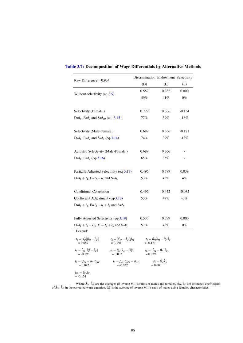
Table 3.7: Decomposition of Wage Differentials by Alternative Methods
Raw Difference = 0.934Discrimination Endowment Selectivity
(D) (E) (S)
Without selectivity (eq-3.9)0.552 0.382 0.000
59% 41% 0%
Selectivity (Female ) 0.722 0.366 -0.154
D=I1, E=I2 and S=I10 (eq- 3.15 ) 77% 39% -16%
Selectivity (Male-Female ) 0.689 0.366 -0.121
D=I1, E=I2 and S=I3 (eq-3.14) 74% 39% -13%
Adjusted Selectivity (Male-Female ) 0.689 0.366 -
D=I1, E=I2 (eq-3.16) 65% 35% -
Partially Adjusted Selectivity (eq-3.17) 0.496 0.399 0.039
D=I1 + I4, E=I2 + I5 and S=I6 53% 43% 4%
Conditional Correlation 0.496 0.442 -0.032
Coefficient Adjustment (eq-3.18) 53% 47% -3%
D=I1 + I4, E=I2 + I5 + I7 and S=I8
Fully Adjusted Selectivity (eq-3.19) 0.535 0.399 0.000
D=I1 + I9 + I10,E = I2 + I5 and S=0 57% 43% 0%
Legend:
I1 = X′F [βM− βF ] I2 = [XM− XF ]βM I3 = θM λM− θF λF
= 0.689 = 0.366 = -0.121
I4 = θM [λ 0F − λF ] I5 = θM [λM− λ 0
F ] I6 = [θM− θF ]λF= -0.193 = 0.033 = 0.039
I7 = [ρM− ρF ]σµF I8 = ρM [σµM− σµF ] I9 = θM λ 0F
= 0.042 = -0.032 = 0.000
I10 = θF λF= -0.154
Where λM , λF are the averages of inverse Mill’s ratios of males and females. θM , θF are estimated coefficientsof λM , λF in the corrected wage equation. λ 0
F is the average of inverse Mill’s ratio of males using females characteristics.
98

The alternative methods of wage differential decompositions are presented in Table 3.7 . The
alternative methods are based on various assumptions regarding the treatment of coefficient and
endowment effects computed from the Probit equations of males and females. Starting from the
first decomposition that is standard Oaxaca, the raw wage differential of 0.94 is decomposed in
to discrimination (59%), endowment (41%) and selectivity effects. The second decomposition is
based on the assumption that there is selection bias against in females only. In this decomposition,
the selectivity is negative indicating that the wage differentials are downward biased in the absence
of selection effects. Further, the discrimination effect is higher in second decomposition relative
to the first one. The assumption of selection bias exists in both males and females lead towards
the third decomposition. The endowment effects are same in the second and third decomposi-
tion obviously due to no change in the coefficients of females and average of the characteristics
of male and females of the Probit selection equations. Further, there are slight changes in the
discrimination and selectivity effects in the third decomposition relative to second. The fourth
decomposition is based on the assumption that the endowment effects of the selection equations
should be adjusted in the endowment and discrimination of the wage differential decompositions,
hence the coefficients effect of the selection equation is termed as selectivity. Further, the sixth
decomposition is based on the assumption that the endowment and coefficient effect of the se-
lection equation are fully adjusted in the like effects of wage differential decomposition. Fourth
and sixth decompositions yield results nearer to the standard Oaxaca decomposition. The fifth
decomposition is based on the assumption that the difference of conditional correlation coefficient
is selectivity whereas the difference in error variances of the wage equations is adjusted in the
endowment effect of the wage differential. Due to the issue of identification of conditional corre-
lation coefficients, normalization is adopted to get the parameters of the inverse mill ratios in both
the equations. Therefore, this decomposition provides 3% lower estimate of the wage differential
(not summing up to 100%).
3.6 Conclusion
The empirical analysis shows the existence of the wage gap between males and females in Pak-
istan. The individual characteristics such as age, level of education, sectors, occupations and
regions play a key role in explaining the amount of this gap. From the decomposition results
the explained component is 41% and unexplained is 59% in the absence of selectivity. However,
when accounted for selection effects in the wage decomposition equations the results are upward
99
biased explaining 39% endowment effect, 77% coefficient effect and -16% the selection effect.
The gender wage gap widens after correcting for selection bias. Gender differences in characteris-
tics determining selection in males and females equation narrows the observed wage gap, whereas
the coefficient effects serve to increase the gap. The results point towards the perceived discrim-
ination in the labour market. The findings imply that a wide wage gap in the labour market is
explained by characteristics such as education and employments types such as sectors and occu-
pations. However, it is has been observed that female remuneration is not based on discrimination
alone rather it depends on the education level which is low in Pakistan which could be a potential
reason to increase gender wage differential in the labour market. Occupation segregation or gen-
der stereotype attributes may also be the possible explanations for discrimination against females.
Therefore, according to the economics literature, the kind of discrimination that exist in Pakistan’s
labour market is actually the pre-market discrimination and the statistical discrimination.29
29Basically the models of discrimination in Economics are divided into two groups. One is competitive that studiesindividual maximising behaviour including discrimination and the other model is collective according to which groupsact against each other in a collective manner. Economic analysis is mainly based on the competitive approach whichis further divided in two groups: taste-based discrimination and statistical discrimination. Beckers model is focusedon the former case whereas, the studies after Phelps (1972) and Arrow (1973) emphasised on the statistical theory.Taste based discrimination means there is a disamenity value to employing minority workers. The main argument o thestatistical discrimination literature is that employers have limited information about the employees skills. This givesthem a reason to use observable characteristics such as race and gender to infer their expected productivity. Most of thestudies in economics focused on the statistical discrimination especially when considering gender or race.
100
Chapter 4
Explaining Occupational Differences across Genders and Regions in
Pakistan
4.1 Introduction
According to the study of ILO (2006), females are considered inferior participants in Pakistan’s
labour market. This perception is based on the traditional view point that the primary responsibil-
ities of females are to perform household and reproductive activities, rather than participating in
education and employment.
(Blau et al. (1986), Blau and Kahn (1996), Bayard et al. (1999), Teo (2003), and Zveglich Jr
and van der Meulen Rodgers (2004)) provide evidence that females are often concentrated in the
low earning jobs while males are usually employed in high income occupations. The point is, if
the criteria of selecting a particular occupation is financial returns, then why do females select
low waged occupations compared to male counterparts who decide to go for the high salaried
employment? The question arises as: to whether it is an individual’s own choice to enter into a
certain occupation, or there are some other factors involved to facilitate their entry into a particular
occupation? The answer to these questions has been explored in many studies emphasising the
issue of occupational choice. However, for an in-depth analysis it is important to understand
the gender differences in the occupations specifically in the context of low-income countries. For
instance, in Pakistan where the disadvantageous position of females and the lower socio-economic
status has not changed much overtime. Few studies 30 have undertaken this issue to confirm the
existence of occupational segregation and concentration of women in low paid jobs (Nasir (2005)).
Females are perceived to be second earners and are therefore are selected in those occupations
where males are least preferred (Siddiqui et al. (2003)). Based on the statistics, another study
inferred that the high gender pay gap and a higher female participation rate in elementary and mid
level occupations is an outcome of the presence of vertical segmentation (SPDC (2008)).
Furthermore, given the evidence of discrimination against women in Pakistan’s labour market
in the previous chapter, the findings indicate the potential existence of occupational segregation.
Hence, this provides motivation for the current chapter to determine the extent of occupational
30Ashraf and Ashraf (1996), Nazli (2004), Siddiqui et al. (2003), Ahmed and Hyder (2008)
101
differences between males and females in Pakistan. None of the studies conducted in Pakistan have
estimated the occupational differences among males and females in the labour market. Therefore,
it is expected that this study will contribute to the literature by using a non-linear decomposition
technique i.e. using a binary dependent variable to decompose the employment differences in nine
occupations across gender and regions.
The main objective of this chapter is to estimate the occupational differences across gender and
regions in Pakistan. In this regard, the occupational gap between males and females within nine
occupations in the labour market has been estimated. Further, for a comprehensive spatial analysis,
the occupational differences are calculated separately for overall Pakistan, its four provinces and
all the districts within each province.
The regions in Pakistan are unique and diversified according to their geographical position.
Within the four provinces there are 110 districts: 36 in Punjab, 22 in Sindh, 24 in KPK and
28 in Baluchistan. Apart from the capital city of Pakistan i.e. Islamabad, the provincial capital
cities in Punjab (Lahore), Sindh (Karachi), KPK (Peshawar) and Baluchistan (Quetta) provide
relatively higher levels of earning opportunities and services to the natives. Moreover, individuals
from nearby cities also get attracted to the big cities in search of jobs and better living standards.
Occupation participation is effected by the difference in the labour market conditions across the
regions. Rural and urban dynamics has also played an important role.
The classification of regions in Punjab province as suggested by Wilder (1999), divides Punjab
into four regions: northern, central, southern and western. This classification is based on the geo-
graphical boundaries, regions economic differences, variations in irrigation, agricultural patterns,
differences in farm-size and land tenure system, and distinct historical, cultural, and linguistic
influences in each region (pg. 34).
Jamal (2011) computes the Index of Multiple Deprivation (IMD) for the provinces and the
respective districts. He has also provided the district ranking based on households socio-economic
deprivation. The index is calculated by using five groups of composite indicators; deprivation in
education, health, housing quality, housing services and household wealth.
Regions of Pakistan are not only distinct in their respective culture, linguistics and ethnic
diversities but also differ in the historical background and socio-economic conditions. The urban
regions of Punjab and Sindh are relatively modern and liberal. Public and civil services are mainly
in the big cities and capital cities. Therefore the smaller regions may feel deprived. There exist
regional disparity among the provinces. Punjab is considered to be the most developed province
102
of all. It is situated near the five rivers with the largest agricultural land and a proper developed
irrigation canal system. It is the most populous province as well. So the population in the rural
areas is mostly engaged in agriculture related occupations. Females are also engaged to the farm
related activities in the form of paid or unpaid work. Punjabis are well represented in the civil
and military services. They have inhereted skills and a relatively better education system. It is a
well known perception among the citizens that the districts or cities close to Lahore are developed
whereas some areas of Southern Punjab are relatively more deprived. According to Jamal (2011)
for district ranking on the basis of IMD, Lahore is the least deprived district whereas Rajanpur is
the highest deprived district in Punjab.
Similarly, in Sindh the urban areas are far better than the rual areas. For instance Karachi is
the most developed city and the largest city of Pakistan. Its population is more than 10 million.
However, the districts like Mirpur Khas, Tando Allah Yar, Jamshoro etc. are very much deprived
of the basic facilities of life including health, education and housing facilities. The most deprived
district is Tharparkar. There exist a big development gap among the districts of Sindh. Sindhi
people are very much conscious about their distinct language and cultural identity.
Khyber Pakhtun khwa (KPK) province was known as NWFP (North West Frontier Province).
It is the home of Pathans ot Pukhtoons. Most of the area is hilly and mountaneous. It’s North
Western Mountains are full of mineral resources and forests. The plains of the province are fertile
and suitable for cultivation of all kinds of crops. The south eastern part of the region is plain.
Therefore, livelihood of people living in mountains and plains varies. The Pathan community
dominates the cultural, social, political and ethnic tribal society. However, it is very different from
the Baloch authoritarian tribe culture. Kohistan is the most deprived region whereas Peshawar and
Khairpur are the lowest deprived districts of this province.
Balochistan is the largest province of Pakistan by area and situated in the southwest of Pak-
istan. On the whole it is dominated by a tribal society lead by the chief of the tribes. People in
the tribes are strictly bound to obey the chief called ‘Sardar” of the tribe. That is why it is the
least developed area. The region basically lacks an adequate infra-structure. Mainly the land is
barren but still agriculture is the major occupation and very limited participation is in industries.
Most of the districts are deprived and largely underdeveloped however, the provincial economy is
dominated by the rich natural resources such as natural gas and coal. The least deprived district is
Quetta whereas the highest deprived distric is Dera Bugti. Due to the tribal society system most
of the females in Balochistan and KPK are not allowed to work outside the house. The female
103
literacy rate in KPK is increasing but it has not been translated to the labour force. Therefore, fe-
males in these regions are mainly engaged in female dominating occupations related to agriculture
or professional jobs (such as teaching or nursing etc.).
Clearly Punjab has an edge over the other provinces which has somehow created disequi-
librium across the regions and smaller regions feel deprived and under-developed. It is imper-
ative to create a working balance between the diversification and unification forces for smooth
governance of Pakistan. Regional equality will help strengthening the government institutions.
The pre-requisite is improving the administrative relationship between the central government and
provinces.
4.2 Literature Review
Occupation segregation has been a topic of interest and considered important in a multidisciplinary
research. There exist several studies on wage inequality and occupation segregation in the labour
market. However, there are a limited number of studies that focus on the gender differential in
occupation structure. It is important to mention here that occupation segregation and occupation
differences are two entirely different concepts. They should not be mixed up and cannot be in-
terpreted interchangeably. By definition they are two entirely different words providing diverse
range of meanings. The segregation is isolation and separation, whereas differences are explained
as dissimilarity, disparity, inequality or gap.
Human capital and discrimination is a key subject matter in labour economics. Empirical
evidence in the literature is on the supply oriented human capital explanation and demand oriented
discrimination explanation. Polachek (1981) argues that individuals vary in their human capital
which may have strong implications on the wage distribution of the population. The study further
claims that within most societies women are by and large relegated to different occupations than
men. It is usually hypothesised that for females time in and out of labour force depends on their
occupation. The results show that home time effects the odds of being in each occupation. Home
time reduces the probability of being in professional and managerial type occupations.
Moheyuddin (2005) explains that human beings can differentiate themselves by obtaining ed-
ucation, skills, training and experience. On the basis of these qualities they select the profession
which may depend on many factors for example earnings, status, management, job security, au-
thorities, working hours, gender, personal interest, white collar, blue collar etc. The study con-
cludes that income and education inequality are the key problems specifically in the developing
104
countries, which in turn, have a negative impact on economic growth.
Identifying the underlying causes of racial and gender differences in education, labour mar-
ket, health, and other outcomes has been the goal of an enormous body of literature in the social
sciences. Since 1973 there exists an extensive empirical literature on the Blinder Oaxaca Decom-
position method. This methodology is applied mainly in the context of linear regression models.
However, binary dependent variables require the estimation of non-linear models. An extension
of OB decomposition approach is by Fairlie (1999, 2005) who developed a decomposition method
for probit and logit models. Yun (2005a,b) also extends it to a detailed decomposition for all
explanatory variables. Bauer and Sinning (2008) applied it to the count data models, including
Poisson and negative binomial zero-inflated models. Bauer and Sinning (2010) have further ex-
tended it to truncated regression and tobit models. This approach has not yet been applied on the
employment or occupation differences across groups except for Blackaby et al. (2002). They used
employment probits to examine the employment differences among ethnic groups and to estimate
selection effects on earnings. Therefore, the main idea of this chapter has been extracted from
Blackaby et al. (2002) and the methodology is applied on the Pakistani data to decompose the
occupation differences across gender and regions in Pakistan.
The topics of occupational segregation, choices and differences are of serious concern in the
Pakistani labour market. It has been observed in various studies that returns to different occu-
pations, a worker receives, vary significantly across occupations in Pakistan. Khan et al. (1985)
found that differences in earnings are due to inter-regional differences and the occupational differ-
ences.
Earnings differentials across various occupations is an area of discussion in the literature of
the labour market of Pakistan. However, there is no single study that highlights the role of gender
differences in occupations. Nasir (2005) investigates the occupational choices. Ahmed and Hyder
(2008) and Irfan et al. (2013) determine the occupational segregation and Nazli (2004) discusses
the role of occupation in determining earnings differences. Ahmad (2001) and Akhtar and Sadiq
(2008) explore the existence of inequality in nine occupations.
Nasir (2005) explores the determinants of occupational choice and provides evidence in sup-
port of the existence of gender segregation in the labour market of Pakistan. The study utilizes
2001-02 cross-section data from the Pakistan Integrated Household Survey (PIHS) with the sample
of 13,793 individuals (86% males and 14% females) aged 10 to 65 years. The determinants in-
clude age, education, training, gender, marital status earnings, occupations, etc. Further, studying
105
in private schools and English as a medium of instruction in schools are considered as important
factors to capture the effect of higher investment in human capital. The descriptive statistics of
the data indicate that the majority of females are related to craft making, agriculture and teaching
profession. The rest of the sectors are male dominated and are considered as high paid sectors. A
Multinomial logit model of occupational choice is employed and Education is the most important
determinant. Due to significant gender differences, separate models are estimated for males and
females. Further, he tries to explore the gender difference due to characteristics and finds that
the differences are not due to characteristics. This study lacks any proper technique for evaluat-
ing the gender differences for instance (Oaxaca Blinder etc.) and just uses the one dimension of
characteristics to explore the gender differences. Few studies in Pakistan have measured occupa-
tional segregation by using the index of dissimilarity proposed by Duncan and Duncan (1955) 31
Nasir (2005) adopts the quantile wage regression approach to explore the gender differences in
public and private sector of Pakistan. The data is taken from 2005-06 Labour Force Survey (LFS),
Pakistan. The sample includes 10,401 workers aged between 14 and 60 (87% males and 13 % fe-
males; 54% in public sector and 46% in private). Four wage determination equations are estimated
for gender and sectors (public and private). Conventional variables such as age, education, expe-
rience, training, marital status, location and occupation are considered as explanatory variables.
The wage differential in the public sector is 9% as compared to 37% in the private sector. After
the confirmation of a pay gap at different points, the study explores occupational segregation. An
Index of dissimilarity (Duncan and Duncan (1955)) by gender is used as the dependent variable
and the wage gap along with the regional dummy variables as explanatory variables. The results
suggest that a wider wage gap has a significant impact on the occupational segregation.
Irfan et al. (2013) utilize the latest data of Pakistan Labour Force Survey (2009-10) of 72,933
individuals and compute the Duncan index of segregation for nine occupations. The findings
confirm the gender based segregation in each occupation especially, in managerial, skilled and
elementary occupations. A Tobit regression is applied to find the the determinants of segrega-
tion. Results show that with an increase in the age of the respondents the segregation is reduced,
whereas with higher education attainment the gender based segregation gets elevated which may
be due to the selection of occupations. The study argues that educated people take into account the
31The formula D = 12 ∑
Ni |mi− fi| is known as Duncan’s D which serves as a measure of dissimilarity between two
distributions. It calculates the percentage of males and females working in a particular occupation. First of all, identifythe number of occupations (e.g. i = 9). Then, the number of males or females in the given occupation should be dividedby the total number of males or females in all of the occupations where mi is the proportion of total males in occupation1...9 relative to the total number of males population in all the occupations, whereas fi is the proportion of total femalesin occupation 1...9 relative to total number of females working in all the occupations.
106
suitability of their gender while selecting a particular profession as some of the occupations are
gender associated occupations. It further states that the provinces of Pakistan vary in behaviour to
one another except Punjab, and this is justified by the argument that there exists more awareness
among Punjabis about the selection of the professions.
Nazli (2004) explains the effect of education, experience and occupation on earnings in Pak-
istan. The Pakistan Socio-Economic Survey (PSES) 1998-99 containing the data of 1,271 indi-
viduals is utilized for the estimation purposes. The education, experience and interaction of these
along with the conventional control variables were considered as determinants. The study found
significant differences in earnings across occupations. However, gender differences are not dis-
cussed in the paper.
The main difference between the existing literature related to Pakistan and this (chapter) re-
search study is that previous studies focused on the issues related to occupational segregation or
occupational choices. More precisely, they have discussed the factors that contribute to the selec-
tion of a specific job or occupation. However, this analysis explores the occupational difference
between males and females who are already working or employed in the particular occupation.
Besides, the study looks into their characteristics to get an idea of what factors explicates the ex-
plained and unexplained part of gender difference in each occupation. Although, a massive work
has been done globally on the labour markets of other countries, there is still a lot that needs to
be done in case of Pakistan. It is expected that this study will contribute to the body of literature
in three different ways. First in terms of data that has been used for the first time that covers
more than 80,000 households over three repeated cross-sections, secondly the methodology has
not been used so far in the studies related to Pakistan and thirdly, it fills the gap by improving upon
the previous studies on occupations in Pakistan’s labour market.
4.3 Data and Variables
This chapter has utilised the pooled data constructed from three cross-section datasets (2005, 2007
and 2009) from Pakistan Social and Living Standard Measurement (PSLM) Survey, as used in
chapters 2 and 3. The PSLM data provides more detailed information on occupations and house-
hold indicators at micro level than Labour Force Survey (LFS) . Moreover, it is logical to use the
same data source in order to make the findings and interpretation convincing and consistent with
the previous chapters.
The dependent variable is a binary variable explaining the difference between males and fe-
107
males in selecting the occupation by taking the value of 1, if participate in the particular occu-
pation and 0 if not. Broadly there are nine occupations of employment in Pakistan; so there are
nine different dependent variables for each of the nine equations. More specifically, the binary
variable explains the probability differential between males and females selecting into occupation
of senior officials, professionals, technicians, clerks, sales persons, skilled workers in agriculture
and fishery, craft and trade workers, plant and machinery operators and unskilled or elementary
occupations.
The explanatory variables used in the analysis are age, age squared, marital status, years of
schooling, location dummy ( i.e. rural-urban), dummies for regions (i.e. four provinces namely
Punjab, Sindh, KPK and Baluchistan) and time dummies. Moreover, the interactive variables of
location and regions are used in the overall Pakistan regression analysis. The selected sample is
individuals from 10 to 60 years old.
Looking at the frequency distribution (see Tables C1 and C2 in appendix) of the occupations
in Pakistan, it is observed that male participation is 85.5% out of the total participation of indi-
viduals in all the nine occupations in overall Pakistan. However, females encompass only 14.5%
of participation. Most of the working class in Pakistan are concentrated in agriculture and fishery.
Further, it is alarming that the majority of people are related to unskilled elementary occupations.
It persuades us to think about the educational background of these individuals. Close examination
of the data reveals that 58.5% of females and 29% of males in the sample are illiterate (see Table
4.1). The mean education level of males in these occupations is 5.2 years i.e. up to primary level,
however, for females it is just 2.9 i.e. approximately three years of schooling. Almost 86% of
females and 82% of males are concentrated in services, agriculture and elementary occupations.
Interestingly, 6.3% of females are professional which is encouraging to know that at least the
6% of females who acquire higher education, are able to exploit the opportunities in the labour
market. Pakistan is a multi-cultural country that comprises of different sub-cultures, norms and
style of living in its provinces. Accordingly, the literacy and employment rate varies across gender
and regions. Despite the provincial disparity on a one to one basis, the overall Pakistan’s data
remains the true representation of all the regions in aggregate terms. The total number of males
are 137,285 (41%) from Punjab, 90,877 (27%) from Sindh, 52,205 (15.5%) from KPK and 55,249
(16.5%) from Baluchistan in the sample, whereas females belong to Punjab are 33,098 (58%),
Sindh 12,313 (21.6%), KPK 5,938 (10.4%) and Baluchistan are 5,732 (10%). These figures not
only explain how the population is spread over the four regions but, also reflect the behaviour of
108
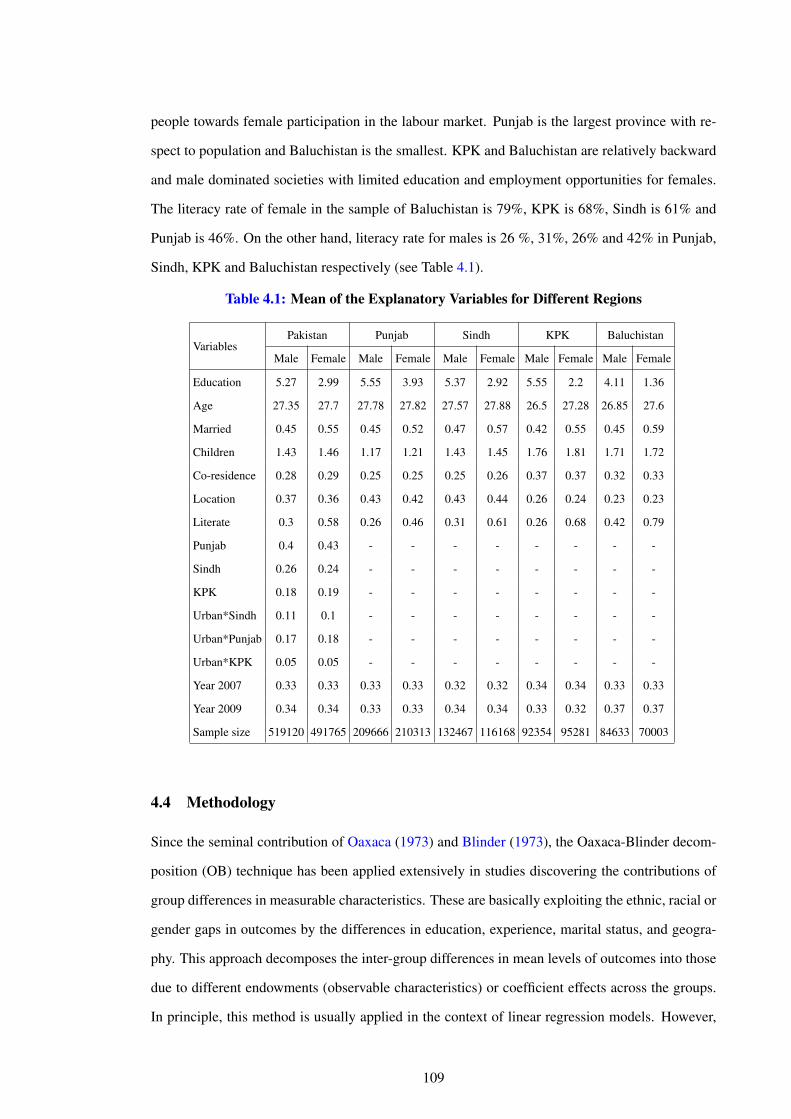
people towards female participation in the labour market. Punjab is the largest province with re-
spect to population and Baluchistan is the smallest. KPK and Baluchistan are relatively backward
and male dominated societies with limited education and employment opportunities for females.
The literacy rate of female in the sample of Baluchistan is 79%, KPK is 68%, Sindh is 61% and
Punjab is 46%. On the other hand, literacy rate for males is 26 %, 31%, 26% and 42% in Punjab,
Sindh, KPK and Baluchistan respectively (see Table 4.1).
Table 4.1: Mean of the Explanatory Variables for Different Regions
VariablesPakistan Punjab Sindh KPK Baluchistan
Male Female Male Female Male Female Male Female Male Female
Education 5.27 2.99 5.55 3.93 5.37 2.92 5.55 2.2 4.11 1.36
Age 27.35 27.7 27.78 27.82 27.57 27.88 26.5 27.28 26.85 27.6
Married 0.45 0.55 0.45 0.52 0.47 0.57 0.42 0.55 0.45 0.59
Children 1.43 1.46 1.17 1.21 1.43 1.45 1.76 1.81 1.71 1.72
Co-residence 0.28 0.29 0.25 0.25 0.25 0.26 0.37 0.37 0.32 0.33
Location 0.37 0.36 0.43 0.42 0.43 0.44 0.26 0.24 0.23 0.23
Literate 0.3 0.58 0.26 0.46 0.31 0.61 0.26 0.68 0.42 0.79
Punjab 0.4 0.43 - - - - - - - -
Sindh 0.26 0.24 - - - - - - - -
KPK 0.18 0.19 - - - - - - - -
Urban*Sindh 0.11 0.1 - - - - - - - -
Urban*Punjab 0.17 0.18 - - - - - - - -
Urban*KPK 0.05 0.05 - - - - - - - -
Year 2007 0.33 0.33 0.33 0.33 0.32 0.32 0.34 0.34 0.33 0.33
Year 2009 0.34 0.34 0.33 0.33 0.34 0.34 0.33 0.32 0.37 0.37
Sample size 519120 491765 209666 210313 132467 116168 92354 95281 84633 70003
4.4 Methodology
Since the seminal contribution of Oaxaca (1973) and Blinder (1973), the Oaxaca-Blinder decom-
position (OB) technique has been applied extensively in studies discovering the contributions of
group differences in measurable characteristics. These are basically exploiting the ethnic, racial or
gender gaps in outcomes by the differences in education, experience, marital status, and geogra-
phy. This approach decomposes the inter-group differences in mean levels of outcomes into those
due to different endowments (observable characteristics) or coefficient effects across the groups.
In principle, this method is usually applied in the context of linear regression models. However,
109
in case of discrete or limited dependent variables, the ordinary least square approach may yield
biased or inconsistent parameter estimates. Hence, it may provide misleading decomposition re-
sults.
To overcome this issue an extension to the OB approach to non-linear models has been in-
troduced. Fairlie (1999, 2005) develop a decomposition method with binary dependent variables.
Afterwards, Yun (2005a) extended this method that allows a detailed decomposition for all ex-
planatory variables in the non-linear model. Later, Machado and Mata (2005) and Melly (2005)
also build up a decomposition methods for quantile regression models. Regarding linear regres-
sions, Montgomery and Powell (2003) applied the OB decomposition based on Full Information
maximum likelihood Methods (FIML) tobit regressions. Further, Fitzenberger et al. (2006) tai-
lored the OB methodology to probit models to decompose changes in net union densities over
time. Bauer and Sinning (2010) extended this approach to the truncated regression and tobit
models. Finally, Bauer et al. (2007) incorporated the theoretical derivation of all the non-linear
approaches to OB mentioned above and extended it to count data models, including zero-inflated
Poisson and negative binomial models. The most relevant study is Blackaby et al. (2002) that
has used employment probits to examine the employment differences among ethnic groups and
to estimate selection effects on earnings. Therefore, the main idea of this paper has adopted and
replicated the employment difference methodology to the gender occupational differences. More
precisely, due to the fact that the outcome variable is binary, the OB decomposition for probit
models is applied in this chapter to explore the occupation differences among the groups of males
and females. It is expected that this study will contribute specifically to fill the research gap spe-
cially in the literature pertaining to Pakistan by introducing a different approach to determining
the gender gaps in occupations.
4.4.1 Oaxaca-Blinder extension to Probit Model
If the outcome variable is binary and the coefficients are from a probit model then, Oaxaca-Blinder
technique cannot be used directly. Therefore, a non-linear decomposition technique is applied that
uses the estimates from a probit model (see, Fairlie (2005)). Using the same Oaxaca (1973) -
Blinder (1973) decomposition approach as in chapter 3, it is possible to decompose occupational
choice probits into explained characteristics and an unexplained coefficient effects.
OCM1 −OCF
1 = f (X)
.
110
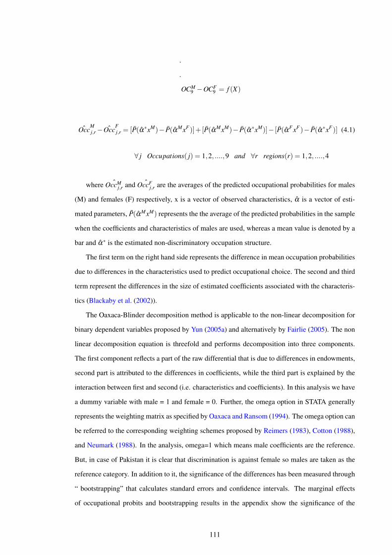
.
.
OCM9 −OCF
9 = f (X)
ˆOccMj,r− ˆOcc
Fj,r = [P(α∗xM)− P(αMxF)]+[P(αMxM)− P(α∗xM)]− [P(αFxF)− P(α∗xF)] (4.1)
∀ j Occupations( j) = 1,2, ....,9 and ∀r regions(r) = 1,2, ....,4
where ˆOccMj,r and ˆOccF
j,r are the averages of the predicted occupational probabilities for males
(M) and females (F) respectively, x is a vector of observed characteristics, α is a vector of esti-
mated parameters, P(αMxM) represents the the average of the predicted probabilities in the sample
when the coefficients and characteristics of males are used, whereas a mean value is denoted by a
bar and α∗ is the estimated non-discriminatory occupation structure.
The first term on the right hand side represents the difference in mean occupation probabilities
due to differences in the characteristics used to predict occupational choice. The second and third
term represent the differences in the size of estimated coefficients associated with the characteris-
tics (Blackaby et al. (2002)).
The Oaxaca-Blinder decomposition method is applicable to the non-linear decomposition for
binary dependent variables proposed by Yun (2005a) and alternatively by Fairlie (2005). The non
linear decomposition equation is threefold and performs decomposition into three components.
The first component reflects a part of the raw differential that is due to differences in endowments,
second part is attributed to the differences in coefficients, while the third part is explained by the
interaction between first and second (i.e. characteristics and coefficients). In this analysis we have
a dummy variable with male = 1 and female = 0. Further, the omega option in STATA generally
represents the weighting matrix as specified by Oaxaca and Ransom (1994). The omega option can
be referred to the corresponding weighting schemes proposed by Reimers (1983), Cotton (1988),
and Neumark (1988). In the analysis, omega=1 which means male coefficients are the reference.
But, in case of Pakistan it is clear that discrimination is against female so males are taken as the
reference category. In addition to it, the significance of the differences has been measured through
“ bootstrapping” that calculates standard errors and confidence intervals. The marginal effects
of occupational probits and bootstrapping results in the appendix show the significance of the
111
explanatory variables (for Pakistan as well as the four provinces namely: Punjab, sindh, KPK and
Balochistan). Further, R-square and z-scores are also given in the appendix (see Tables C1 to C7)
4.5 Decomposition Results of Occupation Probits
The binary outcome variable takes a value of 1 if the individual participates in the particular
occupation and 0 if the individual does not. Occupation probits have been estimated for males and
females along with their marginal effects. On the basis of these, the probit differences between
gender for being in the specific occupation has been decomposed. The employment prospects of
participating in a particular occupation have been examined by decomposing nine probit equations
corresponding to each occupation. The number of observations for males is 520,000 and there are
490,000 females.
In order to get a clear picture of the employment pattern of males and females in all the occupa-
tions, the decomposition analysis is also split over regions. It is well known that Pakistan possesses
a distinct culture due to its religion and historical background, therefore all the provinces, being
situated at different geographical areas have diversified traditions, norms, languages and way of
living (see Castells (2011)). It is expected that occupational participation may vary across genders
and by provinces. Punjab is situated near the five rivers and generally is considered an agricultural
province. It is the most populated region that is why its sample size is bigger than other provinces.
The results for each occupation are presented separately with respect to overall Pakistan, Punjab,
Sindh, KPK and then Baluchistan.
The decomposition results of Senior Officials with respect to all the regions are presented in
Table 4.2 . The explanatory variables that determine the characteristic difference of males and
females as senior officials, managers and legislators include age, age squared, marital status, edu-
cation, an urban dummy, time dummies and regional dummies for Punjab, Sindh and KPK. It has
been observed that the characteristics and coefficients associated with these characteristics differ
across the occupations (see Table 4.3). Overall the empirical findings suggest that the average dif-
ference between the participation rate of males and females as senior official or manager is 0.012
which does not seem to be a big difference. The difference is small in magnitude due to higher
number of observations of not being senior officials. Actually the employed females to male ratio
is 0.066 which means only 6.6 females are employed against 100 males in Pakistan (for refer-
ence see the calculation in Table C18 in the Appendix). Concentrating on Pakistan as a whole the
mean difference in employment is 1.1pp. Consequently in Punjab and Sindh it is 1.2 pp and 1.6
112
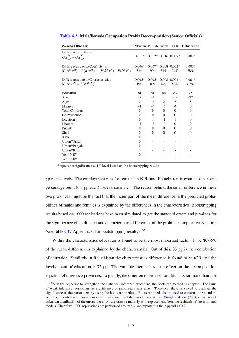
Table 4.2: Male/Female Occupation Probit Decomposition (Senior Officials)
(Senior Officials) Pakistan Punjab Sindh KPK Baluchistan
Differences in Mean0.011* 0.012* 0.016 0.007* 0.007*ˆOccM
j,r− ˆOccFj,r
Differences due to Coefficients 0.006* 0.007* 0.008 0.002* 0.003*[P(αMxM)− P(α∗xM)]− [P(αF xF )− P(α∗xF )] 51% 60% 51% 34% 38%
Differences due to Characteristics 0.005* 0.005* 0.008 0.004* 0.004*[P(α∗xM)− P(αMxF )] 49% 40% 49% 66% 62%
Education 61 51 64 83 75Age -7 -1 -7 -19 -22Age2 2 -2 2 7 8Married -4 -3 -5 -6 0Total Children 0 0 0 0 0Co-residence 0 0 0 0 0Location 0 1 -1 1 0Literate -5 -7 -3 0 0Punjab 0 0 0 0 0Sindh 0 0 0 0 0KPK 0 - - - -Urban*Sindh 0 - - - -Urban*Punjab 0 - - - -Urban*KPK 1 - - - -Year 2007 0 - - - -Year 2009 1 - - - -
*represents significance at 1% level based on the bootstrapping results
pp respectively. The employment rate for females in KPK and Baluchistan is even less than one
percentage point (0.7 pp each) lower than males. The reason behind the small difference in these
two provinces might be the fact that the major part of the mean difference in the predicted proba-
bilities of males and females is explained by the differences in the characteristics. Bootstrapping
results based on 1000 replcations have been simulated to get the standard errors and p-values for
the significance of coefficient and characteristics differential of the probit decomposition equation
(see Table C17 Appendix C for bootstrapping results). 32
Within the characteristics education is found to be the most important factor. In KPK 66%
of the mean difference is explained by the characteristics. Out of this, 83 pp is the contribution
of education. Similarly in Baluchistan the characteristics difference is found to be 62% and the
involvement of education is 75 pp. The variable literate has a no effect on the decomposition
equation of these two provinces. Logically, the criterion to be a senior official is far more than just
32With the objective to strengthen the statistical inference procedure, the bootstrap method is adopted. The issueof weak inferences regarding the significance of parameters may arise. Therefore, there is a need to evaluate thesignificance of the parameters by using the bootstrap method. Bootstrap methods are used to construct the standarderrors and confidence intervals in case of unknown distribution of the statistics (Singh and Xie (2008)). In case ofunknown distribution of the errors, the errors are drawn randomly with replacement from the residuals of the estimatedmodels. Therefore, 1000 replications are performed arbitrarily and reported in the Appendix C17.
113
being able to read and write and do simple arithmetic regardless of gender. It is worth mentioning
here that other factors have either a negligible or a negative effect on the decomposition equation
of senior officials except the interaction of location which shows 1pp contribution in explaining
the difference in Pakistan. Contrarily, in Punjab 60% of the mean difference is explained by the
difference in the coefficient and 40% by the characteristics difference. Again the major contribu-
tor is education but literacy reduces its effect by 7pp. Location has a positive contribution to the
explained part of the decomposition for those residing in the urban areas of KPK. The decom-
position results of Pakistan and Sindh are more or less the same. 49% of the mean difference of
the occupation probability of males and females is explained by the characteristics difference and
51% is explained by the differences in the coefficients associated with it. Education is the major
contributor to the characteristic difference. However, the rest of the factors have either negative or
no effects. Interestingly, location alone has no impact on the explained part but when interacted
with KPK, the contribution is 1pp.
Given the fact that regions are large and heterogeneous in nature. The district dummies for
all the provinces have been incorporated in the analysis to investigate the occupation pattern in
smaller spatial divisions. There are 36 districts in Punjab including the capital city (Islamabad),
22 districts in Sindh, 28 in Baluchistan and 24 in KPK with the total of 110 districts in overall Pak-
istan. Output of occupation Probit decomposition and detailed decomposition results is reported in
the Appendix C. In overall Pakistan, 59.7% of the mean differetial is explained by the difference in
the coefficients (against 51% without districts) and 40.3% by the characteristics difference (against
49% without district dummies). The highest contributing factor is the education with 155pp share
in the characteristics difference. The positive coefficients of Rawalpindi, Jhelum, Chakwal, Sar-
godha, Khushab, Jhang, T.T.Singh, Gujranwala, Gujrat, Hafiza abad, Mandi Bahauddin, Narowal,
Lahore, Kasur, Sheikhupura, Nankana Sahib, Sahiwal, Multan, Khanewal, Pakpattan, Lodhran,
Muzaffargarh, Bahawalpur and Bahawalnagar districts in overall Pakistan equation suggest that
more males are employed as senior officials relative to females. However, in Islamabd. Bhakkar,
Faisalabad, Sialkot, Vehari, DG Khan, Rajanpur and Leiah females participation is more than
males. Interestingly, Lahore, Kasur, Nankana Sahib, Sheikhupura, Khanewal, Pakpattan, Lodhran
and Bahawalnagar districts have shown opposite results in the detailed decomposition of Punjab
province. A positive contribution of females in the senior official occupation is observed in Ghotki
and Jacobabad in overall Pakistan whereas, within Sindh province Ghotki and Jacobabad again,
Shikarpur, Karachi, Dadu and Tando Muhammad Khan are the districts where the gap is relatively
114
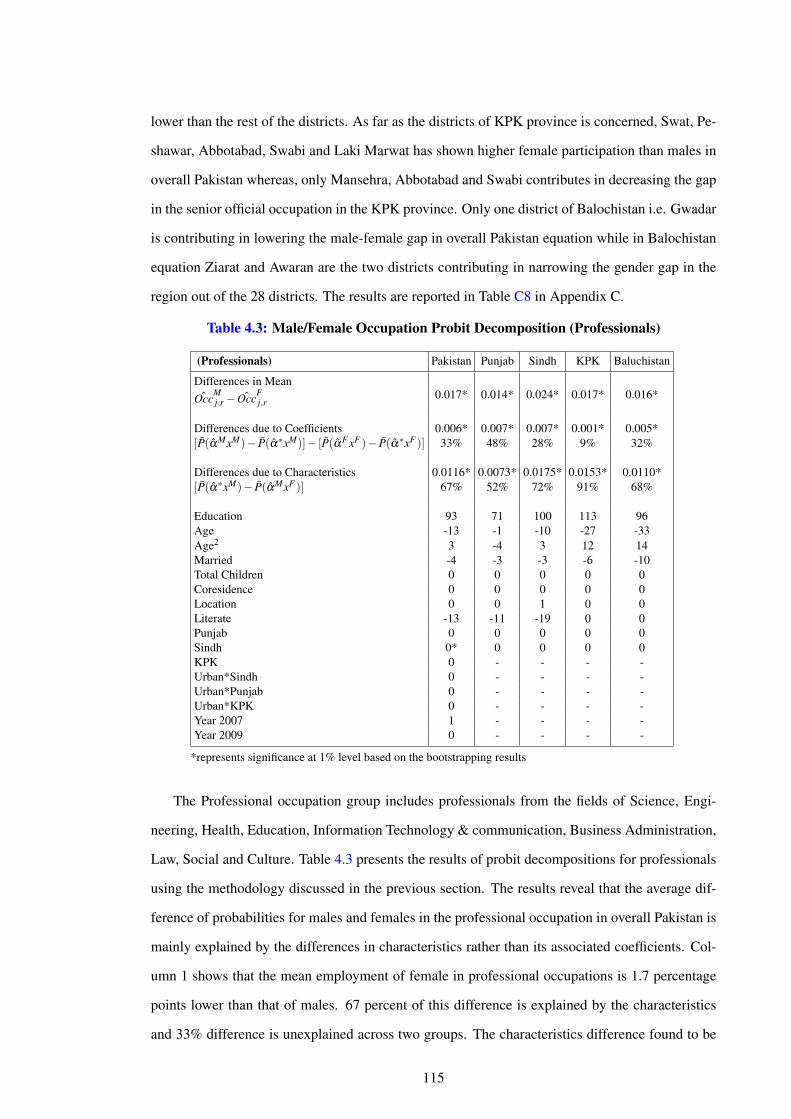
lower than the rest of the districts. As far as the districts of KPK province is concerned, Swat, Pe-
shawar, Abbotabad, Swabi and Laki Marwat has shown higher female participation than males in
overall Pakistan whereas, only Mansehra, Abbotabad and Swabi contributes in decreasing the gap
in the senior official occupation in the KPK province. Only one district of Balochistan i.e. Gwadar
is contributing in lowering the male-female gap in overall Pakistan equation while in Balochistan
equation Ziarat and Awaran are the two districts contributing in narrowing the gender gap in the
region out of the 28 districts. The results are reported in Table C8 in Appendix C.
Table 4.3: Male/Female Occupation Probit Decomposition (Professionals)
(Professionals) Pakistan Punjab Sindh KPK Baluchistan
Differences in Mean0.017* 0.014* 0.024* 0.017* 0.016*ˆOccM
j,r− ˆOccFj,r
Differences due to Coefficients 0.006* 0.007* 0.007* 0.001* 0.005*[P(αMxM)− P(α∗xM)]− [P(αF xF )− P(α∗xF )] 33% 48% 28% 9% 32%
Differences due to Characteristics 0.0116* 0.0073* 0.0175* 0.0153* 0.0110*[P(α∗xM)− P(αMxF )] 67% 52% 72% 91% 68%
Education 93 71 100 113 96Age -13 -1 -10 -27 -33Age2 3 -4 3 12 14Married -4 -3 -3 -6 -10Total Children 0 0 0 0 0Coresidence 0 0 0 0 0Location 0 0 1 0 0Literate -13 -11 -19 0 0Punjab 0 0 0 0 0Sindh 0* 0 0 0 0KPK 0 - - - -Urban*Sindh 0 - - - -Urban*Punjab 0 - - - -Urban*KPK 0 - - - -Year 2007 1 - - - -Year 2009 0 - - - -
*represents significance at 1% level based on the bootstrapping results
The Professional occupation group includes professionals from the fields of Science, Engi-
neering, Health, Education, Information Technology & communication, Business Administration,
Law, Social and Culture. Table 4.3 presents the results of probit decompositions for professionals
using the methodology discussed in the previous section. The results reveal that the average dif-
ference of probabilities for males and females in the professional occupation in overall Pakistan is
mainly explained by the differences in characteristics rather than its associated coefficients. Col-
umn 1 shows that the mean employment of female in professional occupations is 1.7 percentage
points lower than that of males. 67 percent of this difference is explained by the characteristics
and 33% difference is unexplained across two groups. The characteristics difference found to be
115
most important is education. This is partially due to the fact that in the sample males are more
educated than females with 5.27 average years of schooling compared to females’ 2.99 (see Table
4.1). Although, a higher percentage of males is found to be illiterate compared to females, but
those males who attended school may have obtained more years of schooling (with mean of 5
years) than their female counterparts (with mean of 3 years).
Education being the most important factor explaining gender occupational gaps, it explains
93 percentage point (pp) of the difference in professional occupation for overall Pakistan. The
adjustments are made by the factors effecting negatively to the decomposition equation such as
literacy (-13pp). The quadratic term of age is also found to be important in explaining the occupa-
tion difference with the contribution of -10pp. The sample statistics exhibits that the average age
is around 27 years (given the sample size) which is almost same for both male and female. The
other factors have a negligible effect.
Consequently, the gender difference of professionals for each province has been analysed in
the subsequent columns. Female participation rate in professional occupations seems to be lowest
in Sindh of all the regions as the difference is 2.4 percentage points lower than for males. More
than 70 percent of this difference is being explained by the differences in the characteristics across
genders and only 28 percent due the coefficients difference. As within overall Pakistan, education
is the most important contributing factor in explaining the gender differences in the professional
occupation. It explains all the gender difference in the professional occupation which is actually
100 percentage points. The contribution of education is 28 pp higher than the total difference
due to characteristics. It is adjusted by other factors which have negative contribution (i.e. age,
marital status and literate). The next relatively important variable is location which explains that
1 pp of the differences in the professional occupations is due to area of residence. It means
residing in urban areas has a positive and significant effect in explaining the gender differences in
professional occupation. The model predicts that if both males and females live in an urban area,
the participation in the professional occupation will rise by one percentage point.
In KPK province, just over 90 percent of the difference is explained by the difference in char-
acteristics and only 9 percent is due to the difference in unexplained characteristics. It means if the
education inequality is reduced the magnitude of the gap will become narrow. Following the same
pattern, in Baluchistan province, the mean gender difference of the predicted probability of being
professional is explained just below 70 percent by the difference in characteristics and slightly
above 30 percent of the difference is being explained by the differences in the coefficients asso-
116
ciated with it. Again the major share is coming from the education which is 96 percentage point
contribution in the total professional occupation gap. This is adjusted by the negative contribution
of age, marital status, and the literacy variable. The contribution of other individual characteristics
is not much informative as they have negligible effect on the overall difference of professional
occupation.
Conversely, in case of the Punjab province, the situation is quite different from the other re-
gions in Pakistan. 52 percent of the mean difference between male and female predicted occupa-
tional probabilities is being explained by the differences in the coefficients across the groups and
48 percent is explained by the characteristics difference. This potentially indicates a substantial
difference in attitudes towards males and females in this province. However, the contribution of
individual characteristics is more likely from the education which is same as other regions. It is
again more than the size of the overall occupation difference. Although the mean predicted occu-
pation probability difference for males compared to the female group is relatively small compared
to other regions almost half of the difference is explained by the unobserved characteristics.
Probit decomposition results with districts has changed the decomposition of the average dif-
ference of the probabilities of males and females in professional occupation. The percentage
of differences in coefficient has increased to 6% for Pakistan, 9% for Punjab, 1% for Sindh,
14% for KPK and no change for Balochistan. The contributing factor is education which is
more than 100pp for Pakistan, Sindh and KPK and even more than 200 pp for Punjab but has
shown no change in Balochistan. The contribution of each district is less than 0.5%. The share of
Khushab, T.T Singh, Lahore, Lodhran, Nawab Shah, Shikar pur, Larkana, Shahdadkot, Jamshoro,
Dadu,Tando Allah Yar, Tando Muhammad Khan , Karachi, Peshawar, Hangu, D.I. Khan, Mansehra,
Abbotabad, Hairpur, Bannu, Laki Marwat, Quetta, Chagi, Nushki, Sibbi, Ziarat, Awaran, Gwadar
and Panjgan districts in the characteristics effect shows that these districts contribute in lower-
ing the mean difference in the gender gap relative to other districts in Pakistan. For Punjab,
Rawalpindi, Jhelhum, Chakwal, Sargodha, Bhukkar, Jhang, Gujranwala,Gujrat, Sialkot Hafiz
Abad, Narowal, Okara, Vehari, Multan, D.G Khan , Rajanpur, Leiah, Bahawalpur and RY Khan
districts are contributing positively to the differences in characteristics. This means that females
predicted probability of being in the professional occupation is lower than males in these districts
and it is mainly due to the difference in their characteristics hence, widening the occupation gap.
For Sindh Ghotki, Jacobababad, Kashmore, Shikarpur, Larkana, Dadu, Tando Muhammad Khan
Badin, Thatta, Sanghar and Karachi contributing to widen the professional occupation gap be-
117
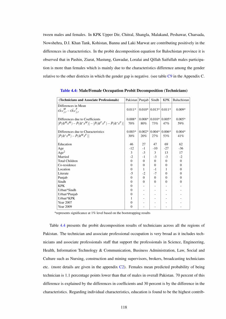
tween males and females. In KPK Upper Dir, Chitral, Shangla, Malakand, Peshawar, Charsada,
Nowshehra, D.I. Khan Tank, Kohistan, Bannu and Laki Marwat are contributing positively in the
differences in characteristics. In the probit decomposition equation for Balochistan province it is
observed that in Pashin, Ziarat, Mastung, Gawadar, Loralai and Qillah Saifullah males participa-
tion is more than females which is mainly due to the characteristics difference among the gender
relative to the other districts in which the gender gap is negative. (see table C9 in the Appendix C.
Table 4.4: Male/Female Occupation Probit Decomposition (Technicians)
(Technicians and Associate Professionals) Pakistan Punjab Sindh KPK Baluchistan
Differences in Mean0.011* 0.010* 0.013* 0.011* 0.009*ˆOccM
j,r− ˆOccFj,r
Differences due to Coefficients 0.008* 0.008* 0.010* 0.005* 0.005*[P(αMxM)− P(α∗xM)]− [P(αF xF )− P(α∗xF )] 70% 80% 73% 47% 59%
Differences due to Characteristics 0.003* 0.002* 0.004* 0.006* 0.004*[P(α∗xM)− P(αMxF )] 30% 20% 27% 53% 41%
Education 46 27 47 69 62Age -12 -1 -10 -27 -36Age2 3 -3 3 13 17Married -2 -1 -3 -3 -2Total Children 0 0 0 0 0Co-residence 0 0 0 0 0Location 0 1 -1 1 0Literate -5 -2 -7 0 0Punjab 0 0 0 0 0Sindh 0 0 0 0 0KPK 0 - - - -Urban*Sindh 0 - - - -Urban*Punjab 0 - - - -Urban*KPK 1 - - - -Year 2007 0 - - - -Year 2009 0 - - - -
*represents significance at 1% level based on the bootstrapping results
Table 4.4 presents the probit decomposition results of technicians across all the regions of
Pakistan. The technician and associate professional occupation is very broad as it includes tech-
nicians and associate professionals staff that support the professionals in Science, Engineering,
Health, Information Technology & Communication, Business Administration, Law, Social and
Culture such as Nursing, construction and mining supervisors, brokers, broadcasting technicians
etc. (more details are given in the appendix C2). Females mean predicted probability of being
technician is 1.1 percentage points lower than that of males in overall Pakistan. 70 percent of this
difference is explained by the differences in coefficients and 30 percent is by the difference in the
characteristics. Regarding individual characteristics, education is found to be the highest contrib-
118
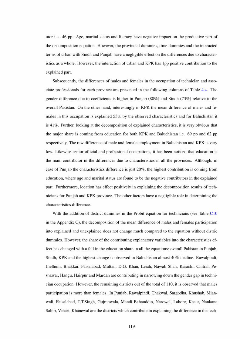
utor i.e. 46 pp. Age, marital status and literacy have negative impact on the productive part of
the decomposition equation. However, the provincial dummies, time dummies and the interacted
terms of urban with Sindh and Punjab have a negligible effect on the differences due to character-
istics as a whole. However, the interaction of urban and KPK has 1pp positive contribution to the
explained part.
Subsequently, the differences of males and females in the occupation of technician and asso-
ciate professionals for each province are presented in the following columns of Table 4.4. The
gender difference due to coefficients is higher in Punjab (80%) and Sindh (73%) relative to the
overall Pakistan. On the other hand, interestingly in KPK the mean difference of males and fe-
males in this occupation is explained 53% by the observed characteristics and for Baluchistan it
is 41%. Further, looking at the decomposition of explained characteristics, it is very obvious that
the major share is coming from education for both KPK and Baluchistan i.e. 69 pp and 62 pp
respectively. The raw difference of male and female employment in Baluchistan and KPK is very
low. Likewise senior official and professional occupations, it has been noticed that education is
the main contributor in the differences due to characteristics in all the provinces. Although, in
case of Punjab the characteristics difference is just 20%, the highest contribution is coming from
education, where age and marital status are found to be the negative contributors in the explained
part. Furthermore, location has effect positively in explaining the decomposition results of tech-
nicians for Punjab and KPK province. The other factors have a negligible role in determining the
characteristics difference.
With the addition of district dummies in the Probit equation for technicians (see Table C10
in the Appendix C), the decomposition of the mean difference of males and females participation
into explained and unexplained does not change much compared to the equation without distric
dummies. However, the share of the contributing explanatory variables into the characteristics ef-
fect has changed with a fall in the education share in all the equations: overall Pakistan in Punjab,
Sindh, KPK and the highest change is observed in Balochistan almost 40% decline. Rawalpindi,
Jhelhum, Bhakkar, Faisalabad, Multan, D.G. Khan, Leiah, Nawab Shah, Karachi, Chitral, Pe-
shawar, Hangu, Hairpur and Mardan are contributing in narrowing down the gender gap in techni-
cian occupation. However, the remaining districts out of the total of 110, it is observed that males
participation is more than females. In Punjab, Rawalpindi, Chakwal, Sargodha, Khushab, Mian-
wali, Faisalabad, T.T.Singh, Gujranwala, Mandi Bahauddin, Narowal, Lahore, Kasur, Nankana
Sahib, Vehari, Khanewal are the districts which contribute in explaining the difference in the tech-
119
nician occupation. In Sindh, Kashmore, Jamshoro, Hyderabad, Matiari, Tando Allah Yar and
Karachi districts are important in explaining the difference in the employment rates of technician
across gender. In KPK, Sangla, peshawar, Charsada, Lakki Marwat, whereas in Bbalochistan
Pashin, Nushki, Sibbi and Gawadar are found to explain the difference in the participation males
and females in this occupation.
Table 4.5: Male/Female Occupation Probit Decomposition (Clerks)
(Clerks) Pakistan Punjab Sindh KPK Baluchistan
Differences in Mean0.014* 0.015* 0.016* 0.012* 0.013*ˆOccM
j,r− ˆOccFj,r
Differences due to Coefficients 0.008* 0.009* 0.009* 0.005* 0.006*[P(αMxM)− P(α∗xM)]− [P(αF xF )− P(α∗xF )] 55% 64% 55% 43% 45%
Differences due to Characteristics 0.006* 0.005* 0.007* 0.007* 0.007*[P(αMxM)− P(α∗xM)]− [P(αF xF )− P(α∗xF )] 45% 36% 45% 57% 55%
Education 55 41 54 75 77Age -12 -1 -10 -23 -36Age2 3 -4 3 10 17Married -1 -1 -1 -6 -2Total Children 0 0 0 0 0Co-residence 0 0 0 0 0Location 0 0 -1 1 0Literate 0 0 0 0 0Punjab 0 0 0 0 0Sindh 0 0 0 0 0KPK 0 - - - -Urban*Sindh 0 - - - -Urban*Punjab 0 - - - -Urban*KPK 0 - - - -Year 2007 -1 - - - -Year 2009 0 - - - -
*represents significance at 1% level based on the bootstrapping results
The employment probit of males and females in the occupation of clerks are presented in
Table 4.5. This occupation basically includes the clerical support workers either it is general office
clerks, secretaries, keyboard operators, tellers, money collectors, support staff or numerical and
material recording clerks. The results show that the mean difference between gender of being
in a clerical occupation varies across the regions but the difference is not substantial (differ by
0.1pp). It is highest in Sindh (1.6pp) and lowest in KPK (1.2pp). For Pakistan as a whole it is
1.4pp. The decomposition output reveals similar results for Pakistan and Sindh with more than
50% of mean difference being explained by the unobserved factors whereas 45% of the difference
is explained by the observed characteristics. The results for Punjab out-stand among the other
regions as the major part (64%) of occupational difference is explained by the non-productive or
unobserved characteristics. Conversely, in case of KPK and Baluchistan most of the difference is
120
being explained by the characteristics difference which is more than 50% for both. The common
finding from the detailed decomposition of the explained part is that the main contribution is
coming from education across all the regions. It is even more than 100% contribution of the
total clerks‘ characteristics effect. This is adjusted by the negative contribution of age and marital
status while the other variables are found to have negligible effect on the decomposition of clerks
occupation. The exceptional factor is location which has a positive 1pp impact on the explained
part of the probit regression for KPK only. Interestingly, literacy plays no role.
The probit occupation results for clerks with district dummies are reported in Table C11 (see
Appendix C). The difference in the explained characteristics has changed by 1% for overall Pak-
istan, Punjab and Sindh. However for KPK the explained differeced is increased by 3% and for
Balochistan it is increased by 8%. Surprisingly, the share of education in explaining the difference
between males and females participation in this occupation has reduced to 6% for Pakistan, 1%
for Punjab, 4% for Sindh, 21% for KPK and 45% for Balochistan. As far as the contribution of
districts is concerned, Chakwal, Gujranwala, Gujrat, Sialkot, Hafiz abad, Lahore , Kasur, Okara,
Rajanpur, Sukkar, Mitiari,Swat, Bannu, Quetta, Pashin, Nushki, Sibbi and Panjgar in Pakistan,
Rawalpindi, Jehlum, Chakwal, Sargodha, Khushab, Jhung, Gujranwala, Gujrat, Sialkot, Hafiz
Abad, Mandi bahauddin, Kasur, Okara, Muzafargarh and Bahawalpur in Punjab, Noshehro Feroz,
Shikarpur, Larkana, Matiari, Tando Allah Yar, Tando Muhammad Khan, Thatta and Mirpur Khas
in Sindh, Swat and Bannu in KPK, Pashin, Nushki, Ziarat, Sibbi, Dera Bugti and Khuzdar are
playing important role in explaining the difference between males and females in this occupation
due to characteristics difference.
Table 4.6 presents the results for services or shop occupation that includes personal services
workers like hairdressers, beauticians cook, waiters, building and housekeeping supervisors and
others. It also includes sales workers such as shop sales person, ticket checkers, cashiers and
others. Moreover, child care and personal care workers and helpers in health services are also
included in this occupation group. The decomposition difference between males and females in the
services related occupations have shown a wide gap relative to the other occupations. It shows that
employment rate for females are almost 20 percentage points lower than that for males working in
this occupation. Furthermore, 105% of this gap is explained by the unobserved or non-productive
characteristics consequently the share of the characteristics difference is negative 5%. The results
of other regions in the subsequent columns of the Table 4.6 show similar decomposition results.
The differences due to characteristics is negative or even less than 1%, whereas the difference due
121
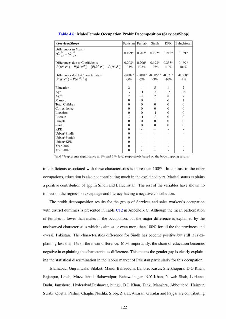
Table 4.6: Male/Female Occupation Probit Decomposition (Services/Shop)
(Services/Shop) Pakistan Punjab Sindh KPK Baluchistan
Differences in Mean0.199* 0.202* 0.192* 0.212* 0.191*ˆOccM
j,r− ˆOccFj,r
Differences due to Coefficients 0.208* 0.206* 0.198* 0.233* 0.199*[P(αMxM)− P(α∗xM)]− [P(αF xF )− P(α∗xF )] 105% 102% 103% 110% 104%
Differences due to Characteristics -0.009* -0.004* -0.005** -0.021* -0.008*[P(α∗xM)− P(αMxF )] -5% -2% -3% -10% -4%
Education 2 1 5 -1 2Age -7 -1 -6 -15 -14Age2 2 -2 2 8 7Married 0 0 1 -1 1Total Children 0 0 0 0 0Co-residence 0 0 0 0 0Location 0 0 -1 0 0Literate -2 -1 -3 0 0Punjab 0 0 0 0 0Sindh 0 0 0 0 0KPK 0 - - - -Urban*Sindh 0 - - - -Urban*Punjab 0 - - - -Urban*KPK 0 - - - -Year 2007 0 - - - -Year 2009 0 - - - -
*and **represents significance at 1% and 5 % level respectively based on the bootstrapping results
to coefficients associated with these characteristics is more than 100%. In contrast to the other
occupations, education is also not contributing much in the explained part. Marital status explains
a positive contribution of 1pp in Sindh and Baluchistan. The rest of the variables have shown no
impact on the regression except age and literacy having a negative contribution.
The probit decomposition results for the group of Services and sales workers’s occupation
with district dummies is presented in Table C12 in Appendix C. Although the mean participation
of females is lower than males in the occupation, but the major difference is explained by the
unobserved characteristics which is almost or even more than 100% for all the the provinces and
overall Pakistan. The characteristics difference for Sindh has become positive but still it is ex-
plaining less than 1% of the mean difference. Most importantly, the share of education becomes
negative in explaining the characteristics difference. This means the gender gap is clearly explain-
ing the statistical discrimination in the labour market of Pakistan particularly for this occupation.
Islamabad, Gujranwala, Silakot, Mandi Bahauddin, Lahore, Kasur, Sheikhupura, D.G.Khan,
Rajanpur, Leiah, Muzzafabad, Bahawalpur, Bahawalnagar, R.Y Khan, Nawab Shah, Larkana,
Dadu, Jamshoro, Hyderabad,Peshawar, hungu, D.I. Khan, Tank, Manshra, Abbotabad, Hairpur,
Swabi, Quetta, Pashin, Chaghi, Nushki, Sibbi, Ziarat, Awaran, Gwadar and Pajgar are contributing
122
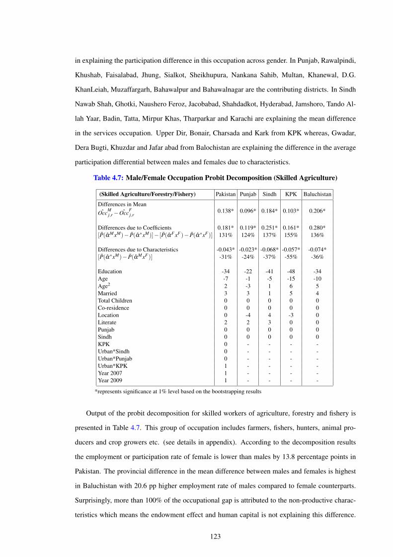
in explaining the participation difference in this occupation across gender. In Punjab, Rawalpindi,
Khushab, Faisalabad, Jhung, Sialkot, Sheikhupura, Nankana Sahib, Multan, Khanewal, D.G.
KhanLeiah, Muzaffargarh, Bahawalpur and Bahawalnagar are the contributing districts. In Sindh
Nawab Shah, Ghotki, Naushero Feroz, Jacobabad, Shahdadkot, Hyderabad, Jamshoro, Tando Al-
lah Yaar, Badin, Tatta, Mirpur Khas, Tharparkar and Karachi are explaining the mean difference
in the services occupation. Upper Dir, Bonair, Charsada and Kark from KPK whereas, Gwadar,
Dera Bugti, Khuzdar and Jafar abad from Balochistan are explaining the difference in the average
participation differential between males and females due to characteristics.
Table 4.7: Male/Female Occupation Probit Decomposition (Skilled Agriculture)
(Skilled Agriculture/Forestry/Fishery) Pakistan Punjab Sindh KPK Baluchistan
Differences in Mean0.138* 0.096* 0.184* 0.103* 0.206*ˆOccM
j,r− ˆOccFj,r
Differences due to Coefficients 0.181* 0.119* 0.251* 0.161* 0.280*[P(αMxM)− P(α∗xM)]− [P(αF xF )− P(α∗xF )] 131% 124% 137% 155% 136%
Differences due to Characteristics -0.043* -0.023* -0.068* -0.057* -0.074*[P(α∗xM)− P(αMxF )] -31% -24% -37% -55% -36%
Education -34 -22 -41 -48 -34Age -7 -1 -5 -15 -10Age2 2 -3 1 6 5Married 3 3 1 5 4Total Children 0 0 0 0 0Co-residence 0 0 0 0 0Location 0 -4 4 -3 0Literate 2 2 3 0 0Punjab 0 0 0 0 0Sindh 0 0 0 0 0KPK 0 - - - -Urban*Sindh 0 - - - -Urban*Punjab 0 - - - -Urban*KPK 1 - - - -Year 2007 1 - - - -Year 2009 1 - - - -
*represents significance at 1% level based on the bootstrapping results
Output of the probit decomposition for skilled workers of agriculture, forestry and fishery is
presented in Table 4.7. This group of occupation includes farmers, fishers, hunters, animal pro-
ducers and crop growers etc. (see details in appendix). According to the decomposition results
the employment or participation rate of female is lower than males by 13.8 percentage points in
Pakistan. The provincial difference in the mean difference between males and females is highest
in Baluchistan with 20.6 pp higher employment rate of males compared to female counterparts.
Surprisingly, more than 100% of the occupational gap is attributed to the non-productive charac-
teristics which means the endowment effect and human capital is not explaining this difference.
123
Therefore, the characteristics effect is -31%. It is also interesting to find out that education has a
negative impact on the explained part. It might be due to the reason that this group of occupation
is more skill oriented. Therefore, the employment of specific skills may be sufficient to be a part
of this occupation. Moreover, the literacy factor is found to be an important contributor among
the characteristics difference. The model predicts that if the literacy level of females is same as
males then the occupation probability for Pakistan and Punjab will rise by 2pp and for Sindh by
3pp. It means that apart from their skills, individuals who can read and write and are capable of
doing simple arithmetic has a positive impact on the labour participation in agriculture, forestry
and fishery sectors. Likewise, marital status also has a positive contribution in explaining the char-
acteristics difference for all the regions. Furthermore, if the females residing in the urban area
of KPK province face the same occupation structure like males then there is 1pp high probability
for her to be a part of this occupation. The other factors exacerbate the explained part with either
negligible or negative contribution.
The probit decomposition results for skilled agriculture and fishery occupation with the district
dummies are given in Table C13. (See Appendix C). The coefficient and characteristics difference
stays almost stagnant compared to the results without districts. Considering the detailed decom-
position of explanatory variables shows no important impact of education in the participation of
this occupation. Number of children and marital status is contributing towards explaining the
lower participation of females than males. For overall Pakistan, Rawalpindi, Chakwal, Jehlum,
Bhakkar, Kasur, D.G. Khan, Rajanpur, Leiah, Nawab Shah, Ghotki, Jacobabad, Shikarpur, Mi-
tiari, Sanghar, Sawat, Chitral, Peshawar,hangu, D.I. Khan, Mansehra, Abbot abad, Bannu and
Laki Marwat have important contribution in explaining the participation gap in this occupation.
From Punjab, Rawalpindi, Bhakkar, Mianwali, Faisalabad, Sheikhupura, Nankana Sahib, sahiwal,
Khanewal, pakpattan, Lodhran, D.G. Khan, Rajanpur, Leiah, Muzaffargarh and Bahawalpur,from
Sindh Nawab Shah,Jacobabad, Shikarpur, Larkana, Dadu, Matiari, Tando Muhammad Khan,
Badin, Sanghar, Mirpur Khas and Karachi are contributing districts in explaining the participa-
tion difference across gender. From KPK, the participation of districts ranges from 1% to 10%
across the districts in skilled agriculture and fishery and forestry. The reason is KPK is gifted with
heavy forests, mountains and fertile plain land. Upper Dir, Chitral (3.7%), Charsada, Nowshehra
(2.4%), Kohat, Kark (10%), Hangu, D.I. Khan, Abbotabad, Kohistan (7%), Mardan and Swabi are
contributing in explaining the gender gap in this occupation. From Balochistan, Pashin, Qilla Ab-
dullah, Chaghi, Nushki, Sibbi, Kalat, Mustang, Kharan, Turbat, Loralai and QilaSaifullah are the
124
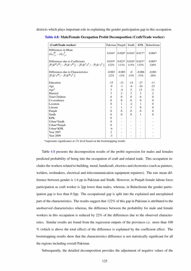
districts which plays important role in explaining the gender participation gap in this occupation.
Table 4.8: Male/Female Occupation Probit Decomposition (Craft/Trade worker)
(Craft/Trade worker) Pakistan Punjab Sindh KPK Baluchistan
Differences in Mean0.016* 0.020* 0.016* 0.017* 0.004*ˆOccM
j,r− ˆOccFj,r
Differences due to Coefficients 0.019* 0.023* 0.018* 0.023* 0.005*[P(αMxM)− P(α∗xM)]− [P(αF xF )− P(α∗xF )] 122% 113% 115% 133% 120%
Differences due to Characteristics -0.003 -0.003 -0 -0.006 -0.001[P(α∗xM)− P(αMxF )] -22% -13% -15% -33% -20%
Education -15 -12 -14 -27 -11Age -9 -1 -6 -24 -23Age2 3 -4 2 12 11Married 3 2 3 3 2Total Children 0 0 0 0 0Co-residence 0 0 0 0 0Location 0 1 -2 1 0Literate 1 1 3 0 0Punjab 0 0 0 0 0Sindh 0 0 0 1 0KPK 0 - - - -Urban*Sindh 0 - - - -Urban*Punjab 0 - - - -Urban*KPK -4 - - - -Year 2007 2 - - - -Year 2009 -3 - - - -
*represents significance at 1% level based on the bootstrapping results
Table 4.8 presents the decomposition results of the probit regression for males and females
predicted probability of being into the occupation of craft and related trade. This occupation in-
cludes the workers related to building, metal, handicraft, electrics and electronics (such as painters,
welders, toolmakers, electrical and telecommunication equipment repairers). The raw mean dif-
ference between gender is 1.6 pp in Pakistan and Sindh. However, in Punjab female labour force
participation as craft worker is 2pp lower than males, whereas, in Baluchistan the gender partic-
ipation gap is less than 0.5pp. The occupational gap is split into the explained and unexplained
part of the characteristics. The results suggest that 122% of this gap in Pakistan is attributed to the
unobserved characteristics whereas, the difference between the probability for male and female
workers in this occupation is reduced by 22% of the differences due to the observed character-
istics. Similar results are found from the regression outputs of the provinces i.e. more than 100
% (which is above the total effect) of the difference is explained by the coefficient effect. The
bootstrapping results show that the characteristics difference is not statistically significant for all
the regions including overall Pakistan.
Subsequently, the detailed decomposition provides the adjustment of negative values of the
125
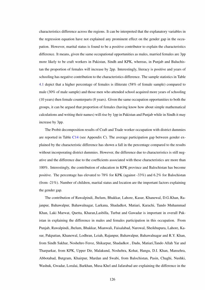
characteristics difference across the regions. It can be interpreted that the explanatory variables in
the regression equation have not explained any prominent effect on the gender gap in the occu-
pation. However, marital status is found to be a positive contributor to explain the characteristics
difference. It means, given the same occupational opportunities as males, married females are 3pp
more likely to be craft workers in Pakistan, Sindh and KPK, whereas, in Punjab and Baluchis-
tan the proportion of females will increase by 2pp. Interestingly, literacy is positive and years of
schooling has negative contribution to the characteristics difference. The sample statistics in Table
4.1 depict that a higher percentage of females is illiterate (58% of female sample) compared to
male (30% of male sample) and those men who attended school acquired more years of schooling
(10 years) then female counterparts (8 years). Given the same occupation opportunities to both the
groups, it can be argued that proportion of females (having know how about simple mathematical
calculations and writing their names) will rise by 1pp in Pakistan and Punjab while in Sindh it may
increase by 3pp.
The Probit decomposition results of Craft and Trade worker occupation with district dummies
are reported in Table C14 (see Appendix C). The average participation gap between gender ex-
plained by the characteristic difference has shown a fall in the percentage compared to the results
without incorporating district dummies. However, the difference due to characteristics is still neg-
ative and the difference due to the coefficients associated with these characteristics are more than
100%. Interestingly, the contribution of education in KPK province and Balochistan has become
positive. The percentage has elevated to 78% for KPK (against -33%) and 6.2% for Balochistan
(from -21%). Number of children, marital status and location are the important factors explaining
the gender gap.
The contribution of Rawalpindi, Jhelum, Bhakkar, Lahore, Kasur, Khanewal, D.G.Khan, Ra-
janpur, Bahawalpur, Bahawalnagar, Larkana, Shadadkot, Matiari, Karachi, Tando Muhammad
Khan, Laki Marwat, Quetta, Kharan,Lasbilla, Turbat and Gawadar is important in overall Pak-
istan in explaining the difference in males and females participation in this occupation. From
Punjab, Rawalpindi, Jhelum, Bhakkar, Mianwali, Faisalabad, Narowal, Sheikhupura, Lahore, Ka-
sur, Pakpattan, Khanewal, Lodhran, Leiah, Rajanpur, Bahawalpur, Bahawalnagar and R.Y. Khan,
from Sindh Sakhar, Noshehro Feroz, Shikarpur, Shadadkot , Dadu, Matiari,Tando Allah Yar and
Tharparkar, from KPK, Upper Dir, Malakund, Noshehra, Kohat, Hangu, D.I. Khan, Mansehra,
Abbotabad, Butgram, Khairpur, Mardan and Swabi, from Balochistan, Pasin, Chaghi, Nushki,
Washuk, Gwadar, Loralai, Barkhan, Musa Khel and Jafarabad are explaining the difference in the
126
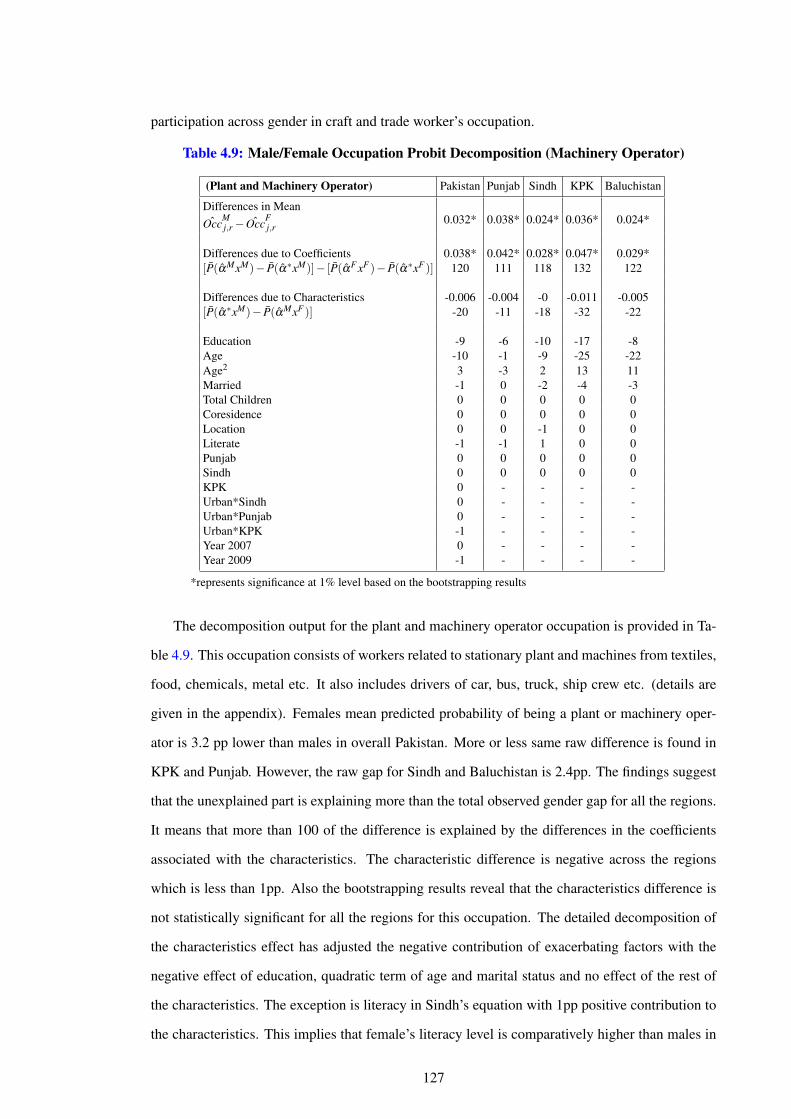
participation across gender in craft and trade worker’s occupation.
Table 4.9: Male/Female Occupation Probit Decomposition (Machinery Operator)
(Plant and Machinery Operator) Pakistan Punjab Sindh KPK Baluchistan
Differences in Mean0.032* 0.038* 0.024* 0.036* 0.024*ˆOccM
j,r− ˆOccFj,r
Differences due to Coefficients 0.038* 0.042* 0.028* 0.047* 0.029*[P(αMxM)− P(α∗xM)]− [P(αF xF )− P(α∗xF )] 120 111 118 132 122
Differences due to Characteristics -0.006 -0.004 -0 -0.011 -0.005[P(α∗xM)− P(αMxF )] -20 -11 -18 -32 -22
Education -9 -6 -10 -17 -8Age -10 -1 -9 -25 -22Age2 3 -3 2 13 11Married -1 0 -2 -4 -3Total Children 0 0 0 0 0Coresidence 0 0 0 0 0Location 0 0 -1 0 0Literate -1 -1 1 0 0Punjab 0 0 0 0 0Sindh 0 0 0 0 0KPK 0 - - - -Urban*Sindh 0 - - - -Urban*Punjab 0 - - - -Urban*KPK -1 - - - -Year 2007 0 - - - -Year 2009 -1 - - - -
*represents significance at 1% level based on the bootstrapping results
The decomposition output for the plant and machinery operator occupation is provided in Ta-
ble 4.9. This occupation consists of workers related to stationary plant and machines from textiles,
food, chemicals, metal etc. It also includes drivers of car, bus, truck, ship crew etc. (details are
given in the appendix). Females mean predicted probability of being a plant or machinery oper-
ator is 3.2 pp lower than males in overall Pakistan. More or less same raw difference is found in
KPK and Punjab. However, the raw gap for Sindh and Baluchistan is 2.4pp. The findings suggest
that the unexplained part is explaining more than the total observed gender gap for all the regions.
It means that more than 100 of the difference is explained by the differences in the coefficients
associated with the characteristics. The characteristic difference is negative across the regions
which is less than 1pp. Also the bootstrapping results reveal that the characteristics difference is
not statistically significant for all the regions for this occupation. The detailed decomposition of
the characteristics effect has adjusted the negative contribution of exacerbating factors with the
negative effect of education, quadratic term of age and marital status and no effect of the rest of
the characteristics. The exception is literacy in Sindh’s equation with 1pp positive contribution to
the characteristics. This implies that female’s literacy level is comparatively higher than males in
127
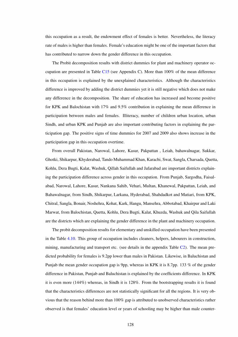
this occupation as a result, the endowment effect of females is better. Nevertheless, the literacy
rate of males is higher than females. Female’s education might be one of the important factors that
has contributed to narrow down the gender difference in this occupation.
The Probit decomposition results with district dummies for plant and machinery operator oc-
cupation are presented in Table C15 (see Appendix C). More than 100% of the mean difference
in this occupation is explained by the unexplained characteristics. Although the characteristics
difference is improved by adding the district dummies yet it is still negative which does not make
any difference in the decomposition. The share of education has increased and become positive
for KPK and Balochistan with 17% and 9.5% contribution in explaining the mean difference in
participation between males and females. Illiteracy, number of children urban location, urban
Sindh, and urban KPK and Punjab are also important contributing factors in explaining the par-
ticipation gap. The positive signs of time dummies for 2007 and 2009 also shows increase in the
participation gap in this occupation overtime.
From overall Pakistan, Narowal, Lahore, Kasur, Pakpattan , Leiah, bahawalnagar, Sukkar,
Ghotki, Shikarpur, Khyderabad, Tando Muhammad Khan, Karachi, Swat, Sangla, Charsada, Quetta,
Kohlu, Dera Bugti, Kalat, Washuk, Qillah Saifullah and Jafarabad are important districts explain-
ing the participation difference across gender in this occupation. From Punjab, Sargodha, Faisal-
abad, Narowal, Lahore, Kasur, Nankana Sahib, Vehari, Multan, Khanewal, Pakpattan, Leiah, and
Bahawalnagar, from Sindh, Shikarpur, Larkana, Hyderabad, Shahdadkot and Matiari, from KPK,
Chitral, Sangla, Bonair, Noshehra, Kohat, Kark, Hangu, Mansehra, Abbotabad, Khairpur and Laki
Marwat, from Balochistan, Quetta, Kohlu, Dera Bugti, Kalat, Khuzda, Washuk and Qila Saifullah
are the districts which are explaining the gender difference in the plant and machinery occupation.
The probit decomposition results for elementary and unskilled occupation have been presented
in the Table 4.10. This group of occupation includes cleaners, helpers, labourers in construction,
mining, manufacturing and transport etc. (see details in the appendix Table C2). The mean pre-
dicted probability for females is 9.2pp lower than males in Pakistan. Likewise, in Baluchistan and
Punjab the mean gender occupation gap is 9pp, whereas in KPK it is 8.7pp. 133 % of the gender
difference in Pakistan, Punjab and Baluchistan is explained by the coefficients difference. In KPK
it is even more (144%) whereas, in Sindh it is 128%. From the bootstrapping results it is found
that the characteristics differences are not statistically significant for all the regions. It is very ob-
vious that the reason behind more than 100% gap is attributed to unobserved characteristics rather
observed is that females’ education level or years of schooling may be higher than male counter-
128
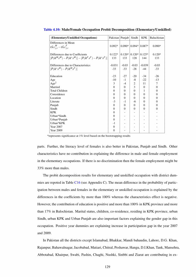
Table 4.10: Male/Female Occupation Probit Decomposition (Elementary/Unskilled)
(Elementary/Unskilled Occupations) Pakistan Punjab Sindh KPK Baluchistan
Differences in Mean0.092* 0.090* 0.094* 0.087* 0.090*ˆOccM
j,r− ˆOccFj,r
Differences due to Coefficients 0.122* 0.120* 0.120* 0.125* 0.120*[P(αMxM)− P(α∗xM)]− [P(αF xF )− P(α∗xF )] 133 133 128 144 133
Differences due to Characteristics -0.031 -0.03 -0.03 -0.039 -0.03[P(α∗xM)− P(αMxF )] -33 -33 -28 -44 -33
Education -23 -27 -20 -34 -26Age -10 -1 -8 -22 -13Age2 3 -4 2 11 7Married 0 0 3 0 0Total Children 0 0 0 1 0Coresidence 0 0 0 0 0Location 0 0 0 0 0Literate -3 -1 -6 0 0Punjab 0 0 0 0 0Sindh 0 0 0 0 0KPK 0 - - - -Urban*Sindh 0 - - - -Urban*Punjab 0 - - - -Urban*KPK -1 - - - -Year 2007 0 - - - -Year 2009 0 - - - -
*represents significance at 1% level based on the bootstrapping results
parts. Further, the literacy level of females is also better in Pakistan, Punjab and Sindh. Other
characteristics have no contribution in explaining the difference in male and female employment
in the elementary occupations. If there is no discrimination then the female employment might be
33% more than males.
The probit decomposition results for elementary and unskilled occupation with district dum-
mies are repoted in Table C16 (see Appendix C). The mean difference in the probability of partic-
ipation between males and females in the elementary or unskilled occupation is explained by the
differences in the coefficients by more than 100% whereas the characteristics effect is negative.
However, the contribution of education is positive and more than 100% in KPK province and more
than 17% in Balochistan. Marital status, children, co-residence, residing in KPK province, urban
Sindh, urban KPK and Urban Punjab are also important factors explaining the gender gap in this
occupation. Positive year dummies are explaining increase in participation gap in the year 2007
and 2009.
In Pakistan all the districts except Islamabad, Bhakkar, Mandi bahaudin, Lahore, D.G. Khan,
Rajanpur, Bahawalnagar, Jacobabad, Matiari, Chitral, Peshawar, Hangu, D.I.Khan, Tank, Mansehra,
Abbotabad, Khairpur, Swabi, Pashin, Chaghi, Nushki, Sinbbi and Ziarat are contributing in ex-
129
plaining the gender difference in the elementary and unskilled occupation. From Punjab and
Sindh no district seems to contribue in explaining the gap. From KPK, Noshehra, Kohat, Kark,
Hangu, Mansehra, Abbotabad, Batgram, Kohistan and Hairpur,from Balochistan, Pashin, Qillah
Abdullah, Chaghi, Nushki, Sibbi, Mastung, Awaran, Kharan, Washuk, Lasbilla, Qillah saifullah,
nasirabad, Jhal Magsi, Jafarabad and Bolan are contributing in explaining the gender gap in this
occupation.
4.6 Conclusion
The main objective of the study is to find the extent of occupational differences between males and
females across the regions in Pakistan. In this regard the employment probit of each occupational
group is decomposed into the explained characteristic effect and unexplained coefficient effect.
The occupation difference is the difference between the averages of predicted occupation proba-
bilities for males and females. Nine probit decomposition equations have been estimated. Further,
the contribution of individual characteristics in explaining differences in occupations across gender
has been calculated using the detailed decomposition method. The main findings from the results
suggest that the characteristics effect is found to be most important in professional as compared
to other occupations. The results demonstrate that the characteristics effect explains more than
60 percent of the mean difference of gender occupational for professionals. Regarding the mean
difference of predicted probabilities of technicians and associate professionals, it is noticed that al-
most 84% of the difference is explained by the unobserved characteristics. The average difference
of predicted probabilities for males and females in clerical related employment is explained 45%
by the characteristics difference, and 55% by the differences associated with the characteristics.
However, it is found that the unobserved characteristics (coefficient effect) explains more than
100% of the the mean gender difference of services and sales, skilled agriculture, forestry & fish-
ery, craft & related trade, plant & machinery operators and elementary or unskilled occupational
probabilities. In summary, the decompositions results of overall Pakistan suggest the existence
of a wide gender gap in all the occupations except for professionals. Most of the differences in
high earning occupations such as professional are explained by the difference in characteristics
compared to the low paid jobs such as clerks, sales, skilled agriculture & fishery, craft & trade,
plant & machinery and unskilled or elementary occupations, where a major part of the raw gender
differentials is attributed to differences in the coefficients, indicating substantial differences in the
attitude towards males and females. It can be interpreted that if females were to face a similar
130
occupation structure as males, given their characteristics, the proportion of females as senior of-
ficials and managers, technicians and associate professionals, and clerical support workers would
increase, while those who are craft & trade related workers, plant and machinery operators and
unskilled workers would fall. The findings are consistent with (Liu, et al (2009)).
The district dummies were incorporated in all the nine occupation Probit equations to gauge
the gender differences in smaller spatial divisions. It has been observed that districts of Punjab
have the highest level of contribution in explaining the gap in senior official, professional and tech-
nician occupation whereas only few districts of Sindh have contributed in explaining the gender
gap in these occupations. However, Punjab and Sindh does not have much contribution in explain-
ing the participation gap in plant and machinery and unskilled occupations. KPK province has
shown important contribution in explaining the gender gap in the skilled agriculture and forestry
occupation. Almost seven to ten districts of Balochistan have contributed in explaining the differ-
ence in the participation of males and females in almost all the occupations. Mainly the magnitude
of the share of the districts is less than 1% in all the equation except for the skilled agriculture and
forestry occupation in which some of the districts of KPK have contributed from Chitral (3%),
Kohistan ( 7%) and Kark (10%).
131
Chapter 5
Chapter 5: Conclusion
5.1 Summary of the thesis
The thesis consists of three essays covering three important issues in the labour market of Pakistan.
The first essay (i.e. second chapter) provides a comprehensive profile of labour market states of
working and not working females and compares it with the male counterparts. The second essay
(i.e. third chapter) explores the gender wage gap, whereas the extent of occupation differences
across gender and regions is explained in the third essay (i.e. fourth chapter). Pooled data con-
structed from the PSLM (2004-09) surveys has been used consistently throughout the thesis due
to the fact that the chapters are inter-related. Nevertheless, the sample size and number of obser-
vations differ in each of the chapters on the basis of their specific objectives. A brief summary of
the three studies is given below.
The second chapter of the thesis enlightens the labour market states of males and females in
Pakistan. In this regard, the labour force is split into the two main groups named as working and
not-working. These groups are further enumerated into four categories each. The working individ-
uals include paid employees, unpaid family helpers, self-employed (in the agriculture sector) and
self-employed (in the non-agriculture sector). On the other hand, the not-working state includes:
ill or handicapped, students, housekeepers and other inactive individuals.
Once these states had been defined, the demand and supply factors were identified to capture
the effect on the individual’s decision about labour market participation. The determinants com-
prised individual’s own as well as household characteristics which served as the set of explanatory
variables in the analysis such as, a quadratic term of age, education, marital status, women headed
household, house ownership, number of dependents, number of children, working people in the
household, co-residence, quadratic term of household income, regional and time dummies.
A Multinomial logit model was applied first by taking working states of females as the de-
pendent variable against the explanatory variables and using not-working as the base category and
then considering not-working states as dependent and working as the base category. The same
procedure was repeated for males. Four models have been estimated altogether.
The main findings suggest that age has a positive and significant impact on all the states of
132
working males and females in labour market with the exception of men as unpaid family helpers.
For females being married, having more than 2 children, ownership of the house, residence within
a joint family or belonging to an urban area, reduces the likelihood to participate in the paid em-
ployment. Conversely, for married men, or those who own a house or live in an urban area there
exists a higher probability to be involved in paid employment. Education has a significant higher
probability for females to participate in all the working states of employment. However, to our sur-
prise education is not increasing the probability for males to participate in any of the four working
states. A higher number of working people in the household increases the likelihood to participate
in all states of employment for both gender groups whereas, an increase in the number of chil-
dren reduces the probability of being in paid employment but increases the probability of being
self-employed for both genders. Similarly living in an extended family enviournment lowers the
probability for men and women being involved in all the working categories with the exception
of unpaid family helpers which is high for males. The likelihood of paid and unpaid employment
gets lower, and self-employment is elevated, relative to not working for males by having more
dependents in the household. On the other hand, it appears to have no impact on females employ-
ment status. It is found that household income has a higher probability for women to work in any
of the working state of labour force, but as the income increases to a large extent the situation is
converse. However, in case of males, when income increases too much, it lowers the probability
of being in paid employment and self-employment (agriculture), whereas, the likelihood of being
unpaid family helpers and self-employed in non-agriculture becomes higher.
Considering the empirical findings of males and females not-working as the dependent vari-
able, the increase in education increases the probability of being in the status of a student relative
to work. Marital status of both genders has a lower probability of being ill, student or having
other reasons for not-working, whereas, married females tend to have higher probability of being
involved in housekeeping. For females, ownership of a house lowers the probability of being a
disabled person or a student, but increases the probability of housekeeping and other reasons for
not-working. On the other hand, for males the probability is lower for being in any of the inactiv-
ity states when own a house. The higher the number of working people in the household the less
likelihood for both the genders of being in any not-working states. As household income increases
for both genders, the likelihood of being in housekeeping or student falls. Men having higher de-
pendents in the house have higher probability of being ill, student housekeeping and other reason
however, the situation is opposite for women with the exception of being ill. Living in an extended
133
family or residing in an urban area have a higher probability for both gender groups to be in all
states of not working relative to working.
The negative marginal effects of dummies for 2007 and 2009 reflects adverse situation of
macroeconomic fundamentals that can be presumed as the consequence of backward linkages in
the labour market. In the presence of backward linkages, the spillover effect of reduced economic
activity resulted in a decrease in employment opportunities for skilled and unskilled labourers.
The second essay explores the gender wage gap in Pakistan. The main objective is to identify
the impact of personal characteristics, human capital endowments, employment states, occupa-
tions, sectors and regions in the determination of wages. Furthermore, it investigates to what
extent the gender wage differential is explained by these factors. Wage determination for males
and females is performed by the Mincerian approach and the gender wage gap is decomposed
by using the (Oaxaca (1973)) methodology. In addition, the alternative approaches proposed by
(Neuman and Oaxaca (2004)) were employed to investigate how much of the gender wage dif-
ferential is explained by the differences in endowments, and how much is due to discrimination
and selectivity individually. In this regard six alternative equations had been estimated; without
selectivity, with females selectivity only, with the difference of males and females selectivity, con-
sidering the variance of errors of wage equations along with the error correlation coefficients of
males and females, and finally, the characteristics and coefficients of the probit equation of males
and females are treated as endowment and discrimination effect.
The debate on discrimination in the Economics literature starts from Becker (1957) book ‘The
Economics of Discrimination’. Basically the models of discrimination in Economics are divided
into two groups. One is competitive that studies individual maximising behaviour including dis-
crimination and the other model is collective according to which groups act against each other
in a collective manner. Economic analysis is mainly based on the competitive approach which is
further divided in two groups: taste-based discrimination and statistical discrimination. Becker’s
model is focused on the former case whereas, the studies after Phelps (1972) and Arrow (1973)
emphasised on the statistical theory. Taste based discrimination means there is a disamenity value
to employing minority workers. The main argument of the statsistical discrimination literature is
that employers have limited information about the employees skills. This gives them a reason to
use observable characteristics such as race and gender to infer their expected productivity. Most
of the studies in economics focused on the statistical discrimination especially when considering
gender or race. Let’s define discrimination in a simple way ‘discrimination is when the members
134
of minority groups are treated less favourably than the members of the majority group given the
identical characteristics of productivity.’ Sometimes the characteristics or the explanatory vari-
ables can be endogenous which means there could be a pre-market discrimination e.g. in terms of
poor schooling or education attainment. In case of Pakistan, it is very much evident that females
face the challenges in the labour market due to low levels of education and lack of competitiveness
compared to male counterparts.
The empirical findings demonstrate the existence of the wage gap between males and females
in Pakistan. The endowment characteristics such as: age, level of education, sectors, occupations
and regions play an important role in determining the amount of this gap. The decomposition
results without taking into account the selectivity show that 41% of the the wage gap is due to dif-
ferences in the explained component and 59% is attributable to the differences in the unexplained
component. However, with the presence of selection effects in the wage decomposition equations,
the results are upward biased explaining 39% endowment effect, 77% coefficient effect and -16%
selection effect. This implies that gender wage gap widens after correcting for a selection bias.
These results indicate the perceived discrimination in the labour market. The findings suggest
that a wide wage gap in the labour market is explained by the sectors of employment (more than
50%), education (approx 13%) and regions 16%. However, it is has been observed that female
remuneration is not based on discrimination alone rather it depends on the education level which
is low in Pakistan providing a potential reason for lower wages in the labour market. Sectoral and
occupational segregation or gender stereotype attributes may also be the possible explanations for
the unfavourable conditions against females.
Provided the evidence of a wide wage gap in the sectors, education and regions, the third
essay focused on finding the extent of occupational differences across gender and regions in Pak-
istan. In this regard, the employment probits of nine occupation groups have been decomposed
into the explained and unexplained part. The occupation difference is the difference between the
averages of predicted occupation probabilities for males and the comparison group of females
being employed in a particular occupation. A detailed decomposition method is applied to gauge
the contribution of individual’s characteristics in explaining differences in each of the occupations.
The main empirical findings suggest that the difference in the professional occupation is explained
by the characteristics effect compared to other occupations which is more than 60 percent of the
mean gender difference. Regarding the mean difference of predicted probabilities of technicians
and associate professionals, it is noted that almost 84% of the difference is explained by the un-
135
observed characteristics. An average difference of predicted probabilities for males and females
in clerical related employment is explained 45% by the characteristics difference and 55% by the
differences associated with the characteristics. However, the mean difference in services and sales
workers, skilled agriculture, forestry and fishery, craft and related trade, plant and machinery op-
erator and elementary or unskilled occupations is explained more than 100% by the differences in
the unobserved characteristics. In summary, the decomposition results of overall Pakistan suggest
the existence of wide gender gap in all the occupations except for professionals. More differ-
ences in high earning jobs for instance, professional occupation is explained by the difference in
characteristics compared to the low paid jobs such as clerks, sales, skilled agriculture & fishery,
craft & trade, plant & machinery and unskilled or elementary occupations, where a major part of
gender differentials is attributed to the differences in the coefficients indicating substantial differ-
ences in the attitude towards males and females. It can be interpreted as, if females were to face
similar occupation structure and as males, given their characteristics, the proportion of females as
senior officials and managers, technicians and associate professionals, and clerical support work-
ers would increase, while for those who are craft and trade related workers, plant and machinery
operators and unskilled workers, the proportion would fall. The major contributing factor in the
detailed decomposition results of characteristics effect is education which is consistently large
across the provinces. The individual’s age, marital status and literacy has some contribution but
is not that substantial. Also, a negligible impact of household related factors (such as number of
children and co-residence) has been observed.
5.2 Policy Implications
The findings from the three chapters in the thesis have lead to the following policy implications:
The results have provided evidence in support of the discrimination against females in the
labour market causing a wide gap in the offered wage and occupations across gender and regions
in Pakistan. The core factor behind this gap is the overall difference in the level of education
across gender. Therefore, it can be inferred that education plays a significant role in determining
the employment status, deriving the wages and selecting an appropriate profession or occupation.
It is of course a primary variable of interest among all the other explanatory variables in the
analysis. Therefore, differences in the years of schooling need urgent attention to resolve the
issues of discrimination, wage gap and occupational differences across gender and regions.
It is a well established fact in literature that higher female labour force participation improves
136
economic growth. However, higher economic growth can not be sustained without a competitive
labour force. It is imperative for Pakistan to take steps that focus on the rise in the females partic-
ipation in the economic activities at first place. It is alarming that Pakistan is lagging far behind
in achieving the MDGs target of gender equality even at primary level of schooling 33. Primary
education is not only a key input to subsequent education levels but it provides the opportunity
to gain basic reading and writing and numeric skills which is attached to the economic and social
returns to move in the contemporary challenging society. Secondly, there is an utmost need to
reformulate the national policies with special focus on education attainment. Particularly, there is
a need to take steps towards improving female enrollment in the institutions34. The Government
should ensure that the policymakers put emphasis on achieving this target. The statistics illustrate
that females with no education attainment or with basic education have a higher participation in
the labour force relative to those with higher education. That is why most of the females are either
involved in low paid jobs or working as unpaid helpers. Typically, the basic reason of not par-
ticipating in the economic activities is the lack of competitiveness as well as low level of human
capital. The skill enhancement programmes such as vocational training and skilled education can
compensate the lack of skills and increase the marginal returns of the female workers. High value
added harvesting, livestock management, technical know how, storage technique and marketing
are the skills that can improve the earning abilities of the agriculture workers. Further, the skills
such as computer basics, stitching, sewing, health worker, community work, etc. can help the in-
dividuals to improve the marginal returns of their human capital by participating effectively in the
manufacturing and services sectors. On the other hand, it has been observed that relatively more
educated females with a higher degree do get involved in professional occupations. The need is
provision of equal opportunities in the education as well as various sectors of the economy.
Those females who prefer to stay home due to housekeeping responsibilities, are likely to have
a reservation wages higher than the offered wage. A low female participation rate is the reflection
of the penalty for the discontinuation in human capital formation as a result of marriage and child-
care activities. As a consequence, employers and coworkers exploit this situation and discriminate
against them. This in turn not only lowers the offered wage but also pushes her down the occupa-
tional ladder. In short, lower offered wages, demand deficiency, and higher reservation wages are
responsible for the low female participation in the labour market. Females participation can also
33The net primary enrolment is the lowest in case of Pakistan relative to South Asian countire. It is 72% in Pakistanas compared to 96% in Bangladesh, 99.6% in India, 94% in Srilanka and 93.6% in South Asia
34Literacy rate is 50% in Pakistan as compared to 59% in Bangladesh, 63% in India, 90% in Srilanka and 67% inSouth Asia. (World Bank (2012))
137
be raised by implementing a minimum wage legislation in an effective manner by penalising the
employer for violating the rule. This will result in an increase in the offered wages that will induce
the females to participate in the labour market activities.
In the light of the findings from the gender wage decomposition equation with selection effects,
it is suggested to provide child care facilities so that they can continue with their jobs without
breaks. It is recommended that region specific policies should be formulated. Given the labour
market conditions, socio-economic circumstances and cultural differences across the provinces,
the policies should be targeted specifically to achieve the desired goals. If women are residing
in a joint family then this issue can be easily resolved otherwise, Kindergarten programs can be
initiated following the developed countries to encourage the schooling. Enforcing the legal rights
and protecting the females against the discriminatory practices in the labour market may encourage
females and their family members to actively participate in the labour market regardless of any
apprehensions they may harbour.
5.3 Limitations
Although more needs to be done in this research area as there is always a room for improvement, it
is noteworthy that despite limitations attached to this study specifically regarding the data related
to Pakista, it does attempt to explore an ignored issue. However, this dissertation is a case study
of Pakistan and therefore, focuses on the household data of Pakistan, the lack of data with the
repeated ID’s over the years may limit the scope of the analysis. Panel or longitudinal data for
Pakistan was not availablewhich impeded the information of the observations collected on the
same individuals at multiple time periods on the same topics for Pakistan. Therefore, the cross-
sections with the same questions and topics have been repeated over time but with different sample
of individual which is the only viable choice for any the researcher who is interested in carrying
out research in this region. Therefore, data constraints is the main limitation that could have the
greatest potential impact on the empirical findings and analysis. For example, it is not possible to
look at female labour market transitions overtime, or model panel dynamics.
Given the limited data set, the study utilizes the PSLM survey which has been designed to
evaluate and monitor the performance of the MDG’s indicators and targets committed by Pakistan
to achieve by 2015. The survey was conducted in the alternate years at provincial and district
levels covering the time period from 2004-2015. However, due to the delays in the output of the
surveys the access to the data became complicated and behind schedule. The (2012-13) was made
138
available later in 2014. The field work of the latest district level survey (2014-15) is in progress.
That is why the study is limited to three repeated district levels cross-sections pooled together for
the analysis rather than pseudo panel.
Moreover, as per the culture of Pakistan two or more families often live together in one house-
hold, therefore, it is impossible to identify the relationship among the individual members of the
household living in the joint or extended family due to the default coding scheme of Pakistan
Bureau of Statistics. It is again due to data constraint that we cannot include the factors linked
with spouse, mother or father’s information, used as explanatory variables in most of the existing
empirical studies. The fact is that individual coding is missing. All the relationships are coded
with reference to the head of household. However, the analysis has fully utilized the maximum
information related to household such as number of children per households instead of children
per mother.
According to the MNL model individuals maximise their utility in an unconstrained environ-
ment. Females maximise their utility to participate in the labour market in a constrained enviourn-
met with certain cultural or relgious and pre-market constraints. It is again the limitation of the
study that the quantitative impact of these challenges cannot be captured rather the economic and
socio-economic issues with the empirical analysis can be investigated. Same is with occupation
choices females have to face pre-market constraints such as low education and lack of access to job
market that leads to low participation especially in male domnating occupations. The classfication
of occupations is in 9 groups. Each group contains a list of related occupations which cannot be
disaggregated for the analysis. It can also be considered as one of the data constraints.
Despite data constraints, the study distinguishes itself by using this survey to formulate a
pooled data for the first time in Pakistan especially related to labour market issues. It is expected
that such a limitation may not affect the quality of the dissertation indeed it is justified to use
this data in theory and in practice as it specifically contributes towards improving the literature
pertaining to Pakistan. It is relatively reliable data compared to LFS, and other studies conducted
up till now (data is either confined to one district or cross-section HIES data).
The lack of an appropriate Household level panel or longitudinal data for the developing econ-
omy is an important constraint. The statistical agencies in developing countries with the financial
priorities typically do not conduct this type of survey. Further, the household surveys are con-
ducted with the aid of financial institutions. However, in Pakistan, there has been only one panel
study which targets the topic of chronic poverty in Pakistan, which is out of the scope of the study.
139
5.4 Future Research
The limitations discussed above can be overcome by incorporating the following suggestions: if
the future research is carried out, complete set of district level PSLM surveys can be used to
construct a pseudo panel, followed by specific tests to run the regression results. In this way it
could significantly strengthen the research findings.
As mentioned above, a good quality and comprehensive panel data is very rare to find in Pak-
istan. In such situations when long term panel data does not exist, the cross-section datasets based
on the surveys with consistent questionnaires can serve as better alternative choice. Although such
data is relatively inferior to panel data, some models can be estimated using the repeated cross-
sections by constructing a pseudo panel. It is a tedious task to track the individual household
overtime therefore, tracking cohorts is suggested by (Deaton (1985)). A cohort is the group with
fixed membership that stays the same throughout the period such as age, gender or region cohorts
or a combination of these. Successive random samples can be generated from the following survey
and the summary statistics will provide the overtime behavioural relationships for the cohorts by
treating it like a panel. One of the advantages of the pseudo panel is that it does not suffer from
the attrition problem as opposed to the panel data. It would then become possible to consider
transitions of female labour market states, and wage dynamics within cohorts, overtime.
140
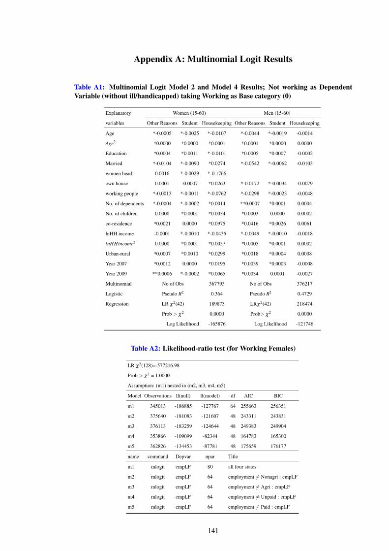
Appendix A: Multinomial Logit Results
Table A1: Multinomial Logit Model 2 and Model 4 Results; Not working as DependentVariable (without ill/handicapped) taking Working as Base category (0)
Explanatory Women (15-60) Men (15-60)
variables Other Reasons Student Housekeeping Other Reasons Student Housekeeping
Age *-0.0005 *-0.0025 *-0.0107 *-0.0044 *-0.0019 -0.0014
Age2 *0.0000 *0.0000 *0.0001 *0.0001 *0.0000 0.0000
Education *0.0004 *0.0011 *-0.0101 *0.0005 *0.0007 -0.0002
Married *-0.0104 *-0.0090 *0.0274 *-0.0542 *-0.0062 -0.0103
women head 0.0016 *-0.0029 *-0.1766
own house 0.0001 -0.0007 *0.0263 *-0.0172 *-0.0034 -0.0079
working people *-0.0013 *-0.0011 *-0.0762 *-0.0298 *-0.0023 -0.0048
No. of dependents *-0.0004 *-0.0002 *0.0014 **0.0007 *0.0001 0.0004
No. of children 0.0000 *0.0001 *0.0034 *0.0003 0.0000 0.0002
co-residence *0.0021 0.0000 *0.0975 *0.0416 *0.0026 0.0061
lnHH income -0.0001 *-0.0010 *-0.0435 *-0.0049 *-0.0010 -0.0018
lnHHincome2 0.0000 *0.0001 *0.0057 *0.0005 *0.0001 0.0002
Urban-rural *0.0007 *0.0010 *0.0299 *0.0018 *0.0004 0.0008
Year 2007 *0.0012 0.0000 *0.0195 *0.0039 *0.0003 -0.0008
Year 2009 **0.0006 *-0.0002 *0.0065 *0.0034 0.0001 -0.0027
Multinomial No of Obs 367793 No of Obs 376217
Logistic Pseudo R2 0.364 Pseudo R2 0.4729
Regression LR χ2(42) 189873 LRχ2(42) 218474
Prob > χ2 0.0000 Prob> χ2 0.0000
Log Likelihood -165876 Log Likelihood -121746
Table A2: Likelihood-ratio test (for Working Females)
LR χ2(128)=-577216.98
Prob > χ2 = 1.0000
Assumption: (m1) nested in (m2, m3, m4, m5)
Model Observations ll(null) ll(model) df AIC BIC
m1 345013 -186885 -127767 64 255663 256351
m2 375640 -181083 -121607 48 243311 243831
m3 376113 -183259 -124644 48 249383 249904
m4 353866 -109099 -82344 48 164783 165300
m5 362826 -134453 -87781 48 175659 176177
name command Depvar npar Title
m1 mlogit empLF 80 all four states
m2 mlogit empLF 64 employment 6= Nonagri : empLF
m3 mlogit empLF 64 employment 6= Agri : empLF
m4 mlogit empLF 64 employment 6= Unpaid : empLF
m5 mlogit empLF 64 employment 6= Paid : empLF
141
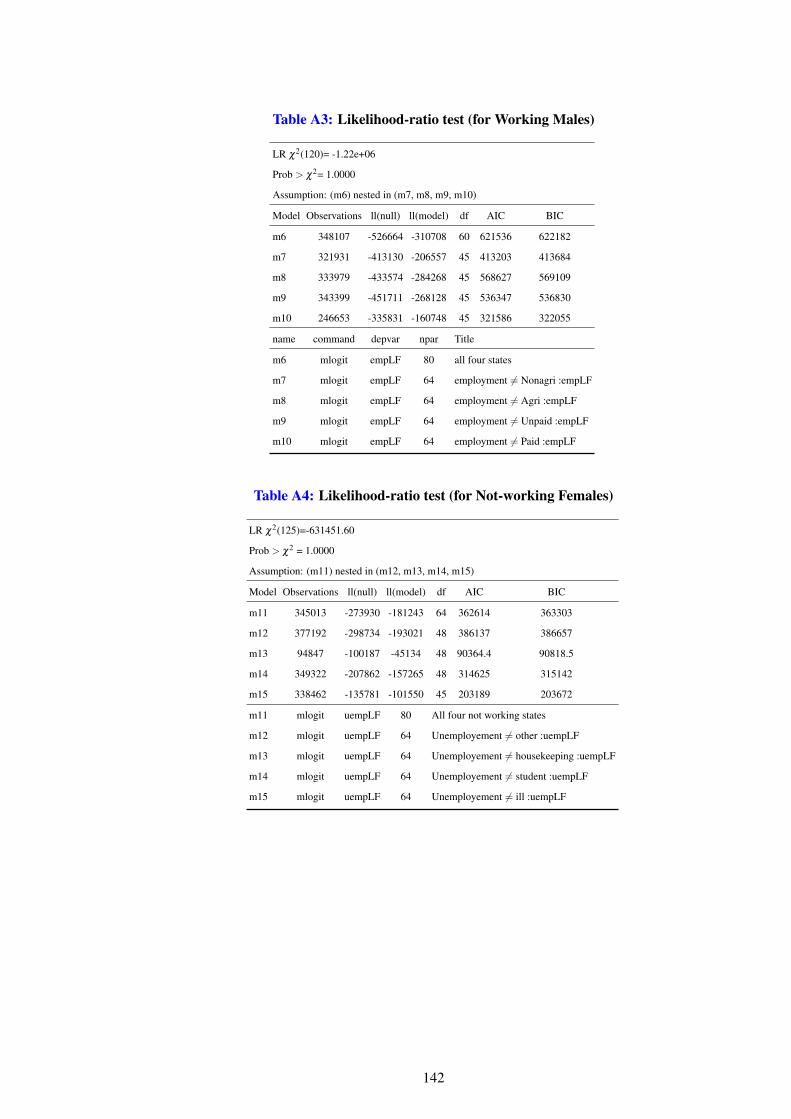
Table A3: Likelihood-ratio test (for Working Males)
LR χ2(120)= -1.22e+06
Prob > χ2= 1.0000
Assumption: (m6) nested in (m7, m8, m9, m10)
Model Observations ll(null) ll(model) df AIC BIC
m6 348107 -526664 -310708 60 621536 622182
m7 321931 -413130 -206557 45 413203 413684
m8 333979 -433574 -284268 45 568627 569109
m9 343399 -451711 -268128 45 536347 536830
m10 246653 -335831 -160748 45 321586 322055
name command depvar npar Title
m6 mlogit empLF 80 all four states
m7 mlogit empLF 64 employment 6= Nonagri :empLF
m8 mlogit empLF 64 employment 6= Agri :empLF
m9 mlogit empLF 64 employment 6= Unpaid :empLF
m10 mlogit empLF 64 employment 6= Paid :empLF
Table A4: Likelihood-ratio test (for Not-working Females)
LR χ2(125)=-631451.60
Prob > χ2 = 1.0000
Assumption: (m11) nested in (m12, m13, m14, m15)
Model Observations ll(null) ll(model) df AIC BIC
m11 345013 -273930 -181243 64 362614 363303
m12 377192 -298734 -193021 48 386137 386657
m13 94847 -100187 -45134 48 90364.4 90818.5
m14 349322 -207862 -157265 48 314625 315142
m15 338462 -135781 -101550 45 203189 203672
m11 mlogit uempLF 80 All four not working states
m12 mlogit uempLF 64 Unemployement 6= other :uempLF
m13 mlogit uempLF 64 Unemployement 6= housekeeping :uempLF
m14 mlogit uempLF 64 Unemployement 6= student :uempLF
m15 mlogit uempLF 64 Unemployement 6= ill :uempLF
142
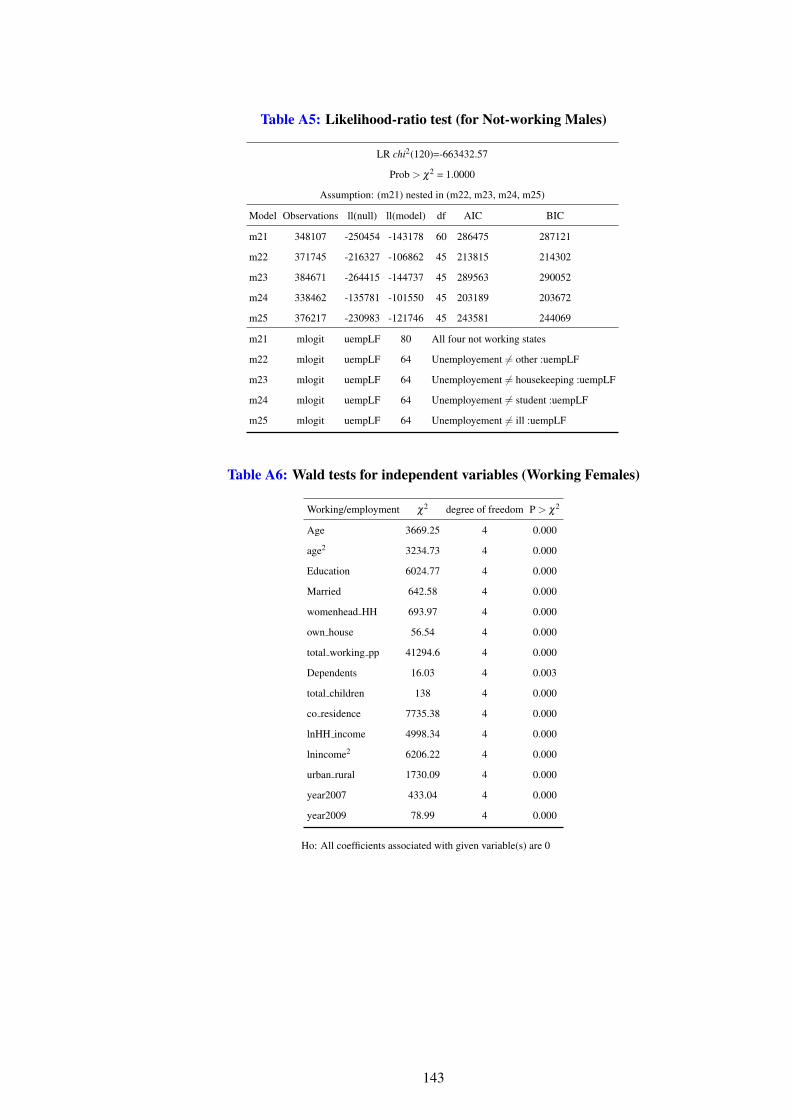
Table A5: Likelihood-ratio test (for Not-working Males)
LR chi2(120)=-663432.57
Prob > χ2 = 1.0000
Assumption: (m21) nested in (m22, m23, m24, m25)
Model Observations ll(null) ll(model) df AIC BIC
m21 348107 -250454 -143178 60 286475 287121
m22 371745 -216327 -106862 45 213815 214302
m23 384671 -264415 -144737 45 289563 290052
m24 338462 -135781 -101550 45 203189 203672
m25 376217 -230983 -121746 45 243581 244069
m21 mlogit uempLF 80 All four not working states
m22 mlogit uempLF 64 Unemployement 6= other :uempLF
m23 mlogit uempLF 64 Unemployement 6= housekeeping :uempLF
m24 mlogit uempLF 64 Unemployement 6= student :uempLF
m25 mlogit uempLF 64 Unemployement 6= ill :uempLF
Table A6: Wald tests for independent variables (Working Females)
Working/employment χ2 degree of freedom P > χ2
Age 3669.25 4 0.000
age2 3234.73 4 0.000
Education 6024.77 4 0.000
Married 642.58 4 0.000
womenhead HH 693.97 4 0.000
own house 56.54 4 0.000
total working pp 41294.6 4 0.000
Dependents 16.03 4 0.003
total children 138 4 0.000
co residence 7735.38 4 0.000
lnHH income 4998.34 4 0.000
lnincome2 6206.22 4 0.000
urban rural 1730.09 4 0.000
year2007 433.04 4 0.000
year2009 78.99 4 0.000
Ho: All coefficients associated with given variable(s) are 0
143
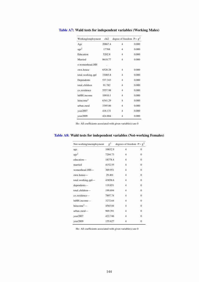
Table A7: Wald tests for independent variables (Working Males)
Working/employment chi2 degree of freedom P> χ2
Age 20867.4 4 0.000
age2 17768 4 0.000
Education 5202.8 4 0.000
Married 8618.77 4 0.000
o.womenhead HH .
own house 6520.28 4 0.000
total working ppl 33085.8 4 0.000
Dependents 537.343 4 0.000
total children 91.782 4 0.000
co residence 5557.98 4 0.000
lnHH income 10910.1 4 0.000
lnincome2 6341.29 4 0.000
urban rural 3395.06 4 0.000
year2007 416.131 4 0.000
year2009 424.884 4 0.000
Ho: All coefficients associated with given variable(s) are 0
Table A8: Wald tests for independent variables (Not-working Females)
Not-working/unemployment χ2 degrees of freedom P> χ2
age 10652.9 4 0
age2 7204.73 4 0
education— 18378.4 4 0
married 4152.55 4 0
womenhead HH— 369.951 4 0
own house— 29.401 4 0
total working ppl— 43858.6 4 0
dependents— 119.851 4 0
total children— 199.694 4 0
co residence— 7897.74 4 0
lnHH income— 3272.64 4 0
lnincome2— 4565.84 4 0
urban rural— 969.391 4 0
year2007 422.746 4 0
year2009 155.627 4 0
Ho: All coefficients associated with given variable(s) are 0
144
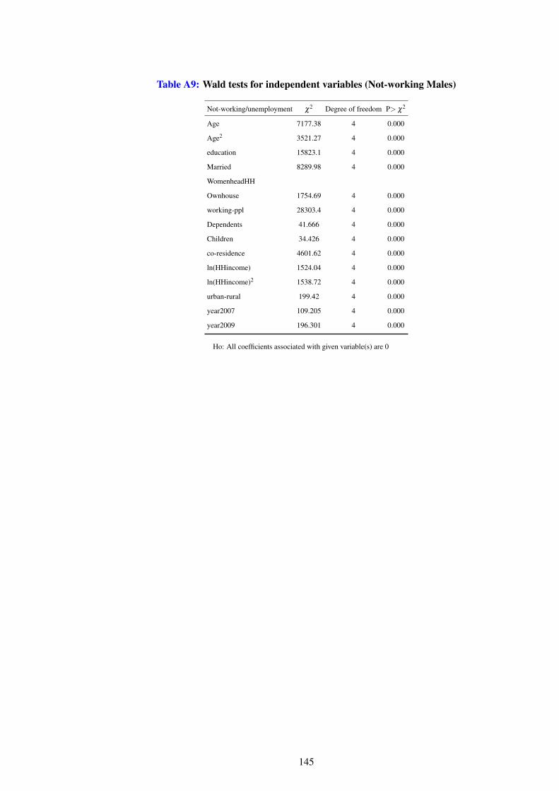
Table A9: Wald tests for independent variables (Not-working Males)
Not-working/unemployment χ2 Degree of freedom P> χ2
Age 7177.38 4 0.000
Age2 3521.27 4 0.000
education 15823.1 4 0.000
Married 8289.98 4 0.000
WomenheadHH
Ownhouse 1754.69 4 0.000
working-ppl 28303.4 4 0.000
Dependents 41.666 4 0.000
Children 34.426 4 0.000
co-residence 4601.62 4 0.000
ln(HHincome) 1524.04 4 0.000
ln(HHincome)2 1538.72 4 0.000
urban-rural 199.42 4 0.000
year2007 109.205 4 0.000
year2009 196.301 4 0.000
Ho: All coefficients associated with given variable(s) are 0
145
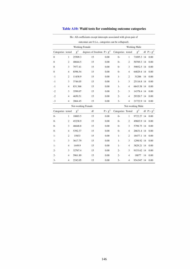
Table A10: Wald tests for combining outcome categories
Ho: All coefficients except intercepts associated with given pair of
outcomes are 0 (i.e., categories can be collapsed).
Working Female Working Male
Categories tested χ2 degrees of freedom P> χ2 Categories tested χ2 df P> χ2
0 1 25509.3 15 0.00 0- 1 71895.3 14 0.00
0 2 40644.5 15 0.00 0- 2 50769.3 14 0.00
0 3 7977.41 15 0.00 0- 3 59052.5 14 0.00
0 4 8596.54 15 0.00 0- 4 64829.4 14 0.00
-1 2 11438.9 15 0.00 1- 2 31206 14 0.00
-1 3 3744.05 15 0.00 1- 3 25116.8 14 0.00
-1 4 831.366 15 0.00 1- 4 6643.58 14 0.00
-2 3 3599.07 15 0.00 2- 3 14378.4 14 0.00
-2 4 4650.51 15 0.00 2- 4 29320.7 14 0.00
-3 4 2064.45 15 0.00 3- 4 21722.9 14 0.00
Not-working Female Not-working Male
Categories tested χ2 df P> χ2 Categories Tested χ2 df P> χ2
0- 1 10003.5 15 0.00 0- 1 9722.27 14 0.00
0- 2 45238.9 15 0.00 0- 2 49603.9 14 0.00
0- 3 46648.8 15 0.00 0- 3 5798.75 14 0.00
0- 4 5392.37 15 0.00 0- 4 26631.4 14 0.00
1- 2 15833 15 0.00 1- 2 18477.1 14 0.00
1- 3 3617.79 15 0.00 1- 3 1298.92 14 0.00
1- 4 1449.9 15 0.00 1- 4 3829.21 14 0.00
2- 3 32767.4 15 0.00 2- 3 9153.62 14 0.00
2- 4 5961.89 15 0.00 2- 4 18877 14 0.00
3- 4 2242.05 15 0.00 3- 4 934.947 14 0.00
146
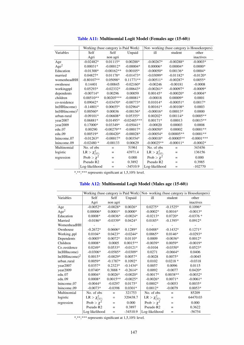
Table A11: Multinomial Logit Model (Females age (15-60))
Working (base category is Paid Work) Not- working (base category is Housekeepers)Variables Self Self Unpaid ill student other
Agri non agri inactivesAge -0.02482* 0.01115* 0.00288* -0.00267* -0.00288* -0.0003*Age2 0.00031* -0.00012* -0.00004* 0.00006* 0.00004* 0.0000*Education -0.01300* -0.00162** 0.00105* -0.00050* 0.00136* 0.0004*married 0.04827* 0.01178* -0.01473* -0.03099* -0.01182* -0.0120*womenheadHH -0.80107** 0.05098* 0.11771** -0.00511* -0.00287* 0.0055*ownhouse 0.14401 -0.00845 -0.02160* -0.00246 -0.00181 -0.0008workingppl 0.05293* -0.02332* -0.00643* -0.00261* -0.00097* -0.0009*dependents -0.00714* 0.00296 0.00059 0.00145* -0.00020* -0.0004*children 0.00510** 0.00205*** -0.00081* -0.00018 0.00009* 0.0001co-residence 0.09042* -0.03470* -0.00773* 0.01014* -0.00051* 0.0017*ln(HHincome) -0.14801* 0.00655* 0.02964* 0.00161* -0.00108* 0.0003ln(HHincome)2 0.00560* 0.00036 -0.00156* -0.00016* 0.00013* 0.0000urban-rural -0.09101* -0.06608* 0.05355* 0.00202* 0.00114* 0.0005**year2007 0.06881* 0.01495* -0.02485*** 0.00171* 0.00013 0.0015**year2009 0.17000* 0.03349* -0.05041* -0.00020 0.00003 0.0008edu 07 0.00290 -0.00279** -0.00017* -0.00050* 0.00002 0.0001**edu 09 0.00519* -0.00420* -0.00028* -0.00054* 0.00005** 0.0001**lnincome 07 -0.01263* -0.00017* 0.00354* -0.00018* -0.00005** -0.0001***lnincome 09 -0.02480 * -0.00133 0.00629 -0.00025** -0.00011* -0.0002*Multinomial No. of obs = 51961 No. of obs = 343456logistic LR > χ2
(57) = 43971.4 LR > χ2(57) = 136156
regression Prob > χ2 = 0.000 Prob > χ2 = 0.000Pseudo R2 = 0.3892 Pseudo R2 = 0.3985
Log-likelihood = -34510.9 Log-likelihood = -102770
*,**,*** represents significant at 1,5,10% level.
Table A12: Multinomial Logit Model (Males age (15-60))
Working (base category is Paid Work) Not- working (base category is Housekeepers)Variables Self Self Unpaid ill student other
Agri non agri inactivesAge -0.0052* -0.0028* 0.0026* 0.0275* -0.1525* 0.1096*Age2 0.00006* 0.0001* 0.0000* -0.0002* 0.0016* -0.0013*Education 0.0008* -0.0036* -0.0024* -0.0213* 0.0720* -0.0376 *Married -0.0186* -0.0339* 0.0424* 0.0185* -0.1395* 0.0912*WomenheadHH - - - - - -Ownhouse -0.2672* 0.0606* 0.1289* 0.0488* -0.1432* 0.1271*Working ppl 0.0104* 0.0423* -0.0244* 0.0065* 0.0146* -0.0293*Dependents -0.0005* 0.0072* 0.0110* 0.0009 -0.0036* 0.0012*Children 0.0008* 0.0005 0.0015** -0.0039* 0.0059* -0.0019*Co residence 0.0249* 0.0533* -0.0121* -0.0104 -0.0350* 0.0523*ln(HHncome) -0.0306* -0.0585* -0.0309* 0.0271 -0.0664* 0.0406ln(HHincome)2 0.0015* -0.0029* 0.0057* -0.0028 0.0075* -0.0045urban rural 0.0059* -0.1787* 0.1092* 0.0102 0.0218 * -0.0318year2007 0.0357* 0.2323* -0.1434* 0.0057 0.0096 0.0115year2009 0.0740* 0.3888 * -0.2614* 0.0092 -0.0077 0.0420*edu 07 0.0004* 0.0026* -0.0020* -0.0017* 0.0038** -0.0032*edu 09 0.0008* 0.0015** -0.0025* -0.0026* 0.0071* -0.0061*lnincome 07 -0.0044* -0.0297 0.0175* 0.0002* -0.0053 0.0035*lnincome 09 -0.0073* -0.0398 0.0301* 0.0012* -0.0079 0.0053*Multinomial No. of obs = 321753 No. of obs = 85209logistic LR > χ2
(57) = 320438.7 LR > χ2(57) = 64470.03
regression Prob > χ2 = 0.000 Prob > χ2 = 0.000Pseudo R2 = 0.3897 Pseudo R2 = 0.3622
Log likelihood = -34510.9 Log-likelihood = -56754
*,**,*** represents significant at 1,5,10% level.
147
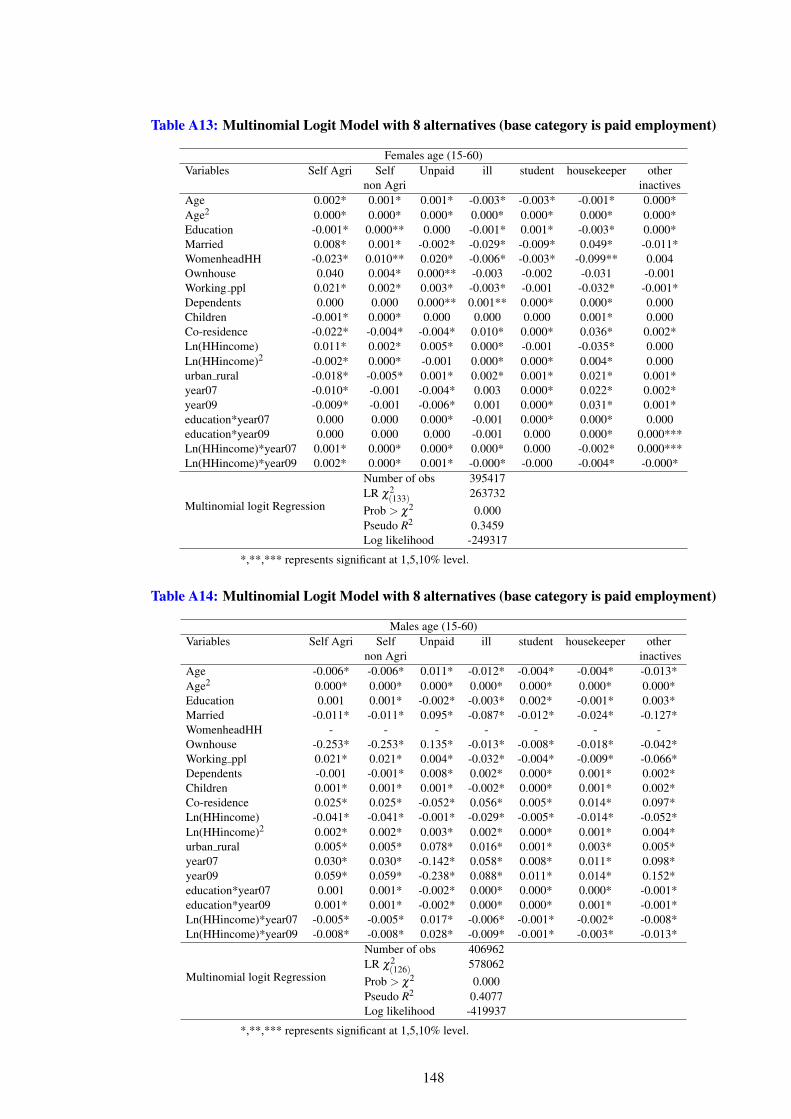
Table A13: Multinomial Logit Model with 8 alternatives (base category is paid employment)
Females age (15-60)Variables Self Agri Self Unpaid ill student housekeeper other
non Agri inactivesAge 0.002* 0.001* 0.001* -0.003* -0.003* -0.001* 0.000*Age2 0.000* 0.000* 0.000* 0.000* 0.000* 0.000* 0.000*Education -0.001* 0.000** 0.000 -0.001* 0.001* -0.003* 0.000*Married 0.008* 0.001* -0.002* -0.029* -0.009* 0.049* -0.011*WomenheadHH -0.023* 0.010** 0.020* -0.006* -0.003* -0.099** 0.004Ownhouse 0.040 0.004* 0.000** -0.003 -0.002 -0.031 -0.001Working ppl 0.021* 0.002* 0.003* -0.003* -0.001 -0.032* -0.001*Dependents 0.000 0.000 0.000** 0.001** 0.000* 0.000* 0.000Children -0.001* 0.000* 0.000 0.000 0.000 0.001* 0.000Co-residence -0.022* -0.004* -0.004* 0.010* 0.000* 0.036* 0.002*Ln(HHincome) 0.011* 0.002* 0.005* 0.000* -0.001 -0.035* 0.000Ln(HHincome)2 -0.002* 0.000* -0.001 0.000* 0.000* 0.004* 0.000urban rural -0.018* -0.005* 0.001* 0.002* 0.001* 0.021* 0.001*year07 -0.010* -0.001 -0.004* 0.003 0.000* 0.022* 0.002*year09 -0.009* -0.001 -0.006* 0.001 0.000* 0.031* 0.001*education*year07 0.000 0.000 0.000* -0.001 0.000* 0.000* 0.000education*year09 0.000 0.000 0.000 -0.001 0.000 0.000* 0.000***Ln(HHincome)*year07 0.001* 0.000* 0.000* 0.000* 0.000 -0.002* 0.000***Ln(HHincome)*year09 0.002* 0.000* 0.001* -0.000* -0.000 -0.004* -0.000*
Multinomial logit Regression
Number of obs 395417LR χ2
(133) 263732Prob > χ2 0.000Pseudo R2 0.3459Log likelihood -249317
*,**,*** represents significant at 1,5,10% level.
Table A14: Multinomial Logit Model with 8 alternatives (base category is paid employment)
Males age (15-60)Variables Self Agri Self Unpaid ill student housekeeper other
non Agri inactivesAge -0.006* -0.006* 0.011* -0.012* -0.004* -0.004* -0.013*Age2 0.000* 0.000* 0.000* 0.000* 0.000* 0.000* 0.000*Education 0.001 0.001* -0.002* -0.003* 0.002* -0.001* 0.003*Married -0.011* -0.011* 0.095* -0.087* -0.012* -0.024* -0.127*WomenheadHH - - - - - - -Ownhouse -0.253* -0.253* 0.135* -0.013* -0.008* -0.018* -0.042*Working ppl 0.021* 0.021* 0.004* -0.032* -0.004* -0.009* -0.066*Dependents -0.001 -0.001* 0.008* 0.002* 0.000* 0.001* 0.002*Children 0.001* 0.001* 0.001* -0.002* 0.000* 0.001* 0.002*Co-residence 0.025* 0.025* -0.052* 0.056* 0.005* 0.014* 0.097*Ln(HHincome) -0.041* -0.041* -0.001* -0.029* -0.005* -0.014* -0.052*Ln(HHincome)2 0.002* 0.002* 0.003* 0.002* 0.000* 0.001* 0.004*urban rural 0.005* 0.005* 0.078* 0.016* 0.001* 0.003* 0.005*year07 0.030* 0.030* -0.142* 0.058* 0.008* 0.011* 0.098*year09 0.059* 0.059* -0.238* 0.088* 0.011* 0.014* 0.152*education*year07 0.001 0.001* -0.002* 0.000* 0.000* 0.000* -0.001*education*year09 0.001* 0.001* -0.002* 0.000* 0.000* 0.001* -0.001*Ln(HHincome)*year07 -0.005* -0.005* 0.017* -0.006* -0.001* -0.002* -0.008*Ln(HHincome)*year09 -0.008* -0.008* 0.028* -0.009* -0.001* -0.003* -0.013*
Multinomial logit Regression
Number of obs 406962LR χ2
(126) 578062Prob > χ2 0.000Pseudo R2 0.4077Log likelihood -419937
*,**,*** represents significant at 1,5,10% level.
148
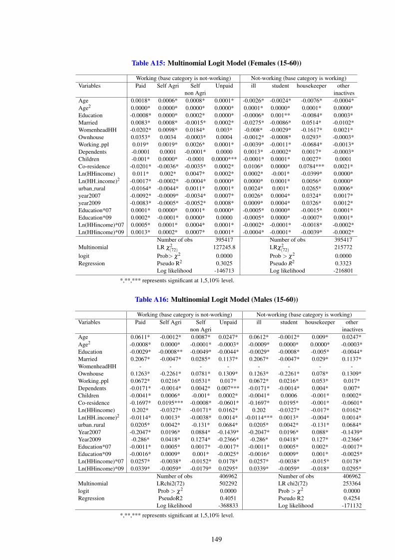
Table A15: Multinomial Logit Model (Females (15-60))
Working (base category is not-working) Not-working (base category is working)Variables Paid Self Agri Self Unpaid ill student housekeeper other
non Agri inactivesAge 0.0018* 0.0006* 0.0008* 0.0001* -0.0026* -0.0024* -0.0076* -0.0004*Age2 0.0000* 0.0000* 0.0000* 0.0000* 0.0001* 0.0000* 0.0001* 0.0000*Education -0.0008* 0.0000* 0.0002* 0.0000* -0.0006* 0.001** -0.0084* 0.0003*Married 0.0083* 0.0008* -0.0015* 0.0002* -0.0275* -0.0086* 0.0514* -0.0102*WomenheadHH -0.0202* 0.0098* 0.0184* 0.003* -0.008* -0.0029* -0.1617* 0.0021*Ownhouse 0.0353* 0.0034 -0.0003* 0.0004 -0.0012* -0.0008* 0.0293* -0.0003*Working ppl 0.019* 0.0019* 0.0026* 0.0001* -0.0039* -0.0011* -0.0684* -0.0013*Dependents -0.0001 0.0001 -0.0001* 0.0000 0.0013* -0.0002* 0.0017* -0.0003*Children -0.001* 0.0000* -0.0001 0.0000*** -0.0001* 0.0001* 0.0027* 0.0001Co-residence -0.0201* -0.0036* -0.0035* 0.0002* 0.0106* 0.0000* 0.0784*** 0.0021*Ln(HHincome) 0.011* 0.002* 0.0047* 0.0002* 0.0002* -0.001* -0.0399* 0.0000*Ln(HH income)2 -0.0017* -0.0002* -0.0004* 0.0000* 0.0000* 0.0001* 0.0056* 0.0000*urban rural -0.0164* -0.0044* 0.0011* 0.0001* 0.0024* 0.001* 0.0265* 0.0006*year2007 -0.0092* -0.0009* -0.0034* 0.0007* 0.0026* 0.0004* 0.0324* 0.0017*year2009 -0.0083* -0.0005* -0.0052* 0.0008* 0.0009* 0.0004* 0.0326* 0.0012*Education*07 0.0001* 0.0000* 0.0001* 0.0000* -0.0005* 0.0000* -0.0015* 0.0001*Education*09 0.0002* -0.0001* 0.0000* 0.0000 -0.0005* 0.0000* -0.0007* 0.0001*Ln(HHincome)*07 0.0005* 0.0001* 0.0004* 0.0001* -0.0002* -0.0001* -0.0018* -0.0002*Ln(HHincome)*09 0.0013* 0.0002* 0.0007* 0.0001* -0.0004* -0.0001* -0.0039* -0.0002*
Number of obs 395417 Number of obs 395417Multinomial LR χ2
(72) 127245.8 LRχ2(72) 215772
logit Prob> χ2 0.0000 Prob > χ2 0.0000Regression Pseudo R2 0.3025 Pseudo R2 0.3323
Log likelihood -146713 Log likelihood -216801
*,**,*** represents significant at 1,5,10% level.
Table A16: Multinomial Logit Model (Males (15-60))
Working (base category is not-working) Not-working (base category is working)Variables Paid Self Agri Self Unpaid ill student housekeeper other
non Agri inactivesAge 0.0611* -0.0012* 0.0087* 0.0247* 0.0612* -0.0012* 0.009* 0.0247*Age2 -0.0008* 0.0000* -0.0001* -0.0003* -0.0009* 0.0000* 0.0000* -0.0003*Education -0.0029* -0.0008** -0.0049* -0.0044* -0.0029* -0.0008* -0.005* -0.0044*Married 0.2067* -0.0047* 0.0285* 0.1137* 0.2067* -0.0047* 0.029* 0.1137*WomenheadHH - - - - - - - -Ownhouse 0.1263* -0.2261* 0.0781* 0.1309* 0.1263* -0.2261* 0.078* 0.1309*Working ppl 0.0672* 0.0216* 0.0531* 0.017* 0.0672* 0.0216* 0.053* 0.017*Dependents -0.0171* -0.0014* 0.0042* 0.007*** -0.0171* -0.0014* 0.004* 0.007*Children -0.0041* 0.0006* -0.001* 0.0002* -0.0041* 0.0006 -0.001* 0.0002*Co-residence -0.1697* 0.0195*** -0.0008* -0.0601* -0.1697* 0.0195* -0.001* -0.0601*Ln(HHincome) 0.202* -0.0327* -0.0171* 0.0162* 0.202 -0.0327* -0.017* 0.0162*Ln(HH income)2 -0.0114* 0.0013* -0.0038* 0.0014* -0.0114*** 0.0013* -0.004* 0.0014*urban rural 0.0205* 0.0042* -0.131* 0.0684* 0.0205* 0.0042* -0.131* 0.0684*Year2007 -0.2047* 0.0196* 0.0884* -0.1439* -0.2047* 0.0196* 0.088* -0.1439*Year2009 -0.286* 0.0418* 0.1274* -0.2366* -0.286* 0.0418* 0.127* -0.2366*Education*07 -0.0011* 0.0005* 0.0017* -0.0017* -0.0011* 0.0005* 0.002* -0.0017*Education*09 -0.0016* 0.0009* 0.001* -0.0025* -0.0016* 0.0009* 0.001* -0.0025*Ln(HHincome)*07 0.0257* -0.0038* -0.0152* 0.0178* 0.0257* -0.0038* -0.015* 0.0178*Ln(HHincome)*09 0.0339* -0.0059* -0.0179* 0.0295* 0.0339* -0.0059* -0.018* 0.0295*
Number of obs 406962 Number of obs 406962Multinomial LRchi2(72) 502292 LR chi2(72) 253364logit Prob > χ2 0.0000 Prob > χ2 0.0000Regression PseudoR2 0.4051 Pseudo R2 0.4254
Log likelihood -368833 Log likelihood -171132
*,**,*** represents significant at 1,5,10% level.
149
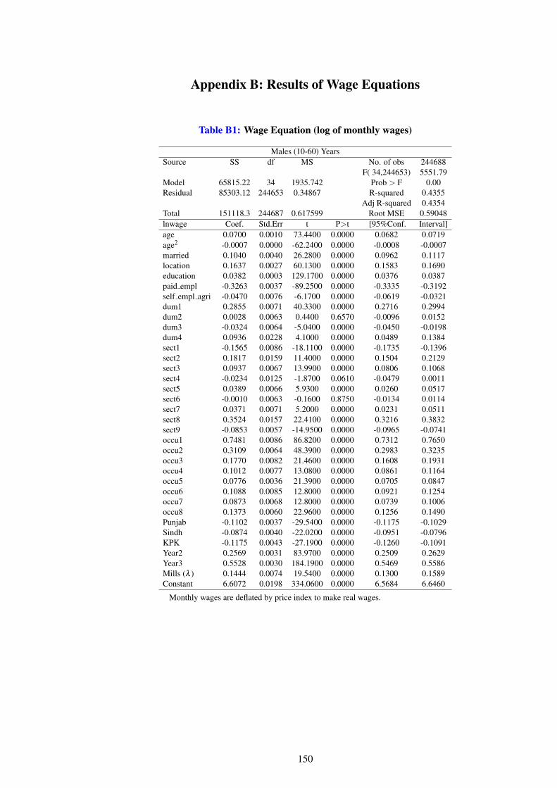
Appendix B: Results of Wage Equations
Table B1: Wage Equation (log of monthly wages)
Males (10-60) YearsSource SS df MS No. of obs 244688
F( 34,244653) 5551.79Model 65815.22 34 1935.742 Prob > F 0.00Residual 85303.12 244653 0.34867 R-squared 0.4355
Adj R-squared 0.4354Total 151118.3 244687 0.617599 Root MSE 0.59048lnwage Coef. Std.Err t P>t [95%Conf. Interval]age 0.0700 0.0010 73.4400 0.0000 0.0682 0.0719age2 -0.0007 0.0000 -62.2400 0.0000 -0.0008 -0.0007married 0.1040 0.0040 26.2800 0.0000 0.0962 0.1117location 0.1637 0.0027 60.1300 0.0000 0.1583 0.1690education 0.0382 0.0003 129.1700 0.0000 0.0376 0.0387paid empl -0.3263 0.0037 -89.2500 0.0000 -0.3335 -0.3192self empl agri -0.0470 0.0076 -6.1700 0.0000 -0.0619 -0.0321dum1 0.2855 0.0071 40.3300 0.0000 0.2716 0.2994dum2 0.0028 0.0063 0.4400 0.6570 -0.0096 0.0152dum3 -0.0324 0.0064 -5.0400 0.0000 -0.0450 -0.0198dum4 0.0936 0.0228 4.1000 0.0000 0.0489 0.1384sect1 -0.1565 0.0086 -18.1100 0.0000 -0.1735 -0.1396sect2 0.1817 0.0159 11.4000 0.0000 0.1504 0.2129sect3 0.0937 0.0067 13.9900 0.0000 0.0806 0.1068sect4 -0.0234 0.0125 -1.8700 0.0610 -0.0479 0.0011sect5 0.0389 0.0066 5.9300 0.0000 0.0260 0.0517sect6 -0.0010 0.0063 -0.1600 0.8750 -0.0134 0.0114sect7 0.0371 0.0071 5.2000 0.0000 0.0231 0.0511sect8 0.3524 0.0157 22.4100 0.0000 0.3216 0.3832sect9 -0.0853 0.0057 -14.9500 0.0000 -0.0965 -0.0741occu1 0.7481 0.0086 86.8200 0.0000 0.7312 0.7650occu2 0.3109 0.0064 48.3900 0.0000 0.2983 0.3235occu3 0.1770 0.0082 21.4600 0.0000 0.1608 0.1931occu4 0.1012 0.0077 13.0800 0.0000 0.0861 0.1164occu5 0.0776 0.0036 21.3900 0.0000 0.0705 0.0847occu6 0.1088 0.0085 12.8000 0.0000 0.0921 0.1254occu7 0.0873 0.0068 12.8000 0.0000 0.0739 0.1006occu8 0.1373 0.0060 22.9600 0.0000 0.1256 0.1490Punjab -0.1102 0.0037 -29.5400 0.0000 -0.1175 -0.1029Sindh -0.0874 0.0040 -22.0200 0.0000 -0.0951 -0.0796KPK -0.1175 0.0043 -27.1900 0.0000 -0.1260 -0.1091Year2 0.2569 0.0031 83.9700 0.0000 0.2509 0.2629Year3 0.5528 0.0030 184.1900 0.0000 0.5469 0.5586Mills (λ ) 0.1444 0.0074 19.5400 0.0000 0.1300 0.1589Constant 6.6072 0.0198 334.0600 0.0000 6.5684 6.6460
Monthly wages are deflated by price index to make real wages.
150
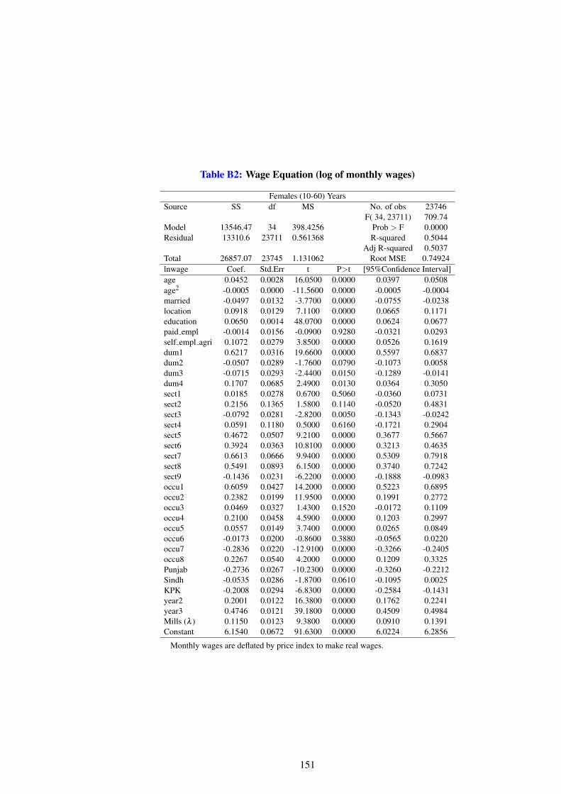
Table B2: Wage Equation (log of monthly wages)
Females (10-60) YearsSource SS df MS No. of obs 23746
F( 34, 23711) 709.74Model 13546.47 34 398.4256 Prob > F 0.0000Residual 13310.6 23711 0.561368 R-squared 0.5044
Adj R-squared 0.5037Total 26857.07 23745 1.131062 Root MSE 0.74924lnwage Coef. Std.Err t P>t [95%Confidence Interval]age 0.0452 0.0028 16.0500 0.0000 0.0397 0.0508age2 -0.0005 0.0000 -11.5600 0.0000 -0.0005 -0.0004married -0.0497 0.0132 -3.7700 0.0000 -0.0755 -0.0238location 0.0918 0.0129 7.1100 0.0000 0.0665 0.1171education 0.0650 0.0014 48.0700 0.0000 0.0624 0.0677paid empl -0.0014 0.0156 -0.0900 0.9280 -0.0321 0.0293self empl agri 0.1072 0.0279 3.8500 0.0000 0.0526 0.1619dum1 0.6217 0.0316 19.6600 0.0000 0.5597 0.6837dum2 -0.0507 0.0289 -1.7600 0.0790 -0.1073 0.0058dum3 -0.0715 0.0293 -2.4400 0.0150 -0.1289 -0.0141dum4 0.1707 0.0685 2.4900 0.0130 0.0364 0.3050sect1 0.0185 0.0278 0.6700 0.5060 -0.0360 0.0731sect2 0.2156 0.1365 1.5800 0.1140 -0.0520 0.4831sect3 -0.0792 0.0281 -2.8200 0.0050 -0.1343 -0.0242sect4 0.0591 0.1180 0.5000 0.6160 -0.1721 0.2904sect5 0.4672 0.0507 9.2100 0.0000 0.3677 0.5667sect6 0.3924 0.0363 10.8100 0.0000 0.3213 0.4635sect7 0.6613 0.0666 9.9400 0.0000 0.5309 0.7918sect8 0.5491 0.0893 6.1500 0.0000 0.3740 0.7242sect9 -0.1436 0.0231 -6.2200 0.0000 -0.1888 -0.0983occu1 0.6059 0.0427 14.2000 0.0000 0.5223 0.6895occu2 0.2382 0.0199 11.9500 0.0000 0.1991 0.2772occu3 0.0469 0.0327 1.4300 0.1520 -0.0172 0.1109occu4 0.2100 0.0458 4.5900 0.0000 0.1203 0.2997occu5 0.0557 0.0149 3.7400 0.0000 0.0265 0.0849occu6 -0.0173 0.0200 -0.8600 0.3880 -0.0565 0.0220occu7 -0.2836 0.0220 -12.9100 0.0000 -0.3266 -0.2405occu8 0.2267 0.0540 4.2000 0.0000 0.1209 0.3325Punjab -0.2736 0.0267 -10.2300 0.0000 -0.3260 -0.2212Sindh -0.0535 0.0286 -1.8700 0.0610 -0.1095 0.0025KPK -0.2008 0.0294 -6.8300 0.0000 -0.2584 -0.1431year2 0.2001 0.0122 16.3800 0.0000 0.1762 0.2241year3 0.4746 0.0121 39.1800 0.0000 0.4509 0.4984Mills (λ ) 0.1150 0.0123 9.3800 0.0000 0.0910 0.1391Constant 6.1540 0.0672 91.6300 0.0000 6.0224 6.2856
Monthly wages are deflated by price index to make real wages.
151
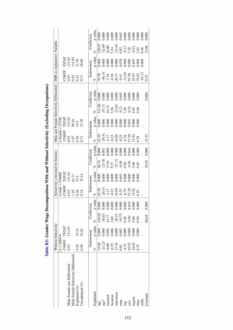
Tabl
eB
3:G
ende
rW
age
Dec
ompo
sitio
nW
ithan
dW
ithou
tSel
ectiv
ity(E
xclu
ding
Occ
upat
ions
)
With
outS
elec
tivity
Sele
ctiv
ityco
rrec
ted
forf
emal
esM
ale
and
Fem
ale
Sele
ctiv
ityD
iffer
entia
lIM
Ras
expl
anat
ory
Var
iabl
en
=26
8434
nm
ale
=24
4688
nfe
mal
e=
2374
6C
OE
FFT
STA
TC
OE
FFT
STA
TC
OE
FFT
STA
TC
OE
FFT
STA
TM
ale-
Fem
ale
raw
Diff
eren
tial
0.93
131.
930.
9313
1.93
0.93
131.
930.
9313
1.93
Mal
e-Fe
mal
eSe
lect
ivity
Diff
eren
tial
--
1.10
61.3
11.
0759
.10
0.93
131.
93E
xpla
ined
(%)
0.38
35.3
30.
3633
.50.
3633
.50.
2211
.78
Une
xpla
ined
(%)
0.56
52.0
10.
7435
.14
0.71
33.3
80.
7138
.09
End
owm
ent
Coe
ffici
ent
End
owm
ent
Coe
ffici
ent
End
owm
ent
Coe
ffici
ent
End
owm
ent
Coe
ffici
ent
Exp
lain
ed%
pva
lue
%p
valu
e%
pva
lue
%p
valu
e%
pva
lue
%p
valu
e%
pva
lue
%p
valu
eag
e33
.49
0.00
013
0.62
0.00
043
.39
0.00
056
.74
0.00
043
.39
0.00
012
1.06
0.00
070
.78
0.00
012
0.07
0.00
0ag
e2-2
1.23
0.00
0-5
8.83
0.00
0-2
9.51
0.00
0-2
3.70
0.00
1-2
9.51
0.00
0-5
3.13
0.00
0-4
8.14
0.00
0-5
2.69
0.00
0m
arri
ed-0
.89
0.09
214
.77
0.00
0-2
.17
0.00
013
.91
0.00
0-2
.17
0.00
016
.14
0.00
0-3
.54
0.00
016
.00
0.00
0lo
catio
n-0
.35
0.00
63.
600.
000
-0.2
30.
009
5.57
0.00
0-0
.23
0.00
05.
380.
009
-0.3
80.
000
5.34
0.00
9ed
ucat
ion
15.1
60.
000
-28.
150.
000
16.0
40.
000
-21.
720.
000
16.0
40.
000
-23.
630.
000
26.1
70.
000
-23.
440.
000
emp
0.01
0.98
2-1
0.75
0.00
0-0
.25
0.64
5-8
.88
0.00
0-0
.25
0.00
0-9
.21
0.64
5-0
.41
0.07
80.
820.
645
org
-6.5
10.
000
9.48
0.00
0-6
.76
0.00
06.
900.
000
-6.7
60.
000
7.26
0.00
0-1
1.03
0.00
0-9
.13
0.00
0se
ct55
.92
0.00
0-0
.81
0.81
057
.20
0.00
0-0
.50
0.84
457
.20
0.84
5-0
.52
0.00
093
.30
0.00
07.
200.
000
regi
on18
.05
0.00
05.
000.
000
15.9
20.
000
2.60
0.00
015
.92
0.00
02.
850.
000
25.9
70.
845
-0.5
20.
000
time
6.35
0.00
00.
500.
000
6.39
0.00
00.
450.
000
6.39
0.00
00.
460.
000
10.4
20.
000
2.83
0.00
0m
ills
--
--
--
--
--
--
-63.
130.
000
0.46
0.00
0C
onst
ant
68.6
40.
000
34.5
80.
000
33.3
30.
000
0.33
33.0
60.
000
152
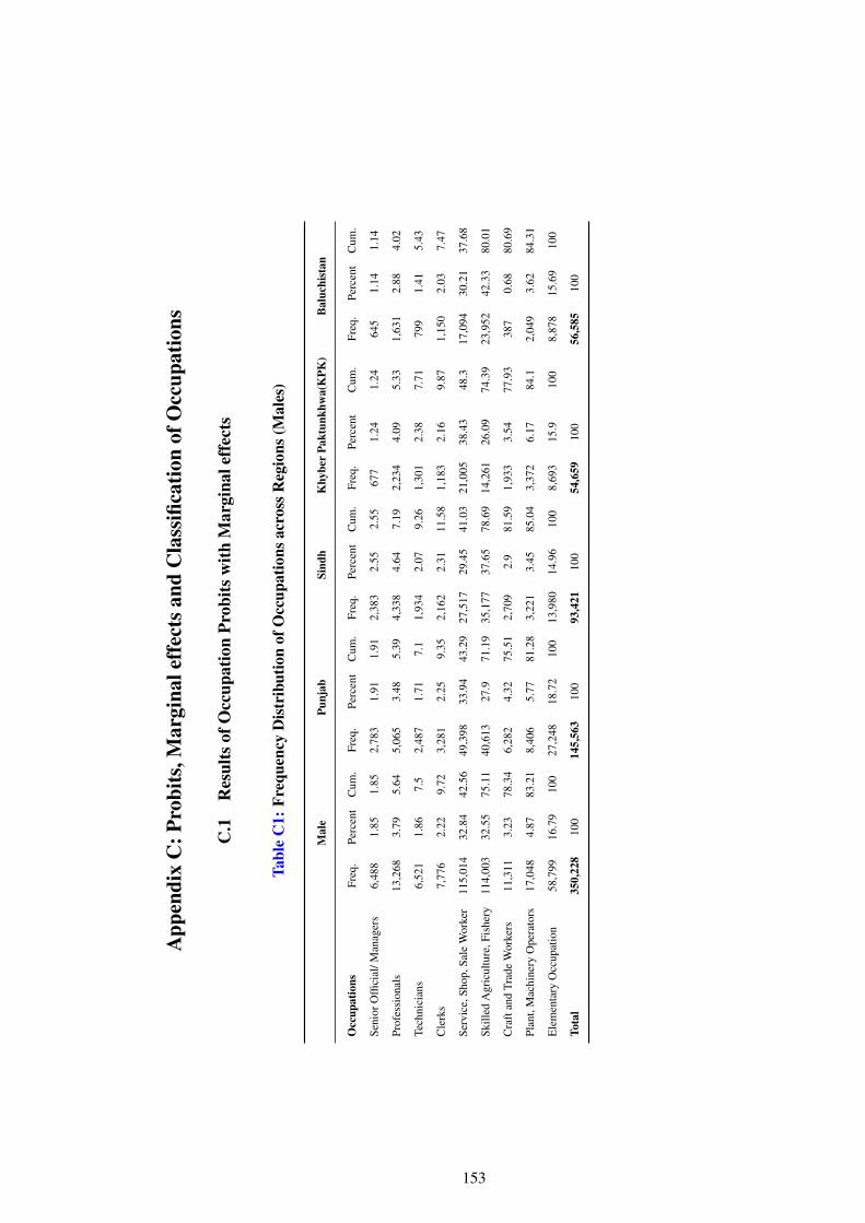
App
endi
xC
:Pro
bits
,Mar
gina
leff
ects
and
Cla
ssifi
catio
nof
Occ
upat
ions
C.1
Res
ults
ofO
ccup
atio
nPr
obits
with
Mar
gina
leff
ects
Tabl
eC
1:Fr
eque
ncy
Dis
trib
utio
nof
Occ
upat
ions
acro
ssR
egio
ns(M
ales
)
Mal
ePu
njab
Sind
hK
hybe
rPa
ktun
khw
a(K
PK)
Bal
uchi
stan
Occ
upat
ions
Freq
.Pe
rcen
tC
um.
Freq
.Pe
rcen
tC
um.
Freq
.Pe
rcen
tC
um.
Freq
.Pe
rcen
tC
um.
Freq
.Pe
rcen
tC
um.
Seni
orO
ffici
al/M
anag
ers
6,48
81.
851.
852,
783
1.91
1.91
2,38
32.
552.
5567
71.
241.
2464
51.
141.
14
Prof
essi
onal
s13
,268
3.79
5.64
5,06
53.
485.
394,
338
4.64
7.19
2,23
44.
095.
331,
631
2.88
4.02
Tech
nici
ans
6,52
11.
867.
52,
487
1.71
7.1
1,93
42.
079.
261,
301
2.38
7.71
799
1.41
5.43
Cle
rks
7,77
62.
229.
723,
281
2.25
9.35
2,16
22.
3111
.58
1,18
32.
169.
871,
150
2.03
7.47
Serv
ice,
Shop
,Sal
eW
orke
r11
5,01
432
.84
42.5
649
,398
33.9
443
.29
27,5
1729
.45
41.0
321
,005
38.4
348
.317
,094
30.2
137
.68
Skill
edA
gric
ultu
re,F
ishe
ry11
4,00
332
.55
75.1
140
,613
27.9
71.1
935
,177
37.6
578
.69
14,2
6126
.09
74.3
923
,952
42.3
380
.01
Cra
ftan
dTr
ade
Wor
kers
11,3
113.
2378
.34
6,28
24.
3275
.51
2,70
92.
981
.59
1,93
33.
5477
.93
387
0.68
80.6
9
Plan
t,M
achi
nery
Ope
rato
rs17
,048
4.87
83.2
18,
406
5.77
81.2
83,
221
3.45
85.0
43,
372
6.17
84.1
2,04
93.
6284
.31
Ele
men
tary
Occ
upat
ion
58,7
9916
.79
100
27,2
4818
.72
100
13,9
8014
.96
100
8,69
315
.910
08,
878
15.6
910
0
Tota
l35
0,22
810
014
5,56
310
093
,421
100
54,6
5910
056
,585
100
153
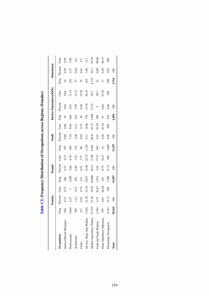
Tabl
eC
2:Fr
eque
ncy
Dis
trib
utio
nof
Occ
upat
ions
acro
ssR
egio
ns(F
emal
es)
Fem
ales
Punj
abSi
ndh
Khy
ber
Pakt
unkh
wa(
KPK
)B
aluc
hist
an
Occ
upat
ions
Freq
.Pe
rcen
tC
um.
Freq
.Pe
rcen
tC
um.
Freq
.Pe
rcen
tC
um.
Freq
.Pe
rcen
tC
um.
Freq
.Pe
rcen
tC
um.
Seni
orO
ffici
al/M
anag
ers
426
0.73
0.73
246
0.73
0.73
107
0.86
0.86
390.
640.
6434
0.59
0.59
Prof
essi
onal
s3,
644
6.27
71,
920
5.66
6.39
890
7.18
8.04
640
10.5
11.1
419
43.
373.
96
Tech
nici
ans
705
1.21
8.21
293
0.86
7.25
132
1.06
9.11
243
3.99
15.1
237
0.64
4.6
Cle
rks
317
0.55
8.75
174
0.51
7.77
800.
659.
7528
0.46
15.5
835
0.61
5.2
Serv
ice,
Shop
,Sal
eW
orke
r7,
435
12.7
821
.54
5,07
314
.96
22.7
31,
129
9.11
18.8
677
812
.76
28.3
545
57.
8913
.1
Skill
edA
gric
ultu
re,F
ishe
ry33
,375
57.3
878
.92
16,6
6649
.15
71.8
88,
481
68.4
187
.27
3,49
657
.35
85.7
4,73
282
.195
.19
Cra
ftan
dTr
ade
Wor
kers
2,76
44.
7583
.67
1,91
15.
6477
.51
497
4.01
91.2
830
55
90.7
510.
8896
.08
Plan
t,M
achi
nery
Ope
rato
rs35
50.
6184
.28
255
0.75
78.2
732
0.26
91.5
451
0.84
91.5
417
0.29
96.3
7
Ele
men
tary
Occ
upat
ion
9,14
315
.72
100
7,36
921
.73
100
1,04
98.
4610
051
68.
4610
020
93.
6310
0
Tota
l58
,164
100
33,9
0710
012
,397
100
6,09
610
05,
764
100
154
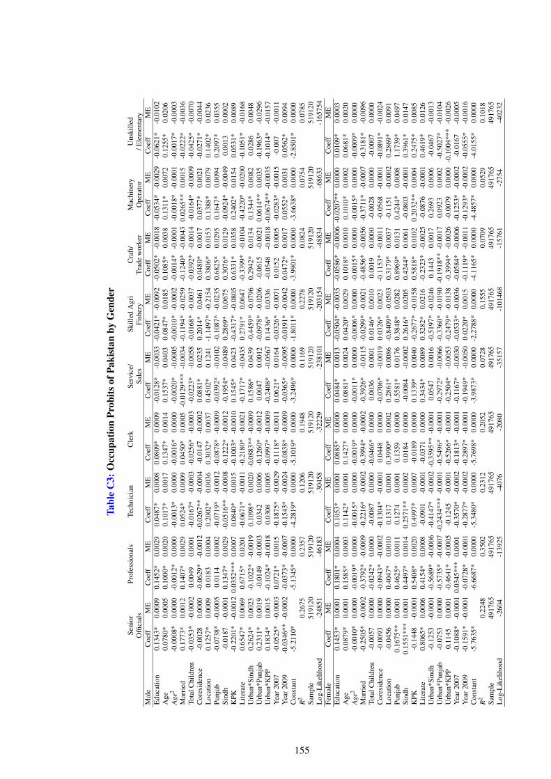
Tabl
eC
3:O
ccup
atio
nPr
obits
ofPa
kist
anby
Gen
der
Seni
orPr
ofes
sion
als
Tech
nici
anC
lerk
Serv
ice/
Skill
edA
gri
Cra
ft/
Mac
hine
ryU
nski
lled
Offi
cial
sSa
les
Fish
ery
Trad
ew
orke
rO
pera
tor
/Ele
men
tary
Mal
eC
oeff
ME
Coe
ffM
EC
oeff
ME
Coe
ffM
EC
oeff
ME
Coe
ffM
EC
oeff
ME
Coe
ffM
EC
oeff
ME
Edu
catio
n0.
1343
*0.
0009
0.14
52*
0.00
290.
0487
*0.
0008
0.08
09*
0.00
09-0
.012
8*-0
.003
3-0
.042
1*-0
.009
2-0
.050
2*-0
.001
8-0
.053
4*-0
.002
9-0
.062
1*-0
.010
2A
ge0.
0780
*0.
0005
0.10
00*
0.00
200.
1017
*0.
0017
0.13
47*
0.00
140.
1537
*0.
0403
0.08
47*
0.01
850.
1085
*0.
0038
0.13
11*
0.00
720.
1255
*0.
0206
Age
2-0
.000
8*0.
0000
-0.0
012*
0.00
00-0
.001
3*0.
0000
-0.0
016*
0.00
00-0
.002
0*-0
.000
5-0
.001
0*-0
.000
2-0
.001
4*-0
.000
1-0
.001
8*-0
.000
1-0
.001
7*-0
.000
3M
arri
ed0.
1773
*0.
0012
0.14
07*
0.00
290.
0524
*0.
0009
0.04
50*
0.00
05-0
.012
9***
-0.0
034
-0.1
194*
-0.0
259
-0.1
240*
-0.0
043
0.02
65**
0.00
15-0
.022
2*-0
.003
6To
talC
hild
ren
-0.0
353*
-0.0
002
0.00
490.
0001
-0.0
167*
-0.0
003
-0.0
256*
-0.0
003
-0.0
223*
-0.0
058
-0.0
168*
-0.0
037
-0.0
392*
-0.0
014
-0.0
164*
-0.0
009
-0.0
425*
-0.0
070
Cor
esid
ence
-0.0
028
0.00
00-0
.062
9*-0
.001
2-0
.026
7**
-0.0
004
-0.0
147
-0.0
002
0.08
81*
0.02
350.
2014
*0.
0461
0.04
80*
0.00
170.
0377
*0.
0021
-0.0
271*
-0.0
044
Loc
atio
n0.
1257
*0.
0009
0.01
830.
0004
0.20
02*
0.00
360.
3032
*0.
0037
0.45
02*
0.12
41-1
.149
7*-0
.215
40.
3806
*0.
0153
0.13
88*
0.00
790.
1402
*0.
0236
Punj
ab-0
.073
8*-0
.000
50.
0114
0.00
02-0
.071
9*-0
.001
2-0
.087
8*-0
.000
9-0
.039
2*-0
.010
2-0
.108
7*-0
.023
50.
6825
*0.
0295
0.16
47*
0.00
940.
2097
*0.
0355
Sind
h-0
.018
7-0
.000
10.
1347
*0.
0029
-0.0
516*
*-0
.000
8-0
.122
2*-0
.001
2-0
.195
4*-0
.048
90.
2869
*0.
0675
0.30
76*
0.01
29-0
.092
4*-0
.004
90.
0013
0.00
02K
PK-0
.220
1*-0
.001
20.
0352
***
0.00
070.
0840
*0.
0015
-0.1
003*
-0.0
010
0.15
45*
0.04
23-0
.431
7*-0
.080
50.
6331
*0.
0358
0.24
02*
0.01
540.
0531
*0.
0089
Lite
rate
0.65
47*
0.00
690.
6715
*0.
0201
-0.0
671*
-0.0
011
-0.2
180*
-0.0
021
-0.1
717*
-0.0
435
0.27
91*
0.06
47-0
.339
9*-0
.010
4-0
.422
0*-0
.020
0-0
.105
1*-0
.016
8U
rban
*Sin
dh0.
2624
*0.
0023
-0.1
022*
-0.0
019
0.10
98*
0.00
20-0
.088
3**
-0.0
009
0.15
86*
0.04
39-0
.445
9*-0
.079
60.
2942
*0.
0134
0.13
44*
0.00
820.
0286
0.00
48U
rban
*Pun
jab
0.23
11*
0.00
19-0
.014
9-0
.000
30.
0342
0.00
06-0
.126
0*-0
.001
20.
0047
0.00
12-0
.097
8*-0
.020
6-0
.061
5-0
.002
10.
0614
**0.
0035
-0.1
963*
-0.0
296
Urb
an*K
PP0.
1834
*0.
0015
-0.1
024*
-0.0
018
0.03
080.
0005
-0.0
997*
-0.0
009
-0.2
408*
-0.0
567
0.14
36*
0.03
36-0
.054
8-0
.001
8-0
.067
4**
-0.0
035
-0.1
014*
-0.0
157
Yea
r200
7-0
.052
5*-0
.000
30.
0721
*0.
0015
-0.1
875*
-0.0
029
-0.1
118*
-0.0
011
0.06
21*
0.01
64-0
.032
6*-0
.007
10.
0152
0.00
05-0
.028
3*-0
.001
5-0
.007
-0.0
011
Yea
r200
9-0
.034
6**
-0.0
002
-0.0
373*
-0.0
007
-0.1
543*
-0.0
024
-0.0
838*
-0.0
009
-0.0
365*
-0.0
095
-0.0
191*
-0.0
042
0.04
72*
0.00
170.
0552
*0.
0031
0.05
62*
0.00
94C
onst
ant
-5.2
110*
-5.1
345*
0.00
00-4
.281
9*0.
0000
-5.1
019*
0.00
00-3
.249
6*0.
0000
-1.8
011*
0.00
00-3
.990
1*0.
0000
-3.6
638*
0.00
00-2
.850
1*0.
0000
R2
0.26
750.
2357
0.12
060.
1948
0.11
690.
2278
0.08
240.
0754
0.07
85Sa
mpl
e51
9120
5191
2051
9120
5191
2051
9120
5191
2051
9120
5191
2051
9120
Log
-Lik
elih
ood
-248
51-4
6183
-304
58-3
2229
-238
101
-203
154
-488
34-6
8633
-165
754
Fem
ale
Coe
ffM
EC
oeff
ME
Coe
ffM
EC
oeff
ME
Coe
ffM
EC
oeff
ME
Coe
ffM
EC
oeff
ME
Coe
ffM
EE
duca
tion
0.14
53*
0.00
010.
1801
*0.
0004
0.10
53*
0.00
010.
0885
*0.
0000
0.04
84*
0.00
13-0
.050
4*-0
.003
5-0
.058
6*-0
.000
6-0
.020
7**
0.00
000.
0109
*0.
0003
Age
0.08
79*
0.00
010.
1585
*0.
0003
0.11
42*
0.00
010.
1427
*0.
0000
0.08
81*
0.00
240.
0420
*0.
0029
0.10
18*
0.00
100.
1010
*0.
0002
0.06
81*
0.00
20A
ge2
-0.0
010*
0.00
00-0
.001
9*0.
0000
-0.0
015*
0.00
00-0
.001
9*0.
0000
-0.0
011*
0.00
00-0
.000
6*0.
0000
-0.0
015*
0.00
00-0
.001
5*0.
0000
-0.0
009*
0.00
00M
arri
ed-0
.250
5*-0
.000
2-0
.379
2*-0
.000
9-0
.221
6*-0
.000
2-0
.399
4*-0
.000
2-0
.392
6*-0
.011
5-0
.029
9*-0
.002
1-0
.485
6*-0
.005
6-0
.371
1*-0
.000
7-0
.318
1*-0
.009
6To
talC
hild
ren
-0.0
057
0.00
00-0
.024
2*0.
0000
-0.0
087
0.00
00-0
.046
6*0.
0000
0.00
360.
0001
0.01
46*
0.00
100.
0019
0.00
00-0
.002
80.
0000
-0.0
007
0.00
00C
ores
iden
ce-0
.009
30.
0000
-0.0
943*
-0.0
002
-0.1
304*
-0.0
001
0.04
480.
0000
-0.0
706*
-0.0
019
0.03
26*
0.00
23-0
.115
3*-0
.001
1-0
.056
8-0
.000
1-0
.089
1*-0
.002
4L
ocat
ion
-0.0
456
0.00
000.
4047
*0.
0010
0.13
170.
0001
0.39
90*
0.00
020.
2861
*0.
0086
-0.8
409*
-0.0
503
0.31
79*
0.00
37-0
.115
1-0
.000
20.
2869
*0.
0091
Punj
ab0.
1675
**0.
0001
0.46
25*
0.00
110.
1274
0.00
010.
1359
0.00
000.
5581
*0.
0176
0.38
48*
0.02
820.
8969
*0.
0131
0.42
44*
0.00
081.
1739
*0.
0497
Sind
h0.
1551
***
0.00
010.
4497
*0.
0014
0.25
71**
0.00
020.
0184
0.00
00-0
.008
4-0
.000
20.
2616
*0.
0205
0.42
44*
0.00
61-0
.080
3-0
.000
10.
3961
*0.
0147
KPK
-0.1
448
-0.0
001
0.54
08*
0.00
200.
4997
*0.
0007
-0.0
189
0.00
000.
1339
*0.
0040
-0.2
677*
-0.0
158
0.58
18*
0.01
020.
2032
**0.
0004
0.24
75*
0.00
85L
itera
te0.
8065
*0.
0006
0.41
54*
0.00
08-0
.090
1-0
.000
1-0
.037
10.
0000
0.34
34*
0.00
890.
3282
*0.
0216
-0.2
323*
-0.0
025
-0.0
876
-0.0
001
0.46
19*
0.01
26U
rban
*Sin
dh-0
.125
3-0
.000
1-0
.568
9*-0
.000
6-0
.414
7*-0
.000
2-0
.359
5**
-0.0
001
0.05
470.
0016
-0.5
197*
-0.0
246
0.14
430.
0017
0.26
930.
0006
-0.0
467
-0.0
013
Urb
an*P
unja
b-0
.075
30.
0000
-0.5
735*
-0.0
007
-0.2
434*
**-0
.000
1-0
.549
6*-0
.000
1-0
.297
2*-0
.006
6-0
.336
0*-0
.019
0-0
.191
8**
-0.0
017
0.09
230.
0002
-0.5
027*
-0.0
104
Urb
an*K
PP0.
1145
0.00
01-0
.464
1*-0
.000
5-0
.124
5-0
.000
1-0
.526
6*-0
.000
1-0
.250
4*-0
.005
3-0
.247
9*-0
.013
8-0
.399
4*-0
.002
6-0
.007
90.
0000
-0.1
004*
**-0
.002
6Y
ear2
007
-0.1
088*
-0.0
001
0.03
45**
*0.
0001
-0.3
570*
-0.0
002
-0.1
813*
-0.0
001
-0.1
167*
-0.0
030
-0.0
533*
-0.0
036
-0.0
584*
-0.0
006
-0.1
253*
-0.0
002
-0.0
167
-0.0
005
Yea
r200
9-0
.159
1*-0
.000
1-0
.072
8*-0
.000
1-0
.287
7*-0
.000
2-0
.289
7*-0
.000
1-0
.194
9*-0
.005
00.
0220
*0.
0015
-0.1
119*
-0.0
011
-0.1
293*
-0.0
002
-0.0
555*
-0.0
016
Con
stan
t-5
.763
5*-6
.668
7*0.
0000
-5.3
480*
0.00
00-5
.769
8*0.
0000
-3.9
873*
0.00
00-2
.278
8*0.
0000
-4.1
165*
0.00
00-4
.485
7*0.
0000
-4.0
155*
0.00
00R
20.
2248
0.35
020.
2312
0.20
520.
0728
0.15
550.
0709
0.05
290.
1018
Sam
ple
4917
6549
1765
4917
6549
1765
4917
6549
1765
4917
6549
1765
4917
65L
og-L
ikel
ihoo
d-2
604
-139
25-4
076
-208
0-3
5157
-101
468
-157
61-2
754
-402
32
155
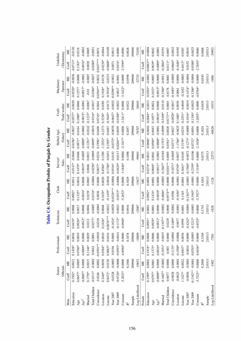
Tabl
eC
4:O
ccup
atio
nPr
obits
ofPu
njab
byG
ende
r
Seni
orPr
ofes
sion
als
Tech
nici
anC
lerk
Serv
ice/
Skill
edA
gri
Cra
ft/
Mac
hine
ryU
nski
lled
Offi
cial
sSa
les
Fish
ery
Trad
ew
orke
rO
pera
tor
/Ele
men
tary
Mal
eC
oeff
ME
Coe
ffM
EC
oeff
ME
Coe
ffM
EC
oeff
ME
Coe
ffM
EC
oeff
ME
Coe
ffM
EC
oeff
ME
Edu
catio
n0.
1502
*0.
0012
0.14
58*
0.00
360.
0419
*0.
0008
0.09
02*
0.00
11-0
.014
7*-0
.004
0-0
.019
6*-0
.003
7-0
.053
7*-0
.003
0-0
.052
0*-0
.003
6-0
.071
3*-0
.013
0
Age
0.06
57*
0.00
050.
0760
*0.
0019
0.09
20*
0.00
170.
1325
*0.
0016
0.14
79*
0.04
060.
0871
*0.
0164
0.10
88*
0.00
600.
1257
*0.
0088
0.11
83*
0.02
16
Age
2-0
.000
7*0.
0000
-0.0
009*
0.00
00-0
.001
2*0.
0000
-0.0
016*
0.00
00-0
.001
9*-0
.000
5-0
.000
9*-0
.000
2-0
.001
5*-0
.000
1-0
.001
7*-0
.000
1-0
.001
6*-0
.000
3
Mar
ried
0.17
59*
0.00
150.
1146
*0.
0029
0.02
120.
0004
0.02
390.
0003
0.00
460.
0013
-0.1
291*
-0.0
242
-0.1
223*
-0.0
067
-0.0
1-0
.000
70.
0028
0.00
05
Tota
lChi
ldre
n-0
.031
3*-0
.000
20.
0042
0.00
01-0
.027
7*-0
.000
5-0
.031
8*-0
.000
4-0
.025
0*-0
.006
9-0
.009
9*-0
.001
9-0
.031
6*-0
.001
7-0
.038
6*-0
.002
7-0
.028
0*-0
.005
1
Cor
esid
ence
0.02
460.
0002
-0.0
391*
*-0
.001
0-0
.021
8-0
.000
40.
0036
0.00
000.
0837
*0.
0234
0.19
96*
0.04
000.
0716
*0.
0041
0.03
04**
0.00
220.
0167
***
0.00
31
Loc
atio
n0.
3449
*0.
0030
0.03
84*
0.00
100.
2426
*0.
0048
0.16
29*
0.00
200.
4584
*0.
1289
-1.2
932*
-0.2
273
0.32
38*
0.01
890.
1928
*0.
0139
-0.0
239*
-0.0
044
Lite
rate
0.84
72*
0.01
380.
9063
*0.
0416
-0.0
676*
**-0
.001
2-0
.143
9*-0
.001
6-0
.170
6*-0
.045
10.
2385
*0.
0483
-0.3
645*
-0.0
171
-0.3
918*
-0.0
233
-0.0
608*
-0.0
109
Yea
r200
7-0
.032
8-0
.000
30.
0194
0.00
05-0
.162
4*-0
.002
9-0
.032
9***
-0.0
004
0.05
16*
0.01
43-0
.037
5*-0
.007
0-0
.064
7*-0
.003
5-0
.029
9**
-0.0
021
0.00
710.
0013
Yea
r200
9-0
.072
0*-0
.000
6-0
.059
3*-0
.001
4-0
.117
2*-0
.002
1-0
.053
3*-0
.000
6-0
.042
9*-0
.011
70.
0204
**0.
0039
-0.0
388*
-0.0
021
0.00
170.
0001
0.04
34*
0.00
80
Con
stan
t-5
.202
5*0.
0000
-4.6
994*
0.00
00-4
.094
0*0.
0000
-5.2
652*
0.00
00-3
.184
6*0.
0000
-2.1
017*
0.00
00-3
.241
1*0.
0000
-3.3
422*
0.00
00-2
.559
9*0.
0000
R2
0.25
660.
1878
0.09
160.
1829
0.10
980.
2057
0.05
220.
0598
0.08
28
Sam
ple
2096
6620
9666
2096
6620
9666
2096
6620
9666
2096
6620
9666
2096
66
Log
-Lik
elih
ood
-106
53-1
8809
-120
87-1
3637
-996
01-7
6707
-260
43-3
2725
-724
50
Fem
ale
Coe
ffM
EC
oeff
ME
Coe
ffM
EC
oeff
ME
Coe
ffM
EC
oeff
ME
Coe
ffM
EC
oeff
ME
Coe
ffM
E
Edu
catio
n0.
1589
*0.
0002
0.19
18*
0.00
080.
0991
*0.
0001
0.09
82*
0.00
010.
0274
*0.
0013
-0.0
606*
-0.0
044
-0.0
684*
-0.0
013
-0.0
303*
-0.0
001
-0.0
063*
*-0
.000
4
Age
0.07
97*
0.00
010.
1373
*0.
0006
0.09
29*
0.00
010.
1424
*0.
0001
0.08
49*
0.00
410.
0589
*0.
0043
0.10
57*
0.00
210.
1033
*0.
0003
0.06
39*
0.00
42
Age
2-0
.000
9*0.
0000
-0.0
016*
0.00
00-0
.001
2*0.
0000
-0.0
018*
0.00
00-0
.001
1*-0
.000
1-0
.000
8*-0
.000
1-0
.001
6*0.
0000
-0.0
015*
0.00
00-0
.000
9*-0
.000
1
Mar
ried
-0.1
607*
-0.0
002
-0.3
451*
-0.0
015
-0.1
347*
*-0
.000
2-0
.466
6*-0
.000
3-0
.366
7*-0
.018
4-0
.135
3*-0
.009
9-0
.516
9*-0
.011
0-0
.336
0*-0
.001
1-0
.286
4*-0
.019
1
Tota
lChi
ldre
n0.
0077
0.00
00-0
.003
0.00
00-0
.022
90.
0000
-0.0
574*
*0.
0000
0.01
01**
0.00
050.
0381
*0.
0028
0.01
73**
0.00
030.
0176
0.00
010.
0111
*0.
0007
Cor
esid
ence
-0.0
028
0.00
00-0
.113
5*-0
.000
4-0
.148
9*-0
.000
20.
0586
0.00
00-0
.107
1*-0
.004
90.
0371
*0.
0027
-0.0
928*
-0.0
017
-0.1
685*
-0.0
005
-0.0
664*
-0.0
042
Loc
atio
n-0
.062
5-0
.000
1-0
.150
0*-0
.000
6-0
.067
7-0
.000
1-0
.165
6*-0
.000
10.
0749
*0.
0037
-1.1
766*
-0.0
825
0.14
80*
0.00
300.
0061
0.00
00-0
.164
8*-0
.010
5
Lite
rate
1.14
27*
0.00
220.
6947
*0.
0036
0.05
990.
0001
0.11
630.
0001
0.36
41*
0.01
850.
3139
*0.
0235
-0.2
551*
-0.0
049
-0.1
052
-0.0
003
0.44
13*
0.03
03
Yea
r200
7-0
.085
6-0
.000
1-0
.001
40.
0000
-0.4
242*
-0.0
004
-0.1
367*
*-0
.000
1-0
.156
0*-0
.007
2-0
.127
3*-0
.008
9-0
.101
6*-0
.001
9-0
.147
4*-0
.000
40.
0152
0.00
10
Yea
r200
9-0
.134
2**
-0.0
001
-0.0
703*
-0.0
003
-0.3
212*
-0.0
003
-0.1
945*
-0.0
001
-0.2
359*
-0.0
106
0.07
32*
0.00
54-0
.135
0*-0
.002
5-0
.130
6*-0
.000
4-0
.038
8*-0
.002
5
Con
stan
t-5
.752
5*0.
0000
-6.0
436*
0.00
00-4
.852
5*0.
0000
-5.7
927*
0.00
00-3
.314
9*0.
0000
-2.1
038*
0.00
00-3
.205
5*0.
0000
-4.0
764*
0.00
00-2
.765
4*0.
0000
R2
0.20
000.
3104
0.17
410.
1843
0.03
750.
1824
0.04
390.
0345
0.04
88
Sam
ple
2103
1321
0313
2103
1321
0313
2103
1321
0313
2103
1321
0313
2103
13
Log
-Lik
elih
ood
-148
2-7
501
-182
8-1
126
-225
73-4
6626
-103
31-1
886
-298
93
156
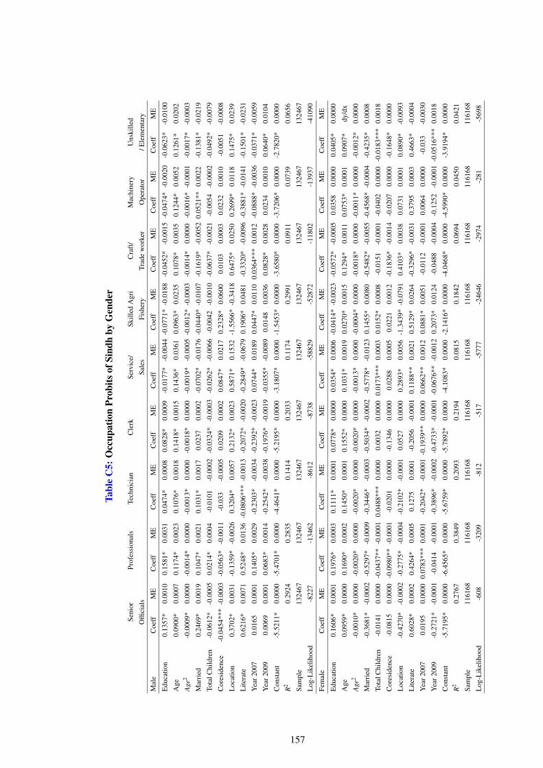
Tabl
eC
5:O
ccup
atio
nPr
obits
ofSi
ndh
byG
ende
r
Seni
orPr
ofes
sion
als
Tech
nici
anC
lerk
Serv
ice/
Skill
edA
gri
Cra
ft/
Mac
hine
ryU
nski
lled
Offi
cial
sSa
les
Fish
ery
Trad
ew
orke
rO
pera
tor
/Ele
men
tary
Mal
eC
oeff
ME
Coe
ffM
EC
oeff
ME
Coe
ffM
EC
oeff
ME
Coe
ffM
EC
oeff
ME
Coe
ffM
EC
oeff
ME
Edu
catio
n0.
1357
*0.
0010
0.15
81*
0.00
310.
0474
*0.
0008
0.08
28*
0.00
09-0
.017
7*-0
.004
4-0
.077
1*-0
.018
8-0
.045
2*-0
.001
5-0
.047
4*-0
.002
0-0
.062
3*-0
.010
0
Age
0.09
00*
0.00
070.
1174
*0.
0023
0.10
76*
0.00
180.
1418
*0.
0015
0.14
36*
0.03
610.
0963
*0.
0235
0.10
78*
0.00
350.
1244
*0.
0052
0.12
61*
0.02
02
Age
2-0
.000
9*0.
0000
-0.0
014*
0.00
00-0
.001
3*0.
0000
-0.0
018*
0.00
00-0
.001
9*-0
.000
5-0
.001
2*-0
.000
3-0
.001
4*0.
0000
-0.0
016*
-0.0
001
-0.0
017*
-0.0
003
Mar
ried
0.24
69*
0.00
190.
1047
*0.
0021
0.10
31*
0.00
170.
0237
0.00
02-0
.070
2*-0
.017
6-0
.044
0*-0
.010
7-0
.161
9*-0
.005
20.
0521
**0.
0022
-0.1
381*
-0.0
219
Tota
lChi
ldre
n-0
.061
2*-0
.000
50.
0214
*0.
0004
-0.0
101
-0.0
002
-0.0
324*
-0.0
003
-0.0
262*
-0.0
066
-0.0
042
-0.0
010
-0.0
637*
-0.0
021
-0.0
054
-0.0
002
-0.0
492*
-0.0
079
Cor
esid
ence
-0.0
454*
**-0
.000
3-0
.056
3*-0
.001
1-0
.033
-0.0
005
0.02
090.
0002
0.08
47*
0.02
170.
2328
*0.
0600
0.01
030.
0003
0.02
320.
0010
-0.0
051
-0.0
008
Loc
atio
n0.
3702
*0.
0031
-0.1
359*
-0.0
026
0.32
04*
0.00
570.
2132
*0.
0023
0.58
71*
0.15
32-1
.556
6*-0
.341
80.
6475
*0.
0250
0.26
99*
0.01
180.
1475
*0.
0239
Lite
rate
0.62
16*
0.00
710.
5248
*0.
0136
-0.0
806*
**-0
.001
3-0
.207
2*-0
.002
0-0
.284
9*-0
.067
90.
1906
*0.
0481
-0.3
320*
-0.0
096
-0.3
881*
-0.0
141
-0.1
501*
-0.0
231
Yea
r200
70.
0165
0.00
010.
1405
*0.
0029
-0.2
303*
-0.0
034
-0.2
392*
-0.0
023
0.07
44*
0.01
890.
0447
*0.
0110
0.03
64**
*0.
0012
-0.0
888*
-0.0
036
-0.0
371*
-0.0
059
Yea
r200
90.
0069
0.00
010.
0683
*0.
0014
-0.2
542*
-0.0
038
-0.1
976*
-0.0
019
-0.0
355*
-0.0
089
0.01
480.
0036
0.08
28*
0.00
280.
0234
0.00
100.
0640
*0.
0104
Con
stan
t-5
.521
1*0.
0000
-5.4
701*
0.00
00-4
.464
1*0.
0000
-5.2
195*
0.00
00-3
.180
7*0.
0000
-1.5
453*
0.00
00-3
.658
0*0.
0000
-3.7
206*
0.00
00-2
.782
0*0.
0000
R2
0.29
240.
2835
0.14
140.
2033
0.11
740.
2991
0.09
110.
0739
0.06
56
Sam
ple
1324
6713
2467
1324
6713
2467
1324
6713
2467
1324
6713
2467
1324
67
Log
-Lik
elih
ood
-822
7-1
3462
-861
2-8
738
-588
29-5
2872
-118
02-1
3937
-410
90
Fem
ale
Coe
ffM
EC
oeff
ME
Coe
ffM
EC
oeff
ME
Coe
ffM
EC
oeff
ME
Coe
ffM
EC
oeff
ME
Coe
ffM
E
Edu
catio
n0.
1606
*0.
0001
0.19
76*
0.00
030.
1111
*0.
0001
0.07
78*
0.00
000.
0354
*0.
0006
-0.0
414*
-0.0
023
-0.0
572*
-0.0
005
0.03
580.
0000
0.04
05*
0.00
00
Age
0.09
59*
0.00
000.
1690
*0.
0002
0.14
50*
0.00
010.
1552
*0.
0000
0.10
31*
0.00
190.
0270
*0.
0015
0.12
94*
0.00
110.
0753
*0.
0001
0.09
07*
dy/d
x
Age
2-0
.001
0*0.
0000
-0.0
020*
0.00
00-0
.002
0*0.
0000
-0.0
020*
0.00
00-0
.001
3*0.
0000
-0.0
004*
0.00
00-0
.001
8*0.
0000
-0.0
011*
0.00
00-0
.001
2*0.
0000
Mar
ried
-0.3
681*
-0.0
002
-0.5
297*
-0.0
009
-0.3
446*
-0.0
003
-0.5
034*
-0.0
002
-0.5
778*
-0.0
123
0.14
55*
0.00
80-0
.548
2*-0
.005
5-0
.456
8*-0
.000
4-0
.423
5*0.
0008
Tota
lChi
ldre
n-0
.014
10.
0000
-0.0
437*
*-0
.000
10.
0488
***
0.00
000.
0032
0.00
000.
0173
***
0.00
030.
0152
*0.
0008
-0.0
151
-0.0
001
-0.0
402
0.00
00-0
.018
3***
0.00
18
Cor
esid
ence
-0.0
815
0.00
00-0
.098
0**
-0.0
001
-0.0
201
0.00
00-0
.134
60.
0000
0.02
880.
0005
0.02
210.
0012
-0.1
836*
-0.0
014
-0.0
207
0.00
00-0
.164
8*0.
0000
Loc
atio
n-0
.427
0*-0
.000
2-0
.277
5*-0
.000
4-0
.210
2*-0
.000
10.
0527
0.00
000.
2893
*0.
0056
-1.3
439*
-0.0
791
0.41
03*
0.00
380.
0731
0.00
010.
0890
*-0
.009
3
Lite
rate
0.60
28*
0.00
020.
4264
*0.
0005
0.12
750.
0001
-0.2
056
-0.0
001
0.11
88**
0.00
210.
5129
*0.
0264
-0.3
296*
-0.0
031
0.37
950.
0003
0.46
63*
-0.0
004
Yea
r200
70.
0195
0.00
000.
0783
***
0.00
01-0
.204
2*-0
.000
1-0
.193
9**
0.00
000.
0662
**0.
0012
0.08
81*
0.00
51-0
.011
2-0
.000
10.
0064
0.00
00-0
.033
-0.0
030
Yea
r200
9-0
.272
1*-0
.000
1-0
.041
4-0
.000
1-0
.389
6*-0
.000
2-0
.473
3*-0
.000
1-0
.067
6**
-0.0
012
0.20
73*
0.01
24-0
.048
8-0
.000
4-0
.125
2-0
.000
1-0
.051
6***
0.00
18
Con
stan
t-5
.719
5*0.
0000
-6.4
565*
0.00
00-5
.675
9*0.
0000
-5.7
892*
0.00
00-4
.108
3*0.
0000
-2.1
416*
0.00
00-4
.046
8*0.
0000
-4.5
990*
0.00
00-3
.919
4*0.
0000
R2
0.27
670.
3849
0.20
930.
2194
0.08
150.
1842
0.06
940.
0450
0.04
21
Sam
ple
1161
6811
6168
1161
6811
6168
1161
6811
6168
1161
6811
6168
1161
68
Log
-Lik
elih
ood
-608
-320
9-8
12-5
17-5
777
-246
46-2
974
-281
-569
8
157
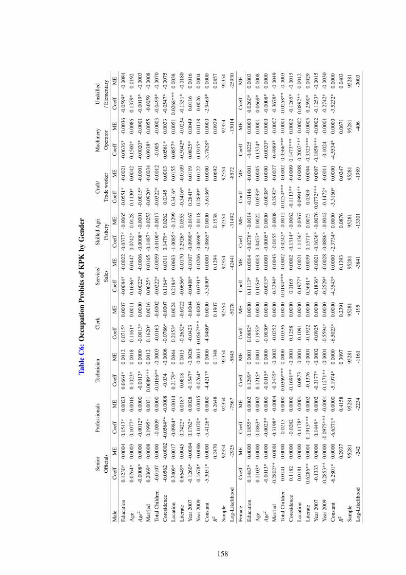
Tabl
eC
6:O
ccup
atio
nPr
obits
ofK
PKby
Gen
der
Seni
orPr
ofes
sion
als
Tech
nici
anC
lerk
Serv
ice/
Skill
edA
gri
Cra
ft/
Mac
hine
ryU
nski
lled
Offi
cial
sSa
les
Fish
ery
Trad
ew
orke
rO
pera
tor
/Ele
men
tary
Mal
eC
oeff
ME
Coe
ffM
EC
oeff
ME
Coe
ffM
EC
oeff
ME
Coe
ffM
EC
oeff
ME
Coe
ffM
EC
oeff
ME
Edu
catio
n0.
1230
*0.
0004
0.15
43*
0.00
230.
0664
*0.
0012
0.07
15*
0.00
07-0
.008
4*-0
.002
2-0
.037
7*-0
.006
5-0
.055
1*-0
.002
1-0
.063
6*-0
.003
6-0
.059
9*-0
.008
4
Age
0.07
64*
0.00
030.
1077
*0.
0016
0.10
23*
0.00
180.
1161
*0.
0011
0.16
96*
0.04
470.
0742
*0.
0128
0.11
30*
0.00
420.
1500
*0.
0086
0.13
79*
0.01
92
Age
2-0
.000
8*0.
0000
-0.0
012*
0.00
00-0
.001
3*0.
0000
-0.0
013*
0.00
00-0
.002
2*-0
.000
6-0
.000
8*-0
.000
1-0
.001
5*-0
.000
1-0
.002
0*-0
.000
1-0
.001
9*-0
.000
3
Mar
ried
0.20
69*
0.00
080.
1995
*0.
0031
0.06
89**
*0.
0012
0.16
20*
0.00
160.
0625
*0.
0165
-0.1
487*
-0.0
253
-0.0
920*
-0.0
034
0.09
38*
0.00
55-0
.005
9-0
.000
8
Tota
lChi
ldre
n-0
.010
70.
0000
-0.0
009
0.00
00-0
.016
6**
-0.0
003
-0.0
163
-0.0
002
-0.0
222*
-0.0
059
-0.0
100*
-0.0
017
-0.0
322*
-0.0
012
-0.0
05-0
.000
3-0
.049
9*-0
.007
0
Cor
esid
ence
-0.0
562
-0.0
002
-0.0
564*
*-0
.000
8-0
.034
-0.0
006
-0.0
786*
-0.0
007
0.11
64*
0.03
110.
1479
*0.
0262
0.03
450.
0013
0.05
61*
0.00
33-0
.054
7*-0
.007
5
Loc
atio
n0.
3409
*0.
0017
-0.0
984*
-0.0
014
0.21
79*
0.00
440.
2153
*0.
0024
0.21
84*
0.06
03-1
.008
5*-0
.129
90.
3416
*0.
0155
0.08
57*
0.00
510.
0268
***
0.00
38
Lite
rate
0.66
49*
0.00
450.
7422
*0.
0187
0.08
180.
0015
-0.2
652*
-0.0
022
-0.0
656*
-0.0
170
0.29
26*
0.05
53-0
.341
6*-0
.010
9-0
.504
2*-0
.023
4-0
.135
1*-0
.018
0
Yea
r200
7-0
.126
0*-0
.000
40.
1762
*0.
0028
-0.1
547*
-0.0
026
-0.0
423
-0.0
004
-0.0
408*
-0.0
107
-0.0
990*
-0.0
167
0.28
41*
0.01
190.
0825
*0.
0049
0.01
160.
0016
Yea
r200
9-0
.167
8*-0
.000
6-0
.107
0*-0
.001
5-0
.076
4*-0
.001
3-0
.056
7***
-0.0
005
-0.0
791*
-0.0
206
-0.0
696*
-0.0
118
0.28
99*
0.01
220.
1915
*0.
0118
0.00
260.
0004
Con
stan
t-5
.305
1*0.
0000
-5.4
126*
0.00
00-4
.421
7*0.
0000
-4.9
480*
0.00
00-3
.389
0*0.
0000
-2.0
865*
0.00
00-3
.613
6*0.
0000
-3.7
828*
0.00
00-2
.946
9*0.
0000
R2
0.24
700.
2648
0.13
480.
1907
0.12
940.
1538
0.06
920.
0929
0.08
57
Sam
ple
9235
492
354
9235
492
354
9235
492
354
9235
492
354
9235
4
Log
-Lik
elih
ood
-292
5-7
567
-584
5-5
078
-424
41-3
1492
-857
2-1
3014
-259
30
Fem
ale
Coe
ffM
EC
oeff
ME
Coe
ffM
EC
oeff
ME
Coe
ffM
EC
oeff
ME
Coe
ffM
EC
oeff
ME
Coe
ffM
E
Edu
catio
n0.
1483
*0.
0000
0.18
55*
0.00
020.
1289
*0.
0001
0.08
82*
0.00
000.
1113
*0.
0014
-0.0
276*
-0.0
014
-0.0
146
-0.0
001
-0.0
225
0.00
000.
0260
*0.
0003
Age
0.11
03*
0.00
000.
1863
*0.
0002
0.12
15*
0.00
010.
1955
*0.
0000
0.10
54*
0.00
130.
0457
*0.
0022
0.05
93*
0.00
050.
1374
*0.
0001
0.06
69*
0.00
08
Age
2-0
.001
3*0.
0000
-0.0
023*
0.00
00-0
.001
5*0.
0000
-0.0
030*
0.00
00-0
.001
3*0.
0000
-0.0
005*
0.00
00-0
.000
8*0.
0000
-0.0
020*
0.00
00-0
.000
8*0.
0000
Mar
ried
-0.2
802*
*-0
.000
1-0
.319
8*-0
.000
4-0
.243
5*-0
.000
2-0
.025
20.
0000
-0.3
294*
-0.0
043
-0.0
155
-0.0
008
-0.2
992*
-0.0
027
-0.4
989*
-0.0
007
-0.3
678*
-0.0
049
Tota
lChi
ldre
n0.
0141
0.00
00-0
.021
30.
0000
-0.0
369*
**0.
0000
-0.0
336
0.00
00-0
.019
4***
-0.0
002
-0.0
242*
-0.0
012
-0.0
254*
**-0
.000
2-0
.056
6***
-0.0
001
-0.0
258*
*-0
.000
3
Cor
esid
ence
0.11
820.
0000
-0.0
282
0.00
00-0
.169
1**
-0.0
001
0.12
580.
0000
0.01
650.
0002
-0.1
314*
-0.0
062
-0.1
113*
*-0
.000
90.
1473
***
0.00
02-0
.126
5*-0
.001
5
Loc
atio
n0.
0181
0.00
00-0
.117
8*-0
.000
1-0
.087
3-0
.000
1-0
.109
10.
0000
-0.1
977*
-0.0
021
-1.1
436*
-0.0
367
-0.0
994*
*-0
.000
8-0
.200
7***
-0.0
002
0.08
92**
0.00
12
Lite
rate
0.62
86**
0.00
010.
1915
***
0.00
02-0
.137
6-0
.000
1-0
.192
20.
0000
0.36
81*
0.00
390.
1571
*0.
0073
0.05
090.
0004
-0.3
323*
**-0
.000
50.
2590
*0.
0029
Yea
r200
7-0
.133
30.
0000
0.14
49*
0.00
02-0
.317
7*-0
.000
2-0
.092
50.
0000
-0.1
836*
-0.0
021
-0.1
636*
-0.0
076
0.07
72**
*0.
0007
-0.1
859*
**-0
.000
2-0
.125
3*-0
.001
5
Yea
r200
9-0
.285
3**
0.00
00-0
.097
5***
-0.0
001
-0.1
271*
*-0
.000
1-0
.559
4*0.
0000
-0.2
529*
-0.0
028
-0.0
886*
-0.0
042
-0.1
472*
-0.0
011
-0.1
024
-0.0
001
-0.2
742*
-0.0
030
Con
stan
t-6
.280
1*0.
0000
-6.6
371*
0.00
00-5
.197
4*0.
0000
-6.5
023*
0.00
00-4
.354
3*0.
0000
-2.3
734*
0.00
00-3
.316
0*0.
0000
-4.5
534*
0.00
00-3
.523
2*0.
0000
R2
0.29
370.
4158
0.30
970.
2391
0.13
930.
0876
0.02
470.
0671
0.04
03
Sam
ple
9528
195
281
9528
195
281
9528
195
281
9528
195
281
9528
1
Log
-Lik
elih
ood
-242
-223
4-1
161
-195
-384
1-1
3301
-198
9-4
06-3
003
158
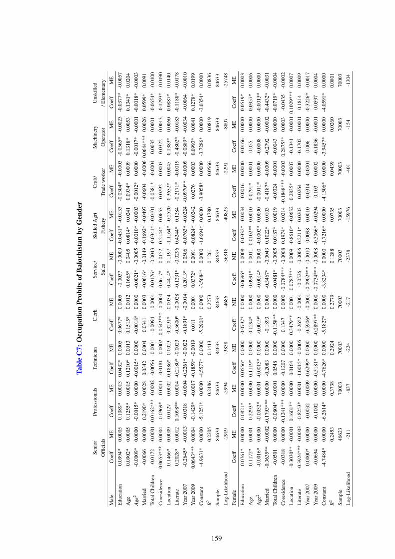
Tabl
eC
7:O
ccup
atio
nPr
obits
ofB
aloc
hist
anby
Gen
der
Seni
orPr
ofes
sion
als
Tech
nici
anC
lerk
Serv
ice/
Skill
edA
gri
Cra
ft/
Mac
hine
ryU
nski
lled
Offi
cial
sSa
les
Fish
ery
Trad
ew
orke
rO
pera
tor
/Ele
men
tary
Mal
eC
oeff
ME
Coe
ffM
EC
oeff
ME
Coe
ffM
EC
oeff
ME
Coe
ffM
EC
oeff
ME
Coe
ffM
EC
oeff
ME
Edu
catio
n0.
0994
*0.
0005
0.10
89*
0.00
130.
0432
*0.
0005
0.06
77*
0.00
05-0
.003
7-0
.000
9-0
.045
1*-0
.013
3-0
.030
4*-0
.000
3-0
.056
5*-0
.002
3-0
.037
7*-0
.005
7
Age
0.09
02*
0.00
050.
1255
*0.
0015
0.12
10*
0.00
130.
1515
*0.
0012
0.16
65*
0.04
050.
0814
*0.
0241
0.09
34*
0.00
090.
1318
*0.
0053
0.13
41*
0.02
04
Age
2-0
.000
9*0.
0000
-0.0
015*
0.00
00-0
.001
5*0.
0000
-0.0
018*
0.00
00-0
.002
1*-0
.000
5-0
.001
0*-0
.000
3-0
.001
2*0.
0000
-0.0
017*
-0.0
001
-0.0
018*
-0.0
003
Mar
ried
-0.0
066
0.00
000.
2190
*0.
0028
0.03
420.
0004
0.03
410.
0003
-0.0
616*
-0.0
149
-0.1
692*
-0.0
497
-0.0
604
-0.0
006
0.06
44**
*0.
0026
0.05
99*
0.00
91
Tota
lChi
ldre
n-0
.017
2-0
.000
1-0
.016
2***
-0.0
002
-0.0
056
-0.0
001
-0.0
094
-0.0
001
-0.0
176*
-0.0
043
-0.0
341*
-0.0
101
-0.0
381*
-0.0
004
0.00
350.
0001
-0.0
654*
-0.0
100
Cor
esid
ence
0.06
53**
*0.
0004
-0.0
969*
-0.0
011
-0.0
181
-0.0
002
-0.0
542*
**-0
.000
40.
0617
*0.
0152
0.21
44*
0.06
530.
0292
0.00
030.
0322
0.00
13-0
.129
3*-0
.019
0
Loc
atio
n0.
1466
*0.
0009
0.01
270.
0002
0.18
86*
0.00
230.
3231
*0.
0034
0.44
14*
0.11
97-1
.116
4*-0
.252
00.
3632
*0.
0045
0.13
83*
0.00
600.
0887
*0.
0140
Lite
rate
0.20
28*
0.00
120.
1098
**0.
0014
-0.2
180*
-0.0
023
-0.3
600*
-0.0
028
-0.1
231*
-0.0
296
0.42
44*
0.12
84-0
.217
1*-0
.001
9-0
.480
2*-0
.018
3-0
.118
8*-0
.017
8
Yea
r200
7-0
.264
5*-0
.001
3-0
.031
8-0
.000
4-0
.226
1*-0
.002
2-0
.189
1*-0
.001
40.
2013
*0.
0506
-0.0
763*
-0.0
224
-0.0
970*
*-0
.000
9-0
.088
9*-0
.003
4-0
.006
4-0
.001
0
Yea
r200
90.
0643
***
0.00
04-0
.142
9*-0
.001
7-0
.185
9*-0
.001
90.
011
0.00
010.
0372
*0.
0091
-0.0
824*
-0.0
242
0.02
760.
0003
0.09
93*
0.00
410.
1278
*0.
0199
Con
stan
t-4
.963
1*0.
0000
-5.1
251*
0.00
00-4
.557
7*0.
0000
-5.2
908*
0.00
00-3
.568
4*0.
0000
-1.6
694*
0.00
00-3
.905
8*0.
0000
-3.7
286*
0.00
00-3
.035
4*0.
0000
R2
0.22
050.
2486
0.14
130.
2273
0.12
610.
1780
0.05
660.
0819
0.08
36
Sam
ple
8463
384
633
8463
384
633
8463
384
633
8463
384
633
8463
3
Log
-Lik
elih
ood
-291
9-5
994
-383
8-4
686
-368
18-4
0823
-229
1-8
807
-257
48
Fem
ale
Coe
ffM
EC
oeff
ME
Coe
ffM
EC
oeff
ME
Coe
ffM
EC
oeff
ME
Coe
ffM
EC
oeff
ME
Coe
ffM
E
Edu
catio
n0.
0761
*0.
0000
0.08
21*
0.00
000.
0556
*0.
0000
0.07
37*
0.00
000.
0696
*0.
0008
-0.0
332*
-0.0
034
-0.0
016
0.00
00-0
.016
60.
0000
0.05
19*
0.00
03
Age
0.11
72*
0.00
010.
2293
*0.
0000
0.11
19*
0.00
000.
1294
*0.
0000
0.09
91*
0.00
110.
0102
**0.
0010
0.07
91*
0.00
010.
055
0.00
000.
0957
*0.
0006
Age
2-0
.001
6*0.
0000
-0.0
032*
0.00
01-0
.001
3*0.
0000
-0.0
019*
0.00
00-0
.001
4*0.
0000
-0.0
002*
0.00
00-0
.001
1*0.
0000
-0.0
008
0.00
00-0
.001
3*0.
0000
Mar
ried
-0.3
635*
*-0
.000
2-0
.179
3***
0.00
00-0
.208
30.
0000
-0.1
893
0.00
00-0
.346
7*-0
.004
30.
1022
*0.
0103
-0.4
187*
-0.0
009
-0.2
792
-0.0
002
-0.4
432*
-0.0
031
Tota
lChi
ldre
n-0
.050
10.
0000
-0.0
804*
-0.0
001
0.05
480.
0000
-0.1
158*
*0.
0000
-0.0
481*
-0.0
005
0.01
87*
0.00
19-0
.032
4-0
.000
1-0
.004
30.
0000
-0.0
719*
-0.0
004
Cor
esid
ence
-0.0
318
0.00
00-0
.124
1***
0.00
00-0
.120
70.
0000
0.13
470.
0000
-0.0
784*
**-0
.000
80.
1974
*0.
0214
-0.1
848*
**-0
.000
30.
2875
**0.
0003
-0.0
435
-0.0
002
Loc
atio
n-0
.303
0**
-0.0
001
0.16
01**
0.00
000.
0164
0.00
000.
3479
**0.
0001
0.07
87**
*0.
0009
-0.8
610*
-0.0
632
0.28
35*
0.00
07-0
.134
1-0
.000
10.
1029
***
0.00
07
Lite
rate
-0.3
924*
**-0
.000
3-0
.825
3*0.
0001
-1.0
015*
-0.0
005
-0.2
652
-0.0
001
-0.0
526
-0.0
006
0.22
11*
0.02
030.
0264
0.00
00-0
.170
2-0
.000
10.
1814
0.00
09
Yea
r200
70.
0000
*0.
0000
-0.0
032
-0.0
009
-0.6
299*
0.00
00-0
.590
6*-0
.000
1-0
.090
2***
-0.0
010
0.00
980.
0010
-0.0
314
-0.0
001
0.00
60.
0000
-0.3
226*
-0.0
017
Yea
r200
9-0
.069
40.
0000
-0.1
002
0.00
00-0
.518
1*0.
0000
-0.2
897*
*0.
0000
-0.0
734*
**-0
.000
8-0
.306
6*-0
.029
40.
103
0.00
02-0
.183
6-0
.000
10.
0597
0.00
04
Con
stan
t-4
.748
4*0.
0000
-6.2
614*
0.00
00-4
.762
6*0.
0000
-5.1
827*
0.00
00-3
.823
4*0.
0000
-1.7
216*
0.00
00-4
.150
6*0.
0000
-3.9
457*
0.00
00-4
.059
1*0.
0000
R2
0.24
530.
3738
0.29
240.
2779
0.12
880.
0735
0.04
390.
0260
0.08
01
Sam
ple
4662
370
003
7000
370
003
7000
370
003
7000
370
003
7000
3
Log
-Lik
elih
ood
-211
-837
-224
-217
-237
8-1
5976
-401
-154
-130
4
159

Table C8: Male/Female Occupation Probit Decomposition (Senior officials).
Senior officials Pakistan Punjab Sindh KPK Balochsitan
Differences in mean 0.011* 0.011* 0.016* 0.006* 0.007*
Differences due to coefficients 0.006* 0.007* 0.010* 0.003* 0.003*
% 59.7 66.2 60.7 44.6 44.5
Difference due to charactersitics 0.004* 0.003* 0.006* 0.003* 0.003*
% 40.3 33.8 39.3 55.4 55.5
Age -13.867 -1.645 -11.863 -16.654 -27.231
Age2 3.078 -3.498 2.652 5.846 10.499
Education 154.645 144.889 150.164 112.722 105.635
Illetrate -96.427 -101.726 -87.146 -43.619 -31.641
Married -9.856 -8.395 -12.041 -4.556 -1.927
Total children 0.307 0.569 0.210 -0.041 0.101
Co residence -0.023 0.016 -0.102 0.032 -0.125
Location 0.155 1.729 -0.360 0.519 -0.250
Islamabad (Capital) -0.060 - - - -
Rawalpindi 0.041 0.001 - - -
Jhelum 0.283 0.642 - - -
Chakwal 0.236 0.624 - - -
Sargodha 0.163 0.215 - - -
Bhakkar -0.013 -0.368 - - -
Khushab 0.074 0.167 - - -
Faisalabad -0.037 -0.084 - - -
Jhang 0.176 0.376 - - -
T.T.Singh 0.012 0.164 - - -
Gujranwala 0.016 0.045 - - -
Gujrat 0.136 0.682 - - -
Sialkot -0.098 0.099 - - -
Hafiza Abad 0.071 0.072 - - -
Mandi Bahauddin 0.167 0.331 - - -
Narowal 0.270 1.184 - - -
Lahore 0.050 -0.241 - - -
Kasur 0.000 -0.265 - - -
Okara -0.033 0.026 - - -
Sheikhupura 0.026 -0.073 - - -
Nankana Sahib 0.024 -0.205 - - -
Vehari -0.150 -0.043 - - -
Sahiwal 0.037 -0.083 - - -
160
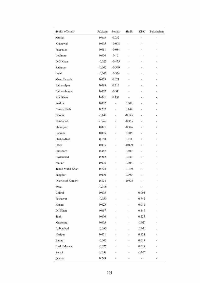
Senior officials Pakistan Punjab Sindh KPK Balochsitan
Multan 0.063 0.032 - - -
Khanewal 0.005 -0.008 - - -
Pakpattan 0.011 -0.084 - - -
Lodhran 0.004 -0.161 - - -
D.G.Khan -0.023 -0.455 - - -
Rajanpur -0.002 -0.399 - - -
Leiah -0.003 -0.334 - - -
Muzaffargarh 0.079 0.021 - - -
Bahawalpur 0.088 0.213 - - -
Bahawalnagar 0.067 -0.311 - - -
R Y Khan 0.041 0.132 - - -
Sukkur 0.002 - 0.009 - -
Nawab Shah 0.237 - 0.144 - -
Ghotki -0.148 - -0.145 - -
Jacobabad -0.267 - -0.355 - -
Shikarpur 0.021 - -0.346 - -
Larkana 0.005 - 0.005 - -
Shahdadkot 0.158 - 0.011 - -
Dadu 0.095 - -0.029 - -
Jamshoro 0.467 - 0.809 - -
Hyderabad 0.212 - 0.049 - -
Matiari 0.026 - 0.004 - -
Tando Muhd Khan 0.722 - -1.149 - -
Sanghar 0.090 - 0.090 - -
District of Karachi 0.374 - -0.975 - -
Swat -0.016 - - - -
Chitral 0.005 - - 0.094 -
Peshawar -0.050 - - 0.742 -
Hangu 0.025 - - 0.011 -
D.I.Khan 0.017 - - 0.446 -
Tank 0.006 - - 0.225 -
Mansehra 0.005 - - -0.027 -
Abbotabad -0.090 - - -0.051 -
Haripur 0.051 - - 0.124 -
Bannu -0.005 - - 0.017 -
Lakki Marwat -0.077 - - 0.018 -
Swabi -0.038 - - -0.057 -
Quetta 0.249 - - - -
161
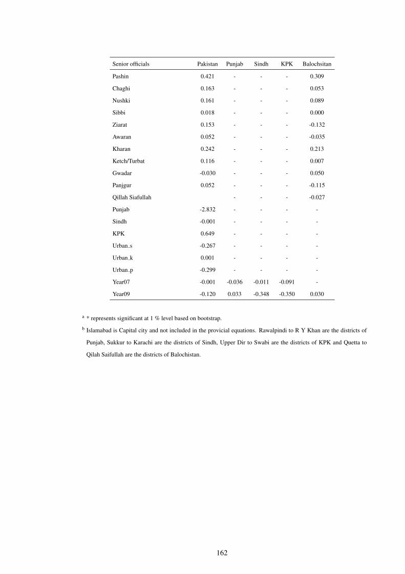
Senior officials Pakistan Punjab Sindh KPK Balochsitan
Pashin 0.421 - - - 0.309
Chaghi 0.163 - - - 0.053
Nushki 0.161 - - - 0.089
Sibbi 0.018 - - - 0.000
Ziarat 0.153 - - - -0.132
Awaran 0.052 - - - -0.035
Kharan 0.242 - - - 0.213
Ketch/Turbat 0.116 - - - 0.007
Gwadar -0.030 - - - 0.050
Panjgur 0.052 - - - -0.115
Qillah Siafullah - - - -0.027
Punjab -2.832 - - - -
Sindh -0.001 - - - -
KPK 0.649 - - - -
Urban s -0.267 - - - -
Urban k 0.001 - - - -
Urban p -0.299 - - - -
Year07 -0.001 -0.036 -0.011 -0.091 -
Year09 -0.120 0.033 -0.348 -0.350 0.030
a * represents significant at 1 % level based on bootstrap.
b Islamabad is Capital city and not included in the provicial equations. Rawalpindi to R Y Khan are the districts of
Punjab, Sukkur to Karachi are the districts of Sindh, Upper Dir to Swabi are the districts of KPK and Quetta to
Qilah Saifullah are the districts of Balochistan.
162

Table C9: Male/Female Occupation Probit Decomposition (Professionals).
Professionals Pakistan Punjab Sindh KPK Balochsitan
Differences in mean 0.017* 0.014* 0.024* 0.016* 0.016*
Differences due to coefficients % 0.006* 0.008* 0.007* 0.003* 0.005*
% 39.2 57.4 29.7 23.4 32.1
Difference due to charactersitics % 0.010* 0.006* 0.017* 0.012* 0.011*
% 60.8 42.6 70.3 76.6 67.9
Age -20.073 -3.244 -12.927 -23.627 -22.826
Age2 5.139 -8.093 3.261 10.157 10.058
Education 181.862 220.505 136.922 134.668 68.991
Illetrate -101.409 -162.615 -54.539 -44.383 14.540
Married -6.741 -6.706 -3.371 -0.164 -2.940
Total children 0.005 0.344 -0.101 0.018 0.051
Co residence 0.135 -0.039 0.230 0.021 0.189
Location 0.015 0.698 0.534 -0.235 -0.013
Islamabad 0.014 - - - -
Rawalpindi 0.125 0.001 - - -
Jhelum 0.157 0.309 - - -
Chakwal 0.156 0.312 - - -
Sargodha 0.150 0.139 - - -
Bhakkar 0.033 0.264 - - -
Khushab -0.026 -0.062 - - -
Mianwali - -0.005 - - -
Faisalabad 0.241 -0.216 - - -
Jhang 0.171 0.245 - - -
T.T.Singh -0.051 -0.117 - - -
Gujranwala 0.170 0.070 - - -
Gujrat 0.348 0.862 - - -
Sialkot 0.170 0.328 - - -
Hafiza Abad 0.066 0.046 - - -
Mandi Bahauddin 0.092 0.138 - - -
Narowal 0.070 0.086 - - -
Lahore -0.093 -1.573 - - -
Kasur 0.000 -0.463 - - -
Okara 0.090 0.054 - - -
Sheikhupura 0.129 -0.127 - - -
Nankana Sahib 0.041 -0.229 - - -
Vehari 0.117 0.094 - - -
163

Professionals Pakistan Punjab Sindh KPK Balochsitan
Sahiwal 0.207 -0.196 - - -
Multan 0.211 0.059 - - -
Khanewal 0.080 -0.016 - - -
Pakpattan 0.039 -0.133 - - -
Lodhran -0.041 0.523 - - -
D.G.Khan 0.057 0.652 - - -
Rajanpur 0.001 0.224 - - -
Leiah 0.004 0.306 - - -
Muzaffargarh 0.129 0.021 - - -
Bahawalpur 0.128 0.159 - - -
Bahawalnagar 0.063 -0.227 - - -
R Y Khan 0.076 0.137 - - -
Sukkur 0.025 - -0.050 - -
Nawab Shah -0.075 - -0.044 - -
Neshero Feroz - - -0.079 - -
Ghotki 0.086 - 0.048 - -
Jacobabad 0.173 - 0.155 - -
Kashmore - - 0.048 - -
Shikarpur -0.009 - 0.180 - -
Larkana -0.010 - 0.019 - -
Shahdadkot -0.135 - -0.010 - -
Dadu -0.039 - 0.014 - -
Jamshoro -0.016 - -0.025 - -
Hyderabad 0.066 - 0.007 - -
Matiari -0.033 - -0.009 - -
Tando Allah Yar - - -0.058 - -
Tando Muhd Khan -0.128 - 0.202 - -
Badin - - 0.002 - -
Thatta - - 0.100 - -
Sanghar 0.067 - 0.028 - -
Mirpur Khas - - -0.382 - -
Tharparkar - - -0.025 - -
District of Karachi -0.015 - 0.117 - -
Upper Dir - - - 0.152 -
Lower Dir - - - -0.069 -
Swat 0.014 - - - -
Chitral 0.006 - - 0.220 -
Shangla - - - 0.070 -
164
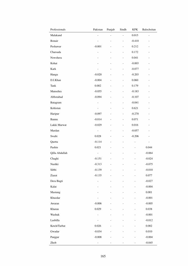
Professionals Pakistan Punjab Sindh KPK Balochsitan
Malakand - - - 0.015 -
Bonair - - - -0.410 -
Peshawar -0.001 - - 0.212 -
Charsada - - - 0.172 -
Nowshera - - - 0.041 -
Kohat - - - -0.003 -
Kark - - - -0.077 -
Hangu -0.020 - - -0.203 -
D.I.Khan -0.004 - - 0.060 -
Tank 0.002 - - 0.179 -
Mansehra -0.055 - - -0.183 -
Abbotabad -0.094 - - -0.107 -
Batagram - - - -0.041 -
Kohistan - - - 0.621 -
Haripur -0.097 - - -0.270 -
Bannu -0.014 - - 0.071 -
Lakki Marwat -0.029 - - 0.016 -
Mardan - - - -0.057 -
Swabi 0.028 - - -0.206 -
Quetta -0.114 - - - -
Pashin 0.021 - - - 0.044
Qilla Abdullah - - - - -0.064
Chaghi -0.151 - - - -0.024
Nushki -0.313 - - - -0.075
Sibbi -0.139 - - - -0.010
Ziarat -0.135 - - - 0.077
Dera Bugti - - - - -0.027
Kalat - - - - -0.004
Mastung - - - - 0.001
Khuzdar - - - - -0.001
Awaran -0.006 - - - -0.005
Kharan 0.029 - - - 0.038
Washuk - - - - -0.001
Lasbilla - - - - -0.012
Ketch/Turbat 0.026 - - - 0.002
Gwadar -0.034 - - - 0.010
Panjgur -0.008 - - - -0.004
Zhob - - - - -0.045
165
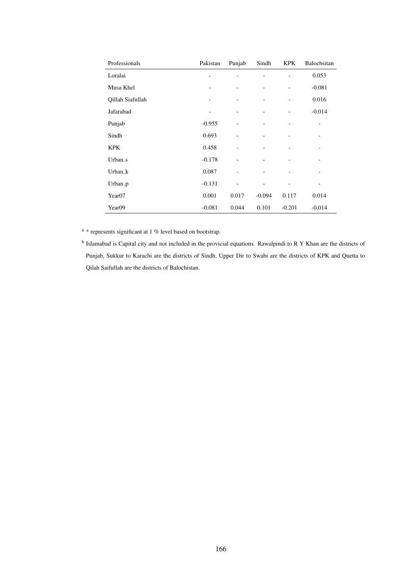
Professionals Pakistan Punjab Sindh KPK Balochsitan
Loralai - - - - 0.053
Musa Khel - - - - -0.081
Qillah Siafullah - - - - 0.016
Jafarabad - - - - -0.014
Punjab -0.955 - - - -
Sindh 0.693 - - - -
KPK 0.458 - - - -
Urban s -0.178 - - - -
Urban k 0.087 - - - -
Urban p -0.131 - - - -
Year07 0.001 0.017 -0.094 0.117 0.014
Year09 -0.081 0.044 0.101 -0.201 -0.014
a * represents significant at 1 % level based on bootstrap.
b Islamabad is Capital city and not included in the provicial equations. Rawalpindi to R Y Khan are the districts of
Punjab, Sukkur to Karachi are the districts of Sindh, Upper Dir to Swabi are the districts of KPK and Quetta to
Qilah Saifullah are the districts of Balochistan.
166
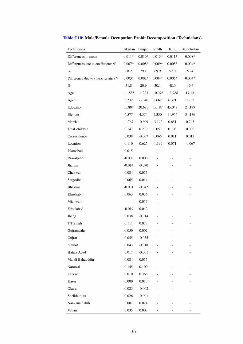
Table C10: Male/Female Occupation Probit Decomposition (Technicians).
Technicians Pakistan Punjab Sindh KPK Balochsitan
Differences in mean 0.011* 0.010* 0.013* 0.011* 0.008*
Differences due to coefficients % 0.007* 0.008* 0.009* 0.005* 0.004*
% 68.2 79.1 69.9 52.0 53.4
Difference due to charactersitics % 0.003* 0.002* 0.004* 0.005* 0.004*
% 31.8 20.9 30.1 48.0 46.6
Age -11.835 -1.223 -10.076 -13.988 -17.121
Age2 3.232 -3.346 2.662 6.321 7.733
Education 35.804 20.683 35.187 45.049 21.179
Illetrate 6.577 4.574 7.330 11.956 34.136
Married -1.767 -0.609 -3.192 0.651 0.743
Total children 0.147 0.279 0.057 0.108 0.000
Co residence 0.038 -0.007 0.065 0.011 0.013
Location 0.110 0.625 -1.399 0.071 -0.067
Islamabad 0.015 - - - -
Rawalpindi -0.002 0.000 - - -
Jhelum -0.014 -0.070 - - -
Chakwal 0.084 0.053 - - -
Sargodha 0.065 0.014 - - -
Bhakkar -0.031 -0.042 - - -
Khushab 0.063 0.036 - - -
Mianwali - 0.057 - - -
Faisalabad -0.019 0.042 - - -
Jhang 0.038 -0.014 - - -
T.T.Singh 0.111 0.073 - - -
Gujranwala 0.050 0.002 - - -
Gujrat 0.055 -0.035 - - -
Sialkot 0.043 -0.018 - - -
Hafiza Abad 0.017 -0.001 - - -
Mandi Bahauddin 0.084 0.055 - - -
Narowal 0.145 0.100 - - -
Lahore 0.010 0.366 - - -
Kasur 0.000 0.013 - - -
Okara 0.025 -0.002 - - -
Sheikhupura 0.026 -0.001 - - -
Nankana Sahib 0.001 0.024 - - -
Vehari 0.035 0.003 - - -
167
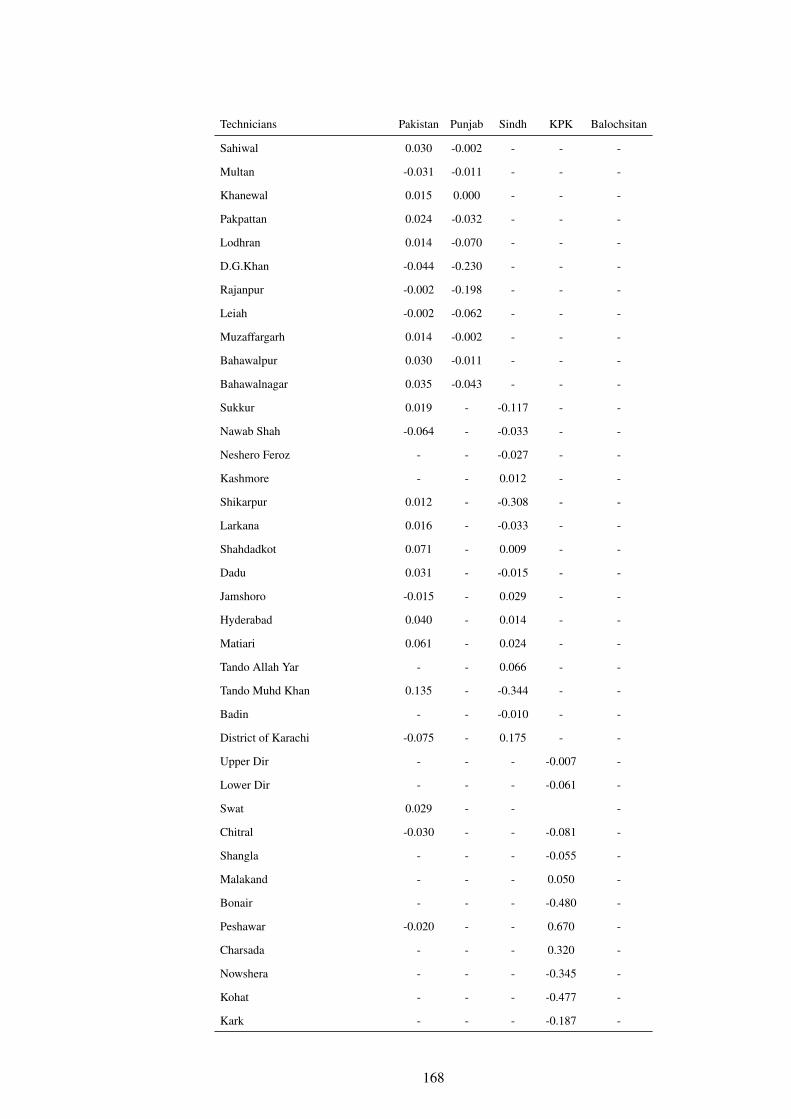
Technicians Pakistan Punjab Sindh KPK Balochsitan
Sahiwal 0.030 -0.002 - - -
Multan -0.031 -0.011 - - -
Khanewal 0.015 0.000 - - -
Pakpattan 0.024 -0.032 - - -
Lodhran 0.014 -0.070 - - -
D.G.Khan -0.044 -0.230 - - -
Rajanpur -0.002 -0.198 - - -
Leiah -0.002 -0.062 - - -
Muzaffargarh 0.014 -0.002 - - -
Bahawalpur 0.030 -0.011 - - -
Bahawalnagar 0.035 -0.043 - - -
Sukkur 0.019 - -0.117 - -
Nawab Shah -0.064 - -0.033 - -
Neshero Feroz - - -0.027 - -
Kashmore - - 0.012 - -
Shikarpur 0.012 - -0.308 - -
Larkana 0.016 - -0.033 - -
Shahdadkot 0.071 - 0.009 - -
Dadu 0.031 - -0.015 - -
Jamshoro -0.015 - 0.029 - -
Hyderabad 0.040 - 0.014 - -
Matiari 0.061 - 0.024 - -
Tando Allah Yar - - 0.066 - -
Tando Muhd Khan 0.135 - -0.344 - -
Badin - - -0.010 - -
District of Karachi -0.075 - 0.175 - -
Upper Dir - - - -0.007 -
Lower Dir - - - -0.061 -
Swat 0.029 - - -
Chitral -0.030 - - -0.081 -
Shangla - - - -0.055 -
Malakand - - - 0.050 -
Bonair - - - -0.480 -
Peshawar -0.020 - - 0.670 -
Charsada - - - 0.320 -
Nowshera - - - -0.345 -
Kohat - - - -0.477 -
Kark - - - -0.187 -
168
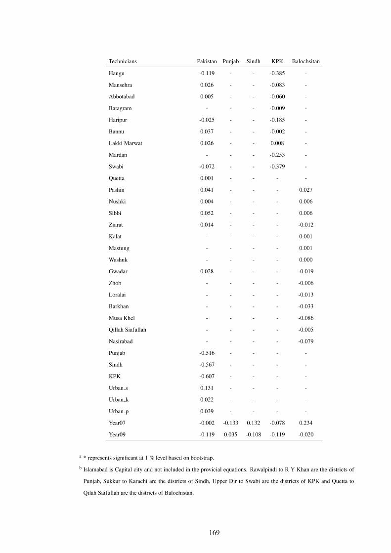
Technicians Pakistan Punjab Sindh KPK Balochsitan
Hangu -0.119 - - -0.385 -
Mansehra 0.026 - - -0.083 -
Abbotabad 0.005 - - -0.060 -
Batagram - - - -0.009 -
Haripur -0.025 - - -0.185 -
Bannu 0.037 - - -0.002 -
Lakki Marwat 0.026 - - 0.008 -
Mardan - - - -0.253 -
Swabi -0.072 - - -0.379 -
Quetta 0.001 - - - -
Pashin 0.041 - - - 0.027
Nushki 0.004 - - - 0.006
Sibbi 0.052 - - - 0.006
Ziarat 0.014 - - - -0.012
Kalat - - - - 0.001
Mastung - - - - 0.001
Washuk - - - - 0.000
Gwadar 0.028 - - - -0.019
Zhob - - - - -0.006
Loralai - - - - -0.013
Barkhan - - - - -0.033
Musa Khel - - - - -0.086
Qillah Siafullah - - - - -0.005
Nasirabad - - - - -0.079
Punjab -0.516 - - - -
Sindh -0.567 - - - -
KPK -0.607 - - - -
Urban s 0.131 - - - -
Urban k 0.022 - - - -
Urban p 0.039 - - - -
Year07 -0.002 -0.133 0.132 -0.078 0.234
Year09 -0.119 0.035 -0.108 -0.119 -0.020
a * represents significant at 1 % level based on bootstrap.
b Islamabad is Capital city and not included in the provicial equations. Rawalpindi to R Y Khan are the districts of
Punjab, Sukkur to Karachi are the districts of Sindh, Upper Dir to Swabi are the districts of KPK and Quetta to
Qilah Saifullah are the districts of Balochistan.
169
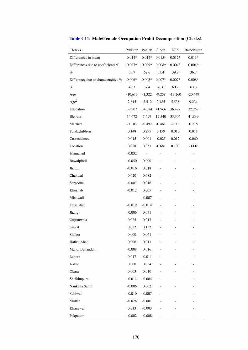
Table C11: Male/Female Occupation Probit Decomposition (Clerks).
Clercks Pakistan Punjab Sindh KPK Balochsitan
Differences in mean 0.014* 0.014* 0.015* 0.012* 0.013*
Differences due to coefficients % 0.007* 0.009* 0.008* 0.004* 0.004*
% 53.7 62.6 53.4 39.8 36.7
Difference due to charactersitics % 0.006* 0.005* 0.007* 0.007* 0.008*
% 46.3 37.4 46.6 60.2 63.3
Age -10.613 -1.322 -9.258 -13.260 -20.449
Age2 2.815 -3.412 2.485 5.538 9.234
Education 39.907 34.384 41.966 36.477 32.257
Illetrate 14.678 7.499 12.540 33.306 41.839
Married -1.103 -0.492 -0.461 -2.001 0.278
Total children 0.148 0.295 0.159 0.010 0.011
Co residence 0.015 0.001 -0.025 0.012 0.060
Location 0.088 0.351 -0.681 0.103 -0.116
Islamabad -0.032 - - - -
Rawalpindi -0.050 0.000 - - -
Jhelum -0.016 0.018 - - -
Chakwal 0.020 0.082 - - -
Sargodha -0.007 0.016 - - -
Khushab -0.012 0.005 - - -
Mianwali -0.007 - - -
Faisalabad -0.019 -0.014 - - -
Jhang -0.006 0.031 - - -
Gujranwala 0.025 0.017 - - -
Gujrat 0.032 0.152 - - -
Sialkot 0.000 0.061 - - -
Hafiza Abad 0.006 0.011 - - -
Mandi Bahauddin -0.008 0.016 - - -
Lahore 0.017 -0.011 - - -
Kasur 0.000 0.034 - - -
Okara 0.003 0.010 - - -
Sheikhupura -0.011 -0.004 - - -
Nankana Sahib -0.006 0.002 - - -
Sahiwal -0.010 -0.007 - - -
Multan -0.028 -0.001 - - -
Khanewal 0.013 -0.003 - - -
Pakpattan -0.002 -0.008 - - -
170
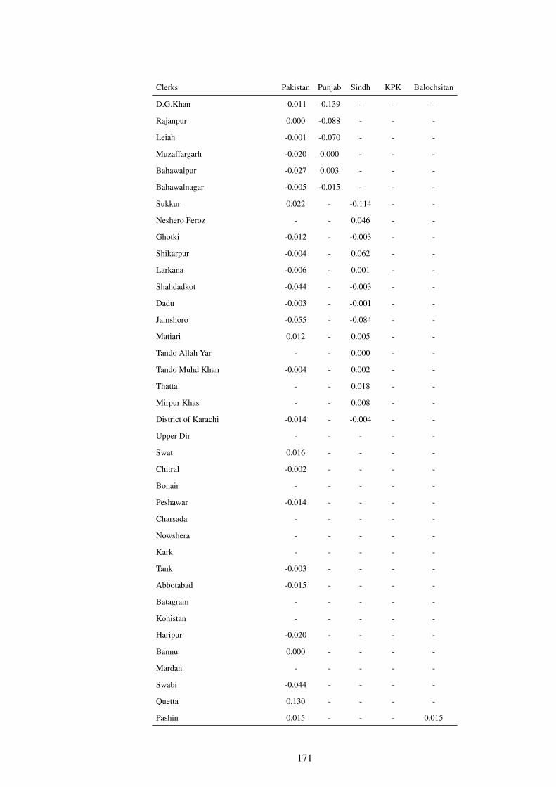
Clerks Pakistan Punjab Sindh KPK Balochsitan
D.G.Khan -0.011 -0.139 - - -
Rajanpur 0.000 -0.088 - - -
Leiah -0.001 -0.070 - - -
Muzaffargarh -0.020 0.000 - - -
Bahawalpur -0.027 0.003 - - -
Bahawalnagar -0.005 -0.015 - - -
Sukkur 0.022 - -0.114 - -
Neshero Feroz - - 0.046 - -
Ghotki -0.012 - -0.003 - -
Shikarpur -0.004 - 0.062 - -
Larkana -0.006 - 0.001 - -
Shahdadkot -0.044 - -0.003 - -
Dadu -0.003 - -0.001 - -
Jamshoro -0.055 - -0.084 - -
Matiari 0.012 - 0.005 - -
Tando Allah Yar - - 0.000 - -
Tando Muhd Khan -0.004 - 0.002 - -
Thatta - - 0.018 - -
Mirpur Khas - - 0.008 - -
District of Karachi -0.014 - -0.004 - -
Upper Dir - - - - -
Swat 0.016 - - - -
Chitral -0.002 - - - -
Bonair - - - - -
Peshawar -0.014 - - - -
Charsada - - - - -
Nowshera - - - - -
Kark - - - - -
Tank -0.003 - - - -
Abbotabad -0.015 - - - -
Batagram - - - - -
Kohistan - - - - -
Haripur -0.020 - - - -
Bannu 0.000 - - - -
Mardan - - - - -
Swabi -0.044 - - - -
Quetta 0.130 - - - -
Pashin 0.015 - - - 0.015
171
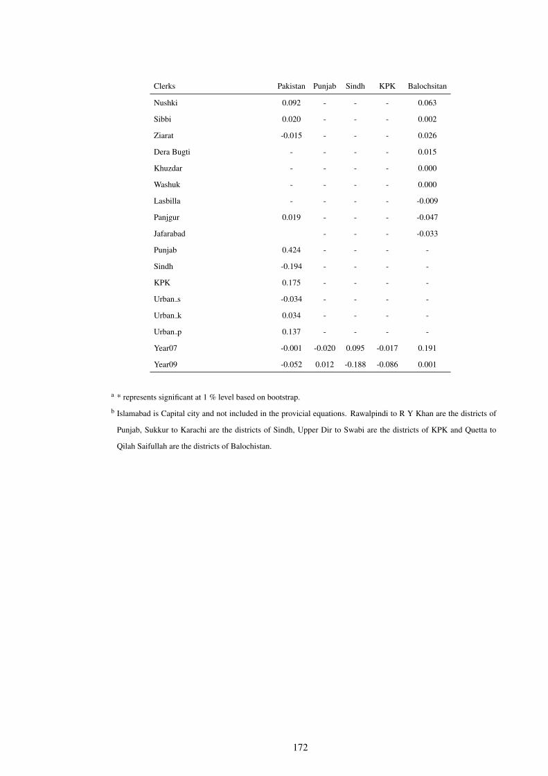
Clerks Pakistan Punjab Sindh KPK Balochsitan
Nushki 0.092 - - - 0.063
Sibbi 0.020 - - - 0.002
Ziarat -0.015 - - - 0.026
Dera Bugti - - - - 0.015
Khuzdar - - - - 0.000
Washuk - - - - 0.000
Lasbilla - - - - -0.009
Panjgur 0.019 - - - -0.047
Jafarabad - - - -0.033
Punjab 0.424 - - - -
Sindh -0.194 - - - -
KPK 0.175 - - - -
Urban s -0.034 - - - -
Urban k 0.034 - - - -
Urban p 0.137 - - - -
Year07 -0.001 -0.020 0.095 -0.017 0.191
Year09 -0.052 0.012 -0.188 -0.086 0.001
a * represents significant at 1 % level based on bootstrap.
b Islamabad is Capital city and not included in the provicial equations. Rawalpindi to R Y Khan are the districts of
Punjab, Sukkur to Karachi are the districts of Sindh, Upper Dir to Swabi are the districts of KPK and Quetta to
Qilah Saifullah are the districts of Balochistan.
172
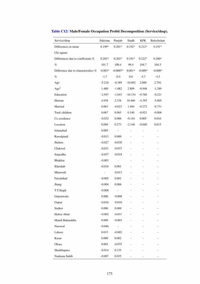
Table C12: Male/Female Occupation Probit Decomposition (Service/shop).
Service/shop Pakistan Punjab Sindh KPK Balochsitan
Differences in mean 0.199* 0.201* 0.192* 0.212* 0.191*
Chi square
Differences due to coefficients % 0.202* 0.202* 0.191* 0.222* 0.200*
% 101.7 100.4 99.4 104.7 104.5
Difference due to charactersitics % -0.003* -0.0007* 0.001* -0.009* -0.008*
% -1.7 -0.4 0.6 -4.7 -4.5
Age -5.218 -0.389 -10.092 2.089 2.792
Age2 1.480 -1.082 2.809 -0.948 -1.289
Education -2.947 -1.643 -10.154 -0.760 -0.221
Illetrate 4.938 2.338 18.460 -4.395 -5.005
Married 0.063 -0.023 1.494 -0.272 -0.731
Total children 0.067 0.065 0.140 -0.021 -0.008
Co residence -0.032 0.006 -0.144 0.005 0.016
Location 0.069 0.273 -2.148 -0.040 0.015
Islamabad 0.005 - - - -
Rawalpindi -0.013 0.000 - - -
Jhelum -0.027 -0.030 - - -
Chakwal -0.031 -0.037 - - -
Sargodha -0.037 -0.018 - - -
Bhakkar -0.003 - - - -
Khushab -0.016 0.001 - - -
Mianwali - -0.013 - - -
Faisalabad -0.005 0.001 - - -
Jhang -0.004 0.006 - - -
T.T.Singh -0.008 - - - -
Gujranwala 0.006 -0.008 - - -
Gujrat -0.016 -0.010 - - -
Sialkot 0.006 0.000 - - -
Hafiza Abad -0.002 -0.031 - - -
Mandi Bahauddin 0.009 -0.003 - - -
Narowal -0.046 - - - -
Lahore 0.015 -0.002 - - -
Kasur 0.000 0.002 - - -
Okara 0.003 -0.075 - - -
Sheikhupura -0.014 0.135 - - -
Nankana Sahib -0.007 0.035 - - -
173
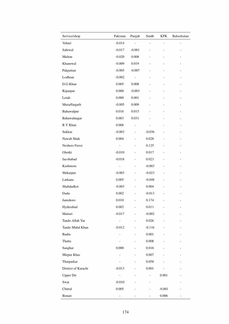
Service/shop Pakistan Punjab Sindh KPK Balochsitan
Vehari -0.014 - - - -
Sahiwal -0.017 -0.001 - - -
Multan -0.020 0.008 - - -
Khanewal -0.009 0.019 - - -
Pakpattan -0.005 -0.007 - - -
Lodhran -0.002 - - - -
D.G.Khan 0.005 0.008 - - -
Rajanpur 0.000 -0.003 - - -
Leiah 0.000 0.001 - - -
Muzaffargarh -0.005 0.009 - - -
Bahawalpur 0.016 0.015 - - -
Bahawalnagar 0.003 0.031 - - -
R Y Khan 0.006 - - - -
Sukkur -0.003 - -0.036 - -
Nawab Shah 0.004 - 0.028 - -
Neshero Feroz - - 0.125 - -
Ghotki -0.010 - 0.017 - -
Jacobabad -0.018 - 0.023 - -
Kashmore - - -0.003 - -
Shikarpur -0.003 - -0.023 - -
Larkana 0.005 - -0.048 - -
Shahdadkot -0.003 - 0.004 - -
Dadu 0.002 - -0.013 - -
Jamshoro 0.010 - 0.174 - -
Hyderabad 0.002 - 0.011 - -
Matiari -0.017 - -0.002 - -
Tando Allah Yar - - 0.026 - -
Tando Muhd Khan -0.012 - -0.116 - -
Badin - - 0.001 - -
Thatta - - 0.008 - -
Sanghar 0.000 - 0.016 - -
Mirpur Khas - - 0.007 - -
Tharparkar - - 0.058 - -
District of Karachi -0.013 - 0.001 - -
Upper Dir - - - 0.001 -
Swat -0.010 - - -
Chitral 0.005 - - -0.001 -
Bonair - - - 0.006 -
174
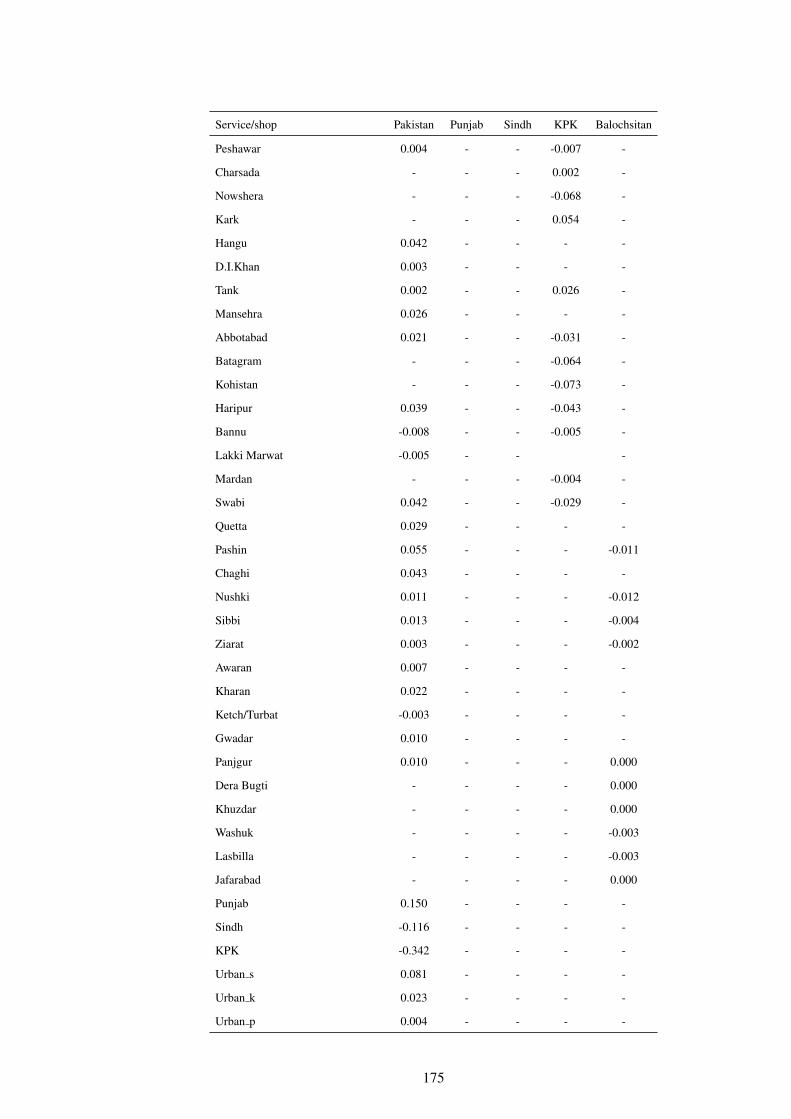
Service/shop Pakistan Punjab Sindh KPK Balochsitan
Peshawar 0.004 - - -0.007 -
Charsada - - - 0.002 -
Nowshera - - - -0.068 -
Kark - - - 0.054 -
Hangu 0.042 - - - -
D.I.Khan 0.003 - - - -
Tank 0.002 - - 0.026 -
Mansehra 0.026 - - - -
Abbotabad 0.021 - - -0.031 -
Batagram - - - -0.064 -
Kohistan - - - -0.073 -
Haripur 0.039 - - -0.043 -
Bannu -0.008 - - -0.005 -
Lakki Marwat -0.005 - - -
Mardan - - - -0.004 -
Swabi 0.042 - - -0.029 -
Quetta 0.029 - - - -
Pashin 0.055 - - - -0.011
Chaghi 0.043 - - - -
Nushki 0.011 - - - -0.012
Sibbi 0.013 - - - -0.004
Ziarat 0.003 - - - -0.002
Awaran 0.007 - - - -
Kharan 0.022 - - - -
Ketch/Turbat -0.003 - - - -
Gwadar 0.010 - - - -
Panjgur 0.010 - - - 0.000
Dera Bugti - - - - 0.000
Khuzdar - - - - 0.000
Washuk - - - - -0.003
Lasbilla - - - - -0.003
Jafarabad - - - - 0.000
Punjab 0.150 - - - -
Sindh -0.116 - - - -
KPK -0.342 - - - -
Urban s 0.081 - - - -
Urban k 0.023 - - - -
Urban p 0.004 - - - -
175
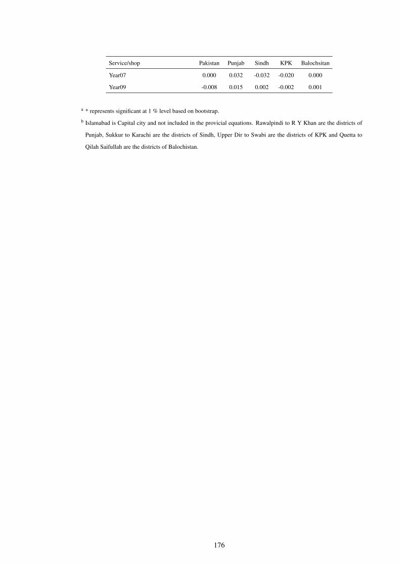
Service/shop Pakistan Punjab Sindh KPK Balochsitan
Year07 0.000 0.032 -0.032 -0.020 0.000
Year09 -0.008 0.015 0.002 -0.002 0.001
a * represents significant at 1 % level based on bootstrap.
b Islamabad is Capital city and not included in the provicial equations. Rawalpindi to R Y Khan are the districts of
Punjab, Sukkur to Karachi are the districts of Sindh, Upper Dir to Swabi are the districts of KPK and Quetta to
Qilah Saifullah are the districts of Balochistan.
176

Table C13: Male/Female Occupation Probit Decomposition (Skilled/agri/fishery).
Skilled/agri/fishery Pakistan Punjab Sindh KPK Balochsitan
Differences in mean 0.138* 0.095* 0.184* 0.103* 0.206*
Differences due to coefficients % 0.182* 0.116* 0.254* 0.159* 0.276*
% 132.0 121.5 138.0 154.5 134.2
Difference due to charactersitics % -0.044* -0.020* -0.070* -0.056* -0.070*
% -32.0 -21.5 -38.0 -54.5 -34.2
Age -6.093 -1.045 -5.216 -99.337 -74.945
Age2 1.500 -2.386 1.377 34.150 31.299
Education -16.856 -5.132 -30.917 -124.261 -62.981
Illetrate -15.234 -12.903 -8.896 104.415 5.914
Married 2.875 3.315 1.394 43.170 71.536
Total children 0.139 0.325 0.077 0.386 0.150
Co residence -0.152 0.060 -0.226 -0.619 -2.782
Location -0.342 -3.314 3.389 -26.918 3.297
Islamabad 0.036 - - - -
Rawalpindi 0.060 0.000 - - -
Jhelum 0.006 -0.080 - - -
Chakwal -0.004 -0.106 - - -
Sargodha -0.015 -0.068 - - -
Bhakkar 0.041 0.442 - - -
Khushab -0.028 -0.087 - - -
Mianwali - 0.068 - - -
Faisalabad -0.033 0.097 - - -
Jhang -0.123 -0.284 - - -
T.T.Singh -0.074 -0.209 - - -
Gujranwala -0.013 -0.030 - - -
Gujrat -0.015 -0.266 - - -
Sialkot -0.023 -0.197 - - -
Hafiza Abad -0.038 -0.047 - - -
Mandi Bahauddin -0.033 -0.123 - - -
Narowal -0.166 -0.791 - - -
Lahore -0.038 -0.057 - - -
Kasur 0.000 0.240 - - -
Okara -0.081 -0.075 - - -
Sheikhupura -0.007 0.041 - - -
Nankana Sahib -0.009 0.118 - - -
Vehari -0.051 -0.075 - - -
177
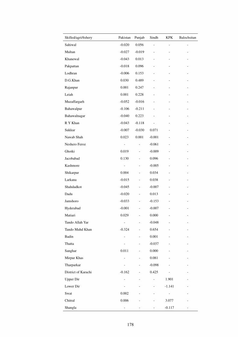
Skilled/agri/fishery Pakistan Punjab Sindh KPK Balochsitan
Sahiwal -0.020 0.056 - - -
Multan -0.027 -0.019 - - -
Khanewal -0.043 0.013 - - -
Pakpattan -0.018 0.096 - - -
Lodhran -0.006 0.153 - - -
D.G.Khan 0.030 0.489 - - -
Rajanpur 0.001 0.247 - - -
Leiah 0.001 0.228 - - -
Muzaffargarh -0.052 -0.016 - - -
Bahawalpur -0.106 -0.211 - - -
Bahawalnagar -0.040 0.223 - - -
R Y Khan -0.043 -0.118 - - -
Sukkur -0.007 -0.030 0.071 - -
Nawab Shah 0.023 0.001 -0.001 - -
Neshero Feroz - - -0.061 - -
Ghotki 0.019 - -0.009 - -
Jacobabad 0.130 - 0.096 - -
Kashmore - - -0.005 - -
Shikarpur 0.004 - 0.034 - -
Larkana -0.015 - 0.038 - -
Shahdadkot -0.045 - -0.007 - -
Dadu -0.020 - 0.013 - -
Jamshoro -0.033 - -0.153 - -
Hyderabad -0.001 - -0.007 - -
Matiari 0.029 - 0.000 - -
Tando Allah Yar - - -0.048 - -
Tando Muhd Khan -0.324 - 0.654 - -
Badin - - 0.001 - -
Thatta - - -0.037 - -
Sanghar 0.011 - 0.000 - -
Mirpur Khas - - 0.081 - -
Tharparkar - - -0.098 - -
District of Karachi -0.162 - 0.425 - -
Upper Dir - - - 1.901 -
Lower Dir - - - -1.141 -
Swat 0.002 - - - -
Chitral 0.006 - - 3.077 -
Shangla - - - -0.117 -
178
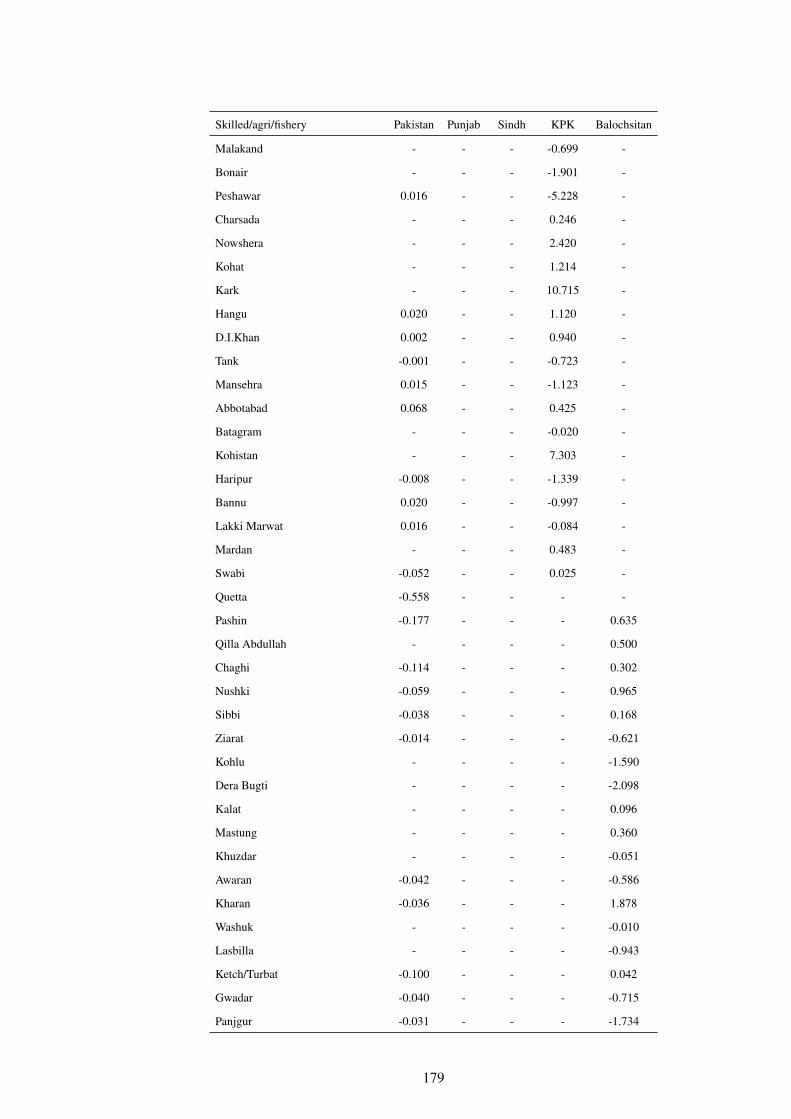
Skilled/agri/fishery Pakistan Punjab Sindh KPK Balochsitan
Malakand - - - -0.699 -
Bonair - - - -1.901 -
Peshawar 0.016 - - -5.228 -
Charsada - - - 0.246 -
Nowshera - - - 2.420 -
Kohat - - - 1.214 -
Kark - - - 10.715 -
Hangu 0.020 - - 1.120 -
D.I.Khan 0.002 - - 0.940 -
Tank -0.001 - - -0.723 -
Mansehra 0.015 - - -1.123 -
Abbotabad 0.068 - - 0.425 -
Batagram - - - -0.020 -
Kohistan - - - 7.303 -
Haripur -0.008 - - -1.339 -
Bannu 0.020 - - -0.997 -
Lakki Marwat 0.016 - - -0.084 -
Mardan - - - 0.483 -
Swabi -0.052 - - 0.025 -
Quetta -0.558 - - - -
Pashin -0.177 - - - 0.635
Qilla Abdullah - - - - 0.500
Chaghi -0.114 - - - 0.302
Nushki -0.059 - - - 0.965
Sibbi -0.038 - - - 0.168
Ziarat -0.014 - - - -0.621
Kohlu - - - - -1.590
Dera Bugti - - - - -2.098
Kalat - - - - 0.096
Mastung - - - - 0.360
Khuzdar - - - - -0.051
Awaran -0.042 - - - -0.586
Kharan -0.036 - - - 1.878
Washuk - - - - -0.010
Lasbilla - - - - -0.943
Ketch/Turbat -0.100 - - - 0.042
Gwadar -0.040 - - - -0.715
Panjgur -0.031 - - - -1.734
179
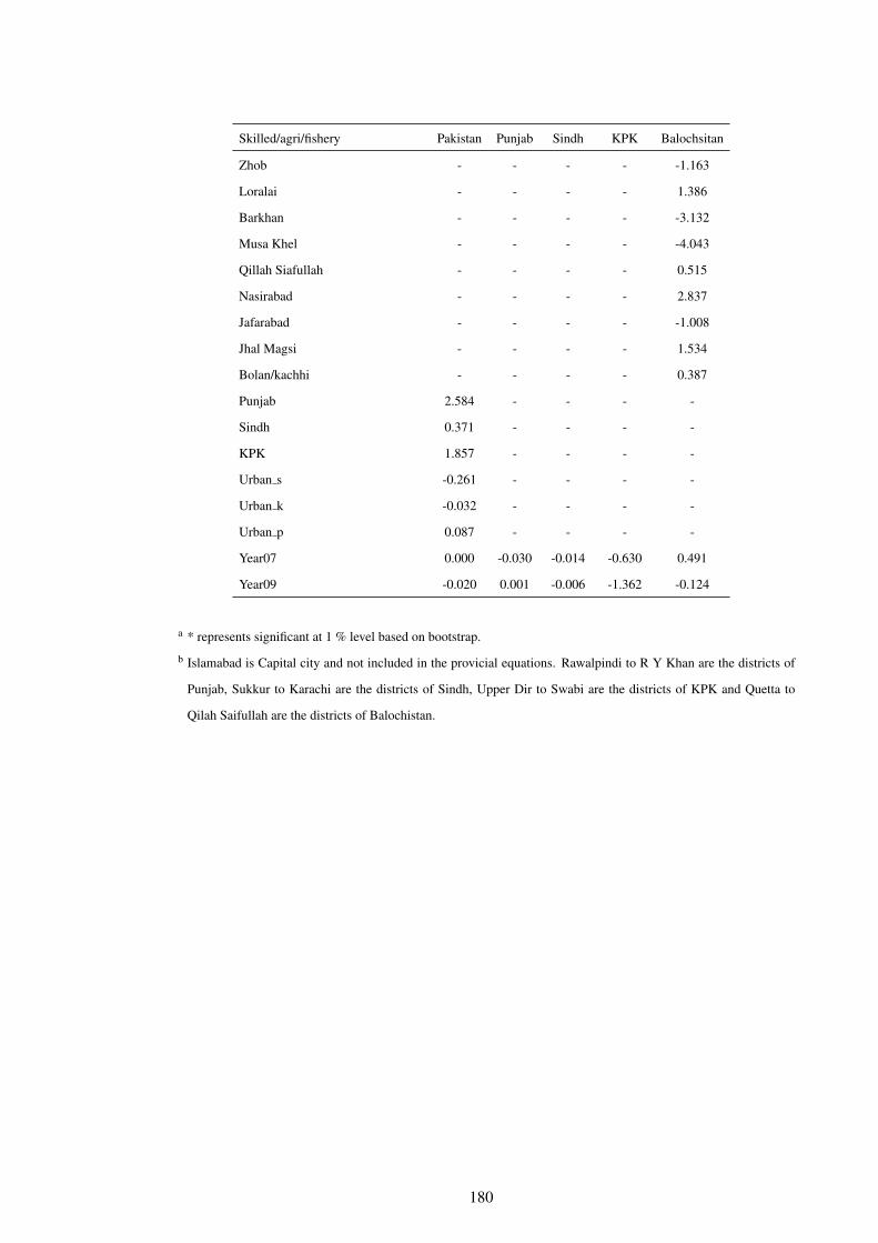
Skilled/agri/fishery Pakistan Punjab Sindh KPK Balochsitan
Zhob - - - - -1.163
Loralai - - - - 1.386
Barkhan - - - - -3.132
Musa Khel - - - - -4.043
Qillah Siafullah - - - - 0.515
Nasirabad - - - - 2.837
Jafarabad - - - - -1.008
Jhal Magsi - - - - 1.534
Bolan/kachhi - - - - 0.387
Punjab 2.584 - - - -
Sindh 0.371 - - - -
KPK 1.857 - - - -
Urban s -0.261 - - - -
Urban k -0.032 - - - -
Urban p 0.087 - - - -
Year07 0.000 -0.030 -0.014 -0.630 0.491
Year09 -0.020 0.001 -0.006 -1.362 -0.124
a * represents significant at 1 % level based on bootstrap.
b Islamabad is Capital city and not included in the provicial equations. Rawalpindi to R Y Khan are the districts of
Punjab, Sukkur to Karachi are the districts of Sindh, Upper Dir to Swabi are the districts of KPK and Quetta to
Qilah Saifullah are the districts of Balochistan.
180

Table C14: Male/Female Occupation Probit Decomposition (Craft/trade).
Craft/trade Pakistan Punjab Sindh KPK Balochsitan
Differences in mean 0.015* 0.019* 0.015* 0.017* 0.003*
Differences due to coefficients % 0.018* 0.021* 0.017* 0.022* 0.004*
% 117.1 109.8 111.2 128.0 107.7
Difference due to charactersitics % -0.002* -0.001* -0.001* -0.004* -0.0003
% -17.1 -9.8 -11.2 -28.0 -7.7
Age -10.099 -1.349 -7.908 43.851 7.651
Age2 2.953 -3.888 2.269 -21.204 -3.603
Education -31.350 -25.626 -30.128 78.070 6.244
Illetrate 23.748 19.068 23.934 -121.454 -15.144
Married 2.840 2.346 3.357 -11.417 -2.908
Total children 0.225 0.349 0.155 -0.507 -0.040
Co residence -0.070 0.021 -0.169 0.116 0.038
Location 0.145 0.740 -1.326 -0.742 0.084
Rawalpindi 0.066 0.000 - - -
Jhelum 0.091 0.054 - - -
Sargodha -0.121 -0.129 - - -
Bhakkar 0.021 0.248 - - -
Khushab -0.046 -0.091 - - -
Mianwali - 0.116 - - -
Faisalabad -0.083 0.108 - - -
Jhang -0.164 -0.260 - - -
T.T.Singh -0.050 -0.134 - - -
Gujranwala -0.269 -0.103 - - -
Gujrat -0.337 -0.839 - - -
Sialkot -0.494 -0.877 - - -
Hafiza Abad -0.073 -0.054 - - -
Mandi Bahauddin -0.066 -0.137 - - -
Narowal -0.460 -1.255 - - -
Lahore 0.079 1.401 - - -
Kasur 0.000 0.290 - - -
Okara -0.049 -0.042 - - -
Sheikhupura -0.106 0.102 - - -
Nankana Sahib -0.006 0.076 - - -
Vehari -0.033 -0.046 - - -
Sahiwal -0.068 0.072 - - -
Multan -0.086 -0.026 - - -
181
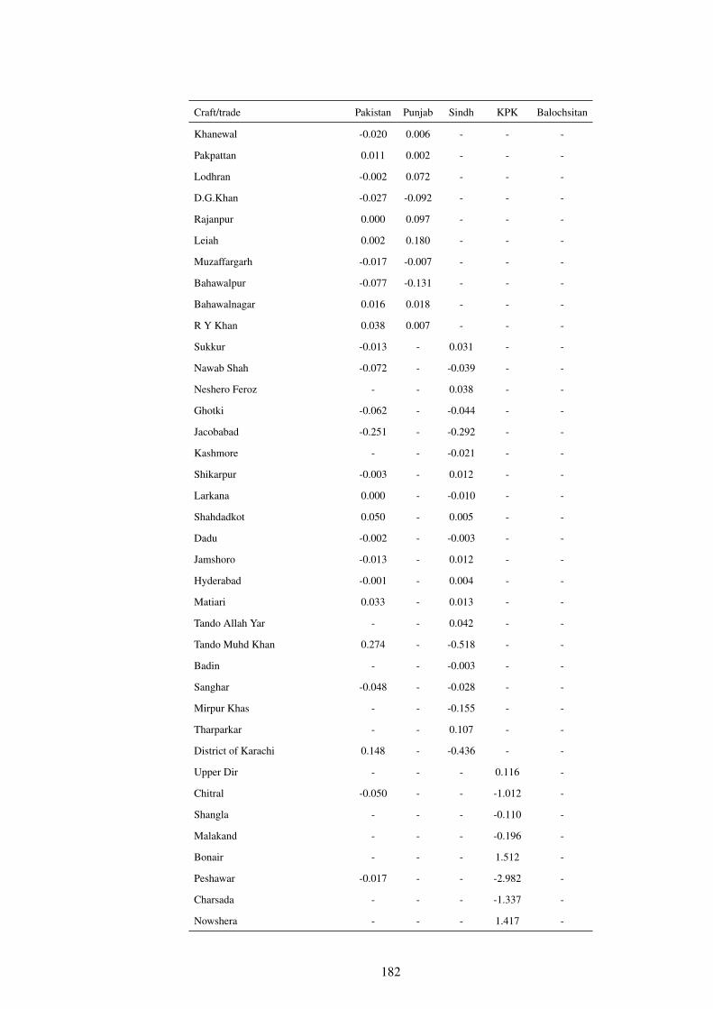
Craft/trade Pakistan Punjab Sindh KPK Balochsitan
Khanewal -0.020 0.006 - - -
Pakpattan 0.011 0.002 - - -
Lodhran -0.002 0.072 - - -
D.G.Khan -0.027 -0.092 - - -
Rajanpur 0.000 0.097 - - -
Leiah 0.002 0.180 - - -
Muzaffargarh -0.017 -0.007 - - -
Bahawalpur -0.077 -0.131 - - -
Bahawalnagar 0.016 0.018 - - -
R Y Khan 0.038 0.007 - - -
Sukkur -0.013 - 0.031 - -
Nawab Shah -0.072 - -0.039 - -
Neshero Feroz - - 0.038 - -
Ghotki -0.062 - -0.044 - -
Jacobabad -0.251 - -0.292 - -
Kashmore - - -0.021 - -
Shikarpur -0.003 - 0.012 - -
Larkana 0.000 - -0.010 - -
Shahdadkot 0.050 - 0.005 - -
Dadu -0.002 - -0.003 - -
Jamshoro -0.013 - 0.012 - -
Hyderabad -0.001 - 0.004 - -
Matiari 0.033 - 0.013 - -
Tando Allah Yar - - 0.042 - -
Tando Muhd Khan 0.274 - -0.518 - -
Badin - - -0.003 - -
Sanghar -0.048 - -0.028 - -
Mirpur Khas - - -0.155 - -
Tharparkar - - 0.107 - -
District of Karachi 0.148 - -0.436 - -
Upper Dir - - - 0.116 -
Chitral -0.050 - - -1.012 -
Shangla - - - -0.110 -
Malakand - - - -0.196 -
Bonair - - - 1.512 -
Peshawar -0.017 - - -2.982 -
Charsada - - - -1.337 -
Nowshera - - - 1.417 -
182
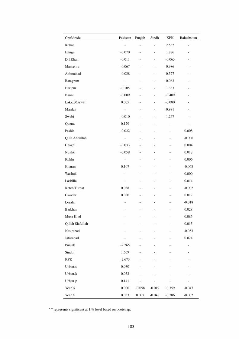
Craft/trade Pakistan Punjab Sindh KPK Balochsitan
Kohat - - - 2.562 -
Hangu -0.070 - - 1.886 -
D.I.Khan -0.011 - - -0.063 -
Mansehra -0.067 - - 0.986 -
Abbotabad -0.038 - - 0.527 -
Batagram - - - 0.063 -
Haripur -0.105 - - 1.363 -
Bannu -0.009 - - -0.409 -
Lakki Marwat 0.005 - - -0.080 -
Mardan - - - 0.981 -
Swabi -0.010 - - 1.257 -
Quetta 0.129 - - - -
Pashin -0.022 - - - 0.008
Qilla Abdullah - - - - -0.006
Chaghi -0.033 - - - 0.004
Nushki -0.059 - - - 0.018
Kohlu - - - - 0.006
Kharan 0.107 - - - -0.068
Washuk - - - - 0.000
Lasbilla - - - - 0.014
Ketch/Turbat 0.038 - - - -0.002
Gwadar 0.030 - - - 0.017
Loralai - - - - -0.018
Barkhan - - - - 0.028
Musa Khel - - - - 0.085
Qillah Siafullah - - - - 0.015
Nasirabad - - - - -0.053
Jafarabad - - - - 0.024
Punjab -2.265 - - - -
Sindh 1.669 - - - -
KPK -2.673 - - - -
Urban s 0.030 - - - -
Urban k 0.032 - - - -
Urban p 0.141 - - - -
Year07 0.000 -0.058 -0.019 -0.359 -0.047
Year09 0.033 0.007 -0.048 -0.786 -0.002
a * represents significant at 1 % level based on bootstrap.
183
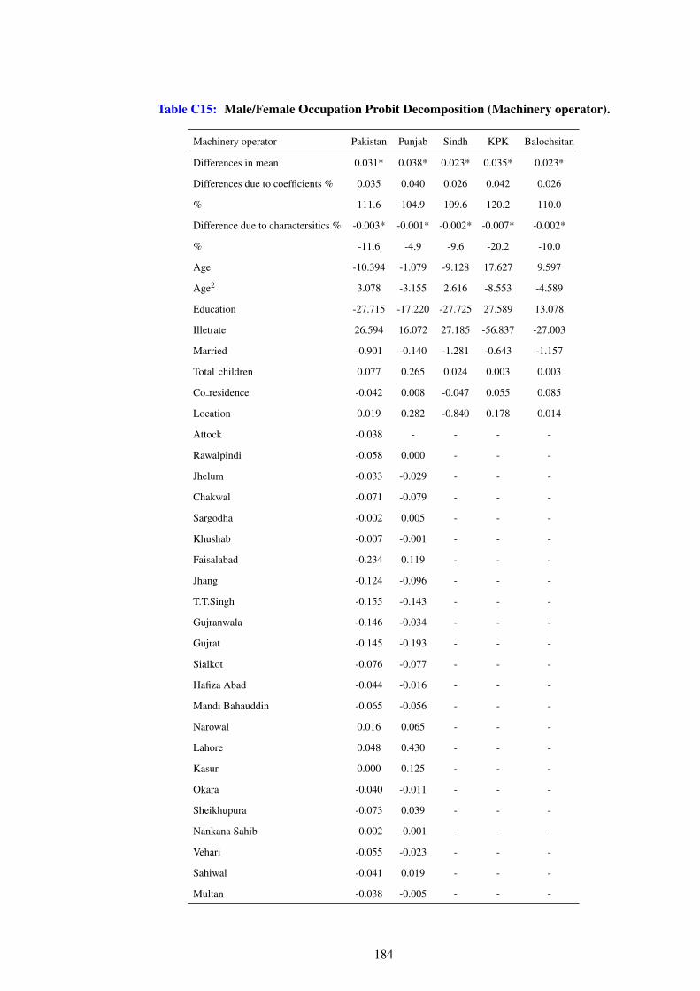
Table C15: Male/Female Occupation Probit Decomposition (Machinery operator).
Machinery operator Pakistan Punjab Sindh KPK Balochsitan
Differences in mean 0.031* 0.038* 0.023* 0.035* 0.023*
Differences due to coefficients % 0.035 0.040 0.026 0.042 0.026
% 111.6 104.9 109.6 120.2 110.0
Difference due to charactersitics % -0.003* -0.001* -0.002* -0.007* -0.002*
% -11.6 -4.9 -9.6 -20.2 -10.0
Age -10.394 -1.079 -9.128 17.627 9.597
Age2 3.078 -3.155 2.616 -8.553 -4.589
Education -27.715 -17.220 -27.725 27.589 13.078
Illetrate 26.594 16.072 27.185 -56.837 -27.003
Married -0.901 -0.140 -1.281 -0.643 -1.157
Total children 0.077 0.265 0.024 0.003 0.003
Co residence -0.042 0.008 -0.047 0.055 0.085
Location 0.019 0.282 -0.840 0.178 0.014
Attock -0.038 - - - -
Rawalpindi -0.058 0.000 - - -
Jhelum -0.033 -0.029 - - -
Chakwal -0.071 -0.079 - - -
Sargodha -0.002 0.005 - - -
Khushab -0.007 -0.001 - - -
Faisalabad -0.234 0.119 - - -
Jhang -0.124 -0.096 - - -
T.T.Singh -0.155 -0.143 - - -
Gujranwala -0.146 -0.034 - - -
Gujrat -0.145 -0.193 - - -
Sialkot -0.076 -0.077 - - -
Hafiza Abad -0.044 -0.016 - - -
Mandi Bahauddin -0.065 -0.056 - - -
Narowal 0.016 0.065 - - -
Lahore 0.048 0.430 - - -
Kasur 0.000 0.125 - - -
Okara -0.040 -0.011 - - -
Sheikhupura -0.073 0.039 - - -
Nankana Sahib -0.002 -0.001 - - -
Vehari -0.055 -0.023 - - -
Sahiwal -0.041 0.019 - - -
Multan -0.038 -0.005 - - -
184
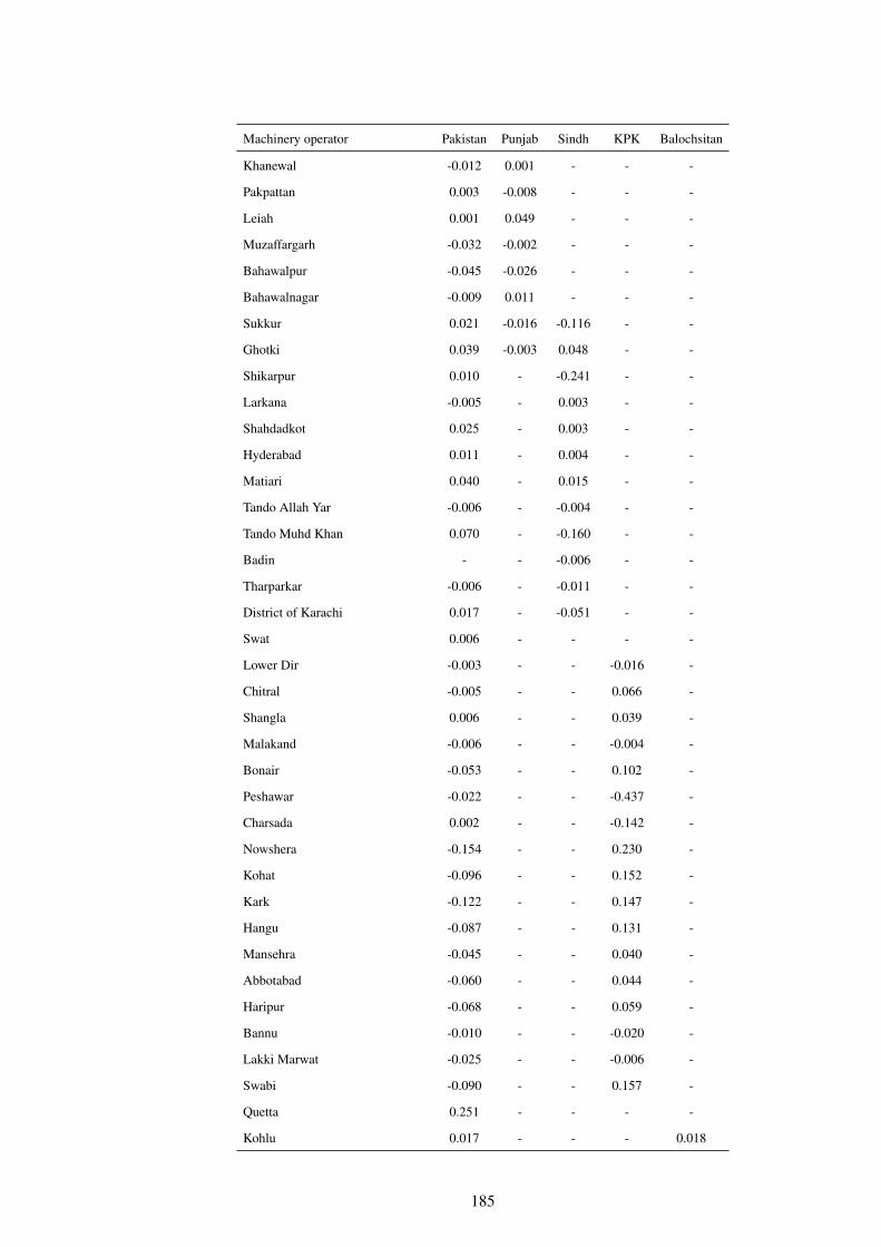
Machinery operator Pakistan Punjab Sindh KPK Balochsitan
Khanewal -0.012 0.001 - - -
Pakpattan 0.003 -0.008 - - -
Leiah 0.001 0.049 - - -
Muzaffargarh -0.032 -0.002 - - -
Bahawalpur -0.045 -0.026 - - -
Bahawalnagar -0.009 0.011 - - -
Sukkur 0.021 -0.016 -0.116 - -
Ghotki 0.039 -0.003 0.048 - -
Shikarpur 0.010 - -0.241 - -
Larkana -0.005 - 0.003 - -
Shahdadkot 0.025 - 0.003 - -
Hyderabad 0.011 - 0.004 - -
Matiari 0.040 - 0.015 - -
Tando Allah Yar -0.006 - -0.004 - -
Tando Muhd Khan 0.070 - -0.160 - -
Badin - - -0.006 - -
Tharparkar -0.006 - -0.011 - -
District of Karachi 0.017 - -0.051 - -
Swat 0.006 - - - -
Lower Dir -0.003 - - -0.016 -
Chitral -0.005 - - 0.066 -
Shangla 0.006 - - 0.039 -
Malakand -0.006 - - -0.004 -
Bonair -0.053 - - 0.102 -
Peshawar -0.022 - - -0.437 -
Charsada 0.002 - - -0.142 -
Nowshera -0.154 - - 0.230 -
Kohat -0.096 - - 0.152 -
Kark -0.122 - - 0.147 -
Hangu -0.087 - - 0.131 -
Mansehra -0.045 - - 0.040 -
Abbotabad -0.060 - - 0.044 -
Haripur -0.068 - - 0.059 -
Bannu -0.010 - - -0.020 -
Lakki Marwat -0.025 - - -0.006 -
Swabi -0.090 - - 0.157 -
Quetta 0.251 - - - -
Kohlu 0.017 - - - 0.018
185
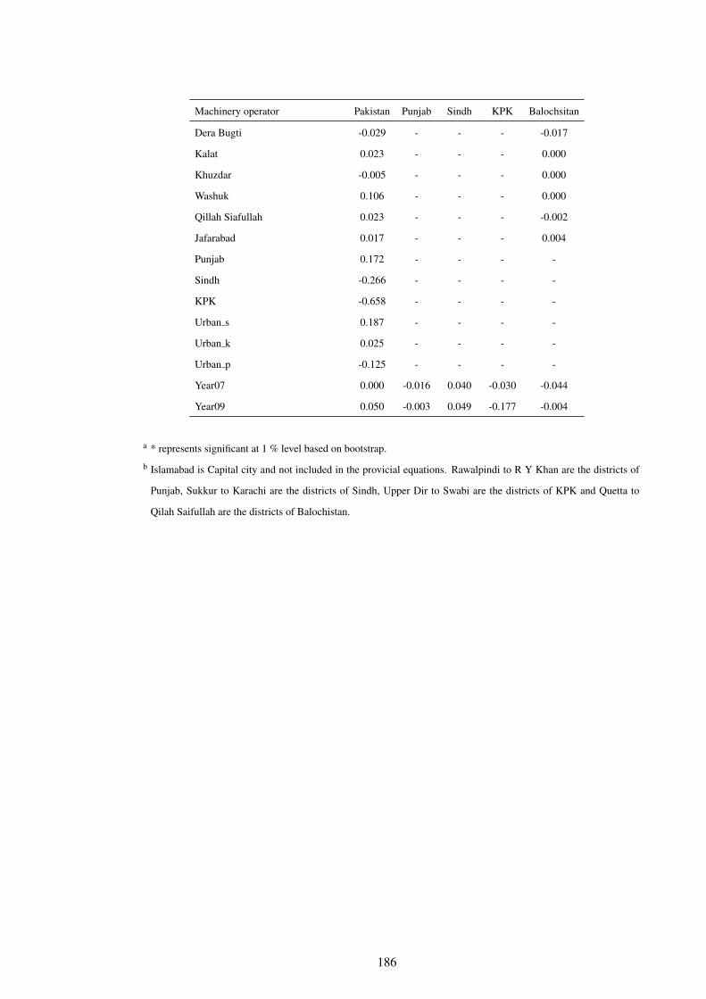
Machinery operator Pakistan Punjab Sindh KPK Balochsitan
Dera Bugti -0.029 - - - -0.017
Kalat 0.023 - - - 0.000
Khuzdar -0.005 - - - 0.000
Washuk 0.106 - - - 0.000
Qillah Siafullah 0.023 - - - -0.002
Jafarabad 0.017 - - - 0.004
Punjab 0.172 - - - -
Sindh -0.266 - - - -
KPK -0.658 - - - -
Urban s 0.187 - - - -
Urban k 0.025 - - - -
Urban p -0.125 - - - -
Year07 0.000 -0.016 0.040 -0.030 -0.044
Year09 0.050 -0.003 0.049 -0.177 -0.004
a * represents significant at 1 % level based on bootstrap.
b Islamabad is Capital city and not included in the provicial equations. Rawalpindi to R Y Khan are the districts of
Punjab, Sukkur to Karachi are the districts of Sindh, Upper Dir to Swabi are the districts of KPK and Quetta to
Qilah Saifullah are the districts of Balochistan.
186

Table C16: Male/Female Occupation Probit Decomposition (Elementry/unskilled).
Elementry/unskilled Pakistan Punjab Sindh KPK Balochsitan
Differences in mean 0.091* 0.090* 0.094* 0.086* 0.100*
Differences due to coefficients % 0.120* 0.119* 0.117* 0.127* 0.121*
% 131.7 131.7 124.3 147.3 121.7
Difference due to charactersitics % -0.029* -0.028* -0.022* -0.040* -0.021*
% -31.7 -31.7 -24.3 -47.3 -21.7
Age -9.753 -1.307 -7.664 92.860 27.859
Age2 2.882 -3.776 2.206 -43.992 -13.504
Education -30.947 -30.560 -29.817 131.847 17.826
Illetrate 6.397 3.388 8.884 -217.244 -45.950
Married 0.592 -0.005 2.596 -19.508 -7.924
Total chil n 0.253 0.307 0.181 -1.832 -0.149
Co residence 0.011 0.005 -0.030 0.074 -0.087
Location 0.035 -0.003 -0.375 1.600 -0.054
Islamabad -0.001 - - - -
Rawalpindi 0.007 0.000 - - -
Jhelum 0.028 0.049 - - -
Chakwal 0.029 0.052 - - -
Sargodha 0.105 0.086 - - -
Bhakkar -0.013 -0.086 - - -
Khushab 0.079 0.098 - - -
Mianwali - -0.004 - - -
Faisalabad 0.030 -0.028 - - -
Jhang 0.059 0.082 - - -
T.T.Singh 0.088 0.124 - - -
Gujranwala 0.042 0.016 - - -
Gujrat 0.028 0.069 - - -
Sialkot 0.172 0.297 - - -
Hafiza Abad 0.029 0.019 - - -
Mandi Bahauddin -0.008 -0.005 - - -
Narowal 0.323 0.777 - - -
Lahore -0.044 -0.653 - - -
Kasur 0.000 -0.100 - - -
Okara 0.019 0.013 - - -
Sheikhupura 0.029 -0.027 - - -
Nankana Sahib 0.005 -0.033 - - -
Vehari 0.069 0.049 - - -
187

Elementry/unskilled Pakistan Punjab Sindh KPK Balochsitan
Sahiwal 0.021 -0.021 - - -
Multan 0.024 0.007 - - -
Khanewal 0.026 -0.004 - - -
Pakpattan 0.012 -0.036 - - -
Lodhran 0.006 -0.064 - - -
D.G.Khan -0.016 -0.169 - - -
Rajanpur -0.001 -0.187 - - -
Leiah 0.000 -0.030 - - -
Muzaffargarh 0.002 0.002 - - -
Bahawalpur 0.000 0.012 - - -
Bahawalnagar -0.003 -0.007 - - -
R Y Khan -0.021 -0.022 - - -
Sukkur 0.001 0.006 0.026 - -
Nawab Shah 0.005 -0.009 -0.006 - -
Neshero Feroz - - -0.113 - -
Ghotki 0.006 - -0.012 - -
Jacobabad -0.141 - -0.204 - -
Kashmore - - -0.007 - -
Shikarpur 0.002 - 0.017 - -
Larkana 0.012 - 0.002 - -
Shahdadkot 0.052 - 0.002 - -
Dadu 0.019 - -0.002 - -
Jamshoro 0.030 - 0.009 - -
Hyderabad -0.022 - -0.010 - -
Matiari -0.021 - -0.010 - -
Tando Allah Yar - - 0.023 - -
Tando Muhd Khan 0.036 - 0.004 - -
Badin - - 0.001 - -
Thatta - - -0.017 - -
Sanghar 0.001 - -0.009 - -
Mirpur Khas - - -0.133 - -
Tharparkar - - 0.065 - -
District of Karachi 0.018 - 0.010 - -
Upper Dir - - - -1.109 -
Lower Dir - - - -0.730 -
Swat 0.037 - - - -
Chitral -0.033 - - 0.077 -
Shangla - - - 0.240 -
188
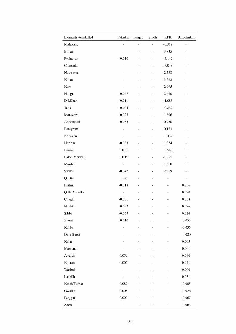
Elementry/unskilled Pakistan Punjab Sindh KPK Balochsitan
Malakand - - - -0.519 -
Bonair - - - 3.835 -
Peshawar -0.010 - - -5.142 -
Charsada - - - -3.048 -
Nowshera - - - 2.538 -
Kohat - - - 3.592 -
Kark - - - 2.995 -
Hangu -0.047 - - 2.690 -
D.I.Khan -0.011 - - -1.085 -
Tank -0.004 - - -0.832 -
Mansehra -0.025 - - 1.806 -
Abbotabad -0.035 - - 0.960 -
Batagram - - - 0.163 -
Kohistan - - - -3.432 -
Haripur -0.038 - - 1.874 -
Bannu 0.013 - - -0.540 -
Lakki Marwat 0.006 - - -0.121 -
Mardan - - - 1.510 -
Swabi -0.042 - - 2.969 -
Quetta 0.130 - - - -
Pashin -0.118 - - - 0.236
Qilla Abdullah - - - - 0.090
Chaghi -0.031 - - - 0.038
Nushki -0.032 - - - 0.076
Sibbi -0.053 - - - 0.024
Ziarat -0.010 - - - -0.055
Kohlu - - - - -0.035
Dera Bugti - - - - -0.020
Kalat - - - - 0.005
Mastung - - - - 0.001
Awaran 0.056 - - - 0.040
Kharan 0.007 - - - 0.041
Washuk - - - - 0.000
Lasbilla - - - - 0.031
Ketch/Turbat 0.080 - - - -0.005
Gwadar 0.008 - - - -0.026
Panjgur 0.009 - - - -0.067
Zhob - - - - -0.063
189
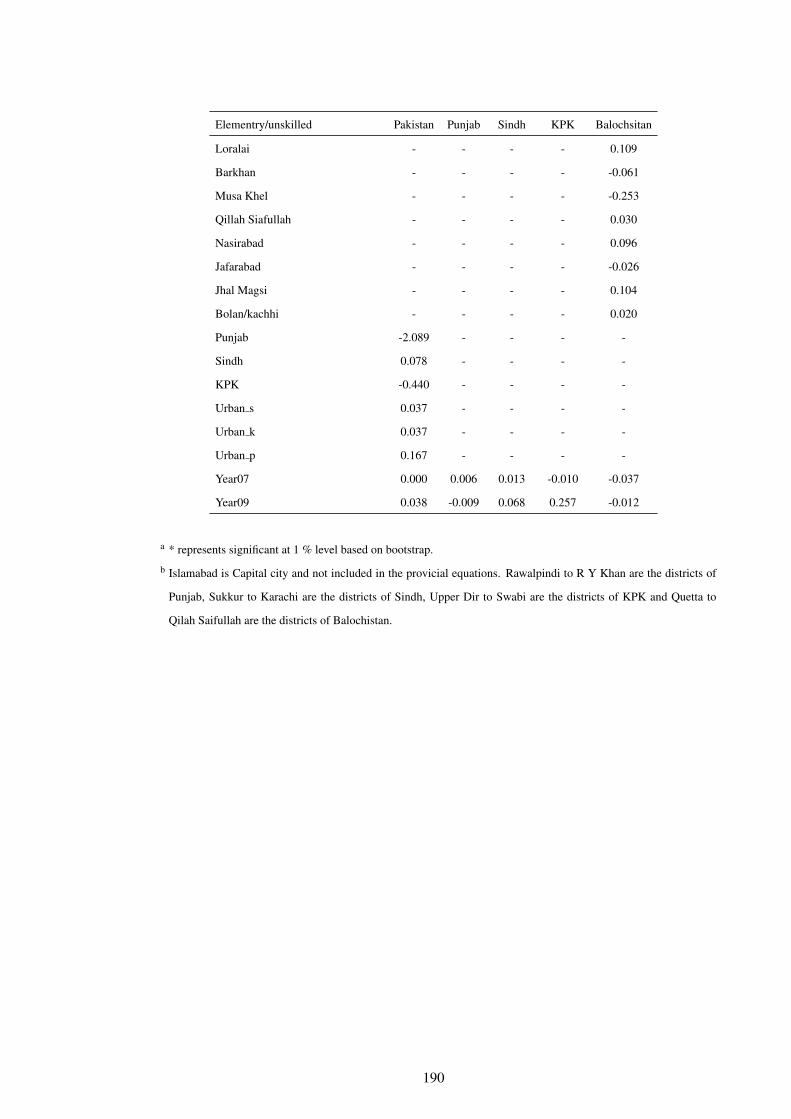
Elementry/unskilled Pakistan Punjab Sindh KPK Balochsitan
Loralai - - - - 0.109
Barkhan - - - - -0.061
Musa Khel - - - - -0.253
Qillah Siafullah - - - - 0.030
Nasirabad - - - - 0.096
Jafarabad - - - - -0.026
Jhal Magsi - - - - 0.104
Bolan/kachhi - - - - 0.020
Punjab -2.089 - - - -
Sindh 0.078 - - - -
KPK -0.440 - - - -
Urban s 0.037 - - - -
Urban k 0.037 - - - -
Urban p 0.167 - - - -
Year07 0.000 0.006 0.013 -0.010 -0.037
Year09 0.038 -0.009 0.068 0.257 -0.012
a * represents significant at 1 % level based on bootstrap.
b Islamabad is Capital city and not included in the provicial equations. Rawalpindi to R Y Khan are the districts of
Punjab, Sukkur to Karachi are the districts of Sindh, Upper Dir to Swabi are the districts of KPK and Quetta to
Qilah Saifullah are the districts of Balochistan.
190
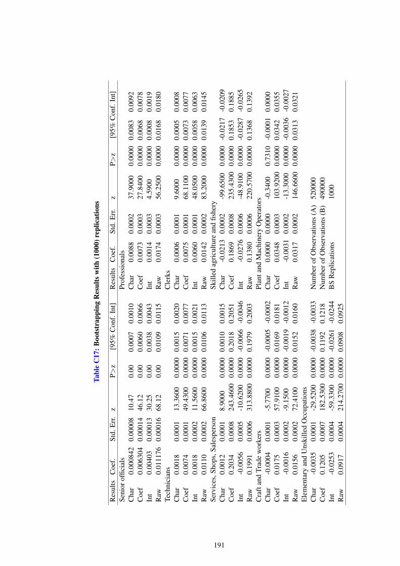
Tabl
eC
17:B
oots
trap
ping
Res
ults
with
(100
0)re
plic
atio
ns
Res
ults
Coe
f.St
d.E
rr.
zP>
z[9
5%C
onf.
Int]
Res
ults
Coe
f.St
d.E
rr.
zP>
z[9
5%C
onf.
Int]
Seni
orof
ficia
lsPr
ofes
sion
als
Cha
r0.
0008
420.
0000
810
.47
0.00
0.00
070.
0010
Cha
r0.
0088
0.00
0237
.900
00.
0000
0.00
830.
0092
Coe
f0.
0063
040.
0001
446
.12
0.00
0.00
600.
0066
Coe
f0.
0073
0.00
0327
.840
00.
0000
0.00
680.
0078
Int
0.00
403
0.00
013
30.2
50.
000.
0038
0.00
43In
t0.
0014
0.00
034.
5900
0.00
000.
0008
0.00
19R
aw0.
0111
760.
0001
668
.12
0.00
0.01
090.
0115
Raw
0.01
740.
0003
56.2
500
0.00
000.
0168
0.01
80Te
chni
cian
sC
lerk
sC
har
0.00
180.
0001
13.3
600
0.00
000.
0015
0.00
20C
har
0.00
060.
0001
9.60
000.
0000
0.00
050.
0008
Coe
f0.
0074
0.00
0149
.430
00.
0000
0.00
710.
0077
Coe
f0.
0075
0.00
0168
.110
00.
0000
0.00
730.
0077
Int
0.00
180.
0002
11.5
600
0.00
000.
0015
0.00
21In
t0.
0060
0.00
0148
.050
00.
0000
0.00
580.
0063
Raw
0.01
100.
0002
66.8
600
0.00
000.
0106
0.01
13R
aw0.
0142
0.00
0283
.200
00.
0000
0.01
390.
0145
Serv
ices
,Sho
ps,S
ales
pers
onSk
illed
agri
cultu
rean
dfis
hery
Cha
r0.
0012
0.00
018.
9000
0.00
000.
0010
0.00
15C
har
-0.0
213
0.00
02-9
9.65
000.
0000
-0.0
217
-0.0
209
Coe
f0.
2034
0.00
0824
3.46
000.
0000
0.20
180.
2051
Coe
f0.
1869
0.00
0823
5.43
000.
0000
0.18
530.
1885
Int
-0.0
056
0.00
05-1
0.62
000.
0000
-0.0
066
-0.0
046
Int
-0.0
276
0.00
06-4
8.91
000.
0000
-0.0
287
-0.0
265
Raw
0.19
910.
0006
313.
8800
0.00
000.
1979
0.20
03R
aw0.
1380
0.00
0622
0.57
000.
0000
0.13
680.
1392
Cra
ftan
dTr
ade
wor
kers
Plan
tand
Mac
hine
ryO
pera
tors
Cha
r-0
.000
40.
0001
-5.7
700
0.00
00-0
.000
5-0
.000
2C
har
0.00
000.
0000
-0.3
400
0.73
10-0
.000
10.
0000
Coe
f0.
0175
0.00
0357
.910
00.
0000
0.01
690.
0181
Coe
f0.
0348
0.00
0310
3.92
000.
0000
0.03
420.
0355
Int
-0.0
016
0.00
02-9
.150
00.
0000
-0.0
019
-0.0
012
Int
-0.0
031
0.00
02-1
3.30
000.
0000
-0.0
036
-0.0
027
Raw
0.01
560.
0002
72.4
100
0.00
000.
0152
0.01
60R
aw0.
0317
0.00
0214
6.66
000.
0000
0.03
130.
0321
Ele
men
tary
and
Uns
kille
dO
ccup
atio
nsC
har
-0.0
035
0.00
01-2
9.52
000.
0000
-0.0
038
-0.0
033
Num
bero
fObs
erva
tions
(A)
5200
00C
oef
0.12
050.
0007
182.
5300
0.00
000.
1192
0.12
18N
umbe
rofO
bser
vatio
ns(B
)49
0000
Int
-0.0
253
0.00
04-5
9.33
000.
0000
-0.0
261
-0.0
244
BS
Rep
licat
ions
1000
Raw
0.09
170.
0004
214.
2700
0.00
000.
0908
0.09
25
191
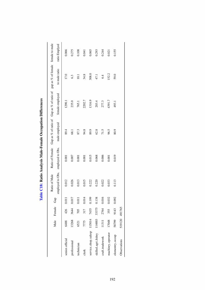
Tabl
eC
18:R
atio
Ana
lysi
sMal
e-Fe
mal
eO
ccup
atio
nD
iffer
ence
s
Mal
eFe
mal
eG
apR
atio
ofM
ale
Rat
ioof
Fem
ale
Gap
as%
ofra
tioof
Gap
as%
ofra
tioof
gap
as%
offe
mal
efe
mal
eto
mal
e
empl
oyed
toO
bs.
empl
oyed
toO
bs.
mal
eem
ploy
edfe
mal
eem
ploy
edto
mal
era
tiora
tioE
mpl
yed
seni
orof
ficia
l64
8842
60.
011
0.01
20.
001
89.4
1290
.117
.00.
066
prof
essi
onal
1326
836
440.
017
0.02
60.
007
68.1
235.
06.
30.
275
tech
nici
an65
2170
50.
011
0.01
30.
001
87.3
765.
110
.10.
108
cler
k77
7531
70.
014
0.01
50.
001
94.8
2202
.734
.80.
041
serv
ice
shop
sale
sp11
5014
7435
0.19
90.
222
0.01
589
.913
16.9
308.
00.
065
skill
edag
rifis
hry
1140
0333
375
0.13
80.
220
0.06
862
.820
3.4
47.1
0.29
3
craf
ttr
adew
ork
1131
127
640.
016
0.02
20.
006
71.5
277.
36.
40.
244
mac
hinr
yop
erat
or17
048
355
0.03
20.
033
0.00
196
.543
91.7
152.
20.
021
elem
entr
yoc
cup
5879
991
430.
092
0.11
30.
019
80.9
493.
159
.00.
155
Obs
erva
tions
5191
2049
1765
192
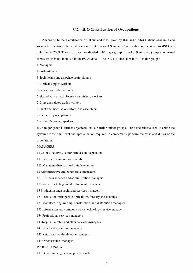
C.2 ILO Classification of Occupations
According to the classification of labour and jobs, given by ILO and United Nations economic and
social classifications, the latest version of International Standard Classification of Occupations (ISCO) is
published in 2008. The occupations are divided in 10 major groups from 1 to 9 and the 0 group is for armed
forces which is not included in the PSLM data. “ The ISCO- divides jobs into 10 major groups:
1-Managers
2-Professionals
3-Technicians and associate professionals
4-Clerical support workers
5-Service and sales workers
6-Skilled agricultural, forestry and fishery workers
7-Craft and related trades workers
8-Plant and machine operators, and assemblers
9-Elementary occupations
0-Armed forces occupations
Each major group is further organized into sub-major, minor groups. The basic criteria used to define the
system are the skill level and specialization required to competently perform the tasks and duties of the
occupations.
MANAGERS
11 Chief executives, senior officials and legislators
111 Legislators and senior officials
112 Managing directors and chief executives
12 Administrative and commercial managers
121 Business services and administration managers
122 Sales, marketing and development managers
13 Production and specialized services managers
131 Production managers in agriculture, forestry and fisheries
132 Manufacturing, mining, construction, and distribution managers
133 Information and communications technology service managers
134 Professional services managers
14 Hospitality, retail and other services managers
141 Hotel and restaurant managers
142 Retail and wholesale trade managers
143 Other services managers
PROFESSIONALS
21 Science and engineering professionals
193
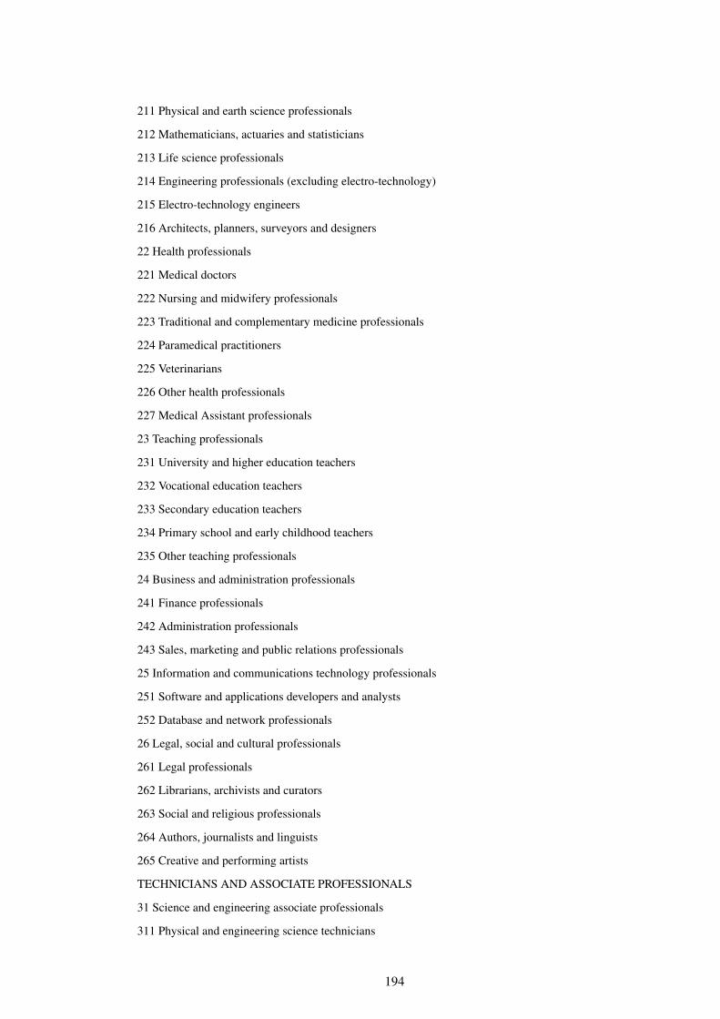
211 Physical and earth science professionals
212 Mathematicians, actuaries and statisticians
213 Life science professionals
214 Engineering professionals (excluding electro-technology)
215 Electro-technology engineers
216 Architects, planners, surveyors and designers
22 Health professionals
221 Medical doctors
222 Nursing and midwifery professionals
223 Traditional and complementary medicine professionals
224 Paramedical practitioners
225 Veterinarians
226 Other health professionals
227 Medical Assistant professionals
23 Teaching professionals
231 University and higher education teachers
232 Vocational education teachers
233 Secondary education teachers
234 Primary school and early childhood teachers
235 Other teaching professionals
24 Business and administration professionals
241 Finance professionals
242 Administration professionals
243 Sales, marketing and public relations professionals
25 Information and communications technology professionals
251 Software and applications developers and analysts
252 Database and network professionals
26 Legal, social and cultural professionals
261 Legal professionals
262 Librarians, archivists and curators
263 Social and religious professionals
264 Authors, journalists and linguists
265 Creative and performing artists
TECHNICIANS AND ASSOCIATE PROFESSIONALS
31 Science and engineering associate professionals
311 Physical and engineering science technicians
194
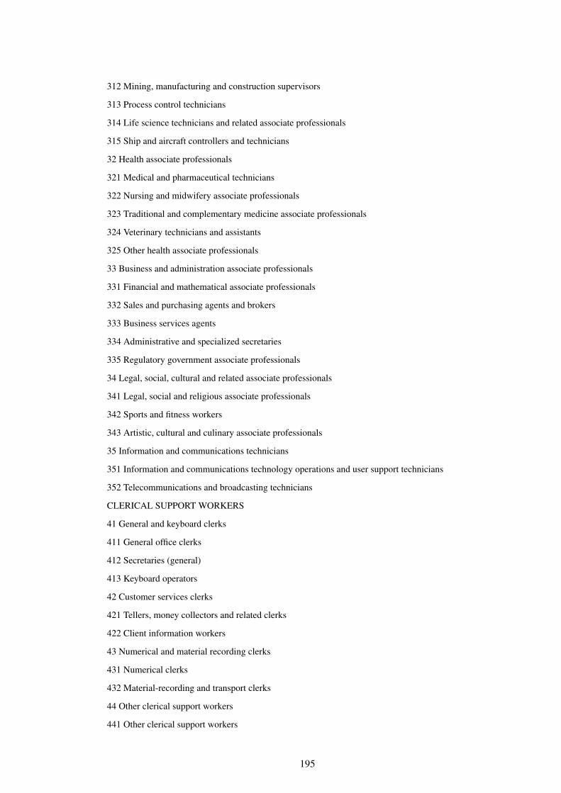
312 Mining, manufacturing and construction supervisors
313 Process control technicians
314 Life science technicians and related associate professionals
315 Ship and aircraft controllers and technicians
32 Health associate professionals
321 Medical and pharmaceutical technicians
322 Nursing and midwifery associate professionals
323 Traditional and complementary medicine associate professionals
324 Veterinary technicians and assistants
325 Other health associate professionals
33 Business and administration associate professionals
331 Financial and mathematical associate professionals
332 Sales and purchasing agents and brokers
333 Business services agents
334 Administrative and specialized secretaries
335 Regulatory government associate professionals
34 Legal, social, cultural and related associate professionals
341 Legal, social and religious associate professionals
342 Sports and fitness workers
343 Artistic, cultural and culinary associate professionals
35 Information and communications technicians
351 Information and communications technology operations and user support technicians
352 Telecommunications and broadcasting technicians
CLERICAL SUPPORT WORKERS
41 General and keyboard clerks
411 General office clerks
412 Secretaries (general)
413 Keyboard operators
42 Customer services clerks
421 Tellers, money collectors and related clerks
422 Client information workers
43 Numerical and material recording clerks
431 Numerical clerks
432 Material-recording and transport clerks
44 Other clerical support workers
441 Other clerical support workers
195
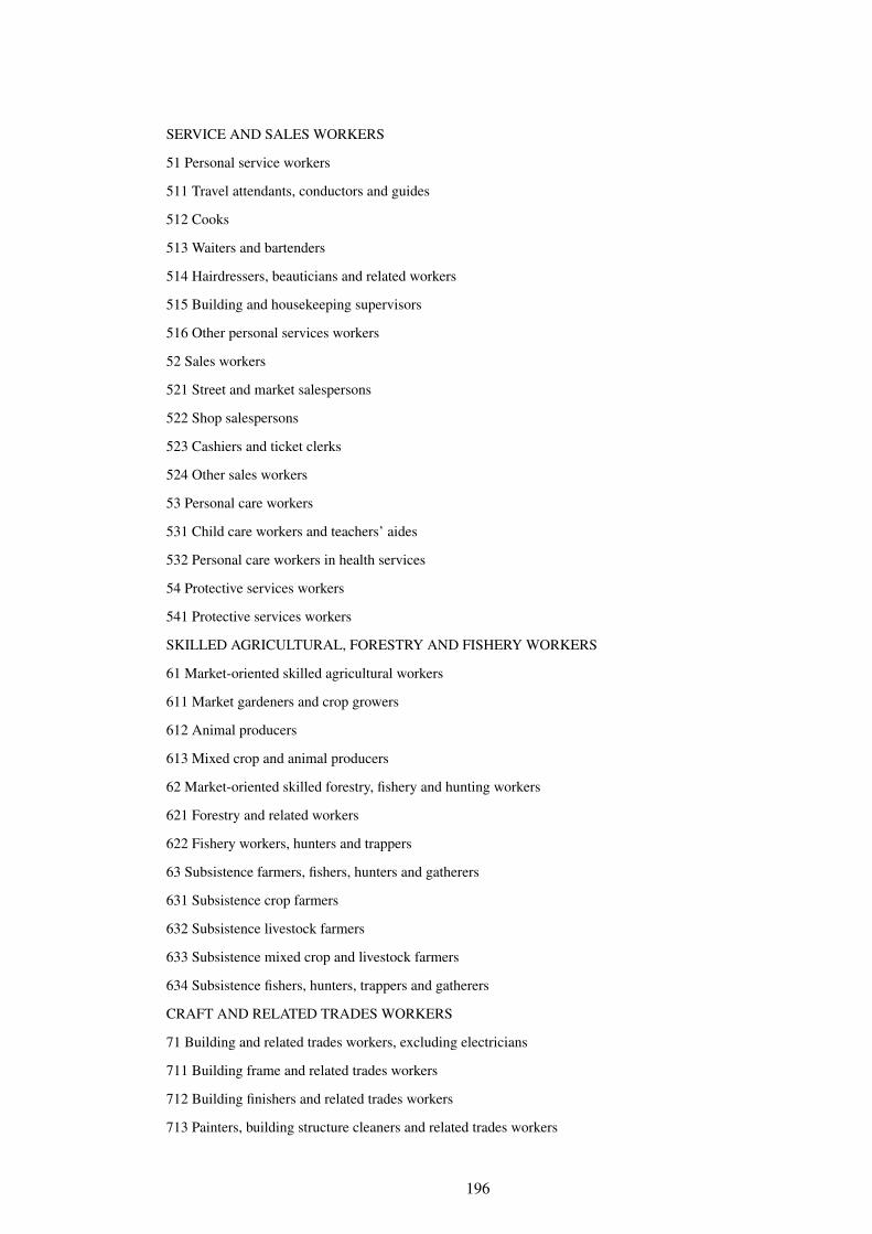
SERVICE AND SALES WORKERS
51 Personal service workers
511 Travel attendants, conductors and guides
512 Cooks
513 Waiters and bartenders
514 Hairdressers, beauticians and related workers
515 Building and housekeeping supervisors
516 Other personal services workers
52 Sales workers
521 Street and market salespersons
522 Shop salespersons
523 Cashiers and ticket clerks
524 Other sales workers
53 Personal care workers
531 Child care workers and teachers’ aides
532 Personal care workers in health services
54 Protective services workers
541 Protective services workers
SKILLED AGRICULTURAL, FORESTRY AND FISHERY WORKERS
61 Market-oriented skilled agricultural workers
611 Market gardeners and crop growers
612 Animal producers
613 Mixed crop and animal producers
62 Market-oriented skilled forestry, fishery and hunting workers
621 Forestry and related workers
622 Fishery workers, hunters and trappers
63 Subsistence farmers, fishers, hunters and gatherers
631 Subsistence crop farmers
632 Subsistence livestock farmers
633 Subsistence mixed crop and livestock farmers
634 Subsistence fishers, hunters, trappers and gatherers
CRAFT AND RELATED TRADES WORKERS
71 Building and related trades workers, excluding electricians
711 Building frame and related trades workers
712 Building finishers and related trades workers
713 Painters, building structure cleaners and related trades workers
196
72 Metal, machinery and related trades workers
721 Sheet and structural metal workers, moulders and welders, and related workers
722 Blacksmiths, toolmakers and related trades workers
723 Machinery mechanics and repairers
73 Handicraft and printing workers
731 Handicraft workers
732 Printing trades workers
74 Electrical and electronic trades workers
741 Electrical equipment installers and repairers
742 Electronics and telecommunications installers and repairers
75 Food processing, wood working, garment and other craft and related trades workers
751 Food processing and related trades workers
752 Wood treaters, cabinet-makers and related trades workers
753 Garment and related trades workers
754 Other craft and related workers
PLANT AND MACHINE OPERATORS AND ASSEMBLERS
81 Stationary plant and machine operators
811 Mining and mineral processing plant operators
812 Metal processing and finishing plant operators
813 Chemical and photographic products plant and machine operators
814 Rubber, plastic and paper products machine operators
815 Textile, fur and leather products machine operators
816 Food and related products machine operators
817 Wood processing and papermaking plant operators
818 Other stationary plant and machine operators
82 Assemblers
821 Assemblers
83 Drivers and mobile plant operators
831 Locomotive engine drivers and related workers
832 Car, van and motorcycle drivers
833 Heavy truck and bus drivers
834 Mobile plant operators
835 Ships’ deck crews and related workers
ELEMENTARY OCCUPATIONS
91 Cleaners and helpers
911 Domestic, hotel and office cleaners and helpers
197
912 Vehicle, window, laundry and other hand cleaning workers
92 Agricultural, forestry and fishery labourers
921 Agricultural, forestry and fishery labourers
93 Labourers in mining, construction, manufacturing and transport
931 Mining and construction labourers
932 Manufacturing labourers
933 Transport and storage labourers
94 Food preparation assistants
941 Food preparation assistants
95 Street and related sales and service workers
951 Street and related service workers
952 Street vendors (excluding food)
96 Refuse workers and other elementary workers
961 Refuse workers
962 Other elementary workers”
(ILO 2008; p. 3-34)
198
ReferencesAddison, T. and L. Demery (1993). Dynamic Ambient Paradigms, pp. 79–99. Understanding the
social effects of policy reform. Washington, D.C. USA: World Bank.
Ahmad, E. and A. Hafeez (2007). Labour supply and earning functions of educated marriedwomen: A case study of Northern Punjab. The Pakistan Development Review 46(1), 45–62.
Ahmad, M. (2001). Estimation of distribution of income among various occupations/professionsin Pakistan. Pakistan Economic and Social Review 39(2), 119–134.
Ahmed, A. M. and A. Hyder (2008). Sticky floors and occupational segregation: Evidence fromPakistan. The Pakistan Development Review 47(4), 837–849.
Akhtar, S. and M. Sadiq (2008). Occupational status and earnings inequality: Evidence from PIHS2001-02 and PSLM 2004-05. The Pakistan Development Review 47(2), 197–213.
Anees, M. (2010). Explaining UK gender pay differentials: Evidence from the BHPS 1995.http://ssrn.com/abstract=1550023. Social Science Research Network.
Arrow, K. (1973). The theory of discrimination. Discrimination in labor markets 3(10), 3–33.
Ashraf, J. and B. Ashraf (1993). Estimating the gender wage gap in Rawalpindi city. The Journalof Development Studies 29(2), 365–376.
Ashraf, J. and B. Ashraf (1996). Evidence on gender wage discrimination from the 1984-85 HIES:A note. Pakistan Journal of Applied Economics 12(1), 85–94.
Ashraf, J. and B. Ashraf (1998a). Earnings in Karachi: Does gender make a difference? PakistanEconomic and Social Review 36(1), 33–46.
Ashraf, J. and B. Ashraf (1998b). Gender earnings and discrimination in Pakistan. Indian Journalof Labour Economics 41(2), 317–326.
Ashraf, J., M. Williams, and R. Aydin (2009). The determinants of gender wage discrimination inPakistan:Econometric evidence from Punjab province. In Conference of Global Business andManagement Forum 2009 (GBMF), GBMF. University of Dhaka, Bangladesh.
Aslam, M. (2009). Education gender gaps in Pakistan: Is the labor market to blame? EconomicDevelopment and Cultural Change 57(4), 747–784.
Aslam, M., G. Kingdon, and M. Soderbom (2008). Girls’ education in the 21st century: Genderequality, empowerment, and economic growth, pp. 67–91. Understanding the social effects ofpolicy reform. Washington, D.C. USA: World Bank.
Atkinson, A. B. (1997). Bringing income distribution in from the cold. The Economic Jour-nal 107(441), 297–321.
Atkinson, A. B. and F. Bourguignon (2000). Handbook of income distribution, Volume 1. Elsevier.
Azid, T., M. Aslam, and M. O. Chaudhary (2001). Poverty, female labour force participation, andcottage industry: A case study of cloth embroidery in rural Multan. The Pakistan DevelopmentReview 40(4), 1105–1118.
Azid, T., R. E. A. Khan, and A. M. Alamasi (2010). Labor force participation of married womenin Punjab (Pakistan). International Journal of Social Economics 37(8), 592–612.
Bahramitash, R. and H. S. Esfahani (2011). The Transformation of Female Labour Market, pp.123–165. Veiled Employment Islamism and the Political Economy of Women’s Employmentin Iran. Newyork: SYRACUSE University Press.
Bauer, T., S. Gohlmann, and M. Sinning (2007). Gender differences in smoking behavior. HealthEconomics 16(9), 895–909.
Bauer, T. K. and M. Sinning (2008). An extension of the Blinder–Oaxaca decomposition to non-linear models. AStA Advances in Statistical Analysis 92(2), 197–206.
199
Bauer, T. K. and M. Sinning (2010). Blinder–Oaxaca decomposition for Tobit models. AppliedEconomics 42(12), 1569–1575.
Bayard, K., J. Hellerstein, D. Neumark, and K. Troske (1999). New evidence on sex segregationand sex differences in wages from matched employee-employer data. Technical report, Nationalbureau of economic research.
Bazen, S. (2011). Econometric methods for labour economics. Oxford University Press.
Becker, G. S. (1957). The economics of discrimination. University of Chicago Press.
Becker, G. S. (1965). A theory of the allocation of time. Economic journal 75(299), 493–517.
Behrman, J. R. and B. L. Wolfe (1984). The socioeconomic impact of schooling in a developingcountry. The Review of Economics and Statistics 66(2), 296–303.
Benham, L. (1974). Benefits of women’s education within marriage. In Economics of the Family:Marriage, Children, and Human Capital, pp. 375–394. University of Chicago Press.
Bergmann, B. R. (1974). Occupational segregation, wages and profits when employers discrimi-nate by race or sex. Eastern Economic Journal 1(2), 103–110.
Bergmann, B. R. (1986). The economic emergence of women. New York: Basic Books.
Bergmann, B. R. (1997). In defense of affirmative action. Basic Books.
Berndt, E. R. (1996). The Practice of Econometrics: Classic and Contemporary. Addison-WesleyPub.
Blackaby, D., D. Leslie, P. Murphy, and N. O’Leary (2002). White/ethnic minority earnings andemployment differentials in Britain: Evidence from the LFS. Oxford Economic Papers 54(2),270–297.
Blackaby, D. H., K. Clark, D. G. Leslie, and P. D. Murphy (1994). Black-white male earnings andemployment prospects in the 1970s and 1980s evidence for Britain. Economics Letters 46(3),273–279.
Blackaby, D. H., D. G. Leslie, P. D. Murphy, and N. C. O’Leary (1998). The ethnic wage gap andemployment differentials in the 1990s: Evidence for Britain. Economics Letters 58(1), 97–103.
Blau, D. M. and P. K. Robins (1988). Child-care costs and family labor supply. The Review ofEconomics and Statistics 70(3), 374–381.
Blau, F. D., M. A. Ferber, A. E. Winkler, and A. E. Winkler (1986). The economics of women,men, and work. Prentice-Hall Englewood Cliffs, NJ.
Blau, F. D. and L. M. Kahn (1996). Wage structure and gender earnings differentials: An interna-tional comparison. Economica 63(250), S29–S62.
Blinder, A. S. (1973). Wage discrimination: Reduced form and structural estimates. Journal ofHuman resources 8(4), 436–455.
Bloom, D. E., D. Canning, G. Fink, and J. E. Finlay (2009). Fertility, female labor force partici-pation, and the demographic dividend. Journal of Economic Growth 14(2), 79–101.
Bradbury, K. and J. Katz (2005). Women’s rise: A work in progress. The Federal Reserve Bankof Boston Regional Review 14(3), 58–67.
Brixiova, Z. and T. Kangoye (2013). Youth employment in Africa: New evidence and policiesfrom Swaziland. Technical report, IZA Discussion Paper.
Brown, R. S., M. Moon, and B. S. Zoloth (1980). Incorporating occupational attainment in studiesof male-female earnings differentials. Journal of Human Resources 15(1), 3–28.
Brown, S., J. Roberts, and K. Taylor (2011). The gender reservation wage gap: Evidence fromBritish panel data. Economics Letters 113(1), 88–91.
200
Browne, I. and J. Misra (2003). The intersection of gender and race in the labor market. AnnualReview of Sociology 29, 487–513.
Cain, G. (1969). Married Women in the Labor Force: An Economic Analysis. Studies in economicsof the Economics Research Center of the University of Chicago. University of Chicago Press.
Cameron, L. A., J. Malcolm Dowling, and C. Worswick (2001). Education and labor marketparticipation of women in Asia: Evidence from five countries. Economic Development andCultural Change 49(3), 459–477.
Castells, M. (2011). The power of identity: The information age: Economy, society, and culture,Volume 2. John Wiley & Sons.
Cheng, S. and J. S. Long (2007). Testing for IIA in the Multinomial Logit Model. SociologicalMethods & Research 35(4), 583–600.
Chiappori, P.-A. (1992). Collective labor supply and welfare. Journal of political Economy 100(3),437.
Chishti, S., A. Lodhi, and S. Rashid (1989). Female labor participation behavior: A case study ofKarachi. Pakistan Journal of Applied Economics 8(2), 157–165.
Chun, H., O. Kim, and I. Lee (2007). Living arrangement and labor supply of married women:An instrumental variable approach. Unpublished working paper, Korea Labor Institute.
Chzhen, Y. (2006). Occupational gender segregation and discrimination in western Europe. InPaper for EPUNet Conference, pp. 8–9.
Chzhen, Y. (2009). The effects of childbirth on womens activity change and occupational mobilityin Europe: Evidence from the European Community Household Panel. Technical report, IRISSat CEPS/INSTEAD.
Cotton, J. (1988). On the decomposition of wage differentials. The Review of Economics andStatistics 70(2), 236–243.
Daniel, W. W. (1968). Racial discrimination in England: Based on the PEP report, Volume 1084.Middlesex: Penguin Books.
Daymont, T. N. and P. J. Andrisani (1984). Job preferences, college major, and the gender gap inearnings. Journal of Human Resources (3), 408–42.
De Munoz, B. R. (2007). Determinants of female labor force participation in Venezuela: A cross-sectional analysis. Ph. D. thesis, University of South Florida.
Deaton, A. (1985). Panel data from time series of cross-sections. Journal of Econometrics 30(12),109 – 126.
DiNardo, J., N. M. Fortin, and T. Lemieux (1996). Labor market institutions and the distributionof wages, 1973-1992: A semiparametric approach. Econometrica 64(5), 1001–1044.
Dolton, P. J. and G. H. Makepeace (1986). Sample selection and male-female earnings differentialsin the graduate labour market. Oxford Economic Papers 38(2), 317–341.
Donald, S. G., D. A. Green, and H. J. Paarsch (2000). Differences in wage distributions betweenCanada and the United States: An application of a flexible estimator of distribution functions inthe presence of covariates. The Review of economic studies 67(4), 609–633.
Du, F. and X. yuan Dong (2010). Womens labor force participation and childcare choices in urbanChina during the economic transition. The University of Winnipeg, Department of EconomicsWorld Paper Number: 2010-04.
Duleep, H. O. and S. Sanders (1994). Empirical regularities across cultures the effect of childrenon woman’s work. Journal of Human Resources 29(2), 328–347.
Duncan, O. D. and B. Duncan (1955). Residential distribution and occupational stratification.American Journal of Sociology 60(5), 493–503.
201
Duryea, S., A. C. Edwards, and M. Ureta (2001). Women in the LAC labour market: The remark-able 1990s. Technical report, William Davidson Institute at the University of Michigan.
Dwyer, J. W. and R. T. Coward (1992). Gender and family care of the elderly. research gapsand opportunities. In J. W. Dwyer and R. T. Coward (Eds.), Gender, Families and Elder Care,Economics of the Family: Marriage, Children, and Human Capital, pp. 151–62. Sage London.
Ejaz, M. (2007). Determinants of female labor force participation in Pakistan an empirical analysisof PSLM (2004-05) micro data. Lahore Journal of Economics Special Edition, 203–233.
Ejaz, M. (2011). The determinants of female labor force participation in Pakistan: An instrumentalvariable approach. Centre for Research in Economics and Business Working Papers No. 01-11.
Epo, B., F. Baye, and N. Manga (2011). Explaining spatial and inter-temporal sources of poverty,inequality and gender disparities in Cameroon: A regression-based decomposition analysis.Poverty and Economic Policy (PEP), Working Paper No. 15-11.
Esfahani, H. S. and P. Shajari (2012). Gender, education, family structure, and the allocation oflabor in Iran. Middle East Development Journal 4(02), 1–40.
Ettner, S. L. (1995). The impact of “parent care” on female labor supply decisions. Demogra-phy 32(1), 63–80.
Evans, M. and H. U. Saraiva (1993). Women’s labour force participation and socioeconomicdevelopment: Influences of local context and individual characteristics in Brazil. British Journalof Sociology 44(1), 25–51.
Even, W. E. and D. A. Macpherson (1993). The decline of private-sector unionism and the genderwage gap. Journal of Human Resources 28(2), 279–296.
Fairlie, R. W. (1999). The absence of the African-American owned business: An analysis of thedynamics of self-employment. Journal of Labor Economics 17(1), 80–108.
Fairlie, R. W. (2005). An extension of the Blinder–Oaxaca decomposition technique to logit andprobit models. Journal of economic and social measurement 30(4), 305–316.
Faridi, M. Z. and A. Basit (2011). Factors determining rural labour supply: A micro analysis.Pakistan Economic and Social Review 49(1), 91–108.
Faridi, M. Z., S. Malik, and A. Basit (2009). Impact of education on female labour force partici-pation in Pakistan: Empirical evidence from primary data analysis. Pakistan Journal of SocialSciences 29(1), 127–140.
Fernandez, R., A. Fogli, and C. Olivetti (2004). Preference formation and the rise of women’slabor force participation: Evidence from WWII. Technical report, National Bureau of EconomicResearch, Inc. NBER Working Papers.
Finegan, T. A. (1962). Hours of work in the united states: A cross-sectional analysis. The Journalof Political Economy 70(5), 452–470.
Firpo, S., N. Fortin, and T. Lemieux (2007). Decomposing wage distributions using recenteredinfluence function regressions. University of British Columbia (June).
Fitzenberger, B., A. Osikominu, and R. Volter (2006). Get training or wait? long-run employmenteffects of training programs for the unemployed in West Germany. Technical Report 38.
Fry, T. R. and M. N. Harris (1996). A Monte Carlo study of tests for the independence of irrelevantalternatives property. Transportation Research Part B: Methodological 30(1), 19–30.
Fry, T. R. and M. N. Harris (1998). Testing for independence of irrelevant alternatives someempirical results. Sociological Methods & Research 26(3), 401–423.
Funding, P. (2001). Education and Earnings in Europe: A Cross Country Analysis of the Returnsto Education. Edward Elgar Publishing.
202
Galor, O. and D. N. Weil (1996). The gender gap, fertility, and growth. The American EconomicReview 86(3), 374–387.
Glick, P. J. (1999). Patterns of employment and earnings in Madagascar. Cornell University Foodand Nutrition Policy Program Working Paper No. 92. Ithaca, NY .
Gray, M. and B. Edwards (2009). Determinants of the labour force status of female carers. Aus-tralian Journal of Labour Economics 12(1), 5–20.
Gray, M., A. Heath, and B. Hunter (2002). An exploration of marginal attachment to the Australianlabour market. Research Discussion Paper 2002-07 Australian Institute of Family Studies, Eco-nomic Research Department, Reserve Bank of Australia, Centre for Aboriginal Economic Pol-icy Research, ANU.
Greenwood, J., A. Seshadri, and M. Yorukoglu (2005). Engines of liberation. The Review ofEconomic Studies 72(1), 109–133.
Greenwood, R., R. Suddaby, and C. R. Hinings (2002). Theorizing change: The role of profes-sional associations in the transformation of institutionalized fields. Academy of managementjournal 45(1), 58–80.
Gronau, R. (1973). The effect of children on the housewife’s value of time. Journal of PoliticalEconomy 81(2), S168–99.
Gronau, R. (1974). Wage comparisons–A selectivity bias. Journal of Political Economy 82(6),1119–1143.
Gronau, R. (1977). Leisure, home production, and work-the theory of the allocation of timerevisited. The Journal of Political Economy 85(6), 1099–1123.
Gunduz-Hocsgor, A. and J. Smits (2008). Variation in labor market participation of marriedwomen in Turkey. In Women’s Studies International Forum, Volume 31, pp. 104–117. Else-vier.
Hafeez, A. and E. Ahmad (2002). Factors determining the labour force participation decision ofeducated married women in a district of Punjab. Pakistan Economic and Social Review 41(1),75–88.
Hamid, S. and S. Z. Al-Jalali (1991). Determinants of the supply of women in the labour market:A micro analysis [with comments]. The Pakistan Development Review 30(4), 755–766.
Hausman, J. and D. McFadden (1984). Specification tests for the multinomial logit model. Econo-metrica: Journal of the Econometric Society 52(5), 1219–1240.
Hausman, J. A. (1982). Labor supply. Working Paper 245, National Bureau of Economic Re-search.
Hausmann, R., L. D. Tyson, L. D. Tyson, and S. Zahidi (2014). The Global Gender Gap Report2014. World Economic Forum, Switzerland.
Heckman, J. (1974). Shadow prices, market wages, and labor supply. Econometrica: journal ofthe econometric society 42(4), 679–694.
Heckman, J. J. (1976). The Common Structure of Statistical Models of Truncation, Sample Selec-tion and Limited Dependent Variables and a Simple Estimator for Such Models, Volume 5 ofAnnals of Economic and Social Measurement.
Heckman, J. J. (1979). Sample selection bias as a specification error. Econometrica: Journal ofthe econometric society 47(1), 153–161.
Horrace, W. C. and R. L. Oaxaca (2001). Inter-industry wage differentials and the gender wagegap: An identification problem. Industrial & Labor Relations Review 54(3), 611–618.
Hotchkiss, J. L. (2006). Changes in behavioral and characteristic determination of female laborforce participation, 1975-2005. Economic Review-Federal Reserve Bank of Atlanta 91(2), 1–20.
203
Hotz, V. J. and R. A. Miller (1993). Conditional choice probabilities and the estimation of dynamicmodels. The Review of Economic Studies 60(3), 497–529.
Hussain, S. (2012). Growth Effects and the Determinants of Female Employment in Pakistan: AMacro- and Microeconomic Analysis. Bochum Studies in International Development. LogosVerlag Berlin GmbH.
Ibraz, T. S. (1993). The cultural context of women’s productive invisibility: A case study of aPakistani village. The Pakistan Development Review 32(1), 101–125.
ILO (2000). Income security and social protection in a changing world. World Labour Report,International Labour Office, Geneva.
ILO (2014). KEY INDICATORS OF THE LABOUR MARKET. International Labour Office,Geneva.
Irfan, M., S. Anwar, W. Akram, and I. Waqar (2013). Occupational gender segregation and itsdeterminants, an analysis of Pakistan labor force market. American Journal of EducationalResearch 1(7), 221–224.
Jamal, H. (2011). Districts indices of multiple deprivations for pakistan, 2011. Social Policy andDevelopment Center (SPDC), Research Report 82.
Jann, B. (2008). The Blinder–Oaxaca decomposition for linear regression models. The StataJournal 8(4), 453–479.
Jones, F. L. and J. Kelley (1984). Decomposing differences between groups a cautionary note onmeasuring discrimination. Sociological Methods & Research 12(3), 323–343.
Joseph, G. (1983). Women at work: The British experience. P. Allan.
Juhn, C., K. M. Murphy, and B. Pierce (1993). Wage inequality and the rise in returns to skill.Journal of political Economy 101(3), 410–442.
Kaas, L. and C. Manger (2012). Ethnic discrimination in Germany’s labour market: A fieldexperiment. German Economic Review 13(1), 1–20.
Kazi, S. and B. Raza (1990). The duality in female employment in Pakistan. Comparative Studiesof South Asia, Africa and the Middle East 10(2), 1–8.
Kazi, S., B. Raza, and N. Aziz (1988). Households headed by women: Income, employment andhousehold organization [with comments]. The Pakistan Development Review 37(4), 781–790.
Khan, S. R., M. Irfan, and S. I. Cohen (1985). Rates of returns to education and the determinantsof earnings in Pakistan [with comments]. The Pakistan Development Review 24(3), 671–683.
Lee, B. S., S. Jang, and J. Sarkar (2008). Women’s labor force participation and marriage: Thecase of Korea. Journal of Asian Economics 19(2), 138–154.
Lee, K. C. and M. H. Pesaran (1993). The role of sectoral interactions in wage determination inthe UK economy. Economic Journal 103(416), 21–55.
Long, J. S. and J. Freese (2006a). Regression models for categorical and limited dependent vari-ables using Stata. Stata Press, College Station, TX.
Long, J. S. and J. Freese (2006b). Regression models for categorical dependent variables usingStata. Stata press.
Machado, J. and J. Mata (2000). Sources of increased wage inequality. Technical report, Mimeo.
Machado, J. A. and J. Mata (2005). Counterfactual decomposition of changes in wage distributionsusing quantile regression. Journal of Applied Econometrics 20(4), 445–465.
Mackellar, L. and R. Bird (1997). Global population ageing, social security and economic growth:Some results from a 2-regional model. In Project LINK meeting. New York, Volume 24.
204
McFadden, D. (1974). Conditional logit analysis of qualitative choice behavior. In Z. P. (Ed.),Frontiers in Econometrics, pp. 105–142. Academic press.
Melly, B. (2005). Decomposition of differences in distribution using quantile regression. LabourEconomics 12(4), 577–590.
Mincer, J. (1962). Labor force participation of married women: A study of labor supply, pp.63–106. Aspects of labor economics. Princeton University Press.
Mincer, J. A. (1974). Schooling, experience, and earnings. Columbia University Press.
Mizala, A., P. Romaguera, and P. Henriquez (1999). Female labor supply in Chile. Technicalreport, Centro de Economıa Aplicada, Universidad de Chile.
Modood, T., R. Berthoud, J. Lakey, J. Y. Nazroo, P. Smith, S. Virdee, and S. Beishon (1997).Ethnic minorities in Britain: diversity and disadvantage. Policy Studies Institute, London.
Moffitt, R. (1984). Profiles of fertility, labour supply and wages of married women: A completelife-cycle model. The Review of Economic Studies 51(2), 263–278.
Moheyuddin, G. (2005). Gender inequality in education: Impact on income, growth and develop-ment. Technical Report 685, University Library of Munich, Germany.
Montgomery, M. and I. Powell (2003). Does an advanced degree reduce the gender wage gap?evidence from MBAs. Industrial Relations: A Journal of Economy and Society 42(3), 396–418.
Mundial, B. (1995). Workers in an integrating world. World Development Report, Washington.
Mundial, B. (2002). World development report 2003: Sustainable development in a dynamicworld.
Nakamura, A. and M. Nakamura (1981). A comparison of the labor force behavior of marriedwomen in the United States and Canada, with special attention to the impact of income taxes.Econometrica 49(2), 451–489.
Naqvi, Z. F., L. Shahnaz, and G. Arif (2002). How do women decide to work in Pakistan?[withcomments]. The Pakistan Development Review 41(4), 495–513.
Nasir, Z. M. (2005). An analysis of occupational choice in Pakistan: A multinomial approach.The Pakistan Development Review 44(1), 57–79.
Nasir, Z. M. and H. Nazli (2000). Education and earnings in Pakistan. Technical report, PakistanInstitute of Development Economics.
Nazli, H. (2004). The effect of education, experience and occupation on earnings: Evidence fromPakistan. The Lahore Journal of Economics 9(2), 1–30.
Neimann, S. (2007). Spousal impact on labor force behavior: New evidence for older marriedcouples in Germany. Ruhr Graduate School in Economics, TU Dortmund University.
Nerlove, M. and S. J. Press (1973). Univariate and multivariate log-linear and logistic models,Volume 1306. Rand Santa Monica, California.
Neuman, S. and R. Oaxaca (2004). Wage decompositions with selectivity-corrected wage equa-tions: A methodological note. Journal of Economic Inequality 2(1), 3–10.
Neumark, D. (1988). Employers’ discriminatory behavior and the estimation of wage discrimina-tion. Journal of Human Resources 23(3), 279–295.
Nielsen, H. S. (2000). Wage discrimination in Zambia: An extension of the Blinder–Oaxacadecomposition. Applied Economics Letters 7(6), 405–408.
Oaxaca, R. (1973). Male-female wage differentials in urban labor markets. International Eco-nomic Review 14(3), 693–709.
205
Oaxaca, R. L. and M. R. Ransom (1988). Searching for the effect of unionism on the wages ofunion and nonunion workers. Journal of Labor Research 9(2), 139–148.
Oaxaca, R. L. and M. R. Ransom (1994). On discrimination and the decomposition of wagedifferentials. Journal of Econometrics 61(1), 5–21.
Oaxaca, R. L. and M. R. Ransom (1999). Identification in detailed wage decompositions. Reviewof Economics and Statistics 81(1), 154–157.
Oppenheimer, V. K. (1982). Work and the family: a study in social demography. Academic Press.
Oswald, C. (1999). Patterns of labour market exit in Germany and the UK. Institute for Socialand Economic Research, University of Essex, UK. Research Paper 99-12 - 01.
Pakistan Economic Survey (2012). Pakistan Economic Survey 2011-2012. Ministry of Finance.
Pakistan Economic Survey (2014). Pakistan Economic Survey 2013-2014. Ministry of Finance.
Peng, K. Z., H.-Y. Ngo, J. Shi, and C.-S. Wong (2009). Gender differences in the work commit-ment of Chinese workers: An investigation of two alternative explanations. Journal of WorldBusiness 44(3), 323–335.
Phelps, E. S. (1972). The statistical theory of racism and sexism. The American Economic Review,659–661.
Polachek, S. W. (1975). Differences in expected post-school investment as a determinant of marketwage differentials. International Economic Review 16(2), 451–470.
Polachek, S. W. (1976). Occupational segregation-alternative hypothesis. Journal of Contempo-rary Business 5(1), 1–12.
Polachek, S. W. (1979). Occupational segregation among women: Theory, evidence, and a prog-nosis, pp. 137–57. Columbia University Press New York, NY.
Polachek, S. W. (1981). Occupational self-selection: A human capital approach to sex differencesin occupational structure. The Review of Economics and Statistics 63(1), 60–69.
Polachek, S. W. and M.-K. Kim (1994). Panel estimates of the gender earnings gap: individual-specific intercept and individual-specific slope models. Journal of Econometrics 61(1), 23–42.
Powell, W. B. (2011). Information acquisition and representation methods for real-time assetmanagement. Technical report, DTIC Document.
Reimers, C. W. (1983). Labor market discrimination against hispanic and black men. The Reviewof Economics and Statistics 65(4), 570–579.
Report, T. G. C. (2010). The global competitiveness report. Technical report, World EconomicForum, Geneva.
Sabir, M. and Z. Aftab (2007). Dynamism in the gender wage gap: evidence from Pakistan. ThePakistan Development Review 46(4), 865–882.
Sackey, H. A. Female labour force participation in Ghana: the effects of education. AfricanEconomic Research Consortium, Nairobi. AERC Research Paper 150.
Safana, S., M. H. Sial, and M. S. Awan (2011). Female labor force participation in Pakistan: Acase of Punjab. Journal of Social and Development Sciences 2(3), 104–110.
Sasaki, M. (2002). The causal effect of family structure on labor force participation amongJapanese married women. Journal of Human Resources 37(2), 429–440.
Sathar, Z. A. and S. Kazi (2000). Women’s autonomy in the context of rural Pakistan. The PakistanDevelopment Review 39(2), 89–110.
Schultz, T. P. (1978). Fertility and child mortality over the life cycle: Aggregate and individualevidence. American Economic Review 68(2), 208–215.
206
Schultz, T. P. (1994). Human capital, family planning, and their effects on population growth. TheAmerican Economic Review 84(2), 255–260.
Shah, N. M. (1986). Changes in female roles in Pakistan: Are the volume and pace ade-quate?(invited lecture). The Pakistan Development Review 25(3), pp–339.
Shah, N. M., N. Abbasi, and I. Alam (1976). Interdistrict and interprovincial differentials incorrelates of female labour force participation, 1961. The Pakistan Development Review 15(4),424–445.
Sheehan, G. and G. Standing (1978). A note on economic activity of women in Nigeria. ThePakistan Development Review 17(2), 253–261.
Siddiqui, R. (2006). Gender and Empowerment: Evidence from Pakistan. Pakistan Institute ofDevelopment Economics, Islamabad, Pakistan.
Siddiqui, R., S. Hamid, et al. (2003). Gender, poverty, and occupational choice in poor and non-poor households: An analysis based on the Household Survey Data of Pakistan. Technicalreport, Pakistan Institute of Development Economics.
Siddiqui, R. and R. Siddiqui (1998). A decomposition of male-female earnings differentials. ThePakistan Development Review 37(4), 885–898.
Singh, K. and M. Xie (2008). Bootstrap: a statistical method. Unpublished manuscript, RutgersUniversity, USA..
Small, K. A. and C. Hsiao (1985). Multinomial logit specification tests. International EconomicReview 26(3), 619–627.
Smith-Lovin, L. and A. R. Tickamyer (1978). Nonrecursive models of labor force participation,fertility behavior and sex role attitudes. American Sociological Review 43(August), 541–557.
SPDC (2008). Women at work. Technical report, Social Policy and Development Centre (SPDC),Karachi, Pakistan.
Spierings, N. and J. Smits (2007). Womens labour market participation in Egypt, Jordan, Mo-rocco, Syria & Tunisia: A three-level analysis. In IZA/World Bank Conference Employmentand Development, June, pp. 8–9.
Standing, G. (1999). Global feminization through flexible labor: A theme revisited. World devel-opment 27(3), 583–602.
Stephens, B. J. (2010). The determinants of labour force status among indigenous Australians.Australian Journal of Labour Economics 13(3), 287–312.
Suits, D. B. (1984). Dummy variables: Mechanics v. interpretation. The Review of Economics andStatistics 66(1), 177–180.
Sweet, J. A. (1973). Women in the labor force. Seminar Press New York.
Tansel, A. (2002). Economic development and female labor force participation in Turkey: Time-series evidence and cross-province estimates. Economic Research Forum for the Arab Coun-tries, Iran & Turkey.
Teo, S. Y. (2003). Occupational segregation and its effect on estimates of the gender wage differ-ential: Evidence from Brunei. Asian Economic Journal 17(4), 341–360.
The World Bank (2003). Sustainable development in a dynamic world: Transforming institutions,growth, and quality of life.
Theil, H. (1969). A multinomial extension of the linear logit model. International EconomicReview 10(3), 251–59.
Tzannatos, Z. (1999). Women and labor market changes in the global economy: growth helps,inequalities hurt and public policy matters. World development 27(3), 551–569.
207
Waite, L. J. (1980). Working wives and the family life cycle. American Journal of Sociology 86(2),272–294.
Wilder, A. (1999). The Pakistani voter: electoral politics and voting behaviour in the Punjab.Oxford University Press.
Winkelmann, L. and R. Winkelmann (1997). Determining the relative labour force status of Maoriand non-Maori using a multinomial logit model. Labour Market Bulletin 1, 24–62.
Winsborough, H. H. and P. Dickinson (1971). Components of negro-white income differences. InProceedings of the Social Statistics Section, Volume 6. American Statistical Association.
Wong, Y. N. (2012). World Development Report 2012: Gender equality and development, Vol-ume 39. Taylor & Francis.
Wooldridge, J. (2010). Econometric Analysis of Cross Section and Panel Data. MIT Press.
World Bank (2012). World development indicators 2012. World Bank Publications.
Yakubu, Y. A. (2010). Factors influencing female labor force participation in South Africa in 2008.African Statistical Journal 11, 85–104.
Yasin, G., I. S. Chaudhry, and S. Afzal (2010). The determinants of gender wage discriminationin Pakistan: econometric evidence from Punjab province. Asian Social Science 6(11), p239.
Yun, M.-S. (2005a). Hypothesis tests when decomposing differences in the first moment. Journalof Economic and Social Measurement 30(4), 295–304.
Yun, M.-S. (2005b). A simple solution to the identification problem in detailed wage decomposi-tions. Economic Inquiry 43(4), 766–772.
Zveglich Jr, J. E. and Y. van der Meulen Rodgers (2004). Occupational segregation and the genderwage gap in a dynamic East Asian economy. Southern Economic Journal 70(4), 850–875.
208


