arX
iv:1
306.
2109
v2 [
cs.IT
] 16
Dec
201
31
Distributed Decision-Making over Adaptive
NetworksSheng-Yuan Tu,Student Member, IEEEand Ali H. Sayed,Fellow, IEEE
Abstract
In distributed processing, agents generally collect data generated by thesameunderlying unknown
model (represented by a vector of parameters) and then solvean estimation or inference task cooperatively.
In this paper, we consider the situation in which the data observed by the agents may have risen from
two differentmodels. Agents do not know beforehand which model accounts for their data and the data
of their neighbors. The objective for the network is for all agents to reach agreement on which model to
track and to estimate this model cooperatively. In these situations, where agents are subject to data from
unknown different sources, conventional distributed estimation strategies would lead to biased estimates
relative to any of the underlying models. We first show how to modify existing strategies to guarantee
unbiasedness. We then develop a classification scheme for the agents to identify the models that generated
the data, and propose a procedure by which the entire networkcan be made to converge towards the same
model through a collaborative decision-making process. The resulting algorithm is applied to model fish
foraging behavior in the presence of two food sources.
Index Terms
Adaptive networks, diffusion adaptation, classification,decision-making, biological networks.
I. INTRODUCTION
Self-organization is a remarkable property of biological networks [2], [3], where various forms of
complex behavior are evident and result from decentralizedinteractions among agents with limited
Copyright (c) 2013 IEEE. Personal use of this material is permitted. However, permission to use this material for any other
purposes must be obtained from the IEEE by sending a request to [email protected].
This work was supported in part by NSF grant CCF-1011918. An earlier conference version of this work appeared in [1]. The
authors are with the Department of Electrical Engineering,University of California, Los Angeles (e-mail: [email protected];

2
capabilities. One example of sophisticated behavior is thegroup decision-making process by animals
[4]. For example, it is common for biological networks to encounter situations where agents need to
decide between multiple options, such as fish deciding between following one food source or another
[5], and bees or ants deciding between moving towards a new hive or another [6], [7]. Although multiple
options may be available, the agents are still able to reach agreement in a decentralized manner and move
towards a common destination (e.g., [8]).
In previous works, we proposed and studied several diffusion strategies [9]–[14] that allow agents
to adapt and learn through a process of in-network collaboration and learning. References [13], [14]
provide overviews of diffusion techniques and their application to distributed adaptation, learning, and
optimization over networks. Examples of further applications and studies appear, e.g., in [15]–[20].
Diffusion networks consist of a collection of adaptive agents that are able to respond to excitations
in real-time. Compared with the class of consensus strategies [21]–[27], diffusion networks have been
shown to remain stable irrespective of the network topology, while consensus networks can become
unstable even when each agent is individually stable [28]. Diffusion strategies have also been shown
to lead to improved convergence rate and superior mean-square-error performance [14], [28]. For these
reasons, we focus in the remainder of this paper on the use of diffusion strategies for decentralized
decision-making.
Motivated by the behavior of biological networks, we study distributed decision-making over networks
where agents are subject to data arising from two different models. The agents do not know beforehand
which model accounts for their data and the data of their neighbors. The objective of the network is for all
agents to reach agreement on one model and to estimate and track thiscommonmodel cooperatively. The
task of reaching agreement over a network of agents subjected to different models is more challenging
than earlier works on inference under a single data model. The difficulty is due to various reasons. First,
traditional (consensus and diffusion) strategies will converge to a biased solution (see Eq. (14)). We
therefore need a mechanism to compensate for the bias. Second, each agent now needs to distinguish
between which model each of its neighbors is collecting datafrom (this is called theobservedmodel)
and which model the network is evolving to (this is called thedesiredmodel). In other words, in addition
to the learning and adaptation process for tracking, the agents should be equipped with a classification
scheme to distinguish between the observed and desired models. The agents also need to be endowed
with a decision process to agree among themselves on a common(desired) model to track. Moreover, the
classification scheme and the decision-making process willneed to be implemented in a fully distributed
manner and in real-time, alongside the adaptation process.
3
There have been useful prior works in the literature on formations over multi-agent networks [29]–
[35] and opinion formation over social networks [36]–[38] using, for example, consensus strategies.
These earlier works are mainly interested in having the agents reach an average consensus state, whereas
in our problem formulation agents will need to reach one of the models and not the average of both
models. Another difference between this work and the earlier efforts is our focus on combining real-time
classification, decision-making, and adaptation into a single integrated framework running at each agent.
To do so, we need to show how the distributed strategy should be modified to remove the bias that would
arise due to the multiplicity of models — without this step, the combined decision-making and adaptation
scheme will not perform as required. In addition, in our formulation, the agents need to continuously
adjust their decisions and their estimates because the models are allowed to change over time. In this way,
reaching a static consensus is not the objective of the network. Instead, the agents need to continuously
adjust and track in a dynamic environment where decisions and estimates evolve with time as necessary.
Diffusion strategies endow networks with such tracking abilities — see, e.g., Sec. VII of [39], where it
is shown how well these strategies track as a function of the level of non-stationarity in the underlying
models.
II. D IFFUSION STRATEGY
Consider a collection ofN agents (or nodes) distributed over a geographic region. Theset of neighbors
(i.e. neighborhood) of nodek is denoted byNk; the number of nodes inNk is denoted bynk. At every
time instant,i, each nodek is able to observe realizations{dk(i), uk,i} of a scalar random processdk(i)
and a1×M row random regressoruk,i with a positive-definite covariance matrix,Ru,k = EuTk,iuk,i > 0.
The regressors{uk,i} are assumed to be temporally white and spatially independent, i.e., EuTk,iul,j =
Ru,kδklδij in terms of the Kronecker delta function. Note that we are denoting random quantities by
boldface letters and their realizations or deterministic quantities by normal letters. The data{dk(i),uk,i}
collected at nodek are assumed to originate from one of two unknowncolumnvectors{w◦0, w
◦1} of size
M in the following manner. We denote the generic observed model by z◦k ∈ {w◦0 , w
◦1}; nodek does not
know beforehand the observed model. The data at nodek are related to its observed modelz◦k via a
linear regression model of the form:
dk(i) = uk,iz◦k + vk(i) (1)
wherevk(i) is measurement noise with varianceσ2v,k and assumed to be temporally white and spatially
independent. The noisevk(i) is assumed to be independent oful,j for all {k, l, i, j}. All random processes
are zero mean.
4
The objective of the network is to haveall agents converge to an estimate foroneof the models. For
example, if the models happen to represent the location of food sources [13], [40], then this agreement will
make the agents move towards one particular food source in lieu of the other source. More specifically,
let wk,i denote the estimator forz◦k at nodek at time i. The network would like to reach an ageement
on a commonq, such that
wk,i → w◦q for q = 0 or q = 1 and for allk as i → ∞ (2)
where convergence is in some desirable sense (such as the mean-square-error sense).
Severaladaptivediffusion strategies for distributed estimation under a common model scenario were
proposed and studied in [9]–[13], following the developments in [41]–[45] — overviews of these results
appear in [13], [14]. One such scheme is the adaptive-then-combine (ATC) diffusion strategy [11], [45].
It operates as follows. We select anN ×N matrix A with nonnegative entries{al,k} satisfying:
1TNA = 1
TN and al,k = 0 if l /∈ Nk (3)
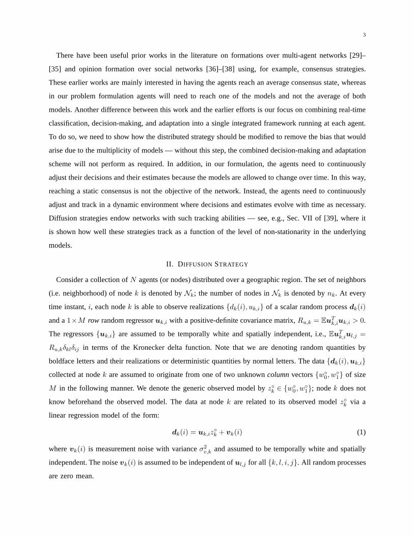
where1N is the vector of sizeN with all entries equal to one. The entryal,k denotes the weight that
nodek assigns to data arriving from nodel (see Fig. 1). The ATC diffusion strategy updateswk,i−1 to
wk,i as follows:
ψk,i = wk,i−1 + µk · uTk,i[dk(i) − uk,iwk,i−1] (4)
wk,i =∑
l∈Nk
al,kψl,i (5)
whereµk is the constantpositive step-size used by nodek. The first step (4) involves local adaptation,
where nodek uses its own data{dk(i),uk,i} to update the weight estimate at nodek from wk,i−1 to
an intermediate valueψk,i. The second step (5) is a combination step where the intermediate estimates
{ψl,i} from the neighborhood of nodek are combined through the weights{al,k} to obtain the updated
weight estimatewk,i. Such diffusion strategies have found applications in several domains including
distributed optimization, adaptation, learning, and the modeling of biological networks — see, e.g., [13],
[14], [40] and the references therein. Diffusion strategies were also used in some recent works [46]–[49]
albeit with diminishing step-sizes (µk(i) → 0) to enforce consensus among nodes. However, decaying
step-sizes disable adaptation once they approach zero. Constant step-sizes are used in (4)-(5) to enable
continuous adaptation and learning, which is critical for the application under study in this work.
When the data arriving at the nodes could have risen from one model or another, the distributed
strategy (4)-(5) will not be able to achieve agreement as in (2) and the resulting weight estimates will
5
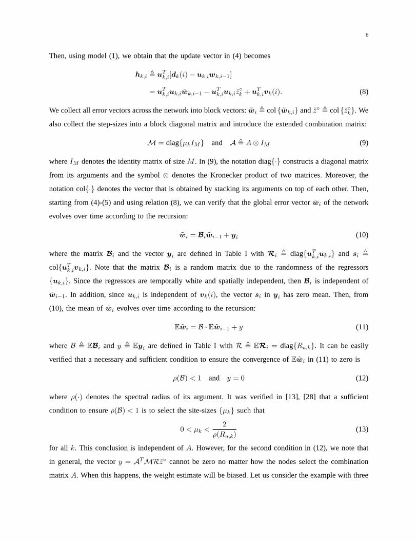
Fig. 1. A connected network where data collected by the agents are influenced by one of two models. The weightal,k scales
the data transmitted from nodel to nodek over the edge linking them.
tend towards a biased value. We first explain how this degradation arises and subsequently explain how
it can be remedied.
Assumption 1 (Strongly connected network). The network topology is assumed to be strongly connected
so that the corresponding combination matrixA is primitive, i.e., there exists an integer powerj > 0
such that[Aj ]l,k > 0 for all l and k.
As explained in [13], Assumption 1 amounts to requiring the network to be connected (where a path
with nonzero weights exists between any two nodes), and for at least one node to have a non-trivial
self-loop (i.e.,ak,k > 0 for at least onek). We conclude from the Perron-Frobenius Theorem [50], [51]
that every primitive left-stochastic matrixA has a unique eigenvalue at one while all other eigenvalues
are strictly less than one in magnitude. Moreover, if we denote the right-eigenvector that is associated
with the eigenvalue at one byc and normalize its entries to add up to one then it holds that:
Ac = c, 1TNc = 1, and 0 < ck < 1. (6)
Let us assume for the time being that the agents in the networkhave agreed on converging towards
one of the models (but they do not know beforehand which modelit will be). We denote the desired
model generically byw◦q . In Section IV, we explain how this agreement process can be attained. Here
we explain that even when agreement is present, the diffusion strategy (4)-(5) leads to biased estimates
unless it is modified in a proper way. To see this, we introducethe following error vectors for any node
k:
wk,i , w◦q −wk,i and z◦k , w◦
q − z◦k. (7)
6
Then, using model (1), we obtain that the update vector in (4)becomes
hk,i , uTk,i[dk(i)− uk,iwk,i−1]
= uTk,iuk,iwk,i−1 − u
Tk,iuk,iz
◦k + u
Tk,ivk(i). (8)
We collect all error vectors across the network into block vectors:wi , col{wk,i} andz◦ , col{z◦k}. We
also collect the step-sizes into a block diagonal matrix andintroduce the extended combination matrix:
M = diag{µkIM} and A , A⊗ IM (9)
whereIM denotes the identity matrix of sizeM . In (9), the notation diag{·} constructs a diagonal matrix
from its arguments and the symbol⊗ denotes the Kronecker product of two matrices. Moreover, the
notation col{·} denotes the vector that is obtained by stacking its arguments on top of each other. Then,
starting from (4)-(5) and using relation (8), we can verify that the global error vectorwi of the network
evolves over time according to the recursion:
wi = Biwi−1 + yi (10)
where the matrixBi and the vectoryi are defined in Table I withRi , diag{uTk,iuk,i} and si ,
col{uTk,ivk,i}. Note that the matrixBi is a random matrix due to the randomness of the regressors
{uk,i}. Since the regressors are temporally white and spatially independent, thenBi is independent of
wi−1. In addition, sinceuk,i is independent ofvk(i), the vectorsi in yi has zero mean. Then, from
(10), the mean ofwi evolves over time according to the recursion:
Ewi = B · Ewi−1 + y (11)
whereB , EBi and y , Eyi are defined in Table I withR , ERi = diag{Ru,k}. It can be easily
verified that a necessary and sufficient condition to ensure the convergence ofEwi in (11) to zero is
ρ(B) < 1 and y = 0 (12)
where ρ(·) denotes the spectral radius of its argument. It was verified in [13], [28] that a sufficient
condition to ensureρ(B) < 1 is to select the site-sizes{µk} such that
0 < µk <2
ρ(Ru,k)(13)
for all k. This conclusion is independent ofA. However, for the second condition in (12), we note that
in general, the vectory = ATMRz◦ cannot be zero no matter how the nodes select the combination
matrix A. When this happens, the weight estimate will be biased. Let us consider the example with three
7
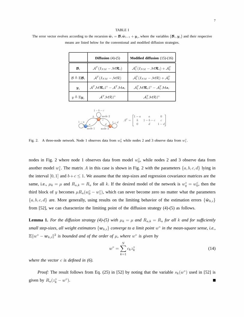
TABLE I
The error vector evolves according to the recursionwi = Biwi−1 + yi , where the variables{Bi,yi} and their respective
means are listed below for the conventional and modified diffusion strategies.
Diffusion (4)-(5) Modified diffusion (15)-(16)
Bi AT (INM −MRi) AT1 (INM −MRi) +AT
2
B , EBi AT (INM −MR) AT1 (INM −MR) +AT
2
yi ATMRiz◦ −ATMsi AT
1 MRiz◦ −AT
1 Msi
y , Eyi ATMRz◦ AT1 MRz◦
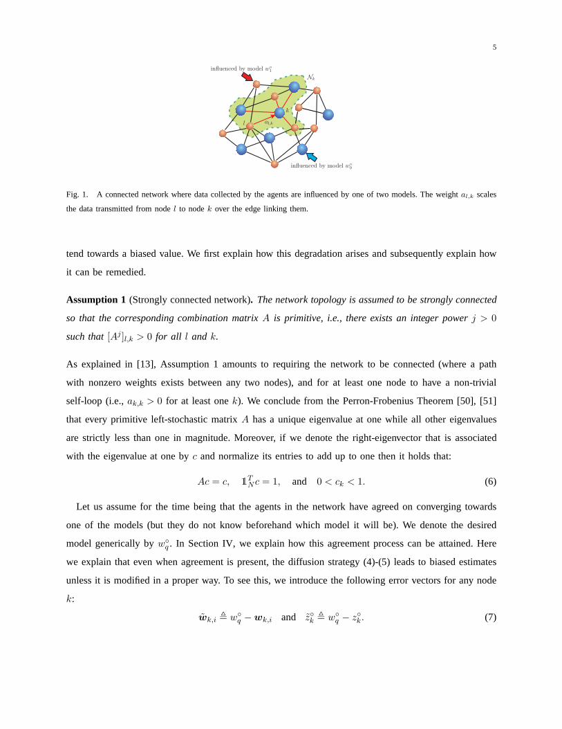
Fig. 2. A three-node network. Node 1 observes data fromw◦0 while nodes 2 and 3 observe data fromw◦
1 .
nodes in Fig. 2 where node 1 observes data from modelw◦0, while nodes 2 and 3 observe data from
another modelw◦1. The matrixA in this case is shown in Fig. 2 with the parameters{a, b, c, d} lying in
the interval[0, 1] andb+ c ≤ 1. We assume that the step-sizes and regression covariance matrices are the
same, i.e.,µk = µ andRu,k = Ru for all k. If the desired model of the network isw◦q = w◦
0, then the
third block of y becomesµRu(w◦0 − w◦
1), which can never become zero no matter what the parameters
{a, b, c, d} are. More generally, using results on the limiting behaviorof the estimation errors{wk,i}
from [52], we can characterize the limiting point of the diffusion strategy (4)-(5) as follows.
Lemma 1. For the diffusion strategy (4)-(5) withµk = µ and Ru,k = Ru for all k and for sufficiently
small step-sizes, all weight estimators{wk,i} converge to a limit pointw◦ in the mean-square sense, i.e.,
E‖w◦ −wk,i‖2 is bounded and of the order ofµ, wherew◦ is given by
w◦ =
N∑
k=1
ckz◦k (14)
where the vectorc is defined in (6).
Proof: The result follows from Eq. (25) in [52] by noting that the variable sk(w◦) used in [52] is
given byRu(z◦k − w◦).
8
Thus, when the agents collect data from different models, the estimates using the diffusion strategy (4)-
(5) converge to a convex combination of these models given by(14), which is different from any of
the individual models becauseck > 0 for all k. A similar conclusion holds for the case of non-uniform
step-sizes{µk} and covariance matrices{Ru,k}.
III. M ODIFIED DIFFUSION STRATEGY
To deal with the problem of bias, we now show how to modify the diffusion strategy (4)-(5). We
observe from the example in Fig. 2 that the third entry of the vector y cannot be zero because the
neighbor of node3 observes data arising from a model that is different from thedesired model. Note
from (8) that the bias term arises from the gradient direction used in computing the intermediate estimates
in (4). These observations suggest that to ensure unbiased mean convergence, a node should not combine
intermediate estimates from neighbors whose observed model is different from the desired model. For
this reason, we shall replace the intermediate estimates from these neighbors by their previous estimates
{wl,i−1} in the combination step (5). Specifically, we shall adjust the diffusion strategy (4)-(5) as follows:
ψk,i = wk,i−1 + µk · uTk,i[dk(i) − uk,iwk,i−1] (15)
wk,i =∑
l∈Nk
(
a(1)l,kψl,i + a
(2)l,kwl,i−1
)
(16)
where the{a(1)l,k } and{a(2)l,k } are two sets of nonnegative scalars and their respective combination matrices
A1 andA2 satisfy
A1 +A2 = A (17)
with A being the original left-stochastic matrix in (3). Note thatstep (15) is the same as step (4).
However, in the second step (16), nodes aggregate the{ψl,i,wl,i−1} from their neighborhood. With such
adjustment, we will verify that by properly selecting{a(1)l,k , a(2)l,k }, unbiased mean convergence can be
guaranteed. The choice of which entries ofA go into A1 or A2 will depend on which of the neighbors
of nodek are observing data arising from a model that agrees with the desired model for nodek.
A. Construction of MatricesA1 andA2
To construct the matrices{A1, A2} we associate two vectors with the network,f andgi. Both vectors
are of sizeN . The vectorf is fixed and itskth entry,f(k), is set tof(k) = 0 when the observed model
for nodek is w◦0; otherwise, it is set tof(k) = 1. On the other hand, the vectorgi is evolving with time;
9
its kth entry is set togi(k) = 0 when the desired model for nodek is w◦0; otherwise, it is set equal to
gi(k) = 1. Then, we shall set the entries ofA1 andA2 according to the following rules:
a(1)l,k,i =
al,k, if l ∈ Nk andf(l) = gi(k)
0, otherwise(18)
a(2)l,k,i =
al,k, if l ∈ Nk andf(l) 6= gi(k)
0, otherwise. (19)
That is, nodes that observe data arising from the same model that nodek wishes to converge to will be
reinforced and their intermediate estimates{ψl,i} will be used (their combination weights are collected
into matrix A1). On the other hand, nodes that observe data arising from a different model than the
objective for nodek will be de-emphasized and their prior estimates{wl,i−1} will be used in the
combination step (16) (their combination weights are collected into matrixA2). Note that the scalars
{a(1)l,k,i, a
(2)l,k,i} in (18)-(19) are now indexed with time due to their dependence ongi(k).
B. Mean-Error Analysis
It is important to note that to construct the combination weights from (18)-(19), each nodek needs
to know what are the observed models influencing its neighbors (i.e.,f(l) for l ∈ Nk); it also needs to
know how to update its objective ingi(k) so that the{gi(l)} converge to the same value. In the next two
sections, we will describe a distributed decision-making procedure by which the nodes are able to achieve
agreement on{gi(k)}. We will also develop a classification scheme to estimate{f(l)} using available
data. More importantly, the convergence of the vectors{f, gi} will occur before the convergence of the
adaptation process to estimate the agreed-upon model. Therefore, let us assume for the time being that
the nodes know the{f(l)} of their neighbors and have achieved agreement on the desired model, which
we are denoting byw◦q , so that (see Eq. (24) in Theorem 2)
gi(1) = gi(2) = · · · = gi(N) = q, for all i. (20)
Using relation (8) and the modified diffusion strategy (15)-(16), the recursion for the global error vector
wi is again given by (10) with the matrixBi and the vectoryi defined in Table I and the combination
matricesA1 andA2 defined in a manner similar toA in (9). We therefore get the same mean recursion
as (11) with the matrixB and the vectory defined in Table I. The following result establishes asymptotic
mean convergence for the modified diffusion strategy (15)-(16).
10
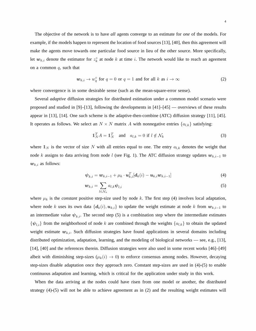
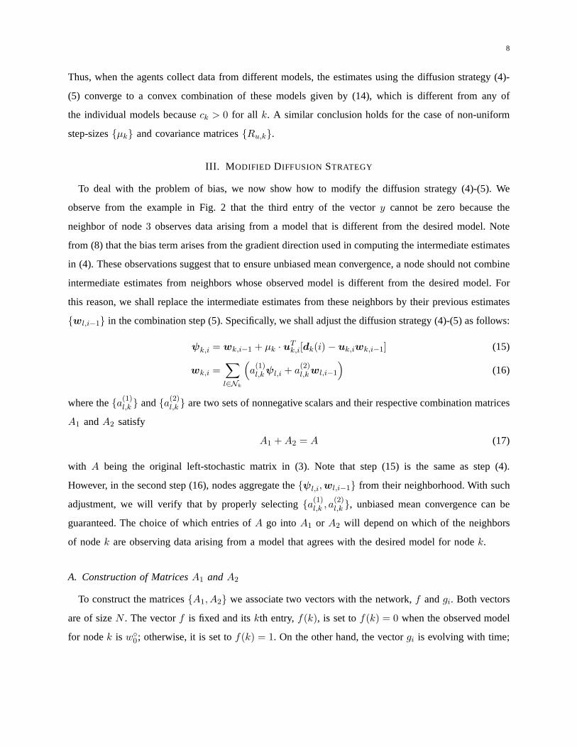
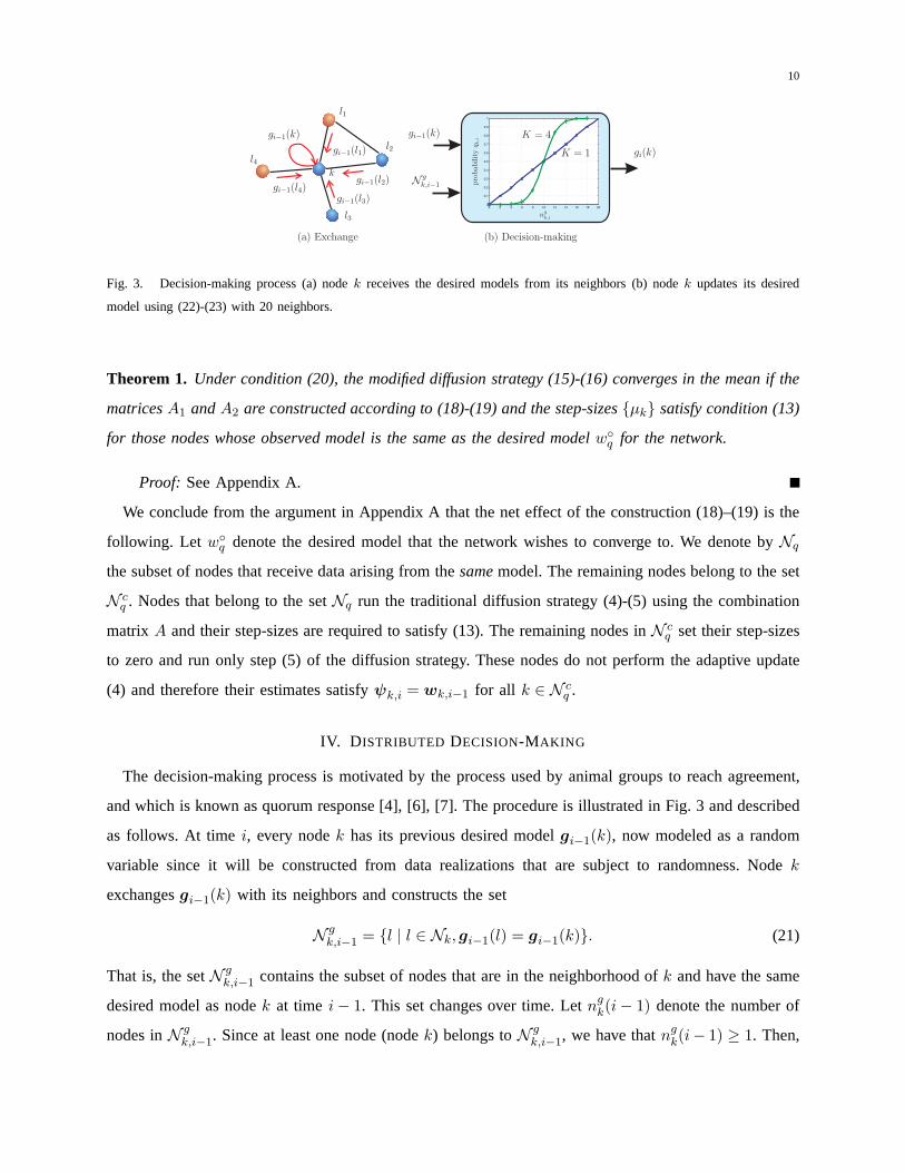
Fig. 3. Decision-making process (a) nodek receives the desired models from its neighbors (b) nodek updates its desired
model using (22)-(23) with 20 neighbors.
Theorem 1. Under condition (20), the modified diffusion strategy (15)-(16) converges in the mean if the
matricesA1 andA2 are constructed according to (18)-(19) and the step-sizes{µk} satisfy condition (13)
for those nodes whose observed model is the same as the desired modelw◦q for the network.
Proof: See Appendix A.
We conclude from the argument in Appendix A that the net effect of the construction (18)–(19) is the
following. Let w◦q denote the desired model that the network wishes to convergeto. We denote byNq
the subset of nodes that receive data arising from thesamemodel. The remaining nodes belong to the set
N cq . Nodes that belong to the setNq run the traditional diffusion strategy (4)-(5) using the combination
matrix A and their step-sizes are required to satisfy (13). The remaining nodes inN cq set their step-sizes
to zero and run only step (5) of the diffusion strategy. Thesenodes do not perform the adaptive update
(4) and therefore their estimates satisfyψk,i = wk,i−1 for all k ∈ N cq .
IV. D ISTRIBUTED DECISION-MAKING
The decision-making process is motivated by the process used by animal groups to reach agreement,
and which is known as quorum response [4], [6], [7]. The procedure is illustrated in Fig. 3 and described
as follows. At timei, every nodek has its previous desired modelgi−1(k), now modeled as a random
variable since it will be constructed from data realizations that are subject to randomness. Nodek
exchangesgi−1(k) with its neighbors and constructs the set
N gk,i−1 = {l | l ∈ Nk,gi−1(l) = gi−1(k)}. (21)
That is, the setN gk,i−1 contains the subset of nodes that are in the neighborhood ofk and have the same
desired model as nodek at time i− 1. This set changes over time. Letngk(i− 1) denote the number of
nodes inN gk,i−1. Since at least one node (nodek) belongs toN g
k,i−1, we have thatngk(i− 1) ≥ 1. Then,
11
one way for nodek to participate in the quorum response is to update its desired modelgi(k) according
to the rule:
gi(k) =
gi−1(k), with probability qk,i−1
1− gi−1(k), with probability 1− qk,i−1
(22)
where the probability measure is computed as:
qk,i−1 =[ng
k(i− 1)]K
[ngk(i− 1)]K + [nk − ng
k(i− 1)]K> 0 (23)
and the exponentK is a positive constant (e.g.,K = 4). That is, nodek determines its desired model in
a probabilistic manner, and the probability that nodek maintains its desired target is proportional to the
Kth power of the number of neighbors having the same desired model (see Fig. 3(b)). Using the above
stochastic formulation, we are able to establish agreementon the desired model among the nodes.
Theorem 2. For a connected network starting from an arbitrary initial selection for the desired models
vector gi at time i = −1, and applying the update rule (21)-(23), then all nodes eventually achieve
agreement on some desired model, i.e.,
gi(1) = gi(2) = . . . = gi(N), as i → ∞. (24)
Proof: See Appendix B.
Although rule (21)-(23) ensures agreement on the decision vector, this construction is still not a
distributed solution for one subtle reason: nodes need to agree on which index (0 or 1) to use to refer to
either model{w◦0, w
◦1}. This task would in principle require the nodes to share someglobal information.
We circumvent this difficulty and develop a distributed solution as follows. Moving forward, we now
associate with each nodek two local vectors{fk,gk,i}; these vectors will play the role of local estimates
for the network vectors{f,gi}. Each node will then assign the index value of one to its observed model,
i.e., each nodek setsfk(k) = 1. Then, for everyl ∈ Nk, the entryfk(l) is set to one if it represents the
same model as the one observed by nodek; otherwise,fk(l) is set to zero. The question remains about
how nodek knows whether its neighbors have the same observed model as its own (this is discussed in
the next section). Here we comment first on how nodek adjusts the entries of its vectorgk,i−1. Indeed,
nodek knows its desired model valuegk,i−1(k) from time i− 1. To assign the remaining neighborhood
entries in the vectorgk,i−1, the nodes in the neighborhood of nodek first exchange their desired model
indices with nodek, that is, they send the information{gl,i−1(l), l ∈ Nk} to nodek. However, since
gl,i−1(l) from nodel is set relative to itsfl(l), nodek needs to setgk,i−1(l) based on the value offk(l).
12
Specifically, nodek will set gk,i−1(l) according to the rule:
gk,i−1(l) =
gl,i−1(l), if fk(l) = fk(k)
1− gl,i−1(l), otherwise. (25)
That is, if nodel has the same observed model as nodek, then nodek simply assigns the value of
gl,i−1(l) to gk,i−1(l).
In this way, computations that depend on the network vectors{f,gi} will be replaced by computations
using the local vectors{fk,gk,i}. That is, the quantities{f(l), gi(l)} in (18)-(19) and (21)-(23) are now
replaced by{fk(l),gk,i(l)}. We verify in the following that using the network vectors{f,gi} is equivalent
to using the local vectors{fk,gk,i}.
Lemma 2. It holds that
f(l)⊕ gi(k) = fk(l)⊕ gk,i(k) (26)
gi(l)⊕ gi(k) = gk,i(l)⊕ gk,i(k) (27)
where the symbol⊕ denotes the exclusive-OR operation.
Proof: Since the values of{fk(l),gl,i(l),gk,i(l)} are set relative tofk(k), it holds that
f(k)⊕ f(l) = fk(k)⊕ fk(l) (28)
f(k)⊕ gi(k) = fk(k)⊕ gk,i(k) (29)
f(k)⊕ gi(l) = fk(k)⊕ gk,i(l) (30)
Then relations (26) and (27) hold in view of the fact:
(a⊕ b)⊕ (a⊕ e) = b⊕ e (31)
for any a, b, ande ∈ {0, 1}.
With these replacements, nodek still needs to set the entries{fk(l)} that correspond to its neighbors,
i.e., it needs to differentiate between their underlying models and whether their data arise from the same
model as nodek or not. We propose next a procedure to determinefk at nodek using the available
estimates{wl,i−1,ψl,i} for l ∈ Nk.
V. MODEL CLASSIFICATION SCHEME
To determine the vectorfk, we introduce the belief vectorbk,i, whoselth entry, bk,i(l), will be a
measure of the belief by nodek that nodel has the same observed model. The value ofbk,i(l) lies in
13
the range[0, 1]. The higher the value ofbk,i(l) is, the more confidence nodek has that nodel is subject
to the same model as its own model. In the proposed construction, the vectorbk,i will be changing over
time according to the estimates{wl,i−1,ψl,i}. Nodek will be adjustingbk,i(l) according to the rule:
bk,i(l) =
αbk,i−1(l) + (1− α), to increase belief
αbk,i−1(l), to decrease belief(32)
for some positive scalarα ∈ (0, 1), e.g.,α = 0.95. That is, nodek increases the belief by combining in
a convex manner the previous belief with the value one. Nodek then estimatesfk(l) according to the
rule:
fk,i(l) =
1, if bk,i(l) ≥ 0.5
0, otherwise(33)
where fk,i(l) denotes the estimate forfk(l) at time i and is now a random variable since it will be
computed from data realizations. Note that the value offk,i(l) may change over time due tobk,i(l).
Since all nodes have similar processing abilities, it is reasonable to consider the following scenario.
Assumption 2 (Homogeneous agents). All nodes in the network use the same step-size,µk = µ, and
they observe data arising from the same covariance distribution so thatRu,k = Ru for all k.
Agents still need to know whether to increase or decrease thebelief in (32). We now suggest a procedure
that allows the nodes to estimate the vectors{fk} by focusing on their behavior in thefar-field regime
when their weight estimates are usually far from their observed models (see (37) for a more specific
description). The far-field regime generally occurs duringthe initial stages of adaptation and, therefore,
the vectors{fk} can be determined quickly during these initial iterations.
To begin with, we refer to the update vector from (8), which can be written as follows for nodel:
hl,i = µ−1(ψl,i −wl,i−1)
= uTl,iul,i(z
◦l −wl,i−1) + u
Tl,ivl(i). (34)
Taking expectation of both sides conditioned onwl,i−1 = wl,i−1, we have that
hl,i , E[hl,i | wl,i−1 = wl,i−1] = Ru(z◦l −wl,i−1). (35)
That is, the expected update direction given the previous estimate,wl,i−1, is a scaled vector pointing
from wl,i−1 towardsz◦l with scaling matrixRu. Note that sinceRu is positive-definite, then the termhl,i
lies in the same half plane of the vectorz◦l − wl,i−1, i.e., hTl,i(z◦l − wl,i−1) > 0. Therefore, the update
14
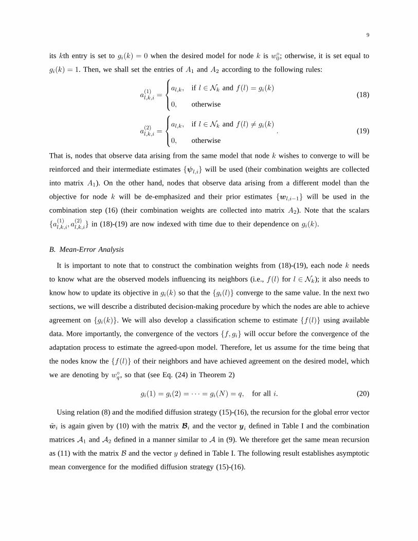
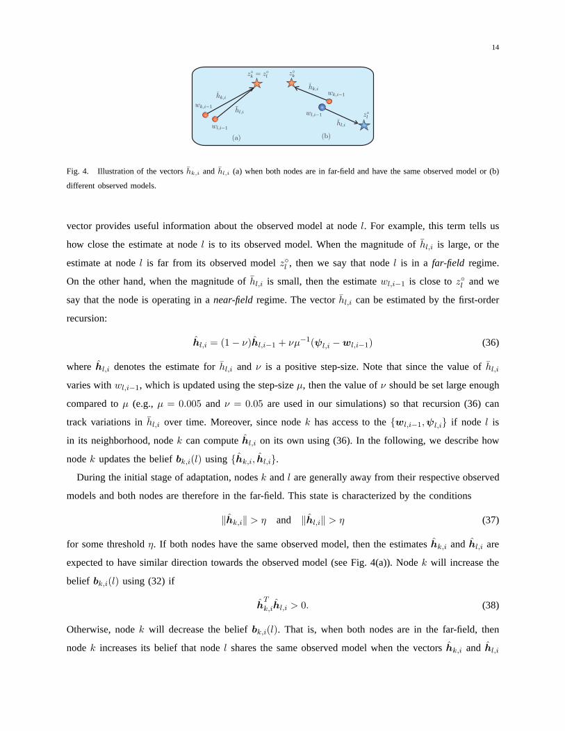
Fig. 4. Illustration of the vectorshk,i and hl,i (a) when both nodes are in far-field and have the same observedmodel or (b)
different observed models.
vector provides useful information about the observed model at nodel. For example, this term tells us
how close the estimate at nodel is to its observed model. When the magnitude ofhl,i is large, or the
estimate at nodel is far from its observed modelz◦l , then we say that nodel is in a far-field regime.
On the other hand, when the magnitude ofhl,i is small, then the estimatewl,i−1 is close toz◦l and we
say that the node is operating in anear-fieldregime. The vectorhl,i can be estimated by the first-order
recursion:
hl,i = (1− ν)hl,i−1 + νµ−1(ψl,i −wl,i−1) (36)
where hl,i denotes the estimate forhl,i and ν is a positive step-size. Note that since the value ofhl,i
varies withwl,i−1, which is updated using the step-sizeµ, then the value ofν should be set large enough
compared toµ (e.g.,µ = 0.005 and ν = 0.05 are used in our simulations) so that recursion (36) can
track variations inhl,i over time. Moreover, since nodek has access to the{wl,i−1,ψl,i} if node l is
in its neighborhood, nodek can computehl,i on its own using (36). In the following, we describe how
nodek updates the beliefbk,i(l) using{hk,i, hl,i}.
During the initial stage of adaptation, nodesk andl are generally away from their respective observed
models and both nodes are therefore in the far-field. This state is characterized by the conditions
‖hk,i‖ > η and ‖hl,i‖ > η (37)
for some thresholdη. If both nodes have the same observed model, then the estimates hk,i and hl,i are
expected to have similar direction towards the observed model (see Fig. 4(a)). Nodek will increase the
belief bk,i(l) using (32) if
hT
k,ihl,i > 0. (38)
Otherwise, nodek will decrease the beliefbk,i(l). That is, when both nodes are in the far-field, then
nodek increases its belief that nodel shares the same observed model when the vectorshk,i and hl,i
15
lie in the same quadrant. Note that it is possible for nodek to increasebk,i(l) even when nodesk and l
have distinct models. This is because it is difficult to differentiate between the models during the initial
stages of adaptation. This situation is handled by the evolving network dynamics as follows. If nodek
considers that the data from nodel originate from the same model, then nodek will use the intermediate
estimateψl,i from nodel in (16). Eventually, from Lemma 1, the estimates at these nodes get close to a
convex combination of the underlying models, which would then enable nodek to distinguish between
the two models and to decrease the value ofbk,i(l). Clearly, for proper resolution, the distance between
the models needs to be large enough so that the agents can resolve them. When the models are very
close to each other so that resolution is difficult, the estimates at the agents will converge towards a
convex combination of the models (which will be also close tothe models). Therefore, the beliefbk,i(l)
is updated according to the following rule:
bk,i(l) =
αbk,i−1(l) + (1− α), if E1
αbk,i−1(l), if Ec1
(39)
whereE1 andEc1 are the two events described by:
E1 : ‖hk,i‖ > η, ‖hl,i‖ > η, and hT
k,ihl,i > 0 (40)
Ec1 : ‖hk,i‖ > η, ‖hl,i‖ > η, and h
T
k,ihl,i ≤ 0. (41)
Note that nodek updates the beliefbk,i(l) only when both nodesk and l are in the far-field.
VI. D IFFUSION STRATEGY WITH DECISION-MAKING
Combining the modified diffusion strategy (15)-(16), the combination weights (18)-(19), the decision-
making process (21)-(23), and the classification scheme (33) and (39) with{f(l), gi(l)} replaced by
{fk,i(l),gk,i(l)}, we arrive at the listing shown in the table. It is seen from the algorithm that the
adaptation and combination steps of diffusion, which correspond to steps 1) and 8), are now separated
by several steps. The purpose of these intermediate steps isto select the combination weights properly
to carry out the aggregation required by step 8). Note that toimplement the algorithm, nodes need to
exchange the quantities{wk,i−1,ψk,i,gk,i−1(k)} with their neighbors. We summarize the computational
complexity and the amount of scalar exchanges of the conventional and modified diffusion strategies in
Table II. Note that the modified strategy still requires in the order ofO(M) computations per iteration.
Nevertheless, the modified diffusion strategy requires about 2nkM more additions and multiplications
than conventional diffusion. This is because of the need to compute the terms{hl,i} in step 2). If the

16
TABLE II
Comparison of the number of multiplications and additions per iteration, as well as the number of scalars that are exchanged
for each iteration of the algorithms at every nodek. In the table, the symbolnk denotes the degree of nodek, i.e., the size of
its neighborhoodNk.
Diffusion (4)-(5) Modified diffusion
Multiplications (nk + 2)M (3nk + 2)M + nk − 1
Additions (nk + 1)M (3nk + 1)M + nk − 1
Scalar exchanges nkM nk(2M + 1)
nodes can afford to exchange extra information, then instead of every node connected to nodel computing
the termhl,i in step 2), this term can be computed locally by nodel and shared with its neighbors. This
reveals a useful trade-off between complexity and information exchange.
Due to the dependency among the steps of the algorithm, the analysis of its behavior becomes
challenging. However, by examining the various steps, someuseful observations stand out. Specifically, it
is observed that the convergence of the algorithm occurs in three phases as follows (see also Sec. VIII):
1) Convergence of the classification scheme: The first phase of convergence happens during the initial
stages of adaptation. It is natural to expect that during this stage, all weight estimates are generally
away from their respective models and the nodes operate in the far-field regime. Then, the nodes
use steps 2)-5) to determine the observed models{fk,i(l)} of their neighbors. We explain later
in Eq. (77) in Theorem 3 that this construction is able to identify the observed models with high
probability. In other words, the classification scheme is able to converge reasonably well and fast
during the initial stages of adaptation.
2) Convergence of the decision-making process: The second phase of convergence happens right
after the convergence of the classification scheme, once the{fk,i(l)} have converged. Because the
nodes now have correct information about their neighbor’s observed models, they use steps 5)-6)
to determine their own desired models{gk,i(k)}. The convergence of this step is ensured by Eq.
(24) in Theorem 2.
3) Convergence of the diffusion strategy: After the classification and decision-making processes con-
verge, the estimates{fk,i(l),gk,i(l)} remain largely invariant and the combination weights in step
7) therefore remain fixed for all practical purposes. Then, the diffusion strategy becomes unbiased
and converges in the mean according to Theorem 1. Moreover, when the estimates are close to
steady-state, those nodes whose observed models are the same as the desired model enter the near-
17
field regime and they stop updating their belief vectors (this will be justified by the future result
(75)).
VII. PERFORMANCE OFCLASSIFICATION PROCEDURE
It is clear that the success of the diffusion strategy and decision-making process depends on the
reliability of the classification scheme in (33) and (39). Inthis section, we examine the probability of
error for the classification scheme under some simplifying conditions to facilitate the analysis. This is a
challenging task to pursue due to the stochastic nature of the classification and decision-making process,
and due to the coupling among the agents. Our purpose in this section is to gain some insights into this
process through a first-order approximate analysis.
Now, there are two types of error. When nodesk and l are subject to the same observed model (i.e.,
z◦k = z◦l andfk(l) = 1), then one probability of error is defined as:
Pe,1 = Pr(
fk,i(l) = 0 | fk(l) = 1)
= Pr (bk,i(l) < 0.5 | z◦k = z◦l ) (42)
where we used rule (33). The second type of probability of error occurs when both nodes have different
observed models (i.e., whenz◦k 6= z◦l andfk(l) = 0) and refers to the case:
Pe,0 = Pr(
fk,i(l) = 1 | fk(l) = 0)
= Pr (bk,i(l) > 0.5 | z◦k 6= z◦l ) . (43)
To evaluate the error probabilities in (42)-(43), we examine the probability distribution of the belief
variablebk,i. Note from (39) that the belief variable can be expressed as:
bk,i(l) = αbk,i−1(l) + (1− α)ξk,i(l) (44)
whereξk,i(l) is a Bernoulli random variable with
ξk,i(l) =
1, with probability p
0, with probability 1− p
. (45)
The value ofp depends on whether the nodes have the same observed models ornot. Whenz◦k = z◦l , the
beliefbk,i(l) is supposed to be increased and the probability of detection, Pd, characterizes the probability
that bk,i(l) is increased, i.e.,
Pd = Pr(ξk,i(l) = 1 | z◦k = z◦l ). (46)
18
In this case, the probabilityp in (45) will be replaced byPd. On the other hand, whenz◦k 6= z◦l , the
probability of false alarm,Pf , characterizes the probability that the beliefbk,i(l) is increased when it is
supposed to be decreased, i.e.,
Pf = Pr(ξk,i(l) = 1 | z◦k 6= z◦l ) (47)
and we replacep in (45) byPf . We will show later (see Lemma 4) how to evaluate the two probabilities
Pd andPf . In the sequel we denote them generically byp.
Expanding (44), we obtain
bk,i(l) = αi+1bk,−1(l) + (1− α)
i∑
j=0
αjξk,i−j(l). (48)
Although it is generally not true, we simplify the analysis by assuming that the{ξk,i(l)} in (45)
are independent and identically distributed (i.i.d.) random variables. This assumption is motivated by
conditions (40)-(41) and by the fact that the type of model that is observed by nodek is assumed to be
independent from the type of model that is observed by nodel. The assumption is also motivated by the
fact that the regression data and noise across all nodes are assumed to be temporally white and independent
over space. Now, sinceα is a design parameter that is smaller than one, after a few iterations, say,C
iterations, the influence of the initial condition in (48) becomes small and can be ignored. In addition, the
distribution ofbk,i(l) can be approximated by the distribution of the following random variable, which
takes the form of a random geometric series:
ζk(l) , (1− α)
C∑
j=0
αjξk,j(l) (49)
where we replaced the indexi − j in (48) by j because the{ξk,i(l)} are assumed to be i.i.d. There
have been several useful works on the distribution functionof random geometric sequences and series
[53]–[55]. However, it is generally untractable to expressthe distribution function in closed form. We
instead resort to the following two inequalities to establish bounds for the error probabilities (42)-(43).
First, for any two generic eventsE1 andE2, if E1 implies E2, then the probability of eventE1 is less
than the probability of eventE2 [56], i.e.,
Pr(E1) ≤ Pr(E2) if E1 ⊆ E2. (50)
The second inequality is the Markov inequality [56], i.e., for any nonnegative random variablex and
positive scalarδ, it holds that
Pr(x ≥ δ) = Pr(x2 ≥ δ2) ≤Ex2
δ2. (51)
19
To apply the Markov inequality (51), we need the second-order moment ofζk(l) in (49), which is difficult
to evaluate because the{ξk,j(l)} are not zero mean. To circumvent this difficulty, we introduce the change
of variable:
ξ◦k,j(l) ,ξk,j(l)− p√
p(1− p). (52)
It can be verified that the{ξ◦k,j(l)} are i.i.d. withzeromean and unit variance. Then, we can write (49)
as
ζk(l) = p(
1− αC+1)
+√
p(1− p)ζ◦k(l) (53)
where the variableζ◦k(l) is defined by
ζ◦k(l) , (1− α)
C∑
j=0
αjξ◦k,j(l) (54)
and its mean is zero and its variance is given by
E(ζ◦k(l))2 =
1− α
1 + α
(
1− α2(C+1))
≈1− α
1 + α. (55)
Then, from (42) and (53) and replacing the probabilityp by Pd and forC large enough so that1−αC+1 ≈
1, we obtain that
Pe,1 ≈ Pr(ζk(l) < 0.5 | z◦k = z◦l )
= Pr
(
ζ◦k(l) <−(Pd − 0.5)√
Pd(1− Pd)| z◦k = z◦l
)
≤ Pr
(
|ζ◦k(l)| >Pd − 0.5
√
Pd(1− Pd)| z◦k = z◦l
)
≤1− α
1 + α·Pd(1− Pd)
(Pd − 0.5)2(56)
where we used (50) and the Markov inequality (51) in the last two inequalities. Note that in (56), we
assume the value ofPd to be greater than0.5. Indeed, as we will argue in Lemma 4, the value ofPd is
close to one. Similarly, replacing the probabilityp by Pf and assuming thatPf < 0.5, we obtain from
(43) and (53) that
Pe,0 ≤1− α
1 + α·Pf (1− Pf )
(0.5 − Pf )2. (57)
To evaluate the upper bounds in (56)-(57), we need the probabilities of detection and false alarm in
(46)-(47). Since the update ofbk,i(l) in (39) depends on{hk,i, hl,i}, we need to rely on the statistical
properties of these latter quantities. In the following, wefirst examine the statistics ofhk,i constructed
via (36) and then evaluatePd andPf defined by (46)-(47).

20
A. Statistics ofhk,i
We first discuss some assumptions that lead to an approximatemodel for the evolution ofhk,i in (72)
further ahead. As we mentioned following (36), since the step-sizes{µ, ν} satisfyµ ≪ ν, the variation
of wk,i−1 can be assumed to be much slower than the variation ofhk,i. For this reason, the analysis in
this section will be conditioned onwk,i−1 = wk,i−1, as we did in (35), and we introduce the following
assumption.
Assumption 3 (Small step-size). The step-sizes{µ, ν} are sufficiently small, i.e.,
0 < µ ≪ ν ≪ 1 (58)
so thatwk,i ≈ wk,i−1 for all k.
In addition, since the update vector from (35) depends on thecovariance matrixRu, we assumeRu is
well-conditioned so that the following is justified.
Assumption 4 (Regression model). The regression covariance matrixRu is well-conditioned such that
it holds that
if ‖z◦k − wk,i−1‖ ≫ 1, then‖hk,i‖ ≫ η (59)
if ‖z◦k − wk,i−1‖ ≪ 1, then‖hk,i‖ ≪ η. (60)
Moreover, the fourth-order moment of the regression data{uk,i} is assumed to be bounded such that
ντ ≪ 1 (61)
where the scalarτ is a bound for
E‖uTk,iuk,i(z
◦k − wk,i−1)− hk,i‖
2
‖hk,i‖2≤ τ (62)
and its value measures the randomness in variables involving fourth-order products of entries ofuk,i.
Note that condition (62) can be rewritten as
(z◦k − wk,i−1)TE(uT
k,iuk,iuTk,iuk,i −R2
u)(z◦k − wk,i−1)
(z◦k − wk,i−1)TR2u(z
◦k − wk,i−1)
≤ τ (63)
which shows that (62) corresponds to a condition on the fourth-order moment of the regression data.
Combining conditions (58) and (61), we obtain the followingconstraint on the step-sizes{µ, ν}:
0 ≪ µ ≪ ν ≪ min{1, 1/τ}. (64)
21
To explain more clearly what conditions (59)-(60) entail, we obtain from (35) that‖hk,i‖2 can be written
as the weighted square Euclidean norm:
‖hk,i‖2 = ‖z◦k − wk,i−1‖
2R2
u
. (65)
We apply the Rayleigh-Ritz characterization of eigenvalues [50] to conclude that
λmin(Ru) · ‖z◦k − wk,i−1‖ ≤ ‖hk,i‖ ≤ λmax(Ru) · ‖z
◦k − wk,i−1‖
whereλmin(Ru) andλmax(Ru) denote the minimum and maximum eigenvalues ofRu. Then, condition
(59) indicates that whenever nodek is operating in the far-field regime, i.e., whenever‖z◦k−wk,i−1‖ ≫ 1,
then we would like
λmin(Ru) · ‖z◦k − wk,i−1‖ ≫ η. (66)
Likewise, whenever‖z◦k − wk,i−1‖ ≪ 1, then
λmax(Ru) · ‖z◦k − wk,i−1‖ ≪ η. (67)
Therefore, the scalarsλmin(Ru)/η andλmax(Ru)/η cannot be too small or too large, i.e., the matrixRu
should be well-conditioned.
We are now ready to model the average update vectorhk,i. From Assumption 3, since the estimate
wk,i−1 remains approximately constant during repeated updates ofhk,i, we first remove the time index
in wk,i−1 and examine the statistics ofhk,i under the conditionwk,i−1 = wk. From (34) and (36), the
expected value ofhk,i givenwk,i−1 = wk converges to
limi→∞
Ehk,i = Ru(z◦k − wk) , hk. (68)
We can also obtain from (34) and (36) that the limiting second-order moment ofhk,i, which is denoted
by σ2h,k
, satisfies:
σ2h,k
, limi→∞
E‖hk,i − hk‖2 = (1− ν)2σ2
h,k+ ν2σ2
h,k (69)
whereσ2h,k , E‖hk,i − hk‖
2 is given by
σ2h,k = E‖uT
k,iuk,i(z◦k − wk)− hk‖
2 + σ2v,kTr(Ru). (70)
Note that the cross term on the right-hand side of (69) is zerobecause the termshk,i−1− hk andhk,i− hk
are independent under the constantwk condition. Note also thathk,i − hk has zero mean. Then, from
(69) and Assumption 3, the varianceσ2h,k
is given by
σ2h,k
=ν
2− νσ2h,k ≈
ν
2σ2h,k. (71)
22
Sincewk,i−1 remains approximately constant, the average update vectorhk,i has mean and second-
order moment close to expressions (68) and (71). We then arrive at the following approximate model for
hk,i.
Assumption 5 (Model for hk,i). The estimatehk,i is modeled as:
hk,i = hk,i +nk,i (72)
wherenk,i is a random perturbation process with zero mean and
E‖nk,i‖2 ≤
ν[τ‖hk,i‖2 + σ2
v,kTr(Ru)]
2(73)
with the scalarτ defined by (61).
Note that since the perturbationnk,i is from the randomness of the regressor and noise processes
{uk,i,vk(i)}, then it is reasonable to assume that the{nk,i} are independent of each other.
Before we proceed to the probability of detection (46) and the probability of false alarm (47), we note
that the update of the beliefbk,i(l) happens only when both nodesk and l are in the far-field regime,
which is determined by the magnitudes ofhk,i andhl,i being greater than the thresholdη. The following
result approximates the probability that a node is classified to be in the far-field.
Lemma 3. Under Assumptions 3-5, it holds that
Pr(‖hk,i‖ > η | ‖z◦k − wk,i−1‖ ≫ 1) ≥ 1−ντ
2(74)
Pr(‖hk,i‖ > η | ‖z◦k − wk,i−1‖ ≪ 1) ≤νσ2
v,kTr(Ru)
2η2. (75)
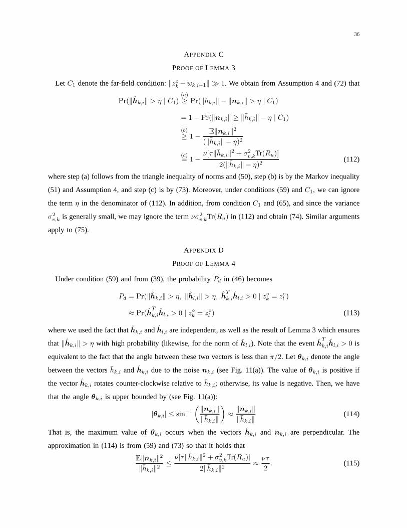
Proof: See Appendix C.
From Assumptions 3-4, the probability in (74) is close to oneand the probability in (75) is close
to zero. Therefore, this approximate analysis suggests that during the initial stages of adaptation, the
magnitude of{‖hk,i‖} successfully determines that the nodes are in the far-field state and they update
the belief using rule (39). When the estimates approach steady-state, the nodes whose observed models
are the same as the desired model satisfy the condition‖z◦k − wk,i−1‖ ≪ 1 and, therefore, they stop
updating their belief vectors in view of (75). On the other hand, when both nodesk andl have observed
models that are different from the desired model (and, therefore, their estimates are away from their
observed models), they will continue to update their beliefs. The proof in Appendix D then establishes
the following bounds onPd andPf .
23
Lemma 4. Under Assumptions 3-5 and during the far-field regime (59), the probabilities of detection
and false alarm defined by (46)-(47) are approximately bounded by
Pd ≥ 1−16ντ
π2and Pf ≤
16ντ
π2. (76)
The above result establishes that the probability of detection is close to one and the probability of false
alarm is close to zero in view ofντ ≪ 1. That is, with high probability, nodek will correctly adjust the
value ofbk,i(l). We then arrive at the following bound for error probabilities in (42)-(43).
Theorem 3. Under Assumptions 3-5 and in the far-field regime (59), the error probabilities{Pe,1, Pe,0}
are approximately upper bounded by
Pu =1− α
1 + α·16ντ
π2·
1− 16ντ/π2
(1/2 − 16ντ/π2)2= O(ν). (77)
Proof: Let the functionf(p) be defined asp(1− p)/(p− 0.5)2. It can be verified that the function
f(p) is strictly increasing whenp ∈ [0, 0.5) and strictly decreasing whenp ∈ (0.5, 1]. From Lemma
4, we conclude thatPd > 0.5 andPf < 0.5. Therefore, an upper bound forPe,1 can be obtained by
replacingPd in (56) by the lower bound in (76). Similar arguments apply tothe upper bound forPe,0.
This result reveals that the{Pe,1, Pe,0} are upper bounded by the order ofν. In addition, the upper bound
Pu also depends on the value ofα used to update the belief in (39). We observe that the larger the value
of α, the smaller the values of the error probabilities. In simulations, we chooseν = 0.05 andα = 0.95,
which will give the upper bound in (77) the valuePu ≈ 0.008τ < ντ . This implies that the classification
scheme (33) identifies the observed models with high probability.
VIII. R ATES OFCONVERGENCE
There are two rates of convergence to consider for adaptive networks running a decision-making
process of the form described in the earlier sections. First, we need to analyze the rate at which the
nodes reach an agreement on a desired model (which corresponds to the speed of the decision-making
process). Second, we analyze the rate at which the estimatesby the nodes converge to the desired model
(which corresponds to the speed of the diffusion adaptation).
A. Convergence Rate of Decision-Making Process
From the proof of Theorem 2 (see Appendix B), the decision-making process can be modeled as a
Markov chain withN + 1 states{χi} corresponding to the number of nodes whose desired vectors are
24
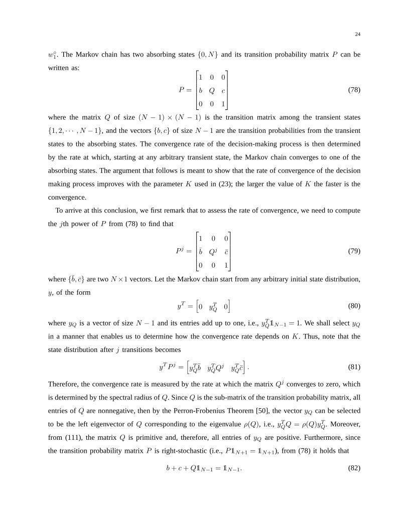
w◦1. The Markov chain has two absorbing states{0, N} and its transition probability matrixP can be
written as:
P =
1 0 0
b Q c
0 0 1
(78)
where the matrixQ of size (N − 1) × (N − 1) is the transition matrix among the transient states
{1, 2, · · · , N − 1}, and the vectors{b, c} of sizeN − 1 are the transition probabilities from the transient
states to the absorbing states. The convergence rate of the decision-making process is then determined
by the rate at which, starting at any arbitrary transient state, the Markov chain converges to one of the
absorbing states. The argument that follows is meant to showthat the rate of convergence of the decision
making process improves with the parameterK used in (23); the larger the value ofK the faster is the
convergence.
To arrive at this conclusion, we first remark that to assess the rate of convergence, we need to compute
the jth power ofP from (78) to find that
P j =
1 0 0
b Qj c
0 0 1
(79)
where{b, c} are twoN×1 vectors. Let the Markov chain start from any arbitrary initial state distribution,
y, of the form
yT =[
0 yTQ 0]
(80)
whereyQ is a vector of sizeN − 1 and its entries add up to one, i.e.,yTQ1N−1 = 1. We shall selectyQ
in a manner that enables us to determine how the convergence rate depends onK. Thus, note that the
state distribution afterj transitions becomes
yTP j =[
yTQb yTQQj yTQc
]
. (81)
Therefore, the convergence rate is measured by the rate at which the matrixQj converges to zero, which
is determined by the spectral radius ofQ. SinceQ is the sub-matrix of the transition probability matrix, all
entries ofQ are nonnegative, then by the Perron-Frobenius Theorem [50], the vectoryQ can be selected
to be the left eigenvector ofQ corresponding to the eigenvalueρ(Q), i.e., yTQQ = ρ(Q)yTQ. Moreover,
from (111), the matrixQ is primitive and, therefore, all entries ofyQ are positive. Furthermore, since
the transition probability matrixP is right-stochastic (i.e.,P1N+1 = 1N+1), from (78) it holds that
b+ c+Q1N−1 = 1N−1. (82)
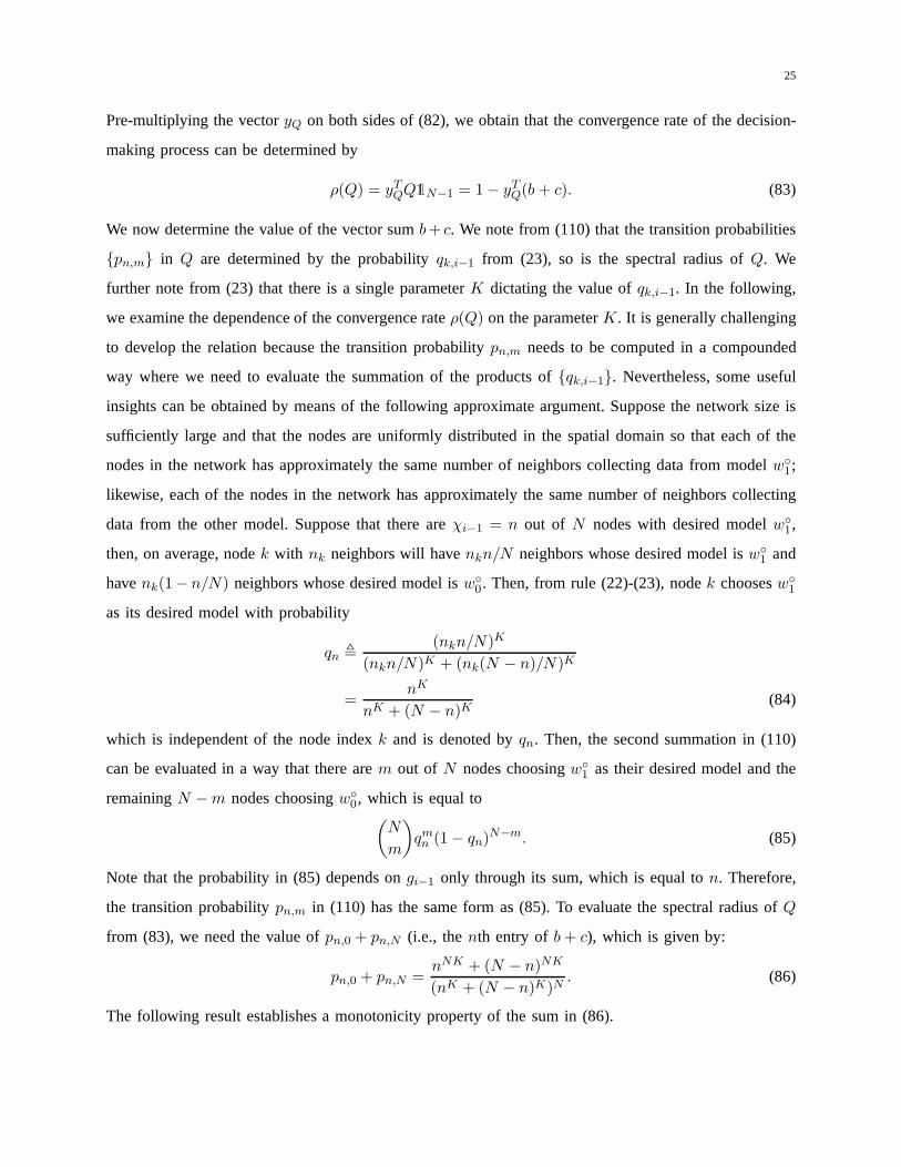
25
Pre-multiplying the vectoryQ on both sides of (82), we obtain that the convergence rate of the decision-
making process can be determined by
ρ(Q) = yTQQ1N−1 = 1− yTQ(b+ c). (83)
We now determine the value of the vector sumb+ c. We note from (110) that the transition probabilities
{pn,m} in Q are determined by the probabilityqk,i−1 from (23), so is the spectral radius ofQ. We
further note from (23) that there is a single parameterK dictating the value ofqk,i−1. In the following,
we examine the dependence of the convergence rateρ(Q) on the parameterK. It is generally challenging
to develop the relation because the transition probabilitypn,m needs to be computed in a compounded
way where we need to evaluate the summation of the products of{qk,i−1}. Nevertheless, some useful
insights can be obtained by means of the following approximate argument. Suppose the network size is
sufficiently large and that the nodes are uniformly distributed in the spatial domain so that each of the
nodes in the network has approximately the same number of neighbors collecting data from modelw◦1;
likewise, each of the nodes in the network has approximatelythe same number of neighbors collecting
data from the other model. Suppose that there areχi−1 = n out of N nodes with desired modelw◦1,
then, on average, nodek with nk neighbors will havenkn/N neighbors whose desired model isw◦1 and
havenk(1−n/N) neighbors whose desired model isw◦0. Then, from rule (22)-(23), nodek choosesw◦
1
as its desired model with probability
qn ,(nkn/N)K
(nkn/N)K + (nk(N − n)/N)K
=nK
nK + (N − n)K(84)
which is independent of the node indexk and is denoted byqn. Then, the second summation in (110)
can be evaluated in a way that there arem out of N nodes choosingw◦1 as their desired model and the
remainingN −m nodes choosingw◦0, which is equal to(
N
m
)
qmn (1− qn)N−m. (85)
Note that the probability in (85) depends ongi−1 only through its sum, which is equal ton. Therefore,
the transition probabilitypn,m in (110) has the same form as (85). To evaluate the spectral radius ofQ
from (83), we need the value ofpn,0 + pn,N (i.e., thenth entry ofb+ c), which is given by:
pn,0 + pn,N =nNK + (N − n)NK
(nK + (N − n)K)N. (86)
The following result establishes a monotonicity property of the sum in (86).
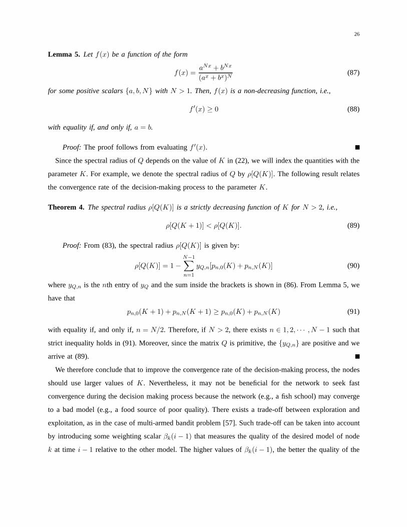
26
Lemma 5. Let f(x) be a function of the form
f(x) =aNx + bNx
(ax + bx)N(87)
for some positive scalars{a, b,N} with N > 1. Then,f(x) is a non-decreasing function, i.e.,
f ′(x) ≥ 0 (88)
with equality if, and only if,a = b.
Proof: The proof follows from evaluatingf ′(x).
Since the spectral radius ofQ depends on the value ofK in (22), we will index the quantities with the
parameterK. For example, we denote the spectral radius ofQ by ρ[Q(K)]. The following result relates
the convergence rate of the decision-making process to the parameterK.
Theorem 4. The spectral radiusρ[Q(K)] is a strictly decreasing function ofK for N > 2, i.e.,
ρ[Q(K + 1)] < ρ[Q(K)]. (89)
Proof: From (83), the spectral radiusρ[Q(K)] is given by:
ρ[Q(K)] = 1−N−1∑
n=1
yQ,n[pn,0(K) + pn,N(K)] (90)
whereyQ,n is thenth entry ofyQ and the sum inside the brackets is shown in (86). From Lemma 5,we
have that
pn,0(K + 1) + pn,N(K + 1) ≥ pn,0(K) + pn,N (K) (91)
with equality if, and only if,n = N/2. Therefore, ifN > 2, there existsn ∈ 1, 2, · · · , N − 1 such that
strict inequality holds in (91). Moreover, since the matrixQ is primitive, the{yQ,n} are positive and we
arrive at (89).
We therefore conclude that to improve the convergence rate of the decision-making process, the nodes
should use larger values ofK. Nevertheless, it may not be beneficial for the network to seek fast
convergence during the decision making process because thenetwork (e.g., a fish school) may converge
to a bad model (e.g., a food source of poor quality). There exists a trade-off between exploration and
exploitation, as in the case of multi-armed bandit problem [57]. Such trade-off can be taken into account
by introducing some weighting scalarβk(i− 1) that measures the quality of the desired model of node
k at time i− 1 relative to the other model. The higher values ofβk(i− 1), the better the quality of the
27
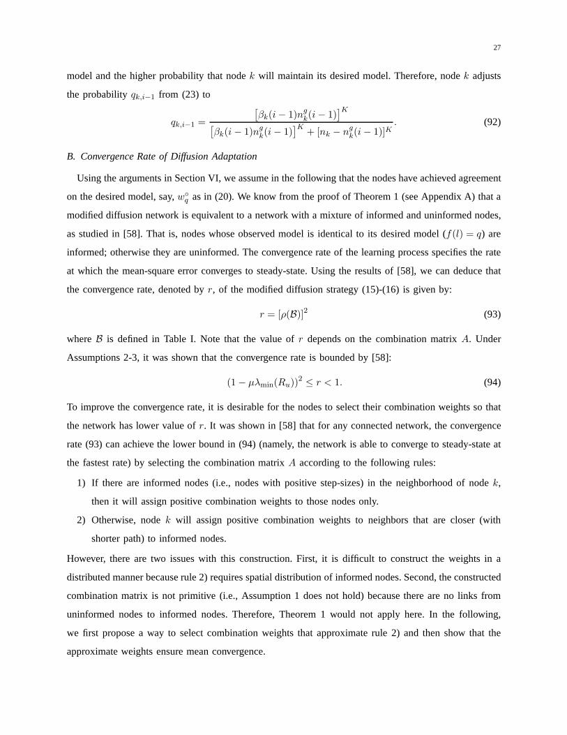
model and the higher probability that nodek will maintain its desired model. Therefore, nodek adjusts
the probabilityqk,i−1 from (23) to
qk,i−1 =
[
βk(i− 1)ngk(i− 1)
]K
[
βk(i− 1)ngk(i− 1)
]K+ [nk − ng
k(i− 1)]K. (92)
B. Convergence Rate of Diffusion Adaptation
Using the arguments in Section VI, we assume in the followingthat the nodes have achieved agreement
on the desired model, say,w◦q as in (20). We know from the proof of Theorem 1 (see Appendix A)that a
modified diffusion network is equivalent to a network with a mixture of informed and uninformed nodes,
as studied in [58]. That is, nodes whose observed model is identical to its desired model (f(l) = q) are
informed; otherwise they are uninformed. The convergence rate of the learning process specifies the rate
at which the mean-square error converges to steady-state. Using the results of [58], we can deduce that
the convergence rate, denoted byr, of the modified diffusion strategy (15)-(16) is given by:
r = [ρ(B)]2 (93)
whereB is defined in Table I. Note that the value ofr depends on the combination matrixA. Under
Assumptions 2-3, it was shown that the convergence rate is bounded by [58]:
(1− µλmin(Ru))2 ≤ r < 1. (94)
To improve the convergence rate, it is desirable for the nodes to select their combination weights so that
the network has lower value ofr. It was shown in [58] that for any connected network, the convergence
rate (93) can achieve the lower bound in (94) (namely, the network is able to converge to steady-state at
the fastest rate) by selecting the combination matrixA according to the following rules:
1) If there are informed nodes (i.e., nodes with positive step-sizes) in the neighborhood of nodek,
then it will assign positive combination weights to those nodes only.
2) Otherwise, nodek will assign positive combination weights to neighbors thatare closer (with
shorter path) to informed nodes.
However, there are two issues with this construction. First, it is difficult to construct the weights in a
distributed manner because rule 2) requires spatial distribution of informed nodes. Second, the constructed
combination matrix is not primitive (i.e., Assumption 1 does not hold) because there are no links from
uninformed nodes to informed nodes. Therefore, Theorem 1 would not apply here. In the following,
we first propose a way to select combination weights that approximate rule 2) and then show that the
approximate weights ensure mean convergence.
28
Let N fk denote the set of nodes that are in the neighborhood ofk and whose observed model is the
same as the desired modelw◦q (i.e., they are informed neighbors)
N fk = {l | l ∈ Nk, f(l) = q}. (95)
Also, letnfk denote the number of nodes in the setN f
k . The selection of combination weights is specified
based on three types of nodes: informed nodes (f(k) = q), uninformed nodes with informed neighbors
(f(k) 6= q andnfk 6= 0), and uninformed nodes without informed neighbors (f(k) 6= q andnf
k = 0). The
first two types correspond to rule 1) and their weights can satisfy rule 1) by setting
al,k =
1/nfk , if l ∈ N f
k
0, otherwise. (96)
That is, nodek places uniform weights on the informed neighbors and zero weights on the others. The
last type of nodes corresponds to rule 2). Since these nodes do not know the distribution of informed
nodes, a convenient choice for the approximate weights theycan select is for them to place zero weights
on themselves and uniform weights on the others, i.e.,
al,k =
1/(nk − 1), if l ∈ Nk and l 6= k
0, otherwise. (97)
Note that the weights from (96)-(97) can be set in a fully distributed manner and in real-time. To show
the mean convergence of the modified diffusion strategy using the combination matrixA constructed
from (96)-(97), we resort to Theorem 1 from [58]. It states that the strategy converges in the mean for
sufficiently small step-sizes if for any nodek, there exists an informed nodel and an integer powerj
such that
[Aj ]l,k > 0. (98)
Condition (98) is clearly satisfied for the first two types of nodes. For any node belonging to the last
type, since the network is connected and from (97), there exists a path with nonzero weight from a node
of the second type (uninformed with informed neighbors) to itself. In addition, there exist direct links
from informed nodes to the nodes of the second type, condition (98) is also satisfied. This implies that
the modified diffusion strategy using the combination weights from (96)-(97) converges in the mean.
IX. SIMULATION RESULTS
We consider a network with 40 nodes randomly connected. The model vectors are set tow◦0 =
[5;−5; 5; 5] and w◦1 = [5; 5;−5; 5] (i.e. M = 4). Assume that the first 20 nodes (nodes 1 through
29
20) observe data originating from modelw◦0, while the remaining nodes observe data originating from
modelw◦1. The regression covariance matrixRu is diagonal with each diagonal entry generated uniformly
from [1, 2]. The noise variance at each node is generated uniformly from[−35,−5] dB. The step-sizes
are set toµ = 0.005, ν = 0.05, andα = 0.95. The thresholdη is set toη = 1. The network employs the
decision-making process withK = 4 in (23) and the uniform combination rule:al,k = 1/nk if l ∈ Nk.
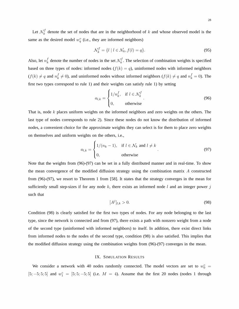
In Fig. 5, we illustrate the network mean-square deviation (MSD) with respect to the two model vectors
over time, i.e.,
MSDq(i) =1
N
N∑
k=1
E‖w◦q −wk,i‖
2 (99)
for q = 0 and q = 1. We compare the conventional ATC diffusion strategy (4)-(5) and the modified
ATC diffusion strategy (15)-(16) with decision-making. Weobserve the bifurcation in MSD curves of
the modified ATC diffusion strategy. Specifically, the MSD curve relative to the modelw◦0 converges
to 23 dB, while the MSD relative tow◦1 converges to -50 dB. This illustrates that the nodes using the
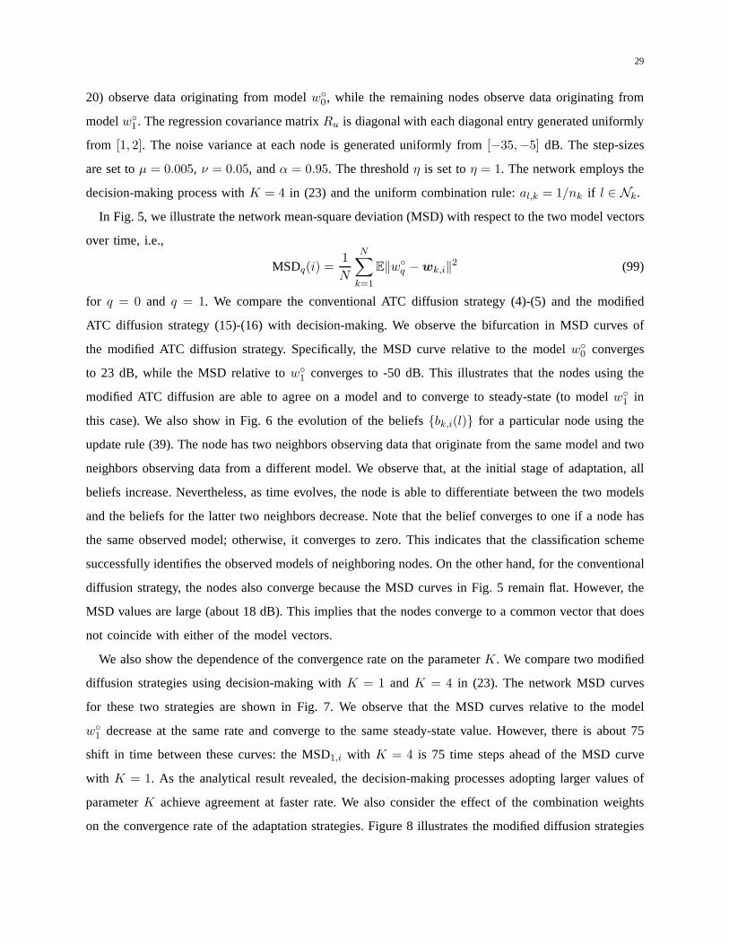
modified ATC diffusion are able to agree on a model and to converge to steady-state (to modelw◦1 in
this case). We also show in Fig. 6 the evolution of the beliefs{bk,i(l)} for a particular node using the
update rule (39). The node has two neighbors observing data that originate from the same model and two
neighbors observing data from a different model. We observethat, at the initial stage of adaptation, all
beliefs increase. Nevertheless, as time evolves, the node is able to differentiate between the two models
and the beliefs for the latter two neighbors decrease. Note that the belief converges to one if a node has
the same observed model; otherwise, it converges to zero. This indicates that the classification scheme
successfully identifies the observed models of neighboringnodes. On the other hand, for the conventional
diffusion strategy, the nodes also converge because the MSDcurves in Fig. 5 remain flat. However, the
MSD values are large (about 18 dB). This implies that the nodes converge to a common vector that does
not coincide with either of the model vectors.
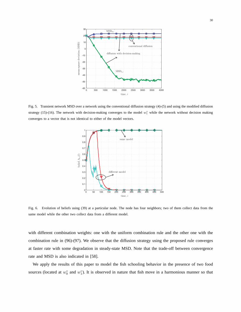
We also show the dependence of the convergence rate on the parameterK. We compare two modified
diffusion strategies using decision-making withK = 1 andK = 4 in (23). The network MSD curves
for these two strategies are shown in Fig. 7. We observe that the MSD curves relative to the model
w◦1 decrease at the same rate and converge to the same steady-state value. However, there is about 75
shift in time between these curves: the MSD1,i with K = 4 is 75 time steps ahead of the MSD curve
with K = 1. As the analytical result revealed, the decision-making processes adopting larger values of
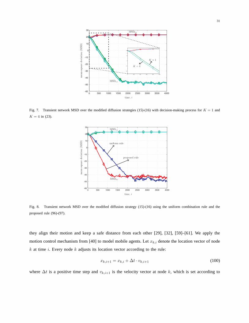
parameterK achieve agreement at faster rate. We also consider the effect of the combination weights
on the convergence rate of the adaptation strategies. Figure 8 illustrates the modified diffusion strategies
30
Fig. 5. Transient network MSD over a network using the conventional diffusion strategy (4)-(5) and using the modified diffusion
strategy (15)-(16). The network with decision-making converges to the modelw◦1 while the network without decision making
converges to a vector that is not identical to either of the model vectors.
Fig. 6. Evolution of beliefs using (39) at a particular node.The node has four neighbors; two of them collect data from the
same model while the other two collect data from a different model.
with different combination weights: one with the uniform combination rule and the other one with the
combination rule in (96)-(97). We observe that the diffusion strategy using the proposed rule converges
at faster rate with some degradation in steady-state MSD. Note that the trade-off between convergence
rate and MSD is also indicated in [58].
We apply the results of this paper to model the fish schooling behavior in the presence of two food
sources (located atw◦0 andw◦
1). It is observed in nature that fish move in a harmonious manner so that
31
Fig. 7. Transient network MSD over the modified diffusion strategies (15)-(16) with decision-making process forK = 1 and
K = 4 in (23).
Fig. 8. Transient network MSD over the modified diffusion strategy (15)-(16) using the uniform combination rule and the
proposed rule (96)-(97).
they align their motion and keep a safe distance from each other [29], [32], [59]–[61]. We apply the
motion control mechanism from [40] to model mobile agents. Let xk,i denote the location vector of node
k at time i. Every nodek adjusts its location vector according to the rule:
xk,i+1 = xk,i +∆t · vk,i+1 (100)
where∆t is a positive time step andvk,i+1 is the velocity vector at nodek, which is set according to
32
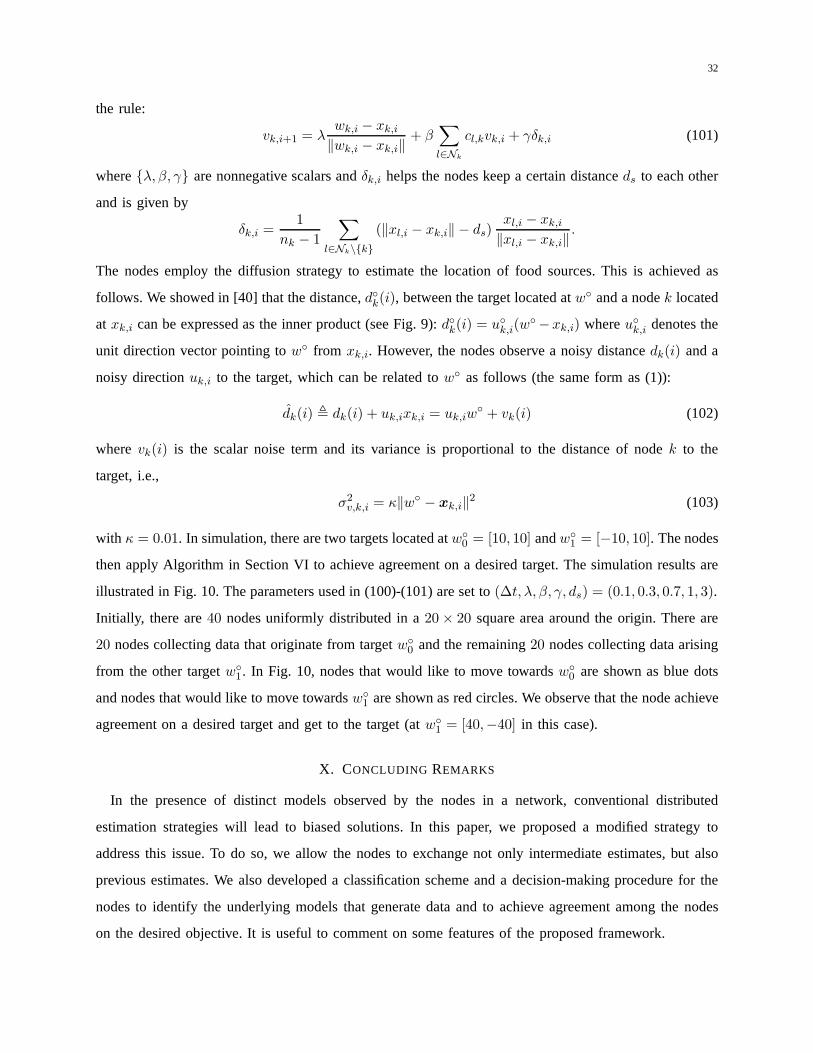
the rule:
vk,i+1 = λwk,i − xk,i
‖wk,i − xk,i‖+ β
∑
l∈Nk
cl,kvk,i + γδk,i (101)
where{λ, β, γ} are nonnegative scalars andδk,i helps the nodes keep a certain distanceds to each other
and is given by
δk,i =1
nk − 1
∑
l∈Nk\{k}
(‖xl,i − xk,i‖ − ds)xl,i − xk,i‖xl,i − xk,i‖
.
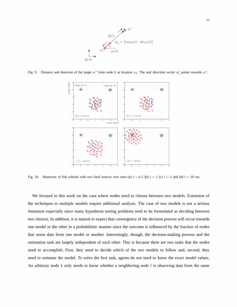
The nodes employ the diffusion strategy to estimate the location of food sources. This is achieved as
follows. We showed in [40] that the distance,d◦k(i), between the target located atw◦ and a nodek located
at xk,i can be expressed as the inner product (see Fig. 9):d◦k(i) = u◦k,i(w◦−xk,i) whereu◦k,i denotes the
unit direction vector pointing tow◦ from xk,i. However, the nodes observe a noisy distancedk(i) and a
noisy directionuk,i to the target, which can be related tow◦ as follows (the same form as (1)):
dk(i) , dk(i) + uk,ixk,i = uk,iw◦ + vk(i) (102)
wherevk(i) is the scalar noise term and its variance is proportional to the distance of nodek to the
target, i.e.,
σ2v,k,i = κ‖w◦ − xk,i‖
2 (103)
with κ = 0.01. In simulation, there are two targets located atw◦0 = [10, 10] andw◦
1 = [−10, 10]. The nodes
then apply Algorithm in Section VI to achieve agreement on a desired target. The simulation results are
illustrated in Fig. 10. The parameters used in (100)-(101) are set to(∆t, λ, β, γ, ds) = (0.1, 0.3, 0.7, 1, 3).
Initially, there are40 nodes uniformly distributed in a20× 20 square area around the origin. There are
20 nodes collecting data that originate from targetw◦0 and the remaining20 nodes collecting data arising
from the other targetw◦1. In Fig. 10, nodes that would like to move towardsw◦
0 are shown as blue dots
and nodes that would like to move towardsw◦1 are shown as red circles. We observe that the node achieve
agreement on a desired target and get to the target (atw◦1 = [40,−40] in this case).
X. CONCLUDING REMARKS
In the presence of distinct models observed by the nodes in a network, conventional distributed
estimation strategies will lead to biased solutions. In this paper, we proposed a modified strategy to
address this issue. To do so, we allow the nodes to exchange not only intermediate estimates, but also
previous estimates. We also developed a classification scheme and a decision-making procedure for the
nodes to identify the underlying models that generate data and to achieve agreement among the nodes
on the desired objective. It is useful to comment on some features of the proposed framework.
33
Fig. 9. Distance and direction of the targetw◦ from nodek at locationxk. The unit direction vectoru◦k points towardsw◦.
Fig. 10. Maneuver of fish schools with two food sources over time (a)t = 0.5 (b) t = 1 (c) t = 2 and (d)t = 20 sec.
We focused in this work on the case where nodes need to choose between two models. Extension of
the techniques to multiple models require additional analysis. The case of two models is not a serious
limitation especially since many hypothesis testing problems tend to be formulated as deciding between
two choices. In addition, it is natural to expect that convergence of the decision process will occur towards
one model or the other in a probabilistic manner since the outcome is influenced by the fraction of nodes
that sense data from one model or another. Interestingly, though, the decision-making process and the
estimation task are largely independent of each other. Thisis because there are two tasks that the nodes
need to accomplish. First, they need to decide which of the two models to follow and, second, they
need to estimate the model. To solve the first task, agents do not need to know the exact model values.
An arbitrary nodek only needs to know whether a neighboring nodel is observing data from the same
34
model or from a different model regardless of the model values. This property enables the initial decision
process to converge faster and to be largely independent of the estimation task.
APPENDIX A
PROOF OFTHEOREM 1
Without loss of generality, letw◦0 be the desired model for the network (i.e.,q = 0 in (20)) and assume
there areN0 nodes with indices{1, 2, . . . , N0} observing data arising from the modelw◦0, while the
remainingN −N0 nodes observe data arising from modelw◦1. Then, we obtain from (7), (18), and (19)
that
z◦k =
0, if k ≤ N0
w◦0 − w◦
1, if k > N0
(104)
a(1)l,k = 0 if l > N0 and a
(2)l,k = 0 if l ≤ N0. (105)
Since the matrixMR is block diagonal, we conclude that
y = 0 and B = AT (INM −MeR) (106)
whereMe is anN ×N block diagonal matrix of the form
Me , diag{µ1IM , · · · , µN0IM , 0, · · · , 0}. (107)
That is, its mean recursion in (11) is equivalent to the mean recursion of a network running the traditional
diffusion strategy (4)-(5) withN0 nodes (nodes 1 toN0) using positive step-sizes andN − N0 nodes
(nodesN0 + 1 to N ) having zero step-sizes. Then, according to Theorem 1 of [58] and under the
assumption that the matrixA is primitive, if the step-sizes{µ1, µ2, · · · , µN0} are set to satisfy (13), then
the spectral radius ofB will be strictly less than one.
APPENDIX B
PROOF OFTHEOREM 2
For a given vectorgi−1, we denote byχi−1 the number of nodes whose desired model isw◦1 at time
i− 1, i.e.,
χi−1 ,
N∑
k=1
gi−1(k). (108)
From (21)-(23), the vectorgi depends only ongi−1. Thus, the value ofχi depends only onχi−1.
Therefore, the evolution ofχi forms a Markov chain withN + 1 states corresponding to the values
35
{0, 1, 2, . . . , N} for χi. To compute the transition probability,pn,m, from stateχi−1 = n to stateχi = m,
let us denote byGn the set of vectorsg = {g(1), g(2), · · · , g(N)} whose entries are either 1 or 0 and
add up ton, i.e.,
Gn =
{
g |N∑
k=1
g(k) = n
}
. (109)
Then, thepn,m can be written as:
pn,m =∑
gi−1
∈Gn
Pr(gi−1)∑
gi∈Gm
N∏
l=1
Pr(gi(l) | gi−1(l)) (110)
wherePr(gi−1) is a priori probability and where the probabilityPr(gi(l) | gi−1(l)) is determined by
(23). Note that for a static network, the transition probability pn,m is independent ofi, i.e., the Markov
chain ishomogeneous[62].
Now we assume thatχi−1 = n 6= 0, N . Since the network is connected, for anygi−1 ∈ Gn at least
one node (say, nodek) has desired modelw◦1 and has a neighbor with distinct desired modelw◦
0 so that
ngk(i− 1) < nk and1− qk,i−1 > 0 from (23). Sinceql,i−1 > 0 for all l, we obtain from (110) that
pn,n−1 ≥∑
gi−1
∈Gn
Pr(gi−1)(1− qk,i−1)∏
l 6=k
ql,i−1 > 0
pn,n > 0 and pn,n+1 > 0 (111)
for n 6= 0, N . Whenn = 0 or n = N , we have thatp0,0 = pN,N = 1. This indicates that the Markov
chain has two absorbing states:χi = 0 (or, gi(1) = gi(2) = · · · = gi(N) = 0) and χi = N (or,
gi(1) = gi(2) = · · · = gi(N) = 1), and for any stateχi different from 0 andN , there is a nonzero
probability traveling from an arbitrary stateχi to state0 and stateN . Therefore, no matter which state
the Markov chain starts from, it converges to state0 or stateN [62, p.26], i.e., all nodes reach agreement
on the desired model.
36
APPENDIX C
PROOF OFLEMMA 3
Let C1 denote the far-field condition:‖z◦k −wk,i−1‖ ≫ 1. We obtain from Assumption 4 and (72) that
Pr(‖hk,i‖ > η | C1)(a)
≥ Pr(‖hk,i‖ − ‖nk,i‖ > η | C1)
= 1− Pr(‖nk,i‖ ≥ ‖hk,i‖ − η | C1)
(b)
≥ 1−E‖nk,i‖
2
(‖hk,i‖ − η)2
(c)= 1−
ν[τ‖hk,i‖2 + σ2
v,kTr(Ru)]
2(‖hk,i‖ − η)2(112)
where step (a) follows from the triangle inequality of normsand (50), step (b) is by the Markov inequality
(51) and Assumption 4, and step (c) is by (73). Moreover, under conditions (59) andC1, we can ignore
the termη in the denominator of (112). In addition, from conditionC1 and (65), and since the variance
σ2v,k is generally small, we may ignore the termνσ2
v,kTr(Ru) in (112) and obtain (74). Similar arguments
apply to (75).
APPENDIX D
PROOF OFLEMMA 4
Under condition (59) and from (39), the probabilityPd in (46) becomes
Pd = Pr(‖hk,i‖ > η, ‖hl,i‖ > η, hT
k,ihl,i > 0 | z◦k = z◦l )
≈ Pr(hT
k,ihl,i > 0 | z◦k = z◦l ) (113)
where we used the fact thathk,i andhl,i are independent, as well as the result of Lemma 3 which ensures
that ‖hk,i‖ > η with high probability (likewise, for the norm ofhl,i). Note that the eventhT
k,ihl,i > 0 is
equivalent to the fact that the angle between these two vectors is less thanπ/2. Let θk,i denote the angle
between the vectorshk,i and hk,i due to the noisenk,i (see Fig. 11(a)). The value ofθk,i is positive if
the vectorhk,i rotates counter-clockwise relative tohk,i; otherwise, its value is negative. Then, we have
that the angleθk,i is upper bounded by (see Fig. 11(a)):
|θk,i| ≤ sin−1
(
‖nk,i‖
‖hk,i‖
)
≈‖nk,i‖
‖hk,i‖(114)
That is, the maximum value ofθk,i occurs when the vectorshk,i and nk,i are perpendicular. The
approximation in (114) is from (59) and (73) so that it holds that
E‖nk,i‖2
‖hk,i‖2≤
ν[τ‖hk,i‖2 + σ2
v,kTr(Ru)]
2‖hk,i‖2≈
ντ
2. (115)
37
Since all nodes start from the same initial estimate (i.e.,wk,−1 = 0 for all k), the estimates{wk,i−1} are
close to each other during the initial stages of adaptation and it is reasonable to assume that‖wk,i−1 −
wl,i−1‖ ≪ ‖z◦k −wk,i−1‖. Therefore, we arrive at the approximationhl,i ≈ hk,i for computingPd. This
implies that the vectorshk,i and hl,i can be modeled as starting approximately at the same location
wk,i−1 but having deviated by anglesθk,i and θl,i, respectively (see Fig. 11(b)). Therefore, the angle
betweenhk,i and hl,i is equal to|θk,i − θl,i|. From (113), we obtain that
Pd ≈ Pr(
|θk,i − θl,i| <π
2| z◦k = z◦l
)
(a)
≥ Pr(
|θk,i|+ |θl,i| <π
2| z◦k = z◦l
)
(b)
≥ Pr
(
‖nk,i‖
‖hk,i‖+
‖nl,i‖
‖hk,i‖<
π
2
)
= 1− Pr(‖nk,i‖+ ‖nl,i‖ ≥ π‖hk,i‖/2) (116)
where step (a) is by the triangle inequality of norms and (50)and step (b) is by (114). To evaluate the
probability in (116), we resort to the following fact. For any two random variablesx andy and for any
constantη, it holds from (50) that
Pr(x+ y > η) ≤ Pr(x > η/2) + Pr(y > η/2). (117)
This leads to
Pd ≥ 1− Pr(‖nk,i‖ > π‖hk,i‖/4) − Pr(‖nl,i‖ > π‖hk,i‖/4). (118)
We then arrive at (76) because
Pd ≥ 1−16(E‖nk,i‖
2 + E‖nl,i‖2)
π2‖hk,i‖2≥ 1−
16ντ
π2(119)
where we used the Markov inequality (51) and (115). Similar arguments apply toPf when z◦k 6= z◦l
by noting that the vectorshk,i and hl,i can again be modeled as starting approximately at the same
locationwk,i−1, but pointing towards different directions:hk,i towardszk and hl,i towardszl, and the
angle between these two vectors now assumes a value close toπ according to Lemma 1.
REFERENCES
[1] S. Y. Tu and A. H. Sayed, “Adaptive decision making over complex networks,”Proc. Asilomar Conference on Signals,
Systems, and Computers, pp. 525–530, Pacific Grove, CA, Nov. 2012.
[2] S. Camazine, J. L. Deneubourg, N. R. Franks, J. Sneyd, G. Theraulaz, and E. Bonabeau,Self-Organization in Biological
Systems. Princeton University Press, 2003.
[3] I. D. Couzin, “Collective cognition in animal groups,”Trends in Cognitive Sciences, vol. 13, pp. 36–43, Jan. 2009.
38
Fig. 11. Illustration of (a) the angleθk,i betweenhk,i and hk,i due to the noisenk,i and (b) the angle betweenhk,i and hl,i
whenz◦k = z◦l .
[4] D. J. T. Sumpter and S. C. Pratt, “Quorum responses and consensus decision making,”Phil. Trans. R. Soc. B, vol. 364,
pp. 743–753, Dec. 2009.
[5] I. D. Couzin, C. C. Ioannou, G. Demirel, T. Gross, C. J. Torney, A. Hartnett, L. Conradt, S. A. Levin, and N. E. Leonard,
“Uninformed individuals promote democratic consensus in animal groups,”Science, vol. 334, pp. 1578–1580, Dec. 2011.
[6] N. F. Britton, N. R. Franks, S. C. Pratt, and T. D. Seeley, “Deciding on a new home: How do honeybees agree?”Proc. R.
Soc. Lond. B, vol. 269, pp. 1383–1388, May 2002.
[7] S. C. Pratt, E. B. Mallon, D. J. T. Sumpter, and N. R. Franks, “Quorum sensing, recruitment, and collective decision-making
during colony emigration by the ant Leptothorax albipennis,” Behav. Ecol. Sociobiol., vol. 52, pp. 117–127, May 2002.
[8] M. Beekman, R. L. Fathke, and T. D. Seeley, “How does an informed minority of scouts guide a honey bee swarm as it
flies to its new home?”Animal Behavior, vol. 71, pp. 161–171, 2006.
[9] C. G. Lopes and A. H. Sayed, “Diffusion least-mean squares over adaptive networks: Formulation and performance
analysis,”IEEE Trans. on Signal Processing, vol. 56, no. 7, pp. 3122–3136, Jul. 2008.
[10] F. S. Cattivelli, C. G. Lopes, and A. H. Sayed, “Diffusion recursive least-squares for distributed estimation overadaptive
networks,” IEEE Trans. on Signal Processing, vol. 56, no. 5, pp. 1865–1877, May 2008.
[11] F. S. Cattivelli and A. H. Sayed, “Diffusion LMS strategies for distributed estimation,”IEEE Trans. on Signal Processing,
vol. 58, no. 3, pp. 1035–1048, Mar. 2010.
[12] J. Chen and A. H. Sayed, “Diffusion adaptation strategies for distributed optimization and learning over networks,” IEEE
Trans. on Signal Processing, vol. 60, no. 8, pp. 4289–4305, Aug 2012.
[13] A. H. Sayed, “Diffusion adaptation over networks,” inAcademic Press Library in Signal Processing,vol. 3, R. Chellapa
and S. Theodoridis, editors, pp. 323-454, Elsevier, 2014. Also available online at http://arxiv.org/abs/1205.4220,May 2012.
[14] A. H. Sayed, S. Y. Tu, J. Chen, X. Zhao, and Z. Towfic, “Diffusion strategies for adaptation and learning over networks,”
IEEE Signal Processing Magazine, vol. 30, no. 3, pp. 155–171, May 2013.
[15] L. Li and J. A. Chambers, “Distributed adaptive estimation based on the APA algorithm over diffusion networks with
changing topology,”Proc. IEEE SSP Workshop, pp. 757–760, Cardiff, Wales, Sep. 2009.
[16] S. Chouvardas, K. Slavakis, and S. Theodoridis, “Adaptive robust distributed learning in diffusion sensor networks,” IEEE
Trans. on Signal Processing, vol. 59, no. 10, pp. 4692–4707, Oct. 2011.
[17] P. D. Lorenzo, S. Barbarossa, and A. H. Sayed, “Bio-inspired decentralized radio access based on swarming mechanisms
over adaptive networks,”IEEE Trans. on Signal Processing, no. 12, pp. 3183–3197, Jun. 2013.
[18] Y. Xia, D. P. Mandic, and A. H. Sayed, “An adaptive diffusion augmented CLMS algorithm for distributed filtering of
non-circular complex signals,”IEEE Signal Processing Letters, no. 11, pp. 659–662, Nov. 2011.
39
[19] N. Takahashi and I. Yamada, “Link probability control for probabilistic diffusion least-mean squares over resource-
constrained networks,”Proc. IEEE ICASSP, pp. 3518–3521, Dallas, TX, Mar. 2010.
[20] Y. K. S. Chouvardas, K. Slavakis and S. Theodoridis, “A sparsity promoting adaptive algorithm for distributed learning,”
IEEE Trans. on Signal Processing, vol. 60, no. 10, pp. 5412–5425, Oct. 2012.
[21] J. N. Tsitsiklis, J. N. Bertsekas, and M. Athans, “Distributed asynchronous deterministic and stochastic gradient optimization
algorithms,” IEEE Trans. on Autom. Control, vol. 31, no. 9, pp. 803–812, Sep. 1986.
[22] A. Nedic and A. Ozdaglar, “Distributed subgradient methods for multi-agent optimization,”IEEE Trans. on Autom. Control,
vol. 54, no. 1, pp. 48–61, Jan. 2009.
[23] I. Schizas, G. Mateos, and G. Giannakis, “Distributed LMS for consensus-based in-network adaptive processing,”IEEE
Trans. on Signal Processing, vol. 57, no. 6, pp. 2365–2382, Jun. 2009.
[24] G. Mateos, I. D. Schizas, and G. B. Giannakis, “Performance analysis of the consensus-based distributed LMS algorithm,”
EURASIP Journal on Advances in Signal Processing, Nov. 2009, doi:10.1155/2009/981030.
[25] A. G. Dimakis, S. Kar, J. M. F. Moura, M. G. Rabbat, and A. Scaglione, “Gossip algorithms for distributed signal
processing,”Proc. IEEE, vol. 98, no. 11, pp. 1847–1864, Nov. 2010.
[26] S. Kar and J. M. F. Moura, “Convergence rate analysis of distributed gossip (linear parameter) estimation: Fundamental
limits and tradeoffs,”IEEE J. Selected Topics in Signal Processing, vol. 5, no. 5, pp. 674–690, Aug. 2011.
[27] ——, “Distributed parameter estimation in sensor networks: Nonlinear observation models and imperfect communication,”
IEEE Trans. on Info. Theory, vol. 58, no. 6, pp. 3575–3605, Jun. 2012.
[28] S. Y. Tu and A. H. Sayed, “Diffusion strategies outperform consensus strategies for distributed estimation over adaptive
networks,” IEEE Trans. on Signal Processing, vol. 60, no. 12, pp. 6217–6234, Dec. 2012.
[29] A. Jadbabaie, J. Lin, and A. S. Morse, “Coordination of groups of mobile autonomous agents using nearest neighbor rules,”
IEEE Trans. on Automatic Control, vol. 48, no. 6, pp. 988–1001, Jun. 2003.
[30] R. Olfati-Saber and R. M. Murray, “Consensus problems in networks of agents with switching topology and time-delays,”
IEEE Trans. on Automatic Control, vol. 49, no. 9, pp. 1520–1533, Sep. 2004.
[31] J. A. Fax and R. M. Murray, “Information flow and cooperative control of vehicle formations,”IEEE Trans. on Autom.
Control, vol. 49, no. 9, pp. 1465–1476, Sep. 2004.
[32] R. Olfati-Saber, “Flocking for multi-agent dynamic systems: algorithms and theory,”IEEE Trans. on Automatic Control,
vol. 51, no. 3, pp. 401–420, Mar. 2006.
[33] M. E. Yildiz, A. Scaglione, and A. Ozdaglar, “Asymmetric information diffusion via gossiping on static and dynamic
networks,” IEEE Proc. of CDC, pp. 7467–7472, Atlanta, GA, Dec. 2010.
[34] U. A. Khan, S. Kar, and J. M. F. Moura, “Higher dimensional consensus: Learning in large-scale networks,”IEEE Trans.
on Signal Processing, vol. 58, no. 5, pp. 2836–2849, May 2010.
[35] P. Forero, A. Cano, and G. B. Giannakis, “Consensus-based distributed support vector machines,”Journal of Machine
Learning Research, vol. 11, pp. 1663–1707, 2010.
[36] C. Castellano, S. Fortunato, and V. Loreto, “Statistical physics of social dynamics,”Rev. Mod. Phys., vol. 81, pp. 591–646,
2009.
[37] D. Acemoglu and A. Ozdaglar, “Opinion dynamics and learning in social networks,”Dynamic Games and Applications,
vol. 1, no. 1, pp. 3–49, 2010.
[38] A. Jadbabaie, P. Molavi, A. Sandroni, and A. Tahbaz-Salehi, “Non-Bayesian social learning,”Games and Economic
Behavior, vol. 76, no. 1, pp. 210–225, Sep. 2012.
40
[39] X. Zhao, S. Y. Tu, and A. H. Sayed, “Diffusion adaptationover networks under imperfect information exchange and
non-stationary data,”IEEE Trans. on Signal Processing, vol. 60, no. 7, pp. 3460–3475, Jul. 2012.
[40] S. Y. Tu and A. H. Sayed, “Mobile adaptive networks,”IEEE J. Selected Topics on Signal Processing, vol. 5, no. 4, pp.
649–664, Aug. 2011.
[41] C. G. Lopes and A. H. Sayed, “Distributed processing over adaptive networks,”Proc. Adaptive Sensor Array Processing
Workshop, pp. 1–5, MIT Lincoln Laboratory, MA, Jun. 2006.
[42] A. H. Sayed and C. G. Lopes, “Adaptive processing over distributed networks,”IEICE Trans. on Fundamentals of
Electronics,Communications and Computer Sciences, vol. E90-A, no. 8, pp. 1504–1510, 2007.
[43] C. G. Lopes and A. H. Sayed, “Diffusion least-mean-squares over adaptive networks,”Proc. IEEE ICASSP, pp. 917–920,
Honolulu, Hawaii, Apr. 2007.
[44] F. S. Cattivelli, C. G. Lopes, and A. H. Sayed, “A diffusion RLS scheme for distributed estimation over adaptive networks,”
Proc. IEEE Workshop on Signal Process. Advances Wireless Comm. (SPAWC), pp. 1–5, Helsinki, Finland, Jun. 2007.
[45] F. S. Cattivelli and A. H. Sayed, “Diffusion LMS algorithms with information exchange,”Proc. Asilomar Conference on
Signals, Systems and Computers, pp. 251–255, Pacific Grove, CA, Nov. 2008.
[46] S. Ram, A. Nedic, and V. V. Veeravalli, “Distributed stochastic subgradient projection algorithms for convex optimization,”
Journal of Optimization Theory and Applications, vol. 147, no. 3, pp. 516–545, 2010.
[47] P. Bianchi, G. Fort, W. Hachem, and J. Jakubowicz, “Convergence of a distributed parameter estimator for sensor networks
with local averaging of the estimates,”Proc. IEEE ICASSP, pp. 3764–3767, Prague, Czech, May 2011.
[48] K. Srivastava and A. Nedic, “Distributed asynchronousconstrained stochastic optimization,”IEEE J. Selected Topics on
Signal Processing, vol. 5, no. 4, pp. 772–790, Aug. 2011.
[49] S. S. Stankovic, M. S. Stankovic, and D. M. Stipanovic, “Decentralized parameter estimation by consensus based stochastic
approximation,”IEEE Trans. on Autom. Control, vol. 56, no. 3, pp. 531–543, Mar. 2011.
[50] R. Horn and C. R. Johnson,Matrix Analysis. Cambridge University Press, 1985.
[51] A. Berman and R. J. Plemmons,Nonnegative Matrices in the Mathematical Sciences, 1994.
[52] J. Chen and A. H. Sayed, “On the limiting behavior of distributed optimization strategies,”Proc. Allerton Conference on
Communication, Control, and Computing, pp. 1535–1542, Allerton, IL, Oct. 2012.
[53] J. F. S. Hill and M. A. Blanco, “Random geometric series and intersymbol interference,”IEEE Trans. on Information
Theory, vol. 19, no. 3, pp. 326–335, May 1973.
[54] P. J. Smith, “The distribution functions of certain random geometric series concerning intersymbol interference,” IEEE
Trans. on Information Theory, vol. 37, no. 6, pp. 1657–1662, Nov. 1991.
[55] A. Bovier and P. Picco, “A law of the iterated logarithm for random geometric series,”The Annals of Probability, vol. 21,
no. 1, pp. 168–184, 1993.
[56] A. Papoulis and S. U. Pillai,Probability, Random Variables, and Stochastic Processes. McGraw-Hill, 2002.
[57] J. C. Gittins,Multi-Armed Bandit Allocation Indices. John Wiley and Sons, New York, NY, 1989.
[58] S. Y. Tu and A. H. Sayed, “On the influence of informed agents on learning and adaptation over networks,”IEEE Trans.
on Signal Processing, vol. 61, no. 6, pp. 1339–1356, Mar. 2013.
[59] V. Gazi and K. M. Passino, “Stability analysis of socialforaging swarms,”IEEE Trans. on Systems, Man, and Cybernetics-
Part B: Cybernetics, vol. 34, pp. 539–557, Feb. 2004.
[60] P. D. Lorenzo and S. Barbarossa, “A bio-inspired swarming algorithm for decentralized access in cognitive radio,”IEEE
Trans. on Signal Processing, vol. 59, no. 12, pp. 6160–6174, Dec. 2013.

41
[61] M. M. Zavlanos, A. Ribeiro, and G. J. Pappas, “Distributed control of mobility& routing in networks of robots,”Proc.
IEEE SPAWC, pp. 236–240, Jun. 2011.
[62] G. F. Lawler,Introduction to Stochastic Processes. Chapman& Hall/CRC, 2006.
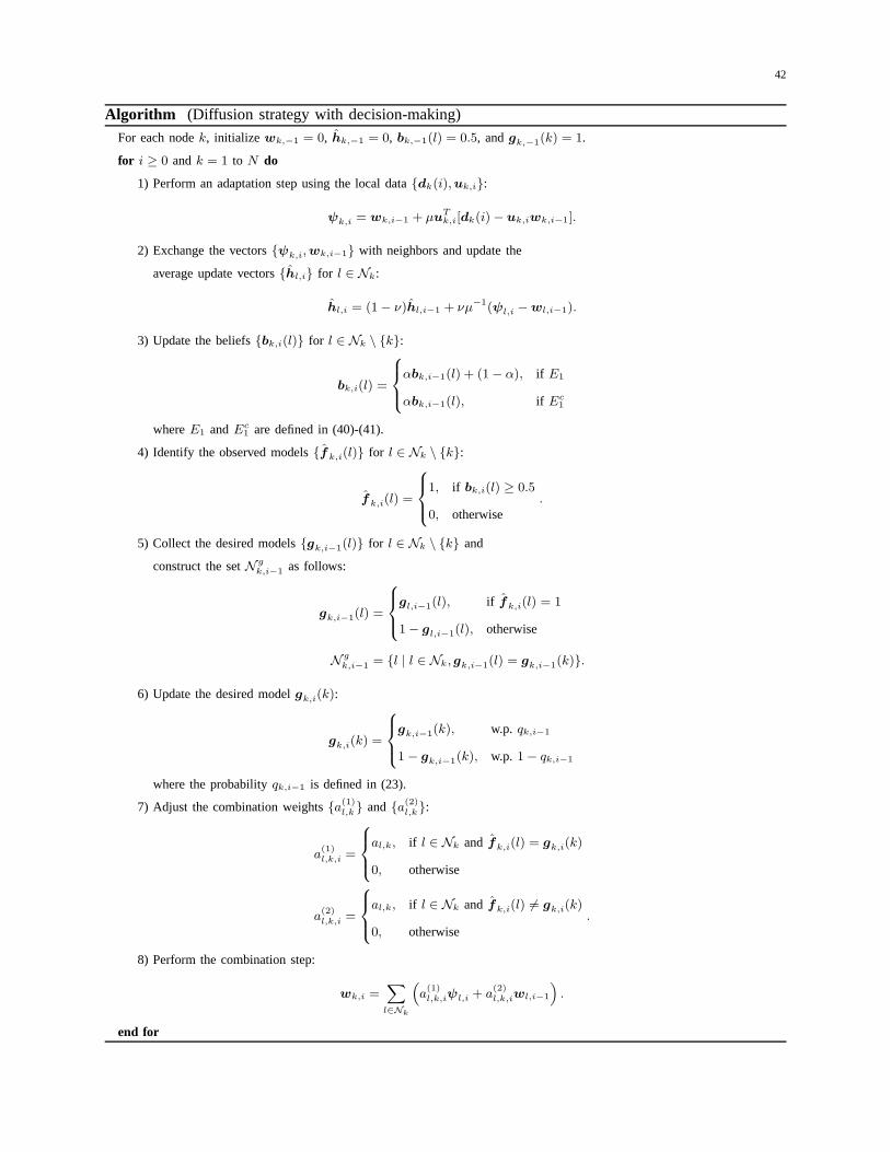
42
Algorithm (Diffusion strategy with decision-making)
For each nodek, initialize wk,−1 = 0, hk,−1 = 0, bk,−1(l) = 0.5, andgk,−1(k) = 1.
for i ≥ 0 andk = 1 to N do
1) Perform an adaptation step using the local data{dk(i),uk,i}:
ψk,i = wk,i−1 + µuTk,i[dk(i)− uk,iwk,i−1].
2) Exchange the vectors{ψk,i,wk,i−1} with neighbors and update the
average update vectors{hl,i} for l ∈ Nk:
hl,i = (1− ν)hl,i−1 + νµ−1(ψl,i −wl,i−1).
3) Update the beliefs{bk,i(l)} for l ∈ Nk \ {k}:
bk,i(l) =
αbk,i−1(l) + (1− α), if E1
αbk,i−1(l), if Ec1
whereE1 andEc1 are defined in (40)-(41).
4) Identify the observed models{fk,i(l)} for l ∈ Nk \ {k}:
fk,i(l) =
1, if bk,i(l) ≥ 0.5
0, otherwise.
5) Collect the desired models{gk,i−1(l)} for l ∈ Nk \ {k} and
construct the setN g
k,i−1 as follows:
gk,i−1(l) =
gl,i−1(l), if fk,i(l) = 1
1− gl,i−1(l), otherwise
N g
k,i−1 = {l | l ∈ Nk, gk,i−1(l) = gk,i−1(k)}.
6) Update the desired modelgk,i(k):
gk,i(k) =
gk,i−1(k), w.p. qk,i−1
1− gk,i−1(k), w.p. 1− qk,i−1
where the probabilityqk,i−1 is defined in (23).
7) Adjust the combination weights{a(1)l,k} and{a(2)
l,k}:
a(1)l,k,i =
al,k, if l ∈ Nk and fk,i(l) = gk,i(k)
0, otherwise
a(2)l,k,i =
al,k, if l ∈ Nk and fk,i(l) 6= gk,i(k)
0, otherwise.
8) Perform the combination step:
wk,i =∑
l∈Nk
(
a(1)l,k,iψl,i + a
(2)l,k,iwl,i−1
)
.
end for


