
Electronic copy available at: http://ssrn.com/abstract=1542364
The authors gratefully acknowledge support from the Research Foundation of the City University of New York andfrom the National Science Foundation under grant number SES-9211228. We are also grateful to Wayne Gray andJoseph Tracy for supplying data, and to Anne Krill, Lou Nadeau, Kamal Desai, Steve Guo, and Evangelica Papaetroufor able research assistance. Helpful comments on earlier versions were provided by Gerald Oettinger, Wayne Gray,Alan Krueger and seminar participants at Hunter College, Columbia University, Princeton University and CERGE-EI,Prague.
Debt, Profitability, and Investment in Workplace Safety
Devra L. Golbe+XQWHU�&ROOHJH�DQG�WKH�*UDGXDWH�&HQWHU��&81<
and
5DQGDOO�.��)LOHU+XQWHU�&ROOHJH�DQG�WKH�*UDGXDWH�&HQWHU��&81<�DQG�&(5*(�(,��3UDJXH�
&]HFK�5HSXEOLF
Abstract:
We investigate how a firm’s financial performance affects workplace safety. We provide empiricalestimates of the relationship between a firm’s financial condition and its investment in workplacesafety using plant-level proxies for safety performance from OSHA records for thirteen largeindustries for the period 1972-87. Our results suggest that firms with higher operating margins aresafer work places as, in general, are firms with more debt in their capital structure. These results areconsistent with a number of theoretical models in which financial factors influence operatingdecisions.
$EVWUDNW�
9�QD§HP�³OgQNX�]NRXPgPH�MDN�RYOLYÈXMH�ILQDQ³Qm�VLWXDFH�ILUP\�EH]SH³QRVW�SUDFRYQmKR�SURVWÎHGm�3RVN\WXMHPH�HPSLULFNk�RGKDG\�Y]WDKX�PH]L�ILQDQ³QmPL�XND]DWHOL�ILUP\�D�MHMmPL�LQYHVWLFHPL�GREH]SH³QRVWL� SUDFRYQmKR� SURVWÎHGm�� 1D§H� RGKDG\� MVRX� ]DOR©HQ\� QD� GDWHFK� QD� ILUHPQm� rURYQL� ]H]g]QDPÖ�26+$��NWHUk�SRSLVXMmFm�SÎLEOL©Q¬�Y¬YRM�EH]SH³QRVWL�SUR�WÎLQgFW�YHON¬FK�SUÖP\VORY¬FKRGYÀWYm�Y�OHWHFK����������'RVD©HQk�Y¬VOHGN\�QD]QD³XMm��©H�ILUP\�V�YÀW§mPL�RSHUD³QmPL�QgNODG\�PDMmEH]SH³QÀM§m�SUDFRYQm�SURVWÎHGm��VWHMQÀ�MDNR�WR�O]H�REHFQÀ�ÎmFL�R�ILUPgFK��NWHUk�PDMm�Y¬UD]QÀM§m�SRGmOGOXKX�YH�VY¬FK�NDSLWgORY¬FK�VWUXNWXUgFK��7\WR�Y¬VOHGN\�RGSRYmGDMm�PQRKD�WHRUHWLFN¬P�PRGHOÖP�YH�NWHU¬FK�ILQDQ³Qm�IDNWRU\�RYOLYÈXMm�RSHUD³Qm�UR]KRGRYgQm�

Electronic copy available at: http://ssrn.com/abstract=1542364
1See Harris and Raviv (1991) and Ravid (1988) for surveys of the literature.
2On risk, see , e.g., Jensen and Meckling (1976), and Golbe (1988). On the level ofinvestment see , e.g., Myers (1977) and Myers and Majluf (1984). On output market effects, seeBrander and Lewis (1986). On input choices see Bronars and Deere (1991), Dasgupta andSengupta (1993), and Kim and Maksimovic (1990a and 1990b).
1
I. Introduction
In this paper we investigate the relationship between firms’ financial condition and their
decisions regarding workplace safety. Workplace injuries and illnesses extract a high cost from
American industry: in 1994, there were 3.8 incidents per 100 workers resulting in lost workdays.
Regulatory and compliance costs are also significant. Fry and Lee (1989) provide estimates that
suggest that firm values decline significantly on announcement of Occupational Safety and Health
Administration (OSHA) enforcement actions. Variation across firms in accident rates and
compliance is considerable, even within a given industry. It is, therefore, important to understand
the factors that affect the firm’s decisions regarding investment in workplace safety. In particular,
we find that firms’ decisions are related to levels of profitability and indebtedness. Understanding
this relationship can contribute to the design of efficient regulatory regimes for workplace safety.
It may also lead to more efficient use of regulatory resources as well as more efficient design of both
public and private insurance schemes. Finally, our results provide additional evidence in support
of the literature linking financial factors to real operating decisions.
Recent theoretical literature suggests that operating and financial decisions are not
independent. Classical microeconomic models of the firm focus on the maximization of operating
income independent of the source of investment funds or the subsequent division of earnings
between equity holders and debt holders. Modigliani and Miller’s (1958, 1963) proof that the value
of the firm is independent of capital structure rests on the notion that the total stream of returns to
the firm is independent of capital structure in frictionless markets. In subsequent work, various
authors have cited a number of avenues through which financing decisions can affect the return
stream (or the market's estimate of the stream). These include taxes, the divergent interests of
managers, shareholders, and bondholders, the effect of information asymmetries, and the possibility
of costly financial distress.1 These factors may affect the amount of risk the firm chooses to bear,
the level of investment, the level of output, and the firm's input choices.2 In this paper, we focus
on the impact of financial structure and profitability on one particular input choice, the firm's

3See, e.g., Viscusi (1979).
2
investment in workplace safety. The empirical results in this study provide evidence that more
profitable firms and more highly leveraged firms are safer places in which to work, although the
impact of leverage on safety is smaller for more profitable firms.
Prior empirical work examining the effects of firm financial condition on safety has produced
mixed results. The most closely related work was motivated by concerns arising from transportation
deregulation and focuses on consumer safety, rather than workplace safety. Golbe (1983), using data
from the railroad industry in the 1960s, presented evidence suggesting that firms in financial
difficulty have weaker safety records. Golbe (1986), Rose (1990), and Talley and Bossert (1990)
studied the relationship between firm profits and airline safety. Golbe found little statistical
relationship between profits and safety while Rose found accident rates to be negatively related to
firm profits (particularly for small airlines). Talley and Bossert found that profitability is related to
maintenance expenditures, but that maintenance expenditures are not significantly related to
accidents. Feinstein (1989), in a study of nuclear power plants, used a different measure of financial
strength based on bond ratings and found no evidence that economic incentives affect safety. Beard
(1992) used cash flow measures in a study of motor carrier safety and found a significant
relationship between safety and financial status.
The remainder of the paper is organized as follows. Section II discusses the relevant theory;
Section III, our data and estimation strategy, and Section IV, our empirical results. Our conclusions
comprise Section V.
II. Theoretical Background
In the basic model of workplace safety, the firm chooses its level of safety investment by
balancing the marginal costs and benefits of such investments.3 Accidents are random events that
depend on the level of safety investment, worker behavior, and perhaps other factors. The benefits
of increased safety include reduced accident costs (including direct costs and worker compensation
premiums) and lower wages (assuming workers demand a compensating differential for hazardous
workplaces). If safety is regulated, the benefits of increased safety investment also include a
decrease in the level of penalties imposed for violating government safety standards. The costs of
increased safety include direct costs of equipment replacement or modification as well as costs

4 Fazzari, Hubbard, and Petersen (1988) provide evidence that such effects areempirically important. See also Calomiris and Hubbard (1990), Hoshi, Kashyap, and Scharfstein(1990), and Cohen (1990).
3
involved in worker training. The effect of safety on productivity is theoretically ambiguous.
Increasing safety may involve reduction of the pace of work, lowering productivity and thereby
imposing a cost. On the other hand, accidents themselves can cause interruption of production and
lost output. Thus whether increased safety raises or lowers productivity depends on the specific
conditions in individual workplaces. This simple model omits any potential influences from
financial structure. There are, however, a number of avenues through which financial factors can
influence operating decisions such as the level and type of safety investment.
Several models suggest that cash flow may affect operating decisions. One plausible route
is through capital market imperfections. Myers and Majluf (1984) argue that information
asymmetries between managers and outsiders may generate a “pecking order” for capital in which
internally generated funds are cheaper than external funds.4 Some investments may be profitable
at the cost of internal funds, but not at the cost of external funds. For firms without financial slack,
increasing cash flow may thus increase investments, including safety investments. Safety
investments may involve considerable information asymmetries, so that such investment may be
particularly sensitive to the availability of internal funds.
Leverage and its attendant risk of bankruptcy may also generate links between financial
structure and investment. Firms in financial distress may have an incentive to incur more risk (e.g.,
Brander and Lewis (1986), Golbe (1988)). Managers whose goal is to maximize the value of equity
may not make efficient investments in safety, because the initial costs of safety investments are
borne by the equity holders, while if the firm goes bankrupt accident costs will be borne by the
bondholders. Higher leverage makes bankruptcy more likely, implying that firms with more debt
might be expected to assume greater risks and hence invest less in safety.
On the other hand, higher leverage may create incentives for greater investment in safety.
First, debt may serve as a monitoring device. Jensen (1986) argues that the increased threat of
bankruptcy which accompanies increased debt forces managers to make more efficient use of the
firm’s resources. Second, while increased debt increases the likelihood of financial distress,
financial distress may not eliminate equity holders' interest in the firm. Only 10% of firms in

5See Weiss (1990) and Wruck (1990) for citations to some other recent papers.
6See Dasgupta and Sengupta (1993) and Bronars and Deere (1991).
4
financial distress proceed to liquidation; in addition, equity holders frequently retain some residual
interest in a firm following a formal bankruptcy in the United States (see Wruck (1990)). Since the
costs of bankruptcy or reorganization can be significant,5 managers will have an incentive to avoid
crossing the threshold that triggers these events. This suggests that firms with greater leverage (and,
therefore, a higher possibility of bankruptcy) will have an incentive to be extra cautious and spend
larger amounts on accident avoidance. Thus, the net effect of leverage on safety investment is
ambiguous. It is clear, however, that the effects of debt should be stronger for firms near financial
distress. We would, therefore, expect that the empirical influence of debt on safety investments will
vary with profitability.
The literature also suggests that capital structure can influence the firm’s input mix. Kim and
Maksimovic (1990a,b) argue that in the presence of conflicts of interest between equity holders and
debt holders, the firm’s choice of inputs will be affected by the existence of debt. In particular,
leveraged firms are likely to show a preference for inputs which can be more easily monitored and
collateralized. To the extent that adherence to OSHA safety standards is capital based and,
therefore, more easily monitored than other kinds of safety techniques, we would expect the firm to
bias its safety technology towards meeting the standards. Note that, in the presence of such an
effect, a decrease in violation of standards may represent not an increase in the firm’s level of safety,
but rather a change (possibly inefficient) in the technology it uses to achieve the desired level of
safety (which itself may be affected by agency costs). The signs of these effects are theoretically
ambiguous and dependent on the firm’s production function.
Similarly, the literature has demonstrated that capital structure may affect the firm’s
bargaining position with its employees.6 Several authors have shown that increased leverage is
advantageous in bilateral bargaining with workers, because it reduces the surplus available for
sharing with input suppliers. Dasgupta and Sengupta (1993) show that debt is negatively correlated
with the (ex ante) bargaining power of the firm, where bargaining power is defined as the share
allocated to the firm in an asymmetric Nash bargaining solution. However, the sign of the
relationship between worker payoff and bargaining power, and hence between debt and worker

7Although the use of accidents or the resulting lost workdays as a measure of safetyinvestment is intuitively appealing, there are a number of potential problems. OSHA does reportthe fraction of workdays lost to occupational accidents. However, in approximately 26 percentof the inspections, data on lost workdays are not reported. In an additional 62 percent of theobservations, lost workdays are reported as zero. While some of these are truly zero, others areundoubtedly missing observations.
5
payoff, is ambiguous. Increased firm bargaining power simultaneously decreases debt and the share
of total surplus claimed by workers. However, lower leverage may decrease agency costs associated
with debt and thus increase the divisible surplus. Consequently, debt and worker payoff may be
positively or negatively correlated. In the context of our model, if workplace safety is one form of
rent-sharing with labor, workplace safety may increase or decrease with leverage.
In sum, the literature suggests a variety of mechanisms through which financial factors can
affect a firm’s investment in workplace safety. We have not addressed the efficiency aspects of
these effects. If workers are imperfectly informed about the likelihood and costs of workplace risks,
and if regulation corrects imperfectly for any such market failures, an all-equity firm will not in
general provide the social-welfare maximizing level of workplace safety. Whether the levered firm
will provide more or less workplace safety than the unleveraged firm, and hence increase or decrease
any inefficiencies, is theoretically ambiguous. Empirical analysis is necessary to ascertain the size
and direction of the effects of leverage and profitability on safety.
III. Data and Estimation
A. Sample and Safety Measures
Measurement of safety investment is a particularly difficult problem, since the firm’s safety
expenditures will often not be so classified. Many, if not most, such costs will be embedded in
equipment or training costs or in a slower speed of the assembly line. Thus, it is difficult to measure
safety investment directly. As proxies, we use the record of plants’ violations of Occupational Safety
and Health Administration (OSHA) standards and the penalties assessed for those violations.7
Although we began with a data set containing records of all OSHA inspections from 1972
through 1987, the sample analyzed was limited in a number of ways. In order to reduce the data set

8In order to match the OSHA data to the financial data discussed below it was necessaryto track the ownership chains of plants by hand.
9Although our financial information is at the firm level, there may be inherentdifferences across plants within a given firm due to age, technology in use, union/managementrelations or other factors.
6
to a tractable size,8 we focused on a subset of thirteen industries. These industries were selected
according to three criteria: (1) a large number of publicly traded firms; (2) a wide variation in
financial performance among those firms; and (3) a high probability of safety problems as indicated
by Bureau of Labor Statistics reports of workplace injuries.
We further limited our analysis to safety inspections. OSHA inspections are directed towards
either violations of safety standards or violations of health standards. The two types of inspections
are independent and conducted by different inspectors. There are a number of reasons to believe that
safety violations will differ from health violations in their relationship to the independent variables.
First, the standards themselves differ. OSHA safety standards tend to be technological in nature,
providing detailed specifications for machinery and procedures, while the health standards are more
outcome-oriented, specifying exposure levels for hazardous substances rather than the use of a
particular technology. Second, the harms to workers, who the standards are intended to deter, are
much more immediate and obvious in the case of safety standards than of health standards. Thus,
firms’ incentives to meet the standards will differ between the two types.
Finally, because we will use panel data estimators (see discussion below), we limited the
analysis sample to plants with more than one inspection.9 After eliminating observations with
missing data, the final sample contained 5,492 inspections in 793 plants. Table 1 shows the number
of firms and plants as well as the mean number of inspections per plant and violations found per
inspection by industry.
OSHA categorizes violations as being either “serious” or “not serious.” Serious violations
differ from other violations in the degree of threat to worker health and safety posed, with serious
violations posing a significant and immediate threat. Violations are assigned to a category according

10Several studies have suggested that OSHA had little, if any, impact on accident rates(see Viscusi (1979), Mendeloff (1979), Smith (1979), McCaffrey, (1983), Bartel and Thomas(1985), and Rusher and Smith (1991)). Other work (Viscusi (1986), Scholz and Gray (1990) andGray and Jones (1991a,b)) has found a small but significant effect from OSHA inspections inincreasing workplace safety.
7
to the standard violated and inspectors are supposed to have no discretion over the category into
which a violation falls. In addition, a small number of “willful and repeated” violations are
categorized as serious no matter what standard is being violated. Serious violations are more likely
to be related to true safety hazards. The reported number of serious violations also seems less likely
to be related to inspectors' discretion. Thus, we focus on models of serious violations, although we
also examine the penalties imposed for violations. Many inspections turned up no cited violations.
As can be seen in Table 2, which shows the frequency distribution of each type of violation, almost
44% of inspections in the sample we are analyzing found no violations at all, while over 70%
discovered no serious violations. Serious violations and all violations are highly related, with a
correlation coefficient of .65 across all inspections in our sample.
Violations of OSHA standards indicate hazards that can be reduced by capital investments
in equipment or changing production speed and technology, actions which we have argued above
are likely to be affected by a firm's financial condition. Although previous research investigating
the link between OSHA and workplace health and safety has produced mixed results,10 it is
important to realize that criticism of OSHA's effectiveness does not necessarily imply that the data
are inappropriate for our research. Explanations for OSHA's small impact on injury and illness rates
fall into two categories. The first is that “the low probability of inspection and small penalties
imposed on violators [provide] little incentive for hazard abatement” (Gray, 1990). Thus, the
assertion is that OSHA citations do not provide sufficient incentives to alter behavior, not that
compliance with OSHA standards would not reduce accidents. The second is that many common
types of workplace accidents are unlikely to be affected by compliance with OSHA standards
(Mendeloff (1979)). Nevertheless, investments that would bring a firm into compliance with OSHA
safety standards should create a reduction in the expected cost of some types of accidents and,
therefore, in the total expected costs due to accidents.

11Defined as 1 - (operating expenses)/(operating revenues). This is essentially a measureof operating income scaled by revenues.
12While cash flow may be a better match for the theoretical constructs discussed above,many of the firms in our sample did not report depreciation, making it impossible for us tocalculate this variable.
13These as well as other variable definitions are summarized in the Data Appendix.
14Operating margin at the sample median was 10.3%. Replication of results using otherdivisions produces the same general patterns discussed below.
15The name of the company that owns each plant found in the OSHA data was matchedby hand to the COMPUSTAT data. If the company name was not found in the COMPUSTATdata, directories of corporate ownership were used to determine if the owner had a listed parentcompany.
8
B. Independent Variables
Previous studies of the impact of the firm’s financial condition on safety have used a variety
of measures of financial condition. Golbe (1983) and (1986) considered net income and rate of
return measures of profitability. Rose (1990) used operating margin11 as a measure of profitability
as well as the interest coverage ratio (as a measure of leverage), and working capital and current
ratios to measure liquidity. Feinstein (1989) constructed a variable based on Moody’s bond ratings
as a measure of financial condition. Talley and Bossert (1990) used operating ratio (operating cost
as a fraction of operating revenue) as a measure of profitability. Beard (1992) used a measure of
capitalized cash flow as a measure of financial condition.
As proxies for the financial and profitability variables specified in the theories described
above we use the firm’s operating margin (operating income divided by sales)12 and debt ratio
(defined as long-term debt divided by the sum of long-term debt, preferred stock and common stock,
all valued at market prices).13 We interact the firm’s debt ratio with a set of three dummy variables,
arbitrarily chosen to divide the sample into three groups: those with negative operating margins,
those with operating margin below 10%, and those with operating margin above 10%.14 This
division was designed to test the hypothesis discussed above that the effect of leverage is greater for
firms near financial distress. Our source for financial data is the R&D Master file assembled from
COMPUSTAT and other sources by the NBER (Cummins, et al 1988).15 This data source presents
a potential problem in that only large, publicly traded firms are covered, thus limiting our sample
through missing data as discussed above. A priori, firms in COMPUSTAT data are more likely to

16See Bronars, Deere and Tracy (1994) for details.
17In addition, inspections are apparently targeted toward larger firms. Unionized plantshave a higher probability of being inspected and are scrutinized more intensively (see Weil(1991)). This suggests the possibility of selection bias in our sample.
9
be financially stable than are small, privately-held firms. However, analysis of the data suggests that
there is sufficient variation in financial condition among the firms in this sample to enable estimation
of the impact of financial conditions on safety investment even though results should be extrapolated
to smaller firms only with considerable caution. Over three percent of inspections in our sample
were for plants whose parent company had negative operating margins. For the full sample, the
mean operating margin was 10% with a standard deviation of 5% while the mean debt ratio was 39%
with a standard deviation of 22%.
In addition to the financial variables of interest, we control for a number of other factors that
may influence safety investments. Weil (1991) discusses a number of avenues through which
unionization may affect safety investment and compliance with OSHA regulations. Unions often
maintain their own health and safety programs. They may also facilitate the exercise of employee
rights to participate in OSHA enforcement. Unfortunately, we do not have a measure of the extent
of union coverage at the plant level where inspections take place. Instead, we are forced to rely on
overall unionization coverage for the parent company across all its operations. We use union
coverage rates supplied by Bronars, Deere, and Tracy (1994). Unionization rates are calculated from
averaged values of union employment (estimated by rescaling Bureau of Labor Statistics data on
major collective bargaining agreements) and total employment (from COMPUSTAT), where data
are averaged over the periods 1971-74, 1975-78, and 1979-82.16 These data are then merged with
our panel, so that for each firm, the union variable will have the same value for 1972-74, another
constant value for 1975-78, and a third for 1979-87. To the extent that union coverage measured at
the firm level and averaged across years measures plant-level coverage with error, the result will be
classical measurement error and our coefficients should be biased towards zero.
We also control for why OSHA undertook each inspection in our sample. The basic
inspection is known as a “general inspection.” While any plant may be subjected to such an
inspection, they are targeted toward larger, more hazardous plants.17 OSHA identifies the riskiest
industries in each state based on state or national injury rates and inspects plants in those industries

18If significant violations are found during an inspection OSHA will revisit the plant at alater date to be sure that these have been corrected. We have excluded these “follow-up”inspections from our analysis since they focus only on areas where previous violations have beenfound and it should be expected that few violations will be found during the reinspection, giventhat firms know the nature of previous violations and that a reinspection will occur. Thus, theyare a poor indicator of how a firm's decisions are influenced by its financial performance.
10
starting with the most dangerous (see Gray, 1990). In addition to general inspections, a plant may
be inspected in response to an accident or a complaint (typically from a worker).18 Among the
inspections we analyzed, 26.4% were general programmed inspections, 59.4% were in response to
complaints, and 14.2% followed accidents. General inspections typically discover significantly
more total violations than more limited types of inspections. The mean number of violations for
general, accident and complaint inspections are 7.6, 3.9 and 2.0, respectively. In contrast, all types
of inspections turn up an average of between one and one-and-a-half serious violations.
It is likely that the number of violations reported (and penalties assessed) will be related to
how long it has been since the previous inspection. We cannot use the actual time elapsed since the
previous inspection, since that variable is undefined for the first inspection. We define a variable
which takes on values from zero to one to proxy the time elapsed since the previous inspection. The
larger this variable, the more time has elapsed since a previous inspection and the more a given
inspection is like a first inspection. For the first general inspection of a plant this variable is equal
to one by definition since our data begins with the inception of OSHA inspections. For accident and
complaint inspections prior to a general inspection it is also set to one. For all other inspections, we
define the time-since-last-inspection variable as:
t = 2e t´
1 % e t´& 1
where tN is the time (in years) since the most recent general inspection. Thus, 0 # t # 1, where t
increases as tN increases.
Differences in plant size may also affect safety violations and (per employee) accident arrival
rates. Larger plants should have more opportunities to violate standards. Plant size may also be
related to a plant’s technological design and, therefore, its underlying safety independent of any
investment decisions by the firm. Thus, we include plant size, measured by number of employees,

19Of course, as Brown and Medoff (1990) show, firm size is also likely to incorporate anumber of other effects and its meaning in empirical work is not well understood.
20These states are Vermont, Indiana, Michigan, Minnesota, Iowa, Maryland, Virginia,North Carolina, South Carolina, Kentucky, Tennessee, Arkansas, New Mexico, Arizona, Nevada,Utah, Wyoming, Washington, California, Oregon and Hawaii.
11
in our estimating equations. We allow for non-linearity in this relationship by also including the
square of employment.19
Twenty-one states have taken advantage of provisions under OSHA legislation to substitute
state-level inspection programs for federal OSHA inspections. Since inspections in these states may
differ in their rigor from federal inspections we include a dummy variable for the state-program
states.20 At the federal level, frequencies and intensities of OSHA regulation enforcement may have
varied across Presidential administrations. In the years immediately following adoption of the act,
inspections were typically brief and trivial violations were often cited. During the Carter
administration, penalties for violations increased, while citations for less important violations
decreased. Under Reagan, the level of penalties assessed fell dramatically, and targeted inspections
and serious violations increased (Gray (1990)).
The issue of whether to control for industry is complicated. Industries may vary by their
“natural compliance” with OSHA regulations (see Bartel and Thomas (1985)). Firms in “naturally
compliant” industries will, all other things the same, show fewer violations. Industry dummies may
also pick up the effects of other omitted variables. On the other hand, if financial performance is
correlated across firms in the same industry, industry dummies could incorporate effects of financial
condition on OSHA violations as well as differences in the responsiveness of different industries to
variations in these conditions. Thus, results containing and omitting industry dummies are reported
below for comparison purposes.
IV. Results
The distribution of number of violations reported in Table 2 suggests that OLS regression
is not the most appropriate method for estimating our model. Only integer values are possible and
the data are dominated by zeros and small values, so that an appeal to approximate continuity is

21 See Gourieroux, Monfort and Trognon (1984), Hausman, Hall and Griliches(1984), and Cameron and Trivedi (1986). See Gray and Jones (1991a) for an application toOSHA violations.
22See Hausman, Hall and Griliches (1984). Wooldridge (1990) discusses the conditionsunder which this quasi-conditional maximum likelihood estimator is consistent andasymptotically normal.
12
inappropriate. When confronted with data of this type, a natural alternative is to use a Poisson
regression model, where the probability of each possible outcome (yt) is given by:
pr(yt) '8
yt
t e &8t
yt !
with 8t = exp(xt$). Such a model can only take integer values, while the exponentiation ensures that
these values will be positive.21
The simple version of the Poisson model suffers from a serious drawback by assuming
equidispersion in the data, implying that the conditional mean and variances in the model are equal
(i.e., E(yt Xt) = var (yt Xt) = exp (Xt$^ )). While the estimated coefficients from this model will
be consistent, if the data are actually overdispersed estimated standard errors will be biased
downwards and significance levels will be overstated. Similarly, underdispersed data will lead to
upwardly biased standard errors.
The most common alternative in such a situation is the Negative Binomial model, which
extends the Poisson regression by assuming that yt, conditional on 8t, follows a Poisson distribution
while 8t itself follows a gamma distribution. Commonly, the form of this gamma distribution is
chosen so that the conditional mean of yt remains the same as the Poisson model (exp (Xt$^ )) but the
variance contains the additional parameter " such that Var[yt] = E[yt]{1 + "E[yt]} to provide for
overdispersed data (see Cameron and Trivedi (1986)).
We take advantage of the fact that most plants were inspected several times over the period
observed to estimate a Negative Binomial model with random plant effects.22 Such a model extends
the simple Poisson model by adding an individual (here plant) effect such that 8it = exp(xit$ + ui ).
If ui is assumed to follow a gamma distribution with parameters (2i ,2i), the result is a Negative
Binomial model with a parameter that varies across plants (indexed by i). 2i/(1+2i) is assumed

23A beta r.v. has the density function f(x) = [B(a,b)]-1xa-1(1-x)b-1 for 0< x< 1, where thebeta function B(a,b) = '(a)'(b)/'(a+b). Its expected value is a/(a+b).
24a/(a+b)= E[1/(1+"i)], so plim(b/a) = E("), and the model without industry effectsimplies a variance to mean ratio of 3.7 and the model with industry effects implies a ratio of 4.5.
25For the cross section estimates, !2) log likelihood = !2(!6448!!6415.6) = 64.86. Forthe panel data estimates, !2) log likelihood = !2(!6374.1!!6308.9) = 130.3 Both statistics aredistributed as chi-square with 12 degrees of freedom; the critical value at the 1% level (2-tailedtest) is 28.3.
13
distributed as a beta (a,b) random variable.23 Note that there is randomness across firms and across
time, because 8it is a realization from a probability distribution. Note also that this procedure
estimates the parameters of the beta distribution but that 2 is not identified, so we cannot compute
expected values for these models.
. Table 3 contains estimates of both a conventional cross-section negative binomial and a
random effects panel-data model. For each model, estimates without and with industry dummies
are reported. The data indicate considerable overdispersion; estimates of ", the overdispersion
parameters in the cross-section estimates, are significantly different from zero and imply an
overdispersion rate of about 7.8. The random effects panel data models imply a mean overdispersion
rate of about 3.7 (without industry effects) or 4.5 (with industry effects).24 Standard likelihood ratio
tests indicate that the industry dummies add significant explanatory power for both models.25 It is
clear that financial results, especially with respect to operating margins, are correlated across firms
in an industry. Inclusion of industry dummies reduces the magnitude of the coefficients on operating
margin by about 50%. Thus, models including industry dummies may understate the effect of
financial variables on safety violations. On the other hand, results omitting them may erroneously
attribute industry differences in intrinsic safety (or intensity of OSHA inspection) to financial
effects. In any case, only the quantitative magnitude and not the general pattern of results depends
on whether we control for industry.
The imposition of random plant effects has a number of significant effects on the estimated
coefficients. Most important, from our point of view, is that the sign of the leverage coefficient is
sensitive to the inclusion or exclusion of these effects. Without plant effects, the debt ratio has a
positive effect on violations which increases in magnitude and significance as operating margin
increases. When we control for random plant effects, leverage has a negative effect on violations

26For the models omitting dummies, !2) log likelihood = !2(!6448!!6374.1) = 147.8. When industry dummies are included, !2) log likelihood = !2(!6415.6!!6308.9) =213.4. Bothstatistics are distributed as chi-square with one degree of freedom; the critical value at the 1%level (2-tailed test) is 7.88.
27Weil (1991) estimates a simple OLS model and finds that unionization is positivelycorrelated with both violations and penalty per violation.
14
that becomes smaller (in absolute value) as operating margin increases. In addition, controlling for
random plant effects switches the coefficient on accident inspections from negative to positive and
eliminates the apparent effect of plant size. We test the alternative specifications using a likelihood
ratio test. The negative binomial model without random effects is nested within the random effects
model. Thus, 2) log likelihood is distributed as chi-square with one degree of freedom. Whether
or not industry dummies are included, the test suggests that the models omitting the random plant
effects can be rejected.26 Thus, in interpreting our results, we focus on the models with plant effects.
It is clear that firms with higher operating margins are cited for fewer serious violations.
This may be because these safety investments are profit maximizing (possibly as a result of relaxing
the liquidity constraint in a “pecking order” model) or because firms with higher operating margins
are generating greater economic rents that must be shared with workers who value safety. The latter
interpretation is consistent with our results for unionization. We find that firms where a greater
fraction of the workers are unionized also have significantly fewer serious OSHA violations.27 This
finding is especially strong since we have not been able to control for such features as the average
age of the capital stock; we would expect to find that unionized workers are concentrated in older
plants that should ceteris paribus have more safety violations due to the use of older technologies
and machinery.
In the cross-section estimates, greater leverage is associated with more citations for firms
with positive operating margin. Once we take into account plant-specific effects with panel data
estimators, there is a strongly significant negative relationship between debt ratios and serious
violations for firms with low operating margins. This relationship becomes much less pronounced
(and may even turn positive) at high levels of operating margin. This suggests that the unmeasured
characteristics of plants which make them prone to more violations are positively correlated with
the leverage ratio of the owning firm. The variation in the effect of debt ratios across different levels
of profitability is attenuated if industry dummies are included in the estimates. Thus, there are

28Even when industry dummies are included, if operating margin is stratified more finelythere are insignificant coefficients on debt ratios at the upper end of the distribution of operatingmargins. Since theory does not enable us to determine exactly where this relationship betweenleverage and safety should disappear, we have elected to report results for a limited number ofcategories.
15
apparently strong intra-industry commonalities in financial performance.28
This negative relationship between leverage and OSHA violations provides evidence relevant
to several of the models described in Section 1. It suggests that if increasing leverage increases the
incentive for managers to take more risks, the effect of that incentive change is outweighed by other
factors such as the increased monitoring by debt holders or the desire to avoid bankruptcy or
reorganization costs that become more likely at higher leverage ratios. The increase in the
importance of debt ratios as operating margin falls adds weight to this conclusion. Second, the
results are consistent with Kim and Maksimovic’s argument that increased leverage biases firms
toward the use of inputs which are more easily monitored. As we noted above, the increase in
compliance with OSHA standards may represent not an increase in workplace safety, but a change
in the technology chosen to achieve a desired level. Finally, we note the hypothesis that leverage
may affect the firm’s bargaining power vis-à-vis its employees, thus generating a correlation
between debt and worker payoffs.
Control variables generally behave in sensible ways. Plant size is positively related to
serious violations when we ignore plant effects. In models with random plant effects, however, plant
size is unrelated to serious violations. This suggests that, at least in part, the effects of plant size
(which may be truly size-related or may be due to other factors correlated with size such as
technological vintage) may be subsumed in the random plant effects. The coefficient of the elapsed-
time variable in the equation for serious violations is significantly different from zero only when
plant effects are included, but industry effects are excluded; in that case the coefficient is negative,
so that fewer violations are found the longer the elapsed time since the previous inspection. This
set of results could arise if inspections are targeted toward more hazardous industries. The time
between inspections will vary negatively with hazardousness and could be expected, therefore, to
be negatively correlated with accidents. When industry dummies are included, they apparently
account for this effect. There is a clear pattern over time (or across administrations) in the number
of violations cited. During the Carter Administration there were more serious violations than at the

29In order to obtain convergence in the state-inspection state results for seriousviolations, it was necessary to combine the Pharmaceuticals, Soaps and Cleaners, Paints andVarnishes, Aircraft, and Oil industries with the reference group (Steel).
16
beginning of our sample period. During the Reagan years, the number of serious violations cited
was lower than during the previous administration but was still greater than in the pre-Carter years.
We cannot tell from the data available to us whether this pattern resulted from increasing compliance
or from a deliberate change in the criteria used to determine whether to issue a citation.
The cross-section estimates suggest that states that conduct their own inspections find fewer
violations , but this effect disappears when plant-level effects are included, suggesting that it is an
artifact of the types of plants found in particular states. We further investigate the effect of the state
opt-out option by analyzing violations separately for state and federal inspection states. Table 4
reports the results of the panel estimates from this analysis.29 Overall, the results are similar between
the two inspection regimes. Operating margin appears to have a greater impact on the number of
violations found and unionization a smaller one when the states control the inspection process. This
last result may occur, in part, because these states are a minority of the sample and are less unionized
than the country as a whole, suggesting both that unions may have less power and that the
measurement error created by attributing national firm-level unionization rates to individual plants
in such states may be greater. While the magnitude of the debt ratio coefficients is not much
different in state-inspection states, the significance is lower, due to smaller sample sizes.
Accident inspections obviously occur only after an accident and focus on specific areas of
a plant where there has been an accident. Not surprisingly, they find more serious violations once
plant-specific effects are taken into account. Inspections in response to complaints find fewer
violations than other types of inspections across the board. This last finding at first appears
somewhat puzzling since one might expect that a worker complaint would be indicative of a
violation. To investigate this result we repeated our estimates excluding inspections generated by
complaints. Results are shown in Table 5; they parallel those for the full set of inspections with two
important differences. In every specification, the negative effect of unionization is substantially
diminished (usually to less than half its previous size), becoming generally insignificant. This
suggests that unions may use OSHA complaints as a way of harassing employers independent of the
actual presence of violations. We also see a difference with respect to the debt ratio variables.

30Estimates for some industries did not converge.
31This variable is reported in units of $10,000.
32Convergence was difficult to obtain. In order to do so, the top 2% of observations(with penalties greater than $10,000) were recoded as $10,000 and a two-limit Tobit model (withthe upper bound at 1 = $10,000) was estimated. As might be expected, the magnitude of thesecoefficients is more sensitive to changes in equation specification than those in the previous tablealthough we have seen no modifications (such as omitting a variable) that alters the main thrustof the results.
17
Operating margin is still significantly negatively related to violations whether industry and plant
effects are included or excluded. However, while debt ratio is significantly related to violations only
when we allow for random plant effects, the relationship has the same pattern across all
specifications: a negative relationship between leverage and violations which is attenuated as
operating margin increases.
Although we do not report the coefficients for the industry dummies, the regression results
show that (after correcting for other variables) citations were highest in the Steel industry, followed
by Construction Machinery, Grinding, Paper, and Automobiles. The fewest violations were found
in Pharmaceuticals, Paints and Varnishes, Petroleum, and Soaps and Cleaners. Since we have
controlled for financial condition in these estimates, these results suggest that not all of the industry
effects are financial in nature and that a case can be made for including the industry dummies.
Financial effects are found even when we limit our analysis to a single industry at a time.
Coefficients on the financial variables are reported in Table 6.30 In every industry in our sample for
which estimates could be obtained, higher operating margins are associated with fewer violations,
suggesting that the result is not an artifact of inter-industry differences. Results with respect to debt
are less clear. Because of smaller sample sizes, we were not able to get estimates with debt ratio
classified by operating margin for all industries. Coefficients on debt are generally negative, but
significant only in Construction Machinery and Autos; only the Auto industry shows an attenuation
in the effect of debt as operating margin rises.
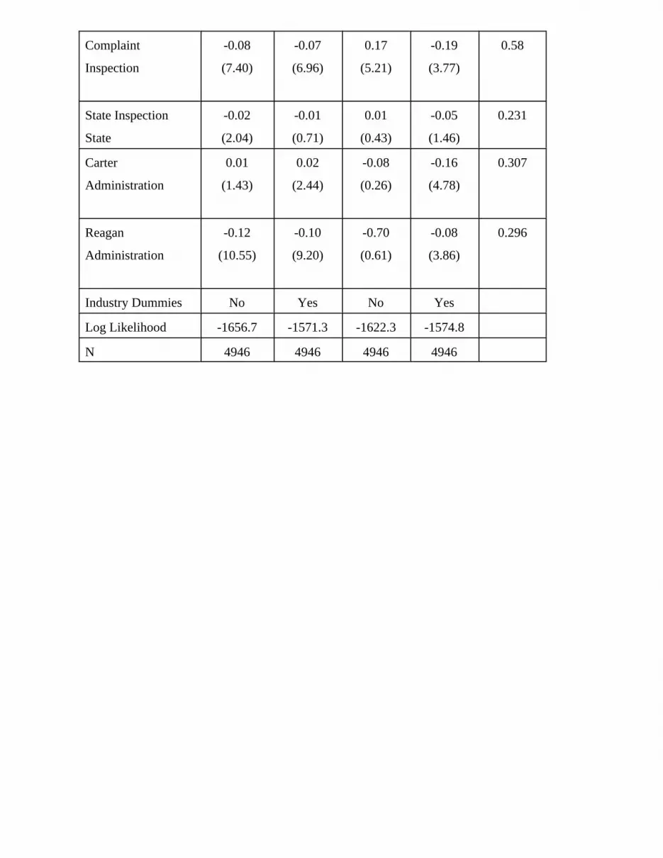
Table 7 contains an analysis of the determinants of total penalties assessed as a result of
inspections.31 Given that total penalties are bounded from below at zero, both cross-section and
random effects panel data Tobit models are presented.32 Results generally parallel those for
violations. Higher operating margins are associated with lower penalties. Debt ratios are positively

18
related to violations when plant effects are ignored, but once plant-specific effects are taken into
account, the results are difficult to interpret, since the signs and significance vary depending on the
inclusion of industry dummies. Plants operated by more unionized firms have lower penalties as
do plants inspected as a result of a worker’s complaint. Once plant-specific effects are taken into
account, when a given plant has more employees it tends to have lower levels of penalties as do
plants that have been inspected longer ago. Again, if OSHA targets inspections toward more
hazardous plants, then time since last inspection will be negatively correlated with hazardousness
and therefore with penalties. The plant size effects are more puzzling since one might expect that
penalties would be higher where more employees are at risk. The plant size results may be, at least
in part, a reflection of vintage effects or financial condition.
The Tobit model makes the implicit assumption that the coefficients in an equation
estimating the amount of penalties conditional on the fact that a firm received any penalty are
identical to those determining the probability of receiving any penalty at all (see Cragg (1971) and
Fin and Schmidt (1984)). This assumption may be questioned given that almost sixty percent of the
inspections in our sample resulted in no penalty. The appropriate alternative in this case is to
estimate a probit model for the probability of any penalty and a truncated regression model for those
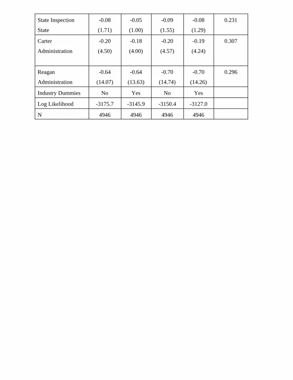
observations that received penalties. Table 8 reports the results of probit estimates of the probability
of an inspection resulting in any penalties. The truncated regression for amount of penalties,
conditional on there being positive penalties, did not converge and Ordinary Least Squares are
inconsistent in such a situation, so no such results are presented. The determinants of the probability
of being penalized appear to differ from those for the number of violations and the amount of
penalties in several significant ways. Once industry is taken into account, there is no relationship
between the probability that a penalty is imposed and a firm’s operating margin even though more
profitable firms have fewer violations and lower levels of penalties. Firms with higher debt ratios
are more likely to be penalized even though they have fewer serious violations. Although this effect
is smaller at higher levels of profitability it is always statistically significant. This result raises
issues of whether OSHA’s propensity to impose penalties reflects actual safety hazards or a
perception by the agency that certain types of firms (i.e., more highly leveraged) should be penalized
independent of their safety performance.

19
V. Conclusions
The results provide strong evidence that financial performance affects firms’ workplace
safety decisions, at least to the extent that these decisions are reflected in compliance with OSHA
standards. Operating margin is consistently negatively related to violations and penalties: firms with
higher operating margins violate fewer OSHA standards and pay lower penalties. While the
statistical relationship with respect to leverage is somewhat less strong, the pattern appears clear:
more highly leveraged firms violate fewer OSHA standards, though the effect is attenuated at higher
levels of operating margin. These findings, that financial factors influence the real decisions of firms
suggests that financial performance, should be considered in setting regulatory policy and allocating
enforcement resources, as well as in determining insurance premiums.

20
REFERENCES
Bartel, Ann P. and Lacy Glenn Thomas (1985) “Direct and Indirect Effects of Regulations: A NewLook at OSHA's Impact,” Journal of Law and Economics, 28, 1-26.
Beard, T. Randolph (1992) “Financial Aspects of Motor Carrier Safety Inspection Performance,”Review of Industrial Organization, 7, 51-64.
Brander, James A. and Tracy R. Lewis (1986) “Oligopoly and Financial Structure: The LimitedLiability Effect,” American Economic Review 76, 956-970.
Bronars, Stephen and Donald Deere (1991 ) “The Threat of Unionization, the Use of Debt, and thePreservation of Shareholder Wealth,” Quarterly Journal of Economics 106(1), 231-54.
______, _____ and Joseph Tracy (1994) “The Effects of Unions on Firm Behavior: An EmpiricalAnalysis Using Firm-Level Data,” Industrial Relations, 33 (4), 426-451.
Brown, Charles and James Medoff (1990) “The Employer Size-Wage Effect” Journal of PoliticalEconomy, 97, 1027-1059.
Calomiris, Charles W. and R. Glenn Hubbard (1990) “Firm Heterogeneity, Internal Finance, and'Credit Rationing,'” The Economic Journal, 100, 90-104.
Cameron, A. Colin and Pravin K. Trivedi (1986) “Econometric Models Based on Count Data:Comparisons and Applications of Some Estimators and Tests,” Journal of AppliedEconometrics, 1, 29-53.
Cohen, Wesley M. (1990) “Incomplete Markets, Intra-Industry Firm Heterogeneity and Investment,”Journal of Economic Behavior and Organization, 14, 223-248.
Cragg, J. (1971) “Some Statistical Models for Limited Dependent Variables with Applications tothe Demand for Durable Goods,” Econometrica, 39, 829-844.
Cummins, Clint, Bronwyn H. Hall, Elizabeth Lederman, and Joy Mundy (1988) The R & D MasterFile Documentation, Technical Working Paper No. 72, Cambridge, Mass., NBER.
Dasgupta, Sudipto and Kunal Sengupta. (1993) “Sunk Investment, Bargaining and Choice of CapitalStructure,” International Economic Review 34(1), 203-220.
Fazzari, Stephen M., R. Glenn Hubbard and Bruce C. Petersen (1988) “Financing Constraints andCorporate Investment,” Brookings Papers on Economic Activity, 141-95.
Feinstein, Jonathan S. (1989) “The Safety Regulation of U.S. Nuclear Power Plants: Violations,Inspections and Abnormal Occurrences,” Journal of Political Economy, 97, 115-154.
Fin, T. and P. Schmidt (1984) “A Test of the Tobit Specification Against an Alternative Suggestedby Cragg,” Review of Economics and Statistics, 66, 174-177.
Fry, Clifford and Insup Lee (1989) “OSHA Sanctions and the Value of the Firm,” Financial Review,24(4), 599-610.
Golbe, Devra. L. (1983) “Product Safety in a Regulated Industry: Evidence from the Railroads, “Economic Inquiry, 21, 39-52.
_____ (1986) “Safety and Profits in the Airline Industry,” Journal of Industrial Organization, 34,305-318.
_____ (1988) “Risk-Taking by Firms Near Bankruptcy,” Economics Letters, 28, 75-79.Gourieroux, C., A. Monfort, and A. Trognon (1984) “Pseudo Maximum Likelihood Methods:
Applications to Poisson Models,” Econometrica, 52, 701-720.
Gray, Wayne. (1990) “OSHA Enforcement: History, Effectiveness, and Proposed Reforms.” PaperPresented at the IRRA Annual Meetings, Washington, DC, mimeo.
_____ and Carol Jones (1991a) “Are OSHA Health Inspections Effective? A Longitudinal Studyin the Manufacturing Sector,” Review of Economics and Statistics, 73, 504-508.
21
______ and _____ (1991b) “Longitudinal Patterns of Compliance with OSHA Health and SafetyRegulations in the Manufacturing Sector,” Journal of Human Resources 26(4), 623-53.
Harris, Milton and Artur Raviv. “The Theory of Capital Structure.” Journal of Finance, 46(1), 297-355.
Hausman, Jerry, Bronwyn H. Hall, and Zvi Griliches (1984) “Econometric Models for Count DataWith an Application to the Patents-R&D Relationship,” Econometrica, 52, 909-938.
Hoshi, T., Kashyap, A. and Scharfstein, D. (1990) “Corporate Structure, Liquidity, and Investment:Evidence from Japanese Industrial Groups,” Quarterly Journal of Economics, 106, 33-60.
Jensen, M. (1986) “Agency Costs of Free Cash Flow, Corporate Finance, and Takeovers,”American Economic Review 76(2), 323-329.
Jensen, M. and W. Meckling. (1976) “Theory of the Firm: Managerial Behavior, Agency Costs, andCapital Structure,” Journal of Financial Economics, 3, 305-60.
Kim, Moshe and V. Maksimovic. (1990a) “Debt and Input Misallocation.” Journal of Finance45(3), 795-816.
_____ and _____(1990b) “Technology, Debt, and the Exploitation of Growth Options,” Journal ofBanking and Finance, 14(6), 1113-31.
McCaffrey, David (1983) “An Assessment of OSHA's Recent Efforts on Injury Rates,” Journal ofHuman Resources, 18, 131-146.
Mendeloff, John (1979) Regulating Safety, Cambridge: MIT University PressModigliani, Franco and Merton Miller (1958) “The Cost of Capital, Corporation Finance, and the
Theory of Investment ,” American Economic Review, 48, 261-97._____ and _____(1963) “Corporate Income Taxes and the Cost of Capital: A Correction,” American
Economic Review, 53, 433-443.Myers, S. (1977) “The Determinants of Corporate Borrowing,” Journal of Financial Economics, 5,
147-75.Myers, S and N. Majluf (1984) “Corporate Financing and Investment Decisions when Firms have
Information that Investors do not Have,” Journal of Financial Economics, 13, 187-221.Ravid, S. Abraham. (1988) “On Interactions of Production and Financial Decisions,” Financial
Management, 87-99.Rose, N. L. (1990) “Profitability and Product Quality: Economic Determinants of Airline Safety
Performance,” Journal of Political Economy, 98, 944 - 964.Rusher, John W. and Robert S. Smith (1991) “Reestimating OSHA's Effects: Have the Data
Changed?” Journal of Human Resources, 26, 212-235.Scholz, John T. and Wayne Gray (1990) “OSHA Enforcement and Workplace Injuries: A
Behavioral Approach to Risk Assessment,” Journal of Risk and Uncertainty, 3, 283-305.Smith, Robert S. (1979) “The Impact of OSHA Inspections on Manufacturing Injury Rates,” Journal
of Human Resources, 14, 144-170.Talley, Wayne and Philip Bossert (1990), “Determinants of Aircraft Accidents and Policy
Implications for Air Safety,” International Journal of Transport Economics, 17, 115-130.Viscusi, W. Kip (1979) “The Impact of Occupational Safety and Health Regulation,” Bell Journal
of Economics, 10, 117-140._____ (1986) “The Impact of Occupational Safety and Health Regulation, 1973-1983.” Rand
Journal of Economics, 17, 567-580.Weil, David (1991) “Enforcing OSHA: The Role of Labor Unions” Industrial Relations, 30(1), 20-
36.Weiss, Lawrence A. (1990) “Bankruptcy Resolution: Direct Costs and Violation of Priority of
Claims,” Journal of Financial Economics, 27(2), 285-314.
22
Wooldridge, Jeffrey M. (1990) “Distribution-Free Estimation of Some Nonlinear Panel DataModels,” Massachusetts Institute of Technology, mimeo.
Wruck, Karen H. (1990) “Financial Distress, Reorganization, and Organizational Efficiency,”Journal of Financial Economics, 27, 419-44.

DATA APPENDIX
Variable Descriptions and Sources
Safety measures are taken from OSHA inspection records. Financial data are derived from
the NBER R&D Master File, which is in turn derived from COMPUSTAT. Firm-level union
coverage rates are from Bronars, Deere, and Tracy (1994).
Serious Violations Violations of particular standards which pose an immediate
health or safety threat. Also included in this category are a small
number of "willful and repeated" violations which would not
otherwise be classified as serious.
Penalties Total penalties assessed in $10,000s, deflated with the GNP
deflator.
Operating Margin (Operating Income before Depreciation)/Sales
Debt Ratio Long Term Debt/ (long-term debt + preferred stock + common
stock) (all valued at market prices)
Inspection
Type
(General
omitted)
Complaint 1 if complaint inspection; 0 otherwise
Follow-Up 1 if follow-up inspection; 0 otherwise
Accident 1 if accident inspection; otherwise
State Inspection 1 for state inspection states; 0 otherwise
Presidential
dummies
(pre-Carter
omitted)
Carter 1 for years 1977-80; 0 otherwise
Reagan 1 for years 1981-87; 0 otherwise
Total Employees total employees in inspected plant, in 1000s, from OSHA records.

Time since first
inspection
1 for first inspections,
otherwise = 2e t´
1 % e t´& 1
where tN = time (in years) since previous general inspection
Unionization Bureau of Labor Statistics (BLS) data on major collective
bargaining agreements are used to estimate unionized
employment by year for each firm. Total employment for each
firm by year is obtained from COMPUSTAT. Unionization rates
were calculated from averaged values of union and total
employment, where data were averaged over the periods 1971-74,
1975-78, and 1979-82. See Bronars, et al for details.

TABLE 1
SAMPLE CHARACTERISTICS
Industry # of Firms # of
Plants
Mean # of
Inspection
s per Plant
Mean # of
Total
Violations
/
Inspection
Mean # of
Serious
Violations
/
Inspection
Pharmaceuticals 9 15 3.4 1.98 0.59
Soaps and Cleaners 15 32 3.3 4.52 0.73
Paints and Varnishes 9 26 3.2 2.82 0.73
Grinding 25 65 3.5 5.3 1.17
Metal Forging 38 81 4.4 3.55 0.72
Farm Machinery 17 53 4.7 6.54 0.67
Construction Machinery 33 115 4.9 5.56 1.26
Automobiles 34 171 5.7 4.81 1.06
Aircraft 26 51 6.3 4.84 0.86
Shipbuilding 18 53 12.2 3.69 0.92
Petroleum 15 34 7.3 3.01 0.79
Paper 13 59 6.9 7.8 1.98
Steel (inc. Minimills) 17 38 33.3 3.6 1.47

TABLE 2
DISTRIBUTION OF NUMBER OF VIOLATIONS
Total
Violations
Serious
Violations
0 44% 70%
1 16% 14%
2 8% 5%
3 5% 3%
4 4% 2%
5 3% 1%
6 3% 1%
7 2% 0.5%
8 2% 0.4%
9 1% 0.4%
10 1% 0.3%
11 or more 11% 2

TABLE 3
DETERMINANTS OF SERIOUS OSHA VIOLATIONS
Negative Binomial Models
No Plant Effects Random Plant EffectsVariable
Mean(Std. Dev.)
Operating Margin -2.91(5.01)
-1.62(1.71)
-7.36(15.27)
-3.61(5.06)
0.102(0.055)
Debt Ratio(Operating Margin #0)
0.16(0.37)
0.33(0.75)
-1.26(5.05)
-0.67(2.39)
0.6181
(0.142)
Debt Ratio(0<OperatingMargin#1)
0.35(2.50)
0.33(2.03)
-0.57(4.64)
-0.50(3.98)
0.4981
(0.218)
Debt Ratio (OperatingMargin >.1)
0.86(4.49)
0.54(2.68)
0.03(0.18)
-0.30(1.49)
0.2871
(0.156)
Unionization -0.57(3.76)
-0.65(3.73)
-0.86(6.35)
-1.11(8.13)
0.432(0.214)
Plant Employment(10,000’s)
3.52(2.84)
3.01(2.12)
-0.44(0.47)
-1.09(1.14)
0.034(0.056)
Plant EmploymentSquared
-4.45(0.98)
-3.64(0.69)
0.73(0.23)
1.72(0.54)
0.005(0.023)
Time Since Last GeneralInspection
-0.05(0.70)
0.13(1.42)
-0.35(4.72)
-0.13(1.56)
0.806(0.306)
Accident Inspection -0.51(3.90)
-0.46(3.61)
0.20(2.59)
0.16(2.00)
0.142
Complaint Inspection -0.62(10.37)
-0.64(8.95)
-0.50(8.50)
-0.48(7.71)
0.594
State Inspection State -0.32(4.08)
-0.28(3.19)
-0.10(1.45)
-0.02(0.33)
0.234
Carter Administration 1.46(22.18)
1.49(19.47)
0.94(17.95)
1.03(19.08)
0.325
Reagan Administration 0.69(10.22)
0.69(8.46)
0.23(3.67)
0.32(5.00)
0.313
Industry Dummies No Yes No Yes
" 5.11(31.8)
4.94(30.9)
a 2.2(8.9)
2.57(7.6)
b 5.2(6.7)
7.89(5.8)
Log Likelihood -6448.0 -6415.6 -6374.1 -6308.9
N 5492 5492 5492 5492
1Conditional on Operating Margin falling in specified range.

TABLE 4
DETERMINANTS OF SERIOUS OSHA VIOLATIONS
by State Inspection Type
Panel Data Estimates
Federal Inspection
States State Inspection States
Operating Margin -6.89
(12.93)
-2.94
(3.60)
-9.70
(6.31)
-8.15
(4.90)
Debt Ratio
(Operating Margin #0)
-1.36
(4.96)
-0.79
(2.42)
-1.38
(1.77)
-0.93
(1.15)
Debt Ratio
(0<Operating
Margin#.1)
-0.62
(4.65)
-0.62
(4.14)
-0.39
(0.89)
-0.09
(0.19)
Debt Ratio
(Operating Margin
>.1)
-0.07
(0.33)
-0.52
(2.14)
0.44
(0.86)
0.72
(1.27)
Unionization -0.84
(5.65)
-1.17
(7.66)
-0.78
(1.90)
-0.71
(1.57)
Plant Employment
(10,000’s)
-0.58
(0.43)
-0.97
(0.74)
-0.08
(0.03)
-0.79
(0.19)
Plant Employment
Squared
-0.90
(0.14)
1.11
(0.24)
0.28
(0.03)
1.21
(0.08)
Time Since Last
General Inspection
-0.43
(4.79)
-0.14
(1.42)
-0.12
(0.68)
-0.14
(0.72)
Accident Inspection 0.17
(2.08)
0.13
(1.49)
0.27
(1.28)
0.25
(1.13)
Complaint Inspection -0.54
(8.09)
-0.51
(7.11)
-0.36
(2.34)
-0.38
(2.47)
Carter Administration 0.96
(15.58)
1.04
(16.49)
0.91
(7.55)
0.98
(7.60)

Reagan Administration 0.26
(3.58)
0.38
(4.92)
0.15
(1.19)
0.16
(1.23)
Industry Dummies No Yes No Yes 2
a 2.15
(7.9)
2.58
(2.4)
2.54
(3.5)
2.64
(3.1)
b 5.6
(5.9)
9.0
(4.9)
4.16
(2.7)
4.51
(2.3)
Log Likelihood -5031 -4971 -1331.9 -1326.3
N 4208 4208 1284 1284
1Conditional on Operating Margin falling in specified range.2Industries with less than two percent (each) of state inspections (Pharmaceuticals, Soaps and
cleaners, Paint and varnishes, Aircraft, and Oil ) combined with reference group (Steel and minimills),
because estimates did not converge with small groups treated separately. These industries together
comprise seven percent of the observations.

TABLE 5
DETERMINANTS OF SERIOUS OSHA VIOLATIONS
Complaint Inspections Omitted
No Plant Effects Random Plant Effects
Operating Margin -3.90(4.7)
-3.62(2.5)
-7.38(8.4)
-3.85(3.4)
Debt Ratio(Operating Margin #0)
-1.02(1.3)
-0.91(1.1)
-1.51(3.7)
-0.89(2.0)
Debt Ratio(0<OperatingMargin#1)
-0.29(1.3)
-0.28(1.0)
-0.74(3.2)
-0.59(2.3)
Debt Ratio(Operating Margin >.1)
0.29(1.0)
0.02(0.0)
-0.30(1.0)
-0.59(1.9)
Unionization -0.20(0.9)
-0.45(1.7)
-0.38(1.4)
-0.53(1.8)
Plant Employment(10,000’s)
11.23(3.6)
11.08(3.5)
-0.62(0.3)
-2.25(0.9)
Plant EmploymentSquared
-23.26(2.4)
-21.4(2.0)
10.06(1.3)
17.11(1.9)
Time Since Last GeneralInspection
0.08(0.9)
0.04(0.3)
-0.06(0.5)
0.08(0.6)
Accident Inspection -0.59(5.2)
-0.49(4.1)
0.29(1.0)
0.20(2.3)
State Inspection State -0.41(4.0)
-0.36(2.8)
-0.12(1.1)
-0.02(0.1)
Carter Administration 1.30(11.1)
1.4(9.0)
0.85(9.4)
0.95(10.3)
Reagan Administration 0.70(8.3)
0.72(6.0)
0.05(0.6)
0.12(1.3)
Industry Dummies No Yes No Yes
" 3.65(20.2)
3.4(18.7)
a 2.2(7.3)
2.3(6.6)
b 3.5(4.7)
4.2(4.3)
Log likelihood -2730.8 -2704.3 -2673.8 -2647.3
N 2062 2062 2062 2062
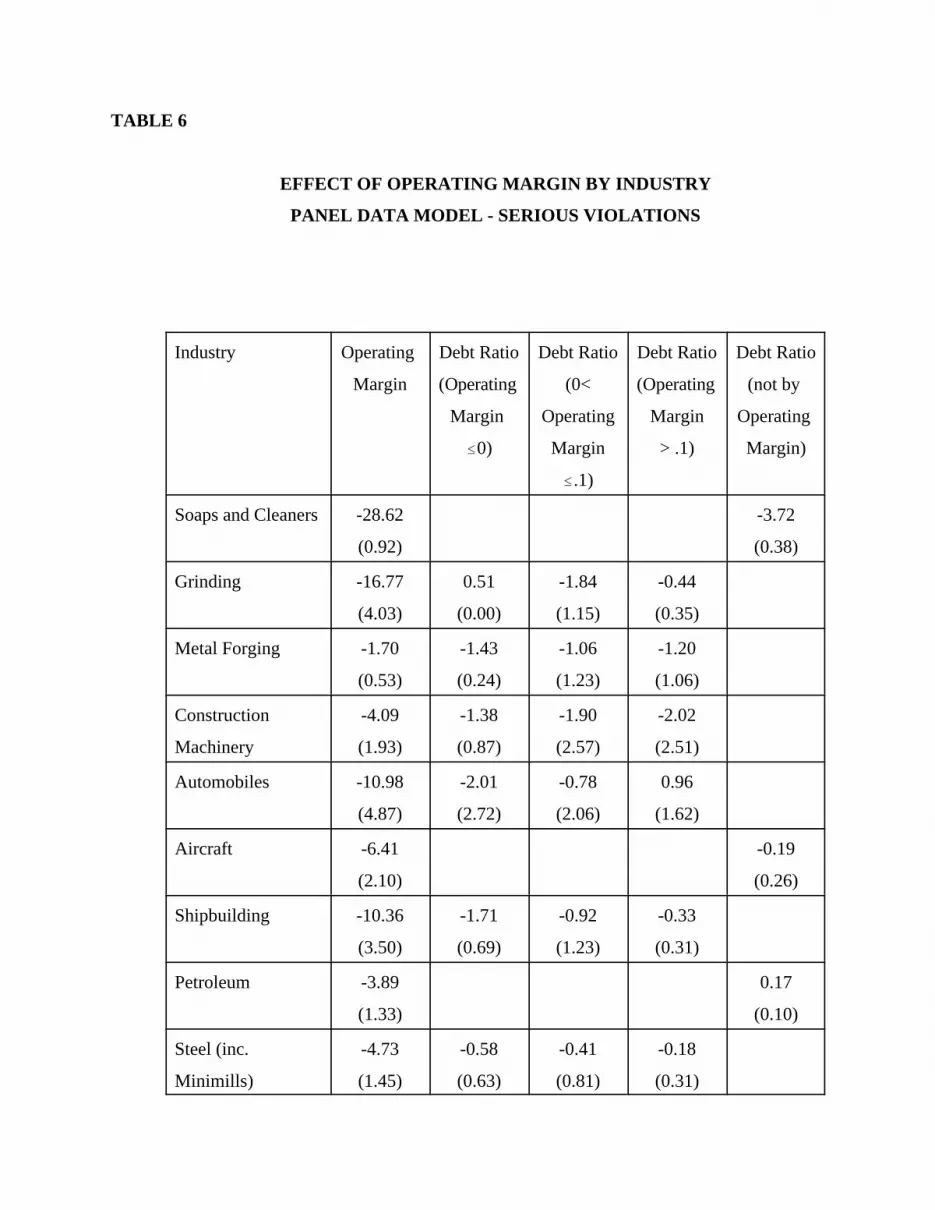
TABLE 6
EFFECT OF OPERATING MARGIN BY INDUSTRY
PANEL DATA MODEL - SERIOUS VIOLATIONS
Industry Operating
Margin
Debt Ratio
(Operating
Margin
#0)
Debt Ratio
(0<
Operating
Margin
#.1)
Debt Ratio
(Operating
Margin
> .1)
Debt Ratio
(not by
Operating
Margin)
Soaps and Cleaners -28.62
(0.92)
-3.72
(0.38)
Grinding -16.77
(4.03)
0.51
(0.00)
-1.84
(1.15)
-0.44
(0.35)
Metal Forging -1.70
(0.53)
-1.43
(0.24)
-1.06
(1.23)
-1.20
(1.06)
Construction
Machinery
-4.09
(1.93)
-1.38
(0.87)
-1.90
(2.57)
-2.02
(2.51)
Automobiles -10.98
(4.87)
-2.01
(2.72)
-0.78
(2.06)
0.96
(1.62)
Aircraft -6.41
(2.10)
-0.19
(0.26)
Shipbuilding -10.36
(3.50)
-1.71
(0.69)
-0.92
(1.23)
-0.33
(0.31)
Petroleum -3.89
(1.33)
0.17
(0.10)
Steel (inc.
Minimills)
-4.73
(1.45)
-0.58
(0.63)
-0.41
(0.81)
-0.18
(0.31)

1Sample restricted to first 30 observations on any plant due to limitations in Limdep.
2Conditional on Operating Margin falling in specified range.
TABLE 7
TOBIT ESTIMATES OF DETERMINANTS OF PENALTIES1
No Plant Effects With Plant Effects Variable
Mean
(Std.
Dev.)
Operating Margin -0.61
(6.29)
-0.14
(1.18)
-0.11
(10.47)
-0.11
(8.14)
0.107
(0.054)
Debt Ratio
(Operating Margin
#0)
-0.02
(0.28)
0.10
(1.72)
0.02
(2.08)
0.004
(0.31)
0.6022
(0.162)
Debt Ratio
(0<Operating
Margin#.1)
0.11
(5.10)
0.10
(4.48)
-0.01
(1.34)
-0.15
(2.66)
0.4802
(0.219)
Debt Ratio
(Operating Margin
>.1)
0.21
(6.34)
0.11
(3.41)
-0.05
(0.90)
-0.03
(0.35)
0.2822
(0.153)
Unionization -0.08
(3.64)
-0.09
(3.67)
0.02
(1.33)
-0.09
(3.87)
0.410
(0.211)
Plant Employment
(10,000’s)
0.21
(1.67)
0.15
(1.13)
-0.01
(0.53)
-0.07
(2.34)
0.035
(0.055)
Plant Employment
Squared
-0.04
(0.17)
0.06
(0.23)
-0.65
(7.01)
-0.11
(3.75)
0.004
(0.024)
Time Since Last
General Inspection
0.01
(0.88)
0.07
(4.60)
-0.10
(3.40)
-0.12
(5.94)
0.815
(0.301)
Accident Inspection 0.04
(2.52)
0.02
(1.57)
0.07
(2.68)
-0.12
(1.32)
0.135
Complaint
Inspection
-0.08
(7.40)
-0.07
(6.96)
0.17
(5.21)
-0.19
(3.77)
0.58
State Inspection
State
-0.02
(2.04)
-0.01
(0.71)
0.01
(0.43)
-0.05
(1.46)
0.231
Carter
Administration
0.01
(1.43)
0.02
(2.44)
-0.08
(0.26)
-0.16
(4.78)
0.307
Reagan
Administration
-0.12
(10.55)
-0.10
(9.20)
-0.70
(0.61)
-0.08
(3.86)
0.296
Industry Dummies No Yes No Yes
Log Likelihood -1656.7 -1571.3 -1622.3 -1574.8
N 4946 4946 4946 4946

1Sample restricted to first 30 observations on any plant due to limitations in Limdep.
2Conditional on Operating Margin falling in specified range.
TABLE 8
DETERMINANTS OF PROBABILITY OF BEING PENALIZED1
No Plant Effects With Plant Effects
Variable
Mean
(Std. Dev.)
Operating Margin -0.89
(2.21)
0.38
(0.73)
-0.70
(1.56)
0.37
(0.61)
0.107
(0.054)
Debt Ratio
(Operating Margin
#0)
0.79
(3.39)
1.07
(4.36)
0.75
(2.98)
1.00
(3.79)
0.6022
(0.162)
Debt Ratio
(0<Operating
Margin#1)
0.60
(6.49)
0.67
(6.85)
0.58
(5.09)
0.67
(5.77)
0.4802
(0.219)
Debt Ratio
(Operating Margin
>.1)
0.73
(5.36)
0.59
(4.05)
0.71
(4.65)
0.63
(4.04)
0.2822
(0.153)
Unionization -0.32
(3.49)
-0.42
(4.16)
-0.27
(2.32)
-0.38
(3.13)
0.410
(0.211)
Plant Employment
(10,000’s)
-1.26
(1.91)
-1.31
(1.81)
-1.35
(1.21)
-1.14
(0.99)
0.035
(0.055)
Plant Employment
Squared
3.40
(1.62)
3.64
(1.56)
3.20
(0.81)
3.05
(0.76)
0.004
(0.024)
Time Since Last
General Inspection
0.27
(4.97)
0.31
(5.00)
0.27
(4.57)
0.29
(4.42)
0.815
(0.301)
Accident Inspection 0.15
(2.43)
0.15
(2.35)
0.14
(2.26)
0.14
(2.20)
0.135
Complaint
Inspection
-0.35
(7.76)
-0.36
(7.82)
-0.38
(8.00)
-0.39
(7.90)
0.58
State Inspection
State
-0.08
(1.71)
-0.05
(1.00)
-0.09
(1.55)
-0.08
(1.29)
0.231
Carter
Administration
-0.20
(4.50)
-0.18
(4.00)
-0.20
(4.57)
-0.19
(4.24)
0.307
Reagan
Administration
-0.64
(14.07)
-0.64
(13.63)
-0.70
(14.74)
-0.70
(14.26)
0.296
Industry Dummies No Yes No Yes
Log Likelihood -3175.7 -3145.9 -3150.4 -3127.0
N 4946 4946 4946 4946


