
Confidence distributions
in statistical inference
Sergei I. Bityukov, Vera V. Smirnova
Institute for High Energy Physics, Protvino, Russia
Nikolai V. Krasnikov
Institute for Nuclear Research RAS, Moscow, Russia
Saralees Nadarajah
University of Manchester, Manchester M13 9PL, United Kingdom
Plan
• Motivation
• A bit of history
• Confidence distributions
• Examples and inferential information contained in
a CD
• Inference: a brief summary
• CDs and pivots
• Applications
• Conclusion
• References

Motivation (I) Common sense
If a procedure states one-to-one correspondence be-
tween the observed value of a random variable and the
confidence interval of any level of significance then
we can reconstruct a unique confidence density of the
parameter and, correspondingly, a unique confidence
distribution.
The confidence distribution is interpreted here in
the same way as confidence interval. From the du-
ality between testing and confidence interval estima-
tion, the cumulative confidence distribution function
for parameter µ evaluated at µ0, F (µ0), is the p−value
of testing H0 : µ ≥ µ0 against its one-side alternative.
It is thus a compact format of representing the infor-
mation regarding µ contained in the data and given
the model. Before the data have been observed, the
confidence distribution is a stochastic element with
quantile intervals (F−1(α1), F−1(1−α2)) which covers the
unknown parameter with probability 1−α1−α2. After
having observed the data, the realized confidence dis-
tribution is not a distribution of probabilities in the
frequentist sense, but of confidence attached to inter-
val statements concerning µ.

Motivation (II) Construction by R.A. Fisher
A following example shows the construction by R.A. Fisher
(B. Efron (1978))
A random variable x with parameter µ
x ∼ N (µ, 1). (1)
Probability density function (pdf) here is
ϕ(x|µ) =1√2π
e−(x−µ)2
2 . (2)
We can write
x = µ + ǫ, (3)
where ǫ ∼ N (0, 1) and µ is a constant.
Let x be a single realization of x. For normal dis-
tribution it is an unbias estimator of parameter µ, i.e.
µ = x, therefore
µ|x = x− ǫ. (4)
As is known (−ǫ) ∼ N (0, 1) due to symmetry of the
bell-shaped curve about its central point, i.e.
µ|x ∼ N (x, 1). (5)

Motivation (II)
Thus we construct the confidence density of the pa-
rameter
ϕ(µ|x) =1√2π
e−(x−µ)2
2 (6)
uniquely for each value of x.
As pointed in paper (Hampel 2006) “Fisher (Fisher
1930; 1933) gave correct interpretation of this “tempt-
ing” result. But starting in 1935 (Fisher 1935), he
really believed he had changed the status of µ from
that of a fixed unknown constant to that of a random
variable on the parameter space with known distri-
bution”. The history and generalization of the last
approach can be found in paper (Hannig 2006).
The fiducial argument is very attractive notion and
sometimes it reopen (see, as an example, (Hassairi
2005) and corresponding critique (Mukhopadhyay 2006)).
In principle, the parameter µ can be a random vari-
able in the case of the random origin of parameter.
We will not discuss here this possibility.
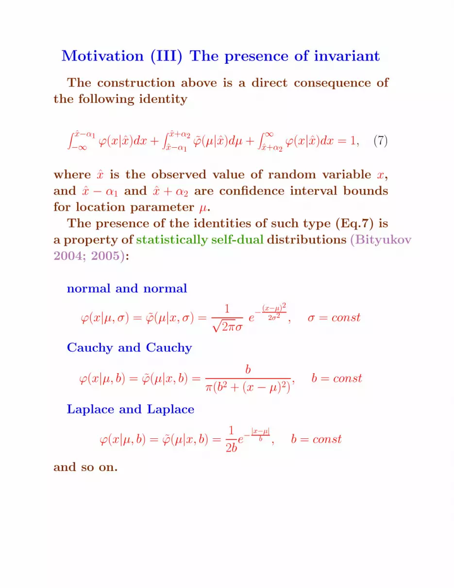
Motivation (III) The presence of invariant
The construction above is a direct consequence of
the following identity
∫ x−α1
−∞ ϕ(x|x)dx +∫ x+α2
x−α1ϕ(µ|x)dµ +
∫ ∞x+α2
ϕ(x|x)dx = 1, (7)
where x is the observed value of random variable x,
and x − α1 and x + α2 are confidence interval bounds
for location parameter µ.
The presence of the identities of such type (Eq.7) is
a property of statistically self-dual distributions (Bityukov
2004; 2005):
normal and normal
ϕ(x|µ, σ) = ϕ(µ|x, σ) =1√2πσ
e−(x−µ)2
2σ2 , σ = const
Cauchy and Cauchy
ϕ(x|µ, b) = ϕ(µ|x, b) =b
π(b2 + (x− µ)2), b = const
Laplace and Laplace
ϕ(x|µ, b) = ϕ(µ|x, b) =1
2be−
|x−µ|b , b = const
and so on.

Motivation (IV) The invariant in the case ofasymmetric distributions
In the case of Poisson and Gamma-distributions we
can also exchange the random variable and the param-
eter, preserving the same formula for the probability
distribution:
f(i|µ) = f(µ|i) =µie−µ
i!
In this case we can use another identity to relate
the pdf of random variable and confidence density of
the parameter for the unique reconstruction of con-
fidence density (Bityukov 2000; 2002) (any another
reconstruction is inconsistent with the identity and,
correspondingly, breaks the probability conservation):
∞∑
i=x+1
µi1e−µ1
i!+
∫ µ2
µ1
µxe−µ
x!dµ +
x∑
i=0
µi2e−µ2
i!= 1 (8)
for any real µ1 ≥ 0 and µ2 ≥ 0 and non-negative integer
x, i.e.
∞∑
i=x+1
f(i|µ1) +∫ µ2
µ1f (µ|x)dµ +
x∑
i=0
f(i|µ2) = 1, (9)
where f(i|µ) = f (µ|i) =µie−µ
i!. Confidence density
f (µ|i) is the pdf of Gamma-distribution Γ1,i+1 and x is
the number of observed events.

A bit of history
The basic notion of CDs traces back to the fidu-
cial distribution of Fisher (1930); however, it can be
viewed as a pure frequentist concept. Indeed, as pointed
out in Schweder (2002) the CD concept is ”Neyman-
nian interpretation of Fisher’s fiducial distribution”
[Neyman (1941)]. Its development has proceeded from
Fisher (1930) through various contributions, just to
name a few, of Kolmogorov (1941), Pitman (1957),
Efron (1993; 1998), Fraser (1991; 1996), Lehmann
(1993), Singh (2001; 2007), Schweder (2002; 2003A)
and others. Bityukov (2002; 2005) developed the ap-
proach for reconstruction of the confidence distribu-
tion densities by using the corresponding identities.
Another useful application of CD is for meta-analysis.
Meta-analysis is the modern term for combining re-
sults from different experiments or trials (see, for ex-
ample, (Hedges 1985)). The consecutive theory of
combining information from independent sources through
CD is proposed in paper (Singh 2005). Recently (Bickel
2006), the method for incorporating expert knowledge
into frequentist approach by combining generalized
confidence distributions is proposed.

Confidence distributions
Suppose X1, X2, . . . , Xn are n independent random
draws from a population F and χ is the sample space
corresponding to the data set Xn = (X1, X2, . . . , Xn)T .
Let θ be a parameter of interest associated with F (Fmay contain other nuisance parameters), and let Θ be
the parameter space.
Definition 1 (Singh 2005): A functionHn(·) = Hn(Xn, (·))on χ×Θ → [0, 1] is called a confidence distribution (CD)
for a parameter θ if
(i) for each given Xn ∈ χ, Hn(·) is a continuous cumu-
lative distribution function;
(ii) at the true parameter value θ = θ0, Hn(θ0) =
Hn(Xn, θ0), as a function of the sample X n, has the uni-
form distribution U(0, 1).
The function Hn(·) is called an asymptotic confi-
dence distribution (aCD) if requirement (ii) above is
replaced by (ii)‘: at θ = θ0, Hn(Xn, θ0)W→ U(0, 1) as n →
+∞, and the continuity requirment onHn(·) is dropped.
Item (i) basically requires the function Hn(·) to be a
distribution function for each given sample.
Item (ii) basically states that the function Hn(·) con-
tains the right amount of information about the true
θ0.

Confidence distributions
We call, when it exists, hn(θ) = H′n(θ) a confidence
density or CD density.
It follows from the definition of CD that if θ <
θ0, Hn(θ)sto≤ 1 − Hn(θ), and if θ > θ0, 1 − Hn(θ)
sto≤ Hn(θ).
Heresto≤ is a stochastic comparison between two ran-
dom variables; i.e. for two random variable Y1 and
Y2, Y1
sto≤ Y2, if P (Y1 ≤ t) ≥ P (Y2 ≤ t) for all t. Thus a
CD works, in a sense, like a compass needle. It points
towards θ0, when placed at θ 6= θ0, by assigning more
mass stochastically to that side (left or right) of θ that
contains θ0. When placed at θ0 itself, Hn(θ) = Hn(θ0) has
the uniform U [0, 1] distribution and thus it is noninfor-
mative in direction.
Definition 1 is very convenient for the purpose of ver-
ifying if a particular function is a CD or an aCD.

Examples and inferential informationcontained in a CD
Example 1 Normal mean and variance (Singh 2005):
Suppose X1, X2, . . . , Xn is a sample from N (µ, σ2), with
both µ and σ2 unknown. A CD for µ is
Hn(y) = Ftn−1(y − X
sn/√n
), where X and s2 are, respectively,
the sample mean and variance, and Ftn−1(·) is a cumula-
tive distribution function of the Student tn−1-distribution.
A CD for σ2 is Hn(y) = 1 − Fχ2n−1
((n− 1)s2
n
y) for y ≥ 0,
where Fχ2n−1
(·) is the cumulative function of the χ2n−1-
distribution.
Example 2 p-value function (Singh 2005): For any
given θ, let pn(θ) = pn(Xn, θ) be a p-value for a one-
sided test K0 : θ ≤ θ versus K0 : θ > θ. Assume that
the p-value is available for all θ. The function pn(·)is called a p-value function. Typically, at the true
value θ = θ0, pn(θ0) as a function of Xn is exactly (or
asymptotically) U(0, 1)-distributed. Also, Hn(·) = pn(·)for every fixed sample is almost always a cumulative
distribution function. Thus, usually pn(·) satisfies the
requirements for a CD.

Inference: a brief summary (Singh 2005)
• Confidence interval. From the definition, it is evi-
dent that the intervals (−∞, H−1n (1−α)], [H−1
n (α),+∞)
and (H−1n (α/2), H−1
n (1−α/2)) provide 100(1−α)%-level
confidence intervals of different kinds for θ, for any
α ∈ (0, 1).
• Point estimation. Natural choices of point estima-
tors of the parameter θ, given Hn(θ), include the
median Mn = H−1n (1/2), the mean θ =
∫ ∞−∞ tdHn(t)
and the maximum point of the CD density
θ = arg maxθhn(θ), hn(θ) = H′n(θ).
• Hypothesis testing. From a CD, one can obtain p-
values for various hypothesis testing problems. The
work (Fraser 1991) developed some results on such
a topic through p-value functions. The natural line
of thinking is to measure the support that Hn(·)lends to a null hypothesis K0 : θ ∈ C. There are
possible two types of support:
1. Strong-support ps(C) =∫
CdHn(θ).
2. Weak-support pw(C) = supθ∈C2min(Hn(θ), 1−Hn(θ)).
If K0 is of the type (−∞, θ0] or [θ0,+∞) or a union
of finitely many intervals, the strong-support ps(C)
leads to the classical p-values.
If K0 is a singleton, that is, K0 is θ = θ0, then the
weak-support pw(C) leads to the classical p-values.

Remarks
Confidence distributions can be viewed as “distribu-
tion estimators” and are convenient for constructing
point estimators, confidence intervals, p−values and
more.
Confidence distributions can be interpreted as ob-
jective Bayesian posteriors (Bayesian posteriors based
on objective priors) that have the desirable properties
of good coverage and invariance to transformations.
In this case, the distribution for frequentist (confi-
dence distribution) and Bayesian (posterior distribu-
tion) are the same, the uncertainty intervals: con-
fidence interval and credible interval, are the same,
and the uncertainty intervals are usually interpreted
in the same way: 95% probability that true value is
in the interval. Other methods, such as profile likeli-
hood, are not dependent on priors, but may be more
difficult to interpret.
In the one parameter model, in paper (Schweder
2002) is defined the confidence distribution notion that
summarizes a family of confidence intervals.

CDs and pivots (Schweder 2003B)
Consider the statistical model for the data X. The
model consists of a family of probability distributions
for X, indexed by the vector parameter (ψ, χ), where
ψ is a scalar parameter of primary interest, and χ is a
nuisance parameter (vector).
Definition 2 : A univariate data-dependent distribution
for ψ, with cumulative distribution function C(ψ;X) and with
quantile function C−1(α;X) is an exact confidence distribu-
tion if Pψχ(ψ ≤ C−1(α;X)) = Pψχ(C(ψ;X) ≤ α) = α for all
α ∈ (0, 1) and for all probability distributions in the statistical
model.
By definition, the stochastic interval (∞, C−1(α;X))
covers ψ with probability α, and is a one-sided con-
fidence interval method with coverage probability α.
The interval (C−1(α;X), C−1(β;X)) will for the same rea-
son cover ψ with probability β−α, and is a confidence
interval method with this coverage probability. When
data have been observed as X = x, the realized nu-
merical interval (C−1(α; x), C−1(β; x)) will either cover
or not cover the unknown true value of ψ. The degree
of confidence β − α that is attached to the realized
interval is inherited from the coverage probability of
the stochastic interval.

CDs and pivots
The confidence distribution has the same dual prop-
erty. Ex ante data, the confidence distribution is a
stochastic entity with probabilistic properties. Ex post
data, however, the confidence distribution is a distri-
bution of confidence that can be attached to interval
statement.
The realized confidence (degree of confidence) C(ψ; x)
is a p−value of the one-sided hypothesis H0 : ψ ≤ ψ0
versus ψ > ψ0 when data have been observed to be
x. The ex ante confidence, C(ψ;X) is by definition uni-
formly distributed. The p−value is just a transforma-
tion of the test statistic to the common scale of the
uniform distributions (ex ante). The realized p−value
when testing the two-sided hypothesis H0 : ψ = ψ0 ver-
sus ψ 6= ψ0 is 2 min{C(ψ0), 1 − C(ψ0)}.

CDs and pivots
Confidence distributions are easily found when piv-
ots (Barndorff 1994) can be identified.
A function of the data and the interest parameter, p(X,ψ),
is a pivot if the probability distribution of p(X,ψ) is the same
for all (ψ, χ), and the function p(X,ψ) is increasing in ψ for
almost all x.
If based on a pivot with cumulative distribution
function F , the cumulative confidence distribution is
C(X,ψ) = F (p(X,ψ)).
From the definition, a confidence distribution is ex-
act if and only if C(X,ψ) ∼ U is a uniformly distributed
pivot.
The self-duality in Eq. 7 is equivalent to the exis-
tence of a linear and symmetrically distributed pivot.

Applications: signal and expectedbackground (Bityukov 2000; 2007)
The confidence density is more informative notion
than the confidence interval. For example, the Gamma-
distribution Γ1,n+1 is the confidence density of the pa-
rameter of Poisson distribution in the case of the n ob-
served events from the Poisson flow of events (Bityukov
2000; 2007). It means that we can reconstruct any
confidence intervals (shortest, central, . . . ) by the di-
rect calculation of the pdf of a Gamma-distribution.
The following example illustrates the advantages of
the confidence density construction.
Let us consider the Poisson distribution with two
components: the signal component with a parameter
µs and background component with a parameter µb,
where µb is known. To construct confidence intervals
for the parameter µs in the case of observed value n,
we must find the distribution f(µs|n).
First let us consider the simplest case n = s + b = 1.
Here s is the number of signal events and b is the num-
ber of background events among the observed number
n of events.
b can be equal to 0 and 1.

Applications: signal and expectedbackground
We know that the b is equal to 0 with probability
p0 = P (b = 0) =µ0b
0!e−µb = e−µb (10)
and the b is equal to 1 with probability
p1 = P (b = 1) =µ1b
1!e−µb = µbe
−µb. (11)
Correspondingly,
P (b = 0|n = 1) = P (s = 1|n = 1) =p0
p0 + p1
and
P (b = 1|n = 1) = P (s = 0|n = 1) =p1
p0 + p1
.
It means that the distribution of the confidence den-
sity f (µs|n = 1) is equal to the weighted sum of distri-
butions
P (s = 1|n = 1)f(µs|s = 1) + P (s = 0|n = 1)f(µs|s = 0), (12)
where the confidence density f(µs|n = 0) is the Gamma
distribution Γ1,1 with the pdf f (µs|s = 0) = e−µs
and the confidence density f (µs|n = 1) is the Gamma
distribution Γ1,2 with the pdf f (µs|s = 1) = µse−µs.

Applications: signal and expectedbackground
As a result, we have the confidence density of the
parameter µs
f(µs|n = 1) =µs + µb1 + µb
e−µs. (13)
Using this formula for f(µs|n = 1), we can construct
the shortest confidence interval of any confidence level
trivially.
In this manner we can construct the confidence den-
sity f (µs|n) for any values of n and µb. From Eq. 9 we
use the confidence densities f (µs|s = i), i = 0, n. Mixing
together the confidence densities with corresponding
conditional probability weights (in analogy with Eq.
12) yields the confidence density
f (µs|n) =(µs + µb)
n
n!n
∑
i=0
µibi!
e−µs. (14)
We have obtained the known formula (Helene 1988;
Zech 1989; D’Agostini 2003). The numerical results of
the calculations of shortest confidence intervals by the
using of this confidence density coincide with Bayesian
confidence intervals constructed by the using the uni-
form prior.

Aplications: quality of planned experiment(Bityukov 2003)
Let us consider the estimation of quality of planned
experiments as another example of the use of confi-
dence density. The approach is based on the analysis
of uncertainty, which will take place under the future
hypotheses testing about the existence of a new phe-
nomenon in Nature.
We consider the Poisson distribution with param-
eter µ and we preserve the notation pf the previous
application. We test a simple statistical hypothesis
H0: new physics is present in Nature (i.e. µ = µs + µb )
against a simple alternative hypothesis
H1: new physics is absent (µ = µb).
The value of uncertainty is determined by the val-
ues of the probability to reject the hypothesis H0 when
it is true (Type I error α) and the probability to ac-
cept the hypothesis H0 when the hypothesis H1 is true
(Type II error β). This uncertainty characterizes the
distinguishability of the hypotheses under the given
choice of critical area.

Aplications: quality of planned experiment
Let both values µs and µb, which are defined in the
previous application, be exactly known. In this sim-
plest case the errors of Type I and II, which will take
place in testing of hypothesis H0 versus hypothesis H1,
can be written as follows:
α =nc∑
i=0
f(i|µs + µb),
β = 1 −nc∑
i=0
f(i|µb), (15)
where f is a Poisson probability function and nc is a
critical value.
Let the values µs = s and µb = b be known, for ex-
ample, from Monte Carlo experiment with integrated
luminosity which is exactly the same as the data lumi-
nosity later in the planned experiment. It means that
we must include the uncertainties in values µs and µbto the system of the equations above.

Aplications: quality of planned experiment
As is shown in ref. (Bityukov 2002) (see, also, the
generalized case in the same reference and in my poster
here) we have the system
α =∫ ∞0f(µ|s+ b)
nc∑
i=0
f(i|µ)dµ =nc∑
i=0
C is+b+i
2s+b+i+1,
β = 1 −∫ ∞0f(µ|b)
nc∑
i=0
f(i|µ)dµ = 1 −nc∑
i=0
C ib+i
2b+i+1
, (16)
where nc is a critical value of the hypotheses testing
about the observability of signal and C iN is
N !
i!(N − i)!.
Note, here the Poisson distribution is a prior dis-
tribution of the expected probabilities and the nega-
tive binomial (Pascal) distribution is a posterior dis-
tribution of the expected probabilities of the random
variable. This is transformation of the estimated con-
fidence densities f(µ|s + b) and f (µ|b) (pdfs of the cor-
responding Γ−distributions) to the space of the ex-
pected values of the random variable.

Conclusion
The notion of confidence distribution, an enterely
frequentist concept, is in essence a Neymanian inter-
pretation of Fisher’s fiducial distribution. It contains
information related to every kind of frequentist in-
ference. The confidence distribution is a direct gen-
eralization of the confidence interval, and is a useful
format of presenting statistical inference.
The follow quotation from Efron(1998) on Fisher’s
contribution of the fiducial distribution seems quite
relevant in the context of CDs:
“. . . but here is a safe prediction for the 21st century:
statisticians will be asked to solve bigger and more
complicated problems. I believe there is a good chance
that objective Bayes methods will be developed for
such problem, and that something like fiducial infer-
ence will play an important role in this development.
Maybe Fisher’s biggest blunder will become a big hit
in the 21st centure!”

References
O.E. Barndorff-Nielsen, D.R. Cox (1994), Inference and Asymp-totics, Chapman & Hall, London, 1994.
D.R. Bickel (2006), Incorporating expert knowledge into fre-quentist interface by combining generalized confidence distribu-
tions, e-Print: math/0602377, 2006.S.I. Bityukov, N.V. Krasnikov, V.A. Taperechkina (2000), Con-
fidence intervals for Poisson distribution parameter, Preprint
IFVE 2000-61, Protvino, 2000; also, e-Print: hep-ex/0108020,2001.
S.I.Bityukov (2002), Signal Significance in the Presence ofSystematic and Statistical Uncertainties, JHEP 09 (2002) 060;
e-Print: hep-ph/0207130;S.I. Bityukov, N.V. Krasnikov (2003), NIM A502 (2003) 795-
798.
S.I. Bityukov, V.A. Taperechkina, V.V. Smirnova (2004), Sta-tistically dual distributions and estimation of the parameters,
e-Print: math.ST/0411462, 2004.S.I. Bityukov, N.V. Krasnikov (2005), Statistically dual dis-
tributions and conjugate families, in Proceedings of MaxEnt’05,August 2005, San Jose, CA, USA.
S.I. Bityukov, N.V. Krasnikov, V.V. Smirnova, V.A. Taperechk-ina (2007), The transform between the space of observed valuesand the space of possible values of the parameter, Proceedings
of Science (ACAT) 062 (2007) 1-9.G. D’Agostini (2003), Bayesian Reasoning in Data Analysis, a
Critical Introduction. World Scientific, Hackensack, NJ, 2003.B. Efron (1978), Controversies in the Foundations of Statistics,
The American Mathematical Monthly, 85(4) (1978) 231-246.B. Efron (1993), Bayes and likelihood calculations from confi-
dence intervals. Biometrika 80 (1993) 3-26. MR1225211.B. Efron (1998), R.A. Fisher in the 21st Century. Stat.Sci. 13
(1998) 95-122.
R.A. Fisher (1930), Inverse probability. Proc. of the Cam-bridge Philosophical Society 26 (1930) 528-535.
R.A. Fisher (1933), The concepts of inverse probability andfiducial probability referring to unknown parameters, Proceed-
ings of the Royal Society, London, A139 (1933) 343-348.

R.A. Fisher (1935), The fiducial argument in statistical infer-
ence, Annals of Eugenics 6 (1935) 391-398.D.A.S. Fraser (1991), Statistical inference: Likelihood to sig-
nificance. J. Amer. Statist. Assoc. 86 (1991) 258-265. MR1137116.D.A.S. Fraser (1996), Comments on “Pivotal inference and the
fiducial argument”, by G. A. Barnard. Internat. Statist. Rev.64 (1996) 231-235.
F. Hampel (2006), The proper fiducial argument, Lecture Notesin Computer Science 4123 (2006) 512-526.
J. Hannig, H. Iyer, P. Patterson (2006), Fiducial generalized
confidence intervals, Journal of the American Statistical Associ-ation 101 (2006) 254-269.
A. Hassairi, A. Masmoudi, C.C. Kokonendji (2005), Implicitdistributions and estimation, Communications in Statistics—Theory
and Methods 34 (2005) 245-252.L.V. Hedges, I. Olkin (1985), Statistical Methods for Meta-
analysis, Academic Press, Orlando, 1985.
A.N. Kolmogorov (1942), The estimation of the mean andprecision of a finite sample of observations (in Russian), Bulletin
of the Academy of Sciences, USSR, Mathematics Series 6 (1942)3-32.
E.L. Lehmann (1993), The Fisher, Neyman-Pearson theoriesof testing hypotheses:One theory or two? J. Amer. Statist. As-
soc. 88 (1993) 1242-1249. MR1245356.N. Mukhopadhyay (2006), Some comments on Hassairi et al.’s
“Implicit distributions and estimation”, Communications in Statistics—
Theory and Methods 35 (2006) 293-297.J. Neyman (1941), Fiducial argument and the theory of con-
fidence intervals. Biometrika 32 (1941) 128-150. MR5582.P.J.G. Pitman (1957), Statistics and science, Journal of the
American Statistical Association 52 (1957) 322-330.T. Schweder and N.L. Hjort (2002), Confidence and likelihood,
Scand. J. Statist. 29 (2002) 309-332.T. Schweder, N.L. Hjort (2003A), Frequentist analogies of pri-
ors and posteriors, in: Econometrics and the Philosophy of Eco-
nomics, Princeton University Press, pp.285-317, 2003.T. Schweder (2003B), Integrative fish stock assessment by fre-
quentist methods: confidence distributions and likelihoods forhowhead whales, Scientia Marina 67 (2003) 89-07.

K. Singh, M. Xie, W. Strawderman. (2001), Confidence dis-
tributions - concept, theory and applications, Technical report,Dept.Statistics, Rutgers Univ., Revised 2004
K. Singh, M. Xie, W.E. Strawderman (2005), Combining in-formation from independent sources through confidence distri-
butions, The Annals of Statistics 33 (2005) 159-183.K. Singh, M. Xie, W. Strawderman. (2007), Confidence distri-
butions (CD) - Distribution Estimator of a Parameter. YehudaVardi Volume. IMS-LNMS. (to appear).
G. Zech (1989), Upper limits in experiments with background
or measurement errors, Nuclear Instruments and Methods inPhysics Research A277 (1989) 608.


