Download - Conditional Volatility Persistence

Conditional Volatility Persistence
Jianxin Wang and Minxian Yang*
January 2017
Abstract
This study presents empirical findings on the determinants of daily volatility persistence. We show that the volatility persistence is strongly influenced by large (negative) returns. After controlling the impact of return, short-term volatility persistence is negatively related to volatility level. There are large variations in the conditional volatility persistence, especially when markets are under stress in 2008-09 and late 2011. We offer an economic explanation for volatility persistence based on information shocks and price discovery. Models with conditional volatility persistence significantly improve one-day volatility forecasts.
* Jianxin Wang ([email protected]) is from the University of Technology Sydney and is the corresponding author. Minxian Yang ([email protected]) is from University of New South Wales.

CVP2017/1 Page1
I. Introduction
In financial markets, volatility is synonymous with risk. Asset pricing, portfolio
selection, and risk management are centred on measuring and forecasting volatility. Volatility
is known to be highly persistent: today’s volatility is significantly correlated with volatility
over 100 days ago. While a large number of models have been developed to capture the
statistical characteristics of volatility dynamics, it remains true today that “a consensus
economic model producing persistence in conditional variance does not exist,” as stated by
Diebold and Lopez (1995). This study presents new evidence on the empirical characteristics
of volatility persistence and examines its economic origins. We show that (1) volatility
persistence varies daily with market state variables, e.g. return and volatility level; (2) price
discovery, the process of incorporating information into asset prices, plays a key role in
determining future volatility persistence; (3) models incorporating these features significantly
improve volatility forecasts.
The initial evidence linking stock return with volatility persistence can be seen from
Figure 1. Let RVt be the daily realized variance and ΔRVt+1 ≡ . The absolute
value of ΔRVt+1 is inversely related to RV persistence: high RV persistence implies a small
change in RV therefore low |ΔRVt+1|, and vice versa for low RV persistence. Figure 1 plots
|ΔRVt+1| against daily return rt for the S&P 500 index ETF (ticker SPY) and the S&P 600
small cap ETF (ticker IJR). The bulk of the data indicates that as rt becomes larger, positive
or negative, |ΔRVt+1| becomes smaller, indicating more stable or persistent RV.
The relationships in Figure 1 suggest that volatility persistence as captured by the
inverse of |ΔRV| varies with return size. In a GARCH(1,1) model with variance equation
, volatility persistence is measured by α+β. If persistence parameters
α and β are an increasing function of return size as suggested in Figure 1, the propagation
from to depends not only on and but also on the time-varying α and β. This
CVP2017/1 Page2
represents a new channel through which volatility propagates over time. Metaphorically the
flow of water from one tank depends not only on the water level ( , ) but also on the
time-varying size of the pipe (α+β).
The idea that volatility persistence is affected by returns is implicit in models that
allow returns to have an asymmetric impact on volatility. In the GARCH model of Glosten,
Jagannathan, and Rankle (GJR, 1993), the variance equation is
and volatility persistence is α+β+λ/2. Thus λ > 0 implies that negative returns
increase tomorrow’s volatility, as well as the dependence of tomorrow’s volatility on today’s
volatility. In general volatility persistence may be dependent on a set of market state variables
Mt: VPt = f(Mt). We term this persistence measure the conditional volatility persistence
(CVP), akin to the conditional volatility in the GARCH-family models. This study identifies
a set of market state variables and estimates daily CVP.
The success of GARCH models has motivated many studies to explore the economic
mechanisms underlying volatility persistence. A partial list of potential explanations for
volatility persistence include (1) persistence in exogenous information arrival, e.g. Laux and
Ng (1993), Andersen and Bollerslev (1997), Fleming, Kirby, Ostdiek (2006, RFS); (2)
endogenous trading-generated information arrival, e.g. Cao, Coval, and Hirshleifer (2002); (3)
heterogeneous trading frequencies by different investors, e.g. Müller, et al. (1997), Xue and
Gençay (2012, JBF); (4) volatility regime shifts, e.g. Lamoureux and Lastrapes (1990, JBES),
Hamilton and Susmel (1994); (5) parameter uncertainty, e.g. Johnson (2000, MF),
Timmermann (2001); (6) information cost as in de Fontnouvelle (2000); (7) learning about
market state or trading strategies in agent-base models, e.g. Brock and LeBaron (1996), He,
Li, and Wang (2015); (8) persistence of wealth distributions, e.g. Cabrales and Hoshi (1996);
(9) time-varying risk aversion, e.g. McQueen and Vorkink (2004); and (10) investor attention
(Andre and Hasler, 2015) and information percolation (Andre, 2013).
CVP2017/1 Page3
Our study makes two contributions to the literature on the economic origins of
volatility persistence. First, we present evidence that market state variables, e.g. return and
volatility, have significant impact on future volatility persistence. As a result, volatility
persistence varies on daily basis, a significant departure from the existing literature. The
variables affecting daily volatility persistence shed new light on the economic mechanism
leading to volatility persistence. Not surprisingly, a calibration of volatility persistence from
today to tomorrow significantly improves volatility forecasts.
Second, we offer a new explanation for volatility persistence based on information
shocks and price discovery. Intraday returns can be decomposed into a random-walk
component reflecting the changes in the efficient price, and a serially correlated component
reflecting the price impact of liquidity and noise trading. The sum of the intraday random-
walk components captures the net price impact of positive and negative information shocks
over a trading day and can be viewed as a proxy for the direction and size of the aggregate
information shock. The sum of the squared random-walk components is widely used in
microstructure literature as a measure for information flow or price discovery, e.g. Hasbrouck
(1991, 1993, and 1995). It is the dominant component of daily realized variance. Empirically
we find that information shocks increase volatility persistence with negative shocks having
greater impact than positive shocks. Large shocks are associated with greater uncertainty
(Panel C of Figure 2) and take longer to be fully priced in. They tend to have a spill-over
effect on tomorrow’s volatility, increasing volatility persistence. On the other hand, we find
that price discovery reduces volatility persistence. Greater price discovery means more
information has been priced in by the end of a trading day, reducing information spill-over
from today to tomorrow and the autocorrelation of daily volatility.
Price discovery is determined by information flow, information quality, and investor
behaviour. Our price discovery-based explanation for volatility persistence is closely related

CVP2017/1 Page4
to earlier information-based explanations. One prominent theory is the mixture of distribution
hypothesis (MDH) developed by Clark (1973) and Tauchen and Pitts (1983) and extended by
Andersen (1996). MDH is centred on a mixing variable It > 0 representing the (latent)
number of information events. Let ri be the return associated with the ith information arrival.
When ri is iid N(0,σ2), daily return is rt = ∑ r with variance σ2It. Therefore variation and
persistence in It leads to variation and persistence in return variance. Laux and Ng (1993),
Andersen and Bollerslev (1997), and He and Velu (2014) find empirical support for MDH
while Lamoureux and Lastrapes (1994), Liesenfeld (1998), and Watanabe (2000) show that
MDH fails to explain volatility persistence. Our explanation is consistent with MDH in that
the exogenous information arrival It is a key determinant of price discovery. Persistence in It
across periods leads to persistence in price discovery across periods, which in turn leads to
persistence in volatility. Our explanation differs from MDH in that volatility persistence is
not solely determined by exogenous information arrivals. Price discovery involves learning,
information searching, and strategic trading by investors. A large information shock may
take a few days to be priced in, leading to a spill-over effect across periods and volatility
persistence even in the absence of new information.1 While information arrivals increase
uncertainty, price discovery is the process of absorbing information shocks and resolving
uncertainty. Price discovery within a period reduces information spill-over to future periods
therefore reduces volatility persistence.
Our price discovery-based explanation for volatility persistence is consistent with
endogenous information arrivals, either through information costs as in de Fontnouvelle
(2000), or through validation of private signals as in Cao, Coval, and Hirshleifer (2002), or
though investor attention (Andre and Hasler, 2015) and information percolation (Andre,
2013). Barriers to information flow or participation by informed investors reduce price
1 An example is the well-known post-earnings-announcement drift where price continues to drift in absence of new information.

CVP2017/1 Page5
discovery, induce delayed price reaction to correlated information, and increase volatility
persistence. When investors have heterogeneous trading frequencies, e.g. Müller, et al. (1997)
and Xue and Gençay (2012, JBF), infrequent traders learn from past prices when they are
absent, similar to the validation of private signals in Cao, Coval, and Hirshleifer (2002). We
differ from agent-based models, e.g. He, Li, and Wang (2015), which typically have agents
switching between fundamental or trend-following traders. There are two equilibriums, each
having a different volatility level and constant volatility persistence. As agents switch
between fundamentalists and trend followers, market equilibrium changes and volatility
persistence is disrupted.
Berger, Chaboud, and Hjalmarsson (2009) find that the sensitivity to information, as
opposed to information flow itself, accounts for a large portion of volatility persistence in the
foreign exchange markets. Conceptually one would expect the sensitivity to information to be
closely related to price discovery in our study. Patton and Shappard (2015) show that “bad
volatility”, defined as the sum of squared negative returns, accounts for most of the volatility
persistence. We show that negative returns are the dominant component of the conditional
volatility persistence (CVP).
Our study is directly related to Ning, Xu, and Wirjanto (2015), who measure volatility
persistence by the tail dependence of RVt and RVt+1, i.e. the probability of both RVt and
RVt+1 being in the left or right tails of the RV distributions. Using a set of copulas, they show
that the right-tail dependence is much higher (75% for S&P 500) than the left-tail dependence
(6%). They conclude that high volatility level is associated with high volatility persistence.
We document a positive unconditional correlation between our CVP and RV. However, after
controlling for the impact of daily returns, our estimated CVP is inversely related to RVt.
Two factors may have contributed to the different conclusions. First, we estimate CVP from a
model for volatility dynamics that incorporates long memory as well as asymmetric return
CVP2017/1 Page6
impact. A jump in volatility always reduces the estimated CVP. This is not the case when
persistence is measured by tail dependence. For example, Table 1 shows that the mean and
standard deviation of the daily realized variance (RV) of SPY are 1.13 and 2.43 (scaled by
104) respectively. On October 10 and 11, 2008, RV was 60.6 and 6.2 respectively. While
these RV values are in the right tails of the RV distribution, a 10-time drop in RV should not
be regarded as a case of volatility persistence. Second, we control for the impact of return on
volatility persistence which is not examined in Ning, Xu, and Wirjanto (2015). Our
estimated CVP is high during the financial crisis of 2008 because of the large negative
returns, not the high volatility.
We estimate volatility persistence from the heterogeneous autoregressive (HAR)
model which was proposed by Corsi (2009) and has been extensively used in many volatility
studies. Our analyses are based SPY and IJR, as well as 87 of the S&P 100 index constituent
stocks. Our empirical findings are summarized as following:
(1) Consistent with Figure 1, volatility persistence increases with the size of daily returns.
Negative returns increase volatility persistence more than positive returns. The evidence
indicates information shocks as a source for the propagation of volatility over time.
(2) After controlling the impact of return, we find that volatility persistence decreases with
daily RV. The positive impact of return is generally larger than the negative impact of
RV, resulting in a right-skewed distribution of the estimated CVP.
(3) After taking into account of the impact from return and RV, we fail to find consistent
impact from other market state variables on volatility persistence, including volatility
jumps, the number of trades, illiquidity, and the imbalance of buy and sell volumes.
(4) Using the Beveridge-Nelson decomposition, we estimate daily information shocks and
price discovery. We find that price discovery accounts for over 90% of daily RV of
market indices and over 80% of daily RV of individual stocks. The size of information

CVP2017/1 Page7
shocks increases volatility persistence, with greater impact from negative shocks. Most of
the impact on volatility persistence comes from shocks above the median value. Non-
information returns have no impact on volatility persistence. Non-information RV has
little impact on future RV.
(5) Out-of-sample forecast comparisons show that models with conditional persistence
significantly outperform models with constant persistence. The average reductions in loss
function values are in the range of 30 to 50%. The CVP models outperform across all size
categories for return and RV and in all forecasting sub-periods.
This paper has the following sections. Section II explains the sample and variable
construction and presents the summary statistics of the key variables. Based on an intuitive
measure for daily volatility persistence, Section III presents preliminary evidence, which
guides the selection of conditioning variables. The empirical evidence on the conditional
volatility persistence and robustness tests are presented in Section IV. Section V links price
discovery to volatility persistence. Section VI compares volatility forecasts of models with
conditional or constant volatility persistence. We conclude in Section VII.
II. Data Sample and Summary Statistics
Our analyses are based on two index ETFs and 87 of the S&P 100 constituent stocks.
The first index ETF is the SPDR S&P 500 ETF (ticker SPY) representing a portfolio of large
stocks. The second is the iShare S&P Small Cap 600 ETF (ticker IJR) representing a
portfolio of small stocks. The S&P 100 constituent stocks are selected to avoid the issue of
thin trading and large bid-ask bounce in small stocks.
Data Sample
SPY was incepted in 1993 and IJR was incepted in May 2000. Both are traded on
NYSE. Our sample for SPY starts from 2 January 2000 and ends on 30 May 2014. To avoid

CVP2017/1 Page8
the period of thin trading and high tracking errors immediately after the inception, the sample
for IJR starts on 2 January 2002 and ends on 30 May 2014. From the S&P 100 constituent
stocks, we remove seven stocks with less than five years of intraday data and six stocks with
share prices dropping below $5 during the sample period. Upon inspecting the stock data, we
find that in 2000 and 2001, several stock-months have less than 15 days of intraday data. Our
sample of 87 stocks starts on or after 2 January 2002 and ends on 31 December 2014.
Intraday 5-minute data are extracted from the Thomson Reuters Tick History (TRTH)
database. Variables extracted include the first, the high, the low, and the last prices, as well
as the volume and the number of trades for each 5-minute interval. Trading on NYSE ends at
1 pm on the day before July 4 and Christmas and the day after Thanksgiving. These days are
excluded from the sample. We also remove days with less than 36 5-minute intervals (3 hours)
possibly due to missing data or slow trading. There were 23 such days for SPY and 16 such
days for IJR, all before 2005. The final samples have 3570 days for SPY and 3082 days for
IJR. Data outside the NYSE trading hours are removed. To filter out data errors, we apply a
filter similar to those of Barndorff-Nielsen, et al. (2009). For each 5-minute return, we
calculate the standard deviation of the remaining returns on the same day. If a return is
outside 6 standard deviations from zero, it is removed. The filter removes 246 intervals for
SPY and 236 for IJR, representing 0.088% and 0.102% of the sample size respectively. The
filter has no effect on 96.3% of the trading days. Of the remaining 3.7% trading days, 2.9%
have unfiltered realized variances larger than the filtered ones by 50% or more. The filter
removes very large price changes not present in the rest of the trading day.
Variable Construction
Our measure for daily volatility is the realized variance (RV). Let ps be the log-price
of an asset at time s which is assumed to follow a continuous stochastic process with a
continuous component and a pure jump component. Let n be the number of intraday intervals
CVP2017/1 Page9
on a trading day. Define ri,t = pi,t - pi-1,t as the return over interval i on day t. RV is defined as
RVt = ∑ , and is a consistent estimator of the true variation of pi,t over day t. We
sample at 5-minute intervals therefore n = 78 for a trading day on NYSE. Measures of daily
RV persistence are described in section III.
We aim to demonstrate that the time-varying RV persistence can be partially
explained by a set of observed variables. The variables we consider include daily return, RV,
volatility jump, number of trades, illiquidity, and the imbalance between buyer- and seller-
initiated volumes. Volatility jumps have been shown to help forecast future volatility. The
continuous component of RVt is termed the bipower variation and is defined as BVt =
∑ , | , |. It converges to the integrated variance as n→ ∞. Following Huang and
Tauchen (2005) and Patton and Sheppard (2015), BVt is calculated using the skip-4 method
to improve its statistical properties. The jump component of RVt is Jt = RVt – BVt.
Barndorff-Nielsen and Shephard (2006) suggest the following statistic for testing Jt = 0:
⁄ ⁄ 1
4⁄ 5 ⁄ max 1, ⁄ ~ 0,1
where QVt ≡ ∑ , | , | , | , | is known as quad-power variation. Let zα be
the left tail of the standard normal distribution with P(Z<zα) = α. Volatility jump on day t is
given by Jt = (RVt – BVt) where I(*) is an indicator function. We choose α = 1%
therefore zα = -2.326. SPY has jumps on 9% and IJR has jumps on 13% of trading days.
Daily illiquidity is measured by the Amihud (2000) measure. It is defined as ILt =
|rt|/Volt where Volt is trading volume in unit of million. We use the bulk volume classification
of O’Hara, et al. (2012) to partition the 5-minute trades into buyer- and seller-initiated
portions. The difference between the two portions is termed the trade imbalance (TImbt).
Recently Barclay? and O’Hara, et al. (2015) show that bulk volume classifications are better
linked to proxies of information-based trading.

CVP2017/1 Page10
Summary Statistics
In this paper returns are calculated in percentage as 100 (pi,t-pi-1,t); therefore realized
variance is inflated by 104. Panel A of Figure 2 presents the time series plots of RV for SPY
and IJR. The surges in RV occurred during the height of the global financial crisis around
October 2008. The distributions of daily RV have very long right tails, as seen in Panel B of
Figure 2. Panel C of Figure 2 shows the contemporaneous relationships between daily RV
and return, often referred as the news impact curve (Engle and Ng, 1993). The lower bound
of RV rises as return increases in size. It rises faster for negative returns, a well-known
feature of volatility in equity markets. Panel C shows that for a given return size, the realized
variance has a wide range of values. Therefore the absolute return is not a measure of return
uncertainty, even though it has been used in many studies as a proxy for return standard
deviation. We argue that daily return is a proxy for the aggregate information shock. It may
not have a monotonic relationship with the associated uncertainty.
Panel A of Table 1 reports the summary statistics of daily variables.2 The average
daily RV is 1.13 for SPY, 1.75 for IJR, and 2.50 for S&P 100 stocks. The medians of RV are
much lower than means due to a small number of high RV days. The highest RV is 60.3 for
SPY and 77.1 for IJR, both occurred on 10 October 2008. On days with volatility jumps, the
average jump size is around 20% (=0.221/1.13) of the average RV for SPY, 24% for IJR, and
29% for stocks. SPY is actively traded and has low illiquidity, while IJR has less trades and
higher illiquidity than stocks. Panel B of Table 1 reports the daily correlations across
variables. Most correlations are consistent with those documented in the literature. RV is
negatively correlated with contemporaneous return and positively correlated with trades,
trade imbalance, and illiquidity. There is a significant positive correlation between return and
trade imbalance.
2 For stocks, the summary statistics are calculated for each stock and then are averaged across stocks.

CVP2017/1 Page11
III. Preliminary Evidence
This section proposes a proxy for volatility persistence and presents preliminary
evidence on time-varying persistence. We show an asymmetric impact from positive and
negative returns to volatility persistence. On most days with mild volatility, persistence
decreases when volatility increases. The visual evidence in this section helps to select
conditioning variables for estimating the conditional volatility persistence in section IV.
A Proxy for Daily Volatility Persistence
The first-order autocorrelation of RV can be estimated from RVt+1 = α + ρ RVt + εt+1.
The coefficient ρ is defined as
where μ = E(RVt). The unconditional ρ can be written as ρ = E[ , ] where , =
E(ρt,t+1|It-1) is the time-varying conditional expectation and It-1 is the information set at t-1.
The unconditional ρis estimated as
∑
from a sample of T days, with ∑ and ∑ . We define
daily volatility persistence as
, ≡ ,
therefore ∑ , . Since E( ) = E[ ∑ , ] = ρ = E[ , ], , can be
viewed as a random draw from the underlying distribution for ρt,t+1 with , = E(ρt,t+1|It-1).
We treat and as constants and use , as a proxy for the time-varying daily RV
persistence. While E( , ) = ∑ , is bounded between -1 and +1, , as a
noisy reflection of the expectation can be outside these bounds. For both SPY and IJR, there
are close to 5% of daily greater than one. Some have extremely large values.

CVP2017/1 Page12
Return, RV, and the time-varying RV persistence
Our proxy for RV persistence allows us to explore how volatility persistence changes
with market conditions without specifying a model for volatility dynamics. Since ,
involves RVt and RVt+1, we examine the impact of the market condition on day t-1. Panel A
of Figure 3 plots , against rt-1 and RVt-1 for SPY and IJR. A striking feature is the
asymmetric responses of to negative and positive returns: while increases with the size of
return, its values are much higher after negative returns than positive returns. For SPY, the
average following negative returns is 1.036 and the average following positive returns is
0.329. This feature is similar to the asymmetric impact of return on volatility level in Panel C
of Figure 2. It suggests that large returns, especially large negative returns, are associated
with greater future volatility persistence. Intuitively large returns are associated with major
news arrivals which take longer for the market to analyse and price. Large negative news
generates not only greater uncertainty but also longer persistence of uncertainty.
Panel B of Figure 3 depicts the relationship between , and RVt-1 when RVt-1 is
below 3. This is the normal range of daily RV, accounting for 93% of trading days for SPY
and 88% of trading days for IJR. We see another striking feature that has not been
documented in the volatility literature: higher RVt-1 is associated with lower , . This
inverse relationship is more pronounced for IJR. Therefore on majority of trading days,
higher volatility is associated with lower future volatility persistence! Only unusually high
RVs are associated with high . This is contrary to the common perception that high
volatility leads to high persistence, as well as the findings of Ning, Xu, and Wirjanto (2015).
However, the finding should not be surprising given the time-series plot and histogram of
daily RV in Figure 2: low volatility is the norm on most days therefore is more persistent;
high volatility is very rare and does not last very long.
CVP2017/1 Page13
IV. Long Memory, Asymmetric Volatility, and Conditional Persistence
In section III, the daily volatility persistence is measured from a simple dynamic
model for RV: RVt+1 = α + ρ RVt + εt+1. It provides a measure of the time-varying daily
volatility persistence using only realized variance. However it does not take into account
some well-known features of volatility dynamics. Daily volatility has long memory, i.e. it is
correlated with volatility in distant past. Taking into account of the long-run dependence
may alter the short-run persistence measured by . In addition, daily volatility is affected by
lagged returns. Controlling such impact may also affect the short-term volatility dependence.
In this section, we take a regression-based approach to measure daily volatility persistence. It
allows us to incorporate the well-known features of volatility dynamics. We then estimate the
time-varying volatility persistence conditional on the lagged return and RV. The
characteristics of the time-varying volatility persistence are examined. The robustness of our
results is tested with additional conditioning variables and sub-period analyses.
A Model of Volatility Dynamics
We use the heterogeneous autoregressive (HAR) model to represent RV dynamics.
Proposed by Corsi (2009), it is a simple model to capture long memory, is parsimonious and
easy to estimate, and has good out-of-sample forecasting performance. For our study, the
model offers an easy way to isolate daily persistence from long-run persistence. We adopt
the specification in Patton and Sheppard (2015) where the self-dependence of RVt+1 is
captured by RV on day t (RVt), the average RV from t-1 to t-4 (RV , ≡ ∑ RV ), and
the average RV from t-5 to t-21 (RV , ≡ ∑ RV ). These are termed the lagged daily,
weekly, and monthly RVs even though they are non-overlapping. The non-overlapping
variables allow us to separate short-term daily volatility persistence from longer-term
dependence. Similarly the lagged daily, weekly, and monthly returns are given by r ,
CVP2017/1 Page14
r , ≡ ∑ and r , ≡ ∑ r and they are non-overlapping. Corsi and Reno (2012)
suggest that r , r , , and r , have heterogeneous effects on future volatility. Our baseline
model of RV dynamics is
(1) RV α β RV β RV , β RV , θ r θ r , θ r , ε
The daily volatility persistence is captured by βD. Variations of the model in (1) have been
extensively used in studies of volatility dynamics.3 Recent studies show that the linear
structure in (1) cannot be rejected (Lahaye and Shaw, 2014) and the deviations from linearity
are very small (Fenger, Mammen, and Vogt, 2015). Previous studies of asymmetric volatility
associated with lagged returns find that the asymmetry is generally larger for broad market
indices than for individual stocks, e.g. Tauchen et al. (1996, JEtrics), and Andersen et al.
(2001, JFE). We allow stock returns and market (S&P 500) returns to affect stock RV by
estimating the model in (1) with separate and joint effects from stock and market returns.
October 10, 2008, has extremely high RV, 60.3 for SPY and 77.1 for IJR, resulting in the
extremely low estimates of daily persistence compared to those of Andersen, et al. (2007)
and Corsi and Reno (2012).4 We treat this day as an outlier and remove it from the analyses.
As pointed out by Patton and Sheppard (2015), because the dependent variable is a
volatility measure, OLS estimates tend to overweigh periods with high volatility and under-
weigh periods with low volatility. As a result, the OLS residuals have heteroskedasticity
related to the level of RV. Patton and Sheppard (2015) use the weighted least squares (WLS)
to overcome this problem. We carry out the WLS estimation by using the inverse of the
squared OLS residuals as the diagonal terms of the weight matrix. For index ETFs, the
standard errors are estimated using the Newey-West robust covariance with automatic lag
3 A partial list of volatility studies using the HAR model includes ABDL (2003), ABD (2007), Busch, et al (2011), Bauer and Vorkink (2011), Park (2011), and Maheu and McCurdy (2011), ABH (2011), McAleer and Medeiros (2011), Patton and Sheppard (2015). 4 Without removing 10 October 2008, the estimated daily persistence is not significantly different from zero at 10% significance for SPY.

CVP2017/1 Page15
selection using Bartlett kernel. For individual stocks, the reported coefficients are the cross-
sectional averages. Following Hameed, Kang, and Viswanathan (2010), the standard error of
the average coefficient is given by
StDev StDev ∑ , ∑ ∑ , , ,
where , is based on the Newey-West standard error of the regression of stock i and
, is the correlation between the regression residuals for stocks i and j. We term the t
statistic from the above equation the HKV t-statistic.
Table 2 reports the estimation results for the model in (1). For SPY and IJR, all lagged
RVs and all lagged returns are significant at 5%, consistent with the presence of long memory
and heterogeneous effects of returns. For individual stocks, we find that stock returns become
insignificant when market returns are included. The HKV t-statistics indicate that the
asymmetry in stock volatility is largely driven by market returns. Only 16% of the stocks
have negative and significant coefficients for daily returns and 10% for weekly returns. On
the other hand, 91-94% of stocks have negative and significant coefficients for daily and
weekly market returns and 60% for monthly return. In the subsequent analyses, we include
only the S&P 500 return when estimating volatility dynamics of individual stocks.5
While the coefficients in Table 2 are broadly similar to those of Andersen, et al. (2007)
and Corsi and Reno (2012), we note that daily RV persistence captured by is much smaller
than the sample first-order autocorrelation of RV from section III. The ratio / is 0.48
for SPY, 0.58 for IJR, and 0.42 for individual stocks: after controlling the long-run
dependence and the impact of lagged returns, the daily dependence of RV is much lower than
the first-order autocorrelation of daily RV.
5 This finding contributes to the discussion on the economic mechanisms underlying the asymmetry in stock volatility. By showing that the asymmetry is unrelated to stock returns, our finding supports asymmetry being mostly driven by the volatility feedback effect, not the firm-level financial leverage.

CVP2017/1 Page16
Conditional Volatility Persistence
Evidence from Section III suggests that the expected daily persistence is time-varying
and depends on market conditions. We modify the model in (1) to allow the daily persistence
coefficient βD to be conditional on market state variables, i.e. , , .
This is termed the conditional volatility persistence (CVPt), with conditioning variables
motivated by the findings in section III:
(2)
To further assess the differential impacts from high and low RVs, daily RV is classified as
or , with = if < δ, 0 otherwise; = if δ, 0 otherwise. In
the first specification in (1), δ is set to 0. In the second specification, δ is chosen by a grid-
search procedure that minimizes the regression sum of squared residuals (SSR). The CVP
parameters in (1) are estimated from the modified HAR model:
(3) , , , ,
Table 3 presents the estimated CVP parameters in (2) from the modified HAR model
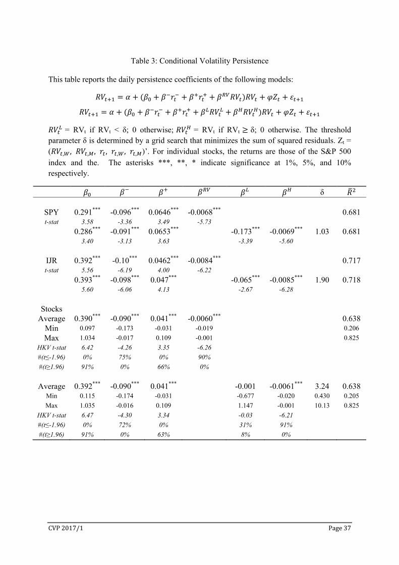
in (3).6 Under the first specification in (2), the CVP coefficients ( , , , and ) are
all statistically significant at 1% for SPY, IJR, and individual stocks. Large returns increase
RV persistence ( 0and 0 . Negative returns have about twice the impact of
positive returns ( / 2). High RV is associated with low future persistence (
0). Individual stock regressions provide clear support to the sign and the significance of the
conditional persistence coefficients: is negative and significant for 75% of the stocks,
is positive and significant for 66% of the stocks, and is negative and significant for 90%
of the stocks. While not reported here, the F statistics resoundingly reject the null hypothesis
6 To conserve space, we do not report the estimated coefficients of the control variables Zt = ( , , , , ,, , , )’. They are qualitatively the same as in Table 2, but numerically much smaller.

CVP2017/1 Page17
of = = =0; both the Aikaike and the Bayesian information criteria are heavily in
favour of the conditional persistence model in (3) over the constant persistence model in (1).
When daily RV is classified as or , the threshold parameter δ is determined
by grid-search. We set the search range from 10 to 90 percentiles of daily RV with step size =
0.01. The optimal value of δ is determined by the lowest SSR for (3). Table 3 shows that the
optimal δ is 1.03 for SPY and 1.90 for IJR. For SPY, there are 72% of daily RV below and
28% above the threshold. The split is 76% and 24% for IJR. Both low and high RVs have
negative coefficients and are associated with lower future RV persistence. The slope is much
steeper for low RV than it is for high RV. For SPY, = -0.175 and the median RV 0.55 <
1.03 (Table 1). On a typical day, RV’s impact on future persistence is -0.175*0.55 = -0.0963.
Assuming return is close to zero on a typical day, this represents a 33% reduction relative to
= 0.291. Similarly for IJR, the impact from a median RV (0.99) is a 16% reduction in
persistence relative to = 0.393. For high RV days, i.e. RVt > δ, the coefficients are
numerically smaller but statistically highly significant. High RV reflects high uncertainty,
which takes longer to resolve. Higher RV is still associated with lower persistence, but at
slower rate of reduction in persistence. We note that is very similar in value to . This
is not surprising since the ranges for are almost the same as the ranges for RVt. From
Table 1, ∈ [1.03, 60.3] and ∈ [0.033, 60.3] for SPY, ∈ [1.9, 77.1] and ∈
[0.095, 77.1] for IJR. The very high overlapping in value between and results in
very similar estimated coefficients.
For individual stocks, the results in Table 3 are based on the S&P 500 index returns
and are qualitatively similar to those of SPY and IJR. Large returns are associated with high
CVP, while high RV is associated with low CVP. Although the average is not significant,
we note that 31% of stocks have negative and significant and only 8% of stocks have
positive and significant . The average is highly significant and reduces CVP. The
CVP2017/1 Page18
thresholds for individual stocks range from 0.43 to 10.13 with an average of 3.24. Again the
values for and are highly overlapping, resulting in similar estimated coefficients.
While not reported here, the F test strongly rejects the CVP coefficients = = = =0
for SPY, IJR, and individual stocks; the Aikaike and the Bayesian information criteria are
very similar for the two models of RV persistence in (2). The adjusted R2s in Table e are
almost identical between the two CVP models. We therefore take the more parsimonious
specification as the baseline model going forward.
For robustness check, we divide the sample into two-year sub-periods. The results are
not reported to conserve space. Negative returns are significant in almost all sub-periods.
The coefficients of RV is negative significant in most sup-periods. The model in (3) works
particularly well during the crisis period of 2008-09, with all conditioning variables highly
significant and = 0.726 for SPY, 0.741 for IJR, 0.645 for stocks.
Characteristics of Conditional Volatility Persistence
Figure 3 depicts the estimated for SPY and
IJR with the estimated coefficients given in Table 3. is very high during the financial
crisis in the second half of 2008. There are a few > 1, 3 in 3547 days (0.08%) for SPY
and 5 in 3059 days (0.16%) for IJR. The summary statistics for is reported in Panel A
of Table 1. The mean of is 0.354 for SPY, 0.456 for IJR, and 0.434 for stocks. is
highly persistent, but is less persistent than RV as indicated by the Ljung-Box statistic,
consistent with the large impact from returns.
Panel B of Table 1 reports the correlations of with other variables. has a
significant positive correlation with return. The effect of rt on t can be written as
| | . Because < 0 and > 0, > 0 and is much larger than ;
therefore the return size effect is larger than the return direction effect. The unconditional

CVP2017/1 Page19
correlation between and RV is positive, which is consistent with Ning, Xu, and Wirjanto
(2015). With the exception of illiquidity for IJR, is positively correlated with trade and
liquidity variables.
To further assess the impact of return and RV on , we decompose the variance of
into components associated with the variances of the orthogonalized , , and .7
The contributions of , , and to the variance of are denoted as w( ), w( ), and
w( ) respectively. The decomposition outcome depends on the order of the variables in the
orthogonalization process. Table 4 reports the summary of w( ), w( ), and w( ) across
3! = 6 permutations for SPY and IJR. For individual stocks, we first calculate the average
w( ), w( ), and w( ) of each stock, then present the summary statistics across all stocks.
The most striking feature of Table 4 is the dominant impact of negative returns on the
variations of volatility persistence: negative returns on average account for 72~76% of
variance; positive returns account for 16~23%; RV accounts for only 5~7%. The median
w( ), w( ), and w( ) across stocks are even more skewed toward negative returns, with
the median w( ) = 85%. For SPY and IJR, the pecking order w( ) > w( ) > w( )
holds in 5 out of the 6 permutations. In both exceptions, w( ) > 82% but w( ) < w( )
10%. Based on the average w( ), w( ), and w( ), 57 out of 87 stocks (66%) have the
same packing order, and 77 out of 87 stocks (89%) have w( ) being the highest of the three
components. Overall we see that the lagged returns, negative and positive, account for almost
95% of the variation in volatility persistence, while the lagged volatility explains the
7 Let y = ax1 + bx2 + cx3. The variance of y is decomposed into components attributed to x1, x2, and x3 based on the following orthogonalization process:
1) Take residuals from regressions x2 = α0 + α1x1 + u21 and x3 = β0 + β1x1 + u31; 2) Run 31 = λ 21 + u32 to get 32 3) y = ax1 + b( 0 + 1x1 + 21) + c( 0 + 1x1 + 31)
= (a+b 1+c 1)x1 + (b+c ) 21 + c 32 + constant = Ax1 + B 21 + c 32 + constant
4) var(y) = A2var(x1) + B2var(u21) +c2var(u32); 5) w(x1) ≡ , w(x2)≡ , and w(x3) ≡ .
CVP2017/1 Page20
remaining 5%. The evidence in Tables 3 and 4 suggests that the propagation of volatility
over time is not due to high volatility itself, but rather the shocks to the broad market
embedded in the current market return.
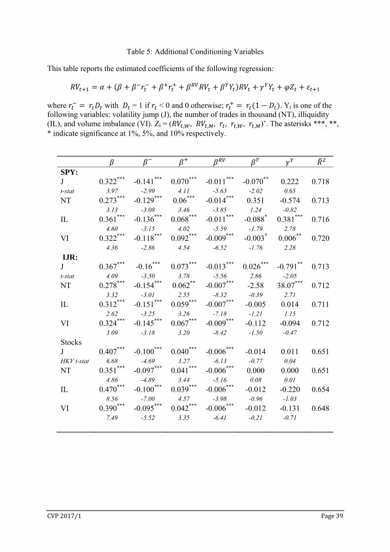
Additional Conditioning Variables
In addition to daily return and RV, we examine whether daily volatility persistence is
affected by volatility jumps (J), number of trades (NT), illiquidity (IL), and the imbalance of
buyer- and seller-initiated volumes (VI). The construction and statistical descriptions of
these variables are given in section II. Let Yt be one of these variables on day t. To assess the
impact of these variables on volatility persistence, we extend the model in (3) to include Yt
and its interaction with RVt:
(4)
Table 5 reports the impact of the additional conditioning variables. For individual
stocks, none of the additional conditioning variables has a significant impact on volatility
level ( ) or volatility persistence ( ). For index ETFs, none of them is significant for both
ETFs. Volatility jumps reduces volatility persistence for SPY but increases persistence for
IJR. Illiquidity and volume imbalance have no effect on the level and the persistence of IJR
volatility. The impact of return and RV on volatility persistence remains intact in Table 3.
Our findings are consistent with those of Gillemot, Farmer, and Lillo (2006), who conclude
that “the long-memory of volatility is dominated by factors other than transaction frequency
or total trading volume.”
Long-run Volatility Persistence
As a final robustness check, we examine whether including long-run conditional
persistence alters the results for daily conditional persistence. Persistence at weekly and
monthly lags is estimated using the regression below:

CVP2017/1 Page21
∑ , , , , ,
where f = day (D), week (W), and month (M). Results presented in Table 6 show that the
daily conditional persistence in Table 3 remain largely intact. There is strong evidence of
weekly and monthly conditional persistence for individual stocks, but only weak evidence for
SPY and IJR. However, unlike positive daily returns which increase daily persistence,
positive weekly and monthly returns reduce the corresponding volatility persistence.
V. Information Flow and Volatility Dynamics
In this section we show that the findings in section IV can be explained by the daily
price discovery and net information flow. Intraday returns are decomposed into a random-
walk component and a serially-correlated component. The random-walk component is
traditionally attributed to the arrival of new information on asset value and is termed the
information component. However it also captures the price effects from shocks to liquidity
demand and supply. The serially-correlated component is termed the liquidity component
and captures all other price impact from trading, e.g. feedback trading, inventory
management, etc. Price discovery or gross information flow is measured by the variance of
the information component. The sum of the information component over a trading day
captures the net effect of positive and negative information flows. We show that (1) net
information flow increases but price discovery decreases volatility persistence; (2) large
negative net information flow has a dominant effect on volatility persistence; (3) the source
of volatility persistence is primarily the gross information flow and the covariance between
information and non-information returns; (4) the source of the so-called “leverage effect” is
primarily the net information flow. These findings shed new light on the mechanisms for
volatility persistence.
CVP2017/1 Page22
Measuring Price Discovery and Information Flows
Let there be S sub-periods on a trading day t, and ps be the logarithmic price observed
at the end of sub-period s.8 It can be viewed as having two components: ps = ms + ns, where
ms is the efficient price and ns is the noise term. The return is rs ≡ ps - ps-1 = Δms + Δns. The
changes in the efficient price Δms are independent over time and represent a permanent shift
in the asset value. The term Δns is serially correlated over time and captures a wide range of
transitory factors, e.g. bid-ask bounce, inventory management, feedback trading, etc. In this
study, Δms and Δns are termed the information and the liquidity returns respectively. Starting
from Hasbrouck (1991ab, 1993, 1995), price discovery is measured by the variance of Δms in
microstructure studies. We follow that tradition and use ∑ ∆m as a measure of price
discovery or gross information flow, and ∑ ∆m as a measure of net information flow, i.e.
the outcome of price discovery over a trading day.
To decompose rs into Δms and Δns, rs is fitted in an AR(K) model: rs = A(L)rs + us
where A(L) = a1L + … + aKLK and L is the lag operator.9 Since A(L)rs captures the
autocorrelations in rs, us captures the innovations in rs and is serially independent. A simple
return decomposition is to set Δms = us and Δns = A(L)rs where Δms and Δns are orthogonal.
We use the Beveridge-Nelson (1980) decomposition which allows Δms and Δns to be
correlated. Let B(L) = (1-A(L))-1 thus rs = B(L)us. B(L) can be decomposed as B(L) = B(1)
+ C(L)(1-L) where ∑ has exponentially decaying coefficient as increases.
The Beveridge-Nelson return decomposition is given by rs = B(1)us + C(L)Δus. Price at time s
is ps = ps-1 + rs = ps-1 + B(1)us + ∑ c Δu . Let Is be the information set at time s which
includes us: lim → E p I = ps-1 + B(1)us. Therefore the random-walk component Δms ≡
B(1)us captures the permanent price shocks from new information. The serially-correlated
8 The t subscript is suppressed when it does not cause confusion. 9 As in Hasbrouck (1991ab and 1993), the AR(K) model is estimated without a constant so that the sum of the estimated residuals, i.e. the aggregate shocks over a trading day, is non-zero.

CVP2017/1 Page23
component Δns ≡ C(L)Δus captures the transitory impact of non-information trading. The
covariance between Δms and Δns is B(1)[1-B(1)]Var(us) = -A(1)Var(Δms).
For each trading day t, we calculate 5-minute returns rs,t, s = 1,…,78. The maximum
number of lags for the AR model is 6, i.e. we allow return autocorrelation up to 30 minutes.
The optimal lag length Kt is determined by the average of the Akaike and Bayesian
information criteria. The AR coefficients are estimated for each trading day t via OLS. Let At
be the sum of the estimated AR coefficients on day t: At ≡ ∑ a , therefore Bt(1) = .
The information return is Δms,t = , and the liquidity return is Δns,t = r ,, . The net
information flow for day t is defined as r , ≡ ∑ , . The net liquidity return is
r , ≡ ∑ r ,, . The daily RVt = ∑ r , is decomposed into three components.
The information RV is defined as RV , ≡ ∑ ∆m , . It measures price discovery or gross
information flow for day t. The liquidity RV is defined as RV , ≡ ∑ ∆n , . The
covariance between r , and r , is given by Covt ≡ -AtRV , . One can easily verify RVinf,t
+ RVliq,t + 2Covt = RVt.10
Table 7 reports the summary statistics of the return and RV decompositions. It shows
that following features:
(1) The information and liquidity returns, rinf and rliq, have very different characteristics.
For example, rinf has higher standard deviation than rliq, consistent with information
trading having greater price impact than liquidity trading. While rinf is negatively
skewed and has low kurtosis, rliq is positively skewed and has much higher kurtosis.
Even though rinf is the sum of the intraday random-walk returns, it has higher Ljung-
Box statistic, thus higher autocorrelations across trading days, than rliq. Since the
10 Since the AR model is estimated without the first K observations, one has to add the first K returns in rs,t to the vector of to make the return and the RV decompositions precise.
CVP2017/1 Page24
AR(K) model does not have a constant, the daily constant is partially embedded in the
estimated residual u , , creating autocorrelation in r , ≡ ∑ , . If rinf is viewed
as the net outcome of price discovery, i.e. the net information flow, perhaps news
arrival is not random: it may persist in one direction for several days.
(2) Daily RV is dominated by its information component. On average RVinf accounts for
93% of daily RV for SPY and IJR, and 83% for large stocks. Therefore daily RV is
mostly driven by price discovery or gross information flow. RVinf is relatively more
stable than RVliq with lower coefficients of variation. It has much higher Ljung-Box
statistic, thus higher persistence. This suggests that price discovery is highly persistent.
While liquidity trading may account for a significant portion of daily trading, its gross
and net price impacts, RVliq and rliq, appear to be relatively small and less persistent.
(3) The mean and median of daily covariance between r and r are around zero.
Stocks have much higher covariance variations than SPY and IJR. The median size of
covariance varies from 5.2% to 8.8% of the daily RV. Covariance is highly negatively
skewed but only mildly persistent. It does not appear that information and liquidity
trading consistently leads to significant co-movements in returns.
Information Flows and Volatility Persistence
To examine the differential impacts of the information and liquidity components on
volatility persistence, we re-estimate the HAR-CVP model in (3) with CVPt specified as
, , , , ,
The negative and positive return components are defined as in eq (2). We do not include
RVliq,t because of the high correlations between RVinf,tRVt and RVliq,tRVt in regression (2),
e.g. 0.886 for SPY. Panel A of Table 8 reports the estimated CVP coefficients. We see three
features in the table:
CVP2017/1 Page25
(1) Large information returns rinf increase RV persistence, with negative information
returns r having greater impact than positive information returns r . Therefore the
strong positive impact of return size on volatility persistence, as reported in Tables 3
and 4, is largely driven by rinf, the outcome of price discovery. Intuitively, large
returns are associated with high volatility via the news impact curve of Engle and Ng
(1993). Large net information flow rinf leads to greater price discovery (RVinf) effort
thus high volatility on the next day.
(2) Liquidity returns rliq, positive or negative, do not affect RV persistence. Note that the
size of rliq is significant relative to rinf. Using standard deviation (Table 8) as a proxy
for return size, the size of rliq is around 28% (stocks) to 46% (SPY) of the size of rinf.
The strong impact from returns on CVP (Tables 3 & 4) and the lack of impact from
rliq on CVP further supports net information flow as an important determinant of
volatility persistence.
(3) RVinf reduces CVP for SPY, IJR, and stocks: more price discovery increases the
information content of price and reduces the spillover of uncertainty over time.
Overall the evidence indicates that gross and net information flows have significant
impact on volatility persistence, while liquidity trading and its price impact do not
affect volatility persistence.
Table 4 shows that negative returns account for up to 87% of the variation of CVP.
Panel A of Table 8 shows that negative information flow r has a dominant impact on CVP.
These findings motivate us to examine the size effect of r using three dummy variables:
D = 1 if rinf,t < 0, 0 otherwise;
D , = 1 if |r , | > Median(|r , | | r , < 0), 0 otherwise;
D%, = 1 if | , |
| , , | > Median
| , |
| , , |, 0 otherwise.
CVP2017/1 Page26
The size dummies are based on the absolute return value (D , ) or the relative size to total
return (D%, ). The conditional volatility persistence is specified as
, % %, % , %,
We estimate the impact of r when it is small ( ), when it is high in value ( ), when it is
high as relative size ( %), and when it is high in both value and relative size ( %). Panel B
of Table 8 reveals some interesting features:
(1) is positive and highly significant: the positive impact of |r | on CVP is from large
|r | above the median value.
(2) % and % are not significant for IJR and stocks. The same is true for SPY if its top
2% daily RV were winsorized. The relative size dummy and the interaction D , D%,
have no effect on most days.
(3) is not significant for IJR and stocks, nor is it for SPY if its top 1% daily RV were
winsorized. Therefore when r is below its median value, it has no effect on
volatility persistence. Only large information shocks increase the spillover of
volatility from today to tomorrow.
Information Flow and Volatility Level
The distinct characteristics of the information and liquidity components, rinf versus rliq
and RVinf versus RVliq, motivate us to explore their impact on future RV level as well as their
own dynamics. We estimate a variation of the standard HAR model:
Y α β RV , β RV , β Cov β RV , β RV ,
θ r , θ r , θ r , θ r , ε
where Y = RV, RVinf, or RVliq. The model separately estimates the impact on future volatility
from the three components of the lagged daily RV. If price discovery or the gross information
flow is highly persistent, βinf is expected to be positive and significant at least for Y = RV and
RVinf. RVliq is small and far less persistent relative to RV and RVinf, therefore may not have a
CVP2017/1 Page27
significant impact on these variables. It is still highly persistent; therefore βliq is expected to
be significant for Y = RVliq. While the covariance between rinf and rliq is mildly persistent,
positive co-movements between information and liquidity trading tends to make price
discovery more difficult, resulting in higher uncertainty and high volatility tomorrow. We
expect βcov to be positive. The separation of the lagged daily return to rinf and rliq is aimed at
testing whether they both lead to the leverage effect or asymmetric volatility.
Table 9 reports the estimated coefficients of the information and liquidity variables. It
shows several new features in volatility dynamics:
(1) βinf is positive and significant for Y = RV, RVinf, and RVliq: RVinf is an important
determinant of tomorrow’s volatility and its components. Note that a positive and
significant βinf indicates that RVinf increases tomorrow’s volatility level, even though
it simultaneously reduces RV persistence as shown in Panel A of Table 9. While CVP
is reduced by RVinf, it remains positive, leading to a positive impact from RVinf to
future volatility level. This is consistent with Table 8, i.e. price discovery measured
by RVinf is the dominant component of daily RV and it is highly persistent. Taken
together with Table 9, we conclude that volatility dynamics is dominated by the gross
and net information flows.
(2) RVliq has limited impact on future volatility: it is marginally significant for SPY and
stocks and Y = RV. Although the contemporaneous correlations between RVinf and
RVliq are quite high, 0.681 for SPY and 0.627 for IJR, RVliq has no impact on future
RVinf. After controlling for the effects of other variables, RVliq shows no daily
persistence for SPY and IJR, contrary to the LB5 in Table 8. While it is persistence
for stocks, the impact from RVinf and Cov appears to be equal or larger.
(3) The daily covariance between rinf and rliq has a strong positive impact on future
volatility, especially for IJR and stocks. There is a strong negative correlation between

CVP2017/1 Page28
Cov and RVinf, -0.465 for SPY and -5.81 for IJR. Therefore price discovery (RVinf) is
low when information and liquidity trading are in the same direction (Cov > 0). Low
price discovery today leads to higher volatility tomorrow.
(4) The net information flow rinf is the main driver of asymmetric volatility or the
leverage effect in volatility dynamics. However rliq also contributes to the leverage
effect in IJR.
VI. Conditional Persistence and Volatility Forecast
This section provides further evidence on the importance of the conditional volatility
persistence. Building on the above analyses, we compare the pseudo-out-of-sample volatility
forecasts based on the standard HAR model (HAR) against those based on the conditional
HAR model (CHAR). In volatility forecast, model parameters are estimated using an
expanding or rolling window. Therefore even in models with constant volatility persistence,
persistence is re-estimated every day. CHAR explicitly allows persistence to be dependent on
return and volatility. If the true persistence indeed varies with return and volatility as
demonstrated in the preceding analyses, the CHAR model should lead to superior out-of-
sample forecasts.
Evaluation of volatility forecast performance is based on two loss functions: the
negative quasi-likelihood function QLIKE( , ) = ln 1 and the logarithmic
mean-squared errors LMSE( , ) = (ln ln )2 where is the forecasted
value of . Patton (2011) shows that QLIKE is robust to the noise in the empirical
volatility measures. Patton and Sheppard (2009) show that QLIKE has the best size-adjusted
power among robust loss functions. The usual mean-squared error (MSE) is often affected by
a few extreme observations. We use the logarithmic MSE to mitigate this problem. Forecasts
are based on 6-year rolling windows, starting in 2006 for SPY and in 2008 for IJR and stocks.
CVP2017/1 Page29
Forecast performance is evaluated by the Diebold-Mariano (1995, DM) test. Taking the HAR
model as the benchmark, a negative DM statistic indicates a reduction in loss value by CHAR
relative to HAR. While HAR is nested in CHAR, Giacomini and White (2006) show that the
DM test remains asymptotically valid when the estimation period is finite.
Panel A of Table 10 provides a summary of QLIKE and LMSE values. For both loss
functions and across SPY, IJR, and stocks, CHAR has lower mean and median loss values
than HAR. The reductions in loss value of CHAR are substantial: e.g. for SPY, CHAR
reduces the average QLIKE by 51% and the average LMSE by 45%. Across SPY, IJR, and
stocks and for both loss functions, the reduction is 44% for the average loss values and 39%
for the median loss values. The DM tests show that the reductions are statistically significant
at 10% for stocks with QLIKE, and are significant at 1% for all other cases. CHAR has
lower average QLIKE for 85% of the stocks and lower average LMSE for 97% of the stocks.
It has lower median loss values than HAR for all stock (100%). We note that the differences
between the average and the median QLIKE are quite large, indicating the presence of a few
very large values. The problem is not as extreme for LMSE but is still prominent.
Panel B of Table 10 compares forecast performance of HAR and CHAR under
different market conditions. Trading days are divided into the high and low RV days based on
the median daily RV. The high and low RV days are further divided into thirds: days in the
bottom third have large negative returns (r<<0), days in the top third have large positive
returns (r>>0), and days in the middle third have small returns (r 0). For each of the six
categories we calculate (LCHAR-LHAR)/LHAR where LCHAR and LHAR are the median loss
function values of HAR and CHAR. Panel B shows that LCHAR < LHAR for all three asset
types and two loss functions. CHAR performs better on low RV days and positive return
days (r>>0). Although negative returns (r<<0) increase persistence more than positive returns,
CVP2017/1 Page30
they are associated with high RVs which reduce volatility persistence. On days with small
returns (r 0), RV is less persistent therefore more difficult to forecast.
Panel C of Table 10 reports the median loss function values in different sub-periods.
CHAR has lower median loss values in all sub-periods for both QLIKE and LMSE. Even
during the global financial crisis, CHAR is able to reduce the forecast losses of HAR by 16%
to 32%. It is interesting to note that CHAR performs much better than HAR after 2010, even
though the in-sample fit of CHAR is not particularly strong in these periods (Table 5).
VII. Conclusion
Contrary to the current literature which views volatility persistence as constant or
slow moving, this study shows that the persistence of daily RV has large variations associated
with daily return and RV. The propagation of volatility over time not only depends on the
level of volatility but also on the time-varying persistence. The finding of return and volatility
level as systematic factors affecting volatility persistence should help guide theoretical
research on the economic mechanisms for volatility persistence.

CVP2017/1 Page31
Reference Aït-Sahalia, Y., Mykland, P. A., & Zhang, L. (2011). Ultra high frequency volatility estimation with dependent microstructure noise. Journal of Econometrics, 160(1), 160-175. Andersen, T., T. Bollerslev, and F. X. Diebold (2007). Roughing it up: Including jump components in the measurement, modeling and forecasting of return volatility. Review of Economics and Statistics 89, 701–720. Andersen, T.G., Bollerslev, T., Diebold, F.X. and Ebens, H., 2001. The distribution of realized stock return volatility. Journal of financial economics, 61(1), pp.43-76. Andersen, T. G., T. Bollerslev, F. X. Diebold, and P. Labys, 2003, “Modeling and Forecasting Realized Volatility,” Econometrica 71, 579–625. Andersen, T. G., Bollerslev, T., & Huang, X. (2011). A reduced form framework for modeling volatility of speculative prices based on realized variation measures. Journal of Econometrics, 160(1), 176-189. Barndorff-Nielsen, O. E. and N. Shephard (2002). Estimating quadratic variation using realised variance. Journal of Applied Econometrics 17, 457-477. Barndorff-Nielsen, O., Shephard, N., 2006. Econometrics of testing for jumps in financial economics using bipower variation. Journal of Financial Econometrics 4, 1–30. Barndorff-Nielsen, O. E., P. R.Hansen, A. Lunde, And N. Shephard (2009): “Realized kernels in practice: trades and quotes,” Econometrics Journal, 12(3), C1–C32. Barndorff-Nielsen, O. E., S. Kinnebrock, And N. Shephard (2010): “Measuring downside risk – realised semivariance,” in Volatility and Time Series Econometrics: Essays in Honor of Robert F. Engle, ed. by T. Bollerslev, J. Russell, and M. Watson. Oxford University Press. Berger, D., Chaboud, A., & Hjalmarsson, E. (2009). What drives volatility persistence in the foreign exchange market?. Journal of Financial Economics, 94(2), 192-213. Bollerslev, T. (2008). Glossary to arch (garch). CREATES Research Paper, 49. Bouchaud, J. P., Matacz, A., Potters, M., 2001. Leverage Effect in Financial Markets: The Retarded Volatility Model. Physical Review Letters 87 (22), 228701. Bouchaud, J. P., Potters, M., 2001. More Stylized Facts of Financial Markets: Leverage Effect and Downside Correlations. Physica A: Statistical Mechanics and its Applications 299 (1), 60–70. Brock, W.A., LeBaron, B., 1996. A dynamic structural model for stock return volatility and trading volume. Review of Economics and Statistics 78, 94–110. Cabrales, A., Hoshi, T., 1996. Heterogeneous beliefs, wealth accumulation, and asset price dynamics. Journal of Economic Dynamics and Control 20, 1073–1100.

CVP2017/1 Page32
Campbell, J.Y. and Hentschel, L., 1992. No news is good news: An asymmetric model of changing volatility in stock returns. Journal of financial Economics, 31(3), pp.281-318. Corsi, F. (2009). A simple approximate long-memory model of realized volatility.Journal of Financial Econometrics 7, 174-196. Corsi, F., & Renò, R. (2012). Discrete-time volatility forecasting with persistent leverage effect and the link with continuous-time volatility modeling. Journal of Business & Economic Statistics, 30(3), 368-380. Holden, C.W. and Subrahmanyam, A., 1992. Long‐lived private information and imperfect competition. The Journal of Finance, 47(1), pp.247-270. Easley, D., M. López de Prado and M. O’Hara, 2012. Flow Toxicity and Liquidity in a High Frequency World. Review of Financial Studies, 25(5), 1547-1493. Easley, D., M. López de Prado and M. O’Hara, 2015. Discerning Information from Trade Data, manuscript. Fengler, M.R., Mammen, E. and Vogt, M., 2015. Specification and structural break tests for additive models with applications to realized variance data. Journal of Econometrics, 188(1), pp.196-218. de Fontnouvelle, P., 2000. Information dynamics in financial markets. Macroeconomic Dynamics 4, 139–169. Forsberg and Ghysels (2007): Why Do Absolute Returns Predict Volatility So Well? J Fin Econometrics. Garman, M. B., and Klass, M. J. 1980. On the estimation of security price volatilities from historical data. Journal of Business 53:67–78. Giacomini, R., & White, H. (2006). Tests of conditional predictive ability. Econometrica, 74(6), 1545-1578. Gillemot, L., Farmer, J. D., & Lillo, F. (2006). There's more to volatility than volume. Quantitative Finance, 6(5), 371-384. Haan, W.D., Spear, S., 1998. Volatility clustering in real interest rates: theory and evidence. Journal of Monetary Economics 41, 431–453. Hameed, A., Kang, W., & Viswanathan, S. (2010). Stock market declines and liquidity. The Journal of Finance, 65(1), 257-293. He, X., & Velu, R. (2014). Volume and volatility in a common-factor mixture of distributions model. Journal of Financial and Quantitative Analysis, 49(01), 33-49. Hellwig, M., 1980. On the Aggregation of Information in Competitive Markets. Journal of Economic Theory 22 (3), 477–498.

CVP2017/1 Page33
Jones, C.M., Kaul, G. and Lipson, M.L., 1994. Information, trading, and volatility. Journal of Financial Economics, 36(1), pp.127-154. Lamoureux, C. G., & Lastrapes, W. D. (1990a). Heteroskedasticity in stock return data: volume versus GARCH effects. The Journal of Finance, 45(1), 221-229. Lamoureux, C. G., & Lastrapes, W. D. (1990b). Persistence in variance, structural change, and the GARCH model. Journal of Business & Economic Statistics, 8(2), 225-234. Lamoureux, C. G., & Lastrapes, W. D. (1994). Endogenous trading volume and momentum in stock-return volatility. Journal of Business & Economic Statistics, 12(2), 253-260. Müller, U., M. Dacorogna, R. Davé, R. Olsen, O. Pictet, and J. von Weizsäcker (1997). Volatilities of different time resolutions - analyzing the dynamics of market components. Journal of Empirical Finance 4, 213–239. Ning, C., Xu, D., & Wirjanto, T. S. (2015). Is volatility clustering of asset returns asymmetric?. Journal of Banking & Finance, 52, 62-76. Parkinson, M. (1980), “The Extreme Value Method for Estimating the Variance of the Rate of Return,” Journal of Business, 53, 61-65
Patton, A. J. (2011). Volatility forecast comparison using imperfect volatility proxies. Journal of Econometrics, 160(1), 246-256.
Patton, A. J., & Sheppard, K. (2009). Evaluating volatility and correlation forecasts. In Handbook of financial time series (pp. 801-838). Springer Berlin Heidelberg. Patton, A. J., & Sheppard, K. (2015). Good volatility, bad volatility: Signed jumps and the persistence of volatility. Review of Economics and Statistics, 97(3), 683-697.
Rogers, L. C. G., and Satchell, S. E. 1991. Estimating variance from high, low and closing prices. Annals of Applied Probability 1:504–12. Smith, L. V., Yamagata, T., 2011. Firm Level Return-Volatility Analysis Using Dynamic Panels. Journal of Empirical Finance 18 (5), 847–867. Tauchen, G., Zhang, H. and Liu, M., 1996. Volume, volatility, and leverage: A dynamic analysis. Journal of Econometrics, 74(1), pp.177-208. Timmermann, A., 2001. Structural breaks, incomplete information and stock prices. Journal of Business and Economics Statistics 19, 299–314 Wang, J., 1994. A Model of Competitive Stock Trading Volume. Journal of Political Economy 102 (1), 127–168. Xue, Y., & Gençay, R. (2012). Trading frequency and volatility clustering.Journal of Banking & Finance, 36(3), 760-773.

CVP2017/1 Page34
Table 1: Data Summary
Return is the percentage change in log daily closing prices. RV is daily realized variance based on 5-minute returns in percentage. CVP is the conditional volatility persistence described in section IV. Jump is volatility jump. Its statistics are based on days with significant positive jumps. Trades are the number of transactions. TImb is the difference between buyer- and seller-initiated trades. Illiq is the Amihud illiquidity measure. LB5 is the Ljung-Box statistic for 5 lags. The asterisks ***, **, * indicate significance at 1%, 5%, and 10% respectively. Panel A: Summary statistics
Mean Median St Dev Skew Kurt LB5 SPY Return 0.008 0.065 1.32 0.029 12.3 38***
RV 1.13 0.551 2.43 11.4 210 6714*** Jump 0.221 0.101 0.468 8.41 97.4 - Trades 23.2 13.0 26.3 1.91 8.36 14596*** TImb -0.091 -0.002 15.4 0.771 18.2 29*** Illiq 0.226 0.059 0.487 4.25 25.7 5462*** CVP 0.354 0.330 0.076 3.01 19.5 709*** IJR Return 0.034 0.100 1.52 -0.306 7.30 20*** RV 1.75 0.990 3.05 9.79 167 5853*** Jump 0.420 0.243 1.26 13.2 189 - Trades 4.58 3.58 4.73 1.49 6.32 10462*** TImb -0.011 -0.002 0.411 0.451 14.7 6.1 Illiq 2.08 0.828 3.90 4.92 40.1 2517*** CVP 0.456 0.431 0.082 2.86 17.2 203*** Stocks Return 0.018 0.037 2.31 -5.37 247 20*** RV 2.50 1.21 5.60 9.64 172 6065*** Jump 0.719 0.354 1.67 7.29 88.2 - Trades 11.8 9.94 7.69 2.34 17.7 9090*** TImb 0.015 0.020 1.37 0.00 18.2 26*** Illiq 1.30 0.772 1.68 8.57 289 870*** CVP 0.434 0.412 0.071 2.71 25.4 356***

CVP2017/1 Page35
Panel B: Correlations Return RV CVP Trades TImb
SPY RV -0.088*** CVP 0.064*** 0.495***
Trades -0.069*** 0.458*** 0.292*** TImb 0.387*** 0.05*** 0.046*** 0.013 Illiq -0.041** 0.089*** 0.042** -0.319*** 0.005
IJR RV -0.039** CVP 0.075*** 0.419***
Trades -0.049*** 0.472*** 0.278*** TImb 0.285*** 0.036** 0.048*** 0.001 Illiq -0.03* 0.027 -0.02 -0.316*** 0.003
Stocks
RV -0.058*** CVP 0.033* 0.281***
Trades -0.048*** 0.432*** 0.193*** TImb 0.514*** 0.011 0.043** -0.02 Illiq -0.127*** 0.146*** 0.037** 0.016 0.009

CVP2017/1 Page36
Table 2: Heterogeneous Autoregressive Models
This table reports the coefficients of the following regression:
, , , , , ,
where and are the realized variance and return of SPY, IJR, and individual stocks. The returns of the S&P 500 index , , , and , are included only for individual stocks. The t-statistics are based on the Newey–West robust covariance with automatic lag selection using Bartlett kernel. The asterisks ***, **, * indicate significance at 1%, 5%, and 10% respectively.
SPY 0.313*** 0.394*** 0.163** -0.305*** -0.434*** -0.498*** 0.154*** 0.631 t-stat 4.50 3.39 2.46 -3.70 -3.90 -2.92 3.53
IJR 0.390*** 0.292*** 0.193*** -0.306*** -0.439*** -0.459** 0.256*** 0.673 t-stat 9.58 4.31 3.10 -4.44 -3.67 -2.58 4.37
Stocks: Average 0.328*** 0.387*** 0.192*** -0.332*** -0.477*** -0.236 0.259*** 0.571
Min 0.121 0.044 0.041 -0.799 -2.782 -1.005 0.073 0.155
Max 0.545 0.735 0.547 -0.071 -0.023 2.295 1.516 0.762
HKV t-stat 5.90 5.63 3.99 -3.18 -3.16 -1.09 3.85
%(t -1.96) 0% 0% 0% 76% 56% 14% 0%
%(t 1.96) 97% 95% 82% 0% 0% 0% 82%
Average 0.278*** 0.371*** 0.211*** -0.084 -0.180 -0.038 -0.569*** -0.927*** -0.957*** 0.414*** 0.591
Min 0.079 0.048 0.060 -0.677 -2.001 -0.928 -8.552 -3.667 -8.380 0.130 0.169
Max 0.530 0.721 0.506 2.338 0.464 4.165 -0.034 -0.292 -0.228 2.658 0.769
HKV t-stat 4.76 5.66 4.62 -0.93 -1.36 -0.17 -3.64 -4.17 -2.95 5.28
%(t -1.96) 0% 0% 0% 16% 10% 5% 91% 94% 60% 0%
%(t 1.96) 87% 95% 93% 0% 1% 0% 0% 0% 0% 100%
CVP2017/1 Page37
Table 3: Conditional Volatility Persistence
This table reports the daily persistence coefficients of the following models:
= RVt if RVt < δ; 0 otherwise; = RVt if RVt δ; 0 otherwise. The threshold parameter δ is determined by a grid search that minimizes the sum of squared residuals. Zt = ( , , , , , , , , )’. For individual stocks, the returns are those of the S&P 500
index and the. The asterisks ***, **, * indicate significance at 1%, 5%, and 10% respectively.
δ
SPY 0.291*** -0.096*** 0.0646*** -0.0068*** 0.681 t-stat 3.58 -3.36 3.49 -5.73
0.286*** -0.091*** 0.0653*** -0.173*** -0.0069*** 1.03 0.681 3.40 -3.13 3.63 -3.39 -5.60
IJR 0.392*** -0.10*** 0.0462*** -0.0084*** 0.717 t-stat 5.56 -6.19 4.00 -6.22
0.393*** -0.098*** 0.047*** -0.065*** -0.0085*** 1.90 0.718 5.60 -6.06 4.13 -2.67 -6.28
Stocks
Average 0.390*** -0.090*** 0.041*** -0.0060*** 0.638 Min 0.097 -0.173 -0.031 -0.019 0.206
Max 1.034 -0.017 0.109 -0.001 0.825
HKV t-stat 6.42 -4.26 3.35 -6.26 #(t≤-1.96) 0% 75% 0% 90% #(t≥1.96) 91% 0% 66% 0%
Average 0.392*** -0.090*** 0.041*** -0.001 -0.0061*** 3.24 0.638
Min 0.115 -0.174 -0.031 -0.677 -0.020 0.430 0.205
Max 1.035 -0.016 0.109 1.147 -0.001 10.13 0.825
HKV t-stat 6.47 -4.30 3.34 -0.03 -6.21
#(t≤-1.96) 0% 72% 0% 31% 91%
#(t≥1.96) 91% 0% 63% 8% 0%

CVP2017/1 Page38
Table 4: CVP Variance Decomposition
This table decomposes the variance of into components associated with the variances of the orthogonalized , , and . The estimated coefficients , , , and are from Table 3. The weights w( ), w( ), and w( ) are the percentages of the variance of associated with the variances of the orthogonalized
, , and respectively. For SPY and IJR, the summary statistics are across six permutations in the orthogonalization process. For stocks, the summary statistics are across all stocks based on the average w( ), w( ), and w( ) of each stock.
w( ) w( ) w( ) SPY
Average 71.8% 22.7% 5.5% Median 72.9% 22.4% 4.7%
Min 53% 6.9% 0.2% Max 86.2% 36.9% 10.1%
IJR
Average 86.7% 8.8% 4.5% Median 87.0% 7.1% 5.0%
Min 75.8% 0.0% 0.6% Max 95.0% 19.2% 5.9%
Stocks
Average 76.5% 16.3% 7.3% Median 84.6% 9.5% 4.4%
Min 2.6% 2.4% 1.5% Max 94.4% 94.4% 49.9%
CVP2017/1 Page39
Table 5: Additional Conditioning Variables
This table reports the estimated coefficients of the following regression:
where with = 1 if < 0 and 0 otherwise; 1 . Yt is one of the following variables: volatility jump (J), the number of trades in thousand (NT), illiquidity (IL), and volume imbalance (VI). Zt = ( , , , , , , , , )’. The asterisks ***, **, * indicate significance at 1%, 5%, and 10% respectively.
SPY: J 0.322*** -0.141*** 0.070*** -0.011*** -0.070** 0.222 0.718 t-stat 3.97 -2.99 4.11 -5.63 -2.02 0.65
NT 0.273*** -0.129*** 0.06*** -0.014*** 0.351 -0.574 0.713 3.13 -3.08 3.46 -3.85 1.24 -0.82
IL 0.361*** -0.136*** 0.068*** -0.011*** -0.088* 0.381*** 0.716 4.60 -3.15 4.02 -5.59 -1.79 2.78
VI 0.322*** -0.118*** 0.092*** -0.009*** -0.003* 0.006** 0.720 4.36 -2.86 4.54 -6.52 -1.76 2.28
IJR: J 0.367*** -0.16*** 0.073*** -0.013*** 0.026*** -0.791** 0.713 t-stat 4.09 -3.50 3.78 -5.56 2.86 -2.05
NT 0.278*** -0.154*** 0.062** -0.007*** -2.58 38.07*** 0.712 3.32 -3.01 2.55 -8.32 -0.39 2.71
IL 0.312*** -0.151*** 0.059*** -0.007*** -0.005 0.014 0.711 2.62 -3.25 3.26 -7.18 -1.21 1.15
VI 0.324*** -0.145*** 0.067*** -0.009*** -0.112 -0.094 0.712 3.09 -3.18 3.20 -8.42 -1.50 -0.47
Stocks
J 0.407*** -0.100*** 0.040*** -0.006*** -0.014 0.011 0.651 HKV t-stat 6.68 -4.69 3.27 -6.13 -0.77 0.04
NT 0.351*** -0.097*** 0.041*** -0.006*** 0.000 0.000 0.651 4.86 -4.89 3.44 -5.16 0.08 0.01
IL 0.470*** -0.100*** 0.039*** -0.006*** -0.012 -0.220 0.654 8.56 -7.00 4.57 -3.98 -0.96 -1.03
VI 0.390*** -0.095*** 0.042*** -0.006*** -0.012 -0.131 0.648 7.49 -5.52 3.35 -6.41 -0.21 -0.71

CVP2017/1 Page40
Table 6: Long-Run Conditional Persistence
This table reports the coefficients of the following regression:
∑ , , , , ,
where f = day (D), week (W), and month (M). The asterisks ***, **, * indicate significance at 1%, 5%, and 10% respectively.
SPY 0.310*** -0.126*** 0.061*** -0.01*** 0.191*** -0.053 -0.041 0 0.349*** -0.156* -0.16 -0.019*** 0.721 4.74 -3.35 3.20 -4.63 2.27 -1.45 -0.83 0.07 4.59 -1.77 -1.59 -3.52
IJR 0.271** -0.149*** 0.058*** -0.008*** 0.167* -0.076* -0.044 -0.001 0.361*** -0.088 -0.028 -0.017*** 0.722
2.32 -3.41 3.11 -11.2 1.65 -1.75 -1.00 -0.28 4.36 -1.26 -0.31 -4.16
Stocks 0.344*** -0.094*** 0.034** -0.006*** 0.388*** -0.071** -0.077*** -0.005** 0.279*** -0.141*** -0.180** -0.010*** 0.659
HKV t-stat 5.45 -4.92 2.43 -5.68 5.07 -2.36 -2.79 -2.46 4.19 -2.74 -2.31 -3.71
%(t -1.96) 0% 83% 0% 86% 0% 31% 45% 44% 0% 57% 46% 69%
%(t 1.96) 89% 0% 41% 0% 94% 1% 2% 1% 84% 1% 0% 0%

CVP2017/1 Page41
Table 7: Information Components of Daily Return and Variance
This table reports the decomposition of daily return and variance into information and liquidity components. rinf and RVinf are the information components of daily return and RV. rliq and RVliq are the liquidity components. Cov is the covariance between rinf and rliq. CV is the coefficient of variation. LB5 is the Ljung-Box statistic for 5 lags. The asterisks ***, **, * indicate significance at 1%, 5%, and 10% respectively.
rinf rliq RVinf RVinf/RV RVliq RVliq/RV Cov 2Cov/RV
SPY Mean 0.015 -0.021 1.06 0.936 0.09 0.081 -0.01 -0.017 Median 0 -0.001 0.477 0.917 0.023 0.044 0.009 0.052 StDev 0.977 0.452 2.68 0.462 0.298 0.183 0.607 0.59 Skew -0.23 1.54 16.3 7.96 11.7 23.7 -16.5 -14.6 Kurt 12.8 54.6 448 168 187 846 446 405 CV 65.1 -21.5 2.5 0.5 3.3 2.3 -60.7 -34.7 LB5 39.0*** 8.96 4240*** 16.9*** 741.2*** 6.58 24.6*** 12.9** IJR Mean -0.006 -0.015 1.68 0.934 0.196 0.111 -0.06 -0.045 Median 0 -0.003 0.838 0.882 0.066 0.07 0.031 0.088 StDev 1.28 0.389 3.54 0.504 0.76 0.154 1.20 0.586 Skew -0.116 0.607 9.53 2.58 23.6 5.76 -20.2 -4.42 Kurt 11.9 60.8 133 16.8 750 64.2 574 35.5 CV -213.3 -25.9 2.1 0.5 3.9 1.4 -20.0 -13.0 LB5 32.6*** 19.8*** 3521*** 39.9*** 83.5*** 10.7* 20.2*** 11.6** Stocks Mean -0.002 0.003 2.37 0.834 0.876 0.271 -0.33 -0.105 Median 0.065 0 0.874 0.745 0.221 0.189 0.038 0.081 StDev 1.01 0.284 20.0 2.47 16.3 2.25 16.4 4.60 Skew -0.117 1.45 17.2 12.2 22.2 16.3 -24.8 -17.9 Kurt 13.2 29.5 558 474 862 694 1059 707 CV -505 94.7 8.4 3.0 18.6 8.3 -49.7 -43.8 LB5 25.0*** 20.8*** 2685*** 18.7*** 799*** 89.7*** 48.3*** 7.9
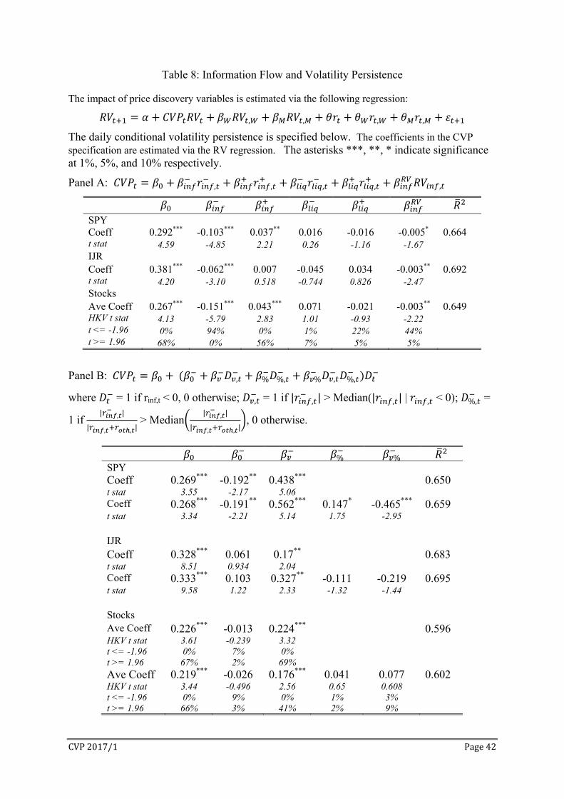
CVP2017/1 Page42
Table 8: Information Flow and Volatility Persistence
The impact of price discovery variables is estimated via the following regression:
, , , ,
The daily conditional volatility persistence is specified below. The coefficients in the CVP specification are estimated via the RV regression. The asterisks ***, **, * indicate significance at 1%, 5%, and 10% respectively.
Panel A: , , , , ,
SPY Coeff 0.292*** -0.103*** 0.037** 0.016 -0.016 -0.005* 0.664 t stat 4.59 -4.85 2.21 0.26 -1.16 -1.67 IJR Coeff 0.381*** -0.062*** 0.007 -0.045 0.034 -0.003** 0.692 t stat 4.20 -3.10 0.518 -0.744 0.826 -2.47 Stocks Ave Coeff 0.267*** -0.151*** 0.043*** 0.071 -0.021 -0.003** 0.649 HKV t stat 4.13 -5.79 2.83 1.01 -0.93 -2.22 t <= -1.96 0% 94% 0% 1% 22% 44% t >= 1.96 68% 0% 56% 7% 5% 5%
Panel B: , % %, % , %,
where = 1 if rinf,t < 0, 0 otherwise; , = 1 if | , | > Median(| , | | , < 0); %, =
1 if | , |
| , , | > Median
| , |
| , , |, 0 otherwise.
% % SPY Coeff 0.269*** -0.192** 0.438*** 0.650 t stat 3.55 -2.17 5.06 Coeff 0.268*** -0.191** 0.562*** 0.147* -0.465*** 0.659 t stat 3.34 -2.21 5.14 1.75 -2.95 IJR Coeff 0.328*** 0.061 0.17** 0.683 t stat 8.51 0.934 2.04 Coeff 0.333*** 0.103 0.327** -0.111 -0.219 0.695 t stat 9.58 1.22 2.33 -1.32 -1.44 Stocks Ave Coeff 0.226*** -0.013 0.224*** 0.596 HKV t stat 3.61 -0.239 3.32 t <= -1.96 0% 7% 0% t >= 1.96 67% 2% 69% Ave Coeff 0.219*** -0.026 0.176*** 0.041 0.077 0.602 HKV t stat 3.44 -0.496 2.56 0.65 0.608 t <= -1.96 0% 9% 0% 1% 3% t >= 1.96 66% 3% 41% 2% 9%
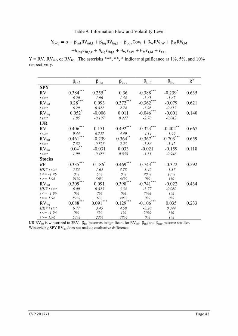
CVP2017/1 Page43
Table 9: Information Flow and Volatility Level
Y α β RV , β RV , β Cov β RV , β RV ,
, , θ r , θ r , ε
Y = RV, RVinf, or RVliq. The asterisks ***, **, * indicate significance at 1%, 5%, and 10% respectively.
β β β θ θ R SPY RV 0.384*** 0.255** 0.36 -0.388*** -0.239* 0.635 t stat 6.20 1.96 1.54 -3.65 -1.67 RVinf 0.28*** 0.093 0.372*** -0.362*** -0.079 0.621 t stat 6.29 0.822 2.74 -3.98 -0.657 RVliq 0.052* -0.006 0.011 -0.046*** -0.001 0.140 t stat 1.85 -0.107 0.227 -2.70 -0.042 IJR RV 0.406*** 0.151 0.492*** -0.323*** -0.402** 0.667 t stat 9.44 0.757 4.49 -4.14 -1.99 RVinf 0.461*** -0.239 0.364** -0.367*** -0.703*** 0.659 t stat 7.82 -0.825 2.23 -3.86 -3.42 RVliq 0.04** -0.031 0.033 -0.021 -0.159 0.118 t stat 1.99 -0.483 0.858 -1.31 -0.946 Stocks
0.335*** 0.186* 0.469*** -0.743*** -0.372 0.592 HKV t stat 5.83 1.65 3.78 -3.46 -1.37 t <= -1.96 0% 5% 0% 90% 13% t >= 1.96 91% 36% 64% 0% 1% RVinf 0.309*** 0.091 0.398*** -0.741*** -0.022 0.434 HKV t stat 6.00 0.823 3.34 -3.77 -0.080 t <= -1.96 0% 7% 0% 76% 1% t >= 1.96 87% 6% 49% 0% 0% RVliq 0.088*** 0.091*** 0.129*** -0.106*** 0.035 0.233 HKV t stat 6.77 3.45 4.58 -3.20 0.344 t <= -1.96 0% 3% 1% 20% 3% t >= 1.96 54% 23% 38% 0% 1%
IJR RVinf is winsorized to 3RV. β becomes insignificant for RVinf. β and β become smaller. Winsorizing SPY RVinf does not make a qualitative difference.
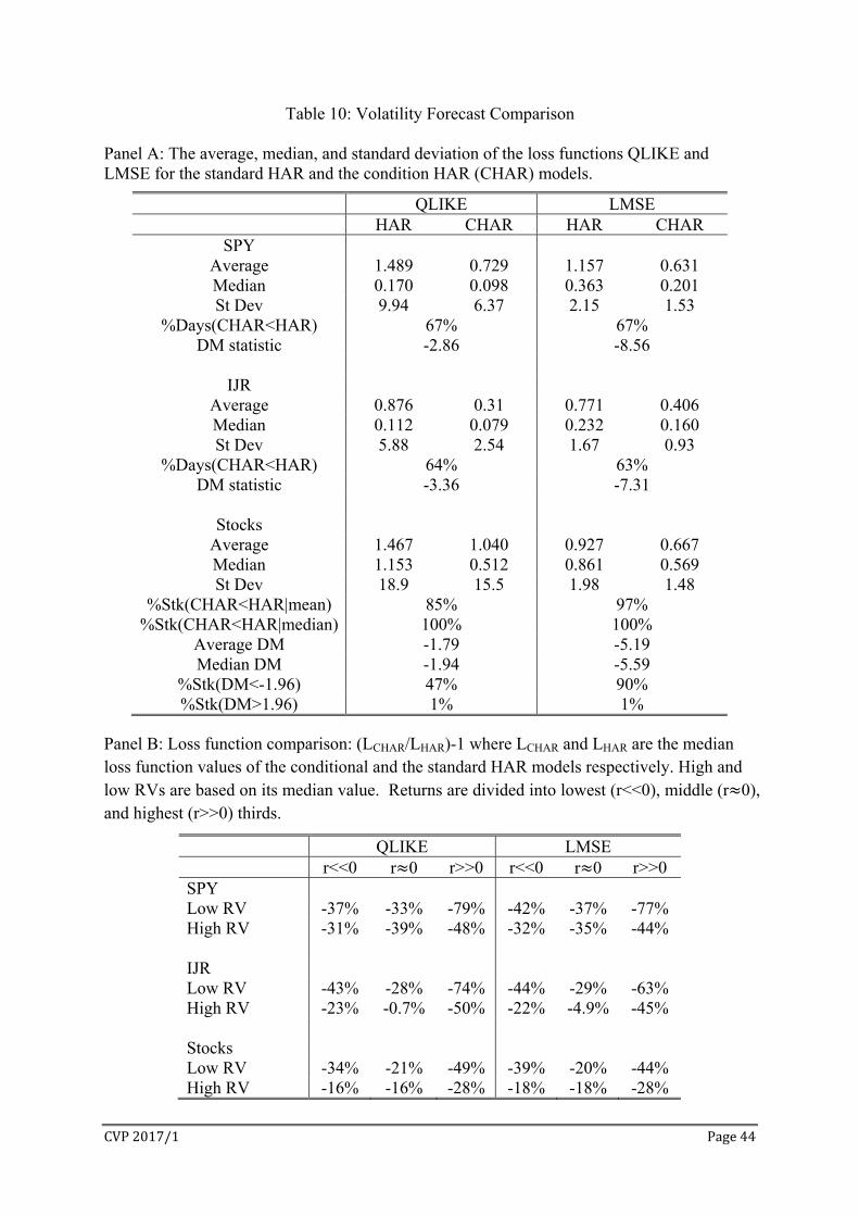
CVP2017/1 Page44
Table 10: Volatility Forecast Comparison
Panel A: The average, median, and standard deviation of the loss functions QLIKE and LMSE for the standard HAR and the condition HAR (CHAR) models.
QLIKE LMSE HAR CHAR HAR CHAR
SPY Average 1.489 0.729 1.157 0.631 Median 0.170 0.098 0.363 0.201 St Dev 9.94 6.37 2.15 1.53
%Days(CHAR<HAR) 67% 67% DM statistic -2.86 -8.56
IJR
Average 0.876 0.31 0.771 0.406 Median 0.112 0.079 0.232 0.160 St Dev 5.88 2.54 1.67 0.93
%Days(CHAR<HAR) 64% 63% DM statistic -3.36 -7.31
Stocks
Average 1.467 1.040 0.927 0.667 Median 1.153 0.512 0.861 0.569 St Dev 18.9 15.5 1.98 1.48
%Stk(CHAR<HAR|mean) 85% 97% %Stk(CHAR<HAR|median) 100% 100%
Average DM -1.79 -5.19 Median DM -1.94 -5.59
%Stk(DM<-1.96) 47% 90% %Stk(DM>1.96) 1% 1%
Panel B: Loss function comparison: (LCHAR/LHAR)-1 where LCHAR and LHAR are the median loss function values of the conditional and the standard HAR models respectively. High and low RVs are based on its median value. Returns are divided into lowest (r<<0), middle (r 0), and highest (r>>0) thirds.
QLIKE LMSE r<<0 r 0 r>>0 r<<0 r 0 r>>0 SPY Low RV -37% -33% -79% -42% -37% -77% High RV -31% -39% -48% -32% -35% -44% IJR Low RV -43% -28% -74% -44% -29% -63% High RV -23% -0.7% -50% -22% -4.9% -45% Stocks Low RV -34% -21% -49% -39% -20% -44% High RV -16% -16% -28% -18% -18% -28%
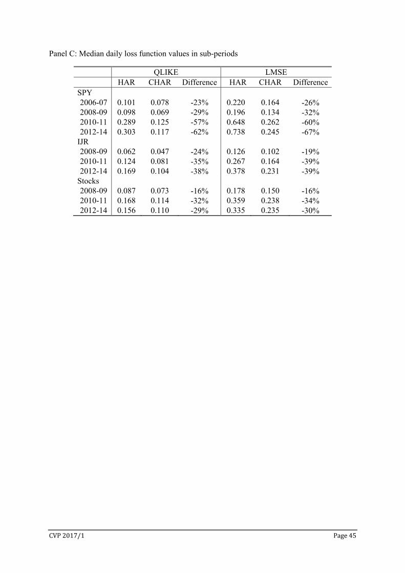
CVP2017/1 Page45
Panel C: Median daily loss function values in sub-periods
QLIKE LMSE HAR CHAR Difference HAR CHAR Difference SPY 2006-07 0.101 0.078 -23% 0.220 0.164 -26% 2008-09 0.098 0.069 -29% 0.196 0.134 -32% 2010-11 0.289 0.125 -57% 0.648 0.262 -60% 2012-14 0.303 0.117 -62% 0.738 0.245 -67% IJR 2008-09 0.062 0.047 -24% 0.126 0.102 -19% 2010-11 0.124 0.081 -35% 0.267 0.164 -39% 2012-14 0.169 0.104 -38% 0.378 0.231 -39% Stocks 2008-09 0.087 0.073 -16% 0.178 0.150 -16% 2010-11 0.168 0.114 -32% 0.359 0.238 -34% 2012-14 0.156 0.110 -29% 0.335 0.235 -30%
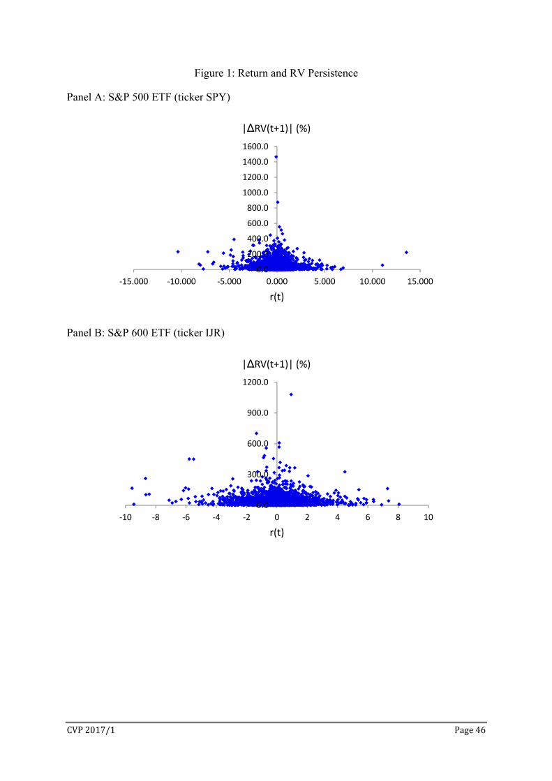
CVP2017/1 Page46
Figure 1: Return and RV Persistence
Panel A: S&P 500 ETF (ticker SPY)
Panel B: S&P 600 ETF (ticker IJR)
0.0
200.0
400.0
600.0
800.0
1000.0
1200.0
1400.0
1600.0
‐15.000 ‐10.000 ‐5.000 0.000 5.000 10.000 15.000
r(t)
|∆RV(t+1)| (%)
0.0
300.0
600.0
900.0
1200.0
‐10 ‐8 ‐6 ‐4 ‐2 0 2 4 6 8 10
r(t)
|∆RV(t+1)| (%)
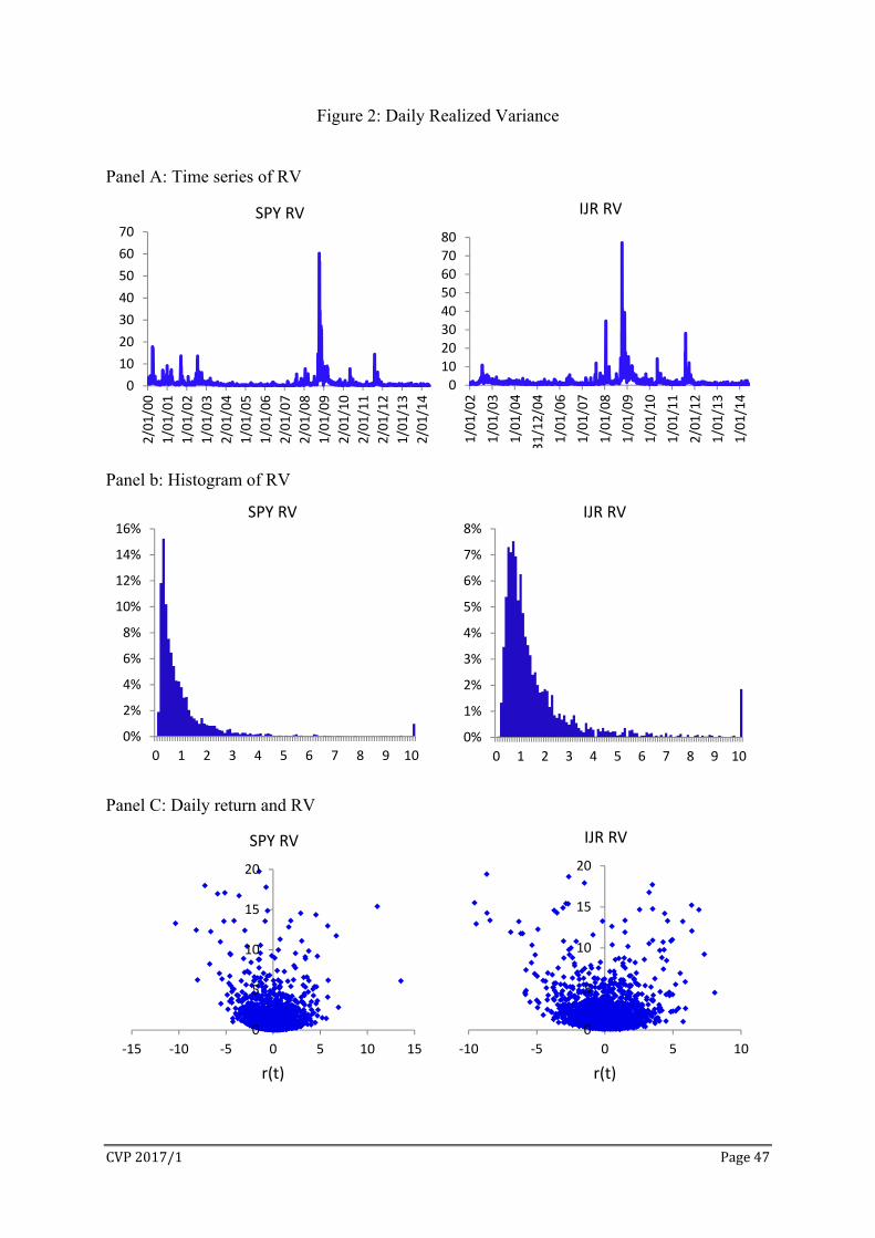
CVP2017/1 Page47
Figure 2: Daily Realized Variance
Panel A: Time series of RV
Panel b: Histogram of RV
Panel C: Daily return and RV
0
10
20
30
40
50
60
70
2/01/00
1/01/01
1/01/02
1/01/03
2/01/04
1/01/05
1/01/06
2/01/07
2/01/08
1/01/09
2/01/10
2/01/11
2/01/12
1/01/13
2/01/14
SPY RV
0
10
20
30
40
50
60
70
80
1/01/02
1/01/03
1/01/04
31/12/04
1/01/06
1/01/07
1/01/08
1/01/09
1/01/10
1/01/11
2/01/12
1/01/13
1/01/14
IJR RV
0%
2%
4%
6%
8%
10%
12%
14%
16%
0 1 2 3 4 5 6 7 8 9 10
SPY RV
0%
1%
2%
3%
4%
5%
6%
7%
8%
0 1 2 3 4 5 6 7 8 9 10
IJR RV
0
5
10
15
20
‐15 ‐10 ‐5 0 5 10 15
r(t)
SPY RV
0
5
10
15
20
‐10 ‐5 0 5 10
r(t)
IJR RV

CVP2017/1 Page48
Figure 3: Return, RV, and the Proxy for RV Persistence
Panel A: Return and the proxy for RV persistence (RVP)
Panel B: RV and the proxy for RV persistence (RVP) when RV 3
‐20
0
20
40
60
80
100
120
140
160
‐12‐10 ‐8 ‐6 ‐4 ‐2 0 2 4 6 8 10 12 14
r(t‐1)‐20
0
20
40
60
80
100
120
140
‐10 ‐8 ‐6 ‐4 ‐2 0 2 4 6 8 10
r(t‐1)
IJR RVP(t,t+1)
‐0.2
‐0.1
0.0
0.1
0.2
0.3
0.4
0 0.5 1 1.5 2 2.5 3
RV(t‐1)
SPY RVP(t,t+1)
‐0.2
‐0.1
0
0.1
0.2
0.3
0.4
0 0.5 1 1.5 2 2.5 3
RV(t‐1)
IJR RVP(t,t+1)
SPY RVP(t,t+1)

CVP2017/1 Page49
Figure 4: Daily Conditional Volatility Persistence
Panel A: Time series of CVP
Panel B: Histogram of CVP.
0
0.2
0.4
0.6
0.8
1
1.2
2/1/00
1/1/01
1/1/02
1/1/03
2/1/04
1/1/05
1/1/06
2/1/07
2/1/08
1/1/09
2/1/10
2/1/11
2/1/12
1/1/13
2/1/14
SPY CVP
0
0.2
0.4
0.6
0.8
1
1.2
2/1/02
2/1/03
2/1/04
1/1/05
2/1/06
2/1/07
2/1/08
2/1/09
2/1/10
2/1/11
3/1/12
2/1/13
2/1/14
IJR CVP
0%
2%
4%
6%
8%
10%
12%
0 0.1 0.2 0.3 0.4 0.5 0.6 0.7 0.8 0.9 1
SPY CVP
0%
2%
4%
6%
8%
10%
12%
0 0.1 0.2 0.3 0.4 0.5 0.6 0.7 0.8 0.9 1
IJR CVP


