
CDMTCSResearchReportSeries
Computable Isomorphism ofBoolean Algebras withOperators
Bakhadyr KhoussainovDepartment of Computer ScienceUniversity of AucklandAuckland, New Zealand
Tomasz KowalskiJAIST, Japan
CDMTCS-181March 2002
Centre for Discrete Mathematics andTheoretical Computer Science
Bakhadyr Khoussainov, Tomasz Kowalski
Computable isomorphisms of Boolean Algebras with Operators
1. Introduction
One of the central topics in computable algebra and model theory is concerned with the study of
computable isomorphisms. Classically, we do not distinguish between isomorphic structures, however, from
computability point of view, isomorphic structures can differ quite dramatically. A typical example is
provided by the linear order of type ω. It has two computable copies such that in one the successor function
is computable, but it is not computable in the other. These are clearly classically isomorphic, but they are
not computably isomorphic.
Computable isomorphisms of structures have been studied intensely for at least three decades. A
number of natural structures arising in universal algebra, such as Boolean algebras, vector spaces, and
Abelian groups have been considered. In the present paper we continue this line of research and study
computable isomorphisms of Boolean algebras with operators (BAOs). Our interest in these particular
structures is twofold. On the one hand, BAOs are frequently encountered in universal algebra, not least in
their connection to modal logic. On the other, there is a considerable body of results about computable
isomorphisms of Boolean algebras, so one may wonder how expanding the language of Boolean algebras
affects computable isomorphisms. Similar investigations have been carried out quite recently in connection
with computable isomorphisms of Abelian groups and ordered Abelian groups. It has been shown in [5] that
the number of computable isomorphism types of any computable linearly ordered Abelian group is either 1
or ω, a fact true also in the class of computable Abelian groups.
Here is an overview of the paper. In the next two sections we introduce basic concepts from computable
model theory and the theory of BAOs. Section 4 will be devoted to computable enumerations of families of
sets. These will play a central role in our results. In Section 5 we construct a BAO with exactly n computable
isomorphism types, for any given n ∈ ω. This shows how the number of computable isomorphism types
changes when we pass from Boolean algebras (where it can only be 1 or ω, see e.g., [2] or [9]) to Boolean
algebras with operators. Finally, we demonstrate that adding a single constant to a computably categorical
BAO can lift the number of isomorphism types of the expanded BAO to 2, and in fact to any finite k.
2. Basics
We begin with presenting basic definitions from computable model theory.
Definition 1. An algebra A = 〈A; fn00 , fn1
1 , . . .〉 is computable if A = ω and the function f(i, x1, . . . , xni) =
fni
i (x1, . . . , xni) is computable. An algebra B is computably presentable if B is (classically) isomorphic to
1
a computable algebra A. In this case, any isomorphism from A onto B is called a computable presentation
(or a computable copy) of B.
For instance, the structure 〈ω; s〉, with s being the successor function, is a computable algebra, andBω—
the Boolean algebra generated by left-closed, right-open intervals of ω under its set-theoretical order—has a
computable presentation.
We are interested in those computable algebras which have the same computable isomorphism types.
We formalise this as follows.
Definition 2. An isomorphism f from a computable algebra B to a computable algebra A is a computable
isomorphism if f itself is a computable function. In this case we say that A and B have the same computable
isomorphism type.
For instance, any two computable copies of ω with successor are computably isomorphic. In general,
two classically isomorphic computable algebras need not be computably isomorphic. The following definition
makes this simple observation precise.
Definition 3. The computable dimension of an algebra A is the number of its computable isomorphism
types. The algebra A is computably categorical if its computable dimension is 1.
A typical example of a computably categorical algebra is any computable finitely generated algebra.
The reason is that any suitable mapping from generators in one computable copy to generators in another
can be extended to a computable isomorphism. As another example we want to mention the following result
obtained independently in [2] and [9] that charcterises computably categorical Boolean algebras.
Theorem 1. A Boolean algebra A is computably categorical if and only if A has finitely many atoms.
Moreover, if A is not computably categorical then its computable dimension is ω.
Usually it is not difficult to find algebras of computable dimension ω or 1. Algebras of finite computable
dimension greater than 1 are much more difficult to come by. Goncharov was the first to construct such
algebras for any given n (cf. [3]).
3. Boolean algebras with operators
Since Theorem 1 above solves completely the question of computable isomorphism types of Boolean
algebras, it seems natural to investigate the same question with respect to algebras which have a Boolean
algebra reduct. A class of such algebras that suggests itself is the class of BAOs. These are Boolean algebras
with additional operations which distribute over join and preserve zero in each argument. More formally, we
have:
Definition 4. A Boolean algebra with operators (BAO) is an algebra A = 〈A;∧,∨,−, fi(i ∈ I), 0, 1〉 suchthat the reduct 〈A;∧,∨,−, 0, 1〉 is a Boolean algebra and each operation fi, (i ∈ I), say of arity k, satisfies
the following:
2
(i) fi(a0, . . . , 0, . . . , ak−1) = 0,
(ii) fi(a0, . . . , b ∨ c, . . . , ak−1) = fi(a0, . . . , b, . . . , ak−1) ∨ fi(a0, . . . , c, . . . , ak−1), in each argument j < k.
In the terminology of [6] the first condition is called normality and the second additivity. Operations
that satisfy (i) and (ii) are called operators. BAOs with (many) unary normal operators are often called
(poly-) modal algebras because of the connection with modal logic. Such are going to be the BAOs we
construct. In the sequel we will adopt the following notational convention. If A is a Boolean algebra, and f
an operator on A, we will write 〈A; f〉, for the algebra 〈A;∧,∨,−, f, 0, 1〉.We will make a particular use of BAOs that arise from certain relational structures akin to unary
algebras, by means of the construction we describe below. Let U = 〈U ; f0〉 be an infinite structure with f0a binary relation such that for each u ∈ U the f0-image of the singleton {u} is a finite nonempty set. It willbe convenient to view f0 as a multi-valued function on U and for that reason we will call structures of this
kind multi-valued unary algebras, although we are ready to give up this mouthful in favour of any better
alternative. For a subset x of U we will write f0[x] for the f0-image of x. Clearly, U is a unary algebra iff
f0[{u}] is a singleton for all u ∈ U . Now, let B be the Boolean algebra 〈B;∪,∩,−, U, ∅〉, where B is the set
of all finite and cofinite subsets of U . Then, define a unary operation f on B by putting:
fx ={f0[x], if x is a finite subset of U ,U, otherwise.
Further, define another unary operation g on B as follows:
gx =
∅, if x = ∅,x−, if x = {u} for some u ∈ U ,U, otherwise.
So defined g will serve as a device for recognising atoms, since it sends every atom into its complement, zero
to zero, and everything else to 1. Let A stand for the algebra 〈B; f, g〉.
Lemma 1. The algebra A is a BAO.
Proof. We need to show that f and g are operators. To see that for f notice first that f0[∅] = ∅. Then,take x, y ⊆ U . If at least one of x, y is cofinite, f(x ∪ y) = U = fx ∪ fy. If both x and y are finite,
f(x ∪ y) = f0[x ∪ y] = f0[x] ∪ f0[y] = fx ∪ fy. Then, consider g(x ∪ y). Only the case where x and y
are atoms is not immediate. Suppose first x �= y. Then x ∪ y is not an atom and x− ∪ y− = U . Thus,
g(x ∪ y) = U = x− ∪ y− = gx ∪ gy as needed. If x = y, the claim holds trivially.
4. Computable enumerations
A standard method of constructing structures of finite computable dimension is to code certain families of
sets into these structures so that computability theoretic properties of the families are reflected in computable
isomorphism types. We need another definition.
Definition 5. A computable enumeration of a family F of computably enumerable subsets of ω is a bijective
mapping ν : ω −→ F such that the set {(i, x) : x ∈ ν(i)} is computably enumerable.
3

Two computable enumerations ν and µ of F are equivalent if there is a computable function f such
that ν(i) = µ(f(i)). The idea behind is that from the ν-code of a set in F we can find its µ-code. One of
the instrumental results in constructing structures of finite computable dimensions is the following theorem
from [3].
Theorem 2. For any n ≤ ω there exists a family F that has exactly n pairwise non-equivalent computable
enumerations.
It is known that any family with finitely many infinite sets (and possibly infinitely many finite ones)
has either exactly one or ω non-equivalent computable enumerations. The construction of an F satisfying
the theorem above requires sophisticated methods from computability theory and is rather complicated.
Fortunately, for the purpose at hand, all we need to know is that such a family exists.
5. BAOs with finite computable dimensions
We start with a countable multi-valued unary algebra U and construct the associated BAO A, as
described at the end of section 3.
Definition 6. A (presentation of) computable multi-valued unary algebra U is locally effective if there
exists an algorithm that for any given u ∈ U computes the cardinality of the set f0[u].
Note that any computable unary algebra is locally effective, as then by definition |f0[u]| = 1, for all
u ∈ U . However it is not at all hard to give examples of computable multi-valued unary algebras that are
not locally effective. Our next lemma exhibits the relationship between computable presentations of U and
the associated BAO A.
Lemma 2. The structure U has a locally effective computable presentation if and only if the algebra A has
a computable presentation.
Proof. Suppose that U has a locally effective computable presentation. We can assume that this presen-
tation is U itself, i.e., in particular, U = ω. Recall that Bω is the Boolean algebra generated by left-closed
right-open intervals of ω under the natural ordering, and that Bω is isomorphic to the algebra of finite and
cofinite subsets of ω. Let B′ω be a computable copy of Bω such that the set of atoms of Bω—denoted At(B′
ω)
later on—is a computable set. Let ϕ : ω −→ At(B′ω) be a computable bijection. The unary multi-valued
function f0 on U naturally induces a computable multi-valued function f ′0 on At(B
′ω) via ϕf0ϕ
−1. Now we
can computably extend f ′0 to a function f
′ as follows:
f ′x =
{ 0, if x = 0,f0[a1] ∨ . . . ∨ f0[an], if x = a1 ∨ . . . ∨ an, and ai ∈ At(B′
ω), 1 ≤ i ≤ n,1, otherwise.
Note that f ′ is a computable function, because U is locally effective. Further, define the function g′ by:
g′x =
{ 0, if x = 0,x−, if x ∈ At(B′
ω),1, otherwise.
4
Clearly, this function is computable as well. Thus, 〈B′ω ; f
′, g′〉 is a computable copy of A, with the isomor-phism established by naturally extending ϕ from atoms onto the whole universe.
For the other direction, assume that A has a computable copyA′. The set U ′ of atoms of A′ is definable
by the formula gx = x−, and therefore computable. On U ′ define a binary relation f ′0 putting xf ′0y iff y ≤ f ′x
in A′. Clearly, 〈U ′; f ′0〉 is a computable structure isomorphic to U. Now, by computability of A′ and the way
f ′ behaves, given an x ∈ U ′ one can compute the number of atoms a1, . . . , an ∈ U ′ with f ′x = y1 ∨ . . . ∨ yn.
By definition we have xf ′0y iff y ∈ {y1, . . . , yn}, and therefore 〈U ′; f ′0〉 is also locally effective.
The proof of the lemma above implicitly defines two transformations: τB and τU . The former transforms
a given computable copy of a multi-valued unary algebra into a computable BAO; the latter transforms a
given computable copy of a BAO into a computable multi-valued unary algebra. It turns out that these
transformations preserve computable isomorphism types. We state this in the next lemma whose proof we
leave to the reader.
Lemma 3. Multi-valued unary algebras U1 and U2 are computably isomorphic if and only if τB(U1) is
computably isomorphic to τB(U2). Similarly, BAOs A1 and A2 are computably isomorphic if and only if
τU (A1) is computably isomorphic to τU (A2).
The two lemmas above show that in order to define BAOs with finite computable dimensions is suffices
to produce unary algebras of finite computable dimensions. The next lemma takes care of this. The reader
will notice that the unary algebras we construct here are not multi-valued, in other words, they are indeed
algebras.
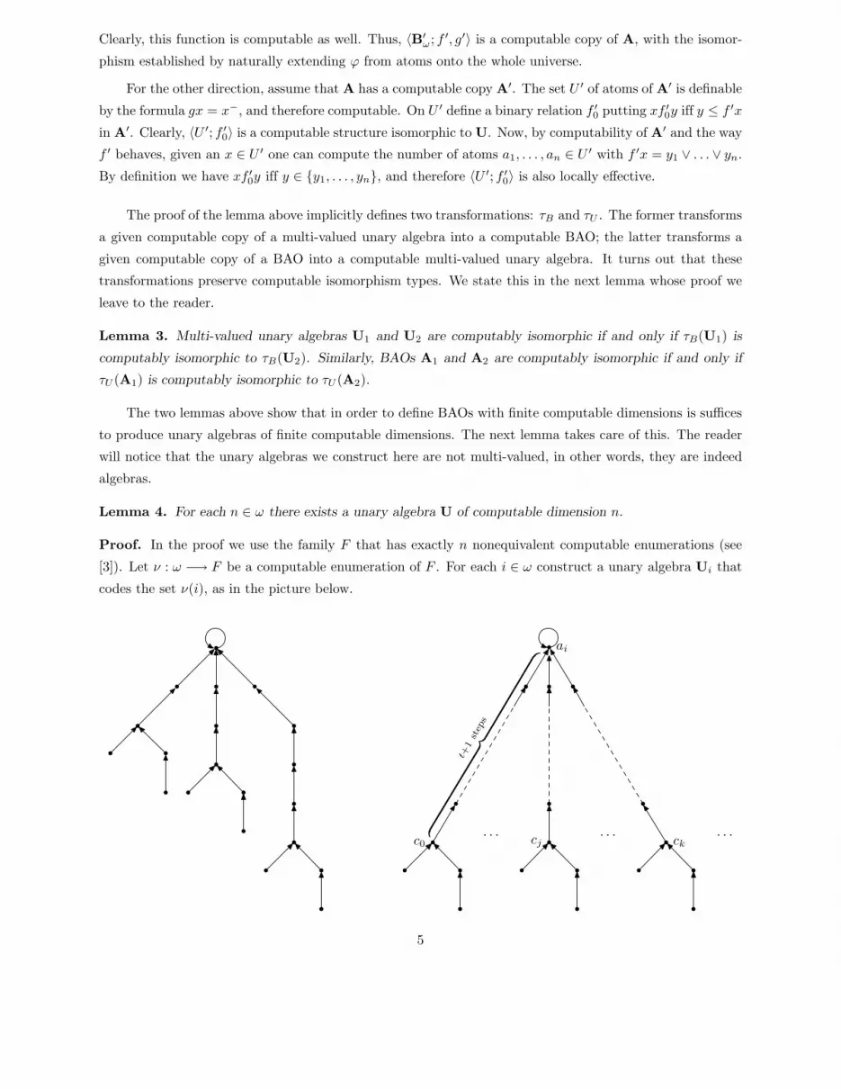
Lemma 4. For each n ∈ ω there exists a unary algebra U of computable dimension n.
Proof. In the proof we use the family F that has exactly n nonequivalent computable enumerations (see
[3]). Let ν : ω −→ F be a computable enumeration of F . For each i ∈ ω construct a unary algebra Ui that
codes the set ν(i), as in the picture below.
t+1
step
s
︷︸︸
︷
. . . . . . . . .c0 cj ck
ai
5
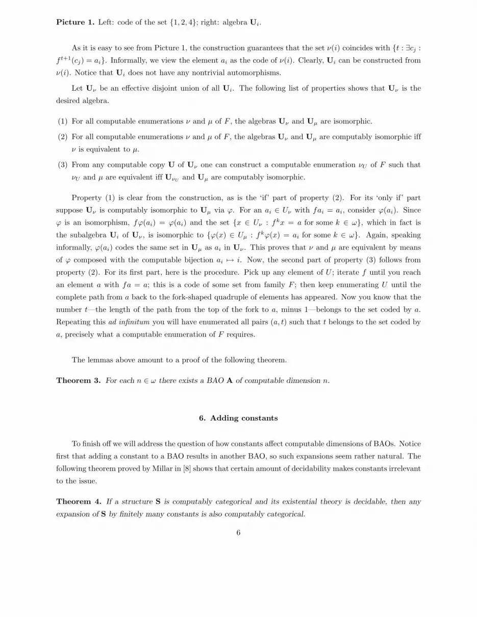
Picture 1. Left: code of the set {1, 2, 4}; right: algebra Ui.
As it is easy to see from Picture 1, the construction guarantees that the set ν(i) coincides with {t : ∃cj :f t+1(cj) = ai}. Informally, we view the element ai as the code of ν(i). Clearly, Ui can be constructed from
ν(i). Notice that Ui does not have any nontrivial automorphisms.
Let Uν be an effective disjoint union of all Ui. The following list of properties shows that Uν is the
desired algebra.
(1) For all computable enumerations ν and µ of F , the algebras Uν and Uµ are isomorphic.
(2) For all computable enumerations ν and µ of F , the algebras Uν and Uµ are computably isomorphic iff
ν is equivalent to µ.
(3) From any computable copy U of Uν one can construct a computable enumeration νU of F such that
νU and µ are equivalent iff UνU and Uµ are computably isomorphic.
Property (1) is clear from the construction, as is the ‘if’ part of property (2). For its ‘only if’ part
suppose Uν is computably isomorphic to Uµ via ϕ. For an ai ∈ Uν with fai = ai, consider ϕ(ai). Since
ϕ is an isomorphism, fϕ(ai) = ϕ(ai) and the set {x ∈ Uν : fkx = a for some k ∈ ω}, which in fact isthe subalgebra Ui of Uν , is isomorphic to {ϕ(x) ∈ Uµ : fkϕ(x) = ai for some k ∈ ω}. Again, speakinginformally, ϕ(ai) codes the same set in Uµ as ai in Uν . This proves that ν and µ are equivalent by means
of ϕ composed with the computable bijection ai �→ i. Now, the second part of property (3) follows from
property (2). For its first part, here is the procedure. Pick up any element of U ; iterate f until you reach
an element a with fa = a; this is a code of some set from family F ; then keep enumerating U until the
complete path from a back to the fork-shaped quadruple of elements has appeared. Now you know that the
number t—the length of the path from the top of the fork to a, minus 1—belongs to the set coded by a.
Repeating this ad infinitum you will have enumerated all pairs (a, t) such that t belongs to the set coded by
a, precisely what a computable enumeration of F requires.
The lemmas above amount to a proof of the following theorem.
Theorem 3. For each n ∈ ω there exists a BAO A of computable dimension n.
6. Adding constants
To finish off we will address the question of how constants affect computable dimensions of BAOs. Notice
first that adding a constant to a BAO results in another BAO, so such expansions seem rather natural. The
following theorem proved by Millar in [8] shows that certain amount of decidability makes constants irrelevant
to the issue.
Theorem 4. If a structure S is computably categorical and its existential theory is decidable, then any
expansion of S by finitely many constants is also computably categorical.
6
However, without the decidability assumption the picture changes quite dramatically, as Cholak, Gon-
charov, Khoussainov and Shore proved in [1]. Namely:
Theorem 5. For each k ∈ ω there is a computably categorical structure S such that the expansion of S by
a single constant has computable dimension k.
The proof of the above theorem proceeds by coding certain computably enumerable families of k-
tuples of sets. We will show that the theorem remains true if S is assumed to be a BAO. In fact, we will
confine ourselves to the case k = 2, the extension to any positive k being rather straightforward given the
constructions in [1]. We will need yet another definition.
Definition 7. Let F be a family of nonempty subsets of ω. We call F symmetric, if (A,B) ∈ F implies
(B,A) ∈ F . The family F is computably enumerable, if there is a bijective mapping ν : ω −→ F such that
the set {(i, x, y) : x ∈ lν(i), y ∈ rν(i)} is computably enumerable, where l and r stand for the left and rightprojections of pairs.
If ν : ω −→ F is a computable enumeration of a symmetric family F , then νd defined as νd(i) =
(rν(i), lν(i)) is another computable enumeration of F . To prove the result we announced, we will need a
symmetric family F for which ν and νd are the only computable enumerations possible. That is the content
of another theorem from [1].
Theorem 6. There is a symmetric family F and its computable enumeration ν such that ν is not equivalent
to νd and every computable enumeration of F is equivalent to either ν of νd.
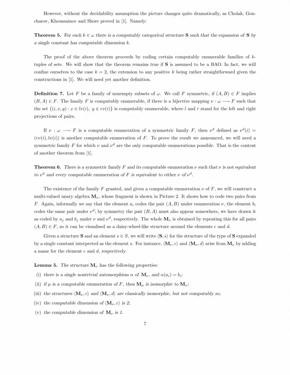
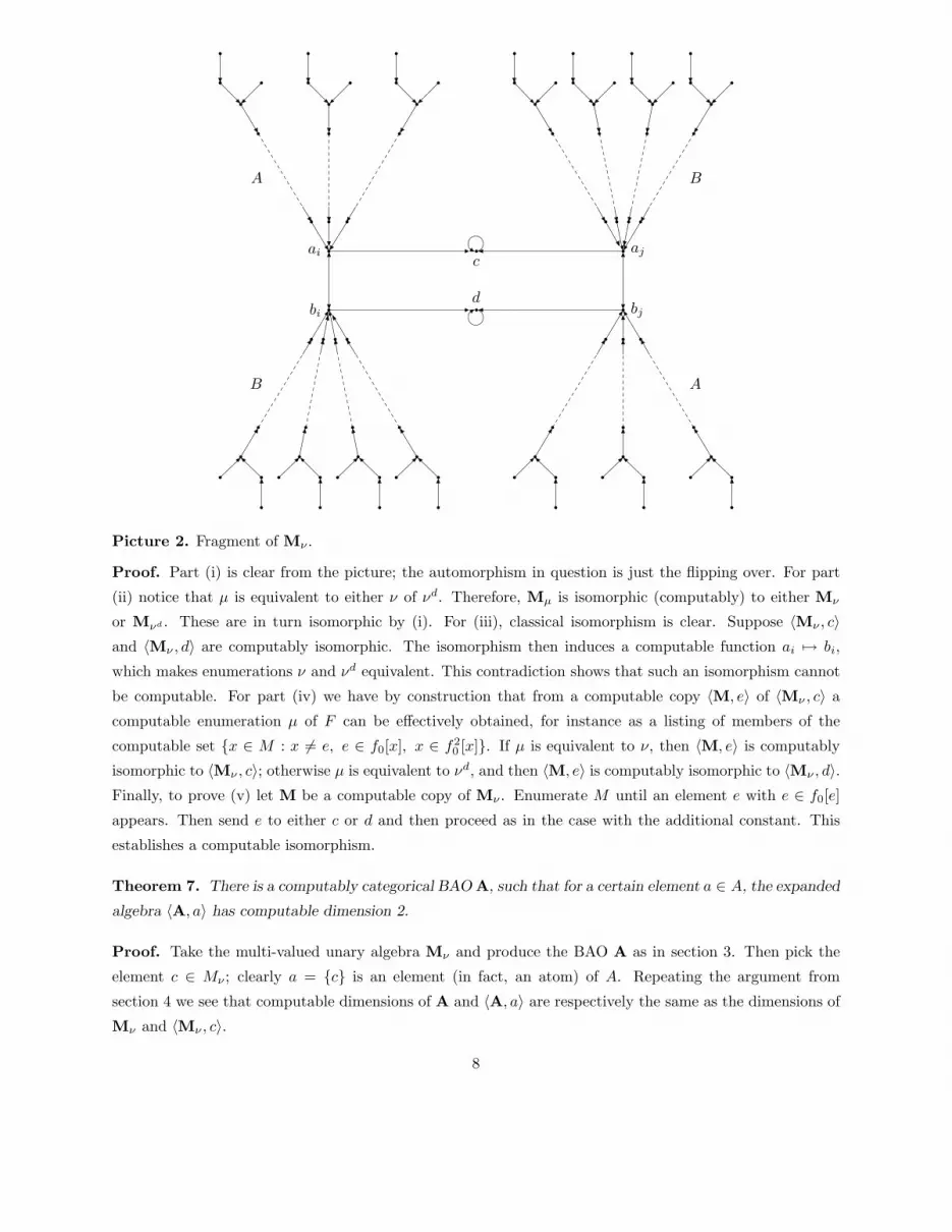
The existence of the family F granted, and given a computable enumeration ν of F , we will construct a
multi-valued unary algebra Mν , whose fragment is shown in Picture 2. It shows how to code two pairs from
F . Again, informally we say that the element ai codes the pair (A,B) under enumeration ν, the element bicodes the same pair under νd; by symmetry the pair (B,A) must also appear somewhere, we have drawn it
as coded by aj and bj under ν and νd, respectively. The whole Mν is obtained by repeating this for all pairs
(A,B) ∈ F , so it can be visualised as a daisy-wheel-like structure around the elements c and d.
Given a structure S and an element s ∈ S, we will write 〈S, s〉 for the structure of the type of S expandedby a single constant interpreted as the element s. For instance, 〈Mν , c〉 and 〈Mν , d〉 arise fromMν by adding
a name for the element c and d, respectively.
Lemma 5. The structure Mν has the following properties:
(i) there is a single nontrivial automorphism α of Mν , and α(ai) = bi;
(ii) if µ is a computable enumeration of F , then Mµ is isomorphic to Mν ;
(iii) the structures 〈Mν , c〉 and 〈Mν , d〉 are classically isomorphic, but not computably so;
(iv) the computable dimension of 〈Mν , c〉 is 2;
(v) the computable dimension of Mν is 1.
7
c
d
ai
bi
aj
bj
A
B
B
A
Picture 2. Fragment of Mν .
Proof. Part (i) is clear from the picture; the automorphism in question is just the flipping over. For part
(ii) notice that µ is equivalent to either ν of νd. Therefore, Mµ is isomorphic (computably) to either Mν
or Mνd . These are in turn isomorphic by (i). For (iii), classical isomorphism is clear. Suppose 〈Mν , c〉and 〈Mν , d〉 are computably isomorphic. The isomorphism then induces a computable function ai �→ bi,
which makes enumerations ν and νd equivalent. This contradiction shows that such an isomorphism cannot
be computable. For part (iv) we have by construction that from a computable copy 〈M, e〉 of 〈Mν , c〉 acomputable enumeration µ of F can be effectively obtained, for instance as a listing of members of the
computable set {x ∈ M : x �= e, e ∈ f0[x], x ∈ f20 [x]}. If µ is equivalent to ν, then 〈M, e〉 is computably
isomorphic to 〈Mν , c〉; otherwise µ is equivalent to νd, and then 〈M, e〉 is computably isomorphic to 〈Mν , d〉.Finally, to prove (v) let M be a computable copy of Mν . Enumerate M until an element e with e ∈ f0[e]
appears. Then send e to either c or d and then proceed as in the case with the additional constant. This
establishes a computable isomorphism.
Theorem 7. There is a computably categorical BAO A, such that for a certain element a ∈ A, the expanded
algebra 〈A, a〉 has computable dimension 2.
Proof. Take the multi-valued unary algebra Mν and produce the BAO A as in section 3. Then pick the
element c ∈ Mν ; clearly a = {c} is an element (in fact, an atom) of A. Repeating the argument fromsection 4 we see that computable dimensions of A and 〈A, a〉 are respectively the same as the dimensions ofMν and 〈Mν , c〉.
8
By coding “families of dimension k”, as they are called in [1], we can also obtain the following general-
isation of Theorem 7, which we will state without proof.
Theorem 8. For any k ∈ ω, there is a computably categorical BAO A, such that for a certain element
a ∈ A, the expanded algebra 〈A, a〉 has computable dimension k.
Closing remarks
As we mentioned in the introduction, the computable dimension of any computable Boolen algebra is
either 1 or ω. In this paper we produced BAOs with computable dimension k, for any k ∈ ω. Although our
construction employed two unary operators, there are ways of achieving the same with only one. It suffices
to say that the simulation technique from [7], enabling one to mimic the action of two operators with only
one, preserves computability. It would be therefore interesting to find a natural variety V of modal algebras
which is not term-equivalent to Boolean algebras and yet the computable dimension of any algebra from
V is either 1 or ω, thus extending the result for Boolean algebras. In the variety of monadic algebras all
subdirectly irreducible members are such, so this variety may well be the first candidate to consider.
References
[1] P. Cholak, S. Goncharov, B. Khoussainov, R. Shore, Computably categorical structures and expansions
by constants, Journal of Symbolic Logic 64, 1999, 13–37.
[2] V. Dzgoev, S. Goncharov, Autostability of models, Algebra and Logic 19, 1980, 45–53.
[3] S. Goncharov, The problem of the number of non-self-equivalent constructivizations, Algebra and Logic
19, 1988, 621–639.
[4] S. Goncharov, A. Nerode, J. Remmel (eds) Handbook of Recursive Mathematics, Studies in Logic and
the Foundations of Mathematics, vols. 138, 139, Elsevier, 1998.
[5] S. Goncharov, S. Lempp, R. Solomon, The computable dimension of ordered Abelian groups, to appear
in Advances of Mathematics.
[6] B. Jonsson, A. Tarski, Boolean algebras with operators. Part I, American Journal of Mathematics 73,
1951, 891–939.
[7] M. Kracht, F. Wolter, Normal modal logics can simulate all others, Journal of Symbolic Logic 64, 1999,
99–138.
[8] T. Millar, Recursive categoricity and persistence, Journal of Symbolic Logic 51, 1986, 430–434.
[9] J. Remmel, Recursive isomorphism types of recursive Boolean algebras, Journal of Symbolic Logic 46,
1981, 572–593.
9


