Download - BIOMEDICAL ASPECTS OF MEMBRANE CHEMISTRY
BIOMEDICAL ASPECTS OF MEMBRANE
CHEMISTRY
A thesis submitted in part fulfilment of the degree of
Doctor of Philosophy
CORINNE E. A. MCEWAN
Department of Chemistry
Supervised by: Professor H. M. Colquhoun and Professor W. Hayes
Sponsored by: BioInteractions Ltd, Reading
2017

ii
Declaration of Original Authorship
I confirm that the research described in this thesis is my own work and that the use of
all materials from other sources has been properly and fully acknowledged.
……………………………………….
Corinne E. A. McEwan
iii
Abstract
This thesis is focused on the development of a prototype membrane medical device for
the treatment of oedema and lymphoedema via interosmolar fluid removal. These
medical disorders disrupt body fluid regulation causing excess fluid to accumulate in
the body’s tissues resulting in swelling of affected areas and can severely impact
quality of life of affected patients.
The device concept was based on a US patent (No. 8,211,053 B2) licensed to
BioInteractions Ltd which proposes, but does not exemplify, an implantable medical
device based on a semipermeable membrane compartment containing trapped
osmotic solutes which can act as a draw solution for the abnormally accumulated fluid
in the tissues surrounding the device, allowing the fluid to be drained from the body.
Following extensive literature research and consultation with experts in the field
(detailed in Chapter 1) it became apparent that alongside the oedema fluid,
accumulated plasma proteins would also require removal to prevent oedema reforming
as a result of protein oncotic pressure. To accommodate this, a design modification
was proposed; employing porous membranes to enable to removal of proteins
alongside the fluid. This adaptation necessarily affected the draw solution selection
limiting the options to high molecular weight species which could be retained by the
porous membrane.
Alongside this clinically-oriented project, a secondary project involved the development
of thin-film composite membranes using novel coatings based on hydrophilic poly-ylids
as well as investigations into a new solvent resistant support membrane.
Chapter 2 focused on investigating the forward osmosis process using a novel
combination of porous ultrafiltration membranes and high molecular weight polymer
and polyelectrolyte draw solutions. The best-performing draw solution and membrane
was found to be 225K sodium polyacrylate and a 50K MWCO polyethersulfone (PES)
UF membrane which were then further studied to determine model oedema fluid
removal performance, membrane fouling properties, osmotic pressure characteristics
and protein transport.
Chapter 3 involved the synthesis and characterisation of novel hydrophilic poly-ylids
derived from the interfacial polycondensation of 1,1’-diamino-4,4’-bipyridinium with
aromatic di-sulfonyl chlorides and di-isocyanates. These poly-ylids were then used to
fabricate thin-film composite nanofiltration membranes, alongside a number of
iv
previously reported acid chloride based poly-ylids for comparison, which were then
analysed in terms of their flux and salt rejection properties. Additionally investigations
into pH effects, surface morphology and biocompatibility were carried out.
Chapter 4 describes the development of solvent resistant thin-film composite
membranes based on poly-ylids synthesised in Chapter 3, in combination with a novel
polyetherketone support membranes. This system enabled the fabrication of
nanofiltration membranes using monomers that were incompatible with a traditional
PES membrane support. The membranes were analysed as described in Chapter 3
and were found to have reasonable flux and salt rejection properties. Additionally,
initial biocompatibility testing found that all three PEK TFC poly-ylid membranes were
able to reduce protein adhesion relative to an uncoated PEK support membrane.
Chapter 5 details the design, fabrication and testing of two generations of device
prototypes using both an in vitro and ex vivo model, both developed specifically for the
project. This chapter provides proof-of-concept for the device, as fluid removal was
successfully demonstrated using a second generation prototype tested in an ex vivo
perfused limb.

v
Acknowledgements
I would first like to thank my PhD supervisor, Professor Howard Colquhoun for all the
support and advice throughout the project. I would also like to thank Professor Hayes
for additional input during the project and Dr Alister McNeish for all the help and advice
with developing the perfused limb model. Additionally I would like to acknowledge my
industrial sponsor BioInteractions Ltd for the opportunity to undertake this PhD, and
also my industrial supervisors; Dr Ajay Luthra (Chief Executive Officer), Simon Onis
(Chief Scientific Officer) and Dr Alan Rhodes (Chief Technical Officer).
I am also grateful to colleagues who have shared their expertise and time to help
progress this project, especially; Amanpreet Kaur (SEM), Krish Kapoor (BCA Assay)
and Tahkur Singh Babra (GPC), the CAF Lab technical staff and all members of both
the Colquhoun and Hayes groups, past and present.
I would also like to thank my undergraduate project student Ben Plackett for helping
with PEK membrane optimisation and producing a brilliant crossflow rig schematic.
Additionally I would like to thank the University of Reading Knowledge Transfer
Partnership team for all their support throughout the project, particularly Deborah
Edwards and Owen Lloyd.
Most importantly I would like to thank my friends and family who have supported me
throughout the highs and lows of this PhD; Kate, my first and best friend in Reading,
the craft club ladies (Clare, Priya, Emma and Emily), my chemistry gurl gang from Bath
Uni (Lucie, Kat, Gem, Mel and Lottie), and most especially my best girlfriends Barbara,
Amy B and Amy C.
I am eternally grateful for my loving and supportive family; my maman cherie and sister
Mathilde for being strong and beautiful women and for always wanting the best for me,
my stepdad Andrew for always being there for me and for being part of our family, my
partner Ben for all the adventures and encouragement and for helping me achieve
things I didn’t think I was capable of.
Finally I would like to dedicate this PhD to my dad Pete, who didn’t get to see me
complete it - thank you for always being of proud me.
vi
Acronyms and Abbreviations
AFM atomic force microscopy
appt. d apparent doublet
BCA bicinchoninic acid assay
BSA bovine serum albumin
c concentration
CC counterion condensation
CDT complex decongestive therapy
Cf feed concentration
Cp permeate concentration
DI deionised
DMF N,N’-dimethylformamide
DMSO dimethyl sulfoxide
DSC differential scanning calorimetry
EAS electrophilic aromatic substitution
ECF extracellular fluid
ESEM environmental scanning electron microscopy
FIB fibrinogen
FO forward osmosis
g acceleration due to gravity
GAGs glycosaminoglycans
GPC gel permeation chromatography
h height
Δh change in height
ICF intracellular fluid
i van’t Hoff Factor
IF interstitial fluid
vii
IPC intermittent pneumatic compression
IR infra-red
Kc capillary filtration coefficient
K-PA potassium polyacrylate
m multiplet
M molarity
MF microfiltration
MLD manual lymphatic drainage
MWCO molecular weight cut-off
MW molecular weight
n moles
Na-PA sodium polyacrylate
NIPAM N-isopropylacrylamide
NMP N-methylpyrrolidone
NMR nuclear magnetic resonance
P pressure
PA polyamide
PAEK polyaryletherketone
PAES polyarylethersulfone
PBS phosphate buffered saline
PEG poly(ethylene glycol)
PEK polyetherketone
PES polyethersulfone
PEO poly(ethylene oxide)
PGs proteoglycans
pm picometers
ppm parts per million
PPS polyphenylenesulphide
viii
PSF polysulfone
PSSA polystyrene sulfonic acid sodium salt
PVP polyvinylpyrrolidone
R rejection
R gas constant
RI refractive index
RO reverse osmosis
s singlet
SEM scanning electron microscopy
SD standard deviation
SDS sodium dodeceyl sulfate
t triplet
t1 absolute viscosity of solvent
t2 absolute viscosity of polymer solution
T temperature
Tdeg degradation temperature
Tg glass transition
Tm melting temperature
TEM transmission electron microscopy
TFC thin-film composite
TGA thermal gravimetric analysis
TMC trimesoyl chloride
UBK unbuffered Krebs solution
UF ultrafiltration
UV/Vis ultraviolet/visible
V volume
ix
Å angstroms
η viscosity
ηabs absolute viscosity
ηinh inherent viscosity
π osmotic pressure
ρ density
σ retention coefficient
x
Table of Contents
CHAPTER 1 – Introduction
1.1 Research Motivation 1
1.2 Membrane Technology 3
1.2.1 Overview and History 3
1.2.2 Membrane Classification 4
1.2.3 Membrane Processes 6
1.2.4 Membrane Fabrication and Characterisation 11
1.2.4.1 Membrane Fabrication 11
1.2.4.2 Membrane Characterisation 14
1.3 Forward Osmosis 18
1.3.1 Overview 18
1.3.2 FO Membranes 19
1.3.3 FO Configuration 20
1.4 Membrane Modification 21
1.4.1 Overview 21
1.4.2 Interfacial Polymerisation 23
1.5 Oedema 23
1.5.1 Overview 23
1.5.2 Fluid Homeostasis 24
1.5.3 Physiology 30
1.5.4 Pathophysiology 35
1.5.5 Clinical Symptoms and Diagnosis 36
1.5.6 Treatment 38
1.5.7 Fluid Composition 39
1.6 Project Aims and Objectives 41
1.7 References 42
CHAPTER 2 – Forward Osmosis Processes with Ultrafiltration Membranes
2.1 Abstract 56
2.2 Introduction 56
2.3 Results and Discussion 58
2.3.1 Initial FO Studies using Ultrafiltration Membranes 58
2.3.1.1 Cellulose Membranes 60
2.3.1.2 PES Membranes 61
xi
2.3.2 Ultrafiltration Membrane Fouling Studies 65
2.3.3 PEG Behaviour in Solution 67
2.3.4 Sodium Polyacrylate Behaviour in Solution 68
2.3.5 Polyacrylate Draw Solution Optimisation 78
2.3.5.1 Molecular Weight Variation 78
2.3.5.2 Variation of Draw Solution Concentration 79
2.3.5.3 Changing Counter-ion Identity 80
2.3.6 Ultrafiltration Membrane Osmotic Pressure Studies 81
2.3.7 Reverse Osmosis vs. Ultrafiltration Membranes 86
2.3.8 Protein Studies 96
2.4 Conclusions 101
2.5 Future Work 103
2.6 Experimental 104
2.6.1 Materials 104
2.6.2 Equipment 105
2.6.3 Methods 106
2.6.3.1 Stirred Cell Forward Osmosis Experiments 106
2.6.3.2 Ultrafiltration Membrane Forward Osmosis Studies 107
2.6.3.3 Ultrafiltration Membrane FO Fouling Studies 108
2.6.3.4 Ultrafiltration Membrane FO Osmotic Pressure Studies 108
2.6.3.5 Reverse Osmosis vs. Ultrafiltration 108
2.6.3.6 Protein Studies 109
2.6.3.7 Commercial Ultrafiltration Membranes 110
2.7 References 111
CHAPTER 3 – Poly-ylid Membranes by Interfacial Polycondensation
3.1 Abstract 113
3.2 Introduction 113
3.3 Results and Discussion 115
3.3.1 Synthesis of 1,1’-Diamino-4,4’-bipyridinium di-iodide 115
3.3.2 Poly-ylid Synthesis 117
3.3.3. Poly-ylid Characterisation 119
3.3.3.1 Infrared Spectroscopy 119
3.3.3.2 1H Nuclear Magnetic Resonance Spectroscopy 123
3.3.3.3 Inherent Viscosity 125
3.3.3.4 Thermogravimetric analysis 126
xii
3.3.3.5 Differential Scanning Calorimetry 127
3.3.4 Membrane Fabrication 131
3.3.5 Membrane Characterisation 131
3.3.5.1 Membrane Permeability 132
3.3.5.2 Salt Rejection 134
3.3.5.3 pH Effects on Permeability 135
3.3.5.4 Surface Morphology 136
3.3.5.5 Biocompatibility Testing 138
3.4 Conclusions 141
3.5 Future Work 143
3.6 Experimental 143
3.6.1 Materials 143
3.6.2 Equipment 144
3.6.3 Methods 145
3.6.3.1 Synthesis of 1,1’-diamino-4,4’-bipyridinium di-iodide 145
3.6.3.2 Stirred Interfacial Polycondensation 146
3.6.3.3 Thin-film Composite Membrane Fabrication 148
3.6.3.4 Membrane Flux Determination 149
3.6.3.5 Membrane Salt Rejection Determination 149
3.6.3.6 pH Effects on Permeability 150
3.6.3.7 Biocompatibility Testing 150
3.7 References 151
CHAPTER 4 – Membranes based on Polyetherketone (PEK)
4.1 Abstract 153
4.2 Introduction 153
4.3 Results and Discussion 155
4.3.1 PEK TFC Membrane Fabrication 155
4.3.2 Membrane Characterisation 156
4.3.2.1 Membrane Permeability 157
4.3.2.2 Salt Rejection 158
4.3.2.3 pH Effects on Permeability 159
4.3.2.4 Surface Morphology 160
4.3.2.5 Biocompatibility Testing 161
4.3.3 PEK Support Membrane Optimisation 162
4.3.3.1 Backing Paper Exploration 162
xiii
4.3.3.2 PEK Crystallisation 164
4.3.3.3 Characterisation of Crystallised PEK Membranes 164
4.3.3.4 Interfacial Polycondensation on a Crystallised PEK
Membrane 166
4.4 Conclusions 167
4.5 Future Work 168
4.6 Experimental 168
4.6.1 Materials 168
4.6.2 Equipment 168
4.6.3 Methods 169
4.6.3.1 PEK Thin-film Composite Membrane Fabrication 169
4.6.3.2 Membrane Flux Determination 170
4.6.3.3 Membrane Salt Rejection Determination 170
4.6.3.4 pH Effects on Permeability 170
4.6.3.5 Biocompatibility Testing 170
4.6.3.6 PEK Crystallisation 170
4.6.3.7 PEK Crystallinity Investigation via DSC Analysis 170
4.6.3.8 MWCO Analysis 170
4.7 References 171
CHAPTER 5 – Device Prototype Design, Fabrication and Testing
5.1 Abstract 172
5.2 Introduction 172
5.3 Results and Discussion 175
5.3.1 Prototype Design 175
5.3.2 Prototype Fabrication 176
5.3.2.1 1st Generation Prototype 176
5.3.2.2 2nd Generation Prototype 177
5.3.3 Prototype Testing 179
5.3.3.1 In vitro Testing 179
5.3.3.2 Perfused Limb Model 182
5.4 Conclusions 185
5.5 Future Work 186
5.6 Experimental 186
5.6.1 Materials 186
5.6.2 Equipment 187
xiv
5.6.3 Methods 187
5.6.3.1 Prototype Fabrication 187
5.6.3.2 Prototype Testing 188
5.7 References 189
1
Chapter 1 - Introduction
1.1 Research Motivation
Oedema and lymphoedema are medical conditions which can have a severe impact on
quality of life. These disorders cause excess fluid to accumulate in the bodies’ tissues -
rather than being returned back to the circulatory system, which thus leads to swelling
in the affected areas. Current treatments for these conditions are labour- and time-
intensive, often requiring high patient compliance to be effective. In this thesis, a new
approach is proposed based on an implantable medical device with a semipermeable
membrane containing an osmotic driving solution which can remove accumulated fluid
in oedema. The main advantage of this approach is that the conditions for fluid removal
do not require harsh suction or pumping and therefore may be more compatible with
treating these conditions.
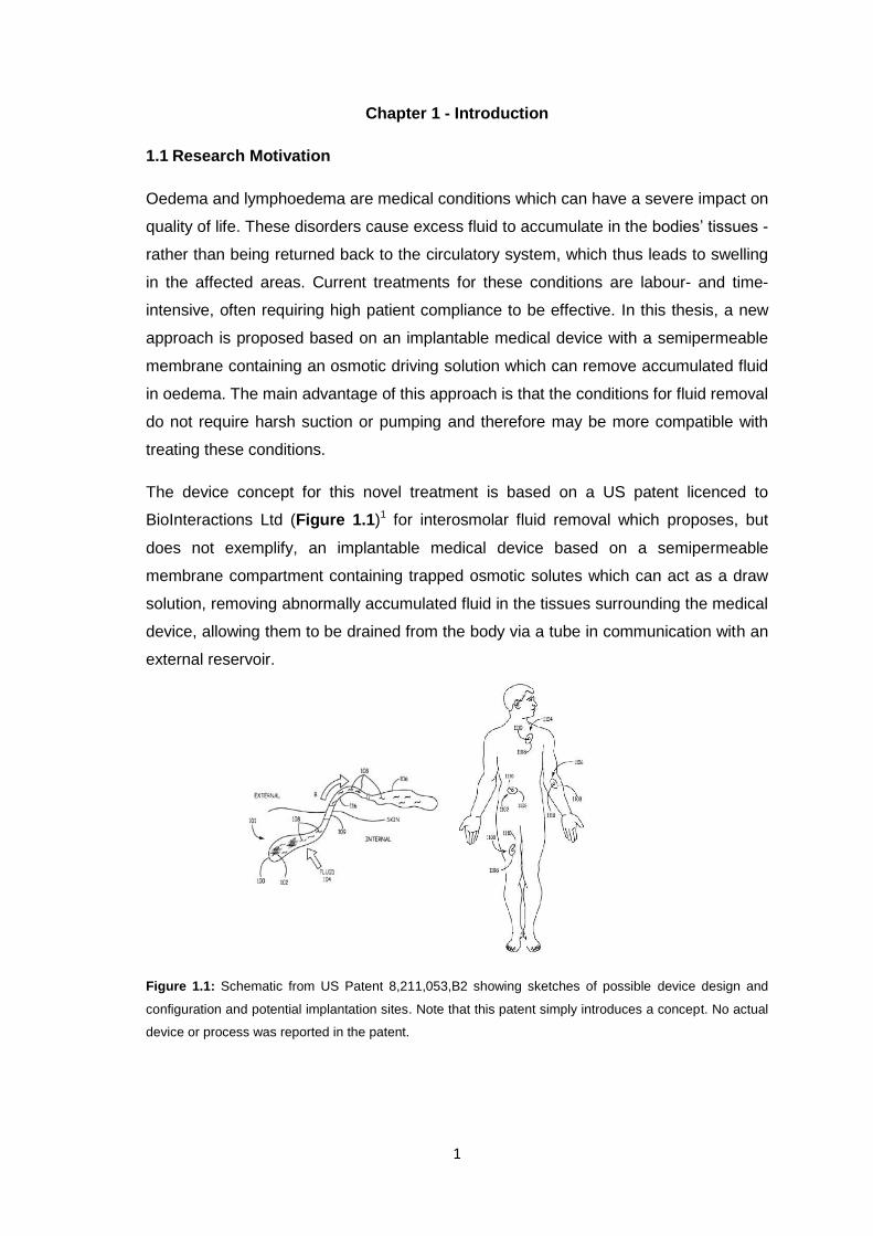
The device concept for this novel treatment is based on a US patent licenced to
BioInteractions Ltd (Figure 1.1)1 for interosmolar fluid removal which proposes, but
does not exemplify, an implantable medical device based on a semipermeable
membrane compartment containing trapped osmotic solutes which can act as a draw
solution, removing abnormally accumulated fluid in the tissues surrounding the medical
device, allowing them to be drained from the body via a tube in communication with an
external reservoir.
Figure 1.1: Schematic from US Patent 8,211,053,B2 showing sketches of possible device design and
configuration and potential implantation sites. Note that this patent simply introduces a concept. No actual
device or process was reported in the patent.
2
The aims of this project were principally to provide proof of concept to support this
proposed device design. In order to achieve this several objectives had to be met:
investigation into the forward osmosis process itself, analysis of potential membranes
and draw solutions, development of bench top model systems and device prototypes,
exploration of device design and finally the development of an ex vivo porcine limb
oedema model for prototype device testing.
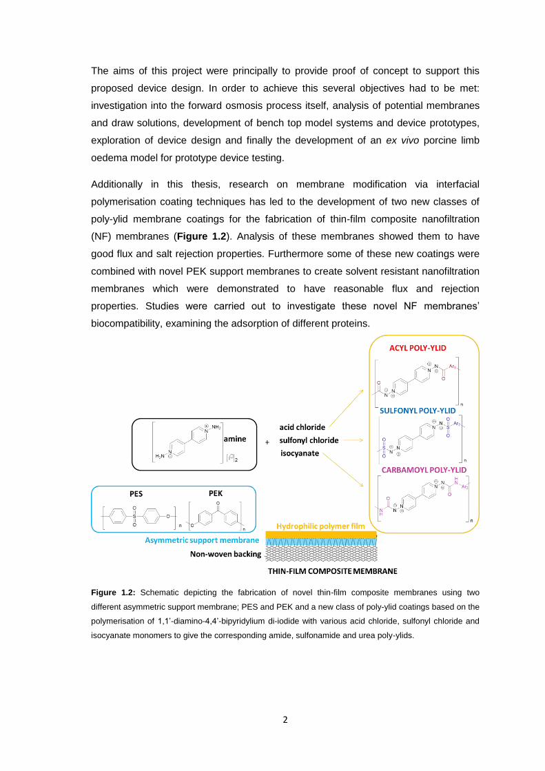
Additionally in this thesis, research on membrane modification via interfacial
polymerisation coating techniques has led to the development of two new classes of
poly-ylid membrane coatings for the fabrication of thin-film composite nanofiltration
(NF) membranes (Figure 1.2). Analysis of these membranes showed them to have
good flux and salt rejection properties. Furthermore some of these new coatings were
combined with novel PEK support membranes to create solvent resistant nanofiltration
membranes which were demonstrated to have reasonable flux and rejection
properties. Studies were carried out to investigate these novel NF membranes’
biocompatibility, examining the adsorption of different proteins.
Figure 1.2: Schematic depicting the fabrication of novel thin-film composite membranes using two
different asymmetric support membrane; PES and PEK and a new class of poly-ylid coatings based on the
polymerisation of 1,1’-diamino-4,4’-bipyridylium di-iodide with various acid chloride, sulfonyl chloride and
isocyanate monomers to give the corresponding amide, sulfonamide and urea poly-ylids.
3
1.2 Membrane Technology
1.2.1 Overview and History
Membranes can be described as semi-permeable interfaces separating two phases,
only allowing certain components to permeate through.2 Whilst there are both synthetic
and biological membranes this review will focus on the former.
Early investigations into membrane science in the 18th century involved experiments
with animal intestines and bladders3 and led to the discovery of the phenomenon which
drives the permeation of water through a semipermeable membrane from an area of
high water concentration to an area of lower water concentration, a process known as
osmosis. The first semisynthetic membranes were developed a century later.4 These
‘collodion’ (nitrocellulose) membranes became commercially available in the 1930’s5
and soon this technology was applied to other polymers.
The next significant breakthrough came in the 1960’s with the development of the first
high flux anisotropic reverse osmosis membrane. Loeb and Sourirajan are widely
credited with making reverse osmosis a practical process for industrial use.2,6,7 With
their development of an anisotropic cellulose acetate membrane (also known as a
Loeb-Sourirajan membrane)8 they were able to make the possibility of desalination by
reverse osmosis an economically viable process.
Michaels at Amicon realised the potential of the asymmetric RO Loeb-Sourirajan
membrane and applied this technology to create asymmetric ultrafiltration membranes
with a skin layer containing pores in the 10-200 Å range.9 These UF membranes
exhibited high retention of macromolecules including proteins and synthetic water-
soluble polymers whilst demonstrating excellent hydraulic permeability.10 Michaels and
his co-workers were able to produce asymmetric cellulose acetate UF membranes
along with other polymers such as polysulfones (PSF), aromatic polyamides (PA) and
polyacrylonitrile.11 These types of membranes are now also used as supports in
composite reverse osmosis membranes.
Another key breakthrough in membrane science was the development of the interfacial
polymerization (IP) technique which lead to the creation of the first non-cellulosic
membrane with comparable flux and salt rejection.12 This type of polymerization was
initially reported by Morgan in 1965.13 However, it was not until it was further developed
by Cadotte at FilmTec Corporation that its potential for RO membrane production was
fully realised.14 Interfacial polymerisation, involving the spontaneous growth of a semi-
permeable polyamide membrane on the surface of a supporting UF membrane, is
currently the most widely used method to manufacture high performance thin-film
4
composite reverse osmosis and nanofiltration membranes.6 The significance of these
membranes is that the two layers (skin layer and microporous substrate layer) of the
anisotropic membrane are prepared separately allowing for individual optimization
before combination to form the asymmetric membrane.6,7 This allows for a great deal of
customisation, and a wide variety of these thin-film composite (TFC) membranes have
since been developed.15
In order to develop a high-performing membrane, there are several factors which need
to be considered. These include the selectivity, defined as the rate at which different
species permeate relative to each other, the permeability which is the absolute rate at
which a permeate traverses a membrane and the flux which is the amount of permeate
that is transported through the membrane per unit membrane area per unit time.16,17
Other practical aspects to consider include; reproducibility, mechanical stability,
resistance to fouling, resistance to chemicals and temperature stability18.
1.2.2 Membrane Classification
Membranes can be classified in a variety of ways. Many membrane classifications
stem from the membrane materials and structure. When considering synthetic
membranes the first key distinction is whether they are based on organic19 or inorganic
materials (such as oxides, ceramic and metals).20 This review will focus on synthetic
polymeric materials which have many advantages including low cost, ease of
manufacture and ability to create a wide range of pore sizes.12
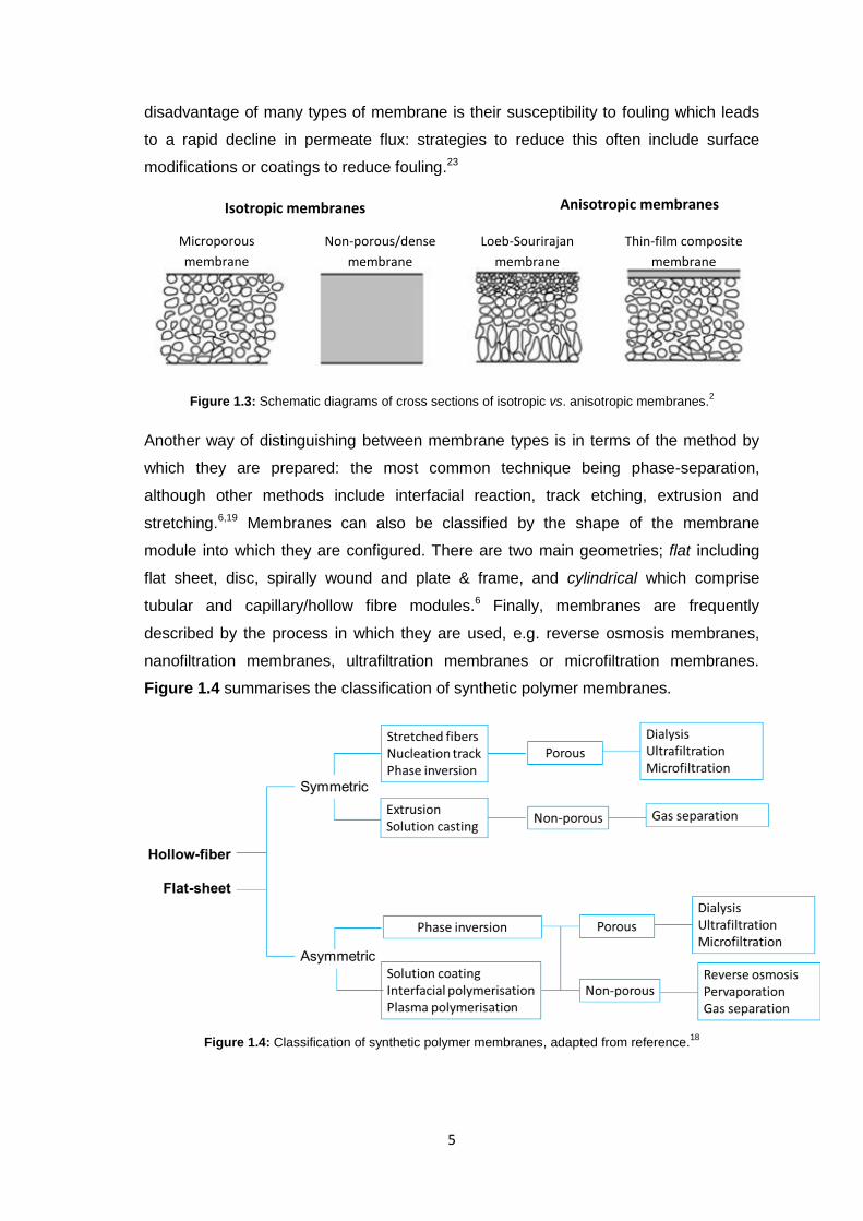
An alternative membrane classification system is based on the composition and
structure of the membrane cross section (Figure 1.3). There are two broad classes;
isotropic (symmetric) which have a uniform composition and structure throughout the
membrane cross-section and anisotropic (asymmetric) which can be homogenous in
chemical composition but not structure (phase separation or Loeb-Sourirajan
membranes). The latter may also be chemically and structurally heterogeneous (thin
film composite).21 Isotropic membranes can further be classified into either
microporous or dense/non-porous membranes.
Anisotropic membranes made of two or more materials are also known as composite
membranes. A classic example of this membrane type is the thin-film composite
membrane as prepared by the interfacial polymerisation technique. As mentioned
above these types of membranes have a significant advantage in that the layers can
be prepared separately. Composite membranes can also have a biocompatible coating
applied to the skin layer for use in medical devices, i.e. dialysis membranes.22 A major
5
disadvantage of many types of membrane is their susceptibility to fouling which leads
to a rapid decline in permeate flux: strategies to reduce this often include surface
modifications or coatings to reduce fouling.23
Figure 1.3: Schematic diagrams of cross sections of isotropic vs. anisotropic membranes.2
Another way of distinguishing between membrane types is in terms of the method by
which they are prepared: the most common technique being phase-separation,
although other methods include interfacial reaction, track etching, extrusion and
stretching.6,19 Membranes can also be classified by the shape of the membrane
module into which they are configured. There are two main geometries; flat including
flat sheet, disc, spirally wound and plate & frame, and cylindrical which comprise
tubular and capillary/hollow fibre modules.6 Finally, membranes are frequently
described by the process in which they are used, e.g. reverse osmosis membranes,
nanofiltration membranes, ultrafiltration membranes or microfiltration membranes.
Figure 1.4 summarises the classification of synthetic polymer membranes.
Figure 1.4: Classification of synthetic polymer membranes, adapted from reference.18
Isotropic membranes Anisotropic membranes
Microporous
membrane
Non-porous/dense
membrane
Loeb-Sourirajan
membrane
Thin-film composite
membrane
6
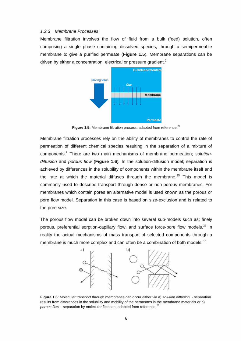
1.2.3 Membrane Processes
Membrane filtration involves the flow of fluid from a bulk (feed) solution, often
comprising a single phase containing dissolved species, through a semipermeable
membrane to give a purified permeate (Figure 1.5). Membrane separations can be
driven by either a concentration, electrical or pressure gradient.2
Figure 1.5: Membrane filtration process, adapted from reference.24
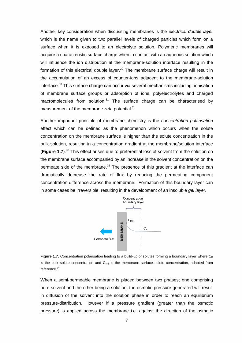
Membrane filtration processes rely on the ability of membranes to control the rate of
permeation of different chemical species resulting in the separation of a mixture of
components.2 There are two main mechanisms of membrane permeation; solution-
diffusion and porous flow (Figure 1.6). In the solution-diffusion model; separation is
achieved by differences in the solubility of components within the membrane itself and
the rate at which the material diffuses through the membrane.25 This model is
commonly used to describe transport through dense or non-porous membranes. For
membranes which contain pores an alternative model is used known as the porous or
pore flow model. Separation in this case is based on size-exclusion and is related to
the pore size.
The porous flow model can be broken down into several sub-models such as; finely
porous, preferential sorption-capillary flow, and surface force-pore flow models.26 In
reality the actual mechanisms of mass transport of selected components through a
membrane is much more complex and can often be a combination of both models.27
Figure 1.6: Molecular transport through membranes can occur either via a) solution diffusion - separation
results from differences in the solubility and mobility of the permeates in the membrane materials or b)
porous flow – separation by molecular filtration, adapted from reference.28
a) b)
7
Another key consideration when discussing membranes is the electrical double layer
which is the name given to two parallel levels of charged particles which form on a
surface when it is exposed to an electrolyte solution. Polymeric membranes will
acquire a characteristic surface charge when in contact with an aqueous solution which
will influence the ion distribution at the membrane-solution interface resulting in the
formation of this electrical double layer.29 The membrane surface charge will result in
the accumulation of an excess of counter-ions adjacent to the membrane-solution
interface.30 This surface charge can occur via several mechanisms including: ionisation
of membrane surface groups or adsorption of ions, polyelectrolytes and charged
macromolecules from solution.31 The surface charge can be characterised by
measurement of the membrane zeta potential.7
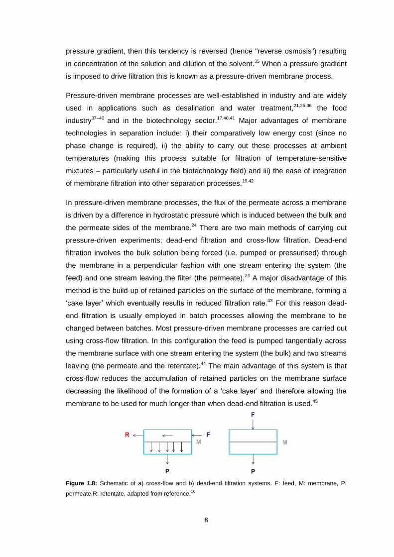
Another important principle of membrane chemistry is the concentration polarisation
effect which can be defined as the phenomenon which occurs when the solute
concentration on the membrane surface is higher than the solute concentration in the
bulk solution, resulting in a concentration gradient at the membrane/solution interface
(Figure 1.7).32 This effect arises due to preferential loss of solvent from the solution on
the membrane surface accompanied by an increase in the solvent concentration on the
permeate side of the membrane.33 The presence of this gradient at the interface can
dramatically decrease the rate of flux by reducing the permeating component
concentration difference across the membrane. Formation of this boundary layer can
in some cases be irreversible, resulting in the development of an insoluble gel layer.
Figure 1.7: Concentration polarisation leading to a build-up of solutes forming a boundary layer where CB
is the bulk solute concentration and CMS is the membrane surface solute concentration, adapted from
reference.34
When a semi-permeable membrane is placed between two phases; one comprising
pure solvent and the other being a solution, the osmotic pressure generated will result
in diffusion of the solvent into the solution phase in order to reach an equilibrium
pressure-distribution. However if a pressure gradient (greater than the osmotic
pressure) is applied across the membrane i.e. against the direction of the osmotic
8
pressure gradient, then this tendency is reversed (hence "reverse osmosis") resulting
in concentration of the solution and dilution of the solvent.35 When a pressure gradient
is imposed to drive filtration this is known as a pressure-driven membrane process.
Pressure-driven membrane processes are well-established in industry and are widely
used in applications such as desalination and water treatment,21,35,36 the food
industry37–40 and in the biotechnology sector.17,40,41 Major advantages of membrane
technologies in separation include: i) their comparatively low energy cost (since no
phase change is required), ii) the ability to carry out these processes at ambient
temperatures (making this process suitable for filtration of temperature-sensitive
mixtures – particularly useful in the biotechnology field) and iii) the ease of integration
of membrane filtration into other separation processes.19,42
In pressure-driven membrane processes, the flux of the permeate across a membrane
is driven by a difference in hydrostatic pressure which is induced between the bulk and
the permeate sides of the membrane.24 There are two main methods of carrying out
pressure-driven experiments; dead-end filtration and cross-flow filtration. Dead-end
filtration involves the bulk solution being forced (i.e. pumped or pressurised) through
the membrane in a perpendicular fashion with one stream entering the system (the
feed) and one stream leaving the filter (the permeate).24 A major disadvantage of this
method is the build-up of retained particles on the surface of the membrane, forming a
‘cake layer’ which eventually results in reduced filtration rate.43 For this reason dead-
end filtration is usually employed in batch processes allowing the membrane to be
changed between batches. Most pressure-driven membrane processes are carried out
using cross-flow filtration. In this configuration the feed is pumped tangentially across
the membrane surface with one stream entering the system (the bulk) and two streams
leaving (the permeate and the retentate).44 The main advantage of this system is that
cross-flow reduces the accumulation of retained particles on the membrane surface
decreasing the likelihood of the formation of a ‘cake layer’ and therefore allowing the
membrane to be used for much longer than when dead-end filtration is used.45
Figure 1.8: Schematic of a) cross-flow and b) dead-end filtration systems. F: feed, M: membrane, P:
permeate R: retentate, adapted from reference.16
9
Pressure-driven processes have many advantages; the permeate can be obtained
extremely pure, the process can be carried out at moderate temperatures so that the
energy requirements are reasonably low and finally such processes are suitable for
easy scaling up or combination with other processes.46
A major disadvantage of pressure-driven membrane processes is their susceptibility to
membrane fouling through the accumulation of retained species on the membrane
surface or within the membrane matrix resulting in a decrease in membrane
permeability.47 There are several different types of foulant; colloidal fouling from
particles such as clay or silica, organic fouling from hydrocarbons and proteins,
inorganic fouling from precipitation and deposition of dissolved salts in scaling (arises
due to changes in pH) or oxidation and finally biofouling from plant matter such as
algae or microbial contamination (biofilm formation).23,47,48
The issue of fouling can be overcome by two main approaches; either pre-treatment of
the feed solution to remove contaminants or modification of operating conditions to
promote membrane cleaning through backwashing or forward flushing to avoid long-
term build-up of deposited matter or by additional chemical/air scouring membrane
cleaning procedures.47 A common pre-treatment in drinking water production is
sterilisation by chlorine. However, this may shorten the membrane usage lifetime since
certain membranes (notably those based on aromatic polyamides) are very susceptible
to degradation by chlorine.
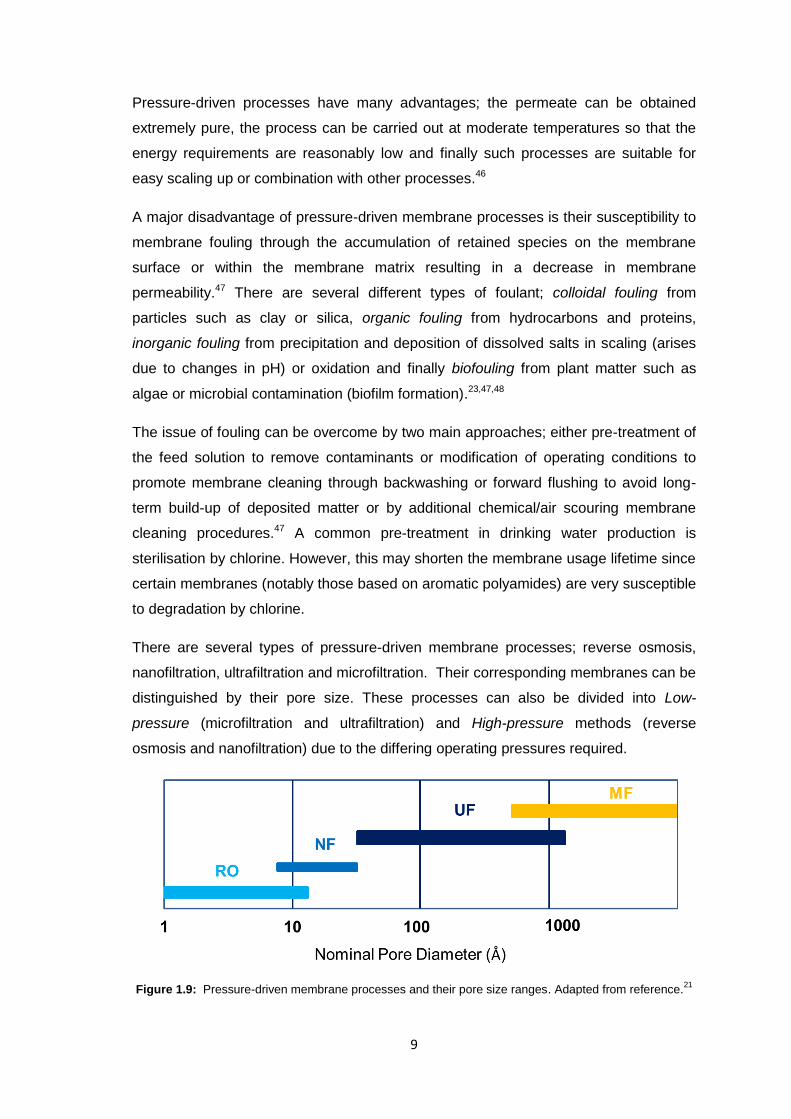
There are several types of pressure-driven membrane processes; reverse osmosis,
nanofiltration, ultrafiltration and microfiltration. Their corresponding membranes can be
distinguished by their pore size. These processes can also be divided into Low-
pressure (microfiltration and ultrafiltration) and High-pressure methods (reverse
osmosis and nanofiltration) due to the differing operating pressures required.
Figure 1.9: Pressure-driven membrane processes and their pore size ranges. Adapted from reference.21
10
Low-Pressure Membrane processes (typically 0.5-2 bar)
Microfiltration
Microfiltration retains and concentrates particles in the “micron” range which typically
encompasses suspended particles or colloids with a radius of 0.10 µm to 5 µm
(depending on the particular membrane pore size) and can include microorganisms
such as bacteria and viruses as well as other particles.49 Although both dead-end and
cross-flow configurations can be used, the latter configuration is preferred as this
avoids the build-up of retained particles on the membrane surface which can reduce
the rate of filtration.50 Microfiltration is used in many industrial applications, including
sterile filtration of pharmaceutical products to produce injectable drug solutions,51 and
in the dairy industry where cross-flow MF is used to remove bacteria from milk.37
Ultrafiltration
Ultrafiltration membranes have a pore diameter in the range 2 - 100 nm.52 Over the
past two decades UF has been widely used in the food processing industry due to its
significant advantages over other separation processes including non-harsh conditions
(ambient temperatures, no need for addition of chemicals) and low energy
requirements.39 UF is used in the dairy industry to fractionate milk for cheese
production and to produce high-calcium milk.38
High-Pressure Membrane Processes (typically 5-100 bar)
Nanofiltration
Nanofiltration is characterised by a membrane pore size range which corresponds to a
molecular weight cut-off of approximately 200 – 1000 Da.53 Nanofiltration is used
primarily in water treatment either to produce drinking water from ground and surface
water or as a pre-treatment for desalination.54 A moderately high pressure of 10-40
bar is typically required.55
Reverse Osmosis
Currently reverse osmosis is the most widely used desalination technology globally.12
Unlike the above three membrane types (NF,UF and MF) reverse osmosis membranes
are non-porous and instead have a complex ‘web-like’ molecular structure forcing the
permeating water through a tortuous pathway between hydrated polymer chains.56
Reverse osmosis requires relatively high operating pressures in comparison to the
other pressure-driven processes both because of the membrane’s inherently low
11
permeability and in order to overcome osmotic pressure.57 Commercial RO
membranes are mainly based on two different types of polymers; cellulose acetate
(CA) or aromatic polyamides (PA). However, the former are limited by their
susceptibility to microbiological attack and sensitivity to pH, so most industrial
applications will preferentially use PA thin film composite RO membranes.58 One
disadvantage of PA membranes is that they are degraded on prolonged exposure to
oxidising agents such as chlorine which is often used as a biocide in water
treatment.59,60
1.2.4 Membrane Fabrication and Characterisation
1.2.4.1 Membrane Fabrication
The most commonly used methods in polymer membrane synthesis include phase
inversion, interfacial polymerisation, stretching, track-etching and electrospinning.7 This
review will focus on the first two methods since they were used to fabricate
membranes for this project. Phase inversion and interfacial polymerisation are used to
produce asymmetric (anisotropic membranes).18
Phase Inversion
Phase inversion involves the controlled conversion of a homogenous polymer solution
from a liquid to a solid state. Although there are several techniques to achieve this,
each involves first casting a film of the polymer solution usually onto a non-woven
backing paper support (in the case of ultrafiltration membrane fabrication) or directly
onto a sheet of glass. Following the film casting the polymer is precipitated which can
be done in a variety of ways:7,18,61
Immersion precipitation
Thermally induced phase separation
Evaporation-induced phase separation
Vapour-induced phase separation
The most common technique – immersion precipitation – involves immersing the
polymer film in a non-solvent bath (typically water). Precipitation occurs due to the
exchange of solvent (within the polymer solution) and non-solvent which therefore
requires these two solvents to be miscible. During this solvent exchange the polymer
solution itself is separated into two phases; a solid polymer-rich phase which forms the
matrix and a liquid polymer-poor phase which forms the pores.62 This process results
12
in the formation of an asymmetric membrane consisting of a dense skin layer on top of
a porous sub layer containing structures such as macrovoids, pores and micropores.63
Membranes created by immersion precipitation have been found to contain key
structural elements such as; cellular structures, nodules, bicontinuous structures and
macrovoids.64 Macrovoids are large conical ‘finger-like cavities’ which can extend
throughout the entire thickness of the membrane and are generally unfavourable as
they are considered to be structural flaws resulting in mechanical weaknesses in the
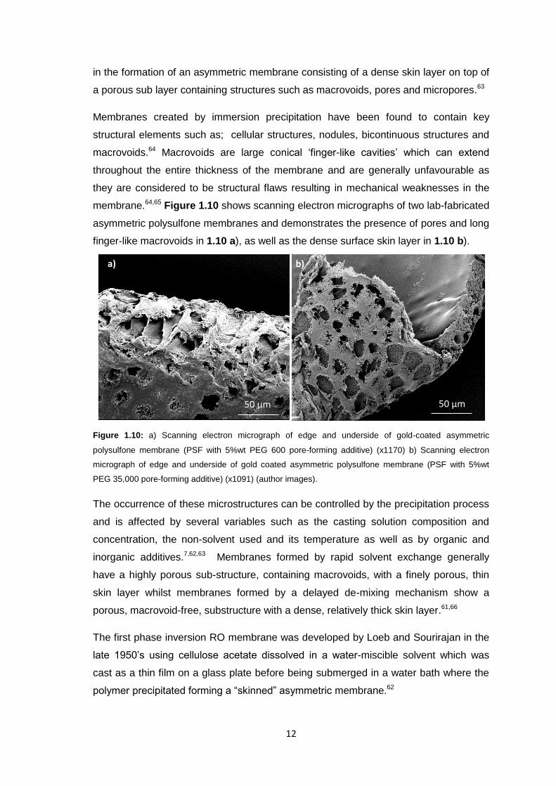
membrane.64,65 Figure 1.10 shows scanning electron micrographs of two lab-fabricated
asymmetric polysulfone membranes and demonstrates the presence of pores and long
finger-like macrovoids in 1.10 a), as well as the dense surface skin layer in 1.10 b).
Figure 1.10: a) Scanning electron micrograph of edge and underside of gold-coated asymmetric
polysulfone membrane (PSF with 5%wt PEG 600 pore-forming additive) (x1170) b) Scanning electron
micrograph of edge and underside of gold coated asymmetric polysulfone membrane (PSF with 5%wt
PEG 35,000 pore-forming additive) (x1091) (author images).
The occurrence of these microstructures can be controlled by the precipitation process
and is affected by several variables such as the casting solution composition and
concentration, the non-solvent used and its temperature as well as by organic and
inorganic additives.7,62,63 Membranes formed by rapid solvent exchange generally
have a highly porous sub-structure, containing macrovoids, with a finely porous, thin
skin layer whilst membranes formed by a delayed de-mixing mechanism show a
porous, macrovoid-free, substructure with a dense, relatively thick skin layer.61,66
The first phase inversion RO membrane was developed by Loeb and Sourirajan in the
late 1950’s using cellulose acetate dissolved in a water-miscible solvent which was
cast as a thin film on a glass plate before being submerged in a water bath where the
polymer precipitated forming a “skinned” asymmetric membrane.62
a) b)
50 µm 50 µm
13
Interfacial Polymerisation
Interfacial polymerisation is a step-growth polymerisation technique which involves
dissolving the monomer reagents in two different insoluble solvents before combining
them to produce a polymer at the solvent interface. The classic example of this
technique is the ‘nylon rope trick’, discovered by Morgan et al. in 1959, which involves
interfacial polymerisation at the interface formed between an aqueous solution of a
diamine and a diacid chloride in organic solvent to produce a nylon filament.67 Before
this discovery, condensation polymerisations usually required high temperatures and
reduced pressures to remove low molecular weight by-products such as water, and so
drive the reaction forward, thus limiting the substrates that could be used. Morgan’s
method, however, allowed such chemistry to be carried out at atmospheric conditions
using basic laboratory equipment.68,69 This novel approach was based on the Schotten-
Bauman reaction where an acid chloride is reacted with a compound containing an OH
or NH bond to form the corresponding esters and amides. In these reactions the two
reactants are dissolved in immiscible solvents so that the reaction occurs at the
interface of a heterogeneous liquid system. If a di-acid chloride and a diol or diamine
are used, then polymers are generally formed.
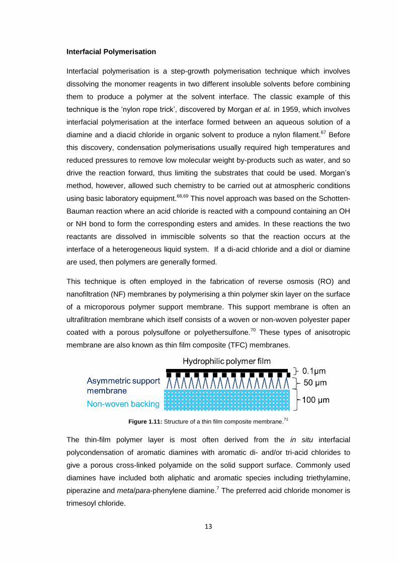
This technique is often employed in the fabrication of reverse osmosis (RO) and
nanofiltration (NF) membranes by polymerising a thin polymer skin layer on the surface
of a microporous polymer support membrane. This support membrane is often an
ultrafiltration membrane which itself consists of a woven or non-woven polyester paper
coated with a porous polysulfone or polyethersulfone.70 These types of anisotropic
membrane are also known as thin film composite (TFC) membranes.
Figure 1.11: Structure of a thin film composite membrane.71
The thin-film polymer layer is most often derived from the in situ interfacial
polycondensation of aromatic diamines with aromatic di- and/or tri-acid chlorides to
give a porous cross-linked polyamide on the solid support surface. Commonly used
diamines have included both aliphatic and aromatic species including triethylamine,
piperazine and meta/para-phenylene diamine.7 The preferred acid chloride monomer is
trimesoyl chloride.
14
A major advantage of the TFC membranes relative to earlier, integral-asymmetric RO
membranes is that the two layers can be independently modified and optimised
allowing for control of properties such as permeability and selectivity 15.
1.2.4.2 Membrane Characterisation
Membranes can be characterised in a variety of ways which are commonly classified
into three main categories; morphology (physical), composition (chemical) and
performance based characterisation techniques (i.e. permeation/flux, fouling and
filtration properties). In order to truly understand all of a membrane’s properties it is
necessary to investigate all three aspects of characterisation.
Membrane Morphology
Membrane morphology characterisation techniques can examine either the membrane
surface or bulk physical structure (see below). When examining the membrane face or
topmost portion responsible for membrane selectivity, electron microscopy and
scanning probe microscopy techniques can be used.
In electron microscopy the sample surface is exposed to a beam of electrons within a
vacuum. There are two basic techniques; transmission electron microscopy (TEM) and
scanning electron microscopy (SEM). In the former a detector will register electrons
passing through the sample whilst in SEM, interaction between the electron beam and
the sample causes the emission of secondary electrons which are then detected and
can be converted into an image. Figure 1.12 shows a SEM micrograph of a gold-
coated polytetrafluoroethylene (PTFE) microfiltration membrane.
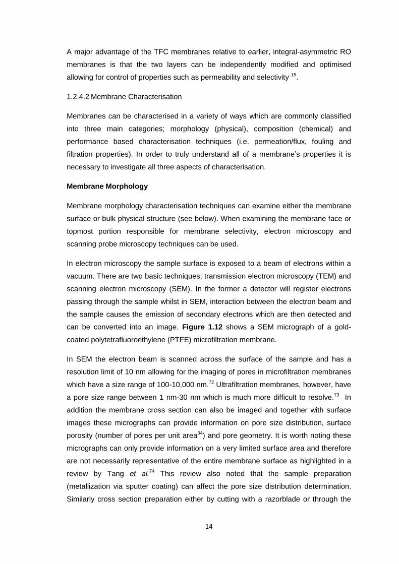
In SEM the electron beam is scanned across the surface of the sample and has a
resolution limit of 10 nm allowing for the imaging of pores in microfiltration membranes
which have a size range of 100-10,000 nm.72 Ultrafiltration membranes, however, have
a pore size range between 1 nm-30 nm which is much more difficult to resolve.73 In
addition the membrane cross section can also be imaged and together with surface
images these micrographs can provide information on pore size distribution, surface
porosity (number of pores per unit area34) and pore geometry. It is worth noting these
micrographs can only provide information on a very limited surface area and therefore
are not necessarily representative of the entire membrane surface as highlighted in a
review by Tang et al.74 This review also noted that the sample preparation
(metallization via sputter coating) can affect the pore size distribution determination.
Similarly cross section preparation either by cutting with a razorblade or through the
15
freeze fracture method can result in membrane compression and tearing.75 An
alternative form of SEM known as environmental scanning electron microscopy
(ESEM) can allow for sample analysis under less harsh conditions as the specimen
chamber is separated from the electron source allowing for a reduced working
pressure.76
Figure 1.12: Scanning electron micrograph of a gold-coated microfiltration membrane (Omnipore™ -
PTFE, pore size 0.1 μm) with retained 0.6 μm latex particles (x 50,000) (author image).
Scanning probe microscopy methods exploit interactions (electromagnetic or
mechanical) between the sample surface and a probe mounted on a flexible cantilever
to map the surface morphology. Atomic force microscopy (AFM) is perhaps the most
well-researched technique and employs a piezo-electric scanner to move the probe
relative to the sample whilst measuring mechanical interactions.76 A great advantage of
the AFM technique is the ability to examine membranes whilst wet, thus simulating
conditions under which the membrane will operate, unlike the electron microscopy
methods which require a dry sample.76 AFM has also been used to determine various
membrane surface characteristics including surface roughness, pore density and pore
size. However this technique is limited by restrictions on the scanning probe tip size
which can affect the scanning depth. Additionally there can be distortion effects which
can lead to overestimation of pore size relative to other techniques.77–79
When investigating the bulk properties of a membrane it is important to distinguish
between porous and dense membranes. The former type are used for microfiltration
and ultrafiltration processes and are identified by the presence of permanent voids or
pores which can be classed as either macropores (r > 50µm), mesopores (2µm ≤ r ≤
50µm) and micropores (r < 2µm).76 These membrane pores can be quantified in
various ways and a common term used to describe the pores is the membrane porosity
(also known as bulk porosity to distinguish from surface porosity) which is defined as
5 µm
16
the volume of the pores divided by the total volume of the membrane (void volume).80
Since the pores are not all of the same size and shape they can also be described by
other means such as the pore size distribution, average pore radius and pore geometry
(i.e. dead or dead-end pores which are not connected to the surface or are only
connected at one end, respectively).
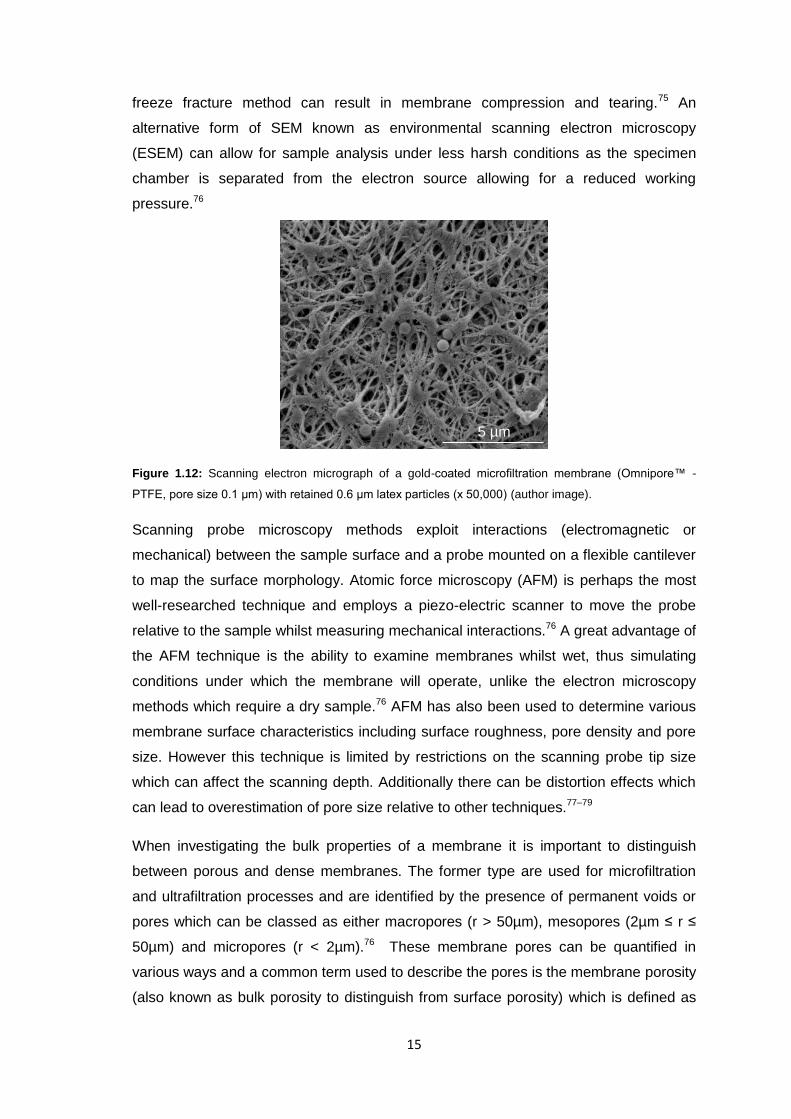
To describe the pore size a system has been developed in order to quantify membrane
filtration properties whereby macromolecules of known molecular weights are filtered
through the membrane and the feed solution is compared with the permeate in order to
determine percentage rejections. From this the membrane molecular weight cut-off
(MWCO) is assigned – a value which corresponds to the minimum molecular weight of
a solute which is 90% rejected. This method is widely accepted and is also used by
membrane manufacturers to classify their products. The most common probe
macromolecules are dextrans and polyethylene glycols (PEGs) and the feed/permeate
solutions are typically analysed using aqueous gel permeation chromatography (GPC)
which can separate these polymers based on their size via a filtration through a column
containing porous beads. Smaller analytes will enter the pores and take longer to
traverse through the column whereas larger polymers will pass through the column
rapidly. The polymers are detected after exiting the column and each one will have a
unique retention time range which can be used to compare the amount of each
polymer within the feed solution and the permeate after filtration through the
membrane. An example of this is shown in Figure 1.13 where a) shows the GPC
chromatograms of individual PEG solutions whilst b) shows the traces produced after
filtration of these PEG feed solutions through a commercial 50K MWCO PES UF
membrane. In the permeate chromatograms the 100K PEG peak is greatly reduced
since the PEG molecular weight is above the membrane MWCO and therefore the
sample is retained by the membrane.
Figure 1.13: Comparison of a) feed and b) permeate GPC traces of indevidual PEG solutions (0.1% w/v in
GPC mobile phase) after filtration with a commercial 50K MWCO PES UF membrane (present project).
6 7 8 9 10
RI (
mV
)
Retention Volume (mL)
6k
35K
100K
6 8 10
RI(
mV
)
Retention volume (mL)
6K
35K
100K
FEED SOLUTIONS PERMEATE SOLUTIONS
a) b)
17
Morphology characterisation methods can allow for the investigation of mechanisms
which lead to changes in membrane performance or to quantify the effects of
modification (i.e. coatings on surface modified membranes) or even to examine the
effects of membrane ageing and changes caused by fouling or exposure to
chemicals.76
Membrane Chemistry
In order to understand the chemistry of membrane materials it is important to fully
characterise these materials and to understand their properties before they are
incorporated into a membrane. Since this review is focused on synthetic polymer
membranes the analysis can involve a wide range of standard polymer
characterisation techniques including NMR and IR spectroscopies, viscosity studies,
thermal analyses, GPC characterisation. The membrane polymers can also be
characterised after incorporation into the membranes themselves. For example, IR
spectroscopy can be used to examine the surface chemistry of membranes. In
particular IR is useful for examining chemical changes in a membrane surface, e.g. as
a result of processes such as chlorination, irradiation or hydrolysis.76 It has also been
used to examine fouling processes: for example Belfer et al. were able to use IR to
identify the presence of adsorbed albumin on surface-modified PES UF after first using
IR to characterise the pristine functionalised membranes.81 This group also monitored
the removal of preservatives from commercial membranes using IR spectroscopic
analysis.
Membrane Performance
In order to fully characterise membranes it is important to understand how they will
function when used in separation processes. Key parameters that need to be
determined for pressure-driven membrane separation processes are described below.
The first key parameter to be measured is usually the membrane flux which relates to
the water permeability and is defined as the amount of permeate produced per unit
area of membrane surface per unit time. This can be measured by filtering deionised
water under standard membrane operating conditions and calculating the average
volume per hour of permeate. Standard units of this parameter are L/m2/h.
A second key parameter is the % rejection which relates to solute permeability. For
dense membranes salt rejection is measured, usually for both mono and divalent salts.
The divalent salts will have a larger hydrated radius and higher rejection rates are
18
expected for them relative to monovalent salts. For porous membranes
macromolecule rejection is measured (i.e. dextrans or PEGs) which can then be used
to determine the MWCO. The salt rejection can be calculated using Equation (1),
where Cp and Cf are the concentrations of the permeate and the feed, respectively:82
𝑅 = (1 −𝐶𝑝
𝐶𝑓) ⨯ 100% (1)
An ideal membrane will exhibit both high flux and high rejection of the target solute.
1.3 Forward Osmosis
1.3.1 Overview
As described above, osmosis is the movement of water through a semipermeable
membrane driven by a difference in osmotic pressure which is generated by differing
solute concentration across the membrane. Forward (direct) osmosis is the term used
to describe a membrane separation process which is driven by a concentration
gradient across a semi-permeable membrane via this naturally occurring phenomenon
of osmosis.83
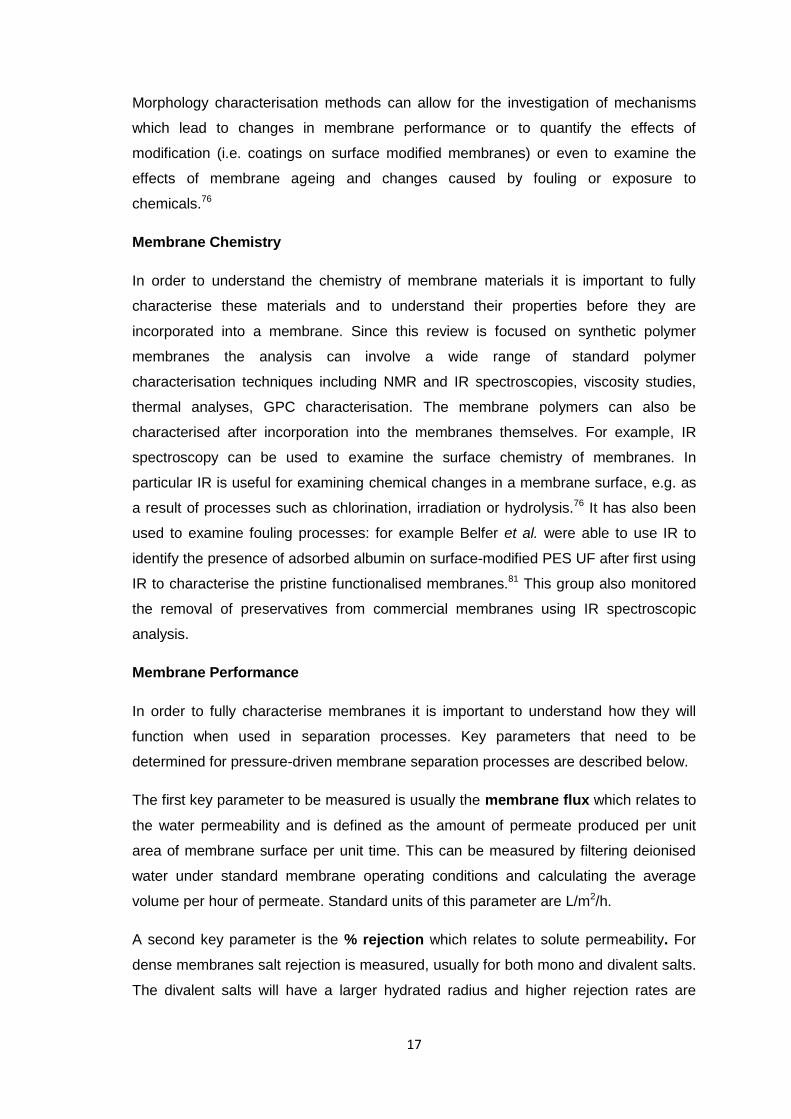
Osmotic pressure (Π) can be defined as the minimum pressure that must be applied to
the draw solution to prevent the influx of solvent from the feed solution in a system
such as the one in the image below where a solution and solvent are separated by a
semipermeable membrane.84
Figure 1.14: Equilibrium involved in calculation of osmotic pressure (Π), adapted from reference.84
Figure 1.14 demonstrates the equilibrium involved in the calculation of osmotic
pressure Π. This equilibrium exists between pure solvent A at pressure p on the left
hand side of the semipermeable membrane (in black) and solvent A as a component of
a solution (containing dissolved solutes) at pressure p+Π on the right hand side of the
19
semipermeable membrane.84 Osmosis is a colligative property meaning it depends
only on the number of solute “particles” (i.e. ions or molecules) present in solution, not
their identity.
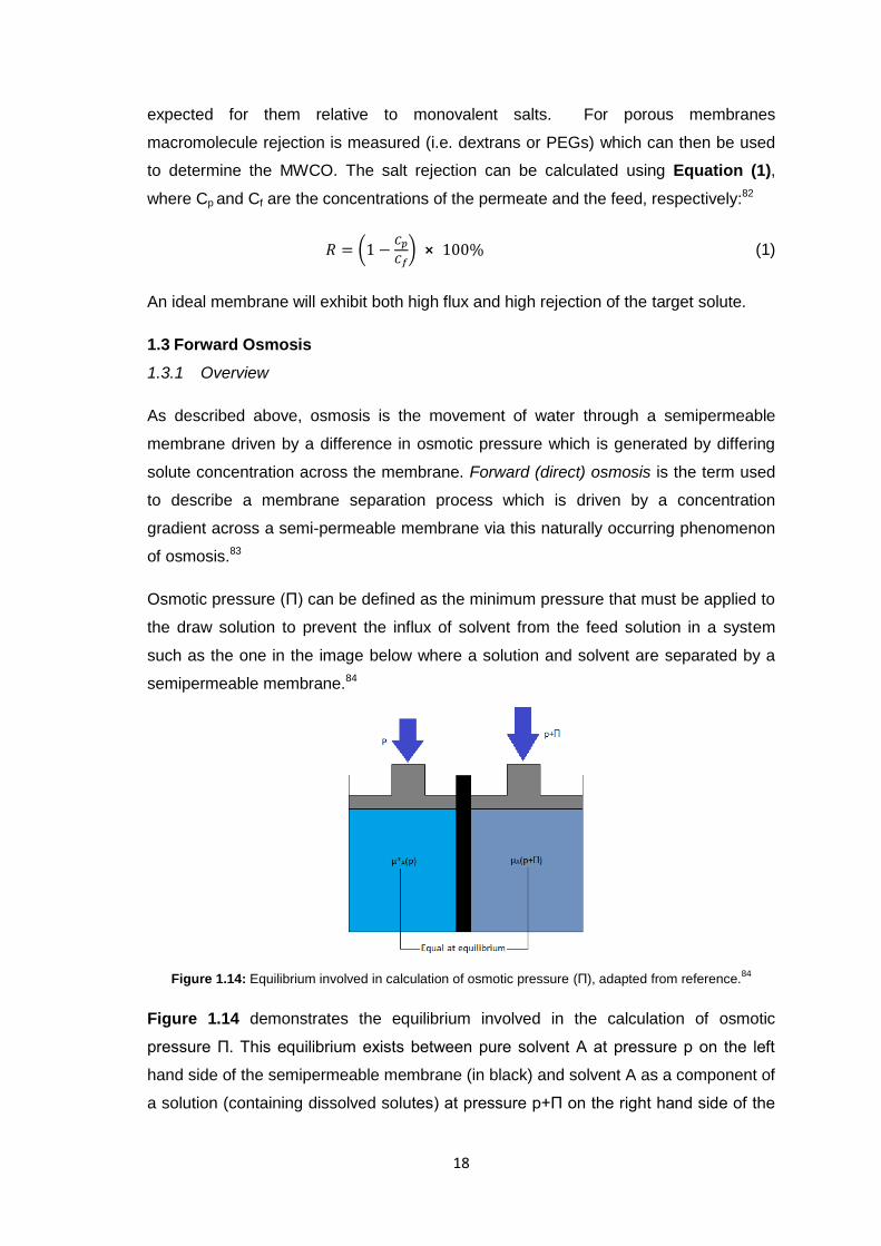
Forward osmosis processes rely on the use of a concentrated "draw" solution which
has a higher osmotic pressure than the feed solution therefore allowing it to draw water
out of the feed. This results in dilution of the draw solution and concentration of the
feed as illustrated in Figure 1.15.
Figure 1.15: The process of forward osmosis relies on the use of a concentrated draw solution to move
fluid from the feed into the draw (diluting it) across a semipermeable membrane, adapted from reference.83
Forward osmosis has attracted increasing attention in recent years due to its many
advantages over the pressure-driven membrane processes. The major benefit of FO
technology is that it operates at no or very low hydraulic pressures since the process is
driven by the concentration gradient. The low hydraulic pressure conditions result in
reduced operating costs, less irreversible fouling and therefore less need for
cleaning.85 Overall these advantages make FO processes potentially much cheaper
and much more energy efficient to run.
Despite these advantages FO technology has been slow to advance since its initial
proposition as an alternative to the energy intensive pressure-driven membrane
processes decades ago.86,87 This is due in part to the fact that (unlike RO) it is not a
route to pure water, and in part to a lack of effective semi-permeable membranes and
draw solutions88 – the two key components of a FO process.
1.3.2 FO Membranes
Any non-porous, selectively permeable membrane can be used for FO and historically
much FO research has been carried out using commercial RO membranes.83 For two
decades the only commercially available FO membrane was a cellulose triacetate
membrane from Hydration Technology Innovations (HTI, Oregon, USA).89 In recent
years however there has been more research into membranes specifically designed for
FO.90 Considerations when designing such membranes include; reduction of the
20
concentration polarisation effect (described above) which results in decreased flux and
inhibiting reverse solute diffusion which decreases the osmotic driving force.90,91
1.3.3 FO System configuration
An ideal draw solution will exhibit the following properties;
1) A significantly higher osmotic pressure than the feed solution, to drive high
permeate flux;92
2) Minimal reverse diffusion, as osmotic draw solutes lost in this way will need
replenishing, which increases cost. Moreover accumulation of these solutes in the feed
may cause problems with disposal or continued processing of the feed;93
3) When FO is used in water purification, a second step will be required to isolate the
water from the diluted draw solution (i.e. re-concentration of draw).
This second step would need to be inexpensive, and result in high recovery of draw
solution, whilst also generating high purity water, for this process to be economic.83,94
This re-concentration step is usually achieved through reverse osmosis or distillation
for standard electrolyte draw solutions which are based on aqueous solutions of
inorganic compounds such as sodium chloride (highly soluble, nontoxic and easily
reconstituted).83,94 Other draw solutions have been explored, including thermolytic
draw solutes such as ammonium carbonate which decompose into volatile gases on
gentle heating.95,96
Although most traditional draw solutions are based on salts or small molecules, some
research has also been done into polymeric draw solutions using hydrogels97,98 and
polyelectrolytes.82,98,99 It is proposed that these high molecular weight draw solutions
may provide an easier route to draw solution regeneration/water isolation and could
avoid issues of draw solution leakage/backflow into the feed. A new class of draw
solutions has been explored by Wang et al. where thermo-sensitive polymer hydrogels
were synthesised and were found to induce high water permeation in osmosis
processes whilst also demonstrating high water release rates under a combination of
pressure and thermal stimuli allowing for the regeneration of the draw solution.97
Chung et al. investigated an alternative strategy - polyelectrolyte draw solutions, in this
case sodium salts of polyacrylic acid (sodium polyacrylate – NaPA) which is known to
be highly water soluble and can therefore create high osmotic pressures whilst being
retained by a forward osmosis membrane due to the expanded confirmation of the
21
polyelectrolyte chain resulting from charge-charge repulsions.82 In experiments using
deionised water feed solutions and forward osmosis membranes the group found that
NaPA was able to generate high water flux with insignificant back diffusion. To
subsequently separate the water from the polyelectrolyte the group employed a
pressure-driven ultrafiltration process although it is reported that increasing the feed
concentration reduced the water production and rejection of the polyacrylate which is
attributed to concentration polarization and fouling effects. Wang et al. also
investigated an alternative draw solution strategy this time using novel thermo-
sensitive polyelectrolytes based on copolymerised N-isopropylacrylamide (NIPAM) the
polymer form of which (PNIPAM) can be used to create a thermo-sensitive hydrogel
which was combined with different amounts of sodium acrylate.100
As mentioned above, a major drawback of the pressure-driven membrane processes is
their susceptibility to fouling. Membrane fouling in FO has also yet to be fully explored
and understood.101 However, for osmotically driven processes fouling is potentially
less of an issue as it is usually more reversible than in membrane processes reliant on
applied hydraulic pressure. This is due to the rejected solutes forming a far less
compacted ‘cake layer’ in osmotically-driven membrane processes than in pressure-
driven membrane processes. It can thus be re-dispersed by simple physical methods
such as hydraulic flushing, without the need for harsh chemicals which could degrade
the membrane.101–103
1.4 Membrane Modification
1.4.1 Overview
In order to achieve the best possible membrane properties it is sometimes beneficial to
either modify the polymers used or to blend them with another polymer or non-polymer
additive. This can allow control of the membrane structure, porosity, pore distribution
and thickness, as well as other properties which will affect the overall selectivity of the
membrane.104 There are several strategies which can be employed to modify
membranes and they can be loosely classed as either bulk or surface modifications.
Membrane surface modifications allow for the retention of desirable bulk mechanical
properties of the polymer whilst achieving suitable surface properties for the end
application105. Surface modification strategies include; membrane coating, grafting and
chemical modification. One of the main applications of membrane surface modification
is to decrease membrane fouling and this is often done through increasing the polymer
surface hydrophilicity.106 The following approaches can be used to modify membranes;
22
Bulk Modification
Additives - where organic (hydrophilic/amphiphilic polymers) or inorganic substances
are mixed with the membrane casting solution to give either polymer blend or
composite membranes, respectively. In composite membranes the two or more
materials have different chemical and/or physical properties allowing them to remain
distinct at a macroscopic level.105
Surface Modification
Coatings - Polymers or small molecules are deposited on the membrane surface
where they adhere through non-covalent interactions to form a membrane coating.
There are several types of coating techniques; hydrophilic thin layer (physical
absorption), coating with a monolayer (Langmuir-Blodgett), deposition from glow
discharge plasma and casting of two or more polymer solutions using simultaneous
spinning equipment.105
Grafting - Grafting involves the addition of polymer chains onto the membrane surface
where they are bound via covalent interactions. There are two key types; ‘grafting-
from’ where active species on an existing membrane surface initiate the polymerisation
of monomers from the surface (graft polymerisation) and ‘grafting-to’ where polymer
chains with reactive side groups are covalently coupled to the membrane surface.107
There are several ways to initiate the polymerisation reaction giving rise to different
sub-categories of grafting; chemical, radiation, plasma photochemical or enzymatic
induced grafting.108 It is also possible to graft either one monomer or a mixture of two
or more.
Chemical modification - This involves treating the membrane with chemical species
which will introduce new functionality on the membrane surface. Reactions which have
been applied to membrane functionalisation include; sulfonation, chloromethylation,
aminomethylation and lithiation.105 Sulfonation of membrane polymers can be achieved
by either post-sulfonation of the final polymer or through copolymerisation with
sulfonated monomer (pre-sulfonation).109 Both strategies involve electrophilic aromatic
substitution (EAS) reactions to introduce the sulfonic acid groups. Poly(arylsulfones)
which include PSF and PES are widely used membrane materials due to their
relatively low cost but, as mentioned above, the hydrophobic nature of these polymers
makes them highly susceptible to fouling. Sulfonation offers a route to increased
membrane surface hydrophilicity therefore decreased fouling tendency.
23
1.4.2 Interfacial Polymerisation
Interfacial polymerisation is an alternative form of membrane modification which not
only modifies the membrane surface but also alters the membrane application. As
outlined in Section 1.2.1 and Section 1.2.4, interfacial polymerisation involves the
spontaneous growth of a semi-permeable polyamide membrane on the surface of a
supporting ultrafiltration membrane effectively converting the UF membrane into a
reverse osmosis membrane or nanofiltration membrane. The porous support is coated
with an ultra-thin yet dense polyamide film allowing this composite membrane to now
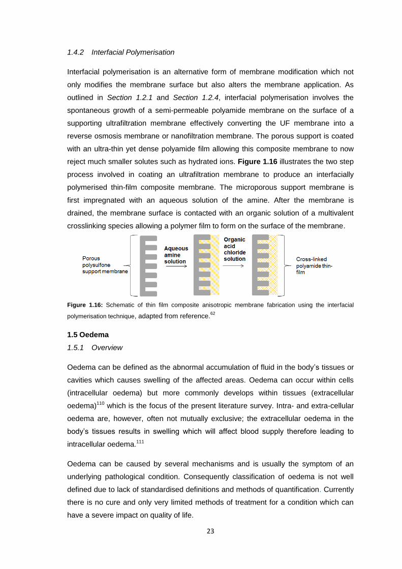
reject much smaller solutes such as hydrated ions. Figure 1.16 illustrates the two step
process involved in coating an ultrafiltration membrane to produce an interfacially
polymerised thin-film composite membrane. The microporous support membrane is
first impregnated with an aqueous solution of the amine. After the membrane is
drained, the membrane surface is contacted with an organic solution of a multivalent
crosslinking species allowing a polymer film to form on the surface of the membrane.
Figure 1.16: Schematic of thin film composite anisotropic membrane fabrication using the interfacial
polymerisation technique, adapted from reference.62
1.5 Oedema
1.5.1 Overview
Oedema can be defined as the abnormal accumulation of fluid in the body’s tissues or
cavities which causes swelling of the affected areas. Oedema can occur within cells
(intracellular oedema) but more commonly develops within tissues (extracellular
oedema)110 which is the focus of the present literature survey. Intra- and extra-cellular
oedema are, however, often not mutually exclusive; the extracellular oedema in the
body’s tissues results in swelling which will affect blood supply therefore leading to
intracellular oedema.111
Oedema can be caused by several mechanisms and is usually the symptom of an
underlying pathological condition. Consequently classification of oedema is not well
defined due to lack of standardised definitions and methods of quantification. Currently
there is no cure and only very limited methods of treatment for a condition which can
have a severe impact on quality of life.
24
1.5.2 Fluid Homeostasis
Oedema arises when systems maintaining fluid homeostasis in the body malfunction,
causing disruption of normal body fluid distribution, and ultimately resulting in the
accumulation of fluid in the affected area. The human body consists of approximately
60% water by weight, or 42 litres for an average 70 kg adult male. The amount is
slightly less in females (55%) due to a higher fat content.111 The principle of
homeostasis requires that total body fluid volume and osmolarity (osmotic
concentration) remain relatively constant. This is achieved by the regulation of two
main factors; sodium balance and water balance. Sodium salts are the principal
paracellular solutes and the regulation of sodium concentration is related to the
circulating fluid volume.112 Proper maintenance of sodium balance ensures that all
tissues are sufficiently perfused with fluid.113 The regulation of water balance is related
to the osmolarity of body fluids and is essential in maintaining normal cell volume.114
The overall volume and osmolarity of the body fluids is regulated by a complex system
involving the brain, the central nervous system and hormones which are responsible
for controlling water and salt excretion by the kidneys in response to detected volume
and osmolarity.115,116
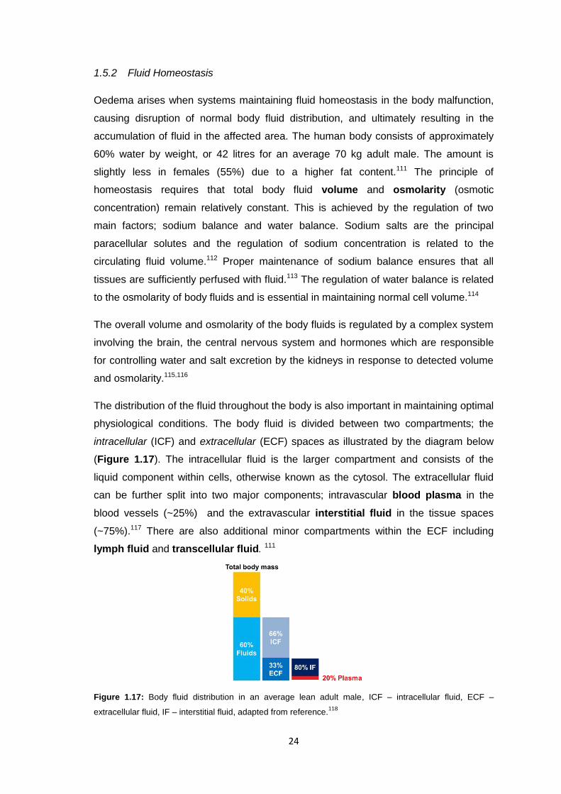
The distribution of the fluid throughout the body is also important in maintaining optimal
physiological conditions. The body fluid is divided between two compartments; the
intracellular (ICF) and extracellular (ECF) spaces as illustrated by the diagram below
(Figure 1.17). The intracellular fluid is the larger compartment and consists of the
liquid component within cells, otherwise known as the cytosol. The extracellular fluid
can be further split into two major components; intravascular blood plasma in the
blood vessels (~25%) and the extravascular interstitial fluid in the tissue spaces
(~75%).117 There are also additional minor compartments within the ECF including
lymph fluid and transcellular fluid. 111
Figure 1.17: Body fluid distribution in an average lean adult male, ICF – intracellular fluid, ECF –
extracellular fluid, IF – interstitial fluid, adapted from reference.118
25
The different compositions of these fluids are essential in maintaining normal
physiological conditions and are maintained by the physiological barriers (e.g. cell
membranes, blood vessel walls) separating them. However, all body fluids will have
approximately the same osmolarity, which is essential in preventing net movement of
water in or out of the cells, which would result in cell shrinkage or swelling.119
There are three key extracellular body fluids which are relevant to extracellular oedema
formation. These include the two major ECF components; blood plasma and interstitial
fluid along with the lymph fluid (a lesser component of the ECF). These fluids are able
able to exchange through a specialised microvascular exchange system (see below),
so that changes in the volume and composition of one fluid will impact on the volume
and composition of the others. It is important to note that the interstitial fluid can also
exchange with the ICF compartment within the cells. The ability for exchange between
all these fluids is paramount to their function; the blood transports substances such as
nutrients, metabolites and oxygen to the cells in the tissues whilst simultaneously
removing cellular waste. The exchange of these substances between the blood plasma
in the capillaries and the intracellular fluid within the cells occurs via an intermediate
fluid – the interstitial fluid bathing the tissue cells. The majority of the interstitial fluid is
returned to the circulation via the lymphatic system.
Compositions of Body Fluids
The blood plasma and the interstitial fluid, being the two major components of the ECF
compartment, can be exchanged across the selectively permeable blood capillary wall
which separates them. These two fluids have similar compositions, although due to the
selective barrier dividing them there is one major difference – the protein content. The
diffusion of blood plasma proteins into the interstitium is severely restricted by their
large molecular size relative to the capillary pores (see Table 1.2). However there are
other routes by which proteins can traverse the membrane and enter the tissues;
specialised vesicles can transport proteins out of the capillary and into the tissues, or
the action of neurotransmitters such as histamine and serotonin can increase capillary
permeability.120–122 Despite this, in normal tissues the rate of protein extravasation is
relatively low and the concentration of protein in the blood plasma is usually 2 to 3
times greater than in the interstitial fluid.123 It is important to note, however, that the
total protein content in the 12 L of interstitial fluid is greater than in the plasma but
because the volume of IF is four times that of the plasma (3 L) the average protein
concentration of the IF is approximately 3 g/dL, i.e. 40% of that in plasma.124
26
Other plasma components are able to traverse the capillary much more freely through
various mechanisms discussed below. These include: hormones, gases (carbon
dioxide and oxygen) and nutrients such as fatty acids, amino acids and glucose.125 The
blood also contains ‘non plasma’ components; white and red blood cells (leukocytes
and erythrocytes) and platelets (thrombocytes)126 which are also not able to readily
permeate through the capillary walls, again due to their large size.
The interstitial fluid is also able to exchange with the intracellular fluid within the tissue
cells themselves. The barrier separating these two fluids is the cell membrane which
has many mechanisms for transporting components in and out of the cell as required,
resulting in a significant difference in the compositions of these two fluids. The major
difference between the ICF and the tissue fluid is in salt composition. Unlike the
extracellular fluids the ICF is high in K+ and low in Na+/Cl- which differs significantly
from the high Na+/Cl- and low K+ levels found in both the tissue fluid and blood plasma.
The intracellular fluid also has a higher amount of protein than both the plasma and the
interstitial fluid (see Table 1.1).
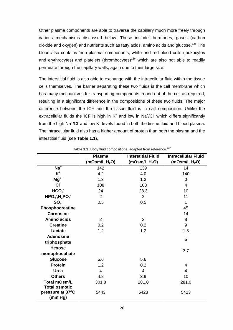
Table 1.1: Body fluid compositions, adapted from reference.127
Plasma
(mOsm/L H2O)
Interstitial Fluid
(mOsm/L H2O)
Intracellular Fluid
(mOsm/L H2O)
Na+ 142 139 14
K+ 4.2 4.0 140
Mg2+ 1.3 1.2 0
Cl- 108 108 4
HCO3- 24 28.3 10
HPO4-,H2PO4
- 2 2 11
SO4- 0.5 0.5 1
Phosphocreatine 45
Carnosine 14
Amino acids 2 2 8
Creatine 0.2 0.2 9
Lactate 1.2 1.2 1.5
Adenosine
triphosphate 5
Hexose
monophosphate 3.7
Glucose 5.6 5.6
Protein 1.2 0.2 4
Urea 4 4 4
Others 4.8 3.9 10
Total mOsm/L 301.8 281.0 281.0 Total osmotic
pressure at 37⁰C
(mm Hg)
5443 5423 5423
27
Finally the interstitial fluid can be converted into lymph fluid. Unlike the above
exchanges between the blood plasma/interstitial fluid or the interstitial fluid/intracellular
fluid, the conversion of interstitial fluid into lymph fluid is a one-way process. This is
due to the structure of the initial lymphatics which consist of overlapping endothelial
cells forming a valve and preventing back-flow of fluid and solutes which, once within
the lymphatic vasculature, from then on is referred to as lymph fluid.128 The fluid
collected is generally thought to have a similar composition to the interstitial fluid111 but
it has been well-documented that the lymph fluid is modified by passage through the
lymph node. This results in changes in protein concentration which are thought to be
involved in establishing the equilibrium of Starling’s forces (see Section 1.5.3).129 Few
studies have analysed the composition of lymph fluid, but analysis of ovine samples
has shown that lymph contains a wide variety of proteins, not all of which are derived
from plasma, suggesting lymph fluid is more than just an ultrafiltrate of plasma.130 As
with plasma, however, the major protein was found to be albumin.
Lymph fluid also contains other components which can include; cytokines (signalling
proteins) extracellular matrix constituents, proteases, intracellular proteins, plasma
proteins, erythrocytes and lymphocytes.130–133
Barriers in Fluid Homeostasis
The blood plasma in the capillary is separated from the interstitial fluid in the tissue
spaces by the capillary wall which consists of a single layer of endothelial cells, less
than 2µm thick, supported on the basement membrane which is part of the surrounding
extracellular matrix (see below) and is secreted by the endothelial cells themselves.125
The basement membrane prevents the passage of macromolecules from within the
blood into the extracellular space.134 The diameter of the blood capillary forces blood
cells to pass in single file.135 There are three types of capillaries with differing
permeabilities according to their function; continuous capillaries, fenestrated
capillaries and sinusoid (discontinuous) capillaries, see Figure 1.19. All three
types have leaky junctions between the endothelial cells creating small pores known as
intracellular junctions (clefts) which allow the diffusion of water, ions and small
hydrophilic molecules, such as urea and glucose, into the interstitium - a process
known as the paracellular pathway.136 These clefts represent 1/1000 of the capillary
surface area and have a radius of 6-7 nm, which is slightly smaller than the diameter of
albumin.124 Clearly the molecular size of plasma components will affect their ability to
pass through the intracellular junctions. The relative permeabilities of a range of
substrates are given in Table 1.2.
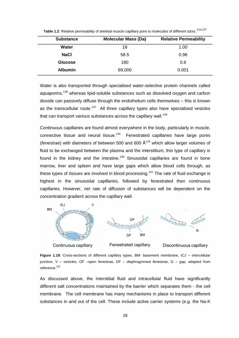
28
Table 1.2: Relative permeability of skeletal muscle capillary pore to molecules of different sizes.124,137
Substance Molecular Mass (Da) Relative Permeability
Water 18 1.00
NaCl 58.5 0.96
Glucose 180 0.6
Albumin 69,000 0.001
Water is also transported through specialised water-selective protein channels called
aquaporins,138 whereas lipid-soluble substances such as dissolved oxygen and carbon
dioxide can passively diffuse through the endothelium cells themselves – this is known
as the transcellular route.137 All three capillary types also have specialised vesicles
that can transport various substances across the capillary wall.139
Continuous capillaries are found almost everywhere in the body, particularly in muscle,
connective tissue and neural tissue.140 Fenestrated capillaries have large pores
(fenestrae) with diameters of between 500 and 600 Å125 which allow larger volumes of
fluid to be exchanged between the plasma and the interstitium, this type of capillary is
found in the kidney and the intestine.135 Sinusoidal capillaries are found in bone
marrow, liver and spleen and have large gaps which allow blood cells through, as
these types of tissues are involved in blood processing.141 The rate of fluid exchange is
highest in the sinusoidal capillaries, followed by fenestrated then continuous
capillaries. However, net rate of diffusion of substances will be dependent on the
concentration gradient across the capillary wall.
Figure 1.19: Cross-sections of different capillary types, BM- basement membrane, ICJ – intercellular
junction, V – vesicles, OF –open fenestrae, DF – diaphragmmed fenestrae, G – gap, adapted from
reference.125
As discussed above, the interstitial fluid and intracellular fluid have significantly
different salt concentrations maintained by the barrier which separates them - the cell
membrane. The cell membrane has many mechanisms in place to transport different
substances in and out of the cell. These include active carrier systems (e.g. the Na-K
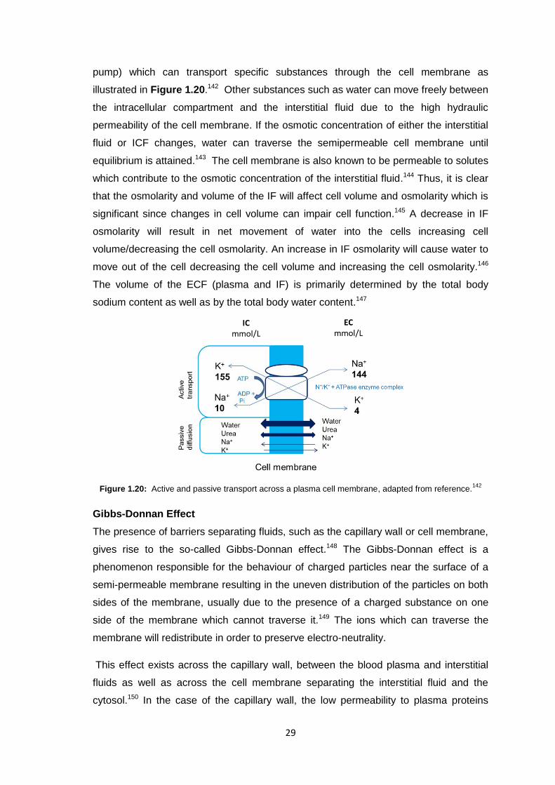
29
pump) which can transport specific substances through the cell membrane as
illustrated in Figure 1.20.142 Other substances such as water can move freely between
the intracellular compartment and the interstitial fluid due to the high hydraulic
permeability of the cell membrane. If the osmotic concentration of either the interstitial
fluid or ICF changes, water can traverse the semipermeable cell membrane until
equilibrium is attained.143 The cell membrane is also known to be permeable to solutes
which contribute to the osmotic concentration of the interstitial fluid.144 Thus, it is clear
that the osmolarity and volume of the IF will affect cell volume and osmolarity which is
significant since changes in cell volume can impair cell function.145 A decrease in IF
osmolarity will result in net movement of water into the cells increasing cell
volume/decreasing the cell osmolarity. An increase in IF osmolarity will cause water to
move out of the cell decreasing the cell volume and increasing the cell osmolarity.146
The volume of the ECF (plasma and IF) is primarily determined by the total body
sodium content as well as by the total body water content.147
Figure 1.20: Active and passive transport across a plasma cell membrane, adapted from reference.142
Gibbs-Donnan Effect
The presence of barriers separating fluids, such as the capillary wall or cell membrane,
gives rise to the so-called Gibbs-Donnan effect.148 The Gibbs-Donnan effect is a
phenomenon responsible for the behaviour of charged particles near the surface of a
semi-permeable membrane resulting in the uneven distribution of the particles on both
sides of the membrane, usually due to the presence of a charged substance on one
side of the membrane which cannot traverse it.149 The ions which can traverse the
membrane will redistribute in order to preserve electro-neutrality.
This effect exists across the capillary wall, between the blood plasma and interstitial
fluids as well as across the cell membrane separating the interstitial fluid and the
cytosol.150 In the case of the capillary wall, the low permeability to plasma proteins
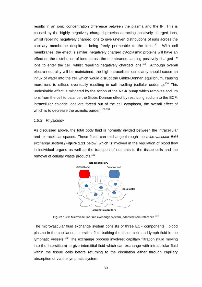
30
results in an ionic concentration difference between the plasma and the IF. This is
caused by the highly negatively charged proteins attracting positively charged ions,
whilst repelling negatively charged ions to give uneven distributions of ions across the
capillary membrane despite it being freely permeable to the ions.150 With cell
membranes, the effect is similar; negatively charged cytoplasmic proteins will have an
effect on the distribution of ions across the membranes causing positively charged IF
ions to enter the cell, whilst repelling negatively charged ions.151 Although overall
electro-neutrality will be maintained, the high intracellular osmolarity should cause an
influx of water into the cell which would disrupt the Gibbs-Donnan equilibrium, causing
more ions to diffuse eventually resulting in cell swelling (cellular oedema).150 This
undesirable effect is mitigated by the action of the Na-K pump which removes sodium
ions from the cell to balance the Gibbs-Donnan effect by restricting sodium to the ECF;
intracellular chloride ions are forced out of the cell cytoplasm, the overall effect of
which is to decrease the osmotic burden.150,151
1.5.3 Physiology
As discussed above, the total body fluid is normally divided between the intracellular
and extracellular spaces. These fluids can exchange through the microvascular fluid
exchange system (Figure 1.21 below) which is involved in the regulation of blood flow
in individual organs as well as the transport of nutrients to the tissue cells and the
removal of cellular waste products.126
Figure 1.21: Microvascular fluid exchange system, adapted from reference.124
The microvascular fluid exchange system consists of three ECF components; blood
plasma in the capillaries, interstitial fluid bathing the tissue cells and lymph fluid in the
lymphatic vessels.152 The exchange process involves; capillary filtration (fluid moving
into the interstitium) to give interstitial fluid which can exchange with intracellular fluid
within the tissue cells before returning to the circulation either through capillary
absorption or via the lymphatic system.
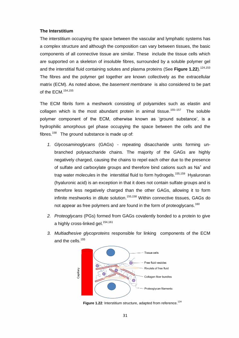
31
The Interstitium
The interstitium occupying the space between the vascular and lymphatic systems has
a complex structure and although the composition can vary between tissues, the basic
components of all connective tissue are similar. These include the tissue cells which
are supported on a skeleton of insoluble fibres, surrounded by a soluble polymer gel
and the interstitial fluid containing solutes and plasma proteins (See Figure 1.22).124,153
The fibres and the polymer gel together are known collectively as the extracellular
matrix (ECM). As noted above, the basement membrane is also considered to be part
of the ECM.154,155
The ECM fibrils form a meshwork consisting of polyamides such as elastin and
collagen which is the most abundant protein in animal tissue.155–157 The soluble
polymer component of the ECM, otherwise known as ‘ground substance’, is a
hydrophilic amorphous gel phase occupying the space between the cells and the
fibres.158 The ground substance is made up of:
1. Glycosaminoglycans (GAGs) - repeating disaccharide units forming un-
branched polysaccharide chains. The majority of the GAGs are highly
negatively charged, causing the chains to repel each other due to the presence
of sulfate and carboxylate groups and therefore bind cations such as Na+ and
trap water molecules in the interstitial fluid to form hydrogels.155,159 Hyaluronan
(hyaluronic acid) is an exception in that it does not contain sulfate groups and is
therefore less negatively charged than the other GAGs, allowing it to form
infinite meshworks in dilute solution.155,158 Within connective tissues, GAGs do
not appear as free polymers and are found in the form of proteoglycans.160
2. Proteoglycans (PGs) formed from GAGs covalently bonded to a protein to give
a highly cross-linked gel.154,161
3. Multiadhesive glycoproteins responsible for linking components of the ECM
and the cells.155
Figure 1.22: Interstitium structure, adapted from reference.124
32
A major role of the ECM component of the interstitium is the regulation of the interstitial
fluid volume which it achieves through the specialised physical and biochemical
properties of its components.162 The proteoglycans are known to immobilise water
molecules, resisting flow through the interstitium and therefore affecting hydraulic
conductivity.160 The polysaccharides can also ‘relax’ the concentration gradient and
therefore the reduce osmotic pressure of the tissue causing water to be drawn in.163
The fibrous component of the ECM also has a role. The entangled structure of the
fibres results in the formation of pores approximately 200-250 Å in diameter.164
Macromolecules such as extravasated plasma proteins, present in the interstitial fluid,
can only reside in regions of the interstitium unoccupied by the structural components
of the ECM and consequently these macromolecules will only occupy a fraction of the
interstitial fluid volume. The larger proteins will remain in the solution phase, as the gel
phase prevents bulk flow of fluid through the interstitium.165 This phenomenon is
known as interstitial exclusion.162 Solute exclusion will vary with hydration state. In
states of increased hydration, the effective pore radii of the gel phase will increase to
give a larger volume for the fluid to be distributed in and in dehydration the reverse is
true.164 Hence, the tissue water content is important as it defines the tissue volume
and controls the space available for molecular transport processes.163
The significance of solute exclusion is related to an oedema-preventing mechanism.
As fluid accumulates in the interstitium, the accessible volume will increase thus
reducing the tissue oncotic pressure making capillary filtration less favourable and
protecting against oedema formation.164 This effect is often referred to as ‘wash-down
of interstitial protein concentration’ and can withstand an increase in capillary pressure
corresponding to 7 mm Hg.111 There are another two safety factors which normally
prevent oedema formation. These include; 1) low tissue compliance when the
interstitial fluid pressure is in the negative pressure range corresponding to 3 mm Hg
and 2) the ability of lymph-flow to increase 10-50 fold to accommodate large
fluctuations in fluid corresponding to 7mm Hg.110,111 Overall, this results in a total safety
factor of 17mm Hg, theoretically allowing the capillary pressure to rise by this amount
before oedema will occur.
Although the fluid in the interstitium is usually found trapped within the ECM to form a
gel there are still small rivulets and vesicles of “free” fluid not associated with
proteoglycan molecules and therefore able to flow freely. This free fluid accounts for
less than 1% in normal tissues, but in oedema, the pockets of free fluid will expand to
give large volumes of freely flowing oedema fluid.124
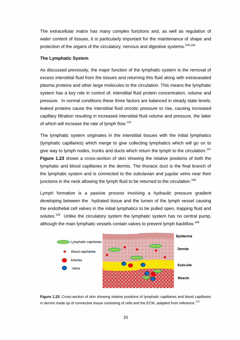
33
The extracellular matrix has many complex functions and, as well as regulation of
water content of tissues, it is particularly important for the maintenance of shape and
protection of the organs of the circulatory, nervous and digestive systems.159,166
The Lymphatic System
As discussed previously, the major function of the lymphatic system is the removal of
excess interstitial fluid from the tissues and returning this fluid along with extravasated
plasma proteins and other large molecules to the circulation. This means the lymphatic
system has a key role in control of; interstitial fluid protein concentration, volume and
pressure. In normal conditions these three factors are balanced in steady state levels;
leaked proteins cause the interstitial fluid oncotic pressure to rise, causing increased
capillary filtration resulting in increased interstitial fluid volume and pressure, the latter
of which will increase the rate of lymph flow.124
The lymphatic system originates in the interstitial tissues with the initial lymphatics
(lymphatic capillaries) which merge to give collecting lymphatics which will go on to
give way to lymph nodes, trunks and ducts which return the lymph to the circulation.167
Figure 1.23 shows a cross-section of skin showing the relative positions of both the
lymphatic and blood capillaries in the dermis. The thoracic duct is the final branch of
the lymphatic system and is connected to the subclavian and jugular veins near their
junctions in the neck allowing the lymph fluid to be returned to the circulation.168
Lymph formation is a passive process involving a hydraulic pressure gradient
developing between the hydrated tissue and the lumen of the lymph vessel causing
the endothelial cell valves in the initial lymphatics to be pulled open, trapping fluid and
solutes.128 Unlike the circulatory system the lymphatic system has no central pump,
although the main lymphatic vessels contain valves to prevent lymph backflow.169
Figure 1.23: Cross-section of skin showing relative positions of lymphatic capillaries and blood capillaries
in dermis made up of connective tissue consisting of cells and the ECM, adapted from reference.170
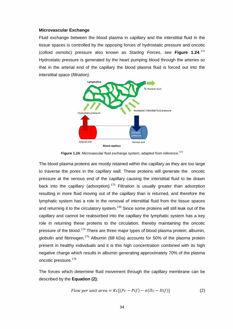
34
Microvascular Exchange
Fluid exchange between the blood plasma in capillary and the interstitial fluid in the
tissue spaces is controlled by the opposing forces of hydrostatic pressure and oncotic
(colloid osmotic) pressure also known as Starling Forces, see Figure 1.24.171
Hydrostatic pressure is generated by the heart pumping blood through the arteries so
that in the arterial end of the capillary the blood plasma fluid is forced out into the
interstitial space (filtration).
Figure 1.24: Microvascular fluid exchange system, adapted from reference.172
The blood plasma proteins are mostly retained within the capillary as they are too large
to traverse the pores in the capillary wall. These proteins will generate the oncotic
pressure at the venous end of the capillary causing the interstitial fluid to be drawn
back into the capillary (adsorption).173 Filtration is usually greater than adsorption
resulting in more fluid moving out of the capillary than is returned, and therefore the
lymphatic system has a role in the removal of interstitial fluid from the tissue spaces
and returning it to the circulatory system.135 Since some proteins will still leak out of the
capillary and cannot be reabsorbed into the capillary the lymphatic system has a key
role in returning these proteins to the circulation, thereby maintaining the oncotic
pressure of the blood.174 There are three major types of blood plasma protein; albumin,
globulin and fibrinogen.175 Albumin (68 kDa) accounts for 50% of the plasma protein
present in healthy individuals and it is this high concentration combined with its high
negative charge which results in albumin generating approximately 70% of the plasma
oncotic pressure.176
The forces which determine fluid movement through the capillary membrane can be
described by the Equation (2);
𝐹𝑙𝑜𝑤 𝑝𝑒𝑟 𝑢𝑛𝑖𝑡 𝑎𝑟𝑒𝑎 = 𝐾𝑐[(𝑃𝑐 − 𝑃𝑖𝑓) − 𝜎(𝛱𝑐 − 𝛱𝑖𝑓)] (2)
35
Where Kc is the capillary filtration coefficient, P is the hydrostatic pressure for the
capillary and interstitial fluid whereas Π is the oncotic pressure again for the capillary
and interstitial fluid.148 The symbol σ represents a retention coefficient which quantifies
the ratio of the oncotic pressure exerted by a given concentration of protein to the
theoretical oncotic pressure expected for a capillary wall which did not allow proteins to
leak through.173,148 This is required as Πc is affected by the permeability of the capillary
since in reality the capillary wall is not a perfect semipermeable membrane and the
plasma proteins are able to leak into the interstitium.173 According to Guyton et al.
normal values for these pressures are; Pc 17-25mm Hg, Pif -3mm Hg, Πc 28mm Hg
(19mm from dissolved proteins and 9mm from the Gibbs-Donnan effect) and Πif 8mm
Hg.124
A positive value for the flow per unit area indicates that capillary filtration is favoured
and a negative value is obtained when capillary absorption is favoured.
1.5.4 Pathophysiology
There are two types of mechanisms which can lead to the development of extracellular
(interstitial) oedema;
1. Non-Inflammatory
a) Disruption of the capillary dynamics resulting in abnormal leakage of plasma
fluid into the interstitium. This can be caused by excessive capillary filtration
due to increased hydrostatic pressure (hydrostatic oedema) or decreased
oncotic pressure preventing reabsorption of fluid back into the capillary, or a
combination of both effects.177
b) Lymphatic obstruction resulting in failure of lymphatic system to return fluid
from the interstitial space back into the blood. This gives rise to a specific form
of oedema known as lymphoedema.111,178
2. Inflammatory
a) Stimulation of the inflammatory immune response resulting in histamine release
which will increase the permeability of the capillary (permeability oedema)
allowing plasma proteins to diffuse into the interstitium.179–181
Causes of non-inflammatory oedema include renal disorders, cirrhosis, congestive
heart failure, nephrotic syndrome and chronic venous insufficiency.177,182 When
caused by right-sided heart failure or other systemic disease the oedema will be
symmetrical and will develop from the ankles upwards.183 Unilateral oedema will
36
usually result from a local cause such as deep vein thrombosis, venous insufficiency or
lymphedema.183,184
Inflammatory oedema is caused by physical damage to the tissue from sprains,
freezing injuries and thermal damage.161,180
1.5.5 Clinical Symptoms And Diagnosis
Initially it can be difficult to distinguish between chronic peripheral oedema and
lymphoedema. The differential diagnosis of swollen limbs includes systemic and local
causes. The former comprising of heart failure, renal disorders, hypoalbuminemia
whereas the latter includes primary and secondary lymphoedema, venous disorders,
bacterial infections and complications following surgery.185,186 A thorough medical
history is required along with a physical examination of the affected area. This
information is usually enough to make a diagnosis, but in some cases if the cause is
not known lymphoscintigraphy may be used to image the lymphatic system and check
for abnormalities. This technique involves an intradermal injection of radiolabelled
colloid into the affected area followed by imaging using a gamma camera to trace the
lymphatic transport of the radiotracer.187 Other techniques which can be used to image
the lymphatic system include magnetic resonance imaging (MRI), computed
tomography (CT) and ultrasound examination.185,187,188
Chronic Oedema
Chronic oedema is a broad term used to describe oedema not caused by lymphatic
obstruction/defects lasting 3 months or more which is not relieved by elevation or bed
rest.189 There are a mixture of causes and ultimately the lymphatic system will be
impacted by the condition if it is not treated.190 Oedema is often not clinically apparent
until at least 2.5-3 L of fluid has accumulated in the interstitium.191 Clinically there are
two types of oedema; pitting and non-pitting oedema, over time pitting oedema can
develop into non-pitting oedema as the subcutaneous tissue becomes fibrotic.192,193
Pitting oedema can be differentiated from non-pitting oedema with a simple test which
involves the physician pressing the affected area with their thumb for a set time then
seeing whether a ‘pit’ is formed. In pitting oedema the resistance to tissue fluid
displacement is lowered by the accumulation of fluid in the interstitium resulting in
dilution of the interstitial gel compartment to produce pockets of water which are easily
displaced by the application of pressure therefore forming a pit.194 The duration that the
pit lasts can also be used to assign the oedema a number in the ‘Pitting Oedema
Scale’ which gives some idea of the severity of the oedema.195
37
Pitting oedema is often caused by systemic diseases such as heart failure and kidney
and liver disorders which result in decreased serum protein, increased systematic
venous pressure.184,196 Other causes of pitting oedema include venous insufficiency
and deep vein thrombosis (DVT).182,197 The accumulated oedema fluid is of low
viscosity and is protein poor.184 Non-pitting oedema occurs in advanced
lymphoedema. Initially the lymphedematous swelling shows pitting, but with time the
tissue becomes fibrotic to give non-pitting oedema.192
Lymphoedema
Lymphoedema can be classed as primary or secondary. Primary lymphoedema
encompasses genetic abnormalities and syndromes and can be further subdivided into
categories based on the age of the patient when the symptoms began to develop.188
Congenital lymphoedema can be detected at birth or within the first two years of life,
lymphoedema praecox usually develops during puberty although can occur into the
early 30’s, and the final type - lymphoedema tarda is detectable after 35 years.198
Secondary or acquired lymphoedema develops as a consequence of disruption or
obstruction of the lymphatics and has many causes. These include; traumatic
lymphoedema in response to direct injury to the lymphatic system, post-infection
lymphoedema often as a result of recurrent cellulitis infections or infection by a
parasitic worm (filariasis) and finally cancer and cancer treatments.187 In the western
world most diagnosed forms of lymphoedema are malignancy-related, but it is thought
that non-cancer forms of the condition are likely to be more prevalent but poorly
recognised and underdiagnosed.199 In developing countries the most common cause is
infection by filariasis which is in fact the most common cause worldwide with an
estimated 120 million people currently infected and nearly 947 million people at risk in
54 countries.200 The clinical classification of lymphedematous swelling is defined by the
stages of lymphoedema outline by the International Society of Lymphology:201
Stage 0 Latent or subclinical condition where swelling is not evident despite impaired
lymph transport. Can exist months or years before overt oedema occurs (stages I–III).
Stage I Early accumulation of fluid relatively high in protein content (e.g. in comparison
with “venous” oedema) that subsides with limb elevation. Pitting may occur.
Stage II Pitting may or may not occur as tissue fibrosis develops. Limb elevation alone
rarely reduces tissue swelling.
Stage III Lymphostatic elephantiasis - pitting is absent. Trophic skin changes, fat
deposits, and warty overgrowths often develop. (Adapted from references188,201)
38
Oedema can also be classified by its localisation; generalized oedema – involving
multiple organs as well as peripheral (subcutaneous) oedema and organ-specific
oedema – i.e. cerebral, pulmonary and peritoneum (ascites).147 The present research
project will focus on the treatment of peripheral oedema, i.e. subcutaneous oedema in
the limbs.
Accumulation of excess interstitial fluid increases the diffusion distance for oxygen and
other nutrients to reach the cells as well impeding the removal of toxic cellular waste
products. In severe cases this disturbance in blood supply to the tissues is known as
ischemia and can result in cell damage and death.202,203
1.5.6 Treatment
Current treatments for oedema/lymphoedema are very limited, and at present there is
no satisfactory resolution for either condition. Since oedema is often the sign of an
underlying medical condition, initial strategies generally aim to treat and manage the
primary cause. Other approaches involve restricting dietary sodium to reduce water
retention, weight loss for obese patients and in certain cases, such as hydrostatic
oedemas caused by congestive heart failure or venous disorders such as chronic
venous insufficiency, the use of diuretics to promote fluid excretion through
kidneys.184,204 Diuretics will have little effect on lymphedematous oedema as
pathogenesis of this condition relies on elevated tissue oncotic pressure from
accumulated macromolecules (mainly proteins) and not excess water retention.205
Lymphoedema treatment can be divided into conservative (non-operative) and
operative approaches, although underpinning both methods is a meticulous skin care
regime along with careful exercise and compression.201 The main approach is Complex
Decongestive Therapy (CDT) which should be performed by a certified therapist and
involves a combination of: lymphatic-specific massage known as manual lymphatic
drainage (MLD), compression in the form of multilayer bandaging and specially
designed compression garments along with the above mentioned exercise and skin
care regimes.205–207 After an intensive CDT course in a clinical setting, the treatment is
adapted to include self-management at home.208 The use of additional compressive
devices alongside the CDT may also be appropriate – intermittent pneumatic
compression (IPC) therapy in particular is considered a safe and effective addition
which has the advantage of being designed for use at home.209 If properly executed
this approach can have very good results, but it is very time- and labour intensive,
requiring specially trained personnel, personalised treatment plans and high patient
compliance to ensure effectiveness.
39
Benzo-pyrones have been investigated as potential drugs for lymphoedema treatments
as they act by reducing vascular permeability, thereby reducing fluid accumulation in
tissues.210 It has also been suggested that they may increase macrophage activity
leading to proteolysis in the interstitium and therefore reducing the tissue oncotic
pressure.211 A recent review of benzo-pyrones as treatment for lymphoedema was
unable to draw conclusions about the effectiveness of the drugs from the available
clinical research and additionally there are concerns regarding side-effects affecting
liver function.210
In extreme cases, or for patients who have not responded to standard treatments,
surgical procedures may be used to reduce limb volume by removing excessive
tissues (debulking procedures) or to bypass lymphatic defects.206 Other indicators for
surgery include recurrent infections, impaired movement or for cosmetic
purposes.206,209
Future approaches in lymphoedema treatment include molecular strategies, and much
research has focused on the identification of molecular targets.212 One such approach
is uses gene therapy particularly for therapeutic lymphangiogenesis where growth
factors can be used to stimulate lymphatic vessel growth.213,214
1.5.7 Fluid Composition
Studies investigating the composition of these fluids are limited by difficulties in
isolating the interstitial fluid in both normal and oedematous tissues. Although many
techniques exist for this purpose they all have their inherent weaknesses, meaning
there is no universally accepted method of interstitial fluid collection.129,165 Techniques
for direct sampling include the wick technique215 and suction blister techniques.216
Many studies also use lymph fluid since it is more accessible and, as discussed above,
the initial lymph fluid is thought to be representative of the interstitial fluid. Microdialysis
is another widely used technique for indirect sampling of fluid from the interstitium. This
minimally invasive technique allows for continuous sampling of small (endogenous and
exogenous) water soluble molecules within the interstitial fluid.217 The technique
involves the insertion of a dialysis catheter (probe) into the tissue of interest using a
guide cannula.218 The probe consists of a shaft with a semipermeable hollow fibre
membrane tip and mimics the structure of a blood capillary.219 The probe has an inlet
and outlet tube and is continuously perfused with a solution with an ionic composition
similar to that of the surrounding tissue fluid (perfusate).218 Water soluble molecules
within the tissues can passively diffuse through the pores of the membrane and leaves
the probe as a dialysate where it can be analysed. Providing there is a suitable assay,
40
virtually any water-soluble molecule in the interstitium can be sampled.218 Commercial
polyethersulfone microdialysis probes are available with a MWCO of 6,000-
100,000 Da.217 This technique has been used to investigate the role of histamine in
oedema formation after thermal injury.121
Normal interstitial fluid protein levels have been quoted as 0.6-3.49 g/dL derived from
normal leg lymph (including plasma protein, cytokine and cellular content)220 and
2.06 g/dL estimated from average protein content of plasma in 20 subjects.221
In the past it was thought that the composition of the accumulated oedema fluid would
vary with the mechanism of oedema formation. Non-inflammatory oedema from
enhanced capillary filtration (increased hydrostatic pressure) or decreased
reabsorption (decreased plasma protein) was thought to result in the accumulation of a
protein-poor fluid know as a transudate.222 In contrast, inflammatory oedema
mechanisms result in increased capillary permeability, therefore allowing plasma
proteins to leak into the interstitium to give a protein rich fluid known as exudate.222 In
lymphoedema it is thought that insufficient interstitial fluid drainage results in the
accumulation of the extravasated proteins resulting in a protein rich fluid.198
Early studies into primary lymphoedema fluid composition corroborated this theory.
Taylor et al. analysed the protein content of fluid obtained from 38 patients with primary
lymphoedema and found an average protein content of 2.8 g/dL although the range
was from 1-5.5 g/dL.223
More recent studies have found the protein content of lymphoedema fluid to be the
same or even lower in comparison to fluid extracted from an unaffected limb. These
studies have often focused on secondary or obstructive lymphoedema. Olszewski et al.
found that the lymph protein content in patients with postoperative and inflammatory
lymphoedema was similar to that found in the controls although cytokine levels were
found to be different with significantly higher levels found in those suffering from
lymphoedema.224 In another study Olszewski et al. reported that the peripheral ‘tissue
fluid-lymph’ of 15 patients suffering from filarial lymphoedema had a total protein
content of 2.37 g/dL with a lymph: serum protein ratio of 0.48 ,whereas controls
exhibited a total protein content of 2.39 g/dL.225 Bates et al. found reduced colloid
osmotic pressures in post-mastectomy arm lymphoedema fluid in comparison to the
normal arm, which again goes against the theory of a high protein concentration.226
There are many theories to explain these findings. One proposal is that, particularly in
the early stages of lymphoedema, the interstitial and lymphatic spaces can expand and
41
accumulate the excess fluid, causing the protein concentration to remain within normal
limits as it is diluted by the accumulated fluid.224 Other theories include: reduced
capillary permeability to plasma proteins, proteolysis within the interstitium, and
increased capillary filtration rate which decreases the transendothelial transfer of
protein.226,227
Other components which have been investigated include lipoproteins, which are
present in the interstitium due to their role in peripheral cell cholesterol
metabolism,165,228 and immune cells (i.e. lymphocytes) to investigate inflammatory
processes and susceptibility to infections.229
1.6 Project Aims and Objectives
The core aim of the project was to develop and test a prototype membrane medical
device for interosmolar fluid removal to treat oedema and related conditions. The major
objective was to obtain proof-of-concept. Though the device concept was described by
a patent, no supporting evidence or data had yet been produced and so all aspects of
the device and process required fundamental investigation. To achieve this, the
following project aims were proposed:
1. thorough background research into the conditions of oedema and
lymphoedema as well as membrane technology, including both literature
research and consultation with clinicians and researchers in the field;
2. practical laboratory work including investigation into the process of forward
osmosis (in particular, using UF membranes and specifically to transport model
oedema fluid and proteins), membranes and membrane modifications and
potential draw solutions;
3. the development of a prototype design and fabrication process, assisted by key
findings from this laboratory work and background research;
4. the development of both an in vitro and ex vivo model in order to test the
prototype devices;
5. prototype testing to attain proof-of-concept.
Alongside the above clinically-oriented project, a secondary project was proposed
involving an investigation into thin-film composite membrane fabrication, to explore
new thin film coatings made from novel poly-ylids and a new solvent resistant support
membrane.
42
1.7 References
1. C. B. Herbert and M. N. Blaine, US Pat. 8211 053 B2 (2012), to Equilibrate,
LLC.
2. R. W. Baker, Membrane Technology and Applications, John Wiley & Sons, Ltd,
Chichester, UK, 2004, pp. 1–14.
3. K. W. Boddeker, J. Membr. Sci., 1995, 100, 65–68.
4. R. E. Kesting, Synthetic Polymeric Membranes A Structural Perspective, Wiley-
Interscience, Irvine, California, 2nd edn., 1985.
5. S. Atkinson, Filtr. Sep., 1992, 36, 28.
6. K. C. Khulbe, C. Y. Feng, and T. Matsuura, in Synthetic Polymeric Membranes
Characterisation by Atomic Force Microscopy, Springer-Verlag, Berlin, 2008, pp.
5–14.
7. B. S. Lalia, V. Kochkodan, R. Hashaikeh, and N. Hilal, Desalination, 2013, 326,
77–95.
8. S. Loeb, in Synthetic Membranes - Volume 1 - Desalination (ACS Symposium
series), Washington, D. C., 1980, pp. 1–9.
9. A. S. Michaels, US Pat. 3 615 024 (1971) to Amicon Corporation.
10. A. S. Michaels, Pure Appl. Chem., 1976, 46, 193–204.
11. R. W. Baker, Membrane Technology and Applications, John Wiley & Sons, Ltd,
Chichester, UK, 2004, pp. 237–272.
12. K. P. Lee, T. C. Arnot, and D. Mattia, J. Membr. Sci., 2011, 370, 1–22.
13. W. J. Lau and A. F. Ismail, in 2nd International Conference on Environmental
Engineering and Applications International Proceedings of Chemical, Biological
and Environmental Engineering, IACSIT Press, Singapore, 2011, vol. 17, pp.
173–177.
14. J. E. Cadotte, US Patent 4,277,344, (1981) to FilmTec Corporation.
15. W. J. Lau, A. F. Ismail, N. Misdan, and M. A. Kassim, Desalination, 2012, 287,
190–199.
43
16. W. J. Koros, Y. H. Ma, and T. Shimidzu, Pure Appl. Chem., 1996, 68, 1479–
1489.
17. R. van Reis and A. Zydney, J. Membr. Sci., 2007, 297, 16–50.
18. I. Pinnau and B. D. Freeman, in ACS Symposium Series No. 744, 1999, vol.
744, p. 1.
19. M. Ulbricht, Polymer , 2006, 47, 2217–2262.
20. R. Mallada and M. Menendez, Eds., in Membrane Science and Technology
Series. Volume 13, Elsevier, Amsterdam, 2008, pp. 1–460.
21. A. Sagle and B. Freeman, Fundamentals of Membranes for Water Treatment,
University of Texas, Austin, 2004.
22. R. Rautenbach and R. Albrecht, in Membrane Processes, John Wiley & Sons,
Ltd, Aarau, Switzerland, 1989, pp. 18–47.
23. W. Guo, H.-H. Ngo, and J. Li, Bioresour. Technol., 2012, 122, 27–34.
24. S. P. Beier, in Pressure Driven Membrane Processes, Bookboon, London, 2nd
edn., 2007, pp. 4–22.
25. J. G. Wijmans and R. W. Baker, J. Membr. Sci., 1995, 107, 1–21.
26. M. E. Williams, A Review of Reverse Osmosis Theory, EET Corporation and
Williams Engineering Services Company Inc, Tennessee, 2003.
27. R. Rautenbach and R. Albrecht, in Membrane Processes, John Wiley & Sons,
Ltd, Aarau, Switzerland, 1989, pp. 48–74.
28. R. W. Baker, Membrane Technology and Applications, John Wiley & Sons, Ltd,
Chichester, UK, 2004, pp. 15–84.
29. A. E. Childress and M. Elimelech, J. Membr. Sci., 1996, 119, 253–268.
30. K. J. Kim, A. G. Fane, M. Nystrom, A. Pihlajamaki, W. R. Bowen, and H.
Mukhtar, J. Membr. Sci., 1996, 116, 149–159.
31. M. Elimelech, W. H. Chen, and J. J. Waypa, Desalination, 1994, 95, 269–286.
32. K. Toyomoto and A. Higuchi,Membrane Science and Technology, eds. Y. Osada
and T. Nakagawa, Marcel Dekker, Inc, New York, US, 1992, pp. 289–331.
44
33. R. W. Baker, Membrane Technology and Applications, John Wiley and Sons,
Ltd, Chichester, UK, 2004.
34. M. Cheryan, Ultrafiltration and Microfiltration Handbook, Techomic Publishing
Company, Inc., Basel, 2nd edn., 1998.
35. S. Jain and S. K. Gupta, J. Membr. Sci., 2004, 232, 45–61.
36. J. G. Jacangelo, R. R. Trussell, and M. Watson, Desalination, 1997, 9164, 119–
127.
37. G. Daufin, J. Escudier, H. Carrere, S. Berot, L. Fillaudeau, and M. Decloux,
Food Bioprod. Process., 2001, 79, 89–102.
38. B. Butchermaker, Filtr. Sep., 2004, 32–33.
39. A. W. Mohammad, C. Y. Ng, Y. P. Lim, and G. H. Ng, Food Bioprocess
Technol., 2012, 5, 1143–1156.
40. R. van Reis and A. Zydney, Curr. Opin. Biotechnol., 2001, 12, 208–11.
41. C. Charcosset, Biotechnol. Adv., 2006, 24, 482–92.
42. A. A. Merdaw, A. O. Sharif, and G. A. W. Derwish, Chem. Eng. J., 2011, 168,
215–228.
43. R. R. Bhave, in Fermentation and Biochemical Engineering Handbook, eds. H.
C. Vogel and C. L. Todaro, Noyes Publication, Westwood, New Jersey, 2nd
edn., 1997, pp. 271–322.
44. M. C. Porter, in Handbook of Industrial Membrane Technology, ed. M. C. Porter,
Noyes Publications, New Jersey, USA, 1990, pp. 61–134.
45. G. Russotti and K. E. Goklen, in Membrane Separations in Biotechnology, ed.
W. K. Wang, Marcel Dekker, Basel, Switzerland, 2nd edn., 2001, pp. 85–188.
46. B. Van der Bruggen, L. Lejon, and C. Vandecasteele, Environ. Sci. Technol.,
2003, 37, 3733–8.
47. W. Gao, H. Liang, J. Ma, M. Han, Z. Chen, Z. Han, and G. Li, Desalination,
2011, 272, 1–8.
48. J. S. Baker and L. Y. Dudley, Desalination, 1998, 118, 81–89.
45
49. J. A. L. Santos, M. Mateus, and J. A. S. Cabral, in Chromatographic and
Membrane Processes in Biotechnology, ed. C. A. Costa, Kluwer Academic
Publishers, Dordrecht, 1991, pp. 177–205.
50. W. S. Winston Ho and K. K. Sirkar, Eds., in Membrane Handbook, Chapman
and Hall, London, Uk, 1992, pp. 455–571.
51. R. W. Baker, in Membrane Technology and Applications, John Wiley & Sons,
Ltd, Chichester, UK, 2004, pp. 275–300.
52. K. C. Khulbe, C. Y. Feng, and T. Matsuura, Synthetic Polymeric Membranes
Characterisation by Atomic Force Microscopy, Springer-Verlag Berlin
Heidelberg, Ottawa, 2008, pp. 101–139.
53. H. Yacubowicz and J. Yacubowicz, Filtr. Sep., 2005, 42, 16–21.
54. N. Hilal, H. Al-Zoubi, N. A. Darwish, A. W. Mohammad, and M. Abu Arabi,
Desalination, 2004, 170, 281–308.
55. T. Thorsen and H. Flogstag, in Nanofiltration in Drinking Water Treatment,
Techneau, Trondheim, 2006, pp. 3–7.
56. L. F. Greenlee, D. F. Lawler, B. D. Freeman, B. Marrot, and P. Moulin, Water
Res., 2009, 43, 2317–48.
57. D. Li and H. Wang, J. Mater. Chem., 2010, 20, 4551.
58. H. B. Park, B. D. Freeman, Z. Zhang, M. Sankir, and J. E. Mcgrath, Angew.
Chemie, Int. Ed., 2008, 47, 6019–6024.
59. G.-D. Kang, C.-J. Gao, W.-D. Chen, X.-M. Jie, Y.-M. Cao, and Q. Yuan, J.
Membr. Sci., 2007, 300, 165–171.
60. I. C. Tessaro, J. B. a. da Silva, and K. Wada, Desalination, 2005, 181, 275–282.
61. I. M. Wienk, R. M. Boom, M. A. M. Beerlage, A. M. W. Bulte, C. A. Smolders,
and H. Strathmann, J. Membr. Sci., 1996, 113, 361–371.
62. R. W. Baker, Membrane Technology and Applications, John Wiley & Sons, Ltd,
Chichester, UK, 2004, pp. 89–155.
63. A. Rahimpour and S. S. Madaeni, J. Membr. Sci., 2007, 305, 299–312.
64. P. Witte van de, P. J. Dijkstra, J. W. A. Berg van den, and J. Feijen, J. Membr.
46
Sci., 1996, 117, 1–31.
65. J. F. Blanco, J. Sublet, Q. T. Nguyen, and P. Schaetzel, J. Membr. Sci., 2006,
283, 27–37.
66. R. M. Boom, I. M. Wienk, T. Van Den Boomgaard, and C. A. Smolders, J.
Membr. Sci., 1992, 73, 277–292.
67. P. W. Morgan and S. L. Kwolek, J. Chem. Educ., 1959, 36, 182.
68. E. L. Wittbecker and P. W. Morgan, J. Polym. Sci., 1959, XL, 521–529.
69. P. W. Morgan and S. L. Kwolek, J. Polym. Sci., 1959, XL, 299–327.
70. J. E. Tomaschke, in Encyclopedia of Separation Science, Vol. III, Membrane
Preparation, Academic Press Inc, 2000, pp. 3319–3331.
71. H. M. Colquhoun, D. Chappell, A. L. Lewis, D. F. Lewis, G. T. Finlan, and P. J.
Williams, J. Mater. Chem., 2010, 20, 4629.
72. M. Mulder, in Basic Principles of Membrane Technology, Kluwer Academic
Publishers, Dordrecht, 2000, pp. 157–208.
73. M. Cheryan, in Ultrafiltration and Microfiltration Handbook, Techomic Publishing
Company, Inc., Basel, 2nd edn., 1998, pp. 71–107.
74. K. L. Tung, K. S. Chang, T. T. Wu, N. J. Lin, K. R. Lee, and J. Y. Lai, Curr. Opin.
Chem. Eng., 2014, 4, 121–127.
75. A. E. Childress, J. A. Brant, P. Rempala, D. W. Phipps, and P. Kwan, Evaluation
of Membrane Characterization Methods, Water Research Foundation, Denver,
2012.
76. R. Bernstein, Y. Kaufman, and V. Freger, in Encyclopedia of Membrane Science
and Technology, eds. E. M. V. Hoek and V. V. Tarabara, John Wiley & Sons,
Inc, 2013, pp. 1–41.
77. N. A. Ochoa, P. Prádanos, L. Palacio, C. Pagliero, J. Marchese, and A.
Hernández, J. Membr. Sci., 2001, 187, 227–237.
78. S. Singh, K. C. Khulbe, T. Matsuura, and P. Ramamurthy, J. Membr. Sci., 1998,
142, 111–127.
79. R. Tamime, Y. Wyart, L. Siozade, I. Baudin, C. Deumie, K. Glucina, and P.
47
Moulin, Membranes (Basel)., 2011, 1, 91–97.
80. K. Smolders and A. C. M. Franken, Desalination, 1989, 72, 249–262.
81. S. Belfer, R. Fainchtain, Y. Purinson, and O. Kedem, J. Membr. Sci., 2000, 172,
113–124.
82. Q. Ge, J. Su, G. L. Amy, and T.-S. Chung, Water Res., 2012, 46, 1318–26.
83. T. Cath, A. Childress, and M. Elimelech, J. Membr. Sci., 2006, 281, 70–87.
84. P. Atkins and J. de Paula, in Atkins’ Physical Chemistry, Oxford University
Press, Oxford, 7th edn., 2006, pp. 160–186.
85. S. Zhao, L. Zou, C. Y. Tang, and D. Mulcahy, J. Membr. Sci., 2012, 396, 1–21.
86. A. Davis and E. Kravath, Desalination, 1975, 16, 151–155.
87. J. O. Kessler and C. D. Moody, Desalination, 1976, 8, 297–306.
88. T.-S. Chung, S. Zhang, K. Y. Wang, J. Su, and M. M. Ling, Desalination, 2012,
287, 78–81.
89. J. Ren and J. R. McCutcheon, Desalination, 2013, 343, 187–193.
90. I. Alsvik and M.-B. Hägg, Polymers (Basel)., 2013, 5, 303–327.
91. Forward Osmosis: Current Status and Perspectives, R. Wang and L. Setiawan,
J. Memb. Sci Virtual Special Issue, 2012.
92. S. K. Yen, F. Mehnas Haja N., M. Su, K. Y. Wang, and T.-S. Chung, J. Membr.
Sci., 2010, 364, 242–252.
93. N. T. Hancock and T. Y. Cath, Environ. Sci. Technol., 2009, 43, 6769–75.
94. A. Achilli, T. Y. Cath, and A. E. Childress, J. Membr. Sci., 2010, 364, 233–241.
95. G. W. Batchelder, W. Ave, and S. Monica, US Pat. 3 171 799 (1965).
96. J. R. McCutcheon, R. L. McGinnis, and M. Elimelech, Desalination, 2005, 174,
1–11.
97. D. Li, X. Zhang, J. Yao, G. P. Simon, and H. Wang, Chem. Commun., 2011, 47,
1710–1712.
98. R. Ou, Y. Wang, H. Wang, and T. Xu, Desalination, 2013, 318, 48–55.
48
99. Q. Ge, P. Wang, C. Wan, and T.-S. Chung, Environ. Sci. Technol., 2012, 46,
6236–43.
100. D. Li, X. Zhang, G. P. Simon, and H. Wang, Water Res., 2013, 47, 209–215.
101. B. Mi and M. Elimelech, J. Membr. Sci., 2010, 348, 337–345.
102. B. Mi and M. Elimelech, J. Membr. Sci., 2008, 320, 292–302.
103. S. Lee, C. Boo, M. Elimelech, and S. Hong, J. Membr. Sci., 2010, 365, 34–39.
104. K. C. Khulbe, C. Feng, and T. Matsuura, J. Appl. Polym. Sci., 2009, 115, 855–
895.
105. N. Nady, M. C. R. Franssen, H. Zuilhof, M. S. M. Eldin, R. Boom, and K.
Schroën, Desalination, 2011, 275, 1–9.
106. D. Rana and T. Matsuura, Chem. Rev., 2010, 110, 2448–71.
107. Z. Xu, L. Wan, and X. Huang, in Surface Engineering of Polymer Membranes,
Springer, Berlin, 2009, pp. 80–149.
108. A. Bhattacharya and B. N. Misra, Prog. Polym. Sci., 2004, 29, 767–814.
109. F. Kucera and J. Jancar, Polym. Eng. Sci., 1998, 3, 783–792.
110. J. Scallan, V. H. Huxley, and R. J. Korthuis, Capillary Fluid Exchange:
Regulation, Functions and Pathology, Morgan and Claypool Life Sciences, San
Rafael, 2010.
111. A. C. Guyton and J. E. Hall, Guyton and Hall Textbook of Medical Physiology,
Saunders Elsevier, Philadelphia, 12th edn., 2011, pp. 283–301.
112. J. D. Louden, Anaesth. Intensive Care Med., 2009, 10, 279–285.
113. A. Ballinger, in Essentials of Kumar and Clark’s Clinical Medicine, eds. P. Kumar
and M. Clark, Elsevier, London, Uk, 5th edn., 2011, pp. 323–353.
114. T. A. Brown, in Rapid Review Physiology, ed. E. F. Goljan, Elsevier Mosby,
Philadelphia, 2nd edn., 2012, pp. 241–246.
115. B. Andersson, Ann. Rev. Physiol., 1977, 39, 185–200.
116. J. C. Atherton, Anaesth. Intensive Care Med., 2006, 7, 227–233.
49
117. S. Cho and J. E. Atwood, Am. J. Med., 2002, 113, 580–586.
118. G. J. Tortora and B. H. Derrickson, Principles of Anatomy and Physiology, John
Wiley & Sons, Ltd, New York, 13th edn., 2012.
119. W. F. Boron and E. L. Boulpap, in Medical Physiology, Saunders Elsevier,
Philadelphia, 2nd edn., 2009, pp. 106–146.
120. H. F. Dvorak, L. F. Brown, M. Detmar, and A. M. Dvorak, Am. J. Pathol., 1995,
146, 1029–1039.
121. A. Papp, M. Härmä, R. Harvima, T. Lahtinen, A. Uusaro, and E. Alhava, Burns,
2005, 31, 476–81.
122. G. Majno and G. E. Palade, J. Biophys. Biochem. Cytol., 1961, 11, 571–605.
123. J. Hankins, J. Infus. Nurs., 2006, 29, 260–265.
124. A. C. Guyton and J. E. Hall, Guyton and Hall Textbook of Medical Physiology,
Saunders Elsevier, Philadelphia, 12th edn., 2011, pp. 155–282.
125. D. N. Granger, in Essential Medical Physiology, eds. L. R. Johnson and J. H.
Byrne, Academic Press Inc, San Diego, California, 3rd Revise., 2003, pp. 235–
244.
126. A. S. Popel and P. C. Johnson, Annu. Rev. Fluid Mech., 2005, 37, 43–69.
127. A. C. Guyton and J. E. Hall, Guyton and Hall Textbook of Medical Physiology,
Saunders Elsevier, Philadelphia, 12th edn., 2001, p. 288.
128. J. Scallan, V. H. Huxley, and R. J. Korthuis, Capillary Fluid Exchange:
Regulation, Functions and Pathology, Morgan and Claypool Life Sciences, San
Rafael, 2010.
129. H. Wiig and M. Swartz, Physiol. Rev., 2012, 92, 1005–60.
130. L. V Leak, L. Liotta, H. Krutzsch, M. Jones, V. Fusaro, S. J. Ross, Y. Zhao, E. F.
Petricoin, and V. Fusaroa, Proteomics, 2004, 4, 753–65.
131. Z. Meng and T. D. Veenstra, Proteomics. Clin. Appl., 2007, 1, 747–57.
132. M. Dzieciatkowska, M. V Wohlauer, E. E. Moore, S. Damle, J. Campsen, M.
Kelher, C. Silliman, A. Banerjee, and K. C. Hansen, Shock, 2012, 35, 331–338.
50
133. W. L. Olszewski, J. Pazdur, E. Kubasiewicz, M. Zaleska, C. J. Cooke, and N. E.
Miller, Arthritis Rheum., 2001, 44, 541–549.
134. M. J. Karnovsky, J. Cell Biol., 1967, 35, 213–36.
135. D. U. Silverthorn, W. C. Ober, C. W. Garrison, A. C. Silverthorn, and B. R.
Johnson, in Human Physiology, Pearson Education, San Francisco, 4th edn.,
2007, pp. 500–524.
136. J. Naish, P. Revest, and D. Syndercombe Court, in Medical Sciences, Elsevier,
London, 1st edn., 2009.
137. J. R. Pappenheimer, Physiol. Rev., 1953, 33, 387–423.
138. R. W. Schrier, Y. C. Chen, and M. A. Cadnapaphornchai, Neuroscience, 2004,
129, 897–904.
139. A. S. Lossinsky and R. R. Shivers, Histol. Histopathol., 2004, 19, 535–64.
140. M. J. Karnovsky, J. Gen. Physiol., 1968, 52, 64–95.
141. M. Pavelka and J. Roth, Functional Ultrastructure - An Atlas of Tissue Biology
and Pathology, Springer, Vienna, 2005.
142. S. Stiller, E. Bonnie-schorn, A. Grassmann, H. Mann, and I. Uhlenbusch-ko,
Semin. Dial., 2001, 14, 337–347.
143. D. U. Silverthorn, W. C. Ober, C. W. Garrison, A. C. Silverthorn, and B. R.
Johnson, in Human Physiology, Pearson Education, San Francisco, 4th edn.,
2007, pp. 129–169.
144. A. Leaf, Ann. N. Y. Acad. Sci., 1959, 72, 396–404.
145. F. Lang, G. L. Busch, M. Ritter, H. Vo, S. Waldegger, and E. Gulbins, Physiol.
Rev., 1998, 78, 247–306.
146. B. M. Koeppen and B. A. Stanton, in Renal Physiology, Elsevier, 5th edn., 2013,
pp. 5–18.
147. S. Gonem, in Diagnosis in Acute Medicine, Radcliffe Publishing Ltd, Abingdon,
UK, 1998, pp. 45–48.
148. J. Waterhouse, M. Sawdon, and E. Kirkman, Anaesth. Intensive Care Med.,
2013, 14, 72–78.
51
149. B. R. Waterhouse and A. D. Farmery, Anaesth. Intensive Care Med., 2012, 13,
573–580.
150. M. K. Nguyen and I. Kurtz, J. Appl. Physiol., 2006, 100, 1293–1300.
151. S. Kurbel, J. Theor. Biol., 2008, 252, 769–72.
152. S. L. Xie, R. K. Reed, B. D. Bowen, and J. L. Bert, Microvasc. Res., 1995, 49,
141–163.
153. K. Aukland and G. Nicolaysen, Physiol. Rev., 1981, 61, 556–643.
154. J. A. Davies, in Encyclopedia of Life Sciences, Nature Publishing Group,
Edinburgh, 2001, pp. 1–7.
155. G. M. Cooper, in The Cell: A Molecular Approach, ed. G. Cooper, Sinauer
Associates, Sunderland, MA, 2nd edn., 2000.
156. B. Alberts, A. Johnson, and J. Lewis, in Molecular Biology of the Cell, Garland
Science, New York, 4th edn., 2002, vol. i.
157. M. L. Tanzer, J. Orthop. Sci., 2006, 11, 326–31.
158. J. E. Scott, J. Anat., 1995, 187, 259–69.
159. J. E. Scott, FSAEB J., 1992, 6, 2639–2645.
160. W. D. Comper and T. C. Laurent, Physiol. Rev., 1978, 58, 255–315.
161. R. K. Reed and K. Rubin, Cardiovasc. Res., 2010, 87, 211–7.
162. H. Wiig, C. Gyenge, P. O. Iversen, D. Gullberg, and O. Tenstad,
Microcirculation, 2008, 15, 283–96.
163. W. D. Comper and O. Zamparo, Biochem. J., 1990, 269, 561–4.
164. J. Scallan, V. Huxley, and R. J. Korthuis, Capillary Fluid Exchange: Regulation,
Functions and Pathology, Morgan and Claypool Life Sciences, San Rafael,
2010.
165. J. Lundberg, M. Rudling, and B. Angelin, J. Lipid Res., 1987, 28, 225–237.
166. J. E. Scott, Pathol. Biol., 2001, 8114, 284–289.
167. M. A. Swartz, Adv. Drug Deliv. Rev., 2001, 50, 3–20.
52
168. W. F. Hamilton and P. Dow, Eds., in Handbook of Physiology, American
Physiological Society, Baltimore, Maryland, 1963.
169. D. Negrini and A. Moriondo, J. Physiol., 2011, 589, 2927–34.
170. K. Alitalo, T. Tammela, and T. V Petrova, Nature, 2005, 438, 946–53.
171. A. E. Taylor, Circ. Res., 1981, 49, 557–575.
172. V. Kumar, A. K. Abbas, and J. C. Aster, Robbins Basic Pathology, Saunders
Elsevier, Philadelphia, 9th edn., 2012.
173. J. R. Levick, Exp. Physiol., 1991, 76, 825–857.
174. O. Stucker, C. Pons-Himbert, and E. Laemmel, Phlebolymphology, 2008, 15,
31–36.
175. A. C. Guyton and J. E. Hall, Guyton and Hall Textbook of Medical Physiology,
Saunders Elsevier, Philadelphia, 12th edn., 2011, pp. 831–836.
176. T. W. Evans, Aliment. Pharmacol. Ther., 2002, 16, 6–11.
177. R. Gordillo, J. Kumar, and R. P. Woroniecki, in Nutrition and Health: Fluid and
Electrolytes in Pediatrics, eds. L. G. Feld and F. J. Kaskel, Humana Press,
Totowa, NJ, 2010, pp. 47–66.
178. P. S. Mortimer and J. R. Levick, Clin. Med., 2004, 4, 448–53.
179. G. Majno, G. E. Palade, and G. I. Schoefl, J. Biophys. Biochem. Cytol., 1961,
11, 607–26.
180. B. V. Reed, Phys. Ther., 1988, 68, 491–5.
181. B. Y. Geraldine, C. C. Michel, and M. E. Phillips, J. Physiol., 1988, 395, 99–114.
182. R. T. Eberhardt and J. D. Raffetto, Circulation, 2005, 111, 2398–409.
183. L. Goldman and A. I. Schafer, in Goldman’s Cecil Medicine, Elsevier Saunders,
24th edn., 2012.
184. J. W. Ely, J. A. Osheroff, M. L. Chambliss, and M. H. Ebell, J. Am. Board Fam.
Med., 2006, 19, 148–60.
185. A. Tiwari, K.-S. Cheng, M. Button, F. Myint, and G. Hamilton, Arch. Surg., 2003,
138, 152–61.
53
186. S. J. Simonian, C. L. Morgan, L. L. Tretbar, and B. Blondeau, in Lymphedema
Diagnosis and Treatment, eds. L. L. Tretbar, C. L. Morgan, S. J. Simonian, and
B. Blondeau, Springer-Verlag, London, 2008, pp. 12–21.
187. A. Szuba and S. G. Rockson, Vasc. Med., 1998, 3, 145–156.
188. A. G. Warren, H. Brorson, L. J. Borud, and S. A. Slavin, Ann. Plast. Surg., 2007,
59, 464–72.
189. C. J. Moffatt, P. J. Franks, D. C. Doherty, A. F. Williams, C. Badger, E. Jeffs, N.
Bosanquet, and P. S. Mortimer, Q. J. Med., 2003, 96, 731–738.
190. British Lymphoedema Society, in What is meant by lymphoedema and chronic
oedema ? The Five Guide, pp. 1–23.
191. H. G. Rennke and B. M. Denker, in Renal Pathophysiology:The Essentials,
Lippincott Williams & Wilkins, Philadelphia, 2nd edn., 2007.
192. K. Kerchner, A. Fleischer, and G. Yosipovitch, J. Am. Acad. Dermatol., 2008, 59,
324–31.
193. O. T. A. Lyons and B. Modarai, Surg., 2013, 31, 218–223.
194. D. O. Bates, J. R. Levick, and P. S. Mortimer, Lymphology, 1994, 27, 159–172.
195. S. B. O’Sullivan and T. J. Schmitz, in Physical rehabilitation: assessment and
treatment, F. A. Davies Company, Philadelphia, 5th edn., 2007, p. 659.
196. S. J. Fruth, in Fundamentals of Physical Therapy Examination: Patient Interview
and Tests & Measures, Jones and Bartlett Publishers, Inc, Burlington, 2013, pp.
115–118.
197. E. J. Topham and P. S. Mortimer, Clin. Med., 2002, 2, 28–31.
198. S. G. Rockson, Am. J. Med., 2001, 110, 288–295.
199. P. S. Mortimer, in Oxford Textbook of Medicine, Oxford University Press,
Oxford, 5th edn., 2012, pp. 3093–3092.
200. WHO, in Lymphaic Filariasis WHO Factsheet No.102, 2016,
http://www.who.int/mediacentre/factsheets/fs102/en.
201. International Society of Lymphology, in Lymphology, 2009, vol. 42, pp. 51–60.
54
202. G. A. Rosenberg, Prog. Cardiovasc. Dis., 1999, 42, 209–16.
203. T. G. Walker, Tech. Vasc. Interv. Radiol., 2009, 12, 117–29.
204. J. G. O’Brien, S. A. Chennubhotla, and R. V Chennubhotla, Am. Fam. Physician,
2005, 71, 2111–2117.
205. S. G. Rockson, J. Am. Coll. Cardiol., 2008, 52, 799–806.
206. P. S. Mortimer, Br. Med. J., 2000, 320, 1527–1529.
207. S. R. Cohen, D. K. Payne, and R. S. Tunkel, Cancer Suppl., 2001, 92, 980–987.
208. H. N. Mayrovitz, Lymphat. Res. Biol., 2009, 7, 101–8.
209. C. J. Chang and J. N. Cormier, Semin. Oncol. Nurs., 2013, 29, 28–40.
210. C. M. A. Badger, N. J. Preston, K. Seers, and P. S. Mortimer, Cochrane Libr.,
2009, 1–42.
211. J. A. Petrek, P. I. Pressman, and R. A. Smith, CA-Cancer J. Clin., 2000, 50,
292-307–11.
212. A. An and S. G. Rockson, Lymphat. Res. Biol., 2004, 2, 173–81.
213. Y. Saito, H. Nakagami, Y. Kaneda, and R. Morishita, Biomed Res. Int., 2013,
2013, 804675.
214. M. E. Baldwin, S. A. Stacker, and M. G. Achen, Bioessays, 2002, 24, 1030–40.
215. H. O. Fadnes and K. Aukland, Microvasc. Res., 1977, 25, 11–25.
216. U. Kiistala, J. Invest. Dermatol., 1967, 50, 129–138.
217. G. F. Clough, AAPS J., 2005, 7, E686-92.
218. M. Müller, Br. Med. J., 2002, 324, 588–591.
219. S. Klaus, M. Heringlake, and L. Bahlmann, Crit. Care, 2004, 8, 363–8.
220. W. L. Olszewski, Lymphat. Res. Biol., 2003, 1, 11–28.
221. N. Fogh-Andersen, B. M. Altura, B. T. Altura, and O. Siggaard-Andersen, Clin.
Chem., 1995, 41, 1522–5.
222. V. Kumar, A. K. Abbas, N. Fausto, and J. C. Aster, in Robbins and Cotran
55
Pathologic Basis of Disease, Saunders Elsevier, Philadelphia, 7th edn., 2009.
223. G. W. Taylor, J. B. Kinmonth, and W. G. Dangerfield, Br. Med. J., 1958, 1,
1159–60.
224. W. L. Olszewski, Lymphat. Res. Biol., 2003, 1, 235–243.
225. W. L. Olszewski, S. Jamal, B. Lukomska, G. Manokaran, S. Pani, V.
Kumaraswami, U. Kubicka, B. Lukomska, F. M. Tripathi, E. Swoboda, F. Meisel-
Mikolajczyk, E. Stelmach and M. Zaleska, Lymphology, 1992, 25, 166–171.
226. D. O. Bates, J. R. Levick, and P. S. Mortimer, J. Physiol., 1994, 477, 355–63.
227. A. W. B. Stanton and P. S. Mortimer, Exp. Physiol., 1999, 84, 405–419.
228. M. N. Nanjee, C. J. Cooke, J. S. Wong, R. L. Hamilton, W. L. Olszewski, and N.
E. Miller, J. Lipid Res., 2001, 42, 639–648.
229. W. Olszewski, A. Engeset, I. Romaniuk, G. I., and A. Ziolkowska, Lymphology,
1990, 23, 23–33.
56
Chapter 2 – Forward Osmosis Processes with Ultrafiltration Membranes
2.1 Abstract
Forward osmosis (FO) processes employing a novel combination of porous
ultrafiltration membranes and high molecular weight draw solutions are described in
this Chapter. This strategy was used to investigate the possibility of transporting
macromolecules, especially proteins along with the water during the forward osmosis
process. This represents an attempt to solve a key issue in oedema treatment; the
presence of excess proteins in the interstitium which generate high oncotic pressures
causing further water accumulation. Investigations compared polymer and
polyelectrolyte solutions to determine the best-performing draw solution. This was
found to be a polyelectrolyte: 225K sodium polyacrylate. This draw solution was
investigated in a variety of studies exploring performance with a model oedema
solution consisting of a physiological salt solution containing 2% high molecular weight
polymer to model the protein content as established by the combination of a literature
survey and consultations with clinicians and researchers in the field. The chosen
physiological salt solution was Krebs solution and the protein model was a synthetic
polymer, 100K polyethylene oxide (PEO). Following studies employing this model
solution it was found that PEO exhibited unwanted complexation behaviour with the
sodium polyacrylate which led to further studies in order to understand both PEO and
sodium polyacrylate behaviour in solution. After employing the PEO based model
oedema solution to optimise the novel FO system (UF membrane with high molecular
weight polymer draws) real proteins were substituted for the model PEO’s. Finally
studies into membrane fouling, system osmotic pressure characteristics and protein
transport were carried out.
2.2 Introduction
Forward osmosis is the naturally occurring phenomenon which takes place when a
semi-permeable membrane is placed between a pure solvent and a solution
containing dissolved solutes; the solvent (usually water) moves from an area of high
water potential to an area of low water potential in the mixture across the
semipermeable membrane (See Figure 2.1). Forward osmosis has been the focus of
significant research in recent years for water purification applications in the hope that it
may provide a low energy alternative to currently used high pressure water purification
processes1–3.
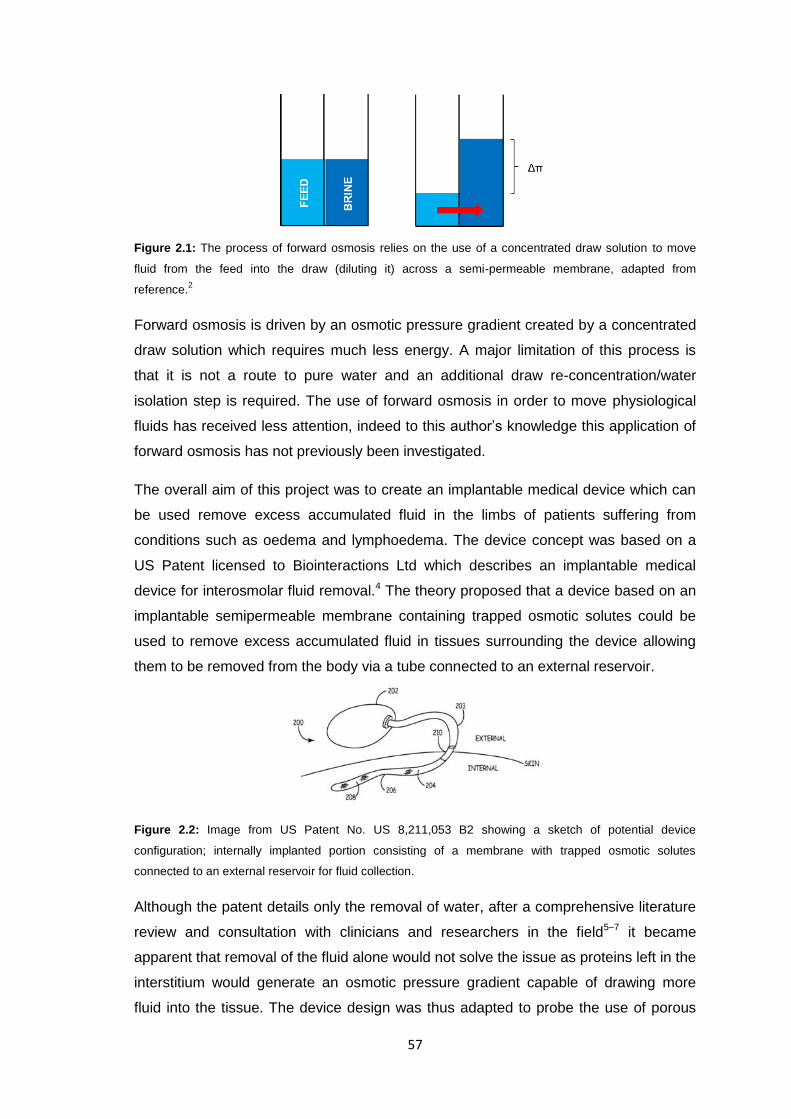
57
Figure 2.1: The process of forward osmosis relies on the use of a concentrated draw solution to move
fluid from the feed into the draw (diluting it) across a semi-permeable membrane, adapted from
reference.2
Forward osmosis is driven by an osmotic pressure gradient created by a concentrated
draw solution which requires much less energy. A major limitation of this process is
that it is not a route to pure water and an additional draw re-concentration/water
isolation step is required. The use of forward osmosis in order to move physiological
fluids has received less attention, indeed to this author’s knowledge this application of
forward osmosis has not previously been investigated.
The overall aim of this project was to create an implantable medical device which can
be used remove excess accumulated fluid in the limbs of patients suffering from
conditions such as oedema and lymphoedema. The device concept was based on a
US Patent licensed to Biointeractions Ltd which describes an implantable medical
device for interosmolar fluid removal.4 The theory proposed that a device based on an
implantable semipermeable membrane containing trapped osmotic solutes could be
used to remove excess accumulated fluid in tissues surrounding the device allowing
them to be removed from the body via a tube connected to an external reservoir.
Figure 2.2: Image from US Patent No. US 8,211,053 B2 showing a sketch of potential device
configuration; internally implanted portion consisting of a membrane with trapped osmotic solutes
connected to an external reservoir for fluid collection.
Although the patent details only the removal of water, after a comprehensive literature
review and consultation with clinicians and researchers in the field5–7 it became
apparent that removal of the fluid alone would not solve the issue as proteins left in the
interstitium would generate an osmotic pressure gradient capable of drawing more
fluid into the tissue. The device design was thus adapted to probe the use of porous
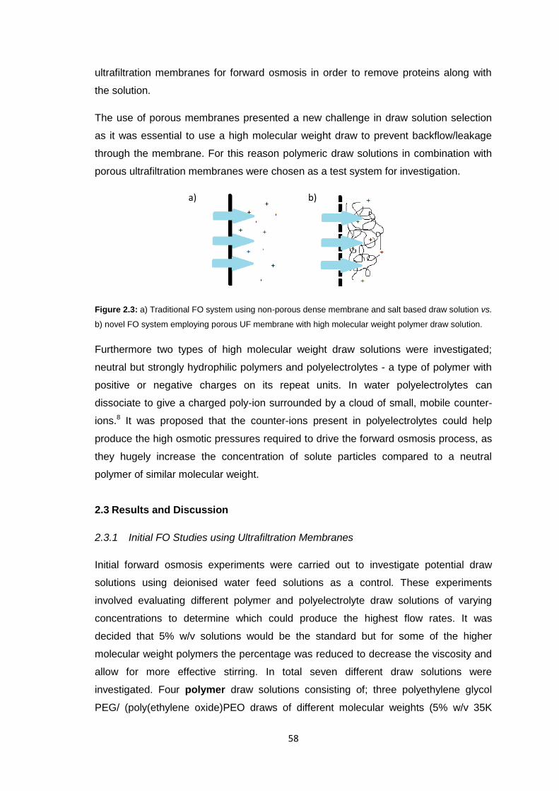
58
ultrafiltration membranes for forward osmosis in order to remove proteins along with
the solution.
The use of porous membranes presented a new challenge in draw solution selection
as it was essential to use a high molecular weight draw to prevent backflow/leakage
through the membrane. For this reason polymeric draw solutions in combination with
porous ultrafiltration membranes were chosen as a test system for investigation.
Figure 2.3: a) Traditional FO system using non-porous dense membrane and salt based draw solution vs.
b) novel FO system employing porous UF membrane with high molecular weight polymer draw solution.
Furthermore two types of high molecular weight draw solutions were investigated;
neutral but strongly hydrophilic polymers and polyelectrolytes - a type of polymer with
positive or negative charges on its repeat units. In water polyelectrolytes can
dissociate to give a charged poly-ion surrounded by a cloud of small, mobile counter-
ions.8 It was proposed that the counter-ions present in polyelectrolytes could help
produce the high osmotic pressures required to drive the forward osmosis process, as
they hugely increase the concentration of solute particles compared to a neutral
polymer of similar molecular weight.
2.3 Results and Discussion
2.3.1 Initial FO Studies using Ultrafiltration Membranes
Initial forward osmosis experiments were carried out to investigate potential draw
solutions using deionised water feed solutions as a control. These experiments
involved evaluating different polymer and polyelectrolyte draw solutions of varying
concentrations to determine which could produce the highest flow rates. It was
decided that 5% w/v solutions would be the standard but for some of the higher
molecular weight polymers the percentage was reduced to decrease the viscosity and
allow for more effective stirring. In total seven different draw solutions were
investigated. Four polymer draw solutions consisting of; three polyethylene glycol
PEG/ (poly(ethylene oxide)PEO draws of different molecular weights (5% w/v 35K
a) b)
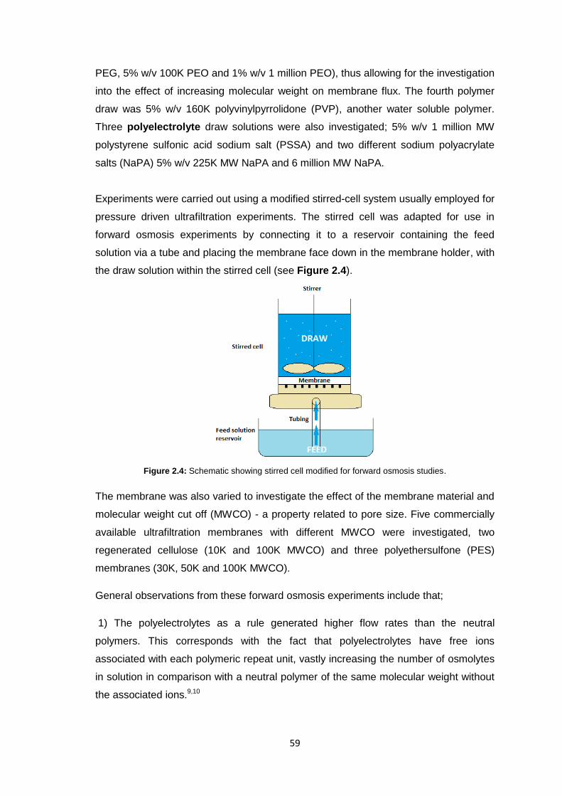
59
PEG, 5% w/v 100K PEO and 1% w/v 1 million PEO), thus allowing for the investigation
into the effect of increasing molecular weight on membrane flux. The fourth polymer
draw was 5% w/v 160K polyvinylpyrrolidone (PVP), another water soluble polymer.
Three polyelectrolyte draw solutions were also investigated; 5% w/v 1 million MW
polystyrene sulfonic acid sodium salt (PSSA) and two different sodium polyacrylate
salts (NaPA) 5% w/v 225K MW NaPA and 6 million MW NaPA.
Experiments were carried out using a modified stirred-cell system usually employed for
pressure driven ultrafiltration experiments. The stirred cell was adapted for use in
forward osmosis experiments by connecting it to a reservoir containing the feed
solution via a tube and placing the membrane face down in the membrane holder, with
the draw solution within the stirred cell (see Figure 2.4).
Figure 2.4: Schematic showing stirred cell modified for forward osmosis studies.
The membrane was also varied to investigate the effect of the membrane material and
molecular weight cut off (MWCO) - a property related to pore size. Five commercially
available ultrafiltration membranes with different MWCO were investigated, two
regenerated cellulose (10K and 100K MWCO) and three polyethersulfone (PES)
membranes (30K, 50K and 100K MWCO).
General observations from these forward osmosis experiments include that;
1) The polyelectrolytes as a rule generated higher flow rates than the neutral
polymers. This corresponds with the fact that polyelectrolytes have free ions
associated with each polymeric repeat unit, vastly increasing the number of osmolytes
in solution in comparison with a neutral polymer of the same molecular weight without
the associated ions.9,10
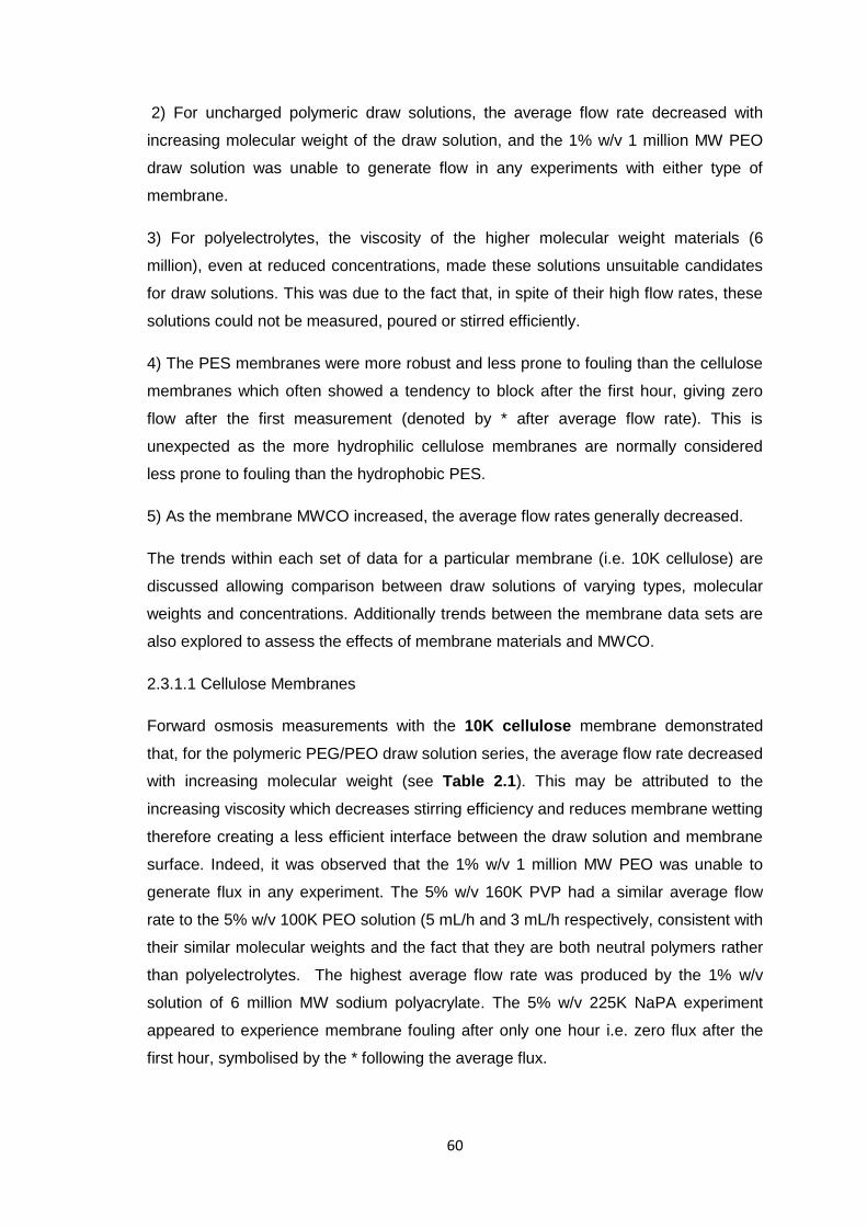
60
2) For uncharged polymeric draw solutions, the average flow rate decreased with
increasing molecular weight of the draw solution, and the 1% w/v 1 million MW PEO
draw solution was unable to generate flow in any experiments with either type of
membrane.
3) For polyelectrolytes, the viscosity of the higher molecular weight materials (6
million), even at reduced concentrations, made these solutions unsuitable candidates
for draw solutions. This was due to the fact that, in spite of their high flow rates, these
solutions could not be measured, poured or stirred efficiently.
4) The PES membranes were more robust and less prone to fouling than the cellulose
membranes which often showed a tendency to block after the first hour, giving zero
flow after the first measurement (denoted by * after average flow rate). This is
unexpected as the more hydrophilic cellulose membranes are normally considered
less prone to fouling than the hydrophobic PES.
5) As the membrane MWCO increased, the average flow rates generally decreased.
The trends within each set of data for a particular membrane (i.e. 10K cellulose) are
discussed allowing comparison between draw solutions of varying types, molecular
weights and concentrations. Additionally trends between the membrane data sets are
also explored to assess the effects of membrane materials and MWCO.
2.3.1.1 Cellulose Membranes
Forward osmosis measurements with the 10K cellulose membrane demonstrated
that, for the polymeric PEG/PEO draw solution series, the average flow rate decreased
with increasing molecular weight (see Table 2.1). This may be attributed to the
increasing viscosity which decreases stirring efficiency and reduces membrane wetting
therefore creating a less efficient interface between the draw solution and membrane
surface. Indeed, it was observed that the 1% w/v 1 million MW PEO was unable to
generate flux in any experiment. The 5% w/v 160K PVP had a similar average flow
rate to the 5% w/v 100K PEO solution (5 mL/h and 3 mL/h respectively, consistent with
their similar molecular weights and the fact that they are both neutral polymers rather
than polyelectrolytes. The highest average flow rate was produced by the 1% w/v
solution of 6 million MW sodium polyacrylate. The 5% w/v 225K NaPA experiment
appeared to experience membrane fouling after only one hour i.e. zero flux after the
first hour, symbolised by the * following the average flux.
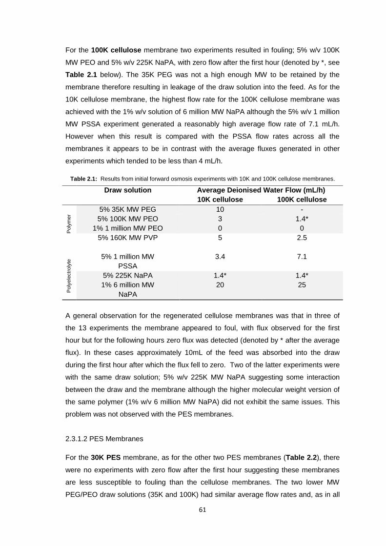
61
For the 100K cellulose membrane two experiments resulted in fouling; 5% w/v 100K
MW PEO and 5% w/v 225K NaPA, with zero flow after the first hour (denoted by *, see
Table 2.1 below). The 35K PEG was not a high enough MW to be retained by the
membrane therefore resulting in leakage of the draw solution into the feed. As for the
10K cellulose membrane, the highest flow rate for the 100K cellulose membrane was
achieved with the 1% w/v solution of 6 million MW NaPA although the 5% w/v 1 million
MW PSSA experiment generated a reasonably high average flow rate of 7.1 mL/h.
However when this result is compared with the PSSA flow rates across all the
membranes it appears to be in contrast with the average fluxes generated in other
experiments which tended to be less than 4 mL/h.
Table 2.1: Results from initial forward osmosis experiments with 10K and 100K cellulose membranes.
Draw solution Average Deionised Water Flow (mL/h)
10K cellulose 100K cellulose
Poly
me
r
5% 35K MW PEG 10 -
5% 100K MW PEO 3 1.4*
1% 1 million MW PEO 0 0
5% 160K MW PVP 5 2.5
Poly
ele
ctr
oly
te 5% 1 million MW
PSSA
3.4 7.1
5% 225K NaPA 1.4* 1.4*
1% 6 million MW
NaPA
20 25
A general observation for the regenerated cellulose membranes was that in three of
the 13 experiments the membrane appeared to foul, with flux observed for the first
hour but for the following hours zero flux was detected (denoted by * after the average
flux). In these cases approximately 10mL of the feed was absorbed into the draw
during the first hour after which the flux fell to zero. Two of the latter experiments were
with the same draw solution; 5% w/v 225K MW NaPA suggesting some interaction
between the draw and the membrane although the higher molecular weight version of
the same polymer (1% w/v 6 million MW NaPA) did not exhibit the same issues. This
problem was not observed with the PES membranes.
2.3.1.2 PES Membranes
For the 30K PES membrane, as for the other two PES membranes (Table 2.2), there
were no experiments with zero flow after the first hour suggesting these membranes
are less susceptible to fouling than the cellulose membranes. The two lower MW
PEG/PEO draw solutions (35K and 100K) had similar average flow rates and, as in all

62
experiments, the 1 million MW PEO had zero flow. The 5% w/v 225K NaPA generated
an average flow rate of 24mL/h, comparable to the 30mL/h flux generated by the much
more viscous and less practical 1% w/v 6 million MW NaPA. Following which, for the
subsequent experiments, it was decided that as the 6 million MW NaPA was not
practical to use and as the 225K NaPA could conceivably generate a similar result, the
6 million MW draw solution could be omitted from further PES studies.
The 50K PES membrane when used in conjunction with the lower MW PEG/PEO draw
solutions gave similar average flow rates to the 30K PES membrane whilst the
1 million MW PEO again gave zero flow. The 5% w/v 225K NaPA again resulted in a
high average flow rate of 26 mL/h, far surpassing the flow rates generated by the other
draw solutions in this data set. As discussed previously this is attributed to the high
osmotic pressure generated by polyelectrolytes, as a result of the associated counter-
ions, relative to neutral polymers.
For the 100K PES membrane the average flow rate generated by the 5% w/v 225K
NaPA was lower than with the lower MWCO PES membranes (30K and 50K MWCO),
but this was in agreement with an observed general trend of average flow rate
decreasing with increasing membrane MWCO, as discussed in Section 2.3.2 and it
was still the highest flow rate for this data set. As with the other membrane data sets,
the 35K PEG and 100K PEO gave similar flow rates.
Table 2.2: Results from initial forward osmosis experiments with 30K, 50K and 100K PES membrane.
Draw solution Average Deionised Water Flow (mL/h)
30K PES 50K PES 100K PES
Poly
me
r
5% 35K PEG 2.3 3.7 3.6
5% 100K PEO 2.4 5 3
1% 1 million MW
PEO
0 0 0
5% 160K MW PVP 5 3.6 2.3
Poly
ele
ctr
oly
te 5% 1 million MW
PSSA
4 2.6 2.3
5% 225K MW NaPA 24 26 10.4
1% 6 million MW
NaPA
30 - -
As mentioned previously none of the PES experiments demonstrated fouling
behaviour that resulted in the discontinuation of flux.
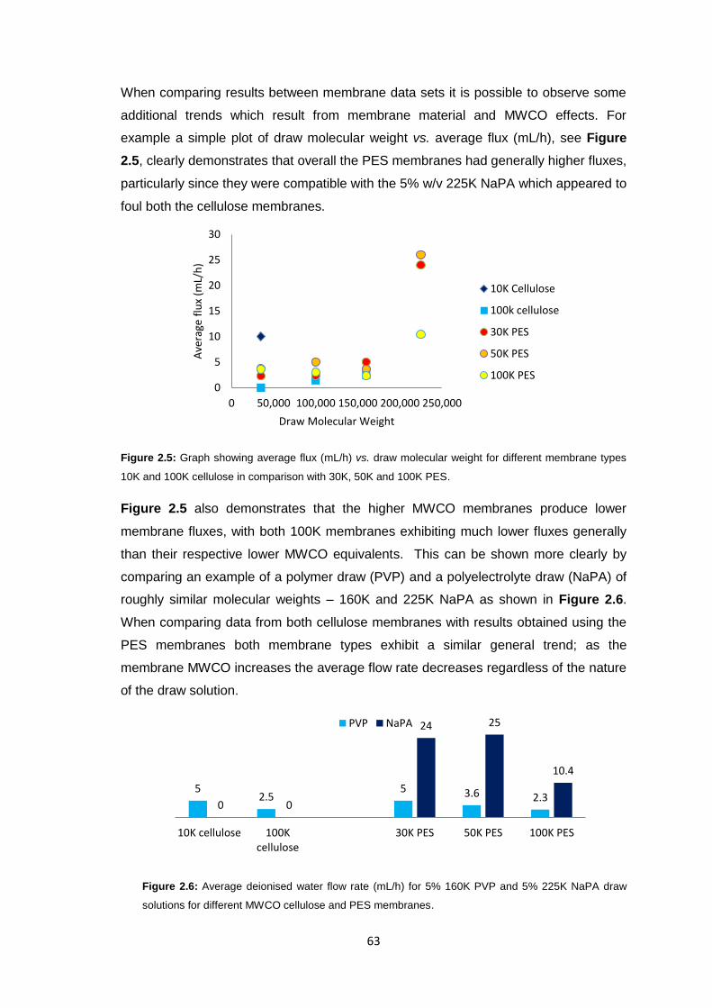
63
When comparing results between membrane data sets it is possible to observe some
additional trends which result from membrane material and MWCO effects. For
example a simple plot of draw molecular weight vs. average flux (mL/h), see Figure
2.5, clearly demonstrates that overall the PES membranes had generally higher fluxes,
particularly since they were compatible with the 5% w/v 225K NaPA which appeared to
foul both the cellulose membranes.
Figure 2.5: Graph showing average flux (mL/h) vs. draw molecular weight for different membrane types
10K and 100K cellulose in comparison with 30K, 50K and 100K PES.
Figure 2.5 also demonstrates that the higher MWCO membranes produce lower
membrane fluxes, with both 100K membranes exhibiting much lower fluxes generally
than their respective lower MWCO equivalents. This can be shown more clearly by
comparing an example of a polymer draw (PVP) and a polyelectrolyte draw (NaPA) of
roughly similar molecular weights – 160K and 225K NaPA as shown in Figure 2.6.
When comparing data from both cellulose membranes with results obtained using the
PES membranes both membrane types exhibit a similar general trend; as the
membrane MWCO increases the average flow rate decreases regardless of the nature
of the draw solution.
Figure 2.6: Average deionised water flow rate (mL/h) for 5% 160K PVP and 5% 225K NaPA draw
solutions for different MWCO cellulose and PES membranes.
0
5
10
15
20
25
30
0 50,000 100,000 150,000 200,000 250,000
Ave
rage
flu
x (m
L/h
)
Draw Molecular Weight
10K Cellulose
100k cellulose
30K PES
50K PES
100K PES
5 2.5
5 3.6 2.3 0 0
24 25
10.4
10K cellulose 100Kcellulose
30K PES 50K PES 100K PES
PVP NaPA
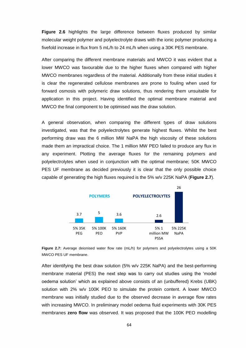
64
Figure 2.6 highlights the large difference between fluxes produced by similar
molecular weight polymer and polyelectrolyte draws with the ionic polymer producing a
fivefold increase in flux from 5 mL/h to 24 mL/h when using a 30K PES membrane.
After comparing the different membrane materials and MWCO it was evident that a
lower MWCO was favourable due to the higher fluxes when compared with higher
MWCO membranes regardless of the material. Additionally from these initial studies it
is clear the regenerated cellulose membranes are prone to fouling when used for
forward osmosis with polymeric draw solutions, thus rendering them unsuitable for
application in this project. Having identified the optimal membrane material and
MWCO the final component to be optimised was the draw solution.
A general observation, when comparing the different types of draw solutions
investigated, was that the polyelectrolytes generate highest fluxes. Whilst the best
performing draw was the 6 million MW NaPA the high viscosity of these solutions
made them an impractical choice. The 1 million MW PEO failed to produce any flux in
any experiment. Plotting the average fluxes for the remaining polymers and
polyelectrolytes when used in conjunction with the optimal membrane; 50K MWCO
PES UF membrane as decided previously it is clear that the only possible choice
capable of generating the high fluxes required is the 5% w/v 225K NaPA (Figure 2.7).
Figure 2.7: Average deionised water flow rate (mL/h) for polymers and polyelectrolytes using a 50K
MWCO PES UF membrane.
After identifying the best draw solution (5% w/v 225K NaPA) and the best-performing
membrane material (PES) the next step was to carry out studies using the ‘model
oedema solution’ which as explained above consists of an (unbuffered) Krebs (UBK)
solution with 2% w/v 100K PEO to simulate the protein content. A lower MWCO
membrane was initially studied due to the observed decrease in average flow rates
with increasing MWCO. In preliminary model oedema fluid experiments with 30K PES
membranes zero flow was observed. It was proposed that the 100K PEO modelling
3.7 5 3.6 2.6
26
5% 35KPEG
5% 100KPEO
5% 160KPVP
5% 1million MW
PSSA
5% 225KNaPA
POLYMERS POLYELECTROLYTES
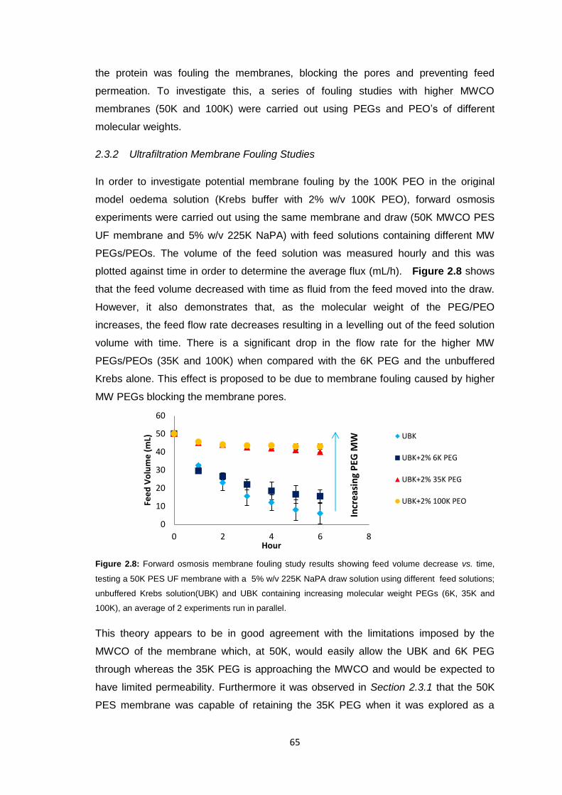
65
the protein was fouling the membranes, blocking the pores and preventing feed
permeation. To investigate this, a series of fouling studies with higher MWCO
membranes (50K and 100K) were carried out using PEGs and PEO’s of different
molecular weights.
2.3.2 Ultrafiltration Membrane Fouling Studies
In order to investigate potential membrane fouling by the 100K PEO in the original
model oedema solution (Krebs buffer with 2% w/v 100K PEO), forward osmosis
experiments were carried out using the same membrane and draw (50K MWCO PES
UF membrane and 5% w/v 225K NaPA) with feed solutions containing different MW
PEGs/PEOs. The volume of the feed solution was measured hourly and this was
plotted against time in order to determine the average flux (mL/h). Figure 2.8 shows
that the feed volume decreased with time as fluid from the feed moved into the draw.
However, it also demonstrates that, as the molecular weight of the PEG/PEO
increases, the feed flow rate decreases resulting in a levelling out of the feed solution
volume with time. There is a significant drop in the flow rate for the higher MW
PEGs/PEOs (35K and 100K) when compared with the 6K PEG and the unbuffered
Krebs alone. This effect is proposed to be due to membrane fouling caused by higher
MW PEGs blocking the membrane pores.
Figure 2.8: Forward osmosis membrane fouling study results showing feed volume decrease vs. time,
testing a 50K PES UF membrane with a 5% w/v 225K NaPA draw solution using different feed solutions;
unbuffered Krebs solution(UBK) and UBK containing increasing molecular weight PEGs (6K, 35K and
100K), an average of 2 experiments run in parallel.
This theory appears to be in good agreement with the limitations imposed by the
MWCO of the membrane which, at 50K, would easily allow the UBK and 6K PEG
through whereas the 35K PEG is approaching the MWCO and would be expected to
have limited permeability. Furthermore it was observed in Section 2.3.1 that the 50K
PES membrane was capable of retaining the 35K PEG when it was explored as a
0
10
20
30
40
50
60
0 2 4 6 8
Fee
d V
olu
me
(m
L)
Hour
UBK
UBK+2% 6K PEG
UBK+2% 35K PEG
UBK+2% 100K PEO
Incr
easi
ng
PEG
MW
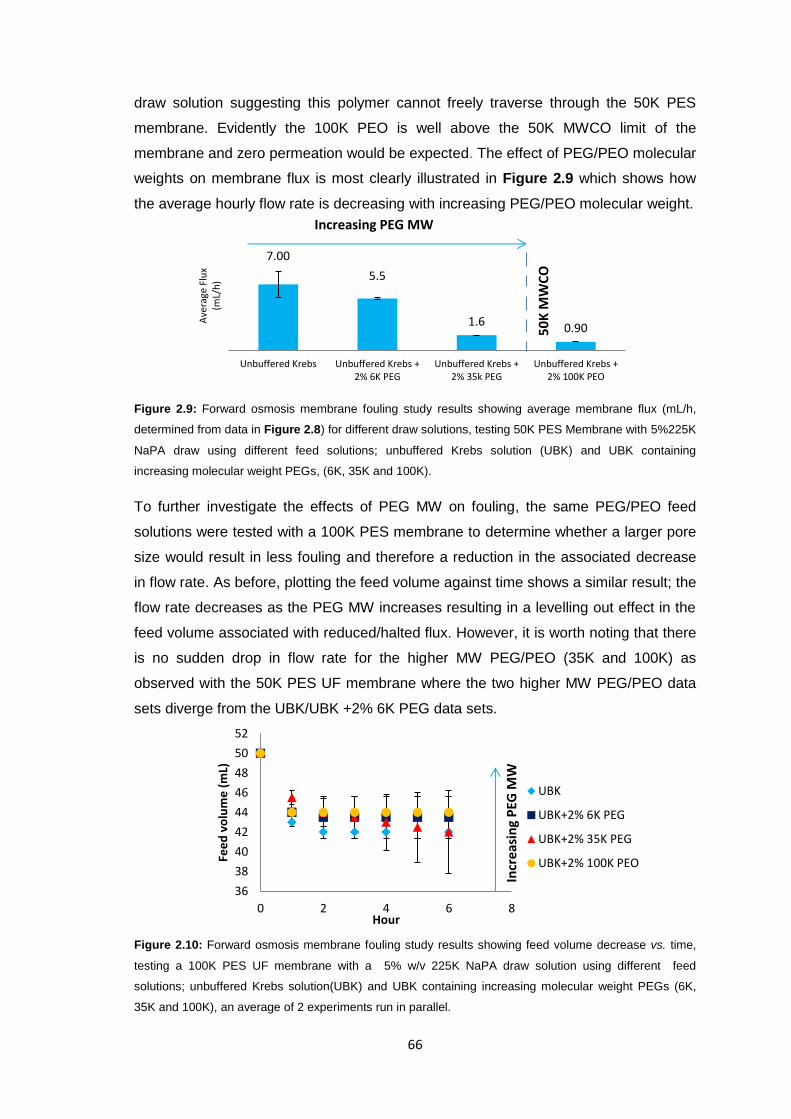
66
draw solution suggesting this polymer cannot freely traverse through the 50K PES
membrane. Evidently the 100K PEO is well above the 50K MWCO limit of the
membrane and zero permeation would be expected. The effect of PEG/PEO molecular
weights on membrane flux is most clearly illustrated in Figure 2.9 which shows how
the average hourly flow rate is decreasing with increasing PEG/PEO molecular weight.
Figure 2.9: Forward osmosis membrane fouling study results showing average membrane flux (mL/h,
determined from data in Figure 2.8) for different draw solutions, testing 50K PES Membrane with 5%225K
NaPA draw using different feed solutions; unbuffered Krebs solution (UBK) and UBK containing
increasing molecular weight PEGs, (6K, 35K and 100K).
To further investigate the effects of PEG MW on fouling, the same PEG/PEO feed
solutions were tested with a 100K PES membrane to determine whether a larger pore
size would result in less fouling and therefore a reduction in the associated decrease
in flow rate. As before, plotting the feed volume against time shows a similar result; the
flow rate decreases as the PEG MW increases resulting in a levelling out effect in the
feed volume associated with reduced/halted flux. However, it is worth noting that there
is no sudden drop in flow rate for the higher MW PEG/PEO (35K and 100K) as
observed with the 50K PES UF membrane where the two higher MW PEG/PEO data
sets diverge from the UBK/UBK +2% 6K PEG data sets.
Figure 2.10: Forward osmosis membrane fouling study results showing feed volume decrease vs. time,
testing a 100K PES UF membrane with a 5% w/v 225K NaPA draw solution using different feed
solutions; unbuffered Krebs solution(UBK) and UBK containing increasing molecular weight PEGs (6K,
35K and 100K), an average of 2 experiments run in parallel.
7.00
5.5
1.6 0.90
Unbuffered Krebs Unbuffered Krebs +2% 6K PEG
Unbuffered Krebs +2% 35k PEG
Unbuffered Krebs +2% 100K PEO
36
38
40
42
44
46
48
50
52
0 2 4 6 8
Fee
d v
olu
me
(m
L)
Hour
UBK
UBK+2% 6K PEG
UBK+2% 35K PEG
UBK+2% 100K PEO
Ave
rage
Flu
x (m
L/h
) Increasing PEG MW
50
K M
WC
O
Incr
easi
ng
PEG
MW
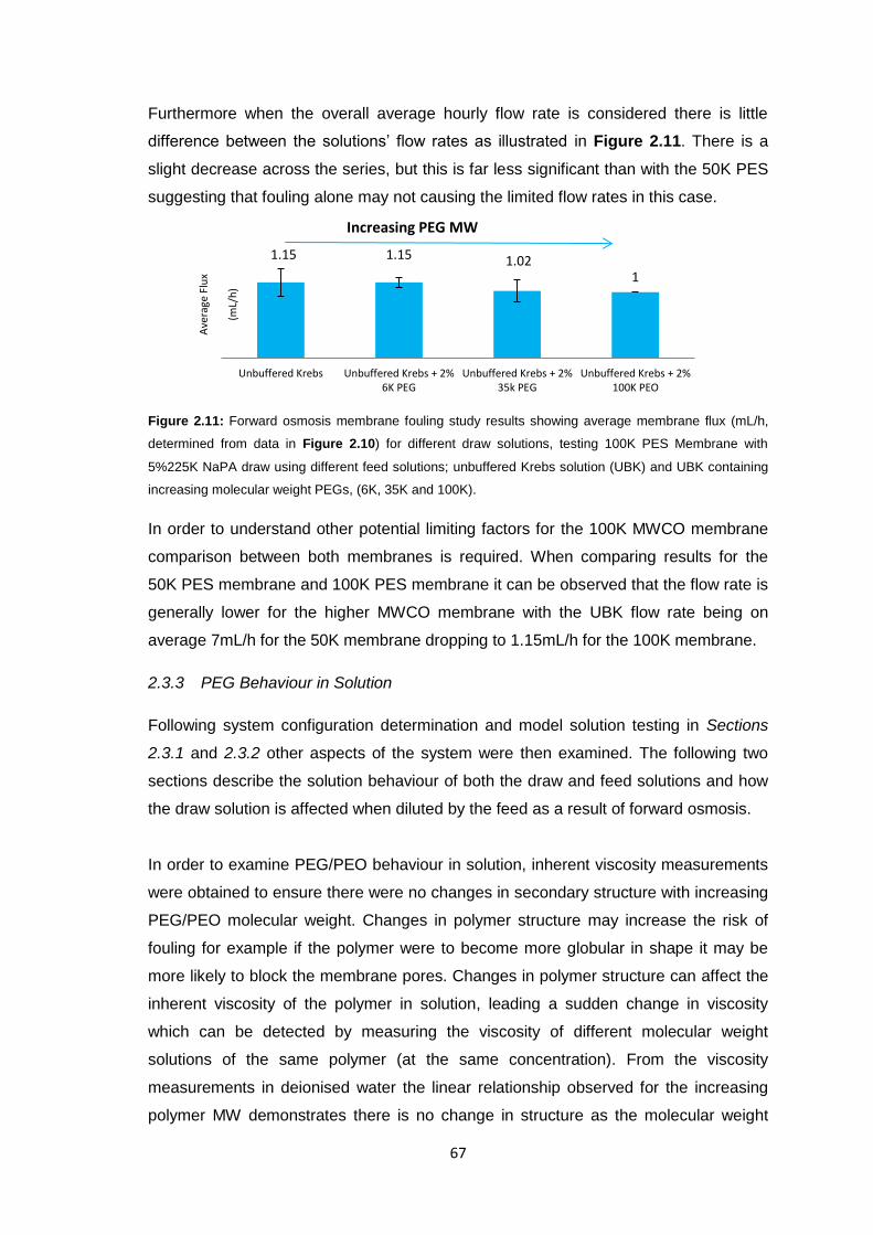
67
Furthermore when the overall average hourly flow rate is considered there is little
difference between the solutions’ flow rates as illustrated in Figure 2.11. There is a
slight decrease across the series, but this is far less significant than with the 50K PES
suggesting that fouling alone may not causing the limited flow rates in this case.
Figure 2.11: Forward osmosis membrane fouling study results showing average membrane flux (mL/h,
determined from data in Figure 2.10) for different draw solutions, testing 100K PES Membrane with
5%225K NaPA draw using different feed solutions; unbuffered Krebs solution (UBK) and UBK containing
increasing molecular weight PEGs, (6K, 35K and 100K).
In order to understand other potential limiting factors for the 100K MWCO membrane
comparison between both membranes is required. When comparing results for the
50K PES membrane and 100K PES membrane it can be observed that the flow rate is
generally lower for the higher MWCO membrane with the UBK flow rate being on
average 7mL/h for the 50K membrane dropping to 1.15mL/h for the 100K membrane.
2.3.3 PEG Behaviour in Solution
Following system configuration determination and model solution testing in Sections
2.3.1 and 2.3.2 other aspects of the system were then examined. The following two
sections describe the solution behaviour of both the draw and feed solutions and how
the draw solution is affected when diluted by the feed as a result of forward osmosis.
In order to examine PEG/PEO behaviour in solution, inherent viscosity measurements
were obtained to ensure there were no changes in secondary structure with increasing
PEG/PEO molecular weight. Changes in polymer structure may increase the risk of
fouling for example if the polymer were to become more globular in shape it may be
more likely to block the membrane pores. Changes in polymer structure can affect the
inherent viscosity of the polymer in solution, leading a sudden change in viscosity
which can be detected by measuring the viscosity of different molecular weight
solutions of the same polymer (at the same concentration). From the viscosity
measurements in deionised water the linear relationship observed for the increasing
polymer MW demonstrates there is no change in structure as the molecular weight
1.15 1.15 1.02 1
Unbuffered Krebs Unbuffered Krebs + 2%6K PEG
Unbuffered Krebs + 2%35k PEG
Unbuffered Krebs + 2%100K PEO
Ave
rage
Flu
x
(mL/
h)
Increasing PEG MW
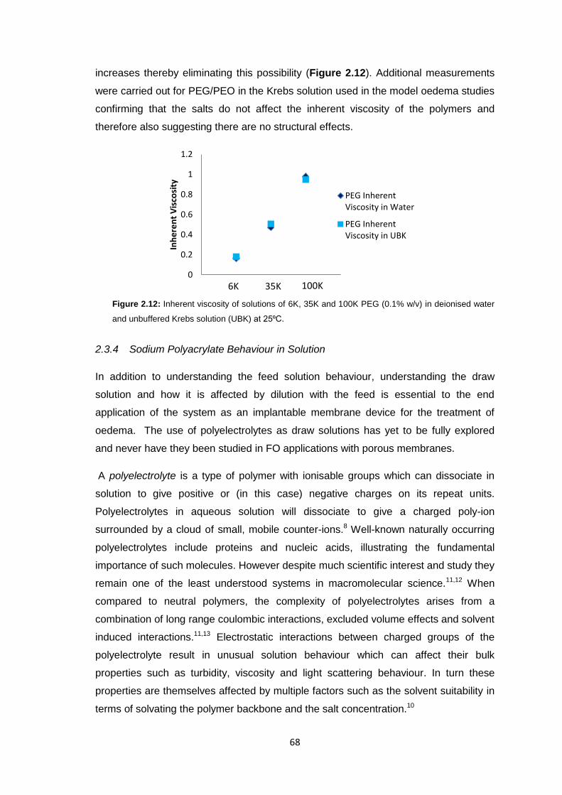
68
increases thereby eliminating this possibility (Figure 2.12). Additional measurements
were carried out for PEG/PEO in the Krebs solution used in the model oedema studies
confirming that the salts do not affect the inherent viscosity of the polymers and
therefore also suggesting there are no structural effects.
Figure 2.12: Inherent viscosity of solutions of 6K, 35K and 100K PEG (0.1% w/v) in deionised water
and unbuffered Krebs solution (UBK) at 25⁰C.
2.3.4 Sodium Polyacrylate Behaviour in Solution
In addition to understanding the feed solution behaviour, understanding the draw
solution and how it is affected by dilution with the feed is essential to the end
application of the system as an implantable membrane device for the treatment of
oedema. The use of polyelectrolytes as draw solutions has yet to be fully explored
and never have they been studied in FO applications with porous membranes.
A polyelectrolyte is a type of polymer with ionisable groups which can dissociate in
solution to give positive or (in this case) negative charges on its repeat units.
Polyelectrolytes in aqueous solution will dissociate to give a charged poly-ion
surrounded by a cloud of small, mobile counter-ions.8 Well-known naturally occurring
polyelectrolytes include proteins and nucleic acids, illustrating the fundamental
importance of such molecules. However despite much scientific interest and study they
remain one of the least understood systems in macromolecular science.11,12 When
compared to neutral polymers, the complexity of polyelectrolytes arises from a
combination of long range coulombic interactions, excluded volume effects and solvent
induced interactions.11,13 Electrostatic interactions between charged groups of the
polyelectrolyte result in unusual solution behaviour which can affect their bulk
properties such as turbidity, viscosity and light scattering behaviour. In turn these
properties are themselves affected by multiple factors such as the solvent suitability in
terms of solvating the polymer backbone and the salt concentration.10
0
0.2
0.4
0.6
0.8
1
1.2
Inh
ere
nt
Vis
cosi
ty
PEG InherentViscosity in Water
PEG InherentViscosity in UBK
6K 35K 100K
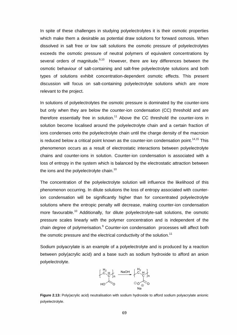
69
In spite of these challenges in studying polyelectrolytes it is their osmotic properties
which make them a desirable as potential draw solutions for forward osmosis. When
dissolved in salt free or low salt solutions the osmotic pressure of polyelectrolytes
exceeds the osmotic pressure of neutral polymers of equivalent concentrations by
several orders of magnitude.9,10 However, there are key differences between the
osmotic behaviour of salt-containing and salt-free polyelectrolyte solutions and both
types of solutions exhibit concentration-dependent osmotic effects. This present
discussion will focus on salt-containing polyelectrolyte solutions which are more
relevant to the project.
In solutions of polyelectrolytes the osmotic pressure is dominated by the counter-ions
but only when they are below the counter-ion condensation (CC) threshold and are
therefore essentially free in solution.11 Above the CC threshold the counter-ions in
solution become localised around the polyelectrolyte chain and a certain fraction of
ions condenses onto the polyelectrolyte chain until the charge density of the macroion
is reduced below a critical point known as the counter-ion condensation point.14,15 This
phenomenon occurs as a result of electrostatic interactions between polyelectrolyte
chains and counter-ions in solution. Counter-ion condensation is associated with a
loss of entropy in the system which is balanced by the electrostatic attraction between
the ions and the polyelectrolyte chain.10
The concentration of the polyelectrolyte solution will influence the likelihood of this
phenomenon occurring. In dilute solutions the loss of entropy associated with counter-
ion condensation will be significantly higher than for concentrated polyelectrolyte
solutions where the entropic penalty will decrease, making counter-ion condensation
more favourable.10 Additionally, for dilute polyelectrolyte-salt solutions, the osmotic
pressure scales linearly with the polymer concentration and is independent of the
chain degree of polymerisation.9 Counter-ion condensation processes will affect both
the osmotic pressure and the electrical conductivity of the solution.11
Sodium polyacrylate is an example of a polyelectrolyte and is produced by a reaction
between poly(acrylic acid) and a base such as sodium hydroxide to afford an anion
polyelectrolyte.
Figure 2.13: Poly(acrylic acid) neutralisation with sodium hydroxide to afford sodium polyacrylate anionic
polyelectrolyte.
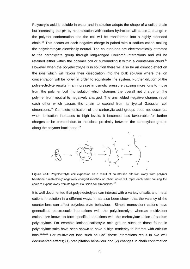
70
Polyacrylic acid is soluble in water and in solution adopts the shape of a coiled chain
but increasing the pH by neutralisation with sodium hydroxide will cause a change in
the polymer conformation and the coil will be transformed into a highly extended
chain.16 This occurs as each negative charge is paired with a sodium cation making
the polyelectrolyte electrically neutral. The counter-ions are electrostatically attracted
to the carboxylate group through long-ranged Coulomb interactions and will be
retained either within the polymer coil or surrounding it within a counter-ion cloud.17
However when the polyelectrolyte is in solution there will also be an osmotic effect on
the ions which will favour their dissociation into the bulk solution where the ion
concentration will be lower in order to equilibrate the system. Further dilution of the
polyelectrolyte results in an increase in osmotic pressure causing more ions to move
from the polymer coil into solution which changes the overall net charge on the
polymer from neutral to negatively charged. The unshielded negative charges repel
each other which causes the chain to expand from its typical Gaussian coil
dimensions.18 Complete ionisation of the carboxylic acid groups does not occur as,
when ionisation increases to high levels, it becomes less favourable for further
charges to be created due to the close proximity between the carboxylate groups
along the polymer back bone.19
Figure 2.14: Polyelectrolyte coil expansion as a result of counter-ion diffusion away from polymer
backbone ‘un-shielding’ negatively charged moieties on chain which will repel each other causing the
chain to expand away from its typical Gaussian coil dimensions.19
It is well documented that polyelectrolytes can interact with a variety of salts and metal
cations in solution in a different ways. It has also been shown that the valency of the
counter-ions can affect polyelectrolyte behaviour. Simple monovalent cations have
generalised electrostatic interactions with the polyelectrolyte whereas multivalent
cations are known to form specific interactions with the carboxylate anion of sodium
polyacrylate. For example ionised carboxylic acid groups such as those found in
polyacrylate salts have been shown to have a high tendency to interact with calcium
ions.16,20,21 For multivalent ions such as Ca2+ these interactions result in two well
documented effects; (1) precipitation behaviour and (2) changes in chain confirmation
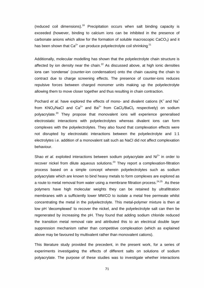
71
(reduced coil dimensions).16 Precipitation occurs when salt binding capacity is
exceeded (however, binding to calcium ions can be inhibited in the presence of
carbonate anions which allow for the formation of soluble macroscopic CaCO3) and it
has been shown that Ca2+ can produce polyelectrolyte coil shrinking.21
Additionally, molecular modelling has shown that the polyelectrolyte chain structure is
affected by ion density near the chain.22 As discussed above, at high ionic densities
ions can ‘condense’ (counter-ion condensation) onto the chain causing the chain to
contract due to charge screening effects. The presence of counter-ions reduces
repulsive forces between charged monomer units making up the polyelectrolyte
allowing them to move closer together and thus resulting in chain contraction.
Pochard et al. have explored the effects of mono- and divalent cations (K+ and Na+
from KNO3/NaCl and Ca2+ and Ba2+ from CaCl2/BaCl2 respectively) on sodium
polyacrylate.20 They propose that monovalent ions will experience generalised
electrostatic interactions with polyelectrolytes whereas divalent ions can form
complexes with the polyelectrolytes. They also found that complexation effects were
not disrupted by electrostatic interactions between the polyelectrolyte and 1:1
electrolytes i.e. addition of a monovalent salt such as NaCl did not affect complexation
behaviour.
Shao et al. exploited interactions between sodium polyacrylate and Ni2+ in order to
recover nickel from dilute aqueous solutions.23 They report a complexation-filtration
process based on a simple concept wherein polyelectrolytes such as sodium
polyacrylate which are known to bind heavy metals to form complexes are explored as
a route to metal removal from water using a membrane filtration process.24,25 As these
polymers have high molecular weights they can be retained by ultrafiltration
membranes with a sufficiently lower MWCO to isolate a metal free permeate whilst
concentrating the metal in the polyelectrolyte. This metal-polymer mixture is then at
low pH ‘decomplexed’ to recover the nickel, and the polyelectrolyte salt can then be
regenerated by increasing the pH. They found that adding sodium chloride reduced
the transition metal removal rate and attributed this to an electrical double layer
suppression mechanism rather than competitive complexation (which as explained
above may be favoured by multivalent rather than monovalent cations).
This literature study provided the precedent, in the present work, for a series of
experiments investigating the effects of different salts on solutions of sodium
polyacrylate. The purpose of these studies was to investigate whether interactions
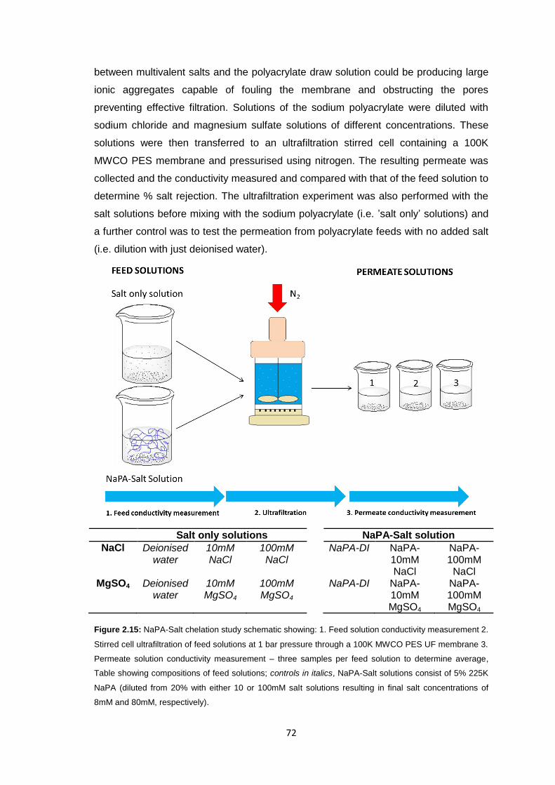
72
between multivalent salts and the polyacrylate draw solution could be producing large
ionic aggregates capable of fouling the membrane and obstructing the pores
preventing effective filtration. Solutions of the sodium polyacrylate were diluted with
sodium chloride and magnesium sulfate solutions of different concentrations. These
solutions were then transferred to an ultrafiltration stirred cell containing a 100K
MWCO PES membrane and pressurised using nitrogen. The resulting permeate was
collected and the conductivity measured and compared with that of the feed solution to
determine % salt rejection. The ultrafiltration experiment was also performed with the
salt solutions before mixing with the sodium polyacrylate (i.e. ’salt only’ solutions) and
a further control was to test the permeation from polyacrylate feeds with no added salt
(i.e. dilution with just deionised water).
Salt only solutions NaPA-Salt solution
NaCl Deionised water
10mM NaCl
100mM NaCl
NaPA-DI NaPA-10mM NaCl
NaPA-100mM NaCl
MgSO4 Deionised water
10mM MgSO4
100mM MgSO4
NaPA-DI NaPA-10mM MgSO4
NaPA-100mM MgSO4
Figure 2.15: NaPA-Salt chelation study schematic showing: 1. Feed solution conductivity measurement 2.
Stirred cell ultrafiltration of feed solutions at 1 bar pressure through a 100K MWCO PES UF membrane 3.
Permeate solution conductivity measurement – three samples per feed solution to determine average,
Table showing compositions of feed solutions; controls in italics, NaPA-Salt solutions consist of 5% 225K
NaPA (diluted from 20% with either 10 or 100mM salt solutions resulting in final salt concentrations of
8mM and 80mM, respectively).
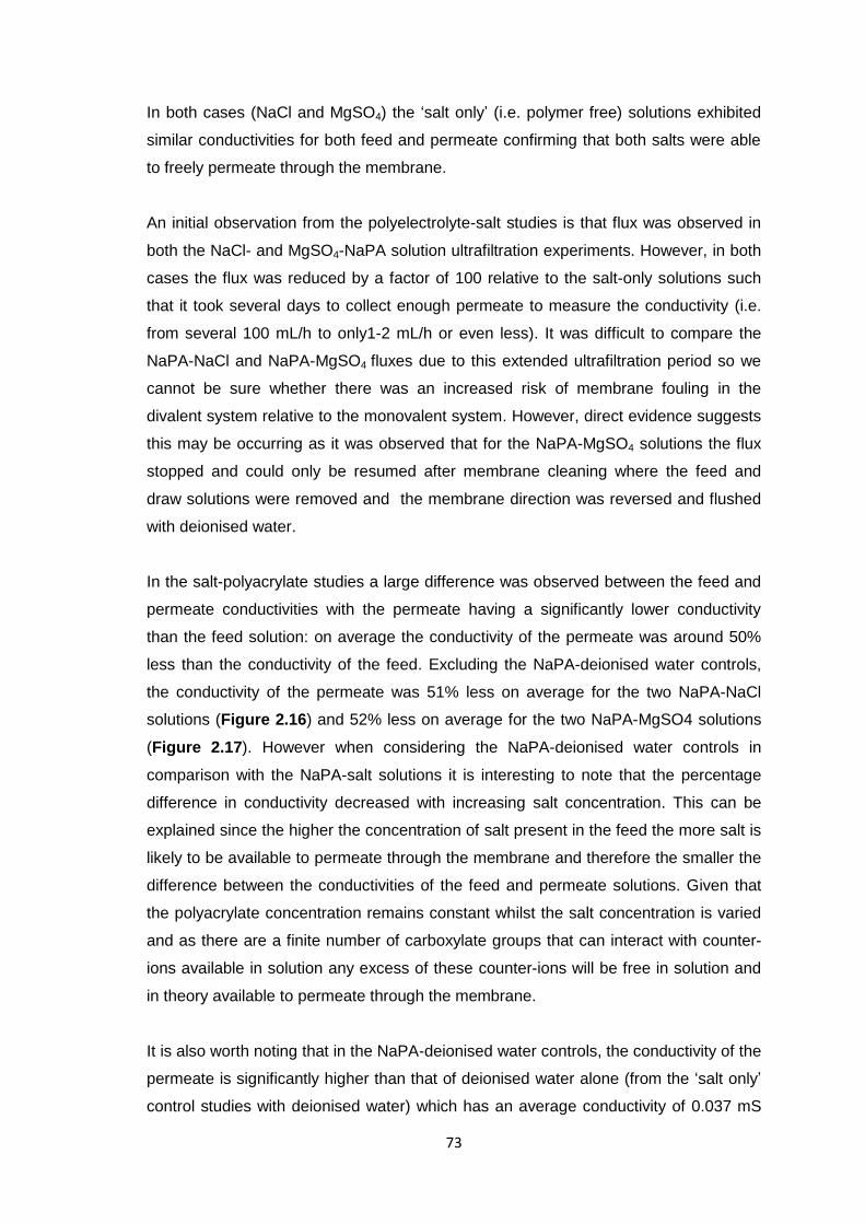
73
In both cases (NaCl and MgSO4) the ‘salt only’ (i.e. polymer free) solutions exhibited
similar conductivities for both feed and permeate confirming that both salts were able
to freely permeate through the membrane.
An initial observation from the polyelectrolyte-salt studies is that flux was observed in
both the NaCl- and MgSO4-NaPA solution ultrafiltration experiments. However, in both
cases the flux was reduced by a factor of 100 relative to the salt-only solutions such
that it took several days to collect enough permeate to measure the conductivity (i.e.
from several 100 mL/h to only1-2 mL/h or even less). It was difficult to compare the
NaPA-NaCl and NaPA-MgSO4 fluxes due to this extended ultrafiltration period so we
cannot be sure whether there was an increased risk of membrane fouling in the
divalent system relative to the monovalent system. However, direct evidence suggests
this may be occurring as it was observed that for the NaPA-MgSO4 solutions the flux
stopped and could only be resumed after membrane cleaning where the feed and
draw solutions were removed and the membrane direction was reversed and flushed
with deionised water.
In the salt-polyacrylate studies a large difference was observed between the feed and
permeate conductivities with the permeate having a significantly lower conductivity
than the feed solution: on average the conductivity of the permeate was around 50%
less than the conductivity of the feed. Excluding the NaPA-deionised water controls,
the conductivity of the permeate was 51% less on average for the two NaPA-NaCl
solutions (Figure 2.16) and 52% less on average for the two NaPA-MgSO4 solutions
(Figure 2.17). However when considering the NaPA-deionised water controls in
comparison with the NaPA-salt solutions it is interesting to note that the percentage
difference in conductivity decreased with increasing salt concentration. This can be
explained since the higher the concentration of salt present in the feed the more salt is
likely to be available to permeate through the membrane and therefore the smaller the
difference between the conductivities of the feed and permeate solutions. Given that
the polyacrylate concentration remains constant whilst the salt concentration is varied
and as there are a finite number of carboxylate groups that can interact with counter-
ions available in solution any excess of these counter-ions will be free in solution and
in theory available to permeate through the membrane.
It is also worth noting that in the NaPA-deionised water controls, the conductivity of the
permeate is significantly higher than that of deionised water alone (from the ‘salt only’
control studies with deionised water) which has an average conductivity of 0.037 mS
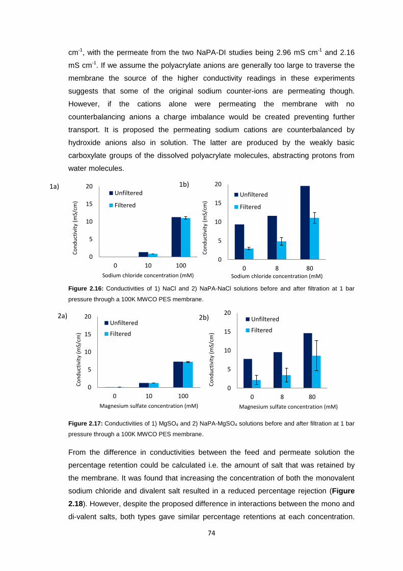
74
cm-1, with the permeate from the two NaPA-DI studies being 2.96 mS cm-1 and 2.16
mS cm-1. If we assume the polyacrylate anions are generally too large to traverse the
membrane the source of the higher conductivity readings in these experiments
suggests that some of the original sodium counter-ions are permeating though.
However, if the cations alone were permeating the membrane with no
counterbalancing anions a charge imbalance would be created preventing further
transport. It is proposed the permeating sodium cations are counterbalanced by
hydroxide anions also in solution. The latter are produced by the weakly basic
carboxylate groups of the dissolved polyacrylate molecules, abstracting protons from
water molecules.
Figure 2.16: Conductivities of 1) NaCl and 2) NaPA-NaCl solutions before and after filtration at 1 bar
pressure through a 100K MWCO PES membrane.
Figure 2.17: Conductivities of 1) MgSO4 and 2) NaPA-MgSO4 solutions before and after filtration at 1 bar
pressure through a 100K MWCO PES membrane.
From the difference in conductivities between the feed and permeate solution the
percentage retention could be calculated i.e. the amount of salt that was retained by
the membrane. It was found that increasing the concentration of both the monovalent
sodium chloride and divalent salt resulted in a reduced percentage rejection (Figure
2.18). However, despite the proposed difference in interactions between the mono and
di-valent salts, both types gave similar percentage retentions at each concentration.
0
5
10
15
20
0 10 100
Sodium chloride concentration (mM)
Unfiltered
Filtered
0
5
10
15
20
0 8 80Sodium chloride concentration (mM)
Unfiltered
Filtered
0
5
10
15
20
0 10 100
Magnesium sulfate concentration (mM)
Unfiltered
Filtered
0
5
10
15
20
0 8 80
Magnesium sulfate concentration (mM)
Unfiltered
Filtered
1a) 1b)
2a) 2b)
Co
nd
uct
ivit
y (m
S/cm
)
Co
nd
uct
ivit
y (m
S/cm
)
Co
nd
uct
ivit
y (m
S/cm
)
Co
nd
uct
ivit
y (m
S/cm
)
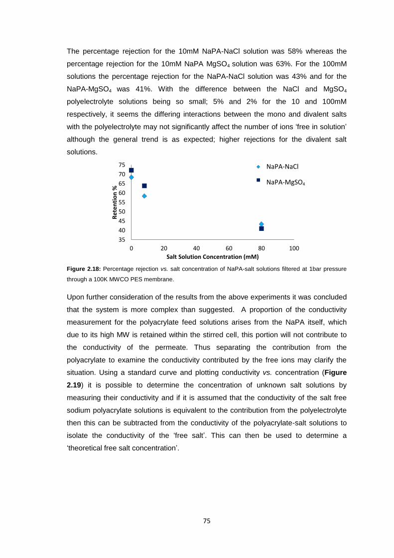
75
The percentage rejection for the 10mM NaPA-NaCl solution was 58% whereas the
percentage rejection for the 10mM NaPA MgSO4 solution was 63%. For the 100mM
solutions the percentage rejection for the NaPA-NaCl solution was 43% and for the
NaPA-MgSO4 was 41%. With the difference between the NaCl and MgSO4
polyelectrolyte solutions being so small; 5% and 2% for the 10 and 100mM
respectively, it seems the differing interactions between the mono and divalent salts
with the polyelectrolyte may not significantly affect the number of ions ‘free in solution’
although the general trend is as expected; higher rejections for the divalent salt
solutions.
Figure 2.18: Percentage rejection vs. salt concentration of NaPA-salt solutions filtered at 1bar pressure
through a 100K MWCO PES membrane.
Upon further consideration of the results from the above experiments it was concluded
that the system is more complex than suggested. A proportion of the conductivity
measurement for the polyacrylate feed solutions arises from the NaPA itself, which
due to its high MW is retained within the stirred cell, this portion will not contribute to
the conductivity of the permeate. Thus separating the contribution from the
polyacrylate to examine the conductivity contributed by the free ions may clarify the
situation. Using a standard curve and plotting conductivity vs. concentration (Figure
2.19) it is possible to determine the concentration of unknown salt solutions by
measuring their conductivity and if it is assumed that the conductivity of the salt free
sodium polyacrylate solutions is equivalent to the contribution from the polyelectrolyte
then this can be subtracted from the conductivity of the polyacrylate-salt solutions to
isolate the conductivity of the ‘free salt’. This can then be used to determine a
‘theoretical free salt concentration’.
35
40
45
50
55
60
65
70
75
0 20 40 60 80 100
Re
ten
tio
n %
Salt Solution Concentration (mM)
NaPA-NaCl
NaPA-MgSO4
NaPA-NaCl
NaPA-MgSO4
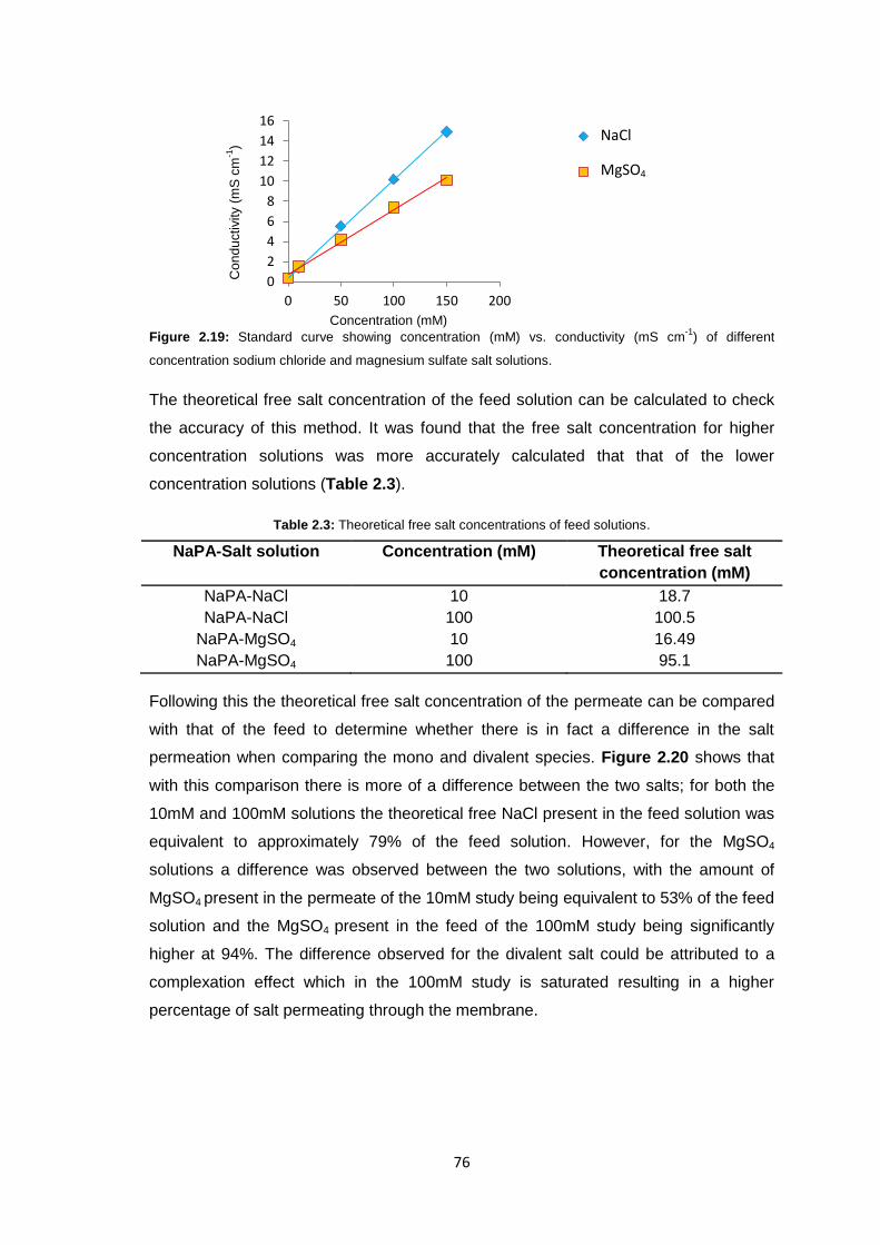
76
Figure 2.19: Standard curve showing concentration (mM) vs. conductivity (mS cm-1
) of different
concentration sodium chloride and magnesium sulfate salt solutions.
The theoretical free salt concentration of the feed solution can be calculated to check
the accuracy of this method. It was found that the free salt concentration for higher
concentration solutions was more accurately calculated that that of the lower
concentration solutions (Table 2.3).
Table 2.3: Theoretical free salt concentrations of feed solutions.
NaPA-Salt solution Concentration (mM) Theoretical free salt
concentration (mM)
NaPA-NaCl 10 18.7
NaPA-NaCl 100 100.5
NaPA-MgSO4 10 16.49
NaPA-MgSO4 100 95.1
Following this the theoretical free salt concentration of the permeate can be compared
with that of the feed to determine whether there is in fact a difference in the salt
permeation when comparing the mono and divalent species. Figure 2.20 shows that
with this comparison there is more of a difference between the two salts; for both the
10mM and 100mM solutions the theoretical free NaCl present in the feed solution was
equivalent to approximately 79% of the feed solution. However, for the MgSO4
solutions a difference was observed between the two solutions, with the amount of
MgSO4 present in the permeate of the 10mM study being equivalent to 53% of the feed
solution and the MgSO4 present in the feed of the 100mM study being significantly
higher at 94%. The difference observed for the divalent salt could be attributed to a
complexation effect which in the 100mM study is saturated resulting in a higher
percentage of salt permeating through the membrane.
0
2
4
6
8
10
12
14
16
0 50 100 150 200
NaCl
MgSO4
NaCl
MgSO4
Concentration (mM)
Co
nd
uctivity (
mS
cm
-1)
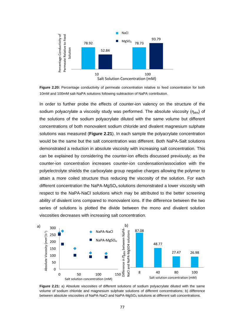
77
Figure 2.20: Percentage conductivity of permeate concentration relative to feed concentration for both
10mM and 100mM salt-NaPA solutions following subtraction of NaPA contribution.
In order to further probe the effects of counter-ion valency on the structure of the
sodium polyacrylate a viscosity study was performed. The absolute viscosity (ηabs) of
the solutions of the sodium polyacrylate diluted with the same volume but different
concentrations of both monovalent sodium chloride and divalent magnesium sulphate
solutions was measured (Figure 2.21). In each sample the polyacrylate concentration
would be the same but the salt concentration was different. Both NaPA-Salt solutions
demonstrated a reduction in absolute viscosity with increasing salt concentration. This
can be explained by considering the counter-ion effects discussed previously; as the
counter-ion concentration increases counter-ion condensation/association with the
polyelectrolyte shields the carboxylate group negative charges allowing the polymer to
attain a more coiled structure thus reducing the viscosity of the solution. For each
different concentration the NaPA-MgSO4 solutions demonstrated a lower viscosity with
respect to the NaPA-NaCl solutions which may be attributed to the better screening
ability of divalent ions compared to monovalent ions. If the difference between the two
series of solutions is plotted the divide between the mono and divalent solution
viscosities decreases with increasing salt concentration.
Figure 2.21: a) Absolute viscosities of different solutions of sodium polyacrylate diluted with the same
volume of sodium chloride and magnesium sulphate solutions of different concentrations; b) difference
between absolute viscosities of NaPA-NaCl and NaPA-MgSO4 solutions at different salt concentrations.
78.92 78.73
52.84
93.79
10 100
NaCl
MgSO4
0
50
100
150
200
250
300
0 50 100 150
Ab
solu
te V
isco
sity
(m
m2 /
s-1)
Salt solution concentration (mM)
NaPA-NaCl
NaPA-MgSO4
87.08
48.77
27.47 26.98
8 40 80 100
Per
cen
tage
Co
nd
uct
ivit
y o
f
Per
mea
te R
elat
ive
to F
eed
Solu
tio
n
Salt Solution Concentration (mM)
Dif
fere
nce
in η
abs b
etw
een
NaP
A-
NaC
l an
d N
aPA
-MgS
O4
so
luti
on
s
Salt solution concentration (mM)
a) b)
NaCl
MgSO4
NaPA-NaCl
NaPA-MgSO4
78
Overall it is clear that the types of salts present in Krebs solution and therefore present
in physiological solutions that would be interacting with the proposed medical device
are capable of interacting with the sodium polyacrylate. The different valencies of the
counter-ions present in such fluids (Table 2.4) may result in different interactions with
the polyacrylate and further work is required to investigate possible effects on
membrane fouling through possible formation of insoluble complexes – which may be
overcome if low MW counter-ions are present i.e. CO32- for Ca2+.21 Polymer uncoiling
effects along with the change in salt concentration produced by an influx of ions will
also affect the osmotic pressure of the system. Furthermore it will be necessary to
probe the interaction between the sodium polyacrylate and the proteins which will be
removed along with the physiological fluid.
Table 2.4: Cations present in Krebs physiological salt solutions
Monovalent Divalent
Na+
K+
Ca2+
Mg2+
2.3.5 Polyacrylate Draw Solution Optimisation
The following studies were carried out to determine whether variations in the
polyacrylate molecular weight, solution concentration and counter-ion could improve
the average forward osmosis flux. The flux is influenced by the osmotic pressure of the
draw solution so modifications to the draw solution that will change the osmotic
pressure properties should have a direct influence on the flux. Osmotic pressure is a
colligative property and therefore is dependent on the concentration of solutes and not
on their identity.
2.3.5.1 Molecular Weight Variation
From the initial studies it was determined that very high molecular weight polyacrylate
solutions (i.e. 6 million MW) despite their high flux generating properties were
unsuitable for use in draw solution applications due to their high viscosity. A lower MW
sodium polyacrylate 225K was found to produce similarly high fluxes without the
limitations imposed by the high viscosity of the higher molecular weight analogues. It
has been stated that the osmotic pressure of polyelectrolytes increases linearly with
the polyelectrolyte concentration whilst being independent of the chain molecular
weight.9,10 However, without directly measuring the osmotic pressure it was evident
that these different MW solutions produced different fluxes. In addition to the standard
225K NaPA draw solution two other MW draw solutions were investigated in FO
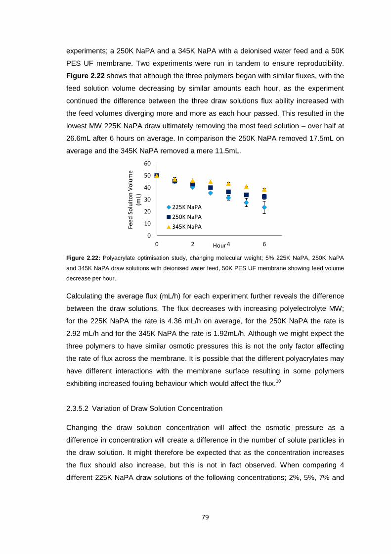
79
experiments; a 250K NaPA and a 345K NaPA with a deionised water feed and a 50K
PES UF membrane. Two experiments were run in tandem to ensure reproducibility.
Figure 2.22 shows that although the three polymers began with similar fluxes, with the
feed solution volume decreasing by similar amounts each hour, as the experiment
continued the difference between the three draw solutions flux ability increased with
the feed volumes diverging more and more as each hour passed. This resulted in the
lowest MW 225K NaPA draw ultimately removing the most feed solution – over half at
26.6mL after 6 hours on average. In comparison the 250K NaPA removed 17.5mL on
average and the 345K NaPA removed a mere 11.5mL.
Figure 2.22: Polyacrylate optimisation study, changing molecular weight; 5% 225K NaPA, 250K NaPA
and 345K NaPA draw solutions with deionised water feed, 50K PES UF membrane showing feed volume
decrease per hour.
Calculating the average flux (mL/h) for each experiment further reveals the difference
between the draw solutions. The flux decreases with increasing polyelectrolyte MW;
for the 225K NaPA the rate is 4.36 mL/h on average, for the 250K NaPA the rate is
2.92 mL/h and for the 345K NaPA the rate is 1.92mL/h. Although we might expect the
three polymers to have similar osmotic pressures this is not the only factor affecting
the rate of flux across the membrane. It is possible that the different polyacrylates may
have different interactions with the membrane surface resulting in some polymers
exhibiting increased fouling behaviour which would affect the flux.10
2.3.5.2 Variation of Draw Solution Concentration
Changing the draw solution concentration will affect the osmotic pressure as a
difference in concentration will create a difference in the number of solute particles in
the draw solution. It might therefore be expected that as the concentration increases
the flux should also increase, but this is not in fact observed. When comparing 4
different 225K NaPA draw solutions of the following concentrations; 2%, 5%, 7% and
0
10
20
30
40
50
60
0 2 4 6
Feed
So
luit
on
Vo
lum
e (m
L)
Hour
225K NaPA
250K NaPA
345K NaPA
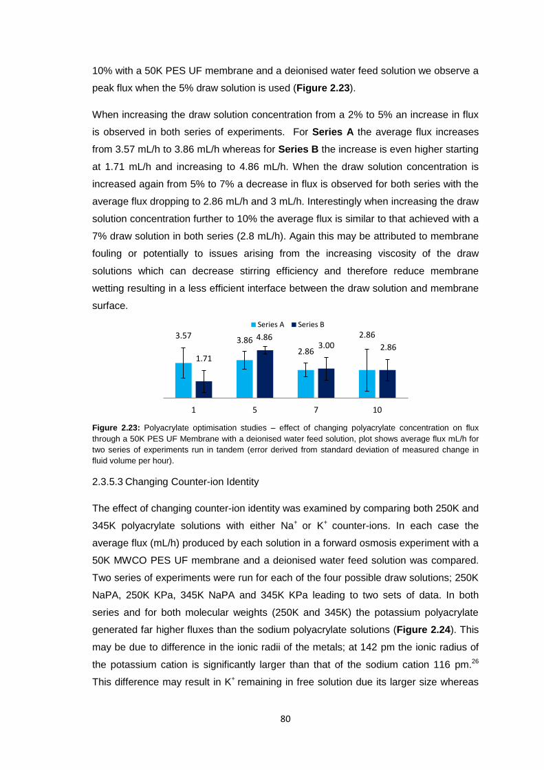
80
10% with a 50K PES UF membrane and a deionised water feed solution we observe a
peak flux when the 5% draw solution is used (Figure 2.23).
When increasing the draw solution concentration from a 2% to 5% an increase in flux
is observed in both series of experiments. For Series A the average flux increases
from 3.57 mL/h to 3.86 mL/h whereas for Series B the increase is even higher starting
at 1.71 mL/h and increasing to 4.86 mL/h. When the draw solution concentration is
increased again from 5% to 7% a decrease in flux is observed for both series with the
average flux dropping to 2.86 mL/h and 3 mL/h. Interestingly when increasing the draw
solution concentration further to 10% the average flux is similar to that achieved with a
7% draw solution in both series (2.8 mL/h). Again this may be attributed to membrane
fouling or potentially to issues arising from the increasing viscosity of the draw
solutions which can decrease stirring efficiency and therefore reduce membrane
wetting resulting in a less efficient interface between the draw solution and membrane
surface.
Figure 2.23: Polyacrylate optimisation studies – effect of changing polyacrylate concentration on flux
through a 50K PES UF Membrane with a deionised water feed solution, plot shows average flux mL/h for
two series of experiments run in tandem (error derived from standard deviation of measured change in
fluid volume per hour).
2.3.5.3 Changing Counter-ion Identity
The effect of changing counter-ion identity was examined by comparing both 250K and
345K polyacrylate solutions with either Na+ or K+ counter-ions. In each case the
average flux (mL/h) produced by each solution in a forward osmosis experiment with a
50K MWCO PES UF membrane and a deionised water feed solution was compared.
Two series of experiments were run for each of the four possible draw solutions; 250K
NaPA, 250K KPa, 345K NaPA and 345K KPa leading to two sets of data. In both
series and for both molecular weights (250K and 345K) the potassium polyacrylate
generated far higher fluxes than the sodium polyacrylate solutions (Figure 2.24). This
may be due to difference in the ionic radii of the metals; at 142 pm the ionic radius of
the potassium cation is significantly larger than that of the sodium cation 116 pm.26
This difference may result in K+ remaining in free solution due its larger size whereas
3.57 3.86
2.86
2.86
1.71
4.86 3.00 2.86
1 5 7 10
Series A Series B
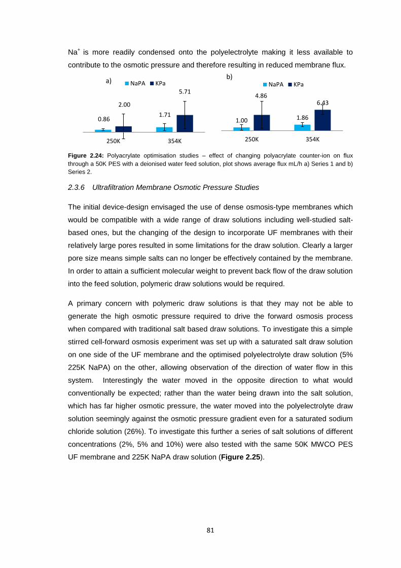
81
Na+ is more readily condensed onto the polyelectrolyte making it less available to
contribute to the osmotic pressure and therefore resulting in reduced membrane flux.
Figure 2.24: Polyacrylate optimisation studies – effect of changing polyacrylate counter-ion on flux
through a 50K PES with a deionised water feed solution, plot shows average flux mL/h a) Series 1 and b)
Series 2.
2.3.6 Ultrafiltration Membrane Osmotic Pressure Studies
The initial device-design envisaged the use of dense osmosis-type membranes which
would be compatible with a wide range of draw solutions including well-studied salt-
based ones, but the changing of the design to incorporate UF membranes with their
relatively large pores resulted in some limitations for the draw solution. Clearly a larger
pore size means simple salts can no longer be effectively contained by the membrane.
In order to attain a sufficient molecular weight to prevent back flow of the draw solution
into the feed solution, polymeric draw solutions would be required.
A primary concern with polymeric draw solutions is that they may not be able to
generate the high osmotic pressure required to drive the forward osmosis process
when compared with traditional salt based draw solutions. To investigate this a simple
stirred cell-forward osmosis experiment was set up with a saturated salt draw solution
on one side of the UF membrane and the optimised polyelectrolyte draw solution (5%
225K NaPA) on the other, allowing observation of the direction of water flow in this
system. Interestingly the water moved in the opposite direction to what would
conventionally be expected; rather than the water being drawn into the salt solution,
which has far higher osmotic pressure, the water moved into the polyelectrolyte draw
solution seemingly against the osmotic pressure gradient even for a saturated sodium
chloride solution (26%). To investigate this further a series of salt solutions of different
concentrations (2%, 5% and 10%) were also tested with the same 50K MWCO PES
UF membrane and 225K NaPA draw solution (Figure 2.25).
0.86 1.71
2.00
5.71
250K 354K
NaPA KPa
1.00 1.86
4.86 6.43
250K 354K
NaPA KPaa)
b)
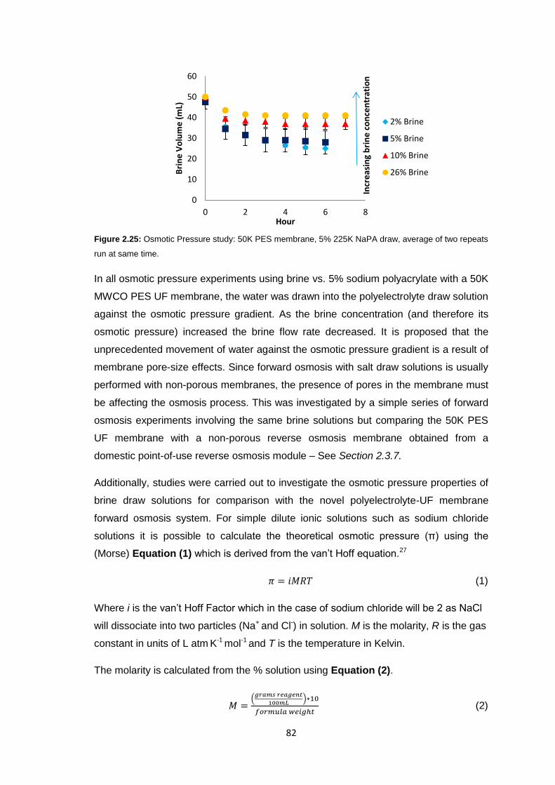
82
Figure 2.25: Osmotic Pressure study: 50K PES membrane, 5% 225K NaPA draw, average of two repeats
run at same time.
In all osmotic pressure experiments using brine vs. 5% sodium polyacrylate with a 50K
MWCO PES UF membrane, the water was drawn into the polyelectrolyte draw solution
against the osmotic pressure gradient. As the brine concentration (and therefore its
osmotic pressure) increased the brine flow rate decreased. It is proposed that the
unprecedented movement of water against the osmotic pressure gradient is a result of
membrane pore-size effects. Since forward osmosis with salt draw solutions is usually
performed with non-porous membranes, the presence of pores in the membrane must
be affecting the osmosis process. This was investigated by a simple series of forward
osmosis experiments involving the same brine solutions but comparing the 50K PES
UF membrane with a non-porous reverse osmosis membrane obtained from a
domestic point-of-use reverse osmosis module – See Section 2.3.7.
Additionally, studies were carried out to investigate the osmotic pressure properties of
brine draw solutions for comparison with the novel polyelectrolyte-UF membrane
forward osmosis system. For simple dilute ionic solutions such as sodium chloride
solutions it is possible to calculate the theoretical osmotic pressure (π) using the
(Morse) Equation (1) which is derived from the van’t Hoff equation.27
𝜋 = 𝑖𝑀𝑅𝑇 (1)
Where i is the van’t Hoff Factor which in the case of sodium chloride will be 2 as NaCl
will dissociate into two particles (Na+ and Cl-) in solution. M is the molarity, R is the gas
constant in units of L atm K-1 mol-1 and T is the temperature in Kelvin.
The molarity is calculated from the % solution using Equation (2).
𝑀 =(
𝑔𝑟𝑎𝑚𝑠 𝑟𝑒𝑎𝑔𝑒𝑛𝑡
100𝑚𝐿)∗10
𝑓𝑜𝑟𝑚𝑢𝑙𝑎 𝑤𝑒𝑖𝑔ℎ𝑡 (2)
0
10
20
30
40
50
60
0 2 4 6 8
Bri
ne
Vo
lum
e (
mL)
Hour
2% Brine
5% Brine
10% Brine
26% Brine
Incr
eas
ing
bri
ne
co
nce
ntr
atio
n
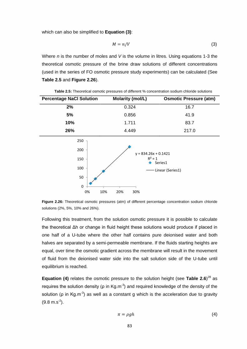
83
which can also be simplified to Equation (3):
𝑀 = 𝑛/𝑉 (3)
Where n is the number of moles and V is the volume in litres. Using equations 1-3 the
theoretical osmotic pressure of the brine draw solutions of different concentrations
(used in the series of FO osmotic pressure study experiments) can be calculated (See
Table 2.5 and Figure 2.26).
Table 2.5: Theoretical osmotic pressures of different % concentration sodium chloride solutions
Percentage NaCl Solution Molarity (mol/L) Osmotic Pressure (atm)
2% 0.324 16.7
5% 0.856 41.9
10% 1.711 83.7
26% 4.449 217.0
Figure 2.26: Theoretical osmotic pressures (atm) of different percentage concentration sodium chloride
solutions (2%, 5%, 10% and 26%).
Following this treatment, from the solution osmotic pressure it is possible to calculate
the theoretical Δh or change in fluid height these solutions would produce if placed in
one half of a U-tube where the other half contains pure deionised water and both
halves are separated by a semi-permeable membrane. If the fluids starting heights are
equal, over time the osmotic gradient across the membrane will result in the movement
of fluid from the deionised water side into the salt solution side of the U-tube until
equilibrium is reached.
Equation (4) relates the osmotic pressure to the solution height (see Table 2.6)28 as
requires the solution density (ρ in Kg.m-3) and required knowledge of the density of the
solution (ρ in Kg.m-3) as well as a constant g which is the acceleration due to gravity
(9.8 m.s-2).
𝜋 = 𝜌𝑔ℎ (4)
y = 834.26x + 0.1421 R² = 1
0
50
100
150
200
250
0% 10% 20% 30%
Series1
Linear (Series1)
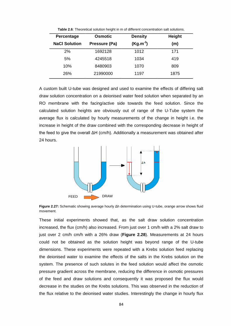
84
Table 2.6: Theoretical solution height in m of different concentration salt solutions.
Percentage
NaCl Solution
Osmotic
Pressure (Pa)
Density
(Kg.m-3)
Height
(m)
2% 1692128 1012 171
5% 4245518 1034 419
10% 8480903 1070 809
26% 21990000 1197 1875
A custom built U-tube was designed and used to examine the effects of differing salt
draw solution concentration on a deionised water feed solution when separated by an
RO membrane with the facing/active side towards the feed solution. Since the
calculated solution heights are obviously out of range of the U-Tube system the
average flux is calculated by hourly measurements of the change in height i.e. the
increase in height of the draw combined with the corresponding decrease in height of
the feed to give the overall ΔH (cm/h). Additionally a measurement was obtained after
24 hours.
Figure 2.27: Schematic showing average hourly Δh determination using U-tube, orange arrow shows fluid
movement.
These initial experiments showed that, as the salt draw solution concentration
increased, the flux (cm/h) also increased. From just over 1 cm/h with a 2% salt draw to
just over 2 cm/h cm/h with a 26% draw (Figure 2.28). Measurements at 24 hours
could not be obtained as the solution height was beyond range of the U-tube
dimensions. These experiments were repeated with a Krebs solution feed replacing
the deionised water to examine the effects of the salts in the Krebs solution on the
system. The presence of such solutes in the feed solution would affect the osmotic
pressure gradient across the membrane, reducing the difference in osmotic pressures
of the feed and draw solutions and consequently it was proposed the flux would
decrease in the studies on the Krebs solutions. This was observed in the reduction of
the flux relative to the deionised water studies. Interestingly the change in hourly flux
FEED DRAW
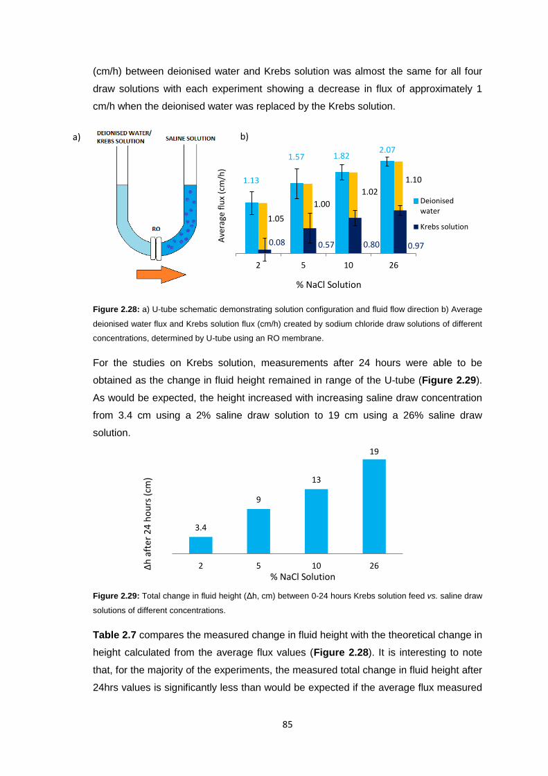
85
(cm/h) between deionised water and Krebs solution was almost the same for all four
draw solutions with each experiment showing a decrease in flux of approximately 1
cm/h when the deionised water was replaced by the Krebs solution.
Figure 2.28: a) U-tube schematic demonstrating solution configuration and fluid flow direction b) Average
deionised water flux and Krebs solution flux (cm/h) created by sodium chloride draw solutions of different
concentrations, determined by U-tube using an RO membrane.
For the studies on Krebs solution, measurements after 24 hours were able to be
obtained as the change in fluid height remained in range of the U-tube (Figure 2.29).
As would be expected, the height increased with increasing saline draw concentration
from 3.4 cm using a 2% saline draw solution to 19 cm using a 26% saline draw
solution.
Figure 2.29: Total change in fluid height (Δh, cm) between 0-24 hours Krebs solution feed vs. saline draw
solutions of different concentrations.
Table 2.7 compares the measured change in fluid height with the theoretical change in
height calculated from the average flux values (Figure 2.28). It is interesting to note
that, for the majority of the experiments, the measured total change in fluid height after
24hrs values is significantly less than would be expected if the average flux measured
1.05
1.00
1.02
1.10 1.13
1.57 1.82 2.07
0.08 0.57 0.80 0.97
2 5 10 26
Deionisedwater
Krebs solution
3.4
9
13
19
2 5 10 26
a) b)
% NaCl Solution
Ave
rage
flu
x (c
m/h
)
% NaCl Solution
Δh
aft
er
24 h
ou
rs (
cm)
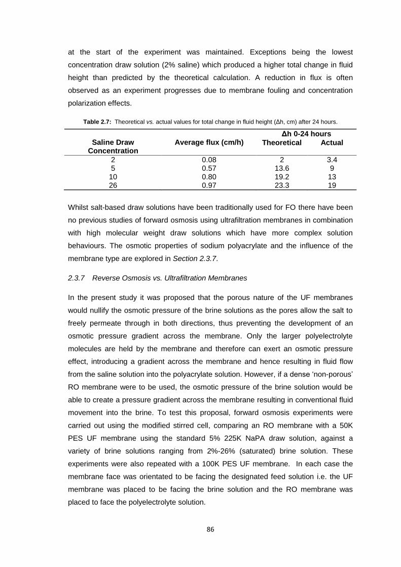
86
at the start of the experiment was maintained. Exceptions being the lowest
concentration draw solution (2% saline) which produced a higher total change in fluid
height than predicted by the theoretical calculation. A reduction in flux is often
observed as an experiment progresses due to membrane fouling and concentration
polarization effects.
Table 2.7: Theoretical vs. actual values for total change in fluid height (Δh, cm) after 24 hours.
Saline Draw
Concentration
Average flux (cm/h)
Δh 0-24 hours
Theoretical Actual
2 0.08 2 3.4 5 0.57 13.6 9
10 0.80 19.2 13 26 0.97 23.3 19
Whilst salt-based draw solutions have been traditionally used for FO there have been
no previous studies of forward osmosis using ultrafiltration membranes in combination
with high molecular weight draw solutions which have more complex solution
behaviours. The osmotic properties of sodium polyacrylate and the influence of the
membrane type are explored in Section 2.3.7.
2.3.7 Reverse Osmosis vs. Ultrafiltration Membranes
In the present study it was proposed that the porous nature of the UF membranes
would nullify the osmotic pressure of the brine solutions as the pores allow the salt to
freely permeate through in both directions, thus preventing the development of an
osmotic pressure gradient across the membrane. Only the larger polyelectrolyte
molecules are held by the membrane and therefore can exert an osmotic pressure
effect, introducing a gradient across the membrane and hence resulting in fluid flow
from the saline solution into the polyacrylate solution. However, if a dense ‘non-porous’
RO membrane were to be used, the osmotic pressure of the brine solution would be
able to create a pressure gradient across the membrane resulting in conventional fluid
movement into the brine. To test this proposal, forward osmosis experiments were
carried out using the modified stirred cell, comparing an RO membrane with a 50K
PES UF membrane using the standard 5% 225K NaPA draw solution, against a
variety of brine solutions ranging from 2%-26% (saturated) brine solution. These
experiments were also repeated with a 100K PES UF membrane. In each case the
membrane face was orientated to be facing the designated feed solution i.e. the UF
membrane was placed to be facing the brine solution and the RO membrane was
placed to face the polyelectrolyte solution.
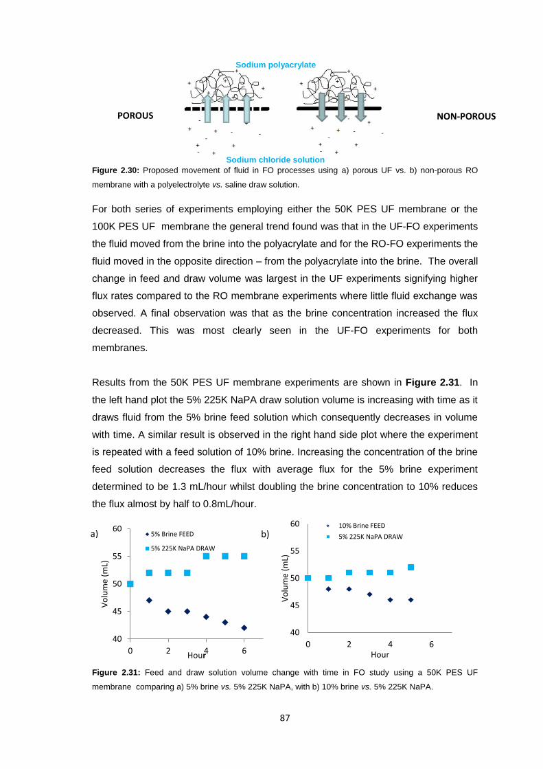
87
Figure 2.30: Proposed movement of fluid in FO processes using a) porous UF vs. b) non-porous RO
membrane with a polyelectrolyte vs. saline draw solution.
For both series of experiments employing either the 50K PES UF membrane or the
100K PES UF membrane the general trend found was that in the UF-FO experiments
the fluid moved from the brine into the polyacrylate and for the RO-FO experiments the
fluid moved in the opposite direction – from the polyacrylate into the brine. The overall
change in feed and draw volume was largest in the UF experiments signifying higher
flux rates compared to the RO membrane experiments where little fluid exchange was
observed. A final observation was that as the brine concentration increased the flux
decreased. This was most clearly seen in the UF-FO experiments for both
membranes.
Results from the 50K PES UF membrane experiments are shown in Figure 2.31. In
the left hand plot the 5% 225K NaPA draw solution volume is increasing with time as it
draws fluid from the 5% brine feed solution which consequently decreases in volume
with time. A similar result is observed in the right hand side plot where the experiment
is repeated with a feed solution of 10% brine. Increasing the concentration of the brine
feed solution decreases the flux with average flux for the 5% brine experiment
determined to be 1.3 mL/hour whilst doubling the brine concentration to 10% reduces
the flux almost by half to 0.8mL/hour.
Figure 2.31: Feed and draw solution volume change with time in FO study using a 50K PES UF
membrane comparing a) 5% brine vs. 5% 225K NaPA, with b) 10% brine vs. 5% 225K NaPA.
40
45
50
55
60
0 2 4 6
Vo
lum
e (m
L)
Hour
5% Brine FEED
5% 225K NaPA DRAW
40
45
50
55
60
0 2 4 6
Vo
lum
e (m
L)
Hour
10% Brine FEED
5% 225K NaPA DRAW
Sodium polyacrylate
Sodium chloride solution
POROUS NON-POROUS
a) b)
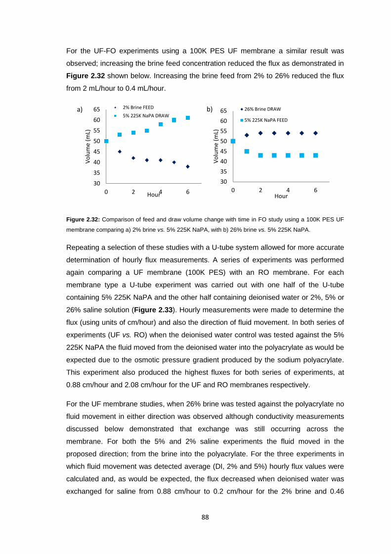
88
For the UF-FO experiments using a 100K PES UF membrane a similar result was
observed; increasing the brine feed concentration reduced the flux as demonstrated in
Figure 2.32 shown below. Increasing the brine feed from 2% to 26% reduced the flux
from 2 mL/hour to 0.4 mL/hour.
Figure 2.32: Comparison of feed and draw volume change with time in FO study using a 100K PES UF
membrane comparing a) 2% brine vs. 5% 225K NaPA, with b) 26% brine vs. 5% 225K NaPA.
Repeating a selection of these studies with a U-tube system allowed for more accurate
determination of hourly flux measurements. A series of experiments was performed
again comparing a UF membrane (100K PES) with an RO membrane. For each
membrane type a U-tube experiment was carried out with one half of the U-tube
containing 5% 225K NaPA and the other half containing deionised water or 2%, 5% or
26% saline solution (Figure 2.33). Hourly measurements were made to determine the
flux (using units of cm/hour) and also the direction of fluid movement. In both series of
experiments (UF vs. RO) when the deionised water control was tested against the 5%
225K NaPA the fluid moved from the deionised water into the polyacrylate as would be
expected due to the osmotic pressure gradient produced by the sodium polyacrylate.
This experiment also produced the highest fluxes for both series of experiments, at
0.88 cm/hour and 2.08 cm/hour for the UF and RO membranes respectively.
For the UF membrane studies, when 26% brine was tested against the polyacrylate no
fluid movement in either direction was observed although conductivity measurements
discussed below demonstrated that exchange was still occurring across the
membrane. For both the 5% and 2% saline experiments the fluid moved in the
proposed direction; from the brine into the polyacrylate. For the three experiments in
which fluid movement was detected average (DI, 2% and 5%) hourly flux values were
calculated and, as would be expected, the flux decreased when deionised water was
exchanged for saline from 0.88 cm/hour to 0.2 cm/hour for the 2% brine and 0.46
30
35
40
45
50
55
60
65
0 2 4 6
Vo
lum
e (m
L)
Hour
2% Brine FEED
5% 225K NaPA DRAW
30
35
40
45
50
55
60
65
0 2 4 6
Vo
lum
e (m
L)
Hour
26% Brine DRAW
5% 225K NaPA FEED
a) b)
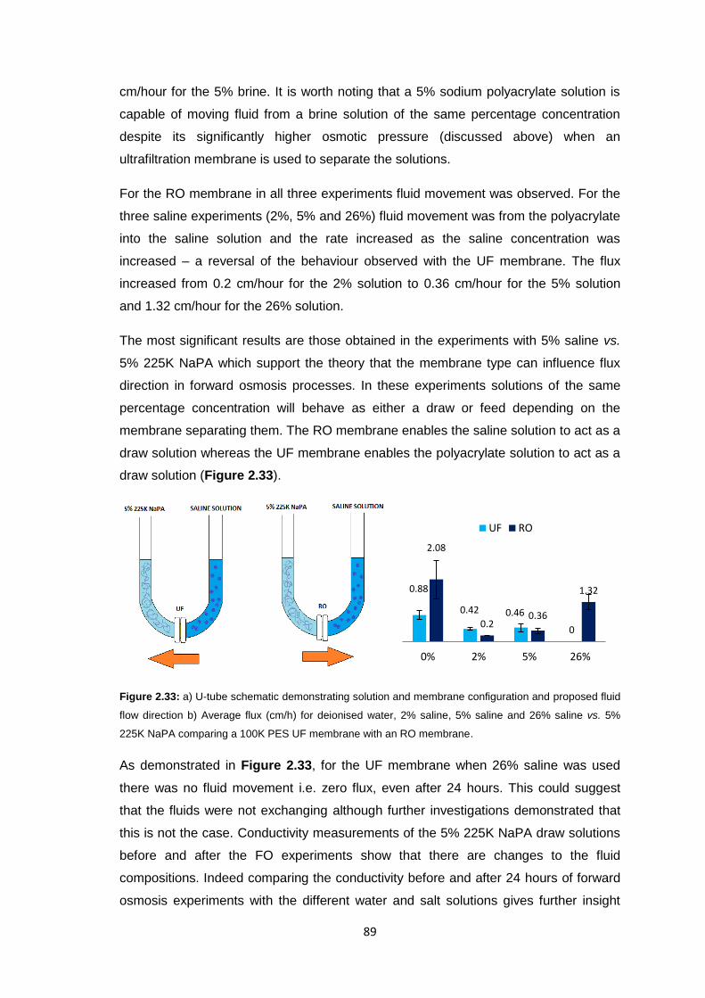
89
cm/hour for the 5% brine. It is worth noting that a 5% sodium polyacrylate solution is
capable of moving fluid from a brine solution of the same percentage concentration
despite its significantly higher osmotic pressure (discussed above) when an
ultrafiltration membrane is used to separate the solutions.
For the RO membrane in all three experiments fluid movement was observed. For the
three saline experiments (2%, 5% and 26%) fluid movement was from the polyacrylate
into the saline solution and the rate increased as the saline concentration was
increased – a reversal of the behaviour observed with the UF membrane. The flux
increased from 0.2 cm/hour for the 2% solution to 0.36 cm/hour for the 5% solution
and 1.32 cm/hour for the 26% solution.
The most significant results are those obtained in the experiments with 5% saline vs.
5% 225K NaPA which support the theory that the membrane type can influence flux
direction in forward osmosis processes. In these experiments solutions of the same
percentage concentration will behave as either a draw or feed depending on the
membrane separating them. The RO membrane enables the saline solution to act as a
draw solution whereas the UF membrane enables the polyacrylate solution to act as a
draw solution (Figure 2.33).
Figure 2.33: a) U-tube schematic demonstrating solution and membrane configuration and proposed fluid
flow direction b) Average flux (cm/h) for deionised water, 2% saline, 5% saline and 26% saline vs. 5%
225K NaPA comparing a 100K PES UF membrane with an RO membrane.
As demonstrated in Figure 2.33, for the UF membrane when 26% saline was used
there was no fluid movement i.e. zero flux, even after 24 hours. This could suggest
that the fluids were not exchanging although further investigations demonstrated that
this is not the case. Conductivity measurements of the 5% 225K NaPA draw solutions
before and after the FO experiments show that there are changes to the fluid
compositions. Indeed comparing the conductivity before and after 24 hours of forward
osmosis experiments with the different water and salt solutions gives further insight
0.88
0.42 0.46
0
2.08
0.2 0.36
1.32
0% 2% 5% 26%
UF RO
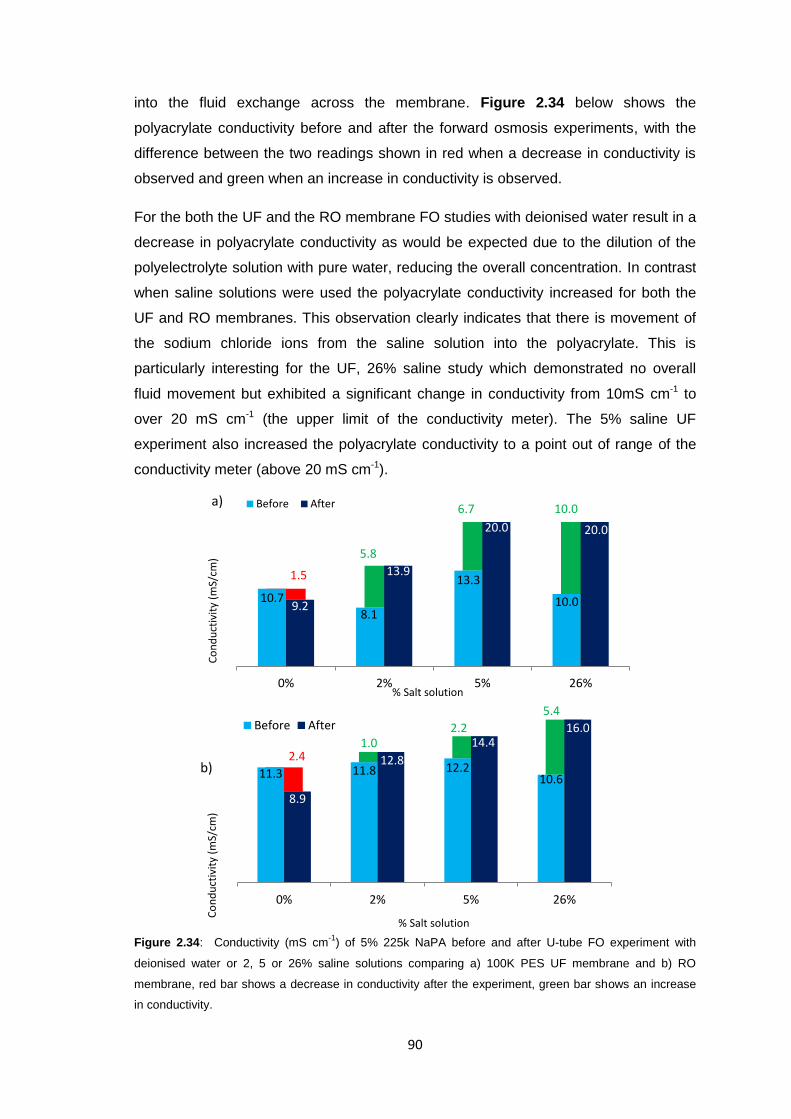
90
into the fluid exchange across the membrane. Figure 2.34 below shows the
polyacrylate conductivity before and after the forward osmosis experiments, with the
difference between the two readings shown in red when a decrease in conductivity is
observed and green when an increase in conductivity is observed.
For the both the UF and the RO membrane FO studies with deionised water result in a
decrease in polyacrylate conductivity as would be expected due to the dilution of the
polyelectrolyte solution with pure water, reducing the overall concentration. In contrast
when saline solutions were used the polyacrylate conductivity increased for both the
UF and RO membranes. This observation clearly indicates that there is movement of
the sodium chloride ions from the saline solution into the polyacrylate. This is
particularly interesting for the UF, 26% saline study which demonstrated no overall
fluid movement but exhibited a significant change in conductivity from 10mS cm-1 to
over 20 mS cm-1 (the upper limit of the conductivity meter). The 5% saline UF
experiment also increased the polyacrylate conductivity to a point out of range of the
conductivity meter (above 20 mS cm-1).
Figure 2.34: Conductivity (mS cm-1
) of 5% 225k NaPA before and after U-tube FO experiment with
deionised water or 2, 5 or 26% saline solutions comparing a) 100K PES UF membrane and b) RO
membrane, red bar shows a decrease in conductivity after the experiment, green bar shows an increase
in conductivity.
1.5
5.8
6.7 10.0
10.7
8.1
13.3
10.0 9.2
13.9
20.0 20.0
0% 2% 5% 26%
Before After
2.4 1.0
2.2
5.4
11.3 11.8 12.2 10.6
8.9
12.8
14.4 16.0
0% 2% 5% 26%
Before After
a)
b)
Co
nd
uct
ivit
y (m
S/cm
) C
on
du
ctiv
ity
(mS/
cm)
% Salt solution
% Salt solution
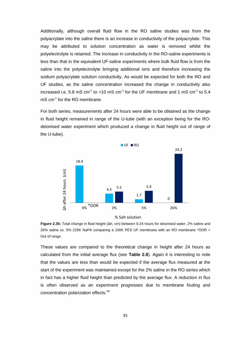
91
Additionally, although overall fluid flow in the RO saline studies was from the
polyacrylate into the saline there is an increase in conductivity of the polyacrylate. This
may be attributed to solution concentration as water is removed whilst the
polyelectrolyte is retained. The increase in conductivity in the RO-saline experiments is
less than that in the equivalent UF-saline experiments where bulk fluid flow is from the
saline into the polyelectrolyte bringing additional ions and therefore increasing the
sodium polyacrylate solution conductivity. As would be expected for both the RO and
UF studies, as the saline concentration increased the change in conductivity also
increased i.e. 5.8 mS cm-1 to >10 mS cm-1 for the UF membrane and 1 mS cm-1 to 5.4
mS cm-1 for the RO membrane.
For both series, measurements after 24 hours were able to be obtained as the change
in fluid height remained in range of the U-tube (with an exception being for the RO-
deionised water experiment which produced a change in fluid height out of range of
the U-tube).
Figure 2.35: Total change in fluid height (Δh, cm) between 0-24 hours for deionised water, 2% saline and
26% saline vs. 5% 225K NaPA comparing a 100K PES UF membrane with an RO membrane *OOR =
Out of range.
These values are compared to the theoretical change in height after 24 hours as
calculated from the initial average flux (see Table 2.8). Again it is interesting to note
that the values are less than would be expected if the average flux measured at the
start of the experiment was maintained except for the 2% saline in the RO series which
in fact has a higher fluid height than predicted by the average flux. A reduction in flux
is often observed as an experiment progresses due to membrane fouling and
concentration polarization effects.29
18.4
4.5
1.7 0
5.5 5.9
24.2
0% 2% 5% 26%
UF RO
*OOR
Δh
aft
er
24
ho
urs
(cm
)
% Salt solution
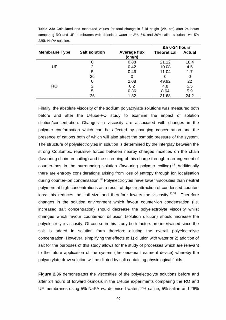
92
Table 2.8: Calculated and measured values for total change in fluid height (Δh, cm) after 24 hours
comparing RO and UF membranes with deionised water or 2%, 5% and 26% saline solutions vs. 5%
225K NaPA solution.
Membrane Type
Salt solution
Average flux
(cm/h)
Δh 0-24 hours
Theoretical Actual
UF
0 0.88 21.12 18.4 2 0.42 10.08 4.5 5 0.46 11.04 1.7 26 0 0 0
RO
0 2.08 49.92 22 2 0.2 4.8 5.5 5 0.36 8.64 5.9 26 1.32 31.68 24.2
Finally, the absolute viscosity of the sodium polyacrylate solutions was measured both
before and after the U-tube-FO study to examine the impact of solution
dilution/concentration. Changes in viscosity are associated with changes in the
polymer conformation which can be affected by changing concentration and the
presence of cations both of which will also affect the osmotic pressure of the system.
The structure of polyelectrolytes in solution is determined by the interplay between the
strong Coulombic repulsive forces between nearby charged moieties on the chain
(favouring chain un-coiling) and the screening of this charge through rearrangement of
counter-ions in the surrounding solution (favouring polymer coiling).11 Additionally
there are entropy considerations arising from loss of entropy through ion localisation
during counter-ion condensation.30 Polyelectrolytes have lower viscosities than neutral
polymers at high concentrations as a result of dipolar attraction of condensed counter-
ions: this reduces the coil size and therefore lowers the viscosity.31,32 Therefore
changes in the solution environment which favour counter-ion condensation (i.e.
increased salt concentration) should decrease the polyelectrolyte viscosity whilst
changes which favour counter-ion diffusion (solution dilution) should increase the
polyelectrolyte viscosity. Of course in this study both factors are intertwined since the
salt is added in solution form therefore diluting the overall polyelectrolyte
concentration. However, simplifying the effects to 1) dilution with water or 2) addition of
salt for the purposes of this study allows for the study of processes which are relevant
to the future application of the system (the oedema treatment device) whereby the
polyacrylate draw solution will be diluted by salt containing physiological fluids.
Figure 2.36 demonstrates the viscosities of the polyelectrolyte solutions before and
after 24 hours of forward osmosis in the U-tube experiments comparing the RO and
UF membranes using 5% NaPA vs. deionised water, 2% saline, 5% saline and 26%
93
saline. When considering the experiments using deionised water (0%) the bulk
movement of the fluid was from the water into the polyacrylate solution for both the UF
and RO membrane. While it might be expected that the impact on the viscosity to be
similar in both cases we instead observe an increase in viscosity in the UF experiment
and a decrease in viscosity in the RO experiment. In both cases the sodium
polyacrylate was diluted but to different extents; for the UF membrane the overall fluid
height difference after 24 hours was 18.3 cm whereas for the RO membrane the fluid
height difference was out of range of the U-tube (Figure 2.35). For the UF experiment
this is equivalent to the movement of 21.6 mL (calculated from the dimensions of the
tube) of fluid from the deionised water into the polyacrylate diluting it by a fifth of its
original volume which results in a small increase in viscosity which could be attributed
to the dilution increasing the osmotic pressure favouring counter-ion diffusion resulting
in polymer uncoiling. Conversely for the RO membrane this viscosity is reduced in the
FO study despite this solution being further diluted which in itself is unexpected since
the more porous UF membrane should produce higher fluxes when compared to the
non-porous RO membrane when using the same draw solution as in this case.
For the 2% saline solution opposite effects on viscosity were observed for the two
different membranes. The UF study showed an increase in polyacrylate viscosity
whereas the RO study showed a decrease in viscosity. Although similar fluid height
changes were obtained after 24 hours for both the UF and the RO experiment (4.5 cm
and 5.5 cm, Figure 2.35) the fluid flux direction must be considered. In the UF study
fluid moved from the saline into the polyacrylate whilst in the RO study bulk fluid flux
was in the reverse direction. In the UF study the polyacrylate is not only diluted but is
also flooded with excess cations, a volume of 4.72 mL of the 2% saline solution moved
into the sodium polyacrylate. The two factors, dilution and cation concentration
increase, will have opposing effects; counter-ions in excess can condense on the
polyacrylate favouring polymer coiling whereas dilution favours counter-ion
displacement through osmotic effects favouring polymer uncoiling. For the RO
membrane a volume of 6.61 mL moved from the polyelectrolyte into the saline
solution, concentrating the polyelectrolyte by approximately a twentieth of its original
volume.
For the 5% saline solution opposite effects on polyacrylate viscosity were observed
for the two different membranes. In these experiments the bulk fluid movement was in
the same direction as observed in the 2% saline experiments (in the UF membrane
experiment the fluid moved from the saline solution into the polyacrylate whilst for the
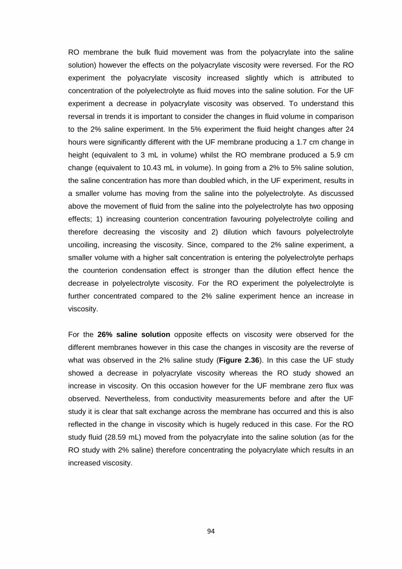
94
RO membrane the bulk fluid movement was from the polyacrylate into the saline
solution) however the effects on the polyacrylate viscosity were reversed. For the RO
experiment the polyacrylate viscosity increased slightly which is attributed to
concentration of the polyelectrolyte as fluid moves into the saline solution. For the UF
experiment a decrease in polyacrylate viscosity was observed. To understand this
reversal in trends it is important to consider the changes in fluid volume in comparison
to the 2% saline experiment. In the 5% experiment the fluid height changes after 24
hours were significantly different with the UF membrane producing a 1.7 cm change in
height (equivalent to 3 mL in volume) whilst the RO membrane produced a 5.9 cm
change (equivalent to 10.43 mL in volume). In going from a 2% to 5% saline solution,
the saline concentration has more than doubled which, in the UF experiment, results in
a smaller volume has moving from the saline into the polyelectrolyte. As discussed
above the movement of fluid from the saline into the polyelectrolyte has two opposing
effects; 1) increasing counterion concentration favouring polyelectrolyte coiling and
therefore decreasing the viscosity and 2) dilution which favours polyelectrolyte
uncoiling, increasing the viscosity. Since, compared to the 2% saline experiment, a
smaller volume with a higher salt concentration is entering the polyelectrolyte perhaps
the counterion condensation effect is stronger than the dilution effect hence the
decrease in polyelectrolyte viscosity. For the RO experiment the polyelectrolyte is
further concentrated compared to the 2% saline experiment hence an increase in
viscosity.
For the 26% saline solution opposite effects on viscosity were observed for the
different membranes however in this case the changes in viscosity are the reverse of
what was observed in the 2% saline study (Figure 2.36). In this case the UF study
showed a decrease in polyacrylate viscosity whereas the RO study showed an
increase in viscosity. On this occasion however for the UF membrane zero flux was
observed. Nevertheless, from conductivity measurements before and after the UF
study it is clear that salt exchange across the membrane has occurred and this is also
reflected in the change in viscosity which is hugely reduced in this case. For the RO
study fluid (28.59 mL) moved from the polyacrylate into the saline solution (as for the
RO study with 2% saline) therefore concentrating the polyacrylate which results in an
increased viscosity.
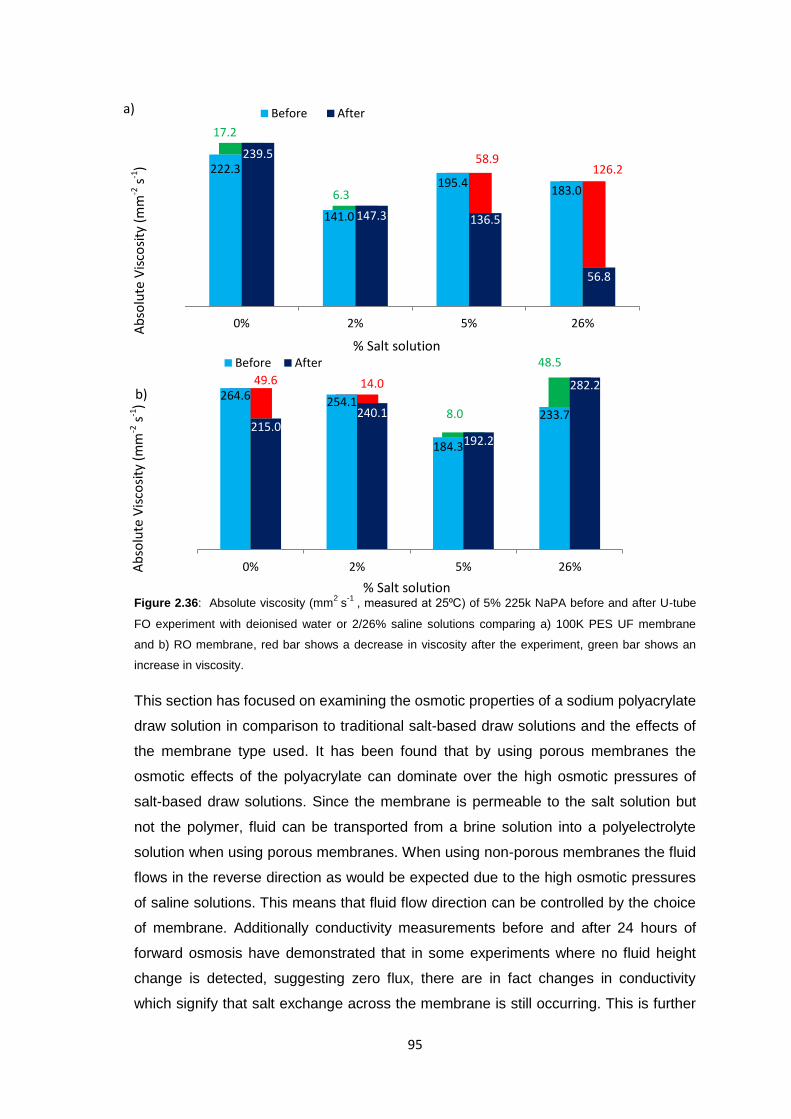
95
Figure 2.36: Absolute viscosity (mm2
s-1
, measured at 25⁰C) of 5% 225k NaPA before and after U-tube
FO experiment with deionised water or 2/26% saline solutions comparing a) 100K PES UF membrane
and b) RO membrane, red bar shows a decrease in viscosity after the experiment, green bar shows an
increase in viscosity.
This section has focused on examining the osmotic properties of a sodium polyacrylate
draw solution in comparison to traditional salt-based draw solutions and the effects of
the membrane type used. It has been found that by using porous membranes the
osmotic effects of the polyacrylate can dominate over the high osmotic pressures of
salt-based draw solutions. Since the membrane is permeable to the salt solution but
not the polymer, fluid can be transported from a brine solution into a polyelectrolyte
solution when using porous membranes. When using non-porous membranes the fluid
flows in the reverse direction as would be expected due to the high osmotic pressures
of saline solutions. This means that fluid flow direction can be controlled by the choice
of membrane. Additionally conductivity measurements before and after 24 hours of
forward osmosis have demonstrated that in some experiments where no fluid height
change is detected, suggesting zero flux, there are in fact changes in conductivity
which signify that salt exchange across the membrane is still occurring. This is further
58.9 126.2
17.2
6.3
222.3
141.0
195.4 183.0
239.5
147.3 136.5
56.8
0% 2% 5% 26%
Before After
49.6 14.0
8.0
48.5
264.6 254.1
184.3
233.7 215.0
240.1
192.2
282.2
0% 2% 5% 26%
Before After
a)
b)
% Salt solution
% Salt solution
Ab
solu
te V
isco
sity
(m
m-2
s-1
) A
bso
lute
Vis
cosi
ty (
mm
-2 s
-1)
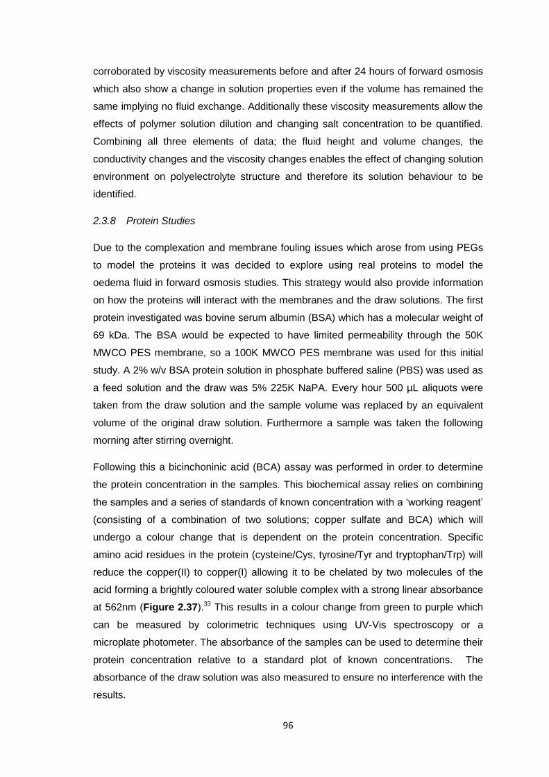
96
corroborated by viscosity measurements before and after 24 hours of forward osmosis
which also show a change in solution properties even if the volume has remained the
same implying no fluid exchange. Additionally these viscosity measurements allow the
effects of polymer solution dilution and changing salt concentration to be quantified.
Combining all three elements of data; the fluid height and volume changes, the
conductivity changes and the viscosity changes enables the effect of changing solution
environment on polyelectrolyte structure and therefore its solution behaviour to be
identified.
2.3.8 Protein Studies
Due to the complexation and membrane fouling issues which arose from using PEGs
to model the proteins it was decided to explore using real proteins to model the
oedema fluid in forward osmosis studies. This strategy would also provide information
on how the proteins will interact with the membranes and the draw solutions. The first
protein investigated was bovine serum albumin (BSA) which has a molecular weight of
69 kDa. The BSA would be expected to have limited permeability through the 50K
MWCO PES membrane, so a 100K MWCO PES membrane was used for this initial
study. A 2% w/v BSA protein solution in phosphate buffered saline (PBS) was used as
a feed solution and the draw was 5% 225K NaPA. Every hour 500 µL aliquots were
taken from the draw solution and the sample volume was replaced by an equivalent
volume of the original draw solution. Furthermore a sample was taken the following
morning after stirring overnight.
Following this a bicinchoninic acid (BCA) assay was performed in order to determine
the protein concentration in the samples. This biochemical assay relies on combining
the samples and a series of standards of known concentration with a ‘working reagent’
(consisting of a combination of two solutions; copper sulfate and BCA) which will
undergo a colour change that is dependent on the protein concentration. Specific
amino acid residues in the protein (cysteine/Cys, tyrosine/Tyr and tryptophan/Trp) will
reduce the copper(II) to copper(I) allowing it to be chelated by two molecules of the
acid forming a brightly coloured water soluble complex with a strong linear absorbance
at 562nm (Figure 2.37).33 This results in a colour change from green to purple which
can be measured by colorimetric techniques using UV-Vis spectroscopy or a
microplate photometer. The absorbance of the samples can be used to determine their
protein concentration relative to a standard plot of known concentrations. The
absorbance of the draw solution was also measured to ensure no interference with the
results.
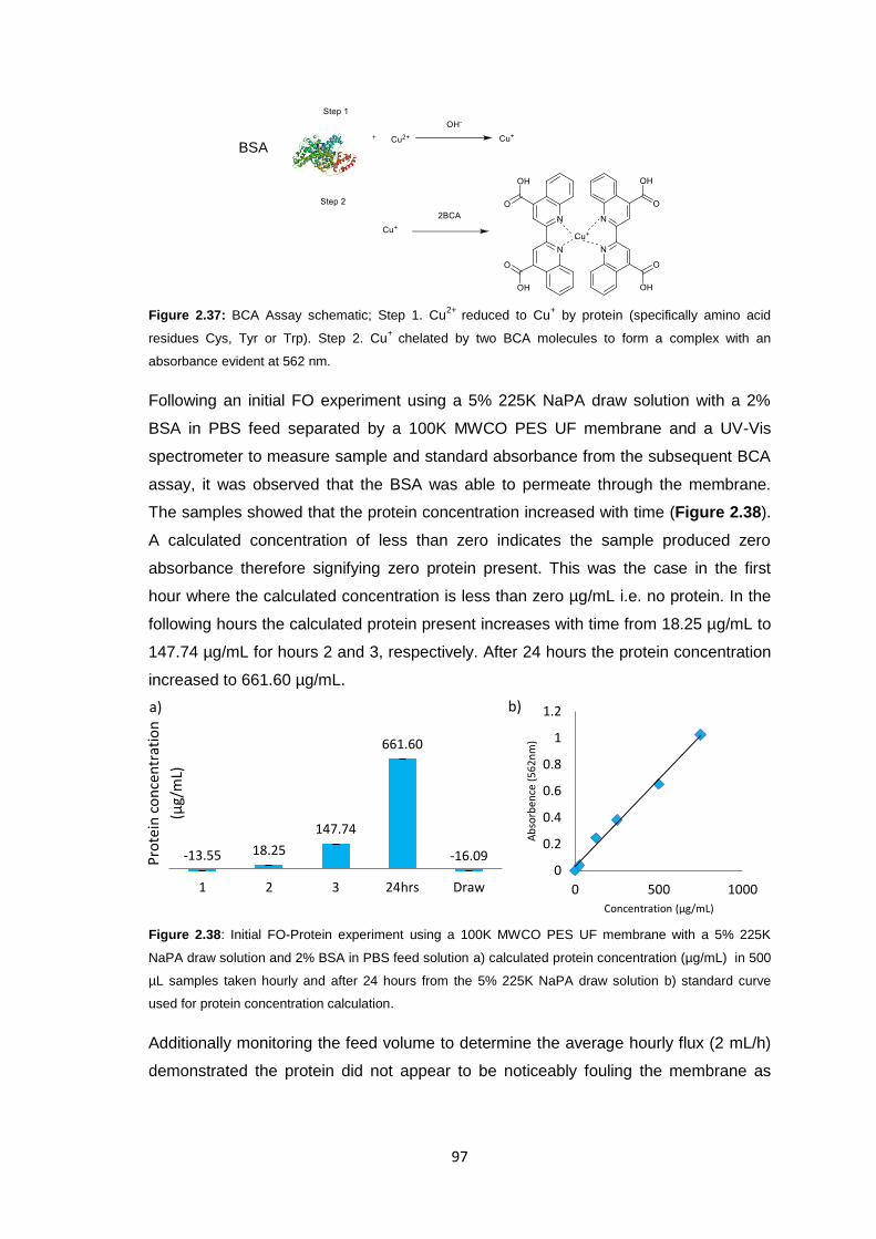
97
Figure 2.37: BCA Assay schematic; Step 1. Cu2+
reduced to Cu+ by protein (specifically amino acid
residues Cys, Tyr or Trp). Step 2. Cu+
chelated by two BCA molecules to form a complex with an
absorbance evident at 562 nm.
Following an initial FO experiment using a 5% 225K NaPA draw solution with a 2%
BSA in PBS feed separated by a 100K MWCO PES UF membrane and a UV-Vis
spectrometer to measure sample and standard absorbance from the subsequent BCA
assay, it was observed that the BSA was able to permeate through the membrane.
The samples showed that the protein concentration increased with time (Figure 2.38).
A calculated concentration of less than zero indicates the sample produced zero
absorbance therefore signifying zero protein present. This was the case in the first
hour where the calculated concentration is less than zero µg/mL i.e. no protein. In the
following hours the calculated protein present increases with time from 18.25 µg/mL to
147.74 µg/mL for hours 2 and 3, respectively. After 24 hours the protein concentration
increased to 661.60 µg/mL.
Figure 2.38: Initial FO-Protein experiment using a 100K MWCO PES UF membrane with a 5% 225K
NaPA draw solution and 2% BSA in PBS feed solution a) calculated protein concentration (µg/mL) in 500
µL samples taken hourly and after 24 hours from the 5% 225K NaPA draw solution b) standard curve
used for protein concentration calculation.
Additionally monitoring the feed volume to determine the average hourly flux (2 mL/h)
demonstrated the protein did not appear to be noticeably fouling the membrane as
-13.55 18.25
147.74
661.60
-16.09
1 2 3 24hrs Draw0
0.2
0.4
0.6
0.8
1
1.2
0 500 1000
Ab
sorb
ence
(5
62
nm
)
Concentration (µg/mL)
a) b)
Pro
tein
co
nce
ntr
atio
n
(µg/
mL)
BSA
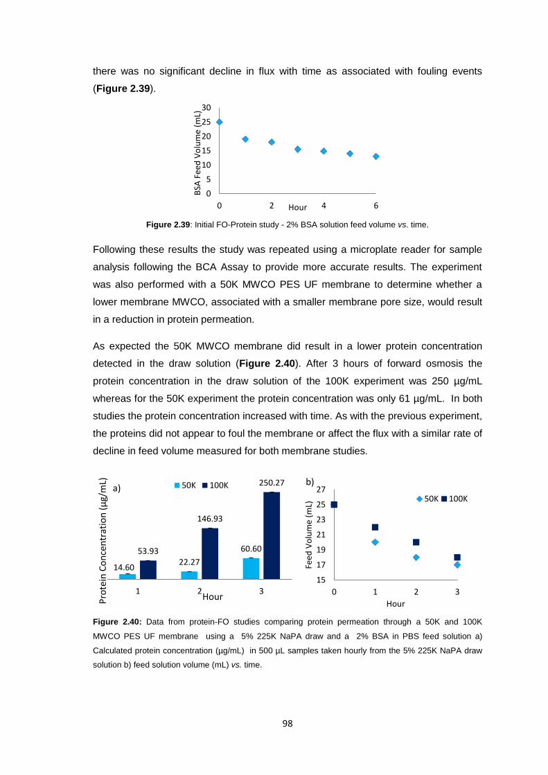
98
there was no significant decline in flux with time as associated with fouling events
(Figure 2.39).
Figure 2.39: Initial FO-Protein study - 2% BSA solution feed volume vs. time.
Following these results the study was repeated using a microplate reader for sample
analysis following the BCA Assay to provide more accurate results. The experiment
was also performed with a 50K MWCO PES UF membrane to determine whether a
lower membrane MWCO, associated with a smaller membrane pore size, would result
in a reduction in protein permeation.
As expected the 50K MWCO membrane did result in a lower protein concentration
detected in the draw solution (Figure 2.40). After 3 hours of forward osmosis the
protein concentration in the draw solution of the 100K experiment was 250 µg/mL
whereas for the 50K experiment the protein concentration was only 61 µg/mL. In both
studies the protein concentration increased with time. As with the previous experiment,
the proteins did not appear to foul the membrane or affect the flux with a similar rate of
decline in feed volume measured for both membrane studies.
Figure 2.40: Data from protein-FO studies comparing protein permeation through a 50K and 100K
MWCO PES UF membrane using a 5% 225K NaPA draw and a 2% BSA in PBS feed solution a)
Calculated protein concentration (µg/mL) in 500 µL samples taken hourly from the 5% 225K NaPA draw
solution b) feed solution volume (mL) vs. time.
0
5
10
15
20
25
30
0 2 4 6B
SA F
eed
Vo
lum
e (m
L)
Hour
14.60 22.27
60.60 53.93
146.93
250.27
1 2 3
50K 100K
15
17
19
21
23
25
27
0 1 2 3
Feed
Vo
lum
e (m
L)
Hour
50K 100Ka)
b)
Hour Pro
tein
Co
nce
ntr
atio
n (
µg/
mL)
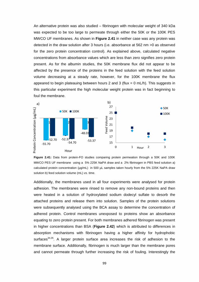
99
An alternative protein was also studied – fibrinogen with molecular weight of 340 kDa
was expected to be too large to permeate through either the 50K or the 100K PES
MWCO UF membranes. As shown in Figure 2.41 in neither case was any protein was
detected in the draw solution after 3 hours (i.e. absorbance at 562 nm >0 as observed
for the zero protein concentration control). As explained above, calculated negative
concentrations from absorbance values which are less than zero signifies zero protein
present. As for the albumin studies, the 50K membrane flux did not appear to be
affected by the presence of the proteins in the feed solution with the feed solution
volume decreasing at a steady rate, however, for the 100K membrane the flux
appeared to begin plateauing between hours 2 and 3 (flux = 0 mL/h). This suggests in
this particular experiment the high molecular weight protein was in fact beginning to
foul the membrane.
Figure 2.41: Data from protein-FO studies comparing protein permeation through a 50K and 100K
MWCO PES UF membrane using a 5% 225K NaPA draw and a 2% fibrinogen in PBS feed solution a)
calculated protein concentration (µg/mL) in 500 µL samples taken hourly from the 5% 225K NaPA draw
solution b) feed solution volume (mL) vs. time.
Additionally, the membranes used in all four experiments were analysed for protein
adhesion. The membranes were rinsed to remove any non-bound proteins and then
were heated in a solution of hydroxylated sodium dodecyl sulfate to desorb the
attached proteins and release them into solution. Samples of the protein solutions
were subsequently analysed using the BCA assay to determine the concentration of
adhered protein. Control membranes unexposed to proteins show an absorbance
equating to zero protein present. For both membranes adhered fibrinogen was present
in higher concentrations than BSA (Figure 2.42) which is attributed to differences in
absorption mechanisms with fibrinogen having a higher affinity for hydrophobic
surfaces34,35. A larger protein surface area increases the risk of adhesion to the
membrane surface. Additionally, fibrinogen is much larger than the membrane pores
and cannot permeate through further increasing the risk of fouling. Interestingly the
-55.70
-52.37
-48.03
-52.70 -54.70
-53.37
1 2 3
50K 100K
15
17
19
21
23
25
27
0 1 2 3
Feed
Vo
lum
e
Hour
50K
100K
a) b)
Pro
tein
Co
nce
ntr
atio
n (
µg/
mL)
Hour
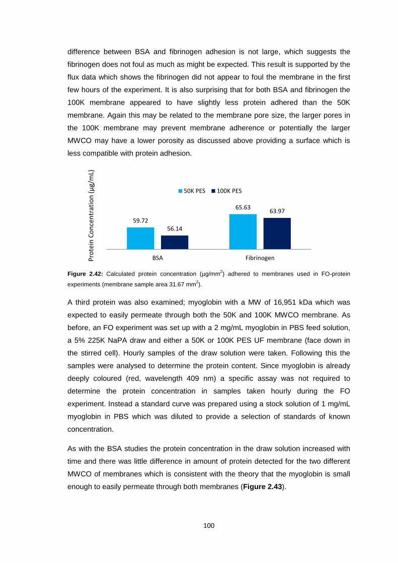
100
difference between BSA and fibrinogen adhesion is not large, which suggests the
fibrinogen does not foul as much as might be expected. This result is supported by the
flux data which shows the fibrinogen did not appear to foul the membrane in the first
few hours of the experiment. It is also surprising that for both BSA and fibrinogen the
100K membrane appeared to have slightly less protein adhered than the 50K
membrane. Again this may be related to the membrane pore size, the larger pores in
the 100K membrane may prevent membrane adherence or potentially the larger
MWCO may have a lower porosity as discussed above providing a surface which is
less compatible with protein adhesion.
Figure 2.42: Calculated protein concentration (µg/mm2) adhered to membranes used in FO-protein
experiments (membrane sample area 31.67 mm2).
A third protein was also examined; myoglobin with a MW of 16,951 kDa which was
expected to easily permeate through both the 50K and 100K MWCO membrane. As
before, an FO experiment was set up with a 2 mg/mL myoglobin in PBS feed solution,
a 5% 225K NaPA draw and either a 50K or 100K PES UF membrane (face down in
the stirred cell). Hourly samples of the draw solution were taken. Following this the
samples were analysed to determine the protein content. Since myoglobin is already
deeply coloured (red, wavelength 409 nm) a specific assay was not required to
determine the protein concentration in samples taken hourly during the FO
experiment. Instead a standard curve was prepared using a stock solution of 1 mg/mL
myoglobin in PBS which was diluted to provide a selection of standards of known
concentration.
As with the BSA studies the protein concentration in the draw solution increased with
time and there was little difference in amount of protein detected for the two different
MWCO of membranes which is consistent with the theory that the myoglobin is small
enough to easily permeate through both membranes (Figure 2.43).
59.72
65.63
56.14
63.97
BSA Fibrinogen
50K PES 100K PES
Pro
tein
Co
nce
ntr
atio
n (
µg/
mL)
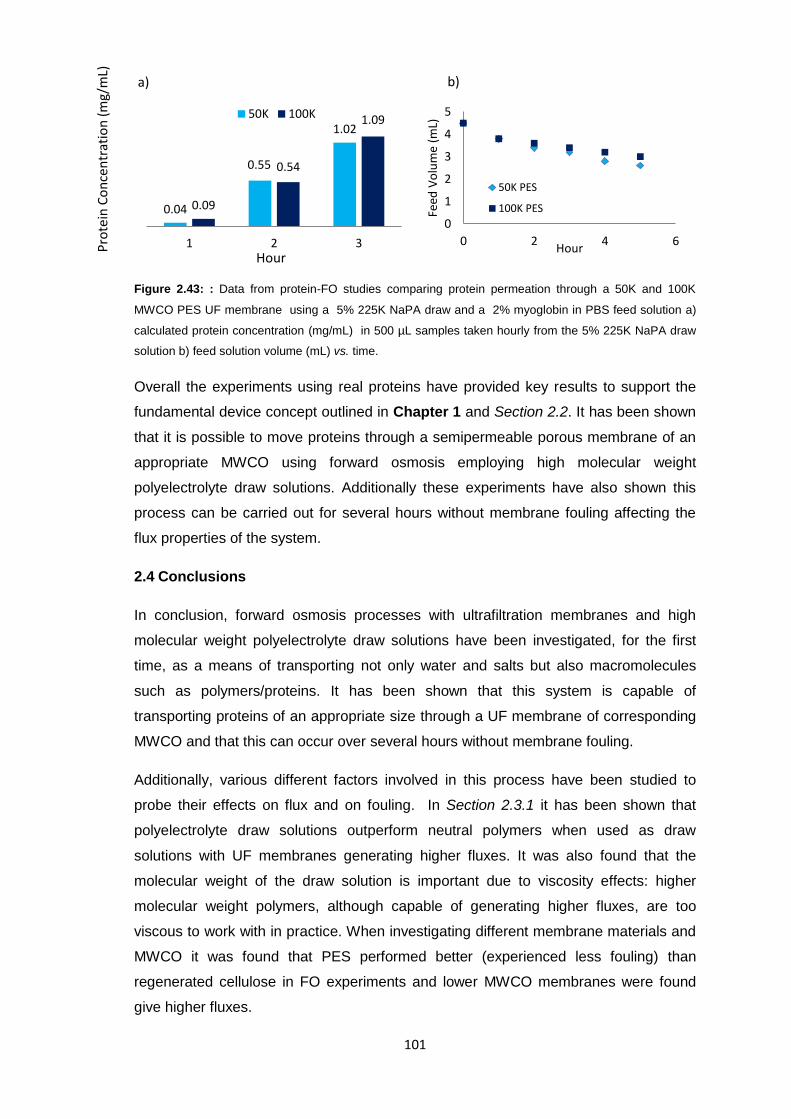
101
Figure 2.43: : Data from protein-FO studies comparing protein permeation through a 50K and 100K
MWCO PES UF membrane using a 5% 225K NaPA draw and a 2% myoglobin in PBS feed solution a)
calculated protein concentration (mg/mL) in 500 µL samples taken hourly from the 5% 225K NaPA draw
solution b) feed solution volume (mL) vs. time.
Overall the experiments using real proteins have provided key results to support the
fundamental device concept outlined in Chapter 1 and Section 2.2. It has been shown
that it is possible to move proteins through a semipermeable porous membrane of an
appropriate MWCO using forward osmosis employing high molecular weight
polyelectrolyte draw solutions. Additionally these experiments have also shown this
process can be carried out for several hours without membrane fouling affecting the
flux properties of the system.
2.4 Conclusions
In conclusion, forward osmosis processes with ultrafiltration membranes and high
molecular weight polyelectrolyte draw solutions have been investigated, for the first
time, as a means of transporting not only water and salts but also macromolecules
such as polymers/proteins. It has been shown that this system is capable of
transporting proteins of an appropriate size through a UF membrane of corresponding
MWCO and that this can occur over several hours without membrane fouling.
Additionally, various different factors involved in this process have been studied to
probe their effects on flux and on fouling. In Section 2.3.1 it has been shown that
polyelectrolyte draw solutions outperform neutral polymers when used as draw
solutions with UF membranes generating higher fluxes. It was also found that the
molecular weight of the draw solution is important due to viscosity effects: higher
molecular weight polymers, although capable of generating higher fluxes, are too
viscous to work with in practice. When investigating different membrane materials and
MWCO it was found that PES performed better (experienced less fouling) than
regenerated cellulose in FO experiments and lower MWCO membranes were found
give higher fluxes.
0.04
0.55
1.02
0.09
0.54
1.09
1 2 3
50K 100K
0
1
2
3
4
5
0 2 4 6
Feed
Vo
lum
e (m
L)
Hour
50K PES
100K PES
a) b)
Hour
Pro
tein
Co
nce
ntr
atio
n (
mg/
mL)
102
In Section 2.3.2 whilst trying to model physiological proteins using PEG/PEO it was
found that the higher molecular weight PEO fouled the membranes but lower
molecular weight PEGs did not create the same drop in membrane flux. Investigations
into PEG behaviour in solution (Section 2.3.3) showed they were not affected by the
salts of the Krebs solution used to simulate physiological interstitial fluid.
When investigating sodium polyacrylate behaviour in solution (Section 2.3.4) it was
found that cations present in physiological salt solutions interact with the polyacrylate
affecting the polymer structure which could potentially influence membrane fouling.
Additionally the change in structure and salt concentration would alter the osmotic
pressure of the system. These complex effects would require further research in the
context of the medical device system to fully understand their implications.
Related to polyacrylate behaviour in solution; in Section 2.3.5 studies were carried out
to optimise the polyacrylate draw by investigation the effect on flux when molecular
weight, polymer concentration and counter-ion identity were varied found that these
three factors could influence the flux of the system. It was found that:
1) the average flux decreases with increasing polyelectrolyte molecular weight;
2) when comparing four different 225K NaPA draw solutions of the following
concentration; 2%, 5%, 7% and 10% with a 50K PES UF membrane and a
deionised water feed solution we observe a peak flux when the 5% draw
solution is used;
3) exchanging sodium for potassium in the polyacrylate salts can also increase
the flux by a factor of up to five, presumably as a result of weaker ion-pairing
with the polyelectrolyte chain.
When investigating the osmotic properties of the system (Section 2.3.6) it was found
that polyacrylate draw solutions could generate large enough osmotic pressure
gradients to transport fluid from brine solutions (traditionally used as draw solutions in
FO with non-porous membranes) into polyacrylate draw solutions. It was proposed this
phenomenon may result from the porosity of the membrane preventing the saline from
exerting any osmotic effects since it can freely permeate through the membrane whilst
the polyelectrolyte is retained on one side. This theory was further examined in
Section 2.3.7 where the osmotic properties of sodium polyacrylic acid was probed
using both porous and non-porous membranes. It was confirmed that by using porous

103
membranes the osmotic effects of the polyacrylate can dominate over the high osmotic
pressures of salt based draw solutions since the membrane is permeable to the salt
solution but not the polymer. This means that fluid can be transported from a brine
solution into a polyelectrolyte solution when using porous membranes whereas when
using non-porous membranes the fluid flows in the reverse direction allowing control of
fluid flow direction by the choice of membrane used. Additionally further information
about the system obtained from conductivity and viscosity measurements before and
after 24 hours of forward osmosis demonstrated that in some experiments where no
fluid height change is detected, suggesting zero flux, there are in fact changes in
conductivity and viscosity which confirm that salt exchange across the membrane is
still occurring. Additionally these viscosity and conductivity measurements allow the
effects of polymer solution dilution and changing salt concentration to be quantified.
The final experiments in this Chapter, Section 2.3.8 explored the behaviour of the
optimised forward osmosis system (determined in Sections 2.3.1 and 2.3.2) with real
proteins. It has been found that it is possible to move proteins through a
semipermeable porous membrane of an appropriate MWCO using forward osmosis
employing high molecular weight polyelectrolyte draw solutions. Additionally these
experiments have shown this process can be carried out for several hours without
membrane fouling affecting the flux properties of the system
Overall this Chapter provided some fundamental results which were then used to
design, develop and fabricate a prototype, membrane-based medical device which
was then tested both in an in vitro system and in an ex-vivo mammalian limb model
specifically designed for the project – see Chapter 5.
2.5 Future Work
In order to continue the work into forward osmosis processes with ultrafiltration
membranes investigated in this chapter, several aspects of this process could be
further studied. For example initial work using PEGs to model proteins resulted in
membrane fouling causing zero flux. To verify this preliminary work was carried out
investigating tagging PEG molecules with a fluorophore in order to identify whether
different MW PEGs were able to permeate through the membranes. This approach
could also potentially quantify the amount of PEG traversing the membrane. In
addition using fluorescently tagged proteins would allow for real-time monitoring and
quantification of proteins being transported via forward osmosis, allowing for a clearer
understanding of this process. This would also remove the need for the complex assay
step simplifying the procedure.
104
The work carried out in this chapter also identified that, in the context of this project, a
better understanding of polyelectrolyte behaviour in solution, particularly with solutions
containing mixtures of salts, is required. For example, whilst interactions with NaCl and
MgSO4 were investigated it would also be beneficial to study the interactions between
the polyacrylate and mono- and divalent salts from the fourth period such as KCl and
CaCl2 for comparison. Particularly since K+ and Ca2+ cations are also present in the
Krebs solution, which was used as a feed solution to simulate oedema fluid.
Additionally, the present work discovered that exchanging potassium ions for sodium
ions in the polyelectrolyte salt draw solution significantly altered the flux generated
(resulting in a fivefold increase) suggesting such a change may have a major effect on
the polyelectrolyte properties. This discovery was only made towards the end of the
present project and clearly warrants more extensive investigation.
2.6 Experimental
2.6.1 Materials
All materials were used as supplied unless otherwise stated. The following materials
were purchased from Fisher Scientific UK Ltd (Leicestershire, UK); Pierce™ BCA
Protein assay kit (containing; Reagent A - bicinchoninic acid, Reagent B - 4% (w/v)
copper sulfate, 2 mg/mL albumin standard ampules), 96-well flat-bottomed
microplates, and micrometre feeler gauges. All membrane disks were obtained from
Merk Millipore (Massachusetts, USA). These included; 10 KDa regenerated cellulose
UF discs, 30 KDa/50 KDa/100 KDa polyethersulfone UF discs and Ultracel® 100 KDa
UF discs. The following polymers were acquired from Poysciences, Inc; 225,000 MW
Poly(acrylic acid) sodium salt (20% aqueous solution), 345,000 MW Poly(acrylic acid)
(25% aqueous solution) 1,000,000 MW poly(acrylic acid, 1,000,000 MW poly(styrene
sulfonic acid) sodium salt. The commercial RO membrane was sourced from a
Vontron® Residential Membrane Element (Vontron®, China). All other materials
including; bovine serum albumin, calcium chloride, diglyme, dimethylformamide,
fibrinogen, glucose, magnesium sulphate, myoglobin from equine skeletal muscle
poly(ethylene glycol) - Mn 600, 6,000 and 35,000 , poly(ethylene oxide)- Mv 100,000
and 1,000,000, polysulfone (average Mw 35K by LS, average Mn 16K), 250,000 MW
poly(acrylic acid) (35% aqueous solution), 45% 160K Mr poly(vinylpyrrolidone) solution,
6,000K MW poly(acrylic acid) sodium salt, phosphate buffered saline, potassium
chloride, potassium phosphate monobasic, sodium azide, sodium chloride, sodium
hydrocarbonate and sodium hydroxide were purchased from Sigma Aldrich (Dorset,
UK).
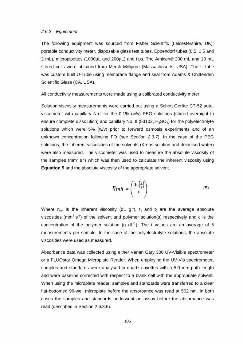
105
2.6.2 Equipment
The following equipment was sourced from Fisher Scientific (Leicestershire, UK);
portable conductivity meter, disposable glass test tubes, Eppendorf tubes (0.5, 1.5 and
2 mL), micropipettes (1000µL and 200µL) and tips. The Amicon® 200 mL and 10 mL
stirred cells were obtained from Merck Millipore (Massachusetts, USA). The U-tube
was custom built U-Tube using membrane flange and seal from Adams & Chittenden
Scientific Glass (CA, USA).
All conductivity measurements were made using a calibrated conductivity meter.
Solution viscosity measurements were carried out using a Schott-Geräte CT-52 auto-
viscometer with capillary No.I for the 0.1% (w/v) PEG solutions (stirred overnight to
ensure complete dissolution) and capillary No. II (53102, H2SO4) for the polyelectrolyte
solutions which were 5% (w/v) prior to forward osmosis experiments and of an
unknown concentration following FO (see Section 2.3.7). In the case of the PEG
solutions, the inherent viscosities of the solvents (Krebs solution and deionised water)
were also measured. The viscometer was used to measure the absolute viscosity of
the samples (mm2 s-1) which was then used to calculate the inherent viscosity using
Equation 5 and the absolute viscosity of the appropriate solvent.
Where ηinh is the inherent viscosity (dL g-1), t1 and t2 are the average absolute
viscosities (mm2 s-1) of the solvent and polymer solution(s) respectively and c is the
concentration of the polymer solution (g dL-1). The t values are an average of 5
measurements per sample. In the case of the polyelectrolyte solutions, the absolute
viscosities were used as measured.
Absorbance data was collected using either Varian Cary 300 UV-Visible spectrometer
or a FLUOstar Omega Microplate Reader. When employing the UV-Vis spectrometer,
samples and standards were analysed in quartz cuvettes with a 5.0 mm path length
and were baseline corrected with respect to a blank cell with the appropriate solvent.
When using the microplate reader, samples and standards were transferred to a clear
flat-bottomed 96-well microplate before the absorbance was read at 562 nm. In both
cases the samples and standards underwent an assay before the absorbance was
read (described in Section 2.6.3.6).
(5)
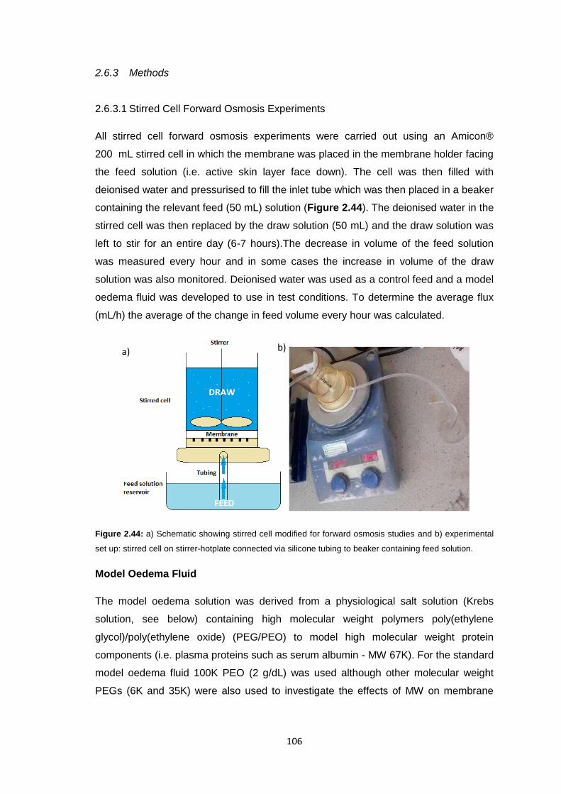
106
2.6.3 Methods
2.6.3.1 Stirred Cell Forward Osmosis Experiments
All stirred cell forward osmosis experiments were carried out using an Amicon®
200 mL stirred cell in which the membrane was placed in the membrane holder facing
the feed solution (i.e. active skin layer face down). The cell was then filled with
deionised water and pressurised to fill the inlet tube which was then placed in a beaker
containing the relevant feed (50 mL) solution (Figure 2.44). The deionised water in the
stirred cell was then replaced by the draw solution (50 mL) and the draw solution was
left to stir for an entire day (6-7 hours).The decrease in volume of the feed solution
was measured every hour and in some cases the increase in volume of the draw
solution was also monitored. Deionised water was used as a control feed and a model
oedema fluid was developed to use in test conditions. To determine the average flux
(mL/h) the average of the change in feed volume every hour was calculated.
Figure 2.44: a) Schematic showing stirred cell modified for forward osmosis studies and b) experimental
set up: stirred cell on stirrer-hotplate connected via silicone tubing to beaker containing feed solution.
Model Oedema Fluid
The model oedema solution was derived from a physiological salt solution (Krebs
solution, see below) containing high molecular weight polymers poly(ethylene
glycol)/poly(ethylene oxide) (PEG/PEO) to model high molecular weight protein
components (i.e. plasma proteins such as serum albumin - MW 67K). For the standard
model oedema fluid 100K PEO (2 g/dL) was used although other molecular weight
PEGs (6K and 35K) were also used to investigate the effects of MW on membrane
a) b)
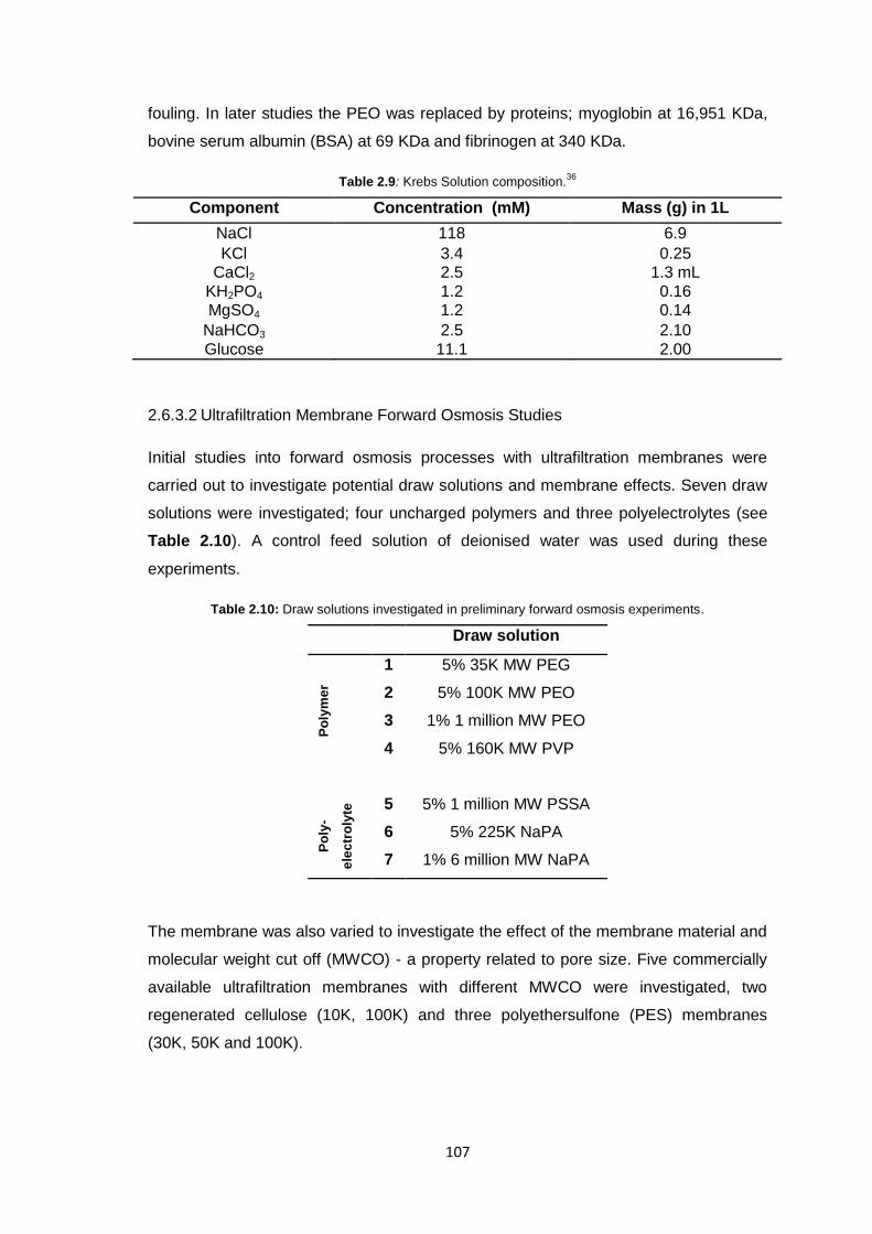
107
fouling. In later studies the PEO was replaced by proteins; myoglobin at 16,951 KDa,
bovine serum albumin (BSA) at 69 KDa and fibrinogen at 340 KDa.
Table 2.9: Krebs Solution composition.36
Component Concentration (mM) Mass (g) in 1L
NaCl 118 6.9
KCl 3.4 0.25 CaCl2 2.5 1.3 mL
KH2PO4 1.2 0.16 MgSO4 1.2 0.14
NaHCO3 2.5 2.10
Glucose 11.1 2.00
2.6.3.2 Ultrafiltration Membrane Forward Osmosis Studies
Initial studies into forward osmosis processes with ultrafiltration membranes were
carried out to investigate potential draw solutions and membrane effects. Seven draw
solutions were investigated; four uncharged polymers and three polyelectrolytes (see
Table 2.10). A control feed solution of deionised water was used during these
experiments.
Table 2.10: Draw solutions investigated in preliminary forward osmosis experiments.
Draw solution
Po
lym
er
1 5% 35K MW PEG
2 5% 100K MW PEO
3 1% 1 million MW PEO
4 5% 160K MW PVP
Po
ly-
ele
ctr
oly
te 5 5% 1 million MW PSSA
6 5% 225K NaPA
7 1% 6 million MW NaPA
The membrane was also varied to investigate the effect of the membrane material and
molecular weight cut off (MWCO) - a property related to pore size. Five commercially
available ultrafiltration membranes with different MWCO were investigated, two
regenerated cellulose (10K, 100K) and three polyethersulfone (PES) membranes
(30K, 50K and 100K).
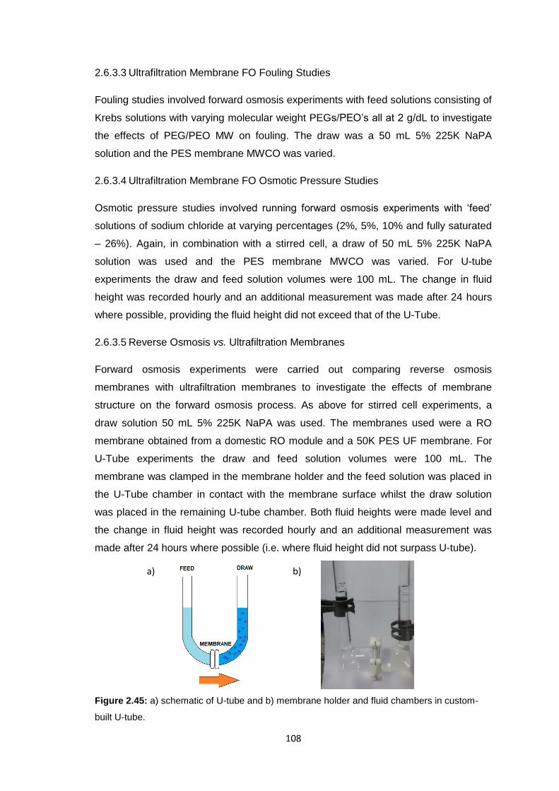
108
2.6.3.3 Ultrafiltration Membrane FO Fouling Studies
Fouling studies involved forward osmosis experiments with feed solutions consisting of
Krebs solutions with varying molecular weight PEGs/PEO’s all at 2 g/dL to investigate
the effects of PEG/PEO MW on fouling. The draw was a 50 mL 5% 225K NaPA
solution and the PES membrane MWCO was varied.
2.6.3.4 Ultrafiltration Membrane FO Osmotic Pressure Studies
Osmotic pressure studies involved running forward osmosis experiments with ‘feed’
solutions of sodium chloride at varying percentages (2%, 5%, 10% and fully saturated
– 26%). Again, in combination with a stirred cell, a draw of 50 mL 5% 225K NaPA
solution was used and the PES membrane MWCO was varied. For U-tube
experiments the draw and feed solution volumes were 100 mL. The change in fluid
height was recorded hourly and an additional measurement was made after 24 hours
where possible, providing the fluid height did not exceed that of the U-Tube.
2.6.3.5 Reverse Osmosis vs. Ultrafiltration Membranes
Forward osmosis experiments were carried out comparing reverse osmosis
membranes with ultrafiltration membranes to investigate the effects of membrane
structure on the forward osmosis process. As above for stirred cell experiments, a
draw solution 50 mL 5% 225K NaPA was used. The membranes used were a RO
membrane obtained from a domestic RO module and a 50K PES UF membrane. For
U-Tube experiments the draw and feed solution volumes were 100 mL. The
membrane was clamped in the membrane holder and the feed solution was placed in
the U-Tube chamber in contact with the membrane surface whilst the draw solution
was placed in the remaining U-tube chamber. Both fluid heights were made level and
the change in fluid height was recorded hourly and an additional measurement was
made after 24 hours where possible (i.e. where fluid height did not surpass U-tube).
Figure 2.45: a) schematic of U-tube and b) membrane holder and fluid chambers in custom-
built U-tube.
a) b)
109
2.6.3.6 Protein Studies
Forward osmosis experiments were performed using the modified stirred cell as
described previously with 5% 225K NaPA draw solution and either a 50K or 100K
membrane face down in the stirred cell with a 2% protein (BSA or fibrinogen) in PBS
solution feed (or plasma). Every hour 500 µL aliquots were taken and the sample
volume was replaced by an equivalent volume of the draw solution. Furthermore a
sample was taken the following morning after stirring overnight.
Following this a bicinchoninic (BCA) Assay was performed in order to determine the
protein concentration in the samples. The absorbance of the draw solution was also
measured to ensure no interference with the results.
Bicinchoninic Acid Assay
The resulting supernatant was analysed using the BCA assay (bicinchoninic acid
assay) to determine the protein concentration present in each sample with respect to a
standard curve of BSA solutions of known concentrations. The calculated
concentration of the unknown samples was then extrapolated to estimate the protein
concentration per unit membrane area.
A standard curve was prepared using a 2 mg/mL stock solution of BSA with dilutions
ranging from 2000-25 µg/mL (Table 2.11). The diluent was PBS.
Table 2.11: Preparation of standard BSA solutions for standard curve
Solution No. Final BSA Concentration
(µg/mL)
Volume of Diluent
(µL)
Volume and source of BSA
(µL)
Final Volume
(µL)
A 2000 0 300 (stock) 300 B 1500 125 375 (stock) 325 C 1000 325 325 (stock) 325 D 750 175 175 (vial B dilution) 350 E 500 325 325 (vial C dilution) 325 F 250 325 325 (vial E dilution) 325 G 125 325 325 (vial F dilution) 550 H 25 400 100 (vial G dilution) 500 I 0 400 0 400
The BCA standard working reagent was prepared by combining the BCA reagent
(component A) with 4% (w/v) CuSO4 (component B) in a ratio of 50:1.
Standards and samples were vortexed before 25 µL of each added to a clear, flat-
bottomed 96-well microplate in triplicate. Following this 200 µL of the BCA standard
110
working reagent was added in a randomised pattern to each well containing a sample
or standard. The microplate was incubated for 37 ⁰C for 30 minutes before measuring
the absorbance at 562nm in a FLUOstar Omega Microplate Reader
For the myoglobin studies due to the proteins inherent colour no assay was required to
provide a measurable colour change. Instead a standard curve was prepared using
solutions of myoglobin of known concentrations (Table 2.12). Standards and samples
were vortexed before 25 µL of each added to a clear, flat-bottomed 96-well microplate
in triplicate following which; the absorbance was measured at 409 nm in a FLUOstar
Omega Microplate Reader.
Table 2.12: Preparation of standard myoglobin solutions for standard curve
Solution No. Final Myoglobin
Concentration (mg/mL)
Volume of Diluent
(µL)
Volume and source of Myoglobin
(µL)
Final Volume
(µL)
A 1 0 500 (stock) 300 B 0.5 250 250 (vial A dilution) 500 C 0.2 400 100 (vial A dilution) 500 D 0.1 450 50 (vial A dilution) 500 E 0.05 475 25 (vial A dilution) 500 F 0 300 300 300
2.6.3.7 Commercial Ultrafiltration Membranes
Commercial ultrafiltration membranes were obtained from Merck Millipore. The
membranes were used as standards to investigate potential draw solutions. The PES-
50K membrane was also used as a solid support for composite nanofiltration
membranes through in-situ interfacial polymerisation on the surface (see Chapter 3).
Table 2.13: Commercial Membrane Materials and MWCO, deionised water (mL/h) at 1 bar.
Composition MWCO Deionised water flux
(mL/h) at 1 bar pressure
Regenerated Cellulose 10K 180
Polyethersulfone 30K 236
Polyethersulfone 50K 336
Polyethersulfone 100K 2088
Regenerated Cellulose 100K 456
111
2.7 References
1. G. M. Geise, H.-S. Lee, D. J. Miller, B. D. Freeman, J. E. McGrath, and D. R.
Paul, J. Polym. Sci., 2010, 48, 1685–1718.
2. T. Cath, A. Childress, and M. Elimelech, J. Membr. Sci., 2006, 281, 70–87.
3. T. S. Chung, X. Li, R. C. Ong, Q. Ge, H. Wang, and G. Han, Curr. Opin. Chem.
Eng., 2012, 1, 246–257.
4. C. B. Herbert and M. N. Blaine, US Pat. 8211 053 B2 (2012) to Equilibirate,
LLC.
5. S. G. Rockson, Am. J. Med., 2001, 110, 288–295.
6. W. L. Olszewski, S. Jamal, B. Lukomska, G. Manokaran, and G. I., Lymphology,
1992, 25, 166–171.
7. V. Kumar, A. K. Abbas, N. Fausto, and J. C. Aster, in Robbins and Cotran
Pathologic Basis of Disease, Saunders Elsevier, Philadelphia, 7th edn., 2009.
8. H. Yang, Q. Zheng, and R. Cheng, Colloids Surfaces A Physicochem. Eng.
Asp., 2012, 407, 1–8.
9. J. M. Carrillo and A. Dobrynin, Polymers (Basel)., 1992, 1897–1913.
10. A. V. Dobrynin and M. Rubinstein, Prog. Polym. Sci., 2005, 30, 1049–1118.
11. J. L. Barrat, Adv. Chem. Phys. Polym. Syst., 1996, 1–66.
12. G. Maurer, S. Lammertz, and L. Ninni Scafer, Adv. Polym. Sci., 2011, 67–136.
13. R. Chang, Y. Kim, and A. Yethiraj, Macromolecules, 2015, 48, 7370–7377.
14. D. Stigter, Biophys. J., 1995, 69, 380–388.
15. H. P. Hsu and E. Lee, Electrochem. commun., 2012, 15, 59–62.
16. R. Schweins and K. Huber, Eur. Phys. J. E, 2001, 5, 117–126.
17. R. R. Netz and D. Andelman, Phys. Rep., 2003, 380, 1–95.
18. T. Kitano, A. Taguchi, I. Noda, and M. Nagasawa, Macromolecules, 1980, 13,
57–63.
19. R. J. Young and P. A. Lovell, Eds., in Introduction to Polymers, Taylor &
Francis, 3rd edn., 2011, pp. 237–268.
20. I. Pochard, P. Couchot, C. Geffroy, A. Foissy, and J. Persello, Rev. L’Institut Fr.
Du Pet., 1997, 52, 251–253.
21. K. Huber, J. Phys. Chem., 1993, 97, 9825–9830.
112
22. M. J. Stevens and S. J. Plimpton, Eur. Phys. J. B - Condens. Matter Complex
Syst., 1998, 2, 341–345.
23. J. Shao, S. Qin, J. Davidson, W. Li, Y. He, and H. S. Zhou, J. Hazard. Mater.,
2013, 244–245, 472–477.
24. H. Jellinek and M. Luh, J. Polym. Sci., 1969, 7, 172–177.
25. R. R. Navarro, S. Wada, and K. Tatsumi, J. Hazard. Mater., 2005, 123, 203–
209.
26. P. Atkins, T. Overton, J. Rourke, M. Weller, and F. Armstrong, in Shriver and
Atkins Inorganic Chemistry, Oxford University Press, 5th edn., 2009, pp. 3–33.
27. Q. Ge, M. Ling, and T.-S. Chung, J. Membr. Sci., 2013, 442, 225–237.
28. F. C. Andrews, Science, 1976, 194, 567–571.
29. S. Zhao, L. Zou, C. Y. Tang, and D. Mulcahy, J. Membr. Sci., 2012, 396, 1–21.
30. D. C. Boris and R. H. Colby, Macromolecules, 1998, 31, 5746–5755.
31. H. Schiessel and P. Pincus, Macromolecules, 1998, 31, 7953–7959.
32. A. J. Konop and R. H. Colby, Macromolecules, 1999, 32, 2803–2805.
33. Thermo Scientific Applications Note, Pierce™ BCA Protein Assay Kit
Instructions , 2013, 1–7.
34. P. Thevenot, W. Hu, and L. Tnag, Curr. Top. Med. Chem., 2011, 8, 270–280.
35. P. Roach, D. Farrar, and C. C. Perry, J. Am. Chem. Soc., 2005, 127, 8168–
8173.
36. M. J. Gardener, C. D. Glen, G. R. Richards, P. M. Vanhoutte, G. Edwards, M.
Fe, and A. H. Weston, Br. J. Pharmacol., 2001, 133, 1145–1153.
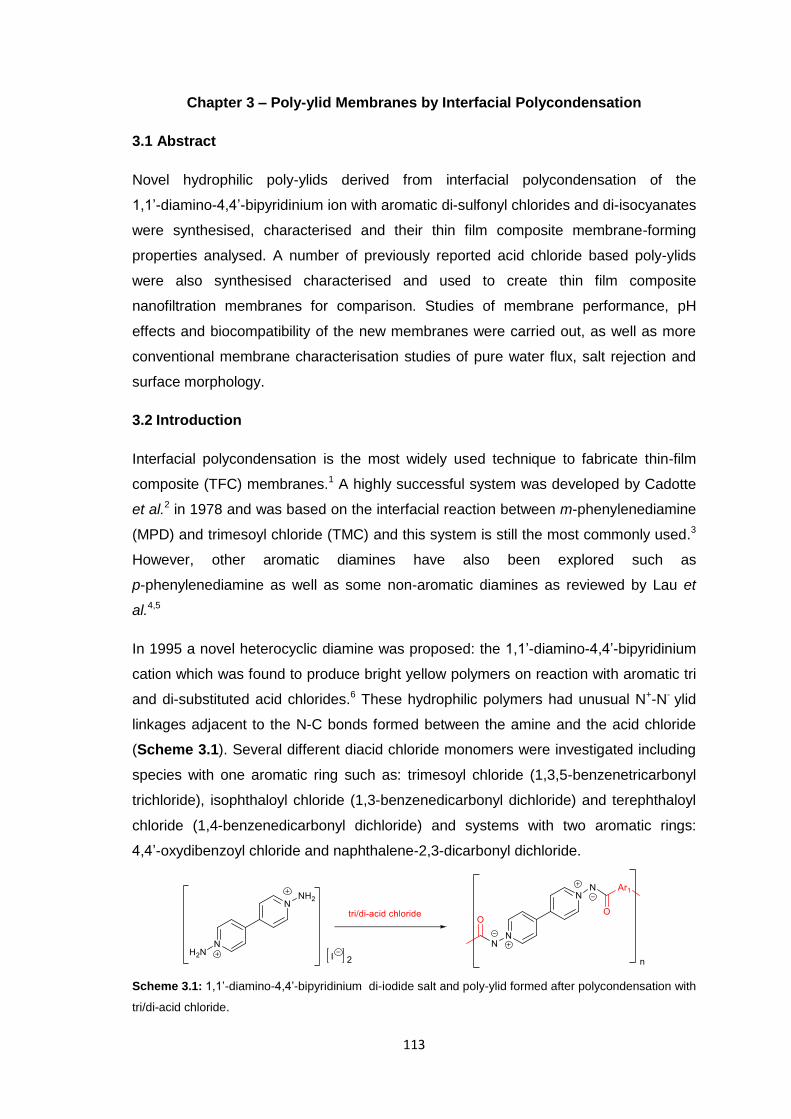
113
Chapter 3 – Poly-ylid Membranes by Interfacial Polycondensation
3.1 Abstract
Novel hydrophilic poly-ylids derived from interfacial polycondensation of the
1,1’-diamino-4,4’-bipyridinium ion with aromatic di-sulfonyl chlorides and di-isocyanates
were synthesised, characterised and their thin film composite membrane-forming
properties analysed. A number of previously reported acid chloride based poly-ylids
were also synthesised characterised and used to create thin film composite
nanofiltration membranes for comparison. Studies of membrane performance, pH
effects and biocompatibility of the new membranes were carried out, as well as more
conventional membrane characterisation studies of pure water flux, salt rejection and
surface morphology.
3.2 Introduction
Interfacial polycondensation is the most widely used technique to fabricate thin-film
composite (TFC) membranes.1 A highly successful system was developed by Cadotte
et al.2 in 1978 and was based on the interfacial reaction between m-phenylenediamine
(MPD) and trimesoyl chloride (TMC) and this system is still the most commonly used.3
However, other aromatic diamines have also been explored such as
p-phenylenediamine as well as some non-aromatic diamines as reviewed by Lau et
al.4,5
In 1995 a novel heterocyclic diamine was proposed: the 1,1’-diamino-4,4’-bipyridinium
cation which was found to produce bright yellow polymers on reaction with aromatic tri
and di-substituted acid chlorides.6 These hydrophilic polymers had unusual N+-N- ylid
linkages adjacent to the N-C bonds formed between the amine and the acid chloride
(Scheme 3.1). Several different diacid chloride monomers were investigated including
species with one aromatic ring such as: trimesoyl chloride (1,3,5-benzenetricarbonyl
trichloride), isophthaloyl chloride (1,3-benzenedicarbonyl dichloride) and terephthaloyl
chloride (1,4-benzenedicarbonyl dichloride) and systems with two aromatic rings:
4,4’-oxydibenzoyl chloride and naphthalene-2,3-dicarbonyl dichloride.
Scheme 3.1: 1,1’-diamino-4,4’-bipyridinium di-iodide salt and poly-ylid formed after polycondensation with
tri/di-acid chloride.
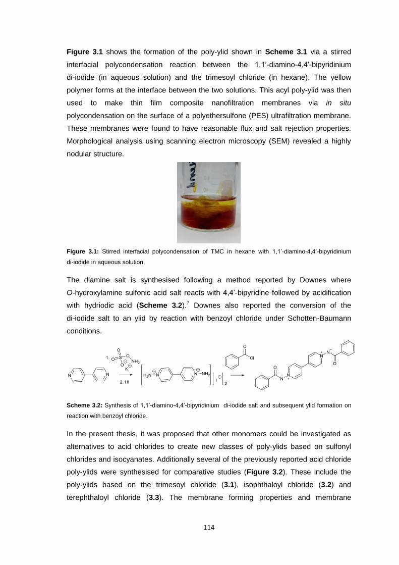
114
Figure 3.1 shows the formation of the poly-ylid shown in Scheme 3.1 via a stirred
interfacial polycondensation reaction between the 1,1’-diamino-4,4’-bipyridinium
di-iodide (in aqueous solution) and the trimesoyl chloride (in hexane). The yellow
polymer forms at the interface between the two solutions. This acyl poly-ylid was then
used to make thin film composite nanofiltration membranes via in situ
polycondensation on the surface of a polyethersulfone (PES) ultrafiltration membrane.
These membranes were found to have reasonable flux and salt rejection properties.
Morphological analysis using scanning electron microscopy (SEM) revealed a highly
nodular structure.
Figure 3.1: Stirred interfacial polycondensation of TMC in hexane with 1,1’-diamino-4,4’-bipyridinium
di-iodide in aqueous solution.
The diamine salt is synthesised following a method reported by Downes where
O-hydroxylamine sulfonic acid salt reacts with 4,4’-bipyridine followed by acidification
with hydriodic acid (Scheme 3.2).7 Downes also reported the conversion of the
di-iodide salt to an ylid by reaction with benzoyl chloride under Schotten-Baumann
conditions.
Scheme 3.2: Synthesis of 1,1’-diamino-4,4’-bipyridinium di-iodide salt and subsequent ylid formation on
reaction with benzoyl chloride.
In the present thesis, it was proposed that other monomers could be investigated as
alternatives to acid chlorides to create new classes of poly-ylids based on sulfonyl
chlorides and isocyanates. Additionally several of the previously reported acid chloride
poly-ylids were synthesised for comparative studies (Figure 3.2). These include the
poly-ylids based on the trimesoyl chloride (3.1), isophthaloyl chloride (3.2) and
terephthaloyl chloride (3.3). The membrane forming properties and membrane
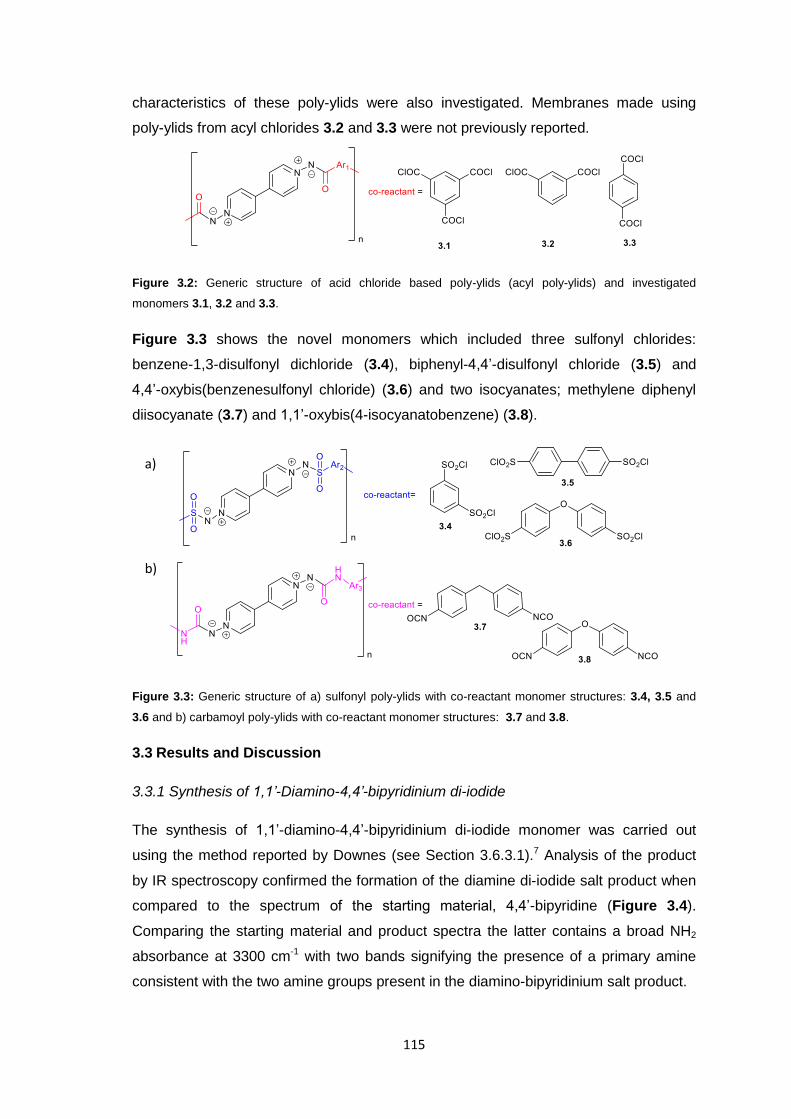
115
characteristics of these poly-ylids were also investigated. Membranes made using
poly-ylids from acyl chlorides 3.2 and 3.3 were not previously reported.
Figure 3.2: Generic structure of acid chloride based poly-ylids (acyl poly-ylids) and investigated
monomers 3.1, 3.2 and 3.3.
Figure 3.3 shows the novel monomers which included three sulfonyl chlorides:
benzene-1,3-disulfonyl dichloride (3.4), biphenyl-4,4’-disulfonyl chloride (3.5) and
4,4’-oxybis(benzenesulfonyl chloride) (3.6) and two isocyanates; methylene diphenyl
diisocyanate (3.7) and 1,1’-oxybis(4-isocyanatobenzene) (3.8).
Figure 3.3: Generic structure of a) sulfonyl poly-ylids with co-reactant monomer structures: 3.4, 3.5 and
3.6 and b) carbamoyl poly-ylids with co-reactant monomer structures: 3.7 and 3.8.
3.3 Results and Discussion
3.3.1 Synthesis of 1,1’-Diamino-4,4’-bipyridinium di-iodide
The synthesis of 1,1’-diamino-4,4’-bipyridinium di-iodide monomer was carried out
using the method reported by Downes (see Section 3.6.3.1).7 Analysis of the product
by IR spectroscopy confirmed the formation of the diamine di-iodide salt product when
compared to the spectrum of the starting material, 4,4’-bipyridine (Figure 3.4).
Comparing the starting material and product spectra the latter contains a broad NH2
absorbance at 3300 cm-1 with two bands signifying the presence of a primary amine
consistent with the two amine groups present in the diamino-bipyridinium salt product.
a)
b)
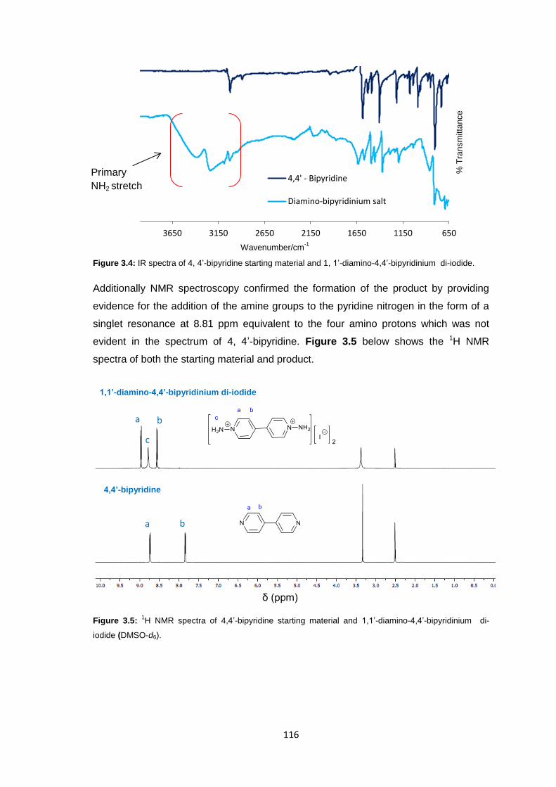
116
Figure 3.4: IR spectra of 4, 4’-bipyridine starting material and 1, 1’-diamino-4,4’-bipyridinium di-iodide.
Additionally NMR spectroscopy confirmed the formation of the product by providing
evidence for the addition of the amine groups to the pyridine nitrogen in the form of a
singlet resonance at 8.81 ppm equivalent to the four amino protons which was not
evident in the spectrum of 4, 4’-bipyridine. Figure 3.5 below shows the 1H NMR
spectra of both the starting material and product.
Figure 3.5: 1H NMR spectra of 4,4’-bipyridine starting material and 1,1’-diamino-4,4’-bipyridinium di-
iodide (DMSO-d6).
650115016502150265031503650
4,4' - Bipyridine
Diamino-bipyridinium salt
Primary
NH2 stretch
a
a b
c
b
% T
ran
sm
itta
nce
Wavenumber/cm-1
δ (ppm)
1,1’-diamino-4,4’-bipyridinium di-iodide
4,4’-bipyridine
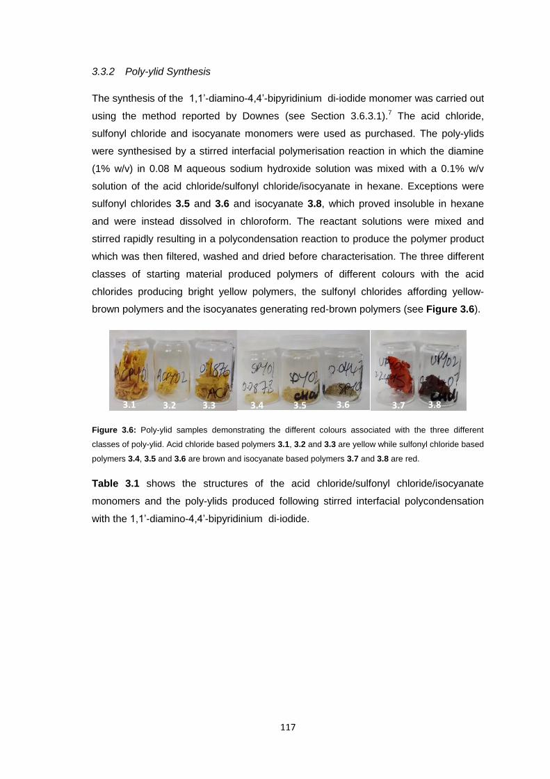
117
3.3.2 Poly-ylid Synthesis
The synthesis of the 1,1’-diamino-4,4’-bipyridinium di-iodide monomer was carried out
using the method reported by Downes (see Section 3.6.3.1).7 The acid chloride,
sulfonyl chloride and isocyanate monomers were used as purchased. The poly-ylids
were synthesised by a stirred interfacial polymerisation reaction in which the diamine
(1% w/v) in 0.08 M aqueous sodium hydroxide solution was mixed with a 0.1% w/v
solution of the acid chloride/sulfonyl chloride/isocyanate in hexane. Exceptions were
sulfonyl chlorides 3.5 and 3.6 and isocyanate 3.8, which proved insoluble in hexane
and were instead dissolved in chloroform. The reactant solutions were mixed and
stirred rapidly resulting in a polycondensation reaction to produce the polymer product
which was then filtered, washed and dried before characterisation. The three different
classes of starting material produced polymers of different colours with the acid
chlorides producing bright yellow polymers, the sulfonyl chlorides affording yellow-
brown polymers and the isocyanates generating red-brown polymers (see Figure 3.6).
Figure 3.6: Poly-ylid samples demonstrating the different colours associated with the three different
classes of poly-ylid. Acid chloride based polymers 3.1, 3.2 and 3.3 are yellow while sulfonyl chloride based
polymers 3.4, 3.5 and 3.6 are brown and isocyanate based polymers 3.7 and 3.8 are red.
Table 3.1 shows the structures of the acid chloride/sulfonyl chloride/isocyanate
monomers and the poly-ylids produced following stirred interfacial polycondensation
with the 1,1’-diamino-4,4’-bipyridinium di-iodide.
3.1 3.2 3.3 3.4 3.5 3.6 3.7 3.8
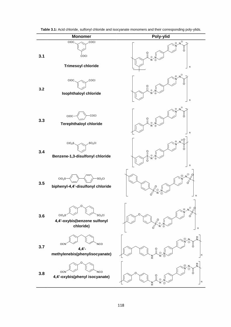
118
Table 3.1: Acid chloride, sulfonyl chloride and isocyanate monomers and their corresponding poly-ylids.
Monomer Poly-ylid
3.1
Trimesoyl chloride
3.2
Isophthaloyl chloride
3.3
Terephthaloyl chloride
3.4
Benzene-1,3-disulfonyl chloride
3.5
biphenyl-4,4’-disulfonyl chloride
3.6
4,4’-oxybis(benzene sulfonyl
chloride)
3.7
4,4’-
methylenebis(phenylisocyanate)
3.8 4,4’-oxybis(phenyl isocyanate)
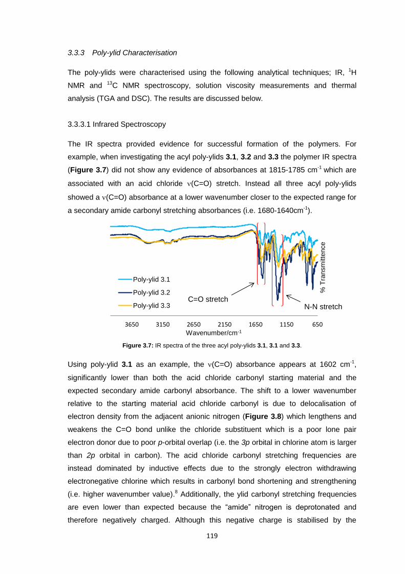
119
3.3.3 Poly-ylid Characterisation
The poly-ylids were characterised using the following analytical techniques; IR, 1H
NMR and 13C NMR spectroscopy, solution viscosity measurements and thermal
analysis (TGA and DSC). The results are discussed below.
3.3.3.1 Infrared Spectroscopy
The IR spectra provided evidence for successful formation of the polymers. For
example, when investigating the acyl poly-ylids 3.1, 3.2 and 3.3 the polymer IR spectra
(Figure 3.7) did not show any evidence of absorbances at 1815-1785 cm-1 which are
associated with an acid chloride (C=O) stretch. Instead all three acyl poly-ylids
showed a (C=O) absorbance at a lower wavenumber closer to the expected range for
a secondary amide carbonyl stretching absorbances (i.e. 1680-1640cm-1).
Figure 3.7: IR spectra of the three acyl poly-ylids 3.1, 3.1 and 3.3.
Using poly-ylid 3.1 as an example, the (C=O) absorbance appears at 1602 cm-1,
significantly lower than both the acid chloride carbonyl starting material and the
expected secondary amide carbonyl absorbance. The shift to a lower wavenumber
relative to the starting material acid chloride carbonyl is due to delocalisation of
electron density from the adjacent anionic nitrogen (Figure 3.8) which lengthens and
weakens the C=O bond unlike the chloride substituent which is a poor lone pair
electron donor due to poor p-orbital overlap (i.e. the 3p orbital in chlorine atom is larger
than 2p orbital in carbon). The acid chloride carbonyl stretching frequencies are
instead dominated by inductive effects due to the strongly electron withdrawing
electronegative chlorine which results in carbonyl bond shortening and strengthening
(i.e. higher wavenumber value).8 Additionally, the ylid carbonyl stretching frequencies
are even lower than expected because the “amide” nitrogen is deprotonated and
therefore negatively charged. Although this negative charge is stabilised by the
650115016502150265031503650%
Tra
nsm
itte
nce
Wavenumber/cm-1
Poly-ylid 3.1
Poly-ylid 3.2
Poly-ylid 3.3C=O stretch
N-N stretch
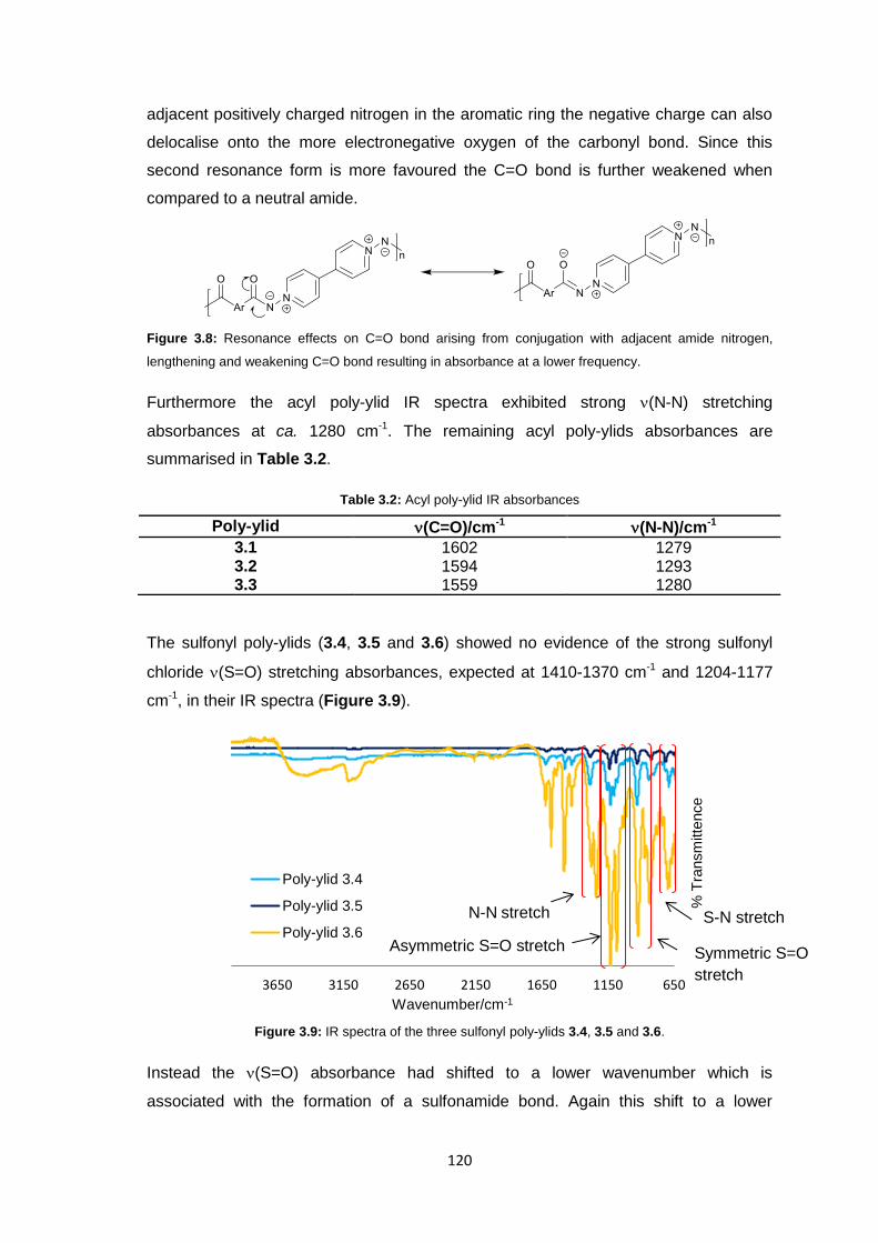
120
adjacent positively charged nitrogen in the aromatic ring the negative charge can also
delocalise onto the more electronegative oxygen of the carbonyl bond. Since this
second resonance form is more favoured the C=O bond is further weakened when
compared to a neutral amide.
Figure 3.8: Resonance effects on C=O bond arising from conjugation with adjacent amide nitrogen,
lengthening and weakening C=O bond resulting in absorbance at a lower frequency.
Furthermore the acyl poly-ylid IR spectra exhibited strong (N-N) stretching
absorbances at ca. 1280 cm-1. The remaining acyl poly-ylids absorbances are
summarised in Table 3.2.
Table 3.2: Acyl poly-ylid IR absorbances
Poly-ylid (C=O)/cm-1 (N-N)/cm-1
3.1 1602 1279 3.2 1594 1293 3.3 1559 1280
The sulfonyl poly-ylids (3.4, 3.5 and 3.6) showed no evidence of the strong sulfonyl
chloride (S=O) stretching absorbances, expected at 1410-1370 cm-1 and 1204-1177
cm-1, in their IR spectra (Figure 3.9).
Figure 3.9: IR spectra of the three sulfonyl poly-ylids 3.4, 3.5 and 3.6.
Instead the (S=O) absorbance had shifted to a lower wavenumber which is
associated with the formation of a sulfonamide bond. Again this shift to a lower
650115016502150265031503650
% T
ransm
itte
nce
Wavenumber/cm-1
Poly-ylid 3.4
Poly-ylid 3.5
Poly-ylid 3.6S-N stretch
Asymmetric S=O stretch
N-N stretch
Symmetric S=O
stretch
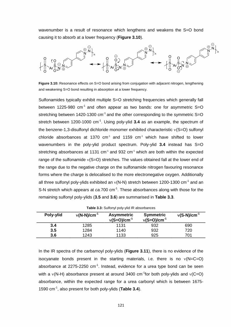
121
wavenumber is a result of resonance which lengthens and weakens the S=O bond
causing it to absorb at a lower frequency (Figure 3.10).
Figure 3.10: Resonance effects on S=O bond arising from conjugation with adjacent nitrogen, lengthening
and weakening S=O bond resulting in absorption at a lower frequency.
Sulfonamides typically exhibit multiple S=O stretching frequencies which generally fall
between 1225-980 cm-1 and often appear as two bands: one for asymmetric S=O
stretching between 1420-1300 cm-1 and the other corresponding to the symmetric S=O
stretch between 1200-1000 cm-1. Using poly-ylid 3.4 as an example, the spectrum of
the benzene-1,3-disulfonyl dichloride monomer exhibited characteristic (S=O) sulfonyl
chloride absorbances at 1370 cm-1 and 1159 cm-1
which have shifted to lower
wavenumbers in the poly-ylid product spectrum. Poly-ylid 3.4 instead has S=O
stretching absorbances at 1131 cm-1 and 932 cm-1
which are both within the expected
range of the sulfonamide (S=O) stretches. The values obtained fall at the lower end of
the range due to the negative charge on the sulfonamide nitrogen favouring resonance
forms where the charge is delocalised to the more electronegative oxygen. Additionally
all three sulfonyl poly-ylids exhibited an (N-N) stretch between 1200-1300 cm-1 and an
S-N stretch which appears at ca.700 cm-1. These absorbances along with those for the
remaining sulfonyl poly-ylids (3.5 and 3.6) are summarised in Table 3.3.
Table 3.3: Sulfonyl poly-ylid IR absorbances
Poly-ylid (N-N)/cm-1 Asymmetric
(S=O)/cm-1
Symmetric
(S=O)/cm-1 (S-N)/cm-1
3.4 1285 1131 932 690 3.5 1284 1140 932 720 3.6 1243 1133 925 701
In the IR spectra of the carbamoyl poly-ylids (Figure 3.11), there is no evidence of the
isocyanate bonds present in the starting materials, i.e. there is no (N=C=O)
absorbance at 2275-2250 cm-1. Instead, evidence for a urea type bond can be seen
with a (N-H) absorbance present at around 3400 cm-1for both poly-ylids and (C=O)
absorbance, within the expected range for a urea carbonyl which is between 1675-
1590 cm-1, also present for both poly-ylids (Table 3.4).
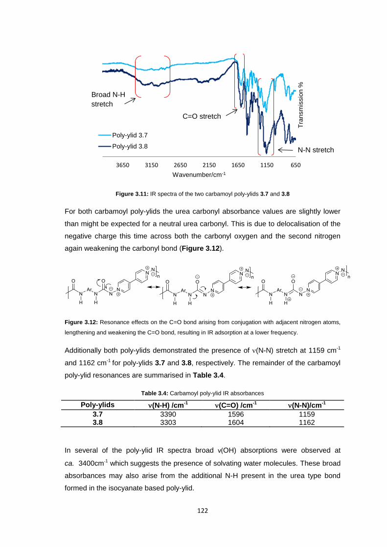
122
Figure 3.11: IR spectra of the two carbamoyl poly-ylids 3.7 and 3.8
For both carbamoyl poly-ylids the urea carbonyl absorbance values are slightly lower
than might be expected for a neutral urea carbonyl. This is due to delocalisation of the
negative charge this time across both the carbonyl oxygen and the second nitrogen
again weakening the carbonyl bond (Figure 3.12).
Figure 3.12: Resonance effects on the C=O bond arising from conjugation with adjacent nitrogen atoms,
lengthening and weakening the C=O bond, resulting in IR adsorption at a lower frequency.
Additionally both poly-ylids demonstrated the presence of (N-N) stretch at 1159 cm-1
and 1162 cm-1 for poly-ylids 3.7 and 3.8, respectively. The remainder of the carbamoyl
poly-ylid resonances are summarised in Table 3.4.
Table 3.4: Carbamoyl poly-ylid IR absorbances
Poly-ylids (N-H) /cm-1 (C=O) /cm-1 (N-N)/cm-1
3.7 3390 1596 1159 3.8 3303 1604 1162
In several of the poly-ylid IR spectra broad ν(OH) absorptions were observed at
ca. 3400cm-1 which suggests the presence of solvating water molecules. These broad
absorbances may also arise from the additional N-H present in the urea type bond
formed in the isocyanate based poly-ylid.
650115016502150265031503650
Tra
nsm
issio
n %
Wavenumber/cm-1
Poly-ylid 3.7
Poly-ylid 3.8
C=O stretch
N-N stretch
Broad N-H
stretch
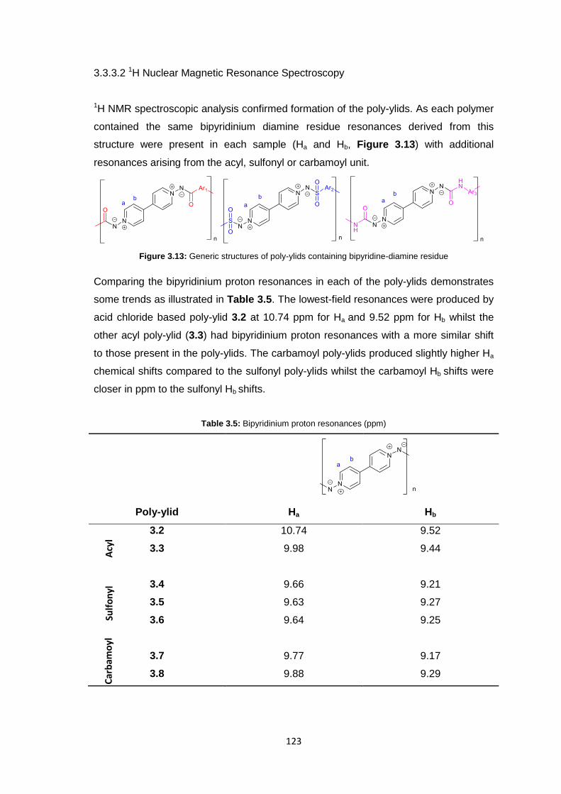
123
3.3.3.2 1H Nuclear Magnetic Resonance Spectroscopy
1H NMR spectroscopic analysis confirmed formation of the poly-ylids. As each polymer
contained the same bipyridinium diamine residue resonances derived from this
structure were present in each sample (Ha and Hb, Figure 3.13) with additional
resonances arising from the acyl, sulfonyl or carbamoyl unit.
Figure 3.13: Generic structures of poly-ylids containing bipyridine-diamine residue
Comparing the bipyridinium proton resonances in each of the poly-ylids demonstrates
some trends as illustrated in Table 3.5. The lowest-field resonances were produced by
acid chloride based poly-ylid 3.2 at 10.74 ppm for Ha and 9.52 ppm for Hb whilst the
other acyl poly-ylid (3.3) had bipyridinium proton resonances with a more similar shift
to those present in the poly-ylids. The carbamoyl poly-ylids produced slightly higher Ha
chemical shifts compared to the sulfonyl poly-ylids whilst the carbamoyl Hb shifts were
closer in ppm to the sulfonyl Hb shifts.
Table 3.5: Bipyridinium proton resonances (ppm)
Poly-ylid Ha Hb
3.2 10.74 9.52
3.3 9.98 9.44
3.4 9.66 9.21
3.5 9.63 9.27
3.6 9.64 9.25
3.7 9.77 9.17
3.8 9.88 9.29
Acy
l Su
lfo
nyl
C
arb
amo
yl
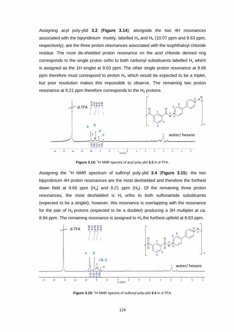
124
Assigning acyl poly-ylid 3.2 (Figure 3.14); alongside the two 4H resonances
associated with the bipyridinium moiety, labelled Ha and Hb (10.07 ppm and 9.63 ppm,
respectively), are the three proton resonances associated with the isophthaloyl chloride
residue. The most de-shielded proton resonance on the acid chloride derived ring
corresponds to the single proton ortho to both carbonyl substituents labelled Hc which
is assigned as the 1H singlet at 9.63 ppm. The other single proton resonance at 8.66
ppm therefore must correspond to proton He which would be expected to be a triplet,
but poor resolution makes this impossible to observe. The remaining two proton
resonance at 9.21 ppm therefore corresponds to the Hd protons.
Figure 3.14: 1H NMR spectra of acyl poly-ylid 3.2 in d-TFA.
Assigning the 1H NMR spectrum of sulfonyl poly-ylid 3.4 (Figure 3.15); the two
bipyridinium 4H proton resonances are the most deshielded and therefore the furthest
down field at 9.66 ppm (Ha) and 9.21 ppm (Hb). Of the remaining three proton
resonances, the most deshielded is Hc ortho to both sulfonamide substituents
(expected to be a singlet), however, this resonance is overlapping with the resonance
for the pair of Hd protons (expected to be a doublet) producing a 3H multiplet at ca.
8.94 ppm. The remaining resonance is assigned to He the furthest upfield at 8.63 ppm.
Figure 3.15: 1H NMR spectra of sulfonyl poly-ylid 3.4 in d-TFA.
a d
e c
b
a b
c& d
e
water/ hexane
d-TFA
water/ hexane
d-TFA
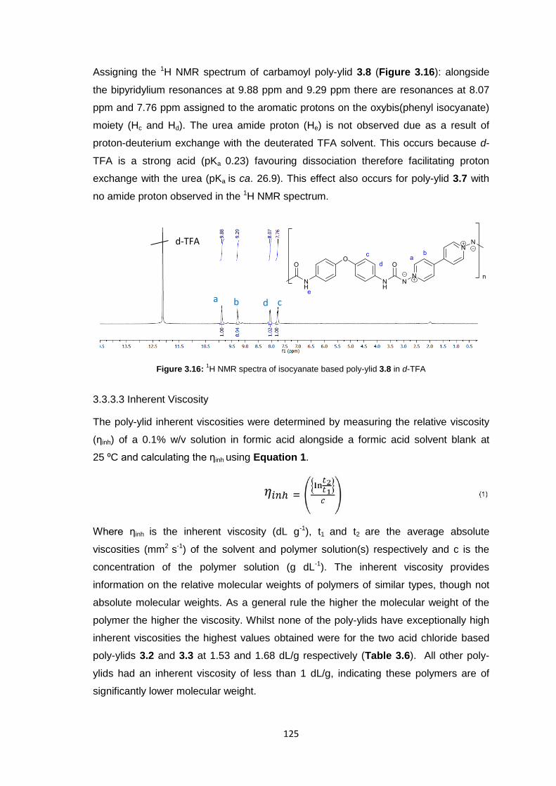
125
Assigning the 1H NMR spectrum of carbamoyl poly-ylid 3.8 (Figure 3.16): alongside
the bipyridylium resonances at 9.88 ppm and 9.29 ppm there are resonances at 8.07
ppm and 7.76 ppm assigned to the aromatic protons on the oxybis(phenyl isocyanate)
moiety (Hc and Hd). The urea amide proton (He) is not observed due as a result of
proton-deuterium exchange with the deuterated TFA solvent. This occurs because d-
TFA is a strong acid (pKa 0.23) favouring dissociation therefore facilitating proton
exchange with the urea (pKa is ca. 26.9). This effect also occurs for poly-ylid 3.7 with
no amide proton observed in the 1H NMR spectrum.
Figure 3.16: 1H NMR spectra of isocyanate based poly-ylid 3.8 in d-TFA
3.3.3.3 Inherent Viscosity
The poly-ylid inherent viscosities were determined by measuring the relative viscosity
(ηinh) of a 0.1% w/v solution in formic acid alongside a formic acid solvent blank at
25 ⁰C and calculating the ηinh using Equation 1.
Where ηinh is the inherent viscosity (dL g-1), t1 and t2 are the average absolute
viscosities (mm2 s-1) of the solvent and polymer solution(s) respectively and c is the
concentration of the polymer solution (g dL-1). The inherent viscosity provides
information on the relative molecular weights of polymers of similar types, though not
absolute molecular weights. As a general rule the higher the molecular weight of the
polymer the higher the viscosity. Whilst none of the poly-ylids have exceptionally high
inherent viscosities the highest values obtained were for the two acid chloride based
poly-ylids 3.2 and 3.3 at 1.53 and 1.68 dL/g respectively (Table 3.6). All other poly-
ylids had an inherent viscosity of less than 1 dL/g, indicating these polymers are of
significantly lower molecular weight.
c d a b
d-TFA
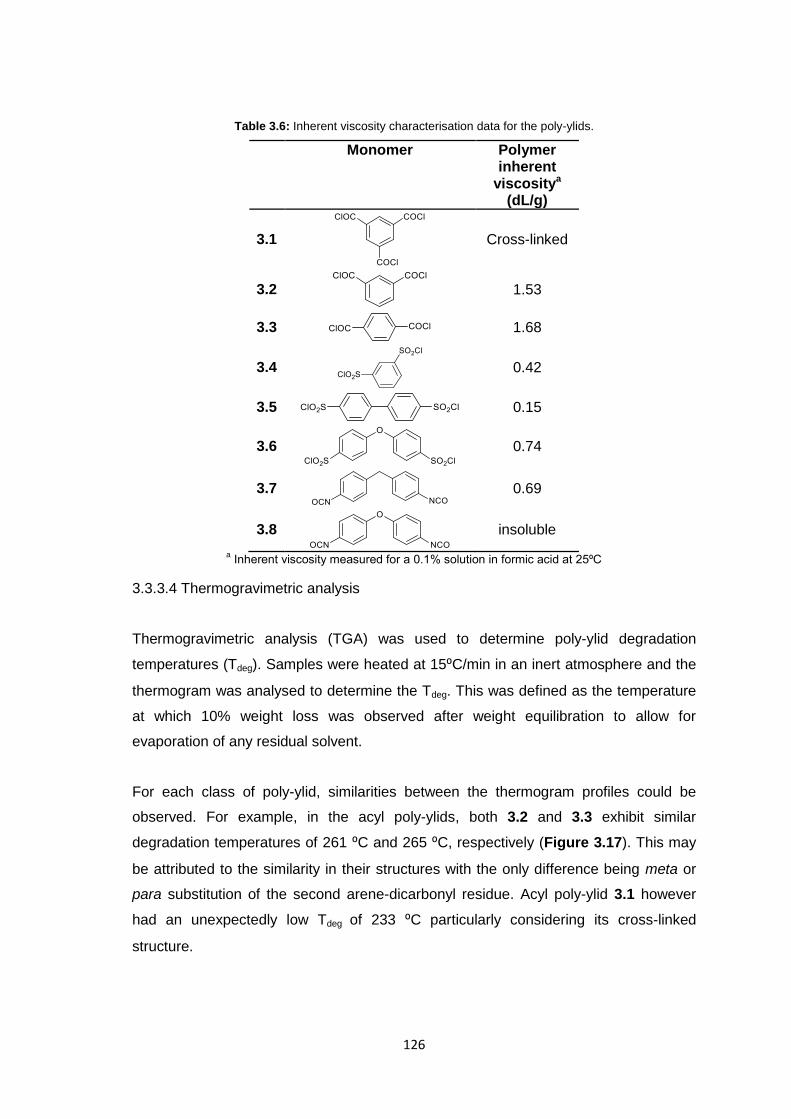
126
Table 3.6: Inherent viscosity characterisation data for the poly-ylids.
Monomer Polymer inherent
viscositya
(dL/g)
3.1
Cross-linked
3.2
1.53
3.3
1.68
3.4
0.42
3.5
0.15
3.6
0.74
3.7
0.69
3.8
insoluble
a Inherent viscosity measured for a 0.1% solution in formic acid at 25⁰C
3.3.3.4 Thermogravimetric analysis
Thermogravimetric analysis (TGA) was used to determine poly-ylid degradation
temperatures (Tdeg). Samples were heated at 15⁰C/min in an inert atmosphere and the
thermogram was analysed to determine the Tdeg. This was defined as the temperature
at which 10% weight loss was observed after weight equilibration to allow for
evaporation of any residual solvent.
For each class of poly-ylid, similarities between the thermogram profiles could be
observed. For example, in the acyl poly-ylids, both 3.2 and 3.3 exhibit similar
degradation temperatures of 261 ⁰C and 265 ⁰C, respectively (Figure 3.17). This may
be attributed to the similarity in their structures with the only difference being meta or
para substitution of the second arene-dicarbonyl residue. Acyl poly-ylid 3.1 however
had an unexpectedly low Tdeg of 233 ⁰C particularly considering its cross-linked
structure.
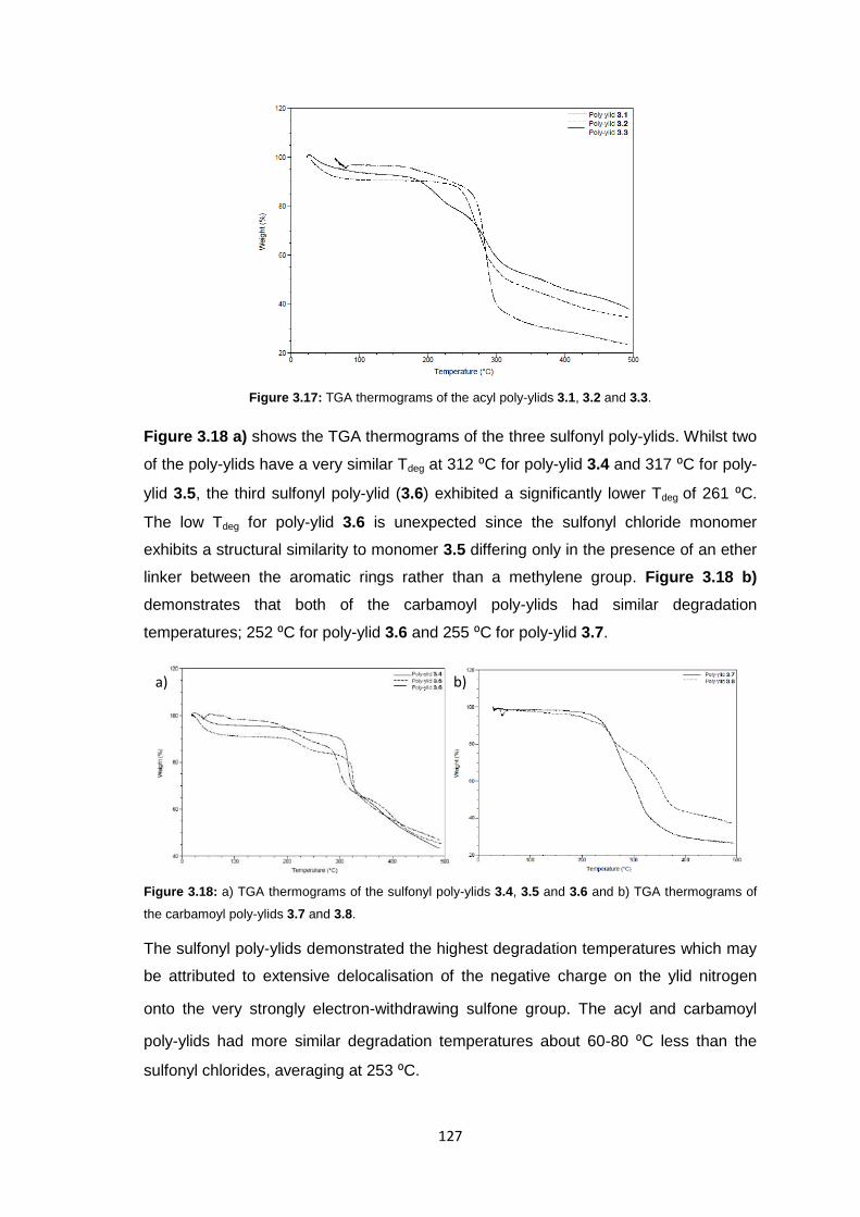
127
Figure 3.17: TGA thermograms of the acyl poly-ylids 3.1, 3.2 and 3.3.
Figure 3.18 a) shows the TGA thermograms of the three sulfonyl poly-ylids. Whilst two
of the poly-ylids have a very similar Tdeg at 312 ⁰C for poly-ylid 3.4 and 317 ⁰C for poly-
ylid 3.5, the third sulfonyl poly-ylid (3.6) exhibited a significantly lower Tdeg of 261 ⁰C.
The low Tdeg for poly-ylid 3.6 is unexpected since the sulfonyl chloride monomer
exhibits a structural similarity to monomer 3.5 differing only in the presence of an ether
linker between the aromatic rings rather than a methylene group. Figure 3.18 b)
demonstrates that both of the carbamoyl poly-ylids had similar degradation
temperatures; 252 ⁰C for poly-ylid 3.6 and 255 ⁰C for poly-ylid 3.7.
Figure 3.18: a) TGA thermograms of the sulfonyl poly-ylids 3.4, 3.5 and 3.6 and b) TGA thermograms of
the carbamoyl poly-ylids 3.7 and 3.8.
The sulfonyl poly-ylids demonstrated the highest degradation temperatures which may
be attributed to extensive delocalisation of the negative charge on the ylid nitrogen
onto the very strongly electron-withdrawing sulfone group. The acyl and carbamoyl
poly-ylids had more similar degradation temperatures about 60-80 ⁰C less than the
sulfonyl chlorides, averaging at 253 ⁰C.
a) b)
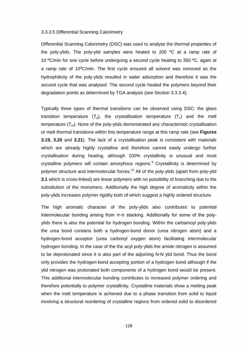
128
3.3.3.5 Differential Scanning Calorimetry
Differential Scanning Calorimetry (DSC) was used to analyse the thermal properties of
the poly-ylids. The poly-ylid samples were heated to 200 ⁰C at a ramp rate of
10 ⁰C/min for one cycle before undergoing a second cycle heating to 350 ⁰C, again at
a ramp rate of 10⁰C/min. The first cycle ensured all solvent was removed as the
hydrophilicity of the poly-ylids resulted in water adsorption and therefore it was the
second cycle that was analysed. The second cycle heated the polymers beyond their
degradation points as determined by TGA analysis (see Section 3.3.3.4).
Typically three types of thermal transitions can be observed using DSC: the glass
transition temperature (Tg), the crystallisation temperature (Tc) and the melt
temperature (Tm). None of the poly-ylids demonstrated any characteristic crystallisation
or melt thermal transitions within this temperature range at this ramp rate (see Figures
3.19, 3.20 and 3.21). The lack of a crystallisation peak is consistent with materials
which are already highly crystalline and therefore cannot easily undergo further
crystallisation during heating, although 100% crystallinity is unusual and most
crystalline polymers will contain amorphous regions.9 Crystallinity is determined by
polymer structure and intermolecular forces.10 All of the poly-ylids (apart from poly-ylid
3.1 which is cross-linked) are linear polymers with no possibility of branching due to the
substitution of the monomers. Additionally the high degree of aromaticity within the
poly-ylids increases polymer rigidity both of which suggest a highly ordered structure.
The high aromatic character of the poly-ylids also contributes to potential
intermolecular bonding arising from π-π stacking. Additionally for some of the poly-
ylids there is also the potential for hydrogen bonding. Within the carbamoyl poly-ylids
the urea bond contains both a hydrogen-bond donor (urea nitrogen atom) and a
hydrogen-bond acceptor (urea carbonyl oxygen atom) facilitating intermolecular
hydrogen bonding. In the case of the the acyl poly-ylids the amide nitrogen is assumed
to be deprotonated since it is also part of the adjoining N-N ylid bond. Thus the bond
only provides the hydrogen-bond accepting portion of a hydrogen bond although if the
ylid nitrogen was protonated both components of a hydrogen bond would be present.
This additional intermolecular bonding contributes to increased polymer ordering and
therefore potentially to polymer crystallinity. Crystalline materials show a melting peak
when the melt temperature is achieved due to a phase transition from solid to liquid
involving a structural reordering of crystalline regions from ordered solid to disordered
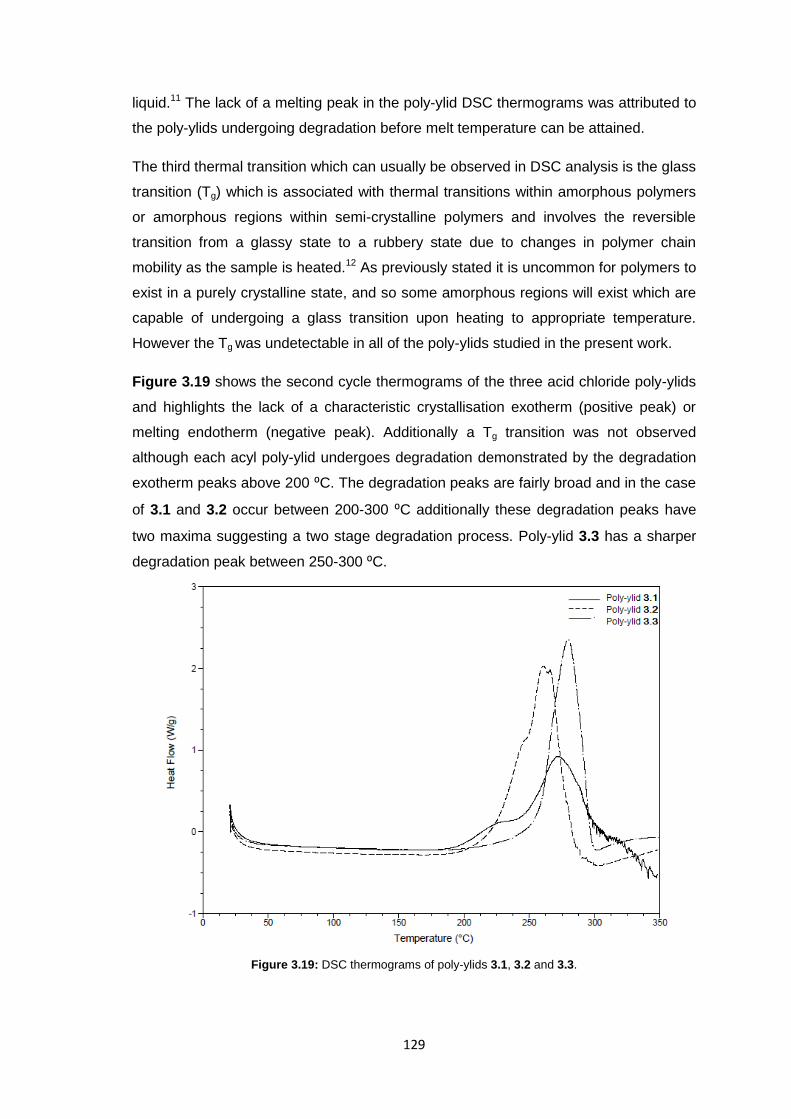
129
liquid.11 The lack of a melting peak in the poly-ylid DSC thermograms was attributed to
the poly-ylids undergoing degradation before melt temperature can be attained.
The third thermal transition which can usually be observed in DSC analysis is the glass
transition (Tg) which is associated with thermal transitions within amorphous polymers
or amorphous regions within semi-crystalline polymers and involves the reversible
transition from a glassy state to a rubbery state due to changes in polymer chain
mobility as the sample is heated.12 As previously stated it is uncommon for polymers to
exist in a purely crystalline state, and so some amorphous regions will exist which are
capable of undergoing a glass transition upon heating to appropriate temperature.
However the Tg was undetectable in all of the poly-ylids studied in the present work.
Figure 3.19 shows the second cycle thermograms of the three acid chloride poly-ylids
and highlights the lack of a characteristic crystallisation exotherm (positive peak) or
melting endotherm (negative peak). Additionally a Tg transition was not observed
although each acyl poly-ylid undergoes degradation demonstrated by the degradation
exotherm peaks above 200 ⁰C. The degradation peaks are fairly broad and in the case
of 3.1 and 3.2 occur between 200-300 ⁰C additionally these degradation peaks have
two maxima suggesting a two stage degradation process. Poly-ylid 3.3 has a sharper
degradation peak between 250-300 ⁰C.
Figure 3.19: DSC thermograms of poly-ylids 3.1, 3.2 and 3.3.
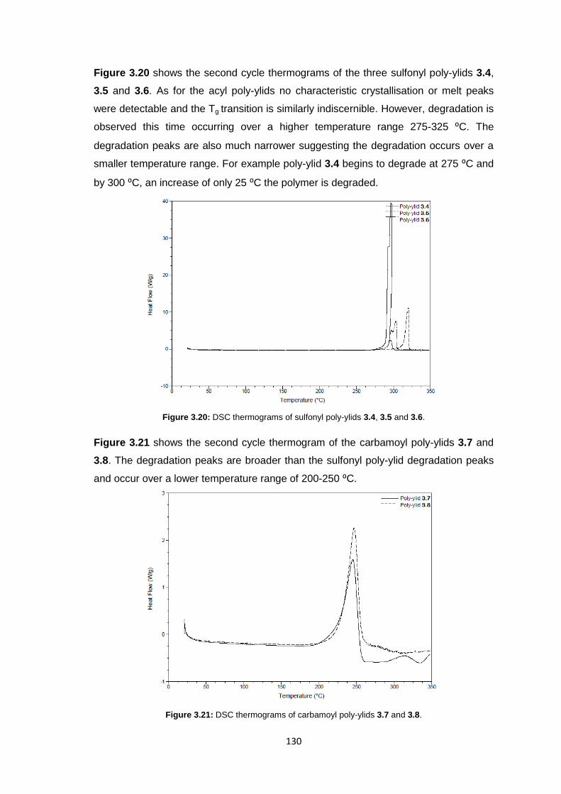
130
Figure 3.20 shows the second cycle thermograms of the three sulfonyl poly-ylids 3.4,
3.5 and 3.6. As for the acyl poly-ylids no characteristic crystallisation or melt peaks
were detectable and the Tg transition is similarly indiscernible. However, degradation is
observed this time occurring over a higher temperature range 275-325 ⁰C. The
degradation peaks are also much narrower suggesting the degradation occurs over a
smaller temperature range. For example poly-ylid 3.4 begins to degrade at 275 ⁰C and
by 300 ⁰C, an increase of only 25 ⁰C the polymer is degraded.
Figure 3.20: DSC thermograms of sulfonyl poly-ylids 3.4, 3.5 and 3.6.
Figure 3.21 shows the second cycle thermogram of the carbamoyl poly-ylids 3.7 and
3.8. The degradation peaks are broader than the sulfonyl poly-ylid degradation peaks
and occur over a lower temperature range of 200-250 ⁰C.
Figure 3.21: DSC thermograms of carbamoyl poly-ylids 3.7 and 3.8.
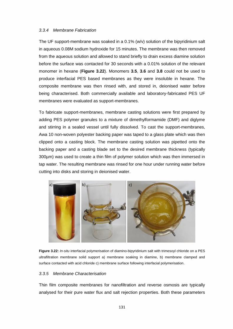
131
3.3.4 Membrane Fabrication
The UF support-membrane was soaked in a 0.1% (w/v) solution of the bipyridinium salt
in aqueous 0.08M sodium hydroxide for 15 minutes. The membrane was then removed
from the aqueous solution and allowed to stand briefly to drain excess diamine solution
before the surface was contacted for 30 seconds with a 0.01% solution of the relevant
monomer in hexane (Figure 3.22). Monomers 3.5, 3.6 and 3.8 could not be used to
produce interfacial PES based membranes as they were insoluble in hexane. The
composite membrane was then rinsed with, and stored in, deionised water before
being characterised. Both commercially available and laboratory-fabricated PES UF
membranes were evaluated as support-membranes.
To fabricate support-membranes, membrane casting solutions were first prepared by
adding PES polymer granules to a mixture of dimethylformamide (DMF) and diglyme
and stirring in a sealed vessel until fully dissolved. To cast the support-membranes,
Awa 10 non-woven polyester backing paper was taped to a glass plate which was then
clipped onto a casting block. The membrane casting solution was pipetted onto the
backing paper and a casting blade set to the desired membrane thickness (typically
300µm) was used to create a thin film of polymer solution which was then immersed in
tap water. The resulting membrane was rinsed for one hour under running water before
cutting into disks and storing in deionised water.
Figure 3.22: In-situ interfacial polymerisation of diamino-bipyridinium salt with trimesoyl chloride on a PES
ultrafiltration membrane solid support a) membrane soaking in diamine, b) membrane clamped and
surface contacted with acid chloride c) membrane surface following interfacial polymerisation.
3.3.5 Membrane Characterisation
Thin film composite membranes for nanofiltration and reverse osmosis are typically
analysed for their pure water flux and salt rejection properties. Both these parameters
a) b) c)
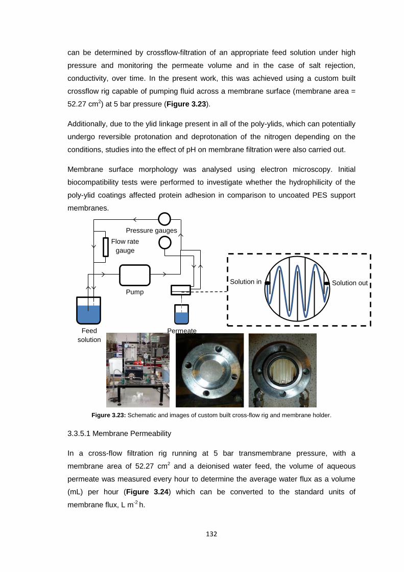
132
can be determined by crossflow-filtration of an appropriate feed solution under high
pressure and monitoring the permeate volume and in the case of salt rejection,
conductivity, over time. In the present work, this was achieved using a custom built
crossflow rig capable of pumping fluid across a membrane surface (membrane area =
52.27 cm2) at 5 bar pressure (Figure 3.23).
Additionally, due to the ylid linkage present in all of the poly-ylids, which can potentially
undergo reversible protonation and deprotonation of the nitrogen depending on the
conditions, studies into the effect of pH on membrane filtration were also carried out.
Membrane surface morphology was analysed using electron microscopy. Initial
biocompatibility tests were performed to investigate whether the hydrophilicity of the
poly-ylid coatings affected protein adhesion in comparison to uncoated PES support
membranes.
Figure 3.23: Schematic and images of custom built cross-flow rig and membrane holder.
3.3.5.1 Membrane Permeability
In a cross-flow filtration rig running at 5 bar transmembrane pressure, with a
membrane area of 52.27 cm2 and a deionised water feed, the volume of aqueous
permeate was measured every hour to determine the average water flux as a volume
(mL) per hour (Figure 3.24) which can be converted to the standard units of
membrane flux, L m-2 h.
Pump
Pressure gauges
Feed
solution
Permeate
Flow rate
gauge
Solution out Solution in
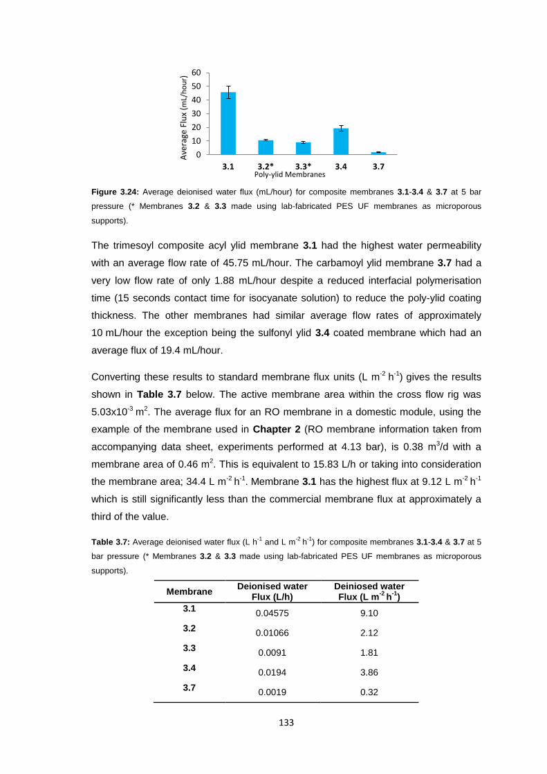
133
Figure 3.24: Average deionised water flux (mL/hour) for composite membranes 3.1-3.4 & 3.7 at 5 bar
pressure (* Membranes 3.2 & 3.3 made using lab-fabricated PES UF membranes as microporous
supports).
The trimesoyl composite acyl ylid membrane 3.1 had the highest water permeability
with an average flow rate of 45.75 mL/hour. The carbamoyl ylid membrane 3.7 had a
very low flow rate of only 1.88 mL/hour despite a reduced interfacial polymerisation
time (15 seconds contact time for isocyanate solution) to reduce the poly-ylid coating
thickness. The other membranes had similar average flow rates of approximately
10 mL/hour the exception being the sulfonyl ylid 3.4 coated membrane which had an
average flux of 19.4 mL/hour.
Converting these results to standard membrane flux units (L m-2 h-1) gives the results
shown in Table 3.7 below. The active membrane area within the cross flow rig was
5.03x10⁻³ m2. The average flux for an RO membrane in a domestic module, using the
example of the membrane used in Chapter 2 (RO membrane information taken from
accompanying data sheet, experiments performed at 4.13 bar), is 0.38 m3/d with a
membrane area of 0.46 m2. This is equivalent to 15.83 L/h or taking into consideration
the membrane area; 34.4 L m-2 h-1. Membrane 3.1 has the highest flux at 9.12 L m-2 h-1
which is still significantly less than the commercial membrane flux at approximately a
third of the value.
Table 3.7: Average deionised water flux (L h-1
and L m-2
h-1
) for composite membranes 3.1-3.4 & 3.7 at 5
bar pressure (* Membranes 3.2 & 3.3 made using lab-fabricated PES UF membranes as microporous
supports).
Membrane Deionised water
Flux (L/h) Deiniosed water Flux (L m
-2 h
-1)
3.1 0.04575 9.10
3.2 0.01066 2.12
3.3 0.0091 1.81
3.4 0.0194 3.86
3.7 0.0019 0.32
0
10
20
30
40
50
60
3.1 3.2* 3.3* 3.4 3.7
Ave
rage
Flu
x (m
L/h
ou
r)
Poly-ylid Membranes
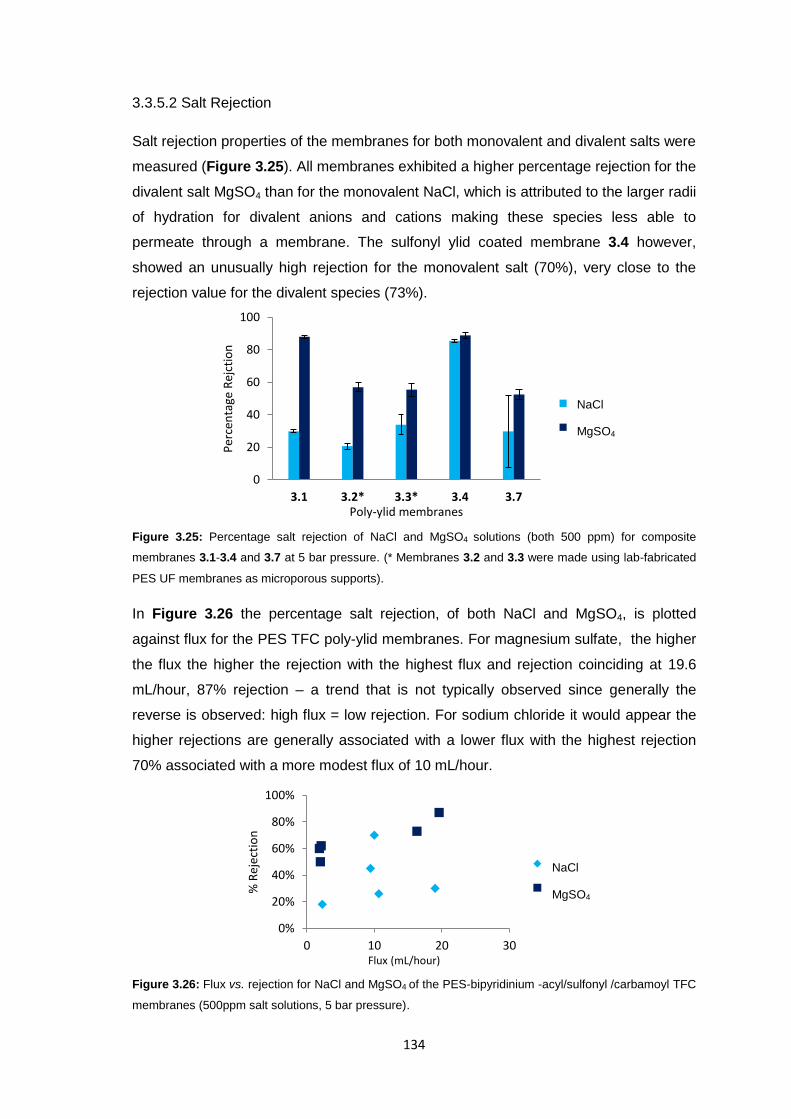
134
3.3.5.2 Salt Rejection
Salt rejection properties of the membranes for both monovalent and divalent salts were
measured (Figure 3.25). All membranes exhibited a higher percentage rejection for the
divalent salt MgSO4 than for the monovalent NaCl, which is attributed to the larger radii
of hydration for divalent anions and cations making these species less able to
permeate through a membrane. The sulfonyl ylid coated membrane 3.4 however,
showed an unusually high rejection for the monovalent salt (70%), very close to the
rejection value for the divalent species (73%).
Figure 3.25: Percentage salt rejection of NaCl and MgSO4 solutions (both 500 ppm) for composite
membranes 3.1-3.4 and 3.7 at 5 bar pressure. (* Membranes 3.2 and 3.3 were made using lab-fabricated
PES UF membranes as microporous supports).
In Figure 3.26 the percentage salt rejection, of both NaCl and MgSO4, is plotted
against flux for the PES TFC poly-ylid membranes. For magnesium sulfate, the higher
the flux the higher the rejection with the highest flux and rejection coinciding at 19.6
mL/hour, 87% rejection – a trend that is not typically observed since generally the
reverse is observed: high flux = low rejection. For sodium chloride it would appear the
higher rejections are generally associated with a lower flux with the highest rejection
70% associated with a more modest flux of 10 mL/hour.
Figure 3.26: Flux vs. rejection for NaCl and MgSO4 of the PES-bipyridinium -acyl/sulfonyl /carbamoyl TFC
membranes (500ppm salt solutions, 5 bar pressure).
0
20
40
60
80
100
3.1 3.2* 3.3* 3.4 3.7
Per
cen
tage
Rej
ctio
n
Poly-ylid membranes
NaCl
MgSO4
0%
20%
40%
60%
80%
100%
0 10 20 30
% R
ejec
tio
n
Flux (mL/hour)
NaCl
MgSO4
NaCl
MgSO4
NaCl
MgSO4
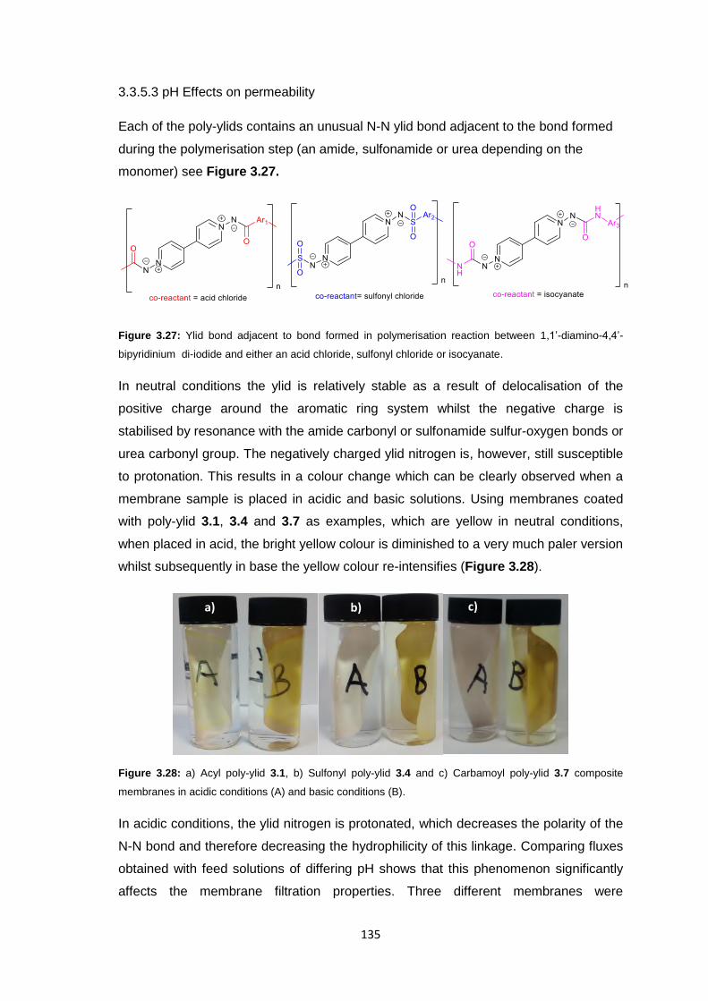
135
3.3.5.3 pH Effects on permeability
Each of the poly-ylids contains an unusual N-N ylid bond adjacent to the bond formed
during the polymerisation step (an amide, sulfonamide or urea depending on the
monomer) see Figure 3.27.
Figure 3.27: Ylid bond adjacent to bond formed in polymerisation reaction between 1,1’-diamino-4,4’-
bipyridinium di-iodide and either an acid chloride, sulfonyl chloride or isocyanate.
In neutral conditions the ylid is relatively stable as a result of delocalisation of the
positive charge around the aromatic ring system whilst the negative charge is
stabilised by resonance with the amide carbonyl or sulfonamide sulfur-oxygen bonds or
urea carbonyl group. The negatively charged ylid nitrogen is, however, still susceptible
to protonation. This results in a colour change which can be clearly observed when a
membrane sample is placed in acidic and basic solutions. Using membranes coated
with poly-ylid 3.1, 3.4 and 3.7 as examples, which are yellow in neutral conditions,
when placed in acid, the bright yellow colour is diminished to a very much paler version
whilst subsequently in base the yellow colour re-intensifies (Figure 3.28).
Figure 3.28: a) Acyl poly-ylid 3.1, b) Sulfonyl poly-ylid 3.4 and c) Carbamoyl poly-ylid 3.7 composite
membranes in acidic conditions (A) and basic conditions (B).
In acidic conditions, the ylid nitrogen is protonated, which decreases the polarity of the
N-N bond and therefore decreasing the hydrophilicity of this linkage. Comparing fluxes
obtained with feed solutions of differing pH shows that this phenomenon significantly
affects the membrane filtration properties. Three different membranes were
a) b) c)
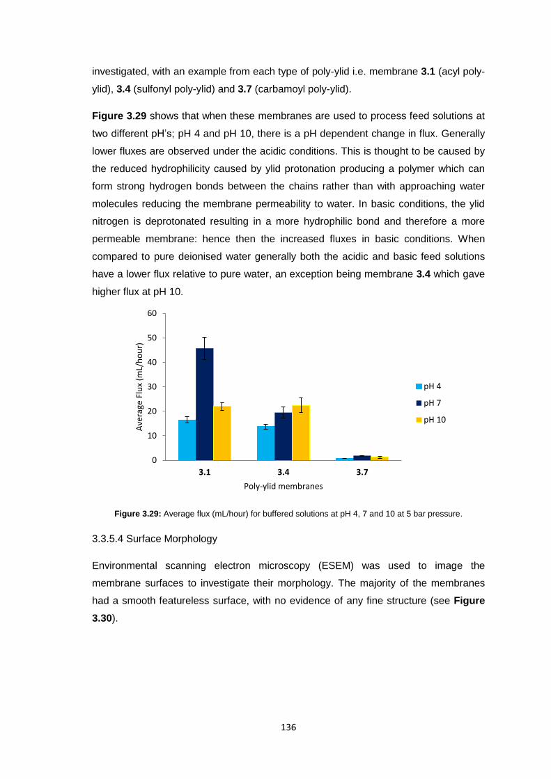
136
investigated, with an example from each type of poly-ylid i.e. membrane 3.1 (acyl poly-
ylid), 3.4 (sulfonyl poly-ylid) and 3.7 (carbamoyl poly-ylid).
Figure 3.29 shows that when these membranes are used to process feed solutions at
two different pH’s; pH 4 and pH 10, there is a pH dependent change in flux. Generally
lower fluxes are observed under the acidic conditions. This is thought to be caused by
the reduced hydrophilicity caused by ylid protonation producing a polymer which can
form strong hydrogen bonds between the chains rather than with approaching water
molecules reducing the membrane permeability to water. In basic conditions, the ylid
nitrogen is deprotonated resulting in a more hydrophilic bond and therefore a more
permeable membrane: hence then the increased fluxes in basic conditions. When
compared to pure deionised water generally both the acidic and basic feed solutions
have a lower flux relative to pure water, an exception being membrane 3.4 which gave
higher flux at pH 10.
Figure 3.29: Average flux (mL/hour) for buffered solutions at pH 4, 7 and 10 at 5 bar pressure.
3.3.5.4 Surface Morphology
Environmental scanning electron microscopy (ESEM) was used to image the
membrane surfaces to investigate their morphology. The majority of the membranes
had a smooth featureless surface, with no evidence of any fine structure (see Figure
3.30).
0
10
20
30
40
50
60
3.1 3.4 3.7
Ave
rage
Flu
x (m
L/h
ou
r)
Poly-ylid membranes
pH 4
pH 7
pH 10
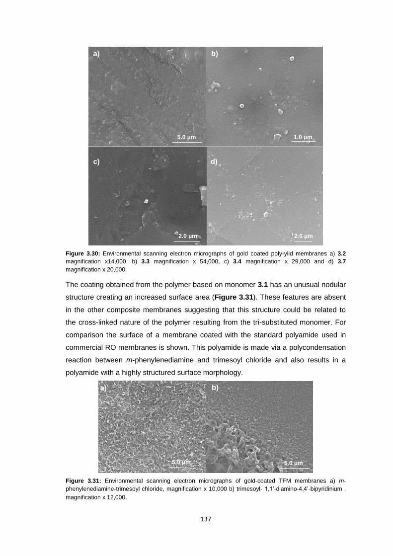
137
Figure 3.30: Environmental scanning electron micrographs of gold coated poly-ylid membranes a) 3.2
magnification x14,000, b) 3.3 magnification x 54,000, c) 3.4 magnification x 29,000 and d) 3.7
magnification x 20,000.
The coating obtained from the polymer based on monomer 3.1 has an unusual nodular
structure creating an increased surface area (Figure 3.31). These features are absent
in the other composite membranes suggesting that this structure could be related to
the cross-linked nature of the polymer resulting from the tri-substituted monomer. For
comparison the surface of a membrane coated with the standard polyamide used in
commercial RO membranes is shown. This polyamide is made via a polycondensation
reaction between m-phenylenediamine and trimesoyl chloride and also results in a
polyamide with a highly structured surface morphology.
Figure 3.31: Environmental scanning electron micrographs of gold-coated TFM membranes a) m-
phenylenediamine-trimesoyl chloride, magnification x 10,000 b) trimesoyl- 1,1’-diamino-4,4’-bipyridinium ,
magnification x 12,000.
a) b)
c) d)
a) b)
5.0 µm 1.0 µm
2.0 µm 2.0 µm
5.0 µm 5.0 µm

138
Blends of monomers 3.1 and 3.4 gave rise to an intermediate structure with nodules
present surrounded by flat featureless surfaces suggesting that perhaps combinations
of monomers could be used to fine tune membrane surface properties as required.
Figure 3.32: Environmental scanning electron micrograph of gold-coated blend composite membrane
(from monomers 3.1 and 3.4, a) 1:1, magnification x 20,000 and b) 2:1, magnification x 6,600.
3.3.5.5 Biocompatibility testing
In order to evaluate the biocompatibility of the poly-ylid coatings, protein adhesion
studies were carried out. Two different plasma proteins were investigated; bovine
serum albumin (BSA) and fibrinogen (FIB). Serum albumin usually makes up
approximately 55% of the blood plasma protein content in humans whilst fibrinogen
represents around 7%.15
To perform the study, coated and uncoated membrane samples were incubated at
37 ⁰C in a 10 mg/mL protein (BSA or fibrinogen) in phosphate buffered (PBS) solution
for 24 hours. Following this the membranes were rinsed to remove any non-adhering
protein and the samples were then heated in sodium dodecyl sulfate (SDS)-hydroxide
to desorb the attached proteins. The resulting supernatant was analysed using the
BCA assay (bicinchoninic acid assay, described in Chapter 2) to determine the protein
concentration present in each sample which was then extrapolated to estimate the
protein concentration per unit membrane area. Control samples in protein-free
solutions (PBS only) were also incubated and assayed. Calculated concentrations
resulting in a ‘negative concentration’ signify zero absorption and therefore zero protein
present.
Figure 3.33 shows the calculated protein concentration (mg/mL) present in 25 µL of
supernatant from the protein denaturation step following 24hrs incubation in a 10
mg/mL BSA solution (69 kDa). The uncoated PES support membrane gave an average
a) b)
2.0 µm 10.0 µm
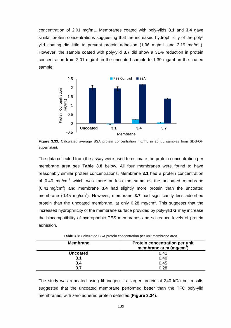
139
concentration of 2.01 mg/mL. Membranes coated with poly-ylids 3.1 and 3.4 gave
similar protein concentrations suggesting that the increased hydrophilicity of the poly-
ylid coating did little to prevent protein adhesion (1.96 mg/mL and 2.19 mg/mL).
However, the sample coated with poly-ylid 3.7 did show a 31% reduction in protein
concentration from 2.01 mg/mL in the uncoated sample to 1.39 mg/mL in the coated
sample.
Figure 3.33: Calculated average BSA protein concentration mg/mL in 25 µL samples from SDS-OH
supernatant.
The data collected from the assay were used to estimate the protein concentration per
membrane area see Table 3.8 below. All four membranes were found to have
reasonably similar protein concentrations. Membrane 3.1 had a protein concentration
of 0.40 mg/cm2 which was more or less the same as the uncoated membrane
(0.41 mg/cm2) and membrane 3.4 had slightly more protein than the uncoated
membrane (0.45 mg/cm2). However, membrane 3.7 had significantly less adsorbed
protein than the uncoated membrane, at only 0.28 mg/cm2. This suggests that the
increased hydrophilicity of the membrane surface provided by poly-ylid G may increase
the biocompatibility of hydrophobic PES membranes and so reduce levels of protein
adhesion.
Table 3.8: Calculated BSA protein concentration per unit membrane area.
Membrane Protein concentration per unit membrane area (mg/cm2)
Uncoated 0.41 3.1 0.40 3.4 0.45 3.7 0.28
The study was repeated using fibrinogen – a larger protein at 340 kDa but results
suggested that the uncoated membrane performed better than the TFC poly-ylid
membranes, with zero adhered protein detected (Figure 3.34).
-0.5
0
0.5
1
1.5
2
2.5
Uncoated 3.1 3.4 3.7
Pro
tein
Co
nce
ntr
atio
n
(mg/
mL)
Membrane
PBS Control BSA
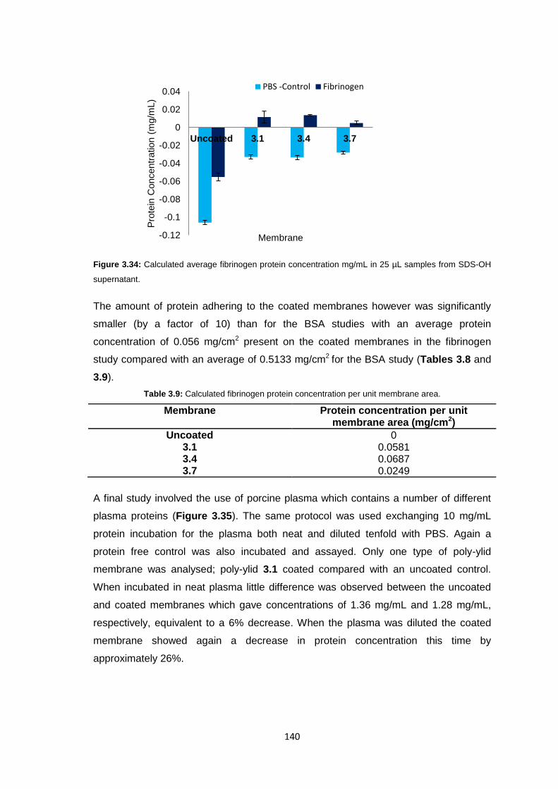
140
Figure 3.34: Calculated average fibrinogen protein concentration mg/mL in 25 µL samples from SDS-OH
supernatant.
The amount of protein adhering to the coated membranes however was significantly
smaller (by a factor of 10) than for the BSA studies with an average protein
concentration of 0.056 mg/cm2 present on the coated membranes in the fibrinogen
study compared with an average of 0.5133 mg/cm2 for the BSA study (Tables 3.8 and
3.9).
Table 3.9: Calculated fibrinogen protein concentration per unit membrane area.
Membrane Protein concentration per unit membrane area (mg/cm2)
Uncoated 0 3.1 0.0581 3.4 0.0687 3.7 0.0249
A final study involved the use of porcine plasma which contains a number of different
plasma proteins (Figure 3.35). The same protocol was used exchanging 10 mg/mL
protein incubation for the plasma both neat and diluted tenfold with PBS. Again a
protein free control was also incubated and assayed. Only one type of poly-ylid
membrane was analysed; poly-ylid 3.1 coated compared with an uncoated control.
When incubated in neat plasma little difference was observed between the uncoated
and coated membranes which gave concentrations of 1.36 mg/mL and 1.28 mg/mL,
respectively, equivalent to a 6% decrease. When the plasma was diluted the coated
membrane showed again a decrease in protein concentration this time by
approximately 26%.
-0.12
-0.1
-0.08
-0.06
-0.04
-0.02
0
0.02
0.04
Uncoated 3.1 3.4 3.7
Pro
tein
Concentr
ation (
mg/m
L)
Membrane
PBS -Control Fibrinogen
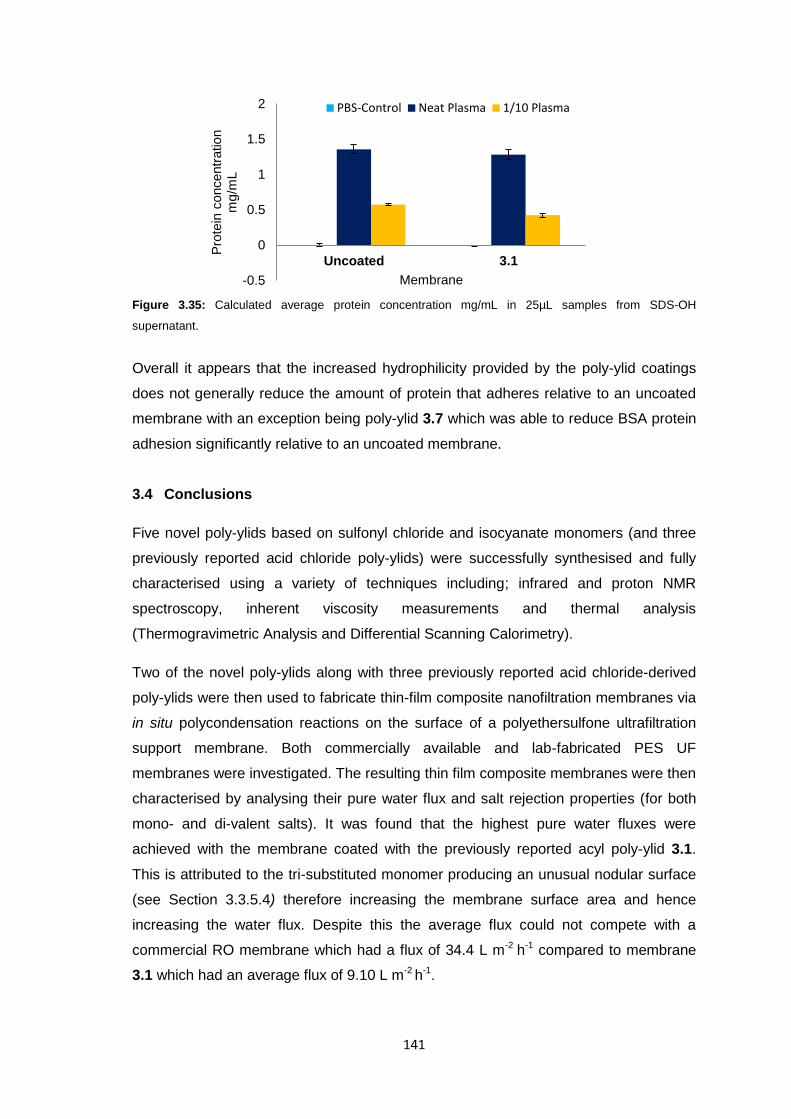
141
Figure 3.35: Calculated average protein concentration mg/mL in 25µL samples from SDS-OH
supernatant.
Overall it appears that the increased hydrophilicity provided by the poly-ylid coatings
does not generally reduce the amount of protein that adheres relative to an uncoated
membrane with an exception being poly-ylid 3.7 which was able to reduce BSA protein
adhesion significantly relative to an uncoated membrane.
3.4 Conclusions
Five novel poly-ylids based on sulfonyl chloride and isocyanate monomers (and three
previously reported acid chloride poly-ylids) were successfully synthesised and fully
characterised using a variety of techniques including; infrared and proton NMR
spectroscopy, inherent viscosity measurements and thermal analysis
(Thermogravimetric Analysis and Differential Scanning Calorimetry).
Two of the novel poly-ylids along with three previously reported acid chloride-derived
poly-ylids were then used to fabricate thin-film composite nanofiltration membranes via
in situ polycondensation reactions on the surface of a polyethersulfone ultrafiltration
support membrane. Both commercially available and lab-fabricated PES UF
membranes were investigated. The resulting thin film composite membranes were then
characterised by analysing their pure water flux and salt rejection properties (for both
mono- and di-valent salts). It was found that the highest pure water fluxes were
achieved with the membrane coated with the previously reported acyl poly-ylid 3.1.
This is attributed to the tri-substituted monomer producing an unusual nodular surface
(see Section 3.3.5.4) therefore increasing the membrane surface area and hence
increasing the water flux. Despite this the average flux could not compete with a
commercial RO membrane which had a flux of 34.4 L m-2 h-1 compared to membrane
3.1 which had an average flux of 9.10 L m-2 h-1.
-0.5
0
0.5
1
1.5
2
Uncoated 3.1
Pro
tein
concentr
ation
mg/m
L
Membrane
PBS-Control Neat Plasma 1/10 Plasma
142
As for the salt rejection studies, when comparing mono and divalent salt rejection, in all
cases the divalent salt showed a higher percentage rejection although membranes
coated with poly-ylid 3.4 showed an unusually high monovalent salt rejection of 70%
relative to the divalent salt rejection at 73%. The highest overall rejection was again
achieved with the poly-ylid 3.1 coating; 88% rejection of the divalent magnesium
sulfate. Novel poly-ylid 3.7 achieved comparable sodium chloride rejection (52%) to
poly-ylids 3.2 (56%) and 3.3 (55%).
Additionally, due to the presence of a novel ylid linker which contains a negatively
charged nitrogen atom susceptible to reversible protonation and deprotonation, further
flux studies under different pH’s were performed to examine the effect of pH on
membrane permeation. It was found that changing the pH of the feed did affect the flux
with all three membranes examined (3.1, 3.4 and 3.7) achieving higher fluxes in basic
conditions than under acidic conditions. It is proposed that this is a result of the
reduced hydrophilicity caused by ylid protonation in acid conditions which produces a
polymer which can form strong hydrogen bonds between the chains rather than
forming hydrogen bonds with approaching water molecules. This then reduces the
membrane permeability to water. In basic and neutral conditions, the ylid nitrogen is
deprotonated resulting in a more hydrophilic bond and therefore a more permeable
membrane, hence then increased fluxes in basic conditions.
Scanning electron microscopy was used to analyse the membrane surface
morphology. It was found that only the tri-substituted crosslinking monomer trimesoyl
chloride was able to produce any morphological effects creating a characteristic
nodular surface. All other poly-ylids produced flat featureless membrane surfaces
although bends of the trimesoyl chloride monomer an a di-substituted sulfonyl chloride
monomer (benzene-1,3-disulfonyl chloride) were able to produce an intermediate
surface structure with both flat and nodular regions.
Initial biocompatibility studies were carried out to examine the effect of the increased
hydrophilicity of the TFC membranes as a result of coating with the highly polar poly-
ylids. Protein adhesion was studied with two different proteins (BSA and fibrinogen)
and porcine plasma containing a mixture of plasma proteins. It was found that the
increased hydrophilicity of the membrane surfaces did not generally decrease the
protein adhesion relative to uncoated control membranes except in one study: poly-ylid
3.7 with BSA.
143
3.5 Future Work
A continuation of the work presented in this chapter should include investigation into
the structure of the novel sulfonyl and carbamoyl poly-ylids by synthesising model
oligomer compounds for single-crystal X-ray diffraction analysis. Additionally
alternative sulfonyl chloride and isocyanate monomers could be synthesised to expand
the library of 1,1’-diamino-4,4’-bipyridylium poly-ylids. Following characterisation of any
novel poly-ylids their membrane forming abilities’ should be assessed.
The existing TFC membranes should be further analysed by investigating their
rejection of different salts or mixtures of salt solutions. Furthermore the effect of
changing pH on flux suggests that the pH of the feed could also affect salt rejection
properties, so analysing the membrane salt rejection at different pH values would also
be worthy of investigation. Additional SEM analysis could be performed to image the
membrane cross-sections for further information on the membrane morphology. The
blended coatings incorporating both trimesoyl chloride and a di-substituted sulfonyl
chloride in different ratios could be analysed in terms of their flux and salt rejection
properties and to quantify the impact of the changing ratio of monomers. Finally, other
biocompatibility experiments could be performed i.e. investigating bacterial adhesion
onto coated vs. uncoated membranes.
3.6 Experimental
3.6.1 Materials
The following materials were sourced from Fisher Scientific UK Ltd (Leicestershire,
UK); Pierce™ BCA Protein assay kit (containing; Reagent A - bicinchoninic acid,
Reagent B - 4% (w/v) copper sulfate, 2mg/mL albumin standard ampules), 96-well flat-
bottomed micro-plates and the micrometre feeler gauge. The 50K MWCO
polyethersulfone UF disks were purchased from Merck Millipore (Massachusetts,
USA). The "Awa 10" backing paper used to fabricate UF membranes was obtained
from Awa Paper Ltd (Japan) and the membrane casting blade was sourced from
Mitutoyo (Japan). The Victrex® 5200 High MW aromatic polyethersulfone also used in
UF membrane fabrication was ex ICI plc. All remaining materials including; acetic acid,
acetone, benzene-1,3-disulfonyl chloride, bovine serum albumin, biphenyl-4,4’-
disulfonyl chloride, 4,4’-bipyridyl dihydrate, deuterated dimethyl sulfonic acid,
deuterated trifluoroacetic acid, diglyme, dimethylformamide, fibrinogen, hexane,
hydriodic acid, hydrochloric acid, hydroxylamine-O-sulfonic acid, isophthaloyl chloride,
magnesium sulphate, methanol, 4,4’-methylenebis(phenylisocyanate), oxybis(benzene
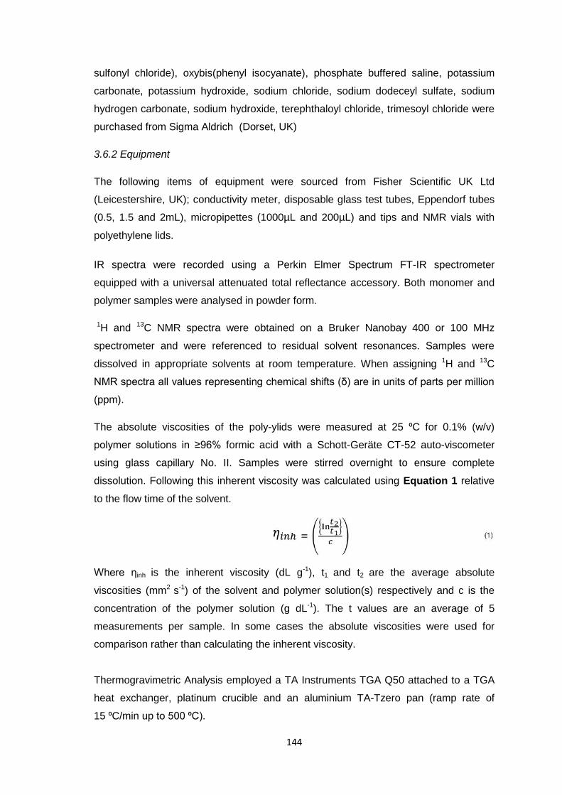
144
sulfonyl chloride), oxybis(phenyl isocyanate), phosphate buffered saline, potassium
carbonate, potassium hydroxide, sodium chloride, sodium dodeceyl sulfate, sodium
hydrogen carbonate, sodium hydroxide, terephthaloyl chloride, trimesoyl chloride were
purchased from Sigma Aldrich (Dorset, UK)
3.6.2 Equipment
The following items of equipment were sourced from Fisher Scientific UK Ltd
(Leicestershire, UK); conductivity meter, disposable glass test tubes, Eppendorf tubes
(0.5, 1.5 and 2mL), micropipettes (1000µL and 200µL) and tips and NMR vials with
polyethylene lids.
IR spectra were recorded using a Perkin Elmer Spectrum FT-IR spectrometer
equipped with a universal attenuated total reflectance accessory. Both monomer and
polymer samples were analysed in powder form.
1H and 13C NMR spectra were obtained on a Bruker Nanobay 400 or 100 MHz
spectrometer and were referenced to residual solvent resonances. Samples were
dissolved in appropriate solvents at room temperature. When assigning 1H and 13C
NMR spectra all values representing chemical shifts (δ) are in units of parts per million
(ppm).
The absolute viscosities of the poly-ylids were measured at 25 ⁰C for 0.1% (w/v)
polymer solutions in ≥96% formic acid with a Schott-Geräte CT-52 auto-viscometer
using glass capillary No. II. Samples were stirred overnight to ensure complete
dissolution. Following this inherent viscosity was calculated using Equation 1 relative
to the flow time of the solvent.
Where ηinh is the inherent viscosity (dL g-1), t1 and t2 are the average absolute
viscosities (mm2 s-1) of the solvent and polymer solution(s) respectively and c is the
concentration of the polymer solution (g dL-1). The t values are an average of 5
measurements per sample. In some cases the absolute viscosities were used for
comparison rather than calculating the inherent viscosity.
Thermogravimetric Analysis employed a TA Instruments TGA Q50 attached to a TGA
heat exchanger, platinum crucible and an aluminium TA-Tzero pan (ramp rate of
15 ⁰C/min up to 500 ⁰C).
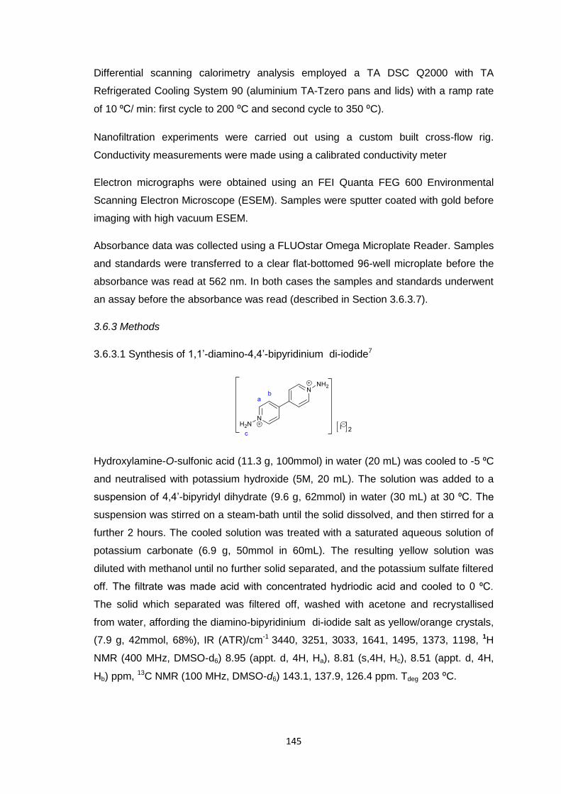
145
Differential scanning calorimetry analysis employed a TA DSC Q2000 with TA
Refrigerated Cooling System 90 (aluminium TA-Tzero pans and lids) with a ramp rate
of 10 ⁰C/ min: first cycle to 200 ⁰C and second cycle to 350 ⁰C).
Nanofiltration experiments were carried out using a custom built cross-flow rig.
Conductivity measurements were made using a calibrated conductivity meter
Electron micrographs were obtained using an FEI Quanta FEG 600 Environmental
Scanning Electron Microscope (ESEM). Samples were sputter coated with gold before
imaging with high vacuum ESEM.
Absorbance data was collected using a FLUOstar Omega Microplate Reader. Samples
and standards were transferred to a clear flat-bottomed 96-well microplate before the
absorbance was read at 562 nm. In both cases the samples and standards underwent
an assay before the absorbance was read (described in Section 3.6.3.7).
3.6.3 Methods
3.6.3.1 Synthesis of 1,1’-diamino-4,4’-bipyridinium di-iodide7
Hydroxylamine-O-sulfonic acid (11.3 g, 100mmol) in water (20 mL) was cooled to -5 ⁰C
and neutralised with potassium hydroxide (5M, 20 mL). The solution was added to a
suspension of 4,4’-bipyridyl dihydrate (9.6 g, 62mmol) in water (30 mL) at 30 ⁰C. The
suspension was stirred on a steam-bath until the solid dissolved, and then stirred for a
further 2 hours. The cooled solution was treated with a saturated aqueous solution of
potassium carbonate (6.9 g, 50mmol in 60mL). The resulting yellow solution was
diluted with methanol until no further solid separated, and the potassium sulfate filtered
off. The filtrate was made acid with concentrated hydriodic acid and cooled to 0 ⁰C.
The solid which separated was filtered off, washed with acetone and recrystallised
from water, affording the diamino-bipyridinium di-iodide salt as yellow/orange crystals,
(7.9 g, 42mmol, 68%), IR (ATR)/cm-1 3440, 3251, 3033, 1641, 1495, 1373, 1198, 1H
NMR (400 MHz, DMSO-d6) 8.95 (appt. d, 4H, Ha), 8.81 (s,4H, Hc), 8.51 (appt. d, 4H,
Hb) ppm, 13C NMR (100 MHz, DMSO-d6) 143.1, 137.9, 126.4 ppm. Tdeg 203 ⁰C.
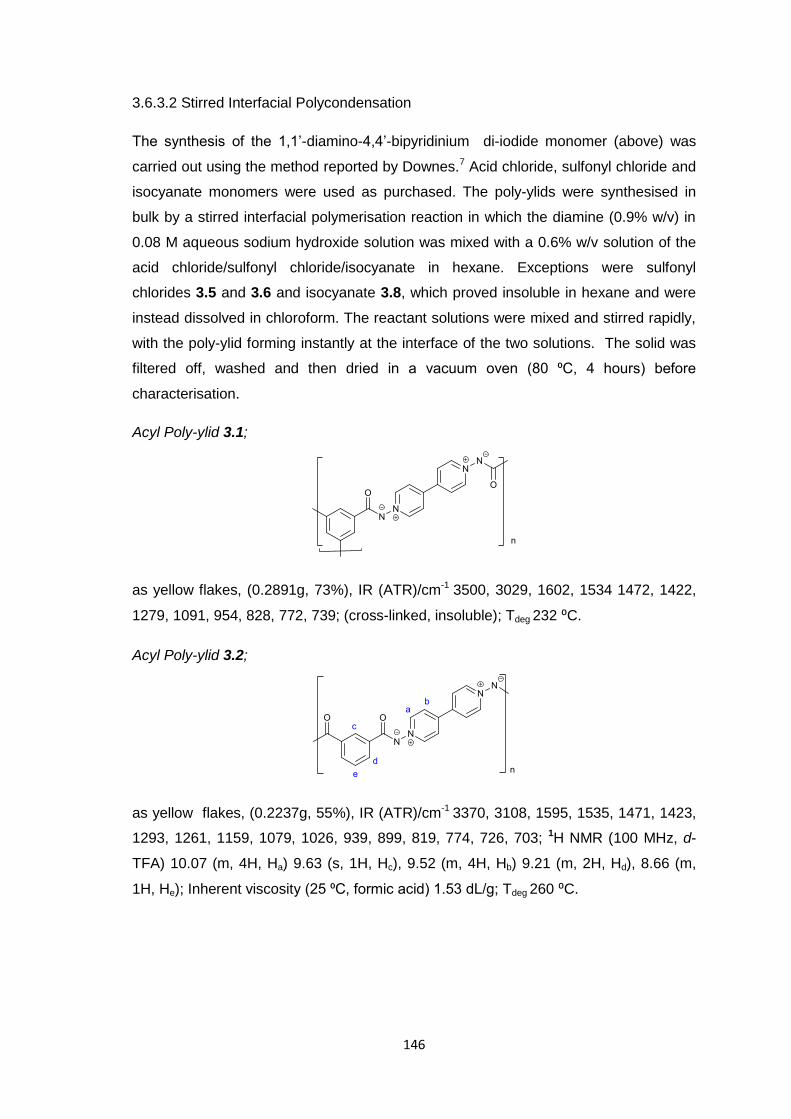
146
3.6.3.2 Stirred Interfacial Polycondensation
The synthesis of the 1,1’-diamino-4,4’-bipyridinium di-iodide monomer (above) was
carried out using the method reported by Downes.7 Acid chloride, sulfonyl chloride and
isocyanate monomers were used as purchased. The poly-ylids were synthesised in
bulk by a stirred interfacial polymerisation reaction in which the diamine (0.9% w/v) in
0.08 M aqueous sodium hydroxide solution was mixed with a 0.6% w/v solution of the
acid chloride/sulfonyl chloride/isocyanate in hexane. Exceptions were sulfonyl
chlorides 3.5 and 3.6 and isocyanate 3.8, which proved insoluble in hexane and were
instead dissolved in chloroform. The reactant solutions were mixed and stirred rapidly,
with the poly-ylid forming instantly at the interface of the two solutions. The solid was
filtered off, washed and then dried in a vacuum oven (80 ⁰C, 4 hours) before
characterisation.
Acyl Poly-ylid 3.1;
as yellow flakes, (0.2891g, 73%), IR (ATR)/cm-1 3500, 3029, 1602, 1534 1472, 1422,
1279, 1091, 954, 828, 772, 739; (cross-linked, insoluble); Tdeg 232 ⁰C.
Acyl Poly-ylid 3.2;
as yellow flakes, (0.2237g, 55%), IR (ATR)/cm-1 3370, 3108, 1595, 1535, 1471, 1423,
1293, 1261, 1159, 1079, 1026, 939, 899, 819, 774, 726, 703; 1H NMR (100 MHz, d-
TFA) 10.07 (m, 4H, Ha) 9.63 (s, 1H, Hc), 9.52 (m, 4H, Hb) 9.21 (m, 2H, Hd), 8.66 (m,
1H, He); Inherent viscosity (25 ⁰C, formic acid) 1.53 dL/g; Tdeg 260 ⁰C.
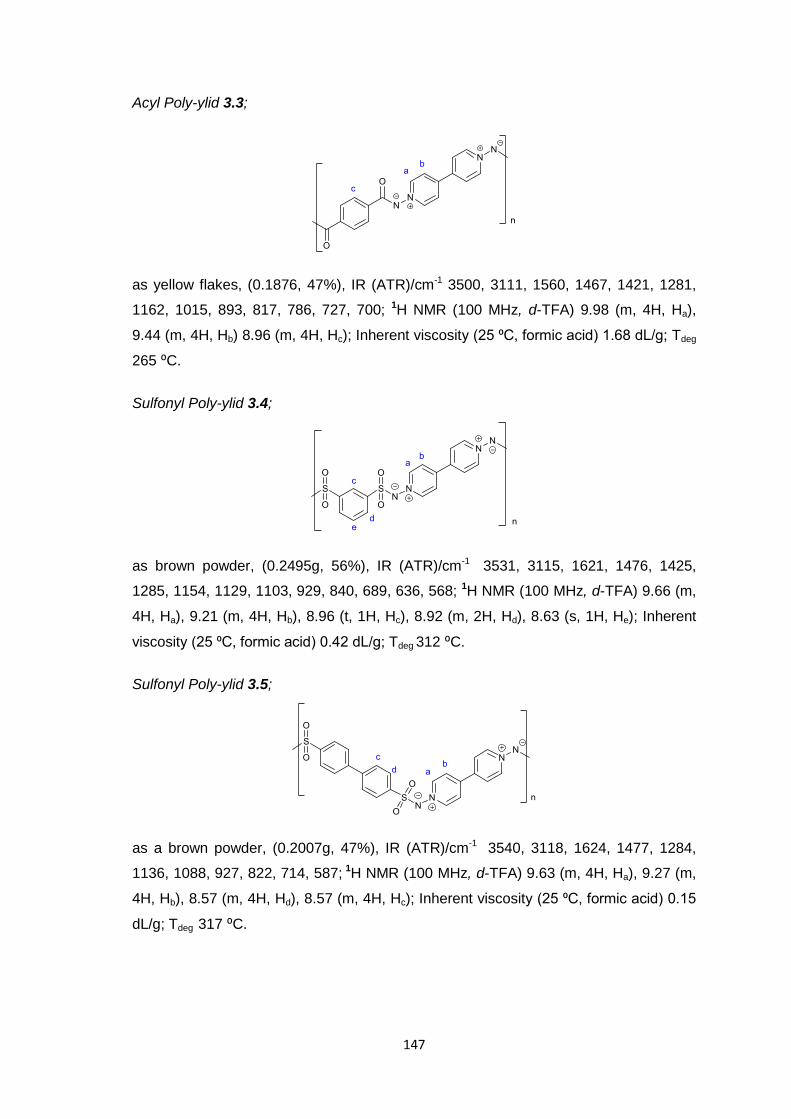
147
Acyl Poly-ylid 3.3;
as yellow flakes, (0.1876, 47%), IR (ATR)/cm-1 3500, 3111, 1560, 1467, 1421, 1281,
1162, 1015, 893, 817, 786, 727, 700; 1H NMR (100 MHz, d-TFA) 9.98 (m, 4H, Ha),
9.44 (m, 4H, Hb) 8.96 (m, 4H, Hc); Inherent viscosity (25 ⁰C, formic acid) 1.68 dL/g; Tdeg
265 ⁰C.
Sulfonyl Poly-ylid 3.4;
as brown powder, (0.2495g, 56%), IR (ATR)/cm-1 3531, 3115, 1621, 1476, 1425,
1285, 1154, 1129, 1103, 929, 840, 689, 636, 568; 1H NMR (100 MHz, d-TFA) 9.66 (m,
4H, Ha), 9.21 (m, 4H, Hb), 8.96 (t, 1H, Hc), 8.92 (m, 2H, Hd), 8.63 (s, 1H, He); Inherent
viscosity (25 ⁰C, formic acid) 0.42 dL/g; Tdeg 312 ⁰C.
Sulfonyl Poly-ylid 3.5;
as a brown powder, (0.2007g, 47%), IR (ATR)/cm-1 3540, 3118, 1624, 1477, 1284,
1136, 1088, 927, 822, 714, 587; 1H NMR (100 MHz, d-TFA) 9.63 (m, 4H, Ha), 9.27 (m,
4H, Hb), 8.57 (m, 4H, Hd), 8.57 (m, 4H, Hc); Inherent viscosity (25 ⁰C, formic acid) 0.15
dL/g; Tdeg 317 ⁰C.
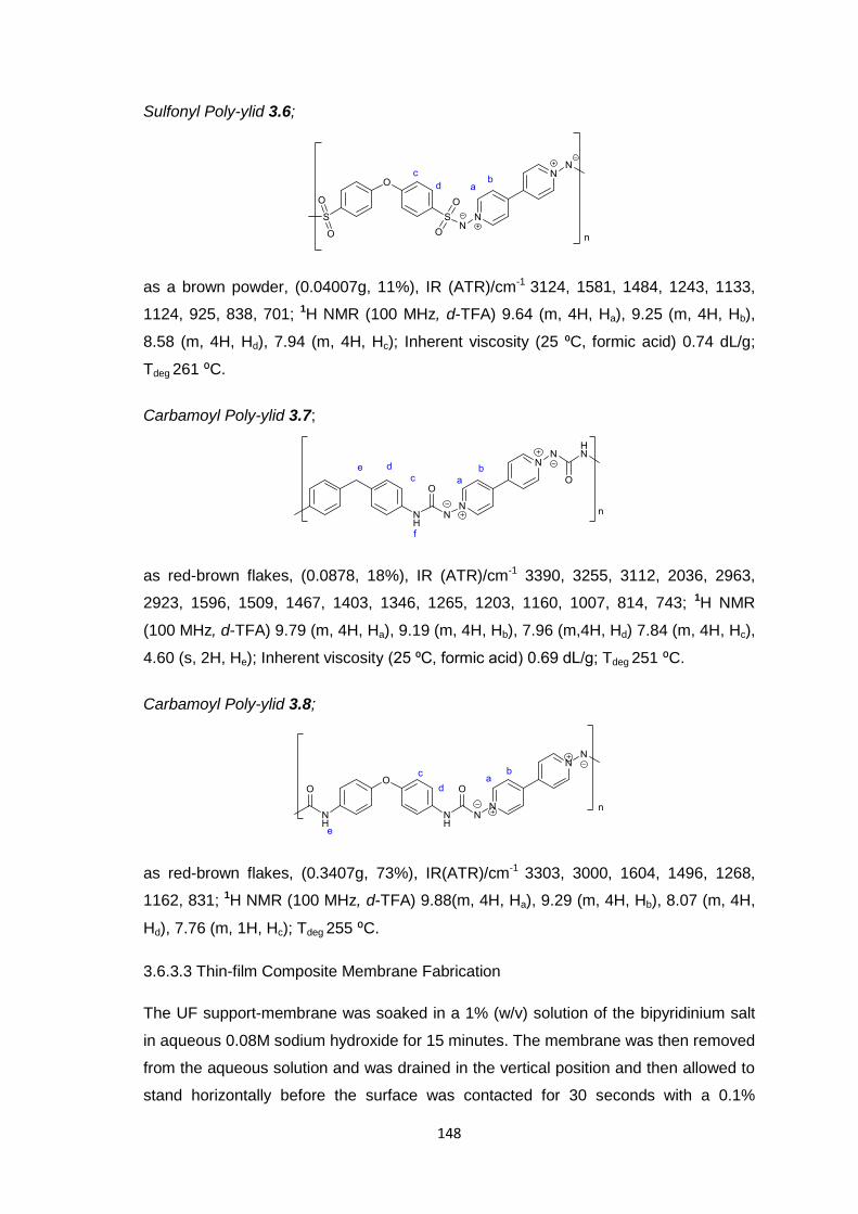
148
Sulfonyl Poly-ylid 3.6;
as a brown powder, (0.04007g, 11%), IR (ATR)/cm-1 3124, 1581, 1484, 1243, 1133,
1124, 925, 838, 701; 1H NMR (100 MHz, d-TFA) 9.64 (m, 4H, Ha), 9.25 (m, 4H, Hb),
8.58 (m, 4H, Hd), 7.94 (m, 4H, Hc); Inherent viscosity (25 ⁰C, formic acid) 0.74 dL/g;
Tdeg 261 ⁰C.
Carbamoyl Poly-ylid 3.7;
as red-brown flakes, (0.0878, 18%), IR (ATR)/cm-1 3390, 3255, 3112, 2036, 2963,
2923, 1596, 1509, 1467, 1403, 1346, 1265, 1203, 1160, 1007, 814, 743; 1H NMR
(100 MHz, d-TFA) 9.79 (m, 4H, Ha), 9.19 (m, 4H, Hb), 7.96 (m,4H, Hd) 7.84 (m, 4H, Hc),
4.60 (s, 2H, He); Inherent viscosity (25 ⁰C, formic acid) 0.69 dL/g; Tdeg 251 ⁰C.
Carbamoyl Poly-ylid 3.8;
as red-brown flakes, (0.3407g, 73%), IR(ATR)/cm-1 3303, 3000, 1604, 1496, 1268,
1162, 831; 1H NMR (100 MHz, d-TFA) 9.88(m, 4H, Ha), 9.29 (m, 4H, Hb), 8.07 (m, 4H,
Hd), 7.76 (m, 1H, Hc); Tdeg 255 ⁰C.
3.6.3.3 Thin-film Composite Membrane Fabrication
The UF support-membrane was soaked in a 1% (w/v) solution of the bipyridinium salt
in aqueous 0.08M sodium hydroxide for 15 minutes. The membrane was then removed
from the aqueous solution and was drained in the vertical position and then allowed to
stand horizontally before the surface was contacted for 30 seconds with a 0.1%
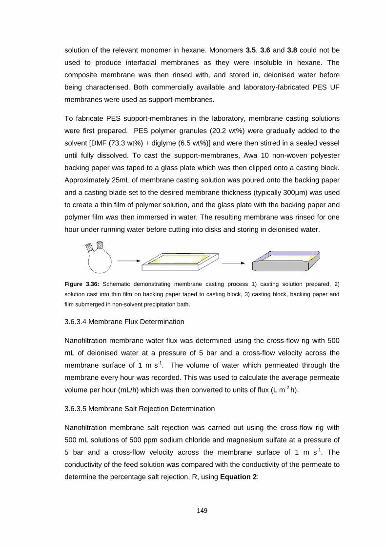
149
solution of the relevant monomer in hexane. Monomers 3.5, 3.6 and 3.8 could not be
used to produce interfacial membranes as they were insoluble in hexane. The
composite membrane was then rinsed with, and stored in, deionised water before
being characterised. Both commercially available and laboratory-fabricated PES UF
membranes were used as support-membranes.
To fabricate PES support-membranes in the laboratory, membrane casting solutions
were first prepared. PES polymer granules (20.2 wt%) were gradually added to the
solvent [DMF (73.3 wt%) + diglyme (6.5 wt%)] and were then stirred in a sealed vessel
until fully dissolved. To cast the support-membranes, Awa 10 non-woven polyester
backing paper was taped to a glass plate which was then clipped onto a casting block.
Approximately 25mL of membrane casting solution was poured onto the backing paper
and a casting blade set to the desired membrane thickness (typically 300µm) was used
to create a thin film of polymer solution, and the glass plate with the backing paper and
polymer film was then immersed in water. The resulting membrane was rinsed for one
hour under running water before cutting into disks and storing in deionised water.
Figure 3.36: Schematic demonstrating membrane casting process 1) casting solution prepared, 2)
solution cast into thin film on backing paper taped to casting block, 3) casting block, backing paper and
film submerged in non-solvent precipitation bath.
3.6.3.4 Membrane Flux Determination
Nanofiltration membrane water flux was determined using the cross-flow rig with 500
mL of deionised water at a pressure of 5 bar and a cross-flow velocity across the
membrane surface of 1 m s-1. The volume of water which permeated through the
membrane every hour was recorded. This was used to calculate the average permeate
volume per hour (mL/h) which was then converted to units of flux (L m-2 h).
3.6.3.5 Membrane Salt Rejection Determination
Nanofiltration membrane salt rejection was carried out using the cross-flow rig with
500 mL solutions of 500 ppm sodium chloride and magnesium sulfate at a pressure of
5 bar and a cross-flow velocity across the membrane surface of 1 m s-1. The
conductivity of the feed solution was compared with the conductivity of the permeate to
determine the percentage salt rejection, R, using Equation 2:
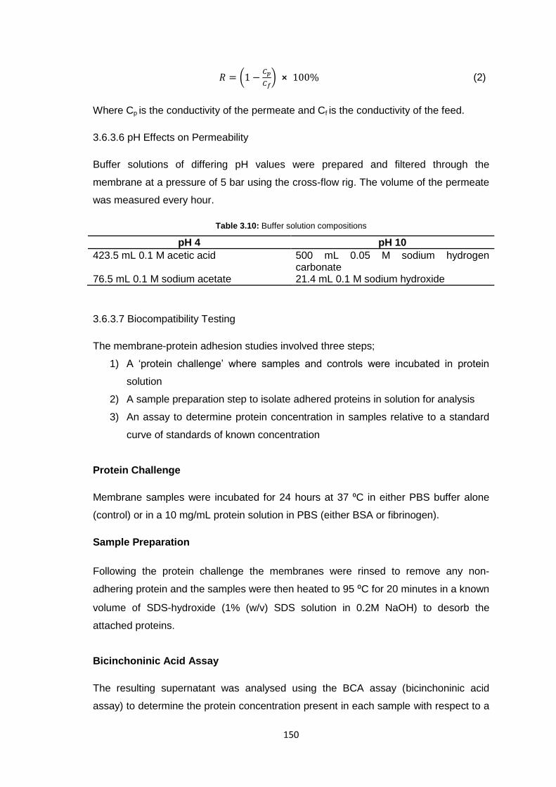
150
𝑅 = (1 −𝐶𝑝
𝐶𝑓) ⨯ 100% (2)
Where Cp is the conductivity of the permeate and Cf is the conductivity of the feed.
3.6.3.6 pH Effects on Permeability
Buffer solutions of differing pH values were prepared and filtered through the
membrane at a pressure of 5 bar using the cross-flow rig. The volume of the permeate
was measured every hour.
Table 3.10: Buffer solution compositions
pH 4 pH 10
423.5 mL 0.1 M acetic acid 500 mL 0.05 M sodium hydrogen carbonate
76.5 mL 0.1 M sodium acetate 21.4 mL 0.1 M sodium hydroxide
3.6.3.7 Biocompatibility Testing
The membrane-protein adhesion studies involved three steps;
1) A ‘protein challenge’ where samples and controls were incubated in protein
solution
2) A sample preparation step to isolate adhered proteins in solution for analysis
3) An assay to determine protein concentration in samples relative to a standard
curve of standards of known concentration
Protein Challenge
Membrane samples were incubated for 24 hours at 37 ⁰C in either PBS buffer alone
(control) or in a 10 mg/mL protein solution in PBS (either BSA or fibrinogen).
Sample Preparation
Following the protein challenge the membranes were rinsed to remove any non-
adhering protein and the samples were then heated to 95 ⁰C for 20 minutes in a known
volume of SDS-hydroxide (1% (w/v) SDS solution in 0.2M NaOH) to desorb the
attached proteins.
Bicinchoninic Acid Assay
The resulting supernatant was analysed using the BCA assay (bicinchoninic acid
assay) to determine the protein concentration present in each sample with respect to a
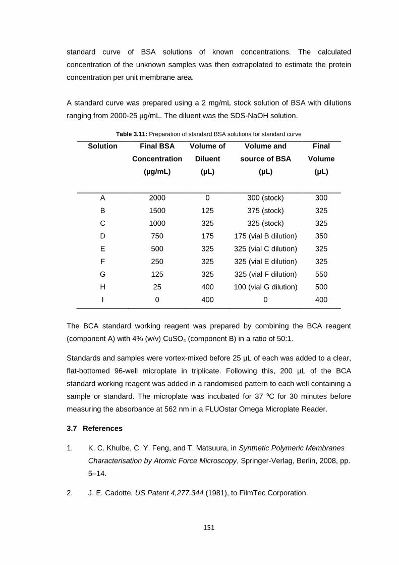
151
standard curve of BSA solutions of known concentrations. The calculated
concentration of the unknown samples was then extrapolated to estimate the protein
concentration per unit membrane area.
A standard curve was prepared using a 2 mg/mL stock solution of BSA with dilutions
ranging from 2000-25 µg/mL. The diluent was the SDS-NaOH solution.
Table 3.11: Preparation of standard BSA solutions for standard curve
Solution Final BSA
Concentration
(µg/mL)
Volume of
Diluent
(µL)
Volume and
source of BSA
(µL)
Final
Volume
(µL)
A 2000 0 300 (stock) 300
B 1500 125 375 (stock) 325
C 1000 325 325 (stock) 325
D 750 175 175 (vial B dilution) 350
E 500 325 325 (vial C dilution) 325
F 250 325 325 (vial E dilution) 325
G 125 325 325 (vial F dilution) 550
H 25 400 100 (vial G dilution) 500
I 0 400 0 400
The BCA standard working reagent was prepared by combining the BCA reagent
(component A) with 4% (w/v) CuSO4 (component B) in a ratio of 50:1.
Standards and samples were vortex-mixed before 25 µL of each was added to a clear,
flat-bottomed 96-well microplate in triplicate. Following this, 200 µL of the BCA
standard working reagent was added in a randomised pattern to each well containing a
sample or standard. The microplate was incubated for 37 ⁰C for 30 minutes before
measuring the absorbance at 562 nm in a FLUOstar Omega Microplate Reader.
3.7 References
1. K. C. Khulbe, C. Y. Feng, and T. Matsuura, in Synthetic Polymeric Membranes
Characterisation by Atomic Force Microscopy, Springer-Verlag, Berlin, 2008, pp.
5–14.
2. J. E. Cadotte, US Patent 4,277,344 (1981), to FilmTec Corporation.
152
3. B. S. Lalia, V. Kochkodan, R. Hashaikeh, and N. Hilal, Desalination, 2013, 326,
77–95.
4. S. Veríssimo, K. V. Peinemann, and J. Bordado, J. Membr. Sci., 2006, 279,
266–275.
5. W. J. Lau, A. F. Ismail, N. Misdan, and M. A. Kassim, Desalination, 2012, 287,
190–199.
6. H. M. Colquhoun, A. L. Lewis, C. A. Mahoney, and D. J. Williams, Polymer ,
1995, 36, 443–446.
7. J. E. Downes, J. Chem. Soc. (C), 1967, 1963–1964.
8. J. Clayden, N. Greeves, S. Warren, and P. Wothers, in Organic Chemistry,
Oxford University Press, Oxford, 2012, pp. 43–79.
9. J. M. G. Cowie, in Polymers: Chemistry and Physics of Moderm Materials,
Nelson Thornes Ltd, Cheltenham, 2002, pp. 247–271.
10. J. D. Roberts and M. C. Caserio, Basic Principles of Organic Chemistry, 1977,
pp. 1419–1459.
11. J. He, W. Liu, and Y.-X. Huang, PLoS One, 2016, 11, 1–12.
12. Mettler Toledo, Applications Note, Thermal Analysis of Polymers - Selected
Applications, 2008, pp. 1–40.
13. S. Sivakova, D. A. Bohnsack, M. E. Mackay, P. Suwanmala, and S. J. Rowan, J.
Am. Chem. Soc., 2005, 127, 18202–18211.
14. B. D. Kaushiva, S. R. McCartney, G. R. Rossmy, and G. L. Wilkes, Polymer ,
2000, 41, 285–310.
15. N. L. Anderson, Mol. Cell. Proteomics, 2002, 1, 845–867.
153
Chapter 4 – Membranes based on Polyetherketone (PEK)
4.1 Abstract
Novel hydrophilic poly-ylids derived from interfacial polycondensation of the 1,1’-
diamino-4,4’-bipyridylium ion with aromatic di-sulfonyl chlorides and di-isocyanates as
described in Chapter 3 were here synthesised on the surfaces of lab-fabricated
polyetherketone (PEK) support membranes to produce thin film composite
nanofiltration membranes with the potential to carry out organic separations, owing to
the crystalline, solvent resistant character of PEK. This strategy also allows the use of
monomers that are not soluble in apolar solvents, such as hexane, which are the only
type of solvents compatible with traditional polysulfone membranes. The latter are non-
crystalline and are therefore readily attacked by many solvents.
4.2 Introduction
Thin film composite (TFC) membranes are traditionally made by coating a polysulfone
support (an ultrafiltration membrane) with a thin polyamide film via interfacial
polycondensation. In the previous chapter (Chapter 3) a novel class of polymer
coatings was explored as a route to new TFC membranes based on polycondensation
between 1,1’-diamino-4,4’-bipyridylium di-iodide and a variety of di and tri-substituted
aromatic monomers to create poly-ylids. Although five novel poly-ylids were
synthesised and characterised (see Figure 4.1) only two of them were suitable for use
in TFC membrane fabrication (3.4 and 3.7). This is due to limitations arising from the
chemical stability of the polysulfone support membrane which is degraded by most
organic solvents. Since the membrane coating process involves an in situ
polycondensation on the membrane surface where the chosen monomer is in an
organic solvent, the chosen solvent must be compatible with the support membrane.
To overcome this limitation, it was decided that alternative support membranes could
be investigated, not only widening the scope of potential monomers but also creating a
completely novel solvent resistant TFC membrane which could have new applications
in organic separations.
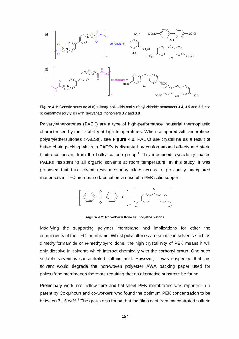
154
Figure 4.1: Generic structure of a) sulfonyl poly-ylids and sulfonyl chloride monomers 3.4, 3.5 and 3.6 and
b) carbamoyl poly-ylids with isocyanate monomers 3.7 and 3.8.
Polyaryletherketones (PAEK) are a type of high-performance industrial thermoplastic
characterised by their stability at high temperatures. When compared with amorphous
polyarylethersulfones (PAESs), see Figure 4.2, PAEKs are crystalline as a result of
better chain packing which in PAESs is disrupted by conformational effects and steric
hindrance arising from the bulky sulfone group.1 This increased crystallinity makes
PAEKs resistant to all organic solvents at room temperature. In this study, it was
proposed that this solvent resistance may allow access to previously unexplored
monomers in TFC membrane fabrication via use of a PEK solid support.
Figure 4.2: Polyethersulfone vs. polyetherketone
Modifying the supporting polymer membrane had implications for other the
components of the TFC membrane. Whilst polysulfones are soluble in solvents such as
dimethylformamide or N-methylpyrrolidone, the high crystallinity of PEK means it will
only dissolve in solvents which interact chemically with the carbonyl group. One such
suitable solvent is concentrated sulfuric acid. However, it was suspected that this
solvent would degrade the non-woven polyester AWA backing paper used for
polysulfone membranes therefore requiring that an alternative substrate be found.
Preliminary work into hollow-fibre and flat-sheet PEK membranes was reported in a
patent by Colquhoun and co-workers who found the optimum PEK concentration to be
between 7-15 wt%.2 The group also found that the films cast from concentrated sulfuric
a)
b)
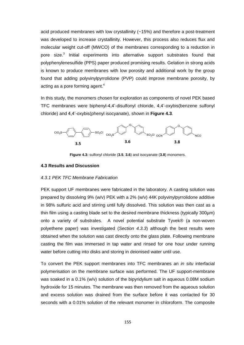
155
acid produced membranes with low crystallinity (~15%) and therefore a post-treatment
was developed to increase crystallinity. However, this process also reduces flux and
molecular weight cut-off (MWCO) of the membranes corresponding to a reduction in
pore size.3 Initial experiments into alternative support substrates found that
polyphenylenesulfide (PPS) paper produced promising results. Gelation in strong acids
is known to produce membranes with low porosity and additional work by the group
found that adding polyvinylpyrrolidone (PVP) could improve membrane porosity, by
acting as a pore forming agent.4
In this study, the monomers chosen for exploration as components of novel PEK based
TFC membranes were biphenyl-4,4’-disulfonyl chloride, 4,4’-oxybis(benzene sulfonyl
chloride) and 4,4’-oxybis(phenyl isocyanate), shown in Figure 4.3.
Figure 4.3: sulfonyl chloride (3.5, 3.6) and isocyanate (3.8) monomers.
4.3 Results and Discussion
4.3.1 PEK TFC Membrane Fabrication
PEK support UF membranes were fabricated in the laboratory. A casting solution was
prepared by dissolving 9% (w/v) PEK with a 2% (w/v) 44K polyvinylpyrrolidone additive
in 98% sulfuric acid and stirring until fully dissolved. This solution was then cast as a
thin film using a casting blade set to the desired membrane thickness (typically 300µm)
onto a variety of substrates. A novel potential substrate Tyvek® (a non-woven
polyethene paper) was investigated (Section 4.3.3) although the best results were
obtained when the solution was cast directly onto the glass plate. Following membrane
casting the film was immersed in tap water and rinsed for one hour under running
water before cutting into disks and storing in deionised water until use.
To convert the PEK support membranes into TFC membranes an in situ interfacial
polymerisation on the membrane surface was performed. The UF support-membrane
was soaked in a 0.1% (w/v) solution of the bipyridylium salt in aqueous 0.08M sodium
hydroxide for 15 minutes. The membrane was then removed from the aqueous solution
and excess solution was drained from the surface before it was contacted for 30
seconds with a 0.01% solution of the relevant monomer in chloroform. The composite
3.5 3.6 3.8
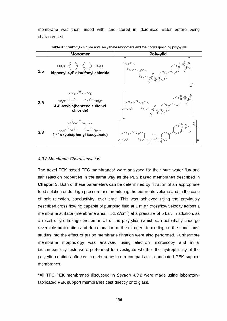
156
membrane was then rinsed with, and stored in, deionised water before being
characterised.
Table 4.1: Sulfonyl chloride and isocyanate monomers and their corresponding poly-ylids
Monomer Poly-ylid
3.5
biphenyl-4,4’-disulfonyl chloride
3.6
4,4’-oxybis(benzene sulfonyl
chloride)
3.8 4,4’-oxybis(phenyl isocyanate)
4.3.2 Membrane Characterisation
The novel PEK based TFC membranes* were analysed for their pure water flux and
salt rejection properties in the same way as the PES based membranes described in
Chapter 3. Both of these parameters can be determined by filtration of an appropriate
feed solution under high pressure and monitoring the permeate volume and in the case
of salt rejection, conductivity, over time. This was achieved using the previously
described cross flow rig capable of pumping fluid at 1 m s-1 crossflow velocity across a
membrane surface (membrane area = 52.27cm2) at a pressure of 5 bar. In addition, as
a result of ylid linkage present in all of the poly-ylids (which can potentially undergo
reversible protonation and deprotonation of the nitrogen depending on the conditions)
studies into the effect of pH on membrane filtration were also performed. Furthermore
membrane morphology was analysed using electron microscopy and initial
biocompatibility tests were performed to investigate whether the hydrophilicity of the
poly-ylid coatings affected protein adhesion in comparison to uncoated PEK support
membranes.
*All TFC PEK membranes discussed in Section 4.3.2 were made using laboratory-
fabricated PEK support membranes cast directly onto glass.
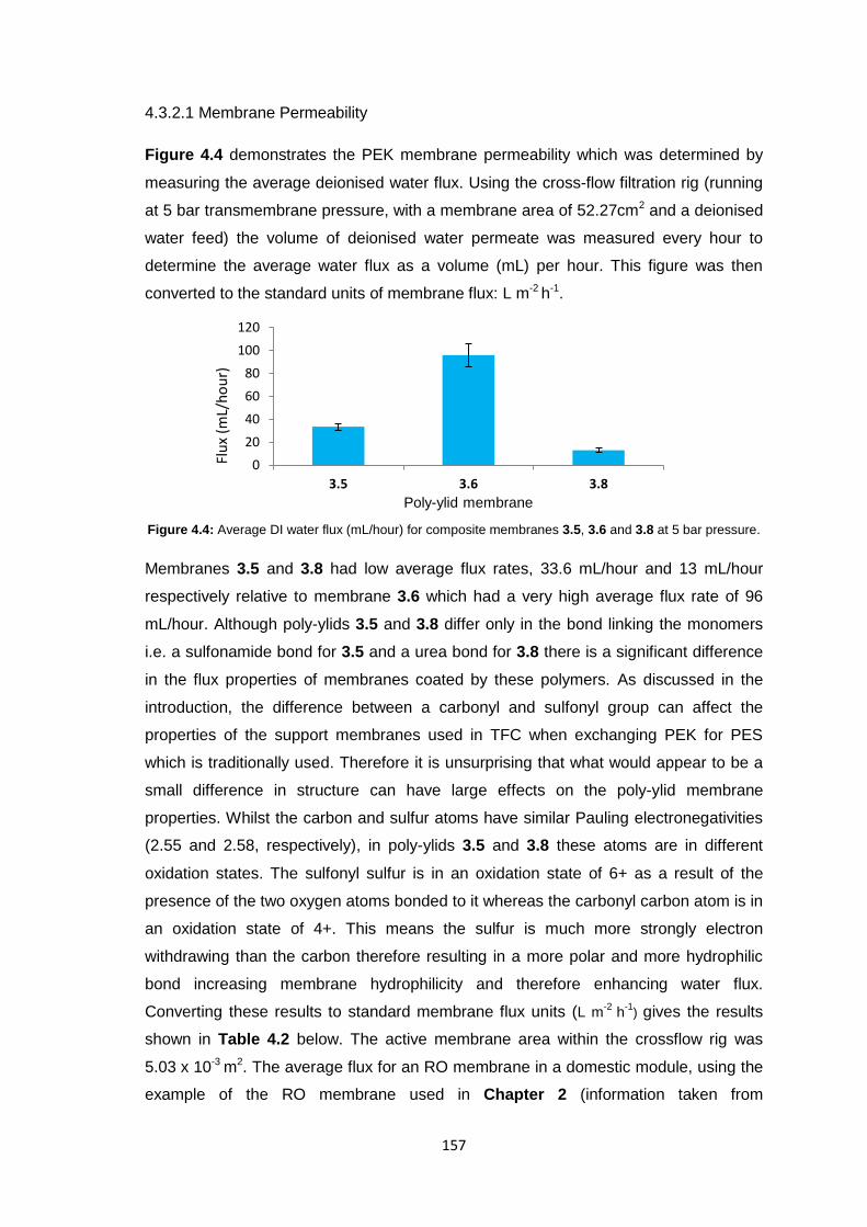
157
4.3.2.1 Membrane Permeability
Figure 4.4 demonstrates the PEK membrane permeability which was determined by
measuring the average deionised water flux. Using the cross-flow filtration rig (running
at 5 bar transmembrane pressure, with a membrane area of 52.27cm2 and a deionised
water feed) the volume of deionised water permeate was measured every hour to
determine the average water flux as a volume (mL) per hour. This figure was then
converted to the standard units of membrane flux: L m-2 h-1.
Figure 4.4: Average DI water flux (mL/hour) for composite membranes 3.5, 3.6 and 3.8 at 5 bar pressure.
Membranes 3.5 and 3.8 had low average flux rates, 33.6 mL/hour and 13 mL/hour
respectively relative to membrane 3.6 which had a very high average flux rate of 96
mL/hour. Although poly-ylids 3.5 and 3.8 differ only in the bond linking the monomers
i.e. a sulfonamide bond for 3.5 and a urea bond for 3.8 there is a significant difference
in the flux properties of membranes coated by these polymers. As discussed in the
introduction, the difference between a carbonyl and sulfonyl group can affect the
properties of the support membranes used in TFC when exchanging PEK for PES
which is traditionally used. Therefore it is unsurprising that what would appear to be a
small difference in structure can have large effects on the poly-ylid membrane
properties. Whilst the carbon and sulfur atoms have similar Pauling electronegativities
(2.55 and 2.58, respectively), in poly-ylids 3.5 and 3.8 these atoms are in different
oxidation states. The sulfonyl sulfur is in an oxidation state of 6+ as a result of the
presence of the two oxygen atoms bonded to it whereas the carbonyl carbon atom is in
an oxidation state of 4+. This means the sulfur is much more strongly electron
withdrawing than the carbon therefore resulting in a more polar and more hydrophilic
bond increasing membrane hydrophilicity and therefore enhancing water flux.
Converting these results to standard membrane flux units (L m-2
h-1
) gives the results
shown in Table 4.2 below. The active membrane area within the crossflow rig was
5.03 x 10⁻³ m2. The average flux for an RO membrane in a domestic module, using the
example of the RO membrane used in Chapter 2 (information taken from
0
20
40
60
80
100
120
3.5 3.6 3.8
Poly-ylid membrane
Flu
x (m
L/h
ou
r)
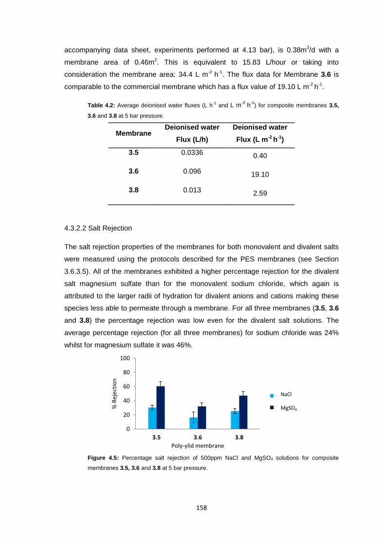
158
accompanying data sheet, experiments performed at 4.13 bar), is 0.38m3/d with a
membrane area of 0.46m2. This is equivalent to 15.83 L/hour or taking into
consideration the membrane area: 34.4 L m-2 h-1. The flux data for Membrane 3.6 is
comparable to the commercial membrane which has a flux value of 19.10 L m-2 h-1.
Table 4.2: Average deionised water fluxes (L h-1
and L m-2
h-1
) for composite membranes 3.5,
3.6 and 3.8 at 5 bar pressure.
Membrane Deionised water
Flux (L/h)
Deionised water
Flux (L m-2 h-1)
3.5 0.0336 0.40
3.6 0.096 19.10
3.8 0.013 2.59
4.3.2.2 Salt Rejection
The salt rejection properties of the membranes for both monovalent and divalent salts
were measured using the protocols described for the PES membranes (see Section
3.6.3.5). All of the membranes exhibited a higher percentage rejection for the divalent
salt magnesium sulfate than for the monovalent sodium chloride, which again is
attributed to the larger radii of hydration for divalent anions and cations making these
species less able to permeate through a membrane. For all three membranes (3.5, 3.6
and 3.8) the percentage rejection was low even for the divalent salt solutions. The
average percentage rejection (for all three membranes) for sodium chloride was 24%
whilst for magnesium sulfate it was 46%.
Figure 4.5: Percentage salt rejection of 500ppm NaCl and MgSO4 solutions for composite
membranes 3.5, 3.6 and 3.8 at 5 bar pressure.
0
20
40
60
80
100
3.5 3.6 3.8
% R
ejec
tio
n
Poly-ylid membrane
NaCl
MgSO4
NaCl
MgSO4
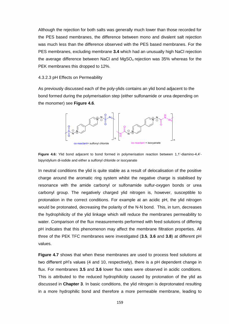
159
Although the rejection for both salts was generally much lower than those recorded for
the PES based membranes, the difference between mono and divalent salt rejection
was much less than the difference observed with the PES based membranes. For the
PES membranes, excluding membrane 3.4 which had an unusually high NaCl rejection
the average difference between NaCl and MgSO4 rejection was 35% whereas for the
PEK membranes this dropped to 12%.
4.3.2.3 pH Effects on Permeability
As previously discussed each of the poly-ylids contains an ylid bond adjacent to the
bond formed during the polymerisation step (either sulfonamide or urea depending on
the monomer) see Figure 4.6.
Figure 4.6: Ylid bond adjacent to bond formed in polymerisation reaction between 1,1’-diamino-4,4’-
bipyridylium di-iodide and either a sulfonyl chloride or isocyanate
In neutral conditions the ylid is quite stable as a result of delocalisation of the positive
charge around the aromatic ring system whilst the negative charge is stabilised by
resonance with the amide carbonyl or sulfonamide sulfur-oxygen bonds or urea
carbonyl group. The negatively charged ylid nitrogen is, however, susceptible to
protonation in the correct conditions. For example at an acidic pH, the ylid nitrogen
would be protonated, decreasing the polarity of the N-N bond. This, in turn, decreases
the hydrophilicity of the ylid linkage which will reduce the membranes permeability to
water. Comparison of the flux measurements performed with feed solutions of differing
pH indicates that this phenomenon may affect the membrane filtration properties. All
three of the PEK TFC membranes were investigated (3.5, 3.6 and 3.8) at different pH
values.
Figure 4.7 shows that when these membranes are used to process feed solutions at
two different pH’s values (4 and 10, respectively), there is a pH dependent change in
flux. For membranes 3.5 and 3.6 lower flux rates were observed in acidic conditions.
This is attributed to the reduced hydrophilicity caused by protonation of the ylid as
discussed in Chapter 3. In basic conditions, the ylid nitrogen is deprotonated resulting
in a more hydrophilic bond and therefore a more permeable membrane, leading to
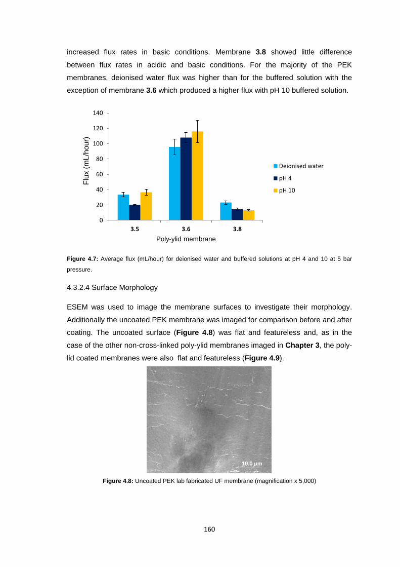
160
increased flux rates in basic conditions. Membrane 3.8 showed little difference
between flux rates in acidic and basic conditions. For the majority of the PEK
membranes, deionised water flux was higher than for the buffered solution with the
exception of membrane 3.6 which produced a higher flux with pH 10 buffered solution.
Figure 4.7: Average flux (mL/hour) for deionised water and buffered solutions at pH 4 and 10 at 5 bar
pressure.
4.3.2.4 Surface Morphology
ESEM was used to image the membrane surfaces to investigate their morphology.
Additionally the uncoated PEK membrane was imaged for comparison before and after
coating. The uncoated surface (Figure 4.8) was flat and featureless and, as in the
case of the other non-cross-linked poly-ylid membranes imaged in Chapter 3, the poly-
lid coated membranes were also flat and featureless (Figure 4.9).
Figure 4.8: Uncoated PEK lab fabricated UF membrane (magnification x 5,000)
0
20
40
60
80
100
120
140
3.5 3.6 3.8
Poly-ylid membrane
Deionised water
pH 4
pH 10
Flu
x (
mL/h
our)
10.0 µm
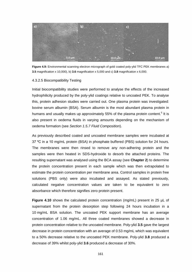
161
Figure 4.9: Environmental scanning electron micrograph of gold coated poly-ylid TFC PEK membranes a)
3.5 magnification x 10,000), b) 3.6 magnification x 5,000 and c) 3.8 magnification x 6,000.
4.3.2.5 Biocompatibility Testing
Initial biocompatibility studies were performed to analyse the effects of the increased
hydrophilicity produced by the poly-ylid coatings relative to uncoated PEK. To analyse
this, protein adhesion studies were carried out. One plasma protein was investigated:
bovine serum albumin (BSA). Serum albumin is the most abundant plasma protein in
humans and usually makes up approximately 55% of the plasma protein content.5 It is
also present in oedema fluids in varying amounts depending on the mechanism of
oedema formation (see Section 1.5.7 Fluid Composition).
As previously described coated and uncoated membrane samples were incubated at
37 ⁰C in a 10 mg/mL protein (BSA) in phosphate buffered (PBS) solution for 24 hours.
The membranes were then rinsed to remove any non-adhering protein and the
samples were then heated in SDS-hydroxide to desorb the attached proteins. The
resulting supernatant was analysed using the BCA assay (see Chapter 2) to determine
the protein concentration present in each sample which was then extrapolated to
estimate the protein concentration per membrane area. Control samples in protein free
solutions (PBS only) were also incubated and assayed. As stated previously,
calculated negative concentration values are taken to be equivalent to zero
absorbance which therefore signifies zero protein present.
Figure 4.10 shows the calculated protein concentration (mg/mL) present in 25 µL of
supernatant from the protein desorption step following 24 hours incubation in a
10 mg/mL BSA solution. The uncoated PEK support membrane has an average
concentration of 1.06 mg/mL. All three coated membranes showed a decrease in
protein concentration relative to the uncoated membrane. Poly-ylid 3.5 gave the largest
decrease in protein concentration with an average of 0.53 mg/mL which was equivalent
to a 50% decrease relative to the uncoated PEK membrane. Poly-ylid 3.8 produced a
decrease of 39% whilst poly-ylid 3.6 produced a decrease of 30%.
a) b) c)
5.0 µm 10.0 µm 10.0 µm
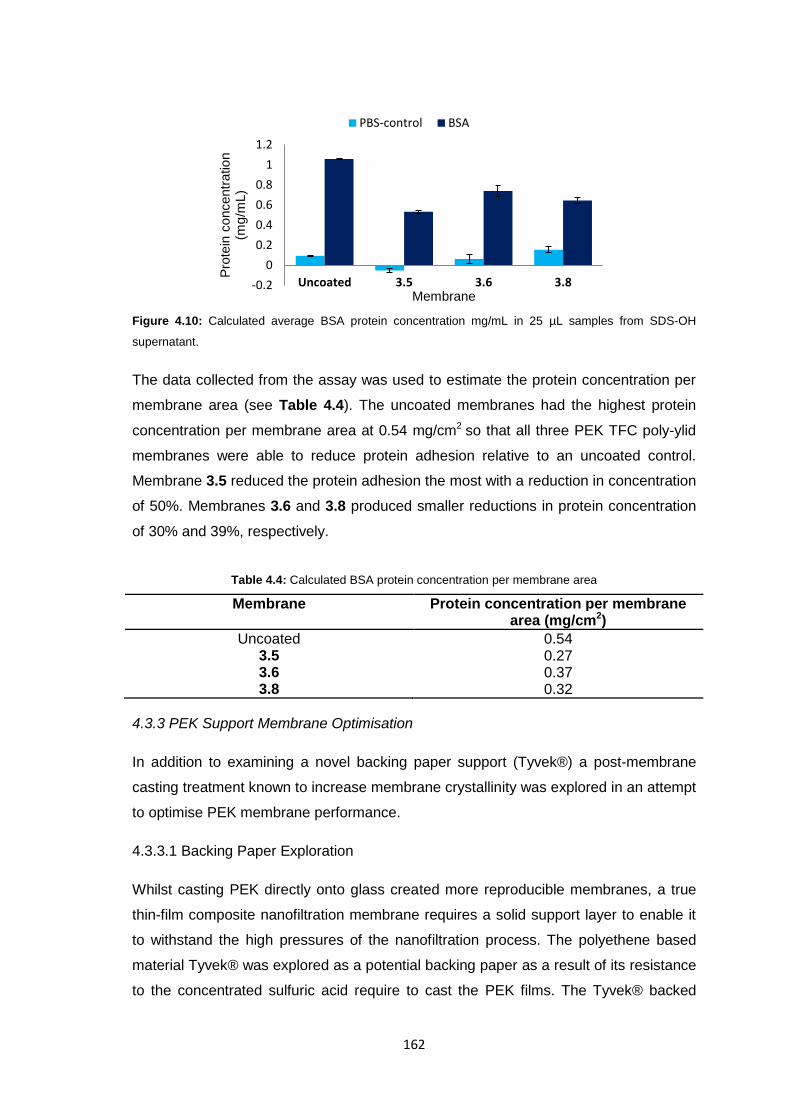
162
Figure 4.10: Calculated average BSA protein concentration mg/mL in 25 µL samples from SDS-OH
supernatant.
The data collected from the assay was used to estimate the protein concentration per
membrane area (see Table 4.4). The uncoated membranes had the highest protein
concentration per membrane area at 0.54 mg/cm2 so that all three PEK TFC poly-ylid
membranes were able to reduce protein adhesion relative to an uncoated control.
Membrane 3.5 reduced the protein adhesion the most with a reduction in concentration
of 50%. Membranes 3.6 and 3.8 produced smaller reductions in protein concentration
of 30% and 39%, respectively.
Table 4.4: Calculated BSA protein concentration per membrane area
Membrane Protein concentration per membrane area (mg/cm2)
Uncoated 0.54 3.5 0.27 3.6 0.37 3.8 0.32
4.3.3 PEK Support Membrane Optimisation
In addition to examining a novel backing paper support (Tyvek®) a post-membrane
casting treatment known to increase membrane crystallinity was explored in an attempt
to optimise PEK membrane performance.
4.3.3.1 Backing Paper Exploration
Whilst casting PEK directly onto glass created more reproducible membranes, a true
thin-film composite nanofiltration membrane requires a solid support layer to enable it
to withstand the high pressures of the nanofiltration process. The polyethene based
material Tyvek® was explored as a potential backing paper as a result of its resistance
to the concentrated sulfuric acid require to cast the PEK films. The Tyvek® backed
-0.2
0
0.2
0.4
0.6
0.8
1
1.2
Uncoated 3.5 3.6 3.8
Pro
tein
concentr
ation
(mg/m
L)
Membrane
PBS-control BSA
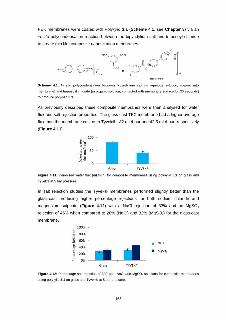
163
PEK membranes were coated with Poly-ylid 3.1 (Scheme 4.1, see Chapter 3) via an
in situ polycondensation reaction between the bipyridylium salt and trimesoyl chloride
to create thin film composite nanofiltration membranes.
Scheme 4.1: In situ polycondensation between bipyridylium salt (in aqueous solution, soaked into
membrane) and trimesoyl chloride (in organic solution, contacted with membrane surface for 30 seconds)
to produce poly-ylid 3.1.
As previously described these composite membranes were then analysed for water
flux and salt rejection properties. The glass-cast TFC membrane had a higher average
flux than the membrane cast onto Tyvek® - 82 mL/hour and 42.5 mL/hour, respectively
(Figure 4.11).
Figure 4.11: Deionised water flux (mL/min) for composite membranes using poly-ylid 3.1 on glass and
Tyvek® at 5 bar pressure.
In salt rejection studies the Tyvek® membranes performed slightly better than the
glass-cast producing higher percentage rejections for both sodium chloride and
magnesium sulphate (Figure 4.12) with a NaCl rejection of 33% and an MgSO4
rejection of 46% when compared to 28% (NaCl) and 32% (MgSO4) for the glass-cast
membrane.
Figure 4.12: Percentage salt rejection of 500 ppm NaCl and MgSO4 solutions for composite membranes
using poly-ylid 3.1 on glass and Tyvek® at 5 bar pressure.
0
50
100
Glass TYVEK®
Dei
on
ised
wat
er
flu
x (m
L/h
ou
r)
0%
20%
40%
60%
80%
100%
Glass TYVEK®
Per
cen
tage
Rej
ecti
on
NaCl
MgSO4
NaCl
MgSO4
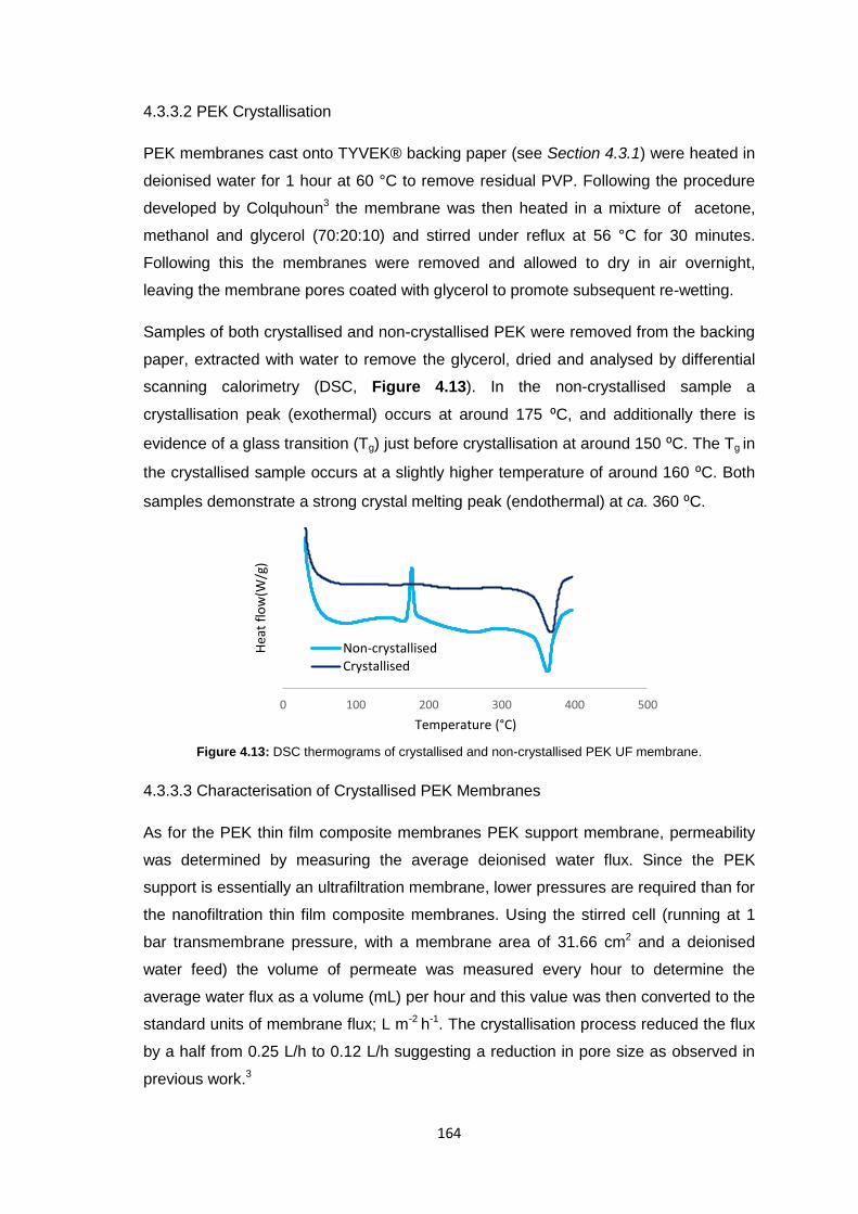
164
4.3.3.2 PEK Crystallisation
PEK membranes cast onto TYVEK® backing paper (see Section 4.3.1) were heated in
deionised water for 1 hour at 60 °C to remove residual PVP. Following the procedure
developed by Colquhoun3 the membrane was then heated in a mixture of acetone,
methanol and glycerol (70:20:10) and stirred under reflux at 56 °C for 30 minutes.
Following this the membranes were removed and allowed to dry in air overnight,
leaving the membrane pores coated with glycerol to promote subsequent re-wetting.
Samples of both crystallised and non-crystallised PEK were removed from the backing
paper, extracted with water to remove the glycerol, dried and analysed by differential
scanning calorimetry (DSC, Figure 4.13). In the non-crystallised sample a
crystallisation peak (exothermal) occurs at around 175 ⁰C, and additionally there is
evidence of a glass transition (Tg) just before crystallisation at around 150 ⁰C. The Tg in
the crystallised sample occurs at a slightly higher temperature of around 160 ⁰C. Both
samples demonstrate a strong crystal melting peak (endothermal) at ca. 360 ⁰C.
Figure 4.13: DSC thermograms of crystallised and non-crystallised PEK UF membrane.
4.3.3.3 Characterisation of Crystallised PEK Membranes
As for the PEK thin film composite membranes PEK support membrane, permeability
was determined by measuring the average deionised water flux. Since the PEK
support is essentially an ultrafiltration membrane, lower pressures are required than for
the nanofiltration thin film composite membranes. Using the stirred cell (running at 1
bar transmembrane pressure, with a membrane area of 31.66 cm2 and a deionised
water feed) the volume of permeate was measured every hour to determine the
average water flux as a volume (mL) per hour and this value was then converted to the
standard units of membrane flux; L m-2 h-1. The crystallisation process reduced the flux
by a half from 0.25 L/h to 0.12 L/h suggesting a reduction in pore size as observed in
previous work.3
0 100 200 300 400 500
Hea
t fl
ow
(W/g
)
Temperature (°C)
Non-crystallisedCrystallised
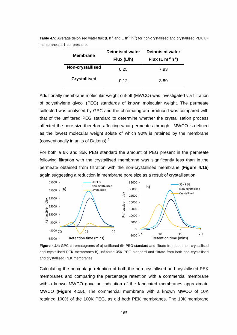
165
Table 4.5: Average deionised water flux (L h-1
and L m-2
h-1
) for non-crystallised and crystallised PEK UF
membranes at 1 bar pressure.
Membrane Deionised water
Flux (L/h)
Deionised water
Flux (L m-2 h-1)
Non-crystallised 0.25 7.93
Crystallised 0.12 3.89
Additionally membrane molecular weight cut-off (MWCO) was investigated via filtration
of polyethylene glycol (PEG) standards of known molecular weight. The permeate
collected was analysed by GPC and the chromatogram produced was compared with
that of the unfiltered PEG standard to determine whether the crystallisation process
affected the pore size therefore affecting what permeates through. MWCO is defined
as the lowest molecular weight solute of which 90% is retained by the membrane
(conventionally in units of Daltons).6
For both a 6K and 35K PEG standard the amount of PEG present in the permeate
following filtration with the crystallised membrane was significantly less than in the
permeate obtained from filtration with the non-crystallised membrane (Figure 4.15)
again suggesting a reduction in membrane pore size as a result of crystallisation.
Figure 4.14: GPC chromatograms of a) unfiltered 6K PEG standard and filtrate from both non-crystallised
and crystallised PEK membranes b) unfiltered 35K PEG standard and filtrate from both non-crystallised
and crystallised PEK membranes.
Calculating the percentage retention of both the non-crystallised and crystallised PEK
membranes and comparing the percentage retention with a commercial membrane
with a known MWCO gave an indication of the fabricated membranes approximate
MWCO (Figure 4.15). The commercial membrane with a known MWCO of 10K
retained 100% of the 100K PEG, as did both PEK membranes. The 10K membrane
-15000
-5000
5000
15000
25000
35000
45000
55000
20 21 22
Ref
ract
ive
ind
ex
Retention time (mins)
6K PEGNon-crystallisedCrystallised
-5000
0
5000
10000
15000
20000
25000
30000
35000
17 18 19 20
Ref
ract
ive
ind
ex
Retention time (mins)
35K PEG
Non-crystallised
Crystalliseda)
b)
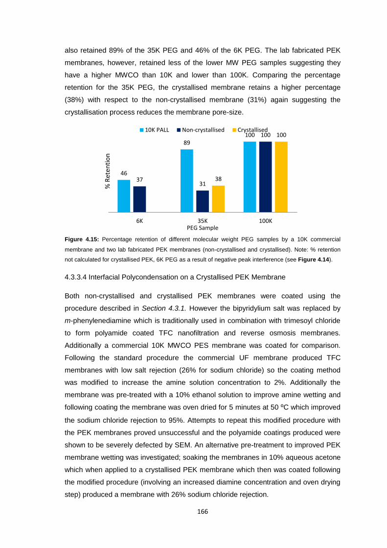
166
also retained 89% of the 35K PEG and 46% of the 6K PEG. The lab fabricated PEK
membranes, however, retained less of the lower MW PEG samples suggesting they
have a higher MWCO than 10K and lower than 100K. Comparing the percentage
retention for the 35K PEG, the crystallised membrane retains a higher percentage
(38%) with respect to the non-crystallised membrane (31%) again suggesting the
crystallisation process reduces the membrane pore-size.
Figure 4.15: Percentage retention of different molecular weight PEG samples by a 10K commercial
membrane and two lab fabricated PEK membranes (non-crystallised and crystallised). Note: % retention
not calculated for crystallised PEK, 6K PEG as a result of negative peak interference (see Figure 4.14).
4.3.3.4 Interfacial Polycondensation on a Crystallised PEK Membrane
Both non-crystallised and crystallised PEK membranes were coated using the
procedure described in Section 4.3.1. However the bipyridylium salt was replaced by
m-phenylenediamine which is traditionally used in combination with trimesoyl chloride
to form polyamide coated TFC nanofiltration and reverse osmosis membranes.
Additionally a commercial 10K MWCO PES membrane was coated for comparison.
Following the standard procedure the commercial UF membrane produced TFC
membranes with low salt rejection (26% for sodium chloride) so the coating method
was modified to increase the amine solution concentration to 2%. Additionally the
membrane was pre-treated with a 10% ethanol solution to improve amine wetting and
following coating the membrane was oven dried for 5 minutes at 50 ⁰C which improved
the sodium chloride rejection to 95%. Attempts to repeat this modified procedure with
the PEK membranes proved unsuccessful and the polyamide coatings produced were
shown to be severely defected by SEM. An alternative pre-treatment to improved PEK
membrane wetting was investigated; soaking the membranes in 10% aqueous acetone
which when applied to a crystallised PEK membrane which then was coated following
the modified procedure (involving an increased diamine concentration and oven drying
step) produced a membrane with 26% sodium chloride rejection.
46
89 100
37 31
100
38
100
6K 35K 100KPEG Sample
10K PALL Non-crystallised Crystallised
% R
ete
nti
on
167
Initial attempts to optimise the PEK membranes have shown that small modifications to
the membrane fabrication procedure can have significant effects on membrane
performance and further work is required in order to develop solvent resistant
membranes with properties which rival existing membrane systems.
4.4 Conclusions
Three novel poly-ylids synthesised in Chapter 3 were used to create solvent resistant
thin film composite nanofiltration membranes based on a lab-fabricated
polyetherketone support. The TFC membranes were characterised in terms of their
deionised water flux and salt rejection properties and were found to perform
reasonably well. Additionally the effect of feed solution pH was investigated and it was
found that (as for the PES based TFC poly-ylid membranes in Chapter 3) the flux
could be affected by pH, with generally lower fluxes in acidic conditions which is
attributed to the reduced hydrophilicity or increased internal hydrogen-bonding as
discussed earlier, caused by ylid protonation which in turn would reduce the membrane
permeability to water. In basic conditions, the ylid nitrogen is deprotonated resulting in
a more hydrophilic bond and therefore a more permeable membrane, hence then
increased flux rates in basic conditions. Furthermore membrane surface morphology
was investigated by scanning electron microscopy and it was found that the poly-ylid
coating formed a flat and featureless film on the PEK surface. Initial biocompatibility
testing found that all three PEK TFC poly-ylid membranes were able to reduce protein
adhesion relative to an uncoated PEK support membrane.
Initial studies into PEK membrane optimisation found that adding a support layer to the
PEK membrane to strengthen it could also improve its salt rejection properties when
compared with a PEK film cast directly onto glass. The additional layer does reduce
the average flux.
Some preliminary work into PEK crystallisation to improve solvent resistance
properties demonstrated that the previously reported crystallisation process can be
used to increase PEK membrane crystallinity and will also reduce the membrane pore
size therefore reducing flux and lowering the MWCO as explored by PEG filtration
coupled with GPC analysis.
Attempts to coat the non-crystallised and crystallised PEK membranes with a
polyamide layer to form thin film composite membranes have shown that a modified
procedure is required when working with these novel PEK support membranes but it
168
has also been demonstrated that small modifications in the membrane fabrication
procedure can have significant effects on membrane performance.
4.5 Future Work
Further research into the work carried out in this chapter could include further
optimisation of the PEK support membranes including developing a protocol for
reproducible membrane fabrication using the additional backing paper support which
was omitted for the TFC membranes analysed in the first sections of the chapter. This
would strengthen the membranes and allow them to better withstand the high
pressures used in nanofiltration. Additionally the protocol for coating onto these
supported PEK membranes requires optimisation again to ensure reproducible results.
Finally, since these membranes have been designed to be solvent resistant; filtration
studies examining flux and rejection in organic solvents could also be performed to test
membrane performance in conditions which standard nanofiltration membranes would
fail.
4.6 Experimental
4.6.1 Materials
The following materials were sourced from Fisher Scientific UK Ltd (Leicestershire,
UK); Pierce™ BCA Protein assay kit (containing; Reagent A - bicinchoninic acid,
Reagent B - 4% (w/v) copper sulfate, 2mg/mL albumin standard ampules), 96-well flat-
bottomed microplates and micrometre feeler gauges. The membrane casting blade
was obtained from Mitutoyo (Japan). The PEK was grade 220P (ex ICI plc.). And the
Tyvek® paper was purchased from Spenic Ltd (Gloucestershire, UK). The remaining
materials; acetic acid, bovine serum albumin, chloroform, hydrochloric acid,
magnesium sulphate, phosphate buffered saline, sodium chloride, sodium dodeceyl
sulfate, sodium hydrogen carbonate, sodium hydroxide, and concentrated sulfuric acid
were obtained from Sigma Aldrich (Dorset, UK) .
4.6.2 Equipment
The following equipment was sourced from Fisher Scientific UK Ltd (Leicestershire,
UK); conductivity meter, disposable glass test tubes, Eppendorf tubes (0.5, 1.5 and 2
mL), micropipettes (1000 µL and 200 µL) and tips, NMR vials with polyethylene lids.
169
Nanofiltration experiments were carried out using a custom built cross-flow rig.
Conductivity measurements were made using a calibrated conductivity meter
Electron micrographs were obtained using an FEI Quanta FEG 600 Environmental
Scanning Electron Microscope (ESEM). Samples were sputter coated with gold before
imaging with high vacuum ESEM.
Absorbance data was collected using a FLUOstar Omega Microplate Reader. Samples
and standards were transferred to a clear flat-bottomed 96-well microplate before the
absorbance was read at 562 nm. In both cases the samples and standards underwent
an assay before the absorbance was read (described in Section 3.6.3.7).
4.6.3 Methods
4.6.3.1 PEK Thin-film composite membrane fabrication
Two steps were required to prepare PEK-TFC membranes; 1) To create PEK support
membranes a casting solution was prepared by adding PEK polymer beads (9 wt%) to
the solvent [conc. sulfuric acid (89 wt%) + 44K PVP (2 wt%)] which was then then
stirred in a sealed vessel until fully dissolved. Following this, thin films were cast from
the polymer solution either directly onto glass or onto the backing paper (Tyvek®)
which was taped to the glass plate. Approximately 25 mL of membrane casting solution
was poured onto the glass/backing paper and a casting blade set to the desired
membrane thickness (300 µm as standard) was used to create a thin film of polymer
solution, following this the glass plate (with the backing paper if being used) and
polymer film was then immersed in water. The resulting membrane was rinsed for one
hour under running water before cutting into disks and storing in DI water.
2) The second step involved coating the PEK support membrane with a thin film of
poly-ylid. The PEK support-membrane was soaked in a 1% (w/v) solution of m-
phenylenediamine in aqueous 0.08M sodium hydroxide for 15 min. The membrane
was then removed from the aqueous solution, drained and allowed to stand briefly in
air before the surface was contacted for 30 s with a 0.1% solution of the relevant
monomer in chloroform. The composite membrane was then rinsed with, and stored in,
DI water before being characterised. Modifications to this second step included 1) Pre-
treating the membranes by soaking in 10% aqueous acetone solution before interfacial
polymerisation, 2) increasing the amine concentration to 2% and 3) oven drying the
membranes for 5mins at 50⁰C following interfacial polymerisation.
170
4.6.3.2 Membrane Flux Determination
See Chapter 3
4.6.3.3 Membrane Salt Rejection Determination
See Chapter 3
4.6.3.4 pH Effects on Permeability
See Chapter 3
4.6.3.5 Biocompatibility Testing
See Chapter 3
4.6.3.6 PEK Crystallisation
Lab-cast PEK membranes were heated in deionised water for 1 hour at 60 °C to
remove any remaining PVP additive, after which they were crystallised using a
procedure described by Colquhoun.3 The membranes were added to a mixture of
acetone, methanol and glycerol (7:1:2) and this solution was heated under reflux at
56 °C for 30 minutes, after which the membranes were removed from the solution and
allowed to air dry overnight.
4.6.3.7 PEK Crystallinity Investigation via DSC Analysis
Samples of both crystallised and non-crystallised PEK were separated from the
backing paper, compressed into pellets and placed into pre-weighed DSC pans. The
pan lids were sealed and the samples were loaded into the DSC instrument. The
samples were heated from 30-400 °C at a ramp rate of 10 °C per minute under a
nitrogen atmosphere.
4.6.3.8 MWCO Analysis
Gel permeation chromatography (GPC) was used to estimate the MWCO of the PEK
membranes before and after the crystallisation process. Stock standard solutions of
known MW PEG’s (6K, 35K and 100K) were prepared using the GPC mobile phase
(0.1% w/v) and stirred overnight to ensure complete dissolution. A fraction of each
standard solution was retained for GPC analysis as a control whilst the remainder of
each PEG solution was filtered through the membrane being analysed (i.e. non-
crystallised or crystallised PEK) using the stirred cell under 1 bar pressure. The first
171
few mL of permeate were discarded for each PEG solution and the membrane was
rinsed with GPC mobile phase between PEG solutions.
Following this a sample of each individual standard or sample solution was manually
injected into the GPC and run through the column (a PL-Aquagel column fitted with a
5µm guard column) at a rate of 1 mL/min after first being filtered through a 1.5µm nylon
syringe filter. All runs were conducted at 40 ⁰C and the samples were detected by and
refractive index detector. Data capture and subsequent analysis were carried out using
Agilent GPC software.
4.7 References
1. P. T. Mcgrail and P. T. Mcgrail, Polym. Int., 1996, 41, 103–121.
2. H. M. Colquhoun, K. Roberts, A. Simpson, and T. Taylor, in Effective Membrane
Processes - New Perspectives, Mechanical Engineering Publications Ltd, 1993,
pp. 371–380.
3. H. Colquhoun, UK Pat. 2285261, 1995, to Northwest Water PLC.
4. H. M. Colquhoun, A. F. Simpson, and V. Rogers, WO Pat. 95/15809, 1995, to
Northwest Water PLC.
5. N. L. Anderson, Mol. Cell. Proteomics, 2002, 1, 845–867.
6. A. Idris, N. Mat Zain, and M. Y. Noordin, Desalination, 2007, 207, 324–339.
.
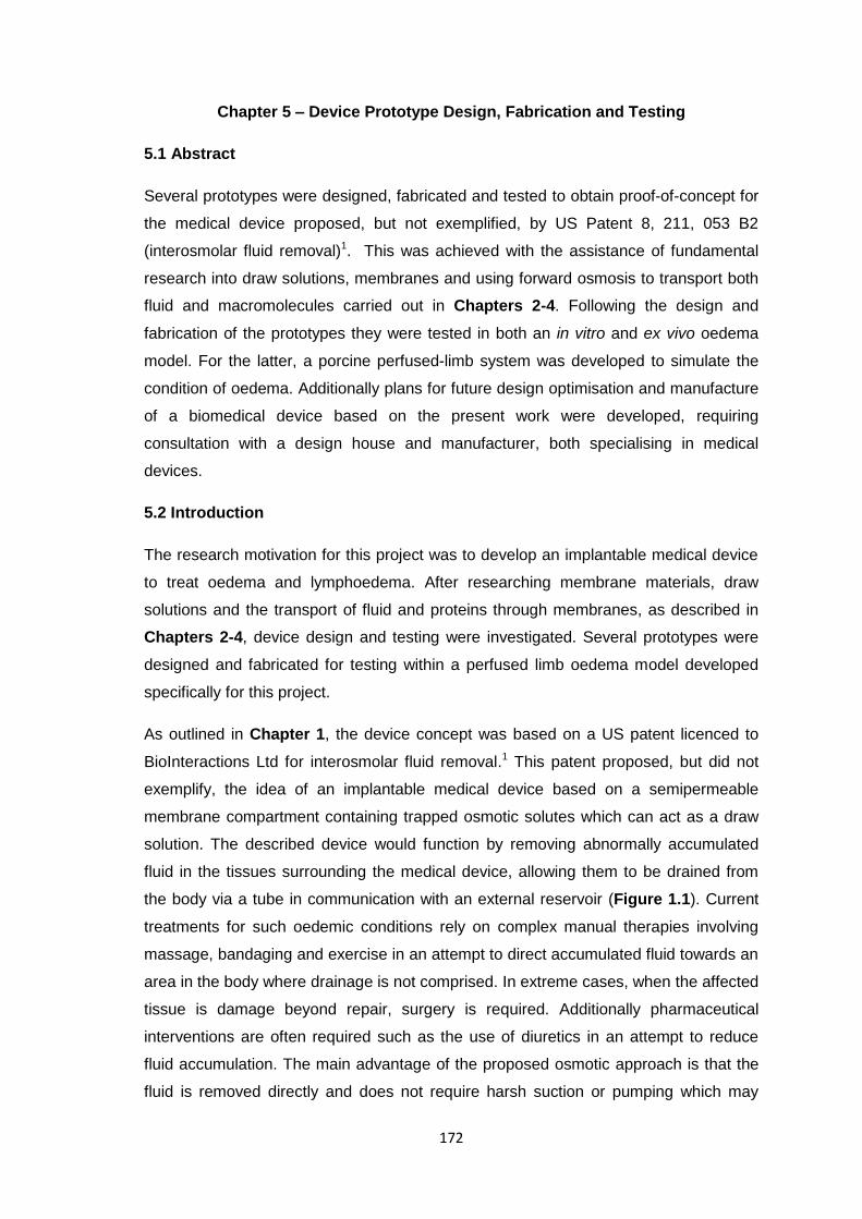
172
Chapter 5 – Device Prototype Design, Fabrication and Testing
5.1 Abstract
Several prototypes were designed, fabricated and tested to obtain proof-of-concept for
the medical device proposed, but not exemplified, by US Patent 8, 211, 053 B2
(interosmolar fluid removal)1. This was achieved with the assistance of fundamental
research into draw solutions, membranes and using forward osmosis to transport both
fluid and macromolecules carried out in Chapters 2-4. Following the design and
fabrication of the prototypes they were tested in both an in vitro and ex vivo oedema
model. For the latter, a porcine perfused-limb system was developed to simulate the
condition of oedema. Additionally plans for future design optimisation and manufacture
of a biomedical device based on the present work were developed, requiring
consultation with a design house and manufacturer, both specialising in medical
devices.
5.2 Introduction
The research motivation for this project was to develop an implantable medical device
to treat oedema and lymphoedema. After researching membrane materials, draw
solutions and the transport of fluid and proteins through membranes, as described in
Chapters 2-4, device design and testing were investigated. Several prototypes were
designed and fabricated for testing within a perfused limb oedema model developed
specifically for this project.
As outlined in Chapter 1, the device concept was based on a US patent licenced to
BioInteractions Ltd for interosmolar fluid removal.1 This patent proposed, but did not
exemplify, the idea of an implantable medical device based on a semipermeable
membrane compartment containing trapped osmotic solutes which can act as a draw
solution. The described device would function by removing abnormally accumulated
fluid in the tissues surrounding the medical device, allowing them to be drained from
the body via a tube in communication with an external reservoir (Figure 1.1). Current
treatments for such oedemic conditions rely on complex manual therapies involving
massage, bandaging and exercise in an attempt to direct accumulated fluid towards an
area in the body where drainage is not comprised. In extreme cases, when the affected
tissue is damage beyond repair, surgery is required. Additionally pharmaceutical
interventions are often required such as the use of diuretics in an attempt to reduce
fluid accumulation. The main advantage of the proposed osmotic approach is that the
fluid is removed directly and does not require harsh suction or pumping which may
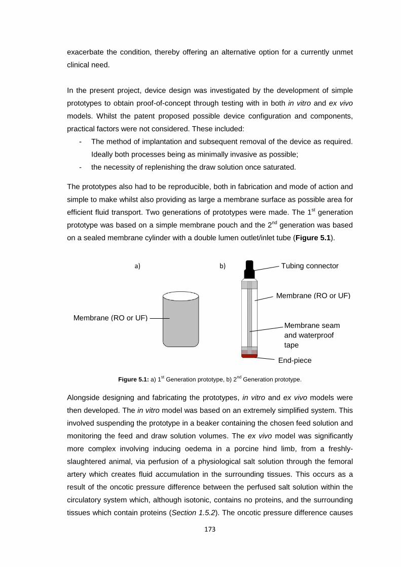
173
exacerbate the condition, thereby offering an alternative option for a currently unmet
clinical need.
In the present project, device design was investigated by the development of simple
prototypes to obtain proof-of-concept through testing with in both in vitro and ex vivo
models. Whilst the patent proposed possible device configuration and components,
practical factors were not considered. These included:
- The method of implantation and subsequent removal of the device as required.
Ideally both processes being as minimally invasive as possible;
- the necessity of replenishing the draw solution once saturated.
The prototypes also had to be reproducible, both in fabrication and mode of action and
simple to make whilst also providing as large a membrane surface as possible area for
efficient fluid transport. Two generations of prototypes were made. The 1st generation
prototype was based on a simple membrane pouch and the 2nd generation was based
on a sealed membrane cylinder with a double lumen outlet/inlet tube (Figure 5.1).
Figure 5.1: a) 1st Generation prototype, b) 2
nd Generation prototype.
Alongside designing and fabricating the prototypes, in vitro and ex vivo models were
then developed. The in vitro model was based on an extremely simplified system. This
involved suspending the prototype in a beaker containing the chosen feed solution and
monitoring the feed and draw solution volumes. The ex vivo model was significantly
more complex involving inducing oedema in a porcine hind limb, from a freshly-
slaughtered animal, via perfusion of a physiological salt solution through the femoral
artery which creates fluid accumulation in the surrounding tissues. This occurs as a
result of the oncotic pressure difference between the perfused salt solution within the
circulatory system which, although isotonic, contains no proteins, and the surrounding
tissues which contain proteins (Section 1.5.2). The oncotic pressure difference causes
a) b) Tubing connector
Membrane (RO or UF)
End-piece
Membrane seam
and waterproof
tape
Membrane (RO or UF)
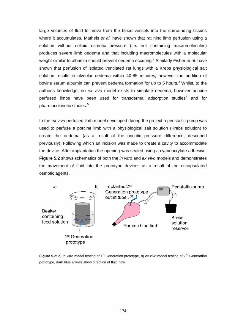
174
large volumes of fluid to move from the blood vessels into the surrounding tissues
where it accumulates. Matheis et al. have shown that rat hind limb perfusion using a
solution without colloid osmotic pressure (i.e. not containing macromolecules)
produces severe limb oedema and that including macromolecules with a molecular
weight similar to albumin should prevent oedema occuring.2 Similarly Fisher et al. have
shown that perfusion of isolated ventilated rat lungs with a Krebs physiological salt
solution results in alveolar oedema within 40-85 minutes, however the addition of
bovine serum albumin can prevent oedema formation for up to 5 hours.3 Whilst, to the
author’s knowledge, no ex vivo model exists to simulate oedema, however porcine
perfused limbs have been used for transdermal adsorption studies4 and for
pharmacokinetic studies.5
In the ex vivo perfused limb model developed during the project a peristaltic pump was
used to perfuse a porcine limb with a physiological salt solution (Krebs solution) to
create the oedema (as a result of the oncotic pressure difference, described
previously). Following which an incision was made to create a cavity to accommodate
the device. After implantation the opening was sealed using a cyanoacrylate adhesive.
Figure 5.2 shows schematics of both the in vitro and ex vivo models and demonstrates
the movement of fluid into the prototype devices as a result of the encapsulated
osmotic agents.
Figure 5.2: a) In vitro model testing of 1st Generation prototype, b) ex vivo model testing of 2
nd Generation
prototype, dark blue arrows show direction of fluid flow.
a) b)
175
5.3 Results and Discussion
5.3.1 Prototype Design
The basic design of the system encompasses two main parts, an implanted device and
an external reservoir. The implanted device consists of a semipermeable membrane
containing trapped osmotic solutes which act as a draw solution for accumulated fluid
in tissue surrounding the implant (see Figure 5.3). The implanted portion of the device
is in communication with the external portion, a fluid reservoir, via a tube connected to
a transdermal port allowing for fluid collected within the implanted device to be drained
and removed.
Figure 5.3: Schematic representation of the components of the proposed implantable membrane device
(and external reservoir) for the treatment of oedema.
Several different designs were proposed based around the general device concept
depicted in Figure 5.3. A key consideration was the implantable pouch portion which
was required to fulfil several design considerations including:
- Material limitations - the majority of the pouch must be made from membrane
and additionally must be made from biocompatible materials and suitable for
sterilization;
- Collapsible design - to aid minimally invasive implantation procedure without
compromising large surface area required for rapid fluid exchange across the
membrane;
- Connected to exterior - through transdermal port;
- Maximum possible membrane area - to ensure efficient exchange of fluids
across the membrane surface.
Figure 5.4 below illustrates some of the proposed designs which were used to discuss
the prototype with a design house, Hunt Developments Ltd.
INTERNAL EXTERNAL
Membrane pouch
containing trapped
osmotic solutes Transdermal port
Connecting tube
Reservoir
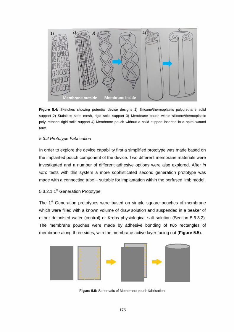
176
Figure 5.4: Sketches showing potential device designs 1) Silicone/thermoplastic polyurethane solid
support 2) Stainless steel mesh, rigid solid support 3) Membrane pouch within silicone/thermoplastic
polyurethane rigid solid support 4) Membrane pouch without a solid support inserted in a spiral-wound
form.
5.3.2 Prototype Fabrication
In order to explore the device capability first a simplified prototype was made based on
the implanted pouch component of the device. Two different membrane materials were
investigated and a number of different adhesive options were also explored. After in
vitro tests with this system a more sophisticated second generation prototype was
made with a connecting tube – suitable for implantation within the perfused limb model.
5.3.2.1 1st Generation Prototype
The 1st Generation prototypes were based on simple square pouches of membrane
which were filled with a known volume of draw solution and suspended in a beaker of
either deionised water (control) or Krebs physiological salt solution (Section 5.6.3.2).
The membrane pouches were made by adhesive bonding of two rectangles of
membrane along three sides, with the membrane active layer facing out (Figure 5.5).
Figure 5.5: Schematic of Membrane pouch fabrication.
Membrane outside Membrane inside
1) 2) 3) 4)
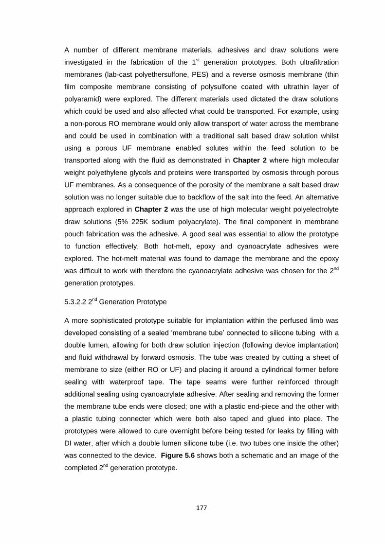
177
A number of different membrane materials, adhesives and draw solutions were
investigated in the fabrication of the 1st generation prototypes. Both ultrafiltration
membranes (lab-cast polyethersulfone, PES) and a reverse osmosis membrane (thin
film composite membrane consisting of polysulfone coated with ultrathin layer of
polyaramid) were explored. The different materials used dictated the draw solutions
which could be used and also affected what could be transported. For example, using
a non-porous RO membrane would only allow transport of water across the membrane
and could be used in combination with a traditional salt based draw solution whilst
using a porous UF membrane enabled solutes within the feed solution to be
transported along with the fluid as demonstrated in Chapter 2 where high molecular
weight polyethylene glycols and proteins were transported by osmosis through porous
UF membranes. As a consequence of the porosity of the membrane a salt based draw
solution was no longer suitable due to backflow of the salt into the feed. An alternative
approach explored in Chapter 2 was the use of high molecular weight polyelectrolyte
draw solutions (5% 225K sodium polyacrylate). The final component in membrane
pouch fabrication was the adhesive. A good seal was essential to allow the prototype
to function effectively. Both hot-melt, epoxy and cyanoacrylate adhesives were
explored. The hot-melt material was found to damage the membrane and the epoxy
was difficult to work with therefore the cyanoacrylate adhesive was chosen for the 2nd
generation prototypes.
5.3.2.2 2nd Generation Prototype
A more sophisticated prototype suitable for implantation within the perfused limb was
developed consisting of a sealed ‘membrane tube’ connected to silicone tubing with a
double lumen, allowing for both draw solution injection (following device implantation)
and fluid withdrawal by forward osmosis. The tube was created by cutting a sheet of
membrane to size (either RO or UF) and placing it around a cylindrical former before
sealing with waterproof tape. The tape seams were further reinforced through
additional sealing using cyanoacrylate adhesive. After sealing and removing the former
the membrane tube ends were closed; one with a plastic end-piece and the other with
a plastic tubing connecter which were both also taped and glued into place. The
prototypes were allowed to cure overnight before being tested for leaks by filling with
DI water, after which a double lumen silicone tube (i.e. two tubes one inside the other)
was connected to the device. Figure 5.6 shows both a schematic and an image of the
completed 2nd generation prototype.
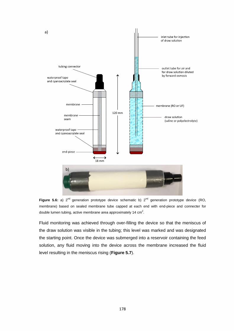
178
Figure 5.6: a) 2nd
generation prototype device schematic b) 2nd
generation prototype device (RO,
membrane) based on sealed membrane tube capped at each end with end-piece and connecter for
double lumen tubing, active membrane area approximately 14 cm2.
Fluid monitoring was achieved through over-filling the device so that the meniscus of
the draw solution was visible in the tubing; this level was marked and was designated
the starting point. Once the device was submerged into a reservoir containing the feed
solution, any fluid moving into the device across the membrane increased the fluid
level resulting in the meniscus rising (Figure 5.7).
a)
b)
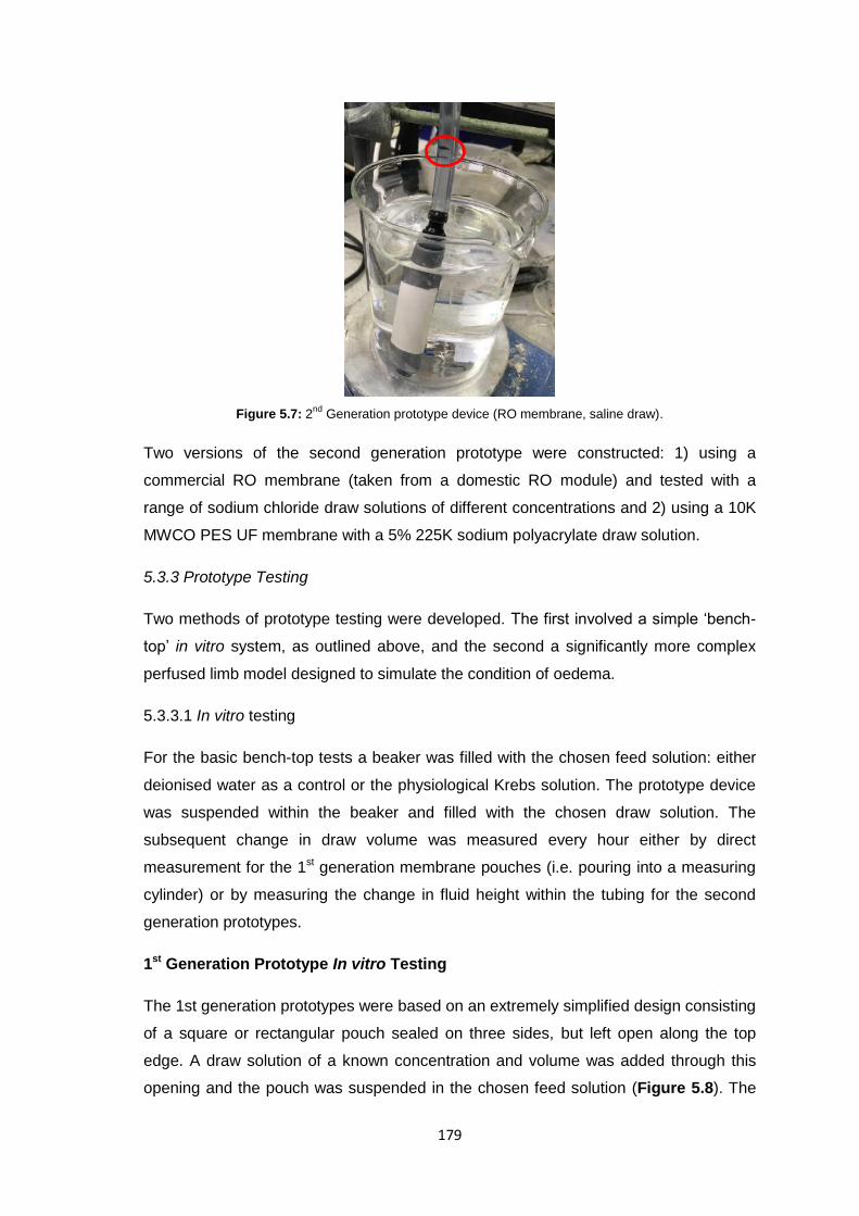
179
Figure 5.7: 2nd
Generation prototype device (RO membrane, saline draw).
Two versions of the second generation prototype were constructed: 1) using a
commercial RO membrane (taken from a domestic RO module) and tested with a
range of sodium chloride draw solutions of different concentrations and 2) using a 10K
MWCO PES UF membrane with a 5% 225K sodium polyacrylate draw solution.
5.3.3 Prototype Testing
Two methods of prototype testing were developed. The first involved a simple ‘bench-
top’ in vitro system, as outlined above, and the second a significantly more complex
perfused limb model designed to simulate the condition of oedema.
5.3.3.1 In vitro testing
For the basic bench-top tests a beaker was filled with the chosen feed solution: either
deionised water as a control or the physiological Krebs solution. The prototype device
was suspended within the beaker and filled with the chosen draw solution. The
subsequent change in draw volume was measured every hour either by direct
measurement for the 1st generation membrane pouches (i.e. pouring into a measuring
cylinder) or by measuring the change in fluid height within the tubing for the second
generation prototypes.
1st Generation Prototype In vitro Testing
The 1st generation prototypes were based on an extremely simplified design consisting
of a square or rectangular pouch sealed on three sides, but left open along the top
edge. A draw solution of a known concentration and volume was added through this
opening and the pouch was suspended in the chosen feed solution (Figure 5.8). The
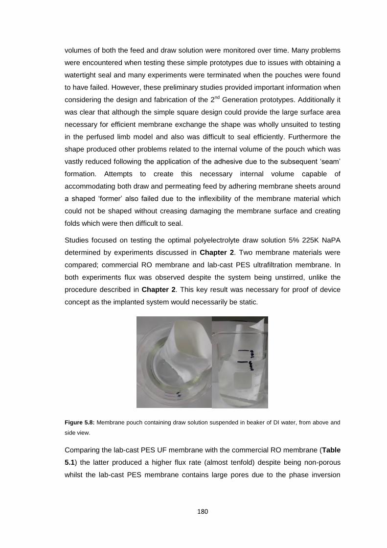
180
volumes of both the feed and draw solution were monitored over time. Many problems
were encountered when testing these simple prototypes due to issues with obtaining a
watertight seal and many experiments were terminated when the pouches were found
to have failed. However, these preliminary studies provided important information when
considering the design and fabrication of the 2nd Generation prototypes. Additionally it
was clear that although the simple square design could provide the large surface area
necessary for efficient membrane exchange the shape was wholly unsuited to testing
in the perfused limb model and also was difficult to seal efficiently. Furthermore the
shape produced other problems related to the internal volume of the pouch which was
vastly reduced following the application of the adhesive due to the subsequent ‘seam’
formation. Attempts to create this necessary internal volume capable of
accommodating both draw and permeating feed by adhering membrane sheets around
a shaped ‘former’ also failed due to the inflexibility of the membrane material which
could not be shaped without creasing damaging the membrane surface and creating
folds which were then difficult to seal.
Studies focused on testing the optimal polyelectrolyte draw solution 5% 225K NaPA
determined by experiments discussed in Chapter 2. Two membrane materials were
compared; commercial RO membrane and lab-cast PES ultrafiltration membrane. In
both experiments flux was observed despite the system being unstirred, unlike the
procedure described in Chapter 2. This key result was necessary for proof of device
concept as the implanted system would necessarily be static.
Figure 5.8: Membrane pouch containing draw solution suspended in beaker of DI water, from above and
side view.
Comparing the lab-cast PES UF membrane with the commercial RO membrane (Table
5.1) the latter produced a higher flux rate (almost tenfold) despite being non-porous
whilst the lab-cast PES membrane contains large pores due to the phase inversion
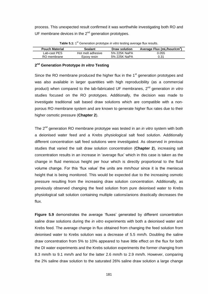
181
process. This unexpected result confirmed it was worthwhile investigating both RO and
UF membrane devices in the 2nd generation prototypes.
Table 5.1: 1st Generation prototype in vitro testing average flux results.
Pouch Material Sealant Draw solution Average Flux (mL/hour/cm2)
Lab-cast PES Hot melt adhesive 5% 225K NaPA 0.055 RO membrane Epoxy resin 5% 225K NaPA 0.31
2nd Generation Prototype In vitro Testing
Since the RO membrane produced the higher flux in the 1st generation prototypes and
was also available in larger quantities with high reproducibility (as a commercial
product) when compared to the lab-fabricated UF membranes, 2nd generation in vitro
studies focused on the RO prototypes. Additionally, the decision was made to
investigate traditional salt based draw solutions which are compatible with a non-
porous RO membrane system and are known to generate higher flux rates due to their
higher osmotic pressure (Chapter 2).
The 2nd generation RO membrane prototype was tested in an in vitro system with both
a deionised water feed and a Krebs physiological salt feed solution. Additionally
different concentration salt feed solutions were investigated. As observed in previous
studies that varied the salt draw solution concentration (Chapter 2), increasing salt
concentration results in an increase in ‘average flux’ which in this case is taken as the
change in fluid meniscus height per hour which is directly proportional to the fluid
volume change. For this ‘flux value’ the units are mm/hour since it is the meniscus
height that is being monitored. This would be expected due to the increasing osmotic
pressure resulting from the increasing draw solution concentration. Additionally, as
previously observed changing the feed solution from pure deionised water to Krebs
physiological salt solution containing multiple cations/anions drastically decreases the
flux.
Figure 5.9 demonstrates the average ‘fluxes’ generated by different concentration
saline draw solutions during the in vitro experiments with both a deionised water and
Krebs feed. The average change in flux obtained from changing the feed solution from
deionised water to Krebs solution was a decrease of 5.5 mm/h. Doubling the saline
draw concentration from 5% to 10% appeared to have little effect on the flux for both
the DI water experiments and the Krebs solution experiments the former changing from
8.3 mm/h to 9.1 mm/h and for the latter 2.6 mm/h to 2.9 mm/h. However, comparing
the 2% saline draw solution to the saturated 26% saline draw solution a large change
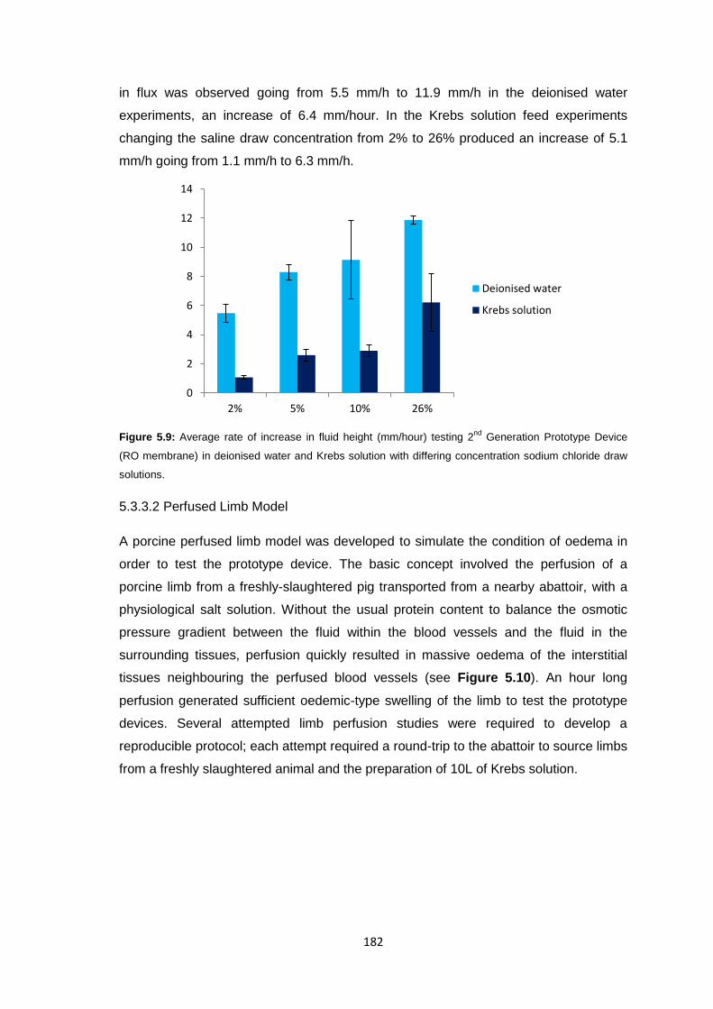
182
in flux was observed going from 5.5 mm/h to 11.9 mm/h in the deionised water
experiments, an increase of 6.4 mm/hour. In the Krebs solution feed experiments
changing the saline draw concentration from 2% to 26% produced an increase of 5.1
mm/h going from 1.1 mm/h to 6.3 mm/h.
Figure 5.9: Average rate of increase in fluid height (mm/hour) testing 2nd
Generation Prototype Device
(RO membrane) in deionised water and Krebs solution with differing concentration sodium chloride draw
solutions.
5.3.3.2 Perfused Limb Model
A porcine perfused limb model was developed to simulate the condition of oedema in
order to test the prototype device. The basic concept involved the perfusion of a
porcine limb from a freshly-slaughtered pig transported from a nearby abattoir, with a
physiological salt solution. Without the usual protein content to balance the osmotic
pressure gradient between the fluid within the blood vessels and the fluid in the
surrounding tissues, perfusion quickly resulted in massive oedema of the interstitial
tissues neighbouring the perfused blood vessels (see Figure 5.10). An hour long
perfusion generated sufficient oedemic-type swelling of the limb to test the prototype
devices. Several attempted limb perfusion studies were required to develop a
reproducible protocol; each attempt required a round-trip to the abattoir to source limbs
from a freshly slaughtered animal and the preparation of 10L of Krebs solution.
0
2
4
6
8
10
12
14
2% 5% 10% 26%
Deionised water
Krebs solution
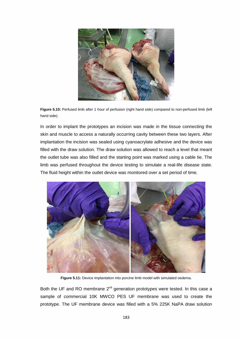
183
Figure 5.10: Perfused limb after 1 hour of perfusion (right hand side) compared to non-perfused limb (left
hand side).
In order to implant the prototypes an incision was made in the tissue connecting the
skin and muscle to access a naturally occurring cavity between these two layers. After
implantation the incision was sealed using cyanoacrylate adhesive and the device was
filled with the draw solution. The draw solution was allowed to reach a level that meant
the outlet tube was also filled and the starting point was marked using a cable tie. The
limb was perfused throughout the device testing to simulate a real-life disease state.
The fluid height within the outlet device was monitored over a set period of time.
Figure 5.11: Device implantation into porcine limb model with simulated oedema.
Both the UF and RO membrane 2nd generation prototypes were tested. In this case a
sample of commercial 10K MWCO PES UF membrane was used to create the
prototype. The UF membrane device was filled with a 5% 225K NaPA draw solution
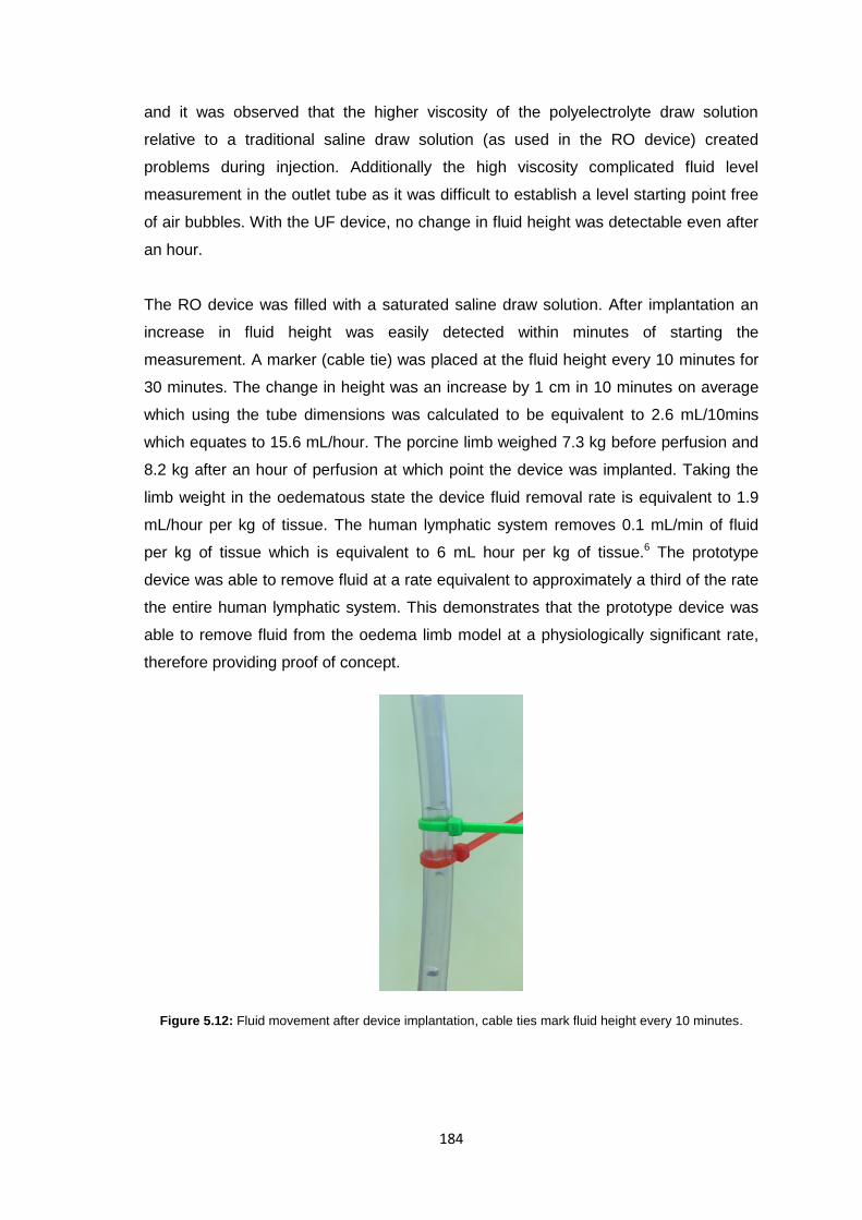
184
and it was observed that the higher viscosity of the polyelectrolyte draw solution
relative to a traditional saline draw solution (as used in the RO device) created
problems during injection. Additionally the high viscosity complicated fluid level
measurement in the outlet tube as it was difficult to establish a level starting point free
of air bubbles. With the UF device, no change in fluid height was detectable even after
an hour.
The RO device was filled with a saturated saline draw solution. After implantation an
increase in fluid height was easily detected within minutes of starting the
measurement. A marker (cable tie) was placed at the fluid height every 10 minutes for
30 minutes. The change in height was an increase by 1 cm in 10 minutes on average
which using the tube dimensions was calculated to be equivalent to 2.6 mL/10mins
which equates to 15.6 mL/hour. The porcine limb weighed 7.3 kg before perfusion and
8.2 kg after an hour of perfusion at which point the device was implanted. Taking the
limb weight in the oedematous state the device fluid removal rate is equivalent to 1.9
mL/hour per kg of tissue. The human lymphatic system removes 0.1 mL/min of fluid
per kg of tissue which is equivalent to 6 mL hour per kg of tissue.6 The prototype
device was able to remove fluid at a rate equivalent to approximately a third of the rate
the entire human lymphatic system. This demonstrates that the prototype device was
able to remove fluid from the oedema limb model at a physiologically significant rate,
therefore providing proof of concept.
Figure 5.12: Fluid movement after device implantation, cable ties mark fluid height every 10 minutes.
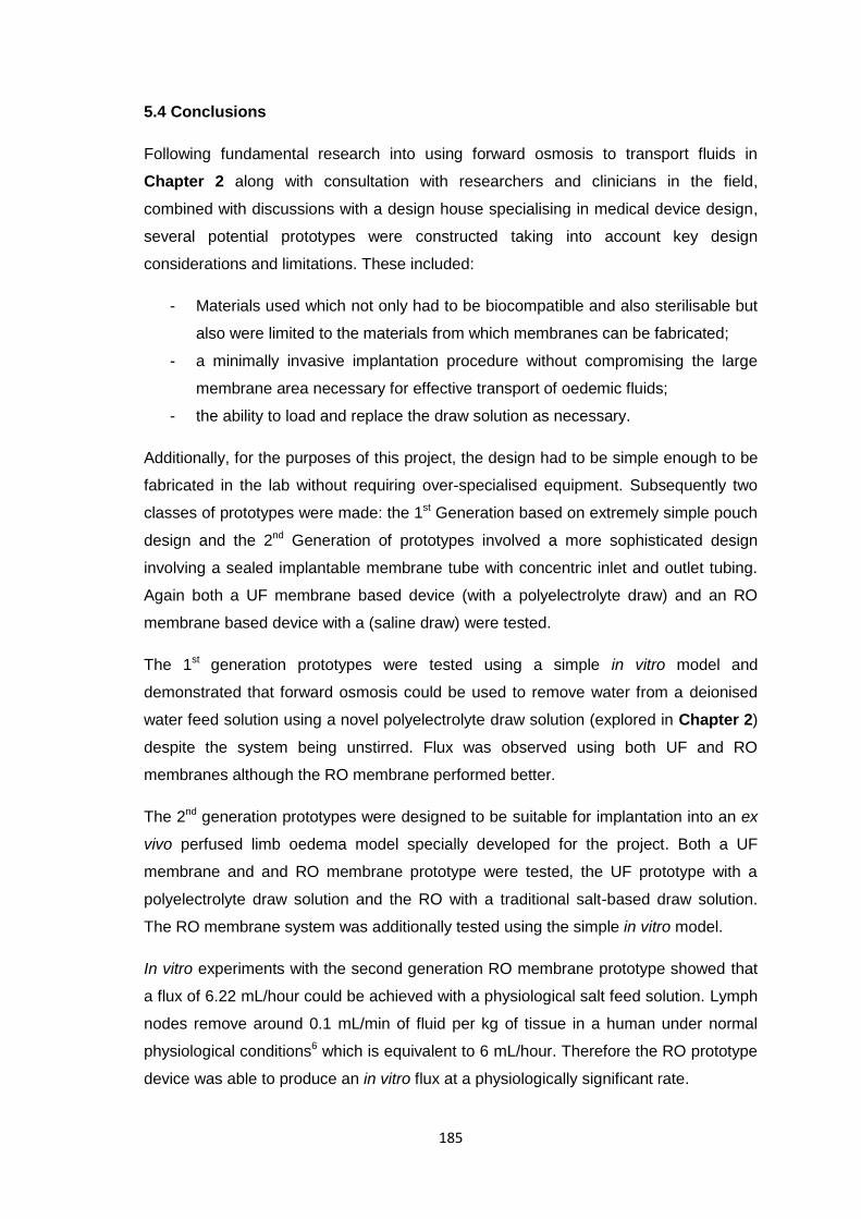
185
5.4 Conclusions
Following fundamental research into using forward osmosis to transport fluids in
Chapter 2 along with consultation with researchers and clinicians in the field,
combined with discussions with a design house specialising in medical device design,
several potential prototypes were constructed taking into account key design
considerations and limitations. These included:
- Materials used which not only had to be biocompatible and also sterilisable but
also were limited to the materials from which membranes can be fabricated;
- a minimally invasive implantation procedure without compromising the large
membrane area necessary for effective transport of oedemic fluids;
- the ability to load and replace the draw solution as necessary.
Additionally, for the purposes of this project, the design had to be simple enough to be
fabricated in the lab without requiring over-specialised equipment. Subsequently two
classes of prototypes were made: the 1st Generation based on extremely simple pouch
design and the 2nd Generation of prototypes involved a more sophisticated design
involving a sealed implantable membrane tube with concentric inlet and outlet tubing.
Again both a UF membrane based device (with a polyelectrolyte draw) and an RO
membrane based device with a (saline draw) were tested.
The 1st generation prototypes were tested using a simple in vitro model and
demonstrated that forward osmosis could be used to remove water from a deionised
water feed solution using a novel polyelectrolyte draw solution (explored in Chapter 2)
despite the system being unstirred. Flux was observed using both UF and RO
membranes although the RO membrane performed better.
The 2nd generation prototypes were designed to be suitable for implantation into an ex
vivo perfused limb oedema model specially developed for the project. Both a UF
membrane and and RO membrane prototype were tested, the UF prototype with a
polyelectrolyte draw solution and the RO with a traditional salt-based draw solution.
The RO membrane system was additionally tested using the simple in vitro model.
In vitro experiments with the second generation RO membrane prototype showed that
a flux of 6.22 mL/hour could be achieved with a physiological salt feed solution. Lymph
nodes remove around 0.1 mL/min of fluid per kg of tissue in a human under normal
physiological conditions6 which is equivalent to 6 mL/hour. Therefore the RO prototype
device was able to produce an in vitro flux at a physiologically significant rate.
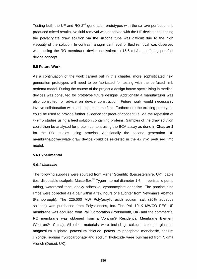
186
Testing both the UF and RO 2nd generation prototypes with the ex vivo perfused limb
produced mixed results. No fluid removal was observed with the UF device and loading
the polyacrylate draw solution via the silicone tube was difficult due to the high
viscosity of the solution. In contrast, a significant level of fluid removal was observed
when using the RO membrane device equivalent to 15.6 mL/hour offering proof of
device concept.
5.5 Future Work
As a continuation of the work carried out in this chapter, more sophisticated next
generation prototypes will need to be fabricated for testing with the perfused limb
oedema model. During the course of the project a design house specialising in medical
devices was consulted for prototype future designs. Additionally a manufacturer was
also consulted for advice on device construction. Future work would necessarily
involve collaboration with such experts in the field. Furthermore the existing prototypes
could be used to provide further evidence for proof-of-concept i.e. via the repetition of
in vitro studies using a feed solution containing proteins. Samples of the draw solution
could then be analysed for protein content using the BCA assay as done in Chapter 2
for the FO studies using proteins. Additionally the second generation UF
membrane/polyacrylate draw device could be re-tested in the ex vivo perfused limb
model.
5.6 Experimental
5.6.1 Materials
The following supplies were sourced from Fisher Scientific (Leicestershire, UK); cable
ties, disposable scalpels, MasterflexTM Tygon internal diameter 1.6mm peristaltic pump
tubing, waterproof tape, epoxy adhesive, cyanoacrylate adhesive. The porcine hind
limbs were collected as a pair within a few hours of slaughter from Newman’s Abattoir
(Farnborough). The 225,000 MW Poly(acrylic acid) sodium salt (20% aqueous
solution) was purchased from Polysciences, Inc. The Pall 10 K MWCO PES UF
membrane was acquired from Pall Corporation (Portsmouth, UK) and the commercial
RO membrane was obtained from a Vontron® Residential Membrane Element
(Vontron®, China). All other materials were including; calcium chloride, glucose,
magnesium sulphate, potassium chloride, potassium phosphate monobasic, sodium
chloride, sodium hydrocarbonate and sodium hydroxide were purchased from Sigma
Aldrich (Dorset, UK).
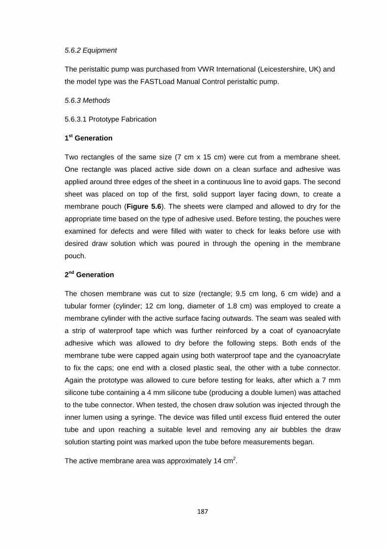
187
5.6.2 Equipment
The peristaltic pump was purchased from VWR International (Leicestershire, UK) and
the model type was the FASTLoad Manual Control peristaltic pump.
5.6.3 Methods
5.6.3.1 Prototype Fabrication
1st Generation
Two rectangles of the same size (7 cm x 15 cm) were cut from a membrane sheet.
One rectangle was placed active side down on a clean surface and adhesive was
applied around three edges of the sheet in a continuous line to avoid gaps. The second
sheet was placed on top of the first, solid support layer facing down, to create a
membrane pouch (Figure 5.6). The sheets were clamped and allowed to dry for the
appropriate time based on the type of adhesive used. Before testing, the pouches were
examined for defects and were filled with water to check for leaks before use with
desired draw solution which was poured in through the opening in the membrane
pouch.
2nd Generation
The chosen membrane was cut to size (rectangle; 9.5 cm long, 6 cm wide) and a
tubular former (cylinder; 12 cm long, diameter of 1.8 cm) was employed to create a
membrane cylinder with the active surface facing outwards. The seam was sealed with
a strip of waterproof tape which was further reinforced by a coat of cyanoacrylate
adhesive which was allowed to dry before the following steps. Both ends of the
membrane tube were capped again using both waterproof tape and the cyanoacrylate
to fix the caps; one end with a closed plastic seal, the other with a tube connector.
Again the prototype was allowed to cure before testing for leaks, after which a 7 mm
silicone tube containing a 4 mm silicone tube (producing a double lumen) was attached
to the tube connector. When tested, the chosen draw solution was injected through the
inner lumen using a syringe. The device was filled until excess fluid entered the outer
tube and upon reaching a suitable level and removing any air bubbles the draw
solution starting point was marked upon the tube before measurements began.
The active membrane area was approximately 14 cm2.
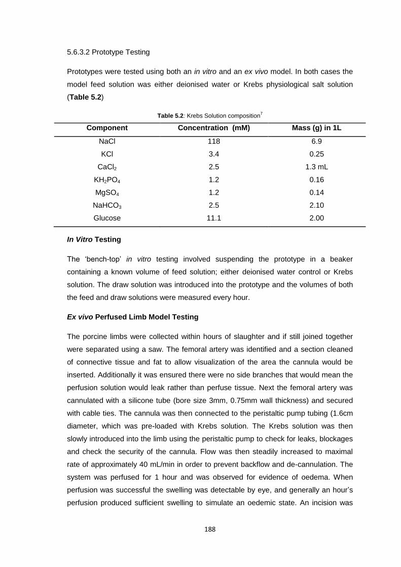
188
5.6.3.2 Prototype Testing
Prototypes were tested using both an in vitro and an ex vivo model. In both cases the
model feed solution was either deionised water or Krebs physiological salt solution
(Table 5.2)
Table 5.2: Krebs Solution composition7
Component Concentration (mM) Mass (g) in 1L
NaCl 118 6.9
KCl 3.4 0.25
CaCl2 2.5 1.3 mL
KH2PO4 1.2 0.16
MgSO4 1.2 0.14
NaHCO3 2.5 2.10
Glucose 11.1 2.00
In Vitro Testing
The ‘bench-top’ in vitro testing involved suspending the prototype in a beaker
containing a known volume of feed solution; either deionised water control or Krebs
solution. The draw solution was introduced into the prototype and the volumes of both
the feed and draw solutions were measured every hour.
Ex vivo Perfused Limb Model Testing
The porcine limbs were collected within hours of slaughter and if still joined together
were separated using a saw. The femoral artery was identified and a section cleaned
of connective tissue and fat to allow visualization of the area the cannula would be
inserted. Additionally it was ensured there were no side branches that would mean the
perfusion solution would leak rather than perfuse tissue. Next the femoral artery was
cannulated with a silicone tube (bore size 3mm, 0.75mm wall thickness) and secured
with cable ties. The cannula was then connected to the peristaltic pump tubing (1.6cm
diameter, which was pre-loaded with Krebs solution. The Krebs solution was then
slowly introduced into the limb using the peristaltic pump to check for leaks, blockages
and check the security of the cannula. Flow was then steadily increased to maximal
rate of approximately 40 mL/min in order to prevent backflow and de-cannulation. The
system was perfused for 1 hour and was observed for evidence of oedema. When
perfusion was successful the swelling was detectable by eye, and generally an hour’s
perfusion produced sufficient swelling to simulate an oedemic state. An incision was
189
made through the skin and the device was introduced before the opening was sealed
using cyanoacrylate adhesive. The draw solution was injected into the prototype device
and the fluid level was noted before starting the experiment. The limb was perfused
throughout the measurement.
5.7 References
1. C. B. Herbert and M. N. Blaine, US Pat. 8 211 053 B2 (2012), to Equilibrate
LLC.
2. G. Matheis, F. Beyersdorf, A. Hanselmann, A. Unger, A. Wildhirt, S. Kruger, G.
Zimmer, and P. Satter, Cardiovasc. Surg., 1994, 2, 725–736.
3. A. B. Fisher, C. Dodia, and J. Linask, Exp. Lung Res., 1980, 1, 13–21.
4. S. Wagner, A. Nogueira, M. Paul, D. Heydeck, S. Klug, and B. Christ, J. Artif.
Organs, 2003, 6, 183–191.
5. M. Friebe, J. Stahl, and M. Kietzmann, J. Vetinary Pharmacol. Ther., 2001, 36,
292–297.
6. G. Pockock, C. D. Richards, and D. Richards, in Human Physiology, Oxford
University Press, Oxford, 2013, pp. 359–443.
7. M. J. Gardener, C. D. Glen, G. R. Richards, P. M. Vanhoutte, G. Edwards, M.
Fe, and A. H. Weston, Br. J. Pharmacol., 2001, 133, 1145–1153.


