
Average Case Computational Complexity Theory
A the& stzbmitted in confoRnity with the teqpirements
for the Degree of Doctor of Philosophy
Graduate Department of Computer Science Univeffify of Toronto
The author has granted a ncm- exclusive licence allowing tfie NatidLi'braryofCauadato reproclace, loan, distn'bute or sen copies of this thesis in microf~m, paper or eiectronr-c fwnats.
The author retains ownership of the copyright in this tbk. Neither the thesisntwsPbstantialexctactshit may be printed or otherwise reproduced without the author's permission.
L'auteur a acco& me licence non excsive permettant a la Bibliotb&ue nationale du Canada de reproduire7 p&er7 distri'buer ou ~ ~ d e s c o p i e s d e c e # e t h ~ s o u s la f m e de microfiche/fikn, de reproduction sur papier ou sm format khtmnique.
L'auteur conserve la propri* du b i t &auteur qui prow cette t h k . Ni la thke ni des erztraits substantiels de celle-ci ne doivent &e imprim& ouanrlrementreprochritssansscw aatarisation.
Average Case Computational CompIexiQ Theory
Dodor of PhiIosophy, I997
Tomoyaki Yamakami
Graduate Departxnent of Computer Science
University of Toronto
Abstract
The hardest problems in the compl&Q class N P are d e d NP-complete. However, not d NP-complete
problems are equally hard to solve b m the average point of view. For example, the Hamiltoniau circuit
problem has been shown to be solvable det-y in polynomial time on the average, whereas the
bounded tiling problem stitl remaius hard to d v e even on the average We therefore need a thorough
analysis of the average behavior of algorithms.
In response to this need, L. Levin initiated in 1984 a theory of average-case NP-completeness. Levin's
theory deals with average-case NP-complete problems using polynomial-time many-one reductions. The
reduciiility is a method by which we can classif3. the distri'bntiond NP problems.
In this thesis, we develop a more general theory of average-case complexity to determine the relative
complex@ of all natural intractable problems. We investigate structure of redua'bilities, in-
cluding a bounded-error probabilistic truth-table reduaiility. We introduce a variety of relativizations of
frmdamental a m a p z e complexity Jasses of distribtttional decision problems. These I.elativizations are
essential when we attempt to expand oar notion of axerage polynomial-time computabihy to deveIop a
hierarchy above amage NP problems.
A- analyses are very sensitive to the choice of pmbabiIity distriiutions. We have o w that
if the input p robabw djstri'ibution decays expanentkdy with size, for instance, all NP-complete problems
are solved "fast" on the average. This phenmneftou does not reflect a signi6cant feature of averagecase
analysis. This thesis includes a thorough and* of stmctttraI properties offeasily computable distnintions
and kasiily sampIable distributions.
In addition, one may ask how we can extract the errsentia average behavior of algorithms independent
of the choice of pmbabiritg. dhtribotians, To arrsarer this question, this thesis introduces the new notion
of computabilitp, which expands the bouudary of feasii1e computabm (snch as
polynamial-time compntabiIity), and asserts the irrvariance of amagmwe cmpkity of algorithms regard-
less of which feasibIy computabIe distributions are chosen. This thesis exiunines the hardness of this red
compdabiE& and its StrncturaI properties
Preface
The theory of averageease NP-completeness came fora3Iy to my attention while I was a visiting scholar
at the Unive&& Ulm from April to August of 1991. In June of 1991, the annual meeting of complexity
theorists from the U n i d t Ulm and the Universitat Polithica de Catalunya was held in BarceIona Uwe
Schiining, the director of the Abteilrmg TheOretiSche Informatik of the UnivedZt Ulm, assigned to young
researchers the topics that would be exeensively studied at that year's meeting: average-case NP-complete
problems and local search problems. Six years before, L. Levin had presented his idea of averagecase
NP-completeness, and several important studies were done dong these lines.
I started reading fhse papers and technical reports and enjoyed discussing Levin's definition of "poly-
nomial on averagen with Rainer Schuler, who was hishiug his thesis on probabilistic computations. The
foundations of this thesis were estabIished during this time, and the results were presented at a conference
in New Delhi in December, 1992.
In June of 1994, I met Rainer SchuIer again at a coaference held m Amsterdam. He had with him a paper
which solved a prob1em we had left open m our 1992 paper. We soon started working together, refining his
key algorithm to construct hard sets which cannot be computab1e in fw31e time. These resalts were h e r
presented at a conference in Xi'an, C h h , m August of 1995 and are also induded in this thesis.
This thesis demands of little preparatory know1edge in the theory of computational compIe&y- Most
concepts are thoroughly defined in each section of this thesis or are self-expknatory-
I am extremely gratefuI to Stephen A. Cook for his hospitality and expert supervision. I thank him
also for his direction and support, without which I could not have come to Canada to pursue my PhD. degree. My thanks also go to my Send Rainer Schder who has been my collaborator since I visited the
Abteilung Theoretische Idormatik of the Unkmi& Ulm m 1991. I w d d like to thank Jie Wang and
Osamn Watanabe for helpfol comments and fmitfd criticism- SpeciaI thanks go to Ymi Gnrevich and ..41aa
Selman for his kindness and support. I am aIso indebted to Leonid Levin and Oded Goldreich fix helpful
commentsents I greatIy appreciate the input of my thesis committee members, Steve Cook, .b Borodin,
Alasdair Urqnhaa, Chariie Radro&, Ytrri G d c h , Anthony 1 Bonner, Rudolf Mathon, and Radford Ned
I thank my Eends Brian ESimn and Lnis Dissett at the University of Toronto for their kind advice and
encouragement. My spedal thauks also go to Eric HarIey and Debby F&pka for pointing out iqpcs and
grammatid errors in an eady mamscr@t.
My parents, Fbjb and Y o d b , hawe supported me emotionaIly and hanciaIly daring my studies m
Toronto. I also thank my grandmother, Nawo, fhm the bottom of my heart for spiritna guidance My great
appreciation &odd go to my h c i e Mitsne Normrra who ha helped me write this thesis-
Tamnto,Canada
May 7,1997
Contents
2 Foundations of Computational Complexity Theory 9
2.1 Introduction .............................................. 9
................................. 2 2 hdamental Notions and Notation 10
22.1 Logic ............................................. 10
2 2 2 SetsandNumbers ...................................... 11
22.3 Graphs ............................................ 13 . . . . . . . . . . . . . . . . . . . . . . . . . . . . . . . . . . 22.4 F i and Infinite Strings 14
22.5 E'unctions . . . . . . . . . . . . . . . . . . . . . . . . . . . . . . . . . . . . . . . . . . . 15 ..................................... 22.6 Asymptotic Notation 17 ..................................... 22.7 Probability Measure 17
2 3 Models of Computation ....................................... 18
2.3.1 DeterministicTuringMachines ............................... 19 ............................. 2.32 Nondekmbkkic Thing machines 20
................................... 23.3 Oracle W g Machine 22 ................................ 23.4 Alternating Thing Machines 23
............................ 23.5 Worst-CaseTime/SpaceComplexity 24 ....................................... 2 4 Randomized Algorithms 25
24.1 RandomInpatDomains ................................... 26
................................ 2.42 Probabilistic lSuing Micbines 27 ................................... 2.5 Worst-case ComplexiQ CIasses 29
.................................... 25.1 Computable hctions 29
2 5 2 Complexity Clanses ...................................... 30 ................................... 2.53 Worst-case Hierarchies 33
............................... 25.4 Polynomial-Tie Reducibilitie 35 ...................................... 25.5 CompIexityCores 36
2 6 One-Wayhctions- ......................................... rn 26-l Hashbctions ........................................ 35
..................................... 2.62 One-way hct ions 38
. . . . . . . . . . . . . . . . . . . . . . . . . . . . . . . . . . . . . . . . . . . 2.7 ReleoantTheoris 42
. . . . . . . . . . . . . . . . . . . . . . . . . . . . . . . . . . . . 2.7.1 Feasl'bIe RedNumbers 42
. . . . . . . . . . . . . . . . . . . . . . . . . . . . . . . . . . . 2.72 Kohogorov Complexi~ 44 . . . . . . . . . . . . . . . . . . . . . . . . . . . . . . . . . 2.73 Resomce-BoundedMm 45
3 General Theory of Average Case CompI&ty 47
3.1 Introduction . . . . . . . . . . . . . . . . . . . . . . . . . . . . . . . . . . . . . . . . . . . . . . 47 . . . . . . . . . . . . . . . . . . . . . . . . . . . . . . . . 3 2 Distributio~~~axtd Density hct ions 49
. . . . . . . . . . . . . . . . . . . . . . . . . . . . . . . . . . . . 3.3 A Notion of Easy-on-Average 53 ...................... . 33.1 Naive Dehitiou of Average Polynomial T i e 53
. . . . . . . . . . . . . . . . . . . . . . . . . . . . . . . . . . . . . . . 3.35 Levb'sDehition 54
. . . . . . . . . . . . . . . . . . . . . . . . . . . . . . . . . . . . . 3.33 Basic Roperties .. 58 . . . . . . . . . . . . . . . . . . . . . . . . . . . . . . . . . . 3.3.4 Different Characterization 62
33.5 Randomhctiom ...................................... 64 .......................... . . . . . . . . . . . . 3.4 A Notion of Domination : 68
..................... 34.1 Dominaton Relations and Eqgivalence Relations 68
................................... 3.12 hbd Roperties 72
.................................. 3.4.3 Randomized Domination 75
. . . . . . . . . . . . . . . . . . . . . . . . . . . . . . . . . . 3.5 Distributional Decision Problems 77
.............................. 3.5.1 Average-CaseCompl~Classes 77
. ................ 3.55 Inclusionsandseparations ..... .-.. 83 .................................. 3.53 Another Characterization 90
............................................ 3.6 Furthdopics 97
4 Feasi'bIe Disttiiations 99
.............................................. 1 Introduction 99
...................................... 4.2 Computable DistnLbutions 101
.......................... 42.1 W o n of CornpntabIe Distrz'butions 101
................................. 422 RMShingsandRareSets 108 .............................. 4.2.3 FanIt-Tolerance 0fDistrriutions 114
. . . . . . . . . . . . . . . . . . . . . . . . . . . . . . . . 4.3 Normalization of Semi-Distributions 117
....................................... 4.4 SampIabte Distributions 120 ........................... 4.4.1 D a o n of SamplabIe Distributions I20
............................. 44.2 Inverbily SampIabIe Distn'bntiom 123
....................... 4.4.3 Ctosme Properties of Samphble Distfi'butions l27
.................................. 4.5 The P a m p = P-samp Qllestion 130
........................................ 4.6 UniversalDistribatiw 133
. . . . . . . . . . . . . . . . . . . . . . . . . . . . . . . . . . . 6.3.1 ReIativizedAvet(P. 3) 205
. . . . . . . . . . . . . . . . . . . . . . . . . . . . . . . . . 6.32 RelativizedAver(BPP, 7) 207 . . . . . . . . . . . . . . . . . . . . . . . . . . . . . . . . . . 63.3 Relativized Aver(NP, F) 209
63.4 Relatrmzed * * . . . . . . . . . . . . . . . . . . . . . . . . . . . . . . . Aver(PSPACE, 7) 214 . . . . . . . . . . . . . . . . . . . . . . . . . . . . . . . . 6.4 Average Polynomial-Time Hierarchy 217
. . . . . . . . . . . . . . . . . . . . . . . . . . . . 6.4.1 Average PoIynomial T i Hierarchy 217 . . . . . . . . . . . . . . . . . . . . . . . . . . . . . . . . 6.4.2 Sparse Interpolation Property 221
. . . . . . . . . . . . . . . . . . . . . . . . . 6.5 Average Polynomial-Tie Alternation Hierarchy 225 . . . . . . . . . . . . . . . . . . . . . . . . . . . . . . . . . . . . . . . 6.6 Average Low Hierarchy 230
7 Quintessential Computability 233
7.1 Introduction . . . . . . . . . . . . . . . . . . . . . . . . . . . . . . . . . . . . . . . . . . . . . . 233 . . . . . . . . . . . . . . . . . . . . . . . . . . . . . . . . . . 7.2 Rea Polynomial-Tie Hierarchy 235
. . . . . . . . . . . . . . . . . . . . . . . . . . . . . . 7.2.1 TheNotionof"ReaICunderF' 236
.............................. 7.2.2 Real Polynomial-Tie Hierarchy 238 ............................... 7 2 3 Nearly-CE and Nearly-A: Sets 241
...................................... 7.2.4 CoIlapsing CIasses 242 ,
...................................... 7.3 hdamental Separations 245 ............................... 7.3.1 Construction of Hard instances 245
. . . . . . . . . . . . . . . . . . . . 7 3 2 Separation from "Quasi? Linear ExponentiaI Time 249 . . . . . . . . . . . . . . . . . . . . . . . . . . . . . 73.3 Separation from Advice Hierarchy 252
7.4 ImmtmItyandBi-I mnnmity . . . . . . . . . . . . . . . . . . . . . . . . . . . . . . . . . . . . . 255 ............................ 7.41 Immune Sets and Complexity COWS 255
..................... 7.4% Bi-Immune Sets and Rggurce-Bounded M e i s m 257
7.5 ClostlrrProperties .......................................... 259 ............................... 7.5.1 Polynomial Time Reduu'bilities 260
7-52 PolynomiaIly h d e d W Operator ........................ 264 ........................... 7.6 Bounded Error Probabilistic PoIpomial Time 266
..................................... 7.7 RandomOracleSeparatio 11s 275
A Small Lemmas 283
References 289
List of Notation 297
Index 300
Chapter
Introduction
The new concept of the "automatic computing spstemn (a term coined by von Neumann) was proposed that
gave rise to cornputem in the mid 1940's. After five decade, compaters have come to permeate our society;
&- preslence spans the range horn wrist watches to weather forrcasting satellites orbiting the earth
The theory of wqmtdmd c m p k i t y has emerged as computer technology has advanced, and now we
face more diEculties than ever. When a problem is given, we must write a program or constract a drcait
to solve it. To minimhe the coat d solving the pmb- we mttst p d I y determine its complexity-
" C o m p I e can be measured in various ways, such as 'We running time spent by an algorithm," "the
memo y space useci for an alga- %he mnnber of basic operations made by an a f g o r i e "the number
of pt~~essors used for a circuit," and so on, Here we foeas on an algorithmic model of computation: tomst-
mse mmplexi~ t h m ~ deafs with the worst behaviors of aIgorithms, that is, the maxbd complexity of
algorithms when an adve~~ary chooses %adD instances. On the contrary, mmge-ease complexity theory
d p t e s algorithms by measorring their complexity on tire aoaage over all Instances.
lkaditid amapase analysis of problems has been performed to determitle the expected nmning
t imem~tapespaeeofalgoti thmstosolve~problernstmd~ ' cesinwhicheachmput
mstance occurs with a certain probabilitp. We have seat that many important problems, such as the traveling
desperscrn probIem aud the E h d t m h circuit problem, are categorized as the hardest to solve among ETP problems. The hardest problems in NP are d e d NP-compIete An NP-complete problems share the same
wimkase opmplex@, but they are not of the same average-case complexity. For example, relatively fast-
on-amqe d e t ~ ' ' "t - have been found for some famous NP-complete probtP_rrls. such as the
graph 3a- problem, and the Ead* circuit problem, under natnrany selected distriinticms.
..41thonghthenotionofexpectedrmmingtime/spaceissimpIe andhmitiq it hislimitations whenusedas
a base of a consistent d coherent theory and does not address the better understanding d the nature of mtractability d problem in both a themetical and practical sasa
In 1984, Ioeonid LevIn I601 presented a one page paper at the Spposimn on Theory of Computing,
STOC, p q a k g the novel idea of - an v,?npiBdtg measare. Levin demonstrated that
arandomEtedverSi~ofanNP-complleteptoblem,~rrmdomited~fitingp~iscOmpI~fota
randomized version of NP. This terse paper shed light on w h averagecase analysis should be. Early works
of Gurevich [36] and Ben-David, Chor, Gddreich, and Lnby [9] expanded Levin's original idea to establish
a coherent framework for averagecase compIexity theory. Siice then, numerous investigations have been
made-
This thesis tries to establish a general, consistent, and coherent theory of computational averagecase
complexity and to contriiute to its adva~~ement. In partl*cnlar, this thesis makes an important addition
to Levin's theory of average-case NPeomplekness by defining averagecase hierarchies founded on average
polynomial-time computable problems, anaIogous to the po1ynomiaI-time hierarchy. In this thesis, we study
the structure and properties of those newly de6ned hierarchies. We also emphasize the investigation of
distriiutions, which is a reced undertaking. The thesis carries out a thorough analysis of computable
distributions and samplable distriiutiom. The most innovative part of this thesis is the introduction in
Chapter 7 of tphtessential oomputability under a giveu set of distributions and its investigations. This
new concept enables us to discuss a wide range of subjects in a- compIexity theory. We use Kolmogorov complexity, resourcebounded measme, and random oracles to understand the true nature of
average behaviors of aIgorithms.
The thesis consists of eight chapters, each of which addresses a separate issue Specificallyt Chapter 2
provides the reader wi th the foundations of the theory of computational complexityt the fundamental notions
and notation, necessary to read the thesis. Most rend& come from the author's work (in collaboration with
R Schnler) on averagecase complexity theory [97,9Stll9], whiIe some new results are appended elsewhere
in the thesis. To avoid confusion, d t s (theorems, lemmas, e k ) with which the author was involved are
Iisted under Major C- at the beginning of each chapter with careful attniution. More detailed
explanations will be found bdm.
Easy on the Average. A naive idea of capturing the average behavior of a function f is given as for-
lows. For a distriitttion p, let as denote by ji the associated (pdabi&) density fWICCi4R The ftmc-
tion f is Uexpeeted polynomial on wverage" if there is a positive integer k snch that, for almost all n,
f ( z ) ~ ( x ) 5 nk, where p,, is the conditionaI distn'bution of p dehed on the sLrings of length n.
However, as dimmed m Section 33, this dehition has serious deficiencies, such as Mdnp the closure prop
erty under composit;on and lack& the property of machbAmdependence. It therefore cannot be the basis
for a consistent, fruitfd theory. In the a- setting, we view a decision problem as a pair consisting
of a set of instances and an input distribntian, called a d&dr&bd (decision) problmt or rrardomized
(&&ion) pproihu. The intended interpretation is that, for an aIgorithm which determines whether z E -4,
each instance z is given to the algorithm with a probabw spedfied by the distribution.
In contrast, Levin [a] d e d a function f po- on p-memge if there exists a positive real wmber 6
snch that the w o n &,,, [z[-Lf(s)dji(z) collvetges- This e q e c h t h is taken over the i&nite set
of a11 mnempw shings. Later h p a g b m [83j: pointed out that we can replace Levin's inhi& arpectation
with a series of- expectations, a an inpnt d e b n ) n ~ h . , - Ltrlsn f ( ~ ) ~ % ~ ( z ) being bounded by O(n), whete en is the con- d i s t n i o n of p on the of length at most TL In other words,
it is d a e r r t to check the -on over all strings of length at most n.
An intuitive characterization of Levin's notion of wynod on pamagen is given by Schap'ire [88] as
fbM t h e exists a polpomia psnch that, for every positive red number r7 F({z 1 f (x ) > p(r-lxl))) < l/r.
Here we remark that can be replaced by jr<,. - Based on Sehapire's formulatian, we are able to extend
M ' s pIyrmnial on p-mmye to t on p-aasoge for an arbitrary function t. Naturdly7 a distributional
decision pmbIem (A,p) is iden- as 4eu.sy8 un mcmge if the problem -4 is computed by a deterministic
'ILring machine which kaIts in po1yuomiaI time on paverage The dection of aU such easy-on-awfage
problems is considered an aveqpcax version of P by many d e r s and is denoted in this thesis by
Aver(P,*) (by AP, AvP, AverP, Aver-P, or Amage-P, elsewhere). This class is fundamental to Levin's
theory of a- N P a m p k n e s s - More generally, we can restrict ourselves to an arbitrary set 3
of distriiutions, and the notation Aver(P,T) denotes the collection of all easyan-average distrriutional
problems (A, p), w h p is taken h 3. Under some natural distn'butiom, several NP-compIete problems
are s o l d k 'Lfast on the a w n For example, the "satisfiabilitp problemn [a, the "graph 3-colorability
problem" [Ill, and the "Hamiltonian circait probIemn with edge probability 1 [13] are h d to be in
Aver@, t ) under some reasonable distriiolls.
On the other hand, an a v e q w a ~ counterpart of the class NP is the collection of all distn'bntionaI
problems which are paits of an NP set and a ferrsibip computabIe distxibution. This collection is denoted
m this thesis by Dist(NP,Pamp) (by W N P , RNP, or Random-NP elsewhere). Levin raised an inttigu-
mg qudm " Can all problems in Dist(NP,P+mmp) d y be "easy" on the average ?" Ben-David,
Chor, GoIdreieh, and Luby [91 gave the folIotrring answer: this is the case d e s s the nodehmb&ic lin-
ear -entiat-time class equaIs its deterministic comtapart. This thesis is motivated by Levin's open
Questioa Chapter 3 is devoted exclusively to mtrodudng Levin's theory of averagecase complexity and its
genemhtion.
To ded 6th the complexity issue, we generaIize the above tmo dasses and introduce the notion Dist (C, F) , which is the conection of alI pairs (A, p), where A E C and p E 3, and the other four fundamental notions
A = w , n A=(BPP77), A-~erlRp,T), and A=(PSPACE,T).
Input Disttr'butions. Here we wonld like to remind the reader that average-case analyses are sensitive
to the doice ofdistributiom, becatrse "aoerage poIycmiaLtime computabB'ity" is fonnded on the Mumior
d the distribntio~~ in gaestior~ The study of distnintions is thedore c r u d in averagPcase complexity
theory. In Chapter 4, we discuss the c o m p l e OffeasiIe distniutionsc In parti&, we shan focus on two
tgpes of distribntions: p o l y n d t i m e cornputabfe ~iutioons and poIynomiaEtime samplable distribu-
tions G d c h [36] cased a distri'bation p poEynomiaLhe conrputa6k if there exists a deterministic Thing
marhine M sach that k(z) - M(z,Oi)[ 5 2-' fm all nonnegative integers i, Een4lavid et al, introdaced p l y n o m i a ~ s ~ d i s t n ~ w h i c h a r e ~ b p r a n d ~ a i g o r i t h m s ( e a l l e d s a m p I i n g &
gnrithms [9] or gemmkxs [96j) wki& nm in time polsnomiaI in the Iength of "ontpbn By Pcomp and
P-satup, we denote the sets of pdymmiaI-time computable and samplable mpectidy- In Secti011~5,mshall~thatpotsP~timesamplable~ati0rt~arrprrciseIy~~asPPsetsto
compute detembWcaUy m polynomial time,
Another important notion in Levin% theory of average-case NPcompleteness is domination relaths
among distriiutions. When a distribution p majorizes another distniution u within a polynomial factor, we
SaY that Cr p0hJlWmidkJ dominates Y. More precisely, p polynomially dominates v if there exists a polynomial p such that p(lz1) - ji(z) 3 5(z) for all strings z. Polynomiadomination of polynomia-time samplable
distributions is closely related to the existence ofcryptographic oneway fnnctions. A (cryptographic uniform)
oneway function is a function which is easy to compute but hard to invert on most instances and is believed
to exist by many mearchers, &-David et ul. 191 first found this connection and showed that if such
oneway functions exist, then there is a polymmbI-time samplable distriiution which is not polynomially
dominated by any polynomial-time computable distriiution. In Section 4.7, we shall show that a much
weaker assumption, the existence of NP sets that are not neariy-RP, is enough to get the same conclusion.
Here, a set A is said to be nearly-RP if some randomized algorithm computes A on most instances, and it
behaves Iike a onesided bounded-error probabilistic madhe w most instances.
Moreover, if two distniutions polpnomially dominate each other, we say that both are polynornially
epiwdent. For example, every distriiution samplabIe dative to BPP sets in time polynomial in the size of
output is polynomialIy equivalent to some polynomiat-time samplable distriiution. Under the assmnption
P = NP, every polynomial-time computable distriiution is polynomially-eqtlivalent to some polynomial-
time samplable distriiution.
Average-Case ReduciiiEty. Chapter 5 focuses on a d e t y of averagxzw red~d~lities. For decades,
d e r s have made great efforts to achieve a better understanding of the structure and properties of
inEradd& problems. The term NP-complete wm coined to d e s a i i the most intraeta6Ie NP problems,
and mafly mterrsting NP-problems are declared to be NP-complete, that is, the hardest problems to solve
in polynomial time.
Levin's innovation is tbe invention d an a- version of such a completeness notion among
distriitttional decision problems. His notion of completeness: is based on worst-case polynomia-time many-
one reduciiility with an extra condition, the stxded d m i n d h condiEton for the reduction function,
which guarantees that the reduction maps more likely instants to more M y instances. Ee showed that
the "randomized bounded tiling problemn is complete for Dist(NP,P-comp) under this type of reductio~
Smce his proof of completeness, only a dozen distriitrdonaI problems have been fotmd to be complete for
Dist(NP, P-comp). Typical examples are: the Pandomized bounded baiting problem" [XI, the "randomized
bounded Post correspondence probIed [S], and the "randomized d problem for The systems" [I121
under p o l y n d t i m e many-one reductions We shall discus the issue of deterministic reductions in Section
5 5
In Section 52, we shall f o d y htmduce the (atrerage) poIynomial-time --One reductions and CUE-
t i d e their structural properties, Wang and Belanger [I121 de6ned polynomial-time isomorphism between
two distriiutiond decision problems and showed that all known complete problems for Dist(NP,P-amp)
are indeed pol&mi& ijOmOlpldc Section 5 3 will show that d tppl*caI d&dmtbd probIems are
CHAPTER I . INTRODUCTION 5
complete for Dist(NP, Pcomp) and also plynomially isomorphic to each other.
Incompleteness resnlts have been achieved by Gurevich [36j and by Wang and &hgr [112]. GnreYich
(361 6rst drew attedion to distriiutions of exponentially-small probability? so-cakd pot dis t r ions , and
demonstrated that no flat distribution makes a distriiutional problem complete for Dist(NP, P-comp) unless
NEXP collapses to EXP. We notice that the distriiution used for the randomized bounded tiling problem,
for example, is not dat. As W q and Belanger pointed out, if we restrict ourselves to on- pcdynomially
honest reductions, we can drop the assumption EXP # NEXP. We shall show that distriitxtions of
another type, d e d sparse distniutions, which were introduced by Gurevich [36], also do not make any
distriiutional problem complete for Dist(NP, P-comp) unless NP coIlapses to P. This incompleteness isme
will be discnssed in Section 5.4.
Another type of important reductiou is Yprobabilistic" or %ndomizedn reduction. In 1988, Venkate
san and Levin [106] used "random reductions" to demonstrate the intwtabiliw of the randomized graph
coIorabiIity problem- Later Ben-David, Chor, Goldreich, and Luby [9] introduced two more notions '(ran-
domized many-one reductions" and "raadomized 'bring ductiom." In Section 5.5, we shall introduce an
averageease version of bormdederror probabilistic truth-table reduciiility. Despite the incornphteness re-
sult of dat distributions, we are able to prove that the randomized bounded halting probIem with a natural
flat distriiution is also complete for DistcNp, P a m p ) mder these reductions.
Average-Case Hieratcbies. In worsase complexity theorg, MeyerStockmeyer's polynomial-time hier-
archy? {A:, !EL, II; I k > 01, has pIayed a central role in capturing the magnittlde of intractability of given
problems. Chapter 6 will discuss a hierarchical issue fiom the averagecase complscity point of view-
The d&duthd polynomial-he hiaorchy under T is an extension of the polynomial-time hierarchy
in which Af; and Ci are replaced with Dist(A1,F) and Dist(EL,F), respectively- We shaII show that each
C-level of the hierarchy under P-comp, Dist(C~,P-comp), has complete problems under poIyuomiaI-time
many-one teducfions.
The notion wiU be introduced of (pM-time ZMng) s s e l f r e d u c j i among distnintiond decision
problems. To determiae the membership z €?A, we recttRiveIy produce other instances y which are of
d e r size than z, and reduce the vestion z E?A to y €?A. Smce the size of instances becomes smaller7
these reductions tenainate in poIynomiaIly-many steps. In worstcase complexity theory, the stishbility
problem, SAT, is a mid exampIe of &-reducible problems- We shall show that most known distriiatid
problems complete for Dist(Zf,P-mp), k 2 I, are seIf-reducible- Whether an complete problems for
Dist(NP, P-eomp) are seIt-reducibIe, however, is an open question. A s an application of se&redua'bitityt we
shan show that DistlNp, P-aimp) G Aver(BPP, *) if and onIy if Dist(NP, P a m p ) G Aver(RP, *).
In Section 6.4, we shaII imsoduce another awmpcase anaIogue of the polynomial-time hierarchgr, called
themaage plpomid-time idermelry under a certain set of distn'bution, to c h d y distributional decision
problems which are hard for Dist(NP,P-camp). The hiemdy is b d t above Averlp,F) and Avet(NP,P) - - u -P- osing-
The model of aternating Tndng machines gives mother * - for the PotynOmiaCtime hi-
erarchy. I n s p i i by this characterization, we shalI introduce in Section 6.5 an menrge pipmid-time
rakmdm kemdy under a set 3 d distn'butions wing a model of alternatitlg T ' g m;urhinplc. Hterest-
ingly, each IeveI of the average polymmia-time alternating hierarchy is characterized by relativized Turing
computability relative to classes in the distai'butional polynomial-time hierarchy. As a d t , in contrast
to the worst-case sitnation, the alternating h i d y is unlikeIy to coincide with the average hierarchy m
general (of course, depending on the tmderIying set of distciiutions).
As an example, we shan locate the pmbabilirtic complexity class Aver(BPP, F) m the average poIynomiat-
time alternation hierarchy.
Quintessential ComputabiIity. In Chapter 7, we s h d shed Light on the collective behavior of distriin-
tional decision problems under a certain set of distri'butions, such as P-comp or P-samp. This a p p d is
new m average-case c o m p w theory and helps us investigate average-case complexity classes m terms of
worst-case complexity classes. More preciseIy, we shall focus on a class of sets S, called "reaI P under a set
7 of distnibati~ns,n which extracts the essentials of averageese complexity dass Aver(P, *) in the sense
that, for every distriiation p in F, the distri'bntional problem (S, p) belongs to Aver(P, *). In other words,
S is computable by some deterministic Tixring machine whose running time is polynomial on paverage.
We are particularIy interested in feasl'ble distributions, such as P a m p . Let as denote by P-,, the
dass 'T under Psomp." We retnrn to Levin's original question, Dist(NP, P-comp) C_?Arer(P, *). Now his question on simpIy be rephrased in terms of worst-case complexity classes as: "Is NP included in
P-,, ?" Based on the average poIynomiaI-time hierarchy, we further define real polynomial-time dasses,
{Ai3, EIF , l IL~ ( k > O), caIled the d p a M - - t i m e IdenmAy un&r 3. This hierarchy enabIes us to generalize Levin's question to any level of the real potynomia-time hierarchy under P-comp: "Is EL inchded
m hikmp ?"
We win show that, fOr evety integer k > 0, A'; E AiF C A; and CE E XiF for my set T of
distributions, where A; is the &-th level of the hear-srponentiaEthe hieratchg-; in particular, P C P3 E E
if k = I. Specifically, let us denote by Phmp the coIlection of sets compntable m poIynomial time on
average under every exponentid-time computabIe distn'bution, Using a notion of compIeJdt9. cores, we are
able to show that P-, cobpses to P. More g e n d y , we are able to prove that = A; and
C:!-Q)mp = CL for dl k > 0.
Section 5.6 wil l discuss hardness d t s ofthe average polynomiaI-time hierarchy under a set of polynomial-
time computable dktriibations, We have already seen the mdusions P G P-, 2 E. In 1995, SchnIer
[92] showed that both indnsions are truly proper nsing a diagonalization over polynomial-time compntabIe
"semi-distn'bttti011~-~ (Later he gave an dtanative proof based on KoImogo~~~ complexi@) We extend his
technique and show m 73J an men more p e COnseQnence: PkmP DTIME(P) fbr each fked constant c > 0. This remit will be extended to any level of the real polynomial-time hierarchy
under P-comp*
A similar technique again enables us to show that A:- has a hard set that is not in AS/m for each constant c > 0, whereAf;lf(n) mgeneralisthecaiIectionofallsets, eachofwhichcanbecompnted by
some A:-type machine with sorue &ice jh&n of length f (n). We note that the dass of sets computed by
non-uniform polynomial-size circuits is Btactly the mion of dl dasses P / nk, k > 0. It does not appear to be
simple to improve our d t to answer the open question of whether dl sets in Pkmp have polpomia-size
circuits. However, Schder [93] recently proved that if aII sets in P-, have polyeomial-size circuits, then
EXP collapses to the second l e d of the polynomial-time hierarchy. Hence, based on the common belief
that EXP is difFerent h r n the po1ynomiaI-time hierarchy, it seems unWrely that an sets in Pbmp have
polynomial-size circuits. These issues win be dhmssed in Section 7-32
Another m i d exampie of intsactabh sets, discussed in Section 7.4, is P-imwme and P-bi-immune
sets. P-immune sets are sets that do not contain any infinite? P-subsets in them, and P-bi-immune sets are
P-immune sets whose complements are also P-immune. We show that there are some non-sparse P-immune
sets m P k m p , but Pp-,-,, has no P-bi-immune sets. This fact exhibii the strunaral d i f f i c e between
Pkmp and the dass ET wbich hsr both P-immune and P-bi-immune sets. Udng the faa regarding
P-bi-immonitp, Pkmp is shown to be mat2 with resped to Ldz's resource-bounded meawe, where a
complexity class is o h Caned d l if it has pmeasnre 0. (Note that E has pmeasure 1.) As an immediate
conseqpence, if NP is included in Pbmp, then NP has pm- 0, and this consequence again contradicts
the popular belief that NP is not smaIL Along the same hes, Schder [W] showed that the --table dosure
of P h m p and the 'Ihring dosnre of P-,, have diflierent measures.
Section 7.5 wiII show that A~Pcomp is not dosed tmder polynomial-time many-one reductions, the ex-
istential opemtors, or the pmbabwc operatom. Hence, the dass P k m p , for example, is structurally
diflikrent fiom most of the weII-known complexity classes, such as P, NP, BPP, and PP. However, it is not
known whether PkmP is dosed under phonest xnany-one reductions. Notice that the cIdss A:-p, real
A: under P-samp, is dosed tmder ghonest polynomial-time many-one distriiutions. We shaU show that if
Phmp is not dosed under phonest polynomial-time many-one reductions, then there is a polgnod-time
sampIab1e distribution which is not po1ynomiaIIy dominated by any poIynomiaI-time computable distri'btt-
tion. Under phonest manyone reductions, we are able to show that there exists a pair of sets in Pmmp which are not redu~ib~e to each other, a so-cded hcmpmble pair.
The qrrintessential complexity class BPPF exhi'b'its another structure. Due to Ben-David, Chor, Gob
Mch, and Luby [9], the assmnption NP E BPPM~ implies the condnsion E BPPkmPT where t the dass of sets compntirbIe m polynomial time with nonadaptive queries to NP oracles. On the
other hand, Schnler and Watanabe [96l extended a resnlt of Venkatesan and Levin [q and showed that
the NP S?BPPMp mestion is equivaIeut to the NP a P P h m p - As shown by Ben-David d UL [9], NP PMp I d to the conclusion E = NE. On the other
han4 NP PmP yields the consequence P # NP. Hence, the N P question cannot be
easily solved in the non-relativized wodd. At this point, we have no prospect for anmmhg Levin's ~nestion
eitherafhmtkty ornegatively. Nowletnstrrmourinteresttoa~onofthisqnestiox~ 1~198'1,
BermdtandGill[8]introducedandi(~ofmndmn~to&mthat PipdifhntbNPin Ym& - .
r e M m d & & M a r e p r e d s e E y , i f a n o r a c l e s e t i s c h o s e n ~ n n d o m , t h e p r o ~ i t y t h ; r t P ~ ~
NPrektipetothiporsdeist I n M o n ? . ? , ~ W s 6 a I I s h o p p t h a f N P a n d P ~ ~ d y e x ~
(ie., NP P-, and PMp NP) in "most" relatlvlzed . * worlds. To be more precise, let us denote
p ~ ~ - c o m p a "naturaln reIativization of the class Pmp relative to oracle X. We wiIl show that, with g NPX, dative to random oracle X. pmbab@ity 1, Z ptx,, and Pp.-p
Chapter 2
Foundat ions of Computational
Complexity Theory
2.1 Introduction
The theory of compctatjonal complexity &st drew attention h m mathematicians as a weak notion of
recursive hctions. To measure the complsdty ofagiven problem, we use particular mdels of computatio~
such as lhring machines, cirdts, or PRAM'S to d v e the problem.
In this chapter, we shall define and explain most ofthe fundamental notions and notations in (worst-cuse)
computational cornplQiEy theory so that the nninitiated reader can read through this thesis without the help
of supplementary textbooks.
In Section !U, we shall cover the elementary notions of gnrpb, numbers, sets, and funcrions. The
basic terminology m pb&ify themy and bgk will be also i n t r odnd The thesis foIlows the standard
terminology often used m mathematics and themticat computer science-
We use - mcdrines = a model of compntatiou. h general, deterministic Thing machines compute
partial renssiae fnnctiom, but our interests lie only m resourcdxnmded computations, and we need the
notions of naming time and tape space of the Thing madhex The reader should pay carefuI attention
to the models we shall use m this thesis becanse ditkent modeIs Iead to different consequences. Several
variations of Ttxhg madines wiII be iatrodaced m Seetion 2.3, and many popuIar complexity classes, such
as P and NP, win be dehed in Section 25. The fiefd of rmrdomired a&iths has grown tremendously in the last decade and has found mimy
appIications because of their sfmplicitp and speed- We shan introduce the basic notions of nndmid
~ ~ p r o b o b i E i s r i c ~ m a d c i n e s , a n d m n d o m ~ i n S e a i a n 2 4 .
InSectionZ.6, trnitrd~/cnrcfimuwitlbeintroduced. HashfanctionsareausefuItoolindesi@ng
raRdomizedaIgo*
Section 2-71 will explain the themy dpd@md analysis initiated by KO and fietiman [55] m the early
1980's. The theory of Kolmogm compleaity also provides us with a succinct description of information.
We also cover the notion of rejowce-bounded K o ~ m 00mpIQity m m and Lutz7s resource-bounded
mensun? theory, which are popular in structaral c o m p I e theory.
For complete references, the reader may refer to [42,91,4,45,80].
Major Contributions. Although this chapter is introd-, a few results are included.
Lemma 2.5.7 offers a new characterization of all A - I d dasses in the poIynod-time hierarchy by
the model of semideterministic alternating Turing machks which w m polynomial time with constant
alternation.
Proposition 2.6.4 shows the existence of an NP set which is not nearly-RP, provided that strong oneway
h c t i o ~ 1 ~ exist-
2.2 Fundamental Not ions and Notation
We shall begin wi th terminology from mathematical logic and then explain mathematical notions and nota-
tions.- graphs, sets, numbers, strings, and functions. This section will include a preliminary introduction to
probability theory.
2.2.1 Logic
In propositional logic, we deal only with Bodean - a h which take d u e s 1 (truth) and 0 (fals-.
(Note that traditionally, in mathematical logic, 0 represents TaIsehood" and 1 represents 9mth.") The
terms are Boolean variables and the logical constants 0 and 1. As Iogioal connectives, we use the symbols
7 (negation), A (conjunction), and V (disjrmction). The set of (proposiEionol) f d o s is defined by the
f0IIowing claflses:
(i) every term is a form*
(ii) if a and @ are formnlas, then -(a), (a 81, and (a V B) are formalas; and
(iii) formulas are d&ed d y by clauses (i)-(fi].
Unless there may be confnsion, we freeIy omit parentheses from formnlasx eg, --a and Q A (B V -y)-
The negation of a Boolean variabIe w is sometimes denoted by iT for simplicity. A Boolean variabIe and its
negation are d e d literals-
Let a = a(z~,z2, ...,z,J beaformnlawithalIdistinctvariablesbeingecplicitlyexhr'b'rtedaszL,z2, ...,%.
We write Vm(a) for the set {z1,z2,. . . ,%). A bnth asignmd for a is a function u : Vm(a) + {T, F).
Given a truth assignment a, we de& an euaZMfion [a], of a on a m the foI1awing recmsive way
(i) mthecasethataisavadabIeq[~I~=Tifand~if~(o)=T;
CHAPTER 2. FOUNDATIONS OF C0MPlJTATIONA.L COMF'LEXlTY THEORY
(i) in the case that a is of the form (b A a), [a], = T if and ody if B], = T and B], = 2'; and
A propositional formula a is sati&.bZe if there exists a truth assignment a for a snch that [aj, = T. In this case, a is said to sdi& a. For example, the fomnla -(z V y) A (-2 V y) is satisfiable, witnessed by
the assignment a such that u(z) = o(y) = T and a(z) = F. A formula a is valid (or a tadology) if [a], = T
for any truth assignment u for a.
For a property Q, the notation VzQ(x) means that Q(x) holds for all elements z, and the notation
32Q(x) means that there ex& an eiemeut x dsfjtng QIx). The notation 3!zQ(z) means that there exists
the unique element z satisfying Q(z). For a property Q de6ned on an idhite set S, we say that 8(z) holds
for almost aU (or dmost may) z in S if the set (s E S [ Q(z) does not hold ) is finite In this case, we also say that 8 holds h o s t crrerywhere. The notation ;ZQ(Z) means that Q(z) holds for a h a t all z, and aa 3 &(a$ means that Q(s) holds for infinitely many s. Cleariy 7 and 7 are dual concepts-
Genedy, for a property Q, we write [Q] = I if Q is true, and [&] = 0 otherwise. For a set ST xs denotes
the chumdaistie fwrction for S that is d&ed as xs(z) = [z E Sj. (Note that "characteristic fnnctions"
here are different from those used in probab* theory.) For brevity, we also use the notation S(z) to mean
x&)-
2.2.2 Sets and Numbers
Sets. Intuitively, a set is a collection of objects, called its members or elements. The notation z E -4
expresses that x is an eIernent of A, and E is called the membership reIatioa The symbol 0 denotes the
enrpdy s d that contains no elements. We use the standard set notation {- I -1. For exampIe, the notation
{z 1 Q(z)) represents the set whose elements x s a w a property Q(z). For two sets A and B, we say A is a &d of B, symbolidly A E B, if every element of A is an dement of B.
For twosets Aand B, the intenedhof Aand Bis denoted A n B andis de6ned by A n B = {a I a € A A b~ B)- TheunionofAand BisdendedA~Bandisd&edbyAUB={aIa~A v ~ E B ) . The
set A-BdenotestheofAandBthatisdhdbpA-B={aIa€A A b 4 B ) .
The of A and B , denoted Ax B, is the set of aII ordered pairs (a, b) snch that a E A and b E B, where an
~ p a i r i s t h e s e t { a , { a , b ) ) . hcontrast,theset{~b)issometimesreferredtoasanunordered~ The
parer set of S is denoted by P(S) and is defmd as the cdIection of aII subsets of S, ie, P(S) = { A [ -4 E S).
For a set ST [Sll denotes the cmdinolity of S that intnitivey expresses the number of elemeats in S. If - 00. S is not finite, then let \IS\ -
Binary Relations. A 6inmy ddim on a set S is a subset of the btesian product S x S, LC, ((a, b) 1 a,Q E S). Conventidy, we write aRb when (qb) E R For a b i i relation R on S, rm say that R
is m j k h e i f & hoIdsfaraIIeIemeuts a € St andthat it is fnmifheif & & a n d bRcimply&Eorall
a,b,c E S. Moreover, a relation R on S is symmetric ifaRb implies bRa for all o,b E S; on the other hd,
Rb-if&aadb&irnplya=bfbraflqb~S.
CEAPTER 2 FOUNDATIONS OF COMPVWZT0NA.L COMPLEXlTY Z'EEORY 12
Nmnbers. Let Z be the set of aIl integers {- - , -2, -1,0, 1, 2, - -1, and let N denote the set of all nonnega-
tive integers, called RwnberS. The set of dl m f h d namkn {z I m, n E 2, n # 0) is simply denoted
by Q and @ denotes the set of all nonnegative! rational numbers. S i I y , the notation B denotes the set
of dl nol MnnbefS, and in mmlar, we denote by R? the set of an nornegative red nnmbers. (Remember
that the superscript + does not mean "positive.") We use the notation cx, to mean the inFnity, and let
P = @ u {oo) a d BO) = I U (00, -m). For the arithmetical operations + (addition) and nd (mnltipli-
cation), we follon the standard conventiox for any nmnbeR r E B and s lit+ - (O), r + oc = oo + r = m,
s - ~ = ~ . s = ~ , - S - O O = cm+(-s) =-00,andO-a,=oo-O=O. Moreover,weassmnethat -a < r
andr < 00 for anydnumberr E 16e
The absolute udtte of a real ntlmber is denoted [rl.
For any two real numbers a and b (a <_ b), Iet (a$) denote an open (dl intewd dehed by (a,&) = {Z E P ( a < z < b); let [a, b) and (a, b] be halfopen intefttab which are defined by [a, 6) = (a, b) u {a} and
(a, b] = (a, b) U {b ) , tespectivelp; and let [u, q be an closed intemui defined by [a, b] = (a, b) u {(a, b).
For a d number 2, let LzJ (pwr of 2) be the maximaI hdeger not exceeding z, and let rxl (ceiling of
2) be the minimd integer not d e r than x.
Lebesgue Measme. For a dosed m t e d I = [qb] of the line It, let III = b - a. Let S = {IC)&c be
a countable coIIection of closed intends on IIP. For a subset E of It, we say that S is a m e r i n g of E if
E rM I t . The Lebesgue onta mcnrmc of a set E, denoted mm(E), is d&ed by
If E is meaStrrabIe, its Lebesgue outer measme is caIIed its W g u e measure (or simply maswe) and is
denoted by m(E). Note that m([O, 1)) = 1. (Thus, m is a probability measure on the sample space [O, 11.)
It is weII known that, sPPDming the Oamn of there exists a noameaSnrabIe set (see, eg, [115]).
PolymminL and Logarithms. We are interested ody in pcdynomids and logarithms w i t h integer
ficients Fatapositiveintegerd,apotpmid (inn) of d@zedisafimctionp(n) ofthefonn:
CHAPTER 2. M)UNDATIONS OF COMPUTATIONAL C0MPI;EXITY THEORY 13
where each % E Z and w # 0- The constants a ~ , a t , . . . ,a are called the eoeffieicntr of the polynomial,
Epomdds are functions of the fotm 2p(*), where p is some poIynomial. In particular, we call a function a
linear--talifit is ofthe form 2Cf+dfm~econstants c,d E v. This thesis uses mainly logorithmJ to h e 2, and for the sake of convenience, we often omit the base and
simply write logz for log2 z. Whenever we ded with logarithms of rational numbers, we follow a special
convention: we define log z to be 0 whenever 0 < z < 1 to simplify the case-by-case description. For brevity?
we also write llog(n) for Llog2(n + 1)j and write ilog(n) for pog2 nl for all n E N. The notation log(k) n denotes k iterations of logarithms, namely, define log(') n = n, and log(k) n =
1og(logQ-') n) for k 2 1. Also Iet log' n = mh{k E N I log(k) n 5 1). The function log* n grows extremely
slowly. For example, Iog' 16 = 3 and Iog' 65536 = 4.
The kth ~ m m o n i c mmber, H ~ , is deiimi by 2, i. The binomial c o e m are defined as follows. for n, k 2 0, if n 2 k, then,
and if k > n, then (P) = 0.
2.2.3 Graphs
A dirrcted graph G is a pair (V,E), where V is a bite set and E is a b i &tion on V (i.6, a subset
of V x V). The set V is d e d a vcrtez set or node set, and its element is caIIed a node or oe&z The set
E is called an edge s d , and its element is d e d an edge. An undirected gmph G = (V,E) is a variation of
ditected graph whose edge set is a sgmmetrk &tion, For an undirected graph, we identi& two edge. (a, b)
and (b, a) and often write {a, b ) as an unordered pair.
We say that a node t is adjacent to a node s if (s, t) is an edge in a graph.
A ( f ini tc)@pafhflengt lrkhandestoanadetmagraphG= (V,E) isa(finite) sequence
(ao,q, ..., vk)ofnodsmNsnchthat s = m , t=vt,and((zi,e+l) ~EforaUiwi thO < i < k. Inthisease,
wesaythat thepathp ~ t h e n d e s v ~ , s , - . - , v t a n d a l s o t h e e d g e s (tl0,q),(g?~f2)~---,(~k-l,~k)- A n d e t i s ~ l e b a n o d e s i f k e x i s t s a p a t h p b s t o t -
ApathissimpfeifaIIndesmthepatharedisthct.
Given apathp = (m,q, ..., vt), a dpdhp' is a subsequence ofp; that is, for some i,j w-ith 0 < i < j k,p'=(vi,v++t,.-.,q).
We can natnrally extend the d e h k h of graphs and paths to in jh i te g m p h and in* patlrs. For
example, an infinite path h m a node s in a graph is an inhite sequence, rather than a bite one, starting
from s.
AgraphGr=(V',E)isasabgraphofG=(V,E)ifV' G V a n d F S E. G i i a s e t V r c V , t h e
snbgraphofG= (V,E) indrroedby V'is thegraphG'=(V',E'), whereE'= {(yo) E E [ y v E V'). Antmdirected~phiseonnededif~twonodesare~Iehmeachdher,
In a graph, a path p = (g,s, ..., uk) forms a qJe if (i) vo = uk and (ii) vo # ui for some i with
0 < i < k. A graph with no cycie is said to be acyclic
A fbmst is an acyclic, undirected graph, and a tree is a connected, acyclic, undirected graph. In particular,
the tree that contains no nodes is called the empty tree or nu22 kee.
A rooted ttee is a tree in which one of the nodes is distinguished from the others; this distinguished node
is called the root of the tree-
Let z and y be any nodes in a rooted tree T = (V,E) with root r. The node y is called an ancestor of
x if there exists a path from r to x which contains y. If y is an ancestor of z, then x is a descedmt of y.
(Note that z is an ancestor and descendant of z i e ) The node y is d e d a pwent of z if (y, z) is an
edge on the path h m r to s. If y is a parent of z, then z is a child of y. Any two nodes which have the
same parent are si6kgs- A node with no children is caIled a leaf (or e z t d node), while the o&a nomleaf
nodes are d e d internut nodes-
A m h t e tooted at z is the tree induced by the set of all descendants of x.
The degree of a node z in a rooted tree T is the number of children of x in T. The depth of a node x is
the length of the path kom the root of T to z. The height of T is the Iargest depth of any node in T.
2.2.4 Finite and Infinite Strings
An dphabet C is a nonempw, bite set. G i i an alphabet Z, a w d or string over C is a finite sequence of
symbols h m Z. The empty Jfring is the uniqtre string consisting of no symbols and is denoted by A. Let
us denote by !P the set of all sttings over X (of course, Z' contains A), and for the sake of convenience, set
9 to be C - {A), the set of dl nonempw strings.
In this thesis, however, we consider only the binary alphabet C = {O,1} (a string over {O, I} is oRen
called a binary Jtt.ingj because this restriction does not affect any of om. arguments.
The Iengtiz of a string z is the wmber of symbok in x and is denoted by lzl. For example, lOllOOl= 5,
and m partienlat, 111 = 0. For every n E N, let C (Zsn, C a , respectively) denote all strhgs of Iength n
(Iength 5 n, Iength 2 n, respectivelgry). We note that a subset of Z' is sometimes called a Impage over E. Fortwostringszand y, the -ofz and y is thestring~0nsistingofthespmbo~ofxfo11dby
the sgmboIs of y, and is denoted by zy (or sometimes x - y). For example, if z = 0110 and y = 1011, then zy = 01lOlIOlI. Given a shing s, SF denotes the set {sy I y E CL). For a string x and a natmd nrrmber
n, the notation zD is reemsivey defined by: z" = A, and flC1 = z - P for n E N
We assume the stadad orderon 2':
(Sort Iength-wise and then sort 1exicographicaIiy.) With respect to this order, z- denotes the pmkcessm
of z if one exists, and 2+ denotes the mazsor of z, Far exampIe, 0 1 W = 0111 and 0110' = 0101- This orderfng enabIes to identify strings wi th naturd nmnbers in the foU- fishiom let a = A, SI = 0, s2 =I, sf = 0 0 , ~ ~ n d s o f d hperal ,Iet s, be then-thstring(N.B. XistheOthstrfng) ofC in the
order. It is easy to see that 1%1= Ilog(n)-
CBUTE23 2, F O ~ A Z 7 O N S OF COMPUTATIONAL COMPLEKITY TBEORY 15
It is convenient to dehne inf;fiite strings as infinite sequences of symbols fiom C. We sometimes dl a
string m C a w e sfring to stress the finiteness of strings. For simplicity, Zoo denotes the set of all infinite
w- Wesaythat z i sapre f ; zo fy , symbo l idyz~ y, i f z s = yforsomestrings. Foras t r ingzanda
natnral number i with i 5 Izj, the notation z+j denotes the &st i bits of z, i.e., the string s such that
1st = i and s C z. For the sake of convenience, whenever i > lzl, set z+j = x. M e n n o r e , by z,i we
mean the string s such that z = zd-1s. Hence, z = zh-124.
Let f beafunctiononN Forase tSECm,Sis of density f(n) ifIISnZkll = f(k) f o r d EN
The cmpkmmt of a set A, SymboIicaIIy x, is Z' - A, and the symmetric dijference of two sets A and
B,symbolidy AAB,is(A-B)u(B-A). The~ointunionofAandB,symbolidyA$B,istheset
( O z I z € A ) u ( l z l x ~ B).
Any subset of (0)' or (1)' is called a tally set, and TAUY denotes the collection of all tally sets. A
set S is (poiynomidly) sparse if there exists a polynomial p such that IIS n CII 5 p(n) for all n E N By SPARSE, we denote the dec t ion of all spatse sets. By definition, TALLY C SPARSE.
Dyadic Rationat Nmnbers. A r d number r in the unit intervaI [O, 11 is uniqudy identified with its
Jhottest binary repmentation, ie., of the form
where all ~ ' s and bj7s are in (0,l) (the term "shortestn is necessary because, for example, the binary
repreSeatatiOnofthenmnberO2is0.1asdasO.0111---1--~). Weusethenotation(a,---aa.bt---bk.-+)2
to denote this ( M e or M d e ) b i i representation. This expression hdps as iden* a real number with
a pair of (bite or infinite) string ~ - . . U O and h---bk..- separated by ".", the delimiter symboL By
padding 0's if if, we can view r as an infinite string m COg.
Let us define dpdic rational numbers as rational numbers w i t h w e binary rrprr~ezltatiom. Here are
examples- 925 is a dyadic rational munber and is identified with the string 1001.01, but 23 is not a dyadic
ra t id number becatlse its binary representation is of the form (10.01001 - - -)2 and is hhite
In general, we wil l be using nary (partial) fimctions- For a function f, dom(f) (domain o f f ) denotes the
set of elements h m which f maps, and ran(f) (mnge off) denotes the set of dements to which f maps
Wesay that f is a(partial) fnnaionfromA to B (or f mapsfiomA to B), symbolidy f : A + B, i f
A = domlf) and ran0 B, and that f is a (partial) h c t i o n on A i f f maps from A to k A fnnrrim f is
me+m (or injedm) if, fm any two dements z, y E domV), f (z) = f (y) implies z = y, and f is d e d ortfo
(or srrjeetme) iE, for every dement y E ran(f), there exists an dement z such that f (z) = y- If a fimction
f is oneone and onto, then we caJi f a 6ij-ecPion (or &diue)).
Far a function f and an eIement y, in general, the notation f -'(y) (insretse image of y by f) denote the
CaAPTER 2. FOUNDATfONS OF COMPUTATIONAL COW- TEEORY 16
set {z E dom(f) I f (x) = 3); however, if this set is a singIeton (i.e, ll{z E dom(f) [ f (x ) = y)ll = I), then
by convention f -'(y) denotes the element z meh that f (z) = y. The lanrbd4 notation m X d d u s is a d tool for describiig functions by their dues. Based on each
d u e f(z) of a function f, the lambda notation "Ax. f (2)" denotes the function f itsetf. Here we shall see
some exampIes. The notation Xz.(clogz + d) expresses the fnnction f defined as f (2) = clog z + d for all 2,
and AdPhfd expresses the frmction f defined as f (r) = 2 e ~ ' + ~ for all t.
For two ftrnctiom f and g, provided that ran@) S dom(f), the composifh f o g expresses the function
h such that h(z) = f @(z)) for all x E dom@).
Wt : say that f mcymcyori;zes g, denoted by f 2 g, if dom@) C dom(f) and f (z) 2 g(z) for all z E dornk).
A function f is [weakfy) innmring (or monotone) if, for every pair of elements z, y E dom(f), z < y
implies f (z) 5 f (91, and a strict& innadng function f is obtained simply by replacing the above condition
f (x) 5 f (3) with f (2) < f (9). Srmikrly, we can de6ne (weakly) dareosing functions and s W y dccnasing
firnctions. A fimction f is un6arnded if, for every z, there exists au dement y > x such that f (y) > f(z). A function f on X' is caIIed tength-immsbg if [f (=)I > lzl for dl z E I?, and f is length-preserving if
If (z)l = 121 for an x E E'.
A hction f h m dom(f) to B is m v e z it, for any r, y E dom(f) and any real namba 7 E [O, 11,
and f is crmearre if we replace the symbol 5 by 2 in the above meqtrality.
A function f on X' is potynomiolty honest (phonest, for short) if there is a polynomial p such that
121 5 p([ f (2) 1) for dl z. ShiIarIy, a frmction f on F is e q m m t i d l g h w t (exphonest, for short) if there
is a constant c > 0 such that 1x1 5 2 ~ I f ( = ) l * for aII x.
aaditionally, a function f on Z* is d e d p o t ~ l y bounded @bounded, for short) if there exists a
polynomial p such that If (z)l p(b[) for dl strings z. A function f h m C to V is i s e d potjFomioay
aoonded @bounded, for short) if there exists a polynomial p such that f(z) p(W) for a?I x 1361. Note
that any composition of two pbotmdd fnnctions is also pboandd S i I y , t z p m d i d y bounded (exp
bounded, for short) hctions are defined by repking An) as above by an exponential Mn). A frmction f fiom dom(f) to B is pojitioe if f(z) > 0 fix all x E dom(n. Gnen a subset S of dome,
wesay that f i s p e e msif f(z) >OforaUs€S.
For any fimctions f and g mapping to F, we denote by f x g, f + g, min{f,g), and max{f,g) the
fimctiom deffned, respectively, a follows for all z, (f x g) (2) = f (z) - g(z), (f i g) (x) = f(z) + g(x),
*{fT91(4 = ~ { f ( & ? ( z ) ) , a d mar(f,d(4 = -{f(z),g(dI- For a function f h m N to IR?, f is neg@ibZe & for every po&tive polynornid p, it holds that f (n) <
for~ostaIlnatmalmtmbeft~
For~~aandb,thendationalbm~tbatthereerjstPan~ePatisfyiagb=e-a The
equidence relation of congruara moddo n, is defined as f 0 I . h ~ two integers a and b are congruact modtJo
n if n[(a - b), and this is denoted by a b (mod n)-
Let f beafmrctionhnN(orR) to$andtetr~B ~fbrewqreaLrmmberc>O,thereexistsanmnber
CILLPTER 2. FOUNDATIONS OF COMPUllATIONAL C O M P J m THEORY 17
E N (or z o E R) such that I f ( y ) - rl < 6 for atl y in N (or R) larger than than, we write lim,, f (2) = r.
Analogously, for an increasing function f from E' to W , the notation m, f (z) = r" means that
(i) f (2) 5 r for all z E C'; and
(ii) for every real nmnber s with s < r, there exists a string z such that s 5 f (z).
2.2.6 Asymptotic Notation
We aften use 0(.) (big oh), o(-) (little oh), a(*) (big omega), w (-) (little omega), and 8(-) (theta) as sets
of functions. Let f be a function from N to P. We f d y dehe five sets, O(f) , o(f ) , !2(f), ~ ( f ) , and
Wfl:
1. O ( f ) is the set of functions 6 such that, for some eonstaat c > 0, h(n) 5 c - f (n) for almost all n.
2. o(f) is the set offunctions h such that, for eoay constant c > 0, h(n) 5 c - f (n) for almost dl n.
3. Q ( f ) is the set of functions h such that, for some constant c > 0, c f (n) 5 h(n) for almost all n.
4. w(f ) is the set of functions h such that, for meq constant c > 0, c - f (n) 5 h(n) for almost all n.
To emphasize the variable n used for the fimction f, we aIso write O(f (n)) for O(f) and similarly for the
other four sets.
For example, An% E o(n2) but h!h2 $ o(n2); XnsZ/2 E w(n) but h . n 2 / 2 4 w(n2).
Definition 23.1 We dehe the foIlowing three notations:
TMitionall y, the notations O(f(n)), etc , are defined as *don-frmctiofls: the notation "g(n) =
O(f(n))," for example, means that g is m O(f(n)). In this thesis, we foI1ow this convention and l d y use the notations 0(-), etc , as if they are "fnnctionsOIISn As an example, when we write that n! = o(&(:)~),
we actualIy mean that the fhnction had belongs to O(&(:)~)-
22.7 Probability Masum
We begin with the hrmal dehitions of probability theory.
A sample space R is an underlying set- This thesis uses a subset of F' as a sample space R. A a-fieId (em amisk of a sampIe space R and a sabset F of P O satisfpfng the fbJJowing conditions:
(3WTER 2- FOUNDAXIONS OF COMPUTATIONAL COW- THEORY
(i) 0 E 1F;
(5) E E F implies E F, where Z = R - E; and
Any set in F is refkmd to as an event.
A pbcrbiIity ma~surr Pr is a hction fiom F to [0, 11 that satisfies the following conditions
(i) for dl set A E R, 0 5 =[A] < 1;
(ii) h[Q] = 1; and
For an went E, the notation Pr[a denotes the prvhbdity of E- A sapport of R is any Fset A for which
R[A] = 1.
The eondaioncl pn,buM@ of El given E2 is denoted by R[& I Ed and is given by
assuming that R [ E 4 > 0.
A p b & B y space is a triplet (Q, F, R), where (R, F) is a c-fidd and Pr is a probabiity measme defined
on the sample space Q. When R is dear fiom the context, fl may be omitted.
A coflection of events {&}iEIt where I is an index set, is independent if, for dl s u b S 1,
R[niEs&] = nips&[&]; or eqrddently, R[Ej I nips&] = R[E,.] for j E I- S i b , it^ is p h i s e indcpau*nt if, for any pair {i, j } C I, R[& n Ej] = R[&] - R[&,].
A (discmte) ntmbm urmdomk X is a fimction over the sample space 0 whose range D is either a W e or
countable h k i t e subset of B such that, for aJJ z E D, {w E R I X(w) 5 z} E E By identifping Xo with N,
we can introduce discrete random variables whose ranges are particular subsets of F. The eqected whrc or apcdatirm of a random variable X is denoted by and is defined by zzEQ 2 -
Pr[X = x].
In this thesis, we deal m=linly with discrete prohWty maacme on a &eId wi th a sample space R Cw,
and the notation Rk] wil l be be to denote the "tmifomn probabilItg. meamte For more details on
probability theory, the reader may refer to a text devoted to the subject, for exampIe [Ill.
2.3 Models of Computation
As a model of ucmmpntati~n,* we ffoco on l b h g moddncs which were introduced by A. 'Ihring and E. Post m the 1930's. This thesis uses the standard models of %ring machines with a bite namber of s--in-
tapes (ie, the tape has a leftmost square but is h&te to the right).
W e s6dl informdly me the term %Igo&hms" and %IgorithmicaIiy compnfab1e" in this thesin Although
thaeisnop~d~onf~theseterms,nestandonthe~rnm~~~knowna9Chmch'sTbesis,
t h a t a t g o d t h m p a r e d e ~ ~ ~ i ~ ~ ~
CHAPTER 2 FOUNDATIONS OF C O i W ~ 4 T I O N A L COMPLEXlTY TBEOBY
head
1 inpatape
loblolol I
1st w o k tape
2nd work tape
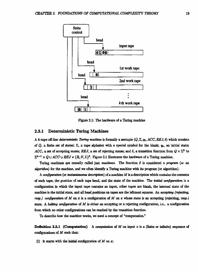
Figure 2.1: The hardware of a W g machine
2.3.1 Deta ' ' tic Tbrbg Machines
A k-tape off-line detaministic %+ng mnchine is formally a sextuple (Q, C, go, ACC, REJ, 6) which consists
of Q, a finite set of states; X, a tape alphabet with a special symbol for the blank; qo, an initial statq
ACC, a set of accepting states; REJ, a set of rejecting states; and 6, a transition function h m Q x Ck to
Zk-I x Q u ACC u REJ x {R, N, L)'. F v 21 mostrates the hardware of a lhrlng machine.
'k ing machhm are camdy caIled just mocirines. !I%e ftmction 6 is considered a progmm (or an
algoritlnn) ffor the madhe, and we often identify a Tbring machine with its program (or algorithm). A a n r ~ (or instwtrmeous desu+pfh) of a machine M is a description which contains the contents
of each tape, the position of each tape head, and the state of the machine, The M a l configwotimr is a
con@natkn m which the input tape contains an input, other tapes are blank, the internal state of the
machine is the initial state, and all head positions on tapes are the leftmost squares. An accepting (rejeding,
resp.) con- of M on z is a cdgtmt ion of M on z whose state is an accepting (rejecting, resp.)
state. A halting con- of M is either an accepting or a rejecting conSgnration, ie., a coxQumtion
h m which no other c o ~ o n s can be reached by the transition functio~
To d e ~ ~ l ' b e how the h e works, we need a concept of "cornputati~n.~
Dehition 2.3-1 (Cornpatation) A a m p t d h of M on input z is a (6nit.e or seqpence of
(i) it starts with the bit id confignration of M on z;
CIEAPTER 2 FOUNDATIONS OF COMPUWUONAL COMPLEXITY TEIEORY
(ii) each step h m a co&tmtion to another c o n f i ~ o n is made by the tramition ftmction; and
(iii) if 6nite, it ends in a Mting conSgmation of M on x.
An accepting (kjeding, resp.) c m p d d h is a computation which terminates in an accepting (rejecting,
resp.) configmation.
A deterministic ' k ing marhine M accepts an input z if there is an accepting computation of M on input
2; otherwise, M rejects z. Denote by L(lld) the set of aII strings which are accepted by M.
Let M(x) denote the output of a machine M on input z if it exists. The Nrming time of M on input z
is the length of the computation of M on x, and we denote by TmeM(x) the running time of M on z. In
the mse where the computation is not finite, we set Time&) = oo.
D-on 21.2 (Tiie/Space Comctii1e) A hct ion f on N is called time-GlltlSaUCtibk if there
exists a deterministic 'king machine M which, on input In, terminates a . d y f (n) steps are made.
A ftmction f on N is qmeconskudibiIity if there exists a detednistic W g machine which, on input In,
it marks the f (n)th square of the fitst work tape (among a bite number of work tapes).
2.3.2 NondeterminiPtic Turing machines
Another important model of computation is "nondeterministic" 'Ihring machines. A nondetffministic lbing
machine is a variant of deterministic Thing machines with the exception that the transition function 6 is a
map kom Q x 8' to P(x~-' x Q u K C u REJ x {KN, L)*). As for nand- ' ' tic ' h b g machines, we dter the dehition of "mmputation" to a set of "compu-
tations," a d e d "computation tree? A w m p f d h tree of .kt on input z is a tree whose nodes are
c o ~ t i o n s of M on x, i~ which the root of the tree is the initid configuration, and the children of each
node are such C O ~ O D S that are rea&abIe ftom the node in one step by the transition fnnction. Ail
codgurations foIIoning each configuration by a single application of the transition function is Caned nun- * . - detennartsttc Jloicts if the mmhr of such consgnrirtions is more than 1- .b accepting (rejectbg, resp.)
c t m p t d h is a path from the root to a leaf which ends wi th an accepting (rejecting, resp-) con@mtion.
The accepting aiteria of nondeterministic %rhg &es is simlt;tr to that of deterministic machines
and is determined by the existence of an accepting oompntatio~~, More precisely, the machine M aaq& x
if there exists an accepting computation of M on input z; otherwise, the machine z.
A nonde&mb&ic ' h b g machine for which the nrrmba of accepting paths on each input is at most
one is d e d uMncbigrmr [I03].
In general, mmapxse aunp1eJdtp measure is sensitne to the dehition of time-complarity of nonde
tmnbhtic 'Ihring machines (see [9Q, and we shodd pay carefd attention to the d M o n of the rmming
time of the machine when dealing w i t h nondeterministic compntati011~
In worst-case a m p l e theory, the nmning time o h nondeterministic 'Ihring machine is o h dehed
to be the minird Iength of allam@ngaxnptttaljonpaths Zone exiskg othempise, it is de6ned b he
ClUFTER 2 FOUM,ATIOPTS OF COMPlYZU7ONAL COMPLEXITY THEORY 21
I. Fix time/space constructibIe corn- bounds [such as "poIynd-timen or Yogarithmic-timev), we
may asmtme that all amputation paths on each input are of the same length, and by convention Iet the
rrmning time be the maximal length of any cornpatation path, since timeconstructible complexity b o d t guarantee that we can modifg any machine having this bound to a machine for which the length of any
computation path is d y t. This is explained as fd lows every time-bounded lhring &a is designed
in sn& a way that each has an internal dock (which does not access oracles), and this dock adjusts the
running time d the machine no matter what computation path it foLlows. We c d the mnr)l;nes esuipped
w i t h i r r t e r n a l c l o c l c s ~ ~ ~
Srnnmhg up, there are three m& of nondeterministic Turing machines together with their ruming-
time criteria-
(i) A model of nondetesministic Turing machines with traditional meaSzFement of running time, namely? the shortest accepting path if one exists, or eke L (or equhdently, taking the shortest rejecting path);
{iij A model of nondeterministic 'ihring machines with strict measurement of nmning time, that is, the shortest accepting path if one exists, or else, the longest rejecting path;
(ii) A model of ctocked nondekmhbtic 'Ihring machines.
As long as the runaing time of a mlchine on an accepting cornpatation path is bounded abcnie by s m e
thmm&m&& jhcrion (most timebtmded c o m p l e cIasses in worst-case cornpkxiQr theory satisfy
this condition), all these definitions are essentially equivaImt (negIecting constant slowdown). Smce average-
case c o m p l e theory does not reqnire this condition, the choice of a model is very important and often
leads as to &&rent mmeqnmces. Ia later chapters, we shaIt discuss the h o k e of models and possible
corlseqlleaces.
HistoricaIly, GciIdreich 1301 &st discnssed the average running t h e of nondeterministic ' k ing machines
and used a model of nm& ' ' tic 'Ittring mnrhines, the lengttts of whose computation paths are m e d
by some tim*bormded deterministic Thing e. His de6nition is actuany eqgivaleut to choosing model
(iii) as desaibed above Later Wang and Belanger [Ill], and also Schnler and Yamakami [97] prrsented mtetestfng resutts based on model (i). In paaicalar? W e r and Yamakami [97] constructed an a m q p
version of the (worsbase) polynomial-time hierarchy b a d on model (i), but the averagecase hierarchy
obtained here does not seem to be a pmper analogue d the worstcase hierarchy (it kds some properties Eke
@ =w). Int6isthesis,we&oosethemostgeneraImodel (i), eveuthoaghthemodelhnot seemto
p k d e the property that time-bounded nondeterministic compntations can be simulated by space-bounded
deterministic muhbe of the same m m p w .
D e f h k b 23.3 (ammine Time of Nondetermmtstrc * . . ThriqMachineP) Foranand' " * '
Ttrring marhine M, the rarcning Eime d M an inpnt x, Trmey(z), is dehed to be the length of the shortest
acceptingcomptrtationpathdM onxifoneexis& otherwise, it is- to be 1-
2.3.3 Oracle Turing Machines
To speed up the computation of an algorithm or to make it as accurate as posslIble, we need a supplementary
source of information which the algorithm can retrieve and ase. Such a source is called an om&, and a
'hing machine equipped with a system retrieving hfkmtbn h m an oracle is d e d an d e !bring
moehine An oracle Thing machine makes a p q to an o d e and receives its answer in a single step. We
start by descriiing those notions f o d y ,
An umck Zlaing mcelrine is a l b b g machine with the foIIowing additional devices: a distinguished tape,
aSLFcaIIedorocletopeor4uffy~andthreedistinguishedsbtes,QUERYtYES,andNO.Acomputation
(tree) of an oracle machine M with an orade (set) on input z is dehed in a way similar way to tbat for
"noa-oraJen 'Ihring machine except that it incorporates oracle qneries Initially the qyery tape is blank. If the machine M enters the QUERY state, then in a single step, M queries a string to the oracle which
appears on the query if this string bdongs to the o d e set, then M enters the YES state; otherwise,
M enters the NO state. h e d i a t d y after each orade query? the query tape becomes bIank,
We can easily extend the definition of made 'bring ma&iues with set macles (or o d e sets) into those
equipped with fundirm f. The d e machine has the QUERY state and the YES state; if it makes
a qgery z to an o d e , then the orade returns the d u e f (2) of the hct ion f in a single step and the
machine enters the YES state; at the same time, the head of the query tape is moved to the leftmost square
of the tape.
Smce orade lhring machines with the enrpfy ma& (ie-, the empty set) can be easily transIated into
non-orade '&hg machines (because we know the o d e answers), we often identify such oracIe machines
with non~rade oms. Zn this sense, without loss of w? we can view aoa-ode Tming machines as
a speciaI case of o d e Thing machines. Therefore, subsequent definitions wiU be stated only for oracle
machines without repeating s i m k dehitiom for nowrade machines
Definition 23.4 (Adaptive/Nonadaptive Query) An oracfe 'bring h e M is said to make
nonadoptirre queriej if, on each computation path, M produces a list ( d e d a qrrery Eist) of aIl strings which
are possibly queried befm the first query is made. Otherwise, M is said to make ndapfioe quaies.
A query list provides us with &dent i n f o d o n about which strings will possiily be queried in futtxe
cantpatations We remark that it is not necessary for an orade machine to query aIl the stzing m the query
Iist*
Let Acc(M, AJ) denote the set of (codes of) accepting compntation paths of M on mput z with d e
A, and Eimit;uly Rej(M, A, z) denotes that of computation paths. Let Q(M, A, z, y) be the set of
~qnededbpMarithoracIeAonmpatzanoompatationpathy. IfMisdderministic,thenwesimply
denote by Q(M,A,z) the set afaII strings queried by M aa inpat t wi th d e A.
By L(M,A) we denote the set of striugs accepted by M wi th orade -4, and we simpIy say that M with
oracIe A moprixs (or QCeCPfS) a sd B if B = L(M,A), For a machine M, MA(z) denotg the output of
a compnhtion of dB un mpat z- For a deterministic 'Zlg d M with an outpat tape (also called a
CZMTER 2, FOUNDATIONS OF COMPUTATIONAL COMPLEXlTY THEORY 23
tnrrrrsb),wesaythatM comprrteJafan&on f if f (x ) =MA(z) foraIIx€@.
B~ Tie$(x), we denote the rmLning time of marhine M with o d e A on input z. S i l y , Space$(z)
denotes the tape space used by M with oracle A on input x. Technically speaking, there are two possible
definitions for Space&(z) depending on whether the space of the query tape is counted. This possibly changes
the power of Wvized space-bounded compIexity classes, su& as PSPACE. In this thesis, we take all
tapes bdnding qaery tapes into consideration m order to measure the tape space used by the machine M
w i t h made A.
2.3.4 Alternating Turing Machines
The notion of olternnting mtdines was introduced by Chandra, Kozen, and Stockmeyer [21] as an
extension of nondeterministic 'Ihring machines.
Each m;lrhine is equipped with extra states, called V (aniversal) and 3 (existentiat). Each configuration in
a finite tree of computation for an a h m d n g 'Lhting machine is labeled as either inrittersul (V) or Qistentiol
0, according to the states of the machine. Next we define an accepting computation tree. F i we
recarsively determine the yes-amfigmutim
(i) a halting codgmation is a ye4conSgnration if it is an accepting configuration;
&) a non-halting 3-oonfigmation is yewdiguration if at least one of its children is so; and
(6) a non-halting V-configuration is a yescon&xation if all of its children are so.
For convenience, ccm6gmations which are not y-11s are called n o - m . m . An accepting
eomputafion bee Tt of M on input z is a subtree of a computation tree T of M on z satisfying the following
conditions
(i) all co&pratioxts m Tt are yea&pr&ions;
(ii) an existmW con@ration in Tt has one child node in T; and
(iii) a m i v e d configmation m T has all of its cbiIdren in T.
The machiue accepts an mput if there exists an accqtkg computation tree (equivaldy, the root of the
computation tree has a ges-eonsgmation); otherwise, che machine q,kds the mpta.
AIternation is the- over~attcompatationpathsfromtheroot toalea& ofthenumber oftimes
in which different Iabels of c o & p a t i o ~ ~ ( i i 3- or V ~ ~ i o n s ) change- Note that, by convention,
the initial con&tuatiion is asmmd to amtriiute the first aItematio11. For example, nondeterministic Thing
machines have 1- kame dl -ens are 3m@mations.
H e r e ~ ~ i m t r o d u c e a ~ ~ d ~ ~ m a r r h i n P I P . ~ e d " s e m i - d e t c ---*t?'
alternating Thing machines, which embodies deterministic computations reiatitre to some dternating ntriag
This notion is asefal fir descfi'b'mg the A-Ievel d the polyaomiaLtime hierarchy, for example (see
Section 25). A semi- - - -
a i t e r n a t i n g ~ ~ i s , m a g h I y s p e a k i n g , a a a t ~ ~ g
CE4FTER 2. FOUNDATIONS OF COMPUTATIONAL COMPLEXITY THEORY 24
machine which puts an additional mtriction on its computation tree. For simplicity, we assume that the
number of nondeterministic choices is 2 Then, any computation path can be encoded as a b i i string.
We IabeI each computation path with this code to chbgukh individual computation paths. For brevity,
write s? to denote the jth string of the set P in the standard order (NB. Om is the 0th string of P).
D M o n 2.3.5 (Semi-Deterministic Alternating lhring Machines) A semi-- . . . *-
ing machine is an alternating lSning machine with the following constraints for the 6rst three series of V-
and 3-con6gurations of the computation trees T, of the machine on each input z.
On input z, the machine starts with an 3state, and during this state the machine produces computation
subpaths. Let m be any such computation subpath and suppose that the marhine makes k queries By
the above coding scheme, the subpath fi is labeled by b = hb2 - -. bk, where bi E (0, I), I 5 i 5 k. Next
the machine enters an V-state in which it produces exactly 2* branches for some m 2 log k, each of which
is labeled by an m bit string c = C I C ~ where cj E (0, 11, I 5 i 5 m. Let be any such a branch
foIIowing m. Consider the current configuration, called cdicrJ, and denote it by 4, where I is the labeI bc
attached to the subpath plpz. At the next step, the machine &oases either an a t e or V-state, depending
on tJxe label 1 (= h bkcL k). The machine enters an 3-state if b, = 1 and c = s y for some j; otherwise,
it enters an V-state
AII critical configurations of the computation tree T= satisfy the fdowing two conditions on their h-
6e& with respect to yes- or n ~ ~ t i o n s : for any two critid codgaratiom dr and 4, where I = h - - - b k e , - - - k andl' = i4---b'&---t$,,, assnmingthat c = q a n d 8 = 9' for some j with 0 5 j < d { k , q,
A semideterministic Ttuing machine M is said to have k-ahm&ms if the maximal alternation of all
comptrtation trees of M is at most k -t 2 (because the &st two alternations are E d and &odd not be
counted).
We dehe the rrmning time of an alternating lhing machine as foIIows.
Dehition 23.6 (Rmming Time of Altematbg Zhring Machines) The rnnning time of an alter-
nating lhring machine on mpttt s is the mm;md height of accepting computation trees of M on % if M
acceptsqotherwise,thenmningtimeisde6nedtobeI.
2.3.5 Worst-case Time/Space Complexity
In womtxae complexity theory, the time (or space) annpiexity of an algorithm is often d d e r e d as a
function dehed an the natttraI numbers N because we are irrterested only in the instances of each Iength
which are hard to compute.
CZMTER 2. FOUNDATIONS OF COWUTATIONAL COMPLEXITY THEORY 25
Dchition 2.3.7 Let M be an o d e TLzring xuachine and A a set. Let t be a function on N, and let 7 be
a set of functions on N
1. The Tming macbe M with made A is d e d t-time bounded (or a t-time Twing mocldne, for short)
if Time&) 5 t([rl) kt all 2. S i l y , M with o d e A is t-space &nmded (or a t-spaw M g
mJdne) if ~pace$(z) I t(lz1) for all 2.
2. The oracle machine M is 7-time bouffded (or a 7-time 3kring machine) if M with o d e A A t-time
bounded for some t in 7. The notion of a 7-space %ing machine is defined anaIogonsly.
Here we use comt iond abbreviations if 7 is the set of polynomials, we say that bi is polpnnid-time
(or polgnomial-space) &taa&d, and simiIarly, if 7 is the set of exponentials (linear-exponentiaIs, Iogarithms,
resp.), M is called apimW-i.he (linew-ezponenticl-time, Iogarithmic-space, resp.) brnnuied
2.4 Randomized Algorithms
In this thesis, we would Iike to use two ditfkrent terms, mndomizcd M g maddnes and probabihtic l k n g
ma&nes, to cope wi th randomized atgorithms.
A nmdomizd Turing m& is a model of randomized computation and a variant of a nondeterministic
Turing machine with no accepting c&& Intnitively, we equip a machine with a s p e d rnechauh for
generating an u n b i i coin flip iu one step which determines the choice of the next consgarations. More
precisely, a randomized lbing mac?he is a 'Ihring macbiue with a distingnished state, d e d &-tossing
state, in which the finite control unit two poss'bIe next states. The (bite or inhite) -on
of a randomized 'Itring machine is determined by its input as well as by the outcomes of the coin tosses
performed by the machine-
We can view randomized Tmiug mdhes as pmtiol functions with two variables, one of which is a
*nsnaln inpd initially written on the input tape, and the other of which is a rnndom input (or m h seed),
that is a b i i sequence representing the oatoomes of the coin tosses. FoRotoing B k and Gurevich [12],
weshallformalizethigmodeIbelow*
A randomized Turing madtine M is equipped with an arndiarp semi-hdWe read-only tape, d e d a
random tape which may consist of an i n . sequence r of %domn bits ( i r E Coo). The head on
the random tape can move d y to the right and cannot stay at the same square after the machine reads a
symbol on the tape. The machine's a m s to the random tape corresponds to a coin-@, and we may say
that the machine pjps a (firir) coin when it accesses the random tape. For each infinite random sequence r,
let R e a d ~ ~ ( t ) be the initia segment of r that is rezrd by M on input z dming its computation. Note that
if a computation is bite, then Read~Jt) is aIso kite, but not c o d y . Let the sampk space ZIM(z) be
R e d that m is the -gne measure cm the Iine BL We d&e fhe probabiIity measme Pr on the sample
CHAP17ER 2 FOUNDATIONS OF COWUTA?IONAL COW- TREORY
space QM ( x ) as foIloftrs: for any event E &(z),
by identiEging [0,1] with !Em. Throughout this thesis, we use Pr[-1 to denote this probabii m m In
if event E consists only of bite strings, then
Abusing notation, we let RM denote the set ((2, s) I s E RM(x)). (Note that Ras is not a sample space.)
We shall dehe the nmning time of the machine M on input z as foIlows. For any input (z, r) E Z' x Zoo,
Iet TM(x, r ) denote the time taken by M on mput z and random input r. Whenever M does not halts, let
TM(z,r) = ao. Next Iet Tlme~(q -) to be the (partkd) function &om Rna(t) to N such that T&r) = T i e M (z; &adM&)) for d r E p. For convenience, if (2, r') RM, then mme~(z ; f ) is undefined.
Unless stated 0th- the notation ks.TimeM(z; s) is used to mean the total function defined as above
h r n I'na to N&.
For each input s to a randomized ntring madine, let US denote by M ( z ) a random variable over the
sample space RM(z). Let Q be a property on {O, 1). Then we denote by Rr[Q(M(z))J the pmbab'ity
that Q(M(z ) ) h01& For the sake of coLwenince, we also use the notation M ( q r ) to mean the output
of a computation by M on mput z with random seed r when r is m OM(=). In the case where r $?
flM (x), let M (q r) be undehed. Thus M(z; r) is a partial fimction The notation Pr,[Q (M(G s))] and
Pr.[Q(M(z;s)) I s E QM(=)] are to denote Raa[Q(M(4)]-
2-4-1 Random-Input Domains
B k and Gnrevich [U] created a general h e w o r k for the average analysis of randomized algorithms based on the notion of ''dil;iti~13~.'' Here we take a simpMed approach.
D-on 2.4.1 ( B a n d o ~ ~ t t t Domain) A subset r of X' x Z' is caIled a mzdbm-input &main
& for z, s,s' E !Em, (z, s) E r, s' 5 s, and s # s' impIy (q 4) 4 r. For each string 2, we set
r ( ~ ) = (S 1 (z,s) E r).
It is important to note that r(z) consists onIy of finite strings and that it may not be a sample space
with respect to Pr became Rp(x)] 5 1.
Dehition 2-42 (Raritp Fbctions) [I21 Let I' be a raudom-input domain. The m+tg /undion of I' is denoted by Ur and d&ed by
1
CBWlER 2. FOUNDATIONS OF COMPUZUTONAI, COMPLEXITY THEORY
In other aords, l /Ur(~) = Prr(z)]. For a raadomid 'Ihring m;vrhine M, let rM = {(x, s) € EM I s is finite}. In particular? when r~ is
almost total, there is no need to Setentiate bemeen r ~ ( x ) and the sample space R&) since R[r&)] =
R[RM(x)] = 1.
De5ition 2.4.3 (Random Mctions) A rmulmn j imdm f is a function from a random-input domain
to P . A random function f wi th its random-input domain I' is called crlmost to td if I' is almost total and
R.V(z,s) < oo I s E Rnr(x)] = 1, where the subscript s in this equation emphasizes the random variable
over RM(z). For a random function f with its random-input domain r, the (dd) ezpatotimr of f
on input Z, symbolically E.[~(x,s) [ s E r(z)], is dehed by
For example? the partial function )cu.TimeM(qs) for a randomized Turing machine M is a random
function fiom RM to N.
2.4.2 Probabilistic Turing Machines
The notion of probabilistic 'I\aing machines was proposed by de Leeaw, Moore, Shannon, a d Shaph [a] in 1955. Pioneer works on probabilistic 'Ihring machines were done by Gill [%I and Santos [86j.
A pmhbilistic Zhfng m c h e Y is a randomized 'lhring machine with the foIIowing accepting criteria:
for every z, either R. [M(q s) = 1 I s E R&)] > f or R,[M(z; s) = 0 I s E fh&)] > [28]. We sap that
M omptrzifPr.[M(z;s) = 1 I s E QM(x)] > $and M mjedszifR,[M(z;s) = O I s € QM(x)] > $. By this definition, the raritg fnnction tlr, of rar is bounded above by 2 because
For a prolmbilistc 'Ihring machine M, let L(M) denote the set of dl strings which are accepted by M. Wesay tha tMnmgnkesDi fD=L(M) .
Let D be the set recognizable by a probabilistic Thing machine M. The arm pmbob*ly of M for D is
the hc t ion e~ defined by
esr(4 = Pry[M(4 # m(4,
C&APTER 2. FOUNDATIONS OF COMPtl'ZUlONAL COMPLEXITY THEORY 28
Another type of meamre was given by Gill [q. For a probabilistic 'Ihring machine M, let D be the set
accepted by M. Set
min{n I Rs [M (z; s) = xD(x) within n steps I s E rrr (x)] > f ) if one exists, T'i'iea(z) =
othcmirk.
Roof. Let t be the error probabilitp bound of M . Hence? 0 5 I < Let c = 1 t -2c and c' = c'I6. For
simplicity, write h(z) = E.rieM(r;s)* 1 s E ru(z)].
Let x be an arbitrary string- By Lemma A.1,
This is eqttivalent to 1
R,[TimeM(r;s) > c' h ( ~ ) ~ * I s E I)M(z)~ < ;.
Let D be the set accepted by M.
The probabiIity that M(z;s) = D(z) in time d - h(z)ll% ip by
R*[M(z;s) = D(z) m time c' - h(z)'/' 1 s E ru(z)]
By the dehition of T i ( z ) , we condude that Tiieb(x) d - h(z)'I6, that k
CEAPEZ 2. FOUNDATfONS OF C O W ~ O N A L COMPLEXITY THEORY 29
De&rition 2.4.5 (Time Cornpkity) A probab i ic Thing mslrhine M is Caned t-time 6ounded (or
a t-time %ring machine) if Tme&(z) 5 t(lz1) for all x. For a set 7 of functions, M is 7-time bounded (or
a 7-time machine) if M is t-time bounded for some t € 7.
2.5 Worst-case Complexi@ Classes
For years, theoretical computer scientists have been interested in resource-bounded computations and have
studied their complexity and structuraI properties. In this section, we shall review central concepts in the
theory of worst-case complexity.
2.5.1 Computable Fnnctions
One of the most natural concepts in worst-case complexity theory is "polynomial-time comptttabilIitytyn .A
function f on C is polynomial-time mputuble (P-computable, for short) if there is a detc ' - tic Wing
machine with one input tape and one output tape (ie., a transducer), which computes f in time polpornid
in terms of length of the input. Denote by FP the collection of all polynomial-time computable functions.
To study algorithms on difFenat objects, such as graphs, sequences, circuits, ete, we use an encoding of
objects into stringq the encoding must be effective and same. In this thesis, we use Regan's paring function
[a as the basis of encoding and extend the function to mnIti-functions. Formdyt a patiing jhdion is a
bijection h m C' x C' onto C'.
F i d that the stat ion z- demtes tho predecessor of string z in the standard order on C' nnless
z is the empty string.
D M o n 2.5.1 ( P e g bction) The fimction (-, -) from C* x C' to Z' is defined as f o U m for
an pairs (x, y) E C' x E',
where d(X) = A, d(0z) = OOd(x), d ( h ) = lld(z), i2[Ox] = Oh, and i&] = 102 for all z.
Below we list without proofs severaI important properties of this paring frmctiow
(i) (,) is monotone, Le, x I d and y 5 y' imp17 (z, y) < (z',y').
(ii) (, ) is compntable in linear-time m the lengths of z and y.
(v) For any maeasing fimction f on C, Cf(x), x)- 2 Cf(z-), z-) fix all z.
CHAPTER 2 FOUNDATIONS OF COh4PUlZXTONAL COMPLEXITY THEORY 30
This paring frmction is recursively generalized to a bijection fiom (Em)' onto C* as (zr ,zz, -. - , zc) = (z~ , (z~ ," ' , z~) ) . It is clear-
2.5.2 Complexity Classes
A annpkitg dass is a cokction of subsets of Z*. For a complexity dass C, the complement of C, denoted
by~7isthecollecti~udsetsSsoehthatC'-SisinC.
Dehition 2.5.2 For a function t on N, let DTIME(t), NTIME(t), and DSPACE(t) denote the c h s
of all sets recognizable by deterministic t-time, nondeterministic t-time, and deterministic t-space Turing
machin=, respectiveIy. Similarly, Id BPTIME(t) denote the class of sets recognizable by t-time bounded
probabilistic M g machines with bounded error probabii , and let -(t) denote the couection of
sets computable by one-sided error, probabilistic (LC, random) t-time lhring machines. For a set 7 of
frmctions, let DTIME(7) = UtETDTIME(t). In a similar fashion, we define NTIME(T), BPTIME(T), and
DSPACE(7).
Using these notations , we can introduce several important complexity classes. For deterministic classes,
we use the following basic comphiQ classes:
2. E = ~ = ( 2 ~ ( " ) ) (linearexponential-time).
A set S in P is said to bepoEynmniodEime cmnputa6le (P-computable, for short). Srmilarly, we use the ter-
minology czponnztial-time mmput4ble (EXP-comp~le , for short) and linem-eqonentiol-time amapuhble
(Ecomputable, for short), respectivety, for sets in EXP and m E. For spacebounded c o m p I e chsses, we trse:
I. PSPACE = DSPACE(~*(')) (polynomial-space).
2 ESPACE = D S P A C E ( ~ ~ ~ ) ) (hear4?xponentiaspaCe).
It is woah noting that PSPACE is dosed iarder oomplement, ie, PSPACE = mPSPACE. For nondeterministic dasces, we set:
CaAPTER 2. FOUNDATIONS OF COMPUZXZTONAL COMPLEXlTY THEORY 31
-y, NP-sets have the foUowing -on by logid terms: a set A is NP if and only if there
exists a set B E P and a p l y n o d p such that A = {z I 3&l= p(]z i ) (x? y) E B]}. For probab ' ic cbsses, let:
1. RP = R3IME(n0(')) (random po1ynomial-time).
2 aE = RTIME(no(')) (random hear-exponential-time).
3. B P P = BPTIME(~O(~)) @ounded-ef~)r probabilistic polynomial-time).
4. BPE = B P T I M E ( ~ ~ ( ~ ) ) (bounded-r probabilistic hear-exponential-time).
The class ZPP (zememr probabilistic polpod-time) is defined by RP n co-RP.
It is important to note that DTIME(O(n)) # NTIME(O(n)) [82]. This is the only separation r e d t we
have known until now.
Other important comp1exitp cIasses are U P and PP. The chss UP (unamhiious polynomial time)
is defined by po1ynomiaI-time unambiions Thing mnrhines. The probabilistic class PP (probabiIistic
po1ynomial time) consists of sets which are dehed by polynomial-time probabilistic Thing machines whose
error pmbab'ity is < 1/2. ActuaIly? the value 1/2 can be replaced by any real number c sa-g 0 < c c 1. By dehition, P E UP E NP and P RP BPP E PP. Using the notion of orade lhriag machines, we can introduce ~ ~ e d e ~ ~ p l e z i t y b. For a set
S and a c o m p l e ekss C, the notation CS (C relative to S) denotes the dass naturdy obtained from
the dehiti01t of C wi th the help of S as oracle, and CD (C relative m V) denotes the union of all cS for
an. S E D. AU c o x n p l e classes defined above ate m d y dtivized wing the notion of oracle %ring
machines, such as pA, w, B P ~ , e, UP, ete
As mentioned before, the empty oracle set does not change the computational power of the %ring
m;lrhines; thus, we have = P, NP@ = NP, e tc We remember an important r e d t due to Zachos (see,
eg.? [lq) that BPF = BPP. Let #P (pronounced "sharp P" or "number P") be the coktion of all functions on !Z' which are
computed by polynomial-time countkg Thing machines. It is not Wdt to see that f is in #P if and
ody if them exist a set A E P and a polynomial p such that f(x) = Il{y E WM) I (z, y) E A}II for dl z.
The counting of soItrti011~ is relevant to probabilistic computation- The following redt shows a relation-
ship between these two notions.
Root Fmt we show the inclusion PP E F. This inclusion is d y seen as fo11ows. For a set A E PP,
there is a pmbddistic %ring machine M- We modify M so that all amputation paths of M on each input
z are of the same length, say p(z). The success probabw of M on z is eqasl to the ratio of [[Aa(M, z)1[ to Hz). Let us d&e f (z) = l~Acc(M,z)[ hr dl z. Obviously f E #P. U 5 g this f, we can determine in
p d y n d time whether 2 - f(z) > !2P(=), which means z E A. A beI- to Pf E p.
CaAPTEIl2. FOUNDATIONS OF COMPUTATIONAL COMPLEXlTY THEORY 32
Next we shall show the other mdnsion that #P E l@'; thus, we have P # ~ C pPP.
Take a #P-function f. There exists a polynomial-time nondeterministic Turing marrhine M such that,
for every z, f (z) equals the nnmber of accepting computation paths of M on inpa z. Take a polynomial p
and assume that the number of non- amputation paths of M on input z is exactly 2 ~ ( b l ) (this
is always true if we pad extra nondeterministic, rejecting paths).CIearly 0 5 f (z) 2p(lZl) for aII z.
We then define the set A = {(q,z) ( IIAcc(M,z)ll 2 i) so that:
f (z) = max{i E N I (si,z) E A).
A b i i search technique hdps as compute the d u e f(z) detc 'SticalIy by simply querying polynomidly-
many strings of the form (si, 3) , 0 5 i _< 2p@4), to or& -4. Therefore, we have f E F'PA.
In the rest of the proof, we mast show that A is in PP. Let us d e h e the following randomid 7 h b g
machine N:
begin randomized algorithm for N
inpat ( ~ i , 2)
if i = 0 then accept and halt
generate a bit i (b E (0, I)) at random
i f b = O thensimulate M onmputzandhalt
generate a string y of length p(IzJ) at random
(assnme that y is the jth string in D'(lzl), where 0p(IzI) is the 0th string)
if j c 2p(Irl) - i then accept else reject
end.
This machine N obviously nms in polynomial time because M does so. It is also easy to see that, for each
(sit 4, 1
Hence, A E PP. 0
A set S is m @P (pronounced "parity Pn) if there exist a poIynomiaI p and a set A E P such that, for
each z, z E S if and onIy if [I{y E CP(lrI) I ( q y ) E A}([ is odd [81]. We remark that UP s $P. A set
S is near-testable if there exists an f E FP such that, for all nonemptp strings z, f (z) = xs(z) + xs(z')
(mod 2). Let NT denote the coIleaion of all near-testable sets [31]. It is known that P C NT G $P and
NT is also indnded in En PSPACE [31]- It is also known that $Pp = $P [IS] and NP s eP [104.
The class P/poIy consFns of all sets A such that there exist a pbounded function f h m N to C' and
a set B E P satk@ng A = {z [ (2, f (kt)} E B). This class is a h known as the colIection of all sets
computable by (non-nnifonn) fhdies cdpolsrnomi&ize cimits.
A s e t S i s m A P T ( o b n o s L ~ ~ } [ ~ ] i f t h e r e ~ a p d p n o m i d p a n d a d e t e r m i n i s t c ~
machine M which accepts S snch that the set {x 1 Tme& 2 p([z[)) is sparse
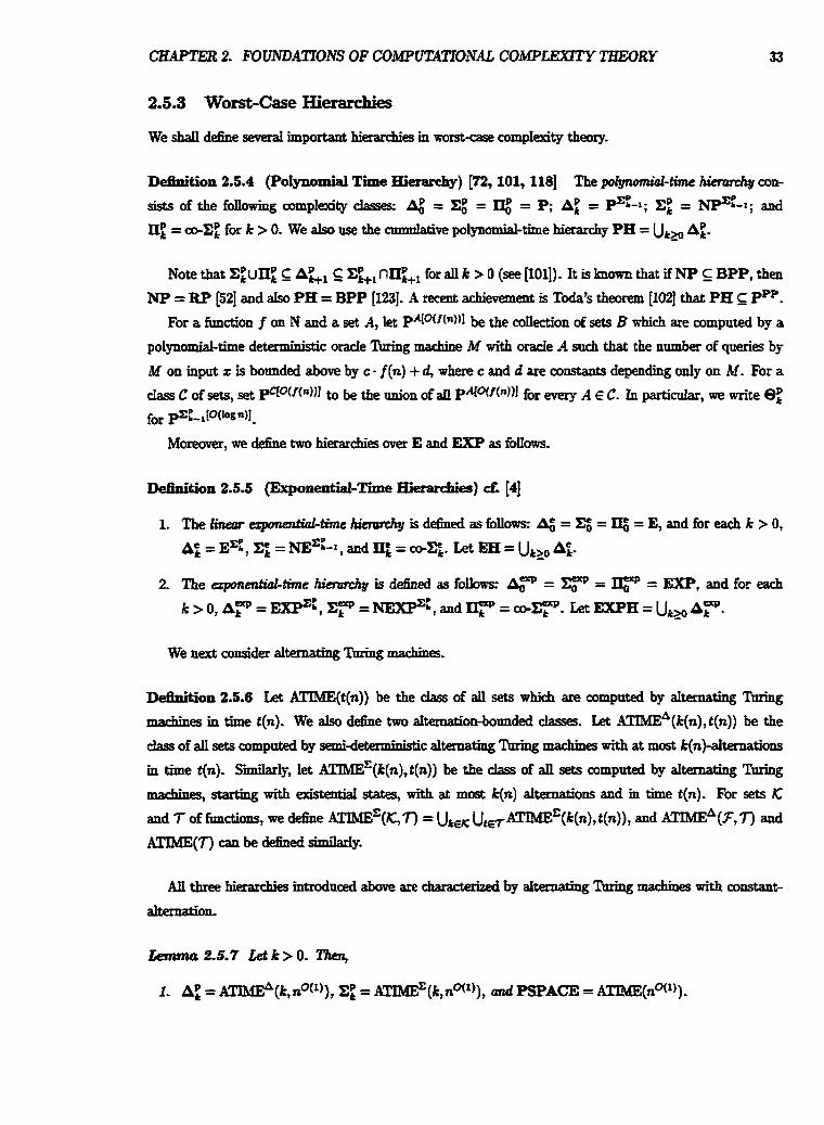
CHAPTER 2. FOUNDATIONS OF COMPUTATIONNU COMPLEXITY THEORY
2.5.3 Worst-case Hierarchies
We shall define several important hierarchies m 7Aorst-case compIexity theory.
DeSnition 2.5.4 (Polynomial T i e Hierarchy) [72, 1Ol,ll8] The pol^-time hi&y con-
sists of &e following compl@ classes: a = Et = = P; Af; = p:-'; Xf; = e:-,; and
= co-zf; for k > 0. We also use the cumdative polynomial-time hierarchy PH = Ut2,, A:.
Note that Ef;uTti c A&, XpH, n c l for all k > 0 (see [IOlj). It is known that if NP BPP, then
NP = RP [52j and also PH = BPP [123]. A recent achievement is Toda's theorem [I021 that PH G pPP.
For a function f on N and a set A, let ~ ~ [ ~ ( f ( ~ ) ) 1 be the coltection of sets B which are computed by a
polynomial-time deterministic o d e Thing machine M with oracle A such that the number of queries by
M on input z is bounded above by c - f (n) + d, where c and d are constants depending only on M. For a
dass C of sets, set pC[O(f(R))I to be the union of all P~[O(~("))I for every A E C. In particular, we write 8; for pC5-l[oclo~)l-
Moreover, we define two hierarchies over E and EXP as foIIows.
Dehition 2.5.5 (Exp~nentiaE~me Hierarchies) cf. [4j
We next consider alternating Thing machhs.
Deanition 2.5.6 Let ATIME(t(n)) be the dass of ail sets which are computed by alternating M g
machines in time t(n). We also d e e two alternation-bounded classes. Let ATIME*(~(~), t(n)) be the
dass of alI sets comptited by semi-deterministic alternating Turing machines with at most k(n)-alternations
in time t(n). S i i I y , let ATIME'(~(~), t(n)) be the cIass of a11 sets computed by alternating
mdbes, starting with existential states? with at mast k(n) alternations and in time t(n). For sets K
and 7 of fimctions, we defme ATIME'(K, 7) = uLElh. utfl ATB@(k(n), t(n)), and ATIME*(F, 7) and
ATIME(7) can be d&ed simiIar1y.
All three hiexarchies introduced above are charaaerized by alternating Thing machines with constant-
alternation.
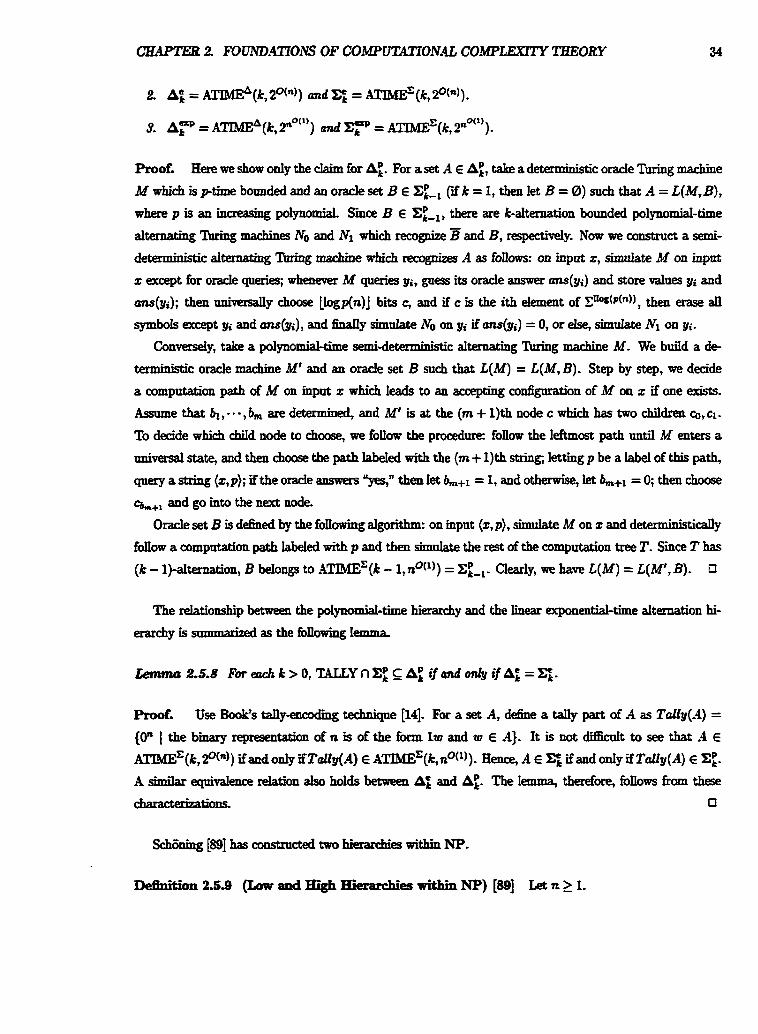
C&APTER 2. FOUNDATIONS OF C O M P M O N A L COMPLEXITY THEORY
Proof. Here we show ody the claim for A:. For a set A E A:, take a deterministic oracle Turing m;trhine
M which is ptime bomded and an oracle set B E Z:-, (ii k = 1, then let B = 0) such that A = L(M, B),
where p is an increasing polynomia. Smce B E C:-,, there are k-aIternation bounded polyuomid-time
alternating 'Ihiug m c h e s No and NI which recognize B and B, respeaively. Now we construct a semi-
deterministic alternating W g mackine which recognizes A as foRows: on input z, simulate M on input
z except for oracle queries; whenever M queries yi, guess its oracle answer mrs(yi) and store d u e s yi and
mrs(~i); then nniversaIIy choose [logp(n)j bits c, and if c is the ith element of C ~ ~ S ~ " ) ) , then erase aii
symbols except yi and m(yi), and simulate No on yj ifm(yi) = 0, or else, simulate Nl on gi.
Conversely7 take a polynomial-time semideterministic alternating Thing machine 116. We build a de-
terministic oracle machine M' and an oracle set B such that L(M) = L(M, B). Step by step, we decide
a computation path of M on input x which leads to an accepting configmation of M on x if one exists.
Assume that h, - . ,6, are determined, and M' is at the (m + 1)th node c which has two children a, Q . To decide which chiId node to choose, we follow the pfocedum fonow the leftmost path until M enters a
universal state, and then choose the path IabeIed with the (m + 1)th string; letting p be a label of this path,
query a string {z ,p) ; if the oracle auswers then Iet k+l = 1, and otherwise? let = 0; then choose
%+, and go into the next node.
Oracle set 3 is d&ed by the f o I I d g algotithm: on input (2, p), simulate M on x and det ' . ' , t idy
foflow a computation path IabeIed with p and then simulate the rest d the computation tree T. Since T has
(k - 1)-alternation, B beIongs to ATIMEE(k - 1,n0(')) = Eft-,. Clearly, we have L(M) = L(Mt, B). D
The relationship between the polynomial-time hierarchy and the hear exponential-time alternation hi-
emdlyissmnmarizedasthefollowing~emma
Proof. Use Book's tdlyencoding techniqge [14]. For a set A, define a tally part of A as Tally(,4) = {On I the binary repeesentation of n is of the form lw and w f A). It is not d i fEdt to see that -4 f
-(kt $'("I) if and only ifTalIy(A) E ATIMEX(k, n0(l)). Hence, A E if and onIp if Tdly(A) f X: . A similar ecpivahce relation also holds between At, and Aft. The lemma, therefore, follows h these
characterizatim n
Definition 2.5.9 (Low and High Hierarchies within NP) [89] Let n 2 1.
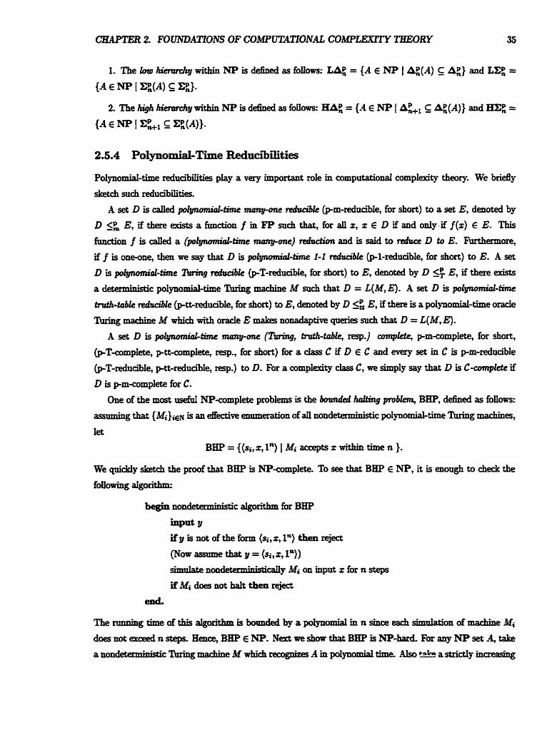
CHAPTER 2. FOUNDATIONS OF CCOMPMONAL COMPLEXITY THEORY 35
2.5.4 Polpornid-Time Reduu'bilities
PoIynod-time redua'bilities play a very important role in computational comp1exity theory We briefly
sketch such reducibiities.
A set D is d e d pd--time ~~~lfy-m reducible (pxt-edncible, for short) to a set E, denoted by
D Ey if there exists a frmction f in FP such that, for all x, x E D if and only.if f (z) E E. This function f is Caned a ( p o I ~ - t i m e mmgpone) redudion and is said to reduce D to E. Mermore ,
if f is one-one, then we say that D is p o I ~ - t i m e 1-1 dur5ble (pl-reducible, for short) to E. A set
D is polynomial-he M g dtu5bIe @T-reducible, for short) to E, denoted by D 5; Ey if there exists
a deterministic polynomial-time Turiug machine M such that D = L(My E). A set D is p f ~ d - t i m e
hdh-table d d f e (ptt-reduciibIe, for short) to ET denoted by D <L E, if there is a polynomial-time orade
ntring machine M which with orade E makes nonadaptive queries such that D = L(MT E). A set D is poIgmmiaLtime many-one (lb+ng, hth-table, resp.) cotnpw pm-compIete, for short,
@T-comp1ete, ptt-complete, resp., for short) for a dass C if D E C and every set m C is pm-reducible
@-T-reduaibIe, ptt-redudbIe, m p . ) to D. For a oomplexitp dass C, we simply say that D is C-complete if
D is pm-compIete for C.
One of the most usefnl NP-complete problems is the bounded h&g problem, BHP, d&ed as follows:
assmning that {Milia is an effective enmneration of aIl nondeterministic polynomial-time 'Ihring machines,
Iet
BHP = {(~i,z,l~) accepts z within time n ).
We quickly sketch the proof that BHP is NP-compIete. To see that BHP € NP, it is enough to check the
following aIgorithm=
begin nondeterministic algorithm for BHP
Y if y is not of the fonn (%,z, In) then re-
(Now assmne that y = (si,z, 1"))
&date nondetem&&idy A& on input x for n steps
if Mi does not halt then reject
end.
The rrmning time of this algorithm is bounded by a polynomial in n since each simnlati.on of machine Mi
does not e d n stepsc Hence, BHP E NP. Next we show that BHP is NP-hard. For my NP set A, take
awn& ~ ' b t i c ~ ~ e M w h i & ~ A I n p o l ~ O m i a l t i m e , A l s o + ~ a s t r i d y m Q e a S f n g
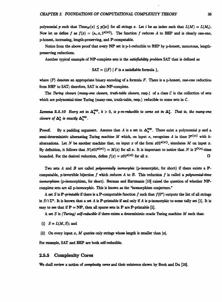
CZIAPTER 2. FOUNDATIONS OF C O M P ~ O N A L COIUPLEXITY THEORY 36
poIynod p such that TimeM(x) 5 p(lzf) for a11 sQbgs X. Let i be an index such that L(M) = L(Mi).
Now let us d e h e f as f(z) = (&,z, ldCI)). The function f reduces A to BHP and is dearly oneone,
phonest, increasing? length-preserping, and P-computabk
Notice from the above proof that every NP set is pl-reducibIe to BHP by phonest, monotone, length-
presenring reductions.
Another typical example of NP-complete sets is the s- problem SAT that is defined as
SAT = ((0 I F is a satisfiable formnla ),
where (F) denotes an appropriate b i i encoding of a formula F. There is a phonest, onmne reduction
h m BEP to SAT; therefore, SAT is also NP-complete-
The TMng closure (many-one cto- truth-tdle &sum, resp.) of a class C is the coIIection of sets
which are polynomial-the 'Ihring (many-one, truth-table, resp.) redua'ble to some sets in C.
kmm 2.5.10 Eaeq set in A?, k > 0, is p-m-du& to some set in A;. That is, the mrmyone
&sum of A; is d y A?.
Roof. By a padding argument. Assume that A is a set in A?. There exist a polynomial p and a
semidaerministic d ~ ~ g 'Ihriog znacbe M which, on inpat z, recognizes A in time 2p(Irl) with k-
alternations. Let N be another marhine that, on input x of the form zOIAlrl), simulates M on input z.
By dehition, it fonons that ~ ( z 0 l ~ ( b l ) ) = M(z ) for dl z. It is important to notice that N is 2°(n)-thoe
bounded. For the desired reduction, dehe f (z) = d l d w ) for all z.
Two sets A and B are called p o l p m i d f y isomorphic (p'imorphic, for short) if there exists a P- computabIe, pinvertiiIe bijection f which reduces A to B. This reduction f is called a potynomicrl-time
isomo~phism (piirnorpht'sm_ for short). Berman and &atmanis [I01 raised the question of whether NP-
complete sets are aIl pisomorpbic This is known as the "isomorphism conjecture."
A set S is P-printcrbk if there is a P-computab1e fmtction f such that f (On) outputs the list of aIl strings
in S n F. It is know that a set A is P-printable if and only if A is pisomorphic to some tdly set [I]. It is
eaq to see that if P = NP, then dl sparse in P are P-printable 111. A set S is ( T m ) self-reddk if there exists a deterministic o d e Thing machine M such that:
(i) S = L(M, S); and
(ii) On every input z, M queries onlg strings whose length is d e r than 121.
For scampIe, SAT and BEP are both &-reducibIe
2.55 Complexity Cores
We shaII review a notion d a ~ l c p & j t y cars and their existence shown by Book and Dtt [16].
CaAPTER 2 FOUNDATIONS OF COMPUTATIONAL COMPLEXITY THEORY 37
D-on 2.5.11 (Complexity Cores) Let A be a set and let C be a dass of sets. An infinite set H
isa complezity cote (or hardcurt!) for4 rrrithrespedtoCif, forevery set CinC,ifCS.4, then C n E is
finite A compIexity core H is d e d pwper if H E R
Lemma 25.12 [IS] Let C be a m a m i d y entanarrble c h of nmrsbe sets. If C is closed under
finite ufilUfilon andjhde midion, then myinfinitt recurJive set A not inC has an injinite recutslae, proper
cmnpkxify core for A with respeEt to C.
Proof. Assume that A is an infinite recursive set not in C. S i C is recursively enumerable, alI subsets
of A that are in C can be effectively enumerated as {Co,C,, . . .). For each k E N, let DL = &, Ci. Note
that Dj Dj+t for every j . Now let D = Ujlo Dj . I f A - D is infinite, then A - D is an hibite proper
complexity core for -4 since any subset C of A that is m C is a subset of D, and thus (AD) n C = 0. Now let us assume that A - D is finite. Them are h h i t d y many k satisfying that Dk # Dk+1 since, otherwise,
C is closed tmdet hite union, and thus A is in C, a contradiction. For each k with Dk # Dk+l, take the
element ak that is the m b h d in Owl - DL. Let H = {ak I DL # Dk+l)- This E is dearly infinite and
aIso a proper complexity core for -4- t l
2.6 One-way Functions
This section will define one-wuy j h d h s . A one-way frmction is a function which is computed easily but
whose inverse is hard to compute. We shall introduce the new notions of newly-RP and nearfvBPP sets
and show that if one-way ftmctiom exist, then an NP sets are nearly-BPP using h h fvndiaz t&gue
2.6.1 Hash Fnnctions
We shall introduce hash fmdow as a useful tool in the discussion of randomized algorithms.
For n, m E N (n < m), let H,, denote the f d y of pairwise independent unioersd hash fwreCionr from
E" to Cm which is defined as follows: a hash fnsction h m H,, is of the form h = (M, b), where M is an
m by n bii matrix and b is a bit vector, and takes its value as h(z) = Mz @ b. Hence, the set Hw, can
be identified with the set of all m by i a + L over {0, I), and each has6 frmction h is encoded into a
string of length m(n + 1). Note that IlH-[f = 2m(n+1)-
Fu n and c and asmme i I n and UX[l> 0- We say that a function h h m F to F* i 4 M n g d k
CHAPTER 2. FOUNDUND4TIONS OF C0MPUZKEON.L COMPLEXITY TEEORY
z on X if h(z)&- # h(w)&* for aII w E X - {x) ; otherwise, h i-indictinguihes x on X .
Proof. 1) Fi x and i, and let p i , = R h [ h i-distingnishes x on X I h E H,,+& Then,
The second ineqdity is shown as follows. In the CalcnIation, we omit the term 4 E H&,,*-"
In computational cumpIexity theory, there 9e sewd dehiti01ls d mtc-woy fonmbrrr A frmction f is p o % i n m n i o n y ~ k @ i ~ I e , f ~ & a t ) ifthereisafrmctionginFPsarh thatgof(2) = x h r
CHAPTER 2. FOUNDATIONS OF CW-ON& COMPLEXITY TKEORY 39
all x, whereas f is w d y p-inoerEible if there is a P-computable function g such that f 0 g(z) = z for all
z E ran(f). Note that if f is weakly pbvertiiIe, then we can determine whether z E ran(f) by checking if
f 0 g(x) = 5.
A ( w d y ) one-way function is a oneone, phonest, P-computabIe function on C' whose inverse is not
computable m polynomial-time (d [80,45,4]). It is shown in [33,53] that one-way functions exist if and
onlJrifP#UP.
In cryptography, slightly di&rent one-way functions are used. We need only uniform one-wayness m
this thesis. A (my') sftwrg one-wq j i m d h is a ftlnction f such that f is P-computabIe and, for all
randomized 'Ihring machines M working in polynomial-the, the function
is negiigi'b1c Hhtad, hpagliazzo, Levin, and Luby [40] showed a dose relationship between the existence
of strong oneway functions and that of pseudwandom (number) generators.
Let us introduce RP-like and BPP-like sets, d e d d p R P and ndvBPP sets, respectively, which
look Iike onesided and -sided, bounded-error probabilistic sets on most instances.
Dehition 2-63 (NearIy-BPP Sets and Nearly-RP Sets) [I191
1. A set A is dg-BPP it, for every po1ynomial p, there exist a set S and a po1ynomial-time randomized
Th ing machine M such that, for each 2,
(i) z E C' - S implies PrM[M(z) # A(z)] 5 $; aud
(ii) R . [ z ~ S [ x ~ ~ ] < ~ f o r ~ o s t d l n .
2. A set A is nearly-RP & for every poIpomial p, there exist a set S and a po1ynomid-time randomized
lhringrnachine M such that,fmeachx,
(i) z E A - S implies RM[M(z) # A(=)] 5 f ;
(ii) x E a - S implies R M [ M ( x ) # A@)] = 9 and
(iii) ~ [ z ~ S ~ z ~ ~ ] < ~ f o t ~ o s t d n -
We can amp@ the success probability of M on string mpds from A - S by repeating its computations
at random. A new Thing machine N is defined as fotloaa on input z (n = [xi), repeatedly nm M on input
z mdependdy p(n) mang times, and accept x if and ody if M(z) = 1 for some trial Consider z in A - S.
Then, the enor pmbabiITtp that N(x) = 0 is at most ( f ) ~ ( ~ ) . Kence, RN[N(z) = A(z)lz 1 - 2*"). On
the other hand, if z E x- S, then RN[N(z) # A(d] = 0. Without loss ofgeneralitg7 we can M e . aomme
that the length of alI nondeterministic computation paths of N cm t is d y p(Iz1) for some plynomid p.
CIearlyI h m the dehition, RP (BPP, resp.) is properly codained in the dass of nearly-RP (neady-
BPP, resp.) sets
Here we show that the assumption that every NP set is nearly-FtP implies that no strong one-way
functions exist.
Proof. Assume that every NP set is nearly-BPP and a strong one-way function exists. By [9], there
exists a length-preSeroIng strong oneway frmction which b oneone on at least f i ddemm in in br each
n, where p is an adequate mcreaSing polynomid Let f be such a function. Let D = (x 1 11 f-l(x)Il = I). We then have [ID r l Fll> & for almost dl n.
Denote by ST the ith string of c*(") (in particular, s t = p-(")). Consider the folIowing sets (T,),: for exh x,
T r = { z s ~ ( 3 z E ~I=Ir (z )=zh the ( i+ l ) - thb i to f z i s l ,OI i<n I). Note that T, n T, = 0 des s z = y. Let A = U,T,. Clearly, A is in irr- By our assumption, for
the polynomial 4n2p(n), there is a set S and a po1ynomiaEtime randomized Turing machine M satishling
conditions (i)-(in) of De6nition 2.6.3(1) wi th [ISII < & for almost dl n. In parti&
Hence, we have:
We assume that, for z 4 S, RM[M(z) = A(%)] 2 I - 244. We then d& the randomized Turing
machine N as foIlows:
begin randomized algorithm for N
inpd z (say, n = 14) let z s X
fari=Oton-1
if M(+) = 1 then let z s zl else let z = z0
end-far
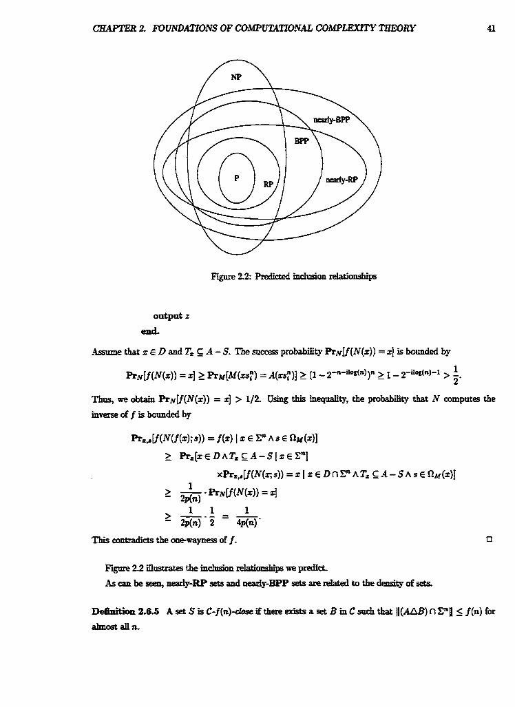
CEAPTER 2- FOWATIONS OF COMPUTATIONAL COMPLEXITY THEORY
Figure 29: Predicted indusion reIationsbips
Thus, we obtain -V(N(z) ) = z] > 112. Using this inequality, the probabii that N computes the
iwerse off is bounded by
This contradicts the one-amguess off.
Figare 22 iaastrates the inclusion relationships we predict,
As can be seen, nearly-RP sets and nearly-BPP sets are related to the dms?y of sets.
* n 2 6 A set S is C-f ( n ) - h e if there exi& a set B m C such that 11(,4AB) n PI1 <_ f (n) for
ahmostalln
(XUlTER 2 FOUNDATlONS OF C O ~ ~ O N A L COMPLEXITY TIIEORY 42
I;emmo 26.6 Let f kofvndionmNstrchfirabf(n) Ew(logn). FwCE {RP,BPP), euery~-2~-f(")-
dose set is nearlyC.
Proof, We rh$l estabIish the lemma for C = BPP. Sice f (n) E ~(Iogn) , we have fim,,,, = 0
for all numb ere>^. ~implierttut&--KxI&=~fororeryconstantc>~. ~ence,2-f(") G O ( & )
for any polynomial p.
Let A be ~~P-2~-f (")c lose- There exist a polynomial-time probab i ic W g machine M and a set
B such that II(AAB) n Fll 5 2n-f(n) for almost all n. In other words, Pr,[rl(z) # B(2) 1 2 E En] 5 2-f (n).
We d&e S = (z I A(z) # B(z)). Then, we have Rn[z E Sj < 2-f("). By the above calcalation, for
any polynomial p, PG[X E I for almost aIl n. This yieIds the desired consequence. 0
2.7 Relevant Theories
In this section, we shall discuss several important and a branches of computationaI complexity theory-
2.7.1 Feasi'ble Real Numbers
A real number is viewed as an infinite sequence of dyadic rational numbers which converges to it. If the
convergence rate is fast enough and the nth dement of the c~~~vergence sequence is &ectively constmctiile,
we can obtain a good approximation scheme for the real nnmber m questior~. KO and fiedman [w called
such real numbers comprrtable d numben and initiated polynomial analysis of the real numbers based on
real nnmbers computable in polpornid time.
D M o n 2.7.1 (Compntable Real Numbers) [55] Let t be a function on N A real number r is
t-time wmpdabk (t-space ctm@abIc, resp.) if thete exists a detcr-minisr'c Tnring machine M which, on
input In, produces dyadic rational nomber d, in time t(n) (using space t(n), resp.) satisfying the condition
k - dn( 5 2-". We cdl the sequence a mntrergm scpeme fbr r.
D M o n 2.7.2 (ConrpatabIe Sequence) A sequence { ~ n ) ~ ~ of real ntrmbers is polynomial-time
computubk (P-computable, for short) if there exists a polynomial p and a deterministic Thing machine M which, on input (In, It), produces a dyadic ratio& rmmber d in time p(n + k) satisfping Id - znl I 2-k-
In polynomial analysis, frmaions map from gl to Be Although these real functions are intriguing, frmctions
we are now interested only m fanaim that are "discre@ mappings h m C to the tmit intend [0,1]. Here
wemodifytheregulard~offeast'bIedfnnctionstosnitotlrsetting-
Dehition 2.73 (Computable ReaEValned F h c t h s ) A function f h m C to !P is d e d t-time
c o m p a t a b k ( t - s p a c e ~ r r s p . ) i f t 6 e t e ~ a d ' -'-'c'hingmacbineMwhichworlcsintime
CHAPTER 2 FOUNDATIONS OF COMPUTATION& COMPLEXITY THEORY
t (using space t, resp.) that 11\8(2,1i) - f (z)l 5 2-' for all i E N and all z E Em.
Hence.
Proof. Since { ~ n ) ~ ~ ~ is computabIe, there is a deterministic Zhting m d h e M 1% - M(ln, 0') 1 < z4 fix all n, i E N. Let N(ln) = ~( ld"+') , on+'). More precisely? N is a d-c 'hhg
marrhine d&ed as bedaar:
CBAPTEa 2. FOUNDATIONS OF COMPUTATIONAL COMPLEXITY THEORY
compute p(n + 1) (needing O@(n + I) + n) steps)
(*I simulate M on input (Mn+'), on+l)
end.
Ifp(n) < n, then we use the convention that whenever M tries to check the i-th bit of the input, it writes
down i in b i i on a checking tape, and then it retrieves the answer automatidy.
Then, the nmaing time of N on input 1" needs at most
c - ( ~ i e ~ ( l ~ ~ + ' ) , on+') + n) I c (t@(n + I) + n + I) + n)
for almost all n, where c is an appropriate positive constant. We next daim that Ir - N(ln)l I rn. This
is seen as f0Uows:
Therefore, r is computable in time O(n + t@(n + I) + n + I)).
The interested reader may refer to [a].
2.7.2 Kohogorov Complexity
In this thesis, we ase Cime-botmdcd generrJizod Kolrnqmw complex@ give^ by Hart * [38]. Intdidy,
the Kolmogomv complexity of a W e string is the length of the shortest program that will generate the
h g .
To dehe Kalmogorov complexity, we need a notion of lnrirrersd %+ng m c b e j that can simniate the
behavior of any other M g machines. We assume that {MiliEN is au & d v e enumeration of all lhring
machks. Now mnsider the follawing machine U: on input (i,x), U simnlates the ith machine Mi on input
2.
-4 code is a prefix-code or instadaneotts code if the set of code words is prefix-free, ie, no code word is
a p& of another code word. A prek-mde is d e d self-delimiEing if there is a Turing machine which (i)
deddes whether a given word is a code word and (ii) computes the decoding frmction.
Letusfixsncharmiversa'IhringmachineU.
&hition 2.7.6 (Kohogomv CompIesity Sets) [38] A Cimedowrded Kobnogm compkdy set
KTb(n),t(n)] is the set of z such that, far some string y of length at most g(lzl), U on input y
outpntszmtimet(l~). Finafixed~tringz~aEime-boundedcondrkoncrl - - Kohogmoo complQiPy set reloPioe
to z, KTb(n), t(n)jz], is simihiy de6ned but using U((g, z)) = z instead of U(y) = z m the above defbition.
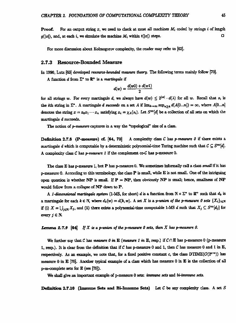
CTlNTER 2 F0ITM)ATIONS OF COMPUTATIONAL COMPLEXITY THEORY 45
Proof. For an output string z , we need to check at most all machines Mi coded by strings i of length
g([z1), and, at each i , we simuIate the machine Mi within t(lz[) steps. 0
For more discussion about KoImogorov complexity, the reader may refer to [62].
2.7.3 Resource-Bounded Measure
in 1990, Lutz [a] developed resrmm-bounded meMwe theory. The foUowing terms mainly folIow [TO].
A function d h m C' to Igt is a martingale if
for all strings w. For every martingale d, we aIwaps have d(w) 5 2Iw1 - d(X) for aIl w. Recall that si is
the ith string in E'. A martingale d succeeds on a set A if h k - snp,,, - d(A[O ... n]) = oo, where AIO ..a]
denotes the string z = z o q - - *zn satisfying zi = xA(si). Let SOD[dj be a collection of all sets on which the
martingale d succeeds.
The notion of pmeosure captures in a way the "topologid size of a class.
Dehition 2.7.8 (P-measure) cf. [a, 701 A complexity class C has p m e m 0 if there exisfsi a
martingale d which is compubbIe by a deterministic polynomial-time Turing machine such that C G Sm[dj. A complexity Jass C ha pmepna 1 if the complement CO-C has pmeasure 0.
The class E has pmeasure I, but P has pmeasure 0. We sometimes informally call a dass smut2 if it has
p -meam 0. According to this terminology, the dass P is smaIl, while E is not small. One of the in-
open question is whether N P is d If P = NP, then obviody N P is small; hence, smaIIness of N P
wodd foIIow from a collapse of NP down to P. A I-dimaui4ncf mmtingate Jystem (I-MS, for short) d is a function born N x C to R? such that 4 is
a martingale for each k E N, where dc(w) = d(k, w). A set X is a punion of tlie pmeosrae O sets (Xi)iE~
if (i) X = UjqN Xi, and (ii) there exists a polynomia-time computable 1-MS d such that Xi S00 [dj] for
- i E N
Jkmma 27.9 [MI If X is a punion of the pmeamre 0 sets, then X has pmeosure 0.
WefmthersaythatChas meruureOinE (meastae 1 inE,resp.) ifCnEhasprneasure0 (p-measure
1, resp-). It is dear from the defhrition that i f C has pmeasnre 0 and 1, then C has measure 0 and 1 in E,
respectiveIy- As an example, we note that, for a fixed positive constant c, the class DTIME(O(2C")) has
measure 0 m E [ 7 ' - Another mid example of a dass which has measure 0 m E is the coIIection of all
pm-cornpkte sets for E (see PI). WeshdIgiveanhqmtantexampIeofpmeasureOsets immtrnesetsand6i-immuneJets
Definition 27.l0 (Immane Sets and Bi-fmmnne Sets) Let C be any complexity Jass. A set S
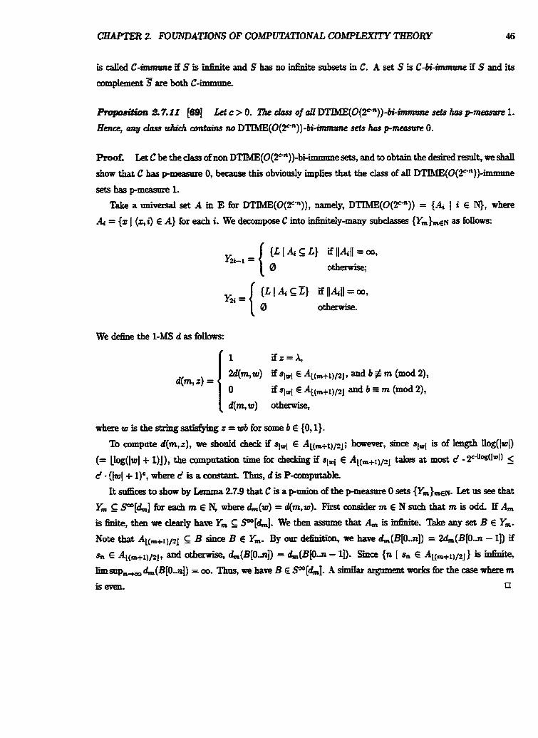
CKAPTER 2 FOUNDATIONS OF COMPUllATIONAL COMPLEXITY THEORY 46
is called C-immune if S is infinite and S ha. no infinite snbsets in C. A set S is C-bi-immune if S and its
complement are both C-immune.
Pmpodim 27-22 [a] Let c > 0. The chPs of aU DTIME(O(Fn))-bi-immune sets has pmeamz 1.
Hence, any c h to&& eontainr no DTIME(0(Yn))-bi-immune sets has p m m 0.
ProoE Let C be the dass of non DTIME(0(2Cn)>b~immurte sets, and to obtain the desired result, we shall show that C has pmeasme 0, because this obviodp impfies that the dass of aII DTIME(O(Fn))-' m e
setshaspmeasnrel. T& a nniverd set A in E for DTIME(O(Fn)), namely* DTIME(O(Fn)) = (A, I i E N), where
Ai = (I I {qi) E A) for each i. we decompose C into bhitdy-many sabdases {Ym)mEN as iotiow~:
We dehe the 1-MS d as follows:
d(m, z) = 2 d h w ) ifslwl E Al(m+rl/21, and i f m (mod 2),
i f s l ~ l E A~rn+1)/2j and b m (mod 2),
where w is the string satisfying r = wb for some b € (0,l).
To compute d(m,z), w e shonld check if sl,,,~ E At(m+tlpJ; however, since slwl is of length Ilog(llol)
(= llog(lwl + I)])* the computation time for checking if slWl E AL(m+l)121 takes at most d 2~-wl~l) 5 d - ([wI+ 1)E, where c' is a constant. Thus, d is P-computable.
It &ces to show by Lemma 2 7 3 that C is a punion a£ the pmeasure 0 sets {Ym)rnEn. Let us see that
Ym C SOD[&] for each rn E & where &(w) = d(m,w). F i h d e r m E N such that m is odd I£ A,,,
is iinhe, then we clearly have Ym G SOO[L]. We then assmne that A, is infinite, Take any set B E Y,.
Note that AL(mC11/21 B since B E Y,. By our dehiion, we have &(B[O..nl) = &(B[O-n - I]) if
Sn E A~(m+1)/2~ t and otherwise, d,,,(B[Od = &(B[OA - ID- Smce {n [ s, E -4L(m+1)/q) is hhite, Iimsupn- &(B[O.al) = oo. Thus, we have B E S00[&]. A similar argument works for the case where m
iseven. 0
Chapter 3
General Theory of Average Case
Complexity
3.1 Introduction
Avefageca~e analyses have been performed to measure the complexity of algorithms and to obtain a better
understanding of the behavior of aIgorithms when input instances are given with some probab*. In this
type of adysis, we should take into consideration that instances of a particular aIgorithm occur with some
probability. In contrast to the approach of b m worst-case anaIpsis, a "problem" here is a pair consisting of a
set of hdmces and an input d k t d u t h which designates the probability of each hstance. These probIems
are called d i&ih&d problem, madonaked problem, or tondom p b k m
Classical average-case analysis rises the expected running time or tape squares m use over an input
instances d the same length, Atthough the notion is simple and intnitioe, it is not a basis for a consistent
and coherent theory of a- mmp1ait.y- Levin's theory of average NP-compIeteness uses instead the
notion of poEynornial on the a o q e and also plynomicl-the mmry-one rcdt&i& among distributiond
decision problems with crucial conditio~m, the d e d dominoEton cmddmw . - for reduction hctiotls This
c3onstraint is essentid in the theory to make the r e d u c i i ~ transitZve and to make the average polynomial-
time cornpaable cIass dosed under the reductions In this chapter, we shaIl review M ' s theory and farther
cultivate a generat hmework of amrageme c o m p l e theorp; we sba[l focus mainIy on the notiom of
po- on peaage and plylomial darination nhticms on which "domination conditions" rdy.
Levin's notion of frmctions being porynarial on p-attaoge has been expanded into random frmctiolls to
cope with the average-case analysis of randomized algorithms.
Section 3% wiU begin with the f d defiinition of disbibufioru (or distn'bation Functions) and (p6-
abilitq] density frvnclions (or probability distributions)- For practicaI reasons, we s h d introdue semi- Wddicnu by e b h t h g the condition that distributions muverge to 1 as input - get larger- Of parthhimportance is the ~ d i s f r i b o p i o n t h a t asiptoeachstringtfte probabilitpofthestdag
CHAPTER 3- GENERAL THEORY OF AVERAGE CASE COMPLEXITY 48
being chosen at random.
In Section 3.3, we shall introduce the notion of t on p-werage which generalizes Levin's ori- notion
of "po1ynomiaI on p-amqe? Brie&, a ftmction g is called polyrumdal m p-memge if, for some positive
number k, the expeaed value of 1x1-I - g(z)'/' over all input strhtgs x under distnLbntion p converges. The
reader may notice that the fimctions which are polynomiaI on paverage are in general not time-constrnctible,
or even computable.
Section 3.4 will introduce of the notions of domin&*m &tiom and e r p b h c e relofions among dis-
tributions- These relations are the essential ingredients of Levin's domination conditions for averagecase
reducti011~.
Section 3.5 wil l introduce two types of averagecase compldty dasses, "randomizedn version of worst-case!
complexity classes aad (Caverage time/- boundedm version of worst-case eomplexiw dasses to descri i
the classes which consist of distrr'butiortal decision problems. We shaII introduce two types of notations:
Dist(C, F) for the randomized complexity dasses, and Aver(C, 7) for average complexi~ cIasses. horn the
dgorithmic point of view, we can consider sets of distnibnod decision problems (D,p) whose underlying
problem D is s01ved in time polynomial on paverage- In particuIar, we W introduce awmgeme analogues
of important complexity classes, such as P, NP, BPP, and PSPACE. However, the reader &odd note
that our average rrmning time and tape space are not measured by timeconstructible functions, and as a
result, fundamental relationships among the average compiexity classes are d y diffe~ent h m those
among worst-case complexity classes.
Major C o ~ i . a t i o ~ ~ ~ . This chapter extends Schapire's -tion of "po1ynomiaI on paveragen
to a more generat notion of Yt on p-average." The reader who is familiar with Levin's origind definition
may h d it intetesting that the arguments used in this thesis to show that a given hction is po1ynod on
p-aoeage are vey different from those used m the Iiteratttre. The basis of this chapter comes from Schder
and Yamakami [9q. Lemma 33.15 gives a h p 1 e but &cient condition for proving a given fnnction g to be polynomial on
paverage. The lemma s h m that if g(z) 5 c. nk + ( e / n * ~ ( ~ ) ) * for dl i with I 5 i 5 n and for
alI z E An, then g is poIynomid on p-;werage, where {4)lsisn is a partition of F. Lemma 3.416 shows that, for a random hct ion h with its random-input domain r, if p -F v and
i({(z, s) 1 h(z, s) > q(r - bl))) < l/r, then h becomes poIynomial on paverage
A genedhtion of Schapires d t is presented as m Proposition 33.17- The proposition a c W y shows
thatt for a good set 7 of strictly increasing frmctiom, g is T on p--average if and ody if the -on of
the waIues IzI-' - fl(g(z)). over dl mpat strings 2, a~nverge~ for some fnnction t in 7. Lexnmas 3320 and 33.21 are new d t s , Lemma 3.320 shows a suEcient condition for a random
fimction g to be poIynomial on pamage, whiIe Leuma 33.21 ghm a necessary condition for g-
Lemma 3.322 shows that, provided a function h is po1ynod on paverage and a random bction g
is palpomkd on p x vareqe, if h(f(z)) - ij(f(z)) 2 1 for all x and k V ( x ) I is polynomial cw paverage,
then the com@on k.g(z , h(z), s) is palymmkd an p-wemge-
tXAFlER 3. GENERAL THEORY OF AVERAGE CASE COMPLEXZTY 49
hposition 3.520 shows that, for example, Aw(BPP,F) is weakly PPdesaiptive.
Lemma 3.5.21 shows that Aver(P,F) and Aver(PSPACE,F) are closed under weak description., and
this lemma combimed with Fbposition 3.522 Ieads to CorolIay 3.523. The corollary shows that P # BPP i m p k the separation of Aver(BPP, *) born Aver(P, *) , whereas the two aveqease compIexity classes
coIIapse if P = PP. (These teSul~ foIIow Proposition 3.522, which shows an extensive generahation of a
d t given by Karg and Schder [q.) Our notion of nondeterministic average poIynomial-time is dearly distinct h m what has been d k u s s d
elsewhere. In parti*, whereas P =?NP is a Ion-standing open question, Theorem 3.524 makes the
interesting obsemations that A*, *) # Aver(NP, *).
The new characterizations of Aver(NP, F) and Awr(BPP,F) are presented in Proposition 3.5.30 and
Proposition 3.5.33. In parti&, the Amplification Lemma (Lemma 3.5.31) in our averagase setting, fol-
lowed by Proposition 3.5.33, is fundamental and hds many applications in later chapters. The Amplification
Lemma amplifies the success probabilitp of randomized algorithms which make bounded-errors.
3.2 Distributions and Density Functions
Amqpcase complexity theory handles problems whose input instances occur with specified probabilities.
This section wiIl introduce the basic concepts of d i d d u t h (or &std&m fundions) and (pro&u&ty)
t h d y fmcfhm. Using the terminoIogy m Section 2.2, om sample space R consists of all finite strings over
(0, I), and the o-fidd is (Q, F), where F is the power set of R. We consider a discrete probability measme
on (Q, B') and caII it a (probability) d e h c t i o ~ Intuitively, a density function provides a probabiIity
that instance s occurs. A distriiution, on the other hand, indicates the total probabi i over all instances
d e r than or equal to a give instance. For practical reasons, we also use the notion of s--disttibtrtions.
De5ition 33.1 (Dktributiops) A senzi-distrtm (or semi-c&std&h ftnction) C( is an increasing
fimction 6rom C' to the uuit real i n t a d [O, 11. A disbadion (or distribuk'on ftnrdion) is a semi-distriiution
which converges to I, ie, b- p(z) = 1.
We do not avoid the possibility that the semi-distn'bution p always takes the value 0, ie, i(z) = 0 for
aII 2; we caII such p triaiol. We remark that there is no feasri'fe way to determine in g e n d whether a given
semi-distniution p is is Nevertheless, we are primarily iderested m non-ttivial semidktriitrtiofl~,
Ben-David, Chor, Go1beich, and Luby [9], among otheq Ogen use semi-distnins m their arguments
instead offdl distihutim because their semi-distndmtions can be normalized to fan distniutions without
changing the compIexity. However, this normahation is not always possr'b1e See Section 42 for more
disassiof~
Next we st& define (probabil*) density fimctions which are probability measures on the u-fidd
Definition 3 3 3 (Density Ehnctions) For a disfxiiution p, its associated (prohMty) densi ty fmcth
ji is defined by the probtrbility ji(z) on mpttt string z as f01Iows:
(Note that a density fnnction is often called a ptob&i& distribution in much of the literature (see,
eg., [Ill) and should not be confased with a "distrriution.")
The reader must keep in mind that if p is a distri'b~on, then b(A) = p(X) by our d&tion. AIso note
that p(x) = z,, P(z) holds for aIL strings x. - We have already seen the notation R[q for event E based on a sample space R which consists of finite
or M e seqnences over (O,1). We reserve this notation for events where each bit of a sequence is chosen
at that is, for any property Q on X* and any subset E of R,
For convenience, we use the notation &ji(z) a g(x)" to mean that the probability b(x) on input string
z is proportional to the value g(x) for every z; more precisely, there exists a constant c > 0 such that
b(z) = e - g(z) for aII an. This c is d e d the nomolting constrmt for g.
For a distri'bution p and a set S, let b(S) denote the sum LES b(z). For example, ji(Esn) = p(ln) and
fi(Z*) = hz- ~(4. Recall that distributions are mappings h m the W e set Zg to the unit real intend [0, 11. We also
cope d etlsdles of- input distribuEimu instead of %hiten distributions- Given a distribution p
and a natural number n, the c o d h d &dt&n of p on !P, denoted by p,,, is the function from C" to
[O, 11 that is defined by its density fimction A as foflonsr for each z E I?,
whenever &(F) # 0; otherwise, A(%) is undefined- Srmitarly, let e, be the e r m d i t h d distribuCion of p
on Esn that is defined by its density function kn as foIIows= for each z m Csn,
(XhUTEB 3. GE2WM.L TBEORY OF AVERAGE CASE COMPLEXlTY 51
Definition 3.25 (Flat Distriiutions) [36J A distn'bution p is called pot if there exists a real number
c > 0 such that P(x) 5 rlZla holds for almost dl z- Notationally, FLAT denotes the collection of all flat
distributions*
For a hct ion f on Z', we write pr1 to denote the distribution defined by its probabii firl(z) =
B({z I i(z) = 2))-
Recall that distn'butions defined m Definition 3.2.1 are unary functions. We can also consider mdi-
dimerrsionat d- For a k-dimensional vector (x1,z2,. . . , zk) over E', if a density function fi is defined, then let
Using an &kcthe encoding of k-dimensional vedors into strings (discmsed in Section 2.5), however, we can
always iden* probability &, 22, . . . , xk) with probability ji((zt, x2,. . . , sk)) defined on X'. In this sense,
we do not need to consider all multi-dimensional distniutions.
To simpIify the descriptions of distnitxtions, we use k(z, y) and b(z, y,z) to denote fi((z,y)) and
ji((x, y?z)), tespectively. We dso use a simpEed definition of distributions- For example, the following
schematic definition &ji(si, z, In) = B(si) - i (z) - 2-2n~(n)-1n really means that
One of the most important distriiutions is the positive distniution where each string is chosen "rmi-
f o d f at random. This distriitrtion is d e d stundud- In this thesis, we use the standard distrr'btrtion
P-d, whose dues are dyadic rationai ntrmbers, that are easiIy sampled by the foIIowing randomized
aIgotithm: pick a n a W number n randomly and then pick a stdng of length n randody. To pick a natural number "rmifodf at random, we first define the translation Tr by Tr(X) = A, Tr(00s) = Wr(s),
Tr(l1s) = Wr(s), and Tr(Ols) = Tr(l0s) = # for a string s, where # is the terminal symbol dBerent
from G and 1. We then generate a string of the form s01 or s10 such that Tr(s) is the nth string w i t h
respect to the standard order in F. By a simple estimation, we have fi-&) = f l r l - * ~ l + l ) - 1 7 where
IIog(4 = LWn + 1) 1 *
Fkom this definition, it foIIows that, for every z,
CHXPlER 3. GENERAL THEORY OF AVERAGE CASE COMPLEXfm 53
For the sake of convenience, we sometimes use the same notation UW,. to mean the standard distribution
on (1).*
Deffnition 3.2.7 (Default D ~ i u t i o n ) For a random-input domain r and a semi-distribution p, we
define the default semi-distn'bution jq induced h m p and r as
where Ur is the rarity function d I'.
In the special case that I' is almost total, for every snbset S C r, it holds that
A function g horn E* to W is called d e g e n d e u n k p if b({z g ( z ) = 00)) = 0.
A set T of distriiutions is Josed under k-addition if, for any k semi-distributions, PI, pz, . . . , pk, &om 3, the distniution v defined by b(z) = 2, - k ( x ) belongs to 3-
For two distniutions p and v, let p $ v denote the distri'bution q such that @(x) = $(u) if x = Ou for
some u; i(z) = $6(u) if r = lu fbr some u; and j(x) = 0, othemise. We say that a set F of distn'butions is
&sad&$if,foranytwodistn~ntio~t~pandvmF,p$vkalsoinT.
3.3 A Notion of Easy-on-Average
To establish a amistent and coherent theory of amqeese compIexity theory, kst we must examine a
Etmdameetat notion of computational ''average complexity" of algorithms, after which we wilI Iook at Levink
innovative idea of how to amend the naive definition.
3-3.1 Naive Definition of Average Polynomial Time
In worst-case complexity theory, a problem k t(n)-time annpfezitg if there is an agorithm M computing
the problem which satides the ineqaditp T i e H ( z ) < t(n) fix ahalmost natnrat rmmbers n and dl inputs
z € 27'. A naive notion of a- c o r n p i e , however, is given by the expect& nmuiug time (or space)
of an algorithm over aII instances of the same Iength under a certain conditio~I distniution. More preciseIy7
an algorithm dtf which w d c s m time f teqaires the ineqaality that &,,TimeM(z) b ( x ) 5 t(n) for
amost all n. ThiS natmd formnlation of an a- c o m p I e might seem to be a start on a general
thtmy of mmgecae complexity- Unfkfmatdy, this ddefinitIw has severat dekienaes- We win see sewal
examples beIow- For brevity, we say that a h&b g u"expected poiynomiaI on paveragen if there exists a
c ~ n s t a a t k > ~ s a c h W f o r a l l n ~ & ~ ~ ~ ~ ~ ~ ( z ) - ~ ( z ) ~ n ~ f k [ ~ .
The ikst exampk is teIated to the mhipIicatian offnndions which are expected p o l y n d on p-average-
Example 33.1 [9] Consider a function g which is d&ed on strings of length n as follows: let g(z) be
2" on n inputs 2, bnt let g(x) be n on the other inputs. Now take a conditional distriiution h: L ( x ) = 2-"
for all z of Iengrh n. It is easy to see that the expectation of g, &+I=n g(z) &(z), is at most hn, but the
expectation of029 L1,1,@(4)2 - L(d? =a?&
Even if g is expeckd polynomial on paverage, ga is no longer eqmted polynomia on paverage-
The m n d example deaIs with the composition offunctions which are expected polynomial on paverage.
ExampIe 3.3.2 [9] For simplidtp, let n be ofthe f o r m for some integer m > 0. Consider the foIloaring
machine M: M is computed in steps on 2"12 shkgs of length n and outpttts a string of length mt and, for the rest of the inpats, M reqnires n2 steps to output a string of length n. The expected nmning time
of this machine M is at most 1 + n2 2-"I2, and hence, M runs in expected polynomial time on pavexage.
Now consider another machine N which needs n3 steps. Clearly N runs in pcdynomial time. However? the
composition of two machines, N(M(z)), needs PI4 + n3 - 2-n/2 steps on the average
Hence, this naive notion of 'expected po1ynorniaI on the averagen is not dosed under composittio~
Example 3.3.3 [9] Consider a problem on directed graph G = G(V, E), where V is a set of vertices aud
E is a set of edges. Let ]lVll= n and 11 El1 = m- Assume that there is an algorithm M which works on this
graph G in time t(G), where t(G) = 2" if m < n312; otherwise, t(G) = n2. Suppose the graph G is given
by its (imcident) matdr repfesentation. Siace encodings of graphs are presented by n vertices? the amage
is taken over all graphs G with n nodes. The expeaed rtmning time Ec t(G) - L(G) is at most
On the other hand, suppose the graph is given by its adjacency list. Then, the expected nmning time is not
expected polynomial on pavetage
The naive definition is dependent on the particular encoding of instances of a given probIm,
As we have seen, the naive definition is not suitable for a coherent theory. In 1984, Levin [60] instead
proposed a new measure d "a- polynomial-timen To understand his measare, we again take a dose
Iook at the definition ofwmtxase a m p l e measure. Remn that an algorithm M needs polynomial time
if Tre~(z) 5 1x1' fbr ahnost aIl z Here we trausfii this in- into another form of ineqpdiQc
I%[-' - %neM (z))'/' 1. A nahnd idea then is that the expectation of 1x1-' - TfrmeM(z)l/k over dl strings
of length n, is bounded by 1; namely* - ~ r r n e ~ ( x ) ' / ~ -A(=) 5 1. hrin was motivated by this
ineqnalitg., b r r t h e ~ o n e s t e p f m t h e r a n d t o a k t h i s ~ o v e r dfinife- Hedehedhisamage-
case complexity me- m o x d m p-ammgem by mpirbg that & . T ~ ( Z ) ~ / ~ - B(z) < oo.
CHAPTER 3 GENERAL TEE0R.Y OF AVERAGE CASE CO-WLEXITY 55
S i his &st paper appeared in 1984 at the 16th STOC conference, several criticisms of Luvin's com-
plexity measnre have arisen. One of them is that his formulation does not seem to reflect the polynomiality
of the nmning time on the average. In 1990, E. Mapiire [q wrote a technical report in which he hibiteti
an emerging theory of Levin's awngxaw NPsompleteness and gave an interesting insight into Levin's
central notion of "polynomial on paverage." He gave an equivaIent fbrmuIatim of this notion.
This thesis m d S e s Schapire's characterization of plynomial on p-lraerage and introduces a more general
notion o f t on p-ttuemge for an arbitrary hc t ion t .
Dehition 3.3.4 (t on p-Average) [w Let t be a kction on F and Iet p be a distribution. Let g
b e a f u n c t i o n f r o m E m t o P .
1. The function g is t on p-uuercge if b((x 1 g ( z ) > t(1zl. r))) < I/r for any positive red number r.
2. The function g is 7 on p-ooeroge if there exists a function t E 7 such that g is t on p-average.
Schapii actually used a function with two variables, t(n, r), instead of the form t(n - r) in the above
definition. In most cases, however, there is no practical difference between these two fnnctions. For this
reason, we use the above definition throughout this thesis. (This issue has been thoroughIy studied by Karg
and M e r [a], and the interested reader may ref' to it.)
Notice, from Def'mition 33.4, that if g is t on pawrage, then g is degenerative under ~ r , Moreover, it
immediatdy follows from DeWtion 33.4 that increasing the d u e of r also increases the probability weight
of the set of strings z with the pmpeay that g ( z ) 5 t(lz[ . r), which is 1 - I /r.
Definition 3.3.5 (Polynornial/Lagarithmic on p-Average) A timction g from E' to P is ply-
n o d on p-memge if there exists a polynomial p such that g is p on p-average S i i l y , g is b g a d h i c
on p-memge if g is q on paverage for some Iogarithmic hc t ion q (i, q(z) = cIog z +d for some constants
c,d E R).
The notion of polynomiol on p-auemge was fkst introduced m [q and used m [a, 88,36,9, Ill], whiIe
the notion of [ogmithnde on p-uuerage was defined by [91 and also rssed in [a].
Roof. Let us assmne that g is q on paverage for some logadmk function q. Suppose without loss of
that q(z) = cbgz + d for constants c, d > 0. Notice that q is strictly mtreaSing. Using this fact,
wehave
CaAPTER 3. GENE3UL THEORY OF AVERAGE CBE COMPLEXITY 57
Roof. The proposition follows b m Lemma 33.8 together w i t h the fact that if t is a polynomial, then
Xz.t(&) and Xr.t(2z3) are both polynomials. El
Under some reasonable constraints, we can further replace an input ensemble { j ~ . & ~ ~ - in the above
pq=i t ion by {pa)nEn. Cai and SeIman [19] frst proposed an idea of restricting Levin's notion of pIy- no& on p-merage to obtain a better tim+hierarchy theorem. The foUowing proposition takes a Merent
fomnlation but shows an essential part of a theorem by Cai and SeIman.
Proposition 3.3.10 Let g be a j b d i o n + C to P and let p be a d i d d d o w If h.fi(E*) E
R(n-k) for some integer k > 0, then the /oUotoiflo dateme& are epivdenk
1- g is polynomial on p-wenage.
Roof. Let g be a frmction kom X' to It+. Asnrme that h . j i (Eb) E ~ ( n ' ~ ) for some k > 0.
We 6rst show that (2) implies (1). Assume that there atis& a polynomial p such that, for every n f N aud every r > 0, jiln({x E Z a I g(x) > ~(1x1 -T))) < l/r. Set n = 0, and then we obtain
Thus, g is polynomial on paverage
Next we shall show the other implication. ,4ssmne that g is polynomial on paverage; namely, for some
appropriate polynomial p, ji((z 1 g ( z ) > p(r -1~1))) < l/r h o b for all red numbers r > 0. Wrthout loss of
generality, we may assume that p is iucteasing.
By the assumption for p, we can assnme that, for some constant c > 0, ji(E*) 2 5 holds for all
positive integers n. For simplicity, assume that c is an integer-
Let us define q as q(z) = p ( 2 c - e 3 ) fm & z. W y q is a pol~pomid In particttlar, by the monotonicits
of P, q(r - m) 2 p(m - bd+2)
for dl rmmbers r,m 2 0,
Now let S be thesetofaIlnattaalnambers n for w b i m ~ , is de61&
Thdore, g is polynomial on average with respect to (pa)meN, and this completes the proof. 0
3.3.3 Basic Properties
The notion of "t on paverage: which we have introduced in the previous section, is essential in om average-
case c o r n p 1 ~ theory. In this section, we shaII discuss its fundamental properties which w9 be used M y
in the later chapters.
The Iemma below is the starting point-
PmoE (1) If 0 c r < 1, then i({z [ t(lxI) > t ( [ x l - r ) ) ) 5 1 < 5. .9ssame r 2 1. In this case, the set
{x [ ~ ( [ z I ) > t(lzI - r ) ) is empty since t is inmaiing. Hen- P({z [ t(lx1) > t ( lx l - r))) = 0 < $. Therefore,
XzJ(izl) is t on paverage-
CHAPTER 3. GENERAC THEORY OF A'VERAGE CASE COMPLEXITY
Notice that f i ( {z E I f i ( 4 9 < <) < L Thus, we condude that
since = 1- 0
Lemma 3.3.11(2), for example, enables us to see that if g is polynomial on v-d-average, &then g is
for some constant c 3 0.
La us r e d l &om Chapter 2 that f w m i r ~ g, denoted by f 2 g, if and ody if f (x) 2 g(z) for all x-
Froof. Assume that f is t on paverage Since f (z) 2 g(x) for all z, it follows that { x I f (x ) > c) {z
g(z) > c} for an arbitrary c Then,
Thus, g is t on paverage 0
As we have seen in Subsection 33.1, Levin's notion of "po1ynomiaI on paveragen is superior to the naive
notion of "average polynomial" because the set of frmctions which are polynomial on paverage is dosed
under dgebraic operations, such as +, x, max, and mln. Here we show a more general cIaim that the set of
h E Amme that P({x I f (z) > p(l4 4)) < l/r and fi({z I g(x) > q(kd - r))) < l/r- For the rase
CaAPTER 3. GENERAL THEORY OF AVERAGE C . COMPLEXITY
f x g, take a function s E 7 such that s(z) 2 p(2z) + q(2z) for all z. Then, we have
Similarly, for the case f, take a function s such that s(z) 1 @(z))'; for the case r - f , take s such that
s(t) 1 r - p(z); and for the case f + g, take a fnnction s such that s(z) 2 p(2z) + q(2z). The case max{f, g)
is derived h m the case f f g since f + g majorizes max{ f, 9). SimilarIy7 mini f, g) becomes 7 on paverage
~~ ={f, 9) W o w W f , 9)-
As for "po1ynomial on paverage," we sball show m the followiug lemma that this notion is invariant to
any application of polynomials. This tenma is duabIe in later chapters.
We call an n-ary function f immmhg (or monotone) if ;f(zl,. . . ,zn) I f (a?. . . , y,) whenever Xi I yi
for an i, 1 5 i 5 n.
knZn~t3.3.14 cf,[38] M k z l c n d l e t g ~ , ...,git befvncEiorrPfrwnC t o p a n d l e t p k a k -
q -g pol^ If dl 11,. . . ,gk mr on p-auentge, then k p ( g l (z), . . . ,gk(x)) is also
polynomial on p-auemge
Roof. Assume that, for each i with 1 i 5 k, the function gi is qi on paverage for some polynomial
qi. By dehition, it follows that fi({z I g&) > qi(lxi - r))) < ; for all positive real ntlmbers r. Now let
S(X) = p(a(kt), . . . , qk(kz)) for all z- Since p is baeasbg, p(zl,. . . , zk) > p(yl,. . . , yk) implies that there
exists a nmnber i such that q > gi- So, we have
The fdowing lemma is of a rather simpIer fonn than Lemma 3.3-11(3), but it is helpful to show elsewhere
that a given hction is palyMmial on paverage.
CKAFTER 3. Gl3lWU.L THEORY OF AVERAGE CASE COMPLEXITY 61
x E A,n, g(x) I c - nd + ( ~ / n * j i ( 4 * ) ) ~ . Then, g is pdyMndal em p-ooetcrge.
Roof. Let us assume that g satisfies the above condition. For every z , let g'(x) = rniu{g(z), c- Ixld) and
/ ( x ) = g(x) - g'(x). Siaee Xz.clzld majorizes g', by Lemma 3612, g' can be shown to be polynomial on
Cr-a=mF-
We next show that g" is aIso polynomial on pa- Let no be the m;nimd integer such that, for aII
n 2 for dl i with 1 5 i k(n) and for all x in 4A , /(z) 5 (c/n2ji(4))*. Also let b = max(g"(x) I
Now consider the polynomial p such that p(z) = (2c.~)~ + b. I t is obvious by our definition that g"(X) 5 p(0)
and g" (2) 5 p(l/n(n + 1)ji(4)) for all x E A,*. By Lemma 3.3-1 1(3), g" is polynomial on paverage.
By Lemma 33.13, g' + g" is also polynomial on pawrage S i g = g' + g", the p r d is completed. 0
We call a set 7 suitable if, for every t E 7, every c E N, and every polynomial p, there are ftmctions
st, a, 33 E. 7 such that st(%) 2 t ( a ) , s&) 2 t@(z)) , and q(z) 2 t(r) + c for an z.
Proof. (If - part) Assume that g is t on p,-+verage for some t E 7. Take an incTeaSing polpomial p
such that If (%)Is p(Iz1) for aIl z , and an integer Q such that g(A) 5 g. Moreover, we let function t' E 7 be such that f ( z ) 2 t(3p(z)%) + Q for dl z- Such a fimction exists because of the dcsare property of 7. Note that, for x E P and r 2 1, t (3p( t l -# .Izlr) 2 t ( 3 l f ( ~ ) [ ~ r ) . We can show that g o f is t' on paverage.
For the sake of c o d e n c e , let A* = {z I f (x ) # A).
ForeaChrZ1,
CHAPTER 3. GENERAL THEORY OF AVERAGE CASE COMPLEXITY 62
(Only if - part) Assume that g o f is t on p-average for some t E T. Take an inaeasing polynomial p
such that 1x1 5 p(lf(x)l) for all z because of the phonesty off. Let us take a function t' E 7 such that f(r) 2 t(p(r)z) + q-, for all z, where g is the same constant as defined above. We also take AA as above.
Note that, for x E Ax and r 2 1,
We show below that g is f on prt-averageC
3.3.4 Different Characterization
As stated before, our definition of "pol1ynorniaI on p-average" is motivated by Schapire's definition, and at
ttSt gIance, it appears to be dSerent from Levin's dehition. In the 6Rt part ofthis section, we shaII prove
by a slightIy more general argument that both dehitions are ecpident. For this purpose, we introduce a
ugoodn set of hctions below.
For a set 7 of functions on e, we call T good iE, for every s E 7 and every constant c E N, there exist
fimctions st, dr E 7 such that s(a) d(z) and s(2) < #(x) for dl z. For exampIe, the set of inmasing
po1ynominllE is a good set of convex functio~ts.
Proof. (Only if - part) Wrthout loss of generalitp* assmne that g(A) = 0 and that g is t on paverage
for some t E 7. Then it foIIows that, for any real number r > 0, fi({z ( g(z) > t(? - [ X I ) ) ) < I/*. By
om as~rmnptiort of 7, we can define a strictly increasing fnnction t' E 7 such that t(9) 5 t'(z) for ail z. In
partidart t(? - 121) 5 t((r - 1 ~ 1 ) ~ ) 5 C(r - 1 ~ 1 ) - Hence, this implig that b({z I g(z) > f(lx[ r))) < I/*.
Wdont loss of generality* we may Iet this t' be t m the rest of the proot
This indicates that* for every integer k > 0, p({x E CC [ 1~1-'t-'(g(z)) > 5)) < l/#. Using this
m e t b m d Zlrl v . f i ( z ) * by
The last term is farther bounded above by
(If - part) Conversely, a s m e that t-'@(z))(xI-'fi(~) 5 N for some number N 2 1 aad some strictly increasing function t E 7. Markov's Inequality (Lemma A.1) enables us to get the inequality that
E({z I I~l-~t- '(g(z)) > r 4 ) ) < I / r for any real number r > 0. This yields b( { z 1 g ( z ) > t ( rN[z [ ) } ) < l / t .
Hence, g is )LZ ~ ( N X ) on paverage- S i there is a bction t' E 7 such that t '(z) 2 t (Nz) for dl z, we get
the desired result that g is 7 on paverage. n
For example, the set of poIynomiaLP, 7 = {A# + d) I k,d >_ O), and the set of logarithms, 7 = {Xr.(kIog t + d) I k, d >_ 01, are both good sets of stdctly increasing functions on P (recall our convention:
logz is defined to be 0 whenever 0 (t < I).
In 1995, Irnpaghm [43] pointed out that k in ' s d-on is eqtlivalent to the statement that the
expectation of a ftmction over all stziugs of length 2 n, is bounded above by a poIynomiaI in n.
In the following theorem, we see Sdmpire's [88j aad Impagliazzo's -on [a].
Pmof. Note that if there exis& a stzing z such that g(2) = 00, then we can redehe g(z) = 0 without
changing the three mnditions above- Hence, we may apsame that g(x) < a, for dl z m the fo1Iowing proof,
The eqyhdnce between (1) and (2) comes b m Proposition 33-17. We next &ow that (2) and (3) are
eqnivalent.
We &=st prove that (2) implies (3). Assmne that LMX ~*fi(z) < cn for some real number 6 > 0.
Consider a large integer e > 0 such that &+,>o %(z) c Let no be the minimd number in S, and
~ e ~ t h a t ~ d > ~ * e f t h a t ~ ~ @ ~ ~ ) ~ f - ~hen, forearhn~S,
iXUFT32 3. GENERAL THEORY OF AVERAGE CASE COMPlJXlTY
Conversely, assume (3); namely, C.+l<n - g ( ~ ) ~ iy,(x) - < c - n + d for all n E S. Notice that
since
To simplify the description, set I& = {z E P I g(z)6/3 5 1x1) and El = {z E Z+ 1 g(x)'l3 > Iz/). It is
important to note that if x E &, then g(z)*/3 > 1zI2. Thus, we have
The first term zEEo b(z) is obviody at most I. Let T be the last term, and we shall focus on it below:
3.3.5 Random F'unctions
Randomized atgorithms are a simple tool for solving probIems ~ ' ' on the average. To cope with the nmning
timefspace of randomized algorithms, we need a notion of polynomial on p-auemge for random functions
because the running time/space forms a random function which depends on random seeds produced by the
inner coin &ping process of the randomized algorithm.
Gnrevich [36j and Blass and Gurevich [I21 formdated a notion of polynomial on p-auemge for random
functions b m a random-input domain r by regniring the convergence of the -on of the value
~ Z ~ - ' ~ ( X , S ) ~ ~ over all pairs (2,s) in r, with respea to its probability b(z) and conditional probabihy
Or(=) - 2-1'1- Our fonrmlaton is a modification of their definition, and it wiII be shown to be m e u t to
theirs at the end of this section.
Detlnition U . l B (t on p-Awmqp) Let t be a function on P and let 7 be a set of fimctions on IF-
Let p be a distniution and let I' be a random-input domain. Let g be a random function from I' to P .
CHAPTER 3 GENERrLL THEORY OF AVERAGE CASE COMPLE?UTY 65
1. A random function g is t on p-menye if h ( { ( z , s) I f (z, s) > t(lt1- r))) < l /r for all real numbers
r > 0.
2 A random function f is 7 on p-aoeroge if there exists a function t E 7 such that f is t on paverage.
The above dehition impIies that if a random function f wi th a random-input domain I' is polynomial on
paverage, then the same function f , viewed as a "regnlaf function with two arguments, is p o l y n d on
ppaverage, ie., &(((z, s) 1 f (z, s) > p(l (z, s} J r))) c l/r for some po1ynomial p. The converse, however,
does not hold in g e n d
A simple observation shows that h(&s) 5 t(0) for all random seeds s E r(X) unless f i ( X ) = 0. This is
seen as foIIows. For any positive reaI number r,
As r approaches oo, the probability Pr,[h(& s) > t(0) [ s E r(X)] goes to 0. Thedore, this probability must
be 0.
The I~mma below provides us with a simpIe and &dent method for proving a random function to be
7 on paverage. For the lemma, wle must recalI the dehition of a conditiond expectation of a random
function.
Fix a random-input domain r. Fa a random frmaion f h m I' to P, the onditiond expectation
E,Eg(z, s) I s E I'(z)] for each x is defined by
Roof. Let t E 7 and assume that k&b(z , s) I s E r(z)] is t on paverage; namely, b({z I E,[g(z, s) I s E I:(z)] > t([zl- r))) < I/r for all r > 0. We shall show that &({(z,s) I g(z,s) > t'(lz1- r))) < lfr for
some t' E 7. Fix r 2 1. Smce t is strictly inQeaSingt h({z [ t-'(E,[g(z,s) I s E I'(z)j) > 121 -4?)) < 1/4? < l/r. By
Jensen7s inegualityt since t-' is a strictly increasing concave function, it fdows that
3- GElWRAL 17HEORY OF AVERAGE CASE COWLEXlTY
Now let Dr = { X I E#[ t - ' (g (~ , s ) ) I s E I'(x)] 5 1x1 - 2r). We then obtain
Let us consider the last two terms in the above inequality- The first term is bounded above by 1/2r. The
second, howevert is bounded above by
because of the assumption z E Dr. Markov's Inequality (Lemma AJ) ensures that this term is bounded
above by 1/2r. Thus, h ( { ( z , s) I t-'@(z, s ) ) > 1x1 4?)) < l / r -
Using the faa that t is strictly increasing, we obtain the conclusion that j ir({(z,s) I g(x, s ) > t(lz1 - @)I) < l /r , Now consider another fimction t' 7 such that t (@) P(x) for dl z, and as a result, we
obtain the inequality A ( { ( z , s) [ g(x, s) > t'(lx[ - r ) } ) < l / r - Therefore, g is 7 on paverage.
Note that the lemma shows only a d c i e n t condition, and the converse of the lemma may not hold in
general. However, if we instead use Gin's measme (m Section 2.4), then we can obtain a neeeaarp condition.
For a random hction f from I' to It?", let f be defined as
Roar. For each x, if f (x) > t ( l z 1 - a), then R s V ( x , s) 5 t(lz1- 2r) 1 s s E(x)] 5 1/2, because f (z) is
the minimat d u e k sa-g that R s V ( z , s) 5 k I s E r(x)] > 1/2 Hence, it fo11ows that
Using this tut, wqgn estimate the vdae ji((z I f (x ) > t(Iz[ - 2r))) as foflm:
As a particular ease, if a random fimction f is polynomial on pawrage, then its associated frmction f is also polsnomid on paverage
CHAPTER 3. GENERAL THEORY OF AVERAGE CASE COMPLEXITY 67
When f(x, a) is given as of the f o m TimeM (z; s) for some bounded-error probabilistic Thing macfiine
M, we can also repIace r ( x ) by Q(x) in the above definition of f' and the 1-
Root For simplicity, write v for p x q. Let us assume that a random bction g is polynomial on
waverage. This implies the sjstemae of an increasing polynomial p, such that +({(z, y, s) I g (z , y,s) > pg(r - (1x1 + Iyl)))) < l/r for any positive real number r. SimiIarly, kom the assumption that k.1 f (x)l is
polynomial on paverage, there exists an in- polynomial pj such that k.[ f (x ) [ is pf on paverage.
Let us also assume that h is q on p-average for some increasing po1ynomial q.
We then define the new random-input domain rt as I' = {(x, s) I (z, f (z), s ) E r). To reach the desired
remit, it d c e s t o show that, for some polynomial p, h r ( { ( x , s) 1 g(x, f (z), s) > p(lx1- Y))) < I/+. This
po1ynomial p is of the fo11owing form:
Let us ~IX r, r > 0, and define Dr = {z E E+ I h(f (2)) 5 q(l f (z)l- 3r) If (z)l pf(lzl - 3 4 ) . Notice
that, by the monotonicity of pf, p,, and q, if z E D,, then
It is not diflicult to see that
CHAPTER 3. GENERAL TZEORY OF AVERAGE CASE COMPLEXITY
At the beginaing of this subsection, we mentioned the @valence between our definition of polynmnial
on p-memge and the definition given by Gurevich [%I, and by Blass and Gurevich [12]. We now present
this equivalence in the fo11mhg proposition.
~ d b n 3.3.28 Letr beandom--inputdomainandktg bearundomfunca'onfiomf t o e . The
f o l h i n g statanents are eplrioorenk
Proof. Sirnilat to Theorem 33.18.
3.4 A Notion of Domination
Another c r u d notion introdaced by LRvin (601 is the the notion of polynomial domination among distri-
butions. The dmktim rehCion wiU be used as a part of the dominotion cm?dition which is an important
ingredient of the poIpomial-time reduability among distributional decision problems in Chapter 5. Mu- itivelj speaking, it ensures that if an aigodhn is %st on the averageD for somedistriiution p, then this
algorithm is also "fast on the amage" for all distniufions which are dominated by p- This Win deftne
the polynonrial domirrcrEion reidion and the polpaomid ~ a l e n c e nddion and explore some frmdamenta
properties as prepatation for Chapter 5.
3.4.1 Domination Relations and Equivalence Relations
First we shall give a general definition of domination reIations.
Dehition 3.4.1 (Domination ~ 0 ~ s ) Let p and v be semi-dishiintions-
1- IRttandTbeafarrctionandasetoffnnctiorts~X'to~,tespectioely. Thesemi-distribationv
taominoteJpift(2)-qz) zji[s) h d z E C, a n d v T - ~ p i f t h e r e e x i s t s a f r m c t i d n f ~ 7
suchthatvt 'domhata~
CHAPTER 3. GENERAI; TaEORY OF -4VERAGE CASE COMPLEXITY 69
2. Let t and T be a function and a set of functions on W, respectively. The distribution v merage t-
d o m i d a p if there exists a function t', from C' to , such that t' is t on p-average and v t'dominates
p, and v wetage 7-dominafes p if there exists a function t in 7 such that v average tdominates p
This dehition enables ns to consider polynomial domination relations and averagepolynomial domina-
tion relations.
Deftnition 3.43 (Polynomial D o ~ t i o n ) Let p and v be any two semi- distribution^^
1. The semidistriiution p polynomioUy &minutes (pdominates, for short) v if there exists a pbotmded
function t such that p tdominatg v. For brevity, the notation v SP p expresses that p pdominates
v-
2. The semi-distribution p merage-polyndly dominates (avpdominates, for short) v if there exists a
polynomial t such that p average tdominates v. The notation p 5- v means that p avpdominates
v.
In [36], polynomiaI domination and average-polynomial domination are called dmnincrtion and Merrk
d c m i n d q respectidy.
As previonsly mentioned, poIynomial domination relations were explicitly introduced by Levin 1601 on his
theory of averagecase complexity as a cettain type of reducibility between two distributions which measures
the complexity of these distributions. H this sense, two distriiutions which dominate each other on be
mnsideted to have h o s t the same degree of complexity. We call them equiodent. Equivalence relations
capture the doseness of two distributions and also give rise to an appropriate "apprcndmationn between
them.
We begin by giving a g e n d dehition of equivalence relations.
1. The distriiution p is T-equioolard to v if p 7dominates v and v Tdominates p
2 The distnitttion p is menage Tquimht to v if p averageTdominates v and u averageTdominates
P-
-on 3.4.4 (PoIynomial Equhdence) A semidistriitttion p is polynomiany equioaknt
(pquhb , for short) to another semi-distribution v if p is t-eqnivalent to v for some pbounded function
t; and p is wange-pdyumzioCly e q h k n t (avpequident, for short) to v if p is average t q u i d e n t to u
for some polynomial t- We me the notation p z p v to mean that p is p-quident to to, and the notation
p+ v tomean thatp L a v p q u h b t tov.
CXUKER 3. GENERAI; THEORY OF AVERAGE CASE COMPLEXITY 70
As an example, let us consider FIATT the set of flat distniutions. This set is invariant with respect to
p-equidence relations- ThiP is seen as fonotas. Smce p is p-equivalent to u, it holds thy # 5 ti(=) 6 p(x)fi(z) for m e pbotmded p. Then, we have
Hence, I@(=) - t(z)[ 5 2-14'' for some d > 0, and in conse~uence, p is Bat.
Domination and equivalence relations are transitive.
Proof. (1) Assume that there are bctions rn and p.r in 7 such that m(r) - ji&) 3 iil (z) and gr(x) - ji3 (x) 2 ji2 (2) for aU z. To obtain the desired redt, we set p(x) = = ( z ) - p2 (2). Then, we have
(2) Immediate h m (1). 0
As an immediate consequence of Lemma 3.3.14, we have seen that if f majorizes g and f is po1ynomial
on paverage, then g is also polynomid on p-a- Wow we shaIl show that if u avpdominntes p and f
is po1ynomi;ll on v-amage, then f becomes poIynomiaI on paverage.
A class 7 of frmctions is said to be closed under c o t n p o ~ with p o t p m i d s if, for any ftrnction t and
any po1pnomi;rl p with integer d a e n t s , t E 7 i m p b k . t ( p ( z ) ) € 7,
h o t (1) Assume that p 5- v, and h is t on u-average for some h a i o n t E 7. Choose a hction
q which is pdynomid on p-average such that, for dl z E Em, '(2) - q(z) 2 fi(z). Fkst notice that if h is
degenerative under v, then h is also degenerative under p since t ( z ) = 0 implies ji(z) = 0 fix any string z- By
om assmnption, P({z 1 h(z) > t(Iz1 or ) } ) < l/r br alI r > 0. Sime the set 7 is dosed tmder composition with
polynomiaIs, we assmne without loss of genefaIitp that h(A) 5 t(O), and therefii fi((zf h(A) > t(0))) = 0.
Smce q is polynomial on paverage, there exists a poiynomial p such that b((z I q(z) > p(lz1- r ) ) ) < l / r for
d r > O .
CELAPTER 3. GENEWL THEORY OF AKEMGE CASE COMPLZXWY n
Let p,, and v, denote the conditional probability of strings of length n of p and v, respectiveIy. Note
that if q(x) 5 p(lzl. r) for a string z of length n, then &[x) 5 p(n . r) - C(z) for alt n E N and r > 0. Now
d&e g as g(x) = t(42 -p(2z)). Smce 7 is dosed under composition with polynomials, g is in 7- We note
that, for all n E N and all r € W , g(n . r) _> t(n - 9 4n2 - p(n + 2r) ) . To complete the proof, we &odd show
that h is g on p-average. This is seen as follows: for every real number r 2 1,
(2) Let us r e d l that v is avpqtident to p if and d y if v avpdominates p and p avgdominates v.
The resnIt thns f011m immediately from (1). 0
Cwkyl?..C.7 LethbeanyfundionfrwnC'toHPtoo. Fordijtri6utionspandv,ifvuup- UP
and h is polynomial on v-marrge, then h is also pEynonu'd on p-avaagc
Corollary 3R7 implies that the avp-equivaIence relations preserve the notion of polynomial on average.
This faa motivates IIS to introduce the two new notions of irrch*n'm and epucrlity among sets of disttiiudons.
These notions win be used in later chapters.
Deftnition 3.4.8 Let f i and 3 2 be two sets of distniuti~ns~
I. FI potynomially indudes (pmdttdes, for short) 32, sgmbowy Fl P F2, if every dishibution m 31 is
peqnivaed to some distriintion m 32. SnniIarly, 31 m m g e polynomialy includes (avpindndes, for
short) 7i, spmbolidy 3i P 32, if every distniution in F1 is a q m p h h to some distniution
in 3 2 -
CHAPTER 3. GENERAL TBEORY OF AVERAGE CASE COMPLEXITY
Proof. By Lemma 3-43 and the definitions.
3.4.2 Fnndamental Properties
The domination relations are of importance in average polynomial-time computation. This subseaion wiH
explore properties of domination relations in reIation to functional composition, and prepare the ground for . -
timmdma d m which wilI be introduced and cultivated in Chapter 5.
Let us be@ w i t h several important properties. Recall that, for a function f and a distn'bution p, the
notation prt denotes the default distniution defined by its probability jirt (z) = ji( f" (x)) .
Proof. (1) Asmme that p 5 p v. There is a pbonnded function s from C' to R+ such that f (z) s(z) 2 fi(z). W h u t loss of geueralitp, we w e e that s(z) 2 1 for alI z. Consider an incfeasing polpnomid p such
that s(z) 5 p(lz[) for all 2. Smce f is phonest, there is an increasing polynomial q such that [zI 5 q(l f (=)I) for aII z. Now we Iet t(y) = max(s(z) I f (z) = y). It is dear h m the definition that, for every y, there is
an dement 2, E f -'(y) such that t(y) s(q,). For this z,, we have
Since p o q is again a polynomial, t should be paoUnded- Hence,
(2) Let f be a one-one, phonest, pbounded function on C. Assume that ~ c f ~ SP v. Take a pbotmded
fimction p h C' to HeC such that fi(f-l(y)) I fib) - p(ly1) for aII y. Write z = f"(y). Then, since
y = f (z), we have b(z) < P( f (z)) pV(z)). Let q(z) = p(f(z)). Notice that q is pbotmded because f is
gbonnded. Thus, we get p s p v o f. Conversely, assume that p SP vo f. There is an hereasing polynomiaI p such that b(x) S f ( f (2)) -p(lzl)
for all z- Since f is phonest, lzl 5 s([f (z)l) fix some polynomial s. Write y = f (z). Then, z = f -'(y)
because f is one-one Let q(z) = p o f-I(%), and then q is pbotmded, because
C&APTER 3. GENER4L. THEORY OF AVERAGE CASE COMPLEXITY 73
Lemma 3..#.11 Let f beafunetiononC andletp andv k d i d d M h s . The folloraitrgstatementsanz
fq?Livalentr
Proof. We shall show the implication b m (2) to (1). Assume that p 5P 7 and P(y) 2 ijf I (y) for ail
y. Choose a function p such that p(x) tj(z) 2 P(z) for all z. Without loss of generality? we assume that
p(r) > 1. Slncetj(z) 2 S?
Candy? we shall show that (1) implie (2). Let us m e that t(p) 2 # for d y, where p is a p-bounded function- We may assume p(r) > 1 for all z. Ia @(z) = #$. Obviously, q is a
semidistriiution. We then have
Prod (Only if - patt) A r n e that p 2 q and C(y) 1 iift (y) for all y. ,As we have seen, the last inequaIity can be repIaced by the corresponding eqnality.
WenotetbattheineqnalityP>iifl m(m) mbereplacedbg-theegnation3=ilf17sine83(ya) > fir L (YO) for some go, then C, fib) = & t(y) +fi(yo) > & iiyt (Y) ++ (yo) = 1, a contradiction. Hence, we may assume that fib) = r j f t (y) for all y.
There is a pbarmded frmction p such that p(z) - ij(z) = i(z) hr aIl z. In particular- if p(z) = 0, then
resetp(z) to be 1 withoutchanpinptheeqnationsincefi(z) =O. So, wecana~smnethatp(z) >oforaUx.
Then,
C&APTER 3. GENERAL THEORY OF AVERAGE CASE COMPLEXITY 74
(If - part) Amme that i(y) 2 xref-l(v) for all z, where p is a pbomded ftmction h m E' to I&+. By Lemma 3.4.13, this is equident to p'(y) - b(y) > ,!if! (y) for some p'. Consider p" such that
p"(y)-&(y) = jip (y) for all y. As above, we can assume that p"(z) > 0 for all z. Let pf (z) = p"(f (2)). Then,
Now dehe q as i(z) = fix each z. ClearIy we have pf (y) -i(y) = fib} =h=P(y) = C ~ E ~ - L ( ~ ) p,(t
and w = & -qO) i1(4 = jifr (d- n
Assume that f is one-one. Then, p,' saw v if and d g if tlrete Qists a j b d i o n p which is polynomrynomral
p-wwage P(Y) 2 &f-z(,) # ff, dl Y-
Proof. We shaIl prove both rldmn simnltanedy because the main ditference is the condition on p.
(Only if - part). Asstme that p(y) &(y) 2 fir, (y) for all y. We can assume without loss of generality
that p(y) > 0 for all y. Dehe p'(z) = p( f (2)) for each z. I f p is pbounded, then p' is aIso pbormded since
f is pbotmded and v(z) 1 = b( f (z)) 1 5 q(l f (2) 1) for some polynomial q. If p is polynomial on wt -average,
Lemma 33.16 infers that p' is polynomial on paverage. For y E ran(n,
(If- part). Asmne that t(y) > # hr sane pbonnded function p. Let p'(p) = maxb(r) I z E f "(y)). I f p is pbounded, then p' is a h pbounded, since f is phonest. I fp is poIynomid on paverage,
then using the fact that f is oneone, lemma 33.16 again shows h t p' is polynomial on pp-av- Then,
The foIlowing lemma is a poIynomiat-egnivaence version of Lemma 3-4-13.
Lemma 34-14 Let f k a phoned, p h m d e d m on C', anb let p and v be distributions.
CaAPTER 3. GENERAL THEORY OF AtrERAGE CASE COMPLEXITY 75
Proof. We shall show both claims at once. We assume that q(x) -jirt (2) 1 P(z) and p(z) - 8(2) > f i P (z)
for all z. Let p'(z) = p( f ( z ) ) and let q'(z) = q(f(x)). By the proof of Lemma 3-4-13, we have P(y) I
xzE f-l(r, # for dl y. The other Man foJl0ws similarly~
If q is p-bounded, then q' is also pbounded since f is pbomded- We show that q' is polynomial on
paverage i£ q is polynomid on waverage- Assome that q is SO on paverage for some increasing polynomial
so- By our assumption, p is polynomia on prl-average- Take a polynomial sl w b e s i q the average-
poIynomiaIity d p. Since f is pbotmded, there exists an inmasing polynomial t such that If (x)l 5 t(lx1)
for all z. Let D, = {y I p(y) 5 sl ( ly l - 2r)). Let s (z ) = so(t(z) s1(2t(z) - z ) - 3t(t)* - r ) for all z. Note that,
for z E !8 and r 2 1,
where y = f (z). For r 2 1,
By domination sl(2n7) - 3 ( y ) 2 @,-I (y ) , therefore the last term of the above inegnalities is bounded by
3.4.3 Randomized Doxuination
We also introduce a randomized vetsion of domination reIaticms and avpdomination relations.
DefZnition 3.4.15 (Randomized dominstian) Let p and v be any two semX&riiutions.
(i) the mdom function p is pbo- and
CEAPTE3 3. GENERAL THEORY OF AVERAGE CASE COMPLEXZTY @) p(z , s) - i ( z , s) 1 b ( z , s) for dI pairs (2, s) E r.
2. The semidistribution u is said to randomly menage pdominate p (avrp-dominate, for short), symbol-
ically p v, if there exist a dom-input domain I' and a random fnnction p from I' to N such
that
(i) the random function p is polynomial on paverage; and
&) p ( z , s ) - t ( z , s) 2 h(2, s) for aIl pairs (z, s) E K'.
To emphasize the random-input domain 7, we use the notations p s?' v and p 3- u.
By dehition, it is immediate that if I' is almost total, then p s P v (p sav v, resp.) implies p 5;P y.
(p sMP yy, resp.). We have shown as in CoroIlary 3.4.7 that if v Sa''P p and h is polynomial on u-average,
then h is also polynomial on paoerage. In the following lemma, we shall show an anaiogous resuit for
avrpdomination relation-
Lemma3.&l6 L e t p a n d v b e C m o ~ . LethbearandomfirndionfromI'toP,tahenK'ir
a rmrdom-input domain Asstcme that, fw some poZymmid q, t ( { (z , s ) I h(z,s) > q(r . Izl))) < l / r holds
for any dnmnbmr >O. I f p $ F ' v , then h ispolyrum#'al onp-avemge.
Proof. The proof is similar to that of Lemma 366(1). Assnme that h is q on waverage. Smce p -? v,
there exists a random fnnction p being po1ynomial on paverage such that p(x, s) - t (2, s) 2 br (2, s) for all
pairs (2,s) E r. Let US consider an incrrasing polynomial q' such that p is q' on p - a q .
Wemlkapositiverealmmbert> 1- L a n s d e h e theset D,= ((2,s) E rI X E EChp(z,s) I q'(1.I - 2r)). Let be an integer snch that co 2 max{h(A,s) I s 6 r(X)). Such an integer exists (see the
obseroation made after W o n 3-3-19]. A s the desired polynomial 4, we set 4(t) = q(@ - q'(2z)) +a for
all z. The probability h ( { ( z , s) [ h(x, s) > @(lzl- r))) is bounded by
The &st term is o b v i d y bounded above by 11% Let T, be the second term. To compute Try we note
that if (2, s) E D,, then q(1zI - r) - O(z,s) 2 h(z, 8). Thus, Tr is calculated as foIIowm
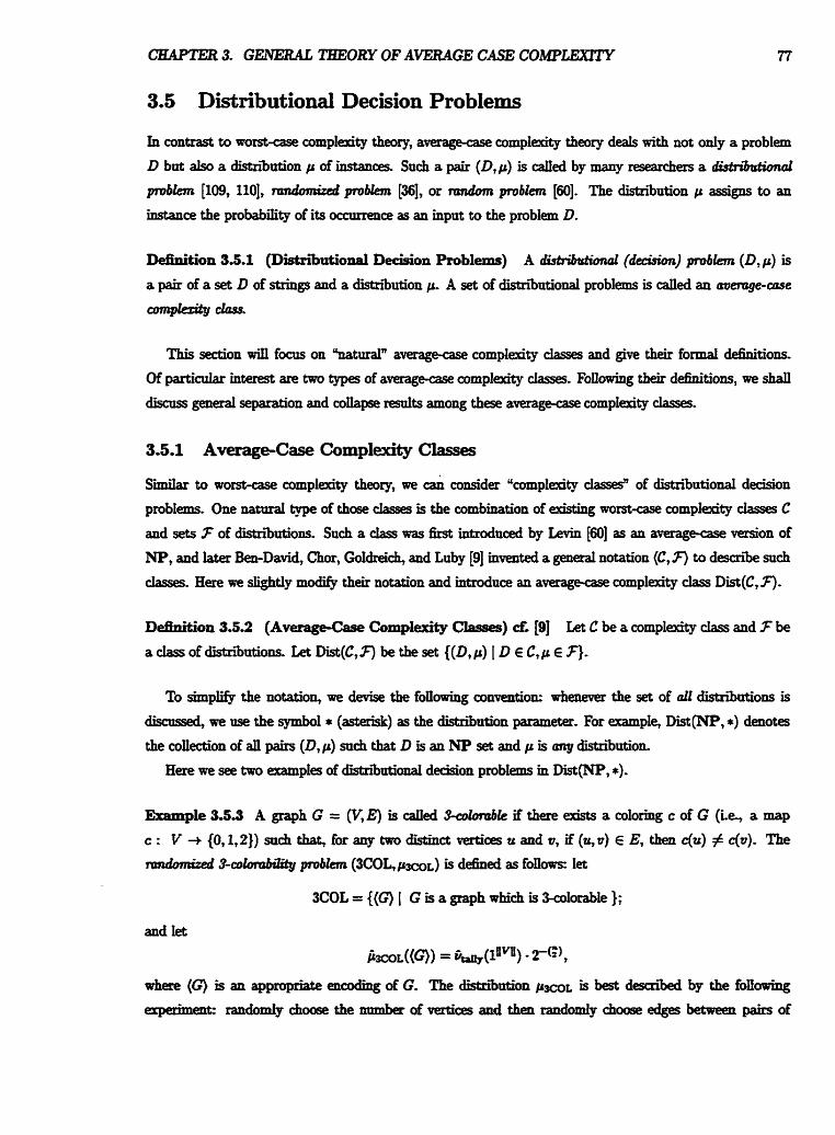
3. GENERAL THEORY OF AVERAGE CASE COMpLExITy
3.5 Distributional Decision Problems
In contrast to worst-case complexity theory, ammpase c o r n p i e theory deaIs with not only a problem
D bat also a distri'btttion p of instances. Such a pair (D,p) is cded by many mearchers a diddkthal
p b h [log, 1101, rmuiomiad pn,blenr [w, or mndom pmblem [60]. The distribution p assigns to an
instance the probability of its cxcmence as an input to the probIem D.
Debition 3-5-1 ( D i i ' b u t i o d Decision ProbIems) A &tdtdhd (decision) pmblenr (D,p) is
a pair of a set D of string and a distriiution p, A set of djstriiutiod probIems is called an merclge-me
cmnplezity
This section wil l focus on "naturaln average-case compl1exity cIasses and give their format definitions.
Of particuIar interest are two types of averagecase complexity &sses. FoIIdg their dehitiom, we shall
discrtss g a d separation and collapse d t s among these averagecase cornpleexity dasses.
3.5.1 Average-Case Complexity Classes
S i to worst-case c o m p l e theory* we consider Ycomplacity clasd' of distributional decision
probIems. One natmaI tppe of those classes is the combiition of exhting worst-case compl- ckffes C
and sets 3 of distn'butiom. Such a dars was first introdwed by Levin [60j zs an aperagpcase version of
NP, and kter Ben-David, Chor, GoIdreich, a d Luby [91 invented a general notation {C, 7) to descrii such
elaaes. Here we sI&htly modify their notation and introduce! an apersge-case compIexity ckss Dist(C, F).
De5ition 3.5.2 (Average-Case Comp1exity Cksses) d [Dl La C be a comple~~& dass and 3 be
a dess of distniuti~ns~ Let Dist(C, F) be the set { (D, p) I D E C, p E F).
To simplifp the notation, we devise the foilowing coIlvention: whenever the set of a22 distriiutions is
discrrssed, we use the symbol * (asterisk) as the distribution panmeter- For example, Dist(NP, *) denotes
the conection of all pairs (D, p) such that D is an NP set and p is any distnitxtio~
Here we see two examp1es of distnibutional decision problem in Dist(NP, *).
Example 3.5.3 A graph G = (V, E) is called kdunzbk if there exists a doring c of G (ie, a map
c : V + {0,1,2)) such that, Tor any two distinct vertices u and w, if (y u) E E, then c(u) # c(v). The
hlorcbi I i ty problem ( ~ C O L , M ~ ~ ) i~ d&d a~ ~OIIOWS. kt
3COL = ((G) I G is a gmph which is 3aIorable );
and Iet
imL((q) = ~pg.(~uvu) . rG) where (G) is an appropriate encoding of G. The distrrintion jim~ is best desaibed by the fdOwEng
experimenk randomly choose the number of vertices and then rand- choose edges between pairs of
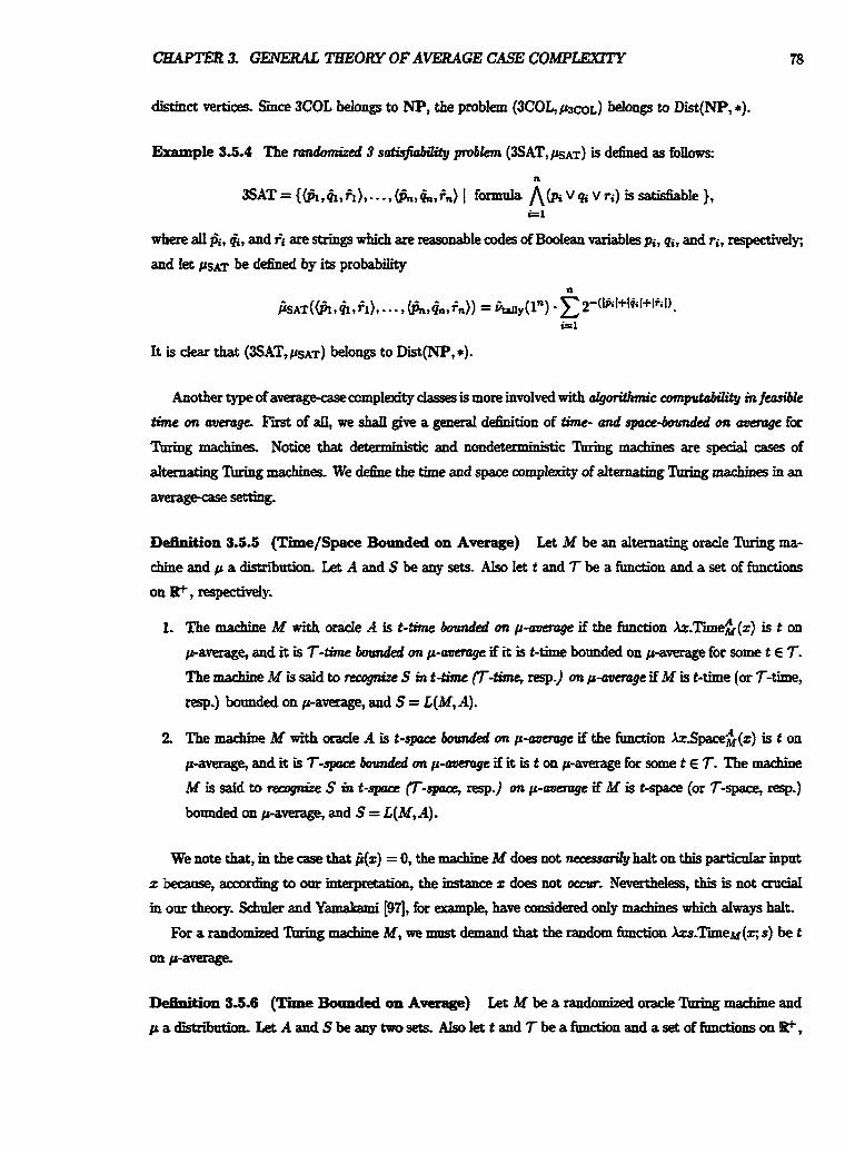
QXAlTER 3. GENE3?AL THEORY OF AVERAGE CASE COMPLkBZTY
distinct vertices Smce 3COL belongs to NP, the problem (3COL, ~ ~ C O L ) belongs to Dist(NP, *).
-1e 3.5.4 The rcndomizcd 3 sotisfiobility problem (~SAT,RAT) is defined as ~OUOWS:
It is clear that (3SKT,pS~~) belongs to Dist(NP, *).
Another type of amqpaseccmplexity classes is more involved with algorithmic computability in feasible
time on atrerogc First of dl, we shaU give a general dehition of time- and space-bounded on merage for
'Paring &es. Notice that m c and nondeterministic 'Itring machines are special cases of alternating Thing machina We dehe the time and space wmplexity of alternating hving machines in an
avempasesetting.
Dehition 5.5.5 (Time / Space Bounded on Average) Let M be an alternating oracle ' h h g ma-
&he and p a distribution. Let A and S be any sets. Also let t and 7 be a function and a set of functions
on El+, respectively.
1. The &e M wit4 oracle A is t-time borrnded on p-avemge if the function Az.Tune$(x) is t on
paverage, and it is 7-Eime bounded on p-werage if it is t-time bounded on p-average for some t E 7. The machiae M is said to ncogntje S in t-time (T-time, resp.) on p-mmgc if M is t-time (or 7-time,
resp.) bounded on p-average, and S = L(M, A).
2. The marhine M with orade A is t-space bounded on p-mmge if the function ~r~pace&(z) is t on
pawrage, and it is 7-space bmrnded on p-memge if it is t on paverage for some t E 7. The machine
M is said to mognke S ah t-space (T-space, resp.) on p-maage if M is t-space (or 7-space, resp.)
boded on p-average, and S = L(M, A).
We note that, m the tzse that fi(z) = 0, the machine M does not necessdy halt on this particular input
z according to om interpretation, the instance z does not occur. Nevertheless, this is not mciaI
m our theory. SehnIer and Yamakami [9?j, for example, have considered onlp machines which always halt.
For a randomized 'Ihring marrfiine M, we must demand that the random function Xzs.TimeM(z; s) be t
mi-==@-
* . DeBmbm 33.6 (Time Bounded on Average) Let M be a randomized orade Timing machine and padistribntion. Let AandSbeanytwosets. AIsolett andTbeafunctionandaset d frmct io~ l son~ ,
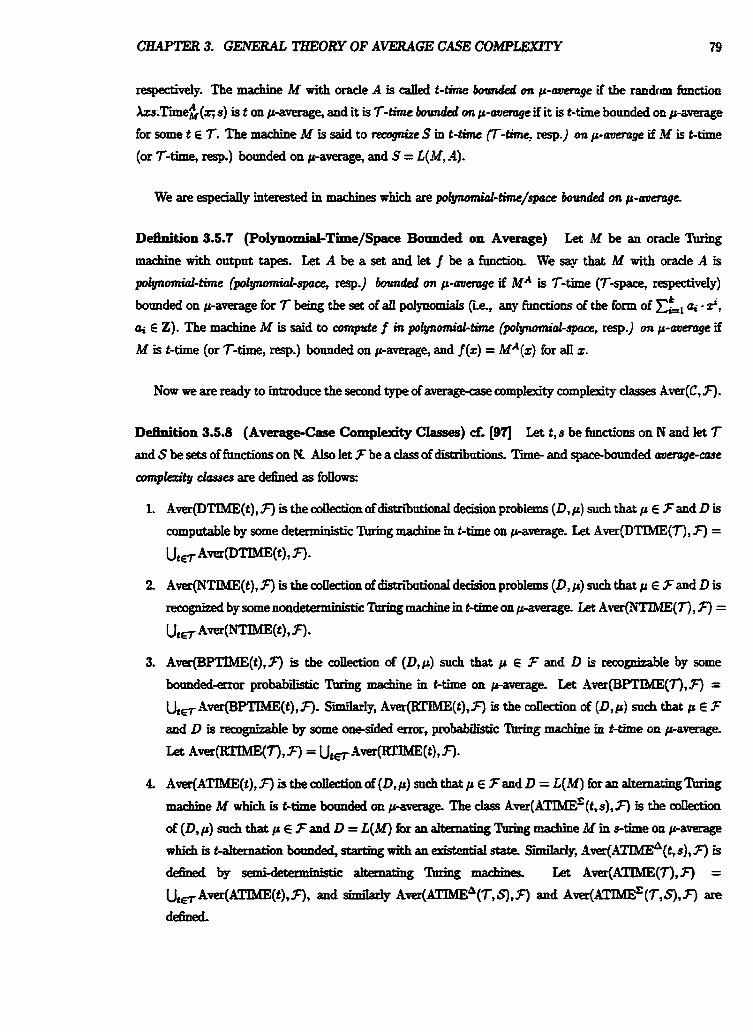
cHAPZW2 3. GENERAL TBEORY OF AVERAGE CASE COMPLEXITY 79
respectively. The machine M with oracle A is Qned t-time bomaded on p-auenuje if the random function
h s . ~ r m e & ( ~ s) is t on p-average, and it is 7-Eime /hm&d on p-uuerage if it is t-time bounded on paverage
for some t E 7. The machine M is said to recognize S in t-bime (T-fime, resp.) on p-merage if M is t-time
(or 7-time, resp.) bounded on paverage, and S = t ( M , A).
We are especially interested in maches which are jwiymnni&time/spue h d e d on p-o0croge.
Dehition 3.5.7 (Polynomial-T0ie/Space Bounded on Average) La M be an oracle Thing
machine with output tapes. Let A be a set and let f be a ha ion . We say that M with oracle A is
polyn-d-time (polynomial-spuce, resp.) bounded on p-aumge if MA is 7-time (7-space, respectiveIy)
bounded on p-average for 7 being the set of all polynomials (Le., any hmctiom of the form of 2, Q. 2, cri E 2). The machine M is said to compute f in polynomial-time ( p ~ l ~ t a - s p a c e , resp.) on p-aoerage if
M is t-time (or 7-time, resp.) bounded on paverage, and f (z) = MA(z) for aII z.
Now we are ready to introduce the second type of averagecase complexity compIexity classes Aver(C, 7).
Dehition 3.5.8 (Average-Case Complexity Classes) d [87] Let t, s be frmctim on N and let 7 and S be sets of functions on N. Also Iet 3 be a class of distributions. Tune and space-bounded mange-case
complexity classes are defined as follows:
Aver@TIME(t), F) is the collection of distn'butional decision problems (D, p) such that p E 3 and D is
computable by some deterministic Turing machine m t-time on paverage- Let Aver@TIME('I-), F ) =
UtE7 A=@TIWt), a- Aver(NTIME(t), F) is the coIIection of distnitrtionaI decision problems {D, p) such that p € F and D is recognized by some nondet -c Thing machine m t-time on paverage tet Aver(Ecl (7-) , F) =
Ulrr A=(NTZME(t) 9 8.
Aver(BPTIME(t),F) is the collection of (D,p) such that p E 3 and D is recognizable by some
botmded-ennr probabilistic %ring machine in t-time on pa mag^ Let Amr(BPTIME(7),F) = UE.rAver(BPTIME(t), F ) Si!uniIarly, Ave@?ME(t),F) is the coIlecti011 of (D,p) such that p E 3
and D is mophb1e by some onesided m r , pmbabilistic lbrhg machine in t-time on paverage
Let A-(ItTfME(7)7 T ) = Ute A = w J m t ) , n* Awr(ATIME(t), F) is the dection of (D, p) such that p E 3 and D = L{M) fbr an al- Tbbg
machine M which is t-time bounded on paverage The class A ~ ~ ~ ( A T I M E ' [ ~ , s), F) is the a ik t ion
of (D, p) such that p € f and D = L(M) for an ahemat& 'ihring marhine M m s-time on paverage
which is t-aI-on bounded, starting with an exbk t td state SmiIarly, 9ver(ATIME?(t, s), 7) Es d e k d by semi-deterministic a k m t b g aIternatiag machines. Let Aver(ATIME(7),7) =
U&ver(=(t),a and MY ~ v e r ( m * V ~ S ) , F ) and ~ v e r ( m V , S ) , ~ ) defined.
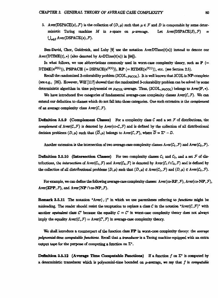
CBAPTER 3. G- TaEORY OF AVEXUGE CASE COMF'LEXlTY 80
5. Aver(DSPACE(s), 7) is the collection of (D, p) snch that p E T and D is computable by some deter-
ministic l h h g machine M in s-space on paverage. Let Aver(DSPACE(S),7) =
USES A=@SPAWs), F).
Ben-David, Chor, Goldreich, and Luby [9] use the notation AverDTime(t(n)) instead to denote our
Aver@TIME(t), *) (also denoted by AvDTime(t(n)) in [q). In what follows, we use abbreviations commonly used m worst-case comp1exity theory, such as P (=
DTIME(no('))), PSPACE (= DWACE(~O('))), RP (= RTIME(no('))), etc. (see Section 2.5).
R e d l the randomized 3-colorabii problem (3COL, ~JCOL). It is well known that 3COL is NP-complete
(see eg., [26]). However, Wilf showed that the randomized kolorabilitp problem can be solved by some
detetministic algorithm in time polynomial on ptcot-average Thus, (3COL+, p3COL) belongs to Aver(P, *).
We have introduced Eve categories of fundamental average-case complexity dasses Aver(C,3). We can
extend our dehition to classes which do not fail into those categories. One such extension is the conqkmd
of an average c o m p l e class Aver(C, F).
Dehition 3.5.9 (Complement Classes) For a complexity dass C and a set 7 of distriintions, the
cmp- of Aver(C,a is denoted by Aver(cc4,F) and is d&ed by the coIlection of all ~ i d i o n a I
decision problems (D,p) such that (n, p) belongs to Aver(C, F), where = X* - D.
Another extension is the intersection of two avempxe complexity classes Aver(C1, T ) and Aver(&, 3).
Detlnition 3.5.10 (Intersection Classes) For two complexity dasses CI and C2, and a set 3 of dis-
tributions, the intersection of Aver(Cl, 3) and Aver(C2, F ) is denoted by Aver(C.1 n C?, 7) and is defined by
the dec t ion of all distn'butiod problems (D, p) snch that (D, p) E Aver(C1, F) and (D, p) E Aver(C2,F)-
For example, we can define the fdowing average-case complexity dasses: Aver(c+R.P, F), Aver(-NF, F), A ~ Z P P , T), and AVFZ(NP n ~ ~ N P , F ) .
Remark 3.5.11 The notation "Aver(-, -)" in which we use parentheses referring to funcCions might be
misleading- The reader should resist the temptation to replace a cIass C m the notation "Aver(C,F)" with
another @olart class C because the eqnality C = C in worst-case complexity theory does not always
imply the eclnalitg Aver(C, F) = Aver(Cf, T ) m a- complex& theory-
We shaIl introduce a cormterpaa of the W o n dass FP in worst-case compIexity theory= the mwqe
poCyromiaf-time computable jhctibm Redl that a k a r u d w is a 'lhting machine equipped with an extra
output tape for the prrrpase of computing a fm!ction on C'.
Deanition S&l2 (Average Time ComputabIe -OILS) It a h c t i o n f on C is computed by
a deterministic transducer which is palyno&time bounded on paverage, we say that f is comptde
C&APTER 3. GENERAL TEEORY OF AVERAGE CASE COMPLEX2TY 81
in time p o w mt p-menzge Let Awx@F,T) denote the collection of an pairs (f, p), where p is a
distribution m 3, and f is a function computable m time polynomial on paverage-
We shall take a qnick g h c e at some fundamental reIationships among average complexity classes. By
the definition of t on p-ooercge, the class Dist@TIME(t),F) is dearly included in Aver@TIME(t),F).
S i i indusions obviously hdd for other fnndamental average complexity classes.
Pmp~dio t z 3.5.13 IRf C f {DTIME(t), NTIME(t), BPTIME(t), FtTME(t), DSPACE(t)) for some in-
&fGnction t on N, a d let 3 be a set of distributions. Then, Dist(C,7) E Aver(C,7).
The next lemma foUm immediately h m Lemmas 3.4.6(1) and Corollary 3.4.7.
b o E Since the sets of polynomiaIs, h@tbms, and exponentiaIs are all dosed under co~~position with
polynomials, the lemma immediately follows h m Lemma 3.4.6. 0
SimiIar simulation techniques show basic indusion relationships among average complexity cIasses.
Proof. We use a standard sbdation technique to show the above indusions of a- campIexily
elasseselasses
(1) Obviouslyf d-c lhring machines are viewed as a special case of one-sided error probabilistic
nuiugIM&ines.
(2) It saffices to note that onesided error probabilistic Thing machines are nondetr ' ' tic lhring
&es because of onesided error probabirtJr- (This is not ttue for -sided error probabilistic &a)
(3) Suppose (D,p) is in Aver(W?ME(t),F)- Take a onesided error, probabilistic lhing madim M reoognizing D in time f on paverage Let us consider the simnlation machine N defined as foIIows
CEWI'ER 3. GENEFLU THEORY OF AVERAGE CASE COMPLEXITY
begin randomized algorithm for N
input z
simulate M on input z
ifMacceptsztheaaccept
simulate M on input z
i fM acteptszthenaccept elsereject
end.
Asmme that z E D. The error occurs if both simnlatious of M on z fail to reach any accepting
c o ~ t i o n . Hence, the error probability of N on input z is at most 1/4. Assume to the contrary that
z 4 D. Because of onesided error probabi , there is no error occurring in the computation of N on z.
Therefore, N has bounded-ermr probability-
By definition, the ntnning time of N on z, Time&), is bounded by a hear function in Time&).
Smce M is t-time bounded on paverage, the function Xz.Tnne~(z) is kc(t(z) + I) on p-average for some
positive constant c
(4) Fitst we observe that any botmded-error probabilistic T h i t g machine M can be simulated deter-
ministidy using at most O(Tiie;;d(z)) tape squares. This is seen as follows. We simuIate M on z by
choosing its con&mations one by one (i.a, using breadth-bt search) and simnlating the corresponding
steps. Assume that we visit enough leaves of the computation tree so that we can determine whether M accepts or rejects z. We then quit the simulation and go into an accepting state if M accepts z, or else go
into a rejecting state. This simnlation needs tape space at most c - (Tiie&(z) f 1) for some f k d constant
c>o.
Now suppose that (D, p) is in Aver(BPTIME(t), F). There exists a bonnded-error probabilistic lhring
machine M which recognizes D in time t on p-average. Smce h.TimeM(%) is t on paverage, Lemma 3322
implies that Xz.Tiiek(z) is A2424 on paverage The claim follows from the observation above.
(5) G i a deterministic Thing machine M, which on inpd z nms using space p(z), the rmmber of
possible co&mations given by M on z is 0 ( 2 p ( r ) ) . Hence, the simulation of M on z takes O(Hz)) time
0
Generafly speaking, the function b.Tm!eM(Z) for a nondeterminirtie madine M is not time
constructii1e; therefore, even if t is tirne-a3nstrnctiiIe, the inclusion Aw@TIhE(t),F)
Aver@SPACE(O(t)),F) may not hold. This sheds Iight on the c r u d difference between worst-case com-
plexity and averagecase complexity.
As an exampIe, we shaII demonstrate a closure property of comp1eJdty ckss mder disjoint
union. It is easy to seem w o r s t ~ c o r n p I ~ t h e o r p t h a t if Aand B are in P, then A@ B is also m P.
Intheaperagecasesetting, wemustaonsiderthedistribntionsasdasthesetsofstrin~
fiemnur 3.5.16 MC E {P,NP,RP,BPP,PSPACE). Letf be a set o f d i d d d o m a;dddr is eIossd I f b m & t e n u ( A t b ~ ) d ( B , p ~ ) minAver(C,3), t i t e n s ~ i s ( A t B B , j ~ ~ @ p ~ ) -
CKAPTER 3. GENEIlAL TIjlEORY OF AVERAGE CASE COMPJXXlTY 83
ProoE We prove the lemma for the ease C = P. The other cases foRow similarly. Assume that (A, pA) and
(B, pB) are in Aver(P,F). There are two deterministic 'Thring ma&iues MA and MB, and two poIynomiaIs
PA and ps such that L(M,q) = A, L(MB) = 8, Xz.TiiMA (z) is PA on PA-average, and h.TimeM, (z) is
p~ on praverage. We assume without Ioss of generality that both PA and p e are increasing. Consider the
following algorithm N.
begin simulation algorithm N mput z
i f z = X then reject z
hdusu&thateitherz=Ouorz=lu
if z = Ou then simulate MA on input u
else simulate MB on input u
Assume that x = Ou for some tr. It is easy to see that there is an absolute constant c > 0 which does not
depend on the choice of z such that TmeN(z ) 5 c. (lzl + TimeMA (u) + 1). I f we take a d a e n t l y large
constad c, a similar ineqtdty holds for MB if z E lCg.
To complete the proof, we &ow that ~ . T ~ N ( z ) is polynomial on p~ $ psaverage- Flrst set s(n) = c . (n+pa(n)+pB(n) f 1 ) . Notethat sisapoIpmial Foreveryrz 1,
1 L 5 - - f i A ( { ~ l ~ ~ e ~ A ( ~ ) > ~ ~ ( ~ * ~ } ~ ) + ~ ~ b 3 ( ( ~ i T ~ e ~ ~ ( ~ ) > ~ ~ ( l l u l - r ) } )
2 1 1 5 - - &({ti 1 T ~ M ~ (u) > pr(lu1- r ) ) ) + 5 - j b ( {a I I i e ~ , , (4 > P B ( ~ I - r ))) 2
Hence, N nms in po1ynomiaI time on v-average.
3.53 Inclusions and Separations
We shall discuss general separation and collapse restllts among averagecase c o m p l e dasses introduced
in the previous snbsection-
The folIowiug proposition shows a basic sepamtion between averakpcase complexity dasses Dist('D,7)
and Aver(C, *).
Let us recA hm Chapter 2 that a talIy set is a subset of (0)' and b m Section 3.2 that vtpny is the
standard distribution that is positive onlp on (0)': We say a (worst-case) amp- dass C is dosed under
~ u n i m r @ i E , f o t a n p s e t s A a n d B i n C , A 8 B i s d s o i n C .
C&APTER 3. CZMBA.L THEORY OF AVERAGE CASE COMPLEXITY &I
3. Assume that D amtains the s d (0)' and is closed under disjoint u k If REC - D # 0 and
DTIME(O(n)) E C, then Aver(C,F) Dist(D, *).
Proof. Consider a set A in REC - D. Define B = (0)' $ A. Thus, (B, my) M ( D , *) since, othemise, A E D by the closure property of V under $. We now show that (B, vuy) E Aver(C, F) . Let M be a deterministic Thhg machine which computes A. This machine since A is recurs i~ Consider
the following algorithm N for B:
begin simnIation algorithm N for B input z
if z E (0)' then accept
h d y such that z = l y
simuIate M on input y and halt
end.
S i T i m e ~ ( 0 ~ ) I at + c for some absolute constant c > 0, we have
1 & ~ ( ( z 1 T i i e ~ ( z ) > clzl r + c)) 5 &U,.({O~ I Tiime~(0~) > cn + c)) = fiully(0) = 0 < - r
for alI r 1 1. Hence, (B, vay) E Aver@TIME(cn + c), 7) C Aver(C, F). D
As a corollary, we get a result shown by Wang and Belanger [lllj regarding the separation between
Dist(NP, *) and Aver(P, *).
Ccnvuc#ar 3-5-18 [Ill] Aver(P,F) Dist(NP, *) for ony set F of distri6trtions tdi vmy E 3.
Next we shall introduce a notion of weakly C-dexriptiuene~~ for averakpcasearmpkity dasses Aver(C, F).
Deanition 36.19 (Weakly DeScriptivene88) Assume that 'D is a T-time or T-space bounded com-
plexity ciass and C is any (worst-case) c o m p w dass. We d the average compIexity class Aver(D,F)
w d y C-desuiptiae iE, for every problem (D,p) E Aver(D,F), there exist a set C E C and s detr - . tic
oracle Tming machine M such that M with oracle C recognizes D in time 7 on p-awage-
Prpposition 3.5.W Let7 be a set of di&&dhs.
3. GENPLAL m O R Y OF AVERAGE CASE COMPLEXrrY 85
Proof, We shall show only the case (3). Let (D, p) be a distributional prob1m in Aver(BPP,7). Take a probabilistic 'Ihring machine M which computes D ip time polynomial on paverage-
We define two sets C' and GI as follows: Iet Co be the set of strings (0, z, In) such that more than half
of the computation paths of M on mput z terminate m accepting codgurations in 1- than n steps; and
kt Cl be the set of strings (I, z, In) such that more than half the paths of M on z terminate in less than n
steps, It is not hard to see that Co and Cl are PP sets. Set C = Co U CI . Let us consider the f0nowi.g deterministic algdrithm N with oracle C:
begin deterministic oracle Turing machine N with oracle C
mput z
forn=Itooodo
query (0, z, In) to oracle C
if (0, x, In) E C then accept and halt qyery (I,z, I*) to oracle C
if (1, z, ln) 4 C then reject and halt -&for
end.
R e d the d-on of Tiie&(z) in W o n 24. By our a t i o n , the algorithm N with orade C
above repeats the for-Imp Time;(z) + I times before accepting or rejecting x, because Tie&(t) is the
minimal number of steps needed to check if M accepts or rejects z. Note that k.Tirmeb (z) is poIynomiaI on
paverage due to Lemma 33.21. M e m o r e , when the algorithm terminates, its output is always correct.
Eence,
Tiie$(z) 5 d - (Tmeh(z) )+ 1)
for some constant d > 0. Sice kTie;(a(z) is polynomial on paverage, obviously N with C compntes D
m polynomial time on p-- D
Provided that C is a T-time or %space bounded comp1exity class, we say that Aver(C,F) is closed
under weak des- if, for every (C+) E Dist(C,F) and every deterministic oracle ntring machine M
with orade C which is 7-time bounded on paverage, the distriiutiond problem (L(M,C),p) belongs to
Aver(C,F). For exampIe, Aver(P,F) and Aver(PSPACE,F) are d d under weak description-
Lemma 3.531 Fm C € (P,PSPACE}, Aver(C73) is daKd trnda w e d description.
ProoE Here we shaIl show that Aver(PS?ACE, F) is dosed under weak description. Let us first assmne
that (C,p) is in in(PSPACE,F). There exists a deterministic 'Ihcing marhine & computing C using
poIynomial spa^ Suppose S m M ( z ) p(lzD fix an Z, where p is an appropriate increasing po1gnomiaL
Consider any m c oracle Turing machine M which, with o d e C, is poIynomlaEtime h d e d
on p-- We must constrncct a deterministic lhring machine which computes C using space polpnomial
CHAPTER 3- GENERAL THEORY OF AVERAGE CASE COMPLEXITY 86
on paverage without any help 6mm o d e s . The idea is to combine two Turing machines Mo and M:
begin detemhistic dgorithm for N input z
SimnIateMonmptxtz
while sirnulaton do
ifhf queries t then sindate Mo on inpd z
if M reaches a halting confignration then output M(z) and halt end-while
end.
It is obvious that N computes C correctly without any oracles. The tape space used by N on input 2,
SpaceN(x), is dearly bounded by
Apply Lemma 3-3-14 to p ( ~ i e f & ) ) , and we mnchtde that X2SpaceN(z) is polynomial on paverage. This
implies that (L(M, C), p) belongs to Aver(PSPACE, F). 0
Let us now see general separation and collapse d t s among a- comp1exity cIasses. For the propo-
sition below, we &st introduce the supplementary notion of safe sets: given a set 7 of functions, we dl 7 safe if (i) for any ftmctions tf,t2,t3 E 7 and any constant c E N, there exists a fnnction s m 7 snch that
c(tl(z) + t* 0 t3(x) f 1) S(Z) for an x, and (ii) for each frmction t E 7, t(z) > t(y) implies z > y for all z
and y-
ProposiPion 3.5.22 kt C k of thefonn DTIME(T), NTIME(T), RTlME(7), BPTIME(T), ATIME(7),
m DSF'ACE(n for sume safe set 7 of fkndhs on El?.
1. IfC REC, tlrar I) - C # 0 implies Aver(Vt +) - Aver(C, *) # 0.
CHAPTER 3. GElWt4.L TBEORY OF AVERAGE CASE COMPLEXITY 87
a proper cornpIexity core C for D wikh respect to C. Note that C C D. Define the distribution p as follows:
if z E C and 1x1 = n, m = iGp -2-M otherwise
for some adequate normalizing amstaut d Since D € V, we have (D, p) E Dist(D, *) C Aver(D, *).
We next show that (D, p) 4 Aver(C, *). ;Issnme that (D, p) € Aver(C, *) via machine M. Suppose that C is a timebounded c o m p l e dass and assume that Xz.Tiie&) is t on p-average for some t E 7. S i C
is a mmpleJdty core, there exists an integer k > O such that, for all z E C with lzl 2 k, Time&) > t(2[zI3)
because, otherwise, the set (z E C I Time&) < t(21sI3)) is an infinite subset of C. Using this fact, we
bound the probabiity of the event that Timew(%) > t(lx( - r) by
This contradicts the assumption (D,p) E Aver(C, *)-
Note that if C is a space-boanded c o m p I ~ b, use SpaceM(z) instead of TieM(z) in the above
argument.
(2) .Assume Z?' C. Let (D, p) be any distnintional problem m Aver(V, 7). Smce .4ver('D, F) is weakly
Vdescriptive, we can take a set D' m 2) and a deterministic o d e Thing machine M such that M is 7 on p-average and computes D with d e D'.
Notice that D' belongs to C. The dosure p r o m of Awr(C,F) under weak description leads to the
conclusion that (L(M, D')p) is m Aver(C, F). 'This impIies the desired resuIt that (D, p) E Avet(C, T). 0
As a corollary, we obtain the faUowing d t -
Interestingly, the class Aver(NP,3) cannot be characterized by the notion of weak NPdescriptkeness.
Moreover, we are able to show that Aver(NP, *) is indeed diikmst h m Aver(P, *)- The theorem bdow
shows the separation between Aver(P, *) and Aver(Nf, *) (see also [m-
ProoE We shalI eonstraa a d i s t n i decision pmb1en.t (Ap) which belongs to Aver(NP, *) but
CKAPTER 3. GElWRAL THEORY OF AVERAGE CASE COMPLElxITy 88
not to Aver(P, *). F i we choose a nonr-, recmshdy enumerable, tdly set A whose dements are
emmerated as A = {M(so), M(sl), M(sr), . . .) by some deterministic transducer M which always hdts and
outputs some strings For simplicity, we assume withont loss of gen- that if M on input w produces x,
then ThneM(w) 2 1x1 + Iwl. W e also choose the distriiution p defined as
Clearly the distniution p is posithe. We daim that the distributional problem (A, p) belong to Aver(NP, *)
but not to Aver(P, *). We note that if (B, v) E Aver(P, *) and v is positive, then B is recmsitre. Smce A is
not recmsive, it is immediate that (A, p) # Aver(P, *).
We next show that (A, p) E A v e r w , *). Let us consider the nondeterministic l t r ing machine N defined by the foIlowing simple nondeterministic algorithm. Remember that A is a tdly set.
begin nondeterministic algorithm for N
input x
if z 4 (0)' then reject
guess a natural number i ( M y guess y)
simulate M on input si
if z = M(%) then accept else reject
end.
Obviousiy N reeogaizes A. Now fir z and let k = min{i E N I M(si) = x). In the case where x f -4,
TrmeN(x) is set to the shortest length of a q-ecting path by om d-on; thus, it is bounded by a constant
independent of x. Let Q be such a constant. Hence,
Suppose x E A. Wdte D, for the set {i 1 I(%) = z}. On mpnt x, the above algorithm takes at most
steps for some p0Sitif4 constant d which is independent of z. S i i A is a t d y set,
where c is the nomaking constant for p We then have
By Lemma 33.15, we condude that X z . T i N ( ~ ) is p o l p o d on paverage- I3
not dectively caldated and often takes extremely d l probability. NonethelessT most distributions we
encounter in practice do not have auy resemblance to this p. When we discuss practical distributions, we
may d c t our interest to such distributions that give r e h i d y high probability for almost all input strings.
Here we call such distributions supportioc
Dehition 3.5.25 (Swpportive Diiiutiooms) A distriiution p is d e d sappmtke if there exists a
polynomialp such that either ji(x) > rfllzl) or F(x) = 0 for every x. A set of distriutiox~~ is called supporEitte
if all of its distributions are supportive- Let SUPP be the collection of all supportive distributions.
For example, the standard distn'bution u-a is supportive s ine firund(2) > rtive&f - 2-14 > Z - * ~ I - ~
for all z.
For any supportive set FT the average cmmp1exity c h s Aver(NP, 3) is not a large dass. The f01lowing
proposition is a consequence of Lemma 33.1 l(2).
Proof. The r d t fotIows h m the simp1e observation that, for a machine M which is t-time bounded on
paverage, TimeM (z) 5 t(lz(/ji(z)) < t([zl- 2dkl)) if ji(z) > - 2-p(lf 1). D
Regarding the Dist(NP,F) E?Aver(P, *) question, it is enough to focus on supportive distniutions in
F. We introduce an additional terminoolog~r: a set 3 of distriiutious is d e d tome if there exists a positive
and supportive distniutio~t
k n m a 3-5-27 Lef 3 be a tame set of d k b i h h m and assunze that T is &sed under 2-oddition. Then,
Dist(NP, F) E Am(P, *) if wrd only if Dist(NP, SUPP n 3) Aver@, *) .
Proof. (Only if - part) Note that Dist(NP, SlTPP n F) Dist(NP, 7). This inclusion obviody yields
the dab.
(If - part) Let us assmne that Dist(NP, SUPP n F) Aver@, *). Moreover, we assmne that (A, p) is
any distnibutional problem m Dist(NP, F). We shalt show that (A, p) belongs to Aver(P, *).
Smce SUPP n 3 # 0, let us take a supportive distrriution WJ &om 3, and then dehe the default
By the assumption that 3 is closed under 2-addition, this distn'btrtion v k t m t e s a member of F. It is also easy to see that v is supportive, and ccnrseqnentIy, we obtain v E SUPP n F. h m Dist(NP, SUPP n a Aver(P, *), it f o ~ m that (Ap) beiongs to Aver(P, *). Notice that v
p-domhtes p because 2 - P(x) 2 fi(z). Corohy 3-47 helps us condude that (A+) is aIso m Aver(P, *).
In the above lemma, we require 3 to be closed under 2-addition. Later we shall see several tame sets of
distributions which contain the standard distriiution and satisfy this requirement.
3.5.3 Another Characterization
Let us consider another characterization of basic averagecase complexity dasses, Aver@, 3), .4ver(NP,T),
and Aver(BPP,T).
The following definition was proposed by Impagbm [43j. Let f be a function on C and S be a set.
We say that an algorithm A conrputes f with bmign f& if (i) it outputs either an element of rau(fl or "?"
and (ii) on input z, if it outputs z which is not "?", then z = f (z). An aIgorithm A computes S with benign
faults if A computes xs with benign faults. We write TimeA(z,6) to denote the running time of A(z, 6).
Dehition 3.5.28 (Benign Algorithm Scheme) [a] Let p be a distriiution and f be a function on
C'. A polynomial-time benign algorithm scheme for f on input ensemble (wn)nEn is an dgorithm A(=, 6)
such that
(i) there exists a polynomial p such that TirmeA(z, 6) 5 p(!zl,1/4;
(ii) A computes f with benign faults; and
(ii) for all6 (0 < 6 < 1) and aII n E N, if wn is defined, then k n ( { z E Esn I A(z,6) =?I) c 6.
Lemma 3.5.29 [43] Let 7 be a set of diskr'bcrtions+ For a d W 3 h t h d probfem (D, p) toitlr p E 7, the
foUaaing stabmds on CpUioalenL-
Proof. First me shan see that (1) implies (2). Assume that (D, p) is in Aver(P,F). There exisis a
det ' ' "c TEng machine M such that L(M) = D and time^ is poIynornia1 on paverage. By Lemma
338, there is a polynomia p such that k n ( { z € Xsn I T.une~(z) > p([xi - r))) < $ for all n E N and all
r > 0. We define the desirrd agOrithm A(z,6) as fall- on input (z,6), A &dates M on input z for
p(Iz1/6) steps and outputs &Tb if M faiIS to halt- Tbis aIgorithm is a benigu algorithm for D on (en)nEn since
To see that (2) implies (I), we assume that A(z,6) is a benign aIgorithm for D on inpd ensemble
k ) r n . We also assmne that A nms in time p(lzl,1/6) far some fixed polynomiaI p. We may take a
C&QPTER 3. GENERAL TBEORY OF AVERAGE CASE COMPLEXITY 91
may polynomial q instead of p, because we can assume that p is maeasing (LC, h.p(n, 6) and Xt.p(m, z)
are incfeasing for each fixed 6 and m); then setting q(z) = p(z, z), we have p(lzl,l/b) 5 q(lzl/b). Moreover,
we specify the form of q(z) as z*C + d by taking sut€iaently large k and d We then asmme that the benign
dgorithm scheme A(x, 15) runs in time (1z1/6)' + d
Now let us d d e r the following algorithm M that computes D:
begin detr ' ' ' 'c aIgorithm M for D
inpat2 for i = 1 to oo
simulate A(z, l/i)
if A(=, l/i) outputs "?" then go to (*)
output A(x7 l / i) and halt
(*I end-for end.
This algorithm M a d y computes D. Let us define s(t) = + dz for all z. For any string z of length
5 n, if the algorithm M hats within the first r iterations of the for-loop, then
In other words, if T i i e ~ ( z ) > s(Iz1- r), then A(z, I/r) =?. Hence, we have
By CorolIary 333, h-Tim&) is polynomial on paverage. 0
We observe that the qnantik charaaerizatiori of nond ' ' ' tic and probabilistic Thing rmchha
hdds alsointhea-setting. E&caIl that,forinstance, allsets inNP can b e d m a d m i d i n terms
of an existential quant5er and sets m P as fo1Iows: a set A is m NP if and onlp if there exist a polynomial
p and a set B E P such that A = ( x f 3yUyl Ip(1xl) A (z, y) E B]) [118]. l~ the fbIIowing, we shall give a logid characterization of the dass Avet(NP, 7).
CHAPTER 3. GENEEbU THEORY OF AVERAGE CASE COMPLEXfm 92
Proof. The proof is straig6dorward and follows from the standard techniqne of encoding nondeterministic
computation paths into strings and from the fact tbat I\z.Time~(x) is polynomial on paverage. 0
Fm we need an amplification lemma
Lenuna 3.5.51 (Amplification Lemma) Let p be wry diskibtrtion, A a set, and d u positive finac-
tion con@&& in polynomial time on p-olrerrrge. Assumc fhot u rrmdomized %kg machine M sdisjies
RM[M(z) = A(z)] 2 ? + & fm all strings z. Then, thae ezists oncrtha rondomiad machine N
suchthat
where p x u u y h t e s the distn'hdim pf de&ed by $(z,y) = b(x) fiuy(y) for On p i m (2, y).
Proof. La us assume that ks.TiieM(z; s) is t on p-average for some increasing polynomial t. -4ssume
also that d is computable in time polynomial on paverage For simplicitp, we assume that d(z) 2 5 for all
z. We set h(z, y) = max{l,lzl+ lyl) and let p(z, y) = 2 d ( ~ ) ~ h ( z , y) for all pairs (x, y). Fmt we show that
p is polynomial on p x uay-average- For simplicitp, we write p' ffot p x p a J r in the following argument.
Proof of Claim Remember that d is polynomial on gaverage. Suppose that d is q on p-average for some
poIynomiaI q, and dehe q' as q'(r) = 2 q ( ~ ) ~ z . Obviously q' is a polynomial. Fa r a r b i i y such that
1. r 1. ~a E, = { ( z , ~ ) I > q(r - I~I>).
Hence, p is polynomial on $-average I
Smce p is poIynomiaI on $-a- m can take a poIynomid q snth that p is q on $-average- The
desired randomized machine N is de6ned by the foflowfng aIgmithm:
begin randomized aIgorithm for N
inpat ( ~ 2 ~ 1 if y fZ (1)' then reject
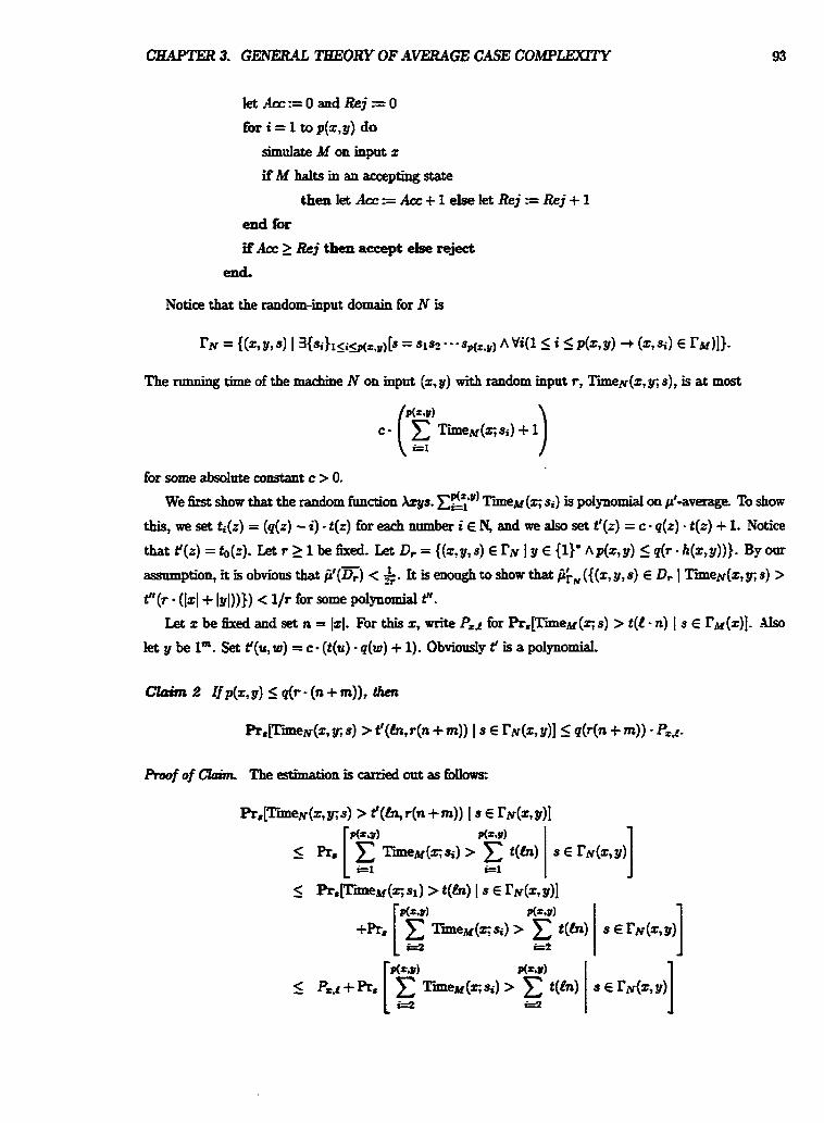
CKAWER 3. GEiVElUL TBEORY OF AVERAGE CASE C O W -
let A c c s O and& :=0
for i = t to p(x, y) do
simnIate M on input z
if M halts in an accepting state
then Iet Acc z= k + 1 else let Rej s Rej + 1
end for
if Acc 2 Rej then accept else reject
end.
Notice that the random-input domain for N is
The nmning time of the machine N on input (x, y ) with random input r, T i e ~ ( z , y; s), is at most
for some absolute constant c > 0.
We first show that the random ftmction ~ z y s . eiv' T i i e ~ ( q si) is po1ynomiaI on pt-average To &ow
this, we set t&) = (q(z) - i) - t (z) for each number i E N, and we also set t'(z) = c - q(z) - t ( z ) + 1. Notice
that t'(z) =to(z). Let r > 1 be fmd. k D+= {(z,y,s) Err I y E {l)'Ap(z,y) Iq(r-h(z,y))). By om
as~nmption, it is obviow that fit(=) < &. h is enough to S ~ O W that fiiN (((2, y, S ) E Dr I T i m e ~ ( ~ , y ; S) > t"(r (1x1 + lgl))}) < l / r for some polynomial t".
Let x be b e d and set n = 1x1. For this z , write P,$ for P r , m e ~ ( z ; s) > t(L - n) I s E r ~ ( z ) ] . .Ah
let y be lm. Set f(u, w) = c (t(u) - q(w) + 1). Oboiottsty t' is a polynomial.
hf of CIaim The estimation is d e d out as fonoars:
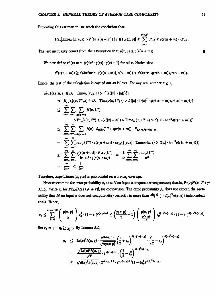
CHAPTER 3. GENERAL THEORY OF AVERAGE CASE COMPLEXITY
Repeating this estimation, we reach the oondnsion that
The Iast inequality comes from the .%?sumption that p(z, y) < q[r(n + m)).
We now define t"(z) = c - (t(@ - q(z)) - q(r) + 1) for all z. Notice tbat
t"(r(n + m)) 1 t'(4n3m2r - q(r(n + m)), r(n + m)) > t'(4n3r - q(r(n + m)), r(n + m)).
Hence, the rest of the dcuIation is carried out as f o h . For any real number r 2 1,
Therefore, ~ S . T I r n e ~ ( 2 , Y;S) k p0lpmid On p X I&@-
Next we examine the error probability p, that N on inpd z outputs a wrong answer; that is, RN[N(z, lm) # A(z)]. Wiite r, for R M [ M ( x ) # A(z)I, for ampatison, The error probability p, does not exceed the pmb
abi& that M on input z does not compute A(z) correctly m more than (= d ( ~ ) ~ h ( z , y)) independdeut
trials. Hence,
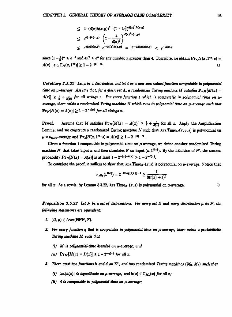
CHAPTER 3. GENER4.L THEORY OF A'CrERAGE CASE COMPl2XR"Y
since (1 - $)n e-4 and 4n2 5 en for any number n greater than 4. Therefore, we obtain Pr,[N(z, lm; s) = A(2) I S E rN(Z, lm)] 2 1 - 2-lrl-m- 0
Cmllarg 3.5.52 Let p be a dktddion and let d be a non-ren, valued jbction computable in polynomial
time on p-merage. Asswnc that, for a given set A, a rmzdOmited Turing machine M satisjies PrM[M(z) = A(x)] 1 $ + & forullstrfngsz. Forewryfundiont w ~ i 9 ~ k i n p o l y n o n r i a l t i t n e o n p -
attemge, there ezists a randomixed %ing rnacirine N which runs in polyrmomral time on p-memge such that
Rrv[N(z) = A(x)l 2 1 - 2-f(r) fm all sdrings x.
Proof. Amme that M &es RM[M(2) = .4(x)] 2 f + & for all x. AppIy the AmpBcation
Lemma, and we construct a randomid ' h h g marhine N such that Xzs.Tiie~(t, y, s) is polynomial on
p x u~Y-average and Pr,[N(z, lm; s) = A(z)] 2 1 - 2'[zl-m.
Given a function t computable m polynomial time on paverage, we define another randomid M g
machine N' that takes input z and then simulates N on input (x, lt(')). By the definition of N', the success
probability RN[N(t) = A(z)] is at least 1 - 2-w-t(z) > - 1 - 2';(=).
To compkte the proot, it dices to show that ks.Tiie~p (5 s) is polynomia on p-average- Notice that
for all z. As a result, by Lanma 3322, h . T i e ~ r (z, s) is polynomiai on paverage- 0
Pmpodkn 3.5.33 Let 7 be a set of &dtdhs . For every set D and every d i d d u t h p in 7, the
fouorping statements me eql&aIatt.-
1- ( 0 , ~ ) ~Ave.r(Bpp,F)-
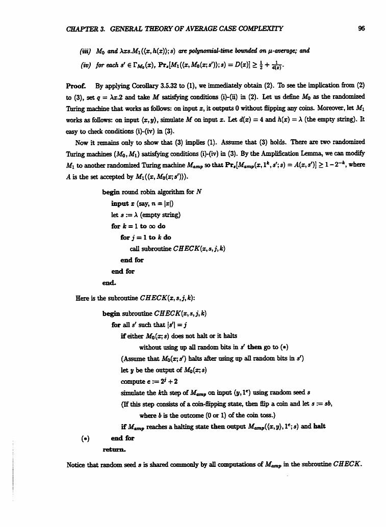
CZAElER 3. GENERAL T&EORY OF AVERAGE CASE COMPLEXITY
(iii) Mo and k s M 1 ((x, h(x)); s) mc potymdaf-time boundkd on p-menzgc; mul
Root By applying C o m ~ 3.532 to (I), we immediately obtain (2). To see the implication h m (2)
to (3), set q = h.2 and take M gtisfying conditions (i)-(ii) in (2). Let us dehe Mo as the randomized
Thing machine that works as foIlows: on input z, it outputs 0 without flipping any coins. Moreover, let MI works as foIIm: on input (z, p), simulate M on mput 2. Let d(z) = 4 and h(z) = A (the empty string). It
easy to check conditions (i)-(iv) in (3).
Now it remains only to show that (3) implies (1). Assome that (3) holds. There are n r ~ , randomized
Thing machines (MOT MI) satisfying conditions (i)-(iv) in (3). By the .4rnplification Lemma, we can modify
MI to another randomized l h h g machine Ma,, so that R, [Ma&, 1 &, s'; s) = A(=, s')] 1 1 - 2-*, where
A is the set accepted by Mt ((2, M o ( ~ d))).
b e e round robin algorithm for N
input x (say, n = 1x1) let s = (empty string)
f o r k = l t o c u d o
for j= l to kdo
caU subroutine CHECK(z, s, j, k)
end for
end for
end.
Here is the subroutine CHECK(%, s, j, k):
begin subroutine CHECK(z, s, j, k)
for aII s' such that Is'[ = j if either Mo(z; s) does not halt or it halts
without using up all random bits m s' then go to (+)
(Assume that Mo(q J) hats after asing up all random bits m $1 Iet y be the output of Mo(z; s) compute e F 2j + 2
sindate the kth step of M, on mput (y, le) using random seed s
(If this step consists d a coin-@ping state, then Bip a coin and let s = sb,
where b is the outcome (0 or 1) of the coin toss.)
if M,, d e s a halting state then output M-&, y), le; s) and hait
(*I end for retrmt
Notice that random seed s is shared commoaly by an computatiiom of M' in the subroutine CHECK-
CHAPTER 3. GENERAL THEORY OF AVERAGE CASE COMPLEXlTY 97
We shall perform worst-case analysis on the running time of the above algorithm, On inpnt z dong with
random seed r, N takes Steps at most
where f is an initial segment of r. Notice that the bct ion &.21h(=)1 is polynomial on paverage by Lemma
33.6. Hence, k-TilllleN(~ r) turns out to be po1ynomial on paverage.
Next we shdl show that R N [ N ( 2 ) = A(%)] 2 t c For each random seed, the success probability does
not dedine below 2/3. Thus, the probability that N(x) coincides with A(z) is at least 2/3- Therefore, (D+)
belongs to Aver(BPP, 7). o
We give a remark to tbe above propositi01~' if MI makes one-sided errors (i.e., ( D , p ) E Aver(RP, *)I, then we can replace the term $ + &J by &.
Further Topics
This section cibases sewral topics which we have not covered in the previous sections.
Rmmiag Time of Nondeterministic Machine. Let us considr the running time of nondeterministic
M g machines- Wang and Belanger [Ill], Schnfa and Yamakami [97], and Karg and SchuIer [48] disepssed
a dose connection between the P =?NP qyestion and the Awr(P,F) =?Aver(NP,F) qnestion based on
the model of d d e d n o n d e t d c 'Ihring machines. As we have seen, this model guarantees that aII
compdation paths in a computation tree of the clocked machines are of the same length.
Here we consider the model for which the nmning time of a nondeterministic flrring machine is d&ed
to be the length of the shortest accepting computation paths when it accepts an inpnt, or else the length
of the longest rejecting cornpubtion paths. We call this restpiction the strid nnnring t h e cnterunr . - for the
machine
To avoid c o ~ o n , we use the notation Aver(NI", 7) to denote the awrage-case cornpleexi~r cIass defined
m terms of nondeterministic 'k ing xnachines, with the strict rrmning time criteria, which nm m p01ynomial
time on average-
For this new dass A p e r W , F ) , we are able to p m that Aver@NF,F) is weakly NPdescriptive, and
thus, P=NPimpIiesAver(P,F) =Aver(NP',F) for anyset Fofdistriiutions-
Aaof of C&im Let (D,p) be a distriiutional pmb1ezn in Aver(NP', F). Let us consider a noxtd-c
' k ing macbe 1\6 which computes D ia polynomial time on pawrage.
Let 6 be the set of sttifl&9 of the form (Op, In) such that M accepts x in Iess than n steps, and Iet Cr bethesetofstringsoftheform (17z7P) s n & t h a t t h e r e & m p n t a t i o n ~ d M o n m p d x w h i c h ~
CHAPTER 3. GENERtQI; THEORY OF AVEZUGE CASE COMPLEXfm 98
Ionger thaa or equaI to n. Now write C for Co U CI. Let us consider the fonowing deterministic algorithm
N with orde C.
begin deterministic oracle Turing marhine N with o d e C input z
forn=l tom do
query (0, z, In) to d e C
if (O,z, 1") E C then accept and halt
query (1, x, In) to oracle C if (1, x , 1") 6 C then reject and halt
end-for
ertd.
On any input z, this algorithm N with oracle C goes through the for-loop TimeM(z) + l times until it
terminates, Notice that when the aIgorithm terminates, its output is always correct. Hence,
for some constant d > 0. Smce k.TieM(Z) is polynod on paverage, obviously N with C computes D in time poIynomial on p-average- I
Heuristic Polynomial T i e . ZmpagliazLo [43] introduced a new notion of "hetnistic plynod-timen
class. We rephrase his d&tion in our setting. We dehe the heuristic polynomial-time class Heur(P,F)
as foRowsOWS
An dgoritlrnt scherne for (D,p) is an algorithm A(z,d) such that k,({z E Csn I A(z,6) # D ( z ) ) ) 5 6 for aII 6 > 0 and a11 n E N We say that a distribntid decision problem (D,p) is in Heur(P,F) if there
exists a polynolniaI-time deterministic algorithm scheme for (D, p).
Obviously Aver(P,F) E Heur(P,F). It is an open probIem whether Dist(NP,F) C Heur(P,F).
Chapter 4
Feasible Distributions
4.1 Introduction
A- d y s i s m g e n d is sensitive to the choice of distniutions, so that we need a careful study of
the behaviors and properties of individual distriiutions. For example, to construct a better dgorithrn which
nms f& on merrrge, instances which occur with high probability &odd be s01ved QtrickIy.
In statistics, Poisson distri'butions, for example, are commonly used for the analysis of events. This type
of distriiution is apprmdmab1e by some appropriate po1ynoW-time algorithms.
In this chapter, we shall f- on fecutile d i & d & h s which are either YeasliIy comptttabIen or "fksi'bbly
pmiua%Ie? This chapter wiII introduce two Merent categories of feaslile ciistri'butioris: pofgn-d-he
wmputubk dC&iMiow and pofymmial-time smtplble &dt&w. The former category was considered
by Levin [g0l and fonnuked by Guretrich [36j; the Iatter was introduced by Ben-David, Chor, Goldreich,
and Luby [9] and has been studied in ayptqraphy.
FoIIOtKing KO and Eti-'s [55] de6nition of p ~ l ~ t i n r e cmptable d fmctionr, Garevich [36j
took a shdar step toward distn'btrtim. Be d e d a distribution "cornpntabIe in po1ynomiaI-timen if there
is a poIynoxniat-time approximation aIgorithm whose outputs asymptotically approach the values of a distri-
bution within an exponentiany matt factor. Section 42 wiIl discuss such diskiitttio~~ which are computable
(or more acamtdy "apprOOdmablen) in pcdynomia time by deterministic %ring machius-
In practice, rather than spedjkgfuu distri'btxtion~~ researchers often loosely deke distrritttions by sim-
ply specifping associated serm-drstn - - %utions. We note that aII polynomiaEtime computabIe semi-distrrr'btttions
are e k t i d y enumerated, whiIe associated fidl distriiutions are not- Remember that our theoq is M
on jkl2 distriiutions, and therefore, whenever we use semidistributions for the purpose of defining /Glf distn'butions, we must puantee the existence of snch j U distri'butions that are proportional to the semi-
distriiutions almcst This process is called a - - ofSemi-distninti~- U d o ~ , not all compntable semidjstributiom axe normaGd to fid distnitrtions of the same c o m p 1 e . Section
4.3 d s h o w t h i s negativemi&.
CHAPTER 4. FEASIB~DISTRIBUTIONS 100
As Gurevich [36j pointed out, the reader may be cantious of the fact that the P-computability of a
density function does not imply that of its asmiatd distriiution de s s P = NP.
One of the most important results in Seaion 4!4? is the Distribution Controlling Lemma proven by
Gafevich [36] and by Belanger and Wang [6]. This lemma enables us in Chapter 5 to prove the existence of
complete distniutiond decision problems for Dist(NP,P-comp).
We shall turn our interest to instances which occur with low probability under most distriiutions com-
putable in polynomial time- These instances are called rare skin@- A set S is d e d polynomial &rare if,
for any polynomial-time computable distniation p, the set { x E S [ i ( x ) > 2-c(l*I)) is finite.
Another category of feasible distributions is amplabk & d t d h s which were first introduced by Ben-
David, Chor, GoIdreich, and Luby [9] in their 1990 confkrence paper. Samplabiity, which is often found m
st'atistical physics, is esrentially a form of psendc+randomness. For example, Ben-David d d [9] showed that
if psendwandom generatom exist, then polynomiaLtime samplable distributions are hard to approximate
in polynomial time. This result wi l l be extended in Section 4.7. In Section 4.4, sampIing algorithms and
samplable distributions wiI l be defined.
Major Contrriutions. Most of the material in this chapter comes !?om Yamalolmi [119].
The formulation of P-samplable distrriutious given in this chapter is merent from what has been defined
by Ben-David, Chor, Goldreich, and Luby [9] and by Schder and Watanabe [96j, and therefore a11 the proofs
are altered.
Given any P - c o m p d l e distrihtion p, Lemma 4.2.8 presents a a a e n t condition of a function f so
that the composition el becomes P a m p a b b I e
Theorem 42.14 shows the existence of poIynonriaIIy C-rare sets of distriiutions. This theorem dates to
Kolmogorov compIeJdty. The theorem actuatly proves that, for any hcmsing, unbounded function s, if l
satisfies 5 logn 5 C(n) n, then the set whase dements are uot in KT[S(n), p(n)+g(n).'wnJ is po1ynomian:y
C-rare
Proposition 43.1 shows that there exists a P - c o m p d e Semi-distn'bution which cannot be normahzed
by a standard method to a fJI distniution computable in poIynomiaI time- In addition, CoroIlary 43.3
gives a &dent condition for P-compntabIe semi-distniutiom to be normalid by a standard method to
distn'butions of the same complexity.
Proposition 42.12 shows that there ex& a positive PcomputabIe distriiution p and an inQeaSing,
exphonest ftmction f m FP such that prl is not pdomioated by any Pamputable distxiiution.
In Proposition 447, IP-samp is shown to be included in P-samp.
Theorem 4.413 asserts that ~ - - s a m ~ peqd P-samp- This redt is a counterpart of the d t
BPF = B P P in worst-case c o m p w theory.
Oneoft6emostimpaaanttheorem~inthis~terisTbeoremrL5.~ whichshowsthat P=PP ifand
only if P-comp = P-samp- Not aU P-samplabIe disbibutiom are therefore computable in polynomial time
d e s P = PP.
CHAPTER 4. FEASIBLE DLSTRIBUTIONS 101
Theorem 4.7.3 shows that if every P-samplabIe distribution is pdominated by some P-compntabte dis-
tribution, then every NP set is nearly-RP.
CbmIIary 4.7.7 shows #P-comp peguals P-samp if NP E BPP. This remlt foffows Proposition 4.7.6,
a careful rn6cation of a result proven by Schuler and Watanabe [96].
Proposition 4-73 shows that IP1-samp is not avp-included in P-comp unless P = RP. Moreaver,
Theorem 4.7.12 shows that P-samp is not pincluded in P-comp ndess P = NP.
4.2 Computable Distributions
It seems natural to consider the sets of all feasibly "computablen distriiutions. Gnrevich [36] first adapted the
idea of the P-amputable red mnnbers used by KO and Ftiedman [55] to define polynomial-time computabii
of distributions. This section win farther explore distributions comprhble in polynoinial time.
4.2.1 De5ition of Computable Distriibutions
Any distriiution treated in this thesis is actually a real-valued function with C' as its domain. Gurevich
has applied the notion of ~~~tinu computcbility of real-valued functions (introduced in Section 2-7)
to distriiutions Here we shall give a more general notion of t-time conrputability and t-space compprtabilidy
of semi-distributions for a fnnction t, which is based on Gurevich's approodmation scheme.
Let us recall how a deterministic Thing marrhine M equipped with an output tape computes a real
nmnber: the machine achtatIy outputs a binary string w, which is interpreted as the dyadic ratio& number
2 1 wi 2-', where w = w ~ q w1,,,l and each Wj is a bit (in (0,l)). We say that M opptoninates
red-value p(z) if Ip(z) - M (z, 0') 1 1 2" for all natmaI numbers i.
Deflnitioa 4.2.1 (Computable Distr'butioas) [55, 361 Let t be a function on N and 7 be a set of
frmctiom on N.
1- A semi-distriiution p is recuffitre (or cornpukr6te) if there exists a detetministic Tming machine M eqnipped with two input tapes and one output tape, which computes namdy, on input (z,oi),
I&)-M(z,oi)l 52-'for ollstringsz~C'and d l n u r n b e r s i ~ ~
2. A semidistriiution p is t-time wmputable (t-spuce computable, resp.) if there exists a deterministi c
'Ihring machine equipped with two input tapes and one output tape which, on input (z, Oi), computes
~ ( 4 time (rising space, tesp-1 w, i)- 3. A semi-distniution is 7-time oomputable (7-space amrpcdc6lq resp.) if it is t-time (t-space, resp.)
comptitabk for some t E 7.
Note that, by Lemma A.4, the Turing m d h e M in -on 4.2.1 uniquely determines the disttiitttion
P-
Figme 4.1 itlrdrates an asymptotic ap@ of the value M(X, OL) ta the vdue of a distribution.
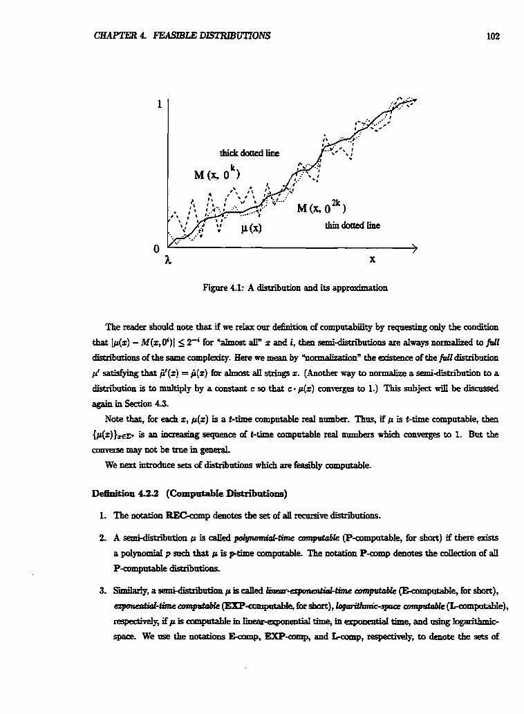
h x
Figme 4.1: A distribution and its approximation
The reader should note that if we relax our dehition of computabii by requesting only the condition
that lp(z) - M(z , o')( I zi for "almost aII" z and i , then semidistriiutions are always normalized to fiJI distriiutions of the same complexity- Here we mean by "normahtion" the existence of the fiJldistrriution
pr satisfying that fir(%) = i(z) fm almost all string z. (Another way to normalize a semi-distriiution to a
distniution is to multiply by a constant c so that c p(x) converges to 1.) This subject wi I l be discussed
again in Section 43-
Note that, for each x, p(z) is a t-time computabk TeaI number. Thus, if p is t-time compntable, then
{ p ( ~ ) ) , ~ p is an inQ.easing sequence of t-time computable real numbers which c o n q to I. &a the
conwse may not be true in generat
We next introdu(3e sets of distniations which are M y computabIe.
MOP 43.2 (Computable Distriiutions)
1- The notation RECcomp denotes the set of ail recnrsive distributions.
2- A semi-distnintion p is c a M pdynomiol-time eonput46le (P-computable, for short) if t h e exists
a po1pomiai p such that p is ptime computable The notation P-comp denotes the coIIection of aIl
P-computabIe distnintions
distributions which are EcomputabIe, EXP-compatabIe, and L-computable
A simple exampIe is the standard distniution v w . It is easy to see fiom its definition that u-d is
L a m putable.
We can aIwaps assmne that M on input (z,Oi) outputs at most i + 1 bits. To see this, let M' be the
machine that m r b as foIIm: it trims the b i i fraction of M(z,Oi+') by rounding it down to i + 1
bits; if the last bii is 1, then it adds 2"'l to make the number of bits at most i + 1. This implies
IM(z, 0') - M1(z, o')( 5 2"", and thns, we get
Example 4.2.3 The nr i fm d i d r h t h over a finite set of integers is P-computable, where we iden*
integers wi th strings. For two distinct natural nmnbers a and b, we define p[,,y as follows:
ExampIe 43.4 Another common dkrete distribution is the P&on distribidion with parameter X > 0
that is defined on (0)' by
for every number n E N We here consider the ose that X is a positive rational nmnber. Notice that
the kth approldmation of the d u e 5 can be computed by a Turing machine m time polynomial in n
and k. S i l y , by considering the power series for e'A, the number e-A is Pamputable. Hence, p is
P-computable
Ben-David, Chor, GoMreich, and Luby [9], on the other hand, define polynomial-time c o m p ~ d
a distribution p m such a way that, for aIT z, the d u e of p(x) is exactly expressed m binary by some
polpomia-time bounded transducer- To distingnish this concept from ours, let us call snch distninti011~
stridly P-cmputde and denote by strict-P-amp the dass of all strictly P-computable distniutions. By
this definition, if p is strictly P-computable, then each d u e p(z) is either 0 or at least 2*lzl) for some
polynomiai p; thns, p is supportme- This Implies that the set strict-Pamp is supportive. SrmiIarly, we
use the notation strict-IiECcomp to denote the set of all distributions which are stridly amptable by
d d e r m i n i s t i c ~ g ~ p l 9 .
It is worth temarking that if a distn'buth is 7-time computable, then the densitp hct ion is aIso 7-time
computable. Theccmverse,hoareper,maymtd~haldsinceitisshmbelooPthatifP#NP,then
there is a P-amnpntable density fimctkm whose associated distribution cannot be computed m p o l y n d
time This d t is dne to Gnrevich [3q.
Proof. Asnrme that P # NP. Take a set A m NP - P such that A = (z I 3y[ly[ = 1x1 A (z, y) E Bl) for
some set B E P. Let r(z) = 0 i£ 121 is odd; otherrioc, @(z) = *i, where lzl = 2n. Clearly v is in P-comp. Now
define the desired distribution p as foffows:
The following summation shows that this p is truly a distniution:
Note that, by clehition, z E A if and only 8 p(zlOlfl) - p(d~*~+') # 0. If p E P-comp, then we have
A E P, a contradiction Therefore, p is not in P-comp. 0
Another observation given by Gnrevich [36j is:
(a) kM(z,Oi) is increasing (ia, z < y implies M(x, 0') 5 M(y,Oi)) for aery i E N.
Proof. Let p be a distniution m P-comp. By definition, there is a polynomial-time Turing machine N such that Ip(z) - N(z , O')ls r'. We defhe the deterministic lbbtg &e M as follows:
else if N(c, O)) > A(€) then set A(c) F A(b)
else set A(c) .r N(c, ok) i f z ~ c t h e n s e t b ~ c e l s e s e t a ~ c
end-repeat
end.
To verify that M satisfies the required conditions is easy- 0
Our apptopdmation scheme is obviously d i f f i t b m the Pwting point model, another popular approxi-
mation scheme given by a pracisia poafirrs-poinf reprw&ah+ becaase, even if p is P-computable, the kth
bit of p(x) may not be computable in time polynomial in 1x1 and k. Nonetheless, the numbers represented
in a finite precision model does not satisfy the law of associativity. AIthough we cannot know any exact pre
cision of the value p(z) in polynomial time in general, it is &dent to know an apprcadmate value M ( z , 0')
within an exponential factor of its true value p(z) when we consider the average behavior of algorithms
under the distniution p
Part of the following usefnl observation was made by Gurevich [XI and by Wang and BeIanger [112].
This lemma is the basis of the proofs of average NP-completeness shown in Chapter 5.
temmo 4.27 (Diiiution Controlling Lemma) [36,112] Let p be a distribution in P a m p .
I . There ezists a positive djddtdion v in strict-Pamp 4 that, for may z, the d u e t(z) hus ut
most 2121 + 4 binmy digits, and 4 - -(z) > F(z) ha.
R o o E (1) Asnrme p E P-comp. I€ there is an z mch that p(x) = 1, then, since the set (y I y 5 x) is hite,wecaneasilyd&evwhich~esthecbim. Intherestofthepmof,wethusassnme that p(z) c 1
for all z.
There exists a polynomial-time lhring machine M such that - M(z, Oi)I < 2-' for aU z and i. For
each string x, take i = 2 1 4 + 1 and let N(z) = ~(z,02l~+I+')- CleatIy we have lp(z) - N(z)j c 2-21f+l-1.
We trim the binary output of N(z] by rounding it down to 2(2+( + 1 di& if the last bit is 0, then cross it
ont; otherwise, add 2-21z+l-' and then cmss out the last bit in order to make the number of b i i at most
212+1+ 1. Now let N'(z) be the result obtained by this process. If z = A, then Nr(z) outputs the &st two
bits of the b i i &don of N(z). Note that [N(z) - Nt(z)l 5 2 * I z + l . By the definition of N', we have
for alI x # A. Hence, b(A) - N'(X)[ < 1 and b(z) - Nr(z}[ < 2-21z+l for all nonempty strings z. Note that Nt(z) i s q r e s e i m binarpwithatmost21z*J + 2 ~ 2 ~ x ~ + 4 ~ s i n c e lz+ls1z1+1+
To get the desired distribution, we dehe
+(N'(A) + 1) ifz=A, P ( 2 ) =
) (Nr(z) - N'(z-) + 2-21z1C1) otherwise
Note that ti(%) > 0 for aB z since N t ( z - ) has at most 2121 bits h m our definition, it is easy to obeain
that &(z) = 1 + N'(z) + 2 &,, 2-4.1 for aII nonempty strings z. Hence, -
For the empty string A, &(A) = N' (A) + I > ji(X) - 1 + 1 = fi(X). For the other strings z,
To show that 2 2-V(+)I, let b(z) be the position of the leftmost digit 1 in the binary fraction of q. That is, Tb(r) 5 < 2 -2-b(t). We daim that 6(2) 5 d(=) +I. Assmne othexwise. S i N ( z ) 2 2-d(z) .
and 9 < e ( z ) C l , b w N(=) - > *(+I -fl(t)+l > - z--d(t)-l . Then, N(=) - 9 > - 2-~(I4)4,
a c o d c t i o n . Using the fyt that ti'(=) d(z) + I, we maciude that 9 2 2d(r) 2 2+(+)-l > - 2-lf(=)l.
0
CHAPTER 4 FEASIBLJ3DISTRIBUTIONS 107
Proof; We assmne that p is a P-comyutable distriiution witnessed by a deterministic polynd-t ime
W g machine hf. Assme a h that a function f is P-computable-
Let us dehe another function g as g(z) = max{z I f (2) 5 z) for each z.
Proof of Claim. Take an appropriate poIynomiaI such that If (z) 1 5 p(lz1) for an strings z. Using this upper
bound of f, we compute g as foIlows:
begin deterministic algorithm for g
mput z
compute the minimal n such that 121 5 p(n)
let a = X and let 6 7 1"
=Peat (binary s'xuch part)
i f a = b then output a
take the mhimaI c such that Il{z I a < z c c)ll > Il{z I c < z 5 b)ll
iff (c) 5 z then set a c else set b := c
end-repeat
d.
The b i i search part of the above dgorithm takes at most O(n) steps, and as a r d t , the algorithm needs
polynomialIy-many steps to compnte g(z). I
Write v for the distriiution k.p(g(z)). We then have:
Let us d&e the deterministic Turing mar)linp N as folI0ws: on input (z, @), simnIate M on input (g(z), @)-
Simce g is Pampatable, the machine N is a h PamputabIe To compIete the proof, we must check the
a~proodmabi~ i tpof~ . This i s~eena~f~now~:
In aqdexity theory, a diaganaIizati011 argmnent is one of the most powerfd and popular tools for
disc.nssinrd a separation of two cornpIexity Note that such an argument is based on the existence of
an e k t b e Cte, recnrsi9e) emmemth of dall elements m question. We already know that, for exampIe, it
is possibIetoewmeateaIIP+mmputabIesetsmane&ctbeway.
The reader may wonder if one can effectively enumerate all distributions. S i P-computable distri-
butions are charaderized by %ring machines, we must emmerate Thing machines which compute such
distributions. It seem, however, difEicult to coMtrnct such an enumeration, because there are two objec-
titles: (I) we must cbedc whether the chosen M g machine, say M, guarautees the convergence of its d u e
to 1 (i.e, lim,+= M(x, 0') = 1) (2) we must dectively check whether the machine satisfies the convergence
scheme, IM(z, 0') - M ( z , Oi)l 5 2-' + 2-j.
To avoid checking the con-ce scheme, let us turn our attention to strictly P-computable distri-
butions. By Lemma 4.2.7(1), we can bound an arbitrary P-computable distribution by mother strictly
P-computable distribution with a constant fsctor. For most applications, we thedore consider strictly P- computable distributions. Can we now enumerate all strictly P-computable distriiutions ? We have to
resolve the problem of checking the convergence of a machine. A d y we do not need to restrict attention
to foll distributions. Schuler [92] kt pointed out the existence of an effective enumeration of all strictly
P-computable semi-dktributions.
Proof. The method of proving this lemma is basidly the same as in Lemma 42.6. Tdce any effective
enumeration of polynomial-time detaministic ' b h g nxxhks, say (M*)iEx. We modify each machine
Mi into another machine Mi which is increasing by an algorithm simiIar to that presented in the proof of
Lemma 42.6 (by replacing N by Mi and M by Mi)). The seqnence {Mil iEN obtained by this modification
as0 becomes an dixtive enumeration of deterministic M g machines, and each M: computes some semi-
diEtrriution m polynomial time. U
Ftom the above theorem, we remark that we cannot exclude the tritriat semi-distriiution kom the en*
mefation.
4.2.2 Rare Strings and Rare Sets
This section will consider input strings which occur rarely for most P-comptrtable distnitrti~ns~ These strings need special anention beguse the set of such strings consists of the most rncult instances for most
aIgorithms to work on in polynomial time
De5ition 4.210 (Ban St-) Let F be an enumeration of semi-distniutions, say F = {h, w , . . .}, and let k,s be fanctions k n N to P. A string z is rmr mah rrspcd to ( k , ~ , a if h(z) < ~ - ~ ( t 4 ) holds
for all i < k([xl). Let RARE(k, s, 7) be the coflection d dl rare strings with respect to (k7 s, 7).
Note that the rareness of a string depends on the etnrmeratian F.
Proof. We 6rst show that, for any integer no > 0, there exists an n with no .I n 5 3% + 6K(no) such .yW that, for each i < k(no), 11{z E IF I B(z) > 2-8(n))n < %. Asrmme o&emise. Let r(n) = 3n +6k(n)
and define 4 = {z E Cn ( h(x) > 2-'(")). Take no such that, for all n with no n 5 r(n& there exists r no)--m+l an i < k(no) satisfying II&I( > k(n) - Pcn)/n. Hence. at least many n's the condition
11411 > k(n) - 2.(") fn for some j < k(w). Let c = Ik~")-')Mf'o)+')+nO k(no
. S i r(n0) > -,, we have
(3) 2 L Then,
The lemma immediately folIows fiom the foUowing meqnalitp:
We can construct a P-computabIe distribution p and an exphonest, P-computab1e function f such that
no distriiutions in P a m p dominate ~ c f l - Recan h m Chapter 2 that p p-&mh&s v if and only if
there is a pbounded function p h m C to P such that p(z) -ji(z) 1 t(z) for an z.
ProposiPion 4.2.f 2 [I191 Them aists a pusilioe P-amptable d i d d t d h p and an inacruing, ap
honest function f in FP judr that ~ l p is not p domkradedbyanyP~tediskiburions.
Proof. We first dehe q as folI0ws:
Let b(z) = $5-(z) + %(z). The distriintion C( is positive and obviously P-compntable For every n 2 2
and for z =v6, we have
y such that logn 5 lyl I 9logn and jyIk-' - &(v) < P(On) for all i < Iogn and all integers k with
15k5 w&&n,wheren=min{r~f15 PI <(r+l)6}3n>213;otharise,l& f(r) =I.
b c t i o n f is ddefined- To see this, consider the case [zl= n6 hr some n 2 213. By choosing logn
as k(n) and n + logn - 2 Ioglogn - 4 as s(n) ir: Lemma 4-2-11, we know that there exists at least one rare
rtMg tO (k,s,F) with 4 n 5 ]y{ 5 9 lop , i.e, fii(y) 5 2-'(") = for all i < l o p . For such a string y, we have
rinalogn 5 ly l s 91ogn, 1610&910gn) < (9bgn)" i fn 2 4, and gklo8n 5 f i i f k 5 wicwn. Hence, f (z) exists. It is easy to see that f is exphonest and also polynomial-time computable.
By definition, for all k and i, [yjk-' - 4(y) c irl (y) for some y, since fifl (y) 2 fi(On).
Inspired by the notion of complexity cores, we shall introduce sets which consist of instances which occur
rareIy under most distributions in question.
Dehition 4.2.13 (PolynomiaIIy L-Rare Sets) Let C be a function on N and let 3 be a set of distribu-
tions. A set S is d e d C - m n with nspect to 3 3, for any distriiation p in F, the set jz E S I P(z) > 2-'(1'1)) is finite. If3isP-comp,t6enwesimpIydthissetSpoIynomioUyf-rme
In what foUows, we shalt show the d a c e of a polynomially &rare set for increasing, unbounded 1 with
the extra condition 5 logn 9 L(n) 5 n. The proof uses Kolmogorov complexity-
PmoE Assume that s is increasing and mtmmded In what f o h , we show a general statement: for
every distriiution p E P-comp, there exists a positive integer SIX& that, for aJl strings z of length 2 no, if z ~~[U(n) ,y(")+ ' (")e~] , then fi(x) 5 2-'(M)- This dearly implies the theorem.
For a distniution p E P-comp, using Lemma 426 , we can take a detemhbtic poiynomia-time 'Xbring
machine M such that, br all i E R fp(z) - M(x,6)1 5 2' and kM(z,O') is increasingcreasing We let T(X) = M(A,O) and T(z) = M(X,OPI+~) - ~(z-,01zf+3 for z E F. For any set A, write T(A) for LEA T(z). Notice that T may not be a distnintion, but T(z) 3 0 holds for all z. Moreover, T appra*imates fi since it fonow~ that
h m the fact that T is P-compatable, we now suppose that T on input z is computable m lzId + d steps
far some positive integer d indepemht of z.
CaAPTER 4. FEASIBLE DLSTRIBUTIONS 111
Consider an integer no Iarge enough so that the hflowing ineqdities always hold: logno 2 2 logio + 9, no 1 4c, and no 2 d + 4, where io and c are constants given later (not depending on the choice of no). For any integer n not smaller than m, let
A, = {z E 'P I T(z) + 2-"* > 2-'(")}.
As for the cardinaIity, we can daim that [[A,,[] c 2'("If'.
hf of CIoim Assmne otherwise. Note that, for each x E &, T(z) > 2-L(n) - 2-n-2 . Hence, we have
Since C(n) 5 n, CZEL fi(z) > 2 - 1 = 1. This is obviously a contradiction. Therefore, l[A,,ll < I
We note that, for each z E C", if fi(x) 5 2'C(n), then z E A. To get the desired conseqgence, we shall show that -4, C KT[2e(n),2C(n)+s(n)1~n]. Fi an integer e with 1 e < P(")+'. Let us take the eth element
of A, in the standard order on E' and consider the foIIotnring deterministic algorithm:
begin deterministic a1gorith.m
inpat (st I %, st)
let j - 0
forallstzbgsymE1do
compute the value T(y) (let this term to be t )
if t + 2-"-* 5 2-' then go to (2)
let jr=j+l
if j = e then output y
(*) end-for oatpat 0
end.
C&APTER 4. FEASIBLE DISTRlBUTIONS
since log n > 2Iogio + 10 and 5 logn I C(n) I n for aIl integers n > no. F d y 7 we shaIl analyze the nmning time of U. Notice that, m the original algorithm as defined above,
there are 2' iterations of the for-loop, and on each of such iterations, for y E Ct, the algorithm needs steps
as many as O ( T i ( y ) + logn + l + loge + 1). Therefore, the nrnning time of U on inpnt (sj,, , sf(,), sn, se)
is at most, for some constant c > 0 (not depending on the choice of n),
since 5c 5 n, t (n) 5 n, and d + 2 5 nd. Thedore, we conclude that we E KT[2(n), $(n)+'(n)l~n]. This
completes the proof. 0
Note that, by Lemma 2.7.7, the set we have used in the above theorem bdongs to the class
DTIME(O(P(")+'(~) -)I. The foIIowing Iemma of W e r [93] has the same fiavor as Theorem 4214 and will be used in Seaion 5.6.
Let k, s and C be functions on N Assume that C and s are nnbotmded and increasing- Moreover, assume
that k(n) - L(n) 5 n, C(n) 1 lOlogn, and k(n) 2 1 for almost all n. For each integer n > 0, we dehe k(n)
strings 4,. . . , 2;") as fo1Iows:
M The proof below is sitnihr to that of Theorem 42-14 For a distniution p E P-camp, take T as in the proof of Theorem 4214, This T also satisfies the ineqaality that l j i(q) - T(p) I 5 2" for all i
with 1 _< i 5 k(n). Assmne that the d u e of T(zI?), where Izl = n, is computed m time (n + m)d + d
fix some p d h e integer d We shaII de6rte co and c' later- Choose no large enough that the selfdelimiting
description of T is d c i d y small, and no > Bc', and d + 2 5 s(%).
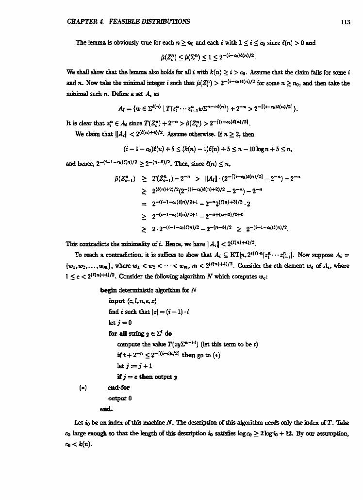
CHAPTER 4 FEASlBLE DJSTRIBUTIONS
We shalI show that the Ipmmn also holds for aII i with k(n) 2 i > Q. Assume that the claim fails for some i
and R. Now take the minimal integer i such that ji(q) > 2-(i-a)C(n)/2 fix some n 2 n ~ , and then take the
minimal su& n. De6ne a set & as
This contradicts the m b h a k y of i. Hence, we have llrltll < 2('(n)*)/2.
To reach a contradiction, it is d c e s to show tbat Ai KT[~, 2*(9'"lz? - - - zr- Now suppose A, = {wl,rnr - . . ,to,,,), where wt < w < . - - < tom, m < 2(t(n)+4)/'. Consider the eth element we of A, where I < e < 2(C(n)*)/2. Consider the bIIowing atgorithm N which computes we:
begin deterministic algorithm for N
inpd {G 4 % G 4 Sndisuchthat lz l=( i -1)-1
let j = O
fotal ls tr ingy~z~b
compute the value T(ryP4') (Iet this term to be t )
if t + 2- < - 2-l(i-c)1/21 t h a go to (*)
let j - j + I
if j = e then output y
(*I end-fm
0- 0 end-
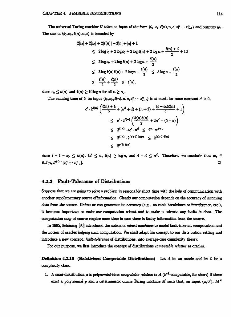
The aniversal lhring machine U takes an input oithe form (io,co,l(n),n,e,z,̂ -+-zF-,) and outputs we.
The size af {io, Q, Qn), n, e) is bounded by
since q 5 k(n) and [(n) 2 10 logn for all n 1 no. The nmning time of U on input ( io , @,l(n),n, e,zr -.. zZt) is at most, for some constant d > 0,
C - 2 ' ( " ) ( ~ + ( n d + d ) + [ n + 2 ) +
d - ~ ( " 1 (- + 2nd + (5 + d))
since i + 1 - co I k(n), 4d 5 n, I(n) 1 Iogn, and 4 + d 5 nd. Therefore, we condude that we E
KT[n, ~ ( ' 7 - ~ l z ? - - zEJ. 0
Suppose that we are going to solve a problem m reasonably short time w i t h the heIp of communication with
another snppIementiVjr source of infarmation. Clearly our computation depends on the accuracy of incoming
data h m the somce, Unless we can gnarantee its accmacp (eg, no cable breakdown or i n t e r f i e , etc-),
it becomes important to make our computation robust and to make it toIerate any f d t s in data. The
compntation may of course reqnire more time m case there is fadB information fiom the somce-
In N85, Schiining [W] introduced the notion of robwb muchim to model fdt-tolerant computation and
the notion of oracles he&zg such compatation. We shaIl adapt his concept to om distribution setting and
introduce a new concept, faPJt-k,Ierance of distributions, into average-case complexity theory.
For our pnrpose, we &st introduce the concept of distriiutio~~s cornputctbk relaEme to orades.
-on 42.U (Belatrvlaea * . ComputabIe Dktxiions) Let A be an orade and let C be a
-pIsrity dass-
1. A semi-distribution p is p o ~ t i r n e conrprrfoble reldiue to A (PA-computable, for short) if there
srist a poIynomiap and a- - - . oracle ' h k g machine M such that, on input (&), MA
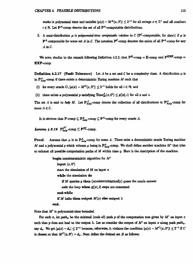
CHAPTER 1. FEASIBLE DISTRIBUTIONS 115
works in poIynomial time and satisfies Ip(x) - MA(z, Oi)I 5 2-' for aH strings x E Em and all numbers
i E K Let PA-comp denote the set of all PA-mmputabb distributians,
2. A semi-distn'bution p is polgnmial-time amputabk relotitle to C (PC-computabIe, for short) if p is
PA-computable for some set A in C. The notation p-mmp denotes the union of all PA-comp for any
A in C.
We note, simiIar to the remark hUowing De5nition 421, that PEtomp = Ecomp and P--comp =
EXP-comp.
Dehition 4.2.17 (Fadt Tolerance) Let A be a set and C be a complexity class. A distribution p is
in P&P-comp if there exists a deterministic Turing machine M such that
(i) for every oracle 0, - M0(z, 0')I 5 2-' holds for a11 i E N and
(ii) there exists a pol~momia p satisfying ~tme&(x, 0') 5 p(lz1, i) for an z and i.
The set -4 is said to help M. Let ~ & ~ - c o r n p denote the colIection of all distributions in P~c,p-comp for
some A E C.
It is obvious that P-p Pup-comp p A a m p for every oracle A.
Proof. Assnme that p is in P&,-comp for some d There & a deterministic oracle Thing machine
M and a polynomial q which witness C( being in P&,,comp. We shall d e h e another machine M' that tries
to exhaust a11 possiile computation paths of M within time q. Here is the description of the machine
begin tun--c algorithm for M'
input (q0')
start the simnlation of M on input z
while the simulation do
if M queries y then (nondeterministidy) guess the o d e answer
exit the loop when q([zj,i) steps are consumed
end-while if M halts then output M(z) else output X
end.
Note that M' is poIpmiai-time bounded.
For each 2, Iet path, be the minimal (code of) path p of the compntation tree given by Mr on input z
such~pdoesmt~eadtotheontptttX Let n s ~ e r t h e o n t p d o f M ' o n i n p u t z a I o n g p a t h ~ ,
say &. We get b(z) - 4 I 2i became, dherwise, it violates the amdition I&) - dfC(z, Oi)l 2 2' if C
is chosen so that MC(z,Oi) = &. Nert & h e the desired set B as MOWS:
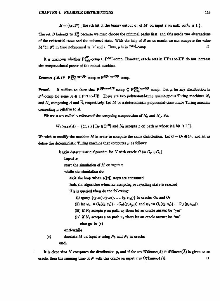
B = {(z, 1") I the ith bit of the binary ontptrt 4 of M' on input z on path path, is 1 ).
The set B belongs to because we must choose the minimal paths first, and this needs two alternations
of the existentiat state and the universal state- With the help of B as an oracle, we can compute the value MA(x,O') in time polynomial in [zj and i. Thns, p is in corn^. 0
~t is UIIICIIOWLI whether ~ P - c o r n p E P - c o m p . ow ever, o d e sets in UP n -UP do not increase
the computational power of the robust &e.
PmoE It d c e s to show that ~ ~ ~ ~ ~ - c o m ~ ~ E ~ - ~ - c o m ~ . Let p be any distriiution in
PA-comp for some A E UP n DUP, There are two polynomial-time unambiguous Thing machines No and Nt computing A and x, mspectiveIy- La M be a deterministic polynomial-time oracle Thing machine
computing p relative to A.
We use a set called a mitness of the acceptiug computation of No and Nr . Set
Witness(A) = {(x,si) I 3tu E zkI[ and No accepts x on path w whose ith bit is 1 I).
We wish to modify the machine M in order to compute the same distnibution. Let 0 = Oo $ Or , and let us
define the deterministic Turing mxrrhinr? that computes p as follows:
It is dear that N computes the distri'bution p, and if the set Witness(A) Witness(TI) is given as an
oracle, then the Rmning time of N with this d e on inpnt z is O(TiieM(z)). 0
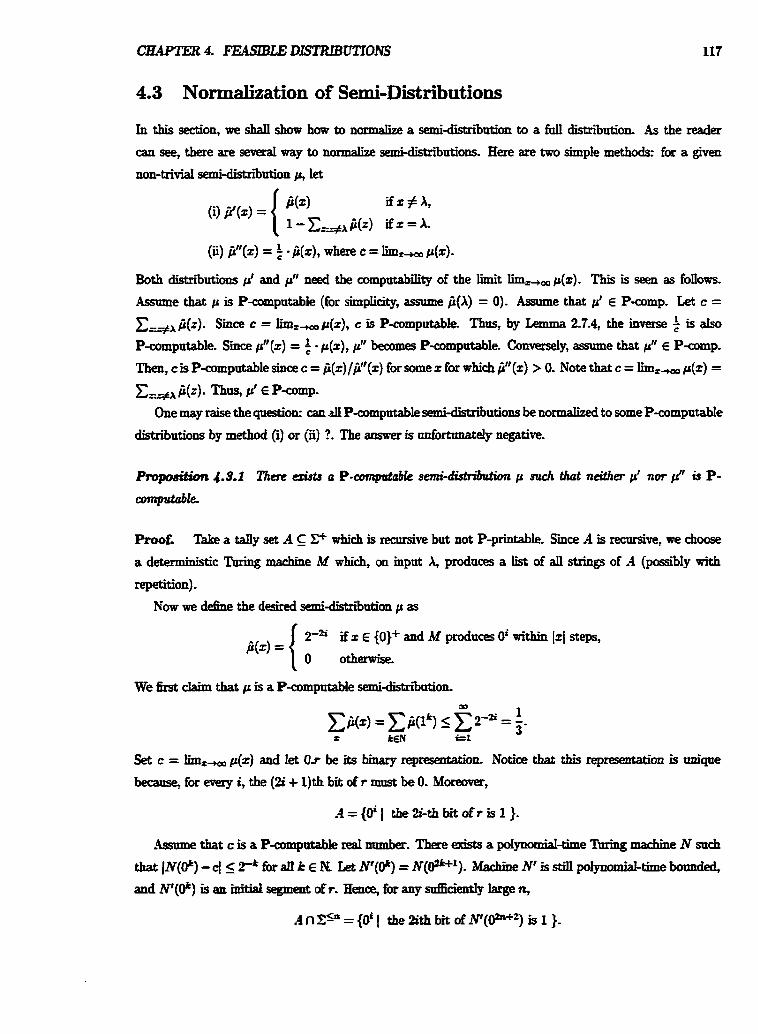
4.3 Normalization of Semi-Distributions
In this section, we shall show how to normalize a semi-distribution to a full distribution. As the reader
can see, there are several way to normalize semi-distriiutions. Here are two simple methods: for a given
non-trivial semidiski'bution p, let
(ii) jiIr(z) = 4 fi(x), where c = limn, p(x).
Both distrtiutions p' and p" need the computab'zlitp of the limit lirn,,, p(z). This is seen as follows.
Asnrme that p is P-compnbbie (for simpLiaty, assume P(X) = 0). Assume that p' E P a m p . Let c = Cr-+X &). Smce c = lim,,, p(z), c is P-computable. Thus, by Lemma 2.7-4, the inverse 1 is also
P-computable. Since p"(z) = $ - &), p" becomes P-computable. Conversely, assume that pt' E P-comp.
Then, cis P-computable since c = ji(z) / j i"(z) for some x for which Ptt(z) > 0. Note that c = lim,, p(z) =
F(z)* T ~ w P' f P-P* One may raise the question: can dl P-compntable semi-distributions be normalized to some P-computabte
distriiutions by method (i) or @) 1. The anmm is dortttnately negative.
Proof. Take a t d y set A P which is d v e but not P-printable. Smce A is reamhe, we choose
a deterministic Turing marhme M which, on input A, produces a list of all strings of A (possibly wi th
repetition).
Now we dehe the desired semi-distribution p as
2-E if z E (0}+ and M produces 0' within 1x1 steps, B(4 =
We first claim that p is a P-computable semi*'bntion.
Set c = I&, p(z) and let O t be its b ' i representation- Notice that this represenWion is
became, for every i, the (2i + 1)th bit of r nmst be 0. Moreover,
.9smme that c is a Pampntable real number. There exists a polynomial-time lhring machine N such that IN(*) - cf I rk for .d k E K Let Nr(@) = ~ ( d H l ) . Machine N' is still p o l y n d t i m e bounded,
and AT'(@) is an initia segment ofr. Heme, fix any ~~Ecieutly Iarge n,
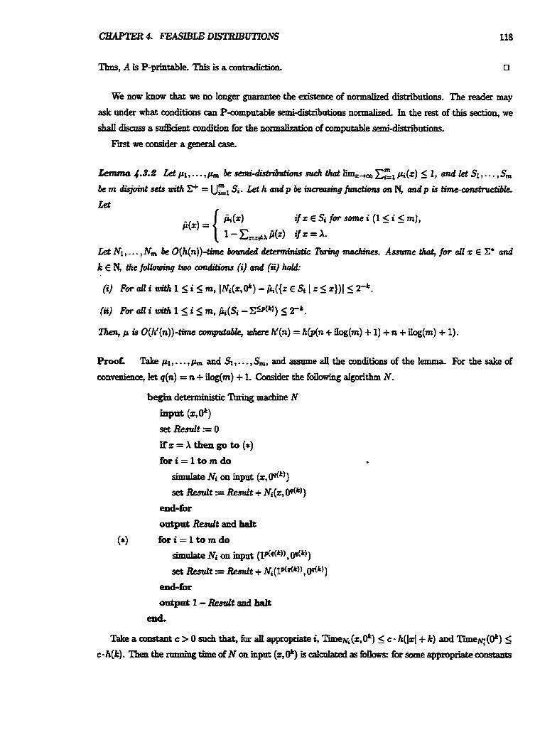
Thus, A is P-printable. This is a contradiction 0
We now know that we no Ionger gnaradee the existence of normaIized distriiutions. The reader may
ask under what conditions can P-computabie semidkfxi'butions normalized. In the rest of this section, we
shalI discnss a &dent condition for the normabthn of computable semidistri'butions.
First we consider a general case.
bem d i s j o i n t s e t ~ t n i t h C + = ~ ~ ~ S ~ . L e t h a n d p b e i n a r e c r s i n g ~ o n N , andpis t i m e - m l e .
Ikt Nl , . . . , Nm bc O(h(n))-time bounded ddennirdstic Ttu+g mneltineg. Assume that, for all z E E* und
k E N, tire folIoloing two conditions (i) and (ii) hold.
Then, p is O(ht(n))-Eime mmputubk, whse h'(n) = hCP(n f iIog(m) + 1) + n + ilog(m) + I).
ProoE Take pl,. . . ,p,,, and 4,. . . ,Sm, and assume sll the conditions of the lemma For the sake of
convenience, let q(n) = n + ilog(m) + 1. Consider the following aIgorithm N.
begin deterministic Turing machine N
(z,@) setResult.=o
ifz = X then go to (*)
f o r i = l t o m d o
siwtIate Ni on input (2, MC)) set Result s Result + N&, O P ( k ) )
end-for
oatput ResuIt and halt
(4 f o r i = l tomdo simuIate Ni on input ( tddk)) , W)) set Result 7 Result + ~ ( l ~ ~ k ~ ) , O q
end-for
0ntptrt1-Resultaadhatt
end,
Take a constant c > 0 such that, for aIl appropriate i, Time&, dt) I c - h(lzl+ k) and T i e q ( @ ) S c- h(k). Then the nmning time of N on input (z,@) is CacnIated as fchws for some appropriate anwants
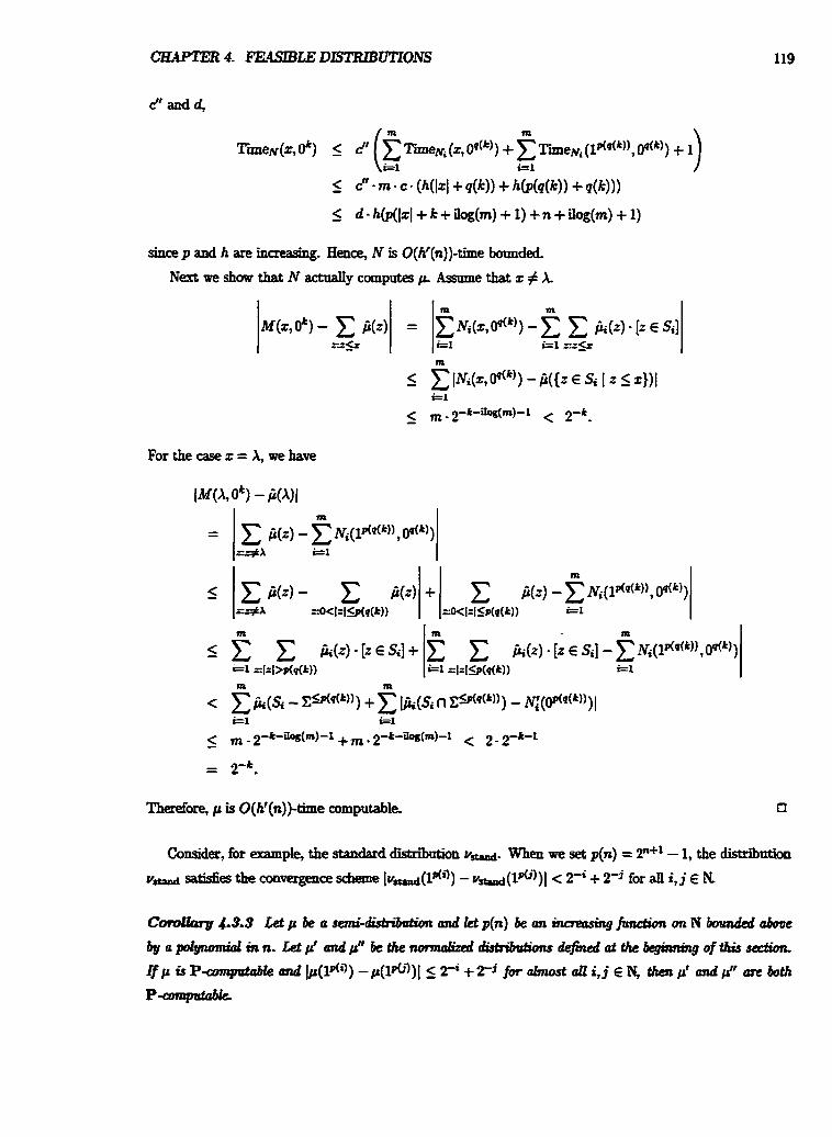
since p and h are increasing. Hence, N is O(ht(n))-time bounded.
Next we show that N actnaIIy computes p Assume that z # A.
Forthecasez= X, we have
Consider7 for example, the standard distribution Y-. When we set p(n) = Ff - I, the distribution
v- satisfies the convergence scheme luw(l~~) - v-(lm)I < 2'i + 2-j for i, j E N.
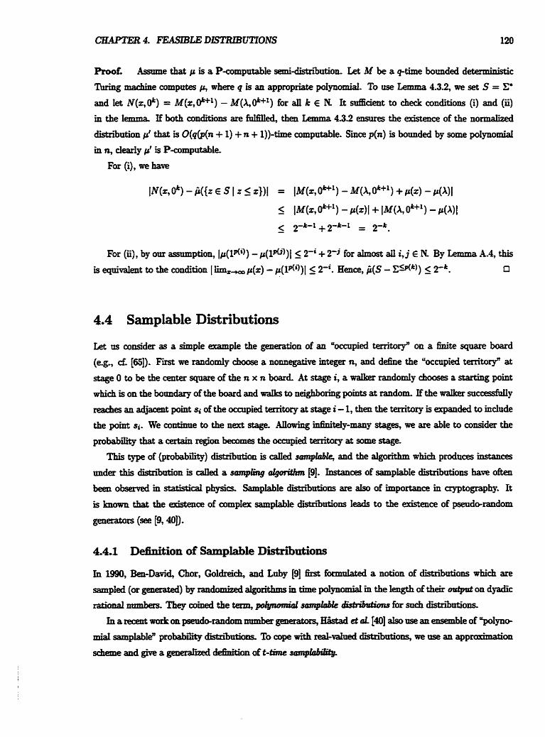
C&4PTER 4. FEASIBLE DISTIilBUTIONS 120
Proof. Assume that p is a P-computable semi-disttl'butio~ Let M be a *time bounded deterministic M g machine computes p, where q is an appropriate po1ynod. To use Lemma 4.32, we set S = C8
and let IV(z,ok) = kf(x,OLCi) - M ( A , e l ) for dl k E N It sufficient to check conditions (i) and (ii)
in the lemma If both conditions are M e d , then Lemma 4.32 ensures the existence of the normalized
distri'bution $ that is O(q(p(n + 1) + n + 1))-time computable. S i p(n) is bounded by some poIynomiai
in n , clearly p' is P-computable.
For (i), we have
or (ii), by our assumptionT Ip(lfli)) - p ( l a ) ) l 5 2-' + 2-J for almost i, j E N. BY emm ma &4-4? this
is equivalent to the condition I lim, p(z) - ~ ( 1 f l q ) l 1 2-'. Hence? fi(S - xCJ(*)) 5 2-'. 0
4.4 Samplable Distributions
Let us consider as a simple example the generation of an LCoccttpied territory" on a finite square board
(eg, d [q). F i we randomly choose a nonnegative integer n, and dehe the "occupied territory" at
stage 0 to be the cexttm sqpare of the n x n board. At stage i, a watker randomly chooses a starting point
which is on the boundary of the board and waIks to neighboring points at random, If the waIker s t t d y
reaches an adjacent point si of the occupied t d o ry at stage i - 1, theu the territory is expanded to include
the point si. We continue to the next stage. Allowing hhikly-many stages, we are able to consider the
pmbabiIity that a certain region becomes the occtfpied territory at some stage.
This type of (probabm) distriiution is d e d swltplobZq and the algolithm which produces instances
under this distrritrtion is d e d a s~~ [9]. Instances of sampIabIe distnitrtions have o h
been o b s d in statistical physics- Samplable distriintions are also of importance in cryptography h
is known that the exkkuce of compIex samphble distrritttions Ieads to the existence of pseudcmmdom
tperato= (a [9? 4).
In 1990, Ben-Dad, Chor, GoIdreich, and Luby [9] hst formulated a notion of distributions which are
sampled (or generated) by randomized dgorithms m time poIynomiaI in the length of their output on dyadic
rational mmbers. They coined the term, potynomial s~l~phbk tW&tdhu for such distriiutions
In a recent w d c on pseud~random rmmber generators, H5stad d d 1401 aIso use an ememble of "po1yne
miat samplabI$ probdi& distxi%* To cope with dtralued dIstniuticms, we use an approodmation
scheme and give a generaIized dehitionoft-tinre J O ~ P ~ ~
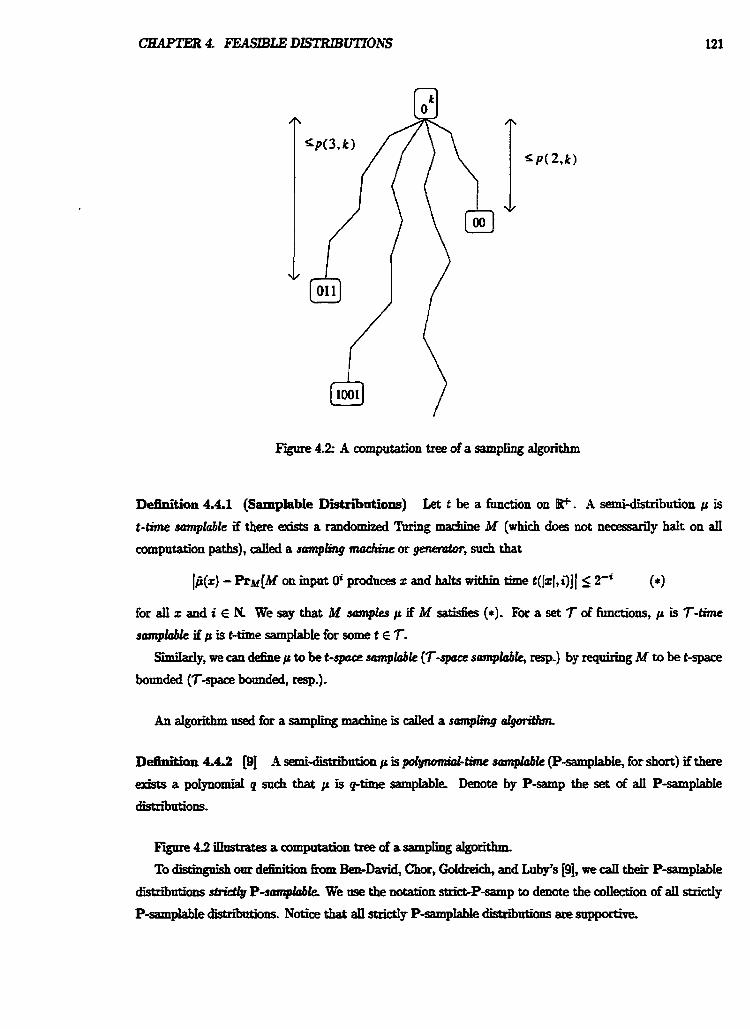
Figure 4.2: A computation tree of a sampling algorithm
D a t i o n 4.4.1 (Samplable Distriintions) Let t be a function on Htt. .4 semi-distribution C( is
t-time swnplable if there exists a randomized M g machine M (which does not newssarily halt on all
computation paths), d e d a $ampling m d i m or genaator, such that
(fi(x) - R M [ M on input 0' produces x and halts within time t([x(,i)]l 2 2" (*)
for all x and i € N We say that M ~ d t n p l c s p if M d e s (*). For a set T of functions, p is T-time
santplablc if p is t-time samplable for some t E 7.
S i y , we can dehe p to be &space samphble (T-space swnplobk, resp-) by rrgniring M to be t-space
bounded (T-space bounded, resp.).
An algorithm nsed for a sam- &e is called a sampling algotithm
D M o n 4.4.2 [Q] A semi-distribution p is pdfFomiaI-time sump&b& (P-samplable, for short) if there
exists a poIynomiaI q such that p is ptiree sampIabIe Denote by P-samp the set of all P-samplable
digtniutions.
Fignre42iIInstratesacompdatiantreeofasampIing~
To distingaish our d M o n &om Ben-David, Chor, Goldreich, and Luby's [9j, we call their P-samplable
distriiutions sfriefly P-scmrplaMe. We use the notation strict-P-samp to denote the coIIection of all sttidy
P-samplable ctistn'bnti~ll~~ Notice that an &y P-sampIable dktributio~t~ are supportive.
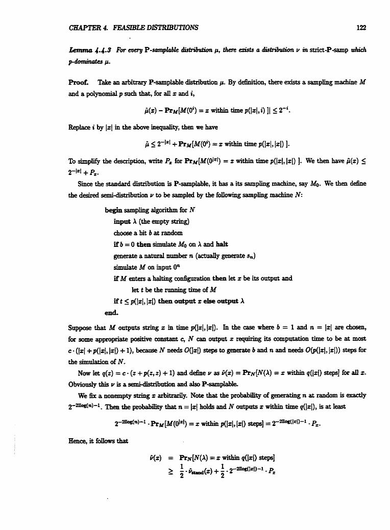
Proof; Take an arbitrary P-samplabIe ~ ~ t x t i o n p. By definition, there exists a sampli~g machine M and a polynomial p such that, for alZ x and i,
Replace i by 1x1 in the above in*, then we have
To sixnplifj, the description, write P. for P r M [ ~ ( 0 i z I ) = z within time p([xl,lxI) 1- We then have b(x) 5 2-121 + P=. Smce the standard distribution is P-samplable, it has a its sampling machine, say &. We then dehe
the desired semi-*'bution v to be sampled by the f o l I d g sampling machine N:
begin sampling algorithm for N input X (the empty string)
choose a bit b at random
if b = 0 then simulate Mo on X and halt generate a n a t d number n ( U p generate 8,)
simulate M on input On
if M enters a halting con&uration then let x be its output and
let t be the running time of M i f t ~ p ( l z ~ , 1 x ~ tilerloatput t &output X
end.
Suppose that M outputs string z in time p([zIy 121). h the case where b = 1 and n = 121 are chosen,
for some appropriate positbe constant c, N can output x reqrtiring its computation time to be at most
c - (1x1 +p(lxl, 1x1) + I)? beeaftSe N needs O(lz1) steps to generate b a d n and needs 0@(lzl, [%I)) steps for
the siwrlation of N. Now Iet p(z) = c - (z +p(z, z) + 1) and d&e v as i(z) = RN[N(A) = z 2 q(lx[) ststeps] for dl z-
Obviously this u is a semi-distll'bution and a h P-samplable.
We fix a nonemptg string x arb'ltrarily~ Note that the probability of gen- n at random is d y
~ 2 n a ( ~ ) - 1 - Then the probabititp that n = 121 holds and N outputs z within time q([zl), is at least
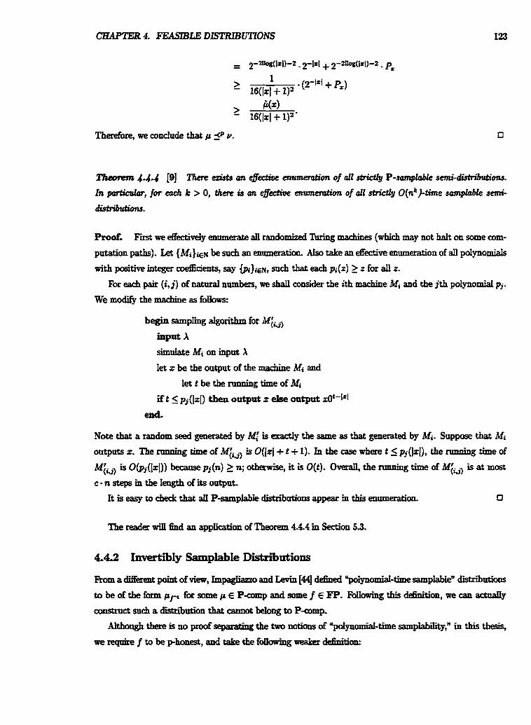
Therefore* we condude that p p v.
Theonm 1.14 [9] There Qists an e f ' mumemkmumemkon of all s b i d l y P-sanplable semi-didd&hw.
In partiah, for each k > 0, them is an geclioe cnumeratitm of all &idly O(nk)-time smnphble semi-
distn'butions.
Proof, F i we effectively enumerate all randomized Turing machines (which may not halt on some com-
putation paths). Let (Mi)yN be snch an enumeration. Atso take an dective enumeration of all poIynomiaIs
with positive integer coeffidents, say @ r ) i c ~ , such that each pi(%) 2 z for aII z.
For each pair (i, j) of natural nambers, we shalt consider the ith machine Mi and the jth p o l p o d p,.
We modify the machine as follows:
begin sampling algorithm for M:ij)
input X
simulate Mi on mput X
Iet z be the output of the machine Mi and
let t be the nmning time of Mi if t 5 ~~(1x1) then output z ehe output dt-lrl
end.
Note that a random seed generated by &! is exactly the same as that generated by Mi- Suppose that Mi outputs x. The runniug time of MiQ, is O([z[ + t + 1). In the case where t 5 p,(]zl), the nmning time of
Miu, is O(pi(lzl)) because pj(n) 2 n; othemk, it is O(t). Overall, the nmning time of Mik, is at .most
c n steps m the Iength of its output-
It is easp to check that alI P-samplabk distri'buti~ appear in this enumeration. 0
The reader will find an application of Theorem 4.4.4 in Section 53.
44.2 herti'bly Samplable Distributions
Ftom a diffefed point of view, ImpagIiazm, and Levin [44] dehed "polynomiaI-time sampIable" distributions
to be of the form p p for m e p f P-comp and some f E FP. FolIowing this dehition, are can achtaiIy
construct such a distriintion that cannot belong to P-comp*
Although there is no proof separating the two notiam of "po~omiaI-time sampIabi&yP in this thesis,
we reqrrire f to be phonest, and take the f m weaker dehitiionr
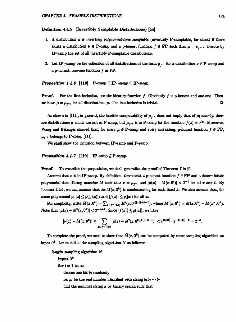
1. A distriintion p is invertibly p o l ~ t i m e smplable (invettiily P-samplable, for short) if there
exists a distriiution u E P-comp and a phonest fnnction f E FP such that p = ur,. Denote by
IP-samp the set of an invertiily P-sampiable distniutions.
2. Let PI-samp be the mnection of all distriiutions of the form p,-, for a distribution u E P-comp and
a phonest, oneone function f in FP.
Roof. For the Erst incIusion, use the identity hc t ion f. Obviously f is phonest and one-one Then, we have p = prl for a11 distri'butions p. The last inclusion is trivia. 0
As shown in [Ill], in general, the feaslile computabiity of p,-I does not imply that of cr; namely, there
are distn'bntions p which are not in P-comp, bnt prr is in P-comp for the function f (z) = 01~1. Moreover,
Wang and Belanger showed that, for every p f P-comp and every increasing, phonest function f E E'P, prr belongs to P-comp [111].
We shan show the inclusion between IP-samp and P-samp.
Proof, To establish the proposition, we shan generalize the proof of Theorem 7 in [9].
Assume that u is in IP-samp. By defiaition, there exist a phonest function f E FP and a dekmhkt i c
polynomial-he Tuxhg machine M such that P = p f t and IF(=) - M(x,oi)I c 2'' for all z and i. By
Cemma 4.2.6, we can assmne that XrJbf(z,p) is nondeaeasing for each fked k- We also assume that, for
some pobomial P, I4 5 ~ ( l f ( 4 I) and If ( 4 l I p(l4 1 for x.
For simpIicitp, adte ~ ( z , @) = &-Ib) ~ ' ( z , O.(lzl)Ck-l), where Mf(z, @) = M(t. Ok) - M(x-,@).
Note that [fi(x) - Mf(x, @)I < rH1. Smce If (%)I S p(Izl), we have
To mmpIete the proof, we need to show that M(Z, @) can be computed by some sampling algorithm on
input @. La us d e h e the sampling algorithm N as foII0ws:
M(z-, ~p(lrl)+~-~) < pi 5 ~ ( z , (jp(l~l)+~-I)
if there is such an z then output f (z) and halt
end-for
end.
It is not difficult to see that ~ ( z , ok) is equal to the probability Pr[N(ok) = z in time q(Iy1, k)] for some
p o l y n o d q- 0
The converse of Proposition 4.4.7 is unlikely to hold; however, we can prove that every P-samplable
distribution is pdominated by some inverh'bly P-samplable distribution.
Lenuna 4 4.8 [I191 For mery p E P-samp, there & a d i d d n d h v E IP-samp such that jt I p v.
Proof. Let p be a P-samplabIe distniution, and let M be a randomized Turing machine witnessing p with
a time-bound polynomial p. We modify the origbl machine M so that, at every c o w o n of M, there
are exactly two nondeterministic choices. Hence, the length of a code which expresses a nondeterminiseic
path of M on each input is at least the size of its output. Moreover, we assume without Ioss of generality
that p is increasing.
We d&e a ftmction f as
output z of M on dl'l on path z' in time ~(31x1) if z = z'l and z exists,
i€z=r'lbutnosuchxexists,
if z = 2'0.
To see that f is P-computable, consider the following deterministic algorithm:
begin dete ' tic algorithm for f input r
if z = 20 then output 2 else compute z' such that z = 21
for n = 1 to lz'[
simulate M on input Cf" on path 2'
if M halts in time p(3n) then let z be its output else go to (*)
if 1x1 = n then output z and halt
(*) end-for
output X
end.
For each z, let A, be the dection of all stzings w such that, on input dlzl on the computation path
encoded by to, dd halts in time p(3[zI) and produces z. By our issumption, if w E A*, then lurl 5 p(31ZI).
[w E 4 RM[M on dlr1 produces z in time p(3IzI)I = 21w, . w
On the o t h a hand, since M appraximam j, we then have B(z) 5 2-*[4 + C I*- Let B(z) = fi-({w I f (w) = 2)). Notice that B(A) > 0. Let Q be the m;nimnl positive integer such
that Q - P(X) 1 $(A). Then, it follows that
Let q(z) = S(p(3z) + 1)* f 6. In the following, we show that q(lx1) -G(z) 2 ji(z). For z = A, this is obviously
the case- For the other strings z E P,
Unfortunately, we do not know whether P-samp S p IP-samp, or whether we can replace IP-samp in
Lemma 4.4.8 by IP1-samp.
Schder and Watanabe 1961 introduced an average version of P-samplable distnitxtions. We give a brief
definition here.
Dehi t ion 4.4.9 (Average Polynomial-T'rme SampIable Distriiutions) [98] A distn'bution p is
werage polynomial-time srrmplclble (average P-samplabIe, for short) if there exists a randomized Tming
rnarhine M and a poIpomiaI p such that
(i) - RMIM(Oi) = z] 5 Ti for arty z and i E & and
(ii) for every number r > 0 and evey ~1 E N,
Let avp-samp denote the set of all average P-samplabIe distn'bntions
We shall show below that average P-samplabilitp- is a natraal extension of P-sampIabiIitp.
Proot. Let p be any P-sampiabIe distribution- Consider a poIpomiaI p and a randomized lhring machine
M which, on mput Oi, samples p(z) m p(lz1,i) steps; that is,
CHAPTER 4. FE,4SIBBLE DLSTRlBUTIONS 127
f o r a R i ~ N a n d z E C .
To show the average P-sampIabiEty of p, we must define another sampling machine that sampIes p in
polynomial time on paverage wifh respect to the Ieugth of its output. Sucb a sampling machine is d&ed
as fouow!x
begin sampling algorithm for N inpllt 0'
simntate M on input 0'
if M reaches a halting state then do the foIIavbg:
let z be its output
let s be the random seed generated so Far
if TiieM(Oi; s) 5 p([zl, i ) then output x and halt f o r i = l t o m d o
fipafaireoin
end-for
end.
By the simnlation, it hIIows that
The rrmning time of N on input 0' dong with random seed s, is the same as that of M on 0' wi th s with
a constant factor.Thus, for an appmpriate constant c > 0, it hoI& that
which implies that p is average P-sampIab1e
4.4.3 C'osure Properties of Samplable Distributions
This snbsection w3t discnss severd properties of P-sampIable and inrertibly P-samplabIe distnittiims.
ProoE Let f be phonest and in FP- ~~e that p = v,, hr some v E P-comp and phonest g E FP.
Then,
CHAPTER 4. m4SIBLE DlSTRlBUTIONS
Proof. Assmne that p E P-samp. By Lemma 4.4.8, we can take a distribution p' fiom IP-samp such
that p SP p'. By Lemma 3.410, p S P pr impIies prl s p pkl. Now let v = p;, . By Lemma 4.4.11, we
conclude that v beIongs to IP-samp. 0
This corohry will be used to prove Propition 7.5.10-
The following theorem is similar to the fact that B P P B ~ ~ = BPP (see, eg., [1231). It states that
PBPP-samp is pegnal to P-samp. However, the proof requires complex d y s i s of a randomized algorithmthm
Roof. Since clear1y P-samp E pBPP-samp, it snffices to show that pBPP-samp EP P-simp. Consider
a distrriution p and assume that p is in pBPP-samp. There exists a M g machine M and an o d e
A E BPP such that Ifi(x) - PrM[MA(@) = 2 m time q([zl, k)]l 5 2-& for all k € & where q is an
appropriate po1ynomiaL We dehe another set At as follows. Let A' = {xlOm 1 z E A, m E N). It is easy to
see that At E BPP. Let N be a po1ynod-time probabilistic Turing machine such that
(by the Amplification Lemma). Let p(n) = 2n + 4 for all n E N Let US consider the fo11owing randomized Tbiug machine M':
begin randomized algorithm for M' input 0'
generate a natntal number at random
let cvunt F 0
forn=no tom do
while the shmkion of M on mput O'Mn)
if M qyeries y then simaIate N on mput l~(*'+P("))-lsl+p(~)
andIetcarnt~crnnrt+l
end-while
(assmnethat Mhaitsandwritesdownastringz)
if& < q(n,i +p(n)) then flip a fair coin rn times,
where m = ( q h i +p(n)) + i +p(n))(d%i + ~ (4 ) - -1 it Is1 = n then output z and balt
(*I end-for end.
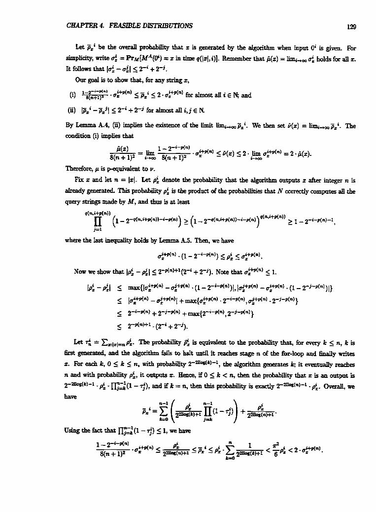
Let pzi be the overall probability that z is generated by the algorithm when input 0' is given For
simplicity, write 4 = Pr,&kfA(O') = z in time &I, i)]. Remember that ji(z) = lim,, ui holds for all z.
It follows that I& - ui[ 5 2-' + 2-'.
Our goal is to show that, for any string z,
By Lemma A.4, (i) impIies the existence of the limit liq- pZi. We then set 3(z) = liw- &' . The
condition (i) impIies that
Therefore, p is p-equivalent to v.
Fix z and let n = 121- Let p i denote the probabiIity that the algorithm outpnts z after integer n is
akeady generated. This probability p: is the product of the probabilities that N correctly computes ait the
query strings made by M, and thus is at Ieast
where the kt hqgality holds by ZRmma AS. Then, we have
Let i, = &rl=Rp$ The pro- 2 is eqoivaent to the probability that, for every k 5 n, k is
fkst generated, and the alpithm fails to haIt nntil it reaches stage n of the for-loop and 6naIly wxites
z. For each k, 0 I k 5 n, with probabilitp 2-a(k)-1, the algorithm generates k it eventnany reaches
n and with probability p:, it oatputs z. Hence, if 0 5 k < n, then the probability that z is an output is
2 - a ~ ( ~ ) - l - p: - r p z ( l - e), and if k = n., then this probability is d y T-(~)-' - p';- Chera& we
have
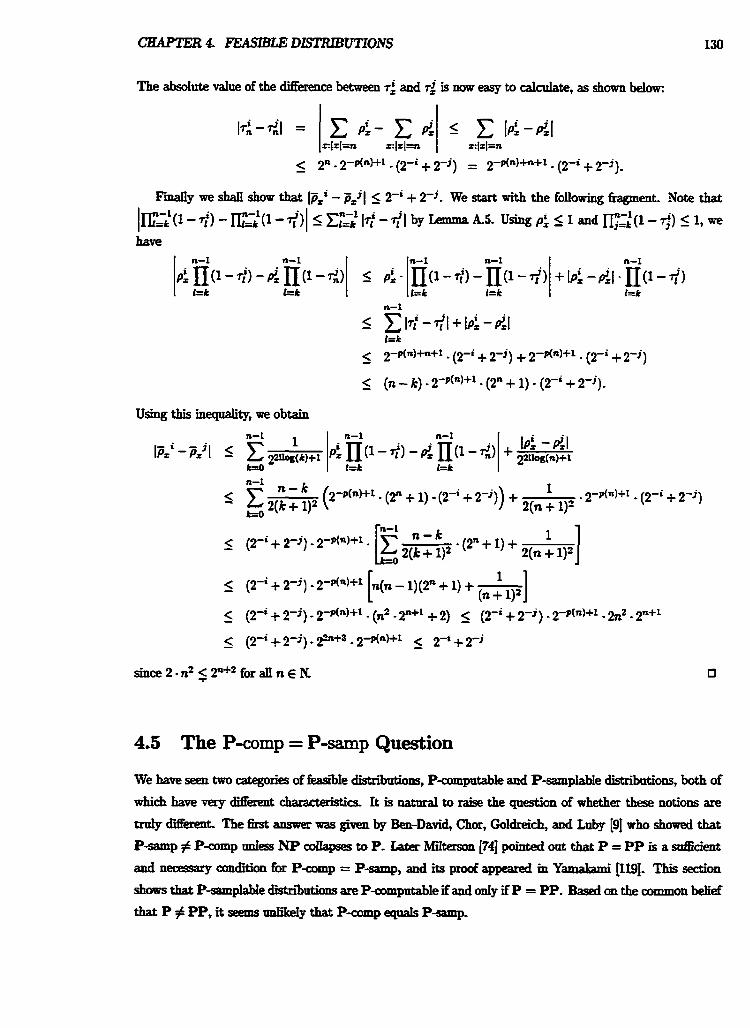
CHAPTER 4- FEASIBLE DISTRIBUTIONS 130
The absolute value of the dXerence between 7: and 7:: is now easy to caIcnIate, = &shown below:
Using this inequality, we obtain
n-I n-k ' 2(k + I)? (27(")+1 - (2n + 1) (2-i + 2-3)) + . 2-~n)" . (2-i + 2-11
ka 2(n + 1)'
We have seen two categories offeas'bIe distriins, Pcamputable and P-samplabIe distnions, both of
which have very di&ent -cs It is natnral to raise the queseion of w M e r these notions are
truly dSrent - The ht auswer was given by Ben-David, Chor, Goldrei4 and Luby 191 who showed that
P-samp # P a m p unless NP c o w to P. Later Miltemon 1741 pointed out that P = PP is a safficieut
and mxsary condition for P u m p = P-samp, and its proof appearrd in Yasnakami [IN]- This section
shows that P-sampM.de distributions are Pamputable if and onIy if P = PP. Based on the common beGef
thatP#PP,itseemsudikeIythatPoompeqnalsP-samp,
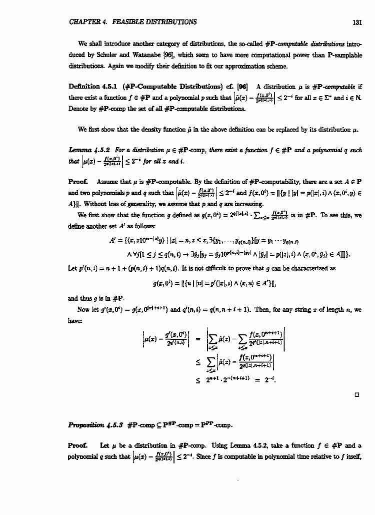
CHAPTER 4. FEASlBLE DLSTRIBUTIONS 131
We shaa intmduce another artegwy of distnbutiorts, the so-cahd #P-cmp&dk d i s t d d i o r r p inkc+
d u d by Schder and Watanabe 1961, which seem to have more computational pawer than P-samplable
distriiutions. Again we modifg their dehition to fit our appraodmation scheme.
Definition 4.5.1 (#P-Computable Di'bufions) d [86] A distribution p is #P-computobk if
thereexistafunction f E #~andapoiynomid~rnchthat [ f i ( z ) - ~ ~ l 5 ~ ' f o r a l l z € P' a n d i ~ N.
Denote by #P-comp the set of all #P-compntabIe d i s t r i i 1 1 ~ .
We bt show that the density function ji in the above W o n can be repIaced by its distribution p-
Proof'. Assume that p is #P-mmpatable. By the definition of #Pcomputabiityt there are a set A E P
and two pdynomidr p and q such that [~ (z ) - 1 5 Ti and f (2, Oi) = Il{p I lyl = p(lz[, i ) A (I, Oi, y) E A) 11. Wdout loss of generality, we w e e that p and q are increasing.
We bt show that the function g defined as g(r,oi) = ~ ( 1 ~ 1 ~ - &= &!&$) is in #P. To see this, we
define another set A' as foIlow9:
and thus g is m #P. Now Iet g'(z,Oi) = g(z7~lzl*') and q'(n,i) = q(m,n + i + 1). Then, For any stxing z of length n, we
have:
f (x, on++') 1 Xr) - E ~ C l z l r + i + l ) --lt -*
Proposition 4.5.3 # P a p E P - c o m p = PPPcomp.
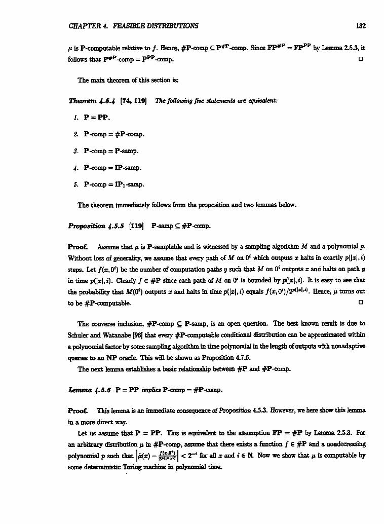
CHAPTER 4. FEASlBLE DISTRIBmONS 132
p is P-comptttabIe relative to f. Hence, #P-comp G P#Pamp. S i FP#' = fl by Lemma 2-53, it
follows that P#P-eomp = ppP-comp. u
The main theorem of this section is:
2 P-comp = #Pcomp.
3. Pcomp = P-samp.
The theorem immediately follows from the proposition and two lemmas below.
PmpmXon 4.5.5 [I191 P-samp C #P-comp.
Proof. Assume that p is P-samplable and is witnessed by a sampling algorithm M and a polynomial p.
Wrthout loss of generality, we assume that every path of M on 0' which outputs z haIts in exactly p(lz{, i )
steps. Let f ( z , 0') be the number of computation paths y such that M on 0' outpnts z and halts on path y
in time p(w , i ) . CIearIy f E #P since each path of M on 0' is bounded by p(Izl,i). It is easy to see that
the probabiIity that M(0') outputs z and hats in time p(lzl,i) equals f ( z , 0')/2~(l'1*17. Hence, p tnrns out
to be #P-computable. n
The converse inclusion, #P-comp E P-samp, is an open qnestion, The best h m result is due to
SchaIer and Watanabe [96] that every #P-compatabIe conditional distnintion can be apprmdmated within
a polynomiaI factor by some sampling algorithm in time polynomiaI m the length of outputs with nonadaptive
queries to an NP orade. This wiII be shown as Proposition 4.7.6-
The next lemma establishes a basic relationship between #P and #P-comp.
Lenuntz 4.5.6 P = PP implies P-comp = #Pcomp.
Roof. This lemma is an immediate amsequence of Propasition 4.53- However, we here &mv this lemma
in a more direct way.
Let us assume that P = PP. This is Bqrrmalient to the assfrmption FP = #P by Lemma 25.3. For
an a r b i i distn'bution p m #P-cmnp, assume that there exists a frmction f E #P and a nondeereasing
pdyn~mialpsuchthn 1jl(z)-=-l < ~ i f O r a l l r a n d i i ~ N~orwerhoathatpiscompdabIebp
some dacxmbktic 'Ihring machine in polynomial time
Define g(z, 0') = &= h(z,x, oi), where h(z, z7 0') = f (2, 0lZl+') - 2dbI*lrl+i)-dlrl*Ir[+i). Since g E #P, it foUows fiom oar assumption that g f FP. We then define the deterministic Thing machine M such that
M(z, 0') outputs g(x, 0') /2Q(~~~94, where q(n, i ) = p(n, n + i ) . Thus, M satisfies:
Hence* p E P-comp. This completes the proof.
In the foUowbg lemma, we prove that PI-samp = P-comp implies P = PP.
kmmu 1.5.7 [I191 If IPl-samp = Pcomp, then P = PP.
Proof. Let as amme that IPt-samp = P-comp: namely, for any p E P-camp and any onesne, phmest,
P-computable function f , the distniution wr is P-computabIe. We shall show that FP = #P, which is
equivalent to P = PP. Given a set A m P and a polynomial p, we set g(z) = (I{y E Hl21) I zy E .4}[1. We can assume without
Ioss of g e n e that p is strictly mmaihg. We want to show that g E FP. Now take the standard distribution v- and detine the onmne, P-computable function f as f o l k .
We also define the invertlily P-sampfabIe distn'bution q by f j = XzU-d(f-L(z)). By our assumption, r ) is
P-mmputabIe. Far the frmction g, we have the fo11owlng simple eqnatiox
where +(n) = n +p(n) + 1. Therefbre, g is P-cornpatab1e.
We comb'me the above Iemmiu and propositions to compIete the main theorem.
4.6 Universal Distributions
This section will iutroduce a slightly weaker notion of u n i d distn'bntiom, d e d prmioetsa.1 M-
bvtiorrp, and shows that there is no paniversaI distnhttion in P a m p , which is due to Sdder [95]. This
result is djfEcnIt to extend to the evert weaker notion of 00-universal distrrbtrticns.
We bqijn with the formal definitian.
Dehition 4.6.1 (7-nniversal djstriiations) Let 7 be a set of distributions and 7 a set of functions
from C to K@. A distniution p is called 7-uniaersd for T if
(i) p E T; and
(in) for every v E 3, there exists a fnnction t E 7 such that t(z) . ji(x) 2 1(z) for all strings x.
In particular, if 7 is the set of pbounded functions, then p is d e d parmersaL
The following theorem of Schuler [95] is a negative reply to the question of whether puniversd P- computable distributions exist for P-comp.
Thwnm 4.6.2 [95] Tlrere is no single P-mmputable disbibvrion which uup-dominotu dl P-computable
dkWutimOM Hence, no puniamal d i & h t h s Gdst in P-comp.
Proof. We shall show the contrapositive of the theorem. Pi we asnrme that p is P-computable and
dominates all other P-mmputable distributions. By Lemma 4.2.7(1), we can assume chat p is farther strictly
P-computable.
Using this p, we shall constrnct a P-mmpntable set which contains one string on each interval F, n E IK
We d e h e the function f fiom (0)' to E' by the foilowing procednrr:
begin deterministic aIgorithm for f input On
if n = 0 then output X
fork=ltondo
(As9amethat~=X) let L = {ale --ak-I~C"-k) and R = {@a2 - * - a ~ + r l F - ~ )
(4 iffi(L) > @(R) then let ak = 0 else let ak F 1
end-for
0UtpIlt a r e - - - &
end.
To check that f is P-computabIe is cay- By the above algarithm, f s;itisfies that [ f (0")1= n for all numbers
n E N Mareover by h e (:), the probability ji(f(On)) is at most 2-' became at each iteration ofthe f d ~ o o p ,
the probability of the set, either R or L, is reduced by halE To get the desired set, we set D = f (ID)'). Fi an a r b i i P - b i - i i e set B in E, and let A = DnB. This set A is inhite became, otherwise, the
difhxtce D - Bn D becomes an Su i te subset of z; this impIies that B is Rot P-immrme, a c o ~ c t i a n .
CHAPTER 4 FEASIBLE DBTRlBUTIONS
We next show that (A, p) E Aver(P, *).
Proof of CIaim She B E E, there exists a deterministic lhring machine Mo which computes B in time 2= + c for some positive constant c To compute A, let as dehe another &e N as follows:
begin deterministic algorithm for N
input z (say, n = 121) compute f (On) in polynomial time
if z # f (On) then *ect and halt
simulate Mo on input z and halt end.
The machine N actually computes A. NOW we must discuss the nmning time of N on input z. Suppose
that z 4 D. In this case, N needs pdynomial time. Next suppose z E D. h this case,
Hence, k.TiieN(z) is polynomial on p-average.
Let us define the dishiiution v as
6.uy(Oltl) if2 E D, C(z) =
otherwise.
Because p avpdominates v, Claim 6 implies (A, v) E Aver(P, *). To get a contradiction, we must show that
(-444 e A m p ? *I- Assmne that (A, v) € Aver(P, *), and we hail derive a contradiction- There aist a deterministic Turing
machine M and a polynomial q such that A is computabIe by M in time q on v-awrage- For every string z
in A,
T'imeaa(z) l n(lzl/~.uy(OIZ1)) 59(814(lzl+ U2)- Next we set p(z) = q(Sr(z + 1)') for aft z. Using this time bound q, the set -4 is mmitten as
A = ( x f M accepts A m time p(lz[) ).
This yields the P-comptttabiritg of R Smce A B, B is not P-immrme, a contradiction.
This completes the proot
Under the assmnption P = NP, Theorem 46.2 can be f i x r tk extended to O(f)-rmmezsat distribtttions, where f is any fanction in the set o(Zn), by a modification of the proof of Lemma 4-1 in [a].
Proof. Assume that P = NP. Assume that f E 0(2"), and p~ is O(n-universaI for P-comp. We note
that g(z) -W(z) > fia(z) hr some g E O(f) siuce p~ is O(f)-miverd Hence, W(z) 2 w- > for almost all z. Let 2-1 be the minimal string zr such that h ( z ) > 2-lfI for all z 2 i.
By de&tition, there is a poIynomiaI-time Thing m;uhine M which computes p ~ . For each z E I?, set
v(z) = M(z,@I=I~) and let i(z) = v(z) - v(z-). In general, v is not a distribution since D does not always
take a nonnegative value. Howeyer, we have fi(z) > 0 for all z 2 2-1. This is seen as fo1ows: for an z,
and thus, E(Z) 1 XI - 2-31rl > o if 2 - Now we de6ne a series of strings (zit i E N) as fobws. For convenience, write R(x, y) if y 3 21'1 and
~ ( y ) - V(Z) 2 21'1 k(y). IRt h the minimal string SU& that R(zi,zi+l) holds. This ~I&S since
otherwise, ii(z:) v(y) - I+;) < 2111 - P(y) for all y of length 2 2ifil, and thas P(y) > & for some
eanstaat c > I. For each integer n > lyj, t(y) > 2" &= = it a contradiction.
The set (zi [ i E N) is expressed by (y I 3m < ly13c0, ...,z,,, = yVi < m[zo 2 z - ~ and zi+l is the
minimal string such that R ( ~ , q + ~ ) l ) , and hence it belongs to NP. Since NP collapses to P, (zi I i E N) is in P. Note that m OD
Let tj(z) = c - 21'I(C(z) + 2-3[zl) if z E {zi[i E N); otherwise it is 0, where c is an appropriate w-tive
constant. The distribution q is obviody c o m p d l e in polynomial time, and thus, q E P-comp.
By our definition, for any constant d > 0, there c&ts an i such that
This is a con&-
4.7 Domination Relations and Equivalence Relations
As seen m Section 3.4, dominatioa relations can be viewed as an ''approJdmationn or a " r e d u c i i ~ between
two distriim*om m average-case oompkxity theory- If two distrriutions dominate each other, m this paper,
we call them "equivaId since they are dose to each other and have h o s t the same degree of mmplexiQ-
Ekpidence relations w a e &st discmsed in [%I using the terminology "appmxhation within constant
faaof to show the closeness of two conditional distnitxtions-
In this sation, we shaIl focrts on (average) po1yuomia-domination and equivalence relations and study
their properties
4.7.1 Condition f
Let us first redl that p pdominates v, denoted by v s p p, if&) -ji(z) >_ fi(z), where p is some pbotmded
fanctim Polgm- . dationsarensefulmaveragecase(pmp1exitytheorysincetheydowt
CXUPlEU 4. FEASIBLE DISTRIBUTIONS 137
change the degree of average ranning time: namely, provided that p pdominates u, if an algorithm requires
polynomial time on paverage, then this algorithm also runs in polynomial time on v-average (see Lemma
3.4.6).
Let us consider the following condition:
Condition I. Every distriiution m P-samp is pdominated by some distribution in P-comp.
The next proposition Iists severaI different conditions which are equivalent to Condition I,
PrapodiCion 1.7.1 The fotlorping amdiths ore equivalent.
I . For every p E P-samp, then ezis& a W b u t i o n v in P-comp such that p SP v.
Proof. Smce IP-samp C P-samp, (1) implies (2). By Lemma 3.4.13(1), (2) is equivalent to (3). We show
that (2) impIies (I). Assume (2). For every p E P-samp, take a p' f Ip-samp which pdominates p by
Lemma 4.48. Use our assumption to obtain a distriiution u E P-comp which pdominates pt- By Lemma
3.45(1), we have p v. 0
By Theorem 4.5.4, Condition I is derived from the assumption P = PP. Ben-David, Chor, Goldreieh,
and Luby [9j further shuw that if Cbndition I holds, then no strong one-way function exists. The foIIowing
is an important fiapent of their prooE
(iii) M o n t n p u t z ~ l i s f s d J e m e n t s 0 f f - ~ ( x ) ( w h e n e o ~ ~ f - ' ( z ) = 0 , M o u P p u t s O ) i n p o l y n o m i a l
Eime unless z E S.
ProoE Now let h({w, 2)) be (y, z) if w E {O)', It/ = [tal, z E x, and f (z) = y. Note that h is d d e h e d and phonest, Take a distriiution p detined as f m . @((w,z)) =-B-(z) - 2*-*(l~l)-~ if w E {O}rT or
else 0- CI-ly, phl E IP-p c Psamp Note that k ( 2 ) > *=. By our assmnption Condition I (as well as Proposition 4.7-1(2)), there are an q E P-comp and a poIyne
midrsuchthrrr(~)-$(*.I) >fihqb,%) krdlyandr- !%, breach)~ran(f),wehavefj(~,z) L $i$ fix some r, where s(n) = 4r(n]nk (n + n' + For each g, let C, = {z I fjb, z) 2 h, r,lr[ <_ 131 + klog lgl}.
Define S = {y I l[C,l] > q(lul)s(ly[), y € ran(f)). Clearly we have S G ran(f). We show that, for almost aIl n, [IS11 < &. Assume otherwise, and kt I/ be an element of S. la n = ly'l. Then we have
a contradiction. Define a k i n g machine M as foil- on input y, by a depth-first search, M computes alI
elements of C. if llC,ll < q(lyI)s(lpl) and lists aR elements z of C, which satisfy f (z) = y, or else M ontpats
0. Since f"(y) C', all elements of f-l(y) are printable in polynomial time if y E 3. This completes the
proof.
Using the bash-function technique of [MI and the ampIification technique of probabiic W g machines,
we on show that Condition I Ieads to the consequence that every N P set is nearIy-RP.
Theorem 4.7.9 [119] Asswne Condition I. Let A be OIQ set in NP. For eany polynomial p with
p(n) 2 I f o r d l n E N, there ezist a set D a d apol3pwmdal-time nnufomiz~ lbingrnaclaine M such that
D A, and, for each z, z E A- D implies RM [M (2) # A(z)] < 4, z 4 A implies PrM [M (2) # A(z)] = 0,
and Pr,,[z E Dl < &J fw almost all n. H- Condition I implies thut mery NP set i s nead*.
Proof'. Assume Condition I Take any set A in NP and any poIynomial q, and we wil l show that -4
satisfies the claim. There exists a set B E P such that A = {z 1 32 E ~ l ~ l [ z z E B]} . Let B, = {z I zz E B )
for each z. Assmne that there exists an increasing polynomial p such that Pr,[z E A] 3 &J for almost aI1
n since, otherwise, the theorem is trivial by &&g D = 0.
We take the set H%n+, of hash fanctiom. Let $ be the kth string in the set x 3 ~ ( " ) with respect to
the standard order. Dehe f (2) = l~$hh(y) ,+&~-~ if z' = zysEh and y E B,; otherwise W, where z € P, h E H,,*, and c = iIog(n). Notice that Is'] 5 If (d)I for all d, For each z, let g(x) = IIlf-'(z)ll-
For brevity, write t(n) = t + n + iIog(n) + (n + I)(n + ibg(n)) + n + do&).
For fixed k, and z of length n, let p b = Rhm[9(k4h~M+E~"-L) = 1 I h E Hn,n.tc, w E P*]. We
k t show that pkJ > & for almost all n. Now we 6.x k and 2, and assume that n = lzl is dcientIy
large and iIog(g(z)) 5 k 5 n. Consider the case iBzI[ > 0. The probability p ~ , is larger than or equal to
the probability over all hw that, for each y m B,, h(y)+& = w + ~ , and h k-distingrdshes y on Bz- Thus,
since logn i c <_ Iogn + 1, For the case [jBza = 0, cIearip p q = 1 since g(Iz$inatn+EO"-k) = I for dl k,
h, and w. This yieIds the desired result,
By Lemma 472, t h e are a set S and a pdynod-time ddeterministic Tming m;uhinn N which m- y(=)
ognkes 3 mch that S r a n 0 and IIS n fin)[ < . We dehe a randomized poIynomia-time
algorithm M as fonows
CHAPTER 4. FEASIBLE DISTRIBUTIONS
choose w and h at random (tu E P*, h E Hn,n+c, c = ilog(n))
let Result = 0
for all k (1 5 k 5 n)
nlll N On dk = ~ S ~ ~ W + ~ O " - ~
let Resuft F OR of Result and N(dk)
end-for
output Result and halt
end.
Cet &, = R h m [ l ~ $ l n r r + ~ ~ ~ ' ~ € S I w E IF*, h E Hn,nk], where c = ilag(n). Using this '&,,
we de6ne D = {z E Cf n A I 3k[irog(llBrII) 5 k 5 n A b r , 2 A 1x1 = n]). We wiI l show that
& n [ ~ E D] < A. Assume otherwise So, we have & > & for some k (dog(ll BJ) I k I n) and
z E Dn. Since
we have max(&, I iIog(llB,II) 5 k 5 n,z E P) < &. This is a contradiction. Therefore, Pr,[z E
Dl < A- Now our goal is to prove that (i) RM [M(z) = A(z) J > for all z in A - D, and (ii) &[M (2) #
A(z)] = 0 for all x $l A. This is enough to establish the theorem because of the worst-case version of
the Amplification Lemma Take any input z of Ieagth n. Let p, = Rh,[A(x) = ORL, N ( 4 ) ) [ h E
Hw,w E P*]. Note that the probabilitp P~M[M(x) = A(z)] is at least p,. .Qsslrme A(z) = 1 fot a
string z E n. Note that if dp E 3 and g(dF) = 1 for some K, then ORL, N(z-~) = 1. Hence,
For the other case A(x) = 0, N ( Z @ - ~ ~ ~ O ~ - ~ ) = 0 for all h, ut, and k; and thus, p, = 2. This compIetes
the proof. n
4.7.2 Condition P
PoIynomiaIdomination relations are useful but too tight to be considered an &ective measnre of "approx-
imation" or "reduabilitf between &sttibutions in a- complexity theory- Gurevich [36] h e r
introduced a weaker farm af domination relations by tegniring a frmction to be p-bounded "on the average"
FoHowing his dehition, we a h Condition I to allow the domination to be, instead, "polynomially-
bounded on the avemge+n
Condition It. Every distribution in P-samp is avpdominated by some distriiution m P-comp.
Obvioasty Condition I irnpIies Condition It, but we suspect that the the umverse impJicatioa may not be
provable afbmtidy.
In the case of avpdominntions, we no 10- prove a similar equivalence as in Proposition 4.7.1. The
fo110wing claim is the best possl'b1e so far.
Proof. By Lemma 3.4.13(2). 0
To see a collSeQtlence of Condition It, we need a notion of Ph, and its strnctnral properties- These
wil I appear in Section 7.5-
We & see the gap between the two notions: #P-camputabiIitp and P-samplability- The next proposition
was shown by Schuler and Watanabe [96] for conditiod distributions- We modifp their proof to accomme
date inhihe distriiutiom. To descni the proposition, we need the notion of *table samplabii of
distnLbutions*
1. A distriiution p is ~ & s m n ~ ~ o ~ c if there exist a randomized o d e ntring machine M, a deterministic
'Ilning machine N, and a pdGomiaI p such that
(i) M with orade A generates p m time poIynomial m the Iength of outputs; and
(ii) on input (Oi, s), N lists all query strings of Q(M, A, Oi, s) m polynomial-time (without any queries)
if s is a code of a computation path given by M wi th orade A on input Oi.
2 The notation Pi-samp derides the co1Iection of all P&axnPMIe distriintio~~~, and Pen-samP denotes
the anion of alI distributions in Pt-samp for any A E C.
ProoE Tahe an arbitrary #P-computabIe distnibntion p- There Bdst a frmdon f E #P and a polynomial
q such tbat [fi(z) - [ 5 2i for an z a d i E N Wrthout loss of g e n e , we can assttrue that this q
isinaxsting. ~asirn~~icitp.,let$,=~~~fmeachi~~ since f €#P,thereexistsasetA~Psuchthat
f (2, 0') = l{w E ~dl*l*) I (06,x, w) E A}[ for dI 2. For brevity, let & = {(w, z) I m E A (Oi,x, w) E
A). Let$ ={am1 (x,w} € & A l z l = n A k l =p(n,i)). Noteby Lenma A-4 that /<-oil sr'+?-j forallidegersi,j>O.
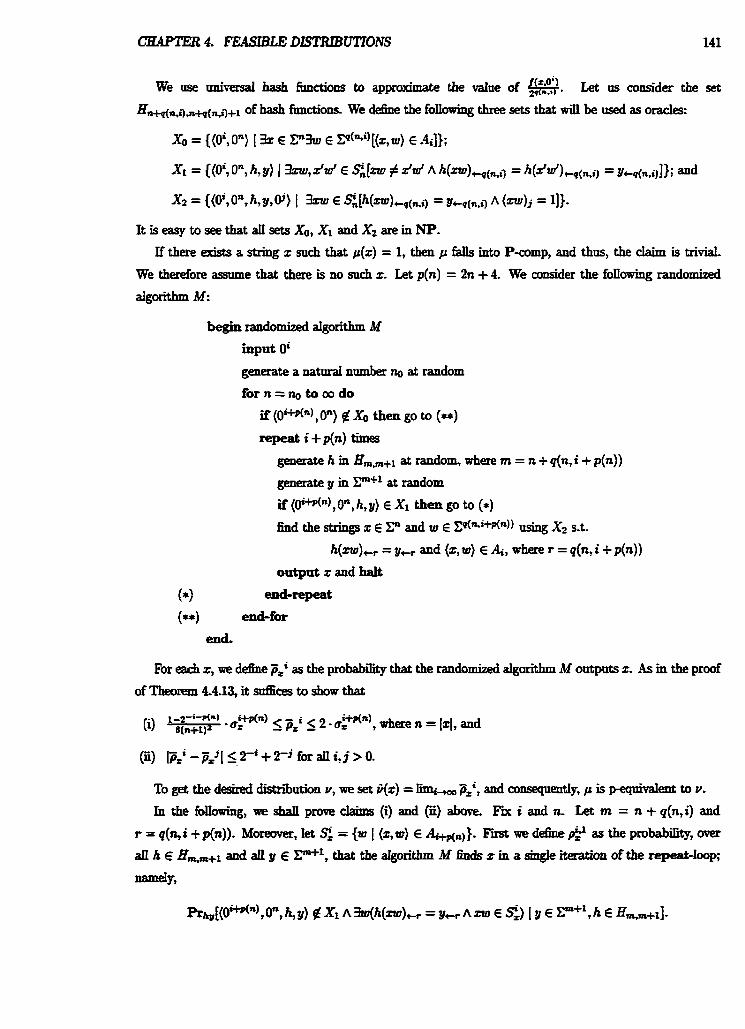
CHAPTER 4. FE.4SIBL.E DLSTRlBUTIONS 141
We use u n i d hash functions to appmxhate the value d w. Let us consider the set
Hn+4(Ri),n+o(Ri7+l of hash frmdion~. We dehe the following three sets that will be used as oracles:
begin randomized algorithm M input 0'
generate a natural number no at random
for n = no to oo do
if ( ~ ~ + p ( ~ ) , on) 4 Xo then go to (**)
repeat i + p(n) times
generate h in Hm,m+l at random, where m = n + q(n, i + p(n))
generate y in P+' at random
if (0'+P(~),0",h,y) E XI then go to (*)
6nd the strings z E FF and w E CQ("'+p(")) us@ X2 st.
h(m), = y,, and (2, w} E Ai, where r = q(n,i +p(n))
output z and halt
(*I end-repeat
(**I end-fm end.
For each z, we W e F,' as the probability that the randomized algorithm M outputs z. As m the proof
of Theorem 44.13, it d c e s to show that
(ii) pXi - p,J[ 5 2' + 2-3 for all i, j > 0.
To get the desired distribution v, we set O(z) = I&- a', and amseqnentIy, p is p-equhdent to v.
In the fo1Iowiag, we shall prove cIahs (i) and (i) above E l i i and n- Let m = n + q(n,i) and
r = q(n,i +p(n)). Moreover, Iet !$ = {w 1 (qw) E &,)). Fm we d& & as the pmbabihy, over
aU h E &,,,+I a d aIl y E C"+I, that the algorith M h d s z in a single iteration of the repeat-Imp;
d y 7
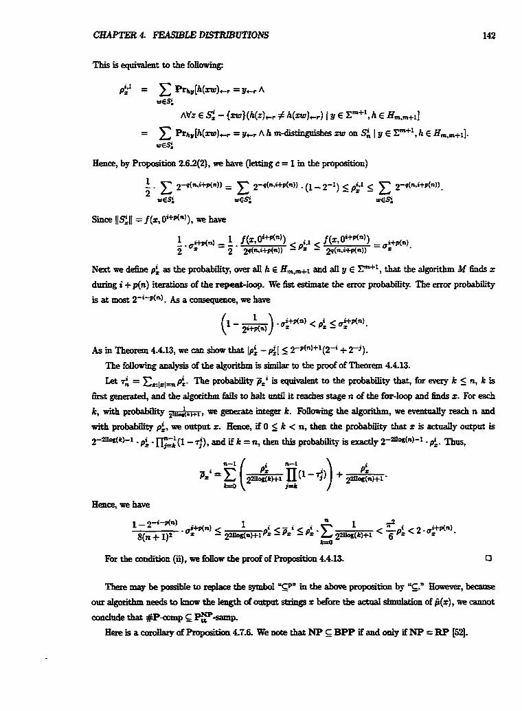
This is equivalent to the following
Hence? by Proposition 262(2), we have (retting c = 1 in the proposition)
Next we define p i as the pmbab*, over all h h HB,,+l and all y E F+', that the algorithm M hds s
dnring i + p(n) iterations of the repeat-Imp. We 6st estimate the error probability. The error probability
is at most 2-i-p(n). As a consequence, we have
As in Theorem 4.4.13, we can show that Ip: -dl 5 2-~(~)+'(2-' + 2-9.
The following analysis of the algorithm is similar to the proof of Theorem 4.4.13.
Let 2 = The probabdity pZi is equivalent to the probability that, for every k 5 n, k is
6rst generated, and the dgodthm faiIs to halt until it reaches stage n of the for-loop and finds z. For each
I , with probability hr we generate integer k. FolIowing the algorithm, we eventually reach n and
with probabilitp p',, we ontpnt z. Hence, if 0 k < n, then the probability that z is actuaJly outpat is 2-*(k)-1 - p; r[$(l- $1, and if k = n, then this pmbabi i is exactly 2-m0g(n)-' . p i . Thus,
Hence, we have
For the condition (ii), we fdIow the proof of Proposition 4-4-13. 0
There may be possibIe to replace the sgmbor T'' m the above proposition by "CF However, because
our algorithm needs to know the Iength of oatput shings z before the actaaI simaktion of P(z), we cannot
condude that #P-comp G F - s a m p
Here is a ooroIlarp of Proposition 4.7.6. We note that NP BPP if and only if NP = RP [521.
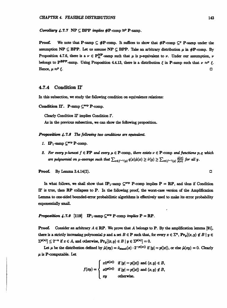
Cod- 4.7.7 NP BPP iinplics #Pamp 9 P-samp.
RooE We note that P-samp E #Psomp. It saffices to show that #Psomp EP P-samp under the
assamption NP E BPP. Let us assume NP E BPP. Take an arbitrary distribution p in #P-amp. By
Proposition 4-76, there is a v E pY-samp such that p is Peqtdpalent to v. Under our assumption, v
belong to ~ ~ ~ ~ - s a m p . Using Proposition 44.13, there is a distn'bution { in P-samp sa& that v np <. Hence, p =P <. I3
4.7.4 Condition II'
In this subsection, we study the foIIowing condition on equivalence relations:
Condition II'. P-samp caw P-comp.
CIear1y Condition II' b p k Condition It. As m the previous subsection, we can show the following proposition.
Proof. ByLemma3.4.14(2). 0
In what foIIows7 we shan show that IP1-samp cav P-eomp implies P = RP, and thus if Condition
II' is true, then Re cokpses to P. In the totlowing proof, the worst-case d o n of the AmpIihtion
Lemms to one-sided bounded-error probabMc algorithms is &ectmely used to make its error probability
exponentianyd 0
P l p p o ~ 4.7.9 [IlS] IP1-samp c- P a m p i r n p b b P = RP.
Root Consider an arb'rtrary A E RP. We prove that A belongs to P. By the amplification lemma [91],
there is a skidy increashg polynomial p and a set B E P such that, for every x E F, Pr,[(x7 g) 6 B [ y E
5 2- if x E A, and otherwise, R&, y) E B I y E = 0.
Let p be the distn'bution d&ed by fi(ly) = fi-(z) - 2-P(lZl) if ly[= ~ ( 1 ~ 1 ) ~ or else i(zp) = 0. CIearIy
/r is P-comptrtabIe- Let
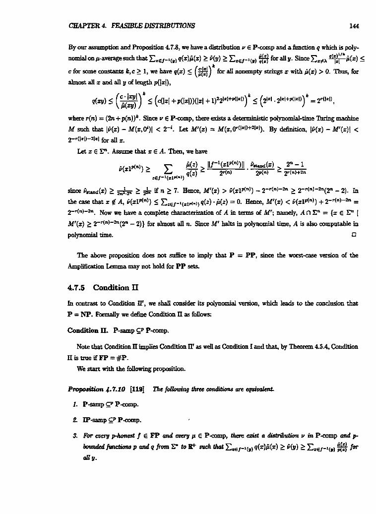
CK4PTEU 4. FEASIBLE DISTRIBUTIONS 144
where r(n) = (2n +p(n))l. Since u E Pcomp, there exists a deterministic polynomial-time M g &e
M such that Ifi(z) - M(z,Oi)l < 2-'. Let M'(z) = ~(z,0~(l~l)+~l'1). By definition, It(z) - Mr(z)l c 2-f(l.+l)-2lrl for 2.
Let z E C. Assume that z E A. Then, we have
since V-&) 2 & 2 & if n 3 7. Hence, M'(z) > fi(zlP(")) - 2-r(n)'2n 3 ~ f ( " ) - * ( 2 ~ - 2). In D, q(z) fi(z) = 0. Hence, Mr(z) < fi(zlp(")) + 2'r(n)-k = the case that z B A, fi(z1dn)) I Cze f - t ( r l ~
2-fln)-&. Now we have a complete c k a c m k t i o n of A in terms of Mf; namely, A n C = (z E C (
Mr(z) 2 2-r(n)-2n(2n - 2)) for almost all n. S ice M' halts in polynomial time, A is aIso computable in
polynomial time. D
The above proposition does not d i c e to imply that P = PP, since the worst-case d o n of the
AmpIification Lemma may not hoId for PP sets.
4.7.5 Condition I1
in contrast to Condition Ll', we shdl consider its polynomial --on, which leads to the mnclasion that
P = NP. Formany we dehe Condition II as f o U m
Condition IL P-samp S p P-comp.
Note that Condition 11 implies Gmdition II' as welI as Condition I and that, by Theom 45.4, Condition
IIis trueif FP =#P. We start wi th the following proposition.
CHAPTER 4. FEASIBLEDISTRIBUTIONS 145
Proof. By lemma 3.4.14(1). 0
B y Proposith 4-7-10, we can replace P-samp in Condition II by a d e r set IP-samp. At the end of
this section,weshallseet&t wealsocanrepIaceP-samp by alargerset #P-comp.
Next we shall prove that Condition II yields the consequence that NP collapses to P. We first strengthen
Lemma 4.7.2 under the assumption that P-samp is pincluded in P-comp.
Lemma 47.11 [I191 Assume that P-samp EP P-eomp- For m y set B E P and any polynomial p, let
SB = {Z I IIBJ <p( l z l ) ) , mrhereB, = {z E ~ 1 ~ 1 I xz E B). There exists a detffmmutre * . .
%ing machine M such that, f m e a c h n ~ N, M on inputt inSgnP listsdlckmentsofB, (whemuerB,=0, M outputs
0) in polynomial time.
Proof. Assume that P-samp CP P-comp. We define a phonest function f as follows: f ((w, yz)) = (ly, z)
if w = s p l for some k, [zl = 191, Izl = k, z & z, and y2 E B; otherwise, (Oy,z). Let fi((ur,z)) =
Vstolrd (z) 2- 21108(Izl)-~ if w E ~ ~ q ( l ~ l ) , or else 0, where no&n) = llog o no&).
Since p,-z E P-samp, our assumption ensures that there are an q E P-comp and a poIynomiaI r such that
r(lyl+Izl).fi,-t((y,z)) 3 i((y,z)) 3 fip((y,z))/r(lyl+lzl) for ally and z. Denote by D, the collection ofz 2-at#[
s d that 2 E land E Br If y E Ss, then llDlill 5 ~(1~1)- Note that fif l((y7z)) = ~&.-2u*nn.l,+~ 9-21.1
For h p h d t p , let q(n) be Zllog'(n) + 2110dh) + 2- Hence, ri((ll, 2)) 2 r(l jl.mlyl, 8 DI. # 0. Let N be a polynomiaI-time Turing machine which computes ij. Let d be the minimal positive in-
teger such that 3 - t(2n) - 29(") 5 2d.no6(n) for almost all n. We define a new machine N' as Nr((y,z)) = ~( (p , z), @lH.uOdlpl)+f ). Hence, Nf((ly, r)) > ri((lg, 2)) - T ~ ~ ~ ~ - ~ - ~ O ~ J J T ~ ) - ' > s- For eK6 y E p,
2.2'" let C, = (2 I N'((~Y, 4) > -1 I4 5 n). 2-2Iv1
We note that if r E C,, then fj((ly,x)) > wi. For each n > 0 and any y E SB n C,
Therefore, IIC,[ 5 Pwn)-0(") - r(!h)* . C1 11D3,-1[ 5 2%(2n)2p(n)3n.
Note that B, E C, if y E SB. Smce C, is printable in poIymmial time, all elements of B, are printable
in po1ynomial time. This completes the proof. U
ProoE h us assame that P-samp P-comp. Let A be an a r b i i set m NP. we shall show that
A E RP sinceP =RP byPsoposition4-73. It d c e s to consideraset A d t h e f o r m A = {x [ 3 E
!F.lx1[~€ ~ 1 ) f o r s o r n e B ~ ~ - Let B , = ( X E X M IzzEB) .
Letnsd*
CHAPTER 4- FEASIBLE DISTRIBUTIONS
Sice B E P, B is also in P. Let Sg = {d ( [&(f I), where Be = { i E zI"~ ( ii E b). We define pk, = P r ~ [ z s ~ h w + + ~ * ' ~ E Sg = 1 1 h E H%,+, A w E Cn+q. We first show that, for
almost a11 n and all z with (IB,I( > 0, pk, > &. Now 6x k and z and assume that n = [zl is sufficiently
large, and ilog(((B,(I) 5 k I n. The probabilitg pkT is at most the sum of the probabilities over all strings
hw that, for each z E B,, h(z)+- = w++, and h k-distingrrishes z on B,. Thus, we have
We apply Lemma 4.7.11 to the set Sh, and we obtain a polynomial-time deterministic Trrring machine
N which recognize Sg. We define a randomized pdynomid-time algorithm M as foUows:
begin randomized algorithm hi
input z (say, n = Izf)
choose w, h at random (w E P, h E IThnfc, c = ilog(n))
let Resutt = 0
f m a l l k ( l < k < n )
ram N on dk = 6 h . p
let R d t = OR of ResJt and N ( 4 )
end-for
oatpat Result
Oar goal is to prove that R M [ M ( x ) = A(z)I 2 6 br almost all x. Take any input z of Iength n.
Let p, = Pm,[A(z) = ORL,N( ik ) ) ( h E Hwk, w E PI. Note that the probability PrM[M(z ) = A(z)] is at Ieagt &.
A(z) = 1. Note that if 0 c gb(dp) < 1 fm some K, then ORL1N( ik ) = 1. The probability
pt = P f k [ A ( x ) = ORLIN(z$) h f H,,*, w E Cn] is at least the smn of the probability over an htu that, for each z E Bz and for some k with IIog(gB(z)) I k I n, h(z)+- = W+H, and h k-distinguishes
z on B,. Hence, p, > gs(z) ( I - F) -Z(W 2 (1 - r E ) Z e 2 For the other case A(z) = 0,
N ( ~ $ I n o ~ 0 " ' ~ ) = 0 for a11 h, w, and k; thns p, = I. This completes the proof. 0
Prod IIf - part) This is obvious a c e #f-comp 1 P-samp by Proposition 45.5-
( M y if- part) Assume Conditi011 IL By Theomin 47.12, we have P = NP- In particnlar, NF _C BPP. By Corolbtp h7.7, evexy #P-a>mpntabIe d i s t r i i is pegnmalent to some distriitrtion which can be
sampled by a randomized 'Jhting machine in time polynomial in its output
4.8 Other Topics
There are several intriguing distniutional issues which are not discussed in this chapter. Here we present
two diffetent approaches.
Ranking Distrr'btttions. Reis&& and Schindehauer [84l introduced a new type of distributioxs that
dows precise compIdty drrcsification of distriiutional problems. They called such diseibutions mhbk
G i a distribution p, its m n b g jkctirn rankP(z) is defined as rank&) = 11 {I I P(z) 2 fi(z)}11. A distriintion p is p o E y n d I l g mr3cbfe (P-fankable, for short) if the fnnction rankP is oneone and P-
mmputab1e [84]. Let P-rank denote the collection of all P-rankable distributions. Note that, for every z,
raakp(z) - /i(x) c, B(z) = 1- This implies that rankP(x) 5 & unless B(z) = 0. In particular, if p is
positive and supportivet log(rax&,(z)) 5 p(lz1) holds for some polynomial p.
For simplicityt let t be a strictly increasing fanction on P. A function f from X* to N is called t-menye
with respect to rankP if x. ,,,,, c+ 5 rn for any number m 2 0. We say that a dkiiution
(D, rankP) is solvable in maoge p v 2 ~ time with Rspcd to mnkaMQ if there exist a p o l y n o ~ p and
a det ' ' t ic 'I\lring machine M computing D such that h.TiieM(z) is gaverage with respect to dP.
Watanabe [I141 pointed out the foIIowing relationship between Psomputable distributions and P- ranlgble distributions. Take a distriiution p satisfping log(I.ankp(x)) 5 [zld for some constant d > O.
Roof Sketch, Assume that f is polynomial on &-average Then we can take constants c, k > 0 such
that, for a11 m > 0,
For any m, let X, be the set of strings z such that T L - I < rankP(z) 5 P. Now we can daim that
there exists a constant e > 0 such that, for any sufTiaently Iarge m,
To show the daim, let X'& = {z E X, I f (z)'fk/W 5 m4) and XE = { x E X, I f (z)'fk/[d > m4). For
On the other hand, the set Xk &i&es that
We note that Belanger and Wang [6] show that X F W P is in Aver(P, *), then any problem in Dist(NP, P-rank)
is solvab1e in average po1ynomial time with respect to rartkabiky.
IndistingaisbabiLity of Distri'bations. Another topic is the complex?y of &triibutioxts. We &dl
f o ~ m Meyet's termino1ogy [q. Two clistriions p and v are called %tatistically indistinguishabIen if
lim,- nk ,,=,, IA(z) - = 0 for d 6 E N p and v are "circuit indistingnishabten it,
for a~ f;unities of polynomial-size circuits C = {Cn}n.N, Lim,- nkl Cn(z)&(x) - A(z))l = o for aD k E & a d uaIgorithmicaIly mdistingnishablen if, for dl polynomial-time probabilistic 'Ihrhrg machines
M, ~im,- nkI & , l , R ~ [ M ( ~ ) = I] - &(z) - S(z))l = 0 for dl k E N Meyer [73] show the foIIowing separation d t :
We do not intend to indude any p d of this theorem. The interested reader may refer to [n].
Chapter 5
Average Polynomial Time
Reducibilit ies
5.1 Introduction
In the early 1970'~~ Cook [a], Karp [49], and Levin [59] took a pioneering step towards the dadication
of the hardest problems in JW. They introduced notions of resourcebounded reduabiies amrmg NP
problems. The idea of these reducibilities is as foflows a problem T is recognized to be at least as lrmd
as auother problem S if the prob1em S can be transformed into the problem T m polynomial time so that
if T is solved easily, then so is S. The problems "hardestn m this sense among NP problems are d e d
NP-d~npkte TypicaI NPuuupIete problem are s- problem, Emniltonicm eireuit probiem,
and trno* sateman problem For more NP-complete problems, see [26J.
In averagecase complexity theory, Levin bas introduced a similar notion of polynomial-time many-one
reduciiihty among d i s t n i a t i d decision probIems and showed that the randomized bottuded tiling problem
is one of the hardest problems m Dist(NP, P-comp). His reduction from a dis tr i iut id problem (-4, p) to
another distn'butional problem (B, u) reqah a polynomial-time many-one reduction that maps set A to set
B and employs a so-ded dorninaEion condifion betwen p and v. This domination condition gnarantees
that instances occuning with high probability are mapped by the reduction to instances oecnrring with
high probabw. This reqnirement is d in Levin's theory of amqpase NP-compIeteness in otder
to ertsme the dosure property of a cIass under these reductions- At the same time, it makes completeness
prooh of given distributional problems diEcnlt to toeve.
SiLevin'sdiscloverpofa~NP-completeness, researchershaveintroducedseveralinteresting
notions of reducibilities into the theory of awmpxse NP-completeness- We will review these redncibitities
m this chapter.
Seaion 5 2 will introduce two ofthe most important reducibiIities among distributional decision pbIems:
determiaistic mmy-one reducibility and TWng reducibihy- Levin [60j introduced a notim of mmy-one
reduciiility, and the notions of deterministic 'Ihring reduablitp and mdom many-one reducibility were
introduced and studied in [60,9,44,12,96]. Other reductions of interest are logspace maLly-one reductions
[9] and logspace many-one reductions which are phonest [321.
Section 52 will introduce detamirristic many-one redtlcibility and po lpmi - t ime is~llorphim among
distn'butiond decision problems, and then the notion of deterministic ZWng reductbility will be introduced.
The Thing reducib'i wiIl be partidarly used to build the average polynomial-time hierarchy in Chapter 6.
In Section 53, we shall &Ti severaI many-ate complete problems for Dist(NP,P-comp). We first
show that the randomiEed &mdd haking p b h is comp1ete for Dist(NP,Pcomp), and then the other
distn'butional problems are shown to be po Iynody isomorphic to this problem.
In Section 5.4, we shall discass several incompleteness d t s , The choice of distributions is important
when one attempts to prove that some distnLbutional probkm is complete for Dist(NP,Pcomp). Some
distriitltions are such that their associated distriiukional problems m o t complete for Dist(NP, P-comp).
For exampIe, fiat distrr'butions aud sparse distributions have this chackm& . . c.
Flat distributions are often arise in graph-dated decision prob1ems; however, no distributional prob1e~1~
with h t distriidions become complete for Dist(NP,P-comp) tmless EXP = NEXP. V d t e s a n and
kvin [I061 proposed new reduction which uses random coin tosses. In Section 5.5, we shaII mintduce
probabilistic reducibility, d e d botcnded-enw prr,ba&Wk trufA-trrbk dvcibility.
In Section 5.6, sone structural d t s are shown.
Major Contrr'butions. Some d t s in Section 5.6 are from Wt11e.r and Yamakami [97l, and Section 5.5
provides a series of new resnltts. More precisely, the following are the major contn'butions to this chapter.
Theorem 5.45 shows that sparse distriiutions fail to make the corresponding distri'btttional problems
pm-compIete for Dist(NP, P-comp) dess P = NP. Lemma 5.5.5 Is a r e l a th id version of the AmpEcation Lemrna (Lemma 3.5.31).
Lemma 55.4 shows that skew avbpptt-rednaiititg is closed under pm-reductions; namely, if (A, p) is
pm-reduaIble to some distn3utional problem which is skew avbpptt-reduui1e to (B, v) , then (A, p) is skew
avbpptt-reduaile to (B, v) . Lemma 5-52 shows that, if (A, p) is skew avbpptt-reduciiile to (B, u), then there exists a pmbIern (B', J)
which is pmredtxu'b1e to (B, v) such that (A, p) is skew avbpptGredu~'b1e to (B', r / ) via a reduction machiae
which queries strings of length greater than the input size.
Proposition 5.6.5 shows that, for every recnrsive set D not m P, them exists an incomparable pairs with
respea to s. Theorem 5.53 shows that the diskiiutiond bounded halting probIem with a fIat distniution is bpptt-
comp1ete for Dist(NP, Pump).
Proposition 5.5-7 introduces a new d t regarding the transitivity of avbpptt- and bpptt-redua'bilities-
5.2 Deterministic Reducibility
Reduciiility is one of the most important took m computatiord complexity theory for assessing the d-
ative comp1- of two given problems, This section wiIl present the formal definitions of deterministic
reduciiilities arnong distributionat decision problems and develop their basic s t r a c t t d properties.
5.2.1 Many-One Reduu'bility
In this section, we shall formally introduce two notions ofmarty-one reduci%Sties: potpMILial-time many-one
and auerrrge potynomicJ-m many-one reduciiihies.
A many-one reducibility among distributional decision problems requires mappings among sets and con-
straints among distniutioons. Let us consider the worst-case polynomial-time many-one reduction f between
two sets A and B. The reduction ensares the relationship A = {z I f (x ) E B). If B is computed by a
machine M in polynomial time, then a simple algorithm N which fiRt computes f(z) and then simuIates
machine M on input f(z) amtany witnesses the P-computability of A. Now we switch h m sets A and B
to two distributional decision problems (A, p) and (B, v). Suppose that (By v) is computed by a machine M in polynomial time on u-average; that is, Az.TiieM(z) is polynomisl on u-average The above dgorithm N
needs at most O(Tmef (2) + TimeM (f (z))) steps, where Timef (x) denotes the time teqnired to compute
f (z). To g~arantee the average polynomial-time comptrtabiIity of (.& p), the dues i(2) and P(f (2)) must
be dosely related This Iast requirement is called a "domination condition" for f.
Fm recdl that the notation vrl denotes the d M t discr'bufion defined kom u and f by its probabiliw
(2) = P({r I f (2) = 2)) for each z.
There are several possr'bilities for domination conditions. Here is a list of popular conditions:
(ii) C(%) 2 zw(p) # for some pbotmded function p.
By Lemma 3.411, condition (in) is equivalent to the condition that p S P 7 and u 2 r)/-~ for some semi-
distribution q, and thnq @) implies (5). By the pmof of Lemma 3.413, (i) implies @) if f is pbotmded
Assume that f is phonest and pbotmded- By Lemma 3-4.12, (ii) implies (iii), and by Lemma 3-4-13, (Z)
implies (i).
In most cases, the choice of domination condition is relatively harmless when one proves atrerage NP- completeness of a given distn'btxtional decision pmbIem, beeatlse most known complete problems are isomor-
phic. In this thesis, however, we shalt use the weakest daminattim condition (ii).
De_&lition 5.2.1 (PoIynodakTime Many-One Reductions) [q Given two distn'butiond decision
pmbIem~ (A, p) and (B, v), (A, p) is edkd p d p m i d - E i r n e nurngonc M l e (p-m-reduu%1e, for short)
to (B, v), denoted by (A, p) Ip, (B, v), if there ez&s a firncticm f such that
(ii) (Domination) p * r), and P 2 for some semi-distn'bution q.
The hc t ion f is d e d a poled-Eime my-one r e d v d h @-m-reduction, for short) jbtcth and is
said to reduce (A,p) to (B,v).
Gurevich [3q expanded many-one redua%iEty by dowing a many-one reduction to be polynomial on the
average. This reduction is known as memge polynonrid-time manpone red~bi l i ty-
Dehition 5.23 (Average Polynomiall-Time Many-One Redo&*ons) [36] Let (A,p) and (B, u)
be two distributional decision problems. (A+) is mmge polyrwmid-time mapone reducible (avpm-
reducibIe, for short) to (B, u), denoted by (A, p) (B, v), if there exists a hc t ion f such that
(ii) (VaIidity) A = (x I f (2) E B); and
(6) (Domination) p 5- q, and P 2 ijrl for some semi-distriiution q.
The condition (iii) on the distriitrtions m the above dehition is simply called the dmninahbn d o n
for the reduction fimction f.
Om definition basicatty foIIows Gorevich's domination condition. Gurevich [36] d&ed his many-one
rednability as follows: (A+) pdynomiaIIy rnatly-one reducible to (B,u) if and only if there erdsts a P-
computab1e function f and a distn'btrtion r) and a set C C_ {z I P(z) > O) such that f reduces An {z I b(z) > 0) to B, p SP I), and GrC(y) = +(y) for dl y, where urc is the &tri'bution satistying that
f
The fo11owing lemma is -0-
Proof. Let us consider the id- fimction f, ie-, f(z) = x for ail z. The assumption p s p v is
eqnivalent to fir, P v- Hence, (D, p) is pm-reduci'bIe to (D, v ) via f. a
The fdowhg lemma is a d tod for proving that the composition of fimctiom is polynomial on
P-average
CHAPTER 5- AVERAGE POLYNOMIAL ZlME REDUCIBEJTES 153
Roof. .4snre that p 5- q and P 2 for some semi-distribution rl. Asmme that f is pf on
waverage, and )LZtJg(z)I is pg on paverage* where pf and p, are appropriate increasing polynomkk Sice
p 5- qt there exists a ftrnction p that is q on paverage, where q is an increasing poIynomial,
p(z) - ij(z) > ji(z) for all 2.
Fii r 2 I. Let us define
where co = j o g(X). Obvionsly s is a poIynomial, and it f o h that
for all strings 2. Let D, = (z E E 1 p ( z ) 5 q(Iz1- 3r) 1g(x)1 5 ~~(121-3r)) . We then have
By om assumption, the first two terms are bounded above by 1/3r. For simplidty, Ilet T, represent the third
tena It &ces to show that Tr 1/3r m the rest of the proof*
Take an arbitrary z E D,, say Izl= n, and let t = g(z ) . I f f (g(z)) > s([z[ - r), then f (2) > pl(p9(3m)
6q(3m) - m2). Since Izl 5 pg(3m), we h a . j(r) > pt(lrl 6q(3m) - m2). Moreover, it holds that j(z) 5 q(3m) - ij(x). Hence, T, is estimated as fobws:
Smce ijg* (2) 5 P(r), we conclude:
In the following, we demonstrate some d the basic properties of manjr-one redua'bilities
CEIAPTER 5. AVERAGE POLYNOMLtll; TIMI3 REDUCIBILITlES 154
Proof. (1)-(2) Clear h m the definitions.
(3) We shaU show the transitivity of SF. First we amme that (AI,k) s k (A2,p2) via fl and
(A?, CI?) (A3, p3) via f2- The domination conditions for fi and f2 ensute the eciaence of two semi-
distributions % and % such that p1 SaVP %, M Saw m, h 2 141 (f;-' (z)), and ir3 2 k.ij2(K1 (2)).
Since f~ and f2 are mafly+ne reductions, we define f as f (z) = f2 0 f~(x). Then function f reduces Al
to At. In the rest of the p m c we s h d check the domination condition for f.
h pl 5 P Q, it follows that there exists a function m, which is poIynomial on pi-average, satisfying
that m (x) - fjx (z) 2 f i ~ (z) for all z- there is another function p2 that is polynomial on p~average
such that pz(x) -%(z) 2 fi2(x) for all x. We assume without loss of generality that m(z) 2 1 and ~ ( z ) > 1
for aIl x.
Let as d e h e p(x) = pz( fI (x)) gt(s) for alI x. Notice that p is polynomial on pl-average. To see this, we first note that pz o f~ is po1ynomial on paverage by Lemma 52.4 because k.l fl(z)/ is polynomial on
pl-average and pz is po lynod on waverage. Since is also polynomial on pi-average, p ttlrns out to be
polynomial on pl-average. Set tj(z) = jh(z)/p(z) for an z. Cleariy 7 is a semi-distriiution.
For any string y in ran(f), letting D, = G'(~) ft ran(fi), i t foIlows that
For each string w in ran(f~),
and thus, we obtain that tj(w) 2 tj(C1(w)). Hence,
Theorem 5.2.6 Let C E {P, NP, RP, BPP, PSPACE). The waage compCaiCy c h Aver(C, *) is dosed
domnmard anda I~-redodions.
Roof. We begin with the dosnre property of Aver(P, *) under S~-reductions. Let us assume that
(Ap) (By v) via f and (B, v) E A-, *). Note that f is computabIe m time poiynomid on p
merage. Let M be a dderministc 'Ihring rnarbine which wrnputes B in polynomiat time on waverage
We can construct another deterministic Thing &e N which, on input x, computes f (z) k t and
then simdates M on input f (x). This madhe N actually computes A, and its running time on input x
needs at most
c - (Tmef (4 + T = e ~ ( f (2)) + 11, whm T i i ( ~ ) denotes the time reqaired to compute the d u e f (z), and c denotes some appropriate
constant independent of z.
Notice that k . i f (=)I is polynomial on paverage. Since Xz..TiieM(x) is polynomial on v - a v e , the
domination condition for f implies, by Lemma 59.4, that kT"eM(f (z)) is also po1ynomial on p-average
Thdo re , N is polynomial-we bounded on payerage.
The proofs for the dasses C E {NP, RP, BPP, =PACE) are simikr. n
5.2.2 Polynomial Time Isomorphism
A ~~~~time I s ~ l z o r p ~ m worst-case complexity theory is a P-cornputable, pmvertible bijection
which pm-reduces a set A to another set B. E d an isomorphism exists, then we say that A is pisomorpiric
to B. Interestingly, most NPamp1ete sets are known to be pisamorphic.
Wang and Beknger [I121 introduced a polynomial-time isomorphism between two distributional problems.
This subsection win ~troduce the notion of polynomial-time ~ o m o ~ z ) ~
We first introdurn a notion of one-one redua%ility.
Defhitio~ 5.2.7 ( P o ~ y n o ~ T 1 ~ 1 e One-One Reductions) For two distriiutional decision problems
(A, p) and (B, v), the problem (A, p) is p o 2 ~ - t i m e one-one d d h @I-dnable, for short) to (B, v),
denoted by (A, p) 5; (B, v), if there exists a oneone, P a m p d I e reduction f wbich pm-reduces (A, p)
to IB, -
Since the reduction f is oneone, the domination condition for f is simply expressed as j+ S P v, or
eqaitmldy p SP v 0 f by Lemma 3.4.10(2).
We then m.ttoduce a polynomial-time isomorphism among distributional decision problems.
De!5itiotlS.2.8 (Polynomiany Isomorphic) [I121 For two distrriutiod decision probiems (Ap)
and (B, u), (A, p) is pI#p Lomorphic ( p io rph i c , for short) to (B, v) if there exists a P-compntabk,
phmrti i le bijection f on F such that (A+) 5; (B, u) via f and (B, u) $ (A, p) via f -'. This f is d e d
a pol@nnd-time isomorplrism (piirnorphism, for short).
Berman and Hartma& [I01 sbon by an aadokg of MyhiIl's isomorphism theorem m recnrsion theorg
that, fix two frmctions which are one-one, hmgth-irncreasing, P-campntable, and pgiatrertIe, if A 5; B via
f and B 5; A via g, then A and B are pisomarphic In fkt, howwer, we need ody the condition that fog
and g 0 f are I m Q e a S l n g instead of both f and g being Iength-imcreaSing. Wang and Belaager [lU]
give an analogous result in awqpczse settirig.
Proof. ,4ssume that f, g, p, and v satisfy the conditions of the proposition. Let p be a polynomial
which is a timebound of P-mmpntabk functions, f, g, f -I, and g-'. We 6n-t dehe two sets Rl and R2
a5 f o b
where (g o n k ( z ) means k applications of the function g o f to z, and in particular, (g o no@) = z.
We claim that Rl U R2 = 3' and Rr fl R2 = 0.
Proof of C k Assume that there is an element x in Rl n R2. We take two strings y and z such that
z = @ o nk[ar) = g o ( f o g)"(z)+ y 6 g ( C ) , and z # f (Em) for some k ,m 1 0. Notice that z E g ( C ) -
O b v i d y k > 0, since o t h m k , y = z and z 4 g(EW), a contradiction, Hence, we have k > 0. H the case wherem 3 k , we have z = g o ( f og)m(z) = ( g ~ f ) ~ o g ( z ) . -4s z = (gof lm(y) and go f is one-one, it follows
that y = @ o Am-' o g(z) = g o (f o g)m-k(z). CIearIy the bst term belongs to g(F), so y is in g(Z9) , a
comadiction. Hence., rn < k. ~ s f n g g o ( f ~ g ) ~ ( r ) =z, wehavex= ( g o n k ( y ) = g o ( f o g ) k - f o f ( y ) , and
thns (f o g)"(z) = ( f o g)k-l [ f (a())- Thus, z = (f o g)k-m-l(f(y)) = f o (go f)k-m-f(y). This implies that
z E fp), a wntradiction. Theref' Rl n R2 = 0. I
h f o f Claim TakeanarbitrarJTzinC- A s s m n e t h a t z = ( g ~ f l ~ ( y ) a n d z = ~ o ( f o g ) ~ ( z ) h
some y, z, m, and k. We also assume that k ,m are muimal- I€ either y g' g(P) or z fZ f(!Em), then z
is in Rl U R2. Now we assnme to the contrary that y = g(wJ and z = f (to,) for some appropriate w9
and to,. h m y = g(wg), it f o b that (g o nk(y) = g 0 ( f 0 g)*(w& h m z = f (KG), it foII0w9 that g o (f o g)"(z) = (g o f)m+l(m,). Botk impIy the same x, and thus we have (g o n L ( y ) = (g o f)"+'(w=)
andgo(fog)k(m,) = g ~ ( f o g ) ~ ( z ) . B y t h e ~ d k a n d m , weco~dndeboth that k = m + l and k = m Thisisacontraclictioa I
It is possible to check whether r E Rt or z E R2 within O((1zI + 2}P([zi)) steps- This is shown as
CaAPTER 5. AVERAGE POLYNOMIAL TIME REDUCIBfllTIES 157
foliows. Notice that f - I o g-l is Parnputable because ran(f) and ran(f) are both P-computable, aud,
more important, it is lengthdecreasing (ia, lzl > I f - ' o g"1) because g o f is length-increasing. Let us
consider the strictly descending cha i~
und f - I o g-' can no longer be applied. This chain comkts of at mast Jzl+ 1 elements. Let F be the last
element of this descending chain. Hence, z = (go nk(F) for some k 1 0. Notice that if F E RI , then all
other elements are in Rt by the d M o n of Rl. In particuIar, z E Rl if and only if t' E Rl. To rhedr
whether z E Rl, we w d d check whether g-' cannot be applied to z, and thus we need O((lz[ + 2)p([zl))
steps. Similarly, we can determine whether z E R2 in O((/z[ + 2)p(lzl)) steps. As a consequence, Rl and R2
are both P-computabIee
SimiIarly, we define Sl and S? as foIIows:
We also have S1 n S2 = 0 and SI U Sz = C*. Moreover, $ and S.L are P-computable.
Let us dehe the desired pisomorphism h as foJlm:
This function h is total became R1 U R2 = C*. Also h is one-one because f and g-' are oneone, and h is
also onto b a m e h(Rl) = S2 and h(R2) = Sl. It is not hard to show that
Hence, h is total and thus a bijection on C'.
We can easily see that h reduces A to B because h(x) = f(x) for all x E RI , and h(z) = gdl(x) for all
z f R2. simn;UIy, h-I reduces B to A.
What remains is to check the domination conditions for h and h-'. It is sufticient to pnme that p 5 P vo h
andv ~ p p o h - ~ - Weshattshowthat p Sp v o h , S i p SP v o f , Iet so beapolynomiasuch
that b(z) 5 so(jzj) - P(f(z)) for all z- S i l y , since p o g S p v, there is a polynomia sl such that
b(g(z)) 5 sl(Iz1) C(z) fOf all Z. Recall that g is phonest, and thus we can take a polynomial q such that
121 5 d1dz)1) far an 2- Let s(n) = +st(q(n))- Ifz E RI, then b(z) 5 ~ ( l z l ) - b ( f ( z ) ) I s(lf l)-fi(h(z))- I f z E R2, then Iet z = g(w), so we have b(g(w)) I so(lw1) f(w) I so(q(b(w) 1 ) ) - fi(ut). This implies that
f (t) I s(]z[) f(h(z)). Therefore, p 5 p o h S i y , we can show that v s p p o h-'.
Tbis completes the p d n
The reader who is iderested in other types of many-one reduciiiIities may refer to [36,9,30,51,44,32,
108)-
C&APTER 5. AVERAGE POLI'NOMIAL TlME REDUCIBlllTIES 158
5.2.3 Deterministic Ttlring Reduu'bility
We turn our attention to Taring reduc i i i . In worst-case comptexity thwy, Cook [22] first formulated
deterministic polynomial-time lhring reductions to show tbat SAT, the satisfiab'ity problem, is one of the
hardest problems that is in NP. A Thing reduction h m a set A to another set B is a deterministic oracle
Turing machine that computes set A with the help of set B as an orade.
In a- co rnp lw theory, Ben-David, Chor, Goldreich, and Luby 191 introduced a similar notion
ofdetermiaistic 'Ilrring reduciiility among distniutional decision problems. We begin with this deterministic
flrring r e d u c i i i . Let us recall that the notation Q(M, B,z ) denotes the set of strings queried by an oracle
'king marhine M with oracle B on input z.
Dehition 5.2.10 @etr ' ' tic Turing Reductions) [9] Let (A, p) and (B, v) be distributional
decision problems.
1. (A, p) is polynomial-tinu M g dud& (pT-reducibIe, hr short) to (B, v), denoted by (A, p) 5; (B, v), if there exist a deterministic oracle 'Ihring machine M and a semi-distnation 7 such that
(i) (EEaencg) M with oracle B is polynomiaI-time bounded;
(ii) (Validity) A = L(M, B); and
(iii) (Domination) C( SP q and 3 2 Xz.ij({z [ z E Q(M, B, 2))) .
2. (A, p) is atmnge polynmniol-time reducible (avpT-redtfdble, for short) to (B, v), symbolidy
(A,p) 9 (B, u), if there exist a dderministic oracle Tmhg machine M and a semi-distribution q
such that
(i) waency) M with oracle B is po1ynorniaI-time bounded on paverage;
(ii) (Valim) -4 = L(M, B); and
(ii) (Domination) p s q q and f 2 Xtj({z I z E Q(M, B,z ) } ) .
The condition (iii) is d e d the dom%&m condition fw the ndrrdion M. originany Ben-David et at [9] used a stronger domination conditioc
for some polynomial p.
ProoE (1)-(3) Clear from the debitions.
(4) Here we show that is transltrve. - . The proofs for the transitivity of the other redncibiIities are
analogous. Now we assume that (D1,pl) is avp-T-redua31e to (D2,p2) via a reduction MI and a semi-
distribution y, and also assume that ( 0 2 , ~ ~ ) is avpT-reducible to (D3,p3) via a reduction Mz and a . . .wm&miiution y. We assume that Q(M1, Dz, z) # 0 for infinitely many z since, otherwise, (D1,pl) E
Aver@', *) and, thus triviaIly (Dl, PI) is avp-T-reducible to (D3, p3). In what follows, we shan show that
(DlIcrl) (D3tP3). By dehition, there exist two functions fl and f2 which are poIynomiaI on PI-average and on praverage,
respeaively, such that fr (z) - 4 (2) 1 fit (x) and f2(z) - 4(z) 3 F2(z) for an 2. Wdout loss of gmerality,
we assmne that f~ (z ) 1 2 and f2(4 1 2 for aI1 strings z.
We dehe a new machine M as f o l l m on input z, M deterministidy simrtlates MI on z, and whenever
Ml queries a string y, M detefmipistically simulates Mz on input 3. In the case where s is the empty string
A, M must be designed not to query any strings (if M2 queries some strings to o d e D3, then their o&
answers are encoded into a program of M). Clearly Dl = L(M, 4 ) ) . Note that
Next we shall show that M and f are both on pr-average We 6xst see that M is @pomiaL
time h d e d on PI-- Let h(z) = b ( ~ , ~ ~ ~ ~rmez(y) fix each z. To compIete the p& by
CHAPTER 5. AVERAGE POLYNOMIAL 2'1343% REDUC3BaJTIES 160
Lemmas 33.13 and 3.3.12, it is safficieut to show that h is polynomial on pl-average since k . ~ i r n e Z (z) is
polynomial on pl-itverage; however, this is not difficult to see.
The proof that f is polynomial on pl-average is sbdar, and thus the claim is established- 0
The transitivity of avp-T-redua'b'i implies the dosure property of A m p , *) under am-reductions.
Proof. Assume that (A, p) (B, v) for some (8, v) E Averp, *). Note that
Sice (B, v) IF (0, v-), by Proposition 5%11(4), we obtain (A, p) s! (0, vapad). Thus, (A, p) E
A=(P,a. 0
5.3 Many-One Complete Problems
We have introduced two types of reduaiilities in the previous section which play a significant roIe
in measming the relative compkity of any two distributional decision problems. If a distriiutional probIem
(A,p) is d u a i I e to another distniutiod probIem (By v), then (B, v) is considered at Ieast as hard as
(A, p) to solve. We wish to see the hardest problems m Di(NP, P-comp) in tbis sense.
The notion of compkte problems was introduced into computational compiexity theory in the early 19707s,
and subsequently many problems have been found to be complete for NP. We generalize the dehition of
"completeness" to our setting below.
Dehition 5.3.1 (Complete ProbIems) Let I, be any reduciiility and Iet C be a cIass of distributional
decision pmbIems,
1. A distnintiond probIem (D, p) is Il,-lrmd for C if every problem (E, q) in C is 5,-reduaiIe to (D, p).
2 A distributiond problem (D, p) is ~,-compiek for C if it is in C and is <,-hard for C.
This section wiII show that several impoaad distniutional decision problems are pmcomplete for
Dist(NP,P-camp), and hence that are among the hardest probIems to sohe.
Intrigningly, Behng~~ and Wang [6] pointed out that most known pm-compIete prob1ems fix Dist(NP, P-comp)
are actnally pixrmorphic. They proposed an version &a conjecture given by Berman and Hart-
manis [lo], known as (Berman-Hartmanis) isomorphism conjecture, that asserts that all pm-amnplete distri-
butional probIems for Dist(NP, P-oomp) are p-isamorphic We refer to this conjecture as the Isomorphism
C ~ - e d w e
CFUPTER 5. AVERAGE POLYNOMIAL TIME REDUCIBIllTIES 161
5.3-1 Randombed Bounded Halting problem
One of the most nsefnl distxiiutional decision probIems is the rnndomLed bounded haitkg problem To
descn i it, we assume an &ective enumeration of an nondeterministic l'hing machines, say { M i ) i E ~ - The
rmrdomized bounded hulting problem (RBHP) is the distributional problem (BHP,wm) that is based on
the bounded ttalting problem
BHP = ((%,x, 1") I Mi accepts z in less than n steps ),
where si is the string corresponding to i and based on the defauIt ptobability
Intuitively, we independently pick up a string s,, a string x, and a wary string 1" at random. Clearly F ~ H P
is supportive and P-computable. We remark here that the choice of Pay(ln) is essentd.
In the foIIowing theorem, we shaU prove that RBKP is SP,-aomplete for Dist(NP, P-comp). This theorem
has been proven in numerous ways (see eg-, [9,30,36,1111). The proof below follows the argument given
by Wang and Belanger [Ill].
53.2 [36] RBHP is<P,-c~mpIetef~rDist(NP,P~p) .
Rod We 6rst note that RBHP is in Dist(NP,Pcomp) because BHP beIongs to NP and ~ B E P is
P-computable.
Consider any distniutional decision problem (D,p) h m Aver(NP, P-comp). There exists a poIynomial-
time nondeterministic 'Ihring machine M which accepts D. For every set D E NP and every distri'bntion
p E P-eomp, we next show that (D, p) I D , Let g be the one-one, pinvertibIe, P-computable
fnnction of Lemma 4.2.7(2). Note that lg(x)l I q(Ix1) for some absolute polynomial q, and that b(z) < 2-b(=)1c2 for a11 x. Now let us consider the machine N that simulates 116 in the following fashim
begin nondderministic 'bring madhe N
inpat Y compute a string z such that y = g(x) by b i i search
(this is done in time p o l y n d in [zl)
if such an z exists then nondderministically simdate M on input z
else reject
end
S i . N is a polynomiat-time nondete * -+ic 'lSxing mnrfiinp_ we take an index i such that L(Mi) =
L(nr). Let p be a polynomial tim&ttud of Mi- The desired reduction f is now defined as f(x) = (si,g(~), ldl'l)). It is not diBeoIt to see that f is one-one and reduces D to BHP. It is d e n t to
check that f sathEes the dcmbatitnt 001~ditioa Let s be any pdynomial such that fi-(si) - ~ ( l t ) 2 256(q(n) + l)'(p(n) -t I)* for all n E N Note that i is a constant and does not depend on R Then, we have:
CHAPTER 5- AVERAGE POLYNOMLQL TIME REDUCIBILEIlES
In Section 6.5, we shdl generalize the problem RBHP in order to show that the generalized RBHP is
also complete for Di(CE, P a m p ) for ea31 k > 0.
5.3.2 Randombed Bounded Tiling problem
The rrmdomized bmmded tiling p b k m (RBTP) is the first problem discovered by Levin [60] to be Ig- complete for Dist(NP,Pamp). RBTP is the distn'bntiond problem (BTP, pm) that is de6ned as follows.
A tile is a quadruple [u, v,z, w] of strings, where u is called 'left: v "top," z ''rightP and w "bottom." We
use the notation le f t[u, v, z, w] to denote the left element u. SimiIar notations are used for "top," "right,"
and "bottom." Let Sn be the n x n square (1,. . . , n) x (1,. . - ,n). Let T be a set of tiIes. A frmction f h m
S, to T is d e d a T-tiling of Sn if le f tu( i + 1, j)] = tightCf(i,j')I and b&om~(i, j + l)] = top[f(i, j)l for
a l l i , j w i t h l S i < n a n d l 5 j < n . Aseqnence (t,, ...,&) isa T-romofIength k i f t i ETforaIIiwith
1 5 i 5 n and left[sj+l] = right[sj] for all j with 1 < j < n. Let
BTP = {(T, In, lk, (tr , . . . , tk)) I (tl, . . . ,tk) is a T-row of length k, 1 5 k 5 n,
3 f V is a T-tiling of S, and Yi[l I i 5 k + f (1,l) = t in}.
Fhc a positive P-compntable distn'bution u for a set T of tiles and let
~ ( ' Z ' ) - h y ( l n ) - f - ~ ~ l ~ i f l s k < n a n d
k ( T , In, lk, (h, - - - 7 tk)) = { 0 T i # 0 f o r a l I i w i t h l i i < _ k ,
0-
where Ti = {t E T I left[t] = right[&]). We remark here that the choice of a default distriiution w for tiles
is not important because it does not affect the proof of Theorem 533.
It is shown that RBTP is pm-redmi to RBHP [a, 361.
Tkomm 5.3.3 [I121 RBTP is pisOmOrpAic to RBHP.
Proof. It is known that BTP is NP-complete. Thns, RBTP is m Dist(NP,Pcomp). In the following, we
shall construct two ontxme, Iengt&mmaing, pberti'iIe, P-computable reductions f and g b m RBHP to RBTP and h m RBTP to RBHP, respectively, with the condition that sP ~BTP o f and pmp szP
p~m o g- This is sufficient to show the theorem, baawe l'mp&bn 5 2 3 yields the existence of a p isomorphismbetweenRBHPandRBTP.
Since BHP E NP, there is a nondeterministic 'Ihring machine M accepting BHP m polynomial time
l k m the Distrib&*on ControIling Lemnta (Lemma Uf), there E&S a total, oneone, phmtible, P-
CHtLPTER 5. AVERAGE P O L Y N O ~ TIlldE REWtTCIBIUTES 163
computabIe trmctian h snc6 that 4 - 2 - i h ( = ) [ < bHp(x) 5 20 - TI''(=)[ 6Df an input z. Tak a polynomial q
such that [h(z) 1 5 q((z1) for a11 z. For each string w, let WL = Omlsl,lw, where m = IsltPI[. Notice that if a string z is given, t h we can
uniqudy determine WL such tbat WL [5 z if one exists. Let M' be the following algorithm:
begin algorithm M' input z
if there is no w such that ut~ L z then reject
(Assume that there is the uuique w such that WL t z.)
check if w = h(z) for some z by a b i i search
(This is done in time poIynomkd in 1x1.)
ifno such x exists then reject
simnlate M on input z
Now write f instead of h(z) for brevity. We then have ZL = Omlslh(,)l h(z) , where m = I$lh(r)ll- Note that
Theftmaion f i s ~ e a n d p i r n r e r t i b 1 e ~ s o i s b Werema&that,hreachiwith 2 < i _ < k , the llllmba of tile r which nuVhes e,ui,#, q to the right Cre, leflftl= W@,lti, #,$I) is 4~ 2, and
comeqdy, the probabiiity that the ith tile of S, is chosen is 1 f2
CEW'TER 5. AVERAGE POLYNOMIAL TIME REDUCIBlU!lZB 164
P m f of Claim Assume that M' accepts astring ZL. By the choice of the initial row of length k, the sequence of the top of the tiles set in the bottom row ofthe square is exady 5~2, where r satis6es [ 5 ~ z l = ~ ( 1 ~ 1 ) . This
is an iaitial ID (ie., instantaneous dewiption) of the rnarhine Mt on input 5~z . The second raw of tiles
tbat match the bottom row repnsents the ID of M' on ZLz obtained by a single application of the transition function d (ie, after one step) because a pair of tiles in (T4) (c~tfe~ponding to J(Po, a) = (4, b, R)) are the
onIy tiles that are diffewnt ftom the symbols on the top of the bottom row. Fkursively we on continue
this argmnent, and then, de~ we rebuild the bistorp of the ID'S of Mt on input &z, we see that the tiles
fill the square. Recall that Mt reaches the accepting state m Iess than p(lz1) steps. Conversely, if the tiles
fllI the square, the sequence of the top of each row dsmi'bg an ID of M' on input ZLZ. This implies that M' accepts 5 ~ . Hence, f becomes a reduction from BEEP to BTP. I
We shodd check the domination condition for f. Let s(z) be a polynomial such that
for all z. Then, we have:
By the -on of s, the last term is bounded by:
CaAPTER 5. AVERAGE POLYNOiUtAL TIME REDUCIBlU!llB 165
Let p be a poIynomia1 which is a time bound of M'. It is obvious that z E L(M) if and only if
ht(z) E L(M3 for all strings z. Let i be an index such that L(Mi) = L(Mr). Let p be a p o l y n o d such
that TmMi (a(%)) 5 p((z() for all Z. D&e g(z) = (si, hr(z), 1P(Iz 1)). Clearly g is one-one, length-inQeaSing,
P-computable, and pinvertiile. Assume that Ihl(z)[ I q(lz1) for some poIynomia1 q. Take a polynomid s'
so that
~'(2) 2 1280. @(z) + 1)2 ( q ( ~ ) + 1)2/V-d(~i).
The foIlowing catculation is similar to the one above.
Hence, we have crrrrp 5 P pBm o g. It is also easy to show that cz~ap o g AP CCBT~. Therefore, ~ B C ~ B E I ~ o g =P
p~m. This completes the proof. n
Knijnenburg 1511 considered complete problems for Dist(PSPACE,P-comp) and pointed out that an
extension of randomized bounded tiling problem becomes <P,-compIete for Dist(PSPACE,P-comp).
5-3.3 Other Complete Problems
BPCP = {((L), 1") I L = ( ( U I , ~ ) , -. . , (%,urn)) A 3k 5 n[ there exists a solution of length k for L 11,
where {L) is the encoding ((ul, q ) , . . . , (%,tt,)), and the distn'bntion ~ B ~ C P is defined by
This deFanIt probabilitp is experimentally given by picking np independently and randondy tm natnral
ntlmbeR nand m, and 2m stxiqs U ~ , - - - , ~ ~ U I , - . . ~ V , , , -
This problem RBEIP is gm-redncible to the randomized bounded Post correspmdence problem RBPCP.
Another problem known to be complete is the Rhndmnized Pdhfmme PmbIem, which was defined by
Gurevich [MI. W q and Belanger [I121 intraduced the RundOmited W d P d h for huc System and
showed that this probIem is pm-compIete for Dist(NP,P-comp).
5.3.4 Hard Problems under Samplable Distriiions
We have seen several intrigning complete problem for Dist(NP, P-comp). A natmal question is: does
the dass Distw, P-samp) have any p-m-eomplete problems ? Ben-David? Chor, Goldreich, and Luby [9]
constructed such a distrr'btrtional problem-
F i of all, we shall dehe a "universal" P-samplable distriiution pu- Take arr e f f d v e enumeration
{%)iEn of an O(n)-time samplabie distrritttions. Let us define pu as follows:
Experimentany, we choose a number i at random, then sample a string under the distribution ~ i . Clearly
pu is a P-sampIabIe distrriution.
Proof. WE must reduce an a r b i i distnitrtiod problem (D, p) in Aver(NP, P-samp) to (BHP, pu).
By Lemma 643, we can take a strictly P-samplable distriiution v such that p i p v. By its samphbilitp,
there exists a randomized lhring machine M sampling v in time q in the length of its output, where q is
an appropriate polynomi=rI, For each z, let g(z) be 20q(1'1)-lrl* Let us define P' by up. W e show that
this distrr'bution J becomes O(n)-sampkble To sample d , we consider the foIIOwing procedure M': on
inpat A, simulate M, and if z is an output of M, then output z~~(w)-l+l* We fhr any random seed s which
leads to the output z. The rrmning time TimeM~ (X; s) is O(T'ihne~(X; s) + q(W)) E O(q(1zl)) because
TimeM(& s) 5 q(lz1). As a dt, it is bounded above by O(n) m the kngth n of output-
We then dehe the set D' by
06vi0tlsly7 lY is in NP since D is so. By the definftion of 9, it fonows that z E D if and only if g(z) E D',
a d - (D? P) I p , (0, t/) 9-
Now we must show that (W,J) is pm-redua'b1e to (BHP, pU). Because D is an NP set, it is recogniz-
able by some nondeterministic 'Ihring machine, say M, m po1ynomid time Let p be a strictly incfeasing
poIynomiaI which bounds the nmuhg time of M. Let i be an index so that L(Mi) = L(M) m the list
{M')im- We take the standard reduction fmtctim f diseassed &re: f (x) = (e ,x , Wl)} for dl z.
Let Timef (2) be the amputation time needed to compute f (z) determiaistldy. Smce f is P-compntable,
for some constaatg d > 0, Timef (z) is bounded by
CHAPTER 5. AVERAGE POLYN0MU.t TIME REI)UCIBIllTIES 167
Thns, f is computable m O(n) steps in the Iength n of its output.
Now define $(z) = g(f-'(z)) for aII z. This q is O(n)-time samplable, and thus there exists an mdex i
such that q = Q. By the definition of p t ~ , fi&) 3 2--(* I-' - iji(z). Then, we have:
Gf(2) . i u ( 4 2 - - 8(i + I)*
Therefore, (A, p) is pm-redua'ble to (BEP, pu) .
5.3.5 Discussion of Complete Problems for Aver(NP, P-comp)
W e have seen several complete probiems for Dist(NP,P-comp) and Di(NP,P-samp). In this subsection,
we shall discnss complete problems for the average-case complexity class Aver(NP, P-comp).
Udortnnately, it is not known whether Aver(NP,P-comp) has any SP,-compIete problems. This is
because of OW d M o n of nondeterministic 'bring and their accepting criteria In this section,
we shall see what happens when we take other mod& of nondeterministic ' k ing machines and accepting
aiteria
However, by W a g and Bdanger [Ill], if we use a 9clo&edn model of nondeterministic lking machines
(thus, all computation paths are assuxned to be of the same length), then any pm-complete pmbIem for
Dist(NP,P-mmp) is complete for Aver(I+W,P-mmp). RecalI the notation Aver(NPb,F) used in
Section 3.6. We shall see a complete problem for Aver(NP',P-comp).
We begin with a general result. Let as expand a notion of "weak Cdescriptiven to u~adeScriptfve" using
any 5,-reduuiiIity.
Dehition 5.5.5 (5,-Desctiptive) Let 5, be any reduaiility. An averagecomplexity cIass Aver(V, a is <,desm+ptiae if, for every problem (D, p) in Aver(V, F), there exisfs a probIem (E, v) in Dist(V, F ) such
that (D,P) So (E,v)-
ProoE Assmne that (A,p) is Sz-complete for Dist(C,F). Let (B,vj be an arbitrary distnintional
problem m .4ver(C, 7). We shaII show that (B, v) is 5,-rednuile to (A, v). Smce Aver(C,F) is 5,- descriptive, there is a problem (B',r/) E Dist(C,F) such that (B,v) is 5,-rednuile to (B', J). From the
asmmption that (&p) is Ipm-oomplete for Dist(C,F), it foIIows that (B',J) 5, (A,p). The transitivity of
s a implies that (B, 4 I* (4 PI* 0
CaAPTER 5. AVERAGE POLYN0MU.L TIME REDUClBILITlES 168
Proof of Cluin~ It d c e s to show that AvercNp',P-comp) is I~desaiptiveve Assnme that (A,p) E Aver(NPD,P-comp). Let M be a nondeterministic M g m;uhinP which computes A m time polynomia
on paverage- Let as take g as in Lemma 42.7(2). Note that g is P-compntable and pinvertt'ble. Then, we
have $(z) < 2-L9(f)1+2 for aIl strings z. We define v as
Ym@(z) ) &mY(ln) if z = {z, In), B(z) = otherwise.
It is not difficult to see that u is a P-computable distriiation and does not depend on p.
To get the desired result, we wodd define a --one reduction f and a set B in NP. Let f (z) =
(g(z) , lrme~(*)) for every 2. We claim that (f, p) E Aver(FP, P-comp) . Note that the fnnction Xz.Time~ (z)
is computable in time polynomial on paverage. Since g E FP, f (z) is computable in time po1ynomial on
paverage. Note that f is one-one. Let B = f (A) , It foUows that 3 E NP since B is computed by the
foUowing lhring machine M':
begin nondeterministic agwithm for M'
inpat b , l n ) compute u f a which f (u) = z
simuIate M on input u for time n
if M fails to halt then reject
output M ( z ) and halt
end.
This implies that (B, u) E Dist(NP, P-comp) . Now we set q(z) = 256()g(x)I + time^ (x) + 1)'. Then,
by Lemma 33.14, q ttrms oat to be pdynoiniaI on paverage.
We next show that &(f (z)) q(x) 2 fi(2). For all 2, we have
If we use the length ofthe longest cornpatation path whenever the madim rejects an input as the rrmning
time, then any pm-complete pmbIem for Dist(NP,P-comp) is a;ppT-complete for Averw,P-comp).
C h h 11 RBHP andRBTP am rrtrpT-complete forAver(BW,Pcomp), arlrereAver@W,Pcomp) is
d e f i n e d ~ o n t h e ~ o f n o n d e t s m a r t s t s c . - - ~ ~ 1 D i t h r r r n r r i n g t i m e d b p f h e ~ e s t
n$xtingpath deneuerit ~ * & cm irqmt.
CHAPTER 5. AVERAGE POLYNOMIAI, TIME REDUCIBaJTlES 169
Pnmf of Ctaim For this daim, it suffices to show that Am(NP',P-comp) is ~Faescriptive. Assume that (A,p) E Aver(NP0,P-amp). Let M be a nondeterministic Turing machine which computes A in time
polynomial on paverage. Assume that g is defined as in Lemma 457(2). Note that g is P-computabIe and
pmvertiiIe. Then, we have fi(z) < 2-Mf)1+2 for aI1 strings z.
RecaIl the proof of CIaim 3 in Section 3.6, and consider the same set C and the deterministic o d e
'Ihring tuachine N that computes D with oracIe C m polynomial time on paverage. Remember that, for
each query string (b, z, ln), z is the only input string that N on input z can query (b, x, 1") to oracle C. Let
$ fimd(x) - ;ully (1") if z = (b, 2, In), P(z) =
otherwise.
It is not difficult to see that v is a P-computable distribution and does not depend on p or C.
We modify the 'Ihring machine N into Nt m the foUowing fashion:
begin algorithm Nt
inpat z
compute u for which g(u) = z simulate N with oracle C on input u
output N'(z) and halt end.
This implies that (B,v) E Dist(NP,P-comp). Now we set q(x) = 512(1g(z)I+ 1 ) 2 ( ~ i e $ ( x ) + 1)'. Then
by Lemma 32-14, q tnrns out to be polynomial on paverag~
For all z, we have the simple estimation, where n = ~rme('N,(x),
5.4 hcompleteness Results
W e shall discus two important distriiutio= fiat distributions and sparse distriitrtions, both of which
possl'by make amdated distriiutid problems incomplete for Dist(NP,Pamp).
54.1 Flat Distributions
CZAPlEX 5. AVERAGE POLYNOMIAL TIME R E D U C l B m 170
We W obserrre the distn'butions of some pm-complete problems discussed in the previous sectio~
Neither p~m, m? nor mpcp, fDr example, is a Bat distributio~ Here a distribution p is fiat if there
exis& a red number E > 0 such that ji(z) 1 2-lrV for all z. This is seen as follows. For example, assuming
that p ~ a ~ is flat (ie., ~~BHP (z) I 2-br for some t > 0), let us consider sufEaently Iarge n, i, and z satisfying
n > (Uog(i) f [ z [ )~ /~ . Then we have
On the other haad, we have
Hence, using the assurctptiion that map is flat,
2--i)-l*l Now we have suaecP < T ~ * ~ - ~ ~ ( . ' - ~ I * ~ , and t k pOg(*lrl*a" < n3 f l ~ ~ ( i ) ~ - /zI2. Thb is &&y
a contradiction. Hence, is not flat.
One might suspect that there is no <P,-complete probIem with a Bat distribution. Gurevich [36j, and
Wang and Belanger [I121 indeed showed that distributional problems with flat distr i iutio~~~ are not complete
hr Dist(NP,Pcomp).
Using the same argument as above, we can show the fonowing result. Under phonest, P-computable,
one-one reductions, there are no complete problems with flat distributions in Dist(NP,Pcomp).
Proofl We s l d prove the conhpodim Assmne that (A,p) is <~-compIete for Dist(NP,Pamp)
under omone, phones~ reductions As RBHP is in Dist(NP,Pamp), there is a phonest, Pampatable,
oneone reduction f that minces RBBP to (A,p). The domination condition for f, by Lemma 3 - U ( 1 ) ,
+hesthat ~BEF SPpof since f isoneone. Since-ismtaflatdistn-brrtion,thenpof isalsono~flat-
CHAPTER 5. AVERAGE P O L Y N O ~ ~ TIME REDUCIB~LJTTES in
As f is phonest, p onnot be flat. To see this, assume that @(x) 5 2-IZr and If (z)lk 5 1x1 for r, k > 0. Thus, Ff (z) 5 2-If (41' 5 2-14? 0
Pmpodion 54.2 [S6] A m m e that EXP # NEXP. For any pat distribution p and any EXP set D, the d 5 t r k h d problem (D, p) is not aopm-hmd fm Dist (NP, P a m p ) .
Roof. Assume that (D,p) is 5?-hard for Dist(NP, P-comp) and show that any set in NEXP is deterministidy solvable in exponential time
Let A be an arbitrary set in NEXP. There is a nondeterministic Thing marhine M which computes A
in time 2p(Ifl), where p is a 6ked polynomial We may assume that p(n) > n + 2Uog(n) + 1 for all n E N For each x, set z! = zOl""*')-l'l-'. We note that if 1x1 = n, then Id) = 2dn). We set At = (z' I z E A).
This At belongs to NP and consequently it is in EXP. Let MN be a d e t ~ ' -stic 'ILring machine which
compaes A' in exponential time.
We define J as follows: .
To see that J is PamputabIe, notice that u'(z)
lim;, V(Z) = &- v-d(u) = 1. Smce (A', J) E Dist(NP,P-comp), om assumption impIies that (A', J) is avprn-redua%le to (D, p)-
Take a reduction f witnessing (A', d) IF (Dl& Note that f is computable in time polynomial on J-
average, and J 4.- q and ji 2 I jy for some semi-distriintion q. We note that, by the dehition of J, f is
actualIy computable m exponential time.
Fbst we show that If(z')l is bounded by a po1ynomial in 1x1. The domination condition yields the
m c e of a function s being polynomial on J a r a y such that jib) > &-l(rl for dl y. In tt 2') particuiar, we have @(f(d)) > h. h u m e that s is q on J-average for some polynomial q. Then, for
almost an x,
for ahcast alI 2. Smce p is flat, for some constant m > 0, we have
This yietds the desired that 1 f (a!)[ 5 (k + 1)" p ( I ~ l ) ~ . Let us consider the following deterministic algorithm M which computes -4.
be* det ' ' ,tic aIgorithm M input z (say, n = 121) compute 2' (= ZOI~"'-"")
compute f (4 (*I simulate on input f (d) and halt
end.
The running time of line (*) is at most s;ponential in Izl since If (d)l is bounded by a polynomial in lzl.
Hence, the total running time of algorithm M is e x p o n d in the length of input. This implies that A is
in EXP. 0
5.4.2 Sparse Distri'butions
Gurevich [36] called a distributional problem (D,p) "sparsen if the set {z I ji(x) > 0) is sparse, where a set
S is (plynomially) spm~c if there is a polynomial p such that IlSn PI1 5 p(n) for aU n E N In this section,
we instead call the distriiution p (pdynomiaUg) spurse if the set {z I ji(z) > 0) is sparse. In other words,
p is positive only on a sparse set. For instance, the standard dktriitxtion on (0)' is sparse.
De0nition 5.4.3 (Sparse Distributions) .A distribution p is called (plynomially) sparse if the set
(2 I b ( 4 > 0) is sparse.
We shall see that any distn'butionaI problems having a flat distriiution cannot be pisomorphic to the
standard compIete problem RBBP.
Proof. Assume that (D, p) is pisomorphic to RBHP via a bijection f. The domination condition by
Lemma 3.412(1) implies that there exists a pbormded hmction p such that p(x) - fi(f (2)) 2 hHP(z). For
the sake of convenience, we set S = {(si,x, In) 1 i,n E N, x E C').
Srncec(~~ ispmitiveonS,thedishibntimpo f isaIsopositiveonS;that is,
By the sparseness of the set (z I F(z) > 01, the set f (a is also sparse. In particular, f (BHP) is sparse.
Therefore, since f is one-one, BHP shodd be sparse This contradicts the fact that BHP is not sparse. D
It is known that, under the isomorphism conjecture, no sparse sets can be NP-complete- In 1988,
Mahaney [66] proved that, without assmning the isotnorp6ism conjecture, there is no sparse NP-compIde
set unless P = NP- Notice that the hmorphb conjecture mnficts with the assumption P # NP. A
similar result also hoIds in our a- environment.
Thecmm 5.4.5 A~swnt that P # NP. For ony set D and ang sparse distribuk'on p, the disCribuEioncl
problem (D, p) is not pm-hard fw Dist(NP, Pcomp).
Proof. Assmning that (D,p) is pm-hard for Dist(NP,P-comp) and p is sparse, we shall show that
NP collapses to P. In wcuIar, (BHP, mm) I L (D, p) via some reduction f, By an argument similar
to that in the proof of Lemma 5.4.4, the domination condition by Lemma 3.4.12(1) implies that there
mists a pbounded function p such that ji(z) 2 &-z(r) for all zn Thus, in particnlar, it holds that
p(z)-fi(f (x ) ) 2 ~ H P ( X ) . As in Lemma5.4.4, the set f (S) is sparse, where S = ((st, x, 1") I i, n E y x E X*). We shall use the Eact that BEP is "seIf-ted~ciite,~ that is, to determine whether (si,z, ln) E BHP, we
can check whether (s,, r, In-') E BHP or {sj1 ,z, I"") E BHP, where jo is an index of the machine that
deterministidy chooses the k t nondeterministic branch and then SimuIates Mi, and jl is similarly defined
by choosing 1 instead of 0. We view tbis process as a tree. S i we can determine whether ( s j , ~ , 1") E BHP within n steps, the height of the tree is n- Now let us consider such a self-reduction tree. This tree may contain
exponentially-many nodes, but when they are mapped by f, there are at most polynomially-many distinct
d u e s taken by f. Hence, many nodes of the tree merge. This motivates us to construct a polynomial-time
dgorithm which cornpates BHP m the b l h b g fashion.
Let us k t describe the main body of the algorithm M helm
begin deterministic algorithm M for BHP
input (si, z, 1")
setVis i t=@andsetDead=0
caIi Murkng((si, r, In), Visit, D a d )
*ect and halt
end.
Marking(tu, Visit, Dead) is the foIIowing subroutine that recnrsiveIy kills nodes which do not lead to an
accepting consgrnratim in a depth-- search:
subrouthe Mofking(zo, Visit, Dead)
if w is a Ieaf and true then accept and halt
set visit*= Visitu {w)
compute f (4 for all nodes u E Vist until neither Visit nor Dead changes
iff (w) = f (u} and u E Dead then set Dead r= Dead u {ur)
ifboth chiIiireu~o,u~ ofu are in Dead then D d .= D&u {u) and Visit -= Visit - {w, UI)
i f u is aleafand f a k thenDead F DeadU{u)
end-f~
construct a left child of w, say tug
call Markkg(wo, Visit, Decrd)
construct a right c ' d of w, say wl
calI Markkg(m, Visit, Deud)
retarn.
The aIgorithm M requires at most poIynoxniaUy-bounded nmning time and also computes BHP. There-
fore, BHP belongs to P. The andusion P = NP follows immediately from the fsct that BHP is pm- complete for NP. D
5.4.3 Unreasonable Distributions
h 1996, Paven and Selman [83j presented another type of incompleteness remlt. They d e d a distribution
p m d k if h . j i ( Z a ) E Q(n-') for some number k > 0. Any distriiutionai decision problem with an
w m s o d l e distribution fails to be hard for Dist(NP, P-comp) tmless NP is smatl (i-e, NP has pmeasure
0). Smce many researchers believe that NP is not small, this result shows another limitation of distrt'btrtions
m distriiutiond complete problem.
Thecmm 54.6 [a] Assume thut NP has pmcarme I. Let D be a set and kt p be such that ~n.ji(.C*) E
f'l(n-*) fm any positive integer k. Tha, the d i s t d t d i d poblem (D ,p ) i s not pm-had fm Dist(NP, Pamp) .
Proof. Assume that k b ( Z a ) E R(n-') for any pasitne integer k. We aLPo apmme that (D ,p ) is
prn-bard for Dist(NP, Pamp). In particular, for any NP set A, the distri'butiond problem (A, v - ~ ) is
pmmduuiie to (D, p). Smce D f EXP, there exist two posititre integers K and c such that D M o q g
to DTIME(c - 2nk* + c). For brevity, we can assume K = k. Note that this assmnptiion does not essentiaIIy
a f k t the following argmnent,
Let {fi)i*c be an effective eumneration of all poIynOmial-time comptttab1e functions- Take any set A in
NP and assume that (A,umd) Ip, (D,p) via f'. We daim the foIlOwing.
Pmof of Claim Assume to the amtray that there exist positive integers k and such that If,(z) ik > lz[ for dl Stings 2 of k t g t h 2 no. We shaIL show that satidies kz . f i@>) E Q(nd) for some d > 0. This
d d y leads to a corrtradi&cm-
implies that i(P) 2 5.nd(C1L)/q(n) for any integer n.
for any number n 2 32. Fix R a r b ' i y but greater than I # ~ . Then,
RecaU that D E DTIME(c - 2nh + c). We d e b the I-MS d as foIIows:
( 1 i f z = &
if Ib(sl=l)lL 5 Isl=ll a d b # V'(slzl) E Dl, whae b E {0, 1 ) and z = wb. It is easy to check that d is P-eomputabIe, Let us check if d succeeds on
D. By the d-on of d, &(D[O.s]) = 2&(D[O-n - I]), where &(w) = d(m, w). Thas, we obtain
lim supn- & (D[O.n]) = 00, and consequently d succeeds on D.
For each i E N, we define the set to be the set on which 4 succeeds- Notice that the eoflection {&IiEN is a punion of all NP sets. We thus condude by L e m d - 7 3 that NP has p m m 0. This contradicts our assumption. 0
5.5 Bounded-Error Probabilistic Reducibility
As seen m Section 5.4, deterministic many-one reductions are so restricted M, under the common belief
that EXP # NEXP, no distii'bntional problems wi th flat distrr%tttio~~~ are complete for Dist(NP, P-comp) . Many "natnral" distri'bnti011~ forgrapbrelated problems are rrctnany flat. Is there any hope that we can prove
such problems to be '%ad" to compute ? Vealrawsan and Levin [10q presented a solution by introducing
another redtta'bilitqr, d e d "random mauy-one reduciiEty," to m e a i m the compiexity of distrtiutional
prob1ems1 Their notion of "random many-one reducibility" was fbrther studied by Impagkm and Levin
[q and extended by Blags and Gtlrevich [I4 (see Section 53).
b m a di&mt point d view, Ben-Dad, Cha, Goldreich, and Lnby [9] introduced a new notion of
"random truth-table (and Thing) reha%*-'' This section wiI l hI1m the idea of b D a v i d et al- and introduce p r o w trrrtlGtabte ndw&By among di9tn'b~onal decision pmbIems. (This name seems
more appropriate than "random reducibilitJP because of its G m h i t y to worst-case prob&Sstic Thing
redactim)
5.5.1 Skew Bounded-Error Probabilistic Reduuiility
Ben-David, Chor, Goldreich, and Luby [9] introduced a notion of nmdom reducibility for which reduction
machines are probabilistic rather than . . . Here we use the phrase skaa bounded-- p r o m
mdh-toble reducibility to describe this type of reductions.
Dehition 5.5.1 (!&w Boded-Error ProbabiIistic 'lhth-lhble Reductions) [9] Let (A, p)
and (B, v) be any distributional decision problems.
1- (Ap) is skew bmmde&ezrw prohtbdi& pdynonicrl-time truth-table reducible (skew bpptt-reducible,
for short) to (B, v) if there exist a randomized oracle %ring machine M, a positive real number c, and
a semi-distribution q such that
(i) (Query Type) M m a k noaadaptive queries;
(ii) (EEciency) M wifh o&e B is polynomial-time bounded;
( i ) (Validity) P r M [ ~ B ( ~ ) = A(z)] 2 3 + r for all z; and
(iv) @ominattion) p s;PY, q and i 2 Xs.ri[{(z, s) I z E Q(M, B, z, s))).
2. (A,p) is skew bounded-error prob&idic ooemge poigmmid-time truth-table reducible (skew avbpp
tt-reducible, for short) to (B, v) if there exist a randomized oracle Thing machine M, a positive real
number r, and a sernidistriiution g such that
(i) (Query Type) M makes nonadaptive queries;
(in) (EEciency) M with oracle B is polynomia-time bounded on paverage;
(iii) (Validity) PrM [AIB (2) = A(x)] > $ + E for all z; and
(iv) Pominati4 p q and fi 2 W ( i ( z , s) I E Q(M, B, x,~))).
Condition (iii) is also caUed the &mhdh condiCion for the redDCti4R M. Ben-David, Chor, Goldreich, and Luby [9] instead used the foUotRing domination condition:
fm some poIynomial p Our condition (ii) is obviously weaker-
In worst-case complexity theory, we oRen assume that an orade 'k ing machine queries ody strings
whose length is larger than that of the input. The motivation is that we can always construct another d e
machine which satisfies this condition without c h @ g the amp- of computations, and also we can itmi
another oracIe set which is very dose to the o c i g i ~ I oracIe set- For example, assmne that poIynomiaI-time
oracle Turing xuachine M with o d e s e t B compdes aset A. We let B' = {(z,z) I z E B) and let M'
sixdate M with the fobwing change to orade ~nedes: if M queries a string z, then M' ~neries a pair
(z,z). Then,deady A i s ~ a m p u t e d b y M ' w i t h d e B ' d a n d B ' 9 ~ B holds W e ~ o b t a i n a r e s n l t ~ t 0 c w e m ~ ~ ~ t h e o r y ; ~ , i t s p d i s m o r e i n m , 1 d
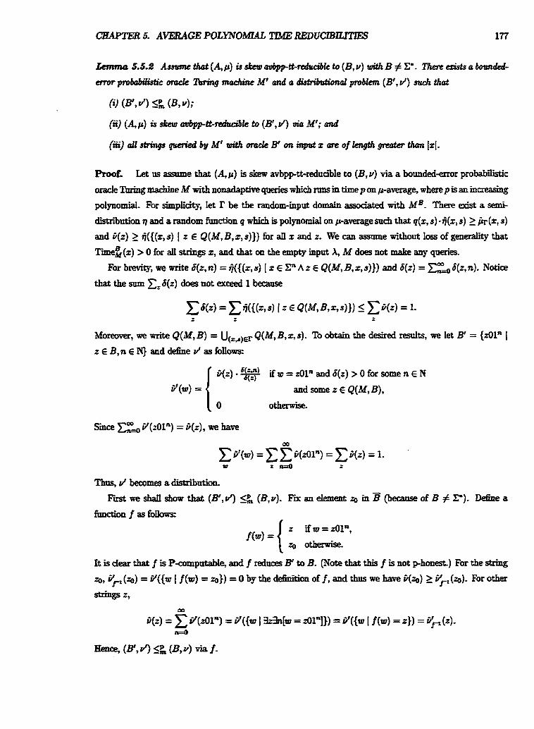
Lemma 5.5.2 A~sume that (44 is skew aobpp#-tedudk to (B, v) with B # C'. There Qists a bvmukd-
error probbdistic om& moddne M' ctnd a d & d d h d problem (B', d ) such that
(iii) all strinqJ queried by M' tDifh o d e B' on input z ore of length greota than 121.
Proof. Let us assume that (A ,p) is skew avbpptt-reduuiIe to (B, v) via a bounded-error probabilistic
oracle Toring marhine M with nonadaptive qumMes which ntns in time p on 1-averageT where p is an inmasing
polynomial. For simpticity, Iet I' be the random-input domain assodated with kfB. There exist a semi-
distll'bution q and a random hetion q which is poIynomiaI on paverage such that q(z, s) -tj(x, s) 2 k(z, s)
and C(z) 1 tj({(z, s) 1 z E Q ( M , B, x, s)}) for aII z and z. We can assmne without loss of generality that
mmeg(z) > 0 for all strings x, and that on the empty input A, M does not make any queries.
For brevity, we write cT(z,rz) = Ij({(z, s) [ z E C A z E Q(M, B,z, s))) and &) = r> 1(z, n). Notice
that the sum c= 6(z) does not exceed 1 because
Moreover, we write Q(MT B) = U(,,,Er Q(M, B, z, s). To obtain the desired results, we let B' = {zOln [
z E B, n E N) and dehe d as f o l l m
G(z) i£ u = zOln and 6(z) > 0 for some n E N iY(w) = and some z E Q(M, B),
otherwise.
Smce i'(zOln) = P(z), we hiwe
Thus, Jbecomesadistribution
Fm we shd show that (H,4 (B,v). Fm an element a in (because of B # C). Deihea
function f as foII0ws: r
{ z ifw=rOln,
fW = a otherwise,
It is clear that f is P-computabIe, and f reduces B' to B- (Note that this f is not phonest.) For the string
a, i$ ( a ) = Y({w [ f (w) = a)) = 0 by the dehition of f, and thus we have ti(*) 1 i'', (lo)- For other
stringg 2 7
m
C(r) = 1 6'(dln) = iY(g I %dn[m = dlu])) = ~ ( { T u 1 f (w) = z}) = gP (r).
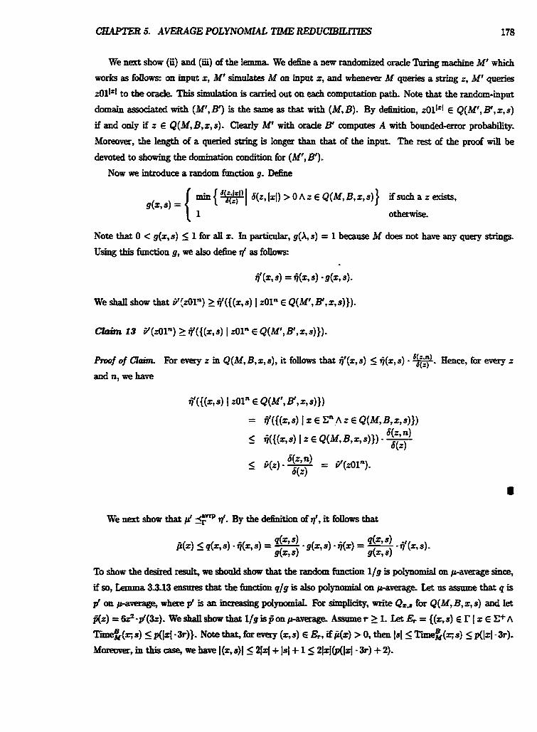
CHAPTER 5. AVeRAGE POLYNOMIAC TIME REDUCIBlLSIlES 178
We next show (ii) and (ii) of the lemma We dehe a new randomized oracle Turing madhe M' which
works as foIIows on input z, M' simnlates M on input x, a d whenever M queries a string z, M' queries
zOlltl to the oracle. This simulation is carried out on each computation path, Note that the random-input
domain associated with (Mf,B3 is the same as that with (M, B). By defbition, zOllrl E Q(M',B1,x,s)
if and only if z E Q(M, B,z,s). CIearly M' wi th orade B' compntes A with bomded-error probabilityty
Moreover, the length of a queried string is longer than that of the input. The rest of the proof will be
devoted to showing the domination condition for (Mr, B').
Now we introduce a random hct ion g. Debe
Note that 0 < g(z,s) < 1 for all z. In particular, g(X, s) = 1 because M does not have any query strings.
Using this frmction g, we also define 7/ as follows:
fir (2, 9) = fxz, 4 9(z, 4.
We shalr show that Y(zOIn) 2 7jf(((z7 s) I zOln E Q(Mr, B', 2, s))).
Chins 23 V(zOln) 1 f({(z, s) 1 zOln E Q(Mf, B',z, s))).
Proof of Cloinr For every z in Q(M, B,z, a), it follows that ij'(+, s) 5 j(z, s) - w. Hence, Tor every r
and n, we have
We next show that p' 3- q'. By the de6nition of$, it follows that
To show the desired resnlt, we should show that the random frmction l/g is polynomial on paverage since,
if so, Lemma 3 3 3 ensures that the fimction q/g is also polynomial on paverage Let us assmne that q is
p' on p-amqp , where # is an inQeaSiTLg polynomial For simpli-, write Q,, for Q(M, B, x, s) and let
Az)=e-#(k) - Weshattshowthat l/gisponp-average Assmner>I. Let&= {(z,s) € r [ z € C f h
T3ne$(z; s) 5 p(lz-1-3r))- Note that, for every (z,s) € E, if E(z) > 0, then Is1 5 Tirmefi(qs) 5 p(lxl - a ) -
Moreover, m this ~ s e , we have I(z,s)l I 2121 + Is1 + I < 2lzj(p(Jzj - 3r) + 2)-
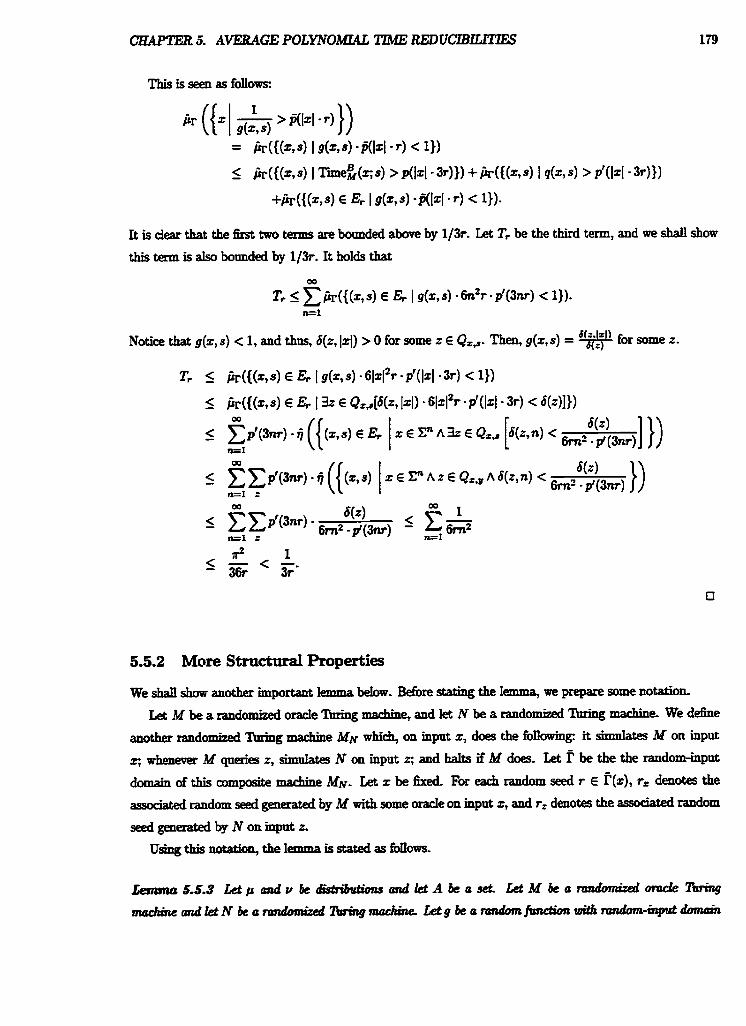
CHAPTER 5. AVERAGE P O L Y N O U TIME REDUCIBEEZES
It is dear that the &st two terms are bounded above by 1/31., Let T, be the third term, and we &ail show
this term is a h bounded by 1/31.. It holds that
Notice that g(z, s) < 1, and thus, 6(z, I t [ ) > 0 for some r E Q.,. Then, g(z,s) = f, wme z-
5.5.2 More Structural Properties
We shall show another important lemma beIow- B&re stating the lemma, we prepare some notation-
Let M be a randomized o d e 'Ihring mlrhinP. and Iet N be a randomized lbring machine We dehe
another =domized 'Ihring machine MN which, on input z, does the hllowing: it simulates M on input
2; whenever M qneries r, shnhtes N on input z; and halts if Ad does. Let f' be the the random-mput
domain of this composite machine MN. Let z be &d For each random seed r E F(x), r, denotes the
assx&ed mdom seed generated by M w i t h some oracle on mput x, and r, denotes the associated random
seed generated by N on mput z.
Using this notation, the lemma is stated as MOWS.
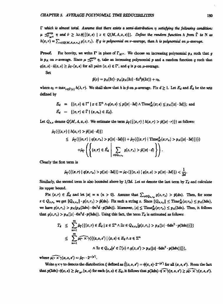
C&QPTER 5. AVERAGE POLWOMC4.L TIME REDUClBlMIZ73S IS0
Proof. For brevity, we write TV in place of r M ~ . We choose an increasing polynomial p~ such that g
is on waverage. Smce p Sm I], take an increasing polynomial p and a random function q such that
q(x, S ) . G(z, s) 2 h r ( 2 , ~ ) for all pain (z, s) E I", and q is p on paverage.
Set
= PA (32) ' PA@A (32) ' 6z2p(3z)) f '3 t
where '3 = wE~(,) h(X, r). We shall show that h is fi on paverage. Fix d 2 1. Let Ed and E~ be the sets
de6ned by
Let Qr, denote Q(M, 42,s). We estimate the term k({(z, r) ( h(z, r ) > @&/ . r ) } ) as fonows:
Clearly the &st term is
SimilarIy, the second term is a h bounded above by 1/3d Let os denote the last term by Td and cafcnbte
Thus, T, is bounded above by the term
Skew avbpptt-reducii turns out to be closed under pm-reduability.
Proof. For simplicity, let us assume titat (Al, pl) SP, (A2, k ) and that (.4=, M) is skew avbpptt-redoable
to (A3,p3). Let f be an appropriate reduction which reduces (AI, p l ) to (AZ,R) with the domination
condition for f. Fbrther? let M be a boundedsrror pmbabiIistic oracle Turing reduction which reduces
(A2tP2) (-43t~33)- We shan consider the randomized agorithm N de!6ned as follows: on in@ z , h t compute f (x ) and
then simnIate M on hput f (2). For each 6 . d 2, since A1 (2) = A*df(z)),
This shows that N is a bodederzof probabilistic orade 'Ibring marhme with o d e &. The estimation of the nmning time of N with d e A3 on mpnt z with random input s, Time2 (z; s),
ismby Tme$ (G s) 5 c (Tie (z) + T i e s (f(z)) + 1)
for some constant c > 0. Notice that Xz-Timef (2) is polynomial on pl-averap, and Azs.TrmeS(f (z)), as
a random fimction, is aIso polpomiaI on pr-average by Lemma 52.4. In comeqaence, ~\zs-Tii$ (Gs) is
p o l ~ d on waverage. To see the domination condition for N, write t& for the defanlt d L E t r r i a t h indud h m and F;YA,.
Then,
For w, it holds that
This sum is taken over all pairs (x,s) € rN~S such that
This condition is equivalent to the condition z E Q(N, &, z , s). NOW let us define p(z, s ) = p ~ ( j ( z ) , s ) -pi (2)
and j(x, s) = f i ~ (z) 2-1.1 fp(z , s ) if s € rNAs (z) , and 0 otherwise. Notice that k-1 f (z)[ is polynomial on
pl-average, and consequently, k r s . p ~ ( f ( z ) , s ) is polynomial on pl-average Thus, p becomes polynomiaI on
PI-average. Then it follows that
This compIetes the p m L D
We need a relativized version of the AmplScation Lemma (Lemma 3.531).
Proof. Let us assume that (A, p) is skew avbpptt-redua'ble to (B, v) via a tandomized Thing madim M and a semi-distniution q. Let r be the random-input domain associated with M with o d e B. We suppose
that PrM[@(z) = A(=)] 2 $ + t Smce p 9 q, there is a random function q which is poIynomia on
p-average such that q(z,s) - ij(z, s) = h(z, s ) for all pairs (x,s) E r. Let be the minimal string that is
not in B. We can assmne that M does not query any strings of length mallet than or equal to Ial- Forthedesiredpmblem (B',r/), weset B={rOlnI Z E B A ~ E N ) andset
Gw(ln) - P(z) if w = dln for some n E N, g(w) = Oiherwife
Obviously d becomes a distribution became G'(rOln) = P(z) for dl strings z.
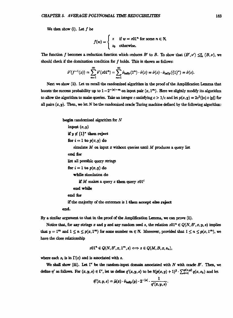
CHAPTER 5. AVERAGE POLWOMTAL TIME R E P U C I B D
We then show (i). Let f be
z i f ~ = z 0 1 ~ f o r s o m e n E N , f (4 =
.?o otherwise
The function f becomes a reduction function which reduces B' to B. To show that (B', d) sp, (B, v), we
should check if the domination condition for f holds. This is shown as follows:
Next we show (i). Let us recall the randomized aIgorithm in the proof of the Amplification Iiemma that boosts the success probability up to 1 - 2-lfl"m on inpd pair (z, lm). Here we slightly modify its dgorithm
to allow the algorithm to make queries. Take an integer c satisfying c > 1/c and let p(z, y) = @(Is1 flyl) for
all pairs (z, y). Then, we let N be the randomized o d e Turing machine defined by the following algorithm:
begin rand& algorithm for N
inpat (z, Y 1 if y 4 (1)' then reject f o r i = l top(x,y) do
sixdate M on input z without gaeries until M produces a query list
end for
Iist all possible query strings
fbr i = 1 to p(z,y) do
while shmhtion do
if M makes a cpery r then query dli
end while
ePd for
if the major& of the oatcomes is 1 then accept else reject
end.
By a simihr argument to that in the proof of the Amplification Lemma, we can prove (ii).
Notice that, for any string z and y and any random seed s, the reIation zOln E Q(N, B', z, y, s) implies
that y = lm and I < n I p(z, lm) for some uuxuber m E N Moreover, provided that I n 5 p(z, lm), we
have the dose reIationship
where each % is in r(z) and is assodated wi th s.
We shall show (iii)- Let fV be the randam-input domain asoc&ed with N with orade B'. Then, we
define rJ as f o l l ~ ~ ~ . Fix (z,Y,s) E F, I& US define b ( ~ , 9, S) to be 8(p(z, y) + 1)* - ziu) &,st) a d let
CaAPTER 5. AVERAGE POLYNOOML4L Tll\dE REDUCJBILITIES 184
Now we must check che domination condition for N; that is, iJ(((z, y,s) I dln E Q(N, Bt,z,y,s))) I 9(z01n) for any z and n. Using the previous calculation, for each string of the form zOlm,
The last term is equivaIent to the foiIowing term:
Therefore,
This compIetes the prooE
5.5.3 Bomded Error Probabilistic Thth Table Reduciiility
An ordinary botmded-ermr probabihtk oracle %ring madhe can rtiminish the error probabm signif-
icantly by repeating the same camp- and taking a majoriv vote to determine the outcomes of the
m & h Om~tedncti~~tdoesnotseemto~thisprapettpbecanseoftightdomination~diti~~~ifm
thedudion- Togaaranteeit,weneedamauy+metra * " asdasthesIommiuction.
Now we introdace onr barmdeckm probabitistic trrrth-taMe red-
De&rition 5.5.6 (Bounded-Error Probabilistic ThtbTabte Redactions) Let (A, p) and (B, v)
be distributional decision problems.
r. (kp) is bwnded-m pwbabdktk polynomial-time W-table redudble (bpptt-reduciile, for short)
to (B,u), denoted by (44 &P (B, v), if there erdsts a distnibutional decision problem (B', J) such
that (A, p) is skw bpp~reduaIbk to (B', v'), and (B', v') is pm-reducible to (B, v).
2. (A, p) is hde&enur pto- memge p o m - C i m c hth-h6& neducible (avbpgtt-reduable,
for short) to (B,v), denoted by (A,p) (B,v), if there adst a distnbutiod decision problem
(Bf, 4 snch that [A, p] is skew avbpptt-redua'bIe to (B', 4, and (B', v') is pm-reducible to (B, P).
In the following, t ~ e &OW basic properties of the dudbilities.
Proof. (1) By definition, detc, ' 'stic %5ng machines are a specid case of probabiIistic M g machines.
(2) The claim of dexiv i ty is obvions by choosing the identity redaction, ie., f {z) = z. (3) Clear from the d~~ (4) Here we that cPP is tran&be. -*g that (AL, PI) IP$ObPP (A2,pz) and (A27 p?) 5zbpp
(&t&), we s h f l sfmw (AI,PI) srPP ( A r ~ 3 ) .
Let (4, &) be a distributional problem such that (A1 , p l ) is skew avbpptt-ceduaIbIe to (4, A) , and
(4, &) is pm-reduciik to (Az7 &)- Suppose that (A2, M) is skew avbpptt-redncibIe to some distri%utionaI
probIem, say (A;, A), which is pm-redua'ble to &,~(3). By Lemma 5.5.4, (44) is skew avbpptt-
ducible to (A;,&). Appty Lemma 5.5.5 to this skew avbpptbrednction to obtain another randomized
d e Tking machine N, another semidistriion 7, and another distniutional problem (g,&) which
s & s k conditions (i)-(E) of the I ~ m m n as weJl as (A:,&) 9, (A3,ps)-
For readability and simplicits, m what fdhws, we on assume that (AL, pL) is sloew avbpptt-reduciile *
to (Az,m) via a Se2HEdtSttliutioo q and a bormded-error probabilistic o d e Tudng machine MI which,
with oracle A?, is polgnomid-time bounded on pz-average Moreover, ~ r , [ ~ p ( z ~ l ~ ; s ) = A2(2) I s E rrC(z7 lml] > 1 - TC'-, pz x U- Ps Q. B L W~({(~ .Y,S) I 2 L Q4(&,47~0. ,4}) for some ~i~~ anctsmnrandon&aade~machine M2 which,withorde&, mmin
polgn- time on waverage By the dominatian mditions, there are random frmctiong m and p2 which are plpnomial on m-average
and Pory~mial on ~2 x v--a- -, that fi (x, s) - i j l (x, 4 2 t r (4 - 2-181, P ~ G -9 -
CaAPTER 5, AVERAGE POLYNOMIAL TIME REDUCZBIIJTlES 186
begin randomized algorithm for N input z (say, n = 1x1) sinmbteMloninptttzrmtilthehstqueryismade complete a list of query strings
let m,* be the number of query strings
resume the simuIation
while simnlation do
if M2 queries z then sirdate M2 on input (2, I"'-=+~)
if MI reaches a halting configuration then output MI (z) and halt end while
end.
Let r be the random seed generated by N with oracle & on input z. Clearly random seed r is associated
with all random seeds generated by M2 with orade A2 on input strings which MI with o d e A2 queries.
For such random seeds, we write r, to de@pate the random seed that is used for the computation of Ml
with o d e A2 on input x, and d r= for the random seed for the computation of M2 with o d e -43 on
input z provided that z is in Q(M1, A2,2, rr ).
Given a pair (2, r) E , the nmning time of N with & as an o r d e on input z with random input r
is bounded bv
CHAPTER 5. AVERAGE POLYNOMIAL TlME REDUCZBIllTIES
It remains to establish the domination condition for N. For each z,
Write &(w, y, s') for p2(w, y, d ) - 8(IyI + I)*. Using the faa that 8[lyI + 1)* - ttrtlY(y) -> 1,
Also we have
Combining both inequalities, we can calculate the lower bound of b3(2) as folloftrs:
fil(4 2 - ~ l . 1 E m - -2-1'4
(t.4 &b? l-=+3,rw1 we..,
F d y we can show the dosure property of the dass Aver(BPP, *) under avbppreductions- This is a direct consequence of Proposition 5.544).
ProoE s'mn'lat to &at of Theorem 5-
5.5.4 Application of Probabilistic Reducibility
The motivation in having introduced the bounded-error probabilistic reduabiIity is to show that distrriu- tiond problems m Dist(NP, P-cornp) with nattd flat distributions become comp1ete. As a simple example?
we shall demonstrate that a h t version of the randomized bounded halting problem is truly complete for
Dist(NP, h m p ) with respect to bpptt-redua'bility.
Let us introduce a flat version of the rmuImnizai lkndai halting p b h (RBHP la) (BHPfta, C ( B H ~ , ~ . ~ ),
in the foflowing fashion:
BHP lclt = {(si, z, t ) / M. accepts z in It[ time }; and
begin randomized algorithm for N input (sit Z, lm)
generate a random seed w of Iength m
query (si, z, ta) to oracle
if (sit Z, w) is in o d e then accept else! reject
end.
Notice that there is no error 3 %HPfId is chosen as an oracle; that is, Pr,[lVBEIPf ((si, z? Im) ; s) = A(=)] = 1 .h N make nonadaptive queries and nms in poiynomial time for any o d e ,
Let c be an integer such that c 2 r/fiwd(si). Let us d&e the semidistriiution 7 as i)(r,s) = bHP (2) - 2-181 for dl pairs (2, s) E r- ; otherwise, 0. We tbezt have
Another significant application d the bppttreduci'bility given by -David et aL [9] is that
butionat NP search p r o b l d with Pmmputable distributions are actually reducibIe to distributional
decision pb1ems m DLPt(NP, Pamp). Nonetheless, sina we have not d e e d udIstnitrtionaI NP search
problems" and the main subject of this thesis is decision problems, we state the resnlt bdow without p d
The intererted reader ximy refer to [9] fix the deWi011 d search probIems and the proof d the theorem.
CHAPTER 5. AVERAGE POLYNOMIAL TIM23 REDUCIBIllTlES 189
p. TRen .thm is a &diu&d &ision probkm (D, v) m Aver(NP, P a m p ) such that (I?, p) is bpptt-
reducible to (B, v ) .
In womkase complexity theory? it is easy to see that if A 5% C and B 55 C, then A @ B C. The same is true m awmgeae eompl-. In the next lemma, we prove this claim.
RsealI from Section 3.5 the W t i o n of p @ v for two distn'butions C( and v.
Proof. We demonstrate only the case gPP. The other eases are somewhat similar. Let us assume
tbat (A, pA) 5Fbpp (C7Q via MA and ( B , ~ B ) <Ppp (C, () via MB. Dehe a new dgorithm N: on input
z, if z = Ou for some u, then simulate MA on input u; if z = lu for some u, then simulate MB on u;
otherwise, reject the input. For the sake of convenience, write v for p~ p ~ . Take a computational path y
of the computation tree given by N on inpat 2. Smce N basically follows either MAIS computation or MB%,
we can determine the unique computation path, which is made by either MA or MB, corresponding to the
computation path spedfied by random input s. We denote this computation path by 9. We show that ( A $ B, Y ) sbp (C, 0 via N. By om assmnptioq there exist semi-distriiutions q~ and
VB that PA 5- '?AT Ccg 9Bt i (2) 5 6 ({(% s) 1 2 E QWA, C7 u7 S) )) and &z) 1 6k({(% s) I 2 E
Q(MB, C, rr, s))) for all z, where IJA and IJg are the induced distniutions Eiom C(A and rMAc , and from p~
and I'G ? respectiveIy. Let q be d&ed as
$ - j ~ ( u ) if z = Ou for some u, i€z=luforsomeu,
otherwise.
It is obvious that q is a distribution. We also let q = q~ @ q ~ . Let
pA(u) if z = Ou,
otherwise
This is seen as foJIows. Assmne that z is of the form Ou. The
W y , we show that t(z) 2 ijr({(z, y) I z E Q(N, C p , y)) ) for all z. For each string z, we have
CBAPTER 5. AVERAGE POLWOMIAL TllldE REDUCIBlLITlES
This compIetes the p t
5.6 Structure of Reducibility
In this section, we shall take a dose look at the structure of the randomized complexity dass Dist(NP, P-comp)
in the Iight of rednciiility. F i we shall review the results of Ben-David, Chor, Goldreich, and Luby [9J.
They proved that if there is a hard distributional problem m Dist(NP,P-amp), there is also a problem
which is in Dist(NP, P-comp) bnt not pm-complete for Dist(NP, P-comp).
P m p o d b n 5.6.1 [9] Let p E strict-REC-comp ond D E REC. Assume that there QiPts a t h e -
corrPtrucfiMe function p such hat p(n) € no(') ond Ip(P(')) - p( la ) ) [ 5 2" + 2-1 for aftnost dl i, j € N If (D,p) 4 Aver(P, *), Men here ezirts a smri-diddution v such that (i) (D, Y ) 4 Aver(P, *), (n) (D, p)
(D, v), (5) (D,P) (D,p), and (itt) Y is computed by an oracle log-space detffministic Timhg machine
n l a t i o e t o t h e ~ o r n J e p .
Proof. The proof proceeds by a d e d slow diagon&don technique. We first enumerate aII quadruples
(Mi, Ni, ci, 4) of a deterministic Turing machine Mi, a determiniStic orade ntring machine N., and natural
numbers ci a d 4. Write also Di for L(&) for brevity- Note that by OW assumption, there exkts a
dekmhi&c Turing machine which exactly computes ji.
For a finite sequence a and an integer k 2 1, let a(k) denote its kth element of a. For a b i t e sequence
u of 0's and I's, Iet
It is easy to see that, for 4 x, fi(x) = 0 if u(Iz1) = 0, and P(z) = i(z) otherwise. Note that the condition
on p that Jp(P('3) - p(lm)l _< 2" + 2-j will be used Iater to goarantee the existence of a "normah&
distribution of Y.
Let us consider the fonowing subprogram Cond(i, a, t):
subroutine Cond(i, a, t)
if t steps are consumed dm* the following computation then return %on
if i = then let i, r= Li/2] and go to (*)
let 6 = [(i - 1)/2J (since i = "odd")
check the fdowing two conditions
(i) D, n C ~ I ~ I # D n Slul; and
(ii) Cso<ltl<lol - TimeMio (x)ll& - 121-I - fi(z) > c, if either (i) or (ii) is true then retmn "yep" else return %on
(*I check the following three conditions
(i) L(N,, Db) n SIUl # D n Glul;
CHAPTER 5 AVERAGE POLYNOMIAL TIME REDUCIBILITLES 191
(ii) ~c,zl<l,,l - Tim:: (z)'/h - - ji(z) > ~ q ; and (i) there exist two z, y of length < lul such that ji(z) > 3(y) = 0, and y f Q(N& Di,, ,x)
if either (i), (ii) , or (iii) is true then return "yes" else return %on
Notice that if Cond(i,o, t) answers W,'' then so d m Cond(i, T, t) for all extensio~ T of u (i-e., r _1 u).
The following is the main body of the algorithm which computes a:
begin deterministic algorithm for u
input k
let t = pgkJ
f o r i = l t o t d o
exit the for-loop when t individual steps are executed in this for-loop
compute 41') ifp(li) > 3 then go to (*)
end-for
output u(k) 7 I and haIt
(*I f o r j = l t o t d o sit the for-loop when t mdividd steps are executed in this for-loop
recompute aCj) (by a recnrsive On)
end-for
let J be the Largest index j for which u(j ) has been recomputed m the above for-loop
if no such J exists then output a@) = 1 and halt
set FJ s o(1)4(2) . .*u(J)
f o r i = l t o J d o
exit the for-loop when t individual steps are executed m this for-loop
call Cond(i, F J , t)
if Cond(i, FJ, t) = 'ho" then exit the for-loop
end-for
let 1 be the S I d & index i f0r which cond(i, FJ, f) anSWerS %on
output u(k) P 1 mod 2 and halt end.
The exit-statement enforce a time bound t (= LlogkJ) on each each for-loop; thns, this aIgorithm
req@res at most O(Iog k) steps. Hence, u is computed by rising 00ogk)-space. By definition, u is correctly
mputab1e using 1%-spacewith thehelp ofp as an orade-
We shalI show that this algodhm c o d y computes o(k) on input k. We assmne that there is no
extension T of u such that Cond(i,r,t) answers -'' Assmne that i is odd. Then r is of the form dm
for some m E N because a(j), j > k, is atways set to be 1. We then have D, n e1'1 = D = 6 1 7 1 . This
implies L(Mh) = D. .b we have LM<ltl - Theas, (x)~'% - - 9(2) 5 G. We remadc that the
d u e P(x) equals ji(z) if 1x1 > 101. Hence, for some constant c > 0, we have
This implies that (D, p) M o w to Aver(P, *), a contradiction.
Now let us consider the other case that i is m. Notice that any extension r of u is of the form dm for
some rn E N. Then L ( N , , D,)~CI~I = DNZ~I~I for all extensions r ofu. Thus, L(Nk, D,) = D. Moreover,
there are no pairs (x, y) such that b(x) > 0, P( y) = 0, and y E Q (N, , D, , z) . RecaU the definition of u. Since
7 = dm, rn E N, it foIlows that, for any y of length great^ than lal, 5(y) = 0- This means that there is no
z (121 > lo[) on which N . queries strings of length greater than lol. In other words, 11 U, Q(Nh7 D,, x) 11 is finite. Let m dehe another lhing marhine N' which sindates Nh on the same input with dl orade answers
born Dh being encoded into its program. Clearly L(N,, D,) = L(N), and Tme~(x) c ( ~ i m e 2 (z) + 1)
for some absolute comtant c > 0. Notice that &,<ltl<lTl - 121-I -Tune:: (2) '1% - j i ( t ) c, for all extensions
T. Hence, we have
This again condudes that (D,p) is in A m p , +), a contradiction. Thdore, the algorithm for o works
PW=IY - By Corohy 43.3, we can normdize v to a W distribution u' such that B' (2) = P(z) for all nonempty
strings 2. 0
kr a simiIar fashion, we can demonstrate the existence of a distniutional problem that is not pT-harder
than a given problem, bnt can be pm-reduced to the giTlen problem,
h o f l Similar to Theorem 56.1. a
Root Assmne that Dist(NP,P-comp) P Aver(P, *). Then, no pmamplete probIem for
Dist(NP,P-comp) belongs to A*, *). Let (D,p) be any anY'buticmaI problem which is pm-complete
h r Dist(NP, P-comp). SinQ (D, p) # A-, *), Propositim 5.62 gmar&es the exkfience of a set E such
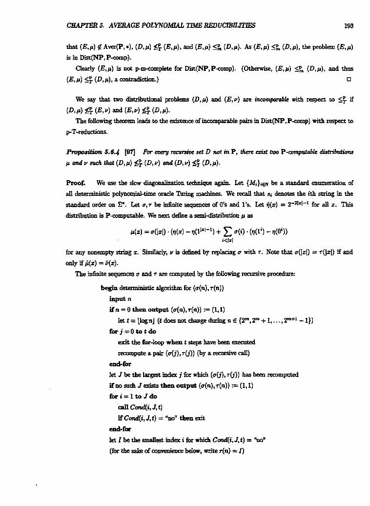
CHAPTER 5. AVEXAGE POLYNOMIAL TIME REDUClBILITIES 193
We say that two distriintionaI problems (D,p) and (E,v) are incompmable with respect to 5; if
(Dl P ) g (6 and (E, 4 2g (D, PI- The foIlowing theorem leads to the existence of incomparable pairs in Dist(NP, P-comp) with respect to
pT-reductions.
Proof. We use the dow diagodhtion technique again. Let {Mi)iEN be a standard enumeration of
aU deterministic polynomia-time o d e Turing machines. We recatt that si denotes the ith strtog in the
standard order on C'. Let m,r be idkite segaences of 0's and 1's. Let i (z ) = 2-21rl-L f ~ r all z . This
distribution is P-computable- We next define a semi-distribution p as
for any nonernpty string z- S i l y , v is defined by repking u with T. Note that u(lz1) = ~(121) if and
only if jqz) = P(x).
The infinite sequences a and T are computed by the fbllowing recursive procednre:
begin deterministic aIgorit6m for (u(n), r(n))
inpat n
i f n = 0 then output (u(n),r(n)) s= (1,l)
Iet t = [Iog nJ (t does not change dnring n E {P, T + 1,. . . , 2m+1 - 1))
for j=O to tdo
exit the for4oop when t steps have been executed
==P* a P* ( ~ l j ) , dj)) @Y a ~~- cam
end-for
let J be the Iargest index j for which (u(j),r(j)) has been recomputed
i f no such J exists then output (u(n),r(n)) = (1,l)
for i=l toJdo
d Cond(i, J, t )
if Cond(i, J, t ) = "no" then &
d f m
let I be be tbe mdex i for which Cond(i, J,t) = "no"
(fmthesakeofcosmenience~, writerfn) =I)
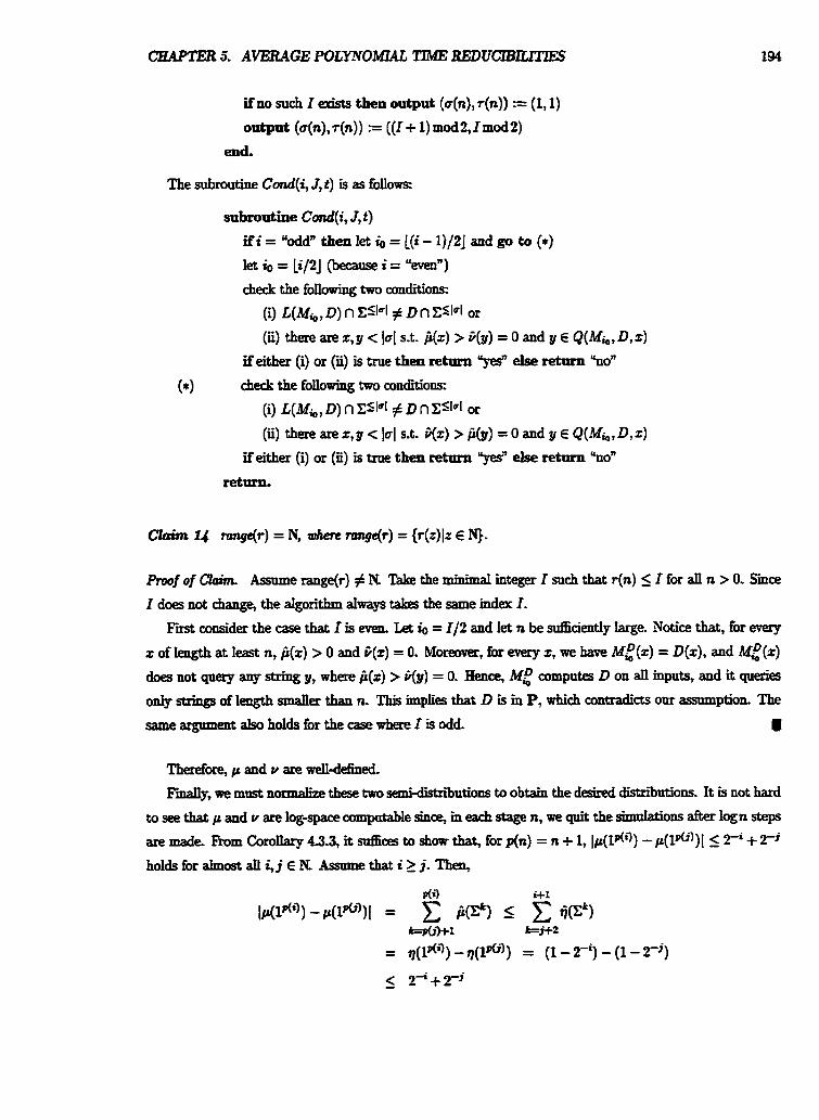
if no such I exists then output ( ~ ( n ) , d n ) ) = (1 , l )
output (u(n), ~ ( n ) ) = ((I + 1) mod 2, I mod2)
end.
The subroutine Cond(i, J, t ) is as follows
subroutine Cond(i, J , t )
if i = "odd" then let io = L(i - 1)/2j and go to (*)
let io = Li/2J (because i = "evenw)
check the fdowing two conditions
(i) L(M,, D) n EslPI # D n 2Slol or
(in) there are x, y < la[ s.t. ji(x) > fi(y) = 0 and y E Q(M,, D,z)
if either (i) or @) is true then mtum "ges" else return %ow
(*I check the folIowing two conditions
(i) L(Mb, D) n ~ l l ~ [ # D n ES[V~ or
(in) there are z , y < [a1 s.t. 32) > ji(y) = 0 and y E Q(Mh, D,z)
if either (i) or @) is true then return "yes" else return "now
return.
Pnwf of Claim. Assume ran&) # N Take the minimd integer I such that r(n) 5 I for all n > 0. Since I does not change, the algorithm always takes the same index I. F i consider the case that I is even, Let io = 112 and let n be sufEciently large. Notice that, for every
z of length at least n, ji(z) > 0 and G(z) = 0. Moreover, for every z, we have ME(=) = D(z) , and ME(%) does not query any string y, where ji(z) > ~) = 0. Hen* ME computes D on all inputs, and it queries
only strings of length smaller than n. This i m p h that D is in P, which contradicts our assmnption. The
same argument also holds for the case whem I is odd I
Therefore, p and v are well-defined. Finany, we must normalize these two semi-distn'butions to obtain the desired distributions. It is not hard
to see that p and v are log-space computable since, m each stage n, we qtdt the simuIations after Iogn steps
are made- Ekom Corollary 4.33, it it to toow that, for p(n) = n + 1, lp(ldg) - p(lP(-f))j 5 Ti + 2-1
holds for almost all i , j E N. Assume that i 2 j . Then,
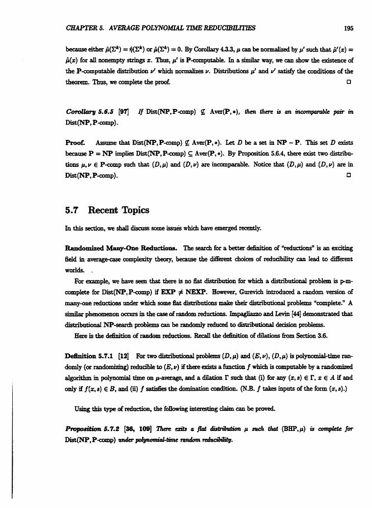
CHAPTER 5. AVERAGE POLYNOMIAL TIME REDUCIBxLxTIx.3s 195
because either ji(Ck) = *(EL) or j i (Xk) = 0. By Corollary 43.3, p can be normalized by p' such that ji' (2) =
ji(z) for an nonempty strings z. Thus, p' is Psomputable- In a Jimilar way, we can show the existence of
the P - c o m p d e distniution d which normakes v. Dishiutions p' and J satis@ the conditions of the
theorern, Thus, we complete the proof. 0
Proof. Asmme that Dist(NP, P-comp) g A m p , *). Let D be a set in NP - P. This set D ackfs
because P = NP implies Dist(NP, P-amp) E Aver(P, *). By Proposition 5.6.4, there exist two distribu-
tions p, v E P-comp such that (D, p) and (D, v ) are incomparable. Notice that (D, p) and (D, v) are in
Dist(NP, P-eomp). 0
5.7 Recent Topics
In this section, we shan discuss some issuis which have emerged recently.
Randomized Many-One Reductions. The search for a better definition of "reductions" is an exciting
field m averageease c o m p l e theory, because the Werent choices of reduciiility can lead to different
worlds. -
For example, we have seen that there is no Bat distrrriution for which a distrritational problem is pm-
complete for Dist(NP,P-amp) if EXP # NEXP. However, Gnrevich introduced a random version of
many-one reductions under which m e Bat distriiutions make their distributional problems "compiete" A
shnilar phenomenon occurs m the case of random reductions. Impagliazzo and Levin [44] demonstrated that
distn'butionaI NP-search proMems can be mdomly reduced to distzibutional decision problems.
Here is the dehition of random redttctions. Recall the debition of dilations from Section 3.6-
DeaPition 5.7.1 [l2l For two dishiiutiona1 problems (D, p) and (E, v), (D, p) is polynomial-time ran-
dody (or randomizing) reduai1e to (E, v) if there exists a fimction f which is mmpdable by a randomized
aIgorithm m poIynomial time on paverage, and a dilation r such that (i) for any (x, s) E r, z E A if and
ody if f (z, s) E B, and (5) f satisfies the domination condition. (NB. f takes inputs of the form (z, s).)
Using this type d reduction, the fbHowing interesting daim can be proved.
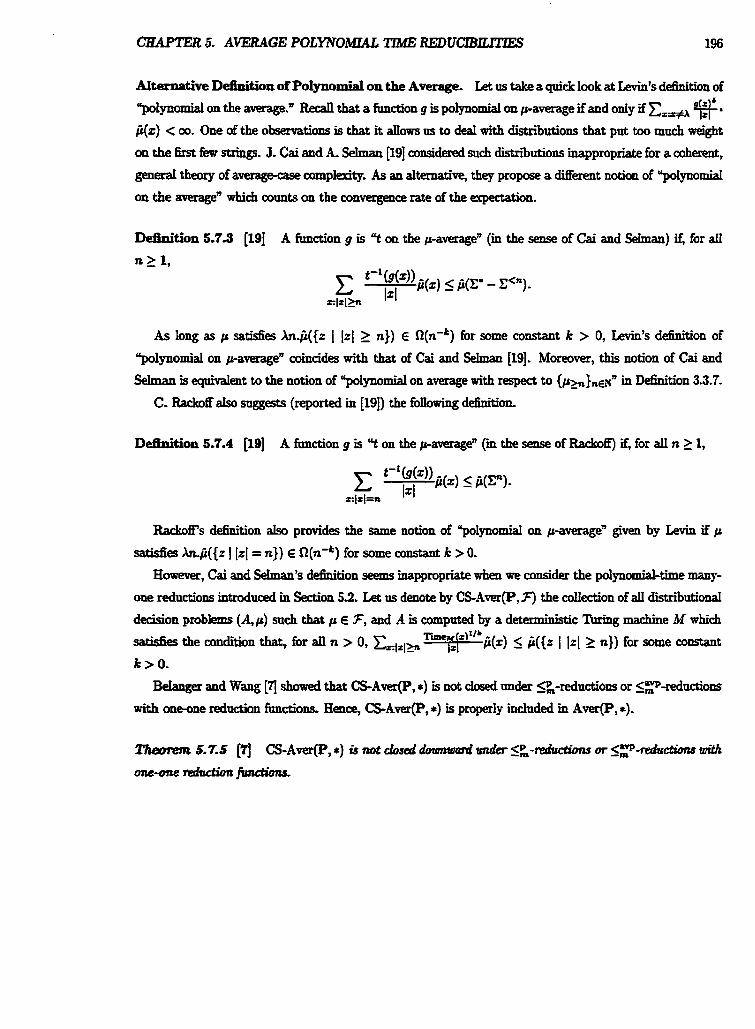
CHAPTER 5- AVERAGE POLYNOA5A.L TIME REDUCIBjLR7ES 196
AIternative Dehition of Polynomial on the Average. Let us take a quick look at Levin's definition of wlynd on the a m n R e d l that a fimction g is polynomial on pawrage if and only if z.,C* fi(z) < 00. One of the obsavations is that it allows us to deaI wi th distniutions that put too much weight
on the &st f m strings. J. Cai and A. SeLnaa [I91 considered such distri'butions inappropriate for a coherent,
generat theory of averagecase complexity. As an alternative, they propose a diffefent notion of " p o l y n o d
on the avgage" which counts on the convergence rate of the expectation.
D W o n 5.7.3 [I91 A function g is "t on the paveragen (in the sense of Cai and Selma) if, for aU
n L 1,
As long as p d e s An-b({z [ It1 1 n)) E R(n-k) for some constant k > 0, Levin's definition of
"polynomial on p-avefagen coincides with that of Cai and Selman [19]. Moreover9 this notion of Cai and
SeIman is equivalent to the notion of "polynomial on average with respect to {ph),&' - in Definition 33.7.
C. Rackoff aIso suggests (reported in [19]) the following definition-
D e n 5.7.4 [In] A function g is "t on the paveragen (m the sense of RackofT) iE, for a11 n 2 1,
Rackofffs definition also provides the same notion of "polynomial on paverage" given by Levin if p
satisfies h K { r I I%[= n)) € Zr(n'k) for some constant k > 0.
However, Cai and SeIman7s d w o n seems inappropriate when we consider the polynomial-time many-
one reductions introduced in Section 5.2. Let us denote by CSAverP, T ) the collection of all distriiutiona1
decision problems (A+) such that p E F, and A is computed by a detemxhbtic %ring machine M which
safSes th condition that, for aU n > 0, &, w j l ( x ) 5 fi({z I It1 2 n}) for some constant
k>O.
Belanger and W q [?'I showed that CS-Amp, *) is not closed under S ~ - r e d u c t i o ~ or ~F-reductions
with o n m e reduction functionsflS Hence, CS-Aver(P, *) is properly included in Aver(P, *).
Chapter 6
Average Case Hierarchies
6.1 Introduction
One of the most novel contributions to worst-case compl- theory is the introduction of the p o l y n d -
t h e hierrrrJry (or poipmid k z d i g ) by M e p and $toclaneyer in 1972. This worst-case hierarchy is
built &om P and NP m a m y similar to how KIeene constructed his arithmetical hierarchy above recursively
enmnerable sets. Notably, the classes of the hierarchy Iies between P and PSPACE. The c~mtmction is
such that the kth I d of the po1ynomial-time hierarchy is d&ed to be the conection of all sets, each of
which can be recognized by a polynomial-tirne deterministc/nondeterministic oracle Thing marhine relative
to some sets in the (k - l)th Id of the hierarchy.
The polynomial-time hierarchy has been studied exhsidy for over two decades with many lntrigtring
resttlts. For example, if the BooIeaa hierarchy over NP coIlapses, then so does the po1ynomial-time hierarchy
[4q, and if the polgnorniai-time hierarchy coIIapses, then the Iow and high hierarchies in NP coRapse [89].
Many NP-hard probIems are chssified into wariors levels in the poIynomia1-time hierarchy-
This chapter wilI b d d a- analogues of the po1ynomi;il-time hierarchy among distnhtional
dedsion prob1ems1 To introduce an average polynomia-time hierarchy, we W begin with the relativization
of the fundamental a9erage-case c o m p I w classes Aver(P, 7) and Aver(NP, F) , relative to a distriitrtional
problem (E,u)* A relarivization ofthe dass Am(P,F) to an orade probtem (E, u) is nattaany induced h n the average
polynomial-time dete ' ' tic Thing reducibiIity defmed in Section 52. A s b n k approach toward a rela-
tivized Aoer(NP,F) is taken by Schder and Yamakami [91 based on the model of docked nondeterministic
lhring xuachines. Here we shall d&e a &athi& Aver(NP,F) in a slightly different way. In Section 5 z
the relativiz;ition of Aver(P,7), Aver(BPP,F), Aver(NP,F), and Aver(PSPACE,F) will be formdated
m terms of various restfictions on average poIpnomia-time oracle 'king machines together with weaker
domination conditions for those machines.
In dativized worlds, we can see a deskable separation d Aver(NP, Pamp) and Aver(P, Pcomp), and
CKAPTER 6. AVERAGE CASEEIEWBm 198
a cohpse between Aver(P, P-comp) and Aver(PSPACE, Pcomp).
In Section 6.4, using lhring redudbiky, we shall introduce an average-case version of the poIynod-
time hierarchy, average polpnosnial-time hierarchy under a set 3 of distributions {Aver(AL, F), Aver(EE, F),
A=@i733 I k > 0). Another effective way of charaaerizing the kth level of the polynomia1-time hierarchy is to use poIynomia1-
time alternating Turing machines wi th k-dternation. This worst-case characterization is trery suggestive
and enables us to build another of average polpornid-time hierarchy using "averageD polynomial-
time alternating 'king machines with constant-alternatioo, We call this a- hierarchy the aaffoge
polylomial-time u h m a h g hiemdg. Section 6.5 wiH formally introduce an average-case alternation hd
erarchy based on average polynomiaI-time alkmating lbring machines with constant-alternation. As the
reader may perceive? however, these two types ofa- hierarchies are unlikely to coinade.
We have seen in the previous chapter that if Dist(NP, P-comp) is not included in A m p , P-comp), then
there are distriintional problems whieh are in Dist(NP,P-cornp) but which are not pm-complete. This
indicates the possibility of a large gap between Aver(P,P-comp) and Aver(NP, P-comp). One approach of
refining this gap indves constructing a hieratchica structure within Aver(NP, P-comp) and sorting out all
distributional problems in Aver(NP, P-comp) into various IeveIs of this hierarchy. This approach was taken
by Sch6ning m w o m e s e complexity theory in 1980, and the hierarchies within N P are d e d the high ond
low iriermdries. A n a d averagecase -on of the Iow hierarc&y, d e d the menage loto irienrrclry rrrithin
Aver(NP,F), wi l l be introduced.
Major Contri'butions. In this chapter, we introduce severaI new hierarchies.
In Proposition 62.8, it foIlows by the self-redua'bihy of RBHP that Dist(NP, P-comp) A m ( B P P , *)
implies Dist(NP, P-comp) G Aver(RP, *). The notion of relativizatian originany comes h m SchuIer and Y ' [951; however7 the relativizations
of the classes Aver(NP,3) and ,4ver(BPP, F) treated in this chapter are dSet-ent fiom those in [97j.
Proposition 63.8 shows that Aver(BPP,F) reIative to Aver(BPP, *) collapse to Aver(BPP, *) for any
set 7 of distributions.
Proposition 63.11 ~ ~ Q W S basic properties of relativized Aver(NP,7), such as re0- and transi-
tivity. In particular* if (A,p) is m A m , *)(By), then aIl problems in Aver(NP,F)(A') belong to
A v ~ ~ ( N P , F ) ( ~ Y ) .
Theorem 63.12 demo~~strates an o r d e separation between Aver(P, P-comp) based on a tally orade con-
struction given by B a h , Gill, and SaIovay [3], whereas Theorem 63.17 shows a collapse of
Aver(PSPACE, P-comp) to A*, P-eomp) m a reIativized worId. The proof uses a d a t h i d -on
of the randomized h d e d halting pmbIem.
Ropasitim 6- I o w s that Auer(PSPACE,F) reI;ltioe to Aver(PSPACE,+) collapses to
AmfPfWACE,T) forangset3ofdistribntions,
Basic indnsion telatianshipq such as Aver(AL, 3) G AWE;, F) G A m ( A ~ l , F), among cksses in
the average polynomiaE-time hierarchy arr shown m Propositim 6.44.
CHAPTER 6. AVERAGE CASE BIERARCfIlES 199
Propusition 6.4.6 shows that a collapse of two levels of the average polynomial-time hierarchy canses anp
higher level of the hierarchy to collapse-
An Important new idea is the use of of alternating machines to build another average-<.ase version of
the polpnomiaI-time hierazchy. Theorem 6.52 gives an oracle characterization of the average polynomial-
time alternating hierarehg; for example, Aver(AAh,,F) is equivalent to the dass Aver(P,F) relative to
Dist(CE, *). A similar characterization holds for Aver(ACR,, 7).
In Propcsition 6.5.4, it is shown that the dass Aver(BPP,F) is included m the second I d of the
average polynomial-time aIternation hierarchy.
Proposition 6.43 and Theorem 6.411 show that many basic average complexity dasses, such as A m p , *)
and Aver(NP, *), have the sparse interpolation property.
6.2 Distributional Polynomial-Time Hierarchy
In the previous chapterl we showed that sweral important distributional decision problems, such as the
bounded halting probIem RBHP, are pm-complete for Dist(NP,Pamp). This section win extend these
completeness resnIts to the class Dist(Ci,P-comp), the kth I d of the "distributional polynomial-time
hieratchy under P-comp."
6.2.1 D M o n of Hierarchy
Randomized complexity dasses are the simplest randomization of existhg worst-case complexity classes. .Is
with the polynomial-time hierarchy, we can comider its nattrral counterpart of &e polynomial-time hieratchy,
the d i d d d m d pdJlnomial-time hierorclry, under a given set of djstriiutions.
We begin with its format dehitiort.
Delinition 62.1 Let T be a set of distriiatio~~~. A d&ibt&d polyunnial-time KefPrthy tu&r 7
consists of the following classes Dist(Ai,F), Dist(CE,F), and Dist(II:,T) for all k >_ 0.
We next demonstrate the existence of pm-complete problems for each dass Dist(!EE,P-comp). We
generalize the randomized bounded halting problem RBHP, seen earlier? to the kth level randomized bounded
halting problem RB*. The kth leaJ rrrndomLzed boanded hdting problem RBHPI is the distriiutional
problem BE@,^^) defiaed m the foIIowlng fashion. Let c r ~ ~ p be the same distribution as in Seaion
53. Assnming that (Mi)ia is an e&tive enumeration of aIl nondeterministic oracle lhring machines, we
define
BHP(A) = ((i,z, In) I Mt accepts z m less than n steps ),
and then set B@ = BHP(0) and B*' = B H P ( B ~ for k 1 I- Next themem proves that, f i r each k, the problem RBHP* is pxmcompIete for Dist(CE,P-comp)- Note
that thecase k = l has been aIreadyshownasmTheorem53.2.
CaAPTER 6. AVERAGE CASElW3RA.R-
Roof. The general case k > 1 is very sidar to the base case k = 1 of Theorem 5.32. We note that
B@ is C~-cornpIte.
For every set D E XE and every distriiutioon p E P-comp, we shaU show that (D+) SP, ( B & , ~ ~ ) .
Notice that BIIP~-' is pwompIete for CE-,, and as a consequence, there exists a polynomial-time non-
deterministic orade 'I\uing machine M computing D with o d e BHP? Let g be the function g defined in Lemma 4.2.7(2). The fimction g satis6ies ji(x) < 2-19(')1+*. Now let i
be aa index such that L(Mi) = L(M). Let p be a polynomial time bound of Mi. For the reduction f from
D to B@, we set f (z) = {~ ,g ( t ) , l~(l'I)). Clearly f is oneone and witnesses the reduction D <k BEP~
because z E D holds exa&y when Mi with o d e BEE'&-' accepts z within p(jz1) steps- To check the
domination condition for f , we simpIy follow a argument similar to that used in the proof of Theorem 5.3.2.
nus obtain (D, P) SL ( B e ? mm)- D
Meyer and Paterson [7l] have introduced the notion of ( p o l y n d - t h e %ring) s d f - d t ~ c i b i l i t y into worst-
case complex& theory.
AIl known NP-complete problems are self-redua'bIe, and every self-redua%le set belongs to PSPACE. It
is natural to ask whether the notion of self-redum'b'i has a counterpart m distn'butiond decision problems.
We shall indeed give in this section the f o n d d-on d an averageease version of self-redua'b'tlility and
show the existence of self-reducii1e sets m each I d of the average p01ynomi;rl-time hierarchy.
We begin by dehing the important concept of a P-eornputabIe, OK partial order on the set F.
Dehition 6.2.3 (OK Partial Order) Let < be a partial order.
1 A partid order < is ~~~tinre cmpdabk (P-computable, for short) if there exists a polynomid-
timedeterminirtc~maehineMsneh that,forewppair (z,y),x < y ifandonly ifM(z,y) = 1.
2. A partial order c is OK if there akts a polynomial p such that
For exampIe, let us write x < y to mean Iz[ < 191 for any pair (2,~)- Then the relation < becomes a
P-eomputabIe, OK totid d e t on C.
The notion OfselErednciiilitp is now stated as f m
CHAPTER 6- AVERAGE CASE HIERARCHIES 201
Definition 62.4 (Self-Redna'bility) [97j A distriiutional dedsion problem (D, p) is (poEyunnial-Eime
ltting) selfreduci6k if there exist an OK partial order and a deterministic oracle Turing machine M such
that (D,p) 5: (D,p) via M, and for every mput z , all query strinp m the computation of M on input z
are smaller than z with respect to the partial order. The machine M is CaIled a self-reducing mcJrine for
( 0 7 P I -
Proof. (1) For any distributionaI probIern (D, p) in Dist(P, *) , there adas a deta ,tic htring machine
M which computes (D, p) without any queries. This machine reduces (D, p) to (D, p). By the definition of
self-reducib'ity, (D, p) out to be self-redualble (2) Assame that (D, p) is &-reducible. Let as take a self-rednurtg &e M for (D,p) . We shall
dehe a 'Ihring &e N which computes D using polynomial space. Below we describe an algorithm for
Nusingarecumbed
begin detE - ' 5c dgorithm for N
input z
s i m h M on mput z
while 5alation do
(*I ifdd r x d s a query z then simulate N on input z
if M reaches a hatting configmation then output M ( z ) and halt
end-while
end.
We must prove that N ases only p o 1 y n d space- Let us analyze the query process of N on input x.
Notice that the space used by the machine M is pbomded, and thus there are at mast exponentially-many
Werent co-. Remember that this number is independent of the choice of oracle. Let us assmne
that m the first r m d of the simnlation of M, M queries at most exponentiany-many striqs, which are in
Q(M, D, 2). The recursive protocol m the line (*) brings another round of the sirnnlation of M on each input
taken from the set Q(M, D , z ) . Fm an a r b i i striug dl) in Q(M, D p ) . h the second round, M makes
another set of gneries, Q(M, D, z(')). To go into the third round, we EK a query string d2) m Q(M, D, z('))
and then consider the set Q(M, D, d2)) of quexy stthgs. Recnrsively, we keep E&g a query string r(3 and
then stapt another round of the simnlaton of M on the input z (0 . This process proceeds until M does not
querpany- Now let us d d e r an arbitrary sequence z ( ~ ) , d 2 ) , . . . , z(*l, - - - taken by the above procednre Smce M
is ad-reducingmlrhinp. thissapncemakesastrictIy descedhgchain with respect to the given OK partial order. This impIies that the length of the dmiu is bounded above by a poEynomiaI m lzl, and the
Iength of ea15 string z('2 is a h bounded by a polynomial m 14. Let p be such a polynomial As a resnlt, N
CaAPTER 6. AVERAGE CASE HIEELARCHIES 202
caa simutate M using p(lzl) blocks on a workug tape, each of which is used to store one of the strings t('7
being queried in each ith round. Therefore, N needs only polynomial space 0
Moreover, the set of all self-reducible problems is closed under pisomorphism; i.e+ if (D,p) is p isomorphic to some distr~bntional problem which is self-reduciile, tben (D, p) is is-reduable
Lemtm 6.2.6 Let (D,p) and (E,v) be any d w h b d w d . . - problems. If (D,p) is pisomorphic to (E, v)
and (E, v) is s e l f - d d l e , then (D, p) is self-reducible-
Roof. Let f be a pisomorphism from (D,p) to (E, v), and let M be a M-reducing machine for (E,v). By the definition of pisornorphism, f is P-computable and pinvertj'ble; that is, f 'I is also P-computable.
smce (D,p) 5; (E, v) via f, there exists a polynomial p such that p(lzl) - 3( f (2)) >_ $(z) for a11 z. SrmilarIy, f'l reduces (E,v) to (D, p), and thus there is a positive, strictly increasing p o l p o d q such
that dlfb)l) - i(z) 1 P(f (dl for d z- We wish to construct another self-reducing machine N for (D, p). Let as define the machine N as follows:
begin deterministic algorithm for N with made
input z start the simulation of M on input f (z) while simulation do
if M queries z then query f -' (t) to orade
if M reaches an accepting configuration then accept
end-while
a~cept
end.
Recatt that D(z) = E(f(z)) and D(f-'(2)) = E(z) for ail strings 2 and 2. h r n these equations, N can reduce D to D in polynomial time. Ehahermore? t h a tAsts a strictIy increasing polynomial q' sucb that
if E is a query string made by N on input z, then If (z)l 5 q'(lzl), since f and f" ate both phonest and
pbomded Next we shall check the domination condition for N. By the domination condition for M7 we can find a
semi-distniution < and a polynomial p' such that p'(lx1) t(z) 2 O(z) and P(z) 1 &{z I z E Q(M, E,z)E)
for d x and z. We dehe the semkWriitztion q by G(x) = &f(z))/s[lxf), where s = q o 6. We first show
that p 9 7 - This is seenas foII0ws- Foreachz, w e b
b these inesnalities, we set t(r) = p(z)p'(f(z))s(z), and thus t(z) ij(z) 2 p(z).
CHrLPTER 6. AVERAGE C,4SE EERARCHIES 203
Th tam xrlEP(IVOT, kf(x)) b egnivala to the &{Y I f (4 E Q(M,E,Y)}, which i~ bounded by
D(f (2)). Therefore, it foIIm that
This compIetes the proof. 13
One of the dassid &-redua'ble NP-complete problems is the satig%biZity problem, SAT. However,
we do not know a simple distriintion p snch that (SAT,p) is Disc(NP,P-camp)-comp1ete. M o m , as
shown by Ranm and P a d [q, SAT is deterministically compntabk m polynomial-time on the average
under some natural distriion. Instead, we consider a skew version of the kth level randomized bounded
halting problem, &ewRBEP$ which is pisomorphic to RBHP'. We waat to show that skewRBHPk is
self-reduciibie. By Lemma 62.6, this implies the sdf-redutibii of RBHPk-
F i we W e the kh Id randomized skew bounded halting problem skewRBHPk as the distriiutiona1
decision probIem (BHPak,, e,,,). .4smming that all nondeterministic 'Ihring machiues take at most
two nondeterministic choices at every step, BHP,,, is the collection of string of the form (si,x, y, l t) ,
[yl 5 t, such that, on iuput z, M$ with oracle BHP~-' dm ' ' t i d y follows the computation path
specified by y duriug the ht lyl nmdeterminish'c choices and then halts in an accepting state within t
steps. The distribution map,, is de6m-A bpr
h o t As mentioned abme, our strategg is to show that (i) skewRBHPk is pisomorphic to RBHPk, and
(ii) skewRBEPk is self-reducible.
We first sketch the prod of statement (i). The p d that sIPewRBHPk RBHP' via a P-computabIe,
plnvertible reduction hc t ion is similar to the proof of Theorem 5.35. The other direction FtB@ 5; &WRB@ is shown by considering the reduction hctian f defined by
It is easy to see that the dation c is P-ie and that it is an OK partial order becanse of the upper
botmd [t'[ on the size of y.
Next let us consider the fo11owing oracIe lhrhg machine N.
begin det ' ' d c algorithm for N
inpd (i, z, 9, t )
if t is not of the form 1" then reject
if 181 > It1 then reject decode the code si and rerover the mrrhine Mi simulate Mi on input z deteminMcally foDowing the oompntation path
encoded by y until the machine either exhausts [ti steps or
makes the (ly( + 11th nondeterministic choice
if either Mi reaches a halting state or it does not halt within It1 steps then go to (*)
query (4 2, YO, t ) and (4 2, Y 1, t ) to o d e
if one of the strings belongs to oracle then accept else reject
(*I if M, accepts z within It1 steps then accept else *ect
end.
We wish to show that N is self-reducing machine- Clearly N reduces BEW~, to BHP~~ , by qnerging
only strings which are Smaner than input with respect to <. To complete the proof we must check the
domination condition for N. Notice that two query strings (si, z, y0, t) and {sit x, yl, t ) uniquely e~l~espond
to input (si, z, y, t). Let us consider the query string (st, z , yO, t). The probability ~ ~ B F K P , ~ (sir 2, YO, t ) is
bOu11ded
since llog(n t I) 5 Ilog(n) + 1 for all n E N. A s i m k ineqnality holds for khc.. (si, x,yl, t). Therefore,
N is a self-reducing machine. 0
As stated before, Wang and Betanger [lU] show that most known distriintionat problems compI& for
Dist(NP,P-comp) are pisoruorphic to each other. Fhm Theorem 62.7, we i m r n W y conclude that
most known pm-compIete problems for Dist(NP, P-comp) are seif-redudbIe. Nevertheless, we do not know whether aZ2 pm-compIete problems for Dist(NP, P-comp) are self'u~'b1e. If the Isomorphism Conjecture
(m Section 53) is tme, then all distdbutid problems in Distw, P-armp) obvionsIy become &-reducible- F d y m this section, we shan demonstmte an application OfseIf-redtxcibili~~ In mm-case complex&
theory, KO [52] and Zachos [I24 use d-reducible sets to show that NP C BPP impIies NP = RP. A simihrargamentcanbecatfiedontiutheaveragpcasesetting-
P n q w d b n 6.2.8 Dist(NP, P a m ) E Aver(BPP, *) if I#rd only if Dist(NP, P a m p ) S Aver(RP, *) .
Roof, Let us assume that Dist(NP, P a m p ) is induded in Aver(BPP, *). We have seen that skeftrRBHP
is sekeducible and compIete for D i s t w , P-comp). It is thus enough to show that &ewRBHP belongs to
Aver(RP, *) because the dass A m , *) is dosed under pm-reductions.
Let M be a seKred~ing machine for skewRBHP which nms in po1ynomiaI time, and a P-computabk,
partial OK order 5 for self-reducibty, Let p be a poiynomial such that TimeM (x) 5 p(lz1) for all z. Let us
consider the self-reducing tree of sk3ewRBHP. By our assumption, there is a botmded-amr probabiIistic 'hr-
ing &e Mo which recognizes BHP in po1ynomial time on mwaverage. Ben&ed by the AmpIification
Lemma, we can assume that PrMo[Mo(z) = BHP(z)] 2 1 - for aII z-
On input (S~,Z~Y, Im), each node of the seif-reducing tree starting fiom the root (si, z, lm) desc r i i
a nondeterministic choice made by the machine Mi on input 2. TO determine the correct outcome of the
machine, we probabilisticalIy trace -he self-teduing tree dong each path as a series of nondeterministic
choices; when we reach a leaf, we check whether the machine reaches an accept@ configuration. This Iast
step is done without any error, and thus we have a one-sided error randomized algorithm-
ThereforeJtBHP is in Aver(RP, *). 0
6.3 Relativization of Average Complexity Classes
In 19?& Baker, Gill, and SoIovay [3] initiated a study of rekivized complexity classes. Early studies
rewaled possliIe worIds in which P = NP = mNP, P # NP = uAW, or P # NP # dW hdds,
This appalIing phenomenon clear1y dec t s the ~ ~ c e in computationd power between determinism and
nondeterminiSlIt
In Chapter 5, we have aiready seen "reIativized computationn in terms of average-case versions of
Thing redua'bilitg. N a t u d y we can expand our boundary to r e b b i d wor1ds. This section wilt in-
traduce four relativized averapxm c o m p l ~ classes: Aver(P,F), Aver(BPP,F), Aver(NP,F), and
Aver(PSPACE, F).
The co~cept of-01~ is another way of viewing 'king reduciiility. w e have already seen two tgpes of
Thing redfta'bilitis: deterministic lhring reducibility and botmded-error probabIistic Thing redua'bility-
Here we shaU introduce the notation ~ v e r ( ~ , F ) ( ~ * ) to denote the coIIection of distniutional prob1ems which
are avpT-reducibIe to a given distributiod probIem (B,v), andogom to the nobtion ia worst-case
comp1- theorp-
Now Iet us iatrodttce a r e k b k t h of the fnndamental average classes Aver(P,F) and Aver(BPP, 7)-
w o n 63.1 (pelatmzea . - Aw(P,F)) [Sfl Let (B,u) be a dis&ibtrtid decision pmbIem- For
CHAPTER 6. AVERAGE CASE HlERARCHIES 206
a set F of distriiutions, denote by ~ v e r ( P , F ) ( ~ # ) the coilection of all distriiutiond decision problems
(A,p) such that there exist a deterministic o d e Turing machine M and a semi-distribution r )
the foIIowing conditions:
(i) (ESciency) M with orade B is polynomia-time bounded on paverage;
(ii) (V'dity) A = L(M, B); and
( i ) (Domination) p 5- q and t 2 Xt.@({z I z E Q(M, BJ))).
To improve readability, we simply say that the orade machine M computes A ioith om& (B,u) in
polynomial time on p-memge if Conditions (i)-(6) are witnessed by M w i t h some ddistriiution q.
We remark that it is posnile to introduce a weaker type of relativization using pT-reductions (see,
cg., [971). However, we believe that average po1ynomial-time Turing reductions are a better choice when
discussing average-case compIexity, becanse the dass Aver(P, *) is dosed under avpT-reductions.
P~~ 6.5.2 [97] Let(A,p) rmd(B,u) bemrydrPffibuftoncrl * . . decision problems, and let 7 be mry
set of d i d d & h s .
Proof. (I) Consider the oracle Thing machine that queries the mpttt string to oracle and then accepts
it exactly when it is in the o d e . (2) This is another interpretation of the t '-' itp property of avp-T-
reducibility. a
Fmally we s h d extend DeMtion 63.1 fiom a single oracle problem to a cJass of oracle problems.
Ropaitions 5 X 1 and 5-53 immediately yield the f b b w i q closure pro@es-

-6. AVERAGE CASEHIERQRCEUB 208
Next we show a colIapse of Aver(BPP,F) relative to Aver(BPP, *) down to Am(BPP,F).
prpposition 6.9.8 A ~ ~ ~ ( B P P , T ) * ~ ~ ~ ~ . ' ) = Aver(BPP, 7) for any set 3 of distribtrtions.
Proof. To prove this proposition, we assume that ( 4 p ) is in AV~~(BPP,F)(~") for some (B, u) E
Aver(BPP, *). In what fobws, we shaIl prove that (A, p) belongs to Aver(BPP, F).
Let M be a bounded-error probabilistic 'Ihsing macbiue which recognizes A with oracle (B, v) in polp*
mia time on paverage. We can amme without Ioss of generality that the error pmbabiliw of the machine
M wi th orade B on input z is bounded above by 1/4.
Let B' = {zOlk I z E B ) and Id
Note that (B'J) is prn-reducible to (B, u). Smce Aver(BPP, *) is closed under gm-redttaions, (B, 4 is in Aver(BPP, *). Using Corollary 3.532, let M,, be a bounded-error pmbabi ic 7 M ~ g machine which
recognizes B' in pofynomial time on d-average with the em>r probability R ~ [ M ~ ~ , ( z o ~ ~ ; s) # @(z0lk)] 5 rk.
Let us define the randomized Turing machine Mo as follows:
begin randomized algorithm for Mo w i t h an orade
input 2
simulate M on input x until the first query is made
if there is no qaerp then output M(z) and batt
f o r k = l to mdo
resume the simulation of M on input z
until the next query is made
(4 if M queries r then query dlkC3 instead and
receive an answer h r n o d e
if M fearhes a hating configmation then output M(z) and halt
encEfm
end.
Note that the pmbabiIity R , [ M ~ (z; s) = A(%)] Is equal to the probability Rah [MB(z; st) = A(z)j, which
is is at least 114. Thus, it is easy to show that A is rea@zed by Mo wi th orade (B',u') by an argument
similar to that for Lemma 5 . 5 2
Next we change the line (*) h m making a queq dlM3 to simnlating M,, on input dlH3. Let N be
the randomized 'lhring mruhinR obtained by this modification- By Lemma 5.53, it follows that the nmning
timeofthemache N is palyDomialonp-average
Consider the ermr probabiZay eN(z) of the machine N (MI input z. On each comprttaticm path generated
by Mo with oacle B' on input z, the error probability that N draws an emrnecms concIttsion is at most the
smn of all error probabilities which are made by the machine Mmp, whieh does not exceed=
Hence, eN(z ) 5 3/8- Therefore, (A, p) is in Aver(BPP, a.
This section introduces a relativization of Aver(NP, F) which win be used to b d d an LCaverage po1ynomial-
time hierarchy" in Section 6.4.
Schder and Yamalcami [9q &st studied an a- version of nondetaministc Turing reducibiity
and introduced a dativized class ~ v e r ( N P , F ) ( ~ p ) reqniring that dl computation paths be pruned to
the same wing a model of docked nondekmb&ic oracle ntring machines. Based on this model,
they introduced a " b i domination condition in such a way that it puts equal weight on all accepting
computation paths if one exists* or eke puts equal weight on all rejecting computation paths. Our model
of nondeterministic ' h k g machines is more general, and we cannot tak the same approach towards the
reIativizatioon of Aver(NP, 3). How can we define a relativization of Aver(NP,F) ? Steve Cook is credited
with the foIlowing idea
Let us reed the model of nondeterministic Thing machines. Our dehition of the nmning time of
nondeterministic lhring xuachines depends only on a shortest accepting computation path whenever it exists.
When we look at a computation tree of a nondeterministic l b h g machine on a particuIar input, we are
interested only m one shortest accepting computation path, pmfOvlded that one exists- Our domination
condition for the oracle machine needs a constraint only on the computation paths of interest.
Let M be a nondderministic o d e M g machine and let A be an o d e Let us recall that Acc(M, -4, z)
(Rej(M, A, z), resp.) denotes the set of (codes of) all accepting (rejecting* resp.) computation paths of M with oracle A on input z. We introduce a %p0opn set Fbp(M, A, z) as fo110ws:
By c&(z), we denote the (mde of the) minimal computation path of M with oracle A on inpat z if
one exists, and otherwise, the (code d the) minimal rejecting computation path. Obviody c&z) is the
minbd cornpatation path in FIip(M, A,z)-
Dehition6.3.9 (Rekhmd . . Aver(NP?F)) Let (B, v) be a dkki'bntiod decision problem- A dis-
tributional probIem (&p) is in ~ v e r @ P , F ) ( ~ p ) if there exist a nondeterministic o d e l h h g mae6ioe
Maudasemi-dIstributicmqsachthat
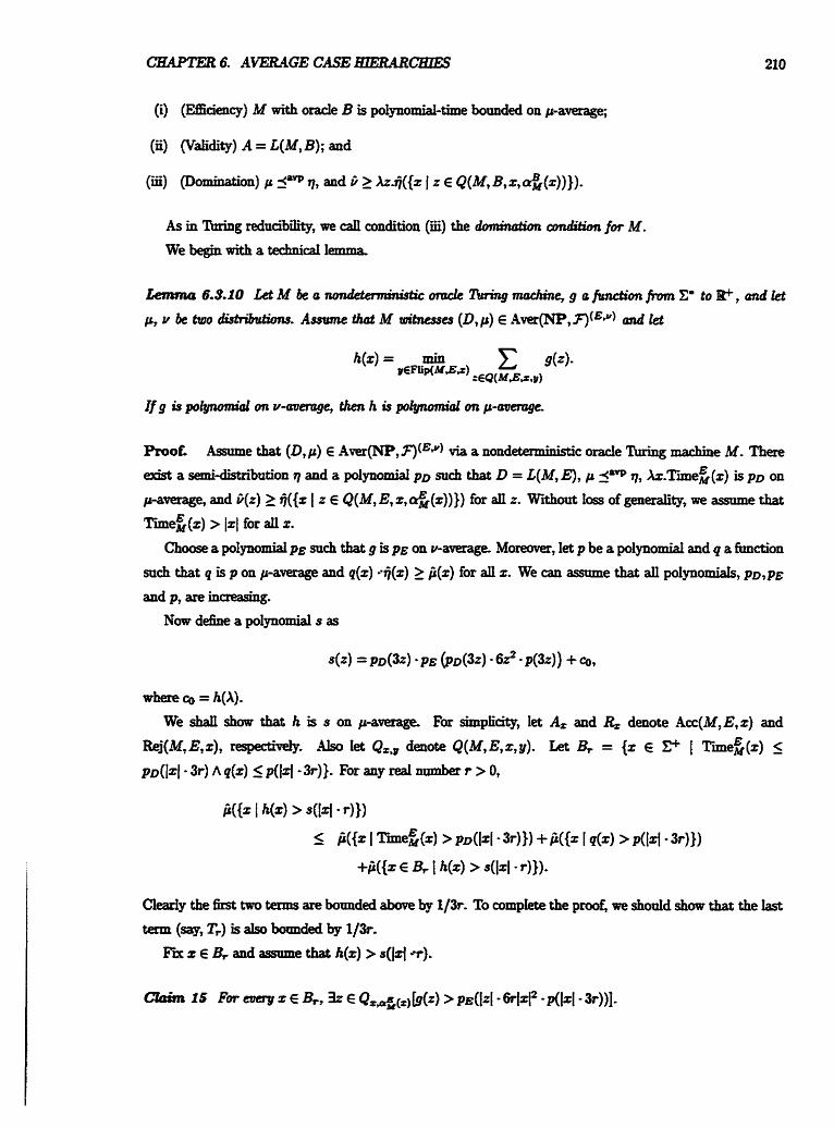
(i) (EEaency) M with oracle B is polynomial-time bounded on paverage;
(ii) (Validity) A = L(M, B); and
As in 'lhring reduciiiIi& we call condition (i) the d m a h t h cm&h fw M. WebeginwithatecbnicaI1emma.
ROOT. Assume that (D, p) Aver(lW, 7) (Ep) via a nondetermiaistic orade Turing machine M. There exist a semi-distxiidion 7 and s polynomial p~ such that D = L(M,E), p Wp rl, k . T i i e ~ ( x ) is p~ on
paverage, and ti(%) 2 @({x I z E Q(M, E, 2, &(x))}) for afl z. Without loss of generality, we a r e e that
~ m e E ( z ) > izl for dI 2.
Choose a polynomial p~ such that g is p~ on paperage. Moreover, let p be a p d y n o d and q a function
such that q is p on pa- and q(z) +(z) 2 P(x) for dl z. We can aPsome that an polynomiak, p ~ , p ~
and p, are mcreashg.
Now define a po1ynomial s as
where ~0 = h(A).
We shall show that h is s on patrerage For simplidtp, let A, and R, denote Acc(M, E,x) and
Rej(M, E,x), m y - Also Iet Ql, denote Q(M, E,z, y). Let B, = {z E CC [ Ti~nef&) 5
p~(1x1- 3r) A q(x) 5 p(1zl- 3r))- For any red number r > 0,
Cleadp the first two tams are bounded above by I/*- To complete the prooc we &odd show that the kit
term (q, Tr) is is asodolmded by I/*. Fix z E B, and asstme that h(z) > ~((21 r).
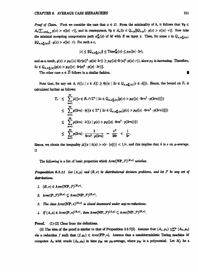
CIIAPTER 6. AVERAGE C A S E ~ C H I E S 211
Note that, for any set A, t({z I z E A)) 2 +((z [ 3 E Q,,afi(,)[z E A])). Hence, the bound on T, is
calcuIated further as fonow~:
Hence, we obtain the ineqaaity b({z I h(x) > s(r. 1x1))) < l/r, and this implies that h is s on paverage
0
The fo11owing is a list of basic properties which A v e r w , F)lBp) satisfies.
P r o p o ~ 6.5.11 Let (A,p) and (B,v) be d k t d d o d decision problems, and let 7 be cmy set of
Pmof. (1)-(2) Clear from the defh&ms. (3) The idea of the proof is Itimilslt to that of Proposition 5-5-7(5)- Assume that (At, pl) 9 (A2, p2)
via a reduction f such that (f,p~) E Aver(FP,*)- Asmme that a nondeterminiseic Thing machine M amp* A2 with o d e (A3,~(3) in time p~ on ~rraverage, where p~ is a polynomiaL Let MI be a
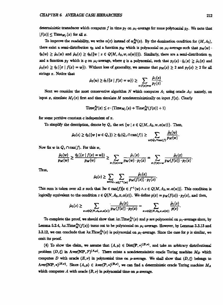
ClMTER 6. AVERAGE CASEHIERARCHIES 212
string z. Notice that
Next we consider the most conservative algorithm N which computes A1 using oracle A3: namely, on
input x, sirnuhe Mf (z) k t and then simnlate M nondeterministicaily on input f (z). Cleariy
for some pcsitive constaat c independent of z-
To simp@ the description, denote by Q, the set (w 1 z E Q(M, &,w, a(w))}- Then,
N m 6x w in Q= n ran(f)- For this w,
i i r (b I f (z )=~) ) h ( 2 ) - fit (4 PM (w) " z f (r)=w CM(W) ' ~f (21 - zg- &df@)~ * ~ f b $
To complete the p- we shodd show that ~z~Tiime$ (z) aud p are plynomid on pt-average since, by
Lemma 5-24 k-Tiie*(f(z)) tmns ont to be poIynomid on pz-aoerage. Eowever, by bp 3Al3 and
33-12, we can conclude that k-~he$(z) is poIynomial on ppaverage. S i the case for p is shdar, we
omit its p d
(4) To show the claim, we assmne that (Ap) E Di9t(P,*)(B+), and take an a r b ' i distniutional
problem ( D , a in Aver(NP,F)(b). There exis& a nondetc ' ' ' t oracle 'Ihring macthe MD which
cornpates D with oracle (Ep) in polynomiaI time on p-aveqe. We sMI show that (D,Q to
~ver(NP, *)(Bg)- Simce (Ap) E A~ee(P,*)(~p), we can find a demmb&ic orade Thing machine MA which computes A with orade (B,v) in polpnomia time on paverage.
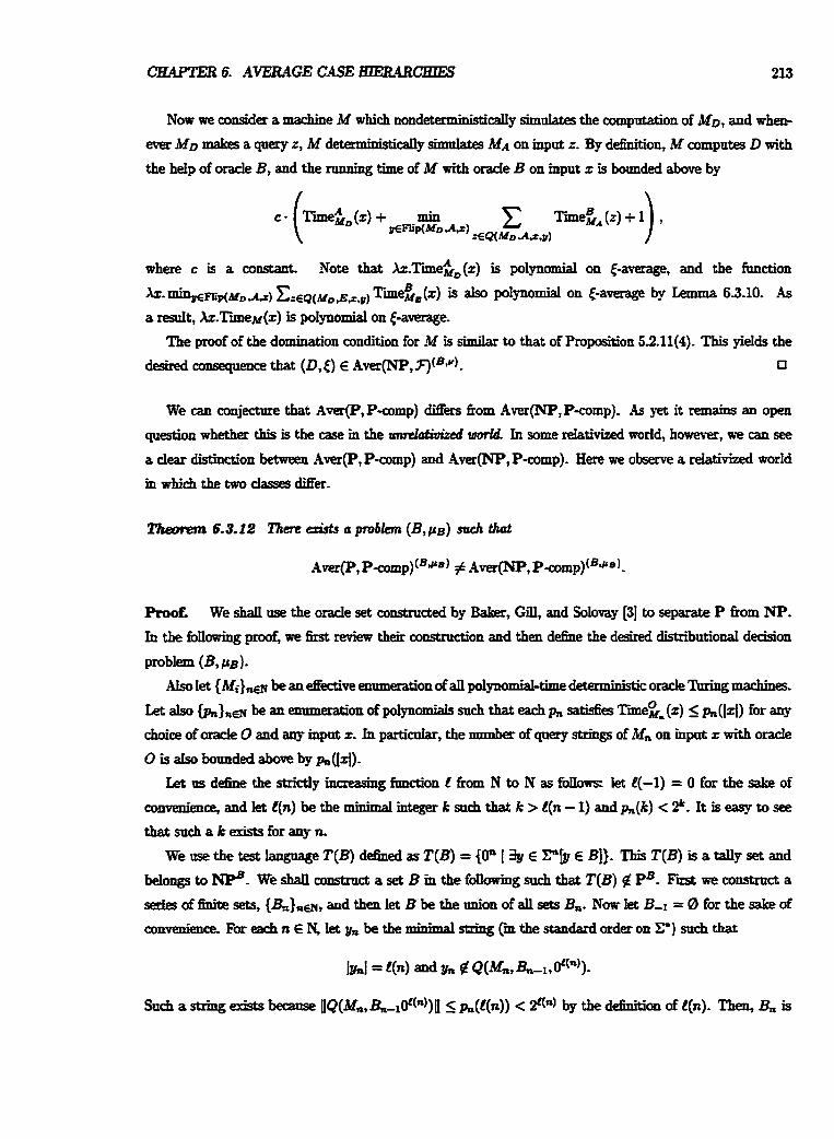
CHrLPTER 6. AVERAGE CASE EIERARCHZES 213
Now we consider a machine M which nondeterministicaily simulates the compdation of MD, and whezr-
ever MD makes a very z, M determiaistically simulates MA on input z. By definition, M computes D with
the help of oracle B, and the nmning time of M with orade B on input z is bounded above by
where e is a mustant. Note that h.Tiie&,(z) is poIynomial on (-average, and the function
k- *EFWMD A) Ct EQ( M~ ,.E~,~) ~ i e ~ ~ ( z ) is also polynomial on c-amage by Lemma 63.10. As a result, Xz.TiieM(x) is polynomial on &average.
The proof of the domination condition for M is similar to that of Proposition 52.11(4). This yields the
desired co~l~equence that (D, Q E Aver(NP, F)(**). 0
W e c a ~ conjectnre that Aver(P,P-comp) M e r s &om Aver(NP,Pamp). As yet it remains an open
question whether this is the case in the t n d a h m d . * world In some rebtivized world, however, we can see
a clear distinction between Aver(P, P-comp) and Aver(NP, P-comp). Here we o h a relativized worId
inwhichthetwodassesdiffer.
Thetnem 6.3.12 T7me aists a problem (B , j r~) such that
ProoE We s6aII me the d e set constructed by Baker, Gill, and Solmy [3] to separate P b m NP. In the fdlowing prod, we first review their construction and then define the desired distri'butiona1 decision
problem (39 PB). AIso Iet {Mi)& be an U v e enumeration of all polynomiaEtime deterministic oracle l b h g machines.
Let a h &Ina be an enumeration of polynomials snch that each p,, safSes ~~rne:~ (2) 5 p,Jlrl) for any
choice of oracle 0 and any input 2. In parti&, the number of query strings of Mn on input z with o d e
0 is a h bounded abm by p,,(lzl).
Let us define the shialy increasing function C from N to N as fbIIows: let t{-I) = 0 for the sake of
convePience, and Iet C(n) be the minimal integer k such that k > C(n - I) a d h ( k ] < P. It is easy to see
that such s k exists for ang n.
We use the test langttage T(B) d&ed as T(B) = {On f 3y E Ply E B]). Tlis T(B) is a tally set and
beIongs to e. We shall construct a set B in the following snch that T(B) 4 PB. Fast we construct a
series of bite sets, {&)aaPI, and then let B be the tmim of all sets Bn- N m let B-1 = 0 for the sake of
commience. For each n E N, Iet yn be the minimll shing (in the standard order on C) such that
Such a string exists because IIQ(Mn,&-loL('))U 5 p,,(C(n)) < P(") by the d-on of l(n). Then, B, is
This shows that T(B) # L(Mn,B) for alZ nnmbers n, and thus T(B) 4 PB.
We then define the distribution p~ for the set B. Let
Consider the distriiutional decision problem (T(B), vay)- Clearly (T(B) , uWy) is in .4ver(~P, Pamp)(B+n).
Now assume to the contrary that (T(B), urJly) beIongs to Aver(P, P-c~mp)(~?"~) . There exists a determin-
istic Thing machine M which computes T(B) with oracle ( B , ~ B ) m poIynomiaI time on ut~lr-average.
Recall that T(B) is a tally set. Smce M is polynomial-time bounded on uuy-average, we condude that
T(B) E PB. This contradicts the fact that T(B) 6 pB.
F i i y we extend Dehition 6.3.1 h r n a single oracle problem to a dass of o d e problems.
Dehition 6.3.13 (Retativiaation) Let C be a elass of distriiutiond decision problems and let f be
a set of distniations. kt A Y ~ ~ ( N P , ~ ) ~ denote the rmion of ~ver(NP, atE*) for any oracle (E, v) c h m
h m C.
As an immediate consequence of Propositiort 63.11, the relativized Aver(NP, *) relative to Aver(P, *) to Aver(NP, *). Note that whether Aver(NP, *) relative to A=(NP, *) coJlapses to A=(NP, *)
is an open question.
Proposition 63.14 will be extended to any l e d of the average polynomial-time hierarcky in Section 6.4.
Another important average compkity class is the coIIection of deterministic average polynomial-space com-
putable sets, Aver(PSPACE,F)- This dasP contains Aver(P,F) and Aver(BPP,F) as subclasses- In this
~-an,weshauintrodnce - . -
a &hmatam of Aver(PSPACE, 7).
CHAPTER 6. AVERAGE C A S E l i E M R ~ 215
Deanition 63.15 (Bektivized Aller(PSPACE, 3)) Let (B, v) be a distributional decision problem.
A distn'butiod problem ( 4 p ) is in A~(PsPAcE,F)(~*) if there exist a deterministic o d e Timing
machine M and a semi-distniution q such that
(i) (EEaency) M wi th orade B is polynomial-space bounded on paverage;
(ii) (Validity) A = L(M, B); and
(ii) (Domination) p saw rl, and P 2 Xt j ( {z 1 z r Q(M,B,x))).
We also call the condition (iii) the dcmhatiun condition for M.
Since oar relativization is similar to that of Aver(P, F), the foIIowing proposition is straightforward.
Propo- 6.3.1 6 Let (A, p) and (B, v) & dist~+buthd decirion problenzs.
Roof. For the proof, we need a relativized d o n of the randomized bounded halting problem
(BHP1(A), p ~ ~ , ) . Assume that {Milia is an &kcthe enumeration of dl deterministic orade Tltring machines. For a set A, let
BEPl(A) = {(O,a,z, 1") I Mi wi th o d e A accepts z ming less than n squares )
~ { ( l , s ~ , x , P ) I Mi with o d e A on t uses at least n squares };
and, for b E {O, I), let
Notice that the distniation m~p, is not dependent on o d e A.
T& the desired set A so that A = BH&(A). We remark that this set A exists became Mi cannot qpery
any strings of length mare than n, and thus, it makes only queries to orade A that are lexicographidy
@er than (b, r, z, In). Now let M = mt. W e shall show that sny distributional problem (D, p)
in ~vet(PSP~c~,~cornp)(AP*) belongs to ~ver(P,~-com~)("+~) . For this pair (D,p), there exists a
d-c 'Ihring machine M c o m p ~ D with o d e A in polynomial time on pmmagc
Let g be the fimction d Lemma 4.2?(2) such that ji(x) < 2-m)l+2 f'or aJI z, and d&e the machine
Mt as fbIIows= on input z, it computes g(z) and then simaktes M on input g(z). Let i be an index such
~&=MrsinceMrisalsodetenninisti~Letns~nsikthef~deterministic~N:
begindetermiaisticalgorithm N input z
compute g" (2) and set u r g"(z)
forn=ltooodo
query (0, si, u, In) to o d e A
if (0, si, u, 1") E A then accept and halt
query (1, si,u, In) to d e A
if (1, sip U, 1") $ A then reject and halt end-for
end.
Notice that the macbine N makes queries only of the form (b, si, g" (z), In), where b f {O, 1) and 1 5 n 5 Tnne& (2) + 1.
It is not difiicult to check that, with oracle A, N computes D correctly. We next check the domination
condition for N. Remember that, hr each query string (b, q,u, In), the string g(u) is the only input on
which N queries it. Smw g is oneone, this correspondence tiom query strings to inputs is also onmne.
Thus, the rest of the prod is analogous to the proof of CIaim 11 in Section 5.3.5.
Let q(z) = 512- (lg(z)l+ 1)" .(Time& (z) + l)*/V-(si). It is obvious that q is plynomid on pawrage
because k.~ime&(z) is polynomial on paverage. As m Theorem 53.2, we have
This indicates that (D, p) belongs to Avet(P, P-cou~p)(~J')- a
We then introduce a relativized dass A ~ ~ ~ ( P s P A C E , F ) ~ for a dass C of distributionat decision prob
Ierns*
Deflnitioa 6.3.18 (Relatkkation) Let C be a cIafs of distriiutional dedsion problems. For a set
7 of distnIbutions, Aver(PSPACE, nC (Aver(PSPACE, F) dative to C) denotes the congaion of aII
distributiod problems m A~~~(PSPACE, T)(Bp) for some (B, v) E C.
PmoE It is clear that Aver(PSPACE,F') C A ~ ~ ~ ( P S P A C E , F ) * ~ ~ * ~ ~ ) . We shall show the
other inclusion. Assume tiat (A, Cc) E A~~~(PSPACE, for some (B, v) E Aver(PSPACE, *). Let
M be a deterministic o d e Thrbg machine which computes A with o d e (B, v) using poiynomial space
on paverage. Since (J3,v) E AverlpspACE,*), there exists a deta ' ' tic Turiug machine MB which
computes 3 using polynomial space on v-average The algorithm we would like to consider here is the
conserrrzrtive one: on input x, simulate M on z except for orade queries; instead of querying a string z,
simnlate MB on z. On each input x, this algorithm uses space at most
for same 6xed constant c > 0.
We can conclude that this bound is poIynomial on p-average since k ~ m a x , ~ ~ ( ~ ~ , , ~pa~eE(z) is poly-
nomial on paverage as in Lemma 6.3.10- Therefore, (A ,p) b d o w to Awr(PSPACE,F). 0
6.4 Average PoIynomiaI-Time Hierarchy
This section will f d p introduce an average-case version of the polynomiaEtime hierarchy. In previous
sections, we introduced relativized Aver(P,F) and cekmed - - A m p , F). These relativized cIasses wiII
be the basis for constructing an averagecase version of the polynomial-time hietiuchy.
6.4.1 Average Polynomial Time Hierarchy
We now give a fimnal dehition of an ctteruge polgmmial-Eime hiawrlry under a particular set of distniu-
tiom. This hierarchy is an averagecase d o p e ofthe polynomial-time hierarchy in worst-case comp1exity
theory.
-n 6.4.1 (Average PoIynomiaETii Hierarchy) [9q Let k > 1 and let 7 be a set of
distnintions.
Prod (I) In the case k = 1, the c[aim for Aver(NP,F) bIIm from Proposition 51.6. Now let
k 2 2 and assmne that ( A p ) 5 7 (3, v) and (B, Y ) E Aver(E!,F). By dehitbn, there exists a probIem
(C&) E Aver(Xi-,, *) such that (B, v) E A v e r ( ~ ~ , F ) ( ~ k ) . Proposition 63.11(3) implies that (A, p) E
~ver(NP, F)(Cd). Using the dehitim again, we obtain (A, p) E Awr(XE, 7).
For the cIass Aver(IIi,F), assume that (A,p) (B, Y ) and also (B, v) is in ~verm;, 7). Note that
(A,p) L)? (B, v) if and only if (zvCr) (B7 v). Ftom this fact, it h[Im that (x,p) E Aver(E!,T).
This is equident to (A, p) E Aver(IIf;.F). (2) SimiIar to (1). If k = I, then the claim is based on Proposition 52.6. For the other case, we use
Reposition 5.5.7(5). 0
In what fiows, we shan see the basic mclnsions among the classes of tbe average polynomial-time
hierarchy. Fttst we want to see the lemma that charaaerizes the relationship between Dist(E;,F) and
A=(CJ;, 7)-
h o E We shaIl show d y case (2) because case (I) foIlows by a similar argument. Let us assume that
(A, p) is in Dist(Chl, 7)- S i A E Z&,, these exists a nondeterministic made 'Ihring machine M which
computes A in pdynomiai time with oracle B in Xi. By a simpIe modikation of M and B, we can assume
the foIIorrPing proper@ on each input z, the madhe makes a query once of the form (z, y), where y is the
(ade of the) computation path. Note that, for every query string, there is the nnique pair of an mpnt and
apath, We shall show that (A, p) E Aver(NP, for some v, Let ns &st define such a distnIbutior~ Let v
Onr d* of v obvioasy gnarantees the domination condition for M- Hence, M recognizes A with or&
B in polynomial time Since (B, v) E Dist(Cg,*), we obtain:
CHAPTER 6. AVERAGE CASEHlERARCHIES
Using Lemma 6.43, we can prove the foUowing proposition.
Proof. (1)-(2) The claims foflow from Lemma 6.4.3. (3) This daim foIlows h m Definition 6.4.1 and from
the facts that ~ v e r ( ~ , F ) ~ A ~ ~ ~ ( N P , F ) ~ and (D,p) E A V ~ ~ ( P , F ) ( ~ & ) . 0
The above proposhion may be taken as evidence that our average polynomial-time hierarchy has a
structure s h k to that of the worst-case polynomial-time hierarchy-
Figure 6.1 illastrates the structure of the average poIynomial-time hkarchy under F-
Proof. Assmne that ( 4 p ) is in ~ v e r ( N P , F ) ~ ~ ~ ~ l * ' ) . By definition, we then have a chain of
membedip rdations (A, p) f Aver(NP, F)(Bp) and (B, v) E Aver(P, *)(cd), where (C, Q E Aver(Ci, *).
By Proposition 63.1 l(4), we can shorten this chain to (A, p) E ~ v e r ( ~ ~ , F)(Cx). This shows that (A, p) is
in Aver(C&, ,a. The converse is even simpIer to prove. Smce Aver(Ci, *) E Aver(AR1, *), it fo11ows that
Theorem 3.5.24 shows the separation between Aver(P, *) and AverlNp, *). Mthough these basic average-
case complexity clases are difhat, we do not conclude that s h k separations occur m the higher I d of the average polywmial-time hierarchy. The reason is that domination conditions restrict the complexiW
of-espedaIl~-- The woftt-case poiJmomial-time hietarcbp eutds the "downwatd maapse" propertg; that is, if any two
I d of the hierarchy colIapse, then the upper levels cohpe down to those 1eveIs. More precisely? if
EE = ELl, then PH = Et. Now we show that the assumption Aver@;, *) = Aver(CRt, *) Ieads to the
cow of the average pdymmiaI-time hierarchy.
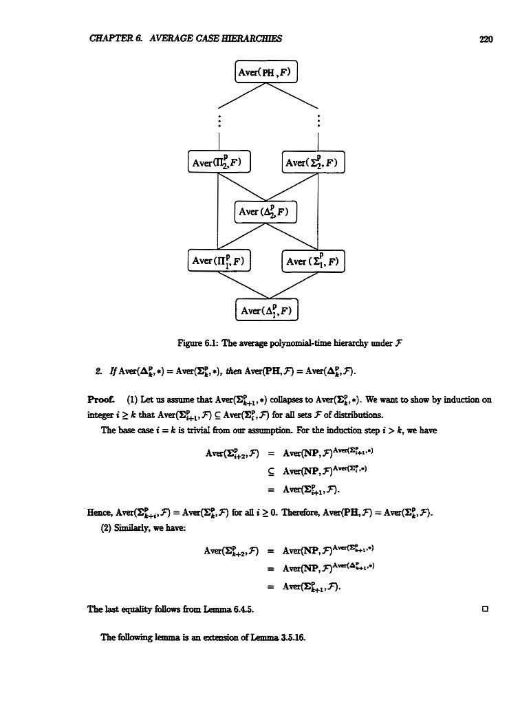
Fgure 6.1: The average poIynomid-time hierarchy under 3
Proof. (1) Let us assume that .4ver(XL,, *) coIlapses to Aver(Ci, *). We want to show by induction on
integer i 2 k that Aver(CR, F ) Aver(Er,F) for all sets 3 of distriiutions.
The base case i = k is hivid b m our assumption- For the induction step i > 5, we have
Proof. Assume that (A, PA) and (B, p ~ ) are in Aver(C, F). The proof is by induction on k 2 I. For the base case k = 1, the daim for C E {P,NP) is immediate from Lanma 3.5.16. Now let us consider
the case C = ahw. Assume that (4 PA) and (B, pB) are hL Aver(mNP, 7). h other words, (&A)
and (Etm) areinAver(NP,F). AgahbgLanma3.5.16, wehave(hE,pA$pP) E Aver(NP,F). - Notice that a $ B = A @ B - {A}, where A is the empty string. Smce PA $ pB(X) = 0, we may ignore A,
and thm ( A t P A 8 p ~ ) E Am(NPtF)- This yields the desired condusion that ( A $ B, @ ps) E
Aver(cpNP, n* For the induction step k > 1, first let C = X!. By our assumption, there exist distn'butional problems
( C O , ~ ) and (C1, &), both of which belongs to Aver(PL1, F), such that (At pA) E A=(NP, F ) ( C o A )
sod (B,CB) Aver (NP,F) (C1~) - It ig &tidy to ~ e e tbat (Co,&) sk (Co @Cl7Co @PI) a d (el,&) 55 (Co@Cl,Q@pl). Forsimplicity,write (C,c) for (Ci$Clt[o~pl). By ourinduction hypothesis,
we obtain (C, Q E Aver(Ek,, 3'). Using Lemma 7212, we get ( A d By M @ pB) ~ v e r ( ~ ~ , T)(C*). As (C, Q is in Aver(E:-,,aF), the pmb1em (A $ B,pA LA p ~ ) is in Aver@';, F). The case C = A: is similar?
and theother a s e C =IIL isobtained withthesameideansedfor thebasemseC=c+NP. a
At last, we may conjecture that, for a naturally selected set 3 of disttz'butions, the average polynomid-
time hierarchy tmder 3 is truly an infinitr?. hierarchy.
6.4.2 Sparse Interpolation Property
We shnn show a basic relationship between worst-case c o m p l e and average-case complexity on strings
w i t h high probability. We kst introduce an interpolction property of an amagxme compIexi@ class
Aver(C,F)- IntnitiveIy, the property says that if we cornpate a set A fast on average tmder a distriiution
which assigns high pmbabllity to instances in a sparse set S, then there is an "interpolad" set B between
A n S and A which is computabIe fist in worst-casec This set B is s coIIection of "easyn instances m A, and
it becomes a good worst-case approodmation of the set A.
Here is the f o d dehition of the sparse ~~ propertyproperty
Deanition 6-4.8 (Sparse fnterpolation Roperty) [9q For a sparse set S and a polynomiaI q, let
fbrdlx~SptOVidedthat)=,~&~-(l. AcIassAver(C,F) h a s t h e s p o r ~ e ~ ~ ~ i & f o r
any set A, any h h i t e sparse set S, and any polynomial q su& that (A, pS,J E A-C, F), there exists a
set B E C suchthat A n S c B S R Theset Biscalledan interpohtofAasdS-
P r o p o ~ 6.4.9 For a doss C E {P, NP. RP, BPP, PSPACE), Aver(C, r) has the sparse interpoldm
-*
Root We first show the case C = NP. T& any sparse set S and a po1ynomial q and assume that
( A ~ s , ~ ) c Aver(NP, *). There exists a nondetermiaistic Turing machine hi which computes A sach that
b - m m e ~ ( z ) is p on psPq-average for some polynomial p. Note that Tune&) 5 p ( l ~ l / j i ~ , ~ ( x ) ) for an x with Ps&) > 0. Let N simdate bf on input x in p([xl q(lz1)) steps. If the simtllation of M does not terminate
withiu p(lxl- q(lz1)) steps, then N rejects z- Let B = L(N). Clearly B A. S i q(lzl) 2 l/fiS,,(z) for dl z E S, N compIetely simulates M on all inputs z in S. Thus, A n S = B n S. Clearly N is polynomia-time
bounded. Therefore, B f NP. The other ~ s e s are treated simhrly, but spedficdy for the case C E {RP, BPP), we must use Tmeb (z)
instead of (z; s) . 0
Proposition 6-42 can be extended to an arbitrary I d of the average po1ynod-time hierarchy. However,
its proof is not as h p I e as that of Proposition 6.4.9. W e first present a key 1emma.
Proof. (I) The proof proceeds by induction on k. The base case k = 1 essentiaIly fotIm h m Proposition
6-49. Assume that (A+) E A m , * ) and Iet S C C and let q be any poIynomid_ There are a
nondeterministic ntring marhine M and a polynomial p such that A = L(M) and B({z [ TiieM(z) > p([z[ - r)}) < l/r for d r > 0.
Let r = q(n), and then b({z 1 Ti&(z) > ~(1x1 q(n))}) < l/q(n). Let Mo simnkte M on the same
input in h e p(n -q(n)); if M accepts z, then & accepts it, or eIse Mo rejects z. SimkIy, let i& simalate
M in time p(n - q(n)); if M rejects z, then Ml accepts it, or else MI ~jects it. Define Co = L(Mo) and
Cl = L(Ml), and let Sf = Sn (G uC1). Clearly A n St E C' E A and an Sf c Cl H Momovert
The mdaccion step is carried out as fbIIows. Let k 2 2 and amme that (A+) E Aver(cE, *). By
definition, there exists a distn'brrh'onal problem (B, v) E Aver@:-, , *) such that (A+) € A-, F)@P). Let M be a nondeterministic o d e l b h g machine which computes A with oracle (B,v) m poiynomial
time on p-aveqp We armme that ~ z ~ T i i e ~ ( z ) is p on pavetage fix some inmasing po1ynomial p.
The domination condition for M impIIes the exisfence of a semk&ri%ution q and a fimction d which is
CaAPTER 6- AVERAGE CASE EiERARCHIES 223
pdyttomial on paverage such that d(x) . ij(x) 2 fi(x) and B(z) 2 ij({z I z E Q(M, B, z, &[z)))) for aU z and z. Assume also that t is a polynomid witnessing that d is polynomial on pawrage-
Consider any set S and any poiynomial q. We d&e T as
For each n E N, let us consider the subset T" of T. Notice that
In the rest of the proof, we use s(n) for t(n - 3q(n)). To use the induction hypothesis, we let Z = { z I 3z E T(z € Q(M, B, z, &x)) ) ) , and we also let
Applying the induction hypothesis to Z and I(n), it foUows that there exist sets 2' G 2 , Ci E EL,, and
C'i E I& such that, for every n E N, P ( P ) - Q(Zm) 5 I/l(n).
Now recall that M queries strings whose Iength is at least the same as that ofthe input and at most the size
ofits nmningtime. Inother words, foreveryz mTn, ifr E Q ( M , B , Z , ~ ~ ( X ) ) , then n< Izl ~ p ( n - 3 q ( n ) ) .
Based on this Fact, we prepare sets &, = {z E Z I n 5 Irl 5 p(n 3q(n))) and 2; = {t E 2' [ n 5 121 5
p(n - 3q(n))l- sme ~ n - ~ : r ( ~ - 2 3 n { ~ ~ ~ ~ l z l s ~ ( n - 3 4 ( n ) ) ) ,
it foUows that
The desired set Sf is d&ed as Mows
Clear1 y Sf S. Using the fact that
by the domination condition, rn obtain &(gn - 23 2 ij(P - Sm). Then,
b(W - fi(T=) < i;i;;r. we et(W - b ( P ) < A- kMokanarade~~withoradeX~~foII~~~.Oninpatx,M~sirmrlategMm
z m time p(]d -a([@), and whenever M queries a string z, No queries both Oz and Lt to its o d e X. If
CHAPTER 6- AVERAGE CASEHIERARCHIES 224
Oz f X and lz fZ X, & continues the simulation wi th the assumption that the made answer is "yes"; if
Or 4 X and lz E X, then it continues the simulation with the oracle answer "non; otherwise, it immediately
rejects the mput 2. The machine MO accepts z exactly when M halts and accepts it. Similarly, we dehe
a machine MI by interchanging the oracle answers and requiring that MI accept the mput z if M halts in
time p(Iz1 3&[)) and otherwise MI rejects z. Now let CO = L(Mo, Ck $ Ci) and Cl = L(M1,C; $ Ci)-
By thedefinitionsofthecuaclemcbes MOandMl,itfolIowsthat AnSrCCo ~ ~ a n d h s ' c ~ ~ GZ. (2) The proof is similar to (1). n
Proof. We show only the case Aver(CE,*) here. The case k = 1 follow &om Propositim 6,423. Let
k 1 2 and assume that (-4,~s.~) E Aver(C,P,*) for a sparse set S and a polynomial q. It foIIows h m
Lemma 6.4.10 that there exist a set C E C! and a subset S' of S such that A n Sf C E A and
&S,~(S") - f i ~ , ~ ( S ~ ) I 1/2q(n) for all n E N It d c e s to show that Sf = S. Asnrme that there exists a
string z E S - Sf. Let n = IzI. Smce fi&) 1 l/q(lzl), it folIm that
This is a contradiction. Hence, Sf = S. 0
The following proposition is another consequence of Lemma 6.4.10, and it win be nsed in the next chapter.
Proof. Let p be any poIynomial A s m e (A, V-) E Aver(CE, *). Take q(n) = 2(n + I)' - p(n). Note
that
We apply Lemma 6.410 to q, A, and C". Then, we have sets Co E CI, 4 E Ti:, and S such that
A I ~ S S C O ~ 4 X f l S ' ~ C I SZ andv-(C-Sm) s l fq(n) f o r a l l n ~ n ObvionsIy,SS'CCoUC1.
Hence, IIq U qn 2 IIS"I[. It scrtlices to show that [ISfnl[2 (1 - A) 2"- Note that
Smce kroad(P - Sn) < l/q(n),
6.5 Average Polynomial-Time Alternation Hierarchy
I . wombcase w m w theory7 alternation plays a varietJr of roles. R e d that AEf; = ATIMEE(k7 nO(l))
and Mf: = &(k,nO(')). Then, we have AEE = C: and Ah: = A: for all k > 0; namely,
the poIgnomiaI-time alternation hierarchy is d y the polynomial-time hierarchy (see Lemma 2-5.1). In what fobws, we intraduce an average version of this polynomial-time dternation hierarchyt an average
polynomia-time aIternation hierarchy under a set of distriiutions, and study its relationship to the average
poIynomial-time hierarchy de6ned in Section 6.4.
D-tion 6.5.1 (Average Polynomial Time Alternation Hierarchy uuder 7) Let k > 0 aud let F be a set of diski'btttio~~. The aoaage p o ~ - t i m e alternating hiermchy under 3 consists of the
fonowing average classes:
1. Aver(AAi, F ) = u ~ > ~ AVE~(ATIME~(~, nC f c), F).
RecaIl that I-alternation bounded alternating 'ihring &es with e x k h t i d states are exactly the
nondeterministic Thing machines. Similarly7 semideterministic l-alternation botmded dternating Thing
machines are determrmstlc * . . ntring ma&hes. Hence, it is dear that Aver(AA;,F) = Aver(P,F) and
Aver(A.X;, 7) = AverlNp,F) for all set F. NePeftheIess , two~Aver(AI:~ ,T) andAver(CE,F) are~ytobethesameeveu6orthesetPof
~ i I y computab1e distributions. The folhwing propasition heIps us tmderstand the gap between these two
ches. Recall that Aver(AR,, F) = ~verfP, F)*-:*') and Aver@Kl F) = .4ver(NP, F)*-:**)-
Prod We pwe (2) here. Fnst are assmne that (A+) E Aver(ACR,,F). There exists a (k + I)-
alternation bounded Thing machine M gnch that A = L(M) and Xz.Tii~(z) is p on pammge, where p
is a polynomial We shall show that A is computable by a nondeterminirtic orad= Taring 'Lhring N with
oracle ( B p ) i n ~ t i m e o n p a v e r a g e .
CEQPTER 6. AVERAGE CASE HIERARCHIES 226
The main idea here is to query sufficiently long strings to the oracle so that the complexiq- of the oracle
set can be substantially rliim;nished. We begin by deb@ the oracle Thing machine N as follows
begin nondeterministic algorithm for N
input z (assuming that z # A)
simdate M on input z during the first series of dikntkl states
until M reaches the universal states
(let y be the code of such a computation path)
choose a path sbrting hzn y nondeterminiSticaIly (ignoring the states of configurations)
and folIow this path until M reaches a halting configuration
(let n be the length of the path from the initial con&mtion)
query the pair (2, ylOn) to the d e
if oracle answers "yes'' then reject eIse accept
end.
Clearly N is a nondeterministic ntring machine whose nmning time is O(TiieM(z)).
Let 3 be the set that is accepted by the bllowing dgorithm. On input (z, ylOn), check if y encodes a
computation of the &st series of ex&ntbl states of M on input z, and if so, then sirdate this path tmtd
M goes into mriversal states. Sinlate the rest of the computation of M within n steps. If a path does not
hat within n steps, then go into an accepting co&gmation immediatdy. It is not di6icult to see that B is in
ATIME'(~, ~ ( n ) ) , and thus B E C:. By definition, A = L(N,B). To see that (A, p) E o n , 4 v e r ~ , F)@*3
for some u, we remark first that Q(N, z, &)) = ({2,y10n)) for some y and n. Next we define
It is easy to check that (4p) E AAP~~(NP,*)(~*) via N. !%hce (B,v) is in Dist(XE,*), we have (A,p) E
Aver(~~,7)==t(%').
Comedy, assmne that (A, p) E A=(NP, 7)h(4b'). There exists a problem (B, v) € Dist[E!, *)
snrh that (A, p) E her(NP, F)(B+') via an appropriate nondeterministic oracle Zhring machine M. A s m e
that B is in &(kYp(n)) for some poIynomiaI p- We can asnre that p is strictly increasing.
Next we define an dternating lhk tg marh;ne N as foIlows. On input z, N &mdates M on mpnt
z starting w i t h an ex&ntbl state. Dnring this akkntid state, if M queries r, then N stores z Cm a
work tape) and guesses its oracle answer m(t) and continue the simuIation until M terminates. On each
mmpatation path, if M reaches an accepting m@mation, then N existentially checks if s E B for all zi
withons(q) = 1. Then N nnioersally chedrsif~ $ B for aILq whichsati&m.s(z+) =Oat onceusing B.
If=(&) = 1 fix all such s, then accept 2; otherwise, q*ect z. It is easy to check that A = L(N). The nmning time af N on input z is at most
for some constant c > 0. Since Xz.TmeM(z) is polynomial on paverage, by Lemma 33.14, h . T i i e ~ ( z ) is
also polynomial on paverage. We then have (A, p) E AVIX(ATIME'(L + 1, no(')), 7) = Aver(AER1, 7).
0
Coro1hn-g 6.53 Let k > 0 and 3 be a sef of d&+h&m-
In worst-case c o m p l e theory, there is a nice characterization of the class PSPACE by polynomial-
time alternating Thing machines: that is, PSPACE = ATINE(no(')). Interestingly, WE & not h o w
whether Aver(PSPACE, F) equals ~ver(AITbfE(n~(~)),T) becanse of the definition of the running time of
alternating ' h h g machine.
In what foIlows, we s h d show that Aver(BPP,F) for a supportive set 3 of distriintions is Iocated
within the average polynomiaLtime alternation hierarchy under 3.
Proof. Asmme that 3 is supportive and Iet (D, p) be an arbitrary problem in Aver(BPP, 7). Smce p is
supportive, we can define a strictly increasing, positive polynomial p such that P(z) 3 2-p(I21) for an z. By
Proposition 3.533, there e x h a randomized Thiag machine M which recognizes D in po1ynomial time on
paverage with error probabilrty 2*1~1)~, ie., &[M(z) # D(z)] < 2-~(l"l)'.
Now Iet us d&e
Apply Lemma 3331 to Xz.TrmeH(z), and we conclude that Xz.Tmeb(z) is polynomial on paverage Let
q be a polynomial such that kc-Tiieb(z) is q on paverage. For this q, we have Timeb(z) q(fxl//i(z)) d e ~ ~ P(z) = 0. Let S = {Z I i (z ) > 0). Then, for a h s t all z in S, Tie;la(z) 5 q(lz1 -2P(lzI)) < 2P(lrl)2-2.
We take a positive integer satisfying Log(Tiieb(z)) < p(1z1)2 - 2 for all z E S wi th 121 2 no. We next cIairn that the pmbabm p, = Pr,[M(z; s) = D(z) I TimeM& s) I Tiieb(z) h s E R&)I
is at least 1 - 2p(12 I)'+'. ~rrst we
CHAPTER 6. AVERAGE CASERTERAR- 228
Notice by the definition of Ti ieb(z) that P r . ~ m e e ~ ( z ; s ) 5 Tiieb(z) I s E R&)] 2 1/2. Hence, the
conditional success pmbabEZity p, is at least
In particularl when m = TimeL(z), p, 2 1 - 2-~(l'l)~+l > - I - 2-Iqrn-l since logm < p([z1)2 - 2.
Let us d&e another Tkhg machine M' that sim&tes M by using an additional input string as a
random seed- Formallyt the algorithm is as f01lows:
begin det erministic algorithm for M'
inpd (w) (say y = ytyr * * - vm, where yi E {& 1),1 I i I m) let i -0
start the simtllation of M on mpat z
wbile the simulation do
if M fips a coin and i 5 m then let its outcome be yi
i f M flipsacomandi>m then enteran infiniteloop l e t i = i + l
end-while
end.
Note that we do not re- the machine M' to exhaust all bits of y on each computation path of M on z;
thus, M' halts on input (2, y) exady when s is a p& of y for some random seed s f ~ M ( x ) -
Towards achiwing our goal, it sufEces from hposition 6.52(2) to show that (D,p) belongs to
~ v e r ( N P ~ F)(E*) for some dbtri'blttional problem (E, v) m Dist(NP, 4. We first define a nondeterministic oracle lhring machine Mo as follows:
begin nondetermisistic algorithm Mo with an oracle
input z
if < no then output D(z)
guessastringto
let m = lwl
simulate M' on input (z, w) for rn steps
if either M' does not halt within rn steps or M' entets a rejecting state
then reject
guess m distinct strings ul, ...,% of length m
qpery the string ( z ,u~ -u,,,,w) to oracle ifthestringis notin the oraclethenaccept elsereject
end.
W e now show that, for any oracle, & is time bounded on p- To show this, it d c e s
to caasider the ease where b[ = Time&(z). F i notice that, fbr any onYe 0, TiieL(2) 5 c - (m +

C&APTER 6. AVERAGE C ' H z 3 B A . R - 229
m2 + I), where c is an appropriate constant. Since k . T r m e ~ ( z ) is pdynomial on p-average, the hct ion
k.Tiie&,(z) is also polynomial on p-average.
Next we shdl define the desired d e E so that D = L(Mo, E) . The set E is defined as the set computed
by the nondeterministic machine MI below. Let u @ a denote the bitaise addition of u and o moddo 2, and
let the algorithm for Ml be as follows
begin nondeterministic algorithm for ML
input (z , ul - - -u,,,, w)
if lut - - # Iw12 then accept
(Now assume that rn = Iwl-)
guess a string v of length m
for i=l tomdo
simtrl;rte M' on input ( z , ~ $ v ) for m steps
if M' does not halt then accept
simtrlate M' on input (2, w ) rn steps
if M' does not halt then accept
if Mr(z , ui @ a) # Mr(z, w) then accept else reject
end-for
end.
Note that MI is polynomial-time bounded, and as a d t , E belonp to NP. Still we must prove that
D = L(Mo, E). For sim~licitg.~ we fhc x and set rn = Treb(z). Let A = {(w, g) E P x X"' 1 Mt(x, w) = M'(z, y)}. Moreover, let
B = {w E C"L I there are more than 2m-1wm-L strings y of length m such that (w, y) E A}.
The cMtinalitJr0f the set Cjo thus is bounded above by
(If - part) Assume that the right side of the equivalence in the daim is true; namely, there exists a
m-tuple ( u ~ , . . ., u,,,) E (IF)"' such that, for every v f P, (w, $ v ) E A hoIds for some i. Fm such an
m-tuple (ul, ...,u,& Let C = {u € P I (w,u) E A). For each y E Ct, there exists a number i snc6 that
(wteu) € A . Foreachi,let C:= ( ~ E P I ~ ~ [ ~ = W $ U A ( W ~ ~ ) EA]). Becauseofthedehitionof~,
11411 = IlC'll for all pairs (i, j ) , 1 i, j 5 m. Since F = r=, C:, we have IICill 2 Zm/m > 2*-t0p-1.
Thdore, w is m B. II
Reedl that x E D if and only if there exist more than 2m-'q(m)-1 strings y of length m such that
( q g ) E A- This is equivalent to saying that there exists a string w of length m such that w E B and
M f ( z , w) = 1. By the above cIaim, it h o b that
This yields the equation D = L(Mo, E). Finany we d e h e the desired distniution v on E as foIlons. Using the frmction c&,,(z), we set P(z) =
i((z z E Q(M& E, z, 4, (z)) )). It is to see that (D, p) is is inAw(N, 3')(&~), and
co~l~eqlfentiy (D,p) is m ~ v e r ( N P , 7 ) ( ~ ~ ) ~ v e r ( N P , 7 ) ~ ~ * ' ) = Aver(AE!,F).
The other daim that Aver(BPP,F) c A~er(An,~ , f l f o l m h m the mdusiom:
6.6 Average Low Hierarchy
The atrerage poIynomiaI-time hierarchy ~ O W S as to construct an a- version of the toto ) r imdig
in NP to refine the stntcture within Atter(NP,F). Pethaps some NP-compIete probIems with nattxral
distri'butiorts which are unknown to be either m A m p , *) or p ~ m p I e t e for Dist(NP,P-comp) fail into
a Iorvt ldaardrg in Aver(NP,P-cc)mp)-
We dehe the relativized average poIyrtOmiaEtime hiefarchp-
Definition 6.6.1 (Relativized Average PoIynomiat Time Hierarchy) Let P be a set of distribu- tiom. For a distribntid decision probIem (Bp), the relaCioited wemge polynomial-time hkmdiy &
3 d d i v e to (B,u) amskts Ofthe fo-g classes
(2ECIER 6. AVERAGE CASE IZZZMU- 231
Dehition 6.63 (Average Low Hierarchy under F) Let k E N
Here we remark that it is open whether each dass of the aPPrage low hierarchy enjoys the sparse inter-
polation p r o w .
Hence, A w ( A L , , *)(**I E Aver(AL,, *), which implies that (D, p) Mow to ~ver(LAk,, n. Snnl't;rtly, we can prove the other indnsion. I3
The assnmptiiopl A m : , *) = Alter(c&,, *) is & a t fm the dao Aver(NP, 3) to coaapSe to the
kth level of the average !ow hieratcbg-
CHAPTER 6. AVERAGE CASEafERARCHES 232
Proof. Let us assume that Aver(Cg, *) = Aver(CK,, *). Let (D, p) be an arbitrary distributional problem
in Aver(NP, 7). We shaII show that (D, p) belongs to Aver(LCE, 7). Since (D, p) E Aver(NP, F), we have
the following inclusions:
Aver(Cg, *) E Aver(Zi, *)(D*) G Aver(CR,, *).
Unfortrmately, we do not know any natural w p l e s of distriintional decision problems falling in the
average low and high hierarchies. The search for such problems is a chanenge.
Chapter 7
Quint essent i d Computability
7.1 Introduction
The most exciting aspect of this thesis is the attempt to investigate the notion of q r t i n t e s s d cmp&MdgT . .
first proposed by Schaler and Yarn- (911. Throughout this thesisT we have developed the avaagecase
complexity theory initiated by Levin. We know that a- compIexity theory is very sensitive to the
choice of distziiutions. For example, if we take a distri'btttion which d m h t enough to 0, then all NP problems are polynomial time soIvabIe on the a- N d e l e s ~ , this type of extreme analysis does not
capture the signiscant feature of average-case complexity theory-
Regarding Levids -on Dist(NP,P-eomp) cAver(P, *), Ben-David, Chor, GoIdreich, and Luby [9]
gave a partially negative answer by dernonstratEng that Dist(NP, P-comp) Am(PT *) d e s s E = NEL This reslllt sttggests one approach to open westions posed m average-case compIexity theory-. embedding
amagewe ampi- dasses into worst-case comp1- theory in such a way that the embedding does
not lose the compIexity of these classes. The simpIest s01ntion is to focns on "rare instances" under (Ceverf'
reasonab1e diss l iat io~~ ThiP notion was developed by SchuIer and Y k d a m i [97j (suggested by Uwe
Sch6aing) . In Section 7.2, we shall formally introduce the notion of kd C under 7." For a (wok-case) mmp1-
class C, %d C mder F represents the class of sets which can be comprttaible on average no matter
what distxi'butions are chosen h m E The simple notation CF was invented by Schder and Yamakami
[ 9 to denote the dass 'real C under 3$ for exampIe, P h m p captures Yred P under P-eomp." Using
this notation, Levin's question Dist(NP, P-comp) c A e T *) can be simply rephrased by the question
NP E1pp-comP in the worst-case setting-
Based on this notion, we are able to iotroduce the d p o w - t i m e k t m h g mcda 7, Xic, qF I k > 0), that esptares the essartiab d the average polynomiaL-time hierarchy under 3. By the
deWtion, -y computabIe dasses ha;oe oery difkent structures from their worskase connter-
For instance, it is mhn,m whether Pr eqaals Uk,,,DTIME(O(nk))r m gemmi, whereas P is
CHsLPTER 7. QUINTESSENTIAL C 0 M P V T A . B ~ 234
Uk.,,, DTIME(O(&)). One of the exciting results here is that the real polynomial-time hierarchy under the
set of recursive distniutions indeed coinades with the worst-case polynomial-time hierarchy- In particu-
lar, Pbmp c05pse~ to P. These &ts support our main focns on feasible distributions in average-case
analysis. Section 7.2 wilI f o d y d&e the notion of "real C under 7" and demonstrate the fundamen-
tal propertks and the eqttivaence betwen the red polynomia-time hierarchy under REEcomp and the
polynomiaEtime hierarchy.
Our interests are now in the real polynomial-time hierarchy under P-comp and its alternation connterpart,
the red --the alternaPi4n IrierOrchy under Pcomp, and we shaU study its properties from the
perspeaive of structural behaviors. The first question we wad to ask ourselves is whether any level of
the ceaI poIynamial-time hierarchy under P-comp contains sets which are hard to compute. Schuler [92)
succeeded in constructing such a hard set within Phmp which cannot be computed by a deterministic
polynomial-time Thing machines. His method is further extended by Schder and Yamagmi [98] to the
separation between DTIME(0(2Cn)) and P-,. In Section 73.1, we sha3 see how to construct hard sets
within and Cg-,,, k E y by using resourcebounded KoImogomv complexity.
Inuarme sets and bi-imwme sets are good examples of hard sets. The dass E, for example, contains
P-immune sets and P-bi-imwme sets, and thus E is different h m P. We shall see that Pkmp contains a
P-immune set of an " a r b i i density. Nonetheless, the class P-,, or even its &tabIe dosure has
no P-biiimmune sets, and as a consequence, the class tmns out to be s d l , i-e, it has pmeasure 0, horn
measure theoretic point of view. This consequence is intriguing in contrast with the faa that the Thing
d o s a r e o f P ~ , , isequaItothedassEXP,whtcbhasprneasure1.
In 1974, Book [15] Erst showed that E is JtruetwrJly di&rem from NP. He actually proved that NP enjoys the cIosure property under pm-reductions, but E does not; therefore, NP cannot eqml E. A simnar
structural,.property characterizg the classes in the real polynomid-time h i d y under P-comp. We shall
see in Section 7.5 chat neither nor S k m p is c l o d under pm-rednctions, and consequently
both A;-, and CE-, are slncduraCIy di&rent from all worst-case complex& cbss which are
cIased under pm-reductions.
In Section 7.6, we shall look at the probabilistic dasses BPP-, and B P P M P 7 which are another
example of weIIaadied quhksmtial comp1exity classes- h e to Ira- and Levin [44 and W e r
and Watanabe [96], the question NF mPPp-com, is known to be equivalent to the question NP C_
? B P P h p . This is not howa for P-, and P-,. The notion of random oracles was introduced by Bennett and Gin [8] in 1981 to prove that the probability
of the event of a d a i i v k i NP coinciding with a relativized P is 0 when oracles are chosen at random.
In Section 7.7, we shall show that neither of the inclusions, NP G Pp-com, nor PPSomp 5 NP, is passiile
relative to a random o d e .
Major Contributions. The author fiwmaks the notion of snbstantiaI computation on the average and
h the hardness and the strnctnral properties of the classes m the real poiynamial-time hierarchy tmder
Pump-
Propositions 7 2 5 and 72.10 show the inclusions among qufntessential computable classes: e-g., A:
AAEF E A ~ F G At,. A similar inclusion holds for the XI; class.
Propaition 7114 shows that, for any dass C of the polynomial-time hierarchy, every set m tin is nnearIy-
C. As a direct consequence, Corollary 72.15 shows that if strong one-way functions exist, then NP is not
included in BPPF for any set of distriiutions 7 which contains at least one supportive distribution.
Lemma 72.16 shows that if Aver(C,F) has the sparse interpolation property, then TAUY n CF C C. This Iemma leads to several interesting consequences including, as m ComUary 72.19, 33: E AHr unless
A., = Pk.
Theorem 72-23 s h m that AEREC-COmp = AAEREC-eomp = A! for my k. S i I y for CiRM=-p and BPPREC-p- In particular, as m Corollary 72.24, the class PEwmp equals P.
Theorem 7.32 shows that, for each constant c > 0, there exists a spa,= set in Mi-, but not in
m A ( k , 0 ( 2 ~ ) ) . A similar qmat ion result holds for AC:-mp-
Proposition 7.3.4 shows that, assuming PPamp # P, either FP g #P or NP BPP hot&.
Proposition 7.3.6 shows that for each constant c > 0, MEkmp is not included m
e ( k , dose. This immediately implies that P-, P-dose.
Theorem 7.3.9 shows that, for each constant c > 0, Aft'-,, is not included in A,P/cn.
Theorem 7.41 shows that there exists a P-immune set m P-,. The final cIaim of Proposition 7.4.5,
that there is no P-bi-immune set m PhmP, comes fiom W e r and Yamakami [98].
Proposition 7.5.10 shows that Pimp and Xi-, are closed under hpm-reducti~ns.
Lemma 75.9 shows that there exists an incomparable pair of sets A and B in P-, with respect to
hpm-reducibility, namely, A &' B and B $2 A.
Proposition 7.5.8 shows that if every P-samplable distriiution is avp-domhated by some Pamputable
distriiution, then AEpTomp is closed downward tmder hpm-reductions.
A s for poIynomiaUy-bounded operatoft, Theorem 7.5.13 shows that the class 3AEp-, is not included
in A~h,p. A s its coroIIarg (CoroIIary 7.5.14), P-P-, N P k m p ifP = NP. Theorem 7.5.16
asserts a similar result about the probabilistic operator PP that the class PP. P-,, is not induded in
F+FccrrnP.
There is a series of random oracle separation results taken from SchuIer and Yamakami [97,98]. Propo-
sition 7.7.4 shows that, reIative to a random oracle, PmP is ddkmt h m NPWp. In Theofem 7.7.6,
it is shown that, dative to a random oracle, NP is not included m P w , , W ~ ~ L W S Themem 7.7.7 shows
that, relative to a random oracle, PMp is not included m PSPACE.
7.2 Red PoIynomiaI-Time Hierarchy
Average-case compIexity theory has given us a different perspective hm warst-case complsritp theory about
what is hard to compute. Some NP-compIete problems have been M y categorized as relativeIy "e&
on the average- This is one of the reasons that Levin asked whether all NP-compIete probIems are %a@
ontheaverage
As shown by Ben-David, Chor, GoIdreich, and Luby [9], Levin's question is closely rekted to the E =?NE
qttestion in worst-case c o m p l e theory. Is there any general way we can disctrss other open questions
m average-case complexity theory in tenns of worst-case compIexi@ cIasses ? Or more bravely* can we
embed om amqpase compIexity clase!~ mto the world of worst-case complexity cl;rsses without losing
atly si@cant feature oftheir average-casecomplexity ? One auswer was presented by Schder and Yamakami
[9q m 1992. They introduced a new notion, d e d d C under F, that enables us to treat an aoeragpease
complexity cIass as a worst-case complexity class.
This section win begin with the notion md C under F and then introduce the d plynumidtime
himmhy.
7.2.1 The Notion of 'CReal C under F
At a conference in 1992, Schtrler and Y M [91 proposed a way that we can bring amageae complex-
ity classes back to the worst-case complexity world. The idea is that rather than argue the average behavior
of an algorithm with respect to each individtta distniution, we wish to extract the hardest instaoces under
eoay distrifiution. Let us consider a set A m P. The set A is not only computable in po1ynomial timet but
also computable m p1ynomi;il time on pavetage under every distniation p In other words, A is ''easy" to
compute regardless of the probability with which each instance occurs. What kind of instances are to
compute on average nnda aU maonable distriiutions like P-computabIe distnLbuti011~ ? We shall formalize
the co11ection of such instances in a more general way.
Formally, we introduce the general notion of "rea C under 3."
De5ition 7.2.1 (Red C under F) [9l] Let C be a complexity dass and let 3 be a class of distniutions.
Assume that Aver(C,F) is defined. The class nol C unda F* symbolically CF, is the dass of sets D such
that (D, p) E Aver(C, *) for every p E 3-
This new notion f 0 n d . k ~ a significant fatme of the associated a- compIexity classes. The next proposition indicates its importan=
PtooE A s s m n e t h a t C ~ ~ s n d ( ~ p ) i s i n D i d ( C , ~ . brnthefaathatAbelongstoVFtitfo~m
that (A, p) E Aver(C, F). Conversely, aenrme that DiPr(C, F) Aver(V, *). Let D be any a set m C. For every p E 3, since (D,p) E Dist(Ct7), we obtai~ (D,p) E Aver(V,F). Hence, D below to VF. u
Fa most dasses C, we immediately candude the inclusion C E CF, since Dist(C,F) S Aves-(C,7)-
An advantage of Propodion 7.22 is that k ' s qnestion Dist(NP,P-comp) CAmfP,*) can be
simplyrephrasedasfoIIons "19NPindudedmP-?D Inanatte!mpttoanswerhis~nestion,we
mast make a careful study of the qnintegsentid c o m p 1 ~ dass Ph,. More genetdy, the qtrestion
Dist(4,Pcomp) CAtrer(AE, *) is transkted into the question EE C?A:-=~ in the worst-case setting.
h m Defhrition 7.2.1, we obtain quintessential complexity cIasses and XgF, where k E N Beedl the definition of the a- compledtg classes, Aver(dVP, F ) and Aver(IIz, F), k E N. These dasles
are cowentionally d & d to be the complements of the original defined-by-machine dasses Aver(NP,F)
and Aver(E:, F). Adapting Dehition 72.1, we are able to &definen the classes (~DNP)~ and IIEF7 Nev-
ertheless, do these classes conflict with the dehition of the comp1ement cIass ? More spec%cally, do they
equal the complements ofNPF and ELF ? The foIlowing lemma shows that W o n 7.2.1 does not eodict
wi th the complmed classes Aver(&, 7) in general.
L e 7 n ~ ~ 7-22? Let C and V be compfzity dasses and 3 be a set of d . .
1. If Aver(C, F) is defb.red, then a d F = (c0-C)~.
Proof. (1) For any set A E dFv we have 2 E CF. For every distribution p E 3, (x, p) E Aver(C,F).
4 our assumption, this is equident to the statement that ( q p ) € A ~ v e r ( d , F ) for every p E 3. Thus,
wehaoeA~(c0-C)~.
Conversely, assume that A E (WF. We have (A,p) E Aver(&, F) for all distriiutions p in 3, and
thus (z p) E Aver(C,F). Hence, a E CF. In other wordst A E d ~ . (2) By a similar, simple argument. a
In particularv we have the m e s IIiF = tmCEF and X S n II:F = (EE for dl k 2 0 and for
any set 3 of distriiutio~~~.
We make the fernark here that idthough we have seen in ComIlary 3.5.18 that Aver(P,P-comp) P Dist(NP, *), we do not know whether PWP P NP.
The foUowing indusion fb11ows immediately kom Coroky 3-47.
W e remark here that pHF is not dehed a9 the union of dl EEF 6X any k E N Hence, despite
Proposition 6.46, we m o t simply conclude that CPF = ELlF implies PHF = EEF. We next locate the newIy d&ed classes Pr, NPF, BPP3, and PSPACET in the worst-case world
3. BPP E BPPp E BPE.
I. PSPACE G PSPAC& c ESPACE.
Proof. We give only the proof of (I) since the rest of the cIaims foIlow by a -sirnilat argument. Since
Dist(P,F) E Aver(P,F), we have P E Pp. To show that PF C_ E, we Id A be any set in PF. Smce
(A,v-d) E Aver(P,T), there exist an increasing poIynomial p and a deterministic Thing machine M 1 which is ptime bounded on v-caverage such that M computes A. Recan that YWd(z) > 8(t,l+l)=-21.[.
It cIear1y holds that, for almost alI z,
for an appropriate consbnt c > 0. Therefore, A bdongs to DTRV~E(O(~~)), which is a subset of E, n
As a final note in this introductory subsection, we wish to demonstrate that the ciass %al P under FLAT" is not a Iarge class, where FLAT denotes the collection of all flat distriiutions. We note that
whether NP PmT is an open question, which is related to the incompleteness of distributional problems
with flat distriitrtion~~ We now rrcall that SUBEXP = n,,, DTIME(~(~~ ' ) ) .
Proof. Assume that A is in PmT. Let p be a distribution such that ji(z) 5 2-lrl*'"" for almost all
z, where e(n) = l/llogn]. This distriiution is flat because e is decreasing. By the choice of A, (A,p) E
Aver(P, *). There is a deterministic 'hing machine M computing A in time p on paverage, where p is a
function from E' to P. Choose constads c, k > 0 such that p(z) c - t ) for almost a11 z-
Let rn be any pasitive integer. Then, for any s&ciently Iarge z,
Thus, A E DTME(o(~R"".)). S m rn is arbitrary, A A E E X P htiows.
7.25 Red PoIynomiaETiie Hierarchy
The notion of computability enables us to translate all- complexity dasses into
wcmtase compIexiQ classes- Tn particular, we can natarally trarrslate the average polynomiaI-time &a-
arc& into its - eoanterpart, We caIl such a hierarchy the d poEynomia-- hiendqt. This
s a b s e c t i o n r a i l l s m d y i t s ~ p r o p e r t i e s
TheSwmaldehitbnoftherealpoIyn~timehierarchyisgivenbelow.
Deenition 73.7 (Beal Po1ynomirrl-Tie Hierarchy d e r 7) [97] Let F be any set of distribn-
tions. The d pol@umid-time hiamJIy rmda 3 consists of hiF, E!F, and IIiF for all naturai numbers
k. Let pHF be the coIIection of all sets A such that (A, p) is in Aver(PH, F) for all distributions p E F-
.4aaogoas to the real polynomial-time hierarchy, we can d&e the raPl plynomid-time o[kmatjon
hiermchg using the average po1yno~-time alternation hierarchy.
Deanition 7.2.9 @teal Polynominr-Time AUe!rnation HIerarcby under F) Let 3 be any set
of distriiutions. The d polywmid-time oltaMtion Idamdiy under 3 consists of AE&, and for dl k E N Let AP& be the cdeetion of all sets A such that (A, p) is in Aver(APH, 7) for dl
distnitrtiom p € 3.
Because of domination conditions imposed on orade 'IIPiag machines, the real polynomial-time hierarchy
forms a subhierarchy of the heas expond-time alternation hierarchy, {A:, q, II; I k > 0).
PmoE Recat that Dist (Ai,F) Aver(AAE, 7) and Dist (Xi, F) Aver(=:, F) for all k > 0. Hence,
A: AA:F and C: The indusions AAS E Air and ACEF CEF come from CoroIlay
6-53. In the following, we show the rest d the daim, namely, AEF A: and X& E q. It suffices to show that (4~-) E Aver@:, *) implies A Q qe This proceeds by induction on k. The
base case k = 1 foIloas b m Lemma 725(2). Let k 2 2 Let (A, b), 1 5 i 5 k, be a distn'butional problem,
where At = A and pl = v-. Assume that (4, h) i) Ave!r(NP, *)(Ai+x*fi+l) via an oracle machine Mi for
alliwith 1 sick. AssmnealsothatA&reeogaizedbyaT'urhgmacbineN whichrrmsinpolynomial
h e on Pk-a- gk(2) = TmelV(z), gi(z) = -&,.&+t$) & Q ( ~ ~ A+Iss) gi+l(z)- It not
Wdt by induction on i to show that is p o l p o d on pl-awage, sinQ gk is p l y n o d on pk-aiemg~
F i w e a m s t r u c t ~ ~ m a c h i n e s ~ , l ~ i ~ k,asintheproofthatAE~=X~. More
preciseIy, the m=uhine M . is d&ed as Mows on input z, M: sbdates in an Bdsteatid state Mi on the same
inpat except fcn orade queries; if Mi qnezies z, then MI guesses its orade answer m ( z ) and matinae the
~wilMireacheanaceeptingeonfigacation,k~dysimalatcsM&, onaIlzaithmrt(z) =O;
then in a rmiversaI state, Mi' simnlates Mi+l on a11 z with m ( z ) = 0; M{ enters an accepting configuration
exactIy when ML, h e s a rejecting configuraton. Otherwise, M{ enters a rejecting codgmatioa It is
obvious that each Mi' is an alternating Thing machine with (k - i + 1)-alternation. Moreover, assuming
x E L(Mi), the length of the minimaI subtree of the computation tree of M,! on x which contains ody
g p e s " - c o ~ t i o n s is bounded by c -gr(x), where c is a positive constant not depending on the choice of z.
Seoond we defiue a new machine M as follows: on mput z, M simulates Mi on z in time 2elrl*; on each
computation path, if Mi does not reach any halting configuration, then M enters a rejecting dgurat ion.
Smce is polynomial on v-d-awmge, z E A if and only if z E L(M). Hence, we have A E q. The case for AEF is shown analogonsly. 0
In worsecase compIexity theory, PH is the union of all sets in CE for any k > 0. NevertheIess, we have
no proof that pHF = Uks CEF. On the other hand, can we show that PHF differs from Uk, C ~ F ?
Smce it is still possible that PF = PHF, the separation between PHF and Uks C i s seems dif5cult to
prove. This situation is s;mitat to the question of ATIME(~O(')) versus u ~ , ~ A T I M E ~ ( ~ , ~ ~ ( ~ ) ) . Because
Uk>o ATIMEZ(k, nO(I)) coincides with P H while ATIME(~O(')) eqnals PSPACE, we do not know whether
P H = PSPACE. Therefore, as mentioned before, we cannot conclude that if Cir = C;+p, then PHF =
q F . We have seen that A: = CE impIies Aver(AAE,F) = Aver(AE;,F). Hence:
Last, we shall demonstrate some basic closnte properties7 under set operators, of cIasses m the real
polynomiaI-time hierarchy under P-comp.
h E Let k > 0. Here we shall show the closme property of XiF under @. Let us assume that A and
B are m XiF: that is, ( 4 p ) E Aver(Ci, P-comp) and (B,p) E Aver(I=E,P-comp) for all distniutions C( in
P-comp. Take an a r b i i distribution p E P-comp. We assume that b(A) = 0 for simplicity. Let g and
a be d&ed as
where b E {O,l). We next de6ne p' as br(A) = 0, and for each nonempty z,
Xz = 6z for some b E {O,l) and z E Cf, i€r=bE{O,l).
he &dm p' becomes a distribution and satisk jI'(0r) = @'(CP) = 4- It is also easy to see that
<~C(becauseb(z) 1 2 - P ( x ) . Hence, (A@B,P) 9m(A@B,Cc3- P-
D e h e ji~(x) = 2 ji'(0z) and ji&) = 2 - jit (lz) for all z. Notice that p' = p,.t @ pg . By the
definition of pt, both and pg are PampufabIe. Thus, we conclude that (A,pA) and (B,pB) are in
Aver(C, P-comp). Lemma 6.4.7 yields the conclusion that (AW, p ~ e p g j E A W C , Pamp), which means
(A $ B, p') E Aver(C, P-amp). Since Aver(C, Pcomp) is dosed under I%-reductions, then (A 63 B, p) is in
Aver(C, Pomp).
Since p is a r b i i , we get A @ B E C-,.
7.2.3 Nearly-Ci and Nearly-A: Sets
In Section 4.7, we introduced the notions of "nearly-RPn and "nearly-BPP" sets. In a similar fashion, we
can extend this notion and introduce the new notions of "nearly-Ef;" and "nearIy-Ap sets. Out goaI here
is to prove that every set m ZiF (AET, resp.) is nearly-Ci (neady-A:, resp.).
Definition 7.2.13 (Nearly-Ci and Neatly-A: Sets) A set A is if, for every p o l p n d
p, there exist a set S and a poIynomial-time alternating Thing machine M whose alternation is at most k
starting wi th an sdstential state such that (i) z E A - S implies M(x) = 1; (ii) x E x- S impiies M(z) = 0;
and (iii) R,[z E S] < for almost all n. smilarly, a notion of *hemlpAin is de[ined by using an
alteroating T m k g machine with a semideterministi c process.
PrqpositiOn7.21~ t e t 3 k a s e t o f d i s k r I b u t i m s t r c l , t l u r t v ~ ~ 3 . LetCbeuneofthefdlotaing
classes, A;, Z:, k E N, BPP, andRP. Then, errerg set in CF is nanfy4.
Roo£ F i we s h d show the case C = E;. The other case C = AfE f o U m s;mnatIy. Let A be
an a r b i i set m Xif. Note that (A,vsrand) E Aver@:,*)- By Proposition 6.4.12, we have two sets
Co E EiandC1 E I I i s u c h h t Co C A , CI C & and I ( G u ~ ( [ 2 (1 -l/p(r~))-2~Coralln E N LaS=F-(C0uC1). ~ e t h e n h a v e p < ~ f ~ a l m ~ s t d l n , a n d a I s o w e h a v e C & = sand
Cl = 2 - S. Thedore, A is m nearly-Ci.
Next we shall prove the proposition fix C = BPP. Assume that 4 f BPPr. Smce v- E 3, we
have (A, V-) E Aver(BPP, T). For OOIlveOience, mite w for v-d. By the d-on of Aver(BPP, F),
there is a bormded-etror probabilistic Thr& machine M computing A m time p on waverage, where p is
an incfeasing p o l y n d In particular, for the randominput domain rM assodated to M, iz., (((2,s) / TiieM(z;s) > p(lzl r))) < l/r for any real number r > 0. By Lemma 3321, it foIlows that B((z I Tirme&(z) > ~(1x1 -r))) < 1/r. We can assume by the Amplification Lemma that &[M(Z) = A(z)l? 5 /6
for all 2.
Take any polynomial q, and let q'(n) = p(n - 40(n + I)* - q(n)). We then d&ue
FlrSt we shall show that the density of S is not so kge. Fix n E N.
Next we define a randomized M g machine N as foIIows: on input z, simulate M on z in time q'(1zi);
if a computation does not terminate, then simpIy reject the input. Note that the error probabi i is less
than 1/6. We shan show that N meetly computes A on most inputs. For s not in S,
Hence, A is nearly-BPP. The case for C = RP is similar. o
Roof. Suppose that there is a strong one-way fnnction. Asme also that NP E BPPF for some F with v-d E 3. By Proposition 72-14, every NP set is nearly-BPP. Proposition 2.6.4 shows that there is
no strong one-way hction, This is a contradiction; hence, NP BPPF. a
7.2.4 Collapsing Classes
Let us return to Levin's or ig id question d whether NP E P-=,. As diseossed in the previous section,
we can now raise the more general question of whether Xi E A$ holds for some F. CIesrIy if P = NP, then NP is indtxded in Pr for an 3. BemDarid d d [9] first gave a partia answer to this question by
showing that Dist(NP, Psomp) A W , *) if E # NE. In other words, NP C PmP implies E = NE Note that E = NE if and d y if TWY n NP P [14]. Hence, Ben-David et d. actuaIIy showed that m y n P M p CP.
We shall generalize this result and show that the M y part of any red average m m p I e dass dapses
to its worstase colmterpafir Fnst we state a technical Iemma R e d the standard distn'bution uuY. In
the rest of this section, we use this distriiution,
Roo& Let A be in TALLY n CF. W e note that (A, uuy) E Am(C, F) since urny E 3. By the s p a ~ e
interpol;itim property for Aver(C, F), there exists a set B in C such that An (0)' E B E A. Since A {O)', wehave A = B. Thus, A belongs to C. R
R d that most average-case complexity classes dimmed in this thesis enjoy the sparse interpolation
property. In partidar, we ha=
S e n d corouaries follow h m Proposition 72-17.
Root The daim f01lows h m the fact that TALLY n A: 'j A: but TWY n Ag E A:. The cases for
ZEF and IIrF are simil=u.
It is anlikely that A! = q; thus we may conjecture that XI AiF for dl 3 which contains u w - In other words, the sets in XE seem hard to compute even on average
When we consider the daPs PMp, the daim of hposition 7217 can be strengthenred in the foIIoning
manner- Recall that a set S is P-printable if and only if there exisfs a poIynomial-time comprrtab1e function
which, on mput On, Iists an strings in S of length r~
R o o E Let A be an arb- set m P- Take any P - p w e set S. Under om a~fltmption, we
map assume that there exists an integet k > 0 such that IIS n PI[ = (n + I ) ~ for dl n E N, since if the
demitp- of S n F does not reach (n + Qk then we cau dete . - ticany add an dement, which is not m S,
to S repeatedly d its density is exactly (n + 1) k.
Let us dehe b(x) a (Iz[ + I ) - ~ - ~ if z E S; else 0. Notice that p is P-computaMe Take a machine
M which computes A in pcdynod time on paverage. There are integers m,c > 0 such that b({z I Ti ieM(x) > c(lz1- r))) < l/r for all r > 0. For any fked z E A n S, we have Time&) 5 ~(Jzl / j i (x))~ I dlzjm(]zl + 1)'D(w2) - Hence, A n S E P.
T h e m halfofthechimfotlmfrom the fact that allsparsesetsmp areP-printableifP=NP- 0:
We have seen that the tally part of quintesSentiany computable dass CF is easily computed, and thus
it collapses to its worstcase counterpart C If we take the set of recllrsive distrtitrtions REGcomp, then
CREC'COmP mUapSeS to C. TO prove this? we show that if Aver(C, BECcomp) has the sparse interpoIation
proper& then Cmcomp C. In the proof of the foIlowing lemma, we again use rWee? recursive, proper
hard cores (see Definition 25.1 1).
Proof. Suppose that A M , REGcomp) has the sparse interpoIation p r o m - The proof is by contra-
diction. Now assume that them exists a set A in C--=, - C. By Lemma 2-5.12,'there Bdsts an infinite,
recarsive, proper hard core H for A with respect to C. We note that if C = P, then H is in the class E (see,
eg., [4]). Thus, for any set B E C, if B E A, then B n H is finite. Now let S be a renndve, W t e , sparse
subset of H. Let q(n) = IIS n Fa. Consider the distriiution psVq sacit that
3- BPPREC-~ = BPP.
has the sparse interpolation property- The daim for C E {BPP, PSPACE) foHm h m Reposition 6.43,
and the claim for C E {A:, El I k > 0) foIIows h m Proposition 6.4.11. 0
Theorem 72.23 indicates that the de$nition of the average polynomial-time hierarchy in Section 6.4 is a
reasonable generabation of the worst-case polynomial-time hierarchy.
Note that? in the proof of Lamna 72.22, the complexity of the distribution psBq depends only on the
comp1exity of the complexity core Since aII sets not in P have comp1exi~ cores in E, we get the foUowing
coronaly.
Complex distributions Eke recursive distributions make quintessential complexity classes lose their average
case nature. This supports our primary interests in feasible distniutions in Chapter 4. In later sections, we
shall f m on qnintessential complexity cIasses under sets of those feasliIe distriiutions.
7.3 Fundamental Separations
We have seen the collapse of the real polynomial-time hierarchy under the set of recursive distributions. This
section shows the sepantiom between the real po1gnornial-time hierarchy under Pcompptrtable distn'butions
and the polynomial-time hierarchy- The technique cultivated in this section is frrndamtal and will be used
again in lateT sections.
7.3.1 Construction of Hard Instances
Three years after the notion PmmP was pmsentd, Schder [92] succeeded in showing that Pkm, # P by constructing a complex set which Iies in the diikeace P h m p - P. A crucial idea in his proof is to h d a
string of earh length which oeaas with low probability by pruning other strings which occur wi th relatively
high probability- The construction needs aa effe&ive enmneration of P-computab1e semi-distn'btxtiom. Later
Schaler and Yamakami 1981 extended this d t to create sets which are hard to compute even by O(P>time
bounded Zitring machines for a eanstant c > 0. CertaWy we cannot extend this r d t to p(n)-time
bounded machines because all in PMP are already in E. Hence, this resnlt seems nearly optimaL
The following lemma w i l l be d m kter sabsectio~ The proof @wen here uses Lemma 42-15, due
to Sfhaler [94, which uses resource-bounded KoImog~f~~ c o m p I e to avoid any enumeration of semi-
distributions for the constrnction of a hard set.
For a set A, define Prefiz(A) = {On1o I 3 w ~ w l = n A w E A]).
Proof. Without loss of generalitp, we may assume that s(n) 5 Iogn for all n. Since k(n) E n(n), we can
take an integer q > 0 such that k(n) 2 2 h a l l n E N Let l(1) = K(1) = 1. For n 2 2, Iet l(n) = 110 lognj
and let K(n) = max{l, Lk(n) /10 - log nl). Now consider an integer nl > 0 such that n 1 40cl - log n for all
n > nr. Obviously, K(n) - I(n) 5 k(n) for all n > 0. Note that, for all n 2 nri Y(n) + l(n) 1 $k(n) Siflce
k(n) 2 rll) log n and, in consequence,
It is also clear that kJ(Izl), k.k([zl), and kK( l z [ ) are unbounded and compntabIe in poIynomia t h e
since k(n), s(n), and An. LlOIognl are timeconstrnctibk
To simplify the following aaalysis, we always disregard the computation time for the dues k(n), t(n),
and k'(n) because, as we have seen, Xzh(ld), Xz.s(Izl), and Xzi(Iz1) are aII P-computable and do not dect
%verageD nmning time
As for the desired het ion h, we define h(ln) to be a string $ - - - z&,) gL(n)-k'(")'(n), where ,Zt =
min(w E I ru ~'T'[n~!i'(~)q) and 4 = min{m E e(n) 1 w $? KT[n,Z'(~"'~r~---z~-J) for all i
with I < i 5 K(n). Obviously, we have Ih(ln)[ = k(n) for all n > 0. Now define the desired set A
as A = {no I 3n[z = f(ln) A ut E !P-lzl A n > 01). Note that A n E" = h(ln)p-lh('")li and thus
llAn !P(l= P-Mn) for at n > 0. We next show that A n B E MiPtomP for aC1 sets B in A:. Now &c a
set B in A;. Consider the following algorithm M:
begin dgorithm M for A n B input z (let n = 121) compute k(n), s(n), L(n) , and K(n) (m polynomial time)
I e ty=X
for i = 1 to K(n) d o
compute $ = min{w E Et(n) [ w 4[n, 2'(ga Ir])
let y = y g
i f y g z then* end.-fiIu
It is to see that the algorithm M computes A n B. For bter convenience, we calI a sbing which goes
into the line (*) a candidate.
Now let p be & P-eomputable distribution. By Lemma 4.215, there exists a mustant Q,M > 0 such
that, for all i with co < i 5 K(n), b(zf - -z~C"-~'(*)) < 2-('-~)'(*). Let d be a iarge mteger so that, in
the following estimation of the time mmplexity of the algorithm, the inequalities (u) and (* * *) below hold
for any integer n > 0. Moreover, we assume that the computation time of the set B on input of iength n is
at most F'-~*' for each n E N Let nz be a constant large enough so that nz > max{%, nl), n 1 W , and
n 2 k ( 1 0 ~ + 1) log n + 1 for all n 2 nr . In what follows, we assume that n is any integer Iarger than nl.
Let Zi be the set of strings of length n which are not rejected through the first i iterations of the for-Imp;
namely, Zi = Z: - - -z~P-~'~(~)- By dehition, Zo = C" and A ZuCn). RecaIL that ji(Zi) < 2-('-")'(").
We then partition 2' mto K(n) +2 subsets, S = {Zc-r - Zi I 1 5 i 5 K(n)) u (Zu(,) -A) u {A). Note that
K(n) + 2 5 n since n 2 n2. By Lemma 33.15, it a c e s to show that, fa some constant c > 0 independeat
of the choice of n, Thne~(z) I nc + (l/n2ji(D))e for a11 t E D, where D is an arbitrary set in S. Note that, to compute zr, m the worst case we have to check alt strings w m c'(") whether w 4
KT[~, 2'(')" I y]. Hence, we need at most 2'(") . 2'mL(*) < - 2kH1)l(") steps because log j 2 s(j). Smce
i l(n) + 1 5 y("), the running time of M on input s which is in - Zi reqtiires
since l o p 2 Iogd + 1, Iogn 3 logi, and I(n) 3 2logn.
Let d be the minimaI integer satisfying the following conditioa- i 2 logi + co + 3 for aII integers i > d
Note that d does not depend on the value of n. Let c = max&d, [5(Iogd + 211)- We examine betow the
nmning time of M for several cases of input string z-
(i) For the computation on all rejected shkgs z in C - Zd, fir i < 4
(ii) For the computation on all @ected shings z in 2'-1 - Zi with d < i < V(n), as we have seen,
TiieM(z) 5 2h'+2)'(n). Note that, since i 2 logi + Q + 3, (bgi + 2)L(n) < (i - co)l(n) - 2 logn Then we
have
(iii) For the computation on all tejected strings x m Zu(n) - A, note that zr zE(,) x. We dso note
that k(n) - K(n)t(n) - 1 5 wk(n)+L. Hence, the time spent for z is
(in) For the computation on aiI strings x in A, we remark that the computation of B needs, by our as-
sumption, at most @-n+c' time Hence, Tie&) < F'"+~. Note that b(A) 5 fi(Zr(,)) < 2-(Y(")-~)t(n).
Reean that K(n)t(n) 2 ik(n) and k(n) 2 $. We Re remark that dn+d 5 e((K(n)t(n) -a) t(n) -2logn).
This is seen as follows: since c 3 4c'~ and n 2 2cl (lOm + 1) log n + I,
n + l n 5 --- + 1 0 ~ - log n
4cr 2c1
Therefore, we have
By Lemma 3.3.15, we condude that krcTi~neM(z) is polynomial on paverage. Smce p is arb'rtrary, AAnB
belongs to AAEkmp.
The same argument can be d e d out for the daim (4).
Next we show that cIaim (5) also holds. To prove (S), we consider the foUowing algorithm Mr.
begin algorithm M' for Prefiz(A)
input z
b d u such that x = 0~-1~l lv
if no such v exists then reject
let y = X
for i = 1 to K(n) do
compute z$' = min{w E z ~ ( ~ ) 1 w p K T [ ~ , ~(g*(y])
let y=&
ifugythenaccept
if y o then reject
Thaorwn 7.3.2 Let k > 1 and let c & any positive real nuder.
1. SPARSE n M;P-, g ATIME~(~, O(yn)).
2. SPARSE n A.E~p,,p -(k, 0 (2~") ) .
Proof. Let c be 6xcL
(1) Let (Mi)iEN be an & c t k enumeration of a11 semideterministic dternating ' h h g machines
which work with at most k-dtemations in time O ( P ) , with W y many tepetitions. Now we de-
fine the diagonaliud set D = (z I z 4 L(MLlwI,II)). It is not hard to see that the set D beIongs to
ATIME~(~ , 0(2(*l)")), but not to ATIMEA(k, O(yn)). By Lemma 7.3.1, we have a set A of density 1
such that A n D E We show that A n D 4 ATIME~(~,O(P)). Assrnne that there exists the
ith machine M, which computes An D. Let z be any string z of Iength 2'. Then,
This is a contradiction. Thus, A fl D # ATIME~(~, 0(2")).
(2) Consider a set A and a fnnction h as de6ned in Lemma 7.3-1 such that A n C = (h(ln)) for a11
n > 0. Recall that A beIong to D T I M E ( O ( ~ ~ ")). By an Wemation" version of a time hierarchy
theorem [99], there is a taIly set B in the d i f f e ~ e ~ l e m ( k , O(F -log n)) - - e ( k , o(P)). Define
C = {z I z E A h 0l21 E B). Clearly C E XiPTOmp by Lemma 7.3.1. Now we prove that C is not in
ATIME~(~,o(~c")). Amme otherwise Consider the following dgorithm that works on (0)':
begin alternating 'Ihring machine
input on compute h(ln) if h(ln) E C then accept else reject
end.
Smce A n E" = {h(ln)) for all n, the abcm aIgarithm computes A. The rrmning time of the algorithm
on input On is
for any & d d y Iarge integer n, where C is an appropriate positirre axmant. Theref' we have B E ~ ' ( k , 0(2~")). This is a contradiction- a
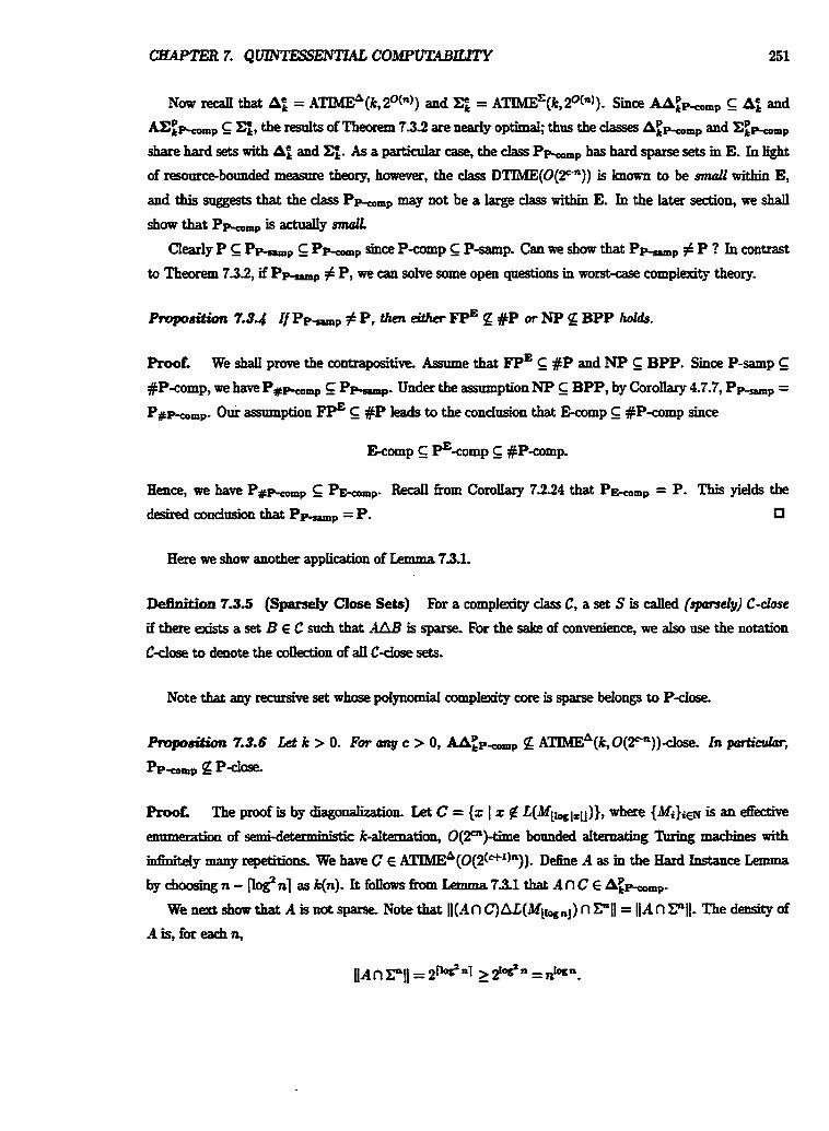
Now recall that At, = ~-(k,*(")) and = ATIME'(~,~~(")). Since Mi-, A; and
ACE-, E Ce,, the results of Theorem 732 are nearly optimal; thus the classes A;-,,,, and Cg-, share hard sets with A: and Fk. As a particular case, the class P-, has hard sparse sets in E. In light
of resourcebounded measure theory, however, the cIass DTIME(0(2Cn)) is known to be small within E, and this suggests that the class P-, may not be a large dass within E. In the later section, we shall
show that P-, is actually smolL
Clearly P E P-, P k m p since P-comp C P-samp. Can we show that P-, # P ? In contrast
to Theorem 7.36, if P-, # P, we can solve some open questions m worst-case complexity theory.
P t o p o ~ 7.84 If Pp-, # P, then either #P or NP BPP holds.
Proof. We shall prove the contrapositive. Asnrme that F P ~ E #P and NP BPP. Sice P-samp c #P-comp, we have P#-,, 5 PMp. Under the assumption NP C BPP, by Corollary 4.7.7, P-, = P#-,,. Oui assumption FPE E #P leads to the condadon that E a m p C #P-comp since
Hence, we have P#-, E P w - Recan from C0roh-y 72.24 that Pkmp = P. This yields the
desired condusion that P-, = P.
Here we show another application of Lemma 7.3.1.
Deenition 7.3.5 (Sparsely Close Sets) For a c o m p l e cIass C, a set S is d e d (qmsdy] C-Jose
if there exists a set B E C such that AAB is sparse. For the sake of convenience, we aIso use the notation
C-cluse to denote the collection of alI Cclose sets.
Note that any recursk set whase polynomial cornp1- core is sparse betongs to P4se
Pmpodkm 7.3.6 Let k > 0. For any c > 0, AA:P-mp A T I M E ~ ( ~ , O ( ~ C ~ ) ) & ~ ~ . In mculat,
Pp-eDmP P - c l e
h E The proof is by diagonalization. Let C = {z I z $! L(Mlh where {Mi)im is an dedive
euumeration of semi-ciderministic k-dkmation, O(P)-time bounded alternating Turing machines wi th
infinitey many repetitions. We have C E ATD&(O(~(*~)")). Dehe A as in the Hard Instance Lemma
bychoosingn-wnl ask(n). It f o I I o t ~ s h ~ ? . 3 J t h a t A ~ C ~ A ~ p - e 0 ~ ~ -
We next show that A is not spame Note that ll(An C)M(Mibnl) n FII = IIAn FII- The density of
A is, for each n,
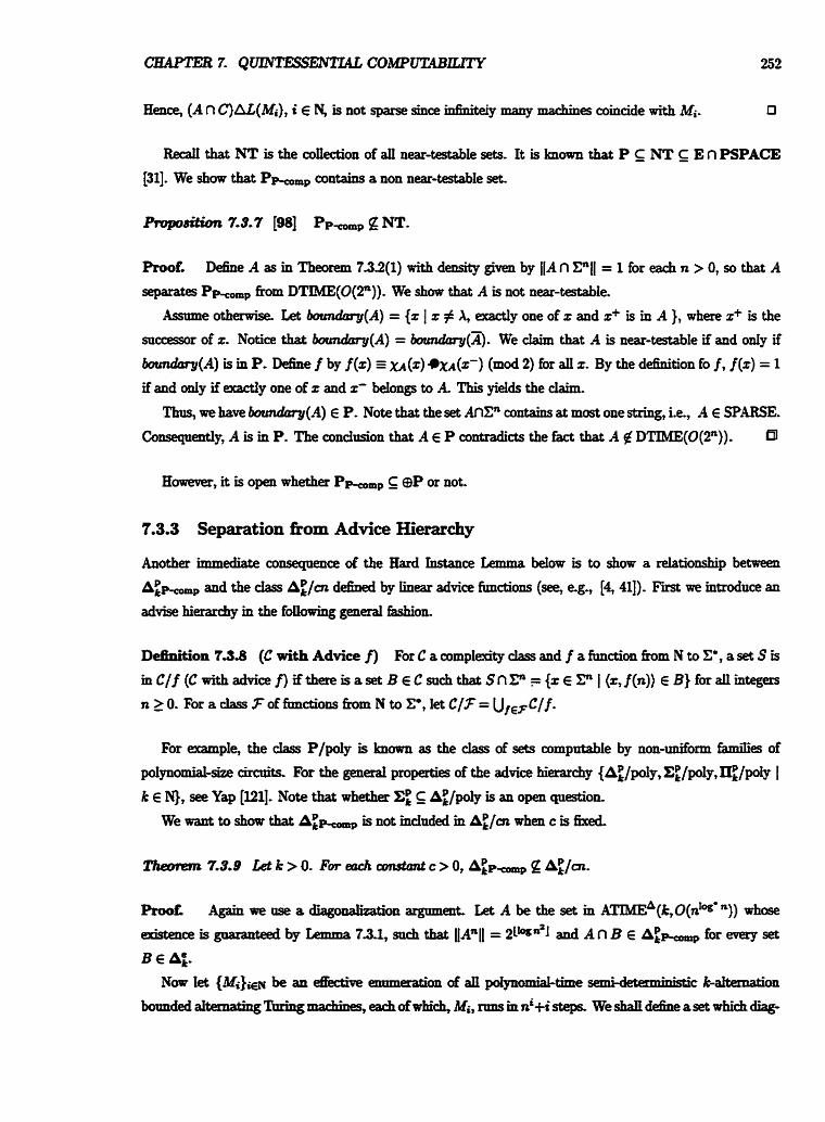
Hence, (A n C ) M ( a ) , i E N, is not sparse since infiniteiy many machines coincide with Mi. 0
Recall that NT is the condon of afl near-testable sets. It is k n m that P NT E n PSPACE [31]. We show that P h m p contains a non neareartestable set.
ProposiEiolr 7.3.7 [98] PP,, P NT.
Root D e f i n e A a s i n T 6 e o m 7 3 2 ( 1 ) v i t h d ~ ~ b y iIAnC"II =l foreachn>O,sothatA
separates Pmmp h m DTIME(O(P)). We show that A is not near-testable. Amme otherwise Let 6arndmy(A) = { x I z # A, d y one of x and z+ is in A }, where z+ is the
successor of x. Notice that bamdmy(A) = ~nmdory(;i). We daim that A is near-testable if and ody if
b t m h y ( A ) is in P. Define f by f(z) r xA(z) ~ ( x - ) (mod 2) for alI x. By the definition fo f , f (x) = 1
if and only if exaaly one of x and 2- belongs to A. This yields the daim.
Thus7 we have h n & y ( A ) E P. Note that the set A n C contains at most one string, i.e., A A SPARSE. Consequently, A is in P. The eonclasion that A E P contradicts the fact that A fZ DTIME(O(Zn)).
However, it is open whether PMmP E $P or not.
7.3.3 Separation &om Advice Hierarchy
Another immediate consequeuce of the Hard Instance Lemma bdow is to show a relationship between
and the dss AE/cn d&ed by linear advice frmctions (see, eg., [4,41]). Fm we introduce an
advise hierarchy m the following general fashion.
Debition7.3.8 (CwithAdvicef) ForCacoanpl~daPsaadfafim~onhmNtof',a~Sis
inC/f (Cnithadvicef) ifthereisaset B E C S U C ~ that Sn!P ={ZE F I (x,f(n)) E B) fordintegers
n > 0. For a class 7 of frmaons h m N to C, let C /F = UIEFC/f-
For example, the c b s P/poly is known as the dass of sets computable by non-dorm fhdies of
polynomial-size cireaits. For the g e n d properties of the advice hierarchy {Af;/poly, EL/poly, IIE/poiy I k E N), see Yap [fill. Note that whether X: A//pIy is an open qnestio~
We want to show that A:- is not included in AE/cn when c is hd
Root Again we use a diagodization argument. Let A be the set m ATIMEA(k,O(n~'")) whose
existence is gwanted by Lanma 7.31, such that [Anll = 2Lbnzl and A n B E A:- for every set
B E A:. NOW let {MiliEn. be an e k t b e enumeration of all p d p d t l m e semi-determiniaic k-*on
bounded alternating 'Ihdngm=uhines7 eachofwhich, Mi, nnrr in nitisteps. We J6all dehe aset which dbg-
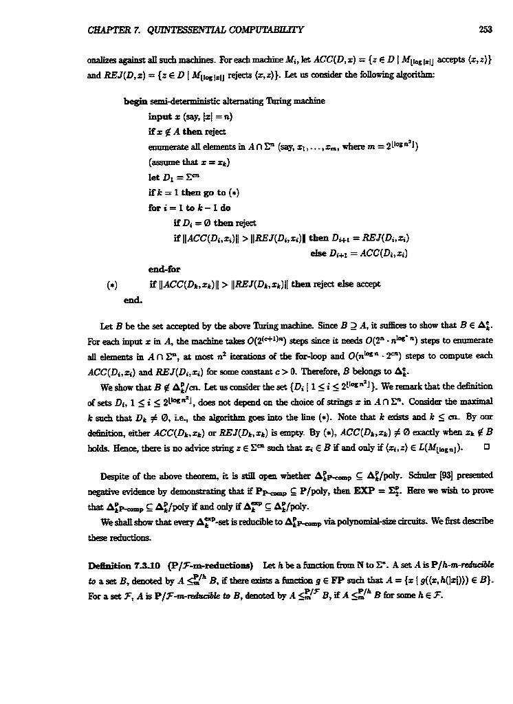
CaAPTER7. QUINTESSENTIAL COMPlXMBEDY 253
Let B be the set accepted by the above 'Iining madhe. Since B 2 A, it d c e s to show that B E A&
For each input z in A, the machine takes 0(2(*')") steps since it needs O(2" - n'q* ") steps to enumerate
all elements in A n P, at most n2 iterations of the for-loop and O(n'wn - 2C") steps to compute each
ACC(Di, q) and REJ(Di, zi) fm some constant c > 0. Therefore, B Bongs to At,.
We show that B f A: / cn Let us consider the set {Di 1 < i < 2Lkn2J}. We remark that the definition
of sets Di, 1 5 i 5 2LfOf5n2J, does not depend on the choice of sthgs z in A n IF. Consider the IMX~WI
k such that Rk # 0, i.e, the algorithm goes into the line (*). Note that k exists and k < cn- By om
definition, either ACC(Dk,zk) or REJ(Dk,zk) is empty- By (*), ACC(Dk,xk) # 0 d y when zk fZ B holds. Hence, there is no advice string z E ECn such that zi E B if and ody if (G, z) E L(MlIognJ). U
Despite of the above theorem, it is still open whether A: /ply. Schder [93] p r d
negative evidence by demonstrating that if P-, E P /poly, then EXP = qP. Here we wish to prove
that A:-, A: / p l y if and ody if A? G A: fpoIy.
We shall show that every AF-set is reduaile to via po1ynomiaEsize circnits. We &st describe
these reductions.
Dehi t ion 7.3.lO (P /3-m-redtlctions) Let h be a fanetion from N to Co. A set A is P /h-m-reddte
to aset B7dendedby~<Ih ~~if thereexistsafnnct ion~~~~suchthat ~={z1g((x,h(lzl))) E B).
For a set 3, A is Pf3-m-redtrdble to B, deaoted by A <IF B, if A B for some h E 3.
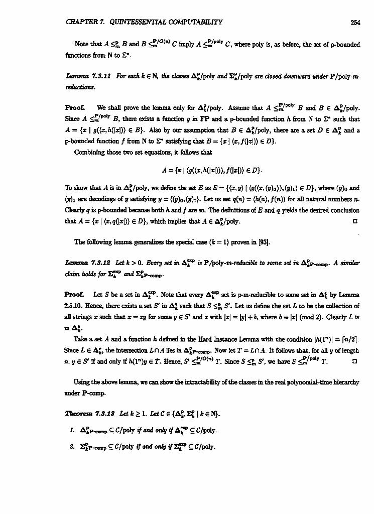
Note that A <g B and B </O(nl C imply A &/po'y C, where pdy is, as More, the set of pbounded
functions h m N to C*.
kmma 7.5.11 For each k E N, the classes AE/poly and C:/poIy me closed dourmrrard under P/poly-rn-
redudr-m.
R w E We shaU prove the lemma only for A:/poly. Asmme that A B and B E A//poly. Since A I ? ~ ~ ~ B, there exists a function g in FP and a pbounded funaim h from N to C* such that
A = (z I g((z, h(lz1)) E B). Also by oar assumption that B E A:/poly, there are a set D E A: and a
pbonnded function f from N to C' satisfying that B = {z I (z, f(lz!)) E D).
Combining those two set equations, it foIIows that
To show that A is in A;/poly, we define the set E as E = {(z, y) I @((%, (y)~)), (y)~) E D), where (y)o and
(Y)I are decohgs of Y stisEPing Y = ((do, (Y)x). Let us set q(n) = ( W , f (4) for =tual numbers n-
Clearly q is pbotmded becanse both h and f are so. The d a o n s of E and q yields the desired condusion
that A = (z I (z,q(lzl)) E D), which implies that -4 E Ailpoly. o
The following lemma generalizes the s p d case (k = I) proven m [93].
k n m a 7.5.12 Let k > 0. Euery set in A? is P/poly-m-red& to some set in A:p,,,- A sirnilat
daim holds for C F and x;~,,~.
ProoE Let S be a set in A?. Note that every Ac;" set is pm-redna%le to some set in A; by Lemma
25-10. Hence, there exists a set St m A; such that S <k SS. Let us define the set L to be the conection of
all strings z such that z = zy for some y E St and z with Izl= [yl+ b, where b r 1x1 (mod 2). Crearly L is in A:.
Take a set A and a function h dehed in the Hard krstance Lemma with the condition Ih(ln)l = [n/21.
She L E A:, the intersection L n A Iies m A:-,,. Now let T = L i7 -4 It foIlows that? for all y of length /W'Y T* R Y ~ ~ t Z a n d o d y Z h ( l n ) y ~ ~ . H ~ s & / ~ ~ ) T . ~ i c e ~ g ~ t , w e h w ~ ~ g o
Using the above lemma, we can show the intractability ofthe classes in the red poIynomiaI-time hierarchy
under P-comp.
Theinwn 7-3-15 Let k 2 I. LetC E (A:,C; f k E N)-
7.4 Immunity and Bi-Tmmnnity
Immttxte sets are another typical example of hard sets. In recursion theory, a set is d e d "imrmme* if it
is inhite but contains no infinite recursive enmnerabIe set. This notion has been adapted to complexity
theory and used in a variety of situations.
Bibimmune sets are d&ed to be immune sets whose compIements are also immune. These notions are
fundaments and have already appeared elsewhere in this thesis. In this section, we shall pay more attention
to the existence of such sets in P h m p .
7.4.1 Immune Sets and Complexity Coma
F i of a, let us r e d the formal dehition of immunity. For a complexity dass C, a set S is C-innmme if
S i s ~ a n d S h a s n o ~ t e s u b s e t s i n C .
A general notion of wmplQity cores has been introduced in Section 3.5, but in this subseaion, we shall
focus only on complexity cores with respect to P, the d e d polyunnial umrplezity cores. For a recursive
set S, a set C is d e d a polynmnial complQity am for S it, for any deterministic Turing machine M computing S and any polynomial p, the set {z E C 1 T i e ~ ( z ) 5 p(jzj)) is finite.
This section wdI show that there exist P-fmmuae sets in PMP, but P-,, has no P-bi-immune sets.
Under the assmaption that P = NP, ail infinite polgnomial complexity cores for sets in P-, are shown
to be hard to compute
We bt show the odstence of a P-immune set m P-, of arbitmy density. The proof bdow uses an
elegant technique deveIoped by KO and Moore [56].
ProoE Let {Pi)m be an dective enumeration of all sets in P, where Pi is deterministidy computed
inni+istepsl
Let c = (1 + 6)/2 and take the set A d&ed in the Hard Instance Lemma such that jlAnll 2 2C". Note
that A E DTIME(O(nlw. n)). Now consider the faowing aIgorithm:
accept
end- for
reject
Let B denote the set accepted by this algorithm and let C = A - B.
Finst, weseetbatCisofd~at least2% ~ m r m e z , ~ E ~ a n d z f ~ . N o t e t h a t z ~ e a n d p ~ Pi
are witnessed through the first for-loop, then i # j by the algorithm, Hence, we have llB n PI1 log' n-
S i IIAnPll Z P , [CnF l l = IIAnIl -IIPII 2 2 " - I o g ' n z P .
We next show that C has no inhi& P-subset, Assume that an idbite set in P is a m b of C. Let io
be any integer that guarantees that Ph is such a set. Consider the mhbal x E f$, fl& such that 1x1 2 io.
By theminhalityOfx,wehavez #Ph f o r d z wi thh 5 IzI a n d t <z. T h u s , x ~ B,acontradiction.
Therefore, C is P-immme-
Now we daim that B is in PkoP since this implies C E PkmP. Let TimeB(z) be the executing
time of this algorithm on input I. It stdEces to show that Tie&) ?c'" for dI x m A, where c' is
an absolute mve constant. Notice that TuneA(z) 5 ~ 1 ~ 1 ~ ' ~ s ' 1.1 for some eonstant c > 0. Thus, the
algorithm takes time - [ C I L ~ * ~ ~ ' 1'1 + (121' + i)] m the second for-loop, and this tenn is bounded by
0(n2 1 ~ * - Za) 0(22n) - The tota exeation h e , TuneB (z) , :), log' n iterations of the first for-hop,
each of which takes O ( p ) steps, and therefore, 5 2 ~ ' " for some eonstant d > 0. a
We note that any P-immune set is a polynomial complexity core for its& Since the P-immune set
constntcted in Theorem 7.4.1 is non-sparse, we imm-e.1~ get the following coroIIary-
Let m recaII the eomplexitp dass APT introduced by Meyer and Patemon [n]. A set S is in APT if and only if the set {z I Tie&) 2 p(lzl)} is sparse for some polynomial p and some deteTminiStic %ring
machine M which computes A.
Proofl This result foUm horn Comkry 7.42 and the fact that a recursive set S is m APT if and only
if any poIpmial complexity core for S is sparse [7 ' . a
W e have aIready seen the existence of pol- t-me sets m Section 42. The particular example
shm there was; based on KoImogorov complexity sets. Here we shaIl present another example of poIgn0-
d y t - r a r e s e t s b a s e d o n c o m p ~ m r e r i n P ~ .
CHAPTER 7. Q-COlldPmILITY 257
Proof. Let S be a comph&y core for A with respect to D T I M E ( ~ ~ ( ' ( ~ ) + ~ ~ ) ) n PP-co,,. To atrive at
a contradiction, we assume that S is not potynomiany t-rare. Fkom this assumption, it follows that there
exists a Pamputable distriitrtion p s a w the condition that the set B = (z E S - {A) I B(z) > ZC("))
isinhi&.
S i A E Pm,, there exists a d-c ' k ing madhe M which computes A in polynomial time
on paperage. Let p be a polynomial such that h .Ti ie~(z) is p on paverage. For any strfng x in B (say,
n = 14>? Time&) 5 p(Y(") - n) 5 (2'(n)+'wn)k
for some constant k > 0 independent oiz. Now we set B' = (z I T i e ~ ( z ) 5 ($(")+'w")~). It is clear
that 3' belongs to D T I M E ( ~ ~ ( ~ [ " ) + ~ ~ ) ) . Notice that B' n S is This obviously contradicts our
assumption that S is a complexity core for R Therefore? S is polynomiaIIy hare. 0
7.4.2 Bi-Immune Sets and Resourcd3ounded Measure
We shan turn om interests to bi-Immune sets. A set S is Caned C-bi-immtme if S and its complement 5 are
both C-immune. The dass of P-bi-immtme sets has a dose connection to fesource-bounded measme theory.
As seen in Proposition 2-7-11, any class which has no P-bi-immtme sets has pmeasnre 0; in other words, it
i s d
It is known that the set E has %tm@f' P-biiimmrme sets 151, and thus E has P-bi-immune sets. It
is important to remember here that a reansioe set S is P-bi-immune if and only if 2' is a polynomial
compIsdty core for S. Hence, E contains a set for which Em is a c o m p l e core- However? we can see m
the following proposition that there are no P-bi-imnmne sets in PMP- This contmt dearly shows the
di&rence between E and P-. W e r and Yamakami 1981 6rst showed that PMP has no P-bi-imrmme sets. Later Schder I941
extended their d as follows.
ProoE. Assume that B is DTIME(O(2en))-bi-' i and 3 is ptt-redtxa'bIe to a set A in Pkmp.
Whout loss of generaIitp7 we assume that c is a positive'hegm. Let Y be a ~~~~~time o r d e Tbkg
machine which reduces B to A with nonadaptive qneries. Let p be a poIynomia such that n ~ ~ l e ~ ( Z ) (= p(I4) foranz- S i A E P ~ , t h e r e i s a ~ c ~ m a c b i n e N w h i c h c o m p u t s Aintimepolpnomia
on p m m g e for every P-compntabIe distnbntion p This shall Iead to a contradiction-
W e d e h e a s e t D a s h h m Foreachn E& kt&= {yI lyl ?n/!kl\y €Q(M,W)),andthen
C&QPTER 7. Q- COMPUTABILITY 258
let D = (0)' U (Un, D,). Fi we shaw that D is P-printaMe. This is seen as follows. Consider the
aIgorithm: on input On, recursively take a natural number k such that k 5 2c - n, and list dl strings in {y E F' I y E Q(M,P)). S i M makes nonadaptive queries in polynomial time, this algorithm writes
down all query of length n in polynomial time. Now let us consider the set A n D. By Lemma 7221, A n D must be in P. The FoIIowing algorithm
00mp~tes B n (0)':
begin algorithm for B n{O)' input on list an queries made by M on mput On
for all query string y
i f l y l 1 h thensetans(y):=[y~ AnD]
(*) else SimuIate N on input y and let an&) be its output
end-all
simdate M on On with oracle {y I cms(y) = 1)
output M(0")
end.
In line (*), the number of steps we need is at most 2elol 5 2~e = 2"j2. Hence, the total number of steps of this aIgorithm is, for some absolute constant d > 0,
fix every sutEaently large integer n. Therefore, the set B 17 (0)' belongs to DTIME(O(F)). A similar
argument shows that B n (0)' is m DTIME(0(2n)).
Notice that at least one of the sets B n(0)' and Fin (0)' is infmite This contradict5 our assumption
that B is DTIME(0(2M))-bLimmnne a
For each constant c > 0, the class of Dm(O(2C"L))-bi-immune sets is known to have pmeasure 1 [HI. In other words, the class of non-DTIME(O(2C"))-b'bimmme sets has pmeasure 0. Eence, by Propositions
7.45 and 2-7-11, the cbss P-, cannot have p-measure 1. Therefore, we obtain the foIIotnring coroIlarff
&= by schder W].
We remark here that the weaker statement that P- has p-meamre 0 wits proved by Schnler and Yamakami [98], and independently by Cai and Selman [Dl. Notice that, as an immediate comeqnence of
C o d h y 7.46, if NP E P-,,, then NP has pmeasure 0-
Deftnition 7.4.7 (Almost Immmity) [24, Tlj A set is d e d atmost P-immmre if it is a union of a
P set and a P-immune set. A set whose complement is almost P-immune is called P-h&k
For aset A, aset S is d e d amaxixdsubset of A ifany infinite subset of A in P is afinite variant
of S, te, IIS - All is Enhe. It is known that, for any h$nite reemsive set A, A is almost P-immune if aud o n I y i f A h a r a ~ s u b s e t inP [24,511.
hmma 74.8 [ 2 4 , q If a set A not in P s a t i q f k A se A via a length-inasaring redudion, then A is P-levelable. Hence, most well-known NP-complete sets m P - h a l e unless p = NP.
Proof. To arrive at a contradiction, we assume that A is almost P-immunee The aImost-P-immunitp
ensures that there is a maximal subset ofA in P. Let E be such aset.
Now wedefine B = {z I x E A f(z) E E). Smee f E FP and E E P, we condude that B is in
P. More~vef, B fl E = 0 by definition. We now show that B is inhite. Assume that B is hite. We
choose an dement x in A - E such that B zI~I-'. The element x exists because A # P bat E E P. Consider the set E, = {z} u {f ('I(=) I k 2 I), where f(')(z) = f (z) and f(k+l)(x) = f (flk)(z)) for each
k > 0. Smce f reduces A to A, E= A. Moreover, E, is h h k e and in P since f is length-increasing
(Le, [ f (2) 1 > 1~1). Note that E, n E # 0 since, otherwise, E U E, is a P-subset of A such that E - E. is
infinite,andonsequentiy EisnotamaximalsubsetofA Sincez#E, thereexistsastringy in Ez-E,
but f(g) E E. Hence, y E B. Clearly lyl > lzI. This contradicts the hitmess of B.
The Iatter part of the daim fo11ows from the fad that most known NP-cornpkte sets A, such as SAT,
Pw* 74.9 Assume that P # NP. If euery set in PPmmp - P is dmst P-immune, then NP g PP-cornp
R o o E Consider the NPampIete set SAT. If P # NP, then SAT is in NP - P and is P-levelable by
Lemma 7.48. Hence, if SAT E Pkmp, then Pkmp - P contakts a set which is not aImost P-immune
To show that an sets m P M ~ - P are almost P-immmre seems difEctxIt. Moreover, we do not know
how to construct a P-Ievelable set in PMmP which is not in P.
7.5 Closure Properties
This sectitm a9 be devoted to dosme properties under severd types of polynomiaLtime reductions- &eean
that, fix a reduu'bilitp I,, a class C is dtwd (dmmrtrrord) u& I,-rebrrcfionr it, fbr every two sets A and
B, A 5, B and B E C impIies A E C- We know that most k n m compIexity classes are dosed under pm-reductions, snch as RP, BPP, NP, PE, PP, @P, etc
In Subsection 75.1, we shall demonstrate that neither A:-, nor 22:-,,, k > 0, is dosed under p
m-reduciiilitp. The la& of this property indicates a structmal difference betmeen P-, and other regular
complexitg classes, such as P, NP and BPP. 'Rms, it presents a partial solution to the NP c?P-,, question. Oar resuit relies on the sets constructed in Section 7.3.1.
In Subsection 7.52, we We &ow that the dass A:-, is not dosed under the polynomially-bounded
operator. This d t dso implies that AEp-e~m~ is d X i t h m CE.
7.5.1 Polynomial Time Reduciiilities
In this subsection, we will discus properties of qnintessential complexity cIasses in relation to warious
polynomid-time reduciiiIities.
We cfaim that there is a the difkence between polyuomid-time truth-table redua'biIity and Turing
reducibility within Pkmp. This claim is p d by demonstrating that the Thing closure of PkOmp is
"large: whereas its truth-table dosare is "smalLn
The foIIowing proposition shows that the 'Rxing dosme of A~~,,, is equal to A T , where k > 0.
Ptvpodion 7.5.1 [94] For each k 2 1, the %ring eloswe of AEp,,, is equal to A T .
Proof. We shall show that every set m A? is pT-reducible to some set in AEPcomp. Let B be an
arb'- set in A; and assume that B E ATIME~(~, 2C") for some constant c > 0. Let A be the set d&ed
in the Hard Instance Lemma We then define the set H as
Smce A is in DTIME(n@"), clearly B' is m Af. Since B' G A, by the Hard Instance Lemma, B' is in
AA~-,,. Hence, P E A:-. Ftom flA n Zhl1 5 1, it Wows that, for all y of length n, y E B if and only if h(ln)y E B'. Recan
that h(ln) is computed by n adaptive qumb to Prefiz(A). This implies that B is pT-duciiIe to
ET $ Pre fiz(A). Let C = Bt Prefiz(A). Since B' E and Pre f k(A) E C is dso m
A~p-oorn, by Lemma 72.12. U
It is not known whether pT-redadbilitp m the above proposition can be replaced by pm-redua%ilitp.
Note that this is the case if Af;p-comP has some pm-complete sets for A;.
RooE Recall fhat EXP has prneisme L The coroIlarp then is immediate h m Corohy 7-46 since,
otherwise, EXP has pmeasare 0, a cmtxadictiam i3
Assmne that there exists a pmredction h m a set A to another set B which is in P*,. The next
ptopositicm dmazmke the reduction when A $€ P.
Proof. Assume that A is pm-reduciie to B in Pbmp via a Pampatable reduction fimction f.
Ebrthermore, assume that there exists a positive constant c satisfying log lzl 5 cl f (%)I for ahnost an z. In
the following, we want to show that A belongs to P.
Let MB be a &e which computes B in polynomial time on vd-average, and consider the following
machine MA: on input z, compute f (z), and accept the input exactly when MB accepts f (2). We thus
for some positive constant & S i B E P-,,, TimeMa,(f (z)) 5 2cIlf(r)l for some constant d > 0. This
implies that
TirneMB(f (2)) $ I f (=)I I ~ z [ ~ ' / ~
The next proposition, due to Wang and Bebger [6] (in a &t setting) and W e r and Yamakami
1981, shows the c l a m property of the class P-,, under restricted reductions.
Proof. Let B be any set in For a set A, we assmne that A 52 B via a P-compntable reduction
f which is increasing and phonest. We shall show that A is aiso in A:-,. For each p E P-comp, let
Y = prl. By the condition on f, we condude that v E Pcomp by Lemma 4.2.8. It is easy to see that if B
is computed by a deterministic ntriag machine M m polynomial time on v-average, then A is computable
in polynomial time on paverage by simdating M(f (2)). 0
As an example application of this proposition, consider the bounded halting prob1em BHP. Note that
BHP is pl-complete for N P under increasing, phonest reductions. Therefore, by Proposition 73.4, if
BHP E P-, then NP is included m PMp.
Next we show that neither A&,,,, nor I::-- is dosed under pm-reducibility. Note that Wang and
Belanger [Ill] have shown a similar result for their dasses APp, ANPp and DNP of distn'butional decision
problems.
Proof. We prove the theorem only for A;%, since the proof for C:* is almost identid Let A be the set in DTIME(O(n@* ")) such that llAnl = I far aU n E N and let h be the frmaion h computable in
time O(nb* ") in ordm to sepatate h m ATIME~(B, 0(2")), both of which are used in Theorem 7-39.
Now we define a reduetion function f as f o l k
~ o t e that if f(Pm) = 2, then n 5 a. ~ e t T = {di I i E N, f (d i ) E A). Clearly T 5% A via f. Note
that the fimction f is not phonest.
We shaII show that f is computable in time O(n). Assmne that z = 02i for some i E N, and let y be a
string of length [log 1zlJ2 in A. By our definition, the computation time off (z), where Izl= n, is at most
for any stafEdently large n.
We next show that T 4 Af;-,. A r n e otherwise. S i T is tally, T is in A:. Note that A! =
ATIME~(L, no(')). Consider the foIIowing algorithm:
begin input x
if z 4 A then reject
take n (5 m) such that f (a2") = z
ifPm ~Tthenaccept elsereject end.
This algorithm computes -4 and is in ~ T I l 4 E * ( k , 0 ( 2 ~ ) ) . This clearly gives a contradiction. Therefore,
T 6 A:P-m,- u
Theorem 7.5.5 yields the signiscaut consequence that the classes in the real poIynomiaI-time hierady
under P a m p are strndatralIy different h m most known woftt-case complexity dasses.
As another application of Theorem 7.5.5, we shall present the following coroIIary, pmven as Lemma
7.1 in [w. The corohy demonstratg the n e e d y of the phonesty condition in Condition I' d&ed in
Section rl7. The proof preseated here is very d&rent fiom Gmevich7s and is based on Theorem 7.55
Proof. Assmning the contrary of the corollary? we shall prove that PMp is dosed under pm-reductions.
This contradicts Theorem 7.5.5.
Assmne that A is pm-redtlcii1e to B via a reduction f, and dso B is in Ph,. We show that
A E Pmp. For every distribution p in P-comp, by our assumption, there is a distriiution v € P a m p
and a function p which is plynomid on paverage such that fi(v) 2 ZE # fm d y. Note that B is computable m polynomial time on waverage. Then A is also computable in polynomial time on paverage.
Since p is arbitrary, A bdonp to PP-comp- D
Let us recall Condition 1'. Condition I' asserts that every P-samplable distrriution is avpdominsted by
some P-computable distribution. Assaming Condition It, P-mp turns out to be dosed under mmy-one
redua%ility with phonest poLynomial-time computable reductions-
Proof. Immediate h m L e m r ~ 6.4.2 and by the same argument in Proposition 7.5.7. 0
E " d y we show the existence of an incomparabIe pair in Ph,, with respect to the h p m - r e d u ~ ' b ~
Proof. R e d h m Theorem 7.4.1 that there is a P-immune set in Pbmp. Let A be such a set, and
let B = {O}'. Note that A f! P. If A 52 B. then A E P since B E P, a contradiction- If B 5% A via a
pdynomiaIIy honest f E FP, then A should not be P-immtme since the bfhite set {f(z) 1 z E B), which
is a subset of A, belongs to P. Both cases mdnce contradictions. 0
Let us next obseme the closure property of average c o r n p I e cIasses under hpm-reductions when
P-sampIabIe distniutions are taken hstead. The P-samphb1e distniutions show us a mkrent worIcL
h o t We ody consider the case A!wp. Anmme that A is pm-redua%le to B via a phonest
reduction f, and B is in We sbdl &ow that A is in
Let p be any distxibuticm in P-samp and d&e v ap v = p p . Distriiution v may not be P-samphbIe,
but by Cornby 4.4J2, we caa find another d i s t r i e J which pdominates v and is in P-samp. Sina
B E A:-, we h a . (B,P') E Ava(A;, *). Note that (A,p) s& ( B , 4 via ff. Hence+ by Lemma
6-42(2), we ham (A,p) € Aver(AI, +)- Hence, A is m Agpl.mP- n
Hence, N is polpnomial-time bounded on yamrage. This contradicts our assumption. 0
Contrary to the sitmion for A:, it is not known whether A:-, E UP- A:pTomp, or ewn whether
A~p-~orn~ C, P. A:-. However, we are able to show that the converse does not hold for A;-,,.
Proof. Assume that Up-A:-,, A:Pcomp. By Theorem 732( l ) , we can define a set A in
m A ( k , 2n) and take a corresponding function h, as de6ned In the proof of Lemma 7.3.1, WE& has the
following property: for each length n, An E (h(In)) and h(ln) is computed in time 0(P). Now define
C = {On I 3y[lyl = n A y E A]). To see that C E UP- AEp-eom,, let B = ( ( ~ ~ ~ ~ , z ) ( 2 E A). By Lemma
7-52, B is also in AEp~om~, and let C = {On I 3y[lyl = n A (y,z) E B]). By our assumption, the set C is also in A:-,,. Smce C is tally, by Proposition 7217, C is in A;.
As a resalt, we have C E m ( k , 0(2")). Consider the following procedure that computes A:
This procedure gnarantees that A is in ATIMEb(k, 0(29), and hence, this contradicts the choice of A. O
-49 an immediate conse~nence d Theorem 7-5-13, we again have Pp-arrn,, # NP and PMP # UP. We note that it is not known whether P-AiFcmnp G CE- Howwerl if 3"-AE-, G CE-,,
then Theorem 75.13 i m p k that P- # NP-, and thus that P # NP.
Moreover* we can consider a restricted tlgpe of probabilistic operator.
Dehition 7-5.15 (Class PP- C) For a complexity dass C, a set S is in P P - C, the d m under Mc
prrrkbibtic opaatm, if there are a polynomial p and a set B E C such that S = { x I ll{y E P(lf 1) I (y, 3 E B)ll > 5 - 2flz"}-
The p r o b a b i i c daPs PP is dosed under this operator, ia, PP- PP PP. A proof techniqne similar to that used for Theorem 75-13 shows the foIIowing theorem.
Proof. Let the set A and the hction h be as defined in the proof of Theorem 1-5-13 but with k = 1.
Recall the algorithm descriied in the proof of Lemma 73.1. Define B to be a set accepted by the foUowing
algorithm
begin input x (say, 1x1 = n)
compute zr = min{w E I w $! KT[n, ~(0 '" ] )
i f l ~ r ~ t h e n y = O e b r e y = l
if z E y ~ l * l - l then accept else reject
end.
By the choice of y in the algorithm, A f7 B = 0 and llB fl PI1 = 5 - 2" for an n. Note that B is in P. Now m Iet A' = A U B. Then, re bave A' E Pkmp Note that either I1A' f l PI1 > $ 2" or IIA' n PI1 = f - 2".
Let C = {On I Il{y E P I y E A')ll > i - 2 )̂. We have C E PP- PkmP by definition, but C 6 Pkm, since if C E Pkmp7 then the same aIgorithm as m the proof of Theorem 7.5.13 computes A m time 0(2^).
0
Theorem 7-5-16 directly shows that PpzomP # PP.
7.6 Bounded Error Probabilistic Polynomial Time
We direct our attention now to the bounded-emr probabilistic complexity dass BPPr- In this section, we
shall discuss the dass BPP3 mrda weak reductions, and consider a result d Schnler and Watanabe [96]
regarding the qnestion NP C-7BPP3. We begin with the dosure property d BPPp,, under phonest bpptt-reductions-
PmaE Assume that A E BPP- and A is bpptt-reducible to B via a phonest reductioa Let
CHAPTER7. QUINTESSENTIAL C O M P m I L l T Y 267
M be such a reduction, ie., a polynomial-time probabilistic 'Ihring machine computing A with bounded
error which accesses oracle B with nonadaptive p h o n e gueries. For simplicity, assume that the number
of queries on each computation path is of the form 2", where m is dependent only on z. Since M makes
phonest queries, for any query z by M on x, 1x1 is bounded above by an abso1ute polynomial p m [zl.
Choose any distribution p m P-samp. We define a distribution v as foIlows:
It is not difEdt to confirm that v is P-samplab1e. To see this, let Mp be a sampling machine which sampies
p and consider the following sampling algorithm:
begin sampling algorithm
input 0'
simulate M, on 0'
let z be an output of Mp on 0'
list a s y z19z2r---,z2m
generate k (I 5 k Zrn) at random
0-a Zk
end.
Hence, (A, v ) E Aver(BPP, P-samp). We now show that (B, p) (AT Y ) via M . It is sttfticient to check
the domination condition for M. This is easily d e d , however- By Proposition 5.5.7(4), (BT p) beIongs to
Aver(BPP, P -mp) . 0
Ben-David d d [9] showed that all distri'butional NP search prob1ems are Ltaadornly" reducible to their
corresponding distniutional decision problems. Later Scbnler and Watanabe [96] rephrased this resalt in
the foflowing f&ihion.
Proof. Assume that NP BPP-,,. For any set A E g, there exists a set B E NP such that
A is pa-reduuile to B. This reduction can be phonest by choosing an appropriate set B. Hence, A is
bpptt-reducii1e to B via some phonest reducti011, Notice that B below to BPPWp by om assnmptioioe
By Proposition 7.6.1, B E BPPWp implies A E BPPP--~. Theretore, we get A E BPPwp.
Impagliazu, and k i n [q demonstrated that distributiod N P decision probiems are "reduaLbIen to
distributiod NP decision problems with standard distribution. Schnter and Watanabe [96j extended their
resuIt m terms of- compntabiE@
Proof, We follow the argument given by Schuler and Watanabe [96]. Let us asstme that NP E BPPw~~sorn,.
Let (A,p) be an arbitmy distn'butional decision problem from Dist(NP,wP-samp). We shall show that (A, p) is m Aver(BPP, *). If B(C) > 1/2 for some n E N, then we can diminnte an strings of Iength
n from the following argmned- Hence, we annnne without loss of gen* that ji(Zn) 5 1/2 for dl n E N S i A E NP, there are a set E E P and a po1ynomiaI p such that A = {x I 3y E P(frl)[(z, y) E 4).
Moreover, h m the fact that A E EXP, we can dehe a deterministic 'Ihring machine MA which recognizes
D m time 2dlrl), where x is any input. For the sake of convenience, we ansume that ~ ( n ) 2 32n3(n + I)* for
d n € N
Smce p is an average P-samplable distribution, there are a generator M for p and a po1ynomial p' such
that (i) Iji(z) - P~~[M(O') = zjl 5 r', and (ii) for every r > 0 and n E N,
Write pj(n) for p'(2j+'(n + q(n))). Let us dehe the function f as ~OIIOWS: for each j with 0 j < q(n),
Therefore, we obtain
For each 2, since LSd,,) 5 1, there exists an index j' such that j(z) 5 Hn) + & - 23*(")+ee'. Let jl be the minimnm of such an index.
On the other hand, if q(n) < p,- (n) - &) - ilog(q(n)), then fi(z) 5 2 - 2-dn) = 2-dn)+I.
Let x?) = (2 E C" I j = j, A q(n) 2 pj=(n) - &) - ilog(q(n))). It foUows that
since q(n) 2 2n3. Therefore, fi(x2)) < $ 2-J for all j with 0 j < p(n).
RecaII that sn denotes the nth string of C' (NB. X is the 0th string), and s p represents the kth string
of Pw("') (N.B. S? = o~'%(~)). Note that Isn( = llog(n).
We begin with the fo11owing NP sets:
A hz of? o hl(v) = h2 of,?' o ht(u1) = =]I;
where I = m - k, h~ E HI,,, and h2 E H4+2- The notation h14z above meaus the concatenadon of three
strings At, ha, and z. Let B = Vi=, Bi. CIearly B is in NP. By the assumption, (B, v-) E Aver(BPP, *)-
Let Q be a d a e n t l y Iarge and fbred amstant* First we s h d dehe the randomized ?tuing m;lrhinp
MO that (i) chacse j at random finm {0, 1,. . . , q(n) - 1) (by choosing a?)), (ii) chooses k at m d o m
h m {O, 1,. . - ,pj(n) - 1) (bg &-g @')), a d (E) (z, ~ f ' ~ ~ ' @ ~ ~ I)). The fohwhg ir a f d descdptimafthisaIgorithm:
begin randomized agorithm for Mo
mpat r (my, = 14)
-Pe ilog(q(n)) generate at random a string s of length iIog(q(n)) such that
s = s ~ ) f i x s o m e j w i t h O ~ j<q(n)
(asllme that s = SF)) -Pe ilog(pi(n)) generate at random a string d of length iIog(pi(n)) such that
The machine Mi rum in poIynomial time because the running time is proportional to the Iength of the
random seeds. The ten& of random seed, is^(")@')[, is at most
for some constad d > 0.
Write d(n7 j7 k ) = s:(~)$(~). La us define h(z) = d(nlj,, &I) and D = ((z, h(r)) I z E Lw ). Note
that, for any z and y, if z , y E x?', then Ih(z)[ = Ih(y)l. For alI z E x,O'Il since Ih(z)l 5 c'(j + Iogn),
we have Ih(z)[ I d -log(l/n2 fi(x2')). By Lemma 3.3.11(3), we condude that k.lh(z)l is Io@thie on
Pa-
Next we d- another randomized orade Turing h e N as follows:
on input (2, h(x)) is at most
for some appropriate constants E', d > 0. T~US, for each z E x!?, d
1 ~ s ~ m e f : ( ( z , h ( ~ ) ) ; s ) I s E r ~ ~ ( ( ~ t h ( z ) ) ) ] < d * -I- d'c'. (a(x .D))n2) -k c'.
By Lemma 3.330, we condude that k .ES[r rme~( ( z7 h(z)); s) I s E rN. ((2, h(x)))] is polynomial on p
average. Therefore, hsJVB((z , h(x)); s ) is polynomial on p-avefage.
Next we shall discuss the success probability of machine N. Fnr z and let n = 121. Let p, be the
probability +dm the algorithm N on input (z, h(x)) succeeds in producing the conect amver. We shall show
a Iower bound of p,. For this purpose, we introduce a new notion. We say that (hl, h2, z) d e k m h s z if
(i) there Bdsts a string v E Zl such that 0 hl(v) = z and h2(4 = z; and
(ii) for all lo E !St, if h2 o fi) o hl (M) = t, then f.) 0 hl (w) = Z.
Fa j and assume that 11lf$))-'(z)11 # 0. Let us chose @ and set I = pj(n) - &'I. Then, p, 2 1/16
fdm fiom the claim betow.
Next we rhall show that n2(hI) 8. Let FZaI = ran( f:) o h l ) The cardinalitp of FZvht b at most 2.
To complete the pmof of the claim, we combine the above results.
This completes the proof. I
Finally we apply Lemma 55.3, and thus there eJdsts a randomized lS.trjng machine MI such that
hs& ((z, h(z)); s) is polynomial on paverage with the condition that, for each s' E l?~,(z),
By the remark fo1loPPing Proposition 3.53, we immediately obtain that (A,p) E Aver(BPP, *). The proof
is completed. 0
The class BPPhmp is d d y related to P-samplable dishiiutions. In the following Ie~nma, we see
that an assumption like NP BPPPeomp causes the P-sarnplable distriitttions relative to NP oracles to
be average P-samplabk
Proof. We shall show only claim (2). Assmne that E BPPpamP- Take an a r b i i ~ ~ ~ - s a m p l a b l e
distriitttion ~ r . By its definition, there exists a sampling a1gorith.n M, a polynomial q, and a set A E NP suck that, for any string z and any number i E N,
Iji(z) - R ~ [ M ~ ( o ' ) = z m time q(lxl, i ) ]] 2-i.
We can assmne without loss of generality that if M wi th orade A on input 0' haIts and outputs z, then its
nmning time does not exceed q(Ix1,i)-
Let us define the set B as fdm
B={(0',ln,s,1j,d) Id€ {O,I}A~E~~~~~AIM~(O~;S)~ =n
A Tiie&(oi; s) 5 q(n, i ) A the j-th bit of MA(Oi; s) is d ).
Let p(n) = 2n+4 for dl n E N Smce B E bP, our assumption ensures the existence of a probabilistic 'king
machine N which accepts B m polynomial time on Y--average w i t h error probability 2*n)-n-'4, where
input is of the form (O', la, s, lj, d). Consider the fbIIowing sampling marhine W.
generate $ at random so that lss'ls q(n, i + p(n))
sets=ss'
for j = 1 t on do
if N((o~+P(~) , in, S, ij, 0)) = ~ ( ( o ' f d ~ ) , in, S, ij, 1)) then go to (*)
if N((o'+~(~), in, S, IJ, 0)) < N ( ( o ~ + ~ ( ~ ) , in, S, ij, 1))
thensetdj=lelsesetdj:=O
end for
output dl& - - - d, and halt
(*I end for end.
In the foIlowing analysis, we fix i and z. Let lzl= n. Set
Write o', to mean P~,[M~(o'+P(~)) = z in time q(lz1, i + p(lz1)) I s € RMA (o'+~"))]- By the dehition of
St,i, we have o', = CaESmSi 2-la[.
Note that the success probab- tfmt each iteration of the second for-loop is at least.
Now let us denote by p i the probabiIity that the machine M' on input o'+P(") with random input s E S=,i
outputs z. The fimction p i dearly does not exceed o',. The Iower bound of p i is dcnlated as fo11-
The last inegnality folIows from Lemma k6-
We then have
As in Theorem 4-4-13, we can show that EJ - p i ] 5 2-' + 2-j for all i, j > 0.
It is not diflidt to show that N' nms in polynomial time on paverage with respect to the size of its
output. Thedore, p belongs to avP-samp. 0
Proof- Assume that NP E BPPhmp. Notice that PC-samp E P avP-samp implies BPPmpamp
BPPpy,. By Proposition 7.6.4, it foIIm that NP E BPPmwp BPPP2~-runp- A simiIar argtxnent Ieads to (2). 0
7.7 Random Oracle Separations
We return to Levin's original qnestion of whether NP E Pkmp. Since this question is difficult to answer,
on. we turn our interest to its reIativizati
Bennett and Gill [8] 6nt d a notion of 'andom odes" and made several important mntriibutious to
computational complerity theory induding the r d t that, dative to a random oracIe, three dasses P, NP, and mNP are Merent. Intrritnety, if we choose an orade set A at random, PA is difberent h m & with
probability 1. In other mads, "most" oracles can separate P h r n NP. In the same paper, Bennett and
GiIl proposed a 'tandom orade hypothesis" that states if a property P holds relative to a random o d e ,
then P dso holds m the non-rektivized world- (Hmwer, this hypothesis is now known to be fdse [a*) To approach Levin's original qnestioq we consider randomly mhhized world We remark that there
is no known inclusion relationship between the dass Pbmp and other wo- complexity dasseq such
as NP and PSPACE. This d o n wi l l discus, reIative to a random oracle, several negatbe resnltts about
these relationships
We identifir a set A with a binarg red nmnber 03 , where r = ~ ( 0 ) ~ ~ ( 1 ) ~ ~ ( 0 0 ) ~ ~ ( 0 1 ) '- -.
De5ition 7.7.1 (Random OracIes) Let @ be a property r e h b i d to o d e X. We say that, (with
p r o ~ l ) ex ~ o ~ r d o t i ~ c t o a ~ m ~ e t ~ ~ t h e ~ b e s g n e m e a s l r r e o f t h e s e t {XI @hoMs}is
1, denoted by m((X I @ halds }) = 1.
In om setting? the Lebesgne meamre behaves Iike a probability measme if the property is W y
evaluated. Here is an emmpIe. Let
Then, cI&y Iv~(z)l = lzl for all z. Consider the event (A I m(z) = o ~ I ) for each 6xed string z. The
measnre of this event, m((A I q ~ ( z ) = Olfl)), is 2-lrI. Hence, for each n E N, m({A I Vy(qA(y) # On))) =
(1 - 2-n)2m, which approaches l/e as n goes to oo.
We shaU show that, with probability 1, NP-, is different from P-,, relative to a random o d e -
In this section, we choose the fdowing relativization of the classes PF and NPF.
&hition 7-72 (Refativization) Let X h a set of strings, and Iet F~ be a set of distributions relative
to X.
1. Let PgX be the collection of all sets A such that, for any distribution p in F ~ , (-4,p) belongs to
~ v e r ( P , F ) ( ~ + ) for some distribution v.
2. Let NP& be the collection of aU sets A such that, for any distribution p in TX, [A,p) Mongs to
AW(NP, 7)(X~) for some distriiution v.
Proof. We can even show the slightIy stronger statmmt that TAUY n NPX CO-NP~ relative to a
random oracle X. This clearly yields the desired conse~nence. In what follows, we shaII prove this stronger
statement.
We ht inwdttce a test language which Lies in I'ALLY n @ for any oracIe set X. For this p-
let ns d&e RANGEA = {On I 3y[m(y) = On]). CleatIy RANGEA is in W Y and also in @ for any
oracle A. Let M be an arbitrary polynomial-time o d e Tming machine Let CO, = {A I Vy[q,&) # On])
and let Ck = {A I m(On) # On h 3 ! y ( ~ ( y ) = On)]. As seen above, m ( c ) = (1 - 2-n)2n for any natural
number n, and c~~l~equently b, m(Pa = 11% where e is the base of the natural logarithms.
Let Y be the probability space of C - {On). We introdace a transformation from CO, x Y to C: x Y as
f (A, y) = (&q~(y)), where A, = A - {ylOm 1 1 I rn I n}. We now claim that f is For any
(B,u) f Ck x Y, there exists a unique y such that I&) = On- Let A = B u (ylOm I 1 5 m 5 n). Then,
q ~ ( 4 # On for an 2 because ~ A ( Y ) # On- Moreaver, for any event E G Ck, we have
Hence, in particular, it holds that
Let as de6ne two conditional probabiIities Let
Proof of CIoim Let n be large enough that 5 &. For any pair (A,z) E CO, x Y, with conditional
probabi i ao, MA accepts On. Let ns fix one of its accepting paths and denote it by p. Let us consider the
oracle set A=. On the path p, the probabii that M does not make aI1 queries of the form zlok, 1 < k < n, is at least 1 - 2 g. With this probability, MA* accepts On. Thus, (lr, can be estimated as f o h :
99 m((A I On E L(M, A) A A E c}) 3 - - loo m(Co,)
FinaIl~ we must c a l c u k the overall error probability c = m({A I MA(on) # RANGEA(On)}). Choose
an integer n Iarge enough that we can guarantee that m ( c ) > $ and 4 > $4. For this n,
Hence, the ermr probability E is not 0. Th, the event that lldA computes the complement of RANGEA has measure 0 by the 0 - I Law. In other words, RANGEX 4 c&Ip relative to a random oracle X.
Using the above proposition, we can show the following separation d.
Proof. For any oracle A, we define RANGGA as the set {z I 3y[q~(y) = 4). CIearIy RANG&A is in
w. In the following, we want to prove that RANGGx is Px-bi-immune relative to a random orade X.
First we claim that is Px-imwure relative to a random oracle X. Let us 6x a polynomial-time
deterministic oracle Thing &e M and I d p be an increasing poIynod whic6 bounds the running
time of M. If L(M, X) is finite reIative to a random oracle X, then the ciaim is trivially true. Now we
assmne otherwise.
We say that y is e x m h d by M on input w if MA on input w queries a string of the form ylOm,
1 l m l l ~ l * Let
EXAMA(w) = {y I MA on w examine y, but there is no v < w such that M* on v examines ).
Using the set EXAMA(w), we dehe W I D A as foUows:
Now we shall show that, relative to a random oracle X, EVIDX is W e .
Proof of CIdim Note that, by the polynomial bound on M, IIExAM~(w)~~ 5 p(lut1) for any string w. Now
fix any sufficiently large string w satisfping IIEXAM~(W)~~ I 21w1/2 for all oracles A. For each y,
For simplidty, we write FA(w) to mean that there exist two sttings z and y such that x 2 w, y in
E X M A (w), and q ~ ( y ) = zrz. The probability that FA(w) holds is at most
Hence, C, =({A I FA(w) holds )) 5 291f < oo. Thns, by BoreK:adeniTs Lemrna (Lemma A.11), m ( { ~ 1: WFA(W))) = 0. ~ h i g implies that m ( { ~ I WIP is idbite 1) = 0. I
Let us define D = { A I L(M, A) is an in&& subset of RANG! and E V I P is bite ). To Iead to a
contradiction, it d c e s to show that m(D) = 0. To do so, for each set A, we shaII define the series of strings
{@)ia as f d m initiall9; set 4 = A, and for each k 2 1, set
Note that zf may not always be dehed. Using this sedes, we de6ne
Dk = {A I zf exisk and Vi c k[zf E RANG:])
forkzl . It isnotdifEcult toseethat Dl 2 D 2 2 - - - > D .
We next daim that, for almost d k, the ratio m(&+l)/m(&) does not exceed some constant c less
than 1.
VP U E E X A M ~ ( @ [ T A ( ~ # z=l A 3 6 U EXM~(W)[~A(Y) = -1; e w l z
Smce = DHI 17 4, the ratio m(&+~)/m(Dk) is e q d to the conditional probabiIity m(Dr+* 1 4). This is bounded by the probability that there exists a shing x accepted by M with o d e A such that
q ~ ( y ) # 222 for dl 9 in E X A M A ( w ) for some zu z, but ~ ( f ) = m for some y' which is not in
Ue EXAM*(W), provided that $ exists. Hence,
The last expression tends to 1 - 1/e as k approaches oa a
Therefore, for almost all k, rn(D~+l) c m(Dk), which implies m(D) = Limk, & This yields the - conciusion m(D) = 0.
The proof that RANGqx is pX-immune relative to a random o d e proceeds simikrly. 0
h o t By Proposition 7-75, there exists a ~~-bi-immtme set in for a random oracle X. Smce Proposition 7-45 is relatbidIe, Pghrnp ha9 no PA-bi-immune sets for any oracle A. Therefore, D@
earmot be induded in ex,, dative to a random o d e X. 0
Take any polynomial-space de* ' ' tic Turing machine M. For each z, Iet C, = {A I ~ ( 0 2 ) @
Q(M, A, z)) and = {A I A $! C,). We shaU show that m(C,) is not smaU
Crcrim 22 m(C,) 2 1/3 for almost all sbings z.
hf of C k h . Notice that the tape space used by the h e M on input z is bounded above by a poIynomial m lzl. Let p be such a poIynomiaL By the space b o d , the wmber of all possible instantaneous
descriptions of M on input x is at most 2~(bl), and this nmaber is irreIevant to the choice of oracles. This
number is aIso an upper bound of the number of queries made by M. On the other hand, to determine
m ( P ) , we need to check at most 2M-' b i i since
The measure of c, is at most the ratio of the number of query strings to the number of bii to determine
ObvionsIy, m(EJ approaches 0 when z grows, and therefore lim,, m(C,) = 1. I
Next let us consider the error probability c = =((A [ ~ ~ ( 2 ) # QUERY(z))). We must show that
e 2 5. Note that
To obtain the desired lower bound of c, we d&e two sets
Next we shall show that m ( c ) = m(Cf). To show this, we f f i e the transformation f, as
It is easy to see that f, is bijective on C,. Hence, from the fact that m({A E Cz
m ( c u Cf), it follows that m ( c ) = $ m({A E C, I z f L(M, A))). A similar argument shows that m({A € C, I z 4 L(M,A) A r)~(O'f) E A)) = $
L(M, A))). By combining the two eqnations, we obtain .
Chapter 8
Conclusion
In the early days of average-case analysis, d e r s had great hopes of solving aIl NP-compIete problems
in average po1ynomial time. The satisbbility probIem, for example, can be solved m average polynomial
time with respect to some n;rtnral input clistrilution, and so have the Hdtonian circuit prob1e.m with some
input dishiiution. As resear& has progressed, however, the realm of averagecase analysis has encountered
the same adty as its worst-case comteqart.
L Levin showed that there are pmb1ems intractable even in the average-ose setting, Since Levin pre-
sented his approach to average-case c o m p I e theory, much research has bee^ devoted to grasping what
the intractability of problems is. These a- adyses have attracted s&nScant attention h m re-
searchers in the other Ed&, such as cryptography and statistical physics- Researchers have continued to
seek for another axnpIete prob1em for Dist(NP,P-comp). At the same time, there have been a number of
diikmnt approaches dedoped to gain a better understanding of a- hfmduble probllm- One of
them is to study the a- c o m p I e of distrriutional search prob1ems. For example, NP search
prob1err1~ have recedy been shown not to be harder than NP-probIems in the a- setting.
This thesis tried to mtri'bute to the development of a general and consistent theory of a m q p a e
c o m p I e - PersonallyT I have been insp'rred by Levin's early question of whether atl NP-compIete problems
are soIvzb1e in poiynomid time on the average with respect to aatnrany selected distrributiom. This westion
is deeply related to the E =?NE question as well as the P =?NP question in worst-case comp1exity theory-
We thns see a tie between amapxse complexity theory and worst-mse compIexity theorp,
Reduu%ilities have phyed a eentrd role in our stndy of the stmctntal properties of those dases. One of
the significant f&tures ofthis thesis is the introduction of two a- versions of the po1ynomiaI-time
hi-, oneby a ~ ~ g r e d u a % ~ e s , and the other by amodel of a1tern;itingTbbgmaches
These two hierarchies pteser~e nmnerotrs properties of the worst-case hierarchy, but they are idrinsicaIIy
difkmnt in c k a c k r because of their sen- to the choice of input distn'bntins, A stntcttllral study
of average classes has commertced in recent years, whexeas there have W y been a namber ofstndies on
worst-case cornpIexi@ dasses.
Another important featnre of this thesis is to introdnce the notion of comp1exity dasses.
-8. CONCLUSION 282
This notion actually enables us to bridge the gap between a- complexity theory and its worst-case
comterpart. In particular, the class P-,, has been thorougidy studied in this thesis. We have seen a
variety of possib'ilities in this direction that contri'bute to an understanding of averakpcase comp1exity.
We regret that there remain many intriguing topics in aveTage-case c o m p I e theory, and we have left
numerous qyestions rmso1ved in tbis thesis- One important direction is the study of distri'butionat search
problems. There are a number of studies in this area (see ag, [9,12, 113,1081).
Average-case complexity theory is a fraitfnlfidd to dtivate. HO-, it is not always easy to seek
the right definition of a- counterparts of &known concepts in worst-case compIdty theory.
For exampIe, we have aIready seen several possible ways of defining the class Aver(NP,F). Consider
the follwing exampIe. Suppose that we wish to ask otuseIves "Is it posslile to dehe in a natwul roay
an average-case version of #P ?" Recall that the #P-frmctions were originaiIy introduced by the model
of polynomial-time counting machines (LC, nondeterministic T b h g machines which sum the number of
accepting co~lfiigmatio). Our definition of nondete ' 'stic ntring machines does not seem to provide
any reasonabIe model for counting ma&ines because not all accepting computation paths are considered in
measuring the nmning time of the machines. One possible way to dehe such a dass, say Aver(#P, F), is
as fonow~:
IMnXon 8.0.8 (Average #P hctiops) A frmction f on E' is caIIed #P-mnpz&le on p-wenye
if there exists a randomized ?hhg machine M such that (i) M is poIynomia1-time bounded on p-average,
and (in) f(z) is the number of accepting computation paths of M on input z- The class Aver(#P,F) is d&ed to be the mnection of an pairs (f, p) such that f is a kct ion which is #P-cornptrtabIe on p-average.
R Impagkzo recentlp expressed the view in [43j that there are five possiibIe worlds we might inhabii: AZ- 9-ca, in which no fntractabIe probIems exist (i-C, P = NP or N P BPP holds); H- in which
there are intractable pmbIexns, but no problems are hard on the average (ie, P # NP P-); Pessi- in which there are hard distn%tttional probIems, but no (strong) one-way functions exist; Minierypt, m
which oneway fimctions exist, but public key cryptography is impossiiIq and C~yphmtk, in which pubic
1Qy crppWPphs is pclssl%le- No matter which world we researchers w d l contime to pursue attempts to understand natural
phenomena.
Appendix A
Small Lemmas
This section provides several important Iemmas used in this thesis
The following inequality is known as Matkovrs bqdhy.
h m m a A . 1 (Markav's Ineqnality) Lefpkadiskibutiunandlet f b e a J h c t h f r o m C ' to* .
For every positive d nu* r, ji({z I f (2) > r - EV(X)l}) < 5, where EV(X)] = C, f (z)ji(z) .
Proof- If EV(X)] = 0, then either f (z) = 0 or P(x) = 0 for all z E C'. Thus, if f(z) > 0, then ji(z) must be 0. This yields the amsequence that ji({z [ f (z) > 0)) = 0 < 5 for all r > 0.
Now we assmne that EV(X)] > 0. Let A = {z I f (z) > r - EV(X)]). Since the case A = 0 is trivial, we
assume otherwise. Dehe tf (z) = 1 if f (z) > t - EV(X)], and 0 otherwise. S i tf (r) < -*11 for dl
ProoE In the case where E[XI = oa, we get
fordlpositivereal nmnbersu, v, and w satisfyingu~ v cut.
Let us fhc o and consider the upper and lower - By the monotonicity of the fanction f , these limits g*(v) and g.(v) exist for any u in the interval (0, oo).
The definition also implies g*(v) 2 g. (v).
Proorf of Claim If z = u, then the claim is trmiaI. Now suppose z > v. Then, by (*), it follm that
f (4 - f (4 f (4 - f ( 4 - 2 - V 4 z - v - 9.(4 < .-
Hence, f(z) - f (v) I c - ( z - o ) .
In the other case where z < v, we get
and thns, we condude that f ( z ) - f (v) 5 c . ( z - o). I
As a s p d case of the above claim, for a random variable X, f ( X ) < c (X - E [ q ) + f (ELXI). By
taking expectati-,
Froof. We &st show that (I) implies (2). This is somewhat straightforward.
k(z, 0') - g(z, @)I = )g(z, 0') - h(z) + h(x) - g(z, @)I
C o d y , we show that (2) implies (1). Asgmne that Ig(z,Oi) - g(z,Di)l 5 2-' + 2-j for almost dl
i,i E N We first note that, for each 2, there exists the limit hj- g(z, 0') by a classical argument m
analysis. We Keen set h(z) = lim- g(z, 0').
Then,
Proof. By induction on n, we shall show that
where nE: lei = 1 if k = 1, aud [bj1 = 1 if k = no The lemma immediately fo11ows ham this
ineqtraIity.
The base case n = 1 is tmia. Assume that n 2 1. S i laA - bB[ 5 la1 - IA - BI + 10 - bl - IB[ holds in
generat, we have
Proot The proof proceeds by induction oa m In the base cases that rn E {O, I), the daim is trivial So,
we m e rn 2 t The induction hypothesis says that (1 - ?-f)'D-l 2 1 - F*-*. Then, we have
APPENDIX A. SMALL LEMMAS
Proof. Suppose 2(k + 1) I n. Notice tbat this assumption implies that 2k + 1 < n since k and n are integers.
Therefore7 we conclude that > ST;.
BeIm we shafI state Stirhg?s form& without pmk.
Lemma A. 8 (Stirling's Formala) n! = =(:)"(I + & + h(n)), where h E 0($) rmd e is the h e
ofthenafTd&7g-
ProoE Suppose that n is even and is of the form 2m. Using Stirling's fonrmla, for any snfficiently Iarge
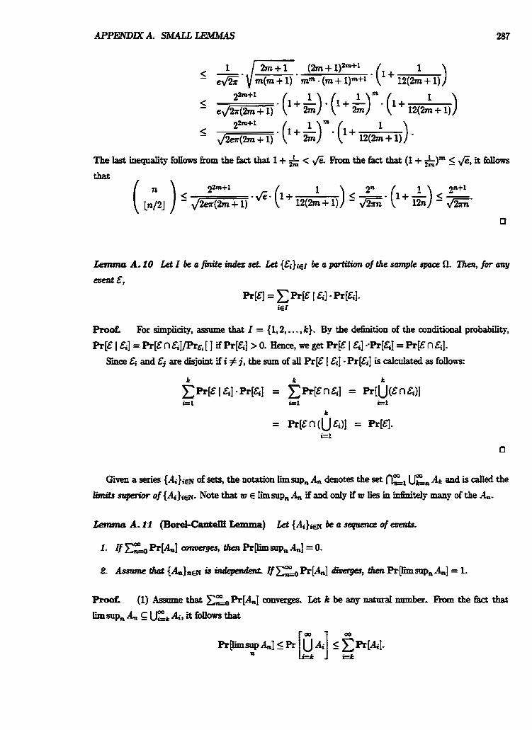
ThelastinequaIi~foIlowsfromthefact that l+& < &. Fromthefaathat (I+&)" 5 &?it fo1Iows
that
Lemma A. 10 Let I be a finite indQ set. Let {&)iEr be a partition of the sample space $2. Then, for m y
ProoE For simplicity, assume that I = {1,2,. . . , k). By the definition of the conditional probabihy,
Pr[& I &] = R[& n &]/PrE, [ I if R[&] > 0. Hence, we get Pr [& I &] Pr[&j = Pr[& n &I.
Sice Ei and Ej are disjoint if i # j, the sum of all Pr[& I &] - R[&] is calculated as foIlm:
Given a series {A+)iEn of sets, the notation b s n p n A, denotes the set c, rh -4c and is called the
Iimits of {&)ia. Note that w E I.imsttpn A,, if and only if w lies in inhibdy many of the &.
PmoE (1) Assmne that &[A,,] ammge% Let k be anp natural mnnber- h the fact that
limsnp,A,~U"i=LAi,itfonowsthat
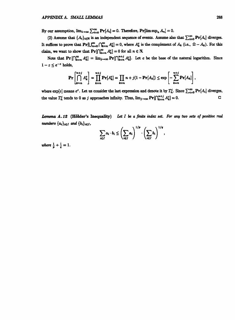
By om assumption, R[&] = 0. Therefore, Rmsap, A,,] = 0.
(2) Assume that {&lie is an independent s e q ~ a ~ e of events. Assame also that Pr[A+] diverges.
It d c e s to prove that R N z n E AL;] = 0, where AT is the complement of At (i.e., f2 - A&). For this
dsLo,aewant toshonthatR[n~A~]=Ofordn~N n+j c Note that P r m k A;] = hi- Prn, AJ. Let e be the base of the natural logarithm. Since
1 - z 5 e-' holds,
where erp[t] meam i. Let us consider the last expresion and denote it by Ti. Since RL4i] diverges,
the value Ili, tends to 0 as j approaches infinity. Thos, Iim j- A:] = 0. 0
Bibliography
[I] E.W. Mender and R Rubinstein, P-printable sets, SL4M 3. CompL, 17 (1988), 1193-1202.
[2] D. An&in, On counting problems and the poIynomial hierarchy? !l%eorrtical: Computer Science 12 (1980).
pp.161-173.
[3] T. Baker, G. GiII, and R Solovay, Rekhbtions ofthe P=?NP question, SLAM J. Cornput. 4 (1975), 431-442.
[4] J. L. B a l k , J. Diaz and J. Gabarr6, Struhaol Cmnplcziry I, Q Springer-Verhg, 19880, 1990@).
[6] J. Belanger and J. Wan& Rankable diskiiatiom do not provide harder instances than anifann dkhhtious,
in Ist Computing and Combimatorics Conference," 1995, Lecture Notes in b p n t e r Sden~e,
VoL959, pp.41049.
[fl J. Beknget and J. Wang, Reductions and con-ae rates of average time, m "Roc. 2nd International
Computing and Combinatorics Conference", Lecture Notes m Computer Sdence, VoL1090, p p ~ 3 0 9 , 1 ! W .
[8] C.H. Bennett and J. Gi& Relatme to a random orade A, # @ # u+w with probablitp 1, SUM J.
Comprt. 10 (1981), 96-113-
[9] S. Ben-David, 13. Char, 0. Goldreich, and M, Lnby, On the theory of average case complerdtp, J. Compct Sysfcm S d 44 (1992), 193-2l9. A prdimkprg oersion appeared m Pmcdbgq 22nd STOC, 1990, pp.37%386.
[lo] L Berman and J. Haraoaais, On isomorphism and density of NP and other complete setq SLAM J- Campat 6 (1977), 305-322.
BIBLIOGRAPHY
R Book and D.2. Do, The a;isteaee and density of generalized c o m p w cares, J. of ACM, 34 (1981),
7lS-730. 1987.
R Book, DZ. Dtr, and D. Rrsso, On polpnamial and generalized complexity cores, in "Proceedings, 3rd
Conference on Structore in CampIadty Thmf, pp236-250,1988.
J. Cai and L A. H e d r a , On the power of parity polynomial time, Moth, Systems Ttreory, 23 (1990),
pp.95-106.
J. Cai and A. Selman, Fme sepamtion of average time c o m p l e dassg, in Tmxd&s, 13th A n n d
Symposium on T b m t i d Computer Sciencen, Leaare Notes in Computer Science, VoI.1046, pp.331-343,
1996.
J. Carter and M. Wegman, Universal dassg of hash frmctions, J. Comput. System Sci., 18 (1979), pp.143454.
A.K. Chaadra, D.C. Kozcn, and LJ. Stodrmeyer, Alternation, J. ACM 28 (1981), 114433.
S. Cook, The complexity of theorem proving procedures, in "Proceedings, 3rd ACM Symposium on Theory of
c ~ m p ~ k g , pp.15i-i5s, an.
K- de W, E-F- Moore, C.E. Shannon, and N. Shapiro, Computability by probabitistic machine, in C-E.
Shannon and J. McCiuthy, e d b s , Automotn Sttrdiy pp.183-212, Princeton University Ress, Princeton, 1955.
DX- h, T- hkowhz, and D A Rum, Structural properties of complexity cores, unpublished manusaipt,
Department of Mathematis, Unbmky of Catifornia at Santa Barbara, 1984.
J. E h c o and M. Paull, Probabilistic andysis of the Davis Putnum procedure for solving the satidability
problem, Discrete Applied Math 5 (1983), 77-87.
M a G a ~ p and DJ. J o k n , Comprtss ond I-, A Guide to the Thtmy of NP-Compfetenus,
W E F h m a n and Company, Ne-a York, 1979.
J. Geske, D. Huynh, and J. A note on a l m ~ h e r e complex sets with application to polyaomial
compIexity degrees, Infmrnorion ond Comprdation 93 (1991), pp.97-104,
J. Gill, Compatationa oompkity of pmbabilirCic nPing machines, S W J. Comput. 6 (l9n), 675-695.
M. GoIdma~, P- &ape, and JJhbd, (m average time hierarchy, Infmm. lhxs+tg tctkrs 49 (1994),
15-20.
0. GoIdmich, Towards a t6eorp of amage case compIeJdtp (a survey), Technical N0.507, W lnstitnte
ofTechaology,=
J. Goldsmith, L.A. D. Joseph, and P. Young, Near-testable sets, SljlM. J. Cornput 20 (1991),
pp.506-523.
P. Grape, Taro results in average case complerdty, Technical Repat TFU'I!A-NA-9105, RoyaI Institate of
Technolagy,SStodrhokn,Saeden, f99L
BIBLIOGRAPHY 291
[34] Y. GafeYich, CrmrpIete and incomplete randomized NP problems, in Tmxdb@, 28th IEEE SymP0s;am on Foandati011~ of Computer Sdence", pp.111-117, 1987-
[35] Y. G d c b , Matrix decomposition is complete for the average case, in *Roceedings, 3lst EEE Symposium
on Foundations of Computer Science", ppB02-811,1990.
[%I Y. Gareoich, A~lenge case wmpleteness, J. CCbmpPrt S y d m Sd 42 (1991), pp.346-398.
[3a J. Hartmanis, Generalized KoImogor~~ complexity and the stntcta~e offeasiile computations, in "Pmeeedings, 24th IEEE Symposium on t& Foundations of Camputer Science," pp.439-445, 1983.
[39] J- HartmanLq N. J-, and V. Sdsm, Sparse sets in NP-P: EXPTIUE msw NEXPTIME, Informo- f h 4nd CorrtmI65 (1985), pp.159-181.
[40j J. HSstad, R ImpagliazP,, L A Levin, and M. L d y , Cbnstrnaion of a pseudc+sandom genefator h n any oneway haion, Technics Report, TR-91-068, hkmitional Computer Sdence Institute, BetkeIey, Catifhia,
1991. ,Pd ' j . versions appeared in the pnxxedinp of the 2lst STOC, 1989, pp.12-24 and the 22nd STOC,
1990, pp-39-
[41] M- Hermo and E. Mapordomo, A note on pofynomial-size circuits with Iow resomcebonnded, Moth SystrmJ
Theory, 27 (19941, pp.347-356.
[&I J.E. Kopuoft and J.D. U?man, InfroducCion to Atchnutu Theory, Lunguugu, and Comput4tion, Addison-
WesIey, M a 3 s d m m q 1979.
[43j R ImpagIkiv, A p e r d view of averagecase complexity, in Thmdings, 10th A n n d Structure in b plexity Theory Conferen~e,~ ppJ34-147, 1995.
144 R Impa%iazP, and L A fRoiq No better ways to generate hard NP-instances than picking d o d y at
random, in Tbmd@s, 31th IEEE Symposiam on Foundations of Comprtter Science", pp.812-821, 1990.
[q DS. Johnson, A d o g of complexity dasses, Chapter 2 of Handbook of Tlicorrticof Computa Sdar&, edited by J. van Leewn, Elsevk Science P u b b B.V, 1990.
BIBLIOGRAPHY
PMW. Knijnenbmg, On tillldomkbg decision problems a sm~ejf of the theory of randomized NP, Technkd
Repott RW-CS88-15, Department of Computer Science, Unwersitg of Utrecht, 1988.
K. KO, Some obsmations on the probabilistic algorithms and NP-hard problems, Infbmatim P&g - 14 (19W7 PP-•
K. KO, On some natural complete operations, l7mmtkd Computer Science, 37 (1985), pp.1-30.
K- KO, C o m p w Theory of Reui l h c h n s , BirkhZuser, Boston, 1991.
K. KO and H. Riedman, CompOtationaI complexity of real fmrctioos, Themt id Computer S~~LILC~, 20 (1982),
pp.323-352.
Idf, KO and D. Moore, Completeness, appmxhation and density? SfAM J. Cornpt., 10 (1981), pp.787-796.
sck Kurtz, On the random d e hypothesis, hf- tmd ConLrof 57 (1983), pp.4&47.
L A Levis, Universd seqaenfial search problems, ProbtemJ o f ln f immth l lmmwum . .
9 (1973), pp.26266.
L. Lwb Aoerage case complete probkms, S . J. Compuf 15 (1986), 28S286. A prelimfnary version
appeared under the tide "Problems, compiete m %verage" instance" in "Proceedings, 16th ACM Symposium
on Themy of Computing", p.465,1984.
M. Li and P. M.B. V i Average case complexity under the tmiverd distri'bution eqyah worst-case corn-
p l e 7 Infbmmfim Procwjing Letters, 42 (1992), pp-14H49.
M. Li and P. V i An intduction to Kotmogm cornpkity d i t s uppkatiow, Springer-Vertag, New
York, 1993-
J E Lrrtz, h o s t -here high nonrmifapm compl-, J. of Cumput. Sysfan S d 44 (1992), 220-258.
S R Wq, Sparse complete sets for NP: solution of a conjecture by Bern& and Harmak, J. Canpld
S d 25 (1988), 13&143.
Y. hdansanr, N. Nisan, and P. T i The compat;rtiona a x q h i t y of mdversal hashing, TRuwet Cbmpd
Sd 107 (m), l2l-133-
E Mayordomo, Almost every set in exponential time is P-bi-immune, Tircortt. Cornput. Sci 136 (1994),
487-506.
E. Mayodorno, Contriintions to the study of resource-bouuded measme PED. dissertation, Sistemes In-
f d c s , Universitat Potitecaica de Catalanya, 1994.
A. Me!yer and M. Patefton, Wtth what freqaency are apparently intractable problems difEcuIt ??, Tecknid
Report MIT/LCS/TM-126, MIT, 1979.
A R Meyer and L.J. Stockmeyer, The equidence problem for regalar expressions w i t h qgarhg reqaires
exponential time, in Tmcedkgs, 13th EEE Symposiam on Switching and .4utomata Theory", 125129,
1972
B. Meyer, Constraaive separation of dasses of mdistingaishable ensembles, Trocedhgs, 9th Annual
Confmce on Strachnre in Complexity T h e , pp.198-204,1994.
P.B. Mitterson, The complerxitp of malign d i e s , SIAM J. Cornput, 22 (1993), 147-156.
R. Motwaai a d P. Ra&am~, lbdmid A~~ Cambridge Univezsity Press, New York, 1995.
M. Mundhenk and R Schder? Raadom hgmges for non-dorm complexity chses, J d of Compkdy
7 (1991), -310.
P. Orponen, D A Rtrsso, and tT. Schiining, Optima approDdmations and potynomially Iedable sets, S U M 3-
~mpd 15 (1986), 39948.
P. Orponen and U. Schhing , On the denshy and complexity of po1ylromhI cores for iatrafitable sets, Inform. '
Contml, 70 (t986), pp.5448.
R 0s- and k Wqderson, One-way fanetions are essentS for non-brivia zemimowledge, in "Proceed-
ings? 2nd kd Symposium on Theory of Computing and Systems," Israel, 1993. An extended abstract appeared
T&d I.eport, ICSI-TR-93-073, Mematid Computer Science Institnte at Berkeley, 1993
C. Papadimitdou and S. Zacbw Two remarks on the power of counting, in T m c d b g s , 6th GI Conference
on Theoretkd Computer Science," LectrPe Notes in Computer Science, VoL145, pp.269-275, Springer-Vbrhg,
Berfia, 1983.
BIBLIOGRAPHY
[q Satoh and 0. W- On set size cornpatison problem, TechnicaI Report of IEICE, 1993.
[a] RE. Schap'ae, The emeqhg theory of a- complexity, Technical Report, .MIT/LCS/TM-431, M a s sachusetts fnstitate of Technology, 1990.
w] U. Schiining, Robust algorithms a diffkrent approach to d e s , Cmnputer Sci- 40 (1985),
pp.51-60.
[91] U. Schiining, Complaify cmd dmcbr~, Lectare Notes in Computer Science, V01.211, Springer-VerIag, 1986.
1921 R Schder, h e properties of sets tractable under every polynomial-time computable distriiution, Infdon Pmcmhg kttem, 55 (1995), pp.175bI84.
[93] R SchaIeq Average polynomial time is hard for exponential time under sn-reductions, in 'cProceedings, 15th
Foundations of Softwae TechnoIogg and Theoreti& Computer Sdencqn Lecture Notes in Computer Science,
VoLIO26, pp.240-247,1995.
[94]: R Schder, avth-table dosure aud 'Ihring dmm of amrage polpnomial time have diEerent measure fa EXP, in Troaxcbgs, 11th Anwal Codme on Compdat id CompIexity," pp.19@197,1996.
[95j R Schnlet, A note on anivefta distniations for polynomUtime computable distniution~, in "PKK.nedings, 12th Annuat IEEE Conf-ce on Computational Complexity," 1997.
[96] R W e r and 0. W m Toarards averagecase corn- andpsis of NP optimization probIenrs, in
loth Axutual Conference on Structure in CompIexitp Theory: pp.I4&159,1995.
(9?j R W e t and T. Ya-ai, Structural ;.rtrerage case compIexity, J. Compul. Syskm Sci 52 (1 996), 308-327.
A preliminary version appeared in 12th Foundatians of Software TechnoIogy and Theomtical h p r t t e r %ha%'' hztnre Notes m b p u t e r Science, VoI-65% pp.12&139, Springer-Verlag, BerBerlin, 1992
[q R Schaler and T. Yamak.ami, Sets ampatabIe in polynomial time on awrage, in of the Ist
Computing and -01 Conferen~e,~ Lecture Notes in Computer Science, Vbl-959, pp.400-409,1995,
Springer-Vedag.
[I001 M. S i , A amp- thenretic approach to randomness, in 15th ACM Symposiam on the
Themy of Cornpotink'' pp.33&335,1983-
[I041 L. Valiant, The c o m p l e of computing the permanent, T f r e o d d Computer Science, 5 (1979), 189-201.
[I051 LG. Valiant and V.V. Vazirani, NP is as e q r as detecting unique solutions, Thamtid Cumpute~ Sckm 47
(1=), PP-.
[I061 R V l and L Levin, Random instances of a graph doring pmbIem are hard, in V g s , 20th
ACM Symposium on Theory of Compating", pp.217-222, 1988.
[I01 R Venhesan and S. RaiagopaIan, Atrerage case intractability of Diophantine and matrix problems, in
24th ACM Symposiom on Theory of Computing", pp.632-642, 1992.
[I081 J. Wang, Average case completeness of a word problem for groups, in "Proceedings, 27th ACM Symposium on Theory of Compating", ~~325434 ,1995 .
[110] J. Wang, A m a p a s e W l e NP probIems, manuscript, 1996.
[ill] J. Wang and J. Belangex, On average P vs. average NP, in C m w 27ieory - Cunwaf Rwemrlr, editors K. Ambos-Spies, S. Homer and U. Schihhtg, Cambridge Oniversitp press, 47-61, 1993. A pteliminary version
appeared in 7th IEEE Conference on Structure in C o m p I e Theory," pp.318-326, 1992
[I121 J. Wang and J. Belanger, On the NP-isomorphism probIem with respect to random instances, J. Cornput-
System Sei, 50 (I995), 151-164. A pteliminarp veRion appeared in =gs, 8th Codereace on Structure
in CompIexity Theory,'' 1993, pp.65-74 under the title: rsOmarphisms of .NP compIete prob1ems on madom instances.
[I131 0- Watanabe, Test instance generation far promised NP search problems, in "Proceedings, 9th Anwa Con- f-ce on Structure in Comp1- Theory," pp20&216,1994.
[I161 EU. Wilber, Raa- and the densitp of hard probIems, in "Proceedings, 24th IEEE Symposium on
Foundations of Computer Science", pp.335-342,1983-
[I201 AC. Yao, Theory and appIicatiom of trapdoor frmctians, in Tmad&s, 23rd A d IEEE Symposinm on
Fonnaations of Computer Sciex~ce,~ 1% pp.80-91.
[I211 C. Yap, Some ~mregaences of non-unifarm conditions on aniform dasses, Thcat . Compu+ Sci 26 (1983). pp.287-300.
[I24 S. Zachas, Collapsing probabilistic polynomiaI ltkudk, in "Ebcdhgs , Conference on Cornputatid Complexity Theoayp Santa Barbara, 1983, pp.7Wl.
[I?? S. Zachas, Robabilistic and games, J. Comprt. Syskm Sci 36 (1988), pp.433-451.
List of Notation
M:F ,239 APHF ,239
mgr , 239
APT ,32
q 7 , 239 <wbPP -tt , 185
A=(-(n,n , 79
A=(-(t)?7) ? 79
A=(ATIME~(~, s), 7) , 79
AVCT(ATIME~(~, S) , T ) ,79
A=(-=(T? a, n , 79
A=(-= (t? 4, T ) ? 79 A=(BPP,T)~ ,207
A=(B-(n,T) ? 79
A=(B-(t), 7) ? 79
Aver(C1 nc2,3) ,80
Aver(-GT) ? 80
A=(-Np,7) , 80 Aver(A:, 3) ,217
Aver@spAcE(S), 7) ? 80
A m s p A c E ( 4 , 7 ) , 80
Aver@T=(n?a ? f9
A m T I M E ( t ) , 7 ) , m
LIST OF N O W O N
D=(t) ? 30
E ,30
E-comp , 102
A; 7 33
EH 7 33
q T 33
C; ? 33 ESPACE ,30
I IA(X) ? 275
Q ? 11
EXP-comp ,102
A T ? 33 EXPH ,33
FLAT, 51
Index
........................... symbols t-time computable -42
............. C.f(n)-close .................................. 41 l-dimensional martingale system -45
............................... C-immune 46. 255 .......................... 7 on paverage .55. 65
.................................. Tdomhate 68 ...................... 7-space machine 25
...................... 7-time Thing machine -25
............................. 7-time bounded -29
............................. 7-time machine -29
............................. EXP-computabIe 30
............................... E-cornputabIe -30
....................................... t. rare 110 ............................... s,.c omplete -160 .............................. <,descriptive -167
.................................... <,.hard -160 ............................... P-computable -30
................................... P-printable 36
............... #P-computabIe on paverage -282 ....................................... a-&Id -17
.................................. i-di-5 37 ............................... i-md&iqui& -38
............................ t on pa- 55, 65
tonaverage
with respect to (phIna - ................ 56
with respect to {p+,),, a ................ 56
................................... t- 68
....................... t-space Turing &e 25
.......................... t-space mmptitable -42
................... t-time Tmhg marhine .2S, 29 .............................. &time botmded -29
A
............................... absolute d u e -12
.................................... accept 20, 22
.................. accepting computation tree -23 ....................................... acydic -14
adaptive query .............................. -22 ...................................... adjacent 13
almost
....................................... all 11 .................................... every 11
.............................. everywhere -11
..................................... totd 26
.............................. almost immune 258
....................... aIrnost polynomial time 32
alphabet ..................................... -14 ................................... &ernation 23
..................................... ancestor -14 . .
assoQatrve .................................... 12 ......................... a ~ b p p t t ~ r e d u c i b ~ 185 .......................... average 7dominate 69
........................... average tdominate 69
average polynomial-time ................... many-one redua%w 152
..................... litring redualiritp -158
average poIynomiaIly eqyal ................... 7 l
.................. average poIynomialIy include iT
............... average-polynomia damiaation 69
averagepalynomiaI equidence .............. -69 . . .............................. -n -69
convex ....................................... -16
...................................... covering 12
......................... critical co~gnration -24
........................................ cycle -14
decreasing
strictly ................................... 16 .................................. weakly -16 .................................. degenerative 53
........................................ degree 14
....................................... density 15
.................. den$@ frmction, probabii 50
......................................... depth 14
................................... descendant 14
.................................... di&reIlce -11
................................ disjoint union -15 .................................. distribution -49
............. T-space sampW1e .. ...... -121 ...................... T-time samplab1e -121
............................. T- ttniversal 134
................ EXP-computable .. .... -102
.......................... E-computable -102
.......................... EcomputabIe -102
................ P-comptttabIe .. ......... 102 ........................... P-sampIab1e -121
~&sam~lab1e .......................... -140 ........................ #PamputabIe -131
............. t-space samplab1e ....... ... I21
........................ t-time samplabIe El
.................... average P-sampIabIe I26
a- polynod-time samplabte ...... I26 wnditio rial......................... ...... 50
........... exponential-time compntab1e -102 fIat .................................. 51, 16!3
.................. h m t i i P-sampIabIe 124
hmrtiii1y polyn@time samplabIe .. - 3 4
hear-exponentiaLthne computab1e ...... 102
Iogarithmic-space computable .......... -102
.............................. p u n i d 134
poIynomia1-time computable .. ... .. ..... 102
............. poIynomial-time samplable -121
................................ standard -51
.................. strictly P-computable -103
strictly P+amplable .................... -121
trivial ................................... -49
uoiform ................................. -50
distn'butional problem. ....................... TI
...................................... domain -15
domination condition ....................... -158
dyadic rational number ..... .. ............... -15
E .......................................... edge 13
edgeset ...................................... 13
element ....................................... 11
.................................... empty set 11
.............................. error probability 27
evpnt ......................................... 18
................................... exphonest -16
w o n .............. ........... .......... 18
expected polynomial on paverage ............ -53
expectedvalue ................................ 18
..................... exponential .......... ... -13
exponentidIy bounded ...... .. .............. .. 16
F ....................................... f o d 10
l MAGE EVALUATION TEST TARGET (QA-3)


