figure 4.1. - mcmaster university 795/plonsey and barr book... · molecular cell biology, 2nd ed....

4CHANNELS

4.1. INTRODUCTION

In the previous chapter it was pointed out that biological cells are enclosed by a plasma mem-brane. This membrane consists of a lipid bilayer and, as seen in Figure 3.1, the hydrophilic polarheads are oriented facing the intracellular and extracellular water-containing media, while thehydrophobic tails, on the other hand, are internal to the membrane. The biophysical consequenceof the lipid is a membrane with the high dielectric constant of oil and the high resistivity of thatmaterial. The thin membrane has a high membrane capacitance of Cm = 1μF/cm2; the lipidmembrane also has a high specific resistance of 109 Ω cm2.

The very high membrane resistance is essentially an insulator to the movement of ions. Ionflux takes place because of the presence of membrane proteins called channels. These membraneproteins lie transverse to the membrane and contribute an aqueous path for ion movement. Spe-cific resistances of biological membrane of 1,000 to 10,000 Ωcm2 are observed. Such specificresistances are much lower than that of lipid membrane alone and occur as a consequence of thepresence of open membrane channels.

But channels do not simply furnish a passive opening for ions to flow. Rather, channels aregenerally selective for a particular ion. In addition, a striking property of channels is that theyhave gates that open and close, and ion flow is controlled through that mechanism.

This chapter is devoted to an examination of channels, their structure and their bioelectricalproperties.

4.2. CHANNEL STRUCTURE BY ELECTRON MICROSCOPY

We first review what has been found from electron microscopy (EM), electron diffraction,molecular biological, and biophysical approaches. The use of electron microscopy and x-raydiffraction requires a regular lattice, but general methods for crystallizing membrane proteinsare not available as yet. There are several purified channel proteins that do form fairly regulartwo-dimensional lattices. These lattices have been investigated with x-ray diffraction and EM.

71

72 CH. 4: CHANNELS

Figure 4.1. Model of the Acetylcholine Receptor that shows the five component subunitsand the aqueous pore. The band locates the membrane bilayers through which the moleculepasses; the lower part is cytoplasmic. From Stroud RM, Finer-Moore J. 1985. Acetylcholinereceptor structure, function, and evolution. Reproduced with permission from Annu RevCell Biol 1:317–351. Copyright c©1985, Annual Reviews Inc.

The achieved resolution of around 17◦A describes a general structure but is not adequate for many

details of interest (e.g., pore cross-section and gates).

A conception of the acetylcholine (ACh) receptor that results is shown in Figure 4.1. Wenote that it contains five component subunits enclosing an aqueous pore. Also, the total lengthsubstantially exceeds the plasma membrane. This molecule has been estimated to be about 120◦A in length, 80

◦A in diameter, with a 2.0–2.5 nm central well. The dimensions of other ionic

channels are not too different.

4.3. CHANNEL STRUCTURE: MOLECULAR GENETICS

An increasingly important technique for investigating channel structure is based on genecloning methods that determine the primary amino acid sequence of channel proteins. Theresults can be tested by determining whether a cell that does not normally make the supposedprotein will do so when provided the cloned message or gene.

Oocytes of the African toad Xenopus laevis are frequently used to examine expression ofputative channel mRNA. The resulting channel properties can be evaluated to determine whetherthe protein synthesized is indeed the desired protein.

Although the primary structure of many channels has now been determined, the rules fordeducing secondary and tertiary structure are not known. Certain educated guesses on foldingof the amino acid chain can be made, however. One involves a search for a run of twenty orso hydrophobic amino acids, since this would just extend across the membrane and have theappropriate intramembrane (intra-lipid) behavior.

In this way the linear amino acid sequence can be converted into a sequence of loops basedon the location of the portions lying within the membrane, within the cytoplasm, and within the

BIOELECTRICITY: A QUANTITATIVE APPROACH 73

Figure 4.2. Proposed Transmembrane Structure of (a) voltage-gated Na+ channel proteinand (b) voltage-gated K+ channel protein. The sodium channel arises from a single gene;it contains 1800–2000 amino acids, depending on the source. About 29 percent of theresidues are identical to those in the voltage-gated Ca++ channel protein. There are fourhomologous domains indicated by the Roman numerals. Each of these is thought to containsix transmembraneα helices (Arabic numerals). Helix number 4 in each domain is thoughtto function as a voltage sensor. The shaker K+ channel protein (b) isolated from Drosophilahas only 616 amino acids; it is similar in sequence and transmembrane structure to eachof the four domains in the Na+ channel protein. From Darnell J, Lodish H, Baltimore D.1990. Molecular cell biology, 2nd ed. New York: Scientific American Books. Adaptedfrom Catterall WA. 1988. Structure and function of voltage-sensitive ion channels. Science242:50–61. Copyright c©1988, American Association for the Advancement of Science.

extracellular space (Figure 4.2). From the membrane portion of the sequence the particular run ofamino acids gives some clues as to the structure of and the boundaries of the ion-conducting (pore-forming) region, as well as the location of charge groups that could enter into voltage-sensinggating charge movement.

74 CH. 4: CHANNELS

This approach was successfully used in the study of shaker1 K+ inactivation. Following acti-vation of this channel, it was noted that the ensuing inactivation was voltage-independent. Voltageindependence implies that the inactivation process must lie outside the membrane (otherwise itwould be subject to the intramembrane electric field).

The amino-terminal cytoplasmic domain of the membrane protein was investigated by con-structing deletion mutants whose channel-gating behavior could then be examined. The resultsdemonstrated that inactivation is controlled by 19 amino acids located at the amino-terminalcytoplasmic side of the channel and that these constituted the ball of a ball and chain.

What appears to be happening is that associated with channel activation is the movement ofnegative charge into the cytoplasmic end of the channel. The negative charge attracts the positivelycharged ball, resulting in closure of the channel by the ball (which exceeds the channel mouth insize). Deletions of this amino acid sequence terminated the channel’s ability to inactivate.

4.3.1. Channel Testing

Some hypotheses can be tested by site-directed mutagenesis involving the deletion or in-sertion of specific protein segments (as just noted). By examining the altered properties of thechannel expressed in Xenopus oocytes, one can make educated guesses concerning the function ofthe respective protein segments. Unfortunately, since the introduced changes can have complexand unknown effects on the tertiary structure, only tentative conclusions can be reached.

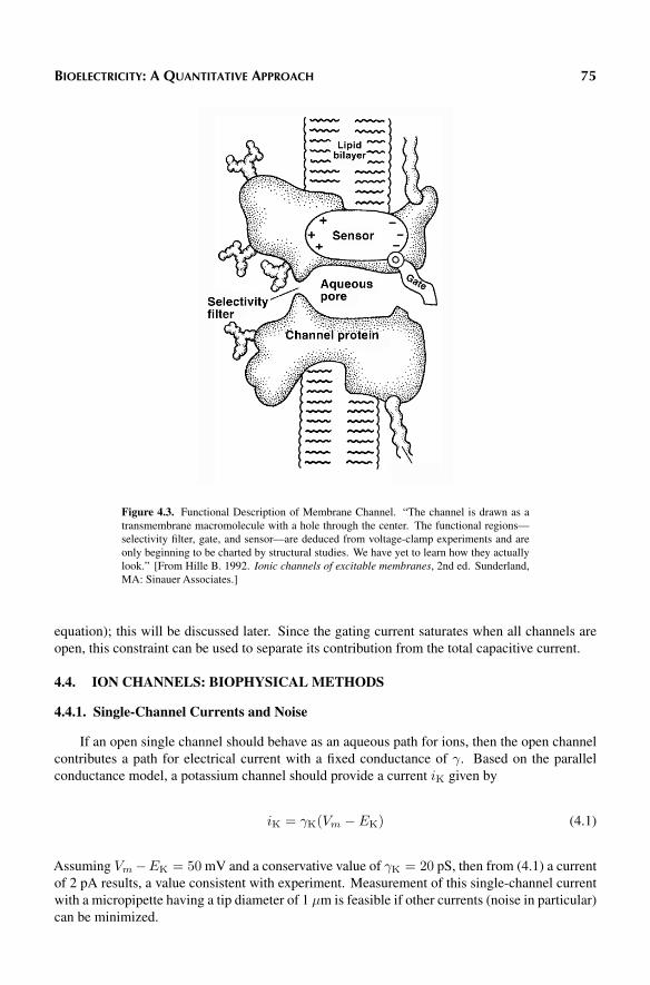
Based on what is known of the channel structure and even more on channel function, Hille[1] constructed the channel cartoon reproduced in Figure 4.3. Referring to this figure we note,for example, that the cross-sectional area of the aqueous channel varies considerably along thechannel length. The variable cross-section is consistent with a recognition that the walls of theenclosing protein are nonuniform.

This shape also could contribute to the channel’s property as a selectivity filter. Measurementsshow that a potassium channel may pass K+ at a rate that is 104 times greater than Na+, eventhough the latter is 0.4

◦A smaller in crystal radius—so that selectivity is not a simple steric

property. The observed high channel selectivity could be related to the particular distribution ofcharges along the walls of the pore, and this possibility can be investigated based on the aminoacids lining the pore.

In Figure 4.1 the barrel stave structure has been thought to facilitate rapid gating. Suchgating could be accomplished by only a small rotation of the contributing components. Thus,small conformational changes could give rise to large changes in the cross-section of the aqueouschannel. The very rapid gating that is observed biophysically requires such structures.

Voltage gating implies that the molecular structure of the channel protein contains effectivelyembedded charges or dipoles—and these are sought within the amino acid sequence. An appliedelectric field causes intramolecular forces that can result in a conformational change.

This movement of charges constitutes a gating current; the charge displacement throughan electrical potential adds or subtracts from the potential energy of the protein, and this canbe related to the density of open or closed channels in a large population (through Boltzmann’s


Figure 4.3. Functional Description of Membrane Channel. “The channel is drawn as atransmembrane macromolecule with a hole through the center. The functional regions—selectivity filter, gate, and sensor—are deduced from voltage-clamp experiments and areonly beginning to be charted by structural studies. We have yet to learn how they actuallylook.” [From Hille B. 1992. Ionic channels of excitable membranes, 2nd ed. Sunderland,MA: Sinauer Associates.]

equation); this will be discussed later. Since the gating current saturates when all channels areopen, this constraint can be used to separate its contribution from the total capacitive current.

4.4. ION CHANNELS: BIOPHYSICAL METHODS

4.4.1. Single-Channel Currents and Noise

If an open single channel should behave as an aqueous path for ions, then the open channelcontributes a path for electrical current with a fixed conductance of γ. Based on the parallelconductance model, a potassium channel should provide a current iK given by

iK = γK(Vm − EK) (4.1)

Assuming Vm−EK = 50 mV and a conservative value of γK = 20 pS, then from (4.1) a currentof 2 pA results, a value consistent with experiment. Measurement of this single-channel currentwith a micropipette having a tip diameter of 1 μm is feasible if other currents (noise in particular)can be minimized.

76 CH. 4: CHANNELS

Figure 4.4. Inside–Out Patch Clamp Configuration. The desired current path through thecell is challenged by the alternate (leakage) pathway available in the region of electrode–membrane contact. A single open channel is assumed to give a membrane conductanceequal to or greater than 20 pS (a resistance of ≤ 50 GΩ). To keep leakage current low(hence minimal loss of signal strength as well as reduced Johnson noise), this resistanceshould be in the tens of gigaohms; fortunately, patch electrodes with 100 GΩ leakageresistance are currently available.

We note that the Johnson noise current is

σn =√

4kTΔf/R = 0.0180 pA (4.2)

based on Δf = 1 kHz, R = 1/20 pS = 5 × 1010 Ω, T = 293 K, and k (Boltzmann’s constant)= 1.38× 10−23. Even with a signal current of 1 pA, an entirely acceptable S/N = 56 results.

The problem in single-channel measurements that results from bringing a micropipette incontact with the cell membrane is illustrated in Figure 4.4. Using conventional techniques wewould have a leakage resistance of 10 MΩ in parallel with that of the channel (5× 1010 Ω). Withthe reduced R value of this combination, (4.2) evaluates a leakage noise current of 1.3 pA. Thisnoise current results in a poor signal-to-noise ratio.

To reduce the noise current by tenfold requires a 100-fold increase in leakage resistance!Such a reduction was achieved by Neher and Sakmann by careful preparation of the electrodetip, preparation of the biological material, and application of a small amount of suction. The


resultant instrument is called a patch clamp. The measurement of these low picoampere-levelcurrents could not have been achieved without the advent of field-effect transistors with low-voltage noise and sub-picoampere input currents.

The choice of tip diameter of around 1 μm is about ten times larger than that used forintracellular micropipettes. The larger tip results in a lower tip resistance, a desirable factorto achieve a lower noise, as noted above. On the other hand, it may mean that more than onechannel will find itself under the patch electrode. An examination of the recorded signal willreveal whether, in fact, only a single channel is accessed.

4.4.2. Voltage-Clamp Methods

Investigations of electrically active membrane often make strategic use of a patch clamp,space clamp or some other form of voltage clamp. To understand why, some background isneeded, so that one understands the historic difficulties such a strategy is designed to overcome.In essence, what was discovered over time was that in such a membrane the conductivity changes,so that Ohm’s law does not hold. Such conductivity changes are now known to arise from theopening or closing of channels. Varying numbers of open channels then produce changes intransmembrane voltage.

Closing the loop, the membrane voltage changes alter the number of channels that are openor closed. There is thus a feedback system, in which transmembrane voltages change channelopenings, and changes in channel openings alter voltages. This feedback mechanism is a beautifulengine for cell activity and response, but one that, in its natural form, is hard to analyze in termsof its components, and next to impossible to evaluate experimentally.

To cut through this complexity, the voltage-clamp experiment was developed over a periodof years in the mid-1900s. Though its origin had an experimental focus, the voltage clamp wasalso a powerful analytical concept. A core goal of the voltage clamp is to break the feedbackloop where voltages affect channels, and channels affect voltages. Breaking the loop allows oneto separate changes in voltage from the changes in the numbers of open channels that result.

The separation is achieved by making transmembrane voltage something the investigatorsets as an independent variable, whether mathematically or experimentally, rather than somethingdetermined intrinsically by the cell, as happens normally. Thereafter the consequences of settingthe voltage are determined, in terms of membrane currents, channels open, or other effects.

In the voltage-clamp protocol (Figure 4.5), the transmembrane voltage is set to two valuesin succession, here designated V 1

m and V 2m. The time periods during which these voltages are

applied are called phase 1 and phase 2. In phase 1, the clamp mechanism and its control systemsupplies enough current of the right polarity to hold the transmembrane voltage at V 1

m until thecell reaches steady state at time t = t1. Then, at time t = 0, there is an abrupt transition fromthe first to the second transmembrane voltage, i.e., a transition from V 1

m to V 2m. In phase 2,

transmembrane voltage V 2m is maintained until a new steady state is reached at time t = t2.

Often the primary focus is on evaluating changes in the state of the membrane during phase2 at times t > 0 such as t = ta or t = tb. At such times an evolution in the number of channels

78 CH. 4: CHANNELS

Figure 4.5. Voltage Clamp, Vm versus Time. Panel A, Concept: The transmembranevoltage is held constant at transmembrane voltage V 1

m until time t = 0, when it is abruptlyshifted to V 2

m. Times t1 and t2 identify the times when the membrane reaches a steadystate in phases 1 and 2. Panel B, Detail: The equilibrium voltage for potassium is EK andthat for sodium ENa. Voltage Vm is an absolute value i.e., relative to Vm = 0, as shownfor V 1

m on the left, while vm (note lower case v) is relative to the resting potential (i.e.,relative to Vr , as shown by v2

m on the right). Time t = ta marks the end of the voltagetransition, while time t = tb occurs later, but before phase 2’s steady state is attained.

that are open and the membrane currents that are flowing through them is taking place, as themembrane evolves into its steady state for phase 2.

These changing numbers of open channels allow changes in ionic currents that are directlyobservable. In this regard, the driving force for sodium ions, VNa = Vm − ENa (shown duringphase 2 by a downward arrow) has a different magnitude and sign than the driving force forpotassium ions VK = Vm − EK (shown during phase 2 by an upward arrow).


In voltage-clamp experiments, transmembrane voltage is set as an independent variable, sothe transmembrane voltage comes about in a way that does not occur naturally. However, theconsequences of setting that membrane voltage, in terms of numbers of channels open or closed,or in terms of membrane current, can be evaluated as a function of time and as a function oftransmembrane voltage. This knowledge then can be integrated into a more complex systemwhere transmembrane voltages as well as channel characteristics evolve in a natural way.

4.4.3. Patch Clamp

If transmembrane currents are measured from a macroscopic cell membrane, the contributingcurrent density will vary with position over the membrane (unless some special effort is made).Such variation may result from propagation of activity, a topic treated in a subsequent chapter.

Because of the nonuniform contributions it may be difficult to interpret the measured current.It will be difficult because the current will originate from multiplicity of channels, and each onemay be behaving differently because of a different transmembrane voltage, temporal phase, etc.(Later, we will describe a “space clamp,” which ensures identical transmembrane voltages for allchannels.)

The patch clamp addresses such difficulty. In the patch clamp, the micropipette tip is small,only around 1μm diameter. As a consequence its measured current is from only the very smallcontacted membrane element. A beneficial corollary is that the confounding effects of spatialvariation of a large membrane area are avoided. The measurement is unaffected by spatialvariations and is hence “space clamped”; the “clamp” in the name “patch clamp” arises from thisfeature.

A downside of restricting measurement to a patch is that the currents through the patch aresmaller than for a larger membrane segment, and thus they are harder to measure. We have notedthat for a patch clamp to work satisfactorily careful preparation is required to ensure an adequatesignal-to-noise ratio. The following is a brief list of pertinent considerations [1].

1. A high-resistance seal is essential to ensure that the leakage currents (and their noisecomponents) are small compared to the desired transmembrane currents.

2. The pipettes should be fire polished and clean. In general, pipettes may be used onlyonce.

3. Cells should be clean and free of connective tissue, adherent cells, and basement mem-brane. Good seals are most readily obtained on cultured cells.

4. The application of gentle suction will increase the resistance of the seal to greater than1010 Ω. This is the desired gigaohm seal (gigaseal), permitting the measurement ofcurrents from membrane areas on the order of 1μm2. This resolution makes possiblerecording currents from single channels.

In Figure 4.6, four configurations of recording from a single-cell membrane using a patchmicropipette are depicted. At the upper left, the gigaseal is established and an on-cell condi-tion results. If a microelectrode is introduced into the cell, currents between that electrode andthe patch electrode must pass through the membrane patch (only). In view of the small size of

80 CH. 4: CHANNELS

Figure 4.6. Four Configurations for Patch Clamping are described. The clean pipette ispressed against a cell to form a tight seal using light suction, and produces the cell attachedor on-cell configuration. Pulling the pipette away from the cell establishes an inside–outpatch. Application of a suction pulse disrupts the membrane patch, allowing electricaland diffusional access to the cell interior for whole-cell recording. Pulling away from thewhole-cell arrangement causes the membrane to re-form into an outside–out configuration.From Hamill OP, et al. 1981. Improved patch clamp techniques for high resolution currentrecording from cells and cell-free membrane patches. Pflugers Arch 391:85–100.


the patch, this size could contain one or only a few channels (or none at all). Application of aconstant transmembrane potential permits the study of a single-channel response.

A momentarily elevated suction will rupture the membrane across the pipette (without de-stroying the seal), yielding the whole-cell configuration. In this situation the entire intracellularspace is accessible via a low resistance to the patch electrode. It can be shown that the intra-cellular space is essentially isopotential. Consequently, currents introduced through the pipetteflow uniformly across the entire cell while the pipette potential is the same as that at all pointson the intracellular cell surface. The macroscopic behavior of the whole cell is examined in thisarrangement; small cells in the diameter range of 5–20 μm can only be measured this way.

If, after establishing a gigaseal, the pipette is quickly withdrawn, then a patch of membranewill be found still in contact with the mouth of the pipette. The pipette may then be readily placedin solutions of arbitrary composition and the resulting transmembrane potentials and currentsmeasured. In this arrangement the inside (cytoplasm side) of the membrane is in contact with thebathing solution (i.e., the extracellular or outside); the arrangement is called inside–out.

If the pipette is pulled away while first in the whole-cell configuration, the membrane willreform in an outside–out configuration, that is, in this case, the outside (extracellular surface) ofthe cell membrane now faces the outside of the micropipette (i.e., the bathing solution). Thesecomments are also illustrated in Figure 4.6.

4.4.4. Single-Channel Currents

Examination of patch-clamp current reveals discontinuities that directly reflect the openingand closing of channel gates. Thus the concept of gated channels is supported by these experimentsand supplements the evidence of gated pores found in EM, x-ray diffraction, and molecularbiological studies.

Typical patch-current recordings are shown in Figure 4.7. The current waveform is interpretedas reflecting the opening and closing of a single channel.

The single-channel record is seen to switch to and from an open or closed state. The time ineach state varies randomly, but if the ratio of open to closed time is evaluated over a sufficientlylong period, then this ratio (with some statistical variation) will be the same over any successivesuch interval. Such a determination gives the expected value or probability that the channel willbe open (closed), a value that is independent of time under these steady-state conditions. Anelectric circuit representation of the single-channel current is given in Figure 4.8.

If the transmembrane potential is suddenly switched to a new value, the probability of thechannel being open also will change, as will be discussed in a later section.

The single-channel behavior is the basis for the macroscopic membrane properties. Whilethe former is statistical in nature, the summation of very large numbers of such contributionsresults in a continuous functional behavior. We will examine this relationship in this chapter andgive further details of macroscopic membrane behavior in subsequent chapters. We will alsoshow that, while the macroscopic properties can be found from the microscopic, to some extent

82 CH. 4: CHANNELS

Figure 4.7. Patch-Clamp Recording of unitary K currents in a squid giant axon during avoltage step from –100 to 50 mV. To avoid the overlying Schwann cells, the axon was cutopen and the patch electrode sealed against the cytoplasmic face of the membrane. (A) Nineconsecutive trials showing channels of 20 pS conductance filtered at 2 kHz bandwidth. (B)Ensemble mean of 40 repeats; these reveal the expected macroscopic behavior. T = 20 ◦C.From Bezanilla F, Augustine GR. 1992. In Ionic channels of excitable membranes, 2nd ed.Ed B Hille. Sunderland, MA: Sinauer Associates.


Figure 4.8. (a) Electrical circuit representation for a single (potassium) channel showingfixed resistance rK, potassium Nernst potentialEK, and the transmembrane potential Vm.The closing and opening of the switch simulates the stochastic opening and closing of thechannel gate. (b) Single-channel current corresponding to (a), where γK = 1/rK. This isan idealization of the recording shown in Figure 4.7.

the inverse is also true, and we will describe how certain microscopic, single-channel statisticalparameters can be found from macroscopic measurements.

4.4.5. Single-Channel Conductance

If a channel behaves ohmically, then in (4.1) its conductance γ is expected to be a constant. Inan experiment byYellen [4], shown in Figure 4.9, a single-channel potassium current is evaluatedas a function of transmembrane voltage. For the voltage range considered we note that a fairlylinear result is obtained supporting the conclusion that γK is constant; its value of 265 pS can befound from the slope of the dotted curve in Figure 4.9.

An estimate of the channel conductance can be obtained based on macroscopic ohmic ideas.For the channel shown in Figure 4.1, the pore diameter is on the order of 20

◦A . If it is assumed

that this is actually a uniform cylinder of length 150◦A (two membrane thicknesses), then the

conductance evaluates to

γ = π(10× 10−8)2/(250× 150× 10−8) = 84 pS (4.3)

based on a bulk resistivity of 250 Ωcm. The resulting value compares with measured valuesof potassium channel conductance of 20 pS and greater, and might be considered surprisinglyclose. In this calculation the macroscopic ohmic behavior of a uniform column of electrolyte hasbeen applied to a channel of atomic dimensions that is also likely to be nonuniform. It ignoreselectrostatic forces between ions and wall charges, possible channel narrowness, etc.

In addition, one should include an access resistance from the mouth of the cylindrical channelinto the open regions of intracellular and extracellular space. This resistance (using an idealizedmodel) is given by ρ/(2a). Including this resistance reduces the channel conductance from 84

84 CH. 4: CHANNELS

Figure 4.9. Current–Voltage Relations for a single BK K(Ca) channel of bovine chromaffincell. The excised outside–out patch was bathed in 160 mM KCl or NaCl and the patchpipette contained 160 mM KCl. In symmetrical K solutions the slope of the dashed line isγ = 265 pS; T = 23 ◦C. From Hille B. 1992. Ionic channels of excitable membranes,2nd ed. Sunderland, MA: Sinauer Associates. Based on measurements of Yellen G. 1984.Ionic permeation and blockade in Ca2+-activated K+ channels of bovine chromaffin cells.J Gen Physiol 84:157–186.

[as found in (4.3)] to 76 pS. In comparison, some measured channel conductances are given inTable 4.1 for sodium and potassium.2

Table 4.1 also shows the measured channel density, obtained using one of two methods. Inone, the macroscopic conductance of a whole cell was measured and then divided by the surfacearea of the cell and by the single-channel conductance. The result is the number of channels perunit area.

A second approach is based on gating-current measurements, and this approach will bedescribed subsequently. The result as seen in Table 4.1 might be thought to give a sparse densityof channels. This conclusion would be reached on Hille’s [1] estimate that perhaps 40,000channels could be physically accommodated in a 1μm2 membrane area.

But another reference value for channel density comes from an evaluation of the quantityof charge needed to change the transmembrane potential by 100 mV. Assuming C = 1μF/cm2

and a voltage change of 100 mV, then fromQ = CV , one obtains 10−7 Coulombs/cm2 or 10−15


Table 4.1. Conductance of Sodium and Potassium Channels

Preparation γ Channels– (pS) (number/μm2)

SodiumSquid giant axon 4 330Frog node 6–8 400–2000Rat node 14.5 700Bovine chromaffin 17 1.5–10

PotassiumSquid giant axon 12 30Frog node 2.7–4.6 570–960Frog skeletal 15 30Mammalian BK 130–240 —

Coulombs per μm2. Multiplication by Avogadro’s number and division by the Faraday results in6200 monovalent ions required per μm2. One channel carrying 1 pA of current moves that manyions in 1 msec. Thus the “sparse” channel density in Table 4.1 is also several orders greater thanan absolute minimum.

4.4.6. Channel Gating

We have mentioned that inactivation of the shaker K+ channel is accomplished with a balland chain configuration (Figure 4.10).

In the study of the ion channel colicin, a radical reconformation accompanies channel openingand closing, described by a “swinging gate” model [3]. In the absence of detailed informationon channel protein structure, gating mechanisms require a degree of guesswork.

In any case it is clear that, for voltage gated channels, the influence of a transmembranepotential on a gate is through the force exerted on charged particles by the electric field withinthe membrane (associated with the gate) in the protein channel. While the total distribution ofcharges in the macromolecule must be zero, we can have local net charge, though charges areprobably organized as dipoles. An adequate force exerted by an electric field will result in aconformational change in which the channel state is switched from closed to open (or vice versa).

At the same time, the charge (dipole) movement contributes to the capacitive current (inmuch the same way as a dielectric displacement current arises from molecular charge movementor dipole orientation). Such currents are called gating currents. Since they saturate at largeenough fields, they can be separated from the remaining (non-saturating) capacitive current,which is linearly dependent on ∂Vm/∂t.

Suppose we assume that the energy required to open a closed channel is supplied throughthe movement of a charge Qg = zqqe through the transmembrane potential Vm, where zq is the

86 CH. 4: CHANNELS

Figure 4.10. A protein ball pops into a pore formed by the bases of four membrane-spanningproteins (one not shown), thereby stopping the flow of potassium ions out of a nerve cell.Based on Hoshi T, Zagotta WW,Aldrich RW. 1990. Biophysical and molecular mechanismsof Shaker potassium channel inactivation. Science 250:506–507, 533–538, 568–571.


valence and qe is the charge. Then Boltzmann’s equation expresses the ratio of open to closedchannels as

[open][closed]

= exp(−w − zqqeVm

kT

)(4.4)

The fraction of open channels is therefore

[open][open + closed]

=1

1 + exp[(w − zqqeVm)/kT ](4.5)

In (4.4) and (4.5) w is the energy required to open the channel when the membrane potentialis zero, i.e., with Vm = 0, and k is Boltzman’s constant. (Recall that the gas constantR = k/qe.)

A plot of (4.5) as a function of Vm for different values of Qg can be compared with themacroscopic dependence of ionic conductance, as a function of Vm, and in this way Qg canbe estimated [1]. Good fits are achieved, but the model is very simple and the interpretationuncertain.

One complication is that the charged particles may not move across the entire membrane(i.e., through the entire voltage Vm). Another complication is that the transitions may not besmooth but take place in steps. (Step behavior is what is believed to occur.) Moreover, if theforce mechanism involves dipole rotation and translation, the energy calculation will necessarilybe different from that assumed in (4.4). Nonetheless, the equations are a starting point.

4.5. MACROSCOPIC CHANNEL KINETICS

The membrane functions by changing the number of open channels in response to a changingtransmembrane voltage, as well as time. It must do so fast enough to allow eye blinks and escapefrom predators, but slow enough that the process does not become uncoordinated or out of control.What equations describe the average number of open channels? What equations describe the ratesof change of the average number if the transmembrane voltage shifts from one value to another?The equations of macroscopic channel kinetics address these questions.

We consider a large membrane area containing N channels of a given ion type. We assumethat each channel’s behavior is independent, though governed by similar statistics. We furtherassume that each channel is either in an open or closed state and that the transition between thesestates is stochastic. Let the number of closed and open channels at any instant be Nc(t) andNo(t), respectively, where Nc and No are random variables; then

N = Nc(t) +No(t) (4.6)

We assume state transitions to follow first-order rate processes. If the rate constant forswitching from a closed to an open state is α while that for switching from an open to a closed

88 CH. 4: CHANNELS

state is β, then the average behavior is described by

αNc ⇀↽ No

β(4.7)

Based on experience with the measurements of Hodgkin and Huxley (to be described inChapter 5), we expect α and β to depend on the transmembrane potential (only) and therefore tobe constant when the potential is fixed (as assumed at this point).

Based on the relation given in (4.7), we have

dNcdt

= βNo − αNc (4.8)

and similarlydNodt

= αNc − βNo (4.9)

If (4.6) is substituted into (4.9); then, after rearranging terms, one has

dNodt

+ (α+ β)No = αN (4.10)

The solution of (4.10) isNo(t) = Ae−(α+β)t +

α

α+ βN (4.11)

Equation (4.11) is important because it shows how the number of open channels can be determinedafter, for example, the voltage transition in a voltage clamp. The equation gives the solutionsfor a time immediately after the voltage change, a long time after the change, or at any time inbetween.

In this regard, in (4.11) constant A has to be determined by the boundary conditions. Herethe boundary condition is the number of open channels at t = 0. For a voltage clamp, that wouldbe the number of open channels existing just before the clamp voltage was set to a new value.

The implications of (4.11) can be seen by considering what happens if a voltage step isintroduced at t = 0. The immediate result of the voltage change will be that α and β switchto new values. Equation (4.11) describes what happens thereafter. If, for example, at t = 0 allchannels were closed, then from (4.11) we have (for t > 0)

No(t) =α

α+ βN(1− e−(α+β)t) (4.12)

Let No(∞) be the probable number of open channels after a sufficiently long time. (“Suffi-ciently long time” means long enough for the negative exponential term in (4.12) to go to zero,compared to other terms.) Then consider again the situation following the change to the new rateconstants α and β.


From (4.12), we see that No moves from a value of zero to a steady-state value of

No(∞) =α

α+ βN (4.13)

Thus, at steady state it is only the average number of open channels that is constant, as theactual number of open channels will fluctuate around this average value. The average numberopen depends on the α and β values that are present at the new transmembrane voltage, so aftera sufficiently long time any previous history is lost.

In the new steady state, the expected (average) value is of interest, but also of interest is thefluctuation around it. One way of thinking about fluctuations is to note the following somewhatsurprising fact: while obtaining (4.11) we assumed a voltage-clamp transition to have occurred.

In fact, expression (4.11) also describes the response to spontaneous fluctuations in thenumber of open channels. Consequently, the kinetic analysis of fluctuations reflects the sametime constants as arise in classical macroscopic analysis. This correspondence is formalized inthe fluctuation-dissipation theorem [2], which exhibits the broader and fundamental nature of thiscorrespondence.

4.6. CHANNEL STATISTICS

We assume that each channel in a population of similar channels switches between openand closed states governed by the same rate constants α and β as govern the ensemble (as wediscussed in the previous section).

We let C identify a closed channel and O the open channel. Then

αC ⇀↽ O

β(4.14)

For example, if we have N = 100 channels and the probability of a channel being open is 50%,then at any instant we have an expected (i.e., steady-state) value of Nc(∞) = No(∞) = 50.

The number 50 is, of course, not the exact value of Nc(t) or No(t) at any t, no matter howlarge. The reason that 50 is not the exact value is because the actual values will fluctuate around50, over time, because the underlying channel behavior is random and 50 is only the average.

From (4.13) we found thatNo(∞), the expected number of open channels under steady-stateconditions, equals [α/(α + β)]N . In view of (4.6), we deduce that Nc(∞) = [β/(α + β)]N .Consequently, for this example, setting α = β = 1 describes both the ensemble as well as thesingle channel.

Suppose the total number of channels is N and under steady-state conditions an averagenumber 〈No〉 are open and an average number 〈Nc〉 are closed. Under these circumstances theprobability, p, of a single channel being open is

p = 〈No〉/N (4.15)

90 CH. 4: CHANNELS

Conversely, the probability, q, of a channel being closed is given by the ratio

q = 〈Nc〉/N (4.16)

Since N = No(t) +Nc(t) = 〈No〉+ 〈Nc〉, then

p+ q = 1 (4.17)

The probability of exactlyNo channels being open can be found by evaluating the probabilityof a specific qualifying distribution (i.e., pNoqN−No) multiplied by the number of different waysin which that distribution can occur (i.e., which of the exactly No channels are open and theremainder closed).

The latter number is given by N !/[No!(N −No)!], arrived at by recognizing that N ! is thetotal number of rearrangements of N completely different channels. However, interchangingopen channels among themselves, No! or closed channels among themselves, (N − No)! areindistinguishable rearrangements. Such indistinguishable rearrangements are divided out.

Thus, the probability of exactly No open channels out of N total channels [which we denoteby BN (No)] is

BN (No) =N !

No!(N −No)!pNoqN−No (4.18)

The distribution (4.18) is given the name Bernoulli.

With p and q defined as above and for an arbitrary well-behaved variable y, the followingrelationship follows from the binomial theorem:

(yp+ q)N =N∑

No=0

BN (No)yNo (4.19)

Equation (4.19) can be confirmed by writing out the series expansion for the left-hand side.The first terms are

(yp)N +N(yp)N−1q +N(N − 1)

2!(yp)N−2q2 + · · · (4.20)

which, using (4.18), can be seen to correspond correctly.

By taking the derivatives of both sides of (4.19) with respect to y one obtains

Np(yp+ q)N−1 =N∑

No=0

NoBN (No)yNo−1

and for y = 1 (4.20) gives

Np =N∑

No=0

NoBN (No) (4.21)


Since BN (No) is the probability of No, its product with No summed over all values of Nocorresponds to the definition of the average value of No (i.e., 〈No〉). Consequently

pN = 〈No〉 (4.22)

Here pN, the probability of a channel being open times the number of channels, is also recognizedas the expected (average) number of open channels, hence confirming (4.22).

If the second derivative of (4.19) is taken with respect to y, and y set equal to unity, then onegets

N(N − 1)p2 =N∑

No=0

No(No − 1)BN (No)

=N∑

No=0

N2oBN (No)−

N∑No=0

NoBN (No) (4.23)

The first term on the right-hand side is the second moment of the distribution of No, designated〈N2

o 〉.

Using (4.22) permits (4.23) to be written as

〈No〉2 −Np2 = 〈No〉2 − 〈No〉 (4.24)

Rearranging terms yieldsNp(1− p) = 〈N2

o 〉 − 〈No〉2 (4.25)

The right-hand side of (4.25) is the variance of No, or σ2. So we have

σ2 = Np(1− p) (4.26)

The importance of the variance is that it is a measure of the deviation around the average. Inthe case of channels, it is important to know not only the average number of channels open (orclosed) but also much deviation from the average can occur, and how often. This information isprovided by the variance and by its square root, the standard deviation. Both are widely used, asthe variance tends to be most convenient in mathematical expressions, but the standard deviationis more convenient when comparing numerical values, especially if by hand.

We note that the variance inNo equals N times the probability of a channel being open timesthe probability of the channel being closed. This important expression relates the macroscopicquantity σ2 to the single-channel, microscopic parameter p.

As an illustration, if the aforementioned channels were all potassium channels then theindividual open-channel current is

ik = γK(Vm − EK) (4.27)

as explained in (4.1).

92 CH. 4: CHANNELS

For N channels with p being the probability of a channel being open, the macroscopic currentIK is given by

IK = NpγK(Vm − EK) (4.28)

Looking at the coefficient, one sees that the macroscopic membrane conductanceGK is given by

GK = NpγK (4.29)

The connection between macroscopic conductance and that of individual channel conductancesis made explicit in (4.29).

4.7. THE HODGKIN–HUXLEY MEMBRANE MODEL

Hodgkin and Huxley showed that the total membrane current could be found as the sum of thecurrents of individual ions. Their mathematical model is presented in Chapter 5. In that chapterwe shall review the extensive measurements made on the squid giant axon and the mathematicalmodel developed to simulate that behavior. That work was published in the early 1950s and muchhas been learned about the underlying single-channel properties since then.

In this section we seek an application of single-channel behavior that leads to the macroscopicbehavior that will later be included in the overall Hodgkin–Huxley model. However, the transitionfrom microscopic to macroscopic is still not fully completed, so that at this time one must beguided by the expected macroscopic result.

For the potassium channel, Hodgkin and Huxley assumed that it would be open only if fourindependent subunits of the channels (which they called “particles”) had moved from a closed toan open position. Letting n be the probability that such a particle is in the “open” position, then

pK = n4 (4.30)

is the probability pK of the potassium channel being open. [As a matter of notation, observe thatn in (4.30) is the probability of a potassium particle being in the open state and thus is not thenumber of channels N , as used earlier in this chapter.]

The movement of the particle from closed to open was assumed to be described by a first-order process with rate constant αn, while the rate constant for going from open to closed is βn.Consequently,

dn

dt= αn(1− n)− βnn (4.31)

where, of course, (1− n) is the probability that the particle is in a closed position.3

Let us first follow the temporal behavior of a single-channel subunit (particle). We assumeit to be closed and investigate the possibility that it will open. To do this we now consider anensemble of a large number of such closed subunits, all of which are assumed independent.


Then at the moment at which a constant voltage is applied, when α assumes a constant valuearising from that voltage, we have for the ensemble

dO

dt= αCN (4.32)

where O is the number of particles that switch to the open position, and CN is the total numberof subunits, all initially closed, in the ensemble.

Dividing through (4.32) by CN gives

ΔOCN

= αΔt (4.33)

But ΔO/CN is the probability that any closed subunit will open in the Δt interval. We cangeneralize this so that if a subunit is closed at t = t1, then the probability that it will open byt = t1 + Δt equals αΔt. Conversely, when the subunit is in the open position, the probabilitythat it will close in the interval Δt is βΔt.

The potassium channel as a whole has several subunits. Specifically, four “n” subunits mustbe in the open position for the channel to be open. The probability of an open potassium channelis thus given by p = n4.

The maximum conductance of N potassium channels occurs when they are all open and is

gK = NγK (4.34)

where N is the number of potassium channels per unit area of membrane, so that gK is a specificconductance.

For large N, where expected values can be assumed,

gK = gKn4 = NγKn

4 (4.35)

If at t = 0 a steady voltage (i.e., “voltage clamp”) is applied for which the related αK andβK are constant, then we can solve (4.31) to give

n(t) = n∞ − (n∞ − no)e−t/τn (4.36)

whereτn = 1/(αK+βK) and n∞ = αK/(αK+βK) (4.37)

Equations (4.36) and (4.37) describe the temporal behavior of the probability function describingthe probability of a subunit being in the open position. It also gives the fraction of all subunitsthat are expected to be in the open position. But n is a random variable and while 〈n〉 gives itsexpected (average) value, its actual value will be different. Hodgkin and Huxley will be seento treat a very large ensemble associated with their macroscopic measurements, in which case

94 CH. 4: CHANNELS

n can be appropriately considered to be a real variable. However, whatever is learned from themacroscopic model can, by a reinterpretation of the meaning of n, be applied to a single channel.

Thus the potassium current through the open channels becomes

IK = gK(Vm − EK) (4.38)

These comments may be readily extended to sodium, calcium, and other channels. Forsodium current, the fundamental change is that the sodium channel is seen as controlled by threeparticles of typem and one of type h. Thus the probability that a sodium channel is open becomes

pNa = m3h (4.39)

With pNa so defined, the conductivity for sodium ions has an analogous form to (4.35),namely,

gNa = gNam3h = NγNam

3h (4.40)

and the equation for the current from sodium ions is likewise analogous

INa = gNa(Vm − ENa) (4.41)

The above equations arise naturally from the understanding of channels as structures withinthe membrane. Historically, however, these equations originated from observations of currentflow across larger segments of tissue, as presented in Chapter 5. It is to the credit of both the earlierand the more recent investigators that there is such a remarkable compatibility of understandingas seen now from both smaller and larger size scales.

4.8. NOTES

1. A mutant of Drosophila characterized by shaking; a consequence of the mutation is abnormal inactivation.

2. Data in Table 4.1 come from Hille B. 1992. Ionic channels of excitable membranes, 2nd ed. Sunderland, MA: SinauerAssociates, and were based on data from published measurements.

3. Note that n is a continuous variable and hence “threshold” is not seen in a single channel. Threshold is a feature ofthe macroscopic membrane with, say, potassium, sodium, and other channels, and describes the condition where thecollective behavior allows a regenerative process to be initiated that constitutes the upstroke of an action potential.This topic will be developed in Chapter 5.

4.9. REFERENCES

1. Hille B. 2001. Ion Channels of excitable membranes, 3rd ed. Sunderland, MA: Sinauer Associates.

2. Kubo R. 1966. Fluctuation dissipation theorem. Rep Prog Phys London 29:255.

3. Simon S. 1994. Enter the “swinging gate.” Nature 371:103–104. See also Slatin SL, Qiu XQ, Jakes KS, FinkelsteinA. 1994. Identification of a translocated protein segment in a voltage-dependent channel. Nature 371:158–161.

4. Yellen G. 1984. Ionic permeation and blockade in Ca2+-activated K+ channels in bovine chromaffin cells. J GenPhysiol 84:157–186.


Additional References

De Felice LJ. 1981. Introduction to membrane noise. New York: Plenum.

De Felice LJ. 1997. Electrical properties of cells. New York: Plenum.

Lodish H, Darnell JE, Edwin J. 1995. Molecular cell biology, 3rd ed. New York: Scientific American Books.

Sakmann B, Neher E, eds. 1995. Single channel recording, 2nd ed. New York: Plenum.

figure 4.1. - mcmaster university 795/plonsey and barr book... · molecular cell biology, 2nd ed....

Documents