figure 1.1 the kuznets transition 4 unveiling inequality · 4 unveiling inequality time stylized...

the transition from a traditional (mostly but not only agricultural)sector to a modern (industrialized) sector drew on, and furtherstrengthened, the dual-economy models that dominated the field(best exemplified by Lewis 1954, 1955/1960, 1958). The argumentsalso emphasized what various authors (for example, Kalecki 1942; Lewis 1954; Nurkse 1953) characterized as the “growth-equity trade-off” whereby “development must be inegalitarian”(Lewis 1976, 26).

In this sense, the popularity of the inverted U-curve hypothesiswas grounded as well in the politics of the international policy-making arena. For example, the predictions of the hypothesis, theidea that “the dynamism of a growing and free economic society”(Kuznets 1955, 9) would eventually lead to a more egalitarian dis-tribution of resources in countries undergoing modernization,

4 Unveiling Inequality

Time

Styl

ized

Inco

me

Lev

els

UpperBound

UpperBound Upper Bound

Lower Bound

Lower Bound

= Stylized population deciles

LowerBound

“Traditional”Array

“Modern”Array

TransitionPeriod

Figure 1.1 The Kuznets Transition

Source: Authors’ illustration.

(although, as we note later in this chapter, some caveats should beobserved in assessing the relative magnitude of these increases).5

There are many ways to measure, or quantify in a single number,the amount of inequality contained in an income distribution (forreviews, see Allison 1978; Atkinson 1970; Jenkins 1991). Throughoutthe remainder of this book, we rely almost exclusively on the Giniindex, the most highly regarded and the best-known summary mea-sure of inequality. The Gini index varies from 1.0 under a conditionof complete inequality (one unit has all the income) to 0.0 under acondition of complete equality (every unit has the same income).The highest observed Gini coefficients for countries, as we showlater in the chapter, are in the mid-.500 range (Brazil), though theycan go as high as the .700 range (South Africa), while the lowestobserved coefficients are just above .200 (Sweden, Norway). A prac-tical reason for using the Gini index is that international sources ofdata—the U.S. Bureau of the Census, the United Nations, the WorldBank—usually report Gini coefficients as the only summary measure

Reinterpreting Within-Country Inequality 9

0.225

0.250

0.275

0.300

0.325

0.350

0.375

0.400

1965 1970 1980 1990 2000 20051975 1985 1995

Gin

i Ind

ex

United States

United Kingdom

Year

Figure 1.2 Increasing Inequality in the United Statesand the United Kingdom

Sources: Authors’ calculations based on Luxembourg Income Study (LIS) (2008).

conduct such an exercise in figure 1.3, where the scale of Gini coefficients depicted on the y-axis ranges from the .200s to the .700s tofully capture the differences in inequality seen around the world.Figure 1.3 presents the Gini index and per capita gross national income(GNI) for ninety-six countries for 2000. Assembling these data is a longand complicated process because the relevant comparable informationon national income distribution (Gini coefficients calculated usingthe same methodological specifications) is not readily available. Theoriginal sample we constructed is rigorous in its comparability (forspecific methodological decisions, as well as the country codes usedin the figure, see the statistical appendix). The sample includes dataon national income distributions for over 84 percent of the world’spopulation in 2000, providing confidence that the patterns weidentify here are indeed relevant for the world as a whole.

Using the sample depicted in figure 1.3, we applied a bivariate clus-ter analysis to the cross-section, identifying two clear clusters of coun-tries: a cluster of countries characterized by relatively low inequality


ARG

AUS

AUTBEL

BFA

BGD

BGR

BLR

BLZ

BOLBRA

BWA

CAF

CAN

CHE

CHL

CHN

CMR

COL

CRI

CYPCZE

DEN

DEU

DOM

ECUEGY

ESPEST

FIN

FRA

GBR

GHA

GINGMB

GRC

GTM

HAI

HND

HRVHUN

ICE

IDN

IND

IRE

ISRITA

JAM

JOR

JPN

KEN

KOR

LKA

LSO

LTU

LUX

LVA

MDA

MDG

MEX

MLT

MRT

MYS

NGANIC

NLDNOR

NPL

NZL

PANPER

PHL

POL

PRI

PRT

PRY

ROM

RUS

SLV

SVK SVN

SUR

SWE

THA

TJK TUR

TWN

UGA

URY

USA

UZB

VEN

ZAF

ZMB

ZWE

0.200

0.250

0.300

0.350

0.400

0.450

0.500

0.550

0.600

0.650

0.700

0.750

5.00 5.50 6.00 6.50 7.00 7.50 8.00 8.50 9.00 9.50 10.00 10.50 11.00Ln (per Capita GNI)

LowInequality Boundary

HighInequality Boundary

Gin

i Ind

ex

Figure 1.3 Income and Inequality, Global Cross-Section, Circa 2000

Source: See statistical appendix for data sources and country codes.

countries can be interpreted as long-term relative stability of com-paratively low, or comparatively high, levels of inequality when theworld as a whole is the basis of comparison. The two clusters, then,tend to display within themselves what Sorokin (1927/1959) oncedenominated “trendless fluctuation.”

In the low-inequality cluster, the trajectories of the United Statesand the United Kingdom are bold-faced to highlight their unique-ness in moving in and out of the cluster. Furthermore, these coun-tries have experienced a steady rise in inequality for several decades,suggesting a substantive shift in their relative levels of inequality asthey move further away from the low-inequality cluster of nations.Yet, even with their rising inequality, these countries are still far fromthe high-inequality cluster, and in fact they continue to stay relativelycloser to (and sometimes back into) the low-inequality cluster. In thissense, a global scale of inequality measurement—here used as ametaphor for the range of observations that are relevant for deter-mining what constitutes high and low inequality—can make a sig-


0.200

0.250

0.300

0.350

0.400

0.450

0.500

0.550

0.600

0.650

0.700

0.750

South Africa

Brazil

United StatesCanada

United Kingdom

JapanFinland

Germany

Chile

Jamaica

Panama Colombia

1960 1965 1970 1975 1980 1985 1990 1995 2000 2005

Gin

i Ind

ex

FranceSwitzerland

Year

Figure 1.4 Trends in High and Low Within-Nation Inequality

Sources: See statistical appendix.

Given the widespread documentation of the trends in figure 1.2,a tendency developed to extrapolate the experience of the UnitedStates as representing a more general trend that all high-incomenations have been experiencing economic restructuring and risinginequality over the last twenty years (see, for example, Friedman2000; Smeeding 2002). But many high-income countries in fact havenot experienced the type of upturn in inequality suggested by theU.S. and U.K. trend. Table 1.1 presents inequality levels acrossEurope over the last fifteen years as measured by the Gini index (formeasurement specifications, see statistical appendix). Of the seven-teen European countries in the table, nine show an actual decrease


Table 1.1 Inequality Trends Across Europe: Gini Coefficients, 1990 to 2006a

Percentage1990 2000 2006 Change

Austria 0.280 0.257 0.250b −10.7Belgium 0.232 0.279 0.280b 20.7Denmark 0.236 0.225 0.228 −3.4Finland 0.210 0.246 0.252 20.0France 0.287 0.278 0.270b −5.9Germany 0.257 0.275 0.270b 5.1Greece — 0.333 0.340b 2.1Ireland 0.328 0.313 0.320b −2.4Italy 0.303 0.333 0.320b 5.6Luxembourg 0.239 0.260 0.268 12.1Netherlands 0.266 0.231 0.260b −2.3Norway 0.231 0.250 0.256 10.8Portugal — 0.360b 0.380b 5.5Spain 0.303 0.336 0.310b 2.3Sweden 0.229 0.252 0.237 3.5Switzerland 0.307 0.280 0.274 −10.7United Kingdom 0.336 0.347 0.345 2.7

European Union (15)c — .290b 0.290b 0.0

Source: Authors’ calculations based on Luxembourg Income Study (LIS) (2008).aNot every country has data for that precise year. Data under column “1990” couldbe drawn from 1991 or 1989, for instance.bEuropean Commission (2008).cExcludes Switzerland and Norway.

By comparison, rates of inequality in East Asia have been signif-icantly lower than in other parts of the world with similar levels ofdevelopment. Many attributed lower initial inequality in East Asiato regional specificities in the interaction between markets and insti-tutional arrangements. Some studies focused on major reforms fol-lowing World War II that confiscated and redistributed land andother assets and imposed progressive taxation on wealth. In somecountries, these government policies—such as wide adoption ofGreen Revolution technology, high investments in rural infrastruc-ture, and limited taxation of agriculture—reflected a concerted


Table 1.2 Inequality Trends Across Latin Americaand the Caribbean: Gini Coefficients1990 to 2006a

Percentage1990 2000 2006 Change

Argentina 0.430 0.483 0.466 7.7Bolivia — 0.600 0.519 −13.5Brazil 0.583 0.571 0.547 −6.6Chile 0.537 0.540 0.532 −0.9Colombia — 0.554 0.544 −1.8Costa Rica 0.422 0.439 0.474 11.0Dominican Republic — 0.500 0.503 0.6Ecuador — 0.542 0.513 −5.4El Salvador 0.505 0.498 0.464 −8.8Guatemala — 0.520 0.467 −10.2Honduras 0.515 0.548 0.534 3.6Jamaica 0.551 0.580 0.580 5.0Mexico 0.507 0.509 0.492 −3.0Nicaragua 0.543 0.542 0.500 −8.6Panama 0.538 0.544 0.528 −1.9Paraguay — 0.546 0.525 −3.8Peru — 0.510 0.466 −8.6Uruguay 0.404 0.421 0.428 5.6Venezuela 0.399 0.418 0.455 12.3

Regional Average 0.495 0.519 0.502 1.5

Source: Authors’ compilation based on Socioeconomic Database for Latin Americaand the Caribbean (SEDLAC) (2008).aNot every country has data for that precise year. Data under column “1990” could bedrawn from 1991 or 1989, for instance.

point emphasized by so many, we can recast both the modern and tra-ditional as having been constituted, in very different ways, by bothHIE and LIE.37

We make a stylized representation of these arguments in figure 3.1.Of course, it is very difficult to attain comparable estimates of trendsin within-country inequality for the period we are considering here.For this reason, all the usual caveats apply: as Kuznets stated inregard to his own hypothesis, the stylized representation in figure 3.1is based on 95 percent speculation and 5 percent fact. In our case, thefacts are drawn from the empirical estimates cited earlier in thischapter. According to these estimates, for much of the period beforethe nineteenth century the incomes of elites in a HIE country wereprobably around 50 percent higher than those of elites in a LIE coun-


Time

Styl

ized

Inco

me

Lev

els

HIE

A B C

HIE

LIE

LIE

LIE

HIE

= Stylized country income deciles

1600s 1800s1700s

Figure 3.1 Stylized Historical Trends in HIE and LIE, 1600s to 1800s


Hong Kong, South Korea, and Singapore). More recently, China andIndia have been characterized by extraordinary rates of growth(although the benefits of this growth have not been equally distrib-uted among all country income deciles), and this has been drivingthe decline in between-country inequality observed in figure 4.1.(The decline begins earlier and is more pronounced when usingPPP-based data.)

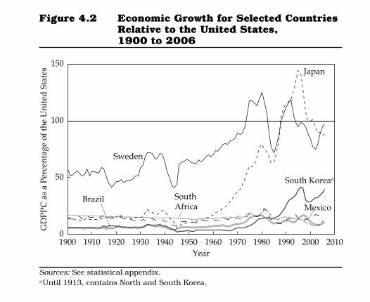
We provide some salient examples of upward mobility in fig-ure 4.2, where relative levels of gross national product per capita(GNPPC) are calculated as a percentage of the gross domesticproduct per capita (GDPPC) of the United States between 1900 and2006. Since the United States is always one of the principal high-income countries for the overall period being considered here,such a measure allows us to capture the relative extent of the mobil-ity experienced by different nations. As indicated by figure 4.2,

Distribution of Income Between Nations 65

0

50

100

150

1900 1910 1920 1930 1940

Sweden

SouthAfrica

Brazil

Japan

South Koreaa

1950Year

1960 1970 1980 1990 2000 2010

GD

PPC

as

a Pe

rcen

tage

of t

he U

nite

d S

tate

s

Mexico

Figure 4.2 Economic Growth for Selected CountriesRelative to the United States, 1900 to 2006

Sources: See statistical appendix.aUntil 1913, contains North and South Korea.

of the rise in between-country inequality to the differential rates ofindustrialization in wealthy and poor nations:

As industrialization took root first in the initially richer nations,the rich became richer and inequality shot up across nations. Now,as industrialization is spreading to poorer nations, poor regionsare reaping the benefits of industrial growth, and inequality isdeclining across nations. In other words, the trajectory of between-nation income inequality over the course of global industrializa-tion is tracing a Kuznets curve.

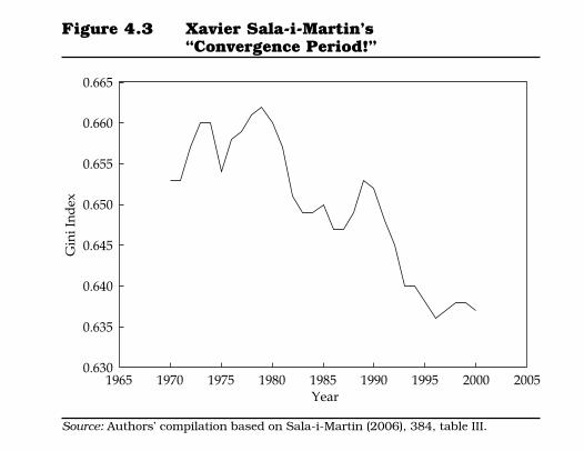
Many other scholars, as well as advocates of globalization, haveadvanced similar interpretations. A good example is provided byXavier Sala-i-Martin (2006), who, in a play on the title of a previ-ous article by Lant Pritchett (1997), simply labels current trends as“Convergence, Big Time” (see figure 4.3).


0.630

0.635

0.640

0.645

0.650

0.655

0.660

0.665

1965 1970 1975 1980 1985 1990 1995 2000 2005

Gin

i Ind

ex

Year

Figure 4.3 Xavier Sala-i-Martin’s “Convergence Period!”

Source: Authors’ compilation based on Sala-i-Martin (2006), 384, table III.

Thus, in an earlier study (Korzeniewicz and Moran 1997), weemphasized the continuing increase in between-country inequalityin the late 1980s and early 1990s.10 In a more recent contribution,Milanovic (2005) concludes that while global inequality (combiningdata on between- and within-country inequality) has remainedrather stable, inequality between countries declined slightly over thelast two decades of the twentieth century, but that this decline issmaller if we take into consideration growing regional disparitieswithin China, and it disappears altogether if China is excluded fromthe sample. Similarly, Robert Hunter Wade (2004, 581; see alsoWade 2008) argues that by several measures world inequality hasbeen increasing over the last two decades; by one measure—averageincomes per capita adjusted by purchasing power parities—betweencountry inequality has declined, “but take out China and even thismeasure shows widening inequality.” And in their review of stud-ies on trends in world inequality over the last decade, Sudir Anand


0.200

0.250

0.300

0.350

0.400

0.450

0.500

0.550

0.600

0.650

0.700

0.750

1965 1970 1975 1980 1985 1990 1995 2000 2005

Gin

i Ind

ex

Year

Figure 4.4 Xavier Sala-i-Martin’s Convergence . . .Not So Much!

Source: Authors’ compilation based on Sala-i-Martin (2006), 384, table III.

and Paul Segal (2008, 83) conclude that “there is insufficient evi-dence to determine the direction of change in global interpersonalinequality.”

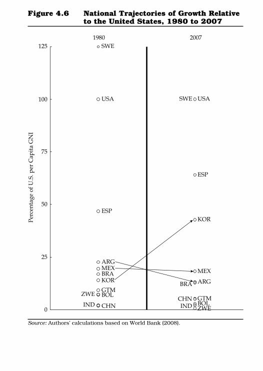
This does not mean that we argue that no convergence is takingplace. Instead, the perspective we have been advancing in this bookcalls for paying attention to institutional equilibria that show con-siderable persistence, and trends so far have not been sufficientlyextended or persistent enough to make a substantive claim that theequilibria of the past few centuries has been left behind. For exam-ple, today as in the past, relative national trajectories are heteroge-neous: some countries (for example, South Korea, more recentlyChina, and to a lesser extent India, and all with different rates ofmobility for various deciles of the population) are undergoing con-siderable upward mobility, but others remain more stable or evenshow some economic decline relative to the United States (for exam-ple, Mexico) (see figure 4.6). Moreover, as in the Schumpeterianprocesses of creative destruction, these divergent outcomes may be


Figure 4.5 Recent Trends in Between-CountryInequality, With and Without China

Source: Authors’ calculations based on World Bank (2008).

0.200

0.250

0.300

0.350

0.400

0.450

0.500

0.550

0.600

0.650

0.700

0.750

Exchange Rate Conversion

Purchasing Power Parity Adjustment

WithoutChina

Within-Country HIE

Within-Country LIE

1970 1975 1980 1985 1990Year

1995 2000 2005 2010

Gin

i Ind

ex


Figure 4.6 National Trajectories of Growth Relativeto the United States, 1980 to 2007

Source: Authors’ calculations based on World Bank (2008).

1980SWE

SWEUSA USA

ESP

ESP

ARGMEXBRAKOR

GTMBOL

CHNCHN

IND

ZWE

ARG

MEX

BRA

KOR

GTMBOLIND ZWE

125

100

75

Perc

enta

ge o

f U.S

. per

Cap

ita

GN

I

50

25

0

2007

the world (represented in the figure by LIE) into richer ones (repre-sented in the figure by LIE). National barriers to entry were rela-tively less pronounced (as suggested by the dotted boundariessurrounding each stylized cluster of country deciles).

By the twentieth century, national barriers to entry had becomemore pronounced as part of an effort to restrict competitive pres-sures or reduce inequality within the LIE cluster. (To represent thestrengthening of such national barriers to entry, we use a solid lineto represent the boundaries surrounding the HIE and LIE clusters atthe end of the transition indicated in figure 4.7.) As these barriers to entry became more pronounced, flows between the two clusters(HIE and LIE, poorer and richer) diminished (as represented bychanges in the arrows indicating mobility across national borders).

Such patterns of interaction bear a striking resemblance to howAdam Smith (1776/1976) described the relationship between town


Time

LIE

LIE

LIE

HIE

= Stylized country income deciles

HIE

HIE

Kuznets’s“Transition”

1800s

Styl

ized

Inco

me

Lev

els

2000s

Figure 4.7 Stylized Trends of HIE and LIE, 1800s to 2000s



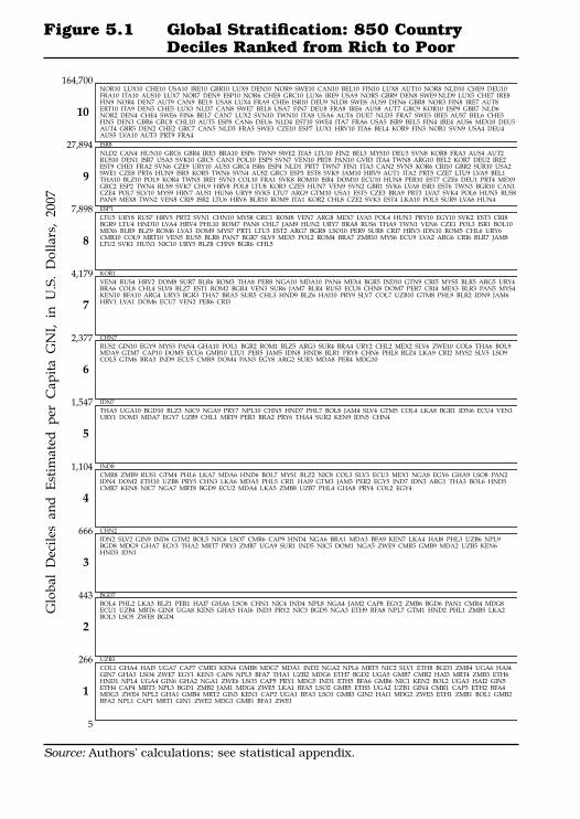
NOR10 LUX10 CHE10 USA10 IRE10 GBR10 LUX9 DEN10 NOR9 SWE10 CAN10 BEL10 FIN10 LUX8 AUT10 NOR8 NLD10 CHE9 DEU10 FRA10 ITA10 AUS10 LUX7 NOR7 DEN9 ESP10 NOR6 CHE8 GRC10 LUX6 IRE9 USA9 NOR5 GBR9 DEN8 SWE9 NLD9 LUX5 CHE7 IRE8 FIN9 NOR4 DEN7 AUT9 CAN9 BEL9 USA8 LUX4 FRA9 CHE6 ISR10 DEU9 NLD8 SWE8 AUS9 DEN6 GBR8 NOR3 FIN8 IRE7 AUT8 ERT10 ITA9 DEN5 CHE5 LUX3 NLD7 CAN8 SWE7 BEL8 USA7 FIN7 DEU8 FRA8 IRE6 AUS8 AUT7 GRC9 KOR10 ESP9 GBR7 NLD6 NOR2 DEN4 CHE4 SWE6 FIN6 BEL7 CAN7 LUX2 SVN10 TWN10 ITA8 USA6 AUT6 DUE7 NLD5 FRA7 SWE5 IRE5 AUS7 BEL6 CHE3 FIN5 DEN3 GBR6 GRC8 CHL10 AUT5 ESP8 CAN6 DEU6 NLD4 EST10 SWE4 ITA7 FRA6 USA5 ISR9 BEL5 FIN4 IRE4 AUS6 MEX10 DEU5 AUT4 GBR5 DEN2 CHE2 GRC7 CAN5 NLD3 FRA5 SWE3 CZE10 ESP7 LUX1 HRV10 ITA6 BEL4 KOR9 FIN3 NOR1 SVN9 USA4 DEU4 AUS5 LVA10 AUT3 PRT9 FRA4

NLD2 CAN4 HUN10 GRC6 GBR4 IRE3 BRA10 ESP6 TWN9 SWE2 ITA5 LTU10 FIN2 BEL3 MYS10 DEU3 SVN8 KOR8 FRA3 AUS4 AUT2 RUS10 DEN1 ISR7 USA3 SVK10 GRC5 CAN3 POL10 ESP5 SVN7 VEN10 PRT8 PAN10 GVR3 ITA4 TWN8 ARG10 BEL2 KOR7 DEU2 IRE2 EST9 CHE1 FRA2 SVN6 CZE9 URY10 AUS3 GRC4 ISR6 ESP4 NLD1 PRT7 TWN7 FIN1 ITA3 CAN2 SVN5 KOR6 CRI10 GBR2 SUR10 USA2 SWE1 CZE8 PRT6 HUN9 ISR5 KOR5 TWN6 SVN4 AUS2 GRC3 ESP3 EST8 SVK9 JAM10 HRV9 AUT1 ITA2 PRT5 CZE7 LTU9 LVA9 BEL1 THA10 BLZ10 POL9 KOR4 TWN5 IRE1 SVN3 COL10 FRA1 SVK8 ROM10 ISR4 DOM10 ECU10 HUN8 PER10 EST7 CZE6 DEU1 PRT4 MEX9 GRC2 ESP2 TWN4 RUS9 SVK7 CHL9 HRV8 POL8 LTU8 KOR3 CZE5 HUN7 VEN9 SVN2 GBR1 SVK6 LVA8 ISR3 EST6 TWN3 BGR10 CAN1 CZE4 POL7 SLV10 MYS9 HRV7 AUS1 HUN6 URY9 SVK5 LTU7 ARG9 GTM10 USA1 EST5 CZE3 BRA9 PRT3 LVA7 SVK4 POL6 HUN5 RUS8 PAN9 MEX8 TWN2 VEN8 CRI9 ISR2 LTU6 HRV6 BLR10 ROM9 ITA1 KOR2 CHL8 CZE2 SVK3 EST4 LKA10 POL5 SUR9 LVA6 HUN4

LTU5 URY8 RUS7 HRV5 PRT2 SVN1 CHN10 MYS8 GRC1 ROM8 VEN7 ARG8 MEX7 LVA5 POL4 HUN3 PRY10 EGY10 SVK2 EST3 CRI8 BGR9 LTU4 HND10 LVA4 HRV4 PHL10 ROM7 PAN8 CHL7 JAM9 HUN2 URY7 BRA8 RUS6 THA9 TWN1 VEN6 CZE1 POL3 ISR1 BOL10 MEX6 BLR9 BLZ9 ROM6 LVA3 DOM9 MYS7 PRT1 LTU3 EST2 ARG7 BGR8 LSO10 PER9 SUR8 CRI7 HRV3 IDN10 ROM5 CHL6 URY6 CMR10 COL9 MRT10 VEN5 RUS5 BLR8 PAN7 BGR7 SLV9 MEX5 POL2 ROM4 BRA7 ZMB10 MYS6 ECU9 LVA2 ARG6 CRI6 BLR7 JAM8 LTU2 SVK1 HUN1 NIC10 URY5 BLZ8 CHN9 BGR6 CHL5

VEN4 RUS4 HRV2 DOM8 SUR7 BLR6 ROM3 THA8 PER8 NGA10 MDA10 PAN6 MEX4 BGR5 IND10 GTN9 CRI5 MYS5 BLR5 ARG5 URY4 BRA6 COL8 CHL4 SLV8 BLZ7 EST1 ROM2 BGR4 VEN3 SUR6 JAM7 BLR4 RUS3 ECU8 CHN8 DOM7 PER7 CRI4 MEX3 BLR3 PAN5 MYS4 KEN10 BFA10 ARG4 URY3 BGR3 THA7 BRA5 SUR5 CHL3 HND9 BLZ6 HAI10 PRY9 SLV7 COL7 UZB10 GTM8 PHL9 BLR2 IDN9 JAM6 HRV1 LVA1 DOM6 ECU7 VEN2 PER6 CRI3

RUS2 GIN10 EGY9 MYS3 PAN4 GHA10 POL1 BGR2 ROM1 BLZ5 ARG3 SUR4 BRA4 URY2 CHL2 MEX2 SLV6 ZWE10 COL6 THA6 BOL9 MDA9 GTM7 CAP10 DOM5 ECU6 GMB10 LTU1 PER5 JAM5 IDN8 HND8 BLR1 PRY8 CHN6 PHL8 BLZ4 LKA9 CRI2 MYS2 SLV5 LSO9 COL5 GTM6 BRA3 IND9 ECU5 CMR9 DOM4 PAN3 EGY8 ARG2 SUR3 MDA8 PER4 MDG10

THA5 UGA10 BGD10 BLZ3 NIC9 NGA9 PRY7 NPL10 CHN5 HND7 PHL7 BOL8 JAM4 SLV4 GTM5 COL4 LKA8 BGR1 IDN6 ECU4 VEN1 URY1 DOM3 MDA7 EGY7 UZB9 CHL1 MRT9 PER3 BRA2 PRY6 THA4 SUR2 KEN9 IDN5 CHN4

CMR8 ZMB9 RUS1 GTM4 PHL6 LKA7 MDA6 HND6 BOL7 MYS1 BLZ2 NIC8 COL3 SLV3 ECU3 MEX1 NGA8 EGY6 GHA9 LSO8 PAN2 IDN4 DOM2 ETH10 UZB8 PRY5 CHN3 LKA6 MDA5 PHL5 CRI1 HAI9 GTM3 JAM3 PER2 EGY5 IND7 IDN3 ARG1 THA3 BOL6 HND5 CMR7 KEN8 NIC7 NGA7 MRT8 BGD9 ECU2 MDA4 LKA5 ZMB8 UZB7 PHL4 GHA8 PRY4 COL2 EGY4

IDN2 SLV2 GIN9 IND6 GTM2 BOL5 NIC6 LSO7 CMR6 CAP9 HND4 NGA6 BRA1 MDA3 BFA9 KEN7 LKA4 HAI8 PHL3 UZB6 NPL9 BGD8 MDG9 GHA7 EGY3 THA2 MRT7 PRY3 ZMB7 UGA9 SUR1 IND5 NIC5 DOM1 NGA5 ZWE9 CMR5 GMB9 MDA2 UZB5 KEN6 HND3 IDN1

BOL4 PHL2 LKA3 BLZ1 PER1 HAI7 GHA6 LSO6 CHN1 NIC4 IND4 NPL8 NGA4 JAM2 CAP8 EGY2 ZMB6 BGD6 PAN1 CMR4 MDG8 ECU1 UZB4 MRT6 GIN8 UGA8 KEN5 GHA5 HAI6 IND3 PRY2 NIC3 BGD5 NGA3 ETH9 BFA8 NPL7 GTM1 HND2 PHL1 ZMB5 LKA2 BOL3 LSO5 ZWE8 BGD4

COL1 GHA4 HAI5 UGA7 CAP7 CMR3 KEN4 GMB8 MDG7 MDA1 IND2 NGA2 NPL6 MRT5 NIC2 SLV1 ETH8 BGD3 ZMB4 UGA6 HAI4 GIN7 GHA3 LSO4 ZWE7 EGY1 KEN3 CAP6 NPL5 BFA7 THA1 UZB2 MDG6 ETH7 BGD2 UGA5 GMB7 CMR2 HAI3 MRT4 ZMB3 ETH6 HND1 NPL4 UGA4 GIN6 GHA2 NGA1 ZWE6 LSO3 CAP5 PRY1 MDG5 IND1 ETH5 BFA6 GMB6 NIC1 KEN2 BOL2 UGA3 HAI2 GIN5 ETH4 CAP4 MRT3 NPL3 BGD1 ZMB2 JAM1 MDG4 ZWE5 LKA1 BFA5 LSO2 GMB5 ETH3 UGA2 UZB1 GIN4 CMR1 CAP3 ETH2 BFA4 MDG3 ZWE4 NPL2 GHA1 GMB4 MRT2 GIN3 KEN1 CAP2 UGA1 BFA3 LSO1 GMB3 GIN2 HAI1 MDG2 ZWE3 ETH1 ZMB1 BOL1 GMB2 BFA2 NPL1 CAP1 MRT1 GIN1 ZWE2 MDG1 GMB1 BFA1 ZWE1

Glo

bal

Dec

iles

and

Est

imat

ed p

er C

apit

a G

NI,

in U

.S.

Dol

lars

, 20

07

164,700

27,894

10

9

8

7

6

5

4

3

2

1

ISR8

7,898 ESP1

4,179 KOR1

2,377 CHN7

1,547 IDN7

1,104 IND8

666 CHN2

443 BGD7

266

5

UZB3

Figure 5.1 Global Stratification: 850 CountryDeciles Ranked from Rich to Poor

Source: Authors’ calculations; see statistical appendix.

Global Stratification 95

Uni

ted

Stat

es

Swed

en

Spai

n

Sout

hK

orea

Mex

ico

Bra

zil

Arg

enti

na

Gua

tem

ala

Chi

na

Bol

ivia

Ind

ia

Zim

babw

e

Glo

bal

Dec

iles

and

Est

imat

ed p

er C

apit

a G

NI,

in U

.S.

Dol

lars

, 20

07

164,700

27,894

10

9

8

7

6

5

4

3

2

1

7,898

4,179

2,377

1,547

1,104

666

443

266

5

USA1

USA2

USA3

USA7USA8USA9

USA10

USA6USA5USA4

SWE1

SWE2SWE3SWE7SWE8SWE9

SWE10

SWE6SWE5SWE4

ESP1

ESP2ESP3

ESP7ESP8ESP9

ESP10

ESP6ESP5ESP4

KOR1

KOR2KOR3

KOR7KOR8KOR9

KOR10

KOR6KOR5KOR4

MEX1

MEX2

MEX3

MEX7

MEX8MEX9

MEX10

MEX6

MEX5

MEX4

BRA1

BRA2

BRA3

BRA7

BRA8

BRA9

BRA10

BRA6

BRA5

BRA4

ARG1

ARG2

ARG3

ARG7

ARG8

ARG9

ARG10

ARG6

ARG5

ARG4

GTM1

GTM2

GTM3

GTM7

GTM8

GTM9

GTM10

GTM6

GTM5

GTM4

CHN1

CHN2

CHN3

CHN7

CHN8

CHN9

CHN10

CHN6

CHN5

CHN4

BOL1

BOL2

BOL3

BOL7

BOL8

BOL9

BOL10

BOL6

BOL5

BOL4

IND1

IND2

IND3

IND7

IND8

IND9

IND10

IND6

IND5

IND4

ZWE1ZWE2ZWE3

ZWE7

ZWE8

ZWE9

ZWE10

ZWE6ZWE5ZWE4

Figure 5.2 Country and Global Income Deciles for Twelve Nations



Figure 5.3 Path 2: Economic Growth as Social Mobility, 1980 and 2007


1980

100

75

50

25

0

Perc

enta

ge o

f U.S

. per

Cap

ita

GN

I2007

KOR10

KOR10

MEX10

MEX10

MEX9

MEX8MEX7MEX6MEX5MEX4MEX3MEX2MEX1

MEX9

MEX8

MEX7MEX6MEX5MEX4MEX3MEX2MEX1

KOR9

KOR8

KOR7

KOR6

KOR5

KOR4

KOR3

KOR2

KOR1

KOR9KOR8KOR7KOR6KOR5KOR4KOR3KOR2KOR1

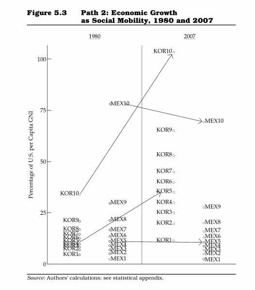
each of the two periods, but the exercise we conducted to constructfigures 5.1 and 5.2 cannot be easily reconstructed for 1980.) In con-trast to figure 4.6, which focused on relative rankings and data inthe relative resources accruing to whole nations, figure 5.3 providesa more disaggregated approach, showing how the various country


Uni

ted

Sta

tes

Mex

ico

Gua

tem

ala

Spai

n

Arg

enti

na

Bol

ivia

Glo

bal

Dec

iles,

in

U.S

. D

olla

rs

164,700

27,894

10

9

8

7

6

5

4

3

2

1

7,898

4,179

2,377

1,547

1,104

666

443

266

5

USA1

USA2

USA3

USA7USA8USA9

USA10

USA6USA5USA4

ESP1

ESP2ESP3

ESP7ESP8ESP9ESP10

ESP6ESP5ESP4

MEX1

MEX2

MEX3

MEX7

MEX8MEX9

MEX10

MEX6

MEX5

MEX4

ARG1

ARG2

ARG3

ARG7

ARG8

ARG9

ARG10

ARG6

ARG5

ARG4

GTM1

GTM2

GTM3

GTM7

GTM8

GTM9

GTM10

GTM6

GTM5

GTM4

BOL1

BOL2

BOL3

BOL7

BOL8

BOL9

BOL10

BOL6

BOL5

BOL4

Figure 5.4 Path 3: Migration As Social Mobility


Statistical Appendix 127

Table A.1 Three-Digit Country Codes

ARG ArgentinaAUS AustraliaAUT AustriaBEL BelgiumBFA Burkina FasoBGD BangladeshBGR BulgariaBLR BelarusBLZ BelizeBOL BoliviaBRA BrazilBWA BotswanaCAF Central African RepublicCAN CanadaCHE SwitzerlandCHL ChileCHN ChinaCMR CameroonCOL ColombiaCRI Costa RicaCYP CyprusCZE Czech RepublicDEN DenmarkDEU GermanyDOM Dominican RepublicECU EcuadorEGY EgyptESP SpainEST EstoniaETH EthiopiaFIN FinlandFRA FranceGBR United KingdomGHA GhanaGIN GuineaGMB GambiaGRC GreeceGTM GuatemalaHAI HaitiHND HondurasHRV CroatiaHUN HungaryICE Iceland

IDN IndonesiaIND IndiaIRE IrelandISR IsraelITA ItalyJAM JamaicaJOR JordanJPN JapanKEN KenyaKOR Republic of KoreaLKA Sri LankaLSO LesothoLTU LithuaniaLUX LuxembourgLVA LatviaMDA MoldovaMDG MadagascarMEX MexicoMLT MaltaMRT MauritaniaMYS MalaysiaNGA NigeriaNIC NicaraguaNLD NetherlandsNOR NorwayNPL NepalNZL New ZealandPAN PanamaPER PeruPHL PhilippinesPOL PolandPRI Puerto RicoPRT PortugalPRY ParaguayROM RomaniaRUS RussiaSLV El SalvadorSVK Slovak RepublicSVN SloveniaSUR SurinameSWE SwedenTHA ThailandTJK Tajikistan

(Table continues on p. 128)

PPP advocates repeatedly appeal to the notion that the foreignexchange–based data are prone to the froth of short-term movements(and references to currency fluctuation are often used to make sucha point). In our analysis, the foreign exchange–based data we use arebased on the Atlas method, as calculated and disseminated by theWorld Bank (and are in fact the GNI figures preferred by the bankitself in policy analysis). The method employs a three-year movingaverage that is explicitly designed to smooth over year-to-year fluc-tuations in currency values.

It is important to note that critics of FX conversions generallyignore (or minimize) the fact that PPP data are themselves subject togreat fluctuations, as shown in table A.2. For example, the latest PPPrevision completed by the World Bank in 2005 adjusted downwardthe estimated income per capita of China by 38 percent (from $6,660to $4,110) and that of India by 36 percent (from $3,460 to $2,210). Thus,any calculation of trends in world income that was done using thepre-2007 estimates of PPP adjustments would now have to be revisedvery substantially as an outcome of fluctuations that were introduced,not by changes in foreign exchange rates, but by measurement errorinvolving over 40 percent of the world’s population. The impact ofthis large measurement error is amplified by the fact that new PPPdata are published only sporadically (more than ten years can passbetween rounds), so researchers working with these data shouldacknowledge the uncertainties inherent in their numbers.

Moreover, advocates of PPP adjustments often make the assertionthat PPP data better reflect the real day-to-day experience of people.If so, we might infer that people would perceive major changes inestimates of PPP, like the significant revisions introduced by theWorld Bank in 2007, as having deep consequences for their dailylives. Instead, people often react to significant changes in exchange

128 Statistical Appendix

Table A.1 (Continued )

TUR TurkeyTWN TaiwanUGA UgandaURY UruguayUSA United States

UZB UzbekistanVEN VenezuelaZAF South AfricaZMB ZambiaZWE Zimbabwe

Source: World Bank (2008).

Statistical Appendix 129

Table A.2 Fluctuations in GNI per Capita: Old and New PPP Estimates for Selected Countries, 2005

Old PPP New PPP Measurement Error Country GNI per Capita GNI per Capita (of Old Figures)Republic of $810 $2,450 203% underestimationthe Congo

Ghana 2,370 1,140 52% overestimationEcuador 4,070 6,390 57% underestimationVenezuela 6,440 9,770 52% underestimationNigeria 1,040 1,530 47% underestimationBangladesh 2,090 1,120 46% overestimationChina 6,600 4,110 38% overestimationIndia 3,460 2,210 36% overestimationSouth 12,120 8,300 32% overestimationAfrica

Argentina 13,920 10,420 25% overestimationTurkey 8,420 10,250 22% underestimationUnited 32,690 32,050 2% overestimationKingdom

Japan 31,410 31,010 1% overestimationUnited 41,950 41,680 1% overestimationStates

Sources: Authors’ calculations based on old PPP figures, World Bank (2006); new PPPfigures, World Bank (2008).

rates (recall political turmoil in Argentina over the collapse of theArgentine peso in 2001), but major adjustments in PPP estimates atthe offices of the World Bank seldom evoke any reaction at all (andoften go unnoticed even by their advocates in academia).

Despite these reservations, as well as the additional theoreticalconsiderations we use to justify our methodological decision to priv-ilege FX conversions, we do report all our relevant results using bothFX- and PPP-adjusted data. We discuss differences in the resultingtrends in chapter 4.

Figures 4.1, 4.5, and 4.6The historical trends in between-country inequality are based onour calculations employing two data sets. For the 1820 to 1990 series,

figure 1.1 the kuznets transition 4 unveiling inequality · 4 unveiling inequality time stylized...

Documents