field test of sub-basalt hydrocarbon exploration with

Geophysical Prospecting, 2015, 63, 1284–1310 doi: 10.1111/1365-2478.12278

Field test of sub-basalt hydrocarbon exploration with marinecontrolled source electromagnetic and magnetotelluric data

G. Michael Hoversten1∗, David Myer2, Kerry Key1†, David Alumbaugh3,Oliver Hermann4 and Randall Hobbet4

1Chevron Energy Technology Company, 6001 Bollinger Canyon Road, K1010 San Ramon, CA 94583, USA, 2Blue Green Geophysics,3Scripps Institution of Oceanography, and 4Chevron Norge AS

Received January 2014, revision accepted January 2015

ABSTRACTThe recent use of marine electromagnetic technology for exploration geophysics hasprimarily focused on applying the controlled source electromagnetic method for hy-drocarbon mapping. However, this technology also has potential for structural map-ping applications, particularly when the relative higher frequency controlled sourceelectromagnetic data are combined with the lower frequencies of naturally occurringmagnetotelluric data. This paper reports on an extensive test using data from 84marine controlled source electromagnetic and magnetotelluric stations for imagingvolcanic sections and underlying sediments on a 128-km-long profile. The profileextends across the trough between the Faroe and Shetland Islands in the North Sea.Here, we focus on how 2.5D inversion can best recover the volcanic and sedimentarysections. A synthetic test carried out with 3D anisotropic model responses showsthat vertically transverse isotropy 2.5D inversion using controlled source electromag-netic and magnetotelluric data provides the most accurate prediction of the resistivityin both volcanic and sedimentary sections. We find the 2.5D inversion works welldespite moderate 3D structure in the synthetic model. Triaxial inversion using thecombination of controlled source electromagnetic and magnetotelluric data provideda constant resistivity contour that most closely matched the true base of the volcanicflows. For the field survey data, triaxial inversion of controlled source electromag-netic and magnetotelluric data provides the best overall tie to well logs with verticallytransverse isotropy inversion of controlled source electromagnetic and magnetotel-luric data a close second. Vertical transverse isotropy inversion of controlled sourceelectromagnetic and magnetotelluric data provided the best interpreted base of thevolcanic horizon when compared with our best seismic interpretation. The structuralboundaries estimated by the 20-!·m contour of the vertical resistivity obtained byvertical transverse isotropy inversion of controlled source electromagnetic and mag-netotelluric data gives a maximum geometric location error of 11% with a mean errorof 1.2% compared with the interpreted base of the volcanic horizon. Both the modelstudy and field data interpretation indicate that marine electromagnetic technologyhas the potential to discriminate between low-resistivity prospective siliciclastic sed-iments and higher resistivity non-prospective volcaniclastic sediments beneath thevolcanic section.

Key words: Electromagnetic, Sub-basalt.

∗E-mail: [email protected]†Now at: NEOS Geosolutions

1284 C⃝ 2015 European Association of Geoscientists & Engineers

CSEM and MMT for hydrocarbon exploration 1285

INTR ODUC TION

Seismic imaging for hydrocarbon reservoirs located beneathbasalt is often challenging due to the high velocity and extremeheterogeneity of basalt flows. When assessing the prospectiv-ity beneath basalt, a critical factor is the presence of sedimentswithin a depth range that will accommodate hydrocarbons. Ifsediments are present, the depth extent and structure of theoverlying basalt is critical to constructing accurate velocitymodels for migration of seismic data and to develop drillingplans. Recent drilling results based on interpretation of thebasalt thickness from seismic data on the Norwegian NorthAtlantic Margin (NAM) have shown misinterpretation of thebasalt thickness in excess of 1 km in some cases. Explorationwells in the NAM cost in the range of hundreds of millionsof U.S. dollars, so there is a significant motivation for usingnew technology to improve base basalt location. In this paper,we demonstrate that a combination of controlled source elec-tromagnetic (CSEM) and marine magnetotelluric (MT) datacan provide inversion models of the basalt section along withunderlying sediment and structures that can be used to dis-criminate between differing seismic interpretations and hencereduce the risk for drilling predictions and improve migrationvelocity models.

Early application of marine MT data focused on imagingthe base of resistive salt bodies (Constable et al. 2000;Hoversten, Morrison, and Constable 1998; Key, Constable,and Weiss 2006), whereas early application of MT andCSEM for imaging the base of basalt was first performed onland. Prieto et al. (1985), Warren and Srnka (1992), Witherset al. (1994), Morrison et al. (1996), and Smith et al. (1999)used MT data to image the base of massive basalt flows inthe Columbia River Basin. More recently, Strack and Pandey(2007) and Colombo et al. (2011) have presented work usingon-shore MT and CSEM for sub–basalt imaging and Jegen etal. (2009) combined gravity and MT data.

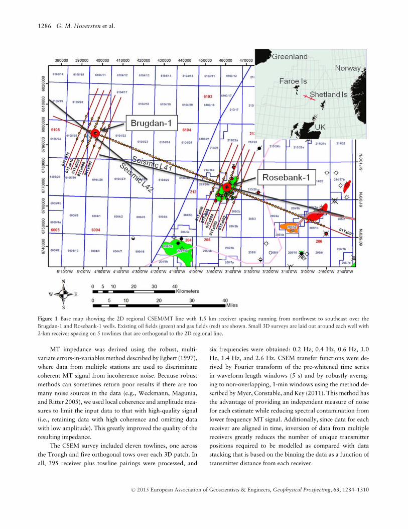
While there are a large number of exploration and pro-duction wells drilled on the NAM, relatively few have beendrilled into basalt, and even fewer have penetrated the base.Only a few cases have been reported where marine CSEM andMT data were acquired over such well penetrations. In 2012,Chevron undertook a calibration survey of CSEM and MTdata on a profile that spans the Faroe–Shetland Trough withthe Faroe Islands to the northwest and the Shetland Islands tothe southeast. This profile connected two wells that had pene-trated the base of massive basalt flows: Brugdan to the north-west and Rosebank to the southeast. While the Rosebank wellpenetrated through basalt flows and underlying volcaniclastic

into prospective siliciclastic sediments, the Brugdan well hittotal depth in volcaniclastic sediments beneath the massivebasalt flows. This test line was selected because we had twowell penetrations of the volcanic section. Furthermore, theseismic definition of the base of the basalt was considered tobe of high quality, at least around the Rosebank well. Thequality of the seismic image of the base of the volcanic sectionis far worse in many other exploration plays.

S U R V E Y G E O M E T R Y A N D D A T APROCES S ING

The calibration survey is a combination of a 128-km-long re-gional 2D line with 86 CSEM/MT receivers connecting thetwo wells, and two small 12×12 km 3D surveys surroundingthe Brugdan and Rosebank wells (Fig. 1). Of the 138 deploy-ments planned for the survey, 135 returned usable CSEM dataand 133 returned usable MT data, resulting in 84 successfulstations along the 2D profile. The receiver spacing on the re-gional 2D line that ties the two wells is 1.5 km, whereas thereceiver spacing of the orthogonal lines that make up the mini-3D surveys around the wells is 2 km. In this paper, we onlyconsider the regional data from the 2D profile.

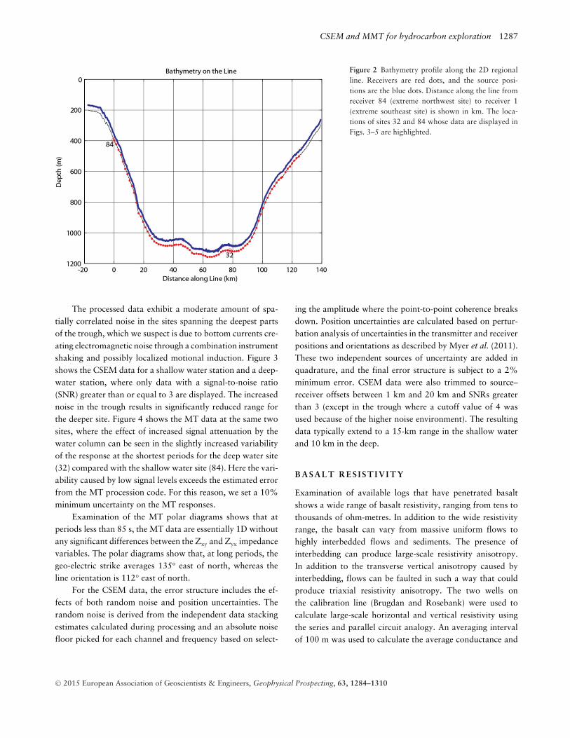
The survey spans the Faroe–Shetland Trough with re-ceivers positioned at seafloor depths varying from 240 m to1180 m (Fig. 2). Continuous measurements of water con-ductivity by the CSEM towfish, augmented by depth versusconductivity profiles measured using expendable bathyther-mographs, show the water conductivity varying from 3.70S/m near the surface to 2.94 S/m at depth. To account forthis variation, we built a stratified water model using the av-eraged conductivity in 100-m-thick layers extending to belowthe thermocline, where the water conductivity stabilizes.

Instruments were deployed using the standard free-falltechnique and most landed within 100 m of their plannedlocations. Since no instrument carried a compass, instrumentorientations were derived by post-processing the CSEM data.The contractor uses multiple, semi-independent methodswhose details are held private as intellectual property. There-fore, we independently validated the reported orientationsusing the orthogonal Procrustes rotation method outlinedin Key and Lockwood (2010). The differences betweenour solutions and the contractors have an approximatelyGaussian distribution with a mean of zero and standarddeviation of about 2°. Perturbation analysis shows that thislevel of orientation uncertainty corresponds to a relativeuncertainty in the modelled CSEM and MT responses that isless than 1% for the inline receivers along the 2D profile.

C⃝ 2015 European Association of Geoscientists & Engineers, Geophysical Prospecting, 63, 1284–1310

1286 G. M. Hoversten et al.

Figure 1 Base map showing the 2D regional CSEM/MT line with 1.5 km receiver spacing running from northwest to southeast over theBrugdan-1 and Rosebank-1 wells. Existing oil fields (green) and gas fields (red) are shown. Small 3D surveys are laid out around each well with2-km receiver spacing on 5 towlines that are orthogonal to the 2D regional line.

MT impedance was derived using the robust, multi-variate errors-in-variables method described by Egbert (1997),where data from multiple stations are used to discriminatecoherent MT signal from incoherence noise. Because robustmethods can sometimes return poor results if there are toomany noise sources in the data (e.g., Weckmann, Magunia,and Ritter 2005), we used local coherence and amplitude mea-sures to limit the input data to that with high-quality signal(i.e., retaining data with high coherence and omitting datawith low amplitude). This greatly improved the quality of theresulting impedance.

The CSEM survey included eleven towlines, one acrossthe Trough and five orthogonal tows over each 3D patch. Inall, 395 receiver plus towline pairings were processed, and

six frequencies were obtained: 0.2 Hz, 0.4 Hz, 0.6 Hz, 1.0Hz, 1.4 Hz, and 2.6 Hz. CSEM transfer functions were de-rived by Fourier transform of the pre-whitened time seriesin waveform-length windows (5 s) and by robustly averag-ing to non-overlapping, 1-min windows using the method de-scribed by Myer, Constable, and Key (2011). This method hasthe advantage of providing an independent measure of noisefor each estimate while reducing spectral contamination fromlower frequency MT signal. Additionally, since data for eachreceiver are aligned in time, inversion of data from multiplereceivers greatly reduces the number of unique transmitterpositions required to be modelled as compared with datastacking that is based on the binning the data as a function oftransmitter distance from each receiver.



Figure 2 Bathymetry profile along the 2D regionalline. Receivers are red dots, and the source posi-tions are the blue dots. Distance along the line fromreceiver 84 (extreme northwest site) to receiver 1(extreme southeast site) is shown in km. The loca-tions of sites 32 and 84 whose data are displayed inFigs. 3–5 are highlighted.

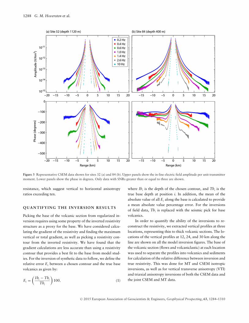
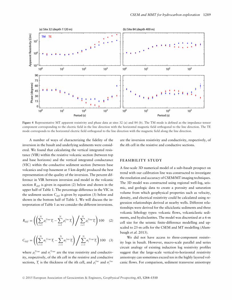
The processed data exhibit a moderate amount of spa-tially correlated noise in the sites spanning the deepest partsof the trough, which we suspect is due to bottom currents cre-ating electromagnetic noise through a combination instrumentshaking and possibly localized motional induction. Figure 3shows the CSEM data for a shallow water station and a deep-water station, where only data with a signal-to-noise ratio(SNR) greater than or equal to 3 are displayed. The increasednoise in the trough results in significantly reduced range forthe deeper site. Figure 4 shows the MT data at the same twosites, where the effect of increased signal attenuation by thewater column can be seen in the slightly increased variabilityof the response at the shortest periods for the deep water site(32) compared with the shallow water site (84). Here the vari-ability caused by low signal levels exceeds the estimated errorfrom the MT procession code. For this reason, we set a 10%minimum uncertainty on the MT responses.

Examination of the MT polar diagrams shows that atperiods less than 85 s, the MT data are essentially 1D withoutany significant differences between the Zxy and Zyx impedancevariables. The polar diagrams show that, at long periods, thegeo-electric strike averages 135° east of north, whereas theline orientation is 112° east of north.

For the CSEM data, the error structure includes the ef-fects of both random noise and position uncertainties. Therandom noise is derived from the independent data stackingestimates calculated during processing and an absolute noisefloor picked for each channel and frequency based on select-

ing the amplitude where the point-to-point coherence breaksdown. Position uncertainties are calculated based on pertur-bation analysis of uncertainties in the transmitter and receiverpositions and orientations as described by Myer et al. (2011).These two independent sources of uncertainty are added inquadrature, and the final error structure is subject to a 2%minimum error. CSEM data were also trimmed to source–receiver offsets between 1 km and 20 km and SNRs greaterthan 3 (except in the trough where a cutoff value of 4 wasused because of the higher noise environment). The resultingdata typically extend to a 15-km range in the shallow waterand 10 km in the deep.

B A S A L T R E S I S T I V I T Y

Examination of available logs that have penetrated basaltshows a wide range of basalt resistivity, ranging from tens tothousands of ohm-metres. In addition to the wide resistivityrange, the basalt can vary from massive uniform flows tohighly interbedded flows and sediments. The presence ofinterbedding can produce large-scale resistivity anisotropy.In addition to the transverse vertical anisotropy caused byinterbedding, flows can be faulted in such a way that couldproduce triaxial resistivity anisotropy. The two wells onthe calibration line (Brugdan and Rosebank) were used tocalculate large-scale horizontal and vertical resistivity usingthe series and parallel circuit analogy. An averaging intervalof 100 m was used to calculate the average conductance and



Figure 3 Representative CSEM data shown for sites 32 (a) and 84 (b). Upper panels show the in-line electric field amplitude per unit transmittermoment. Lower panels show the phase in degrees. Only data with SNRs greater than or equal to three are shown.

resistance, which suggest vertical to horizontal anisotropyratios exceeding ten.

QUANT I F YING THE INVERSION RESULTS

Picking the base of the volcanic section from regularized in-version requires using some property of the inverted resistivitystructure as a proxy for the base. We have considered calcu-lating the gradient of the resistivity and finding the maximumvertical or total gradient, as well as picking a resistivity con-tour from the inverted resistivity. We have found that thegradient calculations are less accurate than using a resistivitycontour that provides a best fit to the base from model stud-ies. For the inversion of synthetic data to follow, we define therelative error Ei between a chosen contour and the true basevolcanics as given by:

Ei =(

Ibi − Tbi

Tbi

)100, (1)

where Ibi is the depth of the chosen contour, and Tbi is thetrue base depth at position i. In addition, the mean of theabsolute value of all Ei along the base is calculated to providea mean absolute value percentage error. For the inversionsof field data, Tbi is replaced with the seismic pick for basevolcanics.

In order to quantify the ability of the inversions to re-construct the resistivity, we extracted vertical profiles at threelocations, representing thin to thick volcanic sections. The lo-cations of the vertical profiles at 12, 24, and 30 km along theline are shown on all the model inversion figures. The base ofthe volcanic section (flows and volcaniclastic) at each locationwas used to separate the profiles into volcanics and sedimentsfor calculation of the relative difference between inversion andtrue resistivity. This was done for MT and CSEM isotropicinversions, as well as for vertical transverse anisotropy (VTI)and triaxial anisotropy inversions of both the CSEM data andthe joint CSEM and MT data.



Figure 4 Representative MT apparent resistivity and phase data at sites 32 (a) and 84 (b). The TM mode is defined as the impedance tensorcomponent corresponding to the electric field in the line direction with the horizontal magnetic field orthogonal to the line direction. The TEmode corresponds to the horizontal electric field orthogonal to the line direction with the magnetic field along the line direction.

A number of ways of characterizing the fidelity of theinversion in the basalt and underlying sediments were consid-ered. We found that calculating the vertical integrated resis-tance (VIR) within the resistive volcanic section (between topand base horizons) and the vertical integrated conductance(VIC) within the conductive sediment section (between basevolcanics and top basement at 5 km depth) produced the bestrepresentation of the quality of the inversion. The percent dif-ference in VIR between inversion and model in the volcanicsection Rdiff is given in equation (2) below and shown in theupper half of Table 1. The percentage difference in the VIC inthe sediment section Cdiff is given by equation (3) below andshown in the bottom half of Table 1. We will discuss the in-terpretation of Table 1 as we consider the different inversions.

Rdiff =((

N∑

i=1

ρTruei Ti −

N∑

i=1

ρ Invi Ti

) /N∑

i=1

ρTruei Ti

)

100 (2)

Cdiff =((

N∑

i=1

σ Truei Ti −

N∑

i=1

σ Invi Ti

) /N∑

i=1

σ Truei Ti

)

100 (3)

where ρTruei and σ True

i are the true resistivity and conductiv-ity, respectively, of the ith cell in the resistive and conductivesections, Ti is the thickness of the ith cell, and ρ Inv

i and σ Invi

are the inversion resistivity and conductivity, respectively, ofthe ith cell in the resistive and conductive sections.

F E A S I B I L I T Y S T U D Y

A fine-scale 3D numerical model of a sub–basalt prospect ontrend with our calibration line was constructed to investigatethe resolution and accuracy of CSEM/MT imaging techniques.The 3D model was constructed using regional well-log, seis-mic, and geologic data to create a porosity and saturationvolume from which geophysical properties such as velocity,density, and electrical resistivity could be calculated using re-gression relationships derived at nearby wells. Different rela-tionships were derived for the siliciclastic sediments and threevolcanic lithology types: volcanic flows, volcaniclastic sedi-ments, and hyaloclastites. The model was discretized at a 6-mcell size for the seismic finite-difference modelling and up-scaled to 25-m cells for the CSEM and MT modelling (Alum-baugh et al. 2013).

We did not have access to three-component resistiv-ity logs in basalt. However, macro-scale parallel and seriescircuit analogy of existing induction log resistivity profilessuggest that the large-scale vertical-to-horizontal resistivityanisotropy can sometimes exceed ten in the highly layered vol-canic flows. For comparison, sediment transverse anisotropy



Table 1 Percentage difference in the VIR between top and base volcanics (upper section) and percentage difference in VIC between base volcanicsand basement at 5-km depth (lower section) at 12 km, 24 km, and 30 km easting along the line shown in Fig. 5. Positive resistance means theinversion has too much resistivity, and positive conductance means the inversion has too little resistivity (or too much conductivity). These sitesare representative of the different volcanic thicknesses along the line. For isotropic inversion, the inverted resistivity is compared with all threeresistivity values in the model. For VTI inversions, the VIR and VIC of the horizontal resistivity is compared with the VIR and VIC of the X andY model resistivity, and the VIR of the inverted vertical resistivity is compared with the VIR of the model vertical resistivity. The percentageerror is color coded so that hot colors are negative error and cool colors are positive error. The average of the absolute values of the percentageerrors is given in the final row of each section in green. The absolute value eliminates the cancellation of equal but opposite errors. Overall, VTIinversion produces the lowest errors over both the resistive and conductive sections.

MTIsotropic VTI Triaxial Isotropic VTI Triaxial Isotropic

ρx 214 -45 -19 162 -53 -13 -84ρy 214 -45 -29 162 -53 -27 -84ρz 26 1 1 5 2 -3 -93ρx 445 61 5 427 -55 2 -65ρy 952 210 105 918 -13 103 -38ρz 11 6 -56 7 -6 -1 -93ρx 119 4 17 138 -46 11 -91ρy 330 104 114 370 6 106 -82ρz -55 -56 -56 -52 -59 -55 -98

263 59 45 249 33 36 81

MTIsotropic VTI Triaxial Isotropic VTI Triaxial Isotropic

ρx -7 -7 -36 -18 -13 -36 -50ρy -7 -7 -13 -18 -13 -13 -50ρz 126 -16 13 97 19 22 21ρx 18 9 -78 34 6 -4 -32ρy 18 9 -64 34 6 -1 -32ρz 188 46 -44 225 32 70 66ρx -19 -6 -37 -26 -4 -25 36ρy -19 -6 -6 -26 -4 -2 36ρz 85 14 53 69 80 69 211

54 13 38 61 20 27 59

CSEM Only CSEM & MT

12km Volcanics (700 m)

% Error in Ver!cal Integrated Resistance (VIR)

Loca!on Component

Loca!on Component

CSEM Only CSEM & MT

12km Sediments

(700 m)

24km Sediments (1000 m)

30km Sediments (2400 m)

Average Abs. Values



Average Abs. Values

% Error in Ver!cal Integrated Conductance (VIC)



values of two to three are common and can sometimes reach afactor of ten or more (Klein et al. 2007; Ellis and MacGregor2012; Colombo et al. 2013).

The assumed coordinate system for the 3D syntheticmodel has the x-direction in the in-line direction and they-direction in the strike direction. Transverse anisotropy isassumed in the sediments, hyaloclastites, and volcaniclasticswith vertical resistivity being 2.5 times larger than thehorizontal resistivity. Because the volcanic flows have ahigh degree of spatial variability in addition to rift-faultingparallel to strike, the flows are assumed to exhibit triaxialanisotropy. The vertical resistivity is five times that of theresistivity perpendicular to strike (x-direction), and theresistivity parallel to strike (y-direction) is half that of theperpendicular resistivity (x-direction). The basement hastransverse anisotropy with the vertical resistivity two timesthe horizontal resistivity. Figure 5 shows depth sections ofthe triaxial resistivity through the long axis of the model. Thesections are parallel to the simulated CSEM acquisition lines.The acquisition lines run approximately 75° from the averagegeologic strike of the 3D model. Ideally, CSEM and MT lineswould be run orthogonal (90°) to geo-electric strike, but theangle of 75° was chosen to allow for inaccuracy in surveydesign when the actual geo-electric strike is unknown.

The synthetic data were generated using the 3D finite-difference algorithm of Commer and Newman (2009). Thefull MT impedance tensor was calculated at five frequenciesper decade from 3×10−4 Hz to 0.63 Hz, for a total of 17frequencies. The CSEM simulations were computed for fivefrequencies (0.125 Hz, 0.25 Hz, 0.5 Hz, 1 Hz and 2 Hz) usingreciprocal sources oriented in the x- and y-directions locatedat the true receiver positions, and electric fields computed atthe true source positions in the direction of the towline. Forthe MT synthetics, 5% random Gaussian noise was added toboth apparent resistivity and phase. The synthetic CSEM datawere contaminated with 2% Gaussian noise for both the in-phase and out-of-phase components, and a 10−15 V/m noisefloor was assumed. In the following discussion, the data fromthe line shown in Fig. 5 will be referred to as the data on “theline.”

Analysis of the 3D synthetic data showed that there wasbetween 2% and 5% numerical noise on the MT and CSEMdata, which we ascertained by comparison between 2D finite-element and 3D finite-difference model responses for a 2Dmodel. Because the 2D FE code uses automated adaptive meshrefinement with demonstrated accuracy to 1% (Key and Ovall2011), deviation from the 2D response from the 3D code isdeemed to be an error in the 3D code arising from the model

grid cell size. Thus, the total noise in the simulated 3D datais greater than the added Gaussian noise. This meant thatsome inversions of synthetic 3D data were fitting numericalnoise when the root-mean-square (RMS) misfit was drivento 1 with the assumed errors equal to the added noise. Justas with field data where the true error may not be capturedin the estimated data errors, we use L-curve analysis for eachinversion of synthetic data, choosing the iteration just past themajor break in RMS versus roughness. It must be noted thatthere is a subjective element to picking the optimal iterationafter the corner in the L curve. Past the corner in the L curve,the inversion models exhibit increased internal structure dueto over fitting of the data. An interpretation has to be made asto how much structure is geologic and how much is spuriousdue to fitting data noise. Our interpretative use of the L curveresulted in RMS data misfits between 1 and 1.5 for all CSEMand MT inversions.

We use the 2.5D inversion code developed at Scripps In-stitution of Oceanography (Key and Ovall 2010; Key 2012)to test its spatial and resistivity resolution on a 3D syntheticmodel data set using various combinations of data: MT only,CSEM only, and joint CSEM and MT data. Joint inversionfor MT and CSEM data simply means, at least in our imple-mentation, that the data array contains both MT and CSEMdata. Therefore, it is essentially the same inversion method-ology as solo inversion. The inversion fits the log10 of MTapparent resistivity, the log10 of electric field amplitude ofCSEM data, and the unwrapped phases in degrees. The modelresistivity values are always bounded between 0.5 !·m and1000 !·m using a non-linear parameter transformation (Key2012). All the MT inversions presented here used both trans-verse electric (TE) and transverse magnetic (TM) mode data.The model roughness penalty was set to use a horizontal tovertical smoothing factor of 3:1 in order to encourage theinversion to prefer horizontal layering in the model. In theanisotropic inversions, an additional regularization penaltyterm against anisotropy was introduced with the objective ofrestricting anisotropy to only where it is required by the data.Through trial and error testing, we found that weighting theanisotropy penalty with a weight of 0.3 relative to the spatialroughness penalty worked well. The starting model for all ofthe inversions of synthetic 3D data was 2 !·m above the topbasalt and 100 !·m below the top of basalt. For our synthetictests, we assumed the top of the basalt was well constrainedby seismic data; hence, we relaxed the inversion’s roughnesspenalty across this known boundary. While the finite-elementmeshes extend to 100 km in all directions to satisfy boundaryconditions, only the region from –5 km to 35 km and 0 km to



Figure 5 Resistivity depth sections along the long axis of the triaxial resistivity model. Sections are !75° off from the average geologic strikeof the model. Model units are overburden sediments (OS), hyaloclastic (HC), volcaniclastic (VC), volcanic flows (VF), underburden sediments(US), and basement (B). Transverse anisotropy is assumed in the sediments, hyaloclastites, and volcaniclastics with vertical resistivity being 2.5times larger than the horizontal resistivity. Because the volcanic flows have a high degree of spatial variability in addition to rift-faulting parallelto strike, the flows are assumed to exhibit triaxial anisotropy. The vertical resistivity (z) is five times that of the resistivity in the in-line direction(x) and the resistivity parallel to strike (y) is half that of the in-line resistivity. The basement has transverse anisotropy with the vertical resistivitytwice the horizontal resistivity.

6 km in X and Z, respectively, are shown, with the exceptionof the MT only inversion that extends to 30 km in Z to showdeep structure.

As discussed, we found that using a resistivity contour asa proxy for the base of the volcanic section was the best wayto provide an interpreted base volcanic from the regularizedinversions. For the synthetic model, the 40-!·m contour wasfound to be close to optimal for all inversions and thus isdisplayed on all inversions for comparison.

Figure 6 shows the MT isotropic inversion along the line,where the data were fit to RMS of 1.5. The inversion in-dicates the presence of the high–resistivity volcanic section;however, the resolution is poor. The lack of resolution of theresistive volcanic section by the MT data is primarily due tothe lower resolution of MT data for resistors compared withconductors, as well as the lack of frequencies above 1 Hz.Figure 7 shows the synthetic and inverse model data for the17 frequencies and 12 receiver positions along the line. Note



Figure 6 2D inversion of the synthetic model MT data at frequencies from 0.65 Hz to 0.003 Hz. The starting model was 2 !·m from theseafloor to top of the volcanics and 100 !·m below the top volcanics. Base flows and base volcanics from the synthetic model are shown asblack lines. The 25- and 40-!·m contours from the inversion are shown as white lines for reference. Relative error calculations between thesynthetic and inverse models at vertical profiles 1, 2, and 3 are given in Table 1.

that the apparent resistivity for both modes at the highest fre-quency of 0.63 Hz only exceeds 2 !·m at sites 6–9, wherethe sediment overburden is thinnest, reaching a maximum of4 !·m at 0.63 Hz at site 8. The apparent resistivity responseindicates a very limited sensitivity to the shallow high resistivevolcanics, as is evidenced by the inversion result in Fig. 6.

Figure 8 shows the isotropic inversion of only the CSEMdata along the line. The base of the high-resistivity flows ismarked “base flows” and the base of the volcaniclastic sec-tion is marked “base volcanic.” In addition, the resistivitycontour that most closely matches the base of the volcanicsection is the 40-!·m contour that is marked as the white line.The maximum error (see equation (1)), between the 40-!·mcontour and the base of the volcanic section is +14% witha mean absolute value error of 5.3%. A visual comparisonbetween the isotropic inversion of Fig. 8 and the model sec-tions of Fig. 5 shows that the isotropic resistivity most closelyresembles the vertical resistivity in the volcanic section andthe horizontal resistivity in the sedimentary section beneath.The general structure of the volcanic section is well recovered,with indication of the less resistive volcaniclastic sedimentsthat lie beneath the flows and extend to the left between 0km and 10 km. The almost layered artefact structure in theconductive overburden is associated with isotropic inversionof anisotropic data. The deeper increase in resistivity to 80!·m at 5-km depth is blurred with a “pull up” in the anticlineunder the volcanics where the thickest section of conductivesediments lies.

Figure 9 shows the vertical profiles at 12 km, 24 km,and 30 km extracted from the model shown in Fig. 8. Theisotropic inversion is shown as the solid red line with the trueanisotropic model in-line (x), strike (y), and vertical (z) resis-tivity values shown as the dashed red, green, and black lines,respectively. Examination of Fig. 9 shows that the isotropicinverse resistivity is closest to the vertical resistivity in the highresistivity volcanic flows and closest to the lower of the twohorizontal resistivities (the strike direction) below the volcanicflows. These observations are borne out in the VIR and VICerrors in the volcanic and sedimentary sections, respectively,shown in Table 1.

Figure 10 shows the horizontal resistivity and the verti-cal resistivity from the VTI inversion of the CSEM–only dataalong the line. The base of flows and volcanics as well as the40-!·m contour are shown as before. In this example, themaximum relative error between the 40-!·m contour and thebase of the volcanic section is –17% with a mean absolutevalue error of 7.5%. Comparing the VTI inversion of Fig. 10with the isotropic inversions of Fig. 8, three major differencesstand out. First, the layered artefacts in the overburden sedi-ments are gone in the VTI inversion. Second, the conductivesediments beneath the volcanics are mainly expressed in thehorizontal resistivity with only a slight indication of the de-crease in resistivity shown in the vertical resistivity. Third, thedeep resistivity structure caused by the transition from sedi-ment to the resistive basement at 5 km is far less extreme inthe VTI inversion. The flat basement resistor at 5-km depth



Figure 7 Synthetic MT apparent resistivity and phase (symbols) and calculated apparent resistivity and phase for sites 1–12 from the inversemodel shown in Fig. 6 (lines). Red symbols and lines show the TE data, and blue symbols and lines show the TM data.

is still not well recovered beneath the thickest sub-volcanicsediment section at around 30-km position.

The high resistivity profile of the volcanics is well re-solved, with the vertical resistivity closely matching the model,as was the case with the isotropic inversion of Fig. 8. In thevolcanics, the inversion horizontal resistivity is over–estimatedcompared with the model. However, in the sub–volcanic sedi-ments, the horizontal resistivity is closer to the model than thevertical resistivity. The inversion vertical resistivity in the sedi-ments is consistently low compared with the model resistivity.

Figure 11 shows the triaxial anisotropy inversion usingboth the CSEM and MT data. The 40-!·m contour of thevertical resistivity is shown in white. The maximum error be-tween the 40-!·m contour and the base of the volcanic sectionis –13%, with a mean absolute value error of 4%.

The major improvement compared to the CSEM–onlyVTI inversion of Fig. 10 is in the sub-volcanic sediments and

the basement resistivity at 5 km. Visually, the deep in-line(x) and strike (y) resistivity shown in Fig. 11 is flatter withless of the depression in the deep resistivity under the thickestpart of the sub-volcanic sediments, around 20-km horizontalposition. The improvements in the sediment resistivity areharder to see from the displays but become apparent whenconsidering the sediment VIC errors shown in Table 1.

Table 1 illustrates some important points about the in-verse model resolution in the resistive and conductive sections.In the resistive volcanic section for volcanic thickness of 700m and 1000 m, the ρz VIR is well determined by all data-typeinversions, with VTI and triaxial performing the best. As thevolcanic section thickens to 2400 m, all the inversions un-derestimate the ρz VIR by at least 50%. Adding MT to theisotropic inversion improves the ρz VIR particularly at thick-ness of 700 m and 1000 m. With a few exceptions, the ρy VIRis always the least accurately recovered. This is not surprising



Figure 8 Isotropic inversion of CSEM only data. The starting model was 2 !·m from the seafloor to top of the volcanics and 100 !·m belowthe top volcanics. The base of the volcanics and base of the high resistivity flows are marked with the black line. The 40-!·m contour fromthe inversion is shown by the white line. Positions of three vertical resistivity profiles shown in Fig. 9 are shown. The relative error calculationsbetween the synthetic model and inverse model at these locations are given in Table 1.

given that our inversions are only using inline CSEM datawhere currents are predominantly in the vertical xz plane andhence have minimal sensitivity to the across line resistivityρy. Although one might expect the addition of TE mode MTdata would improve this situation, the triaxial inversion re-sults for ρy from inverting both CSEM and MT data showno significant improvement over the CSEM only inversion.When considering the average of the absolute value of the er-rors, the VTI and triaxial VIR estimates for both CSEM onlyand CSEM and MT data are close to each other comparedwith the isotropic and MT only values, with the best averageestimates coming for triaxial using CSEM and MT data.

Considering the conductive section between the base ofvolcanics and the basement at 5-km depth, typically, the hori-zontal (ρx and ρy) VIC estimates are better than the VIC fromthe vertical resistivity. The average of the absolute value of theerrors is slightly better for the CSEM-only VTI inversion com-pared with the CSEM and MT data VTI inversion. However,the CSEM and MT VTI average absolute values are skewedby the large ρz VIC error for the 3-km-thick section. If we

consider only the VIC estimates from the horizontal resis-tivity, the CSEM and MT VTI inversion produces a loweraverage of the absolute values of the errors.

Three general statements can be made from Table 1: (i)Overall triaxial inversion produces the best ρz VIR estimatesin the resistive volcanic section; (ii) VTI inversion producesthe best horizontal VIC estimates in the conductive sectionbeneath the volcanics; (iii) the average of the absolute value ofVIC errors for the less-resistive sedimentary section are lowerfor all inversions compared with the average of the absolutevalue of the VIR errors of the more resistive volcanic section.This is consistent with the physics whereby the impressed andinduced current density, and hence response, is much higher inthe conductive sediments compared with the resistive volcanicsection.

In the examples shown in Figs. 8, 10, and 11 we have plot-ted the 40-!·m contour. While each inversion could have itsown optimal contour to match the base volcanics, the 40-!·mcontour is very close to optimal for all three and illustrates animportant point. Figure 12(a) shows the true base volcanics



Figure 9 Vertical profiles of isotropic resistivity from CSEM-only inversion shown in Fig. 8. The inversion resistivity is solid red line, thesynthetic model in-line (x), strike (y), and vertical (z) resistivity are shows as the dashed red, green, and black lines, respectively. The locationof the profiles is marked on Fig. 8 as vertical profiles 1, 2, and 3.

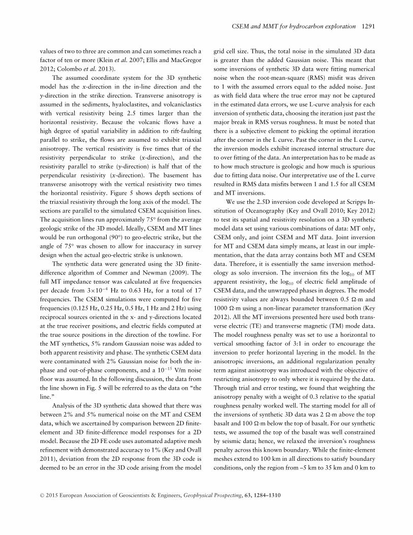
depth with the depths of the 40-!·m contour for the inver-sions shown in Figs. 8, 10, and 11. Figure 12(b) shows thepercentage error as defined by equation (1). Over the entiredepth range of the base of the volcanic section, the 40-!·mcontour of the vertical resistivity from the triaxial inversion ofthe joint data set (Fig. 11) is the closest to the true base. Forboth the isotropic (Fig. 8) and VTI (Fig. 10) inversions, the 40-!·m contour (or any contour) does not fit the true base overthe entire depth range. The isotropic inversion produces thebest match to the true base depths when the volcanic sectionis thin. The MT-only inversion shown in Fig. 7 is by far theworst, not having a constant contour to pick over much of thebase. This suggests that the choice of data and contour to usefor base volcanic interpretation will be situation dependentand should be guided by model studies for particular cases.

F IEL D DA TA INVERSION RESULTS

When considering the inversions of the field data shown here,it is important to keep in mind our two main objectives: to beable to accurately map the base of the high resistivity–velocityvolcanic section and to accurately determine the resistivity ofthe underlying sediments. Accurately predicting the base of thehigh-velocity volcanic sections is needed to determine if under-lying sediments lie within the hydrocarbon play window. Ac-curately predicting the resistivity of the underlying sedimentsis needed to assess if those sediments are non-prospective vol-caniclastics or prospective siliciclastic sediments.

In this section, we consider five separate inversions: (i)an isotropic model with MT data only, (ii) an isotropic modelwith CSEM data only, (iii) a VTI model with CSEM dataonly, (iv) a VTI model using both CSEM and MT data, and(v) a triaxial resistivity model using both CSEM and MT data.In order to quantify the inversion predictions of basalt resis-tance, sub-basalt sediment conductance, and sub-basalt sedi-ment horizontal resistivity at the wells, we use the depth in-tervals defined by the log interpretations. The basalt sectionat the Rosebank well lies between 2572 m and 2911 m andat Brugdan between 1173 m and 3175 m. The sub-basalt sed-iment section at Rosebank is classified as siliciclastic and liesbetween 2911 m and 3400 m. At Brugdan, the sediment sec-tion is classified as volcaniclastic and lies between 3175 mand 3745 m. Table 2 lists the percentage error in section resis-tance and conductance as defined by equations (2) and (3). Inaddition, because we are interested in distinguishing siliciclas-tic from volcaniclastic sediments in the sub-basalt sections,we list the log-averaged horizontal resistivity, the inversionhorizontal resistivity averaged over the same intervals, andthe percentage errors. The percentage error in the resistivityis defines as ((log-inversion)/log)∗100; hence, a positive valuemeans the log value is greater, and a negative value means theinversion value is greater. The MT inversion is not considereddue to its poor to non-existent basalt section definition.

Before making some observations about the results inTable 2, it must be remembered that the induction logs onlymeasure the horizontal resistivity within a few metres of a



Figure 10 Model obtained from VTI inversion of CSEM-only data showing the horizontal (top) and vertical (bottom) resistivity. The startingmodel was 2 !·m from the seafloor to top of the volcanics and 100 !·m below the top volcanics. The base of the volcanics and base of the highresistivity flows are marked with black lines. The 40-!·m contour from the inversion is shown by the white line. The relative error calculationsbetween the synthetic model and inverse model at these locations are given in Table 1.

vertical well. The comparisons are made to the macro-scalelog resistivity, where the log vertical resistivity is the averageover a larger interval of the measured resistivity (arithmeticmean), and the horizontal log resistivity is the inverse of theaverage of the log conductivity (i.e., the harmonic mean of theresistivity).

Table 2 observations are as follows.

i CSEM-only VTI inversion provides the most accurate basaltsection resistance.ii The basalt section resistance is more accurately recoveredat Rosebank where the section is thinner compared with Brug-dan.

iii CSEM-only VTI inversion provides the best sub-basalt sec-tion conductance at Rosebank, and CSEM and MT triaxialinversion provides the best sub-basalt section conductance atBrugdan, although the CSEM-only VTI is a close second tothe CSEM and MT triaxial inversion.iv The conductance of the conductive sections is better re-solved than the resistance of resistive sections.v There is a clear difference in the averaged siliciclastic resis-tivity (Rosebank) compared with the volcaniclastic resistivity(Brugdan). This difference is accurately captured in the hor-izontal resistivity of all the anisotropic inversions with theCSEM and MT triaxial providing the best overall estimates.



Figure 11 Model obtained from inversion for triaxial resistivity using CSEM and MT data. The starting model was 2 !·m from the seafloorto top of the volcanics and 100 !·m below the top volcanics. The base of the volcanics and base of the high resistivity flows are marked withthe black line. The 40-!·m contour from the inversion is shown by the white line. The error in the VIR between top and base volcanics and theVIC between base volcanics and basement at the locations marked as vertical profiles 1, 2, and 3 are given in Table 1.

The difference in resistivity between volcaniclastic and silici-clastic sediments is significantly larger than the percent errorin the anisotropic inversion estimates, supporting the possi-bility of distinguishing between the two types of sediments inanisotropic inversion.

The MT data used in all inversions shown are bothTE and TM modes from 0.75 to 1350 s period. The MTimpedance tensors were rotated to their maximum (averaging23° counter-clockwise from the line direction) prior to inver-sion. The CSEM data used in all inversions have an SNR floorof 4:1 for frequencies of 0.2 Hz, 0.4 Hz, 0.6 Hz, 1.4 Hz, and

2.6 Hz. Just as in the inversion of the synthetic data in thefeasibility section, the inversion fits the log10 of MT apparentresistivity and CSEM amplitude, and the unwrapped phase indegrees. The model resistivity values are always bounded be-tween 0.5 !·m and 1000 !·m. The starting model for all fielddata inversions was 1 !·m below the seafloor with smoothingremoved across the top volcanics, as defined by a picked seis-mic event. The MT-only inversion shown in Fig. 13 has a finalRMS data misfit of 1.5. Other MT inversions were run witha starting model of 1 !·m above and 100 !·m below the topbasalt pick; however, these inversions only differed from the



Table 2 Percentage error in basalt section resistance, percentage error in sub-basalt section conductance, sub-basalt resistivity, and percentageerror in sub-basalt resistivity for the Brugdan and Rosebank wells compared with the four inversions that use CSEM data. The four inversionsare: CSEM-only Isotropic (Fig. 14), CSEM VTI (Fig. 16), CSEM and MT VTI (Fig. 20), and CSEM and MT triaxial (Fig. 22). The volcanicsection at the Rosebank well is 2572 m–2911 m, and at Brugdan, it is 1173 m–3175 m. The sub-basalt sediment section at Rosebank is2911–3400 m, and at Brugdan, it is 3175–3745 m. For the joint triaxial inversion, the dip-oriented resistivity is used as it is closest to the logvalues. Percentage error is defined as ((well-inverse)/well)*100.

CSEM only CSEM & MT

Well Log Averaged Values Isotropic VTI VTI Triaxial

% Error in Inversion Basalt ResistanceRosebank 28355 (ρt) 64.73 −26.62 41.91 56.82Brugdan 154401 (ρt) 80.26 78.50 81.90 80.52

% Error in Inversion Sub-basalt ConcuctanceRosebank 20.3 (σ t) 83.84 3.24 10.04 −19.16Brugdan 43.1 (σ t) −44.12 22.80 38.56 −14.20

Inversion Sub-basalt ResistivityRosebank 3.9 (!m) 24.13 4.03 4.33 3.27Brugdan 19.1 (!m) 13.23 24.71 31.05 16.70

% Error in Inversion Sub-basalt ResistivityRosebank 3.9 (!m) −518.81 −3.35 −11.17 16.08Brugdan 19.1 (!m) 30.61 −29.53 −62.77 12.44

one shown in Fig. 13 below 70 km where we have no control.In general, we have found the inversion algorithm to be quiterobust with respect to the starting model, with the differencebetween half–space and basalt flood starting models minimalin the upper 10 km.

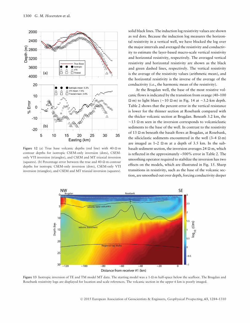
The MT–only inversion (Fig. 13) shows evidence of thevolcanic layer at the northwest (left) end of the line where itsapparent thickness is on the order of 7 km. The lack of reso-lution on the near-surface volcanic section near the middle ofthe profile is likely due to the insensitivity of MT to thin resis-tors, as well as the lack of high-frequency data in the deepestpart of the trough (Morten et al. 2011). East of about –100km the top basalt is coincident with a rise in resistivity, but noindication of base basalt is evident. The seismic basement pickshown in Fig. 13 is based on poorly imaged seismic events par-ticularly on the eastern half of the line. However, the increasein resistivity near 10-km depth in the MT inversion to the eastroughly coincides with the seismic basement pick. The largehigh resistivity structure seen from ! –100 km eastward is as-sociated with the continental crust. In general, the lower crustand upper mantle are expected to be resistive. Hence, it shouldall be resistive and bleed across the seismic Moho boundary,which is estimated to be around 25-km depth in this area(Grad, Tiira, and ESC Working Group 2009). The 2–30 !·mresistivity seen at 10–30 km depth in the westernmost sideof the model is therefore intriguing and likely requires some

partial melt, mantle volatiles, or even a conductive layered in-trusion as observed in the Vøring plateau (Myer et al. 2013),but further exploration of this deep MT result is beyond thescope of this work.

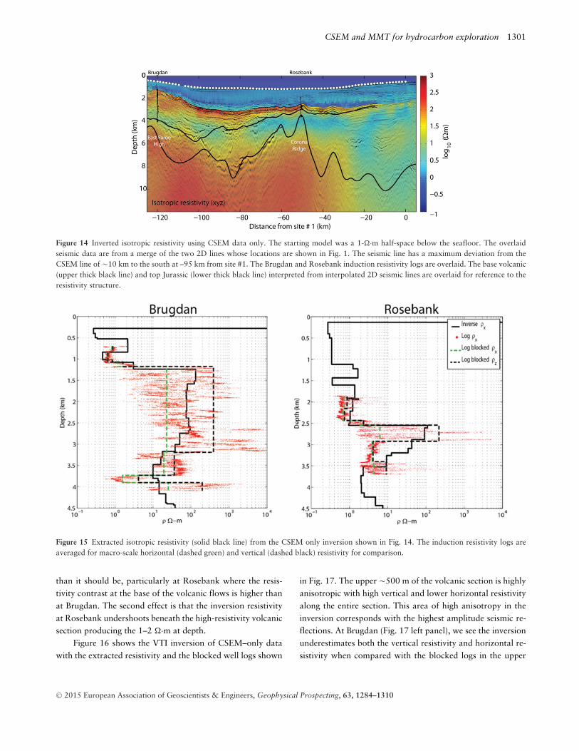
In contrast to the MT inversion, the CSEM–only inver-sion shown in Fig. 14 clearly shows the near-surface volcanicflows. This is expected given the much greater sensitivity ofCSEM data to thin resistors compared with MT data. TheCSEM inversion used the top basalt seismic pick to removesmoothing across this boundary.

In conductive marine environments, conventional hori-zontal dipole–dipole CSEM data normally do not have muchsensitivity below 4–5 km beneath the mud line. However,the depth sensitivity is enhanced by the presence of the near-surface resistive volcanics, which propagate the electromag-netic energy to greater depths. Here, the CSEM–only inversionappears to be sensitive to the resistivity structure at depths of5–6 km below mud line, as evidenced by the indications ofthe mini-basin centred on –85 km in Fig. 14, as well as thetransition from resistive to conductive sediments just to thesoutheast (right) of the Corona Ridge at –30 km position.The East Faroe High under the Brugdan well and the CoronaRidge beneath the Rosebank well are indicated in the CSEMinversion.

Figure 15 shows the isotropic resistivity from Fig. 14 ex-tracted at the locations of the Brugdan and Rosebank wells as



Figure 12 (a) True base volcanic depths (red line) with 40-!·mcontour depths for isotropic CSEM-only inversion (dots), CSEM-only VTI inversion (triangles), and CSEM and MT triaxial inversion(squares). (b) Percentage error between the true and 40-!·m contourdepths for isotropic CSEM-only inversion (dots), CSEM-only VTIinversion (triangles), and CSEM and MT triaxial inversion (squares).

solid black lines. The induction log resistivity values are shownas red dots. Because the induction log measures the horizon-tal resistivity in a vertical well, we have blocked the log overthe major intervals and averaged the resistivity and conductiv-ity to estimate the layer-based macro-scale vertical resistivityand horizontal resistivity, respectively. The averaged verticalresistivity and horizontal resistivity are shown as the blackand green dashed lines, respectively. The vertical resistivityis the average of the resistivity values (arithmetic mean), andthe horizontal resistivity is the inverse of the average of theconductivity (i.e., the harmonic mean of the resistivity).

At the Brugdan well, the base of the most resistive vol-canic flows is indicated by the transition from orange (40–100!·m) to light blues (!10 !·m) in Fig. 14 at !3.2-km depth.Table 2 shows that the percent error in the vertical resistanceis lower for the thinner section at Rosebank compared withthe thicker volcanic section at Brugdan. Beneath 3.2 km, the!13 !·m seen in the inversion corresponds to volcaniclasticsediments to the base of the well. In contrast to the resistivityof 13 !·m beneath the basalt flows at Brugdan, at Rosebank,the siliciclastic sediments encountered in the well (3–4 !·m)are imaged as 1–2 !·m at a depth of 3.5 km. In the sub-basalt sediment section, the inversion averages 24 !·m, whichis reflected in the approximately –500% error in Table 2. Thesmoothing operator required to stabilize the inversion has twoeffects on the models, which are illustrated in Fig. 15. Sharptransitions in resistivity, such as the base of the volcanic sec-tion, are smoothed out over depth, forcing conductivity deeper

Figure 13 Isotropic inversion of TE and TM model MT data. The starting model was a 1-!·m half-space below the seafloor. The Brugdan andRosebank resistivity logs are displayed for location and scale references. The volcanic section in the upper 6 km is poorly imaged.



Figure 14 Inverted isotropic resistivity using CSEM data only. The starting model was a 1-!·m half-space below the seafloor. The overlaidseismic data are from a merge of the two 2D lines whose locations are shown in Fig. 1. The seismic line has a maximum deviation from theCSEM line of !10 km to the south at –95 km from site #1. The Brugdan and Rosebank induction resistivity logs are overlaid. The base volcanic(upper thick black line) and top Jurassic (lower thick black line) interpreted from interpolated 2D seismic lines are overlaid for reference to theresistivity structure.

Figure 15 Extracted isotropic resistivity (solid black line) from the CSEM only inversion shown in Fig. 14. The induction resistivity logs areaveraged for macro-scale horizontal (dashed green) and vertical (dashed black) resistivity for comparison.

than it should be, particularly at Rosebank where the resis-tivity contrast at the base of the volcanic flows is higher thanat Brugdan. The second effect is that the inversion resistivityat Rosebank undershoots beneath the high-resistivity volcanicsection producing the 1–2 !·m at depth.

Figure 16 shows the VTI inversion of CSEM–only datawith the extracted resistivity and the blocked well logs shown

in Fig. 17. The upper !500 m of the volcanic section is highlyanisotropic with high vertical and lower horizontal resistivityalong the entire section. This area of high anisotropy in theinversion corresponds with the highest amplitude seismic re-flections. At Brugdan (Fig. 17 left panel), we see the inversionunderestimates both the vertical resistivity and horizontal re-sistivity when compared with the blocked logs in the upper



Figure 16 Inverted VTI resistivity using CSEM data only. The starting model was a 1-!·m half-space below the seafloor. The overlaid seismicdata are from a merge of the two 2D lines whose location is shown in Fig. 1. The seismic has a maximum deviation from the CSEM line of !10km to the south at –95 km from site #1. The Brugdan and Rosebank induction resistivity logs are overlaid. The base volcanic (upper thick blackline) and top Jurassic (lower thick black line) interpreted from interpolated 2D seismic lines are overlaid for reference to the resistivity structure.

500 m, whereas the inverted horizontal resistivity and verticalresistivity become lower toward the base of the volcanic sec-tion approaching the blocked log horizontal resistivity. Con-versely, the isotropic resistivity at Brugdan (Fig. 15 left panel)lies close to the average of blocked horizontal resistivity andvertical resistivity. To the east at Rosebank, where the vol-canic section thins, the inverted vertical resistivity and hori-zontal resistivity are much closer to the blocked log verticalresistivity and horizontal resistivity. In general, all combina-tions of model anisotropy and data, with the exception ofMT only, more accurately predict the resistivity in the thin-ner volcanic section at Rosebank compared with the thicksection at Brugdan (see Table 2). This is consistent with thefinding on the accuracy of the resistivity–thickness product inthe synthetic model for the thickest portions of the volcanicsection.

Beneath the volcanic section, the vertical resistivity andhorizontal resistivity from the VTI inversion (Fig. 17) arecloser to the blocked log resistivity compared with theisotropic resistivity (Fig. 15). The thin conductive section at!3.7-km depth is not recovered by any of the inversions.

Figure 18 shows the amplitude and phase data fits forthe isotropic inversion of CSEM data (Fig. 14) and the VTIinversion of CSEM data (Fig. 16) at site 84, the shallow siteshown in Fig. 2. Visual comparison of the data fits at this site,as at any other sites, does not reveal any significant differ-ences. A more diagnostic display is to plot histograms of thevalue of the data misfits, observed minus calculated divided(normalized) by the data standard deviations. The normalizeddata misfit histograms for all the data used in the isotropicCSEM data inversion (Fig. 14) and the VTI CSEM data in-version (Fig. 16) are shown in Fig. 19. Figure 19 reveals a



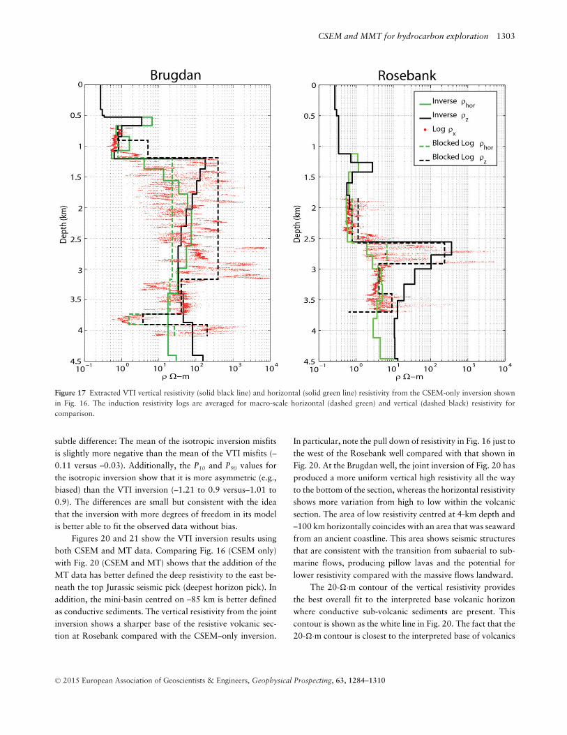
Figure 17 Extracted VTI vertical resistivity (solid black line) and horizontal (solid green line) resistivity from the CSEM-only inversion shownin Fig. 16. The induction resistivity logs are averaged for macro-scale horizontal (dashed green) and vertical (dashed black) resistivity forcomparison.

subtle difference: The mean of the isotropic inversion misfitsis slightly more negative than the mean of the VTI misfits (–0.11 versus –0.03). Additionally, the P10 and P90 values forthe isotropic inversion show that it is more asymmetric (e.g.,biased) than the VTI inversion (–1.21 to 0.9 versus–1.01 to0.9). The differences are small but consistent with the ideathat the inversion with more degrees of freedom in its modelis better able to fit the observed data without bias.

Figures 20 and 21 show the VTI inversion results usingboth CSEM and MT data. Comparing Fig. 16 (CSEM only)with Fig. 20 (CSEM and MT) shows that the addition of theMT data has better defined the deep resistivity to the east be-neath the top Jurassic seismic pick (deepest horizon pick). Inaddition, the mini-basin centred on –85 km is better definedas conductive sediments. The vertical resistivity from the jointinversion shows a sharper base of the resistive volcanic sec-tion at Rosebank compared with the CSEM–only inversion.

In particular, note the pull down of resistivity in Fig. 16 just tothe west of the Rosebank well compared with that shown inFig. 20. At the Brugdan well, the joint inversion of Fig. 20 hasproduced a more uniform vertical high resistivity all the wayto the bottom of the section, whereas the horizontal resistivityshows more variation from high to low within the volcanicsection. The area of low resistivity centred at 4-km depth and–100 km horizontally coincides with an area that was seawardfrom an ancient coastline. This area shows seismic structuresthat are consistent with the transition from subaerial to sub-marine flows, producing pillow lavas and the potential forlower resistivity compared with the massive flows landward.

The 20-!·m contour of the vertical resistivity providesthe best overall fit to the interpreted base volcanic horizonwhere conductive sub-volcanic sediments are present. Thiscontour is shown as the white line in Fig. 20. The fact that the20-!·m contour is closest to the interpreted base of volcanics



Figure 18 (a) and (b) show amplitude and phase of observed (symbols with error bars) and calculated (lines) data for site 84 from isotropicCSEM data inversion, model shown in Fig. 14. (c) and (d) show amplitude and phase of observed (symbols with error bars) and calculated(lines) data for site 84 from VTI CSEM data inversion, model shown in Fig. 16. Each color represents a frequency; frequencies are labeled onpanels (b) and (d).

for the field data inversions where the 40-!·m contour wasoptimal for the synthetic model study reflects the highervolcanic resistivity of the synthetic model compared withthe field study. The maximum percentage difference at anylocation between the 20-!·m contour and the interpreted

base is 11% with a mean difference along the contourof 1.2%.

The inverse horizontal resistivity and vertical resistivityat the well locations (see Fig. 21) show slightly worse corre-lation with the averaged well resistivity compared with that



Figure 19 Histograms of the normalized data residuals for theisotropic (red) and VTI (blue) inversions along with some statistics oftheir distributions. The P10 and P90 values show that, although theVTI inversion is only slightly biased, the isotropic inversion is moreso. Unbiased residuals should have a mean of zero and symmetri-cal P10 and P90 values. N is the total number of data. The isotropicinversion model is shown in Fig. 14; the VTI inversion in Fig. 16.

produced by the VTI CSEM-only inversion shown in Fig. 16,with the thinner volcanic section at Rosebank more accurately

imaged than the thicker Brugdan section (see Table 2 for nu-merical comparison).

Finally, Figs. 22 and 23 show the results from triaxialinversion of joint CSEM and MT data. The spatial variationin the triaxial resistivity shown in Fig. 22 is much larger thanin any of the lower dimensional inversions. The vertical resis-tivity does not have a sharp resistivity contrast at the expectedbase of the volcanic (the interpreted base volcanic being theshallowest black line). The fits to the logs in the basalt sec-tion are worse than the VTI inversions of either CSEM-onlyor CSEM and MT data. However, the fits to the logs in thesub-basalt sediments are the best of any of the inversions (seeTable 2). The in-line (x) resistivity shows two near verticalhigh resistivity structures: one just to the east of the East FareoHigh and the other centred on the Corona Ridge. It is tempt-ing to interpret these as the core of granitic intrusions, butgiven the poor correlations of the models to the logs in theresistive section, this cannot be supported. These structureshave less resistive expressions in the vertical resistivity. TheCorona Ridge appears to have significant horizontal resistiv-ity anisotropy, with a broad resistivity high in the Strike (y)resistivity and a much narrower vertical feature in the in-line(x) resistivity.

Figure 20 Inverted VTI resistivity usingCSEM and MT data. The starting model wasa 1-!·m half-space below the seafloor. Theoverlaid seismic data are from a merge ofthe two 2D lines whose location is shown inFig. 1. The seismic has a maximum devia-tion from the CSEM line of !10 km to thesouth at –95km from site #1. The Brugdanand Rosebank induction resistivity logs areoverlaid. The base volcanic (first black linefrom the top) and top Jurassic (deep blackline) interpreted from interpolated 2D seis-mic lines are overlaid for reference to the re-sistivity structure. The 20-!·m contour fromthe vertical resistivity is overlaid on the ver-tical resistivity section as a white line. Notethat the high correlation between the inter-preted base of the volcanic section and the20-!·m contour.



Figure 21 Extracted VTI vertical resistivity (solid black line) and horizontal (solid green line) resistivity from the joint CSEM and MT datainversion shown in Fig. 20. The induction resistivity logs are averaged for macro-scale horizontal (dashed green) and vertical (dashed black)resistivity for comparison.

The closest resistivity contour in the vertical resistivity is40 !·m and is shown as the white line on the bottom panelof Fig. 22. The contour highlights the pull down in verticalresistivity just to the west of the Rosebank well comparedwith the interpreted base volcanic (black line). The maximumrelative difference at any location between the 40-!·m contourand the interpreted base is 22% with a mean difference alongthe contour of 5.1%.

D I S C U S S I O N

The synthetic model study found that the joint controlledsource electromagnetic (CSEM) and marine magnetotelluric(MT) inversion for vertical transverse anisotropy (VTI) resis-tivity produced better VIR predictions in the volcanic sectionwith CSEM-only VTI inversion producing slightly better VICpredictions in the underlying sediments. The joint inversion offield data with VTI inversion produces closer matches to theblocked logs and a vertical resistivity contour that more closelyfollows the interpreted base volcanic horizon. However, in thefield data, the CSEM and MT data VTI inversion was superiorto the CSEM–only VTI inversion for matching the base of theinterpreted volcanic flows. The field data triaxial inversionsare worse for predicting basalt thickness than suggested by thefeasibility study for triaxial inversion. However, the triaxialjoint inversion does produce slightly better sub-basalt hori-zontal resistivity estimated compared with VTI joint inversion,

but the improvement is small and may not be robust due to theincrease in degrees of freedom for triaxial compared to VTI.Overall, the sensitivity results seen in the feasibility study areborne out in the field data examples. Using only inline E fielddata limits the model parameterization to VTI. We speculatethat, in the synthetic model data, which has primarily Gaus-sian noise, the sensitivity to the strike resistivity (y) is higherthan in the field data where noise is not completely Gaussianand 3D effects are higher. The synthetic model did not includecomplex dike and sill structures that are most likely in the realgeology. Therefore, in the more complex 3D geology seen bythe field data, the in-line CSEM data has less sensitivity to thestrike resistivity than suggested in the synthetic study. Addi-tionally, the 3D MT affects in the field data are most likelylarger than in the synthetic model study, adding more uncer-tainty when trying to invert for triaxial resistivity on a single2D line.

The apparent ability to discriminate between 10-!·m vol-caniclastic and 3–4 !·m siliciclastic sediments in the CSEMfield data inversions was an unexpected result. While moredata and well control will be needed to substantiate the abil-ity to discriminate between volcaniclastic and siliciclastic sed-iments, if true, this capability would significantly enhance thevalue of electromagnetic surveys in sub-volcanic provinces.

The apparent ability of the joint CSEM and MT VTIinversions to produce vertical resistivity where there is a highcorrelation between a constant resistivity contour (20 !·m in



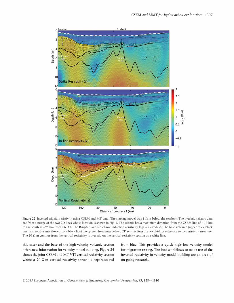
Figure 22 Inverted triaxial resistivity using CSEM and MT data. The starting model was 1 !·m below the seafloor. The overlaid seismic dataare from a merge of the two 2D lines whose location is shown in Fig. 1. The seismic has a maximum deviation from the CSEM line of !10 kmto the south at –95 km from site #1. The Brugdan and Rosebank induction resistivity logs are overlaid. The base volcanic (upper thick blackline) and top Jurassic (lower thick black line) interpreted from interpolated 2D seismic lines are overlaid for reference to the resistivity structure.The 20-!·m contour from the vertical resistivity is overlaid on the vertical resistivity section as a white line.

this case) and the base of the high-velocity volcanic sectionoffers new information for velocity model building. Figure 24shows the joint CSEM and MT VTI vertical resistivity sectionwhere a 20-!·m vertical resistivity threshold separates red

from blue. This provides a quick high–low velocity modelfor migration testing. The best workflows to make use of theinverted resistivity in velocity model building are an area ofon-going research.



Figure 23 Extracted triaxial in-line (x) resistivity (solid red line), strike (y) resistivity (solid green line), and vertical (z) resistivity (solid blackline) from joint inversion of CSEM and MT data shown in Fig. 2. The induction resistivity logs are averaged for macro-scale horizontal (dashedgreen) and vertical (dashed black) resistivity for comparison.

Figure 24 Red–blue plot of the vertical resistivity obtained from VTI inversion of the CSEM and MT data, shown in Fig. 20. Red is verticalresistivity > = 20 !·m, and blue is vertical resistivity < 20 !·m.

CONCLUSIONS

The CSEM and MT calibration line described here demon-strates that high-quality marine CSEM and MT data can pro-vide significant information to reduce uncertainty in base vol-canic picks and to modify seismic interpretations of the base of

the volcanic section as well as sediment constraining basementdepths. In addition, the resistivity images from this survey in-dicate the possibility of distinguishing between volcaniclasticand more conductive siliciclastic sediments. If the ability todistinguish volcaniclastic sediment from siliciclastic sediment



is borne out in further surveys, this could prove to be a signif-icant uplift in what was previously thought of only as a basebasalt mapping technology.

For both the model and field data studies, inversions thatused both CSEM and TE-mode and TM-mode MT data pro-vided the best results. The joint inversion for triaxial resis-tivity provided the best results for the synthetic model. How-ever, for the field data, the best sub-basalt horizontal resis-tivity came from Triaxial joint inversion, whereas the verticalresistivity from VTI joint inversion provided better correla-tion with the interpreted base of the volcanic section. Thismost likely indicates that the data need to be nearly 2D tobe able to distinguish three separate resistivity componentsfrom 2.5D inversion. The increased 3D effects in the volcanicflows with non-Gaussian noise in the field data produce morenon-unique tradeoffs in the three resistivity components inthe volcanic flows. Picking a constant contour of resistivityfrom the isotropic inversion or the vertical resistivity froman anisotropic inversion provided nearly identical average er-rors across the model with the joint inversion triaxial verticalresistivity providing the most accurate base volcanic flow.Additionally, the differences between all inversions in predict-ing the thickness of the volcanic flows at Rosebank (wherewe have a full volcanic section penetration) using the fielddata indicates that isotropic inversion may often be adequate.While VTI 2.5D inversion of field data may provide betterresolution of thicknesses and resistivities, it should be testedagainst models on a case-by-case basis.

A CK NOW LEDGEME NTS

The CSEM survey was acquired by EMGS. The authors wouldlike to thank Chevron Europe and EMGS for permission topublish this work. K. Key acknowledges support from theScripps Seafloor Electromagnetic Methods Consortium.

REFERENCES

Alumbaugh D., Hoversten M., Stefani J. and Thacher C. 2013. A3D model study to investigate EM imaging of sub-basalt structuresin a deep water environment. 83rd SEG meeting, Houston, USA,Expanded Abstracts, 765–769.

Colombo D., Keho T., Janoubi E. and Soyer W. 2011. Sub-basaltimaging with broadband magnetotellurics in NW Saudi Arabia.81st SEG annual meeting, San Antonio, USA, 619–623.

Commer M. and Newman G.A. 2009. Three-dimensional controlled-source electromagnetic and magnetotellurics joint inversion. Geo-physical Journal International 178, 1305–1616.

Connell D. and Key K. 2013. A numerical comparison of time andfrequency-domain marine electromagnetic methods for hydrocar-bon exploration in shallow water. Geophysical Prospecting 61,187–199.

Constable S., Weiss C.J. 2006. Mapping thin resistors and hydro-carbons with marine EM methods: Insights from 1D modeling.Geophysics 71, G43–G51.

Constable S.C., Orange A., Hoversten G.M. and Morrison H.F. 1998.Marine magnetotellurics for petroleum exploration, Part 1: A sea-floor equipment system. Geophysics 63, 816–825.

Egbert G.D. 1997. Robust multiple-station magnetotelluric data pro-cessing. Geophysical Journal International 130(2), 475–496.

Ellis M. and MacGregor L. 2012. An electrical rock physics model forpartially interconnected fluid inclusions/cracks. 82nd SEG annualmeeting, Las Vegas, USA, Expanded Abstracts, 1–5.

Grad M., Tiira T. and ESC Working Group 2009. The Moho depthmap of the European Plate. Geophysical Journal International 176,279–292.

Hoversten G.M., Morrison H.F. and Constable S.C. 1998. Ma-rine magnetotellurics for petroleum exploration, Part 2: Numericalanalysis of subsalt resolution. Geophysics 63, 826–840.

Jegen M.D., Hobbs R.W., Tarits P. and Chave A. 2009. Joint in-version of marine magnetotelluric and gravity data incorporatingseismic constraints Preliminary results of sub-basalt imaging off theFaroe Shelf. Earth and Planetary Science Letters 282(1–4), 47–55.

Key K.W., Constable S.C. and Weiss C.J. 2006. Mapping 3D salt us-ing the 2D marine magnetotelluric method: Case study from GeminiProspect, Gulf of Mexico. Geophysics 71(1), B17–B27.

Key K. and Lockwood A. 2010. Determining the orientation of ma-rine CSEM receivers using orthogonal Procrustes rotation analysis.Geophysics 75(3), F63–F70.

Key K. and Ovall J. 2011. A parallel goal-oriented adaptive finiteelement method for 2.5-D electromagnetic modeling. GeophysicalJournal International 186(1), 137–154.

Key K. 2012. Marine EM inversion using unstructured grids: a 2Dparallel adaptive finite element algorithm. 82nd SEG annual meet-ing, Las Vegas, USA, Expanded Abstracts 1–5.

Klein J.D., Martin P.R. and Allen D.F. 1997. The petrophysics ofelectrically anisotropic reservoirs. The Log Analyst 38, 25–36.

Morten J.P., Fanavoll S. and Mrope F.M. 2001. Sub-basalt ImagingUsing Broadside CSEM. 73rd EAGE Conference and Exhibition,C029.

Morrison H.F., Shoham Y., Hoversten G.M. and Torres-Verdin C.1996. Electromagnetic mapping of electrical conductivity beneaththe Columbia basalts. Geophysical Prospecting 44, 963–986.

Myer D., Constable S. and Key K. 2011. Broad-band waveforms androbust processing for marine CSEM surveys. Geophysical JournalInternational 184(2), 689–698.

Myer D., Constable S. and Key K. 2013. Magnetotelluric evidence forlayered mafic intrusions beneath the Vøring and Exmouth riftedmargins. Physics of the Earth and Planetary Interiors 220, 1–10.

Newman G.A., Commer M. and Carazzone J.J. 2010. Imaging CSEMdata in the presence of electrical anisotropy. Geophysics 75, F51–F61.

Smith T., Hoversten G.M., Gasperikova E. and Morrison F. 1999.Sharp boundary inversion of 2D magnetotellurics data. Geophysi-cal Prospecting 47, 469–486.



Strack K.M. and Pandey P.B. 2007. Exploration with controlled-source electromagnetic under basalt cover in India. The LeadingEdge 26, 260–363.

Warren R.K. and Srnka L.J. 1992. Exploration in the basalt-covered areas of the Columbia River Basin, Washington, usingelectromagnetic array profiling (EMAP). Geophysics 57, 986–993.

Weckmann U., Magunia A. and Ritter O. 2005. Effective noiseseparation for magnetotelluric single site data processing using afrequency domain selection scheme. Geophysical Journal Interna-tional 161(3), 635–652.

Withers R., Eggers D., Fox T. and Crebs T. 1994. A case study ofintegrated hydrocarbon exploration through basalt. Geophysics 59,666–1679.


field test of sub-basalt hydrocarbon exploration with

Documents