field-induced motion of ferroï¬‚uid droplets through

Under consideration for publication in J. Fluid Mech. 1

Field-induced motion of ferrofluid dropletsthrough immiscible viscous media

S. AFKHAMI1, Y. RENARDY1, M. RENARDY1,J. S. R IFFLE2 AND T. St. P IERRE3

1Department of Mathematics, Virginia Tech, Blacksburg, VA 24061-0123, USA2Department of Chemistry, Virginia Tech, Blacksburg, VA 24061-0212, USA

3School of Physics, M013, The University of Western Australia, Crawley, WA 6009, Australia

(Received ?? and in revised form ??)

The motion of a hydrophobic ferrofluid droplet placed in a viscous medium and drivenby an externally applied magnetic field is investigated numerically in an axisymmetricgeometry. Initially, the drop is spherical and placed at a distance away from the magnet.The governing equations are the Maxwell equations for a non-conducting flow, momentumequation and incompressibility. A numerical algorithm is derived to model the interfacebetween a magnetized fluid and a non-magnetic fluid via a volume-of-fluid framework.A continuum-surface-force formulation is used to model the interfacial tension force asa body force, and the placement of the liquids is tracked by a volume fraction function.Three cases are studied. First, where inertia is dominant, the magnetic Laplace numberis varied while the Laplace number is fixed. Secondly, where inertial effects are negligible,the Laplace number is varied while the magnetic Laplace number is fixed. In the thirdcase, the magnetic Bond number and inertial effects are both small, and the magneticforce is of the order of the viscous drag force. The time taken by the droplet to travelthrough the medium and the deformations in the drop are investigated and comparedwith experimental studies and accompanying simpler model of Mefford et al. (2007). Thetransit times are found to compare more favorably than with the simpler model.

1. IntroductionFerrofluids consist of magnetic nanoparticles in a colloidal solution. Recent develop-

ments in the synthesis and characterization of ferrofluids are motivated by biomedicalapplications (Liu et al. 2007), where the treatment of retinal detachment is one example(Mefford et al. 2007). A small amount of ferrofluid is injected into the vitreous cavityof the eye and guided by a permanent magnet inserted outside the scleral wall of theeye. The drop travels toward the side of the eye, until it can seal a retinal hole. Thetime taken for the drop to migrate is an important quantity which needs to be predicted,and which must be relatively short for the feasibility of this procedure. A simplified ex-perimental model of this complex system is investigated in Mefford et al. (2007) witha ferrofluid drop, assumed to be a solid sphere, which moves through a highly viscousNewtonian fluid that represents the vitreous material (Nickerson et al. 2005). By treatingthe sphere as a magnetic particle, the magnetic force acting on it can be simplified asFM (x) = VM(x)μ0(dH/dx), where V is the volume of the sphere, M is the magneti-zation of the ferrofluid droplet, μ0 is the permeability of vacumm, and dH/dx is thegradient of the magnetic field H with respect to the distance x from the permanentmagnet. This magnetic force is balanced with the viscous drag force on the sphere in

2 S. Afkhami, Y. Renardy, M. Renardy, J. Riffle and T. St Pierre

Stokes flow given by 6πηR0U(x), to find the expression for U(x). Integrating this overthe distance to the magnet, an approximate time of travel was obtained and then com-pared with experiments conducted with a sphere filled with a liquid of viscosity 50 Pa s(sodium hyaluronate ProviscTM solution commonly used in eye surgery). Their theoreti-cal value was found to exceed the experimentally measured transit time by roughly 50%.The authors noted one phenomenon in their experiments which was not included in theirtheory: at larger drop sizes, the shape deformed from a sphere to a teardrop as it acceler-ated toward the magnet. Separation of the tail of the teardrop was sometimes observed,resulting in smaller droplets that take longer to travel to the magnet. Another aspectof their estimate for the transit time is the use of the drag coefficient for a solid sphererather than the viscosity-dependent value for a liquid sphere (Clift et al. 1978). The lat-ter improves the gap between theory and experimental data but still leaves significantdiscrepancies due to drop deformation and coupled motion inside the drop.

The understanding of the above process is important for the efficient manipulation ofthe procedure. For instance, the size and the shape of the ferrofluid droplet can influencethe motion of the droplet as it travels in a viscous medium. To investigate the responseof a ferrofluid droplet to an applied magnetic field or to the capillary effects requiresa thorough understanding of ferrohydrodynamics in such a system. The mathematicalformulation of the flow of a ferrofluid is described by Rosensweig (1985). In this paper, wepresent a methodology for the numerical modeling of a two-phase system of immisciblefluids, a ferrofluid and a non-magnetic viscous medium. The magnetic force competeswith the interfacial tension force and viscous drag to deform the drop. Previous numericalstudies are limited to equilibrium shapes of ferrofluid drops (Lavrova et al. 2006, 2004)and interface instabilities (Bashtovoi et al. 2002; Matthies & Tobiska 2005; Knielinget al. 2007). In all these studies, a finite element method was used in which the governingequations of the magnetic liquid are coupled by the force balance at the interface andthe surface tension is applied as a boundary condition at the interface. Here, we developa numerical model, described in section 3, and simulate the field-induced motion of aferrofluid droplet in a viscous medium, with results presented in section 4.

In this paper, the drop is assumed axisymmetric and deformable. We assume the dropsize is small compared with the distance to the boundary of the eye. The magnetic fieldthat is measured in the absence of the drop is used to generate boundary conditions.We investigate the transit time and drop shapes for a number of conditions that includethose of Mefford et al. (2007).

2. Governing equationsA ferrofluid drop is suspended in a viscous medium that is non-magnetizable, as shown

in figure 1. We assume that upon the placement of the magnet, the drop is instantly mag-netized. The classical equations for the evolution of the two-fluid system are the Maxwellequations, the incompressible Navier-Stokes equations, and a constitutive relationshipfor the magnetic induction B (T), magnetic field H (A m−1), and magnetization M(A m−1) (Lavrova et al. 2006). In SI units, M = χmH and

B(x, t) ={μ1H in the ferrofluidμ0H in the viscous medium , (2.1)

where the magnetic permeability of the ferrofluid is μ1 = μ0(1 + χm), and χm is itsmagnetic susceptibility. μ0 = 4π× 10−7 N A−2 is the permeability of vacuum, as well asmany other non-ferromagnetic materials. The Maxwell equations for a non-conductingfluid are ∇·B = 0 and ∇×H = 0. The latter yields a magnetic scalar potential ψ, where

Motion of ferrofluid droplets 3

Figure 1. Schematic of the initial configuration. The computational box covers 0 � z � Lz,0 � r � Lr. Initially, a spherical ferromagnetic drop of radius R is placed a distance L from themagnet at (r, z) = (0, 0).

H = ∇ψ. The former yields

∇ · (μ∇ψ) = 0. (2.2)

The permeability is a constant per fluid, and jumps in value across the interface, so thatψ(x, t) changes as the interface evolves.

The boundary condition on the magnetic field is reconstructed from the experimentalmeasurements of Mefford et al. (2007). In the absence of the drop, they measured themagnitude H(z) as a function of distance from the magnet, z, and fitted the data to a5th degree polynomial, as shown in figure 2. The scalar potential is then a 6th degreepolynomial φ(0, z) = P6(z) along the axis of the cylindrical domain. In the absence ofthe drop, φ satisfies Laplace’s equation 1

r∂∂r (r ∂φ

∂r ) + ∂2φ∂z2 = 0. If there is a solution, it is

analytic and has r2-symmetry. The ansatz φ(r, z) = P6(z)+ r2P4(z)+ r4P2(z)+ r6P0(z)yields

φ(r, z) = P6(z) − 14r2P ′′

6 (z) +164r4P

(iv)6 (z) − 1

(36)(64)r6P

(vi)6 (z). (2.3)

This yields the boundary condition, and also approximates an initial condition when thedrop is relatively small. The lateral size of the computational domain is chosen to besufficiently large so that it is consistent with the assumption that results do not changeif a larger size were used (see section 4.1). These checks were done by calculating thesolution for double the lateral domain size.

The magnetic potential ψ is calculated from equation (2.2). In axisymmetric cylindricalcoordinates,

1r

∂

∂r

(μr∂ψ

∂r

)+

∂

∂z

(μ∂ψ

∂z

)= 0 in Ω, (2.4)


y = -3E-05x5 + 0.0025x4 - 0.0954x3 + 1.7906x2 - 16.99x + 69.605

R2 = 0.9993

0

10

20

30

40

50

60

70

80

0 5 10 15 20 25 30 35

mm

kA/m

Figure 2. Measured data for the magnetic field from figure 3 of Mefford et al. (2007) (�) andfifth degree polynomial fitted to the data (—) as functions of the distance from the magnet.

where Ω denotes the computational domain. The boundary conditions for ψ on thedomain boundaries ∂Ω are defined as

∂ψ

∂n=∂φ

∂non ∂Ω, (2.5)

where ∂/∂n = n · ∇, and n denotes the normal to the boundary ∂Ω.In order to impose the boundary condition in our numerical model, we perform a

transformation of variables to ζ: ψ = φ + ζ, where φ is the potential field without themagnetic medium. One can then rewrite (2.2) such that

∇ · (μ∇ζ) = −∇ · (μ∇φ), (2.6)

where ∇ · (μ∇φ) vanishes everywhere except on the surface between the drop and thesurrounding fluid ∂Ωf and

∂ζ

∂n= 0 on ∂Ω. (2.7)

The well-known Langevin function L(α)=coth α − α−1 is used to describe the mag-netization M = |M| behavior of the ferrofluid versus the strength of the magnetic fieldH:

M(H) = MsL

(μ0m|H|kBT

)H|H| , (2.8)

where the saturation magnetization Ms and the magnetic moment of the particle enteras parameters, T denotes the temperature, and kB is the Boltzmann’s constant. Figure 3compares M vs H for the measured data of Mefford et al. (2007) and the Langevin fit.It is evident that the Langevin function fits the respective experimental data reasonablywell.

Each liquid is identified with a color function,

C(r, z, t) ={

0 in the viscous medium1 in the ferrofluid drop, (2.9)

which advects with the flow. The position of the interface is given by the discontinuities


0

5

10

15

20

25

30

0 100 200 300 400 500

H [kA/m]

M [k

A/m

]

Figure 3. Magnetization behavior of the ferrofluid containing 7 vol. % of magnetite (Fe3O4)particles with a mean diameter of 7nm for figure 3 of Mefford et al. (2007). Measured data (�)is compared with the Langevin fit (—), assuming each of the magnetite particles has a totalmagnetic moment ≈ 2 × 10−19A m2.

in the color function. The fluid equation of motion is

ρdudt

= −∇p+ ∇ · ηS + Fs + ∇ · σm, Si,j =12(∂uj

∂xi+∂ui

∂xj

), (2.10)

where Fs denotes the continuum body force due to interfacial tension,

Fs = γκ̃nδS , κ̃ = −∇ · n. (2.11)

γ denotes the coefficient of interfacial tension, n = ∇C/|∇C| is the normal to the in-terface, δS = |∇C| is the delta-function at the interface, and κ̃ is the curvature. Theviscous stress tensor is ηSi,j where the rate of deformation tensor is Si,j . The magneticstress tensor σm is derived in the Appendix to be BHT, so that the equation of motionbecomes

ρdudt

= −∇p+ ∇ · ηS + Fs + ∇ ·BHT, (2.12)

to be interpreted as a weak formulation.

3. Numerical MethodologyIn the absence of an initially imposed velocity and gravity, and using the following

normalizations for a drop of initial radius R0,

x∗ = x/R0 , t∗ = tη0/(ρ0R

20) , η

∗ = η/η0 , ρ∗ = ρ/ρ0,

u∗ = uρ0R0/η0 , p∗ = pρ0R

20/(η0)

2 , H∗ = H/H0,

the equation of motion becomes

ρ∗du∗

dt∗= −∇∗p∗ + ∇∗ · η∗S∗ + La Fs

∗ + Lam ∇∗ · σ∗m, (3.1)

where the subscript 0 refers to the droplet; i.e., ρ0 and η0 are the ferrofluid density andviscosity, respectively, and H0 is the characteristic scale of the magnetic field strength.


The Laplace number,

La = γρ0R0/η20 , (3.2)

is the ratio of the surface tension to the viscous drag (note that La = 1/(Oh)2 whereOh is the Ohnesorge number). The magnetic Laplace number (or magnetic Reynoldsnumber),

Lam = μ0H20ρ0R

20/η

20 , (3.3)

is the ratio of the magnetic force to inertial force. The ratio of magnetic force to interfacialtension force is named the magnetic Bond number (Baygents et al. (1998); Voltairas et al.(2002)),

Bom = Lam/La. (3.4)

A volume-of-fluid algorithm on a marker-and-cell (MAC) grid of equidistant mesh Δand a computational domain Lr × Lz is used. The discretized color function gives thevolume fraction of the ferrofluid. The advection of the volume fraction function is La-grangian, and the piecewise linear interface reconstruction scheme (PLIC) is used tocalculate the interface position at each time step. The details of the method for theNavier-Stokes equations are given in Lafaurie et al. (1994); Li & Renardy (1999); Liet al. (2000); Scardovelli & Zaleski (1999) and not repeated here. Briefly, a provisionalvelocity field is first predicted and then corrected with the pressure field that is cal-culated as a solution of a Poisson problem. Interfacial tension is discretized using thecontinuum-surface-force model (Brackbill et al. 1992). The new aspect is the extensionof the algorithm to the ferrofluid.

The magnetic potential field is discretized using second-order central differences andis computed as a solution of the Poisson problem (2.6). In axisymmetric coordinates, thediscretization of (2.6) at cell (i, j) yields

∇ · (μ∇ζ)i,j =1ri,j

ri+1/2,jμi+1/2,j(∂ζ∂r )i+1/2,j − ri−1/2,jμi−1/2,j(

∂ζ∂r )i−1/2,j

Δ

+μi,j+1/2(

∂ζ∂z )i,j+1/2 − μi,j−1/2(

∂ζ∂z )i,j−1/2

Δ, (3.5)

where, for instance for the cell face (i+ 1/2, j),

(∂ζ

∂r)i+1/2,j =

ζi+1,j − ζi,jΔ

. (3.6)

A weighted harmonic mean interpolation is used to compute μ at cell face (i+ 1/2, j):

1μi+1/2,j

=12(

1μi,j

+1

μi+1,j),

where1μi,j

=1 − Ci,j

μ0+Ci,j

μ1,

and the discretized color function Cij represents the volume fraction of the ferrofluidin cell (i, j) (Patankar 1980). Analogous relationships can be written for other faces ofa cell. The right hand side of (2.6) is discretized similarly. The boundary condition forcells on the solid boundary is a second-order discretization of a zero gradient boundarycondition for ζ: ∂ζ/∂n = 0. A multigrid Poisson solver is then used to obtain the solutionof the resulting linear set of equations.


(vz)i,j+1/2

(vr)i ,j+1/2

( )�m rz i ,j+1/2 +1/2

( )�m rz i ,j-+1/2 1/2

( )�m rz i- ,j1/2 +1/2

( )

( )

( )

�

�

�

m rr i,j

m rz i,j

m zz i,j

( )

( )

( )

�

�

�

m rr i+1,j

m rz i+1,j

m z i+1,jz

( )

( )

( )

�

�

�

m rr i+1,j+1

m rz i+1,j+1

m z i+1,j+1z

( )

( )

( )

�

�

�

m rr i,j+1

m rz i,j+1

m zz i,j+1

Figure 4. Location of the velocities and the magnetic stress tensor components on a MAC grid.Corner values of the magnetic stress tensor components (rz, at �) are calculated from cell-centervalues (•).

The spatial discretization of the velocity field is based on the MAC grid in figure 4.Therefore, the evaluation of the components of the magnetic stress tensor requires theevaluation of gradients at faces. In axisymmetric coordinates, the divergence of the mag-netic stress tensor is discretized as

er :1

ri+1/2,j

ri+1,j((σm)rr)i+1,j − ri,j((σm)rr)i,j

Δ

+((σm)rz)i+1/2,j+1/2 − ((σm)rz)i+1/2,j−1/2

Δ

ez :1

ri,j+1/2

ri+1/2,j+1/2((σm)rz)i+1/2,j+1/2 − ri−1/2,j+1/2((σm)rz)i−1/2,j+1/2

Δ

+((σm)zz)i,j+1 − ((σm)zz)i,j

Δ, (3.7)

where the components such as (σm)rr are defined in the Appendix. Second-order centraldifferences are used to discretize the components of the magnetic stress tensor at thecenter of a cell and a simple averaging from cell center values is used to extrapolate themagnetic stress components to cell corners.

4. ResultsNumerical simulations are presented in three parts. Section 4.1 concerns tests of the

numerical implementation by focussing on the resulting magnetic fields and by testingfor convergence of the solution with grid refinement. Section 4.2 presents a parametricstudy, varying Lam for fixed La, and vice versa. Section 4.3 contains the application ofour model to the experimental data of Mefford et al. (2007), and examines time takenby the drop to reach the magnet.

Table 1 provides a comprehensive overview over the sets of simulations presented in theremainder of this section. For section 4.3, the magnetic susceptibility is computed usingthe Langevin function via (2.8), and this yields improved agreement with experimentaldata over the linear variation defined by a constant χm. The characteristic scale of themagnetic field strength H0 is taken to be 1 kA m−1 in all the cases in section 4.2,since this is of the same order as the magnetic field strength which is initially inducted


section § 4.2 § 4.2 § 4.3

2R0(mm) 2.5 1 1, 1.8, 2Lr 1.6R0 4R0 4mmLz 12.8R0 24R0 16mmΔ R0/20 R0/12 R0/8, R0/9, R0/10ρ0 1.32 ρv 1.32 ρv 1320 kg m−3

η0 1.5 ηv 1.5 ηv 80 kg m−1s−1

ρv 998 kg m−3

ηv 50 kg m−1s−1

χm 0.25 0.25 *H0(kA m−1) 1 1 1La 5.15 0.002, 0.01, 0.04, 0.1, 0.4Lam 0.3, 1.5, 3.6 0.05Bom 0.06, 0.3, 0.6, 1.2 24, 5, 1, 0.5, 0.1 0.031,0.056,0.063

Table 1. Overview of the sets of simulations presented in sections 4.2-4.3.* The magnetic susceptibility for § 4.3 is computed using the Langevin function.

0

1

2

3

4

5

6

7

8

9

0 10 20 30 40 50

Travel Time[sec]

Dis

tanc

e[m

m]

Δ=1/6Δ=1/12Δ=1/18Δ=1/24

Figure 5. Calculated transit times at different mesh sizes in units of initial drop radius R0. Re-sults are shown to be convergent as the mesh is refined. The parameters are those of section 4.3.

by the magnet on the droplet placed about 12 mm away from the permanent magnet(cf. figure 2). Note that the magnetic field strength varies with location and the choiceof a characteristic scale is not straightforward. Thus, as the droplet moves toward themagnet, the effective magnetic Laplace number increases well beyond our nominal value.

4.1. Magnetic field and imposed boundary condition

Figure 5 shows a convergence test for the calculated travel times, at different mesh sizesin units of the initial droplet radius R0. A droplet of radius 1 mm is centered at a distance10 mm away from the bottom of the 16 mm × 4 mm domain. The time that is requiredfor the droplet to reach the bottom of the domain is calculated at different mesh sizes todemonstrate the spatial convergence of the numerical results. The magnetic susceptibilityused in this case is considered to be constant and χm = 0.25.

We demonstrate the effectiveness of our methodology by presenting the results of thesimulated applied magnetic field using the magnetic field boundary condition (2.3), com-


1

2

3

4

5

6

7

8

9

10

11

12

13

9 10 11 12 13 14 15

mm

kA/m

(a)

(b)

(c)

4

6

8

10

12

14

16

18

20

22

5 6 7 8 9 10 11

mm

kA/m

10

15

20

25

30

35

40

45

50

55

60

1 2 3 4 5 6 7

mm

kA/m

Figure 6. Distribution of the magnetic field (kA m−1) along the centerline of the computationaldomain. The computed magnetic field along the centerline of the domain in the absence of thedrop (-) is compared with the measured magnetic field generated by a permanent magnet (�)from Mefford et al. (2007). The computed magnetic field in the presence of a 2 mm droplet (—)is superposed when the droplet is placed at distances (a) 12 mm, (b) 8 mm, and (c) 4 mm fromthe magnet, respectively. χm = 1.

pared with values measured along the centreline of the domain by Mefford et al. (2007).Figure 6 shows the computed magnetic field along the centerline of the 16 mm × 4 mmdomain (-) compared with the measured magnetic field generated by a permanent mag-net in the absence of a droplet (�). The agreement is excellent, and this also providesa check that the lateral boundary of the computational domain is sufficiently far awayfrom the drop.

In figure 6, the computed magnetic field in the presence of a 2 mm diameter dropletcentered at distances 12 mm, 8 mm, and 4 mm from the bottom of the computational do-main are also presented. Comparison of the variation of numerical results of the magneticfield across the interface is used to check the necessary continuity of B · n.

In figure 7, the magnetic field lines and contour plots of the magnetic field amplitudeare plotted for cases of a 2 mm diameter droplet centered at distances 12 mm, 8 mm,and 4 mm from the bottom of the computational domain. The magnetic field lines in the


viscous medium that is non-magnetizable are distorted in the presence of the ferrofluiddroplet due to having different permeability.

4.2. Variation with La and Lam.

Past theoretical studies have shown that microscopic ferrofluid droplets (2-20μm) de-form to prolate droplets in the direction of the uniform applied magnetic field (Bacri& Salin 1982). Here we also numerically observe that drops elongate in the presence ofnon-uniform magnetic fields. The computational domain is 1.6R0 × 12.8R0. A freely sus-pended ferrofluid droplet of radius R0 (1.25 mm) is initially centered at (0, 10.4R0). Thepermanent magnet is at the bottom of the domain. At the walls, the velocities satisfy noslip. Due to symmetry, only half of the domain is simulated. The mesh size is Δ = R0/20.

The results of the ferrofluid drop elongation upon the magnetic Laplace number Lam

are presented. The value of the magnetic susceptibility is χm = 0.25 and chosen to beconstant during the process. The density ratio is ρdroplet/ρviscous = 1.32 and the viscosityratio is ηdroplet/ηsurrounding = 1.5. The Laplace number is La = 5.15. Figures 8(a-d)show droplet shapes for magnetic Laplace numbers Lam = 0.3, 1.5, 3, and 6 at non-dimensional times τ = tη0/(ρ0R

20). These figures show that the increase of the magnetic

field results in a drop elongation in the direction of the applied magnetic field. While forLam = 0.3 the shape of the droplet remains almost round for all time (figure 8(a)), highermagnetic Laplace numbers result in a dramatic deviation from round shapes to furtherelongated shapes forming columnar configurations. Figures 8(a-d) show that increase ofthe magnetic Laplace number Lam results in a continuous drop prolation accompaniedby a deformation from a round shape to a tear-drop shape. At the highest magneticLaplace number, (figure 8(d)) small surface undulations begin to appear on flat sides ofthe front of the droplet.

Figures 9(a-d) depict velocity fields at τ = 560, 15, 3.3, and 1 corresponding to Lam =0.3, 1.5, 3, and 6, respectively. The motion of the droplet is a function of the variation ofthe magnetic field within the droplet, i.e. the front of the droplet feels a higher magneticforce than the back of the droplet. This effect can be observed from velocity fields infigures 9(b-d) where the portion of the droplet closer to the magnet accelerates muchfaster towards the magnet rather than the section at the back of the droplet.

Ferrofluid drops with different interfacial tension energies deform differently under anapplied magnetic field. A lower surface tension can result in the deviation from a roundshape to a prolate ellipsoid structure which can consequently lead to a higher dropletvelocity. A freely suspended ferrofluid droplet of radius R0 (0.5 mm) is initially centeredat (0, 20R0). The permanent magnet is at the bottom of the domain. At the walls, thevelocities satisfy no slip. Due to symmetry, only half of the domain is simulated. Themesh size is Δ = R0/12, and the computational domain is 4R0 × 24R0. Figure 10 plotsthe calculated transit times for Laplace numbers La = 0.002, 0.01, 0.04, 0.1, and 0.4 forfixed Lam = 0.05. It is evident that the velocity of the droplet varies as a function of theLaplace number for low inertia. A lower surface tension alters the shape of the dropletwhich accounts for the variation in the velocity of the droplet.

In figures 11(a-e), the motion of ferrofluid droplets are shown at different Laplacenumbers at non-dimensional times τ . At low Laplace numbers, the round droplet deformsin the direction of the applied magnetic field forming a prolate shape which in turninfluences the motion of the droplet. In figures 8-9, the magnetic Bond number variesfrom 0.06 to 1.2 with increase in Lam, and results in highly deformed drops for the higherBom. Similarly, though at lower inertia, figure 11 shows that as the Laplace number variesfrom 0.002 to 0.4, Bom decreases from 24 to 0.1, and drop deformation decreases. Hence,


(a)r

z

012349

10

11

12

13

14

15

5.8

4.5

3.5

2.9

r

z

0 1 2 3 49

10

11

12

13

14

15

(b)r

z

01234

6

7

8

9

10

11

4.75

6

9

14

r

z

0 1 2 3 4

6

7

8

9

10

11

(c)r

z

012341

2

3

4

5

6

7

12

16

23

32

46

r

z

0 1 2 3 41

2

3

4

5

6

7

Figure 7. Magnetic field lines (left) and contours of the magnetic field amplitude (kA m−1,right) in the presence of a ferrofluid droplet in a non-magnetizable medium. A droplet of diameter2 mm is centered at distances (a) 12 mm, (b) 8 mm, and (c) 4 mm above the bottom of thecomputational domain. χm = 1.


−2 0 20

2

4

6

8

10

12

14

16

−2 0 20

2

4

6

8

10

12

14

16

−2 0 20

2

4

6

8

10

12

14

16

−2 0 20

2

4

6

8

10

12

14

16

(a) (b) (c) (d)

Figure 8. Droplet shapes at different magnetic Laplace numbers, at fixed La = 5.15: (a) Lam =0.3, τ = 0, 410, 500, 560 (b) Lam = 1.5, τ = 0, 7.5, 11.2, 15 (c) Lam = 3, τ = 0, 1.9, 2.6, 3.3 (d)Lam = 6, τ = 0, 0.6, 0.9, 1. The magnetic Bond numbers are Bom = (a) 0.06, (b) 0.3, (c) 0.6,(d) 1.2.

at both order 1 inertia and small inertia, the drop deforms more for higher Bom, wherethe effect of magnetic force is more important than interfacial tension force.

When increasing the magnetic Laplace number, the differential between the force at thefront of the drop to that at the rear becomes more pronounced and may become strongenough to overcome the tendency of surface tension to keep the drop round. Conversely,when keeping the magnetic Laplace number constant but varying the Laplace number,the ratio of the magnetic effect to the surface tension effect becomes more favourable asthe Laplace number becomes small, and the fact that the strength of the magnetic forceis differentially higher at the front becomes more important. Note that a comparisonof figures 8 and 11 shows quite different drop shapes for comparable magnetic Bondnumbers. Hence, the evolution of drop shapes is dependent on both the magnetic Laplacenumber and the Laplace number.

4.3. Simulation for the parameters of Mefford et al. (2007)

The simulation results of the magnetic field-induced motion of PDMS ferrofluid dropletsin a viscous medium are presented. The diameter and initial position of the ferrofluiddrop are varied. At the walls, the velocities satisfy no slip. Due to symmetry, only halfof the domain is simulated.

A series of computations are performed to calculate the time taken by the ferrofluiddroplet through the viscous medium until the magnet is reached. The droplet modelsa PDMS ferrofluid, with density 1320 kg m−3, and viscosity 80 Pa s. The interfacialtension is estimated at 0.02 N m−1. The viscous medium with density of 998 kg m−3 andviscosity of 50 Pa s models the viscous humor in the eye.

We calculate the travel times for drop diameters 2 mm, 1.8 mm, and 1 mm, positionedat distances 11 mm, 12 mm, and 12 mm away from the bottom of the domain, respectively.The magnetic Laplace number is of the order of 10−7, so that inertia is not important.Moreover, numerical results are checked to be independent of Lam in the asymptotic


0 1 20

10

16

X−Axis0 1 2

0

10

16

X−Axis0 1 2

0

10

16

X−Axis0 1 2

0

10

16

X−Axis(a) (b) (c) (d)

Figure 9. Velocity fields at different magnetic Laplace numbers with fixed La = 5.15: (a)Lam = 0.3, τ = 325, (b) Lam = 1.5, τ = 15, (c) Lam = 3, τ = 3.3, (d) Lam = 6, τ = 1. Themagnetic Bond numbers are Bom = (a) 0.06, (b) 0.3, (c) 0.6, (d) 1.2.

0.5

1.5

2.5

3.5

4.5

5.5

6.5

7.5

8.5

9.5

10.5

0 15 30 45 60 75 90 105 120 135 150 165

Travel Time[sec]

Dis

tanc

e[m

m]

La=0.4La=0.1La=0.04La=0.01La=0.002

Figure 10. Calculated transit times at Laplace numbers ranging from 0.002 to 0.4, correspond-ing to magnetic Bond numbers from 24 down to 0.1 respectively, with fixed Lam = 0.05. Thevelocity of the droplet increases as a result of decreasing the Laplace number.


−2 0 20

2

4

6

8

10

12

−2 0 20

2

4

6

8

10

12

−2 0 20

2

4

6

8

10

12

−2 0 20

2

4

6

8

10

12

−2 0 20

2

4

6

8

10

12

(a) (b) (c) (d) (e)

Figure 11. Droplet shapes at different Laplace numbers with fixed Lam = 0.05: (a)La = 0.002, τ = 0, 75, 112.5, 131.9, (b) La = 0.01, τ = 0, 75, 112.5, 133.2, (c) La = 0.04,τ = 0, 75, 112.5, 131.2, 138.7, (d) La = 0.1, τ = 0, 75, 112.5, 131.2, 138.7, 142.5, (e) La = 0.4,τ = 0, 75, 112.5, 131.2, 138.7, 142.5, 145.2. The magnetic Bond numbers are Bom = (a) 24, (b) 5,(c) 1, (d) 0.5, (e) 0.1.

Droplet Distance from Simulation Experimentaldiameter [mm] magnet [mm] time [s] time [s]

1.0 12 960 9001.8 12 270 2402.0 11 170 150

Table 2. Comparison of numerical and experimental (Mefford et al. 2007) travel times forvarying droplet sizes, initially at various distances from the magnet.

range Lam << 1 even when Lam is taken to be of order 0.1. Since the timestep requiredfor accuracy in the numerical simulations is less restrictive for larger Lam, an optimalvalue is found to minimize the total computational time. The parameter that influencesdrop shape is the ratio of magnetic force to interfacial tension force given by the magneticBond number, ranging from 0.03 to 0.06. The experimental data of Mefford et al. (2007)is fitted with a Langevin function to describe the magnetization versus the magneticfield. For the first and second cases, the mesh size is set to Δ = 0.1 mm and the timestepis Δt = 0.001 s. For the third case, the mesh size is set to Δ = 0.0625 mm and thetimestep is Δt = 0.0005 s. Table 2 shows that the computed travel times predict theexperimentally observed values well.

Figures 12(a-c) show shapes of the droplet as it travels through the viscous medium. Asexpected, higher velocities are computed for larger droplets and the travel time increasessignificantly for droplets placed further away from the magnet compared to a dropletplaced closer. Also, a larger droplet deforms from a sphere to an oval as it approachesthe magnet. This illustrates how the magnetic field gradient in the domain contributesto the deformation of the droplet, since the front of the droplet experiences a greater


−4 −2 0 2 40

2

4

6

8

10

12

14

16

t=0 s

t=60 s

t=120 s

t=160 s

t=170 s

−4 −2 0 2 40

2

4

6

8

10

12

14

16

t=0 s

t=90 s

t=180 s

t=250 s

t=270 s

−4 −2 0 2 40

2

4

6

8

10

12

14

16

t=0 s

t=450 s

t=750 s

t=850 s

t=960 s

(a) (b) (c)

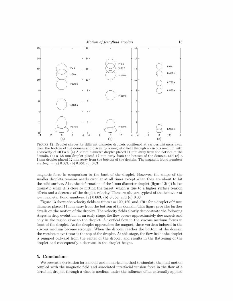
Figure 12. Droplet shapes for different diameter droplets positioned at various distances awayfrom the bottom of the domain and driven by a magnetic field through a viscous medium witha viscosity of 50 Pa s. (a) A 2 mm diameter droplet placed 11 mm away from the bottom of thedomain, (b) a 1.8 mm droplet placed 12 mm away from the bottom of the domain, and (c) a1 mm droplet placed 12 mm away from the bottom of the domain. The magnetic Bond numbersare Bom = (a) 0.063, (b) 0.056, (c) 0.03.

magnetic force in comparison to the back of the droplet. However, the shape of thesmaller droplets remains nearly circular at all times except when they are about to hitthe solid surface. Also, the deformation of the 1 mm diameter droplet (figure 12(c)) is lessdramatic when it is close to hitting the target, which is due to a higher surface tensioneffects and a decrease of the droplet velocity. These results are typical of the behavior atlow magnetic Bond numbers: (a) 0.063, (b) 0.056, and (c) 0.03.

Figure 13 shows the velocity fields at times t = 120, 160, and 170 s for a droplet of 2 mmdiameter placed 11 mm away from the bottom of the domain. This figure provides furtherdetails on the motion of the droplet. The velocity fields clearly demonstrate the followingstages in drop evolution: at an early stage, the flow occurs approximately downwards andonly in the region close to the droplet. A vortical flow in the viscous medium forms infront of the droplet. As the droplet approaches the magnet, these vortices induced in theviscous medium become stronger. When the droplet reaches the bottom of the domainthe vortices move towards the top of the droplet. At this stage, the flow inside the dropletis pumped outward from the center of the droplet and results in the flattening of thedroplet and consequently a decrease in the droplet height.

5. ConclusionsWe present a derivation for a model and numerical method to simulate the fluid motion

coupled with the magnetic field and associated interfacial tension force in the flow of aferrofluid droplet through a viscous medium under the influence of an externally applied


0 1 2 3 40

10

16

X−Axis0 1 2 3 4

0

10

16

X−Axis0 1 2 3 4

0

10

16

X−Axis0 1 2 3 4

0

10

16

X−AxisFigure 13. Velocity fields at times t = 120, 160, and 170 s (from left to right) for a droplet of

2 mm diameter placed 11 mm away from the bottom of the domain. Bom = 0.06.

magnetic field. The ferrohydrodynamic equations and a simple constitutive law are usedto model the magnetic force acting at the interface. The numerical boundary conditionfor the simulation of the magnetic field is based upon measured values at the centerlineof the domain in the absence of the drop. A conservative representation of the magneticfield force for immiscible two-fluid systems is derived.

The droplet undergoes dramatic deformation due to the presence of an external mag-netic field gradient. Its shape is influenced by the magnetic Bond number, as well asinertia. The simulations show that the droplet velocity is mainly influenced by the com-petition between the magnetic force which is proportional to the volume, and the viscousdrag force which is proportional to the radius. Hence, the larger the drop, the fasterthe speed. The initial distance between the ferrofluid droplet and the external magnet isvaried, and the simulated transit times agree well with the experimental measurementsof Mefford et al. (2007). Our study shows that the deformation of the drop accounts forthe difference in the transit times between prior models based on a spherical drop andthe experimental data.

This research is supported by NSF-DMS 0405810, NCSA TG-CTS060013N, and NSF-ARC Materials World Network for the Study of Macromolecular Ferrofluids (DMR-0602932 -LX0668968). We thank O. T. Mefford for discussions and data, and the refereewho provided extensive comments for improvement.


Appendix AThe force acting on a magnetic particle of magnetic moment m is μ0(m·∇)H (Rosensweig

1985). For a magnetized body, this leads to a force density

F = μ0(M · ∇)H. (A 1)

This expression for the magnetic force, however, is not meaningful in the presence ofan interface where both M and H have discontinuities. We therefore use the alternativeform

F = ((B − μ0H) · ∇)H = (B · ∇)H− μ0(H · ∇)H. (A 2)

Taking account of Maxwell’s equations div B = 0 and curlH = 0, we find

F = div(HBT − 12μ0∇|H|2). (A 3)

This conservative form remains meaningful in the presence of discontinuous interfaces.We now set σm = HBT. The second term, − 1

2μ0∇|H|2 is proportional to the identitymatrix, and is absorbed into the pressure field for the entire domain. This does not alterthe interfacial force balance because it is implicitly consistent with the weak formulationwhich is discretized.

In axisymmetric coordinates the magnetic stress tensor is

σm = μ

⎡⎢⎢⎣

(∂φ∂r

)2∂φ∂r

∂φ∂z 0

∂φ∂r

∂φ∂z

(∂φ∂z

)2

00 0 0

⎤⎥⎥⎦ , (A 4)

and

∇ · σm =[1r

∂

∂r[r(σm)rr] +

∂

∂z[(σm)rz]

]er (A 5)

+[1r

∂

∂r[r(σm)rz] +

∂

∂z[(σm)zz]

]ez,

where er and ez are unit vectors in r and z directions.In the momentum equation (2.12), the rate of deformation tensor in axisymmetric

coordinates is

Si,j =

⎡⎣ 2∂vr

∂r∂vr

∂z + ∂vz

∂r 0∂vr

∂z + ∂vz

∂r 2∂vz

∂z 00 0 2 vr

r

⎤⎦ , (A 6)

and

∇ · ηS =[1r

∂

∂r(rηSrr) +

∂

∂zηSrz − 1

rηSθθ

]er (A 7)

+[1r

∂

∂r(rηSrz) +

∂

∂zηSzz

]ez.

REFERENCES

Bacri, J. C. & Salin, D. 1982 Instability of ferrofluid magnetic drops under magnetic field.J. Phys. Lett. 43, 649–654.

Bashtovoi, V., Lavrova, O. A., Polevikov, V. K. & Tobiska, L. 2002 Computer modeling


of the instability of a horizontal magnetic-fluid layer in a uniform magnetic field. J. Magn.Magn. Mater. 252, 299–301.

Baygents, J. C., Rivette, N. J. & Stone, H. A. 1998 Electrohydrodynamic deformationand interaction of drop pairs. J. Fluid Mech 368, 359–375.

Brackbill, J. U., Kothe, D. B. & Zemach, C. 1992 A continuum method for modelingsurface tension. J. Comp. Phys. 100, 335–354.

Clift, R., Grace, J. R. & Weber, M. E. 1978 Bubbles, Drops, and Particles. AcademicPress.

Knieling, H., Richter, R., Rehberg, I., Matthies, G. & Lange, A. 2007 Growth of surfaceundulations at the Rosensweig instability. Phys. Rev. E. 76, 066301.

Lafaurie, B., Nardone, C., Scardovelli, R., Zaleski, S. & Zanetti, G. 1994 Modellingmerging and fragmentation in multiphase flows with SURFER. J. Comp. Phys. 113, 134–147.

Lavrova, O., Matthies, G., Mitkova, T., Polevikov, V. & Tobiska, L. 2006 Numeri-cal treatment of free surface problems in ferrohydrodynamics. J. Phys.: Condens. Matter18(38), S2657–S2669.

Lavrova, O., Matthies, G., Polevikov, V. & Tobiska, L. 2004 Numerical modeling of theequilibrium shapes of a ferrofluid drop in an external magnetic field. Proc. Appl. Math.Mech. 4, 704–705.

Li, J. & Renardy, Y. 1999 Direct simulation of unsteady axisymmetric core-annular flow withhigh viscosity ratio. J. Fluid Mech. 391, 123–149.

Li, J., Renardy, Y. & Renardy, M. 2000 Numerical simulation of breakup of a viscous dropin simple shear flow through a volume-of-fluid method. Phys. Fluids 12, 269–282.

Liu, Xianqiao, Kaminski, Michael D., Riffle, Judy S., Chen, Haitao, Torno, Michael,

Finck, Martha R., Taylor, LaToyia & Rosengart, Axel J. 2007 Preparation andcharacterization of biodegradable magnetic carriers by single emulsion-solvent evaporation.J. Magn. Magn. Mat. 311, 84–87.

Matthies, G. & Tobiska, L. 2005 Numerical simulation of normal-field instability in the staticand dynamic case. J. Magn. Magn. Mater. 289, 346–349.

Mefford, O. T., Woodward, R. C., Goff, J. D., Vadala, T. P., Pierre, T. G. St.,

Dailey, J. P. & Riffle, J. S. 2007 Field-induced motion of ferrofluids through immiscibleviscous media: Testbed for restorative treatment of retinal detachment. J. Magn. Magn.Mater. 311, 347–353.

Nickerson, C. S., Karageozian, H. L., Park, J. John & Kornfield, J. A. 2005 Internaltension: A novel hypothesis concerning the mechanical properties of the vitreous humor.Macromolecular Symposia 227, 183–189.

Patankar, S. V. 1980 Numerical Heat Transfer and Fluid Flow . McGraw-Hill Book Company.Rosensweig, R. E. 1985 Ferrohydrodynamics. Cambridge University Press, New York.Scardovelli, R. & Zaleski, S. 1999 Direct numerical simulation of free surface and interfacial

flow. Ann. Rev. Fluid Mech. 31, 567–604.Voltairas, P. A., Fotiadis, D.I. & Michalis, L.K. 2002 Hydrodynamics of magnetic drug

targeting. J. Biomechanics 35, 813–821.

field-induced motion of ferroï¬‚uid droplets through

Documents