field course in micrometeorology and hydrology · preface the 2011 vintage of field course in...

Field Course in Micrometeorology and

Hydrology Hyytiälä Forestry Field Station

29 Aug - 2 Sep, 2011

Division of Atmospheric Sciences

Department of Physics University of Helsinki

Finland

List of Participants

Hermanni Aaltonen

Juho Aalto

Olle Räty

Juris Burlakovs

Pavel Alekseychik

Saara Lind

Simon Schallhart

Johanna Joensuu

Anni Jokiniemi

Juha-Pekka Jurvanen

Olli Peltola

Jenni Kontkanen

John Backman

Olga Ritenberga

Sofia Mei-Kuei Tu

Juha Heikkilä

Timo Ryyppö

Pekka Rantala

Sami Haapanala

Janne Korhonen

Risto Taipale

Preface

The 2011 vintage of Field Course in Micrometeorology and Hydrology was extremely smooth, efficient, and relaxed. All measurements and data analyses were running already in the evening of the first day, reflecting the high motivation and performance of the students.

The course was held at the Hyytiälä Forestry Field Station of the University of Helsinki from 29 August to 2 September. The kick-off meeting on 28 August and the final meeting on 7 October were held at the Kumpula Campus in Helsinki. The students were from Austria (1), China (1), Finland (13), Latvia (2), and Russia (1).

The course topics were:

1. Rain 2. Eddy covariance fluxes 3. Evaporation from a lake, forest, and wetland 4. Atmospheric profiles in the first 100 meters 5. Thermodynamics of Finnish sauna

Each group prepared an introductory presentation on their topic, carried out practical work (measurements and data analysis) at Hyytiälä, and gave a presentation on their preliminary results. This booklet contains the final group reports.

The course feedback (see next page for a summary) was mainly positive, highlighting the pleasant ambience and the active role of the students. The main complaints were about the short duration of the course, the lack of hands-on measurements (Group 4), and the separate final meeting. In general, the students rated the course as “worthwhile” and the teachers as “proficient”. Thank you!

Helsinki, 12 December 2011

Teachers

Sami Haapanala, Janne Korhonen, and Risto Taipale University of Helsinki, Department of Physics, Division of Atmospheric Sciences

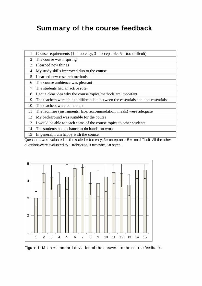
Summary of the course feedback

1 Course requirements (1 = too easy, 3 = acceptable, 5 = too difficult) 2 The course was inspiring 3 I learned new things 4 My study skills improved duo to the course 5 I learned new research methods 6 The course ambience was pleasant 7 The students had an active role 8 I got a clear idea why the course topics/methods are important 9 The teachers were able to differentiate between the essentials and non-essentials

10 The teachers were competent 11 The facilities (instruments, labs, accommodation, meals) were adequate 12 My background was suitable for the course 13 I would be able to teach some of the course topics to other students 14 The students had a chance to do hands-on work 15 In general, I am happy with the course

Question 1 was evaluated on the scale 1 = too easy, 3 = acceptable, 5 = too difficult. All the other questions were evaluated by 1 = disagree, 3 = maybe, 5 = agree.

Figure 1: Mean ± standard deviation of the answers to the course feedback.

1

2

3

4

5

1 2 3 4 5 6 7 8 9 10 11 12 13 14 15

I RAIN

FIELD COURSE IN MICROMETEOROLOGY AND HYDROLOGY

GROUP 1: RAIN

J. AALTO, H. AALTONEN & O. RÄTY

Field course in micrometeorology and hydrology, group 1: Rain Aalto, Aaltonen, Räty

1

INTRODUCTION

Of meteorological variables, rainfall or more generally precipitation which includes solid particles, has been observed and measured the longest time. Precipitation is a major part of global water cycle and affects all kinds of natural and socio-economical systems. The importance of high quality precipitation measurements has long been recognized because man-made systems are more vulnerable and sensitive to the large variability in precipitation. Also the scientific research on the impacts of precipitation changes to different natural systems, profits greatly from reliable observations. Therefore, the development of precipitation measurement technology is constantly going on.

Because currently used measurement methods still include significant errors and biases (eg. Sarkanen 1989, Solantie & Junnila 1995, Ciach 2003, Molini et al. 2005, Wagner 2009, Vuerich et al. 2009) it is important to evaluate the performance of different instruments and identify main problems related their performance. In this study we concentrate on differences between different measurement instruments and precipitation data series. As a part of the study, we conducted precipitation measurements over a week long period in the late-summer conditions with one recording and two traditional non-recording gauges. The data analysis concentrated on precipitation measurements conducted at Siikaneva I and Siikaneva II sites. Also the measurements done at Smear II station were used as data from three different instruments, a weighing gauge, an optical gauge and a tipping bucket gauge, were available. These site specific observations were compared against radar data two assess the usability of radar measurements at these locations. Finally, it was briefly tested what kind of results the tipping bucket gauge would give, if it was corrected with optical gauge data as tipping bucket measurements were found to be useless during winter due to its inability to measure solid rain.

MATERIAL AND METHODS

Precipitation measurement instruments

Rainfall can be measured either by in situ measurements or by remote sensing methods. Rain gauges, which are considered to be the most traditional way to collect precipitation data, offer site specific information on rainfall at varying frequencies depending on the instrument. These instruments can be divided into two categories: recording and non-recording gauges. Non-recording gauges are simple storage devices that measure cumulative precipitation over a certain period. Non-recording gauges are not anymore in operational use in Finland because data collection has to be made manually and is therefore laborious. Recording gauges, on the other hand, are designed to automatically record precipitation amount over a prescribed period and store it as a function of time. As the data used in this study was produced by several different types of recording gauges these are introduced below.

Weighing gauges

Weighing gauges collect a certain amount of rain into a usually cylindrical vessel and measures the weight of accumulated water. The intensity and depth of rainfall can then be calculated from these values. They are considered to be relatively reliable and accurate instruments although low intensity rainfall is usually underestimated (Michaelides 2008). For example, Finnish meteorological institute (FMI) uses operationally this type of gauges.

Tipping bucket rain gauge

Tipping bucket rain gauge measures rainfall by collecting water into a bucket that tips and drains after it has collected a certain amount of rainwater (figure 1). The bucket is installed so that a tipping triggers the magnetic switch which then sends a signal for a data logger. Tipping bucket gauge is not as sensitive for wetting or evaporation losses as non-recording gauges (Wagner 2009). During the


2

winter tipping bucket is useless without a heating and even with the heating results can have significant biases (Groisman et. al. 1994). Further, errors caused by splashing and wind can be problematic with tipping bucket gauge (Wagner 2009, Vuerich et al. 2009). In this work no corrections for wetting, splashing, evaporation or wind losses were studied, mainly due to lack of data or the insufficient temporal resolution of data. In this work we have concentrated on combination of different error factors related to tipping bucket mechanism itself. Based on Vuerich et al. (2009) these factors can be synthesized as follows:

- the uncertainty about the real volume of the bucket when the tipping movement is initiated - the possible different behavior of the two compartments of the bucket - the mechanical error due to the water losses during the tipping movement of the bucket

We were not able to examine these error factors separately in this study. Still it was possible to study the sum of these error factors based on the assumption that the optical rain measurement provides a benchmark for true rainfall.

Figure 1. The tipping bucket rain gauge mechanism (left picture after Marsalek 1981).

Optical gauges

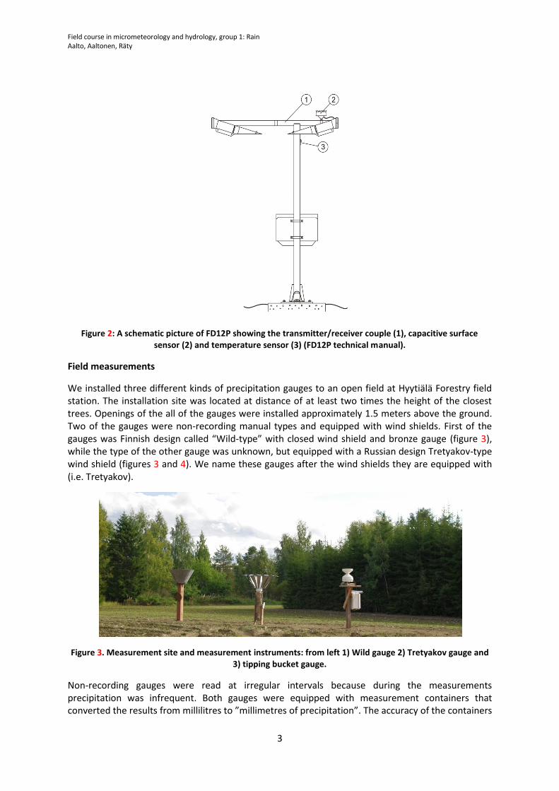
In comparison to older traditional cylindrical and other rainfall amount measuring devices, optical gauges that have been developed during the past couple of decades, base on measuring light scattering from different hydrometeors. Here we introduce Vaisala’s FD12P weather sensor (Vaisala, 2002), which was used in our study. FD12P has an optical sensor consisting of transmitter and receiver parts (see figure 2). The transmitter part, which is tilted 16.5° downwards, produces pulses of near infrared light. The receiver part is also tilted 16.5° downwards and therefore measures forward scattered light at an angle of 33°. This angle is used because it produces a stable response in different kinds of natural fog. The instrument can also detect precipitation droplets from the optical signal and further calculate the precipitation intensity as individual droplets cause rapid changes in the amplitude of scatter signal. The intensity estimate is proportional to the volume of the precipitation droplets.

In addition, with the help of DRD12 rain detector, FD12P can also classify the precipitation type. DRD12 is an analog capacitive surface sensor that measures capacitance changes induced by precipitation. This signal is proportional to the water amount in the sensing surfaces. This signal is converted into a voltage change for further analog measurements. A wind shield is also used to reduce wind induced errors. Further, to make categorization more reliable, a temperature sensor is attached to FD12P. According to manufacturer, the accuracy for precipitation rate is about 0.05mm/h but for the snow, the accuracy can be lower if proper calibration against a high quality weighing gauge is not done (Michaelides, 2008 s.59-72). Yet, in the case of weak precipitation, optical sensor should perform better than weighing or tipping bucket gauges.


3

Figure 2: A schematic picture of FD12P showing the transmitter/receiver couple (1), capacitive surface sensor (2) and temperature sensor (3) (FD12P technical manual).

Field measurements

We installed three different kinds of precipitation gauges to an open field at Hyytiälä Forestry field station. The installation site was located at distance of at least two times the height of the closest trees. Openings of the all of the gauges were installed approximately 1.5 meters above the ground. Two of the gauges were non-recording manual types and equipped with wind shields. First of the gauges was Finnish design called “Wild-type” with closed wind shield and bronze gauge (figure 3), while the type of the other gauge was unknown, but equipped with a Russian design Tretyakov-type wind shield (figures 3 and 4). We name these gauges after the wind shields they are equipped with (i.e. Tretyakov).

Figure 3. Measurement site and measurement instruments: from left 1) Wild gauge 2) Tretyakov gauge and 3) tipping bucket gauge.

Non-recording gauges were read at irregular intervals because during the measurements precipitation was infrequent. Both gauges were equipped with measurement containers that converted the results from millilitres to ”millimetres of precipitation”. The accuracy of the containers


4

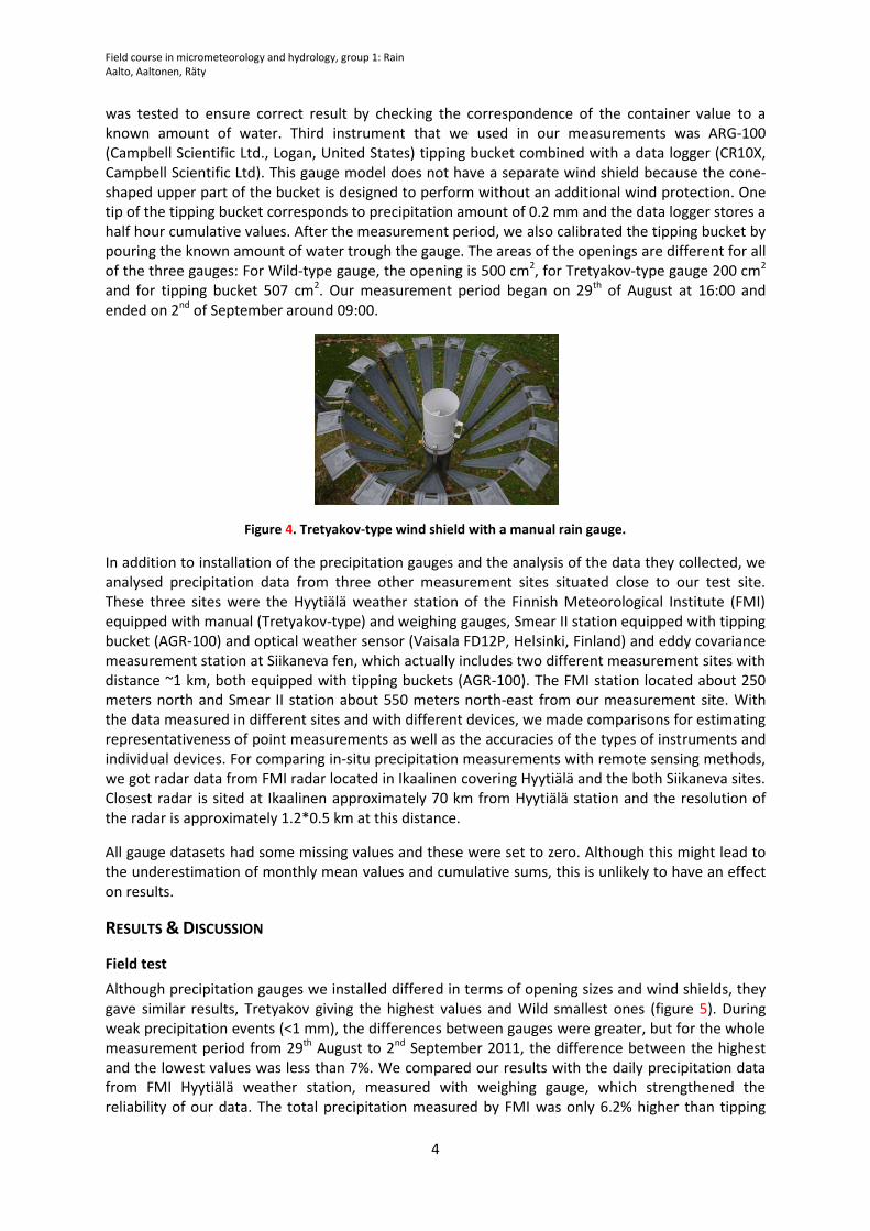
was tested to ensure correct result by checking the correspondence of the container value to a known amount of water. Third instrument that we used in our measurements was ARG-100 (Campbell Scientific Ltd., Logan, United States) tipping bucket combined with a data logger (CR10X, Campbell Scientific Ltd). This gauge model does not have a separate wind shield because the cone-shaped upper part of the bucket is designed to perform without an additional wind protection. One tip of the tipping bucket corresponds to precipitation amount of 0.2 mm and the data logger stores a half hour cumulative values. After the measurement period, we also calibrated the tipping bucket by pouring the known amount of water trough the gauge. The areas of the openings are different for all of the three gauges: For Wild-type gauge, the opening is 500 cm2, for Tretyakov-type gauge 200 cm2 and for tipping bucket 507 cm2. Our measurement period began on 29th of August at 16:00 and ended on 2nd of September around 09:00.

Figure 4. Tretyakov-type wind shield with a manual rain gauge.

In addition to installation of the precipitation gauges and the analysis of the data they collected, we analysed precipitation data from three other measurement sites situated close to our test site. These three sites were the Hyytiälä weather station of the Finnish Meteorological Institute (FMI) equipped with manual (Tretyakov-type) and weighing gauges, Smear II station equipped with tipping bucket (AGR-100) and optical weather sensor (Vaisala FD12P, Helsinki, Finland) and eddy covariance measurement station at Siikaneva fen, which actually includes two different measurement sites with distance ~1 km, both equipped with tipping buckets (AGR-100). The FMI station located about 250 meters north and Smear II station about 550 meters north-east from our measurement site. With the data measured in different sites and with different devices, we made comparisons for estimating representativeness of point measurements as well as the accuracies of the types of instruments and individual devices. For comparing in-situ precipitation measurements with remote sensing methods, we got radar data from FMI radar located in Ikaalinen covering Hyytiälä and the both Siikaneva sites. Closest radar is sited at Ikaalinen approximately 70 km from Hyytiälä station and the resolution of the radar is approximately 1.2*0.5 km at this distance.

All gauge datasets had some missing values and these were set to zero. Although this might lead to the underestimation of monthly mean values and cumulative sums, this is unlikely to have an effect on results.

RESULTS & DISCUSSION

Field test

Although precipitation gauges we installed differed in terms of opening sizes and wind shields, they gave similar results, Tretyakov giving the highest values and Wild smallest ones (figure 5). During weak precipitation events (<1 mm), the differences between gauges were greater, but for the whole measurement period from 29th August to 2nd September 2011, the difference between the highest and the lowest values was less than 7%. We compared our results with the daily precipitation data from FMI Hyytiälä weather station, measured with weighing gauge, which strengthened the reliability of our data. The total precipitation measured by FMI was only 6.2% higher than tipping


5

bucket estimate. Yet, one has to keep in mind that FMI weather station is situated 250 meters away from our measurement site having somewhat different surroundings and therefore the measurements may not be fully comparable. As the FMI data is daily averaged, we were not able to compare it with the data from manual gauges, which were emptied after individual precipitation events, not at daily basis.

During our measurements the weather was calm, all rain events were mainly light, and most important measurements were done in late summer conditions. Windy/stormy weather, heavy rains and especially snowfall would have elicited more differences between gauges depending on wind shields or for example the capacity of the tipping bucket. Besides the heavy rain induced problems, light precipitation events that we experienced several times during the measurement period, are difficult to measure correctly. With intermediate rain intensities, all the devices would have been measured more similar values in comparison to events with lighter or heavier precipitation intensity. In Finland, for example, several studies (e.g. Sarkanen 1989; Solantie & Junila 1995) have been made to generate operational correction factors for precipitation gauges. All these proposed corrections are quite complicated, consisting of several parameters about wind, the state of precipitation, and location of the measurements site. Measurements were not corrected due to short length of the measurement period.

Figure 5. Precipitation measured between 29 August and 2 September 2011 with the three different gauges

at the Hyytiälä Forestry field station.

Gauge climatologies 2006-2009

Climatological differences between the gauges were studied by comparing precipitation

measurements made with the FMI weighing gauge with the tipping bucket (and optical gauge

(FD12P) data measured at the Smear II station. The study period for which the climatological

parameters are calculated is from 2006 to 2009. Monthly mean precipitation values over this period

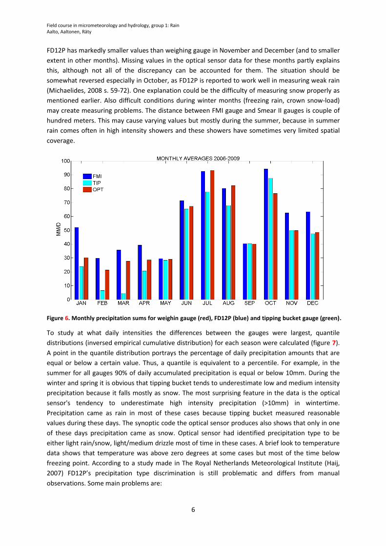
(figure 6) were calculated. From the three gauges, weighing gauge gives largest monthly

accumulated values except in June and July when FD12P measures slightly larger values. The tipping

bucket severely underestimates monthly accumulated precipitation during the winter. This is due to

the fact that the instrument cannot measure snowfall as it doesn't have any kind of heating that

would melt the snow. Also during the summer months tipping bucket underestimates rainfall

significantly in comparison to optical and weighing gauge. Reason for this is that for high intensity

rain tipping bucket tends to lost small amounts of water during a tip (Groisman et.al., 1994).

0

6

12

18

24

1 2 3 4 5 6 7 80

1

2

3

4

513

14

15 Tretyakov

Wild

Tipping bucket

Pre

cip

itation, m

m

Precipitation event

Cum

ula

tive p

recip

itation, m

m


6

FD12P has markedly smaller values than weighing gauge in November and December (and to smaller

extent in other months). Missing values in the optical sensor data for these months partly explains

this, although not all of the discrepancy can be accounted for them. The situation should be

somewhat reversed especially in October, as FD12P is reported to work well in measuring weak rain

(Michaelides, 2008 s. 59-72). One explanation could be the difficulty of measuring snow properly as

mentioned earlier. Also difficult conditions during winter months (freezing rain, crown snow-load)

may create measuring problems. The distance between FMI gauge and Smear II gauges is couple of

hundred meters. This may cause varying values but mostly during the summer, because in summer

rain comes often in high intensity showers and these showers have sometimes very limited spatial

coverage.

Figure 6. Monthly precipitation sums for weighin gauge (red), FD12P (blue) and tipping bucket gauge (green).

To study at what daily intensities the differences between the gauges were largest, quantile

distributions (inversed empirical cumulative distribution) for each season were calculated (figure 7).

A point in the quantile distribution portrays the percentage of daily precipitation amounts that are

equal or below a certain value. Thus, a quantile is equivalent to a percentile. For example, in the

summer for all gauges 90% of daily accumulated precipitation is equal or below 10mm. During the

winter and spring it is obvious that tipping bucket tends to underestimate low and medium intensity

precipitation because it falls mostly as snow. The most surprising feature in the data is the optical

sensor's tendency to underestimate high intensity precipitation (>10mm) in wintertime.

Precipitation came as rain in most of these cases because tipping bucket measured reasonable

values during these days. The synoptic code the optical sensor produces also shows that only in one

of these days precipitation came as snow. Optical sensor had identified precipitation type to be

either light rain/snow, light/medium drizzle most of time in these cases. A brief look to temperature

data shows that temperature was above zero degrees at some cases but most of the time below

freezing point. According to a study made in The Royal Netherlands Meteorological Institute (Haij,

2007) FD12P’s precipitation type discrimination is still problematic and differs from manual

observations. Some main problems are:


7

1. drizzle events are reported with the expense of precipitation events

2. sensor has problems reporting freezing rain properly

3. mixed precipitation (snow + rain) is underrepresented

4. ice pellets are reported too often

5. It does not detect hail

The study agrees with our results in that the winter conditions are problematic for FD12P because

the precipitation type is calculated both from optical and capacitive signal but does not point out

any reasons for these problems.

Figure 7. Quantile plots of daily accumulated precipitation for each gauge at each season.

During the summer and autumn daily precipitation amounts were very similar between all gauges, although weighing gauge measured slightly larger daily accumulated precipitation values. A notable detail is that at this period the largest value during the autumn was measured by tipping bucket gauge. As a summary, both instruments at Smear II location give smaller values than FMI weighing gauge outside summer months and especially during the winter Smear II data should be used extra cautiously.

Radar vs. gauge measurements

Both measurement sites at Siikaneva were equipped with similar kind of tipping buckets. However, as the measurements at Siikaneva site II was started only in July 2011, the dataset for the comparison of the interrelation of these two sites was short. As the landscape is flat and uniform around both sites, it was also optimal to evaluate the spatial representativeness of precipitation measurements. Radar measurements, which we compared to tipping bucket data, seemed to catch


8

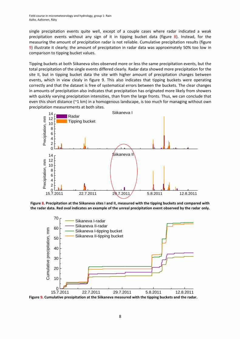
single precipitation events quite well, except of a couple cases where radar indicated a weak precipitation events without any sign of it in tipping bucket data (figure 8). Instead, for the measuring the amount of precipitation radar is not reliable. Cumulative precipitation results (figure 9) illustrate it clearly; the amount of precipitation in radar data was approximately 50% too low in comparison to tipping bucket values. Tipping buckets at both Siikaneva sites observed more or less the same precipitation events, but the total precipitation of the single events differed clearly. Radar data showed more precipitation for the site II, but in tipping bucket data the site with higher amount of precipitation changes between events, which in view clealy in figure 9. This also indicates that tipping buckets were operating correctly and that the dataset is free of systematical errors between the buckets. The clear changes in amounts of precipitation also indicates that precipitation has originated more likely from showers with quickly varying precipitation intensities, than from the large fronts. Thus, we can conclude that even this short distance (~1 km) in a homogenous landscape, is too much for managing without own precipitation measurements at both sites.

Figure 8. Precipitation at the Siikaneva sites I and II, measured with the tipping buckets and compared with the radar data. Red oval indicates an example of the unreal precipitation event observed by the radar only.

Figure 9. Cumulative presipitation at the Siikaneva measured with the tipping buckets and the radar.

15.7.2011 22.7.2011 29.7.2011 5.8.2011 12.8.20110

2

4

6

8

10

12

14

Pre

cip

itation, m

m

Siikaneva II

0

2

4

6

8

10

12

14

Pre

cip

itation, m

m Radar

Tipping bucket

Siikaneva I

15.7.2011 22.7.2011 29.7.2011 5.8.2011 12.8.20110

10

20

30

40

50

60

70

Cum

ula

tive p

recip

itation, m

m

Sikaneva I-radar

Siikaneva II-radar

Siikaneva I-tipping bucket

Siikaneva II-tipping bucket


9

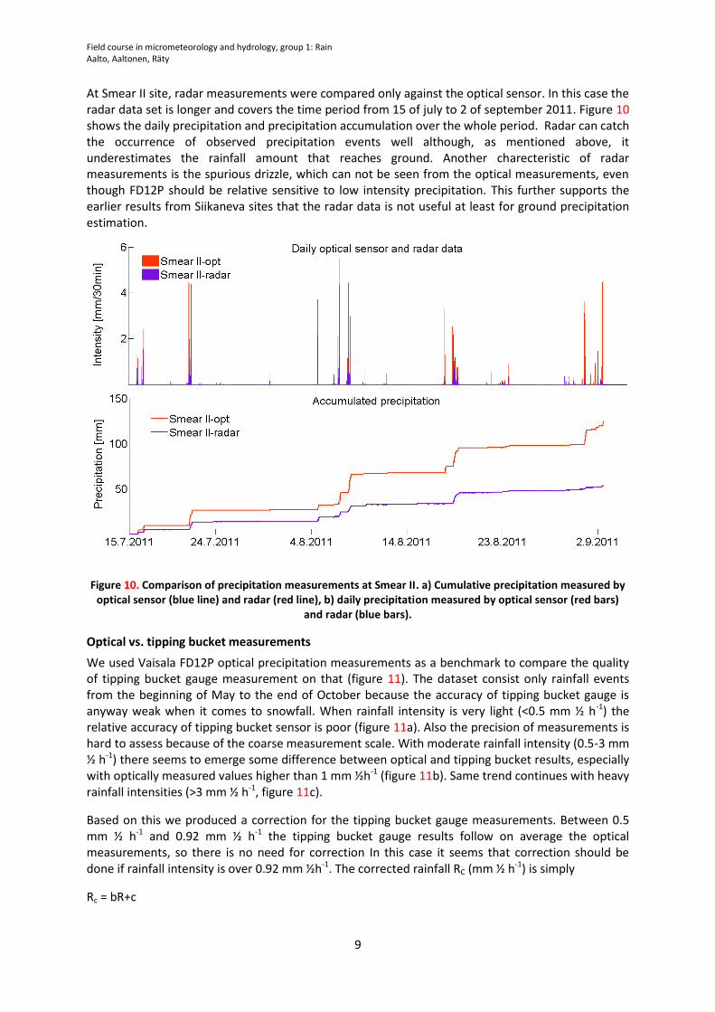
At Smear II site, radar measurements were compared only against the optical sensor. In this case the radar data set is longer and covers the time period from 15 of july to 2 of september 2011. Figure 10 shows the daily precipitation and precipitation accumulation over the whole period. Radar can catch the occurrence of observed precipitation events well although, as mentioned above, it underestimates the rainfall amount that reaches ground. Another charecteristic of radar measurements is the spurious drizzle, which can not be seen from the optical measurements, even though FD12P should be relative sensitive to low intensity precipitation. This further supports the earlier results from Siikaneva sites that the radar data is not useful at least for ground precipitation estimation.

Figure 10. Comparison of precipitation measurements at Smear II. a) Cumulative precipitation measured by optical sensor (blue line) and radar (red line), b) daily precipitation measured by optical sensor (red bars)

and radar (blue bars).

Optical vs. tipping bucket measurements

We used Vaisala FD12P optical precipitation measurements as a benchmark to compare the quality of tipping bucket gauge measurement on that (figure 11). The dataset consist only rainfall events from the beginning of May to the end of October because the accuracy of tipping bucket gauge is anyway weak when it comes to snowfall. When rainfall intensity is very light (<0.5 mm ½ h-1) the relative accuracy of tipping bucket sensor is poor (figure 11a). Also the precision of measurements is hard to assess because of the coarse measurement scale. With moderate rainfall intensity (0.5-3 mm ½ h-1) there seems to emerge some difference between optical and tipping bucket results, especially with optically measured values higher than 1 mm ½h-1 (figure 11b). Same trend continues with heavy rainfall intensities (>3 mm ½ h-1, figure 11c).

Based on this we produced a correction for the tipping bucket gauge measurements. Between 0.5 mm ½ h-1 and 0.92 mm ½ h-1 the tipping bucket gauge results follow on average the optical measurements, so there is no need for correction In this case it seems that correction should be done if rainfall intensity is over 0.92 mm ½h-1. The corrected rainfall RC (mm ½ h-1) is simply

Rc = bR+c


10

Figure 11. Tipping bucket vs. optical rainfall measurement. a) Light rainfall intensity. b) medium rainfall intensity. c) Heavy rainfall intensity.

Figure 12. Residual between optically measured and corrected tipping bucket rainfall measurement; there is

no connection between residual and the optically measured rainfall. The shadowed rectangle shows the ±2xSD area.

, where R is the uncorrected result, b is an empirical correction coefficient and c is an empirical constant. In this case the values for correction coefficient b is 1.16 and for constant c -0.14. After the correction there is no systematical error between Smear II optical and tipping bucket gauge measurements (figure 12). Systematic errors connected to light rainfall (intensity below 0.92 mm ½ h-1) are not studied or corrected. Also the considerable random errors still remain after correction. No other corrections (wetting, evaporation, wind, etc.) were conducted for any of these datasets.


11

How long one should measure with a tipping bucket gauge to reduce the error on acceptable level?

Because of the considerable random error short term tipping bucket gauge measurements can produce significant biases. When measurement period is prolonged the random error is decreased. Based on the real rainfall data recorded between the 1st of May 2005 and the 30th of June 2011 (only data from the beginning of May to the end of October, tipping bucket gauge data corrected with the correction method described earlier) we estimated the effect of measurement period length on measurement error.

The ranking (time vector) of the dataset was randomized 11 times to produce 11 observations for the development of the difference between cumulative optical and tipping bucket gauge measurements (figure 13). On average, the relation between target error and number of required measurement days D can be described with an equation

D = aEb

, where E is the target error, a=0.024 and b=-2.897. The deviation between different randomizations was considerably high. If a target error is wanted to achieve with 99% probability, the number of required measurement days is considerably higher when compared to average result (figure 13). With a good confidence it can be stated that the error is below 5% if the measurement period is at least one year. Still, one randomizing resulted considerably higher number of required measurement days than the upper 99% confidence level. It must be taken into consideration that the number of required measurement days is not fully normally distributed; in some cases the number of required measurement days can be quite a much higher than on average.

Figure 13. Number of measurement days required to achieve certain error level.

Tipping bucket correction and cumulative results

The effect of the tipping bucket gauge correction (see chapter: Optical vs. tipping bucket measurements) on annual cumulative precipitation is 3-6% (figure 14). The optical measurements produce on average 15% higher yearly cumulative precipitation when compared to the uncorrected tipping bucket gauge results, and on average 11% higher results when compared to the corrected tipping bucket gauge results. The results of the optical measurements are not higher than the corrected tipping bucket gauge results year after year.

The result is to some extent different when wintertime data (from the beginning of November to the end of April) is excluded (figure 15): then the effect of the correction is slightly higher (3.5-7%). The


12

optical measurements produce on average 1% higher annual cumulative precipitation when compared to the uncorrected tipping bucket gauge results, and on average 4% lower results when compared to the corrected tipping bucket gauge results.

Figure 14. Annual cumulative precipitation with different methods.

Figure 15. May-Oct cumulative precipitation with different methods.

In most years the optically measured cumulative precipitation matches reasonably with both the uncorrected and corrected tipping bucket gauge results. Our findings suggest that tipping bucket gauge gives acceptable results outside the wintertime. It’s worthwhile to notice that here the optical measurements produce on average 4% lower cumulative precipitation when compared to the corrected tipping bucket gauge measurements even after moderate and heavy rainfall events measured with the tipping bucket gauge are corrected to match the optical measurements. It is possible that this divergence is due to weaknesses of tipping bucket gauge when it comes to measuring light rainfall. But it is surprising that tipping bucket gauge seems to overestimate light rainfall instead of underestimating it. After all, this result can also be caused by some unknown phenomenon during years 2006 and 2007 when the optical measurement show considerably lower


13

cumulative precipitation than the tipping bucket gauge. It is also possible that the divergence between the optical and tipping bucket measurements stems from lack of any corrections (wetting, evaporation, wind, etc.) in our data calculation. On the other hand, also Ciach (2003) has reported 1-3% error to be normal for tipping bucket rain gauge.

CONCLUSIONS

In our field study we conducted precipitation measurements over a week period with two non-recording gauges (Wild and Tretyakov) and with a tipping bucket rain gauge. As the period was rather short, this case study gives only a qualitative picture of the similarities between the gauges in end-summer conditions. All the gauges gave very similar results, although due to short measurement period, the possibly differences between the gauges did not have enough time to occur.

Climatological similarities between precipitation data produced by FMI weighing gauge and two gauges in Smear II station were studied. Results show that the tipping bucket is useless during the local winter as it does not have any kind of heating that would melt the snow. FD12P have some difficulties in measuring high intensity precipitation in spring and winter conditions as it gives significantly smaller values than weighing gauge. Overall, results show that FMI measurements, based on daily and annual precipitation amounts, have largest values and that one should be very cautious when using winter time precipitation data from Smear II station.

To test the usability of radar data as it has large spatial coverage, a comparison between gauge and radar data was done both at Siikaneva I-II and Smear II station locations. Results show that although radar catches single events relatively well, precipitation amounts are significantly smaller than the observed ones. Also drizzle that cannot be seen in observations is present. This is due to the fact that radar measures conditions aloft the observation site. It can “see” low level clouds and precipitation that might evaporate before reaching the ground.

Finally, we tested how well tipping bucket measurements could be improved with the help of optical sensor data at summer conditions. As there were very few data from winter months, they were dropped out before constructing the correction relation. Corrected tipping bucket values for accumulated precipitation were close to optical sensor observations for the study months, although it has to mention that this correction was purely based on constructing statistical relationship between the gauge data sets, not removing physical problems related to instrument itself.

REFERENCES

Ciach, G.J. 2003: Local random errors in tipping bucket rain gauge measurements. J. Atmos. Oceanic Technol. 20, 752-759.

Groisman, Pavel Ya, David R. Legates, 1994: The Accuracy of United States Precipitation Data. Bull.

Amer. Meteor. Soc., 75, 215–227. doi: http://dx.doi.org/10.1175/1520-

0477(1994)075<0215:TAOUSP>2.0.CO;2

Haij, M. 2007: Automated discrimination of precipitation type using the FD12P present weather sensor: evaluation and opportunities. KNMI, R&D Information and Observation Technology,Netherlands, pp. 73.

Marsalek, J. 1981: Calibration of the tipping bucket rain gauge. J. of Hydrol. 53, 343-354.

Michaelides, S. 2008: Precipitation: advances in measurement, estimation, and prediction. Springer-Verlag,Berlin,Germany, pp. 540.

Molini, A., Lanza, L.G., La Barbera, P. 2005: The impact of tipping-bucket raingauge measurement errors on design rainfall for urban scale applications. Hydrol. Process. 19, 1073-1088.

http://dx.doi.org/10.1175/1520-0477%281994%29075%3C0215:TAOUSP%3E2.0.CO;2

http://dx.doi.org/10.1175/1520-0477%281994%29075%3C0215:TAOUSP%3E2.0.CO;2


14

Sarkanen, A. 1989: Sademittausten tuulivirheen korjausmenetelmä. FMI Meteorological publications 13.

Solantie, R. & Junila, P. 1995: Sademäärien korjaaminen Tretjakovin ja Wildin sademittarien vertailumittausten avulla. FMI Meteorological publications 33.

Wagner, A. 2009: Correction of precipitation measurements. FutMon C1-Met-29(BY). http://www.futmon.org/sites/default/files/documenten/Correction_of_precipitation_measurements.pdf

Vaisala, 2002: Weather Sensor FD12P, User's guide in English, Address: http://www.vaisala.com/en/services/technicalsupport/downloads/Pages/User-Manuals.aspx

Vuerich, E., Monesi, C., Lanza, L.G., Stagi, L., Lanzinger, E. 2009: WMO field intercomparison of rainfall intensity gauges. WMO, Instruments and observing methods, report no. 99. http://www.wmo.int/pages/prog/www/IMOP/publications/IOM-99_FI-RI.pdf

II EDDY COVARIANCE

Field Course on Micrometeorology and Hydrology Hyytiälä, Aug 29-Sep 2, 2011

Eddy Covariance Measurements

Group 2 Simon Schallhart, Saara Lind, Pavel Alekseychik, Juris Burlakovs

I. Introduction Flux measurements are widely used to estimate heat, water, and CO2 exchange, as well as methane and other trace gases. Eddy Covariance is one of the most direct and defensible ways to measure such fluxes. The method is mathematically complex, and requires a lot of care setting up and processing data. If net flux is away from the surface, the surface may be called a source. For example, a lake surface is a source of water released into the atmosphere in the process of evaporation. If the opposite is true, the surface is called a sink. For example, a green canopy may be a sink of CO2 during daytime, because green leaves would uptake CO2 from the atmosphere during the process of photosynthesis (Burba and Anderson, 2010). The general principle for flux measurement is to measure how many molecules are moving up and down over time, and how fast they travel. The essence of the method, then, is that vertical flux can be represented as a covariance between measurements of vertical velocity, the up and down movements, and concentration of the entity of interest. Such measurements require very sophisticated instrumentation, because turbulent fluctuations happen very quickly; changes in concentration, density or temperature are small, and need to be measured very fast and with great accuracy. The traditional Eddy Covariance method (EC) calculates only turbulent vertical flux, involves a lot of assumptions, and requires high-end instruments. On the other hand, it provides nearly direct flux measurements if the assumptions are satisfied. Measurements are of course never perfect, because of assumptions, physical phenomena, instrumental problems, and specifics of the particular terrain or setup. As a result, there are a number of potential flux errors, but they can be corrected. In addition to frequency response errors, other key sources of errors include the time delay between wind and concentration measurements (especially important in closed path analyzers with long intake tubes), spikes and noise in the measurements, unleveled instrumentation, the Webb - Pearman - Leuning density term, sonic heat flux errors, band-broadening (for NDIR measurements), spectroscopic effect (for LASER-based measurements), oxygen sensitivity, and data filling errors (Burba and Anderson, 2010). Broadly speaking, eddy covariance technique can be used for various measurements and most of them are counted further in this list: CO2, NH3, HNO3, HCl, HONO, SO2, NH4

+, NO3-, SO4

-, Cl-, VOC’s (f. ex., C2-benzenes, toluene, xylene), trace metals, various PM as well as for latent and sensible heat, ultra-fine, accumulation and coarse mode aerosols, accumulation mode aerosol chemical species, ozone, other types of oxides of nitrogen, formaldehyde. Most important for specific urban air quality monitoring are PM, NOx parameters – sometimes it is directed by the legislation. For

special cases (dump sites and landfills, oil terminals etc.) additional parameters are measured, such as methane, VOC’s, SOx and other. Forests are an important part of the global carbon cycle (Dixon et al., 1994) and the boreal forest in particular is thought to have a strong influence on the net CO2 exchange with the atmosphere (D’Arrigo et al., 1987; Bonan, 1991). Carbon budget models of forests show trends of a net forest carbon sink through the first two-thirds of the 20th century, followed by a decreasing sink and even a carbon source in the latter part of the century (Kurz and Apps, 1999; Chen et al., 2000). This time trend in the model estimates of carbon flux is caused by a changing disturbance regime, mostly driven by increased fire and insect activity. A substantial amount of recent research has been devoted to understanding the impacts of fire on the forest carbon balance (e.g., Harden et al., 2000; Kasischke and Stocks, 2000). For example, in Canada, about 2 million hectares of forest have burned annually on average from 1959 to 1999, with extreme fire years burning more than 7 million hectares (Weber and Stocks, 1998; Stocks et al., 2002). Mean direct carbon emissions from combustion in forest fires have been estimated at about 27 Tg C per year for this period (Amiro et al., 2001). The data from towers, aircraft, and remote sensing/ modeling measure different components of the carbon flux over a range of spatial and temporal scales. However, in all cases, the measurements show that fire reduces the net downward flux, which then increases over time for a period of 10–30 years following fire. Upward net fluxes are only apparent immediately (i.e., within 1 year) after fire and harvesting, and photosynthesis is greater than respiration during the day for the growing season, even during early succession. Although the daily summer-time integral of net ecosystem exchange (NEE) from towers, the afternoon values of NEE from aircraft, and the annual net primary productivity (NPP) estimates from remote sensing/modeling show similar trends with time since fire, we do not yet have annual estimates of NEE. It is likely that heterotrophic respiration during the non-growing season would reduce the annual NEE, perhaps changing the balance to a net carbon source for several years following disturbance. However, a complete carbon balance requires an annual estimate of net biome exchange (NBE), which would incorporate fluxes over the whole forest. (Amiro et al., 2003). During measurements in Hyytiälä area, the source of carbon emissions was also the post-fire boreal forest. The age of the burning event is approximately 2 years. Measurements were conducted by four students using the eddy covariance technique, using the Metek sonic anemometer mounted on mast, the gas analyzer LI-COR 7200 were combined and doing CO2 and H2O measurements at the approximate height of 182 cm from the surface.

Measurements were done during the field course of micrometeorology and hydrology, and those took place in Hyytiälä Forestry Field Station, Southern Finland from 29th of August till 2nd of September. This report is describing some general theoretical and applied aspects of applications of using the eddy covariance technique, as well as giving the inside look in materials and methods used during the field course, then results are given from the short period measurements with some explanations about data were gain from the field work. The report is open to the discussion, in order to correlate short period measurements with theoretical and practical aspects, as well as problems of measurement noises and other disturbing factors analyzed. Flux can be defined as an amount of an entity that passes through a closed (i.e., a Gaussian) surface per unit of time. II. Materials and methods Study site The study site is located near to the Hyytiälä Forestry field station (61° 50' 38.101'' N, 24° 17' 37.561'' E, 170m asl). The 30-year (1971-1990) mean annual air temperature and mean annual precipitation of the study site are 3.3 C and 731 mm, respectively (Drebs et al 2002). The controlled burning of the forest (0.8 ha) took place in June 2009. Prior to the burning there was mature spruce forest growing in the area. First the area was clearcut, stem wood was removed from the site but the slash was left. Since the burning, the area was left to develop on its own. Currently the main vegetation consists of fireweed (Epilobium angustifolium). During the measurement period the plant height was between 1 and 1.5m. The plants had already blossomed and turned to brown. The study site is surrounded by forest. There is also a steep slope from the northern edge down to the south. These factors, as well as the height of the vegetation, were limiting the possible locations for the flux measurements. Finally, the mast was mounted on a tree stump at the highest part of the study site close to the forest edge (Fig 1). Due to this choice, we had to remove all data from 20 to 120 wind directions since it originated from the forest which we were not interested in measuring. However, we were still able to collect an adequate amount of data. Flux measurements For the wind measurements, we used 3D sonic anemometer (model: USA-1 Standard, Metek, Germany) which measures wind components u,v and w and also the acoustic temperature (Ts). The measurement height was 1.82m. For the CO2/H2O concentration

analysis we used infrared gas analyzer (model: LI-7200, LiCor Biosciences, USA). The EC- flux is the covariance between the vertical wind speed (w’) and the high time resolution concentration (c’), as shown in eq.1.

' 'F w c (1) This assumption can be made if following criteria are fulfilled:

- horizontal homogeneous site - flux is turbulent - ‘slow’ chemical reactions (measurement = emission)

This enclosed instrument is somewhat combination of the open and closed path systems; it requires only a short inlet and it can be mounted outside close to the sampling point. It analyses the gas concentrations simultaneously. The inlet (Bev-a-line tubing) was attached under the anemometer with vertical offset of 20 cm and horizontal offset 3 cm to northeast. The inner diameter was 6 mm and length was 4.6 m. In our case, due to the short measurement campaign, there was no need to cut the inlet shorter. An insect screen was attached to the beginning of the inlet. Sample flow was controlled using a flow module (model: 7200-010, LiCor Biosciences, USA). Flow rate was calculated so that Reynolds number was above 2000; the flow in inlet would be turbulent. Calculation was done using eq.2. Flow rate of 8.6 l min-1 was adequate, but to be at the safe side flow rate of 12 l min-1 was used.

)(1000*(min)60**Re*Re lD

AvQvA

QD

H

H (2)

Re = Reynolds number (2000) Q = volumetric flow rate (m3 s-1) DH = D = hydraulic diameter of the inlet (0.006 m) A = cross-sectional area of the tubing (0.000028 m2)

v = kinematic viscosity (m2 s-1), further µv

µ = dynamic viscosity (0.00001837 kg (m*s)-1) = density (1.204 kg m-3)

To store and combine the gas concentration and wind data, analyzer control unit was used (model: LI-7550, LiCor Biosciences, USA). Communication between computer and control unit was done using Ethernet cable. LI-7200 Windows application software was used for the initial set up of the data collection to create the configuration file. The data items, which were collected, are listed in Table 1. For the sonic anemometer, auxiliary inputs were used. Values for the set up are given in Table 2. Data acquisition was done at 10 Hz with 30 min time frame. After the initial set up,

the data was stored on memory stick attached to the analyzer control unit. The measurements of CO2 and H2O fluxes were started on 29th of August and carried out until 2nd of September 2011. Table 1. Collected data items (Reference: Licor manual). Variable Description Time Time in HH:MM:SS:MS Date Date in YY:MM:DD Sequnce number Index value CO2 (mmol/m) CO2 concentration density CO2 Absorptance CO2 raw absorptance value CO2 (µmol/mol) CO2 mole fraction CO2 dry (µmol/mol) CO2 dry mole fraction H2O (mmol/m) H2O concentration density H2O Absorptance H2O raw absorptance value H2O (mmol/mol) H2O mole fraction H2O dry (mmol/mol) H2O dry mole fraction Dew Point (°C) Dew point temperature Cell Temperature (°C) Weighted average temperature of Tin and Tout Temperature In (°C) Temperature at sensor head inlet Temperature Out (°C) Temperature at sensor head outlet Block Temperature (°C) Temperature at IRGA block Total Pressure (kPa) LI-7550 box pressure+head pressure Box Pressure (kPa) Pressure measured at LI-7550 Head Pressure (kPa) Differential pressure measured at sensor head (head-box) Cooler Voltage (v) Detector cooler voltage Diagnostic Value Diagnostic value 0-8191 AGC Automatic gain control 7550 Auxiliary Input 1 Aux 1 7550 Auxiliary Input 2 Aux 2 7550 Auxiliary Input 3 Aux 3 7550 Auxiliary Input 4 Aux 4 Flow Pressure (kPa) 7200-010 pressure (0-5 kPa) Flow Rate (slpm) 7200-010 flow rate in mass flow units of Stardard Liters Per Minute Flow Rate (lpm) 7200-0101 volumetric flow rate corrected for temperature and pressure Flow Power (V) Voltage applied to 7200-010 motor Flow Pressure (kPa) 7200-010 pressure drop, indicates the amount of flow restriction Flow Drive (%) Drive input to 7200-010 displayed as a percentage Integral Integration result Peak Height Integration peak height

CO2 Sample Floating point value, power received from source in absorbing wavelength for CO2

CO2 Reference Floating point value, power received from source in reference wavelength other than CO2

H2O Sample Floating point value, power received from source in absorbing wavelength for H2O

H2O Reference Floating point value, power received from source in reference wavelength other than H2O

Table 2. Anemometer setting during data collection Input Parameter Gain Offset Aux 1 u 8 -20 Aux 2 v 8 -20 Aux 3 w 0.8 -2 Aux 4 Ts 8 -10 Data processing The flux calculations were done using EddyPro Express post-processing software (version 2.3.0, LiCor Biosciences, USA). III. Results Footprint The flux footprint (short: footprint) is the upwind area where emissions are measured by the eddy covariance instruments. In other words, it is the area containing the effective surface sources and sinks contributing to a given measurement point (Kljun et al., 2004). The positioning of the instrument affects this area, as the height of the inlet in principal determines the size of the footprint. The higher the inlet is, the bigger the footprint is. Also the surface roughness influences the size of the measured emission-area. If the measurements take place in a small valley, less area will influence on the measurements, than if the measurement site is in the middle of a plain. Another important factor is the stability of the atmosphere. Strong winds can enlarge the footprint and the wind direction can be the parameter which decides if the measured emissions are from a burned forest or healthy a Scots pine forest. In the field course we decided to measure at the east part of the burned forest, because the common wind direction during the day is south west. In Fig 1 the 70% footprint (70% of the measured emissions are emitted from this area) of our 4 day measurements is shown. The wind direction between 15° and 120° are not useful for our task, as the measured air is from the not burned forest.

Figure 1: Position of the measurement instruments (green arrow) and the 70% footprint area (black circle). The brown area is the burned forest (ignited 2 years ago) and the dark green area is the Scots pine forest. When the wind direction was between 15° and 120° the collected data originated from forest. Time lag Another critical parameter is the lag time. It describes the time difference between measurements, which can occur when instruments do not have the same time settings (different computer clocks) or when one measurement has a time delay, e.g. due to a long inlet line. This lag time is often defined as the maximum of the absolute value of the covariance between the vertical wind speed and the gas concentration in a specified lag time window Fig 2).

-3 -2 -1 0 1 2 30.04

0.05

0.06

CO

2 co

v [m

ol m

-2 s

-1]

lag time [s]

lag times

-3 -2 -1 0 1 2 30.02

0.03

0.04

H2O

cov

[mol

m-2

s-1

]

Figure 2: Lag time spectra calculated with a Matlab routine for one 30min file. A clear maximum of the CO2 covariance coefficient is visible at approx. 0.4 s The water lag time however shown no time lag (maximum at approx. 0 s), which can be a sign of problems with the data. In our setup we calculated the residence time of the sample air in our inlet line, which was 0.6 s (nominal lag time). Based on this the program EddyPro calculated the lag time, which can be up to 3 times the nominal lag time. If there was no significant maximum in the covariance coefficients, 0.6 s was used as the lag time. To check if the lag time was correct, we made one run with 10 s as an upper lag time limit and compared the results. Different results can be seen in Fig 3.

Figure 3: Lag times calculated with the nominal lag time of 0.6 s (x-axis) and a maximum lag time of 10 s (y axis). The nominal lag time in EddyPro is used as an approximation: The program calculates the lag time in a three times nominal lag time window. If no covariance maximum is found, it uses the nominal lag time. It is clearly visible that the biggest difference is at the 0.6 s point, where without a nominal lag time, the program is free to choose longer lag times. As in this graph are 130 data points, mind that some are overlapping.

0

2

4

6

8

10

12

0,00 0,20 0,40 0,60 0,80 1,00 1,20 1,40 1,60 1,80

10 s

ec la

g[s

]

0.6s nom. lag [s]

There are some deviations which are quite interesting; the 10 s lag times which are under 2 s but are not matching with the 0.6 s lag times must be a mistake, as the data set of both calculations was the same. Most change in the time is at 0.6 s, because there are all data points, where no significant maximum could be found in a 1.8 s range. As it seems that the lag time is quite dependent on the choice of the upper limit, we also looked at the influence to the actual flux (Fig 4). Most of the data points are showing no significant change, but the slope of the graph changes from 1 (perfect match) to 1.08. The overall flux over the shown time period rises 12% with the 10 s time lag limit.

Figure 4: Comparison between the CO2 flux with a nominal lag time of 0.6 s and a lag time maximum of 10 s. Just by choosing different lag time limits the slope changed to 1.08.

y = 1.0806x + 0.1888R² = 0.9023

-40,00

-20,00

0,00

20,00

40,00

60,00

80,00

100,00

-40,00 -20,00 0,00 20,00 40,00 60,00 80,00

CO

2flu

x 10

s la

g tim

e [µ

mol

m-2

s-

1 ]

CO2 flux 0.6s nom. lag time [µmol m-2 s-1]

Fluxes & other relevant quantities The EC campaign did not proceed at the desired environmental conditions for the whole of the measurement period. In particular, the air humidity was quite high, indicating the enhancement of the tube transport issues in the enclosed-path gas analyser, and the wind directions were generally exactly the opposite than what we hoped for. The calculated CO2 and H2O fluxes and auxiliary quantities (wind direction, sensible heat flux and friction velocity) are demonstrated in Fig. 5. All this resulted in the big systematic errors, especially visible in the calculated gas fluxes. The unrealistically high CO2 and H2O fluxes both occurred exquisitely at measured RH higher than 90% (Fig. 6), which is again suggestive of the tube condensation problem (also coincided with the night time periods).

Fig. 5. Water vapor and CO2 fluxes, wind direction, sensible heat flux and the friction velocity measured at the burned-down forest site since the evening of 29.08 until noon of 01.09.2011. The ‘bad’ wind directions are restricted to the region between the two horizontal lines.

Fig. 6. Relation between the measured relative humidity and the fluxes. There was an apparent systematic error with u* data: it was never less than ~0.15 m/s. We do not know the reason for such an offset from the expected values. There might have occurred an unknown malfunction/bug in the EddyPro software, or at some other postprocessing step, although this seems improbable. However, the experiment did produce some realistic gas and energy fluxes data. In particular, when the undesired wind directions (i.e. from the nearby forest edge) are filtered out, we can see a rather feasible CO2 flux pattern (Fig. 7). This might also be the indication of certain stability problems, arising from the complex situation at the borderline of the forest and the field grown with dry weeds. The average CO2 flux showed in that case a moderate respiration on the order of 2-3 µmol m-2 s-1.

Fig. 7. The CO2 flux values after the undesired wind directions were removed (red – nighttime, blue – daytime). The outliers are marked with the rectangles. Spectral analysis of the measured quantities was performed in order to access the quality of the final flux values and the credibility of the raw measured data. The nighttime spectra seem to be affected by the high-frequency attenuation (too rapid fall-off at high frequencies due to the tube attenuation), whereas the daytime spectra might be suffering from some white noise (Fig. 8). The tube attenuation problem becomes even better visible in the water spectra for night and day time (Fig. 9). It is easy to see, that the nighttime measurements are affected by a severe underestimation of the high-frequency concentration fluctuations. On this evidence, it is obvious that tube heating is essential for the functioning of the closed- and enclosed-path gas analyzers, as well as for the ultimate output of the EC technique. The unheated tube, especially in the humid conditions, is very unbeneficial for the EC measurements, which require quite very precise measurement of temporally small fluctuations in the gas concentrations

Fig.8. Daytime and nighttime CO2 and w spectra and cospectra (30.08.2011, 5:15 and 13.15), plotted versus the normalized frequency.

Fig. 9. Daytime and nighttime water vapor concentration spectra (30.08.2011, 5:15 and 13.15), plotted versus the normalized frequency.

Conclusions The 3-day EC measurement campaign at the forest burning site has generally proceeded according to standard practices and yielded the following results. The absence of the inlet tube heating had a deteriorating effect on the measured CO2 and H2O concentrations, as there was a considerable water condensation inside the tube, which had in turn been reflected in the calculated CO2 and H2O fluxes. During the periods free of condensation and with the synoptic wind blowing from the desired directions, we could register the moderate CO2 flux of about 2-3 µmol m-2 s-1, and water vapor flux of 1-2 mmol m-2 s-1. However, the choice of the lag time on the postprocessing stage proved to be an important parameter, inducing an order of 10% uncertainty in the fluxes.

IV. References Amiro, B.D., J.I. MacPherson, R.L. Desjardins, J.M. Chen, and J. Liu, 2003. Post-fire carbon dioxide fluxes in the western Canadian boreal forest: evidence from towers, aircraft and remote sensing. Agricultural and Forest Meteorology 115: 91-107. Amiro, B.D., 2001. Paired-tower measurements of carbon and energy fluxes following disturbance in the boreal forest. Global Change Biol. 7, 253–268. Bonan, G.B., 1991. Atmosphere–biosphere exchange of carbon dioxide in boreal forests. J. Geophys. Res. 96, 7301–7312. Burba G. and D. Anderson. 2010. A Brief Practical Guide to Eddy Covariance Flux Measurements: Principles and Workflow Examples for Scientific and Industrial Applications. Lincoln, Nebraska, LICOR. 214 p. Chen, J., Chen, W., Liu, J., Cihlar, J., 2000. Annual carbon balance of Canada’s forests during 1895–1996. Global Biogeochem. Cycles 14, 839–849. D’Arrigo, R., Jacoby, G.C., Fung, I.Y., 1987. Boreal forests and atmosphere–biosphere exchange of carbon dioxide. Nature 329, 321–323. Dixon, R.K., Brown, S., Houghton, R.A., Solomon, A.M., Trexler, M.C., Wisniewski, J., 1994. Carbon pools and flux of global forest ecosystems. Science 263, 185–190. Harden, J.W., Trumbore, S.E., Stocks, B.J., Hirsch, A., Gower, S.T., O’Neill, K.P., Kasischke, E.S., 2000. The role of fire in the boreal carbon budget. Global Change Biol. 6 (Suppl. 1), 174–184. Kasischke, E.S., Stocks, B.J. (Eds.), 2000. Fire, climate change, and carbon cycling in the boreal forest. Ecological Studies 138. Springer, New York.

Kljun, N., P. Calanca, M. W. Rotach, and H. P. Schmid. 2004. A simple parameterization for flux footprint predictions. Boundary Layer Meteorology, 112: 503-523. Kurz, W.A., Apps, M.J., 1999. A 70-year retrospective analysis of carbon fluxes in the Canadian forest sector. Ecol. Appl. 9, 526–547. LI-7200 CO2/H2O Analyzer Instruction Manual, pp. 56-57. Stocks, B.J., Mason, J.A., Todd, J.B., Bosch, E.M., Wotton, B.M., Amiro, B.D., Flannigan, M.D., Hirsch, K.G., Logan, K.A., Martell, D.L., Skinner, W.R., 2002. Large forest fires in Canada, 1959–1997. J. Geophys. Res. (in press). Weber, M.G., Stocks, B.J., 1998.Forest fires and sustainability in the boreal forests of Canada. Ambio 27, 545–550.

III EVAPORATION

FIELD COURSE IN MICROMETEOROLOGY AND HYDROLOGY

Evaporation from a Forest, Wetland and Lake Final Report of the Field Course

Johanna Joensuu, Anni Jokiniemi, Juha-Pekka Jurvanen, Olli Peltola

30.9.2011

1. Introduction

Evaporation is an important part of the water cycle. It is the only way the water gets up to the air to form clouds and rain. It makes vegetation dry and wetness disappear from a rock´s surface, especially in the sunshine.

There are two ways water may be transformed from liquid phase to gas. Transpiration is a process where water comes from plants. Their roots suck water from the ground and they transport it up to the leaves and needles. The water will be released as water vapour to the air within the plants vital functions. The other way is that liquid water transforms to gas strait from any kind of surface, like rocks and lake. This is called evaporation. There is also a term interception for evaporation from plants surface, but the mechanism is the same as in evaporation. In interception water does not come from inside the plant but the water has precipitated on the leaves and evaporates from them without any touch with the ground. Usually evaporation and transpiration are difficult to separate and they are treated together as evapotranspiration. Unfortunately the term evaporation is also commonly used even though people mean evapotranspiration. In this report we are using the more scientific term evapotranspiration.

The amount of evaporation depends on several things. The main factor is the available amount of heat. The most important heat source is sunshine, but in some circumstances a significant part of the energy might come from below, from a warm lake, ground or infrastructure, for example. Also the surface materials have differences because they might absorb the energy well or reflect most of the radiation away. The amount of water has significance too. If the evaporative surface is very wet or even pure water, the possibility for evaporation is bigger than in a dryer place. Also if the air above the surface is saturated or already contains a lot of water vapour, evaporation will not happen or will be small. In this part wind has a big role, because it carries evaporated vapour away so that there is more room for water to evaporate. That is the reason why evaporation is bigger in the windy weather than when it is still.

In vegetated ecosystems, such as forests and wetlands, the vegetation itself has a significant effect on evaporation by modifying its transpiration response to environmental conditions (such as light, temperature and humidity). Considerable differences in evaporation between different types of vegetation were first documented in the 1950’s (Law 1956).

Plants can and do control their gas fluxes by varying the aperture of stomata (Fig.1), small openings on leaf surfaces. Plants open their stomata to let in CO2, which they need for

photosynthesis. At the same time, water vapor escapes into the atmosphere. The CO2 and H2O fluxes of a plant are therefore closely connected. The stomata respond to a variety of environmental variables; for instance, the water content of the air and soil, temperature, radiation and leaf water potential. An increase in VPD (vapor pressure deficit) leads to closing of stomata, representing a negative feedback mechanism.

Another difference in evaporation in different ecosystems arises from interception loss, when some of the precipitation is intercepted in the canopy. The role of interception loss in evaporation from a forest can be significant (e.g. Calder 1976). In low-growing vegetation, this effect is much smaller.

Our aim regarding this field course was to measure the rate of evapotranspiration from three different measurement sites from the same period of time with the eddy covariance method and compare the results. In addition to that our aim was to determine the evaporation rate from the

Figure 1: Tomato leaf stomata. Photo: Wikimedia Commons

Lake Kuivajärvi with at least two methods and then compare the results of these different methods. The data for comparing methods was collected during our stay at Hyytiälä while the data for comparing different sites was measured last year with eddy covariance technique.

In order to compare different methods of measuring evaporation from the Lake Kuivajärvi we decided to use eddy covariance method as our reference measurement. Other means of measuring evaporation from the lake were aerodynamic method and evaporation pans.

We also did some more specific experiments about the circumstances in the lake that effect to the evaporation. Usually, the water surface temperature is an avoided variable when estimating evaporation, because it is so difficult to define. While doing the other measurements, we wanted to observe ourselves how difficult it is to measure and how the temperature changes vertically in the lake and air above it. We wanted to see if there is a big difference in temperatures in the lake and air and whether it is possible to estimate water surface temperature by temperature in 20 cm under or air temperature.

2. Materials and Methods

2.1 Sites The SMEAR II station (Station for Measuring Forest Ecosystem-Atmosphere Relations) is located in Hyytiälä, Southern Finland (61°31' N, 24°17' E, 181 m above sea level). The measurements are done in a southern boreal pine-dominated (Pinus sylvestris L.) stand that was sowed in 1962. The site is relatively rocky and nutrient-poor, classified as Vaccinium type according to the Finnish forest site type classification system. The annual average temperature is 3.3 °C and mean precipitation 713 mm.

The Siikaneva station is located some 5 km west of the SMEAR II site on a southern boreal sedge fen. The fen is treeless and oligotrophic (nutrient-poor). The peat depth at the research site varies between two and four meters. Dominant plant species are mosses, sedges and rannoch-rush (Scheuchzeria palustris L.).

Lake evaporation is measured in Lake Kuivajärvi next to Hyytiälä station. It is a small oblong lake. It´s total length is about 2.5 km but the widest place is only a little more than 300 meters. The area of the lake is 61 ha and it has almost 6 km coastline. Lake Kuivajärvi is a part of Kokemäenjoki ´s water system, one of the most distant lakes of it. That means that a water droplet from Kuivajärvi flows once through Kokemäenjoki to the Baltic Sea, if not evaporated before that. (OIVA 29.8.2011)

2.2 Eddy covariance method

Eddy covariance (EC) method is based on measuring three wind components and gas concentration with high sampling frequency. Usually at least 10 Hz sampling frequency is used. Measurements need to be conducted many times in a second in order to measure all relevant turbulent motions of air. The method relies on the assumption that the measured vertical turbulent flux equals the flux at the surface-atmosphere interface. This assumption is valid over horizontally homogeneous terrain when turbulence is stationary. However eddy covariance measurements can be conducted also above unideal terrain but then surface heterogeneities may induce error to the measurements. The vertical turbulent flux Fc can be calculated as covariance between vertical wind component w and gas concentration c:

(1

2.2.1 Instruments to measure eddy covariance

Evaporation, CO2 flux, sensible heat flux and momentum flux were measured at all the three sites (SMEAR II, Siikaneva and Lake Kuivajärvi) with eddy covariance method. 10 Hz sampling

frequency was used at all three sites and the fluxes were calculated as 30 min averages. The time period used for the analysis was May-October 2010. For Kuivajärvi, data was only available from June and there were significant gap in the dataset.

At the forest site SMEAR II evapotranspiration, CO2 flux and sensible heat flux were measured with sonic anemometer (Solent 1012R, Gill Instruments Ltd., Lymington, UK) and CO2/H2O gas analyzer LI-6262 (Li-Cor Biosciences, USA). The anemometer was situated at 23.3 m height. The tube used for sampling air for LI-6262 was 7 m long and the tube inlet was situated 15 cm below the sonic anemometer. The underlying forest was approximately 18 m high resulting roughly in 13.5 m displacement height.

At the second site, which is located at Siikaneva fen, the used sonic anemometer was USA-1 (METEK, Germany) and CO2/H2O gas analyzer was LI-7000 (Li-Cor Biosciences, USA). Measurement height, i.e. the height where the sonic anemometer is situated, was 2.75 m. Sampling tube attached to LI-7000 was 16.8 m long and the tube inlet was situated 25 cm below the sonic anemometer. Vegetation at the site was low and thus the displacement height was effectively zero.

Evaporation from Lake Kuivajärvi was measured on a raft with eddy covariance method. Sonic anemometer USA-1 (METEK, Germany) and CO2/H2O infrared gas analyzer LI-7000 (Li-Cor Biosciences, USA) were employed to obtain wind, air temperature, CO2 and H2O high frequency data. Air was sampled to LI-7200 gas analyzer with short sampling tube. The sonic anemometer was situated 1.5 m above the water surface and the sampling tube inlet slightly below the anemometer.

In addition to comparing just the evaporation values on each site we compared the effect of CO2 flux, vapor pressure deficit VPD and photosynthetically active radiation PAR. Vapor pressure deficit (VPD, unit kPa) is a representation of how much more water the air could hold in addition to what's already there. This depends on the saturation pressure of water vapor (a function of temperature) and the amount of water present in the air. The latter can be measured as relative humidity (RH, %) or concentration of water vapor (mmol/mol). Since both measures are available from the measurement sites, we compared the VPD values achieved using the two methods at SMEAR II and Siikaneva.

Saturation pressure was calculated as

= 22105649,25 )/( )

(2

where T = temperature (K) (Treier & Palge).

Water vapor pressure was calculated either as

= × (3

Where c_wv = concentration of water vapor (mmol/mol) and P_amb = ambient air pressure (hPa)

Or as

2 = (4

Where P_sat = saturation pressure (Pa) RH = relative humidity (%).

VPD was then calculated as

(5

2.3 Aerodynamic Method

There are several different aerodynamic methods for determining evaporation but we decided to use the bulk-aerodynamic transport equation, which is:

= | |( ) (6

where E is water vapor flux [mmol m-2 s-1], density of the dry air [kg m-3], Cq transfer coefficient for the humidity, |V| absolute value of the wind speed [m s-1], q0 specific humidity [kg kg-1] at the surface of the water and qa specific humidity in the air. The temperature used in q0 calculations was the half-hourly averaged temperature measured 20 cm below the water surface. The density of the dry air was estimated with ideal gas law: = (7

where P is the atmospheric pressure of the dry air [Pa], Rd the gas coefficient of the dry air – Rd = 287 [J kg-1 K-1] and T the air temperature [K]. The transfer coefficient Cq for the humidity was calculated with the following equation:

) ) (8

where k is the von Karman constant (here k = 0.4), z the height of the measurement point - here 1.6 m, z0m the roughness parameter of the surface – here 10-4 m, z0q the height where the surface humidity is q0 – here z0m = z0q and the stability parameter:

= (9

where z is the measurement height and L is the Monin-Obukhov length. EddyPro calculated directly from the data. m and q are the diabatic correction functions:

= 2 + tan , when < 0 (instable stratification) (10

, when > 0 (stable stratification) (11

= 0 , when = 0 (neutral stratification) (12

and

= 2 , when < 0 (instable stratification) (13

, when > 0 (stable stratification) (14

= 0 , when = 0 (neutral stratification) (15

Factors X and Y in above relations are as follows:

= (1 16 ) (16

= (1 16 ) (17

The absolute value of the wind speed mentioned in equation 6 is taken directly from the measurements. Specific humidity q is calculated with the following equation:

= 0,622 (18

where e is the water vapor pressure [Pa] and p is the atmospheric pressure [Pa]. The atmospheric pressure p was given by the measurements but the water vapor pressure e was calculated from the following equation:

= (19

where RH [%] is the relative humidity and esat [Pa] is the saturation water vapor pressure in a given temperature. Saturation water vapor pressure was calculated with the following equation:

( ) = 610,78 (20

where T [°C] is temperature. We got RH, T, p and directly from the measurements so we were able to calculate all the needed factors in eq. 7 in order to determine the rate of evaporation with aerodynamic method.

2.3.1 Measurement mast for aerodynamic method

Our measurement mast was 4.3 m long wooden plank. We attached three temperature and humidity measurement devices at three levels on the mast. Measurement levels from lowest to highest were 0.2 m, 2.1 m and 4.3 m. The surface of the measurement raft itself was some 0.2 m above the water surface. We attached tinfoil cases above the temperature and humidity measurement devices so that they were protected from precipitation and thus from “extra” humidity.

2.3.2 Temperatures in the lake and air

We also did some more specific experiments about the circumstances in the lake that effect to the evaporation. We measured the surface water temperatures and the temperature profile in the lake too. Usually, the surface water temperature is an avoided variable in estimations, because it´s so difficult to define. We wanted to observe ourselves how difficult it is to measure and how the temperature changes vertically in the lake and air above it and estimate the error made by using temperature in 20 cm below instead of the real surface temperature .

Water temperatures deeper in the lake were from below the raft. There is a constant measurement of temperatures in different depths. In practice, there are 15 probes tied in different depths and they measure the temperature in that point every 10 minutes and send the data out. The uppermost probe was situated 20 cm below the water surface and is measuring so called surface temperature, which may be reported in the news and forecasts, even though the real surface temperature might be totally different. Nevertheless it would be impossible to set a probe right below the water surface, because of the waves and water level changes. It is also in safer place hidden under the water.

To measure surface and air temperatures we used three kinds of thermometers. The measurements were done during our visits to the raft for other reasons on Monday, Wednesday and Friday. The first temperature instrument we used was an infrared thermometer. It looks a bit like a gun and is pointed to the target so it´s sensor captures the infrared radiation the targets surface sends and changes it to Celsius grades to the screen, so that the very top layer is measured. We also had an old fashioned thermometer containing just expanding liquid. One measurement was also done with a digital thermometer. The two latter instruments were calibrated

Figure 2: The raft and the mast

by putting them to boiling water and checking the difference to 100 °C. IR couldn’t be calibrated like that but we checked that the emissivity coefficient was for water ( = 0.96)

2.4 Evaporation pans

The evaporation from Lake Kuivajärvi was also estimated using floating evaporation pans. In a normal evaporation pan setup, the pan is usually somewhat warmer than the lake, affecting the evaporation rate from the pan compared to the lake. Letting the pans float on the water instead of setting them on a raft lets the water temperature in the pan follow closely that of the lake, reducing estimation error.

The evaporation pans consisted of six near-rectangular plastic containers, five of which were filled with approximately 500 ml of water and one was left empty to estimate possible precipitation during the measurement. The containers were first weighed empty twice, and the average of these was used as the mass of the empty container. The containers with water were weighed again and then set afloat on the lake, tied to a raft with a loose string (Fig. 3). After 27 hours the pans were collected and weighed again to measure changes in the amount of water inside the pans.

2.5 Software Used

All the needed eddy covariance flux and auxiliary meteorological data from SMEAR II were obtained from SmartSearch website (Junninen et al., 2009). The course organizers provided the flux data from Siikaneva site. For Lake Kuivajärvi, no calculated flux data existed, only raw eddy covariance measurements. In order to obtain 30 min averaged flux data, raw EC data was post-processed with EddyPro software. Before processing the data EddyPro required some settings about the station and data. About the station we set latitude, altitude (141 m in Kuivajärvi) and canopy height (on the lake 0 m). Some basic information about anemometer and gas analyzer and the raw data type were set too like units and the precise types of the instruments. From that the software calculated the raw EC data to further analyzing. All the data analysis was executed with Matlab and Excel softwares.

Figure 3: Evaporation pans floating

3. Results

3.1 Comparison of forest, lake and wetland

Figure 4: Evaporation at three measurement sites obtained with eddy covariance measurement system. The black dots represent half-an-hour mean values and the red lines show the variation of running means, calculated with four day moving window.

Evapotranspiration between 1st of May and 1st of November 2010 at three different ecosystems are shown in Figure 4. From Lake Kuivajärvi the period when data was available is restricted between June and October.

At Siikaneva evapotranspiration reached its maximum value already at latter part of May and the daily mean values stayed on rather constant level until end of August. At forest site SMEAR II the

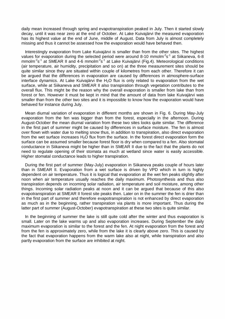
daily mean increased through spring and evapotranspiration peaked in July. Then it started slowly decay, until it was near zero at the end of October. At Lake Kuivajärvi the measured evaporation has its highest value at the end of June, middle of August. Data from July is almost completely missing and thus it cannot be assessed how the evaporation would have behaved then.

Interestingly evaporation from Lake Kuivajärvi is smaller than from the other sites. The highest values for evaporation during the selected period were around 8-10 mmolm-2s-1 at Siikaneva, 6-8 mmolm-2s-1 at SMEAR II and 4-6 mmolm-2s-1 at Lake Kuivajärvi (Fig.4). Meteorological conditions (air temperature, air humidity, precipitation and so on) at the three measurement sites should be quite similar since they are situated within couple of kilometres from each other. Therefore it can be argued that the differences in evaporation are caused by differences in atmosphere-surface interface dynamics. At Lake Kuivajärvi the H2O flux is only related to evaporation from the wet surface, while at Siikaneva and SMEAR II also transpiration through vegetation contributes to the overall flux. This might be the reason why the overall evaporation is smaller from lake than from forest or fen. However it must be kept in mind that the amount of data from lake Kuivajärvi was smaller than from the other two sites and it is impossible to know how the evaporation would have behaved for instance during July.

Mean diurnal variation of evaporation in different months are shown in Fig. 6. During May-July evaporation from the fen was bigger than from the forest, especially in the afternoon. During August-October the mean diurnal variation from these two sites looks quite similar. The difference in the first part of summer might be caused by differences in surface moisture. The fen is almost over flown with water due to melting snow thus, in addition to transpiration, also direct evaporation from the wet surface increases H2O flux from the surface. In the forest direct evaporation form the surface can be assumed smaller because forest floor is dry when compared to a fen. Also stomatal conductance in Siikaneva might be higher than in SMEAR II due to the fact that the plants do not need to regulate opening of their stomata as much at wetland since water is easily accessible. Higher stomatal conductance leads to higher transpiration.

During the first part of summer (May-July) evaporation in Siikaneva peaks couple of hours later than in SMEAR II. Evaporation from a wet surface is driven by VPD which in turn is highly dependent on air temperature. Thus it is logical that evaporation at the wet fen peaks slightly after noon when air temperature usually reaches the daily maximum. Photosynthesis and thus also transpiration depends on incoming solar radiation, air temperature and soil moisture, among other things. Incoming solar radiation peaks at noon and it can be argued that because of this also evapotranspiration at SMEAR II forest site peaks then. Later on in the summer the fen is drier than in the first part of summer and therefore evapotranspiration is not enhanced by direct evaporation as much as in the beginning, rather transpiration via plants is more important. Thus during the latter part of summer (August-October) evapotranspiration at these two sites is quite similar.

In the beginning of summer the lake is still quite cold after the winter and thus evaporation is small. Later on the lake warms up and also evaporation increases. During September the daily maximum evaporation is similar to the forest and the fen. At night evaporation from the forest and from the fen is approximately zero, while from the lake it is clearly above zero. This is caused by the fact that evaporation happens from the warm lake also at night, while transpiration and also partly evaporation from the surface are inhibited at night.

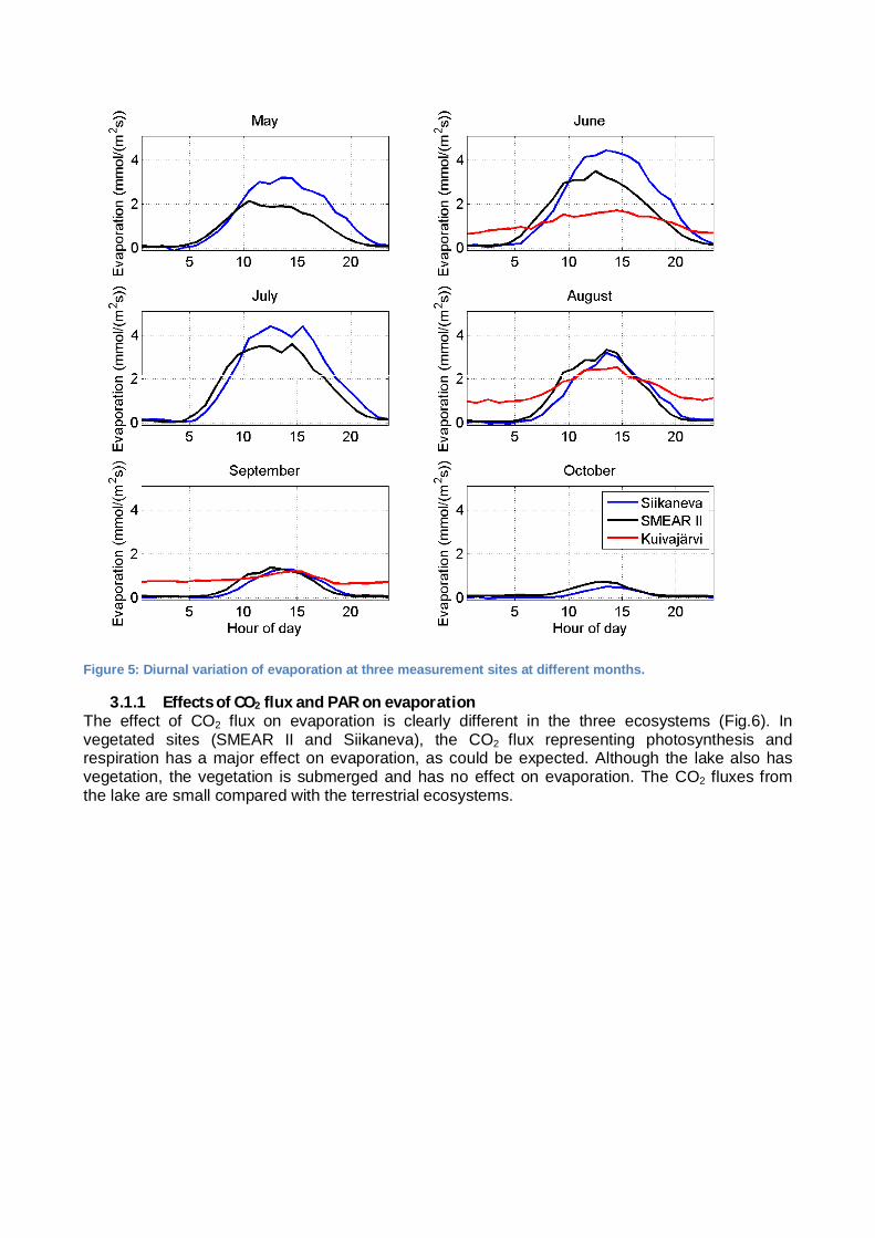
Figure 5: Diurnal variation of evaporation at three measurement sites at different months.

3.1.1 Effects of CO2 flux and PAR on evaporation The effect of CO2 flux on evaporation is clearly different in the three ecosystems (Fig.6). In vegetated sites (SMEAR II and Siikaneva), the CO2 flux representing photosynthesis and respiration has a major effect on evaporation, as could be expected. Although the lake also has vegetation, the vegetation is submerged and has no effect on evaporation. The CO2 fluxes from the lake are small compared with the terrestrial ecosystems.

Figure 6: Evaporation vs. CO2 flux in May, July and September in the three ecosystems (for Kuivajärvi, only July was available). The range and effect of the CO2 flux is clearly different in different ecosystems.

-2

0

2

4

6

8

10

12

-20 -10 0 10 20

H2O flux, mmol/m2/s

CO2 flux, µmol/m2/s

SMEAR II May 2010

-2

0

2

4

6

8

10

12

-20 -10 0 10 20

H2O flux, mmol/m2/s


Siikaneva May 2010

-2

0

2

4

6

8

10

12

-20 -10 0 10 20

H2O flux, mmol/m2/s


SMEAR II July 2010

-2

0

2

4

6

8

10

12

-20 -10 0 10 20

H2O flux, mmol/m2/s


Siikaneva July 2010

-2

0

2

4

6

8

10

12

-20 -10 0 10 20

H2O flux, mmol/m2/s


Kuivajärvi July 2010

-2

0

2

4

6

8

10

12

-20 -10 0 10 20

H2O flux, mmol/m2/s


SMEAR II September 2010

-2

0

2

4

6

8

10

12

-20 -10 0 10 20

H2O flux, mmol/m2/s


Siikaneva September 2010

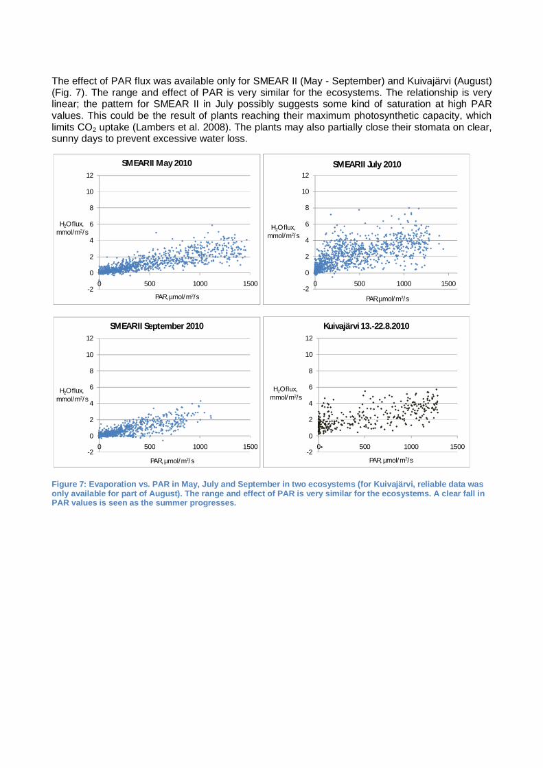
The effect of PAR flux was available only for SMEAR II (May - September) and Kuivajärvi (August) (Fig. 7). The range and effect of PAR is very similar for the ecosystems. The relationship is very linear; the pattern for SMEAR II in July possibly suggests some kind of saturation at high PAR values. This could be the result of plants reaching their maximum photosynthetic capacity, which limits CO2 uptake (Lambers et al. 2008). The plants may also partially close their stomata on clear, sunny days to prevent excessive water loss.

Figure 7: Evaporation vs. PAR in May, July and September in two ecosystems (for Kuivajärvi, reliable data was only available for part of August). The range and effect of PAR is very similar for the ecosystems. A clear fall in PAR values is seen as the summer progresses.

-2

0

2

4

6

8

10

12

0 500 1000 1500

H2O flux, mmol/m2/s

PAR, µmol/m2/s

SMEAR II May 2010

-2

0

2

4

6

8

10

12

0 500 1000 1500

H2O flux, mmol/m2/s

PAR,µmol/m2/s

SMEAR II July 2010

-2

0

2

4

6

8

10

12

0 500 1000 1500

H2O flux, mmol/m2/s

PAR, µmol/m2/s


-2

0

2

4

6

8

10

12

0 500 1000 1500

H2O flux, mmol/m2/s

PAR, µmol/m2/s

Kuivajärvi 13.-22.8.2010

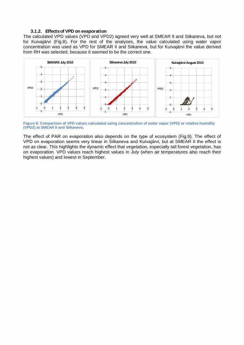
3.1.2. Effects of VPD on evaporation The calculated VPD values (VPD and VPD2) agreed very well at SMEAR II and Siikaneva, but not for Kuivajärvi (Fig.8). For the rest of the analyses, the value calculated using water vapor concentration was used as VPD for SMEAR II and Siikaneva, but for Kuivajärvi the value derived from RH was selected, because it seemed to be the correct one.

Figure 8: Comparison of VPD values calculated using concentration of water vapor (VPD) or relative humidity (VPD2) at SMEAR II and Siikaneva.

The effect of PAR on evaporation also depends on the type of ecosystem (Fig.9). The effect of VPD on evaporation seems very linear in Siikaneva and Kuivajärvi, but at SMEAR II the effect is not as clear. This highlights the dynamic effect that vegetation, especially tall forest vegetation, has on evaporation. VPD values reach highest values in July (when air temperatures also reach their highest values) and lowest in September.

-1

0

1

2

3

4

5

-1 0 1 2 3 4 5

VPD2

VPD

SMEAR II July 2010

-1

0

1

2

3

4

5

-1 0 1 2 3 4 5

VPD2

VPD

Siikaneva July 2010

-1

0

1

2

3

4

5

-1 0 1 2 3 4 5

VPD2

VPD

Kuivajärvi August 2010

Figure 9: The effect of VPD on evaporation. The effect of VPD seems very linear in Siikaneva and Kuivajärvi, but at SMEAR II the effect is not as clear. VPD values reach highest values in July and lowest in September.

-2

0

2

4

6

8

10

12

-1 0 1 2 3

H2O flux, mmol/m2/s

Vapor pressure deficit, kPa

SMEAR II May 2010

-2

0

2

4

6

8

10

12

-1 0 1 2 3

H2O flux, mmol/m2/s


Siikaneva May 2010

-2

0

2

4

6

8

10

12

-1 1 3 5

H2O flux, mmol/m2/s


SMEAR II July 2010

-2

0

2

4

6

8

10

12

0 1 2 3 4 5

H2O flux, mmol/m2/s


Siikaneva July 2010

-2

0

2

4

6

8

10

12

0 1 2 3

H2O flux, mmol/m2/s


Kuivajärvi 13.-22.8.2010

-2

0

2

4

6

8

10

12

-1 0 1 2

H2O flux, mmol/m2/s



-2

0

2

4

6

8

10

12

-1 0 1 2

H2O flux, mmol/m2/s


Siikaneva September 2010

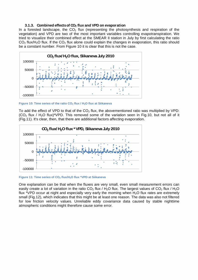
3.1.3. Combined effects of CO2 flux and VPD on evaporation In a forested landscape, the CO2 flux (representing the photosynthesis and respiration of the vegetation) and VPD are two of the most important variables controlling evapotranspiration. We tried to visualize their combined effect at the SMEAR II station in July by first calculating the ratio CO2 flux/H2O flux. If the CO2 flux alone could explain the changes in evaporation, this ratio should be a constant number. From Figure 10 it is clear that this is not the case.

Figure 10: Time series of the ratio CO2 flux / H2O flux at Siikaneva

To add the effect of VPD to that of the CO2 flux, the abovementioned ratio was multiplied by VPD: (CO2 flux / H2O flux)*VPD. This removed some of the variation seen in Fig.10, but not all of it (Fig.11). It's clear, then, that there are additional factors affecting evaporation.

Figure 11: Time series of CO2 flux/H2O flux *VPD at Siikaneva

One explanation can be that when the fluxes are very small, even small measurement errors can easily create a lot of variation in the ratio CO2 flux / H2O flux. The largest values of CO2 flux / H2O flux *VPD occur at night and especially very early the morning when H2O flux rates are extremely small (Fig.12), which indicates that this might be at least one reason. The data was also not filtered for low friction velocity values. Unreliable eddy covariance data caused by stable nighttime atmospheric conditions might therefore cause some error.

-100000

-50000

0

50000

100000

CO2 flux/H2O flux, Siikaneva July 2010

-100000

-50000

0

50000

100000

CO2 flux/H2O flux *VPD, Siikaneva July 2010

Figure 12: Left: Daily variation in CO2 flux/H2O flux *VPD (averaged over July). Right: Daily variation in H2O and CO2 flux (averaged over July).

3.2. Comparing of eddy covariance and aerodynamic methods on the lake

We estimated the rate of evaporation at Lake Kuivajärvi by measuring it with eddy covariance technique and also by calculating it with the aerodynamic method. In figure 13 you can see the evaporation rates given by both methods, RH-profile and temperature profile. E (aero) means the evaporation flux calculated with aerodynamic method and E (EC) is the flux given by eddy covariance method. The measurements presented in fig. 13 were made during 8.29.2011 14:00 - 8.31.2011 8:30.

Figure 13: Temperature profile and RH profile and evaporation rates by aerodynamic and EC –methods on the lake during 3 days.

Figure 13 shows that according to the eddy covariance method the evaporation rate has a distinct diurnal cycle. During daytime evaporation rate is clearly higher than during the nighttime. It can also be seen quite clearly that flux measured with eddy covariance method is consistent with the RH and temperature profiles whereas flux calculated with aerodynamic method does not have as clear diurnal cycle and also seems to lack the distinct consistency with temperature and RH-

-10000

-5000

0

5000

10000

15000

20000

25000

30000

35000

40000

45000CO2 flux/H2O flux

*VPD

CO2 flux/H2O flux * VPD, daily variation in July

-12

-10

-8

-6

-4

-2

0

2

4

6

0

0,5

1

1,5

2

2,5

3

3,5

4CO2 flux,

µmol/m2/s

H2O flux,mmol/m2/s

H2O & CO2 flux, average daily variation in July 2010

H2O flux

CO2 flux

profiles. The fluxes according to aerodynamic method seem especially peculiar at the beginning of measurement period about 8.29./16:00 when there is a dramatic drop in the flux and about 8.30./10:00 when the aerodynamic flux starts to diminish whereas the eddy covariance flux starts to rise. Thus it seems that in the aerodynamic method the water vapour flux variation is mixed with random noise. These differences can be explained though, when we keep in mind that the temperature used for calculating q0 was the temperature at the depth of 20 cm below the water surface. In addition to that we need to examine the variations in the values of average wind speed. Figure 14 shows the water vapour fluxes, temperature at the depth of 20 cm and variation of average wind speed.

Figure 14: Water vapour fluxes, temperature 20 cm below the surface and wind speed in Lake Kuivajärvi.

From figure 14 we can see that the dramatic drop in the flux of aerodynamic method at 8.29./16:00 can be explained with the drastic drop of the wind speed and the decreasing temperature at the depth of 20 cm. The major contributing factor in this situation is the drop in the wind speed. The small values of evaporation at about 8.30./10:00 can similarly be explained with the small values of average wind speeds and temperature at the 20 cm. The average water vapour flux during the measurement period of 8.29.2011 14:00 - 8.31.2011 8:30 according to eddy covariance method was 0.99 mmol m-2 s-1 whereas according to the aerodynamic method the average water vapour flux during the same period was 0.65 mmol m-2 s-1. This suggests that aerodynamic method underestimates the evaporation rate.

In the results above we used the value of 0.3 m specific humidity as the value of specific humidity in the air qa. This would otherwise be alright but we also used the values of wind speeds measured at the height of 1.6 m so that those values are not representing very well the average wind speeds near the ground. In order to get better results we calculated the aerodynamic flux also with using the value of 4.5 m specific humidity as the specific humidity of the air. In figure 15 there is presented comparison of water vapour fluxes in different situations.

As seen from the figure 15 the aerodynamic flux is nearly the same for the both values of qa. The average amount of water evaporated during the measurement period - while using the specific humidity at the height of 4.5 m as a specific humidity of the air - was 0.80 mmol m-2 s-1. This is

some 15 mmol m-2 s-1 larger than the average evaporation while using the specific humidity at 0.3 m as the specific humidity of the air. The average evaporation according to eddy covariance method was 0.99 mmol m-2 s-1. Thus it seems that by using the specific humidity of 4.5 m for the specific humidity of the air the aerodynamic method gives better results.

3.2.2. Lake temperature during the period

In the on day temperature profile (Fig.16) the summer stratification in the water is easy to see. The rest of the week is similar. The bottom water is 4°C, so it is the densest possible and the temperature increases upwards. The probes do not reach the surface but the highest point is 20 cm below the surface and in that depth the daily variation is also possible to see (Fig. 17). In the night temperature decreases and the decreasing continues almost until midday. The minimum temperature is around 10 o´clock, when the sun already warms but the water has not warmed up yet. The temperature near surface decreased also during the week. The period was in the end of summer and the weather was cooling. The week was somewhat cloudy and rainy. Near bottom the temperature is quite stable and has neither a daily variation nor temperature increase as can be seen in a similar plot from 8 m depth (Fig.17 right).

Figure 16: Water temperature profile in Lake Kuivajärvi 28.8.2011. The site was about 12 m deep, but the sensors in 10 m and 12 m did not work (white color)

Figure 15: Water vapour fluxes by EC-method and aerodynamic method with different heights for qa.

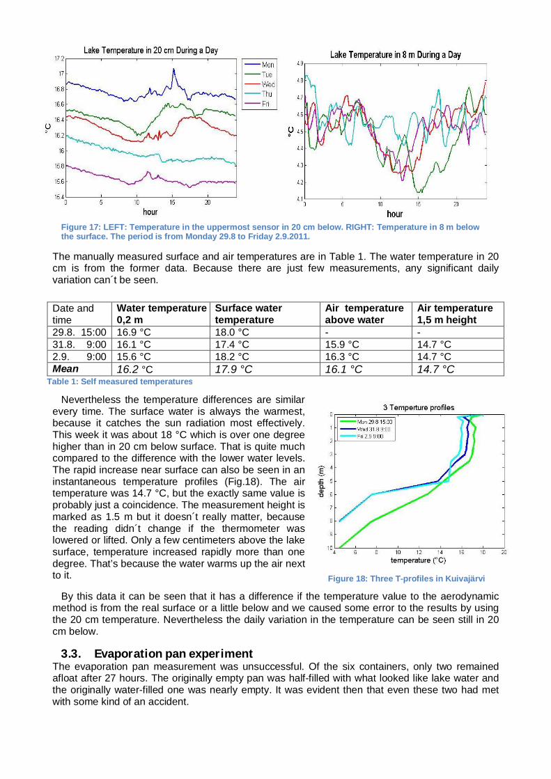
The manually measured surface and air temperatures are in Table 1. The water temperature in 20 cm is from the former data. Because there are just few measurements, any significant daily variation can´t be seen.

Nevertheless the temperature differences are similar every time. The surface water is always the warmest, because it catches the sun radiation most effectively. This week it was about 18 °C which is over one degree higher than in 20 cm below surface. That is quite much compared to the difference with the lower water levels. The rapid increase near surface can also be seen in an instantaneous temperature profiles (Fig.18). The air temperature was 14.7 °C, but the exactly same value is probably just a coincidence. The measurement height is marked as 1.5 m but it doesn´t really matter, because the reading didn´t change if the thermometer was lowered or lifted. Only a few centimeters above the lake surface, temperature increased rapidly more than one degree. That’s because the water warms up the air next to it.

By this data it can be seen that it has a difference if the temperature value to the aerodynamic method is from the real surface or a little below and we caused some error to the results by using the 20 cm temperature. Nevertheless the daily variation in the temperature can be seen still in 20 cm below.

3.3. Evaporation pan experiment The evaporation pan measurement was unsuccessful. Of the six containers, only two remained afloat after 27 hours. The originally empty pan was half-filled with what looked like lake water and the originally water-filled one was nearly empty. It was evident then that even these two had met with some kind of an accident.

Table 1: Self measured temperatures

Date and time

Water temperature 0,2 m

Surface water temperature

Air temperature above water

Air temperature 1,5 m height

29.8. 15:00 16.9 °C 18.0 °C - - 31.8. 9:00 16.1 °C 17.4 °C 15.9 °C 14.7 °C 2.9. 9:00 15.6 °C 18.2 °C 16.3 °C 14.7 °C Mean 16.2 °C 17.9 °C 16.1 °C 14.7 °C

Figure 18: Three T-profiles in Kuivajärvi

Figure 17: LEFT: Temperature in the uppermost sensor in 20 cm below. RIGHT: Temperature in 8 m below the surface. The period is from Monday 29.8 to Friday 2.9.2011.

Nevertheless, the results were calculated for the two containers. According to Table 2, SS Helena gained 12 mm/day. This might be possible, since it rained quite hard during the night; we didn’t compare results with the precipitation group. Since the water in the container was not clear but looked like it contained a lot of humus, we judged it to be lake water. The result is therefore unreliable. Pohjanmaa was nearly empty when picked up, and combined with the 12 mm of “rain” in SS Helena, this would mean evaporation rate of 18 mm/day. If the effect of rain is left out, the evaporation rate from Pohjanmaa is 6 mm/day. Even this is not plausible, since pan evaporation rates in Jokioinen (155 km away) were 33–60 mm during the month of September in 2001–2005 (Korhonen 2007), which equals only 1,1–2,0 mm/day.

Table 2: Results of the evaporation pan measurement. The pans marked with M.I.A. sunk during the experiment.

4. Conclusions

Comparing the three different sites by eddy covariance method revealed that evaporation was much smaller from the lake than from the forest or wetland. Because the sites are close to each other the meteorological conditions are similar. The reason for the difference might be that in the lake only evaporation happens, while in the forest and wetland a significant part of the water vapor flux is transpiration.

Monthly differences were also examined. During May - July evapotranspiration was bigger in the fen than in the forest, but later in the summer and in autumn they were very similar. The reason may be that the fen is wet long after winter, so there is more water to evaporate. In the lake data from the middle summer was missing, but in the beginning of summer the evaporation was quite small, because the water was still cold after winter, but in September it was as big as in other sites.

Daily variation was bigger in the fen and forest because there transpiration is small during the night. In the warm lake evaporation happens despite of sun radiation.

CO2, PAR and VPD values supported the conclusions that the differences in transpiration are a reason for the differences in evapotranspiration. CO2 values were biggest in the vegetated sites

The significant advantage of aerodynamic method is the rather simple measurement setup. Over open water one basically needs only to know the temperature from two levels – the surface and some other measurement level, humidity from just the upper measurement point – since the surface is saturated with water vapour, atmospheric pressure and average wind speed. As a first approximation the transfer coefficient can be estimated to have a value of 10-3 and the density of the dry air can be estimated from the ideal gas law. If the data mentioned above is at hand one can estimate the rate of evaporation with aerodynamic method. Thus one does not necessarily need expensive eddy covariance equipment if a rough estimation of evaporation is enough.

Of course one has to keep in mind that our measurements were made during quite nice weather in the late summer within a relatively short measurement period and we cannot say much about the accuracy of aerodynamic method for example during the late fall. Aerodynamic method seems to overestimate the influence of wind speed changes. Thus it presumably gives better results during periods of steady wind. The results of aerodynamic method could also be improved by using the temperature of the water surface for calculating the specific humidity of water surface q0.

Vessel m (empty), g m (start), g m (end), g Area, m2Evaporation, mm/day

SS Helena 60,757 60,757 895,300 0,062 -12,1St George 62,721 535,853 M.I.A. - - Pohjanmaa 69,856 560,017 133,800 0,062 18,2Santa Maria 73,113 574,090 M.I.A. - - RMS Evaporation 61,266 554,432 M.I.A. - - Titanic 82,500 572,661 M.I.A. - -

It is hard to say how well the aerodynamic method could estimate the evaporation at it's best when the temperature used for calculating q0 would be the actual temperature of the water surface and the used wind speed would be the actual average wind speed observed between the surface and height H, where the specific humidity of the air qa is measured. Although the corrections mentioned above would be taken care of there is still the problem of overestimating the influence of changing wind speed. Comparing eddy covariance measurements to aerodynamic method during our short measurement period show that calculating evaporation with aerodynamic method gives rather good approximation for the amount of water evaporated overall.

One problem in the aerodynamic method is that we used temperature 20 cm under the surface instead of the surface temperature, which is hard to measure exactly. We also tried to find out the difference in the actual surface temperature. The real surface temperature was over one degree warmer than 20 cm below. Anyway the total temperature profile behaves quite differently near surface. In the bottom of the lake temperature is about 4 °C, like usually in the summer. Temperature increases upwards, but right in the surface it makes a quick increase. Also the air temperature is over one degree higher in the layer just above the water than higher.

Nevertheless, comparing eddy covariance measurements to aerodynamic method during our short measurement period show that calculating evaporation with aerodynamic method gives a moderate approximation for the amount of water evaporated overall. Yet it is quite clear that the aerodynamic method is not able to catch the details of the water vapor flux - such as diurnal variation.

The idea about floating evaporation pans was not bad, but the setup should have been done otherwise, so that the pans will not be turned over during the measurement.

5. References

Calder, I.R. 1976. The measurement of water losses from a forested area using a "natural" lysimeter. Journal of Hydrology, Vol. 30, pp. 311-325.

Junninen H, Lauri A, Keronen P, Aalto P, Hiltunen V, Hari P, Kulmala M. 2009. Smart-SMEAR: On-line data exploration and visualization tool for SMEAR stations. Boreal Environ Res 14(4):447-57.

Korhonen, J. (ed.). 2007. Hydrologinen vuosikirja 2001–2005. Suomen ympäristö 44/2007. (in Finnish)

Lambers, H., Chapin III, F. S. & Pons, T. L. 2008. Plant physiological ecology. Springer, New York. 604 p.

Law, F. 1956. The effect of afforestation upon the yield of water catchment areas. Journal of the British Waterworks Association, pp. 489-494.

OIVA - ympäristö- ja paikkatietopalvelu (valtion ympäristöhallinnon virastot)

Treier, V. & Palge, V. Comparison of formulas for calculating water vapour saturation pressure. tehnika.eau.ee/pages/2002/energy/45_treier_palge.pdf

IV PROFILES

Atmospheric profiles in the first 100 meters

Jenni Kontkanen, John Backman, Mei-Kuei Tu, and Olga Ritenberga

1. Introduction The surface layer is one of the main energy-exchanges layers of the atmosphere, and accordingly the transformations of solar energy into other forms of energy are a main subject of meteorology. When studying the behavior of different parameters in the lower most layer of the atmosphere, it’s essential to be able to determine the stability conditions of the boundary layer. Historically, dimensionless ratios of stabilizing and destabilizing factors have been used to simplify this task. One of these stability parameters is Richardson number, the ratio of buoyancy forces to the shear stress forces (Stull, 1988). In addition, the Obukhov length, which is a universal scaling length in the surface layer, can be used to measure the stability of the boundary layer (Foken, 2006). Despite the fact that the stability parameters are very useful, the physical interpretation of their behavior and its connections with the evolution of the boundary layer may not be very obvious. Hence, one of our aims in this work is to study the seasonal and diurnal behavior of different stability parameters at the SMEAR II station.

The lowest layer of atmosphere (atmospheric boundary layer) is connected to vertical transport of quantities such as moisture, heat and momentum (according to Stull, 1988). One of the vertical wind categories is turbulence. The analysis of turbulence processes as presented in the current study focuses on data comparing elaborated in using SMART Search Programming tool. The aim of the analysis of intensity of turbulence was initially to compare changes of vertical fluxes of momentum, sensible heat, and variances of velocity at different heights. However, it was not possible because we did not have sufficient data at different heights and therefore we have decided to made analysis of only two parameters at one height - friction velocity and standard deviation describing the intensity of turbulence.

The stability of the lower most part of the atmosphere is of importance to trace-gas concentration levels. The elevation of the sources and sinks for these trace-gases affect the profiles and thus, the gradient of these. It has been shown that terrestrial ecosystems in the northern and temperate latitudes are large carbon sinks with significant impacts on atmospheric carbon dynamics (Tans et al., 1990). The main factors governing the dynamics of carbon dioxide (CO2) in the canopy of the forest are: turbulent mixing, photosynthesis, and respiration. During photosynthesis, CO2 is consumed in the forest canopy while decomposition of organic material is a source of CO2. Low altitude ozone (O3) is produced via complex photochemical processes from precursor vapours (Seinfeld and Pandis, 2006), above the canopy of the forest. The aim of our study was to show that atmospheric stability can be coupled to trace gas gradients at different heights. We show that atmospheric stability parameters can explain a gradient build-up or, on the contrary, the absence of any gradient. This holds true for both our case study, diurnally, and seasonally.

2. Theory and methods

2.1 The measurement site

In the study, the data of trace gases and flux are taken from Smart-SMEAR database (Junninen et al., 2009) which is the data measured at the SMEAR II (Station for Measuring Ecosystem-Atmosphere Relations) station in Hyytiälä, south-western central Finland (61 50’47’’ N, 24 17’42’’ E, 181 m a.s.l.). The SMEAR II station is located 220 km North-West from Helsinki and the managed stand was established in 1962. It situates inside a boreal forest which main species include Scots pine (Pinus sylvestris) and Norway spruce (Picea abies). The canopy height of the forest in the immeadiate surrounding of the station is roughly 17-18 m. The measurement station has been running continuously since 1996, both by conducting long-term monitoring and as a complementary station for shorter field campaigns (Hari and Kulmala 2005). The flux measurement data comes from a 73 m high mast at the station.

2.2 Atmospheric stability

2.2.1 Richardson numbers

The stability conditions of the boundary layer can be determined by comparing the contributions of buoyancy forces and shear stress forces to the budget of turbulent kinetic energy. The ratio of the contributions of these two effects is called the flux Richardson number and it’s defined as

=

(1)

where g is the acceleration due to gravity, is virtual potential temperature, is turbulent heat flux, is turbulent momentum flux and is wind gradient (Stull, 1988). The numerator of describes the effect of the buoyance and the denominator describes the effect of the shear stress. Because shear stress produces turbulent energy in all circumstances, the shear stress term is always positive and the sign of the flux Richardson number is determined by the buoyancy term. In unstable conditions buoyancy forces produce turbulent kinetic energy and the flux Richardson number becomes negative. On the contrary, in stable conditions buoyancy forces destroy turbulent energy in which case the flux Richardson number becomes positive. In neutral conditions buoyancy forces don’t affect the budget of turbulent kinetic energy and the flux Richardson number is zero.

Flux Richardson number can also be written in a different form by first assuming that the turbulent fluxes are proportional to gradients according to the K-theory and then

approximating the local gradients by using observations from two different heights. In that way we can define the bulk Richardson number as

= ( ) )

( ( ) (2)

where ) and ) represent the values of virtual potential temperature at the heights of and and ( ) and ( ) represent the values of wind speed at those heights (Stull, 1988).

In order to study the behavior of stability parameters in Hyytiälä, Equation (1) and (2) were used to calculate the values of the flux and bulk Richardson number at the height of 22 m. Due to the fact that only a limited amount of parameters are measured at different heights at the SMEAR II station, we were, however, forced to made several calculations before we were able to use the equations (1) and (2).

Because pressure is measured only at ground level at the SMEAR II station, we calculated the pressure p at the heights of 16.8 m, 22 m and 33.6 m by using Equation (3) based on the hydrostatic equation and the ideal gas law:

( ) exp (3)

where is pressure on the ground level, is height, R is gas constant for air and is temperature (Holton, 2004).

After calculating pressure at different heights, we calculated also the potential temperature at different levels by using the equation

( ))

. (4) To account for the effect of water vapor we calculated the virtual potential temperature at different levels by using the equation

= (1 + 0.61 ) (5) where represent the mixing ratio of water vapor (Stull, 1998). In addition, we calculated the wind gradient at the height of 22 m by using the values of winds speed at two levels according to the equation

= ( ) ) (6) where = wind speed, = 16.8 m, = 33.6 m.

2.2.2 Obukhov length

The flux Richardson number can also be expressed as a dimensionless length

(7)

where represents a parameter called the Obukhov length.

Obukhov length is a scaling length used in the surface layer and defined as

= ( )

(8)

where is the friction velocity and k is the von Karman constant.

Obukhov length can be interpreted as the height above the surface at which the loss of turbulent energy caused by the buoyancy forces equals the production of turbulence by shear stress forces. Consequently, the Obukhov length can be used to measure the stability conditions of the boundary layer. When Obukhov length gets small negative values, the conditions are very unstable. In less unstable conditions, Obukhov length gets larger negative values. Respectively, when Obukhov length gets small positive values the boundary layer is very stable and when Obukhov length gets large positive values, the boundary layer is slightly stable. When Obukhov length is very large, either positive or negative, the conditions are neutral (Seinfeld and Pandis, 1998).

To also be able to study the behavior of the Obukhov length at the height of 22 m at the SMEAR II station, we used the values available at smartSearch.

2.3 Atmospheric trace gases

Trace-gas concentrations are constantly changing. Their temporal and spatial dynamics are affected by a variety of environmental factors. These trace-gas species all have their specific source, lifetime and sink(s). The sources of these, to name a few, can be anthropogenic, biological, and photochemical processes. Evidently, these sources can be at ground level, in the canopy or in the photochemical active atmosphere above the canopy of the forest. In a similar way, the sinks can be at different levels. A source of CO2 can be found at ground level while the sink in a forest is mainly in the canopy. Some gases are long lived (e.g. CO2) while other are reactive and have a short lifetime. The later ones are typically oxidizing species, radicals, like hydroxyl radical (OH) and ozone (O3). To understand the behaviour of these different trace gases and their association to micrometeorology we will focus on CO2.

The stability of the lower part of the boundary layer is of importance both to the concentrations of trace gases and their profiles. In a turbulent atmosphere, the entrainment of these trace-gases in the convective boundary layer, suppress the build up of any gradient. Thus, trace-gases are mixed in the convective boundary layer.

LzRi f

Depending on the mixing height, trace gases are diluted differently. The radiative cooling at night can lead to a stable surface layer, which tends to accumulate trace-gases. Above the stable surface layer and beneath the upper-level inversion the characteristics of the gas-profiles are more or less uniform. This layer is called the nocturnal residual layer.

While stratospheric ozone can be explained with the fairly simple Chapman cycle, ground level ozone chemistry is not trivial. Ozone, a secondary species, is formed from the interaction between nitrogen oxides (NOX) and volatile organic compounds (VOC) in the presence of sunlight. As solar irradiance varies, so does the temporal evolution of O3. In a boreal forest, VOC’s and NOX are abundant, thus providing a sink for O3, in addition to the deposition. In the non-urban nocturnal residual layer, these removal processes are absent and O3 lacks a significant sink.

As humankind has got more and more dependent on fossil fuels so has the levels of CO2 increased in the atmosphere. Winter and summertime concentrations of CO2 can be seen varying during the seasons from being the highest in winter and lower in summer (IPCC 2007). However, the carbon uptake by plants is a vital part of the natural carbon cycle. Humankind’s dependence on fossil fuels has increased the atmospheric concentrations of CO2 while plants and oceans act as storages. Furthermore, decomposition of biological material is a source of CO2, thus making a forest a source of CO2 without photosynthesis and a sink with photosynthesis.

Water vapour (H2O) is the most significant greenhouse gas in the atmosphere followed by CO2 (IPCC 2007). Gas phase water vapour in the atmosphere is closely linked to precipitation, soil moisture and plant respiration.

The gas profiles were calculated using trace-gas concentrations at two different levels:

= (8)

where c2 is the concentration at 67 meters and c1 at 17 meters. The denominator is the difference in height between the two measurement points. Firstly, linear regression vas used for six heights, but was proven unreliable as concentrations levelled out during atmospheric unstable conditions, i.e. mixing in the boundary layer was strong.

2.4 Turbulence Intensity Usually, at the level of description of turbulence the term “intensity of turbulence” is used. If intensity of turbulence depends on the standard deviation of mean wind speed, different observations, measurements, chain of parameters, and number of formulas are needed to calculate it. Intensity of turbulence is defined (cp. Stull, 1988) in the following equation:

Standard deviation of mean wind speed (m/s) which is defined as the square root

of the variance - mean wind speed.

So, if the standard deviation has higher values then the intensity of turbulence will also have higher values. Two main parameters – friction velocity and standard deviation of vertical wind speed – were used for analysis of intensity of turbulence. Values of mentioned parameters were downloaded from Smart-SMEAR using Smart-Search tool. Visualization of observed parameters was made by using Microsoft Excel.

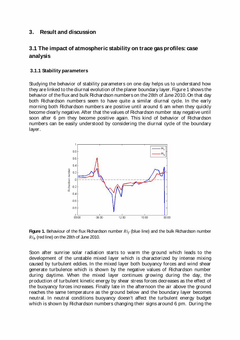
3. Result and discussion

3.1 The impact of atmospheric stability on trace gas profiles: case analysis 3.1.1 Stability parameters Studying the behavior of stability parameters on one day helps us to understand how they are linked to the diurnal evolution of the planer boundary layer. Figure 1 shows the behavior of the flux and bulk Richardson numbers on the 28th of June 2010. On that day both Richardson numbers seem to have quite a similar diurnal cycle. In the early morning both Richardson numbers are positive until around 6 am when they quickly become clearly negative. After that the values of Richardson number stay negative until soon after 6 pm they become positive again. This kind of behavior of Richardson numbers can be easily understood by considering the diurnal cycle of the boundary layer.

Figure 1. Behaviour of the flux Richardson number (blue line) and the bulk Richardson number (red line) on the 28th of June 2010.

Soon after sunrise solar radiation starts to warm the ground which leads to the development of the unstable mixed layer which is characterized by intense mixing caused by turbulent eddies. In the mixed layer both buoyancy forces and wind shear generate turbulence which is shown by the negative values of Richardson number during daytime. When the mixed layer continues growing during the day, the production of turbulent kinetic energy by shear stress forces decreases as the effect of the buoyancy forces increases. Finally late in the afternoon the air above the ground reaches the same temperature as the ground below and the boundary layer becomes neutral. In neutral conditions buoyancy doesn’t affect the turbulent energy budget which is shown by Richardson numbers changing their signs around 6 pm. During the

late evening and nighttime the ground cools down faster than air because of the long-wave radiation. This results in the development of a stable boundary layer where wind speed is usually low and buoyancy forces tend to suppress turbulence. Consequently, the loss of turbulence energy by buoyancy forces dominates over the production of turbulent energy by wind shear. This is shown by the positive values of Richardson numbers at night.

Figure 2. Behaviour of the Obukhov length on the 28th of June 2010.

The behavior of the Obukhov length on the 28th of June 2010 (Figure 2) is consistent with the behavior of flux and bulk Richardson numbers discussed above. During nighttime, from 9 pm to 6 am, the Obukhov length is positive but it doesn’t get values higher than 200 m indicating clearly stable conditions. After 6 am, the Obukhov length suddenly increases and becomes larger than 800 m, which means that the boundary layer start to become less stable because of solar radiation heating up the ground. After that the Obukhov length quickly becomes negative and stays between -20 m and -200 m until 6 pm indicating that the boundary layer is very unstable during the daytime. Soon after 6 pm, the Obukhov length reaches the value of nearly -600 m which is an indication of the conditions starting to become less unstable. After that the Obukhov length suddenly gets large positive values (nearly 800 m) followed by smaller positive values, which means that the boundary layer first becomes slightly stable before the clearly stable conditions prevailing at night. When comparing the behavior of the Obukhov length on this particular day with the typical ranges of Obukhov length over a diurnal cycle presented by Stull (1998), it can be noticed that the variation of Obukhov length on the 28th of June 2010 followed the typical daily behavior of Obukhov length very well.

3.1.2 Trace gas profiles

In Figure 3 both CO2 concentrations, global irradiance, wind speed and the temperature profile is plotted. From midnight to sunrise (approximately 7:30) there is a higher concentration of CO2 at ground level. During these morning hours, until sunrise, there was an inversion layer which accumulated CO2 as organic material decomposed in the absence of photosynthesis. This inversion is also evident, not only from the CO2 gradient but from the temperature profile plotted in the lower part of the figure. There is a clear

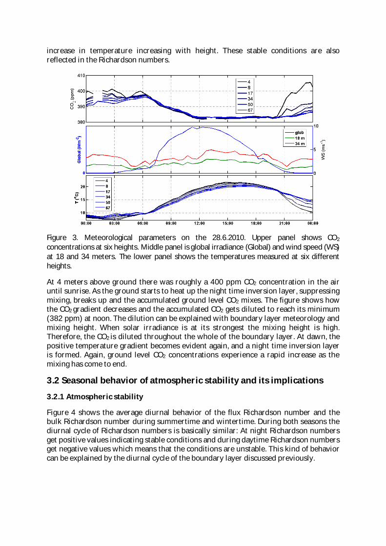
increase in temperature increasing with height. These stable conditions are also reflected in the Richardson numbers.

Figure 3. Meteorological parameters on the 28.6.2010. Upper panel shows CO2 concentrations at six heights. Middle panel is global irradiance (Global) and wind speed (WS) at 18 and 34 meters. The lower panel shows the temperatures measured at six different heights.

At 4 meters above ground there was roughly a 400 ppm CO2 concentration in the air until sunrise. As the ground starts to heat up the night time inversion layer, suppressing mixing, breaks up and the accumulated ground level CO2 mixes. The figure shows how the CO2 gradient decreases and the accumulated CO2 gets diluted to reach its minimum (382 ppm) at noon. The dilution can be explained with boundary layer meteorology and mixing height. When solar irradiance is at its strongest the mixing height is high. Therefore, the CO2 is diluted throughout the whole of the boundary layer. At dawn, the positive temperature gradient becomes evident again, and a night time inversion layer is formed. Again, ground level CO2 concentrations experience a rapid increase as the mixing has come to end.

3.2 Seasonal behavior of atmospheric stability and its implications

3.2.1 Atmospheric stability

Figure 4 shows the average diurnal behavior of the flux Richardson number and the bulk Richardson number during summertime and wintertime. During both seasons the diurnal cycle of Richardson numbers is basically similar: At night Richardson numbers get positive values indicating stable conditions and during daytime Richardson numbers get negative values which means that the conditions are unstable. This kind of behavior can be explained by the diurnal cycle of the boundary layer discussed previously.

FIgure 4. Average diurnal behavior of the flux Richardson number (blue line) and the bulk Richardson number (red line) during summer (June-August) and winter (December-February,2010).

However, the daily variation of Richardson numbers seems to be much more pronounced during summertime than during wintertime. At night, during summer, the mean values of flux and bulk Richardson numbers reach the values of 0.12 and 0.10. During day in summertime the minimum value of both Richardson numbers is about -0.17 on average. However, in wintertime the mean value of the flux Richardson number varies from 0.02 to -0.01 over a diurnal cycle. The mean value of bulk Richardson number even stays negative during the whole day varying from -0.01 to -0.06. These differences in the mean range of Richardson number during summer and winter are probably due to the fact that during winter months, in Finland, the amount of solar radiation reaching the surface during daytime is much smaller than during summer months. Solar radiation being the most important factor leading to the development of the convective mixed layer during daytime, the diurnal cycle of the boundary layer is much less clear when there isn’t much radiation coming to the surface. The small amount of radiation may also not be able to erode the stable inversion layer even during daytime which leads to only small daily changes in the stability.

It can also be noticed that Richardson numbers don’t change their signs from positive to negative at the same time during different seasons. During summer months both Richardson numbers become negative around 6 am and then positive again around 6 pm. However, during winter months flux Richardson number becomes negative only slightly before 10 am and it becomes positive again already around 2 am. The bulk Richardson number, which stays negative during the whole day, starts to decrease in the morning around 9 am and reach the nocturnal values again around 6 pm. The reason for these seasonal differences is obvious: in Finland sunrise takes place much later and sunset earlier during winter months than during summer months.

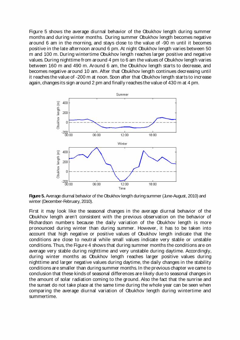
Figure 5 shows the average diurnal behavior of the Obukhov length during summer months and during winter months. During summer Obukhov length becomes negative around 6 am in the morning, and stays close to the value of -90 m until it becomes positive in the late afternoon around 6 pm. At night Obukhov length varies between 50 m and 100 m. During wintertime Obukhov length reaches larger positive and negative values. During nighttime from around 4 pm to 6 am the values of Obukhov length varies between 160 m and 490 m. Around 6 am, the Obukhov length starts to decrease, and becomes negative around 10 am. After that Obukhov length continues decreasing until it reaches the value of -200 m at noon. Soon after that Obukhov length starts to increase again, changes its sign around 2 pm and finally reaches the value of 430 m at 4 pm.

Figure 5. Average diurnal behavior of the Obukhov length during summer (June-August, 2010) and winter (December-February, 2010).

First it may look like the seasonal changes in the average diurnal behavior of the Obukhov length aren’t consistent with the previous observation on the behavior of Richardson numbers because the daily variation of the Obukhov length is more pronounced during winter than during summer. However, it has to be taken into account that high negative or positive values of Obukhov length indicate that the conditions are close to neutral while small values indicate very stable or unstable conditions. Thus, the Figure 4 shows that during summer months the conditions are on average very stable during nighttime and very unstable during daytime. Accordingly, during winter months as Obukhov length reaches larger positive values during nighttime and larger negative values during daytime, the daily changes in the stability conditions are smaller than during summer months. In the previous chapter we came to conclusion that these kinds of seasonal differences are likely due to seasonal changes in the amount of solar radiation coming to the ground. Also the fact that the sunrise and the sunset do not take place at the same time during the whole year can be seen when comparing the average diurnal variation of Obukhov length during wintertime and summertime.

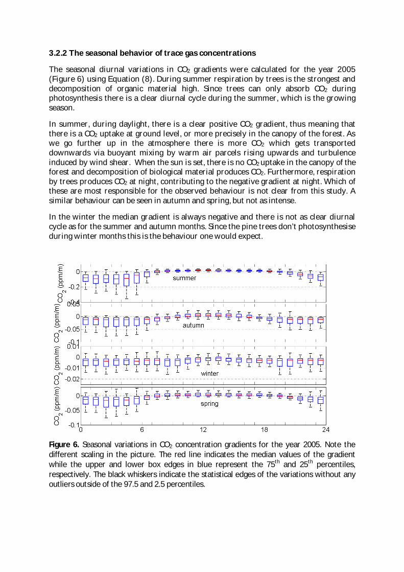
3.2.2 The seasonal behavior of trace gas concentrations

The seasonal diurnal variations in CO2 gradients were calculated for the year 2005 (Figure 6) using Equation (8). During summer respiration by trees is the strongest and decomposition of organic material high. Since trees can only absorb CO2 during photosynthesis there is a clear diurnal cycle during the summer, which is the growing season.

In summer, during daylight, there is a clear positive CO2 gradient, thus meaning that there is a CO2 uptake at ground level, or more precisely in the canopy of the forest. As we go further up in the atmosphere there is more CO2 which gets transported downwards via buoyant mixing by warm air parcels rising upwards and turbulence induced by wind shear. When the sun is set, there is no CO2 uptake in the canopy of the forest and decomposition of biological material produces CO2. Furthermore, respiration by trees produces CO2 at night, contributing to the negative gradient at night. Which of these are most responsible for the observed behaviour is not clear from this study. A similar behaviour can be seen in autumn and spring, but not as intense.

In the winter the median gradient is always negative and there is not as clear diurnal cycle as for the summer and autumn months. Since the pine trees don’t photosynthesise during winter months this is the behaviour one would expect.

Figure 6. Seasonal variations in CO2 concentration gradients for the year 2005. Note the different scaling in the picture. The red line indicates the median values of the gradient while the upper and lower box edges in blue represent the 75th and 25th percentiles, respectively. The black whiskers indicate the statistical edges of the variations without any outliers outside of the 97.5 and 2.5 percentiles.

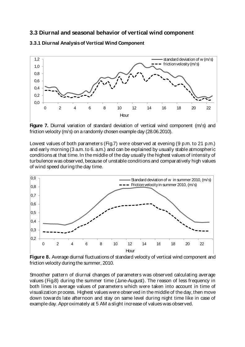
3.3 Diurnal and seasonal behavior of vertical wind component

3.3.1 Diurnal Analysis of Vertical Wind Component

Figure 7. Diurnal variation of standard deviation of vertical wind component (m/s) and friction velocity (m/s) on a randomly chosen example day (28.06.2010). Lowest values of both parameters (Fig.7) were observed at evening (9 p.m. to 21 p.m.) and early morning (3 a.m. to 6. a.m.) and can be explained by usually stable atmospheric conditions at that time. In the middle of the day usually the highest values of intensity of turbulence was observed, because of unstable conditions and comparatively high values of wind speed during the day time.

Figure 8. Average diurnal fluctuations of standard velocity of vertical wind component and friction velocity during the summer, 2010. Smoother pattern of diurnal changes of parameters was observed calculating average values (Fig.8) during the summer time (June-August). The reason of less frequency in both lines is average values of parameters which were taken into account in time of visualization process. Highest values were observed in the middle of the day, then move down towards late afternoon and stay on same level during night time like in case of example day. Approximately at 5 AM a slight increase of values was observed.

0,0

0,2

0,4

0,6

0,8

1,0

1,2

0 2 4 6 8 10 12 14 16 18 20 22

standard deviation of w (m/s)friction velosity (m/s)

Hour

0,2

0,3

0,4

0,5

0,6

0,7

0,8

0,9

0 2 4 6 8 10 12 14 16 18 20 22

Standard deviation of w in summer 2010, (m/s) Friction velocity in summer 2010, (m/s)

Hour

3.3.2 Seasional Analysis of Vertical Wind Component The same parameters were analyzed on a larger temporal scale. 2005 was chosen for finding differences of intensity of turbulence during the year and analyzing seasonal changes. Plotted friction velocity and standard deviation values indicted the same result as in previous cases, i.e., high intensity of turbulence during the day time and minimal values during the night time. The range of unexpected high values of both parameters was also fixed. A subset of data of the period – December to February - was sorted out and another subset was used for plotting parameters during winter time. The analysis based on Fig.9 showed that values of standard deviation and friction velocity are not correct during the winter time – because of the problems with measurement equipment. High values of parameters during the winter time could be also explained by possible high values of wind speed during night time in winter.

Figure 9. Average diurnal fluctuations of standard velocity of vertical wind component and friction velocity during the summer, winter and annual data in 2005. As far as the whole-year data set was plotted without using “incorrect” winter data, the pattern of standard deviation and friction velocity vales is very close to pattern of summer 2005. This means that the highest value was observed during the day time and lowest value during the night time.

4. Conclusions

When studying the behavior of stability parameters, it became apparent, that all stability parameters have a clear diurnal cycle: they are positive during nighttime and negative during daytime. This diurnal variation is closely linked to the diurnal evolution of the boundary layer driven by solar radiation. During daytime when the boundary layer is convectively unstable both buoyancy and wind shear tend to increase the production of turbulent kinetic energy leading to negative values of stability parameters. During nighttime the conditions are stable and buoyancy forces suppress turbulence which results in positive values of stability parameters. Analysis of intensity of turbulence based on standard deviation and friction velocity’s components has shown clear seasonal variation and diurnal changes. The highest intensity of turbulence was observed at the day time during summer. The main reason of higher or lower intensity of turbulence in the first 100 meters refers to the changes in wind speed, because other parameters (e.g. vertical fluxes of heat and momentum) should be more-less constant at this height. Moreover, we also found out that probably due to reduced amount of solar radiation this daily variation of stability parameters is much less pronounced during wintertime than during summertime. There seems to be a clear diurnal behaviour in the Richardson numbers which both are able to explain the behaviour of the trace-gas gradients in the atmosphere.

References

Foken T., 2006: 50 years of the Monin–Obukhov similarity theory, Boundary Layer Meteorology 119 (3), pp. 431–447.

Hari, P. and Kulmala, M., 2005: Station for Measuring Ecosystem–Atmosphere Relations (SMEAR II), Boreal Environment Research, 10, 315–322. Holton J.R., 2004: An introduction to dynamic meteorology. Elsevier Academic Press, San Diego, Calfornia, USA.

Intergovernmental Panel on Climate Change, 2007: Climate Change 2007: The Physical Science Basis. Contribution of Working Group I to the Fourth Assessment Report of the Intergovernmental Panel on Climate Change. Cambridge University Press.

Junninen, H., Lauri, A., Keronen, P. I. R., Aalto, P., Hiltunen, V., Hari, P. & Kulmala, M., 2009, Smart-SMEAR: on-line data exploration and visualization tool for SMEAR stations 2009, Boreal Environment Research. 14, p. 447-457. 11 p. Seinfeld, J. och Pandis, S., 2006: Atmospheric Chemistry and Physics - From airpollution to climate change. Wiley-Interscience.

Stull, R. B., 1988: An introduction to boundary layer meteorology. Kluwer Academic Publisher, Dordrect, the Neatherlands.

Tampieri F., Viana S., Yague C. 2011. Studying the height of atmospheric stable boundary layer from turbulence moments at different heights. Geophysical Research Abstracts. Vol.13., EG 2011-5026.

Tans, P.P., I.Y. Fung and T. Takahashi, 1990: Observational constraints on the global atmospheric CO2 budget. Science 247:1431--1438.

V SAUNA

The Sauna mystery Why is Sauna so hot?

Juha Heikkilä, Timo Ryyppö, and Pekka Rantala

30.09.2011

Table of Contents

1. Introduction .................................................................................................................................... 2

2. Theory ............................................................................................................................................. 3

2.1. Heat transfer ........................................................................................................................... 3

3. Material and methods .................................................................................................................... 4

3.1. Sauna ....................................................................................................................................... 4

3.2. Net radiation ........................................................................................................................... 5

3.3. Temperature and relative humidity ........................................................................................ 5

3.4. Absolute water vapor concentration ...................................................................................... 6

3.5. Heat transfer studies ............................................................................................................... 6

3.6. Keeping drinks cool ................................................................................................................. 7

4. Results ............................................................................................................................................. 7

4.1. Temperature and humidity ..................................................................................................... 7

4.1.1. Temperature vs. humidity ............................................................................................... 7

4.1.2. Temperature profiles .................................................................................................... 10

4.1.3. Stone and stove temperatures ..................................................................................... 11

4.2. Sauna is hot place – why? ..................................................................................................... 12

4.2.1. What is the hottest place in sauna? .............................................................................. 14

4.3. Radiation ............................................................................................................................... 15

4.4. Keeping drinks cool ............................................................................................................... 16

4.5. Feeling of löyly ...................................................................................................................... 18

5. Conclusions ................................................................................................................................... 19

6. References .................................................................................................................................... 20

2

1. Introduction

Sauna has always been an important place especially for Finns. It offers a place to relax, to think, to

talk, to have a good time. How can a dim room with a hot stove and people sitting naked do that?

That’s the sauna mystery. And we are set to solve it!

Not quite, at least not all of it. We don’t want to bust all the sauna myths. We are interested in what

makes sauna feel so hot. Hermans and Vesala (2007) have discussed qualitatively heat transfer

mechanisms in sauna. We wanted to take one step further and do wide range of experiments in

sauna.

Saunas can be divided in two groups depending on how they are heated: with wood or with

electricity. Wood heated saunas are more common in summer cottages and in rural houses. Electric

saunas are more common in cities; you can even find one in an apartment house. When you throw

water on stones, it vaporizes and spreads to sauna. This water throw is called löyly, one löyly

normally lasts 1-3 minutes, depending on water and sauna volume and how person experiences the

warm feeling during löyly. Wood heated saunas are thought as more traditional ones and they are

supposed to give you a better löyly. Quality of löyly is normally described by hard or soft, soft being

better. Sauna size can be anything from small two person sauna to a large one where you can fit a

football team or even a military company.

Heat is energy so we can equally talk about energy transfer. Energy transfer in form of heat can be

classified into different mechanisms. We look into four of them more closely. Heat transfer by

conduction occurs between two bodies with different temperatures through a layer of some

material. No mass transfer is involved. In conduction kinetic energy is exchanged between the

particles that make up the layer. Energy is always transferred from a body of higher temperature to

a body of lower temperature. In sauna for example, energy is transferred from hot air to cooler skin

through a thin layer of air.

Radiation is transfer of energy by electromagnetic radiation. All matter with temperature above

absolute zero emits thermal radiation. Radiation wavelength depends on temperature of the matter

according to Planck’s law (Physical Chemistry, p.506).

Convection can happen when there is a temperature gradient in fluid causing density differences

and therefore buoyancy forces that drive the convection. Heat transfer by convection occurs

through particle movement, so it also involves mass transfer.

Phase change (water evaporation/condensation in our case) is an efficient way to transfer energy.

Energy transfer by phase change is called latent heat flux, and in our case we talk about latent heat

of vaporization. When water evaporates it needs energy for phase change from liquid to gas and

releases energy when water vapor condenses to liquid.

Our objective was to study how is heat transferred in sauna, what happens when you throw water to

stones and what is the hottest place in sauna. We also studied what is the best way to keep your

drinks cool while in sauna.

3

2. Theory

2.1. Heat transfer

In sauna, the energy can be transferred by electromagnetic radiation, by conduction, by transfer of

mass and by convection (forced or free). The net exchange of heat energy for a body (for

example a student) with mass can be determined in a form

, (1)

where is change in body temperature and some average heat capacity in constant pressure.

We assumed that our physical body (still for example the student) does not do any work in the

sauna, therefore, the energy equation can be written in a form

, (2)

where is the net heat exchange by latent heating (mass transfer), by conduction, by forced

convection and by radiation respectively.

The latent heating can be formulated in a form

(3)

where is the latent heat of water vapor and the amount of condensed water.

The conductive heat flux per area unit can be assumed to be directly proportional to the

temperature gradient (Fourier’s law, see e.g. Vesala, 2004, pp. 38):

, (4)

where is the conductivity of air and is temperature. Forced convection can be also

determined almost similarly (Vesala, 2004, pp. 42−44)

, (5)

where is the dimensionless Nusselt’s number, is temperature difference between the body

and ambient air and is a characteristic length scale. Nusselt’s number describes actually the ratio

between conductive and convective heat transfer, and according to experiments, it has a following

equation for a flow past cylinder (almost like the student) in the range of :

, (6)

where is a characteristic velocity scale, density of air and dynamic viscosity. However, the

equations (5) and (6) are highly experimental, therefore, it is difficult to get any accurate values for

. The Reynold’s number of sauna was approximately

- - 1 m . (7)

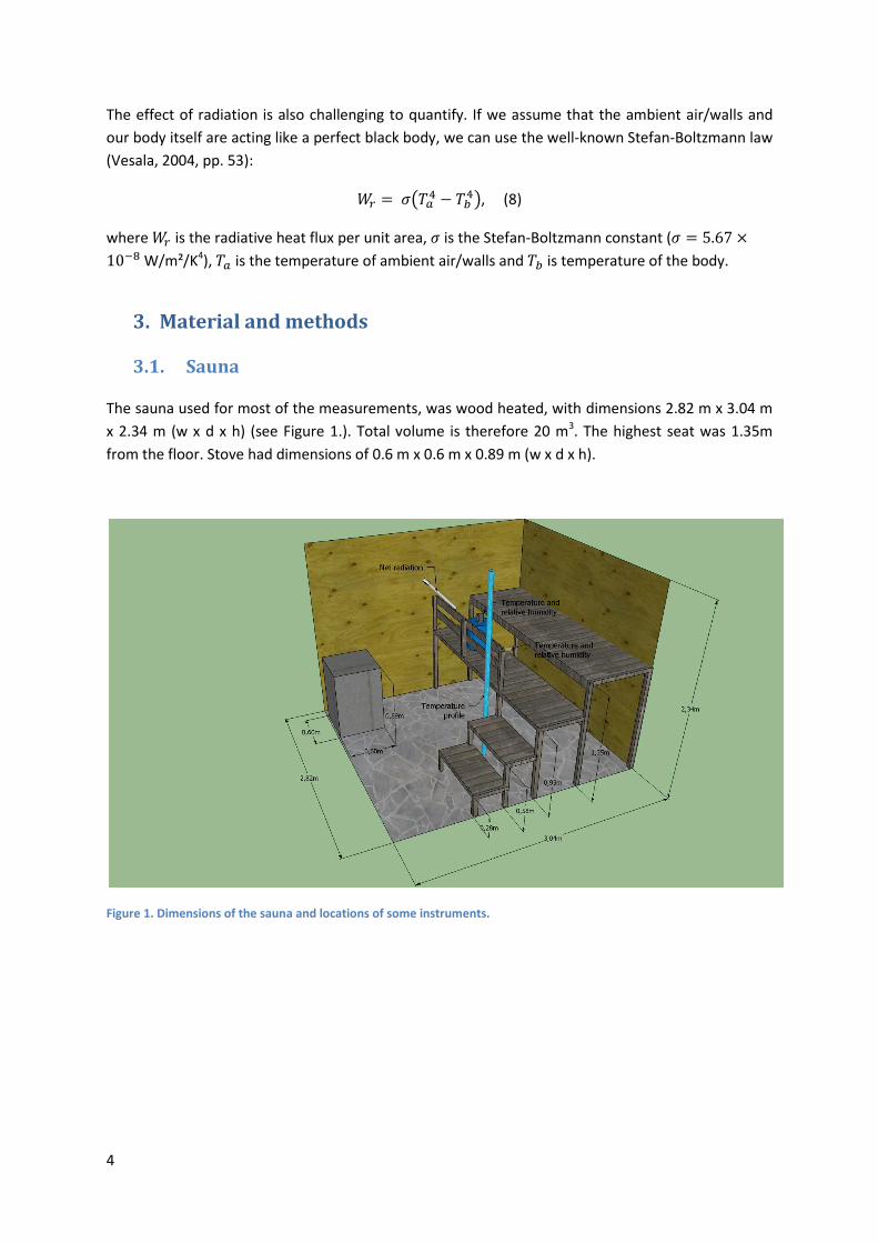
4

The effect of radiation is also challenging to quantify. If we assume that the ambient air/walls and

our body itself are acting like a perfect black body, we can use the well-known Stefan-Boltzmann law

(Vesala, 2004, pp. 53):

, (8)

where is the radiative heat flux per unit area, is the Stefan-Boltzmann constant (

W/m²/K4), is the temperature of ambient air/walls and is temperature of the body.

3. Material and methods

3.1. Sauna

The sauna used for most of the measurements, was wood heated, with dimensions 2.82 m x 3.04 m

x 2.34 m (w x d x h) (see Figure 1.). Total volume is therefore 20 m3. The highest seat was 1.35m

from the floor. Stove had dimensions of 0.6 m x 0.6 m x 0.89 m (w x d x h).

Figure 1. Dimensions of the sauna and locations of some instruments.

5

Figure 2. Places of numbered temperature sensors used to measure horizontal temperature profiles (see section 4.1.2).

3.2. Net radiation

REBS Q7.1 net radiometer was used to measure net radiation level from the stove and surroundings

to a test person. REBS contains a high output 60 junction thermopile. It generates a millivolt signal

proportional to the net radiation level. Net radiation level is calculated as:

(9)

where Q is net radiation level, V is thermopile voltage and F is calibration factor. Unit for net

radiation level is W/m2.

We measured the net flux from stove with REBS net radiometer. Radiometer was next to wall on

1.60 m height and was directed toward the stove, the distance from the radiometer sensor head to

the stove was 1.15 m. On a second day REBS net radiometer was in same position as before during

the heating. When sauna was heated, radiometer was used to measure total heat flux to human skin

from the stove and the sauna walls.

3.3. Temperature and relative humidity

Temperature and relative humidity were measured with Rotronic Hygrolog and Delta Ohm DO 9847

instruments. Delta has saving interval of 1 s and Rotronic 15 s. We also had small temperature

sensors (Thermochron iButton) with saving interval of 1 minute that were used to measure

temperature profile in the sauna. iButton sensors had measurement accuracy of 1°C. Infrared

thermometer was used to measure surface temperatures of different objects in the sauna.

On first day we measured vertical temperature profile and stove’s stone temperatures while sauna

was heating and when it was ready to use. Vertical temperature profile was measured from seven

different heights, from floor level to ceiling (see Figure 1). We also had two temperature/relative

humidity sensors (Delta and Rotronic) on 1.25 m and 1.35 m heights with their positions fixed.

Vertical temperature profile was measured with K-type thermocouple sensor, attached to a

multimeter. The measurement data was recorded manually. Temperatures were measured every 10

minutes. Stove’s stone temperatures were measured with IR-sensor from two different stones and

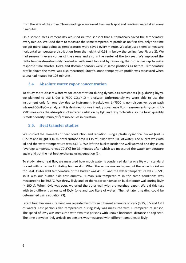
6

from the side of the stove. Three readings were saved from each spot and readings were taken every

5 minutes.

On a second measurement day we used iButton sensors that automatically saved the temperature

every minute. We used them to measure the same temperature profile as on first day, only this time

we got more data points as temperatures were saved every minute. We also used them to measure

horizontal temperature distribution from the height of 0.58 m below the ceiling (see Figure 2). We

had sensors in every corner of the sauna and also in the center of the top seat. We improved the

Delta temperature/humidity controller with small fan and by removing the protective cap to make

response time shorter. Delta and Rotronic sensors were in same positions as before. Temperature

profile above the stove was also measured. Stove’s stone temperature profile was measured when

sauna had heated for 105 minutes.

3.4. Absolute water vapor concentration

To study more closely water vapor concentration during dynamic circumstances (e.g. during löyly),

we planned to use Li-Cor LI-7500 CO2/H2O – analyzer. Unfortunately we were able to use the

instrument only for one day due to instrument breakdown. LI-7500 is non-dispersive, open path

infrared CO2/H2O – analyzer. It is designed for use in eddy covariance flux measurements systems. LI-

7500 measures the absorption of infrared radiation by H2O and CO2 molecules, so the basic quantity

is molar density (mmol/m3) of molecules in question.

3.5. Heat transfer studies

We studied the moments of heat conduction and radiation using a plastic cylindrical bucket (radius

0.27 m and height 0.16 m, total surface area 0.135 m2) filled with 10 l of water. The bucket was with

lid and the water temperature was 33.5°C. We left the bucket inside the well warmed and dry sauna

(average temperature was 70.8°C) for 33 minutes after which we measured the water temperature

again and got the net heat exchange using equation (1).

To study latent heat flux, we measured how much water is condensed during one löyly on standard

bucket with outer wall imitating human skin. When the sauna was ready, we put the same bucket on

top seat. Outer wall temperature of the bucket was 41.5°C and the water temperature was 36.5°C,

so it was our human skin test dummy. Human skin temperature in the same conditions was

measured to be 39.5°C. We threw löyly and let the vapor condense on bucket outer wall during löyly

(≈ 100 s). When löyly was over, we dried the outer wall with pre-weighed paper. We did this test

with two different amounts of löyly (one and two liters of water). The net latent heating could be

determined using equation (3).

Latent heat flux measurement was repeated with three different amounts of löyly (0.25, 0.5 and 1.0 l

of water). Test person’s skin temperature during löyly was measured with IR-temperature sensor.

The speed of löyly was measured with two test persons with known horizontal distance on top seat.

The time between löyly arrivals on persons was measured with different amounts of löyly.

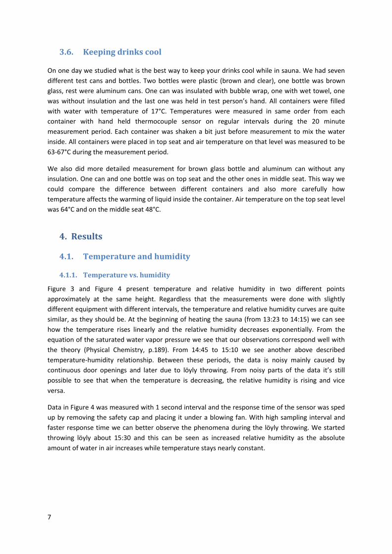
7

3.6. Keeping drinks cool

On one day we studied what is the best way to keep your drinks cool while in sauna. We had seven

different test cans and bottles. Two bottles were plastic (brown and clear), one bottle was brown

glass, rest were aluminum cans. One can was insulated with bubble wrap, one with wet towel, one

was without insulation and the last one was held in test person’s hand. All containers were filled

with water with temperature of 17°C. Temperatures were measured in same order from each

container with hand held thermocouple sensor on regular intervals during the 20 minute

measurement period. Each container was shaken a bit just before measurement to mix the water

inside. All containers were placed in top seat and air temperature on that level was measured to be

63-67°C during the measurement period.

We also did more detailed measurement for brown glass bottle and aluminum can without any

insulation. One can and one bottle was on top seat and the other ones in middle seat. This way we

could compare the difference between different containers and also more carefully how

temperature affects the warming of liquid inside the container. Air temperature on the top seat level

was 64°C and on the middle seat 48°C.

4. Results

4.1. Temperature and humidity

4.1.1. Temperature vs. humidity

Figure 3 and Figure 4 present temperature and relative humidity in two different points

approximately at the same height. Regardless that the measurements were done with slightly

different equipment with different intervals, the temperature and relative humidity curves are quite

similar, as they should be. At the beginning of heating the sauna (from 13:23 to 14:15) we can see

how the temperature rises linearly and the relative humidity decreases exponentially. From the

equation of the saturated water vapor pressure we see that our observations correspond well with

the theory (Physical Chemistry, p.189). From 14:45 to 15:10 we see another above described

temperature-humidity relationship. Between these periods, the data is noisy mainly caused by

continuous door openings and later due to löyly throwing. From noisy parts of the data it’s still

possible to see that when the temperature is decreasing, the relative humidity is rising and vice

versa.

Data in Figure 4 was measured with 1 second interval and the response time of the sensor was sped

up by removing the safety cap and placing it under a blowing fan. With high sampling interval and

faster response time we can better observe the phenomena during the löyly throwing. We started

throwing löyly about 15:30 and this can be seen as increased relative humidity as the absolute

amount of water in air increases while temperature stays nearly constant.

8

Figure 3.Temperature and relative humidity measured with Rotronic Hygrolog sensor at the height of 125 cm. Sampling interval was 15 seconds.

Figure 4. Temperature and relative humidity measured with Delta Ohm DO 9847 sensor the height of 135 cm. Sampling interval was 1 second and the sensor’s respond time was sped up with a little fan.

9

The relation between löyly thrown to the stove with temperature and relative humidity is shown in

Figure 5. Throwing löyly i.e. water to the stove increases the relative humidity for a while as the

water evaporates from hot stones to the air. An interesting phenomenon we found was the

temporary temperature decrease after löyly. This might be related to the evaporation of water from

the stoves or turbulent air mixing. Evaporation needs energy for phase transition. It binds energy

from the stove stones and from warm air as latent heat. When the energy is taken from the air it

cools down until the latent heat from water vapor is released again. Another explanation can be the

flows which occur after throwing löyly. Flows mix low level cool air with upper level warm air

decreasing the temperature at the top level of sauna. It’s likely that the both methods described

above affect at the same time.

The temperature decrease and relative humidity are proportional to the amount of löyly. However,

the length of löyly i.e. how wide is the peak (in Figure 5) is, isn’t directly proportional. Besides the

amount of löyly, also the time spent to throwing water and the place of stove (side, middle, etc.) you

throw water matters. For example if you throw water to cold side stones it takes longer to evaporate

than thrown evenly around the stove to warm stones.

Figure 5. Same as Figure 4 but with shorter time line. Black numbers above peaks are the amount of löyly thrown to the stove.

10

4.1.2. Temperature profiles

Before starting the heating of the sauna, the air was well mixed and no stratification was observed

(see Figure 6). Soon after the heating was started (12:23 o’clock) stratification took place and grew

larger till 15:10 when the sauna was ready. After that only few piece of wood was added to the stove

at the time and the vertical temperature profile as well as the vertical temperature gradient

remained quite unchanged. Sudden drop in temperatures was measured at 14:15 caused by the

accidently died out of the stove (i.e. coffee break). Temperature profiles were plotted as a contour

line map (Figure 6) and using cubic interpolation (not shown here). The figures were almost

identical, but the contour line figure was smoother and therefore it’s presented in this paper.

Figure 6. Sauna’s vertical temperature profile as a function of time. Temperatures were measured at seven different levels and are presented here as a contour line map.

Horizontal temperature distribution measured at the height of 176 cm is presented in Figure 7 (see

Figure 2 for sensor displacement). There seems to be no horizontal temperature gradient except

near the stove (Sensor 11). The horizontal temperatures in different locations seem to correspond

well with the temperature vertical profile data at the height of 177 cm. For some reason Sensor 9

which was part of the vertical profile chain, started to give greater values at 14:15 than rest of the

sensors. After 15:00 the Sensor 9 seemed to start to follow other sensor but that wasn’t the case

after all and finally the values dropped radically. There might be some technical problems with the

sensor 9 but we cannot be sure. The problems however aren’t related to the throwing of löyly

because the problems had already started before that.

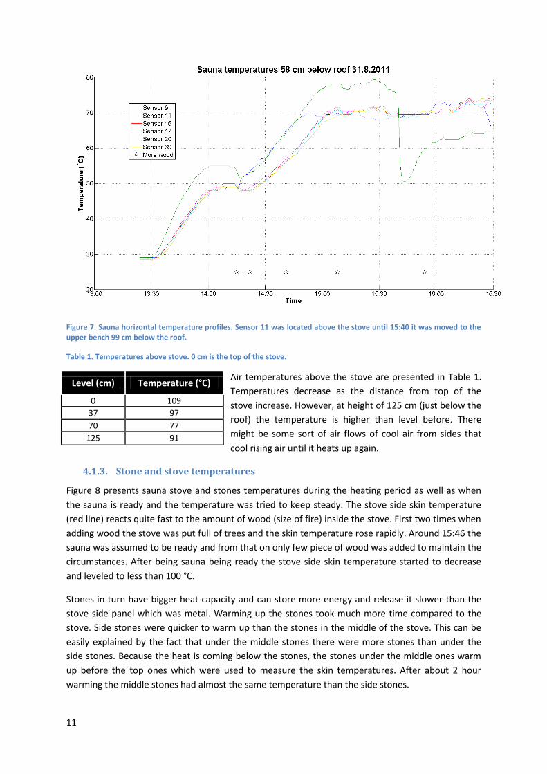
11

Figure 7. Sauna horizontal temperature profiles. Sensor 11 was located above the stove until 15:40 it was moved to the upper bench 99 cm below the roof.

Table 1. Temperatures above stove. 0 cm is the top of the stove.

Air temperatures above the stove are presented in Table 1.

Temperatures decrease as the distance from top of the

stove increase. However, at height of 125 cm (just below the

roof) the temperature is higher than level before. There

might be some sort of air flows of cool air from sides that

cool rising air until it heats up again.

4.1.3. Stone and stove temperatures

Figure 8 presents sauna stove and stones temperatures during the heating period as well as when

the sauna is ready and the temperature was tried to keep steady. The stove side skin temperature

(red line) reacts quite fast to the amount of wood (size of fire) inside the stove. First two times when

adding wood the stove was put full of trees and the skin temperature rose rapidly. Around 15:46 the

sauna was assumed to be ready and from that on only few piece of wood was added to maintain the

circumstances. After being sauna being ready the stove side skin temperature started to decrease

and leveled to less than 100 °C.

Stones in turn have bigger heat capacity and can store more energy and release it slower than the

stove side panel which was metal. Warming up the stones took much more time compared to the

stove. Side stones were quicker to warm up than the stones in the middle of the stove. This can be

easily explained by the fact that under the middle stones there were more stones than under the

side stones. Because the heat is coming below the stones, the stones under the middle ones warm

up before the top ones which were used to measure the skin temperatures. After about 2 hour

warming the middle stones had almost the same temperature than the side stones.

Level (cm) Temperature (°C)

0 109

37 97

70 77

125 91

12

Figure 8. Sauna stove and stones skin temperatures with error bars. For every point three measurements were done and the mean value and standard deviation were calculated. Mean values are plotted and standard deviation used as an error estimate.

4.2. Sauna is hot place – why?

We studied different heating mechanisms and their moments in the sauna using the theoretical and

practical tools described in chapters 2 and 3, respectively. Our hypothesis was that the latent

heating is the most important and convection is the second important factor in heat transfer (≈ the

feeling of hotness) in the sauna. What was the truth? Well, read the following chapters!

First, we figured out the significance of the conductive and radiative heating. We assumed that the

sauna was dry (no condensation on the bucket), the bucket was very light comparing to the mass of

water and the flow velocities were low, therefore, convection could be negligible.

According to the equation (1), the net heat exchange was approximately J kg-1 K-1 × 3 K ×

10 kg J if we assume that J kg-1 K-1 which is valid value in 1 atm pressure and

20°C temperature. The average (during time t) heat flux per unit area was then

m-2 125460 J/0.135 m2 /(33 × 60 s) ≈ 470 W/m2, (10)

which sounds a quite realistic result. On the other hand, it was possible to calculate the net heat flux

of radiation using the equation (8). Employing the values 41.5 K +273.15 K (the temperature of

the body) and 70.8 K + 273.15 K (the temperature of ambient air/walls), we got for the result

W/m2 (radiative heat flux per unit area) and further, W/m2 – 240 W/m² 230

W/m2 (conductive heat flux per unti area). According to this result, the conductive heat flux seems to

be in the same magnitude as the radiative net heat flux. The result means also that the thermal

boundary layer thickness was approximately 3 mm for the value of W/m/K (see

equation 4) which sounds also quite reasonable value indeed.

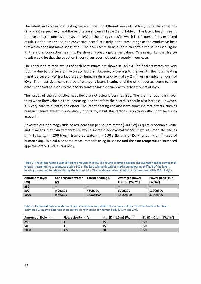
13

The latent and convective heating were studied for different amounts of löyly using the equations

(2) and (5) respectively, and the results are shown in Table 2 and Table 3. The latent heating seems

to have a major contribution (several kW) to the energy transfer which is, of course, fairly expected

result. On the other hand, the convective heat flux is only in the same range as the conductive heat

flux which does not make sense at all. The flows seem to be quite turbulent in the sauna (see Figure

9), therefore, convective heat flux should probably get larger values. One reason for the strange

result would be that the equation theory gives does not work properly in our case.

The concluded relative results of each heat source are shown in Table 4. The final estimates are very

roughly due to the several inaccuracy factors. However, according to the results, the total heating

might be several kW (surface area of human skin is approximately 2 m2) using typical amount of

löyly. The most significant source of energy is latent heating and the other sources seem to have

only minor contributions to the energy transferring especially with large amounts of löyly.

The values of the conductive heat flux are not actually very realistic. The thermal boundary layer

thins when flow velocities are increasing, and therefore the heat flux should also increase. However,

it is very hard to quantify the effect. The latent heating can also have some indirect effects, such as

humans cannot sweat so intensively during löyly but this factor is also very difficult to take into

account.

Nevertheless, the magnitude of net heat flux per square meter (1000 W) is quite reasonable value

and it means that skin temperature would increase approximately 5°C if we assumed the values

kg, J/kg/K (same as water), s (length of löyly) and m2 (area of

human skin). We did also some measurements using IR-sensor and the skin temperature increased

approximately 3−6°C during löyly.

Table 2. The latent heating with different amounts of löyly. The fourth column describes the average heating power if all energy is assumed to condensate during 100 s. The last column describes maximum power peak if half of the latent heating is assumed to release during the hottest 10 s. The condensed water could not be measured with 250 ml löyly.

Amount of löyly [ml]

Condensated water [g]

Latent heating [J] Averaged power (100 s) [W/m²]

Power peak (10 s) [W/m²]

250 − − − − 500 0.2±0.05 450±100 500±100 1200±300 1000 0.6±0.05 1350±100 1500±100 3700±300

Table 3. Estimated flow velocities and heat convection with different amounts of löyly. The heat transfer has been estimated using two different characteristic length scales for human body (0.1 m and 1m).

Amount of löyly [ml] Flow velocity [m/s] (D = 1.0 m) [W/m²] (D = 0.1 m) [W/m²]

250 1 150 250 500 1 150 250 1000 1.5 200 350

14

Table 4. Roughly approximated relative proportions of each energy source using different volumes of löyly. The last column describes the magnitude of the total heat flux per square meter.

Amount of löyly [ml]

[%] [%] [%] [%] [W/m2]

250 33 33 − 33 ≈ 500 500 20 20 40 20 ≈ 1000 1000 10 10 70 10 ≈ 2000

Figure 9: Water vapor concentration [mmol/m3] during löyly measured by Li-Cor LI-7500. Behavior of the concentration

seems to be chaotic, therefore, flows during löyly are also probably turbulent.

4.2.1. What is the hottest place in sauna?

It seems that the latent heating is the most important factor in the sauna mystery. Therefore, the

next hypothesis could be that the hottest place in sauna is in area of the most massive latent

heating, thus, we tried to figure out where this place might be located.

We did some human subject researching and got very predictable result: the hottest place is in the

opposite corner to the stove. Why? Well, the latent heating is spread by flows and the flows are

forced to move along the walls and the roof. And further, we can assume that the flows and fluxes of

latent heating are colliding in the opposite corner to the stove, and therefore it has to be also the

hottest, best and most painful place in the whole sauna. We do not have any other evidence, such

as independent measurements, for this argument but we have very strong feeling (also literally) that

things are going like this.

15

4.3. Radiation

In our measurements the feeling of warmth which human feels isn’t due to the radiation from the

stove, at least if you’re not just above the stove. Figure 10 shows that the net radiation at 115 cm

distance from stove at 160 cm height is around 5 W/m2. Adding wood to the stove temporary

increases the radiation for a short time but doesn’t raise the net radiation very high. The data for the

Figure 10 was from the heating period of sauna which gives greater values compared to the sauna

which is ready and only a little fire is maintained in the heart of stove.

There is a great difference in the net radiations between the sensor data and the calculations using

Stefan-Boltzmann law (see sections 2.1 and 4.2). The sensor viewing angle is quite big and at 115 cm

distance from the stove it measures more than just the stove. We can approximate, using the

sensors distance from stove and stove’s dimensions that stove fills roughly 1/5 of field of vision of

the sensor. In the Stefan-Boltzmann law we assume that the net radiation is calculated between the

stove and the human. The sensor on one side sees the radiation from the stove and walls and the

other side from human and walls. Because the sensor measures more than just the stove and the

human body, the results are hard to compare reliable with the theory.

Figure 10. Net radiation during the heating of sauna.

Figure 11 shows net radiation measured above the stove as well as between human and different

directions. Net radiation approximately 50 cm above the stove was about 22 W/m2 which is twice as

the biggest radiation measured during the heating time at longer distance from stove. The net

radiation above the stove might have been bigger than we measured because we had to remove the

instrument after a while to avoid the meltdown of plastic parts. When sitting on the middle of upper

bench the net radiations from the stove and the back wall directions to human are quite similar, ≈ 8

W/m2. Net radiation from roof was in turn less than half of the stove and wall. The distance between

head and roof compared to human and wall or stove is much shorter which might explain the

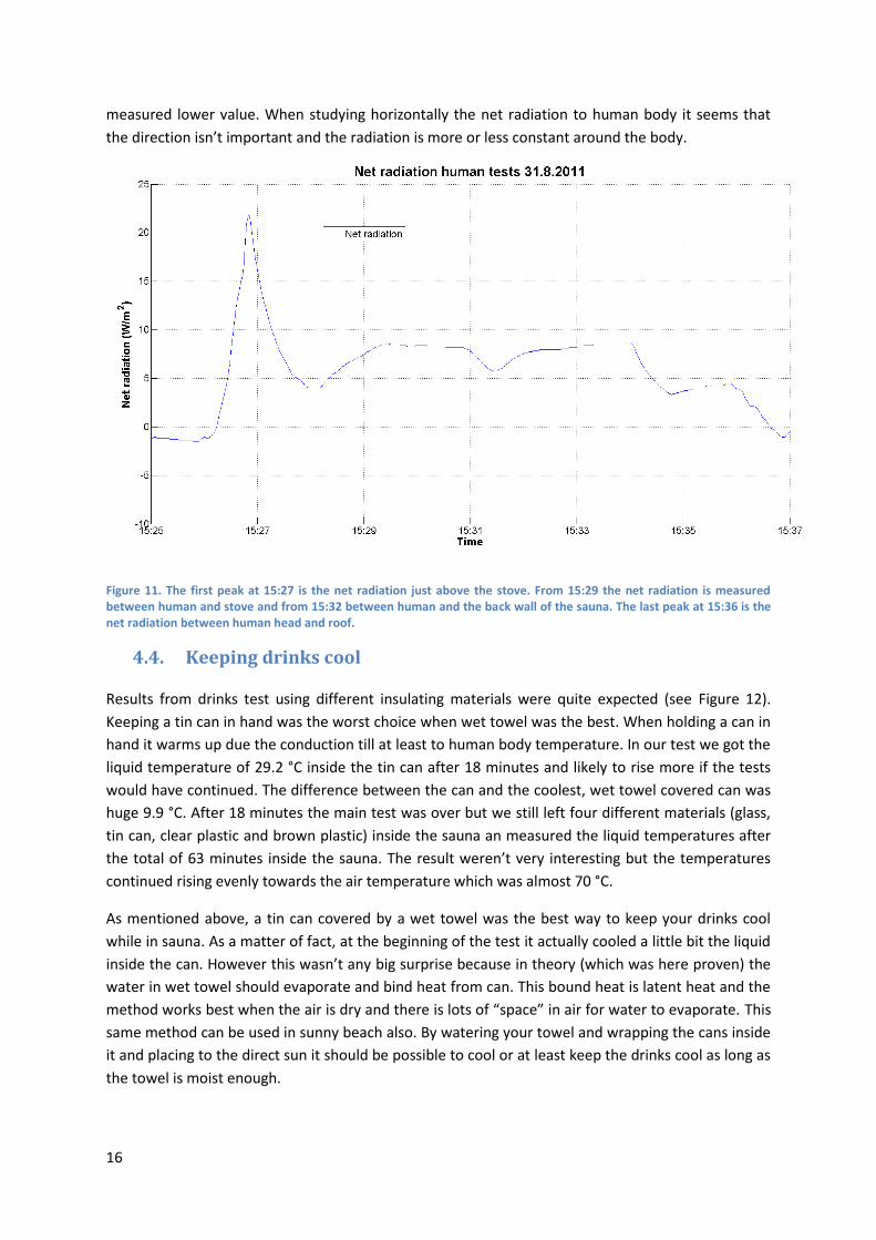
16

measured lower value. When studying horizontally the net radiation to human body it seems that

the direction isn’t important and the radiation is more or less constant around the body.

Figure 11. The first peak at 15:27 is the net radiation just above the stove. From 15:29 the net radiation is measured between human and stove and from 15:32 between human and the back wall of the sauna. The last peak at 15:36 is the net radiation between human head and roof.

4.4. Keeping drinks cool

Results from drinks test using different insulating materials were quite expected (see Figure 12).

Keeping a tin can in hand was the worst choice when wet towel was the best. When holding a can in

hand it warms up due the conduction till at least to human body temperature. In our test we got the

liquid temperature of 29.2 °C inside the tin can after 18 minutes and likely to rise more if the tests

would have continued. The difference between the can and the coolest, wet towel covered can was

huge 9.9 °C. After 18 minutes the main test was over but we still left four different materials (glass,

tin can, clear plastic and brown plastic) inside the sauna an measured the liquid temperatures after

the total of 63 minutes inside the sauna. The result weren’t very interesting but the temperatures

continued rising evenly towards the air temperature which was almost 70 °C.

As mentioned above, a tin can covered by a wet towel was the best way to keep your drinks cool

while in sauna. As a matter of fact, at the beginning of the test it actually cooled a little bit the liquid

inside the can. However this wasn’t any big surprise because in theory (which was here proven) the

water in wet towel should evaporate and bind heat from can. This bound heat is latent heat and the

method works best when the air is dry and there is lots of “space” in air for water to evaporate. This

same method can be used in sunny beach also. By watering your towel and wrapping the cans inside

it and placing to the direct sun it should be possible to cool or at least keep the drinks cool as long as

the towel is moist enough.

17

Figure 12. Liquid temperatures inside different bottle types with different insulating materials.

When comparing the liquid and skin temperatures in two different levels the liquid temperatures

behaved the same way as in material test. The liquids inside glasses and tin cans without any

insulating material warmed up quite linear. The skin temperatures of glasses and cans were as for

totally different than liquid temperatures. At the first few minutes the skin temperatures where

rising then decreasing and then again rising except for the lower bench tin which first decreased and

the behaved like the rest. The variation in skin temperatures might be the result from can/glass skin

balancing between hotter air and colder liquid. At first the temperature difference between skin and

air is bigger than between skin and liquid and the skin temperature is rising. When the skin

temperature is rising, the temperature difference between skin and air is decreasing and the

difference between skin and liquid grows bigger as the liquid doesn’t warm up as fast as the

tin/glass. Increased skin-liquid temperature difference might cause the temporary cooling in the skin

temperatures. The height of upper bench was 135 cm and air temperature about 64 °C and for lower

bench 93 cm and about 48 °C, respectively. However, the variation in skin temperatures is in small

scale (few degrees) and could be read as a measurement error in harsh sauna conditions.

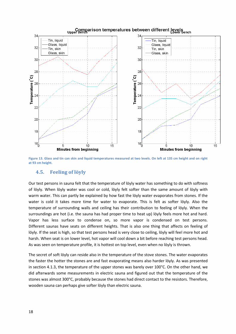
18

Figure 13. Glass and tin can skin and liquid temperatures measured at two levels. On left at 135 cm height and on right at 93 cm height.

4.5. Feeling of löyly

Our test persons in sauna felt that the temperature of löyly water has something to do with softness

of löyly. When löyly water was cool or cold, löyly felt softer than the same amount of löyly with

warm water. This can partly be explained by how fast the löyly water evaporates from stones. If the

water is cold it takes more time for water to evaporate. This is felt as softer löyly. Also the

temperature of surrounding walls and ceiling has their contribution to feeling of löyly. When the

surroundings are hot (i.e. the sauna has had proper time to heat up) löyly feels more hot and hard.

Vapor has less surface to condense on, so more vapor is condensed on test persons.

Different saunas have seats on different heights. That is also one thing that affects on feeling of

löyly. If the seat is high, so that test persons head is very close to ceiling, löyly will feel more hot and

harsh. When seat is on lower level, hot vapor will cool down a bit before reaching test persons head.

As was seen on temperature profile, it is hottest on top level, even when no löyly is thrown.

The secret of soft löyly can reside also in the temperature of the stove stones. The water evaporates

the faster the hotter the stones are and fast evaporating means also harder löyly. As was presented

in section 4.1.3, the temperature of the upper stones was barely over 100°C. On the other hand, we

did afterwards some measurements in electric sauna and figured out that the temperature of the

stones was almost 300°C, probably because the stones had direct contact to the resistors. Therefore,

wooden sauna can perhaps give softer löyly than electric sauna.

19

5. Conclusions

The harsh temperature and humidity conditions in sauna put our measurement equipment to their

limits. Many of the equipment and the equations and constants were designed and optimal for NTP

conditions. That’s why our results must not interpret as an absolute truth but more like a guide lines

and indicatives.

Our main scientific problem was that what makes sauna feel hot. What are the major heat transfer

mechanisms in sauna conditions? We used different approaches to examine the different heat

transfer mechanisms. In static conditions in warmed up sauna, the main mechanisms for heat

transfer are conductive and radiative heat flux. Their power is around 240 W/m2 each. During löyly

latent heat seems to play major role with power of 500-1500 W/m2 depending on size of löyly.

Radiative, conductive and convective all have minor roles during löyly, with relative contribution of

10-20% each of total power.

Temperature and relative humidity behavior in sauna was like in theory it should be. When the

temperature rises linearly, the relative humidity decreases exponentially. When throwing löyly, the

temperature temporarily decreased while the relative humidity increased. The peaks were

proportional to the amount of löyly (water). Vertically sauna temperature was stratified immediately

after the heating started. Horizontally the temperature profiles were uniform except above the

stove where higher temperatures were measured. Temperatures of stove stones were place

depended. It took much longer time for the middle stones to warm up compared to the side stones.

The surface temperature of stove was much more sensitive to the size of fire in the stove heart than

the stones.

The feeling of löyly is a personal matter, but some hints for soft löyly can be given. Colder löyly water

seems to produce softer löyly than warm one. The height of seats is important, when persons sit a

bit lower, not just below the ceiling, hot water vapor has some time to cool while descending, and

thus producing softer löyly.

The measurements made in sauna were extremely interesting. We could not find similar

measurements from the literature so we see us as pioneers in the field of sauna. We hope that in

future we could continue the studies about the sauna with more suitable instruments which tolerate

the heat better. But meanwhile we keep enjoying löyly and spread the Good News about sauna. And

finally the ultimate result of our experiments; The best way to keep your drink cool in a sauna seems

to be wrapping a wet towel or bubble wrap around it and no major difference between uninsulated

glass bottle and aluminum could be found. Anyhow, we recommend you to drink your drinks as fast

as you can to avoid even the slightest temperature contamination.

20

6. References

Hermans, L.F.J. and Vesala, T. The sauna – revisited. Europhysics news, vol. 38, 6. 2007. http://dx.doi.org/10.1051/epn:2007025

Physical Chemistry, 4th ed. Laidler, Meiser, Sanctuary, New York, 2003.

Vesala, T. (2004): Ympäristöfysiikan perusteet – Johdatus siirtoilmiöihin ja ilmakehän fysiikkaa.

Report Series in Aerosol Science, Yliopistopaino.

field course in micrometeorology and hydrology · preface the 2011 vintage of field course in...

Documents