feynman's ratchet and pawl - rockefeller...

Journal of' Stuti.stic.ul Physics, Vol. 93, Nos. 314,. 1998

Feynman's Ratchet and Pawl

Marcelo 0. Magnascol and Gustavo ~tolovitzky'.

Received February 6, 1998; final May 14, 1998 -- - -

While many papers in the last few years have dealt with various equations euphemistically called "ratchets, '~he original Feyman two-temperature setup has been left largelq unchallenged. We present here a look at the details of how this famous engine actually generates motion from a temperature difference.

Maxwell understood correctly that the Second Law is certain only in a statistical sense. He attempted to show this(') by the device now called "Maxwell demon:" a being of molecu1a.r size who would sort fast molecules from slow molecu-les, thus generating (a thermal gradient out of an initially isothermal condition. Unfortunately, Maxwell did not realize that the demon would itself be subject to fluctuations of the same type and size as those it was trying to take advantage of. By the 20s and 30s people like Smolu~hovsky(~) and S ~ i l a r d ( ~ ) showed that once a system is in thermal contact with a reservoir it does not matter whether it is large or small at the molecular scale: the operations of the demon will always be subject to the Second Law. They started a long tradition(" 5 9 6 , of the Maxwell demon as a means to probe the underlying nature of statistical mechanics at the small scale, with the Second Law no longer into question.

But then the nature of the game changed dramatically, and not from within physics. Advances in molecular biology made it clear that cells are populated with molecular machinery operating near the limits of thermal energies, and that these machinery do indeed perform the kinds of tasks usually entrusted to Maxwell demons. We are, in a sense, made of demons.

1 Center for studies in Physics and Biology, The Rockefeller University, New York, New York 10021.

2 Current address: IBM Thomas J. Watson Research Center, Yorktown Heights, New York 10598.

Magnasco and Stolovitzky 61 6

We propose here a retreat to the purely conceptual realm, to consider Feynman7s Ratchet and Pawl mechanism, just for the fun of understanding some details of irreversible systems subject to multiple temperatures. ~ h , picture that emerges is substantially more complicated, but also more rich than Feynman's analysis outlined: a story of probability currents circulating in large eddies, shedding small amounts of probability on their borders to make the engine work. We'll build from discussions of how to generate motion from thermal gradients, as outlined by ~andauer,"') Buttiker") and

r

van ampe en,'^) and from detailed analysis of the intrinsic losses incurred when touching two thermal baths simultaneously, as outlined by Parrondo and ~ s p a f i o l , ( l ~ ) and by Sekimoto.(ll)

We'll proceed as follows. We'll set up our equations modeling the ratchet. Then we'll argue a boundary layer approximation (BLA) that collapses to a case studied by Buttiker, and show how this picture for- malizes Feynman7s discussion. We'll then do numerical simulation, and show that the boundary layer approximation is incorrect because it assumes a single layer: the motion of the system is organized in an elongated roll, with an updraft bottom layer and a downdraft upper layer. While the net difference between top and bottom currents that provides the interwell motion is reasonably described by the BLA, neither the large- scale picture nor the resulting losses are. Furthermore, upon reversal of the temperature difference, a new mechanism arises that never operates in the vicinity of the boundary at all. We'll wrap up by analyzing these features in analytical detail for a linear system.

1. RATCHET AND PAWL

We will not here review Feynman's setup, lest we might, by doing so, deprive the-reader from a perfect excuse to read once more Chapter 46 of the Lectures on

We'll work in the overdamped regime, since the underdamped system gives essentially similar answers at a much higher cost, and underdamped systems are physically much more difficult to realize. We'll call x the degree of freedom associated to the ratchet-axle-vane system (p.b.c., since it's an angle) and y the position of the pawl; the shape of the ratchet's teeth enters as a boundary condition (See Fig. 1). Then,

Feynman's Ratchet and Pawl

x (Ratchet)

Fig. 1. Sketch of the configuration space of the engine. The vertical coordinate is the position of the pawl, while the horizontal coordinate is the position of the ratchet (modulo a single tooth). The curve represents the boundary of the ratchet; since the pawl cannot penetrate it, the region below is forbidden to the system. The ratchet and pawl degrees of freedom are in contact with different heat reservoirs; hence diffusion due to temperature is elliptic.

where T, is the temperature matrix, which we'll assume to be of the form

We'll usually be thinking of V(x, y) = U ( y ) + Lx, where U is the potential energy of the pawl, which presses it upon the teeth, while L is the load on the ratchet (the weight of the flea); we'll use L = 0 from here on. (We'll also have to complicate this form due to problems with the boundary conditions.) The associated Fokker-Planck system for steady state is

We'll call the quantity in parentheses J, the probability current. When T , = T, (and L=O) the Boltzmann distribution is the sole

stable solution of this system, which is thus in thermodynamic equilibrium. When T , # T, (still L = 0) something funny happens. The Boltzmann

form P a exp( - U(y)/kT,) satisfies the Fokker-Planck equation; because JGO, it would seem to satisfy the boundary conditions trivially. This hap- Pens because the (impenetrable) boundary conditions are actually more

618 Magnasco and Stolovitzky

involved and slightly horrible: we explicitly have to set P = 0 outside the ratchet, which leads to J acquiring a Dirac 6 precisely on the boundary. The prefactor of this 8 vanishes in detailed balance, but it does not for T , # T 2 .

A slightly more convenient way to see this is as follows. Let's remove the boundary condition altogether, and declare the potential to smoothly diverge at the ratchet surface: this is, after all, the physical situation leading to the boundary condition in its limit. Then, whenever the shape of the ratchet's teeth is sloped with respect to the horizontal or vertical, we get a coupling between the x and y degrees of freedom in the potential. The current J cannot be zero then because J = -VVP - V P - 0 would imply that

So we are requiring that both V ln P and T - V In P be gradients of a scalar field, which is not possible unless T , = T, or P is of the form Q(x) R ( y ) (i.e., x and y are independent degrees of freedom,) This also highlights a technical problem with this system: though we get elliptic operators, they are not conformal, and hence much of the artillery for solving Laplace-like systems won't work here.

2. EFFICIENCY

Recently, Parrondo and ~spafiol(~O) have noted that the axle joining vane and ratchet establishes communication between the two ireservoirs. They develop a particularly clear example: instead of the ratchet-and-pawl system on the right reservoir, they just have another vane; in this case the axle serves as a thermal conduit between the two reservoirs, and beat flows between them, marring the efficiency of the device. We'll assume henceforth that we have taken account of this issue: i.e., that the temperature T, has already been properly renormalized so as to take into account t.his effect. Furthermore, we'll take these energy losses for granted and look for brand new ones. It is not clear that this is 100% proper: we should really consider the three dimensional system of vane/ratchet/pawl; however, this seems at the time the most innocuous of our approximations. (Also, the limit of an infinitely stiff axle cannot be taken within the overdamped regime, see Appendix B.) Sekimoto(ll) has computed numerical solutions to the Fokker-Planck equation for a ratchet-pawl ratchet-pawl system, and found that for the particular cases chosen the efficiency is substantially below the Carnot efficiency argued by Feynman.

Feynman's Ratchet and P a w l 619

The core of Feynman7s argument is that there will be a value of the weight of the flea (the load) for which the average speed will be zero (called the "stall load"). He then argues that this is a "quasistatic" case on which maximal eficiency will be attained. The central point brought forth by Parrondo and Espaiiol is that the ratchet-and-pawl is never quasistatic, because (unlike the Carnot engine) it's never in contact with just one single bath: it's always in contact with both.

It's simple to show in closed form that the ratchet is not quasistatic at stall load. In fact, it's shown by Eq. ( I ) : if the two temperatures are different, and the ratchet's teeth are not exactly horizontal or exactly vertical, detailed balance is structurally impossible; this is true at any load, and in particular at stall load. So there are currents at stall load, and with them a direction in time and irreversibility, since currents are not invariant under time reversal. With this irreversibility comes, obviously, a finite amount of entropy produced per unit of time; but since the work done per unit of time against the load is zero, the efficiency, rather than being maximal, is exactly zero, and the ratchet achieves maximal efficiency only at a finite speed.

However, such an argument is correct but hardly illuminating. We will try now to describe in which fashion the ratchet-and-pawl operates, giving a detailed dynamical picture of how it "leaks" energy between the baths. In doing so, we will learn a few things about nonequilibrium systems.

3. BOUNDARY LAYER APPROXIMATION

If both temperatures are small enough that the system is confined to a narrow probability band in the vicinity of the ratchet's boundary, we could think of the system as essentially one dimensional. In this case, we can note that along this probability strip, the "effective" temperature is a function of the local slope of the boundary: T,,= t . T . t, where t is the vector tangent to the boundary. (This is the same as computing the temperature by intersecting the ellipsoid at some slope.)

This type of system, and the conditions on the space-varying temperature and potential to obtain motion have been extensively studied by Landa~er , '~) ~uttiker,") and van amp en.'^) In order to obtain motion, we have to satisfy

where the integral is taken along one loop of the periodic coordinate x. In our particular realization we would have an extra twist: the potential enters the equations through h(x), the shape of the ratchet: V(x, y ) -+ V(x, h(x)),


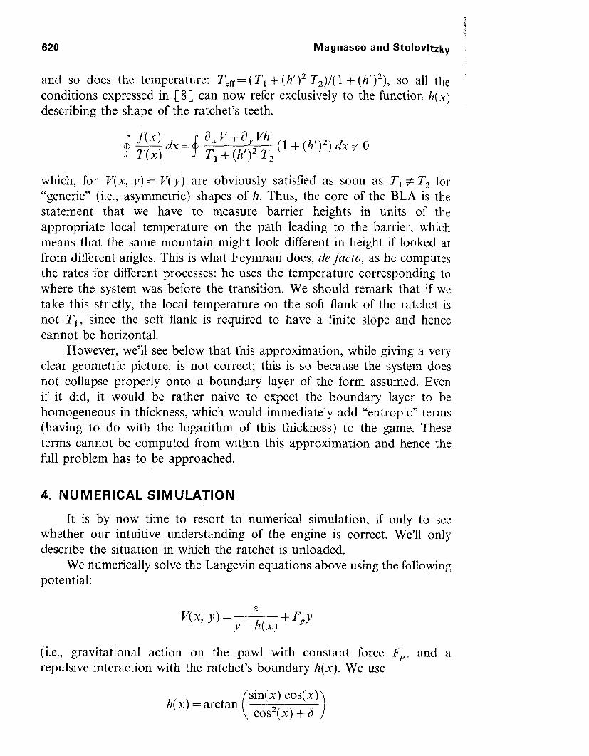
and so does the temperature: T,= ( T1 + (h')2 T2)/( 1 + (h')2), SO all the conditions expressed in 181 can now refer exclusively to the function h ( ~ ) describing the shape of the ratchet's teeth.

which, for V(x, y) = V(y) are obviously satisfied as soon as T1 # T, for "generic" (i.e., asymmetric) shapes of h. Thus, the core of the BLA is the statement that we have to measure barrier heights in units of the appropriate local temperature on the path leading to the barrier, which means that the same mountain might look different in height if looked at from different angles. This is what Feynman does, de facto, as he computes the rates for different processes: he uses the temperature corresponding to where the system was before the transition. We should remark that if we take this strictly, the local temperature on the soft flank of the ratchet is not TI, since the soft flank is required to have a finite slope and hence cannot be horizontal.

However, we'll see below that this approximation, while giving a very clear geometric picture, is not correct; this is so because the system does not collapse properly onto a boundary layer of the form assumed. Even if it did, it would be rather naive to expect the boundary layer to be homogeneous in thickness, which would immediately add "entropic" terms (having to do with the logarithm of this thickness) to the game. These terms cannot be computed from within this approximation and hence the full problem has to be approached.

4. NUMERICAL SIMULATION

It is by now time to resort to numerical simulation, if only to see whether our intuitive understanding of the engine is correct. We'll only describe the situation in which the ratchet is unloaded.

We numerically solve the Langevin equations above using the following potential:

(i.e., gravitational action on the pawl with constant force F,, and a repulsive interaction with the ratchet's boundary h(x). We use

sin(x) cos(x) h(x) = arctan

cos2(x) + 6

Feynman's Ratchet and Pawl 62 1

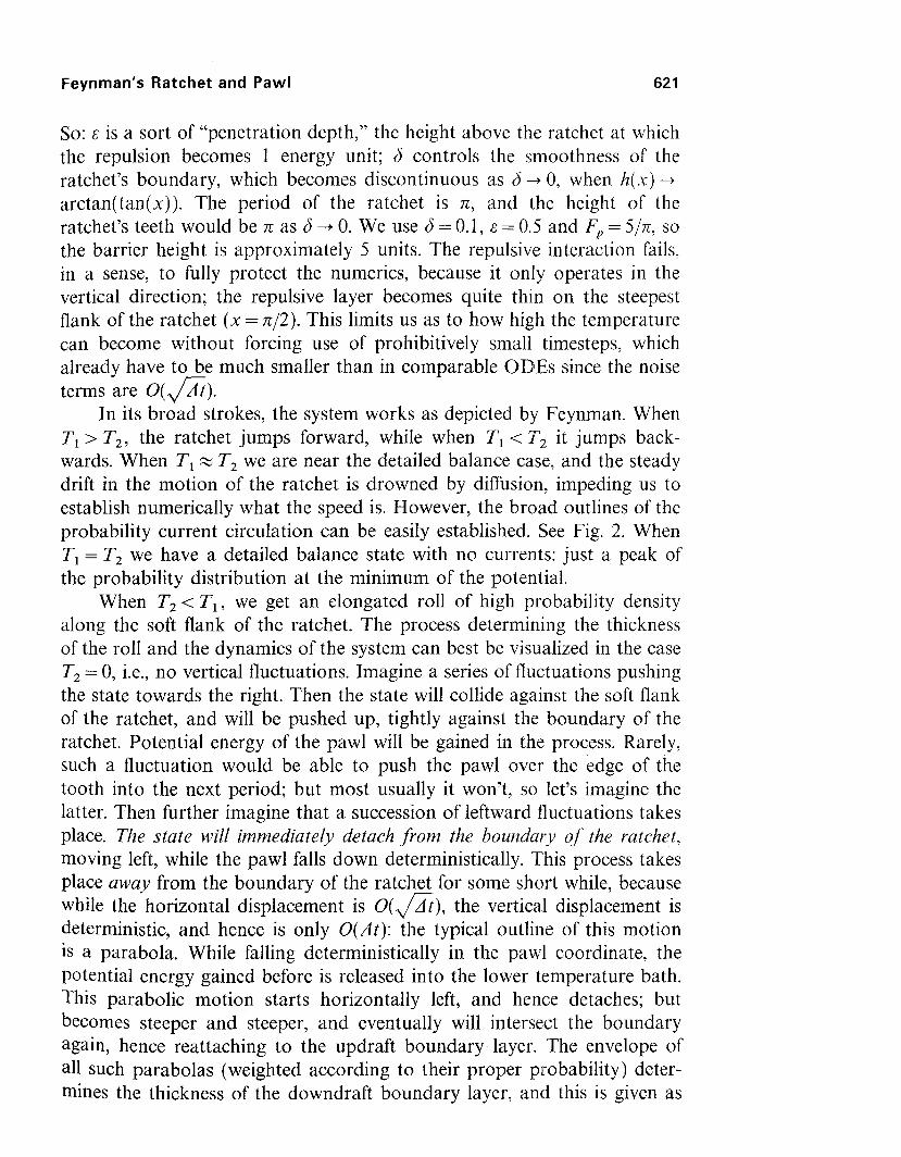
So: E is a sort of "penetration depth," the height above the ratchet at which the repulsion becomes 1 energy unit; S controls the smoothness of the ratchet's boundary, which becomes discontinuous as 6 -+ 0, when h ( x ) -+

arctan(tan(x)). The period of the ratchet is n-, and the height of the ratchet's teeth would be n- as 6 -+ 0. We use 6 = 0.1, E = 0.5 and F, = 5/n, so the barrier height is approximately 5 units. The repulsive interaction fails, in a sense, to fully protect the numerics, because it only operates in the vertical direction; the repulsive layer becomes quite thin on the steepest flank of the ratchet (x = 71.12). This limits us as to how high the temperature can become without forcing use of prohibitively small timesteps, which already have to be much smaller than in comparable ODES since the noise terms are o(@).

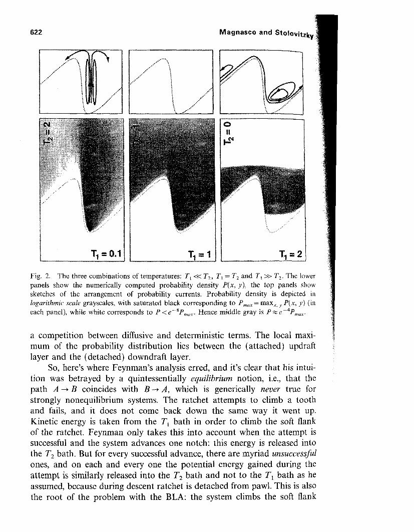
In its broad strokes, the system works as depicted by Feynman. When TI > T2, the ratchet jumps forward, while when T, < Ip; it jumps backwards. When T , = T2 we are near the detailed balance case, and the steady drift in the motion of the ratchet is drowned by diffusion, impeding us to establish numerically what the speed is. However, the broad outlines of the probability current circulation can be easily established. See Fig. 2. When T, = T, we have a detailed balance state with no currents: just a peak of the probability distribution at the minimum of the potential.

When T2 < T , , we get an elongated roll of high probability density along the soft flank of the ratchet. The process determining the thickness of the roll and the dynamics of the system can best be visualized in the case T2 = 0, i.e., no vertical fluctuations. Imagine a series of fluctuations pushing the state towards the right. Then the state will collide against the soft flank of the ratchet, and will be pushed up, tightly against the boundary of the ratchet. Potential energy of the pawl will be gained in the process. Rarely, such a fluctuation would be able to push the pawl over the edge of the tooth into the next period; but most usually it won't, so let's imagine the latter. Then further imagine that a succession of leftward fluctuations takes place. The state will immediately detach from the boundary of the ratchet, moving left, while the pawl falls down deterministically. This process takes place away from the boundary of the ratchet for some short while, because while the horizontal displacement is 0 the vertical displacement is deterministic, and hence is only O(At): the typical outline of this motion is a parabola. While falling deterministically in the pawl coordinate, the potential energy gained before is released into the lower temperature bath. This parabolic motion starts horizontally left, and hence detaches; but becomes steeper and steeper, and eventually will intersect the boundary again, hence reattaching to the updraft boundary layer. The envelope of all such parabolas (weighted according to their proper probability) deter- mines the thickness of the downdraft boundary layer, and this is given as

Ma~lnasco and StoInui+,t-..

Fig. 2. The three combinations of temperatures: T, << T,, T , = T, and T , >> T,. The lower panels show the numerically computed probability density P(x, j ~ ) ~ the top panels show sketches of the arrangement of probability currents. Probability density is depicted in logarithmic scale grayscales, with saturated black corresponding to P,,, = max , , P(x, y ) (in each panel), while white corresponds to P < e-8P,u,. Hence middle gray is P % e-4P,u,.

a competition between diffusive and deterministic terms. The local maxi- 1 mum of the probability distribution lies between the (attached) updraft layer and the (detached) downdraft layer.

So, here's where Feynman's analysis erred, and it's clear that his intuition was betrayed by a quintessentially equilibrium notion, i.e., that the path A -+ B coincides with B -+ A, which is generically never true for strongly nonequilibrium systems. The ratchet attempts to climb a tooth and fails, and it does not come back down the same way it went up. Kinetic energy is taken from the T , bath in order to climb the soft flank of the ratchet. Feynman only takes this into account when the attempt is successful and the system advances one notch: this energy is released into the T, bath. But for every successful advance, there are myriad unsuccessful ones, and on each and every one the potential energy gained during the attempt is similarly released into the T, bath and not to the T , bath as he assumed, because during descent ratchet is detached from pawl. This is also the root of the problem with the BLA: the system climbs the soft flank

Feynman's Ratchet and Pawl 623

tightly pressed against the ratchet, but comes down detached from this boundary. The motion of the system cannot truly be described by a single one-dimensional layer. The rate for the successful attempts is approximated appropriately by the BLA, because it only depends on the net current on the roll. But because the dissipation due to currents is of the order O(J2/P), by cancelling two large opposing currents into a small net current, the BLA hides a central mechanism of dissipation. All the time, between successful jumps, the system is losing power, because it's transmitting energy from the high temperature bath to the low temperature bath through terms analogous to those of Parrondo and Espafiol; but here the axle is no longer the culprit, it's the coupling between ratchet and pawl itself: the ratchet kicks the pawl up, and the pawl dissipates this energy through viscosity. Because energy is taken from the high-temperature bath and dissipated into the low temperature one, entropy is being generated.

When T , << T, the mechanism changes dramatically in shape, and the BLA is no longer correct even pictorially. If T, + 0, then the particle will slide back to the bottom of the tooth, and then jump vertically from there, forming a small vertical "geyser" of probability and currents. The width of this geyser is controlled by T I , so if T , is small enough the probability that the left side of the geyser will collide with the top of the ratchet becomes zero, whenever the ratchet shape is not perfectly sharp (i.e., the maximum and the minimum do not coincide). (If the ratchet has an overhang, the geyser becomes a familiar "histeresis loop.") Thus, when operating in "reverse," there is a finite value of T , at which backwards motion is maxi- mized, an effect that was not mentioned in the Lectures. We can note that this mechanism somewhat resembles the "ratchet" described in ref. 12, while the former one somewhat resembles that of ref. 13.

5 . EFFICIENCY AGAIN

It should be clear by now why Feynman's argument for the efficiency of the ratchet approaching Carnot's is incorrect. For one, thinking back into the problem, there are three energy scales to contend with: kT,, kT,, and Q, the barrier height (energy required to lift the pawl so the ratchet can advance). It seems rather inconceivable that Q could dropout of the efficiency formula in order to give the Carnot efficiency ATIT, except perhaps in a special limit, Q >> T or viceversa. We'll examine what the eficiency is for both of these limits.

The Parrondo-Espaiiol analysis has shown a loss of efficiency due to the axle coupling. We've shown another loss, of a similar nature, due to the ratchet-pawl coupling. Even then, it would be interesting to know the relative magnitude of the effects we're discussing here.


In the low T regime the probability distribution clusters at the bottom of the ratchet. The jumps that provide work become rarer at the rate of

exp(Q/kT,,), an essential singularity in T ; however, the energy losses due to the various couplings vanish only algebraically (see next section). Thus, the efficiency drops to zero. In the high T regime, jumps are frequent. Unfortunately, they are frequent either way. As T-, co the system is dominated by random motion, with the drift being small by cornparison. If the pawl's excursion in the vertical direction is not somehow limited, most of the motion of the system is carried out entirely outside the ratchet region. Even if it is confined by some form of restraint, most of the motion is dominated by violent collisions between ratchet and pawl (lossy), and by the thermal conductivity of the axle (also lossy). In this regime, the work done can be seen to diminish algebraically or stay constant at best, while the heat transfer increases as T. Hence the ef'ficiency drops to zero once more, but this time algebraically.

Thus the highest eficiency of the ratchet is achieved when T w Q, the one regime that's hardest to analyze. We hence turn our back on the dif- ficulties of this problem, and establish the extent of conductive losses in the simplest case: the bottom of a quadratic well.

6. TWO-DIMENSIONAL LINEAR SYSTEM

Consider two l-D Brownian particles with coordinates x and y and equal mass m, contained in separate reservoirs at temperatures T, and T,. The particles, each of which experiences its own harmonic potential with spring constant k, interact through a spring (constant R) that connects them.

The Langevin equations for this system are

where k , is Boltzmann constant, y is the friction coefficient (assumed to be the same for both reservoirs), and 5 , and [, are uncorrelated white noises.

The stationary Fokker-Planck equation corresponding to these Langevin equations is


where f = (f,, f,) = ( -kx+ R(y-x) , -ky+ R ( x y ) ) is the force, Tis an diagonal matrix with diagonal entries T, and T,, and P(x, y ) is the stationary distribution. Solving Eq. (5) (see Appendix A), we find that

P(x, y ) = N exp - 1 k + R

1 + 6 [ T (1 + 6a) x2 + R X ~

where T=(T,+ Ty)/2, 6 = ( T x - TY)/2T, a = ( ~ / ( k + R ) ) ~ - 1 and N is a normalization constant. Clearly 0 < 6 < 1, and - 1 < cc < 0.

The streamlines of the probability current coincide with the improba- bility curves (see Appendix A) which are determined by P(x, y ) = const. The latter is the equation of an ellipse rotated an angle 4, where

A few particular cases are 6 = 0, for which 4 = 7~/4 (as it should be in the isothermal case), and R + co, for wh.ich 4 = 7114. Also it is clear that $( -4 = - 4 ( 4 .

The ratio of the square of the axes of this ellipse is

6.1. Is an Experimental Realization Possible?

This system could be experimentally envisioned in the following way. Take to beads of diameter of approximately 1 pm. Trap them with laser tweezers, separated at a distance of the order of the 10 to1 15 pm. Tether the beads at the extremes of a il phage DNA molecule. The typical spring constant at the end of the well formed by the tweezers is

where typically V, z 150 k , T and r z 350 nm. The "dynamic" spring constant of the DNA is, according to the formula of Marko and Siggia(14)


where L = 16,500 nm is the length of the DNA, A = 50 nnn is its persistence length, and d is the actual distance between extremes of the DNA molecule. Doing the numbers one obtains that at d/L = 0.92, the ratio of k,,,,,/k,, z 1. Thus the effects of the interaction can be felt strongly, and we can probe an interesting regime.

Let us compute the temperature difference necessary for the non- isothermal effects to be seen. If k = R, the square of the ratio of the smaller to larger axis is 113 in the isothermal case. If the two beads are located in heated up and coned down stripes, the temperature difference necessary to make the aforementioned ratio differ in a 20% is of about 50". This difference amounts to a thermal gradient of 5,000°/nm, enough to set huge thermal currents of water in motion, and mask the effect that was purported to be seen.

This problem becomes larger when the characteristic size of the physical realization gets smaller, and hence multiple temperature "'Maxwell demons" become not just untenable, but plain ridiculous when considering the nano- meter-scale machinery of molecular biology. However, this does not mean that the study of multiple temperatures is irrelevant for biology at large. There are many, many instances in biological syste:ms where noise amplitudes depend on content The evolution of genomes is one such case: mutations of genetic material can be understood as a diffusion process in sequence space, subject to selection from a "fitness lantdscape;" but the amount of mutations can vary both in time and along the genome.(15) When a neuron relays a message to another neuron, the message is inevitably amicted by noise; however, this noise depends on what the message is.(16)

6.2. Entropy Production

The heat given by the thermal bath at T, that is not dissipated in that same bath will flow through the spring R to the other reservoir at temperature T,. The amount of heat per unit time extracted from the reservoir x is

For a general discussion of the thermal bath kinetics in this kind of models, see S e k i m ~ t o . ( ~ ~ ) Likewise dQ,,/dt = R(Jix), and thus dQ,/dt = - dQ,/dt, which is nothing but the conservation of energy.


The heat Q, is interchanged at temperature Tx, while the heat Q, does it at T,. Thus there is an entropy production of

We compute ( i y ) in Appendix A, from where the entropy production turns out to be

As expected, the entropy production vanishes both when R = 0 and when 6 = 0. Otherwise it is positive.

7. OUTLOOK

The ratchet-and-pawl engine has provided physicists with untold amounts of excitement and insight for many years, from Srnolu~howski,(~) through Brillouin's analysis of electrical diodes,(4) to the vivid and fascinating exposition by Feynman.(5) That we have found some fault with Feynman's analysis of the efficiency is of no real importance: this engin.e has given us, and will continue to give, excitement and insight into the realm of nonequilibrium systems. We've contributed a small grain to its illustrious history: an image of large-scale rolls of circulating probability attached to its boundary.

As with any other system with a "hard" breaking of detailed balance, systems with multiple temperatures along different degrees of freedom are, prima facie, hard to analyze. However, there does not seem to be anything within the theory that actually makes them intractable: the:y are modeled, after all, by elliptic linear PDEs, and hence rate rather modestly on the intractability scale. We expect that, as more systems are brought to scrutiny by emerging applications, c our arsenal of analytical tools will rapidly enlarge.

APPENDIX A

It can be surmised from the Langevin equations (which are linear, and forced with Gaussian noise), that the solution to Eq. ( 5 ) will be a bivariate Gaussian:


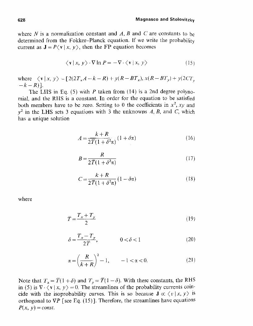
where N is a normalization constant and A, B and C are constants to be determined from the Fokker-Planck equation. If we write the probability current as J = P(v I x, y), then the FP equation becomes

where ( v 1 x, y ) = [2(2TxA - k - R) + y ( R - BT,), x ( R - BT,) + y(2CTY - k - R ) ] .

The LHS in Eq. (5) with P taken from (14) is a 2nd degree polyno- mial, and the RHS is a constant. In order for the equation to be satisfied both members have to be zero. Setting to 0 the coefficients in x2, xy and y2 in the LHS sets 3 equations with 3 the unknowns A, B, and C, which has a unique solution

where

Note that T, = T( 1 + 6) and T, = T(1- 6). With these constants, the RHS in (5) is V . ( v I x, y ) = 0. The streamlines of the proba,bility currents coincide with the isoprobability curves. This is so because J oc ( V 1 x, y) is orthogonal to V P [see Eq. (15)l. Therefore, the streamlines have equations P(x, y ) = const.


APPENDIX B

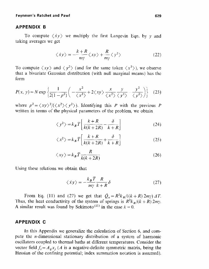
To compute ( i y ) we multiply the first Langevin Eqn. by y and taking averages we get

To compute ( xy ) and ( Y2) (and for the same token (.x2) ), we observe that a bivariate Gaussian distribution (with null marginal means) has the form

1 x2 P(x, y) = N exp x Y + 2(xy) ---- --

( x 2 > (y2> (y2)

where p2 = ( xy ) 2 / ( ( ~ 2 ) ( y2) ). Identifying this P with the previous P written in terms of the physical parameters of the problem, we obtain

(xy) = k,T R

k(k + 2R)

Using these relations we obtain that

k B T R ( i y ) =

my k + R 6

From Eq. (11) and (27) we get that Q,= ~ ~ k , / ( ( k + R ) 2my) AT. Thus, the heat conductivity of the system of springs is R2k,/(k + R) 2my. A similar result was found by Sekimoto(ll) in the case k = 0.

APPENDIX C

In this Appendix we generalize the calculation of Section 6, and compute the n-dimensional stationary distribution of a system of harmonic oscillators coupled to thermal baths at different temperatures. Consider the vector field f.= A,x, ( A is a negative-definite symmetric matrix, being the Hessian of the confining potential; index summation notation is assumed).

Magnasco and Stolovitzky 630

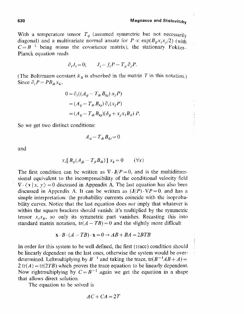
With a temperature tensor T, (assumed symmetric but not necessarily diagonal) and a multivariate normal ansatz for P c;c e x p ( B 0 x i ~ / 2 ) (with C = B-I being minus the covariance matrix), the stationary Fokker- Planck equation reads

(The Boltzmann constant k , is absorbed in the matrix T in this notation.) Since aiP = PBikxk,

0 = ai((AO - TikBkj) xjP)

= (A,- T,B,) ai(xjP)

= (A, - TikBkj)(a0 + xj.XIBil) P.

So we get two distinct conditions:

and

The first condition can be written as V . J/P = 0, and is the multidimen- sional equivalent to the incompressibility of the conditional velocity field V - ( v I x, y ) = 0 discussed in Appendix A. The last equation has also been discussed in Appendix A. It can be written as (JIR) V P = 0. and has a simple interpretation: the probability currents coincide with the isoprobability curves. Notice that the last equation does not imply that whatever is within the square brackets should vanish: it's multiplied by the symmetric tensor xixk, so only its symmetric part vanishes. Recasting this into standard matrix notation, tr(A - TB) = 0 and the slightly more difficult

In order for this system to be well defined, the first (trace) condition should be linearly dependent on the last ones, otherwise the system would be over- determined. Leftmultiplying by B- ' and taking the trace, ~ ~ ( B - I A B + A ) =

2 tr(A) = tr(2TB) which proves the trace equation to be linearly dependent. Now rightmultiplying by C=B-' again we get the equation in a shape that allows direct solution.

The equation to be solved is


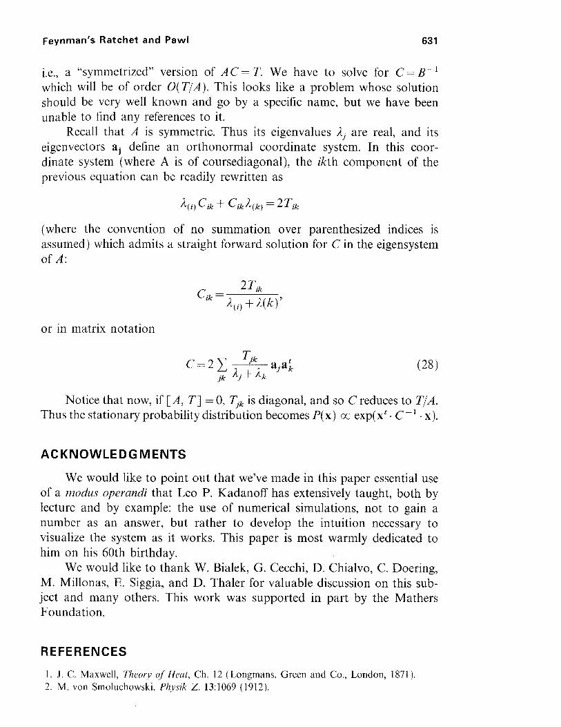
i.e., a "symmetrized" version of AC= T. We have to solve for C= B-' which will be of order O(T/A). This looks like a problem whose solution should be very well known and go by a specific name, but we have been unable to find any references to it.

Recall that A is symmetric. Thus its eigenvalues /2, are real, and its eigenvectors aj define an orthonormal coordinate system. In this coordinate system (where A is of coursediagonal), the ikth component of the previous equation can be readily rewritten as

(where the convention of no summation over parenthesized indices is assumed) which admits a straight forward solution for C in the eigensystem of A:

or in matrix notation

Notice that now, if [A, TI = 0, Tjk is diagonal, and so C reduces to TIA. Thus the stationary probability distribution becomes P(x) K exp(xf . C-' x).

ACKNOWLEDGMENTS

We would like to point out that we've made in this paper essential use of a modus operandi that Leo P. Kadanoff has extensively taught, both by lecture and by example: the use of numerical simulations, not to gain a number as an answer, but rather to develop the intuition necessary to visualize the system as it works. This paper is most warmly dedicated to him on his 60th birthday.

We would like to thank W. Bialek, G. Cecchi, D. Chialvo, C. Doering, M. Millonas, E. Siggia, and D. Thaler for valuable discussion on this subject and many others. This work was supported in part by the Mathers Foundation.

REFERENCES

1. J . C. Maxwell, Theory of' Heat, Ch. 12 (Longmans, Green and Co., London, 1871 ). 2. M. von Smoluchowski, Physik 2. 13:1069 (1912).

632 Magnasco and StOlOvitzky

3. L. Szilard, Z. Physik 53340-856 (1929). 4. L. Brillouin, Phys. Rev. 78:627-628 ( 1950). 5. R. P. Feynman, R. B. Leighton, and M. Sands, The Feynrnan Lectures on Phy,,lcs

(Addison-Wesley, Reading, Massachusetts, 1966), Vol. I, Chapter 46. 6. H. S. Leff and A. F. Rex, Muxwell's Demon: Informution, Entropy, Computing, A. Hilger

(Europe) and Princeton U.P. (USA) (1990). 7. R. Landauer, J. Applied Phys. 33:2209 (1962). 8. M. Biittiker, Z. Phys. B 68:161 (1987). 9. N. G. van Kampen, IBM J. Res. Develop. 32: 107 ( 1988); Z. Phys. B 68:135 (1987).

10. J. Parrondo and P. Espafiol, Am. J. of Phys. 64: 1 125 ( 1996). 11. K. Sekimoto, J. Phys. Soc. Jpn. 66:1234 (1997). 12. A. Ajdari and J. Prost, C. R. Acad. Sci. Paris IZ 315: 1635 (1993). 13. M. 0. Magnasco, Phys. Rev. Lett. 71:10, 1477 (1993). 14. J. Marko and E. Siggia, Macromolecules 28:8759-8770 (1995). 15. M. 0. Magnasco and D. S. Thaler, Phys. Lett. A 221:287 (1996). 16. R. R. de Ruyter van Steveninck et al., Science 275:1805 (1997).

feynman's ratchet and pawl - rockefeller...

Documents