few problems with regularized coulomb law

Mechanics & Industry 16, 202 (2015)c© AFM, EDP Sciences 2015DOI: 10.1051/meca/2014075www.mechanics-industry.org

Mechanics&Industry

Few problems with regularized Coulomb law

Jean-Louis Ligiera and Philippe Bonhote

HEIG-VD, Comatec, 1 route de Cheseaux, 1400 Yverdon-les-bains, Suisse

Received 8 May 2014, Accepted 22 September 2014

Abstract – The main idea is to present some problems where the friction obeys to regularized Coulomblaw. Mathematically, it is usual that the friction law is supposed to be the Coulomb law which is controlledby a function “sign” with discontinuity at the origin. In reality, friction phenomenon corresponds to anaverage continuous behavior. From a modelling point of view, the simplest way to get this continuity isto regularize friction law. Obviously, friction problems become more complicated due to the fact that thefriction law exhibits two phases of behavior. Solving problems with this friction law could bring somespecial results. To present them, the problems considered in this paper are related to the bending of twobeams in contact under a certain pressure and to the transversal strain of an elastic thin strip in contactwith a rigid body. For these two problems, analytical solutions are presented and also some finite elementsimulations for comparison.

Key words: Friction / contact / Coulomb / microslip

1 Introduction

Already, Leonardo da Vinci [1] engineers and physi-cists consider friction in mechanic problems. Particularlyin dry friction, it is usual to consider the Coulomb friction.This law of friction is very useful for many problems dueto its simplicity. However, it is more and more frequentthat the accurate behavior simulation of mechanical sys-tems operating with friction needs to consider refined lawsof friction. These laws allow having a better behavior de-scription of the body interfaces in contact. From a practi-cal point of view, the friction law is dependent to the typeof problem. For example for metal forming, rubber frictionor earthquake, engineers use very different types of law forsimulation [2]. It has been observed for instance that indynamic situation, the interface controls the damping andthe stiffness of the joint but these characteristics affect thedynamic response of the complex structures having joints.It could concern the determination of the natural frequen-cies, the stick-slip phenomenon and the exact location ofthe components during “stop and go” displacements [3,4]or the impact description of the collision inside a multi-body system [5]. In term of quasi static situation, theinterface behavior will define the microslip between thedifferent components. This displacement will be impor-tant to estimate the fretting risk for example with Ruiz

a Corresponding author:[email protected]

criterion [6], the cumulative microslip between the compo-nents of the assembly structure [7,8] or the global stiffnessof a conrod with a fitted bearing. Also various situationsare considered like dynamic or quasi-static situation, lu-bricated or dry contact, micro-scale or macro-scale. Inthis paper, we will focus our analysis on dry friction inquasi static condition at a micro-scale. Quasi-static situ-ation means sliding speed will be lower than few μm.s−1.For this situation, two regimes can be distinguished: pre-sliding regime and gross-sliding regime. For the last one,it corresponds to macro-slip. But pre-sliding regime repre-sents the elastic deformation and the local micro-slidingalso called microslip that will occur in the contact in-terface before macro-slip can be observed. The level ofmicroslip has a strong influence on the contact stiffnessin apparently static interfaces. Taking into account thisphenomenon from a realistic way will affect the behaviorof assembly components or screw joints.

It is well known that the standard Coulomb law doesnot allow representing this phenomenon. The standardrelationship describing the tangential load during slidingat a constant speed v, is:

FT = μ0FNsign(v) (1)

where μ0 is the dynamic friction coefficient.One of the weaknesses of the Coulomb modeling is

induced by the fact that the relationship between slidingdisplacement and the tangential load is discontinue. To

Article published by EDP Sciences

http://dx.doi.org/10.1051/meca/2014075

http://www.mechanics-industry.org

http://www.edpsciences.org

J.-L. Ligier and P. Bonhote: Mechanics & Industry 16, 202 (2015)

Nomenclature

ai Constantsb Width beam (mm)E Young modulus (MPa)FN Normal load (N)FT Tangential load (N)Fthre Threshold load (N)G Shear modulus (MPa)h Half beam height and plate thickness (mm)I Quadratic moment of the cross section (mm4)ki ConstantsK Stiffness (MPa.μm−1)KT Tangential contact stiffness (MPa.μm−1)ki CoefficientsL Length of the beam or the plate (mm)Mf Bending moment (Nm)N Normal force (N)P Pressure (MPa)Pr Contact pressure (MPa)S Normal cross section of the plate (mm2)tp Plate thickness (mm)T Shear force (N)u Displacement (mm)UN Normal displacement due to normal load (mm)UM Normal displacement due to bending moment (mm)v Velocity (mm.s−1)w Bending deflection (mm)x Space variable (mm)X Location of friction regime change (mm)y Space variable (mm)α Coefficient (–)ν Poisson ratio (–)μ Friction factor (–)μ0 Dynamic friction factor (–)σxy Shear stress (MPa)τ Shear stress at the interface (MPa)ξ Space variable

overcome this difficulty, it is quite usual to regularize theCoulomb friction [9]. One easy way consists to adopt therelationship for the tangential force intensity:

FT = μ0FN tanh (αu) (2)

with FN, FT = normal, tangential load and u thedisplacement.

But the regularization is not enough realistic forsmall pre-sliding. Berthoud, Baumberger, Bureau [10,11]have precisely shown the behavior during the pre-slidingregime. At the beginning of the tangential loading themicro-displacement varies linearly with respect to theloading and is elastic. A creep phenomenon follows thisdisplacement but is related to the sliding velocity. To sim-plify our modelling we consider assembly components inpre-sliding regime where micro-sliding occurs at very lowspeed in order to neglect the creep period. The regular-ized Coulomb law adopted in this paper is described inFigure 1.

Fig. 1. Coulomb laws.

In the first regime phase, the relation between theshear stress and the displacement is:

τ = KTΔu (3)

where Δu corresponds to the relative displacement at theinterface between two bodies in contact and KT repre-sents the tangential stiffness.

When the shear stress reaches the Coulomb frictionstress, μP , the behavior stops to be elastic.

This behavior is also related to the Iwan model [12]which corresponds to “Coulomb” slider connected to aspring. It is also similar to bristle model used to modeldynamic friction [13].

The difficult point with the regularized friction law isto determine the tangential stiffness. It has been shownthat the tangential stiffness is due to the elastic responseof the interface zone [14] and more particularly to the sur-face asperities. From the modelling done by Greenwoodand Williamson [15], which describes, from a statisticalpoint of view, the normal contact stiffness between roughsurfaces, Sherif and Kossa [16] have shown that from atheoretical point of view the tangential stiffness is:

KT =π (1 − ν)2 (2 − ν)

KN (4)

They have also demonstrated the number of contactsat the interface is proportional to the normal load, themean size of the elementary contact aera is independentof the normal load, and for relatively low normal loadeach asperity behaves independently. From an experimen-tal and numerical point of view Gonzalez-Valadez andMedina [17–19] have obtained that the ratio between thetwo stiffnesses is comprised between 0.5 to 0.7.

From a practical point of view, the normal stiffnesscould be determined with the Greenwood-Williamsonmodel and the physical and geometrical characteristicscould be deduced from the roughness measurements andthe relationships proposed by Robbe-Valloire [20]. In mi-croslip regime, the equivalent behavior of the interface issummarized in Figure 2.

202-page 2


Fig. 2. Stiffness equivalence.

Several devices have been developed to precisely mea-sure precisely the tangential stiffness. With a device usingmicrowaves Valadez and Dwyer-Joyce [17] have confirmedexperimentally that for very low load the shear stiffnessis directly related to the normal pressure as presented byBerthoud [10].

In this paper we propose the analytical solutions totwo problems with regularized friction law. It is quiteusual to find solution with standard Coulomb friction butless with regularized Coulomb law. It is also important tohighlight that many numerical simulations codes (finiteelement, multi-body dynamic. . . ) use regularized frictionlaws. But codes do generally not request the value ofthe tangential stiffness. Implicitly, the codes use a de-fault value of the stiffness which is very high and propor-tional to the length of the element. Sometimes the stiff-ness is inversely proportional to the depth of the elementin contact.

As the tangential stiffness is very important in the as-sembly complex structures, the analytical solutions, de-termined in this paper, will allow:

– to be able to identify the tangential stiffness with sim-ple experiment measurements;

– to characterize the difference we can get between the-ory and finite element calculation.

2 Friction problems

As relative displacements at the interface betweenbodies in contact could result:

– from direct longitudinal effect;– from indirect transversal effect induced by striction,

two problems with these two effects are solved in thispaper. The Coulomb law and regularized are considered.The characteristics of these law are given in Figure 1.

2.1 Twin beams under mutual friction

At first we are looking at a twin cantilever beam sys-tem. The cantilever beams are pressed together with auniform and moderate pressure P . The transverse loadapplied at the end of the two beams produces frictionat the interface as soon as relative displacement appearsbetween the two beams (cf. Fig. 3).

Fig. 3. Twin beams under bending.

The cross section of each beam is rectangular (b.2h)with 2h for the height of the beam. h is supposed to bequite small in order to neglect shear strain in the beam.Due to the low value of P , transversal and longitudinalstrains are negligible and do not introduce behaviour dif-ference between twin beams.

2.1.1 Standard Coulomb friction

Before considering the regularized Coulomb frictionthe problem is solved with standard Coulomb friction.This kind of friction will occur at the interface betweenthe two beams when the shear stress will be higher thanadherence stress between the two beams due to the pres-sure P . By the way, for low load the two beams remainsolidary. They form a beam 4h height under a shearingforce 2F . With strength of material [21] we know that theshear stress induced by a shear force 2F on a rectangularcross section is:

σxy (y) =3F

4hb

(1 −

( y

2h

)2)

(5)

for y measured from the beam interface.The deflection is:

w (x) =F

16Ebh3

(3Lx2 − x3

)(6)

Slip at the interface will not occur as shear stress (5) willremain lower than the adherence μP . So, it involves thatthe loading will be lower than the threshold force Fthre:

F < Fthre =4μbhP

3(7)

We consider that the static friction coefficient, μ, is thesame than the dynamic friction coefficient to avoid con-sidering a sudden instability when the adherence ceases tomaintain the beams solidary. For comparison with finiteelement, it will be easier.

In the case where slip occurs, the beam deflections willbe the same for the two beams and will be due to a new

202-page 3


Fig. 4. Beam bending.

bending moment, Mf , taking into account the shear stressat the interface. Its expression is:

Mf = (F − μPbh) (L − x) (8)

The deflection, after solving the differential equation ofthe bending beam, for one beam, will be:

w (x) =(F − μPbh)

4Ebh3

(3Lx2 − x3

)(9)

In summary for Coulomb friction, the deflection at theend of the beam will be:⎧⎪⎨⎪⎩

F < Fthres =4μbhP

3; w (L) =

FL3

8Ebh3

F > Fthres =4μbhP

3; w (L) =

(F − μbhP )L3

2Ebh3

(10)

2.1.2 Regularized friction

With regularized law of friction it is necessary to sup-pose that a part of the interface is subject to micro-elastic-slip and the other one is subject to macro slip as describedin Figure 4.

In Figure 4, the new quantity to determine is the shearstress in the micro-elastic-slip area. To do that we mustdetermine the torsor in any cross section of the beam. Asthe system is symmetric to respect to the interface, we willjust analyze the lower beam. So, we have to consider: thenormal force, the shearing force and the bending momentwhich act at the point x along the center line of the lowerbeam:

for x < X

⎧⎪⎪⎪⎪⎪⎪⎪⎨⎪⎪⎪⎪⎪⎪⎪⎩

N (x) = (X − L)μbP − bX∫x

τ (ξ) dξ

T (x) = F

Mf (x) = F (L − x) − (L − X)μbhP

−bhX∫x

τ (ξ) dξ

(11)

and

for x > X

⎧⎪⎪⎪⎪⎨⎪⎪⎪⎪⎩

N (x) = −bL∫x

τ (ξ) dξ

T (x) = F

Mf (x) = F (L − x) − bhL∫x

τ (ξ) dξ

(12)

To start the resolution, we must determine the shearstress in the first part of the beam where the shear stressis controlled by micro-elastic-slip regime, it means:

τ (x) = 2KT (uN (x) + uM (x)) (13)

where uN and uM are the displacements of the lower beamdue to the normal force and to the bending moment.

The factor 2 takes into account the fact that the upperbeam has the same but opposite displacements than thelower beam. The equations which allow determining thesedisplacements are:

uN (x) =1

2Eh

x∫0

⎛⎝(X − L)μP −

X∫x

τ (ξ) dξ

⎞⎠ dx (14)

uM (x) = hw′ (x) (15)

and

w′′ (x) =3

2Ebh3

(F (L − x) − (L − X) μbhP

− bh

X∫x

τ (ξ) dξ

)(16)

After deriving the shear stress equation and combiningwith the four previous equations, the relationship definingthe shear stress is:

τ ′′ (x) − k20τ (x) = −k1F (17)

with

k0 = 2

√KT

Eh, k1 =

3KT

Ebh2

Taking into account that the shear stress is null for x = 0and is equal to the Coulomb shear stress for x = X , thesolution of the differential equation is:

τ (x) =k1

k20

F (1 − cosh(k0x))

+(μPk2

0 + k1F (cosh(k0X) − 1)) sinh(k0x)

k20 sinh(k0X)

(18)

With this new expression of the interface shear stress, itis now possible to solve the bending equation in order toobtain the bending deflection. After solving the equationand considering the boundary condition of the cantileverbeam, the deflection solution is:

w (x) = k5x2

2+ k2F

x3

6+ k6 (cosh(k0x) − 1)

+ k7 (sinh(k0x) − k0x) (19)

202-page 4


Fig. 5. X variations with respect to F .

where

k2 =−3

8Ebh3, k4 =

−9F

8Ebh3, k6 =

k3

k30

, k7 =k4

k30

,

k3 =3

8hKT sinh(k0X)(μPk2

0 + k1F (cosh(k0X) − 1),

k4 =−9F

8Ebh3, k6 =

k3

k30

, k7 =k4

k30

,

k5 = −k2FX − cosh(k0X)k3

k0− sinh(k0X)

k4

k0

+3 (L − X)

2Ebh3(F − μhbP )

The expression of the bending deflection can be intro-duced in the shear stress equation. But the shear stressat x = X must be equal to the Coulomb friction. Thislast condition is used to determine X . So, we obtain thefollowing equation to solve:

τ (X) = KT (uN (X) − uM (X)) =μP

KT(20)

This equation has not an analytical solution and mustbe solved numerically. The numerical data we considerare close to those of a test bench. Tangential stiffnessis deduced of the beams roughness R = 3.1 μm andrelationship (19). Numerical date is the following:

L = 200 mm, E = 210 GPa, h = 10 mm, b = 20 mm,

P = 1 MPa, μ = 0.3, KT = μP/5e − 4 MPa.mm−1

After solving numerically the previous equation we getX with respect to F . Figure 5 gives the evolution of X .It can be observed that for certain loadings, X can behigher than the length of the beam. In that case, there isonly one regime of friction along the beam interface. Thissituation will be detailed further away.

As X can be determined, we can write the deflectionand the slope at x = X :

w (X) = k5X2

2+ k2F

X3

6+ k6 (cosh(k0X) − 1)

+ k7 (sinh(k0X) − k0X)

w′ (X) = k5X + k2FX2

2+ k6k0 sinh(k0X)

+ k7k0 (cosh(k0X) − 1) (21)

These expressions will constitute the boundary conditionsfor the second part of the beam. In that case, the bendingmoment is known and the resolution is quite usual andgives for the deflection in x = L, called wT (L):

wT (L)=(F − μPbh)

12Ebh3(L − X)3 + w′ (X) (L − X)+w(X)

(22)Equation (22) represents the deflection solution for thecase where the two regimes of friction exist along theinterface.

For the situation where the only friction regime ismicro-elastic-slip (X > L), the loading torsor is quitesimple: ⎧⎪⎪⎪⎪⎪⎨

⎪⎪⎪⎪⎪⎩

N (x) = −bL∫x

τ (ξ) dξ

T (x) = F

Mf (x) = F (L − x) − bhL∫x

τ (ξ) dξ

(23)

The resolution is similar to the previous one. The differ-ential equation determining the shear stress is the same.However, there is a new boundary condition:

for x = L, τ (L) = KT uT (L) (24)

Then, the solution for the shear stress becomes:

τ (x) =k1

k20

F (1 − cosh(k0x))

+(uT (L) k2

0KT + k1F (cosh(k0L) − 1)) sinh(k0x)

k20 sinh(k0L)

(25)

The calculation of the beam deflection gives the solution

w (x) = k8x2

2+ k2F

x3

6+ k10 (cosh(k0x) − 1)

+ k7 (sinh(k0x) − k0x) (26)

where

k8 = −k2FL − cosh(k0L)k9

k0− sinh(k0L)

k4

k0, k10 =

k9

k30

k9 =3

8hKT sinh(k0L)(uT (L)KT k2

0+k1F (cosh(k0L)−1)

202-page 5


The solution of the beam deflection is expressed with re-spect to the total displacement uT (L). It involves calcu-lating this term. So, we have to define uN and uM for thisnew situation.

For the displacement induced by the normal force, therelationship is:

uN (L) =1

2Eh

L∫0

⎛⎝−

L∫x

τ (ξ) dξ

⎞⎠ dx (27)

After calculation, we get:

uN (L) = k11F + k12uT (L) (28)

with

k11 =k1L

4Ehk30

(k0L − tanh

(k0L

2

)),

k12 =KT

2Ehk20

(k0L coth (k0L) − 1)

For the displacement induced by the bending we have:

uM (L) = hw′ (L) (29)

After calculation and using previous results, we obtain:

uM (L) = k13F + k14uT (L) (30)

with

k13 = k2hL2

2+

3hk1L

2 sinh (k0L)Ehk30

(1 − cosh (k0L)) ,

k14 =3KT

2Ehk20

(k0L coth (k0L) − 1)

AsuT (L) = 2 (uN (L) + uM (L)) (31)

we can get the relationship:

uT (L) =−2 ((k11 + k13))F

(1 + 2 (k12 + k14))(32)

For this situation, the bending deflection at the end ofthe beam is proportional to F .

w (L) = k8L2

2+ k2F

L3

6+ k10 (cosh(k0L) − 1)

+ k7 (sinh(k0L) − k0L) (33)

2.1.3 Numerical simulation and comparison

It is interesting to plot the deflection with respect to Ffor different values of KT. It allows assessing the KT influ-ence, particularly with respect to the standard Coulombfriction. It also shows the possibility to assess the micro-contact elasticity by measuring the deflection at the end

Fig. 6. Deflection for the two friction laws.

Fig. 7. Reduced tangential stiffness.

Fig. 8. Finite element model.

of the beam. With the same numerical data than previ-ously, we can obtain the following plots for various KT

(cf. Fig. 6). In Figure 6, it can be observed that the dif-ference between the two approaches, standard Coulombfriction and regularized Coulomb friction, is not so impor-tant. As it is quite easy to modify the tangential stiffnessby modifying the roughness, we simulate the case wherethe nominal tangential stiffness is divided by 5. Resultsare plotted in Figure 7. In that case, we can observe astrong difference which could be easy to detect by mea-surements. These differences highlight the importance tocorrectly choose KT.

For the comparison with finite element method, wehave simulated the problem with Ansys. The mesh usedfor the simulation is illustrated in Figure 8. 2000 quadraticplane stress elements have been used for the mesh andquadratic contact elements surface to surface model the

202-page 6


Fig. 9. Comparison analytical and F.E. solutions.

interface. More refined meshes have also been tested butno numerical modifications of the results have been ob-served. The important point to notice is that finite ele-ment codes use a certain value of KT by default. However,this KT value depends to the mesh size. It involves thatfor accurate slip values at the interface, the tangentialstiffness has to be imposed by the user. Several resolutionmethods have also been tested (penalty, Lagrange, aug-mented Lagrange) and each one gives the same results.

Implicitly, with the friction orientation, monotonicloading is supposed. After performing various finite el-ement calculations, we get the comparison between ana-lytical solution and numerical solution. In Figure 9, wecan observe that analytical and numerical solutions arevery close.

In summary, this modelling shows:

– a very good agreement between finite element and an-alytical approach. Thus, analytical approach can beused as benchmark for new contact element. It couldhelp to evaluate error introduced by the use of shellelement in this kind of problem. It can also determine:

– when simplifying assumption of the analytical modelis not valid. For instance, when the beam thicknesspossesses non negligible shear strain;

– the importance to control KT, usually given by defaultin finite element code;

– an experimental way to identify KT and μ by deflec-tion measurements. Curve slope variation (cf. Fig. 11)is directly related to μ and the change location willdetermine KT.

2.2 Plate friction

For the second problem, we consider a situation wherewe can get an analytical solution to compare with finiteelements results. For this case the longitudinal displace-ment is due to striction effect induced by the contact

Fig. 10. Plate on the rigid plane.

Fig. 11. Equilibrium of an elementary strip.

pressure. Let a plate lying on a rigid plan. The frictionbetween the plate and the rigid surface obeys to a regu-larized Coulomb law as described in Figure 10. The plateis supposed to be quite wide as we can consider the prob-lem in strain plane situation (width � length). As thethickness of the plate, tp, is sufficiently thin, we can ne-glect shear strain in the plate. A pressure P is applied onthe upper surface of the plate as illustrated in Figure 10.

2.2.1 Contact pressure

Before solving the problem it is interesting to showthat contact pressure between the beam and the rigidplane is mainly constant and equal to P , to do that wemust consider an elementary strip of beam as describedin Figure 11.

The strip equilibrium brings the equations:⎧⎪⎪⎨⎪⎪⎩

dQ

dx= Pr (x) − P

dMf

dx= Q + μhPr (x)

(34)

with Mf = bending moment and Q = shear load.As the plate remains straight in its contact with the

rigid plane, it involves that the second and the thirdderivation of the deflection, called y(x), are null along the

202-page 7


x axis. Mathematically, it is expressed by the relationship:

y′′′ (x) =M ′

f

EI− k

GSQ′′ (35)

with EI = flexural rigidity modulus, GS = shear rigiditymodulus, k = shear correction factor.

Reintroducing equilibrium equations (34) in this de-flection equation (35) gives:

GS

kEI

(Q + μhQ′ +

μtp2

P

)− Q′′ = 0 (36)

The general solution is:

Q = −μtp2

P + eax (A cosh (a2x) + B sinh (a2x)) (37)

with

a1 =μtpGS

kEI; a2 =

√(2a1

μtp

)2

+ 2a1

Taking into account the boundary condition Q(0) = 0and Q(L) = 0, the previous expression becomes:

Q =μtp2

P [ea1x (cosh (a2x) − B sinh (a2x)) − 1] (38)

with

B =e−a1L − cosh(a2L)

sinh(a2L)

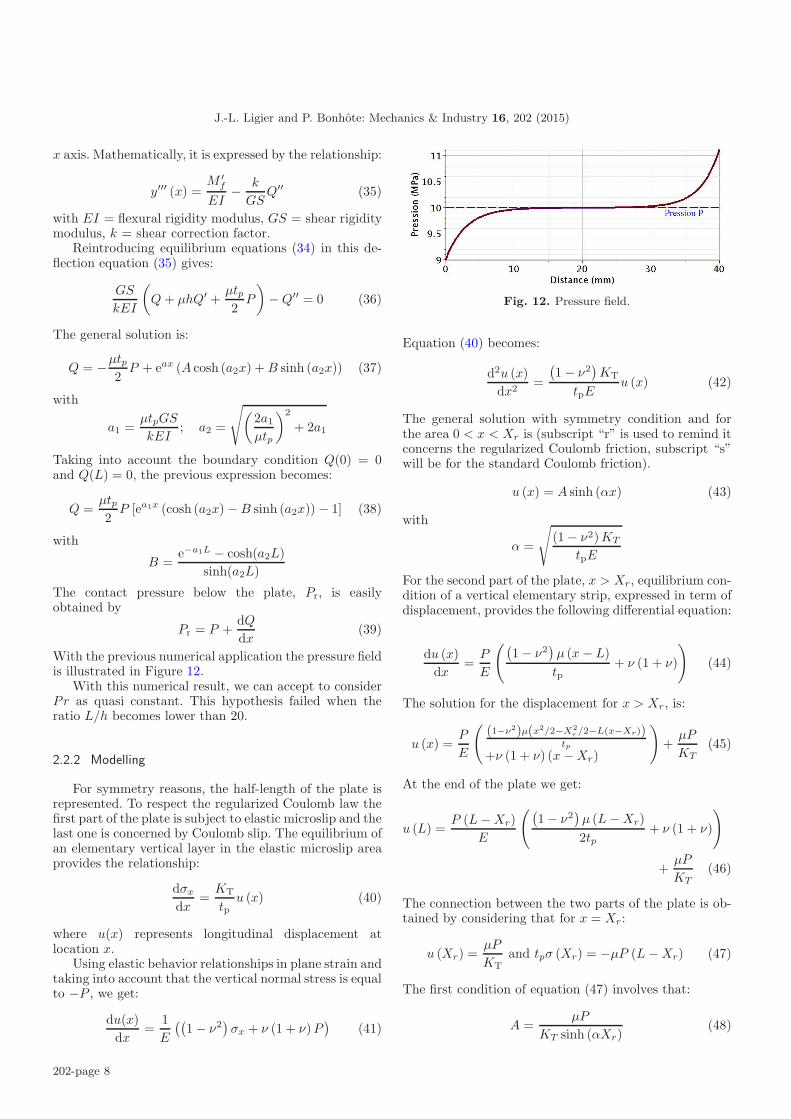
The contact pressure below the plate, Pr, is easilyobtained by

Pr = P +dQ

dx(39)

With the previous numerical application the pressure fieldis illustrated in Figure 12.

With this numerical result, we can accept to considerPr as quasi constant. This hypothesis failed when theratio L/h becomes lower than 20.

2.2.2 Modelling

For symmetry reasons, the half-length of the plate isrepresented. To respect the regularized Coulomb law thefirst part of the plate is subject to elastic microslip and thelast one is concerned by Coulomb slip. The equilibrium ofan elementary vertical layer in the elastic microslip areaprovides the relationship:

dσx

dx=

KT

tpu (x) (40)

where u(x) represents longitudinal displacement atlocation x.

Using elastic behavior relationships in plane strain andtaking into account that the vertical normal stress is equalto −P , we get:

du(x)dx

=1E

((1 − ν2

)σx + ν (1 + ν)P

)(41)

Fig. 12. Pressure field.

Equation (40) becomes:

d2u (x)dx2

=

(1 − ν2

)KT

tpEu (x) (42)

The general solution with symmetry condition and forthe area 0 < x < Xr is (subscript “r” is used to remind itconcerns the regularized Coulomb friction, subscript “s”will be for the standard Coulomb friction).

u (x) = A sinh (αx) (43)

with

α =

√(1 − ν2)KT

tpE

For the second part of the plate, x > Xr, equilibrium con-dition of a vertical elementary strip, expressed in term ofdisplacement, provides the following differential equation:

du (x)dx

=P

E

((1 − ν2

)μ (x − L)tp

+ ν (1 + ν)

)(44)

The solution for the displacement for x > Xr, is:

u (x) =P

E

((1−ν2)μ(x2/2−X2

r /2−L(x−Xr))tp

+ν (1 + ν) (x − Xr)

)+

μP

KT(45)

At the end of the plate we get:

u (L) =P (L − Xr)

E

((1 − ν2

)μ (L − Xr)2tp

+ ν (1 + ν)

)

+μP

KT(46)

The connection between the two parts of the plate is ob-tained by considering that for x = Xr:

u (Xr) =μP

KTand tpσ (Xr) = −μP (L − Xr) (47)

The first condition of equation (47) involves that:

A =μP

KT sinh (αXr)(48)

202-page 8


The second one becomes a transcendent equation:

tpEμα

(1 − ν2)KT tanh (αXr)=

νtp1 − ν

− μ (L − Xr) (49)

It is interesting to notice that the Xr solution is inde-pendent to P . Generally, this equation has no analyticalsolution. But for high value of Xr, we can get an approx-imated solution by considering that the term tanh(αXr)is equivalent to 1. Then the solution becomes:

Xr ≈ L +tpEα

(1 − ν2)KT− νtp

μ (1 − ν)(50)

To complete this approach, the solution for stan-dard Coulomb friction law is considered. After solvingthe differential equation (44), the general displacementsolution is:

u (x)=P

E

((1 − ν2

) μ

tp

(x2

2− Lx

)+ν (1 + ν)x

)+ cste

(51)The integration constant will be defined by the condition:

u(Xs) = 0

Then, the transition between stick zone and slip zone, de-fined by Xs, verifies the condition that the axial strain isnull and axial strain is obtained by deriving equation (51):

Xs =(

L − νtp(1 − ν)μ

)(52)

It follows that the displacement at the end of the platewill be:

u(L) =(1 + ν) ν2tpP

(1 − ν)μE(53)

2.2.3 Numerical simulation and comparison

In finite element simulation we cannot treat the prob-lem by using beam or shell element in which no stric-tion effect under transversal pressure is considered. Planestrain elements are used. The mesh is represented in Fig-ure 13. Refined meshes have also been tested and no dif-ference has been noted.

At this stage we can perform some comparisons be-tween the different approaches. The numerical applicationwe consider is:

L = 10 mm, tP = 0.2 mm, E = 70 GPa, ν = 0.3,

μ = 0.3, P = 10 MPa.

In Figure 14, the displacement at the end of the plate,u(L), shows big variation for low KT values. Such varia-tions may be due to large variations in roughness.

In order to detect some difference between analyticaland finite element solution we can look at the X valuewith respect to the friction coefficient and the tangentialstiffness (cf. Fig. 15). This parameter must vary between0 and L.

Fig. 13. Plate mesh.

Fig. 14. Displacement comparison.

Fig. 15. X with respect to friction and stiffness.

In summary of this squeezed plate problem, it is found:– a contact pressure model which allows to determine if

contact pressure can be considered as constant;– very good agreement between finite element and ana-

lytical solutions. As mentioned earlier, the analyticalapproach can be used as benchmark for new contactelement. It could help to evaluate error introduced bythe use of shell element in this kind of problem. It canalso determine when simplifying assumption of the an-alytical model is not valid;

– a perfect bonding occurs for high friction coefficient;– roughness and pressure contact control the location of

slipping interface.

3 Conclusion

The consideration of the regularized Coulomb frictionin the behavior of assembly complex structures allows toget more realistic response particularly in the microslipregime. During a loading, it involves a better prediction ofslipping area instead a sudden slip of the whole interfacewith the standard Coulomb law.

202-page 9


The cantilever twin beams problem has shown possi-bilities to assess tangential stiffness and friction coefficientby beam deflection measurements. It has also been shownthat simulation with finite element code needs to be ac-curate on the implicit tangential stiffness used in codeto get realistic results like relative displacements betweentwo bodies in contact.

The problem of a plate squeezed on a rigid plan pro-vides an analytical solution which allows assessing somebehavior differences between regularized and standardCoulomb friction law and between analytical solution andfinite element simulation.

By default, finite element codes try to get Coulombfriction but mesh size modifies the KT default value.

The two analytical solutions obtained in this papercan be used as benchmark solutions.

References

[1] D. Dowson, History of tribology. 2nd edn., John Wiley,1998

[2] V.L. Popov, Contact mechanics and friction, physicalprinciples and application, Springer Verlag, 2010

[3] Y. Song et al., Simulation of dynamics of beam structureswith bolted joints using adjusted Iwan beam elements, J.Sound. Vib. 273 (2004) 249–276

[4] H.A. Sherif, Effect of contact stiffness on the establish-ment of self-excited vibrations, Wear 141 (1991) 227–234

[5] P. Flores, J. Ambrosio, J.C.P. Claro, H.M. Lankarani,Influence of the contact-impact model on the dynamicresponse of multi-body systems, ImechE 2006, Vol. 220,Part K, pp. 21–34.

[6] K. Anandavel, R.V. Prakash, Extension of Ruiz criterionfor evaluation of 3-D fretting fatigue damage parameter,Procedia Engineering 55 (2013) 655–660

[7] J.-L. Ligier, N. Antoni, Cumulative microslip in conrodbig end bearing system, ASME 8-10 (2006)

[8] N. Antoni, Q.-S. Nguyen, J.-L. Ligier, P. Saffre, J. Pastor,On the cumulative microslip phenomenon, Eur. J. Mech.– A/Solids 26 (2007) 626–646

[9] D.D. Quinn, A new regularization of Coulomb friction, J.Vib. Acoust. 126 (2004) 391–397

[10] P. Berthoud, T. Baumberger, Shear stiffness of a solid–solid multicontact interface, Proc. R. Soc. Lond. A 454(1998) 1615–1634

[11] L. Bureau, T. Baumberger, C. Caroli, O. Ronsin, Lowvelocity friction between macroscopic solids. C. R. Acad.Sci. Paris, t.2, Serie IV, 2001, pp. 699–707

[12] W.D. Iwan, A distributed element model for hysteresisand its steady–state dynamic response, ASME J. Appl.Mech. 33 (1966) 893–900

[13] J. Liang, S. Fillmore, O. Ma, An extended bristle frictionforce model with experimental validation, Mech. Mach.Theory 56 (2012) 91–100

[14] J.J. O’Connor, K.L. Johnson, The role of surface asper-ities in transmitting tangential forces between metals,Wear 6 (1963) 118–139

[15] J.A. Greenwood, J.B.P. Williamson, Contact of nomi-nally flat surfaces, Proc. R. Soc. Lond. A 295 (1966) 300

[16] H.A. Sherif, S.S. Kossa, Relationship between normaland tangential contact stiffness of nominally flat surfaces,Wear 151 (1991) 49–62

[17] M. Gonzalez-Valadez, A. Baltazar, R.S. Dwyer-Joyce,Study of interfacial stiffness ratio of a rough surface incontact using a spring model, Wear 268 (2010) 373–379

[18] M. Gonzalez-Valadez, R.S. Dwyer-Joyce, On the inter-face stiffness in rough contacts using ultrasonic waves,Ingenieria Mecanica 3 (2008) 29–36

[19] S. Medina, D. Nowell, D. Dini, Analytical and numericalmodels for tangential stiffness of rough elastic contacts,Tribol. Lett. 49 (2013) 103–115

[20] F. Robbe-Valloire, Statistical analysis of asperities on arough surface, Wear 249 (2001) 401–408

[21] S. Timoshenko, Resistance des materiaux, Dunod, 1990

202-page 10

few problems with regularized coulomb law

Documents