FeT’ 2009FeT 20098th IFAC International Conference on Fieldbuses & Networks in Industrial & Embedded SystemsIndustrial & Embedded Systems

May 20-22, 2009Hanyang University, AnsanRepublic of Korea

PREPRINTS

TABLE OF CONTENTS

Preface……………………………………………………………………………………….7 Conference organization……………………………………………………..………….8 Reviewers……………………………………………………………………………………9

Session : Wireless Sensor Networks

H-NAMe: A Hidden-Node Avoidance Mechanism for Wireless Sensor Networks……………10 Anis Koubâa - ISEP-IPP – Portugal. Al-Imam Muhammad Ibn Saud University - Saudi Arabia.Ricardo Severino - ISEP-IPP - Portugal.Mário Alves - ISEP-IPP - Portugal.Eduardo Tovar - ISEP-IPP - Portugal.

On improving reliability of star-topology Wireless Sensor Network……………………………20 P. Ferrari - University of Brescia - Italy.A. Flammini - University of Brescia - Italy.D. Marioli - University of Brescia - Italy.E. Sisinni - University of Brescia - Italy

Routing Protocol for Wireless Sensor Networks in Home Automation………………………27 Xiao Hui Li - Wuhan University of Science and Technology - China.Hong Qin Xu - Zhejiang University - China.Seung Ho Hong- Hanyang University - Korea.Zhi Wang- Zhejiang University - China.Xiang Fan Piao - Yanbian University - Korea.

Analysis of Low Powered Sensor Node Using Data Compression……………………………34 Hyo-deok Shin - Hanyang University - Korea.Sang-wook Ahn - Hanyang University - Korea.Tae-hoon Song - HUINS Inc. - Korea.Sang-hyeon Baeg - Hanyang University - Korea.

Session : Control Systems

Wireless Model Based Predictive Networked Control System…………………………………40 Alphan Ulusoy - Sabanci University - Turkey.Ahmet Onat - Sabanci University - Turkey.Ozgur Gurbuz - Sabanci University - Turkey.

Time Constraints in PID controls with Send-on-Delta…………………………………………48 Volodymyr Vasyutynskyy - Dresden University of Technology - Germany.Klaus Kabitzsch - Dresden University of Technology - Germany.

Online adaptation of the IEEE 802.15.4 parameters for wireless networked control systems………………………………………………………………56 N. Boughanmi - LORIA - France.YQ. Song - LORIA - France.

1

E. Rondeau - CRAN Université - France.Optimal Control with Packet Drops in Networked Control Systems…………………………..64 Flavia Felicioni - Universidad Nacional de Rosario - France.François Simonot - Nancy Université - France.Françoise Simonot-Lion - Nancy Université - France.Ye-Qiong Song - Nancy Université - France.

Codesign Strategy based upon Supervisory Fuzzy Control for Networked Control Systems and Real Time Computing……………………………………….72 PAUL E. MENDEZ - Universidad Nacional Autónoma de México - Mexico.HÉCTOR BENÍTEZ-PÉREZ - Universidad Nacional Autónoma de México - Mexico.

Session : PHY & MAC

WUR-MAC: Energy efficient Wakeup Receiver based MAC Protocol………………………..79 S. Mahlknecht - Vienna University of Technology - Austria.M. Spinola Durante - Vienna University of Technology - Austria.

An Efficient Channel Selection Algorithm for Congnitive Radio Networks……………………84 Thi Hong Chau Pham - University of Ulsan - Korea.Insoo Koo - University of Ulsan - Korea.

Wireless Field Buses for Aerospace Ground and In-Flight Testing: an Experiment…………89 Julien HENAUT - LAAS - Université de Toulouse- France.Akram HKIRI - LAAS - Université de Toulouse - France.Pascal BERTHOU - LAAS - Université de Toulouse - France.Daniela DRAGOMIRESCU - LAAS - Université de Toulouse - France.Thierry GAYRAUD - LAAS - Université de Toulouse - France.Robert PLANA - LAAS - Université de Toulouse - France.

Performance Evaluation of the IEEE 802.11 WLAN Supporting Quality of Service…..…..…97 Adel BEDOUI - Laboratoire SYSCOM - Tunisie.Kamel BARKAOUI - Laboratoire CEDRIC - France.Karim Djouani - Laboratoire LISSSI - France.

Managing the virtual collision in IEEE 802.11e EDCA…………………………………………104 Mohamad El Masri - LAAS - Université de Toulouse - France.Slim Abdellatif - LAAS - Université de Toulouse - France.

Session : ZigBee

Dynamic GTS Scheduling of Periodic Skippable Slots in IEEE 802.15.4 Wireless Sensor Networks………………………………………………………………………110 Tiago Semprebom - Federal University of Santa Catarina - Brazil.Carlos Montez - Federal University of Santa Catarina - Brazil.Ricardo Moraes - Federal University of Santa Catarina - Brazil.Francisco Vasques -University of Proto - Portugal.Paulo Portugal -University of Proto -Portugal.

2

Performance Evaluation of Time-Triggered IEEE 802.15.4 for Wireless Industrial Network………………………………………………………….……………118 Jee Hun Park - Pusan National University - Korea.Suk Lee - Pusan National University - Korea.Kyung Chang Lee - Pukyong National University - Korea.A Beacon-Aware Device For The Interconnection of ZigBee Networks……………………123 M. I. Benakila - France.L. George - France.S. Femmam - France.

Session : Distributed Systems and Middleware

Field Bus Abstraction as a Means to Enable Network-Independent Applications…………131 Stefan Theurich - Technische Universität Dresden - Germany.Christian Hahn - Technische Universität Dresden - Germany.Roman Frenzel - Technische Universität Dresden - Germany.Martin Wollschlaeger - Technische Universität Dresden - Germany.

Implementation of EtherCAT Master Middleware Component for Distributed Robot Control Architecture……………………………………………………………………….……..139 Yongseon Moon - Sunchon National University - Korea.Tuan Anh Vo Trong - Sunchon National University - Korea.Nak Yong Ko - Chosun University - Korea.Kwangjin Kim - Chosun University - Korea.Youngchul Bae - Chonnam National University - Korea.

Transaction Safe Field Devices Base of System Wide Data Consistency…………………144 Thorsten Szczepanski - ifak system GmbH- Germany.René Simon - HS Harz - Germany.Sören Scharf - ifak system GmbH - Germany.

Industrial Session

Introduction of RAPIEnet Technology……………………………………………………………152 Daehyun Kwon – LS Industrial Systems - Korea.

Industrial Session

Ethernet-based Factory Automation Network "CC-Link IE" -concept and technology-...…154 Kazuhiro Kusunoki, Dr.Eng-Technical Task Force Chair Person, CC-Link Partner Association

Invited Speaker

Networked Control Systems: From Independent Designes of the Network Qos and the Control to Co-desgin……………………………………………………155 Prof. Ye Qiong Song- Institut National Polytechnique de Lorraine

3

Session : Network Dependability

A Survey of Ethernet Redundancy Methods for Real-Time Ethernet Networks and its Possible Improvements………………………………………………………………………...…163Lukasz Wisniewski - Ostwestfalen-Lippe University of Applied Sciences - GermanyMohsin Hameed - Ostwestfalen-Lippe University of Applied Sciences - Germany.Sebastian Schriegel - Ostwestfalen-Lippe University of Applied Sciences - Germany.Juergen Jasperneite - Ostwestfalen-Lippe University of Applied Sciences - Germany.WSN Security Scheme Based on Ultrasonic Device Locating………………………………171 Herbert Schweinzer - Vienna University of Technology - Austria.Gerhard Spitzer - Vienna University of Technology - Austria.

Hybrid-time Chaotic Encryption and Sender Authentication of Data Packets in Automation Networks………………………………………………………………………..……179 Wolfgang A. Halang - Fernuniversität - Germany.Wallace K.S. Tang - City University of Hong Kong - China.Ho Jae Lee - Inha University – Korea.J. Gonzalo Baraias Ramírez - IPICYT - Mexico.

Highly Available and Reliable Networks based on Commercial-off-the-shelf Hard- and Software……………………………………………………………………………….………185 Thomas Turek - Vienna University of Technology - Austria.Heimo Zeilinger - Vienna University of Technology - Austria. Berndt Sevcik - Vienna University of Technology - Austria. Edger Holleis - Vienna University of Technology - Austria.Gerhard Zucker - Vienna University of Technology - Austria.

Session : Applications

WAVE Based Architecture for Safety Services Deployment in Vehicular Networks………191 Nuno Ferreira - Universidade de Aveiro - Portugal.Tiago Meireles - Universidade de Aveiro - Portugal.José Fonseca - Universidade de Aveiro - Portugal.João Nuno Matos - Universidade de Aveiro - Portugal. Jorge Sales Gomes - BRISA - Portugal.

Using Low-Power Radios for Mobile Robots Navigation………………………………………198 Hongbin Li - Zhejiang University - China.Luis Almeida - University of Porto - IEETA - Portugal.Fausto Carramate - University of Aveiro - Portugal.Zhi Wang - Zhejiang University - China.Youxian Sun - Zhejiang University - China.

Behavior Recognition and Prediction with Hidden Markov Models for Surveillance Systems…………………………………………………………………………204 Josef Mitterbauer - Vienna University of Technology - Austria.Dietmar Bruckner - Vienna University of Technology - Austria.Rosemarie Velik - Vienna University of Technology - Austria.

Automated Buildings as Active Energy Consumers……………………………………………212 Friederich Kupzog - Vienna University of Technology - Austria.Klaus Pollhammer - Vienna University of Technology - Austria.

4

Timing properties requirements and robustness analysis of a platoon of vehicles…………218 Lionel Havet - INRIA - France.François Simonot - University of Nancy - France.

Work in progress -

Compression of Inertial and Magnetic Sensor Data for Network Transmission……………226 Young Soo Suh – University of Ulsan - Korea.

A Study on the Development of Embedded System Software for Ubiquitous Sensor Networks using UML………………………………………………………………………………230 Jong-Won Choi - Hanyang University - Korea.Dong-Jin Lim - Hanyang University - Korea.

Introducing a simulation tool for WirelessHART networks………………………..…………234 A. Depari - University of Brescia - Italy.P. Ferrari - University of Brescia - Italy.A. Flammini - University of Brescia - Italy.E. Sisinni - University of Brescia - Italy.

Multiple Camera-based Correspondences of People using Camera Networks and Context Information………………………………………………………………………………238 Hyun-uk Chae - University of Ulsan - Korea.Suk-Ju Kang - University of Ulsan - Korea.Kang-Hyun Jo - University of Ulsan - Korea.

Work in progress -

Automatically Rotating PDP TV Using Multiple Sensor Information………………..………242 Jong-Tae Seo - Hanyang University - Korea.Seok Cheol Park - Hanyang University - Korea.Songjun Lee - Hanyang University - Korea.Byung-Ju Yi - Hanyang University - Korea.

A case study on wireless networks for agricultural applications……………………………246 P. Mariño - University of Vigo - Spain.F.P. Fontán - University of Vigo - Spain.M.A. Domínguez - University of Vigo - Spain.S. Otero - University of Vigo - Spain.

An Autonomous Adaptive Multiagent Model for Building Automation………………………250 Tehseen Zia - Vienna University of Technology - Austria.Roland Lang - Vienna University of Technology - Austria.Harold Boley - National Research Council Canada Fredericton - Canada.Dietmar Bruckner - Vienna University of Technology - Austria.Gerhard Zucker - Vienna University of Technology - Austria.

5

Work in progress -

Lightweight Data Duplication for Fault Tolerant Structural Health Monitoring System……255 Yoshinao Matsushiba - Keio University - Japan.Hiroaki Nishi - Keio University - Japan.

An Approach to Remote Monitoring and Control based on OPC Connectivity……………259 Vu Van Tan - University of Ulsan - Korea.Dae-Seung Yoo - University of Ulsan - Korea.Myeong-Jae Yi - University of Ulsan - Korea.

A Dynamic Software Configuration Model Based on Embedded System…………………263 CHEN Heping - Wuhan University of Science and Technology - China.WANG Jincun - Wuhan University of Science and Technology - China.CHEN Bin - Wuhan University of Science and Technology - China.LI Xiaohui - Wuhan University of Science and Technology - China.

Control of IPMC Actuator using Self-sensing Method……………………………………….267 Bonmin Koo - Hanyang University - Korea.Doo-su Na - Hanyang University - Korea.Songjun Lee - Hanyang University - Korea.

6

Behavior Recognition and Prediction WithHidden Markov Models for Surveillance

Systems

Josef Mitterbauer ∗ Dietmar Bruckner ∗∗ Rosemarie Velik ∗∗∗

∗ Vienna University of Technology, Austria, Europe (e-mail:mitterbauer@ict.tuwien.ac.at).

∗∗ Vienna University of Technology, Austria, Europe (e-mail:bruckner@ict.tuwien.ac.at).

∗∗∗ Vienna University of Technology, Austria, Europe (e-mail:velik@ict.tuwien.ac.at).

Abstract: A method for learning models of a person’s behavior in a building is described. Theperson’s movements and some activities are detected by sensors. From the sensor values a HiddenMarkov Model (HMM) is learned. Once a model is built, it allows calculating of predictions ofthe person’s behavior with respect to incoming sensor values. A method for learning HMMstructures from sample data is described.

Keywords: Building Automation, Hidden Markov Models, Scenario Recognition, AmbientAssisted Living, Behavior Prediction

1. INTRODUCTION

Up to now, advances in the electronics industry havedriven growth in several areas like home entertainment,surveillance, home automation products (e.g. lighting,heating, and power), home appliances (e.g. laundry ma-chines, fridges, etc.), and ad-hoc wireless sensor networks(AWSN), which promise to add a truly ambient intelligentcomponent to the home. The future home clearly repre-sents an opportunity for the convergence of these differenttechnologies far beyond the level of integration seen today,like e.g. proposed in (Baker et al. (2006)).

Continuously improvements of technologies in the fieldof building automation systems make them better andcheaper. Due to the improvements in the field of sen-sors, actuators and communication systems, increasinglyefficient systems can be realized. But together with theefficiency also the complexity increases. For handling theexpected complexity in future times, new methods for theprocessing of sensor values become necessary. The use ofstatistic methods is one possibility for describing recog-nized situations in buildings. It is an interesting questionif it is possible to derive prognoses for expected futuresituations from such models.

Hidden Markov Models (HMM) for system analysis havebeen used for speech recognition (Rabiner and Juang(1986)), for automated process discovery in software (Cookand Wolf (1999)), for software self-awareness (Bowring andHarrold (2004)) and for modeling sensor data in buildingautomation (Bruckner (2007)).

How far the theory about Hidden Markov Models (HMM)is useful for describing the behavior of persons in a roomand to make predictions about a person’s behavior out ofthe learned descriptions, will be determined in this work.

The calculation of these predictions is based on commonalgorithms. In which way data of different sensor types canbe integrated in one model and which predictions such asystem can make, is also topic of this work. “Predictionof behavior” in this work means the calculation of theprobability of possible actions (which can be perceivedby the system) a person can do next. Those actions withthe highest probability will be the prediction (Mitterbauer(2008)).

2. BACKGROUND

The first part of this section gives an overview about thetest environment which was used to apply the system andthe algorithms. In the second part we give an introductionof Hidden Markov Model’s structure learning principles onwhich our approach of learning is based on.

2.1 Application Environment

As part from the Artificial Recognition System project (seePratl and Palensky (2005)), at the Institute of ComputerTechnology (ICT) a room was equipped with several sen-sors to build a test environment for building automationsystems. Since this is the institute’s kitchen, it is calledSmart Kitchen (SmaKi), see (Soucek et al. (2000)) and(Goetzinger (2006)). The ICT is not a normal household,for this reason there is some office stuff in the kitchen,like a copier and a bookshelf. A server cabinet containsthe hardware for processing sensor data. Figure 1 showsthe layout of the SmaKi and the installed sensors whichare used for this work. At the left hand side there isthe door, on the right a shelf. At the bottom there area shelf, a copier and a bookshelf. On the top there arethe kitchenette with a coffee machine, a fridge, a server

Fig. 1. Layout of Smart Kitchen

cabinet and a desk. The coffee machine and the fridge aremost frequently used appliances in our office kitchen. Inthe server cabinet there is some hardware for the sen-sor evaluation and a computer for data processing. Allmentioned objects are static, i.e. they don’t move around.This is a kind of a priori knowledge. At the center ofthe right third of the room there are a table and somechairs. These are movable objects, however, they have nosensors and therefore they cannot be detected directly. Thecause of changes of sensors in the kitchen are humans, sowhen taking only the changes of sensor values we get theinformation about activity of humans.

As shown in Figure 1 there are three different kindsof sensors: Several tactile sensors on the floor, threemovement detection sensors mounted at the walls, andthree so called switch sensors. These switch sensors area door switch, indicating if the door is opened or closed,a fridge switch with the same functionality like the doorswitch and a coffee machine switch, which is indicating ifthe coffee machine is in use. The three movement detectionsensors have a sphere of action which is indicated by thelines between the sensors, but one should be aware thatthis is only an estimation. The placement of the 97 tactilesensors is also shown (the small, gridded rectangles).

From these three types of sensors we get three types ofinformation: From the tactile floor sensors the position(P) of a person can be calculated. A kind of redundancy isgiven by the movement detection sensors which indicatea movement (M) in their sphere of action. The switch(S) sensors give information about some activities ofpersons, like opening the fridge or making coffee. In thisconfiguration all movement indications and activities areassociated to positions: Only if a person is near a switch,the person can activate this switch, for movements thisassociation is obvious. This is important for the first stepof horizontally merging described in Section 3.3.

2.2 Hidden Markov Models

Hidden Markov Models (HMMs) are used where it is notpossible or useful to directly model observation sequences,but rather to model the underlying source for the changein observations.

In comparison to the room which should be observed(as described above), there are some similarities: Fromthe point of view of a computer system, there exists a

kind of inner states of the room, i.e. the people insidethe room. These people are not directly visible, only thetriggering of sensors can be observed, but we know thatthis is influenced by persons. So it is possible to drawconclusions to the inner state from the observed sensoremissions. As we have a model of the inner state, it canbe calculated what will happen next in the model. Thisabstract prediction is transformed to a prediction in thereal world. Thus HMMs seem to be a promising approachto achieve the goal of predicting the behavior of personsin buildings.

The following section give an short introduction intoMarkov models of various complexity up to HMMs andtheir most useful algorithms.

1) Markov Chain

Assume random variates Xn that take discrete valuesa1, . . . , aN then a discrete Markov Chain of first order is asequence of

P (xn = ain |xn−1 = ain−1 , . . . , x1 = ai1) == P (xn = ain

|xn−1 = ain−1)

This means that the probability for being in some state atsome time is only dependent on the previous state.

2) Markov Model

A Markov Model (MM) is a Markov Chain with a finitestate space. For this reason a MM can be describedby a directed graph, extended by an output alphabet.This is very similar to a finite state automaton (FSA)with the difference that the transitions in a MM arerepresented by probabilities (Bishop (1995)). So it is a kindof probabilistic automaton. A probabilistic automaton isa generalization of a non-deterministic finite automaton.Each state produces some output symbol which is anelement of the output symbol alphabet Σ.

In some cases such a model is not sufficient, especially ifthe states are not known. If there is no idea of the drivingforce behind a process, an MM can’t be built. For suchproblems a Hidden Markov Model could be an appropriateanswer.

A Hidden Markov Model (HMM) is a Markov Model (MM)extended by an emission probability distribution over theoutput symbols for each state. As defined in (Rabiner andJuang (1986)), an HMM is a quintuple λ = (S,A,B, π,Σ)whereS = {S1, . . . , Sn} set of statesA = {aij} transition probability matrixB = {b1 . . . , bn} set of emission probability distributionsπ initial state distribution vectorΣ output alphabet

This model is called Hidden Markov Model because thestates are not visible. An observer can only see a sequenceof output symbols. This sequence allows conclusions aboutthe sequence of states. The recognition of a specific outputsymbol at a current instant by an observer is called anobservation.

3) Hidden Markov Model Algorithms

After having selected the HMM to model a specific process,there are three possible tasks to accomplish with themodel.

(1) Inferring the probability of an observation sequencegiven the fully characterized model (evaluation).

(2) Finding the path of hidden states that most probablygenerated the observed output (decoding).

(3) Generating a HMM given sequences of observations(learning).

In case of learning an HMM, structure learning (findingthe appropriate number of states and possible connections)and parameter estimation (fitting the HMM parameters,such as transition and emission probability distributions)must be distinguished.

1) Forward algorithm: Consider a problem where we havedifferent models for the same process and a sample obser-vation sequence and want to know which model has thebest probability of generating that sequence. This task isaccomplished by the Forward Algorithm.

2) Viterbi algorithm: The Viterbi algorithm addresses thedecoding problem. Thereby we have a particular HMMand an observation sequence and want to determine themost probable sequence of hidden states that producedthat sequence.

3) Forward Backward and Baum-Welsh algorithm: Thisalgorithms addresses the third - and most difficult - prob-lem of HMMs: to find a method to compute and adjustthe models parameters to maximize the probability ofthe observation sequence given the model. Unfortunately,there is no analytical way to accomplish this task. All wecan do is locally optimize the probability of the observa-tion sequence given different models. The computing ofthe HMM’s parameters is done in the forward backwardalgorithm (FBA), and re-estimating the parameters is thescope of the Baum-Welsh algorithm (BWA).

In the following we describe the method of learning anHMM’s structure from scratch which was used at thiswork. The model’s parameters are computed by statemerging, using the described formulas.

3. STRUCTURE LEARNING

One approach is to choose the HMM topology by hand,however, this would be a long winded process and theoptimization process would be very costly, since the Baum-Welch algorithm has to be applied to many different mod-els, because at the beginning there is absolutely no ideahow the structure of such a model could be. In (Stolckeand Omohundro (1993)) the authors describe a techniquefor learning structures of HMMs from examples, i.e. todefine the number of states and the connectivity (the non-zero transitions and emissions). The introduced inductionprocess starts with the most specific model consistent withthe training data and generalizes by successively mergingstates. The basic ideas of this approach are used in thisproject. So we start building HMMs from scratch by usingtraining data.

At the beginning each state of the HMM is associatedwith exact one senor value. Due to generalization by statemerging, states become a more abstract representationwhich includes information of person’s positions (fromthe tactile sensors) as well as information about activities(from the switch sensors).

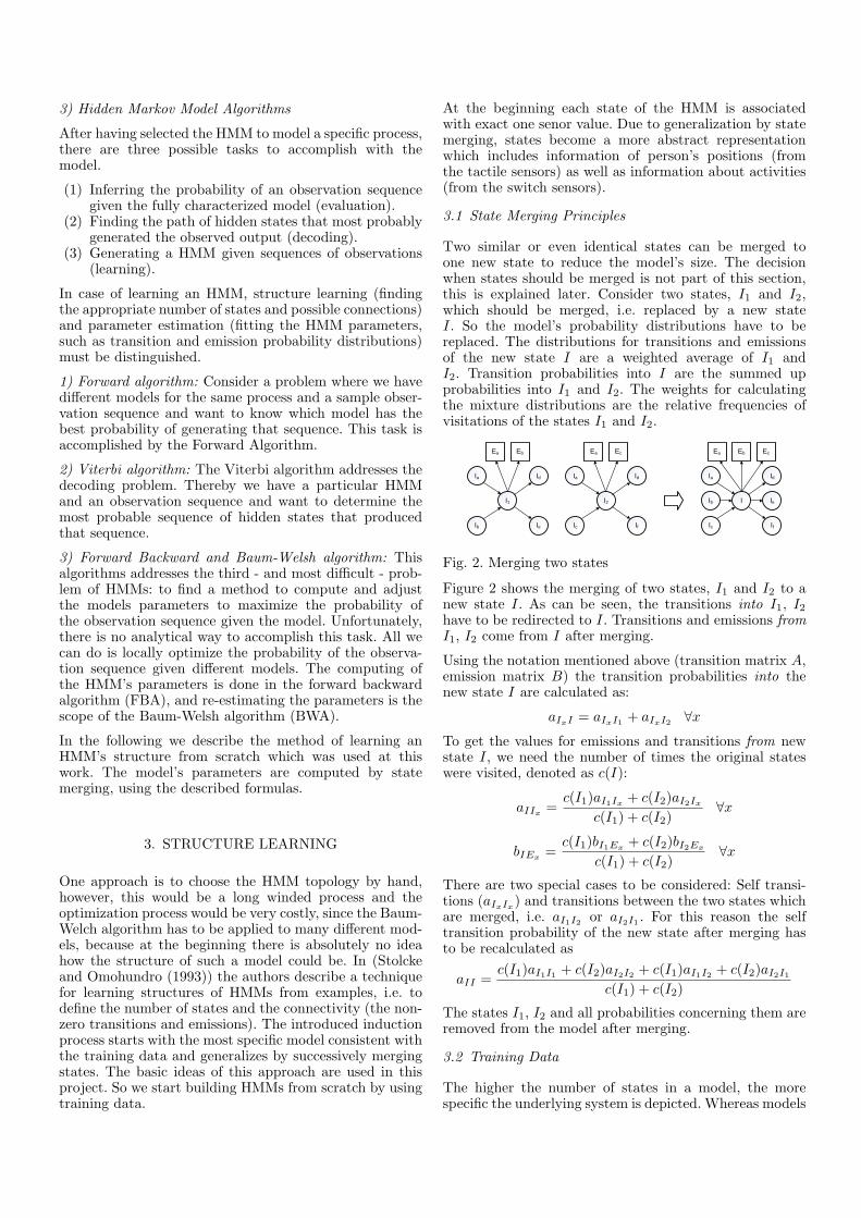
3.1 State Merging Principles

Two similar or even identical states can be merged toone new state to reduce the model’s size. The decisionwhen states should be merged is not part of this section,this is explained later. Consider two states, I1 and I2,which should be merged, i.e. replaced by a new stateI. So the model’s probability distributions have to bereplaced. The distributions for transitions and emissionsof the new state I are a weighted average of I1 andI2. Transition probabilities into I are the summed upprobabilities into I1 and I2. The weights for calculatingthe mixture distributions are the relative frequencies ofvisitations of the states I1 and I2.

I1 I2

Ia

Ib

Id

Ie

Ia

Ic

Id

If

Ea Eb EcEa

Ia

Ib

Ie

If

Ea Eb

Ic

Id

Ig

Ih

EdEc

I

I

Ia

Ic

Id

If

EcEa

Ib Ie

Eb

Fig. 2. Merging two states

Figure 2 shows the merging of two states, I1 and I2 to anew state I. As can be seen, the transitions into I1, I2have to be redirected to I. Transitions and emissions fromI1, I2 come from I after merging.

Using the notation mentioned above (transition matrix A,emission matrix B) the transition probabilities into thenew state I are calculated as:

aIxI = aIxI1 + aIxI2 ∀xTo get the values for emissions and transitions from newstate I, we need the number of times the original stateswere visited, denoted as c(I):

aIIx =c(I1)aI1Ix

+ c(I2)aI2Ix

c(I1) + c(I2)∀x

bIEx=c(I1)bI1Ex

+ c(I2)bI2Ex

c(I1) + c(I2)∀x

There are two special cases to be considered: Self transi-tions (aIxIx) and transitions between the two states whichare merged, i.e. aI1I2 or aI2I1 . For this reason the selftransition probability of the new state after merging hasto be recalculated as

aII =c(I1)aI1I1 + c(I2)aI2I2 + c(I1)aI1I2 + c(I2)aI2I1

c(I1) + c(I2)

The states I1, I2 and all probabilities concerning them areremoved from the model after merging.

3.2 Training Data

The higher the number of states in a model, the morespecific the underlying system is depicted. Whereas models

with a lower number of states represent a generalizationof the underlying process. The resulting inexactness isintended, because this raises the chance that a later per-ceived scenario can be represented by the model. However,with a too generic model it is not possible to elaboratedifferences between the scenarios. For this reason one ofthe key challenges is to find the balance between a veryspecific model with the risk of not finding a representationfor a particular scenario on the one hand and a very genericmodel, which produces results for every situation but littlesignificance, on the other hand.

When a person moves around in the room several sensorsare triggered. For each sensor value which is retrieved anew state is created which has exact one emission. Thesymbol of this emission contains a representation of thesensor value. A new transition is added to the predecessorstate with the actually created state as destination. Thus,we get a chain of states where each one has exact oneemission.

Such a chain represents a (very specific) scenario. To geta reasonable model out of that scenarios, we introduce anartificial start state which is the same for all chains, thesame with an artificial end state, respectively.

Afterwards the following three steps are applied:

(1) Merge Horizontally(2) Merge Vertically(3) Merge Sequences of States

These steps are explained in the following.

3.3 Merge Horizontally

A person standing in the SmaKi can trigger several tactilefloor sensors. If a person’s foot is placed over two sensorseither the one or the other or both can be triggered, likeshown in Figure 3. We want to model different positionsin some meaningful way, so we don’t need exact values.An accuracy which allows us to distinguish if a switch canbe reached from a person at a position would be enough.For this reason the HMM is generalized by merging stateswith similar positions.

Fig. 3. Person’s foot placement

As mentioned above, the information of other sensors isassociated to positions. For this reason the informationfrom switch and movement sensors are added to stateswhich have already at least one emission which representsa position.

3.4 Merge Vertically

To construct a general model of the values learned fromeach person, the gained chains are joined together. Onlychains with a minimal number of states are added to theglobal model. Figure 4 shows such a global model. Thegrayed, dotted chain indicates that there are several otherchains. For convenience an artificial start and end state

are added. The circle around the successors of the startstate indicate the first step of merging, the comparison ofthese states.

P,M

...

P,SP

P,M,S

...

P,M,M

P,P,M ...

... ...

Fig. 4. HMM before merging vertically

Once the chains are joined together we can merge themodel globally. The idea is to reuse parts of chains.Consider the following example, shown in Figure 5. Oneperson enters the room and walks along a path, i.e. theperson produces the sequence of positions (A,B,C,D,E).Another person who walks around, produces the sequence(A,B,C, F,G). In our model this is represented by twochains, corresponding to the positions. These chains aresimilar until the point where one person goes to (D) andthe other one to (F ). So we can merge the start of thesequences in our model and stop where the scenarios differ.

A B C

D

E

F

G

Table

Fig. 5. Splitting Paths of two different Persons in a Room

Beginning from the artificial start state, any two successorstates are compared if they are similar (within an ap-plication dependent similarity criterion). If similarity isgiven, the states are merged. This procedure is repeateduntil nothing could be merged anymore. At the person-movement example above, the first three states would bemerged, because the sequence (A,B,C) is the same for bothpersons. A resulting model of Horizontal Merging from thestart is shown in Figure 6. The same can be done withthe end of the sequences. So we use the same algorithmstarting from the artificial end state in back direction.

...

P,S

P,P,M,S

...

P,M,M

P,P,P,M

...

... ...

Fig. 6. HMM after merging vertically

3.5 Merge Sequences

As described in the previous section we get a model wheresimilar start-sequences and end-sequences are merged to-gether, with the limitation of comparing only two states.Another approach is to search the model for sequencesof several states in the midst of the model, like shown in

. A

B

B.

C

C

.

.

BA

. .

CA

A B C

Fig. 7. Comparing and merging sequences of states

CA

. A B. C

.

.

. .

A BB C

Fig. 8. Back transition as a consequence of sequencemerging

A

B C

D

EF

G

Table

X

Fig. 9. Person going around a table

Figure 7. For better readability the more abstract notation(A,B,C) is used for the symbols, i.e. two states are similar ifthey contain the same letter. States with a ‘.’ are not of in-terest for this example. If two similar sequences are found,the start and the end state of such a sequence is merged.The states between start and end of one chain becomeuseless since they cannot be reached anymore (shown bythe grayed sequence in Figure 7). However, this algorithmcan cause back transitions. As can be seen in Figure 7 thesame sequence can appear several times within one chain.If the algorithm is applied several times, all occurrences ofthe sequence (A,B,C) are merged together. This results ina model shown in Figure 8. We get a transition from a statelater in the scenario back to a state which occurred earlier.This transition is called a back transition. This transitionsviolate the temporal order of states in a scenario. However,back transitions could be suppressed, but it might be ofinterest allowing them.

Consider the following scenario, (shown in Figure 9. Aperson walks around the table several times. This results ina sequence (A,B,C,D,E, F,G,A,B,C, . . .). If back tran-sitions are allowed, the laps are merged. This results ina sequence (A,B,C,D,E, F,G,A) where only the prob-abilities for incoming transitions of state ‘A’ have to berecalculated. The count of laps gets lost. If this is anintended behavior depends on the application.

4. RESULTS AND FURTHER WORK

In the first part of this section we describe how thepredictions are generated from the model, the second partdescribes how this predictions are verified and finally wegive a suggestion how such systems could be improved.

4.1 Prediction

The theory of HMMs is used to model the behavior ofa person. This is based on the person’s positions. Howsuch a model is built is described in Section 3. Once wehave a model we can solve the Evaluation Problem tomake predictions. To accomplish this task the forwardprobability αt(i) has to be calculated. This can be doneby using the forward algorithm described in Rabiner andJuang (1986):

The forward variable or forward probability is defined as

αt(i) = Pr(O1, O2, . . . , Ot, Qt = i|λ).

This is the probability of a partial observation sequencewith length t, for state qi, given the model λ. αt(i) can becalculated inductively by the following algorithm:

1. α1(i) = πibi(O1) 1 ≤ i ≤ N

2. for t = 1, . . . , T − 1; 1 ≤ j ≤ N

αt+1(j) =

[N∑

i=1

αt(j)aij

]bj(Ot+1)

3. P r(O|λ) =N∑

i=1

αT (i)

If we calculate the forward probability αt(i) for a partialobservation sequence of length t, we get for each state Qt

the probability of being in that state. To get a predictionabout the next observed symbol s, the joint probabilitiesof forward probability αt(i), transition probability aij andemission probability for symbol s at next state bjs haveto be summed up. So for each symbol s a next stepprobability σt+1(s) can be calculated as:

σt+1(s) =∑

αt(i)aijbjs ∀i, j, s

The most probable symbol s∗t+1 at the next step, i.e. theprediction is:

s∗t+1 = arg max[σt+1(s)] ∀s

4.2 Verification of Predcitions

The different methods of structure learning result in dif-ferent HMMs. The quality of prediction is analyzed byusing the SmaKi environment described in Section 2.1.The predicted position is compared to the position whichoccurred in reality at the next step of the person. We definethe distance between theses positions as the quality of theprediction.

To make the distances of different models comparable, thesame sample data was used to create the models. Afterthis initial procedure, the different merging strategies areapplied to the model. Then the same scenario is testedwith each model. The test scenario is quite simple: Aperson enters the empty room (i.e. there are no otherpersons), walks to the fridge, opens the fridge, closesthe fridge, goes on to the server cabinet (where a screenwith a visualization of triggered sensors is located), turnsaround and leaves the room. The results are shown in thefollowing.

0

0,5

1

1,5

2

2,5

3

1 3 5 7 9 11 13 15 17 19 21 23 25 27 29 31 33 35 37 39 41

Steps

Dis

tanc

e [m

]

d(P1)d(P2)d(P3)

Fig. 10. Evaluation of a horizontally merged HMM

0

0,5

1

1,5

2

2,5

3

1 3 5 7 9 11 13 15 17 19 21 23 25 27 29 31 33 35 37 39 41 43 45 47

Steps

Dis

tanc

e [m

]

d(P1)d(P2)d(P3)

Fig. 11. Evaluation of a fully merged HMM

Figure 10 shows the evaluation of a horizontally mergedHMM. At the x-axis there is the count of steps, at the y-axis the distance as mentioned above. The series d(P1) rep-resents the prediction with the highest probability, seriesd(P2) the second highest and d(P3) the third one. Beforewe start the interpretation of this diagram, we shouldremember the tactile sensors from which the positionsare calculated: They have a size of 600 x 175 mm, so alldistances below 0.6 m are only one sensor-size away (in thedimension of the lower resolution). As can be seen, d(P1) isonly from step 10 to 14 above the value of 0.6 m, however,d(P2) has lots of higher deviations. Finally d(P3) has stillhigher deviations than d(P2). This is what we expected:The prediction with the highest probability gives the bestestimations. If we compare this to Figure 11, which showsthe evaluation of a fully merged HMM, it can be seen thatthe predictions get even better. The term fully means thatmerging of sequences, like described in Section 3.5, is alsoapplied. The vertically merging, which is the next stepafter the horizontal merging is not mentioned here, sincethis results in very little differences in our application.

4.3 Further Work

The represented model works quite well for the intendedpurpose. However, it has a weak time representation. Theoccurrence of events is ordered, but the duration betweentwo occurring events is not evaluated. With the simpletime model of the current system, scenarios with similarvalues but different durations will be identified as the

same, because the time span where nothing happened isnot taken into account. To provide a better representationof time, the standard approach of HMMs is not sufficient.In (Russell and Moore (1985)) a system of a higher ordermodel, the Hidden Semi Markov Model is described. Suchmodels could be used to overcome the weak modeling oftime within the standard HMMs. So the system shouldbe able to distinguish better between persons who triggertactile floor sensors and objects doing this.

REFERENCES

Baker, C.R., Markovsky, Y., van Greuen, J., Rabaey, J.,Wawrzynek, J., and Zuma, A.W. (2006). A plattformfor smart-home environments. In Proceedings of the 2thIEEE International Conference on Intelligent Environ-ments.

Bishop, C.M. (1995). Neural Networks for Pattern Recog-nition. New York NY.: Oxford University Press Inc.

Bowring, J.M.R.J.F. and Harrold, M.J. (2004). Tripewire:Mediating software self-awareness. In Proceedings of the2nd ICSE Workshop on Remote Analysis and Measure-ment of Software Systems (RAMSS04), 11–14.

Bruckner, D. (2007). Probabilistic Models in Building Au-tomation: Recognizing Scenarios with Statistical Meth-ods. Ph.D. thesis, Vienna University of Technology,Institute of Computer Technology.

Cook, J.E. and Wolf, A.L. (1999). Automating processdiscovery through event-data analysis. In Proceedingsof the 17th International Conference on Software Engi-neering (ICSE95), 73–82.

Goetzinger, S. (2006). Scenario Recognition Based on aBionic Model for Multi-Level Symbolization. Master’sthesis, Vienna University of Technology, Institute ofComputer Technology.

Mitterbauer, J. (2008). Behavior Recognition and Predic-tion in Building Automation Systems. Master’s thesis,Vienna University of Technology, Institute of ComputerTechnology.

Pratl, G. and Palensky, P. (2005). Project ars - the nextstep towards an intelligent environment. In Vienna Uni-versity of Technology, Institute of Computer Technology.

Rabiner, L.R. and Juang, B.H. (1986). An introduction tohidden Markov models. IEEE ASSAP Magazine 3.

Russell, M. and Moore, R. (1985). Explicit modelling ofstate occupancy in hidden markov models for automaticspeech recognition. In VProc. IEEE Int. Conf. onAcoustics, Speech and Signal Processing, 5–8.

Soucek, S., Russ, G., and Tamarit, C. (2000). The smartkitchen project - an application on fieldbus technologyto domotics. In Proceedings of the 2nd InternationalWorkshop on Networked Appliances (IWNA2000), 1.

Stolcke, A. and Omohundro, S. (1993). Hidden markovmodel induction by bayesian model merging. In Hanson,Stephen J. ; Cowan, Jack D. ; Giles, C. L. (eds.):Advances in Neural Information Processing Systems Bd.5, 11–18.