feras a s saleh a thesis - welcome to spectrum: concordia ... · list of figures ... moreover,...
TRANSCRIPT
Multi-Tier Supplier Quality Evaluation in Global Supply Chains
Feras A S Saleh
A Thesis
in
The Department
of
Concordia Institute for Information Systems Engineering (CIISE)
Presented in Partial Fulfillment of the Requirements For the Degree of
Master of Applied Science (Quality Systems Engineering) at
CONCORDIA UNIVERSITY
Montreal, Quebec, Canada
November 2015
© Feras A S Saleh, 2015

CONCORDIA UNIVERSITY
School of Graduate Studies
This is to certify that the thesis prepared
By: Feras A S Saleh
Entitled: Multi-Tier Supplier Quality Evaluation in Global Supply Chains
and submitted in partial fulfillment of the requirements for the degree of
Master of Applied Science (Quality Systems Engineering)
complies with the regulations of the University and meets the accepted standards with
respect to originality and quality.
Signed by the final Examining Committee:
Dr. Mohammad Mannan
Dr. Govind Gopakumar
Chair
Examiner
Dr. Jia Yuan Yu
Examiner
Dr. Anjali Awasthi Supervisor
Approved by:
Chair of Department or Graduate Program
Dean of Faculty
Date
iii
Abstract
Multi-Tier Supplier Quality Evaluation in Global Supply Chains
Feras A S Saleh
Concordia University
Supplier quality evaluation is a critical part of quality management in global supply chains. Poor
supplier quality results in not only monetary losses but also negatively impacts the business
potential and future growth of buyer organizations. In this thesis, we propose a multi-tier supplier
quality evaluation framework based on total cost of ownership and data envelopment analysis for
quality management in global supply chains. The proposed approach comprises of three main
steps. Firstly, we group the upstream suppliers based on common attributes using hierarchical
cluster analysis. Then, we calculate the total cost of ownership for the grouped suppliers and their
sub-suppliers using various qualitative and quantitative factors that are vital for quality
management in global supply chains. In the third and the last step, we apply data envelopment
analysis to compute the efficiencies of various suppliers to identify the best one (s) and
recommend for selection. A numerical application is provided.
The proposed approach is very useful to decision makers in benchmarking supplier quality
performances and setting improvement targets for supplier quality development in global supply
chains.

iv
Acknowledgments
I would like to express my sincere gratitude to my supervisor, Dr. Anjali Awasthi, for her
patience, guidance, and encouragement that she provided during this thesis work. I am truly
thankful for her support, time and being there to answer my questions and queries so promptly.
Her insightful discussions and suggestions made this work possible.
I would like to thank all the faculty members of Concordia Institute for Information Systems
Engineering for the wonderful academic experience and the enormous knowledge they support
their students with.
Finally, I would like to thank my wife and the mother of my two daughters, for her
understanding and being so supportive during this journey.
Thank you.

v
Table of Contents
List of Figures ........................................................................................................................... vii
List of Tables............................................................................................................................ viii
Chapter 1 Introduction ................................................................................................................. 1
1.1 Problem Definition ............................................................................................................ 3
Chapter 2 Literature Review ........................................................................................................ 5
2.1 Challenges for quality management in global supply chains ............................................... 5
2.2 Collaboration for improving supply chain quality .............................................................. 8
2.3 Evaluating supplier quality ............................................................................................... 10
2.3.1 Total Cost of Ownership (TCO) ................................................................................ 12
2.3.2 Analytic Hierarchy Process (AHP) ............................................................................ 16
2.3.3 Goal Programming (GP) ........................................................................................... 19
2.3.4 Data Envelopment Analysis (DEA) ........................................................................... 21
2.4 Supplier Quality Evaluation Framework .......................................................................... 27
2.4.1 Problem definition and formulation of criteria ........................................................... 30
2.4.2 Pre-qualification ........................................................................................................ 30
2.4.3 Final choice phase ..................................................................................................... 31
2.4.4 The Proposed Framework.......................................................................................... 31
Chapter 3 Solution Approach ..................................................................................................... 33
3.1 Grouping of upstream suppliers using hierarchical cluster analysis .................................. 33
3.1.1 Hierarchical Cluster Analysis .................................................................................... 34
3.2 Multi-tier supplier quality evaluation using TCO and DEA .............................................. 38
3.2.1 Total Cost of Ownership ........................................................................................... 40
vi
3.2.2 Network DEA ........................................................................................................... 40
3.3 Recommendations for improving supplier quality ............................................................ 42
Chapter 4 Numerical Application .............................................................................................. 44
4.1 Hierarchical cluster analysis ............................................................................................. 44
4.1.1 Data Normalization ................................................................................................... 45
4.1.2 Assigning weights to product types ........................................................................... 46
4.1.3 Applying hierarchical clustering ................................................................................ 47
4.1.4 Recommendations ..................................................................................................... 49
4.2 TCO and DEA ................................................................................................................. 50
4.2.1 Recommendations ..................................................................................................... 57
4.3 Sensitivity analysis .......................................................................................................... 57
4.3.1 First Scenario: Evaluate without manufacturing and technology costs ....................... 57
4.3.2 Second Scenario: Evaluate without quality costs and price ........................................ 58
4.3.3 Third Scenario: Evaluate without logistics and after sale costs .................................. 59
4.3.4 Fourth Scenario: Evaluate without social and environmental costs ............................ 60
4.4 Results Validation ............................................................................................................ 62
Chapter 5 Conclusions and Future Work .................................................................................... 71
5.1 Conclusions ..................................................................................................................... 71
5.2 Future Work .................................................................................................................... 71
5.3 SWOT analysis ................................................................................................................ 72
References ................................................................................................................................. 73
Appendix A ............................................................................................................................... 85
vii
List of Figures
Figure 1.1 Toyota vehicles recall in 2010 (Edwards, 2010, February 4) ....................................... 2
Figure 2.1 Supply chain example (Regan, 2015) .......................................................................... 5
Figure 2.2 Multi-tier supply chain ................................................................................................ 7
Figure 2.3 Hierarchical Structure ............................................................................................... 17
Figure 3.1 A sample dendrogram ............................................................................................... 36
Figure 3.2 Best cut method ........................................................................................................ 37
Figure 4.1 Dendrogram with best cut ......................................................................................... 48
Figure 4.2 Example of 3-tier suppliers ....................................................................................... 50
Figure 4.3 Suppliers' efficiency scores ....................................................................................... 54
Figure 4.4 Efficiencies of the three suppliers ............................................................................. 55
Figure 4.5 The supply chain of the Iranian beverage corporations’ case ..................................... 63
Figure 5.1 SWOT analysis ......................................................................................................... 72
viii
List of Tables
Table 2.1 Dickson supplier evaluation criteria ........................................................................... 11
Table 2.2 Total cost of ownership literature review .................................................................... 13
Table 2.3 AHP Measurement Scale ........................................................................................... 18
Table 2.4 Summary of popular supplier evaluation techniques ................................................... 26
Table 2.5 de Boer et al. (2001) supplier selection framework ..................................................... 28
Table 3.1 TCO costs' Categories ................................................................................................ 39
Table 4.1 Hypothetical upstream suppliers ................................................................................. 45
Table 4.2 Normalized Data ........................................................................................................ 46
Table 4.3 Weighted product types .............................................................................................. 47
Table 4.4 Cluster analysis final results ....................................................................................... 48
Table 4.5 Descriptive statistics .................................................................................................. 49
Table 4.6 Hypothetical data generated using Excel random routine ............................................ 53
Table 4.7 Efficiency scores ........................................................................................................ 54
Table 4.8 Input targets ............................................................................................................... 56
Table 4.9 Efficiency scores without manufacturing cost............................................................. 58
Table 4.10 Efficiency scores without technology cost ................................................................ 58
Table 4.11 Efficiency scores without quality cost ...................................................................... 59
Table 4.12 Efficiency scores without price ................................................................................ 59
Table 4.13 Efficiency scores without logistics cost .................................................................... 60
Table 4.14 Efficiency scores without after sale cost ................................................................... 60
Table 4.15 Efficiency scores without social and environmental costs ......................................... 61
Table 4.16 Description of the used notations .............................................................................. 62
ix
Table 4.17 The data of the Iranian beverage case study .............................................................. 69
Table 4.18 Calculation results of the Iranian beverage case study .............................................. 69
1
Chapter 1
Introduction
With the complexity of today’s supply chains; firms have difficulty keeping track of all the
activities happening in the supply chain. Less visibility and control of key processes have
become the result of manufacturing, logistics and other roles such as outsourcing (Morehouse and
Cardoso, 2011). As a result, the supply chain is now more vulnerable to frauds than before.
Babies got poisoned by contaminated milk in China (Bradley, 2008) because one supplier
decided to use melamine instead of protein nitrogen to gain some extra profit. In 2007, Canadian
pet food manufacturing and retailer, Menu Food, had a massive recall of one popular pet food
product because it caused sickness and death of animals as a result of high melamine level in
some ingredients imported from Chinese suppliers (Chen et al., 2014). Moreover, Mattel recalled
millions of toys in 2007 because the used paint contained high level of lead (Viswanadham and
Samvedi, 2013).

2
Figure 1.1 Toyota vehicles recall in 2010 (Edwards, 2010, February 4)
As a result, firms have strived to achieve successful supply chain collaboration. Collaboration can
improve the traceability and visibility among the supply chain (Sarpong, 2014), which in turn
improves the quality of the final product or service. Moreover, collaboration can deliver
significant benefits to all parties such as excess inventory reduction, bullwhip avoidance,
business synergy enhancement, flexibility and increase joint innovation (Cao and Zhang, 2011).
Supply chain performance enhancement (Vereecke and Muylle, 2006) by leveraging the
knowledge and resources of suppliers (Cao and Zhang, 2011) are some results of a successful
collaboration.
Although product design, warehousing, and distributions centers can all be the subject of quality
improvement programs; in this thesis we are focusing on purchasing as it contributes the most to
the cost of quality. Both supplier evaluation and selection are essential for the success of the focal
firm (Choi and Hartley, 1996; Singh, 2014). We argue that evaluation of the current suppliers is
3
the first step toward a successful collaboration relationship. Evaluation will reveal the weak areas
of each supplier and recommend methods for improvement. Moreover, this evaluation will be the
basis for supplier development program. We propose an approach based on Total Cost of
Ownership (TCO) and Data Envelopment Analysis (DEA) due to their respective advantages.
TCO looks beyond the quoted cost to cover additional true costs related to the entire purchasing
cycle. In addition to the quoted price, it may include order placement costs, research costs,
transportation costs, receiving costs, inspection costs, holding costs, and disposal costs (Bhutta
and Huq, 2002). Consequently, TCO would help to understand the true costs associated with the
quality of the purchased items.
DEA is a powerful non-parametric analysis technique that considers both quantitative and
qualitative data. DEA does not require the decision maker to assign weights to each indicator but
calculates weights from the given data. Additionally, DEA finds the efficient decision making
units (suppliers) and computes the amount and source of inefficiency of inefficient suppliers
(Cooper et al., 2007). It provides improvement targets for inefficient suppliers to become
efficient. These targets values can be the basis of a new supplier improvement program.
1.1 Problem Definition
Supplier evaluation process is very critical to purchasing management. It is a complex multiple
criteria decision making problem that requires careful selection of criteria (Omurca, 2013). Both
qualitative and quantitative criteria should be used in evaluating the supplier performance.
Additionally, it should speak the language of business, or money, to ensure acceptance among
purchasing managers. It must also reflect the network structure of the supply chain. As a result,
all the n-tier suppliers and the linkages between them should be evaluated for overall quality
management in supply chains.

4
The aim of this thesis is to develop a multi-tier supplier quality evaluation framework for
improving the quality of global supply chains. This involves:
1. Grouping of upstream suppliers using hierarchical cluster analysis
2. Evaluation of supplier quality at multiple tiers.
3. Identification of improvement targets for poorly performing suppliers and
recommendations generation.

5
Chapter 2
Literature Review
2.1 Challenges for quality management in global supply chains
Mentzer et al. (2001) define supply chain as a set of firms that have direct upstream and
downstream flows of products, services, finances, and information from a source to a customer.
According to Bozarth and Handfield (2006), supply chain can be defined as a network of
manufacturers and service providers that work together to transform and transport goods from the
raw materials stage through the end user. Figure 2.1 illustrates the various stakeholders involved
in a supply chain.
Figure 2.1 Supply chain example (Regan, 2015)
6
Supply chain can be classified into two main categories: product supply chain and service supply
chain. Automobiles, electronics, fresh foods are some examples of product supply chain.
Examples of service supply chain are healthcare, education, banking etc. The quality
management practices may vary depending on the nature of supply chain. For example, fresh
fruit supply chains have a long lead-time and a very high uncertainty level with regards to supply
and demand. It requires an efficient management and the use of modern decision technology tools
(Soto-Silva et al., 2015). Automobiles industry have very complex supply chains that start from
extracting the basic raw materials until the delivery of final product. These supply chains
requires innovative approaches to manage different supply chain activities (Vonderembse et al.,
2006). In electronics supply chain, demand uncertainty and inventory control challenges are the
main side effects due to the short life cycle of these products. Moreover, the complexity of these
products requires a wide range of supply materials (Tse et al., 2016). For service supply chains,
e.g. healthcare, the supply chain starts from supplying state of the art equipment and medicines
from warehouses to clinics and hospitals. Management faces major challenges in managing these
supply chains because of their great impacts on public health. It requires precise medical supply
according to patient’s needs (Jahantigha and Malmir, 2015).
In today’s world it is not possible for a single organization to own its entire supply chain like the
Ford Company in the first half of the 20th
century (Gelderman, 1989). To stay competitive in
global market; organizations have to outsource many critical business processes and value chain
activities to suppliers thousands of miles away to reduce cost or increase responsiveness
(Nieminen and Takala, 2006). Therefore, the supply chain has become more and more complex.
Especially when the direct supplier (first tier) outsources part of its business to another supplier
7
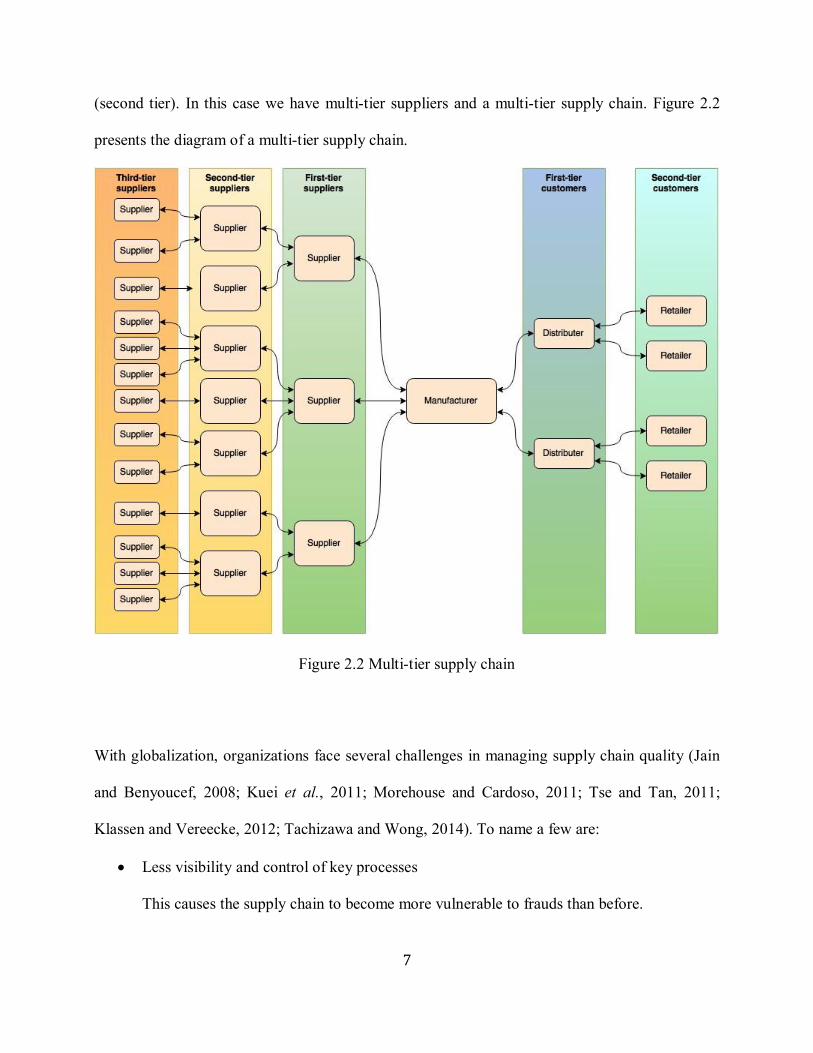
(second tier). In this case we have multi-tier suppliers and a multi-tier supply chain. Figure 2.2
presents the diagram of a multi-tier supply chain.
Figure 2.2 Multi-tier supply chain
With globalization, organizations face several challenges in managing supply chain quality (Jain
and Benyoucef, 2008; Kuei et al., 2011; Morehouse and Cardoso, 2011; Tse and Tan, 2011;
Klassen and Vereecke, 2012; Tachizawa and Wong, 2014). To name a few are:
Less visibility and control of key processes
This causes the supply chain to become more vulnerable to frauds than before.
8
Protecting the environment
Considering the environment in order to survive in today’s environmentally conscious
market.
Social issues
Labour practices by global suppliers in developing countries, which includes worker
safety, working conditions, workers’ rights and child’s labour.
Inventory reduction
Applying JIT philosophy can lead to significant cost-savings, however, the supply chain
may become more vulnerable as they have very little inventory to buffer any interruptions
in supply.
Adopting advanced technologies
To facilitate effective decision making; firms should identify technology applications that
participate effectively in the global progress. Examples of such technology are enterprise
resource planning (ERP), customer relationship management (CRM), and product
lifecycle management (PLM).
Therefore, firms are striving to achieve successful supply chain collaboration to limit some of
these impacts. Collaboration can improve the traceability and visibility among the supply chain
members (Sarpong, 2014), which in turn improves the quality of the final product or service.
2.2 Collaboration for improving supply chain quality
Anthony (2000) stated that supply chain collaboration occurs “when two or more companies
share the responsibility of exchanging common planning, management, execution, and
performance measurement information”. Furthermore, he suggested “Collaborative relationships
9
transform how information is shared between companies and drive change to the underlying
business processes”.
In today’s business environment; collaboration is more important than ever as technologies are
rapidly changing, competition is growing, outsourcing is increasing, and the growth of very
specialised companies is taking place (Sarpong, 2014). Several authors have discussed the
benefits of successful collaboration. We mentioned some of these benefits in the previous
chapter. Other benefits include more sales volume from downstream buyers, lower operational
costs, word-of-mouth referrals, and new product and process innovations resulting from a
working relationship between trusting partners (Sarpong, 2014). Additionally, collaboration
improves and assists the environment and social aspects of sustainability (MacCarthy and
Jayarathne 2012).
Many firms have started to realize that it is not enough to collaborate with the first-tier suppliers
only. To achieve the full potential benefits of collaboration; firms should collaborate with lower
tier suppliers as well. For example, Puma’s sustainability report covers up to the fourth tier of
suppliers, and Nike is auditing hundreds of second-tier apparel suppliers (Lee et al., 2012). IKEA
is working with its suppliers to comply with the code of conduct (Andersen and Skjoett-Larsen,
2009). Similarly, Hewlett-Packard and Migros manage sub-suppliers to ensure they fulfill the
requirements of corporate sustainability standards (Grimm et al., 2014).
The first step in collaboration is partner selection which starts with supplier evaluation in buyer-
supplier partnerships. In the following section we will explore different approaches for supplier
evaluation and reveal their weaknesses and strengths.
10
2.3 Evaluating supplier quality
Supplier evaluation is a multi-criteria decision making problem that involves several qualitative
and quantitative factors. Several studies have been conducted to develop decision-making models
that can address this problem effectively (Zeydan et al., 2011). Ghodsypour and O’Brien (1998)
classify supplier evaluation models into two groups: single objective models and multiple
objective models. Single objective models use one criterion, such as the cost, as an objective
function and other criteria as constraints. This approach has two weaknesses: it weights all
constraints equally which rarely happens in reality, and it faces significant difficulties when
considering qualitative factors. Moreover, it is very risky to rely on a single criterion when
evaluating a supplier. Therefore, using a multi-criteria approach is preferable over the single
criterion approach (Zeydan et al., 2011).
One of the earliest contributions to supplier evaluation and selection criteria was of Dickson
(1966). In his study he identified 23 criteria for supplier evaluation. Furthermore, he found that
quality, delivery and performance history are the most important criteria (see Table 2.1). Erdem
and Gocen (2012) list 60 criteria for supplier evaluation among which price, quality, availability
and delivery are the most significant ones. These results confirm the multi-criteria nature of
supplier evaluation problem.

11
Evaluation Criteria Rank
Quality 1
Delivery 2
Performance History 3
Warranties and claim policies 4
Production facilities and capacity 5
Price 6
Technical capability 7
Financial position 8
Procedural compliance 9
Communication system 10
Reputation and position in industry 11
Desire for business 12
Management and organization 13
Operating controls 14
Repair service 15
Attitude 16
Impression 17
Packaging ability 18
Labor relations record 19
Geographical location 20
Amount of past business 21
Training aids 22
Reciprocal arrangements 23
Table 2.1 Dickson supplier evaluation criteria
According to Ho et al. (2010) and Erdem and Gocen (2012), supplier evaluation and selection
approaches can be classified into:
Linear weighting models such as Analytic hierarchy process, interpretative structure
modeling, fuzzy set theory, and total cost of ownership.
Mathematical programming models such as data envelopment analysis, linear
programming, mix integer programming, and goal programming.
Artificial intelligence models and Statistical/probabilistic models such as case based
reasoning, genetic algorithm, neural network, and expert systems.
Supplier evaluation should be extended beyond the first-tier suppliers to cover all suppliers across
the supply chain. Many researches consider this as one way to manage the supply chain (Rao,
12
2002; Zhu and Sarkis, 2004; Andersen and Skjoett-Larsen, 2009; Mueller et al., 2009; Zhu et al.,
2012). Ho et al. (2010) and Noshad and Awasthi (2015) reviewed several published articles on
multi-criteria decision making approaches for supplier evaluation and selection. DEA was the
most popular individual approach per Ho et al. (2010) while AHP and DEA based approaches
were the most popular per Noshad and Awasthi (2015). In the following section we will examine
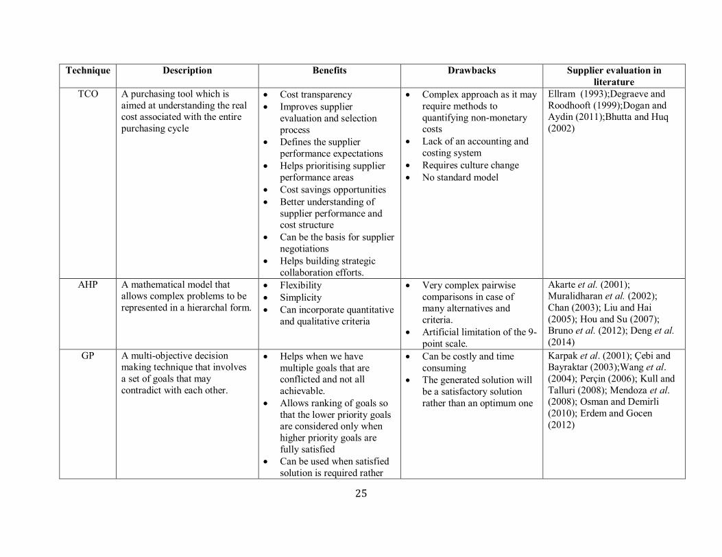
popular approaches found in literature. Additionally, a summary for these approaches is
presented in table 2.4.
2.3.1 Total Cost of Ownership (TCO)
An IT research and advisory company called Gartner was the original developer of the total cost
of ownership (TCO) concept in 1987. They used it to compute the total costs of owning and
managing IT infrastructure in a company (Bermen et al., 2007). Later, the concept has been used
to calculate total cost of purchased goods in general (Ellram, 1993). TCO is a purchasing tool and
a philosophy which is aimed at understanding the real cost of buying a particular good or service
from a supplier (Ellram, 1995). It is a complex approach that requires the firm to determine the
associated costs and find ways to quantify non-monetary costs if they want to better understand
and manage their costs. It may include in addition to the quoted price, order placement costs,
research costs, transportation costs, receiving costs, inspection costs, holding costs, and disposal
costs (Bhutta and Huq, 2002).
Although there are other selection and evaluation approaches closely related to TCO, such as life-
cycle costing, zero-base pricing, cost-based supplier evaluation, and cost ratio method, none of
them received significant, widespread support in literature or in practice (Ellram, 1995).
Complexity, situation-specific application, over-reliance on some factors and inadequate
13
consideration of others are some of the factors that could be the reasons behind the lack of
support (Bhutta and Huq, 2002).
Author, Year Incentive to Use TCO TCO Cost Categories
Bhutta and
Huq (2002) Supplier Selection Manufacturing
Quality
Technology
After sales services
Degraeve and
Roodhooft
(1999)
Supplier Selection Three hierarchic levels:
Supplier level activities
Ordering level activities
Unit level activities
Degraeve et
al. (2005) Evaluating organization’s strategic
procurement options
Purchasing managers performances evaluation
Understanding the costs of purchasing
activities
Cost matrix of supplier,
product, order, unit (cash, non
cash) versus acquisition, reception, possession,
utilization, elimination
Dogan and Aydin (2011)
Supplier Selection Product design cost
Downtime cost
Logistics cost
Operation cost
Quality related cost
Administrative cost
Transaction cost
Ellram (1993) Supplier performance evaluation
Decision making
Supplier selection
Understanding the costs of purchasing
activities
Pre-Transaction costs
Transaction costs
Post-Transaction costs
Hurkens et al.
(2006)
Negotiating prices
Identify and prioritize improvement actions
Understand the consequences of changing
volume allocation among suppliers.
Dealer buy
Quality confirmation
Quality check
Adverse buy
Warehousing (Handling,
Inventory holding, Storing)
Supplier returns
Supplier monitoring
Cash flow
Maltz and
Ellram (1997) Including non-monetary factors into make/buy
decisions
Management
Quality
Delivery
Service
Communications
Price
Table 2.2 Total cost of ownership literature review
14
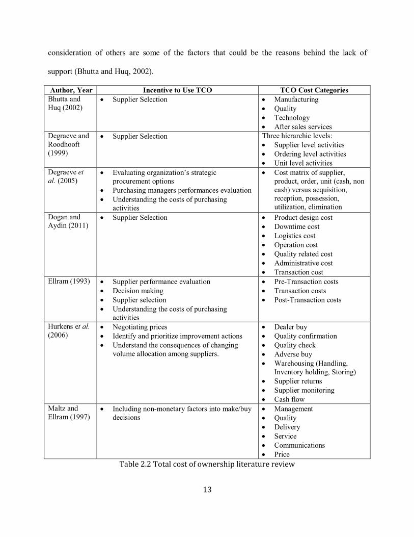
On the other hand, there has been more focus on TCO among the published articles. Table 2.2
highlights some of these articles along with the incentives of using TCO and the cost categories
suggested by different researchers. It can be seen that many researches have considered supplier
selection as the main reason for choosing TCO while others considered supplier evaluation as the
main motive. But the common reason is to reveal the true cost of purchasing activities (Ellram,
1993). Only (Maltz and Ellram, 1997) considered it from another perspective by incorporating
TCO into the make/buy decision.
2.3.1.1 Barriers to TCO
Despite these efforts, TCO is still a complex approach and many organizations face a lot of
difficulties and barriers when trying to implement it. Ellram (1995) considered lack of an
accounting and costing system as a major challenge. Many organizations use activity based
costing as a way to overcome this barrier (Ellram, 1993; Ellram, 1995; Sohal and Chung, 1998).
Culture change is another barrier, a change from price orientation towards understanding total
cost. That’s why TCO is considered more a philosophy than a tool (Ellram, 1995). Furthermore,
there is no standard model for TCO analysis. Using TCO models may vary inside the
organization according to the importance of the purchase (Ellram, 1995; Ferrin and Plank, 2002).
2.3.1.2 Benefits of TCO
TCO delivers many benefits to organizations. Cost transparency is pointed as the basic advantage
of applying a TCO approach (Bremen et al., 2007). Other benefits considered by Ellram (1995)
are improving the supplier evaluation and selection process, defining the supplier performance
expectations for the organization and the supplier, help prioritize areas in which supplier
performance would be most beneficial (such as supplier continuous improvement), creating
15
major cost saving opportunities, improving firm’s understanding of supplier performance and
cost structure, and using cost information as a basis for supplier negotiations. Only Bhutta and
Huq (2002) pointed out that TCO helps in building strategic collaboration efforts.
2.3.1.3 TCO Cost Categories
Table 2.2 illustrates that authors categorized cost according to the functional departments in an
organization. Maltz and Ellram (1997) used the categories as management, quality, delivery,
service, communications, and price. Ellram (1993) suggested a more general approach based on
the order of occurrence: pre-transaction costs, transaction costs, post-transaction costs. Pre-
transaction costs involve all costs related to activities that occur prior to order placement such as
identifying requirements, searching for a supplier, negotiation, and supplier evaluation.
Transaction costs occur at the time of purchasing and receiving the ordered item. Price, delivery
charges, and inspection are some examples of transaction costs. Post-transaction costs occur after
closing the order. In other words, post- transaction costs include all activities that happen after the
organization owns the ordered item such as maintenance costs and quality failures costs (Ellram,
1993).
Hurkens et al. (2006) conducted a study on a service sector organization (a vehicle glass repair
and replacement company) to show how TCO information can influence strategic decision
regarding allocation of volumes. They used the cost categories as buying from dealer, quality
confirmation, quality check, adverse buy, supplier returns, supplier monitoring, and cash flow.
Bhutta and Huq (2002) categorized production into manufacturing, quality, technology, and after
sales services costs to compare between total cost of ownership and analytic hierarchy process
approaches. Manufacturing costs include raw material, labor, and machine depreciation. Quality
costs are related to activities performed to monitor and control quality such as inspection, cost of
16
rework, and scrap. Designing and engineering costs are some examples of technology costs.
Finally after sales costs are related to after sales activities such as warranty and customer claims
(Bhutta and Huq, 2002; Garfamy, 2006).
Degraeve and Roodhooft (1999) developed a decision-making model to minimize TCO when
selecting a supplier. The model is based on three hierarchical levels. The first level is the
supplier’s activities that are performed when a specific supplier is used. For example, inspection
and quality audit. On the next level we have ordering level activities. Activities on this level
should be performed each time an order is assigned to a supplier. Unit level activities are at the
last level and performed for a unit in a specific order. For example, production downtown cost
related to a defective item purchased from a supplier.
Degraeve et al. (2005) presenting a matrix model consisting of supplier level, product level, order
level, and unit level activities and their associated life cycle costs. Furthermore, Dogan and Aydin
(2011) proposed a model that combines total cost of ownership and Bayesian networks to
efficiently select a supplier using product design cost, downtime cost, logistics cost, operation
cost, quality related cost, administrative cost, and transaction cost as the cost categories.
Researchers have presented different costs categories to serve different purposes as can be seen
from the previous section but no study so far, according to our knowledge, suggested cost
categories from collaboration perspective. This thesis is trying to fulfill this gap by incorporating
collaboration into our selection of the cost categories.
2.3.2 Analytic Hierarchy Process (AHP)
Saaty first developed the Analytic Hierarchy Process (AHP) method in 1980. AHP provides a
multiple criteria framework for situations involving intuitive, rational, quantitative, and
17
qualitative aspects. It provides a mathematical model to assign weights to multiple alternatives
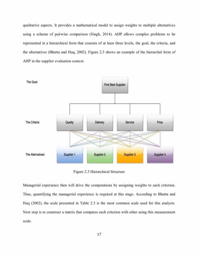
using a scheme of pairwise comparison (Singh, 2014). AHP allows complex problems to be
represented in a hierarchical form that consists of at least three levels, the goal, the criteria, and
the alternatives (Bhutta and Huq, 2002). Figure 2.3 shows an example of the hierarchal form of
AHP in the supplier evaluation context.
Figure 2.3 Hierarchical Structure
Managerial experience then will drive the computations by assigning weights to each criterion.
Thus, quantifying the managerial experience is required at this stage. According to Bhutta and
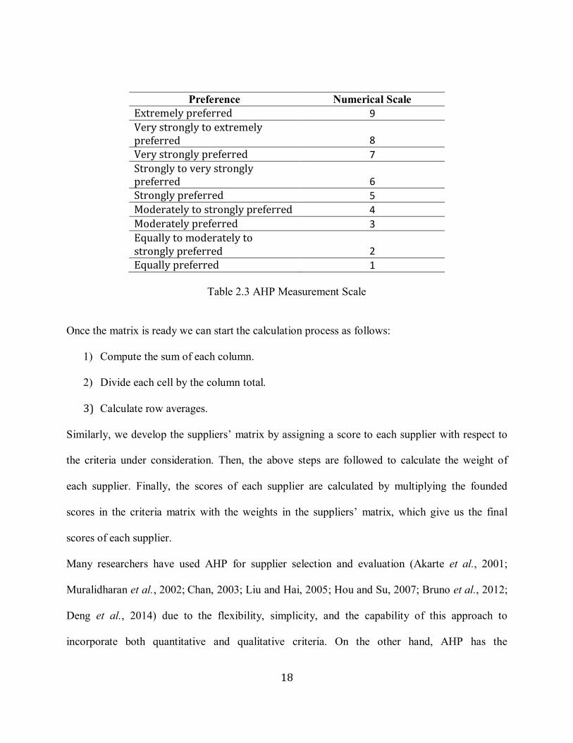
Huq (2002), the scale presented in Table 2.3 is the most common scale used for this analysis.
Next step is to construct a matrix that compares each criterion with other using this measurement
scale.
18
Preference Numerical Scale
Extremely preferred 9
Very strongly to extremely preferred 8
Very strongly preferred 7
Strongly to very strongly preferred 6
Strongly preferred 5
Moderately to strongly preferred 4
Moderately preferred 3
Equally to moderately to strongly preferred 2
Equally preferred 1
Table 2.3 AHP Measurement Scale
Once the matrix is ready we can start the calculation process as follows:
1) Compute the sum of each column.
2) Divide each cell by the column total.
3) Calculate row averages.
Similarly, we develop the suppliers’ matrix by assigning a score to each supplier with respect to
the criteria under consideration. Then, the above steps are followed to calculate the weight of
each supplier. Finally, the scores of each supplier are calculated by multiplying the founded
scores in the criteria matrix with the weights in the suppliers’ matrix, which give us the final
scores of each supplier.
Many researchers have used AHP for supplier selection and evaluation (Akarte et al., 2001;
Muralidharan et al., 2002; Chan, 2003; Liu and Hai, 2005; Hou and Su, 2007; Bruno et al., 2012;
Deng et al., 2014) due to the flexibility, simplicity, and the capability of this approach to
incorporate both quantitative and qualitative criteria. On the other hand, AHP has the
19
disadvantage that the number of pairwise comparisons may become very large when having
many alternatives and criteria (𝑛(𝑛 − 1)/2). Additionally, another disadvantage is the artificial
limitation of the 9-point scale. For instance, if alternative X is 5 times more important than
alternative Y, which is 5 times more important than alternative Z. In this case, it is not possible
for AHP to handle the fact that alternative X is 25 times more important alternative Z (Macharis
et al., 2004).
2.3.3 Goal Programming (GP)
Charnes and Cooper first presented this technique in 1961. Later, Lee and Ignizio improved it in
1972 and 1976 respectively. Goal programming (GP) is a multi-objective decision making
technique (Bal et al., 2006). GP involves a set of goals that may often contradict each other.
Therefore, it is not possible to satisfy all goals at the same time as achieving one goal may cause
another goal to deviate from its own target. Thus, the purpose of GP is to minimize the deviation
between achievement of goals and their aspiration levels (Liao and Kao, 2010).
To construct a GP model, we use the following steps (Ignizio, 1976):
i. Define the decision variables.
ii. Determine the goal and system constraints.
iii. Decide the preemptive priority factors and the relative weights.
iv. Define the nonnegative requirement.
The mathematical formulation for GP can be as following (Romero, 2004):
Min ∑ | 𝑓j(𝑋) − 𝑏𝑖|q𝑖=1
subject to
𝑋 ∈ 𝐹
where
20
𝐹 is a feasible set
𝑋 is an element of 𝐹
𝑓j(𝑋) is a linear function of 𝑖𝑡ℎ goal.
𝑏i is the aspiration level of the 𝑖𝑡ℎgoal.
𝑞 is the total number of goals
GP is useful in the cases of multiple goals that are conflicting and not all achievable.
Subsequently, goal programming allows ranking of goals so that the lower priority goals are
considered only when higher priority goals are fully satisfied. Also GP is useful when a
satisfactory solution is required rather than an optimized solution (Hughes and Grawoig, 1973).
As a result, various studies used GP for supplier selection and evaluation either as an individual
approach or combined with other approach such as AHP. For instance, Karpak et al. (2001) and
Osman and Demirli (2010) developed GP model to evaluate suppliers and allocate orders. Çebi
and Bayraktar (2003) applied an integrated AHP-GP approach for supplier selection. Weights of
suppliers were evaluated using AHP. Then the GP model uses these weights as an input for
finding the best supplier. Wang et al. (2004), Perçin (2006), Kull and Talluri (2008), Mendoza et
al. (2008) and Erdem and Gocen (2012) presented different AHP-GP approaches for supplier
selection and evaluation.
GP has some problems. One major problem arises from the requirement of setting the goal
achieving order, i.e., the weights of each goal. If the model did not produce an acceptable
solution then the purchasing managers may alter the priority structure until an acceptable solution
is generated. This may be costly and time consuming (Karpak et al., 2001). Furthermore, the goal
achievement nature of GP may not be appropriate for supplier evaluation for the purpose of
21
collaboration. As stated before, GP will not achieve all goals at the same time and the generated
solution is satisfactory rather than an optimum one.
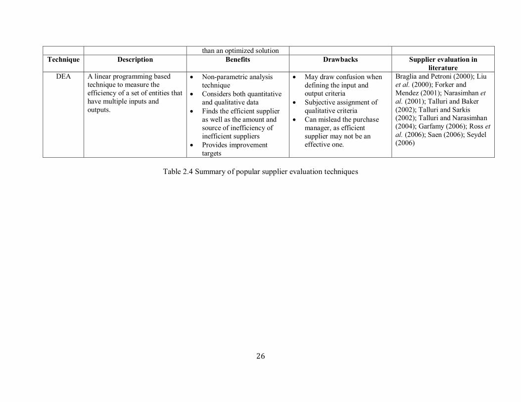
2.3.4 Data Envelopment Analysis (DEA)
2.3.4.1 Basic Model
DEA is a popular technique for supplier evaluation and selection (Braglia and Petroni, 2000; Liu
et al., 2000; Forker and Mendez, 2001; Narasimhan et al., 2001; Talluri and Baker, 2002; Talluri
and Sarkis, 2002; Talluri and Narasimhan, 2004; Garfamy, 2006, Ross et al., 2006; Saen, 2006;
Seydel, 2006).
DEA was originally developed by (Charnes et al., 1978) to evaluate non-profit and public sector
organizations. It was known as the Charnes, Cooper and Rhoades (CCR) model. Since then DEA
has become one of the most effective techniques to measure the performance of organizations
such as business firms, government departments, hospitals etc. It does not require the decision
maker to define weights for each indicator. It simply calculates the weights from the given data.
Moreover, DEA is capable of distinguishing the benchmark entities based on the efficiency score
and finding the amount and source of inefficiency of inefficient entities (Cooper et al., 2007).
The objective of DEA is to find the efficiency score of all units under evaluation. These units are
called decision-making units or (DMUs). DMU is defined as an entity that consumes inputs to
produce outputs and whose performance is to be evaluated (Cooper et al., 2007). DMUs can be
the members of a supply chain, firms or simply departments of a single organization.
The first step in evaluating the performance of a DMU is finding a virtual DMU that will be the
most efficient unit (called efficient frontier). Then DEA compares all DMUs to the efficient
frontier to find their efficiency scores. The efficiency score is defined as weighted sum of outputs

22
divided by weighted sum of inputs. This does not mean we need to assign weights as DEA
calculates weights automatically based on the given inputs and outputs. Cooper et al. (2007) set
the following rules for selecting the inputs and outputs:
All inputs and outputs should have numerical data which is assumed to be equal or greater
than zero.
The selection of inputs, outputs and DMUs should be relevant to the study.
Efficiency scores should reflect the following principles:
i. Smaller input amounts are preferable.
ii. Larger output amounts are preferable.
The measurement units across the different inputs and outputs should not be the same.
Suppose we have 𝑛 different DMUs and each one has 𝑚 input items and 𝑠 output items.
Efficiency =Sum of weighted outputs
Sum of weighted inputs
which can be reformulated per CCR-DEA (Cooper et al., 2007) into the following linear
program:
Min 𝜃𝑝
∑ 𝑥𝑖𝑗𝜆𝑗 ≤ 𝜃𝑝𝑋𝑖𝑝𝑛𝑗 for all 𝑖 = 1, … . , 𝑚
subject to
∑ 𝑦𝑟𝑗𝜆𝑗 ≥ 𝑦𝑟𝑝𝑛𝑗 for all 𝑟 = 1, … . , 𝑠
∑ 𝜆𝑗 = 1𝑛𝑗
where:
𝜃𝑝 is the efficiency score of DMUp ( the DMU under evaluation )
𝑋𝑖𝑝 is the consumed amount of input 𝑖 by DMUp

23
𝑦𝑟𝑝 is the produced amount of output 𝑟 by DMUp
𝜆𝑗 is the computed weights associated with DMUj determining whether it is a benchmark for
DMUp
𝑥𝑖𝑗 is the consumed amount of input 𝑖 by DMUj
𝑦𝑟𝑗 is the produced amount of output 𝑟 by DMUj
The above equations simply mean that the computed virtual DMU should satisfy two conditions:
(i) consume the same or less input amount than DMUp. (ii) Produce the same or more output than
DMUp.
Moreover, we should note the following:
i. DMUp is efficient when 𝜃𝑝 = 1.
ii. DMUp is inefficient when 𝜃𝑝 < 1.
iii. Efficiency cannot be greater than 1.
2.3.4.2 Network DEA
The major drawback of traditional DEA is that it treats DMUs as a “black box” by considering
only the initial inputs and the final outputs and omits the actual activities happening inside (Lewis
and Sexton, 2004; Kao, 2009; Zhu, 2009; Azbari et al., 2014; Yang et al., 2014). For example,
traditional DEA can be used for selecting an efficient supplier among proposed suppliers for a
new product but it cannot be used to evaluate the current upstream suppliers, as it will ignore the
sub-suppliers and current linkages between them. Therefore, network DEA is preferable in these
cases for its advantages over the traditional DEA. Specially, its ability to detect efficiencies
missed by the traditional DEA. Network DEA considers the intermediate linkages as the outputs
of the previous stages and the inputs to the next stage.

24
Many approaches for network DEA have been presented over the years. Aoki et al. (2010)
developed a network DEA model based on the RAM model presented by Cooper et al. (1999) to
optimize the supply chain. Mirhedayatian et al. (2014) proposed a network DEA model to assess
green supply chain management in the existence of dual-role factors, undesirable outputs, and
fuzzy data. Tajbakhsh and Hassini (2014) developed a multi-stage DEA capable of evaluating the
sustainability of the supply chain members. Chen and Yan (2011) created three network DEA
models to evaluate the performance of supply chains under the concept of centralized,
decentralized, and mixed organizational mechanisms.
Despite its many benefits, DEA has some drawbacks. First, the decision-maker may be confused
when defining the input and output criteria. Second drawback comes from the subjective
assignment of qualitative criteria. Finally, DEA finds the efficient supplier who generates more
output while using less input. Therefore, can an efficient supplier be considered an effective one?
(Ho et al., 2010).
This thesis is using the network DEA model presented by Zhu (2009) which embodies the
structure of the supply chain to define and evaluate efficiency of the supply chain and its
individual members. Moreover, the model yields a list of optimal values for all members that
establish an efficient supply chain.
25
Technique Description Benefits Drawbacks Supplier evaluation in
literature
TCO A purchasing tool which is
aimed at understanding the real cost associated with the entire
purchasing cycle
Cost transparency
Improves supplier
evaluation and selection
process
Defines the supplier
performance expectations
Helps prioritising supplier
performance areas
Cost savings opportunities
Better understanding of
supplier performance and cost structure
Can be the basis for supplier
negotiations
Helps building strategic
collaboration efforts.
Complex approach as it may
require methods to
quantifying non-monetary costs
Lack of an accounting and
costing system
Requires culture change
No standard model
Ellram (1993);Degraeve and
Roodhooft (1999);Dogan and Aydin (2011);Bhutta and Huq
(2002)
AHP A mathematical model that allows complex problems to be
represented in a hierarchal form.
Flexibility
Simplicity
Can incorporate quantitative
and qualitative criteria
Very complex pairwise
comparisons in case of many alternatives and
criteria.
Artificial limitation of the 9-
point scale.
Akarte et al. (2001); Muralidharan et al. (2002);
Chan (2003); Liu and Hai
(2005); Hou and Su (2007); Bruno et al. (2012); Deng et al.
(2014)
GP A multi-objective decision making technique that involves
a set of goals that may
contradict with each other.
Helps when we have
multiple goals that are conflicted and not all
achievable.
Allows ranking of goals so
that the lower priority goals are considered only when
higher priority goals are
fully satisfied
Can be used when satisfied
solution is required rather
Can be costly and time
consuming
The generated solution will
be a satisfactory solution
rather than an optimum one
Karpak et al. (2001); Çebi and Bayraktar (2003);Wang et al.
(2004); Perçin (2006); Kull and
Talluri (2008); Mendoza et al. (2008); Osman and Demirli
(2010); Erdem and Gocen
(2012)
26
than an optimized solution
Technique Description Benefits Drawbacks Supplier evaluation in
literature
DEA A linear programming based technique to measure the
efficiency of a set of entities that
have multiple inputs and
outputs.
Non-parametric analysis
technique
Considers both quantitative
and qualitative data
Finds the efficient supplier
as well as the amount and
source of inefficiency of
inefficient suppliers
Provides improvement
targets
May draw confusion when
defining the input and output criteria
Subjective assignment of
qualitative criteria
Can mislead the purchase
manager, as efficient
supplier may not be an effective one.
Braglia and Petroni (2000); Liu et al. (2000); Forker and
Mendez (2001); Narasimhan et
al. (2001); Talluri and Baker
(2002); Talluri and Sarkis (2002); Talluri and Narasimhan
(2004); Garfamy (2006); Ross et
al. (2006); Saen (2006); Seydel (2006)
Table 2.4 Summary of popular supplier evaluation techniques
27
2.4 Supplier Quality Evaluation Framework
de Boer et al. (2001) developed a decision making framework for supplier selection that expands
the purchasing model of Faris et al. (1967) and the model of Kraljic (1983) to include more
situations that are not usually found in literature. They differentiate between three types of
procurement situations: first time buy, modified rebuy, and straight rebuy of routine and strategic
items. Additionally, they propose four phases of the supplier selection process: problem
formulation, formulation of criteria, qualification, and supplier selection. Their framework is
presented in table 2.5.
First time buy situation usually consists of a brand new product or service with unknown
suppliers. In this phase, the level of uncertainty is the highest and no previous historical data
about the suppliers is available. As a result, this is the most complex procurement situation and
group decision-making is required to solve it.
Modified rebuy is related to buying a new product or service from a known supplier or buying a
modified or existing product from a new supplier. The uncertainty level in this case is moderate.
On the other hand, in straight rebuy situation we have enough information about the required
product or service. Furthermore, an agreement already exists with a known supplier and it is just
a matter of placing an order.

28
First Time Buy Modified Rebuy
(Leverage Items)
Straight Rebuy
(Routine Items)
Straight Rebuy
(Strategic Items)
Problem Definition Whether to use a supplier or
not
Either to use more, less or
other suppliers
Do we need to replace the
current supplier?
How to deal with the current
supplier?
Formulation of
Criteria Various importance levels
Unrepeatable decision
No previously defined
criteria or suppliers
historical data available
Moderate to high
importance
Repeatable decision
Previously defined
criteria and suppliers
historical data available
Low to moderate
importance
Repeatable decision
Previously defined
criteria and suppliers
historical data available
High importance
Repeatable evaluation
Previously defined
criteria and suppliers
historical data available
Qualification Various importance levels
Small initial set of
suppliers
Sorting rather than
ranking
No historical data
available
Large number of initial
suppliers
Sorting and ranking
Historical data available
Large number of initial
suppliers
Sorting rather than
ranking
Historical data available
Very small number of
suppliers
Sorting rather than
ranking
Historical data available
Choice Small initial set of
suppliers
Ranking rather than
sorting
Several criteria
A lot of interaction
No historical data
available
Various importance levels
One time used
Small to moderate
number of initial suppliers
Ranking rather than
sorting
How to allocate volume?
Less criteria
Fewer interaction
Historical data available
Model can be used again
Small to moderate
number of initial suppliers
Ranking rather than
sorting
Less criteria
Fewer interaction
Historical data available
Model can be used again
Single sourcing rather
than multiple sourcing
Very small number of
suppliers (usually one)
Historical data available
It is evaluation rather than
selection
Sole sourcing
Table 2.5 de Boer et al. (2001) supplier selection framework

29
It can be noticed from table 2.5, that although de Boer et al. (2001) presented different important
levels for the first buy situations but steps of the supplier selection process are the same
regardless of the importance. In the rebuy situations, selection steps may vary. In the following
paragraphs we will show how de Boer et al. (2001) linked these variations to Kraljic (1983)
model.
Kraljic (1983) classified the purchase items into leverage, strategic, bottleneck, and routine. In
the case of routine item, de Boer et al., (2001) indicated that it is not worthy for an organization
to frequently search for new suppliers that could supply the item because of its low value.
Therefore, similar routine items are usually purchased from one or two suppliers. As per de Boer
et al. (2001) any modification related to the specifications of the purchased items are dealt by the
current supplier. An evaluation of the supplier is carried out periodically and a new supplier is
selected if needed.
Similarly, bottleneck and strategic items have fixed suppliers. The current supplier deals with any
changes to the specifications of these items. The reason behind this is different from that of the
routine items. These items involve high supply risk because of their unique specifications or the
rare material. Therefore, the decision models are only for evaluation and monitoring these
suppliers.
On the other hand, modified rebuy situations are usually related to leverage items. In this case,
there are many suppliers to select from. A frequent selection of suppliers occurs more often
because of high value of these items. An agreed vendor list is the outcome of the first three steps
(Problem definition, formulation of criteria and prequalification) and the final supplier is selected
from this list (de Boer et al., 2001).
30
In the section below, we will list the different methods found in literature for different phases of
supplier selection process.
2.4.1 Problem definition and formulation of criteria
For the problem definition phase, there are not many works on supplier selection. de Boer et al.
(2001) found two methods that can be used for formulation of criteria. The first technique is
called Interpretive Structural Modelling (ISM). The second method is an expert system that
covers different phases in the selection process including the supplier selection criteria. This
system is based on literature review and knowledge of a senior purchasing manager.
2.4.2 Pre-qualification
de Boer et al. (2001) defined pre-qualification as the process of selecting an acceptable set of
suppliers from the whole set. The methods commonly used in this phase are categorical methods,
data envelopment analysis, cluster analysis and case based reasoning systems.
In categorical methods, the supplier is evaluated based on both the buyer’s experience and
historical data. The supplier is evaluated as positive, neutral or negative. The buyer later gives an
overall rating and the suppliers are classified into these three categories.
de Boer et al. (2001) suggested DEA and cluster analysis for categorizing suppliers prior to the
final selection. Case based reasoning can also be used. It is a software system based on artificial
intelligence that aids decision makers with helpful information and experiences from past
decisions.
31
2.4.3 Final choice phase
In this phase, linear weighting, total cost of ownership, mathematical programming, statistical
and artificial intelligence based models are often used for selecting the appropriate suppliers (de
Boer et al., 2001).
In linear weighting models, each criterion is given a weight. Then the weights are multiplied by
the criteria ratings and summed. AHP is an example of this method.
Total cost of ownership is a tool and philosophy to achieve a better understanding of the real cost
of buying a particular good or service from a supplier (Ellram, 1995). Mathematical
programming models aid the decision maker in formulating the purchasing problem into an
objective mathematical formula that should be maximized or minimized by altering the values of
its variables (de Boer et al., 2001).
Statistical models deal with “stochastic uncertainty” related to supplier selection.
Finally, artificial intelligence based models are learning based software systems that can be
consulted for selecting an appropriate supplier.
2.4.4 The Proposed Framework
de Boer et al. (2001) addressed supplier evaluation mainly at one level whereas in this thesis we
propose a framework for multi-tier supplier evaluation. Therefore, we are dealing with a different
problem as shown below:
Problem definition
Evaluate the current n-tier suppliers to study the possibility of collaboration.
Formulation of criteria
The historical data is available as we are evaluating existing suppliers. Both qualitative
and quantitative criteria are used in evaluating the supplier performance.
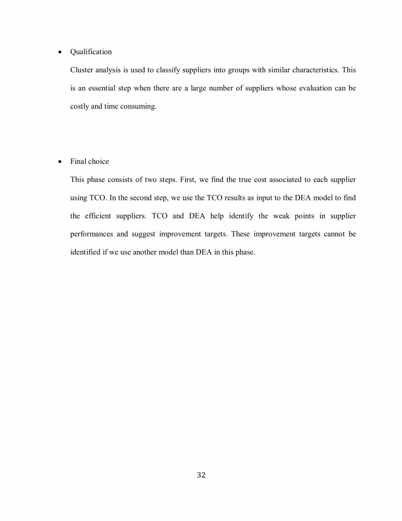
32
Qualification
Cluster analysis is used to classify suppliers into groups with similar characteristics. This
is an essential step when there are a large number of suppliers whose evaluation can be
costly and time consuming.
Final choice
This phase consists of two steps. First, we find the true cost associated to each supplier
using TCO. In the second step, we use the TCO results as input to the DEA model to find
the efficient suppliers. TCO and DEA help identify the weak points in supplier
performances and suggest improvement targets. These improvement targets cannot be
identified if we use another model than DEA in this phase.
33
Chapter 3
Solution Approach
Our solution approach involves three main steps:
1. Grouping of upstream suppliers using hierarchical cluster analysis
2. Multi-tier supplier quality evaluation using TCO and DEA
3. Identifying targets for improving poor quality suppliers performance
3.1 Grouping of upstream suppliers using hierarchical cluster analysis
The first step involves classifying suppliers into groups on the basis of similar characteristics.
This is an essential step when there are a large number of suppliers that make the evaluation
process costly and time consuming. In this step, we will classify only the first-tier suppliers as the
lower-tier suppliers will be grouped automatically based on their first-tier suppliers. We base our
classification on the following criteria. These criteria were identified based on our previous
experience with supply chain projects.
Cost of Quality
It is the cost related with avoiding poor quality or cost that is encountered as a result of poor
quality. It can be categorized into prevention costs, appraisal costs, internal costs, and external
failure costs (Evan and Lindsay, 2005).
Risk
Supply risk is defined as “the probability of an incident associated with inbound supply from
individual supplier failures or the supply market occurring, in which its outcomes result in the

34
inability of the purchasing firm to meet customer demand or cause threats to customer life and
safety” (Zsidisin, 2003).
Location
It is a numerical value to represent the supplier geographical location (country name).
Product type
A numerical value to represent the type of product purchased from the supplier. For instance, raw
material, spare parts, and packaging materials.
Organization profile (size)
It is the number of employees in supplier’s firm.
Cost sustainability
Energy cost, water cost, social policies, fines and penalties.
3.1.1 Hierarchical Cluster Analysis
Hierarchical cluster analysis can be classified into: agglomerative approaches and divisive
approaches. Agglomerative approach is a bottom-up approach where initially each value is a
cluster in its own. Then each pair of clusters is merged together until only one cluster is left. On
the other hand, divisive approach considers the whole dataset as one cluster at the beginning, and
then splits them into further clusters (Al Salem, 2012).
In order to use these approaches, first distance measure needs to be chosen. Al Salem (2012)
listed the following measures to find how two objects are similar or dissimilar:
1. Euclidean distance: It is a popularly used measure. Euclidean distance uses the formula
𝑑𝑖𝑗 = √∑ (𝑥𝑖𝑘 − 𝑥𝑗𝑘)2p
k=1 to compute the distance between two objects 𝑥𝑖𝑘 and 𝑥𝑗𝑘 for
suppliers 𝑖 and 𝑗 under the 𝑘𝑡ℎ variable value of the 𝑝-dimension.

35
2. Manhattan distance: It calculates total absolute distance between two objects under the
𝑘𝑡ℎ variable value of the p-dimension using the formula, 𝑑𝑖𝑗 = ∑ |𝑥𝑖𝑘 − 𝑥𝑗𝑘|pk=1 .
3. Minkowski distance: The previous two measures are a special case of this one.
𝑑𝑖𝑗 = (∑ |𝑥𝑖𝑘 − 𝑥𝑗𝑘|pk=1
𝑟)
1/𝑟 𝑟 ≥ 1
Next step is to link the objects to clusters using one of the below linkage methods as per Al
Salem (2012):
1. Single linkage distance: The linkage is determined based on the minimum distance
between two objects.
2. Complete linkage: The linkage is determined based on the maximum distance between
two objects.
3. Average linkage: The linkage is determined based on the average distance between
elements of one cluster and the other clusters.
The linkage of objects to clusters will construct a tree diagram called dendrogram. A dendrogram
shows how the elements of each cluster are connected and the distance at which clusters are
joined. Figure 3.1 illustrates a sample dendrogram.
36
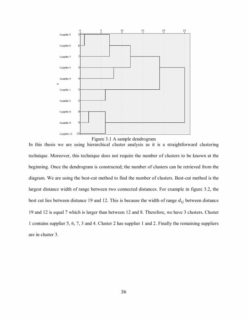
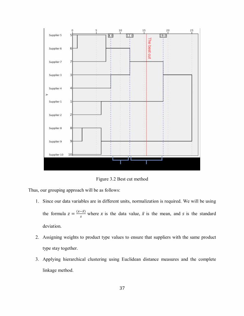
Figure 3.1 A sample dendrogram
In this thesis we are using hierarchical cluster analysis as it is a straightforward clustering
technique. Moreover, this technique does not require the number of clusters to be known at the
beginning. Once the dendrogram is constructed; the number of clusters can be retrieved from the
diagram. We are using the best-cut method to find the number of clusters. Best-cut method is the
largest distance width of range between two connected distances. For example in figure 3.2, the
best cut lies between distance 19 and 12. This is because the width of range 𝑑𝑖𝑗 between distance
19 and 12 is equal 7 which is larger than between 12 and 8. Therefore, we have 3 clusters. Cluster
1 contains supplier 5, 6, 7, 3 and 4. Cluster 2 has supplier 1 and 2. Finally the remaining suppliers
are in cluster 3.
37
Figure 3.2 Best cut method
Thus, our grouping approach will be as follows:
1. Since our data variables are in different units, normalization is required. We will be using
the formula 𝑧 =(𝑥−�̅�)
𝑠 where 𝑥 is the data value, �̅� is the mean, and 𝑠 is the standard
deviation.
2. Assigning weights to product type values to ensure that suppliers with the same product
type stay together.
3. Applying hierarchical clustering using Euclidean distance measures and the complete
linkage method.

38
3.2 Multi-tier supplier quality evaluation using TCO and DEA
Our evaluation framework is based on Total Cost of Ownership (TCO) and Data Envelopment
Analysis (DEA). The first step involves finding the true cost associated to each supplier using
TCO. We will go beyond the quoted price and try to figure out how much it will cost us if we
continue dealing with the current suppliers. Furthermore, we will not just evaluate the first tier
(direct) suppliers but all the n-tier suppliers. This is important if we are aiming towards a
successful collaboration.
We will expand the model presented by Garfamy (2006) to include categories related to global
supply chain collaboration. Our approach evaluates the whole upstream suppliers whereas
Garfamy (2006) approach could be useful to select the best supplier among the suppliers
supplying a given part. Therefore, to evaluate our networked suppliers we will need different
DEA than the one Garfamy (2006) has used. We will use the Network DEA model presented by
Zhu (2009) as stated in the previous chapter.
39
TCO Categories TCO Sub Categories Author Global
Context
Measurement Method Product
Vs.
Service
Input/
Output
Manufacturing
Costs
Raw Material Bhutta and Huq (2002) Yes Quantitative costs P I
Labour Yes Quantitative costs P I
Machine depreciation Yes Quantitative costs P I
Quality Costs Quality Audit Cost Song et al. (2007) Yes Qualitative cost:
Inspection cost and validation cost:
Standard cost per hour x time spent
P,S I
Rework Cost Song et al. (2007) Yes Rework cost per unit x number of unit reworked P I
Quality Confirmation Hurkens et al. (2006) Yes Qualitative cost:
Labor cost of quality confirmation:
No. of assigned people x Labor cost x Percentage of
labor spent on quality confirmation.
Quality confirmation cost per supplier:
No. of checks required to accept a new item x
Labor cost of quality confirmation.
P,S I
Design Costs Technological capability Dogan (2011) Yes Qualitative cost:
He propose an assumption that the design cost will decrease if the supplier is technologically capable,
flexible and financially healthy supplier
P I
Flexibility Yes P I
Financial Factors Yes P I
Logistics Costs Freight Dogan (2011) Yes Quantitative costs P I
Handling and packaging Yes Quantitative costs P I
Tariffs, duties and Import
fees
Yes Quantitative costs P I
Customer Service Yes Quantitative costs P I
Outbound costs Yes Quantitative costs P I
Tariffs warehousing Yes Quantitative costs P I
After sale service Service Cost Bhutta and Huq (2002) Yes Quantitative costs P I
Social /
Environmental
Costs
Energy Cost None Yes Quantitative costs P I
Water Cost None Yes Quantitative costs P I
Social Policies None Yes Inspection Cost:
No. of assigned people x Labor cost x Percentage of
labor spent on inspection.
P,S I
Fines and Penalties None Yes Quantitative cost P I
Price
Price Bhutta and Huq (2002) Yes Quantitative costs P,S I
Table 3.1 TCO costs' Categories

40
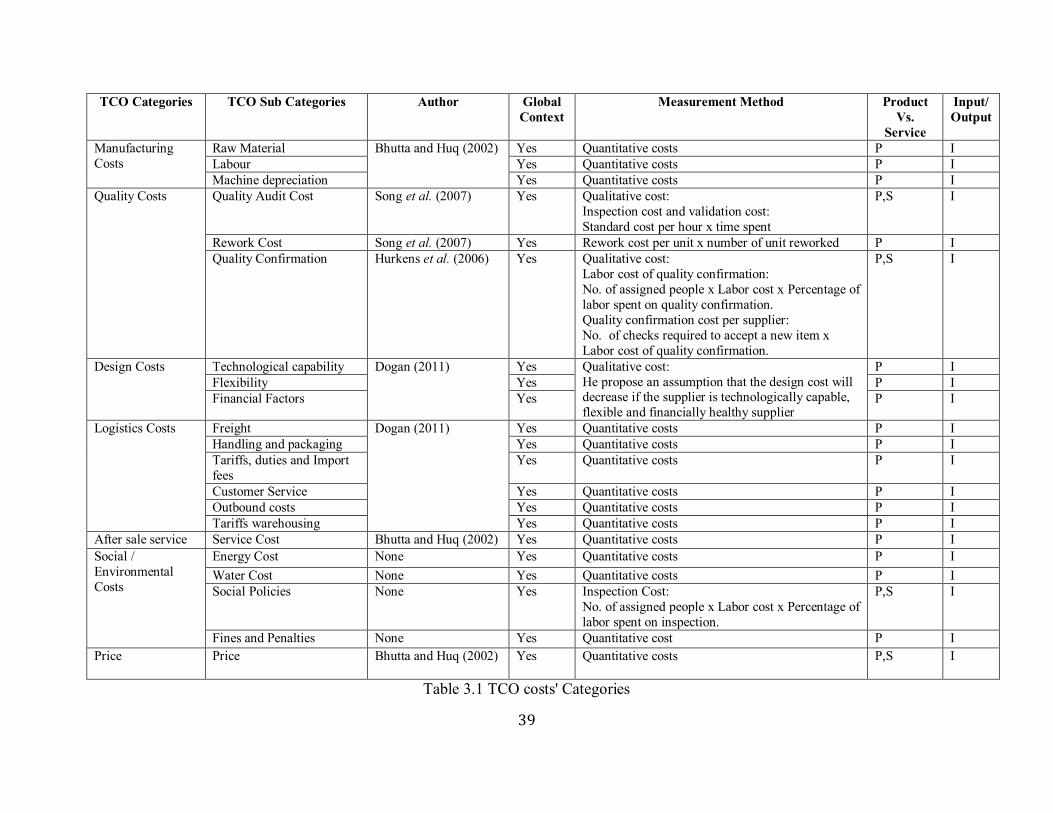
3.2.1 Total Cost of Ownership
Direct and indirect costs are broken down into 6 categories. These TCO costs can be considered
as a guide depending on the industry or service type. Table 3.1 details these cost categories. The
total cost of ownership of each supplier is calculated as the quoted price plus the associated costs.
3.2.2 Network DEA
Suppose we have 𝑛 tier suppliers under evaluation (𝑛 DMUs). For each supplier we have 𝐽
observations and a different set of inputs and outputs. If these inputs and outputs are associated
with a specific member of the supply chain, we call them “direct” inputs and direct outputs (Zhu,
2009). We refer to them as DIΔ and DO Δ , where, DIΔ represents the direct inputs and DO Δ
represents the direct outputs for a supply chain member Δ.
There are also “intermediate” inputs and outputs between two supply chain members, where
usually the outputs from one member become inputs to other member. Calculation of the
intermediate measures should be done through coordination among the members of the supply
chain (Parlar and Weng, 1997;Thomas and Griffin, 1996). For example, one member would like
to maximize the price while the other may prefer to minimize the cost.
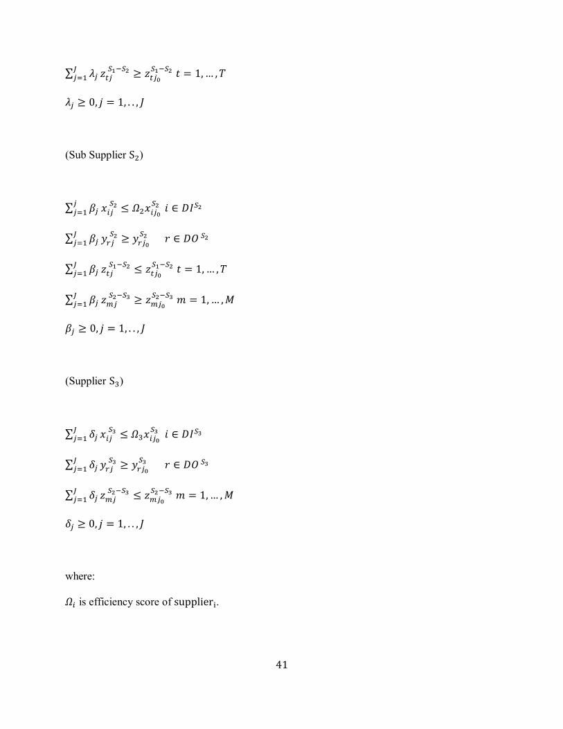
In our module we will use the network DEA formula presented by (Zhu, 2009):
𝛺∗ = min ∑ 𝑤𝑖
𝑛𝑖=1 𝛺𝑖
∑ 𝑤𝑖𝑛𝑖=1
subject to
( 𝑆𝑢𝑏 − 𝑆𝑢𝑏 𝑆𝑢𝑝𝑝𝑙𝑖𝑒𝑟 𝑆1)
∑ 𝜆𝑗𝐽𝑗=1 𝑥𝑖𝑗
𝑆1 ≤ 𝛺1𝑥𝑖𝑗0
𝑆1 𝑖 ∈ 𝐷𝐼𝑆1
∑ 𝜆𝑗𝐽𝑗=1 𝑦𝑟𝑗
𝑆1 ≥ 𝑦𝑟𝑗0
𝑆1 𝑟 ∈ 𝐷𝑂 𝑆1
41
∑ 𝜆𝑗𝐽𝑗=1 𝑧𝑡𝑗
𝑆1−𝑆2 ≥ 𝑧𝑡𝑗0
𝑆1−𝑆2 𝑡 = 1, … , 𝑇
𝜆𝑗 ≥ 0, 𝑗 = 1, . . , 𝐽
(Sub Supplier S2)
∑ 𝛽𝑗𝑗𝑗=1 𝑥𝑖𝑗
𝑆2 ≤ 𝛺2𝑥𝑖𝑗0
𝑆2 𝑖 ∈ 𝐷𝐼𝑆2
∑ 𝛽𝑗𝐽𝑗=1 𝑦𝑟𝑗
𝑆2 ≥ 𝑦𝑟𝑗0
𝑆2 𝑟 ∈ 𝐷𝑂 𝑆2
∑ 𝛽𝑗𝐽𝑗=1 𝑧𝑡𝑗
𝑆1−𝑆2 ≤ 𝑧𝑡𝑗0
𝑆1−𝑆2 𝑡 = 1, … , 𝑇
∑ 𝛽𝑗𝐽𝑗=1 𝑧𝑚𝑗
𝑆2−𝑆3 ≥ 𝑧𝑚𝑗0
𝑆2−𝑆3 𝑚 = 1, … , 𝑀
𝛽𝑗 ≥ 0, 𝑗 = 1, . . , 𝐽
(Supplier S3)
∑ 𝛿𝑗𝐽𝑗=1 𝑥𝑖𝑗
𝑆3 ≤ 𝛺3𝑥𝑖𝑗0
𝑆3 𝑖 ∈ 𝐷𝐼𝑆3
∑ 𝛿𝑗𝐽𝑗=1 𝑦𝑟𝑗
𝑆3 ≥ 𝑦𝑟𝑗0
𝑆3 𝑟 ∈ 𝐷𝑂 𝑆3
∑ 𝛿𝑗𝐽𝑗=1 𝑧𝑚𝑗
𝑆2−𝑆3 ≤ 𝑧𝑚𝑗0
𝑆2−𝑆3 𝑚 = 1, … , 𝑀
𝛿𝑗 ≥ 0, 𝑗 = 1, . . , 𝐽
where:
𝛺𝑖 is efficiency score of supplieri.

42
𝛺∗ is the optimum efficiency of the supply chain, can be viewed as the supply chain best practice
when it’s equal to 1
𝑤𝑖 is a user specific weight preference assigned to reflect the preference over each supplier.
𝜆𝑗 is the 𝑗𝑡ℎ observation computed weights of the sub-sub-supplier.
𝛽𝑗 is the 𝑗𝑡ℎ observation computed weights of the sub-supplier.
𝛿𝑗 is the 𝑗𝑡ℎ observation computed weights of the supplier.
𝑥𝑖𝑗 𝛥 is the consumed amount of input i by supplier Δ in the 𝑗𝑡ℎ observation.
𝑦𝑟𝑗 𝛥 is the produced amount of output r by supplier Δ in the 𝑗𝑡ℎ observation.
𝑧𝑡𝑗 𝑆1−𝑆2 is the 𝑡𝑡ℎ intermediate output from sub-sub-supplier S1 to sub-supplier S2 in the 𝑗𝑡ℎ
observation.
𝑧𝑚𝑗 𝑆2−𝑆3 is the 𝑚𝑡ℎ intermediate output from sub-supplier S2 to supplier S3 in the 𝑗𝑡ℎ observation.
Additional constraints can be added. For example, if we have intermediate outputs that go from
supplier S3 to sub-supplier S2, then we have ∑ 𝛿𝑗𝐽𝑗=1 𝑧𝑔𝑗
𝑆3−𝑆2 ≥ 𝑧𝑔𝑗0
𝑆3−𝑆2 𝑔 = 1, … , 𝐺.
Basically the module will try to find the efficiency of each supplier by comparing each input or
output with different observations of that input or output. Supply chain efficiency 𝛺∗ is equal to 1
(best practice values of inputs and outputs) when the efficiencies of all suppliers equal 1.
3.3 Recommendations for improving supplier quality
The third and final goal of this thesis is to find recommendations to improve the quality of
suppliers. We will base our recommendations on the results of cluster analysis as well as TCO
and DEA. We will analyze the results of cluster analysis using descriptive statistics. This will
43
give us a better overview of the results. TCO and DEA results will help identify weak points in
the supplier performance and suggest improvement targets.

44
Chapter 4
Numerical Application
In this chapter we present two examples to demonstrate the capabilities of our framework. The
first example illustrates the hierarchical cluster technique using the criteria presented previously,
and the next example shows the application of TCO and DEA approach.
4.1 Hierarchical cluster analysis
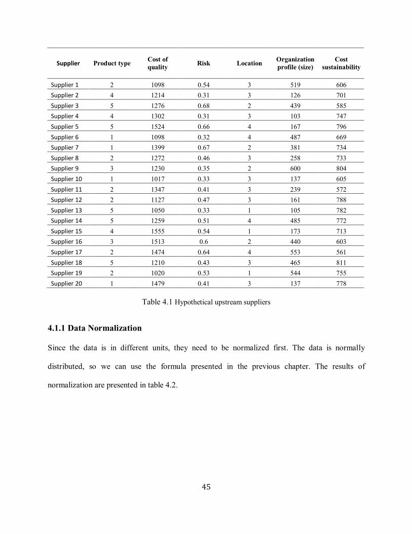
In a global supply chain, let’s assume that we have 20 upstream suppliers. The clustering is done
using the following criteria:
Product type
Cost of Quality
Risk
Location
Organization profile (size)
Cost sustainability
The numerical values of these criteria were generated using Excel random number generator
routine (see table 4.1). Following steps are used in our clustering technique:
1. Data normalization
2. Assigning weights to product types
3. Applying hierarchical clustering
45
Supplier Product type Cost of
quality Risk Location
Organization
profile (size)
Cost
sustainability
Supplier 1 2 1098 0.54 3 519 606
Supplier 2 4 1214 0.31 3 126 701
Supplier 3 5 1276 0.68 2 439 585
Supplier 4 4 1302 0.31 3 103 747
Supplier 5 5 1524 0.66 4 167 796
Supplier 6 1 1098 0.32 4 487 669
Supplier 7 1 1399 0.67 2 381 734
Supplier 8 2 1272 0.46 3 258 733
Supplier 9 3 1230 0.35 2 600 804
Supplier 10 1 1017 0.33 3 137 605
Supplier 11 2 1347 0.41 3 239 572
Supplier 12 2 1127 0.47 3 161 788
Supplier 13 5 1050 0.33 1 105 782
Supplier 14 5 1259 0.51 4 485 772
Supplier 15 4 1555 0.54 1 173 713
Supplier 16 3 1513 0.6 2 440 603
Supplier 17 2 1474 0.64 4 553 561
Supplier 18 5 1210 0.43 3 465 811
Supplier 19 2 1020 0.53 1 544 755
Supplier 20 1 1479 0.41 3 137 778
Table 4.1 Hypothetical upstream suppliers
4.1.1 Data Normalization
Since the data is in different units, they need to be normalized first. The data is normally
distributed, so we can use the formula presented in the previous chapter. The results of
normalization are presented in table 4.2.

46
Supplier Product type Cost of
quality Risk Location
Organization
profile (size)
Cost
sustainability
Supplier 1 -0.6176 -1.0058 0.5035 0.3065 1.0785 -1.1529
Supplier 2 0.6827 -0.3399 -1.2780 0.3065 -1.1170 -0.0549
Supplier 3 1.3328 0.0161 1.5878 -0.7152 0.6315 -1.3956
Supplier 4 0.6827 0.1653 -1.2780 0.3065 -1.2455 0.4768
Supplier 5 1.3328 1.4398 1.4329 1.3283 -0.8880 1.0431
Supplier 6 -1.2678 -1.0058 -1.2006 1.3283 0.8997 -0.4247
Supplier 7 -1.2678 0.7222 1.5104 -0.7152 0.3075 0.3265
Supplier 8 -0.6176 -0.0069 -0.1162 0.3065 -0.3796 0.3149
Supplier 9 0.0325 -0.2480 -0.9682 -0.7152 1.5310 1.1355
Supplier 10 -1.2678 -1.4708 -1.1231 0.3065 -1.0556 -1.1644
Supplier 11 -0.6176 0.4237 -0.5035 0.3065 -0.4857 -1.5458
Supplier 12 -0.6176 -0.8393 -0.0387 0.3065 -0.9215 0.9506
Supplier 13 1.3328 -1.2814 -1.1231 -1.7370 -1.2343 0.8813
Supplier 14 1.3328 -0.0815 0.2711 1.3283 0.8885 0.7657
Supplier 15 0.6827 1.6178 0.5035 -1.7370 -0.8544 0.0838
Supplier 16 0.0325 1.3767 0.9682 -0.7152 0.6371 -1.1875
Supplier 17 -0.6176 1.1528 1.2780 1.3283 1.2684 -1.6730
Supplier 18 1.3328 -0.3628 -0.3486 0.3065 0.7768 1.2164
Supplier 19 -0.6176 -1.4536 0.4260 -1.7370 1.2181 0.5692
Supplier 20 -1.2678 1.1815 -0.5035 0.3065 -1.0556 0.8350
Table 4.2 Normalized Data
4.1.2 Assigning weights to product types
There are 5 different product types in our example, so we need to assign weights to each product
type to ensure that all suppliers of the same product type are grouped together and not divided in
different clusters. Therefore, the product types will be multiplied by their corresponding weights.
As a result, the clustering technique will group suppliers first based on the product type and then
on the remaining criteria. Table 4.3 reports the data after assigning weights.
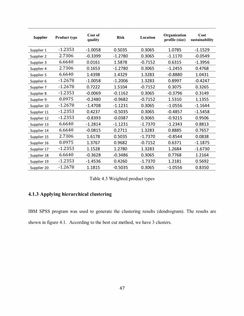
47
Supplier Product type Cost of
quality Risk Location
Organization
profile (size)
Cost
sustainability
Supplier 1 -1.2353 -1.0058 0.5035 0.3065 1.0785 -1.1529
Supplier 2 2.7306 -0.3399 -1.2780 0.3065 -1.1170 -0.0549
Supplier 3 6.6640 0.0161 1.5878 -0.7152 0.6315 -1.3956
Supplier 4 2.7306 0.1653 -1.2780 0.3065 -1.2455 0.4768
Supplier 5 6.6640 1.4398 1.4329 1.3283 -0.8880 1.0431
Supplier 6 -1.2678 -1.0058 -1.2006 1.3283 0.8997 -0.4247
Supplier 7 -1.2678 0.7222 1.5104 -0.7152 0.3075 0.3265
Supplier 8 -1.2353 -0.0069 -0.1162 0.3065 -0.3796 0.3149
Supplier 9 0.0975 -0.2480 -0.9682 -0.7152 1.5310 1.1355
Supplier 10 -1.2678 -1.4708 -1.1231 0.3065 -1.0556 -1.1644
Supplier 11 -1.2353 0.4237 -0.5035 0.3065 -0.4857 -1.5458
Supplier 12 -1.2353 -0.8393 -0.0387 0.3065 -0.9215 0.9506
Supplier 13 6.6640 -1.2814 -1.1231 -1.7370 -1.2343 0.8813
Supplier 14 6.6640 -0.0815 0.2711 1.3283 0.8885 0.7657
Supplier 15 2.7306 1.6178 0.5035 -1.7370 -0.8544 0.0838
Supplier 16 0.0975 1.3767 0.9682 -0.7152 0.6371 -1.1875
Supplier 17 -1.2353 1.1528 1.2780 1.3283 1.2684 -1.6730
Supplier 18 6.6640 -0.3628 -0.3486 0.3065 0.7768 1.2164
Supplier 19 -1.2353 -1.4536 0.4260 -1.7370 1.2181 0.5692
Supplier 20 -1.2678 1.1815 -0.5035 0.3065 -1.0556 0.8350
Table 4.3 Weighted product types
4.1.3 Applying hierarchical clustering
IBM SPSS program was used to generate the clustering results (dendrogram). The results are
shown in figure 4.1. According to the best cut method, we have 3 clusters.
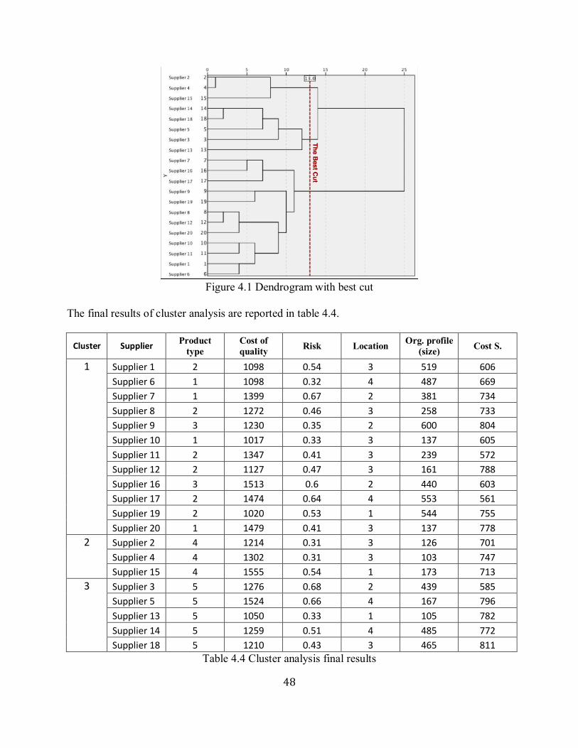
48
Figure 4.1 Dendrogram with best cut
The final results of cluster analysis are reported in table 4.4.
Cluster Supplier Product
type
Cost of
quality Risk Location
Org. profile
(size) Cost S.
1 Supplier 1 2 1098 0.54 3 519 606
Supplier 6 1 1098 0.32 4 487 669
Supplier 7 1 1399 0.67 2 381 734
Supplier 8 2 1272 0.46 3 258 733
Supplier 9 3 1230 0.35 2 600 804
Supplier 10 1 1017 0.33 3 137 605
Supplier 11 2 1347 0.41 3 239 572
Supplier 12 2 1127 0.47 3 161 788
Supplier 16 3 1513 0.6 2 440 603
Supplier 17 2 1474 0.64 4 553 561
Supplier 19 2 1020 0.53 1 544 755
Supplier 20 1 1479 0.41 3 137 778
2 Supplier 2 4 1214 0.31 3 126 701
Supplier 4 4 1302 0.31 3 103 747
Supplier 15 4 1555 0.54 1 173 713
3 Supplier 3 5 1276 0.68 2 439 585
Supplier 5 5 1524 0.66 4 167 796
Supplier 13 5 1050 0.33 1 105 782
Supplier 14 5 1259 0.51 4 485 772
Supplier 18 5 1210 0.43 3 465 811
Table 4.4 Cluster analysis final results

49
4.1.4 Recommendations
After examining table 4.5, it looks like product number 4 is purchased from 3 small organizations
with a high cost of quality and a relatively high cost sustainability. As a result, the supply chain
may become more vulnerable with regards to this product. We recommend either engaging these
suppliers in a supplier development program or try to deal with new suppliers.
Complete Linkage Minimum Maximum Mean Std.
Deviation
1 Product type 1.00 3.00 - -
Cost of quality 1017.00 1513.00 1256.1667 183.98361
Risk .32 .67 .4775 .11963
Organization profile (size) 137.00 600.00 371.3333 175.68532
Cost sustainability 561.00 804.00 684.0000 90.84352
Number of Suppliers 12
2 Product type 4.00 4.00 - -
Cost of quality 1214.00 1555.00 1357.0000 177.02825
Risk .31 .54 .3867 .13279
Organization profile (size) 103.00 173.00 134.0000 35.67913
Cost sustainability 701.00 747.00 720.3333 23.86071
Number of Suppliers 3
3 Product type 5.00 5.00 - -
Cost of quality 1050.00 1524.00 1263.8000 170.64642
Risk .33 .68 .5220 .14957
Organization profile (size) 105.00 485.00 332.2000 181.17726
Cost sustainability 585.00 811.00 749.2000 92.96074
Number of Suppliers 5
Table 4.5 Descriptive statistics
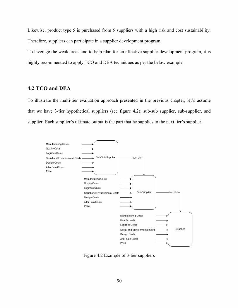
50
Likewise, product type 5 is purchased from 5 suppliers with a high risk and cost sustainability.
Therefore, suppliers can participate in a supplier development program.
To leverage the weak areas and to help plan for an effective supplier development program, it is
highly recommended to apply TCO and DEA techniques as per the below example.
4.2 TCO and DEA
To illustrate the multi-tier evaluation approach presented in the previous chapter, let’s assume
that we have 3-tier hypothetical suppliers (see figure 4.2): sub-sub supplier, sub-supplier, and
supplier. Each supplier’s ultimate output is the part that he supplies to the next tier’s supplier.
Figure 4.2 Example of 3-tier suppliers

51
The inputs and outputs of each supplier are based on the following TCO cost categories which
were presented in table 3.1:
Inputs:
Manufacturing Costs, cost amount was generated randomly between these ranges:
o Sub-sub supplier values ranged between 50 and 130
o Sub supplier values ranged between 70 and 200
o Supplier values ranged between 200 and 370
Quality Costs, cost amount was generated randomly between these ranges:
o Sub-sub supplier and sub supplier values ranged between 20 and 40
o Supplier values ranged between 30 and 65
Logistics Costs, cost amount was generated randomly between these ranges:
o Sub-sub supplier values ranged between 70 and 170
o Sub supplier values ranged between 90 and 180
o Supplier values ranged between 200 and 340
Social and Environmental, cost amount was generated randomly between these ranges:
o Sub-sub supplier values ranged between 30 and 80
o Sub supplier values ranged between 50 and 120
o Supplier values ranged between 100 and 160
Design Costs, cost amount was generated randomly between these ranges:
o Sub-sub supplier values ranged between 50 and 70
o Sub supplier values ranged between 60 and 99
o Supplier values ranged between 100 and 160
52
After Sale Costs, cost amount was generated randomly between these ranges:
o Sub-sub supplier and sub supplier values ranged between 20 and 50
o Supplier values ranged between 30 and 60
Price, cost amount was generated randomly between these ranges:
o Sub-sub supplier values ranged between 100 and 220
o Sub supplier values ranged between 300 and 400
o Supplier values ranged between 600 and 780
Output:
Item Unit
The data is presented in table 4.6. Our goal is to evaluate the suppliers and the whole upstream
supply chain. For this, we will apply the network DEA presented in the previous chapter to find
the efficiency of each supplier starting from observation 1 until 10. The complete linear
programming for this example is listed in appendix A. Table 4.7 and figure 4.3 report the
obtained efficiency scores of our linear programming.
Please note the following:
𝛺∗ is efficiency score of the supply chain
Ω1 is efficiency score of the sub-sub supplier.
Ω2 is efficiency score of the sub-supplier.
Ω3 is efficiency score of the supplier.
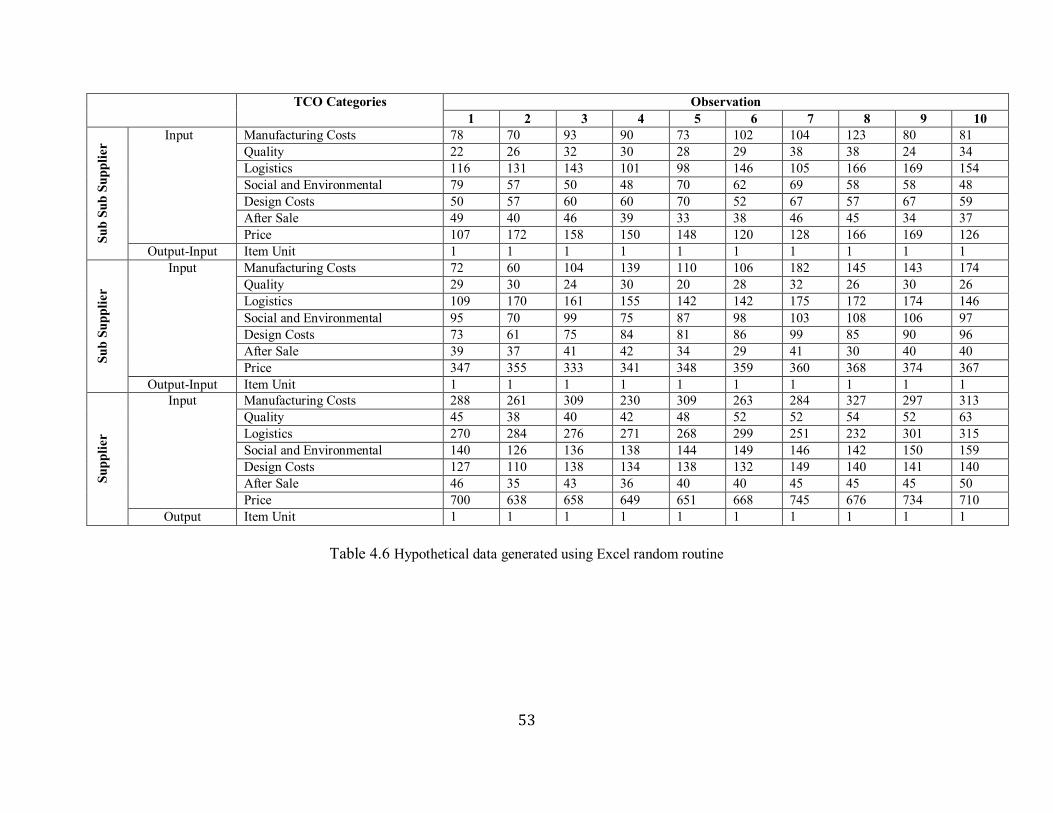
53
TCO Categories Observation
1 2 3 4 5 6 7 8 9 10
Su
b S
ub
Su
pp
lier
Input Manufacturing Costs 78 70 93 90 73 102 104 123 80 81
Quality 22 26 32 30 28 29 38 38 24 34
Logistics 116 131 143 101 98 146 105 166 169 154
Social and Environmental 79 57 50 48 70 62 69 58 58 48
Design Costs 50 57 60 60 70 52 67 57 67 59
After Sale 49 40 46 39 33 38 46 45 34 37
Price 107 172 158 150 148 120 128 166 169 126
Output-Input Item Unit 1 1 1 1 1 1 1 1 1 1
Su
b S
up
pli
er
Input Manufacturing Costs 72 60 104 139 110 106 182 145 143 174
Quality 29 30 24 30 20 28 32 26 30 26
Logistics 109 170 161 155 142 142 175 172 174 146
Social and Environmental 95 70 99 75 87 98 103 108 106 97
Design Costs 73 61 75 84 81 86 99 85 90 96
After Sale 39 37 41 42 34 29 41 30 40 40
Price 347 355 333 341 348 359 360 368 374 367
Output-Input Item Unit 1 1 1 1 1 1 1 1 1 1
Su
pp
lier
Input Manufacturing Costs 288 261 309 230 309 263 284 327 297 313
Quality 45 38 40 42 48 52 52 54 52 63
Logistics 270 284 276 271 268 299 251 232 301 315
Social and Environmental 140 126 136 138 144 149 146 142 150 159
Design Costs 127 110 138 134 138 132 149 140 141 140
After Sale 46 35 43 36 40 40 45 45 45 50
Price 700 638 658 649 651 668 745 676 734 710
Output Item Unit 1 1 1 1 1 1 1 1 1 1
Table 4.6 Hypothetical data generated using Excel random routine
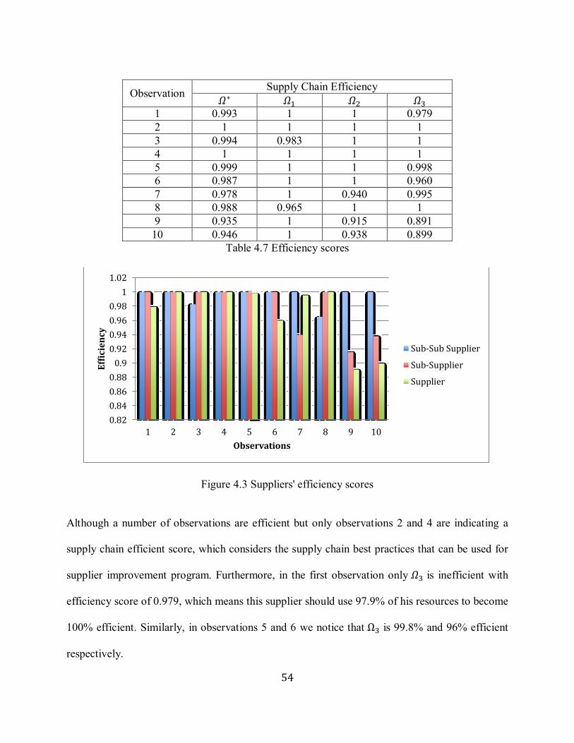
54
Observation Supply Chain Efficiency
𝛺∗ 𝛺1 𝛺2 𝛺3
1 0.993 1 1 0.979
2 1 1 1 1
3 0.994 0.983 1 1
4 1 1 1 1
5 0.999 1 1 0.998
6 0.987 1 1 0.960
7 0.978 1 0.940 0.995
8 0.988 0.965 1 1
9 0.935 1 0.915 0.891
10 0.946 1 0.938 0.899
Table 4.7 Efficiency scores
Figure 4.3 Suppliers' efficiency scores
Although a number of observations are efficient but only observations 2 and 4 are indicating a
supply chain efficient score, which considers the supply chain best practices that can be used for
supplier improvement program. Furthermore, in the first observation only 𝛺3 is inefficient with
efficiency score of 0.979, which means this supplier should use 97.9% of his resources to become
100% efficient. Similarly, in observations 5 and 6 we notice that Ω3 is 99.8% and 96% efficient
respectively.
0.82
0.84
0.86
0.88
0.9
0.92
0.94
0.96
0.98
1
1.02
1 2 3 4 5 6 7 8 9 10
Eff
icie
ncy
Observations
Sub-Sub Supplier
Sub-Supplier
Supplier
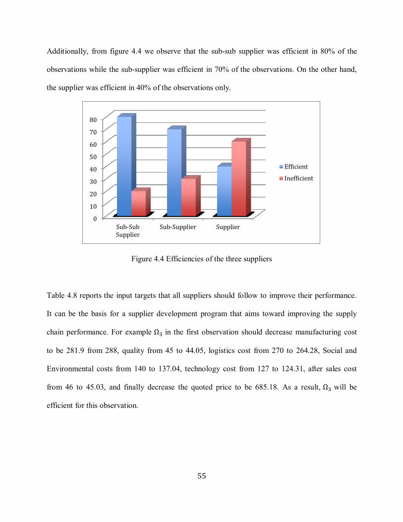
55
Additionally, from figure 4.4 we observe that the sub-sub supplier was efficient in 80% of the
observations while the sub-supplier was efficient in 70% of the observations. On the other hand,
the supplier was efficient in 40% of the observations only.
Figure 4.4 Efficiencies of the three suppliers
Table 4.8 reports the input targets that all suppliers should follow to improve their performance.
It can be the basis for a supplier development program that aims toward improving the supply
chain performance. For example Ω3 in the first observation should decrease manufacturing cost
to be 281.9 from 288, quality from 45 to 44.05, logistics cost from 270 to 264.28, Social and
Environmental costs from 140 to 137.04, technology cost from 127 to 124.31, after sales cost
from 46 to 45.03, and finally decrease the quoted price to be 685.18. As a result, Ω3 will be
efficient for this observation.
0
10
20
30
40
50
60
70
80
Sub-SubSupplier
Sub-Supplier Supplier
Efficient
Inefficient
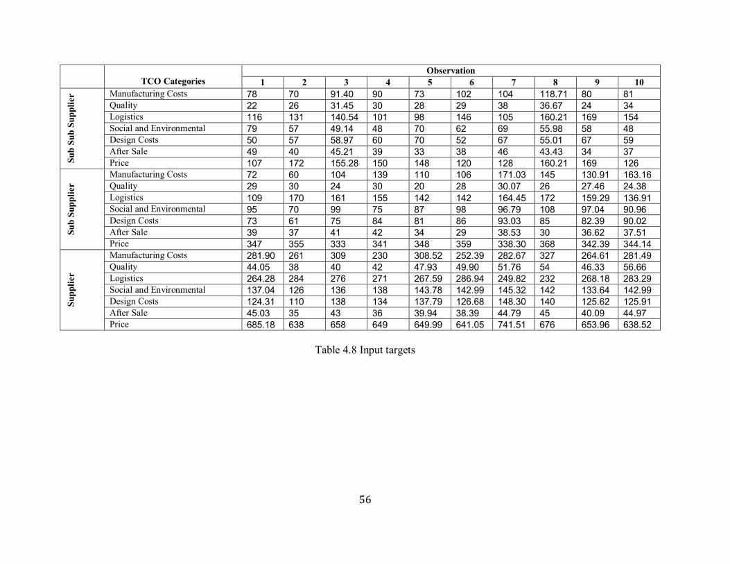
56
TCO Categories
Observation
1 2 3 4 5 6 7 8 9 10
Su
b S
ub
Su
pp
lier Manufacturing Costs 78 70 91.40 90 73 102 104 118.71 80 81
Quality 22 26 31.45 30 28 29 38 36.67 24 34
Logistics 116 131 140.54 101 98 146 105 160.21 169 154
Social and Environmental 79 57 49.14 48 70 62 69 55.98 58 48
Design Costs 50 57 58.97 60 70 52 67 55.01 67 59
After Sale 49 40 45.21 39 33 38 46 43.43 34 37
Price 107 172 155.28 150 148 120 128 160.21 169 126
Su
b S
up
pli
er
Manufacturing Costs 72 60 104 139 110 106 171.03 145 130.91 163.16
Quality 29 30 24 30 20 28 30.07 26 27.46 24.38
Logistics 109 170 161 155 142 142 164.45 172 159.29 136.91
Social and Environmental 95 70 99 75 87 98 96.79 108 97.04 90.96
Design Costs 73 61 75 84 81 86 93.03 85 82.39 90.02
After Sale 39 37 41 42 34 29 38.53 30 36.62 37.51
Price 347 355 333 341 348 359 338.30 368 342.39 344.14
Su
pp
lier
Manufacturing Costs 281.90 261 309 230 308.52 252.39 282.67 327 264.61 281.49
Quality 44.05 38 40 42 47.93 49.90 51.76 54 46.33 56.66
Logistics 264.28 284 276 271 267.59 286.94 249.82 232 268.18 283.29
Social and Environmental 137.04 126 136 138 143.78 142.99 145.32 142 133.64 142.99
Design Costs 124.31 110 138 134 137.79 126.68 148.30 140 125.62 125.91
After Sale 45.03 35 43 36 39.94 38.39 44.79 45 40.09 44.97
Price 685.18 638 658 649 649.99 641.05 741.51 676 653.96 638.52
Table 4.8 Input targets
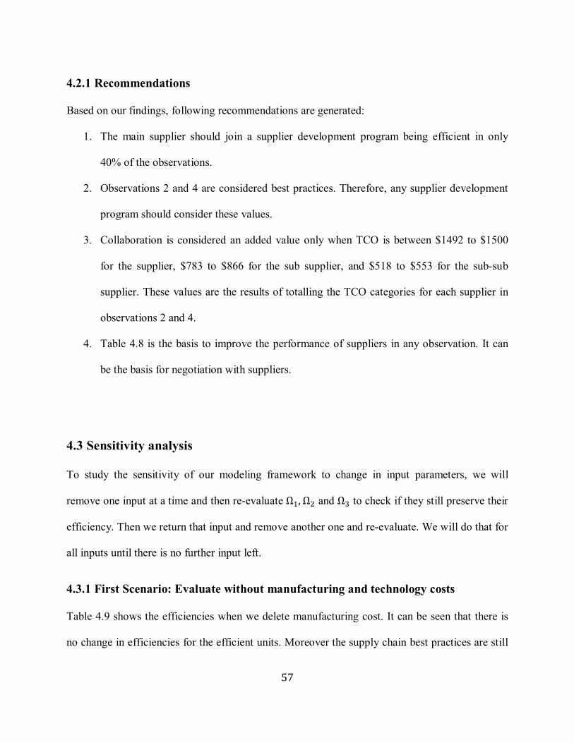
57
4.2.1 Recommendations
Based on our findings, following recommendations are generated:
1. The main supplier should join a supplier development program being efficient in only
40% of the observations.
2. Observations 2 and 4 are considered best practices. Therefore, any supplier development
program should consider these values.
3. Collaboration is considered an added value only when TCO is between $1492 to $1500
for the supplier, $783 to $866 for the sub supplier, and $518 to $553 for the sub-sub
supplier. These values are the results of totalling the TCO categories for each supplier in
observations 2 and 4.
4. Table 4.8 is the basis to improve the performance of suppliers in any observation. It can
be the basis for negotiation with suppliers.
4.3 Sensitivity analysis
To study the sensitivity of our modeling framework to change in input parameters, we will
remove one input at a time and then re-evaluate Ω1, Ω2 and Ω3 to check if they still preserve their
efficiency. Then we return that input and remove another one and re-evaluate. We will do that for
all inputs until there is no further input left.
4.3.1 First Scenario: Evaluate without manufacturing and technology costs
Table 4.9 shows the efficiencies when we delete manufacturing cost. It can be seen that there is
no change in efficiencies for the efficient units. Moreover the supply chain best practices are still
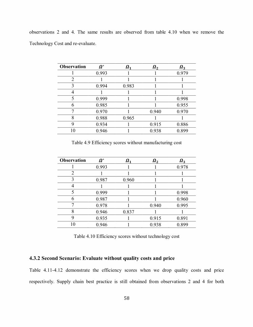
58
observations 2 and 4. The same results are observed from table 4.10 when we remove the
Technology Cost and re-evaluate.
Observation 𝜴∗ 𝜴𝟏 𝜴𝟐 𝜴𝟑
1 0.993 1 1 0.979
2 1 1 1 1
3 0.994 0.983 1 1
4 1 1 1 1
5 0.999 1 1 0.998
6 0.985 1 1 0.955
7 0.970 1 0.940 0.970
8 0.988 0.965 1 1
9 0.934 1 0.915 0.886
10 0.946 1 0.938 0.899
Table 4.9 Efficiency scores without manufacturing cost
Observation 𝜴∗ 𝜴𝟏 𝜴𝟐 𝜴𝟑
1 0.993 1 1 0.978
2 1 1 1 1
3 0.987 0.960 1 1
4 1 1 1 1
5 0.999 1 1 0.998
6 0.987 1 1 0.960
7 0.978 1 0.940 0.995
8 0.946 0.837 1 1
9 0.935 1 0.915 0.891
10 0.946 1 0.938 0.899
Table 4.10 Efficiency scores without technology cost
4.3.2 Second Scenario: Evaluate without quality costs and price
Table 4.11-4.12 demonstrate the efficiency scores when we drop quality costs and price
respectively. Supply chain best practice is still obtained from observations 2 and 4 for both

59
inputs. However, Ω2 becomes inefficient in observation 8 when we remove quality cost.
Likewise, Ω1becomes inefficient in observation 7.
Observation 𝜴∗ 𝜴𝟏 𝜴𝟐 𝜴𝟑
1 0.992 1 1 0.976
2 1 1 1 1
3 0.988 0.979 1 0.984
4 1 1 1 1
5 0.999 1 1 0.998
6 0.987 1 1 0.960
7 0.978 1 0.940 0.995
8 0.984 0.965 0.988 1
9 0.935 1 0.915 0.891
10 0.946 1 0.938 0.899
Table 4.11 Efficiency scores without quality cost
Observation 𝜴∗ 𝜴𝟏 𝜴𝟐 𝜴𝟑
1 0.993 1 1 0.979
2 1 1 1 1
3 0.989 0.983 0.984 1
4 1 1 1 1
5 0.990 1 1 0.969
6 0.977 1 1 0.930
7 0.926 0.951 0.831 0.995
8 0.988 0.965 1 1
9 0.913 1 0.847 0.891
10 0.924 1 0.911 0.860
Table 4.12 Efficiency scores without price
4.3.3 Third Scenario: Evaluate without logistics and after sale costs
On the other hand, when we calculate efficiency scores without logistics cost we observe that Ω1
and Ω3 lose their efficient scores in observations 7 and 8 respectively as seen in table 4.13.
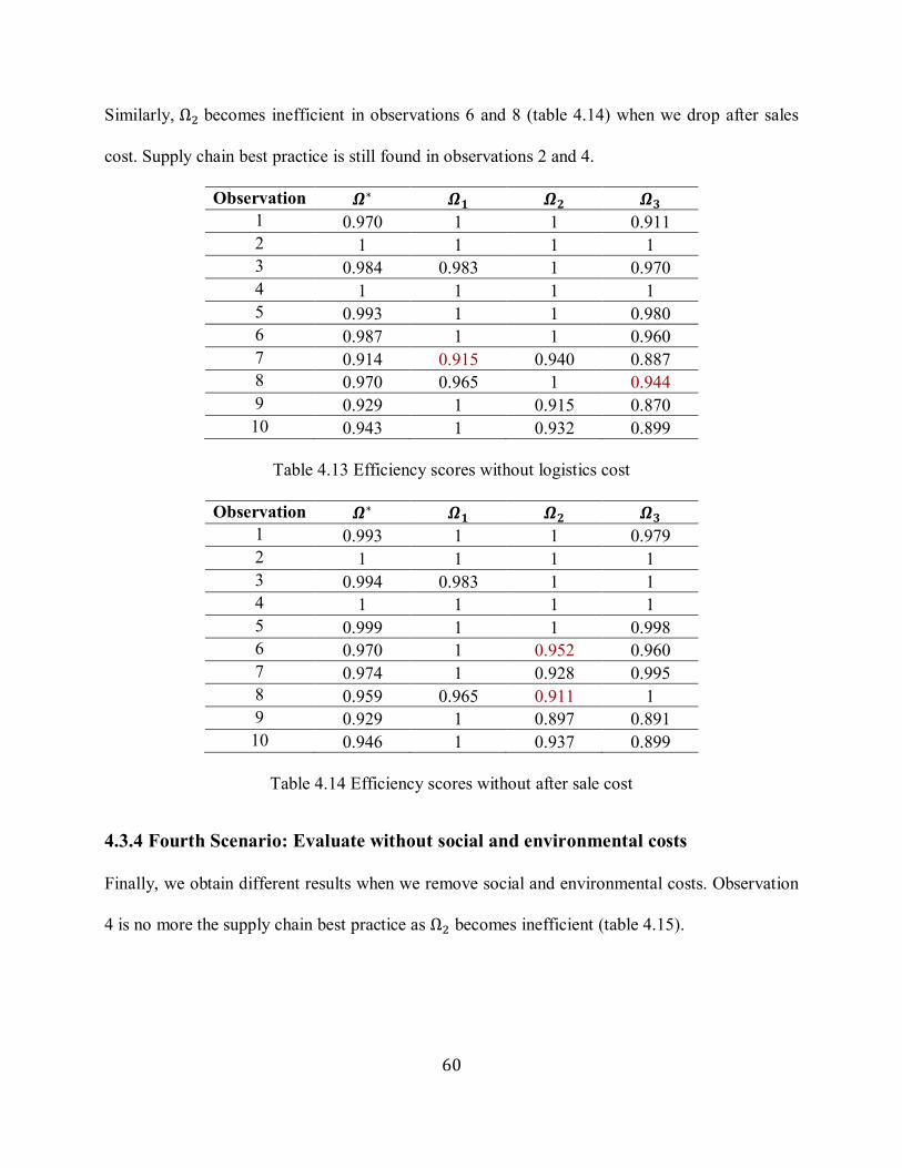
60
Similarly, Ω2 becomes inefficient in observations 6 and 8 (table 4.14) when we drop after sales
cost. Supply chain best practice is still found in observations 2 and 4.
Observation 𝜴∗ 𝜴𝟏 𝜴𝟐 𝜴𝟑
1 0.970 1 1 0.911
2 1 1 1 1
3 0.984 0.983 1 0.970
4 1 1 1 1
5 0.993 1 1 0.980
6 0.987 1 1 0.960
7 0.914 0.915 0.940 0.887
8 0.970 0.965 1 0.944
9 0.929 1 0.915 0.870
10 0.943 1 0.932 0.899
Table 4.13 Efficiency scores without logistics cost
Observation 𝜴∗ 𝜴𝟏 𝜴𝟐 𝜴𝟑
1 0.993 1 1 0.979
2 1 1 1 1
3 0.994 0.983 1 1
4 1 1 1 1
5 0.999 1 1 0.998
6 0.970 1 0.952 0.960
7 0.974 1 0.928 0.995
8 0.959 0.965 0.911 1
9 0.929 1 0.897 0.891
10 0.946 1 0.937 0.899
Table 4.14 Efficiency scores without after sale cost
4.3.4 Fourth Scenario: Evaluate without social and environmental costs
Finally, we obtain different results when we remove social and environmental costs. Observation
4 is no more the supply chain best practice as Ω2 becomes inefficient (table 4.15).
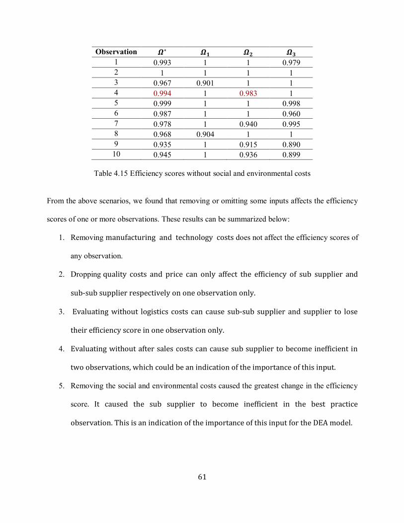
61
Observation 𝜴∗ 𝜴𝟏 𝜴𝟐 𝜴𝟑
1 0.993 1 1 0.979
2 1 1 1 1
3 0.967 0.901 1 1
4 0.994 1 0.983 1
5 0.999 1 1 0.998
6 0.987 1 1 0.960
7 0.978 1 0.940 0.995
8 0.968 0.904 1 1
9 0.935 1 0.915 0.890
10 0.945 1 0.936 0.899
Table 4.15 Efficiency scores without social and environmental costs
From the above scenarios, we found that removing or omitting some inputs affects the efficiency
scores of one or more observations. These results can be summarized below:
1. Removing manufacturing and technology costs does not affect the efficiency scores of
any observation.
2. Dropping quality costs and price can only affect the efficiency of sub supplier and
sub-sub supplier respectively on one observation only.
3. Evaluating without logistics costs can cause sub-sub supplier and supplier to lose
their efficiency score in one observation only.
4. Evaluating without after sales costs can cause sub supplier to become inefficient in
two observations, which could be an indication of the importance of this input.
5. Removing the social and environmental costs caused the greatest change in the efficiency
score. It caused the sub supplier to become inefficient in the best practice
observation. This is an indication of the importance of this input for the DEA model.
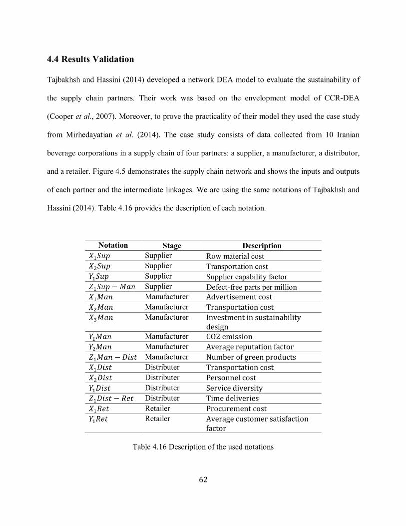
62
4.4 Results Validation
Tajbakhsh and Hassini (2014) developed a network DEA model to evaluate the sustainability of
the supply chain partners. Their work was based on the envelopment model of CCR-DEA
(Cooper et al., 2007). Moreover, to prove the practicality of their model they used the case study
from Mirhedayatian et al. (2014). The case study consists of data collected from 10 Iranian
beverage corporations in a supply chain of four partners: a supplier, a manufacturer, a distributor,
and a retailer. Figure 4.5 demonstrates the supply chain network and shows the inputs and outputs
of each partner and the intermediate linkages. We are using the same notations of Tajbakhsh and
Hassini (2014). Table 4.16 provides the description of each notation.
Notation Stage Description
𝑋1𝑆𝑢𝑝 Supplier Row material cost
𝑋2𝑆𝑢𝑝 Supplier Transportation cost
𝑌1𝑆𝑢𝑝 Supplier Supplier capability factor
𝑍1𝑆𝑢𝑝 − 𝑀𝑎𝑛 Supplier Defect-free parts per million
𝑋1𝑀𝑎𝑛 Manufacturer Advertisement cost
𝑋2𝑀𝑎𝑛 Manufacturer Transportation cost
𝑋3𝑀𝑎𝑛 Manufacturer Investment in sustainability design
𝑌1𝑀𝑎𝑛 Manufacturer CO2 emission
𝑌2𝑀𝑎𝑛 Manufacturer Average reputation factor
𝑍1𝑀𝑎𝑛 − 𝐷𝑖𝑠𝑡 Manufacturer Number of green products
𝑋1𝐷𝑖𝑠𝑡 Distributer Transportation cost
𝑋2𝐷𝑖𝑠𝑡 Distributer Personnel cost
𝑌1𝐷𝑖𝑠𝑡 Distributer Service diversity
𝑍1𝐷𝑖𝑠𝑡 − 𝑅𝑒𝑡 Distributer Time deliveries
𝑋1𝑅𝑒𝑡 Retailer Procurement cost
𝑌1𝑅𝑒𝑡 Retailer Average customer satisfaction factor
Table 4.16 Description of the used notations

63
Figure 4.5 The supply chain of the Iranian beverage corporations’ case
Tajbakhsh and Hassini (2014) model:
𝑀𝑖𝑛 𝛺∗ − 휀 × 𝑆𝑙𝑎𝑐𝑘
subject to
( Supplier Sup)
∑ 𝜆𝑗𝐽𝑗=1 𝑥𝑖𝑗
𝑆𝑢𝑝+ 𝑠𝑖
𝑆𝑢𝑝= 𝛺𝑆𝑢𝑝𝑥𝑖𝑗0
𝑆𝑢𝑝 𝑖 ∈ 𝐷𝐼𝑆𝑢𝑝
∑ 𝜆𝑗𝐽𝑗=1 𝑦𝑟𝑗
𝑆𝑢𝑝− 𝑠𝑟
𝑆𝑢𝑝= 𝑦𝑟𝑗0
𝑆𝑢𝑝 𝑟 ∈ 𝐷𝑂 𝑆𝑢𝑝
∑ 𝜆𝑗𝐽𝑗=1 𝑧𝑡𝑗
𝑆𝑢𝑝−𝑀𝑎𝑛+ 𝑠𝑡
𝑆𝑢𝑝−𝑀𝑎𝑛= 𝑧𝑡𝑗0
𝑆𝑢𝑝−𝑀𝑎𝑛 𝑡 = 1, … , 𝑇
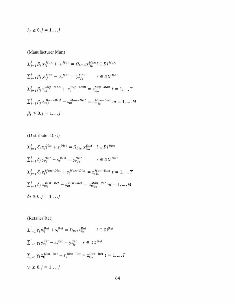
64
𝜆𝑗 ≥ 0, 𝑗 = 1, . . , 𝐽
(Manufacturer Man)
∑ 𝛽𝑗𝑗𝑗=1 𝑥𝑖𝑗
𝑀𝑎𝑛 + 𝑠𝑖 𝑀𝑎𝑛 = 𝛺𝑀𝑎𝑛𝑥𝑖𝑗0
𝑀𝑎𝑛 𝑖 ∈ 𝐷𝐼𝑀𝑎𝑛
∑ 𝛽𝑗𝐽𝑗=1 𝑦𝑟𝑗
𝑀𝑎𝑛 − 𝑠𝑟 𝑀𝑎𝑛 = 𝑦𝑟𝑗0
𝑀𝑎𝑛 𝑟 ∈ 𝐷𝑂 𝑀𝑎𝑛
∑ 𝛽𝑗𝐽𝑗=1 𝑧𝑡𝑗
𝑆𝑢𝑝−𝑀𝑎𝑛+ 𝑠𝑡
𝑆𝑢𝑝−𝑀𝑎𝑛= 𝑧𝑡𝑗0
𝑆𝑢𝑝−𝑀𝑎𝑛 𝑡 = 1, … , 𝑇
∑ 𝛽𝑗𝐽𝑗=1 𝑧𝑚𝑗
𝑀𝑎𝑛−𝐷𝑖𝑠𝑡 − 𝑠𝑚 𝑀𝑎𝑛−𝐷𝑖𝑠𝑡 = 𝑧𝑚𝑗0
𝑀𝑎𝑛−𝐷𝑖𝑠𝑡 𝑚 = 1, … , 𝑀
𝛽𝑗 ≥ 0, 𝑗 = 1, . . , 𝐽
(Distributor Dist)
∑ 𝛿𝑗𝐽𝑗=1 𝑥𝑖𝑗
𝐷𝑖𝑠𝑡 + 𝑠𝑖 𝐷𝑖𝑠𝑡 = 𝛺𝐷𝑖𝑠𝑡𝑥𝑖𝑗0
𝐷𝑖𝑠𝑡 𝑖 ∈ 𝐷𝐼𝐷𝑖𝑠𝑡
∑ 𝛿𝑗𝐽𝑗=1 𝑦𝑟𝑗
𝐷𝑖𝑠𝑡 − 𝑠𝑟 𝐷𝑖𝑠𝑡 = 𝑦𝑟𝑗0
𝐷𝑖𝑠𝑡 𝑟 ∈ 𝐷𝑂 𝐷𝑖𝑠𝑡
∑ 𝛿𝑗𝐽𝑗=1 𝑧𝑡𝑗
𝑀𝑎𝑛−𝐷𝑖𝑠𝑡 + 𝑠𝑡 𝑀𝑎𝑛−𝐷𝑖𝑠𝑡 = 𝑧𝑡𝑗0
𝑀𝑎𝑛−𝐷𝑖𝑠𝑡 𝑡 = 1, … , 𝑇
∑ 𝛿𝑗𝐽𝑗=1 𝑧𝑚𝑗
𝐷𝑖𝑠𝑡−𝑅𝑒𝑡 − 𝑠𝑚 𝐷𝑖𝑠𝑡−𝑅𝑒𝑡 = 𝑧𝑚𝑗0
𝑀𝑎𝑛−𝑅𝑒𝑡 𝑚 = 1, … , 𝑀
𝛿𝑗 ≥ 0, 𝑗 = 1, . . , 𝐽
(Retailer Ret)
∑ γjJj=1 xij
Ret + 𝑠i Ret = Ω𝑅𝑒𝑡xij0
Ret 𝑖 ∈ DIRet
∑ γjJj=1 yrj
Ret − 𝑠r Ret = yrj0
Ret 𝑟 ∈ DO Ret
∑ γjJj=1 ztj
Dist−Ret + 𝑠t Dist−Ret = ztj0
Dist−Ret 𝑡 = 1, … , 𝑇
γj ≥ 0, 𝑗 = 1, . . , 𝐽
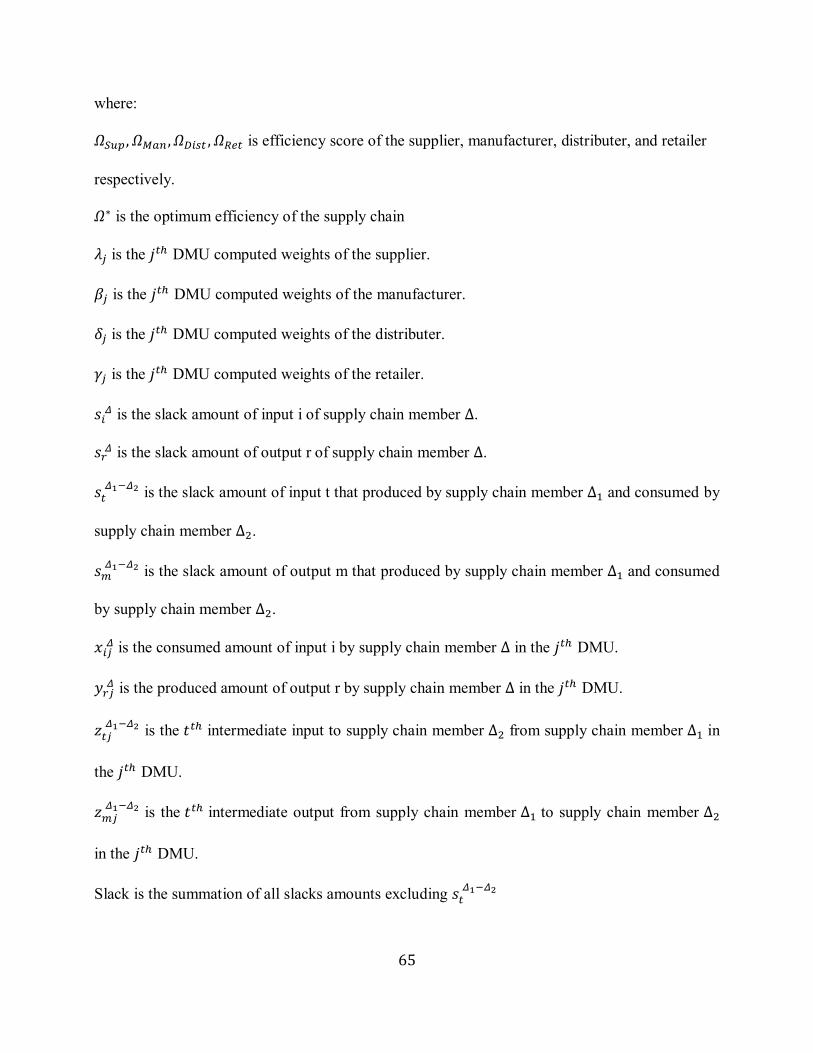
65
where:
𝛺𝑆𝑢𝑝 , 𝛺𝑀𝑎𝑛 , 𝛺𝐷𝑖𝑠𝑡 , 𝛺𝑅𝑒𝑡 is efficiency score of the supplier, manufacturer, distributer, and retailer
respectively.
𝛺∗ is the optimum efficiency of the supply chain
𝜆𝑗 is the 𝑗𝑡ℎ DMU computed weights of the supplier.
𝛽𝑗 is the 𝑗𝑡ℎ DMU computed weights of the manufacturer.
𝛿𝑗 is the 𝑗𝑡ℎ DMU computed weights of the distributer.
𝛾𝑗 is the 𝑗𝑡ℎ DMU computed weights of the retailer.
𝑠𝑖 𝛥 is the slack amount of input i of supply chain member Δ.
𝑠𝑟 𝛥 is the slack amount of output r of supply chain member Δ.
𝑠𝑡 𝛥1−𝛥2 is the slack amount of input t that produced by supply chain member Δ1 and consumed by
supply chain member Δ2.
𝑠𝑚 𝛥1−𝛥2 is the slack amount of output m that produced by supply chain member Δ1 and consumed
by supply chain member Δ2.
𝑥𝑖𝑗 𝛥 is the consumed amount of input i by supply chain member Δ in the 𝑗𝑡ℎ DMU.
𝑦𝑟𝑗 𝛥 is the produced amount of output r by supply chain member Δ in the 𝑗𝑡ℎ DMU.
𝑧𝑡𝑗 𝛥1−𝛥2 is the 𝑡𝑡ℎ intermediate input to supply chain member Δ2 from supply chain member Δ1 in
the 𝑗𝑡ℎ DMU.
𝑧𝑚𝑗 𝛥1−𝛥2 is the 𝑡𝑡ℎ intermediate output from supply chain member Δ1 to supply chain member Δ2
in the 𝑗𝑡ℎ DMU.
Slack is the summation of all slacks amounts excluding 𝑠𝑡 𝛥1−𝛥2

66
Mirhedayatian et al. (2014) model:
where:
𝑚k is number of inputs corresponds to 𝑘𝑡ℎ supply chain member.
𝑖 is a numerical index corresponds to inputs of supply chain members.
R𝑘𝐷 is number of desirable outputs corresponds to 𝑘𝑡ℎ supply chain member.

67
r𝑘𝐷 is a numerical index corresponds to corresponds to desirable outputs of supply chain
members.
R𝑘𝑈𝐷 is number of undesirable outputs corresponds to 𝑘𝑡ℎ supply chain member.
r𝑘𝑈𝐷 is a numerical index corresponds to corresponds to undesirable outputs of supply chain
members.
𝐾 is number of supply chain members.
𝑘 is a numerical index correspond to supply chain members.
𝑛 is the number of DMUs.
𝑗 is a numerical index correspond to DMUs.
𝑥𝑖𝑗𝑘 is the 𝑖𝑡ℎ input of 𝑘𝑡ℎ supply chain member of 𝑗𝑡ℎ DMU
𝑦𝑟𝑘
𝐷𝑗𝑘𝐷
is the 𝑟𝑘𝐷 𝑡ℎ
desirable output of 𝑘𝑡ℎ supply chain member of 𝑗𝑡ℎ DMU
𝑦𝑟𝑘
𝑈𝐷𝑗𝑘𝑈𝐷
is the 𝑟𝑘𝑈𝐷 𝑡ℎ
undesirable output of 𝑘𝑡ℎ supply chain member of 𝑗𝑡ℎ DMU
𝑦𝑟𝑘
𝐷0𝑘𝐷
is the 𝑟𝑘𝐷 𝑡ℎ
desirable output of 𝑘𝑡ℎ supply chain member of the DMU under evaluation
(𝐷𝑀𝑈0)
𝑦𝑟𝑘
𝑈𝐷0𝑘𝑈𝐷
is the 𝑟𝑘𝑈𝐷 𝑡ℎ
undesirable output of 𝑘𝑡ℎ supply chain member of the DMU under evaluation
(𝐷𝑀𝑈0)
𝑤𝑓𝑗𝑘 is the dual role factor corresponds to 𝑘𝑡ℎ supply chain member of 𝑗𝑡ℎ DMU.
𝐹 is number of dual role factor corresponds to 𝑘𝑡ℎ supply chain member of 𝑗𝑡ℎ DMU.
𝑓 is a numerical index of dual role factor corresponds to 𝑘𝑡ℎ supply chain member of 𝑗𝑡ℎ DMU.
𝑍𝑠(𝑘,ℎ)𝑗(𝑘,ℎ)
is the Intermediate measures from 𝑘𝑡ℎ supply chain member to ℎ𝑡ℎ supply chain member
of 𝑗𝑡ℎ DMU.
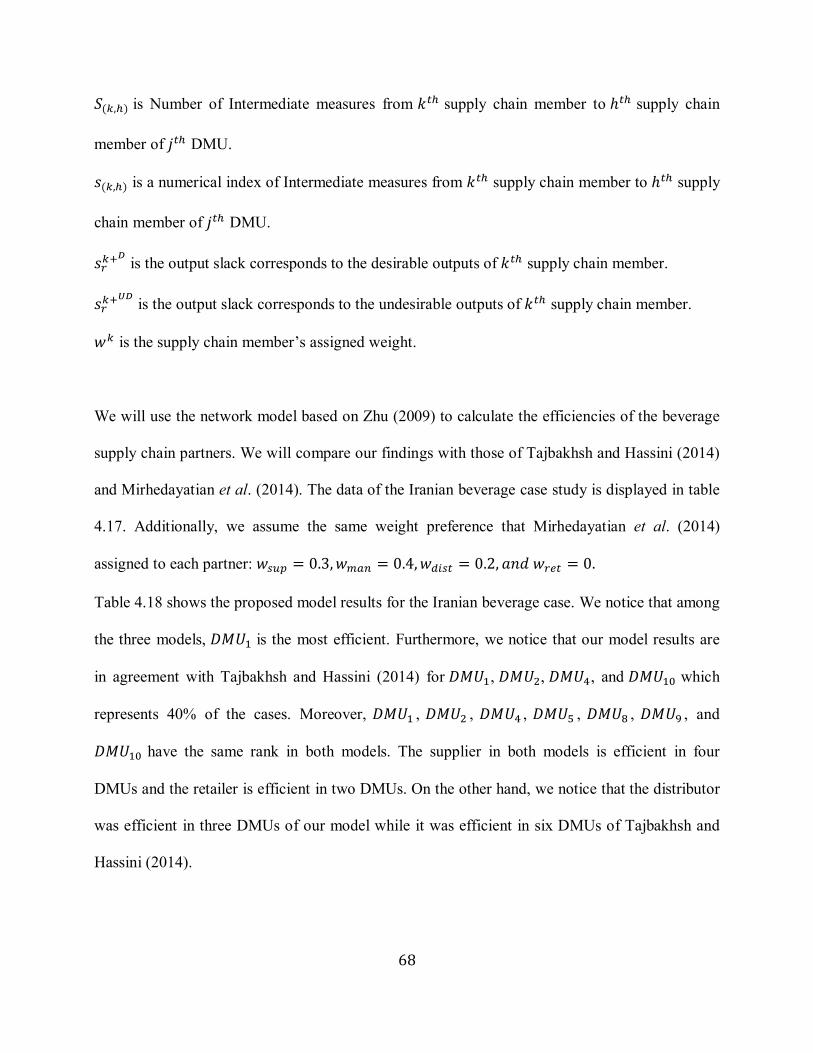
68
𝑆(𝑘,ℎ) is Number of Intermediate measures from 𝑘𝑡ℎ supply chain member to ℎ𝑡ℎ supply chain
member of 𝑗𝑡ℎ DMU.
𝑠(𝑘,ℎ) is a numerical index of Intermediate measures from 𝑘𝑡ℎ supply chain member to ℎ𝑡ℎ supply
chain member of 𝑗𝑡ℎ DMU.
𝑠𝑟𝑘+𝐷
is the output slack corresponds to the desirable outputs of 𝑘𝑡ℎ supply chain member.
𝑠𝑟𝑘+𝑈𝐷
is the output slack corresponds to the undesirable outputs of 𝑘𝑡ℎ supply chain member.
𝑤𝑘 is the supply chain member’s assigned weight.
We will use the network model based on Zhu (2009) to calculate the efficiencies of the beverage
supply chain partners. We will compare our findings with those of Tajbakhsh and Hassini (2014)
and Mirhedayatian et al. (2014). The data of the Iranian beverage case study is displayed in table
4.17. Additionally, we assume the same weight preference that Mirhedayatian et al. (2014)
assigned to each partner: 𝑤𝑠𝑢𝑝 = 0.3, 𝑤𝑚𝑎𝑛 = 0.4, 𝑤𝑑𝑖𝑠𝑡 = 0.2, 𝑎𝑛𝑑 𝑤𝑟𝑒𝑡 = 0.
Table 4.18 shows the proposed model results for the Iranian beverage case. We notice that among
the three models, 𝐷𝑀𝑈1 is the most efficient. Furthermore, we notice that our model results are
in agreement with Tajbakhsh and Hassini (2014) for 𝐷𝑀𝑈1, 𝐷𝑀𝑈2, 𝐷𝑀𝑈4, and 𝐷𝑀𝑈10 which
represents 40% of the cases. Moreover, 𝐷𝑀𝑈1 , 𝐷𝑀𝑈2 , 𝐷𝑀𝑈4 , 𝐷𝑀𝑈5 , 𝐷𝑀𝑈8 , 𝐷𝑀𝑈9 , and
𝐷𝑀𝑈10 have the same rank in both models. The supplier in both models is efficient in four
DMUs and the retailer is efficient in two DMUs. On the other hand, we notice that the distributor
was efficient in three DMUs of our model while it was efficient in six DMUs of Tajbakhsh and
Hassini (2014).
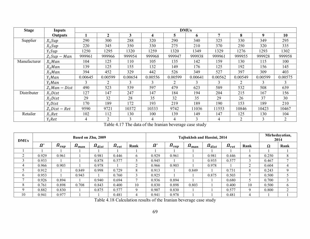
69
Stage Inputs
Outputs
DMUs
1 2 3 4 5 6 7 8 9 10
Supplier 𝑋1𝑆𝑢𝑝 290 300 288 320 290 340 325 330 349 295
𝑋2𝑆𝑢𝑝 220 345 350 330 275 210 370 250 320 335
𝑌1𝑆𝑢𝑝 1250 1295 1320 1259 1320 1349 1329 1276 1293 1302
𝑍1𝑆𝑢𝑝 − 𝑀𝑎𝑛 999961 999966 999954 999968 999947 999938 999961 999955 999928 999958
Manufacturer 𝑋1𝑀𝑎𝑛 104 125 110 105 135 142 159 130 115 100
𝑋2𝑀𝑎𝑛 139 125 155 132 149 176 125 192 156 145
𝑋3𝑀𝑎𝑛 394 452 329 442 526 349 527 397 309 403
𝑌1𝑀𝑎𝑛 0.00645 0.00599 0.00654 0.00556 0.00599 0.00641 0.00562 0.00549 0.00599 0.00575
𝑌2𝑀𝑎𝑛 3 2 3 3 2 3 3 2 3 3
𝑍1𝑀𝑎𝑛 − 𝐷𝑖𝑠𝑡 490 523 539 597 479 623 589 532 508 639
Distributer 𝑋1𝐷𝑖𝑠𝑡 127 147 247 147 184 194 204 215 167 156
𝑋2𝐷𝑖𝑠𝑡 29 32 28 35 32 35 29 26 37 30
𝑌1𝐷𝑖𝑠𝑡 170 189 172 193 219 189 190 153 189 210
𝑍1𝐷𝑖𝑠𝑡 − 𝑅𝑒𝑡 9590 9721 10372 10333 9742 11036 11553 10846 10423 10467
Retailer 𝑋1𝑅𝑒𝑡 102 112 130 100 139 149 147 125 130 104
𝑌1𝑅𝑒𝑡 4 2 3 4 4 3 4 2 3 2
Table 4.17 The data of the Iranian beverage case study
DMUs Based on Zhu, 2009 Tajbakhsh and Hassini, 2014
Mirhedayatian,
2014
𝜴∗ 𝜴𝒔𝒖𝒑 𝜴𝒎𝒂𝒏 𝜴𝒅𝒊𝒔𝒕 𝜴𝒓𝒆𝒕 Rank 𝜴∗ 𝜴𝒔𝒖𝒑 𝜴𝒎𝒂𝒏 𝜴𝒅𝒊𝒔𝒕 𝜴𝒓𝒆𝒕 Rank Rank
1 1 1 1 1 1 1 1 1 1 1 1 1 1 1
2 0.929 0.961 1 0.981 0.446 6 0.929 0.961 1 0.981 0.446 6 0.250 8
3 0.933 1 1 0.878 0.577 5 0.945 1 1 0.935 0.577 3 0.467 7
4 0.966 0.903 1 0.978 1 2 0.966 0.903 1 0.978 1 2 0.604 4
5 0.912 1 0.849 0.998 0.729 8 0.913 1 0.849 1 0.731 8 0.243 9
6 0.953 1 0.943 1 0.760 3 0.925 1 1 0.875 0.503 7 0.500 5
7 0.926 0.894 1 0.940 0.694 7 0.936 0.894 1 1 0.680 5 0.700 3
8 0.761 0.898 0.708 0.843 0.400 10 0.830 0.898 0.803 1 0.400 10 0.500 6
9 0.882 0.830 1 0.875 0.577 9 0.907 0.830 1 1 0.577 9 0.800 2
10 0.941 0.977 1 1 0.481 4 0.941 0.978 1 1 0.481 4 1 1
Table 4.18 Calculation results of the Iranian beverage case study
70
On comparing with Mirhedayatian et al. (2014), we observe that our results are more similar to
Tajbakhsh and Hassini (2014) than Mirhedayatian et al., (2014). This is because our model and
Tajbakhsh and Hassini (2014) model are based on the same structure. The only difference is the
use of slacks in Tajbakhsh and Hassini (2014) model. On the other hand, Mirhedayatian et al.
(2014) model is based on a fuzzy structure and non-radial objective function (Tajbakhsh and
Hassini, 2014).
We observed from the numerical example and the Iranian beverage case that the based on Zhu
(2009) network DEA model has the ability to deal with different supply chain network structures.
Additionally, the model can work with large and small number of inputs and outputs.

71
Chapter 5
Conclusions and Future Work
5.1 Conclusions
In this thesis we propose a framework for evaluating the quality of multi-tier suppliers in global
supply chains. The proposed framework involves three steps. In the first step, suppliers are
grouped based on common characteristics using hierarchical cluster analysis. Next for each
group, the total cost of ownership of each supplier is calculated using different qualitative and
quantitative cost categories. In the third and the final step, data envelopment analysis is used to
evaluate the efficiency of each supplier with respect to the computed cost categories.
The proposed framework can help the decision maker answer the following questions:
Which is the most efficient supplier?
How can an inefficient supplier become efficient?
What is the supply chain best practice? In other words, when will the supply chain be
efficient?
The strength of the proposed framework is that it takes into account the network structure of the
supply chain. It can deal with n-tier suppliers.
The limitation is the lack of real data in our study. The numerical examples are based on random
data generated by Excel.
5.2 Future Work
Future research can involve:
Other cost categories that are critical to buyer-supplier collaboration.
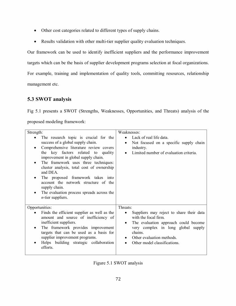
72
Other cost categories related to different types of supply chains.
Results validation with other multi-tier supplier quality evaluation techniques.
Our framework can be used to identify inefficient suppliers and the performance improvement
targets which can be the basis of supplier development programs selection at focal organizations.
For example, training and implementation of quality tools, committing resources, relationship
management etc.
5.3 SWOT analysis
Fig 5.1 presents a SWOT (Strengths, Weaknesses, Opportunities, and Threats) analysis of the
proposed modeling framework:
Strength:
The research topic is crucial for the
success of a global supply chain.
Comprehensive literature review covers
the key factors related to quality
improvement in global supply chain.
The framework uses three techniques:
cluster analysis, total cost of ownership
and DEA.
The proposed framework takes into
account the network structure of the supply chain.
The evaluation process spreads across the
n-tier suppliers.
Weaknesses:
Lack of real life data.
Not focused on a specific supply chain
industry.
Limited number of evaluation criteria.
Opportunities:
Finds the efficient supplier as well as the
amount and source of inefficiency of
inefficient suppliers.
The framework provides improvement
targets that can be used as a basis for supplier improvement programs.
Helps building strategic collaboration
efforts.
Threats:
Suppliers may reject to share their data
with the focal firm.
The evaluation approach could become
very complex in long global supply
chains.
Other evaluation methods.
Other model classifications.
Figure 5.1 SWOT analysis

73
References
1. Akarte, M.M., Surendra, N.V., Ravi, B., Rangaraj, N. (2001), Web based casting supplier
evaluation using analytical hierarchy process, Journal of the Operational Research
Society, 52(5), 511–522.
2. Al Salem, A.A. (2012), An integrated model for supplier quality evaluation, (Master’s
thesis, Concordia University, Montreal, Canada), Retrieved from
http://spectrum.library.concordia.ca/974017/
3. Andersen, M., Skjoett-Larsen, T. (2009), Corporate social responsibility in global supply
chains, Supply Chain Management: An International Journal, 14, 75–86.
4. Anthony, T. (2000), Supply chain collaboration: success in the new internet economy,
Achieving Supply Chain Excellence Through Technology, 2, 41-44.
5. Azbari, M. E., Olfat, L. , Amiri, M., Soofi, J. B. (2014), A network data envelopment
analysis model for supply chain performance evaluation: real case of Iranian
pharmaceutical industry, International Journal of Industrial Engineering and Production
Research, 25(2), 125-137.
6. Bal H., Örkcü H.H. , Çelebioğlu S. (2006), An experimental comparison of the new goal
programming and the linear programming approaches in the two-group discriminant
problems, Computers & Industrial Engineering, 50, 296-311.
7. Bhutta, K.S., Huq, F. (2002), Supplier selection problem: a comparison of the total cost of
ownership and analytic hierarchy process approaches, Supply Chain Management: An
International Journal, 7(3), 126-35.
8. Bozarth, C. C., Handfield, R. B. (2006). Introduction to operations and supply chain
management. New Jersey: Pearson Prentice Hall.
74
9. Bradley, D. (2008), Melamine scandal widens, Sciencebase. Retrieved from
http://www.sciencebase.com/science-blog/milky-melamine.html
10. Braglia, M., Petroni, A., (2000), A quality assurance-oriented methodology for handling
trade-offs in supplier selection, International Journal of Physical Distribution and
Logistics Management, 30(2), 96–111.
11. Bremen, P., Oehmen, J., Alard, R. (2007), Cost-transparent sourcing in china applying
total cost of ownership, In: Proceedings of the 2007 IEEE, 262–266.
12. Bruno, G., Esposito, E., Genovese, A., Passaro, R. (2012), AHP-based approaches for
supplier evaluation: problems and perspectives, Journal of Purchasing & Supply
Management, 18(3), 159-172.
13. Çebi, F., Bayraktar, D. (2003), An integrated approach for supplier selection, Logistics
Information Management, 16(6), 395–400.
14. Cao, M., Zhang, Q. (2011), Supply chain collaboration: Impact on collaborative
advantage and firm performance, Journal of Operations Management 29, 163–180.
15. Chan, F.T.S. (2003), Interactive selection model for supplier selection process: An
analytical hierarchy process approach, International Journal Production Research 41(15),
3549–3579.
16. Charnes, A., Cooper, W.W., Rhodes, E. (1978), Measuring the efficiency of decision
making units, European Journal of Operational Research, 2(6), 429-444.
17. Chen, C., Yan, H. (2011), Network DEA model for supply chain performance evaluation,
European Journal of Operational Research, 213, 147–155.
75
18. Chen, C., Zhang, J., Delaurentis T. (2014), Quality control in food supply chain
management: An analytical model and case study of the adulterated milk incident in
China, International Journal of Production Economics, 152, 188–199.
19. Choi, T.Y., Hartley, J.L. (1996). An exploration of supplier selection practices across the
supply chain. Journal of Operations Management, 14, 333–345.
20. Cooper, W.W., Park, K.S., Paster, J.T. (1999), RAM: a range adjusted measure of
inefficiency for use with additive models and relations to other models and measures in
DEA, Journal of Productivity Analysis, 11, 5–42.
21. Cooper, W.W., Seiford, L.M., Tone, K. (2007), Data envelopment analysis: a
comprehensive text with models, applications, references and DEA-solver software,
Springer, USA.
22. de Boer, L., Labro, E., Morlacchi, P. (2001), A review of methods supporting supplier
selection, European Journal of Purchasing & Supply Management, 7(2),75–89.
23. Degraeve, Z., Roodhooft, F. (1999), Effectively selecting suppliers using total cost of
ownership, The Journal of Supply Chain Management, 35(1), 5–11.
24. Degraeve, Z., Roodhooft, F., Doveren, B.V. (2005), The use of total cost of ownership for
strategic procurement: a company-wide management information system, Journal of the
Operational Research Society, 56, 51-59.
25. Deng, X., Hub, Y.,Deng, Y., Mahadevan, S. (2014), Supplier selection using AHP
methodology extended by D numbers, Expert Systems with Applications, 41(1), 156–167.
26. Dickson, G. W. (1966), An analysis of vendor selection systems and decisions, Journal of
Purchasing, 2, 5–17.
76
27. Dogan, I., Aydin, N. (2011), Combining Bayesian networks and total cost of ownership,
Computers & Industrial Engineering, 61, 1072–1085.
28. Edwards, A. (2010, February 4), Moving forward ... fast Toyota accelerator pedal
problem prompts massive recall, halts production on 11 models, The Ithacan, Retrieved
from https://mbarriedesigns.wordpress.com/2010/03/
29. Ellram, L.M. (1993), Total cost of ownership: Elements and implementation.,
International Journal of Purchasing and Materials Management, 29, 2-11.
30. Ellram, L.M. (1995), Total cost of ownership: an analysis approach for purchasing,
International Journal of Physical Distribution and Logistics Management, 25(8), 4-23.
31. Erdem, A., Gocen, E. (2012), Development of a decision support system for supplier
evaluation and order allocation, Expert Systems with Applications, 39(5), 4927–4937.
32. Evans J.R., Lindsay W.L. (2005), An introduction to six sigma & process improvement,
USA: South-Western Cengage Learning.
33. Ferrin, B. G., Plank, R. E. (2002), Total cost of ownership models: an exploratory study,
Journal of Supply Chain Management, 38,18–29.
34. Forker, L.B., Mendez, D., (2001), An analytical method for benchmarking best peer
suppliers, International Journal of Operations and Production Management, 21(1–2), 195–
209.
35. Garfamy, R.M. (2006), A data envelopment analysis approach based on total cost of
ownership for supplier selection, Journal of Enterprise Information Management, 19(6),
662 – 678.
36. Gelderman, C. (1989). Henry Ford: The wayward capitalist. New York: St. Martins Press.

77
37. Ghodsypour, S. H., O’Brien, C. O. (1998), A decision support system for supplier
selection using an integrated analytic hierarchy process and linear programming.
International Journal of Production Economics, 56, 199–212.
38. Grimm, J. H., Hofstetter, J. S., Sarkis, J. (2014), Exploring sub-suppliers' compliance
with corporate sustainability standards, Journal of Cleaner Production, 1-14.
39. Ho, W., Xu, X., Dey, P.K. (2010), Multi-criteria decision making approaches for supplier
evaluation and selection: a literature review, European Journal of Operational Research,
202, 16–24.
40. Hou, J., Su, D. (2007), EJB–MVC oriented supplier selection system for mass
customization, Journal of Manufacturing Technology Management 18(1), 54– 71.
41. Hughes, A.J., Grawoig, D.E. (1973), Linear programming: an emphasis on decision
making, Don Mills, ON: Addison-Wesley Publishing Company.
42. Hurkens, K., van der Valk, W., Wynstra, F. (2006), Total cost of ownership in the
services sector: a case study, The Journal of Supply Chain Management, 42, 27-37.
43. Ignizio, J.P. (1976), Goal programming and extensions. Toronto, ON: Lexington.
44. Jain, V., Benyoucef, L. (2008), Managing long supply chain networks: Some emerging
issues and challenges, Journal of Manufacturing Technology Management, 19(4), 469–
496.
45. Jahantigh, F.F., Malmir, B. (2015), Development of a supply chain model for healthcare
industry, In: Proceedings of the 2015 International Conference on Industrial Engineering
and Operations Management.
46. Kao, C. (2009), Efficiency decomposition in network data envelopment analysis: A
relational model, European Journal of Operational Research, 192, 949–962.

78
47. Karpak, B., Kumcu, E., Kasuganti, R.R. (2001), Purchasing materials in the supply chain:
Managing a multi-objective task, European Journal of Purchasing and Supply
Management, 7(3), 209–216.
48. Klassen, R.D., Vereecke, A. (2012), Social issues in supply chains: Capabilities link
responsibility, risk (opportunity), and performance, International Journal of Production
Economics, 140(1), 103–115.
49. Kraljic, P., (1983), Purchasing must become supply management, Harvard Business
Review 61(5), 109-117.
50. Kuei , C.-H. , Madu , C. N., Lin , C. (2011), Developing global supply chain quality
management systems, International Journal of Production Research, 49(15), 4457–4481.
51. Kull, T.J., Talluri, S. (2008), A supply-risk reduction model using integrated multi-
criteria decision making, IEEE Transactions on Engineering Management, 55(3), 409–
419.
52. Lee, H., Plambeck, E., Yatsko, P. (2012), Embracing green in China [. . .] with an NGO
nudge, Supply Chain Management Review, May/June, 38-45.
53. Lewis, H.F., Sexton, T.R. (2004), Network DEA: efficiency analysis of organizations
with complex internal structure, Computers and Operations Research, 31, 1365–1410.
54. Liao, C.-N., Kao, H.-P. (2010), Supplier selection model using Taguchi loss function,
analytical hierarchy process and multi-choice goal programming, Comp and Industrial
Engineering, 58, 571–577.
55. Liu, J., Ding, F.Y., Lall, V., (2000), Using data envelopment analysis to compare
suppliers for supplier selection and performance improvement, Supply Chain
Management: An International Journal, 5(3), 143–150.

79
56. Liu, F.H.F., Hai, H.L. (2005), The voting analytic hierarchy process method for selecting
supplier, International Journal of Production Economics 97(3), 308– 317.
57. MacCarthy, B.L., Jayarathne, P.G.S.A. (2012), Sustainable collaborative supply networks
in the international clothing industry: a comparative analysis of two retailers, Production
Planning and Control, 23(4), 252-268.
58. Macharis, C., Springael J., De Brucker, K., Verbeke, A. (2004), Promethee and AHP: the
design of operational synergies in multicriteria analysis. Strengthening Promethee with
ideas of AHP, European Journal of Operational Research, 153, 307−317.
59. Maltz, A.B., Ellram, L.M. (1997), Total cost of relationship: an analytical framework for
the logistics outsourcing decision," Journal of Business Logistics, 18, 45-66.
60. Mendoza, A., Santiago, E., Ravindran, A.R. (2008), A three-phase multicriteria method to
the supplier selection problem, International Journal of Industrial Engineering, 15(2),
195–210.
61. Mentzer, J.T., De Witt, W., Keebler, J.S., Min, S., Nix, N.W., Smith, C.D., Zacharia, Z.G.
(2001), Defining supply chain management, Journal of Business Logistics, 22(2), 1-25.
62. Mirhedayatian, S.M., Azadi, M., Saen, R.F. (2014), A novel network data envelopment
analysis model for evaluating green supply chain management, International Journal of
Production Economics, 147, 544–554.
63. Morehouse, J.E., Cardoso, L. (2011), Consumer product fraud – how to stop the fraud
now, Quarter 2, Retrieved from
http://www.supplychainquarterly.com/topics/Strategy/scq201102fraud

80
64. Mueller, M., dos Santos, V.G., Seuring, S. (2009), The contribution of environmental and
social standards towards ensuring legitimacy in supply chain governance, Journal of
Business Ethics, 89(4), 509-523.
65. Muralidharan, C., Anantharaman, N., Deshmukh, S.G. (2002), A multi-criteria group
decision-making model for supplier rating, Journal of Supply Chain Management 38(4),
22–33.
66. Narasimhan, R., Talluri, S., Mendez, D. (2001), Supplier evaluation and rationalization
via data envelopment analysis: An empirical examination, Journal of Supply Chain
Management, 37(3), 28–37.
67. Nieminen, P., Takala, J. (2006), Achieving better on-time delivery performance with the
help of internal dependencies in the production, International Journal of Management and
Enterprise Development, 3, 181–190.
68. Noshad, K., Awasthi, A. (2015), Supplier quality development: A review of literature and
industry practices, International Journal of Production Research, 53(2), 466-487.
69. Omurca, S.I. (2013), An intelligent supplier evaluation, selection and development
system, Applied Soft Computing, 13, 690–697.
70. Osman, H., Demirli, K. (2010), A bilinear goal programming model and a modified
Benders decomposition algorithm for supply chain reconfiguration and supplier selection,
International Journal of Production Economics, 124, 97–105.
71. Parlar, M., Weng, Z.K. (1997), Designing a firm's coordinated manufacturing and supply
decisions with short product life cycle, Management Science 43(10), 1329-1344.
72. Perçin, S. (2006), An application of the integrated AHP–PGP model in supplier selection,
Measuring Business Excellence, 10 (4), 34–49.
81
73. Rao, P. (2002), Greening the supply chain: a new initiative in South East Asia,
International Journal of Operations and Production Management, 22(5/6), 632-655.
74. Regan, C. (2015), Social supply chain – technology or innovation first, Retrieved from
https://smbp.uwaterloo.ca/2015/02/social-supply-chain-technology-or-innovation-first
75. Romero, C. (2004), A general structure of achievement function for a goal programming
model, European Journal of Operational Research, 153, 675–686.
76. Ross, A., Buffa, F.P., Dröge, C., Carrington, D. (2006), Supplier evaluation in a dyadic
relationship: An action research approach, Journal of Business Logistics, 27(2), 75–102.
77. Saen, R.F. (2006), A decision model for selecting technology suppliers in the presence of
nondiscretionary factors, Applied Mathematics and Computation, 181(2), 1609–1615.
78. Sarpong, S. (2014), Traceability and supply chain complexity: confronting the issues and
concerns, European Business Review, 26(3), 271 – 284.
79. Seydel, J., (2006), Data envelopment analysis for decision support, Industrial
Management and Data Systems, 106(1), 81–95.
80. Simatupang, T.M., Sridharan, R. (2002), The collaborative supply chain, International
Journal of Logistics Management, 13(1), 15-30.
81. Simatupang, T.M., Sridharan, R. (2005), An integrative framework for supply chain
collaboration. International Journal of Logistics Management 16(2), 257–274.
82. Singh, A. (2014), Supplier evaluation and demand allocation among suppliers in a supply
chain, Journal of Purchasing and Supply Management, 20, 167–176.
83. Sohal, A.S., Chung, W.W.C. (1998), Activity based costing in manufacturing: two case
studies on implementation, Integrated Manufacturing Systems, 9(3), 137–147.
82
84. Song, N., Platts, K., Bance, D. (2007), Total acquisition cost of overseas
outsourcing/sourcing – a framework and a case study, Journal of Manufacturing
Technology Management, 18(7), 858–875.
85. Soto-Silva, W.E., Nadal-Roig, E., González-Araya, M.C., Pla-Aragones, L.M. (2015),
Operational research models applied to the fresh fruit supply chain, European Journal of
Operational Research, 000, 1–11.
86. Tachizawa, E.M., Wong, C.Y. (2014), Towards a theory of multi-tier sustainable supply
chains: a systematic literature review, Supply Chain Management: An International
Journal, 19(5/6), 643-663.
87. Tajbakhsh, A., Hassini, E. (2014), A data envelopment analysis approach to evaluate
sustainability in supply chain networks. Journal of Cleaner Production,
doi:10.1016/j.jclepro.2014.07.054.
88. Talluri, S., Baker, R.C., (2002), A multi-phase mathematical programming approach for
effective supply chain design, European Journal of Operational Research, 141(3), 544–
558.
89. Talluri, S., Narasimhan, R., (2004), A methodology for strategic sourcing, European
Journal of Operational Research, 154(1), 236–250.
90. Talluri, S., Sarkis, J., (2002), A model for performance monitoring of suppliers,
International Journal of Production Research, 40(16), 4257–4269.
91. Thomas, D.J., Griffin, P.M. (1996), Coordinated supply chain management, European
Journal of Operational Research, 94(1), 1-15.
92. Tse, Y. K., Tan, K.H. (2011), Managing product quality risk in a multi-tier global supply
chain, International Journal of Production Research, 49,139–158.

83
93. Tse, Y. K., Zhang, M., Akhtar, P., MacBryde, J. (2016), Embracing supply chain agility:
an investigation in the electronics industry, 21(1).
94. Vereecke, A., Muylle, S. (2006). Performance improvement through supply chain
collaboration in Europe. International Journal of Operations and Production Management,
26(11), 1176-1198.
95. Viswanadham, N., Samvedi, A. (2013). Supplier selection based on supply chain
ecosystem, performance and risk criteria. International Journal of Production Research,
51(21), 6484-6498.
96. Vonderembse, M.A., Uppal, M., Huang, S.H., Dismukes, J.P. (2006), Designing supply
chains: towards theory development, International Journal of Production Economics,
100(2), 223-238.
97. Wang, G., Huang, S.H., Dismukes, J.P. (2004), Product-driven supply chain selection
using integrated multi-criteria decision-making methodology, International Journal of
Production Economics, 91(1), 1–15.
98. Yang, Z.F., Shi, Y., Wang, B., Yan, H. (2014), Website quality and profitability
evaluation in ecommerce firms using two-stage DEA model, Procedia Computer Science,
30, 4-13.
99. Zeydan, M., Çolpan, C., C. Çobanoğlu, C. (2011), A combined methodology for supplier
selection and performance evaluation, Expert Systems with Applications, 38(3), 2741–
2751.
100. Zhu, Q. and Sarkis, J. (2004), Relationships between operational practices and
performance among early adopters of green supply chain management practices in

84
Chinese manufacturing enterprises, Journal of Operations Management, 22(3), 265-
289.
101. Zhu, Q., Sarkis, J. , Lai, K.H. (2012), Green supply chain management
innovation diffusion and its relationship to organizational improvement: an
ecological modernization perspective, Journal of Engineering and Technology
Management, 29 (1), 168-185.
102. Zhu, J. (2009), Quantitative models for performance evaluation and benchmarking
data envelopment analysis with spreadsheets (2nd ed.). Worcester, MA: Springer.
103. Zsidisin, G. A. (2003), A grounded definition of supply risk, Journal of Purchasing
and Supply Management, 9, 217–224.
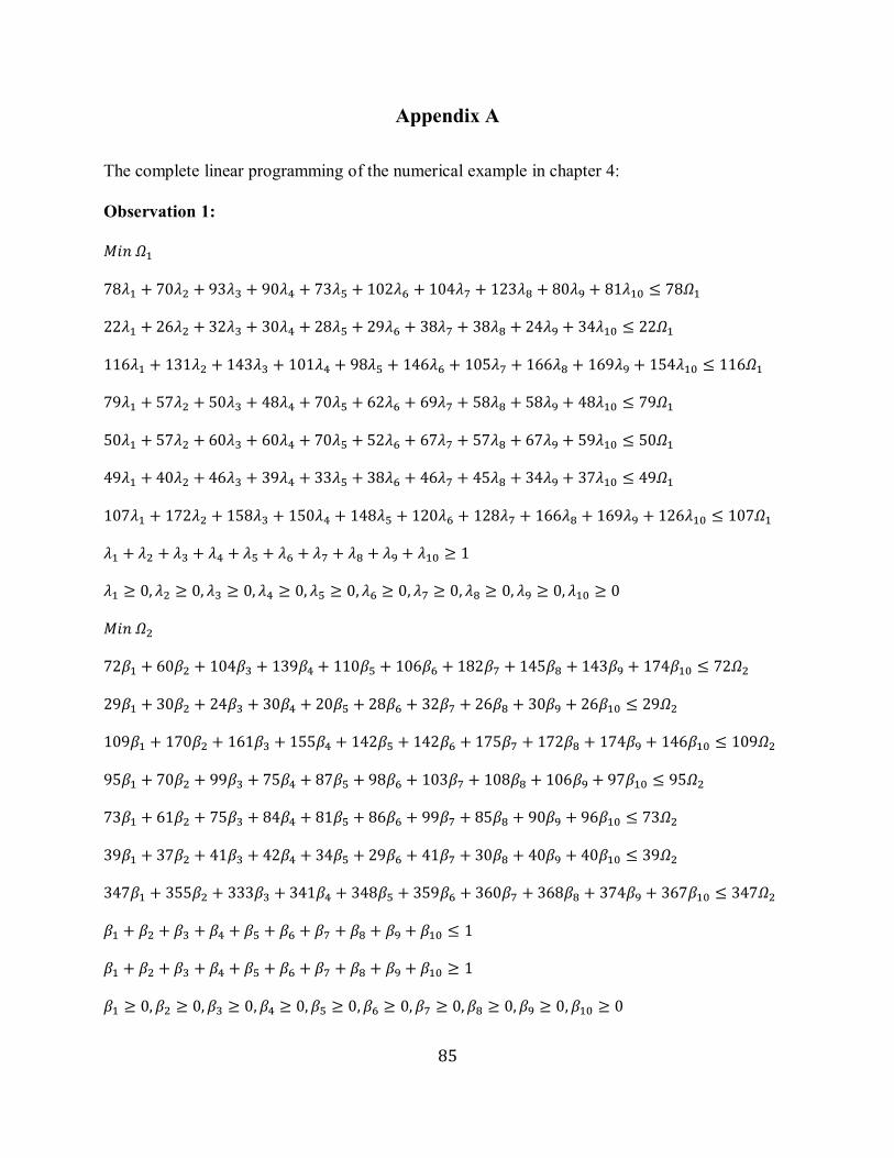
85
Appendix A
The complete linear programming of the numerical example in chapter 4:
Observation 1:
𝑀𝑖𝑛 𝛺1
78𝜆1 + 70𝜆2 + 93𝜆3 + 90𝜆4 + 73𝜆5 + 102𝜆6 + 104𝜆7 + 123𝜆8 + 80𝜆9 + 81𝜆10 ≤ 78𝛺1
22𝜆1 + 26𝜆2 + 32𝜆3 + 30𝜆4 + 28𝜆5 + 29𝜆6 + 38𝜆7 + 38𝜆8 + 24𝜆9 + 34𝜆10 ≤ 22𝛺1
116𝜆1 + 131𝜆2 + 143𝜆3 + 101𝜆4 + 98𝜆5 + 146𝜆6 + 105𝜆7 + 166𝜆8 + 169𝜆9 + 154𝜆10 ≤ 116𝛺1
79𝜆1 + 57𝜆2 + 50𝜆3 + 48𝜆4 + 70𝜆5 + 62𝜆6 + 69𝜆7 + 58𝜆8 + 58𝜆9 + 48𝜆10 ≤ 79𝛺1
50𝜆1 + 57𝜆2 + 60𝜆3 + 60𝜆4 + 70𝜆5 + 52𝜆6 + 67𝜆7 + 57𝜆8 + 67𝜆9 + 59𝜆10 ≤ 50𝛺1
49𝜆1 + 40𝜆2 + 46𝜆3 + 39𝜆4 + 33𝜆5 + 38𝜆6 + 46𝜆7 + 45𝜆8 + 34𝜆9 + 37𝜆10 ≤ 49𝛺1
107𝜆1 + 172𝜆2 + 158𝜆3 + 150𝜆4 + 148𝜆5 + 120𝜆6 + 128𝜆7 + 166𝜆8 + 169𝜆9 + 126𝜆10 ≤ 107𝛺1
𝜆1 + 𝜆2 + 𝜆3 + 𝜆4 + 𝜆5 + 𝜆6 + 𝜆7 + 𝜆8 + 𝜆9 + 𝜆10 ≥ 1
𝜆1 ≥ 0, 𝜆2 ≥ 0, 𝜆3 ≥ 0, 𝜆4 ≥ 0, 𝜆5 ≥ 0, 𝜆6 ≥ 0, 𝜆7 ≥ 0, 𝜆8 ≥ 0, 𝜆9 ≥ 0, 𝜆10 ≥ 0
𝑀𝑖𝑛 𝛺2
72𝛽1 + 60𝛽2 + 104𝛽3 + 139𝛽4 + 110𝛽5 + 106𝛽6 + 182𝛽7 + 145𝛽8 + 143𝛽9 + 174𝛽10 ≤ 72𝛺2
29𝛽1 + 30𝛽2 + 24𝛽3 + 30𝛽4 + 20𝛽5 + 28𝛽6 + 32𝛽7 + 26𝛽8 + 30𝛽9 + 26𝛽10 ≤ 29𝛺2
109𝛽1 + 170𝛽2 + 161𝛽3 + 155𝛽4 + 142𝛽5 + 142𝛽6 + 175𝛽7 + 172𝛽8 + 174𝛽9 + 146𝛽10 ≤ 109𝛺2
95𝛽1 + 70𝛽2 + 99𝛽3 + 75𝛽4 + 87𝛽5 + 98𝛽6 + 103𝛽7 + 108𝛽8 + 106𝛽9 + 97𝛽10 ≤ 95𝛺2
73𝛽1 + 61𝛽2 + 75𝛽3 + 84𝛽4 + 81𝛽5 + 86𝛽6 + 99𝛽7 + 85𝛽8 + 90𝛽9 + 96𝛽10 ≤ 73𝛺2
39𝛽1 + 37𝛽2 + 41𝛽3 + 42𝛽4 + 34𝛽5 + 29𝛽6 + 41𝛽7 + 30𝛽8 + 40𝛽9 + 40𝛽10 ≤ 39𝛺2
347𝛽1 + 355𝛽2 + 333𝛽3 + 341𝛽4 + 348𝛽5 + 359𝛽6 + 360𝛽7 + 368𝛽8 + 374𝛽9 + 367𝛽10 ≤ 347𝛺2
𝛽1 + 𝛽2 + 𝛽3 + 𝛽4 + 𝛽5 + 𝛽6 + 𝛽7 + 𝛽8 + 𝛽9 + 𝛽10 ≤ 1
𝛽1 + 𝛽2 + 𝛽3 + 𝛽4 + 𝛽5 + 𝛽6 + 𝛽7 + 𝛽8 + 𝛽9 + 𝛽10 ≥ 1
𝛽1 ≥ 0, 𝛽2 ≥ 0, 𝛽3 ≥ 0, 𝛽4 ≥ 0, 𝛽5 ≥ 0, 𝛽6 ≥ 0, 𝛽7 ≥ 0, 𝛽8 ≥ 0, 𝛽9 ≥ 0, 𝛽10 ≥ 0

86
𝑀𝑖𝑛 𝛺3
288𝛿1 + 261𝛿2 + 309𝛿3 + 230𝛿4 + 309𝛿5 + 263𝛿6 + 284𝛿7 + 327𝛿8 + 297𝛿9 + 313𝛿10 ≤ 288𝛺3
45𝛿1 + 38𝛿2 + 40𝛿3 + 42𝛿4 + 48𝛿5 + 52𝛿6 + 52𝛿7 + 54𝛿8 + 52𝛿9 + 63𝛿10 ≤ 45𝛺3
270𝛿1 + 284𝛿2 + 276𝛿3 + 271𝛿4 + 268𝛿5 + 299𝛿6 + 251𝛿7 + 232𝛿8 + 301𝛿9 + 315𝛿10 ≤ 270𝛺3
140𝛿1 + 126𝛿2 + 136𝛿3 + 138𝛿4 + 144𝛿5 + 149𝛿6 + 146𝛿7 + 142𝛿8 + 150𝛿9 + 159𝛿10 ≤ 140𝛺3
127𝛿1 + 110𝛿2 + 138𝛿3 + 134𝛿4 + 138𝛿5 + 132𝛿6 + 149𝛿7 + 140𝛿8 + 141𝛿9 + 140𝛿10 ≤ 127𝛺3
46𝛿1 + 35𝛿2 + 43𝛿3 + 36𝛿4 + 40𝛿5 + 40𝛿6 + 45𝛿7 + 45𝛿8 + 45𝛿9 + 50𝛿10 ≤ 46𝛺3
700𝛿1 + 638𝛿2 + 658𝛿3 + 649𝛿4 + 651𝛿5 + 668𝛿6 + 745𝛿7 + 676𝛿8 + 734𝛿9 + 710𝛿10 ≤ 700𝛺3
𝛿1 + 𝛿2 + 𝛿3 + 𝛿4 + 𝛿5 + 𝛿6 + 𝛿7 + 𝛿8 + 𝛿9 + 𝛿10 ≤ 1
𝛿1 + 𝛿2 + 𝛿3 + 𝛿4 + 𝛿5 + 𝛿6 + 𝛿7 + 𝛿8 + 𝛿9 + 𝛿10 ≥ 1
𝛿1 ≥ 0, 𝛿2 ≥ 0, 𝛿3 ≥ 0, 𝛿4 ≥ 0, 𝛿5 ≥ 0, 𝛿6 ≥ 0, 𝛿7 ≥ 0, 𝛿8 ≥ 0, 𝛿9 ≥ 0, 𝛿10 ≥ 0
Observation 2:
𝑀𝑖𝑛 𝛺1
78𝜆1 + 70𝜆2 + 93𝜆3 + 90𝜆4 + 73𝜆5 + 102𝜆6 + 104𝜆7 + 123𝜆8 + 80𝜆9 + 81𝜆10 ≤ 70𝛺1
22𝜆1 + 26𝜆2 + 32𝜆3 + 30𝜆4 + 28𝜆5 + 29𝜆6 + 38𝜆7 + 38𝜆8 + 24𝜆9 + 34𝜆10 ≤ 26𝛺1
116𝜆1 + 131𝜆2 + 143𝜆3 + 101𝜆4 + 98𝜆5 + 146𝜆6 + 105𝜆7 + 166𝜆8 + 169𝜆9 + 154𝜆10 ≤ 131𝛺1
79𝜆1 + 57𝜆2 + 50𝜆3 + 48𝜆4 + 70𝜆5 + 62𝜆6 + 69𝜆7 + 58𝜆8 + 58𝜆9 + 48𝜆10 ≤ 57𝛺1
50𝜆1 + 57𝜆2 + 60𝜆3 + 60𝜆4 + 70𝜆5 + 52𝜆6 + 67𝜆7 + 57𝜆8 + 67𝜆9 + 59𝜆10 ≤ 57𝛺1
49𝜆1 + 40𝜆2 + 46𝜆3 + 39𝜆4 + 33𝜆5 + 38𝜆6 + 46𝜆7 + 45𝜆8 + 34𝜆9 + 37𝜆10 ≤ 40𝛺1
107𝜆1 + 172𝜆2 + 158𝜆3 + 150𝜆4 + 148𝜆5 + 120𝜆6 + 128𝜆7 + 166𝜆8 + 169𝜆9 + 126𝜆10 ≤ 172𝛺1
𝜆1 + 𝜆2 + 𝜆3 + 𝜆4 + 𝜆5 + 𝜆6 + 𝜆7 + 𝜆8 + 𝜆9 + 𝜆10 ≥ 1
𝜆1 ≥ 0, 𝜆2 ≥ 0, 𝜆3 ≥ 0, 𝜆4 ≥ 0, 𝜆5 ≥ 0, 𝜆6 ≥ 0, 𝜆7 ≥ 0, 𝜆8 ≥ 0, 𝜆9 ≥ 0, 𝜆10 ≥ 0
𝑀𝑖𝑛 𝛺2
72𝛽1 + 60𝛽2 + 104𝛽3 + 139𝛽4 + 110𝛽5 + 106𝛽6 + 182𝛽7 + 145𝛽8 + 143𝛽9 + 174𝛽10 ≤ 60𝛺2
29𝛽1 + 30𝛽2 + 24𝛽3 + 30𝛽4 + 20𝛽5 + 28𝛽6 + 32𝛽7 + 26𝛽8 + 30𝛽9 + 26𝛽10 ≤ 30𝛺2
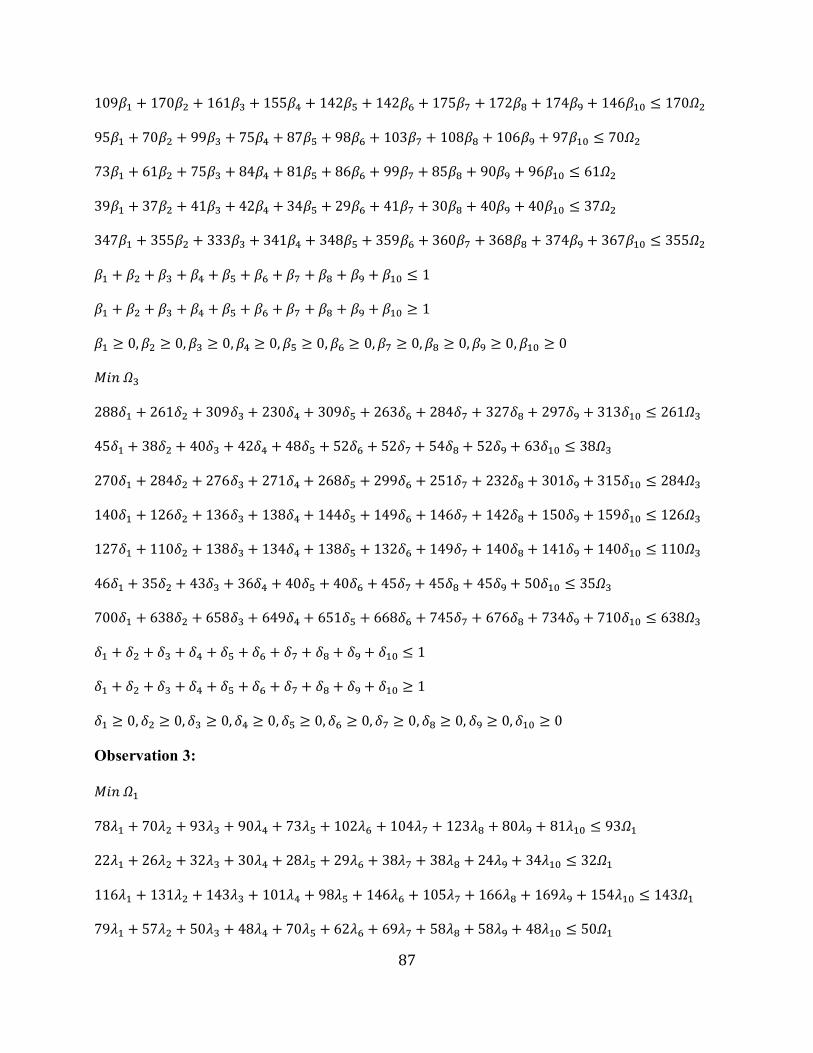
87
109𝛽1 + 170𝛽2 + 161𝛽3 + 155𝛽4 + 142𝛽5 + 142𝛽6 + 175𝛽7 + 172𝛽8 + 174𝛽9 + 146𝛽10 ≤ 170𝛺2
95𝛽1 + 70𝛽2 + 99𝛽3 + 75𝛽4 + 87𝛽5 + 98𝛽6 + 103𝛽7 + 108𝛽8 + 106𝛽9 + 97𝛽10 ≤ 70𝛺2
73𝛽1 + 61𝛽2 + 75𝛽3 + 84𝛽4 + 81𝛽5 + 86𝛽6 + 99𝛽7 + 85𝛽8 + 90𝛽9 + 96𝛽10 ≤ 61𝛺2
39𝛽1 + 37𝛽2 + 41𝛽3 + 42𝛽4 + 34𝛽5 + 29𝛽6 + 41𝛽7 + 30𝛽8 + 40𝛽9 + 40𝛽10 ≤ 37𝛺2
347𝛽1 + 355𝛽2 + 333𝛽3 + 341𝛽4 + 348𝛽5 + 359𝛽6 + 360𝛽7 + 368𝛽8 + 374𝛽9 + 367𝛽10 ≤ 355𝛺2
𝛽1 + 𝛽2 + 𝛽3 + 𝛽4 + 𝛽5 + 𝛽6 + 𝛽7 + 𝛽8 + 𝛽9 + 𝛽10 ≤ 1
𝛽1 + 𝛽2 + 𝛽3 + 𝛽4 + 𝛽5 + 𝛽6 + 𝛽7 + 𝛽8 + 𝛽9 + 𝛽10 ≥ 1
𝛽1 ≥ 0, 𝛽2 ≥ 0, 𝛽3 ≥ 0, 𝛽4 ≥ 0, 𝛽5 ≥ 0, 𝛽6 ≥ 0, 𝛽7 ≥ 0, 𝛽8 ≥ 0, 𝛽9 ≥ 0, 𝛽10 ≥ 0
𝑀𝑖𝑛 𝛺3
288𝛿1 + 261𝛿2 + 309𝛿3 + 230𝛿4 + 309𝛿5 + 263𝛿6 + 284𝛿7 + 327𝛿8 + 297𝛿9 + 313𝛿10 ≤ 261𝛺3
45𝛿1 + 38𝛿2 + 40𝛿3 + 42𝛿4 + 48𝛿5 + 52𝛿6 + 52𝛿7 + 54𝛿8 + 52𝛿9 + 63𝛿10 ≤ 38𝛺3
270𝛿1 + 284𝛿2 + 276𝛿3 + 271𝛿4 + 268𝛿5 + 299𝛿6 + 251𝛿7 + 232𝛿8 + 301𝛿9 + 315𝛿10 ≤ 284𝛺3
140𝛿1 + 126𝛿2 + 136𝛿3 + 138𝛿4 + 144𝛿5 + 149𝛿6 + 146𝛿7 + 142𝛿8 + 150𝛿9 + 159𝛿10 ≤ 126𝛺3
127𝛿1 + 110𝛿2 + 138𝛿3 + 134𝛿4 + 138𝛿5 + 132𝛿6 + 149𝛿7 + 140𝛿8 + 141𝛿9 + 140𝛿10 ≤ 110𝛺3
46𝛿1 + 35𝛿2 + 43𝛿3 + 36𝛿4 + 40𝛿5 + 40𝛿6 + 45𝛿7 + 45𝛿8 + 45𝛿9 + 50𝛿10 ≤ 35𝛺3
700𝛿1 + 638𝛿2 + 658𝛿3 + 649𝛿4 + 651𝛿5 + 668𝛿6 + 745𝛿7 + 676𝛿8 + 734𝛿9 + 710𝛿10 ≤ 638𝛺3
𝛿1 + 𝛿2 + 𝛿3 + 𝛿4 + 𝛿5 + 𝛿6 + 𝛿7 + 𝛿8 + 𝛿9 + 𝛿10 ≤ 1
𝛿1 + 𝛿2 + 𝛿3 + 𝛿4 + 𝛿5 + 𝛿6 + 𝛿7 + 𝛿8 + 𝛿9 + 𝛿10 ≥ 1
𝛿1 ≥ 0, 𝛿2 ≥ 0, 𝛿3 ≥ 0, 𝛿4 ≥ 0, 𝛿5 ≥ 0, 𝛿6 ≥ 0, 𝛿7 ≥ 0, 𝛿8 ≥ 0, 𝛿9 ≥ 0, 𝛿10 ≥ 0
Observation 3:
𝑀𝑖𝑛 𝛺1
78𝜆1 + 70𝜆2 + 93𝜆3 + 90𝜆4 + 73𝜆5 + 102𝜆6 + 104𝜆7 + 123𝜆8 + 80𝜆9 + 81𝜆10 ≤ 93𝛺1
22𝜆1 + 26𝜆2 + 32𝜆3 + 30𝜆4 + 28𝜆5 + 29𝜆6 + 38𝜆7 + 38𝜆8 + 24𝜆9 + 34𝜆10 ≤ 32𝛺1
116𝜆1 + 131𝜆2 + 143𝜆3 + 101𝜆4 + 98𝜆5 + 146𝜆6 + 105𝜆7 + 166𝜆8 + 169𝜆9 + 154𝜆10 ≤ 143𝛺1
79𝜆1 + 57𝜆2 + 50𝜆3 + 48𝜆4 + 70𝜆5 + 62𝜆6 + 69𝜆7 + 58𝜆8 + 58𝜆9 + 48𝜆10 ≤ 50𝛺1

88
50𝜆1 + 57𝜆2 + 60𝜆3 + 60𝜆4 + 70𝜆5 + 52𝜆6 + 67𝜆7 + 57𝜆8 + 67𝜆9 + 59𝜆10 ≤ 60𝛺1
49𝜆1 + 40𝜆2 + 46𝜆3 + 39𝜆4 + 33𝜆5 + 38𝜆6 + 46𝜆7 + 45𝜆8 + 34𝜆9 + 37𝜆10 ≤ 46𝛺1
107𝜆1 + 172𝜆2 + 158𝜆3 + 150𝜆4 + 148𝜆5 + 120𝜆6 + 128𝜆7 + 166𝜆8 + 169𝜆9 + 126𝜆10 ≤ 158𝛺1
𝜆1 + 𝜆2 + 𝜆3 + 𝜆4 + 𝜆5 + 𝜆6 + 𝜆7 + 𝜆8 + 𝜆9 + 𝜆10 ≥ 1
𝜆1 ≥ 0, 𝜆2 ≥ 0, 𝜆3 ≥ 0, 𝜆4 ≥ 0, 𝜆5 ≥ 0, 𝜆6 ≥ 0, 𝜆7 ≥ 0, 𝜆8 ≥ 0, 𝜆9 ≥ 0, 𝜆10 ≥ 0
𝑀𝑖𝑛 𝛺2
72𝛽1 + 60𝛽2 + 104𝛽3 + 139𝛽4 + 110𝛽5 + 106𝛽6 + 182𝛽7 + 145𝛽8 + 143𝛽9 + 174𝛽10 ≤ 104𝛺2
29𝛽1 + 30𝛽2 + 24𝛽3 + 30𝛽4 + 20𝛽5 + 28𝛽6 + 32𝛽7 + 26𝛽8 + 30𝛽9 + 26𝛽10 ≤ 24𝛺2
109𝛽1 + 170𝛽2 + 161𝛽3 + 155𝛽4 + 142𝛽5 + 142𝛽6 + 175𝛽7 + 172𝛽8 + 174𝛽9 + 146𝛽10 ≤ 161𝛺2
95𝛽1 + 70𝛽2 + 99𝛽3 + 75𝛽4 + 87𝛽5 + 98𝛽6 + 103𝛽7 + 108𝛽8 + 106𝛽9 + 97𝛽10 ≤ 99𝛺2
73𝛽1 + 61𝛽2 + 75𝛽3 + 84𝛽4 + 81𝛽5 + 86𝛽6 + 99𝛽7 + 85𝛽8 + 90𝛽9 + 96𝛽10 ≤ 75𝛺2
39𝛽1 + 37𝛽2 + 41𝛽3 + 42𝛽4 + 34𝛽5 + 29𝛽6 + 41𝛽7 + 30𝛽8 + 40𝛽9 + 40𝛽10 ≤ 41𝛺2
347𝛽1 + 355𝛽2 + 333𝛽3 + 341𝛽4 + 348𝛽5 + 359𝛽6 + 360𝛽7 + 368𝛽8 + 374𝛽9 + 367𝛽10 ≤ 333𝛺2
𝛽1 + 𝛽2 + 𝛽3 + 𝛽4 + 𝛽5 + 𝛽6 + 𝛽7 + 𝛽8 + 𝛽9 + 𝛽10 ≤ 1
𝛽1 + 𝛽2 + 𝛽3 + 𝛽4 + 𝛽5 + 𝛽6 + 𝛽7 + 𝛽8 + 𝛽9 + 𝛽10 ≥ 1
𝛽1 ≥ 0, 𝛽2 ≥ 0, 𝛽3 ≥ 0, 𝛽4 ≥ 0, 𝛽5 ≥ 0, 𝛽6 ≥ 0, 𝛽7 ≥ 0, 𝛽8 ≥ 0, 𝛽9 ≥ 0, 𝛽10 ≥ 0
𝑀𝑖𝑛 𝛺3
288𝛿1 + 261𝛿2 + 309𝛿3 + 230𝛿4 + 309𝛿5 + 263𝛿6 + 284𝛿7 + 327𝛿8 + 297𝛿9 + 313𝛿10 ≤ 309𝛺3
45𝛿1 + 38𝛿2 + 40𝛿3 + 42𝛿4 + 48𝛿5 + 52𝛿6 + 52𝛿7 + 54𝛿8 + 52𝛿9 + 63𝛿10 ≤ 40𝛺3
270𝛿1 + 284𝛿2 + 276𝛿3 + 271𝛿4 + 268𝛿5 + 299𝛿6 + 251𝛿7 + 232𝛿8 + 301𝛿9 + 315𝛿10 ≤ 276𝛺3
140𝛿1 + 126𝛿2 + 136𝛿3 + 138𝛿4 + 144𝛿5 + 149𝛿6 + 146𝛿7 + 142𝛿8 + 150𝛿9 + 159𝛿10 ≤ 136𝛺3
127𝛿1 + 110𝛿2 + 138𝛿3 + 134𝛿4 + 138𝛿5 + 132𝛿6 + 149𝛿7 + 140𝛿8 + 141𝛿9 + 140𝛿10 ≤ 138𝛺3
46𝛿1 + 35𝛿2 + 43𝛿3 + 36𝛿4 + 40𝛿5 + 40𝛿6 + 45𝛿7 + 45𝛿8 + 45𝛿9 + 50𝛿10 ≤ 43𝛺3
700𝛿1 + 638𝛿2 + 658𝛿3 + 649𝛿4 + 651𝛿5 + 668𝛿6 + 745𝛿7 + 676𝛿8 + 734𝛿9 + 710𝛿10 ≤ 658𝛺3
𝛿1 + 𝛿2 + 𝛿3 + 𝛿4 + 𝛿5 + 𝛿6 + 𝛿7 + 𝛿8 + 𝛿9 + 𝛿10 ≤ 1
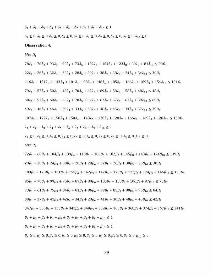
89
𝛿1 + 𝛿2 + 𝛿3 + 𝛿4 + 𝛿5 + 𝛿6 + 𝛿7 + 𝛿8 + 𝛿9 + 𝛿10 ≥ 1
𝛿1 ≥ 0, 𝛿2 ≥ 0, 𝛿3 ≥ 0, 𝛿4 ≥ 0, 𝛿5 ≥ 0, 𝛿6 ≥ 0, 𝛿7 ≥ 0, 𝛿8 ≥ 0, 𝛿9 ≥ 0, 𝛿10 ≥ 0
Observation 4:
𝑀𝑖𝑛 𝛺1
78𝜆1 + 70𝜆2 + 93𝜆3 + 90𝜆4 + 73𝜆5 + 102𝜆6 + 104𝜆7 + 123𝜆8 + 80𝜆9 + 81𝜆10 ≤ 90𝛺1
22𝜆1 + 26𝜆2 + 32𝜆3 + 30𝜆4 + 28𝜆5 + 29𝜆6 + 38𝜆7 + 38𝜆8 + 24𝜆9 + 34𝜆10 ≤ 30𝛺1
116𝜆1 + 131𝜆2 + 143𝜆3 + 101𝜆4 + 98𝜆5 + 146𝜆6 + 105𝜆7 + 166𝜆8 + 169𝜆9 + 154𝜆10 ≤ 101𝛺1
79𝜆1 + 57𝜆2 + 50𝜆3 + 48𝜆4 + 70𝜆5 + 62𝜆6 + 69𝜆7 + 58𝜆8 + 58𝜆9 + 48𝜆10 ≤ 48𝛺1
50𝜆1 + 57𝜆2 + 60𝜆3 + 60𝜆4 + 70𝜆5 + 52𝜆6 + 67𝜆7 + 57𝜆8 + 67𝜆9 + 59𝜆10 ≤ 60𝛺1
49𝜆1 + 40𝜆2 + 46𝜆3 + 39𝜆4 + 33𝜆5 + 38𝜆6 + 46𝜆7 + 45𝜆8 + 34𝜆9 + 37𝜆10 ≤ 39𝛺1
107𝜆1 + 172𝜆2 + 158𝜆3 + 150𝜆4 + 148𝜆5 + 120𝜆6 + 128𝜆7 + 166𝜆8 + 169𝜆9 + 126𝜆10 ≤ 150𝛺1
𝜆1 + 𝜆2 + 𝜆3 + 𝜆4 + 𝜆5 + 𝜆6 + 𝜆7 + 𝜆8 + 𝜆9 + 𝜆10 ≥ 1
𝜆1 ≥ 0, 𝜆2 ≥ 0, 𝜆3 ≥ 0, 𝜆4 ≥ 0, 𝜆5 ≥ 0, 𝜆6 ≥ 0, 𝜆7 ≥ 0, 𝜆8 ≥ 0, 𝜆9 ≥ 0, 𝜆10 ≥ 0
𝑀𝑖𝑛 𝛺2
72𝛽1 + 60𝛽2 + 104𝛽3 + 139𝛽4 + 110𝛽5 + 106𝛽6 + 182𝛽7 + 145𝛽8 + 143𝛽9 + 174𝛽10 ≤ 139𝛺2
29𝛽1 + 30𝛽2 + 24𝛽3 + 30𝛽4 + 20𝛽5 + 28𝛽6 + 32𝛽7 + 26𝛽8 + 30𝛽9 + 26𝛽10 ≤ 30𝛺2
109𝛽1 + 170𝛽2 + 161𝛽3 + 155𝛽4 + 142𝛽5 + 142𝛽6 + 175𝛽7 + 172𝛽8 + 174𝛽9 + 146𝛽10 ≤ 155𝛺2
95𝛽1 + 70𝛽2 + 99𝛽3 + 75𝛽4 + 87𝛽5 + 98𝛽6 + 103𝛽7 + 108𝛽8 + 106𝛽9 + 97𝛽10 ≤ 75𝛺2
73𝛽1 + 61𝛽2 + 75𝛽3 + 84𝛽4 + 81𝛽5 + 86𝛽6 + 99𝛽7 + 85𝛽8 + 90𝛽9 + 96𝛽10 ≤ 84𝛺2
39𝛽1 + 37𝛽2 + 41𝛽3 + 42𝛽4 + 34𝛽5 + 29𝛽6 + 41𝛽7 + 30𝛽8 + 40𝛽9 + 40𝛽10 ≤ 42𝛺2
347𝛽1 + 355𝛽2 + 333𝛽3 + 341𝛽4 + 348𝛽5 + 359𝛽6 + 360𝛽7 + 368𝛽8 + 374𝛽9 + 367𝛽10 ≤ 341𝛺2
𝛽1 + 𝛽2 + 𝛽3 + 𝛽4 + 𝛽5 + 𝛽6 + 𝛽7 + 𝛽8 + 𝛽9 + 𝛽10 ≤ 1
𝛽1 + 𝛽2 + 𝛽3 + 𝛽4 + 𝛽5 + 𝛽6 + 𝛽7 + 𝛽8 + 𝛽9 + 𝛽10 ≥ 1
𝛽1 ≥ 0, 𝛽2 ≥ 0, 𝛽3 ≥ 0, 𝛽4 ≥ 0, 𝛽5 ≥ 0, 𝛽6 ≥ 0, 𝛽7 ≥ 0, 𝛽8 ≥ 0, 𝛽9 ≥ 0, 𝛽10 ≥ 0

90
𝑀𝑖𝑛 𝛺3
288𝛿1 + 261𝛿2 + 309𝛿3 + 230𝛿4 + 309𝛿5 + 263𝛿6 + 284𝛿7 + 327𝛿8 + 297𝛿9 + 313𝛿10 ≤ 230𝛺3
45𝛿1 + 38𝛿2 + 40𝛿3 + 42𝛿4 + 48𝛿5 + 52𝛿6 + 52𝛿7 + 54𝛿8 + 52𝛿9 + 63𝛿10 ≤ 42𝛺3
270𝛿1 + 284𝛿2 + 276𝛿3 + 271𝛿4 + 268𝛿5 + 299𝛿6 + 251𝛿7 + 232𝛿8 + 301𝛿9 + 315𝛿10 ≤ 271𝛺3
140𝛿1 + 126𝛿2 + 136𝛿3 + 138𝛿4 + 144𝛿5 + 149𝛿6 + 146𝛿7 + 142𝛿8 + 150𝛿9 + 159𝛿10 ≤ 138𝛺3
127𝛿1 + 110𝛿2 + 138𝛿3 + 134𝛿4 + 138𝛿5 + 132𝛿6 + 149𝛿7 + 140𝛿8 + 141𝛿9 + 140𝛿10 ≤ 134𝛺3
46𝛿1 + 35𝛿2 + 43𝛿3 + 36𝛿4 + 40𝛿5 + 40𝛿6 + 45𝛿7 + 45𝛿8 + 45𝛿9 + 50𝛿10 ≤ 36𝛺3
700𝛿1 + 638𝛿2 + 658𝛿3 + 649𝛿4 + 651𝛿5 + 668𝛿6 + 745𝛿7 + 676𝛿8 + 734𝛿9 + 710𝛿10 ≤ 649𝛺3
𝛿1 + 𝛿2 + 𝛿3 + 𝛿4 + 𝛿5 + 𝛿6 + 𝛿7 + 𝛿8 + 𝛿9 + 𝛿10 ≤ 1
𝛿1 + 𝛿2 + 𝛿3 + 𝛿4 + 𝛿5 + 𝛿6 + 𝛿7 + 𝛿8 + 𝛿9 + 𝛿10 ≥ 1
𝛿1 ≥ 0, 𝛿2 ≥ 0, 𝛿3 ≥ 0, 𝛿4 ≥ 0, 𝛿5 ≥ 0, 𝛿6 ≥ 0, 𝛿7 ≥ 0, 𝛿8 ≥ 0, 𝛿9 ≥ 0, 𝛿10 ≥ 0
Observation 5:
𝑀𝑖𝑛 𝛺1
78𝜆1 + 70𝜆2 + 93𝜆3 + 90𝜆4 + 73𝜆5 + 102𝜆6 + 104𝜆7 + 123𝜆8 + 80𝜆9 + 81𝜆10 ≤ 73𝛺1
22𝜆1 + 26𝜆2 + 32𝜆3 + 30𝜆4 + 28𝜆5 + 29𝜆6 + 38𝜆7 + 38𝜆8 + 24𝜆9 + 34𝜆10 ≤ 28𝛺1
116𝜆1 + 131𝜆2 + 143𝜆3 + 101𝜆4 + 98𝜆5 + 146𝜆6 + 105𝜆7 + 166𝜆8 + 169𝜆9 + 154𝜆10 ≤ 98𝛺1
79𝜆1 + 57𝜆2 + 50𝜆3 + 48𝜆4 + 70𝜆5 + 62𝜆6 + 69𝜆7 + 58𝜆8 + 58𝜆9 + 48𝜆10 ≤ 70𝛺1
50𝜆1 + 57𝜆2 + 60𝜆3 + 60𝜆4 + 70𝜆5 + 52𝜆6 + 67𝜆7 + 57𝜆8 + 67𝜆9 + 59𝜆10 ≤ 70𝛺1
49𝜆1 + 40𝜆2 + 46𝜆3 + 39𝜆4 + 33𝜆5 + 38𝜆6 + 46𝜆7 + 45𝜆8 + 34𝜆9 + 37𝜆10 ≤ 33𝛺1
107𝜆1 + 172𝜆2 + 158𝜆3 + 150𝜆4 + 148𝜆5 + 120𝜆6 + 128𝜆7 + 166𝜆8 + 169𝜆9 + 126𝜆10 ≤ 148𝛺1
𝜆1 + 𝜆2 + 𝜆3 + 𝜆4 + 𝜆5 + 𝜆6 + 𝜆7 + 𝜆8 + 𝜆9 + 𝜆10 ≥ 1
𝜆1 ≥ 0, 𝜆2 ≥ 0, 𝜆3 ≥ 0, 𝜆4 ≥ 0, 𝜆5 ≥ 0, 𝜆6 ≥ 0, 𝜆7 ≥ 0, 𝜆8 ≥ 0, 𝜆9 ≥ 0, 𝜆10 ≥ 0
𝑀𝑖𝑛 𝛺2
72𝛽1 + 60𝛽2 + 104𝛽3 + 139𝛽4 + 110𝛽5 + 106𝛽6 + 182𝛽7 + 145𝛽8 + 143𝛽9 + 174𝛽10 ≤ 110𝛺2
29𝛽1 + 30𝛽2 + 24𝛽3 + 30𝛽4 + 20𝛽5 + 28𝛽6 + 32𝛽7 + 26𝛽8 + 30𝛽9 + 26𝛽10 ≤ 20𝛺2
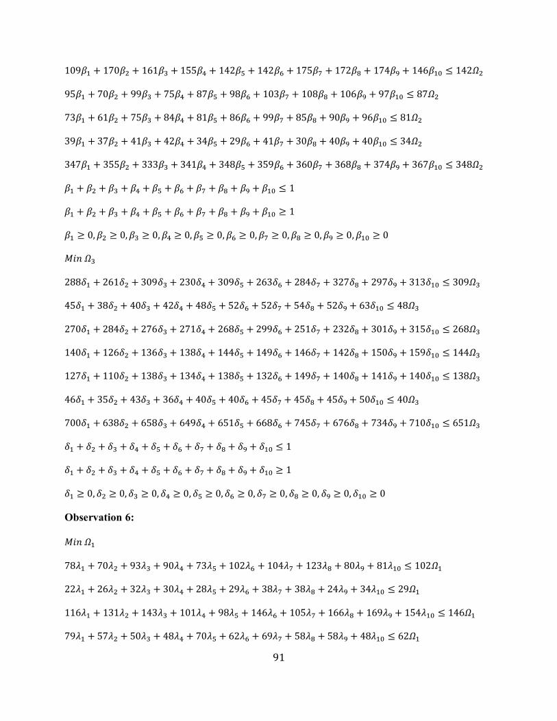
91
109𝛽1 + 170𝛽2 + 161𝛽3 + 155𝛽4 + 142𝛽5 + 142𝛽6 + 175𝛽7 + 172𝛽8 + 174𝛽9 + 146𝛽10 ≤ 142𝛺2
95𝛽1 + 70𝛽2 + 99𝛽3 + 75𝛽4 + 87𝛽5 + 98𝛽6 + 103𝛽7 + 108𝛽8 + 106𝛽9 + 97𝛽10 ≤ 87𝛺2
73𝛽1 + 61𝛽2 + 75𝛽3 + 84𝛽4 + 81𝛽5 + 86𝛽6 + 99𝛽7 + 85𝛽8 + 90𝛽9 + 96𝛽10 ≤ 81𝛺2
39𝛽1 + 37𝛽2 + 41𝛽3 + 42𝛽4 + 34𝛽5 + 29𝛽6 + 41𝛽7 + 30𝛽8 + 40𝛽9 + 40𝛽10 ≤ 34𝛺2
347𝛽1 + 355𝛽2 + 333𝛽3 + 341𝛽4 + 348𝛽5 + 359𝛽6 + 360𝛽7 + 368𝛽8 + 374𝛽9 + 367𝛽10 ≤ 348𝛺2
𝛽1 + 𝛽2 + 𝛽3 + 𝛽4 + 𝛽5 + 𝛽6 + 𝛽7 + 𝛽8 + 𝛽9 + 𝛽10 ≤ 1
𝛽1 + 𝛽2 + 𝛽3 + 𝛽4 + 𝛽5 + 𝛽6 + 𝛽7 + 𝛽8 + 𝛽9 + 𝛽10 ≥ 1
𝛽1 ≥ 0, 𝛽2 ≥ 0, 𝛽3 ≥ 0, 𝛽4 ≥ 0, 𝛽5 ≥ 0, 𝛽6 ≥ 0, 𝛽7 ≥ 0, 𝛽8 ≥ 0, 𝛽9 ≥ 0, 𝛽10 ≥ 0
𝑀𝑖𝑛 𝛺3
288𝛿1 + 261𝛿2 + 309𝛿3 + 230𝛿4 + 309𝛿5 + 263𝛿6 + 284𝛿7 + 327𝛿8 + 297𝛿9 + 313𝛿10 ≤ 309𝛺3
45𝛿1 + 38𝛿2 + 40𝛿3 + 42𝛿4 + 48𝛿5 + 52𝛿6 + 52𝛿7 + 54𝛿8 + 52𝛿9 + 63𝛿10 ≤ 48𝛺3
270𝛿1 + 284𝛿2 + 276𝛿3 + 271𝛿4 + 268𝛿5 + 299𝛿6 + 251𝛿7 + 232𝛿8 + 301𝛿9 + 315𝛿10 ≤ 268𝛺3
140𝛿1 + 126𝛿2 + 136𝛿3 + 138𝛿4 + 144𝛿5 + 149𝛿6 + 146𝛿7 + 142𝛿8 + 150𝛿9 + 159𝛿10 ≤ 144𝛺3
127𝛿1 + 110𝛿2 + 138𝛿3 + 134𝛿4 + 138𝛿5 + 132𝛿6 + 149𝛿7 + 140𝛿8 + 141𝛿9 + 140𝛿10 ≤ 138𝛺3
46𝛿1 + 35𝛿2 + 43𝛿3 + 36𝛿4 + 40𝛿5 + 40𝛿6 + 45𝛿7 + 45𝛿8 + 45𝛿9 + 50𝛿10 ≤ 40𝛺3
700𝛿1 + 638𝛿2 + 658𝛿3 + 649𝛿4 + 651𝛿5 + 668𝛿6 + 745𝛿7 + 676𝛿8 + 734𝛿9 + 710𝛿10 ≤ 651𝛺3
𝛿1 + 𝛿2 + 𝛿3 + 𝛿4 + 𝛿5 + 𝛿6 + 𝛿7 + 𝛿8 + 𝛿9 + 𝛿10 ≤ 1
𝛿1 + 𝛿2 + 𝛿3 + 𝛿4 + 𝛿5 + 𝛿6 + 𝛿7 + 𝛿8 + 𝛿9 + 𝛿10 ≥ 1
𝛿1 ≥ 0, 𝛿2 ≥ 0, 𝛿3 ≥ 0, 𝛿4 ≥ 0, 𝛿5 ≥ 0, 𝛿6 ≥ 0, 𝛿7 ≥ 0, 𝛿8 ≥ 0, 𝛿9 ≥ 0, 𝛿10 ≥ 0
Observation 6:
𝑀𝑖𝑛 𝛺1
78𝜆1 + 70𝜆2 + 93𝜆3 + 90𝜆4 + 73𝜆5 + 102𝜆6 + 104𝜆7 + 123𝜆8 + 80𝜆9 + 81𝜆10 ≤ 102𝛺1
22𝜆1 + 26𝜆2 + 32𝜆3 + 30𝜆4 + 28𝜆5 + 29𝜆6 + 38𝜆7 + 38𝜆8 + 24𝜆9 + 34𝜆10 ≤ 29𝛺1
116𝜆1 + 131𝜆2 + 143𝜆3 + 101𝜆4 + 98𝜆5 + 146𝜆6 + 105𝜆7 + 166𝜆8 + 169𝜆9 + 154𝜆10 ≤ 146𝛺1
79𝜆1 + 57𝜆2 + 50𝜆3 + 48𝜆4 + 70𝜆5 + 62𝜆6 + 69𝜆7 + 58𝜆8 + 58𝜆9 + 48𝜆10 ≤ 62𝛺1
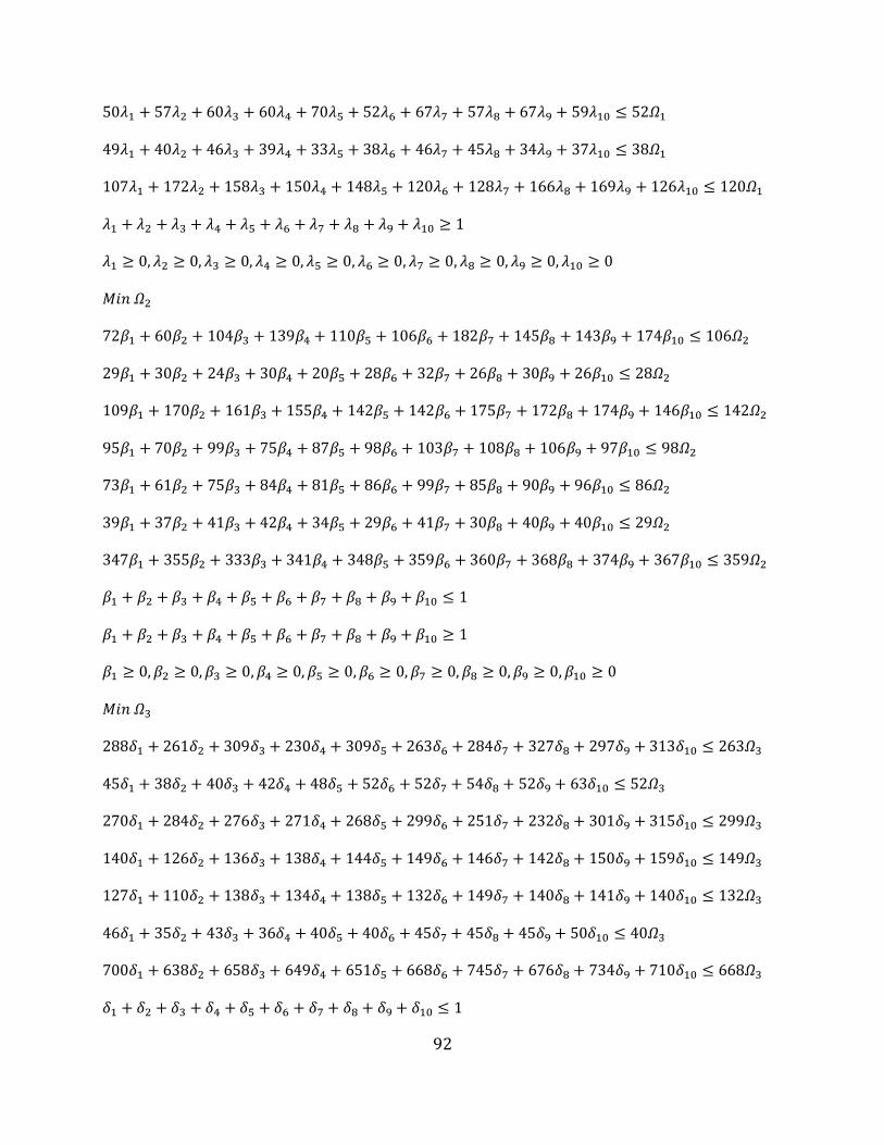
92
50𝜆1 + 57𝜆2 + 60𝜆3 + 60𝜆4 + 70𝜆5 + 52𝜆6 + 67𝜆7 + 57𝜆8 + 67𝜆9 + 59𝜆10 ≤ 52𝛺1
49𝜆1 + 40𝜆2 + 46𝜆3 + 39𝜆4 + 33𝜆5 + 38𝜆6 + 46𝜆7 + 45𝜆8 + 34𝜆9 + 37𝜆10 ≤ 38𝛺1
107𝜆1 + 172𝜆2 + 158𝜆3 + 150𝜆4 + 148𝜆5 + 120𝜆6 + 128𝜆7 + 166𝜆8 + 169𝜆9 + 126𝜆10 ≤ 120𝛺1
𝜆1 + 𝜆2 + 𝜆3 + 𝜆4 + 𝜆5 + 𝜆6 + 𝜆7 + 𝜆8 + 𝜆9 + 𝜆10 ≥ 1
𝜆1 ≥ 0, 𝜆2 ≥ 0, 𝜆3 ≥ 0, 𝜆4 ≥ 0, 𝜆5 ≥ 0, 𝜆6 ≥ 0, 𝜆7 ≥ 0, 𝜆8 ≥ 0, 𝜆9 ≥ 0, 𝜆10 ≥ 0
𝑀𝑖𝑛 𝛺2
72𝛽1 + 60𝛽2 + 104𝛽3 + 139𝛽4 + 110𝛽5 + 106𝛽6 + 182𝛽7 + 145𝛽8 + 143𝛽9 + 174𝛽10 ≤ 106𝛺2
29𝛽1 + 30𝛽2 + 24𝛽3 + 30𝛽4 + 20𝛽5 + 28𝛽6 + 32𝛽7 + 26𝛽8 + 30𝛽9 + 26𝛽10 ≤ 28𝛺2
109𝛽1 + 170𝛽2 + 161𝛽3 + 155𝛽4 + 142𝛽5 + 142𝛽6 + 175𝛽7 + 172𝛽8 + 174𝛽9 + 146𝛽10 ≤ 142𝛺2
95𝛽1 + 70𝛽2 + 99𝛽3 + 75𝛽4 + 87𝛽5 + 98𝛽6 + 103𝛽7 + 108𝛽8 + 106𝛽9 + 97𝛽10 ≤ 98𝛺2
73𝛽1 + 61𝛽2 + 75𝛽3 + 84𝛽4 + 81𝛽5 + 86𝛽6 + 99𝛽7 + 85𝛽8 + 90𝛽9 + 96𝛽10 ≤ 86𝛺2
39𝛽1 + 37𝛽2 + 41𝛽3 + 42𝛽4 + 34𝛽5 + 29𝛽6 + 41𝛽7 + 30𝛽8 + 40𝛽9 + 40𝛽10 ≤ 29𝛺2
347𝛽1 + 355𝛽2 + 333𝛽3 + 341𝛽4 + 348𝛽5 + 359𝛽6 + 360𝛽7 + 368𝛽8 + 374𝛽9 + 367𝛽10 ≤ 359𝛺2
𝛽1 + 𝛽2 + 𝛽3 + 𝛽4 + 𝛽5 + 𝛽6 + 𝛽7 + 𝛽8 + 𝛽9 + 𝛽10 ≤ 1
𝛽1 + 𝛽2 + 𝛽3 + 𝛽4 + 𝛽5 + 𝛽6 + 𝛽7 + 𝛽8 + 𝛽9 + 𝛽10 ≥ 1
𝛽1 ≥ 0, 𝛽2 ≥ 0, 𝛽3 ≥ 0, 𝛽4 ≥ 0, 𝛽5 ≥ 0, 𝛽6 ≥ 0, 𝛽7 ≥ 0, 𝛽8 ≥ 0, 𝛽9 ≥ 0, 𝛽10 ≥ 0
𝑀𝑖𝑛 𝛺3
288𝛿1 + 261𝛿2 + 309𝛿3 + 230𝛿4 + 309𝛿5 + 263𝛿6 + 284𝛿7 + 327𝛿8 + 297𝛿9 + 313𝛿10 ≤ 263𝛺3
45𝛿1 + 38𝛿2 + 40𝛿3 + 42𝛿4 + 48𝛿5 + 52𝛿6 + 52𝛿7 + 54𝛿8 + 52𝛿9 + 63𝛿10 ≤ 52𝛺3
270𝛿1 + 284𝛿2 + 276𝛿3 + 271𝛿4 + 268𝛿5 + 299𝛿6 + 251𝛿7 + 232𝛿8 + 301𝛿9 + 315𝛿10 ≤ 299𝛺3
140𝛿1 + 126𝛿2 + 136𝛿3 + 138𝛿4 + 144𝛿5 + 149𝛿6 + 146𝛿7 + 142𝛿8 + 150𝛿9 + 159𝛿10 ≤ 149𝛺3
127𝛿1 + 110𝛿2 + 138𝛿3 + 134𝛿4 + 138𝛿5 + 132𝛿6 + 149𝛿7 + 140𝛿8 + 141𝛿9 + 140𝛿10 ≤ 132𝛺3
46𝛿1 + 35𝛿2 + 43𝛿3 + 36𝛿4 + 40𝛿5 + 40𝛿6 + 45𝛿7 + 45𝛿8 + 45𝛿9 + 50𝛿10 ≤ 40𝛺3
700𝛿1 + 638𝛿2 + 658𝛿3 + 649𝛿4 + 651𝛿5 + 668𝛿6 + 745𝛿7 + 676𝛿8 + 734𝛿9 + 710𝛿10 ≤ 668𝛺3
𝛿1 + 𝛿2 + 𝛿3 + 𝛿4 + 𝛿5 + 𝛿6 + 𝛿7 + 𝛿8 + 𝛿9 + 𝛿10 ≤ 1

93
𝛿1 + 𝛿2 + 𝛿3 + 𝛿4 + 𝛿5 + 𝛿6 + 𝛿7 + 𝛿8 + 𝛿9 + 𝛿10 ≥ 1
𝛿1 ≥ 0, 𝛿2 ≥ 0, 𝛿3 ≥ 0, 𝛿4 ≥ 0, 𝛿5 ≥ 0, 𝛿6 ≥ 0, 𝛿7 ≥ 0, 𝛿8 ≥ 0, 𝛿9 ≥ 0, 𝛿10 ≥ 0
Observation 7:
𝑀𝑖𝑛 𝛺1
78𝜆1 + 70𝜆2 + 93𝜆3 + 90𝜆4 + 73𝜆5 + 102𝜆6 + 104𝜆7 + 123𝜆8 + 80𝜆9 + 81𝜆10 ≤ 104𝛺1
22𝜆1 + 26𝜆2 + 32𝜆3 + 30𝜆4 + 28𝜆5 + 29𝜆6 + 38𝜆7 + 38𝜆8 + 24𝜆9 + 34𝜆10 ≤ 38𝛺1
116𝜆1 + 131𝜆2 + 143𝜆3 + 101𝜆4 + 98𝜆5 + 146𝜆6 + 105𝜆7 + 166𝜆8 + 169𝜆9 + 154𝜆10 ≤ 105𝛺1
79𝜆1 + 57𝜆2 + 50𝜆3 + 48𝜆4 + 70𝜆5 + 62𝜆6 + 69𝜆7 + 58𝜆8 + 58𝜆9 + 48𝜆10 ≤ 69𝛺1
50𝜆1 + 57𝜆2 + 60𝜆3 + 60𝜆4 + 70𝜆5 + 52𝜆6 + 67𝜆7 + 57𝜆8 + 67𝜆9 + 59𝜆10 ≤ 67𝛺1
49𝜆1 + 40𝜆2 + 46𝜆3 + 39𝜆4 + 33𝜆5 + 38𝜆6 + 46𝜆7 + 45𝜆8 + 34𝜆9 + 37𝜆10 ≤ 46𝛺1
107𝜆1 + 172𝜆2 + 158𝜆3 + 150𝜆4 + 148𝜆5 + 120𝜆6 + 128𝜆7 + 166𝜆8 + 169𝜆9 + 126𝜆10 ≤ 128𝛺1
𝜆1 + 𝜆2 + 𝜆3 + 𝜆4 + 𝜆5 + 𝜆6 + 𝜆7 + 𝜆8 + 𝜆9 + 𝜆10 ≥ 1
𝜆1 ≥ 0, 𝜆2 ≥ 0, 𝜆3 ≥ 0, 𝜆4 ≥ 0, 𝜆5 ≥ 0, 𝜆6 ≥ 0, 𝜆7 ≥ 0, 𝜆8 ≥ 0, 𝜆9 ≥ 0, 𝜆10 ≥ 0
𝑀𝑖𝑛 𝛺2
72𝛽1 + 60𝛽2 + 104𝛽3 + 139𝛽4 + 110𝛽5 + 106𝛽6 + 182𝛽7 + 145𝛽8 + 143𝛽9 + 174𝛽10 ≤ 182𝛺2
29𝛽1 + 30𝛽2 + 24𝛽3 + 30𝛽4 + 20𝛽5 + 28𝛽6 + 32𝛽7 + 26𝛽8 + 30𝛽9 + 26𝛽10 ≤ 32𝛺2
109𝛽1 + 170𝛽2 + 161𝛽3 + 155𝛽4 + 142𝛽5 + 142𝛽6 + 175𝛽7 + 172𝛽8 + 174𝛽9 + 146𝛽10 ≤ 175𝛺2
95𝛽1 + 70𝛽2 + 99𝛽3 + 75𝛽4 + 87𝛽5 + 98𝛽6 + 103𝛽7 + 108𝛽8 + 106𝛽9 + 97𝛽10 ≤ 103𝛺2
73𝛽1 + 61𝛽2 + 75𝛽3 + 84𝛽4 + 81𝛽5 + 86𝛽6 + 99𝛽7 + 85𝛽8 + 90𝛽9 + 96𝛽10 ≤ 99𝛺2
39𝛽1 + 37𝛽2 + 41𝛽3 + 42𝛽4 + 34𝛽5 + 29𝛽6 + 41𝛽7 + 30𝛽8 + 40𝛽9 + 40𝛽10 ≤ 41𝛺2
347𝛽1 + 355𝛽2 + 333𝛽3 + 341𝛽4 + 348𝛽5 + 359𝛽6 + 360𝛽7 + 368𝛽8 + 374𝛽9 + 367𝛽10 ≤ 360𝛺2
𝛽1 + 𝛽2 + 𝛽3 + 𝛽4 + 𝛽5 + 𝛽6 + 𝛽7 + 𝛽8 + 𝛽9 + 𝛽10 ≤ 1
𝛽1 + 𝛽2 + 𝛽3 + 𝛽4 + 𝛽5 + 𝛽6 + 𝛽7 + 𝛽8 + 𝛽9 + 𝛽10 ≥ 1
𝛽1 ≥ 0, 𝛽2 ≥ 0, 𝛽3 ≥ 0, 𝛽4 ≥ 0, 𝛽5 ≥ 0, 𝛽6 ≥ 0, 𝛽7 ≥ 0, 𝛽8 ≥ 0, 𝛽9 ≥ 0, 𝛽10 ≥ 0
𝑀𝑖𝑛 𝛺3

94
288𝛿1 + 261𝛿2 + 309𝛿3 + 230𝛿4 + 309𝛿5 + 263𝛿6 + 284𝛿7 + 327𝛿8 + 297𝛿9 + 313𝛿10 ≤ 284𝛺3
45𝛿1 + 38𝛿2 + 40𝛿3 + 42𝛿4 + 48𝛿5 + 52𝛿6 + 52𝛿7 + 54𝛿8 + 52𝛿9 + 63𝛿10 ≤ 52𝛺3
270𝛿1 + 284𝛿2 + 276𝛿3 + 271𝛿4 + 268𝛿5 + 299𝛿6 + 251𝛿7 + 232𝛿8 + 301𝛿9 + 315𝛿10 ≤ 251𝛺3
140𝛿1 + 126𝛿2 + 136𝛿3 + 138𝛿4 + 144𝛿5 + 149𝛿6 + 146𝛿7 + 142𝛿8 + 150𝛿9 + 159𝛿10 ≤ 146𝛺3
127𝛿1 + 110𝛿2 + 138𝛿3 + 134𝛿4 + 138𝛿5 + 132𝛿6 + 149𝛿7 + 140𝛿8 + 141𝛿9 + 140𝛿10 ≤ 149𝛺3
46𝛿1 + 35𝛿2 + 43𝛿3 + 36𝛿4 + 40𝛿5 + 40𝛿6 + 45𝛿7 + 45𝛿8 + 45𝛿9 + 50𝛿10 ≤ 45𝛺3
700𝛿1 + 638𝛿2 + 658𝛿3 + 649𝛿4 + 651𝛿5 + 668𝛿6 + 745𝛿7 + 676𝛿8 + 734𝛿9 + 710𝛿10 ≤ 745𝛺3
𝛿1 + 𝛿2 + 𝛿3 + 𝛿4 + 𝛿5 + 𝛿6 + 𝛿7 + 𝛿8 + 𝛿9 + 𝛿10 ≤ 1
𝛿1 + 𝛿2 + 𝛿3 + 𝛿4 + 𝛿5 + 𝛿6 + 𝛿7 + 𝛿8 + 𝛿9 + 𝛿10 ≥ 1
𝛿1 ≥ 0, 𝛿2 ≥ 0, 𝛿3 ≥ 0, 𝛿4 ≥ 0, 𝛿5 ≥ 0, 𝛿6 ≥ 0, 𝛿7 ≥ 0, 𝛿8 ≥ 0, 𝛿9 ≥ 0, 𝛿10 ≥ 0
Observation 8:
𝑀𝑖𝑛 𝛺1
78𝜆1 + 70𝜆2 + 93𝜆3 + 90𝜆4 + 73𝜆5 + 102𝜆6 + 104𝜆7 + 123𝜆8 + 80𝜆9 + 81𝜆10 ≤ 123𝛺1
22𝜆1 + 26𝜆2 + 32𝜆3 + 30𝜆4 + 28𝜆5 + 29𝜆6 + 38𝜆7 + 38𝜆8 + 24𝜆9 + 34𝜆10 ≤ 38𝛺1
116𝜆1 + 131𝜆2 + 143𝜆3 + 101𝜆4 + 98𝜆5 + 146𝜆6 + 105𝜆7 + 166𝜆8 + 169𝜆9 + 154𝜆10 ≤ 166𝛺1
79𝜆1 + 57𝜆2 + 50𝜆3 + 48𝜆4 + 70𝜆5 + 62𝜆6 + 69𝜆7 + 58𝜆8 + 58𝜆9 + 48𝜆10 ≤ 58𝛺1
50𝜆1 + 57𝜆2 + 60𝜆3 + 60𝜆4 + 70𝜆5 + 52𝜆6 + 67𝜆7 + 57𝜆8 + 67𝜆9 + 59𝜆10 ≤ 57𝛺1
49𝜆1 + 40𝜆2 + 46𝜆3 + 39𝜆4 + 33𝜆5 + 38𝜆6 + 46𝜆7 + 45𝜆8 + 34𝜆9 + 37𝜆10 ≤ 45𝛺1
107𝜆1 + 172𝜆2 + 158𝜆3 + 150𝜆4 + 148𝜆5 + 120𝜆6 + 128𝜆7 + 166𝜆8 + 169𝜆9 + 126𝜆10 ≤ 166𝛺1
𝜆1 + 𝜆2 + 𝜆3 + 𝜆4 + 𝜆5 + 𝜆6 + 𝜆7 + 𝜆8 + 𝜆9 + 𝜆10 ≥ 1
𝜆1 ≥ 0, 𝜆2 ≥ 0, 𝜆3 ≥ 0, 𝜆4 ≥ 0, 𝜆5 ≥ 0, 𝜆6 ≥ 0, 𝜆7 ≥ 0, 𝜆8 ≥ 0, 𝜆9 ≥ 0, 𝜆10 ≥ 0
𝑀𝑖𝑛 𝛺2
72𝛽1 + 60𝛽2 + 104𝛽3 + 139𝛽4 + 110𝛽5 + 106𝛽6 + 182𝛽7 + 145𝛽8 + 143𝛽9 + 174𝛽10 ≤ 145𝛺2
29𝛽1 + 30𝛽2 + 24𝛽3 + 30𝛽4 + 20𝛽5 + 28𝛽6 + 32𝛽7 + 26𝛽8 + 30𝛽9 + 26𝛽10 ≤ 26𝛺2
109𝛽1 + 170𝛽2 + 161𝛽3 + 155𝛽4 + 142𝛽5 + 142𝛽6 + 175𝛽7 + 172𝛽8 + 174𝛽9 + 146𝛽10 ≤ 172𝛺2

95
95𝛽1 + 70𝛽2 + 99𝛽3 + 75𝛽4 + 87𝛽5 + 98𝛽6 + 103𝛽7 + 108𝛽8 + 106𝛽9 + 97𝛽10 ≤ 108𝛺2
73𝛽1 + 61𝛽2 + 75𝛽3 + 84𝛽4 + 81𝛽5 + 86𝛽6 + 99𝛽7 + 85𝛽8 + 90𝛽9 + 96𝛽10 ≤ 85𝛺2
39𝛽1 + 37𝛽2 + 41𝛽3 + 42𝛽4 + 34𝛽5 + 29𝛽6 + 41𝛽7 + 30𝛽8 + 40𝛽9 + 40𝛽10 ≤ 30𝛺2
347𝛽1 + 355𝛽2 + 333𝛽3 + 341𝛽4 + 348𝛽5 + 359𝛽6 + 360𝛽7 + 368𝛽8 + 374𝛽9 + 367𝛽10 ≤ 368𝛺2
𝛽1 + 𝛽2 + 𝛽3 + 𝛽4 + 𝛽5 + 𝛽6 + 𝛽7 + 𝛽8 + 𝛽9 + 𝛽10 ≤ 1
𝛽1 + 𝛽2 + 𝛽3 + 𝛽4 + 𝛽5 + 𝛽6 + 𝛽7 + 𝛽8 + 𝛽9 + 𝛽10 ≥ 1
𝛽1 ≥ 0, 𝛽2 ≥ 0, 𝛽3 ≥ 0, 𝛽4 ≥ 0, 𝛽5 ≥ 0, 𝛽6 ≥ 0, 𝛽7 ≥ 0, 𝛽8 ≥ 0, 𝛽9 ≥ 0, 𝛽10 ≥ 0
𝑀𝑖𝑛 𝛺3
288𝛿1 + 261𝛿2 + 309𝛿3 + 230𝛿4 + 309𝛿5 + 263𝛿6 + 284𝛿7 + 327𝛿8 + 297𝛿9 + 313𝛿10 ≤ 327𝛺3
45𝛿1 + 38𝛿2 + 40𝛿3 + 42𝛿4 + 48𝛿5 + 52𝛿6 + 52𝛿7 + 54𝛿8 + 52𝛿9 + 63𝛿10 ≤ 54𝛺3
270𝛿1 + 284𝛿2 + 276𝛿3 + 271𝛿4 + 268𝛿5 + 299𝛿6 + 251𝛿7 + 232𝛿8 + 301𝛿9 + 315𝛿10 ≤ 232𝛺3
140𝛿1 + 126𝛿2 + 136𝛿3 + 138𝛿4 + 144𝛿5 + 149𝛿6 + 146𝛿7 + 142𝛿8 + 150𝛿9 + 159𝛿10 ≤ 142𝛺3
127𝛿1 + 110𝛿2 + 138𝛿3 + 134𝛿4 + 138𝛿5 + 132𝛿6 + 149𝛿7 + 140𝛿8 + 141𝛿9 + 140𝛿10 ≤ 140𝛺3
46𝛿1 + 35𝛿2 + 43𝛿3 + 36𝛿4 + 40𝛿5 + 40𝛿6 + 45𝛿7 + 45𝛿8 + 45𝛿9 + 50𝛿10 ≤ 45𝛺3
700𝛿1 + 638𝛿2 + 658𝛿3 + 649𝛿4 + 651𝛿5 + 668𝛿6 + 745𝛿7 + 676𝛿8 + 734𝛿9 + 710𝛿10 ≤ 676𝛺3
𝛿1 + 𝛿2 + 𝛿3 + 𝛿4 + 𝛿5 + 𝛿6 + 𝛿7 + 𝛿8 + 𝛿9 + 𝛿10 ≤ 1
𝛿1 + 𝛿2 + 𝛿3 + 𝛿4 + 𝛿5 + 𝛿6 + 𝛿7 + 𝛿8 + 𝛿9 + 𝛿10 ≥ 1
𝛿1 ≥ 0, 𝛿2 ≥ 0, 𝛿3 ≥ 0, 𝛿4 ≥ 0, 𝛿5 ≥ 0, 𝛿6 ≥ 0, 𝛿7 ≥ 0, 𝛿8 ≥ 0, 𝛿9 ≥ 0, 𝛿10 ≥ 0
Observation 9:
𝑀𝑖𝑛 𝛺1
78𝜆1 + 70𝜆2 + 93𝜆3 + 90𝜆4 + 73𝜆5 + 102𝜆6 + 104𝜆7 + 123𝜆8 + 80𝜆9 + 81𝜆10 ≤ 80𝛺1
22𝜆1 + 26𝜆2 + 32𝜆3 + 30𝜆4 + 28𝜆5 + 29𝜆6 + 38𝜆7 + 38𝜆8 + 24𝜆9 + 34𝜆10 ≤ 24𝛺1
116𝜆1 + 131𝜆2 + 143𝜆3 + 101𝜆4 + 98𝜆5 + 146𝜆6 + 105𝜆7 + 166𝜆8 + 169𝜆9 + 154𝜆10 ≤ 169𝛺1
79𝜆1 + 57𝜆2 + 50𝜆3 + 48𝜆4 + 70𝜆5 + 62𝜆6 + 69𝜆7 + 58𝜆8 + 58𝜆9 + 48𝜆10 ≤ 58𝛺1
50𝜆1 + 57𝜆2 + 60𝜆3 + 60𝜆4 + 70𝜆5 + 52𝜆6 + 67𝜆7 + 57𝜆8 + 67𝜆9 + 59𝜆10 ≤ 67𝛺1
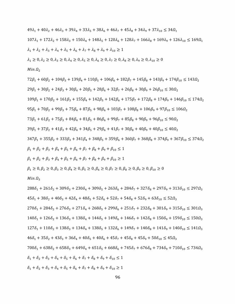
96
49𝜆1 + 40𝜆2 + 46𝜆3 + 39𝜆4 + 33𝜆5 + 38𝜆6 + 46𝜆7 + 45𝜆8 + 34𝜆9 + 37𝜆10 ≤ 34𝛺1
107𝜆1 + 172𝜆2 + 158𝜆3 + 150𝜆4 + 148𝜆5 + 120𝜆6 + 128𝜆7 + 166𝜆8 + 169𝜆9 + 126𝜆10 ≤ 169𝛺1
𝜆1 + 𝜆2 + 𝜆3 + 𝜆4 + 𝜆5 + 𝜆6 + 𝜆7 + 𝜆8 + 𝜆9 + 𝜆10 ≥ 1
𝜆1 ≥ 0, 𝜆2 ≥ 0, 𝜆3 ≥ 0, 𝜆4 ≥ 0, 𝜆5 ≥ 0, 𝜆6 ≥ 0, 𝜆7 ≥ 0, 𝜆8 ≥ 0, 𝜆9 ≥ 0, 𝜆10 ≥ 0
𝑀𝑖𝑛 𝛺2
72𝛽1 + 60𝛽2 + 104𝛽3 + 139𝛽4 + 110𝛽5 + 106𝛽6 + 182𝛽7 + 145𝛽8 + 143𝛽9 + 174𝛽10 ≤ 143𝛺2
29𝛽1 + 30𝛽2 + 24𝛽3 + 30𝛽4 + 20𝛽5 + 28𝛽6 + 32𝛽7 + 26𝛽8 + 30𝛽9 + 26𝛽10 ≤ 30𝛺2
109𝛽1 + 170𝛽2 + 161𝛽3 + 155𝛽4 + 142𝛽5 + 142𝛽6 + 175𝛽7 + 172𝛽8 + 174𝛽9 + 146𝛽10 ≤ 174𝛺2
95𝛽1 + 70𝛽2 + 99𝛽3 + 75𝛽4 + 87𝛽5 + 98𝛽6 + 103𝛽7 + 108𝛽8 + 106𝛽9 + 97𝛽10 ≤ 106𝛺2
73𝛽1 + 61𝛽2 + 75𝛽3 + 84𝛽4 + 81𝛽5 + 86𝛽6 + 99𝛽7 + 85𝛽8 + 90𝛽9 + 96𝛽10 ≤ 90𝛺2
39𝛽1 + 37𝛽2 + 41𝛽3 + 42𝛽4 + 34𝛽5 + 29𝛽6 + 41𝛽7 + 30𝛽8 + 40𝛽9 + 40𝛽10 ≤ 40𝛺2
347𝛽1 + 355𝛽2 + 333𝛽3 + 341𝛽4 + 348𝛽5 + 359𝛽6 + 360𝛽7 + 368𝛽8 + 374𝛽9 + 367𝛽10 ≤ 374𝛺2
𝛽1 + 𝛽2 + 𝛽3 + 𝛽4 + 𝛽5 + 𝛽6 + 𝛽7 + 𝛽8 + 𝛽9 + 𝛽10 ≤ 1
𝛽1 + 𝛽2 + 𝛽3 + 𝛽4 + 𝛽5 + 𝛽6 + 𝛽7 + 𝛽8 + 𝛽9 + 𝛽10 ≥ 1
𝛽1 ≥ 0, 𝛽2 ≥ 0, 𝛽3 ≥ 0, 𝛽4 ≥ 0, 𝛽5 ≥ 0, 𝛽6 ≥ 0, 𝛽7 ≥ 0, 𝛽8 ≥ 0, 𝛽9 ≥ 0, 𝛽10 ≥ 0
𝑀𝑖𝑛 𝛺3
288𝛿1 + 261𝛿2 + 309𝛿3 + 230𝛿4 + 309𝛿5 + 263𝛿6 + 284𝛿7 + 327𝛿8 + 297𝛿9 + 313𝛿10 ≤ 297𝛺3
45𝛿1 + 38𝛿2 + 40𝛿3 + 42𝛿4 + 48𝛿5 + 52𝛿6 + 52𝛿7 + 54𝛿8 + 52𝛿9 + 63𝛿10 ≤ 52𝛺3
270𝛿1 + 284𝛿2 + 276𝛿3 + 271𝛿4 + 268𝛿5 + 299𝛿6 + 251𝛿7 + 232𝛿8 + 301𝛿9 + 315𝛿10 ≤ 301𝛺3
140𝛿1 + 126𝛿2 + 136𝛿3 + 138𝛿4 + 144𝛿5 + 149𝛿6 + 146𝛿7 + 142𝛿8 + 150𝛿9 + 159𝛿10 ≤ 150𝛺3
127𝛿1 + 110𝛿2 + 138𝛿3 + 134𝛿4 + 138𝛿5 + 132𝛿6 + 149𝛿7 + 140𝛿8 + 141𝛿9 + 140𝛿10 ≤ 141𝛺3
46𝛿1 + 35𝛿2 + 43𝛿3 + 36𝛿4 + 40𝛿5 + 40𝛿6 + 45𝛿7 + 45𝛿8 + 45𝛿9 + 50𝛿10 ≤ 45𝛺3
700𝛿1 + 638𝛿2 + 658𝛿3 + 649𝛿4 + 651𝛿5 + 668𝛿6 + 745𝛿7 + 676𝛿8 + 734𝛿9 + 710𝛿10 ≤ 734𝛺3
𝛿1 + 𝛿2 + 𝛿3 + 𝛿4 + 𝛿5 + 𝛿6 + 𝛿7 + 𝛿8 + 𝛿9 + 𝛿10 ≤ 1
𝛿1 + 𝛿2 + 𝛿3 + 𝛿4 + 𝛿5 + 𝛿6 + 𝛿7 + 𝛿8 + 𝛿9 + 𝛿10 ≥ 1
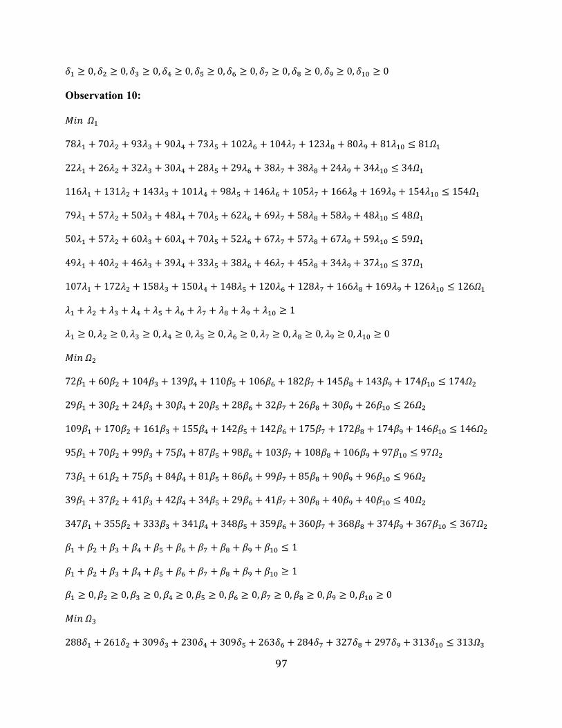
97
𝛿1 ≥ 0, 𝛿2 ≥ 0, 𝛿3 ≥ 0, 𝛿4 ≥ 0, 𝛿5 ≥ 0, 𝛿6 ≥ 0, 𝛿7 ≥ 0, 𝛿8 ≥ 0, 𝛿9 ≥ 0, 𝛿10 ≥ 0
Observation 10:
𝑀𝑖𝑛 𝛺1
78𝜆1 + 70𝜆2 + 93𝜆3 + 90𝜆4 + 73𝜆5 + 102𝜆6 + 104𝜆7 + 123𝜆8 + 80𝜆9 + 81𝜆10 ≤ 81𝛺1
22𝜆1 + 26𝜆2 + 32𝜆3 + 30𝜆4 + 28𝜆5 + 29𝜆6 + 38𝜆7 + 38𝜆8 + 24𝜆9 + 34𝜆10 ≤ 34𝛺1
116𝜆1 + 131𝜆2 + 143𝜆3 + 101𝜆4 + 98𝜆5 + 146𝜆6 + 105𝜆7 + 166𝜆8 + 169𝜆9 + 154𝜆10 ≤ 154𝛺1
79𝜆1 + 57𝜆2 + 50𝜆3 + 48𝜆4 + 70𝜆5 + 62𝜆6 + 69𝜆7 + 58𝜆8 + 58𝜆9 + 48𝜆10 ≤ 48𝛺1
50𝜆1 + 57𝜆2 + 60𝜆3 + 60𝜆4 + 70𝜆5 + 52𝜆6 + 67𝜆7 + 57𝜆8 + 67𝜆9 + 59𝜆10 ≤ 59𝛺1
49𝜆1 + 40𝜆2 + 46𝜆3 + 39𝜆4 + 33𝜆5 + 38𝜆6 + 46𝜆7 + 45𝜆8 + 34𝜆9 + 37𝜆10 ≤ 37𝛺1
107𝜆1 + 172𝜆2 + 158𝜆3 + 150𝜆4 + 148𝜆5 + 120𝜆6 + 128𝜆7 + 166𝜆8 + 169𝜆9 + 126𝜆10 ≤ 126𝛺1
𝜆1 + 𝜆2 + 𝜆3 + 𝜆4 + 𝜆5 + 𝜆6 + 𝜆7 + 𝜆8 + 𝜆9 + 𝜆10 ≥ 1
𝜆1 ≥ 0, 𝜆2 ≥ 0, 𝜆3 ≥ 0, 𝜆4 ≥ 0, 𝜆5 ≥ 0, 𝜆6 ≥ 0, 𝜆7 ≥ 0, 𝜆8 ≥ 0, 𝜆9 ≥ 0, 𝜆10 ≥ 0
𝑀𝑖𝑛 𝛺2
72𝛽1 + 60𝛽2 + 104𝛽3 + 139𝛽4 + 110𝛽5 + 106𝛽6 + 182𝛽7 + 145𝛽8 + 143𝛽9 + 174𝛽10 ≤ 174𝛺2
29𝛽1 + 30𝛽2 + 24𝛽3 + 30𝛽4 + 20𝛽5 + 28𝛽6 + 32𝛽7 + 26𝛽8 + 30𝛽9 + 26𝛽10 ≤ 26𝛺2
109𝛽1 + 170𝛽2 + 161𝛽3 + 155𝛽4 + 142𝛽5 + 142𝛽6 + 175𝛽7 + 172𝛽8 + 174𝛽9 + 146𝛽10 ≤ 146𝛺2
95𝛽1 + 70𝛽2 + 99𝛽3 + 75𝛽4 + 87𝛽5 + 98𝛽6 + 103𝛽7 + 108𝛽8 + 106𝛽9 + 97𝛽10 ≤ 97𝛺2
73𝛽1 + 61𝛽2 + 75𝛽3 + 84𝛽4 + 81𝛽5 + 86𝛽6 + 99𝛽7 + 85𝛽8 + 90𝛽9 + 96𝛽10 ≤ 96𝛺2
39𝛽1 + 37𝛽2 + 41𝛽3 + 42𝛽4 + 34𝛽5 + 29𝛽6 + 41𝛽7 + 30𝛽8 + 40𝛽9 + 40𝛽10 ≤ 40𝛺2
347𝛽1 + 355𝛽2 + 333𝛽3 + 341𝛽4 + 348𝛽5 + 359𝛽6 + 360𝛽7 + 368𝛽8 + 374𝛽9 + 367𝛽10 ≤ 367𝛺2
𝛽1 + 𝛽2 + 𝛽3 + 𝛽4 + 𝛽5 + 𝛽6 + 𝛽7 + 𝛽8 + 𝛽9 + 𝛽10 ≤ 1
𝛽1 + 𝛽2 + 𝛽3 + 𝛽4 + 𝛽5 + 𝛽6 + 𝛽7 + 𝛽8 + 𝛽9 + 𝛽10 ≥ 1
𝛽1 ≥ 0, 𝛽2 ≥ 0, 𝛽3 ≥ 0, 𝛽4 ≥ 0, 𝛽5 ≥ 0, 𝛽6 ≥ 0, 𝛽7 ≥ 0, 𝛽8 ≥ 0, 𝛽9 ≥ 0, 𝛽10 ≥ 0
𝑀𝑖𝑛 𝛺3
288𝛿1 + 261𝛿2 + 309𝛿3 + 230𝛿4 + 309𝛿5 + 263𝛿6 + 284𝛿7 + 327𝛿8 + 297𝛿9 + 313𝛿10 ≤ 313𝛺3
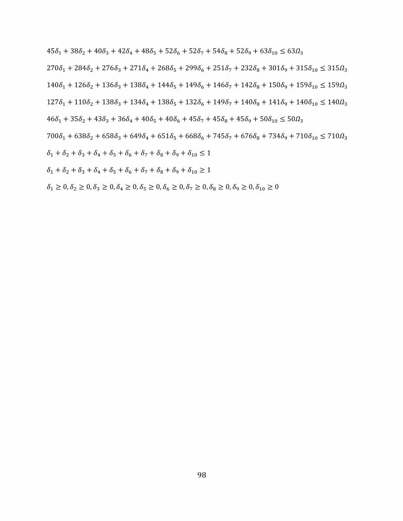
98
45𝛿1 + 38𝛿2 + 40𝛿3 + 42𝛿4 + 48𝛿5 + 52𝛿6 + 52𝛿7 + 54𝛿8 + 52𝛿9 + 63𝛿10 ≤ 63𝛺3
270𝛿1 + 284𝛿2 + 276𝛿3 + 271𝛿4 + 268𝛿5 + 299𝛿6 + 251𝛿7 + 232𝛿8 + 301𝛿9 + 315𝛿10 ≤ 315𝛺3
140𝛿1 + 126𝛿2 + 136𝛿3 + 138𝛿4 + 144𝛿5 + 149𝛿6 + 146𝛿7 + 142𝛿8 + 150𝛿9 + 159𝛿10 ≤ 159𝛺3
127𝛿1 + 110𝛿2 + 138𝛿3 + 134𝛿4 + 138𝛿5 + 132𝛿6 + 149𝛿7 + 140𝛿8 + 141𝛿9 + 140𝛿10 ≤ 140𝛺3
46𝛿1 + 35𝛿2 + 43𝛿3 + 36𝛿4 + 40𝛿5 + 40𝛿6 + 45𝛿7 + 45𝛿8 + 45𝛿9 + 50𝛿10 ≤ 50𝛺3
700𝛿1 + 638𝛿2 + 658𝛿3 + 649𝛿4 + 651𝛿5 + 668𝛿6 + 745𝛿7 + 676𝛿8 + 734𝛿9 + 710𝛿10 ≤ 710𝛺3
𝛿1 + 𝛿2 + 𝛿3 + 𝛿4 + 𝛿5 + 𝛿6 + 𝛿7 + 𝛿8 + 𝛿9 + 𝛿10 ≤ 1
𝛿1 + 𝛿2 + 𝛿3 + 𝛿4 + 𝛿5 + 𝛿6 + 𝛿7 + 𝛿8 + 𝛿9 + 𝛿10 ≥ 1
𝛿1 ≥ 0, 𝛿2 ≥ 0, 𝛿3 ≥ 0, 𝛿4 ≥ 0, 𝛿5 ≥ 0, 𝛿6 ≥ 0, 𝛿7 ≥ 0, 𝛿8 ≥ 0, 𝛿9 ≥ 0, 𝛿10 ≥ 0